Modern Random Access for Satellite Communications arXiv ...
196
U NIVERSITY OF G ENOA DEPARTMENT OF ELECTRICAL,ELECTRONIC AND TELECOMMUNICATION ENGINEERING AND NAVAL ARCHITECTURE (DITEN) PHD IN S CIENCE AND TECHNOLOGY FOR ELECTRONIC AND TELECOMMUNICATION ENGINEERING Modern Random Access for Satellite Communications PhD Thesis Federico Clazzer Genova, April 2017 Tutor: Co-Tutor: Prof. Mario Marchese Dr. Gianluigi Liva Supervisor: Dr. Andrea Munari Coordinator of the PhD Course: Prof. Mario Marchese arXiv:1706.10198v1 [cs.IT] 30 Jun 2017
-
Upload
khangminh22 -
Category
Documents
-
view
0 -
download
0
Transcript of Modern Random Access for Satellite Communications arXiv ...
UNIVERSITY OF GENOADEPARTMENT OF ELECTRICAL, ELECTRONIC AND TELECOMMUNICATION
ENGINEERING AND NAVAL ARCHITECTURE (DITEN)
PHD IN SCIENCE AND TECHNOLOGY FOR ELECTRONIC AND
TELECOMMUNICATION ENGINEERING
Modern Random Access
for Satellite Communications
PhD Thesis
Federico Clazzer
Genova, April 2017
Tutor: Co-Tutor:
Prof. Mario Marchese Dr. Gianluigi Liva
Supervisor:
Dr. Andrea Munari
Coordinator of the PhD Course: Prof. Mario Marchese
arX
iv:1
706.
1019
8v1
[cs
.IT
] 3
0 Ju
n 20
17

Contents
List of Figures iv
List of Tables ix
List of Abbreviations xiii
Acknowledgments - Ringraziamenti xvii
Abstract xix
Sommario xxi
Introduction 1
1 Basics of Random Access - ALOHA and Slotted ALOHA 7
1.1 ALOHA . . . . . . . . . . . . . . . . . . . . . . . . . . . . . . . . . . . . . . . . 8
1.2 Slotted ALOHA . . . . . . . . . . . . . . . . . . . . . . . . . . . . . . . . . . . . 10
1.3 Considerations on ALOHA and Slotted ALOHA . . . . . . . . . . . . . . . . . 11
1.4 Other Fundamental Protocols in Random Access . . . . . . . . . . . . . . . . . 13
2 Preliminaries 19
2.1 The Scenario . . . . . . . . . . . . . . . . . . . . . . . . . . . . . . . . . . . . . . 19
2.2 Time Diversity . . . . . . . . . . . . . . . . . . . . . . . . . . . . . . . . . . . . . 20
2.3 Channel Models . . . . . . . . . . . . . . . . . . . . . . . . . . . . . . . . . . . . 20
2.4 Successive Interference Cancellation . . . . . . . . . . . . . . . . . . . . . . . . 22
2.5 Decoding Conditions . . . . . . . . . . . . . . . . . . . . . . . . . . . . . . . . . 23
i
ii CONTENTS
3 The Role of Interference Cancellation in Random Access Protocols 25
3.1 Recent Random Access Protocols . . . . . . . . . . . . . . . . . . . . . . . . . . 25
3.1.1 Slot Synchronous Random Access . . . . . . . . . . . . . . . . . . . . . 26
3.1.2 Asynchronous Random Access . . . . . . . . . . . . . . . . . . . . . . . 30
3.1.3 Tree-Splitting Algorithms . . . . . . . . . . . . . . . . . . . . . . . . . . 36
3.1.4 Random Access Without Feedback . . . . . . . . . . . . . . . . . . . . . 45
3.2 Applicable Scenarios . . . . . . . . . . . . . . . . . . . . . . . . . . . . . . . . . 49
3.3 Open Questions . . . . . . . . . . . . . . . . . . . . . . . . . . . . . . . . . . . . 51
3.4 Conclusions . . . . . . . . . . . . . . . . . . . . . . . . . . . . . . . . . . . . . . 52
4 Asynchronous RA with Time Diversity and Combining: ECRA 55
4.1 Introduction . . . . . . . . . . . . . . . . . . . . . . . . . . . . . . . . . . . . . . 56
4.2 System Model . . . . . . . . . . . . . . . . . . . . . . . . . . . . . . . . . . . . . 56
4.2.1 Modeling of the Decoding Process . . . . . . . . . . . . . . . . . . . . . 58
4.2.2 Enhanced Contention Resolution ALOHA Decoding Algorithm . . . . 59
4.2.3 Summary and Comments . . . . . . . . . . . . . . . . . . . . . . . . . . 62
4.3 Packet Loss Rate Analysis at Low Channel Load . . . . . . . . . . . . . . . . . 63
4.3.1 Packet Loss Rate Approximation . . . . . . . . . . . . . . . . . . . . . . 64
4.3.2 Vulnerable Period Duration for Asynchronous RA with FEC . . . . . . 65
4.3.3 Vulnerable Period Duration for Asynchronous RA with MRC and d = 2 66
4.4 Performance Analysis . . . . . . . . . . . . . . . . . . . . . . . . . . . . . . . . 67
4.4.1 Numerical Results . . . . . . . . . . . . . . . . . . . . . . . . . . . . . . 69
4.5 Detection, Combining and Decoding - A Two-Phase Procedure . . . . . . . . . 75
4.5.1 Detection and Decoding . . . . . . . . . . . . . . . . . . . . . . . . . . . 76
4.5.2 Hypothesis Testing, Interference-Aware Rule . . . . . . . . . . . . . . . 79
4.6 Two-Phase Procedure Numerical Results . . . . . . . . . . . . . . . . . . . . . 80
4.6.1 ROC Comparison . . . . . . . . . . . . . . . . . . . . . . . . . . . . . . . 80
4.6.2 ECRA Detection and Replicas Coupling Performance . . . . . . . . . . 80
4.6.3 Spectral Efficiency . . . . . . . . . . . . . . . . . . . . . . . . . . . . . . 81
4.7 Conclusions . . . . . . . . . . . . . . . . . . . . . . . . . . . . . . . . . . . . . . 83
5 Layer 3 Throughput and PLR Analysis for Advanced RA 85
5.1 Introduction . . . . . . . . . . . . . . . . . . . . . . . . . . . . . . . . . . . . . . 86
5.2 System Model . . . . . . . . . . . . . . . . . . . . . . . . . . . . . . . . . . . . . 86
5.3 L3 Throughput and Packet Loss Rate Analysis . . . . . . . . . . . . . . . . . . 87
CONTENTS iii
5.3.1 Asynchronous RA Protocols . . . . . . . . . . . . . . . . . . . . . . . . . 87
5.3.2 Slot Synchronous RA Protocols . . . . . . . . . . . . . . . . . . . . . . . 88
5.4 Numerical Results . . . . . . . . . . . . . . . . . . . . . . . . . . . . . . . . . . . 91
5.4.1 Asynchronous and Slot Synchronous RA Layer 3 Performance Com-
parison . . . . . . . . . . . . . . . . . . . . . . . . . . . . . . . . . . . . . 92
5.4.2 Slot Synchronous Layer 2 and Layer 3 Comparison . . . . . . . . . . . 95
5.4.3 Layer 3 Slot Synchronous Bounds . . . . . . . . . . . . . . . . . . . . . 96
5.5 Conclusions . . . . . . . . . . . . . . . . . . . . . . . . . . . . . . . . . . . . . . 98
6 IRSA over the Rayleigh Block Fading Channel 101
6.1 Introduction . . . . . . . . . . . . . . . . . . . . . . . . . . . . . . . . . . . . . . 101
6.2 System Model . . . . . . . . . . . . . . . . . . . . . . . . . . . . . . . . . . . . . 102
6.2.1 Access Protocol . . . . . . . . . . . . . . . . . . . . . . . . . . . . . . . . 102
6.2.2 Received Power and Fading Models . . . . . . . . . . . . . . . . . . . . 103
6.2.3 Graph Representation . . . . . . . . . . . . . . . . . . . . . . . . . . . . 103
6.2.4 Receiver Operation . . . . . . . . . . . . . . . . . . . . . . . . . . . . . . 105
6.3 Decoding Probabilities . . . . . . . . . . . . . . . . . . . . . . . . . . . . . . . . 107
6.4 Density Evolution Analysis and Decoding Threshold Definition . . . . . . . . 108
6.5 Numerical Results . . . . . . . . . . . . . . . . . . . . . . . . . . . . . . . . . . . 111
6.6 Conclusions . . . . . . . . . . . . . . . . . . . . . . . . . . . . . . . . . . . . . . 112
7 Random Access with Multiple Receivers 115
7.1 Introduction . . . . . . . . . . . . . . . . . . . . . . . . . . . . . . . . . . . . . . 115
7.2 System Model and Preliminaries . . . . . . . . . . . . . . . . . . . . . . . . . . 116
7.2.1 Notation . . . . . . . . . . . . . . . . . . . . . . . . . . . . . . . . . . . . 118
7.3 Uplink Performance . . . . . . . . . . . . . . . . . . . . . . . . . . . . . . . . . 119
7.3.1 Uplink Throughput . . . . . . . . . . . . . . . . . . . . . . . . . . . . . . 119
7.3.2 Packet Loss Probability . . . . . . . . . . . . . . . . . . . . . . . . . . . 125
7.4 An Achievable Downlink Upper Bound . . . . . . . . . . . . . . . . . . . . . . 128
7.4.1 Bounds for Downlink Rates . . . . . . . . . . . . . . . . . . . . . . . . . 128
7.4.2 Random Linear Coding . . . . . . . . . . . . . . . . . . . . . . . . . . . 130
7.5 Simplified Downlink Strategies . . . . . . . . . . . . . . . . . . . . . . . . . . . 132
7.5.1 Common Transmission Probability . . . . . . . . . . . . . . . . . . . . . 134
7.5.2 Distinct Transmission Probabilities . . . . . . . . . . . . . . . . . . . . . 135
7.6 On the Impact of Finite-Buffer Size on Downlink Strategies . . . . . . . . . . . 143
iv CONTENTS
7.7 Conclusions . . . . . . . . . . . . . . . . . . . . . . . . . . . . . . . . . . . . . . 149
Conclusions 151
Selected List of Publications 155
Other Publications 157
List of Figures
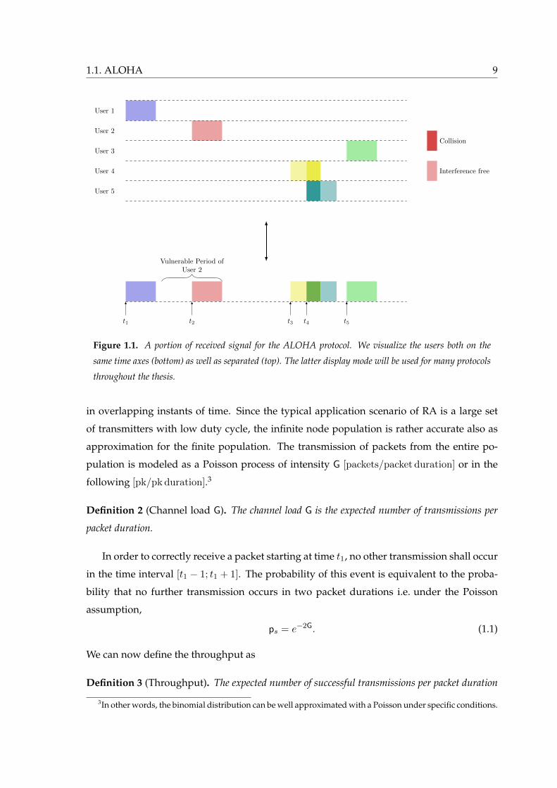
1.1 A portion of received signal for the ALOHA protocol. We visualize the users
both on the same time axes (bottom) as well as separated (top). The latter
display mode will be used for many protocols throughout the thesis. . . . . . 9
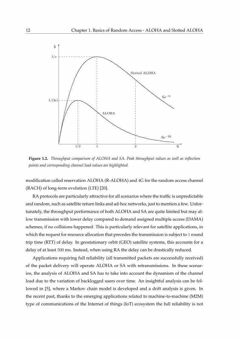
1.2 Throughput comparison of ALOHA and slotted ALOHA (SA). Peak through-
put values as well as inflection points and corresponding channel load values
are highlighted. . . . . . . . . . . . . . . . . . . . . . . . . . . . . . . . . . . . . 12
3.1 Example of a received medium access (MAC) frame for contention resolution
diversity slotted ALOHA (CRDSA) and the successive interference cancella-
tion (SIC) iterative procedure. . . . . . . . . . . . . . . . . . . . . . . . . . . . . 28
3.2 Throughput comparison of SA, diversity slotted ALOHA (DSA), CRDSA and
irregular repetition slotted ALOHA (IRSA) under the collision channel. Both
DSA and CRDSA send two copies for each transmitted packet and CRDSA
employs SIC at the receiver side. In IRSA each user picks a degree d following
the probability mass function (p.m.f.) Λ. Specifically, with probability 1/2
two copies will be sent, with probability 0.28 three and with probability 0.22
eight. The use of variable number of replicas per user greatly improves the
throughput compared to CRDSA although for very high channel load values,
the degradation is more severe. . . . . . . . . . . . . . . . . . . . . . . . . . . . 31
3.3 Hidden terminal scenario. NodeA and nodeB want to communicate to node
C and they are not able to sense each other since they are out of the reception
range. . . . . . . . . . . . . . . . . . . . . . . . . . . . . . . . . . . . . . . . . . . 32
v
vi LIST OF FIGURES
3.4 ZigZag decoding procedure. The interference free portion s1 of user B first
transmission is removed from the second transmission and reveals s2, i.e. the
first portion of user A’s transmission. This portion is then used back in the
first collision to remove interference and revealing portion s3. Proceeding
iteratively between the two collisions portion by portion, the packets can be
successfully decoded. . . . . . . . . . . . . . . . . . . . . . . . . . . . . . . . . . 34
3.5 ZigZag receiver operations depicted via functional flow chart. . . . . . . . . . 35
3.6 Two consecutive collisions of two packets a and b composed by 3 symbols
each. Both packets are transmitted twice and the receiver stores y1 and y2.
The corresponding factor graph of the two collisions shows how the symbols
of individual packets are connected to the received symbols. The check nodes
denoted with f1x and f2x are responsible for computing the probability den-
sity function (p.d.f.) or log-lokelihood ratios of received bits, given the noisy
observations y1x and y2x. The two options correspond to the sum-product or
max-product algorithms respectively. . . . . . . . . . . . . . . . . . . . . . . . 37
3.7 Standard and modified tree algorithms for the same collision example. . . . . 39
3.8 Successive interference cancellation tree algorithm (SICTA) collision resolu-
tion algorithm for the collision example of Figure 3.7. . . . . . . . . . . . . . . 41
3.9 Throughput as a function of the channel load for throughput invariant (TI)
sequences under the ι-multi-packet reception (ι-MPR) channel for different
values of ι. . . . . . . . . . . . . . . . . . . . . . . . . . . . . . . . . . . . . . . . 47
LIST OF FIGURES vii
4.1 SIC procedure in enhanced contention resolution ALOHA (ECRA), first phase.
The decoder starts looking for replicas that can be successfully decoded. The
first to be found is replica C2 which is collision-free. After successfully decod-
ing, the information on the location of replica C1 is retrieved from the header.
So, the data carried by C2 can be re-encoded, re-modulated, frequency offset
and epoch are superimposed on the signal and its interference contribution
is removed from both locations within the received signal. The interference
caused on replica A2 is now removed. The decoder can successfully decode
also replica A2 and - applying the same procedure - remove its interference
together with the one of replica A1. Now, replica B1 is collision-free, can be
successfully decoded and its interference contribution, together with the one
of replica B2, can be removed. Finally, replica D1, also collision-free, is cor-
rectly decoded and removed from the received signal, together with its twin
D2. Unfortunately user 5 and 6 replicas are in a collision pattern that cannot
be resolved by SIC only, and still remain in the received signal after the end
of the first phase. . . . . . . . . . . . . . . . . . . . . . . . . . . . . . . . . . . . 60
4.2 Example of collision pattern blocking SIC. Different portions of replicas F1
and F2 are collision-free. When selection combining (SC) is applied, ECRA
selects these portions, creates a combined observation and attempts decoding
on it. . . . . . . . . . . . . . . . . . . . . . . . . . . . . . . . . . . . . . . . . . . 62
4.3 Throughput S vs. channel load G for ALOHA, contention resolution ALOHA
(CRA), ECRA selection combining (ECRA-SC) and ECRA maximal-ratio com-
bining (ECRA-MRC), P/N = 6 dB and R = 1.5. . . . . . . . . . . . . . . . . . . 70
4.4 Packet error rate pl vs. channel load G for ALOHA, CRA, ECRA-SC and
ECRA-MRC, P/N = 6 dB and R = 1.5. The average value of α used in the ap-
proximation of pl for ECRA-MRC is derived through Monte Carlo simulations. 71
4.5 Spectral efficiency ξ vs. channel load G for ECRA-SC, ECRA-MRC, CRA and
CRDSA. . . . . . . . . . . . . . . . . . . . . . . . . . . . . . . . . . . . . . . . . 72
4.6 Normalised capacity η for ALOHA, CRA, ECRA-SC and ECRA-MRC with
Pg/N = 6 dB and corresponding rate. . . . . . . . . . . . . . . . . . . . . . . . . 74
4.7 Transmitted signals. Each user sends two replicas of duration Tp seconds that
occupy 3 time slots in the example. . . . . . . . . . . . . . . . . . . . . . . . . . 76
4.8 The non-coherent soft-correlator and the interference-aware soft-correlator
used for the detection of candidate replicas. . . . . . . . . . . . . . . . . . . . . 77
viii LIST OF FIGURES
4.9 Receiver operating characteristics (ROC) for the non-coherent and interference-
aware soft-correlation synchronization rules, with G = 0.5, 1.5, equal re-
ceived power, Es/N0 = 10 dB and nsw = 32 symbols. . . . . . . . . . . . . . . 81
4.10 Detection probability PD for a fixed threshold ψ∗ independent from the chan-
nel traffic using Ψ(1) and correct combining probability PCC with Ψ(2). . . . . 82
4.11 Spectral efficiency of ECRA-maximal-ratio combining (MRC) with the pro-
posed two phase detection and combining technique compared to the ideal
ECRA-MRC. . . . . . . . . . . . . . . . . . . . . . . . . . . . . . . . . . . . . . . 83
5.1 Layer 3 throughput comparison with fX(x) = 12δ(x− 1) + 1
2δ(x− 2). . . . . . 93
5.2 Layer 3 packet loss rate (PLR) comparison with fX(x) = 12δ(x− 1) + 1
2δ(x− 2). 94
5.3 Layer 3 throughput simulations with fX(x) = e−x. . . . . . . . . . . . . . . . . 94
5.4 Layer 3 PLR simulations with fX(x) = e−x. . . . . . . . . . . . . . . . . . . . . 95
5.5 Layer 2 and 3 throughput simulations with fX(x) = 12δ(x− 1) + 1
2δ(x− 2). . 96
5.6 Layer 2 and 3 PLR simulations with fX(x) = 12δ(x− 1) + 1
2δ(x− 2). . . . . . . 97
5.7 Layer 3 throughput comparison between exact and approximated performance
considering fX(x) = 12δ(x− 1) + 1
2δ(x− 2). . . . . . . . . . . . . . . . . . . . . 97
5.8 Layer 3 PLR comparison between exact and approximated performance con-
sidering fX(x) = 12δ(x− 1) + 1
2δ(x− 2). . . . . . . . . . . . . . . . . . . . . . . 98
6.1 Graph representation of MAC frame. . . . . . . . . . . . . . . . . . . . . . . . . 104
6.2 Tree representation of the MAC frame. . . . . . . . . . . . . . . . . . . . . . . . 108
6.3 Throughput values achieved by the burst node distributions in Table 6.1, ver-
sus the channel load. Various frame sizes ms, B = 20 dB, b? = 3 dB. . . . . . . 113
6.4 PLR values achieved by the burst node distributions in Table 6.1, versus the
channel load. Various frame sizes ms, B = 20 dB, b? = 3 dB. . . . . . . . . . . 114
7.1 Reference topology for the system under consideration. . . . . . . . . . . . . . 117
7.2 Average uplink throughput vs channel load under different erasure proba-
bilities. Continuous lines indicate the performance in the presence of two
receivers, whereas dashed lines report the behaviour of pure SA. . . . . . . . 120
7.3 Maximum uplink throughput vs erasure rate. The red continuous line reports
the performance S∗ul,2 of a two-receiver scheme, while blue circled markers
indicate Sul,2(1/(1 − ε)), and the dashed black line shows the behaviour of
pure SA. . . . . . . . . . . . . . . . . . . . . . . . . . . . . . . . . . . . . . . . . 121
LIST OF FIGURES ix
7.4 Average uplink throughput vs channel load for different number of relays K.
The erasure probability has been set to ε = 0.5. . . . . . . . . . . . . . . . . . . 125
7.5 Maximum achievable throughput S∗ul,K as a function of the number of relays
K for an erasure rate ε = 0.5. The gray curve reports the load on the channel
G∗K needed to reach S∗ul,K. . . . . . . . . . . . . . . . . . . . . . . . . . . . . . . . 126
7.6 Probability ζK that a packet sent by a user is not received by any of the relays.
Different curves indicate different values of K, while the erasure probability
has been set to ε = 0.2. . . . . . . . . . . . . . . . . . . . . . . . . . . . . . . . . 127
7.7 Downlink throughput vs rate for different implementation of a dropping pol-
icy. ε = 0.3, G = 1/(1− ε) ∼ 1.43. . . . . . . . . . . . . . . . . . . . . . . . . . . 136
7.8 Markov chain of the evolution of the matrix rank as row vectors are added.
The state number represents the rank value. . . . . . . . . . . . . . . . . . . . . 146
7.9 Random linear coding (RLC) under finite buffer size. We compare the Monte
Carlo simulations with the developed analytical tool using Markov chains,
up to 80 slots as buffer size. Higher buffer sizes are obtained via Monte Carlo
simulations. . . . . . . . . . . . . . . . . . . . . . . . . . . . . . . . . . . . . . . 148
7.10 Comparison of dropping policies and RLC for finite-buffer scenarios. Various
buffer dimensions are selected. . . . . . . . . . . . . . . . . . . . . . . . . . . . 149

List of Tables
6.1 Optimised user node degree distribution and corresponding threshold G? for
pl = 10−2. . . . . . . . . . . . . . . . . . . . . . . . . . . . . . . . . . . . . . . . . 112
xi

List of Abbreviations
Acronyms
5G fifth generation
ACRDA asynchronous contention resolution diversity ALOHA
AIS automatic identification system
ASM application-specific messages
AWGN additive white gaussian noise
CDMA code division multiple access
CRA contention resolution ALOHA
CRC cyclic redundancy check
CRDSA contention resolution diversity slotted ALOHA
CRI collision resolution interval
CSA coded slotted ALOHA
CSI channel state information
CSMA carrier sense multiple access
CSMA/CA CSMA collision avoidance
CSMA/CD CSMA collision detection
DAMA demand assigned multiple access
DE density evolution
xiii
xiv LIST OF ABBREVIATIONS
D&F decode and forward
DSA diversity slotted ALOHA
DVB-RCS2 Digital Video Broadcasting - Return Channel Satellite 2nd Generation
E-SSA enhanced-spread spectrum ALOHA
ECRA enhanced contention resolution ALOHA
ECRA-MRC ECRA maximal-ratio combining
ECRA-SC ECRA selection combining
EGC equal-gain combining
ETSI European Telecommunications Standards Institute
FDMA frequency division multiple access
FEC forward error correction
GW gateway
GEO geostationary orbit
GPRS general packet radio service
GSM global system for mobile communications
i.i.d. independent and identically distributed
IC interference cancellation
IoT Internet of things
ι-MPR ι-multi-packet reception
IP internet protocol
IRSA irregular repetition slotted ALOHA
ITU International Telecommunications Union
LDPC low density parity check
LRT likelihood ratio test
xv
LTE long-term evolution
LTE-A LTE-Advanced
M2M machine-to-machine
MAC medium access
MF matched filter
MF-TDMA multi-frequency time division multiple access
ML maximum likelihood
MPR multi-packet reception
MRC maximal-ratio combining
MUD multiuser detection
p.d.f. probability density function
PLR packet loss rate
p.m.f. probability mass function
R-ALOHA reservation ALOHA
r.v. random variable
RA random access
RACH random access channel
RFID radio frequency identification
RLC random linear coding
ROC receiver operating characteristics
RTS/CTS request to send / clear to send
RTT round trip time
S-MIM S-band mobile interactive multimedia
SA slotted ALOHA
xvi LIST OF ABBREVIATIONS
SC selection combining
SI shift invariant
SIC successive interference cancellation
SICTA successive interference cancellation tree algorithm
SINR signal-to-interference and noise ratio
SNR signal-to-noise ratio
TDMA time division multiple access
TI throughput invariant
C-UCP C-unresolvable collision pattern
V2V vehicle-to-vehicle
VDES VHF data exchange system
VF virtual frame
WAVE wireless access in vehicular environments
Acknowledgments - Ringraziamenti
Dopo tutti questi anni di studio vorrei spendere alcune parole sulla persone che mi sono
state vicine, mi hanno incoraggiato, mi hanno aiutato, dato indicazioni e suggerimenti.
Prima di tutto vorrei esprimire profonda gratitudine per il mio relatore, Prof. Mario
Marchese, per avermi accettato come suo studente e il suo supporto durante tutto il dot-
torato. Le sue indicazioni sono stati fondamentali.
Vorrei ringraziare Gianluigi, per il suo instancabile aiuto, per i suoi suggerimenti e per la
sua guida. Sono innumerevoli le cose che ho imparato in questi anni, e moltissime le devo
a lui. A tutto questo si aggiunge che in lui ho trovato non solo un mentore ma anche un
amico.
Vorrei ringraziare Andrea, per le lunghe chiacchierate, sulla tesi, sui nostri articoli e non
solo. Se mi sono appassionato alla ricerca e’ anche grazie a lui (o per colpa sua, dipende da
come la si vede).
I wish to express my gratitude to Prof. Alex Graell i Amat and Prof. Petar Popovski for
their competent feedback during the review phase of the thesis. The quality of thesis has
profoundly improved thank to them.
I would like to thank all my present and past colleagues – or better friends – at the
Satellite Network department at the German Aerospace Center (DLR). Thanks to Sandro,
Matteo and Hermann to let me come to DLR for my Master’s thesis and for offering me
a position later. Without them, this thesis would not be here. Thanks to Christian, for his
patience in the early stage of my research. Thanks to our coffee break and lunch break gang,
(rigorously in alphabetical order, and hoping not to forget anyone), Alessandro, Andrea,
Andreas, Benny, Cristina, Estefania, Fran, Giuliano, Giuseppe, Jan, Javi, Maria-Antonietta,
Romain, Stefan, Svilen, Thomas, Tudor and Vincent. All the laughes we had together, helped
me to start every day, even to most heavy one, with a smile on the face. A special thanks to
my former officemate Tom. And a very special thanks to my current officemate Balazs. He
helped me not only with the everyday issues, but also far beyond!
Un grazie particolare agli amici vicini e lontani. Loro sanno chi sono.

xviii Acknowledgments - Ringraziamenti
La fortuna di trovare un amico sincero, come un vero fratello, e senza eguali. Anche se
la distanza e grande e gli impegni nella vita diventano sempre di piu, lui sara sempre al tuo
fianco pronto a farti sorridere della piu piccola stupidaggine. Grazie Michel.
Senza i miei genitori, non sarei diventato cio che sono, e questa tesi non sarebbe qui.
Grazie a mia mamma per il suo amore e per avermi insegnato il valore della perseveranza.
Grazie a mio papa per il suo amore e per avermi insegnato cosa vuol dire appassionarsi.
Grazie a mia nonna, che non ha mai smesso di vedermi come un bambino ma anche che
e sempre orgogliosa di chiamarmi Ingegnere.
Per ultima anche se dovrebbe essere in cima alla lista, l’amore della mia vita, Viviana.
Quanta strada abbiamo fatto da quando ci siamo conosciuti. Siamo cresciuti insieme, siamo
cambiati e il nostro amore si e rafforzato. In te ho trovato non solo un’amica ma anche una
confidente.
Mi scuso se per mia mancanza, ho dimenticato qualcuno. Non me ne vogliate.
Federico
Germering
February 2017
Abstract
The exponential increase in communication-capable devices, requires the development
of new and highly efficient communication protocols. One of the main limitation in nowa-
days wireless communication systems is the scarcity of the frequency spectrum. Moreover,
the arise of a new paradigm – called in general machine-to-machine (M2M) – changes the
perspective of communication, from human-centric to machine-centric. More and more au-
tonomous devices, not directly influenced by humans, will be connected and will require to
exchange information. Such devices can be part of a sensor network monitoring a portion
of a smart grid, or can be cars driving on highways. Despite their heterogeneous nature,
these devices will be required to share common frequency bands calling for development of
efficient MAC protocols.
The class of random access (RA) MAC is one possible solution to the heterogeneous
nature of M2M type of communication systems. Although being quite simple, these pro-
tocols allow transmitters to share the medium without coordination possibly accommodat-
ing traffic with various characteristics. On the other hand, classical RA, as ALOHA or SA,
are, unfortunately, much less efficient than orthogonal multiple access, where collisions are
avoided and the resource is dedicated to one terminal. However, in the recent years, the
introduction of advanced signal processing techniques including interference cancellation,
allowed to reduce the gap between RA and orthogonal multiple access. Undubitable advan-
tages, as very limited signaling required and very simple transmitters, lead to a new wave
of interest.
The focus of the thesis is two-folded: on the one hand we analyse the performance of
advanced asynchronous random access systems, and compare them with slot synchronous
ones. Interference cancellation is not enough, and combining techniques are required to
achieve the full potential of asynchronous schemes, as we will see in the thesis. On the other
hand, we explore advanced slot synchronous RA with fading channels or with multiple
receivers, in order to gain insights in how their optimisation or performance are subject to
change due to the channel and topology.


Sommario
L’aumento esponenziale di terminali in grado di comunicare, richiama l’attenzione sulla
necessita di sviluppare nuovi ed efficienti protocolli di comunicazione. Una delle princi-
pali limitazioni negli attuali sistemi di comunicazioni radio e la scarsita di banda allocata,
che rende di primaria importanza la possibilita di allocare nella stessa frequenza il mag-
gior numero di transmettitori concorrenti. In questo scenario, si presenta la nascita di un
nuovo paradigma di comunicazione, chiamato comunemente M2M communication, che e
rivoluzionario in quanto sposta il punto di vista, centrandolo sulla macchina invece che
sull’inidividuo. Un numero sempre crescente di oggetti autonomi, quindi non direttamente
sotto l’influenza o il comando umano, saranno connessi e avranno la necessita di comu-
nicare con l’esterno o tra loro. Esempi possono essere la rete di sensori che monitora la
smart grid, oppure autoveicoli in movimento nelle citta o sulle autostrade. Nonstante la
loro natura eterogenea, tutti questi terminali avranno la necessita di condividere le stesse
radio frequenze. Alla luce di questo, nuovi ed efficienti protocolli MAC dovranno essere
sviluppati.
I protocolli RA per il MAC sono una possibile risposta alla natura eterogenea delle reti
M2M. Pur essendo relativamente semplici, questa classe di protocolli permette di condi-
videre la frequenza senza la necessita di coordinamento tra i terminali, e permettendo la
trasmissione dati di varia lunghezza o con caratteristiche differenti. D’altra parte, schemi
classici RA, come ALOHA e SA, sono molto meno efficienti di schemi che evitano collisioni
e che riservano le risorse per un unico transmittitore alla volta, come time division multiple
access (TDMA), ad esempio. Negli ultimi anni, inoltre, l’introduzione di tecniche evolute
di processamento del segnale, come la cancellazione di interferenza, ha permesso di ridurre
la distanza di prestazioni tra queste due classi di protocolli. Chiari vantaggi dei protocolli
RA sono la ridottissima necessita di scambio di meta dati e la ridotta complessita dei trans-
mettitori. Per questi motivi, un rinnovato interesse da parte della comunita scientifica si e
manifestato recentemente.
L’obiettivo della tesi e duplice: da un lato ci occuperemo di analizzare il comportamento
xxii Sommario
di protocolli RA asincroni e li confronteremo con quelli sincroni a livello di slot. L’utilizzo
di tecniche di cancellazione di interference non reiscono da sole a sfruttare l’intera poten-
zialita di questi protocolli. Per questo motive introdurremo tecniche di combining nel nuovo
schema chiamato ECRA. Ci occuperemo inoltre, di valutare l’impatto di nuovi modelli di
canale con fading o di topoligie con ricevitori multipli su protocolli sincroni a livello di slot.
L’analisi teorica sara supportata mediante simulazioni al computer, per verificare i benefici
delle scelte effettuate.

Introduction
The most difficult thing is the
decision to act, the rest is merely
tenacity
Amelia Earhart
The problem of sharing the wireless medium amongst several transmitters [1] has its
roots in the origin of radio communication. The problem can be formulated with the help
of a toy example. Let us assume that two transmitters would like to send packets to a com-
mon receiver sharing the wireless medium. A first option would be to equally split the time
between the two transmitters, dedicating the first half to the transmission of the first user
and the second to the second user. Similarly, we could split the bandwidth into two equally
spaced carriers and dedicate one to each of the transmitters. A second option, valuable if the
transmitters have seldom packets to be sent, is to let them access the wireless medium with
their packets whenever they are generated, regardless of the medium activity. If a collision
happens, the receiver notifies the transmitters which, after a random time, will retransmit
their packets. The two presented options correspond to two medium access (MAC) classes:
in the first class a dedicated, non-interfering resource is assigned to each of the transmit-
ters, while in the second class transmitters are allowed to access the medium whenever a
data packet is generated, no matter what the medium activity is. In the former class fall
paradigms like time division multiple access (TDMA), frequency division multiple access
(FDMA) and code division multiple access (CDMA) [2], where the orthogonal resources as-
signed to the transmitters are time slots, frequency carriers or code sequences respectively.
To the latter class belong all random access (RA) solutions, from ALOHA [3] and slotted
ALOHA (SA) [4] to carrier sensing techniques as carrier sense multiple access (CSMA) [5].
While orthogonal schemes are efficient when the scenario is static, i.e. the number of trans-
mitters and their datarate requirements are constant, RA is particularly indicated for very
dynamic situations as well as when a very large transmitter population features a small
2 Introduction
transmission duty cycle [5] (the transmission time is very small compared to the time when
the transmitter remains idle). The latter case is when the number of active transmitters com-
pared to the total population is very small and time for transmitting a packet is rather limited
compared to the time where the transmitter remains idle. A third class of MAC protocols
is demand assigned multiple access (DAMA) [6]. Users ask for the resources to transmit in
terms of time slots or frequency bands to a central entity, which dynamically allocates them.
Once the users receive the notification on how to exploit the resources, they are granted in-
terference free access to the channel, as for orthogonal schemes. These protocols are effective
when the amount of data to be transmitted largely exceeds the overhead required to assign
the resources, being the overhead typically some form handshake procedure. In all the cases
where the packets to be transmitted are small compared to the handshake messages, DAMA
becomes inefficient.
The increasing demand of efficient solutions for addressing the concurrent access to
the medium of heterogeneous terminals in wireless communications calls for development
of advanced MAC solutions. Two main research fields are emerging: on the one hand
very large or continuous data transmissions serving streaming services, and on the other
hand, small data transmission supporting recent paradigms like Internet of things (IoT) and
machine-to-machine (M2M) communications [7]. In the latter scenarios, RA is an effective
solution, but old paradigms like ALOHA or SA are not able to meet the requirements in
terms of throughput and packet loss rate (PLR). Nonetheless, in the recent past these pro-
tocols have been rediscovered and improved thanks to new signal processing techniques.
Interestingly, one of the most recent research waves in this field has come from the typical
application scenario of RA, i.e. satellite communications. This peculiar application scenario,
in fact, prevents the use of carrier sensing techniques due to the vast satellite footprint that
allows transmitters hundreds of kilometer far apart to transmit concurrently but precludes
the sensing of mutual activity. The key advancement of the RA solution proposed leverages
on successive interference cancellation (SIC) that can be included in the multiuser detection
(MUD) techniques [8]. The possibility to iteratively clean the received signal from correctly
received packets reduces the occupation of the channel and possibly leads to further correct
receptions.
Interestingly, several other application scenarios other than satellite communications
have recently shown that RA protocols can be beneficial. When for instance, there are tight
constraints on the transmitter complexity and cost, RA protocols can be one of the most
promising choices due to their extremely simple transmitters. Some typical examples are
3
vehicular ad hoc networks [9] and radio frequency identification (RFID) communication
systems [10]. RA is also beneficial when the round trip time (RTT) of the communication
system is significantly large, i.e. several milliseconds or more as in the case of satellite com-
munication [11] and underwater communication [12]. In this way the users are allowed to
immediately transmit the information without the need of waiting for the procedure of re-
questing and getting the resource allocated typical of DAMA, which has a minimum delay
of 1 RTT.
In this regard, the focus of the thesis is on advanced RA solutions targeting satellite com-
munications as well as small data transmissions, e.g. M2M and IoT [13]. We start with a brief
review of the basic ALOHA and SA protocols followed by some key definitions in the sec-
ond Chapter. Chapter 3 aims at highlighting the beneficial role of interference cancellation
(IC) in four different classes of RA protocols, i.e. asynchronous, slot synchronous, tree-based
and without feedback. Interestingly, in all the last three cases it has been demonstrated
that under the collision channel (see Chapter 2 for the definition) the limit of 1 [pk/slot] in
throughput can be achieved when SIC is adopted.1 Time slotted RA schemes have always
been preferred in literature because of two main reasons: they present better performance
compared to their asynchronous counterparts and they are easier to treat from an analytical
perspective. Bearing this in mind, Chapter 4 tries to answer the following two key questions:
• Are there any techniques that allow asynchronous RA schemes to compete with the
comparable time-slotted ones?
• Is there a way to analyse systematically such schemes?
The first question finds an answer in the first Chapter, making use of enhanced contention
resolution ALOHA (ECRA), which adopts time diversity at the transmitter and SIC, together
with combining techniques at the receiver. Under some scenarios, we show that ECRA out-
performs its slot synchronous counterpart. The second question also finds a partial answer
in the same Chapter. An analytical approximation of the PLR is derived, which is shown
to be tight under low to moderate channel load conditions. Combining techniques require
perfect knowledge of all the packet positions of a specific transmitter before decoding. A
practical suboptimal solution, which has a very limited performance loss compared to the
ideal case, is provided in the second part of Chapter 4, .
Recent RA protocols including ECRA are particularly efficient and some of them have
been proposed in recent standard as options also for data transmission. Nevertheless, a com-
1Nonetheless, not all schemes achieving this limit are practical. More details can be found in Chapter 3.

4 Introduction
parison between these schemes at higher layers is still missing. To this regard, in Chapter 5
we aim at addressing the following question:
• If the packets to be transmitted follow a generic packet duration distribution, possibly
exceeding the duration of a time slot, what are the throughput and PLR performance
of time-slotted compared to asynchronous RA schemes?
In the case of asynchronous RA packets of any duration can be transmitted through the
channel, while for time-slotted schemes fragmentation and possbily padding shall take
place. For time-slotted scheme we provide an analytical expression of both throughput and
PLR at higher layers (compared to the MAC) so to avoid specific higher layer simulations.
An approximation which does not require the perfect knowledge of the packet distribution,
but requires just the mean, is also presented.
Along a similar line, in Chapter 6 we will move to time-slotted RA where nodes can send
an arbitrary number of replicas of their packets. There the probability mass function (p.m.f.)
is optimised in order to maximise the throughput. The typical channel model considered for
the repetition p.m.f. optimisation of such schemes is the collision channel, which may not
be sufficiently precise in many situations. Therefore, we answer these two key questions:
• How does the analytical optimisation change when considering fading channels and
the capture effect (see Chapter 2 for the definition)?
• What is the impact of mismatched optimisation over a collision channel, when the
system works over a fading channel?
In particular, the Chapter focuses on Rayleigh block fading channel.
Finally, in Chapter 7 we expand the considered topology including multiple non-
cooperative receivers and a final single receiver, in the uplink and downlink respectively.
In future satellite networks there will be hundreds or even thousands of flying satellites [14]
resulting in more than one satellite at each instant in time possibly receiving the transmitted
signal. We let the transmitters use SA over a packet erasure channel to transmit to the re-
lays in the uplink. In the downlink, i.e. from the relays to the final destination - called also
gateway (GW) - TDMA is adopted. Two options are investigated from an analytical per-
spective: random linear coding (RLC), in which every relay creates a given number of linear
combinations of the received packets and forwards them to the relay; dropping policies,
where packets are enqueued with a certain probability, that may depend on the uplink slot
observation (whether a packet suffered interference or not). For the latter, several options
are analysed. It is proven that RLC is able to achieve the upper bound on the downlink

5
rate, nonetheless it requires an infinite observation window of the uplink. The key novel
question answered in this Chapter is:
• What is the impact of finite buffer memory on the performance of RLC compared to
the dropping policies?
We shall note that this scenario implicitly imposes a finite observation window for the RLC.
An analytical model employing two Markov chains is developed to compare the RLC per-
formance under finite buffer size with the dropping policies undergoing the same limita-
tions. It is shown that for limited downlink resources, dropping policies are able to largely
outperform RLC, despite their simplicity.
Finally, in the conclusion Chapter the main results of the thesis are summarised together
with the suggestion of some future insightful research directions.

Chapter 1Basics of Random Access - ALOHA and
Slotted ALOHA
Computers are only capable of a
certain kind of randomness because
computers are finite devices
Tristan Perich
The focus of the first Chapter is on the basics of random access (RA) protocols. An
overview of the channel access policies of the two pioneering protocols, ALOHA invented
by Abramson [3] and slotted ALOHA (SA) invented by Roberts [4] as well as their perfor-
mance are given. To introduce them there are several possible ways and we would like to
mention two: the one presented in the book of Bertsekas and Gallager [5] and the one in the
book of Kleinrock [15].
Two versions of the original ALOHA and SA protocols can be found in the literature. The
first option allows retransmissions upon unsuccessful reception, caused by collisions with
other concurrent transmissions. The transmitters enable the receiver to detect a collision via
the cyclic redundancy check (CRC) field appended to the packet, while the receiver notifies
them via feedback about the detected collision. The second option instead does not consider
retransmissions and let the protocols operate in open loop. Such configuration relies on pos-
sible higher layer for guaranteeing reliability, if necessary. Throughout the description of
the two protocols, we will consider both options highlighting the differences.
8 Chapter 1. Basics of Random Access - ALOHA and Slotted ALOHA
1.1 ALOHA
The multiple access protocol ALOHA invented by Abramson [3] has been primarily de-
veloped as a strategy to connect various computers of the University of Hawaii via radio
communications [16]. In the early 1970s there was a need to provide connectivity to termi-
nals of the University distributed on different islands and ALOHA has been the proposed
solution.1
The main idea is to a population of nodes2 transmit a packet to the single receiver when-
ever it is generated at the local source, regardless of the medium activity. In particular,
each node, upon generation of the packet, transmits it immediately. If a collision occurs,
the receiver detects the collision via checking the CRC field of the decoded packets and all
collided users involved are considered lost. At this point in time, depending whether re-
transmissions are enabled or not, two different behaviors are followed. In the latter case (no
retransmissions), the packets are declared lost and no further action is taken by the transmit-
ters. In the former case, instead (with retransmissions), the receiver feeds back a notification
of the occurred collision to the users involved. The collided nodes, after a random interval of
time, retransmit the packets. From the time when the node realises that a collision occurred
until the retransmission the node is said to be backlogged.
When a node starts transmitting at time instant t1 and assuming that the duration of
each transmission is normalised to 1, every other transmission in the interval [t1 − 1; t1 + 1]
will cause a collision (see Figure 1.1). This interval is also called vulnerable period [15].
Definition 1 (Vulnerable Period). For a reference packet, the vulnerable period is the interval of
time in which any other start of transmission causes a destructive collision.
In ALOHA the vulnerable period for any packet equals to two packet durations. A com-
mon assumption is that there is an infinite population of nodes and every new arrival is
associated to a new node. Such assumption can be casted to any finite number of transmit-
ters setting, associating to each transmitter a set of virtual nodes of the infinite . Nonethe-
less, a different behaviour can be expected in the two scenarios. When a finite population
is considered, packets arriving at the same node are forced to be sent in non-overlapping
intervals of time, which is not the case for the assumption of infinite population. In that
case, in fact, the virtual nodes act independently and multiple packets can be transmitted
1It is of undeniable interest for the curious reader the anecdotal account of the development of the ALOHA
system given by Abramson in [16], where system design challenges are pointed out as well as the practical
impact that such a system had in the 70s to both radio and satellite systems.2We will use the words node, user and transmitter interchangeably throughout the thesis.
1.1. ALOHA 9
User 1
User 2
User 3
User 4
User 5
Collision
Interference free
Vulnerable Period ofUser 2
t1 t2 t5t3 t4
Figure 1.1. A portion of received signal for the ALOHA protocol. We visualize the users both on the
same time axes (bottom) as well as separated (top). The latter display mode will be used for many protocols
throughout the thesis.
in overlapping instants of time. Since the typical application scenario of RA is a large set
of transmitters with low duty cycle, the infinite node population is rather accurate also as
approximation for the finite population. The transmission of packets from the entire po-
pulation is modeled as a Poisson process of intensity G [packets/packet duration] or in the
following [pk/pk duration].3
Definition 2 (Channel load G). The channel load G is the expected number of transmissions per
packet duration.
In order to correctly receive a packet starting at time t1, no other transmission shall occur
in the time interval [t1 − 1; t1 + 1]. The probability of this event is equivalent to the proba-
bility that no further transmission occurs in two packet durations i.e. under the Poisson
assumption,
ps = e−2G. (1.1)
We can now define the throughput as
Definition 3 (Throughput). The expected number of successful transmissions per packet duration
3In other words, the binomial distribution can be well approximated with a Poisson under specific conditions.
10 Chapter 1. Basics of Random Access - ALOHA and Slotted ALOHA
is called throughput, and is given by
S(G) = Gps [pk/pk duration] . (1.2)
Therefore, for ALOHA inserting equation (1.1) into equation (1.2) yields,
S(G) = Ge−2G [pk/pk duration] . (1.3)
We now derive the channel load for which the peak throughput of ALOHA is found. We
compute the derivative of the throughput4 as a function of the channel load G as,
S′(G) = e−2G (1− 2G) .
Setting it equal to zero gives
S′(G) = 0⇒ 1− 2G = 0⇒ G =1
2.
By noting that for 0 ≤ G < 1/2 the derivative is positive while for G > 1/2 it is negative, we
are ensured that this is the only maximum of the function. Substituting the value of G = 1/2
in equation (1.3) we obtain the peak throughput of
S(0.5) =1
2e∼= 0.18 [pk/pk duration] .
1.2 Slotted ALOHA
The first and most relevant evolution of ALOHA has been SA invented by Roberts [4]. It
has to be noted that the main impairment to successful transmission in ALOHA is coming
from interference. Whenever two packets collide, even partially, they are lost at the receiver.5
In ALOHA, this is particularly detrimental because every transmission starting one packet
duration before, till one after, the start of a reference packet can cause a destructive collision.
In SA this effect is mitigated introducing time slots. A common clock dictates the start of a
time slot. Upon local generation of a packet, a node waits until the start of the upcoming
slot before transmission. The time slot has a duration equal to the packet length. Although
requiring additional delay for a packet transmission w.r.t. ALOHA, SA reduces the vulner-
able period from two to one packet duration. In fact, only packets starting in the same time
slot cause a destructive collision.4We denote with f ′(x) the derivative of f(x).5This is true under the collision channel model.
1.3. Considerations on ALOHA and Slotted ALOHA 11
As previously, an infinite population of nodes is generating traffic modeled as a Pois-
son process of intensity G [pk/pk duration] which in this case can be also measured in
[packets/slot] or [pk/slot] in the following. In contrast with ALOHA, the reference packet
transmission starting at time t1 (being t1 the beginning of a slot) can be correctly received
when no other transmission occurs in the time interval [t1; t1 + 1] which corresponds to the
time slot chosen for transmission. The probability of this event is equivalent to the proba-
bility that no further transmission occurs in one packet duration i.e.
ps = e−G.
Exploiting equation (1.2) we can write the throughput expression for SA as
S(G) = Ge−G [pk/slot] .
Similarly to ALOHA, we derive here the channel load for which the peak throughput of
SA can be found. We start from the derivative of the throughput
S′(G) = e−G (1− G)
And it holds
S′(G) = 0⇒ 1− G = 0⇒ G = 1.
Also in this case, the derivative is positive for 0 ≤ G < 1 and negative for G > 1, confirming
that G = 1 is the global maximum of the throughput function. Computing the throughput
for G = 1 gives the well-known peak throughput of SA
S(1) =1
e∼= 0.36 [pk/slot] .
1.3 Considerations on ALOHA and Slotted ALOHA
ALOHA-like RA protocols have been used since the second half of the seventies in
highly successful communications systems and standards, ranging from Ethernet [17], to
the Marisat system [18] that nowadays has become Inmarsat. Most recently they have been
employed in mobile networks as in 2G global system for mobile communications (GSM) and
general packet radio service (GPRS) [19] for signaling and control purposes, in 3G using a
12 Chapter 1. Basics of Random Access - ALOHA and Slotted ALOHA
1/2
1/(2e)
ALOHA
Ge−2G
1
1/e
2
Slotted ALOHA
Ge−G
G
S
Figure 1.2. Throughput comparison of ALOHA and SA. Peak throughput values as well as inflection
points and corresponding channel load values are highlighted.
modification called reservation ALOHA (R-ALOHA) and 4G for the random access channel
(RACH) of long-term evolution (LTE) [20].
RA protocols are particularly attractive for all scenarios where the traffic is unpredictable
and random, such as satellite return links and ad-hoc networks, just to mention a few. Unfor-
tunately, the throughput performance of both ALOHA and SA are quite limited but may al-
low transmission with lower delay compared to demand assigned multiple access (DAMA)
schemes, if no collisions happened. This is particularly relevant for satellite applications, in
which the request for resource allocation that precedes the transmission is subject to 1 round
trip time (RTT) of delay. In geostationary orbit (GEO) satellite systems, this accounts for a
delay of at least 500 ms. Instead, when using RA the delay can be drastically reduced.
Applications requiring full reliability (all transmitted packets are successfully received)
of the packet delivery will operate ALOHA or SA with retransmissions. In these scenar-
ios, the analysis of ALOHA and SA has to take into account the dynamism of the channel
load due to the variation of backlogged users over time. An insightful analysis can be fol-
lowed in [5], where a Markov chain model is developed and a drift analysis is given. In
the recent past, thanks to the emerging applications related to machine-to-machine (M2M)
type of communications of the Internet of things (IoT) ecosystem the full reliability is not
1.4. Other Fundamental Protocols in Random Access 13
required anymore. In applications like sensor networks, metering applications, etc. in fact,
the transmitted data is repetitive so if one transmission is lost, is not particularly dangerous
as long as a minimum successful probability can be ensured.
Recent RA protocols are able to drastically improve the throughput performance and to
guarantee high successful reception probability for a vast range of channel loads. Further-
more, considering satellite communication systems, retransmissions will suffer of at least 1
RTT delay. In view of this, our focus will be on RA without retransmissions.
1.4 Other Fundamental Protocols in Random Access
Before moving to the preliminaries, a brief review of the historical milestones is of utmost
importance. This Section gives an overview on the different research paths that have been
founded starting from the seventies and have developed and evolved until the latest days
in the field of RA.
As already noted, the approach followed by ALOHA and SA poses a number of ques-
tions and one of the first to be addressed concerned the stability of the channel. We consider
a channel access where retransmissions are allowed and newly generated traffic can also
be transmitted over the channel. If the overall channel traffic exceeds a certain rate, more
and more collisions will appear, triggering a vicious circle. An increasing amount of traf-
fic is pushed into the network that will lower even more the probability of collision free
transmissions leading to a zero throughput equilibrium point. Kleinrock and Lam in [21]
observed that, assuming an infinite population of transmitters, the tradeoffs of the equi-
librium throughput-delay are not sufficient for characterising the ALOHA system and also
channel stability must be considered. In fact, on the throughput-delay characteristic, each
throughput operating point below the channel capacity (which is 0.36 in case of SA) has two
equilibrium solutions. This suggests that the assumption of equilibrium conditions may
not always be valid. In this work they developed a Markovian model for SA allowing the
performance evaluation and design of SA. They also introduced a new performance metric,
the average up time, that represents a measure of the stability. The consequent problem
was to define the dynamic control for the unstable SA, which has been addressed by the
same authors in [22]. In this second work the authors present three channel control pro-
cedures and determine the optimal two-action control policy for each of them. In [23] the
authors addressed the same problem for the finite user population and for the same three
control policies. Thanks to the work of Jenq [24], the question about the number of theo-
retically possible stable points for SA is answered and has been found to be either one or
14 Chapter 1. Basics of Random Access - ALOHA and Slotted ALOHA
three equilibrium points. The first and last one are stable and the second one is unstable.
All the research works mentioned until now assume that the transmitters have no possibil-
ity to buffer their packets. Extensions to the work on the stability where this assumption is
relaxed and infinite buffers are considered, has been done first in [25] where a simple bound
for the stability region was obtained. Tsybakov and Mikhailov [25] derived the exact stabil-
ity region for ALOHA in the case of 2 users in the symmetric case, i.e. all input rates and
transmission probabilities are the same, applying stability criteria already derived for gen-
eral cases by Malyshev in [26]. Extensions to higher number of users have been derived by
Mensikov in [27] and Malyshev and Mensikov in [28]. In [29] the stability region for the case
of finite user population with infinity buffer size is also addressed and for the case of 2 users
it is exactly determined using a different approach with respect to Tsybakov and Mikhailov,
that introduces hypothetical auxiliary systems and simplifies the derivation. Furthermore,
the relation and interaction between the two queues is explicitly shown. Applying the same
approach for all the other cases, more tight inner bounds are derived6.
Only a few years after the pioneering work on stability, Capetanakis [35] (work which de-
rives from his PhD thesis [36]) and at the same time independently, Tsybakov and Mikhailov
[37] opened a new a very productive research area in RA protocols, the so-called collision-
resolution algorithms or splitting algorithms. These protocols are characterized by two opera-
tion modes, a normal mode which is normally SA and a collision resolution mode. The latter
is entered whenever a collision takes place and is exploited by the collided transmitters for
retransmissions until the collision is resolved. In the collision mode all other transmitters are
prevented from accessing the medium. In this way, the collision-resolution algorithms do
not guarantee that newly arrived packets can be immediately transmitted, as was originally
allowed by both ALOHA and SA. During the collision resolution period the transmitters
collided are probabilistically split into a transmitting set and an idle set. The algorithms dif-
fer in the rules applied for the split into the two sets during the collision resolution period
as well as in the rules for allowing the packets not involved in the collision to transmit after
the collision is resolved. The main achievements by the collision-resolution algorithms are
a maximum throughput larger than 1/e and the proof of stability rather than operating hy-
pothesis. In particular, the maximum stable throughput of the collision-resolution algorithm
of Capetanakis, Tsybakov and Mikhailov is 0.429, that have been extended by Massey [1] to
0.462 and by Gallager up to 0.487 [38]. During the same years, there has been a lot of work
also in finding upper bounds on the multiple access channel capacity, which has its tight-
6In the same years a number of other authors investigated the stability of the channel for SA with different
flavours. Works worth to be mentioned are, for example, [30–34]
1.4. Other Fundamental Protocols in Random Access 15
est result in 0.568 demonstrated by Tsybakov and Likhanov [39]7. Extensions to the case of
more than two classes in which the colliding users are split has been investigated by Mathys
and Flajolet in [42] showing that ternary splitting (three classes) is optimal for most of the
channel access policies. In their analysis they also considered the case in which users are not
blocked during the collision resolution but can access the channel. They called this channel
access policy free access protocol.
Collision-resolution algorithms require a feedback channel to operate in order to actively
resolve collisions. An orthogonal research direction has been to investigate what are the per-
formances of RA protocols when feedback is not possible. The first insightful investigation
of this scenario was done by Massey and Mathys in [43]. The main outcome of their anal-
ysis is the fact that, surprisingly, the symmetric capacity, i.e. all users adopt the same rate,
equals to 1/e as in the case of SA with feedback. Even more astonishing is that this result is
achieved for both time slotted as well as for the asynchronous case. In this way, the simple
ALOHA without feedback achieves a symmetric capacity of 1/e. The approach proposed
by Massey and Mathys is to associate to the users different access sequences, i.e. slots where
the user can send packets in the shared medium. At the same time the users encode their
packets via erasure correcting codes. The receiver is able to retrieve a packet if a sufficient
number of codeword segments is received without collisions (i.e. time slots carry a single
packet transmission). Crucial is therefore, a proper access sequence selection for ensuring
that enough collision free segments can be received. Independently, having access only to
the abstract and the presentation of Massey of the paper [44], Tsybakov and Likhanov [45]
derived the capacity region under the assumption of maximum distance separable codes.
Massey’s approach, although rather simple, is subject to practical issues especially when the
set of users accessing the medium becomes large and varying. Hui [46] considers a more
practical scenario where packets are recoverable only if the collisions in which they are in-
volved are not affecting the vital part of the packet. This is normally the header, where all
the physical layer related sections are placed for carrier, phase, time acquisition for example.
Under this assumption the capacity attainable is reduced to 0.295.
Although being already known from the 50s, bandwidth expansion through spreading
techniques has been extensively investigated starting from the 70s [47, 48].8 A first attempt
7A good list of references on works dealing with collision-resolution algorithms and their maximum through-
put as well as upper bounds on the capacity of the multiple access channel can be found in [40]. A survey on
Russian works on the topic, that have been particularly prolific, is given in [41].8A precise and comprehensive definition of spread spectrum communication can be found in [49], while a
worth reading overview of this class of techniques can be found in [50].
16 Chapter 1. Basics of Random Access - ALOHA and Slotted ALOHA
to analyse the throughput-delay characteristic of RA spread spectrum systems can be found
in [51]. Pursley [52], investigates frequency hopping in a satellite network scenario. One
of the main outcomes of his work is that time synchronous and asynchronous spread spec-
trum random access have similar throughput performance, differently from their narrow-
band counterpart where a factor two is present. In particular, he shows that the throughput
of slotted ALOHA spread spectrum is between the lower and upper bounds of the ALOHA
spread spectrum throughput performance. Furthermore, the author conjectures that the
throughput of the asynchronous system falls between the one of the time slotted system
and the lower bound, although no proof is presented in the paper. Motivated by this, the
authors in [53] investigate the time slotted random access spread spectrum scenario only
and derive a generic analytical model of the throughput in such networks. Finally a qual-
itative comparison between code division multiple access (CDMA) and spread spectrum
ALOHA is presented in [6], where advantages and disadvantages of the two approaches are
highlighted.
During the same years, a conceptual enhancement of the RA protocols brought to the
idea of carrier sense multiple access (CSMA). Assuming that the terminals have the possi-
bility to sense the channel before transmitting, the throughput and delay performance can
be improved. In [54] the throughput and delay analytical performance are derived for three
versions of the CSMA protocol, non-persistent, 1-persistent and p-persistent. The first two
versions of the protocol have in common the behaviour when the channel is sensed idle,
i.e. in both cases the terminal transmits the packet with probability 1. When the channel is
sensed busy instead, in the non-persistent CSMA, the terminal schedules the retransmission
some time later and before transmitting senses again the channel and repeats the proce-
dure, while the 1-persistent CSMA persists to sense the channel until it is found idle and
then it sends the packet. The p-persistent CSMA instead, transmits with probability p when
the channel is idle and with probability 1 − p delays the transmission for one slot. If the
channel is busy instead, the terminal keeps sensing the channel until it becomes idle. The
investigation assumed line-of-sight for all terminals and that they are all within the range of
each other. Relaxation of these assumptions and a deep investigation of a very fundamental
problem of the carrier sensing capability, the hidden terminal problem, has been given in the
subsequent paper of the same authors [55]. The extension of the original CSMA to embed
collision detection, i.e. CSMA collision detection (CSMA/CD) given by Metcalfe in [17], has
been adopted for Ethernet. Another extension that permits collision avoidance, i.e. CSMA
collision avoidance (CSMA/CA) given by Colvin in [56], has been adopted for the medium
1.4. Other Fundamental Protocols in Random Access 17
access (MAC) of 802.119 known also as Wi-Fi.
All the works presented until now rely on the destructive collision channel model, which
can be over pessimistic in some scenarios. Due to the difference in the received power
caused for example by difference in relative distance between transmitters and the receiver,
packets colliding might be correctly received, i.e. captured. The capture effect [4] has been
investigated already by Roberts in its pioneering work on SA. Metzener in [57] showed that
dividing the transmitters into two groups, one transmitting at high power and one at low
power, could turn into a double of the maximum achievable throughput. Abramson in [58]
derived a closed form solution of the throughput under capture in the special case of con-
stant traffic density. Raychaudhuri in [59] presented a modification of SA including CDMA
and as a consequence exploiting multi-packet reception. The outcome of the work is that
the performance of CDMA-SA is similar to the SA scheme, but multiaccess coding provides
higher capacity and more graceful degradation. Ghez and her co-authors in [60], introduced
the multi-packet reception matrix which is a very useful representation of the physical layer.
Each row of the matrix represents a possible collision size, i.e. the number of colliding pack-
ets, and each entry εn,k represents the probability that assuming that n packets are trans-
mitted, k are successfully received. Exploiting this representation, the physical layer can be
decoupled from the MAC allowing elegant representation of the throughput. Zorzi and Rao
in [61] studied the probability of capture in presence of fading and shadowing considering
the near-far effect and investigated the stability sufficient conditions in terms of the users
spatial distribution. A very insightful overview of cross-layer approaches and multi-user
detection techniques for RA protocols has been given by Tong in [62].
9In [15] a very didactic derivation of the thorughput and delay performance of CSMA has been carried out
by the author.


Chapter 2Preliminaries
Mathematics is the art of giving the
same name to different things
Henri Poincare
In this second Chapter the main ingredients that will be relevant in the upcoming Chap-
ters are presented. We will first describe the scenario that will serve most of the RA
paradigms. The concept of time diversity is then introduced and a set of definitions for
the channel models, successive interference cancellation (SIC) and decoding conditions are
presented.
2.1 The Scenario
A population of users, potentially infinitely many, and among those only some are active
at the same time, is assumed. They are sharing a common communication channel and want
to transmit to one receiver. The users are unable to both coordinate among each other and
also to sense the channel.
This is the typical scenario for satellite communications. There in fact, the large footprint
of the satellite hinders the effectiveness of channel sensing among transmitters on ground.
Coordination, which is typical of orthogonal schemes, like time division multiple access
(TDMA) or frequency division multiple access (FDMA), as well as of demand assignment
protocols, requires the use of a handshake mechanism between the transmitters and a cen-
tral node. This is very inefficient if the data transmission is small compared to the control
messages exchanged during the resources reservation, which is normally the case in mes-
saging applications. For example, a four time handshake to send a single packet produces
20 Chapter 2. Preliminaries
an overhead of 80% if all packets are of the same size.
2.2 Time Diversity
The main idea of diversity is to counteract fading events by sending different signals
carrying the same information. Fading affects these signals independently and the receiver
is able to benefit from the signal(s) that are in good channel conditions, i.e. not affected by
deep fades [63].
Diversity can be achieved in several ways. Diversity over time, i.e. time diversity, may be
attained via repetition coding. The same signal is repeated (or coded and interleaved) and
sent through the channel by spreading the transmission over a time larger than the chan-
nel coherence time. Diversity can also be obtained over frequency, i.e. frequency diversity, if
the channel is frequency selective. The same signal is sent at the same time over different
frequencies. Space diversity is also a possibility when the transmitter and/or receiver are
equipped with multiple antennas that are spaced sufficiently apart.
Throughout the entire thesis time diversity will be a recurrent concept. Anyhow, it is im-
portant to highlight here that we will consider it in a slightly different context with respect
to the one of fading channels. In fact, time diversity is used to counteract the effect of inter-
ference rather then the fading of the channel. In most of the cases we will assume additive
white gaussian noise (AWGN) with interfering packets coming from the random activity
typical of ALOHA-like protocols. Two effects pushing against each other arise when time
diversity is used in RA. On the one hand, multiple replicas may increase the probability
that at least one of them can be successfully decoded. On the other hand, an increase of the
physical channel load leads to an increasing number of collisions. It turns out that up to a
certain channel load, the former effect is predominant, leading to higher throughput, while
after this critical point, the latter effect takes over deteriorating the performance compared
to protocols without time diversity. The channel load up to which the former beneficial
effect takes place can be greatly improved with the presence of SIC at the receiver.1
2.3 Channel Models
In this Section we define the channel models that are considered in the thesis. The first
and simplest channel model is the collision channel, typically adopted for investigation of
MAC protocols, including RA. In a collision channel, whenever a packet is received collision
1For more details on the SIC definition see Section 2.4.

2.3. Channel Models 21
free, i.e. none of the received symbols are affected by interference, the packet is successfully
decoded with probability 1. Otherwise, whenever a packet is affected by interference (even
by one packet symbol only) the packet cannot be decoded.
The collision channel model lacks of accuracy especially when the received power among
colliding packets is very different, or the collided portion is very small compared to the
packet size. A more accurate channel considers white Gaussian noise as impairment, i.e. the
AWGN channel model. This model is typically adopted in satellite communication systems
with fixed terminals where a very strong line of sight is present due to the presence of direc-
tive antennas. Depending on the received power and the employed channel code, packets
may be lost even without suffering any interference. On the other hand, not all collisions
lead to unsuccessful reception. In fact, if the interference power is sufficiently low, or the
collided portion of the packet is sufficiently small, forward error correction (FEC) may be
able to counter act it and the receiver can still correctly recover the packet. The latter effect
is known as the capture effect and has been considered first for SA in random access research
literature [4].
A third model that takes into consideration multipath fading is described in the follow-
ing. Communication over the wireless medium may be affected by reflection, distortion
and attenuation due to the surrounding environment. In this context, the transmitted sig-
nal is split into multiple paths experiencing different levels of attenuation, delay and phase
shift when arriving to the receiver. All these signals create interference at the receiver in-
put which can be constructive or destructive. This phenomenon is called multipath fading.
Since a precise modeling requires to perfectly know attenuation, delay and phase shifts for
all the paths, such description becomes easily impractical as the number of paths increases.
An alternative is to exploit the central limit theorem assuming that these parameters can
be modeled as r.v. and resorting to a statistical model. For example, if no predominant
path is present and the number of paths is large enough, the envelope of the received signal
becomes a lowpass zero mean complex Gaussian process with independent real and imagi-
nary parts. The amplitude is Rayleigh distributed while the phase is uniform in [0, 2π) and
the received power follows an exponential distribution.
Depending on the considered scenario, fading channels can be frequency selective or/and
time selective. If the coherence bandwidth is smaller than the transmitted signal bandwidth
occupation, then the signal suffers from independent fading on different frequency portions
of the signal. In a similar way, if the coherence time is smaller than the transmitted signal
duration, then the signal is subject to independent fading in consecutive portions of the
22 Chapter 2. Preliminaries
transmission. In our case, we will consider only time selective fading, which is a good
model for mobile radio communications [64]. Moreover, since we are considering small
packet transmissions, the coherence time of the channel is considered to be equal or greater
than a packet duration or time slot. Therefore, we resort to a block fading channel model,
in which a block corresponds to a time slot and an independent fading coefficient is seen by
packets sent in different time slots.2 In the Rayleigh block fading channel model the received
power is drawn from a probability density function (p.d.f.) of the form fP(p) = 1P
exp[
pP
]for p ≥ 0 with P being the average received power. The received power is then constant
for an entire block which corresponds to a set of subsequent symbols. Block by block the
received power is i.i.d..
2.4 Successive Interference Cancellation
The capture effect leads to the possibility of correctly receiving a packet even in presence
of underlying interference. But once decoding is successful, the underlying transmissions
are left without attempting detection or decoding and the receiver moves forward. This
stems from the fact that the interference of the decoded packet is still present and in many
cases is predominant over the other transmissions leading to prohibitive conditions for the
decoder. Nonetheless, one could think of exploiting the retrieved information coming from
the decoded packet and removing its interference contribution on the received signal. In
this way, the underlying transmissions will benefit from an increased signal-to-interference
and noise ratio (SINR) and may be possibly decoded. We can iterate decoding and interfer-
ence cancellation several times, until underlying packets are discovered and the decoding
is successful. This iterative procedure is commonly known as successive interference cancella-
tion and is proven to achieve capacity in the multiple access scenario [63] for some specific
scenarios.
Indeed, SIC can be triggered by the presence of FEC that yields more robust transmis-
sions against interference. Another possibility to help SIC is to adopt different transmission
power levels for different packets so to enable the capture effect and to increase the proba-
bility of correct decoding. In uncoordinated access, as RA, each user may decide to transmit
with a power level independently sampled from a distribution (that can be continuous or
2In reality, some correlation between fading coefficients affecting consecutive time slots is present. Never-
theless, in our case, a given transmitter chooses to transit its replicas in consecutive time slots with probability
1/ms, where ms is the number of slots per frame. For sufficiently large frames, this probability is vanishing
small.
2.5. Decoding Conditions 23
discrete) equal for all users. Several works have focused on deriving the best distribution so
to achieve the highest throughput [65–67].
2.5 Decoding Conditions
Before going into the details, we will define some important quantities necessary for this
section:
• P: received power;
• N: noise power;
• Z: aggregate interference power;
• R: transmission rate measured in [bit/symbol];
• I: Instantaneous mutual information.
When we will not adopt the collision channel model, more sophisticated decoding condi-
tions will be considered. In order to determine if a received packet can be successfully
decoded without deploying a real decoder, we will adopt an abstraction of the decoding
condition. A first option is to use the capacity based decoding condition which is based on the
Shannon-Hartley theorem [68, 69],
Definition 4 (Point-to-Point Capacity-Based Decoding Condition under AWGN). Assuming
an AWGN channel, a received packet can be successfully decoded iff
R < log2
(1 +
P
N
).
There are some implicit assumptions underlying this model that we highlight: the capac-
ity of the channel can be achieved via a Gaussian codebook and asymptotically long packets.
Anyhow this definition holds for point-to-point links or for noise limited scenarios where
the interference level is much below the noise power. In RA this is normally not the case
since the interference power is commonly of the same order of magnitude of the received
power and cannot be neglected. Therefore we will resort to the block interference model [70].
We consider ns parallel Gaussian channels [71], one for each packet symbol. Over these
symbols different levels of interference will be observed, depending on the number of in-
terfering packets and their power. Let us consider a very simple example, we assume an
24 Chapter 2. Preliminaries
AWGN channel and a SA system, in which transmission are organized into slots of dura-
tion equal to the packet size. The interference power seen over each packet symbol will be
constant over the entire packet. If instead we consider an ALOHA protocol, where no slots
are present, the interference power over each packet symbol may change due to the random
nature of packet arrivals, but nevertheless it is correlated across symbols.
Definition 5 (Capacity-Based Decoding Condition under Block Interference). Assuming an
AWGN channel and a Gaussian codebook, a received packet can be successfully decoded iff
R <1
ns
ns−1∑i=0
log2
(1 +
P
N + Zi
)
where Zi is the aggregate interference power over the i-th packet symbol.
In particular, we are taking I = log2
(1 + P
N+Zi
), with I the instantaneous mutual infor-
mation for each symbol in the packet and averaging over all packet symbols. When con-
sidering time slotted systems as SA, the interference level is constant over an entire packet
duration because all transmissions are synchronized at slot level. In this way we can sim-
plify the capacity-based decoding condition as
Definition 6 (Capacity-Based Decoding Condition Time Slotted Systems). Assuming an
AWGN channel and a Gaussian codebook, a received packet can be successfully decoded iff
R < log2
(1 +
P
N + Z
).
Chapter 3The Role of Interference Cancellation in
Random Access Protocols
All truths are easy to understand
once they are discovered; the point is
to discover them
Galileo Galilei
In this third Chapter the benefits of interference cancellation adopted recently in RA are
highlighted. The role of interference cancellation is brought to the attention of the reader
through the selection of four RA schemes. These schemes are the representatives of four
classes of RA protocols. Their concept and behaviour as well as the design criteria are pre-
sented. At the end of the Chapter, we present some applicable scenarios of interest. The
Chapter is concluded with a selection of open questions in the area.
3.1 Recent Random Access Protocols
In the early 2000s renewed interest in random access (RA) driven both by new applica-
tion scenarios and by the exploitation of advanced signal processing techniques led to an
exciting number of new RA protocols. In this Section, we review in detail a selection of the
most promising ones. Hints and reference to modifications or enhancements of the basic
protocols are given to the interested readers. Four classes of protocols are considered:
1. slot-synchronous;
2. asynchronous (including spread-spectrum protocols);

26 Chapter 3. The Role of Interference Cancellation in Random Access Protocols
3. tree-splitting algorithms;
4. without feedback;
3.1.1 Slot Synchronous Random Access
The first class of schemes is the slot-synchronous, with slotted ALOHA (SA) being the
pioneer and original root of these protocols. In SA, if the number of users accessing the
common medium is small, we are in the case of low channel load, the probability that more
than one packet is transmitted concurrently in a slot is quite limited.
Exploiting this observation and letting the users transmit multiple times the same packet,
increases the probability of receiving correctly at least one of them. Choudhury and Rap-
paport have been the first observing this feature [72] in the diversity slotted ALOHA (DSA)
protocol. Unfortunately, the replication of packets is beneficial only for low channel load,
because as soon as the number of users accessing the medium increases, the collision prob-
ability increases as well and the replication of packets is only detrimental. Even more, the
replication of packets increases the physical channel load, lowering the throughput com-
pared to the simple SA under the same logical load conditions.
Choudry and Rappaport in [72] considered not only time-diversity in SA but also fre-
quency-diversity. In this second variant of the scheme, users are allowed to transmit their
packets in multiple frequencies at the same time. Although being conceptually the dual of
the time-diversity scheme, this second variant poses some practical requirements on the ter-
minals increasing their complexity and reducing the appeal. If users are allowed to transmit
in multiple-frequencies concurrently, more than one transmission chain is required.
The replication of packets alone is beneficial only at low channel loads and does not bring
any improvement in terms of maximum achievable throughput. Relevant improvements
come when is coupled with more advanced receivers that exploit iterative algorithms. After
almost 25 years from [72], Casini and his co-authors come out with a very attractive mod-
ification of the DSA protocol, the contention resolution diversity slotted ALOHA (CRDSA)
scheme [73], that adds at the receiver interference cancellation. Transmissions are organized
into frames, where users are allowed to transmit only once. The users replicate their packets
two (or more) times and place the replicas in slots selected uniformly at random, providing
in all replicas the information on the selected slots. At the receiver, successive interference
cancellation (SIC) exploits the presence of multiple replicas per user for clearing up colli-
sions. Every time a packet is decoded, SIC reconstructs the waveform and subtracts it from
all the slot locations selected for transmission by the corresponding user, possibly removing
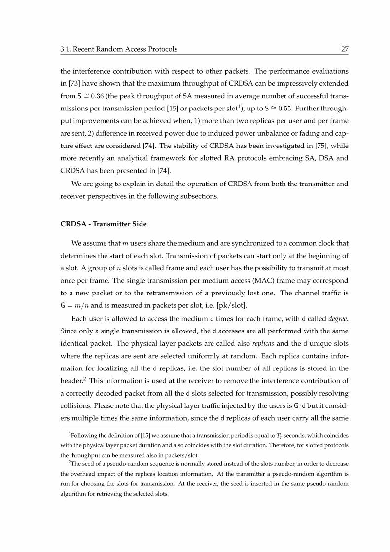
3.1. Recent Random Access Protocols 27
the interference contribution with respect to other packets. The performance evaluations
in [73] have shown that the maximum throughput of CRDSA can be impressively extended
from S ∼= 0.36 (the peak throughput of SA measured in average number of successful trans-
missions per transmission period [15] or packets per slot1), up to S ∼= 0.55. Further through-
put improvements can be achieved when, 1) more than two replicas per user and per frame
are sent, 2) difference in received power due to induced power unbalance or fading and cap-
ture effect are considered [74]. The stability of CRDSA has been investigated in [75], while
more recently an analytical framework for slotted RA protocols embracing SA, DSA and
CRDSA has been presented in [74].
We are going to explain in detail the operation of CRDSA from both the transmitter and
receiver perspectives in the following subsections.
CRDSA - Transmitter Side
We assume thatm users share the medium and are synchronized to a common clock that
determines the start of each slot. Transmission of packets can start only at the beginning of
a slot. A group of n slots is called frame and each user has the possibility to transmit at most
once per frame. The single transmission per medium access (MAC) frame may correspond
to a new packet or to the retransmission of a previously lost one. The channel traffic is
G = m/n and is measured in packets per slot, i.e. [pk/slot].
Each user is allowed to access the medium d times for each frame, with d called degree.
Since only a single transmission is allowed, the d accesses are all performed with the same
identical packet. The physical layer packets are called also replicas and the d unique slots
where the replicas are sent are selected uniformly at random. Each replica contains infor-
mation for localizing all the d replicas, i.e. the slot number of all replicas is stored in the
header.2 This information is used at the receiver to remove the interference contribution of
a correctly decoded packet from all the d slots selected for transmission, possibly resolving
collisions. Please note that the physical layer traffic injected by the users is G ·d but it consid-
ers multiple times the same information, since the d replicas of each user carry all the same
1Following the definition of [15] we assume that a transmission period is equal to Tp seconds, which coincides
with the physical layer packet duration and also coincides with the slot duration. Therefore, for slotted protocols
the throughput can be measured also in packets/slot.2The seed of a pseudo-random sequence is normally stored instead of the slots number, in order to decrease
the overhead impact of the replicas location information. At the transmitter a pseudo-random algorithm is
run for choosing the slots for transmission. At the receiver, the seed is inserted in the same pseudo-random
algorithm for retrieving the selected slots.
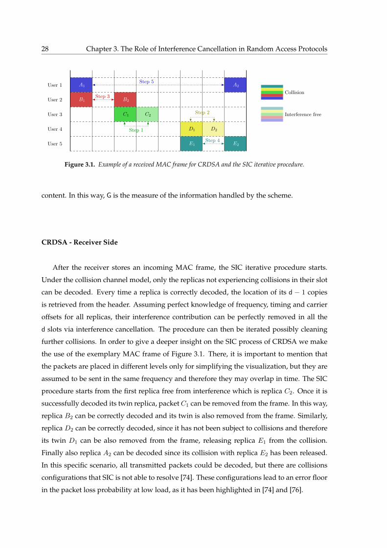
28 Chapter 3. The Role of Interference Cancellation in Random Access Protocols
User 1
User 2
User 3
User 4
User 5
A1 A2
B1 B2
C1 C2
D1 D2
E1 E2
Collision
Interference free
Step 1
Step 2
Step 5
Step 3
Step 4
Figure 3.1. Example of a received MAC frame for CRDSA and the SIC iterative procedure.
content. In this way, G is the measure of the information handled by the scheme.
CRDSA - Receiver Side
After the receiver stores an incoming MAC frame, the SIC iterative procedure starts.
Under the collision channel model, only the replicas not experiencing collisions in their slot
can be decoded. Every time a replica is correctly decoded, the location of its d − 1 copies
is retrieved from the header. Assuming perfect knowledge of frequency, timing and carrier
offsets for all replicas, their interference contribution can be perfectly removed in all the
d slots via interference cancellation. The procedure can then be iterated possibly cleaning
further collisions. In order to give a deeper insight on the SIC process of CRDSA we make
the use of the exemplary MAC frame of Figure 3.1. There, it is important to mention that
the packets are placed in different levels only for simplifying the visualization, but they are
assumed to be sent in the same frequency and therefore they may overlap in time. The SIC
procedure starts from the first replica free from interference which is replica C2. Once it is
successfully decoded its twin replica, packet C1 can be removed from the frame. In this way,
replica B2 can be correctly decoded and its twin is also removed from the frame. Similarly,
replica D2 can be correctly decoded, since it has not been subject to collisions and therefore
its twin D1 can be also removed from the frame, releasing replica E1 from the collision.
Finally also replica A2 can be decoded since its collision with replica E2 has been released.
In this specific scenario, all transmitted packets could be decoded, but there are collisions
configurations that SIC is not able to resolve [74]. These configurations lead to an error floor
in the packet loss probability at low load, as it has been highlighted in [74] and [76].

3.1. Recent Random Access Protocols 29
CRDSA Evolutions and Some Results
The exploitation of interference cancellation pioneered by CRDSA and its outstanding
performance compared to SA and DSA, lead to a new wave of interest for RA protocols
in the research community. Among the evolutions of CRDSA, we would like to mention
three of them, i.e. irregular repetition slotted ALOHA (IRSA) [77], coded slotted ALOHA
(CSA) [78,79] and Frameless ALOHA [80]. In IRSA the link between SIC and iterative decod-
ing on bipartite graphs has been for the first time established. This intuition directly leads
to the exploitation of tools used typically for the analysis and optimisation of iteratively-
decodable codes to the optimisation of CRDSA. The similitude holds replacing the check
nodes with time slots and variable nodes with the users. In this context, each replica is
represented as an edge between a variable node and a check node. The observation that
irregular bipartite graph constructions (variable number of edges emanating from the vari-
able nodes) lead to better iterative decoding threshold with respect to regular graphs (fixed
number of edges emanating from the variable nodes) [77], suggests that allowing a variable
number of replicas per user improves the performance of CRDSA. Moreover, the probability
distribution of the degree can be optimised in order to achieve the maximum throughput.3
Liva [77] used density evolution for the optimisation and showed a consistent improvement
in the throughput performance (as can be observed in Figure 3.2). A further evolution of
CRDSA is CSA [78, 79] where the replicas of each user are not simple repetition of the same
information, but are instead an encoded sequence that is defined independently by each
user. By means of density evolution, the degree distribution is optimised in order to ob-
tain the maximum throughput. Recently, it has been demonstrated that a proper design of
the degree probability mass function in IRSA and CSA achieves 1 pk/slot throughput [81],
which is the maximum achievable under the collision channel.
Along a similar line of research, the work of Stefanovic and his co-authors in [80], in-
vestigates the behaviour of RA protocols with repetitions where the frame dimension is
not set a-priori but it is dynamically adapted for maximising the throughput. The scheme
resembles to rateless codes (called also fountain codes) [82], a forward error correction con-
struction where no code rate is set a-priori and the sources keeps sending encoded symbols
until the message is correctly received. In a similar way, an increasing number of users shar-
ing the channel are allowed to send their data, until a target throughput is reached. At this
point the frame is stopped and unresolved users are notified.
3Although the argument of the optimisation holds for asymptotically large frames, simulation results have
proven that good degree distributions in the asymptotic domain perform also well in the finite frame scenario.
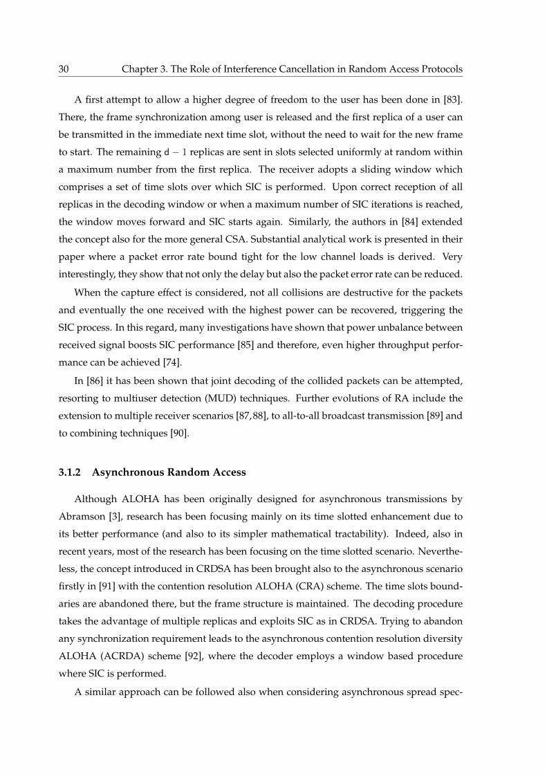
30 Chapter 3. The Role of Interference Cancellation in Random Access Protocols
A first attempt to allow a higher degree of freedom to the user has been done in [83].
There, the frame synchronization among user is released and the first replica of a user can
be transmitted in the immediate next time slot, without the need to wait for the new frame
to start. The remaining d − 1 replicas are sent in slots selected uniformly at random within
a maximum number from the first replica. The receiver adopts a sliding window which
comprises a set of time slots over which SIC is performed. Upon correct reception of all
replicas in the decoding window or when a maximum number of SIC iterations is reached,
the window moves forward and SIC starts again. Similarly, the authors in [84] extended
the concept also for the more general CSA. Substantial analytical work is presented in their
paper where a packet error rate bound tight for the low channel loads is derived. Very
interestingly, they show that not only the delay but also the packet error rate can be reduced.
When the capture effect is considered, not all collisions are destructive for the packets
and eventually the one received with the highest power can be recovered, triggering the
SIC process. In this regard, many investigations have shown that power unbalance between
received signal boosts SIC performance [85] and therefore, even higher throughput perfor-
mance can be achieved [74].
In [86] it has been shown that joint decoding of the collided packets can be attempted,
resorting to multiuser detection (MUD) techniques. Further evolutions of RA include the
extension to multiple receiver scenarios [87,88], to all-to-all broadcast transmission [89] and
to combining techniques [90].
3.1.2 Asynchronous Random Access
Although ALOHA has been originally designed for asynchronous transmissions by
Abramson [3], research has been focusing mainly on its time slotted enhancement due to
its better performance (and also to its simpler mathematical tractability). Indeed, also in
recent years, most of the research has been focusing on the time slotted scenario. Neverthe-
less, the concept introduced in CRDSA has been brought also to the asynchronous scenario
firstly in [91] with the contention resolution ALOHA (CRA) scheme. The time slots bound-
aries are abandoned there, but the frame structure is maintained. The decoding procedure
takes the advantage of multiple replicas and exploits SIC as in CRDSA. Trying to abandon
any synchronization requirement leads to the asynchronous contention resolution diversity
ALOHA (ACRDA) scheme [92], where the decoder employs a window based procedure
where SIC is performed.
A similar approach can be followed also when considering asynchronous spread spec-
3.1. Recent Random Access Protocols 31
0 0.1 0.2 0.3 0.4 0.5 0.6 0.7 0.8 0.9 10
0.1
0.2
0.3
0.4
0.5
0.6
0.7
0.8
Channel load G [pk/slot]
Thr
ough
put
S[p
k/slo
t]
Slotted ALOHADSA, d = 2CRDSA, d = 2IRSA, Λ = 0.5x2 + 0.28x3 + 0.22x8
Figure 3.2. Throughput comparison of SA, DSA, CRDSA and IRSA under the collision channel. Both
DSA and CRDSA send two copies for each transmitted packet and CRDSA employs SIC at the receiver
side. In IRSA each user picks a degree d following the p.m.f. Λ. Specifically, with probability 1/2 two
copies will be sent, with probability 0.28 three and with probability 0.22 eight. The use of variable number
of replicas per user greatly improves the throughput compared to CRDSA although for very high channel
load values, the degradation is more severe.

32 Chapter 3. The Role of Interference Cancellation in Random Access Protocols
A BC
Figure 3.3. Hidden terminal scenario. Node A and node B want to communicate to node C and they are
not able to sense each other since they are out of the reception range.
trum random access as in [93], with the enhanced-spread spectrum ALOHA (E-SSA). Prior
transmission on the channel, each packet symbol is multiplied with a spreading sequence,
possibly different user by user. It is important to stress that here no replicas are used,
i.e. each terminal sends only one packet per transmission. At the receiver side, SIC is
employed for removing interference once packets are correctly decoded. In this way the
throughput performance can be drastically improved [94]. Thanks to its remarkable per-
formance, E-SSA has been selected by European Telecommunications Standards Institute
(ETSI) as one of the two options for the return link MAC layer of the S-band mobile inter-
active multimedia (S-MIM) standard [95]. The aim of S-MIM is to standardise messaging
services over S-band via geostationary orbit (GEO) satellites.
Being a very interesting solution, the extension of CRDSA to asynchronous schemes has
minor differences to its original. For this reason, we will focus here on a slightly different
issue that is typical in wireless MAC and also in RA: the hidden terminal problem and a
new way of combating it employing interference cancellation (IC). Let us assume that the
terminals are employing CSMA collision avoidance (CSMA/CA) as medium access as in
IEEE 802.11 standard and are able to sense the channel. Unfortunately, if two terminals
that are not in reciprocal radio reception range want to communicate with a third node as in
Figure 3.3, there is a probability that the two terminal transmissions collide at the receiver re-
sulting in the hidden terminal problem. In order to overcome possible collisions, the request
to send / clear to send (RTS/CTS) procedure is suggested by the standard, but it is disabled
by default from the access points manufacturers due to its significant impact on the over-
all throughput [96]. A new way of counteracting the hidden terminal problem without the
need of RTS/CTS has been firstly proposed by Gollakota and Katabi in [96] with the ZigZag
decoding. The core idea is to exploit asynchrony between successive collisions. Terminals
that collide once, are with high probability susceptible to collide again in the retransmission
phases. On the other hand, successive collisions are likely to have different interference-free
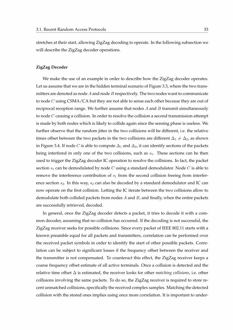
3.1. Recent Random Access Protocols 33
stretches at their start, allowing ZigZag decoding to operate. In the following subsection we
will describe the ZigZag decoder operations.
ZigZag Decoder
We make the use of an example in order to describe how the ZigZag decoder operates.
Let us assume that we are in the hidden terminal scenario of Figure 3.3, where the two trans-
mitters are denoted as nodeA and nodeB respectively. The two nodes want to communicate
to node C using CSMA/CA but they are not able to sense each other because they are out of
reciprocal reception range. We further assume that nodes A and B transmit simultaneously
to node C causing a collision. In order to resolve the collision a second transmission attempt
is made by both nodes which is likely to collide again since the sensing phase is useless. We
further observe that the random jitter in the two collisions will be different, i.e. the relative
times offset between the two packets in the two collisions are different ∆1 6= ∆2, as shown
in Figure 3.4. If node C is able to compute ∆1 and ∆2, it can identify sections of the packets
being interfered in only one of the two collisions, such as s1. These sections can be then
used to trigger the ZigZag decoder IC operation to resolve the collisions. In fact, the packet
section s1 can be demodulated by node C using a standard demodulator. Node C is able to
remove the interference contribution of s1 from the second collision freeing from interfer-
ence section s2. In this way, s2 can also be decoded by a standard demodulator and IC can
now operate on the first collision. Letting the IC iterate between the two collisions allow to
demodulate both collided packets from nodes A and B, and finally, when the entire packets
are successfully retrieved, decoded.
In general, once the ZigZag decoder detects a packet, it tries to decode it with a com-
mon decoder, assuming that no collision has occurred. If the decoding is not successful, the
ZigZag receiver seeks for possible collisions. Since every packet of IEEE 802.11 starts with a
known preamble equal for all packets and transmitters, correlation can be performed over
the received packet symbols in order to identify the start of other possible packets. Corre-
lation can be subject to significant losses if the frequency offset between the receiver and
the transmitter is not compensated. To counteract this effect, the ZigZag receiver keeps a
coarse frequency offset estimate of all active terminals. Once a collision is detected and the
relative time offset ∆ is estimated, the receiver looks for other matching collisions, i.e. other
collisions involving the same packets. To do so, the ZigZag receiver is required to store re-
cent unmatched collisions, specifically the received complex samples. Matching the detected
collision with the stored ones implies using once more correlation. It is important to under-
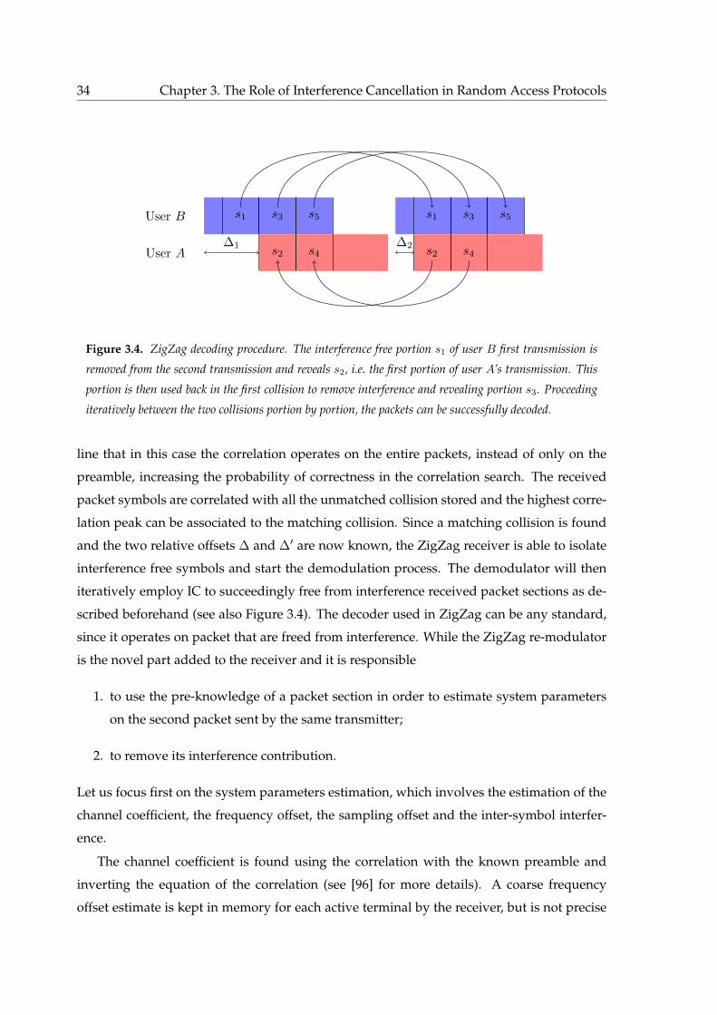
34 Chapter 3. The Role of Interference Cancellation in Random Access Protocols
User B
User A
s1 s1
s2s2
s3 s3
s4s4
s5 s5
∆1 ∆2
Figure 3.4. ZigZag decoding procedure. The interference free portion s1 of user B first transmission is
removed from the second transmission and reveals s2, i.e. the first portion of user A’s transmission. This
portion is then used back in the first collision to remove interference and revealing portion s3. Proceeding
iteratively between the two collisions portion by portion, the packets can be successfully decoded.
line that in this case the correlation operates on the entire packets, instead of only on the
preamble, increasing the probability of correctness in the correlation search. The received
packet symbols are correlated with all the unmatched collision stored and the highest corre-
lation peak can be associated to the matching collision. Since a matching collision is found
and the two relative offsets ∆ and ∆′ are now known, the ZigZag receiver is able to isolate
interference free symbols and start the demodulation process. The demodulator will then
iteratively employ IC to succeedingly free from interference received packet sections as de-
scribed beforehand (see also Figure 3.4). The decoder used in ZigZag can be any standard,
since it operates on packet that are freed from interference. While the ZigZag re-modulator
is the novel part added to the receiver and it is responsible
1. to use the pre-knowledge of a packet section in order to estimate system parameters
on the second packet sent by the same transmitter;
2. to remove its interference contribution.
Let us focus first on the system parameters estimation, which involves the estimation of the
channel coefficient, the frequency offset, the sampling offset and the inter-symbol interfer-
ence.
The channel coefficient is found using the correlation with the known preamble and
inverting the equation of the correlation (see [96] for more details). A coarse frequency
offset estimate is kept in memory for each active terminal by the receiver, but is not precise
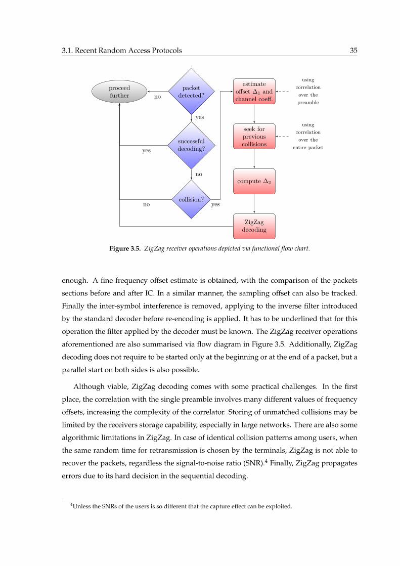
3.1. Recent Random Access Protocols 35
packetdetected?
successfuldecoding?
collision?
estimateoffset ∆1 andchannel coeff.
seek forpreviouscollisions
compute ∆2
ZigZagdecoding
proceedfurther
usingcorrelation
over thepreamble
usingcorrelation
over theentire packet
yes
no
yes
no
no yes
Figure 3.5. ZigZag receiver operations depicted via functional flow chart.
enough. A fine frequency offset estimate is obtained, with the comparison of the packets
sections before and after IC. In a similar manner, the sampling offset can also be tracked.
Finally the inter-symbol interference is removed, applying to the inverse filter introduced
by the standard decoder before re-encoding is applied. It has to be underlined that for this
operation the filter applied by the decoder must be known. The ZigZag receiver operations
aforementioned are also summarised via flow diagram in Figure 3.5. Additionally, ZigZag
decoding does not require to be started only at the beginning or at the end of a packet, but a
parallel start on both sides is also possible.
Although viable, ZigZag decoding comes with some practical challenges. In the first
place, the correlation with the single preamble involves many different values of frequency
offsets, increasing the complexity of the correlator. Storing of unmatched collisions may be
limited by the receivers storage capability, especially in large networks. There are also some
algorithmic limitations in ZigZag. In case of identical collision patterns among users, when
the same random time for retransmission is chosen by the terminals, ZigZag is not able to
recover the packets, regardless the signal-to-noise ratio (SNR).4 Finally, ZigZag propagates
errors due to its hard decision in the sequential decoding.
4Unless the SNRs of the users is so different that the capture effect can be exploited.

36 Chapter 3. The Role of Interference Cancellation in Random Access Protocols
Extension of ZigZag, The SigSag Decoder
An extension of ZigZag, called SigSag decoding, has been proposed in [97]. The au-
thors define a procedure where soft-information of each symbol is exploited. In fact, ZigZag
decoding can be seen as a special instance of belief propagation where only the back-
substitution is applied. This corresponds to belief propagation in the high-SNR regime.
SigSag decoding uses an iterative soft message passing algorithm running over the factor
graph of the linear equations that represent packet collisions. In particular, a factor graph
representation of the collisions is associated to the consecutive collisions, as we can see from
Figure 3.6. There two variations of SigSag can be applied, the sum-product algorithm or
the max-product algorithm [98, 99]. The former aims at minimising the bit-error rate via
computing the marginals of each bit. The latter aims at minimising the block-error rate
computing jointly the most likely codeword.
SigSag counteracts succesfully the error propagation introduced by ZigZag, and is able
to profit from larger packet sizes. This effect comes from the message passing algorithm that
profits from larger graphs. Nevertheless, SigSag is not able to resolve collisions where the
relative distance between the users is the same, as in ZigZag. On the other hand, for the
two-user cases and with at least one bit difference in the collision pattern, the authors in [97]
have shown that SigSag is optimal, so it performs as maximum likelihood (ML) decoding.
3.1.3 Tree-Splitting Algorithms
Carefully looking at the tree-splitting collision resolution algorithm, Yu and Giannakis
[100] observed that SIC can be particularly useful in order to reduce the collision resolution
interval (CRI), i.e. the protocol phase in which collisions among multiple transmitters are
resolved through an algorithm.
Let us start with the system model assumptions. In the following, an infinite population
of users sharing a common channel and transmitting to a single receiver is considered. Time
is slotted and slots have a duration equal to the physical layer packets. Poisson arrivals with
a total rate λ distributed over the users is assumed. The collision channel model is adopted
and instantaneous 0/k/e feedback is provided to the users. At the end of each slot the users
are informed errorlessly about the outcome of the last slot. Idle (0) is returned when no
transmission took place. The number of correctly decoded packets (k) is returned in case of
successful decoding (more than one packet per slot can be decoded when SIC is employed,
as we will see later). Finally, if none of the previous two cases happened, an erroneous
reception (e) due to a collision appears in the last slot.
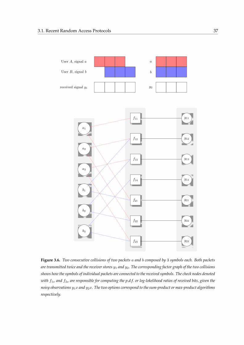
3.1. Recent Random Access Protocols 37
User A, signal a
User B, signal b
received signal y1
a
b
y2
a1
a2
a3
b1
b2
b3
f11
f12
f13
f14
f21
f22
f23
y11
y12
y13
y14
y21
y22
y23
Figure 3.6. Two consecutive collisions of two packets a and b composed by 3 symbols each. Both packets
are transmitted twice and the receiver stores y1 and y2. The corresponding factor graph of the two collisions
shows how the symbols of individual packets are connected to the received symbols. The check nodes denoted
with f1x and f2x are responsible for computing the p.d.f. or log-lokelihood ratios of received bits, given the
noisy observations y1x and y2x. The two options correspond to the sum-product or max-product algorithms
respectively.
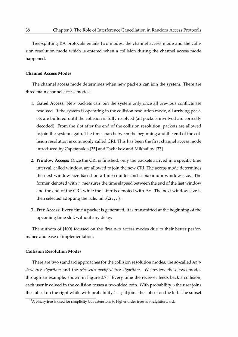
38 Chapter 3. The Role of Interference Cancellation in Random Access Protocols
Tree-splitting RA protocols entails two modes, the channel access mode and the colli-
sion resolution mode which is entered when a collision during the channel access mode
happened.
Channel Access Modes
The channel access mode determines when new packets can join the system. There are
three main channel access modes:
1. Gated Access: New packets can join the system only once all previous conflicts are
resolved. If the system is operating in the collision resolution mode, all arriving pack-
ets are buffered until the collision is fully resolved (all packets involved are correctly
decoded). From the slot after the end of the collision resolution, packets are allowed
to join the system again. The time span between the beginning and the end of the col-
lision resolution is commonly called CRI. This has been the first channel access mode
introduced by Capetanakis [35] and Tsybakov and Mikhailov [37].
2. Window Access: Once the CRI is finished, only the packets arrived in a specific time
interval, called window, are allowed to join the new CRI. The access mode determines
the next window size based on a time counter and a maximum window size. The
former, denoted with τ , measures the time elapsed between the end of the last window
and the end of the CRI, while the latter is denoted with ∆τ . The next window size is
then selected adopting the rule: min∆τ, τ.
3. Free Access: Every time a packet is generated, it is transmitted at the beginning of the
upcoming time slot, without any delay.
The authors of [100] focused on the first two access modes due to their better perfor-
mance and ease of implementation.
Collision Resolution Modes
There are two standard approaches for the collision resolution modes, the so-called stan-
dard tree algorithm and the Massey’s modified tree algorithm. We review these two modes
through an example, shown in Figure 3.7.5 Every time the receiver feeds back a collision,
each user involved in the collision tosses a two-sided coin. With probability p the user joins
the subset on the right while with probability 1− p it joins the subset on the left. The subset
5A binary tree is used for simplicity, but extensions to higher order trees is straightforward.
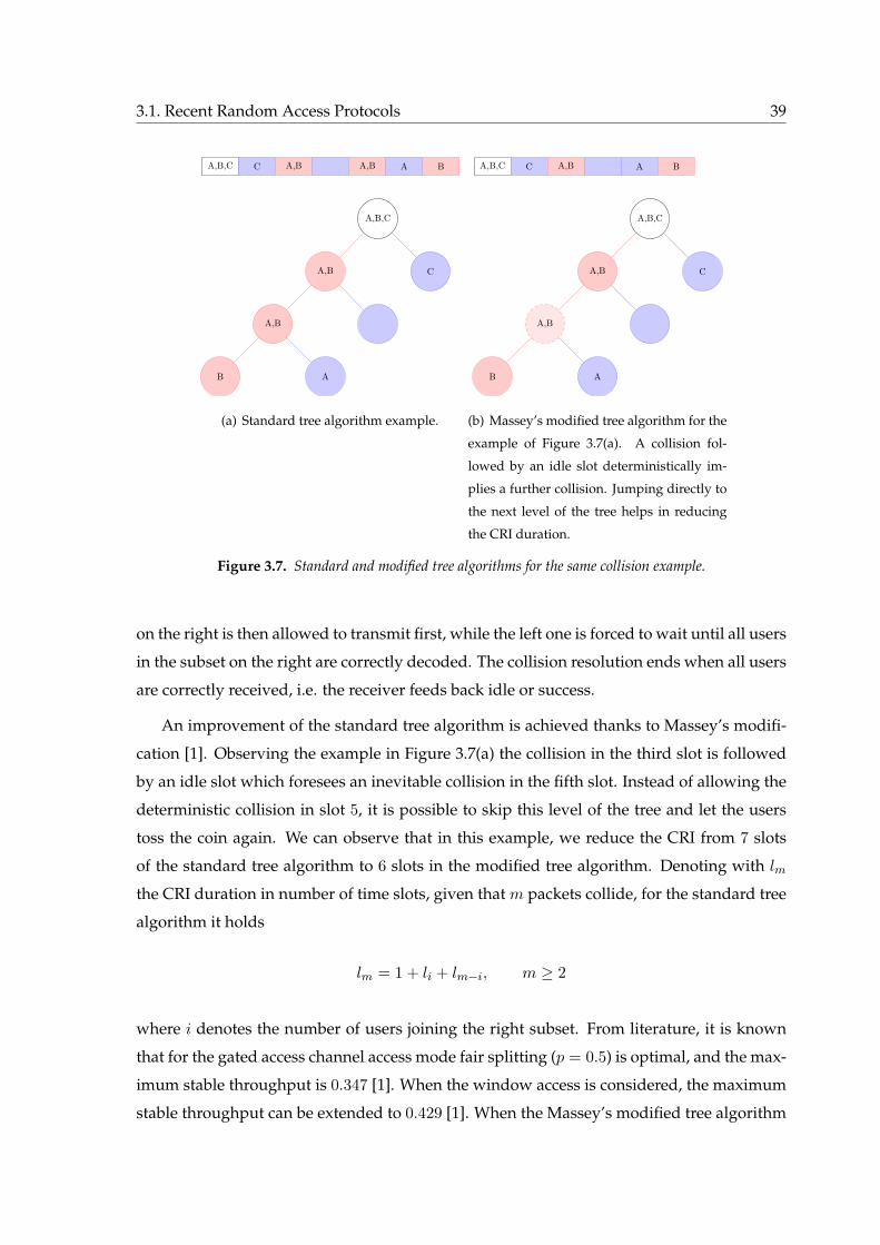
3.1. Recent Random Access Protocols 39
A,B,C
CA,B
A,B
AB
A,B,C C A,B A,B A B
(a) Standard tree algorithm example.
A,B,C
CA,B
A,B
AB
A,B,C C A,B A B
(b) Massey’s modified tree algorithm for the
example of Figure 3.7(a). A collision fol-
lowed by an idle slot deterministically im-
plies a further collision. Jumping directly to
the next level of the tree helps in reducing
the CRI duration.
Figure 3.7. Standard and modified tree algorithms for the same collision example.
on the right is then allowed to transmit first, while the left one is forced to wait until all users
in the subset on the right are correctly decoded. The collision resolution ends when all users
are correctly received, i.e. the receiver feeds back idle or success.
An improvement of the standard tree algorithm is achieved thanks to Massey’s modifi-
cation [1]. Observing the example in Figure 3.7(a) the collision in the third slot is followed
by an idle slot which foresees an inevitable collision in the fifth slot. Instead of allowing the
deterministic collision in slot 5, it is possible to skip this level of the tree and let the users
toss the coin again. We can observe that in this example, we reduce the CRI from 7 slots
of the standard tree algorithm to 6 slots in the modified tree algorithm. Denoting with lm
the CRI duration in number of time slots, given that m packets collide, for the standard tree
algorithm it holds
lm = 1 + li + lm−i, m ≥ 2
where i denotes the number of users joining the right subset. From literature, it is known
that for the gated access channel access mode fair splitting (p = 0.5) is optimal, and the max-
imum stable throughput is 0.347 [1]. When the window access is considered, the maximum
stable throughput can be extended to 0.429 [1]. When the Massey’s modified tree algorithm
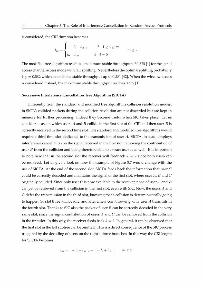
40 Chapter 3. The Role of Interference Cancellation in Random Access Protocols
is considered, the CRI duration becomes
lm =
1 + li + lm−i, if 1 ≥ i ≥ m
l0 + lm, if i = 0m ≥ 2.
The modified tree algorithm reaches a maximum stable throughput of 0.375 [1] for the gated
access channel access mode with fair splitting. Nevertheless the optimal splitting probability
is p = 0.582 which extends the stable throughput up to 0.381 [42]. When the window access
is considered instead, the maximum stable throughput reaches 0.462 [1].
Successive Interference Cancellation Tree Algorithm (SICTA)
Differently from the standard and modified tree algorithms collision resolution modes,
in SICTA collided packets during the collision resolution are not discarded but are kept in
memory for further processing. Indeed they become useful when SIC takes place. Let us
consider a case in which users A and B collide in the first slot of the CRI and then user B is
correctly received in the second time slot. The standard and modified tree algorithms would
require a third time slot dedicated to the transmission of user A. SICTA, instead, employs
interference cancellation on the signal received in the first slot, removing the contribution of
user B from the collision and being therefore able to extract user A as well. It is important
to note here that in the second slot the receiver will feedback k = 2 since both users can
be resolved. Let us give a look on how the example of Figure 3.7 would change with the
use of SICTA. At the end of the second slot, SICTA feeds back the information that user C
could be correctly decoded and maintains the signal of the first slot, where user A, B and C
originally collided. Since only user C is now available to the receiver, none of user A and B
can yet be retrieved from the collision in the first slot, even with SIC. Now, the users A and
B defer the transmission in the third slot, knowing that a collision is deterministically going
to happen. So slot three will be idle, and after a new coin throwing, only user A transmits in
the fourth slot. Thanks to SIC also the packet of user B can be correctly decoded in the very
same slot, since the signal contribution of users A and C can be removed from the collision
in the first slot. In this way, the receiver feeds back k = 2. In general, it can be observed that
the first slot in the left subtree can be omitted. This is a direct consequence of the SIC process
triggered by the decoding of users on the right subtree branches. In this way the CRI length
for SICTA becomes
lm = 1 + li + lm−i − 1 = li + lm−i m ≥ 2.
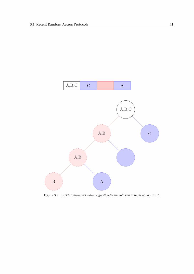
3.1. Recent Random Access Protocols 41
A,B,C
CA,B
A,B
AB
A,B,C C A
Figure 3.8. SICTA collision resolution algorithm for the collision example of Figure 3.7.
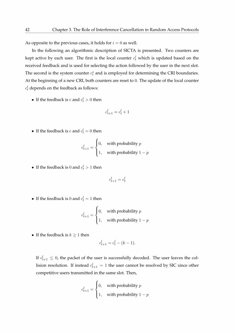
42 Chapter 3. The Role of Interference Cancellation in Random Access Protocols
As opposite to the previous cases, it holds for i = 0 as well.
In the following an algorithmic description of SICTA is presented. Two counters are
kept active by each user. The first is the local counter clt which is updated based on the
received feedback and is used for selecting the action followed by the user in the next slot.
The second is the system counter cst and is employed for determining the CRI boundaries.
At the beginning of a new CRI, both counters are reset to 0. The update of the local counter
clt depends on the feedback as follows:
• If the feedback is e and clt > 0 then
clt+1 = clt + 1
• If the feedback is e and clt = 0 then
clt+1 =
0, with probability p
1, with probability 1− p
• If the feedback is 0 and clt > 1 then
clt+1 = clt
• If the feedback is 0 and clt = 1 then
clt+1 =
0, with probability p
1, with probability 1− p
• If the feedback is k ≥ 1 then
clt+1 = clt − (k − 1).
If clt+1 ≤ 0, the packet of the user is successfully decoded. The user leaves the col-
lision resolution. If instead clt+1 = 1 the user cannot be resolved by SIC since other
competitive users transmitted in the same slot. Then,
clt+1 =
0, with probability p
1, with probability 1− p
3.1. Recent Random Access Protocols 43
A user retransmits the packet in slot t every time clt = 0. The system counter is updated as
follows
• If feedback is e
cst+1 = cst + 1
• If feedback is 0
cst+1 = cst
• If feedback is k
cst+1 = cst − (k − 1).
The current collision resolution algorithm stops when the system counter reaches 0.
In [100] the authors show that for the gated access the maximum stable throughput of
SICTA is 0.6931. Interestingly it is achieved for binary j = 2 fair splitting, unlike the standard
tree algorithm where the optimum was achieved with ternary j = 3 splitting (instead of
dividing the users into two classes depending on the outcome of the coin flipping procedure,
they are divided into three classes). For SICTA, the maximum stable throughput S follows6
S ≈ ln j
j− 1.
We can observe that,
• For j→∞ the maximum stable throughput of SICTA degenerates rapidly towards the
standard tree algorithm;
• SICTA exceeds the upper bound derived by Tsybakov and Likhanov of 0.568 [39]. We
shall note here that the upper bound by Tsybakov and Likhanov is valid for ternary
feedback (idle, collision, success). Indeed, as pointed out in a seminal work of Massey
[101], a more proper bound for random access with multiplicity feedback, as SICTA is,
is due to Pippinger [102] and it is 1.
Moving to the window access, the maximum stable throughput S is as well 0.693 but it is
reached for a maximum window size tending to infinite, i.e. ∆τ → ∞, which corresponds
6Details on the stable throughput expression are here omitted and can be found in [100].
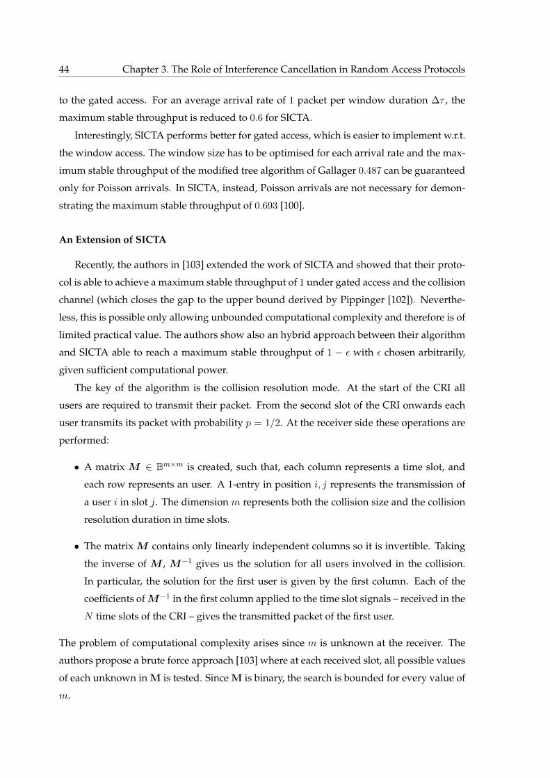
44 Chapter 3. The Role of Interference Cancellation in Random Access Protocols
to the gated access. For an average arrival rate of 1 packet per window duration ∆τ , the
maximum stable throughput is reduced to 0.6 for SICTA.
Interestingly, SICTA performs better for gated access, which is easier to implement w.r.t.
the window access. The window size has to be optimised for each arrival rate and the max-
imum stable throughput of the modified tree algorithm of Gallager 0.487 can be guaranteed
only for Poisson arrivals. In SICTA, instead, Poisson arrivals are not necessary for demon-
strating the maximum stable throughput of 0.693 [100].
An Extension of SICTA
Recently, the authors in [103] extended the work of SICTA and showed that their proto-
col is able to achieve a maximum stable throughput of 1 under gated access and the collision
channel (which closes the gap to the upper bound derived by Pippinger [102]). Neverthe-
less, this is possible only allowing unbounded computational complexity and therefore is of
limited practical value. The authors show also an hybrid approach between their algorithm
and SICTA able to reach a maximum stable throughput of 1 − ε with ε chosen arbitrarily,
given sufficient computational power.
The key of the algorithm is the collision resolution mode. At the start of the CRI all
users are required to transmit their packet. From the second slot of the CRI onwards each
user transmits its packet with probability p = 1/2. At the receiver side these operations are
performed:
• A matrix M ∈ Bm×m is created, such that, each column represents a time slot, and
each row represents an user. A 1-entry in position i, j represents the transmission of
a user i in slot j. The dimension m represents both the collision size and the collision
resolution duration in time slots.
• The matrix M contains only linearly independent columns so it is invertible. Taking
the inverse of M , M−1 gives us the solution for all users involved in the collision.
In particular, the solution for the first user is given by the first column. Each of the
coefficients of M−1 in the first column applied to the time slot signals – received in the
N time slots of the CRI – gives the transmitted packet of the first user.
The problem of computational complexity arises since m is unknown at the receiver. The
authors propose a brute force approach [103] where at each received slot, all possible values
of each unknown in M is tested. Since M is binary, the search is bounded for every value of
m.

3.1. Recent Random Access Protocols 45
The authors are able to upper bound the average time of the CRI lm as
lm ≤ m+m−1∑k=1
1
2k − 1≈ m for sufficiently large m.
3.1.4 Random Access Without Feedback
If feedback is not possible due to the lack of dedicated return channel or due to hardware
limitations, we speak about RA without feedback. A way to approach channel capacity in
such scenarios is to let users adopt protocol sequences which dictates the time slots where the
users are active. Protocol sequences are deterministic, but each user picks a sequence at
random from the pool and the user will become active in a time slot which is independent
from the other users, preserving the random nature of the channel access.
Protocol sequences for the RA without feedback channel have been mainly studied for
the collision channel. Only recently authors in [104] investigated the protocol sequences’
design and performance for the ι-multi-packet reception (ι-MPR) channel. The ι-MPR chan-
nel model ensures that collisions involving up to ι users can be successfully resolved, i.e. all
the ι users involved in the collision can be successfully decoded by means of multi-packet
reception (MPR) techniques.7
The sequences are periodic and in general the throughput depends on the relative shifts
among the users. A first class is the so-called shift invariant (SI) sequences. Their peculiar
property is that their generalised Hamming cross-correlation functions are independent of
relative shifts.8 A second class are the throughput invariant (TI) sequences where instead
the throughput is shift invariant. The advantages of TI sequences are strictly positive and
maximal worst case throughput among all protocol sequence based access schemes and ease
to use with forward error correction (FEC) due to the shift invariant property.
Let us have a look at the system model. We consider a slot synchronous system where all
nu users’ transmissions are synchronised at slot level. Each user’s packet occupies exactly
one time slot. The user i’s protocol sequence is a deterministic and periodic binary sequence
b(i) :=[b(i)0 , b
(i)1 , ..., b
(i)L−1
]that determines the instants in time where user i will transmit,
i.e. user i transmits in slot t iff b(i)t−τi = 1. The protocol sequence duration or sequence period
7The ι-MPR channel model can emulate the behaviour of a receiver able to do interference cancellation, when
adopting the proper ι. More in general, the adoption of the MPR matrix representation [60] can lead to a precise
characterization of the SIC behaviour but it is not considered by the authors in the paper [104].8The generalised Hamming cross-correlation function can be seen as the number of slot indices where the
two sequences have both an entry equal to one. A formal definition can be found in [105]. For SI sequences in
particular, the generalised Hamming cross-correlation function it is invariant to sequence shifts.

46 Chapter 3. The Role of Interference Cancellation in Random Access Protocols
in time slots is L. The subtraction is therefore a modulo-L subtraction. User i has a relative
shift of τi time slots w.r.t. the receiver’s common clock time indexed by t. The relative shifts
τi, i = 1, ..., nu of the users are independently chosen and are not known to the common
receiver. The duty factor d(i)f of user i’s protocol sequence is defined as the fraction of ones
in b(i) over its length, or more formally
d(i)f :=
1
L
L−1∑t=0
b(i)t .
It is assumed that each sequence has a non-zero duty factor and that there are at most ι− 1
all one sequences.
Throughput Analysis
The analysis of [104] aims at deriving the throughput of TI sequences and shows that
it is dependent on the duty factors of the sequences only. The full derivation including the
case of non symmetric duty factors for the users is presented in [104], while here only the
final throughput result for the symmetric duty cycle case is recalled:
S = nu
ι−1∑k=1
(nu − 1
k
)dk+1f (1− df )nu−1−k.
The channel load G is then G = nudf . As mentioned by Zhang, the throughput S of the
system depends only on the duty factor, on the maximum collision size such that all packets
can be still correctly decoded the parameter ι and the number nu of users in the system. For
every couple of total active users nu and ι, there is an optimal duty factor that maximises
the throughput. This can be found following the approach of [106], where the transmission
probability is the equivalent of the duty factor. Noticeably, no feedback is required in this
approach with respect to the slotted ALOHA system considered in [106].
Construction of Minimum Period TI Sequences
In this Section we present the construction of minimum period TI sequences. The im-
portance of minimum period sequences relies in the higher robustness against performance
variability over short time periods given the same target performance. Without going into
theoretical details, Zhang and his co-authors demonstrated that minimum period TI se-
quences can be built from SI sequences. A possible construction can be found in [107] and
is recalled here through an example.
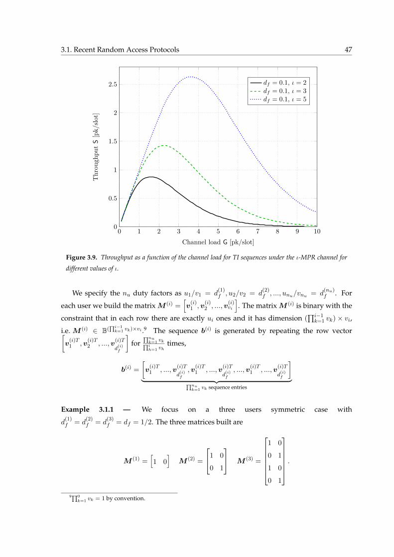
3.1. Recent Random Access Protocols 47
0 1 2 3 4 5 6 7 8 9 100
0.5
1
1.5
2
2.5
Channel load G [pk/slot]
Thr
ough
put
S[p
k/slo
t]
df = 0.1, ι = 2df = 0.1, ι = 3df = 0.1, ι = 5
Figure 3.9. Throughput as a function of the channel load for TI sequences under the ι-MPR channel for
different values of ι.
We specify the nu duty factors as u1/v1 = d(1)f , u2/v2 = d
(2)f , ..., unu/vnu = d
(nu)f . For
each user we build the matrix M (i) =[v
(i)1 ,v
(i)2 , ...,v
(i)vi
]. The matrix M (i) is binary with the
constraint that in each row there are exactly ui ones and it has dimension (∏i−1k=1 vk)× vi,
i.e. M (i) ∈ B(∏i−1k=1 vk)×vi .9 The sequence b(i) is generated by repeating the row vector[
v(i)T1 ,v
(i)T2 , ...,v
(i)T
d(i)f
]for
∏nuk=1 vk∏ih=1 vh
times,
b(i) =
[v
(i)T1 , ...,v
(i)T
d(i)f
,v(i)T1 , ...,v
(i)T
d(i)f
, ...,v(i)T1 , ...,v
(i)T
d(i)f
]︸ ︷︷ ︸∏nu
k=1 vk sequence entries
Example 3.1.1 — We focus on a three users symmetric case with
d(1)f = d
(2)f = d
(3)f = df = 1/2. The three matrices built are
M (1) =[1 0
]M (2) =
1 0
0 1
M (3) =
1 0
0 1
1 0
0 1
.
9∏0k=1 vk = 1 by convention.
48 Chapter 3. The Role of Interference Cancellation in Random Access Protocols
The following three bit sequences can be obtained:
b(1) = [10101010]
b(2) = [10011001]
b(3) = [10100101] .
Some Recent Results of SI Sequences with Interference Cancellation
Recently, the research group published a work in which the protocol sequences used in
the collision channel without feedback are investigated together with SIC [105]. The main
result achieved is the demonstration that, with proper sequence selection and when SIC
is employed at the receiver, the limit of 1 packet per slot is reachable. Some important
consequences are
• The zero-error capacity region of a RA system without feedback employing SIC is
coincident with the one of a system guaranteeing orthogonal multiple access, e.g. time
division multiple access (TDMA). In this way, the lack of orthogonality, which does not
guarantee interference free transmissions to the user, does not harm the performance
as long as SIC can be performed at the receiver. It is here important to underline that
ideal SIC is assumed, i.e. perfect interference cancellation of correctly decoded packets
is performed.
• The symmetric case (typical for many systems) in which all users transmit with the
same rate is on the outer boundary of the capacity region, i.e. also the symmetric case
achieves 1 packet per slot capacity. This result is particularly interesting because it
is in contrast with the case without SIC [43]. In that case in fact, the symmetric case
minimises the capacity.
• The outer boundary of the zero-error capacity region with rational components can be
achieved (which means that it is possible to reach zero-error capacity with rate points
that lie on the outer boundary) only with the help of SI sequences. Minimum period
SI sequences are therefore the sequences with smallest period possible reaching the
outer boundary of the zero-error capacity region. Construction of these follows the
procedure presented in the previous Section.
• For the symmetric case, the minimum period is nu!, which is consistently smaller than
nnuu , the minimum period of the case without SIC [104].
3.2. Applicable Scenarios 49
3.2 Applicable Scenarios
The improvements in the efficiency of recent RA protocols, observable from all the pre-
viously presented schemes and not limited to them, widen the scenarios where RA schemes
can be used. A selection of four possible areas in which recent RA schemes are identified as
suitable candidates for future communication systems or standards is the following:
• satellite communication systems and machine-to-machine (M2M);
• long-term evolution (LTE) and the upcoming fifth generation (5G);
• vehicle-to-vehicle (V2V) communication systems;
• Underwater communication systems.
For each of the four areas we give a brief overview of the typical challenges as well as some
hints on how RA protocols manage to overcome them.
Satellite Communication Systems and M2M
From the origin of ALOHA, the typical scenario of such RA protocols has been the satel-
lite communication system. The distance between transmitting terminals prevents the use
of sensing techniques deployed in terrestrial RA based systems, such as carrier sense mul-
tiple access (CSMA), while the peculiar very long round trip time limits the efficiency of
on-demand systems such as demand assigned multiple access (DAMA). The former is due
to the wide footprint of GEO satellites guarantee connectivity to terminals and that can be
thousands of kilometers far apart. The latter, instead, is due to the extreme transmission
delay (up to 500 ms round trip time delay) that a GEO satellite link suffers which affects any
communication and may restrict the usage of handshake mechanisms necessary for DAMA-
like protocols to allocate resources to the terminals.
This is the reason why a number of different satellite standards foresee the use of RA
protocols. The Digital Video Broadcasting - Return Channel Satellite 2nd Generation (DVB-
RCS2) [108] adopts both CRDSA [73] and IRSA [77] as options, not only for the user terminal
logon at the beginning of a session, but also foresees the possibility to use these protocols
for data communication through reserved slots in the multi-frequency time division mul-
tiple access (MF-TDMA) frames. The emerging market of mobile satellite terminals calls
for development of suitable satellite systems able to cope with this extremely challenging
scenario. A first answer comes from the novel S-MIM standard [95]. It comprises forward
and return links for bi-directional communication and for the return link (from gateway,

50 Chapter 3. The Role of Interference Cancellation in Random Access Protocols
through satellite to mobile terminal) one of the two options is to use RA for communication.
In particular E-SSA [93] is foreseen as the RA MAC option.
Nowadays, the use of satellites for communication is the only option for ships that are
in oceanic travel. In order to incorporate the automatic identification system (AIS) and
application-specific messages (ASM) [109] messaging systems in a more wide communica-
tion system, the novel VHF data exchange system (VDES) has been recently introduced [110]
and is currently under standardization by International Telecommunications Union (ITU).
Safety critical messages for collision avoidance, as provided by AIS, are sharing the channel
with other types of messages. VDES aims at releasing the AIS channels from non-safety crit-
ical traffic which is reverted to ASM and other dedicated channels. Satellite and terrestrial
components are both considered for non-safety critical messaging. For the former, RA with
both narrowband and spread spectrum communication systems is allowed. In this regard
both CRA [91] enhanced contention resolution ALOHA (ECRA) [111] or E-SSA [93] appear
to be good candidates.
LTE and 5G
The M2M application in terrestrial mobile networks is a big driver as well. Many recent
works focus on the investigation of RA for M2M applications in LTE or LTE-Advanced (LTE-
A) [13]. In today’s LTE the RA procedure comprises a four messages handshake in order to
establish a connection. Precisely, RA is used in LTE for the network logon or for request of
resources for transmission or re-establish a connection after failure. Alternatives that avoid
the need of a four message handshake providing the same reliability can be foreseen from
the discussed protocols of the previous Sections.
One of the consortia looking at the upcoming 5G is proposing asynchronous RA for some
M2M traffic classes, especially the ones of Internet of things (IoT) where sporadic and low
duty cycles prevail over typical traffic [112]. Foreseen advantages are drastic reduction in
signaling overhead as well as reduction of device energy consumption due to relaxation of
synchronization requirements.
Vehicle-to-Vehicle (V2V) Communication Systems
A dedicated working group of IEEE is working on a modification of the 802.11 standard
in order to satisfy the peculiar features of a V2V scenario [9]. The wireless access in vehicular
environments (WAVE) standard, i.e. 802.11p, proposes the use of CSMA/CA as MAC pro-
tocol. Unfortunately, under several aspects CSMA/CA appears to be not the optimal choice.
3.3. Open Questions 51
In fact, it provides large throughput when the user population is rather limited, the traffic
generated by each terminal is large and there are limited delay constraints. There are many
situations in which V2V faces different conditions from the one better suited for CSMA/CA.
In this regard alternatives are required. Ivanov and his co-authors propose a modification
of the CSA protocol [79], the so-called all to all CSA [76], in which CSA operates in a scenario
where terminals are both transmitters and receivers. When a terminal is not transmitting, it
has the receiver circuit activated and is able to possibly decode incoming messages. Many
of the limitations of CSMA/CA are shown to be overcome by this protocol [76].
Underwater Communication Systems
In recent years, driven by the development of underwater sensors and underwater man-
ned and unmanned vehicles, underwater ad-hoc networks have been deeply investigated.
Due to their peculiar features imposed by the use of acoustic waves as communication
medium like high propagation delay, limited bandwidth and data rate, noise, energy con-
sumption and high bit error rates [113], the design of efficient MAC protocol is of upmost
importance. Due to the similarity with the satellite channel, ALOHA-like protocols have
been proposed as suitable alternatives [12, 114]. Interestingly, advanced signal processing
techniques that include SIC, have not been studied in the context of underwater communi-
cation systems yet.
3.3 Open Questions
Although RA has been well investigated in past years, it still present open research fields
areas. In this Section we give a non-comprehensive list of unanswered questions. It is im-
portant to mention here that this is a partial and biased list and does not have the aim to
cover all important open questions and issues of the field.
• Comparison between time synchronous and asynchronous RA with time diversity
and SIC. Since the introduction of time diversity with the presence of replicas, e.g.
CRDSA or CRA, and advanced signal processing at the receiver with SIC, a fair and
comprehensive comparison between time synchronous and asynchronous schemes is
missing. Furthermore, the presence of combining, e.g. ECRA, provides a further di-
mension for the comparison that shall be taken into account as well. Finally, spread
spectrum techniques with SIC shall also be included in the picture. A first attempt was
done in [115] where a first comparison between CRDSA, ACRDA and E-SSA was pre-
52 Chapter 3. The Role of Interference Cancellation in Random Access Protocols
sented. Nevertheless, the focus of this Capter is different and therefore this compari-
son has been done for a single specific setting. Another work worth to be mentioned
is [116] where ACRDA and E-SSA are compared.
• Energy efficiency. Traditionally, RA schemes without sensing capabilities have been
used in scenarios where the energy efficiency per successful transmission has never
been an issue, like in satellite networks where the terminals are normally connected
to the power line. Nevertheless, these schemes are gaining momentum for other type
of applications, like sensor networks, were instead the energy consumption is one of
the key design factors. In this regard, the energy efficiency of such advanced schemes
is only partially considered as side effect in works as [77] and requires much more
attention. Not only the transmitter side is of upmost interest but also the receiver side.
All schemes adopting SIC will have a burden in complexity at the receiver that will
definitively have a big impact on the energy consumption. Battery-based receivers are
required to save energy as much as possible and such investigation has to be carried
out for letting these schemes become appealing.
• Delay performance. The use of SIC brings undoubtable advantages. In many situa-
tions it has also a positive impact in the delay performance, e.g. in ZigZag or SICTA
the possibility to use SIC reduces the probability of retransmission in the first case and
the CRI average duration in the second case, such that in both cases lower average de-
lay is expected. Unfortunately this is not the case when we consider CRDSA or CRA.
There, in fact, packets prior decoding need to wait for the reception of entire frames
and the delay performance can become worse than in SA or ALOHA.
• Robustness against traffic and channel conditions. The more the protocol perfor-
mance is pushed to the limit, the more the sensibility to change in the traffic conditions
increases. In this way, the channel load, the channel conditions, or received SNR, may
impact negatively the scheme behaviour as soon as they differ from the values consid-
ered in the scheme optimisation. It would be important to assess robustness of such
schemes to variations in the traffic conditions as well as in the channel conditions.
3.4 Conclusions
In this Chapter the role of interference cancellation applied to recent RA protocols was
highlighted. Starting from the original ideas in ALOHA and SA, several recent schemes
3.4. Conclusions 53
were proposed. Many of them shared the use of SIC at the receiver to improve the perfor-
mance. Four schemes were selected, each one representing a specific class of RA schemes
and their basics were recalled. For some schemes, performance figures were presented,
while for others the design basics were described. The Chapter gave an overview of scenar-
ios that can particularly benefit from such advanced protocols, ranging from satellite net-
works, to terrestrial (as 5G) and going towards vehicular and underwater communication
systems. Finally a selection of open questions was given.

Chapter 4Asynchronous Random Access with
Time Diversity and Combining: the
ECRA Approach
Some great things are born from
laziness and meditation
Elliott Erwitt
The fourth Chapter presents the novel ECRA decoding procedure for asynchronous ran-
dom access protocols. We first focus on the system model detailing the transmitter and
receiver operations while highlighting the use of SIC in combination with combining tech-
niques, as the key aspect of the ECRA decoding procedure. We present an analytical approx-
imation for the packet loss rate (PLR) performance of asynchronous random access tight for
moderate channel load conditions which includes ECRA as a special case. Numerical re-
sults evaluate the goodness of such approximation and rise the attention to scenarios where
ECRA is able to outperform slot synchronous schemes as CRDSA. In order to benefit from
combining techniques, the perfect knowledge of replicas position has to be guaranteed prior
decoding. To achieve this stringent requirement, the two last Sections present a modification
of ECRA. A two-phase approach that avoids the need to signal the replicas position within
the header, but relies only on non-coherent soft-correlation for the detection and replicas
matching is introduced. The Chapter finishes with concluding remarks.
56 Chapter 4. Asynchronous RA with Time Diversity and Combining: ECRA
4.1 Introduction
In asynchronous RA protocols, CRA [91] has been the first attempt to mimic the im-
provements given by CRDSA. Time slots are removed, but frames are kept and users are
allowed to transmit their replicas within the frame without any constraint except avoiding
self-interference. At the receiver, SIC is employed to improve the performance, similarly to
the slotted counterpart CRDSA. Recently, ACRDA [92] has removed also the frame structure
still present in CRA, reducing once more the transmitter complexity. However, both CRA
and ACRDA do not exploit the inherent time diversity of the interference among replicas
which naturally arises due to the asynchronous nature of the protocol, i.e. different portions
of replicas of a given user might be interfered.
Driven by this observation, the present Chapter introduces the ECRA asynchronous RA
scheme. It employs combining techniques in order to resolve collision patterns where SIC
alone is unable to succeed. The main contributions can be summarised as:
• Extension of asynchronous RA protocols towards combining techniques such as selection
combining (SC), equal-gain combining (EGC) and maximal-ratio combining (MRC)
[117, 118]. The novel ECRA exploits time diversity of the interference pattern suffered
by the replicas for creating a combined observation at the receiver on which decoding
is attempted.
• Development of an analytical approximation of the PLR performance for asynchronous RA
schemes particularly tight for low channel load. The approximation focuses on a subset
of collision patterns unresolvable with SIC.
• Comparison of ECRA with asynchronous and slot synchronous protocols under several metrics
as throughput, spectral efficiency and normalised capacity.
4.2 System Model
We assume an infinite user population generating traffic following a Poisson process of
intensity G. The channel load1 G is measured in packet arrivals per packet duration Tp. Upon
arrival, each user replicates his packet d times, with d the repetition degree of the system.
The first replica is transmitted immediately while the remaining d−1 are sent within a virtual
1The channel load corresponds to the logical load G since it takes into consideration the net information trans-
mitted, depurated from the number of replicas per user d.
4.2. System Model 57
frame (VF) of duration Tf starting at the beginning of the first replica.2 As a consequence,
virtual frames are asynchronous among users. Replicas are sent such that self-interference
is avoided. The time location within the VF of each replica is stored in a dedicated portion
of the packet header. Each replica is composed by k information bits. In order to protect
the packets against channel impairments and interference, we adopt a channel code C with
Gaussian codebook. We define the coding rate R = k/ns, where ns is the number of symbols
within each packet after channel encoding and modulation. We denote with Ts the duration
of a symbol so that Tp = Tsns. Replicas are then transmitted through an additive white
gaussian noise (AWGN) channel.
Let us consider the transmitted signal x(u) of the u-th user,
x(u)(t) =
ns−1∑i=0
a(u)i g(t− iTs).
Where a(u) =(a
(u)0 , a
(u)1 , . . . , a
(u)ns−1
)is the codeword of user u and g(t) = F−1
√CR(f)
is the pulse shape, being CR(f) the frequency response of the raised cosine filter. The signal
of the generic user u is affected by a frequency offset modeled as an uniformly distributed
random variable f (u) ∼ U [−fmax; fmax] and an epoch, also modeled as an uniformly dis-
tributed random variable ε(u) ∼ U [0;Ts). Both frequency offset and epoch are common to
each replica of the same user, but independent user by user. The phase offset is modeled
as a random variable uniformly distributed between 0 and 2π, i.e. ϕ(u,r) ∼ U [0; 2π), and it
is assumed to be independent replica by replica. Assuming that fmaxTs 1, the received
signal y(t) after matched filtering can be approximated as
y(t) ∼=∑u
d−1∑r=0
x(u)(t− ε(u) − T (u,r) − t(u)0 )ej(2πf (u)+ϕ(u,r)) + n(t). (4.1)
With x(u) =∑ns−1
i=0 a(u)i g(t − iTs), where g(t) = F−1 CR(f). In equation (4.1), T (u,r) is the
delay w.r.t. the VF frame start for user u and replica r, while t(u)0 is the u-th user delay w.r.t.
the common reference time. The noise term n(t) is given by n(t) , ν(t)∗h(t), where ν(t) is a
white Gaussian process with single-sided power spectral densityN0 and h(t) is the matched
filter (MF) impulse response of the root raised cosine filter, i.e. h(t) = F−1√
CR(f)
.
For the u-th user, r-th replica, assuming an ideal estimate of the epoch ε(u), the fre-
quency offset f (u) and the phase offset ϕ(u,r), the discrete-time version of the received signal
y(u,r) = (y(u,r)0 , ..., y
(u,r)ns−1) is given by
y(u,r) = x(u) + z(u,r) + n.
2It is important to underline that the concept of VF has been firstly introduced in ACRDA [92] and was not
present neither in CRA nor in the first statement of ECRA [111].
58 Chapter 4. Asynchronous RA with Time Diversity and Combining: ECRA
Here x(u) = a(u), and z(u,r) is the interference contribution over the user-u replica-r signal
and n = (n0, ..., nns−1) are the samples of a complex discrete white Gaussian process with
ni ∼ CN (0, 2σ2n).
The instantaneous signal-to-interference and noise ratio (SINR) γ for the i-th sample of
the u-th user r-th replica is
γ(u,r)i =
P(u)i
N + Z(u,r)i
with P(u)i , E
[|a(u)i |2
], N = 2σ2
n and Z(u,r)i , E
[|z(u,r)i |2
], which is the aggregate interference
power contribution on the i-th sample of the considered replica. Throughout the Chapter,
we assume that all users are received with the same power, i.e. perfect power control is
adopted. Hence, P(u)i = P and Z
(u,r)i = m
(u,r)i P, where m(u,r)
i denotes the number of active
interferers over the i-th symbol of the u-th user r-th replica. The aggregate interference
is modeled as a memoryless discrete Gaussian process with zi ∼ CN(
0,m(u,r)i P
)and the
SINR thus becomes
γ(u,r)i =
P
N +m(u,r)i P
.
The SINR vector over the ns symbols of the considered replica is denoted with
γ(u,r) = (γ(u,r)0 , γ
(u,r)1 , ..., γ
(u,r)ns−1).
4.2.1 Modeling of the Decoding Process
Typically, the destructive collision channel model is adopted [62] in the analysis of the
MAC layer of RA protocols. This physical layer abstraction assumes that only packets re-
ceived collision-free can be correctly decoded, while all packets involved in collisions are
lost. For asynchronous schemes, where packets are protected with a channel code, this as-
sumption is particularly pessimistic. In fact, low levels of interference can be counteracted
by the error correction code and some collisions can be resolved.
Motivated by this, we resort to a block interference model [70] given by ns parallel Gaussian
channels [71] (one for each replica symbol), where the i-th channel is characterised by a SNR
γi.3 The instantaneous mutual information over the i-th channel I(γi) is
I(γi) = log2(1 + γi).
Differently from the classical parallel Gaussian channel problem of finding the best power
allocation per channel in order to maximise capacity (cf. Chapter 10.4 of [71]), here channel
state information (CSI) is not present at the transmitter since the interference contribution
3We are omitting here the superscript (u, r) for ease of notation.
4.2. System Model 59
cannot be predicted due to the uncoordinated user transmissions. Therefore, the power
allocation over the channels, i.e. symbols of the replica, is kept constant and is not subject to
optimisation. The instantaneous mutual information averaged over the ns parallel channels
is
I(γ) =1
ns
ns−1∑i=0
I(γi) =1
ns
ns−1∑i=0
log2(1 + γi). (4.2)
Interference has been modeled similarly in [119]. We introduce a binary variable D mod-
elling the decoding process, such that
D = 1 if decoding succeeds
D = 0 otherwise.
We have
D = I
R ≤ I(γ)
(4.3)
where IX denotes the indicator (Inverson) function.4 Observe that, the destructive colli-
sion model is a special case, where the rate R is chosen such that only packets collision-free
can be succesfully decoded, i.e. R = log2
(1 + P
N
). The decoding process model based on the
threshold induced by the selected rate, has some non-negligible effect on the performance
with respect to more accurate models that take into account the specific channel code and
block length. Nevertheless, it is a good first approximation for highlighting the improve-
ments given by the proposed scheme.
4.2.2 Enhanced Contention Resolution ALOHA Decoding Algorithm
At the receiver, ECRA follows a two-phase procedure in order to decode the received
packets. The receiver will operate with a sliding window, similarly to [83, 92]. The decoder
starts operating on the first W samples, with W the designed window size.
SIC phase
During the first phase, the decoder seeks for replicas that can be successfully decoded.
Making the use of the example shown in Figure 4.1 where a degree d = 2 has been selected,
we describe the SIC procedure. The first replica that can be decoded is C2. Thanks to the
pointer to the position of all replicas of this user in the header, the decoder can retrieve
the position of replica C1 as well. In this way, replica C2 can be re-encoded, re-modulated,
4This model allows to take into account features like channel coding, multi-packet reception and capture
effect [60, 61].
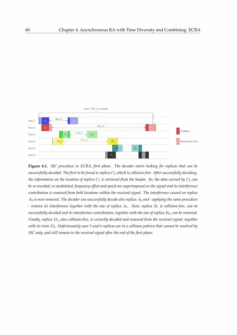
60 Chapter 4. Asynchronous RA with Time Diversity and Combining: ECRA
A1 A2
B1 B2
C1 C2
D1 D2
E1 E2
F1 F2
User 1 VF, Tf seconds
User 1
User 2
User 3
User 4
User 5
User 6
Collision
Interference free
Step 1
Step 2
Step 3
Step 4
Figure 4.1. SIC procedure in ECRA, first phase. The decoder starts looking for replicas that can be
successfully decoded. The first to be found is replica C2 which is collision-free. After successfully decoding,
the information on the location of replica C1 is retrieved from the header. So, the data carried by C2 can
be re-encoded, re-modulated, frequency offset and epoch are superimposed on the signal and its interference
contribution is removed from both locations within the received signal. The interference caused on replica
A2 is now removed. The decoder can successfully decode also replica A2 and - applying the same procedure
- remove its interference together with the one of replica A1. Now, replica B1 is collision-free, can be
successfully decoded and its interference contribution, together with the one of replica B2, can be removed.
Finally, replica D1, also collision-free, is correctly decoded and removed from the received signal, together
with its twin D2. Unfortunately user 5 and 6 replicas are in a collision pattern that cannot be resolved by
SIC only, and still remain in the received signal after the end of the first phase.
4.2. System Model 61
frequency offset and epoch are superimposed on the signal and its interference contribution
is removed from both locations within the received signal. In the following we assume ideal
SIC, i.e. the entire interference contribution is removed from the received signal. Replica A2
is now released from the interference and can also be correctly decoded. In this scenario, the
SIC procedure is iterated until none of the replicas can be successfully decoded anymore.
At the end of SIC, users 1, 2, 3, 4 can be correctly decoded, while users 5 and 6 remain still
unresolved, due to the presence of reciprocal interference that cannot be counteracted by the
channel code.
Combining phase
In the second phase of ECRA, combining techniques are applied on the received pack-
ets unable to be decoded in the first phase, and on these combined observations decoding is
attempted. The formal definition of a combined observation is as follows:
Definition 7 (Combined observation). Consider the d observations of the u-th packet,
y(u,1),y(u,2), ...,y(u,d) with y(u,r) =(y
(u,r)0 , y
(u,r)1 , ..., y
(u,r)ns−1
). We define the combined obser-
vation the vector
y(u) =(y
(u)0 , y
(u)1 , ..., y
(u)ns−1
)with y(u)
i being a suitable function of the individual observation samples y(u,1)i , y
(u,2)i , ..., y
(u,d)i , i.e.
y(u)i := f
(y
(u,1)i , y
(u,2)i , ..., y
(u,d)i
).
Any of selection combining (SC), equal-gain combining (EGC) or maximal-ratio combin-
ing (MRC) [117,118] can be applied in the second phase of ECRA, although our focus will be
on SC and MRC. If SC is adopted, the combined observation is composed by the replica sec-
tions with the highest SINR, i.e. for each observed symbol, the selection combiner chooses
the replica with the highest SINR. Hence, the instantaneous mutual information of the u-th
user combined observation, i-th symbol after SC is
I(γSi
)= log2
(1 + γS
i
)= log2
(1 + max
r
[γ
(u,r)i
]).
Figure 4.2 depicts the situation at the beginning of the second phase for the example pre-
sented in Figure 4.1. The selection combiner selects the first part of replica F1 and the second
part of F2 creating a combined observation free from interference.
In ECRA maximal-ratio combining (ECRA-MRC) instead, each replica’s observed sym-
bol of a given user is weighted proportionally to its squared root mean received signal
level [117]. In this way, the SINR at the output of the combiner is the sum of all replicas
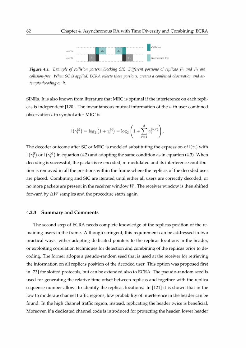
62 Chapter 4. Asynchronous RA with Time Diversity and Combining: ECRA
E1 E2
F1 F2
User 5
User 6
Collision
Interference free
Figure 4.2. Example of collision pattern blocking SIC. Different portions of replicas F1 and F2 are
collision-free. When SC is applied, ECRA selects these portions, creates a combined observation and at-
tempts decoding on it.
SINRs. It is also known from literature that MRC is optimal if the interference on each repli-
cas is independent [120]. The instantaneous mutual information of the u-th user combined
observation i-th symbol after MRC is
I(γMi
)= log2
(1 + γM
i
)= log2
(1 +
d∑r=1
γ(u,r)i
).
The decoder outcome after SC or MRC is modeled substituting the expression of I(γi) with
I(γSi
)or I
(γMi
)in equation (4.2) and adopting the same condition as in equation (4.3). When
decoding is successful, the packet is re-encoded, re-modulated and its interference contribu-
tion is removed in all the positions within the frame where the replicas of the decoded user
are placed. Combining and SIC are iterated until either all users are correctly decoded, or
no more packets are present in the receiver window W . The receiver window is then shifted
forward by ∆W samples and the procedure starts again.
4.2.3 Summary and Comments
The second step of ECRA needs complete knowledge of the replicas position of the re-
maining users in the frame. Although stringent, this requirement can be addressed in two
practical ways: either adopting dedicated pointers to the replicas locations in the header,
or exploiting correlation techniques for detection and combining of the replicas prior to de-
coding. The former adopts a pseudo-random seed that is used at the receiver for retrieving
the information on all replicas position of the decoded user. This option was proposed first
in [73] for slotted protocols, but can be extended also to ECRA. The pseudo-random seed is
used for generating the relative time offset between replicas and together with the replica
sequence number allows to identify the replicas locations. In [121] it is shown that in the
low to moderate channel traffic regions, low probability of interference in the header can be
found. In the high channel traffic region, instead, replicating the header twice is beneficial.
Moreover, if a dedicated channel code is introduced for protecting the header, lower header
4.3. Packet Loss Rate Analysis at Low Channel Load 63
loss probability are expected.5
When correlation techniques are adopted, no overhead due to a dedicated field in the
header is necessary, and replicas are detected and combined before decoding [122]. A two-
phase procedure is proposed in [122]. First the detection of the replicas on the channel is
carried out and second, the matching between replicas belonging to the same user is per-
formed. In both phases a simple non-coherent soft-correlation metric is applied. Details on
the procedure as well as numerical results can be found in Sections 4.5 and 4.6.
The MRC combining technique requires the knowledge of the SINR symbol-by-symbol,
in order to choose the optimal weights [117] beforehand the combination is done. In case
this information cannot be retrieved, combining can be applied with equal weights for all
the symbols, i.e. EGC.
The scenarios under consideration in the work of [96] and its extension [97], are similar
to the one that can block the SIC procedure (see Figure 4.2), although some differences in the
solutions between their work and ECRA can be identified. ECRA creates the combined ob-
servation and tries decoding on it, while [96] requires an iterative demodulation procedure
within packet portions, that may increases the overall packet decoding delay. Furthermore,
in [96] an error in one decoded bit propagates to the entire packet unless compensated by
further errors. This is due to the iterative procedure applied which subtracts the uncorrect
bit from the same packet in the second collision, while in ECRA an error in one decoded bit
will not affect any other portion of the packet.
4.3 Packet Loss Rate Analysis at Low Channel Load
In this Section a PLR approximation tight for low channel load conditions is derived.
Packet losses are caused by particular interference patterns that SIC is not able to resolve.
In the slotted synchronous RA protocols, these patterns are analogous to the stopping sets
present in the low density parity check (LDPC) codes [123] and can be analysed exploit-
ing tools from coding theory and graph theory. In the asynchronous RA schemes, a graph
representation is not straightforward since no discrete objects as slots are present anymore.
Therefore, we resort to investigate the collision patterns that involve two users only, with a
generic degree d and conjecture that these are the patterns driving the PLR, especially at low
channel loads. In the next Section the approximation of the PLR is compared with Monte
Carlo simulations in order to verify its tightness. A set of definitions are required for the
5Dedicated channel code applied to the headers can allow retrieving the information about replica locations
although the packet itself is not decodable due to collisions.
64 Chapter 4. Asynchronous RA with Time Diversity and Combining: ECRA
analysis.
Definition 8 (Collision cluster S). Consider a subset S of users. Assume that packets of all users
in Sc (complementary of the subset S) have been successfully decoded. The subset S is referred to as
collision cluster iff no packet replicas for the users in S is collision-free.
Under the assumption of collision channel, none of the users in the collision cluster can
be successfully decoded. Conversely, when a channel code C is employed by each transmit-
ted packet, the collision cluster might be resolvable, leading to the following definition.
Definition 9 (C-unresolvable collision pattern). Given each packet encoded with a channel code
C, a C-unresolvable collision pattern (C-UCP) L is a collision cluster where no user in the set can
be successfully decoded.
Every C-UCP is also a collision cluster, but not viceversa. In order to evaluate the prob-
ability of C-UCP involving two users only, a generalization of the definition of vulnerable
period [15] is required.
Definition 10 (C-vulnerable period for |S| = 2). Consider the transmission of a packet protected
with a channel code C between time τ and τ + Tp. The packet’s C-vulnerable period is the interval
of time [τ − τ∗l , τ + τ∗r ] in which the presence of a single interferer leads to a failure in the decoding.
Hence, the vulnerable period duration Tv is defined as
Tv = τ∗l + τ∗r .
In slotted synchronous schemes under the collision channel model, τ∗l = 0 and τ∗r = Tp so
Tv = Tp. For asynchronous schemes in general and therefore for ECRA, it holds τ∗l = τ∗r , τ∗.The vulnerable period duration for asynchronous schemes is Tv = 2τ∗. Considering the col-
lision channel model, the vulnerable period duration is then Tv = 2Tp. So, the duration
of packets’ vulnerable period is doubled in asynchronous schemes w.r.t. comparable syn-
chronous ones [15].
4.3.1 Packet Loss Rate Approximation
In this Section we derive an approximation of the PLR, denoted as pl. The approach
follows [84] extending the investigation to asynchronous schemes. Let us consider the user
u. We denote with LS the set of all possible C-UCP that cause the loss of user u packets and
with L∗ the unique type of C-UCP that we consider to drive the PLR performance pl. Let
np = Tf/Tp denote the VF length measured in packet durations and nv = bTf/Tvc denote the
4.3. Packet Loss Rate Analysis at Low Channel Load 65
number of disjoint vulnerable periods per VF. Clearly np ≥ d. The PLR can be approximated
with
pl = Pr
⋃L∈LS
u ∈ L
≤ ∑L∈LS
Pr u ∈ L ≈ Pr u ∈ L∗
=∞∑m=2
e−npG (npG)m
m!Pr u ∈ L∗|m .
(4.4)
The probability pl is first upper bounded with the union bound and then approximated
considering only one type of C-UCP, i.e. L∗. Finally we take the expectation of active users
number over the u-th user VF. The C-UCP L∗ considered in the analysis is formed by two
users only with a generic degree d. Let αu(L∗,m) be the number of combinations of m users
taken two by two and βd(L∗) be the number of ways in which d replicas can be placed into a
VF. Finally, βu−d(L∗) denotes the number of possible ways that the two users can place their
replicas. Making the assumption that L∗ spans at most Tf seconds in order to simplify the
derivation, the probability that the user u belongs to the C-UCP L∗ is
Pr u ∈ L∗|m ≈ αu(L∗,m)βd(L∗)βu−d(L∗)
2
m(4.5)
The quantity αu is αu(L∗,m) =(m2
). The considered user u sends its first replica immedi-
ately, while the remaining d− 1 replicas start times are selected uniformly at random within
Tf seconds, so βd(L∗) ≈(nv−1d−1
). Finally, the number of ways in which two users can select
their position for the replicas follows βu−d(L∗) ≈ nv(nv−1d−1
)2. Substituting into equation (4.5)
these values
Pr u ∈ L∗|m ≈(m2
)nv(nv−1d−1
) 2
m=
(m2
)d(nvd
) 2
m. (4.6)
Finally, inserting the result of equation (4.6) in equation (4.4), we can approximate the PLR
pl as
pl ≈∞∑m=2
e−npG (npG)m
m!
(m2
)d(nvd
) 2
m. (4.7)
The PLR approximation directly depends on the vulnerable period duration via nv. In
the next Sections the vulnerable period duration is computed for two scenarios of interest,
including the MRC case.
4.3.2 Vulnerable Period Duration for Asynchronous RA with FEC
In this scenario, replicas are protected by a channel code so that not all collisions are
destructive. The only C-UCP to be considered is the one involving two users and their
replicas. We recall that perfect power control is assumed so that both users are received
66 Chapter 4. Asynchronous RA with Time Diversity and Combining: ECRA
with the same power P. Without loss of generality, we focus on replica r involved in an
C-UCP of type L∗ which has a first section free of interference and a second part interfered.
The selected rate R determines what it is the minimum fraction of interference-free replica
ϕa that still allows correct decoding, i.e.
ϕa log2
(1 +
P
N
)+ (1− ϕa) log2
(1 +
P
N + P
)= R. (4.8)
For the sake of simplicity we denote as
Rf = log2
(1 +
P
N
)Ri = log2
(1 +
P
N + P
)and we solve equation (4.8) for ϕa
ϕa =R− Ri
Rf − Ri. (4.9)
Equation (4.9) is valid for R ≥ log2
(1 + P
N+P
). In fact, for R < Ri no C-UCPs involving
only two users can be observed, and regardless the level of interference, packets involved in
collisions with only one other packet can always be decoded. In this way,
ϕa =
R−Ri
Rf−Rifor R ≥ Ri
0 for R < Ri
It is worth noticing that ϕa is constrained to 0 ≤ ϕa ≤ 1, since the selectable rate R is
R ≤ log2
(1 + P
N
)= Rf for reliable communication.
In this way, τ∗ = ϕaTp and therefore the vulnerable period is reduced to
Tv = 2τ∗ = 2ϕaTp. And finally nv = bTf/Tvc = bTf/(2ϕaTp)c. Inserting the value of nv
in equation (4.7) we obtain the final expression of the PLR approximation for asynchronous
RA schemes. Note that for ϕa → 0, nv → +∞ and therefore the PLR approximation in
equation (4.7) tends to 0.
4.3.3 Vulnerable Period Duration for Asynchronous RA with MRC and d = 2
Similarly to the previous Section, L∗ is the considered C-UCP where two users are inter-
fering each other and they are received with the same power P. In this scenario the degree
is fixed to d = 2. The focus is on the combined observation after MRC. Without loss of
generality, it is assumed that the first section of both replicas is free of interference, while
there is a second part where just one replica is interfered and in the end there is the last part

4.4. Performance Analysis 67
where both replicas are interfered. We aim at computing the minimum combined observa-
tion portion interference free ϕm that is required for correctly decoding the user after MRC.
It holds
ϕm log2
(1 + 2
P
N
)+µ log2
(1 +
P
N+
P
N + P
)+(1−ϕm−µ) log2
(1 + 2
P
N + P
)= R. (4.10)
For the sake of simplicity we use the following notation
Rf = log2
(1 + 2
P
N
)Ri1 = log2
(1 +
P
N+
P
N + P
)Ri2 = log2
(1 + 2
P
N + P
).
So that equation (4.10) becomes
ϕmRf + µRi1 + (1− ϕm − µ)Ri2 = R. (4.11)
In order to solve equation (4.11), µ is expressed as a function of ϕm, as µ = αϕm, where
0 ≤ α ≤ (1 − ϕm)/ϕm. When α = 0, there are no portions where only one out of the two
replicas is interfered, while α = (1−ϕm)/ϕm represents the case when there are no portions
where both replicas are interfered. Solving (4.11) for ϕm gives
ϕm =R− Ri2
Rf − Ri2 + α(Ri1 − Ri2).
Also in this case, for R < Ri2 we have ϕm = 0 which means that no C-UCP involving two
replicas can be found,
ϕm =
R−Ri2
Rf−Ri2+α(Ri1−Ri2) for R ≥ Ri2
0 for R < Ri2
The average vulnerable period duration over the two replicas is Tv = 2τ∗ = 2(ϕm + µ
2
)Tp =
2ϕm(1 + α
2
)Tp.6 And finally nv = bTf/Tvc = bTf/
(2ϕm
(1 + α
2
)Tp)c.
4.4 Performance Analysis
In this Section ECRA-SC and ECRA-MRC are compared to the reference CRA protocol as
well as with ALOHA. For this first comparison two metrics are considered, the PLR and the
6It is important to underline that the expression of the average vulnerable period duration presented is valid
no matter how the two replicas are interfered, i.e. also when the portions interfered are not both at the beginning
of the packets.
68 Chapter 4. Asynchronous RA with Time Diversity and Combining: ECRA
throughput. The throughput S is defined as the expected number of successfully decoded
packets per packet duration Tp,
S = (1− pl) G.
The ECRA algorithm is also compared to slotted synchronous RA protocols as CRDSA. Since
a channel code C is adopted by the proposed scheme, the throughput is not anymore a suf-
ficient metric. While for slotted synchronous protocols packets are decoded only if they are
received collision-free,7 in the asynchronous case up to a certain level of interference colli-
sions can still be resolved. The level of interference that can be sustained depends on the se-
lected rate R. In the former case, regardless of the selected rate, the throughput performance
remains the same, while in the latter lower rates lead to higher throughput. Nevertheless,
lowering the rate decreases the information carried by each packet. This tradeoff is captured
by the spectral efficiency ξ,
ξ = (1− pl) G R [b/s/Hz].
Although ECRA can outperform considerably the ALOHA protocol, on average it requires
more power. In fact, this scheme assumes to replicate each packet sent in the frame d times.
In order to take into account the increase in average power, we follow the approach of [58],
that was extended for slotted synchronous protocols as CRDSA and IRSA in [77]. The nor-
malised capacity η is defined as the ratio between the maximum achievable spectral efficiency
of one of the RA schemes and the channel capacity of multiple access Gaussian channel
under the same average power constraint. The idea is to compute the maximum spectral
efficiency of the asynchronous MAC schemes (ECRA-SC or ECRA-MRC) and normalise it
to the sum rate capacity of the multiple access Gaussian channel Cg = log2(1+Pg/N). This is
achieved by fixing the average aggregate received signal power Pg equal in all the schemes.
In this way, for the RA protocols the user transmission power Pt takes into account the fact
that the channel is used intermittently but d times w.r.t. ALOHA, i.e. Pt =PgG·d . The ultimate
performance of the asynchronous RA schemes is given by the maximum spectral efficiency
ξ∗ defined as
ξ∗ = maxR∈[0,..,R∗]
S(G) R (4.12)
where for each channel traffic value, the rate R which maximises the spectral efficiency is
chosen.8 Unfortunately, the throughput expression S(G) is not available in closed form for7This holds assuming that no power unbalance is present between the received packets and the channel code
cannot counteract any collision, i.e. log2
(1 + P
N+P
)< R ≤ log2
(1 + P
N
).
8The maximum possible rate for reliable communication R∗ is R∗ = log2(1 + Pt/N) and depends upon the
selected channel load G.
4.4. Performance Analysis 69
ECRA-SC and ECRA-MRC, so only a numerical evaluation of equation (4.12) is possible.
The normalised capacity η is defined as
η =ξ∗
Cg,
where, depending on the RA, a different expression of ξ∗ will be used.
4.4.1 Numerical Results
In the following, numerical results for ECRA-SC and ECRA-MRC schemes are presented.
The packets sent by the users are composed by k = 1000 bits, which translate into ns = (k/R)
symbols. The transmission period is then Tp = Tsns. The VF duration Tf is selected to be
equal to 200 packet durations, i.e. Tf = 200Tp. We recall that the number of users generating
traffic follows a Poisson distribution with mean G measured in packets per Tp durations, and
each of the users transmits d = 2 replicas per generated packet. The decoder operates on a
window of W = 3Tf symbols and once either the maximum number of SIC iterations is ex-
pired or no more packets can be successfully decoded, it is shifted forward by ∆W = 20Tp.
Ideal interference cancellation is assumed and the block interference model introduced in
Section 4.2.1 is used for determining the successful decoding of a packet.
We present first the simulations of the throughput and PLR for both ECRA-SC and
ECRA-MRC. For reference purposes also CRA and the ALOHA protocols are depicted in
the figures. The assumptions are P/N = 6 dB and R = 1.5 equal for all users. In Figure 4.3
we present the throughput S vs. the channel load G. ECRA-MRC largely outperforms both
ECRA-SC and CRA: reaching a maximum throughput of S = 1.32 at G = 1.35, which is
more than twice the one of CRA (S = 0.58) and it increases by 89% with respect to the one
of ECRA-SC (S = 0.70). Furthermore, the throughput of ECRA-MRC follows linearly the
channel load up to 1.3 packets per Tp, implying very limited PLR. In fact, looking at the PLR
performance in Figure 4.4, ECRA-MRC is able to maintain the PLR below 10−3 for channel
load below 1.2 packets per Tp. In other words for a target PLR of pl = 10−3, ECRA-MRC can
be operated up to G = 1.2, while both ECRA-SC and CRA only up to G ∼= 0.3 and G ∼= 0.2
respectively. The gain of ECRA-MRC with respect to both ECRA-SC and CRA in terms of
PLR is of at least one order of magnitude, except in the very high channel load region, where
it largely exceeds this value. It is also shown in the figure, that this protocol is the only one
that can maintain pl ≤ 10−4 for channel load values up to G = 0.6. Very low PLR are par-
ticularly appealing in specific scenarios as satellite applications or control channels where
reliability can be as important as efficiency.
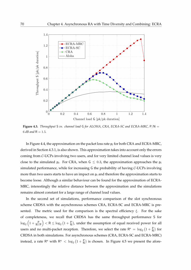
70 Chapter 4. Asynchronous RA with Time Diversity and Combining: ECRA
0 0.2 0.4 0.6 0.8 1 1.2 1.40
0.2
0.4
0.6
0.8
1
1.2
1.4
Channel load G [pk/pk duration]
Thr
ough
put
S[p
k/pk
dura
tion]
ECRA-MRCECRA-SCCRAAloha
Figure 4.3. Throughput S vs. channel load G for ALOHA, CRA, ECRA-SC and ECRA-MRC, P/N =
6 dB and R = 1.5.
In Figure 4.4, the approximation on the packet loss rate pl for both CRA and ECRA-MRC,
derived in Section 4.3.1, is also shown. This approximation takes into account only the errors
coming from C-UCPs involving two users, and for very limited channel load values is very
close to the simulated pl. For CRA, when G ≤ 0.3, the approximation approaches the pl
simulated performance, while for increasing G the probability of having C-UCPs involving
more than two users starts to have an impact on pl and therefore the approximation starts to
become loose. Although a similar behaviour can be found for the approximation of ECRA-
MRC, interestingly the relative distance between the approximation and the simulations
remains almost constant for a large range of channel load values.
In the second set of simulations, performance comparison of the slot synchronous
scheme CRDSA with the asynchronous schemes CRA, ECRA-SC and ECRA-MRC is pre-
sented. The metric used for the comparison is the spectral efficiency ξ. For the sake
of completeness, we recall that CRDSA has the same throughput performance S for
log2
(1 + P
N+P
)< R ≤ log2
(1 + P
N
), under the assumption of equal received power for all
users and no multi-packet reception. Therefore, we select the rate Rs = log2
(1 + P
N
)for
CRDSA in both simulations. For asynchronous schemes (CRA, ECRA-SC and ECRA-MRC)
instead, a rate Ra with Ra < log2
(1 + P
N
)is chosen. In Figure 4.5 we present the afore-
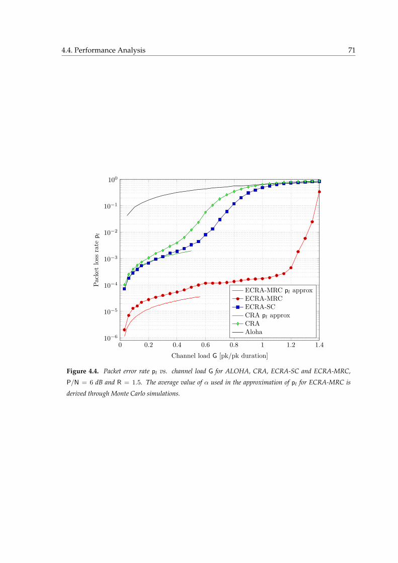
4.4. Performance Analysis 71
0 0.2 0.4 0.6 0.8 1 1.2 1.410−6
10−5
10−4
10−3
10−2
10−1
100
Channel load G [pk/pk duration]
Pack
etlo
ssra
tep l
ECRA-MRC pl approxECRA-MRCECRA-SCCRA pl approxCRAAloha
Figure 4.4. Packet error rate pl vs. channel load G for ALOHA, CRA, ECRA-SC and ECRA-MRC,
P/N = 6 dB and R = 1.5. The average value of α used in the approximation of pl for ECRA-MRC is
derived through Monte Carlo simulations.
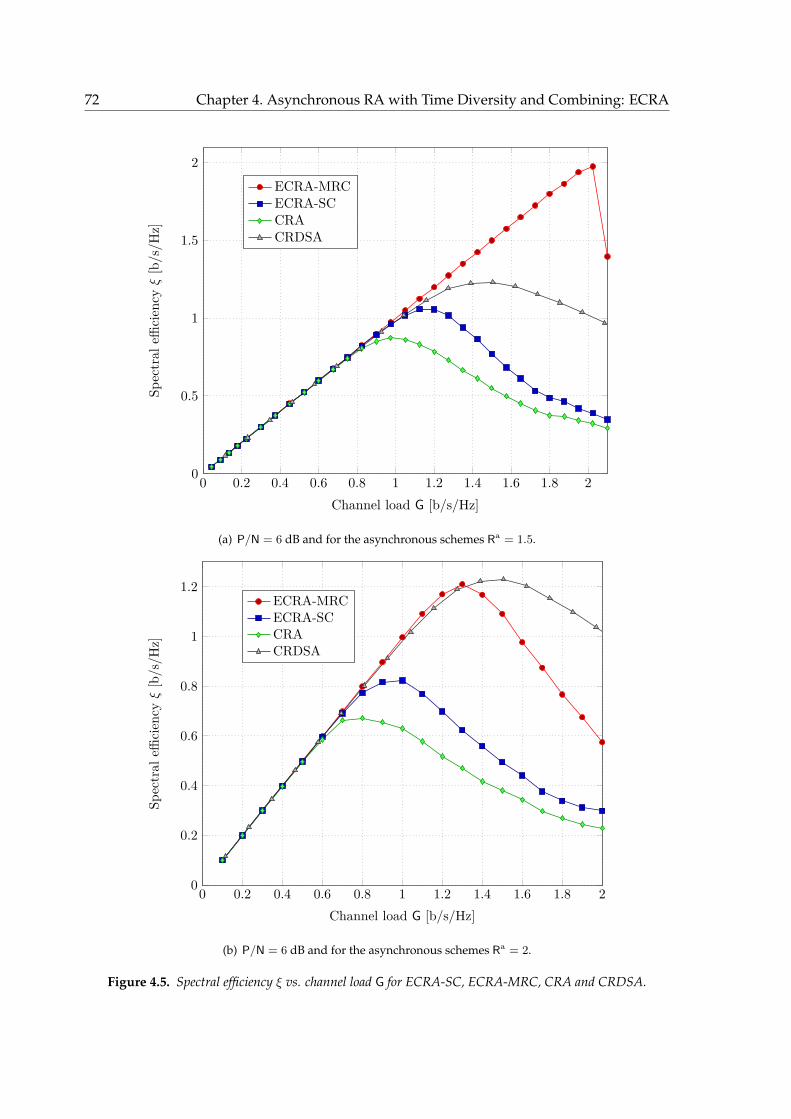
72 Chapter 4. Asynchronous RA with Time Diversity and Combining: ECRA
0 0.2 0.4 0.6 0.8 1 1.2 1.4 1.6 1.8 20
0.5
1
1.5
2
Channel load G [b/s/Hz]
Spectral
efficien
cyξ[b/s/H
z]
ECRA-MRCECRA-SCCRACRDSA
(a) P/N = 6 dB and for the asynchronous schemes Ra = 1.5.
0 0.2 0.4 0.6 0.8 1 1.2 1.4 1.6 1.8 20
0.2
0.4
0.6
0.8
1
1.2
Channel load G [b/s/Hz]
Spectral
efficien
cyξ[b/s/H
z]
ECRA-MRCECRA-SCCRACRDSA
(b) P/N = 6 dB and for the asynchronous schemes Ra = 2.
Figure 4.5. Spectral efficiency ξ vs. channel load G for ECRA-SC, ECRA-MRC, CRA and CRDSA.
4.4. Performance Analysis 73
mentioned comparison. We select P/N = 6 dB and in the first scenario the rate for the
asynchronous schemes is Ra = 1.5, (Figure 4.5(a)), while in the second one it is Ra = 2, (Fig-
ure 4.5(b)). In the former scenario, ECRA-MRC is able to largely outperform CRDSA as well
as all other asynchronous schemes. Outstandingly, ECRA-MRC reaches spectral efficiencies
up to 2 b/s/Hz while under similar conditions CRDSA can only exceed 1.2 b/s/Hz. The re-
sult is a gain of 60% in the maximum spectral efficiency of ECRA-MRC over CRDSA. On the
other hand, ECRA-MRC is particularly sensible to the channel load working point. In fact,
once the maximum spectral efficiency is reached, the performance degrade drastically. This
is not the case for CRDSA and the other asynchronous schemes, which are subject to a more
graceful degradation after the maximum spectral efficiency. Finally, observe that ECRA-SC
is able to reach spectral efficiencies of 1.05 b/s/Hz which is 85% of the one of CRDSA.
In the second scenario, instead, CRDSA is able to slightly outperform ECRA-MRC. Note
that CRDSA uses the same rate in both scenarios, while the asynchronous schemes are using
a rate of Ra = 2, greater than the one of the first scenario. ECRA-MRC benefits from lower
PLR in the increasing slope of spectral efficiency thanks to a rate able to counteract small
levels of interference. Nonetheless, after the maximum spectral efficiency of 1.21 b/s/Hz
is reached, the performance degrade rapidly. CRDSA instead benefits from a more gradual
increase in spectral efficiency towards the maximum and also a more graceful degradation.
As a final remark, ECRA-MRC – as well as asynchronous schemes in general – is very sensi-
tive to the selected rate. More conservative rates, i.e. lower rates lead to better performance
with respect to more aggressive ones. Although we can expect great improvements adopt-
ing ECRA-MRC, less robustness in terms of channel load conditions around the maximum
spectral efficiency has to be taken into account w.r.t. CRDSA or the other asynchronous
schemes, including ECRA-SC.
The last set of simulations shows the comparison among ALOHA, CRA, ECRA-SC and
ECRA-MRC, in terms of the normalised capacity η. Pg/N = 6 dB is selected and the results
are presented in Figure 4.6. The normalised capacity for ECRA-MRC can reach up to 75% of
the MAC channel capacity, for a channel load G = 5 with rate R ∼= 0.35; see Figure 4.6(b). At
this channel load, the gain is 50% with respect to ECRA-SC and 67% with respect to CRA.
Interestingly, the normalised capacity for ECRA-MRC as well as for both ECRA-SC and CRA
is relatively constant for heavy channel load i.e. G > 3. In this way, the schemes appear
to be robust against channel load fluctuations. On the other hand, the rate for which the
maximum spectral efficiency ξ∗ (and so the normalised capacity) of the schemes is achieved
decreases as the channel load increases, see Figure 4.6(b). Therefore the system would be
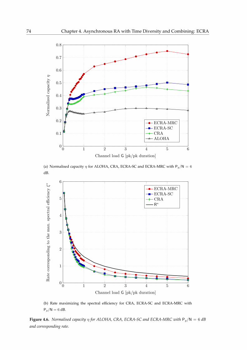
74 Chapter 4. Asynchronous RA with Time Diversity and Combining: ECRA
0 1 2 3 4 5 60
0.1
0.2
0.3
0.4
0.5
0.6
0.7
0.8
Channel load G [pk/pk duration]
Nor
mal
ized
capa
cityη
ECRA-MRCECRA-SCCRAALOHA
(a) Normalised capacity η for ALOHA, CRA, ECRA-SC and ECRA-MRC with Pg/N = 6
dB.
0 1 2 3 4 5 60
1
2
3
4
5
6
Channel load G [pk/pk duration]
Ratecorrespo
ndingto
themax
.spectral
efficien
cyξ∗
ECRA-MRCECRA-SCCRAR∗
(b) Rate maximizing the spectral efficiency for CRA, ECRA-SC and ECRA-MRC with
Pg/N = 6 dB.
Figure 4.6. Normalised capacity η for ALOHA, CRA, ECRA-SC and ECRA-MRC with Pg/N = 6 dB
and corresponding rate.
4.5. Detection, Combining and Decoding - A Two-Phase Procedure 75
required to adapt the rate in order to reach the best performance in terms of normalised
capacity. Nevertheless, the adaptation of the rate remains quite limited in this channel load
region, ranging from a maximum of 0.53 at G = 3 to a minimum of 0.27 at G = 6 for ECRA-
MRC. For limited channel load, all the schemes perform very close, with ALOHA being
slightly the best option. This is due to the low collision probability and the benefit of double
transmit power of ALOHA compared to CRA or ECRA since no replicas are sent.
In Figure 4.6(b), the rate corresponding to the maximum spectral efficiency for ECRA-
MRC, ECRA-SC and CRA is shown. The maximum possible rate under this scenario is also
depicted with a solid line in the figure. For limited channel load, the maximum spectral
efficiency is achieved when using the maximum rate allowed, supporting the fact that colli-
sions of received packets are seldom, and the spectral efficiency can be maximised pushing
the rate as much as it is allowed. On the other hand, as soon as the channel load exceeds
G = 0.3 − 0.4, the maximum spectral efficiency is reached for rate values below the max-
imum one. In this way, the maximum spectral efficiency under moderate to high channel
load conditions can be maximised taking a margin with respect to the maximum rate. This
margin is helpful to counteract part of the collisions and at the same time does not reduces
heavily the spectral efficiency.9
4.5 Detection, Combining and Decoding - A Two-Phase Procedure
In this Section we present the procedure that can be adopted for allowing ECRA to do
combining without the need of decoding the packets beforehand. The key idea is to do split
the detection, combining and decoding into a two phase procedure:
1. Detection Phase: All candidate replicas are detected exploiting the sync word com-
mon to every user which is concatenated to the packet, in the first phase.
2. Replica Matching Phase: A data-aided non-coherent soft-correlation on candidates
surviving the matching criterion is carried out and the first d− 1 matches are declared
as replicas belonging to the same user. On them we apply combining and decoding is
attempted on the combined observation.
Differently to the original ECRA transmission procedure, here we introduce (optional)
time slots. We shall note that the time slots are not necessary for the correct behaviour of
the two-phase procedure, but are easing the second phase reducing the number of possible9Please note that the rate for ALOHA is not depicted in Figure 4.6(b) because it has a different degree d, and
therefore the results are not comparable.

76 Chapter 4. Asynchronous RA with Time Diversity and Combining: ECRA
User 1
User 2
User 3
Virtual frame for User 1, duration Tf
∆T
∆T
∆T
Tp
Figure 4.7. Transmitted signals. Each user sends two replicas of duration Tp seconds that occupy 3 time
slots in the example.
replicas’ matches, as we will see later. In the same way as the original ECRA transmission
procedure, each user arranges its transmission within a VF. The VF are asynchronous among
users. Differently from the original ECRA, each VF is divided in ms slots of duration ∆T , so
that Tf = ms ∆T , see also Figure 4.7. Users transmit d replicas of duration Tp seconds within
the VF. Each replica is transmitted over np consecutive slots within the VF and we have that
a replica duration is a multiple of the slot duration, Tp = np ∆T . Each replica is composed by
ns modulated symbols and the symbol duration is Ts, so ns Ts = np ∆T = Tp. Each replica is
transmitted starting from a slot index chosen uniformly at random in [0,ms − np − 1], reject-
ing starting slot indexes which lead to self-interference among replicas of a user’s packet.
In contrast to CRA [91] and the first version of ECRA [111], no pointer field is required in
the header for localizing the replicas position. The first section of each replica is a sync word
composed by nsw binary symbols s = (s0, ..., snsw−1) common to all users, with si ∈ −1,+1for i = 0, ..., nsw−1. The sync word is concatenated with the BPSK modulated data part and
sent through an AWGN channel. The data part carries the actual information and the re-
dundancy introduced by the channel code.
4.5.1 Detection and Decoding
At the receiver side, the incoming signal y(t) is sampled and input to the frame start
detector. The receiver will operate with a sliding window, similarly to [83, 92]. The decoder
starts operating on the first W samples, with W the designed window size. First it detects
candidate replicas.
Detection Phase
In the first phase the non-coherent soft-correlation metric [124] is used for identifying
candidates replicas; see Figure 4.8(a). Within a receiver window, a threshold-based test is
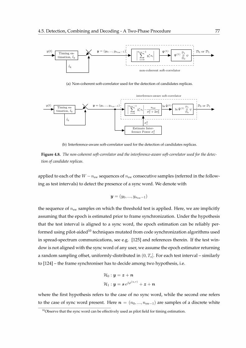
4.5. Detection, Combining and Decoding - A Two-Phase Procedure 77
Timing es-timation, tk
∣∣∣∣∣
nsw−1∑
i=0
y∗i si
∣∣∣∣∣ Ψ(1)D1
≷D0
ψ
non-coherent soft-correlator
y(t)
tk
y = (y0, ..., ynsw−1) Ψ(1) D0 or D1
(a) Non-coherent soft-correlator used for the detection of candidates replicas.
Timing es-timation, tk
∣∣∣∣∣
nsw−1∑
i=0
y∗i si
∣∣∣∣∣−nsw
σ2z + 2σ2
n
Estimate Inter-ference Power σ2
z
ln Ψ(1)D1
≷D0
ψ
interference-aware soft-correlator
y(t)
tk
y = (y0, ..., ynsw−1)
σ2z
ln Ψ(1) D0 or D1
(b) Interference-aware soft-correlator used for the detection of candidates replicas.
Figure 4.8. The non-coherent soft-correlator and the interference-aware soft-correlator used for the detec-
tion of candidate replicas.
applied to each of the W −nsw sequences of nsw consecutive samples (referred in the follow-
ing as test intervals) to detect the presence of a sync word. We denote with
y = (y0, ..., ynsw−1)
the sequence of nsw samples on which the threshold test is applied. Here, we are implicitly
assuming that the epoch is estimated prior to frame synchronization. Under the hypothesis
that the test interval is aligned to a sync word, the epoch estimation can be reliably per-
formed using pilot-aided10 techniques mutated from code synchronization algorithms used
in spread-spectrum communications, see e.g. [125] and references therein. If the test win-
dow is not aligned with the sync word of any user, we assume the epoch estimator returning
a random sampling offset, uniformly-distributed in (0, Ts]. For each test interval – similarly
to [124] – the frame synchroniser has to decide among two hypothesis, i.e.
H0 : y = z + n
H1 : y = s ejϕ(u,r)
+ z + n
where the first hypothesis refers to the case of no sync word, while the second one refers
to the case of sync word present. Here n = (n0, ..., nsw−1) are samples of a discrete white
10Observe that the sync word can be effectively used as pilot field for timing estimation.
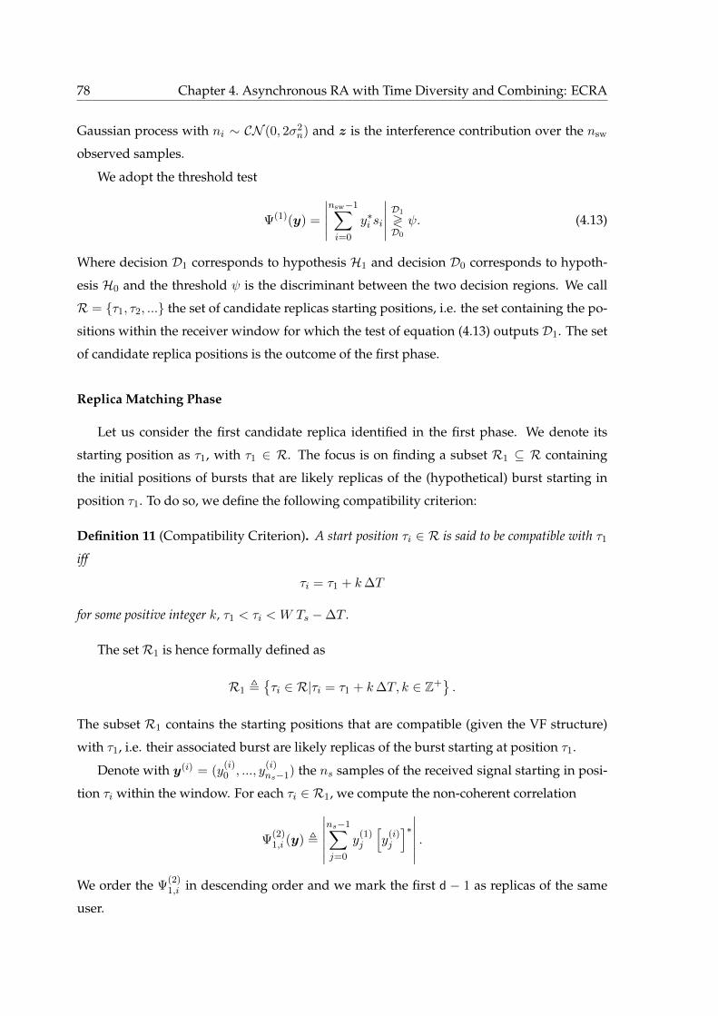
78 Chapter 4. Asynchronous RA with Time Diversity and Combining: ECRA
Gaussian process with ni ∼ CN (0, 2σ2n) and z is the interference contribution over the nsw
observed samples.
We adopt the threshold test
Ψ(1)(y) =
∣∣∣∣∣nsw−1∑i=0
y∗i si
∣∣∣∣∣ D1
≷D0
ψ. (4.13)
Where decision D1 corresponds to hypothesis H1 and decision D0 corresponds to hypoth-
esis H0 and the threshold ψ is the discriminant between the two decision regions. We call
R = τ1, τ2, ... the set of candidate replicas starting positions, i.e. the set containing the po-
sitions within the receiver window for which the test of equation (4.13) outputs D1. The set
of candidate replica positions is the outcome of the first phase.
Replica Matching Phase
Let us consider the first candidate replica identified in the first phase. We denote its
starting position as τ1, with τ1 ∈ R. The focus is on finding a subset R1 ⊆ R containing
the initial positions of bursts that are likely replicas of the (hypothetical) burst starting in
position τ1. To do so, we define the following compatibility criterion:
Definition 11 (Compatibility Criterion). A start position τi ∈ R is said to be compatible with τ1
iff
τi = τ1 + k∆T
for some positive integer k, τ1 < τi < W Ts −∆T .
The setR1 is hence formally defined as
R1 ,τi ∈ R|τi = τ1 + k∆T, k ∈ Z+
.
The subset R1 contains the starting positions that are compatible (given the VF structure)
with τ1, i.e. their associated burst are likely replicas of the burst starting at position τ1.
Denote with y(i) = (y(i)0 , ..., y
(i)ns−1) the ns samples of the received signal starting in posi-
tion τi within the window. For each τi ∈ R1, we compute the non-coherent correlation
Ψ(2)1,i (y) ,
∣∣∣∣∣∣ns−1∑j=0
y(1)j
[y
(i)j
]∗∣∣∣∣∣∣ .We order the Ψ
(2)1,i in descending order and we mark the first d − 1 as replicas of the same
user.
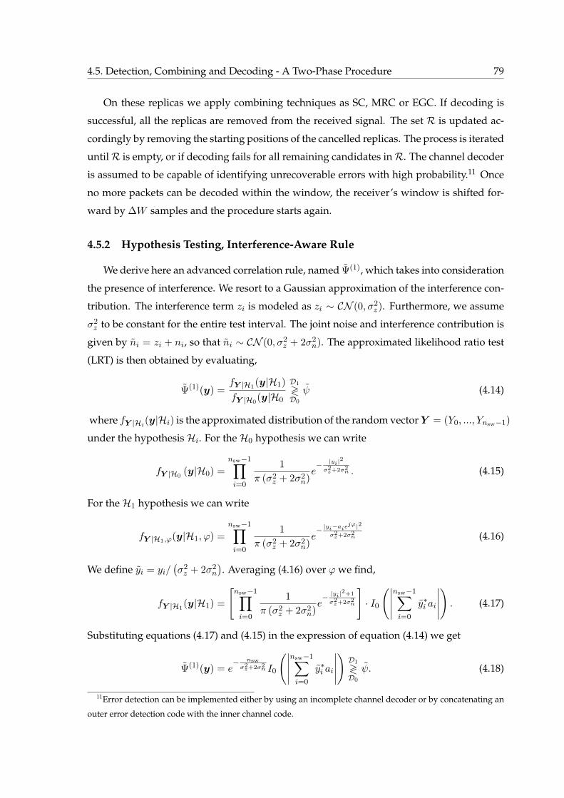
4.5. Detection, Combining and Decoding - A Two-Phase Procedure 79
On these replicas we apply combining techniques as SC, MRC or EGC. If decoding is
successful, all the replicas are removed from the received signal. The set R is updated ac-
cordingly by removing the starting positions of the cancelled replicas. The process is iterated
untilR is empty, or if decoding fails for all remaining candidates inR. The channel decoder
is assumed to be capable of identifying unrecoverable errors with high probability.11 Once
no more packets can be decoded within the window, the receiver’s window is shifted for-
ward by ∆W samples and the procedure starts again.
4.5.2 Hypothesis Testing, Interference-Aware Rule
We derive here an advanced correlation rule, named Ψ(1), which takes into consideration
the presence of interference. We resort to a Gaussian approximation of the interference con-
tribution. The interference term zi is modeled as zi ∼ CN (0, σ2z). Furthermore, we assume
σ2z to be constant for the entire test interval. The joint noise and interference contribution is
given by ni = zi + ni, so that ni ∼ CN (0, σ2z + 2σ2
n). The approximated likelihood ratio test
(LRT) is then obtained by evaluating,
Ψ(1)(y) =fY |H1
(y|H1)
fY |H0(y|H0
D1
≷D0
ψ (4.14)
where fY |Hi(y|Hi) is the approximated distribution of the random vector Y = (Y0, ..., Ynsw−1)
under the hypothesisHi. For theH0 hypothesis we can write
fY |H0(y|H0) =
nsw−1∏i=0
1
π (σ2z + 2σ2
n)e− |yi|2σ2z+2σ2
n . (4.15)
For theH1 hypothesis we can write
fY |H1,ϕ(y|H1, ϕ) =
nsw−1∏i=0
1
π (σ2z + 2σ2
n)e− |yi−aie
jϕ|2σ2z+2σ2
n (4.16)
We define yi = yi/(σ2z + 2σ2
n
). Averaging (4.16) over ϕ we find,
fY |H1(y|H1) =
[nsw−1∏i=0
1
π (σ2z + 2σ2
n)e− |yi|
2+1
σ2z+2σ2
n
]· I0
(∣∣∣∣∣nsw−1∑i=0
y∗i ai
∣∣∣∣∣). (4.17)
Substituting equations (4.17) and (4.15) in the expression of equation (4.14) we get
Ψ(1)(y) = e− nswσ2z+2σ2
n I0
(∣∣∣∣∣nsw−1∑i=0
y∗i ai
∣∣∣∣∣)D1
≷D0
ψ. (4.18)
11Error detection can be implemented either by using an incomplete channel decoder or by concatenating an
outer error detection code with the inner channel code.
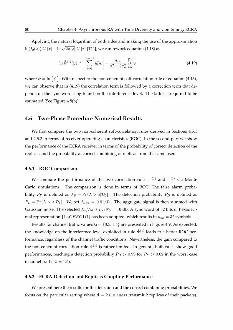
80 Chapter 4. Asynchronous RA with Time Diversity and Combining: ECRA
Applying the natural logarithm of both sides and making the use of the approximation
ln(I0(x)) ∼= |x| − ln√
2π|x| ∼= |x| [124], we can rework equation (4.18) as
ln Ψ(1)(y) ∼=∣∣∣∣∣nsw−1∑i=0
y∗i ai
∣∣∣∣∣− nsw
σ2z + 2σ2
n
D1
≷D0
ψ (4.19)
where ψ = ln(ψ)
. With respect to the non-coherent soft-correlation rule of equation (4.13),
we can observe that in (4.19) the correlation term is followed by a correction term that de-
pends on the sync word length and on the interference level. The latter is required to be
estimated (See Figure 4.8(b)).
4.6 Two-Phase Procedure Numerical Results
We first compare the two non-coherent soft-correlation rules derived in Sections 4.5.1
and 4.5.2 in terms of receiver operating characteristics (ROC). In the second part we show
the performance of the ECRA receiver in terms of the probability of correct detection of the
replicas and the probability of correct combining of replicas from the same user.
4.6.1 ROC Comparison
We compare the performance of the two correlation rules Ψ(1) and Ψ(1) via Monte
Carlo simulations. The comparison is done in terms of ROC. The false alarm proba-
bility PF is defined as PF = PrΛ > λ|D0. The detection probability PD is defined as
PD = PrΛ > λ|D1. We set fmax = 0.01/Ts. The aggregate signal is then summed with
Gaussian noise. The selected Es/N0 is Es/N0 = 10 dB. A sync word of 32 bits of hexadeci-
mal representation 1ACFFC1D has been adopted, which results in nsw = 32 symbols.
Results for channel traffic values G = 0.5, 1.5 are presented in Figure 4.9. As expected,
the knowledge on the interference level exploited in rule Ψ(1) leads to a better ROC per-
formance, regardless of the channel traffic conditions. Nevertheless, the gain compared to
the non-coherent correlation rule Ψ(1) is rather limited. In general, both rules show good
performances, reaching a detection probability PD > 0.99 for PF > 0.02 in the worst case
(channel traffic G = 1.5).
4.6.2 ECRA Detection and Replicas Coupling Performance
We present here the results for the detection and the correct combining probabilities. We
focus on the particular setting where d = 2 (i.e. users transmit 2 replicas of their packets).
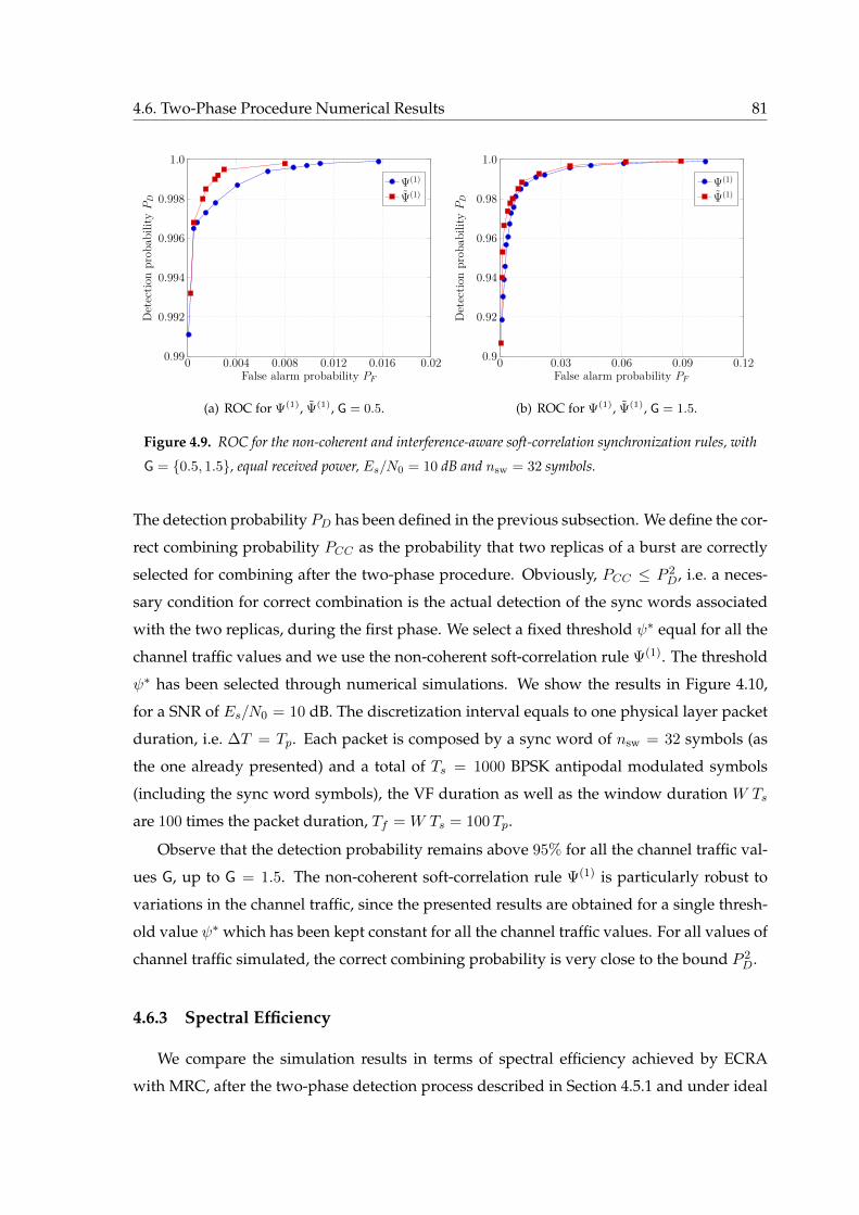
4.6. Two-Phase Procedure Numerical Results 81
0 0.004 0.008 0.012 0.016 0.020.99
0.992
0.994
0.996
0.998
1.0
False alarm probability PF
Det
ectio
npr
obab
ility
PD
Ψ(1)
Ψ(1)
(a) ROC for Ψ(1), Ψ(1), G = 0.5.
0 0.03 0.06 0.09 0.120.9
0.92
0.94
0.96
0.98
1.0
False alarm probability PF
Det
ectio
npr
obab
ility
PD
Ψ(1)
Ψ(1)
(b) ROC for Ψ(1), Ψ(1), G = 1.5.
Figure 4.9. ROC for the non-coherent and interference-aware soft-correlation synchronization rules, with
G = 0.5, 1.5, equal received power, Es/N0 = 10 dB and nsw = 32 symbols.
The detection probability PD has been defined in the previous subsection. We define the cor-
rect combining probability PCC as the probability that two replicas of a burst are correctly
selected for combining after the two-phase procedure. Obviously, PCC ≤ P 2D, i.e. a neces-
sary condition for correct combination is the actual detection of the sync words associated
with the two replicas, during the first phase. We select a fixed threshold ψ∗ equal for all the
channel traffic values and we use the non-coherent soft-correlation rule Ψ(1). The threshold
ψ∗ has been selected through numerical simulations. We show the results in Figure 4.10,
for a SNR of Es/N0 = 10 dB. The discretization interval equals to one physical layer packet
duration, i.e. ∆T = Tp. Each packet is composed by a sync word of nsw = 32 symbols (as
the one already presented) and a total of Ts = 1000 BPSK antipodal modulated symbols
(including the sync word symbols), the VF duration as well as the window duration W Ts
are 100 times the packet duration, Tf = W Ts = 100Tp.
Observe that the detection probability remains above 95% for all the channel traffic val-
ues G, up to G = 1.5. The non-coherent soft-correlation rule Ψ(1) is particularly robust to
variations in the channel traffic, since the presented results are obtained for a single thresh-
old value ψ∗ which has been kept constant for all the channel traffic values. For all values of
channel traffic simulated, the correct combining probability is very close to the bound P 2D.
4.6.3 Spectral Efficiency
We compare the simulation results in terms of spectral efficiency achieved by ECRA
with MRC, after the two-phase detection process described in Section 4.5.1 and under ideal
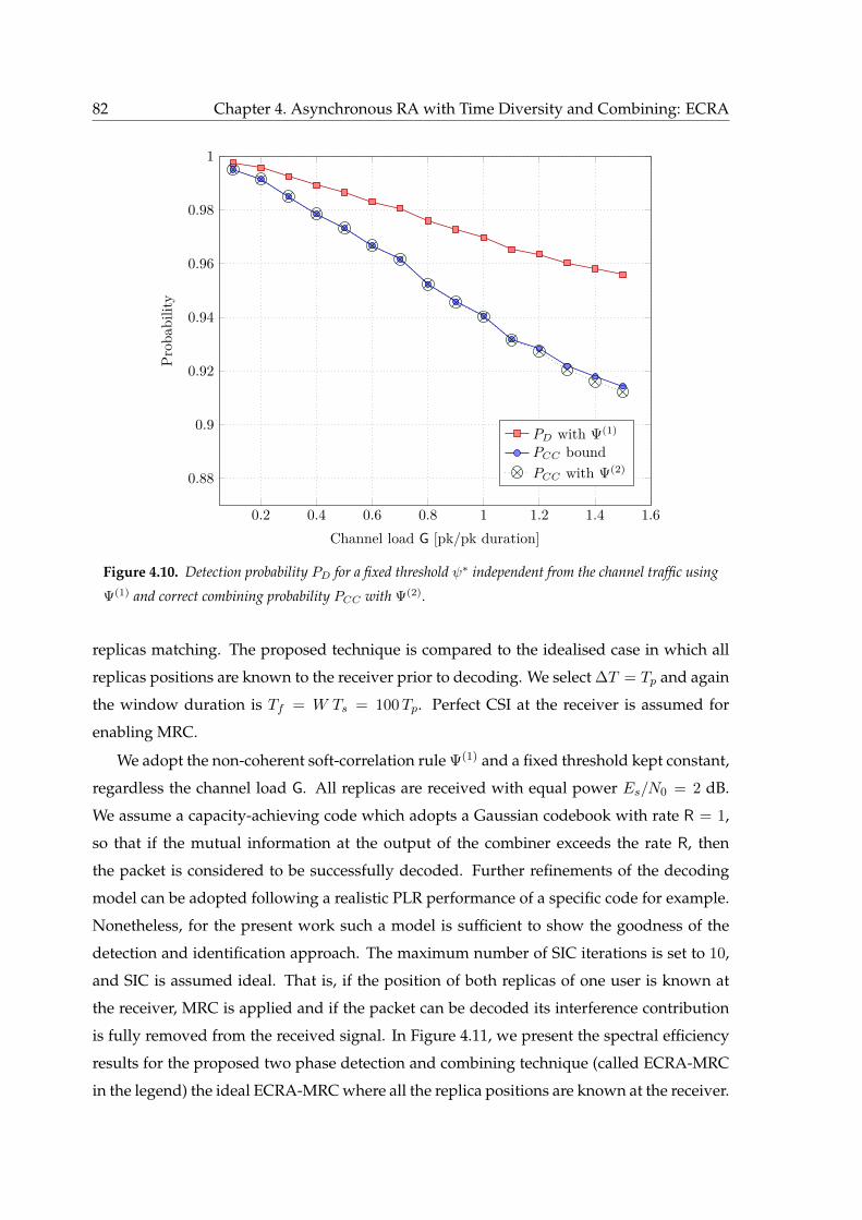
82 Chapter 4. Asynchronous RA with Time Diversity and Combining: ECRA
0.2 0.4 0.6 0.8 1 1.2 1.4 1.6
0.88
0.9
0.92
0.94
0.96
0.98
1
Channel load G [pk/pk duration]
Prob
abili
ty
PD with Ψ(1)
PCC boundPCC with Ψ(2)
Figure 4.10. Detection probability PD for a fixed threshold ψ∗ independent from the channel traffic using
Ψ(1) and correct combining probability PCC with Ψ(2).
replicas matching. The proposed technique is compared to the idealised case in which all
replicas positions are known to the receiver prior to decoding. We select ∆T = Tp and again
the window duration is Tf = W Ts = 100Tp. Perfect CSI at the receiver is assumed for
enabling MRC.
We adopt the non-coherent soft-correlation rule Ψ(1) and a fixed threshold kept constant,
regardless the channel load G. All replicas are received with equal power Es/N0 = 2 dB.
We assume a capacity-achieving code which adopts a Gaussian codebook with rate R = 1,
so that if the mutual information at the output of the combiner exceeds the rate R, then
the packet is considered to be successfully decoded. Further refinements of the decoding
model can be adopted following a realistic PLR performance of a specific code for example.
Nonetheless, for the present work such a model is sufficient to show the goodness of the
detection and identification approach. The maximum number of SIC iterations is set to 10,
and SIC is assumed ideal. That is, if the position of both replicas of one user is known at
the receiver, MRC is applied and if the packet can be decoded its interference contribution
is fully removed from the received signal. In Figure 4.11, we present the spectral efficiency
results for the proposed two phase detection and combining technique (called ECRA-MRC
in the legend) the ideal ECRA-MRC where all the replica positions are known at the receiver.

4.7. Conclusions 83
0 0.2 0.4 0.6 0.8 1 1.2 1.4 1.6 1.80
0.2
0.4
0.6
0.8
1
1.2
1.4
1.6
Channel load G [b/s/Hz]
Spectral
efficien
cyξ[b/s/H
z]
ECRA-MRC IdealECRA-MRCCRA
Figure 4.11. Spectral efficiency of ECRA-MRC with the proposed two phase detection and combining
technique compared to the ideal ECRA-MRC.
The proposed technique is close to the performance of the ideal case. The maximum spectral
efficiency exceeds 1.4 b/s/Hz, which is only 8% less than the maximum spectral efficiency
of the ideal case. For reference, also the performance without MRC is depicted in the figure
(CRA in the legend).
4.7 Conclusions
In this Chapter we presented a novel RA decoding algorithm named ECRA. Motivated
by the presence of C-UCPs within frames, ECRA tried to reduce their detrimental impact on
the receiver’s SIC procedure applying combing techniques. ECRA exploited the presence
of multiple instances of the same packet in order to trigger a SIC procedure. In addition,
ECRA tried to reduce interference of asynchronous protocols attempting to resolve partial
collisions among packets, with the creation of a combined observation. The combined ob-
servation was either generated from the lowest interfered parts of the replicas sent within
the frame, i.e. SC, or from the weighted combination of the replicas symbols of each user,
i.e. MRC. An analytical framework for evaluating a lower bound on the C-UCP for CRA
with and without channel coding as well as ECRA was developed. The lower bound was
84 Chapter 4. Asynchronous RA with Time Diversity and Combining: ECRA
then used for computing an approximation of the PLR which was found to be tight in the
low channel load region. A comprehensive framework with several metrics was also de-
rived, in order to compare both asynchronous and slot synchronous schemes with channel
coding. An investigation on the performance of ECRA under average power constraint was
also performed. Numerical simulations showed that ECRA in both its variants, largely out-
performed CRA in all the considered scenarios for both throughput and PLR. Furthermore
ECRA-MRC was able to double the maximum throughput w.r.t. CRA while ECRA-SC had
an improvement of 21% in the maximum throughput w.r.t. CRA. For a properly selected
rate, ECRA-MRC was also able to outperform CRDSA with the same number of replicas.
Finally, ECRA-MRC showed remarkable performance gains in terms of normalised capacity
w.r.t. the other asynchronous RA schemes reaching up to 75% the MAC channel capacity.
In order to present a practical way to exploit the ECRA concept, a two-phase procedure
was also proposed which avoided the need of pointers to the replicas. Candidate replicas
were identified thanks to the presence of a common sync word using non-coherent soft-
correlation. In the second phase, data-aided non-coherent soft-correlation was applied in
order to rank the candidate replicas and the first d− 1 were declared as replicas of the same
users, on top of which decoding was attempted. We showed that in a very simple setup, this
approach was very close to the ideal performance of ECRA.
Chapter 5Layer 3 Throughput and Packet Loss
Rate Analysis for Advanced Random
Access
The most exciting phrase to hear in
science, the one that heralds the most
discoveries, is not “Eureka!” (I found
it!) but “That’s funny...”
Isaac Asimov
In the previous Chapter we focused on the investigation of ECRA. We showed that in
specific scenarios (code rate, received SNR) asynchronous RA was able to outperform also
slot synchronous RA as CRDSA. In this Chapter we further elaborate on this comparison,
moving one layer above the MAC. We want to verify if the identified benefits of asyn-
chronous RA are still present when higher layers generate packets with variable data con-
tent. While with asynchronous RA, packets can be transmitted whichever size they have, for
slot synchronous systems packets might not fit into one MAC time slot, requiring fragmen-
tation and eventually padding. Nonetheless, it is known from the literature that for ALOHA
under the collision channel model, the packet size distribution maximising the throughput
is the one having all packets with the same size [58, 126, 127].
The degradation due to the variable packet size for asynchronous RA schemes, and
the degradation due to fragmentation and padding overhead for the time synchronous RA
schemes, lead to interesting – yet unexplored – research which option leads to better results
in terms of layer 3 throughput and PLR.

86 Chapter 5. Layer 3 Throughput and PLR Analysis for Advanced RA
5.1 Introduction
For new RA protocols the investigation of higher layer throughput is a very important
and still a missing element in literature. The possibility to exploit gains in terms of through-
put and PLR also at higher layers can open to RA protocols new application scenarios still
considered unsuitable for such protocols.
In this Chapter we analyse and investigate the layer 3 throughput and PLR of framed
asynchronous and slot synchronous RA protocols, such as ALOHA, SA, CRA, CRDSA,
ECRA and IRSA. A generic layer 3 packet length distribution fX(x) is assumed. We pro-
pose an analytical expression of the layer 3 throughput and PLR for slot synchronous RA
so to avoid numerical simulations dedicated to such layer. It will require knowledge of the
packet successful probability at layer 2 and the distribution fX(x). For the cases in which
the latter is not available we elaborate a bound (lower bound for the layer 3 throughput
and upper bound for the layer 3 PLR) that requires the knowledge only on the average of
the distribution fX(x). We provide finally numerical results for the performance of all the
considered schemes.
5.2 System Model
We consider a population of nu users sharing the medium. Each user generates packets
of layer 3 where the duration is subject to a generic probability measure fX(x).1 The proba-
bility measure captures the behaviour of the traffic profile followed by the users. We assume
that the probability measure fX(x) is equal for all the users and can be either continuous or
discrete. The user cannot forward the next layer 3 packet to the layer 2 until the all the pre-
vious layer 2 packet segments have been sent. Furthermore, for the investigation carried out
in this Chapter, the protocol is assumed to work in open loop, i.e. no feedback and packet
acknowledgment procedure is here considered.
All the layer 2 MAC protocols evaluated in the following are RA, either asynchronous
or slot synchronous. We consider framed ALOHA [128, 129], SA, CRA, CRDSA, ECRA and
IRSA. For all protocols, a frame structure is included, in which appear all packet transmis-
sions of the active users. In this way, every time a layer 3 packet is generated, it is forwarded
to layer 2 and it is sent in the upcoming frame. For slot synchronous systems, before it can be
sent, it is eventually fragmented and sent in consecutive frames. This requires also the asyn-
1The probability measure fX(x) corresponds to the p.d.f. in case of continuous random variable, or corre-
sponds to the p.m.f. in case of discrete random variable.

5.3. L3 Throughput and Packet Loss Rate Analysis 87
chronous schemes to have a (possibly loose) time synchronization to the frame start. The
analysis performed in Section 5.3 is independent of the specific protocol and can be applied
also to other RA schemes. The time is composed by frames of duration Tf . Each user can try
to transmit only once for each MAC frame and we assume that all users have always packets
to be sent. Upon the generation of more than one packet per frame, the users need to store
or discard the exceeding packets (depending on the protocol implementation). The physical
layer packets are supposed to have a duration of Tp. Concerning slot synchronous proto-
cols, the frames are further subdivided in slots of a fixed duration Tl. In slot synchronous
schemes, the physical layer packet duration has to be equal to the slot duration in order to
fit in the time slot, i.e. Tp = Tl, while in asynchronous schemes this constraint is relaxed.
We define the offered traffic load G as the fraction of time occupied by transmissions. In
formulas, G = (nu Tp) / Tf . In the slot synchronous schemes we can write also G = nu/ms,
where ms = Tf/ Tp = Tf/ Tl is the number of slots that constitute each MAC frame.
5.3 L3 Throughput and Packet Loss Rate Analysis
The throughput is one of the mostly used performance metrics for RA protocols and it is
defined as the average number of decoded packets per packet duration. We recall that ps is
the probability of success which is in general function of both the channel load G but also of
the packet duration distribution fX(x),
S = G ps(G, fX(x)).
The packet loss rate pl is the probability of packet loss or unsuccessful decoding, i.e.
pl = 1− ps(G, fX(x)).
For simplicity of notation these dependencies are neglected in the following.
5.3.1 Asynchronous RA Protocols
When employing asynchronous framed protocols, as framed ALOHA or CRA, all layer 3
packet durations not exceeding the frame duration can be accommodated in the MAC frame.
In this way, no fragmentation of layer 3 packets is required and the successful decoding
probability of layer 3 packets ps3 coincides with the successful decoding probability of
88 Chapter 5. Layer 3 Throughput and PLR Analysis for Advanced RA
layer 2 packets ps. Therefore, the layer 3 throughput S3 of asynchronous RA protocols is
S3 = G ps3 = G ps = S.
And the layer 3 PLR is
pl3 = 1− ps3 = 1− ps = pl.
5.3.2 Slot Synchronous RA Protocols
Although users at layer 3 generate packets whose durations are ruled by fX(x) probabil-
ity measure, slot synchronous schemes cannot accommodate packets with generic duration
at MAC layer, and fragmentation is needed. When a layer 3 packet has to be fragmented,
additional overhead is added to the fragmented layer 2 packets. Two types of overhead
are added to the layer 2 packets: 1) fragmentation overhead and 2) padding overhead. The
former is due to the need to have a layer 3 header for each fragment, where the fields to
both route the packet in the network and to recompose the packet at the destination are
contained. Header fields dedicated to fragmentation must include: original-not-fragmented
packet identifier, fragment identifier, and either overall number of fragments or indicator
about last/not last fragment. For example, concerning internet protocol (IP) layer 3 protocol,
the fields identification, offset and flag M are used, respectively, for the aims listed above.
The padding overhead is needed in order to fulfill layer 2 slot duration requirements.
Layer 3 throughput S3 for slotted schemes is
S3 = G ps3 (1−Of ) (1−Op), 0 ≤ Of ≤ 1, 0 ≤ Op ≤ 1 (5.1)
where Of is the fragmentation overhead and Op is the padding overhead. Layer 3 PLR pl3
for slotted schemes is
pl3 = 1− ps3. (5.2)
The successful decoding probability of layer 3 packets ps3 in the slot synchronous schemes is
the probability that all the layer 2 packets composing the layer 3 packet are received correctly
weighted with the probability that this specific layer 3 duration has been selected,
ps3 = p1ps + p2p2s + ...+ pnpns + ... =
∞∑i=1
pipis,
∞∑i=1
pi = 1. (5.3)
Example 5.3.1 — Case fX(x) = 12δ(x− 1) + 1
2δ(x− 2):
5.3. L3 Throughput and Packet Loss Rate Analysis 89
We can suppose for example, that the layer 3 packet duration distribution p.m.f. fX(x)
results in 50% of layer 3 packets with a duration of one layer 2 packet and 50% of layer 3
packets with a duration of two layer 2 packets, i.e. fX(x) = 12δ(x − 1) + 1
2δ(x − 2). The
layer 3 successful decoding probability for the first packet duration (one layer 2 packet) is
simply ps. Actually, we need only that the layer 2 received packet is successfully decoded.
While for the second packet duration (two layer 2 packets) the probability is p2s because
two consecutive layer 2 packets must be successfully decoded. In this way, equation (5.3)
becomes for this example
ps3 =1
2ps +
1
2p2s.
Note that we can write the closed form expression of ps when considering SA protocol. In
this case ps = e−G assuming an infinite user population [58] and we can further write
ps3 =1
2e−G +
1
2e−2G.
Computation of pi
In general, fX(x) can be continuous, i.e. the layer 3 packet durations may not be con-
strained to be a multiple of layer 2 packet durations. In these scenarios the computation of
pi is of paramount importance to determine the layer 3 successful decoding probability ps3.
The generic pi value is computed as the definite integral of the p.d.f. fX(x) in the interval
from the layer 2 duration i−1 to the layer 2 duration i, where i = 1, ...,∞ are discrete layer 2
durations (i = 1 means one layer 2 packet duration),
pi =
∫ i
i−1fX(x)dx i = 1, ...,∞. (5.4)
Example 5.3.2 — Case fX(x) = e−x:
As second example, we assume fX(x) = e−x, the exponential distribution with mean of
one layer 2 packet duration. In this example, according to equation (6.10), pi are
pi =
∫ i
i−1fX(x)dx =
∫ i
i−1e−xdx =
[−e−x
]ii−1
= e−i (e− 1) i = 1, ...,∞.
After the discretization, the mean of the exponential distribution will be greater than one
layer 2 packet duration. This is due to the discretization process, which is a ceiling operation.
90 Chapter 5. Layer 3 Throughput and PLR Analysis for Advanced RA
In general, the expected value of fX(x) after discretization, E[fX(x)] can be written as
E[fX(x)] =∞∑i=1
i pi, (5.5)
where the result is expressed in layer 2 packet durations. The values of pi are computed
according to equation (6.10). In the case of the exponential distribution, equation (5.5) be-
comes
E[fX(x)] =e
e− 1∼= 1.58.
Distribution fX(x) Unknown
In some situations fX(x) or its expression after discretization are not known. This pre-
vents the analytical computation of pi, but we would like to be able to analytically evaluate
the successful decoding probability of layer 3 packets ps3 also in these situations. We assume
that the expected value of the probability measure after discretization E[fX(x)] is available
or can be measured at the receiver.2 We can then compute a lower bound to the successful
decoding probability of layer 3 packets exploiting Jensen’s inequality [130] as
ps3 ≥ ps3 = (ps)E[fX(x)] . (5.6)
In this way the throughput in equation (5.1) can be bounded from below by
S3 ≥ G ps3 (1−Of ) (1−Op), 0 ≤ Of ≤ 1, 0 ≤ Op ≤ 1. (5.7)
While the PLR in equation (5.2) can be bounded from above by
pl3 ≤ 1− ps3. (5.8)
Numerical results showing the difference between ps3 and ps3 in terms of layer 3 throughput
and PLR are given in the next Section.
Additional Remarks
The analytical framework developed provides the possibility to evaluate the layer 3
throughput S3 and PLR pl3 in case of slot synchronous schemes without the need of nu-
merical simulation of this layer. Two possibilities can be followed:
1. When ps and fX(x) are available, one can use equations (5.1), (5.2), (5.3), (6.10);
2The packets correctly decoded will contain the sequence number needed for layer 3 packet reconstruction
that can be used to numerically evaluate E[fX(x)].
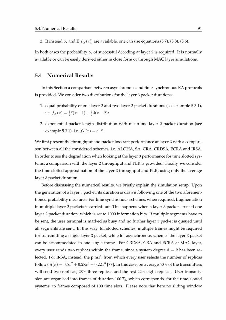
5.4. Numerical Results 91
2. If instead ps and E[fX(x)] are available, one can use equations (5.7), (5.8), (5.6).
In both cases the probability ps of successful decoding at layer 2 is required. It is normally
available or can be easily derived either in close form or through MAC layer simulations.
5.4 Numerical Results
In this Section a comparison between asynchronous and time synchronous RA protocols
is provided. We consider two distributions for the layer 3 packet durations:
1. equal probability of one layer 2 and two layer 2 packet durations (see example 5.3.1),
i.e. fX(x) = 12δ(x− 1) + 1
2δ(x− 2);
2. exponential packet length distribution with mean one layer 2 packet duration (see
example 5.3.1), i.e. fX(x) = e−x.
We first present the throughput and packet loss rate performance at layer 3 with a compari-
son between all the considered schemes, i.e. ALOHA, SA, CRA, CRDSA, ECRA and IRSA.
In order to see the degradation when looking at the layer 3 performance for time slotted sys-
tems, a comparison with the layer 2 throughput and PLR is provided. Finally, we consider
the time slotted approximation of the layer 3 throughput and PLR, using only the average
layer 3 packet duration.
Before discussing the numerical results, we briefly explain the simulation setup. Upon
the generation of a layer 3 packet, its duration is drawn following one of the two aforemen-
tioned probability measures. For time synchronous schemes, when required, fragmentation
in multiple layer 2 packets is carried out. This happens when a layer 3 packets exceed one
layer 2 packet duration, which is set to 1000 information bits. If multiple segments have to
be sent, the user terminal is marked as busy and no further layer 3 packet is queued until
all segments are sent. In this way, for slotted schemes, multiple frames might be required
for transmitting a single layer 3 packet, while for asynchronous schemes the layer 3 packet
can be accommodated in one single frame. For CRDSA, CRA and ECRA at MAC layer,
every user sends two replicas within the frame, since a system degree d = 2 has been se-
lected. For IRSA, instead, the p.m.f. from which every user selects the number of replicas
follows Λ(x) = 0.5x2 + 0.28x3 + 0.22x8 [77]. In this case, on average 50% of the transmitters
will send two replicas, 28% three replicas and the rest 22% eight replicas. User transmis-
sion are organised into frames of duration 100Tp, which corresponds, for the time-slotted
systems, to frames composed of 100 time slots. Please note that here no sliding window
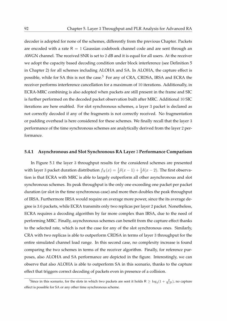
92 Chapter 5. Layer 3 Throughput and PLR Analysis for Advanced RA
decoder is adopted for none of the schemes, differently from the previous Chapter. Packets
are encoded with a rate R = 1 Gaussian codebook channel code and are sent through an
AWGN channel. The received SNR is set to 2 dB and it is equal for all users. At the receiver
we adopt the capacity based decoding condition under block interference (see Definition 5
in Chapter 2) for all schemes including ALOHA and SA. In ALOHA, the capture effect is
possible, while for SA this is not the case.3 For any of CRA, CRDSA, IRSA and ECRA the
receiver performs interference cancellation for a maximum of 10 iterations. Additionally, in
ECRA-MRC combining is also adopted when packets are still present in the frame and SIC
is further performed on the decoded packet observation built after MRC. Additional 10 SIC
iterations are here enabled. For slot synchronous schemes, a layer 3 packet is declared as
not correctly decoded if any of the fragments is not correctly received. No fragmentation
or padding overhead is here considered for these schemes. We finally recall that the layer 3
performance of the time synchronous schemes are analytically derived from the layer 2 per-
formance.
5.4.1 Asynchronous and Slot Synchronous RA Layer 3 Performance Comparison
In Figure 5.1 the layer 3 throughput results for the considered schemes are presented
with layer 3 packet duration distribution fX(x) = 12δ(x− 1) + 1
2δ(x− 2). The first observa-
tion is that ECRA with MRC is able to largely outperform all other asynchronous and slot
synchronous schemes. Its peak throughput is the only one exceeding one packet per packet
duration (or slot in the time synchronous case) and more then doubles the peak throughput
of IRSA. Furthermore IRSA would require on average more power, since the its average de-
gree is 3.6 packets, while ECRA transmits only two replicas per layer 2 packet. Nonetheless,
ECRA requires a decoding algorithm by far more complex than IRSA, due to the need of
performing MRC. Finally, asynchronous schemes can benefit from the capture effect thanks
to the selected rate, which is not the case for any of the slot synchronous ones. Similarly,
CRA with two replicas is able to outperform CRDSA in terms of layer 3 throughput for the
entire simulated channel load range. In this second case, no complexity increase is found
comparing the two schemes in terms of the receiver algorithm. Finally, for reference pur-
poses, also ALOHA and SA performance are depicted in the figure. Interestingly, we can
observe that also ALOHA is able to outperform SA in this scenario, thanks to the capture
effect that triggers correct decoding of packets even in presence of a collision.
3Since in this scenario, for the slots in which two packets are sent it holds R ≥ log2(1 + PN+P
), no capture
effect is possible for SA or any other time synchronous scheme.
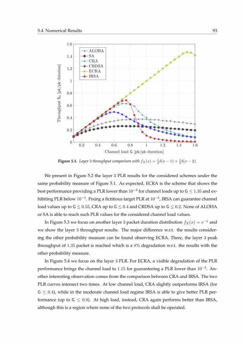
5.4. Numerical Results 93
0.2 0.4 0.6 0.8 1 1.2 1.4 1.60
0.2
0.4
0.6
0.8
1
1.2
1.4
1.6
Channel load G [pk/pk duration]
Thr
ough
put
S 3[p
k/pk
dura
tion]
ALOHASACRACRDSAECRAIRSA
Figure 5.1. Layer 3 throughput comparison with fX(x) = 12δ(x− 1) + 1
2δ(x− 2).
We present in Figure 5.2 the layer 3 PLR results for the considered schemes under the
same probability measure of Figure 5.1. As expected, ECRA is the scheme that shows the
best performance providing a PLR lower than 10−3 for channel loads up to G ≤ 1.35 and ex-
hibiting PLR below 10−4. Fixing a fictitious target PLR at 10−2, IRSA can guarantee channel
load values up to G ≤ 0.55, CRA up to G ≤ 0.4 and CRDSA up to G ≤ 0.2. None of ALOHA
or SA is able to reach such PLR values for the considered channel load values.
In Figure 5.3 we focus on another layer 3 packet duration distribution fX(x) = e−x and
we show the layer 3 throughput results. The major difference w.r.t. the results consider-
ing the other probability measure can be found observing ECRA. There, the layer 3 peak
throughput of 1.35 packet is reached which is a 8% degradation w.r.t. the results with the
other probability measure.
In Figure 5.4 we focus on the layer 3 PLR. For ECRA, a visible degradation of the PLR
performance brings the channel load to 1.15 for guaranteeing a PLR lower than 10−3. An-
other interesting observation comes from the comparison between CRA and IRSA. The two
PLR curves intersect two times. At low channel load, CRA slightly outperforms IRSA (for
G ≤ 0.4), while in the moderate channel load regime IRSA is able to give better PLR per-
formance (up to G ≤ 0.8). At high load, instead, CRA again performs better than IRSA,
although this is a region where none of the two protocols shall be operated.
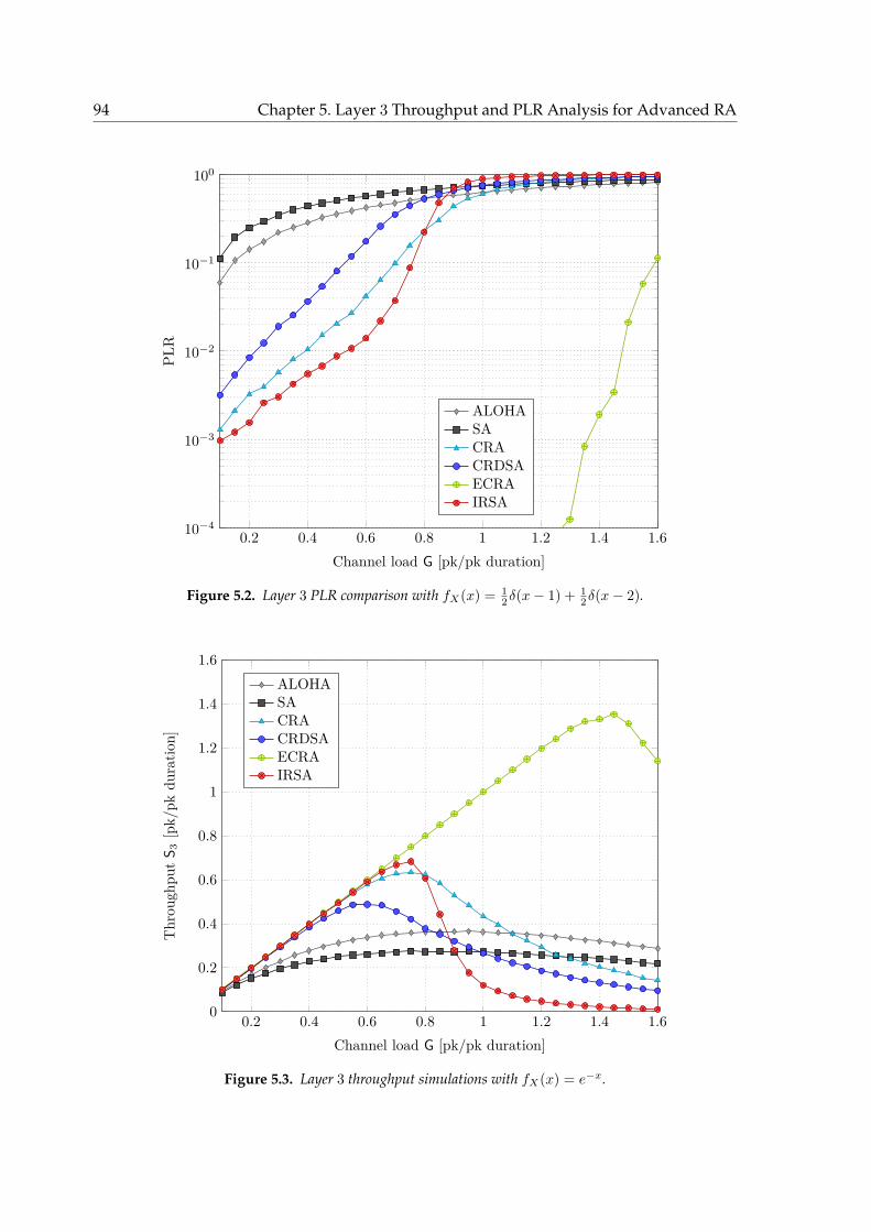
94 Chapter 5. Layer 3 Throughput and PLR Analysis for Advanced RA
0.2 0.4 0.6 0.8 1 1.2 1.4 1.610−4
10−3
10−2
10−1
100
Channel load G [pk/pk duration]
PLR
ALOHASACRACRDSAECRAIRSA
Figure 5.2. Layer 3 PLR comparison with fX(x) = 12δ(x− 1) + 1
2δ(x− 2).
0.2 0.4 0.6 0.8 1 1.2 1.4 1.60
0.2
0.4
0.6
0.8
1
1.2
1.4
1.6
Channel load G [pk/pk duration]
Thr
ough
put
S 3[p
k/pk
dura
tion]
ALOHASACRACRDSAECRAIRSA
Figure 5.3. Layer 3 throughput simulations with fX(x) = e−x.
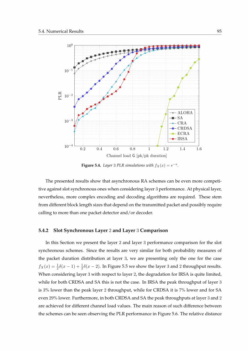
5.4. Numerical Results 95
0.2 0.4 0.6 0.8 1 1.2 1.4 1.610−4
10−3
10−2
10−1
100
Channel load G [pk/pk duration]
PLR
ALOHASACRACRDSAECRAIRSA
Figure 5.4. Layer 3 PLR simulations with fX(x) = e−x.
The presented results show that asynchronous RA schemes can be even more competi-
tive against slot synchronous ones when considering layer 3 performance. At physical layer,
nevertheless, more complex encoding and decoding algorithms are required. These stem
from different block length sizes that depend on the transmitted packet and possibly require
calling to more than one packet detector and/or decoder.
5.4.2 Slot Synchronous Layer 2 and Layer 3 Comparison
In this Section we present the layer 2 and layer 3 performance comparison for the slot
synchronous schemes. Since the results are very similar for both probability measures of
the packet duration distribution at layer 3, we are presenting only the one for the case
fX(x) = 12δ(x− 1) + 1
2δ(x− 2). In Figure 5.5 we show the layer 3 and 2 throughput results.
When considering layer 3 with respect to layer 2, the degradation for IRSA is quite limited,
while for both CRDSA and SA this is not the case. In IRSA the peak throughput of layer 3
is 3% lower than the peak layer 2 throughput, while for CRDSA it is 7% lower and for SA
even 29% lower. Furthermore, in both CRDSA and SA the peak throughputs at layer 3 and 2
are achieved for different channel load values. The main reason of such difference between
the schemes can be seen observing the PLR performance in Figure 5.6. The relative distance
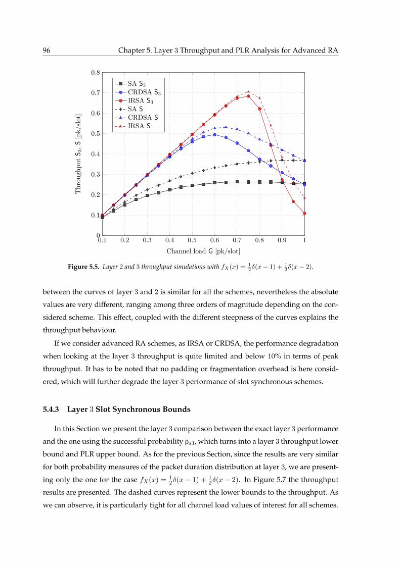
96 Chapter 5. Layer 3 Throughput and PLR Analysis for Advanced RA
0.1 0.2 0.3 0.4 0.5 0.6 0.7 0.8 0.9 10
0.1
0.2
0.3
0.4
0.5
0.6
0.7
0.8
Channel load G [pk/slot]
Thr
ough
put
S 3,S
[pk/
slot]
SA S3CRDSA S3IRSA S3SA SCRDSA SIRSA S
Figure 5.5. Layer 2 and 3 throughput simulations with fX(x) = 12δ(x− 1) + 1
2δ(x− 2).
between the curves of layer 3 and 2 is similar for all the schemes, nevertheless the absolute
values are very different, ranging among three orders of magnitude depending on the con-
sidered scheme. This effect, coupled with the different steepness of the curves explains the
throughput behaviour.
If we consider advanced RA schemes, as IRSA or CRDSA, the performance degradation
when looking at the layer 3 throughput is quite limited and below 10% in terms of peak
throughput. It has to be noted that no padding or fragmentation overhead is here consid-
ered, which will further degrade the layer 3 performance of slot synchronous schemes.
5.4.3 Layer 3 Slot Synchronous Bounds
In this Section we present the layer 3 comparison between the exact layer 3 performance
and the one using the successful probability ps3, which turns into a layer 3 throughput lower
bound and PLR upper bound. As for the previous Section, since the results are very similar
for both probability measures of the packet duration distribution at layer 3, we are present-
ing only the one for the case fX(x) = 12δ(x− 1) + 1
2δ(x− 2). In Figure 5.7 the throughput
results are presented. The dashed curves represent the lower bounds to the throughput. As
we can observe, it is particularly tight for all channel load values of interest for all schemes.
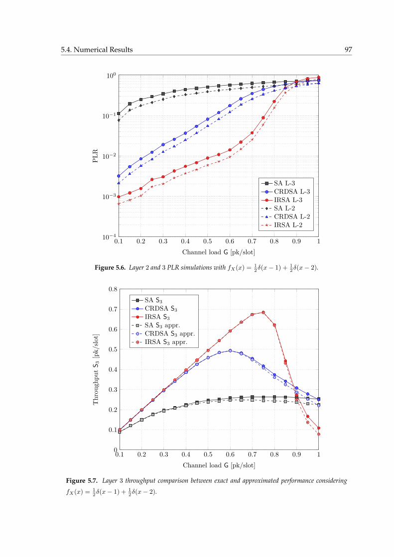
5.4. Numerical Results 97
0.1 0.2 0.3 0.4 0.5 0.6 0.7 0.8 0.9 110−4
10−3
10−2
10−1
100
Channel load G [pk/slot]
PLR
SA L-3CRDSA L-3IRSA L-3SA L-2CRDSA L-2IRSA L-2
Figure 5.6. Layer 2 and 3 PLR simulations with fX(x) = 12δ(x− 1) + 1
2δ(x− 2).
0.1 0.2 0.3 0.4 0.5 0.6 0.7 0.8 0.9 10
0.1
0.2
0.3
0.4
0.5
0.6
0.7
0.8
Channel load G [pk/slot]
Thr
ough
put
S 3[p
k/slo
t]
SA S3CRDSA S3IRSA S3SA S3 appr.CRDSA S3 appr.IRSA S3 appr.
Figure 5.7. Layer 3 throughput comparison between exact and approximated performance considering
fX(x) = 12δ(x− 1) + 1
2δ(x− 2).
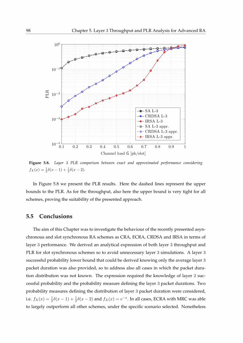
98 Chapter 5. Layer 3 Throughput and PLR Analysis for Advanced RA
0.1 0.2 0.3 0.4 0.5 0.6 0.7 0.8 0.9 110−4
10−3
10−2
10−1
100
Channel load G [pk/slot]
PLR
SA L-3CRDSA L-3IRSA L-3SA L-3 appr.CRDSA L-3 appr.IRSA L-3 appr.
Figure 5.8. Layer 3 PLR comparison between exact and approximated performance considering
fX(x) = 12δ(x− 1) + 1
2δ(x− 2).
In Figure 5.8 we present the PLR results. Here the dashed lines represent the upper
bounds to the PLR. As for the throughput, also here the upper bound is very tight for all
schemes, proving the suitability of the presented approach.
5.5 Conclusions
The aim of this Chapter was to investigate the behaviour of the recently presented asyn-
chronous and slot synchronous RA schemes as CRA, ECRA, CRDSA and IRSA in terms of
layer 3 performance. We derived an analytical expression of both layer 3 throughput and
PLR for slot synchronous schemes so to avoid unnecessary layer 3 simulations. A layer 3
successful probability lower bound that could be derived knowing only the average layer 3
packet duration was also provided, so to address also all cases in which the packet dura-
tion distribution was not known. The expression required the knowledge of layer 2 suc-
cessful probability and the probability measure defining the layer 3 packet durations. Two
probability measures defining the distribution of layer 3 packet duration were considered,
i.e. fX(x) = 12δ(x− 1) + 1
2δ(x− 2) and fX(x) = e−x. In all cases, ECRA with MRC was able
to largely outperform all other schemes, under the specific scenario selected. Nonetheless
5.5. Conclusions 99
it was also the scheme that was more sensible to the distribution of layer 3 packet dura-
tions. We presented also a comparison between layer 3 and layer 2 performance for slot syn-
chronous schemes, and we showed that limited performance loss were achieved by schemes
like CRDSA and IRSA (below 10% in terms of peak throughput loss). Finally, we compared
the derived bound with the exact performance for the slot synchronous schemes, and we
showed that very minor differences could be found. Moreover, the bounds were particu-
larly tight for all channel load values of interest.

Chapter 6Irregular Repetition Slotted ALOHA
over the Rayleigh Block Fading Channel
The littlest thing can cause a ripple
effect that changes your life
Ted Mosby
Until now we have shown the performance of some advanced asynchronous and slot
synchronous RA schemes without taking into consideration the possibility of fading. The
recently proposed slot synchronous IRSA [77] scheme is subject to optimisation of the user
degree distribution for the collision channel model. In this Chapter we aim at extending the
analysis for the Rayleigh block fading channel. The result is two-folded, on the one hand we
extend the optimisation procedure for fading channels, showing that for a certain average
SNR and decoding threshold, throughput exceeding 1 [pk/slot] can be achieved. On the
other hand, the benefit of such optimisation compared to a mismatched one that uses the
collision channel model in spite of the correct Rayleigh block fading one.
6.1 Introduction
The collision channel model is a rather simple one, which assumes that 1) noise can be
neglected, such that a transmission can be decoded from a singleton slot by default, and
2) no transmission can be decoded from a collision slot. This model has a limited practical
applicability and does not describe adequately the wireless transmission scenarios where
the impact of fading and noise cannot be neglected. In particular, fading may incur power
variations among signals observed in collisions slot, allowing the capture effect to occur, when

102 Chapter 6. IRSA over the Rayleigh Block Fading Channel
sufficiently strong signals may be decoded. In the context of slotted ALOHA, numerous
works assessed the performance of the scheme for different capture effect models [4,61,129,
131–133]. One of the standardly used models is the threshold-based one, in which a packet
is captured, i.e. decoded, if its SINR is higher then a predefined threshold, c.f. [61, 132–134].
A brief treatment of the capture effect in IRSA framework was made in [77], pointing out
the implications related to the asymptotic analysis. In [135], the method for the computation
of capture probabilities for the threshold-based model in single-user detection systems with
Rayleigh fading was presented and instantiated for the frameless ALOHA framework [136].
In this Chapter, we extend the treatment of the threshold-based capture effect for IRSA
framework. First, we derive the exact expressions of capture probabilities for the threshold-
based model and Rayleigh block-fading channel. Next we formulate the asymptotic perfor-
mance analysis. We then optimise the scheme, in terms of deriving the optimal repetition
strategies that maximise throughput given a target PLR. Finally, the obtained distributions
are investigated in the finite frame length scenario via simulations. We show that IRSA ex-
hibits a remarkable throughput performance that is well over 1 [pk/slot], for target PLR,
SNR and threshold values that are valid in practical scenarios. This is demonstrated both
for asymptotic and finite frame length cases, showing also that the finite-length performance
indeed tends to the asymptotic one as the frame length increases.
6.2 System Model
6.2.1 Access Protocol
For the sake of simplicity, we focus on a single batch arrival of nu users having a sin-
gle packet (or burst) each, and contending for the access to the common receiver. The link
time is organised in a MAC frame of duration Tf , divided into ms slots of equal duration
Tl = Tf/ms, indexed by j ∈ 1, 2, . . . ,ms. The transmission time of each packet equals the
slot duration. The system load G is defined as
G =nums
[pk/slot] .
According to the IRSA protocol, each user selects a repetition degree d by sampling a
p.m.f. Λddmaxd=2 and transmits d identical replicas of its burst in d randomly chosen slots of
the frame. It is assumed that the header of each burst replica carries information about the
locations (i.e. slot indexes) of all d replicas. The p.m.f. Λd is the same for all users and is
sampled independently by different users, in an uncoordinated fashion. The average burst

6.2. System Model 103
repetition degree is d =∑dmax
d=2 d Λd, and its inverse
R =1
d(6.1)
is called the rate of the IRSA scheme. Each user is then unaware of the repetition degree em-
ployed by the other users contending for the access. The number of burst replicas colliding
in slot j is denoted by cj ∈ 1, 2, . . . , nu. Burst replicas colliding in slot j are indexed by
i ∈ 1, 2, . . . , cj.
6.2.2 Received Power and Fading Models
We consider a Rayleigh block fading channel model, i.e. fading is Rayleigh distributed,
constant and frequency flat in each block, while it is independent and identically distributed
(i.i.d.) on different blocks. Independent fading between different burst replicas is also as-
sumed. In this way, the power of a burst replica i ∈ 1, 2, . . . , cj received in slot j, denoted
as Pij , is modeled as a random variable (r.v.) with negative exponential distribution
fP (p) =
1P
exp[− p
P
], p ≥ 0
0, otherwise
where P is the average received power. This is assumed to be the same for all burst replicas
received in the MAC frame by using, e.g. a long-term power control. The r.v.s Pij are i.i.d.
for all pairs (i, j). If we denote by N the noise power, the SNR r.v. Bij = Pij/N is also
exponentially distributed as
fB (b) =
1B
exp[− b
B
], b ≥ 0
0, otherwise
where the average SNR is given by
B =P
N.
6.2.3 Graph Representation
In order to analyse the SIC process, we introduce the graph representation of a MAC
frame [77]. As depicted in Figure 6.1, a MAC frame is represented as a bipartite graph
G = (B,Sl, E) consisting of a set B of nu burst nodes (or user nodes), one for each user, a set
Sl of ms slot nodes, one per slot, and a set E of edges, one per transmitted burst replica. A
burst node bk ∈ B is connected to a slot node lj ∈ Sl if and only if user k has a burst replica
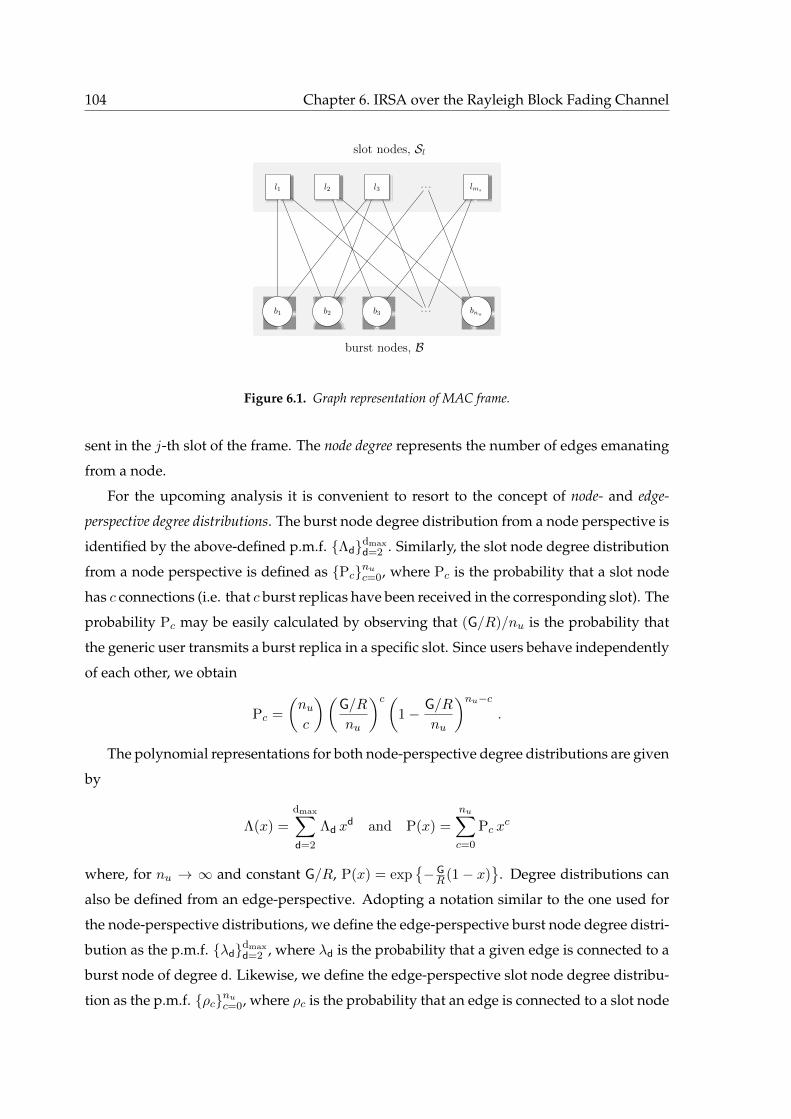
104 Chapter 6. IRSA over the Rayleigh Block Fading Channel
b1 b2 b3 . . . bnu
l1 l2 l3 . . . lms
burst nodes, B
slot nodes, Sl
Figure 6.1. Graph representation of MAC frame.
sent in the j-th slot of the frame. The node degree represents the number of edges emanating
from a node.
For the upcoming analysis it is convenient to resort to the concept of node- and edge-
perspective degree distributions. The burst node degree distribution from a node perspective is
identified by the above-defined p.m.f. Λddmaxd=2 . Similarly, the slot node degree distribution
from a node perspective is defined as Pcnuc=0, where Pc is the probability that a slot node
has c connections (i.e. that c burst replicas have been received in the corresponding slot). The
probability Pc may be easily calculated by observing that (G/R)/nu is the probability that
the generic user transmits a burst replica in a specific slot. Since users behave independently
of each other, we obtain
Pc =
(nuc
)(G/R
nu
)c(1− G/R
nu
)nu−c.
The polynomial representations for both node-perspective degree distributions are given
by
Λ(x) =
dmax∑d=2
Λd xd and P(x) =
nu∑c=0
Pc xc
where, for nu → ∞ and constant G/R, P(x) = exp−GR(1− x)
. Degree distributions can
also be defined from an edge-perspective. Adopting a notation similar to the one used for
the node-perspective distributions, we define the edge-perspective burst node degree distri-
bution as the p.m.f. λddmaxd=2 , where λd is the probability that a given edge is connected to a
burst node of degree d. Likewise, we define the edge-perspective slot node degree distribu-
tion as the p.m.f. ρcnuc=0, where ρc is the probability that an edge is connected to a slot node

6.2. System Model 105
of degree c. From the definitions we have λd = d Λd/ (∑
t tΛt) and ρc = cPc/ (∑
t tPt); it can
be shown that, for nu → ∞ and constant G/R, ρc = exp−G/R(G/R)c−1/(c− 1)!. The cor-
responding polynomial representation are λ(x) =∑dmax
d=2 λd xd−1 and ρ(x) =
∑nuc=0 ρc x
c−1.
Note that λ(x) = Λ′(x)/Λ′(1) and ρ(x) = P′(x)/P′(1).1
6.2.4 Receiver Operation
In our model, the receiver is always able to detect burst replicas received in a slot, i.e. to
discriminate between an empty slot where only noise samples are present and a slot in which
at least one burst replica has been received. Moreover, a threshold-based capture model
for the receiver is assumed, by which the generic burst replica i is successfully decoded
(i.e. captured) in slot j if the SINR exceeds a certain threshold b?, namely,
Prburst replica i decoded =
1,Pij
N+Zij≥ b?
0, otherwise.(6.2)
The quantity Zij in (6.2) denotes the power of the interference impairing replica i in slot j.
In our system model the threshold b? fulfills b? ≥ 1, which corresponds to a conventional
narrowband single-antenna system. As we are considering a SIC-based receiver, under the
assumption of perfect IC the quantity Zij is equal to sum of the powers of those bursts that
have not yet been cancelled from slot j in previous iterations (apart form burst i). Specifi-
cally,
Zij =∑
u∈Rj\iPuj (6.3)
where Puj is the power of burst replica u not yet cancelled in slot j and Rj denotes the set
of remaining burst replicas in slot j. Exploiting (6.3), after simple manipulation we obtain
PijN + Zij
=Bij
1 +∑
u∈Rj\i Buj.
Hence, in the adopted threshold-based capture model the condition PijN+Zij
≥ b? in (6.2) may
be recast as
Bij1 +
∑u∈Rj\i Buj
≥ b? . (6.4)
When processing the signal received in some slot j, if burst replica i is successfully de-
coded due to fulfillment of (6.4), then 1) its contribution of interference is cancelled from1We recall that, notation f ′(x) denotes the derivative of f(x).
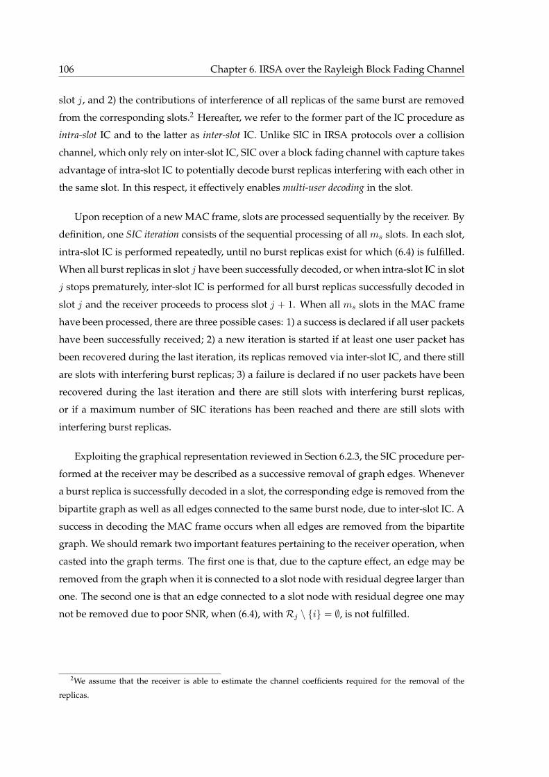
106 Chapter 6. IRSA over the Rayleigh Block Fading Channel
slot j, and 2) the contributions of interference of all replicas of the same burst are removed
from the corresponding slots.2 Hereafter, we refer to the former part of the IC procedure as
intra-slot IC and to the latter as inter-slot IC. Unlike SIC in IRSA protocols over a collision
channel, which only rely on inter-slot IC, SIC over a block fading channel with capture takes
advantage of intra-slot IC to potentially decode burst replicas interfering with each other in
the same slot. In this respect, it effectively enables multi-user decoding in the slot.
Upon reception of a new MAC frame, slots are processed sequentially by the receiver. By
definition, one SIC iteration consists of the sequential processing of all ms slots. In each slot,
intra-slot IC is performed repeatedly, until no burst replicas exist for which (6.4) is fulfilled.
When all burst replicas in slot j have been successfully decoded, or when intra-slot IC in slot
j stops prematurely, inter-slot IC is performed for all burst replicas successfully decoded in
slot j and the receiver proceeds to process slot j + 1. When all ms slots in the MAC frame
have been processed, there are three possible cases: 1) a success is declared if all user packets
have been successfully received; 2) a new iteration is started if at least one user packet has
been recovered during the last iteration, its replicas removed via inter-slot IC, and there still
are slots with interfering burst replicas; 3) a failure is declared if no user packets have been
recovered during the last iteration and there are still slots with interfering burst replicas,
or if a maximum number of SIC iterations has been reached and there are still slots with
interfering burst replicas.
Exploiting the graphical representation reviewed in Section 6.2.3, the SIC procedure per-
formed at the receiver may be described as a successive removal of graph edges. Whenever
a burst replica is successfully decoded in a slot, the corresponding edge is removed from the
bipartite graph as well as all edges connected to the same burst node, due to inter-slot IC. A
success in decoding the MAC frame occurs when all edges are removed from the bipartite
graph. We should remark two important features pertaining to the receiver operation, when
casted into the graph terms. The first one is that, due to the capture effect, an edge may be
removed from the graph when it is connected to a slot node with residual degree larger than
one. The second one is that an edge connected to a slot node with residual degree one may
not be removed due to poor SNR, when (6.4), withRj \ i = ∅, is not fulfilled.
2We assume that the receiver is able to estimate the channel coefficients required for the removal of the
replicas.
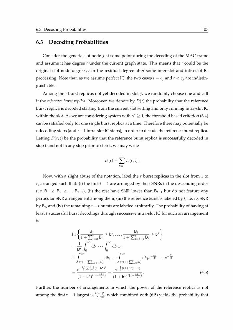
6.3. Decoding Probabilities 107
6.3 Decoding Probabilities
Consider the generic slot node j at some point during the decoding of the MAC frame
and assume it has degree r under the current graph state. This means that r could be the
original slot node degree cj or the residual degree after some inter-slot and intra-slot IC
processing. Note that, as we assume perfect IC, the two cases r = cj and r < cj are indistin-
guishable.
Among the r burst replicas not yet decoded in slot j, we randomly choose one and call
it the reference burst replica. Moreover, we denote by D(r) the probability that the reference
burst replica is decoded starting from the current slot setting and only running intra-slot IC
within the slot. As we are considering system with b? ≥ 1, the threshold based criterion (6.4)
can be satisfied only for one single burst replica at a time. Therefore there may potentially be
r decoding steps (and r−1 intra-slot IC steps), in order to decode the reference burst replica.
Letting D(r, t) be the probability that the reference burst replica is successfully decoded in
step t and not in any step prior to step t, we may write
D(r) =
r∑t=1
D(r, t) .
Now, with a slight abuse of the notation, label the r burst replicas in the slot from 1 to
r, arranged such that: (i) the first t − 1 are arranged by their SNRs in the descending order
(i.e. B1 ≥ B2 ≥ . . .Bt−1), (ii) the rest have SNR lower than Bt−1 but do not feature any
particular SNR arrangement among them, (iii) the reference burst is labeled by t, i.e. its SNR
by Bt, and (iv) the remaining r− t bursts are labeled arbitrarily. The probability of having at
least t successful burst decodings through successive intra-slot IC for such an arrangement
is
Pr
B1
1 +∑r
i=2 Bi≥ b?, . . . ,
Bt1 +
∑ri=t+1 Bi
≥ b?
=1
Br
∫ ∞0
dbr · · ·∫ ∞
0dbt+1
×∫ ∞
b?(1+∑ri=t+1 bi)
dbt · · ·∫ ∞
b?(1+∑ri=2 bi)
db1e− br
B · · · e−b1B
=e−
b?
B
∑t−1i=0(1+b?)i
(1 + b?)t(r−t+1
2)
=e−
1B
((1+b?)t−1)
(1 + b?)t(r−t+1
2 ). (6.5)
Further, the number of arrangements in which the power of the reference replica is not
among the first t − 1 largest is (r−1)!(r−t)! , which combined with (6.5) yields the probability that
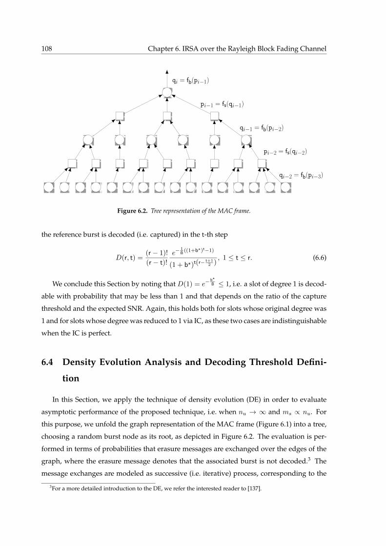
108 Chapter 6. IRSA over the Rayleigh Block Fading Channel
qi−2 = fb(pi−3)
pi−2 = fs(qi−2)
qi−1 = fb(pi−2)
pi−1 = fs(qi−1)
qi = fb(pi−1)
Figure 6.2. Tree representation of the MAC frame.
the reference burst is decoded (i.e. captured) in the t-th step
D(r, t) =(r − 1)!
(r − t)!
e−1B
((1+b?)t−1)
(1 + b?)t(r− t+12 )
, 1 ≤ t ≤ r. (6.6)
We conclude this Section by noting that D(1) = e−b?
B ≤ 1, i.e. a slot of degree 1 is decod-
able with probability that may be less than 1 and that depends on the ratio of the capture
threshold and the expected SNR. Again, this holds both for slots whose original degree was
1 and for slots whose degree was reduced to 1 via IC, as these two cases are indistinguishable
when the IC is perfect.
6.4 Density Evolution Analysis and Decoding Threshold Defini-
tion
In this Section, we apply the technique of density evolution (DE) in order to evaluate
asymptotic performance of the proposed technique, i.e. when nu → ∞ and ms ∝ nu. For
this purpose, we unfold the graph representation of the MAC frame (Figure 6.1) into a tree,
choosing a random burst node as its root, as depicted in Figure 6.2. The evaluation is per-
formed in terms of probabilities that erasure messages are exchanged over the edges of the
graph, where the erasure message denotes that the associated burst is not decoded.3 The
message exchanges are modeled as successive (i.e. iterative) process, corresponding to the
3For a more detailed introduction to the DE, we refer the interested reader to [137].
6.4. Density Evolution Analysis and Decoding Threshold Definition 109
decoding algorithm described in Section 6.2.4 in the asymptotic case, when the lengths of
the loops in the graph tends to infinity. Specifically, the i-th iteration consists of the update
of the probability qi that an edge carries an erasure message from a burst node to a slot node,
followed by the update of the probability pi that an edge carries an erasure message from a
slot node to a burst node. These probabilities are averaged over all edges in the graph. We
proceed by outlining the details.
The probability that an edge carries an erasure message from burst nodes to slot nodes
in the i-th iteration is
qi =
dmax∑d=1
λd q(d)i =
dmax∑d=1
λd pd−1i−1 =: fb(pi−1) (6.7)
where λd is the probability that an edge is connected to a burst node of degree d (see Sec-
tion 6.2.3) and q(d)i is the probability that an edge carries an erasure message given that it is
connected to a burst node of degree d. In the second equality we used the fact that the an
outgoing message from a burst node carries an erasure only if all incoming edges carry an
erasure, i.e. q(d)i = pd−1
i−1 .
Similarly, the probability that an edge carries an erasure message from SNs to BNs in i-th
iteration is
pi =+∞∑c=1
ρc p(c)i (6.8)
where ρc is the probability that an edge is connected to a slot node of degree c, and where
p(c)i is the probability that an edge carries an erasure message given that it is connected to a
slot node of degree c. This probability may be expressed as
p(c)i = 1−
c∑r=1
D(r)
(c− 1
r − 1
)qr−1i (1− qi)
c−r, (6.9)
where summation is done over all possible values of the reduced degree r, i.e. 1 ≤ r ≤ c, the
term(c−1r−1
)qr−1i (1 − qi)
c−r corresponds to the probability that the degree of the slot node is
reduced to r and D(r) is the probability that the burst corresponding to the outgoing edge is
decoded when the (reduced) degree of the slot node is r.4
4As it happens in the asymptotic case, the loops in the graph are assumed to be of infinite length, such that
the tree representation in Figure 6.2 holds, the reduction of the slot degree happens only via inter-slot IC, which
is implicitly assumed in the term(c−1r−1
)qr−1i (1 − qi)
c−r. On the other hand, D(r) expresses the probability that
an outgoing edge from the slot node is decoded using intra-slot IC (see Section 6.3). In other words, inter- and
intra-slot IC are in the asymptotic evaluation separated over DE iterations.
110 Chapter 6. IRSA over the Rayleigh Block Fading Channel
Combining (6.9) and the expression for the edge-oriented slot-node degree distribution
(see Section 6.2.3) into (6.8) yields
pi = 1− e− GR
∞∑c=1
(G
R
)c−1 c∑r=1
D(r)
(r − 1)!qr−1i (1− qi)
c−r. (6.10)
It can be shown that in case of perfect IC, (6.10) becomes
pi = 1− e− GR
+∞∑r=1
D(r)
(r − 1)!
(G
Rqi
)r−1 +∞∑c=0
(GR(1− qi)
)cc!
= 1− e− GRqi
+∞∑r=1
D(r)
(r − 1)!
(G
Rqi
)r−1
, (6.11)
where D(r) =∑r
t=1D(r, t), see (6.6). Further, defining zt = (1 + b?)t, (6.11) becomes
pi = 1− e− GRqi
+∞∑r=1
(G
Rqi
)r−1 r∑t=1
e−1B
(zt−1)
(r − t)!z(r− t+1
2 )t
= 1− e− GRqi
+∞∑t=1
(GRqi)t−1
z( t−1
2 )t
e−1B
(zt−1)+∞∑r=0
(GRqi)r
r!zrt
= 1−+∞∑t=1
(GRqi)t−1
z( t−1
2 )t
e−(zt−1)
(1B
+GR
qizt
)
=: fs(qi) . (6.12)
A DE recursion is obtained combining (6.7) with (6.12), consisting of one recursion for
qi and one for pi. In the former case, the recursion takes the form qi = (fb fs)(qi−1) for
i ≥ 1, with initial value q0 = 0. In the latter case, it assumes the form pi = (fs fb)(pi−1)
for i ≥ 1, with initial value p0 = fs(0). Note that the DE recursion for pi allows express-
ing the asymptotic PLR of an IRSA scheme in a very simple way. More specifically, let
p∞(G, Λd , B, b?) = limi→∞ pi be the limit of the DE recursion, where we have explicitly
indicated that the limit depends on the system load, on the burst node degree distribu-
tion, on the average SNR, and on the threshold for successful intra-slot decoding. Since[p∞(G, Λd , B, b?)
]d represents the probability that a user packet associated with a burst
node of degree d is not successfully received at the end of the decoding process, the asymp-
totic PLR is given by
pl(G, Λd , B, b?) =
dmax∑d=2
Λd
[p∞(G, Λd , B, b?)
]d.
Next, we introduce the concept of asymptotic decoding threshold for an IRSA scheme over
the considered block fading channel model and under the decoding algorithm described in
Section 6.2.4. Let pl be a target PLR. Then, the asymptotic decoding threshold, denoted by
6.5. Numerical Results 111
G? = G?(Λd , B, b?, pl), is defined as the supremum system load value for which the target
PLR is achieved in the asymptotic setting:
G? = supG≥0G : pl(G, Λd , B, b?) < pl.
6.5 Numerical Results
Table 6.1 shows some degree distributions designed combining the DE analysis devel-
oped in Section 6.4 with the differential evolution optimisation algorithm proposed in [138].
For each design we set pl = 10−2, B = 20 dB, and b? = 3 dB, and we constrained the opti-
misation algorithm to find the distribution Λd with the largest threshold G?, subject to a
given average degree5 d and maximum degree dmax = 16.
For all chosen average degrees, the G? threshold of the optimised distribution largely
exceeds the value 1 [pk/slot], the theoretical limit under a collision channel model. In gen-
eral, the higher is the average degree d, the larger is the load threshold G?. However, as d
increases, more complex burst node distributions are obtained. For instance, under a d = 4
constraint, the maximum degree is dmax = 16 (i.e. a user may transmit up to 16 copies of its
packet); when reducing d, the optimisation converges to degree distributions with a lower
maximum degree, and degree-2 nodes become increasingly dominant.
To assess the effectiveness of the proposed design approach, tailored to the block fading
channel with capture, we optimised a distribution Λ5(x) using the DE recursion over the
collision channel [77] and again constraining the optimisation to d = 4 and dmax = 16. As
from Table 6.1, due to the mismatched channel model, we observe a 7% loss in terms of G?
threshold w.r.t. the distribution Λ1(x) that fulfills the same constraints but was obtained
with the DE developed in this Chapter.
In order to investigate the performance of the optimised distributions in a finite frame
length setting, we ran Monte Carlo simulations setting ms = 200 (unless otherwise stated),
B = 20 dB, b? = 3 dB, and the maximum number of IC iterations to 20. Figure 6.3 illus-
trates the throughput S, defined as the average number of successfully decoded packets per
slot, versus the channel load. Even in the relatively short frame regime ms = 200, all dis-
tributions exhibit peak throughput exceeding 1 [pk/slot]. The distribution Λ2(x) is the one
achieving the highest throughput of 1.52 [pk/slot], although Λ1(x) is the distribution with
the highest threshold G?. It is important to recall that the threshold is computed for a target
5A constraint on the average degree d can be turned into a constraint on the rateR as there is a direct relation
between the two; see also equation (6.1).
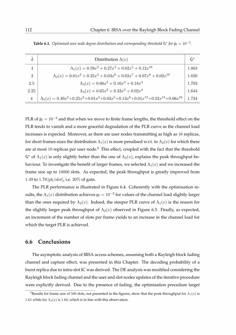
112 Chapter 6. IRSA over the Rayleigh Block Fading Channel
Table 6.1. Optimised user node degree distribution and corresponding threshold G? for pl = 10−2.
d Distribution Λ(x) G?
4 Λ1(x) = 0.59x2 + 0.27x3 + 0.02x5 + 0.12x16 1.863
3 Λ2(x) = 0.61x2 + 0.25x3 + 0.03x6 + 0.02x7 + 0.07x8 + 0.02x10 1.820
2.5 Λ3(x) = 0.66x2 + 0.16x3 + 0.18x4 1.703
2.25 Λ4(x) = 0.65x2 + 0.33x3 + 0.02x4 1.644
4 Λ5(x) = 0.49x2+0.25x3+0.01x4+0.03x5+0.13x6+0.01x13+0.02x14+0.06x16 1.734
PLR of pl = 10−2 and that when we move to finite frame lengths, the threshold effect on the
PLR tends to vanish and a more graceful degradation of the PLR curve as the channel load
increases is expected. Moreover, as there are user nodes transmitting as high as 16 replicas,
for short frames sizes the distribution Λ1(x) is more penalised w.r.t. to Λ2(x) for which there
are at most 10 replicas per user node.6 This effect, coupled with the fact that the threshold
G? of Λ1(x) is only slightly better than the one of Λ2(x), explains the peak throughput be-
haviour. To investigate the benefit of larger frames, we selected Λ1(x) and we increased the
frame size up to 10000 slots. As expected, the peak throughput is greatly improved from
1.49 to 1.79 [pk/slot], i.e. 20% of gain.
The PLR performance is illustrated in Figure 6.4. Coherently with the optimisation re-
sults, the Λ1(x) distribution achieves pl = 10−2 for values of the channel load slightly larger
than the ones required by Λ2(x). Indeed, the steeper PLR curve of Λ1(x) is the reason for
the slightly larger peak throughput of Λ2(x) observed in Figure 6.3. Finally, as expected,
an increment of the number of slots per frame yields to an increase in the channel load for
which the target PLR is achieved.
6.6 Conclusions
The asymptotic analysis of IRSA access schemes, assuming both a Rayleigh block fading
channel and capture effect, was presented in this Chapter. The decoding probability of a
burst replica due to intra-slot IC was derived. The DE analysis was modified considering the
Rayleigh block fading channel and the user and slot nodes updates of the iterative procedure
were explicitly derived. Due to the presence of fading, the optimisation procedure target
6Results for frame size of 500 slots, not presented in the figures, show that the peak throughput for Λ1(x) is
1.61 while for Λ2(x) is 1.60, which is in line with this observation.
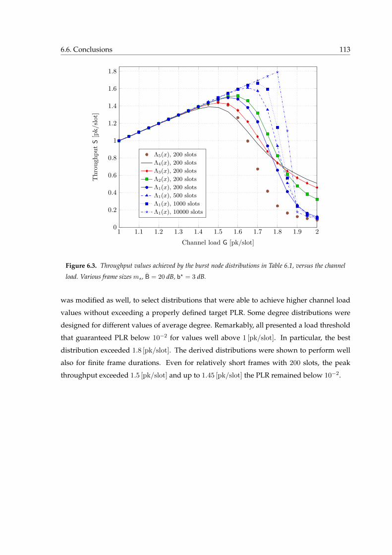
6.6. Conclusions 113
1 1.1 1.2 1.3 1.4 1.5 1.6 1.7 1.8 1.9 20
0.2
0.4
0.6
0.8
1
1.2
1.4
1.6
1.8
Channel load G [pk/slot]
Thr
ough
put
S[p
k/slo
t]
Λ5(x), 200 slotsΛ4(x), 200 slotsΛ3(x), 200 slotsΛ2(x), 200 slotsΛ1(x), 200 slotsΛ1(x), 500 slotsΛ1(x), 1000 slotsΛ1(x), 10000 slots
Figure 6.3. Throughput values achieved by the burst node distributions in Table 6.1, versus the channel
load. Various frame sizes ms, B = 20 dB, b? = 3 dB.
was modified as well, to select distributions that were able to achieve higher channel load
values without exceeding a properly defined target PLR. Some degree distributions were
designed for different values of average degree. Remarkably, all presented a load threshold
that guaranteed PLR below 10−2 for values well above 1 [pk/slot]. In particular, the best
distribution exceeded 1.8 [pk/slot]. The derived distributions were shown to perform well
also for finite frame durations. Even for relatively short frames with 200 slots, the peak
throughput exceeded 1.5 [pk/slot] and up to 1.45 [pk/slot] the PLR remained below 10−2.

114 Chapter 6. IRSA over the Rayleigh Block Fading Channel
1 1.1 1.2 1.3 1.4 1.5 1.6 1.7 1.8 1.9 210−4
10−3
10−2
10−1
100
Channel load G [pk/slot]
pack
etlo
ssra
tep l
Λ5(x), 200 slotsΛ4(x), 200 slotsΛ3(x), 200 slotsΛ2(x), 200 slotsΛ1(x), 200 slotsΛ1(x), 500 slotsΛ1(x), 1000 slotsΛ1(x), 10000 slots
Figure 6.4. PLR values achieved by the burst node distributions in Table 6.1, versus the channel load.
Various frame sizes ms, B = 20 dB, b? = 3 dB.
Chapter 7Random Access with Multiple
Receivers
It is the weight, not numbers of
experiments that is to be regarded
Isaac Newton
7.1 Introduction
Until now we have focused on the simple a basic scenario in which a plurality of user
terminals want to communicate in an uncoordinated fashion to a single receiver. Different
RA techniques have been investigated, both involving time synchronization (at slot or at
frame level) or completely asynchronous. In this Chapter we follow a parallel research di-
rection, in which the transmitter can rely on spatial diversity. In particular, we expand the
simple topology typical of MAC channel, in two directions. Firstly, we add a finite number
of non-cooperative receivers (called also relays) and secondly, we complement the uplink
of such a system with a downlink or wireless backhaul link,1 where the receivers forward
the successfully received packets to a single common gateway (GW). In order to take into
account variability of user-relay links, a packet erasure channel is considered in the uplink
phase. Specifically, each user-rely link is considered active with probability 1−ε on a slot-by-
slot basis. Furthermore, SA is considered as channel access policy for each such link. In the
1In the following we will use the term downlink for referring to such link, in accordance to satellite commu-
nications nomenclature in which the return uplink refers to the users to satellite communication link and the
downlink refers to the satellite to gateway link. In terrestrial networks the name downlink shall be substituted
with the more appropriate wireless backhaul link.
116 Chapter 7. Random Access with Multiple Receivers
downlink phase, the relays forward the correctly received packets or linear combinations of
them.
In this Chapter we aim at characterising the uplink aggregate throughput seen at all
receivers as well as the PLR. We derive the upper bound on the downlink rate defined as
number of total downlink transmission per uplink time slot and we show that with random
linear coding (RLC) the bound can be achieved letting the observation of time slots in the
uplink grow very large. We then propose alternative low complexity downlink policies
that allow the relays to drop some of the correctly received packets eventually based on the
observation of the uplink slots. Finally, we address the scenario in which the relays have
a finite memory so that only a finite number of correctly decoded packets can be collected
before starting the downlink phase. In this case, we first derive an analytical expression of
the performance for RLC and we compare this solution with the dropping policies. We are
then able to show that under some dowlink rate conditions and for some buffer sizes, the
simple dropping policies are able to largely outperform RLC.
Note that part of the Chapter has been already published in [87] and the author of the
thesis is not co-author of that work. Nonetheless, a recall of the general framework is con-
sidered fundamental for giving a proper understanding of the contribution of the thesis’
author which mainly focuses on Section 7.6.
SA with space (antenna) diversity was analysed in [139] under the assumption of
Rayleigh fading and shadowing, with emphasis on the two-antenna case. The authors in [88]
address also a similar scenario, although in their case SIC is introduced at the relays. De-
pending on the considered policy, both inter-relay and intra-relay SIC are also applied.
7.2 System Model and Preliminaries
Throughout this Chapter, we focus on the topology depicted in Figure 7.1, where an
infinite population of users wants to deliver information in the form of data packets to a
collecting GW. The transmission process is divided in two phases, referred to as uplink and
downlink, respectively. During the former, data are sent in an uncoordinated fashion over a
shared wireless channel to a set of K receivers or relays, which, in turn, forward collected
information to the GW in the downlink.
As to the uplink, time is divided in successive slots, and transmission parameters in
terms of packet length, coding and modulation are fixed such that one packet can be sent
within one time unit. Users are assumed to be slot-synchronized, and SA [3] is employed as
medium access policy. Furthermore, the number of users accessing the channel in a generic
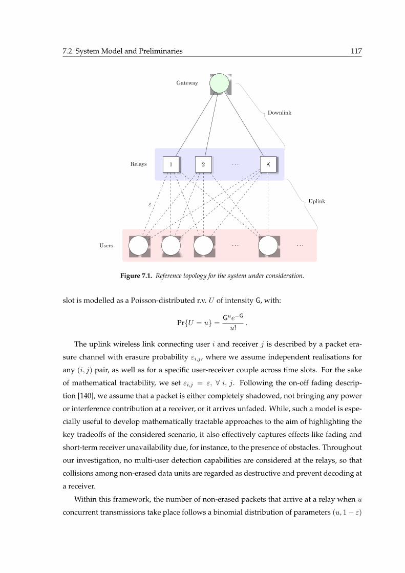
7.2. System Model and Preliminaries 117
. . . . . .
1 2 . . . K
ε
Users
Relays
Gateway
Uplink
Downlink
Figure 7.1. Reference topology for the system under consideration.
slot is modelled as a Poisson-distributed r.v. U of intensity G, with:
PrU = u =Gue−G
u!.
The uplink wireless link connecting user i and receiver j is described by a packet era-
sure channel with erasure probability εi,j , where we assume independent realisations for
any (i, j) pair, as well as for a specific user-receiver couple across time slots. For the sake
of mathematical tractability, we set εi,j = ε, ∀ i, j. Following the on-off fading descrip-
tion [140], we assume that a packet is either completely shadowed, not bringing any power
or interference contribution at a receiver, or it arrives unfaded. While, such a model is espe-
cially useful to develop mathematically tractable approaches to the aim of highlighting the
key tradeoffs of the considered scenario, it also effectively captures effects like fading and
short-term receiver unavailability due, for instance, to the presence of obstacles. Throughout
our investigation, no multi-user detection capabilities are considered at the relays, so that
collisions among non-erased data units are regarded as destructive and prevent decoding at
a receiver.
Within this framework, the number of non-erased packets that arrive at a relay when u
concurrent transmissions take place follows a binomial distribution of parameters (u, 1− ε)
118 Chapter 7. Random Access with Multiple Receivers
over one slot. Therefore, a successful reception occurs with probability u(1−ε)εu−1, and the
average throughput experienced at each of the K receivers, in terms of decoded packets per
slot, can be computed as:
Ssa =∞∑u=0
Gue−G
u!u(1− ε)εu−1 = G(1− ε)e−G(1−ε) , (7.1)
corresponding to the performance of a SA system with erasures. On the other hand, a spatial
diversity gain can be triggered when the relays are considered jointly, since independent
channel realisations may lead them to retrieve different information units over the same
time slot. In order to quantify this beneficial effect, we label a packet as collected when it has
been received by at least one of the relays, and we introduce the uplink throughput Sul,K as the
average number of collected packets per slot. Despite its simplicity, such a definition offers
an effective characterisation of the beneficial effects of diversity, by properly accounting for
both the possibility of retrieving up to minu,K distinct data units or multiple times the
same data unit over a slot, as will be discussed in details in Section 7.3.1. On the other
hand, Sul,K also quantifies the actual amount of information that can be retrieved by the set
of receivers, providing an upper bound for the overall achievable end-to-end performance,
and setting the target for the design of any relay-to-GW delivery strategy.
For the downlink phase, we focus on a decode and forward (D&F) approach, so that each
receiver re-encodes and transmits only packets it has correctly retrieved during the uplink
phase, or possibly linear combinations thereof. A finite downlink capacity is assumed, and
relays have to share a common bandwidth to communicate to the GW by means of a TDMA
scheme. In order to get an insightful characterisation of the optimum achievable system
performance, we assume relay-to-GW links to be error free, and let resource allocation for
the D&F phase be performed ideally and without additional cost by the central collecting
unit.
7.2.1 Notation
Prior to delving into the details of our mathematical framework, we introduce in the
following some useful notation. All the variables will be properly introduced when needed
in the discussion, and the present Section is simply meant to offer a quick reference point
throughout the reading.
K relays are available, and, within time slot l, the countably infinite set of possible out-
comes at each of them is labeled as Ωl := ωl0, ωl1, ωl2, . . . , ωl∞ for each l = 1, 2, . . . ,mul.
Here, ωl0 denotes the erasure event (given either by a collision or by an idle slot), while ωlj
7.3. Uplink Performance 119
indicates the event that the packet of the j-th user arriving in slot l was received. According
to this notation, we define as X lk the random variables with alphabet N, where X l
k = j if ωljwas the observation at relay k. When needed for mathematical discussion, we let the uplink
operate for mul time slots. In this case, let Amulk be the set of collected packets after mul time
slots at receiver k, where Amulk (⋃mull=1 Ωl\ωl0. That is, we do not add the erasure events to
Amulk . The number of received packets at relay k after mul time slots is thus |Amulk |.In general, the complement of a set A is indicated as Ac. We write vectors as bold
variables, e.g. w, while matrices and their transposes are labeled by uppercase bold letters,
e.g. B and BT .
7.3 Uplink Performance
With reference to the topology of Figure 7.1, we first consider the uplink phase. In or-
der to gather a comprehensive description of the improvements enabled by receiver diver-
sity, we characterise the system by means of two somewhat complementary metrics: uplink
throughput (Section 7.3.1) and packet loss rate (Section 7.3.2).
7.3.1 Uplink Throughput
Let us focus on the random access channel, and, following the definition introduced in
Section 7.2, let C be the number of packets collected by the relays over one slot. C is a
r.v. with outcomes in the set 0, 1, 2, . . . ,K, where the maximum value occurs when the
K receivers decode distinct packets due to different erasure patterns. The average uplink
throughput can thus be expressed by conditioning on the number of concurrent transmis-
sions as:
Sul,K =EU [E[ C |U ] ]=
∞∑u=0
Gue−G
u!
K∑c=0
cPrC = c |U = u. (7.2)
While equation (7.2) formula holds for any K, the computation of the collection probabilities
intrinsically depends on the number of available relays. In this perspective, we articulate
our analysis by first considering the two-receiver case, to then extend the results for an
arbitrary topology.
The Two-Receiver Case
Let us first then focus on the case in which only two relays are available. Such a scenario
allows a compact mathematical derivation of the uplink throughput, as the events leading
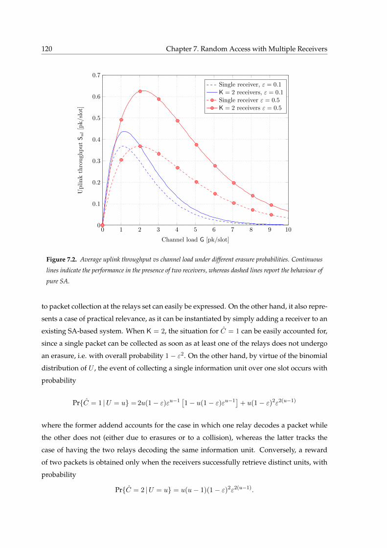
120 Chapter 7. Random Access with Multiple Receivers
0 1 2 3 4 5 6 7 8 9 100
0.1
0.2
0.3
0.4
0.5
0.6
0.7
Channel load G [pk/slot]
Uplinkthrough
putSul[pk/slot]
Single receiver, ε = 0.1K = 2 receivers, ε = 0.1Single receiver ε = 0.5K = 2 receivers ε = 0.5
Figure 7.2. Average uplink throughput vs channel load under different erasure probabilities. Continuous
lines indicate the performance in the presence of two receivers, whereas dashed lines report the behaviour of
pure SA.
to packet collection at the relays set can easily be expressed. On the other hand, it also repre-
sents a case of practical relevance, as it can be instantiated by simply adding a receiver to an
existing SA-based system. When K = 2, the situation for C = 1 can be easily accounted for,
since a single packet can be collected as soon as at least one of the relays does not undergo
an erasure, i.e. with overall probability 1− ε2. On the other hand, by virtue of the binomial
distribution of U , the event of collecting a single information unit over one slot occurs with
probability
PrC = 1 |U = u = 2u(1− ε)εu−1[1− u(1− ε)εu−1
]+ u(1− ε)2ε2(u−1)
where the former addend accounts for the case in which one relay decodes a packet while
the other does not (either due to erasures or to a collision), whereas the latter tracks the
case of having the two relays decoding the same information unit. Conversely, a reward
of two packets is obtained only when the receivers successfully retrieve distinct units, with
probability
PrC = 2 |U = u = u(u− 1)(1− ε)2ε2(u−1).
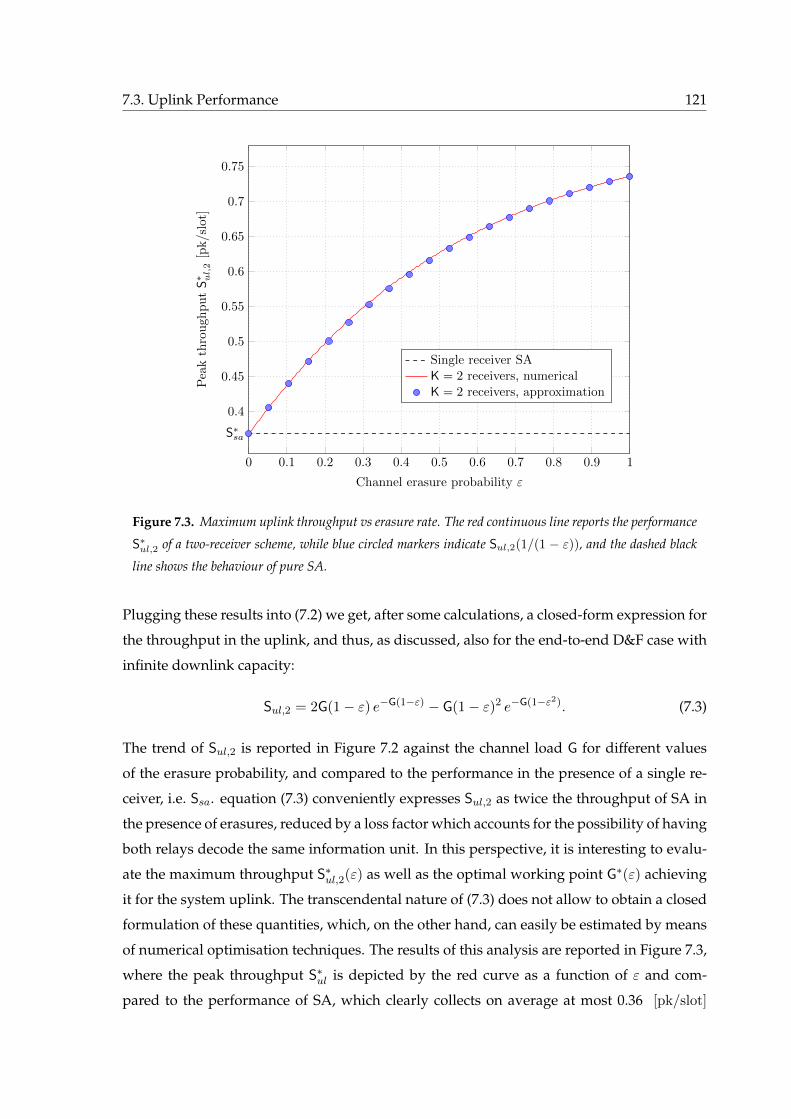
7.3. Uplink Performance 121
0 0.1 0.2 0.3 0.4 0.5 0.6 0.7 0.8 0.9 1
0.4
0.45
0.5
0.55
0.6
0.65
0.7
0.75
S∗sa
Channel erasure probability ε
Peakthrough
putS∗ ul,2[pk/slot]
Single receiver SAK = 2 receivers, numericalK = 2 receivers, approximation
Figure 7.3. Maximum uplink throughput vs erasure rate. The red continuous line reports the performance
S∗ul,2 of a two-receiver scheme, while blue circled markers indicate Sul,2(1/(1 − ε)), and the dashed black
line shows the behaviour of pure SA.
Plugging these results into (7.2) we get, after some calculations, a closed-form expression for
the throughput in the uplink, and thus, as discussed, also for the end-to-end D&F case with
infinite downlink capacity:
Sul,2 = 2G(1− ε) e−G(1−ε) − G(1− ε)2 e−G(1−ε2). (7.3)
The trend of Sul,2 is reported in Figure 7.2 against the channel load G for different values
of the erasure probability, and compared to the performance in the presence of a single re-
ceiver, i.e. Ssa. equation (7.3) conveniently expresses Sul,2 as twice the throughput of SA in
the presence of erasures, reduced by a loss factor which accounts for the possibility of having
both relays decode the same information unit. In this perspective, it is interesting to evalu-
ate the maximum throughput S∗ul,2(ε) as well as the optimal working point G∗(ε) achieving
it for the system uplink. The transcendental nature of (7.3) does not allow to obtain a closed
formulation of these quantities, which, on the other hand, can easily be estimated by means
of numerical optimisation techniques. The results of this analysis are reported in Figure 7.3,
where the peak throughput S∗ul is depicted by the red curve as a function of ε and com-
pared to the performance of SA, which clearly collects on average at most 0.36 [pk/slot]
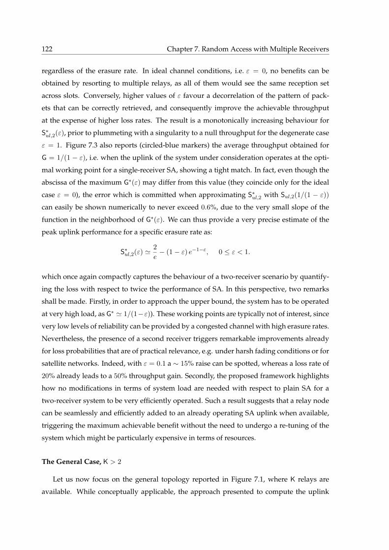
122 Chapter 7. Random Access with Multiple Receivers
regardless of the erasure rate. In ideal channel conditions, i.e. ε = 0, no benefits can be
obtained by resorting to multiple relays, as all of them would see the same reception set
across slots. Conversely, higher values of ε favour a decorrelation of the pattern of pack-
ets that can be correctly retrieved, and consequently improve the achievable throughput
at the expense of higher loss rates. The result is a monotonically increasing behaviour for
S∗ul,2(ε), prior to plummeting with a singularity to a null throughput for the degenerate case
ε = 1. Figure 7.3 also reports (circled-blue markers) the average throughput obtained for
G = 1/(1 − ε), i.e. when the uplink of the system under consideration operates at the opti-
mal working point for a single-receiver SA, showing a tight match. In fact, even though the
abscissa of the maximum G∗(ε) may differ from this value (they coincide only for the ideal
case ε = 0), the error which is committed when approximating S∗ul,2 with Sul,2(1/(1 − ε))can easily be shown numerically to never exceed 0.6%, due to the very small slope of the
function in the neighborhood of G∗(ε). We can thus provide a very precise estimate of the
peak uplink performance for a specific erasure rate as:
S∗ul,2(ε) ' 2
e− (1− ε) e−1−ε, 0 ≤ ε < 1.
which once again compactly captures the behaviour of a two-receiver scenario by quantify-
ing the loss with respect to twice the performance of SA. In this perspective, two remarks
shall be made. Firstly, in order to approach the upper bound, the system has to be operated
at very high load, as G∗ ' 1/(1−ε)). These working points are typically not of interest, since
very low levels of reliability can be provided by a congested channel with high erasure rates.
Nevertheless, the presence of a second receiver triggers remarkable improvements already
for loss probabilities that are of practical relevance, e.g. under harsh fading conditions or for
satellite networks. Indeed, with ε = 0.1 a ∼ 15% raise can be spotted, whereas a loss rate of
20% already leads to a 50% throughput gain. Secondly, the proposed framework highlights
how no modifications in terms of system load are needed with respect to plain SA for a
two-receiver system to be very efficiently operated. Such a result suggests that a relay node
can be seamlessly and efficiently added to an already operating SA uplink when available,
triggering the maximum achievable benefit without the need to undergo a re-tuning of the
system which might be particularly expensive in terms of resources.
The General Case, K > 2
Let us now focus on the general topology reported in Figure 7.1, where K relays are
available. While conceptually applicable, the approach presented to compute the uplink
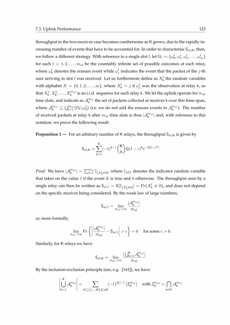
7.3. Uplink Performance 123
throughput in the two-receiver case becomes cumbersome as K grows, due to the rapidly in-
creasing number of events that have to be accounted for. In order to characterise Sul,K, then,
we follow a different strategy. With reference to a single slot l, let Ωl := ωl0, ωl1, ωl2, . . . , ωl∞for each l = 1, 2, . . . ,mul be the countably infinite set of possible outcomes at each relay,
where ωl0 denotes the erasure event while ωlj indicates the event that the packet of the j-th
user arriving in slot l was received. Let us furthermore define as X lk the random variables
with alphabet X = 0, 1, 2, . . . ,∞, where X lk = j if ωlj was the observation at relay k, so
that X1k , X
2k , . . . , X
mulk is an i.i.d. sequence for each relay k. We let the uplink operate for mul
time slots, and indicate as Amulk the set of packets collected at receiver k over this time-span,
where Amulk (⋃mull=1 Ωl\ωl0 (i.e. we do not add the erasure events to Amulk ). The number
of received packets at relay k after mul time slots is thus |Amulk | and, with reference to this
notation, we prove the following result:
Proposition 1 — For an arbitrary number of K relays, the throughput Sul,K is given by
Sul,K =K∑
k=1
(−1)k−1
(K
k
)G(1− ε)ke−G(1−εk)
Proof. We have |Amulk | =∑mul
l=1 IXlk 6=0, where IE denotes the indicator random variable
that takes on the value 1 if the event E is true and 0 otherwise. The throughput seen by a
single relay can then be written as Sul,1 = E[IXlk 6=0] = PrX l
k 6= 0, and does not depend
on the specific receiver being considered. By the weak law of large numbers,
Sul,1 = limmul→∞
|Amulk |mul
or, more formally,
limmul→∞
Pr
∣∣∣∣ |Amulk |mul
− Sul,1
∣∣∣∣ > ε
= 0 for some ε > 0.
Similarly, for K relays we have
Sul,K = limmul→∞
|⋃Kk=1Amulk |mul
By the inclusion-exclusion principle (see, e.g. [141]), we have∣∣∣∣∣K⋃
k=1
Amulk
∣∣∣∣∣ =∑
K⊆1,...,K,K6=∅(−1)|K|−1
∣∣ImulK∣∣ with ImulK =
⋂k∈KAmulk
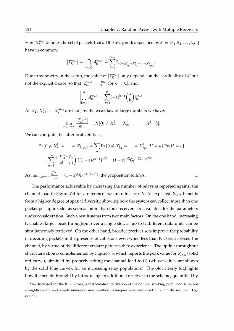
124 Chapter 7. Random Access with Multiple Receivers
Here, ImulK denotes the set of packets that all the relay nodes specified byK = k1, k2, . . . , k|K|have in common:
∣∣ImulK∣∣ =
∣∣∣∣∣⋂k∈KAmulk
∣∣∣∣∣ =
mul∑l=1
I06=Xlk1
=Xlk2
=...=Xlk|K|
Due to symmetry in the setup, the value of∣∣ImulK
∣∣ only depends on the cardinality of K but
not the explicit choice, so that∣∣ImulK
∣∣ = ιmulk for k = |K|, and,∣∣∣∣∣K⋃
k=1
Amulk
∣∣∣∣∣ =K∑
k=1
(−1)k−1
(K
k
)ιmulk .
As X1k , X
2k , . . . , X
mulk are i.i.d., by the weak law of large numbers we have:
limmul→∞
∣∣ImulK∣∣
mul= Pr[0 6= X l
k1= X l
k2= . . . = X l
k|K|].
We can compute the latter probability as
Pr0 6= X lk1
= . . . = X lk|K| =
∑u
Pr0 6= X lk1
= . . . = X lk|K| |U = uPrU = u
=∞∑u=1
e−GGu
u!
(u
1
)((1− ε)εu−1
)|K|= (1− ε)|K|Ge−G(1−ε|K|)
As limmul→∞ιmulkmul
= (1− ε)kGe−G(1−εk), the proposition follows.
The performance achievable by increasing the number of relays is reported against the
channel load in Figure 7.4 for a reference erasure rate ε = 0.5. As expected, Sul,K benefits
from a higher degree of spatial diversity, showing how the system can collect more than one
packet per uplink slot as soon as more than four receivers are available, for the parameters
under consideration. Such a result stems from two main factors. On the one hand, increasing
K enables larger peak throughput over a single slot, as up to K different data units can be
simultaneously retrieved. On the other hand, broader receiver sets improve the probability
of decoding packets in the presence of collisions even when less than K users accessed the
channel, by virtue of the different erasure patterns they experience. The uplink throughput
characterisation is complemented by Figure 7.5, which reports the peak value for S∗ul,K (solid
red curve), obtained by properly setting the channel load to G∗ (whose values are shown
by the solid blue curve), for an increasing relay population.2 The plot clearly highlights
how the benefit brought by introducing an additional receiver to the scheme, quantified by
2As discussed for the K = 2 case, a mathematical derivation of the optimal working point load G∗ is not
straightforward, and simple numerical maximisation techniques were employed to obtain the results of Fig-
ure 7.5.
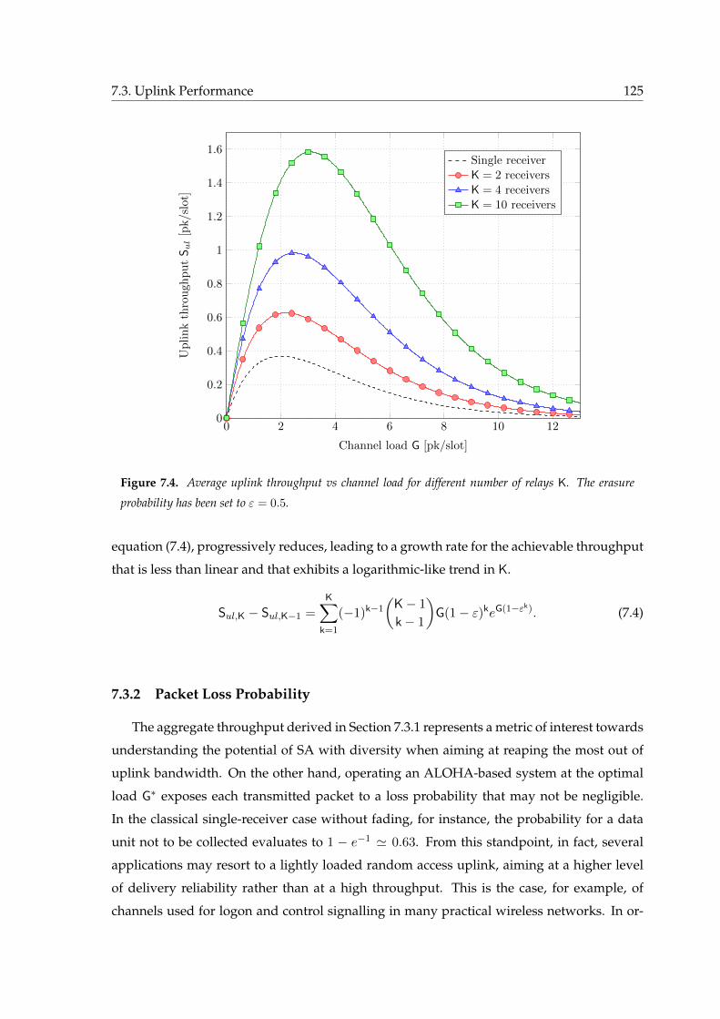
7.3. Uplink Performance 125
0 2 4 6 8 10 120
0.2
0.4
0.6
0.8
1
1.2
1.4
1.6
Channel load G [pk/slot]
UplinkthroughputSul[pk/slot]
Single receiverK = 2 receiversK = 4 receiversK = 10 receivers
Figure 7.4. Average uplink throughput vs channel load for different number of relays K. The erasure
probability has been set to ε = 0.5.
equation (7.4), progressively reduces, leading to a growth rate for the achievable throughput
that is less than linear and that exhibits a logarithmic-like trend in K.
Sul,K − Sul,K−1 =K∑
k=1
(−1)k−1
(K− 1
k− 1
)G(1− ε)keG(1−εk). (7.4)
7.3.2 Packet Loss Probability
The aggregate throughput derived in Section 7.3.1 represents a metric of interest towards
understanding the potential of SA with diversity when aiming at reaping the most out of
uplink bandwidth. On the other hand, operating an ALOHA-based system at the optimal
load G∗ exposes each transmitted packet to a loss probability that may not be negligible.
In the classical single-receiver case without fading, for instance, the probability for a data
unit not to be collected evaluates to 1 − e−1 ' 0.63. From this standpoint, in fact, several
applications may resort to a lightly loaded random access uplink, aiming at a higher level
of delivery reliability rather than at a high throughput. This is the case, for example, of
channels used for logon and control signalling in many practical wireless networks. In or-
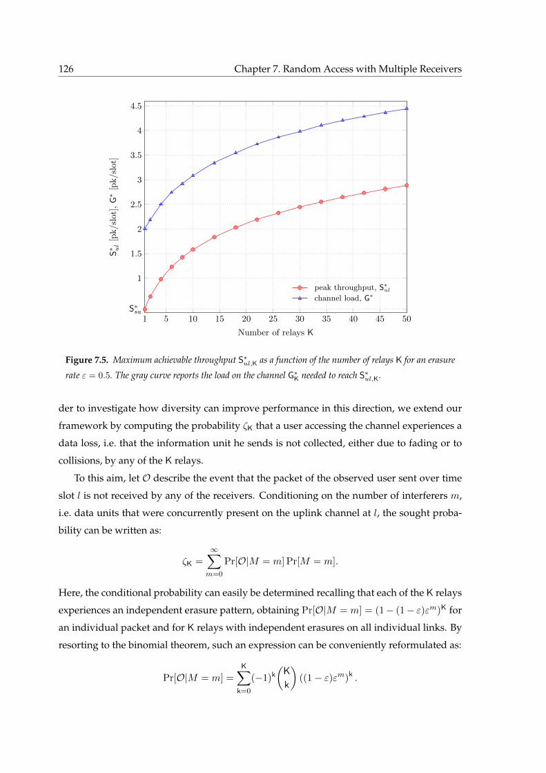
126 Chapter 7. Random Access with Multiple Receivers
1 5 10 15 20 25 30 35 40 45 50
1
1.5
2
2.5
3
3.5
4
4.5
S∗sa
Number of relays K
S∗ ul[pk/slot],G∗[pk/slot]
peak throughput, S∗ul
channel load, G∗
Figure 7.5. Maximum achievable throughput S∗ul,K as a function of the number of relays K for an erasure
rate ε = 0.5. The gray curve reports the load on the channel G∗K needed to reach S∗
ul,K.
der to investigate how diversity can improve performance in this direction, we extend our
framework by computing the probability ζK that a user accessing the channel experiences a
data loss, i.e. that the information unit he sends is not collected, either due to fading or to
collisions, by any of the K relays.
To this aim, let O describe the event that the packet of the observed user sent over time
slot l is not received by any of the receivers. Conditioning on the number of interferers m,
i.e. data units that were concurrently present on the uplink channel at l, the sought proba-
bility can be written as:
ζK =∞∑m=0
Pr[O|M = m] Pr[M = m].
Here, the conditional probability can easily be determined recalling that each of the K relays
experiences an independent erasure pattern, obtaining Pr[O|M = m] = (1− (1− ε)εm)K for
an individual packet and for K relays with independent erasures on all individual links. By
resorting to the binomial theorem, such an expression can be conveniently reformulated as:
Pr[O|M = m] =
K∑k=0
(−1)k
(K
k
)((1− ε)εm)k .
7.3. Uplink Performance 127
10−3 10−2 10−1 10010−4
10−3
10−2
10−1
100
Channel load G [pk/slot]
Packet
loss
probab
ilityζ K
Single receiverK = 2 receiversK = 3 receiversK = 4 receiversK = 5 receiversK = 10 receivers
Figure 7.6. Probability ζK that a packet sent by a user is not received by any of the relays. Different curves
indicate different values of K, while the erasure probability has been set to ε = 0.2.
On the other hand, the number of interferers seen by a user that accesses the channel at
time l still follows a Poisson distribution of intensity G, so that, after simple calculations we
finally get:
ζK =
K∑k=0
(−1)k
(K
k
)(1− ε)ke−G(1−εk). (7.5)
Figure 7.6 reports the behaviour of ζK as a function of G when the erasure rate over a
single link is set to ε = 0.2. Different lines indicate the trend when increasing the number of
receivers from 1 to 10. As expected, when G → 0, a user accessing the channel is not likely
to experience any interference, so that failures can only be induced by erasures, leading to
an overall loss probability of εK. In this perspective, the availability of multiple receivers
triggers a dramatic improvement, enabling levels of reliability that would otherwise not be
possible irrespective of the channel configuration. On the other hand, equation (7.5) turns
out to be useful for system design, as it allows to determine the load that can be supported
on the uplink channel while guaranteeing a target loss rate. Also in this case diversity can
significantly ameliorate the performance. As shown in Figure 7.6, for example, a target loss
rate ζK = 5 · 10−2 is achieved by a three- and four-receiver scheme under 6− and 10−fold

128 Chapter 7. Random Access with Multiple Receivers
larger loads compared to the K = 2 case, respectively.
7.4 An Achievable Downlink Upper Bound
The analysis carried out in Section 7.3 has characterised the average number of packets
that can be decoded at the relay set when SA is used in the uplink. We now consider the
complementary task of delivering what has been collected to a central GW. In doing so, we
aim at employing the minimum number of resources in terms of transmissions that have to
be performed by the relays, while not allowing any information exchange among them. In
particular, we consider a finite-capacity downlink, where the K receivers share a common
bandwidth to communicate with the GW by means of a TDMA scheme, and we assume
that each of them can reliably deliver exactly one packet, possibly composed of a linear
combination of what has been collected, over one time unit. It is clear that K Ssa slots are
sufficient to deliver all the collected data on average, but it can be inefficient since the same
packet can be collected by more than one relay. We focus on a horizon ofmul slots to operate
the uplink, after which the downlink phase starts.
We structure our analysis in two parts. First, in Section 7.4.1, we derive lower bounds
for the rates (in terms of downlink slots allocated per uplink slot) that have to be assigned to
receivers in order to deliver the whole set of data units collected in the uplink over the mul
slots. Then, Section 7.4.2 shows how a simple forwarding strategy based on random linear
network coding suffices to achieve optimality, completing the downlink phase in Sul,K slots
for asymptotically large values of mul.
Prior to delving into the details, let us introduce some useful notation. We denote the L-
bit data part of packets of the j-th user arriving in time slot l as W lk ∈ W , withW = F2L ∪ e,
where e is added as the erasure symbol. We furthermore assume that the receiver can de-
termine the corresponding user through a packet header, i.e. the receiver knows both j and
l after successful reception. As the uplink operates over mul time slots, relay k observes the
vector wk = [W 1k , . . . , W
mulk ]. In each time slot, the tuple (W l
1, Wl2, . . . , W
lK) is drawn from a
joint probability distribution PW1...WKwhich is governed by the uplink, and different relays
might receive the same packet.
7.4.1 Bounds for Downlink Rates
Each relay k transmits a packet in each of its mulRk downlink slots. We are interested in
the set of rates (Rk)Kk=1 such that the gateway can recover all packets (with high probability).
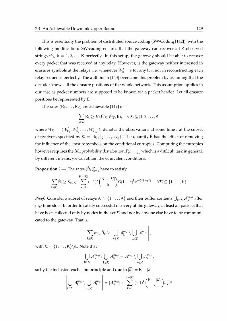
7.4. An Achievable Downlink Upper Bound 129
This is essentially the problem of distributed source coding (SW-Coding [142]), with the
following modification: SW-coding ensures that the gateway can recover all K observed
strings wk, k = 1, 2, . . . ,K perfectly. In this setup, the gateway should be able to recover
every packet that was received at any relay. However, is the gateway neither interested in
erasures symbols at the relays, i.e. whenever W lk = e for any k, l, nor in reconstructing each
relay sequence perfectly. The authors in [143] overcame this problem by assuming that the
decoder knows all the erasure positions of the whole network. This assumption applies in
our case as packet numbers are supposed to be known via a packet header. Let all erasure
positions be represented by E.
The rates (R1, . . . , RK) are achievable [142] if∑k∈K
Rk ≥ H(WK|WK, E), ∀ K ⊆ [1, 2, . . . ,K]
where WK = (W lk1, W l
k2, . . . , W l
k|K|), denotes the observations at some time l at the subset
of receivers specified by K = k1, k2, . . . , k|K|. The quantity E has the effect of removing
the influence of the erasure symbols on the conditional entropies. Computing the entropies
however requires the full probability distributionPW1...WKwhich is a difficult task in general.
By different means, we can obtain the equivalent conditions:
Proposition 2 — The rates (Rk)Kk=1 have to satisfy
∑k∈K
Rk≥ Sul,K+
K−|K|∑k=1
(−1)k
(K− |K|
k
)G(1− ε)ke−G(1−εk), ∀K ⊆ 1, . . . ,K
Proof. Consider a subset of relays K ⊆ 1, . . . ,K and their buffer contents⋃
k∈KAmulk after
mul time slots. In order to satisfy successful recovery at the gateway, at least all packets that
have been collected only by nodes in the set K and not by anyone else have to be communi-
cated to the gateway. That is,
∑k∈K
mul Rk ≥
∣∣∣∣∣∣⋃
k∈KAmulk \
⋃k∈KAmulk
∣∣∣∣∣∣ ,with K = 1, . . . ,K\K. Note that⋃
k∈KAmulk \
⋃k∈KAmulk = Amul\
⋃k∈KAmulk ,
so by the inclusion-exclusion principle and due to |K| = K− |K|∣∣∣∣∣∣⋃
k∈KAmulk \
⋃k∈KAmulk
∣∣∣∣∣∣ = |AmulK |+K−|K|∑
k=1
(−1)k
(K− |K|
k
)amulk
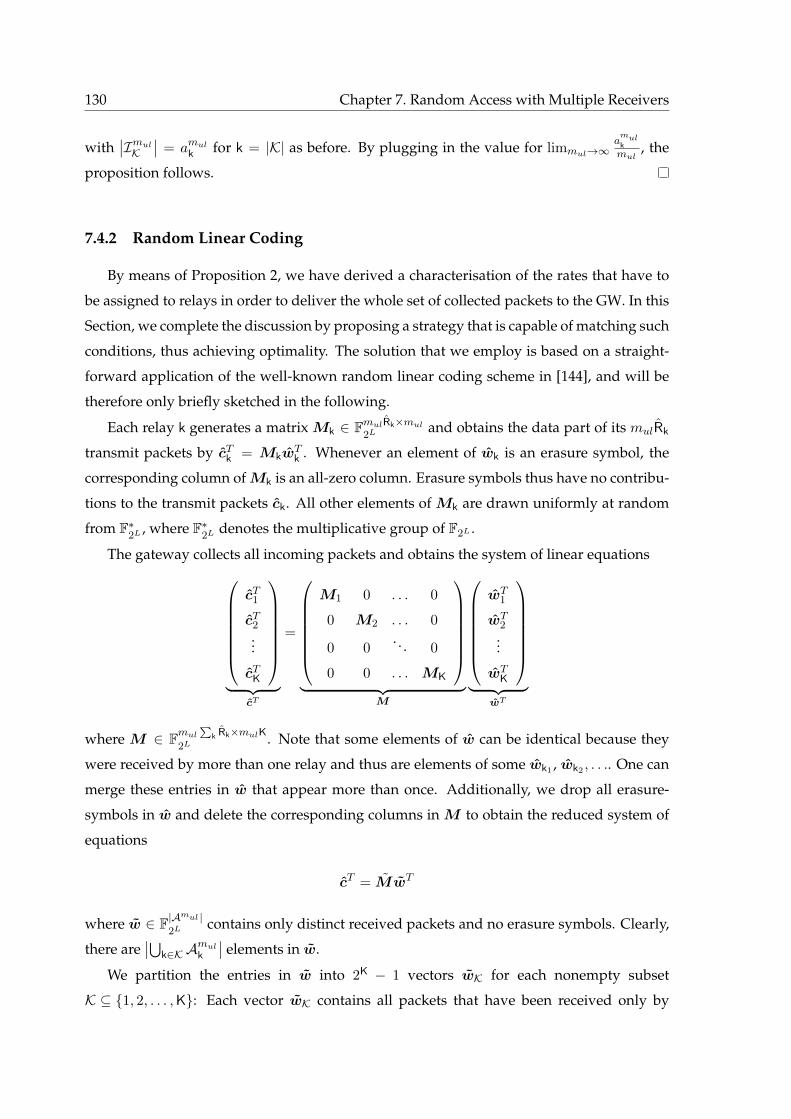
130 Chapter 7. Random Access with Multiple Receivers
with∣∣ImulK
∣∣ = amulk for k = |K| as before. By plugging in the value for limmul→∞amulkmul
, the
proposition follows.
7.4.2 Random Linear Coding
By means of Proposition 2, we have derived a characterisation of the rates that have to
be assigned to relays in order to deliver the whole set of collected packets to the GW. In this
Section, we complete the discussion by proposing a strategy that is capable of matching such
conditions, thus achieving optimality. The solution that we employ is based on a straight-
forward application of the well-known random linear coding scheme in [144], and will be
therefore only briefly sketched in the following.
Each relay k generates a matrix Mk ∈ FmulRk×mul2L
and obtains the data part of its mulRk
transmit packets by cTk = MkwTk . Whenever an element of wk is an erasure symbol, the
corresponding column of Mk is an all-zero column. Erasure symbols thus have no contribu-
tions to the transmit packets ck. All other elements of Mk are drawn uniformly at random
from F∗2L
, where F∗2L
denotes the multiplicative group of F2L .
The gateway collects all incoming packets and obtains the system of linear equationscT1
cT2...
cTK
︸ ︷︷ ︸
cT
=
M1 0 . . . 0
0 M2 . . . 0
0 0. . . 0
0 0 . . . MK
︸ ︷︷ ︸
M
wT
1
wT2
...
wTK
︸ ︷︷ ︸
wT
where M ∈ Fmul∑
k Rk×mulK2L
. Note that some elements of w can be identical because they
were received by more than one relay and thus are elements of some wk1 , wk2 , . . .. One can
merge these entries in w that appear more than once. Additionally, we drop all erasure-
symbols in w and delete the corresponding columns in M to obtain the reduced system of
equations
cT = MwT
where w ∈ F|Amul |
2Lcontains only distinct received packets and no erasure symbols. Clearly,
there are∣∣⋃
k∈KAmulk
∣∣ elements in w.
We partition the entries in w into 2K − 1 vectors wK for each nonempty subset
K ⊆ 1, 2, . . . ,K: Each vector wK contains all packets that have been received only by
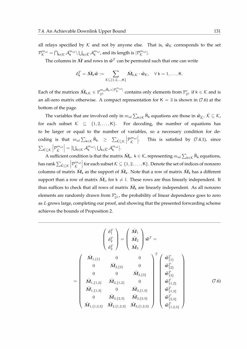
7.4. An Achievable Downlink Upper Bound 131
all relays specified by K and not by anyone else. That is, wK corresponds to the set
PmulK =⋂
k∈KAmulk \⋃k∈KAmulk , and its length is |PmulK |.
The columns in M and rows in wT can be permuted such that one can write
cTk = Mkw :=∑
K⊆1,2,...,KMk,K · wK, ∀ k = 1, . . . ,K.
Each of the matrices Mk,K ∈ FmulRk×|PmulK |
2Lcontains only elements from F∗
2Lif k ∈ K and is
an all-zero matrix otherwise. A compact representation for K = 3 is shown in (7.6) at the
bottom of the page.
The variables that are involved only in mul∑
k∈K Rk equations are those in wK, K ⊆ K,
for each subset K ⊆ 1, 2, . . . ,K. For decoding, the number of equations has
to be larger or equal to the number of variables, so a necessary condition for de-
coding is that mul∑
k∈K Rk ≥ ∑K⊆K
∣∣∣PmulK
∣∣∣. This is satisfied by (7.4.1), since∑K⊆K
∣∣∣PmulK
∣∣∣ =∣∣⋃
k∈KAmulk \⋃k∈KAmulk
∣∣.A sufficient condition is that the matrix Mk, k ∈ K, representingmul
∑k∈K Rk equations,
has rank∑K⊆K
∣∣∣PmulK
∣∣∣ for each subsetK ⊆ 1, 2, . . . ,K. Denote the set of indices of nonzero
columns of matrix Mk as the support of Mk. Note that a row of matrix Mk has a different
support than a row of matrix Ml, for k 6= l. These rows are thus linearly independent. It
thus suffices to check that all rows of matrix Mk are linearly independent. As all nonzero
elements are randomly drawn from F∗2L
, the probability of linear dependence goes to zero
as L grows large, completing our proof, and showing that the presented forwarding scheme
achieves the bounds of Proposition 2.
cT1
cT2
cT3
=
M1
M2
M3
wT =
=
M1,1 0 0
0 M2,2 0
0 0 M3,3
M1,1,2 M2,1,2 0
M1,1,3 0 M3,1,3
0 M2,2,3 M3,2,3
M1,1,2,3 M2,1,2,3 M3,1,2,3
T
wT1
wT2
wT3
wT1,2
wT1,3
wT2,3
wT1,2,3
(7.6)
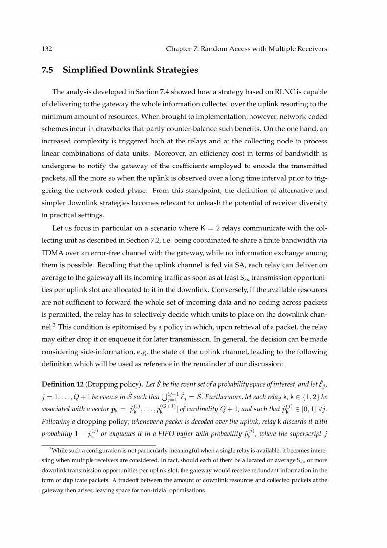
132 Chapter 7. Random Access with Multiple Receivers
7.5 Simplified Downlink Strategies
The analysis developed in Section 7.4 showed how a strategy based on RLNC is capable
of delivering to the gateway the whole information collected over the uplink resorting to the
minimum amount of resources. When brought to implementation, however, network-coded
schemes incur in drawbacks that partly counter-balance such benefits. On the one hand, an
increased complexity is triggered both at the relays and at the collecting node to process
linear combinations of data units. Moreover, an efficiency cost in terms of bandwidth is
undergone to notify the gateway of the coefficients employed to encode the transmitted
packets, all the more so when the uplink is observed over a long time interval prior to trig-
gering the network-coded phase. From this standpoint, the definition of alternative and
simpler downlink strategies becomes relevant to unleash the potential of receiver diversity
in practical settings.
Let us focus in particular on a scenario where K = 2 relays communicate with the col-
lecting unit as described in Section 7.2, i.e. being coordinated to share a finite bandwidth via
TDMA over an error-free channel with the gateway, while no information exchange among
them is possible. Recalling that the uplink channel is fed via SA, each relay can deliver on
average to the gateway all its incoming traffic as soon as at least Ssa transmission opportuni-
ties per uplink slot are allocated to it in the downlink. Conversely, if the available resources
are not sufficient to forward the whole set of incoming data and no coding across packets
is permitted, the relay has to selectively decide which units to place on the downlink chan-
nel.3 This condition is epitomised by a policy in which, upon retrieval of a packet, the relay
may either drop it or enqueue it for later transmission. In general, the decision can be made
considering side-information, e.g. the state of the uplink channel, leading to the following
definition which will be used as reference in the remainder of our discussion:
Definition 12 (Dropping policy). Let S be the event set of a probability space of interest, and let Ej ,j = 1, . . . , Q+ 1 be events in S such that
⋃Q+1j=1 Ej = S. Furthermore, let each relay k, k ∈ 1, 2 be
associated with a vector pk = [p(1)k , . . . , p
(Q+1)k ] of cardinality Q+ 1, and such that p(j)
k ∈ [0, 1] ∀j.Following a dropping policy, whenever a packet is decoded over the uplink, relay k discards it with
probability 1 − p(j)k or enqueues it in a FIFO buffer with probability p(j)
k , where the superscript j
3While such a configuration is not particularly meaningful when a single relay is available, it becomes intere-
sting when multiple receivers are considered. In fact, should each of them be allocated on average Ssa or more
downlink transmission opportunities per uplink slot, the gateway would receive redundant information in the
form of duplicate packets. A tradeoff between the amount of downlink resources and collected packets at the
gateway then arises, leaving space for non-trivial optimisations.
7.5. Simplified Downlink Strategies 133
indicates that event Ej was observed at the time of reception.
This family of strategies do not entail any complexity in terms of packet-level coding,
and represent a simple and viable alternative for the downlink. On the other hand, in con-
trast to NC-based solutions, dropping policies are inherently not able to ensure delivery
of the whole retrieved information set as soon as non-null dropping probabilities are con-
sidered, since a data unit may be discarded by all the relays that successfully decoded it.
In order to further investigate this tradeoff, we will present and discuss some variations
of such an approach, optimising the probability of discarding a packet to maximise infor-
mation delivered to the gateway for a given downlink rate. From this standpoint, while
the provided definition is fairly general, out of practical considerations we will restrict our-
selves to strategies that base the buffering decision on observations of the uplink channel,
e.g. on the presence or absence of interference affecting the retrieved packet.
Let us introduce some notation and specify the framework that will be later used through-
out this Section. We model each relay as an infinite buffer which, under any dropping policy,
experiences an arrival rate that is a fraction of Ssa. Furthermore, we assume the downlink
to be dimensioned for the system to be stable, i.e. such that all enqueued packets can be
eventually delivered to the gateway and, consistently with Section 7.4, indicate with Rk the
average number of transmissions performed by relay k in the downlink per uplink slot.
Under these hypotheses, the aggregate rate R =∑
k Rk can be regarded as a key design
parameter, as it characterises the minimum amount of downlink resources that have to be
allocated to properly implement a dropping policy under consideration.4 In turn, we evalu-
ate the performance of such strategies by means of the downlink throughput Sdl, computed
as the average number of packets collected at the gateway per each uplink slot. Clearly, this
quantity is bounded from above by Sul, i.e. the amount of information successfully gathered
by the set of relays from the user population. Finally, we introduce the downlink capacity
of the system as Cdl(R) = supSdl | R, pl, where pl indicates the probability that a packet
collected by the set of relays is not retrieved at the gateway.5 Within this framework, the
insights of Section 7.4.1 can be revisited and summarised by the following result:
4From a queueing theory viewpoint, the downlink is stable as soon as the actual rate R∗k offered to relay k
satisfies R∗k > Rk, ∀k.5In the case of dropping policies, this may happen when all the relays that received the data unit decide not
to enqueue it in their buffers for subsequent transmission.
134 Chapter 7. Random Access with Multiple Receivers
Corollary 1 — The downlink capacity of the system satisfies:
Cdl(R) =
R for R < Sul
Sul for R ≥ Sul
Proof. For R ≥ Sul, the result is simply a reformulation of the propositions of Section 7.4.1
when K = 2. Conversely, let β = R/Sul < 1, and assume that each relay drops a packet
received over the uplink with probability 1 − β. It immediately follows that the average
number of collected data units evaluates to β Sul, so that the downlink phase is equivalent
to the one of a system serving an uplink throughput of R packets per slot. The propositions
of Section 7.4.1 apply again to the scaled downlink, proving the result.
Theorem 1 characterises the capacity region of the complete topology under considera-
tion, specifying for any uplink configuration, i.e. for any (G, ε) pair, the achievable through-
put Sdl when a certain amount of resources is allocated to the downlink. In this perspective,
thus, it offers an upper bound to the performance of any forwarding strategy, and allows
us to evaluate the efficiency of the different dropping policies that will be introduced in the
following.
7.5.1 Common Transmission Probability
As a starting point, consider the basic case in which both relays employ a common and
single probability 1−p to drop packets irrespectively of any external observation (i.e. Q = 0).
In this condition, the average traffic forwarded by each receiver to the gateway scales by a
factor p with respect to the incoming uplink flow, and the overall average amount of em-
ployed resources in the downlink evaluates to R = 2p Ssa. Due to the lack of coordination
among receivers, not all the performed transmissions bring innovative information to the
collecting unit, so that the downlink throughput exhibits a loss with respect to R. More pre-
cisely, by the combinatorial technique discussed in Section 7.3, the probability of having the
same packet forwarded twice can be expressed as p2 u(1− ε)2ε2(u−1), under the assumption
that u users concurrently accessed the uplink channel in the slot observed by the receivers.
Taking the expectation over the Poisson traffic distribution, we then get
Sdl = R− p2 G(1− ε)2e−G(1−ε2) = R− R2(eG(1−ε)2
/4G), (7.7)
where the second equality directly follows from the expression of Ssa in (7.1). The achiev-
able performance is summarized in Figure 7.7, where the red slid line (labelled Common
7.5. Simplified Downlink Strategies 135
Prob.) reports the dependency of Sdl on the overall downlink rate as per equation (7.7) in
the exemplary case ε = 0.3 and G = 1/(1 − ε). The plot also reports the system capacity
curve Cdl(R), which divides the plane in two regions and highlights downlink throughput
values that can be aimed for. Moreover, we show results for Ssa ≤ R ≤ 2 Ssa. In fact, while
for R > 2 Ssa no dropping is required, and on average all the traffic can be delivered to
the gateway, the investigated rates correspond to configurations in which a non-trivial op-
timisation can be performed to leverage receiver diversity. It is apparent that the simple
dropping scheme under analysis exhibits quite a large performance gap with respect to the
upper bound. This inefficiency is further stressed by the fact that there exists a threshold rate
R∗ > Ssa such that for downlink rates lower than R∗, it holds Sdl(R) < Ssa.6 In other words,
in the operating region Ssa < R < R∗, a system enjoying receiver diversity in the uplink is
seen at the gateway as performing worse than a simpler configuration with a single relay
with allocated fewer downlink resources.7 This comes as no surprise, since not only does
the considered policy resort to no form of coding, but also, in the absence of coordination
among relays, it makes no attempt to reduce the likelihood of forwarding duplicate packets.
In order to overcome these limitations, we propose in the following the use of distinct drop-
ping probabilities for the relays and a careful tuning of their value exploiting available side
information.
7.5.2 Distinct Transmission Probabilities
Uplink-Condition Agnostic Policy
A straightforward modification of the balanced policy consists in letting receivers drop
incoming packets with different probabilities. We still assume that buffering decisions are
made at a receiver blindly, i.e. they are not based on any observation of the uplink channel
(Q = 0). For this uplink-agnostic strategy, the downlink phase is then completely specified
by the pair (p1, p2).8 In this case, the average number of transmissions in the downlink
evaluates to R = (p1 + p2) Ssa, and the throughput can readily be expressed following com-
binatorial arguments as:
Sdl = R− p1p2 G(1− ε)2e−G(1−ε2). (7.8)
6By simple manipulations of (7.7), R∗ = 2G e−G(1−ε)2(
1−√
1− (1− ε) e−Gε(1−ε))
.7Notice in fact that a single relay without any dropping policy would employ on average Ssa downlink
transmissions to deliver to the gateway the whole information set it collects in the uplink.8We omit the superscripts in p(1)
1 and p(1)2 for the sake of notation readability.
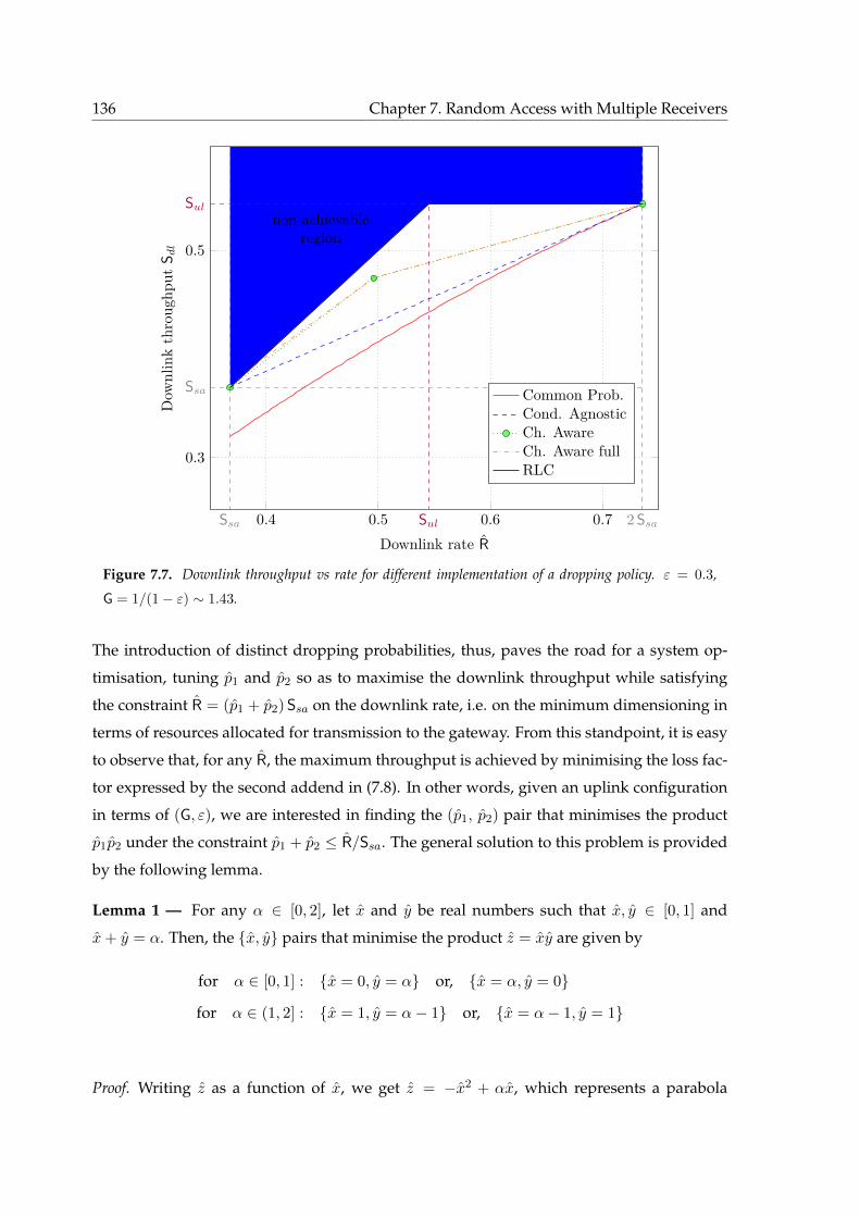
136 Chapter 7. Random Access with Multiple Receivers
0.4 0.5 0.6 0.7
0.3
0.5
Ssa 2 Ssa
Ssa
Sul
Sul
non-achievableregion
Downlink rate R
Dow
nlin
kth
roug
hput
S dl
Common Prob.Cond. AgnosticCh. AwareCh. Aware fullRLC
Figure 7.7. Downlink throughput vs rate for different implementation of a dropping policy. ε = 0.3,
G = 1/(1− ε) ∼ 1.43.
The introduction of distinct dropping probabilities, thus, paves the road for a system op-
timisation, tuning p1 and p2 so as to maximise the downlink throughput while satisfying
the constraint R = (p1 + p2) Ssa on the downlink rate, i.e. on the minimum dimensioning in
terms of resources allocated for transmission to the gateway. From this standpoint, it is easy
to observe that, for any R, the maximum throughput is achieved by minimising the loss fac-
tor expressed by the second addend in (7.8). In other words, given an uplink configuration
in terms of (G, ε), we are interested in finding the (p1, p2) pair that minimises the product
p1p2 under the constraint p1 + p2 ≤ R/Ssa. The general solution to this problem is provided
by the following lemma.
Lemma 1 — For any α ∈ [0, 2], let x and y be real numbers such that x, y ∈ [0, 1] and
x+ y = α. Then, the x, y pairs that minimise the product z = xy are given by
for α ∈ [0, 1] : x = 0, y = α or, x = α, y = 0
for α ∈ (1, 2] : x = 1, y = α− 1 or, x = α− 1, y = 1
Proof. Writing z as a function of x, we get z = −x2 + αx, which represents a parabola
7.5. Simplified Downlink Strategies 137
with downward concavity and zeroes for x = 0 and x = α. Furthermore, impos-
ing the conditions x ∈ [0, 1] and α − x = y ∈ [0, 1], the region of interest restricts to
max0, α− 1 ≤ x ≤ minα, 1. When α ≤ 1, the minimum value of z in the studied do-
main is thus reached either when x = 0 or x = α, while, for α ∈ (1, 2] the minimum value is
obtained for x = α− 1 and x = 1. The values of y follow immediately.
In this way, the optimal setup for an uplink-agnostic policy is given by picking p1 = 1
and p2 = R/Ssa − 1.9 Under these conditions, the maximum throughput evaluates to
Sdl = R(
1− (1− ε) e−Gε(1−ε))
+ G(1− ε)2e−G(1−ε2), (7.9)
reported as a function of R by the dashed blue line in Figure 7.7. It is clear that the linear
trend exhibited by the presented solution triggers remarkable improvement over the bal-
anced approach, especially when little resources are available in the downlink. Moreover,
straightforward manipulations of (7.9) show how allowing the relays to employ different
dropping probabilities is sufficient for the system to always outperform a single-receiver
configuration in the downlink rate region of interest (i.e. Sdl ≥ Ssa), thus overcoming the
inefficiency that beset the baseline scheme. Such a result is achieved by simply letting one
of the two receivers always forward all its incoming packets, allocating to it (on average)
Ssa downlink transmissions per uplink slot, while resorting to the contributions of its fellow
relay only when additional resources are available. In this perspective, the policy under
discussion also represents a smart way to seamlessly take advantage of diversity in already
deployed systems. In fact, a scenario operated via a single relay can be upgraded by plug-
ging in an additional receiver, and by incrementally allocating to it downlink bandwidth,
without any change to the forwarding policy of the original relay.
Channel-Aware Policies
A further extension of the considered policies consists in having relays make an edu-
cated choice on whether to drop or enqueue a data unit based on the observation of what
happened on the uplink channel. The intuition in fact suggests that it is more likely for a
packet to be retrieved by both receivers if it was the only one sent over the slot of interest,
whereas the presence of several information units in an uplink slot reduces the chance for
9Clearly, the symmetric configuration p1 = R/Ssa − 1, p2 = 1 yields the same result. This remark holds for
all the considered policies, and will not be further stressed.
138 Chapter 7. Random Access with Multiple Receivers
one of them to be decoded twice. A reasonable approach, even in the absence of any com-
munication among relays, would then then be to increase the dropping probability in the
former case, and reduce it in the latter to prevent duplicate transmissions in the downlink.
More formally, let us first consider the simple case in which each collector distinguishes
between two situations, basing its decision on whether the retrieved packet was the only
one on the channel (i.e. no interference) or whether more than one users accessed the uplink
channel over that slot (i.e. presence of interference). In the former condition, receiver i drops
with probability p(1)i , while in the latter case the packet is discarded with probability p
(2)i .
While this decision rule may appear elusive under the abstraction of on-off fading, as no
incoming power is detected when a packet is erased, it turns out to be of high relevance in
practical systems where a data unit can often be decoded even in the presence of a certain
level of interference e.g. by leveraging the capture effect [145].10
In accordance with the introduced framework, we can express the average number of
downlink transmissions per uplink slot as
R =(p
(1)1 + p
(1)2
)(1− ε)Ge−G +
∞∑u=2
Gue−G
u!u (1− ε)εu−1
(p
(2)1 + p
(2)2
),
where the first member accounts for the case in which no interference was detected, whereas
the summation considers all the situations in which at least one interfering packet affected
the reception of the data unit of interest. Similarly, we can compute the probability that a
data unit is forwarded twice towards the gateway, so that the overall throughput evaluates
to
Sdl = R− p(1)1 p
(1)2 G(1− ε)2e−G −
∞∑u=2
Gue−G
u!u (1− ε)2ε2(u−1)p
(2)1 p
(2)2 .
Simple manipulations lead to the tackled optimisation problem:
maximise Sdl = R− c p(1)1 p
(1)2 − d p
(2)1 p
(2)2
s.t. R = a(p
(1)1 + p
(1)2
)+ b
(p
(2)1 + p
(2)2
) (7.10)
with coefficients a = G(1 − ε)e−G, b = G(1 − ε)e−G(eGε − 1
), c = G(1 − ε)2e−G, and
d = G(1− ε)2e−G(eGε2 − 1
). The solution is offered by the following result:
Proposition 3 — Let R1 =
R | R ∈ [Ssa, a+ 2b)
and R2 =
R | R ∈ [a+ 2b, 2Ssa]
. Then,
the maximum downlink throughput achievable with the proposed interference-aware pol-
10From this viewpoint, we also remark that detecting the presence or absence of interference can be rather
easily accomplished by evaluating the noise level that affects the reception of a decoded data packet.
7.5. Simplified Downlink Strategies 139
icy is given by
Sdl =
R (1− d/b) + dSsa/b for R ∈ R1
R (1− c/a) + c(Ssa + b)/a− d for R ∈ R2
(7.11)
As a preliminary remark, note that all the coefficients a, b, c, d in (7.10) are strictly positive,
and that, for any admissible values of G and ε, the inequality c/a > d/b holds. For the sake
of a simplified notation, let p(1)1 = x1, p(1)
2 = x2, p(2)1 = y1, and p(2)
2 = y2. Furthermore, let us
introduce α = x1 + y1 and β = x2 + y2, with α, β ∈ [0, 2], as well as the auxiliary function
f(x) = c (x1y1) + d (x2y2), where x = [x1, x2, y1, y2] and f(x) ≥ 0. We are then interested in
maximising S = R− f(x) subject to R = aα+ bβ or, equivalently in minimising f(x) under
the same constraint. Let us notice that the first addend of f(x) only contains the variables
that determine α, while the second addend of f(x) solely defines the value of β. It is then
possible to solve the optimisation problem by considering four non-overlapping regions:
G1 = x |α ∈ [0, 1], β ∈ [0, 1], G2 = x |α ∈ (1, 2], β ∈ [0, 1], G3 = x |α ∈ [0, 1], β ∈(1, 2], G4 = x |α ∈ (1, 2], β ∈ (1, 2]. G1 can immediately be discarded as α, β < 1 imply
R < a+ b = Ssa, identifying a condition which is not of interest. In the remaining regions,
for any α and β the values of the optimisation variables that maximise the throughput can
be found resorting to Lemma 1. In particular:
• for x ∈ G2: α ∈ [0, 1] implies x1 = 1 and y1 = α−1, while β ∈ (1, 2] implies x2 = β and
y2 = 0. By the last condition we can write f(x) = c(α− 1) so that the optimum lies in
the (α, β) pair that satisfies the constraint on R with minimum α. The solution follows
as β = 1, α = (R− b)/a with a corresponding throughput S = R− (c/a)(R− Ssa).
• by a symmetrical reasoning, for x ∈ G3 the optimal solution is given by α = 1 and
β = (R − a)/b, with a throughput S = R − (d/b)(R − Ssa) achieved for x1 = 1, y1 = 0,
x2 = 1 and y2 = (R− Ssa)/b.
• for x ∈ G4: by Lemma 1, x1 = 1, x2 = 1, so that f(x) = c(α − 1) + d(β − 1). Re-
calling that β = (R − aα)/b, we can then write f(x) = α(c − ad/b) − c − d − Rd/b,
which represents a straight line with positive slope and minimum in the left ex-
tremal point of the α domain. Imposing β ∈ (1, 2], the support of interest follows as:
max1, (R− 2b)/a ≤ α ≤ min2, (R− b)/a. Two cases have then to be distinguished.
When (R−2b)/a < 1, α = 1 and the problem collapses to the solution found for region
G3. Conversely, when R ≥ a + 2b, the optimum is achieved for α = (R − 2b)/a and
β = 2, for a throughput S = R− (c/a)(R−Ssa− b)− dwith x1 = 1, y1 = (R−Ssa− b)/a,
x2 = 1, y2 = 1.
140 Chapter 7. Random Access with Multiple Receivers
Comparing the throughputs of the different configurations and taking advantage of the in-
equality c/a > d/b it is immediate to verify that the optimal solution is to pick x ∈ G3 for
R ∈ [Ssa, a+ 2b) and x ∈ G4 for R ∈ [a+ 2b, 2Ssa], stating the result of the proposition.
The solution is obtained by setting the dropping probabilities for relay k = 1 as
[ p(1)1 = 1, p
(2)1 = 1 ] and for relay k = 2 as [ p
(1)2 = 0, p
(2)2 = (R − Ssa)/b ] when R ∈ R1.
Conversely, for R ∈ R2, the optimal working point is achieved for [ p(1)1 = 1, p
(2)1 = 1 ], and
[ p(1)2 = (R− Ssa − b)/a, p(2)
2 = 1 ].
The performance offered by the considered scheme is once again reported in Figure 7.7
(green dotted line). As per (7.11), the plot highlights two regions both exhibiting a linear
dependence of the achievable downlink throughput on R. In particular, when the overall
downlink rate is lower that a+ 2b, the optimal allocation consists in having one of the relay,
say k = 1, forwarding all the incoming traffic, while the other, say k = 2, only forwarding
packets that were decoded in the uplink in the presence of interference. This confirms the
intuition that data units collected when the SA channel was accessed by more than one user
bring a higher reward in terms of throughput when forwarded to the gateway. On the other
hand, when enough resources in the downlink are available for k = 2 to deliver all such
packets, the policy naturally enables it to gradually enqueue and transmit also information
units collected in the absence of interference. The higher probability for them to be dupli-
cates of what is forwarded by k = 1 is reflected in the lower slope of the throughput curve in
the rightmost region. The figure clearly stresses the remarkable improvement unleashed by
taking into account even partial information on the state of the uplink channel, proving how
simple strategies can indeed provide performance that are not too far from the bound repre-
sented by RLC. From this standpoint, two remarks are in order. In the first place, we notice
that the switching point between R1 and R2 can be expressed as a+2b = 2Ssa−G(1−ε)e−G.
For a given congestion level G in the uplink, then, higher erasure rates result in an extension
of the region with higher throughput slope, further reducing the gap of the interference-
aware dropping policy with respect to the upper bound. This trend is consistent with the
stronger uncorrelation induced by larger values of ε over the sets of collected packets at the
two relays and hints at how the additional diversity likely to characterise uplink channels in
real systems (see, e.g. [145]) may further benefits the class of proposed downlink strategies.
Moreover, while interference detection represents a simple and practically viable basis to
tune the dropping probabilities, the question on how more detailed side-information would
impact the performance naturally arises.
In order to investigate this aspect, let us focus on the ideal case in which, at every given
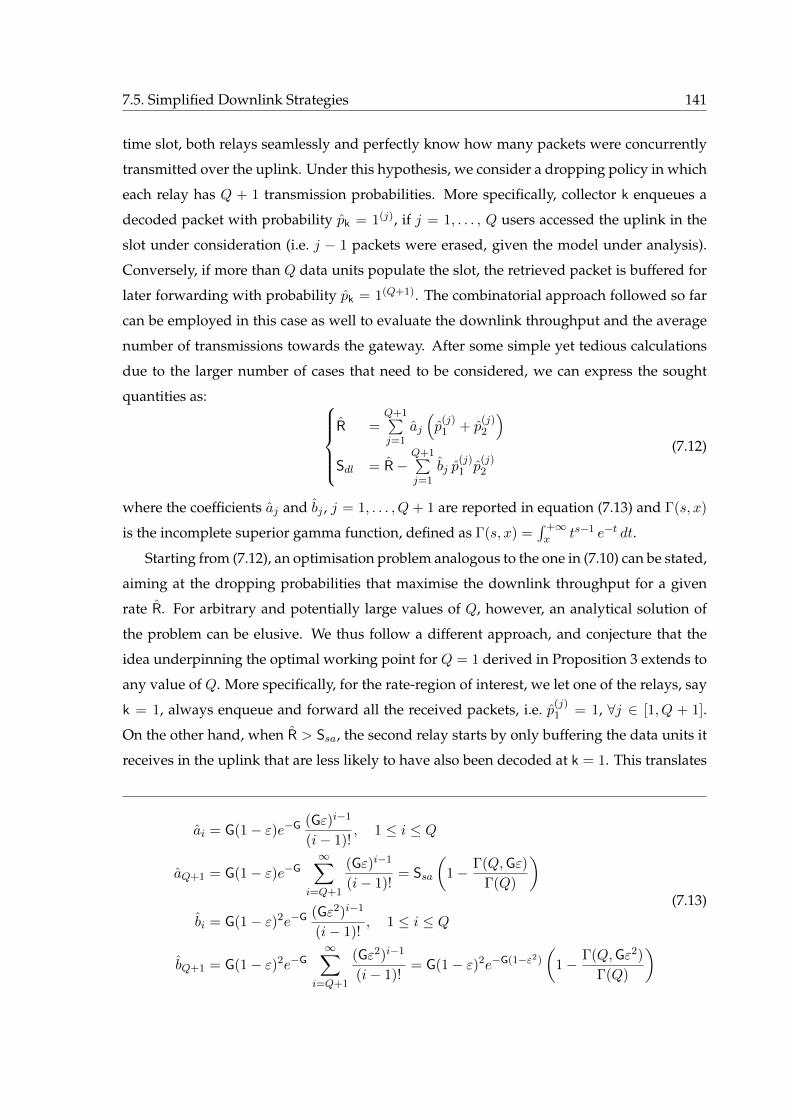
7.5. Simplified Downlink Strategies 141
time slot, both relays seamlessly and perfectly know how many packets were concurrently
transmitted over the uplink. Under this hypothesis, we consider a dropping policy in which
each relay has Q + 1 transmission probabilities. More specifically, collector k enqueues a
decoded packet with probability pk = 1(j), if j = 1, . . . , Q users accessed the uplink in the
slot under consideration (i.e. j − 1 packets were erased, given the model under analysis).
Conversely, if more than Q data units populate the slot, the retrieved packet is buffered for
later forwarding with probability pk = 1(Q+1). The combinatorial approach followed so far
can be employed in this case as well to evaluate the downlink throughput and the average
number of transmissions towards the gateway. After some simple yet tedious calculations
due to the larger number of cases that need to be considered, we can express the sought
quantities as: R =
Q+1∑j=1
aj
(p
(j)1 + p
(j)2
)Sdl = R−
Q+1∑j=1
bj p(j)1 p
(j)2
(7.12)
where the coefficients aj and bj , j = 1, . . . , Q + 1 are reported in equation (7.13) and Γ(s, x)
is the incomplete superior gamma function, defined as Γ(s, x) =∫ +∞x ts−1 e−t dt.
Starting from (7.12), an optimisation problem analogous to the one in (7.10) can be stated,
aiming at the dropping probabilities that maximise the downlink throughput for a given
rate R. For arbitrary and potentially large values of Q, however, an analytical solution of
the problem can be elusive. We thus follow a different approach, and conjecture that the
idea underpinning the optimal working point for Q = 1 derived in Proposition 3 extends to
any value of Q. More specifically, for the rate-region of interest, we let one of the relays, say
k = 1, always enqueue and forward all the received packets, i.e. p(j)1 = 1, ∀j ∈ [1, Q + 1].
On the other hand, when R > Ssa, the second relay starts by only buffering the data units it
receives in the uplink that are less likely to have also been decoded at k = 1. This translates
ai = G(1− ε)e−G (Gε)i−1
(i− 1)!, 1 ≤ i ≤ Q
aQ+1 = G(1− ε)e−G∞∑
i=Q+1
(Gε)i−1
(i− 1)!= Ssa
(1− Γ(Q,Gε)
Γ(Q)
)
bi = G(1− ε)2e−G (Gε2)i−1
(i− 1)!, 1 ≤ i ≤ Q
bQ+1 = G(1− ε)2e−G∞∑
i=Q+1
(Gε2)i−1
(i− 1)!= G(1− ε)2e−G(1−ε2)
(1− Γ(Q,Gε2)
Γ(Q)
)(7.13)
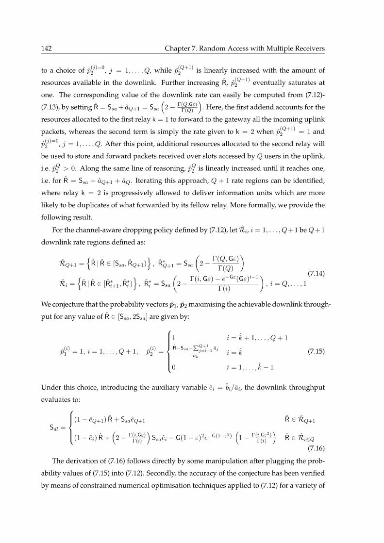
142 Chapter 7. Random Access with Multiple Receivers
to a choice of p(j)=02 , j = 1, . . . , Q, while p(Q+1)
2 is linearly increased with the amount of
resources available in the downlink. Further increasing R, p(Q+1)2 eventually saturates at
one. The corresponding value of the downlink rate can easily be computed from (7.12)-
(7.13), by setting R = Ssa+ aQ+1 = Ssa(
2− Γ(Q,Gε)Γ(Q)
). Here, the first addend accounts for the
resources allocated to the first relay k = 1 to forward to the gateway all the incoming uplink
packets, whereas the second term is simply the rate given to k = 2 when p(Q+1)2 = 1 and
p(j)=02 , j = 1, . . . , Q. After this point, additional resources allocated to the second relay will
be used to store and forward packets received over slots accessed by Q users in the uplink,
i.e. pQ2 > 0. Along the same line of reasoning, pQ2 is linearly increased until it reaches one,
i.e. for R = Ssa + aQ+1 + aQ. Iterating this approach, Q + 1 rate regions can be identified,
where relay k = 2 is progressively allowed to deliver information units which are more
likely to be duplicates of what forwarded by its fellow relay. More formally, we provide the
following result.
For the channel-aware dropping policy defined by (7.12), let Ri, i = 1, . . . , Q+1 be Q+1
downlink rate regions defined as:
RQ+1 =
R | R ∈ [Ssa, RQ+1), R∗Q+1 = Ssa
(2− Γ(Q,Gε)
Γ(Q)
)Ri =
R | R ∈ [R∗i+1, R
∗i ), R∗i = Ssa
(2− Γ(i,Gε)− e−Gε(Gε)i−1
Γ(i)
), i = Q, . . . , 1
(7.14)
We conjecture that the probability vectors p1, p2 maximising the achievable downlink through-
put for any value of R ∈ [Ssa, 2Ssa] are given by:
p(i)1 = 1, i = 1, . . . , Q+ 1, p
(i)2 =
1 i = k + 1, . . . , Q+ 1
R−Ssa−∑Q+1j=i+1
aj
aki = k
0 i = 1, . . . , k − 1
(7.15)
Under this choice, introducing the auxiliary variable ei = bi/ai, the downlink throughput
evaluates to:
Sdl =
(1− eQ+1) R + SsaeQ+1 R ∈ RQ+1
(1− ei) R +(
2− Γ(i,Gε)Γ(i)
)Ssaei − G(1− ε)2e−G(1−ε2)
(1− Γ(i,Gε2)
Γ(i)
)R ∈ Ri≤Q
(7.16)
The derivation of (7.16) follows directly by some manipulation after plugging the prob-
ability values of (7.15) into (7.12). Secondly, the accuracy of the conjecture has been verified
by means of constrained numerical optimisation techniques applied to (7.12) for a variety of
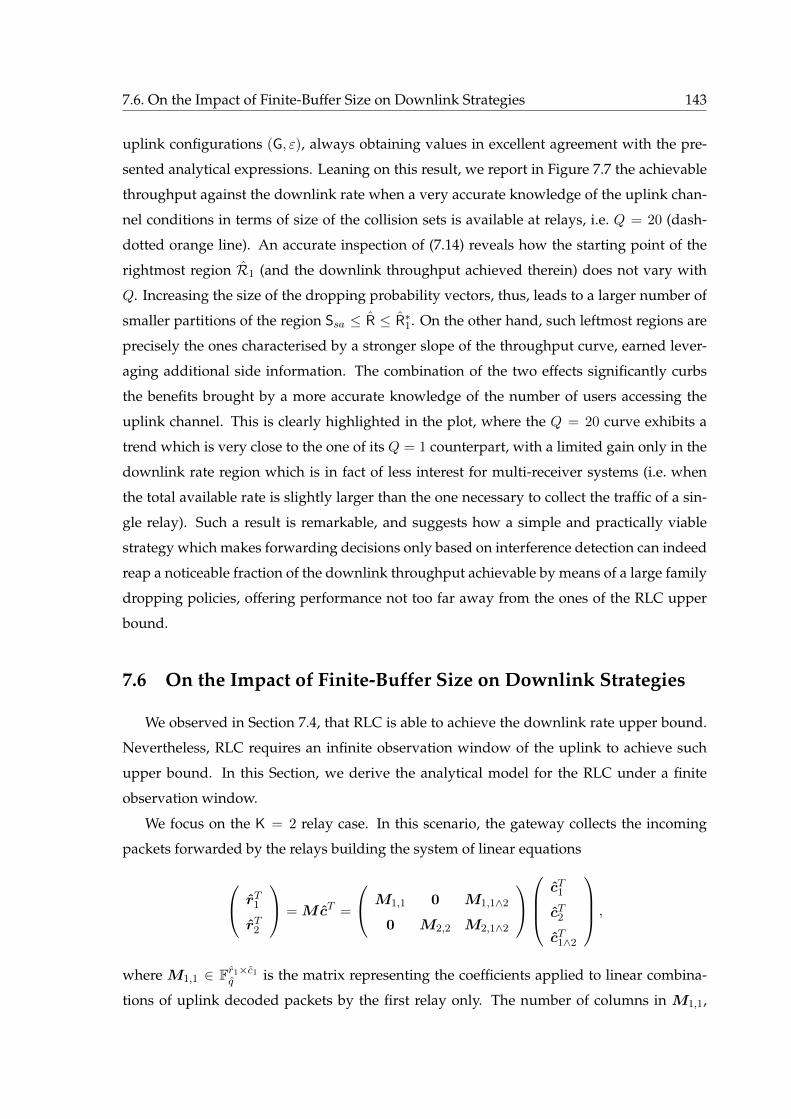
7.6. On the Impact of Finite-Buffer Size on Downlink Strategies 143
uplink configurations (G, ε), always obtaining values in excellent agreement with the pre-
sented analytical expressions. Leaning on this result, we report in Figure 7.7 the achievable
throughput against the downlink rate when a very accurate knowledge of the uplink chan-
nel conditions in terms of size of the collision sets is available at relays, i.e. Q = 20 (dash-
dotted orange line). An accurate inspection of (7.14) reveals how the starting point of the
rightmost region R1 (and the downlink throughput achieved therein) does not vary with
Q. Increasing the size of the dropping probability vectors, thus, leads to a larger number of
smaller partitions of the region Ssa ≤ R ≤ R∗1. On the other hand, such leftmost regions are
precisely the ones characterised by a stronger slope of the throughput curve, earned lever-
aging additional side information. The combination of the two effects significantly curbs
the benefits brought by a more accurate knowledge of the number of users accessing the
uplink channel. This is clearly highlighted in the plot, where the Q = 20 curve exhibits a
trend which is very close to the one of its Q = 1 counterpart, with a limited gain only in the
downlink rate region which is in fact of less interest for multi-receiver systems (i.e. when
the total available rate is slightly larger than the one necessary to collect the traffic of a sin-
gle relay). Such a result is remarkable, and suggests how a simple and practically viable
strategy which makes forwarding decisions only based on interference detection can indeed
reap a noticeable fraction of the downlink throughput achievable by means of a large family
dropping policies, offering performance not too far away from the ones of the RLC upper
bound.
7.6 On the Impact of Finite-Buffer Size on Downlink Strategies
We observed in Section 7.4, that RLC is able to achieve the downlink rate upper bound.
Nevertheless, RLC requires an infinite observation window of the uplink to achieve such
upper bound. In this Section, we derive the analytical model for the RLC under a finite
observation window.
We focus on the K = 2 relay case. In this scenario, the gateway collects the incoming
packets forwarded by the relays building the system of linear equations
rT1
rT2
= McT =
M1,1 0 M1,1∧2
0 M2,2 M2,1∧2
cT1
cT2
cT1∧2
,
where M1,1 ∈ Fr1×c1q is the matrix representing the coefficients applied to linear combina-
tions of uplink decoded packets by the first relay only. The number of columns in M1,1,
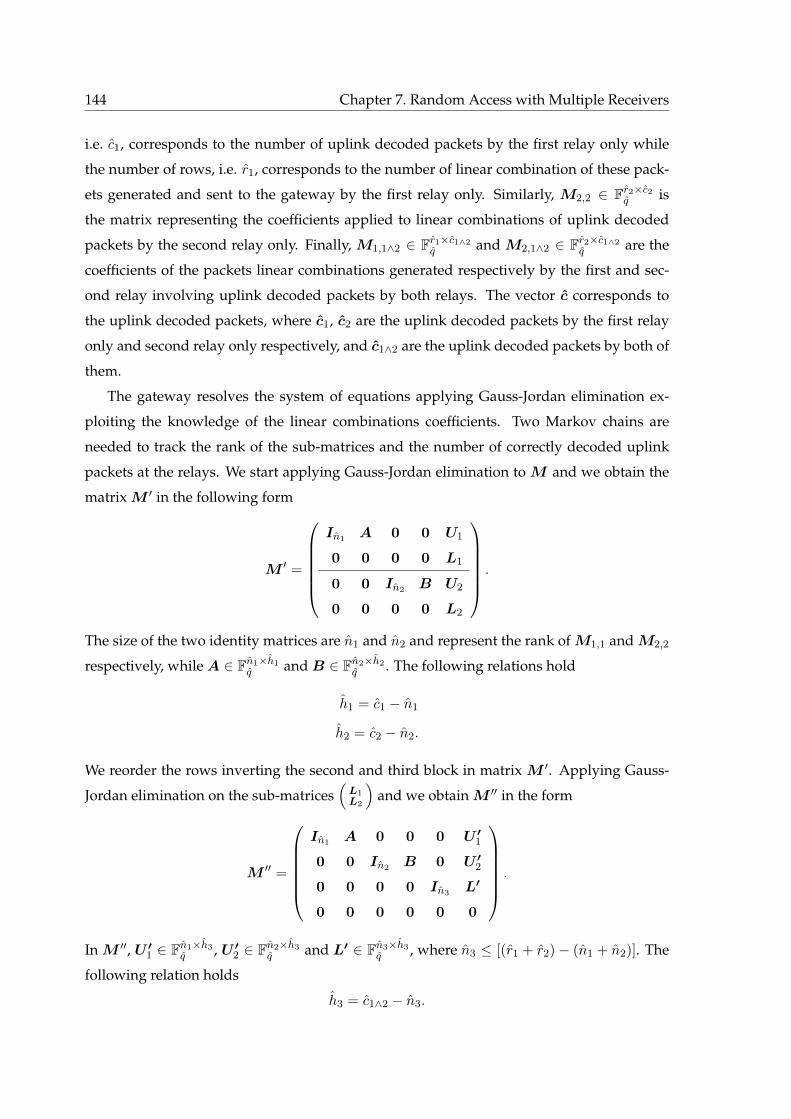
144 Chapter 7. Random Access with Multiple Receivers
i.e. c1, corresponds to the number of uplink decoded packets by the first relay only while
the number of rows, i.e. r1, corresponds to the number of linear combination of these pack-
ets generated and sent to the gateway by the first relay only. Similarly, M2,2 ∈ Fr2×c2q is
the matrix representing the coefficients applied to linear combinations of uplink decoded
packets by the second relay only. Finally, M1,1∧2 ∈ Fr1×c1∧2q and M2,1∧2 ∈ Fr2×c1∧2
q are the
coefficients of the packets linear combinations generated respectively by the first and sec-
ond relay involving uplink decoded packets by both relays. The vector c corresponds to
the uplink decoded packets, where c1, c2 are the uplink decoded packets by the first relay
only and second relay only respectively, and c1∧2 are the uplink decoded packets by both of
them.
The gateway resolves the system of equations applying Gauss-Jordan elimination ex-
ploiting the knowledge of the linear combinations coefficients. Two Markov chains are
needed to track the rank of the sub-matrices and the number of correctly decoded uplink
packets at the relays. We start applying Gauss-Jordan elimination to M and we obtain the
matrix M ′ in the following form
M ′ =
In1 A 0 0 U1
0 0 0 0 L1
0 0 In2 B U2
0 0 0 0 L2
.
The size of the two identity matrices are n1 and n2 and represent the rank of M1,1 and M2,2
respectively, while A ∈ Fn1×h1q and B ∈ Fn2×h2
q . The following relations hold
h1 = c1 − n1
h2 = c2 − n2.
We reorder the rows inverting the second and third block in matrix M ′. Applying Gauss-
Jordan elimination on the sub-matrices(
L1L2
)and we obtain M ′′ in the form
M ′′ =
In1 A 0 0 0 U ′
1
0 0 In2 B 0 U ′2
0 0 0 0 In3 L′
0 0 0 0 0 0
.
In M ′′, U ′1 ∈ Fn1×h3
q , U ′2 ∈ Fn2×h3
q and L′ ∈ Fn3×h3q , where n3 ≤ [(r1 + r2)− (n1 + n2)]. The
following relation holds
h3 = c1∧2 − n3.
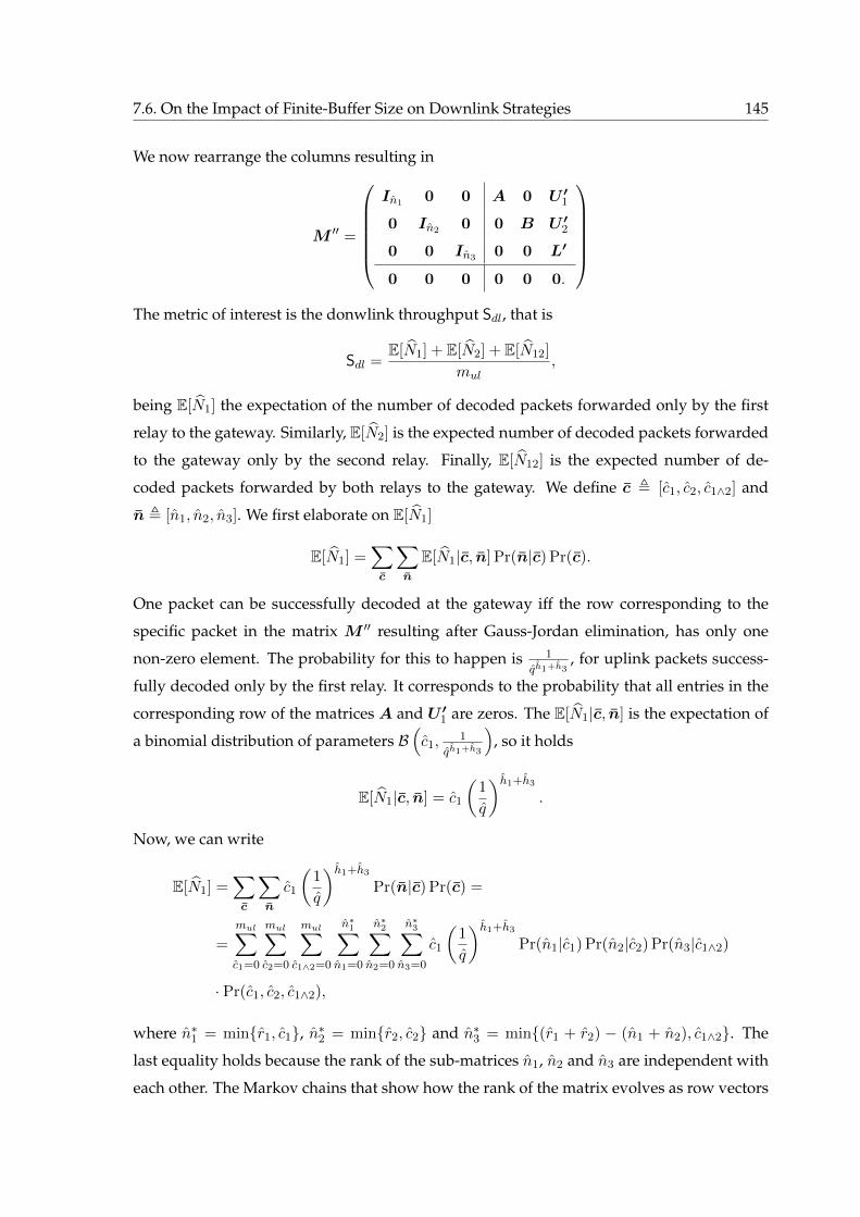
7.6. On the Impact of Finite-Buffer Size on Downlink Strategies 145
We now rearrange the columns resulting in
M ′′ =
In1 0 0 A 0 U ′
1
0 In2 0 0 B U ′2
0 0 In3 0 0 L′
0 0 0 0 0 0.
The metric of interest is the donwlink throughput Sdl, that is
Sdl =E[N1] + E[N2] + E[N12]
mul,
being E[N1] the expectation of the number of decoded packets forwarded only by the first
relay to the gateway. Similarly, E[N2] is the expected number of decoded packets forwarded
to the gateway only by the second relay. Finally, E[N12] is the expected number of de-
coded packets forwarded by both relays to the gateway. We define c , [c1, c2, c1∧2] and
n , [n1, n2, n3]. We first elaborate on E[N1]
E[N1] =∑c
∑n
E[N1|c, n] Pr(n|c) Pr(c).
One packet can be successfully decoded at the gateway iff the row corresponding to the
specific packet in the matrix M ′′ resulting after Gauss-Jordan elimination, has only one
non-zero element. The probability for this to happen is 1
qh1+h3, for uplink packets success-
fully decoded only by the first relay. It corresponds to the probability that all entries in the
corresponding row of the matrices A and U ′1 are zeros. The E[N1|c, n] is the expectation of
a binomial distribution of parameters B(c1,
1
qh1+h3
), so it holds
E[N1|c, n] = c1
(1
q
)h1+h3
.
Now, we can write
E[N1] =∑c
∑n
c1
(1
q
)h1+h3
Pr(n|c) Pr(c) =
=
mul∑c1=0
mul∑c2=0
mul∑c1∧2=0
n∗1∑n1=0
n∗2∑n2=0
n∗3∑n3=0
c1
(1
q
)h1+h3
Pr(n1|c1) Pr(n2|c2) Pr(n3|c1∧2)
· Pr(c1, c2, c1∧2),
where n∗1 = minr1, c1, n∗2 = minr2, c2 and n∗3 = min(r1 + r2) − (n1 + n2), c1∧2. The
last equality holds because the rank of the sub-matrices n1, n2 and n3 are independent with
each other. The Markov chains that show how the rank of the matrix evolves as row vectors

146 Chapter 7. Random Access with Multiple Receivers
0 1 2 3
1
qb
1− 1
qb
q
qb
1− q
qb
q2
qb
1− q2
qb
q3
qb
1− q3
qb
Figure 7.8. Markov chain of the evolution of the matrix rank as row vectors are added. The state number
represents the rank value.
F1×cq are added one by one as shown in Figure 7.8. The probability that a matrix belonging
to Fn×cq has rank xn = minn, c can be written in a recursive way [146, 147] as
Pr(n|c) =
P1,c(0) =1
qc
P1,c(1) = 1− 1
qc
Pn,c(xn) =
(qxn
qc
)Pn−1,c(xn) +
(1− qxn−1
qc
)Pn−1,c(xn − 1), xn = minn, c.
Where n and c can be substituted with any couple (n1, c1), or (n2, c2) or also (n3, c1∧2).
The quantity E[N2|c, n] is the expectation of the binomial distribution B(c2,
1
qh2+h3
), while
E[N12|c, n] is the expectation of the binomial distribution B(c1∧2,
1
qh3
), so we can write,
E[N2] =∑c
∑n
c2
(1
q
)h2+h3
Pr(n|c) Pr(c)
E[N12] =∑c
∑n
c1∧2
(1
q
)h3
Pr(n|c) Pr(c).
The joint probability mass function Pr(c) for the random vector c1, c2, c1∧2 can be tracked
effectively by means of a homogeneous Markov chain, leaning on the assumed indepen-
dence of channel realizations across uplink slots. To this aim, let Xl = c(l)1 , c
(l)2 , c
(l)1∧2 be the
state at the start of slot l, indicating the number of packets received so far by the first relay
solely, by the second relay and by both of them, respectively. For the sake of compactness,
let us furthermore denote PrXl+1 = i′, j′, k′
∣∣Xl = i, j, k
as P(i,j,k)→(i′,j′,k′). Following
this notation, each time unit can see five possible transitions for the chain, whose probabili-
7.6. On the Impact of Finite-Buffer Size on Downlink Strategies 147
ties follow by simple combinatorial arguments similar to the ones discussed in Section 7.3:
P(i,j,k)→(i,j,k) = 1− 2G(1− ε)e−G(1−ε) + G(1− ε)2 e−G(1−ε2)(1 + Gε2
)P(i,j,k)→(i+1,j,k) = G(1− ε)e−G(1−ε) − G(1− ε)2 e−G(1−ε2)
(1 + Gε2
)P(i,j,k)→(i,j+1,k) = G(1− ε)e−G(1−ε) − G(1− ε)2 e−G(1−ε2)
(1 + Gε2
)P(i,j,k)→(i,j,k+1) = G(1− ε)2 e−G(1−ε2)
P(i,j,k)→(i+1,j+1,k) = (Gε)2 (1− ε)2 e−G(1−ε2)
The defined probabilities uniquely identify the transition matrix for the Markov chain
under consideration, so that the sought probability mass function follows as its mul-th step
evolution when forcing the initial state as X0 = 0, 0, 0.We present first the results for RLC for finite buffer size in Figure 7.9. If the buffer size
is small, i.e. 25 slots, the performance of RLC is particularly degraded with respect to the
results for infinite buffer length, with a loss that can exceed 50% for small downlink rates.
A very tight match of the Monte Carlo simulations with the Markov model presented in
this Section can also be observed, especially for buffer sizes of 80 slots. For this reason,
we depicted only the Monte Carlo simulations for higher buffer sizes. The results show
a threshold behaviour: below the downlink rate that allows the two relays to send to the
gateway all the received packets, which corresponds to R = Sul = 0.545 in this scenario,
the downlink throughput is particularly limited. The reason relies on the fact that in most
of the cases the matrix is rank-deficient and very few packets can be decoded. This is true
in general, regardless of the buffer size. Instead, for R > 0.545, RLC allows the correct
decoding of most of the packets and, for high buffer sizes, RLC is able to reach the infinite
buffer bound. This is the ultimate limit of the scheme and determines the non-achievable
region of downlink throughput. The higher the buffer size, the lower is the downlink rate
necessary for reaching the infinite buffer throughput bound. The high sensitivity of RLC
on the downlink rate is detrimental, especially for scenarios where the uplink throughput is
subject to quick and large variations. In these scenarios, in fact, the downlink rate shall be
adapted accordingly, in order to avoid the region of low throughput.
In Figure 7.10 we show the comparison between RLC and two dropping policies, the
common transmission probability and the channel-aware policy. The choice of showing
only two dropping policies is driven by the sake of clarity. The two chosen policies can be
regarded as worst and best case respectively. Three buffer sizes are selected, i.e. 25, 100 and
500 slots for comparing three different scenarios: small buffer size, which is the case when
packets have stringent delay constraint, medium buffer size and large buffer size, where
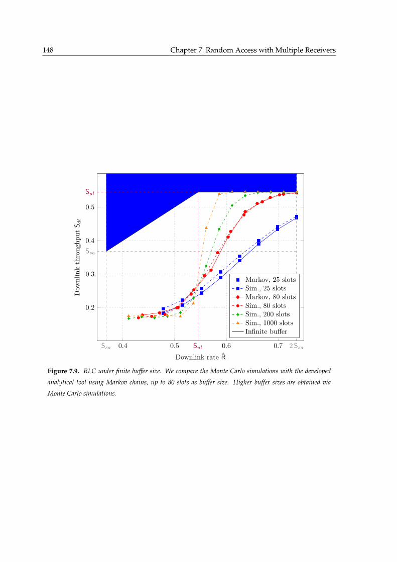
148 Chapter 7. Random Access with Multiple Receivers
0.4 0.5 0.6 0.7
0.2
0.3
0.4
0.5
Ssa 2 Ssa
Ssa
Sul
Sul
Downlink rate R
Dow
nlinkthroug
hput
S dl
Markov, 25 slotsSim., 25 slotsMarkov, 80 slotsSim., 80 slotsSim., 200 slotsSim., 1000 slotsInfinite buffer
Figure 7.9. RLC under finite buffer size. We compare the Monte Carlo simulations with the developed
analytical tool using Markov chains, up to 80 slots as buffer size. Higher buffer sizes are obtained via
Monte Carlo simulations.
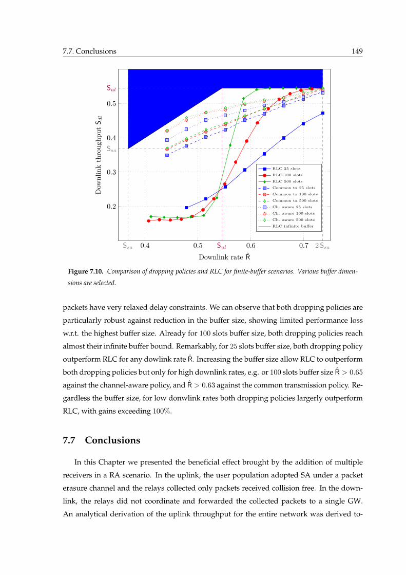
7.7. Conclusions 149
0.4 0.5 0.6 0.7
0.2
0.3
0.4
0.5
Ssa 2 Ssa
Ssa
Sul
Sul
Downlink rate R
Dow
nlin
kth
roug
hput
S dl
RLC 25 slots
RLC 100 slots
RLC 500 slots
Common tx 25 slots
Common tx 100 slots
Common tx 500 slots
Ch. aware 25 slots
Ch. aware 100 slots
Ch. aware 500 slots
RLC infinite buffer
Figure 7.10. Comparison of dropping policies and RLC for finite-buffer scenarios. Various buffer dimen-
sions are selected.
packets have very relaxed delay constraints. We can observe that both dropping policies are
particularly robust against reduction in the buffer size, showing limited performance loss
w.r.t. the highest buffer size. Already for 100 slots buffer size, both dropping policies reach
almost their infinite buffer bound. Remarkably, for 25 slots buffer size, both dropping policy
outperform RLC for any dowlink rate R. Increasing the buffer size allow RLC to outperform
both dropping policies but only for high downlink rates, e.g. or 100 slots buffer size R > 0.65
against the channel-aware policy, and R > 0.63 against the common transmission policy. Re-
gardless the buffer size, for low donwlink rates both dropping policies largerly outperform
RLC, with gains exceeding 100%.
7.7 Conclusions
In this Chapter we presented the beneficial effect brought by the addition of multiple
receivers in a RA scenario. In the uplink, the user population adopted SA under a packet
erasure channel and the relays collected only packets received collision free. In the down-
link, the relays did not coordinate and forwarded the collected packets to a single GW.
An analytical derivation of the uplink throughput for the entire network was derived to-
150 Chapter 7. Random Access with Multiple Receivers
gether with the PLR. Improvements w.r.t. the single receiver scenario were highlighted in
the multi-receiver case and a logarithmic trend in the throughput increase as the number
of relays was increased was shown. For the downlink, first we derived an upper bound on
the downlink rate, measured in downlink transmission per uplink slot. Through the use
of RLC, a solution that reached the upper bound was presented that nonetheless relied on
the assumption of infinite observation of the uplink. It also required the linear combina-
tion of collected packets at the relays and solving a system of equations at the gateway. In
order to reduce complexity at the gateway alternative solutions based on dropping poli-
cies were also introduced and analysed. The key observation was that part of the collected
packets at one relay was also correctly collected at a second one, with a given probability.
In this way, properly sizing the queueing probability of collected packets leaded to a more
efficient use of the downlink. Although viable, these solutions had a non-negligible per-
formance loss compared to RLC when an infinite uplink observation was guaranteed. We
relaxed this assumption moving towards relay having finite buffers. In this scenario we de-
rived a Markov chain model capturing the performance of the RLC solution. Comparing it
with the dropping policies showed that for limited downlink resources and stringent buffer
constraints, the dropping policies largely outperformed RLC. Nonetheless, RLC could be
improved following two paths: on one hand, one could adopt a low-density approach, in
which the number of packets involved in the linear combinations sent to the GW becomes
smaller, which corresponds to a sparse matrix. A second possibility would be to back-off
in the number of linear combinations forwarded. Reducing the number of generated linear
combinations would have a two-folded effect: could help when the downlink resources are
scarce, but does not guarantee vanishing small error probability.
Conclusions
The good ideas will survive
Quentin Tarantino
The thesis focused on medium access RA protocols dedicated to variable and bursty
channel traffic. Several aspects were addressed, from the performance of asynchronous RA
protocols employing SIC and combining techniques, to optimisation of the repetition degree
for time slotted schemes under fading channels. The key findings of the thesis and future
research directions are summarised as follows.
• Asynchronous RA: Bundling the use of SIC together with combining techniques as
SC or MRC in RA with time diversity had a strong beneficial impact, leading such
schemes to compete with comparable slot synchronous ones. An analytical approx-
imation of the PLR tight for low to moderate channel loads was derived and was
shown to be useful for the design of such schemes. Practical aspects drove the design
of a blind physical layer scheme for detection and combining that did not require any
prior knowledge on the association between received packets and the user to which
they belong. Numerical results demonstrated its applicability with very limited losses
compared to the ideal scenario.
Comparison at higher layer between asynchronous and slot synchronous schemes
showed that higher benefits could be expected for the former ones especially when
packets exceeded the slot duration and fragmentation was required in the latter ones.
Analytical derivation of higher layer performance for the latter schemes was provided,
so that no simulations of higher layers were required. When no knowledge of the prob-
ability measure defining the packet duration was available, an approximation based
on the solely mean was given.
One of the key research directions in this area shall focus on deriving a proper an-
alytical model capturing the behaviour of SIC. This would open an entire new field
152 Conclusions
where for example, the users can use irregular repetition as in the slot synchronous
case. With such a model, one could optimise the p.m.f. adopted by the user in order
to maximise the throughput.
Another interesting aspect is the delay that a user experience from transmission of the
first replica until its correct decoding. This aspect is particularly relevant for the layer 3
comparison and shall be addressed in the future. A possible improvement of the slot
synchronous schemes include the exploitation of the outcome for the first fragment
sent in the first frame in order to choose the number of replicas to be sent in the second
frame.
• Time slotted irregular repetition RA: Irregular repetition of the physical layer pack-
ets brought undoubtable gains in the performance compared to the regular case. Ex-
tension of the optimisation procedure in order to include the Rayleigh block fading
channel and the capture effect was provided. A non-negligible improvement in terms
of achievable throughput and PLR was shown compared to the optimisation over the
collision channel.
A straightforward extension of the framework shall consider other types of fading, e.g.
Rice. In order to identify the ultimate performance of such scheme under fading, we
shall derive an upper bound on the achievable rate, as is done for the collision channel.
Although very appealing, its practical feasibility shall be considered.
• RA with multiple receivers: Expanding the topology to consider multiple non-
cooperative receivers for a RA uplink under the packet erasure channel, called for
development of efficient solutions to forward the collected messages to a common
gateway. RLC was proven to achieve the best possible performance, but required an
infinite amount of time for observing and collecting the uplink packets. Dropping
policies were less efficient, but did not require infinite observation of the uplink. A
buffer limited analytical model for the RLC was here derived and it was shown via
numerical simulations that dropping policies were able to largely outperform RLC for
many practical buffer sizes especially when the downlink resource was scarce.
A possible extension of this framework would be to consider more advanced random
access strategies for the uplink, as for example CSA. As for the downlink, we could
consider network coding strategies with probability of dropping packets correctly re-
ceived from the uplink, in order to cope with finite length buffers so to compete with
the simplified dropping policies.
153
Finally, we present a quick recap of the thesis contributions.
• A novel asynchronous RA scheme named ECRA was presented in Chapter 4;
• A novel detection and combining methodology for asynchronous RA protocols was
developed in Chapter 4;
• A new methodology for assessing the layer 3 performance of RA protocols was devel-
oped in Chapter 5;
• A new methodology for the analysis of irregular slot synchronous RA schemes was
presented in Chapter 6;
• A new methodology for the analysis of finite buffer RLC was presented in Chapter 7.

Selected List of Publications
Part of the work presented in this thesis has also appeared in the articles reported below.
Journal Papers
[J2] F. Clazzer, C. Kissling, M. Marchese, ”Enhancing Contention Resolution ALOHA us-
ing Combining Techniques”, submitted to IEEE Transactions on Communications.
[J1] A. Munari, M. Heindlmaier, F. Clazzer, G. Liva, ”On the Capacity of Slotted ALOHA
with Multiple Receivers”, in preparation for the IEEE Transaction on Information The-
ory.
Conference Papers
[C6] F. Clazzer, E. Paolini, I. Mambelli and C. Stefanovic, ”Irregular Repetition Slotted
ALOHA over the Rayleigh Block Fading Channel with Capture”, accepted for pub-
lication in the IEEE International Conference on Communications (ICC), 2017.
[C5] F. Clazzer, F. Lazaro, G. Liva, M. Marchese, ”Detection and Combining Techniques for
Asynchronous Random Access with Time Diversity”, in Proceedings of the 11th Inter-
national ITG Conference on Systems, Communications and Coding (SCC), Hamburg,
Germany, February 2017.
[C4] A. Munari, F. Clazzer, ”Multi-Receiver Aloha Systems - a Survey and New Results”,
in Proceedings of the IEEE International Conference on Communications (ICC), Work-
shop on Massive Uncoordinated Access Protocols (MASSAP), London, UK, June 2015.
[C3] F. Clazzer, M. Marchese, ”Layer 3 Throughput Analysis for Advanced ALOHA Proto-
cols”, in Proceedings of the IEEE International Conference on Communications (ICC),
156 Selected List of Publications
Workshop on Massive Uncoordinated Access Protocols (MASSAP), pp.533-538, Syd-
ney, Australia, June 2014.
[C2] F. Clazzer, C. Kissling, ”Optimum Header Positioning in Successive Interference Can-
cellation (SIC) based ALOHA”, in Proceedings of the IEEE International Conference
on Communications (ICC), pp.2869-2874, Budapest, Hungary, June 2013.
[C1] F. Clazzer, C. Kissling, ”Enhanced Contention Resolution ALOHA - ECRA”, in Pro-
ceedings of the 9th International ITG Conference on Systems, Communications and
Coding (SCC), pp.1-6, Munich, Germany, January 2013.

Other Publications
Below are reported other articles submitted or published during the Ph.D. that are not
appearing in the thesis.
Journal Papers
[J3] F. Clazzer, F. Lazaro, S. Plass, ”Enhanced AIS Receiver Design for Satellite Reception”,
CEAS Space Journal, Vol. 8, No. 4, pp. 257-268, December 2016.
[J2] Z. Katona, F. Clazzer, K. Shortt, S. Watts, Lexow, H.P., R. Winduratna, ”Performance,
Cost Analysis, and Ground Segment Design of Ultra High Throughput Multi-Spot
Beam Satellite Networks applying different Capactiy Enhancing Techniques”, Inter-
national Journal of Satellite Communications and Networking, Vol. 34, No. 4, pp.
547-573, July/August 2016.
[J1] P.-D. Arapoglou, A. Ginesi, S. Cioni, S. Erl, F. Clazzer, S. Andrenacci, A. Vanelli-Coralli,
”DVB-S2X-Enabled Precoding for High Throughput Satellite Systems”, International
Journal of Satellite Communications and Networking, Vol. 34, No. 3, pp. 439-455,
May/June 2016.
Conference Papers
[C10] F. Clazzer, A. Munari, F. Giorgi, ”Asynchronous Random Access Schemes for the
VDES Satellite Uplink”, submitted to the IEEE/MTS Oceans’17, 2017.
[C9] F. Giorgi, F. Clazzer, A. Munari, ”Asynchronous Random Access Protocols for the Mar-
itime Satellite Channel”, submitted to the IEEE Global Communications Conference
(GLOBECOM), 2017.
[C8] A. Stajkic, F. Clazzer, G. Liva, ”Neighbor Discovery in Wireless Networks: A Graph-
based Analysis and Optimization”, in Proceedings of the IEEE International Confer-
158 Other Publications
ence on Communications (ICC), Workshop on Massive Uncoordinated Access Proto-
cols (MASSAP), pp. 511-516, Kuala Lumpur, Malaysia, May 2016.
[C7] S. Plass, F. Clazzer, F. Bekkadal, ”Current Situation and Future Innovations in Arctic
Communications”, in Proceedings of the IEEE 82nd Vehicular Technology Conference
(VTC Fall), pp. 1-7, Boston, MA, USA, September 2015.
[C6] F. Clazzer, F. Lazaro, S. Plass, ”New Receiver Algorithms for Satellite AIS”, in Pro-
ceedings of the Deutscher Luft- und Raumfahrtkongress, pp. 1-7, Rostock, Germany,
September 2015.
[C5] F. Clazzer, A. Munari, ”Analysis of Capture and Multi-Packet Reception on the AIS
Satellite System”, Proceedings of the IEEE/MTS Oceans’15, pp.1-9, Genova, Italy, May
2015.
[C4] S. Plass, F. Clazzer, F. Bekkadal, Y. Ibnyahya, M. Manzo, ”Maritime Communications
- Identifying Current and Future Satellite Requirements & Technologies”, in Proceed-
ings of the 20th Ka and Broadband Communications, Navigation and Earth Observa-
tion Conference, pp. 1-8, Vietri, Italy, October 2014.
[C3] F. Clazzer, A. Munari, S. Plass, B. Suhr, ”On the Impact of Coverage Range on AIS
Message Reception at Flying Platforms”, in Proceedings of the 7th Advanced Satel-
lite Multimedia Conference and the 13th Signal Processing for Space Communications
Workshop (ASMS/SPSC), pp.128-135, Livorno, Italy, September 2014.
[C2] F. Clazzer, A. Munari, M. Berioli, F. Lazaro, ”On the Characterization of AIS Traffic
at the Satellite”, in Proceedings of the IEEE/MTS Oceans’14, pp.1-9, Taipei, Taiwan,
April 2014.
[C1] C. Kissling, F. Clazzer, ”LDPC Code Performance and Optimum Code Rate for Con-
tention Resolution Diversity ALOHA”, in Proceedings of the IEEE Global Communi-
cation Conference (GLOBECOM), pp.2954-2960, Atlanta, GA, USA, December 2013.
Bibliography
[1] J. L. Massey, “Collision-Resolution Algorithm and Random-Access Communication,”
Multi-User Communication Systems, vol. Editor G. Longo, pp. 73–137, 1981.
[2] R. Rom and M. Sidi, Multiple Access Protocols: Performance and Analysis, M. Gerla,
A. Lazar, and P. Kuehn, Eds. Springer-Verlag, 1990.
[3] N. Abramson, “The ALOHA system: Another alternative for computer communi-
cations,” in Proceedings of the 1970 Fall Joint Computer Conference, AFIPS Conference,
vol. 37, Montvale, N. J., 1970, pp. 281–285.
[4] L. G. Roberts, “ALOHA packet system with and without slots and capture,” Proceed-
ings of the International Conference of Special Interest Group on Data Communications (SIG-
COMM), vol. 5, pp. 28–42, April 1975.
[5] D. Bertsekas and R. Gallager, Data Networks. Prentice Hall, 1987.
[6] N. Abramson, “Multiple Access in Wireless Digital Networks,” Proceedings of IEEE,
vol. 82, no. 9, pp. 1360–1370, September 1994.
[7] G. Wu, S. Talwar, K. Johnsson, N. Himayat, and K. Johnson, “M2M: From Mobile to
Embedded Internet,” IEEE Communications Magazine, vol. 49, no. 4, pp. 36–43, April
2011.
[8] S. Verdu, Multiuser Detection. Cambridge University Press, 1998.
[9] H. Menouar, F. Filali, and M. Lenardi, “A Survey and Qualitative Analysis of MAC
Protocols for Vehicular Ad Hoc Networks,” IEEE Wireless Communications, vol. 13,
no. 5, pp. 30–35, October 2006.
159
160 BIBLIOGRAPHY
[10] Y. He and X. Wang, “An ALOHA-Based Improved Anti-Collision Algorithm for RFID
Systems,” IEEE Wireless Communications, vol. 20, no. 5, pp. 152–158, October 2013.
[11] H. Peyravi, “Medium Access Control Protocols Performance in Satellite Communica-
tions,” IEEE Communications Magazine, vol. 37, no. 3, pp. 62–71, March 1999.
[12] D. Pompili and I. Akyildiz, “Overview of Networking Protocols for Underwater Wire-
less Communications,” IEEE Communications Magazine, vol. 47, no. 1, pp. 97–102, Jan-
uary 2009.
[13] A. Laya, L. Alonso, and J. Alonso-Zarate, “Is the Random Access Channel of LTE and
LTE-A Suitable for M2M Communications? A Survey of Alternatives,” IEEE Commu-
nications Surveys and Tutorials, vol. 16, no. 1, pp. 4–16, First Quarter 2014.
[14] “http://oneweb.world/.”
[15] L. Kleinrock, Queueing Systems - Volume II: Computer Applications. John Wiley & Sons,
1976.
[16] N. Abramson, “Development of the ALOHANET,” IEEE Transactions on Information
Theory, vol. IT-31, no. 2, pp. 119–123, March 1985.
[17] B. Metcalfe and D. R. Boggs, “Ethernet: Distributed Packet Switching for Local Com-
puter Networks,” Communications of the ACM, vol. 19, no. 7, pp. 395–404, July 1976.
[18] D. W. Lipke, D. W. Swearingen, J. F. Parker, E. E. Steinbrecher, T. O. Clavit, and H. Do-
del, “Marisat - A Maritime Satellite Communications System,” COMSAT Technical Re-
view, vol. 7, pp. 351–391, November 1977.
[19] J. Cai and D. J. Goodman, “General Packet Radio Service in GSM,” IEEE Communica-
tions Magazine, vol. 35, no. 10, pp. 122–131, October 1997.
[20] A. Laya, C. Kalalas, F. Vazquez-Gallego, L. Alonso, and J. Alonso-Zarate, “Goodbye,
ALOHA!” IEEE Access, vol. 4, pp. 2029–2044, April 2016.
[21] L. Kleinrock and S. Lam, “Packet Switching in a Multiaccess Broadcast Channel: Per-
formance Evaluation,” IEEE Transactions on Communications, vol. COM-23, no. 4, pp.
410–423, April 1975.
[22] S. S. Lam and L. Kleinrock, “Packet Switching in a Multiaccess Broadcast Channel: Dy-
namic Control Procedures,” IEEE Transactions on Communications, vol. COM-23, no. 9,
pp. 891–904, September 1975.
BIBLIOGRAPHY 161
[23] A. B. Carleial and M. E. Hellman, “Bistable Behavior of ALOHA-Type Systems,” IEEE
Transactions on Communications, vol. COM-23, no. 4, pp. 401–410, April 1975.
[24] Y.-C. Jenq, “On the Stability of Slotted ALOHA Systems,” IEEE Transactions on Com-
munications, vol. COM-28, no. 11, pp. 1936–1939, November 1980.
[25] B. S. Tsybakov and V. A. Mikhailov, “Ergodicity of sloted ALOHA system,” Problemy
Peredachi Informatsii, vol. 15, pp. 73–87, 1979.
[26] V. A. Malyshev, “Classification of two-dimensional positive random walks and almost
linear semimartingals,” Dokl. Akad., Nauk SSSR, vol. 22, pp. 136–138, 1972.
[27] M. V. Mensikov, “Ergodicity and transience conditions for random walks in the posi-
tive octant of space,” Soviet. Math. Dokl., vol. 15, pp. 1118–1121, 1974.
[28] V. A. Malyshev and M. V. Mensikov, “Ergodicity, continuity and analyticity of count-
able Markov chains,” Trans. Moscow Math. Soc., vol. 39, pp. 3–48, 1979.
[29] R. R. Rao and A. Ephremides, “On the Stability of Interacting Queues in A Multiple-
Access System,” IEEE Transactions on Information Theory, vol. 34, no. 5, pp. 918–930,
September 1988.
[30] B. Metcalfe, “Steady-state analysis of a slotted and controlled Aloha system with
blocking,” Proceedings of the International Conference of Special Interest Group on Data
Communications (SIGCOMM), vol. 5, no. 1, pp. 24–31, January 1975.
[31] M. J. Ferguson, “On the Control, Stability, and Waiting Time in a Slotted ALOHA
Random-Access System,” IEEE Transactions on Communications, vol. 23, no. 11, pp.
1306–1311, November 1975.
[32] Y.-C. Jenq, “Optimal Retransmission Control of Slotted ALOHA Systems,” IEEE Trans-
actions on Communications, vol. COM-29, no. 6, pp. 891–895, June 1981.
[33] T. N. Saadawi and A. Ephremides, “Analysis, Stability, and Optimization of Slotted
ALOHA with a Finite Number of Buffered Users,” IEEE Transactions on Automatic Con-
trol, vol. AC-26, no. 3, pp. 680–689, June 1981.
[34] W. Szpankowski, “Stability Conditions for some Distributed Systems: Buffered Ran-
dom Access Systems,” Advances in Applied Probability, vol. 26, no. 2, pp. 498–515, June
1994.
162 BIBLIOGRAPHY
[35] J. I. Capetanakis, “Tree Algorithms for Packet Broadcast Channels,” IEEE Transactions
on Information Theory, vol. 25, no. 5, pp. 505–515, September 1979.
[36] ——, “The multiple access broadcast channel: Protocol and capacity considerations,”
Ph.D. dissertation, Department of Electrical Engineering, Massachusset Institute of
Technology, Cambridge, MA, August 1977.
[37] B. S. Tsybakov and V. A. Mikhailov, “Free synchronous packet access in a broadcast
channel with feedback,” Problemy Peredachi Informatsii, vol. 14, no. 4, pp. 32–59, Octo-
ber 1978.
[38] R. Gallager, “A perspective on Multiaccess Channels,” IEEE Transactions on Information
Theory, vol. 31, no. 2, pp. 124–142, March 1985.
[39] B. S. Tsybakov and N. B. Likhanov, “Upper bound on the capacity of a random
multiple-access system,” Problemy Peredachi Informatsii, vol. 23, no. 3, pp. 64–78, 1987.
[40] D. S. Chan and T. Berger, “Upper Bound for the Capacity of Multiple Access Protocols
on Multipacket Reception Channels,” in Proceedings of the IEEE International Sympo-
sium on Information Theory (ISIT), Cambridge, MA, USA, July 2012, pp. 1603–1607.
[41] B. S. Tsybakov, “Survey of USSR Contributions to Random Multiple-Access Commu-
nications,” IEEE Transactions on Information Theory, vol. IT-31, no. 2, pp. 143–165, March
1985.
[42] P. Mathys and P. Flajolet, “Q-ary collision resolution algorithms in random-access sys-
tems with free or blocked channel access,” IEEE Transactions on Information Theory,
vol. 31, no. 2, pp. 217–243, March 1985.
[43] J. L. Massey and P. Mathys, “The Collision Channel Without Feedback,” IEEE Transac-
tions on Information Theory, vol. IT-31, no. 2, pp. 192–204, March 1985.
[44] J. L. Massey, “The Capacity of the Collision Channel Without Feedback,” in Proceedings
of the IEEE International Symposium of Information Theory (ISIT), Les Arcs, France, 1982.
[45] B. S. Tsybakov and N. B. Likhanov, “Packet Switching in a Channel Without Feed-
back,” Problemy Peredachi Informatsii, vol. 19, no. 2, pp. 69–84, Apr.-June 1983.
[46] J. Y. N. Hui, “Multiple Accessing for the Collsion Channel Without Feedback,” IEEE
Journal on Selected Areas in Communications, vol. SAC-2, no. 4, pp. 575–582, July 1984.
BIBLIOGRAPHY 163
[47] R. A. Scholtz, “The Spread Spectrum Concept,” IEEE Transactions on Communications,
vol. COM-25, no. 8, pp. 748–755, August 1977.
[48] R. E. Kahn, S. A. Gronemeyer, J. Burchfiel, and R. C. Kunzelman, “Advances in Packet
Radio Technology,” Proceedings of the IEEE, vol. 66, no. 11, pp. 1468–1496, November
1978.
[49] R. L. Pickholtz, D. L. Schilling, and L. B. Milstein, “Theory of Spread-Spectrum Com-
munications - A Tutorial,” IEEE Transactions on Communications, vol. COM-30, no. 5,
pp. 855–884, May 1982.
[50] M. B. Pursley, “The Role of Spread Spectrum in Packet Radio Networks,” Proceedings
of the IEEE, vol. 75, no. 1, pp. 116–134, January 1987.
[51] D. Raychaudhuri, “Performance Analysis of Random Access Packet-Switched Code
Division Multiple Access Systems,” IEEE Transactions on Communications, vol. COM-
29, no. 6, pp. 895–901, June 1981.
[52] M. B. Pursley, “Frequency-Hop Transmission for Satellite Packet Switching and Ter-
restrial Packet Radio Networks,” IEEE Transactions on Information Theory, vol. IT-32,
no. 5, pp. 652–667, September 1986.
[53] A. Polydoros and J. Silvester, “Slotted Random Access Spread-Spectrum Networks:
An Analytical Framework,” IEEE Journal on Selected Areas in Communications, vol.
SAC-5, no. 6, pp. 989–1002, July 1987.
[54] L. Kleinrock and F. A. Tobagi, “Packet Switching in Radiochannelsd: Part I-Carrier
Sense Multiple-Access Modes and Their Throughput-Delay Characteristics,” IEEE
Transactions on Communications, vol. COM-23, no. 12, pp. 1400–1416, December 1975.
[55] F. A. Tobagi and L. Kleinrock, “Packet Switching in Radio Channels: Part II-The Hid-
den Terminal Problem in Carrier Sense Multiple-Access and the Busy-Tone Solution,”
IEEE Transactions on Communications, vol. COM-23, no. 12, pp. 1417–1433, December
1975.
[56] A. Colvin, “CSMA with collision avoidance,” Computer Communications, vol. 6, no. 5,
pp. 227–235, October 1983.
[57] J. J. Metzener, “On Improving Utilization in ALOHA Networks,” IEEE Transactions on
Communications, vol. COM-24, no. 4, pp. 447–448, April 1976.
164 BIBLIOGRAPHY
[58] N. Abramson, “The Throughput of Packet Broadcasting Channels,” IEEE Transactions
on Communications, vol. 25, no. 1, pp. 117–128, January 1977.
[59] D. Raychaudhuri, “Performance Analysis of Random Access Packet-Switched Code
Division Multiple Access Systems,” IEEE Transactions on Communications, vol. COM-
29, no. 6, pp. 895–901, June 1981.
[60] S. Ghez, S. Verdu, and S. C. Schwartz, “Stability Properties of Slotted Aloha with Mul-
tipacket Reception Capability,” IEEE Transactions on Automatic Control, vol. 33, no. 7,
pp. 640–649, July 1988.
[61] M. Zorzi and R. R. Rao, “Capture and Retransmission Control in Mobile Radio,” IEEE
Journal on Selected Areas in Communications, vol. 12, no. 8, pp. 1289–1298, October 1994.
[62] L. Tong and P. Venkitasubramaniam, “Signal Processing in Random Access,” IEEE
Signal Processing Magazine, vol. 21, no. 5, pp. 29–39, September 2004.
[63] D. Tse and P. Viswanath, Fundamentals of Wireless Communications. Cambridge Uni-
versity Press, 2005.
[64] E. Biglieri, Coding for Wireless Channels, R. Gallager and J. K. Wolf, Eds. Springer,
2005.
[65] D. Warrier and U. Madhow, “On the Capacity of Cellular CDMA with Successive
Decoding and Controlled Power Disparities,” in Proceedings of the 48th IEEE Vehicular
Technology Conference (VTC), Ottawa, Canada, May 1998, pp. 1873–1877.
[66] J. G. Andrews and T. H. Meng, “Optimum Power Control for Successive Interference
Cancellation With Imperfect Channel Estimation,” IEEE Transactions on Wireless Com-
munications, vol. 2, no. 2, pp. 375–383, March 2003.
[67] A. Agrawal, J. G. Andrews, J. M. Cioffi, and T. H. Meng, “Iterative Power Control for
Imperfect Successive Interference Cancellation,” IEEE Transactions on Wireless Commu-
nications, vol. 4, no. 3, pp. 878–884, May 2005.
[68] C. E. Shannon, “A Mathematical Theory of Communication,” The Bell System Technical
Journal, vol. 27, pp. 379–423, 623–656, July, October 1948.
[69] R. V. L. Hartley, “Transmission of Information,” The Bell Labs Technical Journal, vol. 7,
no. 3, pp. 535–563, July 1928.
BIBLIOGRAPHY 165
[70] R. J. McEliece and W. E. Stark, “Channels with Block Interference,” IEEE Transactions
on Information Theory, vol. IT-30, no. 1, pp. 44–53, January 1984.
[71] T. M. Cover and J. A. Thomas, Elements of Information Theory, 2nd edition. John Wiley
& Sons, 2006.
[72] G. Choudhury and S. Rappaport, “Diversity ALOHA - A Random Access Scheme for
Satellite Communications,” IEEE Transactions on Communications, vol. 31, no. 3, pp.
450–457, March 1983.
[73] E. Casini, R. De Gaudenzi, and O. del Rio Herrero, “Contention Resolution Diver-
sity Slotted ALOHA (CRDSA): An Enhanced Random Access Scheme for Satellite Ac-
cess Packet Networks,” IEEE Transactions on Wireless Communications, vol. 6, no. 4, pp.
1408–1419, April 2007.
[74] O. del Rio Herrero and R. de Gaudenzi, “Generalized Analytical Framework for the
Performance Assessment of Slotted Random Access Protocols,” IEEE Transactions on
Wireless Communications, vol. 13, no. 2, pp. 809–821, February 2014.
[75] C. Kissling, “On the stability of Contention Resolution Diversity Slotted ALOHA
(CRDSA),” in Proceedings of the IEEE Global Communication Conference (GLOBECOM),
Houston, TX, USA, December 2011, pp. 1–6.
[76] M. Ivanov, F. Brannstrom, A. Graell i Amat, and P. Popovski, “Error Floor Analysis of
Coded Slotted ALOHA Over Packet Erasure Channel,” IEEE Communications Letters,
vol. 19, no. 3, pp. 419–422, March 2015.
[77] G. Liva, “Graph-Based Analysis and Optimization of Contention Resolution Diversity
Slotted ALOHA,” IEEE Transactions on Communications, vol. 59, no. 2, pp. 477–487,
February 2011.
[78] E. Paolini, G. Liva, and M. Chiani, “High Throughput Random Access via Codes on
Graphs: Coded Slotted ALOHA,” in Proceedings of the IEEE International Conference on
Communications (ICC), Kyoto, Japan, June 2011, pp. 1–6.
[79] ——, “Coded Slotted ALOHA: A Graph-Based Method for Uncoordinated Multiple
Access,” IEEE Transactions on Information Theory, vol. 61, no. 12, pp. 6815–6832, De-
cember 2015.
166 BIBLIOGRAPHY
[80] C. Stefanovic and P. Popovski, “ALOHA Random Access that Operates as a Rateless
Code,” IEEE Transactions on Communications, vol. 61, no. 11, pp. 4653–4662, November
2013.
[81] K. R. Narayanan and H. D. Pfister, “Iterative Collision Resolution for Slotted ALOHA:
An Optimal Uncoordinated Transmission Policy,” in Proceedings of the 7th International
Symposium on Turbo Codes and Iterative Information Processing (ISTC), Gothenburg, Swe-
den, August 2012, pp. 136–139.
[82] J. Byers, M. Luby, M. Mitzenmacher, and A. Rege, “A Digital Fontain approach to Re-
liable Distribution of Bulk Data,” in Proceedings of the International Conference of Special
Interest Group on Data Communications (SIGCOMM), vol. 28, no. 4, October 1998, pp.
56–67.
[83] A. Meloni, M. Murroni, C. Kissling, and M. Berioli, “Sliding Window-Based Con-
tention Resolution Diversity Slotted ALOHA,” in Proceedings of the IEEE Global Com-
munications Conference (GLOBECOM), Anaheim, CA, USA, December 2012, pp. 3305–
3310.
[84] E. Sandgren, A. Graell i Amat, and F. Brannstrom, “On Frame Asynchronous Coded
Slotted ALOHA: Asymptotic, Finite Length, and Delay Analysis,” Accepted for the
IEEE Transactions on Communications, 2016.
[85] J. G. Andrews, “Interference Cancellation for Cellular Systems: A Contemporary
Overview,” IEEE Wireless Communications, vol. 12, no. 2, pp. 19–29, April 2005.
[86] M. Ghanbarinejad and C. Schlegel, “Irregular Repetition Slotted ALOHA with Mul-
tiuser Detection,” in Proceedings of the 10th Annual Conference on Wireless On-demand
Network Systems and Services (WONS), Banff, AB, March 2013, pp. 201–205.
[87] A. Munari, M. Heindlmaier, G. Liva, and M. Berioli, “The Throughput of Slotted
ALOHA with Diversity,” in Proceedings of the 51st Annual Allerton Conference on Com-
munications, Control, and Computing, Monticello, IL, USA, October 2013, pp. 698–706.
[88] D. Jakovetic, D. Bajovic, D. Vukobratovic, and V. Crnojevic, “Cooperative Slotted
Aloha for Multi-Base Station Systems,” IEEE Transactions on Communications, vol. 63,
no. 4, pp. 1443–1456, April 2015.
[89] M. Ivanov, F. Brannstrom, G. Graell i Amat, and P. Popovski, “All-to-all Broadcast
for Vehicular Networks Based on Coded Slotted ALOHA,” in Proceedings of the IEEE
BIBLIOGRAPHY 167
International Conference on Communications - Workshop on Massive Uncoordinated Access
Protocols (MASSAP), London, UK, June 2015, pp. 2046–2050.
[90] H.-C. Bui, K. Zidane, J. Lacan, and M.-L. Boucheret, “A Multi-Replica Decoding Tech-
nique for Contention Resolution Diversity Slotted Aloha,” in Proceedings of the 82nd
IEEE Vehicular Technology Conference (VTC-Fall), Boston, MA, September 2015, pp. 1–6.
[91] C. Kissling, “Performance Enhancements for Asynchronous Random Access Protocols
over Satellite,” in Proceedings of the IEEE International Conference on Communications
(ICC), Kyoto, Japan, June 2011, pp. 1–6.
[92] R. De Gaudenzi, O. del Rio Herrero, G. Acar, and E. Garrido Barrabes, “Asynchronous
Contention Resolution Diversity ALOHA: Making CRDSA Truly Asynchronous,”
IEEE Transactions on Wireless Communications, vol. 13, no. 11, pp. 6193–6206, November
2014.
[93] O. del Rio Herrero and R. De Gaudenzi, “High Efficiency Satellite Multiple Access
Scheme for Machine-to-Machine Communications,” IEEE Transactions on Aerospace and
Electronic Systems, vol. 48, no. 4, pp. 2961–2989, October 2012.
[94] G. Gallinaro, F. Di Cecca, M.-A. Marchitti, R. De Gaudenzi, and O. del Rio Herrero,
“Enhanced spread spectrum ALOHA system level performance assessment,” Interna-
tional Journal on Satellite Communications and Networking, vol. 32, no. 6, pp. 485–503,
November-December 2014.
[95] S. Scalise, C. Parraga Niebla, R. De Gaudenzi, O. del Rio Herrero, D. Finocchiaro, and
A. Arcidiacono, “S-MIM: A Novel Radio Interface for Efficient Messaging Services
over Satellite,” IEEE Communications Magazine, vol. 51, no. 3, pp. 119–125, March 2013.
[96] S. Gollakota and D. Katabi, “ZigZag Decoding: Combating Hidden Terminals in Wire-
less Networks,” in Proceedings of the International Conference of Special Interest Group on
Data Communications (SIGCOMM), Seattle, WA, USA, August 2008, pp. 159–170.
[97] A. S. Tehrani, A. G. Dimakis, and M. J. Neely, “SigSag: Iterative Detection through
Soft Message-Passing,” IEEE Journal of Selected Topics in Signal Processing, vol. 5, no. 8,
pp. 1512–1523, December 2011.
[98] F. R. Kschischang, B. J. Frey, and H. A. Loeliger, “Factor Graphs and the Sum-
Product Algorithm,” IEEE Transactions on Information Theory, vol. 47, no. 2, pp. 498–
519, Febraury 2001.

168 BIBLIOGRAPHY
[99] T. J. Richardson and R. L. Urbanke, “The Capacity of Low-Density Parity-Check Codes
Under Message-Passing Decoding,” IEEE Transactions on Information Theory, vol. 47,
no. 2, pp. 599–618, February 2001.
[100] Y. Yu and G. B. Giannakis, “High-Throughput Random Access Using Successive In-
terference Cancellation in a Tree Algorithm,” IEEE Transactions on Information Theory,
vol. 53, no. 12, pp. 4628–4639, December 2007.
[101] J. L. Massey, “Channel Models for Random Access Systems,” Performance Limits in
Communication Theory and Practice, vol. 142, Part 3, pp. 391–402, 1988, NATO ASI Se-
ries.
[102] N. Pippinger, “Bound on the Performance of Protocols for a Multiple-Access Broad-
cast Channel,” IEEE Transactions on Information Theory, vol. IT-27, no. 2, pp. 145–151,
March 1981.
[103] G. T. Peeters and B. Van Houdt, “On the Capacity of a Random Access Channel with
Successive Interference Cancellation,” in Proceedings of the IEEE International Conference
on Communications (ICC), Workshop on Massive Uncoordinated Access Protocols (MAS-
SAP), London, U.K., June 2015, pp. 2051–2056.
[104] Y. Zhang, Y.-H. Lo, W. S. Wong, and F. Shu, “Protocol Sequences for the Multiple-
Packet Reception Channel Without Feedback,” IEEE Transactions on Communications,
vol. 64, no. 4, pp. 1687–1698, April 2016.
[105] J. Zhang, Y. Chen, Y.-H. Lo, and W. S. Wong, “Achieving Zero-Error
Capacity 1 for a Collision Channel Without Feedback,” Available at:
http://arxiv.org/pdf/1609.05448v1.pdf, 2016.
[106] Y. H. Bae, B. D. Choi, and A. S. Alfa, “Achieving Maximum Throughput in Random
Access Protocols with Multipacket Reception,” IEEE Transactions on Mobile Computing,
vol. 13, no. 3, pp. 497–511, March 2014.
[107] K. W. Shum, C. S. Chen, C. W. Sung, and W. S. Wong, “Shift-Invariant Protocol Se-
quences for the Collision Channel Without Feedback,” IEEE Transactions on Information
Theory, vol. 55, no. 7, pp. 3312–3322, July 2009.
[108] Digital Video Broadcasting (DVB); Second Generation DVB Interactive Satellite System
(DVB-RCS2); Part 2: Lower Layers for Satellite standard, Digital Video Boradcasting
(DVB) Std. EN 301 545-2, Rev. 1.2.1, April 2014.
BIBLIOGRAPHY 169
[109] Technical characteristics for an automatic identification system using time-division multiple
access in the VHF maritime mobile band, International Telecommunications Union Std.
M.1371-5, Febraury 2014.
[110] Technical characteristics for a VHF data exchange system in the VHF maritime mobile band,
International Telecommunications Union Std. M.2092-0, October 2015.
[111] F. Clazzer and C. Kissling, “Enhanced Contention Resolution ALOHA - ECRA,” in
Proceedings of the International ITG Conference on Systems, Communications and Coding
(SCC), Munich, Germany, January 2013.
[112] G. Wunder, P. Jung, M. Kasparick, T. Wild, F. Schaich, Y. Chen, S. Ten Brink, I. Gaspar,
N. Michailow, A. Festag, L. Mendes, N. Cassiau, D. Ktenas, M. Dryianski, S. Pietrzyk,
B. Eged, P. Vago, and F. Wiedmann, “5GNOW: Non-Orthogonal, Asynchronous Wave-
forms for Future Mobile Applications,” IEEE Communicatons Magazine, vol. 52, no. 2,
pp. 97–105, February 2014.
[113] K. Chen, M. Ma, E. Cheng, F. Yuan, and W. Su, “A Survey on MAC Protocols for
Underwater Wireless Sensor Networks,” IEEE Communications Surveys and Tutorials,
vol. 16, no. 3, pp. 1433–1447, Third Quarter 2014.
[114] J. Cui, J. Kong, M. Gerla, and S. Zhou, “The Challenges of Building Scalable Mo-
bile Underwater Wireless Sensor Networks for Aquatic Applications,” IEEE Networks,
vol. 20, no. 3, pp. 12–18, May-June 2006.
[115] R. De Gaudenzi, O. Del Rio Herrero, G. Gallinaro, S. Cioni, and P.-D. Arapoglou,
“Random Access SScheme for Satellite Networks: from VSAT to M2M - A Survey,” to
appear in the Internation Journal of Satellite Communications and Networking, 2016.
[116] A. Biason, A. Dittadi, and M. Zorzi, “Spreading and Repetitions in Satellite MAC
Protocols,” in Proceedings of the IEEE International Conference on Communications (ICC),
Kuala Lumpur, Malaysia, May 2016, pp. 1–6.
[117] D. G. Brennan, “Linear Diversity Combining Techniques,” Proceedings of the IRE,
vol. 47, no. 6, pp. 1075–1102, June 1959.
[118] W. C. Jakes, Microwave Mobile Communication. Wiley-IEEE Press, 1974.
[119] G. Thomas, “Capacity of the Wireless Packet Collision Channel With Feedback,” IEEE
Transactions on Information Theory, vol. 46, no. 3, pp. 1141–1144, May 2000.

170 BIBLIOGRAPHY
[120] J. H. Winters, “Optimum Combining in Digital Mobile Radio with Cochannel interfer-
ence,” IEEE Journal on Selected Areas in Communications, vol. SAC-2, no. 4, pp. 528–539,
July 1984.
[121] F. Clazzer and C. Kissling, “Optimum Header Positioning in Successive Interference
Cancellation (SIC) based ALOHA,” in Proceedings of the IEEE International Conference
on Communications (ICC), Budapest, Hungary, June 2013, pp. 2869–2874.
[122] F. Clazzer, F. Lazaro, G. Liva, and M. Marchese, “Detection and Combining Techniques
for Asynchronous Random Access with Time Diversity,” in Accepted for pubblication at
the 11th International ITG Conference on Systems, Communications and Coding, Available
at: http://arxiv.org/abs/1604.06221, 2016.
[123] M. Ivanov, F. Brannstrom, A. Graell i Amat, and P. Popovski, “Error Floor Analysis of
Coded Slotted ALOHA Over Packet Erasure Channels,” IEEE Communications Letters,
vol. 19, no. 3, pp. 419–422, March 2015.
[124] M. Chiani, “Noncoherent Frame Synchronization,” IEEE Transactions on Communica-
tions, vol. 58, no. 5, pp. 1536–1545, May 2010.
[125] A. Polydoros and C. Weber, “A Unified Apporach to Serial Search Spread-Spectrum
Code Acquisition Part I: General Theory,” IEEE Transactions on Communications,
vol. 32, no. 5, pp. 542–549, May 1984.
[126] M. J. Ferguson, “An Approximate Analysis of Delay for Fixed and Variable Length
Packets in an Unslotted ALOHA Channel,” IEEE Transactions on Communications, vol.
COM-25, no. 7, pp. 644–654, July 1977.
[127] S. Bellini and F. Borgonovo, “On the Throughput of an ALOHA Channel with Variable
Length Packets,” IEEE Transactions on Communications, vol. COM-28, no. 11, pp. 1932–
1935, November 1980.
[128] H. Okada, Y. Nakanishi, and Y. Igarashi, “Analysis of Framed ALOHA Channel in
Satellite Packet Switching Networks,” in Proceedings of the 4th International Conference
on Computer Communication, September 1978, pp. 617–622.
[129] J. E. Wieselthier, A. Ephremides, and L. A. Michaels, “An Exact Analysis and Perfor-
mance Evaluation of Framed ALOHA with Capture,” IEEE Transactions on Communi-
cations, vol. 37, no. 2, pp. 125–137, February 1989.
BIBLIOGRAPHY 171
[130] J. L. Jensen, “Sur les fonctions convexes et les inegalites entre les valeurs moyennes,”
Acta mathematica, vol. 30, pp. 175–193, 1905.
[131] C. Namislo, “Analysis of Mobile Radio Slotted ALOHA Networks,” IEEE Journal on
Selected Areas in Communications, vol. 2, no. 4, pp. 583–588, July 1984.
[132] M. Zorzi, “Capture Probabilities in Random-Access Mobile Communications in the
Presence of Rician Fading,” IEEE Transactions on Vehicular Technology, vol. 46, no. 1,
pp. 96–101, February 1997.
[133] A. Zanella and M. Zorzi, “Theoretical Analysis of the Capture Probability in Wireless
Systems with Multiple Packet Reception Capabilities,” IEEE Transactions on Communi-
cations, vol. 60, no. 4, pp. 1058–1071, April 2012.
[134] G. D. Nguyen, A. Ephremides, and J. E. Wieselthier, “On Capture in Random-Access
Systems,” in Proceedings of the IEEE International Symposium on Information Theory
(ISIT), Seattle, WA, USA, July 2006, pp. 2072–2076.
[135] C. Stefanovic, M. Momoda, and P. Popovski, “Exploiting Capture Effect in Frame-
less ALOHA for Massive Wireless Random Access,” in Proceedings of IEEE Wireless
Communications and Networking Conference (WCNC), Istanbul, Turkey, May 2014, pp.
1762–1767.
[136] C. Stefanovic, P. Popovski, and D. Vukobratovic, “Frameless ALOHA Protocol for
Wireless Networks,” IEEE Communications Letters, vol. 16, no. 12, pp. 2087–2090, De-
cember 2012.
[137] T. Richardson and R. Urbanke, Modern Coding Theory. Cambridge University Press,
2007.
[138] R. Storn and K. Price, “Differential Evolution - A Simple and Efficient Heuristic for
global Optimization over Continuous Spaces,” Journal of Global Optimization, vol. 11,
no. 4, pp. 341–359, Dec. 1997.
[139] M. Zorzi, “Mobile Radio Slotted ALOHA with Capture, Diversity and Retransmission
Control in the Presence of Shadowing,” Wireless Networks, vol. 4, pp. 379–388, August
1994.
[140] E. Perron, M. Rezaeian, and A. Grant, “The On-Off Fading Channel,” in Proceedings of
the IEEE International Symposium on Information Theory (ISIT), Yokohama, Japan, July
2003, pp. 244–248.
[141] A. B. Slomson, An Introduction to Combinatorics. Chapman and Hall, 1991.
[142] D. Slepian and J. Wolf, “Noiseless Coding of Correlated Information Sources,” IEEE
Transactions on Information Theory, vol. 19, no. 4, pp. 471–480, July 1973.
[143] A. F. Dana, R. Gowaikar, R. Palanki, B. Hassibi, and M. Effros, “Capacity of Wireless
Erasure Networks,” IEEE Transactions on Information Theory, vol. 52, no. 3, pp. 789–804,
March 2006.
[144] T. Ho, M. Medard, R. Koetter, D. R. Karger, M. Effros, J. Shi, and B. Leong, “A Ran-
dom Linear Network Coding Approach to Multicast,” IEEE Transactions on Information
Theory, vol. 52, no. 10, pp. 4413–4430, October 2006.
[145] A. Munari, F. Clazzer, and G. Liva, “Multi-Receiver Aloha - a Survey and New Re-
sults,” in Proceedings of the IEEE International Conference on Communications (ICC), Work-
shop on Massive Uncoordinated Access Protocols (MASSAP), London (UK), June 2015, pp.
2108–2114.
[146] G. Landsberg, “Ueber eine Anzahlbestimmung und eine damit zusammenhaengende
Reihe,” Journal fuer die reine und angewandte Mathematik, vol. 111, pp. 87–88, 1893.
[147] V. F. Kolchin, Random Graphs. Cambridge University Press, 1999.