UNIVERSIDADE FEDERAL DE SANTA MARIACENTRO DE CIÊNCIAS NATURAIS E EXATAS

PROGRAMA DE PÓS-GRADUAÇÃO EM FÍSICA

Rafael Maroneze

SIMULAÇÃO NUMÉRICA DOS REGIMES DA CAMADA LIMITEESTÁVEL.

Santa Maria, RS2019

Rafael Maroneze

SIMULAÇÃO NUMÉRICA DOS REGIMES DA CAMADA LIMITE ESTÁVEL.

Tese de Doutorado apresentada ao Pro-grama de Pós-Graduação em Física, Áreade Concentração em Áreas clássicas da fe-nomenologia e suas aplicações, da Univer-sidade Federal de Santa Maria (UFSM, RS),como requisito parcial para obtenção do graude Doutor em Física.

ORIENTADOR: Prof. Otávio Costa Acevedo

Santa Maria, RS2019

Sistema de geração automática de ficha catalográfica da UFSM. Dados fornecidos pelo autor(a). Sob supervisão da Direção da Divisão de Processos Técnicos da Biblioteca Central. Bibliotecária responsável Paula Schoenfeldt Patta CRB 10/1728.

Maroneze, Rafael SIMULAÇÃO NUMÉRICA DOS REGIMES DA CAMADA LIMITEESTÁVEL. / Rafael Maroneze.- 2019. 156 p.; 30 cm

Orientador: Otávio Costa Acevedo Tese (doutorado) - Universidade Federal de SantaMaria, Centro de Ciências Naturais e Exatas, Programa dePós-Graduação em Física, RS, 2019

1. Turbulência 2. Camada limite estável I. CostaAcevedo, Otávio II. Título.

©2019Todos os direitos autorais reservados a Rafael Maroneze. A reprodução de partes ou do todo deste trabalhosó poderá ser feita mediante a citação da fonte.Endereço: Rua Agrimensor João Alves dos Santos, 55Fone (0xx) 55 99946 4846; End. Eletr.: rafaelmaroneze@gmail.com

Rafael Maroneze

SIMULAÇÃO NUMÉRICA DOS REGIMES DA CAMADA LIMITE ESTÁVEL.

Tese de Doutorado apresentada ao Pro-grama de Pós-Graduação em Física, Áreade Concentração em Áreas clássicas da fe-nomenologia e suas aplicações, da Univer-sidade Federal de Santa Maria (UFSM, RS),como requisito parcial para obtenção do graude Doutor em Física.

Aprovado em 11 de novembro de 2019:

Otávio Costa Acevedo, Dr. (UFSM)(Presidente/Orientador)

Gervásio Annes Degrazia, Dr. (UFSM)

José Carlos Merino Mombach, Dr. (UFSM)

Maria Assunção Faus da Silva Dias, Phd. (USP) (videoconferência)

Nelson Luís da Costa Dias, Dr. (UFPR) (videoconferência)

Santa Maria, RS2019

DEDICATÓRIA

à meus pais, avós e irmão.

AGRADECIMENTOS

À Universidade Federal de Santa Maria pelo suporte ao longo desses 9 anos, o que

possibilitou eu cursar e concluir graduação, mestrado e doutorado.

À CAPES pelo financiamento dessa pesquisa, mas também agradeço pelo suporte

financeiro dado à grande parte da pesquisa brasileira.

À minha família que sempre me apoiou e incentivou ao longo da minha formação.

Gostaria de agradecer em especial a meus pais Valmir e Rosa que sempre me apoiaram

e ajudaram quando mais precisava. Também não posso esquecer de agradecer ao meu

colega de quarto e irmão Adriano pelo seu companheirismo, e é claro aos meus avós Mario

e Maria, que sempre estiveram ao meu lado.

Aos professores Otávio Costa Acevedo e Felipe Denardin Costa pelas ideias, dedi-

cação, confiança e amizade que foram fundamentais no desenvolvimento deste trabalho.

Não existem palavras que possam expressar minha gratidão a vocês.

Aos meus amigos e colegas do Grupo de Turbulência Atmosférica de Santa Maria

(GruTA): Daiaa, Ivan Mauricio, Michel e Osmar.

Aos meus amigo Viviane Guerra, Giuliano Demarco, Franciano Scremin Puhales,

Luis Gustavo Nogueira Martins e Alessandro Eugenio Denardin Pozzobon, Vagner Anabor,

Gervásio Annes Degrazia e Luca Mortarini.

Aos membros da comissão examinadora pelas contribuições nesse trabalho.

O único lugar onde o sucesso vem antes

do trabalho é no dicionário.

(Albert Einstein)

RESUMO

SIMULAÇÃO NUMÉRICA DOS REGIMES DA CAMADA LIMITEESTÁVEL.

AUTOR: Rafael MaronezeORIENTADOR: Otávio Costa Acevedo

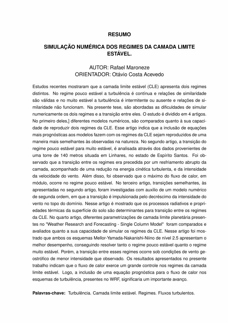
Estudos recentes mostraram que a camada limite estável (CLE) apresenta dois regimes

distintos. No regime pouco estável a turbulência é contínua e relações de similaridade

são válidas e no muito estável a turbulência é intermitente ou ausente e relações de si-

milaridade não funcionam. Na presente tese, são abordadas as dificuldades de simular

numericamente os dois regimes e a transição entre eles. O estudo é dividido em 4 artigos.

No primeiro deles,] diferentes modelos numéricos, são comparados quanto à sua capaci-

dade de reproduzir dois regimes da CLE. Esse artigo indica que a inclusão de equações

mais prognósticas aos modelos fazem com os regimes da CLE sejam reproduzidos de uma

maneira mais semelhantes às observadas na natureza. No segundo artigo, a transição do

regime pouco estável para muito estável, é analisada através dos dados provenientes de

uma torre de 140 metros situada em Linhares, no estado de Espírito Santos. Foi ob-

servado que a transição entre os regimes era precedida por um resfriamento abrupto da

camada, acompanhado de uma redução na energia cinética turbulenta, e da intensidade

da velocidade do vento. Além disso, foi observado que o máximo do fluxo de calor, em

módulo, ocorre no regime pouco estável. No terceiro artigo, transições semelhantes, às

apresentadas no segundo artigo, foram investigadas com auxilio de um modelo numérico

de segunda ordem, em que a transição é impulsionada pelo decréscimo da intensidade do

vento no topo do domínio. Nesse artigo é mostrado que os processos radiativos e propri-

edades térmicas da superfície do solo são determinantes para transição entre os regimes

da CLE. No quarto artigo, diferentes parametrizações de camada limite planetária presen-

tes no "Weather Research and Forecasting - Single Column Model" foram comparados e

avaliados quanto a sua capacidade de simular os regimes da CLE. Nesse artigo foi mos-

trado que ambos os esquemas Mellor-Yamada-Nakanishi-Niino de nível 2.5 apresentam o

melhor desempenho, conseguindo resolver tanto o regime pouco estável quanto o regime

muito estável. Porém, a transição entre esses regimes ocorre sob condições de vento ge-

ostrófico de menor intensidade que observado. Os resultados apresentados no presente

trabalho indicam que o fluxo de calor exerce um grande controle nos regimes da camada

limite estável. Logo, a inclusão de uma equação prognóstica para o fluxo de calor nos

esquemas de turbulência, presentes no WRF, significaria um importante avanço.

Palavras-chave: Turbulência. Camada limite estável. Regimes. Fluxos turbulentos.

ABSTRACT

NUMERICAL SIMULATION OF THE STABLE BOUNDARY LAYERREGIMES.

AUTHOR: Rafael MaronezeADVISOR: Otávio Costa Acevedo

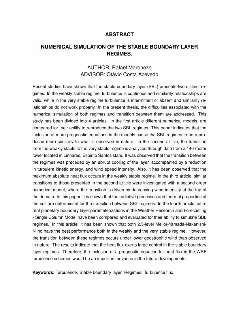
Recent studies have shown that the stable boundary layer (SBL) presents two distinct re-

gimes. In the weakly stable regime, turbulence is continous and similarity relationships are

valid, while in the very stable regime turbulence is intermittent or absent and similarity re-

lationships do not work properly. In the present thesis, the difficulties associated with the

numerical simulation of both regimes and transition between them are addressed. This

study has been divided into 4 articles. In the first article different numerical models, are

compared for their ability to reproduce the two SBL regimes. This paper indicates that the

inclusion of more prognostic equations in the models cause the SBL regimes to be repro-

duced more similarly to what is observed in nature. In the second article, the transition

from the weakly stable to the very stable regime is analyzed through data from a 140-meter

tower located in Linhares, Espirito Santos state. It was observed that the transition between

the regimes was preceded by an abrupt cooling of the layer, accompanied by a reduction

in turbulent kinetic energy, and wind speed intensity. Also, it has been observed that the

maximum absolute heat flux occurs in the weakly stable regime. In the third article, similar

transitions to those presented in the second article were investigated with a second-order

numerical model, where the transition is driven by decreasing wind intensity at the top of

the domain. In this paper, it is shown that the radiative processes and thermal properties of

the soil are determinant for the transition between SBL regimes. In the fourth article, diffe-

rent planetary boundary layer parameterizations in the Weather Research and Forecasting

- Single Column Model have been compared and evaluated for their ability to simulate SBL

regimes. In this article, it has been shown that both 2.5-level Mellor-Yamada-Nakanishi-

Niino have the best performance both in the weakly and the very stable regime. However,

the transition between these regimes occurs under lower geostrophic wind than observed

in nature. The results indicate that the heat flux exerts large control in the stable boundary

layer regimes. Therefore, the inclusion of a prognostic equation for heat flux in the WRF

turbulence schemes would be an important advance in the future developments.

Keywords: Turbulence. Stable boundary layer. Regimes. Turbulence flux

LISTA DE ABREVIATURAS E SIGLAS

u Componente zonal do vento

v Componente meridional do vento

ψ Direção do vento

l Comprimento de mistura

ω Velocidade angular da terra

κ Constante de Von Kármám

e Energia cinética turbulenta

θ Temperatura potencial do ar

θg Temperatura do solo

u′2 Componente zonal da variância da velocidade do vento

v′2 Componente meridional da variância da velocidade do vento

w′2 Componente vertical da variância da velocidade do vento

θ′2 Variância da temperatura potencial

Km Difusividade turbulenta de momentum

KH Difusividade turbulenta de calor

ug Componente zonal do vento geostrófico

vg Componente meridional do vento geostrófico

Qc Cobertura de nuvens

u∗ Velocidade de fricção

θ∗ Escala de temperatura

cg Capacidade térmica da superfície por unidade de área

H0 Fluxo de calor sensível superficial

I↓ Radiação de onda longa proveniente da atmosfera

Rig Número de Richardson gradiente

Rif Número de Richardson fluxo

w′θ′ Fluxo de energia na forma de calor sensível

u′w′ Componente zonal do fluxo de momentum

v′w′ Componente meridional do fluxo de momentum

VTKE Escala de velocidade turbulenta

SUMÁRIO

1 INTRODUCAO . . . . . . . . . . . . . . . . . . . . . . . . . . . . . . . . . . . . . . . . . . . . . . . . . . . . . . . . . . . . . . . . . 192 EQUAÇÕES BÁSICAS DA CLP . . . . . . . . . . . . . . . . . . . . . . . . . . . . . . . . . . . . . . . . . . . . . . . . 312.0.1 Equação de estado. . . . . . . . . . . . . . . . . . . . . . . . . . . . . . . . . . . . . . . . . . . . . . . . . . . . . . . . . . . . . . . . . . . 312.0.2 Conservação da massa (Equação da continuidade) . . . . . . . . . . . . . . . . . . . . . . . . . . . . 312.0.3 Segunda Lei de Newton . . . . . . . . . . . . . . . . . . . . . . . . . . . . . . . . . . . . . . . . . . . . . . . . . . . . . . . . . . . . . 322.0.4 Conservação da energia térmica (1º lei da termodinâmica) . . . . . . . . . . . . . . . . . . . . 332.0.5 Equações médias . . . . . . . . . . . . . . . . . . . . . . . . . . . . . . . . . . . . . . . . . . . . . . . . . . . . . . . . . . . . . . . . . . . . 332.1 PROBLEMA DO FECHAMENTO . . . . . . . . . . . . . . . . . . . . . . . . . . . . . . . . . . . . . . . . . . . . . . . . . . . . . 373 ARTIGO 1 - SIMULATING THE REGIME TRANSITION OF THE STABLE BOUN-

DARY LAYER USING DIFFERENT SIMPLIFIED MODELS . . . . . . . . . . . . . . . . . . . . . 394 ARTIGO 2 - THE NOCTURNAL BOUNDARY LAYER TRANSITION FROM

WEAKLY TO VERY STABLE. PART I: OBSERVATIONS. . . . . . . . . . . . . . . . . . . . . . . . 575 ARTIGO 3 - THE NOCTURNAL BOUNDARY LAYER TRANSITION FROM

WEAKLY TO VERY STABLE. PART II: NUMERICAL SIMULATION WITH ASECOND-ORDER MODEL . . . . . . . . . . . . . . . . . . . . . . . . . . . . . . . . . . . . . . . . . . . . . . . . . . . . . 73

6 ARTIGO 4 - HOW IS THE TWO-REGIME STABLE BOUNDARY LAYER SOL-VED BY THE DIFFERENT PBL SCHEMES IN WRF. . . . . . . . . . . . . . . . . . . . . . . . . . . . 89

7 DISCUSSÃO . . . . . . . . . . . . . . . . . . . . . . . . . . . . . . . . . . . . . . . . . . . . . . . . . . . . . . . . . . . . . . . . . . . 1298 CONCLUSÕES. . . . . . . . . . . . . . . . . . . . . . . . . . . . . . . . . . . . . . . . . . . . . . . . . . . . . . . . . . . . . . . . .137

ANEXO A – ENERGIA CINÉTICA TURBULENTA . . . . . . . . . . . . . . . . . . . . . . . . . . . . . . 141ANEXO B – FLUXO DE CALOR SENSíVEL. . . . . . . . . . . . . . . . . . . . . . . . . . . . . . . . . . . .147ANEXO C – VARIÂNCIA DE TEMPERATURA. . . . . . . . . . . . . . . . . . . . . . . . . . . . . . . . . .151REFERÊNCIAS BIBLIOGRÁFICAS . . . . . . . . . . . . . . . . . . . . . . . . . . . . . . . . . . . . . . . . . . . . 153

1 INTRODUCAO

A camada limite planetária (CLP) é a parte da troposfera onde o escoamento do

fluido e os fluxos de momentum, energia na forma de calor sensível e outros são influenci-

ados pela presença da superfície terrestre, que os torna turbulentos. A turbulência, por sua

vez, tem caráter altamente difusivo, sendo um processo bastante eficiente no transporte e

na mistura de quantidades ao longo da CLP. Assim, a turbulência faz com que a presença

da superfície terrestre seja efetivamente sentida até o topo da CLP, que pode ser da ordem

de quilômetros.

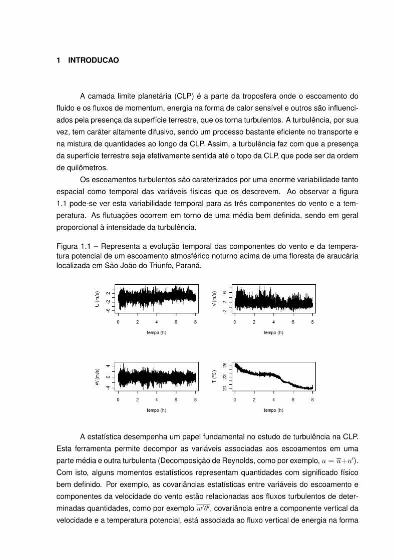
Os escoamentos turbulentos são caraterizados por uma enorme variabilidade tanto

espacial como temporal das variáveis físicas que os descrevem. Ao observar a figura

1.1 pode-se ver esta variabilidade temporal para as três componentes do vento e a tem-

peratura. As flutuações ocorrem em torno de uma média bem definida, sendo em geral

proporcional à intensidade da turbulência.

Figura 1.1 – Representa a evolução temporal das componentes do vento e da tempera-tura potencial de um escoamento atmosférico noturno acima de uma floresta de araucárialocalizada em São João do Triunfo, Paraná.

A estatística desempenha um papel fundamental no estudo de turbulência na CLP.

Esta ferramenta permite decompor as variáveis associadas aos escoamentos em uma

parte média e outra turbulenta (Decomposição de Reynolds, como por exemplo, u = u+u′).

Com isto, alguns momentos estatísticos representam quantidades com significado físico

bem definido. Por exemplo, as covariâncias estatísticas entre variáveis do escoamento e

componentes da velocidade do vento estão relacionadas aos fluxos turbulentos de deter-

minadas quantidades, como por exemplo w′θ′, covariância entre a componente vertical da

velocidade e a temperatura potencial, está associada ao fluxo vertical de energia na forma

20

de calor sensível através da relação H = ρcpw′θ′.

A energia cinética turbulenta (ECT) é definida como energia cinética das flutuações

turbulentas de velocidade por unidade de massa e é dada por e = 12(u′2 + v′2 + w′2), onde

u′2, v′2 e w′2 representam as variâncias das três componentes turbulentas do vento. Isto

evidencia a importância da estatística no presente estudo, citada no parágrafo anterior.

A ECT é uma das quantidades mais importantes utilizadas no estudo de turbulência na

camada limite (STULL, 1988).

Durante o dia, a superfície do solo é aquecida pela radiação eletromagnética de

onda curta proveniente do sol, deixando a temperatura do solo maior que a temperatura da

atmosfera. Isto acarreta o surgimento de um fluxo de energia na forma de calor sensível

do solo para a atmosfera, que aquece as camadas de ar adjacentes ao solo e as torna me-

nos densas que as superiores, dando início a um movimento convectivo. Esse processo

está associado à produção térmica de turbulência. Durante o dia, há também a produção

mecânica de turbulência devido ao cisalhamento do vento. A camada limite que se desen-

volve durante o dia é caracterizada pela produção térmica e mecânica de turbulência e é

denominada camada limite convectiva (CLC). A altura dessa camada é da ordem de um

quilômetro.

Ao pôr do sol, o fluxo de energia na forma de calor sensível inverte o sinal, passando

a ser da atmosfera para a superfície do solo. Isso ocorre porque a superfície do solo esfria-

se mais rapidamente que a atmosfera, devido à radiação eletromagnética de onda longa

emitida pela superfície exceder a emissão correspondente da atmosfera para a superfície.

Com isso, os níveis inferiores ficam com uma temperatura menor que os superiores e

qualquer movimento ascendente tende a ser desacelerado devido a ação das forças de

empuxo. A atuação das forças de empuxo tornam a camada estável, ou seja, uma parcela

de fluido que por algum motivo é deslocada verticalmente de baixo para cima encontra

regiões mais quentes e portanto menos densas, sendo forçada a descer. O processo

descrito anteriormente representa à destruição térmica de turbulência. A camada acima da

superfície caracterizada pelos resquícios e pela dissipação da CLC é denominada camada

limite residual.

Junto à superfície, a camada limite que se desenvolve durante a noite e que é carac-

terizada pela destruição térmica e pela produção mecânica de turbulência é denominada

camada limite estável (CLE).

Muitos estudos, tanto observacionais (MALHI, 1995; OHYA; NEFF; MERONEY,

1997; MAHRT, 1998; ACEVEDO; FITZJARRALD, 2003; SUN et al., 2012; ACEVEDO

et al., 2016; LAN et al., 2018; ACEVEDO et al., 2019) quanto de modelagem numérica

(MCNIDER et al., 1995; WIEL et al., 2002b; COSTA et al., 2011; MARONEZE et al., 2019)

evidenciam a existência de dois regimes distintos na camada limite estável. A CLE é usual-

mente classificada como muito estável ou pouco estável, mas estas classificações podem

variar entre os estudos (MAHRT, 1998).

21

O regime pouco estável normalmente ocorre em condições de ventos intensos e/ou

com uma cobertura de nuvens significativa, caracterizando uma camada limite quase neu-

tra ou pouco estratificada. Nesse regime, a turbulência é bem desenvolvida e contínua

tanto no espaço quanto no tempo sendo, em geral, bem descrita pela teoria da similari-

dade (MAHRT, 2014). Já, o regime muito estável normalmente ocorre em condições de

ventos fracos e de céu claro (MAHRT, 1998), de modo que a perda radiativa superficial

seja intensa e, como consequência, uma intensa estratificação térmica é desenvolvida.

No regime muito estável a mistura turbulenta é drasticamente reduzida, podendo ser in-

termitente. Escoamentos turbulentos, muito estratificados, não são bem descritos pelos

conceitos clássicos, e sua descrição completa permanece sendo um desafio (MAHRT,

2014).

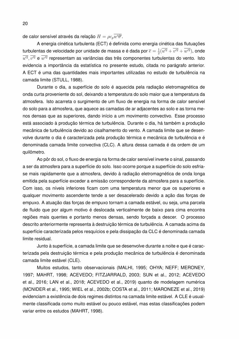
Figura 1.2 – Velocidade de fricção na noite do dia 25 para 26 de janeiro de 2001.

Fonte: Costa et al.(2011)

Na CLE é frequentemente observado que a turbulência é não continua no espaço e

no tempo. Essa descontinuidade temporal caracteriza a turbulência intermitente, que causa

alterações na evolução média da camada limite atmosférica estratificada e que pode resul-

tar em comportamento oscilatório da temperatura do ar, do vento e dos fluxos turbulentos

próximos à superfície (WIEL et al., 2002a). Chama-se intermitência global quando todas as

escalas do escoamento turbulento são suprimidas e restabelecidas de maneira sucessiva

e não previsível, caracterizando uma alternância entre períodos de turbulência de baixa in-

tensidade ou de turbulência quase inexistente, e períodos turbulentos intensos ao longo de

uma mesma noite (figura 1.2) (COSTA et al., 2011). A intermitência global é um fenômeno

comum na camada limite muito estável, cuja compreensão e descrição matemática ainda

é limitada.

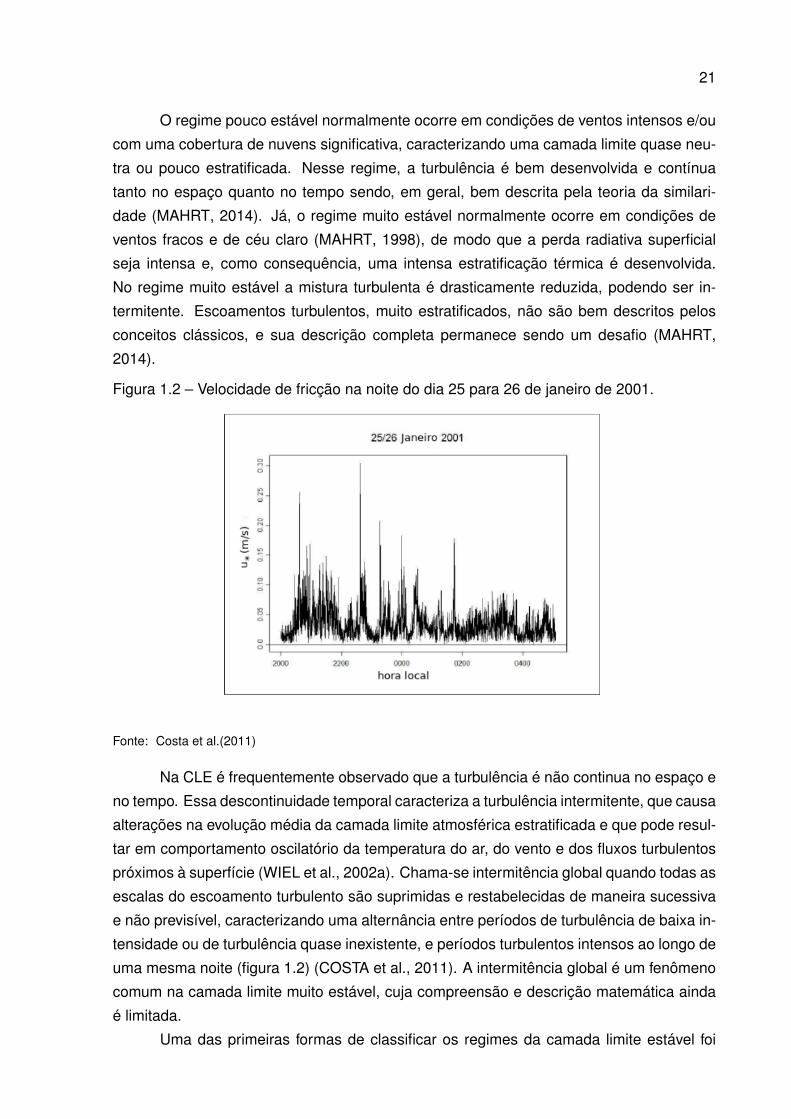
Uma das primeiras formas de classificar os regimes da camada limite estável foi

22

através da dependência do fluxo de energia na forma de calor sensível com a estabilidade

do escoamento (figura 1.3). No regime fracamente estável, também chamado de pouco

estável, a magnitude do fluxo de energia na forma de calor sensível cresce com a estabi-

lidade do escoamento devido ao aumento do gradiente vertical de temperatura até atingir

um valor máximo. No regime muito estável, a magnitude do fluxo de energia na forma

de calor sensível decresce com o aumento da estabilidade do escoamento, devido à forte

redução da atividade turbulenta. Entretanto, de acordo com Monahan et al. (2015), parâ-

metros de estabilidade, como o comprimento de Obukhov ou o número de Richardson, por

si só não são capazes de distinguir os regimes da CLE. Além disso, Acevedo et al. (2019)

observaram que o máximo do fluxo de calor, em módulo, ocorre no regime pouco estável,

portanto esta quantidade não deve ser utilizada como um marcador da transição entre os

regimes da CLE.

Figura 1.3 – Fluxo de energia na forma de calor sensível em função da estabilidade.

Fonte: Adaptado de Mahrt, 1998.

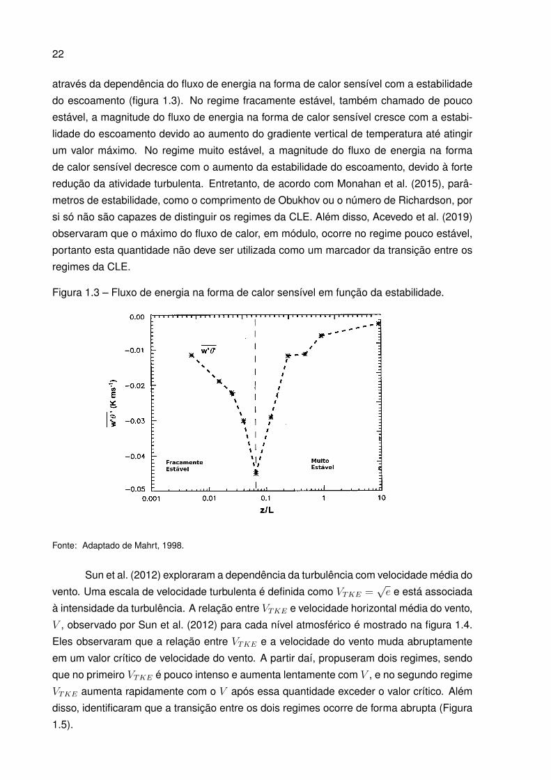
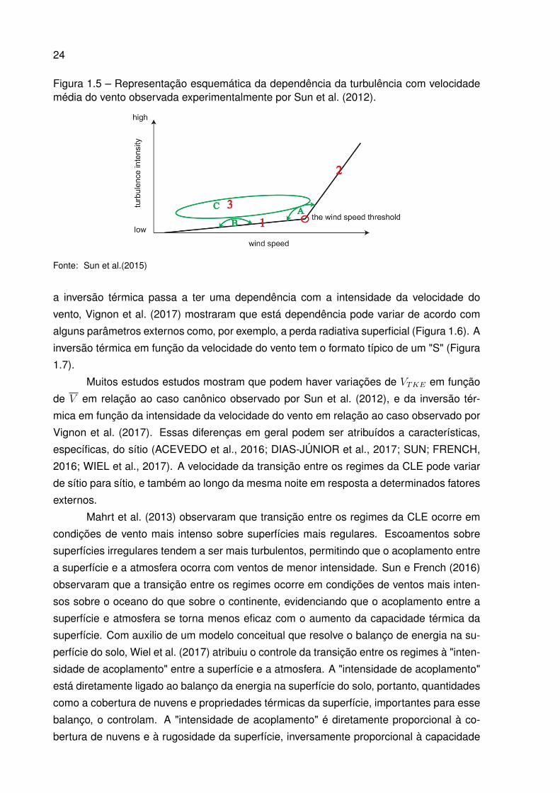
Sun et al. (2012) exploraram a dependência da turbulência com velocidade média do

vento. Uma escala de velocidade turbulenta é definida como VTKE =√e e está associada

à intensidade da turbulência. A relação entre VTKE e velocidade horizontal média do vento,

V , observado por Sun et al. (2012) para cada nível atmosférico é mostrado na figura 1.4.

Eles observaram que a relação entre VTKE e a velocidade do vento muda abruptamente

em um valor crítico de velocidade do vento. A partir daí, propuseram dois regimes, sendo

que no primeiro VTKE é pouco intenso e aumenta lentamente com V , e no segundo regime

VTKE aumenta rapidamente com o V após essa quantidade exceder o valor crítico. Além

disso, identificaram que a transição entre os dois regimes ocorre de forma abrupta (Figura

1.5).

23

Figura 1.4 – Dependência da turbulência com velocidade média do vento obtida experi-mentalmente por Sun et al. (2012).

Fonte: Sun et al. (2012)

De acordo com Sun et al. (2012), quando a intensidade do vento é menor que o

valor limite, a turbulência é controlada pelo cisalhamento do vento local, enquanto que é

o cisalhamento global do vento ao longo de toda CLE que controla a turbulência quando

esse limite é excedido. Esse conceito indica uma situação em que a CLE está verticalmente

acoplada ao topo da camada, quando os ventos excedem o valor limite. Uma classificação

alternativa, porém não excludente da anterior, da CLE, é relacionada com o estado de aco-

plamento das parcelas de ar próximas à superfície e dos níveis superiores da atmosfera.

Em condições turbulentas, diferentes níveis da atmosfera mantém-se unidos entre si e a

ao topo da CLE, representando o estado acoplado, que geralmente coincide com o regime

pouco estável. Por outro lado, se não há ocorrência de ventos de intensa magnitude, a su-

perfície tende a se desacoplar dos níveis atmosféricos superiores. O estado desacoplado,

pode ser relacionado ao regime muito estável da CLE (COSTA et al., 2011).

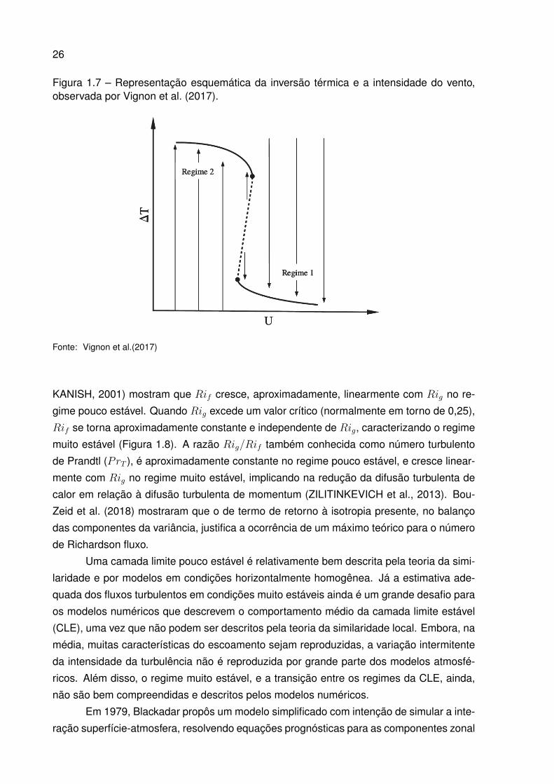
Outra forma objetiva de classificar os regimes da CLE é através da relação entre a

inversão térmica e a intensidade da velocidade do vento, Vignon et al. (2017) observaram

a existência de dois limites assintóticos para essa relação, coincidindo com cada um dos

regimes da CLE. No regime muito estável, esse valor assintótico, em geral, é superior a

3-5 K, pois o fluxo turbulento de calor não é intenso suficiente para manter a superfície

acoplada aos níveis superiores da CLE, mais quentes, então devido a perda radiativa do

solo uma intensa estratificação térmica se desenvolve. No regime pouco estável esse limite

se aproxima de zero, pois a intensidade da turbulência é suficiente para que as camadas

de ar mais quentes, dos níveis superiores da CLE, passem a influenciar o que ocorre

na superfície, reduzindo a estratificação térmica. Entre esses dois limites assintóticos,

24

Figura 1.5 – Representação esquemática da dependência da turbulência com velocidademédia do vento observada experimentalmente por Sun et al. (2012).

Fonte: Sun et al.(2015)

a inversão térmica passa a ter uma dependência com a intensidade da velocidade do

vento, Vignon et al. (2017) mostraram que está dependência pode variar de acordo com

alguns parâmetros externos como, por exemplo, a perda radiativa superficial (Figura 1.6). A

inversão térmica em função da velocidade do vento tem o formato típico de um "S" (Figura

1.7).

Muitos estudos estudos mostram que podem haver variações de VTKE em função

de V em relação ao caso canônico observado por Sun et al. (2012), e da inversão tér-

mica em função da intensidade da velocidade do vento em relação ao caso observado por

Vignon et al. (2017). Essas diferenças em geral podem ser atribuídos a características,

específicas, do sítio (ACEVEDO et al., 2016; DIAS-JÚNIOR et al., 2017; SUN; FRENCH,

2016; WIEL et al., 2017). A velocidade da transição entre os regimes da CLE pode variar

de sítio para sítio, e também ao longo da mesma noite em resposta a determinados fatores

externos.

Mahrt et al. (2013) observaram que transição entre os regimes da CLE ocorre em

condições de vento mais intenso sobre superfícies mais regulares. Escoamentos sobre

superfícies irregulares tendem a ser mais turbulentos, permitindo que o acoplamento entre

a superfície e a atmosfera ocorra com ventos de menor intensidade. Sun e French (2016)

observaram que a transição entre os regimes ocorre em condições de ventos mais inten-

sos sobre o oceano do que sobre o continente, evidenciando que o acoplamento entre a

superfície e atmosfera se torna menos eficaz com o aumento da capacidade térmica da

superfície. Com auxilio de um modelo conceitual que resolve o balanço de energia na su-

perfície do solo, Wiel et al. (2017) atribuiu o controle da transição entre os regimes à "inten-

sidade de acoplamento" entre a superfície e a atmosfera. A "intensidade de acoplamento"

está diretamente ligado ao balanço da energia na superfície do solo, portanto, quantidades

como a cobertura de nuvens e propriedades térmicas da superfície, importantes para esse

balanço, o controlam. A "intensidade de acoplamento" é diretamente proporcional à co-

bertura de nuvens e à rugosidade da superfície, inversamente proporcional à capacidade

25

Figura 1.6 – Diferença de temperatura entre 10 metros e a temperatura da superfície emfunção da intensidade da velocidade do vento em 10 metros para quatro diferentes faixasde perda radiativa superficial, especificada no topo de cada painel, obtidas por Vignon et al.(2017) com as medidas meteorológicas provenientes de uma torre de 45 metros localizadaem Dome C.

Fonte: Vignon et al.(2017)

calorífica do solo e por fim é diretamente proporcional a temperatura do substrato, que

está diretamente ligado ao fluxo molecular de calor no solo. Um acréscimo na cobertura

de nuvens faz com que a radiação de onda longa, de maior intensidade, chegue à superfí-

cie do solo, mantendo-a mais quente, e consequentemente o escoamento torna-se menos

estável e mais turbulento do que em uma situação semelhante sem nuvens. Quando a

capacidade térmica da superfície do solo é reduzida observa-se um efeito semelhante ao

descrito anteriormente, pois nesse caso a superfície esfria a uma taxa menor do que es-

friaria um solo de maior capacidade térmica, sob as mesma condições de perda radiativa.

Um substrato mais quente faz com que a transferência de calor, das camadas mais pro-

fundas do solo em direção à superfície do solo, seja mais intenso, mantendo a superfície

do solo mais quente do que ela estaria se substrato estivesse mais frio. "Intensidades de

acoplamento" maiores permitem que a transição entre os regimes da CLE, pouco estável

e muito estável, ocorra com ventos de menor intensidade.

A existência de dois regimes distintos na CLE também pode ser estabelecida atra-

vés da relação entre o número de Richardson fluxo (Rif ) e o número de Richardson gra-

diente (Rig) (ZILITINKEVICH et al., 2013; BOU-ZEID et al., 2018). Tanto observações

(OHYA, 2001; PARDYJAK; MONTI; FERNANDO, 2002) quanto simulações numéricas (NA-

26

Figura 1.7 – Representação esquemática da inversão térmica e a intensidade do vento,observada por Vignon et al. (2017).

Fonte: Vignon et al.(2017)

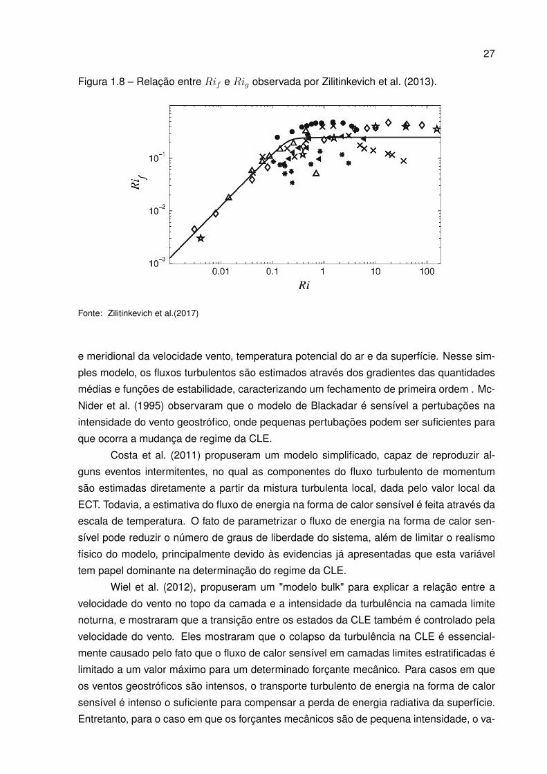
KANISH, 2001) mostram que Rif cresce, aproximadamente, linearmente com Rig no re-

gime pouco estável. Quando Rig excede um valor crítico (normalmente em torno de 0,25),

Rif se torna aproximadamente constante e independente de Rig, caracterizando o regime

muito estável (Figura 1.8). A razão Rig/Rif também conhecida como número turbulento

de Prandtl (PrT ), é aproximadamente constante no regime pouco estável, e cresce linear-

mente com Rig no regime muito estável, implicando na redução da difusão turbulenta de

calor em relação à difusão turbulenta de momentum (ZILITINKEVICH et al., 2013). Bou-

Zeid et al. (2018) mostraram que o de termo de retorno à isotropia presente, no balanço

das componentes da variância, justifica a ocorrência de um máximo teórico para o número

de Richardson fluxo.

Uma camada limite pouco estável é relativamente bem descrita pela teoria da simi-

laridade e por modelos em condições horizontalmente homogênea. Já a estimativa ade-

quada dos fluxos turbulentos em condições muito estáveis ainda é um grande desafio para

os modelos numéricos que descrevem o comportamento médio da camada limite estável

(CLE), uma vez que não podem ser descritos pela teoria da similaridade local. Embora, na

média, muitas características do escoamento sejam reproduzidas, a variação intermitente

da intensidade da turbulência não é reproduzida por grande parte dos modelos atmosfé-

ricos. Além disso, o regime muito estável, e a transição entre os regimes da CLE, ainda,

não são bem compreendidas e descritos pelos modelos numéricos.

Em 1979, Blackadar propôs um modelo simplificado com intenção de simular a inte-

ração superfície-atmosfera, resolvendo equações prognósticas para as componentes zonal

27

Figura 1.8 – Relação entre Rif e Rig observada por Zilitinkevich et al. (2013).

Fonte: Zilitinkevich et al.(2017)

e meridional da velocidade vento, temperatura potencial do ar e da superfície. Nesse sim-

ples modelo, os fluxos turbulentos são estimados através dos gradientes das quantidades

médias e funções de estabilidade, caracterizando um fechamento de primeira ordem . Mc-

Nider et al. (1995) observaram que o modelo de Blackadar é sensível a pertubações na

intensidade do vento geostrófico, onde pequenas pertubações podem ser suficientes para

que ocorra a mudança de regime da CLE.

Costa et al. (2011) propuseram um modelo simplificado, capaz de reproduzir al-

guns eventos intermitentes, no qual as componentes do fluxo turbulento de momentum

são estimadas diretamente a partir da mistura turbulenta local, dada pelo valor local da

ECT. Todavia, a estimativa do fluxo de energia na forma de calor sensível é feita através da

escala de temperatura. O fato de parametrizar o fluxo de energia na forma de calor sen-

sível pode reduzir o número de graus de liberdade do sistema, além de limitar o realismo

físico do modelo, principalmente devido às evidencias já apresentadas que esta variável

tem papel dominante na determinação do regime da CLE.

Wiel et al. (2012), propuseram um "modelo bulk" para explicar a relação entre a

velocidade do vento no topo da camada e a intensidade da turbulência na camada limite

noturna, e mostraram que a transição entre os estados da CLE também é controlado pela

velocidade do vento. Eles mostraram que o colapso da turbulência na CLE é essencial-

mente causado pelo fato que o fluxo de calor sensível em camadas limites estratificadas é

limitado a um valor máximo para um determinado forçante mecânico. Para casos em que

os ventos geostróficos são intensos, o transporte turbulento de energia na forma de calor

sensível é intenso o suficiente para compensar a perda de energia radiativa da superfície.

Entretanto, para o caso em que os forçantes mecânicos são de pequena intensidade, o va-

28

lor máximo do fluxo de energia na forma de calor sensível é pequeno quando comparado

à taxa de resfriamento radiativo da superfície. Nesse caso, o gradiente de temperatura

cresce rapidamente, sobre superfícies com baixa capacidade térmica, e a turbulência, em

grande parte, é suprimida pela intensa estratificação. Eles também mostraram que há um

limite de velocidade do vento (sendo este da ordem de 5, 0 m/s) abaixo do qual a turbulên-

cia é pouco intensa para sustentar o fluxo de calor turbulento necessário para compensar a

perda de energia radiativa da superfície para as camadas de ar adjacentes a ela. A discus-

são realizada por Wiel et al. (2012) mostra que o fluxo de energia na forma de calor exerce

grande controle no colapso da turbulenta na CLE e também na transição entre os regimes.

Este fato foi corroborado por Acevedo et al. (2016), que mostraram que o termo da des-

truição térmica de turbulência na equação de balanço de ECT tem importância relativa no

balanço total muito maior no estado desacoplado.

Estudos sobre o comportamento e a estimativa adequada dos fluxos turbulentos

em uma camada limite estável são de grande importância para diferentes áreas da socie-

dade. Entre essas estão: a agricultura, meio ambiente (através do estudo da dispersão de

poluentes), geração de energias renováveis (energia eólica), mudanças climáticas, entre

outras. Na agricultura, a estimativa correta da temperatura mínima é muito importante para

a previsão de geadas. Por exemplo, a ocorrência de geada, na primavera, é prejudicial para

prática agrícola, de modo que o congelamento das flores de uma árvore frutífera provoca

perdas significativas na produtividade. Já na aviação, isso se traduz na redução no número

de voos devido à ocorrência de neblina, o que pode causar perdas econômicas significati-

vas. O desenvolvimento de parametrizações para CLE que seja capaz capaz de resolver

tanto o regime muito estável como o pouco estável é fundamental para estudos como de

controle de ar, dispersão de poluentes, a previsão de temperaturas mínimas, entre outros.

A presente tese visa identificar os principais mecanismos responsáveis pela tran-

sição entre os regimes da camada limite estável, e contribuir no desenvolvimento de uma

nova parametrização para camada limite planetária que seja capaz de reproduzir adequa-

damente os dois regimes da CLE, e futuramente sua implementação no modelos atmosfé-

ricos, tais como o WRF.

Há anos conhece se bem a existência dos dois regimes da CLE, pouco e muito

estável, sabe-se a ocorrência de um ou de outro regime está extremamente associada a

intensidade do vento, forçante mecânico, e ao balanço de energia da superfície do solo,

forçantes externos ao escoamento (SUN et al., 2012; ACEVEDO et al., 2016; WIEL et

al., 2017; MARONEZE et al., 2019, entre outros). Entretanto, embora seja conhecido que

alguns forçantes externos ao escoamento, como cobertura de nuvens, está associado a

ocorrência do regime pouco estável ou do regime muito estável, ainda não sabe-se bem

como cada um desses fatores controla os regimes da CLE. Além disso, não existe con-

senso de como ocorre a transição entre os regimes das CLE. Devido a esses motivos e a

outros motivos, modelar uma camada limite estável permanece sendo grande desafio.

29

A presente tese está divida em 4 diferentes artigos. No artigo 1 ("Simulating the

Regime Transition of the Stable Boundary Layer Using Different Simplified Models", publi-

cado na revista Boundary-Layer Meteorology ) serão comparados três diferentes modelos

numéricos baseados no modelo proposto por Costa et al. (2011), de uma ordem e meia,

que são utilizados para descrever o comportamento médio de uma camada limite noturna.

No modelo e − FH , o fluxo de energia na forma de calor sensível será estimado através

de uma equação prognóstica. Uma vez que a equação prognóstica para o fluxo de ener-

gia na forma de calor sensível depende da variância da temperatura potencial, no modelo

e−FH − σθ será incluída uma equação prognóstica para a variância da temperatura, a fim

de acrescentar mais graus de liberdade ao sistema e de modo a acrescentar detalhamento

físico à solução. Ao longo desse artigo, serão realizadas comparações entre as diferentes

soluções obtidas pelos modelos variando diferentes parâmetros. Além disso, esse traba-

lho visa determinar o menor número de equações prognósticas necessário para que um

modelo de coluna simples consiga reproduzir os dois regimes da CLE, adequadamente.

Acevedo et al. (2018) realizaram uma descrição detalhada dos dados micromete-

orológicos provenientes de uma torre de 140 metros situada em Linhares, no estado de

Espírito Santos, sudoeste do Brasil. Uma grande variedade de fenômenos micrometeoro-

lógicos foram observados, em detalhes, nessa torre, como por exemplo, a ocorrência de

dois regimes na CLE e a transição entre eles ao longo de uma mesma noite. Com a ocor-

rência do regime pouco estável durante a primeira metade da noite, enquanto na segunda

metade a ocorrência do regime muito estável. Utilizando esse mesmo conjunto de dados

micrometeorológicos, Acevedo et al. (2019) (artigo 2, "The nocturnal boundary layer transi-

tion from weakly to very stable. Part I: Observations", publicado na revista Quarterly Jour-

nal of the Royal Meteorological Society ) observaram, em muitas noites, um resfriamento

abrupto da camada acompanhado de uma redução na energia cinética turbulenta (ECT),

e na intensidade da velocidade do vento. Nesse estudo Acevedo et al. (2019) propuseram

que a transição entre o regime pouco estável e o muito estável ocorre simultaneamente

com o máximo resfriamento do níveis inferiores da camada limite. No artigo 3 ("The noc-

turnal boundary layer transition from weakly to very stable. Part II: Numerical simulation

with a second-order model", publicado na revista Quarterly Journal of the Royal Meteoro-

logical Society ), transições semelhantes, as observadas por Acevedo et al. (2019), são

investigadas com auxilio de um modelo numérico unidimensional de segunda ordem, com

o balanço de energia resolvido na superfície, através do método "Force-Restore" proposto

por Blackadar (1979). Nesse modelo, a transição é impulsionada pelo decréscimo da inten-

sidade da velocidade do vento no topo do domínio, simulações com diferentes coberturas

de nuvens e propriedades térmicas da superfície são realizadas.

Os esquemas de turbulência hoje utilizados nos modelos numéricos de previsão de

tempo e clima (MNPTC) são de primeira ordem, onde apenas as equações prognósticas

para variáveis médias são resolvidas e todos os momentos estatísticos de ordem mais alta

30

são parametrizados, ou são modelos ECT, em que a energia cinética turbulenta é resol-

vida prognosticamente. Os esquemas de turbulência presentes no WRF são equivalentes

aos modelos Mellor-Yamada 1-, 2-, 2.5 e 3-nível, em que o fluxo de calor é parametri-

zado. Maroneze et al. (2019) (artigo 1) mostraram que o regime muito estável da CLE

só é representado adequadamente quando o fluxo de calor e a variância de tempera-

tura são resolvidos prognosticamente. Assim, no artigo 4 ("How is the two-regime stable

boundary layer solved by the different PBL schemes in WRF?", submetido para revista

Geophysical Research Letters), cinco diferentes esquemas de turbulência para CLP, com

diferentes configurações, presentes no "Weather Research and Forecasting - Single Co-

lumn Model"(WRF-SCM) serão comparadas e avaliadas quanto a capacidade de resolver

adequadamente os regimes da CLE. Esse esquemas são: Mellor-Yamada-Nakanishi-Niino

(MYNN,Nakanishi e Niino (2006), Nakanishi e Niino (2009)), Mellor-Yamada-Janjic (MYJ,

Janjic (1994)), "Quasi-Normal Scale Elimination "(QNSE, Sukoriansky, Galperin e Perov

(2005)), "University of Washington (TKE) Boundary Layer Scheme"(UWBLS, Bretherton e

Park (2009)) e Bougeault-Lacarrere (BouLac,Bougeault e Lacarrere (1989)).

2 EQUAÇÕES BÁSICAS DA CLP

Os movimentos atmosféricos obedecem os princípios fundamentais da Física, tais

como a conservação da energia (primeira lei da termodinâmica), conservação da massa,

conservação do momentum (segunda lei de Newton) e a lei dos gases ideais. As leis

fundamentais da mecânica de fluídos e da termodinâmica, que governam os movimentos

atmosféricos, podem ser expressas em termos de equações diferencias parciais que en-

volvem as variáveis do campo (velocidade do vento, temperatura, umidade, etc) como va-

riáveis dependentes, o espaço e o tempo como variáveis independentes (HOLTON, 2004).

2.0.1 Equação de estado

O estado termodinâmico dos gases presentes na camada limite, como uma boa

aproximação, podem ser descritos pela lei dos gases ideais:

p = ρR′Tv , (2.1)

onde p é a pressão, ρ é a densidade do ar úmido, R′ é constante dos gases para o ar

seco (R′ = 287J.K−1kg−1) e Tv é a temperatura absoluta virtual que é dada por Tv =

T (1 + 0, 6r), sendo que r representa a úmidade específica.

2.0.2 Conservação da massa (Equação da continuidade)

A equação da continuidade, ou de conservação da massa, pode ser dada por:

∂ρ

∂t+∂ (ρUj)

∂xj= 0 , (2.2)

onde Uj são as componentes da velocidade do vento. Pode-se dizer que um escoamento

é incompressível quando a divergência da velocidade do vento é nula(∂Uj

∂xj= 0)

.

32

2.0.3 Segunda Lei de Newton

A segunda lei de Newton aplicada a um fluído pode ser escrita na notação tensorial

como:

∂Ui∂t

+ Uj∂Ui∂xj

= −δi3g − fεij3Uj −1

ρ

∂p

∂xi+

1

ρ

∂τij∂xj

.

I II III IV V V I(2.3)

I → Variação Euleriana de velocidade.

II → Transporte advectivo de velocidade.

III → Aceleração da gravidade efetiva. Aceleração da gravidade efetiva é a soma

da aceleração gravitacional com a aceleração centrifuga devido a rotação da Terra, ou seja

a Terra é um sistema de referencia não inercial.

IV → Aceleração devido à força de Coriolis, proveniente da rotação da Terra.

V → Aceleração devido ao gradiente de pressão.

V I → Dissipação, devido viscosidade do fluido.

As equações para as componentes da velocidade do vento zonal, meridional e ver-

tical, desconsiderando o termo de dissipação molecular, podem ser escritas respectiva-

mente como:du

dt= −1

ρ

∂p

∂x− fv , (2.4)

dv

dt= −1

ρ

∂p

∂y+ fu , (2.5)

dw

dt= −1

ρ

∂p

∂z− g , (2.6)

O vento geostrófico é definido como o vento horizontal que resulta de um equilíbrio

entre a força devido ao gradiente de pressão (horizontal) e a força de Coriolis. Na micro-

meteorologia é comum aproximar o termo do gradiente de pressão horizontal utilizando a

conceito de vento geostrófico:

fuG = −1

ρ

∂p

∂ye fvG =

1

ρ

∂p

∂x, (2.7)

sendo uG e vG as componentes do vento geostrófico, respectivamente, zonal e meridional.

A temperatura potencial θ é definida como a temperatura que uma parcela de ar

teria se fosse expandida ou comprimida adiabaticamente de seu estado real de pressão e

temperatura a um valor referência de pressão:

θ = T

(p0p

) R

Cp .

onde P0 = 1000 mb, R é a constante dos gases para o ar e CP o calor específico do ar a

33

pressão constante.

2.0.4 Conservação da energia térmica (1º lei da termodinâmica)

A primeira lei da termodinâmica descreve a conservação da entalpia, com a contri-

buição tanto da transferência de energia na forma de calor sensível quanto latente. O vapor

de água presente no ar não apenas absorve e libera energia na forma de calor sensível

associada à sua temperatura, mas também pode absorver e liberar energia na forma de

calor latente durante alguma mudança de fase. A equação associada a conservação da

energia térmica pode ser escrita como:

∂θ

∂t+ Uj

∂θ

∂xj= νθ

∂2θ

∂x2j− 1

ρcp

∂Q

∂xj− LpE

ρcp.

I II III IV V I

(2.8)

I → Variação Euleriana da temperatura potencial.

II → Transporte advectivo de temperatura potencial.

III → Termo de difusão molecular.

IV → Termo associado à divergência da radiação.

V I → Está associado à liberação de energia na forma de calor latente durante as

mudanças de fase.

Na equação acima, E, νθ, Lp e cp representam, respectivamente, a informação

sobre a mudança de fase, a difusividade térmica, o calor latente associado à mudança de

fase E e o calor específico para o ar úmido.

2.0.5 Equações médias

A partir das equações de conservação de momentum e energia, considerando o

equilíbrio hidrostático, um ambiente idealizado seco e horizontalmente homogêneo, utili-

zando a decomposição de Reynolds e aplicando a média de Reynolds, obtem-se as equa-

ções para as variáveis médias do escoamento (Costa et al., 2011):

∂u

∂t= f(v − vg)−

∂(u′w′)

∂z, (2.9)

∂v

∂t= −f(u− ug)−

∂(v′w′)

∂z, (2.10)

34

∂θ

∂t= −∂(w′θ′)

∂z. (2.11)

Nas equações anteriores e nas seguintes, não aparecem os termos de advecção horizontal

pelo vento médio. Isto ocorre porque o presente trabalho foca nos processos de interação

entre a superfície e a atmosfera, considerando para tanto uma coluna vertical, sem trans-

portes horizontais. Entretanto, no mundo real estes termos advectivos são importantes,

sendo frequentemente dominantes. Da mesma forma, termos viscosos, de divergência de

fluxos radiativo e de aquecimento por liberação de energia na forma de calor latente não

foram incluídos.

Equações prognóstica para as componentes horizontais da variâncias da veloci-

dade do vento(u′2, v′2

), em condições de homogeneidade horizontal, podem ser escritas

como (Anexo A, equação A.20):

∂u′2

∂t= −2u′w′

∂u

∂z︸ ︷︷ ︸−∂w

′u′2

∂z︸ ︷︷ ︸−2

ρ

∂u′p′

∂x︸ ︷︷ ︸+

2

ρp′∂u′

∂x︸ ︷︷ ︸−εu︸︷︷︸ , (2.12)

∂v′2

∂t= −2v′w′

∂v

∂z︸ ︷︷ ︸−∂w

′v′2

∂z︸ ︷︷ ︸−2

ρ

∂v′p′

∂y︸ ︷︷ ︸+

2

ρp′∂v′

∂y︸ ︷︷ ︸−εv︸︷︷︸ .

I II III IV V

(2.13)

I → Termo associado à a produção da variância devido ao cisalhamento do vento.

II → Termo associado ao transporte turbulento de variância ao longa da vertical

vertical.

III → Termo associado ao transporte turbulento de variância devido as flutuações

de pressão.

IV → Termo associado a redistribuição de pressão (retorno à isotropia).

V → Termo associado à dissipação viscosa da variância.

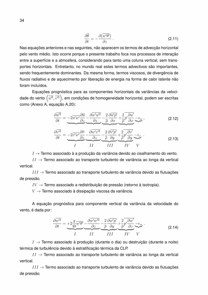
A equação prognóstica para componente vertical da variância da velocidade do

vento, é dada por:

∂w′2

∂t= +2

g

Θw′θ′

︸ ︷︷ ︸−∂w

′w′2

∂z︸ ︷︷ ︸−2

ρ

∂w′p′

∂y︸ ︷︷ ︸+

2

ρp′∂w′

∂z︸ ︷︷ ︸−εw︸︷︷︸ .

I II III IV V

(2.14)

I → Termo associado à produção (durante o dia) ou destruição (durante a noite)

térmica de turbulência devido à estratificação térmica da CLP.

II → Termo associado ao transporte turbulento de variância ao longa da vertical

vertical.

III → Termo associado ao transporte turbulento de variância devido as flutuações

de pressão.

35

IV → Termo associado a redistribuição de pressão (retorno à isotropia).

V → Termo associado à dissipação viscosa da variância.

A principal fonte de variância na equação 2.14 é o termo de redistribuição de pres-

são, que transfere energia das componentes horizontais da variância do vento para o com-

ponente vertical. Esse termo não é totalmente compreendido e desempenha um papel

importante na equação 2.14. Portanto, uma forma para determinar a componente vertical

da variância da velocidade vento é através da definição da ECT (DEARDORFF, 1974).

Através da definição da energia cinética turbulenta e de algumas manipulações al-

gébricas das equações acima, pode-se escrever uma equação prognóstica para ECT, con-

siderando a turbulência horizontalmente homogênea. A derivação detalhada desta equa-

ção é mostrada no Anexo A.

∂e

∂t= −u′w′∂u

∂z− v′w′∂v

∂z︸ ︷︷ ︸+g

Θw′θ′

︸ ︷︷ ︸− ∂

∂z

[(w′e′) +

p′w′

p0

]

︸ ︷︷ ︸−ε︸︷︷︸ .

I II III IV

(2.15)

I → Termo associado à produção mecânica de turbulência devido ao cisalhamento

do vento.

II → Termo associado à produção (durante o dia) ou destruição (durante a noite)

térmica de turbulência devido à estratificação térmica da CLP.

III → Termo associado ao transporte turbulento de ECT na vertical.

IV → Termo associado à dissipação viscosa de ECT.

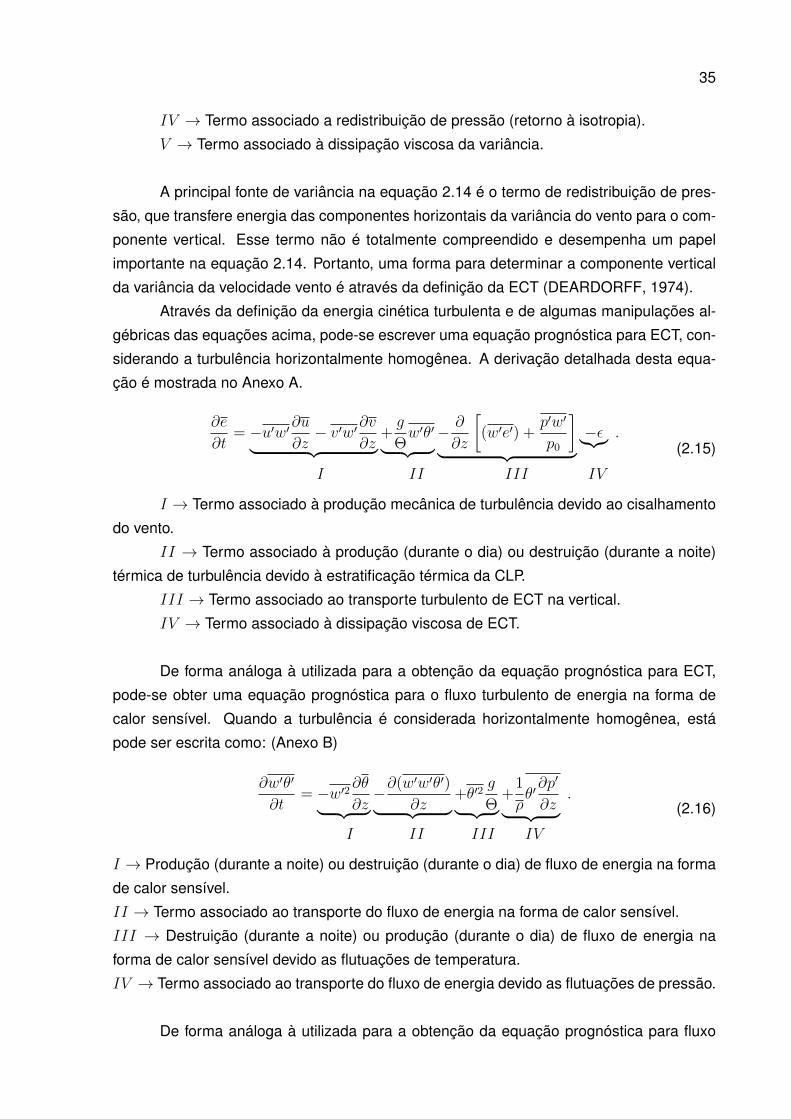
De forma análoga à utilizada para a obtenção da equação prognóstica para ECT,

pode-se obter uma equação prognóstica para o fluxo turbulento de energia na forma de

calor sensível. Quando a turbulência é considerada horizontalmente homogênea, está

pode ser escrita como: (Anexo B)

∂w′θ′

∂t= −w′2∂θ

∂z︸ ︷︷ ︸−∂(w′w′θ′)

∂z︸ ︷︷ ︸+θ′2

g

Θ︸ ︷︷ ︸+

1

ρθ′∂p′

∂z︸ ︷︷ ︸.

I II III IV

(2.16)

I → Produção (durante a noite) ou destruição (durante o dia) de fluxo de energia na forma

de calor sensível.

II → Termo associado ao transporte do fluxo de energia na forma de calor sensível.

III → Destruição (durante a noite) ou produção (durante o dia) de fluxo de energia na

forma de calor sensível devido as flutuações de temperatura.

IV → Termo associado ao transporte do fluxo de energia devido as flutuações de pressão.

De forma análoga à utilizada para a obtenção da equação prognóstica para fluxo

36

de calor sensível, pode-se obter as equações prognósticas para o fluxo turbulento de mo-

mentum. Quando a turbulência é considerada horizontalmente homogênea, está pode ser

escrita como:

∂u′w′

∂t= −w′2∂u

∂z︸ ︷︷ ︸−∂(w′u′w′)

∂z︸ ︷︷ ︸+p′

ρ

[∂u′

∂z+∂w′

∂x

]

︸ ︷︷ ︸, (2.17)

∂v′w′

∂t= −w′2∂v

∂z︸ ︷︷ ︸−∂(w′v′w′)

∂z︸ ︷︷ ︸+p′

ρ

[∂v′

∂z+∂w′

∂y

]

︸ ︷︷ ︸.

I II III

(2.18)

I → Produção (durante a noite) ou destruição (durante o dia) de fluxo de energia na forma

de calor sensível.

II → Termo associado ao transporte do fluxo de energia na forma de calor sensível.

III → Termo associado ao transporte do fluxo de energia devido as flutuações de pressão.

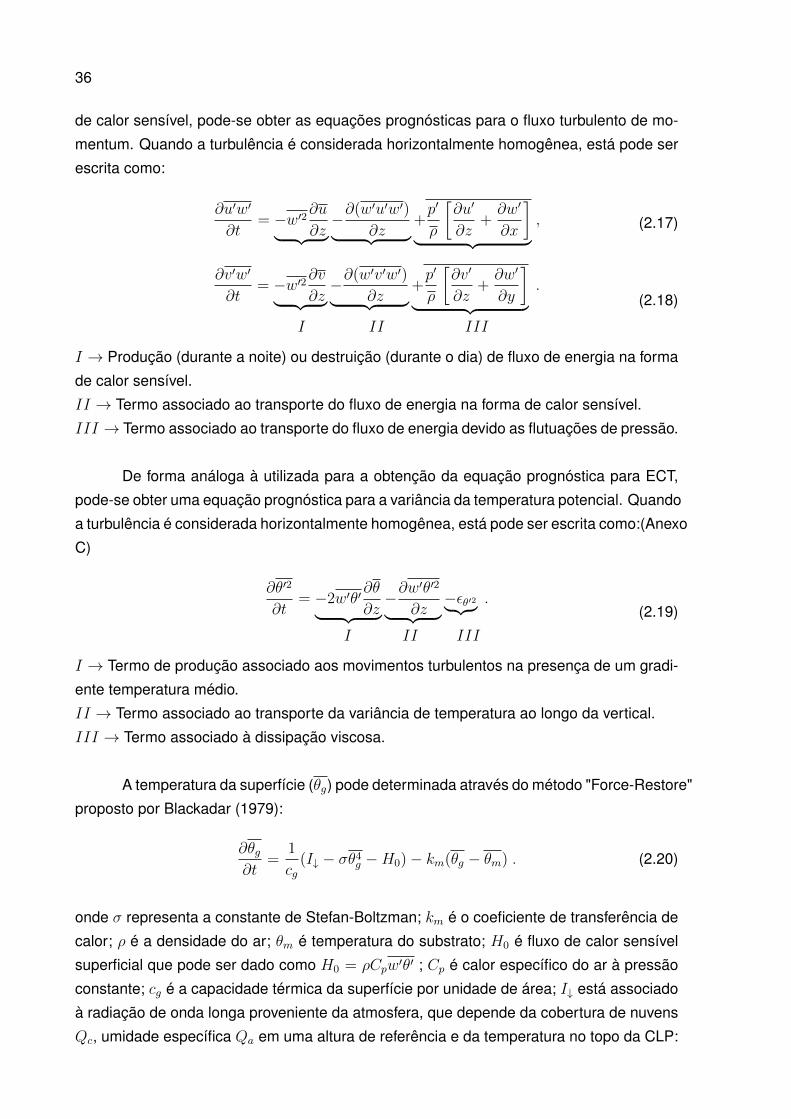
De forma análoga à utilizada para a obtenção da equação prognóstica para ECT,

pode-se obter uma equação prognóstica para a variância da temperatura potencial. Quando

a turbulência é considerada horizontalmente homogênea, está pode ser escrita como:(Anexo

C)

∂θ′2

∂t= −2w′θ′

∂θ

∂z︸ ︷︷ ︸−∂w

′θ′2

∂z︸ ︷︷ ︸−εθ′2︸ ︷︷ ︸ .

I II III

(2.19)

I → Termo de produção associado aos movimentos turbulentos na presença de um gradi-

ente temperatura médio.

II → Termo associado ao transporte da variância de temperatura ao longo da vertical.

III → Termo associado à dissipação viscosa.

A temperatura da superfície (θg) pode determinada através do método "Force-Restore"

proposto por Blackadar (1979):

∂θg∂t

=1

cg(I↓ − σθ4g −H0)− km(θg − θm) . (2.20)

onde σ representa a constante de Stefan-Boltzman; km é o coeficiente de transferência de

calor; ρ é a densidade do ar; θm é temperatura do substrato; H0 é fluxo de calor sensível

superficial que pode ser dado como H0 = ρCpw′θ′ ; Cp é calor específico do ar à pressão

constante; cg é a capacidade térmica da superfície por unidade de área; I↓ está associado

à radiação de onda longa proveniente da atmosfera, que depende da cobertura de nuvens

Qc, umidade específica Qa em uma altura de referência e da temperatura no topo da CLP:

37

I↓ = σ(Qc + 0, 67(1−Qc)(1670Qa)0,08)θ4 . (2.21)

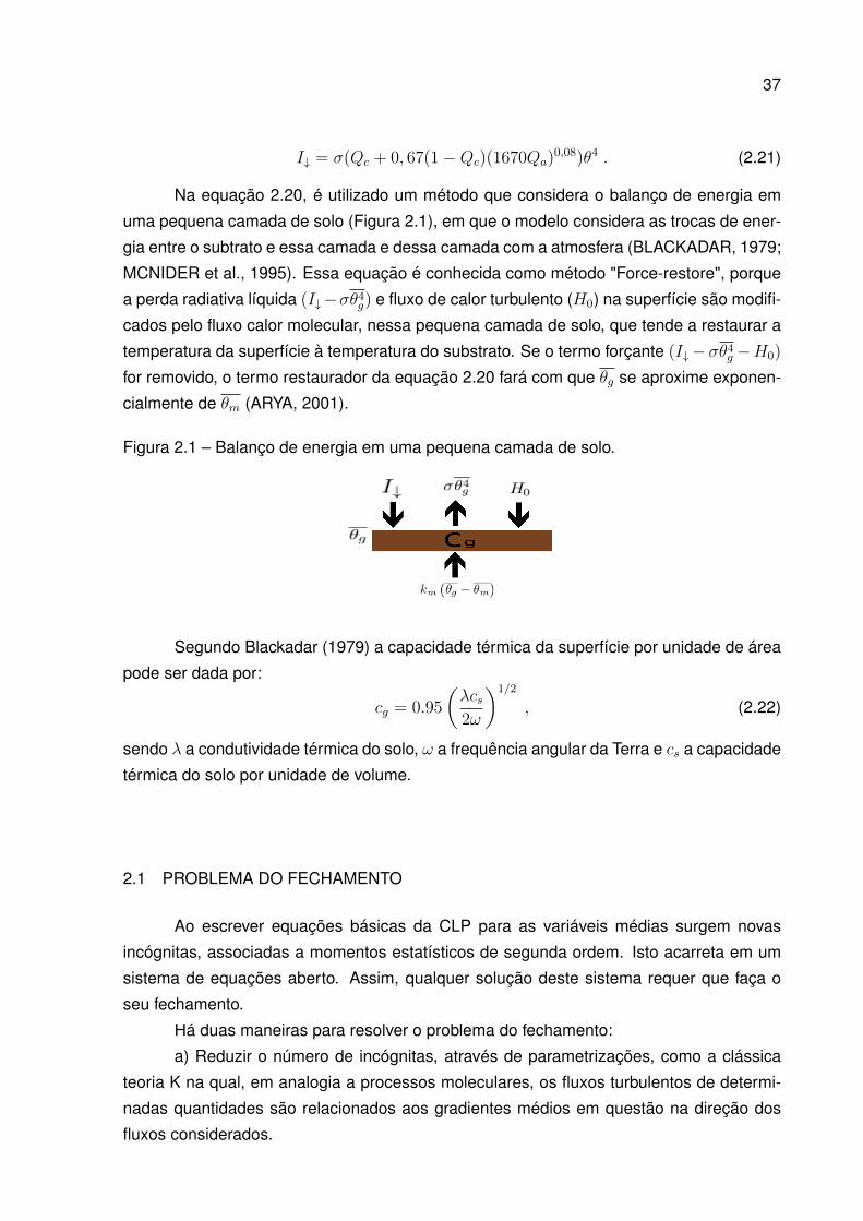
Na equação 2.20, é utilizado um método que considera o balanço de energia em

uma pequena camada de solo (Figura 2.1), em que o modelo considera as trocas de ener-

gia entre o subtrato e essa camada e dessa camada com a atmosfera (BLACKADAR, 1979;

MCNIDER et al., 1995). Essa equação é conhecida como método "Force-restore", porque

a perda radiativa líquida (I↓−σθ4g) e fluxo de calor turbulento (H0) na superfície são modifi-

cados pelo fluxo calor molecular, nessa pequena camada de solo, que tende a restaurar a

temperatura da superfície à temperatura do substrato. Se o termo forçante (I↓− σθ4g −H0)

for removido, o termo restaurador da equação 2.20 fará com que θg se aproxime exponen-

cialmente de θm (ARYA, 2001).

Figura 2.1 – Balanço de energia em uma pequena camada de solo.

Segundo Blackadar (1979) a capacidade térmica da superfície por unidade de área

pode ser dada por:

cg = 0.95

(λcs2ω

)1/2

, (2.22)

sendo λ a condutividade térmica do solo, ω a frequência angular da Terra e cs a capacidade

térmica do solo por unidade de volume.

2.1 PROBLEMA DO FECHAMENTO

Ao escrever equações básicas da CLP para as variáveis médias surgem novas

incógnitas, associadas a momentos estatísticos de segunda ordem. Isto acarreta em um

sistema de equações aberto. Assim, qualquer solução deste sistema requer que faça o

seu fechamento.

Há duas maneiras para resolver o problema do fechamento:

a) Reduzir o número de incógnitas, através de parametrizações, como a clássica

teoria K na qual, em analogia a processos moleculares, os fluxos turbulentos de determi-

nadas quantidades são relacionados aos gradientes médios em questão na direção dos

fluxos considerados.

38

b) Escrever equações prognósticas para as incógnitas, através de manipulações

algébricas das equações básicas da CLP.

Entretanto, ao escrever as equações prognósticas para os momentos de segunda

ordem, surgem incógnitas de terceira ordem, como pode ser visto nas equações 2.15-2.19,

que são prognósticas para momentos de segunda ordem e apresentam sempre alguns

termos de terceira ordem. Assim, a solução de escrever equações prognósticas para todas

as novas incógnitas nunca resolve o problema do fechamento, pois sempre surgirão novas

incógnitas, mantendo o número de variáveis maior que o de equações. Portanto, sempre

será necessário que os momentos estatísticos de alguma ordem sejam parametrizados

em termos dos de ordem mais baixa para que seja possível obter solução (normalmente

numérica) para o sistema de equações básicas da CLP para as variáveis médias.

As aproximações ou premissas de fechamento são nomeadas através das equa-

ções prognósticas de maior ordem mantidas no sistemas de equações utilizadas para

descrever o escoamento. Assim, por exemplo, para o fechamento de primeira ordem as

equações prognósticas para os momentos estatísticos de primeira ordem são mantidas,

enquanto os momentos de segunda ordem são aproximados ou parametrizados. Analo-

gamente, para um fechamento de segunda ordem são mantidas as equações para os mo-

mentos estatísticos de primeira e de segunda ordem, aproximando os termos de terceira

ordem.

Nem sempre é necessário escrever equações prognósticas para todos momentos

estatísticos de segunda ou terceira ordem, pois algumas quantidades tem maior importân-

cia física que outros. Portanto, sistemas de equações que mantém equações prognósticas

para energia cinética turbulenta e variância da temperatura, além das equações para os

momentos estatísticos de primeira ordem, podem ser classificados como um sistema com

fechamento de uma ordem e meia, intermediários aos de primeira e segunda ordem, pois

resolvem alguns momentos estatísticos de segunda ordem, mas não todos (STULL, 1988).

Assim, modelos numéricos, como o proposto no artigo 1, que resolvem equações

prognósticas para velocidade do vento, temperatura, energia cinética turbulenta, fluxo de

energia na forma de calor sensível e para a variância da temperatura são classificados

como modelos de uma ordem e meia. Já, o modelo proposto no artigo 3 corresponde à

um modelo de segunda ordem completa.

Mellor e Yamada (1974) propuseram quatro diferentes níveis para fechamento da

turbulência. Os níveis 1 e 2 são basicamente esquemas de primeira ordem, sem equações

prognósticas para quaisquer variáveis turbulentas. Já, o nível 3 equações prognósticas

para ECT e variância de temperatura são resolvidas. Por fim o nível 4, todos os momentos

estatísticos de segunda ordem, como fluxo de momentum, de calor e as variâncias das

componentes da velocidade do vento e da temperatura potencial, são resolvidas prognos-

ticamente. Posteriormente, Mellor e Yamada (1982) propuseram o fechamento de nível

2.5, em que a ECT é o único momento de segunda ordem resolvido prognóstico.

Boundary-Layer Meteorologyhttps://doi.org/10.1007/s10546-018-0401-3

RESEARCH ART ICLE

Simulating the Regime Transition of the Stable BoundaryLayer Using Different Simplified Models

Rafael Maroneze1 ·Otávio C. Acevedo1 · Felipe D. Costa2 · Jielun Sun3

Received: 27 April 2018 / Accepted: 23 October 2018© Springer Nature B.V. 2018

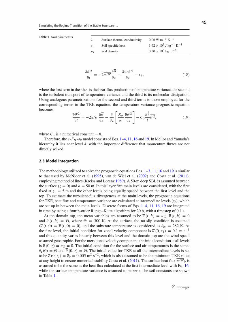
AbstractThe transition between the stable and the near-neutral regimes corresponding to weak andstrong winds in the stable boundary layer is investigated using four one-dimensional numer-ical models with increasing numbers of prognostic equations for turbulent variables. Thebasic state for all the models includes prognostic equations for mean horizontal wind speed,and air and surface temperatures. The simplest model of the four has turbulence variablesparametrized using a long-tail stability function and the gradient Richardson number. Thecomplexity of the other three models increases by introducing one more prognostic equa-tion to each model to reduce the number of parametrized turbulent variables: a prognosticequation for turbulent kinetic energy (TKE, e model), an additional prognostic equation forheat fluxes (e-FH model), and an additional prognostic equation for temperature variances(e-FH -σθ model). Results for all modells are similar in the strong-wind regime. The twostability regimes can be identified in the relationship between the turbulence velocity scalederived from TKE andmean wind speed from the three models with resolved TKE. However,the weak-wind regime can only be resolved with heat fluxes and temperature variance solvedby prognostic equations. Simulations with the removal of the buoyancy term associated withheat fluxes in the TKE equation only result in the strong-wind regime, showing that this termcontrols the regime transition.

Keywords Stable boundary layer · Strong-wind regime · Transition · Weak-wind regime

1 Introduction

Many studies have shown the existence of two regimes or states in the stable boundarylayer (SBL), usually classified as very or weakly stable (Malhi 1995; Oyha et al. 1997;Mahrt 1998), although this classification criterion varies between studies. The weakly stableregime normally occurs in the presence of consistently strong winds and/or cloud cover

B Rafael Maronezerafaelmaroneze@gmail.com

1 Departamento de Física, Universidade Federal de Santa Maria, Santa Maria, RS, Brazil

2 Universidade Federal do Pampa-Campus, Alegrete, RS, Brazil

3 NorthWest Research Associates, Boulder, CO 80301, USA

123

3 ARTIGO 1 - SIMULATING THE REGIME TRANSITION OF THE STABLE BOUNDARY

LAYER USING DIFFERENT SIMPLIFIED MODELS

R. Maroneze et al.

(Acevedo and Fitzjarrald 2003), such that strong shear-generated turbulent mixing reducesthe boundary-layer stratification, or cloud cover reduces air–surface temperature differences.The very stable regime, on the other hand, is characterized by weak winds and clear skies,corresponding to strong net radiative cooling at the surface (Mahrt 1998). In the very stableregime the turbulent mixing is weak and possibly intermittent.

Amethod to identify the two SBL regimes uses the relation between heat flux and stabilitydue to Mahrt (1998). In the weakly stable regime the heat-flux magnitude increases withstability due to the increase of vertical temperature gradient as a result of the upward transferof cold near-surface air. In the very stable regime, the heat-flux magnitude decreases withstability because turbulent mixing is suppressed by the atmospheric stable stratification. Analternative SBL classification refers to the coupling state between near-surface air and theupper SBL levels. When mechanical forcing for turbulence generation is strong the weaklystable SBL is coupled to the surface. In contrast, when the mechanical forcing is weak, theatmosphere above tends to be decoupled from the surface, corresponding to the very stableSBL regime (Costa et al. 2011).

Sun et al. (2012) observed that the relationship between the turbulence velocity scale(VT K E ) and mean wind speed abruptly changes at a critical value of mean wind speed (V ) ata given height, characterizing the hockey stick transition between the stable (weak wind) andthe near-neutral (strong wind) regimes (Sun et al. 2015). For the weak-wind regime, VT K E

increases slightly with V , and for the strong-wind regime VT K E increases rapidly with Vwhen V exceeds the critical value.

For some decades simple models have been used to describe the interactions betweenturbulence, mean wind speed and stability whitin the SBL. Blackadar (1979) introduced amodel for air–surface interactions inwhich prognostic equations for the velocity components,air and surface temperatures are solved. Turbulent fluxes are estimated using a first-orderclosure with the gradients of mean quantities and stability functions. McNider et al. (1995)showed that in the Blackadar model very small pertubations of the geostrophic wind speedare sufficient to force the SBL to switch regimes.

It is not yet entirely clear why there are two different regimes with such contrastingcharacteristics, and the abrupt transition between them illustrated in the modelling resultsof McNider et al. (1995) and observations presented by Acevedo and Fitzjarrald (2003).Using simple reasoning based on energy budget and similarity arguments, van de Wiel et al.(2012a) argued that there is a minimum wind speed above which the turbulent energy isable to totally transfer the cold air from the radiatively cooled surface to the atmosphereabove. Sun et al. (2016) suggested that in the weak-wind regime the energy supplied bythe mean wind shear is partially converted to turbulent potential energy (TPE), defined asTPE ≡ 1/2 [(g/�N )]2 θ ′2, where g is the acceleration due to gravity, � is the referencetemperature, N is the Brunt-Vaisala frequency and θ ′2 is the temperature variance, limitingthe increase of turbulent kinetic energy (TKE). In the strong-wind regime, on the other hand,TPE is reduced because the thermal gradient is reduced by turbulent mixing, allowing mostof the shear-generated energy to be converted to TKE.

The present study tests the hypothesis that simple models are able to capture importantaspects of the regime transition if the main physical processes driving the transition areincluded in their formulations. Four different numerical models with an increasing numberof prognostic equations are considered and their ability to reproduce the regime transitionis evaluated. The simplest one (long-tail model) solves prognostic equations for mean windspeed, mean temperature and surface temperature and uses a long-tail stability function toestimate turbulence as a function of the atmospheric stability. In the second model (emodel),

123

40

Simulating the Regime Transition of the Stable Boundary…

TKE is directly solved by a prognostic equation. In addition to the set-up of the e model,a prognostic equation for heat fluxes is added in the third model (e-FH model). Finally,an additional prognostic equation for θ ′2 is also considered in the fourth model (e-FH -σθ

model). Through this systematic approach, we address the role of the heat flux and θ ′2 in theobserved regime transition.

2 Models

2.1 Historical Background

In early studies, turbulence in the atmospheric boundary layer was parametrized and onlymean variables are solved by prognostic equations. These are the first-order schemes. Ingeneral, turbulence is parametrized similarly to molecular diffusion except that an eddy dif-fusivity (K ) is applied rather than molecular diffusivity to relate fluxes to the mean gradients.The eddy diffusivity K was first assumed to be invariant (e.g., Ekman 1905; Taylor 1915),then to be an exponential function of height z (e.g., Köhler 1933),and later to be the widelyused K = κu∗z, where κ is the von Karman constant, u∗ is the friction velocity. Followingthe suggestions of similarity approaches by Heisenberg (1948), Blackadar (1962) proposedK = l2S, where l = κz is the mixing length and S is the local wind shear.

Solving selected turbulence variables with prognostic equations while defining the othersthrough parametrizations is commonly referred as a higher-order closure scheme, which wasintroduced in the 1960s (Donaldson and Rosenbaum 1968; Kline et al. 1968). Mellor andYamada (1974) classified the sophistication of the turbulence closure in four levels. Theirdefinitions of levels 1 and 2 are basically first-order schemes with no prognostic equationsfor any turbulence variables. Their level-3 scheme solves prognostic equations for TKE andtemperature variances. In their level-4 scheme, all the turbulence variables of second-ordermoments, such as momentum and heat fluxes and variances of velocity components andtemperature, are solved prognostically. Later on, Mellor and Yamada (1982) proposed a 2.5-level scheme, in which TKE is the only second-order moment that is solved prognostically.Meanwhile, Wyngaard and Coté (1974) proposed to add a prognostic equation for the turbu-lence dissipation rate to simulate the convective boundary layer (CBL). Applying the sameapproach, Wyngaard (1975) demonstrated its success in simulating the SBL.

A major problem with lower-order schemes concerns their excessive turbulent mixing, acommonly used solution forwhich is the use of a stability function,which forces the reductionof mixing as the stability increases. Commonly used stability functions may be described asshort-tail, when turbulence is reduced to zero at a Richardson number larger than a criticalvalue; or long-tail, when turbulent mixing never totally disappears even at large stability. Theshort-tail stability function is used in the Mellor and Yamada levels-1, -2, and -2.5 schemes,the long-tail stability function such as those developed by Louis (1979) and Delage (1997)are widely used in numerical weather and climate models because of their ability to mantainfinite turbulent mixing even in very stable conditions. It is a means of simulating localizedturbulence activity, which in nature may occur in parts of a numerical grid cell. Besides,maintaining weak turbulence provides an effective means of avoiding the so-called runawaycooling problem (Louis 1979; Steeneveld et al. 2006) that may occur when turbulence issuppressed abruptly by a short-tail approach, causing the surface to be cooled indefinitelythrough longwave radiation loss.

123

41

R. Maroneze et al.

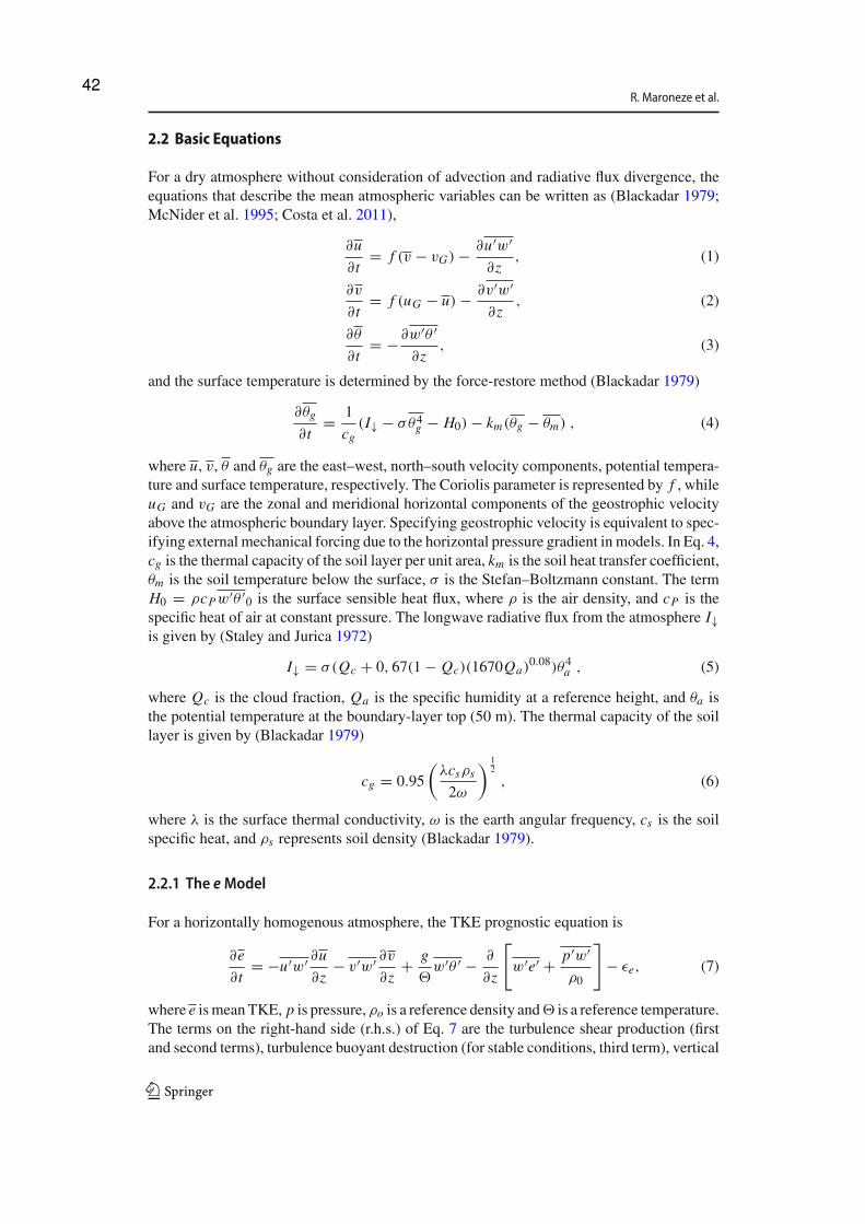
2.2 Basic Equations

For a dry atmosphere without consideration of advection and radiative flux divergence, theequations that describe the mean atmospheric variables can be written as (Blackadar 1979;McNider et al. 1995; Costa et al. 2011),

∂u

∂t= f (v − vG) − ∂u′w′

∂z, (1)

∂v

∂t= f (uG − u) − ∂v′w′

∂z, (2)

∂θ

∂t= −∂w′θ ′

∂z, (3)

and the surface temperature is determined by the force-restore method (Blackadar 1979)

∂θg

∂t= 1

cg(I↓ − σθ4g − H0) − km(θg − θm) , (4)

where u, v, θ and θg are the east–west, north–south velocity components, potential tempera-ture and surface temperature, respectively. The Coriolis parameter is represented by f , whileuG and vG are the zonal and meridional horizontal components of the geostrophic velocityabove the atmospheric boundary layer. Specifying geostrophic velocity is equivalent to spec-ifying external mechanical forcing due to the horizontal pressure gradient in models. In Eq. 4,cg is the thermal capacity of the soil layer per unit area, km is the soil heat transfer coefficient,θm is the soil temperature below the surface, σ is the Stefan–Boltzmann constant. The termH0 = ρcPw′θ ′

0 is the surface sensible heat flux, where ρ is the air density, and cP is thespecific heat of air at constant pressure. The longwave radiative flux from the atmosphere I↓is given by (Staley and Jurica 1972)

I↓ = σ(Qc + 0, 67(1 − Qc)(1670Qa)0.08)θ4a , (5)

where Qc is the cloud fraction, Qa is the specific humidity at a reference height, and θa isthe potential temperature at the boundary-layer top (50 m). The thermal capacity of the soillayer is given by (Blackadar 1979)

cg = 0.95

(λcsρs2ω

) 12

, (6)

where λ is the surface thermal conductivity, ω is the earth angular frequency, cs is the soilspecific heat, and ρs represents soil density (Blackadar 1979).

2.2.1 The eModel

For a horizontally homogenous atmosphere, the TKE prognostic equation is

∂e

∂t= −u′w′ ∂u

∂z− v′w′ ∂v

∂z+ g

�w′θ ′ − ∂

∂z

[w′e′ + p′w′

ρ0

]− εe, (7)

where e ismeanTKE, p is pressure,ρo is a reference density and� is a reference temperature.The terms on the right-hand side (r.h.s.) of Eq. 7 are the turbulence shear production (firstand second terms), turbulence buoyant destruction (for stable conditions, third term), vertical

123

42

Simulating the Regime Transition of the Stable Boundary…

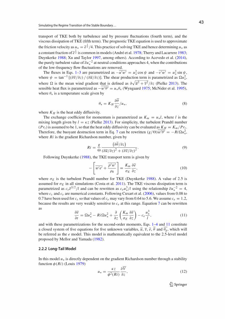
transport of TKE both by turbulence and by pressure fluctuations (fourth term), and theviscous dissipation of TKE (fifth term). The prognostic TKE equation is used to approximate

the friction velocity as u∗ = e12 /4. This practice of solving TKE and hence determining u∗ as

a constant fraction of e12 is common inmodels (André et al. 1978; Therry and Lacarrere 1983;

Duynkerke 1988; Xu and Taylor 1997, among others). According to Acevedo et al. (2014),the purely turbulent value of eu−2∗ at neutral conditions approaches 4, when the contributionsof the low-frequency flow fluctuations are removed.

The fluxes in Eqs. 1–3 are parametrized as −u′w′ = u2∗ cosψ and −v′w′ = u2∗ sinψ ,where ψ = tan−1 [(∂v/∂z) / (∂u/∂z)]. The shear production term is parametrized as �u2∗,where � is the mean wind gradient that is defined as ∂

√u2 + v2/∂z (Pielke 2013). The

sensible heat flux is parametrized as −w′θ ′ = u∗θ∗ (Wyngaard 1975; McNider et al. 1995),where θ∗ is a temperature scale given by

θ∗ = KH∂θ

∂z/u∗, (8)

where KH is the heat eddy diffusivity.The exchange coefficient for momentum is parametrized as Km = u∗l, where l is the

mixing length given by l = κz (Pielke 2013). For simplicity, the turbulent Prandtl number(Prt ) is assumed to be 1, so that the heat eddy diffusivity can be evaluated as KH = Km/Prt .Therefore, the buoyant destruction term in Eq. 7 can be rewritten (g/�)w′θ ′ = −Ri�u2∗,where Ri is the gradient Richardson number, given by

Ri = g

�

(∂θ/∂z

)(∂u/∂z)2 + (∂v/∂z)2

. (9)

Following Duynkerke (1988), the TKE transport term is given by

−[w′e′ + p′w′

ρ0

]= Km

σE

∂e

∂z, (10)

where σE is the turbulent Prandtl number for TKE (Duynkerke 1988). A value of 2.5 isassumed for σE in all simulations (Costa et al. 2011). The TKE viscous dissipation term isparametrized as cεe3/2/l and can be rewritten as ceu3∗/l using the relationship eu−2∗ = 4,where cε and ce are numerical constants. Following Cuxart et al. (2006), values from 0.08 to0.7 have been used for cε so that values of ce may vary from 0.64 to 5.6.We assume ce = 1.2,because the results are very weakly sensitive to ce at this range. Equation 7 can be rewrittenas

∂e

∂t= �u2∗ − Ri�u2∗ + ∂

∂z

(Km

σE

∂e

∂z

)− ce

u3∗l

, (11)

and with these parametrizations for the second-order moments, Eqs. 1–4 and 11 constitutea closed system of five equations for five unknown variables, u, v, e, θ and θg , which willbe referred as the e model. This model is mathematically equivalent to the 2.5-level modelproposed by Mellor and Yamada (1982).

2.2.2 Long-Tail Model

In this model u∗ is directly dependent on the gradient Richardson number through a stabilityfunction φ(Ri) (Louis 1979)

u∗ = κz

φ2(Ri)

∂V

∂z, (12)

123

43

R. Maroneze et al.

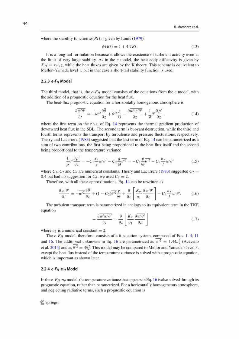
where the stability function φ(Ri) is given by Louis (1979)

φ(Ri) = 1 + 4.7Ri . (13)

It is a long-tail formulation because it allows the existence of turbulent activity even atthe limit of very large stability. As in the e model, the heat eddy diffusivity is given byKH = κu∗z, while the heat fluxes are given by the K theory. This scheme is equivalent toMellor–Yamada level 1, but in that case a short-tail stability function is used.

2.2.3 e-FH Model

The third model, that is, the e-FH model consists of the equations from the e model, withthe addition of a prognostic equation for the heat flux.

The heat-flux prognostic equation for a horizontally homogenous atmosphere is

∂w′θ ′∂t

= −w′2 ∂θ

∂z+ θ ′2 g

�− ∂w′w′θ ′

∂z+ 1

ρθ ′ ∂ p

′

∂z, (14)

where the first term on the r.h.s. of Eq. 14 represents the thermal gradient production ofdownward heat flux in the SBL. The second term is buoyant destruction, while the third andfourth terms represents the transport by turbulence and pressure fluctuations, respectively.Therry and Lacarrere (1983) suggested that the last term of Eq. 14 can be parametrized as asum of two contributions, the first being proportional to the heat flux itself and the secondbeing proportional to the temperature variance

1

ρθ ′ ∂ p′

∂z= −C1

εe

ew′θ ′ − C2

g

�θ ′2 = −C2

g

�θ ′2 − Cθ

u∗l

w′θ ′ (15)

where C1, C2 and Cθ are numerical constants. Therry and Lacarrere (1983) suggested C2 =0.4 but had no suggestion for Cθ ; we used Cθ = 2.

Therefore, with all these approximations, Eq. 14 can be rewritten as

∂w′θ ′∂t

= −w′2 ∂θ

∂z+ (1 − C2)θ ′2 g

�+ ∂

∂z

[Km

σ1

∂w′θ ′∂z

]− Cθ

u∗l

w′θ ′. (16)

The turbulent transport term is parametrized in analogy to its equivalent term in the TKEequation

− ∂w′w′θ ′∂z

= ∂

∂z

[Km

σ1

∂w′θ ′∂z

](17)

where σ1 is a numerical constant = 2.The e-FH model, therefore, consists of a 6-equation system, composed of Eqs. 1–4, 11

and 16. The additional unknowns in Eq. 16 are parametrized as w′2 = 1.44u2∗ (Acevedo

et al. 2014) and as θ ′2 = 4θ2∗ . This model may be compared to Mellor and Yamada’s level 3,except the heat flux instead of the temperature variance is solved with a prognostic equation,which is important as shown later.

2.2.4 e-FH-�� Model

In the e-FH -σθ model, the temperature variance that appears inEq. 16 is also solved through itsprognostic equation, rather than parametrized. For a horizontally homogeneous atmosphere,and neglecting radiative terms, such a prognostic equation is

123

44

Simulating the Regime Transition of the Stable Boundary…

Table 1 Soil parametersλ Surface thermal conductivity 0.06 W m−1 K−1

cs Soil specific heat 1.92 × 103 J kg−1 K−1

ρs Soil density 0.30 × 103 kg m−3

∂θ ′2∂t

= −2w′θ ′ ∂θ

∂z− ∂w′θ ′2

∂z− εθ , (18)

where the first term in the r.h.s. is the heat-flux production of temperature variance, the secondis the turbulent transport of temperature variance and the third is its molecular dissipation.Using analogous parametrizations for the second and third terms to those employed for thecorresponding terms in the TKE equation, the temperature variance prognostic equationbecomes

∂θ ′2∂t

= −2w′θ ′ ∂θ

∂z− ∂

∂z

[Km

σ1

∂θ ′2∂z

]− C3

e12

lθ ′2, (19)

where C3 is a numerical constant = 8.Therefore, the e-FH -σθ model consists of Eqs. 1–4, 11, 16 and 19. InMellor andYamada’s

hierarchy it lies near level 4, with the important difference that momentum fluxes are notdirectly solved.

2.3 Model Integration

The methodology utilized to solve the prognostic equations Eqs. 1–3, 11, 16 and 19 is similarto that used by McNider et al. (1995), van de Wiel et al. (2002) and Costa et al. (2011),employing method of lines (Kreiss and Lorenz 1989). A 50-m deep SBL is assumed betweenthe surface (z = 0) and h = 50 m. In this layer five main levels are considered, with the firstfixed at z1 = 5 m and the other levels being equally spaced between the first level and thetop. To estimate the turbulent-flux divergences at the main levels, the prognostic equationsfor TKE, heat flux and temperature variance are calculated at intermediate levels (zi ), whichare set up in between the main levels. Discrete forms of Eqs. 1–4, 11, 16, 19 are integratedin time by using a fourth-order Runge–Kutta algorithm for 20 h, with a timestep of 0.1 s.

At the domain top, the mean variables are assumed to be u (t, h) = uG , v (t, h) = 0and θ (t, h) = �, where � = 300 K. At the surface, the no-slip condition is assumed(u (t, 0) = v (t, 0) = 0), and the substrate temperature is considered as θm = 282 K. Atthe first level, the initial condition for zonal velocity component is u (0, z1) = 0.1 m s−1

and this quantity varies linearly between this level and the domain top are the wind speedassumed geostrophic. For themeridional velocity component, the initial condition at all levelsis v (0, z) = vG = 0. The initial condition for the surface and air temperatures is the same:θg(0) = � and θ (0, z) = �. The initial value for TKE at all the intermediate levels is setto be e (0, zi ) = e0 = 0.005 m2 s−2, which is also assumed to be the minimum TKE valueat any height to ensure numerical stability Costa et al. (2011). The surface heat flux w′θ ′

0 isassumed to be the same as the heat flux calculated at the first intermediate level with Eq. 16,while the surface temperature variance is assumed to be zero. The soil constants are shownin Table 1.

123

45

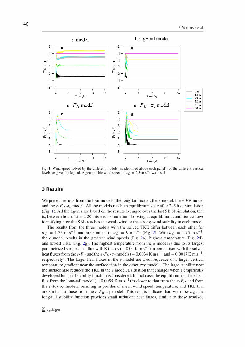
R. Maroneze et al.

Fig. 1 Wind speed solved by the different models (as identified above each panel) for the different verticallevels, as given by legend. A geostrophic wind speed of uG = 2.5 m s−1 was used

3 Results

We present results from the four models: the long-tail model, the e model, the e-FH modeland the e-FH -σθ model. All the models reach an equilibrium state after 2–5 h of simulation(Fig. 1). All the figures are based on the results averaged over the last 5 h of simulation, thatis, between hours 15 and 20 into each simulation. Looking at equilibrium conditions allowsidentifying how the SBL reaches the weak-wind or the strong-wind stability in each model.

The results from the three models with the solved TKE differ between each other foruG = 1.75 m s−1, and are similar for uG = 9 m s−1 (Fig. 2). With uG = 1.75 m s−1,the e model results in the greatest wind speeds (Fig. 2a), highest temperature (Fig. 2d),and lowest TKE (Fig. 2g). The highest temperature from the e model is due to its largestparametrized surface heat flux with K theory (− 0.04 Km s−1) in comparison with the solvedheat fluxes from the e-FH and the e-FH -σθ models (− 0.0034Km s−1 and− 0.0017Km s−1,respectively). The larger heat fluxes in the e model are a consequence of a larger verticaltemperature gradient near the surface than in the other two models. The large stability nearthe surface also reduces the TKE in the e model, a situation that changes when a empiricallydeveloped long-tail stability function is considered. In that case, the equilibrium surface heatflux from the long-tail model (− 0.0055 K m s−1) is closer to that from the e-FH and fromthe e-FH -σθ models, resulting in profiles of mean wind speed, temperature, and TKE thatare similar to those from the e-FH -σθ model. This results indicate that, with low uG , thelong-tail stability function provides small turbulent heat fluxes, similar to those resolved

123

46

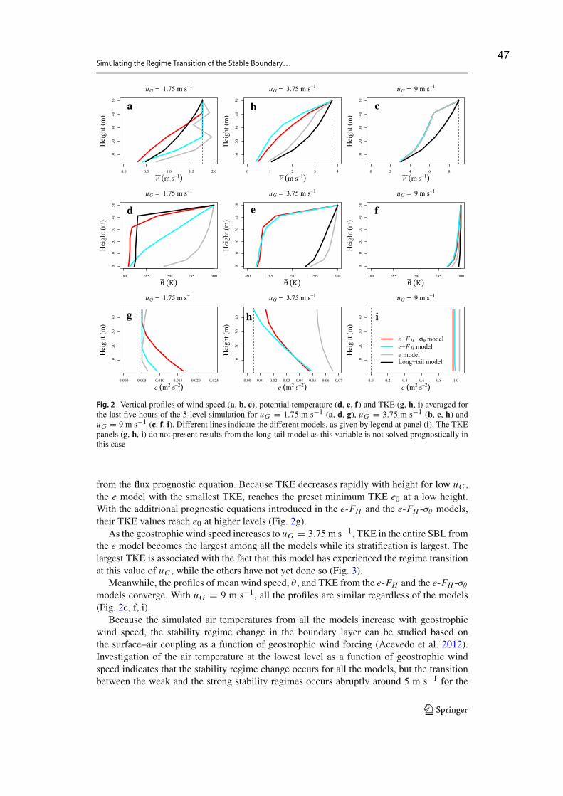
Simulating the Regime Transition of the Stable Boundary…

V (m s−1)

Hei

ght (

m)

uG = 1.75 m s−1

a

V (m s−1)

Hei

ght (

m)

uG = 3.75 m s−1

b

0.0 0.5 1.0 1.5 2.0 40 1 2 3 0 2 4 6 8

V (m s−1)

Hei

ght (

m)

c

uG = 9 m s−1

θ (K)

Hei

ght (

m)

d

uG = 1.75 m s−1

280 285 290 295 300 280 285 290 295 300

θ (K)

Hei

ght (

m)

e

uG = 3.75 m s−1

280 285 290 295 300

010

2030

4050

θ (K)

Hei

ght (

m)

f

uG = 9 m s−1

e (m2 s−2)

Hei

ght (

m)

g

uG = 1.75 m s−1

e (m2 s−2)

Hei

ght (

m)

h

uG = 3.75 m s−1

0.000 0.005 0.010 0.015 0.020 0.025 0.00 0.01 0.02 0.03 0.04 0.05 0.06 0.07 0.0 0.2 0.4 0.6 0.8 1.0

1020

3040

50

1020

3040

50

1020

3040

50

010

2030

4050

010

2030

4050

1020

3040

1020

3040

1020

3040

e (m2 s−2)

Hei

ght (

m)

i

uG = 9 m s−1

e−FH−σθ modele−FH modele modelLong−tail model

Fig. 2 Vertical profiles of wind speed (a, b, c), potential temperature (d, e, f) and TKE (g, h, i) averaged forthe last five hours of the 5-level simulation for uG = 1.75 m s−1 (a, d, g), uG = 3.75 m s−1 (b, e, h) anduG = 9 m s−1 (c, f, i). Different lines indicate the different models, as given by legend at panel (i). The TKEpanels (g, h, i) do not present results from the long-tail model as this variable is not solved prognostically inthis case

from the flux prognostic equation. Because TKE decreases rapidly with height for low uG ,the e model with the smallest TKE, reaches the preset minimum TKE e0 at a low height.With the additrional prognostic equations introduced in the e-FH and the e-FH -σθ models,their TKE values reach e0 at higher levels (Fig. 2g).

As the geostrophic wind speed increases to uG = 3.75m s−1, TKE in the entire SBL fromthe e model becomes the largest among all the models while its stratification is largest. Thelargest TKE is associated with the fact that this model has experienced the regime transitionat this value of uG , while the others have not yet done so (Fig. 3).

Meanwhile, the profiles of mean wind speed, θ , and TKE from the e-FH and the e-FH -σθ

models converge. With uG = 9 m s−1, all the profiles are similar regardless of the models(Fig. 2c, f, i).

Because the simulated air temperatures from all the models increase with geostrophicwind speed, the stability regime change in the boundary layer can be studied based onthe surface–air coupling as a function of geostrophic wind forcing (Acevedo et al. 2012).Investigation of the air temperature at the lowest level as a function of geostrophic windspeed indicates that the stability regime change occurs for all the models, but the transitionbetween the weak and the strong stability regimes occurs abruptly around 5 m s−1 for the

123

47

R. Maroneze et al.

0 5 10 15 20

285

290

295

300

V (m s−1)

θ 1( K

)

e−FH−σθ modele−FH modele modelLong−tail model

Fig. 3 Equilibrium temperature at the lowest vertical level as a function of the geostrophic wind speed foreach of the formulations considered, according to legend

e-FH and the e-FH -σθ models. Acevedo et al. (2012) compared simple TKE schemes with orwithout stability functions, and found that the use of stability functions causes the transitionto become less abrupt than when they are not used. This value is close to the range of theminimum geostrophic wind speed for maintaining moderate to strong turbulence found byvan de Wiel et al. (2012a, b), based on similarity and energy budget arguments. Similarly,using an extensive observational dataset, van der Linden et al. (2017) showed that quantitiessuch as friction velocity and sensible heat flux have, on the average, magnitudes substantiallylarger than zero only for geostrophic wind speeds > 4 m s−1. The use of a stability functioncauses surface air temperatures to approach those from the e-FH and e-FH -σθ models in theweak-wind regime. However, the regime transition of the model that uses stability functionoccurs at the same low geostrophic wind speed that drives the regime transition in the emodel.

The relationship between the turbulence velocity scale VT K E and the mean wind speedV at a given height has been used to determine the SBL stability regimes (Sun et al. 2012).The results from the three models with TKE solved show distinctively different relationshipsbetween both quantities (Fig. 4), and in the strong-wind regime, the relationship is verysimilar among the models. That is, VT K E increases linearly with V , and the rate of increasevaries with height. At all the levels, the VT K E × V lines from the strong-wind regime maybe extrapolated towards the origin (V = 0 and VT K E = 0) (dashed lines in Fig. 4). The maindifferences between the models occur in the weak-wind regime and, more importantly, in thetransition between the weak-wind and the strong-wind regimes. In the simple emodel, VT K E

varies significantly and is nearly independent of V for wind speeds smaller than the transitionthresholdwind speed VT (Fig. 4a). This near independence between VT K E and V in theweak-wind regime is not largely affected when a prognostic equation for the heat flux is included(Fig. 4b). However, the additional inclusion of a prognostic equation for the temperaturevariance in the e-FH -σθ makes it possible to define aweak-wind regimewhere VT K E linearly

123

48

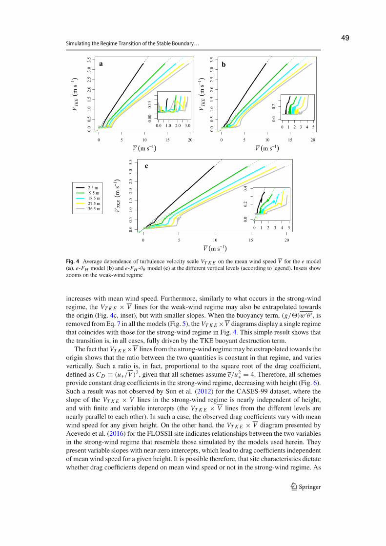
Simulating the Regime Transition of the Stable Boundary…

V (m s−1)

VTK

E(m

s−1)

a

0.00

0.15

0 5 10 15 20 0 5 10 15 20

0.0

0.5

1.0

1.5

2.0

2.5

3.0

3.5

0.0

0.5

1.0

1.5

2.0

2.5

3.0

3.5

V (m s−1)

VTK

E(m

s−1)

b

0.0 1.0 2.0 3.0 0 1 2 3 4 5

0.0

0.2

0 5 10 15 20

0.0

0.5

1.0

1.5

2.0

2.5

3.0

3.5

V (m s−1)

VTK

E(m

s−1)

c

0 1 2 3 4 5

0.0

0.2

0.42.5 m

9.5 m18.5 m27.5 m36.5 m

Fig. 4 Average dependence of turbulence velocity scale VT K E on the mean wind speed V for the e model(a), e-FH model (b) and e-FH -θθ model (c) at the different vertical levels (according to legend). Insets showzooms on the weak-wind regime

increases with mean wind speed. Furthermore, similarly to what occurs in the strong-windregime, the VT K E × V lines for the weak-wind regime may also be extrapolated towardsthe origin (Fig. 4c, inset), but with smaller slopes. When the buoyancy term, (g/�)w′θ ′, isremoved fromEq. 7 in all themodels (Fig. 5), the VT K E ×V diagrams display a single regimethat coincides with those for the strong-wind regime in Fig. 4. This simple result shows thatthe transition is, in all cases, fully driven by the TKE buoyant destruction term.

The fact that VT K E×V lines from the strong-wind regimemay be extrapolated towards theorigin shows that the ratio between the two quantities is constant in that regime, and variesvertically. Such a ratio is, in fact, proportional to the square root of the drag coefficient,defined as CD ≡ (u∗/V )2, given that all schemes assume e/u2∗ = 4. Therefore, all schemesprovide constant drag coefficients in the strong-wind regime, decreasing with height (Fig. 6).Such a result was not observed by Sun et al. (2012) for the CASES-99 dataset, where theslope of the VT K E × V lines in the strong-wind regime is nearly independent of height,and with finite and variable intercepts (the VT K E × V lines from the different levels arenearly parallel to each other). In such a case, the observed drag coefficients vary with meanwind speed for any given height. On the other hand, the VT K E × V diagram presented byAcevedo et al. (2016) for the FLOSSII site indicates relationships between the two variablesin the strong-wind regime that resemble those simulated by the models used herein. Theypresent variable slopes with near-zero intercepts, which lead to drag coefficients independentof mean wind speed for a given height. It is possible therefore, that site characteristics dictatewhether drag coefficients depend on mean wind speed or not in the strong-wind regime. As

123

49

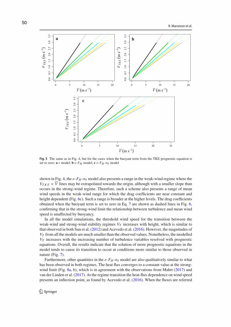
R. Maroneze et al.

V (m s−1)

VTK

E(m

s−1)

a

V (m s−1)

VTK

E(m

s−1)

b

0 5 10 15 20 0 5 10 15 20

0 5 10 15 20 25

0.0

0.5

1.0

1.5

2.0

2.5

3.0

3.5

0.0

0.5

1.0

1.5

2.0

2.5

3.0

3.5

0.0

0.5

1.0

1.5

2.0

2.5

3.0

3.5

V (m s−1)

VTK

E(m

s− 1)

c

Fig. 5 The same as in Fig. 4, but for the cases when the buoyant term from the TKE prognostic equation isset to zero: a e model; b e-FH model; c e-FH -σθ model

shown in Fig. 4, the e-FH -σθ model also presents a range in the weak-wind regime where theVT K E × V lines may be extrapolated towards the origin, although with a smaller slope thanoccurs in the strong-wind regime. Therefore, such a scheme also presents a range of meanwind speeds in the weak-wind range for which the drag coefficients are near constant andheight dependent (Fig. 6c). Such a range is broader at the higher levels. The drag coefficientsobtained when the buoyant term is set to zero in Eq. 7 are shown as dashed lines in Fig. 6,confirming that in the strong-wind limit the relationship between turbulence and mean windspeed is unaffected by buoyancy.

In all the model simulations, the threshold wind speed for the transition between theweak-wind and strong-wind stability regimes VT increases with height, which is similar tothat observed in both Sun et al. (2012) and Acevedo et al. (2016). However, the magnitudes ofVT from all themodels aremuch smaller than the observed values. Nonetheless, themodelledVT increases with the increasing number of turbulence variables resolved with prognosticequations. Overall, the results indicate that the solution of more prognostic equations in themodel tends to cause its transition to occur at conditions more similar to those observed innature (Fig. 7).

Furthermore, other quantities in the e-FH -σθ model are also qualitatively similar to whathas been observed in both regimes. The heat flux converges to a constant value at the strong-wind limit (Fig. 8a, b), which is in agreement with the observations from Mahrt (2017) andvan der Linden et al. (2017). At the regime transition the heat-flux dependence on wind speedpresents an inflection point, as found by Acevedo et al. (2016). When the fluxes are referred

123

50

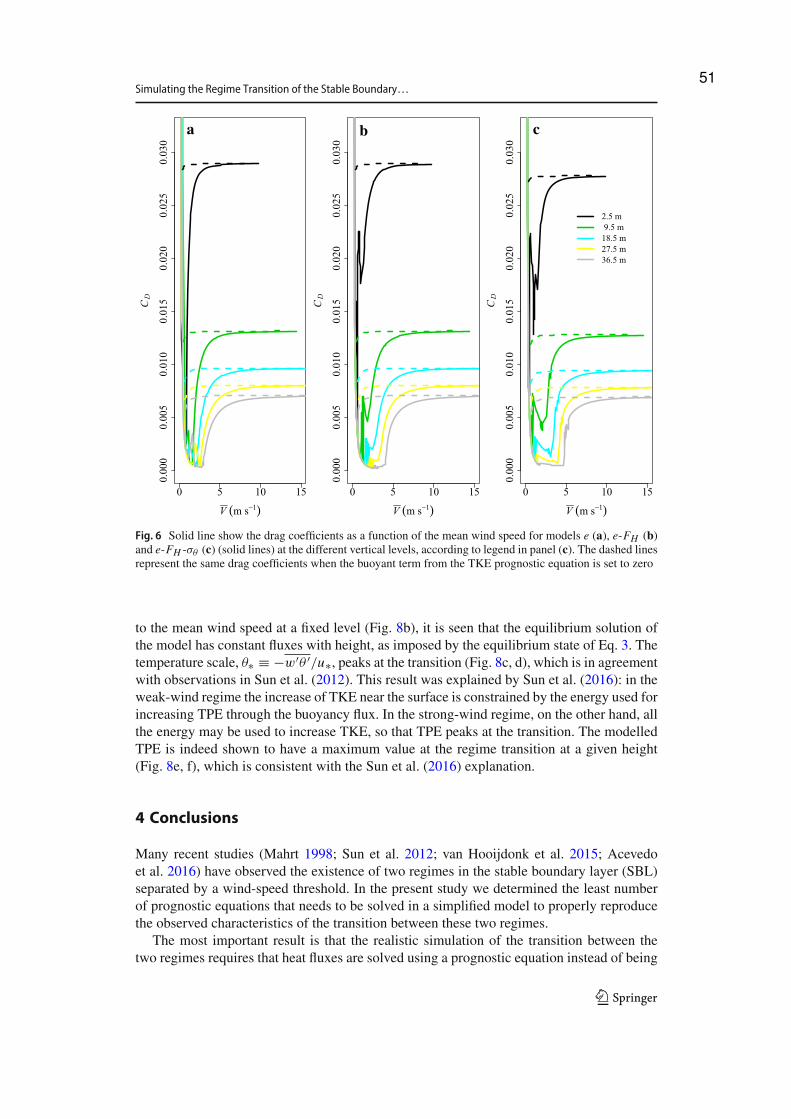
Simulating the Regime Transition of the Stable Boundary…

V (m s−1)

CD

a

V (m s−1)

CD

b

0 5 10 15 0 5 10 15 0 5 10 15

0.00

00.

005

0.01

00.

015

0.02

00.

025

0.03

0

0.00

00.

005

0.01

00.

015

0.02

00.

025

0.03

0

0.00

00.

005

0.01

00.

015

0.02

00.

025

0.03

0V (m s−1)

CD

2.5 m 9.5 m18.5 m27.5 m36.5 m

c

Fig. 6 Solid line show the drag coefficients as a function of the mean wind speed for models e (a), e-FH (b)and e-FH -σθ (c) (solid lines) at the different vertical levels, according to legend in panel (c). The dashed linesrepresent the same drag coefficients when the buoyant term from the TKE prognostic equation is set to zero

to the mean wind speed at a fixed level (Fig. 8b), it is seen that the equilibrium solution ofthe model has constant fluxes with height, as imposed by the equilibrium state of Eq. 3. Thetemperature scale, θ∗ ≡ −w′θ ′/u∗, peaks at the transition (Fig. 8c, d), which is in agreementwith observations in Sun et al. (2012). This result was explained by Sun et al. (2016): in theweak-wind regime the increase of TKE near the surface is constrained by the energy used forincreasing TPE through the buoyancy flux. In the strong-wind regime, on the other hand, allthe energy may be used to increase TKE, so that TPE peaks at the transition. The modelledTPE is indeed shown to have a maximum value at the regime transition at a given height(Fig. 8e, f), which is consistent with the Sun et al. (2016) explanation.

4 Conclusions

Many recent studies (Mahrt 1998; Sun et al. 2012; van Hooijdonk et al. 2015; Acevedoet al. 2016) have observed the existence of two regimes in the stable boundary layer (SBL)separated by a wind-speed threshold. In the present study we determined the least numberof prognostic equations that needs to be solved in a simplified model to properly reproducethe observed characteristics of the transition between these two regimes.

The most important result is that the realistic simulation of the transition between thetwo regimes requires that heat fluxes are solved using a prognostic equation instead of being

123

51

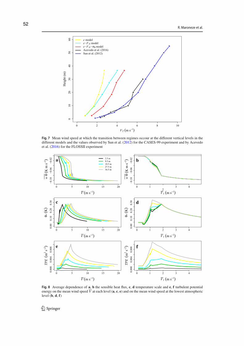
R. Maroneze et al.

0 2 4 6 8 10

010

2030

4050

60

VT (m s−1)

Hei

ght (

m)

e modele−FH modele−FH−σθ modelAcevedo et al. (2016)Sun et al. (2012)

Fig. 7 Mean wind speed at which the transition between regimes occour at the different vertical levels in thedifferent models and the values observed by Sun et al. (2012) for the CASES-99 experiment and by Acevedoet al. (2016) for the FLOSSII experiment

V (m s−1)

w θ

(Km

s−1) a 2.5 m

9.5 m18.5 m27.5 m36.5 m

0 5 10 15 20 0 12

3 4

V1 (m s−1)

w θ

(Km

s−1) b

V (m s−1)

θ *(K

)

c

0 5 10 15 20 0 1 2 3 4

V1 (m s−1)

θ *(K

)

d

−0.1

0−0

.06

−0.0

2

−0.1

0−0

.06

−0.0

2

0.00

0.10

0.20

0.30

0.00

0.10

0.20

0.30

0.00

00.

004

0.00

8

V (m s−1)

TPE

(m2

s−2) e

0 5 10 15 20 0 1 2 3 40.00

00.

004

0.00

8

V1 (m s−1)

TPE

(m2

s−2) f

Fig. 8 Average dependence of a, b the sensible heat flux, c, d temperature scale and e, f turbulent potentialenergy on the mean wind speed V at each level (a, c, e) and on the mean wind speed at the lowest atmosphericlevel (b, d, f)

123

52

Simulating the Regime Transition of the Stable Boundary…

parametrized. This result confirms the role of heat fluxes in determining the regime transitionfound in previous studies. For example, van de Wiel et al. (2012a) associated the thresholdwind speed with the maximum downward heat flux through the surface energy balance; Sunet al. (2016) found the small increase of TKE with wind speed in the weak-wind regime withthe heat flux through its effect on turbulent potential energy; Acevedo et al. (2016) showedthat the buoyant destruction is relatively much more important to the TKE budget in theweak-wind than in the strong-wind regime.

The present study further demonstrates that the strong-wind regime is approximately inde-pendent of heat fluxes and can be achieved regardless of the number of prognostic equationsbeing used and whether or not the buoyant term is included in the TKE budget equation.Therefore, in the strong-wind regime the turbulent flow is mainly driven by shear productionand dissipation, while in the weak-wind regime, complex variations of the turbulent vari-ables are controlled by heat fluxes. In addition, the observed increase of TKE with meanwind speed in the weak-wind regime can only be simulated when the prognostic equation fortemperature variance is included. Future studies may address the question whether additionalprognostic equations further improve the representation of the weak-wind regime.

Turbulence schemes used in numerical weather and climate models are either first-order,in which case they solve prognostic equations for mean variables and parametrize all higher-order moments, or they are TKE models, for which the only higher-order moment solved isTKE (Cuxart et al. 2006; Svensson et al. 2011). These are equivalent to the Mellor–Yamada1-, 2- and 2.5-levelmodels.We have shown that inclusion of an additional prognostic equationfor heat fluxes can directly solve the effects of heat transfer on atmospheric motions so thatstability functions, which are empirically developed based on simple similarity theories,are no longer required. In addition, the transition between the two stability regimes can besimulated more realistically. Considering current difficulties current performing numericalweather prediction of the SBL especially in the weak-wind (stable) regime (Battisti et al.2017), the addition of prognostic equations for heat transfer may be highly beneficial fortheir performance.

Acknowledgements The study was supported by Conselho Nacional de Desenvolvimento Científico e Tec-nológico (CNPq) (Grant No. 307024/2017-2) and by Coordenação de Aperfeiçoamento de Pessoal de NívelSuperior (CAPES).

References

Acevedo OC, Fitzjarrald DR (2003) In the core of the night-effects of intermittent mixing on a horizontallyheterogeneous surface. Boundary-Layer Meteorol 106(1):1–33

Acevedo OC, Costa FD, Degrazia GA (2012) The coupling state of an idealized stable boundary layer.Boundary-Layer Meteorol 145(1):211–228

Acevedo OC, Costa FD, Oliveira PE, Puhales FS, Degrazia GA, Roberti DR (2014) The influence of submesoprocesses on stable boundary layer similarity relationships. J Atmos Sci 71(1):207–225

Acevedo OC, Mahrt L, Puhales FS, Costa FD, Medeiros LE, Degrazia GA (2016) Contrasting structuresbetween the decoupled and coupled states of the stable boundary layer. Q JRMeteorol Soc 142(695):693–702. https://doi.org/10.1002/qj.2693

André J, De Moor G, Lacarrere P, Du Vachat R (1978) Modeling the 24-hour evolution of the mean andturbulent structures of the planetary boundary layer. J Atmos Sci 35(10):1861–1883

Battisti A, Acevedo OC, Costa FD, Puhales FS, Anabor V, Degrazia GA (2017) Evaluation of nocturnaltemperature forecasts provided by the weather research and forecast model for different stability regimesand terrain characteristics. Boundary-Layer Meteorol 162(3):523–546

Blackadar A (1979) High resolution models of the planetary boundary layer. Adv Environ Sci Eng 1(1):50–85

123

53

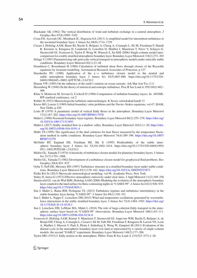
R. Maroneze et al.

Blackadar AK (1962) The vertical distribution of wind and turbulent exchange in a neutral atmosphere. JGeophys Res 67(8):3095–3102

Costa FD, Acevedo OC, Mombach JC, Degrazia GA (2011) A simplified model for intermittent turbulence inthe nocturnal boundary layer. J Atmos Sci 68(8):1714–1729

Cuxart J, Holtslag AAM, Beare RJ, Bazile E, Beljaars A, Cheng A, Conangla L, Ek M, Freedman F, HamdiR, Kerstein A, Kitagawa H, Lenderink G, Lewellen D, Mailhot J, Mauritsen T, Perov V, Schayes G,Steeneveld GJ, Svensson G, Taylor P, Weng W, Wunsch S, Xu KM (2006) Single-column model inter-comparison for a stably stratified atmospheric boundary layer. Boundary-LayerMeteorol 118(2):273–303

Delage Y (1997) Parameterising sub-grid scale vertical transport in atmospheric models under statically stableconditions. Boundary-Layer Meteorol 82(1):23–48

Donaldson C, Rosenbaum H (1968) Calculation of turbulent shear flows through closure of the Reynoldsequations by invariant modelling. Aeronautical Research Associates of Princeton, p 127

Duynkerke PG (1988) Application of the e−ε turbulence closure model to the neutral andstable atmospheric boundary layer. J Atmos Sci 45(5):865–880. https://doi.org/10.1175/1520-0469(1988)045<0865:AOTTCM>2.0.CO;2

Ekman VW (1905) On the influence of the earth’s rotation on ocean currents. Ark Mat Astr Fys 2:11HeisenbergW (1948) On the theory of statistical and isotropic turbulence. Proc R Soc Lond A 195(1042):402–

406Kline S, Morkovin M, Sovran G, Cockrell D (1968) Computation of turbulent boundary layers. In: AFOSR-

IFP-stanford conference, vol 2Köhler H (1933) Meteorologische turbulenz untersuchungen. K Seven vetenskakad handl 13Kreiss HO, Lorenz J (1989) Initial-boundary value problems and the Navier–Stokes equations, vol 47. SIAM,

New Delhi, p 420Louis JF (1979) A parametric model of vertical Eddy fluxes in the atmosphere. Boundary-Layer Meteorol

17(2):187–202. https://doi.org/10.1007/BF00117978Mahrt L (1998) Nocturnal boundary-layer regimes. Boundary-LayerMeteorol 88(2):255–278. https://doi.org/

10.1023/A:1001171313493Mahrt L (2017) Stably stratified flow in a shallow valley. Boundary-Layer Meteorol 162(1):1–20. https://doi.

org/10.1007/s10546-016-0191-4Malhi YS (1995) The significance of the dual solutions for heat fluxes measured by the temperature fluctu-

ation method in stable conditions. Boundary-Layer Meteorol 74(4):389–396. https://doi.org/10.1007/BF00712379

McNider RT, England DE, Friedman MJ, Shi X (1995) Predictability of the stable atmo-spheric boundary layer. J Atmos Sci 52(10):1602–1614. https://doi.org/10.1175/1520-0469(1995)052<1602:POTSAB>2.0.CO;2

Mellor GL, Yamada T (1974) A hierarchy of turbulence closure models for planetary boundary layers. J AtmosSci 31(7):1791–1806

Mellor GL, Yamada T (1982) Development of a turbulence closure model for geophysical fluid problems. RevGeophys 20(4):851–875

Oyha Y, Neff DE, Meroney RN (1997) Turbulence structure in a stratified boundary layer under stable condi-tions. Boundary-Layer Meteorol 83(1):139–162. https://doi.org/10.1023/A:1000205523873

Pielke RA Sr (2013) Mesoscale meteorological modeling, vol 98. Academic Press, New YorkStaley D, Jurica G (1972) Effective atmospheric emissivity under clear skies. J Appl Meteorol 11(2):349–356Steeneveld GJ, van de Wiel BJH, Holtslag AAM (2006) Modeling the evolution of the atmospheric boundary

layer coupled to the land surface for three contrasting nights in “CASES-99”. J Atmos Sci 63(3):920–935.https://doi.org/10.1175/JAS3654.1

Sun J, Mahrt L, Banta RM, Pichugina YL (2012) Turbulence regimes and turbulence intermittency in thestable boundary layer during “CASES-99”. J Atmos Sci 69(1):338–351

Sun J, Mahrt L, Nappo C, Lenschow DH (2015) Wind and temperature oscillations generated by waveturbu-lence interactions in the stably stratified boundary layer. J Atmos Sci 72(4):1484–1503. https://doi.org/10.1175/JAS-D-14-0129.1

Sun J, Lenschow DH, LeMone MA, Mahrt L (2016) The role of large-coherent-Eddy transport in the atmo-spheric surface layer based on “CASES-99” observations. Boundary-Layer Meteorol 160(1):83–111.https://doi.org/10.1007/s10546-016-0134-0

Svensson G, Holtslag AAM, Kumar V, Mauritsen T, Steeneveld GJ, Angevine WM, Bazile E, Beljaars A, deBruijn EIF, Cheng A, Conangla L, Cuxart J, Ek M, Falk MJ, Freedman F, Kitagawa H, Larson VE, LockA, Mailhot J, Masson V, Park S, Pleim J, Söderberg S, Weng W, Zampieri M (2011) Evaluation of thediurnal cycle in the atmospheric boundary layer over land as represented by a variety of single-columnmodels: the second “GABLS” experiment. Boundary-Layer Meteorol 140(2):177–206

Taylor MG (1915) I: Eddy motion in the atmosphere. Philos Trans R Soc Lond A 215(523–537):1–26

123

54

Simulating the Regime Transition of the Stable Boundary…

Therry G, Lacarrere P (1983) Improving the Eddy kinetic energy model for planetary boundary layer descrip-tion. Boundary-Layer Meteorol 25(1):63–88. https://doi.org/10.1007/BF00122098

van Hooijdonk IGS, Donda JMM, Clercx HJH, Bosveld FC, van de Wiel BJH (2015) Shear capacity asprognostic for nocturnal boundary layer regimes. J Atmos Sci 72(4):1518–1532. https://doi.org/10.1175/JAS-D-14-0140.1

van der Linden SJA, Baas P, van Hooft JA, van Hooijdonk IGS, Bosveld FC, van de Wiel BJH (2017) Localcharacteristics of the nocturnal boundary layer in response to external pressure forcing. J Appl MeteorolClim 56(11):3035–3047. https://doi.org/10.1175/JAMC-D-17-0011.1

van de Wiel B, Ronda R, Moene A, De Bruin H, Holtslag A (2002) Intermittent turbulence and oscillations inthe stable boundary layer over land “part I”: a bulk model. J Atmos Sci 59(5):942–958

van de Wiel BJH, Moene AF, Jonker HJJ, Baas P, Basu S, Donda JMM, Sun J, Holtslag AAM (2012a)The minimum wind speed for sustainable turbulence in the nocturnal boundary layer. J Atmos Sci69(11):3116–3127. https://doi.org/10.1175/JAS-D-12-0107.1

van de Wiel BJH, Moene AF, Jonker HJJ (2012b) The cessation of continuous turbulence as precursor of thevery stable nocturnal boundary layer. J Atmos Sci 69(11):3097–3115. https://doi.org/10.1175/JAS-D-12-064.1

Wyngaard JC (1975) Modeling the planetary boundary layer: extension to the stable case. Boundary-LayerMeteorol 9(4):441–460. https://doi.org/10.1007/BF00223393

Wyngaard JC, Coté O (1974) The evolution of a convective planetary boundary layera higher-order-closuremodel study. Boundary-Layer Meteorol 7(3):289–308

Xu D, Taylor PA (1997) On turbulence closure constants for atmospheric boundary-layer modelling: neutralstratification. Boundary-Layer Meteorol 84(2):267–287

123

55

56

Received: 26 March 2019 Revised: 1 August 2019 Accepted: 7 August 2019

DOI: 10.1002/qj.3642

R E S E A R C H A R T I C L E

The nocturnal boundary layer transition from weakly to verystable. Part I: Observations

Otávio C. Acevedo1 Rafael Maroneze1 Felipe D. Costa2 Franciano S. Puhales1

Gervásio A. Degrazia1 Luis G. Nogueira Martins1 Pablo E. Soares de Oliveira1 Luca Mortarini1,3

1Department of Physics, Universidade

Federal de Santa Maria, Santa Maria, Brazil

2Universidade Federal do Pampa, Alegrete,

Brazil

3Institute of Atmospheric Sciences and

Climate - National Research Council, Turin,

Italy

CorrespondenceOtávio C. Acevedo, Departamento de Física,

Universidade Federal de Santa Maria, Santa

Maria, RS 97105-900, Brazil.

Email: otavio@ufsm.br

AbstractThe nocturnal boundary-layer regime transition from weakly stable (strong wind)

to very stable (weak wind) is analyzed using 10 levels of turbulence observations

made at a 140 m micrometeorological mast near the southeastern Brazilian coast.

The combination of synoptic and local flow favors the systematic occurrence of

such a transition, typically 5 to 7 h after sunset. The regime transition is marked by

decreases in temperature, wind speed, turbulent kinetic energy (TKE) and absolute

heat flux. The decrease in temperature is often abrupt and the inflection point in the

temperature series marks the regime transition. Absolute heat flux peaks before the

transition during the weakly stable period, while temperature variance peaks near

the transition. Composites from 36 cases when the cooling rate exceeded 2 ◦C/h are

used to describe the vertical structure of the stable boundary layer (SBL) in both

regimes. For these abrupt transitions, dimensionless variables that relate thermal and

mechanical properties of the flow are compared as indicators of the SBL regime,

and the gradient Richardson number is found to be better for that purpose. The abso-

lute heat flux is shown to be proportional to the cube of the wind speed only in the

strong wind limit of the very stable regime. Simulations of similar transitions using

a second-order model are described in Part II.

K E Y W O R D Sheat flux, regime transitions, stable boundary layer, very stable regime, weakly stable regime

1 INTRODUCTION

The stable boundary layer (SBL) has been characterized as

a two-regime system by a number of studies in recent years.

Since Mahrt et al. (1998), the two regimes have been referred

to as weakly stable and very stable, and they also suggested

there should be a transitional regime between the two. In

terms of numerical modeling, McNider et al. (1995) showed

that a very simplified two-layer scheme that represents the

exchange between the surface and the SBL is also bi-stable.

Along these lines of identifying two contrastingly different

regimes of the SBL, Van de Wiel et al. (2003) identified that

there are situations when the occurrence of intermittency is

favored, while in others turbulence remains fully developed.

The former may be associated with the very stable regime

and the latter with the weakly stable regime. This classifica-

tion has been corroborated numerically by Costa et al. (2011),

who showed that surface-generated intermittent turbulence

may arise in a simplified model, but only in the very stable

regime.

More recently, different studies have shown that there is

a wind speed threshold that triggers the transition between

the two regimes, so that the very stable regime has been

also called the weak-wind regime, and the weakly stable

Q J R Meteorol Soc. 2019;1–16. wileyonlinelibrary.com/journal/qj © 2019 Royal Meteorological Society 1

4 ARTIGO 2 - THE NOCTURNAL BOUNDARY LAYER TRANSITION FROM WEAKLY

TO VERY STABLE. PART I: OBSERVATIONS

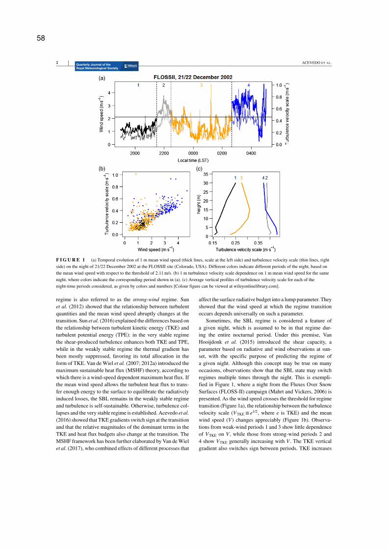
2 ACEVEDO ET AL.

F I G U R E 1 (a) Temporal evolution of 1 m mean wind speed (thick lines, scale at the left side) and turbulence velocity scale (thin lines, right

side) on the night of 21/22 December 2002 at the FLOSSII site (Colorado, USA). Different colors indicate different periods of the night, based on

the mean wind speed with respect to the threshold of 2.11 m/s. (b) 1 m turbulence velocity scale dependence on 1 m mean wind speed for the same

night, where colors indicate the corresponding period shown in (a). (c) Average vertical profiles of turbulence velocity scale for each of the

night-time periods considered, as given by colors and numbers [Colour figure can be viewed at wileyonlinelibrary.com].

regime is also referred to as the strong-wind regime. Sun

et al. (2012) showed that the relationship between turbulent

quantities and the mean wind speed abruptly changes at the

transition. Sun et al. (2016) explained the differences based on

the relationship between turbulent kinetic energy (TKE) and

turbulent potential energy (TPE): in the very stable regime

the shear-produced turbulence enhances both TKE and TPE,

while in the weakly stable regime the thermal gradient has

been mostly suppressed, favoring its total allocation in the

form of TKE. Van de Wiel et al. (2007; 2012a) introduced the

maximum sustainable heat flux (MSHF) theory, according to

which there is a wind-speed dependent maximum heat flux. If

the mean wind speed allows the turbulent heat flux to trans-

fer enough energy to the surface to equilibrate the radiatively

induced losses, the SBL remains in the weakly stable regime

and turbulence is self-sustainable. Otherwise, turbulence col-

lapses and the very stable regime is established. Acevedo et al.(2016) showed that TKE gradients switch sign at the transition

and that the relative magnitudes of the dominant terms in the

TKE and heat flux budgets also change at the transition. The

MSHF framework has been further elaborated by Van de Wiel

et al. (2017), who combined effects of different processes that

affect the surface radiative budget into a lump parameter. They

showed that the wind speed at which the regime transition

occurs depends universally on such a parameter.

Sometimes, the SBL regime is considered a feature of

a given night, which is assumed to be in that regime dur-

ing the entire nocturnal period. Under this premise, Van

Hooijdonk et al. (2015) introduced the shear capacity, a

parameter based on radiative and wind observations at sun-

set, with the specific purpose of predicting the regime of

a given night. Although this concept may be true on many

occasions, observations show that the SBL state may switch

regimes multiple times through the night. This is exempli-

fied in Figure 1, where a night from the Fluxes Over Snow

Surfaces (FLOSS-II) campaign (Mahrt and Vickers, 2006) is

presented. As the wind speed crosses the threshold for regime

transition (Figure 1a), the relationship between the turbulence

velocity scale (VTKE ≡ e1/2, where e is TKE) and the mean

wind speed (V) changes appreciably (Figure 1b). Observa-

tions from weak-wind periods 1 and 3 show little dependence

of VTKE on V , while those from strong-wind periods 2 and

4 show VTKE generally increasing with V . The TKE vertical

gradient also switches sign between periods. TKE increases

58

ACEVEDO ET AL. 3

with height in the very stable periods and decreases with

height in the weakly stable ones (Figure 1c).

Although previous studies, such as those by Sun et al.(2012; 2015; 2016), Van de Wiel et al. (2012a; 2012b; 2017)

and Van Hooijdonk et al. (2015) provide explanations on the

physical controls of the mean wind speed for the SBL regime,

there are still many doubts regarding the triggering of the tran-

sition and how the vertical structure of the SBL changes from

one to the other regime. Detailed observations of such transi-

tions offer a good opportunity to understand why there are two

contrasting regimes in the SBL, but it is crucial that the timing

of the transition is precisely determined in such an analysis.

In the present study, we look at observations made at a 140 m

micrometeorological tower in southeastern Brazil, equipped

with 11 turbulence observation levels (Acevedo et al., 2018).

A very systematic pattern of progressive increase in static sta-

bility through the night is observed at the site when large-scale

northerly winds prevail. In this situation, the first hours of the

night are always weakly stable, while the latest portions are

systematically in the very stable regime. Moreover, in most

cases the transition between the two regimes is abrupt, marked

by an intense cooling that may reach more than 1 ◦C over

10 min, causing a temperature inflection point. The present

study aims at describing these occurrences, looking at the

vertical structure of mean and turbulent quantities before and

after the transition. In a companion article (Maroneze et al.,2019), similar transitions from the weakly to the very stable

regime are simulated using a second-order model for the SBL.

Therefore, this first part, based on observations, is primarily

descriptive of the SBL state in each of the regimes and dur-

ing the transition between them. The second part (Maroneze

et al., 2019) is primarily explanatory, addressing the budgets

of the second-order moments as well as the role of external

forcings.

2 OBSERVATIONS

The observations used in the study have been performed at

a 140 m micrometeorological mast in southeastern Brazil

(Acevedo et al., 2018), between August 2016 and June 2017.

There were initially 11 levels of turbulence observations, at

the heights of 1, 2, 5, 9, 20, 37, 56, 75, 94, 113 and 132 m

from the ground. They were made with sonic anemometers

CSAT3B, from Campbell Sci., Inc. at all levels, except for

20 m, where an Infrared Gas Analyser and Sonic Anemome-

ter (IRGASON) was used. The 1 m CSAT3B was removed

in December 2016, and because of that the 2 m level is used

in this article as a reference for observations near the ground.

The IRGASON data failed in January 2017, so the data from

20 m are only used until that date.

Statistical moments of the quantities sampled by the sonic

anemometer are determined for 1-minute data windows. The

choice of a small data window follows recent practice in SBL

studies (Mahrt et al., 2013; Acevedo et al., 2016; Stiper-

ski et al., 2019) and is chosen to avoid contamination from

low-frequency fluctuations, especially in the horizontal wind

components and vertical fluxes.

The tower is located next to a thermal power plant, at

4 km from the coastline. Roughness elements near the tower

consist of a group of 9 m trees to the east, and the power

plant buildings, about 150 m to the south. When mean winds

are southerly, they flow past the plant before reaching the

tower, largely affecting both turbulence and thermal struc-

ture (Acevedo et al., 2018). For this reason, in the present

study only nights when the mean wind speed had constantly

a northerly component have been used. This is the dominant

wind direction in post-frontal situations, so that a total of 113

nights with such a condition are available. The main focus of

the study is the commonly observed nocturnal transition from

the weakly to the very stable regime. It is a systematic feature

at the site on nights when the large-scale flow has a northerly

meridional component. As will be shown in section 4, the

transition is initiated by a mean wind speed that decreases

steadily in magnitude at higher levels. This is a combination

between a northerly synoptic flow (Figure 2), that keeps the

meridional component of the mean wind at the top of the

tower roughly constant throughout the night (Figure 3, black

line), and a varying sea-breeze component in the zonal direc-

tion (Figure 3, blue line), characterized by offshore flow in

the afternoon that steadily decreases in magnitude, eventually

switching to onshore in the middle of the night.

3 CASE-STUDIES

A typical transition from the weakly to the very stable regime

occurred on the night of 31 December 2016 (Figure 4). The

transition happened between 2300 and 0000 LST (UTC – 3

h), when the 2 m temperature dropped 2 ◦C over 1 h. Fur-

ther cooling followed, but at a slower rate. Besides the sharp

surface decreases in mean wind speed (Figure 4a), temper-

ature (Figure 4b), TKE (Figure 4c) and absolute heat flux

(Figure 4d), the two regimes have contrasting vertical struc-

tures. A strong thermal stratification only sets up after the

transition (Figure 4b), and although the entire tower layer

cools faster after the transition than it does before it, the cool-

ing is appreciably larger at the lowest 20 m than above these

levels. Episodes of enhanced heat flux occur intermittently

in the very stable regime both near the surface and at higher

levels (Figure 4d).

Similar transitions occur in most of the nights when the

large-scale winds have a northerly component, characteris-

tic of post-frontal situations. However, some aspects of the

transition may differ largely among the different nights. It

may occur earlier, such as is the case in Figure 5a, when it

happened near 2100 LST, or later, as in Figure 5b, when it

59

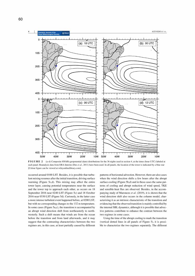
4 ACEVEDO ET AL.

F I G U R E 2 (a–d) Composite 850 hPa geopotential (dam) distributions for the 36 nights used in section 4, at the times (hour UTC) labeled at

each panel. Reanalysis data from ERA-Interim (Dee et al., 2011) have been used. In all panels, the location of the tower is indicated by a blue star

[Colour figure can be viewed at wileyonlinelibrary.com].

occurred around 0100 LST. Besides, it is possible that turbu-

lent mixing resumes after the initial transition, driving surface

warming (Figure 5c,d). This mixing may affect the entire

tower layer, causing potential temperatures near the surface

and the tower top to approach each other, as occurs on 18

September 2016 near 0240 LST (Figure 5c) and 18 October

2016 near 0330 LST (Figure 5d). Curiously, in the latter case

a more intense turbulent event happened before, at 0200 LST,

but with no corresponding changes to the 132 m temperature.

In some cases (Figure 5a,c), the transition is accompanied by

an abrupt wind direction shift from northeasterly to north-

westerly. Such a shift means that winds are from the ocean

before the transition and from land afterwards, and it may

suggest that the contrasting characteristics between the two

regimes are, in this case, at least partially caused by different

patterns of horizontal advection. However, there are also cases

when the wind direction shifts a few hours after the abrupt

surface cooling (Figure 5b,d) and in these cases the same pat-

terns of cooling and abrupt reduction of wind speed, TKE

and sensible-heat flux are observed. Besides, in the accom-

panying study of Maroneze et al. (2019), it is shown that the

wind direction shift also occurs in the column model, char-

acterizing it as an intrinsic characteristic of the transition and

evidencing that the observed transition is mainly controlled by

the internal SBL dynamics, although it is possible that advec-

tive patterns contribute to enhance the contrast between the

two regimes in some cases.

Using the time of the abrupt cooling to mark the transition

(vertical dotted lines in all panels of Figure 5), it is possi-

ble to characterize the two regimes separately. The different

60

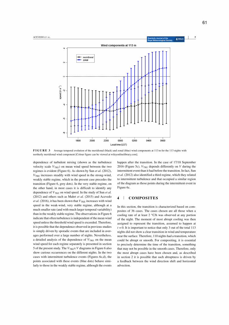
ACEVEDO ET AL. 5

F I G U R E 3 Average temporal evolution of the meridional (black) and zonal (blue) wind components at 113 m for the 113 nights with

northerly meridional wind component [Colour figure can be viewed at wileyonlinelibrary.com].

dependence of turbulent mixing (shown as the turbulence

velocity scale VTKE) on mean wind speed between the two

regimes is evident (Figure 6). As shown by Sun et al. (2012),

VTKE increases steadily with wind speed in the strong-wind,

weakly stable regime, which in the present case precedes the

transition (Figure 6, grey dots). In the very stable regime, on

the other hand, in most cases it is difficult to identify any

dependence of VTKE on wind speed. In the study of Sun et al.(2012) and others such as Mahrt et al. (2015) and Acevedo

et al. (2016), it has been shown that VTKE increases with wind

speed in the weak-wind, very stable regime, although at a

much smaller rate (and with much larger temporal variability)

than in the weakly stable regime. The observations in Figure 6

indicate that often turbulence is independent of the mean wind

speed unless the threshold wind speed is exceeded. Therefore,

it is possible that the dependence observed in previous studies

is simply driven by sporadic events that are included in aver-

ages performed over a large number of nights. Nevertheless,

a detailed analysis of the dependence of VTKE on the mean

wind speed for each regime separately is presented in section

5 of the present study. The VTKEx V diagrams in Figure 6 also

show curious occurrences on the different nights. In the two

cases with intermittent turbulence events (Figures 6c,d), the

points associated with these events (blue dots) behave simi-

larly to those in the weakly stable regime, although the events

happen after the transition. In the case of 17/18 September

2016 (Figure 5c), VTKE depends differently on V during the

intermittent event than it had before the transition. In fact, Sun

et al. (2012) also identified a third regime, which they related

to intermittent turbulence and that occupied a similar region

of the diagram as those points during the intermittent event in

Figure 6c.

4 COMPOSITES

In this section, the transition is characterized based on com-

posites of 36 cases. The cases chosen are all those when a

cooling rate of at least 2 ◦C/h was observed at any portion

of the night. The moment of most abrupt cooling was then

assigned to represent the transition, assumed to happen at

t = 0. It is important to notice that only 3 out of the total 113

nights did not show a clear transition in wind and temperature

near the surface. Therefore, 110 nights had a transition, which

could be abrupt or smooth. For compositing, it is essential

to precisely determine the time of the transition, something

that may not be possible in the smooth cases. Therefore, only

the most abrupt cases have been chosen and, as described

in section 2 it is possible that such abruptness is driven by

a feedback between the wind direction shift and horizontal

advection.

61

6 ACEVEDO ET AL.

0.9 1.9 2.8 3.8

4.7

5.7

6.6

7.6

7.6

8.5

8.5

9.5

2000 2200 0000 0200 0400

20

40

60

80

100

120

Wind speed (m s- 1

)

Local time (LST)

(a) (b)

(c) (b)

heig

ht (m

)a

241

25.3

25.9

26.5

27.

1

27.

7

28.3

28.3

28.9

2000 2200 0000 0200 0400

20

40

60

80

100

120

Potential temperature (C)

Local time (LST)

heig

ht (m

)

b

0.0

7

0.0

7

0.1

4

0.21

0.28

0.35

0.43

0.5

0.5

0.5

0

.5

0.5

7

0.6

4

2000 2200 0000 0200 0400

20

40

60

80

100

120

Local time (LST)

heig

ht (m

)

c

−19.6

−17.3

−17.3

−15.1

−

12.8

−

12.8

−12.8

−12.8

−10.6

−8.3

−6.1

−6.1

−3.8

−3.8

−1.6

−

1.6

−1.6

−

1.6

−1.6

2000 2200 0000 0200 0400

20

40

60

80

100

120

Heat flux (W m- 2

)Turbulent kinetic energy (m2 2 s

-)

Local time (LST)

heig

ht (m

)

d

F I G U R E 4 Nocturnal evolution of (a) mean wind speed, (b) potential temperature, (c) TKE and (d) heat flux, at all levels on the night of 31

December 2016/1 January 2017 [Colour figure can be viewed at wileyonlinelibrary.com].

The composites are averages of 10-hour time windows,

from 5 h before to 5 h after the transition, over the 36 nights.

Transitions have been found to occur as early in the night as

2037 LST and as late as 0210 LST but the vast majority (27

out of 36) happened between 2300 and 0100 LST.

Typically, temperature, mean wind speed and TKE all

decrease near the surface in the strong-wind (weakly sta-

ble) period that precedes the transition (Figure 7a). The rate

of decrease of all these quantities in the first 4.5 h of the

composites is appreciably smaller than what is observed in

the hour centered at the time of most abrupt cooling. At the

pre-transition period, mean wind speed, temperature and TKE

are all coupled to each other. The external large-scale forc-

ing drives the mean wind speed decrease, which reduces TKE

shear production and, therefore, TKE itself. At the same time,

radiative loss at the surface cools the surface and the air in

contact with it, by conduction. As TKE and the heat flux are

still intense enough, the air cooled near the surface is trans-

ported to upper levels, over the entire tower layer. The abso-

lute heat flux (−𝑤′𝜃′) peaks about 3 h before the transition,

on average (Figure 7b). It implies that such a maximum hap-

pens in the weakly stable period, when mean wind speed and

temperature are still decaying at a small rate. The initial heat

flux increase in magnitude may be attributed to the fact that

many of the composites start shortly after sunset. In that case,

the absolute heat flux increase is driven by thermal gradi-

ent production (TGP), the term in the heat flux budget that is

proportional to the thermal gradient (which largely increases

after sunset) and to the vertical velocity variance (still large

in the period). At some point, the thermal gradient increase is

62

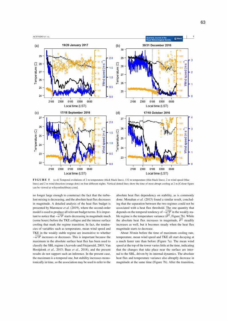
ACEVEDO ET AL. 7

F I G U R E 5 (a–d) Temporal evolutions of 2 m temperature (thick black lines), 132 m temperature (thin black lines), 2 m wind speed (blue

lines) and 2 m wind direction (orange dots) on four different nights. Vertical dotted lines show the time of most abrupt cooling at 2 m [Colour figure

can be viewed at wileyonlinelibrary.com].

no longer large enough to counteract the fact that the turbu-

lent mixing is decreasing, and the absolute heat flux decreases

in magnitude. A detailed analysis of the heat flux budget is

presented by Maroneze et al. (2019), where the second-order

model is used to produce all relevant budget terms. It is impor-

tant to notice that −𝑤′𝜃′ starts decreasing in magnitude much

(some hours) before the TKE collapse and the intense surface

cooling that mark the regime transition. In fact, the tenden-

cies of variables such as temperature, mean wind speed and

TKE in the weakly stable regime are insensitive to whether

−𝑤′𝜃′ increases or decreases. This is important because the

maximum in the absolute surface heat flux has been used to

classify the SBL regime (Acevedo and Fitzjarrald, 2003; Van

Hooijdonk et al., 2015; Baas et al., 2018), and the present

results do not support such an inference. In the present case,

the maximum is a temporal one, but stability increases mono-

tonically in time, so the association may be used to refer to the

absolute heat flux dependency on stability, as is commonly

done. Monahan et al. (2015) found a similar result, conclud-

ing that the separation between the two regimes could not be

associated with a heat flux threshold. The one quantity that

depends on the temporal tendency of −𝑤′𝜃′ in the weakly sta-

ble regime is the temperature variance (𝜃′2, Figure 7b). While

the absolute heat flux increases in magnitude, 𝜃′2 steadily

increases as well, but it becomes steady when the heat flux

magnitude starts to decrease.

About 30 min before the time of maximum cooling rate,

temperature, mean wind speed and TKE all start decaying at

a much faster rate than before (Figure 7a). The mean wind

speed at the top of the tower varies little at the time, indicating

that the changes that take place near the surface are inter-

nal to the SBL, driven by its internal dynamics. The absolute

heat flux and temperature variance also abruptly decrease in

magnitude at the same time (Figure 7b). After the transition,

63

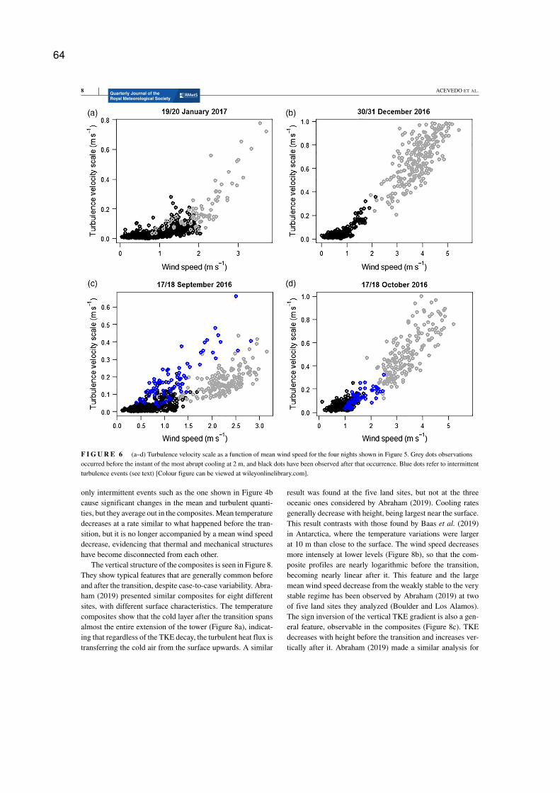
8 ACEVEDO ET AL.

F I G U R E 6 (a–d) Turbulence velocity scale as a function of mean wind speed for the four nights shown in Figure 5. Grey dots observations

occurred before the instant of the most abrupt cooling at 2 m, and black dots have been observed after that occurrence. Blue dots refer to intermittent

turbulence events (see text) [Colour figure can be viewed at wileyonlinelibrary.com].

only intermittent events such as the one shown in Figure 4b

cause significant changes in the mean and turbulent quanti-

ties, but they average out in the composites. Mean temperature

decreases at a rate similar to what happened before the tran-

sition, but it is no longer accompanied by a mean wind speed

decrease, evidencing that thermal and mechanical structures

have become disconnected from each other.

The vertical structure of the composites is seen in Figure 8.

They show typical features that are generally common before

and after the transition, despite case-to-case variability. Abra-

ham (2019) presented similar composites for eight different

sites, with different surface characteristics. The temperature

composites show that the cold layer after the transition spans

almost the entire extension of the tower (Figure 8a), indicat-

ing that regardless of the TKE decay, the turbulent heat flux is

transferring the cold air from the surface upwards. A similar

result was found at the five land sites, but not at the three

oceanic ones considered by Abraham (2019). Cooling rates

generally decrease with height, being largest near the surface.

This result contrasts with those found by Baas et al. (2019)

in Antarctica, where the temperature variations were larger

at 10 m than close to the surface. The wind speed decreases

more intensely at lower levels (Figure 8b), so that the com-

posite profiles are nearly logarithmic before the transition,

becoming nearly linear after it. This feature and the large

mean wind speed decrease from the weakly stable to the very

stable regime has been observed by Abraham (2019) at two

of five land sites they analyzed (Boulder and Los Alamos).

The sign inversion of the vertical TKE gradient is also a gen-

eral feature, observable in the composites (Figure 8c). TKE

decreases with height before the transition and increases ver-

tically after it. Abraham (2019) made a similar analysis for

64

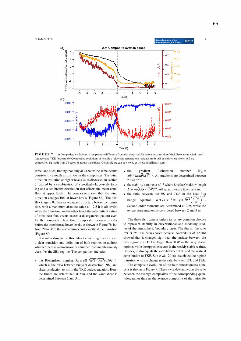
ACEVEDO ET AL. 9

F I G U R E 7 (a) Composited evolutions of temperature difference from that observed 5 h before the transition (black line), mean wind speed

(orange) and TKE (brown); (b) Composited evolutions of heat flux (blue) and temperature variance (red). All quantities are shown at 2 m;

composites are made from 36 cases of abrupt transitions [Colour figure can be viewed at wileyonlinelibrary.com].

three land sites, finding that only at Cabauw the same occurs

consistently enough as to show in the composites. The wind

direction evolution at higher levels is, as discussed in section

2, caused by a combination of a northerly large-scale forc-

ing and a sea-breeze circulation that affects the mean zonal

flow at upper levels. The composite shows that the wind

direction changes first at lower levels (Figure 8d). The heat

flux (Figure 8e) has an organized structure before the transi-

tion, with a maximum absolute value at −2.5 h at all levels.

After the transition, on the other hand, the intermittent nature

of most heat flux events causes a disorganized pattern even

for the composited heat flux. Temperature variance peaks

before the transition at lower levels, as shown in Figure 7b, but

from 20 to 80 m the maximum occurs exactly at the transition

(Figure 8f).

It is interesting to use this dataset consisting of cases with

a clear transition and definition of both regimes to address

whether there is a dimensionless number that unambiguously

classifies the SBL regime. The comparison includes:

• the Richardson number Ri ≡ 𝑔Θ−1𝑤′𝜃′(𝑢′𝑤′𝜕𝑢∕𝜕𝑧)−1,

which is the ratio between buoyant destruction (BD) and

shear production terms in the TKE budget equation. Here,

the fluxes are determined at 2 m, and the wind shear is

determined between 2 and 5 m;

• the gradient Richardson number Rig ≡

𝑔Θ−1Δ𝑧Δ𝜃(Δ𝑉 )−2. All gradients are determined between

2 and 37 m;

• the stability parameter zL−1 where L is the Obukhov length

𝐿 ≡ −𝑢3∗Θ(𝜅𝑔𝑤′𝜃′)−1. All quantities are taken at 2 m;

• the ratio between the BD and TGP in the heat flux

budget equation, 𝐵𝐷 𝑇𝐺𝑃 −1≡ −𝑔Θ−1𝜃′2

(𝑤′2𝜕𝜃

𝜕𝑧

)−1

.

Second-order moments are determined at 2 m, while the

temperature gradient is considered between 2 and 5 m.

The three first dimensionless ratios are common choices

to represent stability in observational and modeling stud-

ies of the atmospheric boundary layer. The fourth, the ratio

BD TGP−1 has been chosen because Acevedo et al. (2016)

showed that it changes sign near the surface between the

two regimes, as BD is larger than TGP in the very stable

regime, while the opposite occurs in the weakly stable regime.

Besides, it also equals the ratio between TPE and the vertical

contribution to TKE. Sun et al. (2016) associated the regime

transition with the change in the ratio between TPE and TKE.

The composite evolution of the four dimensionless num-

bers is shown in Figure 9. These were determined as the ratio

between the average composites of the corresponding quan-

tities, rather than as the average composite of the ratios for

65

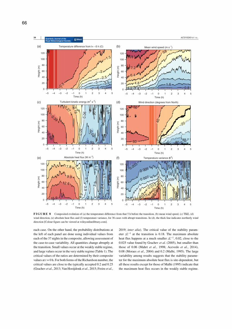
10 ACEVEDO ET AL.

−4 −3.5 −3

−2.5

−2

−1.5 −1

−0.5

0

0

Temperature difference from t= −5 h (C)

0

20

40

60

80

100

120

−5 −4 −3 −2 −1

Time (h)

(a) (b)

(c) (d)

(e) (f)

He

igh

t (m

)

0.8 1.6

2.4 3.2

4 4.8

5.6

6.4

7.2

8

Mean wind speed (m s- 1

)

0

20

40

60

80

100

120

−5 −4 −3 −2 −1 5

Time (h)

He

igh

t (m

)

0.03

0.0

3

0.0

4

0.0

4

0.0

6

0.0

6

0.0

6

0.0

9

0.1

9

0.27

0.39

0.5

6

Turbulent kinetic energy (m2 s

- 2)

0

20

40

60

80

100

120

−5 −4 −3 −2 −1

Time (h)

He

igh

t (m

)

0 0 0

20

40

60

60 60

0 0 0 −80

−60 −40

−20

0

Wind direction (degrees from North)

0

20

40

60

80

100

120

−5 −4 −3 −2 −1 5

Time (h)

He

igh

t (m

)

1.9

2.4

2.4

2

.4

2.4

2

.4

2.4

3.1

3.1

3.1

3.1

3.9

3.9

4.9

6.2 7.8

9.9

12.6

15.9

Absolute heat flux (W m- 2

)

0

20

40

60

80

100

120

−5 −4 −3 −2 −1

Time (h)

He

igh

t (m

)

0.0

03

0.005

0.0

05

0.0

05

0.007 0.009

0.0

09

0.011

0.0

11

0.013

0.0

13

0.015

0.0

19

Temperature variance (K2)

0

20

40

60

80

100

120

−5 −4 −3 −2 −1

0 1 2 3 4 5 0 1 2 3 4

0 1 2 3 4 5 0 1 2 3 4

0 1 2 3 4 5 0 1 2 3 4 5

Time (h)

He

igh

t (m

)

F I G U R E 8 Composited evolution of (a) the temperature difference from that 5 h before the transition, (b) mean wind speed, (c) TKE, (d)

wind direction, (e) absolute heat flux and (f) temperature variance, for 36 cases with abrupt transitions. In (d), the thick line indicates northerly wind

direction [Colour figure can be viewed at wileyonlinelibrary.com].

each case. On the other hand, the probability distributions at

the left of each panel are done using individual values from

each of the 37 nights in the composite, allowing assessment of

the case-to-case variability. All quantities change abruptly at

the transition. Small values occur at the weakly stable regime,

and large values occur in the very stable regime (Table 1). The

critical values of the ratios are determined by their composite

values at t = 0 h. For both forms of the Richardson number, the

critical values are close to the typically accepted 0.2 and 0.25

(Grachev et al., 2013; Van Hooijdonk et al., 2015; Freire et al.,

2019; inter alia). The critical value of the stability param-

eter zL−1 at the transition is 0.18. The maximum absolute

heat flux happens at a much smaller zL−1, 0.02, close to the

0.025 value found by Grachev et al. (2005), but smaller than

those of 0.06 (Mahrt et al., 1998; Acevedo et al., 2014),

0.08 (Moraes et al., 2004) and 0.2 (Malhi, 1995). The large

variability among results suggests that the stability parame-

ter for the maximum absolute heat flux is site-dependent, but

all these results except for those of Malhi (1995) indicate that

the maximum heat flux occurs in the weakly stable regime.

66

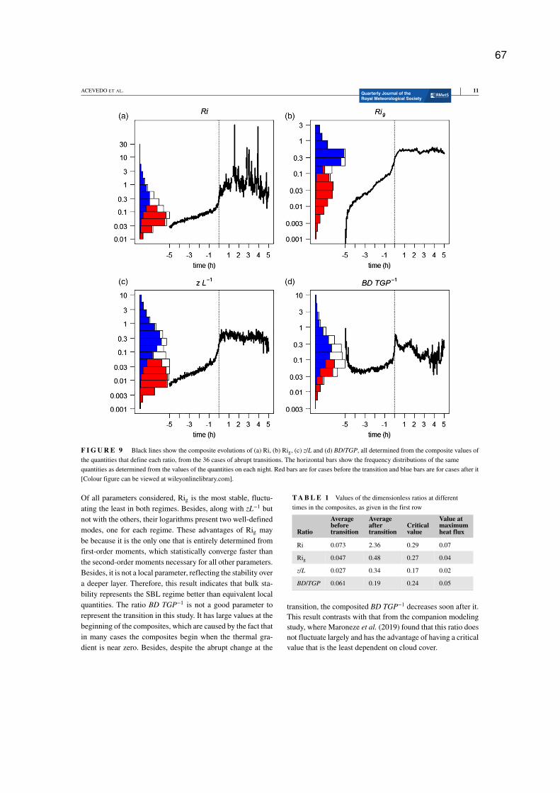
ACEVEDO ET AL. 11

F I G U R E 9 Black lines show the composite evolutions of (a) Ri, (b) Rig, (c) z/L and (d) BD/TGP, all determined from the composite values of

the quantities that define each ratio, from the 36 cases of abrupt transitions. The horizontal bars show the frequency distributions of the same

quantities as determined from the values of the quantities on each night. Red bars are for cases before the transition and blue bars are for cases after it

[Colour figure can be viewed at wileyonlinelibrary.com].

Of all parameters considered, Rig is the most stable, fluctu-

ating the least in both regimes. Besides, along with zL−1 but

not with the others, their logarithms present two well-defined

modes, one for each regime. These advantages of Rig may

be because it is the only one that is entirely determined from

first-order moments, which statistically converge faster than

the second-order moments necessary for all other parameters.

Besides, it is not a local parameter, reflecting the stability over

a deeper layer. Therefore, this result indicates that bulk sta-

bility represents the SBL regime better than equivalent local

quantities. The ratio BD TGP−1 is not a good parameter to

represent the transition in this study. It has large values at the

beginning of the composites, which are caused by the fact that

in many cases the composites begin when the thermal gra-

dient is near zero. Besides, despite the abrupt change at the

T A B L E 1 Values of the dimensionless ratios at different

times in the composites, as given in the first row

Ratio

Averagebeforetransition

Averageaftertransition

Criticalvalue

Value atmaximumheat flux

Ri 0.073 2.36 0.29 0.07

Rig 0.047 0.48 0.27 0.04

z/L 0.027 0.34 0.17 0.02

BD/TGP 0.061 0.19 0.24 0.05

transition, the composited BD TGP−1 decreases soon after it.

This result contrasts with that from the companion modeling

study, where Maroneze et al. (2019) found that this ratio does

not fluctuate largely and has the advantage of having a critical

value that is the least dependent on cloud cover.

67

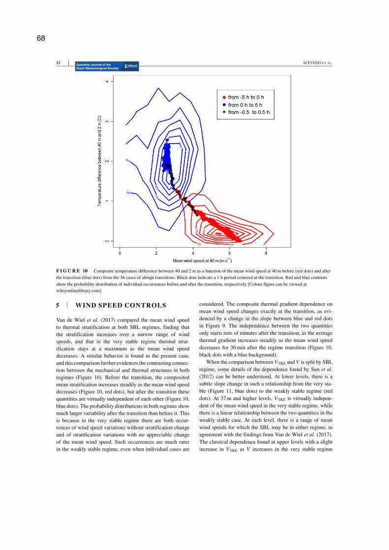
12 ACEVEDO ET AL.

F I G U R E 10 Composite temperature difference between 40 and 2 m as a function of the mean wind speed at 40 m before (red dots) and after

the transition (blue dots) from the 36 cases of abrupt transitions. Black dots indicate a 1 h period centered at the transition. Red and blue contours

show the probability distribution of individual occurrences before and after the transition, respectively [Colour figure can be viewed at

wileyonlinelibrary.com].

5 WIND SPEED CONTROLS

Van de Wiel et al. (2017) compared the mean wind speed

to thermal stratification at both SBL regimes, finding that

the stratification increases over a narrow range of wind

speeds, and that in the very stable regime thermal strat-

ification stays at a maximum as the mean wind speed

decreases. A similar behavior is found in the present case,

and this comparison further evidences the contrasting connec-

tion between the mechanical and thermal structures in both

regimes (Figure 10). Before the transition, the composited

mean stratification increases steadily as the mean wind speed

decreases (Figure 10, red dots), but after the transition these

quantities are virtually independent of each other (Figure 10,

blue dots). The probability distributions in both regimes show

much larger variability after the transition than before it. This

is because in the very stable regime there are both occur-

rences of wind speed variations without stratification change

and of stratification variations with no appreciable change

of the mean wind speed. Such occurrences are much rarer

in the weakly stable regime, even when individual cases are

considered. The composite thermal gradient dependence on

mean wind speed changes exactly at the transition, as evi-

denced by a change in the slope between blue and red dots

in Figure 9. The independence between the two quantities

only starts tens of minutes after the transition, as the average

thermal gradient increases steadily as the mean wind speed

decreases for 30 min after the regime transition (Figure 10,

black dots with a blue background).

When the comparison between VTKE and V is split by SBL

regime, some details of the dependence found by Sun et al.(2012) can be better understood. At lower levels, there is a

subtle slope change in such a relationship from the very sta-

ble (Figure 11, blue dots) to the weakly stable regime (red

dots). At 37 m and higher levels, VTKE is virtually indepen-

dent of the mean wind speed in the very stable regime, while

there is a linear relationship between the two quantities in the

weakly stable case. At each level, there is a range of mean

wind speeds for which the SBL may be in either regime, in

agreement with the findings from Van de Wiel et al. (2017).

The classical dependence found at upper levels with a slight

increase in VTKE as V increases in the very stable regime

68

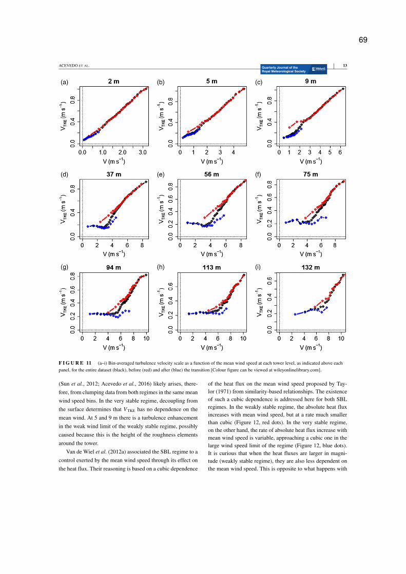
ACEVEDO ET AL. 13

F I G U R E 11 (a–i) Bin-averaged turbulence velocity scale as a function of the mean wind speed at each tower level, as indicated above each

panel, for the entire dataset (black), before (red) and after (blue) the transition [Colour figure can be viewed at wileyonlinelibrary.com].

(Sun et al., 2012; Acevedo et al., 2016) likely arises, there-

fore, from clumping data from both regimes in the same mean

wind speed bins. In the very stable regime, decoupling from

the surface determines that VTKE has no dependence on the

mean wind. At 5 and 9 m there is a turbulence enhancement

in the weak wind limit of the weakly stable regime, possibly

caused because this is the height of the roughness elements

around the tower.

Van de Wiel et al. (2012a) associated the SBL regime to a

control exerted by the mean wind speed through its effect on

the heat flux. Their reasoning is based on a cubic dependence

of the heat flux on the mean wind speed proposed by Tay-

lor (1971) from similarity-based relationships. The existence

of such a cubic dependence is addressed here for both SBL

regimes. In the weakly stable regime, the absolute heat flux

increases with mean wind speed, but at a rate much smaller

than cubic (Figure 12, red dots). In the very stable regime,

on the other hand, the rate of absolute heat flux increase with

mean wind speed is variable, approaching a cubic one in the

large wind speed limit of the regime (Figure 12, blue dots).

It is curious that when the heat fluxes are larger in magni-

tude (weakly stable regime), they are also less dependent on

the mean wind speed. This is opposite to what happens with

69

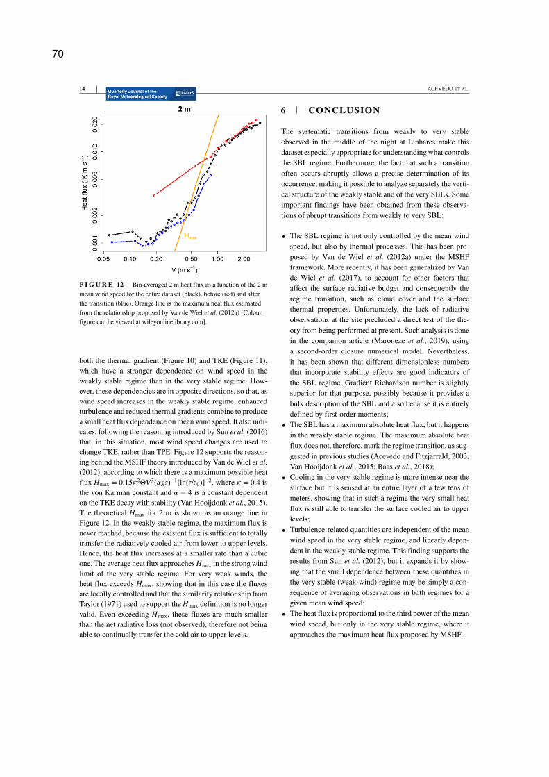
14 ACEVEDO ET AL.

F I G U R E 12 Bin-averaged 2 m heat flux as a function of the 2 m

mean wind speed for the entire dataset (black), before (red) and after

the transition (blue). Orange line is the maximum heat flux estimated

from the relationship proposed by Van de Wiel et al. (2012a) [Colour

figure can be viewed at wileyonlinelibrary.com].

both the thermal gradient (Figure 10) and TKE (Figure 11),

which have a stronger dependence on wind speed in the

weakly stable regime than in the very stable regime. How-

ever, these dependencies are in opposite directions, so that, as

wind speed increases in the weakly stable regime, enhanced

turbulence and reduced thermal gradients combine to produce

a small heat flux dependence on mean wind speed. It also indi-

cates, following the reasoning introduced by Sun et al. (2016)

that, in this situation, most wind speed changes are used to

change TKE, rather than TPE. Figure 12 supports the reason-

ing behind the MSHF theory introduced by Van de Wiel et al.(2012), according to which there is a maximum possible heat

flux Hmax = 0.15𝜅2ΘV3(𝛼gz)−1[ln(z/z0)]−2, where 𝜅 = 0.4 is

the von Karman constant and 𝛼 = 4 is a constant dependent

on the TKE decay with stability (Van Hooijdonk et al., 2015).

The theoretical Hmax for 2 m is shown as an orange line in

Figure 12. In the weakly stable regime, the maximum flux is

never reached, because the existent flux is sufficient to totally

transfer the radiatively cooled air from lower to upper levels.

Hence, the heat flux increases at a smaller rate than a cubic

one. The average heat flux approaches Hmax in the strong wind

limit of the very stable regime. For very weak winds, the

heat flux exceeds Hmax, showing that in this case the fluxes

are locally controlled and that the similarity relationship from

Taylor (1971) used to support the Hmax definition is no longer

valid. Even exceeding Hmax, these fluxes are much smaller

than the net radiative loss (not observed), therefore not being

able to continually transfer the cold air to upper levels.

6 CONCLUSION

The systematic transitions from weakly to very stable

observed in the middle of the night at Linhares make this

dataset especially appropriate for understanding what controls

the SBL regime. Furthermore, the fact that such a transition

often occurs abruptly allows a precise determination of its

occurrence, making it possible to analyze separately the verti-

cal structure of the weakly stable and of the very SBLs. Some

important findings have been obtained from these observa-

tions of abrupt transitions from weakly to very SBL:

• The SBL regime is not only controlled by the mean wind

speed, but also by thermal processes. This has been pro-

posed by Van de Wiel et al. (2012a) under the MSHF

framework. More recently, it has been generalized by Van

de Wiel et al. (2017), to account for other factors that

affect the surface radiative budget and consequently the

regime transition, such as cloud cover and the surface

thermal properties. Unfortunately, the lack of radiative

observations at the site precluded a direct test of the the-

ory from being performed at present. Such analysis is done

in the companion article (Maroneze et al., 2019), using

a second-order closure numerical model. Nevertheless,

it has been shown that different dimensionless numbers

that incorporate stability effects are good indicators of

the SBL regime. Gradient Richardson number is slightly

superior for that purpose, possibly because it provides a

bulk description of the SBL and also because it is entirely

defined by first-order moments;

• The SBL has a maximum absolute heat flux, but it happens

in the weakly stable regime. The maximum absolute heat

flux does not, therefore, mark the regime transition, as sug-

gested in previous studies (Acevedo and Fitzjarrald, 2003;

Van Hooijdonk et al., 2015; Baas et al., 2018);

• Cooling in the very stable regime is more intense near the

surface but it is sensed at an entire layer of a few tens of

meters, showing that in such a regime the very small heat

flux is still able to transfer the surface cooled air to upper

levels;

• Turbulence-related quantities are independent of the mean

wind speed in the very stable regime, and linearly depen-

dent in the weakly stable regime. This finding supports the

results from Sun et al. (2012), but it expands it by show-

ing that the small dependence between these quantities in

the very stable (weak-wind) regime may be simply a con-

sequence of averaging observations in both regimes for a

given mean wind speed;

• The heat flux is proportional to the third power of the mean

wind speed, but only in the very stable regime, where it

approaches the maximum heat flux proposed by MSHF.

70

ACEVEDO ET AL. 15

In a companion article, Maroneze et al. (2019) extend the

present analysis using a second-order model and addressing

aspects that have not been discussed here, such as the role of

cloudiness and surface thermal properties and the budgets of

second-order moments such as turbulence kinetic energy, heat

flux and temperature variance.

Although the systematic occurrence of the weakly to very

stable transition at Linhares make the tower an appropriate

laboratory to study this phenomenon, it is important to notice

that the opposite transition, from very to weakly stable very

rarely occurs there. Therefore, it is still unclear whether there

is hysteresis in this transition and whether it is triggered by

the same external factors found to be important in the present

study. Besides, the fact discussed in the introduction that

multiple transitions often occur in the same night has not

been addressed here either. These are interesting analyses

that may be done in the future, but they will certainly demand

a different dataset.

ACKNOWLEDGEMENTS

The study has been developed within the context of a Research

and Development project sponsored by companies Linhares

Geração S.A. and Termelétrica Viana S.A., and named

“Desenvolvimento de um modelo operacional para simulaçãoem tempo real da dispersão atmosférica de poluentes emiti-dos por termelétrica a gás natural”. The Project is within the

context of the investment programme in Research and Devel-

opment, regulated by Brazilian National Agency for Electric

Energy. The authors thank deeply all support provided by

these companies for the development of the present work. The

study also has been partially supported by Brazilian funding

agencies CNPq and CAPES. The latter funds graduate stud-

ies of the second author. Three anonymous reviewers offered

valuable comments and suggestions.

ORCIDOtávio C. Acevedo https://orcid.org/0000-0003-2606-

4726

Rafael Maroneze https://orcid.org/0000-0002-3025-9676

REFERENCES

Abraham C. (2019) Regime occupation and transition informationobtained from observable meteorological state variables in the sta-bly stratified nocturnal boundary layer. PhD Thesis, University of

Victoria, Victoria, BC, Canada.

Acevedo, O.C., Costa, F.D., Oliveira, P.E.S., Puhales, F.S., Degrazia,

G.A. and Roberti, D.R. (2014) The influence of submeso processes

on stable boundary layer similarity relationships. Journal of theAtmospheric Sciences, 71, 207–225.

Acevedo, O.C., Degrazia, G.A., Puhales, F.S., Martins, L.G.N., Oliveira,

P.E.S., Teichrieb, C.A., Silva, S.M., Maroneze, R., Bodmann, B.,

Mortarini, L., Cava, D. and Anfossi, D. (2018) Monitoring the

micrometeorology of a coastal site next to a thermal power plant

from the surface to 140 m. Bulletin of the American MeteorologicalSociety, 99, 725–738. https://doi.org/10.1175/BAMS-D-17-0134.1.

Acevedo, O.C. and Fitzjarrald, D.R. (2003) In the core of the

night – effects on intermittent mixing on a horizontally heteroge-

neous surface. Boundary-Layer Meteorology, 106, 1–33.

Acevedo, O.C., Mahrt, L., Puhales, F.S., Costa, F.D., Medeiros, L.E. and

Degrazia, G.A. (2016) Contrasting structures between the decoupled

and coupled states of the stable boundary layer. Quarterly Journal ofthe Royal Meteorological Society, 142, 693–702. https://doi.org/10.

1002/qj.2693.

Baas, P., van de Wiel, B.J.H., van der Linden, S.J.A. and Bosveld, F.C.

(2018) From near-neutral to strongly stratified: adequately modelling

the clear-sky nocturnal boundary layer at Cabauw. Boundary-LayerMeteorology, 166, 217–238. https://doi.org/10.1007/s10546-017-

0304-8.

Baas, P., van de Wiel, B.J.H., van Meijgaard, E., Vignon, E., Genthon,

C., van der Linden, S.J.A. and de Roode, S.R. (2019) Transitions

in the wintertime near-surface temperature inversion at Dome C,

Antarctica. Quarterly Journal of the Royal Meteorological Society,

145(720), 930–946. https://doi.org/10.1002/qj.3450.

Costa, F.D., Acevedo, O.C., Mombach, J.C.M. and Degrazia, G.A.

(2011) A simplified model for intermittent turbulence in the noc-

turnal boundary layer. Journal of the Atmospheric Sciences, 68,

1714–1729.

Dee, D.P., Uppala, S.M., Simmons, A.J., Berrisford, P., Poli, P.,

Kobayashi, S., Andrae, U., Balmaseda, M.A., Balsamo, G., Bauer, P.,

Bechtold, P., Beljaars, A.C.M., van de Berg, L., Bidlot, J., Bormann,

N., Delsol, C., Dragani, R., Fuentes, M., Geer, A.J., Haimberger,

L., Healy, S.B., Hersbach, H., Hólm, E.V., Isaksen, L., Kållberg,

P., Köhler, M., Matricardi, M., McNally, A.P., Monge-Sanz, B.M.,

Morcrette, J.J., Park, B.K., Peubey, C., de Rosnay, P., Tavolato, C.,

Thépaut, J.N. and Vitart, F. (2011) The ERA-Interim reanalysis: con-

figuration and performance of the data assimilation system. Quar-terly Journal of the Royal Meteorological Society, 137, 553–597.

https://doi.org/10.1002/qj.828.

Freire, L.S., Chamecki, M., Bou-Zeid, E. and Dias, N.L. (2019) Critical

flux Richardson number for Kolmogorov turbulence enabled by TKE

transport. Quarterly Journal of the Royal Meteorological Society,

145(721), 1551–1558. https://doi.org/10.1002/qj.3511.

Grachev, A.A., Andreas, E.L., Fairall, C.W., Guest, P.S. and Persson,

P.O.G. (2013) The critical Richardson number and limits of appli-

cability of local similarity theory in the stable boundary layer.

Boundary-Layer Meteorology, 147, 51–82. https://doi.org/10.1007/

s10546-012-9771-0.

Grachev, A.A., Fairall, C.W., Persson, P.O.G., Andreas, E.L. and Guest,

P.S. (2005) Stable boundary-layer scaling regimes: the SHEBA

data. Boundary-Layer Meteorology, 116, 201–235. https://doi.org/

10.1007/s10546-004-2729-0.

Mahrt, L., Sun, J., Blumen, W., Delany, T. and Oncley, S. (1998) Noc-

turnal boundary-layer regimes. Boundary-Layer Meteorology, 88,

255–278.

Mahrt, L., Sun, J. and Stauffer, D. (2015) Dependence of turbulent veloc-

ities on wind speed and stratification. Boundary-Layer Meteorology,

155, 55–71. https://doi.org/10.1007/s10546-014-9992-5.

Mahrt, L., Thomas, C., Richardson, S., Seaman, N., Stauffer, D. and Zee-

man, M. (2013) Non-stationarity generation of weak turbulence for

very stable and weak-wind conditions. Boundary-Layer Meteorol-ogy, 147, 179–199.

71

16 ACEVEDO ET AL.

Mahrt, L. and Vickers, D. (2006) Extremely weak mixing in stable

conditions. Boundary-Layer Meteorology, 119, 19–39.

Malhi, Y.S. (1995) The significance of the dual solutions for heat fluxes

measured by the temperature fluctuation method in stable conditions.

Boundary-Layer Meteorology, 74, 389–396.

Maroneze, R., Acevedo, O.C., Costa, F.D., Puhales, F.S., Demarco, G.

and Mortarini, L. (2019) The nocturnal boundary later transition

from weakly to very stable. Part 2: Numerical simulation with a

second-order model. Quarterly Journal of the Royal MeteorologicalSociety.

McNider, R.T., England, D.E., Friedman, M.J. and Shi, X. (1995) Pre-

dictability of the stable atmospheric boundary layer. Journal of theAtmospheric Sciences, 52, 1602–1614.

Monahan, A., Rees, T., He, Y. and McFarlane, N. (2015) Multiple

regimes of wind, stratification, and turbulence in the stable boundary

layer. Journal of the Atmospheric Sciences, 72, 3178–3198. https://

doi.org/10.1175/JAS-D-14-0311.1.

Moraes, O.L.L., Acevedo, O.C., Silva, R., Magnago, R. and Siqueira,

A.C. (2004) Nocturnal surface-layer characteristics at the bottom of

a valley. Boundary-Layer Meteorology, 112, 159–177.

Stiperski, I., Calaf, M. and Rotach, M.W. (2019) Scaling, anisotropy, and

complexity in near-surface atmospheric turbulence. Journal of Geo-physical Research: Atmospheres, 124, 1428–1448. https://doi.org/

10.1029/2018JD029383.

Sun, J., Lenschow, D.H., LeMone, M.A. and Mahrt, L. (2016) The role

of large-coherent eddy transport in the atmospheric surface layer

based on CASES-99 observations. Boundary-Layer Meteorology,

160, 83–111.

Sun, J., Mahrt, L., Banta, R.M. and Pichugina, Y.L. (2012) Turbu-

lence regimes and turbulence intermittency in the stable boundary

layer during CASES-99. Journal of the Atmospheric Sciences, 69,

338–351.

Sun, J., Mahrt, L., Nappo, C. and Lenschow, D.H. (2015) Wind and

temperature oscillations generated by wave-turbulence interactions

in the stably stratified boundary layer. Journal of the AtmosphericSciences, 72, 1484–1503.

Taylor, P.A. (1971) A note on the log-linear velocity profile in stable

conditions. Quarterly Journal of the Royal Meteorological Society,

97, 326–329.

Van de Wiel, B.J.H., Moene, A.F., Hartogensis, O.K., de Bruin,

H.A.R. and Holtslag, A.A.M. (2003) Intermittent turbulence in

the stable boundary layer over land. Part III: A classification for

observations during CASES-99. Journal of the Atmospheric Sci-ences, 60, 2509–2522.

Van de Wiel, B.J.H., Moene, A.F. and Jonker, H.J.J. (2012b) The ces-

sation of continuous turbulence as precursor of the very stable

nocturnal boundary layer. Journal of the Atmospheric Sciences, 69,

3116–3127.

Van de Wiel, B.J.H., Moene, A.F., Jonker, H.J.J., Baas, P., Basu,

S., Donda, J.M.M., Sun, J. and Holtslag, A.A.M. (2012a) The

minimum wind speed for sustainable turbulence in the noctur-

nal boundary layer. Journal of the Atmospheric Sciences, 69,

3097–3115.

Van de Wiel, B.J.H., Moene, A.F., Steeneveld, G.J., Hartogensis, O.K.

and Holtslag, A.A.M. (2007) Predicting the collapse of turbulence in

stably stratified boundary layers. Flow, Turbulence and Combustion,

79, 251–274. https://doi.org/10.1007/s10494-007-9094-2.

Van de Wiel, B.J.H., Vignon, E., Baas, P., van Hooijdonk, I.G.S.,

van der Linden, S.J.A., van Hooft, J.A., Bosveld, F.C., de Roode,

S.R., Moene, A.F. and Genthon, C. (2017) Regime transitions in

near-surface temperature inversions: a conceptual model. Journal ofthe Atmospheric Sciences, 74, 1057–1073.

Van Hooijdonk, I.G.S., Donda, J.M.M., Clercx, J.H., Bosveld, F.C. and

van de Wiel, B.J.H. (2015) Shear capacity as prognostic for nocturnal

boundary layer regimes. Journal of the Atmospheric Sciences, 72,

1518–1532.

How to cite this article: Acevedo OC, Maroneze R,

Costa FD, et al. The nocturnal boundary layer

transition from weakly to very stable. Part

I: Observations. Q J R Meteorol Soc. 2019;1–16.

https://doi.org/10.1002/qj.3642

72

Received: 26 March 2019 Revised: 7 June 2019 Accepted: 7 August 2019

DOI: 10.1002/qj.3643

R E S E A R C H A R T I C L E

The nocturnal boundary layer transition from weakly to verystable. Part II: Numerical simulation with a second-order model

Rafael Maroneze1 Otávio C. Acevedo1 Felipe D. Costa2 Franciano S. Puhales1

Giuliano Demarco3 Luca Mortarini1,4

1Departamento de Física, Universidade

Federal de Santa Maria, Santa Maria, Brazil

2Universidade Federal do Pampa-Campus

Alegrete, Brazil

3Departamento de Engenharia Mecânica,

Universidade Federal de Santa Maria, Santa

Maria, Brazil

4Institute of Atmospheric Sciences and

Climate - National Research Council, Turin,

Italy

CorrespondenceRafael Maroneze, Departamento de Física,

Universidade Federal de Santa Maria, Santa

Maria, Brazil.

Email: rafaelmaroneze@gmail.com

AbstractObservations of the vertical and temporal structure of the nocturnal boundary layer

before and after a transition from the weakly to the very stable regime have been pre-

sented in Part I. Here, similar transitions are investigated using a one-dimensional

second-order closure numerical model, with an energy budget solved at the surface.

The transition is driven by a decreasing mean wind at the top of the domain, and sim-

ulations with different cloud covers and surface thermal properties are considered.

The time of the transition depends on the wind speed at the top of the domain and on

the “coupling strength” between the surface and the atmosphere, which is affected

by the cloud cover and surface thermal properties. The vertical profiles and temporal

evolutions of the terms of the budgets of turbulent kinetic energy (TKE), heat flux

and temperature variance are presented. Of these, only TKE budget presents the same

dominant terms in both regimes. Absolute heat flux in the model is proportional to

the cube of the wind speed in the very stable regime.

K E Y W O R D Sregime transitions, second-order closure model, stable boundary layer, very stable regime, weakly stable

regime

1 INTRODUCTION

The existence of two distinct regimes in the stable bound-

ary layer (SBL) has been firmly established in recent years.

In both observational (Mahrt, 1998; Acevedo and Fitzjar-

rald, 2003; Van de Wiel et al., 2003; Sun et al., 2012; Lan

et al., 2018) and modeling (McNider et al., 1995; Van de Wiel

et al., 2002; Costa et al., 2011; Maroneze et al., 2019) studies,

it is evident that under strong winds there is a weakly sta-ble regime of fully developed turbulence, while under weak

winds turbulence may be intermittent or absent, leading the

SBL to be commonly referred to as very stable. Although

it is certain that the mean wind speed has a crucial role in

determining the SBL regime (Sun et al., 2012; Van de Wiel

et al., 2012), it has also been observed that the threshold

wind speed varies between sites and between nights at the

same site. Therefore, other conditions are also important, and

Van de Wiel et al. (2012) suggested that those are related to

the radiative loss at the surface. Mahrt et al. (2013) found

that transition wind speed increases with decreasing surface

roughness and this result has been later confirmed both by

Sun and French (2016) and Guerra et al. (2018). In this case,

rougher surfaces tend to be more turbulent for the same mean

wind speed, allowing the coupling between surface and atmo-

sphere to occur at lower mean wind speeds. Sun and French

(2016) found that the regime transition happens at higher

wind speeds over the ocean than over land, showing that the

coupling becomes less effective with increased surface heat

capacity. This reasoning has been expanded by Van de Wiel

et al. (2017), who attributed the control of the regime tran-

sition to the “coupling strength” between the surface and the

atmosphere. It is affected by the surface energy budget, being

Q J R Meteorol Soc. 2019;1–16. wileyonlinelibrary.com/journal/qj © 2019 Royal Meteorological Society 1

5 ARTIGO 3 - THE NOCTURNAL BOUNDARY LAYER TRANSITION FROM WEAKLY

TO VERY STABLE. PART II: NUMERICAL SIMULATION WITH A SECOND-ORDER

MODEL

2 MARONEZE ET AL.

therefore dependent on the quantities that control this budget,

such as cloudiness and the surface thermal properties. A gen-

eral review on the external controls on the internal SBL flow

and its coupling state is provided by Steeneveld (2014).

Baas et al. (2018) used a single column model that solves

first-order equations and TKE to simulate the SBL over a

large range of stabilities as observed at the Cabauw tower,

in the Netherlands. Their model was found to “… represent

regime transitions in a natural way”. Later, Baas et al. (2019)

used a similar model to simulate regime transitions observed

in Antarctica, finding that such a model reproduces the

complex relationship between surface thermal inversion and

mean wind speed. Holdsworth and Monahan (2019) looked

at the weakly to very stable transition using a first-order

model with turbulent mixing determined by stability func-

tions. They performed idealized equilibrium simulations for

different geostrophic winds and found that external factors

such as cloudiness, soil thermal conductivity or the Coriolis

parameter also affect the SBL regime. Their study, therefore,

corroborates the assertion that the wind speed that triggers the

regime transition depends largely on the coupling strength.

In a companion article, Acevedo et al. (2019), hereinafter

A19) analyzed 36 nights when a transition from the weakly

to the very stable regime was evident, using 10 levels of tur-

bulence observations taken at a 140 m tower. The transition

from weakly to SBL happened systematically at the site of

the tower, being driven by a superposition of a northerly

synoptic flow with a sea-breeze forcing in the east–west

direction. Such a superposition caused the mean large-scale

wind to continually decrease in magnitude throughout the

night. As a consequence, the shear production term in the

turbulent kinetic energy (TKE) budget equation also con-

tinually decreases in magnitude and a regime transition

occurs at some point along the night. In A19, many aspects

of the vertical structure of the SBL in each regime and at

the transition between regimes have been analyzed in detail.

However, there were also important aspects that locally con-

trol the regime transition, such as cloudiness, that could not

be addressed because of limitations of the dataset. More-

over, those observations refer to a single location, so that

their analysis precludes any conclusion on how the transi-

tion is affected by different site characteristics that affect the

coupling strength, such as the surface thermal properties.

In the present study, a complete second-order model

is used to simulate a situation that mimics the transitions

described by A19. To do that, the mean wind speed at the

top of the domain model is forced to decrease continually

throughout the night. The radiative budget is solved at the

surface, allowing variations in processes that affect it, such

as cloud cover and the surface thermal properties. There-

fore, the use of such a model allows addressing the role of

cloudiness and of the large-scale wind together. Furthermore,

it allows generalizing the conclusions to different locations,

by considering different values of soil properties such as its

heat capacity and its temperature at larger depths. In contrast

with previous studies that used first-order (Holdsworth and

Monahan, 2019) or TKE models (Baas et al., 2018; 2019), the

present use of a complete second-order version allows inves-

tigating the budgets of high-order moments such as TKE,

heat flux and temperature variance both in terms of tempo-

ral evolution and vertical structure. The analysis identifies the

terms that dominate the respective budgets in the different

SBL regimes. Therefore, the main purpose of this second part

is to explain certain aspects of the transitions that cannot be

analyzed with turbulence observations alone.

2 THE MODEL

An idealized dry boundary layer is represented by the follow-

ing set of equations (Blackadar, 1979; McNider et al., 1995;

Costa et al., 2011; Maroneze et al., 2019):

𝜕𝑢

𝜕𝑡= 𝑓 (𝑣 − 𝑣𝐺) −

𝜕𝑢′𝑤′

𝜕𝑧, (1)

𝜕𝑣

𝜕𝑡= 𝑓 (𝑢G − 𝑢) − 𝜕𝑣′𝑤′

𝜕𝑧, (2)

𝜕𝜃

𝜕𝑡= −𝜕𝑤′𝜃′

𝜕𝑧. (3)

Assumptions of horizontal homogeneity, incompressibil-

ity and of no radiative flux divergence in the atmosphere have

been made. The ground surface temperature is determined by

a force-restore method proposed by Blackadar (1979):

𝜕𝜃g

𝜕𝑡= 1

𝑐g

(𝐼↓ − 𝜎𝜃4g − 𝐻0) − 𝑘m(𝜃g − 𝜃m). (4)

In Equations 1–4, 𝑢, 𝑣, 𝜃, 𝜃g are respectively the zonal

and meridional wind components, potential temperature and

ground surface temperature. The Coriolis parameter is given

by f , while uG and vG are the zonal and meridional compo-

nents of the geostrophic wind. The geostrophic wind com-

ponents are used in single-column models to specify the

large-scale pressure gradients, which represent an external

mechanical forcing. The turbulent momentum fluxes are

given by 𝑢′𝑤′ and 𝑣′𝑤′, while 𝑤′𝜃′ is the turbulent heat flux.

In Equation 4, cg is the thermal capacity of the soil layer per

unit area; 𝜎 is the Stefan–Boltzmann constant; km = 1.18 𝜔 is

the soil heat transfer coefficient (where 𝜔 is Earth's angular

frequency) and 𝜃m is the soil temperature below the surface.

The term 𝐻0 = 𝜌𝑐𝑃 𝑤′𝜃′0 is the surface sensible-heat flux,

where 𝜌 is the air density, and cP is the specific heat of air

at constant pressure. Following Staley and Jurica (1972), the

long-wave radiation from the atmosphere I↓ is given by:

𝐼↓ = 𝜎[𝑄c + 0.67(1 − 𝑄c)(1670𝑄a)0.08]𝜃4a , (5)

74

MARONEZE ET AL. 3

where Qc is the cloud fraction, Qa the specific humidity at

a reference height, and 𝜃a is the potential temperature at the

boundary-layer top (140 m). The thermal capacity of the soil

layer per unit area cg can be determined as:

𝑐g = 0.95

(𝜆𝑐s𝜌s

2𝜔

) 1

2

, (6)

where 𝜆 is the ground thermal conductivity, cs is the soil

specific heat and 𝜌s represents soil density (Blackadar, 1979).

For a horizontally homogeneous atmosphere, the prognos-

tic equation for TKE (𝑒) is:

𝜕𝑒

𝜕𝑡= −𝑢′𝑤′ 𝜕𝑢

𝜕𝑧− 𝑣′𝑤′ 𝜕𝑣

𝜕𝑧+ 𝑔

Θ𝑤′𝜃′

− 𝜕

𝜕𝑧

[𝑤′𝑒 + 𝑝′𝑤′

𝜌0

]− 𝜀𝑒, (7)

where p is pressure, 𝜌0 is a reference density and Θ is a refer-

ence temperature. On the right-hand side (r.h.s) of Equation 7,

the first and second terms represent the turbulence shear

production (SP); the third term is the turbulence buoyant

destruction under stable conditions (BDe); the fourth term

is the vertical transport of TKE both by turbulence and by

pressure fluctuations (TRe) and the fifth term is TKE viscous

dissipation (DISe).

The prognostic equations for the momentum flux compo-

nents (𝑢′𝑤′, 𝑣′𝑤′) are:

𝜕𝑢′𝑤′

𝜕𝑡= −𝑤′2 𝜕𝑢

𝜕𝑧− 𝜕𝑤′𝑢′𝑤′

𝜕𝑧+ 𝑝′

𝜌0

[𝜕𝑢′

𝜕𝑧+ 𝜕𝑤′

𝜕𝑥

], (8)

𝜕𝑣′𝑤′

𝜕𝑡= −𝑤′2 𝜕𝑣

𝜕𝑧− 𝜕𝑤′𝑣′𝑤′

𝜕𝑧+ 𝑝′

𝜌0

[𝜕𝑣′

𝜕𝑧+ 𝜕𝑤′

𝜕𝑦

], (9)

where the first terms on the r.h.s of Equations 8 and 9 are the

production of momentum flux by the mean wind shear, and

the second and third terms represent the transport of momen-

tum flux by turbulence and pressure fluctuations, respectively.

The prognostic equations for the horizontal velocity vari-

ances components (𝑢′2, 𝑣′2) are:

𝜕𝑢′2

𝜕𝑡= −2𝑢′𝑤′ 𝜕𝑢

𝜕𝑧− 𝜕𝑤′𝑢′2

𝜕𝑧− 2

𝜌0

𝜕𝑢′𝑝′

𝜕𝑥+ 2𝑝′

𝜌0

𝜕𝑢′

𝜕𝑥− 𝜀𝑢,

(10)

𝜕𝑣′2

𝜕𝑡= −2𝑣′𝑤′ 𝜕𝑣

𝜕𝑧− 𝜕𝑤′𝑣′2

𝜕𝑧− 2

𝜌0

𝜕𝑣′𝑝′

𝜕𝑦+ 2𝑝′

𝜌0

𝜕𝑣′

𝜕𝑦− 𝜀𝑣,

(11)

where the first terms on the r.h.s of Equations 10 and 11 are the

production of velocity variance by the mean wind shear, while

the second and third terms represent the transport of velocity

variance by turbulence and pressure fluctuations, respectively.

The fourth term is the pressure redistribution term (return to

isotropy) and the fifth is the molecular dissipation of velocity

variance.

The prognostic equation for the heat flux (𝑤′𝜃′) is:

𝜕𝑤′𝜃′

𝜕𝑡= −𝑤′2 𝜕𝜃

𝜕𝑧+ 𝑔

Θ𝜃′2 − 𝜕𝑤′𝑤′𝜃′

𝜕𝑧+ 1

𝜌0

𝜃′ 𝜕𝑝′

𝜕𝑧, (12)

where the first term on the r.h.s represents the thermal gradi-

ent production of downward heat flux in an SBL (TGP), the

second term is heat flux buoyant destruction (BDf ), and the

third and fourth terms represent the transport of heat flux by

turbulence and pressure fluctuations, respectively.

The prognostic equation for temperature variance is:

𝜕𝜃′2

𝜕𝑡= −2𝑤′𝜃′ 𝜕𝜃

𝜕𝑧− 𝜕𝑤′𝜃′2

𝜕𝑧− 𝜀𝜃, (13)

where the first term in the r.h.s is the heat flux production of

temperature variance (Pr), the second is its turbulent transport

(TR𝜃) and the third term is its molecular dissipation (DIS𝜃).

The prognostic equation for the vertical velocity variance

is:

𝜕𝑤′2

𝜕𝑡= 2

𝑔

Θ𝑤′𝜃′ − 𝜕𝑤′𝑤′𝑤′

𝜕𝑧− 2

𝜌0

𝜕𝑤′𝑝′

𝜕𝑧+ 2𝑝′

𝜌0

𝜕𝑤′

𝜕𝑧− 𝜀𝑤,

(14)

where the first term on the r.h.s represents the turbulence

buoyant destruction (for stable conditions), the second and

third terms represent the transport of vertical velocity vari-

ance by turbulence and pressure fluctuations, respectively.

The fourth term is the pressure redistribution of turbulence

among the different components and the fifth is the molecular

dissipation of velocity variance. It is interesting to verify that

the main source term in Equation 14 is the pressure redistribu-

tion term, which transfers energy from the horizontal velocity

variances to the vertical component. As this source term is not

fully understood and it plays a major role in the equation, the

vertical velocity variance is determined, following Deardorff

(1974), from the TKE definition:

𝑤′2 = 2𝑒 − 𝑢′2 − 𝑣′2. (15)

Following Deardorff (1973), the last term of Equations 8

and 9 is parametrized as

𝑝′

𝜌0

[𝜕𝑢′

𝜕𝑧+ 𝜕𝑤′

𝜕𝑥

]= 𝑐1𝑒

𝜕𝑢

𝜕𝑧− 𝑐2

𝑒1∕2

𝑙𝑢′𝑤′ and

𝑝′

𝜌0

[𝜕𝑣′

𝜕𝑧+ 𝜕𝑤′

𝜕𝑦

]= 𝑐1𝑒

𝜕𝑣

𝜕𝑧− 𝑐2

𝑒1∕2

𝑙𝑣′𝑤′, (16)

where c1, c2 are numerical constants.

75

4 MARONEZE ET AL.

The dissipation terms in Equations 7, 10, 11 and 13 are

parameterized as

𝜀𝑒 = 𝑐8𝑒

3∕2

𝑙, 𝜀𝑢 = 𝜀𝑣 = 𝑐3

𝑒3∕2

𝑙and 𝜀𝜃 = 𝑐7

√𝑒

𝑙𝜃′2,

(17)

where c3, c8 and c9 are numerical constants.

Following Rotta (1951), the third term on the r.h.s of

Equations 10 and 11 is parametrized as

2𝑝′

𝜌0

𝜕𝑢′

𝜕𝑥= −𝑐4

√𝑒

𝑙

(𝑢′2 − 2𝑒

3

)and

2𝑝′

𝜌0

𝜕𝑣′

𝜕𝑦= −𝑐4

√𝑒

𝑙

(𝑣′2 − 2𝑒

3

), (18)

where c4 is a numerical constant.

Following Therry and Lacarrere (1983) the last term of

Equation 12 can be parametrized as a sum of two contribu-

tions, the first being proportional to the heat flux (P1) itself

and the second being proportional to the temperature variance

(P2):1

𝜌0

𝜃′ 𝜕𝑝′

𝜕𝑧= 𝑃 1 + 𝑃 2, (19)

where

𝑃 1 = −𝑐6𝑒

1∕2

𝑙𝑤′𝜃′ and 𝑃 2 = −𝑐5

𝑔

Θ𝜃′2, (20)

c5 and c6 are numerical constants.

Following Duynkerke (1988), the TKE transport term is

given by:

− 𝜕

𝜕𝑧

[𝑤′𝑒 + 𝑝′𝑤′

𝜌0

]= 𝜕

𝜕𝑧

[𝐾𝑚

𝜎𝑒

𝜕𝑒

𝜕𝑧

], (21)

where 𝜎e is the turbulent Prandtl number for TKE, and

Km is the exchange coefficient for momentum, which is

parametrized as 𝐾𝑚 = 0.325𝑒1∕2

𝑙. A value of 2.5 is assumed

for 𝜎e in the simulation (Costa et al., 2011).

Baas et al. (1962) suggested that:

1

𝑙= 1

𝜅𝑧+ 1

𝜆0

, (22)

where l is a mixing length, 𝜅 is von Karman constant, and

following Therry and Lacarrere (1983) 𝜆0 is assumed to be

50 m.

In analogy with Equation 21, the transport terms are

parametrized as

−𝜕𝑤′𝑢′𝑤′

𝜕𝑧= 𝜕

𝜕𝑧

[𝐾𝑚

𝜕𝑢′𝑤′

𝜕𝑧

],

−𝜕𝑤′𝑣′𝑤′

𝜕𝑧= 𝜕

𝜕𝑧

[𝐾𝑚

𝜕𝑣′𝑤′

𝜕𝑧

],

−𝜕𝑤′𝑢′2

𝜕𝑧= 𝜕

𝜕𝑧

[𝐾𝑚

𝜕𝑢′2

𝜕𝑧

],−𝜕𝑤′𝑣′2

𝜕𝑧= 𝜕

𝜕𝑧

[𝐾𝑚

𝜕𝑣′2

𝜕𝑧

],

−𝜕𝑤′𝜃′2

𝜕𝑧= 𝜕

𝜕𝑧

[𝐾𝑚

𝜕𝜃′2

𝜕𝑧

]and

−𝜕𝑤′𝑤′𝜃′

𝜕𝑧= 𝜕

𝜕𝑧

[𝐾𝑚

𝜕𝑤′𝜃′

𝜕𝑧

].

With all approximations, the final set of second-order

prognostic equations is:

𝜕𝑢′𝑤′

𝜕𝑡− 𝜕

𝜕𝑧

[𝐾𝑚

𝜕𝑢′𝑤′

𝜕𝑧

]= −𝑤′𝑢′

𝜕𝑢

𝜕𝑧− 𝑐1

√𝑒

𝑙𝑢′𝑤′

+ 𝑐2𝑒𝜕𝑢

𝜕𝑧, (23)

𝜕𝑣′𝑤′

𝜕𝑡− 𝜕

𝜕𝑧

[𝐾𝑚

𝜕𝑣′𝑤′

𝜕𝑧

]= −𝑤′𝑣′

𝜕𝑣

𝜕𝑧− 𝑐1

√𝑒

𝑙𝑣′𝑤′

+ 𝑐2𝑒𝜕𝑢

𝜕𝑧, (24)

𝜕𝑣′2

𝜕𝑡− 𝜕

𝜕𝑧

[𝐾𝑚

𝜕𝑣′2

𝜕𝑧

]= −2𝑣′𝑤′ 𝜕𝑣

𝜕𝑧− 𝑐3

𝑒3∕2

𝑙

− 𝑐4

√𝑒

𝑙

(𝑣′2 − 2𝑒

3

), (25)

𝜕𝑢′2

𝜕𝑡− 𝜕

𝜕𝑧

[𝐾𝑚

𝜕𝑢′2

𝜕𝑧

]= −2𝑣′𝑤′ 𝜕𝑢

𝜕𝑧− 𝑐3

𝑒3∕2

𝑙

− 𝑐4

√𝑒

𝑙

(𝑢′2 − 2𝑒

3

), (26)

𝜕𝑤′𝜃′

𝜕𝑡− 𝜕

𝜕𝑧

[𝐾𝑚

𝜕𝑤′𝜃′

𝜕𝑧

]= −𝑤′2 𝜕𝜃

𝜕𝑧

− (1 − 𝑐5)𝑔

Θ𝜃′2 − 𝑐6

√𝑒

𝑙𝑤′𝜃′, (27)

𝜕𝜃′2

𝜕𝑡− 𝜕

𝜕𝑧

[𝐾𝑚

𝜕𝜃′2

𝜕𝑧

]= −2𝑤′𝜃′ 𝜕𝜃

𝜕𝑧− 𝑐7

√𝑒

𝑙𝜃′2, (28)

𝜕𝑒

𝜕𝑡− 𝜕

𝜕𝑧

[𝐾𝑚

𝜎𝑒

𝜕𝑒

𝜕𝑧

]= −𝑢′𝑤′ 𝜕𝑢

𝜕𝑧− 𝑣′𝑤′ 𝜕𝑣

𝜕𝑧

− 𝑔

Θ𝑤′𝜃′ − 𝐶8

(𝑒)3∕2

𝑙. (29)

A 140 m high domain is assumed from the ground surface

(z = 0) to h = 140 m. Forty main levels are considered in this

layer, with the first one fixed at z1 = 0.20 m. The grid spacing

increases linearly with height as zi = zi−1 +Δ zi, where

Δ𝑧𝑖 =𝑧1 + (𝑖 − 1)𝐴

𝐵. (30)

76

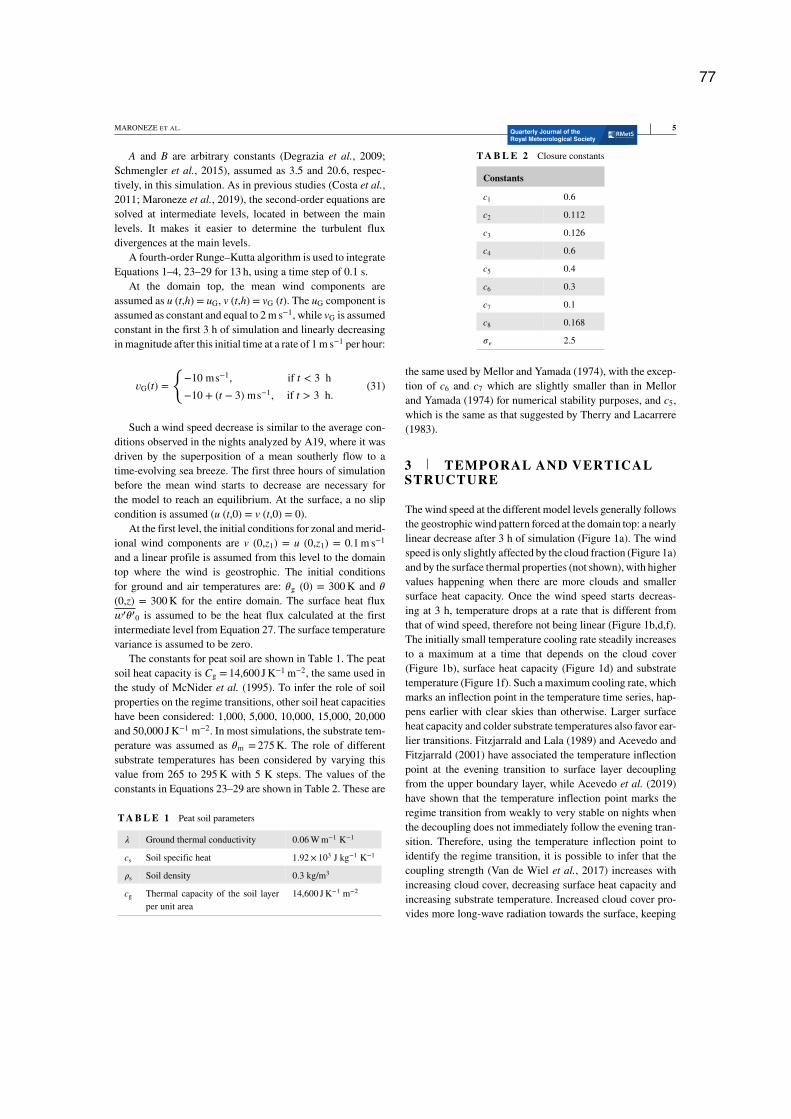
MARONEZE ET AL. 5

A and B are arbitrary constants (Degrazia et al., 2009;

Schmengler et al., 2015), assumed as 3.5 and 20.6, respec-

tively, in this simulation. As in previous studies (Costa et al.,2011; Maroneze et al., 2019), the second-order equations are

solved at intermediate levels, located in between the main

levels. It makes it easier to determine the turbulent flux

divergences at the main levels.

A fourth-order Runge–Kutta algorithm is used to integrate

Equations 1–4, 23–29 for 13 h, using a time step of 0.1 s.

At the domain top, the mean wind components are

assumed as u (t,h) = uG, v (t,h) = vG (t). The uG component is

assumed as constant and equal to 2 m s−1, while vG is assumed

constant in the first 3 h of simulation and linearly decreasing

in magnitude after this initial time at a rate of 1 m s−1 per hour:

𝑣G(𝑡) =

{−10 ms−1, if 𝑡 < 3 h

−10 + (𝑡 − 3) ms−1, if 𝑡 > 3 h.(31)

Such a wind speed decrease is similar to the average con-

ditions observed in the nights analyzed by A19, where it was

driven by the superposition of a mean southerly flow to a

time-evolving sea breeze. The first three hours of simulation

before the mean wind starts to decrease are necessary for

the model to reach an equilibrium. At the surface, a no slip

condition is assumed (u (t,0) = v (t,0) = 0).

At the first level, the initial conditions for zonal and merid-

ional wind components are v (0,z1) = u (0,z1) = 0.1 m s−1

and a linear profile is assumed from this level to the domain

top where the wind is geostrophic. The initial conditions

for ground and air temperatures are: 𝜃g (0) = 300 K and 𝜃

(0,z) = 300 K for the entire domain. The surface heat flux

𝑤′𝜃′0 is assumed to be the heat flux calculated at the first

intermediate level from Equation 27. The surface temperature

variance is assumed to be zero.

The constants for peat soil are shown in Table 1. The peat

soil heat capacity is Cg = 14,600 J K−1 m−2, the same used in

the study of McNider et al. (1995). To infer the role of soil

properties on the regime transitions, other soil heat capacities

have been considered: 1,000, 5,000, 10,000, 15,000, 20,000

and 50,000 J K−1 m−2. In most simulations, the substrate tem-

perature was assumed as 𝜃m = 275 K. The role of different

substrate temperatures has been considered by varying this

value from 265 to 295 K with 5 K steps. The values of the

constants in Equations 23–29 are shown in Table 2. These are

T A B L E 1 Peat soil parameters

𝜆 Ground thermal conductivity 0.06 W m−1 K−1

cs Soil specific heat 1.92× 103 J kg−1 K−1

𝜌s Soil density 0.3 kg/m3

cg Thermal capacity of the soil layer

per unit area

14,600 J K−1 m−2

T A B L E 2 Closure constants

Constants

c1 0.6

c2 0.112

c3 0.126

c4 0.6

c5 0.4

c6 0.3

c7 0.1

c8 0.168

𝜎e 2.5

the same used by Mellor and Yamada (1974), with the excep-

tion of c6 and c7 which are slightly smaller than in Mellor

and Yamada (1974) for numerical stability purposes, and c5,

which is the same as that suggested by Therry and Lacarrere

(1983).

3 TEMPORAL AND VERTICALSTRUCTURE

The wind speed at the different model levels generally follows

the geostrophic wind pattern forced at the domain top: a nearly

linear decrease after 3 h of simulation (Figure 1a). The wind

speed is only slightly affected by the cloud fraction (Figure 1a)

and by the surface thermal properties (not shown), with higher

values happening when there are more clouds and smaller

surface heat capacity. Once the wind speed starts decreas-

ing at 3 h, temperature drops at a rate that is different from

that of wind speed, therefore not being linear (Figure 1b,d,f).

The initially small temperature cooling rate steadily increases

to a maximum at a time that depends on the cloud cover

(Figure 1b), surface heat capacity (Figure 1d) and substrate

temperature (Figure 1f). Such a maximum cooling rate, which

marks an inflection point in the temperature time series, hap-

pens earlier with clear skies than otherwise. Larger surface

heat capacity and colder substrate temperatures also favor ear-

lier transitions. Fitzjarrald and Lala (1989) and Acevedo and

Fitzjarrald (2001) have associated the temperature inflection

point at the evening transition to surface layer decoupling

from the upper boundary layer, while Acevedo et al. (2019)

have shown that the temperature inflection point marks the

regime transition from weakly to very stable on nights when

the decoupling does not immediately follow the evening tran-

sition. Therefore, using the temperature inflection point to

identify the regime transition, it is possible to infer that the

coupling strength (Van de Wiel et al., 2017) increases with

increasing cloud cover, decreasing surface heat capacity and

increasing substrate temperature. Increased cloud cover pro-

vides more long-wave radiation towards the surface, keeping

77

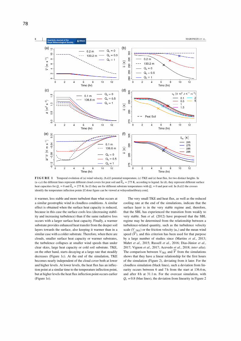
6 MARONEZE ET AL.

F I G U R E 1 Temporal evolution of (a) wind velocity, (b,d,f) potential temperature, (c) TKE and (e) heat flux, for two distinct heights. In

(a–c,e) the different lines represent different cloud covers for peat soil and 𝜃m = 275 K, according to legend. In (d), they represent different surface

heat capacities for Qc = 0 and 𝜃m = 275 K. In (f) they are for different substrate temperatures with Qc = 0 and peat soil. In (b,d,f) the crosses

identify the temperature inflection points [Colour figure can be viewed at wileyonlinelibrary.com].

it warmer, less stable and more turbulent than what occurs at

a similar geostrophic wind in cloudless conditions. A similar

effect is obtained when the surface heat capacity is reduced,

because in this case the surface cools less (decreasing stabil-

ity and increasing turbulence) than if the same radiative loss

occurs with a larger surface heat capacity. Finally, a warmer

substrate provides enhanced heat transfer from the deeper soil

layers towards the surface, also keeping it warmer than in a

similar case with a colder substrate. Therefore, when there are

clouds, smaller surface heat capacity or warmer substrates,

the turbulence collapses at smaller wind speeds than under

clear skies, large heat capacity or cold soil substrate. TKE,

on the other hand, starts decaying at a large rate that steadily

decreases (Figure 1c). At the end of the simulation, TKE

becomes nearly independent of the cloud cover both at lower

and higher levels. At lower levels, the heat flux has an inflec-

tion point at a similar time to the temperature inflection point,

but at higher levels the heat flux inflection point occurs earlier

(Figure 1e).

The very small TKE and heat flux, as well as the reduced

cooling rate at the end of the simulations, indicate that the

surface layer is in the very stable regime and, therefore,

that the SBL has experienced the transition from weakly to

very stable. Sun et al. (2012) have proposed that the SBL

regime may be determined from the relationship between a

turbulence-related quantity, such as the turbulence velocity

scale (V TKE) or the friction velocity (𝑢∗) and the mean wind

speed (𝑉 ), and this criterion has been used for that purpose

by a large number of studies since (Martins et al., 2013;

Mahrt et al., 2015; Russell et al., 2016; Dias-Júnior et al.,2017; Vignon et al., 2017; Acevedo et al., 2018; inter alia).

The comparison between VTKE and 𝑉 from the simulations

shows that they have a linear relationship for the first hours

of the simulation (Figure 2), deviating from it later. For the

cloudless simulation (black lines), such a deviation from lin-

earity occurs between 6 and 7 h from the start at 136.6 m,

and after 8 h at 31.1 m. For the overcast simulation, with

Qc = 0.8 (blue lines), the deviation from linearity in Figure 2

78

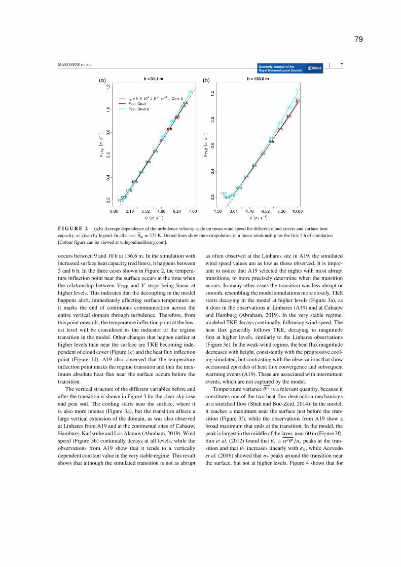
MARONEZE ET AL. 7

F I G U R E 2 (a,b) Average dependence of the turbulence velocity scale on mean wind speed for different cloud covers and surface heat

capacity, as given by legend. In all cases, 𝜃m = 275 K. Dotted lines show the extrapolation of a linear relationship for the first 5 h of simulation

[Colour figure can be viewed at wileyonlinelibrary.com].

occurs between 9 and 10 h at 136.6 m. In the simulation with

increased surface heat capacity (red lines), it happens between

5 and 6 h. In the three cases shown in Figure 2, the tempera-

ture inflection point near the surface occurs at the time when

the relationship between VTKE and 𝑉 stops being linear at

higher levels. This indicates that the decoupling in the model

happens aloft, immediately affecting surface temperature as

it marks the end of continuous communication across the

entire vertical domain through turbulence. Therefore, from

this point onwards, the temperature inflection point at the low-

est level will be considered as the indicator of the regime

transition in the model. Other changes that happen earlier at

higher levels than near the surface are TKE becoming inde-

pendent of cloud cover (Figure 1c) and the heat flux inflection

point (Figure 1d). A19 also observed that the temperature

inflection point marks the regime transition and that the max-

imum absolute heat flux near the surface occurs before the

transition.

The vertical structure of the different variables before and

after the transition is shown in Figure 3 for the clear-sky case

and peat soil. The cooling starts near the surface, where it

is also more intense (Figure 3a), but the transition affects a

large vertical extension of the domain, as was also observed

at Linhares from A19 and at the continental sites of Cabauw,

Hamburg, Karlsruhe and Los Alamos (Abraham, 2019). Wind

speed (Figure 3b) continually decays at all levels, while the

observations from A19 show that it tends to a vertically

dependent constant value in the very stable regime. This result

shows that although the simulated transition is not as abrupt

as often observed at the Linhares site in A19, the simulated

wind speed values are as low as those observed. It is impor-

tant to notice that A19 selected the nights with most abrupt

transitions, to more precisely determine when the transition

occurs. In many other cases the transition was less abrupt or

smooth, resembling the model simulations more closely. TKE

starts decaying in the model at higher levels (Figure 3a), as

it does in the observations at Linhares (A19) and at Cabauw

and Hamburg (Abraham, 2019). In the very stable regime,

modeled TKE decays continually, following wind speed. The

heat flux generally follows TKE, decaying in magnitude

first at higher levels, similarly to the Linhares observations

(Figure 3e). In the weak-wind regime, the heat flux magnitude

decreases with height, consistently with the progressive cool-

ing simulated, but contrasting with the observations that show

occasional episodes of heat flux convergence and subsequent

warming events (A19). These are associated with intermittent

events, which are not captured by the model.

Temperature variance 𝜃′2 is a relevant quantity, because it

constitutes one of the two heat flux destruction mechanisms

in a stratified flow (Shah and Bou-Zeid, 2014). In the model,

it reaches a maximum near the surface just before the tran-

sition (Figure 3f), while the observations from A19 show a

broad maximum that ends at the transition. In the model, the

peak is largest in the middle of the layer, near 60 m (Figure 3f).

Sun et al. (2012) found that 𝜃∗ ≡ 𝑤′𝜃′∕𝑢∗ peaks at the tran-

sition and that 𝜃* increases linearly with 𝜎𝜃 , while Acevedo

et al. (2016) showed that 𝜎𝜃 peaks around the transition near

the surface, but not at higher levels. Figure 4 shows that for

79

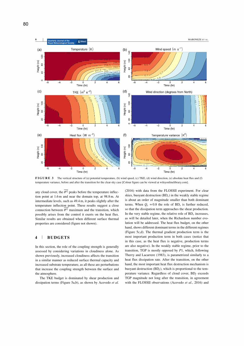
8 MARONEZE ET AL.

F I G U R E 3 The vertical structure of (a) potential temperature, (b) wind speed, (c) TKE, (d) wind direction, (e) absolute heat flux and (f)

temperature variance, before and after the transition for the clear-sky case [Colour figure can be viewed at wileyonlinelibrary.com].

any cloud cover, the 𝜃′2 peaks before the temperature inflec-

tion point at 1.6 m and near the domain top, at 98.8 m. At

intermediate levels, such as 49.4 m, it peaks slightly after the

temperature inflection point. These results suggest a close

connection between 𝜃′2 maximum and the transition, which

possibly arises from the control it exerts on the heat flux.

Similar results are obtained when different surface thermal

properties are considered (figure not shown).

4 BUDGETS

In this section, the role of the coupling strength is generally

assessed by considering variations in cloudiness alone. As

shown previously, increased cloudiness affects the transition

in a similar manner as reduced surface thermal capacity and

increased substrate temperature, as all these are perturbations

that increase the coupling strength between the surface and

the atmosphere.

The TKE budget is dominated by shear production and

dissipation terms (Figure 5a,b), as shown by Acevedo et al.

(2016) with data from the FLOSSII experiment. For clear

skies, buoyant destruction (BDe) in the weakly stable regime

is about an order of magnitude smaller than both dominant

terms. When Qc = 0.8 the role of BDe is further reduced,

so that the dissipation term approaches the shear production.

In the very stable regime, the relative role of BDe increases,

as will be detailed later, when the Richardson number evo-

lution will be addressed. The heat flux budget, on the other

hand, shows different dominant terms in the different regimes

(Figure 5c,d). The thermal gradient production term is the

most important production term in both cases (notice that

in this case, as the heat flux is negative, production terms

are also negative). In the weakly stable regime, prior to the

transition, TGP is mostly opposed by P1, which, following

Therry and Lacarrere (1983), is parametrized similarly to a

heat flux dissipation rate. After the transition, on the other

hand, the most important heat flux destruction mechanism is

buoyant destruction (BDf ), which is proportional to the tem-

perature variance. Regardless of cloud cover, BDf exceeds

TGP magnitude not long after the transition, in agreement

with the FLOSSII observations (Acevedo et al., 2016) and

80

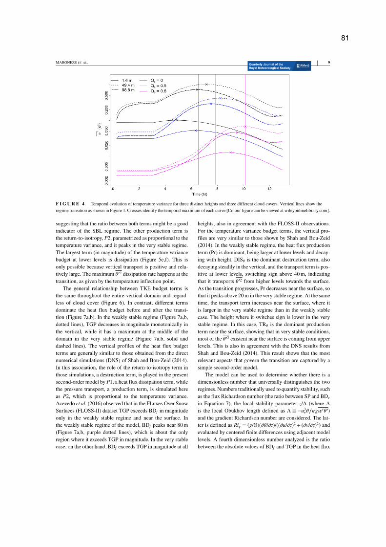
MARONEZE ET AL. 9

F I G U R E 4 Temporal evolution of temperature variance for three distinct heights and three different cloud covers. Vertical lines show the

regime transition as shown in Figure 1. Crosses identify the temporal maximum of each curve [Colour figure can be viewed at wileyonlinelibrary.com].

suggesting that the ratio between both terms might be a good

indicator of the SBL regime. The other production term is

the return-to-isotropy, P2, parametrized as proportional to the

temperature variance, and it peaks in the very stable regime.

The largest term (in magnitude) of the temperature variance

budget at lower levels is dissipation (Figure 5e,f). This is

only possible because vertical transport is positive and rela-

tively large. The maximum 𝜃′2 dissipation rate happens at the

transition, as given by the temperature inflection point.

The general relationship between TKE budget terms is

the same throughout the entire vertical domain and regard-

less of cloud cover (Figure 6). In contrast, different terms

dominate the heat flux budget before and after the transi-

tion (Figure 7a,b). In the weakly stable regime (Figure 7a,b,

dotted lines), TGP decreases in magnitude monotonically in

the vertical, while it has a maximum at the middle of the

domain in the very stable regime (Figure 7a,b, solid and

dashed lines). The vertical profiles of the heat flux budget

terms are generally similar to those obtained from the direct

numerical simulations (DNS) of Shah and Bou-Zeid (2014).

In this association, the role of the return-to-isotropy term in

those simulations, a destruction term, is played in the present

second-order model by P1, a heat flux dissipation term, while

the pressure transport, a production term, is simulated here

as P2, which is proportional to the temperature variance.

Acevedo et al. (2016) observed that in the FLuxes Over Snow

Surfaces (FLOSS-II) dataset TGP exceeds BDf in magnitude

only in the weakly stable regime and near the surface. In

the weakly stable regime of the model, BDf peaks near 80 m

(Figure 7a,b, purple dotted lines), which is about the only

region where it exceeds TGP in magnitude. In the very stable

case, on the other hand, BDf exceeds TGP in magnitude at all

heights, also in agreement with the FLOSS-II observations.

For the temperature variance budget terms, the vertical pro-

files are very similar to those shown by Shah and Bou-Zeid

(2014). In the weakly stable regime, the heat flux production

term (Pr) is dominant, being larger at lower levels and decay-

ing with height. DIS𝜃 is the dominant destruction term, also

decaying steadily in the vertical, and the transport term is pos-

itive at lower levels, switching sign above 40 m, indicating

that it transports 𝜃′2 from higher levels towards the surface.

As the transition progresses, Pr decreases near the surface, so

that it peaks above 20 m in the very stable regime. At the same

time, the transport term increases near the surface, where it

is larger in the very stable regime than in the weakly stable

case. The height where it switches sign is lower in the very

stable regime. In this case, TR𝜃 is the dominant production

term near the surface, showing that in very stable conditions,

most of the 𝜃′2 existent near the surface is coming from upper

levels. This is also in agreement with the DNS results from

Shah and Bou-Zeid (2014). This result shows that the most

relevant aspects that govern the transition are captured by a

simple second-order model.

The model can be used to determine whether there is a

dimensionless number that universally distinguishes the two

regimes. Numbers traditionally used to quantify stability, such

as the flux Richardson number (the ratio between SP and BDe

in Equation 7), the local stability parameter z/Λ (where Λis the local Obukhov length defined as Λ ≡ −𝑢3

∗𝜃∕𝜅𝑔𝑤′𝜃′)

and the gradient Richardson number are considered. The lat-

ter is defined as Rig = (g/Θ)(𝜕𝜃/𝜕z)/((𝜕u/𝜕z)2 + (𝜕v/𝜕z)2) and

evaluated by centered finite differences using adjacent model

levels. A fourth dimensionless number analyzed is the ratio

between the absolute values of BDf and TGP in the heat flux

81

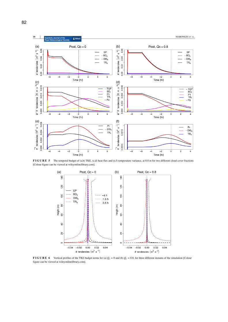
10 MARONEZE ET AL.

F I G U R E 5 The temporal budget of (a,b) TKE, (c,d) heat flux and (e,f) temperature variance, at 8.8 m for two different cloud cover fractions

[Colour figure can be viewed at wileyonlinelibrary.com].

F I G U R E 6 Vertical profiles of the TKE budget terms for (a) Qc = 0 and (b) Qc = 0.8, for three different instants of the simulation [Colour

figure can be viewed at wileyonlinelibrary.com].

82

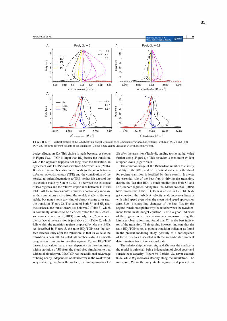
MARONEZE ET AL. 11

F I G U R E 7 Vertical profiles of the (a,b) heat flux budget terms and (c,d) temperature variance budget terms, with (a,c) Qc = 0 and (b,d)

Qc = 0.8, for three different instants of the simulation [Colour figure can be viewed at wileyonlinelibrary.com].

budget (Equation 12). This choice is made because, as shown

in Figure 5c,d, −TGP is larger than BDf before the transition,

while the opposite happens not long after the transition, in

agreement with FLOSSII observations (Acevedo et al., 2016).

Besides, this number also corresponds to the ratio between

turbulent potential energy (TPE) and the contribution of the

vertical turbulent fluctuations to TKE, so that it is a test of the

association made by Sun et al. (2016) between the existence

of two regimes and the relative importance between TPE and

TKE. All these dimensionless numbers continually increase

as the simulations evolve from the weakly stable to the very

stable, but none shows any kind of abrupt change at or near

the transition (Figure 8). The value of both Rif and Rig near

the surface at the transition are just below 0.2 (Table 3), which

is commonly assumed to be a critical value for the Richard-

son number (Freire et al., 2019). Similarly, the z/Λ value near

the surface at the transition is just above 0.1 (Table 3), which

falls within the transition regime proposed by Mahrt (1998).

As described in Figure 5, the ratio BDf /TGP near the sur-

face exceeds unity after the transition, so that its value at the

transition is near 0.8. As noted, all numbers exhibit a smooth

progression from one to the other regime. Rig and BDf /TGP

have critical values that are least dependent on the cloudiness,

with a variation of 5% from the cloud-free simulation to that

with total cloud cover. BDf /TGP has the additional advantage

of being nearly independent of cloud cover in the weak wind,

very stable regime. Near the surface, its limit approaches 1.2

2 h after the transition (Table 4), tending to stay at that value

further along (Figure 8j). This behavior is even more evident

at upper levels (Figure 8k,l).

The common usage of the Richardson number to classify

stability in the SBL, and of its critical value as a threshold

for regime transition is justified by these results. It attests

the essential role of the heat flux in driving the transition,

despite the fact that BDe is much smaller than both SP and

DISe in both regimes. Along this line, Maroneze et al. (2019)

have shown that if the BDe term is absent in the TKE bud-

get equation, the turbulent velocity scale increases linearly

with wind speed even when the mean wind speed approaches

zero. Such a controlling character of the heat flux for the

regime transition explains why the ratio between the two dom-

inant terms in its budget equation is also a good indicator

of the regime. A19 made a similar comparison using the

Linhares observations and found that Rig is the best indica-

tor of the transition. Their results, however, indicate that the

ratio BDf /TGP is not as good a transition indicator as found

in the present modeling study, possibly as a consequence

of the difficulties associated with the second-order moment

determination from observational data.

The relationship between Rig and Rif near the surface in

the model is universal, being independent of cloud cover and

surface heat capacity (Figure 9). Besides, Rif never exceeds

0.26, while Rig increases steadily along the simulation. The

maximum Rif in the very stable regime is dependent on

83

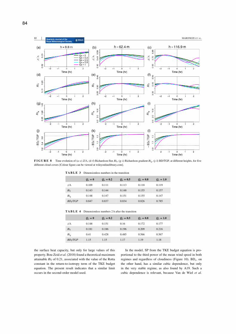
12 MARONEZE ET AL.

F I G U R E 8 Time evolution of (a–c) Z/Λ, (d–f) Richardson flux Rif, (g–i) Richardson gradient Rig, (j–l) BD/TGP, at different heights, for five

different cloud covers [Colour figure can be viewed at wileyonlinelibrary.com].

T A B L E 3 Dimensionless numbers in the transition

Qc = 0 Qc = 0.2 Qc = 0.5 Qc = 0.8 Qc = 1.0

z/Λ 0.109 0.111 0.113 0.118 0.119

Rif 0.143 0.144 0.148 0.155 0.157

Rig 0.148 0.147 0.151 0.155 0.147

BDf/TGP 0.847 0.837 0.834 0.826 0.785

T A B L E 4 Dimensionless numbers 2 h after the transition

Qc = 0 Qc = 0.2 Qc = 0.5 Qc = 0.8 Qc = 1.0

z/Λ 0.148 0.151 0.16 0.172 0.177

Rif 0.181 0.186 0.196 0.209 0.216

Rig 0.41 0.428 0.485 0.566 0.567

BDf/TGP 1.15 1.15 1.17 1.19 1.18

the surface heat capacity, but only for large values of this

property. Bou-Zeid et al. (2018) found a theoretical maximum

attainable Rif of 0.21, associated with the value of the Rotta

constant in the return-to-isotropy term of the TKE budget

equation. The present result indicates that a similar limit

occurs in the second-order model used.

In the model, SP from the TKE budget equation is pro-

portional to the third power of the mean wind speed in both

regimes and regardless of cloudiness (Figure 10). BDe, on

the other hand, has a similar cubic dependence, but only

in the very stable regime, as also found by A19. Such a

cubic dependence is relevant, because Van de Wiel et al.

84

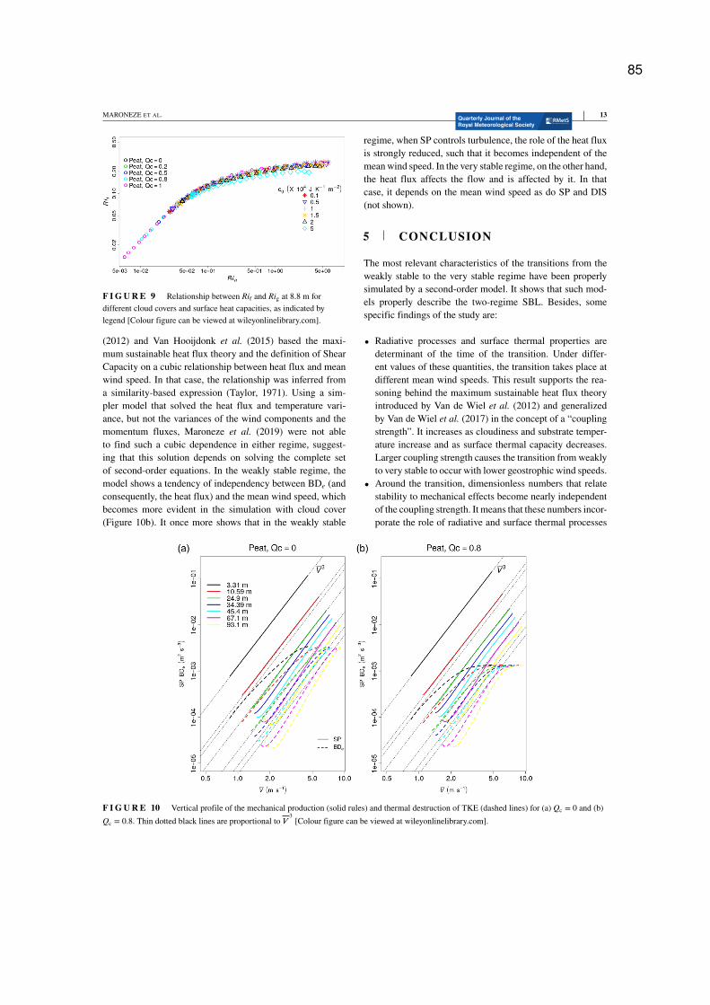
MARONEZE ET AL. 13

F I G U R E 9 Relationship between Rif and Rig at 8.8 m for

different cloud covers and surface heat capacities, as indicated by

legend [Colour figure can be viewed at wileyonlinelibrary.com].

(2012) and Van Hooijdonk et al. (2015) based the maxi-

mum sustainable heat flux theory and the definition of Shear

Capacity on a cubic relationship between heat flux and mean

wind speed. In that case, the relationship was inferred from

a similarity-based expression (Taylor, 1971). Using a sim-

pler model that solved the heat flux and temperature vari-

ance, but not the variances of the wind components and the

momentum fluxes, Maroneze et al. (2019) were not able

to find such a cubic dependence in either regime, suggest-

ing that this solution depends on solving the complete set

of second-order equations. In the weakly stable regime, the

model shows a tendency of independency between BDe (and

consequently, the heat flux) and the mean wind speed, which

becomes more evident in the simulation with cloud cover

(Figure 10b). It once more shows that in the weakly stable

regime, when SP controls turbulence, the role of the heat flux

is strongly reduced, such that it becomes independent of the

mean wind speed. In the very stable regime, on the other hand,

the heat flux affects the flow and is affected by it. In that

case, it depends on the mean wind speed as do SP and DIS

(not shown).

5 CONCLUSION

The most relevant characteristics of the transitions from the

weakly stable to the very stable regime have been properly

simulated by a second-order model. It shows that such mod-

els properly describe the two-regime SBL. Besides, some

specific findings of the study are:

• Radiative processes and surface thermal properties are

determinant of the time of the transition. Under differ-

ent values of these quantities, the transition takes place at

different mean wind speeds. This result supports the rea-

soning behind the maximum sustainable heat flux theory

introduced by Van de Wiel et al. (2012) and generalized

by Van de Wiel et al. (2017) in the concept of a “coupling

strength”. It increases as cloudiness and substrate temper-

ature increase and as surface thermal capacity decreases.

Larger coupling strength causes the transition from weakly

to very stable to occur with lower geostrophic wind speeds.

• Around the transition, dimensionless numbers that relate

stability to mechanical effects become nearly independent

of the coupling strength. It means that these numbers incor-

porate the role of radiative and surface thermal processes

F I G U R E 10 Vertical profile of the mechanical production (solid rules) and thermal destruction of TKE (dashed lines) for (a) Qc = 0 and (b)

Qc = 0.8. Thin dotted black lines are proportional to 𝑉3

[Colour figure can be viewed at wileyonlinelibrary.com].

85

14 MARONEZE ET AL.

in their definition. This is especially true for the gradi-

ent Richardson number and for the ratio between buoyant

destruction and thermal gradient production in the heat

flux budget, although the latter was not found to describe

well the process in the observational study of A19.

• The heat flux controls the transition, despite its small mag-

nitude. The dominant terms in its budget change between

regimes. In the heat flux budget, thermal gradient produc-

tion dominates in the weakly stable case, while buoyant

destruction dominates in the very stable regime.

• The temperature variance (𝜃′2) peaks a little before the

transition near the surface and close to the transition at

higher levels. This peak is relevant because in the present

case 𝜃′2 is numerically solved by a prognostic equation,

while A19 found a similar peak from the observations. In

that case, the maximum could be contaminated by the rapid

cooling experienced around the transition, but the present

modeling results indicate it is genuine.

• The relative magnitudes of the TKE budget terms are very

little dependent on the SBL regime, while the same does

not occur for the terms of the heat flux and temperature

variance budgets. In these cases, different dominant terms

occur at different times relative to the transition and also at

different heights.

The simulations have provided a good representation

of the observed quantities, showing the usefulness of the

second-order model as a tool to simulate regime transitions

in the SBL. A complete validation still demands a com-

parison of its results to real cases observed at sites with

different surface characteristics. Nevertheless, the result sen-

sitivity to external factors such as cloudiness, surface heat

capacity and substrate temperature indicate that such a vali-

dation is likely to be achieved. Therefore, in the future similar

second-order models may be used for describing other cases,

even if no corresponding observations are available. As an

example, one may consider the opposite process, of a tran-

sition from very to weakly stable, which may be forced by

increasing the mechanical forcing at domain top. It may

also be used to simulate case-studies of particularly interest-

ing and relevant occurrences, such as top-down propagating

intermittent events driven by wind speed enhancement aloft,

the effects of abrupt variability of cloud cover, or the SBL

response to low-frequency variability in the large-scale wind

forcing.

ACKNOWLEDGEMENTS

The study has been developed within the context of a Research

and Development project sponsored by companies Linhares

Geração S.A. and Termelétrica Viana S.A., and named

“Desenvolvimento de um modelo operacional para simulação

em tempo real da dispersão atmosférica de poluentes emitidos

por termelétrica a gás natural”. The Project is within the

context of the investment programme in Research and Devel-

opment, regulated by Brazilian National Agency for Electric

Energy. The authors thank deeply all support provided by

these companies for the development of the present work. The

study also has been partially supported by Brazilian funding

agencies CNPq and CAPES (Finacial code 001). The latter

funds graduate studies of the first author.

ORCID

Rafael Maroneze https://orcid.org/0000-0002-3025-9676

Otávio C. Acevedo https://orcid.org/0000-0003-2606-

4726

REFERENCES

Abraham, C. (2019) Regime occupation and transition informationobtained from observable meteorological state variables in the sta-bly stratified nocturnal boundary layer. PhD Thesis, University of

Victoria, Victoria, BC, Canada.

Acevedo, O.C., Degrazia, G.A., Puhales, F.S., Martins, L.G., Oliveira,

P.E., Teichrieb, C., Silva, S.M., Maroneze, R., Bodmann, B., Mor-

tarini, L., Cava, D. and Anfossi, D. (2018) Monitoring the microm-

eteorology of a coastal site next to a thermal power plant from the

surface to 140 m. Bulletin of the American Meteorological Society,

99, 725–738.

Acevedo, O.C. and Fitzjarrald, D.R. (2001) The early evening

surface-layer transition: temporal and spatial variability. Journal ofthe Atmospheric Sciences, 58, 2650–2667.

Acevedo, O.C. and Fitzjarrald, D.R. (2003) In the core of the

night-effects of intermittent mixing on a horizontally heterogeneous

surface. Boundary-Layer Meteorology, 106, 1–33.

Acevedo, O.C., Mahrt, L., Puhales, F.S., Costa, F.D., Medeiros, L.E. and

Degrazia, G.A. (2016) Contrasting structures between the decoupled

and coupled states of the stable boundary layer. Quarterly Journal ofthe Royal Meteorological Society, 142, 693–702. https://doi.org/10.

1002/qj.2693.

Acevedo, O.C., Rafael, M., Costa, F.D., Puhales, F.S., Mortarini, L.,

Degrazia, G.A., Martins, L.G.N. and Oliveira, P.E.S. (2019) The

nocturnal boundary layer transition from weakly to very stable.

Part I: Observations. Quarterly Journal of the Royal MeteorologicalSociety. https://doi.org/10.1002/qj.3642.

Baas, P., van de Wiel, B., van der Linden, S. and Bosveld, F. (2018) From

near-neutral to strongly stratified: adequately modelling the clear-sky

nocturnal boundary layer at Cabauw. Boundary-Layer Meteorology,

166, 217–238.

Baas, P., van de Wiel, B.J., van Meijgaard, E., Vignon, E., Genthon, C.,

van der Linden, S.J. and de Roode, S.R. (2019) Transitions in the

wintertime near-surface temperature inversion at Dome C, Antarc-

tica. Quarterly Journal of the Royal Meteorological Society, 145,

930–946.

Blackadar, A. (1962) The vertical distribution of wind and turbulent

exchange in a neutral atmosphere. Journal of Geophysical Research,

67, 3095–3102.

Blackadar, A. (1979) High resolution models of the planetary bound-

ary layer. Advances in Environmental Science and Engineering, 1,

50–85.

86

MARONEZE ET AL. 15

Bou-Zeid, E., Gao, X., Ansorge, C. and Katul, G.G. (2018) On the role

of return to isotropy in wall-bounded turbulent flows with buoyancy.

Journal of Fluid Mechanics, 856, 61–78.

Costa, F.D., Acevedo, O.C., Mombach, J.C. and Degrazia, G.A. (2011) A

simplified model for intermittent turbulence in the nocturnal bound-

ary layer. Journal of the Atmospheric Sciences, 68, 1714–1729.

Deardorff, J.W. (1973) Three-dimensional numerical modeling of

planetary boundary layer. In: Haugen, D.A. (Ed.) Workshop onMicrometeorology. Boston, MA: American Meteorological Society,

pp. 271–311.

Deardorff, J.W. (1974) Three-dimensional numerical study of the

height and mean structure of a heated planetary boundary layer.

Boundary-Layer Meteorology, 7, 81–106.

Degrazia, G.A., Rizza, U., Puhales, F.S., Goulart, A.G., Carvalho, J.,

Welter, G.S. and Marques Filho, E.P. (2009) A variable mesh spacing

for large-eddy simulation models in the convective boundary layer.

Boundary-Layer Meteorology, 131, 277–292.

Dias-Júnior, C.Q., Sá, L.D., Marques Filho, E.P., Santana, R.A., Mauder,

M. and Manzi, A.O. (2017) Turbulence regimes in the stable bound-

ary layer above and within the Amazon forest. Agricultural andForest Meteorology, 233, 122–132.

Duynkerke, P.G. (1988) Application of the E – 𝜀 turbulence closure

model to the neutral and stable atmospheric boundary layer. Journalof the Atmospheric Sciences, 45, 865–880. https://doi.org/10.1175/

1520-0469(1988)045<0865:AOTTCM>2.0.CO;2.

Fitzjarrald, D.R. and Lala, G.G. (1989) Hudson valley fog environments.

Journal of Applied Meteorology, 28, 1303–1328.

Freire, L.S., Chamecki, M., Bou-Zeid, E. and Dias, N.L. (2019) Critical

flux Richardson number for Kolmogorov turbulence enabled by TKE

transport. Quarterly Journal of the Royal Meteorological Society,

145(721), 1551–1558. https://doi.org/10.1002/qj.3511.

Guerra, V.S., Acevedo, O.C., Medeiros, L.E., Oliveira, P.E.S. and San-

tos, D.M. (2018) Small-scale horizontal variability of mean and tur-

bulent quantities in the nocturnal boundary layer. Boundary-LayerMeteorology, 169, 395–411. https://doi.org/10.1007/s10546-018-

0381-3.

Holdsworth, A.M. and Monahan, A.H. (2019) Turbulent collapse and

recovery in the stable boundary layer using an idealized model of

pressure-driven flow with a surface energy budget. Journal of theAtmospheric Sciences, 76, 1307–1327.

Lan, C., Liu, H., Li, D., Katul, G.G. and Finn, D. (2018) Distinct tur-

bulence structures in stably stratified boundary layers with weak

and strong surface shear. Journal of Geophysical Research: Atmo-spheres, 123, 7839–7854.

Mahrt, L. (1998) Nocturnal boundary-layer regimes. Boundary-Layer Meteorology, 88, 255–278. https://doi.org/10.1023/A:

1001171313493.

Mahrt, L., Sun, J. and Stauffer, D. (2015) Dependence of turbulent veloc-

ities on wind speed and stratification. Boundary-Layer Meteorology,

155, 55–71.

Mahrt, L., Thomas, C., Richardson, S., Seaman, N., Stauffer, D. and Zee-

man, M. (2013) Non-stationary generation of weak turbulence for

very stable and weak-wind conditions. Boundary-Layer Meteorol-ogy, 147, 179–199. https://doi.org/10.1007/s10546-012-9782-x.

Maroneze, R., Acevedo, O.C., Costa, F.D. and Sun, J. (2019) Simulating

the regime transition of the stable boundary layer using different sim-

plified models. Boundary-Layer Meteorology, 170, 305–321. https://

doi.org/10.1007/s10546-018-0401-3.

Martins, H.S., Sá, L.D.A. and Moraes, O.L.L. (2013) Low level jets

in the Pantanal wetland nocturnal boundary layer – case studies.

American Journal of Environmental Engineering, 3, 32–47.

McNider, R.T., England, D.E., Friedman, M.J. and Shi, X. (1995) Pre-

dictability of the stable atmospheric boundary layer. Journal ofthe Atmospheric Sciences, 52, 1602–1614. https://doi.org/10.1175/

1520-0469(1995)052<1602:POTSAB>2.0.CO;2.

Mellor, G.L. and Yamada, T. (1974) A hierarchy of turbulence closure

models for planetary boundary layers. Journal of the AtmosphericSciences, 31, 1791–1806.

Rotta, J.C. (1951) Statistische theorie nichthomogener turbulenz.

Zeitschrift für Physik, 129, 547–572.

Russell, E.S., Liu, H., Gao, Z., Lamb, B. and Wagenbrenner, N. (2016)

Turbulence dependence on winds and stability in a weak-wind

canopy sublayer over complex terrain. Journal of GeophysicalResearch: Atmospheres, 121, 11502–11515.

Schmengler, M., Costa, F.D., Acevedo, O.C., Puhales, F.S., Demarco,

G., Martins, L.G.N. and Medeiros, L.E. (2015) Comparison of mix-

ing length formulations in a single-column model simulation for a

very stable site. American Journal of Environmental Engineering, 5,

106–118.

Shah, S.K. and Bou-Zeid, E. (2014) Direct numerical simulations of tur-

bulent Ekman layers with increasing static stability: modifications

to the bulk structure and second-order statistics. Journal of FluidMechanics, 760, 494–539.

Staley, D. and Jurica, G. (1972) Effective atmospheric emissivity under

clear skies. Journal of Applied Meteorology, 11, 349–356.

Steeneveld, G.-J. (2014) Current challenges in understanding and fore-

casting stable boundary layers over land and ice. Frontiers in Envi-ronmental Science, 2, 41. https://doi.org/10.3389/fenvs.2014.00041.

Sun, J. and French, J.R. (2016) Air–sea interactions in light of new

understanding of air–land interactions. Journal of the AtmosphericSciences, 73, 3931–3949. https://doi.org/10.1175/JAS-D-15-0354.1.

Sun, J., Lenschow, D.H., LeMone, M.A. and Mahrt, L. (2016) The role

of large-coherent-eddy transport in the atmospheric surface layer

based on CASES-99 observations. Boundary-Layer Meteorology,

160, 83–111. https://doi.org/10.1007/s10546-016-0134-0.

Sun, J., Mahrt, L., Banta, R.M. and Pichugina, Y.L. (2012) Turbu-

lence regimes and turbulence intermittency in the stable boundary

layer during CASES-99. Journal of the Atmospheric Sciences, 69,

338–351.

Taylor, P.A. (1971) A note on the log-linear velocity profile in stable

conditions. Quarterly Journal of the Royal Meteorological Society,

97, 326–329.

Therry, G. and Lacarrère, P. (1983) Improving the eddy kinetic energy

model for planetary boundary layer description. Boundary-LayerMeteorology, 25, 63–88. https://doi.org/10.1007/BF00122098.

Van de Wiel, B.J.H., Moene, A.F., Hartogensis, O.K., de Bruin, H.A.R.

and Holtslag, A.A.M. (2003) Intermittent turbulence in the stable

boundary layer over land. Part III: A classification for observa-

tions during CASES-99. Journal of the Atmospheric Sciences, 60,

2509–2522.

Van de Wiel, B.J.H., Ronda, R.J., Moene, A.F., de Bruin, H.A.R. and

Holtslag, A.A.M. (2002) Intermittent turbulence and oscillations in

the stable boundary layer over land. Part I: A bulk model. Journal ofthe Atmospheric Sciences, 59, 942–958.

Van de Wiel, B.J.H., Moene, A.F., Jonker, H.J.J., Baas, P., Basu, S.,

Donda, J.M.M., Sun, J. and Holtslag, A.A.M. (2012) The minimum

wind speed for sustainable turbulence in the nocturnal boundary

87

16 MARONEZE ET AL.

layer. Journal of the Atmospheric Sciences, 69, 3116–3127. https://

doi.org/10.1175/JAS-D-12-0107.1.

Van de Wiel, B.J.H., Vignon, E., Baas, P., van Hooijdonk, I.G.S.,

van der Linden, S.J.A., van Hooft, J.A., Bosveld, F.C., de Roode,

S.R., Moene, A.F. and Genthon, C. (2017) Regime transitions in

near-surface temperature inversions: a conceptual model. Journal ofthe Atmospheric Sciences, 74, 1057–1073. https://doi.org/10.1175/

JAS-D-16-0180.1.

Van Hooijdonk, I.G.S., Donda, J.M.M., Clercx, H.J.H., Bosveld, F.C.

and van de Wiel, B.J.H. (2015) Shear capacity as prognostic for noc-

turnal boundary layer regimes. Journal of the Atmospheric Sciences,

72, 1518–1532. https://doi.org/10.1175/JAS-D-14-0140.1.

Vignon, E., van de Wiel, B.J.H., van Hooijdonk, I.G.S., Genthon, C., van

der Linden, S.J.A., van Hooft, J.A., Baas, P., Maurel, W., Traullé, O.

and Casasanta, G. (2017) Stable boundary-layer regimes at Dome C,

Antarctica: observation and analysis. Quarterly Journal of the RoyalMeteorological Society, 143, 1241–1253.

How to cite this article: Maroneze R, Acevedo OC,

Costa FD, Puhales FS, Demarco G, Mortarini L. The

nocturnal boundary layer transition from weakly to

very stable. Part II: Numerical simulation with a

second-order model. Q J R Meteorol Soc. 2019;1–16.

https://doi.org/10.1002/qj.3643

88

manuscript submitted to Geophysical Research Letters

How is the two-regime stable boundary layer solved by1

the different PBL schemes in WRF?2

Rafael Maroneze 13

Otavio Costa Acevedo 14

Felipe Denardin Costa 25

Franciano Scremim Puhales 16

Vagner Anabor 17

Luca Mortarini 138

1Universidade Federal de Santa Maria92Universidade Federal do Pampa Campus-Alegrete10

3Institute of Atmospheric Sciences and Climate - National Research Council11

Key Points:12

• Planetary Boundary Layer Schemes13

• Stable Boundary Layer regimes14

• WRF15

Corresponding author: Rafael Maroneze, rafaelmaroneze@gmail.com

–1–

6 ARTIGO 4 - HOW IS THE TWO-REGIME STABLE BOUNDARY LAYER SOLVED BY

THE DIFFERENT PBL SCHEMES IN WRF

manuscript submitted to Geophysical Research Letters

Abstract16

Five planetary boundary layer (PBL) schemes of the Weather Research and Forecast-17

ing (WRF) model are compared with respect to their ability to simulate the very sta-18

ble and the weakly stable regime of the stable boundary layer. This is done for single19

column models where the large-scale mechanical forcing, represented by geostrophic winds,20

ranges from 0.5 to 12 m s−1. The comparison relies on the relationship between turbu-21

lence velocity scale and the mean wind speed, between thermal gradient and the mean22

wind speed and between flux and gradient Richardson numbers. The 2.5-level Mellor-23

Yamada-Nakanishi-Niino scheme is shown to simulate the very stable regime better than24

the other schemes, mainly because its heat eddy diffusivity decreases with respect to the25

momentum eddy diffusivity as the stability increases, while the same is not verified in26

the other schemes compared.27

1 Introduction28

Weather Research and Forecasting (WRF) (Skamarock et al., 2008) is currently29

the most used model for both research and numerical weather prediction (NWP) in the30

world. WRF applications are beyond NWP, as it is also employed for the prediction of31

a large range of Earth systems such as air chemistry, hydrology, wind and solar energy,32

wildland fires, hurricanes, regional climate, and others (Powers et al., 2017). Most of these33

applications demand a correct simulation of both daytime and nighttime periods, specif-34

ically at levels near the surface, within the planetary boundary layer (PBL). The present35

study addresses a difficulty that affects most PBL numerical schemes: the representa-36

tion of turbulence in weak wind nocturnal conditions.37

The existence of two distinct regimes in the stable boundary layer (SBL) has been38

known for many years (Andre & Mahrt, 1982; Mahrt & Gamage, 1987). More recently,39

the two regimes have been classified both observationally and in modelling as weakly sta-40

ble and very stable (Mahrt, 1998; Sun et al., 2012; Van de Wiel et al., 2002; Acevedo et41

al., 2016, among others). In the weakly stable regime, turbulence is relatively well de-42

veloped and continuous both in space and time. This regime typically occurs in condi-43

tions of strong wind and/or large cloud cover (Mahrt, 1998), which determine a weakly44

stratified or quasi-neutral boundary layer. Usually, this regime is well described by sim-45

ilarity theory (Mahrt, 2014) and, for this reason, it is expected to be well simulated by46

numerical PBL schemes, such as those employed in WRF. On the other hand, the very47

stable regime typically occurs with weak winds and clear sky, so that the surface radia-48

tive loss is large and, as a consequence, an intense stratification develops. In the very49

stable regime, turbulent mixing is largely suppressed, being localized (intermittent) both50

in space and time, or absent. Situations of very strong thermal stratification are not well51

described by classical concepts and their full description remains a challenge (Mahrt, 2014).52

Improving the simulation of the very stable regime by numerical schemes is a major mi-53

crometeorological challenge (Van de Wiel et al., 2017; Battisti et al., 2017; Baas et al.,54

2019; Holdsworth & Monahan, 2019; Lapo et al., 2019; Maroneze et al., 2019, n.d.).55

Sun et al. (2012) and Van de Wiel et al. (2012) have identified that the transition56

between SBL regimes at a given vertical level is controlled by the mean wind speed at57

that level. Since then, the practice of analyzing turbulent quantities as a function of the58

wind speed has become common (Acevedo et al., 2016; Vignon et al., 2017; Lan et al.,59

2018). However, the local wind speed used in such classifications is a variable internal60

to the SBL dynamics, being largely dependent on other quantities such as the thermal61

stratification and turbulent mixing. For this reason, specially in modelling studies, it is62

interesting to relate the SBL regimes to external parameters. In that regard, the most63

commonly used parameter to represent the large-scale mechanical forcing is the geostrophic64

wind (McNider et al., 1995; Van de Wiel et al., 2002; Costa et al., 2011; van der Linden65

et al., 2017).66

–2–

90

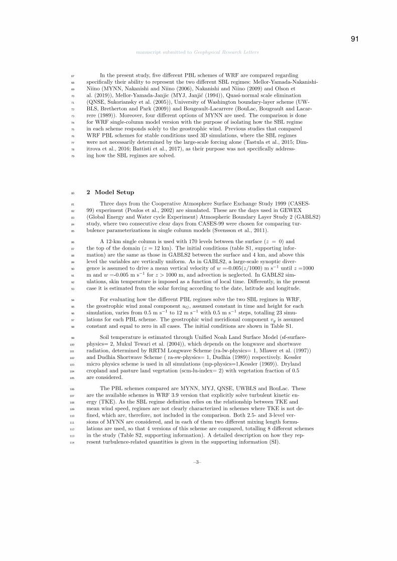
manuscript submitted to Geophysical Research Letters

In the present study, five different PBL schemes of WRF are compared regarding67

specifically their ability to represent the two different SBL regimes: Mellor-Yamada-Nakanishi-68

Niino (MYNN, Nakanishi and Niino (2006), Nakanishi and Niino (2009) and Olson et69

al. (2019)), Mellor-Yamada-Janjic (MYJ, Janjic (1994)), Quasi-normal scale elimination70

(QNSE, Sukoriansky et al. (2005)), University of Washington boundary-layer scheme (UW-71

BLS, Bretherton and Park (2009)) and Bougeault-Lacarrere (BouLac, Bougeault and Lacar-72

rere (1989)). Moreover, four different options of MYNN are used. The comparison is done73

for WRF single-column model version with the purpose of isolating how the SBL regime74

in each scheme responds solely to the geostrophic wind. Previous studies that compared75

WRF PBL schemes for stable conditions used 3D simulations, where the SBL regimes76

were not necessarily determined by the large-scale forcing alone (Tastula et al., 2015; Dim-77

itrova et al., 2016; Battisti et al., 2017), as their purpose was not specifically address-78

ing how the SBL regimes are solved.79

2 Model Setup80

Three days from the Cooperative Atmosphere Surface Exchange Study 1999 (CASES-81

99) experiment (Poulos et al., 2002) are simulated. These are the days used in GEWEX82

(Global Energy and Water cycle Experiment) Atmospheric Boundary Layer Study 2 (GABLS2)83

study, where two consecutive clear days from CASES-99 were chosen for comparing tur-84

bulence parameterizations in single column models (Svensson et al., 2011).85

A 12-km single column is used with 170 levels between the surface (z = 0) and86

the top of the domain (z = 12 km). The initial conditions (table S1, supporting infor-87

mation) are the same as those in GABLS2 between the surface and 4 km, and above this88

level the variables are vertically uniform. As in GABLS2, a large-scale synoptic diver-89

gence is assumed to drive a mean vertical velocity of w =-0.005(z/1000) m s−1 until z =100090

m and w =-0.005 m s−1 for z > 1000 m, and advection is neglected. In GABLS2 sim-91

ulations, skin temperature is imposed as a function of local time. Differently, in the present92

case it is estimated from the solar forcing according to the date, latitude and longitude.93

For evaluating how the different PBL regimes solve the two SBL regimes in WRF,94

the geostrophic wind zonal component uG, assumed constant in time and height for each95

simulation, varies from 0.5 m s−1 to 12 m s−1 with 0.5 m s−1 steps, totalling 23 simu-96

lations for each PBL scheme. The geostrophic wind meridional component vg is assumed97

constant and equal to zero in all cases. The initial conditions are shown in Table S1.98

Soil temperature is estimated through Unified Noah Land Surface Model (sf-surface-99

physics= 2, Mukul Tewari et al. (2004)), which depends on the longwave and shortwave100

radiation, determined by RRTM Longwave Scheme (ra-lw-physics= 1, Mlawer et al. (1997))101

and Dudhia Shortwave Scheme ( ra-sw-physics= 1, Dudhia (1989)) respectively. Kessler102

micro physics scheme is used in all simulations (mp-physics=1,Kessler (1969)). Dryland103

cropland and pasture land vegetation (scm-lu-index= 2) with vegetation fraction of 0.5104

are considered.105

The PBL schemes compared are MYNN, MYJ, QNSE, UWBLS and BouLac. These106

are the available schemes in WRF 3.9 version that explicitly solve turbulent kinetic en-107

ergy (TKE). As the SBL regime definition relies on the relationship between TKE and108

mean wind speed, regimes are not clearly characterized in schemes where TKE is not de-109

fined, which are, therefore, not included in the comparison. Both 2.5- and 3-level ver-110

sions of MYNN are considered, and in each of them two different mixing length formu-111

lations are used, so that 4 versions of this scheme are compared, totalling 8 different schemes112

in the study (Table S2, supporting information). A detailed description on how they rep-113

resent turbulence-related quantities is given in the supporting information (SI).114

–3–

91

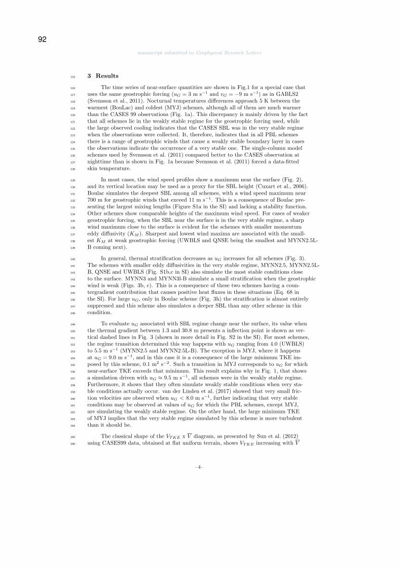
manuscript submitted to Geophysical Research Letters

3 Results115

The time series of near-surface quantities are shown in Fig.1 for a special case that116

uses the same geostrophic forcing (uG = 3 m s−1 and vG = −9 m s−1) as in GABLS2117

(Svensson et al., 2011). Nocturnal temperatures differences approach 5 K between the118

warmest (BouLac) and coldest (MYJ) schemes, although all of them are much warmer119

than the CASES 99 observations (Fig. 1a). This discrepancy is mainly driven by the fact120

that all schemes lie in the weakly stable regime for the geostrophic forcing used, while121

the large observed cooling indicates that the CASES SBL was in the very stable regime122

when the observations were collected. It, therefore, indicates that in all PBL schemes123

there is a range of geostrophic winds that cause a weakly stable boundary layer in cases124

the observations indicate the occurrence of a very stable one. The single-column model125

schemes used by Svensson et al. (2011) compared better to the CASES observation at126

nighttime than is shown in Fig. 1a because Svensson et al. (2011) forced a data-fitted127

skin temperature.128

In most cases, the wind speed profiles show a maximum near the surface (Fig. 2),129

and its vertical location may be used as a proxy for the SBL height (Cuxart et al., 2006).130

Boulac simulates the deepest SBL among all schemes, with a wind speed maximum near131

700 m for geostrophic winds that exceed 11 m s−1. This is a consequence of Boulac pre-132

senting the largest mixing lengths (Figure S1a in the SI) and lacking a stability function.133

Other schemes show comparable heights of the maximum wind speed. For cases of weaker134

geostrophic forcing, when the SBL near the surface is in the very stable regime, a sharp135

wind maximum close to the surface is evident for the schemes with smaller momentum136

eddy diffusivity (KM ). Sharpest and lowest wind maxima are associated with the small-137

est KM at weak geostrophic forcing (UWBLS and QNSE being the smallest and MYNN2.5L-138

B coming next).139

In general, thermal stratification decreases as uG increases for all schemes (Fig. 3).140

The schemes with smaller eddy diffusivities in the very stable regime, MYNN2.5, MYNN2.5L-141

B, QNSE and UWBLS (Fig. S1b,c in SI) also simulate the most stable conditions close142

to the surface. MYNN3 and MYNN3l-B simulate a small stratification when the geostrophic143

wind is weak (Figs. 3b, c). This is a consequence of these two schemes having a coun-144

tergradient contribution that causes positive heat fluxes in these situations (Eq. 68 in145

the SI). For large uG, only in Boulac scheme (Fig. 3h) the stratification is almost entirely146

suppressed and this scheme also simulates a deeper SBL than any other scheme in this147

condition.148

To evaluate uG associated with SBL regime change near the surface, its value when149

the thermal gradient between 1.3 and 30.8 m presents a inflection point is shown as ver-150

tical dashed lines in Fig. 3 (shown in more detail in Fig. S2 in the SI). For most schemes,151

the regime transition determined this way happens with uG ranging from 4.0 (UWBLS)152

to 5.5 m s−1 (MYNN2.5 and MYNN2.5L-B). The exception is MYJ, where it happens153

at uG = 9.0 m s−1, and in this case it is a consequence of the large minimum TKE im-154

posed by this scheme, 0.1 m2 s−2. Such a transition in MYJ corresponds to uG for which155

near-surface TKE exceeds that minimum. This result explains why in Fig. 1, that shows156

a simulation driven with uG ≈ 9.5 m s−1, all schemes were in the weakly stable regime.157

Furthermore, it shows that they often simulate weakly stable conditions when very sta-158

ble conditions actually occur. van der Linden et al. (2017) showed that very small fric-159

tion velocities are observed when uG < 8.0 m s−1, further indicating that very stable160

conditions may be observed at values of uG for which the PBL schemes, except MYJ,161

are simulating the weakly stable regime. On the other hand, the large minimum TKE162

of MYJ implies that the very stable regime simulated by this scheme is more turbulent163

than it should be.164

The classical shape of the VTKE x V diagram, as presented by Sun et al. (2012)165

using CASES99 data, obtained at flat uniform terrain, shows VTKE increasing with V166

–4–

92

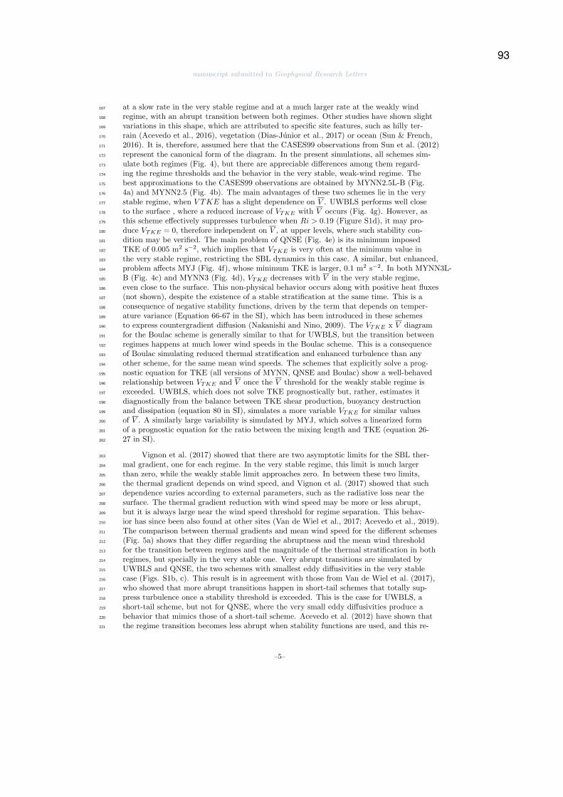
manuscript submitted to Geophysical Research Letters

at a slow rate in the very stable regime and at a much larger rate at the weakly wind167

regime, with an abrupt transition between both regimes. Other studies have shown slight168

variations in this shape, which are attributed to specific site features, such as hilly ter-169

rain (Acevedo et al., 2016), vegetation (Dias-Junior et al., 2017) or ocean (Sun & French,170

2016). It is, therefore, assumed here that the CASES99 observations from Sun et al. (2012)171

represent the canonical form of the diagram. In the present simulations, all schemes sim-172

ulate both regimes (Fig. 4), but there are appreciable differences among them regard-173

ing the regime thresholds and the behavior in the very stable, weak-wind regime. The174

best approximations to the CASES99 observations are obtained by MYNN2.5L-B (Fig.175

4a) and MYNN2.5 (Fig. 4b). The main advantages of these two schemes lie in the very176

stable regime, when V TKE has a slight dependence on V . UWBLS performs well close177

to the surface , where a reduced increase of VTKE with V occurs (Fig. 4g). However, as178

this scheme effectively suppresses turbulence when Ri > 0.19 (Figure S1d), it may pro-179

duce VTKE = 0, therefore independent on V , at upper levels, where such stability con-180

dition may be verified. The main problem of QNSE (Fig. 4e) is its minimum imposed181

TKE of 0.005 m2 s−2, which implies that VTKE is very often at the minimum value in182

the very stable regime, restricting the SBL dynamics in this case. A similar, but enhanced,183

problem affects MYJ (Fig. 4f), whose minimum TKE is larger, 0.1 m2 s−2. In both MYNN3L-184

B (Fig. 4c) and MYNN3 (Fig. 4d), VTKE decreases with V in the very stable regime,185

even close to the surface. This non-physical behavior occurs along with positive heat fluxes186

(not shown), despite the existence of a stable stratification at the same time. This is a187

consequence of negative stability functions, driven by the term that depends on temper-188

ature variance (Equation 66-67 in the SI), which has been introduced in these schemes189

to express countergradient diffusion (Nakanishi and Nino, 2009). The VTKE x V diagram190

for the Boulac scheme is generally similar to that for UWBLS, but the transition between191

regimes happens at much lower wind speeds in the Boulac scheme. This is a consequence192

of Boulac simulating reduced thermal stratification and enhanced turbulence than any193

other scheme, for the same mean wind speeds. The schemes that explicitly solve a prog-194

nostic equation for TKE (all versions of MYNN, QNSE and Boulac) show a well-behaved195

relationship between VTKE and V once the V threshold for the weakly stable regime is196

exceeded. UWBLS, which does not solve TKE prognostically but, rather, estimates it197

diagnostically from the balance between TKE shear production, buoyancy destruction198

and dissipation (equation 80 in SI), simulates a more variable VTKE for similar values199

of V . A similarly large variability is simulated by MYJ, which solves a linearized form200

of a prognostic equation for the ratio between the mixing length and TKE (equation 26-201

27 in SI).202

Vignon et al. (2017) showed that there are two asymptotic limits for the SBL ther-203

mal gradient, one for each regime. In the very stable regime, this limit is much larger204

than zero, while the weakly stable limit approaches zero. In between these two limits,205

the thermal gradient depends on wind speed, and Vignon et al. (2017) showed that such206

dependence varies according to external parameters, such as the radiative loss near the207

surface. The thermal gradient reduction with wind speed may be more or less abrupt,208

but it is always large near the wind speed threshold for regime separation. This behav-209

ior has since been also found at other sites (Van de Wiel et al., 2017; Acevedo et al., 2019).210

The comparison between thermal gradients and mean wind speed for the different schemes211

(Fig. 5a) shows that they differ regarding the abruptness and the mean wind threshold212

for the transition between regimes and the magnitude of the thermal stratification in both213

regimes, but specially in the very stable one. Very abrupt transitions are simulated by214

UWBLS and QNSE, the two schemes with smallest eddy diffusivities in the very stable215

case (Figs. S1b, c). This result is in agreement with those from Van de Wiel et al. (2017),216

who showed that more abrupt transitions happen in short-tail schemes that totally sup-217

press turbulence once a stability threshold is exceeded. This is the case for UWBLS, a218

short-tail scheme, but not for QNSE, where the very small eddy diffusivities produce a219

behavior that mimics those of a short-tail scheme. Acevedo et al. (2012) have shown that220

the regime transition becomes less abrupt when stability functions are used, and this re-221

–5–

93

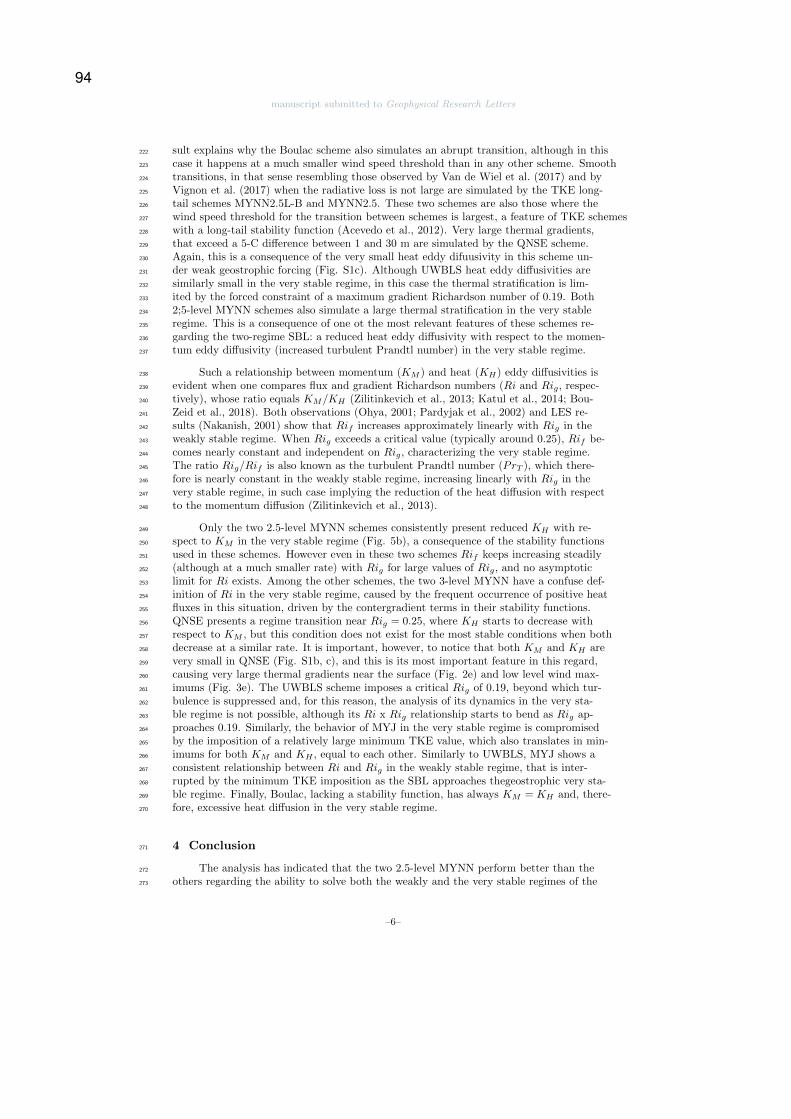
manuscript submitted to Geophysical Research Letters

sult explains why the Boulac scheme also simulates an abrupt transition, although in this222

case it happens at a much smaller wind speed threshold than in any other scheme. Smooth223

transitions, in that sense resembling those observed by Van de Wiel et al. (2017) and by224

Vignon et al. (2017) when the radiative loss is not large are simulated by the TKE long-225

tail schemes MYNN2.5L-B and MYNN2.5. These two schemes are also those where the226

wind speed threshold for the transition between schemes is largest, a feature of TKE schemes227

with a long-tail stability function (Acevedo et al., 2012). Very large thermal gradients,228

that exceed a 5-C difference between 1 and 30 m are simulated by the QNSE scheme.229

Again, this is a consequence of the very small heat eddy difuusivity in this scheme un-230

der weak geostrophic forcing (Fig. S1c). Although UWBLS heat eddy diffusivities are231

similarly small in the very stable regime, in this case the thermal stratification is lim-232

ited by the forced constraint of a maximum gradient Richardson number of 0.19. Both233

2;5-level MYNN schemes also simulate a large thermal stratification in the very stable234

regime. This is a consequence of one ot the most relevant features of these schemes re-235

garding the two-regime SBL: a reduced heat eddy diffusivity with respect to the momen-236

tum eddy diffusivity (increased turbulent Prandtl number) in the very stable regime.237

Such a relationship between momentum (KM ) and heat (KH) eddy diffusivities is238

evident when one compares flux and gradient Richardson numbers (Ri and Rig, respec-239

tively), whose ratio equals KM/KH (Zilitinkevich et al., 2013; Katul et al., 2014; Bou-240

Zeid et al., 2018). Both observations (Ohya, 2001; Pardyjak et al., 2002) and LES re-241

sults (Nakanish, 2001) show that Rif increases approximately linearly with Rig in the242

weakly stable regime. When Rig exceeds a critical value (typically around 0.25), Rif be-243

comes nearly constant and independent on Rig, characterizing the very stable regime.244

The ratio Rig/Rif is also known as the turbulent Prandtl number (PrT ), which there-245

fore is nearly constant in the weakly stable regime, increasing linearly with Rig in the246

very stable regime, in such case implying the reduction of the heat diffusion with respect247

to the momentum diffusion (Zilitinkevich et al., 2013).248

Only the two 2.5-level MYNN schemes consistently present reduced KH with re-249

spect to KM in the very stable regime (Fig. 5b), a consequence of the stability functions250

used in these schemes. However even in these two schemes Rif keeps increasing steadily251

(although at a much smaller rate) with Rig for large values of Rig, and no asymptotic252

limit for Ri exists. Among the other schemes, the two 3-level MYNN have a confuse def-253

inition of Ri in the very stable regime, caused by the frequent occurrence of positive heat254

fluxes in this situation, driven by the contergradient terms in their stability functions.255

QNSE presents a regime transition near Rig = 0.25, where KH starts to decrease with256

respect to KM , but this condition does not exist for the most stable conditions when both257

decrease at a similar rate. It is important, however, to notice that both KM and KH are258

very small in QNSE (Fig. S1b, c), and this is its most important feature in this regard,259

causing very large thermal gradients near the surface (Fig. 2e) and low level wind max-260

imums (Fig. 3e). The UWBLS scheme imposes a critical Rig of 0.19, beyond which tur-261

bulence is suppressed and, for this reason, the analysis of its dynamics in the very sta-262

ble regime is not possible, although its Ri x Rig relationship starts to bend as Rig ap-263

proaches 0.19. Similarly, the behavior of MYJ in the very stable regime is compromised264

by the imposition of a relatively large minimum TKE value, which also translates in min-265

imums for both KM and KH , equal to each other. Similarly to UWBLS, MYJ shows a266

consistent relationship between Ri and Rig in the weakly stable regime, that is inter-267

rupted by the minimum TKE imposition as the SBL approaches thegeostrophic very sta-268

ble regime. Finally, Boulac, lacking a stability function, has always KM = KH and, there-269

fore, excessive heat diffusion in the very stable regime.270

4 Conclusion271

The analysis has indicated that the two 2.5-level MYNN perform better than the272

others regarding the ability to solve both the weakly and the very stable regimes of the273

–6–

94

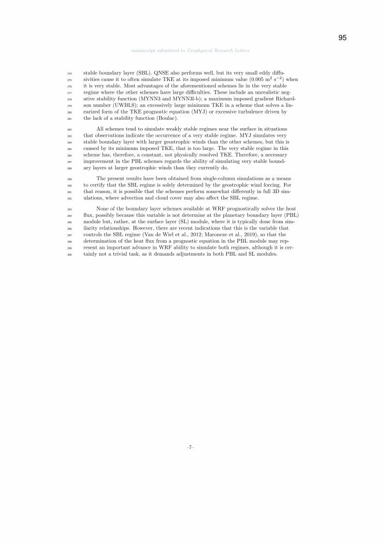
manuscript submitted to Geophysical Research Letters

stable boundary layer (SBL). QNSE also performs well, but its very small eddy diffu-274

sivities cause it to often simulate TKE at its imposed minimum value (0.005 m2 s−2) when275

it is very stable. Most advantages of the aforementioned schemes lie in the very stable276

regime where the other schemes have large difficulties. These include an unrealistic neg-277

ative stability function (MYNN3 and MYNN3l-b); a maximum imposed gradient Richard-278

son number (UWBLS); an excessively large minimum TKE in a scheme that solves a lin-279

earized form of the TKE prognostic equation (MYJ) or excessive turbulence driven by280

the lack of a stability function (Boulac).281

All schemes tend to simulate weakly stable regimes near the surface in situations282

that observations indicate the occurrence of a very stable regime. MYJ simulates very283

stable boundary layer with larger geostrophic winds than the other schemes, but this is284

caused by its minimum imposed TKE, that is too large. The very stable regime in this285

scheme has, therefore, a constant, not physically resolved TKE. Therefore, a necessary286

improvement in the PBL schemes regards the ability of simulating very stable bound-287

ary layers at larger geostrophic winds than they currently do.288

The present results have been obtained from single-column simulations as a means289

to certify that the SBL regime is solely determined by the geostrophic wind forcing. For290

that reason, it is possible that the schemes perform somewhat differently in full 3D sim-291

ulations, where advection and cloud cover may also affect the SBL regime.292

None of the boundary layer schemes available at WRF prognostically solves the heat293

flux, possibly because this variable is not determine at the planetary boundary layer (PBL)294

module but, rather, at the surface layer (SL) module, where it is typically done from sim-295

ilarity relationships. However, there are recent indications that this is the variable that296

controls the SBL regime (Van de Wiel et al., 2012; Maroneze et al., 2019), so that the297

determination of the heat flux from a prognostic equation in the PBL module may rep-298

resent an important advance in WRF ability to simulate both regimes, although it is cer-299

tainly not a trivial task, as it demands adjustments in both PBL and SL modules.300

–7–

95

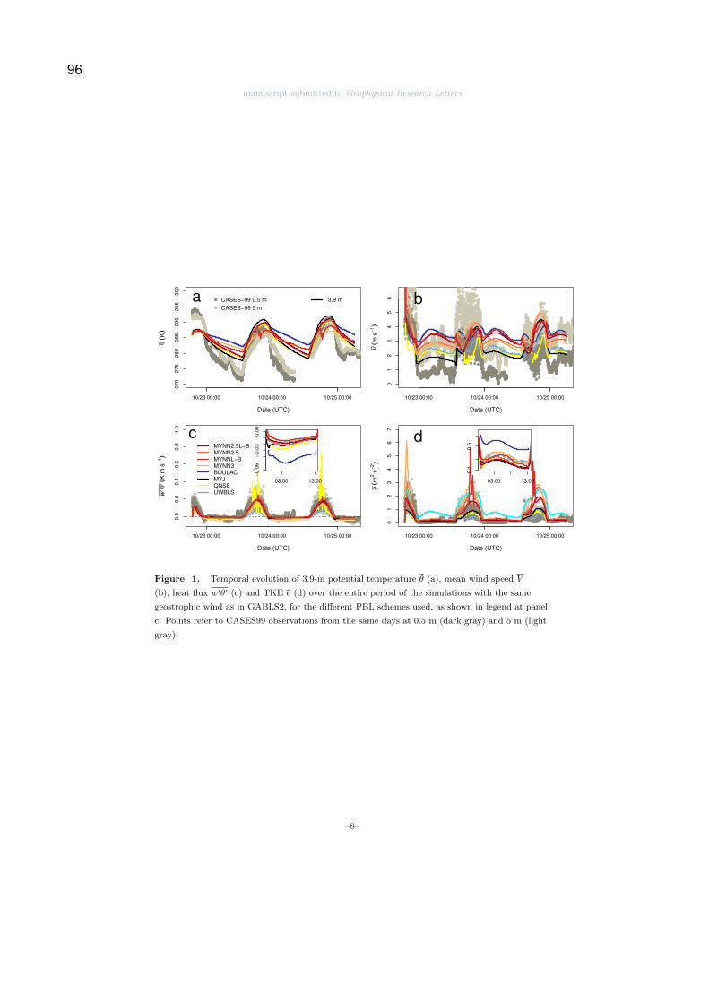
manuscript submitted to Geophysical Research Letters

10/23 00:00 10/24 00:00 10/25 00:00

27

02

75

28

02

85

29

02

95

30

0

Date (UTC)

θ (

K)

CASES−99 0.5 m

CASES−99 5 m

a 3.9 m

10/23 00:00 10/24 00:00 10/25 00:00

01

23

45

6

Date (UTC)

V (

m s

−1)

b

10/23 00:00 10/24 00:00 10/25 00:00

0.0

0.2

0.4

0.6

0.8

1.0

Date (UTC)

w, θ

, (K

m s

−1)

cMYNN2.5L−BMYNN2.5MYNNL−BMYNN3BOULACMYJQNSEUWBLS

03:00 13:00

−0

.06

−0

.03

0.0

0

10/23 00:00 10/24 00:00 10/25 00:00

01

23

45

67

Date (UTC)

e (

m2 s

−2)

d

03:00 13:00

0.1

0.5

Figure 1. Temporal evolution of 3.9-m potential temperature θ (a), mean wind speed V

(b), heat flux w′θ′ (c) and TKE e (d) over the entire period of the simulations with the same

geostrophic wind as in GABLS2, for the different PBL schemes used, as shown in legend at panel

c. Points refer to CASES99 observations from the same days at 0.5 m (dark gray) and 5 m (light

gray).

–8–

96

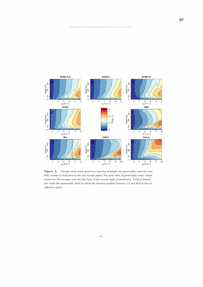
manuscript submitted to Geophysical Research Letters

Figure 2. Average mean wind speed as a function of height and geostrophic wind for each

PBL scheme as indicated at the top of each panel. For each value of geostrophic wind, values

shown are the averages over the last hour of the second night of simulation. Vertical dashed

line mark the geostrophic wind in which the thermal gradient between 1.3 and 30.8 m has an

inflection point.

–9–

97

manuscript submitted to Geophysical Research Letters

Figure 3. The same as in Figure 2, but for potential temperature. Vertical dashed line mark

the geostrophic wind in which the thermal gradient between 1.3 and 30.8 m has an inflection

point.

–10–

98

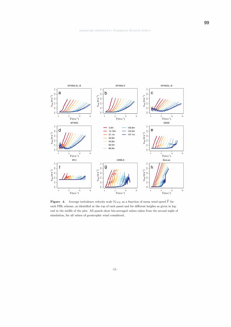
manuscript submitted to Geophysical Research Letters

0 5 10 15

0.0

0.2

0.4

0.6

0.8

1.0

V (m s−1)

VT

KE (

m s

−1)

MYNN2.5L−B

a

0 5 10 15

0.0

0.2

0.4

0.6

0.8

1.0

V (m s−1)

VT

KE (

m s

−1)

MYNN2.5

b

0 5 10 15

0.0

0.2

0.4

0.6

0.8

1.0

V (m s−1)

VT

KE (

m s

−1)

MYNN3L−B

c

0 5 10 15

0.0

0.2

0.4

0.6

0.8

1.0

V (m s−1)

VT

KE (

m s

−1)

MYNN3

d3.9m

12.19m

21.1m

30.8m

44.8m

64.5m

86.8m

106.8m

134.9m

147.1m

0 5 10 15

0.0

0.2

0.4

0.6

0.8

1.0

V (m s−1)

VT

KE (

m s

−1)

QNSE

e

0 5 10 15

0.0

0.2

0.4

0.6

0.8

1.0

V (m s−1)

VT

KE (

m s

−1)

MYJ

f

0 5 10 15

0.0

0.2

0.4

0.6

0.8

1.0

V (m s−1)

VT

KE (

m s

−1)

UWBLS

g

0 5 10 15

0.0

0.2

0.4

0.6

0.8

1.0

V (m s−1)

VT

KE (

m s

−1)

BouLac

h

Figure 4. Average turbulence velocity scale VTKE as a function of mean wind speed V for

each PBL scheme, as identified at the top of each panel and for different heights as given in leg-

end in the midlle of the plot. All panels show bin-averaged values taken from the second night of

simulation, for all values of geostrophic wind considered.

–11–

99

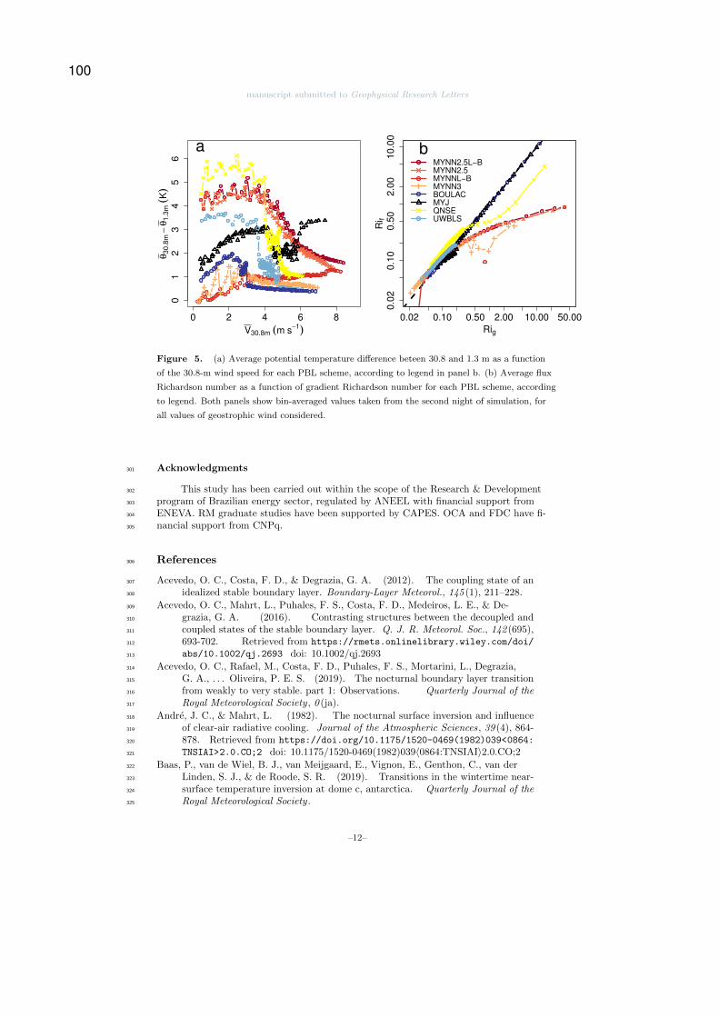
manuscript submitted to Geophysical Research Letters

0 2 4 6 8

01

23

45

6

V30.8m (m s−1)

θ30.8

m−

θ1.3

m (

K)

a

0.02 0.10 0.50 2.00 10.00 50.00

0.0

20.1

00.5

02.0

010.0

0

Rig

Ri f

MYNN2.5L−BMYNN2.5MYNNL−BMYNN3BOULACMYJQNSEUWBLS

b

Figure 5. (a) Average potential temperature difference beteen 30.8 and 1.3 m as a function

of the 30.8-m wind speed for each PBL scheme, according to legend in panel b. (b) Average flux

Richardson number as a function of gradient Richardson number for each PBL scheme, according

to legend. Both panels show bin-averaged values taken from the second night of simulation, for

all values of geostrophic wind considered.

Acknowledgments301

This study has been carried out within the scope of the Research & Development302

program of Brazilian energy sector, regulated by ANEEL with financial support from303

ENEVA. RM graduate studies have been supported by CAPES. OCA and FDC have fi-304

nancial support from CNPq.305

References306

Acevedo, O. C., Costa, F. D., & Degrazia, G. A. (2012). The coupling state of an307

idealized stable boundary layer. Boundary-Layer Meteorol., 145 (1), 211–228.308

Acevedo, O. C., Mahrt, L., Puhales, F. S., Costa, F. D., Medeiros, L. E., & De-309

grazia, G. A. (2016). Contrasting structures between the decoupled and310

coupled states of the stable boundary layer. Q. J. R. Meteorol. Soc., 142 (695),311

693-702. Retrieved from https://rmets.onlinelibrary.wiley.com/doi/312

abs/10.1002/qj.2693 doi: 10.1002/qj.2693313

Acevedo, O. C., Rafael, M., Costa, F. D., Puhales, F. S., Mortarini, L., Degrazia,314

G. A., . . . Oliveira, P. E. S. (2019). The nocturnal boundary layer transition315

from weakly to very stable. part 1: Observations. Quarterly Journal of the316

Royal Meteorological Society , 0 (ja).317

Andre, J. C., & Mahrt, L. (1982). The nocturnal surface inversion and influence318

of clear-air radiative cooling. Journal of the Atmospheric Sciences, 39 (4), 864-319

878. Retrieved from https://doi.org/10.1175/1520-0469(1982)039<0864:320

TNSIAI>2.0.CO;2 doi: 10.1175/1520-0469(1982)039〈0864:TNSIAI〉2.0.CO;2321

Baas, P., van de Wiel, B. J., van Meijgaard, E., Vignon, E., Genthon, C., van der322

Linden, S. J., & de Roode, S. R. (2019). Transitions in the wintertime near-323

surface temperature inversion at dome c, antarctica. Quarterly Journal of the324

Royal Meteorological Society .325

–12–

100

manuscript submitted to Geophysical Research Letters

Battisti, A., Acevedo, O. C., Costa, F. D., Puhales, F. S., Anabor, V., & Degrazia,326

G. A. (2017). Evaluation of nocturnal temperature forecasts provided by the327

weather research and forecast model for different stability regimes and terrain328

characteristics. Boundary-Layer Meteorol., 162 (3), 523–546.329

Bougeault, P., & Lacarrere, P. (1989). Parameterization of orography-induced tur-330

bulence in a mesobeta–scale model. Monthly Weather Review , 117 (8), 1872-331

1890. Retrieved from https://doi.org/10.1175/1520-0493(1989)117<1872:332

POOITI>2.0.CO;2 doi: 10.1175/1520-0493(1989)117〈1872:POOITI〉2.0.CO;2333

Bou-Zeid, E., Gao, X., Ansorge, C., & Katul, G. G. (2018). On the role of return to334

isotropy in wall-bounded turbulent flows with buoyancy. Journal of Fluid Me-335

chanics, 856 , 61–78.336

Bretherton, C. S., & Park, S. (2009). A new moist turbulence parameterization337

in the community atmosphere model. Journal of Climate, 22 (12), 3422-3448.338

Retrieved from https://doi.org/10.1175/2008JCLI2556.1 doi: 10.1175/339

2008JCLI2556.1340

Costa, F. D., Acevedo, O. C., Mombach, J. C., & Degrazia, G. A. (2011). A simpli-341

fied model for intermittent turbulence in the nocturnal boundary layer. J. At-342

mos. Sci., 68 (8), 1714–1729.343

Cuxart, J., Holtslag, A. A. M., Beare, R. J., Bazile, E., Beljaars, A., Cheng, A., . . .344

Xu, K.-M. (2006). Single-column model intercomparison for a stably stratified345

atmospheric boundary layer. Boundary-Layer Meteorol., 118 (2), 273–303.346

Dias-Junior, C. Q., Sa, L. D., Marques Filho, E. P., Santana, R. A., Mauder, M.,347

& Manzi, A. O. (2017). Turbulence regimes in the stable boundary layer348

above and within the amazon forest. Agricultural and forest meteorology , 233 ,349

122–132.350

Dimitrova, R., Silver, Z., Zsedrovits, T., Hocut, C. M., Leo, L. S., Di Sabatino, S.,351

& Fernando, H. J. S. (2016, Jun 01). Assessment of planetary boundary-352

layer schemes in the weather research and forecasting mesoscale model us-353

ing materhorn field data. Boundary-Layer Meteorology , 159 (3), 589–609.354

Retrieved from https://doi.org/10.1007/s10546-015-0095-8 doi:355

10.1007/s10546-015-0095-8356

Dudhia, J. (1989). Numerical study of convection observed during the win-357

ter monsoon experiment using a mesoscale two-dimensional model. Jour-358

nal of the Atmospheric Sciences, 46 (20), 3077-3107. Retrieved from359

https://doi.org/10.1175/1520-0469(1989)046<3077:NSOCOD>2.0.CO;2360

doi: 10.1175/1520-0469(1989)046〈3077:NSOCOD〉2.0.CO;2361

Holdsworth, A. M., & Monahan, A. H. (2019). Turbulent collapse and recovery in362

the stable boundary layer using an idealized model of pressure-driven flow with363

a surface energy budget. Journal of the Atmospheric Sciences(2019).364

Janjic, Z. I. (1994). The step-mountain eta coordinate model: Further developments365

of the convection, viscous sublayer, and turbulence closure schemes. Monthly366

Weather Review , 122 (5), 927-945. Retrieved from https://doi.org/10.1175/367

1520-0493(1994)122<0927:TSMECM>2.0.CO;2 doi: 10.1175/1520-0493(1994)368

122〈0927:TSMECM〉2.0.CO;2369

Katul, G. G., Porporato, A., Shah, S., & Bou-Zeid, E. (2014, Feb). Two phenomeno-370

logical constants explain similarity laws in stably stratified turbulence. Phys.371

Rev. E , 89 , 023007. Retrieved from https://link.aps.org/doi/10.1103/372

PhysRevE.89.023007 doi: 10.1103/PhysRevE.89.023007373

Kessler, E. (1969). On the distribution and continuity of water substance in atmo-374

spheric circulations. In On the distribution and continuity of water substance375

in atmospheric circulations (pp. 1–84). Boston, MA: American Meteorologi-376

cal Society. Retrieved from https://doi.org/10.1007/978-1-935704-36-2 1377

doi: 10.1007/978-1-935704-36-2 1378

Lan, C., Liu, H., Li, D., Katul, G. G., & Finn, D. (2018). Distinct turbulence struc-379

tures in stably stratified boundary layers with weak and strong surface shear.380

–13–

101

manuscript submitted to Geophysical Research Letters

Journal of Geophysical Research: Atmospheres, 123 (15), 7839–7854.381

Lapo, K., Nijssen, B., & Lundquist, J. D. (2019). Evaluation of turbulence sta-382

bility schemes of land models for stable conditions. Journal of Geophysi-383

cal Research: Atmospheres, 124 (6), 3072-3089. Retrieved from https://384

agupubs.onlinelibrary.wiley.com/doi/abs/10.1029/2018JD028970 doi:385

10.1029/2018JD028970386

Mahrt, L. (1998, Aug 01). Nocturnal boundary-layer regimes. Boundary-Layer387

Meteorol., 88 (2), 255–278. Retrieved from https://doi.org/10.1023/A:388

1001171313493 doi: 10.1023/A:1001171313493389

Mahrt, L. (2014). Stably stratified atmospheric boundary layers. Annual Review390

of Fluid Mechanics, 46 (1), 23-45. Retrieved from https://doi.org/10.1146/391

annurev-fluid-010313-141354 doi: 10.1146/annurev-fluid-010313-141354392

Mahrt, L., & Gamage, N. (1987). Observations of turbulence in stratified flow.393

Journal of the Atmospheric Sciences, 44 (7), 1106-1121. Retrieved from394

https://doi.org/10.1175/1520-0469(1987)044<1106:OOTISF>2.0.CO;2395

doi: 10.1175/1520-0469(1987)044〈1106:OOTISF〉2.0.CO;2396

Maroneze, R., Acevedo, O. C., Costa, F. D., Puhales, F. S., Demarco, G., & Mor-397

tarini, L. (n.d.). The nocturnal boundary layer transition from weakly to very398

stable. part 2: Numerical simulation with a second order model. Quarterly399

Journal of the Royal Meteorological Society , 0 (0), 16. doi: 10.1002/qj.3643400

Maroneze, R., Acevedo, O. C., Costa, F. D., & Sun, J. (2019, Feb 01). Sim-401

ulating the regime transition of the stable boundary layer using differ-402

ent simplified models. Boundary-Layer Meteorology , 170 (2), 305–321.403

Retrieved from https://doi.org/10.1007/s10546-018-0401-3 doi:404

10.1007/s10546-018-0401-3405

McNider, R. T., England, D. E., Friedman, M. J., & Shi, X. (1995). Predictabil-406

ity of the stable atmospheric boundary layer. J. Atmos. Sci., 52 (10), 1602-407

1614. Retrieved from https://doi.org/10.1175/1520-0469(1995)052<1602:408

POTSAB>2.0.CO;2 doi: 10.1175/1520-0469(1995)052〈1602:POTSAB〉2.0.CO;2409

Mlawer, E. J., Taubman, S. J., Brown, P. D., Iacono, M. J., & Clough, S. A.410

(1997). Radiative transfer for inhomogeneous atmospheres: Rrtm, a val-411

idated correlated-k model for the longwave. Journal of Geophysical Re-412

search: Atmospheres, 102 (D14), 16663-16682. Retrieved from https://413

agupubs.onlinelibrary.wiley.com/doi/abs/10.1029/97JD00237 doi:414

10.1029/97JD00237415

Mukul Tewari, N., Tewari, M., Chen, F., Wang, W., Dudhia, J., LeMone, M., . . .416

others (2004). Implementation and verification of the unified noah land sur-417

face model in the wrf model (formerly paper number 17.5). In 20th conference418

on weather analysis and forecasting/16th conference on numerical weather419

prediction (pp. 11–15).420

Nakanish, M. (2001, Jun 01). Improvement of the mellor–yamada turbulence clo-421

sure model based on large-eddy simulation data. Boundary-Layer Meteorology ,422

99 (3), 349–378. Retrieved from https://doi.org/10.1023/A:1018915827400423

doi: 10.1023/A:1018915827400424

Nakanishi, M., & Niino, H. (2006, May 01). An improved mellor–yamada425

level-3 model: Its numerical stability and application to a regional pre-426

diction of advection fog. Boundary-Layer Meteorology , 119 (2), 397–407.427

Retrieved from https://doi.org/10.1007/s10546-005-9030-8 doi:428

10.1007/s10546-005-9030-8429

Nakanishi, M., & Niino, H. (2009). Development of an improved turbulence closure430

model for the atmospheric boundary layer. Journal of the Meteorological Soci-431

ety of Japan. Ser. II , 87 (5), 895-912. doi: 10.2151/jmsj.87.895432

Ohya, Y. (2001, Jan 01). Wind-tunnel study of atmospheric stable boundary lay-433

ers over a rough surface. Boundary-Layer Meteorology , 98 (1), 57–82. Re-434

trieved from https://doi.org/10.1023/A:1018767829067 doi: 10.1023/A:435

–14–

102

manuscript submitted to Geophysical Research Letters

1018767829067436

Olson, J. B., Kenyon, J. S., Angevine, W., Brown, J. M., Pagowski, M., Suselj, K.,437

et al. (2019). A description of the mynn-edmf scheme and the coupling to438

other components in wrf–arw.439

Pardyjak, E. R., Monti, P., & Fernando, H. J. S. (2002). Flux richardson number440

measurements in stable atmospheric shear flows. Journal of Fluid Mechanics,441

459 , 307–316. doi: 10.1017/S0022112002008406442

Poulos, G. S., Blumen, W., Fritts, D. C., Lundquist, J. K., Sun, J., Burns,443

S. P., . . . Jensen, M. (2002). Cases-99: A comprehensive investigation444

of the stable nocturnal boundary layer. Bulletin of the American Mete-445

orological Society , 83 (4), 555-582. Retrieved from https://doi.org/446

10.1175/1520-0477(2002)083<0555:CACIOT>2.3.CO;2 doi: 10.1175/447

1520-0477(2002)083〈0555:CACIOT〉2.3.CO;2448

Powers, J. G., Klemp, J. B., Skamarock, W. C., Davis, C. A., Dudhia, J., Gill,449

D. O., . . . Duda, M. G. (2017). The weather research and forecasting model:450

Overview, system efforts, and future directions. Bulletin of the American451

Meteorological Society , 98 (8), 1717-1737. Retrieved from https://doi.org/452

10.1175/BAMS-D-15-00308.1 doi: 10.1175/BAMS-D-15-00308.1453

Skamarock, W. C., Klemp, J. B., Dudhia, J., Gill, D. O., Barker, D. M., Wang, W.,454

& Powers, J. G. (2008). A description of the advanced research wrf version 3.455

ncar technical note-475+ str.456

Sukoriansky, S., Galperin, B., & Perov, V. (2005, Nov 01). ‘application of a new457

spectral theory of stably stratified turbulence to the atmospheric bound-458

ary layer over sea ice’. Boundary-Layer Meteorology , 117 (2), 231–257.459

Retrieved from https://doi.org/10.1007/s10546-004-6848-4 doi:460

10.1007/s10546-004-6848-4461

Sun, J., & French, J. R. (2016). Air–sea interactions in light of new understanding of462

air–land interactions. Journal of the Atmospheric Sciences, 73 (10), 3931-3949.463

Retrieved from https://doi.org/10.1175/JAS-D-15-0354.1 doi: 10.1175/464

JAS-D-15-0354.1465

Sun, J., Mahrt, L., Banta, R. M., & Pichugina, Y. L. (2012). Turbulence regimes466

and turbulence intermittency in the stable boundary layer during “cases-99”.467

J. Atmos. Sci., 69 (1), 338–351.468

Svensson, G., Holtslag, A. A. M., Kumar, V., Mauritsen, T., Steeneveld, G. J.,469

Angevine, W. M., . . . Zampieri, M. (2011). Evaluation of the diurnal cycle in470

the atmospheric boundary layer over land as represented by a variety of single-471

column models: the second “gabls” experiment. Boundary-Layer Meteorol.,472

140 (2), 177–206.473

Tastula, E.-M., Galperin, B., Dudhia, J., LeMone, M. A., Sukoriansky, S., &474

Vihma, T. (2015). Methodical assessment of the differences between475

the qnse and myj pbl schemes for stable conditions. Quarterly Journal476

of the Royal Meteorological Society , 141 (691), 2077-2089. Retrieved from477

https://rmets.onlinelibrary.wiley.com/doi/abs/10.1002/qj.2503 doi:478

10.1002/qj.2503479

van der Linden, S. J. A., Baas, P., van Hooft, J. A., van Hooijdonk, I. G. S.,480

Bosveld, F. C., & van de Wiel, B. J. H. (2017). Local characteristics of the481

nocturnal boundary layer in response to external pressure forcing. J. Appl.482

Meteorol. Climat., 56 (11), 3035-3047. Retrieved from https://doi.org/483

10.1175/JAMC-D-17-0011.1 doi: 10.1175/JAMC-D-17-0011.1484

Van de Wiel, B. J. H., Moene, A. F., Jonker, H. J. J., Baas, P., Basu, S., Donda,485

J. M. M., . . . Holtslag, A. A. M. (2012). The minimum wind speed for sustain-486

able turbulence in the nocturnal boundary layer. Journal of the Atmospheric487

Sciences, 69 (11), 3116-3127. Retrieved from https://doi.org/10.1175/488

JAS-D-12-0107.1 doi: 10.1175/JAS-D-12-0107.1489

Van de Wiel, B. J. H., Ronda, R. J., Moene, A. F., De Bruin, H. A. R., & Holt-490

–15–

103

manuscript submitted to Geophysical Research Letters

slag, A. A. M. (2002). Intermittent turbulence and oscillations in the491

stable boundary layer over land. part i: A bulk model. Journal of the At-492

mospheric Sciences, 59 (5), 942-958. Retrieved from https://doi.org/493

10.1175/1520-0469(2002)059<0942:ITAOIT>2.0.CO;2 doi: 10.1175/494

1520-0469(2002)059〈0942:ITAOIT〉2.0.CO;2495

Van de Wiel, B. J. H., Vignon, E., Baas, P., van Hooijdonk, I. G. S., van der Linden,496

S. J. A., Antoon van Hooft, J., . . . Genthon, C. (2017). Regime transitions497

in near-surface temperature inversions: A conceptual model. Journal of the498

Atmospheric Sciences, 74 (4), 1057-1073. Retrieved from https://doi.org/499

10.1175/JAS-D-16-0180.1 doi: 10.1175/JAS-D-16-0180.1500

Vignon, E., van de Wiel, B. J., van Hooijdonk, I. G., Genthon, C., van der Linden,501

S. J., van Hooft, J. A., . . . Casasanta, G. (2017). Stable boundary-layer502

regimes at dome c, antarctica: observation and analysis. Quarterly Journal of503

the Royal Meteorological Society , 143 (704), 1241–1253.504

Zilitinkevich, S. S., Elperin, T., Kleeorin, N., Rogachevskii, I., & Esau, I. (2013,505

Mar 01). A hierarchy of energy- and flux-budget (efb) turbulence closure mod-506

els for stably-stratified geophysical flows. Boundary-Layer Meteorology , 146 (3),507

341–373. Retrieved from https://doi.org/10.1007/s10546-012-9768-8508

doi: 10.1007/s10546-012-9768-8509

–16–

104

GEOPHYSICAL RESEARCH LETTERS

Supporting Information for ”How is the two-regime

stable boundary layer solved by the different PBL

schemes in WRF?”

Rafael Maroneze 1

Otavio Costa Acevedo 1

Felipe Denardin Costa 2

Franciano Scremim Puhales 1

Vagner Anabor 1

Luca Mortarini 13

1Universidade Federal de Santa Maria

2Universidade Federal do Pampa Campus-Alegrete

3Institute of Atmospheric Sciences and Climate - National Research Council

Contents of this file

1. Description of the PBL schemes

2. Figures S1-S2

3. Tables S1-S3

October 18, 2019, 2:18pm

105

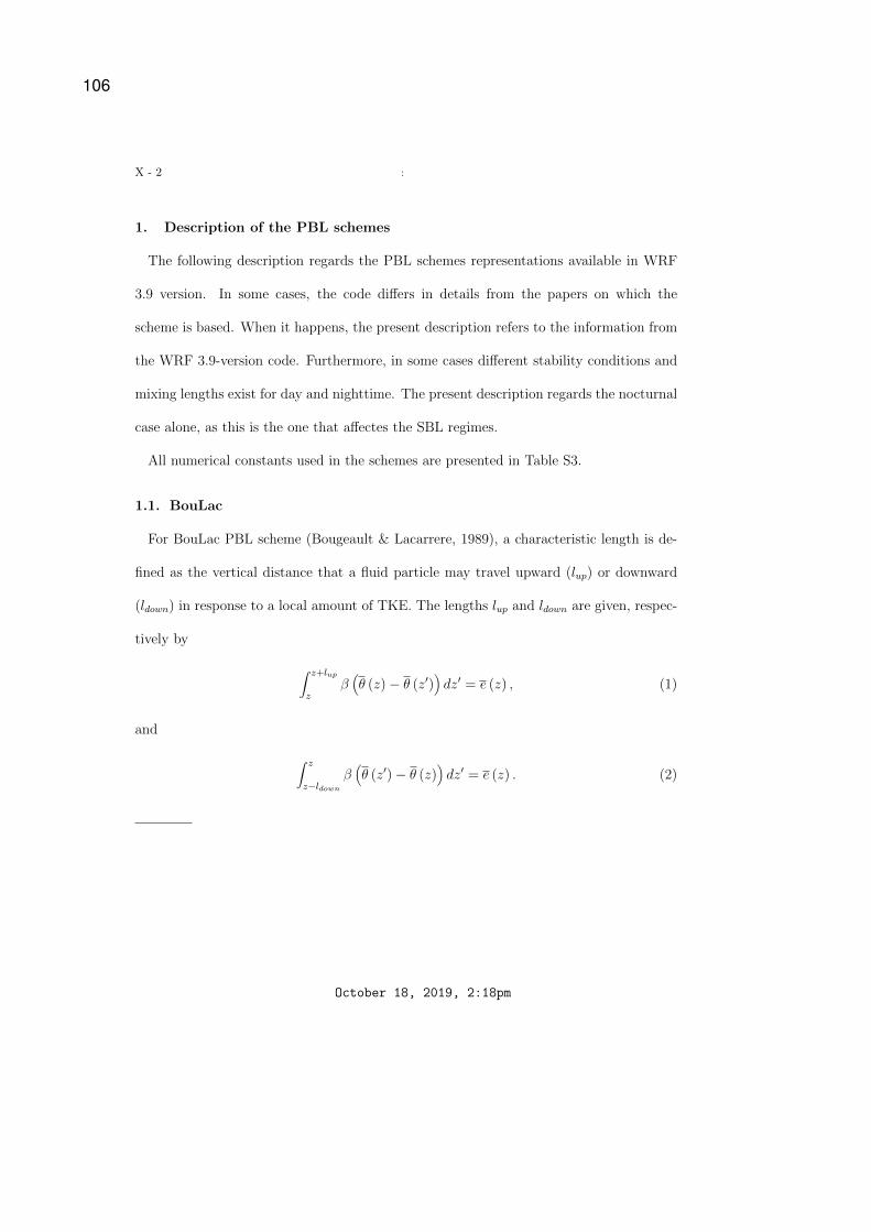
X - 2 :

1. Description of the PBL schemes

The following description regards the PBL schemes representations available in WRF

3.9 version. In some cases, the code differs in details from the papers on which the

scheme is based. When it happens, the present description refers to the information from

the WRF 3.9-version code. Furthermore, in some cases different stability conditions and

mixing lengths exist for day and nighttime. The present description regards the nocturnal

case alone, as this is the one that affectes the SBL regimes.

All numerical constants used in the schemes are presented in Table S3.

1.1. BouLac

For BouLac PBL scheme (Bougeault & Lacarrere, 1989), a characteristic length is de-

fined as the vertical distance that a fluid particle may travel upward (lup) or downward

(ldown) in response to a local amount of TKE. The lengths lup and ldown are given, respec-

tively by

∫ z+lup

zβ(θ (z)− θ (z′)

)dz′ = e (z) , (1)

and

∫ z

z−ldown

β(θ (z′)− θ (z)

)dz′ = e (z) . (2)

October 18, 2019, 2:18pm

106

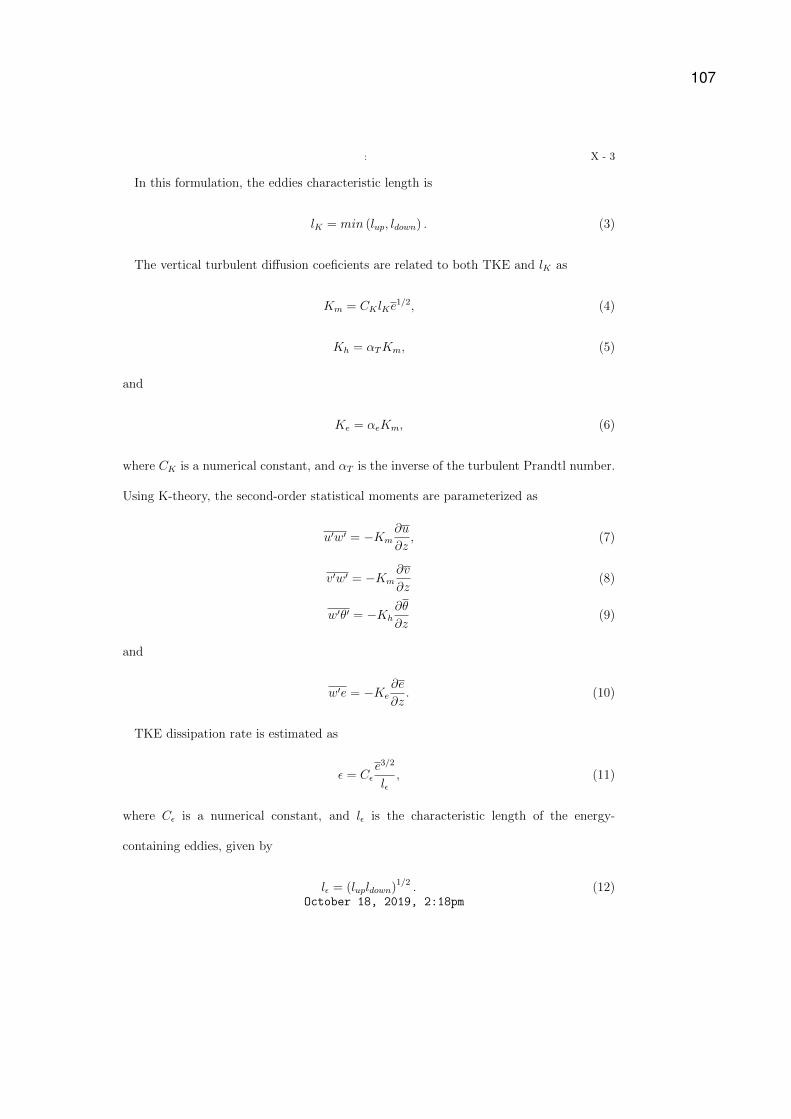
: X - 3

In this formulation, the eddies characteristic length is

lK = min (lup, ldown) . (3)

The vertical turbulent diffusion coeficients are related to both TKE and lK as

Km = CK lKe1/2, (4)

Kh = αTKm, (5)

and

Ke = αeKm, (6)

where CK is a numerical constant, and αT is the inverse of the turbulent Prandtl number.

Using K-theory, the second-order statistical moments are parameterized as

u′w′ = −Km∂u

∂z, (7)

v′w′ = −Km∂v

∂z(8)

w′θ′ = −Kh∂θ

∂z(9)

and

w′e = −Ke∂e

∂z. (10)

TKE dissipation rate is estimated as

ε = Cεe3/2

lε, (11)

where Cε is a numerical constant, and lε is the characteristic length of the energy-

containing eddies, given by

lε = (lupldown)1/2 . (12)October 18, 2019, 2:18pm

107

X - 4 :

Therefore, the prognostic equation for TKE solved by the scheme is

∂e

∂z= Km

(∂u

∂z

)2

+

(∂v

∂z

)2− g

ΘKh

∂θ

∂z+

∂

∂z

(Ke

∂e

∂z

)− Cε

e3/2

lε. (13)

Minimum values for Km and for TKE are assumed as 0.1 m2 s−1 and 0.0001 m2 s−2

respectively. BouLac scheme does not use a stability function.

1.2. Mellor Yamada Janjic

For the Mellor Yamada Janjic PBL scheme (Janji, 1994), the turbulent length scale is

defined as (Mellor & Yamada, 1974):

lt =l0κz

κz + l0, (14)

where

l0 =

∫∞0 α |z| qdz∫∞

0 qdz. (15)

As in Mellor and Yamada (1974), q2 is defined as twice TKE (q2 = 2e) In (14) and (15),

κ is the von Karman constant and α is a numerical constant, whose values are given in

table S1. The dimensionless vertical gradients of wind speed and temperature are defined,

respectively, as

GM ≡l2tq2

(∂u

∂z

)2

+

(∂v

∂z

)2 , (16)

and

GH ≡l2tq2βg∂θV∂z

. (17)

In (16), β = 1/Θ. For MYJ the stability functions form momentum (SM) and heat

(SH) are the same as those in Mellor and Yamada (1982), but written in terms of the

October 18, 2019, 2:18pm

108

: X - 5

above defined quantities:

SM =ASM

GH +BSM

(CSMGM +DSM

GH)GH + FSMGM +GSM

GH + 1, (18)

and

SH ≡(ASH

GM +BSHGH) + A2

(CSMGM +DSM

GH)GH + FSMGM +GSM

GH + 1, (19)

where ASM, BSM

,CSM,DSM

,FSM,GSM

,ASH,BSH

and CSHare numerical constants given by

ASM= −3A1A2 (3A2 + 3B2C1 + 12A1C1 −B2) ,

BSM= A1 (1− 3C1) ,

CSM= 18A2

1A2 (B2 − 3A2) ,

DSM= 9A1A

22 (12A1 + 3B2) ,

FSM= 6A2

1,

GSM= 3A2 (7A1 +B2) ,

ASH= 18A2

1A2C1,

BSH= 9A1A

22,

CSH= A2,

where the numerical constants A1,A2,B1,B2 and C1 values are shown in table S1.

The vertical turbulent diffusion coeficients are related to SM , SH and q:

KM = ltqSM , (20)

KH = ltqSH , (21)

October 18, 2019, 2:18pm

109

X - 6 :

and the second-order statistical moments are parameterized as in equations 7-9. MYJ

TKE disipation is assumed as

εq =q3

B1lt. (22)

Lacking a transport term, the prognostic equation for q is

∂q

∂t=

(q2

lt

) [SMGM + SHGH −

1

B1

], (23)

Equation 23 may be rewritten as

d

dt

(ltq

)=

A(ltq

)4+B

(ltq

)2

C(ltq

)4+D

(ltq

)2+ 1− 1

B1, (24)

where the right-hand side is defined as R. Its derivative with respect to lt/q is defined as

R′:

dR

d(ltq

) = R′ = −2

[(AD −BC)

(ltq

)5+ 2A

(ltq

)3+B

(ltq

)]

[C(ltq

)4+D

(ltq

)2+ 1

]2 . (25)

The functions A, B, C and D are given by

A ={

[−3A1A2 (3A2 + 3B2c1 + 18A1C1 −B2) (βg)] gM −[BSH

(βg)2]gH}gH ,

B = BSMgM − (A2βg) gH ,

C ={

[CSM(βg)] gM −

[DSH

(βg)2]gH}gH

and

D = FSMgM −GSH

(βg) gH .

where the dimensionless vertical gradients of mean wind speed and virtual temperature

are defined as

gM =GM

l2tq2

October 18, 2019, 2:18pm

110

: X - 7

and

gH =GH

l2tq2βg

Equation 24 is linearized as

d(ltq

)i+1

dt= Ri +R′i

[(ltq

)

i+1

−(ltq

)

i

](26)

whose solution is

(ltq

)

i+1

=

(l

q

)

i

−[R

R′

]

i+

{[R

R′

]

i+

[(ltq

)

0

−(ltq

)

i

]}exp [∆tR′i] (27)

which needs to be found iteratively. In general, two interactions are sufficient, so that q2

depends on (l/q)3, given by eq. 27 after two interactions:

q2 =l2t(ltq

)2

3

. (28)

Equations 24-28 do not solve TKE transport. It is estimated at a later step where TKE

is vertically diffused as its value at a given value is adjusted with respect to the value at

neighbor levels:

q2(zi) =−Cr(zi)q2(zi+1) +RQ(zi)

CM(zi)(29)

where

CR(zi) = −DTZ(zi)AKq(zi)

CM = CR(zi−1)CF (zi) + (AKq(zi−1) + AKq(zi))DTZ(zi) + 1

RQ(zi) = RQ(zi−1)CF (zi) + q2(zi)

AKq(zi) =5√q2(zi)l(zi)

zi+1 − zi+2

DTZ(zi) =2∆t

zi − zi+2

October 18, 2019, 2:18pm

111

X - 8 :

CF =−DTZ(zi)AKq(zi−1)

CM(zi−1).

A TKE minimum value of 0.1 m2 s−2 is assumed.

1.3. QNSE

For stable conditions the mixing length in QNSE is given by

lq =1

l−1b + l−1

s

(30)

where lb and ls are defined as

lb =κz

1 + κzλ

and

ls =

√0.5q2

N

where q2 is TKE, N is the BruntVisl frequency and λ = 0.0063u∗/f .

The stability functions are defined in terms of the gradient Richradson number

(Sukoriansky et al., 2005)

αM =1 + AM1Ri

2g

1 + AM2Rig + AM3Ri2g(31)

αH =AH1 + AH2Rig + AH3Ri

2g

1 + AH4Rig + AH5Ri2g(32)

where AM1, AM2, AM3, AH1, AH2, AH3, AH4 and AH5 are numerical constants.

The vertical turbulent diffusion coeficients are related to αM , αH and q:

KM = lqqαM , (33)

KH = lqqαH , (34)

and the second-order statistical moments are parameterized as in equations 7-9.

October 18, 2019, 2:18pm

112

: X - 9

Lacking a transport term, the prognostic equation for TKE is

∂q2

∂z= 2

Km

(∂u

∂z

)2

+

(∂v

∂z

)2− g

ΘKh

∂θV∂z− Ce

(0.5q2)3/2

lq

(35)

TKE transport is determined as in MYJ (equation 29). A minimum TKE of 0.005 m2s−2

is imposed.

1.4. MYNN

The original MYNN length mixing (bl-mynn-mixlength=0) is calculated as the harmonic

average between a turbulent (lT ), a surface-layer (lS) and a buyoant (lB) length scale:

1

l=

1

lT+

1

lS+

1

lB(36)

where:

lT =

∫HPBL0 0.23 |z| qdz∫HPBL

0 qdz. (37)

lS = κz[1 + 2.7 min

(z

L, 1)]

(38)

lB =q

N(39)

where L is the MoninObukhov length and N is the BruntVisl frequency. In the L-B

versions of MYNN (bl-mynn-mixlength=1), an additional correction for the mixing length

is used, originating mixing-length l′:

l′ = l(1−WT ) + 0.4LBouLac ∗WT (40)

October 18, 2019, 2:18pm

113

X - 10 :

where LBouLac is given by eq. 3, and WT :

WT = 0.5tgh

[z − (zi2 + h1)

h2

]+ 0.5 (41)

where zi2 is the PBL height and h1 = 0.3zi2 and h2 = h1/2.

Level 2

Although no level-2 MYNN PBL schemes are explicitly used in the present study, it is

necessary to define its equations before showing those for levels 2.5 and 3.

As defined in Mellor and Yamada (1974, 1982), in level-2 parameterizations TKE is

estimated through the balance between shear production, buoyant destruction and dissi-

pation

q22 = b1l

2

sm

(∂u

∂z

)2

+

(∂v

∂z

)2+ sh

g

Θ

∂θV∂z

(42)

where sh and sm are the stability functions for heat and momentum, respectively:

sh = 3a2 (g1 + g2)rfc − rf1− rf (43)

and

sm =a1

a2

f1

f2

rf1 − rfrf2 − rf

sh. (44)

which are functions of the level-2 flux Richardson number (rf), defined as

rf = min[ri1

(Rig + ri2 −

√Ri2g − ri3Rig + r2

i2

), rfc

](45)

where Rig is the gradient Richardson number, rfc is the critical flux Richardson number:

rfc =g1

g1 + g2

. (46)

The other quantities in eqs. 43-45 are numerical constants:

f1 = b1 (g1 − c1) + 3a2 (1− c2) (1− c5) + 2a1 (1− c2) ,October 18, 2019, 2:18pm

114

: X - 11

f2 = b1 (g1 + g2)− 3a1 (1− c2) ,

rf1 =b1 (g1 − c1)

f1

,

rf2 =b1g1

f2

,

ri1 =1

2

a2

a1

f2

f1

,

ri2 = rf1a1

a2

f1

f2

and

ri3 = 4rf2a1

a2

f1

f2

− 2ri2.

A correction that allows a variable critical Richardson number and avoids negative TKE

in stable condions uses

a2 =a′2

1 +Rig

following Canuto, Cheng, Howard, and Esau (2008) and Kitamura (2010).

Level 2.5

In level 2.5, a prognostic equation for q2 is solved

∂q2

∂t= 2lq

sm2.5

(∂u

∂z

)2

+

(∂v

∂z

)2+ sh2.5

g

Θ

∂θV∂z

+

∂

∂z

[3lqsm2.5

∂q2

∂z

]− 2q3

b1l(47)

If q2 < q22 (level-2 TKE, equation 42 ), the stability functions for momentum (sm2.5)

and heat (sm2.5) are

sm2.5 = sm

√q2

q22

, (48)

sh2.5 = sh

√q2

q22

, (49)

while, on the other hand, if q2 > q22, these stability functions are:

sm2.5 =q2a1 (e2 − 3c1e4)

D2.5

, (50)

October 18, 2019, 2:18pm

115

X - 12 :

sh2.5 =q2 (e2 + 3c1e5)

D2.5

, (51)

where e1, e2, e3, e4, e5 and D2.5 are

e1 = q2 − 3a2b2 (1− c3) l2g

Θ

∂θV∂z

,

e2 = q2 − 9a1a2 (1− c2) l2g

Θ

∂θV∂z

,

e3 = e1 + 9a22 (1− c2) (1− c5) l2

g

Θ

∂θV∂z

,

e4 = e1 − 12a1a2 (1− c2) l2g

Θ

∂θV∂z

,

e5 = 6a21l

2

(∂u

∂z

)2

+

(∂v

∂z

)2

and

D2.5 = e2e4 + e3e5.

The vertical eddy diffusivities are related to sm2.5, sh2.5, l and q:

KM = lqsm2.5, (52)

KH = lqsh2.5, (53)

and the second-order statistical moments are parameterized as in equations 7-9.

The variance of temperature, variance of total water content and covariance of θl and

qw are diagnostically estimated as

θ′l2

2.5 = αcb2lqsh2.5

(∂θl∂z

)2

, (54)

q′w2

2.5 = αcb2lqsh2.5

(∂qw∂z

)2

, (55)

θ′lq′w2.5 = αcb2lqsh2.5

∂qw∂z

∂θl∂z

(56)

October 18, 2019, 2:18pm

116

: X - 13

These quantities are not used in 2.5 level schemes, but they are important to calculate

the contergradients and stability functions of MYNN 3-level. The parameter αc is defined

as (Nakanishi & Niino, 2009)

αc =

{q/q2, if q < q2

1, if q ≥ q2. (57)

Level 3

In level 3, the stability function for momentum (sm) is split in two parts, the first is

the stability functions from level-2.5 (sm2.5), and the second part is a correction (sm′)

(Nakanishi & Niino, 2009):

sm = sm2.5 + sm′ , (58)

The second part sm′ is defined as

sm′ =l2αce

′6gΘ

(θ′2V − θ′2V 2.5

)

D3

α2c

(9a2

2 (1− c2) (1− c5) + 12a1a2 (1− c2)) a1

a2

(59)

where e′2, e′3, e′4, e′5, e′6 and D3 are given by

D3 = e′2e′4 + e′3e

′5,

e′2 = q2 − 9a1a2 (1− c2) l2g

Θ

∂θV∂z

α2c ,

e′3 = q2 + 9a22 (1− c2) (1− c5) l2

g

Θ

∂θV∂z

α2c ,

e′4 = q2 − 12a1a2 (1− c2) l2g

Θ

∂θV∂z

α2c ,

e′5 = 6a21l

2

(∂u

∂z

)2

+

(∂v

∂z

)2α2

c

and

e′6 = 3a2 (1− c3)g

Θ.

October 18, 2019, 2:18pm

117

X - 14 :

The vertical eddy difuusivitys are related to sm, sh2.5, l and q as:

KM = lqsm, (60)

KH = lqsh2.5 (61)

and the second-order statistical moments parameterized are given by

u′w′ = −KM∂u

∂z(62)

v′w′ = −KM∂v

∂z(63)

w′θ′l = −lq[sh2.5

∂θl∂z

+ Γθ

](64)

w′θ′V = −lq[sh2.5

∂θV∂z

+ ΓV

](65)

w′q′w = −lq[sh2.5

∂qw∂z

+ Γq

](66)

The quantities Γtheta, Γq and ΓV are countergradient contributions

Γθ =−e′7αce′6

(θ′lθ′V − θ′lθ′V 2.5

)

D3

, (67)

ΓV =e′7αce

′6gΘ

(θ′2V − θ′2V 2.5

)

D3

, (68)

Γq =−e′7αce′6

(q′wθ

′V − q′wθ′V 2.5

)

D3

, (69)

where θ′lθ′V , q′wθ

′V , θ′V

2 and e′7 are given by

θ′lθ′V = βθθ′l

2 + βqθ′lq′w,

q′wθ′V = βθθ′lqw + βqq′w

2,

October 18, 2019, 2:18pm

118

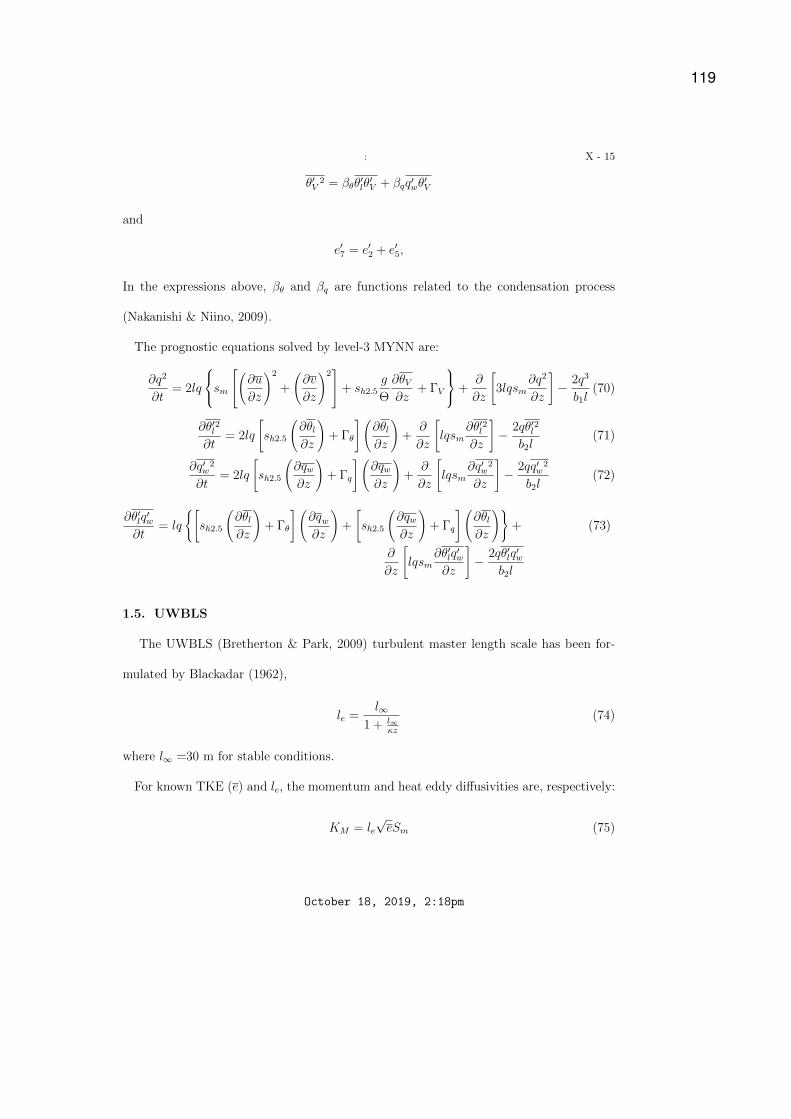
: X - 15

θ′V2 = βθθ′lθ

′V + βqq′wθ

′V

and

e′7 = e′2 + e′5,

In the expressions above, βθ and βq are functions related to the condensation process

(Nakanishi & Niino, 2009).

The prognostic equations solved by level-3 MYNN are:

∂q2

∂t= 2lq

sm

(∂u

∂z

)2

+

(∂v

∂z

)2+ sh2.5

g

Θ

∂θV∂z

+ ΓV

+

∂

∂z

[3lqsm

∂q2

∂z

]− 2q3

b1l(70)

∂θ′l2

∂t= 2lq

[sh2.5

(∂θl∂z

)+ Γθ

](∂θl∂z

)+

∂

∂z

[lqsm

∂θ′l2

∂z

]− 2qθ′l

2

b2l(71)

∂q′w2

∂t= 2lq

[sh2.5

(∂qw∂z

)+ Γq

](∂qw∂z

)+

∂

∂z

[lqsm

∂q′w2

∂z

]− 2qq′w

2

b2l(72)

∂θ′lq′w

∂t= lq

{[sh2.5

(∂θl∂z

)+ Γθ

](∂qw∂z

)+

[sh2.5

(∂qw∂z

)+ Γq

](∂θl∂z

)}+ (73)

∂

∂z

[lqsm

∂θ′lq′w

∂z

]− 2qθ′lq

′w

b2l

1.5. UWBLS

The UWBLS (Bretherton & Park, 2009) turbulent master length scale has been for-

mulated by Blackadar (1962),

le =l∞

1 + l∞κz

(74)

where l∞ =30 m for stable conditions.

For known TKE (e) and le, the momentum and heat eddy diffusivities are, respectively:

KM = le√eSm (75)

October 18, 2019, 2:18pm

119

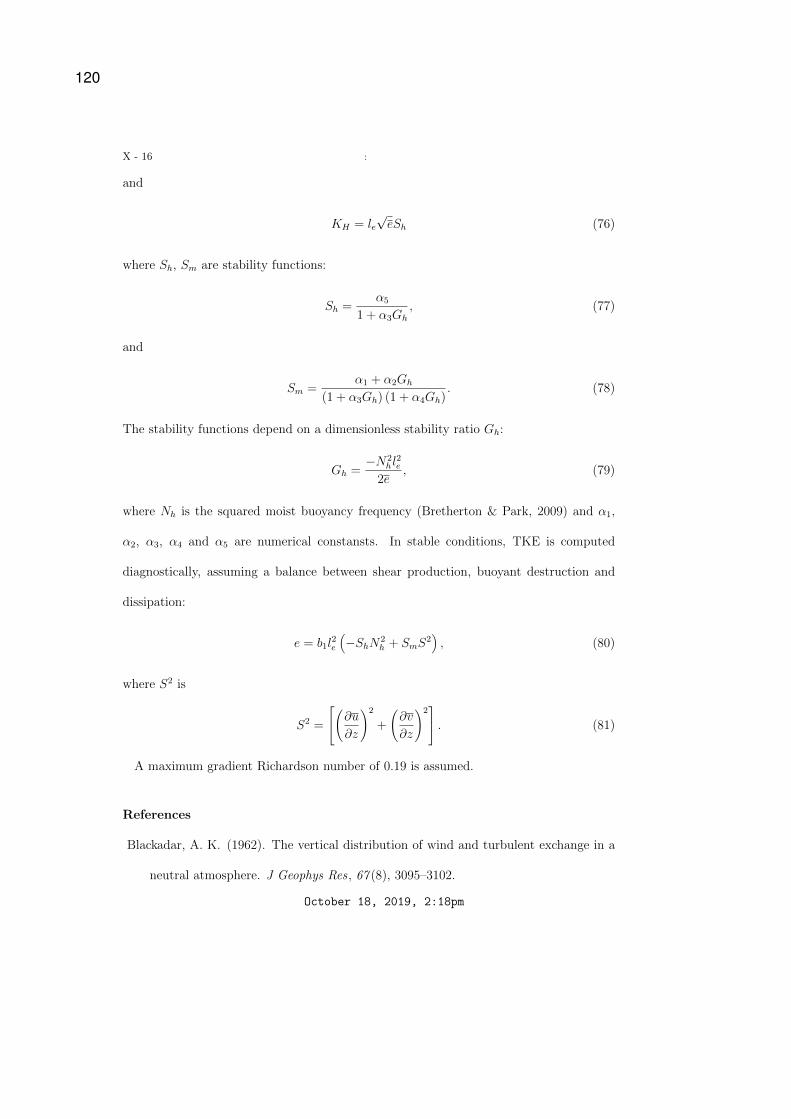
X - 16 :

and

KH = le√eSh (76)

where Sh, Sm are stability functions:

Sh =α5

1 + α3Gh

, (77)

and

Sm =α1 + α2Gh

(1 + α3Gh) (1 + α4Gh). (78)

The stability functions depend on a dimensionless stability ratio Gh:

Gh =−N2

h l2e

2e, (79)

where Nh is the squared moist buoyancy frequency (Bretherton & Park, 2009) and α1,

α2, α3, α4 and α5 are numerical constansts. In stable conditions, TKE is computed

diagnostically, assuming a balance between shear production, buoyant destruction and

dissipation:

e = b1l2e

(−ShN2

h + SmS2), (80)

where S2 is

S2 =

(∂u

∂z

)2

+

(∂v

∂z

)2 . (81)

A maximum gradient Richardson number of 0.19 is assumed.

References

Blackadar, A. K. (1962). The vertical distribution of wind and turbulent exchange in a

neutral atmosphere. J Geophys Res , 67 (8), 3095–3102.

October 18, 2019, 2:18pm

120

: X - 17

Bougeault, P., & Lacarrere, P. (1989). Parameterization of orography-induced tur-

bulence in a mesobeta–scale model. Monthly Weather Review , 117 (8), 1872-1890.

Retrieved from https://doi.org/10.1175/1520-0493(1989)117<1872:POOITI>2

.0.CO;2 doi: 10.1175/1520-0493(1989)117〈1872:POOITI〉2.0.CO;2

Bretherton, C. S., & Park, S. (2009). A new moist turbulence parameterization in the

community atmosphere model. Journal of Climate, 22 (12), 3422-3448. Retrieved

from https://doi.org/10.1175/2008JCLI2556.1 doi: 10.1175/2008JCLI2556.1

Canuto, V. M., Cheng, Y., Howard, A. M., & Esau, I. N. (2008). Stably stratified

flows: A model with no ri(cr). Journal of the Atmospheric Sciences , 65 (7), 2437-

2447. Retrieved from https://doi.org/10.1175/2007JAS2470.1 doi: 10.1175/

2007JAS2470.1

Janji, Z. I. (1994). The step-mountain eta coordinate model: Further developments

of the convection, viscous sublayer, and turbulence closure schemes. Monthly

Weather Review , 122 (5), 927-945. Retrieved from https://doi.org/10.1175/1520

-0493(1994)122<0927:TSMECM>2.0.CO;2 doi: 10.1175/1520-0493(1994)122〈0927:

TSMECM〉2.0.CO;2

Kitamura, Y. (2010). Modifications to the mellor-yamada-nakanishi-niino (mynn) model

for the stable stratification case. Journal of the Meteorological Society of Japan. Ser.

II , 88 (5), 857–864.

Mellor, G. L., & Yamada, T. (1974). A hierarchy of turbulence closure models for

planetary boundary layers. J. Atmos. Sci., 31 (7), 1791–1806.

Mellor, G. L., & Yamada, T. (1982). Development of a turbulence closure model for

October 18, 2019, 2:18pm

121

X - 18 :

geophysical fluid problems. Rev. Geophys., 20 (4), 851–875.

Nakanishi, M., & Niino, H. (2009). Development of an improved turbulence closure

model for the atmospheric boundary layer. Journal of the Meteorological Society of

Japan. Ser. II , 87 (5), 895-912. doi: 10.2151/jmsj.87.895

Sukoriansky, S., Galperin, B., & Perov, V. (2005, Nov 01). ‘application of a new spectral

theory of stably stratified turbulence to the atmospheric boundary layer over sea ice’.

Boundary-Layer Meteorology , 117 (2), 231–257. Retrieved from https://doi.org/

10.1007/s10546-004-6848-4 doi: 10.1007/s10546-004-6848-4

October 18, 2019, 2:18pm

122

: X - 19

Table S1. Initial vertical profiles

z(m) u (m s−1) v (m s−1) θ (K) qw (kg kg−1)

0 uG vG 288 0.0025

200 uG vG 286 0.0025

850 uG vG 286 0.0025

900 uG vG 288 0.0025

1000 uG vG 292 0.0005

2000 uG vG 300 0.0030

3500 uG vG 310 0.0020

4000 uG vG 312 0.0015

6000 uG vG 312 0.0001

12000 uG vG 312 0.0001

October 18, 2019, 2:18pm

123

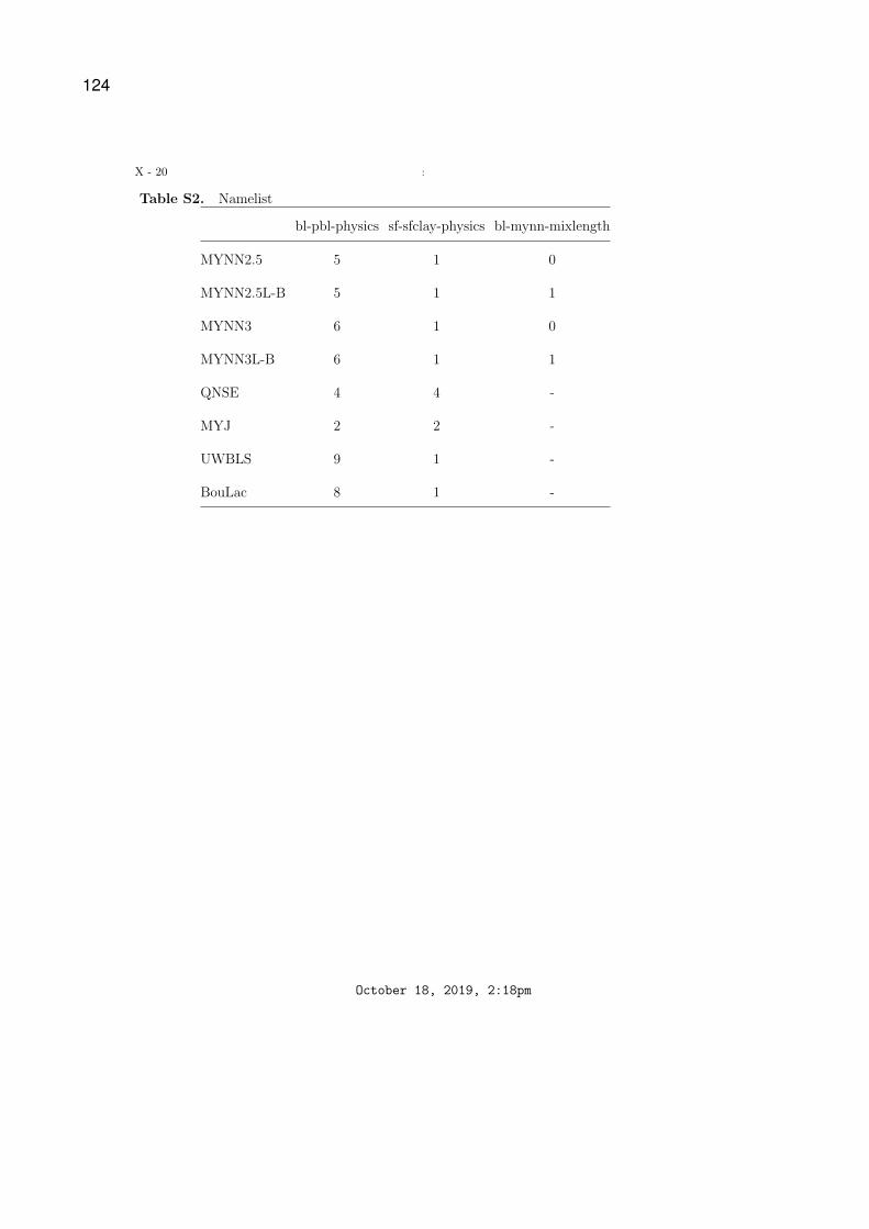
X - 20 :

Table S2. Namelist

bl-pbl-physics sf-sfclay-physics bl-mynn-mixlength

MYNN2.5 5 1 0

MYNN2.5L-B 5 1 1

MYNN3 6 1 0

MYNN3L-B 6 1 1

QNSE 4 4 -

MYJ 2 2 -

UWBLS 9 1 -

BouLac 8 1 -

October 18, 2019, 2:18pm

124

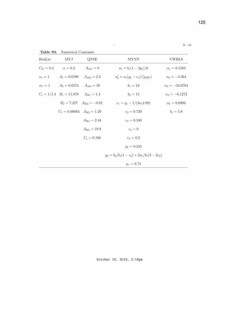
: X - 21

Table S3. Numerical Constants

BouLac MYJ QNSE MYNN UWBLS

CK = 0.4 α = 0.3 AM1 = 8 a1 = b1(1− 3g1)/6 α1 = 0.5562

αe = 1 A1 = 0.6599 AM2 = 2.3 a′2 = a1(g1 − c1)/(g1pr) α2 = −4.364

αT = 1 A2 = 0.6574 AM3 = 35 b1 = 24 α3 = −34.6764

Cε = 1/1.4 B1 = 11.878 AH1 = 1.4 b2 = 15 α4 = −6.1272

B2 = 7.227 AH2 = −0.01 c1 = g1 − 1/(3a12.88) α5 = 0.6986

C1 = 0.00083 AH3 = 1.29 c2 = 0.729 b1 = 5.8

AH4 = 2.44 c3 = 0.340

AH5 = 19.8 c4 = 0

Ce = 0.166 c5 = 0.2

g1 = 0.235

g2 = b2/b1(1− c3) + 2a1/b1(3− 2c2)

pr = 0.74

October 18, 2019, 2:18pm

125

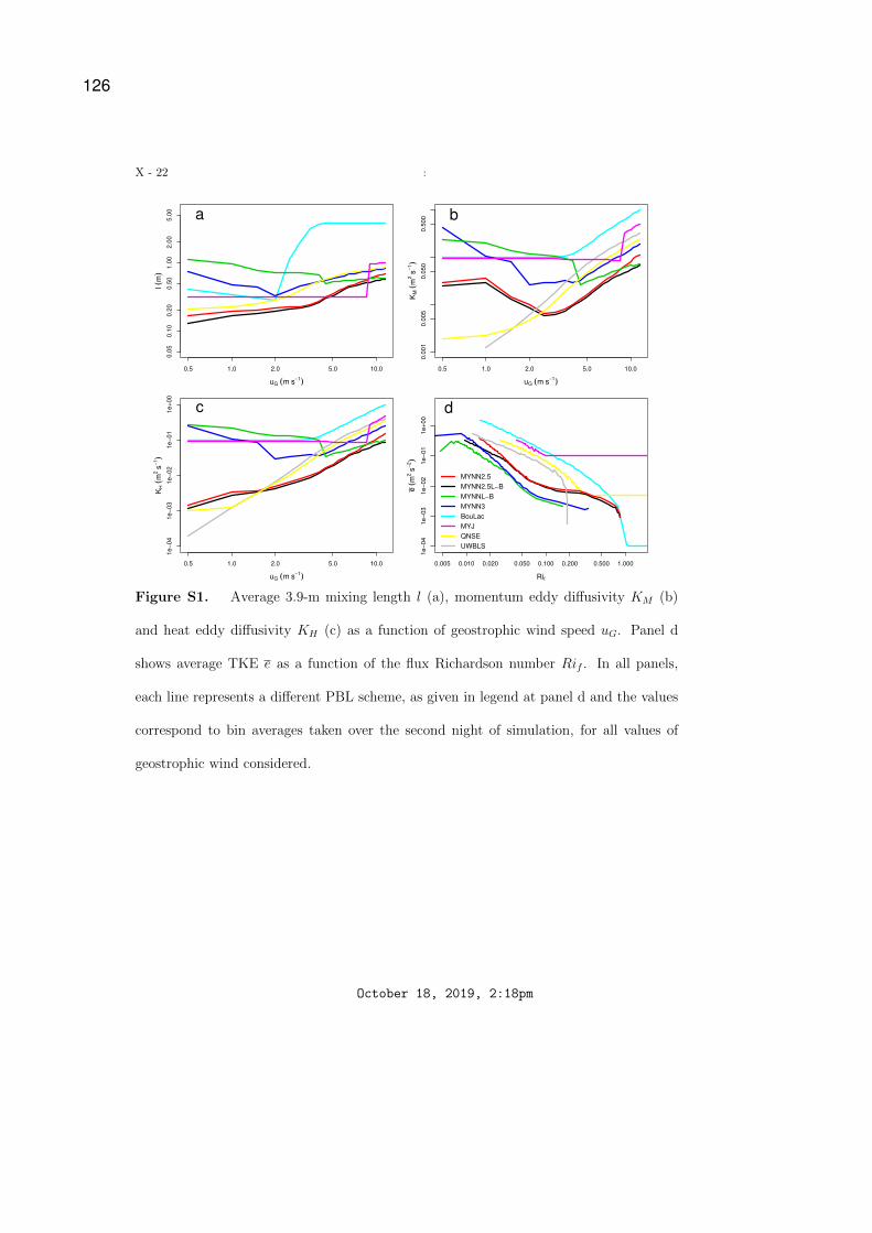
X - 22 :

0.5 1.0 2.0 5.0 10.0

0.0

50

.10

0.2

00

.50

1.0

02

.00

5.0

0

uG (m s−1)

l (m

)

a

0.5 1.0 2.0 5.0 10.0

0.0

01

0.0

05

0.0

50

0.5

00

uG (m s−1)

KM

(m

2 s

−1)

b

0.5 1.0 2.0 5.0 10.0

1e

−0

41

e−

03

1e

−0

21

e−

01

1e

+0

0

uG (m s−1)

KH (

m2 s

−1)

c

0.005 0.010 0.020 0.050 0.100 0.200 0.500 1.000

1e

−0

41

e−

03

1e

−0

21

e−

01

1e

+0

0

Rif

e (

m2 s

−2)

d

MYNN2.5

MYNN2.5L−B

MYNNL−B

MYNN3

BouLac

MYJ

QNSE

UWBLS

Figure S1. Average 3.9-m mixing length l (a), momentum eddy diffusivity KM (b)

and heat eddy diffusivity KH (c) as a function of geostrophic wind speed uG. Panel d

shows average TKE e as a function of the flux Richardson number Rif . In all panels,

each line represents a different PBL scheme, as given in legend at panel d and the values

correspond to bin averages taken over the second night of simulation, for all values of

geostrophic wind considered.

October 18, 2019, 2:18pm

126

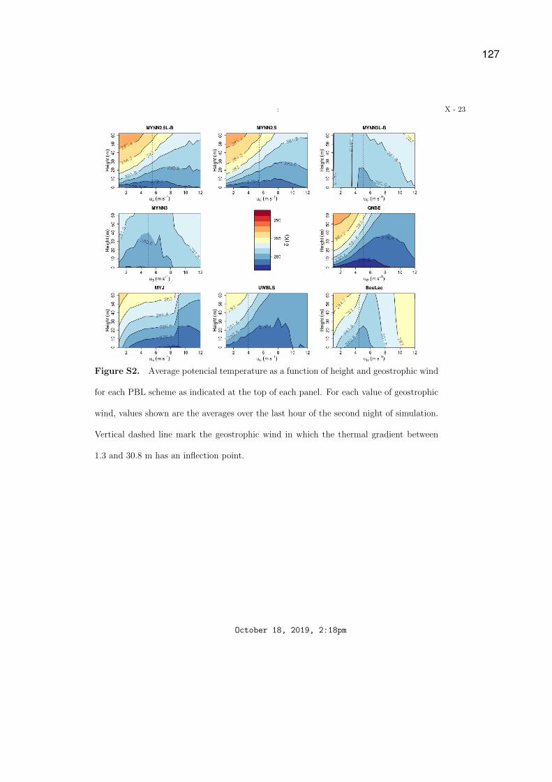
: X - 23

Figure S2. Average potencial temperature as a function of height and geostrophic wind

for each PBL scheme as indicated at the top of each panel. For each value of geostrophic

wind, values shown are the averages over the last hour of the second night of simulation.

Vertical dashed line mark the geostrophic wind in which the thermal gradient between

1.3 and 30.8 m has an inflection point.

October 18, 2019, 2:18pm

127

128

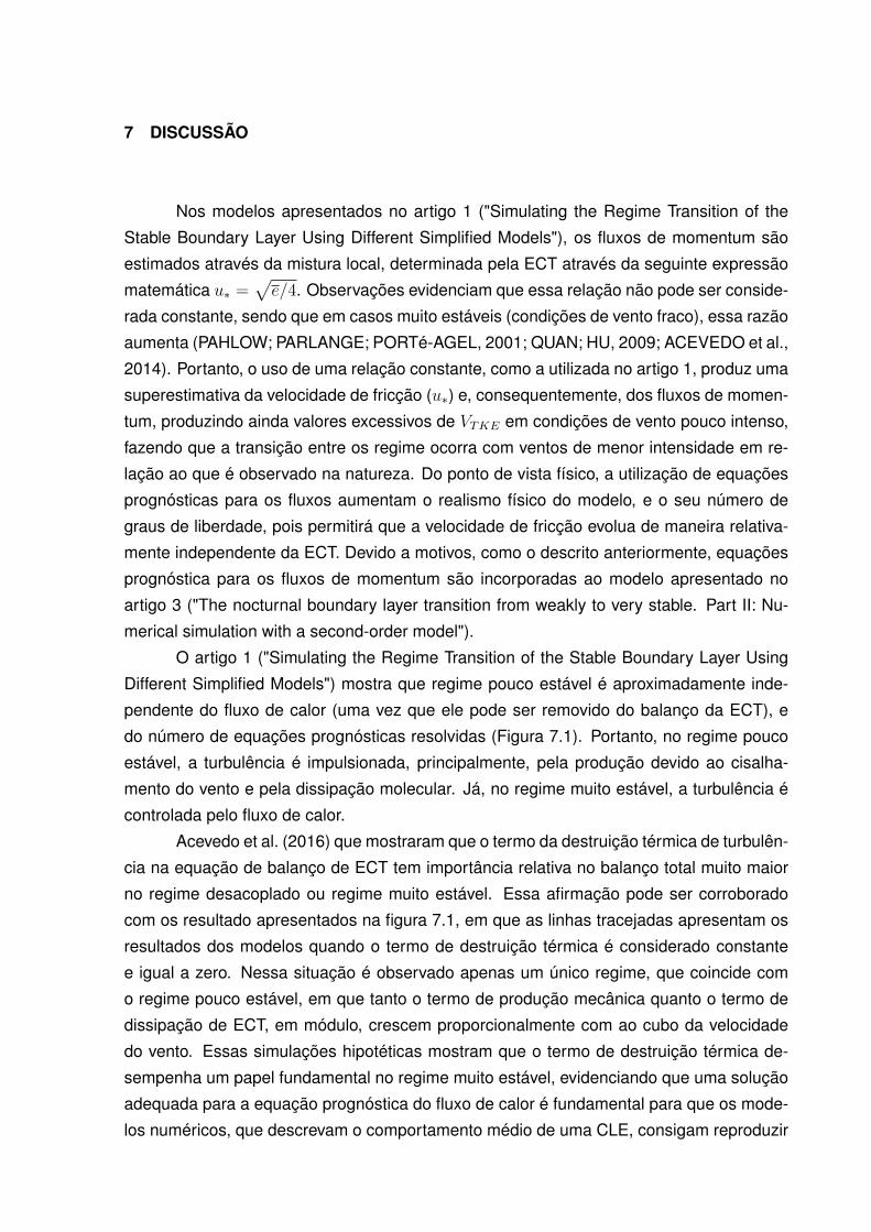
7 DISCUSSÃO

Nos modelos apresentados no artigo 1 ("Simulating the Regime Transition of the

Stable Boundary Layer Using Different Simplified Models"), os fluxos de momentum são

estimados através da mistura local, determinada pela ECT através da seguinte expressão

matemática u∗ =√e/4. Observações evidenciam que essa relação não pode ser conside-

rada constante, sendo que em casos muito estáveis (condições de vento fraco), essa razão

aumenta (PAHLOW; PARLANGE; PORTé-AGEL, 2001; QUAN; HU, 2009; ACEVEDO et al.,

2014). Portanto, o uso de uma relação constante, como a utilizada no artigo 1, produz uma

superestimativa da velocidade de fricção (u∗) e, consequentemente, dos fluxos de momen-

tum, produzindo ainda valores excessivos de VTKE em condições de vento pouco intenso,

fazendo que a transição entre os regime ocorra com ventos de menor intensidade em re-

lação ao que é observado na natureza. Do ponto de vista físico, a utilização de equações

prognósticas para os fluxos aumentam o realismo físico do modelo, e o seu número de

graus de liberdade, pois permitirá que a velocidade de fricção evolua de maneira relativa-

mente independente da ECT. Devido a motivos, como o descrito anteriormente, equações

prognóstica para os fluxos de momentum são incorporadas ao modelo apresentado no

artigo 3 ("The nocturnal boundary layer transition from weakly to very stable. Part II: Nu-

merical simulation with a second-order model").

O artigo 1 ("Simulating the Regime Transition of the Stable Boundary Layer Using

Different Simplified Models") mostra que regime pouco estável é aproximadamente inde-

pendente do fluxo de calor (uma vez que ele pode ser removido do balanço da ECT), e

do número de equações prognósticas resolvidas (Figura 7.1). Portanto, no regime pouco

estável, a turbulência é impulsionada, principalmente, pela produção devido ao cisalha-

mento do vento e pela dissipação molecular. Já, no regime muito estável, a turbulência é

controlada pelo fluxo de calor.

Acevedo et al. (2016) que mostraram que o termo da destruição térmica de turbulên-

cia na equação de balanço de ECT tem importância relativa no balanço total muito maior

no regime desacoplado ou regime muito estável. Essa afirmação pode ser corroborado

com os resultado apresentados na figura 7.1, em que as linhas tracejadas apresentam os

resultados dos modelos quando o termo de destruição térmica é considerado constante

e igual a zero. Nessa situação é observado apenas um único regime, que coincide com

o regime pouco estável, em que tanto o termo de produção mecânica quanto o termo de

dissipação de ECT, em módulo, crescem proporcionalmente com ao cubo da velocidade

do vento. Essas simulações hipotéticas mostram que o termo de destruição térmica de-

sempenha um papel fundamental no regime muito estável, evidenciando que uma solução

adequada para a equação prognóstica do fluxo de calor é fundamental para que os mode-

los numéricos, que descrevam o comportamento médio de uma CLE, consigam reproduzir

130

Figura 7.1 – Perfil vertical dos termos associados à produção mecânica de ECT (linhapreta), destruição térmica de ECT (linha vermelha) e dissipação de ECT (linha azul clara)provenientes dos modelos e, e−FH e e−FH−σθ. Já as linhas tracejadas são os resultadosobtidos pelo modelos quando a distruição térmica é considera constante e igual a zero.

0.5 1.0 2.0 5.0 10.0

1e

−0

51

e−

01

V1 (m s−1)

EC

T T

erm

os (

m2 s

−3)

a 2,5 m

PMD TDIS

modelo e

0.5 1.0 2.0 5.0 10.0

1e

−0

51

e−

01

V1 (m s−1)

EC

T T

erm

os (

m2 s

−3)

b

modelo e−FH

2,5 m

0.5 1.0 2.0 5.0 10.0

1e

−0

51

e−

01

V1 (m s−1)

EC

T T

erm

os (

m2 s

−3)

c 2,5 m

modelo e−FH−σθ

0.5 1.0 2.0 5.0 10.0

1e

−0

51

e−

01

V1 (m s−1)

EC

T T

erm

os (

m2 s

−3)

d 18,5 m

0.5 1.0 2.0 5.0 10.0

1e

−0

51

e−

01

V1 (m s−1)

EC

T T

erm

os (

m2 s

−3)

e 18,5 m

0.5 1.0 2.0 5.0 10.0

1e

−0

51

e−

01

V1 (m s−1)

EC

T T

erm

os (

m2 s

−3)

f 18,5 m

0.5 1.0 2.0 5.0 10.0

1e

−0

51

e−

01

V1 (m s−1)

EC

T T

erm

os (

m2 s

−3)

g 36,5 m

0.5 1.0 2.0 5.0 10.0

1e

−0

51

e−

01

V1 (m s−1)

EC

T T

erm

os (

m2 s

−3)

h 36,5 m

0.5 1.0 2.0 5.0 10.0

1e

−0

51

e−

01

V1 (m s−1)

EC

T T

erm

os (

m2 s

−3)

36,5 mi

de forma correta os dois regimes da CLE. Uma solução para fluxo de calor só pode ser

obtida de forma completamente adequada se e somente se a variância de temperatura

e a componente vertical da variância da velocidade do vento forem estimados através de

equações prognósticas. Por este motivo equações prognósticas para a componentes da

variância da velocidade do vento foram incluídas no modelo apresentado no artigo 3 ("The

nocturnal boundary layer transition from weakly to very stable. Part II: Numerical simula-

tion with a second-order model"), tornando-o um modelo de segundo ordem completo, ou

conforme a classificação de Mellor e Yamada (1974) um modelo de nível 4.

Acevedo et al. (2019) (artigo 2, "The nocturnal boundary layer transition from wea-

kly to very stable. Part I: Observations") observaram, em muitas noites, um resfriamento

abrupto da camada acompanhado de uma redução na energia cinética turbulenta (ECT),

e na intensidade da velocidade do vento. Nesse estudo a transição entre o regime pouco

estável e o muito estável foi marcada exatamente no instante de tempo em que ocorre

resfriamento máximo nos níveis inferiores da camada limite. No artigo 3 ("The nocturnal

boundary layer transition from weakly to very stable. Part II: Numerical simulation with a

second-order model"), transições semelhantes, as observadas por Acevedo et al. (2019),

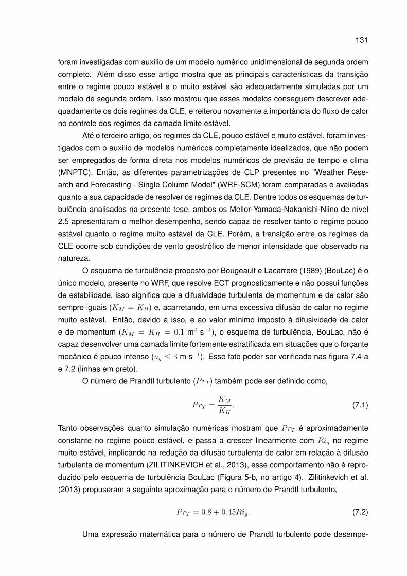
131

foram investigadas com auxilio de um modelo numérico unidimensional de segunda ordem

completo. Além disso esse artigo mostra que as principais características da transição

entre o regime pouco estável e o muito estável são adequadamente simuladas por um

modelo de segunda ordem. Isso mostrou que esses modelos conseguem descrever ade-

quadamente os dois regimes da CLE, e reiterou novamente a importância do fluxo de calor

no controle dos regimes da camada limite estável.

Até o terceiro artigo, os regimes da CLE, pouco estável e muito estável, foram inves-

tigados com o auxílio de modelos numéricos completamente idealizados, que não podem

ser empregados de forma direta nos modelos numéricos de previsão de tempo e clima

(MNPTC). Então, as diferentes parametrizações de CLP presentes no "Weather Rese-

arch and Forecasting - Single Column Model" (WRF-SCM) foram comparadas e avaliadas

quanto a sua capacidade de resolver os regimes da CLE. Dentre todos os esquemas de tur-

bulência analisados na presente tese, ambos os Mellor-Yamada-Nakanishi-Niino de nível

2.5 apresentaram o melhor desempenho, sendo capaz de resolver tanto o regime pouco

estável quanto o regime muito estável da CLE. Porém, a transição entre os regimes da

CLE ocorre sob condições de vento geostrófico de menor intensidade que observado na

natureza.

O esquema de turbulência proposto por Bougeault e Lacarrere (1989) (BouLac) é o

único modelo, presente no WRF, que resolve ECT prognosticamente e não possui funções

de estabilidade, isso significa que a difusividade turbulenta de momentum e de calor são

sempre iguais (KM = KH) e, acarretando, em uma excessiva difusão de calor no regime

muito estável. Então, devido a isso, e ao valor mínimo imposto à difusividade de calor

e de momentum (KM = KH = 0.1 m2 s−1), o esquema de turbulência, BouLac, não é

capaz desenvolver uma camada limite fortemente estratificada em situações que o forçante

mecânico é pouco intenso (ug ≤ 3 m s−1). Esse fato poder ser verificado nas figura 7.4-a

e 7.2 (linhas em preto).

O número de Prandtl turbulento (PrT ) também pode ser definido como,

PrT =KM

KH

. (7.1)

Tanto observações quanto simulação numéricas mostram que PrT é aproximadamente

constante no regime pouco estável, e passa a crescer linearmente com Rig no regime

muito estável, implicando na redução da difusão turbulenta de calor em relação à difusão

turbulenta de momentum (ZILITINKEVICH et al., 2013), esse comportamento não é repro-

duzido pelo esquema de turbulência BouLac (Figura 5-b, no artigo 4). Zilitinkevich et al.

(2013) propuseram a seguinte aproximação para o número de Prandtl turbulento,

PrT = 0.8 + 0.45Rig. (7.2)

Uma expressão matemática para o número de Prandtl turbulento pode desempe-

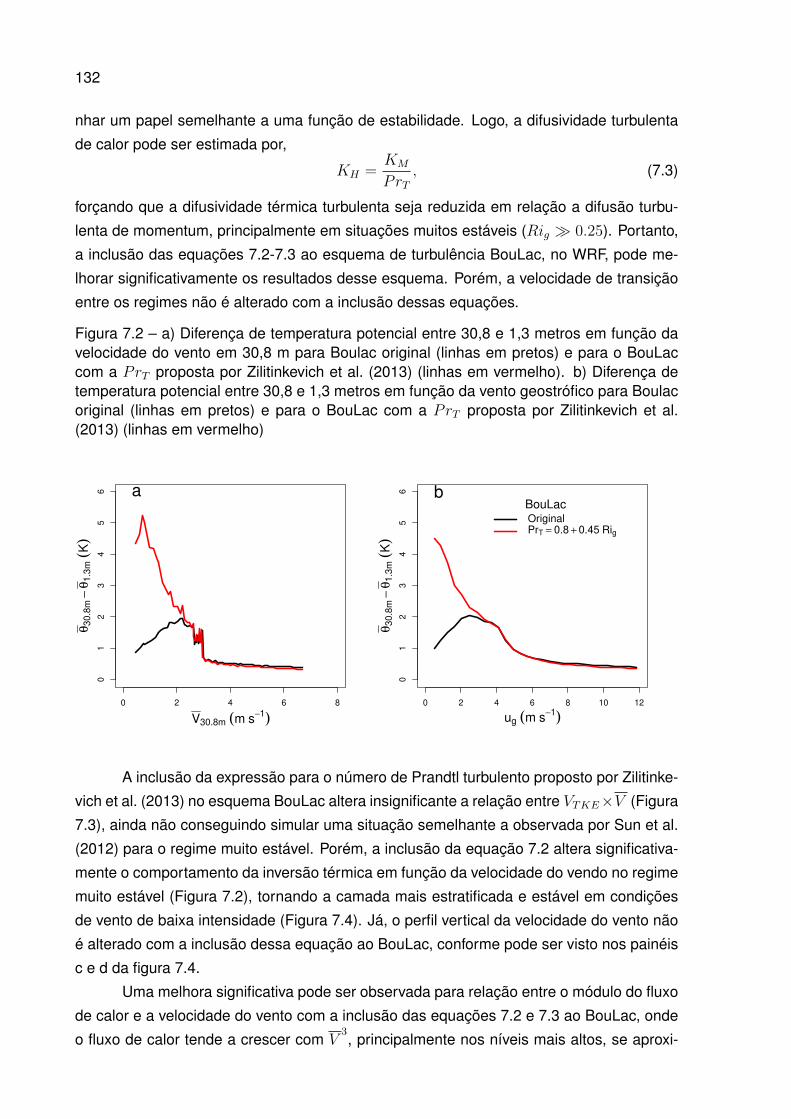
132

nhar um papel semelhante a uma função de estabilidade. Logo, a difusividade turbulenta

de calor pode ser estimada por,

KH =KM

PrT, (7.3)

forçando que a difusividade térmica turbulenta seja reduzida em relação a difusão turbu-

lenta de momentum, principalmente em situações muitos estáveis (Rig � 0.25). Portanto,

a inclusão das equações 7.2-7.3 ao esquema de turbulência BouLac, no WRF, pode me-

lhorar significativamente os resultados desse esquema. Porém, a velocidade de transição

entre os regimes não é alterado com a inclusão dessas equações.

Figura 7.2 – a) Diferença de temperatura potencial entre 30,8 e 1,3 metros em função davelocidade do vento em 30,8 m para Boulac original (linhas em pretos) e para o BouLaccom a PrT proposta por Zilitinkevich et al. (2013) (linhas em vermelho). b) Diferença detemperatura potencial entre 30,8 e 1,3 metros em função da vento geostrófico para Boulacoriginal (linhas em pretos) e para o BouLac com a PrT proposta por Zilitinkevich et al.(2013) (linhas em vermelho)

0 2 4 6 8

01

23

45

6

V30.8m (m s−1)

θ30.8

m−

θ1.3

m (

K)

a

0 2 4 6 8 10 12

01

23

45

6

ug (m s−1)

θ30.8

m−

θ1.3

m (

K)

bBouLacOriginalPrT = 0.8 + 0.45 Rig

A inclusão da expressão para o número de Prandtl turbulento proposto por Zilitinke-

vich et al. (2013) no esquema BouLac altera insignificante a relação entre VTKE×V (Figura

7.3), ainda não conseguindo simular uma situação semelhante a observada por Sun et al.

(2012) para o regime muito estável. Porém, a inclusão da equação 7.2 altera significativa-

mente o comportamento da inversão térmica em função da velocidade do vendo no regime

muito estável (Figura 7.2), tornando a camada mais estratificada e estável em condições

de vento de baixa intensidade (Figura 7.4). Já, o perfil vertical da velocidade do vento não

é alterado com a inclusão dessa equação ao BouLac, conforme pode ser visto nos painéis

c e d da figura 7.4.

Uma melhora significativa pode ser observada para relação entre o módulo do fluxo

de calor e a velocidade do vento com a inclusão das equações 7.2 e 7.3 ao BouLac, onde

o fluxo de calor tende a crescer com V3, principalmente nos níveis mais altos, se aproxi-

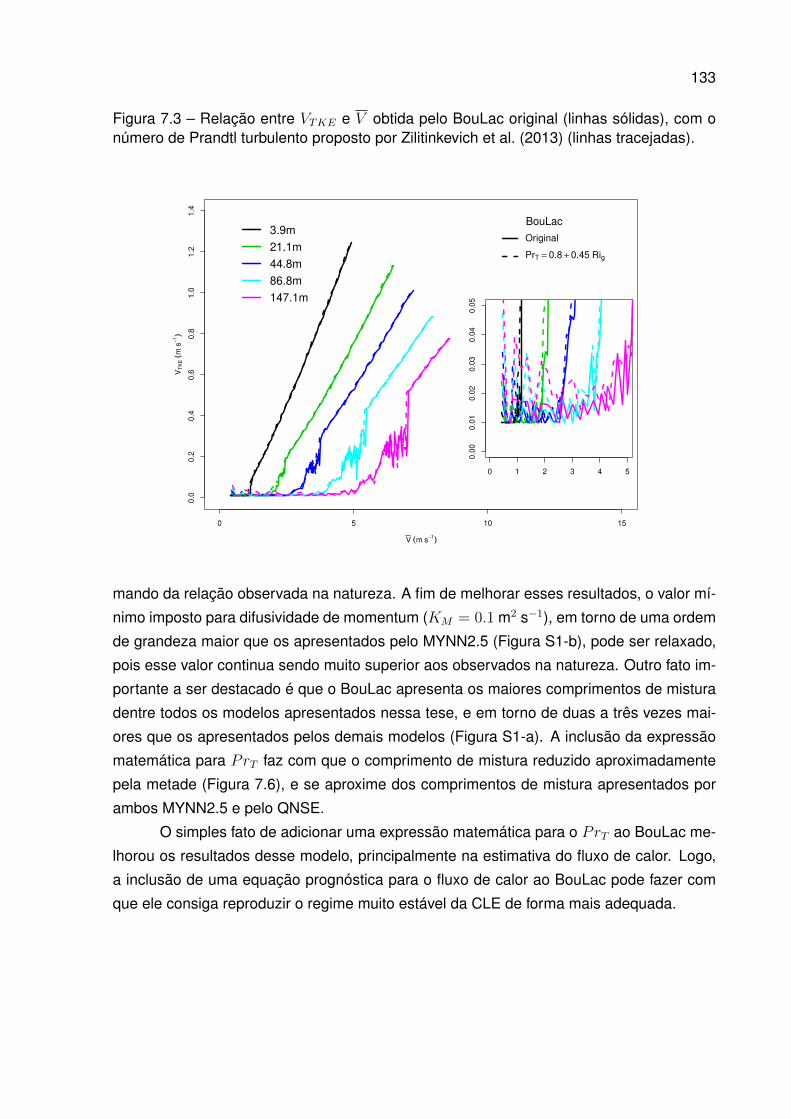
133

Figura 7.3 – Relação entre VTKE e V obtida pelo BouLac original (linhas sólidas), com onúmero de Prandtl turbulento proposto por Zilitinkevich et al. (2013) (linhas tracejadas).

0 5 10 15

0.0

0.2

0.4

0.6

0.8

1.0

1.2

1.4

V (m s−1)

VT

KE (

m s

−1)

3.9m

21.1m

44.8m

86.8m

147.1m

BouLac

Original

PrT = 0.8 + 0.45 Rig

0 1 2 3 4 50

.00

0.0

10

.02

0.0

30

.04

0.0

5

mando da relação observada na natureza. A fim de melhorar esses resultados, o valor mí-

nimo imposto para difusividade de momentum (KM = 0.1 m2 s−1), em torno de uma ordem

de grandeza maior que os apresentados pelo MYNN2.5 (Figura S1-b), pode ser relaxado,

pois esse valor continua sendo muito superior aos observados na natureza. Outro fato im-

portante a ser destacado é que o BouLac apresenta os maiores comprimentos de mistura

dentre todos os modelos apresentados nessa tese, e em torno de duas a três vezes mai-

ores que os apresentados pelos demais modelos (Figura S1-a). A inclusão da expressão

matemática para PrT faz com que o comprimento de mistura reduzido aproximadamente

pela metade (Figura 7.6), e se aproxime dos comprimentos de mistura apresentados por

ambos MYNN2.5 e pelo QNSE.

O simples fato de adicionar uma expressão matemática para o PrT ao BouLac me-

lhorou os resultados desse modelo, principalmente na estimativa do fluxo de calor. Logo,

a inclusão de uma equação prognóstica para o fluxo de calor ao BouLac pode fazer com

que ele consiga reproduzir o regime muito estável da CLE de forma mais adequada.

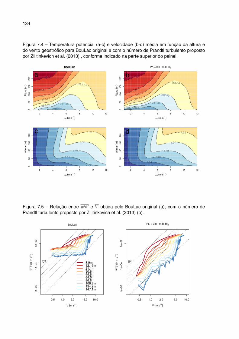
134

Figura 7.4 – Temperatura potencial (a-c) e velocidade (b-d) média em função da altura edo vento geostrófico para BouLac original e com o número de Prandtl turbulento propostopor Zilitinkevich et al. (2013) , conforme indicado na parte superior do painel.

2 4 6 8 10 12

050

100

150

200

BOULAC

uG (m s−1)

Altura

(m

)

a

2 4 6 8 10 12

050

100

150

200

PrT = 0.8 + 0.45 Rig

uG (m s−1)

Altura

(m

)

b

2 4 6 8 10 12

050

100

150

200

uG (m s−1)

Altura

(m

)

c

2 4 6 8 10 12

050

100

150

200

uG (m s−1)

Altura

(m

)

d

Figura 7.5 – Relação entre w′θ′ e V obtida pelo BouLac original (a), com o número dePrandtl turbulento proposto por Zilitinkevich et al. (2013) (b).

0.5 1.0 2.0 5.0 10.0

1e−

06

1e−

04

1e−

02

V (m s−1)

w, θ

, (K

m s

−1)

BouLac

V3

3.9m12.19m21.1m30.8m44.8m64.5m86.8m106.8m134.9m147.1m

0.5 1.0 2.0 5.0 10.0

1e−

06

1e−

04

1e−

02

V (m s−1)

w, θ

, (K

m s

−1)

PrT = 0.8 + 0.45 Rig

V3

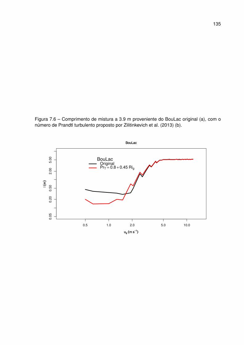
135

Figura 7.6 – Comprimento de mistura a 3.9 m proveniente do BouLac original (a), com onúmero de Prandtl turbulento proposto por Zilitinkevich et al. (2013) (b).

0.5 1.0 2.0 5.0 10.0

0.0

50.2

00.5

02.0

05.0

0

ug (m s−1)

l (m

)

BouLac

ug (m s−1)

l (m

)

BouLac

BouLacOriginalPrT = 0.8 + 0.45 Rig

136

8 CONCLUSÕES

A presente tese foi divida em 4 diferentes artigos. No primeiro deles ("Simulating

the Regime Transition of the Stable Boundary Layer Using Different Simplified Models") 3

diferentes modelos numéricos, utilizados para descrever o comportamento médio de uma

camada limite estável, são comparados quanto a sua capacidade de reproduzir dois regi-

mes da CLE. Esses modelos são: e, em que a energia cinética turbulenta (ECT) é o único

momento estatístico de segunda ordem resolvido através de uma equação prognóstica; o

e − FH , em o fluxo de calor sensível é estimado através de uma equação prognóstica; o

modelo e− FH − σθ, em que a variância de temperatura passa a ser calculada através de

uma equação prognóstica.

No segundo artigo (The nocturnal boundary layer transition from weakly to very

stable. Part I: Observations), a transição do regime pouco estável para muito estável da

CLE, é analisada através dos dados micrometeorológicos provenientes de uma torre de

140 metros situada em Linhares, no estado de Espírito Santos, sudoeste do Brasil. Foi

observado que a transição entre os regimes era precedida por um resfriamento abrupto da

camada, acompanhado de uma redução na energia cinética turbulenta, e da intensidade

da velocidade do vento. No terceiro artigo ("The nocturnal boundary layer transition from

weakly to very stable. Part II: Numerical simulation with a second-order model"), transições

semelhantes, às apresentadas no segundo artigo, foram investigadas com auxilio de um

modelo numérico unidimensional de segunda ordem, em que a transição é impulsionada

pelo decréscimo da intensidade do vento no topo do domínio. Nesse artigo o papel dos

processos radiativos e das propriedades térmicas da superfície do solo sob a transição

também foi investigado.

No quarto artigo ("How is the two-regime stable boundary layer solved by the dif-

ferent PBL schemes in WRF?"), seis diferentes parametrizações de camada limite pla-

netária (CLP) presentes no "Weather Research and Forecasting - Single Column Mo-

del" (WRF-SCM) foram comparados e avaliados quanto a sua capacidade de simular

os regimes da CLE: Mellor-Yamada-Nakanishi-Niino nível 2.5 (MYNN2.5, MYNN2.5L-B

), Mellor-Yamada-Nakanishi-Niino nível 3 (MYNN3, MYNN3L-B ), Mellor-Yamada-Janjic

(MYJ), "Quasi-Normal Scale Elimination" (QNSE), "University of Washington (TKE) Boun-

dary Layer Scheme" (UWBLS) e Bougeault-Lacarrere (BouLac).

Os principais resultados obtidos na presente tese podem ser sumarizados como:

• Os regimes da CLE não são apenas controlados pela intensidade da velocidade do

vento, mas também pelos processos térmicos.

• No regime muito estável a energia cinética turbulenta cresce com a intensidade do

vento a uma pequena taxa. Essa situação só pode ser simulada quando equações

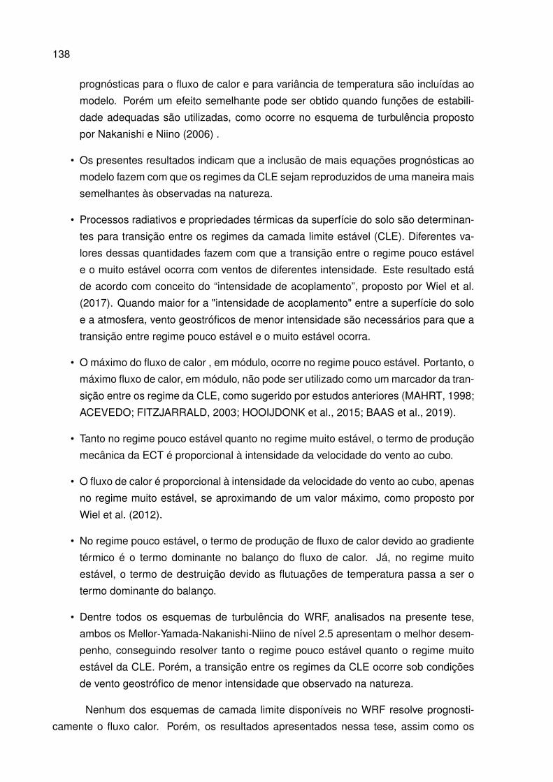
138

prognósticas para o fluxo de calor e para variância de temperatura são incluídas ao

modelo. Porém um efeito semelhante pode ser obtido quando funções de estabili-

dade adequadas são utilizadas, como ocorre no esquema de turbulência proposto

por Nakanishi e Niino (2006) .

• Os presentes resultados indicam que a inclusão de mais equações prognósticas ao

modelo fazem com que os regimes da CLE sejam reproduzidos de uma maneira mais

semelhantes às observadas na natureza.

• Processos radiativos e propriedades térmicas da superfície do solo são determinan-

tes para transição entre os regimes da camada limite estável (CLE). Diferentes va-

lores dessas quantidades fazem com que a transição entre o regime pouco estável

e o muito estável ocorra com ventos de diferentes intensidade. Este resultado está

de acordo com conceito do “intensidade de acoplamento”, proposto por Wiel et al.

(2017). Quando maior for a "intensidade de acoplamento" entre a superfície do solo

e a atmosfera, vento geostróficos de menor intensidade são necessários para que a

transição entre regime pouco estável e o muito estável ocorra.

• O máximo do fluxo de calor , em módulo, ocorre no regime pouco estável. Portanto, o

máximo fluxo de calor, em módulo, não pode ser utilizado como um marcador da tran-

sição entre os regime da CLE, como sugerido por estudos anteriores (MAHRT, 1998;

ACEVEDO; FITZJARRALD, 2003; HOOIJDONK et al., 2015; BAAS et al., 2019).

• Tanto no regime pouco estável quanto no regime muito estável, o termo de produção

mecânica da ECT é proporcional à intensidade da velocidade do vento ao cubo.

• O fluxo de calor é proporcional à intensidade da velocidade do vento ao cubo, apenas

no regime muito estável, se aproximando de um valor máximo, como proposto por

Wiel et al. (2012).

• No regime pouco estável, o termo de produção de fluxo de calor devido ao gradiente

térmico é o termo dominante no balanço do fluxo de calor. Já, no regime muito

estável, o termo de destruição devido as flutuações de temperatura passa a ser o

termo dominante do balanço.

• Dentre todos os esquemas de turbulência do WRF, analisados na presente tese,

ambos os Mellor-Yamada-Nakanishi-Niino de nível 2.5 apresentam o melhor desem-

penho, conseguindo resolver tanto o regime pouco estável quanto o regime muito

estável da CLE. Porém, a transição entre os regimes da CLE ocorre sob condições

de vento geostrófico de menor intensidade que observado na natureza.

Nenhum dos esquemas de camada limite disponíveis no WRF resolve prognosti-

camente o fluxo calor. Porém, os resultados apresentados nessa tese, assim como os

139

resultados apresentados por Wiel et al. (2012), indicam que o fluxo de calor exerce um

grande controle nos regimes da CLE. Logo, a inclusão de uma equação prognóstica para

o fluxo de calor nos esquemas de turbulência, presentes no WRF, significaria um impor-

tante avanço. Espera-se que, assim o WRF consiga simular de forma adequada ambos os

regimes da CLE.

Diante ao exposto na presente tese, esforços foram concentrados na inclusão de

uma equação prognóstica no esquemas de turbulência, BouLac, presente na versão 3.9

do WRF. Porém, ao realizar essa tarefa foi deparado com os seguintes desafios, o fluxo de

calor superficial é estimado através de similaridade (Monin Obukhov) no módulo "Surface

Layer" e na sequência essa quantidade é utilizada para estimar a temperatura do solo e

atualizada no módulo "Land-Surface". No desenvolvimento da presente tese foi possível

realizar as alterações os esquemas de turbulência, das quais foi apresentada na seção

de discussão. Já, a inclusão da equação prognóstica para o fluxo de calor nos esquemas

de turbulência não é uma tarefa trivial, pois essa ação exige ajustes tanto módulos de

"Surface-Layer" quanto no de "Land-Surface". A inclusão de uma equação ao esquema

de turbulência já foi finalizada. Porém, as alterações dos módulos "Surface Layer" e "Land

Surface" ainda estão em desenvolvimento. Essas alterações são necessárias para que

não ocorra conflito entre o fluxo de calor obtido pelo esquema de turbulência e o obtido

pelo "Surface Layer". Como perspectivas pretende-se finalizar as alterações necessárias

ao "Surface Layer" e ao "Land Surface", e futuramente a inclusão de equações prognóstica

para o fluxo de momentum, uma vez que foi mostrado que um modelo de segundo ordem é

capaz de reproduzir de forma satisfatória muitas características da transição entre o regime

pouco estável e o muito estável. Com isso, espera-se implementar uma parametrização

completa que seja mais adequada na simulação das características que contrastam entre

os dois regimes. Também espera-se que esta parametrização resolva situações muito

estáveis com valores de forçante mecânico maiores do que ocorre nas parametrizações

existentes atualmente, e mais próximas ao que é observado na natureza.

140

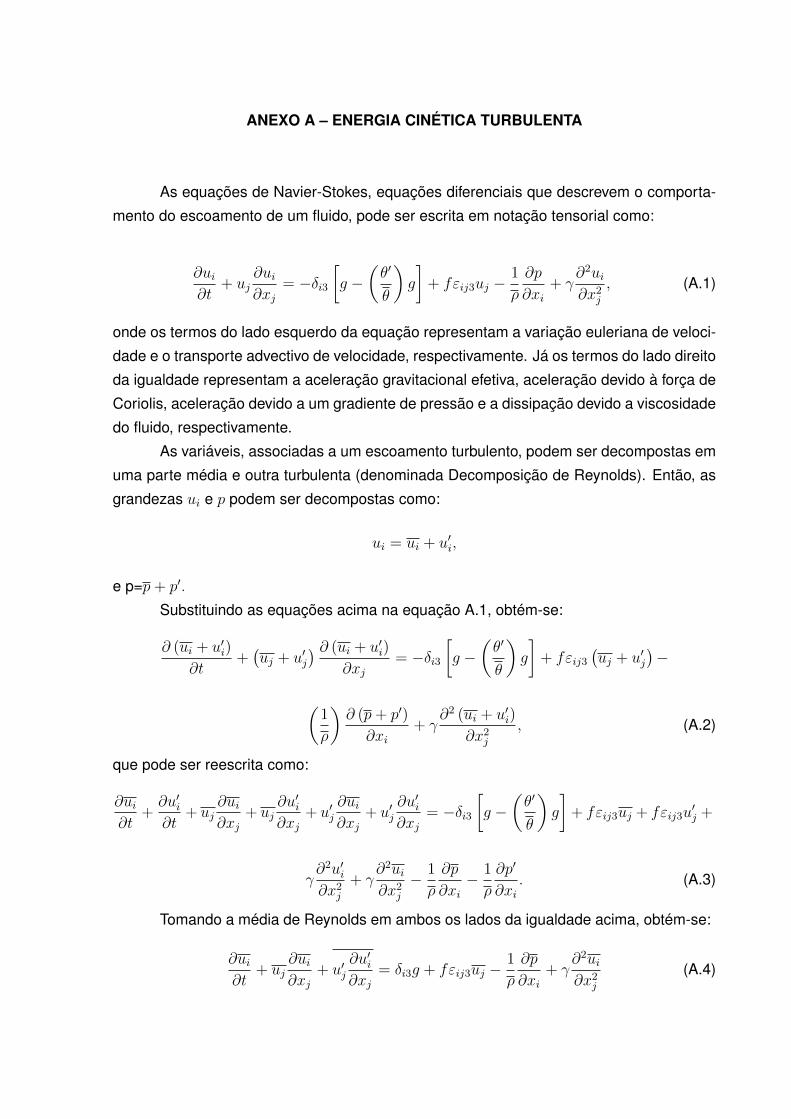
ANEXO A – ENERGIA CINÉTICA TURBULENTA

As equações de Navier-Stokes, equações diferenciais que descrevem o comporta-

mento do escoamento de um fluido, pode ser escrita em notação tensorial como:

∂ui∂t

+ uj∂ui∂xj

= −δi3[g −

(θ′

θ

)g

]+ fεij3uj −

1

ρ

∂p

∂xi+ γ

∂2ui∂x2j

, (A.1)

onde os termos do lado esquerdo da equação representam a variação euleriana de veloci-

dade e o transporte advectivo de velocidade, respectivamente. Já os termos do lado direito

da igualdade representam a aceleração gravitacional efetiva, aceleração devido à força de

Coriolis, aceleração devido a um gradiente de pressão e a dissipação devido a viscosidade

do fluido, respectivamente.

As variáveis, associadas a um escoamento turbulento, podem ser decompostas em

uma parte média e outra turbulenta (denominada Decomposição de Reynolds). Então, as

grandezas ui e p podem ser decompostas como:

ui = ui + u′i,

e p=p+ p′.

Substituindo as equações acima na equação A.1, obtém-se:

∂ (ui + u′i)

∂t+(uj + u′j

) ∂ (ui + u′i)

∂xj= −δi3

[g −

(θ′

θ

)g

]+ fεij3

(uj + u′j

)−

(1

ρ

)∂ (p+ p′)

∂xi+ γ

∂2 (ui + u′i)

∂x2j, (A.2)

que pode ser reescrita como:

∂ui∂t

+∂u′i∂t

+ uj∂ui∂xj

+ uj∂u′i∂xj

+ u′j∂ui∂xj

+ u′j∂u′i∂xj

= −δi3[g −

(θ′

θ

)g

]+ fεij3uj + fεij3u

′j +

γ∂2u′i∂x2j

+ γ∂2ui∂x2j− 1

ρ

∂p

∂xi− 1

ρ

∂p′

∂xi. (A.3)

Tomando a média de Reynolds em ambos os lados da igualdade acima, obtém-se:

∂ui∂t

+ uj∂ui∂xj

+ u′j∂u′i∂xj

= δi3g + fεij3uj −1

ρ

∂p

∂xi+ γ

∂2ui∂x2j

(A.4)

142

Através da equação da continuidade, sabe-se que

∂u′j∂xj

= 0,

logo,

u′i∂u′j∂xj

= 0.

Tomando a média de Reynolds na equação acima, temos que:

u′i∂u′j∂xj

= 0,

que pode ser somado a equação A.4 sem alterá-la. Portanto,

∂ui∂t

+ uj∂ui∂xj

+ u′i∂u′j∂xj

+ u′j∂u′i∂xj

= δi3g + fεij3uj −1

ρ

∂p

∂xi+ γ

∂2ui∂x2j

. (A.5)

Através da regra do produto sabemos que:

u′i∂u′j∂xj

+ u′j∂u′i∂xj

=∂u′ju

′i

∂xj.

Logo, a equação A.5 pode ser reescrita como:

∂ui∂t

+ uj∂ui∂xj

+∂u′ju

′i

∂xj= δi3g + fεij3uj −

1

ρ

∂p

∂xi+ γ

∂2ui∂x2j

, (A.6)

Subtraindo A.6 de A.3, temos que:

∂u′i∂t

+ uj∂u′i∂xj

+ u′j∂ui∂xj

+ u′j∂u′i∂xj−∂u′iu

′j

∂xj= δi3

(θ′

θ

)g+

fεij3u′j −

1

ρ

∂p′

∂xi+ γ

∂2u′i∂x2j

. (A.7)

Quando multiplicada por 2u′i, a equação acima pode ser escrita como:

2u′i∂u′i∂t

+ 2u′iuj∂u′i∂xj

+ 2u′iu′j

∂ui∂xj

+ 2u′iu′j

∂u′i∂xj− 2u′i

∂u′iu′j

∂xj= 2u′iδi3

(θ′

θ

)g + 2u′ifεij3u

′j −

2u′i1

ρ

∂p′

∂xi+ 2u′iγ

∂2u′i∂x2j

(A.8)

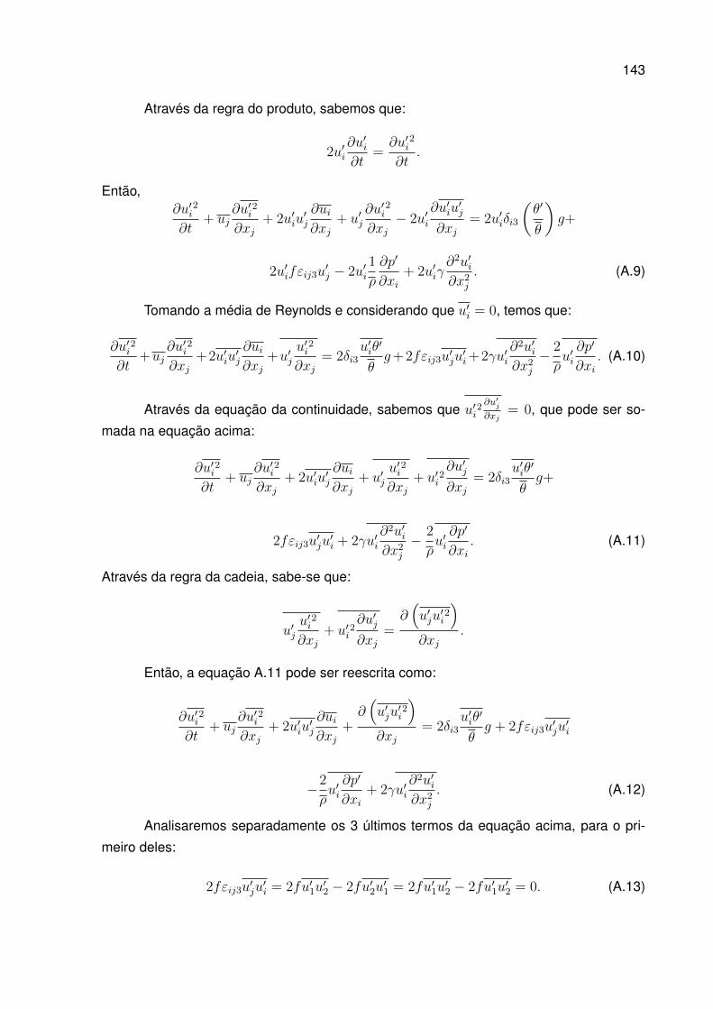
143

Através da regra do produto, sabemos que:

2u′i∂u′i∂t

=∂u′i

2

∂t.

Então,∂u′i

2

∂t+ uj

∂u′i2

∂xj+ 2u′iu

′j

∂ui∂xj

+ u′j∂u′i

2

∂xj− 2u′i

∂u′iu′j

∂xj= 2u′iδi3

(θ′

θ

)g+

2u′ifεij3u′j − 2u′i

1

ρ

∂p′

∂xi+ 2u′iγ

∂2u′i∂x2j

. (A.9)

Tomando a média de Reynolds e considerando que u′i = 0, temos que:

∂u′i2

∂t+uj

∂u′i2

∂xj+2u′iu

′j

∂ui∂xj

+u′ju′i

2

∂xj= 2δi3

u′iθ′

θg+2fεij3u′ju

′i+2γu′i

∂2u′i∂x2j− 2

ρu′i∂p′

∂xi. (A.10)

Através da equação da continuidade, sabemos que u′i2∂u′j∂xj

= 0, que pode ser so-

mada na equação acima:

∂u′i2

∂t+ uj

∂u′i2

∂xj+ 2u′iu

′j

∂ui∂xj

+ u′ju′i

2

∂xj+ u′i

2∂u′j∂xj

= 2δi3u′iθ′

θg+

2fεij3u′ju′i + 2γu′i

∂2u′i∂x2j− 2

ρu′i∂p′

∂xi. (A.11)

Através da regra da cadeia, sabe-se que:

u′ju′i

2

∂xj+ u′i

2∂u′j∂xj

=∂(u′ju

′i2)

∂xj.

Então, a equação A.11 pode ser reescrita como:

∂u′i2

∂t+ uj

∂u′i2

∂xj+ 2u′iu

′j

∂ui∂xj

+∂(u′ju

′i2)

∂xj= 2δi3

u′iθ′

θg + 2fεij3u′ju

′i

−2

ρu′i∂p′

∂xi+ 2γu′i

∂2u′i∂x2j

. (A.12)

Analisaremos separadamente os 3 últimos termos da equação acima, para o pri-

meiro deles:

2fεij3u′ju′i = 2fu′1u

′2 − 2fu′2u

′1 = 2fu′1u

′2 − 2fu′1u

′2 = 0. (A.13)

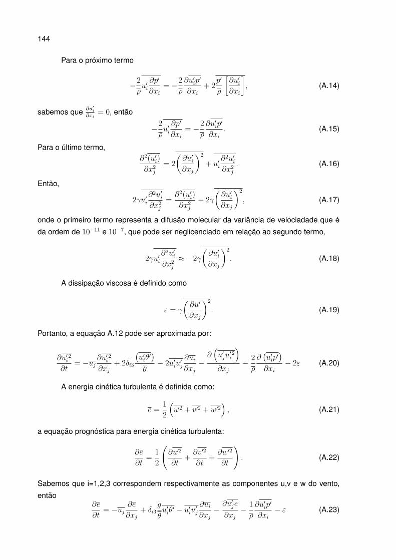
144

Para o próximo termo

−2

ρu′i∂p′

∂xi= −2

ρ

∂u′ip′

∂xi+ 2

p′

ρ

[∂u′i∂xi

], (A.14)

sabemos que ∂u′i∂xi

= 0, então

−2

ρu′i∂p′

∂xi= −2

ρ

∂u′ip′

∂xi. (A.15)

Para o último termo,∂2(u′i)

∂x2j= 2

(∂u′i∂xj

)2

+ u′i∂2u′i∂x2j

. (A.16)

Então,

2γu′i∂2u′i∂x2j

=∂2(u′i)

∂x2j− 2γ

(∂u′i∂xj

)2

, (A.17)

onde o primeiro termo representa a difusão molecular da variância de velociadade que é

da ordem de 10−11 e 10−7, que pode ser neglicenciado em relação ao segundo termo,

2γu′i∂2u′i∂x2j

≈ −2γ

(∂u′i∂xj

)2

. (A.18)

A dissipação viscosa é definido como

ε = γ

(∂u′

∂xj

)2

. (A.19)

Portanto, a equação A.12 pode ser aproximada por:

∂u′i2

∂t= −uj

∂u′i2

∂xj+ 2δi3

(u′iθ′)

θ− 2u′iu

′j

∂ui∂xj−∂(u′ju

′i2)

∂xj− 2

ρ

∂(u′ip′)

∂xi− 2ε (A.20)

A energia cinética turbulenta é definida como:

e =1

2

(u′2 + v′2 + w′2

), (A.21)

a equação prognóstica para energia cinética turbulenta:

∂e

∂t=

1

2

(∂u′2

∂t+∂v′2

∂t+∂w′2

∂t

). (A.22)

Sabemos que i=1,2,3 correspondem respectivamente as componentes u,v e w do vento,

então∂e

∂t= −uj

∂e

∂xj+ δi3

g

θu′iθ′ − u′iu′j

∂ui∂xj−∂u′je

∂xj− 1

ρ

∂u′ip′

∂xi− ε (A.23)

145

Considerando homogeneidade horizontal, a equação prognóstica para ECT pode

ser escrita como:

∂e

∂t= −u′w′∂u

∂z− v′w′∂v

∂z+g

θw′θ′ − ∂ew′

∂z− 1

ρ

∂w′p′

∂z− ε. (A.24)

146

ANEXO B – FLUXO DE CALOR SENSÍVEL

A derivada parcial de w′θ′ em relação ao tempo, pode ser escrita como:

∂w′θ′

∂t= θ′

∂w′

∂t+ w′

∂θ′

∂t. (B.1)

A partir da decomposição de Reynolds, temos que:

∂θ′

∂t=∂θ

∂t− ∂θ

∂t. (B.2)

A equação associada a conservação da energia térmica pode ser escrita como:

∂θ

∂t+ uj

∂θ

∂xj= νθ

∂2θ

∂x2j, (B.3)

quando os termos de divergência de radiação e o termo de calor latente são desprezados.

A equação acima pode ser escrita como:

∂θ

∂t= −u∂θ

∂x− v ∂θ

∂y− w∂θ

∂z+ νθ

∂2θ

∂x2j(B.4)

Lembrando que

u = u+ u′, v = v + v′, w = w′ e θ = θ + θ′.

Logo, a equação B.4 pode ser escrita como:

∂θ

∂t= −(u+ u′)

∂(θ + θ′)

∂x− (v + v′)

∂(θ + θ′)

∂y− w′∂(θ + θ′)

∂z+

νθ∂2(θ + θ′)

∂x2+ νθ

∂2(θ + θ′)

∂y2+ νθ

∂2(θ + θ′)

∂z2, (B.5)

que pode ser reescrito como:

∂θ

∂t= −u∂θ

∂x− u∂θ

′

∂x− u′ ∂θ

∂x− u′∂θ

′

∂x− v ∂θ

∂x− v∂θ

′

∂x− v′ ∂θ

∂x− v′∂θ

′

∂x− w′∂θ

′

∂z− w′∂θ

∂z

νθ∂2θ

∂x2+ νθ

∂2θ′

∂x2+ νθ

∂2θ

∂y2+ νθ

∂2θ

∂y2+ νθ

∂2θ′

∂y2+ νθ

∂2θ

∂z2+ νθ

∂2θ′

∂z2(B.6)

Podemos adicionar −θ′ ∂u′∂x−θ′ ∂v′

∂y−θ′ ∂w′

∂z= 0 a equação acima sem altera-lá. Logo,

∂θ

∂t= −u∂θ

∂x− u∂θ

′

∂x− u′ ∂θ

∂x− u′∂θ

′

∂x− v ∂θ

∂x− v∂θ

′

∂x− v′ ∂θ

∂x− v′∂θ

′

∂x− w′∂θ

′

∂z− w′∂θ

∂z−

148

θ′∂u′

∂x− θ′∂v

′

∂y− θ′∂w

′

∂z+ νθ

∂2θ

∂x2+ νθ

∂2θ′

∂x2+ νθ

∂2θ

∂y2+ νθ

∂2θ

∂y2+ νθ

∂2θ

∂z2+ νθ

∂2θ′

∂z2. (B.7)

Aplicando a regra do produto, a equação acima pode ser reescrita como:

∂θ

∂t= −u∂θ

∂x− u∂θ

′

∂x− u′ ∂θ

∂x− v ∂θ

∂x− v∂θ

′

∂x− v′ ∂θ

∂x− w′∂θ

∂z− ∂u′θ′

∂x− ∂v′θ′

∂y− ∂w′θ′

∂z+

νθ∂2θ

∂x2+ νθ

∂2θ′

∂x2+ νθ

∂2θ

∂y2+ νθ

∂2θ

∂y2+ νθ

∂2θ

∂z2+ νθ

∂2θ′

∂z2. (B.8)

Tomando média de Reynolds na equação acima, obtém-se:

∂θ

∂t= −u∂θ

∂x− v ∂θ

∂y− ∂u′θ′

∂x− ∂v′θ′

∂y− ∂w′θ′

∂z+ νθ

∂2θ

∂x2+ νθ

∂2θ

∂y2+ νθ

∂2θ

∂z2. (B.9)

Lembrando que,∂θ′

∂t=∂θ

∂t− ∂θ

∂t, (B.10)

temos que:

∂θ′

∂t= −u∂θ

∂x− u∂θ

′

∂x− u′ ∂θ

∂x− v ∂θ

∂x− v∂θ

′

∂x− v′ ∂θ

∂x− w′∂θ

∂z− ∂u′θ′

∂x− ∂v′θ′

∂y− ∂w′θ′

∂z−

(−u∂θ

∂x− v ∂θ

∂y− ∂u′θ′

∂x− ∂v′θ′

∂y− ∂w′θ′

∂z

)+ νθ

∂2θ′

∂x2+ νθ

∂2θ′

∂y2+ νθ

∂2θ′

∂z2, (B.11)

que pode ser escrita como:

∂θ′

∂t= −u∂θ

′

∂x−u′ ∂θ

∂x−v∂θ

′

∂x−v′ ∂θ

∂x−w′∂θ

∂z− ∂u

′θ′

∂x− ∂v

′θ′

∂y− ∂w

′θ′

∂z+∂u′θ′

∂x+∂v′θ′

∂y+∂w′θ′

∂z

+νθ∂2θ′

∂x2+ νθ

∂2θ′

∂y2+ νθ

∂2θ′

∂z2. (B.12)

Sabemos também que∂w′

∂t=θ′

θg − 1

ρ

∂p′

∂z, (B.13)

multiplicando por θ′, temos que:

θ′∂w′

∂t=θ′2

θg − θ′

ρ

∂p′

∂z. (B.14)

149

Tomando a média de Reynolds da equação acima, obtém-se que:

θ′∂w′

∂t=θ′2

θg − θ′

ρ

∂p′

∂z(B.15)

Multiplicando a equação B.12 por w′,

w′∂θ′

∂t= w′

(−u∂θ

′

∂x− u′ ∂θ

∂x− v∂θ

′

∂z− v′∂θ

∂z− w′∂θ

∂z− ∂u′θ′

∂x− ∂v′θ′

∂y− ∂w′θ′

∂z

)+

w′(∂u′θ

∂x+∂v′θ

∂y+∂w′θ

∂z

)+ w′

(νθ∂2θ′

∂x2+ νθ

∂2θ′

∂y2+ νθ

∂2θ′

∂z2.

)(B.16)

Subtraindo w′θ′(∂u′∂x

+ ∂v′∂y

+ ∂w′∂z

)= 0 da equação acima e tomando a média de

Reynolds obtemos:

w′∂θ′

∂t= −uw′∂θ

′

∂x− u′w′ ∂θ

∂x− vw′∂θ

′

∂y− v′w′ ∂θ

∂y−w′2∂θ

∂z−w′∂u

′θ′

∂x−w′∂v

′θ′

∂y−w′∂w

′θ′

∂z−

w′θ′(∂u′

∂x+∂v′

∂y+∂w′

∂z

)+ w′

(νθ∂2θ′

∂x2+ νθ

∂2θ′

∂y2+ νθ

∂2θ′

∂z2.

)(B.17)

Considerando a turbulência horizontalmente homogenia, a equação acima pode ser

escrita como:

w′∂θ′

∂t= −w′2∂θ

∂z− w′θ′∂w

′

∂z− w′∂w

′θ′

∂z= −w′2∂θ

∂z− ∂w′w′θ′

∂z+ νθw′

∂2θ′

∂z2, (B.18)

simulações numéricas mostram que o último termo da equação acima é muitas ordens de

grandezas menor que os demais termos da equação, podendo ser desprezado. Voltando

a equação B.1, obtém-se que

∂w′θ′

∂t= θ′

∂w′

∂t+ w′

∂θ′

∂t= −w′2∂θ

∂z− ∂w′w′θ′

∂z+θ′2

θg − θ′

ρ

∂p′

∂z(B.19)

Portanto, a equação prognóstica para o fluxo de calor pode ser dada por:

∂w′θ′

∂t= −w′2∂θ

∂z+θ′2

θg − ∂w′w′θ′

∂z− θ′

ρ

∂p′

∂z. (B.20)

150

ANEXO C – VARIÂNCIA DE TEMPERATURA

Partindo da equação B.12,

∂θ′

∂t= −u∂θ

′

∂x−u′ ∂θ

∂x−v∂θ

′

∂x−v′ ∂θ

∂x−w′∂θ

∂z− ∂u

′θ′

∂x− ∂v

′θ′

∂y− ∂w

′θ′

∂z+∂u′θ′

∂x+∂v′θ′

∂y+∂w′θ′

∂z+

νθ∂2θ′

∂x2+ νθ

∂2θ′

∂y2+ νθ

∂2θ′

∂z2. (C.1)

Sabemos que∂θ′2

∂t= 2θ′

∂θ′

∂t(C.2)

então a equação C.1 pode ser substituída em C.2, obtendo:

∂θ′2

∂t= 2θ′

(−u∂θ

′

∂x− u′ ∂θ

∂x− v∂θ

′

∂x− v′ ∂θ

∂x− w′∂θ

∂z− ∂u′θ′

∂x− ∂v′θ′

∂y− ∂w′θ′

∂z

)+

2θ′(∂u′θ′

∂x+∂v′θ′

∂y+∂w′θ′

∂z+ νθ

∂2θ′

∂x2+ νθ

∂2θ′

∂y2+ νθ

∂2θ′

∂z2

). (C.3)

Pode ser somado θ′2(∂u′

∂x+ ∂v′

∂y+ ∂w′

∂z) = 0 à equação acima sem altera-lá, obtendo

∂θ′2

∂t= 2θ′

(−u∂θ

′

∂x− u′ ∂θ

∂x− v∂θ

′

∂x− v′ ∂θ

∂x− w′∂θ

∂z− ∂u′θ′

∂x− ∂v′θ′

∂y− ∂w′θ′

∂z

)+

2θ′(∂u′θ′

∂x+∂v′θ′

∂y+∂w′θ′

∂z+ νθ

∂2θ′

∂x2+ νθ

∂2θ′

∂y2+ νθ

∂2θ′

∂z2

)+

θ′2(∂u′

∂x+∂v′

∂y+∂w′

∂z

)(C.4)

tomando a média de Reynolds e considerando a turbulência horizontalmente homogênea,

obtemos:∂θ′2

∂t= −2w′θ′

∂θ

∂z− ∂w′θ′2

∂z+ 2νθθ′

∂2θ′

∂z2. (C.5)

considerando o termos de dissipação 2νθθ′∂2θ′∂z2

= −εθ′2 . A equação prognóstica para vari-

ância de temperatura pode ser dada por:

∂θ′2

∂t= −2w′θ′

∂θ

∂z− ∂w′θ′2

∂z− εθ′2 . (C.6)

152

REFERÊNCIAS BIBLIOGRÁFICAS

ACEVEDO, O. C. et al. The influence of submeso processes on stable boundary layersimilarity relationships. Journal of the Atmospheric Sciences, v. 71, n. 1, p. 207–225,2014. Disponível em: <https://doi.org/10.1175/JAS-D-13-0131.1>.

. Monitoring the micrometeorology of a coastal site next to a thermal power plant fromthe surface to 140 m. Bulletin of the American Meteorological Society, v. 99, n. 4, p.725–738, 2018.

ACEVEDO, O. C.; FITZJARRALD, D. In the core of the night – effects of intermittent mixingon a horizontally heterogeneous surface. Bound.-Layer Meteor., v. 106, p. 1–33, 2003.

ACEVEDO, O. C. et al. Contrasting structures between the decoupled and coupled statesof the stable boundary layer. Q.J.R. Meteorol. Soc.. doi: 10.1002/qj.269, 2016.

. The nocturnal boundary layer transition from weakly to very stable. part 1: Observa-tions. Quarterly Journal of the Royal Meteorological Society, v. 0, n. ja, p. 16, 2019.

ARYA, P. S. Introduction to micrometeorology. [S.l.]: Elsevier, 2001. v. 79.

BAAS, P. et al. Transitions in the wintertime near-surface temperature inversion at dome c,antarctica. Quarterly Journal of the Royal Meteorological Society, Wiley Online Library,2019.

BLACKADAR, A. High resolution models of the planetary boundary layer. Adv Environ SciEng, Gordon and Breach, v. 1, n. 1, p. 50–85, 1979.

BOU-ZEID, E. et al. On the role of return to isotropy in wall-bounded turbulent flows withbuoyancy. Journal of Fluid Mechanics, Cambridge University Press, v. 856, p. 61–78,2018.

BOUGEAULT, P.; LACARRERE, P. Parameterization of orography-induced turbulence ina mesobeta–scale model. Monthly Weather Review, v. 117, n. 8, p. 1872–1890, 1989.Disponível em: <https://doi.org/10.1175/1520-0493(1989)117<1872:POOITI>2.0.CO;2>.

BRETHERTON, C. S.; PARK, S. A new moist turbulence parameterization in the communityatmosphere model. Journal of Climate, v. 22, n. 12, p. 3422–3448, 2009. Disponível em:<https://doi.org/10.1175/2008JCLI2556.1>.

COSTA, F. D. et al. A simplified model for intermittent turbulence in the nocturnal boundarylayer. Journal of the Atmospheric Sciences, v. 68, n. 8, p. 1714–1729, 2011. Disponívelem: <https://doi.org/10.1175/2011JAS3655.1>.

DEARDORFF, J. W. Three-dimensional numerical study of the height and mean structureof a heated planetary boundary layer. Boundary-Layer Meteorology, Springer, v. 7, n. 1,p. 81–106, 1974.

DIAS-JÚNIOR, C. Q. et al. Turbulence regimes in the stable boundary layer above andwithin the amazon forest. Agricultural and forest meteorology, Elsevier, v. 233, p. 122–132, 2017.

HOLTON, J. R. An Introduction to Dynamic Meteorology. 4. ed. [S.l.]: Elsevier AcademicPress, 2004. 535 p.

154

HOOIJDONK, I. G. S. van et al. Shear capacity as prognostic for nocturnal boundary layerregimes. J. Atmos. Sci., v. 72, n. 4, p. 1518–1532, 2015. Disponível em: <https://doi.org/10.1175/JAS-D-14-0140.1>.

JANJIc, Z. I. The step-mountain eta coordinate model: Further developments of the con-vection, viscous sublayer, and turbulence closure schemes. Monthly Weather Review,v. 122, n. 5, p. 927–945, 1994. Disponível em: <https://doi.org/10.1175/1520-0493(1994)122<0927:TSMECM>2.0.CO;2>.

LAN, C. et al. Distinct turbulence structures in stably stratified boundary layers with weakand strong surface shear. Journal of Geophysical Research: Atmospheres, Wiley OnlineLibrary, v. 123, n. 15, p. 7839–7854, 2018.

MAHRT, L. Nocturnal boundary-layer regimes. Boundary-Layer Meteorology, v. 88,n. 2, p. 255–278, Aug 1998. ISSN 1573-1472. Disponível em: <https://doi.org/10.1023/A:1001171313493>.

. Stably stratified atmospheric boundary layers. Annual Review of Fluid Me-chanics, v. 46, n. 1, p. 23–45, 2014. Disponível em: <https://doi.org/10.1146/annurev-fluid-010313-141354>.

MAHRT, L. et al. Non-stationary generation of weak turbulence for very stable and weak-wind conditions. Boundary-Layer Meteorology, v. 147, n. 2, p. 179–199, May 2013. ISSN1573-1472. Disponível em: <https://doi.org/10.1007/s10546-012-9782-x>.

MALHI, Y. S. The significance of the dual solutions for heat fluxes measured by the tem-perature fluctuation method in stable conditions. Boundary-Layer Meteorology, v. 74,n. 4, p. 389–396, Jun 1995. ISSN 1573-1472. Disponível em: <https://doi.org/10.1007/BF00712379>.

MARONEZE, R. et al. Simulating the regime transition of the stable boundary layer usingdifferent simplified models. Boundary-Layer Meteorology, v. 170, n. 2, p. 305–321, Feb2019. ISSN 1573-1472. Disponível em: <https://doi.org/10.1007/s10546-018-0401-3>.

MCNIDER, R. T. et al. Predictability of the stable atmospheric boundary layer. Journal ofthe Atmospheric Sciences, v. 52, n. 10, p. 1602–1614, 1995. Disponível em: <https://doi.org/10.1175/1520-0469(1995)052<1602:POTSAB>2.0.CO;2>.

MELLOR, G. L.; YAMADA, T. A hierarchy of turbulence closure models for planetary boun-dary layers. J. Atmos. Sci., v. 31, n. 7, p. 1791–1806, 1974.

. Development of a turbulence closure model for geophysical fluid problems. Rev. Ge-ophys., Wiley Online Library, v. 20, n. 4, p. 851–875, 1982.

MONAHAN, A. H. et al. Multiple regimes of wind, stratification, and turbulence in the stableboundary layer. Journal of the Atmospheric Sciences, v. 72, n. 8, p. 3178–3198, 2015.Disponível em: <https://doi.org/10.1175/JAS-D-14-0311.1>.

NAKANISH, M. Improvement of the mellor–yamada turbulence closure model based onlarge-eddy simulation data. Boundary-Layer Meteorology, v. 99, n. 3, p. 349–378, Jun2001. ISSN 1573-1472. Disponível em: <https://doi.org/10.1023/A:1018915827400>.

NAKANISHI, M.; NIINO, H. An improved mellor–yamada level-3 model: Its numerical sta-bility and application to a regional prediction of advection fog. Boundary-Layer Meteo-rology, v. 119, n. 2, p. 397–407, May 2006. ISSN 1573-1472. Disponível em: <https://doi.org/10.1007/s10546-005-9030-8>.

155

. Development of an improved turbulence closure model for the atmospheric boundarylayer. Journal of the Meteorological Society of Japan. Ser. II, v. 87, n. 5, p. 895–912,2009.

OHYA, Y. Wind-tunnel study of atmospheric stable boundary layers over a rough surface.Boundary-Layer Meteorology, v. 98, n. 1, p. 57–82, Jan 2001. ISSN 1573-1472. Disponí-vel em: <https://doi.org/10.1023/A:1018767829067>.

OHYA, Y.; NEFF, D. E.; MERONEY, R. N. Turbulence structure in a stratified boundary layerunder stable conditions. Boundary-Layer Meteorology, v. 83, n. 1, p. 139–162, Apr 1997.ISSN 1573-1472. Disponível em: <https://doi.org/10.1023/A:1000205523873>.

PAHLOW, M.; PARLANGE, M. B.; PORTé-AGEL, F. On monin–obukhov similarity in thestable atmospheric boundary layer. Boundary-Layer Meteorol., v. 99, p. 225–248, 2001.

PARDYJAK, E. R.; MONTI, P.; FERNANDO, H. J. S. Flux richardson number measurementsin stable atmospheric shear flows. Journal of Fluid Mechanics, Cambridge UniversityPress, v. 459, p. 307–316, 2002.

QUAN, L. H.; HU, F. Relationship between turbulent flux and variance in the urban canopy.Meteorol. Atmos. Phys., v. 104, p. 29–36, 2009.

STULL, R. B. An Introduction to Boundary Layer Meteorology. Dordrecht, The Nether-lands: Kluwer Academic Publishers, 1988. 666 p.

SUKORIANSKY, S.; GALPERIN, B.; PEROV, V. ‘application of a new spectral theory ofstably stratified turbulence to the atmospheric boundary layer over sea ice’. Boundary-Layer Meteorology, v. 117, n. 2, p. 231–257, Nov 2005. ISSN 1573-1472. Disponível em:<https://doi.org/10.1007/s10546-004-6848-4>.

SUN, J.; FRENCH, J. R. Air–sea interactions in light of new understanding of air–landinteractions. Journal of the Atmospheric Sciences, v. 73, n. 10, p. 3931–3949, 2016.Disponível em: <https://doi.org/10.1175/JAS-D-15-0354.1>.

SUN, J. et al. Turbulence regimes and turbulence intermittency in the stable boundary layerduring cases-99. Journal of the Atmospheric Sciences, v. 69, n. 1, p. 338–351, 2012.Disponível em: <https://doi.org/10.1175/JAS-D-11-082.1>.

VIGNON, E. et al. Stable boundary-layer regimes at dome c, antarctica: observation andanalysis. Quarterly Journal of the Royal Meteorological Society, Wiley Online Library,v. 143, n. 704, p. 1241–1253, 2017.

WIEL, B. J. H. V. de et al. The minimum wind speed for sustainable turbulence in the noc-turnal boundary layer. Journal of the Atmospheric Sciences, v. 69, n. 11, p. 3116–3127,2012. Disponível em: <https://doi.org/10.1175/JAS-D-12-0107.1>.

. Intermittent turbulence and oscillations in the stable boundary layer over land. partii: A system dynamics approach. Journal of the Atmospheric Sciences, v. 59, n. 17,p. 2567–2581, 2002. Disponível em: <https://doi.org/10.1175/1520-0469(2002)059<2567:ITAOIT>2.0.CO;2>.

WIEL, B. J. H. Van de et al. Intermittent turbulence and oscillations in the stable boundarylayer over land. part i: A bulk model. Journal of the Atmospheric Sciences, v. 59, n. 5,p. 942–958, 2002. Disponível em: <https://doi.org/10.1175/1520-0469(2002)059<0942:ITAOIT>2.0.CO;2>.

156

. Regime transitions in near-surface temperature inversions: A conceptual model.Journal of the Atmospheric Sciences, v. 74, n. 4, p. 1057–1073, 2017. Disponível em:<https://doi.org/10.1175/JAS-D-16-0180.1>.

ZILITINKEVICH, S. S. et al. A hierarchy of energy- and flux-budget (efb) turbulence clo-sure models for stably-stratified geophysical flows. Boundary-Layer Meteorology, v. 146,n. 3, p. 341–373, Mar 2013. ISSN 1573-1472. Disponível em: <https://doi.org/10.1007/s10546-012-9768-8>.