TECHNICAL NOTES

Radial Basis Function Neural Network Models for PeakStress and Strain in Plain Concrete under Triaxial Stress

Chao-Wei Tang1

Abstract: In the analysis or design process of reinforced concrete structures, the peak stress and strain in plain concrete under triaxialstress are critical. However, the nonlinear behavior of concrete under triaxial stresses is very complicated; modeling its behavior istherefore a complicated task. In the present study, several radial basis function neural network �RBFN� models have been developed forpredicting peak stress and strain in plain concrete under triaxial stress. For the purpose of constructing the RBFN models, 56 recordsincluding normal- and high-strength concretes under triaxial loads were retrieved from literature for analysis. The K-means clusteringalgorithm and the pseudoinverse technique were employed to train the network for extracting knowledge from training examples. Besides,the performance of the developed RBFN models was estimated by the method of three-way data splits and K-fold cross-validation. On theother hand, a comparative study between the RBFN models and existing regression models was made. The results demonstrate theversatility of RBFN in constructing relationships among multiple variables of nonlinear behavior of concrete under triaxial stresses.Moreover, the results also show that the RBFN models provided better accuracy than the existing parametric models, both in terms ofroot-mean-square error and correlation coefficient.

DOI: 10.1061/�ASCE�MT.1943-5533.0000077

CE Database subject headings: Reinforced concrete; Stress; Strain; Neural networks; Concrete structures.

Author keywords: Concrete; Triaxial stress; Peak stress; Peak strain; Neural networks.

Introduction

The response of a reinforced concrete structure is determined sub-stantially by the material response of the plain concrete of whichit is composed. However, in many structural situations, concreteis subjected simultaneously to various stresses in a number ofdirections, such as a beam-column joint under axial load and bi-axial bending. Hence in the analysis or design process of realthree-dimensional reinforced concrete structures, a realistic repre-sentation of the multiaxial stress-strain curve or peak stress andstrain of concrete is greatly required.

It is well known that concrete is a composite material, com-posed of aggregates of varying sizes embedded in a matrix ofhardened cement paste; its strength is a function of the strength ofaggregate, cement paste, admixtures used, and the interaction be-tween the components. The stress-strain curves of the two princi-pal components are essentially linear, except at very high stresslevels �Mindness et al. 2003�. Their differential response in con-crete to an applied stress leads to inelastic behavior, and thestress-strain curve is highly nonlinear. In view of this, during thelast few decades, there was a great effort aimed at developing

1Associate Professor, Dept. of Civil Engineering and EngineeringInformatics, Cheng-Shiu Univ., No. 840, Chengcing Rd., NiaosongTownship, Kaohsiung County, Taiwan. E-mail: tangcw@csu.edu.tw

Note. This manuscript was submitted on January 16, 2009; approvedon December 14, 2009; published online on December 28, 2009. Discus-sion period open until February 1, 2011; separate discussions must besubmitted for individual papers. This technical note is part of the Journalof Materials in Civil Engineering, Vol. 22, No. 9, September 1, 2010.

©ASCE, ISSN 0899-1561/2010/9-923–934/$25.00.

JOURNAL OF MAT

Downloaded 15 Aug 2010 to 120.118.132.168. Redistrib

analytical models that accurately predict the response of plainconcrete to variable loading. Most early models focused on elas-ticity theory, yet more recently proposed models utilize generaltheories of solid mechanics including plasticity theory, damagetheory, and fracture mechanics. By methods well described in thestudy of mechanics of materials, the multiaxial stress situationcan be reduced to three normal stresses acting on three mutuallyperpendicular planes and thus ASTM C801 provides a standardtest method for determining the mechanical properties of hard-ened concrete under triaxial loads.

The research on concrete under triaxial compressive loading isinvolving more and more investigators. A number of analyticalmodels have been reported on the behavior of concrete undertriaxial stress and the characteristic parameters for these modelshave been carefully examined since the 1980s �Ahamd and Shah1982; Wang et al. 1987; Mander et al. 1988; Sheikh and Toklucu1993; Cusson and Paultre 1995; El-Dash and Ahmad 1995;Menétrey and Willam 1996; Attard and Setunge 1996; Imranand Pantazopoulou 1996; Nielsen 1998; Razvi and Saatcioglu,1999; Mei et al. 2001; Candappa et al. 2001; Sfer et al. 2002;Lokuge et al. 2005�. Generally speaking, a multivariable nonlin-ear regression analysis is performed so that the major parameters�such as concrete strength, level of confining stress, moisture con-tent, and load path� are calibrated to fit the experimental resultsand to derive the relationships among the involved parameters.However, the nonlinear behavior of concrete under triaxialstresses is very complicated; modeling its behavior is therefore ahard task. Besides, to apply the statistical approach in a complexnonlinear system is quite tough since choosing a fitting regressionequation involves technique and experience. Hence it would be of

interest to develop new methods that are easier, convenient, and

ERIALS IN CIVIL ENGINEERING © ASCE / SEPTEMBER 2010 / 923

ution subject to ASCE license or copyright. Visithttp://www.ascelibrary.org

more accurate than the existing methods in light of the availabil-ity of more experimental data and recent advance in the area ofdata analysis techniques.

As stated previously, traditional nonlinear regression analysisis obviously inadequate when it comes to modeling data that con-tains highly nonlinear characteristics. By contrast, an artificialneural network �ANN� is a powerful data-modeling tool that isable to capture and represent complex input-output relationships.Especially the true power and advantage of neural networks liesin their ability to represent nonlinear relationships and in theirability to learn these relationships directly from the data beingmodeled. Recent researches have shown that ANN-based model-ing is an alternative method for modeling complex nonlinear re-lationship. As a result, ANN modeling techniques have beenrapidly applied in such diverse fields as engineering, business,psychology, science, and medicine over the past few decades.During the last two decades, in civil engineering, the methodol-ogy of ANN has been successfully applied to model the structuralbehavior and properties of concrete materials such as strength,durability, expansion, and constitutive modeling �Ghaboussi et al.1991; Yeh 1999; Zhao and Ren 2002; Tang et al. 2003, 2007; Jainet al. 2008�.

ANN virtually consists of a number of processing elements �orartificial neurons� that are arranged logically into three or morelayers and interact with each other via weighted connections toconstitute a network. Therefore, ANN is a viable computationalmodel for a wide variety of problems. The most commonly usedANN is probably the multilayer perceptrons �MLPs� networkwith back-propagation algorithm that uses the gradient-descentmethod to minimize the error between the network outputs andthe target outputs �Rumelhart et al. 1986�. However, for nonlinearmodeling themes in real applications, MLP networks have poorprocess interpretability and are hindered by problems associatedwith weight optimization such as slow learning and local minimi-zation �Jang et al. 1997�. Since the 1990s, a special kind of neuralnetwork, i.e., the so-called radial basis function network �RBFN�,has been applied as alternatives to alleviate some of the limita-tions of MLP networks �Bishop 1997�.

In view of the above statements, this study aimed at investi-gating the application of RBFN in predicting the peak stress andits corresponding strain in plain concrete under triaxial stress.First, some fundamental aspects and mathematical equations forthe nonlinear constitutive stress-strain relationships of confinedconcrete are introduced to highlight the difficulties associatedwith analytical model for hardened concrete under triaxial loads.Subsequently, a brief overview on the RBFN-based methodologyfor modeling is described. Then, 56 records including normal-and high-strength concretes were retrieved from existing literature�Attard and Setunge 1996; Imran and Pantazopoulou 1996� foranalysis. Moreover, the calculated results were compared with theexperimental values and with those determined from the Attardand Setunge �1996� and Richart et al. �1928� models.

Behavior of Concrete under Triaxial Stress

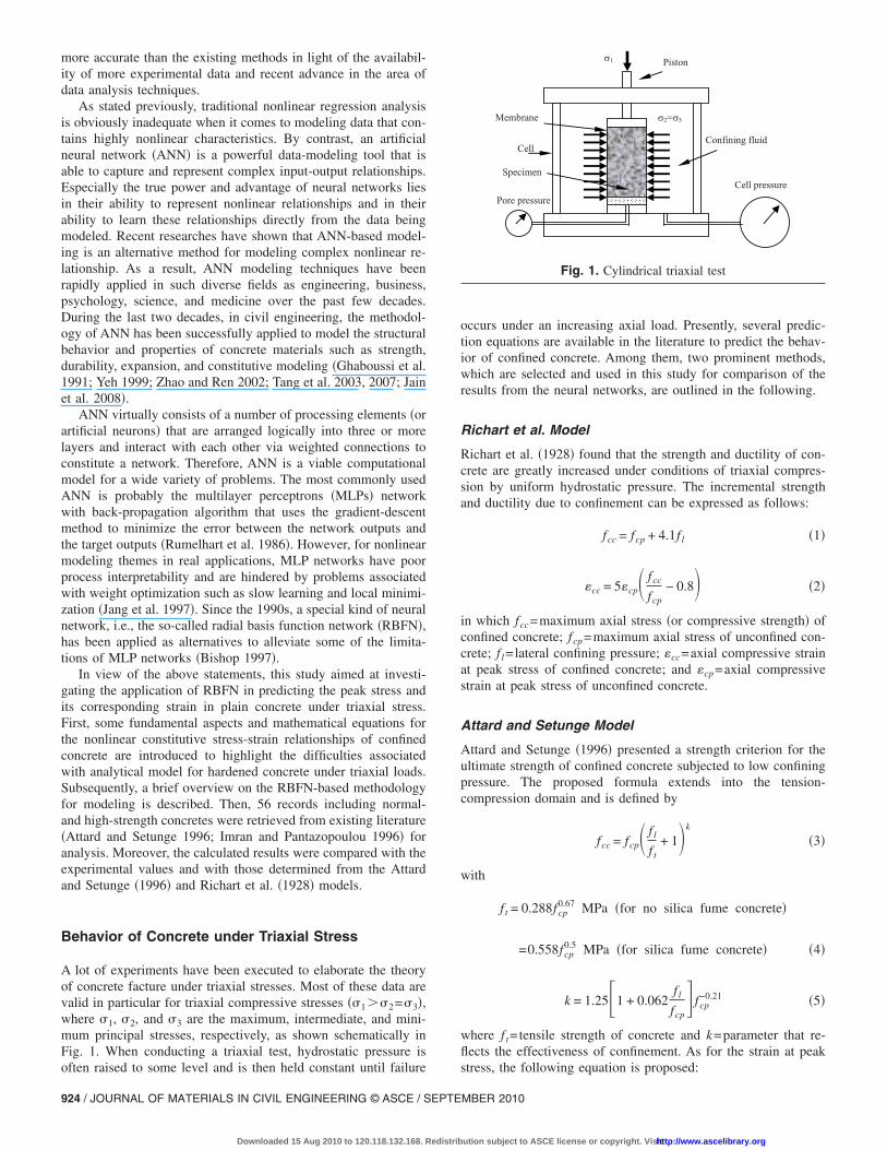
A lot of experiments have been executed to elaborate the theoryof concrete facture under triaxial stresses. Most of these data arevalid in particular for triaxial compressive stresses ��1��2=�3�,where �1, �2, and �3 are the maximum, intermediate, and mini-mum principal stresses, respectively, as shown schematically inFig. 1. When conducting a triaxial test, hydrostatic pressure is

often raised to some level and is then held constant until failure

924 / JOURNAL OF MATERIALS IN CIVIL ENGINEERING © ASCE / SEPTE

Downloaded 15 Aug 2010 to 120.118.132.168. Redistrib

occurs under an increasing axial load. Presently, several predic-tion equations are available in the literature to predict the behav-ior of confined concrete. Among them, two prominent methods,which are selected and used in this study for comparison of theresults from the neural networks, are outlined in the following.

Richart et al. Model

Richart et al. �1928� found that the strength and ductility of con-crete are greatly increased under conditions of triaxial compres-sion by uniform hydrostatic pressure. The incremental strengthand ductility due to confinement can be expressed as follows:

fcc = fcp + 4.1f l �1�

�cc = 5�cp� fcc

fcp− 0.8� �2�

in which fcc=maximum axial stress �or compressive strength� ofconfined concrete; fcp=maximum axial stress of unconfined con-crete; f l=lateral confining pressure; �cc=axial compressive strainat peak stress of confined concrete; and �cp=axial compressivestrain at peak stress of unconfined concrete.

Attard and Setunge Model

Attard and Setunge �1996� presented a strength criterion for theultimate strength of confined concrete subjected to low confiningpressure. The proposed formula extends into the tension-compression domain and is defined by

fcc = fcp� f l

f t+ 1�k

�3�

with

f t = 0.288fcp0.67 MPa �for no silica fume concrete�

=0.558fcp0.5 MPa �for silica fume concrete� �4�

k = 1.25�1 + 0.062f l

fcp� fcp

−0.21 �5�

where f t=tensile strength of concrete and k=parameter that re-flects the effectiveness of confinement. As for the strain at peak

2=3

Pore pressure

1 Piston

CellConfining fluid

Membrane

SpecimenCell pressure

Fig. 1. Cylindrical triaxial test

stress, the following equation is proposed:

MBER 2010

ution subject to ASCE license or copyright. Visithttp://www.ascelibrary.org

Table 1. Experimental Data and Predicted Results of Various Models

Number Mix w /cfcp

�MPa�f l

�MPa� �cp

Ec

�MPa�

Experimentalresults

RBFNmodel

Richart et al.model

Attard and Setungemodel

Type ofsubset

SourceRef.

fcc

�MPa� �cc

fRBF

�MPa� �RBF

fR

�MPa� �R

fA

�MPa� �A

1 aR 0.26 120.0 0.5 0.00300 55700 125 0.00260 126 0.00266 122 0.00363 124 0.00312 Training Attard andSetunge�1996�

2 1.0 0.00300 55700 128 0.00290 129 0.00284 124 0.00400 129 0.00325 Training3 5.0 0.00300 55700 165 0.00380 158 0.00382 141 0.00863 158 0.00423 Training4 10.0 0.00300 55700 192 0.00530 192 0.00528 161 0.01200 187 0.00545 Training5 15.0 0.00300 55700 220 0.00600 217 0.00602 182 0.01550 212 0.00668 Training6 20.0 0.00300 55700 234 0.00800 231 0.00799 202 0.01725 235 0.00790 Training7 bR 0.30 120.0 5.0 0.00280 52800 168 0.00420 161 0.00420 141 0.00840 158 0.00394 Training8 10.0 0.00280 52800 187 0.00480 189 0.00480 161 0.01062 187 0.00509 Training9 15.0 0.00280 52800 211 0.00570 208 0.00570 182 0.01342 212 0.00623 Training10 cR 0.35 110.0 5.0 0.00280 55400 150 0.00350 148 0.00350 131 0.00789 147 0.00412 Training11 10.0 0.00280 55400 175 0.00440 174 0.00440 151 0.01107 175 0.00545 Training12 15.0 0.00280 55400 192 0.00600 192 0.00600 172 0.01324 200 0.00677 Training13 dR 0.26 100.0 1.0 0.00270 52900 106 0.00310 113 0.00315 104 0.00351 108 0.00300 Test14 5.0 0.00270 52900 121 0.00360 129 0.00295 121 0.00554 136 0.00419 Test15 10.0 0.00270 52900 144 0.00470 149 0.00405 141 0.00864 163 0.00567 Test16 15.0 0.00270 52900 165 0.00580 165 0.00589 162 0.01148 187 0.00716 Test17 aB 0.26 132.0 5.0 0.00340 49300 180 0.00500 170 0.00684 153 0.00958 171 0.00457 Validation18 10.0 0.00340 49300 200 0.00580 193 0.00732 173 0.01216 202 0.00574 Validation19 15.0 0.00340 49300 222 0.00780 213 0.00929 194 0.01499 228 0.00691 Validation20 dB 0.26 126.0 5.0 0.00340 49400 162 0.00500 165 0.00655 147 0.00826 164 0.00467 Validation21 10.0 0.00340 49400 186 0.00710 189 0.00702 167 0.01150 194 0.00595 Training22 15.0 0.00340 49400 211 0.00890 211 0.00900 188 0.01487 220 0.00722 Training23 aH 0.26 118.0 5.0 0.00280 57800 154 0.00380 159 0.00380 139 0.00707 156 0.00398 Training24 10.0 0.00280 57800 173 0.00490 185 0.00490 159 0.00933 185 0.00515 Training25 15.0 0.00280 57800 201 0.00620 203 0.00620 180 0.01265 210 0.00633 Training26 bH 0.30 110.0 5.0 0.00280 58700 153 0.00410 146 0.00410 131 0.00827 147 0.00412 Training27 10.0 0.00280 58700 164 0.00550 170 0.00550 151 0.00967 175 0.00545 Training28 15.0 0.00280 58700 185 0.00590 188 0.00590 172 0.01235 200 0.00677 Training29 cH 0.35 100.0 5.0 0.00260 54600 127 0.00390 130 0.00390 121 0.00611 136 0.00403 Training30 10.0 0.00260 54600 153 0.00520 146 0.00520 141 0.00949 163 0.00546 Training31 15.0 0.00260 54600 169 0.00750 159 0.00750 162 0.01157 187 0.00689 Training32 dH 0.26 96.0 5.0 0.00280 55800 119 0.00370 125 0.00370 117 0.00615 128 0.00444 Training33 10.0 0.00280 55800 147 0.00520 146 0.00520 137 0.01024 153 0.00608 Training34 15.0 0.00280 55800 157 0.00530 164 0.00530 158 0.01170 175 0.00772 Training35 eH 0.45 60.0 1.0 0.00210 45100 67 0.00270 89 0.00269 64 0.00333 67 0.00257 Training36 5.0 0.00210 45100 98 0.00480 100 0.00482 81 0.00875 89 0.00445 Training37 10.0 0.00210 45100 122 0.00760 114 0.00759 101 0.01295 112 0.00679 Training38 15.0 0.00210 45100 145 0.00990 130 0.00990 122 0.01698 132 0.00914 Training39 Batch 1 0.40 73.4 3.2 0.00325 37131 96 0.00495 96 0.00463 86 0.00830 94 0.00504 Training Imran and

Pantazopoulou�1996�

40 6.4 0.00325 37131 109 0.00650 106 0.00625 100 0.01108 111 0.00682 Training41 12.8 0.00325 37131 126 0.01045 128 0.01123 126 0.01483 139 0.01040 Training42 25.6 0.00325 37131 169 0.02050 171 0.02006 178 0.02435 186 0.01754 Training43 38.4 0.00325 37131 204 0.03105 206 0.03017 231 0.03218 225 0.02469 Training44 51.2 0.00325 37131 241 0.04090 230 0.04162 283 0.04028 261 0.03183 Training45 Batch 2 0.55 47.4 2.2 0.00280 34895 58 0.00430 58 0.00470 56 0.00583 61 0.00460 Training46 4.3 0.00280 34895 67 0.00690 65 0.00771 65 0.00868 72 0.00640 Training47 8.6 0.00280 34895 84 0.01460 81 0.01383 83 0.01349 92 0.00999 Training48 17.2 0.00280 34895 118 0.02530 117 0.02487 118 0.02367 125 0.01718 Training49 30.1 0.00280 34895 161 0.03600 170 0.03738 171 0.03637 167 0.02797 Training50 43.0 0.00280 34895 205 0.04730 215 0.04673 224 0.04926 206 0.03876 Training51 Batch 3 0.75 28.6 1.1 0.00260 26173 34 0.00470 36 0.00543 33 0.00486 35 0.00406 Training52 2.1 0.00260 26173 36 0.00675 39 0.00771 37 0.00612 41 0.00552 Training53 4.2 0.00260 26173 48 0.01385 46 0.01255 46 0.01144 51 0.00843 Training54 8.4 0.00260 26173 65 0.02375 62 0.02211 63 0.01919 69 0.01426 Training55 14.7 0.00260 26173 92 0.03425 87 0.03496 89 0.03151 93 0.02301 Training56 21.0 0.00260 26173 115 0.04460 114 0.04469 115 0.04161 116 0.03176 TrainingRange of parameters: w /c: 0.26–0.75; fcp: 28.6–132.0 �MPa�; fcc: 33.6–240.5 �MPa�; f l: 0.5–51.2 �MPa�; Ec: 26173–58700 �MPa�;�cp: 0.00210–0.003400.00210–0.00340; �cc: 0.00260–0.04460

Note: w /c=water-cement �or binder� ratio; fcp=maximum axial stress of unconfined concrete; f l=lateral confining pressure; �cp=axial compressive strainat peak stress of unconfined concrete; Ec=modulus of elasticity of concrete; fcc=maximum axial stress of confined concrete; �cc=axial compressive strainat peak stress of confined concrete; fRBF=predicted peak stress using RK14-F4�4–11-1� model; �RBF=predicted peak strain using RK14-E4�4–11-1�model; fR=predicted peak stress using Eq. �1�; �R=predicted peak strain using Eq. �2�; fA=predicted peak stress using Eq. �3�; �A=predicted peak strain

using Eq. �6�.

JOURNAL OF MATERIALS IN CIVIL ENGINEERING © ASCE / SEPTEMBER 2010 / 925

Downloaded 15 Aug 2010 to 120.118.132.168. Redistribution subject to ASCE license or copyright. Visithttp://www.ascelibrary.org

�cc = �cp�1 + �17 − 0.06fcp�� f l

fcp�� �6�

RBFN Modeling of Concrete under Triaxial Stress

Fig. 2 shows the typical architecture of a RBFN with an inputlayer of D neurons, a hidden layer of M neurons, an output layerof P neurons, adjustable weights that exist only between the hid-den and output layers, and biases at each output neuron. The inputlayer serves only as input distributor to the hidden layer, wherethey are transformed into a high-dimensional feature space usingradial basis functions, called basis functions. The basis functionsare exponentially decaying nonlinear functions and are radialfunctions, which have radial symmetry with respect to a center.The centers can be regarded as the neurons �or nodes� of thehidden layer. Each neuron in the hidden layer is a radial function.Then, the transformed data in this space are linearly transformedin order to approximate the target outputs. A commercially avail-able software package, statistica Neural Networks, was used toestablish RBFN models for predicting the peak stress and strain inplain concrete under triaxial stress. Details on the establishmentof the RBFN models, along with sources of the data that are usedin the development, are described below.

Data Set

The experimental data used in this study include 56 records,which are taken from the tests carried out by Attard and Setunge�1996� and Imran and Pantazopoulou �1996�. The tests were doneon cylindrical specimens using a triaxial cell and the stress pathwas followed in the conventional cylindrical triaxial test. In otherwords, axial compressive stress was gradually applied under dis-placement control, while the level of confining pressure wasmaintained. The complete list of the data is given in Table 1,where the name and the source of each specimen are referenced.To avoid the over-fit phenomenon, the so-called “three-way datasplits” �i.e., divide the available data into training, validation, andtest set� were adopted. Furthermore, in order to make the best useof limited data for training, model selection, and performanceestimation, the method of K-fold cross validation was alsoadopted in the present study �Vapnik 1998�. The data were ran-domly split into K equal parts and two different numbers of Kwere chosen �i.e., K=8 and K=14�. For each of K experiments,K-2 folds were used for training, while the remaining twofoldswere used for validation and testing, respectively. This procedure

Outputs

Input layer(D neurons)

Hidden layer(M neurons)

Output layer(P neurons)

Inputs x=(x1,…,xD)

y1

yk

yPxD

xi

x1

wk0

wp0

w11

wkj

wPMhM(x)

(M, M)

(j, j)

h1(x)

hj(x)

(1, 1)

w10

Nonlinear mapping Linear mapping

Fig. 2. Architecture of a typical RBFN

is illustrated in Fig. 3 for K=8.

926 / JOURNAL OF MATERIALS IN CIVIL ENGINEERING © ASCE / SEPTE

Downloaded 15 Aug 2010 to 120.118.132.168. Redistrib

Selection of Input and Output Variables for RBFNModels

Determining the network architecture is one of the most importanttasks in the development of ANN models. Generally speaking, itrequires the selection of the input and output parameters whichwill restrict the number of the input and output nodes of thenetwork. Fortunately, selection of input variables for a networkmodel could be guided by examining those parameters given inthe aforementioned references since the existing empirical equa-tions represent a survey of various statistical regression attemptsfor correlations between the behavior of confined concrete andcharacteristic parameters. Various RBFN models were consideredfor predicting peak stress, fcc, and corresponding strain, �cc, inplain concrete under triaxial stress. After a series of simulations, itwas found that the best input representation for the different out-put variables �i.e., fcc and �cc� consisted of four variables: maxi-mum axial stress of unconfined concrete, fcp; lateral confiningpressure, f l; axial compressive strain at peak stress of unconfinedconcrete, �cp; and modulus of elasticity of concrete, Ec. The ar-chitectures of the developed ANN models for fcc and �cc areshown separately in Table 2. The first column in Table 2 denotesthe K-fold partition and the neural network structure for fcc. Forexample, RK8-F1�4–10-1� stands for the RBFN model using theexperiment 1 of eightfold partitions �see Fig. 3� and it has threelayers �i.e., four input neurons in the first layer, one hidden layerwith 10 hidden neurons in the second layer, and one output neu-ron in the third layer�. In addition, several MLP models are alsodeveloped for comparison �see Table 2�.

Network Topology and Training Algorithm

The training of a RBFN takes place in two distinct stages. Usu-ally, the centers and width factors of the radial basis functionsmust be set, then the linear output layer is optimized. In the study,the centers stored in the radial hidden layer were optimized firstusing a kind of unsupervised training technique, i.e., the K-meansmethod �Moody and Darken 1989�. A set of data points was se-lected at random from the training data subset. These data pointswere the seeds of an incremental K-means clustering procedureand these K-means centers were used as centers in the RBFN.Then the width of the data was reflected in the radial deviationsand deviations were assigned by the K-nearest neighbor method.In other words, each basis’s deviation is individually set to themean distance to its K nearest neighbors. Hence, deviations aresmaller in tightly packed areas of space, preserving detail, andhigher in sparse areas of space. After centers and deviations wereset, the linear output layer was optimized using the pseudoinverse

Fig. 3. Data set in eightfold partition

technique �Haykin 1999�.

MBER 2010

ution subject to ASCE license or copyright. Visithttp://www.ascelibrary.org

As previously mentioned, the data set was divided into threesubsets: training, validation, and test cases. To reiterate, the neuralnetworks were trained using the training subset only. The valida-tion subset was used to keep an independent check on the perfor-

Table 2. Architecture of ANN Models

RBFN model for fcc

Inputvariables

Outputvariable

RK8-F1�4–10-1� fcp , f l ,�cp ,Ec fcc

RK8-F2�4–18-1� fcp , f l ,�cp ,Ec fcc

RK8-F3�4–8-1� fcp , f l ,�cp ,Ec fcc

RK8-F4�4–5-1� fcp , f l ,�cp ,Ec fcc

RK8-F5�4–23-1� fcp , f l ,�cp ,Ec fcc

RK8-F6�4–4-1� fcp , f l ,�cp ,Ec fcc

RK8-F7�4–16-1� fcp , f l ,�cp ,Ec fcc

RK8-F8�4–7-1� fcp , f l ,�cp ,Ec fcc

RK14-F1�4–13-1� fcp , f l ,�cp ,Ec fcc

RK14-F2�4–14-1� fcp , f l ,�cp ,Ec fcc

RK14-F3�4–19-1� fcp , f l ,�cp ,Ec fcc

RK14-F4�4–11-1� fcp , f l ,�cp ,Ec fcc

RK14-F5�4–7-1� fcp , f l ,�cp ,Ec fcc

RK14-F6�4–8-1� fcp , f l ,�cp ,Ec fcc

RK14-F7�4–11-1� fcp , f l ,�cp ,Ec fcc

RK14-F8�4–6-1� fcp , f l ,�cp ,Ec fcc

RK14-F9�4–14-1� fcp , f l ,�cp ,Ec fcc

RK14-F10�4–21-1� fcp , f l ,�cp ,Ec fcc

RK14-F11�4–15-1� fcp , f l ,�cp ,Ec fcc

RK14-F12�4–10-1� fcp , f l ,�cp ,Ec fcc

RK14-F13�4–10-1� fcp , f l ,�cp ,Ec fcc

RK14-F14�4–18-1� fcp , f l ,�cp ,Ec fcc

RK14-F4�3–7-1� fcp , f l ,�cpc fcc

RK14-F4�2–7-1� fcp , f l fcc

MLP model for fcc

Inputvariables

Outputvariable

MK8-F1�4–10-1� fcp , f l ,�cp ,Ec fcc

MK8-F2�4–4-1� fcp , f l ,�cp ,Ec fcc

MK8-F3�4–4-1� fcp , f l ,�cp ,Ec fcc

MK8-F4�4–6-1� fcp , f l ,�cp ,Ec fcc

MK8-F5�4–9-1� fcp , f l ,�cp ,Ec fcc

MK8-F6�4–5-1� fcp , f l ,�cp ,Ec fcc

MK8-F7�4–11-1� fcp , f l ,�cp ,Ec fcc

MK8-F8�4–11-1� fcp , f l ,�cp ,Ec fcc

MK14-F1�4–17-1� fcp , f l ,�cp ,Ec fcc

MK14-F2�4–6-1� fcp , f l ,�cp ,Ec fcc

MK14-F3�4–11-1� fcp , f l ,�cp ,Ec fcc

MK14-F4�4–12-1� fcp , f l ,�cp ,Ec fcc

MK14-F5�4–8-1� fcp , f l ,�cp ,Ec fcc

MK14-F6�4–5-1� fcp , f l ,�cp ,Ec fcc

MK14-F7�4–8-1� fcp , f l ,�cp ,Ec fcc

MK14-F8�4–6-1� fcp , f l ,�cp ,Ec fcc

MK14-F9�4–6-1� fcp , f l ,�cp ,Ec fcc

MK14-F10�4–4-1� fcp , f l ,�cp ,Ec fcc

MK14-F11�4–7-1� fcp , f l ,�cp ,Ec fcc

MK14-F12�4–8-1� fcp , f l ,�cp ,Ec fcc

MK14-F13�4–6-1� fcp , f l ,�cp ,Ec fcc

MK14-F14�4–13-1� fcp , f l ,�cp ,Ec fcc

MK14-F4�3–7-1� fcp , f l ,�cp fcc

MK14-F4�2–5-1� fcp , f l fcc

mance of the networks during training, with deterioration in the

JOURNAL OF MAT

Downloaded 15 Aug 2010 to 120.118.132.168. Redistrib

validation errors indicating overlearning. If overlearning occurs,the software stops training the network and restores it to the statewith minimum validation error. The validation error was also usedby the software to select between the available networks. How-

RBFN model for �cc

Inputvariables

Outputvariable

RK8-E1�4–15-1� fcp , f l ,�cp ,Ec �cc

RK8-E2�4–16-1� fcp , f l ,�cp ,Ec �cc

RK8-E3�4–12-1� fcp , f l ,�cp ,Ec �cc

RK8-E4�4–11-1� fcp , f l ,�cp ,Ec �cc

RK8-E5�4–16-1� fcp , f l ,�cp ,Ec �cc

RK8-E6�4–9-1� fcp , f l ,�cp ,Ec �cc

RK8-E7�4–12-1� fcp , f l ,�cp ,Ec �cc

RK8-E8�4–11-1� fcp , f l ,�cp ,Ec �cc

RK14-E1�4–13-1� fcp , f l ,�cp ,Ec �cc

RK14-E2�4–15-1� fcp , f l ,�cp ,Ec �cc

RK14-E3�4–17-1� fcp , f l ,�cp ,Ec �cc

RK14-E4�4–11-1� fcp , f l ,�cp ,Ec �cc

RK14-E5�4–6-1� fcp , f l ,�cp ,Ec �cc

RK14-E6�4–5-1� fcp , f l ,�cp ,Ec �cc

RK14-E7�4–11-1� fcp , f l ,�cp ,Ec �cc

RK14-E8�4–12-1� fcp , f l ,�cp ,Ec �cc

RK14-E9�4–11-1� fcp , f l ,�cp ,Ec �cc

RK14-E10�4–12-1� fcp , f l ,�cp ,Ec �cc

RK14-E11�4–6-1� fcp , f l ,�cp ,Ec �cc

RK14-E12�4–12-1� fcp , f l ,�cp ,Ec �cc

RK14-E13�4–10-1� fcp , f l ,�cp ,Ec �cc

RK14-E14�4–14-1� fcp , f l ,�cp ,Ec �cc

RK14-E4�3–7-1� fcp , f l ,�cpc �cc

RK14-E4�2–12-1� fcp , f l �cc

MLP model for �cc

Inputvariables

Outputvariable

MK8-E1�4–8-1� fcp , f l ,�cp ,Ec �cc

MK8-E2�4–5-1� fcp , f l ,�cp ,Ec �cc

MK8-E3�4–7-1� fcp , f l ,�cp ,Ec �cc

MK8-E4�4–5-1� fcp , f l ,�cp ,Ec �cc

MK8-E5�4–2-1� fcp , f l ,�cp ,Ec �cc

MK8-E6�4–5-1� fcp , f l ,�cp ,Ec �cc

MK8-E7�4–7-1� fcp , f l ,�cp ,Ec �cc

MK8-E8�4–8-1� fcp , f l ,�cp ,Ec �cc

MK14-E1�4–5-1� fcp , f l ,�cp ,Ec �cc

MK14-E2�4–5-1� fcp , f l ,�cp ,Ec �cc

MK14-E3�4–6-1� fcp , f l ,�cp ,Ec �cc

MK14-E4�4–6-1� fcp , f l ,�cp ,Ec �cc

MK14-E5�4–5-1� fcp , f l ,�cp ,Ec �cc

MK14-E6�4–6-1� fcp , f l ,�cp ,Ec �cc

MK14-E7�4–7-1� fcp , f l ,�cp ,Ec �cc

MK14-E8�4–7-1� fcp , f l ,�cp ,Ec �cc

MK14-E9�4–5-1� fcp , f l ,�cp ,Ec �cc

MK14-E10�4–3-1� fcp , f l ,�cp ,Ec �cc

MK14-E11�4–2-1� fcp , f l ,�cp ,Ec �cc

MK14-E12�4–6-1� fcp , f l ,�cp ,Ec �cc

MK14-E13�4–14-1� fcp , f l ,�cp ,Ec �cc

MK14-E14�4–4-1� fcp , f l ,�cp ,Ec �cc

MK14-E4�3–6-1� fcp , f l ,�cp �cc

MK14-E4�2–2-1� fcp , f l �cc

ever, if a large number of networks are tested, a random sampling

ERIALS IN CIVIL ENGINEERING © ASCE / SEPTEMBER 2010 / 927

ution subject to ASCE license or copyright. Visithttp://www.ascelibrary.org

Table 3. Summary of RMS Error and Pearson Correlation Coefficient for fcc

ANN model

RMS error �MPa� Pearson correlation coefficient

Trainingsubset

Validationsubset

Testsubset

Trainingsubset

Validationsubset

Testsubset

RK8-F1�4–10-1� 8.93 6.62 18.86 0.9853 0.9903 0.9865RK8-F2�4–18-1� 6.55 5.85 3.38 0.9924 0.9850 0.9956RK8-F3�4–8-1� 10.90 10.21 6.38 0.9800 0.9680 0.9741RK8-F4�4–5-1� 16.19 16.39 9.45 0.9556 0.9463 0.9815RK8-F5�4–23-1� 2.50 10.43 13.74 0.9990 0.9070 0.9203RK8-F6�4–4-1� 7.28 9.48 17.60 0.9614 0.9895 0.9485RK8-F7�4–16-1� 6.51 26.84 31.07 0.9847 0.9962 0.9248RK8-F8�4–7-1� 7.23 13.14 21.25 0.9859 0.9643 0.9836Average 8.26 12.37 15.22 0.9805 0.9683 0.9644

RK14-F1�4–13-1� 6.16 4.79 9.70 0.9927 0.9864 0.9907RK14-F2�4–14-1� 3.52 5.95 10.28 0.9975 0.9997 0.9852RK14-F3�4–19-1� 6.92 5.89 2.81 0.9915 0.9998 0.9987RK14-F4�4–11-1� 6.19 7.63 5.92 0.9930 0.9807 0.9967RK14-F5�4–7-1� 12.76 6.47 6.48 0.9686 0.9896 0.9707RK14-F6�4–8-1� 8.74 6.75 4.71 0.9861 0.9783 0.9951RK14-F7�4–11-1� 7.34 5.53 8.44 0.9906 0.9887 0.9770RK14-F8�4–6-1� 11.18 17.00 9.22 0.9774 0.9721 0.9399RK14-F9�4–14-1� 1.39 14.47 8.26 0.9997 0.9665 0.9949RK14-F10�4–21-1� 4.48 10.10 17.75 0.9962 0.9893 0.9861RK14-F11�4–15-1� 5.54 4.20 13.29 0.9934 0.9989 0.9831RK14-F12�4–10-1� 8.25 10.96 2.92 0.9825 0.9986 0.9995RK14-F13�4–10-1� 8.23 10.38 17.22 0.9823 0.9988 1.0000RK14-F14�4–18-1� 5.99 14.86 13.77 0.9928 0.9825 0.9969RK14-F1�4–13-1� 6.91 8.93 9.34 0.9872 0.9869 0.9818Average 6.16 4.79 9.70 0.9927 0.9864 0.9907

MK8-F1�4–10-1� 5.38 6.93 13.49 0.9943 0.9819 0.9910MK8-F2�4–4-1� 9.37 5.00 8.76 0.9863 0.9957 0.9795MK8-F3�4–4-1� 9.39 4.02 8.15 0.9843 0.9816 0.9675MK8-F4�4–6-1� 13.42 3.58 10.59 0.9833 0.9938 0.9650MK8-F5�4–9-1� 8.67 4.35 10.95 0.9877 0.9886 0.9924MK8-F6�4–5-1� 10.12 3.28 5.44 0.9824 0.9988 0.9808MK8-F7�4–11-1� 9.77 1.23 8.36 0.9698 0.9998 0.9994MK8-F8�4–11-1� 5.91 9.97 9.06 0.9908 0.9867 0.9984Average 9.00 4.80 9.35 0.9849 0.9909 0.9843

MK14-F1�4–17-1� 15.07 5.07 17.80 0.9932 0.9884 0.9930MK14-F2�4–6-1� 8.32 2.57 12.04 0.9860 0.9981 0.9699MK14-F3�4–11-1� 10.99 3.08 14.81 0.9873 0.9991 0.9978MK14-F4�4–12-1� 8.08 2.19 12.22 0.9889 0.9983 0.9991MK14-F5�4–8-1� 7.53 2.31 3.95 0.9892 0.9941 0.9925MK14-F6�4–5-1� 9.31 3.37 6.14 0.9842 0.9844 0.9909MK14-F7�4–8-1� 8.68 3.27 8.01 0.9868 0.9913 0.9918MK14-F8�4–6-1� 7.61 5.99 5.80 0.9898 0.9869 0.9939MK14-F9�4–6-1� 7.16 9.18 8.09 0.9915 0.9826 0.9866MK14-F10�4–4-1� 12.23 2.00 7.06 0.9752 0.9989 0.9965MK14-F11�4–7-1� 10.29 0.37 18.20 0.9789 0.9999 0.9995MK14-F12�4–8-1� 8.83 0.91 5.94 0.9799 0.9999 1.0000MK14-F13�4–6-1� 7.50 0.53 3.76 0.9853 0.9998 0.9989MK14-F14�4–13-1� 6.68 8.02 2.51 0.9912 0.9934 0.9998Average 9.16 3.49 9.02 0.9882 0.9926 0.9911

RK14-F4�3–7-1� 11.10 5.58 12.57 0.9774 0.9854 0.9996RK14-F4�2–7-1� 9.70 3.73 9.03 0.9828 0.9929 0.9990MK14-F4�3–7-1� 6.28 3.22 10.30 0.9929 0.9906 0.9991MK14-F4�2–5-1� 7.78 3.36 9.57 0.9889 0.9901 0.9983

928 / JOURNAL OF MATERIALS IN CIVIL ENGINEERING © ASCE / SEPTEMBER 2010

Downloaded 15 Aug 2010 to 120.118.132.168. Redistribution subject to ASCE license or copyright. Visithttp://www.ascelibrary.org

Table 4. Summary of RMS Error and Pearson Correlation Coefficient for �cc

ANN model

RMS error Pearson correlation coefficient

Trainingsubset

Validationsubset

Testsubset

Trainingsubset

Validationsubset

Testsubset

RK8-E1�4–15-1� 0.00238 0.00067 0.00128 0.9505 0.9841 0.9897RK8-E2�4–16-1� 0.00315 0.00071 0.00052 0.9664 0.9083 0.9354RK8-E3�4–12-1� 0.00265 0.00109 0.00107 0.9770 0.9738 0.8635RK8-E4�4–11-1� 0.00398 0.00069 0.00107 0.9555 0.9211 0.9666RK8-E5�4–16-1� 0.00078 0.00314 0.00156 0.9980 0.9058 0.9106RK8-E6�4–9-1� 0.00226 0.00427 0.00528 0.9742 0.9793 0.9872RK8-E7�4–12-1� 0.00045 0.01631 0.00972 0.9879 0.9448 0.9563RK8-E8�4–11-1� 0.00144 0.00059 0.00941 0.9861 0.9717 0.9147Average 0.00214 0.00343 0.00374 0.9744 0.9486 0.9405

RK14-E1�4–13-1� 0.00260 0.00060 0.00121 0.9750 0.9839 0.9745RK14-E2�4–15-1� 0.00224 0.00036 0.00132 0.9816 0.9844 0.9647RK14-E3�4–17-1� 0.00281 0.00077 0.00077 0.9706 0.9929 0.9321RK14-E4�4–11-1� 0.00050 0.00160 0.00046 0.9991 0.9943 0.9523RK14-E5�4–6-1� 0.00341 0.00099 0.00109 0.9494 0.9888 0.9641RK14-E6�4–5-1� 0.00412 0.00270 0.00241 0.9371 0.9651 0.9988RK14-E7�4–11-1� 0.00218 0.00118 0.00305 0.9827 0.9651 0.8319RK14-E8�4–12-1� 0.00220 0.00124 0.00067 0.9821 0.9059 0.9208RK14-E9�4–11-1� 0.00262 0.00176 0.00128 0.9750 0.9956 0.9043RK14-E10�4–12-1� 0.00276 0.00288 0.00478 0.9649 0.9861 0.9746RK14-E11�4–6-1� 0.00205 0.00161 0.00408 0.9796 0.9965 0.9548RK14-E12�4–12-1� 0.00119 0.00554 0.00157 0.9922 0.9981 0.9942RK14-E13�4–10-1� 0.00156 0.00656 0.00104 0.9766 0.9948 0.9958RK14-E14�4–14-1� 0.00090 0.00009 0.01312 0.9958 0.9974 0.9945RK14-E1�4–13-1� 0.00222 0.00199 0.00263 0.9722 0.9726 0.9424Average 0.00260 0.00060 0.00121 0.9750 0.9839 0.9745

MK8-E1�4–8-1� 0.00146 0.00025 0.00066 0.9932 0.9703 0.9905MK8-E2�4–5-1� 0.00307 0.00042 0.00061 0.9685 0.9387 0.9569MK8-E3�4–7-1� 0.00148 0.00033 0.00094 0.9929 0.9869 0.9568MK8-E4�4–5-1� 0.00189 0.00052 0.00080 0.9882 0.9311 0.9716MK8-E5�4–2-1� 0.00205 0.00116 0.00168 0.9868 0.9768 0.8900MK8-E6�4–5-1� 0.00098 0.00112 0.00221 0.9952 0.9965 0.9828MK8-E7�4–7-1� 0.00064 0.00435 0.00216 0.9767 0.9954 0.9940MK8-E8�4–8-1� 0.00106 0.00026 0.00866 0.9926 0.9919 0.9878Average 0.00158 0.00105 0.00222 0.9868 0.9734 0.9663

MK14-E1�4–5-1� 0.00116 0.00037 0.00050 0.9951 0.9674 0.9974MK14-E2�4–5-1� 0.00138 0.00022 0.00077 0.9932 0.9819 0.9475MK14-E3�4–6-1� 0.00295 0.00014 0.00045 0.9677 0.9971 0.9926MK14-E4�4–6-1� 0.00143 0.00026 0.00090 0.9927 0.9730 0.9917MK14-E5�4–5-1� 0.00183 0.00021 0.00087 0.9880 0.9942 0.9692MK14-E6�4–6-1� 0.00140 0.00021 0.00117 0.9931 0.9670 0.9873MK14-E7�4–7-1� 0.00155 0.00024 0.00041 0.9912 0.9891 0.9676MK14-E8�4–7-1� 0.00129 0.00045 0.00114 0.9929 0.9745 0.9163MK14-E9�4–5-1� 0.00190 0.00040 0.00133 0.9869 0.9850 0.9233MK14-E10�4–3-1� 0.00142 0.00068 0.00260 0.9931 0.9993 0.9938MK14-E11�4–2-1� 0.00048 0.00110 0.00190 0.9963 0.9987 0.9992MK14-E12�4–6-1� 0.00089 0.00299 0.00363 0.9975 0.9946 0.9971MK14-E13�4–14-1� 0.00095 0.00128 0.00468 0.9913 0.9966 0.9957MK14-E14�4–4-1� 0.00198 0.00007 0.00980 0.9799 0.9977 0.9918Average 0.00147 0.00062 0.00215 0.9892 0.9805 0.9712

RK14-E4�3–7-1� 0.00338 0.00165 0.00126 0.9576 0.9633 0.9928RK14-E4�2–12-1� 0.00141 0.00028 0.00061 0.9927 0.9974 0.9889MK14-E4�3–6-1� 0.00156 0.00023 0.00140 0.9911 0.9797 0.9939MK14-E4�2–2-1� 0.00208 0.00035 0.00153 0.9843 0.9518 0.9882

JOURNAL OF MATERIALS IN CIVIL ENGINEERING © ASCE / SEPTEMBER 2010 / 929

Downloaded 15 Aug 2010 to 120.118.132.168. Redistribution subject to ASCE license or copyright. Visithttp://www.ascelibrary.org

effect can kick in and one may get a network with a good vali-dation error which is not actually indicative of good generaliza-tion capabilities. Therefore, a third subset �i.e., the test subset�was maintained and one could visually inspect performance aftertraining.

A great amount of networks were tested. The best networkfound for a great diversity of ANN models was retained. Theperformance of the developed ANN was measured in two aspects:one is the value of root-mean-square �RMS� error of the networkoutput to the target output and the other is the Pearson correlationcoefficient, r, between the network output and the target output.In principle, the lower the RMS error value or the higher the rvalue is, the better the prediction relationship will be. Judgingfrom Tables 3 and 4, it can be concluded that the developedRBFN models had a good generalization performance in terms ofthe average RMS error and r values obtained from the K-foldcross-validation with K=14. Especially, the average r values forthe training, validation, and testing subsets are all greater than0.97 �see Tables 3 and 4�. The results demonstrate the peak stressand strain in plain concrete under triaxial stress can be accuratelyestimated using four input variables �i.e., fcp, f l, �cp, and Ec�. Thisis quite consistent with most existing analytical methods. Besides,as compared with MLPs �refer to Tables 3 and 4�, RBFNs notonly trained quite rapidly during training but also provided fairlygood accuracy.

Comparison with Empirical Equations

In order to evaluate the capabilities of RBFNs in predictingthe peak stress and strain of plain concrete under triaxial stress,two developed RBFN models �i.e., RK14-F4�4–11-1� for fcc

Fig. 4. Experimental versus pred

and RK14-E4�4–11-1� for �cc� were chosen. A comparison of

930 / JOURNAL OF MATERIALS IN CIVIL ENGINEERING © ASCE / SEPTE

Downloaded 15 Aug 2010 to 120.118.132.168. Redistrib

the predicated results obtained with the two RBFN models andthe aforementioned empirical equations are given in Table 1. InTable 1, all models used the same training, validation, and testingdata to calculate the predicted peak stress, fccp, and its corre-sponding axial strain, �ccp, in confined concrete. Regarding all 56specimens, the experimental peak stress �fcce collected from theliterature� is plotted against the predicted values, as shown inFigs. 4�a–c�. To show the overall trend of correlation, the theoret-ical line with fcce / fccp=1 was drawn on the graphs along with thedata points plotted. The nearer the points gather around the diag-onal line, the better are the predicted values. Figs. 4�a and b�show that the correlation between the values of fcce and fccp wasdeemed satisfactory for the weaker specimens by Eqs. �1� and �3�,while the correlation for the stronger specimens was more scat-tered, particularly by Eq. �1�. By contrast, Fig. 4�c� clearly showsthat the less scatter of data around the diagonal line confirms thefact that neural network-based model is an excellent predictor forthe value of fcc. Overall, it can be observed that a larger variationin the accuracy was noticed in the Richart et al. model. Therefore,based on the 56 records, an improved equation for Eq. �1� isproposed as follows:

fcc = 1.2fcp + 3.4f l �7�

where the parameters are as previously defined. The coefficient ofdetermination, R2, of Eq. �7� is 0.97 and thus a superior fcce ver-sus fccp plot is obtained, as shown in Fig. 4�d�.

As for the axial compressive strain at peak stress of confinedconcrete, the experimental strain ��cce collected from the litera-ture� is also plotted against the predicted values ��ccp�, as shownin Fig. 5. It is evident from Figs. 5�a and b� that the correlation

eak stresses of confined concrete

icted p

between the values of �cce and �ccp was less than satisfactory

MBER 2010

ution subject to ASCE license or copyright. Visithttp://www.ascelibrary.org

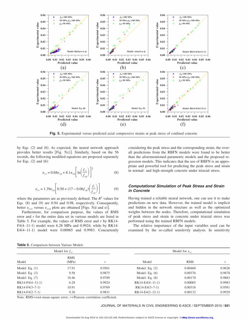
by Eqs. �2� and �6�. As expected, the neural network approachprovides better results �Fig. 5�c��. Similarly, based on the 56records, the following modified equations are proposed separatelyfor Eqs. �2� and �6�:

�cc = 0.68�cp + 8.1�cp�ln� fcc

fcp��2

�8�

�cc = 1.39�cp�0.50 + �17 − 0.06fcp�� f l

fcp�� �9�

where the parameters are as previously defined. The R2 values forEqs. �8� and �9� are 0.94 and 0.98, respectively. Consequently,better �cce versus �ccp plots are obtained �Figs. 5�d and e��.

Furthermore, for comparison purpose, the values of RMSerror and r for the entire data set in various models are listed inTable 5. For example, the values of RMS error and r by RK14-F4�4–11-1� model were 6.28 MPa and 0.9924, while by RK14-E4�4–11-1� model were 0.00065 and 0.9983. Concurrently

Table 5. Comparison between Various Models

Model for fcc

ModelRMS�MPa� r

Model: Eq. �1� 17.91 0.9561

Model: Eq. �3� 9.58 0.9875

Model: Eq. �7� 10.46 0.9789

RK14-F4�4–11-1� 6.28 0.9924

RK14-F4�3–7-1� 10.91 0.9769

RK14-F4�2–7-1� 9.36 0.9831

0.00 0.01 0.02 0.03 0.04 0.05 0.06Predicted value

0.00

0.01

0.02

0.03

0.04

0.05

0.06

Exp

erim

entalv

alue

Model: Richart et al.

fcp>100 MPa50 MPafcp100 MPafcp<50 MPa

0.00 0.01P

0.00

0.01

0.02

0.03

0.04

0.05

0.06

Exp

erim

entalv

alue

(a)

0.00 0.01 0.02 0.03 0.04 0.05 0.06Predicted value

0.00

0.01

0.02

0.03

0.04

0.05

0.06

Exp

erim

entalv

alue

Model: Eq. (8)

fcp>100 MPa50 MPafcp100 MPafcp<50 MPa

0.00 0.01P

0.00

0.01

0.02

0.03

0.04

0.05

0.06

Exp

erim

entalv

alue

(d)

Fig. 5. Experimental versus predicted axial co

Note: RMS=root-mean-square error; r=Pearson correlation coefficient.

JOURNAL OF MAT

Downloaded 15 Aug 2010 to 120.118.132.168. Redistrib

considering the peak stress and the corresponding strain, the over-all predictions from the RBFN models were found to be betterthan the aforementioned parametric models and the proposed re-gression models. This indicates that the use of RBFN is an appro-priate and powerful tool for predicting the peak stress and strainin normal- and high-strength concrete under triaxial stress.

Computational Simulation of Peak Stress and Strainin Concrete

Having trained a reliable neural network, one can use it to makepredictions on new data. However, the trained model is implicitand hidden in the network structure as well as the optimizedweights between the nodes. Therefore, computational simulationof peak stress and strain in concrete under triaxial stress wasperformed using the trained RBFN models.

The relative importance of the input variables used can beexamined by the so-called sensitivity analysis. In sensitivity

Model for �cc

Model RMS r

Model: Eq. �2� 0.00460 0.9626

Model: Eq. �6� 0.00376 0.9878

Model: Eq. �8� 0.00170 0.9883

RK14-E4�4–11-1� 0.00065 0.9983

RK14-E4�3–7-1� 0.00318 0.9581

RK14-E4�2–12-1� 0.00132 0.9929

3 0.04 0.05 0.06d value

odel: Attard et al.

Pacp100 MPaa

0.00 0.01 0.02 0.03 0.04 0.05 0.06Predicted value

0.00

0.01

0.02

0.03

0.04

0.05

0.06

Exp

erim

entalv

alue

Model: RK14-E4(4-11-1)

fcp>100 MPa50 MPafcp100 MPafcp<50 MPa

(c)

3 0.04 0.05 0.06d value

Model: Eq. (9)

Pacp100 MPaa

0.00 0.01 0.02 0.03 0.04 0.05 0.06Predicted value

0.00

0.01

0.02

0.03

0.04

0.05

0.06

Exp

erim

entalv

alue

Model: RK14-E4(2-12-1)

fcp>100 MPa50 MPafcp100 MPafcp<50 MPa

(f)

sive strains at peak stress of confined concrete

0.02 0.0redicte

M

fcp>100 M50 MPaffcp<50 MP

(b)

0.02 0.0redicte

fcp>100 M50 MPaffcp<50 MP

(e)

mpres

ERIALS IN CIVIL ENGINEERING © ASCE / SEPTEMBER 2010 / 931

ution subject to ASCE license or copyright. Visithttp://www.ascelibrary.org

analysis, the data set is submitted to the network repeatedly,with each variable in turn treated as missing, and the resultingnetwork error is recorded. If an important variable is removed inthis fashion, the error will increase a great deal; if an unimportantvariable is removed, the error will not increase very much. Thesensitivity analysis of the RBFN models shows that lateral con-fining pressure, f l, and maximum axial stress of unconfined con-crete, fcp, were the main influential factors in predicting fcc and�cc �Table 6�. Therefore, several RBFN models using only twoparameters �i.e., f l and fcp� or three parameters �i.e., f l, fcp, and�cp� as the input variables were also developed. The architectureof those ANN models is shown in Table 2 and they also have agood performance in predicting fcc and �cc �see Tables 3 and 4�.For example, Fig. 4�e� demonstrates that RK14-F4�2–7-1� modelusing f l and fcp as the input variables had an accurate estimate offcc. Another example is RK14-E4�2–12-1� model with f l and fcp

as the input variables. It could make an accurate estimate of �cc

Table 6. Sensitivity Analysis of Input Variables

ANN model for fcc

Rank of variable

Training subset Training subset

fcp f l �cp Ec fcp f l �cp E

RK8-F1�4–10-1� 1 2 3 4 1 2 3 4

RK8-F2�4–18-1� 2 1 4 3 1 2 3 4

RK8-F3�4–8-1� 2 1 4 3 1 2 3 4

RK8-F4�4–5-1� 2 1 4 3 3 1 2 4

RK8-F5�4–23-1� 2 1 4 3 3 1 2 4

RK8-F6�4–4-1� 2 1 4 3 2 1 4 3

RK8-F7�4–16-1� 1 2 3 4 1 2 4 3

RK8-F8�4–7-1� 1 2 3 4 1 2 4 3

RK14-F1�4–13-1� 2 1 4 3 1 2 3 4

RK14-F2�4–14-1� 1 2 4 3 1 2 4 3

RK14-F3�4–19-1� 1 2 4 3 2 1 4 3

RK14-F4�4–11-1� 2 1 4 3 1 2 3 4

RK14-F5�4–7-1� 1 2 4 3 1 2 4 3

RK14-F6�4–8-1� 1 2 4 3 1 2 4 3

RK14-F7�4–11-1� 2 1 4 3 1 2 4 3

RK14-F8�4–6-1� 2 1 4 3 3 1 2 4

RK14-F9�4–14-1� 1 2 4 3 2 1 4 3

RK14-F10�4–21-1� 1 2 4 3 3 1 2 4

RK14-F11�4–15-1� 2 1 4 3 1 3 4 2

RK14-F12�4–10-1� 2 1 3 4 2 1 4 3

RK14-F13�4–10-1� 2 1 4 3 1 3 4 2

RK14-F14�4–18-1� 2 1 4 3 2 1 3 4

Note: The smaller the number of rank, the more important the variable.

0 10 20 30 40 50 60Lateral confining pressure (MPa)

50

100

150

200

250

300

350

Peak

stress

(MPa

)

Experimental result (fcp=73.4 MPa)RK14-F4(4-11-1) (fcp=73.4 MPa)Experimental result (fcp=47.4 MPa)

RK14-F4(4-11-1) (fcp=47.4 MPa)

0 10 20 30 40 50 60Lateral confining pressure (MPa)

50

100

150

200

250

300

350

Peak

stress

(MPa

)

RK14-F4(2-7-1) (fcp=73.4 MPa)Test results (fcp=73.4 MPa)RK14-F4(2-7-1) (fcp=47.4 MPa)Test results (fcp=47.4 MPa)

(a) (b)

Fig. 6. RBFN simulated peak stress versus lateral confining pressurecurve

932 / JOURNAL OF MATERIALS IN CIVIL ENGINEERING © ASCE / SEPTE

Downloaded 15 Aug 2010 to 120.118.132.168. Redistrib

�Fig. 5�f��. On the whole, however, the results indicate that reduc-ing the number of inputs had a negative effect upon the predictionaccuracy of fcc and �cc �Table 5�.

Based on the above analysis, it is feasible to simulate the fcc

versus f l or �cc versus f l relationship curves for concrete with aspecific strength. For example, the RBFN simulated chart for therelationship between fcc and f l are proposed for concrete with fcp

of 73.4 and 47.4 MPa �Fig. 6�. The experimental results are alsoshown in Fig. 6 for comparison. As can be seen from Fig. 6, thesimulation curve demonstrates that the predicated peak stress in-creased with increasing confining pressure for a fixed concretestrength. Especially, the simulation curve using four input vari-ables fitted very well to experimental data �Fig. 6�a��. By contrast,using two input variables, the resulting simulation curve becameflatter at higher confining pressure and was thus less adequate�Fig. 6�b��. In addition, Fig. 7 shows the RBFN simulated chartfor the relationship between �cc and f l. The axial strain at peak

NN model for �cc

Rank of variable

Training subset Training subset

fcp f l �cp Ec fcp f l �cp Ec

RK8-E1�4–15-1� 2 1 4 3 3 2 4 1

RK8-E2�4–16-1� 3 1 4 2 2 1 4 3

RK8-E3�4–12-1� 3 1 4 2 4 2 3 1

RK8-E4�4–11-1� 3 1 4 2 4 3 1 2

RK8-E5�4–16-1� 3 1 4 2 3 1 4 2

RK8-E6�4–9-1� 3 1 4 2 4 1 3 2

RK8-E7�4–12-1� 3 1 4 2 3 1 4 2

RK8-E8�4–11-1� 3 1 4 2 4 1 3 2

K14-E1�4–13-1� 2 1 4 3 3 2 4 1

K14-E2�4–15-1� 2 1 4 3 1 3 4 2

K14-E3�4–17-1� 2 1 4 3 3 4 2 1

K14-E4�4–11-1� 3 1 4 2 1 4 2 3

RK14-E5�4–6-1� 4 1 3 2 1 3 4 2

RK14-E6�4–5-1� 2 1 4 3 3 2 4 1

K14-E7�4–11-1� 3 1 4 2 4 2 3 1

K14-E8�4–12-1� 3 1 4 2 4 1 3 2

K14-E9�4–11-1� 3 1 4 2 1 2 3 4

K14-E10�4–12-1� 2 1 4 3 2 1 4 3

K14-E11�4–6-1� 3 1 4 2 3 1 4 2

K14-E12�4–12-1� 3 1 4 2 3 1 4 2

K14-E13�4–10-1� 2 1 4 3 3 2 4 1

K14-E14�4–14-1� 2 1 4 3 2 3 4 1

0 10 20 30 40 50 60Lateral confining pressure (MPa)

0

20000

40000

60000

80000

Peak

strain

(10

-6) Test results (fcp=73.4 MPa)

RK14-E4(4-11-1) (fcp=73.4 MPa)Test results (fcp=47.4 MPa)RK14-E4(4-11-1) (fcp=47.4 MPa)

0 10 20 30 40 50 60Lateral confining pressure (MPa)

0

20000

40000

60000

80000

Peak

strain

(10

-6) Test results (fcp=73.4 MPa)

RK14-E4(2-12-1) (fcp=73.4 MPa)Test results (fcp=47.4 MPa)RK14-E4(2-12-1) (fcp=47.4 MPa)

(a) (b)

Fig. 7. RBFN simulated peak strain versus lateral confining pressurecurve

Ac

R

R

R

R

R

R

R

R

R

R

R

R

MBER 2010

ution subject to ASCE license or copyright. Visithttp://www.ascelibrary.org

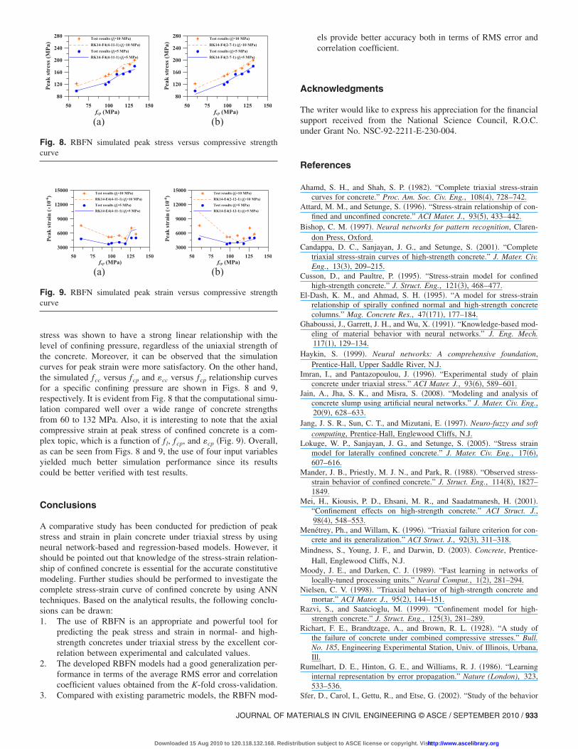
stress was shown to have a strong linear relationship with thelevel of confining pressure, regardless of the uniaxial strength ofthe concrete. Moreover, it can be observed that the simulationcurves for peak strain were more satisfactory. On the other hand,the simulated fcc versus fcp and �cc versus fcp relationship curvesfor a specific confining pressure are shown in Figs. 8 and 9,respectively. It is evident from Fig. 8 that the computational simu-lation compared well over a wide range of concrete strengthsfrom 60 to 132 MPa. Also, it is interesting to note that the axialcompressive strain at peak stress of confined concrete is a com-plex topic, which is a function of f l, fcp, and �cp �Fig. 9�. Overall,as can be seen from Figs. 8 and 9, the use of four input variablesyielded much better simulation performance since its resultscould be better verified with test results.

Conclusions

A comparative study has been conducted for prediction of peakstress and strain in plain concrete under triaxial stress by usingneural network-based and regression-based models. However, itshould be pointed out that knowledge of the stress-strain relation-ship of confined concrete is essential for the accurate constitutivemodeling. Further studies should be performed to investigate thecomplete stress-strain curve of confined concrete by using ANNtechniques. Based on the analytical results, the following conclu-sions can be drawn:1. The use of RBFN is an appropriate and powerful tool for

predicting the peak stress and strain in normal- and high-strength concretes under triaxial stress by the excellent cor-relation between experimental and calculated values.

2. The developed RBFN models had a good generalization per-formance in terms of the average RMS error and correlationcoefficient values obtained from the K-fold cross-validation.

50 75 100 125 150fcp (MPa)

80

120

160

200

240

280

Peak

stress

(MPa

)Test results (fl=10 MPa)RK14-F4(4-11-1) (fl=10 MPa)Test results (fl=5 MPa)RK14-F4(4-11-1) (fl=5 MPa)

50 75 100 125 150fcp (MPa)

80

120

160

200

240

280

Peak

stress

(MPa

)

Test results (fl=10 MPa)RK14-F4(2-7-1) (fl=10 MPa)Test results (fl=5 MPa)RK14-F4(2-7-1) (fl=5 MPa)

(a) (b)

Fig. 8. RBFN simulated peak stress versus compressive strengthcurve

50 75 100 125 150fcp (MPa)

3000

6000

9000

12000

15000

Peak

strain

(10

-6) Test results (fl=10 MPa)

RK14-E4(4-11-1) (fl=10 MPa)Test results (fl=5 MPa)RK14-E4(4-11-1) (fl=5 MPa)

50 75 100 125 150fcp (MPa)

3000

6000

9000

12000

15000

Peak

strain

(10

-6) Test results (fl=10 MPa)

RK14-E4(2-12-1) (fl=10 MPa)Test results (fl=5 MPa)RK14-E4(2-12-1) (fl=5 MPa)

(a) (b)

Fig. 9. RBFN simulated peak strain versus compressive strengthcurve

3. Compared with existing parametric models, the RBFN mod-

JOURNAL OF MAT

Downloaded 15 Aug 2010 to 120.118.132.168. Redistrib

els provide better accuracy both in terms of RMS error andcorrelation coefficient.

Acknowledgments

The writer would like to express his appreciation for the financialsupport received from the National Science Council, R.O.C.under Grant No. NSC-92-2211-E-230-004.

References

Ahamd, S. H., and Shah, S. P. �1982�. “Complete triaxial stress-straincurves for concrete.” Proc. Am. Soc. Civ. Eng., 108�4�, 728–742.

Attard, M. M., and Setunge, S. �1996�. “Stress-strain relationship of con-fined and unconfined concrete.” ACI Mater. J., 93�5�, 433–442.

Bishop, C. M. �1997�. Neural networks for pattern recognition, Claren-don Press, Oxford.

Candappa, D. C., Sanjayan, J. G., and Setunge, S. �2001�. “Completetriaxial stress-strain curves of high-strength concrete.” J. Mater. Civ.Eng., 13�3�, 209–215.

Cusson, D., and Paultre, P. �1995�. “Stress-strain model for confinedhigh-strength concrete.” J. Struct. Eng., 121�3�, 468–477.

El-Dash, K. M., and Ahmad, S. H. �1995�. “A model for stress-strainrelationship of spirally confined normal and high-strength concretecolumns.” Mag. Concrete Res., 47�171�, 177–184.

Ghaboussi, J., Garrett, J. H., and Wu, X. �1991�. “Knowledge-based mod-eling of material behavior with neural networks.” J. Eng. Mech.117�1�, 129–134.

Haykin, S. �1999�. Neural networks: A comprehensive foundation,Prentice-Hall, Upper Saddle River, N.J.

Imran, I., and Pantazopoulou, J. �1996�. “Experimental study of plainconcrete under triaxial stress.” ACI Mater. J., 93�6�, 589–601.

Jain, A., Jha, S. K., and Misra, S. �2008�. “Modeling and analysis ofconcrete slump using artificial neural networks.” J. Mater. Civ. Eng.,20�9�, 628–633.

Jang, J. S. R., Sun, C. T., and Mizutani, E. �1997�. Neuro-fuzzy and softcomputing, Prentice-Hall, Englewood Cliffs, N.J.

Lokuge, W. P., Sanjayan, J. G., and Setunge, S. �2005�. “Stress strainmodel for laterally confined concrete.” J. Mater. Civ. Eng., 17�6�,607–616.

Mander, J. B., Priestly, M. J. N., and Park, R. �1988�. “Observed stress-strain behavior of confined concrete.” J. Struct. Eng., 114�8�, 1827–1849.

Mei, H., Kiousis, P. D., Ehsani, M. R., and Saadatmanesh, H. �2001�.“Confinement effects on high-strength concrete.” ACI Struct. J.,98�4�, 548–553.

Menétrey, Ph., and Willam, K. �1996�. “Triaxial failure criterion for con-crete and its generalization.” ACI Struct. J., 92�3�, 311–318.

Mindness, S., Young, J. F., and Darwin, D. �2003�. Concrete, Prentice-Hall, Englewood Cliffs, N.J.

Moody, J. E., and Darken, C. J. �1989�. “Fast learning in networks oflocally-tuned processing units.” Neural Comput., 1�2�, 281–294.

Nielsen, C. V. �1998�. “Triaxial behavior of high-strength concrete andmortar.” ACI Mater. J., 95�2�, 144–151.

Razvi, S., and Saatcioglu, M. �1999�. “Confinement model for high-strength concrete.” J. Struct. Eng., 125�3�, 281–289.

Richart, F. E., Brandtzage, A., and Brown, R. L. �1928�. “A study ofthe failure of concrete under combined compressive stresses.” Bull.No. 185, Engineering Experimental Station, Univ. of Illinois, Urbana,Ill.

Rumelhart, D. E., Hinton, G. E., and Williams, R. J. �1986�. “Learninginternal representation by error propagation.” Nature (London), 323,533–536.

Sfer, D., Carol, I., Gettu, R., and Etse, G. �2002�. “Study of the behavior

ERIALS IN CIVIL ENGINEERING © ASCE / SEPTEMBER 2010 / 933

ution subject to ASCE license or copyright. Visithttp://www.ascelibrary.org

of concrete under triaxial compression.” J. Eng. Mech., 128�2�, 156–163.

Sheikh, S. A., and Toklucu, M. T. �1993�. “Reinforced concrete columnsconfined by circular spirals and hoops.” ACI J., 90�5�, 542–553.

Tang, C. W., Chen, H. J., and Yen, T. �2003�. “Modeling the confinementefficiency of reinforced concrete columns with rectilinear transversesteel using artificial neural networks.” J. Struct. Eng., 129�6�, 775–783.

Tang, C. W., Lin, Y., and Kuo, S. F. �2007�. “Investigation on correlationbetween pulse velocity and compressive strength of concrete usingANNs.” Comput. Concr., 4�6�, 437–456.

934 / JOURNAL OF MATERIALS IN CIVIL ENGINEERING © ASCE / SEPTE

Downloaded 15 Aug 2010 to 120.118.132.168. Redistrib

Vapnik, V. �1998�. Statistical learning theory, Wiley, New York.

Wang, C. Z., Guo, Z. H., and Zhang, X. Q. �1987�. “Experimental inves-tigation of biaxial and triaxial compressive concrete strength.” ACIMater. J., 84, 92–100.

Yeh, I. C. �1999�. “Design of high-performance concrete mixture usingneural networks and nonlinear programming.” J. Comput. Civ. Eng.,13�1�, 36–42.

Zhao, Z., and Ren, L. �2002�. “Failure criterion of concrete under triaxialstresses using neural networks.” Comput. Aided Civ. Infrastruct. Eng.,17�1�, 68–73.

MBER 2010

ution subject to ASCE license or copyright. Visithttp://www.ascelibrary.org