Raccolta delle principali attività di diffusione

Giovanni Puglisi

Report RdS/PAR2016/272

Agenzia nazionale per le nuove tecnologie, l’energia e lo sviluppo economico sostenibile MINISTERO DELLO SVILUPPO ECONOMICO

RACCOLTA DELLE PRINCIPALI ATTIVITÀ DI DIFFUSIONE

G. Puglisi (ENEA) Settembre 2017 Report Ricerca di Sistema Elettrico

Accordo di Programma Ministero dello Sviluppo Economico - ENEA

Piano Annuale di Realizzazione 2016

Area: Efficienza energetica e risparmio di energia negli usi finali elettrici e interazione con altri vettori energetici

Progetto: D1 - Tecnologie per costruire gli edifici del futuro

Obiettivo: F. Comunicazione e diffusione dei risultati

Responsabile del Progetto: Giovanni Puglisi, ENEA

3

Indice

1 INTRODUZIONE .......................................................................................................................................................... 4

2 ELENCO PUBBLICAZIONI............................................................................................................................................. 4

3 ARTICOLI E PRESENTAZIONI A CONVEGNI. ................................................................................................................ 6

ACCORDO DI PROGRAMMA MISE-ENEA

4

1 Introduzione

Il rapporto descrive le attività messe in atto per la comunicazione e diffusione dei risultati prodotti dal progetto D1 “tecnologie per costruire gli edifici del futuro” relativo all’Accordo di Programma MiSE-ENEA, piano annuale di realizzazione 2016.

Tali attività sono state suddivise, per ciascuna linea in cui è diviso il progetto, in:

pubblicazioni su riviste specializzate o su atti di convegni,

presentazioni a convegni.

Nei paragrafi successivi si riportano rispettivamente l’elenco delle pubblicazioni, gli articoli integrali e le pe presentazioni ai convegni.

2 ELENCO PUBBLICAZIONI

Di seguito sono riportate le pubblicazioni suddivise per linee.

Linea a From natural systems to lighting electronics: designing melanin-inspired electroluminescent

materials. V. Criscuolo, P. Manini, C.T. Prontera, A. Pezzella, M.G. Maglione, P. Tassini, C. Minarini. BioEL2017 International Winterschool on Bioelectronics, Kirchberg in Tirol, Austria.

Controlling of (supra)Molecular Structure of Polymers from Natural Sources to Assess their Electrical Properties. Ri Xu, C.T. Prontera, L.G. Simao Albano, E. Di Mauro, P. Kumar, P. Manini, C. Santato, F. Soavi. MRS spring 2017, Phoenix, USA.

Melanins in bioelectronics: a survey of the role of these natural pigments from bio-interfaces to (opto)electronic devices. P. Manini, V. Criscuolo, L. Migliaccio, C.T. Prontera, A. Pezzella, O. Crescenzi, M. d’Ischia, S, Parisi, M. Barra, A. Cassinese, P. Maddalena, M.G. Maglione, P. Tassini, C. Minarini. e-MRS spring 2017, Strasbourg, France.

From Melanins to OLED Devices: Taking Inspiration from the Black Human Pigments for the Design of Innovative Electroluminescent Materials. P. Manini, C. T. Prontera, V. Criscuolo, A. Pezzella, O. Crescenzi, M. Pavone, M. d’Ischia, M. G. Maglione, P. Tassini, C. Minarini. SCI 2017, Paestum (SA), Italy.

Shedding Light on the Hydratation-Dependent Electrical Conductivity in Melanin Thin Films. Ri Xu, L.G. Simao Albano, E. Di Mauro, S. Zhang, P. Kumar, C. Santato, C.T. Prontera. MRS fall 2016, Boston, USA.

Advancing the Knowledge of the Structural Properties of the Biocompatible and Biodegradable Electroactive Eumelanin Polymer. D Boisvert, C.T. Prontera, S. Francoeur, A. Badia, C. Santato. MRS spring 2017, Phoenix, USA.

Designing dopamine-based electroluminescent complexes for innovative melanin-inspired OLED devices. C.T. Prontera, P. Manini, V. Criscuolo, A. Pezzella, O. Crescenzi, M. Pavone, M. d’Ischia, M.G. Maglione, P. Tassini, C. Minarini. ISNSC9 (2017), Napoli, Italy.

5

Synthesis and Photo-Physical Properties of Dopamine-Inspired Iridium Complexes for OLED Applications. C.T. Prontera, V. Criscuolo, A. Pezzella, M.G. Maglione, P. Tassini, C. Minarini, M. d’Ischia, P. Manini. SCI 2017, Paestum (SA), Italy.

G.Zizzo, M.Beccalia, M.Bonomolo, B.Di Pietra, M.G.Ippolito, D.La Cascia, G.Leone, V.Lo Brano, F.Monteleone: A Feasibility Study of Some DSM Enabling Solutions in Small Islands: the Case of Lampedusa – ( Journal Energy - September 2017, EGY11563)

L. Martirano, E. Habib, G. Greco, M. Manganelli, A. Ruvio, B. Di Pietra, A. Pannicelli, S. Piccinelli, G. Puglisi, P. Regina: An example of smart building with a km zero energy performance, ( IAS Annual Meeting, October 1-5, 2017, Cincinnati, OH, USA.)

Bertini, L. Canale, M. Dell’Isola, B. Di Pietra, G. Ficco, G.Puglisi, S. Stoklin: Impatto della contabilizzazione del calore sui consumi energetici in Italia – 17th CIRIAF Congress – Perugia 6-7 Aprile 2017

M. A. Ancona, L. Branchini, A. De Pascale, F. Melino, B. Di Pietra: Renewable Energy Systems Integration for Efficiency Improvement of a CHP Unit (ASME Turbo Expo Conference - June 26 - 30, 2017, Charlotte, NC USA)

Linea b

M. Di Somma, B. Yan, N. Bianco, G. Graditi, P. B. Luh, L. Mongibello, V. Naso, Multi-objective design optimization of distributed energy systems through cost and exergy assessments, Applied Energy, Volume 204, 15 October 2017, Pages 1299-1316.

Di Somma M., Yan B., Bianco N., Luh P.B., Graditi G., Mongibello L., Naso V., Design optimization of a distributed energy system through cost and exergy assessments, Energy Procedia 105 (2017), 2451 – 2459.

L. Mongibello, G. Graditi, Cold storage for a single-family house in Italy, Energies 2016, 9(12), 1043.

Luigi Mongibello, Nicola Bianco, Martina Caliano, Giorgio Graditi, A new approach for the dimensioning of an air conditioning system with cold thermal energy storage, Energy Procedia 105 (2017), 4295 – 4304.

Linea c

Vox Giuliano, Blanco Ileana, Fuina Silvana, Campiotti Carlo Alberto,Scarascia Mugnozza Giacomo , and Schettini Evelia. Evaluation of wall surface temperatures in green facades". Proceedings of the Institution of Civil Engineers - Engineering Sustainability 2017, vol 170:6, 334-344. ISSN 1478-4629; E-ISSN 1751-7680.

Blanco, I., Scarascia Mugnozza, G., Schettini, E., Puglisi, G., Campiotti, C.A. and Vox, G. (2017). Design of a solar cooling system for greenhouse conditioning in a Mediterranean area. Acta Hortic. 1170, 485-492. DOI: 10.17660/ActaHortic.2017.1170.60. https://doi.org/10.17660/ActaHortic.2017.1170.60 .

Bibbiani, C., Campiotti, C.A., Schettini, E. and Vox, G. (2017). A sustainable energy for greenhouses heating in Italy: wood biomass. Acta Hortic. 1170, 523-530. DOI: 10.17660/ActaHortic.2017.1170.65. https://doi.org/10.17660/ActaHortic.2017.1170.65 .

Blanco, I., Schettini, E., Scarascia Mugnozza, G., Campiotti, C.A., Giagnacovo, G. and Vox, G. (2017). Vegetation as a passive system for enhancing building climate control. Acta Hortic. 1170, 555-562. DOI: 10.17660/ActaHortic.2017.1170.69. https://doi.org/10.17660/ActaHortic.2017.1170.69 .

R. Di Bonito1, D. Biagiotti2,3, G. Giagnacovo2, M. Canditelli4, C.A. Campiotti2, Use of compost as amendment for soilless substrates of plants in green roof installations, Acta Hortic. 1146. ISHS

ACCORDO DI PROGRAMMA MISE-ENEA

6

2016. DOI 10.17660/ActaHortic.2016.1146.19, Proc. III Int. Sym. on Organic Matter Mgt. and Compost Use in Hort.

Linea d

Buratti, C., Moretti, E., Zinzi, M., High energy-efficient windows with silica aerogel for building refurbishment: Experimental characterization and preliminary simulations in different climate conditions, Buildings, Volume 7, Issue 1, 2017, Article number 8.

Elisa Moretti, Michele Zinzi, Emiliano Carnielo, Francesca Merli. Advanced Polycarbonate Transparent Systems with Aerogel: Preliminary Characterization of Optical and Thermal Properties,Energy Procedia, Volume 113, May 2017, Pages 9-16.

Michele Zinzi, Paolo Ruggeri, Fabio Peron, Emiliano Carnielo, Alessandro Righi, Experimental Characterization and Energy Performances of Multiple Glazing Units with Integrated Shading Devices, Energy Procedia, Volume 113, May 2017, Pages 1-8.

Alessandro Fontia, Gabriele Comodia,*, Stefano Pizzutib, Alessia Arteconic, Lieve Helsend, Low order grey-box models for short-term thermal behavior prediction in buildings, ScienceDirect, Energy Procedia 105 ( 2017 ) 2107 – 2112

linea e

Caldera M., Puglisi G., Zanghirella F., Margiotta F., Ungaro P., Talucci V., Cammarata G. (2017). Proposal of a survey-based methodology for the determination of the energy consumption in the residential sector, International Journal of Heat and Technology, Vol. 35, Sp. 1, pp. S152-S158, DOI: 10.18280/ijht.35Sp0121 (articolo presentato al 2nd AIGE/IIETA International Conference, Genova, 12-13 giugno 2017)

3 Articoli e presentazioni a convegni.

XXVI Congresso Nazionale della Società Chimica Italiana XXX Y000

From Melanins to OLED Devices: Taking Inspiration from the Black Human Pigments

for the Design of Innovative Electroluminescent Materials.

Paola Manini,a Carmela Tania Prontera,

a Valeria Criscuolo,

a Alessandro Pezzella,

a Orlando

Crescenzi,a Michele Pavone,

a Marco d’Ischia,

a Maria Grazia Maglione,

b Paolo Tassini,

b Carla

Minarinib

a Department of Chemical Sciences, University of Naples "Federico II", via Cintia 4, I-80126 Napoli, IT;

b Laboratory

of Nanomaterials and Devices, ENEA C. R. Portici, Piazzale E. Fermi, Portici (NA), IT; paola.manini@unina.it

The growing expansion and impact of OLED devices in our everyday life have stimulated the

synthesis of a wide plethora of electroluminescent materials with the aim of improving the

efficiency and the life-time of the device as well as of selectively tuning the wavelength of the

emitting light.

In the frame of our research activity aimed at exploring the role of melanins, the dark pigments

found in mammalian skin, hair and eyes, as soft organic semiconductors in bio-electronic devices

(1), we have undertaken a new challenge: to obtain innovative electroluminesct compounds from

black melanin pigments.

The strategy of this research activity has been based on the use of melanin precursors, such as 5,6-

dihydroxyindole and dopamine, as starting compounds for the synthesis of fluorescent or

phosphorescent materials for applications as emitting layer in OLED devices (2).

NH

OH

OH

OH

OHNH

2

NH

RO OR

NH

RO

RO

NH OR

OR

N

CH3O

CH3O

N

CH3O

CH3O

N

CH3O

CH3O

R

N

CH3O

CH3O

COOH

N

N

N

O

N

C

Y

N

M

N

X

X

N

5,6-Dihydroxyindole Dopamine

M = Ir, X = CM = Ru, X = N

Phosphorescent Transition Metal Complexes

Fluorescent Heterocyclic Platforms

Figure 1

In this communication we will discuss the synthesis of a set melanin-inspired electroluminescent

compounds; we will report on their photo-physical and electrical properties; the fabrication and

characterization of the corresponding OLED devices will also be presented.

References

(1) Pezzella, A.; Barra, M.; Musto, A.; Navarra, A.; Alfé, M.; Manini, P.; Parisi, S.; Cassinese,

A.; Criscuolo, V.; d’Ischia, M. Mater. Horiz. 2015, 2, 212.

(2) Manini, P.; Criscuolo, V.; Ricciotti, L.; Pezzella, A.; Barra, M.; Cassinese, A.; Crescenzi,

O.; Maglione M.G.; Tassini, P.; Minarini, C.; Barone, V.; d’Ischia, M. ChemPlusChem, 2015, 80,

919.

2017 E-MRS Fall Meeting & Exhibit Nov 27 - Dec 2, 2016, Boston, Massachusetts (USA)

2017 E-MRS Spring Meeting & Exhibit April 17-21, 2017, Phoenix, Arizona (USA)

Designing dopamine-based electroluminescent

complexes for innovative melanin-inspired OLED devices

C.T. Prontera,a* P. Manini,a V. Criscuolo,a A. Pezzella,a O. Crescenzi,a M. Pavone,a M. d’Ischia,a M.G. Maglione,b P. Tassini,b C. Minarinib

a Department of Chemical Sciences, University of Naples "Federico II", via Cintia 4, I-80126 Napoli, IT;

b Laboratory of Nanomaterials and Devices, ENEA C. R. Portici, Piazzale E. Fermi, Portici (NA), IT;

*carmelatania.prontera@unina.it

R

Ligand Synthesis

Iridium Complexes Ruthenium Complexes

300 400 500 600 700 800

0.0

0.2

0.4

0.6

0.8

1.0

Norm

aliz

ed Inte

nsity (

a.u

.)

Wavelength (nm)

Ir_CHQ Abs

Ir_CHQ PL

Ir_CQ Abs

Ir_CQ PL

b)

References [1] Pezzella, A.; Barra, M.; Musto, A.; Navarra, A.; Alfé, M.; Manini, P.; Parisi, S.; Cassinese, A.; Criscuolo, V.; d’Ischia, M. Mater. Horiz. 2015, 2, 212. [2] Manini, P.; Criscuolo, V.; Ricciotti, L.; Pezzella, A.; Barra, M.; Cassinese, A.; Crescenzi, O.; Maglione M.G.; Tassini, P.; Minarini, C.; Barone, V.; d’Ischia, M. ChemPlusChem, 2015, 80, 919.

Ir_PHQ Ir_FPHQ Ir_OMePHQ Ir_CNPHQ Ir_CHQ Ir_CQ Ir_DHQ

Φ (λexc,nm)1 0.41 (480) 0.24 (480) 0.21 (490) 0.11 (656) 0.14 (480) 0.36 (450) 0.40 (450)

Φ (λexc,nm)2 0.30 (480) 0.70 (480) 0.61 (490) 0.14 (653) 0.25(480) 0.50 (450) 0.38 (450)

Ru_CHQ_SO3CF3 Ru_CHQ_PF6 Ru_CQ_SO3CF3 Ru_CQ_PF6

Φ (λexc,nm)1 0.015 (500) 0.085 (506) 0.064 (504) 0.061 (606)

Φ (λexc,nm)2 0.024 (506) 0.010 (506) 0.089 (504) 0.14 (606)

0 2 4 6 8 10 12

0

100

200

300

Cu

rre

nt

De

nsity (

mA

/cm

2)

Voltage (V)

e)

0

100

200

300

Lu

min

an

ce

(cd

/m2)

Lum. Max (cd/m2)

Eff. max (cd/A)

CBP:RuCHQ_ SO3CF3 8%

311.83@12 V 0.073@12 V

CBP:RuCHQ_ PF6 2%

106.6@10V 0.039@6.2 V

CBP:RuCQ_ SO3CF3 2%

116.5@11.8 V 0.073@9 V

CBP:RuCQ_ PF6 2%

154@12.5 V 0.046@10.5 V

Lum. Max (cd/m2)

Eff. max (cd/A)

CBP:Ir_PHQ 2% 527.75@11 V 0.49@9 V

CBP:Ir_FPHQ 6% 764@10 V 0.92@8.5 V

CBP:Ir_OMePHQ 2%

2475.43@14 V 1.78@13 V

CBP:Ir_CNPHQ 2%

469.06@14 V 0.33@10 V

CBP:Ir_CHQ 6% 3031@11.3 V 1.09@8.4 V

CBP:Ir_CQ 12% 7161@9.3 V 3.6@8.2 V

Ir_DHQ (LEEC) 138@23 V 0.07@23 V

400 500 600 700 800

0.0

0.2

0.4

0.6

0.8

1.0

No

rma

lize

d E

L I

nte

nsity (

a.u

.)

Wavelength (nm)

i)

0 2 4 6 8 10

0

100

200

300

400

Curr

ent D

ensity (

mA

/cm

2)

Voltage (V)

2000

4000

6000

8000

Lum

inance (

cd/m

2)

h)

300 400 500 600 700 800

0.0

0.2

0.4

0.6

0.8

1.0

Norm

aliz

ed Inte

nsity (

a.u

.)

Wavelength (nm)

Abs

PL

a)

In the last decades, metal–organic complexes have attracted much attention due to their enormous potential application in optoelectronic devices. In this work, dopamine, the catecholic neurotransmitter and monomer precursor of polydopamine, is used as starting compound for the synthesis of a series of etherocyclic compound to behave as ligands for bio-inspired phosphorescent iridium and ruthenium complexes.

[1] determined relatively to fluorescein = 0.9 in a 0.1 M solution of NaOH); [2] determined in oxygen free solutions of DCM

[a] Normalized absorbance and emission spectrum of Ir_DHQPF6; [b] Normalized absorbance and emission spectrum of Ir_CHQ and Ir_CQ; [c] Normalized absorbance spectrum of Ir_PHQ complexes series; [d] Normalized emission spectrum of Ir_PHQ complexes series; [e] Photo-physical characteristics of iridium complexes ;

e)

f) g) m)

[f] OLED device structure; [g] LEEC device structure; [h]IV-EL graph of CBP:Ir_CQ 12% OLED device; [i] Normalized Electroluminescence spectrum of CBP:Ir_CQ 12% OLED device; [l] OLED picture; [m] device performances with optimal iridium complexes percentage;

c)

[a] Normalized absorbance and emission spectrum of RuCHQ_SO3CF3 and RuCHQ_PF6; [b] Normalized absorbance and emission spectrum of RuCQ_SO3CF3 and RuCQ_PF6; [c] photo-physical characteristics of ruthenium complexes ;

d)

400 500 600 700 800

0.0

0.2

0.4

0.6

0.8

1.0

No

rma

lize

d E

L I

nte

nsity (

a.u

.)

Wavelength (nm)

f)

h)

e)

[f] IV-EL graph of CBP:RuCHQ_SO3CF3 8% OLED device; [g] Normalized Electroluminescence spectrum of CBP:RuCHQ_SO3CF3 8% OLED device; [h] OLED picture;

[d] OLED device structure; [e] device performances with optimal ruthenium complexes percentage;

300 400 500 600

0.0

0.2

0.4

0.6

0.8

1.0

Norm

aliz

ed

Abso

rba

nce (

a.u

.)

Wavelength (nm)

Ir_PHQ

Ir_FPHQ

Ir_OMePHQ

Ir_CNPHQ

c)

500 600 700 800

0.0

0.2

0.4

0.6

0.8

1.0

No

rma

lize

d P

L I

nte

nsity (

a.u

.)

Wavelength (nm)

Ir_PHQ

Ir_FPHQ

Ir_OMePHQ

Ir_CNPHQ

d)

300 400 500 600 700 800 900

0.0

0.2

0.4

0.6

0.8

1.0

Norm

aliz

ed

Inte

nsity (

a.u

.)

Wavelength (nm)

RuCHQ_SO3CF3 Abs

RuCHQ_SO3CF3 PL

RuCHQ_PF6 Abs

RuCHQ_PF6 PL

a)

300 400 500 600 700 800 900

0.0

0.2

0.4

0.6

0.8

1.0

Norm

aliz

ed

Inte

nsity (

a.u

.)

Wavelength (nm)

RuCQ_SO3CF3 Abs

RuCQ_SO3CF3 PL

RuCQ_PF6 Abs

RuCQ_PF6 PL

b)

4-7th September 2017 – Napoli

Synthesis and Photo-Physical Properties of Dopamine-Inspired

Iridium Complexes for OLED Applications

C.T. Prontera,a* V. Criscuolo,a A. Pezzella,a M.G. Maglione,b P. Tassini,b C. Minarini,b M. d’Ischia,a P. Maninia

a Department of Chemical Sciences, University of Naples "Federico II", via Cintia 4, I-80126 Napoli, IT;

b Laboratory of Nanomaterials and Devices, ENEA C. R. Portici, Piazzale E. Fermi, Portici (NA), IT;

*carmelatania.prontera@unina.it

R

In the last decades, metal–organic complexes have attracted much attention due to their enormous potential application in optoelectronic devices. In this work dopamine, the catecholic neurotransmitter and monomer precursor of neuromelanin and polydopamine, is used as starting compound for the synthesis of a set of heterocyclic compounds with different substituents. Iridium(III) complexes were obtained with the dopamine-inspired ligands and the effects of the different groups on the optical and electroluminescence characteristics were studied.

250 300 350 400 450 500 550 600 650

0,0

0,2

0,4

0,6

0,8

1,0

Abs (

no

rm)

Wavelength (nm)

Ir_PHQ

Ir_FPHQ

Ir_OMePHQ

Ir_CNPHQ

Series 1

250 300 350 400 450 500 550 600 650

0,0

0,2

0,4

0,6

0,8

1,0

Ab

s (

no

rm)

Wavelength (nm)

Ir_PHQ

Ir_FPHQ

Ir_OMePHQ

Ir_CNPHQ

Series 2

250 300 350 400 450 500 550 600 650

0,0

0,2

0,4

0,6

0,8

1,0

Ab

s (

no

rm)

Wavelength (nm)

Ir_PHQ

Ir_FPHQ

Ir_OMePHQ

Series 3

Ir_PHQ_1 Ir_FPHQ_1 Ir_OMePHQ_1 Ir_CNPHQ_1 Ir_PHQ_2 Ir_FPHQ_2 Ir_OMePHQ_2 Ir_CNPHQ_2 Ir_PHQ_3 Ir_FPHQ_3 Ir_OMePHQ_3

Φ (λexc,nm)1 0.41% (480) 0.24% (480) 0.21% (490) 0.11% (540) 0.14% (500) 0.15 % (480) 0.15% (490) 0.14% (540) 0.18% (500) 0.19% (480) 0.13% (490)

Φ (λexc,nm)2 0.30% (480) 0.70% (480) 0.61% (490) 0.14% (540) 0.26% (500) 0.40 % (480) 0.23% (490) 0.15% (540) 0.23% (500) 0.22% (480) 0.19% (490)

[1] determined relatively to fluorescein = 0.9 in a 0.1 M solution of NaOH); [2] determined in oxygen free solutions of DCM

550 600 650 700 750 800 850 900

0,0

0,2

0,4

0,6

0,8

1,0

PL

(n

orm

)

Wavelength (nm)

Ir_PHQ exc 480

Ir_FPHQ exc 480

Ir_OMePHQ exc 490

Ir_CNPHQ exc 540

Series 1

550 600 650 700 750 800 850

0,0

0,2

0,4

0,6

0,8

1,0

PL

(n

orm

)

Wavelength (nm)

Ir_PHQ exc 500

Ir_FPHQ exc 480

Ir_OMePHQ exc 490

Ir_CNPHQ exc 540

Series 2

550 600 650 700 750 800

0,0

0,2

0,4

0,6

0,8

1,0

PL

(n

orm

)

Wavelength (nm)

Ir_PHQ exc 500

Ir_FHQ exc 480

Ir_OMePHQ exc 490

Series 3

0 2 4 6 8 10 12 14

0

50

100

150

200

250

300

Curr

en

d D

ensity (

mA

/cm

2)

Voltage (V)

0

1000

2000

3000

Lu

min

an

ce

(cd

/m2)

400 500 600 700 800

0.0

0.2

0.4

0.6

0.8

1.0

No

rma

lize

d E

L I

nte

nsity (

a.u

.)

Wavelength (nm)

XXVI Congresso Nazionale della Società Chimica Italiana 10-14 Settembre 2017, Paestum (SA)

SYNTHESIS

PHOTO-PHYSICAL CHARACTERIZATION

Device 2%

Lum. Max (cd/m2)

Eff. max (cd/A)

Λmax EL (nm)

Device 6%

Lum. Max (cd/m2)

Eff. max (cd/A)

Λmax EL (nm)

Device 12%

Lum. Max (cd/m2)

Eff. max (cd/A)

Λmax EL (nm)

F1 261.0@10.5V 0.25 @8.3V 600 F1 764@10V 0.92@8.5V 605 F1 687@13.5V 0.17 @13.5V 605

F2 1092@11V 0.35@11V 585 F2 384.9@12.2V 0.55 @10V 605 F2 472.2@13V 0.35@11V 605

F3 591.5@10.7V 0.55 @8V 580 F3 343@10.7V 0.27 @9.2V 602 F3 175@10V 0.07 @10V 602

Device 2%

Lum. Max (cd/m2)

Eff. max (cd/A)

Λmax EL (nm)

Device 6%

Lum. Max (cd/m2)

Eff. max (cd/A)

Λmax EL (nm)

Device 12%

Lum. Max (cd/m2)

Eff. max (cd/A)

Λmax EL (nm)

OMe1 2475.4@14V 1.78 @13V 606 OMe1 319.4@10V 0.064 @10V 603 OMe1 580.5@12V 0.18 @12V 608

OMe2 1008@13V 0.81 @11V 612 OMe2 524.1@13V 0.29 @9V 618 OMe2 620.6@13V 0.52 @10V 618

OMe3 583.7@12V 0.34 @9V 615 OMe3 745.7@13V 0.24 @11V 616 OMe3 425.6@13V 0.18 @11V 619

Device 2%

Lum. Max (cd/m2)

Eff. max (cd/A)

Λmax EL (nm

Device 6%

Lum. Max (cd/m2)

Eff. max (cd/A)

Λmax EL (nm

Device 12%

Lum. Max (cd/m2)

Eff. max (cd/A)

Λmax EL (nm)

H1 527.8@11V 0.49@9V 610 H1 718.9@15V 0.92 @10V 610 H1 709.3@12V 0.54 @10V 615

H2 682.4 @11V 0.29@10V 620 H2 496@15.5V 0.56 @10V 620 H2 483.6@12V 0.32 @9V 624

H3 600.6@10V 0.64@7.8V 620 H3 435@16V 0.55 @11.5V 625 H3 518.7@12V 0.44@10.5V 625

Device 2%

Lum. Max (cd/m2)

Eff. max (cd/A)

Λmax EL (nm

Device 6%

Lum. Max (cd/m2)

Eff. max (cd/A)

Λmax EL (nm

Device 12%

Lum. Max (cd/m2)

Eff. max (cd/A)

Λmax EL (nm)

CN1 469.1@14V 0.33 @10V 628 CN1 256.7@13V 0.065 @12V 638 CN1 385.6@13V 0.17 @12V 635

CN2 323.5@10V 0.15 @10V 635 CN2 159.7@13V 0.051 @11V 639 CN2 161.1 @12V 0.056 @12V 640

The best devices in terms of luminance and turn-on voltage resulted those prepared by using a 2% wt of the iridium(III) complexes. The electroluminescence maximum and the CIE coordinates show a red shift as a function of the percentage of the complex used in the device and with the substituent (F OMe H CN).

DEVICE CHARACTERISTICS

The absorption and emission profiles were influenced by the nature of the group on the phenyl substituent. All the complexes exhibited a red-orange emission. The R groups induced shifts of the emission maxima in the order F<OMe<H<CN. Higher quantum yealds were observed in oxygen depleted solutions.

OLED device were fabricated to test the complexes as emitters. Emitting layer was composed of a blend in which the complexes were used as guests at different percentage within CBP (host). The emitting layer was realized by solution processing techniques (spin coating).

The synthesis of the dopamine-inspired C^N cyclometalating ligands was performed via a Bischler-Napieralski reaction affording a set of 6,7-dimethoxy-3,4-dihydroisoquinolines substituted on the 1 position with phenyl residues, functionalized on the para-position with different groups (PHQs). The iridium(III) complexes were obtained via the synthetic strategy of Nonoyama involving the intermediate formation of a dinuclear chloro-bridged iridium complex. The important aspect of this work is that by using an excess of the cyclometalating ligands it was possible to isolate for the first time one-pot a set of three different neutral iridium(III) complexes deriving from the insertion of one, two or three dihydroisoquinoline ligands.

IV-EL and Electroluminescence spectrum of CBP:IrOMePHQ1 2%

OLED Devices

structure

* Pure red CIE coordinates

FINANCIAL SUPPORT •Program Agreement (Ricerca di Sistema Elettrico) between ENEA and Italian Ministry of Economic Development (MISE); •Italian Project RELIGHT (REsearch for LIGHT); •European Commission (PolyMed project in the FP7-PEOPLE-2013-IRSES frame, r.n. IRSES-GA-2013-612538) .

BioEl2017 International Winterschool on Bioelectronics

11th - 18th March, 2017, Kirchberg in Tirol, Austria

2017 E-MRS Spring Meeting & Exhibit May 22-26, 2017, Strasbourg, France

Cod_048_pp_1

Perugia, Italy. April 6-7, 2017

17th CIRIAF National Congress Sustainable Development, Human Health and Environmental Protection

Impatto della contabilizzazione del calore sui consumi energetici in Italia

I. Bertini2, L. Canale1*, M. Dell’Isola1, B. Di Pietra2, G. Ficco1, G.Puglisi2, S. Stoklin1

1 Dipartimento di Ingegneria Civile e Meccanica (DICEM), Università di Cassino e del Lazio

Meridionale, Via G. Di Biasio 43, 03043 Cassino, Italy 2 ENEA Agenzia Nazionale per le nuove tecnologie, l'energia e lo sviluppo sostenibile, Unità Tecnica

Efficienza Energetica

* Author to whom correspondence should be addressed. E-Mail: l.canale@unicas.it

Abstract: Heat accounting in residential buildings has been identified by the European

Union (EU) as one of the main drivers to reduce energy consumption in the residential

sector. To this aim, the European Directive 2012/27/EU and the Italian Decree nr.

102/2012 and subsequent modifications set the obligation for apartment and multi-

apartment buildings supplied by a common central heating source or by a district

heating/cooling network, to install, by December the 31st 2016, sub-metering systems to

allow a fair cost allocation through the tenants. In Italy the obligation has been recently

extended to June, the 30th, 2017.

In several studies conducted in different EU Member States a very wide range of variability

(8-40%) of the expected benefit of heat accounting systems has been found.

Unfortunately, specific studies regarding the Italian territory and the Mediterranean

climate conditions are still lacking. Nevertheless, due to the large number of buildings

virtually subject to the obligation, the potential for energy savings in Italy could be among

the highest in Europe. In the present study, after a brief analysis of energetic benefit of

common heat accounting systems, the authors evaluate the potential impact of such

systems on the energy consumption of the Italian residential building stock. To this end,

the Italian residential building stock has been analyzed through both the ISTAT census

2011 and a recent statistical analysis performed by ENEA based on ISTAT data.

Keywords: efficienza energetica, contabilizzazione del calore, termoregolazione.

17th

CIRIAF National Congress

Cod_048_pp_2

1. Introduzione

Nel 2012 l'Unione Europea ha formalizzato la sua attenzione verso una maggiore consapevolezza

dei consumi energetici delle utenze energivore emanando la Energy Efficiency Directive 2012/27/EU

[1]. In particolare, l'articolo 9 stabilisce che il consumatore debba essere incoraggiato a gestire meglio

i propri consumi attraverso la contabilizzazione individuale e la fatturazione informativa. Nello stesso

articolo si stabilisce l'obbligo per tutti gli Stati Membri di installare, entro il 31 Dicembre 2016 (in

Italia recentemente prorogato al 30 Giugno 2017), sistemi di contabilizzazione individuale del calore

in tutte quelle utenze del settore residenziale alimentate da una fonte di

riscaldamento/raffrescamento centralizzata e/o da teleriscaldamento/teleraffrescamento, a patto

che la loro installazione sia efficiente in termini di rapporto costi/benefici.

Celenza et al. (2015) [2] hanno evidenziato che, nei confronti dell'obbligo imposto dalla direttiva,

gli Stati Membri hanno adottato strategie politiche variabili: Germania ed Austria, ad esempio,

obbligano quasi la totalità degli edifici all'installazione di tali sistemi, mentre Finlandia e Svezia

esentano la quasi totalità degli edifici potenzialmente soggetti all'obbligo della direttiva europea,

ritenendo in ogni caso svantaggioso il loro rapporto costi/benefici.

Sono pochi i lavori che affermano l'impossibilità di confermare l'esistenza di un reale beneficio. Tra

questi, uno studio commissionato al Boverket dallo stato svedese [3], conclude che la

contabilizzazione individuale e la fatturazione basata sulla misura della temperatura non è

conveniente, richiedendo investimenti infruttuosi per i proprietari. La restante letteratura scientifica

europea riguardante la stima dei benefici attesi dall'installazione dei sistemi di contabilzzazione

individuale nelle utenze alimentate da impianti centralizzati o da teleriscaldamento, è tuttavia

concorde nell'affermare l'esistenza di un beneficio quantificato di fatto in un range di variabilità 8-

40%.

Una sintesi degli ultimi 85 anni di letteratura è presentata in un recente lavoro di review

bibliografica pubblicato da Felsmann et al. al termine del 2015 [4]. Nello studio si conclude che il

risparmio di energia ottenbile in Europa derivante da una fatturazone basata sui reali consumi

individuali si attesta in media al 20%. Tale stato dell’arte analizza i risultati di 32 studi, relativi a Stati

Membri dai climi continentali (Polonia, Germania, Austria, Svizzera, Russia etc.), di cui soltanto 5 sono

basati sulla misura del risparmio effettivo effettuata sulla base dell'osservazione sperimentale degli

edifici nelle stagioni di riscaldamento precedente e successiva all'installazione di misuratori di calore.

Analisi sperimentali più recenti confermano i benefici stimati da Felsmann per climi continentali in

grandi condomini come conseguenza congiunta della termoregolazione e contabilizzazione. Cholewa

et al. [5] hanno inoltre analizzato il consumo di energia di 40 appartamenti in Polonia per oltre 17

stagioni di riscaldamento. Nella metà degli appartamenti investigati è stata sperimentata la

ripartizione dei consumi energetici prima e dopo l'installazione di sistemi di termoregolazione e

contabilizzazione del calore, mentre l'altra metà ha continuato a dividere collettivamente la spesa. Lo

studio ha mostrato un risparmio medio del 26,6%, dovuto sia al controllo termico dell'ambiente

interno che alla contabilizzazione del calore. Iordache et al. [6] hanno, invece, analizzato un

condominio in Romania di 160 unità abitative nella stagione precedente e successiva all'installazione

di valvole termostatiche e ripartitori di calore, osservando una riduzione media dei consumi del 24%

(di cui il 15% attribuibile alla termoregolazione e il 9% alla degli utenti).

Perugia, Italy. April 6-7, 2017

Cod_048_pp_3

Per la sola termoregolazione, FIRE ha recentemente condotto per ENEA uno studio sperimentale

[7] in nove condomini italiani alimentati da teleriscaldamento nelle fasce climatiche E ed F. Lo studio

ha mostrato una riduzione media dei consumi negli ultimi 4 anni grazie ai sistemi di termoregolazione

dell’ordine del 10%. In particolare, 6 condomini, dopo una fase iniziale di assestamento, hanno avuto

effettive riduzioni, in 1 caso si sono avute riduzioni più limitate mentre in 2 casi i consumi sono

rimasti pressochè costanti o addirittura aumentati.

Si deve comunque sottolineare che, a conoscenza degli autori, non esistono campagne

sperimentali estensive a lungo termine né studi riguardanti la quantificazione empirica di tale

beneficio per climi mediterranei e per i quali risulta difficile estendere i risultati Europei citati a causa

delle forti differenze climatiche e ancora della diversa connotazione costruttiva del parco edilizio

nazionale.

In questo studio, a valle di un'analisi statistica del patrimonio edilizio italiano, gli autori stimano ed

analizzano l’impatto dei sistemi di misura e contabilizzazione sui consumi energetici in Italia in

relazione agli adempimenti fissati dalla D.Lgs. 102 e s.m.i. e dalla European Directive 2012/27/EU e

presentano i primi risultati di una più estesa campagna sperimentale attualmente in corso.

2. Analisi dei benefici potenzialmente ottenibili e dei possibili fattori di influenza

La variabilità dei benefici potenzialmente ottenibili dalla termoregolazione e contabilizzazione del

calore è connessa anche alla diversa impostazione metodologica degli studi (es.: dimensione e

composizione del campione, presenza o meno di un gruppo di controllo, durata temporale

dell’investigazione e conseguente possibilità di osservare gli effetti di lunga durata e la persistenza

dei risparmi energetici nel tempo).

Si può comunque affermare con una certa ragionevolezza, che il beneficio ottenibile, così come i

consumi energetici, risulta variabile in funzione di diversi fattori quali:

i) il reddito delle famiglie residenti: in generale la correlazione tra i consumi energetici e le

caratteristiche delle famiglie è nota alla letteratura scientifica da tempo [8, 9, 10]. A questo

proposito, Cayla et al. [11] hanno dimostrato la dipendenza lineare dal reddito del livello

del fattore di servizio per scopi di riscaldamento degli ambienti;

ii) la tipologia di feedback e livello di informazione dell’utente: la consapevolezza e la

partecipazione del cliente finale stimolata anche attraverso una più frequente e dettagliata

informazione sui consumi può generare fino al 4% ca. sul totale del risparmio [12]; anche la

modalità con cui tale informativa viene trasmessa al cliente può avere rilevanza;

iii) il tempo intercorso dall’installazione dei sistemi di termoregolazione e contabilizzazione: in

generale il beneficio atteso si realizza pienamente dal secondo anno dall'installazione dei

sistemi di contabilizzazione individuale; in un'analisi di Siggelsten [13] si evidenzia in

particolare che il risparmio ottenibile al secondo anno è circa doppio rispetto a quello

dell'anno immediatamente successivo all'installazione;

iv) il criterio adottato per la ripartizione delle spese in contesti con più unità immobiliari: una

prevalenza della quota connessa ai consumi involontari rispetto a quella connessa ai

consumi volontari disincentiva il cliente finale ad adottare comportamenti virtuosi di

17th

CIRIAF National Congress

Cod_048_pp_4

risparmio energetico. A tal proposito l'Olanda, con uno studio pilota coinvolgente circa 100

unità abitative, ha dimostrato la sostanziale inefficienza della "socializzazione" dei consumi

energetici normalmente praticata senza contabilizzazione [14, 15];

v) le condizioni climatiche (i.e. zona climatica): il risparmio energetico atteso dall’utilizzo di

sistemi di termoregolazione è influenzato dagli apporti gratuiti e dalle variazioni climatiche

giornaliere [5, 6, 7].

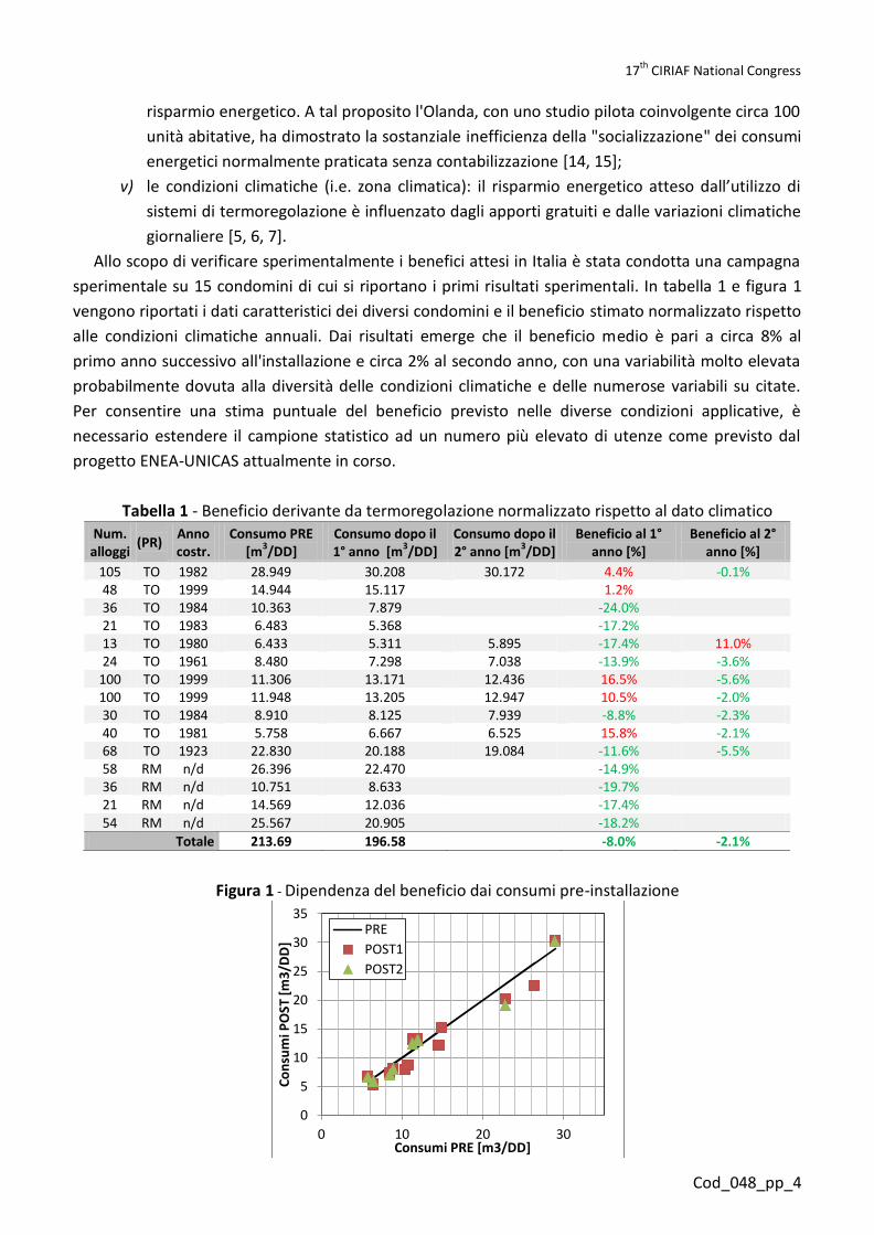
Allo scopo di verificare sperimentalmente i benefici attesi in Italia è stata condotta una campagna

sperimentale su 15 condomini di cui si riportano i primi risultati sperimentali. In tabella 1 e figura 1

vengono riportati i dati caratteristici dei diversi condomini e il beneficio stimato normalizzato rispetto

alle condizioni climatiche annuali. Dai risultati emerge che il beneficio medio è pari a circa 8% al

primo anno successivo all'installazione e circa 2% al secondo anno, con una variabilità molto elevata

probabilmente dovuta alla diversità delle condizioni climatiche e delle numerose variabili su citate.

Per consentire una stima puntuale del beneficio previsto nelle diverse condizioni applicative, è

necessario estendere il campione statistico ad un numero più elevato di utenze come previsto dal

progetto ENEA-UNICAS attualmente in corso.

Tabella 1 - Beneficio derivante da termoregolazione normalizzato rispetto al dato climatico Num. alloggi

(PR) Anno costr.

Consumo PRE [m3/DD]

Consumo dopo il 1° anno [m3/DD]

Consumo dopo il 2° anno [m3/DD]

Beneficio al 1° anno [%]

Beneficio al 2° anno [%]

105 TO 1982 28.949 30.208 30.172 4.4% -0.1% 48 TO 1999 14.944 15.117

1.2%

36 TO 1984 10.363 7.879

-24.0%

21 TO 1983 6.483 5.368

-17.2%

13 TO 1980 6.433 5.311 5.895 -17.4% 11.0% 24 TO 1961 8.480 7.298 7.038 -13.9% -3.6%

100 TO 1999 11.306 13.171 12.436 16.5% -5.6% 100 TO 1999 11.948 13.205 12.947 10.5% -2.0% 30 TO 1984 8.910 8.125 7.939 -8.8% -2.3% 40 TO 1981 5.758 6.667 6.525 15.8% -2.1% 68 TO 1923 22.830 20.188 19.084 -11.6% -5.5% 58 RM n/d 26.396 22.470

-14.9%

36 RM n/d 10.751 8.633

-19.7%

21 RM n/d 14.569 12.036

-17.4%

54 RM n/d 25.567 20.905

-18.2%

Totale 213.69 196.58

-8.0% -2.1%

Figura 1 - Dipendenza del beneficio dai consumi pre-installazione

0

5

10

15

20

25

30

35

0 10 20 30

Co

nsu

mi P

OST

[m

3/D

D]

Consumi PRE [m3/DD]

PRE

POST1

POST2

Perugia, Italy. April 6-7, 2017

Cod_048_pp_5

3. Impatto dell’istallazione dei sistemi di contabilizzazione in Italia

Al fine di consentire una stima del beneficio energetico connesso alla contabilizzazione dei

consumi di energia termica nel settore residenziale in Italia, è stata effettuata un'analisi dei consumi

energetici per riscaldamento connessi al patrimonio edilizio nazionale. Lo studio è basato sull'analisi

statistica delle caratteristiche geometriche (i.e. superfici utili, numero piani, numero appartamenti)

ed impiantistiche (i.e. riscaldamento centralizzato e autonomo) degli edifici derivanti dall'ultimo

censimento ISTAT [16], delle caratteristiche tipologiche e costruttive degli "edifici tipo" (i.e.

trasmittanze, rendimenti di impianto etc.) [17, 18], delle modalità di conduzione degli impianti e dei

dati climatici regionali [19].

In particolare, nel 2011 in Italia ISTAT ha censito 31,138,278 abitazioni. Di queste, circa il 22% non

è abitato, mentre risulta occupato esclusivamente da persone non residenti lo 0.001% degli alloggi,

che è ritenuto trascurabile ai fini della presente analisi. ISTAT divide le abitazioni italiane censite nel

2011 in 6 categorie occupazionali e 9 epoche costruttive (con riferimento agli anni 1918, 1945, 1960,

1970, 1980, 1990, 2000, 2005 e successivi).

Con esclusivo riferimento agli alloggi occupati da persone residenti, dai dati in tabella 2 si evince

che circa il 64% degli alloggi italiani rientra nella categoria di edificio multifamiliare, mentre la

restante quota parte si divide equamente tra le restanti tipologie (mono/bi-familiare). Ai fini della

presente analisi è utile osservare che circa il 70% delle abitazioni occupate da persone residenti è

stata edificata prima del 1980, ovvero prima che venisse emanato qualsiasi obbligo legislativo

relativamente all'efficienza energetica degli edifici (Legge 373 del 1976). Di questi, circa il 45% è

rappresentato da edifici multifamiliari.

Tabella 2 - Abitazioni italiane occupate da persone residenti per categoria occupazionale ed epoca

costruttiva (elaborazione UNICAS di dati ISTAT)

Categoria occupazionale

Numero di abitazioni

nell'edificio

Valori assoluti

Valori percentuali

Pre 1980 1981 - 2000 Post 2001 Tutte le epoche

Monofamiliare 1 4,688,972 19% 14.27% 3.82% 1.39% 19.48%

Bifamiliare 2 3,995,081 17% 12.32% 3.32% 0.96% 16.60%

Multifamiliare

3-4 3,518,114 15%

44.85% 13.28% 5.79% 63.92% 5-8 3,443,130 14%

9-15 3,044,095 13%

16 e più 5,375,902 22%

Totali 24,065,294 100% 71.44% 20.43% 8.13% 100.00%

Per poter tenere conto della variabilità delle condizioni climatiche e della geometria costruttiva

degli edifici (i.e. le superfici disperdenti) delle singole regioni italiane, il database ISTAT è stato

interrogato su base regionale, al fine di individuare: i) il numero di abitazioni per categoria

occupazionale ed epoca costruttiva, ii) il numero medio di piani fuori terra degli edifici per categoria

occupazionale, iii) le superfici medie utili delle abitazioni occupate da persone residenti. In fig. 3(a) e

2(b) vengono mostrati i risultati più significativi di tale analisi.

17th

CIRIAF National Congress

Cod_048_pp_6

Figura 2. - (a) Distribuzione regionale delle categorie occupazionali (valori assoluti); (b) Incidenza

percentuale regionale di edifici per numero di piani (elaborazione UNICAS di dati ISTAT)

Infine, relativamente alle considerazioni più specificatamente impiantistiche, dai dati ISTAT si

evince che circa il 18.75% del totale degli impianti di riscaldamento in abitazioni occupate da persone

residenti in Italia è del tipo centralizzato, come mostrato in tabella 3. In figura 3, è inoltre visualizzata

la distribuzione percentuale regionale degli impianti centralizzati da cui si evince che circa il 55% del

totale di impianti centralizzati nazionale si distribuisce tra sole 3 regioni (Piemonte, Lombardia e

Lazio), mentre tale tipologia impiantistica è praticamente trascurabile in 5 regioni (incidenza inferiore

all'1%), delle quali solo la Valle d'Aosta situata nel Nord Italia. E' opportuno sottolineare che, nelle

stesse regioni nelle quali si registra la percentuale più elevata di impianti centralizzati, si riscontra

anche la prevalenza della categoria edilizia multifamiliare a 16 e più abitazioni, ad eccezione della

Campania (fig. 2 e 3).

Tabella 3 - Abitazioni occupate da persone

residenti per tipo di impianto, valori assoluti e

percentuali (elaborazioni UNICAS di dati ISTAT)

Figura 3 - Distribuzione regionale delle

abitazioni con impianto centralizzato sul totale

italiano (elaborazioni UNICAS di dati ISTAT)

Tipologia di impianto che

alimenta l'abitazione

Numero

impianti

[-]

Percentuale

impianti

[% ]

Impianto centralizzato ad

uso a più abitazioni 4,871,072 18.75%

Impianto autonomo ad uso

alla singola abitazioni 15,717,341 60.51%

Apparecchi singoli fissi per

l'intera abitazione 2,137,636 8.23%

Apparecchi singoli fissi per

alcune parti dell'abitazione 3,246,891 12.50%

TOT. 25,972,940 100 %

0.0E+00

2.0E+05

4.0E+05

6.0E+05

8.0E+05

1.0E+06

1.2E+06

Pie

mo

nte

Val

le d

'Ao

sta

/ V

allé

e…

Ligu

ria

Lom

bar

dia

Tren

tin

o A

lto

Ad

ige

/…

Ven

eto

Friu

li-V

ene

zia

Giu

lia

Emili

a-R

om

agn

a

Tosc

ana

Um

bri

a

Mar

che

Lazi

o

Ab

ruzz

o

Mo

lise

Cam

pan

ia

Pu

glia

Bas

ilica

ta

Cal

abri

a

Sici

lia

Sard

egn

a

1 2 3-4

5-8 9-15 16 e più

Numero di abitazioni nell'edificio

0%

20%

40%

60%

80%

100%

Pie

mo

nte

Val

le d

'Ao

sta

/ V

allé

e…

Lig

uri

a L

om

bar

dia

Tre

nti

no

Alt

o A

dig

e /…

Ven

eto

Fri

uli-

Ven

ezi

a G

iulia

Em

ilia-

Ro

mag

na

To

scan

a U

mb

ria

Mar

che

Laz

io A

bru

zzo

Mo

lise

Cam

pan

ia P

ugl

ia B

asili

cata

Cal

abri

a S

icili

a S

ard

egn

a

4 e più 3 2 1

Numero di piani fuori terra

0%

5%

10%

15%

20%

25%

30%

Pie

mo

nte

Val

le d

'Ao

sta

/ V

allé

e…

Lig

uri

a

Lo

mb

ard

ia

Tre

nti

no

Alt

o A

dig

e /…

Ven

eto

Fri

uli-

Ven

ezi

a G

iulia

Em

ilia-

Ro

mag

na

To

scan

a

Um

bri

a

Mar

che

Laz

io

Ab

ruzz

o

Mo

lise

Cam

pan

ia

Pu

glia

Bas

ilica

ta

Cal

abri

a

Sic

ilia

Sar

deg

na

Perugia, Italy. April 6-7, 2017

Cod_048_pp_7

3.1. Definizione degli "edifici tipo" e stima del fabbisogno termico per riscaldamento

I dati ricavati dall'analisi statistica sono stati utili alla definizione della geometria degli edifici tipo

(in termini di superfici utili, numero di piani, categoria occupazionale ed epoca costruttiva) utilizzati

per caratterizzare su base regionale l’intero parco edilizio residenziale. E' stata in particolare operata

la classificazione degli edifici tipo in 54 classi (6 categorie di occupazione per 9 epoche costruttive),

poi associate a ciascuna regione assegnando un valore caratteristico, alle seguenti grandezze

geometriche e costruttive caratteristiche:

i) numero medio di piani per categoria occupazionale, determinato mediante media pesata

numero di piani/numero edifici;

ii) altezza interpiano, ricavato dalla caratterizzazione del parco edilizio nazionale uso ufficio

pubblicata da ENEA [18] (variabile in funzione della sola epoca costruttiva, passando da un

massimo di 3.4 m, relativo all'epoca costruttiva meno recente, ad un minimo di 2.9 m,

relativo all'epoca costruttiva più recente);

iii) superfici disperdenti degli edifici tipo, ipotizzando: i) unico volume riscaldato di forma

cubica; ii) rapporto superfici finestrate/ superficie utile dell’abitazione pari all'attuale limite

di legge (1/8) per tutte le tipologie ed epoche costruttive; iii) superfici disperdenti

orizzontali e verticali (solaio, copertura e pareti opache) divise in parti uguali per tutti gli

appartamenti componenti l'edificio;

iv) maggiorazione per ponti termici pari al 10% per tutte le tipologie ed epoche costruttive;

v) trasmittanze tipo delle superfici opache e finestrate differenziate rispetto alle epoche

costruttive (figura 4), ricavate sulla base del rapporto TABULA [17], in cui vengono

individuate le tipologie costruttive nazionali ed il relativo periodo di maggiore diffusione,

per la sola fascia climatica E. Ai fini del presente studio tali tipologie costruttive sono state

ritenute rappresentative di tutto il territorio nazionale. Per tenere in considerazione sia gli

interventi di retrofit già avvenuti sulle superfici opache e finestrate di tutto il territorio

nazionale, che la variabilità climatica delle caratteristiche costruttive dei diversi parchi

edilizi regionali, le trasmittanze medie degli edifici antecedenti il 1990 sono state ridotte

percentualmente in funzione del dato climatico e delle regioni.

Figura 4 - Trasmittanze medie stimate del patrimonio edilizio nazionale

(elaborazione UNICAS di dati TABULA [17])

0.0

1.0

2.0

3.0

4.0

5.0

6.0

7.0

19

18 e

pre

ced

enti

19

19-1

945

19

46-1

960

19

61-1

970

19

71-1

980

19

81-1

990

19

91-2

000

20

01-2

005

20

06 e

succ

ess

ivi

U [

W/m

2/K

]

InfissiPavimentoParetiSolaio

17th

CIRIAF National Congress

Cod_048_pp_8

Il calcolo del fabbisogno di energia primaria h24 (Asset Rating) per la climatizzazione invernale

italiana è stato effettuato in forma semplificata descritta nell'Allegato 2 del Decreto Ministeriale del

26/06/2009 ed attingendo sia alla normativa tecnica UNI TS 11300 [20] che al rapporto TABULA [17],

sotto le seguenti ipotesi semplificative: i) apporti gratuiti solari calcolati in maniera forfetaria per un

edificio reale di riferimento e variabile in funzione della latitudine; ii) rendimenti dei sottosistemi di

emissione, distribuzione e regolazione pari a 0.95 indipendentemente dalla categoria edilizia e

dall'epoca costruttiva; iii) generatore interno fino al 1975, esterno nelle epoche successive; v) caldaia

standard con bruciatore atmosferico con camino <10 m per le categorie mono/bi-familiare, con

camino >10 m per la categoria multifamiliare; iv) caldaia a condensazione per gli edifici costruiti dopo

il 2006; v) assenza di ambienti non riscaldati nell'edificio; vi) fattore di utilizzazione degli apporti

gratuiti pari a 0.95.

L'energia primaria nelle effettive condizioni di utilizzo dell'impianto (Operational Rating) è stata

quindi determinata, per ciascuna categoria edilizia e ciascuna regione, utilizzando i coefficienti di

intermittenza precedentemente stimati da ENEA a valle di un'analisi campionaria che ha coinvolto

20,000 unità abitative del territorio italiano. I coefficienti di intermittenza sono stati resi disponibili su

base provinciale, per 6 province rappresentative delle rispettive fasce climatiche del territorio italiano

e per singola unità abitativa (monofamiliare, plurifamiliare, appartamento primo piano,

appartamento ultimo piano, appartamento piano intermedio). I suddetti coefficienti provinciali sono

stati quindi estesi all'intera regione conservando la corrispondenza tra la fascia climatica di

appartenenza della provincia ed il dato climatico regionale. Quest'ultimo è fornito, fino all'anno 2009,

dal database EUROSTAT liberamente accessibile online [19].

3.2. Impatto della contabilizzazione e termoregolazione

Il consumo per riscaldamento invernale del parco edilizio nazionale ad uso residenziale calcolato

dagli autori utilizzando il modello descritto ammonta a 20.37 Mtep. Il dato ottenuto è stato

confrontato con quelli dei Piani Energetici ed Ambientali Regionali (PEAR), resi disponibili da ENEA

[21], ed i Bilanci Energetici Nazionali (BEN), dal Ministero dello Sviluppo Economico [22], con

l'obiettivo di validare il modello di calcolo utilizzato e le sue ipotesi di base. Sfortunatamente, non è a

tutt'oggi disponibile un dato certo del consumo residenziale strettamente legato al riscaldamento

degli edifici. Infatti nei bilanci energetici, questa voce risulta generalmente accorpata nella macro

area "Residenziale", comprendente i consumi energetici derivanti da: riscaldamento e raffrescamento

degli edifici, illuminazione ed apparecchiature elettriche domestiche, uso cottura e produzione di

acqua calda sanitaria. L'Unione Europea [23] stima che circa il 78% del consumo totale del settore

residenziale europeo sia imputabile al solo riscaldamento e raffrescamento degli edifici residenziali.

Tale percentuale risulta comunque variabile in funzione delle condizioni climatiche, oscillando tra

l'80% per i climi più freddi e il 50% dei climi più caldi. A tal proposito, in tabella 4 dati dei consumi

residenziali dei bilanci energetici nazionali EUROSTAT dal 1990 al 2015 [22], sono stati coniugati con

quelli di un'analisi condotta da ENEA relativi ai soli consumi per condizionamento degli edifici

residenziali dal 2000 al 2013 [24] al fine di individuare una percentuale media riferibile alle condizioni

climatiche italiane. Ulteriore problematica deriva dal fatto che i Piani Energetici e Ambientali

Regionali (PEAR) sono stati emanati dalle regioni in anni differenti, a partire dal 1998 (regione Liguria)

Perugia, Italy. April 6-7, 2017

Cod_048_pp_9

fino ad arrivare al più recente, datato 2013 (regione Molise). Al fine di consentirne un confronto, tutti

i dati sono stati attualizzati rispetto all'anno di riferimento 2017, considerando un incremento

percentuale dei consumi per riscaldamento degli edifici dell'1% annuo (tabella 4 (a)). Il confronto tra i

consumi calcolati con il modello ed il dato attualizzato è riportato su base regionale e nazionale in

tabella 4 (b).

Tab. 4 - (a) Consumi residenziali (BEN) e quota parte per condizionamento dal 1990 al 2015; (b)

Confronto tra i consumi per riscaldamento calcolati ed il dato da PEAR attualizzato. (Elaborazioni

UNICAS di dati EUROSTAT [20] ed ENEA [25]) (a) (b)

Year

Italian residential sector consumption

(EUROSTAT) [Mtep]

Space heating (ENEA) [Mtep]

Share for space

heating [%]

Consumo per riscaldamento

calcolato attualizzato

[Mtep]

Consumi PEAR

attualizzati [Mtep]

Errore percentuale

regionale [%]

1990 26.06

Sardegna 0.283 0.335 -15.52% 1995 26.32

Sicilia 0.599 0.552 8.54%

2000 27.59 16.7 60.42 % Calabria 0.267 0.241 10.81% 2001

17.1

Basilicata 0.140 0.133 5.35%

2002

17.2

Puglia 0.815 0.830 -1.88% 2003

19.7

Campania 0.777 0.791 -1.79%

2004

19.2

Molise 0.119 0.121 -2.03% 2005 33.92 21.7 63.88 % Abruzzo 0.259 0.245 5.49% 2006

21.1

Lazio 1.593 1.851 -13.97%

2007

20.0

Marche 0.525 0.491 6.85% 2008

22.8

Umbria 0.225 0.224 0.63%

2009

23.3

Toscana 1.324 1.335 -0.82% 2010 35.39 23.9 67.50 % Emilia 1.672 1.485 12.57% 2011 32.38 20.0 61.77 % Friuli-Ven. 0.424 0.392 8.28% 2012 34.35 22.2 64.69 % Veneto 3.799 3.995 -4.90% 2013 34.23 22.2 64.91 % Trentino 0.552 0.529 4.41% 2014 29.55

Lombardia 3.805 3.651 4.20%

2015 32.49

Liguria 0.685 0.729 -6.05%

Media 64.02 % Valle d'Ao. 0.101 0.087 16.17% 16.17% Piemonte 2.407 2.254 6.77% 6.77%

Incremento % annuo (2000-2013) 2.56 % Tot. BEN attualizzato Err%

Incremento % annuo (2003-2013) 1.15 % Italia 20.370 21.212 -3.97%

Dal confronto dei dati di consumo regionali è stato possibile validare il modello proposto. Mentre

l'errore medio risulta contenuto entro un margine di circa -4% sul dato nazionale, a livello regionale il

consumo per riscaldamento stimato dagli autori presenta scostamenti consistenti ma accettabili

(entro un range di circa ± 20%). Si deve comunque considerare che il confronto su base regionale è

alterato dalla mancanza di un dato di consumo attuale, nonché dalla variabilità climatica della

percentuale uso riscaldamento applicata al consumo uso residenziale PEAR.

Il potenziale impatto dell'installazione dei sistemi di termoregolazione e contabilizzazione del

calore in Italia, è stato quindi calcolato "filtrando" i consumi totali regionali rispetto: i) alla

percentuale totale di impianti centralizzati regionale, ii) all'energia primaria dell'abitazione tipo

stimata in asset rating (per tener conto dell'obbligo di legge derivante dal D.Lgs. 102/2014 e s.m.i.),

iii) alla categoria occupazionale dell'abitazione (escluse le monofamiliari).

17th

CIRIAF National Congress

Cod_048_pp_10

Il rapporto costi/benefici dell'installazione dei sistemi di termoregolazione e contabilizzazione

risulta infatti strettamente connesso al consumo iniziale (i.e. pre-intervento) dell'edificio. Come

anche riportato da Celenza et al. [2], esiste infatti un valore minimo di energia primaria per

riscaldamento, EPH, al di sotto della quale l'efficacia economica dell'intervento di installazione non è

dimostrata. L'Autorità per l'Energia Elettrica ed il Gas e il Sistema Idrico (AEEGSI) nel DCO 252/2016

presenta un'analisi di fattibilità tecnico-economica dell'installazione di contatori individuali di calore

in un edificio di 5 appartamenti, il cui risultato porterebbe ad esentare dall'obbligo di installazione di

tali sistemi gli edifici aventi EPH inferiore a 80 kWh/m2/anno e di obbligare tutti gli edifici aventi un

valore certificato di EPH desumibile dall'Attestato di Prestazione Energetica (APE) superiore a 155

kWh/m2/anno. Nello stesso documento, l'AEEGSI individua un livello minimo (10%) e massimo (20%)

di beneficio atteso in ambito nazionale.

Tenuto conto di quanto su citato, i consumi associati al beneficio minimo (10%) sono stati

decurtati del contributo di tutti gli edifici aventi EPH (in Asset Rating) inferiore a 155 kWh/m2/anno,

quelli associati al beneficio massimo (20%) sono stati decurtati del contributo di tutti gli edifici aventi

EPH (in Asset Rating) inferiore a 80 kWh/m2/anno. Come anche riportato in tabella 5, se tutti gli edifici

potenzialmente obbligati installassero i sistemi di contabilizzazione e termoregolazione del calore, ne

deriverebbe un beneficio atteso tra 0.247 e 0.839 Mtep/anno.

Tabella 5 - Riepilogo consumi stimati e risparmio potenzialmente ottenibile

(dati attualizzati al 2017)

Appartamenti con impianti centralizzati

[%]

Consumo da impianto

centralizzato [Mtep]

Consumo da impianti

centralizzati (Ep>155 kWh/m2)

[Mtep]

Consumo da impianti

centralizzati (Ep>80 kWh/m2)

[Mtep]

Risparmio (beneficio 10%)

[Mtep]

Risparmio (beneficio 20%)

[Mtep]

Sardegna 11.61% 0.0329 0.0098 0.0226 0.0010 0.0045 Sicilia 6.63% 0.0397 0.0000 0.0231 0.0000 0.0046 Calabria 5.91% 0.0158 0.0000 0.0097 0.0000 0.0019 Basilicata 7.43% 0.0104 0.0045 0.0083 0.0004 0.0017 Puglia 8.04% 0.0655 0.0184 0.0446 0.0018 0.0089 Campania 10.34% 0.0804 0.0040 0.0484 0.0004 0.0097 Molise 8.39% 0.0100 0.0058 0.0087 0.0006 0.0017 Abruzzo 9.53% 0.0246 0.0000 0.0161 0.0000 0.0032 Lazio 27.61% 0.4398 0.1923 0.3998 0.0192 0.0800 Marche 9.97% 0.0523 0.0347 0.0476 0.0035 0.0095 Umbria 11.96% 0.0269 0.0082 0.0215 0.0008 0.0043 Toscana 14.68% 0.1944 0.1179 0.1798 0.0118 0.0360 Emilia 18.82% 0.3147 0.2065 0.2935 0.0206 0.0587 Friuli-Ven. 18.72% 0.0794 0.0047 0.0548 0.0005 0.0110 Veneto 13.99% 0.5317 0.4366 0.5129 0.0437 0.1026 Trentino 45.61% 0.2518 0.1797 0.2457 0.0180 0.0491 Lombardia 31.97% 1.2164 0.5244 1.0820 0.0524 0.2164 Liguria 33.02% 0.2261 0.1396 0.2223 0.0140 0.0445 Valle d'Ao. 47.36% 0.0480 0.0448 0.0477 0.0045 0.0095 Piemonte 39.49% 0.9505 0.5425 0.9078 0.0543 0.1816

Italia

[Mtep] 0.247 0.839 [%] 1.21% 4.12%

Perugia, Italy. April 6-7, 2017

Cod_048_pp_11

4. Conclusioni

In questo lavoro sono stati presentati i primi risultati di una campagna sperimentale UNICAS-ENEA

attualmente in corso che evidenziano una elevata variabilità del beneficio connesso all'installazione

di sistemi di termoregolazione e contabilizzazione del calore negli edifici residenziali forniti da

impianti di riscaldamento centralizzati. Sebbene alcuni edifici oggetto di studio abbiano addirittura

aumentato i loro consumi, è stato rilevato un risparmio medio degli edifici oggetto di intervento

prossimo al 10% al secondo anno successivo all'installazione dei sistemi di contabilizzazione e

regolazione. In 7 di 8 casi nei quali era disponibile il dato di consumo al secondo anno successivo

all'installazione (compresi anche quelli in cui il consumo dell'edificio è aumentato), si conferma infatti

la tendenza ad un'ulteriore diminuzione dei consumi (mediamente 2 punti percentuali in meno

rispetto all'anno precedente).

Al fine di valutare il potenziale impatto dell'installazione dei sistemi di contabilizzazione e

termoregolazione negli edifici obbligati dal D.Lgs. 102/2014 e s.m.i., è stata condotta un'analisi dei

consumi energetici per riscaldamento del settore residenziale italiano attraverso la caratterizzazione

del parco edilizio di ciascuna regione del territorio nazionale.

L'analisi mostra che il risparmio complessivo ottenibile su base nazionale attualizzato al 2017 è

compreso tra 0.247 e 0.839 Mtep, valori rispettivamente associati ad un beneficio per

termoregolazione e contabilizzazione pari al 10 ed al 20%. Inoltre, in corrispondenza di un beneficio

medio pari al 10%, per 3 regioni italiane (Abruzzo, Sicilia e Calabria) il risparmio ottenibile sarebbe

limitato. E' comunque auspicabile una calibrazione più accurata del modello di calcolo attraverso: i)

una migliore caratterizzazione delle trasmittanze per ciascuna fascia climatica e/o regione italiana

(anche attingendo alle banche dati regionali in corso di costruzione), ii) la determinazione del numero

di edifici che già hanno installato sistemi di contabilizzazione e termoregolazione, iii) il reperimento

dei dati di consumo per riscaldamento del parco residenziale italiano e regionale.

Gli autori ritengono che sia comunque necessaria l'estensione della campagna sperimentale

attualmente in corso ad un numero consistente di condomini al fine di individuare il beneficio medio

applicabile al territorio italiano ed i possibili fattori di influenza.

Riconoscimenti

Il presente lavoro è stato sviluppato nell’ambito delle attività del Progetto ENEA Ricerca di Sistema

Elettrico e del Progetto PRIN 2015 “Riqualificazione del Parco Edilizio esistente in ottica NZEB (Nearly

Zero Energy Buildings): Costruzione di un network nazionale per la ricerca”.

Bibliografia

[1] Direttiva 2012/27/UE del Parlamento Europeo e del Consiglio del 25 ottobre 2012, sull'efficienza energetica, che modifica le direttive 2009/125/CE e 2010/30/UE e abroga le direttive 2004/8/CE e 2006/32/CE. Gazzetta Ufficiale dell’Unione Europea n. L 31, 2012.

17th

CIRIAF National Congress

Cod_048_pp_12

[2] Celenza, Dell'Isola, Ficco, Greco e Grimaldi, «Economic and technical feasibility of metering and sub-metering systems for heat accounting,» International Journal of Energy Economics Efficiency, 2016.

[3] Boverket, «Individual metering and charging in existing buildings,» Boverket, December, 2015.

[4] Clemens Felsmann, Juliane Schmidt, Tomasz Mróz. Effects of Consumption-Based Billing Depending on the Energy Qualities of Buildings in the EU., 2015.

[5] T. Cholewa e A. Siuta-Olcha, «Long term experimental evaluation of the influence of heat cost allocators on energy consumption in a multifamily building,» Energy and Buildings, 2015.

[6] F. Iordache e V. Iordache, «Energy Savings in Blocs of Flats Due to Individual Heat Metering,» in Proceedings of Clima 2007 WellBeing Indoors, 2007.

[7] E. Biele, D. D. Santo e G. Tomassetti, «Analisi dell'impatto delle valvole termostatiche sui consumi finali degli utenti collegati alle reti di teleriscaldamento dei Comuni montani delle zone climatiche E ed F,» 2014.

[8] O. G. Santin, L. Itard e H. Visscher, «The effect of occupancy and building characteristics on energy use for space and water heating in Dutch residential stock,» Energy and Buildings, 2009.

[9] V. CR, Analysis of the energy requirement for household consumption, Netherlands Environmental Assessment Agency, 2005.

[10] W. Biesiot e K. Noorman, «Energy requirements of household consumption: a case study of NL,» Ecological Economics, Vol. %1 di %2Vol. 28, No. 3, n. ISSN 0921-8009, 1999.

[11] J.-M. Caylaa, N. Maizia e C. Marchandb, «The role of income in energy consumption behaviour: Evidence from French households data,» Energy Policy, vol. Volume 39, n. Issue 12, p. 7874–7883, 2011.

[12] S. Andersen, R. K. Andersen e B. W. Olesen, «Influence of heat cost allocation on occupants' control of indoor environment in 56 apartments: Studied with measurements, interviews and questionnaires,» Building and Environment, vol. Volume 101, p. 1–8, 2016.

[13] S. S., «Reallocation of heating costs due to heat transfer between adjacent apartments.,» Energy and Buildings, vol. 75, p. 256–263, 2014.

[14] E. Edelenbos, Customer-friendly Individual Heat Metering in the Netherlands, 2014.

[15] E. Edelenbos e F. Martins, «Cost effectiveness of individual metering/billing,» Concerted Action for the Energy Efficiency Directive, 2014.

[16] ISTAT, «Censimento Popolazione Abitazioni,» 2011. [Online]. Available: http://dati-censimentopopolazione.istat.it/Index.aspx?lang=it.

[17] V. Corrado, I. Ballarini e S. P. Corgnati, «Building Typology Brochure – Italy Fascicolo sulla Tipologia Edilizia Italiana,» Politecnico di Torino – Dipartimento Energia; Gruppo di Ricerca TEBE, Torino, 2014.

[18] F. Margiotta e G. Puglisi, «Caratterizzazione del parco edilizio nazionale Determinazione dell’edificio tipo per uso ufficio,» ENEA, 2009.

[19] «EUROSTAT - Your Key to European statistics,» [Online]. Available: http://ec.europa.eu/eurostat/data/database.

[20] UNI 11300:2014, Prestazioni energetiche degli edifici, Milano: Ente Nazionale Italiano di Unificazione.

[21] ENEA, «OSSERVATORIO POLITICHE ENERGETICO-AMBIENTALI,» [Online]. Available: http://enerweb.casaccia.enea.it/enearegioni/UserFiles/Pianienergetici/pianienergetici.htm.

[22] «Ministero dello Sviluppo Economico - Statistiche dell'Energia,» [Online]. Available: http://dgsaie.mise.gov.it/dgerm/ben.asp.

Perugia, Italy. April 6-7, 2017

Cod_048_pp_13

[23] E. Commission, «Communication from the Commission to the European Parliament, the Council, the European Economic and Social Committee and the Committee of the Regions on an EU Strategy for Heating and Cooling,» 2016.

[24] ENEA, «Energy Efficiency trends and policies in ITALY,» 2015.

1 Copyright © 2017 by ASME

Proceedings of ASME Turbo Expo 2017 ASME Turbo Expo 2017: Power for Land, Sea and Air

June 26-30, 2017, Charlotte, NC USA

GT2017-64193

Renewable Energy Systems Integration for Efficiency Improvement of a CHP Unit

M. A. Ancona, L. Branchini, A. De Pascale, F. Melino DIN – Alma Mater Studiorum, Università di Bologna

Viale del Risorgimento 2, 40136 Bologna, Italy

B. Di Pietra ENEA – Energy Efficiency Technical Unit Via Anguillarese 301, 00123 Roma, Italy

ABSTRACT In the next years energy grids are expected to become

increasingly complex, due to the integration between

traditional generators (operating with fossil fuels, especially

natural gas), renewable energy production systems and

storage devices. Furthermore, the increase of installed

distributed generation systems is posing new issues for the

existing grids. The integration involves both electric grids

and thermal networks, such as district heating networks. In

this scenario, it is fundamental to optimize the production

mix and the operation of each system, in order to maximize

the renewable energies exploitation, minimize the economic

costs (in particular the fossil fuel consumption) and the

environmental impact.

The aim of this paper is the analysis of different

solutions in terms of energy generators mix, in order to

define the optimal configuration for a given network.

With this purpose, in this study a real district heating

network served by a combined heat and power unit and four

boilers has been considered. The current mode of operation

of the selected network has been simulated with an in-house

developed software, in order to individuate eventual

criticism and/or improvement possibility. On the basis of

the obtained results, several scenarios have been developed

by considering the addition of thermal or electric energy

production systems from renewable energy sources and/or

heat pumps.

For a given scenario, a whole year of operation has

been simulated with an in-house developed software, called

EGO (Energy Grid Optimizer), based on genetic algorithms

and able to define the load distribution of a number of

energy systems operating into an energy grid, with the aim

to minimize the total cost of the energy production. Further

considered constraints have been the avoiding of thermal

dissipations and the minimization of the electric energy sale

to the national grid (in order to increase the grid stability).

The carried out analysis has allowed to evaluate the

yearly fuel consumption, the yearly electric energy sold to

the network and the yearly electric energy purchased from

the network, for each of the developed configurations. In

this study the obtained results have been discussed in order

to compare the proposed scenarios and to define an optimal

solution, which enables to reduce the yearly operation costs

of the production plant.

NOMENCLATURE F fuel consumption [kWh]

E electric energy [kWh]

I solar irradiation [Wh/m2]

Q thermal power [kW]

S surface [m2]

T temperature [°C]

V volume [m3]

Greek symbolsη conversion efficiency [-]

Subscripts and Superscripts

i initial

max maximum

min minimum

th thermal

Acronyms

AB Auxiliary Boiler

AC Absorption Chiller

CC Compression Chiller

CHP Combined Heat and Power

COP Coefficient of Performance

DH District Heating

DHN District Heating Network

EGO Energy Grid Optimizer

ES Energy Storage

HP Heat Pump

ICE Internal Combustion Engine

IHENA Intelligent Heat Energy Network Analysis

LP Linear Programming

MILP Mixed Integer Linear Programming

PM Prime Mover

PV PhotoVoltaic

RES Renewable Energy Source

RGe Renewable Generator-electric energy

2 Copyright © 2017 by ASME

RGt Renewable Generator-thermal energy

TES Thermal Energy Storage

TSP Thermal Solar Panels

INTRODUCTION In the last years, energy grids became a central issue

for the achievement of the standards imposed by

international regulations on environment preservation

matter. With this purpose, the integration between

renewable energy sources generation and traditional

production systems has been promoted for the fulfillment of

the users need [1, 2]. The consequent increase in the

complexity of the energy networks develops new

challenges in energy sector.

Relating to the thermal energy field, District Heating

Networks (DHNs) are largely diffused [3], since the

elimination of the combustion systems at the final users of

thermal energy allows to drastically reduce both pollutant

and thermal emissions at the city area. Furthermore, DHNs

enable to increase the safety conditions and to eliminate the

transportation of fuel to the residential areas.

Often, in order to promote an efficient thermal energy

production, DHNs are supplied with the heat produced by

means of Combined Heat and Power (CHP) units. For

example, in Finland the 80% of the heat distributed through

DHN is produced by centralized CHP units [4, 5], while in

China about the 62.9% of district heat is produced in

cogeneration [6]. In this kind of networks, an energy

efficiency improvement and a costs reduction can be

reached with an optimal location of the peak boilers, as

reported in [7].

For further efficiency improvement, however, the

integration of Renewable Energy Sources (RES) in the

CHP-DH scenario can be seen as an interesting solution.

The intermittent and non-programmable nature of these

typology of energy source can be overcome with the

introduction of opportune storage systems [8]. In Europe,

some instances of integrated thermal grids are present,

considering the integration of different technologies – such

as heat pumps, solar panels, waste-to-energy systems, CHP,

etc. – with renewable sources for the production of thermal

energy [9, 10]. As an example, at the Delft University of

Technology the 17% of thermal and cooling needs is

currently provided by a system which includes CHP units,

geothermal systems and aquifer thermal storage [11],

allowing an energy saving equal to about the 10%.

Particularly, the positive effect of the introduction of heat

pumps in district heating networks has been studied and

confirmed [12, 13].

The increasing complexity of these energy networks

makes of fundamental importance the correct management

of the production system operation. The determination of

ideal systems set up, as well as the control and operation of

the integrated network, is not easy. With this purpose,

several optimization algorithms can be applied [14-19]. As

an example, an optimization algorithm based on a Mixed

Integer Linear Programming (MILP) model has been

developed in [20] for the minimization of the annual cost of

a CHP-DH network, integrated with a solar thermal plant

and supplying industrial users. Furthermore, in [21] the

thermal storage size – for a combined cooling, heat and

power unit integrated with RES – has been optimized with

a TRNSYS unsteady model. Other energy grids

management optimization strategies, finally, regard the

demand side, as for the Linear Programming (LP) model

proposed in [22] for the minimization of the users total

energy costs.

The aim of this study consists in the optimization of

these complex networks management by means of an in-

house developed calculation model based on genetic

algorithms [23]. The model allowed both the identification

of the typology and of the optimal position for the

generation systems to be installed and the definition of the

optimal yearly operational profile of each system. In more

detail, starting from an existing district heating network

supplied by a CHP unit, different scenarios will be

proposed, considering the integration of various production

system (such as both renewable thermal and electric

generators, heat pumps) to be installed at the centralized

thermal power station and/or at the final users.

The innovative aspects – in addition to the developed

optimization strategies – relate to the improvement in

performance and management of an existing network

supplying both residential and tertiary users, as well as the

consideration of electric energy renewable generators (and

not only – as usually in this kind of analysis – thermal

energy renewable production systems).

The optimal strategy has been determined for each

presented scenario and the optimal configuration has been

fixed on the basis of the annual costs.

CALCULATION METHODOLOGY

Reference Case As starting point for the optimization analysis, an

existing District Heating Network (DHN) has been

considered. This network is located in the city of Bologna

(in the North of Italy) and it is supplied by a thermal power

station consisting of an Internal Combustion Engine (ICE),

operating as Combined Heat and Power (CHP) unit, and

four auxiliary boilers. Relating to the electric production of

the CHP unit, it is used to move the pumping station of the

plant and – if exceeding the pumps need – it is sold to the

national electric grid.

The configuration of the thermal power station is

shown in Figure 1, while the technical data of the before-

mentioned generation systems are presented in Table 1.

The produced hot water is supplied to the network at

10 bar and 80°C÷90°C, while the pressure drop across all

the network’s path (supply plus return paths) is about 6 bar.

Table 1 – Generation systems main parameters.

Internal Combustion Engine (CHP Unit)

Model Jenbacher JMS 420

Fuel type Natural gas

Design Electric Power 1415 kW

Design Thermal Power 1492 kW

Design Electric Efficiency 41.9%

Design Thermal Efficiency 44.2%

Auxiliary Boilers (each one)

Design Thermal Power 2900 kW

Design Thermal Efficiency 80%

3 Copyright © 2017 by ASME

T T

T T

T T

T T

T T

BOILER #1

BOILER #2

BOILER #3

BOILER #4

DHN inlet(thermal power station outlet)

DHN outlet(thermal power

station inlet)

INTERNAL COMBUSTION

ENGINE

Figure 1 – Configuration of the considered thermal power station.

The considered DHN – presented in Figure 2 – supplies

17 thermal users, composed by 13 residential consumers

(for a total of 960 housing units) and four tertiary utilities

(two schools, 1 day-hospital building and 1 super-market).

The correspondence between identification number and

typology of utility is listed in Table 2. Furthermore, the

network’s length is about 4 km, considering both the supply

and the return paths. All the connected utilities are served

by the DHN for both space heating and hot water needs,

excepting for the super-market where only space heating is

needed.

Based on the available measured experimental data, the

peaks of thermal need for each utility have been fixed

separately for space heating and hot water, as presented

respectively in Figure 3 and in Figure 4. The values of the

peak thermal needs had then enabled to determine, for each

utility, the daily hourly profile of thermal need for space

heating and hot water by applying non-dimensional curves

available in literature [24]. Obviously, as suggested in [24],

different profiles have been considered depending on the

considered typology of utility as well as on the thermal

need typology, as presented in Appendix.

In particular, two representative days have been

considered and set for the further optimization analysis: one

winter typical day (space heating and hot water needs) and

one summer typical day (only hot water is needed). Then,

considering for the utility substations a thermal exchange

effectiveness equal to the 99% and for the secondary

distribution circuit an efficiency around the 95% (values

evaluated through the in-house developed software

IHENA), for a typical winter day and for a typical summer

day, the real needs which the DHN has to guarantee have

been determined.

Thus, as fixed by the Italian framework for the

considered location, 183 days a year have been modeled

with the winter typical day (so both space heating and hot

water are considered) and 182 days with the summer typical

one. With these assumptions the hourly thermal need

profiles in a whole year have been determined, for space

heating and hot water separately and for each utility.

Consequently, the network behavior has been analyzed

by applying an in-house developed software named IHENA

(Intelligent Heat Energy Network Analysis) [25]: this

software – on the basis of the geometry of the network, the

utilities thermal needs and the characteristics of the heat

source (i.e. pressures and temperatures at the outlet and at

the return of the thermal power station, as well as the

pumping system efficiency) – enables to obtain the thermal

power to be produced by the centralized plant, the required

electric power for the pumping station and the thermal

dissipations through the network.

Once evaluated the hourly thermal power profile to be

produced, the operation mode of the centralized station has

to be set. With this purpose, an in-house developed

software has been applied in order to determine the optimal

operation of the generation systems. This software, called

EGO (Energy Grid Optimizer) and described in the

following paragraph, allowed to define the operation of the

thermal station during a year [23]. Thus, the energy fluxes

of the plant and the fuel costs for the whole year have been

evaluated.

It must be highlighted that this solution, fixed by

Authors as Reference Case, is already an optimized solution

– in terms of operational management – for the existing

network, due to the application of EGO. However, the

change in the production plant configuration represents an

interesting issue for the further optimization of the CHP-

DHN operation and for the minimization of both the

auxiliary boilers use and the operational costs.

15

08

0706

09

13

0301

02

14

05

04

11

12

1017

16

Thermal Power Station

Figure 2 – Schematic of the district heating network set as Reference Case.

Table 2 – Utilities identification numbers and associated typology.

ID Typology

From #1 to #13 Residential Utility

#14 Infant School

#15 Primary School

#16 Day-Hospital

#17 Supermarket

4 Copyright © 2017 by ASME

0

100

200

300

400

500

600

700

800

900

1,000

1,100

1,200

1 2 3 4 5 6 7 8 9 10 11 12 13 14 15 16 17

Peak

Th

erm

al

Need

[kW

]

Utility ID

Figure 3 – Peak space heating needs for each utility.

0

10

20

30

40

50

60

70

80

90

100

1 2 3 4 5 6 7 8 9 10 11 12 13 14 15 16 17

Peak

Th

erm

al

Ne

ed

[k

W]

Utility ID

Figure 4 – Peak hot water needs for each utility.

Calculation model – software EGO In order to develop the load distribution optimization in

a smart grid characterized by electrical, thermal, cooling

and fuel energy fluxes, a new software has been developed

by University of Bologna. The software, named EGO

(Energy Grids Optimizer) is able to define the load

distribution of a number of energy systems operating into a

smart grid with the aim of minimize the total cost of the

energy production.

More in details, the realized software can simulate an

energy grid, consisting in a (i) arbitrary number of prime

movers (PM) even in CHP application, (ii) generators from

renewable source (solar thermal panels – RGt – wind

turbines and photovoltaic panels – RGe), (iii) energy

storage devices – ES (for both electrical and thermal

energy), (iv) thermal generators (auxiliary boilers – AB –

and heat pumps – HP), (v) cooling machines (compressor –

CC – and absorption chillers – AC). The previous

generators are used to cover the electrical, thermal and

cooling energy load requested by an utility (or a group of

utilities); the grid is also connected with the electric grid

and the gas distribution network.

The calculation core of the software consists of a

genetic algorithm based on the minimization of an objective

function which expresses the total cost of energy

production.

More in details, the input section requires:

electrical, thermal and cooling power required by the

utilities; further, from Figure 1 it can be noted that it is

also possible to define the gas demand (for direct use)

for the utilities;

definition of the number, typology, and main

characteristics of:

o prime movers (electrical and thermal design power

output, efficiency, off-design behavior, etc.);

o renewable source generators (peak power,

performance, etc.);

o heating and cooling systems (size, performance,

off-design behavior, etc.):

o electrical and thermal energy storage devices

(maximum storable energy);

the tariff scenario (purchased and sold electrical

energy value, cost of the fuel, etc.);

a series of parameters characteristic of the genetic

algorithm (as will be better explained in the following

of this paragraph).

Software’s output will be the load of each involved

energy systems, in order to minimize the total cost of

energy furnishing for the utilities.

A detailed description of the algorithm and deeper

discussion about the software are presented in [23].

Case studies With the aim of analyzing the possibility to add

different electric and/or thermal generation systems and

optimizing the management of the network, various

scenarios in terms of considered production systems have

been considered:

1. Case 1: in addition to the generation systems currently

installed, this case considers the installation at the

thermal power station of solar thermal panels and of a

thermal energy storage system (Figure 5a);

2. Case 2: this scenario – in addition to the CHP units and

the auxiliary boilers – considers the installation of

photovoltaic (PV) panels feeding a heat pump (HP),

both the systems installed at the thermal power station.

The electric power at the input of the heat pumps can

be given by the PV panels (firstly) and by the CHP unit

(as second option), while there is no connection

between the national electric grid and the HP (Figure

5b);

3. Case 3: in the third proposed configuration the

photovoltaic panels are installed, along with heat

pumps, directly at the utility substations (Figure 5c). It

must be highlighted that the installation of PV panels

and HPs involves not the totality of the users but only a

fraction of them. The choice of the involved utilities is

part of the analysis and it has been made with the

purpose of unloading the centralized thermal power

station, in particular by closing one of the two rings of

the network. Moreover, the avoidance of the produced

heat dispersion and the minimization of the electric

energy introduction into the grid have been maintained

for the choice. After this preliminary investigation, the

right ring of the network has been fixed for the further

analysis, i.e. the involved utilities are those with ID #6,

#11, #13, #14, #16, #20, #25 and #29.

In order to give an immediate comprehension of the

proposed configurations, all the analyzed cases are

summarized in Table 3.

5 Copyright © 2017 by ASME

AB #1

AB #2

AB #3

AB #4

CHP Unit

National

Electric Grid

CH4

Natural Gas

Network

DHN

Pumping

Station

UTILITIES

TSP

TES

a)

AB #1

AB #2

AB #3

AB #4

CHP Unit

National

Electric Grid

CH4

Natural Gas

Network

DHN

Pumping

Station

UTILITIES

PV

HP

b)

AB #1

AB #2

AB #3

AB #4

CHP Unit

National

Electric Grid

CH4

Natural Gas

Network

DHN

Pumping

Station

UTILITIES

HP

c)

PV

Figure 5 – Case studies configurations: a) Case 1; b) Case 2; c) Case 3.

Table 3 – Summary of the analyzed configurations.

Ref.

Case Case 1 Case 2 Case 3

ICE • • • •

Aux. Boilers • • • •

Thermal Solar

Panels •

Thermal

Energy Storage •

PV Panels

(centralized) •

PV Panels

(distributed) •

HP

(centralized) •

HP

(distributed) •

Other assumptions The proposed cases have been simulated with the

software EGO in order to evaluate the optimal yearly

operational set up. As well as for the Reference Case, the

constraint of completely avoiding thermal energy

dissipation has been imposed for the operating of the CHP

unit.

All the simulations have been carried out considering

for the utilities the same thermal needs of the Reference

Case. This assumption entails that the hourly profile of the

centralized thermal power station production remains the

same of the Reference Case, excepting for what regard

Case 3. In the last proposed configuration, indeed, the solar

PV panels and the heat pumps are placed at the utilities (i.e.

distributed generation systems are considered). Thus, in this

case the utilities’ need is partially covered by the thermal

energy produced directly at the utilities themselves,

avoiding a part of the thermal dissipations through the

DHN.

Moreover, further considerations can be made about

the introduction of renewable energy generation systems

(thermal od PV panels) as well as of the heat pumps and the

thermal storage system. The main characteristics of the

introduced systems – listed in Table 4 – have been defined

as follows:

Thermal Solar Panels (TSP) – Case 1: the size of

the TSP has been fixed considering the real

available surface at the thermal power station. The

tilt and the azimuth angles have been chosen on

the basis of the optimum for the considered city

(latitude 44°30'27"00 N, longitude 11°21'5"04 E).

Thermal Energy Storage (TES) – Case 1: the

volume of the thermal storage tank has been

defined as the minimum volume to obtain at the

end of the day the complete restitution of the

stored energy (i.e. every 24 hour the same

conditions can be registered for the tank).

Centralized PV panels – Case 2: similarly to the

considerations made for the TSP, the available

surface at the thermal power station has been

considered to fix the PV size. The produced

electric energy is used (i) for the centralized heat

pump, (ii) for the pumping station and (iii) only

6 Copyright © 2017 by ASME

the possible surplus is sold to the national electric

grid.

Centralized Heat Pump – Case 2: the Coefficient

Of Performance (COP) has been chosen on the

basis of the available literature [26] considering a

large-scale HP. The size of the HP, for this case,

has been determined with the aim of completely

recovering the ICE available heat and

contemporarily operating the HP with the electric

energy produced by PV panels and ICE, in order to

minimize the electric energy exchange with the

grid. Thus, the size of the centralized heat pump

becomes a result of the optimization analysis.

Distributed PV panels – Case 3: as explained in

the previous section Case studies, the first step of

the analysis related to Case 3 involved the choice

of the utilities to be considered for the distributed

generation. Once fixed the involved substations

(right ring of the DHN, utilities with ID #6, #11,

#13, #14, #16, #20, #25 and #29), the surface of

PV panels has been set on the basis of the roof

available surfaces faced to South.

Distributed Heat Pumps – Case 3: in this case, the

distributed HPs are supplied by (i) the PV panels

production and (ii) the ICE generated electric

energy. Obviously, HPs are present only at the

utility where also distributed PV panels are

installed. the considered COP, as it can be seen in

Table 4, is lower than the one for Case 2, due to

the lower HP size [26].

Table 4 – Main parameters of the systems considered in the proposed variation scenarios.

Thermal Solar Panels

Typology plate

S 300 m2

η 80%

Tilt Angle 30°

Facing South

Thermal Storage Tank

V 1 m3

Tmin 70 °C

Tmax 130 °C

Ti 70 °C

Solar PV Panels

S 300 m2

η 10%

Tilt Angle 30°

Facing South

Centralized Heat Pump

COP 4

Distributed PV Panels

η 10%

Tilt Angle 30°

Facing South

Distributed Heat Pumps

COP 3

Solar Irradiation The production obtainable from the solar panels – for

both thermal and PV panels – has been evaluated starting

from the measured data of solar irradiation profile on a

horizontal surface [27] in the city of Bologna. The solar

radiation etching on a surface with a tilt angle equal to 30°

and facing the South has been calculated, extracting the

yearly solar irradiation profile to be applied for the

analyzed cases. In Figure 6, the obtained profiles for a

typical winter day (i.e. January) and for a typical summer

day (i.e. July) are shown. Different conversion efficiencies

have been then considered (as it can be seen in Table 4) for

the evaluation of the thermal solar production and for the

PV case.

0

100

200

300

400

500

600

700

0 1 2 3 4 5 6 7 8 9 10 11 12 13 14 15 16 17 18 19 20 21 22 23 24

Typical summer dayTypical winter day

I [W

h/m

2]

h/day Figure 6 – Incident solar irradiation on a solar panel faced to South and with a tilt angle equal to 30°, for a typical summer day (orange line) and for a typical winter day (yellow line).

RESULTS AND DISCUSSIONS

In Figure 7 the hourly profiles – for typical winter and

summer days separately – of the thermal power production

in the considered scenarios are shown along with the

production mix. In more detail, in the presented figure the

centralized thermal production (by means of various

generation systems, based on the considered case study)

and the distributed thermal generation have been

distinguished. All the plotted curves show the same

qualitative trend with two peaks of thermal production (at 9

a.m. and 8 p.m. respectively), but different quantitative

behavior can be observed. As it can be clearly seen, indeed,

the introduction of distributed generation systems (Case 3)

allows to considerably unload the centralized thermal

power station, both in winter (see Figure 7-g) and summer

seasons (see Figure 7-h). The remaining amount of thermal

energy for the fulfillment of the utilities’ need is guaranteed

by the distributed heat pumps (Figures 7-i and 7-j, for

winter and summer days respectively).

On the other hand, relating to Reference Case, Case 1

and Case 2, the same trend of production can be seen at the

thermal power station (see Figures from 7-a to 7-f).

However, as already discussed, this production is

guaranteed by a different mix of production systems, that is

a result of the optimization analysis depending on the

considered case.

7 Copyright © 2017 by ASME

0

1000

2000

3000

4000

5000

6000

7000

8000

9000

10000

11000

12000

1 2 3 4 5 6 7 8 9 10 11 12 13 14 15 16 17 18 19 20 21 22 23 24

Qth

[k

W]

h/day

AUXILIARY

BOILERS

ICE

Qth

[k

W]

a)

0

100

200

300

400

500

600

700

800

900

1 2 3 4 5 6 7 8 9 10 11 12 13 14 15 16 17 18 19 20 21 22 23 24

Qth

[k

W]

h/day

AUXILIARY

BOILERS

Qth

[k

W]

b)

0

1000

2000

3000

4000

5000

6000

7000

8000

9000

10000

11000

12000

1 2 3 4 5 6 7 8 9 10 11 12 13 14 15 16 17 18 19 20 21 22 23 24

Qth

[k

W]

h/day

AUXILIARY

BOILERS

ICE

Qth

[k

W]

c)

STP

0

100

200

300

400

500

600

700

800

900

1 2 3 4 5 6 7 8 9 10 11 12 13 14 15 16 17 18 19 20 21 22 23 24

Qth

[k

W]

h/day

Qth

[k

W]

d)

AUXILIARY

BOILERS

STP

0

1000

2000

3000

4000

5000

6000

7000

8000

9000

10000

11000

12000

1 2 3 4 5 6 7 8 9 10 11 12 13 14 15 16 17 18 19 20 21 22 23 24

Qth

[k

W]

h/day

AUXILIARY

BOILERS

Qth

[k

W]

e)

ICE

PV + HP

0

100

200

300

400

500

600

700

800

900

1 2 3 4 5 6 7 8 9 10 11 12 13 14 15 16 17 18 19 20 21 22 23 24

Qth

[k

W]

h/day

Qth

[k

W]f)

AUXILIARY

BOILERS

PV + HP

0

1000

2000

3000

4000

5000

6000

7000

8000

9000

10000

11000

12000

1 2 3 4 5 6 7 8 9 10 11 12 13 14 15 16 17 18 19 20 21 22 23 24

Qth

[k

W]

h/day

g)

Qth

[k

W]

AUXILIARY

BOILERS

ICE

0

100

200

300

400

500

600

700

800

900

1 2 3 4 5 6 7 8 9 10 11 12 13 14 15 16 17 18 19 20 21 22 23 24

Qth

[k

W]

h/day

h)

AUXILIARY BOILERS

Qth

[k

W]

0

1000

2000

3000

4000

5000

6000

7000

8000

9000

10000

11000

12000

1 2 3 4 5 6 7 8 9 10 11 12 13 14 15 16 17 18 19 20 21 22 23 24

Qth

[k

W]

h/day

i)

Qth

[k

W]

Distributed

PV + HPs

0

100

200

300

400

500

600

700

800

900

1 2 3 4 5 6 7 8 9 10 11 12 13 14 15 16 17 18 19 20 21 22 23 24

Qth

[k

W]

h/day

Distributed

PV + HPs

Qth

[k

W]

j)

Figure 7 – Thermal production profiles along with the production systems mix for the presented cases: a) Reference Case typical winter day (thermal power station), b) Reference Case typical summer day (thermal power station), c) Case 1 typical winter day (thermal power station), d) Case 1 typical summer day (thermal power station), e) Case 2 typical winter day (thermal power station), f) Case 2 typical summer day (thermal power station), g) Case 3 typical winter day (thermal power station), h) Case 3 typical summer day (thermal power station), i) Case 3 typical winter day (distributed generation units), j) Case 3 typical summer day (distributed generation units).

8 Copyright © 2017 by ASME

First of all, the optimization of the analyzed

configurations, by means of the application of the software

EGO, allowed to set the optimal operation profile for the

CHP unit. In Figure 8 the results for all the analyzed cases

during the typical winter day are presented. Relating to the

summer period, instead, the optimal solution identified by

the software is the complete shutdown of the internal

combustion engine, due to the low thermal needs of the

utilities.

As it can be seen from Figure 8, for the Reference Case

– Figure 8 a) – and for the Case 1 – Figure 8 b) – the ICE in

winter operates from 8 p.m. to 20 p.m. included (when the

utilities thermal needs are higher than the ICE capacity) and

– when operating – it works always at the rated power.

Relating to Case 2, instead, the internal combustion engine

operation results extended, working from 6 a.m. to 23 a.m.

included, for a total of around 3000 equivalent operating

h/year. Furthermore, Figure 8 c) shows that in this case not

only the rated power but also the off-design operation of the

ICE is considered. This evidence is due to the will of

contemporarily avoiding the thermal energy dissipations,

operating the heat pump using the CHP unit produced

electric energy and minimizing the introduction of

electricity into the national electric grid. Further increase in

the ICE operational range can be reached with Case 3 – see

Figure 8 d) – in which the CHP unit works from 5 a.m. to

23 p.m. included, thanks to the introduction of the

distributed generation systems.

Relating to the Reference Case, evidently, only the

auxiliary boilers provide in winter for the remaining

amount of thermal energy to be produced, once the CHP

heat is completely recovered, as well as they provide for the

whole production in summer season. For what regard the

Case 1, instead, the installed thermal solar panels along

with the thermal energy storage contribute to the thermal

energy need fulfillment within the auxiliary boilers. This

fact entails in the reduction of the auxiliary boilers

operation, with consequent benefits in fuel consumption (as

better explained in the following of this paragraph). It is

also essential to highlight that the thermal solar panels

production and the stored thermal energy are completely

recovered during the day (and every day/year), thus – as

happens for the ICE production – no thermal dissipation

occurs. Similarly, in Case 2 and in Case 3, all the electric

energy produced from renewable energy source (i.e. by

means of the PV panels) is used for the thermal energy

production through the centralized heat pump (Case 2) or

the distributed HPs (Case 3). During winter, the PV-HPs

contribute with the auxiliary boilers and the ICE to the

thermal energy production, while in summer period only

PV-HPs and boilers operate.

Based on the results of the carried out simulations with

the software EGO, the evaluation of the yearly fuel

consumption, the yearly purchase of electric energy from

the grid and the yearly sale of the exceeding electricity to

the grid has been made. As a result, the yearly fuel

consumption for each of the analyzed cases is shown in the

bar graph of Figure 9. As it can be seen, all the elaborated

configurations allow to decrease the fuel consumption with

respect to the Reference Case (representing the current

configuration of the considered CHP-DH network), with a

maximum percentage saving equal to about the 57%

achieved in Case 2 (fuel consumption decreasing from

35000 MWh to 15000 MWh).

Furthermore, in Figure 10 the yearly purchase of

electric energy from the national electric grid is shown for

the analyzed cases. As evident considering the CHP unit

operation, the same amount of electric energy has to be

annually purchased for the Reference Case and Case 1

(equal to 800 MWh/year), while a reduction can be seen for

the Case 2 (around the 14%) and for the Case 3 (maximum

reduction, equal to about the 30%). The decrease in

electricity purchase reached in cases 2 and 3 is clearly due

to the installation of the PV panels that – coupled with the

heat pumps – enables to obtain the double advantage of fuel

consumption and electric energy purchase decrease.

0.0

0.2

0.4

0.6

0.8

1.0

1 2 3 4 5 6 7 8 9 10 11 12 13 14 15 16 17 18 19 20 21 22 23 24

ICE

lo

ad [

-]

h/day

a)

0.0

0.2

0.4

0.6

0.8

1.0

1 2 3 4 5 6 7 8 9 10 11 12 13 14 15 16 17 18 19 20 21 22 23 24

ICE

lo

ad [

-]

h/day

b)

0.0

0.2

0.4

0.6

0.8

1.0

1 2 3 4 5 6 7 8 9 10 11 12 13 14 15 16 17 18 19 20 21 22 23 24

c)

ICE

lo

ad [

-]

h/day

0.0

0.2

0.4

0.6

0.8

1.0

1 2 3 4 5 6 7 8 9 10 11 12 13 14 15 16 17 18 19 20 21 22 23 24

d)

h/day

ICE

lo

ad [

-]

Figure 8 – Daily operation profile of the CHP unit in a typical winter day: a) Reference Case, b) Case 1, c) Case 2 and d) Case 3.

9 Copyright © 2017 by ASME

Finally, the electric energy annually sold to the national

electric grid for each configuration is presented in Figure

11. Relating to Reference Case and Case 1, all the electric

energy produced with the ICE is sold to the network

excepting for the internal self-consumption of the pumping

station (that requires only the 8% of the ICE capacity, thus

a high excess of electricity is present).

The introduction of the heat pumps with an optimum

management, instead, allows to completely avoid the

introduction of electricity into the national grid in Case 2

and to reduce the sale of about the 85% (see Figure 11).

This condition is particularly desirable since a higher

electric grid stability can be guaranteed.

As a consequence, these results seems to indicate the

Case 2 as the best viable solution for the considered CHP-

DH network, allowing contemporarily the reduction of the

fuel consumption and of the purchase of electric energy, the

elimination of the electricity sale and the avoidance of

thermal energy dispersion. Generally speaking, the

developed analysis indicates that heat pumps coupled with

RES generation can be regarded as promising way for

complex energy network efficiency improvement, even

more when then the production is centralized.

0

5,000

10,000

15,000

20,000

25,000

30,000

35,000

40,000

Reference Case Case 1 Case 2 Case 3

F [

MW

h]

Figure 9 – Yearly fuel consumption (ICE plus auxiliary boilers).

0

100

200

300

400

500

600

700

800

900

Reference Case Case 1 Case 2 Case 3

E [

MW

h]

Figure 10 – Electric energy yearly purchased from the national electric grid.

0

500

1,000

1,500

2,000

2,500

3,000

3,500

Reference Case Case 1 Case 2 Case 3

E [

MW

h]

Figure 11 – Electric energy yearly sold to the national electric grid.

CONCLUDING REMARKS The aim of this paper is the analysis of different

solutions in terms of energy generators mix, in order to

define the optimal configuration for a given network. Thus,

an existing DHN has been considered as starting point for

the optimization analysis and three different alternative

scenarios (in terms of installed production systems) have

been proposed, considering renewable energy generators

(both thermal and electric), heat pumps and thermal energy

storage and evaluating the possibility to introduce

distributed generators to unload the centralized power

station.

Firstly, the network behavior has been analyzed by

applying an in-house developed software named IHENA

(Intelligent Heat Energy Network Analysis) in order to

define the annual hourly profile of thermal energy to be

produced and guaranteed.

Consequently, the proposed cases have been simulated

with the software EGO (Energy Grid Optimizer) in order to

evaluate the optimal yearly operational set up. The

simulations have been carried out with the purpose of (i)

minimizing the energy production costs, (ii) minimizing the

exchange of electric energy with the national electric grid,

(iii) minimizing the auxiliary boilers use, (iv) optimizing

the CHP unit operation and (v) maximizing the exploitation

of renewable energy sources, with a complete avoidance of

produced thermal energy dissipations.

The results of the analysis show that all the proposed

alternative configurations enable to decrease the fuel

consumption with respect to the starting Reference Case,

with a maximum percentage saving equal to about the 57%

(Case 2) achieved when centralized PV panels and heat

pump are considered in addition to the current thermal

power station set up (CHP unit and four auxiliary boilers).

Furthermore, in this case the electric energy sale to the grid

results eliminated and the purchase of electricity reduced

(around the 14%). Thus, Case 2 seems to represent the best

solution for the considered existing network, considerably

reducing the operating costs.

In any case, all the proposed set up allow to improve

the CHP-DH network efficiency relating to the current

plant configuration performance. Further analysis will

investigate the economic aspects linked to the investments

required for the current plant modification.

10 Copyright © 2017 by ASME

REFERENCES [1] International Energy Agency. Renewable energy

medium-term market report 2014 – market analysis

and forecast to 2020. Paris, France; 2014.

[2] Directive 2009/28/EC of the European Parliament and

of the Council of 23 April 2009 on the promotion of

the use of energy from renewable sources and

amending and subsequently repealing Directives

2001/77/EC and 2003/30/EC (Text with EEA

relevance).

[3] Connolly D, Lund H, Mathiesen BV, Werner S,

Möller B, Persson U, et al. Heat roadmap Europe:

combining district heating with heat savings to

decarbonize the EU energy system. Energy Policy

2014;65:475–89.

[4] Statistics Finland. Energy.

http://www.stat.fi/til/ene_en.html. 2012 [assessed

17.03.15].

[5] J. Ortiga, J.C. Bruno, A. Coronas, Operational

optimisation of a complex trigeneration system

connected to a district heating and cooling network.

Appl. Therm. Eng. 51 (2) (2013) 1536–1542.

[6] H. Wang, W. Yin, E. Abdollahi, R. Lahdelma, W.

Jiao. Modelling and optimization of CHP based

district heating system with renewable energy

production and energy storage. Applied Energy 159

(2015) 401–421.

[7] Wang H, Lahdelma R, Wang X, Jiao W, Zhu C, Zou

P. Analysis of the location for peak heating in CHP

based combined district heating systems. Applied

Thermal Engineering 87 (2015) 402–411.

[8] A. Arteconi, N.J. Hewitt, F. Polonara, Domestic

demand-side management (DSM): role of heat pumps

and thermal energy storage (TES) systems. Appl.

Therm. Eng. 51 (2013) 155–165.

[9] Böttger D, Götz M, Lehr N, Kondziella H, Bruckner

T. Potential of the power-to heat technology in district

heating grids in Germany. Energy Proc. 2014;46:246–

53.

[10] Sartor K, Quoilin S, Dewallef P. Simulation and

optimization of a CHP biomass plant and district

heating network. Appl Energy 2014;130:474–83.

[11] Schmidt RF, Fevrier N, Dumas P. Smart cities and

communities, key to innovation integrated solution –

smart thermal grids; 2013.

[12] T. Ommen, W.B. Markussen, B. Elmegaard, Heat

pumps in combined heat and power systems. Energy

76 (2014) 989–1000.

[13] B. Bach, J. Werling, T. Ommen, M. Münster, J.M.

Morales, B. Elmegaard, Integration of largescale heat

pumps in the district heating systems of Greater

Copenhagen. Energy 107 (2016) 321–334.

[14] Chicco G, Mancarella P. Matrix modelling of

smallscale trigeneration systems and application to

operational optimization. Energy 34 (2009) 261–73.

[15] Lozano M, Carvalho M, Serra L. Operational

strategies and marginal costs in a simple trigeneration

systems. Energy 34 (2009) 2001–8.

[16] Curti V, von Spakovsky M, Favrat D. An environomic

approach for the modeling and optimization of a

district heating network based on centralized and

decentralized heat pumps, cogeneration and/or gas

furnace. Part ii: application. Int J Therm Sci 39 (2000)

731–41.

[17] Ren H, Zhou W, Nakagami K, Gao W, Wu Q. Multi-

objective optimization for the operation of distributed

energy systems considering economic and

environmental aspects. Applied Energy 87 (2010)

3642–51.

[18] Chinese D. Optimal size and lay-out planning for

district heating and cooling networks with distributed

generation options. Int J Energy Sector Manage 2

(2008) 385–419.

[19] Tveit T, Savola T, Gebremedhin A, Fogelholm C.

Multi-period MINLP model for optimising operation

and structural changes to CHP plants in district

heating networks with long-term thermal storage.

Energy Conversion and Management 50 (2009) 639–

47.

[20] Buoro D, Pinamonti P, Reini M. Optimization of a

distributed cogeneration system with solar district

heating. Applied Energy 124 (2014) 298–308.

[21] Chesi A, Ferrara G, Ferrari L, Magnani S, Tarani F.

Influence of the heat storage size on the plant

performance in a smart user case study. Applied

Energy 112 (2013)1454–65.

[22] Ali M, Jokisalo J, Siren K, Lehtonen M. Combining

the demand response of direct electric space heating

and partial thermal storage using LP optimization.

Electr Power Syst Res 106 (2014) 160–7.

[23] Ancona MA, Bianchi M, Branchini L, De Pascale A,

Melino F, Peretto A. Generation Side Management In

Smart Grid. Proceedings of ASME-ATI-UIT

Conference. Naples, May 17-20th

, 2015.

[24] Macchi E, Campanari S, Silva P. La

microcogenerazione a gas naturale. 2005, Polipress

ISBN: 8873980163.

[25] Ancona MA, Branchini L, De Pascale A, Melino F.

Smart District Heating: Distributed Generation

Systems’ Effects on the Network. Energy Procedia 75

(2015) 1208-1213.

[26] Bianchi M, Spina PR, Tomassetti, G, Forni D, Ferrero

E. Le tecnologie innovative ed efficienti nei sistemi di

generazione in assetto co-trigenerativo e nei sistemi

integrati con unità a pompa di calore nelle

applicazioni industriali e del terziario. Report

RSE/2009/18

[27] http://www.solaritaly.enea.it/

11 Copyright © 2017 by ASME

APPENDIX

In this section the hourly non-dimensional profiles

assumed for the space heating and hot water needs are

presented. The typical profiles are shown in Figure A1

and in Figure A2 for residential utilities, in Figure A3

and Figure A4 for school utilities, in Figure A5 and

Figure A6 for hospital utilities and in Figure A7 and

Figure A8 for super-markets.

0.0

0.1

0.2

0.3

0.4

0.5

0.6

0.7

0.8

0.9

1.0

1 2 3 4 5 6 7 8 9 10 11 12 13 14 15 16 17 18 19 20 21 22 23 24

Sp

ac

e H

eati

ng

Th

erm

al N

ee

d [

-]

h/day

0.0

0.1

0.2

0.3

0.4

0.5

0.6

0.7

0.8

0.9

1.0

1 2 3 4 5 6 7 8 9 10 11 12 13 14 15 16 17 18 19 20 21 22 23 24

Ho

t W

ate

r T

he

rma

l N

ee

d [

-]

h/day

Figure A1 – Space heating non-dimensional thermal need hourly profile for a residential utility.

Figure A2 – Hot water non-dimensional thermal need hourly profile for a residential utility.

0.0

0.1

0.2

0.3

0.4

0.5

0.6

0.7

0.8

0.9

1.0

1 2 3 4 5 6 7 8 9 10 11 12 13 14 15 16 17 18 19 20 21 22 23 24

h/day

Sp

ace H

eati

ng

Th

erm

al N

ee

d [

-]

0.0

0.1

0.2

0.3

0.4

0.5

0.6

0.7

0.8

0.9

1.0

1 2 3 4 5 6 7 8 9 10 11 12 13 14 15 16 17 18 19 20 21 22 23 24

h/day

Ho

t W

ate

r T

he

rmal N

eed

[-]

Figure A3 – Space heating non-dimensional thermal need hourly profile for a school.

Figure A4 – Hot water non-dimensional thermal need hourly profile for a school.

0.0

0.1

0.2

0.3

0.4

0.5

0.6

0.7

0.8

0.9

1.0

1 2 3 4 5 6 7 8 9 10 11 12 13 14 15 16 17 18 19 20 21 22 23 24

h/day

Sp

ac

e H

eati

ng

Th

erm

al N

ee

d [

-]

0.0

0.1

0.2

0.3

0.4

0.5

0.6

0.7

0.8

0.9

1.0

1 2 3 4 5 6 7 8 9 10 11 12 13 14 15 16 17 18 19 20 21 22 23 24

h/day

Ho

t W

ate

r T

he

rma

l N

ee

d [

-]

Figure A5 – Space heating non-dimensional thermal need hourly profile for a day-hospital.

Figure A6 – Hot water non-dimensional thermal need hourly profile for a day-hospital.

0.0

0.1

0.2

0.3

0.4

0.5

0.6

0.7

0.8

0.9

1.0

1 2 3 4 5 6 7 8 9 10 11 12 13 14 15 16 17 18 19 20 21 22 23 24

h/day

Sp

ace H

eati

ng

Th

erm

al N

eed

[-]

Figure A7 – Space heating non-dimensional thermal need hourly profile for a super market.

A feasibility study of some DSM enabling solutions in small islands:The case of Lampedusa

G. Zizzo a, *, M. Beccali a, M. Bonomolo a, B. Di Pietra b, M.G. Ippolito a, D. La Cascia a,G. Leone a, V. Lo Brano a, F. Monteleone b

a DEIM e Department of Energy, Information Engineering and Mathematical Models, Universit�a di Palermo, Palermo, Italyb ENEA e Italian National Agency for New Technologies, Energy and Sustainable Economic Development, Portici, Italy

a r t i c l e i n f o

Article history:Received 21 November 2016Received in revised form23 August 2017Accepted 17 September 2017Available online 18 September 2017

Keywords:ICTSmall islandsEnergy efficiencyBAC2012/27/EU directiveEN 15232 standard

a b s t r a c t

The paper addresses the issue of the transition from a traditional electrical systemwithout automation toa newer active and smart system allowing the possibility of implementing Demand Side Managementpolicies, for little islands not supplied by the main grid. In particular, the paper focuses on two maintopics related to the definition of:

� an effective control, monitoring and communication system as a tool for the full exploitation ofthe opportunities given by Demand Response policies;

� some solutions for the automation of the end-users’ electrical installations, in order to offer to theutility flexibility to be used for the improvement of the generation and distribution efficiency.

After a brief discussion on the international regulatory framework on automation and ICT ap-plications for power systems, the paper presents a feasibility study, based on the characteristicsof the island of Lampedusa, of a hierarchical architecture of a suitable control system and ofsome DSM enabling solutions for residential end-users. The proposed solutions are definedtaking into account some main elements:

� distribution grids in small islands are generally equipped with outdated and hardly automatabledevices;

� utilities in small islands have reduced budget for new investments;� not less important, the most of the inhabitants has low income and unfamiliarity withautomation.Therefore, main features of the proposed DSM enabling technologies are low cost and ease ofuse.

© 2017 Elsevier Ltd. All rights reserved.

1. Introduction

Although small islands not connected to the main power gridhave significant availability of Renewable Energy Sources (RESs), atthe dawn of their electrification, after World War II, the only wayfor them to produce electricity was to resort to diesel generators.

It is well-known that the production cost of such generators isvery high with respect to other technologies while, on the otherhand, the economy of small islands is quasi-totally based on fishingand tourism during summer period [1]. Thanks to the considerablecash inflow from foreign aid, tourism, and remittances from citi-zens working abroad, many small islands have been able to financetheir energy imports [2], whereas in other cases local Governmentshave established financial subsidies with the purpose of reducingthe electricity costs for the inhabitants of the small islands [3e5].The process is quite different from that occurring in Pacific Small* Corresponding author.

E-mail address: gaetano.zizzo@unipa.it (G. Zizzo).

Contents lists available at ScienceDirect

Energy

journal homepage: www.elsevier .com/locate/energy

https://doi.org/10.1016/j.energy.2017.09.0690360-5442/© 2017 Elsevier Ltd. All rights reserved.

Energy 140 (2017) 1030e1046

Island Developing States (SIDS), where donor agencies and inter-national organizations play major roles in funding the exploitationof renewable resources [6,7]. In addition, for many SIDS the elec-tricity production cost from imported fossil fuels is so high and thecost of renewable energy technology has fallen so significantly thattransitioning towards renewable energy is likely to produce costsavings [8].

In Italy, because of state subsidies, small islands' electrical util-ities had no interest in the promotion of RES-based systems orother technological solutions for improving the generation anddistribution efficiency of their plants, until in 2014 the ItalianGovernment started a reform process for abolishing the supportmechanism [9e12], obliging small islands' electrical utilities tolaunch a renovation process in order to enhance the efficiency oftheir generation and distribution plants.

In this new context, RES exploitation, building energy efficiency,building and grid automation and DSM applications in small islandsnot connected to the main grid have recently become very topicaland urgent issues, onwhichmany research institution are currentlydiscussing. Nevertheless, while many recent scientific papersdemonstrate the interest of the scientific community in the pro-motion of RES-based technologies in small islands all around theworld [13e20], few examples of application of DSM actions to thisparticular Micro-Grids (MGs) are found in literature. On the otherside, it is worth to highlight that building automation technologies(BAT) and building energy management systems (BEMS) can play acrucial role in reducing the energy consumption and the depen-dence on fossil fuel. Indeed, in a realistic scenario, ICT and auto-mation are able to reduce the current energy consumption of 13%by 2035 [21].

The Department of Energy, Information Engineering andMathematical Models of the University of Palermo (DEIM), incollaboration with the Italian National Agency for New Technolo-gies, Energy and Sustainable Economic Development (ENEA) hasfaced this issue in the last few years, producing a feasibility studyaddressing the transition from a “fuel-based” traditional central-ized electrical system to a newer active and smart “renewables-based” one. In particular, in some previous works [22e25] the issueof the exploitation of RES-based generators, battery storage sys-tems and switchable capacitor banks for improving the energy ef-ficiency of Mediterranean small islands power system has beenfaced. This paper focuses on three different topics:

� role that the automation of the end-users’ electrical installationshave in the improvement of a MGs generation and distributionefficiency;

� definition of an effective and low expensive control architecturefor exploiting the opportunities offered by DR policies;

� identification of technologies and replicable solutions for theautomation and the integration into a smart micro-grid of atypical house and a typical hotel of a small Mediterraneanislands.

With reference to the first topic, it has to be cited a very inter-esting scientific paper where 105 pilot installations are analyzedand it is shown how ICT can play a potential role in improving theenergy performance of buildings by the implementation of effec-tive solutions that take advantage of the energy interactions be-tween all the parts included in a building [26]. Also in Ref. [27],L�opez-Gonz�alez et al., by analyzing more than 9400 energy per-formance certificates, show how the use of BACS and TBM systemscan reduce building energy consumption by up to 26.36%. Finally, in[28e30] is shown the potential of automation and smart meteringfor reducing CO2 emissions and energy consumptions.

Moreover, many papers can be found in the most recent litera-ture dealing with DR policies. For example, in Ref. [31] the authorspropose a load shedding algorithm able tomaximize the power saleandminimize the power surplus for satisfaction of power suppliers,and at the same timemaximize end-users satisfaction. In Ref. [32] amultiagent-based distributed load shedding scheme is proposedfor restoring frequency in MGs considering both the associated costand the load flexibility. In Ref. [33] an agent basedmarketmodel forincluding DR in the combined operation of MGs is proposed andsimulated. In Ref. [34] the author propose a two-stage stochasticframework for day-ahead scheduling of MGs, showing that thecoordination of EES systems and DR policies can affect economy ofmicrogrids. Analogously, in Ref. [35] a stochastic programmingmodel is proposed to optimize the performance of smart micro-grids in a short term by minimizing operating costs and emis-sions in presence of renewable sources.

Finally, papers [36] and [37] present two comprehensive re-views of optimal control techniques and load shedding schemesapplied to the energy management and control of MGs. As it can benoticed from the example reported above, the most of the papersdeals with the definition of load management algorithms and

Nomenclature

AEEGSI Italian Authority of Electric Energy, Gas and WaterResource

BAC Building Automation and ControlBAN Building Area NetworkBAT Building Automation TechnologyBEMS Building Energy Management SystemDC Data ConcentratorDR Demand ResponseDSM Demand Side ManagementDSO Distribution System OperatorDSS Decision Support SystemEES Electric Energy StorageEMC Electromagnetic CompatibilityEMS Energy Management SystemEPBD Energy Performance Building DirectiveESWH Electric Storage Water Heater

EU European UnionFLEX FlexibleICT Information and Communication TechnologyITU International Telecommunications UnionLAN Local Area NetworkLC Local ControllerLV Low VoltageMG Micro-GridMGSC Micro-Grid Supervisory ControllerMV Medium VoltageNAN Neighborhood Area NetworkPAN Personal Area NetworkPLC Power Line CommunicationRCU Room Control UnitRES Renewable Energy SourcesSIDS Small Island Developing StatesVAT Value Added Tax

G. Zizzo et al. / Energy 140 (2017) 1030e1046 1031

schemes for smart islanded MGs, taking into account also the fre-quency and voltage security issue.

On the contrary, few efforts have been done in proposingtechnological solutions able to overcome the limits imposed bypractical, cultural and economical issues. In fact, as highlighted bysome recent research papers, the income and education levels,affect the openness towards energy savings and automation andalso the preference of particular automation levels [38e41].

The novelty of the present work is to propose a low cost andfeasible hierarchical architecture of a load management system forsmall islands' microgrids and some technological solutions for theautomation of electrical installations of residential building, basedon the analysis of the actual needs of the inhabitants of Lampedusaand of the actual state of its power generation and distributionsystem. The work summarizes the results of a technical-economicfeasibility study that starts from the data provided by SE.Li.S. SpA,the local electrical utility, surveys of the distribution system and ofthe buildings of the island, and direct interviews of the inhabitants.

The remainder of the paper is organized as hereafter:

� Section 2 describes the proposed control, monitoring andcommunication system for islanded MGs and reports someconsiderations on its practice managing;

� Section 3 reports a technical-economic feasibility study of somereplicable solutions for the automation and the integration intoa smart micro-grid of a typical house and a typical hotel of smallMediterranean islands. The study is carried out by consideringtwo actual existing building located in Lampedusa. Finally, aproposal of a control algorithm for exploiting the loads flexi-bility for improving the energy efficiency of the island isdescribed in subsection 3.4;

� Section 4 reports the results of a study aiming at demonstratingthe positive effects of automation on the reduction of the overallelectricity consumption of the island;

� Section 5 contains the conclusions of the paper.

2. Control and communication system architecture

2.1. Regulatory and technical framework

According to the European Smart Grid Task Force definition,Smart Grids are power systems able to actually integrate thebehavior and the actions of all users connected to them, in order toassure an economical and sustainable power system with low en-ergy losses, high quality of the supply and safety for persons [42].The integration and synchronization of the actions of the varioususers requests a rapid and effective exchange of information be-tween all the players involved and specific key-nodes of the LV andMV networks, even in presence of significant distances. The infor-mation exchange by ICT systems in the power grid involves variousareas:

� loads and generators monitoring and control;� electric energy storage (EES) management;� voltage and frequency regulation;� short/long-term scheduling;� ancillary services;� grid monitoring;� state estimation;� protection against fault effects and fault detection;� measurement service;� signals transmission and elaboration.

In the last few years, ICT, smart metering and automation have

been the subjects of several initiative from various stakeholders:EU, national governments, industry, utilities and standard com-mittees [43,44].

The European Directive 2009/72/EC [45], concerning commonrules for the internal market in electricity, requires EU-MemberStates to replace at least 80% of electricity meters with smart me-ters by 2020, in the case of positive cost-benefit analysis. Moreover,EU-Member States must implement intelligent metering systems.Similarly, the European Directive 2009/73/EC [46] recommendsthat the EU-Member States introduce smart metering systems orsmart grids for the natural gas distribution systems, so encouragingan active participation of the end-users to the natural gasmarket. Inaddition, the Energy Performance of Buildings Directive 2010/31/EU [47] specifies that EU-Member States have to encourage theintroduction of active control systems and intelligent meters in thecase of construction or major renovation of buildings. The EnergyEfficiency Directive 2012/27/EU [48] supports the implementationof new energy services based on the collection of data from smartmeters, Demand Response (DR) services, and dynamic prices. Smartmeters for EU Countries must comply with the Measuring In-struments Directive 2004/22/EC [49] and the Recommendation2012/148/EU [50] reports the minimum functionalities that smartmetering systems should provide to the end-users.

One of the most debated standards in the field of automation inbuildings is the European Standard EN 15232 [51] that devisesterminology, rules and methodologies for estimating the impact ofBuilding Automation and Control (BAC) and Technical BuildingManagement (TBM) systems on the energy performance and theenergy use in buildings.

ISO/IEC 14543-3 [52] standard series define the characteristic ofthe KNX network communication protocol for building automation,including both wired and wireless communications media and in-dependent of the hardware used in the house. ISO/IEC 14543-3standards have approved CENELEC EN 50090 document as inter-national standard accepted worldwide including China (GB/T20965 Standard [53]) and US (ANSI/ASHRAE Standard 135 [54]).

IEEE published several guides and standards, delineating valu-able and practical indications for Smart Grid interoperability ofenergy technology and information technology operation with theelectric power system, end-use applications, storage systems andloads [55e57]. Among these, one of the most recent is the IEEEApproved Draft Standard for Green Smart Home and ResidentialQuarter Control Network that provides protocols for measurementand control networks for home and residential quarters so that theycan achieve green, smarter functions.

Considering the various tasks in a Smart grid, an effectivemonitoring, control and telecommunication system for a small is-land should, first of all, be consistent with the layout of the powernetwork and should include:

� a communication system able to reach the entire territory;� network components and devices for data exchange with thepower system;

� human interfaces, where needed;� Decision Support Systems (DSS);� smart meters installed at every monitored and controlled bus;� sensors and probes for measuring and monitoring specificrelevant parameters (voltages, currents and power flows,average and minimum power factors, etc).

One of the most difficult issue to be faced is related to the designof the control system and consists in the management of a veryhigh number of devices and variables. Indeed, in MV and LV dis-tribution networks the buses to bemonitored can be thousands. Forthis reason, the control system should also include calculators

G. Zizzo et al. / Energy 140 (2017) 1030e10461032

having very great memory space, a great amount of storage duringthe solution of the problem and very low computational time.Moreover, the designer of the control systemmust select, among allthe measured parameters, those to analyze for every differentpurpose of the control system. This can be done by dividing thecontrol system into tiers or levels as described in Ref. [58]. Theauthors of the review paper focalize the attention on the hierar-chical control layers of micro-grids and on the functions of the MGSupervisory Controller (MGSC) or MG central controller and of theLocal Controllers. The study in Ref. [58] deals with the possibility ofincreasing the efficiency of the system and also with all the tasks ofa micro-grid. The hierarchical architecture here proposed has,certainly, a general application. Therefore, on the basis of the actualtrend for micro-grid control, the most suitable structure for themonitoring, control and telecommunication of a small island notconnected to the main grid, with only one fuel-based power plantand two different voltage levels, is characterized by a hierarchicalstructure like the one represented in Fig. 1, with the following threelevels:

� 1: Smart Building;� 2: Smart Micro-Grid;� 3: Smart Grid.

In the case of Lampedusa, the MV grid is characterized by four10 kV lines, 39 kiosk and 13 pole-mounted MV/LV substations.About 30 kiosk substations supply residential end-users with anaverage of about 90 domestic end-user per substation. The mostpart of the kiosk substations is installed in the town of Lampedusawhere about the 85% of the total island's population lives. Thesedata were used for better define the three levels of the controlsystems.

2.2. Level 1: smart building

Level 1 is related to the single domestic/residential or com-mercial/industrial building and is characterized by the presence of:

� a Building Management System (BMS), that is the LocalController that communicates with the other levels;

� one or more smart meters installed within the mainswitchboards;

� sensors, controlled outlets, dimmers, controlled switches;� a Building Area Network (BAN).

Level 1 may also include other Local Controller (LC) as EnergyManagement Systems (EMSs) included in small generating units(Photovoltaic or Wind systems prevalently) or EES systemsmounted in or out the buildings.

The major Building Automation systems currently available inthe market are distinguished on the basis of their primary domainof functionality: BACnet, KNX, LonWorks, Modbus, etc [59]. TheBAN can be both wired and wireless. Fig. 2 synthetizes the mostrecent technologies for both the types of solutions [43,44].

Wired BAN uses electrical wiring single, multiple twisted paircables, coaxial cables or optical fiber for connecting the devices andsensors inside the building and sends the data outside the buildingthanks to an internet connection. Among the various powerline

Fig. 1. Monitoring, control and communication system architecture for a small island.

WIREDElectrical

Wal wiring

WIRnngg,

DEDREgg, telephonee line,lectricaa

coaxialwirinngl ww

aall cablesgg,eesss,

lephee, ttess, op al

ee linehonaall fiber

WIRELESSWRadio

ELESSWIREoo Frequency

BANBACommunica n

ANnn and networkunica nn and ne

technologies

HomePlugHomePlugEthernetEthXthXX-

netrnherXX--10XX 0101

InsteonInsteonITU G.hn

ZZ-Z-WaveZZ WWWaveWiFiW

ONEWNNEE-

iWiFEE--NETONNEE NNET

6LoWPAN6LoWPAPP NZigBeeZigBeeEnOcean

Insteon

Fig. 2. BAN communications and network technologies [43,44].

G. Zizzo et al. / Energy 140 (2017) 1030e1046 1033

communication (PLC) technologies, the most known are X-10,mainly used for lighting and security sensors, and HomePlug.HomePlug AV and AV2 technology is becoming more and moreinteresting thanks to the possibility of using house's powerlineinstead of Ethernet cables and, at the same time, to extend thecoverage of a Wi-Fi network [60]. A step forward is done by theInsteon technology, allowing to connect simple and low cost de-vices using both the house's electrical wiring and Radio Frequency(RF), in a peer-to-peer exchange, without the need of a centralcontroller [61].

In the case of Wireless BAN, the BMS can use the Wi-Fi LAN ofthe building itself or, a Z-Wave protocol, for communicating withthe controlled devices. The Z-Wave protocol is an interoperable,wireless, RF-based communications technology designed specif-ically for control and monitoring applications and devices in resi-dential and commercial buildings. Z-Wave operates usually at900 MHz and its action range is about 30 m. The InternationalTelecommunications Union (ITU) has included Z-Wave as an optionin the international standard G.9959, devoted to provide guidelinesfor sub-1-GHz wireless devices [62]. Wireless systems have thepotential of being the most used inside buildings. Indeed wirelessneeds a non-invasive installation process, which eliminates theneed to run new cables for connecting the devices and sensors,providing, at the same time, the best performance in terms of self-consumption [63]. Usually the components can be installed in anywall switch box, and can be also easily removed and installed in anew location if the needs of control or monitoring change.

2.3. Level 2: smart micro-grid

Level 2 is related to the LV system between a MV/LV substationand all the supplied buildings.

A data concentrator (DC) is located in every substation and ex-changes data and command signals with the BMS/EMS in Level 3and with the MGSC in the central power plant. Pole-mountedsubstations are not appropriate for the installation of sensitivedevices like the DC; therefore, it is preferable to install DCs onlyinside kiosk substations. For implementing DR actions andproviding ancillary services to the power system, every smartbuilding will send its flexible (FLEX) and not-flexible power profilesto the DC. The DC collects data coming from clusters of homoge-neous users in order to create a database of aggregated loads (FLEX,NOFLEX and TOTAL). The substations and the buildings areincluded in a Neighborhood Area Network (NAN). The communi-cation infrastructure of the NAN can be achieved by adoptingseveral solutions [64]:

� PLC;� Optical Fiber;� Wi-Fi or WiMax systems;� the 4G or the new 5G [65] mobile phone network.

In particular, both PLC and cellular network allows to use theexisting networks in small islands, with a relevant reduction of thedevelopment and installation costs. PLC, seen from the point ofview of the Utility, seems to be the most promising way for havingthe full control of the transmission medium for Smart Micro-Grid,without depending of a third party company [66]. Nevertheless,in small islands, electric lines and substations' switchboards areusually very old and in poor conditions, and this could increase thenoise interference phenomena that can affect PLC technology.Therefore, in some cases, the use of the mobile phone network,generally younger than the electrical one, can be a valid alternativeto PLC in small islands, especially in presence of 4G or 5G tech-nology, assuring high performance and data transmission rate.

Table 1 reports a summary of the frequency band and limitation ofeach of the above-listed technologies.

2.4. Level 3: smart grid

Level 3 is related to the MV system between the central powerplant and the MV/LV substations. The connection between eachsubstation's DC and theMGSC can be done using optical fiber cableslaid in the same ducts used for the passage of MV cable lines. TheMGSC receives from the DCs information related to aggregatedloads and it has to elaborate a small amount of data. For example, inthe case of Lampedusa, where there are almost 4000 end-users and39 kiosk substations, each substation's DC has to collect the datacoming frommore or less 100 BMSs and the MGSC has to elaboratethe data coming from almost 40 DCs.

3. Feasibility study for the automation and integration of twotypical buildings in a smart grid

3.1. The smart house

According to the last statistics [67,68], more than the 80% of thetotal 2850 houses in Lampedusa are 1e2 floors stone-built build-ings hosting only one apartment per floor with an average of fourrooms per apartment. The average apartment size is about 110 m2

and the most widespread energy performance class according tothe EPBD is G (typical situation in small island located in the southof Italy). The 71% of the families are composed by 1 up to 3 mem-bers and the working-force population (age 20e60) is about the60% of the total.

Therefore, the feasibility study presented in this section con-siders a real existing apartment for a typical 3-members family inLampedusa, with four rooms, as represented in Fig. 3. Table 2 re-ports the main characteristics of this house.

A data survey done by the DEIM in 2016 shows that domesticend-users in Lampedusa share many common features. ElectricStorageWater Heaters (ESWHs) fulfil the domestic hotwater needs,sometimes integrated by thermal solar collectors. Air-conditioningsystems are used for summer cooling and winter heating. No RES-based electrical generators or electric energy storage systems arepresent, even if the most suitable RES-based technology to beexploited in the island is photovoltaic, as shown in Ref. [25]. Theyearly average electricity consumption of a typical apartment likethat in Fig. 3 is 4500 kWh, that is about the 150% of the yearlyenergy consumption of the average Italian family with two-threepersons [69].

The transformation of the apartment into a smart house re-quires the installations of sensors, components and devices able to:

� receive and send information and command signals;� control specific electric loads.

In order to define properly the devices to be installed and the DRlogics, the daily electricity consumption of the whole apartmentand of its ESWH have been monitored for about one year. Inparticular, the choice of measuring ESWH's electricity consump-tions has been driven by a specific query of the same island's in-habitants, that identify the cause of their high energyconsumptions with the use of ESWHs. An interesting results of themeasurement campaign is that the average evening demand peakof the house occurs at the same time of the average evening de-mand peak of the ESWH. Interesting reductions of the evening peakcould therefore be obtained by load shifting techniques applied tothe ESWH and the other energy intensive loads (dishwasher, heatpumps and washing machine).

G. Zizzo et al. / Energy 140 (2017) 1030e10461034

Starting from this scenario (Scenario D.0: existing not auto-mated house), three possible scenarios are imagined where theproposed BAC systems allow to:

� reduce the energy consumption of the apartment;� influence the daily load profile of the apartment according tocommand signals coming from the DC in the secondary sub-station, by controlling some flexible (FLEX) loads.

In all the proposed scenarios, the BAC systems operate on thelighting system and on the following flexible loads:

� the heat pump;� the ESWH;� the dishwasher;� the washing machine.

In all the proposed scenarios, the lighting system is controlledby external light and motion detectors, but it is not controllable bythe DSO for implementing DR programs. The control of the FLEXloads by the DC, makes the apartment participating to DR pro-grams, contributing in this way to improve the energy efficiency ofthe island's power system and obtaining, in return to this contri-bution, an economic benefit thanks to specific agreements with theDSO.

3.1.1. Scenario D.1The first scenario covers the installation of a BAC system

including:

� a control panel with touch screen (BMS or local control unit);

� two actuators for controlling the FLEX loads and the lightingsystem in the four rooms;

� a webserver for exchanging data with the DC;

Table 1Frequency bands, limitations and advantages of various communication technologies.

Technology Frequency Band[GHz]

Limitations Advantages

5G 27, 37, 39 High frequency band fees, still not present in small islands Very high speed, very high performance4G 0.8e2.6 High frequency band fees, not present in some small islands High speed, high performancePLC 0.001e0.03 Noise sensitivity Low costs, no need of a third party

companyWiMax 2.5, 3.5, 5.8 Not widespread, weather conditions can interrupt the signal, Very power intensive

technologyNeed of a few number of stations

Fig. 3. Plan of the house.

Table 2Data of the house.

Technological plantsService SystemSanitary Hot Water production 80 L Electric Storage Water Heater e 1.2 kWHeating/Cooling Heat Pump - 2.6 kWAutomation Not presentBAN WiFiAppliances and LoadsDevices Power [kW]n.1 Fridge/freezer 0.3n.1 TV 0.25n.1 Washing machine 2.5n.1 Dishwasher 2.2n.1 Electric oven 2.2n.1 Microwave oven 0.8n.1 Fan 0.2n.1 Electric iron 2.2n.2 Water system electric pump 0.37Kitchen lighting system: 4 lamps 0.60Living room lighting system: 4 lamps 0.60Bathroom lighting system: 2 lamp 0.36Bedroom lighting system: 3 lamps 0.47

G. Zizzo et al. / Energy 140 (2017) 1030e1046 1035

� two smart meters for measuring the consumption of theapartment and of the FLEX loads;

� two power supply devices;� four light and motion detectors (one for each room).

Fig. 4 shows the layout of the proposed system. All the com-ponents are inside a wall-mounted electric panel (automationpanel) and supplied by the main switchboard of the apartment. InTable 3 all the components to be installed in order to realize sce-nario D.1 and the related purchase and installation costs aredetailed.

The total cost of this solution is about 4340 V and includes therealization of three new electric circuits for the connection of themain switchboard to the automation board:

� the first circuit provides the supply to the devices of the BACsystem installed into the automation board;

� the other two circuits supply the lighting system, the air-conditioner, the FLEX loads and what has to be modified in or-der to include the relay operated activators of the BAC system.

Moreover, starting from the output terminal strips of the actu-ators, eight new branch lines reach the closer connection boxeswhere the connection to the existing lines (supplying thecontrolled lamps and loads) can be accomplished. Finally, the costincludes also the realization of the communication bus for theconnection of all the light and motion detectors to the local controlunit in order to send to the lighting activator the commands forswitching on/off the lamps depending on the outdoor light in-tensity and on the presence of persons within the rooms.

Scenario D.1 has the advantage of minimizing the length of thecommunication BUS cables because most of the devices are withinthe automation board. On the other side, making new branch linesfrom the automation board to the controlled loads is a very invasive

operation that elevates the total cost of this Scenario actions.

3.1.2. Scenario D.2The second scenario is very similar to the first one, but the local

control unit is not included in the BAC system. For configuring sucha system, the end-user can access to a webpage using his ownlaptop, tablet or mobile phone. Scenario D.2 allows to obtain sig-nificant economic savings in realizing the BAC system, consideringthat the local control unit account for 33% of the total cost of theBAC system in Scenario D.1. Moreover, Scenario D.2 represents theconfiguration the market looks at, being more inclined towards thepromotion of the usage of the smart devices already possessed bythe end-user than towards the installation of new expensivedevices.

The total cost of this solution, represented in Fig. 4, is about 2910V.

3.1.3. Scenario D.3In the third scenario, eight contactors are used instead of the

two relay operated activators. Differently from the activators, thecontactors are installed inside the existing junction boxes in variouspoints of the house in the positions that minimize the carrying outof building works and the modifications to the existing electriclines.

Scenario D.3 needs the installation of only one power supplybecause the communication BUS no longer requires its dedicatedpower supply unit given that the control signals to the contactorsare sent using a particular switch for electric boards and a router.

Fig. 5 shows the system layout. In Table 4, all the components tobe installed in order to realize scenario D.1 and the related purchaseand installation costs are detailed.

The total cost of this solution, represented in Fig. 5, is about 3940V.

Touchscreen - local control unit

Communication BUS

230Va.c. line

Power supplyfor BUS KNX

Automatic double pole thermalmagnetic circuit breaker withearth leakage module230V 16A 6kA 30mA

Power sypplyfor Touchscreen

24Vd.c. line

WebserverWebserver

230Va.c. line

SOLUTION D.2

SOLUTION D.1

Fig. 4. Scenarios D.1 and D.2: BAC system's layout.

G. Zizzo et al. / Energy 140 (2017) 1030e10461036

3.2. The smart hotel

A survey done by the DEIM in 2016 allowed to collect the basicinformation for the feasibility study. All the hotels in Lampedusahave been recently refurbished and show similar envelope fea-tures: double-glass windows with aluminum (thermal break) ortimber frame, reinforced concrete structures with no insulatedwalls and insulated roofs. The most of the hotels are equipped witha centralized thermal plant for winter heating and domestic hotwater production and single-split systems for cooling installed inthe rooms. Currently, no RES-based electricity generators are pre-sent but about 65% of the hotels owns a thermal solar plant. All thehotels share almost common appliances equipment, and no BACsystems are present.

From the analysis of the energy bills provided by SE.LI.S, anyearly electricity consumption of about 2500 kWh/bed has been

found, while daily consumption is correlated to the tourist presencein the island. Indeed, the maximum two-monthly consumptionoccurs in the period JulyeAugust, corresponding to the maximumtwo-monthly value for tourist influx.

The case study considers a hotel located in the Lampedusa citycenter with 20 rooms and accommodation for 44 guests on twofloors. The hotel has a centralized heat pump providing heat and/orair-conditioning and sanitary hot water and is devoid of any BAC orTBM system. The plans of the two floors are reported in Fig. 6. Theautomation of a hotel for achieving an improvement of the energyperformance and for the participation to DR programs is a morecomplex task with respect to the case of the house.

The major criticism is that the hotel guests request a comfortlevel adequate to the room price and the hotel star rating. Thisimplies that the load profile flexibility that the hotel can offer to thegrid must be limited so as to not create discomfort to the guests.

The DC will send control signals to the hotel BMS only forobtaining ancillary services during emergency operation or forslightly varying the hotel electric profile in specific period of theday. On the other side, the hotel's BAC and TBM system can effi-caciously minimize the energy squandering due to an often not

wise behaviour of those guests who have the inclination to notswitch off the light leaving the room, use the air-conditionerkeeping the windows wide open, reduce/increase the room tem-perature below/above the set-point value corresponding to themaximum comfort for people and to the maximum efficiency forthe building-plant system.

Technical literature reports that the application of BAC and TBMsystems to the hotel sector has the potentiality of reduce the energyconsumption for lighting, heating/cooling and ventilation for about5 %e20% depending on the hotel star rating, the performance classof the building and the number of guests per year [70e73]. Takinginto account the above-reported considerations, the present casestudy contemplates two different scenarios.

3.2.1. Scenario H.1In the first scenario, the TBM system includes a central unit (the

Table 3Scenario D.1: Purchase and installation costs of the BAC system's components.

Component Unit price [V] Quantity Total price [V]

Power supply 114.45 2 228.90Digital Smart Meter for single-phase systems 215.95 2 431.90Webserver 966.00 1 966.00Local Central Unit/Touch screen 1314.95 1 1314.954 Output Relay Operator Activator 265.65 2 531.30Motion and light sensor 137.90 4 551.6024 modules resin wall-mounted box for automation board with circuit breakers 163.80 1 163.80New lines and related works 145.60 1 145.60TOTAL 4334.05

Fig. 5. Scenarios D.3: BAC system's layout.

Table 4Scenario D.3: Purchase and installation costs of the BAC system's components.

Component Unit price [V] Quantity Total price [V]

Power supply 114.45 1 114.45Digital Smart Meter for single-phase systems 215.95 2 431.90Smartlink Ethernet 245.00 1 245.00Local Central Unit/Touch screen 1314.95 1 1314.952 poles 25 A contactor 122.50 8 980.00Motion and light sensor 137.90 4 551.6024 modules resin wall-mounted box for automation board with circuit breakers 163.80 1 163.80New lines and related works 131.60 1 131.60TOTAL 3933.30

G. Zizzo et al. / Energy 140 (2017) 1030e1046 1037

BMS of the hotel) hosting a management software and 20 localRoom Control Units (RCUs), connected to the BMS by the structuredcabling of the hotel itself and using the TCP-IP transmission pro-tocol. The control system design starts from the peculiarities of thechosen hotel and takes into account the following tasks in order to:

� assure ad adequate comfort level to the hotel's guests;� implement predictive maintenance programs for minimizingthe exercise costs;

� minimize the inconveniences due to faults at critical compo-nents like the centralized heat pump or the electric pump of thewater system;

� measure the electric consumption of the whole hotel, of eachroom and of the technological plants;

� improve the energy efficiency of the building-plant system.

The block diagram depicted in Fig. 7 shows the connection

between a RCU and the local devices and components. The RCUchosen is able to:

� switch off the lighting system (except a courtesy lamp close tothe entrance door), if nobody is inside the room;

� detach all the electric outlets (except a courtesy electric outletfor recharging portable devices like laptop or mobile phone andthe electric outlet supplying the fridge), if nobody is inside theroom;

� open the entrance door by sending a command to the electric-strike lock when the guest's key-card is introduced in the key-card reader;

� send an alarm signal to the personnel at the reception in case ofemergency into the room;

� detach the air-conditioner when the entrance room or thewindows are wide open;

� inhibit the regulation of the room's temperature outside anestablished range around the optimal summer or winter designtemperature (normally ± 1.5 �C are allowed around the set-pointtemperature);

� monitor the electric consumption of the loads and the daily loadprofile of the room.

In order to achieve all the above-listed functions, the originalrooms electrical installations have to be modified as depicted inFig. 8. The local electric board has to be upgraded so as to:

� create a new circuit devoted to supply the RCU;� create a new circuit for supplying the courtesy lamp, the air-conditioner and the two privileged electric outlets;

� avoid the possibility of supplying the other electric loads after allthe guests have left the room.

The total cost calculated for implementing the Scenario H.1 isabout 39200 V, including also the cost for programming the BMS,the cost for installing two new 12-outlet network switches forconnecting the RCUs to the existing computer network of the hoteland the cost for the expansion of the horizontal cabling (20 newcopper UTP cables and RJ45 outlets for connecting the newswitches to the RCUs and related PVC trunking system in thecorridor). Table 5 reports the costs of the single components.

3.2.2. Scenario H.2In this scenario, the hotel is devoid of the necessary devices for

Fig. 6. Plans of the hotel.

Fig. 7. Connections between a RCU and the local devices and components.Fig. 8. Junction boxes and conduits for connecting the automation devices to theelectrical installation.

G. Zizzo et al. / Energy 140 (2017) 1030e10461038

communicatingwith the DC. There is not a BMS and all the RCUs arestand-alone devices not connected among themselves and to anycentral controller. The RCUs are able to implement the samefunctions defined for the first scenario but the total cost is stronglyreduced to 28360 V (about 27% less the cost of solution H.1) eventhanks to the minor cost of the stand-alone RCUs with respect tothose built for being integrated in a computer network.

The very significant limit of this solution is the impossibility ofmaking the hotel part of the smart grid, participating to DR pro-grams. Nevertheless, it will contribute to the overall improvementof the island's power system performance by reducing its ownelectrical consumption thanks to the actions of the RCUs. Table 6reports the costs of the single components for the Scenario H.2.

3.3. Summary of the results and discussion

Different solutions have been proposed for the automation,control and monitoring of two typical buildings of a small island,different for the control actions that each can allow to be imple-mented and for the total costs. It is noteworthy that the ratio be-tween the BMS cost and the number of persons hosted by thebuilding is higher for the house that for the hotel.

Tables 7 and 8 report a synthesis of the comparison of theproposed scenarios for the house and for the hotel, respectively.VAT must be charged to all the costs reported in Tables 7 and 8.

Among the solutions listed in Tables 8 and 9, D.3 and H.1 arechosen. D.3 is indeed the solution that represents the bestcompromise between reduction of the installation costs and ease ofuse, being less expensivewith respect to D.1 and including the localtouchscreen. H.2 has been excluded because, besides less expensivethan H.1, does not allow the participation of the hotel to DR pro-grams. Anyway, it is still a valid solution to be suggested to hotelowners that needs to reduce the energy costs of their hotelsremaining out from the smart grid. In particular, solution H.2, in themost realistic scenario considering the communication systeminvolving only users located in the urban center of the island, couldbe applied in hotels located in the north of the island, far from the

urban center and from the MGSC.The proposed technological solutions can be easily integrated in

the control and communication system represented in Fig. 1 but arenot suitable to be adopted in smart grids with distributed man-agement algorithms.

3.4. Demand response control logic

Considering the control architecture and the technological so-lutions depicted in the previous sections, it is possible do draw themain step of a suitable algorithm to be implemented in theMGSC inorder to achieve an overall efficiency improvement of the genera-tion and distribution system of the island, so as to promote de-carbonization.

Firstly, an optimization time interval and a reasonable shortoperation time step must be established. Considering the naturalperiodicity of the load profiles, the optimization time interval is setequal to 24 h, while the elaboration time step is assumed equal to15 min, being the same time interval used by the energy meters forregistering the energy consumption of the end-users. If necessary,the operation time step could be reduced to 10 min, according toother experiences of smart grids in the state of the art [74].

For every day, the MGSC taking into account the flexibilityoffered by the end-users, solve an optimization problem aiming at:

� minimizing the daily energy losses in distribution lines andtransformers;

� maximizing the overall generation efficiency of the island;� minimizing the discomfort for the end-users, due to theexploitation of their flexibility.

The mathematical formulation of the multi-objective optimi-zation problem is not in the aims of this paper and will be pre-sented in a future work. Nonetheless, it is worth to highlight thatthe second objective depends on the efficiency curves (as functionof the generated active power) of the thermal and RES-basedgenerators of the island, while the third objective can be

Table 5Scenario H.1: Purchase and installation costs of the BAC system's components.

Component Unit price [V] Quantity Total price [V]

BMS within a 1900 rack, including power supply and management software 6352.50 1 6352.50RCU 424.55 20 8491.00Internal key-card reader 150.50 20 301.00External key-card reader 146.30 20 2926.00Magnetic opening detector 110.60 40 4424.00Distribution board 354.20 20 7084.0012 modules resin wall-mounted box for automation board 34.30 20 686.00New lines and related works inside 20 rooms 3278.10 1 3278.1012-outlet network switch including connection 490.00 2 980.00PVC trunking in the hotel corridor for UTP cables enclosure 700.00 1 700.00UTP cable from the floor's network switch to the RCU e RJ45 outlet included 63.00 20 1260.00TOTAL 39191.60

Table 6Scenario H.2: Purchase and installation costs of the BAC system's components.

Component Unit price [V] Quantity Total price [V]

Stand-alone RCU 347.20 20 6944.00Internal key-card reader 150.50 20 3010.00External key-card reader 146.30 20 2926.00Magnetic opening detector 110.60 40 4424.00Distribution board 354.20 20 7084.0012 modules resin wall-mounted box for automation board 34.30 20 686.00New lines and related works inside 20 rooms 3278.10 1 3278.10TOTAL 28352.10

G. Zizzo et al. / Energy 140 (2017) 1030e1046 1039

expressed in various way:

� total number of end-users whose daily load profile is modifiedfollowing a command from the DSO;

� average or maximum time delay experienced by the end-usersin the use of their shiftable loads (washing machine, dish-washer, etc.);

� energy shifted from a time interval to another divided the totalenergy consumed in one day;

� a combination of the above indicators;� other indicators.

The solution of the optimization problem is an optimal dailyload profile (and the corresponding optimal generation profile) that

can be achieved by varying the quota of the total FLEX load at eachoperation time step.

In Fig. 9 the exchange of data between MGSC, generators (G), DCand BMS is represented.

Table 7Comparison of the scenarios D.1, D.2 and D.3.

Scenario Cost[V]

Assets Weak spots

D.1 4340 � Most complete solution� Control from the DSO� Participation to DR programs� A touch screen for a most comfortable local control to

the end-user

� High cost� If the only actuator of the system fails, no load control can be achieved� Need of realizing new power lines from the automation board to the controlled loads

D.2 2910 � Most economical solution � If the only actuator of the system fails, no load control can be achieved� Need of realizing new power lines from the automation board to the controlled loads� No touch screen present. Need of a smartphone or a PC for setting and using the system and

for monitoring the loads.D.3 3940 � Intermediate scenario for cost

� Same monitoring and control functions of the firstscenario

� If suitably installed, contactors avoid the realization ofnew branch lines

� The communication BUS must be installed also outside the automation board

Table 8Comparison of the scenarios H.1 and H.2.

Scenario Cost[V]

Assets Weak spots

H.1 39200 � Most complete solution� Control from the DSO� Participation to DR programs� The hotel manager can monitor and control the whole building using a

management software� A predictive maintenance can be implemented thanks to the monitoring� BAC efficiency class A can be achieved

� High cost� Modifications to the existing computer network of the hotel are requested� Carrying out of expensive building works

H.2 28360 � Most economical solution� No modifications to the existing computer network of the hotel are

requested

� The hotel can't take part to DR programs including� The hotel can't of take advantages from the load aggregation� The hotel manager can't monitor and control the energy consumptions and

the usage of the hotel� The automation does not support predictive maintenance� BAC efficiency class A can't be achieved

Table 9System's data.

LV cableType FG7ORConductor cross-section 50 mm2

Series distributed resistance 0.389 U/kmSeries distributed reactance 0.0779 U/kmTotal length of each LV line 120 mMV/LV TransformerRated power 400 kV AAPrimary rated voltage 10 kVSecondary rated voltage 0.4 kVShort-circuit voltage 6%Rated short-circuit power losses 4600 WRated open-circuit power losses 610 W

Fig. 9. Information flows in the automated system.

G. Zizzo et al. / Energy 140 (2017) 1030e10461040

A suitable algorithm for managing such a system can be sum-marized in the following step.

STEP 1: Every day, the MGSC solves the multi-objective opti-mization problem starting from the foreseen total load profileand daily FLEX load profile of the island for the next 24 h. Thisoperation can be done at any time but it is suggested to performbetween 3:00 and 4:00 in the morning when energy demand isusually flat and the prediction error is the smallest.STEP 2: The MGSC sends to each dispatchable generator itsoptimal generation profile for the day, obtained solving theoptimization problem taking into account the efficiency curvesand technical constraints of the generators. Stops for mainte-nance and redundancy of some key generators are taken intoaccount, according to the security procedure of the utility.STEP 3: The MGSC sends to each DC the optimal load profile ofthe substation desired for the day.STEP 4: Each DC elaborates the data received by the MGSC andsends to every (or some) of the BMS of the supplied facilities acommand for modifying their load profiles.

Nevertheless, being in general the actual operative conditionsquite different from the foreseen ones, an on-line correction isneeded every 15 min. Therefore, the algorithm needs further stepsfor updating the solution of the multi-objective optimizationproblem.

STEP 5: Every 15 min each BMS sends to the DC an informationpack (DATA1 in Fig. 9) containing the value of the average powerPh taken from the grid in the hth time interval and the allowedpositive/negative variations of the above value (DPh(>) andDPh(<)) in the same time interval, achievable thanks to specificcontrol actions on the local FLEX loads;STEP 6: Every 15 min each DC, having collected all the DATA1information packs from the BMSs, sends to the MGSC an infor-mation pack (DATA2 in Fig. 9) containing the value of theaverage power PTh flowing through the substation's transformerin the hth time interval and the allowed positive/negative var-iations of the above value (DPTh(>) and DPTh(<)) in the sametime interval, achievable thanks to specific control actions onthe FLEX loads of the supplied facilities;STEP 7: Every 15 min the MGSC repeats the resolution of theoptimization problem using the real data received from the DCand from the generators (DATA3) and sends to each generator acommand for modifying its working point (DATA4) and to eachDC the desired value of power requested in that time interval(DATA5).STEP 8: Every 15 min, each DC elaborates the data received bytheMGSC and sends to every or some of the BMS of the suppliedfacilities a command for modifying their electricity consump-tions (DATA6).STEP 9: Every BMS modifies its electricity consumption ac-cording to the command signal from the DC.STEP 10: The procedure is re-initialized from STEP 5 every15 min and from STEP 1 at 0:00 of the following day.

4. Impact of automation on the electricity consumption ofthe island

In the present section the positive impact of automation interms of reduction of the overall electricity consumption of theisland is demonstrated. In particular, two cases are examined:

� CASE 1: the BAC system of each house is set for minimizing thedaily energy consumption of the end-user, reducing the energywaste;

� CASE 2: the LCU of each house receives a command signal fromthe DC that impose to maintain the power peak below 2 kW.

In the first case each LCU acts as an independent control systemthat does not communicate with the DC of the substation supplyingthe house and is devoted to assure to the end-user the maximumenergy saving. In the second case, the end-users are involved in aDR mechanism whose first aim is to provide a benefit for the grid.

4.1. System's data

The example considers the system represented in Fig. 10,comprising one 400 kVA oil-insulated MV/LV distribution trans-former supplying five identical LV cable lines and 100 houses(contracted power in the range 3e10 kW). More in detail, each linesupplies 20 houses (10 couples of houses indicated with H1, H2,etc.). The characteristics of cables and transformer are listed inTable 9. The houses are supposed identical and equipped with theappliances and devices reported in the previous Table 2. For pre-senting more clearly the results of the analysis, the presence ofother loads different from the residential ones (street lighting,commercial building, etc.) is not considered, being these loads notcontrolled by the control system.

For simulating the effects of automation on the daily load profileof a generic house, the simulation tool described in Ref. [75] isapplied. The software, developed by the University of Palermo andvalidated on three real pilot installations, is able to evaluate thedaily load profile of a typical Italian house starting from the usageprobability and the working cycle of each appliance, also in pres-ence of various load control logics and local electricity generation.The appliances' usage probability vary with latitude (daylight,external temperature, number of sunny and rainy days, etc. affectsthe use of various loads) and with the socio-economic context.Being still in course a research for assessing the usage probability ofthemost common appliances installed at residential facilities in theisland of Lampedusa, the software runs elaborating typical data for

Fig. 10. Simplified scheme of the LV grid supplied by a distribution transformer.

G. Zizzo et al. / Energy 140 (2017) 1030e1046 1041

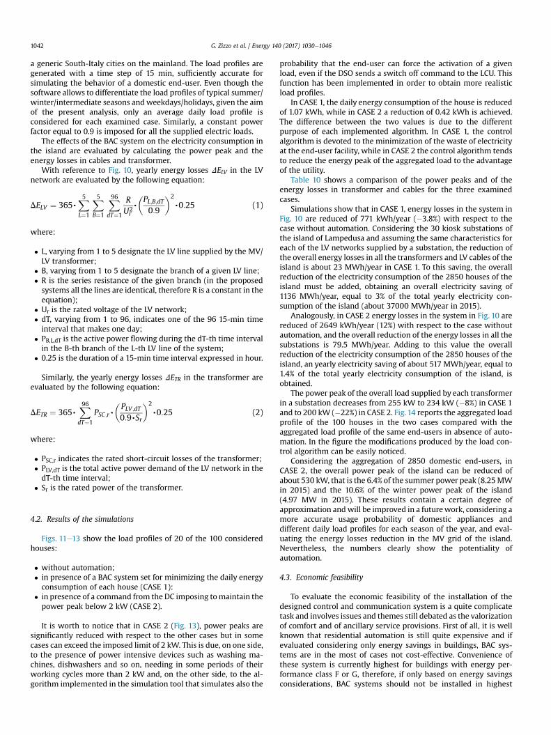
a generic South-Italy cities on the mainland. The load profiles aregenerated with a time step of 15 min, sufficiently accurate forsimulating the behavior of a domestic end-user. Even though thesoftware allows to differentiate the load profiles of typical summer/winter/intermediate seasons andweekdays/holidays, given the aimof the present analysis, only an average daily load profile isconsidered for each examined case. Similarly, a constant powerfactor equal to 0.9 is imposed for all the supplied electric loads.

The effects of the BAC system on the electricity consumption inthe island are evaluated by calculating the power peak and theenergy losses in cables and transformer.

With reference to Fig. 10, yearly energy losses DELV in the LVnetwork are evaluated by the following equation:

DELV ¼ 365,X5L¼1

X5B¼1

X96dT¼1

RU2r,

�PL;B;dT0:9

�2

,0:25 (1)

where:

� L, varying from 1 to 5 designate the LV line supplied by the MV/LV transformer;

� B, varying from 1 to 5 designate the branch of a given LV line;� R is the series resistance of the given branch (in the proposedsystems all the lines are identical, therefore R is a constant in theequation);

� Ur is the rated voltage of the LV network;� dT, varying from 1 to 96, indicates one of the 96 15-min timeinterval that makes one day;

� PB,L,dT is the active power flowing during the dT-th time intervalin the B-th branch of the L-th LV line of the system;

� 0.25 is the duration of a 15-min time interval expressed in hour.

Similarly, the yearly energy losses DETR in the transformer areevaluated by the following equation:

DETR ¼ 365,X96dT¼1

PSC;r,�PLV ;dT0:9,Sr

�2

,0:25 (2)

where:

� PSC,r indicates the rated short-circuit losses of the transformer;� PLV,dT is the total active power demand of the LV network in thedT-th time interval;

� Sr is the rated power of the transformer.

4.2. Results of the simulations

Figs. 11e13 show the load profiles of 20 of the 100 consideredhouses:

� without automation;� in presence of a BAC system set for minimizing the daily energyconsumption of each house (CASE 1):

� in presence of a command from the DC imposing tomaintain thepower peak below 2 kW (CASE 2).

It is worth to notice that in CASE 2 (Fig. 13), power peaks aresignificantly reduced with respect to the other cases but in somecases can exceed the imposed limit of 2 kW. This is due, on one side,to the presence of power intensive devices such as washing ma-chines, dishwashers and so on, needing in some periods of theirworking cycles more than 2 kW and, on the other side, to the al-gorithm implemented in the simulation tool that simulates also the

probability that the end-user can force the activation of a givenload, even if the DSO sends a switch off command to the LCU. Thisfunction has been implemented in order to obtain more realisticload profiles.

In CASE 1, the daily energy consumption of the house is reducedof 1.07 kWh, while in CASE 2 a reduction of 0.42 kWh is achieved.The difference between the two values is due to the differentpurpose of each implemented algorithm. In CASE 1, the controlalgorithm is devoted to the minimization of the waste of electricityat the end-user facility, while in CASE 2 the control algorithm tendsto reduce the energy peak of the aggregated load to the advantageof the utility.

Table 10 shows a comparison of the power peaks and of theenergy losses in transformer and cables for the three examinedcases.

Simulations show that in CASE 1, energy losses in the system inFig. 10 are reduced of 771 kWh/year (�3.8%) with respect to thecase without automation. Considering the 30 kiosk substations ofthe island of Lampedusa and assuming the same characteristics foreach of the LV networks supplied by a substation, the reduction ofthe overall energy losses in all the transformers and LV cables of theisland is about 23 MWh/year in CASE 1. To this saving, the overallreduction of the electricity consumption of the 2850 houses of theisland must be added, obtaining an overall electricity saving of1136 MWh/year, equal to 3% of the total yearly electricity con-sumption of the island (about 37000 MWh/year in 2015).

Analogously, in CASE 2 energy losses in the system in Fig. 10 arereduced of 2649 kWh/year (12%) with respect to the case withoutautomation, and the overall reduction of the energy losses in all thesubstations is 79.5 MWh/year. Adding to this value the overallreduction of the electricity consumption of the 2850 houses of theisland, an yearly electricity saving of about 517 MWh/year, equal to1.4% of the total yearly electricity consumption of the island, isobtained.

The power peak of the overall load supplied by each transformerin a substation decreases from 255 kW to 234 kW (�8%) in CASE 1and to 200 kW (�22%) in CASE 2. Fig.14 reports the aggregated loadprofile of the 100 houses in the two cases compared with theaggregated load profile of the same end-users in absence of auto-mation. In the figure the modifications produced by the load con-trol algorithm can be easily noticed.

Considering the aggregation of 2850 domestic end-users, inCASE 2, the overall power peak of the island can be reduced ofabout 530 kW, that is the 6.4% of the summer power peak (8.25MWin 2015) and the 10.6% of the winter power peak of the island(4.97 MW in 2015). These results contain a certain degree ofapproximation andwill be improved in a futurework, considering amore accurate usage probability of domestic appliances anddifferent daily load profiles for each season of the year, and eval-uating the energy losses reduction in the MV grid of the island.Nevertheless, the numbers clearly show the potentiality ofautomation.

4.3. Economic feasibility

To evaluate the economic feasibility of the installation of thedesigned control and communication system is a quite complicatetask and involves issues and themes still debated as the valorizationof comfort and of ancillary service provisions. First of all, it is wellknown that residential automation is still quite expensive and ifevaluated considering only energy savings in buildings, BAC sys-tems are in the most of cases not cost-effective. Convenience ofthese system is currently highest for buildings with energy per-formance class F or G, therefore, if only based on energy savingsconsiderations, BAC systems should not be installed in highest

G. Zizzo et al. / Energy 140 (2017) 1030e10461042

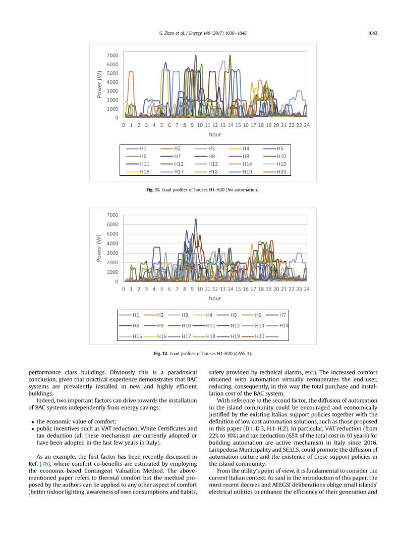
performance class buildings. Obviously this is a paradoxicalconclusion, given that practical experience demonstrates that BACsystems are prevalently installed in new and highly efficientbuildings.

Indeed, two important factors can drive towards the installationof BAC systems independently from energy savings:

� the economic value of comfort;� public incentives such as VAT reduction, White Certificates andtax deduction (all these mechanism are currently adopted orhave been adopted in the last few years in Italy).

As an example, the first factor has been recently discussed inRef. [76], where comfort co-benefits are estimated by employingthe economic-based Contingent Valuation Method. The above-mentioned paper refers to thermal comfort but the method pro-posed by the authors can be applied to any other aspect of comfort(better indoor lighting, awareness of own consumptions and habits,

safety provided by technical alarms, etc.). The increased comfortobtained with automation virtually remunerates the end-user,reducing, consequently, in this way the total purchase and instal-lation cost of the BAC system.

With reference to the second factor, the diffusion of automationin the island community could be encouraged and economicallyjustified by the existing Italian support policies together with thedefinition of low cost automation solutions, such as those proposedin this paper (D.1-D.3, H.1-H.2). In particular, VAT reduction (from22% to 10%) and tax deduction (65% of the total cost in 10 years) forbuilding automation are active mechanism in Italy since 2016.Lampedusa Municipality and SE.LI.S. could promote the diffusion ofautomation culture and the existence of these support policies inthe island community.

From the utility's point of view, it is fundamental to consider thecurrent Italian context. As said in the introduction of this paper, themost recent decrees and AEEGSI deliberations oblige small islands'electrical utilities to enhance the efficiency of their generation and

01000200030004000500060007000

0 1 2 3 4 5 6 7 8 9 10 11 12 13 14 15 16 17 18 19 20 21 22 23 24

Power

(W)

hour

H1 H2 H3 H4 H5H6 H7 H8 H9 H10H11 H12 H13 H14 H15H16 H17 H18 H19 H20

Fig. 11. Load profiles of houses H1-H20 (No automation).

0

1000

2000

3000

4000

5000

6000

7000

0 1 2 3 4 5 6 7 8 9 10 11 12 13 14 15 16 17 18 19 20 21 22 23 24

Power

(W)

hour

H1 H2 H3 H4 H5 H6 H7

H8 H9 H10 H11 H12 H13 H14

H15 H16 H17 H18 H19 H20

Fig. 12. Load profiles of houses H1-H20 (CASE 1).

G. Zizzo et al. / Energy 140 (2017) 1030e1046 1043

distribution plants by new investments in RESs and automation[12], [77e80]. The proposed architecture of the control andcommunication system, is able to assure a reduction of the waste ofelectricity in the island, according to the above national mandatorydispositions and, at the same time, to provide additional services tothe utility. Indeed, implementing suitable algorithms, the controland communication system is able to:

� enhance the security of the system during a sudden lack of oneof the diesel generator of the island's power plant, by loadshifting actions;

� collect data on the user's behavior in order to define customizedcontrol logics for specific groups of aggregated end-users;

� promote the diffusion and the participation to DR mechanismsof RES-based generators;

� monitor voltages and currents in grid's nodes and branchesreducing the possibilities of faults;

� allow distributed generator and battery storage systems to takepart to voltage and frequency regulation, according to themandatory technical Italian standards CEI 0e16 and CEI 0e21[81,82];

� improve the voltage profile;� avoid electricity thefts;� solve network congestions and maximize the exploitation ofRES-based generators.

The economic value of all the above-listed functions and theavoided costs due to their implementation largely justify the costfor the adoption of grid automation.

5. Conclusions and future works

The paper has presented a hierarchical architecture of a suitablecontrol, monitoring and communication system for a little islandand has proposed some suitable solutions for the automation oftwo actual buildings located in the Island of Lampedusa.

Looking at the feasibility study presented on the two casestudies, some considerations can be made.

First, a smart micro-grid of a small island can be equated with aSmart City with regard to extension, position and numerousness ofloads and generators.

Second, although the concept of ICT for Smart City is instantlyassociated with the one of economy, looking at the advantages forboth the DSO and the end-user (due to the reduction of the elec-tricity need thanks to DR policies ad BAC systems), ICT allows manyother applications related to user security and comfort that, for theaim of the present work, the Authors did not consider.

Actually, the design of a Smart Island should cover many other

01000200030004000500060007000

0 1 2 3 4 5 6 7 8 9 10 11 12 13 14 15 16 17 18 19 20 21 22 23 24

Power

(W)

hour

H1 H2 H3 H4 H5H6 H7 H8 H9 H10H11 H12 H13 H14 H15H16 H17 H18 H19 H20

Fig. 13. Load profiles of houses H1-H20 (CASE 2).

Table 10Comparison of power peak and energy losses with and without automation for a generic substation.

Power peak at transformer [kVA] Transformer's energy losses [kWh/year] LV system's energy losses [kWh/year] Total energy losses [kWh/year]

Without automation 255 18250 2177 20427CASE 1 234 17520 1971 19491CASE 2 200 15700 1683 17383

0

50000

100000

150000

200000

250000

0 1 2 3 4 5 6 7 8 9 10 11 12 13 14 15 16 17 18 19 20 21 22 23 24

Power

(W)

hour

NO Automation CASE 1 CASE 2

Fig. 14. Aggregated load profile of 100 houses in the three examined situations.

G. Zizzo et al. / Energy 140 (2017) 1030e10461044

factors like:

� the energetic independency of the island;� the development plan of the electric grid;� the economic development of the area, promoting the rise ofnew services;

� faults detection, isolation, and recovery;� grid and generators monitoring for predictive maintenance;� the capacity of giving an adequate and fast reply to the pertur-bations in the grid;

� frequency and voltage regulation;� the quality of the supply;� the traffic management;� the tourism development;� the integration of Electric Vehicles in the grid and the optimi-zation of their recharge;

� the accessibility of the services of the building and of the islandby creating suitable human interfaces;

� the availability to the end-users of information related to theoffered services.

In order to give effect to all the above-listed possibilities, manyother components and devices have to be installed in the buildingsin addition to those proposed in the present feasibility study, with aconsequent outstanding increment of the total cost of the BACsystems.

Moreover, according to the most recent technical standards, theimplementation of additional control actions to those that allow aneconomic saving for the end-user and the realization of DR pro-grams, could imply a modification of the means of transmissionproposed for the communication between the three tiers of thesmart grid [55,56].

Finally, with regard to the economic investments for the existinggrid upgrading, some solutions for creating a DC inside a secondarysubstations have been investigated. By examining the devicesoffered by the main brand in the ICT and automation field, anaverage cost equal to 8000V for a DC has been estimated, includingthe costs for programming and set-up activities. The estimated costcan raise or decrease depending on the functions that the DC canimplement.

Finally, for completing the control system ad adequate tele-communication infrastructure must be built. In an existingnetwork, being fundamental to avoid or minimize the excavationsfor new cable communication lines in the city, the simplest andcheapest way for connecting the DC to the various BMSs is to use aradio wave connection that implies the installation of a basetransceiver station at every secondary cabin and at every connectedbuilding.

Acknowledgments

The study presented is the result of a collaboration betweenENEA (Italian National Agency for New Technologies, Energy andSustainable Economic Development) and the DEIM (Department ofEnergy, Information Engineering and Mathematics) of the Univer-sity of Palermo in the framework of the “Analisi delle tecnologie perla climatizzazione e sistemi ICT applicati agli utenti finali delle isoleminori non connesse alla RTN al fine di efficientare il sistemaelettrico isolano” (“Electric system efficiency in small islands notinterconnected to the main power grid. Analysis of Renewable, Air-conditioning and ICT technologies for end-users”) Italian scientificresearch project.

References

[1] Nicolosi A, Sapone N, Cortese L, Marcian�o C. Fisheries-related tourism insouthern Tyrrhenian coastline. Procedia - Soc Behav Sci 2016;223:416e21.

[2] Niles K, Lloyd B. Energy for sustainable development, small island developingstates (SIDS) & energy aid: impacts on the energy sector in the Caribbean andPacific, vol. 17; 2013. p. 521e30.

[3] Gils HC, Simon S. Carbon neutral archipelago e 100% renewable energy supplyfor the Canary Islands. Appl Energy 2017;188:342e55.

[4] Scobie M. Fossil fuel reform in developing states: the case of Trinidad andTobago, a petroleum producing small Island developing State. Energy Policy2017;104:265e73.

[5] Weisser D. On the economics of electricity consumption in small islanddeveloping states: a role for renewable energy technologies? Energy Policy2014;32:127e40.

[6] Keeley AR. Renewable Energy in Pacific Small Island Developing States: therole of international aid and the enabling environment from donor's per-spectives. J Clean Prod 2017;147:29e36.

[7] Dornan M, Shah KU. Energy policy, aid, and the development of renewableenergy resources in Small Island Developing States. Energy Policy 2016;98:759e67.

[8] Spiegel-Feld D, Rudyk B, Philippidis G. Allocating the economic benefits ofrenewable energy between stakeholders on Small Island Developing States(SIDS): arguments for a balanced approach. Energy Policy 2016;98:744e8.

[9] Italian Decree 24 June 2014, n. 91, “Disposizioni urgenti per il settore agricolo,la tutela ambientale e l'efficientamento energetico dell'edilizia scolastica euniversitaria, il rilancio e lo sviluppo delle imprese, il contenimento dei costigravanti sulle tariffe elettriche, nonch�e per la definizione immediata diadempimenti derivanti dalla normativa europea”.

[10] Italian Law 11 August 2014, n. 116, “Conversione in legge, con modificazioni,del decreto-legge 24 giugno 2014, n. 91”.

[11] AEEGSI Deliberation 447/2014/R/EEL, “Avvio di procedimento per l’adozionedi provvedimenti dell'Autorit�a ai fini dell’attuazione della legge 116/2014, intema di riduzione delle bollette elettriche a favore dei clienti forniti in media ebassa tensione”.

[12] AEEGSI Document 598/2014/R/EEL, “Orientamenti per la riforma delle inte-grazioni tariffarie per le imprese elettriche minori non interconnesse”.

[13] Rodrigues EMG, Os�orio GJ, Godina R, Bizuayehu AW, Lujano-Rojas JM,Matiasa JCO, et al. Modelling and sizing of NaS (sodium sulfur) battery energystorage system for extending wind power performance in Crete Island. Energy2015;90(2):1606e17.

[14] Lau KY, Tan CW, Yatim AHM. Photovoltaic systems for Malaysian islands:effects of interest rates, diesel prices and load sizes. Energy 2015;83:204e16.

[15] Thomas D, Deblecker O, Ioakimidis CS. Optimal design and techno-economicanalysis of an autonomous small isolated microgrid aiming at high RESpenetration. Energy 2016;116(1):364e79.

[16] M€oller B, Sperling K, Nielsen S, Smink C, Kerndrup S. Bernd M€oller. Creatingconsciousness about the opportunities to integrate sustainable energy onislands. Energy 2012;48(1):339e45.

[17] Reyasudin Basir Khan M, Jidin R, Pasupuleti J, Azwa Shaaya S. Optimal com-bination of solar, wind, micro-hydro and diesel systems based on actualseasonal load profiles for a resort island in the South China Sea. Energy2015;82:80e97.

[18] Cozzolino R, Tribioli L, Bella G. Power management of a hybrid renewablesystem for artificial islands: a case study. Energy 2016;106:774e89.

[19] Fazelpour F, Soltani N, Rosen MA. Feasibility of satisfying electrical energyneeds with hybrid systems for a medium-size hotel on Kish Island, Iran. En-ergy 2014;73:856e65.

[20] Rodrigues EMG, Godina R, Santos SF, Bizuayehu AW, Contreras J, Catal~ao JPS.Energy storage systems supporting increased penetration of renewables inislanded systems. Energy 2014;75:265e80.

[21] Waide P, Ure J, Karagianni N, Smith G, Bordass W. The scope for energy andCO2 savings in the EU through the use of building automation technology.Waide Strategic Efficiency. 2014. p. 1e78. Available at:, http://www.leonardo-energy.org/resources/249.

[22] Cosentino V, Favuzza S, Graditi G, Ippolito MG, Massaro F, Riva Sanseverino E,et al. Smart renewable generation for an islanded system. Technical andeconomic issues of future scenarios. Energy 2012;39(1):196e204.

[23] Ippolito MG, Di Silvestre ML, Riva Sanseverino E, Zizzo G, Graditi G. Multi-objective optimized management of electrical energy storage systems in anislanded network with renewable energy sources under different designscenarios. Energy 2014;64:648e62.

[24] Riva Sanseverino E, Riva Sanseverino R, Favuzza S, Vaccaro V. Near zero en-ergy islands in the Mediterranean: supporting policies and local obstacles.Energy Policy 2014;66:592e602.

[25] Di Silvestre ML, La Cascia D, Riva Sanseverino E, Zizzo G. Improving the energyefficiency of an islanded distribution network using classical and innovativecomputation methods. Util Policies 2016;40:58e66.

[26] Mor�an AJ, Profaizer P, Zapater MH, Valdavida MA, Bribi�an IZ. Information andCommunications Technologies (ICTs) for energy efficiency in buildings: re-view and analysis of results from EU pilot projects. Energy Build 2016;127:128e37.

G. Zizzo et al. / Energy 140 (2017) 1030e1046 1045

[27] L�opez-Gonz�alez LM, L�opez-Ochoa LM, Las-Heras-Casas J, García-Lozano C.Update of energy performance certificates in the residential sector and sce-narios that consider the impact of automation, control and managementsystems: a case study of La Rioja. Appl Energy 2016;178:308e22.

[28] Zhang C, Liu C. The impact of ICT industry on CO2 emissions: a regionalanalysis in China. Renew Sustain Energy Rev 2015;44:12e9.

[29] Sekki T, Airaksinen M, Saari A. Effect of energy measures on the values ofenergy efficiency indicators in Finnish daycare and school buildings. EnergyBuild 2017;139:124e32.

[30] Ayodele TR, Ogunjuyigbe ASO, Atiba IA. Assessment of the impact of infor-mation feedback of prepaid meter on energy consumption of city residentialbuildings using bottom-up load modeling approach. Sustain Cities Soc2017;30:171e83.

[31] Choi Y, Lim Y, Hak-Man K. Optimal load shedding for maximizing satisfactionin an islanded microgrid. Energies 2017;10(45):1e13.

[32] Wu X, Jiang P, Lu J. Multiagent-based distributed load shedding for islandedmicrogrids. Energies 2014;7:6050e62.

[33] Kumar Nunna HSVS, Saklani AM, Sesetti A, Battula S, Doolla S, Srinivasan D.Multi-agent based Demand Response management system for combinedoperation of smart microgrids. Sustain Energy, Grids Netw 2016;6:25e34.

[34] Geramifar H, Shahabi M, Barforoshi T. Coordination of energy storage systemsand DR resources for optimal scheduling of microgrids under uncertainties.IET Renew Power Gener 2017;11(2):378e88.

[35] Aghajani GR, Shayanfar HA, Shayeghi H. Demand side management in a smartmicro-grid in the presence of renewable generation and demand response.Energy 2016;126:622e37.

[36] Minchala-Avila LI, Garza-Castanon LE, Vargas-Martınez A, Zhang Y. A reviewof optimal control techniques applied to the energy management and controlof microgrids. Procedia Comput Sci 2015;52:780e7.

[37] Najihah N, Bakara A, Hassana MY, Sulaima MF, Nasird MNM, Khamis A.Microgrid and load shedding scheme during islanded mode: a review. RenewSustain Energy Rev 2017;71:161e9.

[38] Ahmadi-Karvigh S, Ghahramani A, Becerik-Gerber B, Soibelman L. One sizedoes not fit all:understanding user preferences for building automation sys-tems. Energy Build 2017;145:163e73. http://dx.doi.org/10.1016/j.enbuild.2017.04.015.

[39] Paço A, Lavrador T. Environmental knowledge and attitudes and behaviourstowards energy consumption. J Environ Manag 2017;197:384e92.

[40] Hara K, Uwasu M, Kishita Y, Takeda H. Determinant factors of residentialconsumption and perception of energy conservation: time-series analysis bylarge-scale questionnaire in Suita, Japan, 87; 2015. p. 240e9.

[41] Good N, Ellis KA, Mancarella P. Review and classification of barriers and en-ablers of demand response in the smart grid. Renew Sustain Energy Rev2017;72:57e72.

[42] EU smart grid task force, https://ec.europa.eu/energy/en/topics/markets-and-consumers/smart-grids-and-meters/smart-grids-task-force.

[43] Kailas A, Cecchi V, Mukherjee A. A survey of communications and networkingtechnologies for energy management in buildings and home automation.J. Comput. Net. Commun. 2012;2012:1e12. 932181.

[44] Toschi GM, Campos LB, Cugnasca CE. Home automation networks: a survey.Comput Stand Interfaces 2017;50:42e54.

[45] Directive 2009/72/EC of the European Parliament and of the Council of 13 July2009 concerning common rules for the internal market in electricity.

[46] Directive 2009/73/EC of the European Parliament and of the Council of 13 July2009 concerning common rules for the internal market in natural gas andrepealing Directive 2003/55/EC (Text with EEA relevance).

[47] Directive 2010/31/EU of the European parliament and of the council of 19 May2019 on the energy performance of buildings.

[48] Directive 2012/27/EU of the European parliament and of the council of 25october 2012 on energy efficiency, amending directives 2009/125/EC and2010/30/EU and repealing directives 2004/8/EC and 2006/32/EC.

[49] Directive 2004/22/EC of the European parliament and of the council of 31march 2004 on measuring instruments (Text with EEA relevance).

[50] 2012/148/EU: commission Recommendation of 9 March 2012 on preparationsfor the roll-out of smart metering systems.

[51] European Technical Standard EN 15232. Energy performance of buildings e

impact of building automation, control, and building Management. second ed.Brussels: CEN; 2012.

[52] ISO/IEC standard 14543e3 (series), information technology - home Electronicsystems (HES) architecture.

[53] Chinese Standard GB/T 20965-2013, Control network HBES technicalspecification.

[54] ANSI/ASHRAE standard 135-2016, BACnet®ea data communication protocolfor building automation and control networks.

[55] IEEE standard 2030.2e2015, IEEE guide for the interoperability of energy

storage systems integrated with the electric power infrastructure.[56] IEEE standard 2030-2011, IEEE guide for smart grid interoperability of energy

technology and information technology operation with the electric powersystem (EPS), end-use applications, and loads.

[57] P1888.4/D1.7, oct 2016, IEEE approved Draft standard for green smart homeand residential quarter control network protocol.

[58] Meng L, Riva Sanseverino E, Luna A, Dragicevic T, Vasquez JC, Guerrero JM.Microgrid supervisory controllers and energy management systems: a liter-ature review. Renew Sustain Energy Rev 2016;60:1263e73.

[59] Lilis G, Conus G, Asadi N, Kayal M. Towards the next generation of intelligentbuilding: an assessment study of current automation and future IoT basedsystems with a proposal for transitional design. Sustain Cities Soc 2017;28:473e81.

[60] HomePlug homepage, Available at: http://www.homeplug.org/explore-homeplug/overview/.

[61] Insteon Whitepaper: the details, version 2.0, Available at: http://cache.insteon.com/documentation/insteon_details.pdf.

[62] International Standard ITU G.9959. Short range narrow-band digital radio-communication transceivers - PHY, MAC, SAR and LLC layer specifications.2015.

[63] Altmann M, Schlegl P, Volbert K. A low-power wireless system for energyconsumption analysis at mains sockets. EURASIP J Embed Syst 2017;8:1e11.

[64] Yan Y, Qian Y, Sharif H, Tipper D. A survey on smart grid communicationinfrastructures: motivations, requirements and challenges. IEEE CommunSurv Tutorials 2013;15(1) [IEEE].

[65] Gupta A, Jha RK. A survey of 5G network: architecture and emerging tech-nologies. IEEE Access 2015;3:1206e32.

[66] Torsten Berger L, Schwager A, Escudero-Garz�as JJ. Power line communicationsfor smart grid applications. J Electr Comput Eng 2013;2013:1e16. 712376.

[67] Istat, population housing census 2011, in http://dati-censimentopopolazione.istat.it/Index.aspx?lang¼en cit. 10/10/2016.

[68] ISTAT, L'Italia in 150 anni. Sommario di statistiche storiche 1861-2010, cap 15.Avellino. 2011.

[69] AEEGSI, Indagine conoscitiva sui prezzi finali dell’energia elettrica e del gasnaturale, Report 174/2015/I/COM.

[70] Garofalo E, Gargiulo A, Lembo E, Marazzi R, Rondena E, Moneta D, et al.Renewable energy sources' development in small island not interconnected tothe main grid (in Italian, orginal title: sviluppo delle Fonti Energetiche Rin-novabili nelle Isole minori non interconnesse). Ricerca sul Sistema EnergeticoeRSE S.p.A. Technical Report. 2015.

[71] Technical pubblication “Building automation e impact on energy efficiencyApplication per EN 15232 eu.bac product certification”. Siemes.

[72] Hotel Energy Solutions. Analysis on energy use by european hotels: onlinesurvey and desk research. Hotel Energy Solutions Project Publications; 2011.

[73] Strategies for C&I demand Response: hotels and motels, at https://bizenergyadvisor.com/members/TAS-RB-7/Research_Brief/DRStrategiesHotelsMotels.

[74] Zanella A, Bui N, Castellani A, Vangelista L, Zorzi M. Internet of things forsmart cities. IEEE Internet Things J 2014;1(1):22e32.

[75] Graditi G, Ippolito MG, Lamedica R, Piccolo A, Ruvio A, Santini E, et al. Inno-vative control logics for a rational utilization of electric loads andair-conditioning systems in a residential building. Energy Build 2015;102:1e17.

[76] Buso T, Dell'Anna F, Becchio C, Bottero MC, Cognati SP. Of comfort and cost:examining indoor comfort conditions and guests' valuations in Italian hotelrooms. Energy Research Social Sci 2017. http://dx.doi.org/10.1016/j.erss.2017.01.006 (in press) Available online 5 February 2017.

[77] Law decree 24/06/2014, n. 91, “Disposizioni urgenti per il settore agricolo, latutela ambientale e l'efficientamento energetico dell'edilizia scolastica e uni-versitaria, il rilancio e lo sviluppo delle imprese, il contenimento dei costigravanti sulle tariffe elettriche, nonche' per la definizione immediata diadempimenti derivanti dalla normativa europea”.

[78] Deliberation 21/11/2014 AEGGSI 574/2014/R/eel: “Disposizioni relativeall’integrazione dei sistemi di accumulo di energia elettrica nel sistema elet-trico nazionale”.

[79] Deliberation 18/12/2014 AEEGSI 642/2014/R/eel: “Ulteriori disposizioni rela-tive all’installazione e all’utilizzo dei sistemi di accumulo. Disposizioni relativeall’applicazione delle Norme CEI 0e16 e CEI 0-21”.

[80] Deliberation 16/07/2015 AEEGSI 360/2015/R/eel: “Proroga in meritoall’obbligatoriet�a dei ritardi nell’attivazione di alcune funzioni previste per lagenerazione distribuita”.

[81] CEI Standard 0-16. Reference technical rules for the connection of active andpassive consumers to the HV and MV electrical networks of distributionCompany. 2014.

[82] CEI Standard 0-21. Reference technical rules for the connection of active andpassive users to the LV electrical Utilities. 2014.

G. Zizzo et al. / Energy 140 (2017) 1030e10461046

An example of smart building

with a km zero energy performance

Luigi Martirano, Emanuele Habib, Giacomo Greco, Matteo Manganelli, Alessandro Ruvio

Faculty of Civil and Industrial Engineering Sapienza University of Rome, Italy

martirano@uniroma1.it

Biagio Di Pietra, Alessandro Pannicelli, Sara Piccinelli, Giovanni Puglisi, Pasquale Regina

Italian National Agency for New Technologies (ENEA) Rome, Italy

biagio.dipietra@enea.it

Abstract—Environmental concerns and European policies push for more energy efficient buildings, towards the goal of Nearly Zero Energy Buildings (nZEBs), buildings with an high efficiency and for which the low amount of energy required for the fixed technical systems (TBS) is covered by energy from renewable sources produced on-site. Innovative technical solutions and social/economic schemes are key elements to this purpose. Results on the simulation of energy performance and control system behavior of a real case are analyzed. The paper shows that the sizing of the local photovoltaic system (PV) based on the yearly energy spent by the TBS allows to obtain the nZEB qualification but it doesn't determine an optimal power behavior. The solution proposed in this work is to arrange a microgrid with a unique point of connection to the grid that includes the local generation systems, the common electric heating system by source grounded heat pumps and the residential units of a part of the buildings. Sizing of on-site power generation from renewable sources, like PV, may be developed based on the energy demand. The microgrid is managed by a common building automation control system (BACS). Control strategies have been analyzed, in order to realize demand-side management (DSM) actions, combining the advantages of thermal inertia, flexible loads, energy pricing and local generation. The DSM strategy operating on the controllable loads and on the electric and thermal storage can reach a “near zero power behavior” so the building can become a “km zero energy building” (KZEB).

Keywords—Nearly Zero Energy Buildings. Micro grid. Load management. Electric power systems. Thermal energy storage. Photovoltaic systems. Building Management Systems.

I. INTRODUCTION

Developing a strategy to make buildings more efficient and sustainable is a priority in the most recent European energy policies [1]. In particular, “buildings can use automation and controls to serve their occupants better, and to provide flexibility for the electricity system through reducing and shifting demand, and thermal storage” [1]. The introduction of distributed generation owned by the private users and other technologies, like electric energy storage, is changing the characteristics of consumer side of grid. Actions by the European Union introduce the definitions of the new concepts of aggregator, union, and community. In a

traditional definition, the aggregator is a virtual aggregation of single users and it is only capable of purchasing energy and reselling it to the users, thus it can only take advantage of energy prices. The union is a physical union of single users in a large user, around a common point of connection with the grid, and it can take advantage of new technical solutions (e.g., sharing local power generation or energy storage) to benefit of more convenient economic conditions, not only for energy prices but also other economic components of the electricity bill (network components, green charges, taxes). The community is a new solution under construction by European Committees that can be considered a middle way between an aggregator and an union. An example of aggregator that operates in the energy market is the energy demand aggregator (EDA). In the most accepted way, the EDA collects a large group of energy consumers, even if related to different nodes of the network, and it manages the global energy demand in order to optimize the global economic impact. An advanced way considers the group of energy consumers supplied by the same node of the network. One way used by the EDA is to manage the global electric load by controlling or turning off some of its loads and by managing generation and storage. As previously investigated by the authors, in the present Italian context there are limitations to the exploitation of distributed generation systems and innovative tariffs [2]. In previous papers the authors demonstrated that in a microgrid management, the control of electric loads and HVAC systems and exploitation of thermal inertia can be useful elements towards more efficient and sustainable buildings [2]-[4]. The aggregations of the users can be profitable both for the cost-effectiveness of DG and for the proper operation of the electricity network itself, increasing power quality. This more relevant whenever transport capacity is lacking, since the coordination of sources and loads inside the aggregation encourages self-consumption, mitigating the upstream grid in terms of power flows, with the consequent deferral of new investments. The economic impact of the aggregation for the users depends on the kind of model accepted (aggregator, union or community) and on the effectiveness of control strategies.

Page 1 of 8

978-1-5090-4894-6/17/$31.00 © 2017 IEEE

draft

Solutions developed for residential and tertiary mixed users, like large buildings, may be further developed in urban perspective. This might be a promising solution for grids with increasing power demand or distributed generation.

II. NEARLY ZERO ENERGY BUILDINGS NZEB

Residential and commercial buildings are strategic for pursuing energy efficiency policies, as identified by the European energy policy. This has lead to the provision of nearly zero energy building (nZEB) performance for all new buildings in Europe, starting from 2020 for privates ones and 2018 for public ones. As a consequence, this requires to install local renewable energy sources (RES), like photovoltaic (PV), in order to balance reach the quantity of energy necessary to classify the building as anZEB. nZEB means a building that has a very high energy performance, as determined in accordance with Annex I of Directive 2010/31/EU [5]. The nearly zero or very low amount of energy required should be covered to a very significant extent by energy from renewable sources, favoring energy from renewable sources produced on-site or nearby. Starting from a basic performance for new buildings or starting from actual performance for existing buildings, to obtain the nZEB qualification, the designers have to reduce the energy uses by passive measures (envelope insulation and efficient technical systems). The residual energy demand has to be supplied mainly by local generation from RES. The qualification takes care of yearly balance. The nZEB classification considers: - the energy spent for the fixed Technical Building Systems

(TBS) as heating, ventilation, air conditioned HVAC and domestic hot water DHW. This amount depends on the envelope insulation, the efficiency of the TBS and the building automation control systems (BACS) [6].

- the global annual primary energy amount, not considering the instantaneous power.

This paper shows that in a nZEB, the energy yearly balance (for fixed technical systems) can be equal or close to zero, but the instantaneous electric power may be far from zero with the possibility to determine severe chaotic phenomena. It is possible to have excessive peak and holes in enduser's power profiles with periods in which energy is provided to the grid, that is not economically advantageous due to the strong asymmetry between purchase and resale pricing, as in the latter network components, green charges, taxes are not compensated. In this framework, the authors investigated Demand Side Management (DSM) strategies operating on the controllable loads, considering not only the fixed systems (HVAC and DHW) but all the electric loads [7]-[9]. The goal is to reach a “near zero power behavior” with optimal exploitation of local RES [10]. Electric loads in a building may be divided into uncontrollable, shiftable and controllable loads. Shiftable (or plannable) loads can be shifted in time (with limitations) without affecting users’ comfort, but once they become uncontrollable until the duty cycle ends. Washing machines

and dishwashers may be assumed to be plannable and are considered so in this work. Controllable loads can be modified at any operation time (with limitations) exploiting the inertia of the operated system. Heat pumps are the main controllable load in this work. Their operation is assumed to be managed via the central control of local ambient and main system set-point temperatures. All other loads are uncontrollable, i.e., any change in the operation would affect users’ comfort.

III. NEW MODELS

The evolution of electric systems for smart buildings and nZEBs regards: - Technologies - Regulations, economy and management The technologies for smart electric systems (BACS- and DMS-compatible) are already available, while innovation is needed regarding the technical and economic regulations, economic agreements, management strategies [11]-[13]. In general, three categories of aggregation can be distinguished [14]: - Aggregations with “fundamental” or “intrinsic” value,

which does not depend on regulation, market awareness or technologies, and is permanent in time;

- Aggregations with “transitory” value, which contribute to a better power system operation but their value can decrease with better regulations, management or technologies;

- Aggregations with “opportunistic” value, which respond to regulation or market “flaws”.

The concept of aggregation generates, in general, two different kind of values: - A “system value” - A “private value” With respect to the advancement of regulations and technologies, the three aggregation categories can be associated to the value (value versus regulation/technologies), as shown in Figure 1.

Figure 1. Value of aggregators based on technology and regulatory

context. Elaborated from [14]

In the traditional scheme, on one hand, there is a system value, because grid services are provided (e.g., chaotic phenomena

Page 2 of 8

978-1-5090-4894-6/17/$31.00 © 2017 IEEE

draft

are reduced). On the other hand, there is little or no private value, because the benefits for the users are limited. The energy consumption is only shifted and not reduce, PV is not fully exploited, time slots are not beneficial. The only benefit comes from incentives, in case this activity is supported. In this scheme, only a virtual aggregation is possible, via a virtual power plant (VPP), not a real one. An operation and management entity is needed. The proposed scheme is based on a microgrid with a single point of connection (POC) to the grid. There is a single billing system for the whole microgrid. The aggregate is regarded as a large consumer, which purchases energy on behalf of all users and subdivides it among them. It is important to note that this entity does not purchase and resell energy but it only fulfills collective energy payments and subdivides them among users. This is similar to the management of other systems in buldings, like water and district heating supply. It may be regarded as an ESCO operating the building. A significant private value may be achieved, due to the redistribution of supply savings. These savings can be achieved via: - Economy of scale, i.e., energy can be purchased in bulk at

more beneficial tariffs - Increased RES (PV) self-consumption percent and extent,

i.e., net metering applies not only to common areas but also to the aggregate users

- DSM activities, which are economically beneficial in this case

- Dynamic pricing In the present Italian context, an important barrier is that, in case the energy is billed with respect to the aggregate rather than individual users, quantification of billing components is lost [2]. Present billing components are: 1. Energy and dispatch price 2. Network charges 3. Charges owed to GSE (the company in charge of energy

incentive programs) and to the Ministry of Economy and Finances

4. VAT and taxes While it is acceptable to quantify items 1 and 2 basing on the aggregate consumption (as these items are directly related to energy), this is not acceptable for items 3 and 4, because it would underestimate due charges and taxes. As some charges fund PV support programs, inter alia, PV exploitation would be self-defeating. Given these two schemes, an intermediate scheme may be further implemented, wherein a dual metering is used: Energy is metered in aggregated form while charges and taxes are quantified individually via single meters.

IV. AN EXAMPLE OF A SMART BUILDING WITH A KM ZERO

ENERGY PERFORMANCE

The reasearch considers a real example of a smart building classified nZEB. It is a complex constitued by two residential/commercial smart buildings in Campobasso, central Italy, made of two towers (A and B) and a common basement used for commercial units and parking [4]. Figure 2

shows a sketch of the building and its utilization. Table I describes the utilization of the building and its main characteristics.

TOWER B

92UNITS

west side

72UNITS

Commercial

6 kW

TOWER A

6 kW

126 kW

8

Commercial

6 kW

8

12

6 kW

8

6 kW

6 kW

8

6 kW

12

6 kW

6 kW

12

12

6 kW

Park

6 kW

8

6 kW

8

12

8

6 kW

east side6 kW

8

Park

6 kW

12

6 kW

8

8

Figure 2. Case study building.

TABLE I

CHARACTERISTICS OF THE BUILDINGS Area Type of units Characteristics Tower A Apartments 92 units 50 m2 each Tower B Apartments 72 units 75 m2 each Basement Commercial 2000 m2 total Basement Parking 2000 m2 total

The complex is classified nZEB as thermal insulation satisfies requirements and the yearly energy consumed by the fixed technical systems is covered by the local PV generation. Fixed Technical Systems. The building is gas-free and full electric. Power is supplied by an single point of connection with the grid and a private MV/LV substation. Heating and cooling are provided by a common station equipped with three reversible Ground Source Heat Pumps (GSHPs) with a rated electric power of 70 kW each. In dwellings, floor heating systems are used. DHW is centralized. A photovoltaic system (PV) is used as local generation. Electric loads of Tower A. The private electric microgrid supplies also the residential units of Tower A. The maximum power of each apartment is 6 kW, mainly due to electric stove. Electric loads of Tower B. The electric loads of tower B and the commercial units are supplied directly by the public netowrk by independent Point of Connections, one for each unit. BACS. A central building automation control system (BACS) connected to a central computer operates and manages all the systems by a SCADA software. At the end, the private microgrid supplies: - the fixed technical system for all the complex of two towers; - the common lighting and other common loads - the single residential units of only tower A. Table II shows the global load demand of the complex (average-peak demand).

Page 3 of 8

978-1-5090-4894-6/17/$31.00 © 2017 IEEE

draft

Figure 3. Suggested microgrid.

TABLE II

ELECTRIC POWER DEMAND Private Microgrid

Max (kW) Average (kW) GSHPs A 70 40 GSHPs B 70 40 GSHPs C 70 40

Fixed Tech.Systems 210 120 Tower A Units 100 60 Common loads 10 10

Global Microgrid (Union)

320 190

Public Network Tower B 100 60 Commercial 80 50

Global Microgrid (aggregator)

500 300

According to the regulations, the suggested model was organized in an hybrid system:

- Union for fixed and units tower A (Global power of 190-320 kW)

- Aggregator for the union plus tower B, plus commercial (Global power of 300-500 kW).

Figure 4. Picture of the case study building under construction, with a

private MV/LV substation.

A photovoltaic system is installed on top of the tower A, with 100 kW rated power. Figure 3 shows the suggested architecture for the microgrid. Several simulations were done to evaluate both the annual consumptions and the daily

profiles. Table III shows a synthesis of the annual energy spent by the building and global energy generated by the PV system.

TABLE III YEARLY ENERGY SPENT IN THE MICROGRID AND YEARLT ENERGY

GENERATED BY THE PV SYSTEM kW h MWh

GSHP A 40 1020 40,8

GSHP B 40 1020 40,8

GSHP C 40 1020 40,8

Total  120 122,4

Tower A 60 1425 85,5

Common 10 3000 30

Total 190 237,9

PV 100 1295 129,5

Fixed systems

Union

Table III shows that the energy generated by the PV is sufficient to equalize the energy spent by fixed systems. The building obtained the qualification of nZEB according to: 1) High level of insulation, with a building to ambient heat

transfer coefficient H = 31 W/K 2) High performance of the TBS (floor heating) 3) Ground source heat pumps with high value of the CoP 4) Photovoltaic system of 100 kW and about 130MWh/year 5) Domotic in all the units to better exploit the TBS Yet preliminary simulation has shown that chaotic phenomena of voltage and power fluctuations, may arise during the day and especially in the summer period. A second question concerns the economic aspects. The locally generated energy, that is not self consumed and provided to the grid is valued with a low price, lower than the energy generated and self consumed. In order to solve these problems the authors suggested to operate 2 actions: i. The electric microgrid with a single point of connection

and a private distribution system, including also the residential units of Tower A, has been organized.

ii. The microgrid is managed by the a central Building Energy Management System (BEMS) in order to better exploit the local energy by increasing the self consumption and to optimize the power profile at the point of connection, to take advantage of dynamic supply contracts.

Electric microgrid. In previous papers by the authors [3]-[4], preliminary configurations of the case study were investigated. In this work, the final configuration of the microgrid is considered, as follows (Figure 3):

- Tower A: all loads (GSHPs and residential units) - Tower B: GSHPs - Commercial area: GSHPs

The suggested microgrid is composed by: - a single POC with the DSO at the HV level 300 kW, 20kV 3 wires 50 Hz, and a substation HV/LV with a single 400 kVA transformer (Figure 4); - a low voltage main switch board (MSB) to supply both the TBS (heating, elevators, etc.) and the units;

Page 4 of 8

978-1-5090-4894-6/17/$31.00 © 2017 IEEE

draft

- a common photovoltaic system (PV) installed on the roof of the building and connected to the MSB; - a distribution power system from the MSB for all common TBSs; - a feeder distribution from the MSB supplying each unit of Tower A by an independent feeder in a radial scheme; - a local panel (ULP) for each unit of the Tower A for the local system.

Figure 5. MV/LV substation with a single 400 kVA transformer.

Concerning electric supplies of users in tower B and commercial areas, they are directly connected to the grid in the final configuration, thus they cannot be controlled and their energy is not included in the microgrid balance. Considering that whole HVAC system (GSHPs of Tower A, B and Commercial) can be controlled, there is a greater possibility to exploit the thermal inertia and the temperature set points, with respect to previous configuration. Building Energy Management System BEMS. The Tower A is fully wired with an HBES system. Each residential unit of Tower A is supposed to be equipped with a smart dishwashing machine, a smart washing machine, electric cooking devices, a refrigerator, and other usual domestic appliances. The management of the energy systems is organized with a central Building Energy Management System (BEMS) located in the SCADA that manages the whole building as a large user. The goal of the BEMS is to optimize the energy and economic performance of the grid (peak shaving, self-consumption, dynamic price of the energy). The presence of an integrated BACS can transform the individual users (apartments and commercial units) of few kW in a single large user (building) of hundreds kW with the possibility to operate demand side management (DSM) by an user common point of view. The BEMS controls the large load of the HVAC system by exploiting thermal inertia of the tanks as an energy storage, and the inertia of the well-insulated units, by forcing local and central temperature set points according to the actual global net load and the generation. The BEMS controls also the washing smart appliances (dishwashers and washing machines) of the single units, by a user software (APP) connected to the BEMS that permits to shift the starting times. The general aim of BEMS is: 1) to take advantage of the PV self-consumption, as much as

possible;

2) to maintain a controlled profile according to the actual cost of the energy by optimizing the energy costs in a dynamic scenario with special contracts;

3) to avoid changes of direction of the power in the POC and to minimize the power.

V. SIMULATIONS

As described previous a paper by the authors, a complete bottom-up model of the systems has been developed [4]. Electric devices are defined by their peak load, duty cycle, and energy demand in a fifteen-minutes period. Their actual load is simulated with a statistical approach simulating the presence and the habits of users. These are used also as input parameters for the heating and cooling model of the building, together with climate data. Heating loads are used to simulate the temperature of the central thermal energy storage and the operation of the heat pumps. Local ambient temperature is PI controlled. Heat pumps operation is on-off controlled in as many steps as the number of compressors of each unit. More details on these models are reported in previous papers from the authors [3]-[4]. In this work 4 different scenarios are simulated: Scenario 1. Only fixed systems (GSHPs) with PV Firstly, conventional system use with a microgrid supplying only the GSHPs, and without BEMS, has been simulated. The model generates a reference single unit residential load profile. The yearly energy spent is evaluate about 123 MWh. The yeary energy generated by the PV is about 130 MWh. During the summer months: - the power injected into the grid can reach values of about

100 kW, the entire amount of the power generated by the PV system, also if the buildings demand is positive.

- The self-consumption ratio of the energy generated by the PV is very low.

Figure 6 shows the monthly energy spent by the TBS (positive 12 bars) and the monthly energy generated by the PV system (negative 12 bars). The black line is the monthly balance. Let’s note that during the summer period the black line is negative, so generated energy is more locally consumed energy.

Figure 6. Scenario 1. Monthly energy spent by the TBS (positive

values) vs monthly energy generated by the PV system. The black line is the monthly balance.

Page 5 of 8

978-1-5090-4894-6/17/$31.00 © 2017 IEEE

draft

Figure 7. Scenario 2. Monthly energy spent by the microgrid

(positive values) vs monthly energy generated by the PV system. The black line is the monthly balance.

Scenario 2. Private Microgrid (GSHPs and Tower A) with PV. In a second scenario the microgrid is simulated with the residential units of Tower A. The suggested model [3]-[4] allows to obtain an aggregation of many dwellings with stochastic occupation and use that is the building load profile at POC. The yearly energy spent is evaluated about 240 MWh. Figure 7 shows the monthly energy spent by the microgrid including Tower A and TBS (positive 12 bars) and the monthly energy generated by the PV system (negative 12 bars). The black line is the monthly balance. Let’s note that during the summer period the black line is quite equal to zero and negative only for August. Yet, as there is no control, the mean zero energy demand of the system comes out from averaging periods in which PV generation is much higher than local loads and periods in which the whole load is positive. In this scenario during the summer months: - the power injected into the grid can reach values of about 50 kW; -the self-consumption ratio of the energy generated by the PV is about 50%. Figure 8 and Figure 9 show an example of daily profile in August and March, respectevely. Scenario 3. Private Microgrid with PV and BEMS The microgrid is the same of the Scenario 2 but a suggested DSM operated by the BEMS has been simulated. The scopes of the DSM are: - minimizing the power peaks; - maximizing self-consumption of PV electricity; - controlling the net global demand at the point of

connection; - minimizing the bill in a scenario with a more dynamic

cost of the electricity; - in a future scenario, optimizing the performance of an

electric vehicle charging station. The simulated BEMS controls: - heating and cooling set-point temperatures, - refrigerators operation to avoid peaks; - empty runs of the elevators. - smart appliances (dishwashers DWs and washing machines

WMs) scheduling;

Figure 8. Scenario 2: daily power profile - August day.

Figure 9. Scenario 2: daily power profile - March day.

Figure 10. Scenario 3: daily power profile - August day.

Figure 11. Scenario 3: daily power profile - March day.

The overall rule for the BEMS is to preserve users' comportment, free to use the services and the appliances at will [10]. The HBES is able to control in real time:

Page 6 of 8

978-1-5090-4894-6/17/$31.00 © 2017 IEEE

draft

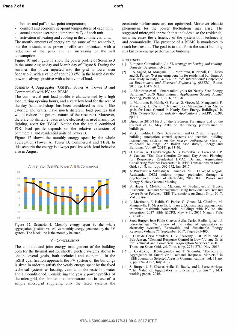
- boilers and puffers set-point temperature; - comfort and economy set-point temperatures of each unit; - actual ambient set-point temperature TS of each unit. - activation of heating and cooling in the commercial unit. The montly amounts of energy are the same of the scenario 2, but the instantaneous power profile are optimized with a reduction of the peak and an increasing of the self consumption. Figure 10 and Figure 11 show the power profile of Scenario 3 in the same August day and March day of Figure 8. During the summer, the power injected into the grid is lower than Scenario 2, with a value of about 20 kW. In the March day the power is always positive with a behavior of load. Scenario 4. Aggregator (GSHPs, Tower A, Tower B and Commercial) with PV and BEMS The commercial unit load profile is characterized by a high load, during opening hours, and a very low load for the rest of the day (standard shops has been considered as others, like catering and crafts, have much different load profiles that would reduce the general nature of the research). Moreover, there are no shiftable loads as the electricity is used mainly for lighting, apart for HVAC. Notice that the actual combined POC load profile depends on the relative extension of commercial and residential units of Tower B. Figure 12 shows the monthly energy spent by the whole aggregation (Tower A, Tower B, Commercial and TBS). In this scenario the energy is always positive with load behavior also in August.

Figure 12. Scenario 4. Monthly energy spent by the whole aggregation (positive values) vs monthly energy generated by the PV system. The black line is the monthly balance.

V – CONCLUSIONS

The common and joint energy management of the building both for the thermal and for strictly electric systems allows to obtain several goals, both technical and economic. In the nZEB qualification approach, the PV system of the buildings is sized in order to satisfy the yearly energy spent by the fixed technical systems as heating, ventilation domestic hot water and air conditioned. Considering the yearly power profiles of the microgrid, the simulations demonstrate that in case of a simple microgrid supplying only the fixed systems the

economic performance are not optimized. Moreover chaotic phenomena for the power fluctuations may arise. The suggested microgrid approach that includes also the residential units increases the efficiency of the system both technically and economically. The presence of a BEMS is mandatory to reach best results. The goal is to transform the smart building in a km zero energy performance building. REFERENCES [1] European Commission, An EU strategy on heating and cooling,

Brussels, Belgium, Feb 2016 [2] I. A. Sajjad, M. Manganelli, L. Martirano, R. Napoli, G. Chicco

and G. Parise, "Net metering benefits for residential buildings: A case study in Italy," 2015 IEEE 15th International Conference on Environment and Electrical Engineering (EEEIC), Rome, 2015, pp. 1647-1652.

[3] L. Martirano et al., "Smart micro grids for Nearly Zero Energy Buildings," 2016 IEEE Industry Applications Society Annual Meeting, Portland, OR, 2016, pp. 1-8.

[4] L. Martirano; E. Habib; G. Parise; G. Greco; M. Manganelli; F. Massarella; L. Parise, "Demand Side Management in Micro-grids for Load Control in Nearly Zero Energy Buildings," in IEEE Transactions on Industry Applications , vol.PP, no.99, pp.1-1

[5] Directive 2010/31/EU of the European Parliament and of the Council of 19 May 2010 on the energy performance of buildings.

[6] M.G. Ippolito, E. Riva Sanseverino, and G. Zizzo, “Impact of building automation control systems and technical building management systems on the energy performance class of residential buildings: An Italian case study”, Energy and Buildings, Vol. 69 (2014), p. 33-40.

[7] O. Erdinç, A. Taşcıkaraoğlu, N. G. Paterakis, Y. Eren and J. P. S. Catalão, "End-User Comfort Oriented Day-Ahead Planning for Responsive Residential HVAC Demand Aggregation Considering Weather Forecasts," in IEEE Transactions on Smart Grid, vol. 8, no. 1, pp. 362-372, Jan. 2017

[8] A. Prudenzi; A. Silvestri; R. Lamedica; M. C. Falvo; M. Regoli, Residential DSM actions impact prediction through a psychological model of electricity, 2012 IEEE Power and Energy Society General Meeting

[9] B. Hayes; I. Melatti; T. Mancini; M. Prodanovic; E. Tronci, Residential Demand Management Using Individualized Demand Aware Price Policies, IEEE Transactions on Smart Grid, 2017, Vol.8, Issue 3

[10] L. Martirano, E. Habib, G. Parise, G. Greco, M. Cianfrini, M. Manganelli, F. Massarella, L. Parise, Demand side management in mixed residential/commercial buildings with PV on site generation, 2017 IEEE I&CPS, May 8-11, 2017 Niagara Falls (Canada)

[11] Scott Burger, Jose Pablo Chaves-Ávila, Carlos Batlle, Ignacio J. Pérez-Arriaga, “A review of the value of aggregators in electricity systems”, Renewable and Sustainable Energy Reviews, Volume 77, September 2017, Pages 395-405.

[12] I. Diaz de Cerio Mendaza, I. G. Szczesny, J. R. Pillai and B. Bak-Jensen, "Demand Response Control in Low Voltage Grids for Technical and Commercial Aggregation Services," in IEEE Trans. on Smart Grid, vol. 7, no. 6, pp. 2771-2780, Nov. 2016.

[13] L. Gkatzikis, I. Koutsopoulos and T. Salonidis, "The Role of Aggregators in Smart Grid Demand Response Markets," in IEEE Journal on Selected Areas in Communications, vol. 31, no. 7, pp. 1247-1257, July 2013.

[14] S. Burger, J. P. Chaves-Ávila, C. Batlle, and I. Perez-Arriaga, “The Value of Aggregators in Electricity Systems.” , MIT working paper, 2016.

Page 7 of 8

978-1-5090-4894-6/17/$31.00 © 2017 IEEE

draft

BIOGRAPHIES Luigi Martirano (StM’98-M02-SM11) received the M.S. and Ph.D. degrees in Electrical Engineering in 1998 and 2003, respectively, from the Sapienza University, Rome Italy. In 2000, he joined the Department of Astronautics, Electrical and Energy Engineering of the Sapienza University of Rome where he’s currently an Associate Professor of Electrical Power Systems. Emanuele Habib received M.S. degree in Mechanical Engineering in 2002 and Ph.D. in Applied Physics in 2007. In 2011, he joined the Department of Astronautics, Electrical and Energy Engineering of the Sapienza University of Rome where he is currently an Assistant Professor of Applied Physics. Giacomo Greco (StM’14) received the B.D. in 2012 in Automation Engineering and the M.D. in Electrical Engineering in 2016 from the Sapienza University, Rome Italy. He is a PhD student at Sapienza University of Rome. Matteo Manganelli received his BSc degree cum laude in 2010 and MSc degree cum laude in 2013 in Energy Engineering from Sapienza University of Rome (Italy). Since 2014 he is a PhD student in Electrical Engineering in the same University. Alessandro Ruvio received his M.Sc. with honours in Electrical Engineering from the University of Rome Sapienza in 2012. He is with Dept. of Electrical Engineering as Assistant research from 2012. He is currently a PhD Student. Biagio di Pietra has been a Researcher with a permanent contract at Italian National Agency for New Technologies, Energy and Sustainable Economic Development since 2004. Alessandro Pannicelli has been a Researcher with a permanent contract at Italian National Agency for New Technologies, Energy and Sustainable Economic Development. Sara Piccinelli has been a Researcher with a permanent contract at Italian National Agency for New Technologies, Energy and Sustainable Economic Development. Giovanni Puglisi has been a Researcher with a permanent contract at Italian National Agency for New Technologies, Energy and Sustainable Economic Development. Pasquale Regina has been a Researcher with a permanent contract at Italian National Agency for New Technologies, Energy and Sustainable Economic Development.

Page 8 of 8

978-1-5090-4894-6/17/$31.00 © 2017 IEEE

draft

1876-6102 © 2017 The Authors. Published by Elsevier Ltd. This is an open access article under the CC BY-NC-ND license (http://creativecommons.org/licenses/by-nc-nd/4.0/).Peer-review under responsibility of the scientific committee of the 8th International Conference on Applied Energy.doi: 10.1016/j.egypro.2017.03.706

Energy Procedia 105 ( 2017 ) 2451 – 2459

ScienceDirect

The 8th International Conference on Applied Energy – ICAE2016

Design optimization of a distributed energy system through cost and exergy assessments

Marialaura Di Somma*,a, Bing Yanc, Nicola Biancob, Giorgio Graditia, Peter B. Luhc, Luigi Mongibelloa, Vincenzo Nasob

aENEA – Italian National Agency for New Technologies, Energy and Sustainable Economic Development, CR Portici, 80055

Portici, Italy bDipartimento di Ingegneria Industriale (DII), Università degli studi Federico II, P.le Tecchio, Napoli 80125, Italy

cDepartment of Electrical and Computer Engineering, University of Connecticut, Storrs, CT 06269, USA

Abstract

In recent years, Distributed Energy Systems (DESs) have been recognized as a good option for sustainable development of future energy systems. With growing environmental concerns, design optimization of DESs through economic assessments only is not sufficient. To achieve long-run sustainability of energy supply, the key idea of this paper is to investigate exergy assessments in DES design optimization to attain rational use of energy resources while considering energy qualities of supply and demand. By using low-temperature sources for low-quality thermal demand, the waste of high-quality energy can be reduced, and the overall exergy efficiency can be increased. Based on a pre-established superstructure, the aim is to determine numbers and sizes of energy devices in the DES and the corresponding operation strategies. A multi-objective linear problem is formulated to reduce the total annual cost and increase the overall exergy efficiency. The Pareto frontier is found to provide different design options for planners based on economic and sustainability priorities, through minimizing a weighted-sum of the total annual cost and primary exergy input, by using branch-and-cut. Numerical results demonstrate that different optimized DES configurations can be found according to the two objectives. Moreover, results also show that the total annual cost and primary exergy input are reduced by 20% - 30% as compared with conventional energy supply systems.

© 2016 The Authors. Published by Elsevier Ltd. Selection and/or peer-review under responsibility of ICAE

Keywords: Distributed Energy System; Design optimization; Annual cost; Exergy efficiency; Multi-objective linear problem.

1. Introduction

In recent years, depletion of fossil energy resources and global warming problems have prompted worldwide awareness about sustainability of energy supply. Distributed Energy Systems (DESs) have been recognized as a good option for sustainable development of future energy systems [1, 2]. A DES may consists of small-scale technologies including renewable ones and storage units, providing electric and thermal energy close to end-users [1]. To achieve the expected potentials of DESs, it is necessary to

* Corresponding author. Tel.: +39 0817723204; fax: +39 0817723344. E-mail address: marialaura.disomma@enea.it.

Available online at www.sciencedirect.com

© 2017 The Authors. Published by Elsevier Ltd. This is an open access article under the CC BY-NC-ND license (http://creativecommons.org/licenses/by-nc-nd/4.0/).Peer-review under responsibility of the scientific committee of the 8th International Conference on Applied Energy.

2452 Marialaura Di Somma et al. / Energy Procedia 105 ( 2017 ) 2451 – 2459

determine the system configuration rationally by selecting the appropriate energy devices, identifying their numbers and sizes, and the corresponding operation strategies, to match energy requirements of a specific end-user [2]. Design optimization of a DES is therefore essential for future energy planning, and inherently involves multiple and conflicting objectives [3, 4]. For instance, the interest of DES developers in achieving a system configuration with lowest costs might conflict with the interest of energy legislations, such as the EU ones, for sustainability concerns on reducing the waste of fossil energy resources and environmental impacts [4, 5]. In such a context, a multi-objective approach helps identify balancing solutions between economic and sustainability priorities to promote participation in the decision-making process and facilitate collective decisions [3].

According to [5], application of exergy principles in energy supply systems can achieve rational use of energy resources by taking into account the different energy quality levels of energy supply and building demand. In the literature, exergy has been linked to sustainability of energy supply since it clearly identifies the efficiency in energy resource use, and the importance of including exergy in energy legislations was discussed [5, 6]. DESs provide a great opportunity to demonstrate the effectiveness of exergy analysis in designing sustainable energy systems since multiple energy resources with different quality levels can be used to satisfy various user demand with different quality levels. By using low exergy sources, e.g., solar thermal or waste heat of power generation, for low-quality thermal demand, the waste of high-quality energy can be reduced, thereby increasing the overall exergy efficiency of DESs.

In previous works, exergy was investigated in DES operation through a multi-objective approach [7, 8]. With fixed DES configurations, optimized operation strategies were established by considering energy costs and exergy efficiency. As regards DES design optimization, most studies focused on minimizing the total annual cost as a crucial objective for DES developers [2, 9 - 13]. Also, before optimizing the design, “superstructures” were pre-established with energy devices chosen among the most commonly used ones in practical DESs. To identify the size of an energy device, several sizes were pre-fixed as possible choices to be selected through binary decision variables [2, 9 - 11]. However, how to select these sizes among the almost infinite possible solutions available in the market is difficult. Conversely, the size of an energy device was a continuous decision variable within the entire available size range, with efficiencies as well as specific capital and operation and maintenance (O&M) costs assumed constant in the entire size range [12, 13], while neglecting their variations with the sizes, which is significant for certain devices.

In this paper, exergy assessments are investigated in DES design optimization through a multi-objective approach. Based on a pre-established superstructure with multiple energy devices, a multi-objective linear problem is formulated to determine numbers and sizes of energy devices with the corresponding operation strategies on the Pareto frontier, thereby providing different design options for planners based on economic and sustainability priorities. In modeling energy devices, the entire size range available in the market as well as the variations of efficiencies, specific capital and O&M costs with sizes are taken into account. The economic objective is formulated as the total annual cost (total annualized investment cost, total annual O&M and energy cost) to be minimized. The exergetic objective is to maximize the overall exergy efficiency of the DES. With given energy demand, the total exergy required to meet the demand is known, and the exergetic objective is formulated as the total annual primary exergy input to be minimized. The Pareto frontier is found by minimizing a weighted sum of the two objectives, by using branch-and-cut. Numerical results show that different optimized DES configurations are found according to the two objectives. The Pareto frontier provides good balancing solutions for planners based on economic and sustainability priorities. The optimized DES configurations allow to reduce the total annual cost and primary exergy input by 20% - 30% as compared with conventional energy supply systems (CESs), where grid power is used for the electricity demand, natural gas boilers for domestic hot water (DHW) and space heating (SH) demand, and electric chillers for space cooling demand (SC).

Marialaura Di Somma et al. / Energy Procedia 105 ( 2017 ) 2451 – 2459 2453

2. Problem formulation and solution methodology

The DES superstructure consisting of the energy devices considered in the design optimization problem is shown in Fig. 1. Electricity demand and electricity required by heat pumps can be satisfied by grid power and Combined Heat and Power (CHP) systems. SC demand can be satisfied by CHPs, natural gas and biomass boilers through absorption chillers, heat pumps and thermal storage, whereas SH demand by CHPs, natural gas and biomass boilers, and thermal storage. DHW demand can be satisfied by CHPs, natural gas and biomass boilers, solar thermal collectors and thermal storage.

2.1. Decision variables

The decision variables include: existence, numbers, and sizes of energy devices; operation status (on/off) and energy rates provided by energy devices; capacities of thermal storage devices; heat rates input and output to/from thermal storage devices; electricity rate bought from the power grid. Existence and operation status of energy devices are binary. Numbers of energy devices are also determined through binary decision variables to be explained later. All the other decision variables are continuous.

2.2. Economic objective

The economic objective is to minimize the total annual cost of the DES, CTOT, formulated as the sum of the total annualized investment cost, and the total annual O&M and energy costs:

&

GRID

TOT INV O M FUEL PURC C C C C , (1)

where CINV is the annualized investment cost of all energy devices of the DES, CO&M is the total annual O&M cost of all energy devices, CFUEL is the total annual cost of consumed fuels, and GRID

PURC is the annual

cost of purchasing electricity from the power grid. The annualized investment cost of energy devices is obtained through the capital recovery factor [2, 9 -

13], and the annual O&M cost of energy devices depends on the DES operation:

, , & , , ,, 1 / 1 1 , i i

i i

i ii i

K KN N

INV i c i i k i O M i i k d hr ti k i k d hr

C CRF C S CRF r r r C OM R D , (2)

where CRFi is the capital recovery factor of technology i; ki is the energy device associated with technology

Fig. 1. Superstructure representation of the design optimization problem of the DES.

2454 Marialaura Di Somma et al. / Energy Procedia 105 ( 2017 ) 2451 – 2459

i, where Ki is its maximum number; iki

S,

is the designed size of device ki; Cc,i is the specific capital cost; r

is the interest rate; Ni is the lifetime in years; OMi is the O&M cost; , , ,ii k d hrR is the energy rate provided by

the device ki at hour hr of day d; and Dt is the time interval length (1 hour). The total annual costs of the consumed fuels and purchased grid power are formulated as:

, , , , ,/ , , , , i

ii

KGRID GRID

FUEL fuel i i k d hr i fuel t PUR e hr d hr ti k d hr d hr

C P R LHV D i NGICE NGboiler Bioboiler C P E D , (3)

where ηi is the energy efficiency (thermal or electrical); Pfuel,i and LHVfuel are the price and lower heat value of the corresponding fuel (i.e., natural gas and biomass fuels), respectively; Pe,hr is the time-of-day unit price of electricity from the power grid; and ,

GRID

d hrE is the electricity rate taken from the grid.

2.3. Exergetic objective

The exergetic objective is to maximize the overall exergy efficiency of the DES, as the ratio of the total annual exergy output (exergy required to meet the given user demand), Exout, to the total annual primary exergy input, Exin. With given energy demand, the total exergy required to meet the demand is known, and the overall exergy efficiency can be increased by reducing the total primary exergy input. At the supply side, the input energy carriers are grid power, natural gas, biomass and solar energy. Therefore, the exergetic objective is formulated as the total annual primary exergy input to be minimized as:

, ,in j d hr tj d hr

Ex Ex D , (4)

where Exj,d,hr is the exergy rate input to the DES related to the energy carrier j. Electricity from the power grid is an energy carrier provided by power generation plants, and the exergy

input rate to the DES depends on the exergy efficiency of the plants, εgen [7]:

, , , / , ,GRID

e d hr d hr genEx E ε d hr , (5)

The exergy input rates of natural gas and biomass depend on their specific chemical exergy:

, , , , , / , ,

, , , , , ,

i

ii

K

fuel d hr fuel i k d hr i fuel fuel fuel fueli k fuel

Ex ex R LHV ex LHV

fuel natural gas biomass i NGICE NGboiler Bioboiler d hr, (6)

where exfuel is the specific chemical exergy of the fuel, and ςfuel is the exergy factor [14]. Thermal energy output of solar thermal collectors at the corresponding temperature level is considered

as the primary energy source [7]. The exergy input rate to solar thermal collectors, ExST,d,hr, is defined as:

, , , , 0, ,1 / , ,out

ST d hr ST d hr d hr collEx R T T d hr , (7)

where T0,d,hr and outcollT are the reference temperature (hourly ambient temperature), and the temperature of

the heat transfer fluid at the exit of the collector field (assumed constant), respectively.

2.4. Constraints

Three main categories of constraints are established: design constraints, energy balances and operation constraints. As for design constraints, the designed size of the energy device ki has to be within the minimum and maximum sizes of the related technology Si

min and Simax available in the market:

min max

, , , , , i i ii i k i k i i k i iS x S S x i k K , (8)

where , ii kx is a binary decision variable, which is equal to 1 if the device ki is implemented in the DES

configuration. For the solar collector array, the designed area has to be lower than the available one. In the design optimization problem, the entire size range available in the market as well as the variations of efficiencies, specific capital and O&M costs with sizes are taken into account. These characteristics are

Marialaura Di Somma et al. / Energy Procedia 105 ( 2017 ) 2451 – 2459 2455

usually piecewise linear functions of the size, which is a continuous decision variable, thereby making the problem nonlinear. To avoid this, the key idea is to divide the entire size range of an energy device into several small ranges, so that these characteristics can be assumed constant in each size range. Consider CHP with a gas-fired internal combustion engine (ICE) as an example. The designed size of CHP in the range l is limited by its minimum and maximum values minCHP

lS and maxCHP

lS in this range:

, , , ,

min max , 1, , CHP l CHP l CHP l CHP l

CHP CHP CHP CHP CHP CHP

l k k l k k CHP CHPl

S x S S x x l k K , (9)

where CHP

lkCHPS

,and CHP

lkCHPx

,are defined similarly as in Eq (8) in the range l. Also, the summation of binary decision

variables CHP

lkCHPx

, over l has to be smaller than or equal to 1, ensuring that at most one range is selected.

To satisfy the given user demand, electricity, DHW, SH and SC energy balances are formulated based on the DES superstructure shown in Fig. 1. As for operation constraints, the energy rate provided by each energy device is limited by its minimum part load and the capacity. Still considering the CHP example, the electricity rate,

hrdkCHPR

,,is limited by its minimum and maximum values min

CHPkR and max

CHPkR if the device is on:

min max min max

, , , , , , , ,, , , , ,CHP CHP CHP CHP CHP CHP CHP CHP CHP

CHP CHP CHP

k k d hr k d hr k k d hr k k l k k l CHP CHPl l

R x R R x R r S R S k K d hr , (10)

where , ,CHPk d hrx is the on/off status of CHP, and rCHP is the minimum part load (expressed in percentage of

the designed size). The product of one continuous decision variable and one binary decision variable is linearized in a standard way. Beyond ICE, CHPs also involve heat recovery units for thermal purposes. The heat rate recovered by CHPs is subdivided among the heating coils for DHW and SH demand, and absorption chillers for SC as modeled in [7]. CHP ramp-rate constraints are also included to limit power generation between two successive time-steps. The natural gas and biomass boilers can be used to meet DHW and SH demand, and SC through absorption chillers. As regards solar thermal collectors, the heat rate provided is related to the designed area through the hourly solar irradiance and the thermal efficiency. For the operation of thermal storage devices, the amount of energy stored at the beginning of each time interval equals the non-dissipated energy stored at the beginning of the previous time interval (based on the storage loss fraction), plus the net energy flow (heat input rate to the storage minus heat output rate from the storage) [2, 7].

2.5. Optimization method

With the exergetic objective function formulated in Eq. (4) and the economic one formulated in Eq. (1), the problem has two objective functions to be minimized. To solve this multi-objective optimization problem, a single objective function is formulated as a weighted sum of the total annual cost, CTOT, and the total annual primary exergy input, Exin, to be minimized:

1obj TOT inF c C Ex , (11)

where constant c is a scaling factor, chosen such that c CTOT and Exin have the same order of magnitude. The Pareto frontier is found by varying the weight ω in the interval 0 – 1. The solution that minimizes the total annual cost can be found when ω = 1, whereas the one that minimizes the total annual primary exergy input (i.e., maximizes the overall exergy efficiency) when ω = 0. The problem formulated above is linear, and involves both discrete and continuous variables, so this is to be solved by branch-and-cut, which is powerful for mixed-integer linear optimization problems, and easy to code by using commercial solvers.

3. Numerical testing

Numerical testing is presented below, where a hypothetic cluster of 30 buildings located in Torino (Italy) is chosen as the targeted end-user. The method developed in Section 2 is implemented by using IBM ILOG CPLEX Optimization Studio Version 12.6, a popular and powerful solver where branch-and-cut is implemented with flexibility and high-performance.

2456 Marialaura Di Somma et al. / Energy Procedia 105 ( 2017 ) 2451 – 2459

3.1. Input data

Each building has a surface area of 5000 m2, and a shape factor S/V of 0.5 m-1. The hourly energy rate demand for electricity, DHW, SH, and SC for four representative days per season are used as input data, based on [15, 16]. To compute the annual energy requirements, the year is assumed to include 90, 92, 91, and 92 days in the cold, cold-mid, hot-mid, and hot seasons, respectively. Table 1 shows the peak and average energy rate demand of the end-user for the four representative season days as well as the annual energy requirements. The average hourly solar irradiance profiles (on a south-oriented and 35° tilted surface) have been assumed for each representative season day [17]. The technical and economic information of energy devices are summarized in Table 2 [18, 19]. The unit price of grid power is assumed as 0.15 €/kWh, and the unit prices of natural gas and biomass (wood pellet) are assumed as 0.477 €/Nm3, and 120 €/ton, respectively. The exergy efficiency of power generation plants is assumed as 0.40, based on the fossil fuel energy mix for electricity production and on the average efficiency of fossil fuel-fired electricity production in Italy [20]. The exergy factors of natural gas and biomass are assumed as 1.04 and 1.16 [14], respectively. A 5% interest rate is assumed to evaluate the total annualized investment cost.

3.2. Pareto frontier

The optimization problem is solved within few hours with a mixed integer gap lower than 0.15% on a PC with 2.60GHz (2 processors) Intel(R) Xeon(R) E5 CPU and 32G RAM. The Pareto frontier is shown in Fig. 2a. The point marked with a is obtained under exergetic optimization (ω = 0), and the point marked with b is obtained under economic optimization (ω = 1). The points between these two extreme points are found by subdividing the weight interval into 10 equally-spaced points. Each point on the Pareto frontier corresponds to a different optimized configuration of the DES. Fig. 2b shows the percentages of reduction in the total annual cost and increase in the total annual primary exergy input obtained by varying the weight ω from 0 to 1 with a 0.1 increase.

3.3. Optimized DES configurations

The optimized configurations of the DES (numbers, sizes and total installed capacities of energy devices), and the economic and exergetic performances for points a and b on the Pareto frontier are shown in Table 3. For the illustration purpose, the point marked with c in Fig. 2a (obtained for ω = 0.2) is also selected as an attractive economic/exergetic balancing solution. Under exergetic optimization, the total capacity of CHP is the largest among the three configurations. This highlights its importance for the exergetic objective, due to the possibility of waste heat recovery for thermal purposes, thereby promoting efficient use of the energy resource. As ω increases, the total capacity reduces, reaching the minimum under

Table 1. Peak and average energy rate demand (MW) in the representative season days and annual energy requirements of the building cluster (MWh).

Season Electricity DHW SH SC Peak Average Annual Peak Average Annual Peak Average Annual Peak Average Annual

Cold 0.86 0.52 1114 1.30 0.25 544.3 5.50 2.88 6227 0 0 0 Cold-mid 0.86 0.52 1139 1.30 0.25 556.4 3.22 1.53 3378 0 0 0 Hot-mid 0.86 0.52 1126 1.30 0.25 550.3 0 0 0 0 0 0 Hot 0.86 0.52 1139 1.30 0.25 556.4 0 0 0 4.47 1.47 3235

Table 2. Technical and economic information of energy devices. Energy device Size range

(kW) Specific capital

cost O&M costs

(€/kWh) Efficiency Lifetime

Electrical Thermal CHP gas-fired ICE 20-5000 1495-840 €/kW 0.020-0.008 0.28-0.41 0.68-0.40 20 NG boiler 10-2000 100 €/kW 0.0014 0.9 15 Biomass boiler 10-2000 400 €/kW 0.0027 0.85 15 Solar Thermal (ST) - 200 €/m2 0.0057 0.6 15 Air-source heat pump 10-6000 460 €/kW 0.0025 COP=3.0-3.5 20 Absorption chiller 10-5000 510-230 €/kW 0.0020 COP=0.8 20 Thermal storage - 20 €/kWh 0.0012 loss fraction=0.05 20

Marialaura Di Somma et al. / Energy Procedia 105 ( 2017 ) 2451 – 2459 2457

Fig. 2. a) Pareto frontier; b) Percentages of reduction in annual cost and increase in annual primary exergy input for ω varying from 0 to 1 with a 0.1 increase.

economic optimization, due to its high investment cost. Conversely, the total capacity of natural gas boiler is maximum under economic optimization, due to the low investment and O&M costs. The natural gas boiler is not chosen at point c, under a higher weight of the exergetic objective, highlighting that natural gas, as high-quality energy, should not be used for low-quality thermal demand. The choice of one natural gas boiler of 345 kW under exergetic optimization is due to the large sizes of the two CHPs, characterized by high minimum part loads, below of which they cannot operate.

The biomass boiler is not chosen in any configuration. Under exergetic optimization, although both wood and natural gas are high-quality energy, the efficiency of the biomass boiler is lower than that of the gas-fired boiler. The biomass boiler is also inconvenient for the economic objective due to the high investment cost. The area of the solar thermal array is maximum and the same for points a and c, under a higher weight of the exergetic objective, highlighting the convenience of solar thermal for the exergetic objective, due to low exergy of the thermal energy output from the collectors. Also the total capacities of heat pump and absorption chiller reach the maximum under exergetic optimization, highlighting their convenience for the exergetic purpose, due to the high conversion efficiency and the possibility of waste heat recovery for the SC demand, respectively. When ω increases, the total capacities reduce in order to reduce the total annual cost.

The capacity of the DHW thermal storage is maximum and the same for points a and c, since it is related to the thermal energy provided by the solar thermal plant. The capacity of the SH thermal storage is maximum under exergetic optimization, due to large amount of exhaust gas from CHPs. Conversely, the capacity of the SC thermal storage is minimum and the same for points a and c, whereas it strongly increases under economic optimization. By increasing the storage capacity, the size of the absorption chiller can be strongly reduced, thereby reducing the total investment costs.

In Table 3, the total annual cost and primary exergy input are also reported for an optimized CES system, where grid power is used for the electricity demand, natural gas boilers for DHW and SH demand, and

Table 3. Optimized solutions resulting from the analysis of the Pareto Frontier.

Optimized solutions Point a Point c Point b CES CHP Number - Sizes - Total (kWel) 2 - 1006/2130 - 3136 2 - 453/1103 - 1556 2 - 300/1007 - 1307 NG boiler Number – Sizes, Total (kWth) 1 - 345 - 345 0 2 - 260/807 – 1067 Biomass boiler Number - Sizes - Total (kWth) 0 0 0 Solar Thermal Area (m2) 1485 1485 0 Heat pump Number - Sizes - Total (kWth) 2 - 360/5732 - 6092 2 - 995/2563 - 3558 2 - 402/2466 - 2868 Absorption chiller Number - Sizes - Total (kWth) 2 - 300/1298 - 1589 1 - 1450 - 1450 1 - 1000 – 1000 DHW storage Total capacity (kWhth) 2746 2746 2063 SH storage Total capacity (kWhth) 2268 1382 1450 SC storage Total capacity (kWhth) 948 948 2406 Total annual cost (million €) 1.517 1.374 1.290 1.913 Total annual primary exergy input (GWh) 18.620 18.864 19.753 27.641

2458 Marialaura Di Somma et al. / Energy Procedia 105 ( 2017 ) 2451 – 2459

electric chillers for SC demand (same configurations attained under economic and exergetic optimization). As compared with CES, the total annual cost and primary exergy input of the DES are both reduced by 33% under economic and exergetic optimization. Moreover, as compared with CES, the total annual cost of the DES under exergetic optimization is reduced by 21%, whereas the total annual primary exergy input under the economic optimization is reduced by 28%.

3.4. Operation strategies of optimized DES configurations under economic and exergetic optimization

For each optimized configuration, different operation strategies of energy devices are found. For the illustration purpose, Fig. 3 shows the operation strategies of the DES (electricity and thermal energy provided by energy devices) in the four representative season days at points a and b of the Pareto frontier for a) electricity, b) DHW and c) SH/SC demand. As shown in Fig. 3a, grid power is generally lower than the electricity provided by CHPs, highlighting that CHP is convenient for both objectives. The contrary occurs in the hot mid-season day under exergetic optimization. In this day, only electricity and DHW demand need to be satisfied, and solar thermal is preferred instead of waste heat from CHPs to meet the demand as shown in Fig. 3b. The integration of the natural gas boiler is due to the large sizes of the CHPs, as discussed earlier. Conversely, waste heat from CHPs is mostly used under economic optimization. In Fig. 3c for SH and SC, heat pumps are mostly used under both exergetic and economic optimization. For SC, the absorption chiller is used more under exergetic optimization than under economic one. Moreover, both Fig.s 3b and c show that to meet the DHW and SH demand, natural gas boilers are more used under economic optimization than under exergetic one.

4. Conclusions

In this paper, exergy assessments are investigated in DES design optimization for sustainable development of energy supply systems. Based on a pre-established superstructure, a multi-objective linear problem is formulated to determine numbers and sizes of energy devices with the corresponding operation strategies through cost and exergy assessments. The Pareto frontier is found through minimizing a weighted sum of the total annual cost and primary exergy input by using branch-and-cut. Numerical results demonstrate that different optimized DES configurations are found according to the two objectives, and the Pareto frontier provides good balancing solutions for planners based on economic and sustainability priorities. The optimized DES configurations allow to reduce the total annual cost and primary exergy input by 20% - 30% as compared with CES. Although there are no exergy requirements (as a methodology or an indicator) yet in current energy legislations, results underline that exergy assessments may allow to meet the main goal of energy legislations in sustainability of energy supply.

Fig. 3. Operation strategies of the DES in the four season days at points a and b of the Pareto frontier for a) Electricity, b) DHW, c) SH/SC demand

Marialaura Di Somma et al. / Energy Procedia 105 ( 2017 ) 2451 – 2459 2459

Acknowledgement

Authors thank ENEA for funding this study within the Italian Research Program “Ricerca di Sistema Elettrico – PAR 2015, “Area: Efficienza energetica e risparmio di energia negli usi finali elettrici ed interazione con altri vettori energetici”.

References [1] Kari A, Arto S. Distributed energy generation and sustainable development. Renew Sustain Energy Rev 2006;10:539–58. [2] Ren H, Gao W. A MILP model for integrated plan and evaluation of distributed energy systems. Appl En 2010;87(3):1001-

1014. [3] Ren H, Zhou W, Nakagami KI, Gao W, Wu Q. Multi-objective optimization for the operation of distributed energy systems

considering economic and environmental aspects. Appl En 2010;87(12):3642-3651. [4] Alarcon-Rodriguez A, Ault G, Galloway G. Multi-objective planning of distributed energy resources: A review of the state-

of-the-art. Renew Sustain Energy Rev 2010;14:1353–66. [5] ECBCS - Annex 49 - Low Exergy Systems for High Performance Buildings and Communities, homepage. Available

<http://www.ecbcs.org/annexes/annex49.htm>. [6] Dincer I, Rosen M. Exergy-Energy, Environment and Sustainable Development. 1st Ed., Elsevier Publication, Oxford, UK,

(2007). [7] Di Somma M, Yan B, Bianco N, Luh PB, Graditi G, Mongibello L, Naso V. Operation optimization of a distributed energy

system considering energy costs and exergy efficiency. Energ Convers Manage 2015;103:739-751. [8] Yan B, Di Somma M, Bianco N, Luh PB, Graditi G, Mongibello L, Naso V. Exergy-based operation optimization of a

distributed energy system through the energy-supply chain. Appl Therm Eng 2016;101:741-751. [9] Mehleri ED, Sarimveis H, Markatos NC, Papageorgiou LG. A mathematical programming approach for optimal design of

distributed energy systems at the neighbourhood level. Energy 2012;44:396-104. [10] Hawkes AD, Leach MA. Modelling high level system design and unit commitment for a microgrid. Appl En 2009;86(7):253-

1265. [11] Omu A, Choudhary R, Boies A. Distributed energy resource system optimisation using mixed integer linear programming.

Energy Policy 2013:61, 249-266. [12] Zhou Z, Zhang J, Liu P, Li Z, Georgiadis MC, Pistikopoulos EN. A two-stage stochastic programming model for the optimal

design of distributed energy systems. Appl En 2013;103:135-144. [13] Zhou Z, Liu P, Li Z, Ni W. An engineering approach to the optimal design of distributed energy systems in China. Appl

Therm Eng 2013;53:387-96. [14] Kotas YJ. The exergy method for thermal plant analysis. reprint ed. Malabar, FL: Krieger; 1995. [15] Mongibello L, Bianco N, Caliano M, Graditi G. Influence of heat dumping on the operation of residential micro-CHP

systems. Appl En 2015;160:206-220. [16] Barbieri ES, Melino F, Morini M. Influence of the thermal energy storage on the profitability of micro CHP systems for

residential building applications. Appl En 2012;97:714–22. [17] ASHRAE International Weather files for Energy Calculations (IWEC weather files). Users manual and CD-ROM, American

Society of Heating, Refrigerating and Air-Conditioning Engineers, Atlanta, GA, USA, 2001. [18] Darrow, K., Tidball, R., Wang, J., & Hampson, A. 2015. Catalog of CHP technologies. Available:

https://www.epa.gov/sites/production/files/2015-07/documents/catalog_of_chp_technologies.pdf. [19] Technology Data for Energy Plants. Energinet.dk (2012). Available:

http://www.energinet.dk/SiteCollectionDocuments/Danske%20dokumenter/Forskning/Technology_data_for_energy_plants.pdf. [20] Trudeau N, Francoeur M. Energy Efficiency indicators for Public Electricity Production from fossil fuels. OECD/IEA, 2008.

Biography

Marialaura Di Somma received the Ph. D degree in Mechanical Systems Engineering from the Università di Napoli Federico II, Italy, in 2016. She is a research associate at ENEA RC Portici, Italy. Her research interests include design and operation optimization of distributed energy systems through multi-objective criteria.

Multi-objective design optimization of distributed energy systemsthrough cost and exergy assessmentsq

M. Di Somma a,⇑, B. Yan b, N. Bianco c, G. Graditi a, P.B. Luh b, L. Mongibello a, V. Naso c

a ENEA, Italian National Agency for New Technologies, Energy and Sustainable Economic Development, CR Portici, 80055 Portici, ItalybDepartment of Electrical and Computer Engineering, University of Connecticut, Storrs, CT 06269, USAcDipartimento di Ingegneria Industriale (DII), Università degli studi Federico II, P.le Tecchio, Napoli 80125, Italy

h i g h l i g h t s

� Exergy in design optimization of distributed energy systems (DESs).� Multi-objective design optimization of DESs through cost and exergy assessments.� Balancing solutions for planners based on economic and sustainability priorities.� Cost and primary exergy of DESs reduced by 21–36% as compared with conventional systems.� Exergy analysis for sustainable development of energy supply systems.

a r t i c l e i n f o

Article history:Received 13 January 2017Received in revised form 6 March 2017Accepted 22 March 2017Available online xxxx

Keywords:Distributed energy systemDesign optimizationMulti-objective linear programmingAnnual costExergy efficiency

a b s t r a c t

In recent years, distributed energy systems (DESs) have been recognized as a promising option for sus-tainable development of future energy systems, and their application has increased rapidly with support-ive policies and financial incentives. With growing concerns on global warming and depletion of fossilfuels, design optimization of DESs through economic assessments for short-run benefits only is not suf-ficient, while application of exergy principles can improve the efficiency in energy resource use for long-run sustainability of energy supply. The innovation of this paper is to investigate exergy in DES design toattain rational use of energy resources including renewables by considering energy qualities of supplyand demand. By using low-temperature sources for low-quality thermal demand, the waste of high-quality energy can be reduced, and the overall exergy efficiency can be increased. The goal of the designoptimization problem is to determine types, numbers and sizes of energy devices in DESs to reduce thetotal annual cost and increase the overall exergy efficiency. Based on a pre-established DES superstruc-ture with multiple energy devices such as combined heat and power and PV, a multi-objective linearproblem is formulated. In modeling of energy devices, the novelty is that the entire available size rangesand the variation of their efficiencies, capital and operation and maintenance costs with sizes are consid-ered. The operation of energy devices is modeled based on previous work on DES operation optimization.By minimizing a weighted sum of the total annual cost and primary exergy input, the problem is solvedby branch-and-cut. Numerical results show that the Pareto frontier provides good balancing solutions forplanners based on economic and sustainability priorities. The total annual cost and primary exergy inputof DESs with optimized configurations are reduced by 21–36% as compared with conventional energysupply systems, where grid power is used for the electricity demand, and gas-fired boilers and electricchillers fed by grid power for thermal demand. A sensitivity analysis is also carried out to analyze theinfluence of energy prices and energy demand variation on the optimized DES configurations.

� 2017 Elsevier Ltd. All rights reserved.

1. Introduction

In recent years, depletion of fossil energy resources and globalwarming problems have prompted worldwide awareness aboutsustainability of energy supply. In such context, Distributed EnergySystems (DESs) have been recognized as a promising option for

http://dx.doi.org/10.1016/j.apenergy.2017.03.1050306-2619/� 2017 Elsevier Ltd. All rights reserved.

q The short version of the paper was presented at ICAE2016 on Oct 8-11, Beijing,China. This paper is a substantial extension of the short version of the conferencepaper.⇑ Corresponding author.

E-mail address: marialaura.disomma@enea.it (M. Di Somma).

Applied Energy xxx (2017) xxx–xxx

Contents lists available at ScienceDirect

Applied Energy

journal homepage: www.elsevier .com/locate /apenergy

Please cite this article in press as: Di Somma M et al. Multi-objective design optimization of distributed energy systems through cost and exergy assess-ments. Appl Energy (2017), http://dx.doi.org/10.1016/j.apenergy.2017.03.105

sustainable development of future energy systems [1–6]. A DESrefers to a multi-input and multi-output energy system, consistingof multiple small-scale technologies, including renewable ones andstorage units, providing electric and thermal energy close to end-users [1–8]. Therefore, as compared with conventional energy sup-ply systems, DESs may employ a wide range of technologies,thereby offering the possibility to integrate renewables as well asto recover waste heat from power generation processes for thermalpurposes in buildings [2–4]. The application of DESs has increasedrapidly in recent years with the supportive government policiesand financial incentives [1,3,4,8]. However, to achieve the expectedpotentials of DESs, it is necessary to determine the system config-uration rationally by selecting the appropriate energy devices, andidentifying their numbers and sizes, and the corresponding opera-tion strategies, to match energy requirements of a specific end-

user [2,9–11]. Design optimization of a DES is therefore essentialfor future energy planning, and inherently involves multiple andconflicting objectives [12–15]. For instance, the interest of DESdevelopers in achieving a system configuration with lowest costsmight conflict with the interest of energy legislations such as theEU ones in increasing sustainability of energy supply, which canbe attained by reducing the waste of fossil energy resources andenvironmental impacts [15,16]. In such a context, a multi-objective approach helps identify balancing solutions to promoteparticipation in the decision-making process and facilitate collec-tive decisions [12].

According to [16], application of exergy principles in buildingenergy supply systems may promote rational use of energyresources, by taking into account the different energy quality levelsof energy supply and those of building demand. Electrical and

Nomenclature

A area (m2)c constant in Eq. (34) (kW h/€)C cost (€)Cc specific capital cost (€/kW) - (€/kW h) - (€/m2)Cd,hr cooling rate (kW)COP coefficient of performanceCRF capital recovery factorDR maximum ramp-down rate (kW)Dt length of the time interval (h)e minimum part loadEd,hr electricity rate (kW)exBio specific chemical exergy of biomass (kW h/kg)exNG specific chemical exergy of natural gas (kW h/N m3)Ex exergy (kW h)Exd,hr exergy rate (kW)Fobj objective functionFq Carnot factorG natural gas volumetric flow rate (N m3/h)Hd,hr heating rate (kW)I total solar irradiance (kW/m2)LHVBio lower heat value of biomass (kW h/kg)LHVNG lower heat value of natural gas (kW h/N m3)ni total number of energy devices associated with technol-

ogy iN lifetime (years)OM O&M cost (€/kW h)PBio biomass price (€/ton)Pe electricity price (€/kW h)PNG natural gas price (€/N m3)r interest rateRd,hr energy rate (kW)S designed size (kW) – (kW h)T temperature (K)UR maximum ramp-up rate (kW)x binary decision variable

Greek symbolsegen exergy efficiency of electricity generation1FUEL exergy factor of fuelg efficiencyu storage loss fractionw overall exergy efficiencyx weight in Eq. (34)

Superscript/subscripts0 referenceAbs absorption chiller

ASHP air source heat pumpBio biomassBioboil biomass boilerCHP NGICE combined heat and power with gas-fired internal

combustion engineCHP NGMTG combined heat and power with gas-fired micro-

turbinecoll collectord daydem demandDHW domestic hot watere electricityES electrical storageFUEL fuelGRID power gridhr houri index of technologyin inputINV investmentj energy carrierl rangeki energy device associated with technology iKi maximum number of energy devices associated with

technology imax maximummin minimumNG natural gasNGboil gas-fired boilerO&M operation and maintenanceout outputPV photovoltaicreq requiredSC space coolingSH space heatingSOLAR solarST solar thermalsto storedTES thermal energy storageth thermalTOT total

AcronymsCHP combined heat and powerDES distributed energy systemMOLP multi-objective linear programmingO&M operation and maintenance

2 M. Di Somma et al. / Applied Energy xxx (2017) xxx–xxx

Please cite this article in press as: Di Somma M et al. Multi-objective design optimization of distributed energy systems through cost and exergy assess-ments. Appl Energy (2017), http://dx.doi.org/10.1016/j.apenergy.2017.03.105

chemical energy are high-quality energy, whereas low-temperature heat is low-quality energy. In current energy supplysystems, energy is commonly supplied as electricity or as fossilenergy carriers, whose energy quality is unnecessarily high to meetlow-quality thermal demand in buildings, and the First Law ofThermodynamics does not consider the energy quality degradationoccurring in such processes. Conversely, based on the Second Lawof Thermodynamics, by reducing the supply of high-quality energyfor thermal demand in buildings through the usage of low-temperature sources, efficient use of the potential (i.e., quality) ofthe energy resources is promoted. Since energy resources, and par-ticularly fossil fuels, are limitedly available, better exploiting theirpotential allows to reduce their waste. In this way, lifetime of fossilfuels can be extended, and the environmental impacts derivedfrom their use can be reduced [16]. In the literature, exergy analy-sis has been linked to sustainability of energy supply which isessential for the long run, since it clearly identifies the efficiencyin energy resource use, by considering their potential; and theimportance of including exergy in energy legislations was dis-cussed [16–21]. Exergy was investigated in performance evalua-tion of single energy supply systems, as cogeneration systems[22–25], renewable energy sources [26,27], various types of heatpumps [28–30], and thermal energy storage [31–33] with theaim to reduce energy quality degradation in designing and manag-ing these systems, thereby improving sustainability of energy sup-ply. DESs provide a great opportunity to demonstrate theeffectiveness of exergy analysis in designing more sustainableenergy systems since multiple energy resources with differentenergy quality levels can be used to satisfy user various demandwith different quality levels. By using low exergy sources, e.g., solarthermal or waste heat of power generation, for low-quality ther-mal demand, and high exergy sources for electricity demand, thewaste of high-quality energy can be reduced, thereby increasingthe overall exergy efficiency of DESs.

In previous work, exergy modeling and optimization wereinvestigated in DES operations through a multi-objective approach[34,35]. Based on fixed DES configurations (types, numbers andsizes of energy devices), optimized operation strategies wereestablished by considering energy costs and exergy efficiency. Asfor design optimization of DESs, most studies in the literaturefocused on minimizing the total annual cost (annualized invest-ment costs and annual operating costs of the system) as a crucialobjective for DES developers [2,36–42]. Beyond minimizing costsonly, design optimization of DESs through multi-objectiveapproach to reduce also environmental impact was analyzed. In[43], a multi-objective linear programming (MOLP) model wasestablished to find the optimal configuration and operation of aDES for an industrial area while reducing the total annual costand CO2 emission. The problem was solved by using the compro-mise programming method. In [44], a MOLP model was developedto optimally design and operate an energy system consisting ofbuildings equipped with small-size Combined Heat and Power(CHP) plants, with the aim to reduce both annual costs and CO2

emission. In [45], a general framework was developed to studythe application of energy hubs for determining the optimal designand operation of DESs in urban areas according to economic andenvironmental objectives, and the multi-objective optimizationproblem was solved by using branch-and-cut. In all the analyzedworks, before optimizing the design, ‘‘superstructures” were pre-established with energy devices chosen among the most com-monly used ones in practical DESs. Moreover, to identify the sizeof an energy device, several sizes were pre-fixed as possiblechoices to be selected through binary decision variables [2,36–40,44,45]. However, it is difficult to select the sizes among thealmost infinite possible solutions available in the market. Con-versely, the size of an energy device was a continuous decision

variable within the entire available size range, with efficienciesas well as specific capital and operation and maintenance (O&M)costs assumed constant in the entire size range and their variationswith the sizes were not considered [41,42]. The size of an energydevice was a continuous decision variable within the entire avail-able size range in [43], with prices and efficiencies approximatedas linear functions of the size.

The innovation of this paper is to investigate exergy in DESdesign optimization through a multi-objective approach to attainrational use of energy resources considering economic and sustain-ability priorities. A superstructure is pre-established with multipleenergy devices, such as CHPs with natural gas-fired internal com-bustion engines and micro-turbines as prime movers, natural gasand biomass boilers, solar thermal collectors, PV, reversible air-source heat pumps, single-stage absorption chillers, and electricaland thermal energy storage devices. Given user demand includeselectricity, domestic hot water, space heating, and space cooling.To take both cost and exergy assessments into account, a MOLPproblem is formulated, and the goal is to determine types, numbersand sizes of energy devices in the DES with the correspondingoperation strategies on the Pareto frontier, thereby providing dif-ferent design options for planners based on short- and long-runpriorities. In modeling of energy devices, the key novelty is thatthe entire size ranges available in the market as well as the varia-tions of efficiencies, specific capital and O&M costs with sizes aretaken into account, based on a detailed market analysis. Thesecharacteristics are usually piecewise linear functions of the devicesize, which is a continuous decision variable, thereby making theproblem nonlinear. To maintain the problem linearity, the key ideais to divide the entire size range of an energy device into severalsmall ranges, so that these characteristics can be assumed constantin each size range. The daily operation of energy devices is mod-eled based on previous work on operation optimization of DESs[34]. The economic objective is formulated as the total annual cost(total annualized investment cost, total annual O&M and energycost) to be minimized. The exergetic objective is to maximize theoverall exergy efficiency of the DES, defined as the ratio of the totalannual exergy required to meet the given energy demand to thetotal annual primary exergy input to the system. Assuming knownthe energy demand, the total exergy required to meet the demandis also known. Therefore, the exergetic objective is formulated asthe total annual primary exergy input to be minimized. By mini-mizing a weighted sum of the total annual cost and primary exergyinput, the problem is solved by branch-and-cut. The general math-ematical formulation established and the optimization methodprovided could be applicable in real contexts, thereby providingdecision support to planners. Given the input data, such as end-user demand, local climate data, energy prices and technical andeconomic information of the candidate energy devices, the modelallows to obtain their optimized combination, and the correspond-ing operation strategies through cost and exergy assessments. Asan illustrative example, the model is implemented for a hypotheticbuilding cluster located in Italy. The optimization is carried out onan hourly basis for four representative season days. Numericalresults demonstrate that exergy analysis is a powerful tool fordesigning more sustainable energy supply systems based on theuse of renewables and low-temperature sources for thermaldemand in buildings, and that good balancing options for plannersare found on the Pareto frontier. Moreover, the total annual costand primary exergy input of DESs with optimized configurationsare significantly reduced, by 21–36% as compared with conven-tional energy supply systems, where grid power is used for theelectricity demand, natural gas boilers for domestic hot waterand space heating demand, and electric chillers fed by grid powerfor space cooling demand. In addition, a sensitivity analysis is car-ried out to analyze the influence of key parameters such as energy

M. Di Somma et al. / Applied Energy xxx (2017) xxx–xxx 3

Please cite this article in press as: Di Somma M et al. Multi-objective design optimization of distributed energy systems through cost and exergy assess-ments. Appl Energy (2017), http://dx.doi.org/10.1016/j.apenergy.2017.03.105

prices and energy demand variation on the optimized DES config-urations and the related economic and exergetic performances.

In the following, Section 2 is on the problem formulation andthe optimization method. Numerical testing is presented and dis-cussed in Section 3. Sensitivity analysis is presented in Section 4.

2. Problem formulation and optimization method

The superstructure of the DES under consideration is shown inFig. 1. The energy devices are chosen among the most commonlyused ones in practical DESs.

Electricity demand and electricity required by heat pumps canbe satisfied by grid power, by the electricity provided by CHPs withnatural gas-fired internal combustion engines and micro-turbinesas prime movers, PV, and by the electricity discharged from theelectrical storage. It is assumed that all the electricity providedby CHPs and PV is self-consumed, while no extra electricity is soldback to the power grid. Domestic hot water demand can be satis-fied by thermal energy provided by CHPs, natural gas and biomassboilers, solar thermal collectors, and by thermal energy dischargedfrom the storage. Space heating demand can be satisfied by ther-mal energy provided by CHPs, natural gas and biomass boilers,heat pumps, and by thermal energy discharged from the storage.Space cooling demand can be satisfied by thermal energy providedby CHPs, natural gas and biomass boilers through the absorptionchillers, heat pumps, and by thermal energy discharged from thestorage.

In the following, the decision variables are first introduced inSection 2.1. The economic and exergetic objectives are presentedin nd 2.22.3, respectively. The constraints are established in Sec-tion 2.4. The optimization method is discussed in Section 2.5.

2.1. Decision variables

In the optimization problem, the decision variables include:existence, numbers, and sizes of energy devices; operation status(on/off) and energy rates provided by energy devices; capacitiesof electrical and thermal storage devices; electricity and heat rateinput and output to/from electrical and thermal storage devices,

respectively; and electricity rate bought from the power grid. Exis-tence and operation status of energy devices are binary. Numbersof energy devices are also determined through binary decisionvariables to be explained later. All the other decision variablesare continuous.

2.2. Economic objective

The economic objective is to minimize the total annual cost ofthe DES, CTOT, formulated as the sum of the total annualized invest-ment cost, and the total annual O&M and energy costs:

CTOT ¼ CINV þ CO&M þ CFUEL þ CGRID; ð1Þwhere CINV is the annualized investment cost of all energy devices inthe DES; CO&M is the total annual O&M cost of all energy devices;CFUEL is the total annual cost of consumed fuels; and CGRID is theannual cost of purchasing electricity from the power grid.

The total annualized investment cost of the energy devices isformulated as:

CINV ¼Xi

XKi

ki

CRFi Cc;iSi;ki� �

;

CRFi ¼ r 1þ rð ÞNi= 1þ rð ÞNi � 1h i

; ð2Þ

where CRFi is the capital recovery factor of technology i; Ki is themaximum number of energy devices associated with technology i,which is assumed to be known; ki is the energy device associatedwith technology i; Si;ki is the designed size of device ki; Cc,i is thespecific capital cost; r is the interest rate; and Ni is the lifetime.The size of electrical and thermal energy storage devices representsthe capacity expressed in kW h, and the specific capital cost isexpressed in €/kW h. The size of the solar thermal collectors isexpressed in terms of the total surface of collectors to be installed,and the specific capital cost is expressed in €/m2.

The total annual O&M cost of energy devices is formulated as:

CO&M ¼Xi

XKi

ki

Xd

Xhr

OMiRi;ki ;d;hrDt ; ð3Þ

Fig. 1. Superstructure representation of the DES for the design optimization problem.

4 M. Di Somma et al. / Applied Energy xxx (2017) xxx–xxx

Please cite this article in press as: Di Somma M et al. Multi-objective design optimization of distributed energy systems through cost and exergy assess-ments. Appl Energy (2017), http://dx.doi.org/10.1016/j.apenergy.2017.03.105

where OMi is the O&M cost of the technology i; Ri;ki ;d;hr is the energyrate provided by the energy device ki at hour hr of day d; and Dt isthe length of the time interval (1 h). For electrical and thermal stor-age devices, the O&M costs are based on their capacities.

The total annual cost of the consumed fuels is formulated as:

CFUEL ¼X

i2 CHP NGICE; CHP NGMTG;NG boilf g

XKi

ki

XdX

hr

PNG Ri;kid;hr= giLHVNGð Þ� �Dt þ

Xi2 Bioboilf g

XKi

ki

Xd

Xhr

PBio Ri;kid;hr= giLHVBioð Þ� �Dt; ð4Þ

where gi is the energy efficiency (thermal or electrical); PNG and PBioare the price of natural gas and biomass, respectively; and LHVNG

and LHVBio are the lower heat value of natural gas and biomass,respectively.

The annual cost of purchased grid power is formulated as:

CGRID ¼Xd

Xhr

Pe;hrEGRID;d;hrDt; ð5Þ

where Pe,hr is the time-of-day unit price of electricity from thepower grid, and EGRID,d,hr is the electricity rate taken from the grid.

2.3. Exergetic objective

The exergetic objective is to maximize the overall exergy effi-ciency of the DES, w, defined as the ratio of the total annual exergyoutput, Exout, to the total annual primary exergy input, Exin[34,46,47]:

w ¼ Exout=Exin: ð6ÞThe total annual exergy output is the total annual exergy

required to meet the given user demand in the whole year, formu-lated as:

Exout ¼Xdem

Xd

Xhr

Exdemd;hrDt ; dem 2 fe; DHW; SH; SCg; ð7Þ

where Exdemd;hr is the total exergy rate required to meet the electricityand thermal demand (domestic hot water, and space heating andcooling). In buildings, energy demands are characterized by differ-ent energy quality levels. To meet the electricity demand, the high-est quality of energy is needed. The exergy rate required to meet theelectricity demand, Exed;hr; can be evaluated as follows [34,35,48]:

Exed;hr ¼ Eed;hr; 8d;8hr; ð8Þ

where Eed;hr is the electricity demand rate.

As for thermal demand, the energy quality depends on temper-ature required – the lower the temperature required, the lower theexergy [16,48]. The exergy rate required to meet the demand ofdomestic hot water can be formulated as:

ExDHWd;hr ¼ HDHWd;hr FDHW

q;d;hr; 8d;8hr; ð9Þ

where HDHWd;hr is the heat demand rate for domestic hot water, and

FDHWq;d;hr is the Carnot factor, formulated as [16,34,35,48]:

FDHWq;d;hr ¼ 1� T0;d;hr=T

DHWreq ; 8d;8hr; ð10Þ

which depends on both the temperature required for the domestichot water, TDHW

req , which is assumed to be known based on [49], andthe reference temperature, T0,d,hr, assumed to be known as the aver-aged ambient temperature at hour hr of day d [16,34]. The exergyrate required to meet the demand of space heating and coolingcan be formulated similarly.

At the supply side, the input energy carriers are grid power, nat-ural gas, biomass, and solar energy. The total annual primaryexergy input is formulated as:

Exin ¼Xj

Xd

Xhr

Exj;d;hrDt; j 2 fGRID; FUEL; SOLARg; ð11Þ

where Exj,d,hr is the exergy rate input to the DES related to theenergy carrier j. As well as for the demand side, also the supply sideis characterized by different energy quality levels.

Electricity from the power grid is an energy carrier provided bypower generation plants, and the exergy input rate to the DES,ExGRID,d,hr, depends on the exergy efficiency of the plants, egen[34,35]:

ExGRID;d;hr ¼ EGRID;d;hr=egen; 8d;8hr; ð12ÞThe exergy input rates of fuels (natural gas and biomass)

depend on their specific chemical exergy:

ExFUEL;d;hr ¼X

i2fCHP NGICE; CHP NGMTG; NGboilg

XKi

ki

exNGðRi;ki ;d;hr=ðgiLHVNGÞÞ

þX

i2fBioboilg

XKi

ki

exBioðRi;ki ;d;hr=ðgiLHVBioÞÞ;

exFUEL ¼ 1FUELLHVFUEL;

FUEL 2 fNG;Biog;8d;8hr; ð13Þ

where exFUEL is the specific chemical exergy of the fuel, and 1FUEL isthe exergy factor [50].

As for solar energy, thermal energy output of the solar thermalcollectors at the corresponding temperature levels, and electricityoutput of PV are considered as the primary energy sources[51,52], respectively. The exergy input rate to solar thermal collec-tors, ExST,d,hr, is formulated as:

ExST;d;hr ¼ HST;d;hrð1� T0;d;hr=ToutcollÞ; 8d; 8hr; ð14Þ

where HST, d, hr is the heat rate provided by solar thermal collectors,and T0,d,hr and Tout

coll are the reference temperature, assumed as theaveraged ambient temperature at hour h of day d [16,34], and thetemperature of the heat transfer fluid at the exit of the collectorfield (assumed constant), respectively.

The exergy input rate to PV, ExPV,d,hr, is formulated as:

ExPV ;d;hr ¼ EPV ;d;hr; 8d; 8hr: ð15Þ

where EPV, d, hr is the electricity rate provided by PV.Therefore, the exergy rate of solar energy input to the DES is for-

mulated as:

ExSOLAR;d;hr ¼ ExST;d;hr þ ExPV ;d;hr; 8d;8hr: ð16Þ

Since energy demand as well as the temperatures required for thedemand of domestic hot water, and space heating and cooling areassumed known, the total exergy required to meet the demand isalso known, and the overall exergy efficiency can be increased byreducing the total primary exergy input. Therefore, the exergeticobjective is formulated as the total annual primary exergy inputto the DES to be minimized as in Eq. (11).

2.4. Constraints

The constraints in the optimization problem include designconstraints, energy balances and operation constraints, as dis-cussed below.

M. Di Somma et al. / Applied Energy xxx (2017) xxx–xxx 5

Please cite this article in press as: Di Somma M et al. Multi-objective design optimization of distributed energy systems through cost and exergy assess-ments. Appl Energy (2017), http://dx.doi.org/10.1016/j.apenergy.2017.03.105

2.4.1. Design constraintsThe designed size of the energy device ki has to be within the

minimum and maximum sizes of the related technology Simin and

Simax available in the market:

Smini xi;ki 6 Si;ki 6 Smax

i xi;ki ; ki 6 Ki; ni ¼XKi

ki

xi;ki ; 8i; ð17Þ

where xi;ki is a binary decision variable, which is equal to 1 if thedevice ki is implemented in the DES configuration; and ni is the totalnumber of energy devices associated with technology i imple-mented in the DES configuration. As for solar collector and PVarrays, the total designed area has to be lower than the availableone. In the design optimization problem, the entire size range avail-able in the market as well as the variations of efficiencies, specificcapital and O&M costs with sizes, are taken into account. Thesecharacteristics are usually piecewise linear functions of the size,which is a continuous decision variable, thereby making the prob-lem nonlinear. To avoid this, the key idea is to divide the entire sizerange of an energy device into several small ranges, so that thesecharacteristics can be assumed constant in each size range. Con-sider CHP with a natural gas-fired internal combustion engine asan example. The designed size of CHP in range l is limited by its

minimum and maximum values Smin; lCHP NGICE and Smax; l

CHP NGICE in this range:

Smin; lCHP NGICEx

lkCHP NGICE

6 SlkCHP NGICE6 Smax; l

CHP NGICExlkCHP NGICE

;Xl

xlkCHP NGICE6 1; 8l; kCHP NGICE 6 KCHP NGICE; ð18Þ

where SlkCHP NGICEand xlkCHP NGICE

are defined similarly as in Eq. (17) in

range l. Also the summation of binary decision variables xlkCHP NGICE

over l has to be smaller than or equal to 1, ensuring that at mostone range can be selected for each energy device associated to eachtechnology.

2.4.2. Energy balancesTo satisfy the given user demand, electricity, domestic hot

water, and space heating and cooling energy balances are formu-lated in the following.

For electricity, the sum of the electricity demand and the totalelectricity required by the reversible air source heat pumps hasto be satisfied by the sum of the total electricity provided by CHPs,PV, grid power, and electrical storage:

Eed;hr þ

XkASHP

EkASHP ;d;hr ¼ EPV ;d;hr þX

kCHP NGICE

EkCHP NGICE ;d;hr

þX

kCHP NGMTG

EkCHP NGMTG ;d;hr þ EGRID;d;hr

þ Ee ;outES;d;hr � Ee; in

ES;d;hr ; 8d;hr; ð19Þ

where Ee ;outES;d;hr and Ee; in

ES;d;hr are the electricity rates discharged andcharged from/to the storage, respectively, which are both continu-ous decision variables.

For the domestic hot water demand, the demand has to be sat-isfied by the total thermal energy provided by CHPs, natural gasand biomass boilers, solar thermal collectors, and thermal storage:

HDHWd;hr ¼

XkCHP NGICE

HDHWkCHP NGICE ;d;hr

þX

kCHP NGMTG

HDHWkCHP NGMTG ;d;hr

þXkNGboil

HDHWkNGboil ;d;hr

þXkBioboil

HDHWkBioboil ;d;hr

þ HST;d;hr þ HDHW ; outTES;d;hr

� HDHW ; inTES;d;hr ; 8d;hr; ð20Þ

where HDHW; outTES;d;hr and HDHW; in

TES;d;hr are the heat rates discharged andcharged from/to the storage, respectively, which are both continu-ous decision variables.

The space heating and space cooling energy balances are formu-lated in a similar way.

2.4.3. Operation constrainsFor most of the energy devices included in the DES superstruc-

ture, the common constraint is the capacity constraint. The energyrate provided by each energy device is limited by its minimum partload and the capacity, if the device is on. Still considering the CHPwith a natural gas-fired internal combustion engine as an example,the electricity rate, EkCHP NG ICE ;d;hr , is limited by the minimum and

maximum rated output EminkCHP NG ICE

and EmaxkCHP NG ICE

, if the device is on:

EminkCHP NG ICE

xkCHP NG ICE ;d;hr 6 EkCHP NG ICE ;d;hr 6 EmaxkCHP NG ICE

xkCHP NG ICE ;d;hr ;

8kCHP NGICE; 8d; hr; ð21Þ

where xkCHP NG ICE ;d;hr is the on/off status of CHP. The minimum partload and the maximum rated output are obtained based on thedesign capacity of CHP as follows:

EminkCHPNGICE

¼ ekCHPNG ICE

Xl

SlkCHPNGICE; Emax

kCHPNGICE¼Xl

SlkCHPNGICE;

8kCHPNGICE; ð22Þ

where ekCHP NG ICEis the minimum part load expressed in percentage of

the designed size. The product of one continuous and one binarydecision variables is linearized in a standard way [53].

In the following, the additional constraints of each energydevice are presented.

2.4.3.1. CHP systems. Two types of CHPs are involved in the DESsuperstructure, i.e., CHPs with gas-fired internal combustionengine and with micro-turbines. They consist of prime movers tomeet the electricity load, and heat recovery units providing ther-mal energy to meet the demand of domestic hot water and spaceheating, and to meet the demand of space cooling through absorp-tion chillers. Operation constraints for CHPs with gas-fired internalcombustion engine as prime mover are presented below.

The ramp rate constraint limits the variations in the power gen-eration between two successive time steps to be within the ramp-down, DRkCHP NGICE

, and ramp-up, URkCHP NGICE[34,54]:

DRkCHP NGICE6 EkCHPNGICE ;d;hr � EkCHPNGICE ;d;hr�1 6 URkCHPNGICE ;

8kCHP NG ICE; 8d;hr; ð23Þ

where the ramp-down and the ramp-up and are expressed in per-centage of the designed size.

The volumetric flow rate of natural gas, GkCHP NGICE ;d;hr , required bythe CHP to provide the electricity rate, EkCHP NG ICE ;d;hr , is formulated as:

GkCHP NGICE ;d;hr ¼ EkCHP NGICE ;d;hr=ðge;kCHP NGICELHVNGÞ;

8kCHP NGICE; 8d;hr: ð24Þ

In the above, ge;kCHP NGICEis the electrical efficiency of the CHP, formu-

lated as:

ge;kCHP NGICE¼

Xl

xlkCHP NGICEgle;kCHP NGICE

; 8kCHP NGICE; ð25Þ

where gle;kCHP NGICE

is the electrical efficiency of the CHP in the range l.The heat rate recovered from the CHP, HkCHP NGICE ;d;hr , is formulated

as:

HkCHP NGICE ;d;hr ¼ EkCHP NGICE ;d;hrgth;kCHP NGICE=ge;kCHP NGICE

;

8kCHP NGICE; 8d;hr ; ð26Þ

where gth;kCHP NGICEis the thermal efficiency of the CHP defined simi-

larly as in Eq. (25).

6 M. Di Somma et al. / Applied Energy xxx (2017) xxx–xxx

Please cite this article in press as: Di Somma M et al. Multi-objective design optimization of distributed energy systems through cost and exergy assess-ments. Appl Energy (2017), http://dx.doi.org/10.1016/j.apenergy.2017.03.105

The heat rate recovered by CHP is subdivided to meet thedemand of domestic hot water and space heating, and to meetthe demand of space cooling through the absorption chillers:

HkCHP NGICE ;d;hr ¼ HDHWkCHP NGICE ;d;hr

þ HSHkCHP NGICE ;d;hr

þ HSCkCHP NGICE ;d;hr

; 8kCHP NGICE; 8d;hr: ð27ÞConstraints for CHPs with micro-turbines as prime movers are sim-ilar to those formulated above.

2.4.3.2. Boilers. Natural gas and biomass boilers may be involved tomeet the demand of domestic hot water, space heating, and tomeet the demand of space cooling through absorption chillers.Operation constraints for gas-fired boilers are presented below.

The volumetric flow rate of natural gas, GkNGBoil ;d;hr , required bythe gas-fired boiler to provide the heat rate, HkNGBoil ;d;hr , is formulatedas:

GkNGBoil ;d;hr ¼ HkNGBoil ;d;hr=ðgth;kNGBoilLHVNGÞ; 8kNGBoil; 8d;hr; ð28Þ

where gth;kNGBoilis the thermal efficiency of the boiler defined simi-

larly as in Eq. (25). The heat rate provided by the boiler is subdi-vided to meet the demand of domestic hot water and spaceheating, and to meet the demand of space cooling through theabsorption chillers:

HkNGBoil ;d;hr ¼ HDHWkNGBoil ;d;hr

þ HSHkNGBoil ;d;hr

þ HSCkNGBoil ;d;hr

;

8kkNGBoil ; 8d;hr : ð29ÞConstraints for biomass boilers are similar to those formulatedabove.

2.4.3.3. Solar energy systems. Solar PV and solar thermal collectorsmay be involved to meet the electricity load and the domestichot water demand, respectively.

The electricity rate provided by solar PV, EPV ;d;hr , is formulated as[36,55]:

EPV ;d;hr ¼ APVgPV Id;hr; 8d;hr ; ð30Þwhere APV is the total area to be installed, gPV is the electrical effi-ciency, and Id,hr is the hourly solar irradiance in day d.

The heat rate provided by solar thermal collectors can beexpressed in a similar way.

2.4.3.4. Absorption chiller. Absorption chillers may be involved tomeet the demand of space cooling, powered by the total thermalenergy recovered from CHPs, and provided by natural gas and bio-mass boilers. The cooling rate provided by the absorption chiller,CkAbs ;d;hr , is expressed as:

CkAbs ;d;hr ¼X

kCHP NGICE

HSCkCHP NGICE ;d;hr

þX

kCHP NGMTG

HSCkCHP NGMTG ;d;hr

þXkNGboil

HSCkNGboil ;d;hr

0@

þXkBioboil

HSCkBioboil ;d;hr

1ACOPkAbs ; 8kAbs; 8d;hr ; ð31Þ

where COPkAbs is the coefficient of performance of the absorptionchiller defined similarly as in Eq. (25).

2.4.3.5. Reversible air source heat pump. Reversible air source heatpumps may be involved to meet the space heating and coolingdemand in heating and cooling mode, respectively. In the heatingmode, the electricity rate required by the air source heat pump,ESHkASHP ;d;hr

, to provide the heat rate, HSHkASHP ;d;hr

, is formulated as:

ESHkASHP ;d;hr

¼ HSHkASHP ;d;hr

=COPSHkASHP

; 8kASHP ; 8d; hr; ð32Þ

where COPSHkASHP

is the coefficient of performance of the heat pump inthe hating mode defined similarly as in Eq. (25).

Modeling of cooling mode is similar to that of heating describedabove.

2.4.3.6. Energy storage devices. For the operation of energy storagedevices, the amount of energy stored at the beginning of each timeinterval equals the non-dissipated energy stored at the beginningof the previous time interval (based on the storage loss fraction),plus the net energy flow (energy input rate to the storage minusenergy output rate from the storage) [2,34]. For the electricalenergy storage, it can be expressed as:

Ee;stoES;d;hr ¼ Ee;sto

ES;d;hr�1ð1�uESðDtÞÞ þ ðEe;inES;d;hr � Ee;out

ES;d;hrÞDt ;

8d; hr; ð33Þwhere uES(Dt) is the loss fraction, which takes into account the dis-sipated energy during the time interval, Dt.

Modeling of thermal storage systems for domestic hot water,and space heating and cooling is similar to that described above.

2.5. Optimization method

With the exergetic objective function formulated in Eq. (11) andthe economic one formulated in Eq. (1), the problem has two objec-tive functions to be minimized. To solve this multi-objective opti-mization problem, a single objective function is formulated as aweighted sum of the total annual cost, CTOT, and the total annualprimary exergy input, Exin, to be minimized:

Fobj ¼ cxCTOT þ ð1�xÞExin; ð34Þwhere constant c is a scaling factor, chosen such that c CTOT and Exinhave the same order of magnitude. The Pareto frontier is found byvarying the weight x in the interval 0–1. The solution that mini-mizes the total annual cost can be found when x = 1, whereas theone that minimizes the total annual primary exergy input (i.e., max-imizes the overall exergy efficiency) can be found when x = 0. Theproblem formulated above is linear, and involves both discrete andcontinuous variables. Branch-and-cut, which is powerful for mixed-integer linear problems, is therefore used.

3. Numerical testing

The method developed in Section 2 is implemented by usingIBM ILOG CPLEX Optimization Studio Version 12.6. A hypotheticcluster of 30 buildings of residential sector located in Turin (Italy)is chosen as the targeted end-user. The optimization is carried outon an hourly basis for a representative day per season to reduce thevariables number and the model complexity [2,41,42].

In the following, the input data are described in Section 3.1. ThePareto frontier is presented in Section 3.2. The optimized DESs con-figurations obtained under the economic and exergetic optimiza-tion as well as under two representative trade-off points on thePareto frontier are compared in Section 3.3. The operation strate-gies of the energy devices in the optimized DES configurationsunder the economic and exergetic optimization are presented inSection 3.4.

3.1. Input data

The required input data include energy demand of the buildingcluster, solar energy availability, prices and exergy factors of pri-mary energy carriers, and technical and economic information ofenergy devices as presented in the following.

M. Di Somma et al. / Applied Energy xxx (2017) xxx–xxx 7

Please cite this article in press as: Di Somma M et al. Multi-objective design optimization of distributed energy systems through cost and exergy assess-ments. Appl Energy (2017), http://dx.doi.org/10.1016/j.apenergy.2017.03.105

3.1.1. Energy demand of the building clusterEach building is assumed to have a surface area of 5000 m2, and

a shape factor S/V of 0.5 m�1. The hourly energy rate demand forelectricity, domestic hot water, space heating, and space coolingof the building cluster for four representative season days are builtbased on [56–58], as shown in Fig. 2. To compute the annualenergy requirements of the building cluster, the year is assumedto include 90 days in the cold season (December – February),92 days in the cold mid-season (October 15 – November 30, andMarch 1 – April 15), 91 days in the hot mid-season (April15 – May 31, and September 1 – October 15), and 92 days in thehot season (June – August). This assumption is based on the cli-matic characteristics of the zone, and on the period establishedby the current Italian law when it is possible to turn on the heatingsystems in the relative climatic zone (from mid-October tomid-April). Table 1 shows the annual energy requirements of thebuilding cluster.

3.1.2. Solar energy availabilityInformation about solar energy is taken from the meteorological

data in Turin [59]. The hourly solar irradiance on a 35� tilted sur-face for each representative season day is evaluated as the averageof the hourly mean values of the solar irradiance in the correspond-ing hour of all days in the relative season. The average hourly solarirradiance profiles for the four representative season days areshown in Fig. 3. The maximum available area for installation ofsolar collector and PV arrays is assumed as 5000 m2.

3.1.3. Prices and exergy factors of primary energy carriersEnergy prices are chosen according to the Italian market. The

unit price of grid power is assumed as 0.15 €/kW h, whereas theunit prices of natural gas and biomass (wood pellet) are assumedas 0.477 €/N m3, and 120 €/ton, respectively. The exergy efficiencyof power generation plants is assumed as 0.40, based on the fossil

fuel energy mix for electricity production and on the average effi-ciency of fossil fuel-fired electricity production in Italy [60,61]. Theexergy factors of natural gas and biomass are assumed as 1.04 and1.16 [50], respectively. In the evaluation of the Carnot factor for thesolar exergy input rate (Eq. (14)), the temperature of the heattransfer fluid at the exit of the collector field is assumed constantand equal to 353.15 K.

3.1.4. Technical and economic information of energy devicesThe technical and economic information of energy devices are

summarized in Table 2, and they are based on a detailed marketanalysis [36–38,44,62–69]. For each energy device, Table 2 shows:the minimum and maximum sizes, specific capital costs, O&Mcosts, efficiencies and lifetime. For CHPs, specific capital costs,O&M costs as well as electrical and thermal efficiencies stronglyvary with the sizes. For CHPs with gas-fired internal combustionengine and with micro-turbines, the entire size ranges availablein the market are divided into several small ranges, respectively,while the characteristics assumed in each size range are shownin Fig. 4a and b [62,64,68]. Similarly, the capital cost of single-stage absorption chillers is also subject to economies of scale,and the specific capital cost assumed in each size range is shownin Fig. 5 [64,68]. Conversely, O&M costs and efficiencies areassumed constant and equal to the average values in the size range,due to the slight variation of these characteristics with sizes. For

Fig. 2. Hourly mean energy rate demand of the hypothetic building cluster: (a) a representative cold season day; (b) a representative cold mid-season day; (c) arepresentative hot mid-season day; and (d) a representative hot season day.

Table 1Annual energy requirements of the building cluster (MW h).

Season Electricity Domestic hot water Space heating Space cooling

Cold 1114 544.3 6227 0Cold-mid 1139 556.4 3378 0Hot-mid 1126 550.3 0 0Hot 1139 556.4 0 3235

8 M. Di Somma et al. / Applied Energy xxx (2017) xxx–xxx

Please cite this article in press as: Di Somma M et al. Multi-objective design optimization of distributed energy systems through cost and exergy assess-ments. Appl Energy (2017), http://dx.doi.org/10.1016/j.apenergy.2017.03.105

Fig. 4. Specific capitals costs and efficiencies vs. sizes of: (a) CHP with gas-fired internal combustion engine and (b) CHP with gas-fired micro-turbines.

Table 2Technical and economic information of energy devices.

Energy device Size range (kW) Specific capital cost O&M costs (€/kW h) Efficiency Lifetime

Electrical Thermal

CHP NG ICE 20–5000 840–1495 €/kW 0.008–0.023 0.28–0.41 0.40–0.68 20CHP NG MTG 30–300 1630–2492 €/kW 0.011–0.019 0.26–0.32 0.44–0.52 20NG boiler 10–2000 100 €/kW 0.0014 0.9 15Biomass boiler 10–2000 400 €/kW 0.0027 0.85 15Solar PV – 2000 €/kWp 0.010 0.14 30Solar thermal – 200 €/m2 0.0057 0.6 15Air-source heat pump 10–5000 460 €/kW 0.0025 COPSH = 3.5 20

COPSC = 3.0Absorption chiller 10–5000 230–510 €/kW 0.0020 COP = 0.8 20Electrical storage – 350 €/kW h 0.005 uES = 0.25 5Thermal storage – 20 €/kW h 0.0012 uTES = 0.05 20

Fig. 3. Average hourly solar irradiance profiles for the four representative season days.

M. Di Somma et al. / Applied Energy xxx (2017) xxx–xxx 9

Please cite this article in press as: Di Somma M et al. Multi-objective design optimization of distributed energy systems through cost and exergy assess-ments. Appl Energy (2017), http://dx.doi.org/10.1016/j.apenergy.2017.03.105

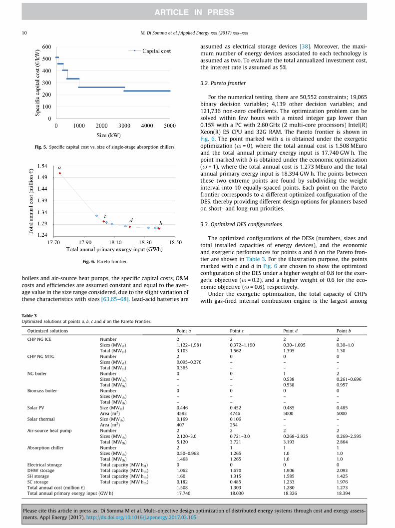
boilers and air-source heat pumps, the specific capital costs, O&Mcosts and efficiencies are assumed constant and equal to the aver-age value in the size range considered, due to the slight variation ofthese characteristics with sizes [63,65–68]. Lead-acid batteries are

assumed as electrical storage devices [38]. Moreover, the maxi-mum number of energy devices associated to each technology isassumed as two. To evaluate the total annualized investment cost,the interest rate is assumed as 5%.

3.2. Pareto frontier

For the numerical testing, there are 50,552 constraints; 19,065binary decision variables; 4,139 other decision variables; and121,736 non-zero coefficients. The optimization problem can besolved within few hours with a mixed integer gap lower than0.15% with a PC with 2.60 GHz (2 multi-core processors) Intel(R)Xeon(R) E5 CPU and 32G RAM. The Pareto frontier is shown inFig. 6. The point marked with a is obtained under the exergeticoptimization (x = 0), where the total annual cost is 1.508 MEuroand the total annual primary exergy input is 17.740 GW h. Thepoint marked with b is obtained under the economic optimization(x = 1), where the total annual cost is 1.273 MEuro and the totalannual primary exergy input is 18.394 GW h. The points betweenthese two extreme points are found by subdividing the weightinterval into 10 equally-spaced points. Each point on the Paretofrontier corresponds to a different optimized configuration of theDES, thereby providing different design options for planners basedon short- and long-run priorities.

3.3. Optimized DES configurations

The optimized configurations of the DESs (numbers, sizes andtotal installed capacities of energy devices), and the economicand exergetic performances for points a and b on the Pareto fron-tier are shown in Table 3. For the illustration purpose, the pointsmarked with c and d in Fig. 6 are chosen to show the optimizedconfiguration of the DES under a higher weight of 0.8 for the exer-getic objective (x = 0.2), and a higher weight of 0.6 for the eco-nomic objective (x = 0.6), respectively.

Under the exergetic optimization, the total capacity of CHPswith gas-fired internal combustion engine is the largest among

Table 3Optimized solutions at points a, b, c and d on the Pareto Frontier.

Optimized solutions Point a Point c Point d Point b

CHP NG ICE Number 2 2 2 2Sizes (MWel) 1.122–1.981 0.372–1.190 0.30–1.095 0.30–1.0Total (MWel) 3.103 1.562 1.395 1.30

CHP NG MTG Number 2 0 0 0Sizes (MWel) 0.095–0.270 – – –Total (MWel) 0.365 – – –

NG boiler Number 0 0 1 2Sizes (MWth) – – 0.538 0.261–0.696Total (MWth) – – 0.538 0.957

Biomass boiler Number 0 0 0 0Sizes (MWth) – – – –Total (MWth) – – – –

Solar PV Size (MWel) 0.446 0.452 0.485 0.485Area (m2) 4593 4746 5000 5000

Solar thermal Size (MWth) 0.169 0.106 – –Area (m2) 407 254 – –

Air-source heat pump Number 2 2 2 2Sizes (MWth) 2.120–3.0 0.721–3.0 0.268–2.925 0.269–2.595Total (MWth) 5.120 3.721 3.193 2.864

Absorption chiller Number 2 1 1 1Sizes (MWth) 0.50–0.968 1.265 1.0 1.0Total (MWth) 1.468 1.265 1.0 1.0

Electrical storage Total capacity (MW hel) 0 0 0 0DHW storage Total capacity (MW hth) 1.062 1.670 1.906 2.093SH storage Total capacity (MW hth) 1.60 1.315 1.585 1.425SC storage Total capacity (MW hth) 0.182 0.485 1.233 1.976Total annual cost (million €) 1.508 1.303 1.280 1.273Total annual primary exergy input (GW h) 17.740 18.030 18.326 18.394

Fig. 5. Specific capital cost vs. size of single-stage absorption chillers.

Fig. 6. Pareto frontier.

10 M. Di Somma et al. / Applied Energy xxx (2017) xxx–xxx

Please cite this article in press as: Di Somma M et al. Multi-objective design optimization of distributed energy systems through cost and exergy assess-ments. Appl Energy (2017), http://dx.doi.org/10.1016/j.apenergy.2017.03.105

the four configurations, and similarly for CHPs with gas-firedmicro-turbine. This highlights the importance of CHPs for the exer-getic objective, due to the possibility of waste heat recovery forthermal purposes, thereby promoting efficient use of the energyresource through a better exploitation of its potential. The large-size CHPs with gas-fired internal combustion engine are selectedto satisfy the high electricity loads, whereas the small-size CHPswith micro-turbine are selected to satisfy the low electricity loads.As x increases, only CHPs with internal combustion engines areselected instead of CHPs with micro-turbines, due to their highertotal energy efficiency and lower investment and O&M costs. Thechosen CHPs are one small and one large in order to cover mostof the electricity load until their minimum part loads. However,the total capacity of CHPs with internal combustion enginesreduces, reaching the minimum under the economic optimization,mostly due to the high investment cost. Conversely, the totalcapacity of natural gas boilers reaches the maximum under theeconomic optimization, due to the low investment and O&M costs,whereas they are not selected under the exergetic optimizationand under a higher weight of the exergetic objective (at point c).This result clearly indicates that natural gas, as a high-qualityenergy resource, should not be used for low-quality thermaldemand.

Biomass boilers are not selected in any configuration. Theabsence of biomass boilers under the exergetic optimizationclearly shows that exergy analysis is a powerful tool for designingmore sustainable energy supply systems, showing that biomass asa high-quality renewable energy resource, should not be used forlow quality thermal demand. Biomass could be used instead formeeting high exergy demand such as for electricity generation,with a better exploitation of the potential of the fuel. In DES designoptimization, minimization of not only fossil but also renewableexergy input promotes efficient use of all energy resources, whilehighlighting that even renewable energy sources need to be usedefficiently based on their potential. This result agrees with thosepresented in [34], where in the operation optimization of a DES,biomass boilers were not used under the exergetic optimization,but they were used under the energy cost minimization due tothe low price of biomass. Moreover, this result also agrees withthose presented in [16], where different energy systems (i.e., gas-fired boiler, biomass boiler, ground-source heat pump, and wastedistrict heat) were compared through exergy analysis to meet ther-mal demand in buildings. It was shown that exergy input of thebiomass boilers is the largest among the four options, since bio-mass, although renewable, is a high-quality energy resource,thereby resulting to be not convenient to meet low-quality thermaldemand. As for DES design optimization, also under the economicoptimization, biomass boilers are not selected due to the highinvestment cost.

As for solar energy systems, the entire available area is occupiedin all the optimized configurations. Under the economic optimiza-tion, the entire area is occupied by PV arrays, highlighting the con-venience of this technology for the economic objective, especiallythanks to the current low costs. The size of PV arrays decreasesas x decreases, reaching the minimum under the exergetic opti-mization, since the available area is also occupied by solar thermalcollectors, whose area is equal to 0 under the economic optimiza-tion, and reaches the maximum under the exergetic optimization.This result highlights the convenience of solar thermal for the exer-getic purpose, due to the low exergy related to the thermal energyoutput from the collectors, used to meet the low-quality thermaldemand.

The total capacities of air-source heat pumps and absorptionchillers increase as x decreases, reaching the maximum underthe exergetic optimization, highlighting their convenience for theexergetic purpose, due to the high conversion efficiency and the

possibility of waste heat recovery for space cooling demand,respectively. When x increases, their total capacities reduce,thereby reducing the total annual cost. Electrical storage (i.e.,lead–acid battery) is never selected. The high investment costmakes this technology not competitive. Therefore, it is not selectedunder the economic optimization. Under the exergetic optimiza-tion, electrical storage is not selected mostly due to the high stor-age loss fraction. As for thermal storage for space cooling demand,the capacity strongly increases as the weight for the economicobjective increases, reaching the maximum under the economicoptimization. This result clearly shows the economic convenienceof the thermal storage for the space cooling demand, whose capac-ity is strongly related to the sizing of absorption chillers. With lar-ger storage capacity, smaller size of absorption chillers are needed,and the total investment cost reduces.

The capacity of thermal storage for domestic hot water demandis maximum under the economic optimization. The capacity ofthermal storage for space heating demand slightly changes withthe weight and is maximum under the exergetic optimization. Dif-ferently from the thermal storage for space cooling, whose capacityis strongly related to the sizing of absorption chillers, the capacitiesof thermal storage for domestic hot water and space heatingdemand mostly depend on the amount of exhaust gas recoveredby CHPs, and therefore depend on the operation strategies of mul-tiple energy devices to be discussed later.

The total annual cost and primary exergy input are also investi-gated for a conventional energy supply system, where grid poweris used for the electricity demand, gas-fired boilers for domestichot water and space heating demand, and electric chillers fed bygrid power for space cooling demand. The total annual cost is equalto 1.914 MEuro, and the total annual primary exergy input is equalto 27.641 GW h. Fig. 7 shows the reduction in total annual cost andprimary exergy input of the DES configurations at points a, b, c andd on the Pareto frontier, as compared with the conventional energysupply system. The maximum reduction in total annual cost, equalto 33.5%, is attained under the economic optimization, whereas thereduction in the total annual primary exergy input is the minimumone, equal to 33.5%. Conversely, the maximum reduction in totalannual primary exergy input, equal to 35.8%, is attained underthe exergetic optimization, whereas the reduction in total annualcost is the minimum one, equal to 21.2%. Therefore, in all the opti-mized DES configurations, strong reduction in total annual cost andprimary exergy input is attained as compared with the conven-tional energy supply system.

Fig. 7. Reduction in total annual cost and primary exergy input of the optimizedDES configurations at points a, b, c and d on the Pareto frontier, as compared withthe conventional energy supply system.

M. Di Somma et al. / Applied Energy xxx (2017) xxx–xxx 11

Please cite this article in press as: Di Somma M et al. Multi-objective design optimization of distributed energy systems through cost and exergy assess-ments. Appl Energy (2017), http://dx.doi.org/10.1016/j.apenergy.2017.03.105

3.4. Operation strategies of energy devices in the optimized DESconfigurations under economic and exergetic optimization

For different optimized DES configurations, different operationstrategies of energy devices are found. For the illustration purpose,the operation strategies of the energy devices in the optimized DESconfigurations obtained under the exergetic and economic opti-mization in the four representative season days are compared inFig. 8.

Fig. 8a for electricity, shows the total grid power, and the totalelectricity provided by CHPs and PV to meet the load as the sumof the total demand and the total electricity required by air-source heat pumps in the four representative season days. Underboth exergetic and economic optimization, electricity from powergrid is generally lower than the electricity provided by CHPs, high-lighting that CHP is convenient for both objectives. Moreover, CHPswith micro-turbines are used only under the exergetic optimiza-tion, since they are not selected under the economic optimizationas presented in the previous subsection, and the electricity pro-vided is smaller than that provided by CHPs with internal combus-tion engines, coherently with the larger size of the latter CHPs. Inthe hot mid-season day, the total electricity provided by CHPs islower than in the other days under both the exergetic and eco-nomic optimization, since only electricity and domestic hot waterdemand need to be satisfied in this day. In this day, under the exer-getic optimization, the electricity from power grid is larger than in

the other days, and it is also larger than the total electricity pro-vided by CHPs, due to the contribution of solar thermal to meetthe domestic hot water demand, as shown in Fig. 8b. It can be alsonoted that the electricity provided by PV is slightly larger under theeconomic optimization than under the exergetic one, coherentlywith the larger size of PV attained under the economic optimiza-tion as discussed in the previous subsection.

Fig. 8b for domestic hot water demand shows the total thermalenergy provided by CHPs, gas-fired boilers, solar thermal collec-tors, as well as the total thermal energy input and output to/fromthe storage to meet the total demand in the four representativeseason days. Under the economic optimization, the thermal energyfrom exhaust gas is larger than under the exergetic one. This is dueto the fact that, in absence of solar thermal, a larger amount ofexhaust gas is used to meet the demand as compared to the exer-getic optimization. Natural gas boilers are only used under the eco-nomic optimization, since they are not selected under the exergeticoptimization as presented in the previous subsection. As for ther-mal storage, it is generally more used under the economic opti-mization than under the exergetic one, due to the larger amountof exhaust gas, which also explains the larger capacity requiredunder the economic optimization.

Fig. 8c for space heating and cooling demand shows the totalthermal energy provided by CHPs, gas-fired boilers, air-source heatpumps, absorption chillers as well as the total thermal energyinput and output to/from the storage systems to meet the total

Fig. 8. Operation strategies of optimized DES configurations at points a and b in the four season days for (a) electricity; (b) domestic hot water; and (c) space heating andcooling.

12 M. Di Somma et al. / Applied Energy xxx (2017) xxx–xxx

Please cite this article in press as: Di Somma M et al. Multi-objective design optimization of distributed energy systems through cost and exergy assess-ments. Appl Energy (2017), http://dx.doi.org/10.1016/j.apenergy.2017.03.105

demands in the four representative season days. For space heating,heat pumps are mostly used to meet the demand under both exer-getic and economic optimization, highlighting that this technologyis convenient for both the objectives. Heat pumps are generallymore used under the exergetic optimization than under the eco-nomic one. Similarly to the case of domestic hot water demand,natural gas boilers are only used under the economic optimization.As for thermal storage, the slightly larger capacity required underthe exergetic optimization than under the economic one is dueto the fact that with a larger usage of heat pumps to meet thedemand, a larger amount of exhaust gas is dispatched to chargethe storage, as compared with what occurs under the economicoptimization. For space cooling demand, similar to space heatingdemand, heat pumps are mostly used to meet the demand underboth exergetic and economic optimization. The thermal energyprovided by the absorption chillers is larger under the exergeticoptimization than under the economic one, coherently with thelarger size attained under the exergetic optimization as presentedin the previous subsection. As for thermal storage, it is much moreused under the economic optimization than under the exergeticone, in accordance to the larger capacity required under the eco-nomic optimization.

4. Sensitivity analysis

A sensitivity analysis is carried out to investigate the influenceof key parameters such as energy prices and energy demand scaleon the optimized DES configurations and the related economic andexergetic performances. In the following, the results of the sensi-tivity analysis on energy prices and energy demand scale are pre-sented and discussed in s 4.1 and 4.2, respectively.

4.1. Energy price sensitivity

The operation strategies of energy devices strongly depend onenergy prices, which in turn affect their combination and sizes inthe DES configurations attained by the optimization model. Withthe increasing consumption of energy resources, energy pricesare expected to increase in next years. In the multi-objective opti-mization problem, the effect of the energy price increase is maxi-mum under the economic optimization, while no effects areunder the exergetic optimization. Results of the economic opti-mization carried out by considering the increase of electricityand natural gas price are presented and discussed in the following.As for biomass, the effect of the price increase is not investigated,since even with the current price, biomass boilers are not selectedunder the economic optimization.

4.1.1. Electricity price sensitivity under the economic optimizationThe results obtained for electricity price increases of 25% until

100% of the current value are compared in Fig. 9. Fig. 9a showsthe increase in the total annual cost and primary exergy input ascompared with those obtained with the current electricity price.It can be noted that the economic performance are more affectedby the electricity price increase than the exergetic ones. However,the effect of electricity price increase on the economic performanceis not that significant: when the electricity price is twice of the cur-rent one, the increase in the total annual cost is less than 2%. This isdue to the fact that, even with the current electricity price, electric-ity from the power grid is much less than that provided by CHPs asdiscussed in the previous section.

For the illustration purpose, the total installed capacities ofenergy devices in the optimized DES configurations obtained with50% and 100% electricity price increase and those obtained withthe current electricity price are compared in Fig. 9b. As the electric-

ity price increases, the total installed capacity of CHP with gas-firedinternal combustion engine increases, since CHPs become moreconvenient. Similar to the current electricity price, also with higherelectricity prices, CHPs with gas- fired micro-turbine are not cho-sen, due to the high investment costs. When electricity priceincreases, the size of PV systems reduces, due to the larger capacityof CHPs used to meet the electricity load. Solar thermal is notselected as occurs with the current electricity price. The totalcapacity of air-source heat pumps and gas-fired boilers remainsalmost unchanged. However, the total capacity of heat pumpsreaches the maximum when the electricity price is twice of thecurrent one due to their high conversion efficiencies, whereas thecontrary occurs for gas-fired boilers. With larger usage of heatpumps, boilers are less used to meet the space heating demand.Biomass boilers are not selected due to the high investment costs.As for absorption chillers, the total capacity reaches the maximumwhen the electricity price is twice of the current one, mainly due tothe larger usage of CHPs and consequent larger amount of exhaustgas used for the space cooling demand. This latter also explains thesignificant increase of the capacity of storage for the space coolingdemand occurring when the electricity price increases.

The effect of electricity price increase on the exergetic perfor-mances is negligible. However, the small increase in the totalannual primary exergy input occurring for higher electricity pricesis due to the reduction in the usage of PV systems and the conse-quent larger usage of natural gas in CHPs to meet the electricityload. This result highlights the importance of PV systems for theexergetic purpose, since the usage of electricity from PV systemsto meet high-quality electricity demand results to be better thanburning natural gas.

4.1.2. Natural gas price sensitivity under the economic optimizationFor natural gas price increases of 25% until 100% of the current

value, the results are compared in Fig. 10. Fig. 10a shows theincrease in the total annual cost and primary exergy input as com-pared with those obtained with the current natural gas price. It canbe noted that the natural gas price increase has larger effects onboth the economic and exergetic performances than electricityprice increase: when the natural gas price is twice of the currentone, the increase in the total annual cost and primary exergy inputare equal to 22.6% and 33.5%, respectively. With the current price,natural gas is the most used primary energy carrier, since it is usedto feed both CHPs and gas-fired boilers, which are much usedunder the economic optimization, as discussed in the previous sec-tion. Therefore, the effect of natural gas increase on the economicand exergetic performances becomes significant.

The total installed capacities of energy devices in the optimizedDES configurations obtained with 50% and 100% natural gas priceincrease and those obtained with the current natural gas priceare compared in Fig. 10b. As the natural gas price increases, thetotal installed capacity of CHP with gas-fired internal combustionengine dramatically reduces, reaching the minimum when thegas price is twice of the current one, whereas CHPs with gas-fired micro-turbine are not selected as occurs with the current nat-ural gas price. The total installed capacity of gas-fired boilersreduces as the gas price increases, even though the reduction ofthe total capacity is not such significant as that of CHPs. This isbecause when natural gas price increases, grid power becomesmuch more convenient than CHPs to meet the electricity load,due to the high investment costs. The increase of natural gas pricehas a lower impact on the installed capacity of gas-fired boilers.Although the gas price increase, gas-fired boilers have low invest-ment costs, and they are still convenient for the economic objec-tive. When natural gas price increases, biomass boilers becomemore convenient than gas-fired boilers, and they are selected inthe optimized DESs configurations, although their investment

M. Di Somma et al. / Applied Energy xxx (2017) xxx–xxx 13

Please cite this article in press as: Di Somma M et al. Multi-objective design optimization of distributed energy systems through cost and exergy assess-ments. Appl Energy (2017), http://dx.doi.org/10.1016/j.apenergy.2017.03.105

costs are higher. For higher natural gas prices, the size of PV sys-tems reduces, since the available area for installation of solar sys-tems is also occupied by solar thermal collectors used to meet thedemand of domestic hot water. As for air-source heat pumps, theirinstalled capacity significantly increases when natural gas priceincreases, due to the strong reduction of exhaust gas from CHPsto meet the demand of space heating and cooling. This latter alsoexplains the significant reduction of the total installed capacityof absorption chillers and of the required capacity of the storagefor space cooling demand. The reduction of exhaust gas from CHPsunder higher natural gas prices also explains the reduced requiredcapacities of storage for domestic hot water and space heatingdemands. Similar to the current natural gas price, electrical storageis not selected due to the high investment costs.

The strong reduction in the usage of CHPs is one of the mostimportant factors influencing the strong increase in the totalannual primary exergy input occurring for natural gas price

increases higher than 25% of the current value. This result underli-nes the importance of waste heat recovery from CHPs for the exer-getic perspective, since, in absence of exhaust gas, othercombustion-based energy devices are used to meet the thermaldemand, thereby increasing the waste of high-quality energy.Another important factor influencing the increase in the totalannual primary exergy is the usage of biomass boilers used to meetthe thermal demand. As discussed earlier, biomass is a high-qualityrenewable energy resource, and it should not be used to meet low-quality thermal demand.

4.2. Energy demand scale sensitivity

The types, number and sizes of energy devices in the DES con-figurations strongly depend on energy demand, which is one ofthe uncertainty factors at the demand side. In the multi-objectiveoptimization problem, the effect of energy demand variation is

Fig. 9. (a) Economic and exergetic performance of optimized DES configurations under the economic optimization for electricity price increases of 25% until 100% of thecurrent value. (b) Total installed capacity of energy devices for various electricity price increases.

Fig. 10. (a) Economic and exergetic performance of optimized DES configurations under the economic optimization for natural gas price increases of 25% until 100% of thecurrent value. (b) Total installed capacity of energy devices for various natural gas price increases.

14 M. Di Somma et al. / Applied Energy xxx (2017) xxx–xxx

Please cite this article in press as: Di Somma M et al. Multi-objective design optimization of distributed energy systems through cost and exergy assess-ments. Appl Energy (2017), http://dx.doi.org/10.1016/j.apenergy.2017.03.105

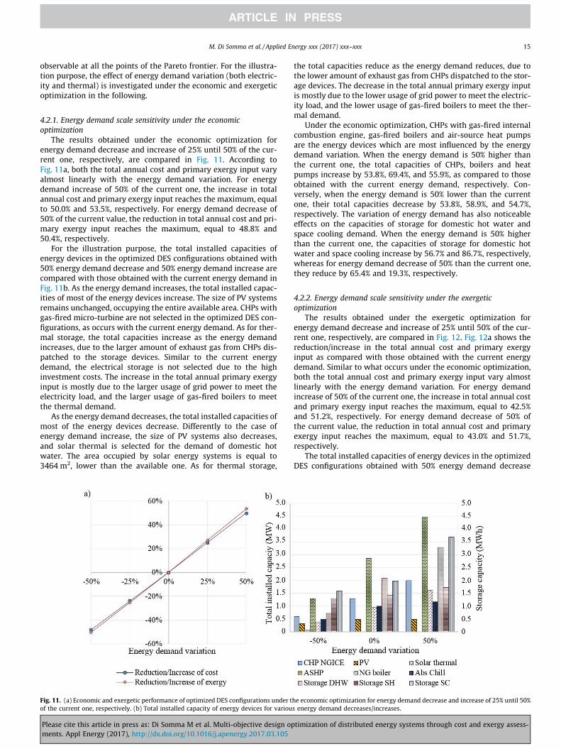
observable at all the points of the Pareto frontier. For the illustra-tion purpose, the effect of energy demand variation (both electric-ity and thermal) is investigated under the economic and exergeticoptimization in the following.

4.2.1. Energy demand scale sensitivity under the economicoptimization

The results obtained under the economic optimization forenergy demand decrease and increase of 25% until 50% of the cur-rent one, respectively, are compared in Fig. 11. According toFig. 11a, both the total annual cost and primary exergy input varyalmost linearly with the energy demand variation. For energydemand increase of 50% of the current one, the increase in totalannual cost and primary exergy input reaches the maximum, equalto 50.0% and 53.5%, respectively. For energy demand decrease of50% of the current value, the reduction in total annual cost and pri-mary exergy input reaches the maximum, equal to 48.8% and50.4%, respectively.

For the illustration purpose, the total installed capacities ofenergy devices in the optimized DES configurations obtained with50% energy demand decrease and 50% energy demand increase arecompared with those obtained with the current energy demand inFig. 11b. As the energy demand increases, the total installed capac-ities of most of the energy devices increase. The size of PV systemsremains unchanged, occupying the entire available area. CHPs withgas-fired micro-turbine are not selected in the optimized DES con-figurations, as occurs with the current energy demand. As for ther-mal storage, the total capacities increase as the energy demandincreases, due to the larger amount of exhaust gas from CHPs dis-patched to the storage devices. Similar to the current energydemand, the electrical storage is not selected due to the highinvestment costs. The increase in the total annual primary exergyinput is mostly due to the larger usage of grid power to meet theelectricity load, and the larger usage of gas-fired boilers to meetthe thermal demand.

As the energy demand decreases, the total installed capacities ofmost of the energy devices decrease. Differently to the case ofenergy demand increase, the size of PV systems also decreases,and solar thermal is selected for the demand of domestic hotwater. The area occupied by solar energy systems is equal to3464 m2, lower than the available one. As for thermal storage,

the total capacities reduce as the energy demand reduces, due tothe lower amount of exhaust gas from CHPs dispatched to the stor-age devices. The decrease in the total annual primary exergy inputis mostly due to the lower usage of grid power to meet the electric-ity load, and the lower usage of gas-fired boilers to meet the ther-mal demand.

Under the economic optimization, CHPs with gas-fired internalcombustion engine, gas-fired boilers and air-source heat pumpsare the energy devices which are most influenced by the energydemand variation. When the energy demand is 50% higher thanthe current one, the total capacities of CHPs, boilers and heatpumps increase by 53.8%, 69.4%, and 55.9%, as compared to thoseobtained with the current energy demand, respectively. Con-versely, when the energy demand is 50% lower than the currentone, their total capacities decrease by 53.8%, 58.9%, and 54.7%,respectively. The variation of energy demand has also noticeableeffects on the capacities of storage for domestic hot water andspace cooling demand. When the energy demand is 50% higherthan the current one, the capacities of storage for domestic hotwater and space cooling increase by 56.7% and 86.7%, respectively,whereas for energy demand decrease of 50% than the current one,they reduce by 65.4% and 19.3%, respectively.

4.2.2. Energy demand scale sensitivity under the exergeticoptimization

The results obtained under the exergetic optimization forenergy demand decrease and increase of 25% until 50% of the cur-rent one, respectively, are compared in Fig. 12. Fig. 12a shows thereduction/increase in the total annual cost and primary exergyinput as compared with those obtained with the current energydemand. Similar to what occurs under the economic optimization,both the total annual cost and primary exergy input vary almostlinearly with the energy demand variation. For energy demandincrease of 50% of the current one, the increase in total annual costand primary exergy input reaches the maximum, equal to 42.5%and 51.2%, respectively. For energy demand decrease of 50% ofthe current value, the reduction in total annual cost and primaryexergy input reaches the maximum, equal to 43.0% and 51.7%,respectively.

The total installed capacities of energy devices in the optimizedDES configurations obtained with 50% energy demand decrease

Fig. 11. (a) Economic and exergetic performance of optimized DES configurations under the economic optimization for energy demand decrease and increase of 25% until 50%of the current one, respectively. (b) Total installed capacity of energy devices for various energy demand decreases/increases.

M. Di Somma et al. / Applied Energy xxx (2017) xxx–xxx 15

Please cite this article in press as: Di Somma M et al. Multi-objective design optimization of distributed energy systems through cost and exergy assess-ments. Appl Energy (2017), http://dx.doi.org/10.1016/j.apenergy.2017.03.105

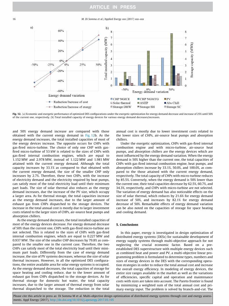
and 50% energy demand increase are compared with thoseobtained with the current energy demand in Fig. 12b. As theenergy demand increases, the total installed capacities of most ofthe energy devices increase. The opposite occurs for CHPs withgas-fired micro-turbine. The choice of only one CHP with gas-fired micro-turbine of 53 kW is related to the sizes of CHPs withgas-fired internal combustion engines, which are equal to1.152 MW and 2.978 MW, instead of 1.122 MW and 1.981 MWattained with the current energy demand. Although the totalcapacity increases by 33.1% as compared to that obtained withthe current energy demand, the size of the smaller CHP onlyincreases by 2.7%. Therefore, these two CHPs, with the increaseof electricity demand and the electricity required by heat pumps,can satisfy most of the total electricity load until their minimumpart loads. The size of solar thermal also reduces as the energydemand increases, due the increase of the PV size, which occupya larger area. As for thermal storage, the total capacities increaseas the energy demand increases, due to the larger amount ofexhaust gas from CHPs dispatched to the storage devices. Theincrease in the total annual cost is mostly due to larger investmentcosts related to the larger sizes of CHPs, air-source heat pumps andabsorption chillers.

As the energy demand decreases, the total installed capacities ofmost of the energy devices decrease. For energy demand decreaseof 50% than the current one, CHPs with gas-fired micro-turbine arenot selected. This is related to the sizes of CHPs with gas-firedinternal combustion engines, which are equal to 0.227 MW and0.937 MW. The size of the smaller CHP decreases by 79.8% as com-pared to the smaller one in the current case. Therefore, the twoCHPs can satisfy most of the total electricity load until their mini-mum part loads. Differently from the case of energy demandincrease, the size of PV systems decreases, whereas the size of solarthermal increases. However, in all the optimized DES configura-tions, the entire available area for solar energy systems is occupied.As the energy demand decreases, the total capacities of storage forspace heating and cooling reduce, due to the lower amount ofexhaust gas from CHPs dispatched to the storage devices. As forthermal storage for domestic hot water, the total capacityincreases, due to the larger amount of thermal energy from solarthermal dispatched to the storage. The reduction in the total

annual cost is mostly due to lower investment costs related tothe lower sizes of CHPs, air-source heat pumps and absorptionchillers.

Under the exergetic optimization, CHPs with gas-fired internalcombustion engine and with micro-turbine, air-source heatpumps, and absorption chillers are the energy devices which aremost influenced by the energy demand variation. When the energydemand is 50% higher than the current one, the total capacities ofCHPs with gas-fired internal combustion engine, heat pumps, andabsorption chillers increase by 33.1%, 50.0%, and 100.0%, as com-pared to the those attained with the current energy demand,respectively. The total capacity of CHPs with micro-turbine reducesby 85.5%. Conversely, when the energy demand is 50% lower thanthe current one, their total capacities decrease by 62.5%, 60.7%, and34.3%, respectively, and CHPs with micro-turbine are not selected.The variation of energy demand has also noticeable effects on thesize of solar thermal, which reduces by 21.6% for energy demandincrease of 50%, and increases by 82.1% for energy demanddecrease of 50%. Remarkable effects of energy demand variationcan be also noted on the capacities of storage for space heatingand cooling demand.

5. Conclusions

In this paper, exergy is investigated in design optimization ofdistributed energy systems (DESs) for sustainable development ofenergy supply systems through multi-objective approach for notneglecting the crucial economic factor. Based on a pre-established DES superstructure with multiple energy devices suchas combined heat and power and PV, a multi-objective linear pro-gramming problem is formulated to determine types, numbers andsizes of energy devices in the DES with the corresponding opera-tion strategies in order to reduce the total annual cost and increasethe overall exergy efficiency. In modeling of energy devices, theentire size ranges available in the market as well as the variationsof efficiencies, specific capital and operation and maintenancecosts with sizes are taken into account. The Pareto frontier is foundby minimizing a weighted sum of the total annual cost and pri-mary exergy input. The problem is solved by branch-and-cut. The

Fig. 12. (a) Economic and exergetic performance of optimized DES configurations under the exergetic optimization for energy demand decrease and increase of 25% until 50%of the current one, respectively. (b) Total installed capacity of energy devices for various energy demand decreases/increases.

16 M. Di Somma et al. / Applied Energy xxx (2017) xxx–xxx

Please cite this article in press as: Di Somma M et al. Multi-objective design optimization of distributed energy systems through cost and exergy assess-ments. Appl Energy (2017), http://dx.doi.org/10.1016/j.apenergy.2017.03.105

models and methods provided can be applied in real contexts.Given the needed input data, the model allows to obtain the opti-mized combination of the candidate energy devices and the corre-sponding operation strategies through cost and exergyassessments, thereby providing decision support to planners.

Numerical results demonstrate that exergy analysis is a power-ful tool for designing more sustainable energy supply systemsbased on the use of renewables and low-temperature sources forthermal demand in buildings, and on a better exploitation of thehigh potential of fossil fuels. Moreover, the Pareto frontier providesgood balancing solutions for planners based on economic and sus-tainability priorities. It is found that, through proper design opti-mization, DESs can offer a good investment opportunity whencompared with conventional energy supply systems, throughrational use of energy resources. The total annual cost and primaryexergy input of DESs with optimized configurations are signifi-cantly reduced as compared with a conventional energy supplysystem, where grid power is used for the electricity demand, gas-fired boilers for domestic hot water and space heating demand,and electric chillers fed by grid power for space cooling demand.As compared with the conventional case, the maximum reductionin the total annual cost and primary exergy input are equal to33.5% and 35.8%, respectively. Also in the other points of the Paretofrontier, a strong reduction in total annual cost and primary exergyinput is attained. In addition, a sensitivity analysis is carried out toanalyze the influence of key parameters, such as energy prices andenergy demand variation on the optimized DES configurations andthe related economic and exergetic performances. It is found thatnatural gas price increase has larger effects than the electricityprice increase on the optimized DES configurations and economicand exergetic performances, whereas the effects of energy demandvariation are noticeable under both the economic and the exergeticoptimization. The results found in this work clearly indicate that,among the candidate energy devices, combined heat and powersystems with gas-fired internal combustion engine are the bestoptions for both reduction of cost and primary exergy input,whereas solar energy systems are important for the exergeticpurpose.

Although there are no exergy requirements as a methodology oran indicator yet in current energy legislations, results underlinethat exergy assessments may allow to meet the main goal ofenergy legislations in improving sustainability of energy supply.Minimization of not only fossil but also renewable exergy inputpromotes an efficient energy resource use through the reductionof the waste of high-quality energy, by avoiding burning processesand substituting them by low-temperature sources for thermaldemand in buildings.

References

[1] Kari A, Arto S. Distributed energy generation and sustainable development.Renew Sustain Energy Rev 2006;10:539–58.

[2] Ren H, Gao W. A MILP model for integrated plan and evaluation of distributedenergy systems. Appl Energy 2010;87(3):1001–14.

[3] Akorede MF, Hizam H, Poresmaeil E. Distributed energy resources and benefitsto the environment. Renew Sustain Energy Rev 2010;14:724–34.

[4] Pepermans G, Driesen J, Haesoldoncklx D, Belmans R, D’haeseleer W.Distributed generation: definition, benefits and issues. Energy Policy2005;33:787–98.

[5] Söderman J, Pettersson F. Structural and operational optimisation ofdistributed energy systems. Appl Therm Eng 2006;26:1400–8.

[6] Bayod-Rujula AA. Future development of the electricity systems withdistributed generation. Energy 2009;34(3):377–83.

[7] Huang J, Jiang C, Xu R. A review on distributed energy resources and microgrid.Renew Sustain Energy Rev 2008;12(9):2472–83.

[8] Han J, Ouyang L, Xu Y, Zeng R, Kang S, Zhang G. Current status of distributedenergy system in China. Renew Sustain Energy Rev 2016;55:288–97.

[9] Chinese D, Meneghetti A. Optimisation models for decision support in thedevelopment of biomass-based industrial district-heating networks in Italy.Appl Energy 2005;82(3):228–54.

[10] Manfren M, Caputo P, Costa G. Paradigm shift in urban energy systems throughdistributed generation: methods and models. Appl Energy 2011;88(4):1032–48.

[11] Ruan Y, Liu Q, Zhou W, Firestone R, Gao W, Watanabe T. Optimal option ofdistributed generation technologies for various commercial buildings. ApplEnergy 2009;86(9):1641–53.

[12] Ren H, Zhou W, Nakagami KI, Gao W, Wu Q. Multi-objective optimization forthe operation of distributed energy systems considering economic andenvironmental aspects. Appl Energy 2010;87(12):3642–51.

[13] Pohekar SD, Ramachandran M. Application of multi-criteria decision making tosustainable energy planning—a review. Renew Sustain Energy Rev 2004;8(4):365–81.

[14] Wang JJ, Jing YY, Zhang CF, Zhao JH. Review on multi-criteria decision analysisaid in sustainable energy decision-making. Renew Sustain Energy Rev 2009;13(9):2263–78.

[15] Alarcon-Rodriguez A, Ault G, Galloway G. Multi-objective planning ofdistributed energy resources: a review of the state-of-the-art. Renew SustainEnergy Rev 2010;14:1353–66.

[16] ECBCS – Annex 49 – Low Exergy Systems for High Performance Buildings andCommunities, homepage. Available <http://www.ecbcs.org/annexes/annex49.htm>.

[17] Dincer I, Rosen MA. Energy, environment and sustainable development. ApplEnergy 1999;64(1):427–40.

[18] Dincer I, Rosen MA. Exergy-energy, environment and sustainabledevelopment. 1st ed. Oxford, UK: Elsevier Publication; 2007.

[19] Dincer I, Rosen MA. Exergy: energy, environment and sustainabledevelopment. Newnes; 2012.

[20] Wall G, Gong M. On exergy and sustainable development—part 1: conditionsand concepts. Exergy Int J 2001;1(3):128–45.

[21] Rosen MA, Dincer I, Kanoglu M. Role of exergy in increasing efficiency andsustainability and reducing environmental impact. Energy Policy 2008;36(1):128–37.

[22] Bilgen E. Exergetic and engineering analyses of gas turbine based cogenerationsystems. Energy 2000;25(12):1215–29.

[23] Gonçalves P, Angrisani G, Rosselli C, Gaspar AR, Da Silva MG. Comparativeenergy and exergy performance assessments of a microcogenerator unit indifferent electricity mix scenarios. Energy Convers Manage 2013;73:195–206.

[24] Feidt M, Costea M. Energy and exergy analysis and optimization of combinedheat and power systems. Comparison of various systems. Energies2012;5:3701–22.

[25] Barelli L, Bidini G, Gallorini F, Ottaviano A. An energetic–exergetic analysis of aresidential CHP system based on PEM fuel cell. Appl Energy 2011;88(12):4334–42.

[26] Hepbasli A. A key review on exergetic analysis and assessment of renewableenergy resources for a sustainable future. Renew Sustain Energy Rev 2008;12(3):593–661.

[27] Kalogirou SA, Karellas S, Badescu V, Braimakis K. Exergy analysis on solarthermal systems: a better understanding of their sustainability. RenewableEnergy 2016;85:1328–33.

[28] Hepbasli A, Akdemir O. Energy and exergy analysis of a ground source(geothermal) heat pump system. Energy Convers Manage 2004;45(5):737–53.

[29] Tsaros TL, Gaggioli RA, Domanski PA. Exergy analysis of heat pumps. ASHRAETrans 1987;93(2):1781–93.

[30] Crawford RR. An experimental laboratory investigation of second law analysisof a vapor-compression heat pump. ASHRAE Trans 1988;94(2):1491–504.

[31] Bjurström H, Carlsson B. An exergy analysis of sensible and latent heat storage.J Heat Recov Syst 1985;5(3):233–50.

[32] Dincer I. On thermal energy storage systems and applications in buildings.Energy Build 2002;34(4):377–88.

[33] Koca A, Oztop HF, Koyun T, Varol Y. Energy and exergy analysis of a latent heatstorage system with phase change material for a solar collector. RenewableEnergy 2008;33(4):567–74.

[34] Di Somma M, Yan B, Bianco N, Luh PB, Graditi G, Mongibello L, et al. Operationoptimization of a distributed energy system considering energy costs andexergy efficiency. Energy Convers Manage 2015;103:739–51.

[35] Yan B, Di Somma M, Bianco N, Luh PB, Graditi G, Mongibello L, et al. Exergy-based operation optimization of a distributed energy system through theenergy-supply chain. Appl Therm Eng 2016;101:741–51.

[36] Mehleri ED, Sarimveis H, Markatos NC, Papageorgiou LG. A mathematicalprogramming approach for optimal design of distributed energy systems atthe neighbourhood level. Energy 2012;44:396–1104.

[37] Mehleri ED, Sarimveis H, Markatos NC, Papageorgiou LG. Optimal design andoperation of distributed energy systems: application to Greek residentialsector. Renewable Energy 2013;51:331–42.

[38] Hawkes AD, Leach MA. Modelling high level system design and unitcommitment for a microgrid. Appl Energy 2009;86(7):253–1265.

[39] Omu A, Choudhary R, Boies A. Distributed energy resource systemoptimisation using mixed integer linear programming. Energy Policy2013;61:249–66.

[40] Wouters C, Fraga ES, James AM, Polykarpou EM. Mixed-integer optimisationbased approach for design and operation of distributed energy systems. In:Power engineering conference (AUPEC), 2014 Australasian Universities IEEE. p.1–6.

[41] Zhou Z, Zhang J, Liu P, Li Z, Georgiadis MC, Pistikopoulos EN. A two-stagestochastic programming model for the optimal design of distributed energysystems. Appl Energy 2013;103:135–44.

M. Di Somma et al. / Applied Energy xxx (2017) xxx–xxx 17

Please cite this article in press as: Di Somma M et al. Multi-objective design optimization of distributed energy systems through cost and exergy assess-ments. Appl Energy (2017), http://dx.doi.org/10.1016/j.apenergy.2017.03.105

[42] Zhou Z, Liu P, Li Z, Ni W. An engineering approach to the optimal design ofdistributed energy systems in China. Appl Therm Eng 2013;53:387–96.

[43] Buoro D, Casisi M, De Nardi A, Pinamonti P, Reini M. Multicriteria optimizationof a distributed energy supply system for an industrial area. Energy2013;58:128–37.

[44] Bracco S, Dentici G, Siri S. Economic and environmental optimization model forthe design and the operation of a combined heat and power distributedgeneration system in an urban area. Energy 2013;55:1014–24.

[45] Maroufmashat A, Sattari S, Roshandel R, Fowler M, Elkamel A. Multi-objectiveoptimization for design and operation of distributed energy systems throughthe multi-energy hub network approach. Ind Eng Chem Res 2016;55(33):8950–66.

[46] Ramirez-Elizondo LM, Paap GC, Ammerlaan R, Negenborn RR, Toonssen R. Onthe energy, exergy and cost optimization of multi-energy-carrier powersystems. Int J Exergy 2013;13:364–85.

[47] Krause T, Kienzle F, Art S, Andersson G. Maximizing exergy efficiency inmulticarrier energy systems. In: Proceedings of IEEE power and energy societygeneral meeting; Minneapolis, USA; 2010 June 25–29.

[48] Lu H, Alanne K, Martinac I. Energy quality management for building clustersand districts (BCDs) though multi-objective optimization. Energy ConversManage 2014;79:525–33.

[49] ANSI/ASHRAE Standard 55. Thermal environmental conditions for humanoccupancy; 2013. <http://www.techstreet.com/products/1868610>.

[50] Kotas YJ. The exergy method for thermal plant analysis. reprint ed. Malabar,FL: Krieger; 1995.

[51] Torìo H, Angelotti A, Schmidt D. Exergy analysis of renewable energy-basedclimatisation systems for buildings: a critical view. Energy Build2009;41:248–71.

[52] Torìo H, Schmidt D. Framework for analysis of solar energy systems in the builtenvironment from an exergy perspective. Renew Energy 2010;35:2689–97.

[53] Available online: <http://www.ibm.com/developerworks/forums/thread.jspa?threadID=368044>.

[54] Aiying R, Risto L. Aneffective heuristic for combinedheat-and-power productionplanning with power ramp constraints. Appl Energy 2007;84:307–25.

[55] Weber C, Shah N. Optimisation based design of a district energy system for aneco-town in the United Kingdom. Energy 2011;36(2):1292–308.

[56] Mongibello L, Bianco N, Caliano M, Graditi G. Influence of heat dumping on theoperation of residential micro-CHP systems. Appl Energy 2015;160:206–20.

[57] Barbieri ES, Melino F, Morini M. Influence of the thermal energy storage on theprofitability of micro CHP systems for residential building applications. ApplEnergy 2012;97:714–22.

[58] Bianchi M, De Pascale A, Spina PR. Guidelines for residential micro-CHPsystems design. Appl Energy 2012;97:673–85.

[59] ASHRAE International Weather files for Energy Calculations (IWEC weatherfiles). Users manual and CD-ROM, American Society of Heating, Refrigeratingand Air-Conditioning Engineers, Atlanta, GA, USA; 2001.

[60] Deloitte. European Energy Market reform – Country Profile: Italy. Availableonline: <https://www2.deloitte.com/content/dam/Deloitte/global/Documents/Energy-and-Resources/gx-er-market-reform-italy.pdf>.

[61] Trudeau N, Francoeur M. Energy Efficiency indicators for Public ElectricityProduction from fossil fuels. OECD/IEA; 2008.

[62] Darrow K, Tidball R, Wang J, Hampson A. Catalog of CHP technologies; 2015.Available: <https://www.epa.gov/sites/production/files/2015-07/documents/catalog_of_chp_technologies.pdf>.

[63] Technology Data for Energy Plants. Energinet.dk; 2012. Available: <https://www.energinet.dk/SiteCollectionDocuments/Danske%20dokumenter/Forskning/Technology_data_for_energy_plants.pdf>.

[64] Goldstein L, Hedman B, Knowles D, Freedman SI, Woods R, Schweizer T. Gas-fired distributed energy resource technology characterizations. NationalRenewable Energy Laboratory; 2003, NREL/TP-620-34783. Available: <http://www.nrel.gov/docs/fy04osti/34783.pdf> <http://www.nrel.gov/docs/fy04osti/34783.pdf>.

[65] Technology Roadmap: Energy-efficient Buildings: Heating and CoolingEquipment. OECD/IEA; 2011. Available: <https://www.iea.org/publications/freepublications/publication/buildings_roadmap.pdf>.

[66] Research on cost and performance of heating and cooling technologies. FinalReport. Department of Energy and Climate Change; 2013. Available: <https://www.gov.uk/government/uploads/system/uploads/attachment_data/file/204275/Research_on_the_costs_and_performance_of_heating_and_cooling_technologies__Sweett_Group_.pdf>.

[67] Heat Pumps: Technology Brief. IEA-ETSAP and IRENA; 2013. Available:<https://www.irena.org/DocumentDownloads/Publications/IRENA-ETSAP%20Tech%20Brief%20E12%20Heat%20Pumps.pdf>.

[68] Combined Heat and Power: Policy Analysis and 2011 – 2030 MarketAssessment. ICF International, Inc; 2012. Available: <http://www.energy.ca.gov/2012publications/CEC-200-2012-002/CEC-200-2012-002.pdf>.

[69] Thermal Energy Storage: Technology Brief. IEA-ETSAP and IRENA; 2013.Available: <https://www.irena.org/DocumentDownloads/Publications/IRENA-ETSAP%20Tech%20Brief%20E17%20Thermal%20Energy%20Storage.pdf>.

18 M. Di Somma et al. / Applied Energy xxx (2017) xxx–xxx

Please cite this article in press as: Di Somma M et al. Multi-objective design optimization of distributed energy systems through cost and exergy assess-ments. Appl Energy (2017), http://dx.doi.org/10.1016/j.apenergy.2017.03.105

1876-6102 © 2017 The Authors. Published by Elsevier Ltd. This is an open access article under the CC BY-NC-ND license (http://creativecommons.org/licenses/by-nc-nd/4.0/).Peer-review under responsibility of the scientific committee of the 8th International Conference on Applied Energy.doi: 10.1016/j.egypro.2017.03.900

Energy Procedia 105 ( 2017 ) 4295 – 4304

ScienceDirect

The 8th International Conference on Applied Energy – ICAE2016

A new approach for the dimensioning of an air conditioning system with cold thermal energy storage

Luigi Mongibelloa,*, Nicola Biancob, Martina Calianob, Giorgio Graditia aENEA Italian National Agency for New Technologies, Energy and Sustainable Economic Development - Portici RC, 80055

Portici (NA), Italy bDipartimento di Ingegneria Industriale (DII) – Università degli Studi Federico II, 80125 Napoli, Italy

Abstract

In this work, a new approach for the design of air conditioning systems with cold thermal energy storage is described and tested, considering the case study represented by a vapor-compression chiller, coupled with a chilled water storage system, producing cooling for a small multi-apartment building situated in Italy. In the present approach, at the aim of limiting shut-downs and start-ups of the chiller, which involve inefficiencies during transients, and can lead to a drastic reduction of the equipment lifetime, the nominal power of the chiller, and the amount of cooling to be stored are first estimated in a pre-design phase. Successively, the outputs of the pre-design are used to fix the size of the cold storage tank, and to set up the numerical simulation of the cold thermal energy storage system. Finally, the results of the numerical simulation of the cold storage system are used to evaluate the effective size of the chiller. Both the pre-design and the numerical simulations of the cold storage systems have been done by means of home-made numerical tool realized with Simulink.

In the paper, the specifications relative to the operational strategy are explored, and the analytical models used for the numerical simulation of the cold storage system relative to the Italian case study are reported in detail. Finally, the results of the pre-design, and of the cold storage system simulations relative to the case study are presented and discussed. The results relative to the Italian case study demonstrates the effectiveness of the present approach in limiting the number of shut-downs and start-ups of the chiller.

The present approach can represent a useful tool for the economic optimization of the design of air conditioning systems. © 2016 The Authors. Published by Elsevier Ltd. Selection and/or peer-review under responsibility of ICAE Keywords: cold storage ; chilled water ; partial storage strategy ; numerical simulation

* Corresponding author. Tel.: +39-081-7723584; fax: +39-081-7723345. E-mail address: luigi.mongibello@enea.it.

Available online at www.sciencedirect.com

© 2017 The Authors. Published by Elsevier Ltd. This is an open access article under the CC BY-NC-ND license (http://creativecommons.org/licenses/by-nc-nd/4.0/).Peer-review under responsibility of the scientific committee of the 8th International Conference on Applied Energy.

4296 Luigi Mongibello et al. / Energy Procedia 105 ( 2017 ) 4295 – 4304

1. Introduction Cold thermal energy storage (CTES) in HVAC&R systems can allow to shift the electric

demand/electric rate fully or partially from on-peak hours to off-peak ones. This generally implies a reduction of the operating costs and of the equipment ones, since thermal energy storage allows to reduce the equipment size, and to have longer operating hours of compressors and pumps, and chillers and cooling towers at full load at lower outdoor temperatures during nighttime. Nevertheless, in general the use of thermal energy storage systems also presents some drawbacks, which essentially are the high initial costs, complicated operation, maintenance and control, and high encumbrance [1,2]. For a generic application, the design of such a system is strongly interconnected with the operation strategy, that can follow a full storage or a partial storage approach, depending essentially on the user demand, the electricity tariffs, and the equipment efficiencies and costs.

The effectiveness of cold storage in obtaining a profitable peak load shifting for refrigeration systems has been demonstrated by a number of works. Many control strategies and several storage materials have been tested to the purpose, with chilled water and ice being the most used cold storage materials. Lin et al. [3] conducted a thermo-economic analysis of an air conditioning system with chilled water storage, in which part of the chilled water back from the user is mixed to the chilled water supplied to the user, and analyzed the thermodynamic performance influence on cost saving. Yan et al. [4] optimized the design of an air conditioning system based on the use of a seasonal heat pipe-based ice storage system. Following their approach, during winter the seasonal ice storage system collects cold energy from ambient low-temperature air. In summer, ice cold energy is extracted for air conditioning, and the melted ice is used as storage medium for chilled water storage. Soler et al. [5] analyzed the performance of a cooling network composed of eight chillers with different capacities and coefficients of performance, and a storage system, at the aim of maximizing chillers operating efficiency, and minimizing the number of shut-downs and start-ups. Meyer and Emery [6] optimized from the economical point of view the operation of an air conditioning system composed of two chillers, one designated for ice storage charging, the other for direct cooling, an air-handling unit, a cooling tower, and water pumps. Habeebullah [7] investigated the economic feasibility of retrofitting an ice thermal energy storage system for an air conditioning system, considering both full storage and partial storage approach.

In the last years, great attention has been also addressed to phase change materials (PCMs) different from ice, which have the potential to considerably lower the size of the storage, and consequently its encumbrance that represents one of the main limits of such systems [8-10].

In this work, a new approach for the dimensioning of air conditioning systems with cold thermal energy storage is described and tested, considering the case study represented by a vapor-compression chiller coupled with a chilled water cold storage system producing cooling for a small multi-apartment building situated in Italy.

In the first part of the paper, the specifications relative to the operational strategy adopted, and to the analytical models used for the numerical simulation of the cold storage system are discussed. Successively, the user thermal and electricity demand for air-conditioning in the summer season are reported. Finally, the results of the pre-design, and of the cold storage system simulations relative to the case study are presented and discussed.

2. Operation strategy and simulation model

2.1. Operation strategy and pre-design

Luigi Mongibello et al. / Energy Procedia 105 ( 2017 ) 4295 – 4304 4297

Considering, for example, an air conditioning system based on an electric chiller and without cold

storage, for a generic user and for a fixed set-point of the internal ambient temperature, generally the chiller operation cannot be continuous during the hours characterized by a refrigeration load that is lower than the minimum chiller thermal power. Indeed, in those hours, the controller of the air conditioning system would switch off the system each time the user internal ambient temperature reaches the predetermined set-point.

In the present approach for the dimensioning of an air conditioning system with cold thermal energy storage, in order to limit the number of shut-downs and start-ups of the chiller, the nominal power of the chiller, and the amount of cooling to be stored are calculated, in a pre-design phase, applying the following operation constraints: during its operation, the chiller has to work at constant power; the chiller cannot feed the cold storage system only, that, in other words, means that cooling can be accumulated only when the chiller has to feed the user; the ratio between the cooling power transferred to the user and the chiller power has to be higher than or equal to a predetermined minimum value, otherwise the chiller is shut down. Successively, the outputs of the pre-design are used to fix the size of the cold storage tank, and to set up the numerical simulation of the cold thermal energy storage system. Finally, the numerical results are used to evaluate the effective size of the chiller.

2.2. Chilled water storage tank model

One-dimensional analytical models have been used in order to simulate the cold water storage tank and the coiled tube heat exchanger [11]. Fig. 1 shows a sketch of the close vertical cylindrical tank with a single immersed serpentine considered in the present study. The internal water volume is divided into isothermal nodes representing water layers of equal volume. The energy balance for each node is written as:

Fig. 1. Sketch of the cold water storage tank

tank

ambwcond

coil

wHTFwpww R

TTQR

TTdt

dTcVw

(1)

where Qcond represents the conductive heat exchange with adjacent layers. The thermal resistance relative to each layer of the storage wall has been evaluated as:

ext_convcondint_convtank RRRR (2)

4298 Luigi Mongibello et al. / Energy Procedia 105 ( 2017 ) 4295 – 4304

where

tankint_tankint_int_conv Ah

R 1 (3)

The mean convective heat transfer coefficient relative to the inner tank wall in equation (3) is

evaluated using the Nusselt number correlation for free convection relative to vertical flat plate [12]. The conductive thermal resistance relative to the tank wall has been evaluated as:

layerins

tank_in

tank_out

cond k

rr

ln

R2

(4)

It has been assumed that the tank thickness is equal to the insulation thickness (0.1m, expanded

polyurethane), namely that the conductive thermal resistance relative to the tank steel wall is negligible. The convective thermal resistance relative to the external tank wall has been evaluated as:

tank_exttank_extext_conv Ah

R 1 (5)

For each time-step and for each node, the energy balance equations system composed of equation (1)

written for all nodes is solved using the implicit Euler method. The empirical reversion-elimination algorithm [13,14] has been adopted in order to include the effects of natural convection heat transfer between the water layers at different heights on the thermal stratification inside the tank.

A transient one-dimensional model has been adopted for the evaluation of the temperature field of the heat transfer fluid (HTF) flowing through the immersed coil heat exchanger.

Also the heat exchanger has been divided in isothermal nodes representing tube sections having the same volume. For each node, the energy balance equation is given by:

out_HTFin_HTFHTFpHTFHTFcoil

HTFtankHTFpnodHTF TTcV

RTT

dtdTcV

HTF (6)

The thermal resistance between the HTF in the coil heat exchanger and the water in the cold storage

tank is given by:

condext_convint_convcoil RRRR (7)

where

coilint_int_coilint_conv Ah

R 1 (8)

Luigi Mongibello et al. / Energy Procedia 105 ( 2017 ) 4295 – 4304 4299

The mean internal convective heat transfer coefficient in equation (8) is evaluated using the

Gnielinski’s correlation for coiled tube heat exchanger [15] for the Nusselt number calculation. The external convective thermal resistance has been evaluated as:

coilextcoilextextconv Ah

R__

_1 (9)

The mean external convective heat transfer coefficient in equation (9) is evaluated using the Morgan’s

correlation for natural convection for horizontal cylinders [16] for the evaluation of the Nusselt number. The conductive thermal resistance of the coil has been neglected, because its order of magnitude is

much lower than the internal and external convective thermal resistances. For each time-step and for each node, equation (6) is solved using the implicit Euler method. The coupling between the cold water tank balance equations system and the one relative to the

serpentine has been dealt with an iterative approach.

3. Case study In the analysed application, the user is represented by a small multi-apartment building, characterized

by a total surface area equal to 800 m2 and an envelope shape factor of 0.5 m-1, and situated in the Italian climatic zone E. The yearly thermal energy demand and the daily thermal and electrical load profiles for the air conditioning in the warm season have been evaluated as in reference [17]. In particular, it has been considered that the air conditioning in the warm season is realized by means of an electrical vapour-compression chiller with a hydronic loop, the yearly thermal energy demand is 21 kWh/m2/yr, and that the daily thermal and electrical load profiles are the same for all the operation days. Fig. 2 shows the hourly averaged thermal and electrical load profiles for refrigeration relative to the user for the standard day considered.

The electrical load profile has been evaluated considering the EER of the chiller depending on the ambient temperature. Fig. 3 shows the variation of the EER as a function of the hourly averaged ambient temperature. In this figure, the temperature profile and the EER one are normalized using the maximum average temperature equal to 28°C, and the maximum value of EER equal to 3, respectively. Thus, with reference to the Fig. 2, and without considering a cold storage integrated into the refrigeration system, for the present user it is necessary a chiller of 7.9 kW of nominal electric power in order to fulfill the request for air conditioning in the summer season.

Fig. 2. Refrigeration load of the user Fig. 3. Non-dimensional temperature and EER profiles

4300 Luigi Mongibello et al. / Energy Procedia 105 ( 2017 ) 4295 – 4304

4. Results

4.1. Pre-design and operation strategy implementation Fig. 4 shows the thermal and electrical powers of the chiller through the day, resulting from the pre-

design relative to the considered case study, obtained by fixing the minimum ratio between the cooling power to the user and the chiller power to 0.5, while Fig. 5 shows on the same graph the resulting chiller thermal power and the refrigeration loads. It can be noticed the peak-shaving effect due to the cold storage. Fig. 6 shows, for each hour of the day, the minutes of continuous operation of the chiller. It can be noticed that the present operation strategy involves only 10 shut-downs and start-ups a day, However, it can be also seen that a large part of the chiller production still remains concentrated in the on-peak hours.

Fig. 4. Chiller power with cold storage Fig. 5. Chiller thermal power and refrigeration loads

Fig. 6. Minutes of operation of the chiller Fig. 7. Difference between the chiller thermal production and the refrigeration loads

Fig. 7 shows, for each hour of the day, the difference between the chiller thermal production and the refrigeration load. Thus, with the adopted approach, the resulting chiller thermal power for the refrigeration system with cold storage is constant and equal to 10.2 kW, with a maximum absorbed electric power of 4.2 kW, that is about the half of the maximum electric power that is needed in the case without the cold storage. The resulting amount of cooling to be stored is 33.6 kWh, that is about the 18% of the user daily total request.

The implementation of the above operation strategy, as well as the numerical simulation of cold storage system, has been performed by means of a home-made tool realized in Simulink. To the purpose, with reference with the simplified layout of the refrigeration system shown in Fig. 8, it has been assumed that the HTF exits the chiller at a constant temperature Tc,out=7.0°C, and at a constant flowrate of 0.4 kg/s.

Luigi Mongibello et al. / Energy Procedia 105 ( 2017 ) 4295 – 4304 4301

Owing to the assumption of constant chiller thermal power, the expected temperature of the HTF at the inflow section of the chiller is equal to Tc,in=13.1°C. The operation constraint of fixing the minimum ratio between the cooling power to the user and the chiller power to 0.5 is equivalent to fixing the minimum ratio between the mass flow rate through the user and the mass flow rate through the chiller to 0.5.

During chiller operation, the mass flow rate of HTF through the user is controlled by means of valve V1 so that the temperature at the user exit, i.e. at point A, is equal to Tc,in. In case the valve V1 is partially open, the HTF passing through V1 goes to the cold storage tank charging it. A further control is applied by means of valve V2 in order to maintain the temperature at point B equal to Tc,in. In this case the valve V3 is fully open while valve V4 is fully close.

Otherwise, in case valve V1 is fully close, which implies that all HTF from the chiller goes to the user and that the HTF exits the user at a temperature that is higher than Tc,in, the cold storage tank is discharged.

Fig. 8. Layout of the refrigeration system Fig. 9. HTF temperature profiles at the tank heat exchanger inflow and outflow sections, and at the chiller inflow section

In this case, a control is applied by means of valve V3 in order to maintain the HTF temperature at point C equal to Tc,in, and valve V2 is fully closed. 4.2. Cold storage tank numerical simulation

The size of the water tank is calculated by using the value of the cooling to be stored coming from the pre-design, i.e. 33.6 kWh, and the difference between the HTF inflow and outflow temperatures relative to the chiller, namely 13.1°C and 7°C, respectively. The resulting water volume is equal to about 4.8 m3. Finally, a commercial cylindrical tank with a capacitance of 4 m3 has been used for the simulations. The tank height from its bottom surface is equal to 2.55 m (not including insulation), and the entire external surface of the tank is insulated by means of a 0.1 m layer of rigid expanded polyurethane. The tank is provided with a single 1” serpentine with a heat exchange surface of 12 m2, and the tank capacitance does not include the volume occupied by the serpentine. The inflow section of the serpentine is placed at 5 cm from the tank bottom surface, while the outflow one at 5 cm from the tank top surface. The results of the numerical simulation presented in this section refer to a spatial discretization of the tank realized using 50 nodes, while the serpentine discretization has been made so that its nodes represent the serpentine portions included in the tank layers relative to the tank nodes. A time-step of 60 s has been adopted. Independency of results from the spatial discretization and time-step has been assured.

At each time-step, the HTF mass flow rate flowing through the tank heat exchanger, and the HTF temperature at the inflow section of the heat exchanger are evaluated according to the operation strategy

4302 Luigi Mongibello et al. / Energy Procedia 105 ( 2017 ) 4295 – 4304

reported in section 4.1. The main outputs of the numerical simulation are the temperatures at the tank and serpentine nodes.

The following results refer to periodic conditions, obtained starting from an initial temperature of the tank water and of the HTF in the serpentine equal to 13.1°C.

Fig. 9 shows the temporal evolution of the HTF temperature at the serpentine outflow during the day, the one relative to the HTF temperature at the serpentine inflow, and the resulting temporal evolution of the HTF temperature at the chiller inflow, while Fig 10 shows the HTF mass flow rate through the serpentine and through the user.

In Fig. 9, it can be noticed that, from h=5 to the end of the storage charging phase, the HTF temperature at the chiller inflow is lower than the nominal chiller inflow temperature, i.e. 13.1°C. This is because, in that time interval, the HTF temperature at the serpentine outflow is lower than 13.1°C, implying that the chiller has to work at a lower power in that period in order to maintain the HTF temperature at its outflow constant and equal to 7°C.

It can be also noticed that, at the end of the discharging phase, the HTF temperature at the serpentine outflow, and the one at the chiller inflow are higher than 13.1°C. In this case, the chiller has to work consuming a higher electrical power than the one evaluated in the pre-design, up to 6.1 kW, in order to keep the outflow temperature constant and equal to 7°C, implying that the chiller operating at a constant absorbed electric power of 4.2 kW, together with the considered commercial size of the cold storage tank, is not capable to fulfill continuously the user request.

The above consideration are evident if Fig 11, showing the cold energy taken and released from the storage during the day evaluated in the pre-feasibility analysis, and the ones resulting from the numerical simulations, is analyzed. In fact, it can be seen that, at the end of the charging phase, the storage system accumulates less cold than the one resulting from the pre-feasibility analysis. Moreover, it can be seen that at the end of the discharging phase, the cold released by the storage system is much lower than the one evaluated in the pre-feasibility analysis. This results are essentially due to chosen tank size, to the storage degradation due to the cold energy losses through the tank external walls, and to the degradation of the temperature stratification inside the tank. Figure 12 and 13 show the evolution of the water temperature profile in the tank during the charging phase and the discharging one, respectively.

Thus, considering the operation strategy and the size of the cold storage system adopted in this study, in the case with cold storage it is necessary to have a chiller, provided with an inverter, characterized by a maximum absorbed electric power of 6.1 kW, that, however, is well below the one relative to the case without the cold storage, namely 8 kW. Table 1 shows the storage tank and chiller sizes obtained by varying the minimum ratio between the cooling power transferred to the user and the chiller power.

Fig. 10. HTF mass flow rate through the tank heat Fig. 11. Cooling energy taken and released from the cold water tank exchanger and the user

Luigi Mongibello et al. / Energy Procedia 105 ( 2017 ) 4295 – 4304 4303

Fig. 12. Temperature profiles in the cold water tank during the Fig. 13. Temperature profiles in the cold water tank during the charging phase (hc=0 refers to the beginning of the phase) discharging phase (hd=0 refers to the beginning of the phase)

Table 1. Main results by varying the minimum ratio between the cooling power transferred to the user and the chiller power Minimum ratio between

the cooling power transferred to the

user and the chiller power

Storage capacity (pre-design)

(kWh)

Storage volume (pre-design)

(m3)

Storage volume (simulation)

(m3)

Chiller powers (pre-design) (kWt , kWe)

Chiller power (simulation) (kWt , kWe)

0 59.9 11.4 8.0 (7.6 , 3.2) (11.5 , 4.8) 0.25 51.84 8.85 8.0 (8.3 , 3.5) (11.4 , 4.7) 0.5 33.60 4.80 4.0 (10.2 , 4.2) (13.5 , 5.6)

0.75 23.35 2.85 2.0 (11.8 , 4.9) (15.1 , 6.3) 1 0 0 - (20.6 , 7.9) -

5. Conclusion

In this work, a new approach for the design of air conditioning systems with cold thermal energy storage is described and tested, considering the case study represented by a vapor-compression chiller, coupled with a chilled water storage system, producing cooling for a small multi-apartment building situated in Italy.

The specifications relative to the operational strategy have been reported, and the characteristics of the analytical models used for the numerical simulation of the cold storage system relative to the Italian case study have been shown as well. The results relative to the Italian case study have demonstrated the effectiveness of the present approach in limiting the number of shut-downs and start-ups of the chiller. References [1] Silvetti B, MacCracken M. Thermal storage and deregulation. ASHRAE Journal, 1998;4:55–59. [2] Wang SK. Handbook of air conditioning and refrigeration. 2nd ed. New York: McGraw-Hill; 2001. [3] Lin H, Li XH, Cheng PS, Xu BG. Thermoeconomic evaluation of air conditioning system with chilled water storage. Energy Conversion and Management, 2014;85: 328–32. [4] Yan C, Shi W, Li X, Zhao Y. Optimal design and application of a compound cold storage system combining seasonal ice storage and chilled water storage. Applied Energy, 2016;171:1–11. [5] Soler MS, Sabaté CC, Santiago VB, Jabbari F. Optimizing performance of a bank of chillers with thermal energy storage. Applied Energy, 2016;172:275–85. [6] Kintner-Meyer M, Emery A. Optimal control of an HVAC system using cold storage and building thermal capacitance. Energy and Buildings, 1995;23(1):19–31. [7] Habeebullah BA. Economic feasibility of thermal energy storage systems. Energy and Buildings, 2007;39:355–63. [8] Sun Y, Wang S, Xiao F Gao D. Peak load shifting using different cold thermal energy storage facilities in commercial buildings: A review. Energy Conversion and Management, 2013;71:101–14. [9] Navidbakhsh M, Shirazi A, Sanaye S. Four E analysis and multi-objective optimization of an ice storage system incorporating PCM as the partial cold storage for air-conditioning applications. Applied Thermal Engineering, 2013;58(1-2): 30–41. [10] Oró E, Depoorter V, Plugradt NSJ. Overview of direct air free cooling and thermal energy storage potential energy savings in data centres. Applied Thermal Engineering, 2015;85:100–110.

4304 Luigi Mongibello et al. / Energy Procedia 105 ( 2017 ) 4295 – 4304

[11] Mongibello L, Bianco N, Caliano M, de Luca A, Graditi G. Transient analysis of a solar domestic hot water system using two different solvers. Energy Procedia, 2015;81:89-99. [12] Bejan A, Kraus AD. Heat Transfer Handbook, Hoboken: John Wiley & Sons Inc. 2003. [13] Mather DW, Hollands KGT, Wright JL. Single- and Multi-Tank energy storage for solar heating systems: Fundamentals. Solar Energy 2002;73:3-13. [14] Newton BJ, Schmid M, Mitchell JW, Beckman WA. Storage tank models. Proceedings of ASME/JSME/JSES International Solar Energy Conference 1995, Maui, Hawaii. [15] Gnielinski Y. Heat transfer and pressure drop in helically coiled tubes. 8th International Heat Transfer Conference 1986;6:2847–54. [16] Morgan VT. The overall convective heat transfer from smooth circular cylinders. Adv. Heat Transfer 1975;11:199-264. [17] Mongibello L, Bianco N, Caliano M, Graditi G. Influence of heat dumping on the operation of residential micro-CHP system. Applied Energy, 2015;160:206–20. Acknowledgement

This work was funded within the Italian Research Program “Ricerca di Sistema Elettrico – PAR 2015, Area: Efficienza energetica e risparmio di energia negli usi finali elettrici ed interazione con altri vettori energetici”.

Biography

Luigi Mongibello, PhD. He graduated in aerospace engineering at the University of Naples “Federico II” (Italy) in 2002, where he completed, in 2005, a doctorate in aerospace engineering with a thesis on actuators for flow control. His research activities are focused on the experimentation, simulation, and optimization of components and systems for solar collectors, CSP and DES plants, and on the thermal design of PV, BIPV and CPV systems.

energies

Article

Cold Storage for a Single-Family House in Italy

Luigi Mongibello * and Giorgio Graditi

ENEA—Italian National Agency for New Technologies, Energy and Sustainable Economic Development,Portici Research Center-Piazzale E. Fermi, 1, 80055 Portici (NA), Italy; giorgio.graditi@enea.it* Correspondence: luigi.mongibello@enea.it; Tel.: +39-081-7723584

Academic Editor: Francesco AsdrubaliReceived: 13 September 2016; Accepted: 6 December 2016; Published: 12 December 2016

Abstract: This work deals with the operation, modeling, simulation, and cost evaluation of twodifferent cold storage systems for a single-family house in Italy, that differ from one another on thecold storage material. The two materials used to perform the numerical simulations of the coldstorage systems are represented by cold water and a phase change material (PCM), and the numericalsimulations have been realized by means of numerical codes written in Matlab environment. The mainfinding of the present work is represented by the fact that, for the considered user characteristics,and under the Italian electricity tariff policy, the use of a proper designed cold storage systemcharacterized by an effective operation strategy could represent a viable solution from an economicalpoint of view.

Keywords: cold storage; cold water; PCM; simulation; single-family house; economic analysis

1. Introduction

The adoption of thermal energy storage in air conditioning systems permits the shifting of theelectric demand/electric rate fully or partially from on-peak hours to off-peak ones. This generallyimplies a reduction of the operating costs and of the equipment ones, since thermal energy storageallows reduction of the equipment size, and to have longer operating hours of compressors andpumps, and chillers and cooling towers at full load at lower outdoor temperatures during night-time.Nevertheless, in general, the use of thermal energy storage systems also presents some drawbacks,which essentially are the high initial costs; complicated operation, maintenance, and control; and highencumbrance [1,2].

The effectiveness of cold storage in obtaining a profitable peak load shifting for refrigerationsystems has been demonstrated by a number of works. Many control strategies and several storagematerials have been tested to the purpose, with chilled water and ice being the most used cold storagematerials. Lin et al. [3] conducted a thermo-economic analysis of an air conditioning system withchilled water storage, in which part of the chilled water back from the user is mixed with the chilledwater supplied to the user, and analyzed the thermodynamic performance influence on cost savings.Yan et al. [4] optimized the design of an air conditioning system based on the use of a seasonal heatpipe-based ice storage system. Following their approach, during winter the seasonal ice storagesystem collects ‘cold energy’ from ambient low-temperature air. In summer, ice cold is extracted for airconditioning, and the melted ice is used as storage medium for chilled water storage. Soler et al. [5]analyzed the performance of a cooling network composed of eight chillers with different capacitiesand coefficients of performance, and a storage system, with the aim of maximizing chiller operatingefficiency and minimizing the number of shut-downs and start-ups. Meyer and Emery [6] economicallyoptimized the operation of an air conditioning system composed of two chillers, one designated for icestorage charging, the other for direct cooling, an air-handling unit, a cooling tower, and water pumps.

Energies 2016, 9, 1043; doi:10.3390/en9121043 www.mdpi.com/journal/energies

Energies 2016, 9, 1043 2 of 16

Habeebullah [7] investigated the economic feasibility of retrofitting an ice thermal energy storagesystem for an air conditioning system, considering both full storage and partial storage approaches.

In the last years, great attention has been also addressed to phase change materials (PCMs)different from ice, which have the potential to considerably lower the size of the storage, andconsequently its encumbrance that represents one of the main limits of such systems [8–10].

This work relies on a novel approach for the design of refrigeration systems with cold storage forsingle-family houses in Italy. This approach consists of two stages: the first one, that in the followingis referred to as pre-design, relies on the implementation of an original operation strategy for therefrigeration system based on partial storage, and aims to perform the dimensioning of the cold storagesystem and a first dimensioning of the chiller; in the second one, the results of the pre-design are usedto set up the numerical simulation of the cold storage system, whose results are used to fix the finalsize of the chiller.

The above design approach has been applied in order to characterize two different cold storagesystems for a single-family house in Italy, that differ from one another on the cold storage material.In particular, the operation, modeling, simulation, and cost evaluation of the two storage systemsare presented in this work. The two materials used to perform the numerical simulations of the coldstorage systems are represented by cold water and a phase change material (PCM), and the numericalsimulations have been realized by means of numerical codes written in Matlab environment.

In the first part of the paper, the characteristics of the user thermal and electricity demand forair-conditioning in the summer season are described. Successively, the specifications of the operationstrategy adopted, and of the analytical models used for the numerical simulations, are explained indetail. Finally, the results of pre-design, of simulations, and of an economic analysis are presentedand discussed.

2. Case Study

In the present study, the user is represented by a single-family house, characterized by a surfacearea equal to 200 m2 and an envelope shape factor of 0.9 m−1, and situated in the Italian climaticzone E. The yearly thermal energy demand and the daily thermal and electrical load profiles for the airconditioning in the warm season have been evaluated as in reference [11]. In particular, it has beenconsidered that the air conditioning in the warm season is limited to the months of June, July, andAugust, and that is realized by means of an electrical vapor compression chiller with a hydronic loop.The yearly thermal energy demand has been fixed to 21 kWh/m2/year, and the same daily thermaland electrical load profiles have been used for all the operation days. Figure 1 shows the hourlyaveraged thermal and electrical load profiles for refrigeration of the considered user for the standardday considered. The electrical load profile has been evaluated considering the energy efficiency ratio(EER) of the chiller depending on the ambient temperature. Figure 2 shows the variation of the EERas a function of the hourly averaged ambient temperature. The temperature profile and the EER onehave been normalized using the maximum average temperature equal to 28 ◦C, and the maximumvalue of EER equal to 3, respectively.

Thus, with reference to the Figure 1, and without considering a cold storage integrated into therefrigeration system, for the present user it is necessary to have a chiller of at least 2 kW of nominalelectrical power, corresponding to the maximum electrical load, in order to fulfill the request for airconditioning in the summer season.

Energies 2016, 9, 1043 3 of 16Energies 2016, 9, 1043 3 of 16

Figure 1. Refrigeration loads of the user.

Figure 2. Non-dimensional temperature and EER profiles.

3. Operation Strategy and Methodologies of Analysis

With the aim of performing a reasonable integration and dimensioning of a cold storage system into the hydronic loop of the refrigeration system for the single-family house under study, a qualitative preliminary analysis has been done in order to evaluate what could be the most convenient approach between full storage and partial storage. The above analysis has been done taking into consideration that the Italian scenario concerning the electricity tariff allows private consumers to benefit from a reduced price of the electricity when it is used during night-time at off-peak hours. Nevertheless, it has emerged that partial storage is likely more convenient than full storage, mainly because the difference between the tariffs in on-peak hours and off-peak ones is not so high. Moreover, full storage would require a much larger tank for the cold storage, and it would also require a chiller with nominal power not much lower than the one in the case without storage. For the above reasons, the partial storage approach could be preferable and has been adopted in this study.

3.1. Operation Strategy and Pre-Design

3.1.1. Assumptions and Pre-Design

Considering the refrigeration loads reported in Figure 1, it is clear that, without cold storage, and for a fixed set-point of the user internal ambient temperature, the chiller operation cannot be continuous during the hours characterized by a refrigeration load that is lower than the minimum chiller thermal power. In those hours, the controller of the refrigeration system would implement several shut-downs of the chiller, that generally affects the chiller lifetime negatively. Indeed, the controller would switch off the chiller each time the user internal ambient temperature has reached

Figure 1. Refrigeration loads of the user.

Energies 2016, 9, 1043 3 of 16

Figure 1. Refrigeration loads of the user.

Figure 2. Non-dimensional temperature and EER profiles.

3. Operation Strategy and Methodologies of Analysis

With the aim of performing a reasonable integration and dimensioning of a cold storage system into the hydronic loop of the refrigeration system for the single-family house under study, a qualitative preliminary analysis has been done in order to evaluate what could be the most convenient approach between full storage and partial storage. The above analysis has been done taking into consideration that the Italian scenario concerning the electricity tariff allows private consumers to benefit from a reduced price of the electricity when it is used during night-time at off-peak hours. Nevertheless, it has emerged that partial storage is likely more convenient than full storage, mainly because the difference between the tariffs in on-peak hours and off-peak ones is not so high. Moreover, full storage would require a much larger tank for the cold storage, and it would also require a chiller with nominal power not much lower than the one in the case without storage. For the above reasons, the partial storage approach could be preferable and has been adopted in this study.

3.1. Operation Strategy and Pre-Design

3.1.1. Assumptions and Pre-Design

Considering the refrigeration loads reported in Figure 1, it is clear that, without cold storage, and for a fixed set-point of the user internal ambient temperature, the chiller operation cannot be continuous during the hours characterized by a refrigeration load that is lower than the minimum chiller thermal power. In those hours, the controller of the refrigeration system would implement several shut-downs of the chiller, that generally affects the chiller lifetime negatively. Indeed, the controller would switch off the chiller each time the user internal ambient temperature has reached

Figure 2. Non-dimensional temperature and EER profiles.

3. Operation Strategy and Methodologies of Analysis

With the aim of performing a reasonable integration and dimensioning of a cold storage systeminto the hydronic loop of the refrigeration system for the single-family house under study, a qualitativepreliminary analysis has been done in order to evaluate what could be the most convenient approachbetween full storage and partial storage. The above analysis has been done taking into considerationthat the Italian scenario concerning the electricity tariff allows private consumers to benefit from areduced price of the electricity when it is used during night-time at off-peak hours. Nevertheless, it hasemerged that partial storage is likely more convenient than full storage, mainly because the differencebetween the tariffs in on-peak hours and off-peak ones is not so high. Moreover, full storage wouldrequire a much larger tank for the cold storage, and it would also require a chiller with nominal powernot much lower than the one in the case without storage. For the above reasons, the partial storageapproach could be preferable and has been adopted in this study.

3.1. Operation Strategy and Pre-Design

3.1.1. Assumptions and Pre-Design

Considering the refrigeration loads reported in Figure 1, it is clear that, without cold storage,and for a fixed set-point of the user internal ambient temperature, the chiller operation cannot becontinuous during the hours characterized by a refrigeration load that is lower than the minimumchiller thermal power. In those hours, the controller of the refrigeration system would implementseveral shut-downs of the chiller, that generally affects the chiller lifetime negatively. Indeed, the

Energies 2016, 9, 1043 4 of 16

controller would switch off the chiller each time the user internal ambient temperature has reachedthe predetermined set-point. Taking into account the above considerations, in the present study theamount of cold to be stored, and the nominal power of the chiller, in the case with cold storage, havebeen initially calculated by considering the following assumptions:

1. during its operation, the chiller has to work at constant power, constant mass flow rate, andconstant outflow temperature Tc,out;

2. the ratio between the cooling power transferred to the user and the chiller power has to be higherthan or equal to a predetermined minimum value, otherwise the chiller is shut down;

3. the chiller cannot feed the cold storage system only, that, in other words, means that the cold canbe accumulated only when the chiller has to feed the user.

Clearly, assumption 1 implies that also the inflow temperature of the chiller Tc,in is constant.The above assumptions allow to uniquely identify the size of the chiller and the total amount

of cold to be stored for the considered user. Later in the paper, it will be shown that this operationalapproach involves a relatively low size of the cold storage tank, a considerable reduction of the chillerpower with respect to the case without the cold storage, and also that the chiller operates continuouslyfor great part of the day. The results of the pre-design are then used to fix the size of the cold storagetank, and to set up the numerical simulation of the cold thermal energy storage system. Finally,the numerical results are used to evaluate the effective size of the chiller.

3.1.2. Operation of the Refrigeration System with Cold Storage

Figure 3 shows a schematic of the layout of the refrigeration system adopted for theimplementation of the operational approach described in the previous section.

During chiller operation, the mass flow rate of the heat transfer fluid (HTF) through the user iscontrolled by means of valve V1 so that the temperature at the user exit—i.e., at point A—is equal toTc,in. In case the valve V1 is partially open, the HTF passing through V1 goes to the cold storage tankcharging it. A further control is applied by means of valve V2 in order to maintain the temperature atpoint B equal to Tc,in. In this case the valve V3 is fully open while valve V4 is fully close.

Otherwise, in case valve V1 is fully close, which implies that all HTF from the chiller goes to theuser and that the HTF exits the user at a temperature that is higher than Tc,in, the cold storage tankis discharged. In this case, a control is applied by means of valve V3 in order to maintain the HTFtemperature at point C equal to Tc,in, and also V2 is fully closed.

Assumptions 1 and 2 of the operational approach imply that the mass flow rate of HTF flowingthrough the user has to be higher than or equal to a minimum value, fixed equal to half the nominalHTF mass flow rate through the chiller, otherwise the chiller is shut down.

Energies 2016, 9, 1043 4 of 16

the predetermined set-point. Taking into account the above considerations, in the present study the amount of cold to be stored, and the nominal power of the chiller, in the case with cold storage, have been initially calculated by considering the following assumptions:

1. during its operation, the chiller has to work at constant power, constant mass flow rate, and constant outflow temperature Tc,out;

2. the ratio between the cooling power transferred to the user and the chiller power has to be higher than or equal to a predetermined minimum value, otherwise the chiller is shut down;

3. the chiller cannot feed the cold storage system only, that, in other words, means that the cold can be accumulated only when the chiller has to feed the user.

Clearly, assumption 1 implies that also the inflow temperature of the chiller Tc,in is constant. The above assumptions allow to uniquely identify the size of the chiller and the total amount of

cold to be stored for the considered user. Later in the paper, it will be shown that this operational approach involves a relatively low size of the cold storage tank, a considerable reduction of the chiller power with respect to the case without the cold storage, and also that the chiller operates continuously for great part of the day. The results of the pre-design are then used to fix the size of the cold storage tank, and to set up the numerical simulation of the cold thermal energy storage system. Finally, the numerical results are used to evaluate the effective size of the chiller.

3.1.2. Operation of the Refrigeration System with Cold Storage

Figure 3 shows a schematic of the layout of the refrigeration system adopted for the implementation of the operational approach described in the previous section.

During chiller operation, the mass flow rate of the heat transfer fluid (HTF) through the user is controlled by means of valve V1 so that the temperature at the user exit—i.e., at point A—is equal to Tc,in. In case the valve V1 is partially open, the HTF passing through V1 goes to the cold storage tank charging it. A further control is applied by means of valve V2 in order to maintain the temperature at point B equal to Tc,in. In this case the valve V3 is fully open while valve V4 is fully close.

Otherwise, in case valve V1 is fully close, which implies that all HTF from the chiller goes to the user and that the HTF exits the user at a temperature that is higher than Tc,in, the cold storage tank is discharged. In this case, a control is applied by means of valve V3 in order to maintain the HTF temperature at point C equal to Tc,in, and also V2 is fully closed.

Assumptions 1 and 2 of the operational approach imply that the mass flow rate of HTF flowing through the user has to be higher than or equal to a minimum value, fixed equal to half the nominal HTF mass flow rate through the chiller, otherwise the chiller is shut down.

Figure 3. Layout of the refrigeration system.

3.2. Cold Water Storage Tank Model

Figure 3. Layout of the refrigeration system.

Energies 2016, 9, 1043 5 of 16

3.2. Cold Water Storage Tank Model

1D analytical models have been used in order to simulate the cold water storage tank and thecoiled tube heat exchanger [12]. Figure 4 shows a sketch of the close vertical cylindrical tank with asingle immersed serpentine considered in the present study. This cold water storage tank configuration,in which the HTF is separated from the water in the tank, permits the use of HTFs different from water,and consequently allows HTF temperatures at the chiller outflow (Tc,out) even slightly higher than0 ◦C, as for example 1 ◦C or 2 ◦C. Indeed, in such cases it would be not possible to use water as HTFsince water could freeze inside the chiller, and a mixture of water and antifreeze should be used.

Energies 2016, 9, 1043 5 of 16

1D analytical models have been used in order to simulate the cold water storage tank and the coiled tube heat exchanger [12]. Figure 4 shows a sketch of the close vertical cylindrical tank with a single immersed serpentine considered in the present study. This cold water storage tank configuration, in which the HTF is separated from the water in the tank, permits the use of HTFs different from water, and consequently allows HTF temperatures at the chiller outflow (Tc,out) even slightly higher than 0 °C, as for example 1 °C or 2 °C. Indeed, in such cases it would be not possible to use water as HTF since water could freeze inside the chiller, and a mixture of water and antifreeze should be used.

Figure 4. Sketch of the cold water storage tank.

The internal water volume is divided into isothermal nodes representing water layers of equal volume. The energy balance for each node is written as:

( ) ( )HTFw

w w ambww w p cond

coil tank

T T T TdTV c Qdt R R

ρ− −

= + − (1)

where Qcond represents the conductive heat exchange with adjacent layers. The thermal resistance relative to each layer of the storage wall has been evaluated as:

extconvcondconvtank RRRR _int_ ++= (2)

where

int_tankint_tankconv_int AhR

1= (3)

The mean convective heat transfer coefficient relative to the inner tank wall in Equation (3) is evaluated using the Nusselt number correlation for free convection relative to a vertical flat plate [13].

The conductive thermal resistance relative to the tank wall has been evaluated as:

layerins

in_tank

out_tank

cond k

r

r

RΔ

=π2

ln

(4)

It has been assumed that the tank thickness is equal to the insulation thickness (0.1 m, expanded polyurethane), namely that the conductive thermal resistance of the tank steel wall is negligible.

The convective thermal resistance relative to the external tank wall has been evaluated as:

ext_tankext_tankconv_ext AhR

1= (5)

For each time-step and for each node, the energy balance equations system composed of Equation (1) written for all nodes is solved using the implicit Euler method. The empirical reversion-elimination algorithm [14,15] has been adopted in order to include the effects of natural

Figure 4. Sketch of the cold water storage tank.

The internal water volume is divided into isothermal nodes representing water layers of equalvolume. The energy balance for each node is written as:

ρwVwcpw

dTw

dt=

(THTF − Tw)

Rcoil+ Qcond −

(Tw − Tamb)

Rtank(1)

where Qcond represents the conductive heat exchange with adjacent layers. The thermal resistancerelative to each layer of the storage wall has been evaluated as:

Rtank = Rconv_int + Rcond + Rconv_ext (2)

whereRconv_int =

1hint_tank Aint_tank

(3)

The mean convective heat transfer coefficient relative to the inner tank wall in Equation (3) isevaluated using the Nusselt number correlation for free convection relative to a vertical flat plate [13].

The conductive thermal resistance relative to the tank wall has been evaluated as:

Rcond =ln(

rout_tankrin_tank

)2πkins∆layer

(4)

It has been assumed that the tank thickness is equal to the insulation thickness (0.1 m, expandedpolyurethane), namely that the conductive thermal resistance of the tank steel wall is negligible.

The convective thermal resistance relative to the external tank wall has been evaluated as:

Rconv_ext =1

hext_tank Aext_tank(5)

For each time-step and for each node, the energy balance equations system composed of Equation (1)written for all nodes is solved using the implicit Euler method. The empirical reversion-eliminationalgorithm [14,15] has been adopted in order to include the effects of natural convection heat transferbetween the water layers at different heights on the thermal stratification inside the tank.

Energies 2016, 9, 1043 6 of 16

A transient one-dimensional model has been adopted for the evaluation of the temperature fieldof the HTF flowing through the immersed coil heat exchanger. The HTF considered is water.

Also, the heat exchanger has been divided in isothermal nodes representing tube sections havingthe same volume. For each node, the energy balance equation is given by:

ρHTFVnodcpHTF

dTHTF

dt=

(Ttank − THTF)

Rcoil+ ρHTF

.VHTFcpHTF(THTF_in − THTF_out) (6)

The thermal resistance between the HTF in the coil heat exchanger and the water in the coldstorage tank is given by:

Rcoil = Rconv_int + Rconv_ext + Rcond (7)

whereRconv_int =

1hint_coil Aint_coil

(8)

The mean internal convective heat transfer coefficient in Equation (8) is evaluated using theGnielinski’s correlation for coiled tube heat exchanger [16] for the Nusselt number calculation.

The external convective thermal resistance has been evaluated as:

Rconv_ext =1

hext_coil Aext_coil(9)

The mean external convective heat transfer coefficient in Equation (9) is evaluated using theMorgan’s correlation for natural convection for horizontal cylinders [17] for the Nusselt number.

The conductive thermal resistance of the coil has been neglected, because its order of magnitudeis much lower than the internal and external convective thermal resistances.

For each time-step and for each node, Equation (6) is solved using the implicit Euler method.The coupling between the cold water tank balance equations system and the one relative to the

serpentine has been dealt with an iterative approach.

3.3. PCM Storage Tank Model

Figure 5 shows a schematic of the cylindrical cold storage tank with a PCM as storage materialconsidered in this study. The inflow and outflow plenums for the HTF are connected by uniformlydistributed straight parallel 1/4” pipes passing through the PCM material placed in the central body ofthe tank, and composing the heat exchanger.

Energies 2016, 9, 1043 6 of 16

convection heat transfer between the water layers at different heights on the thermal stratification inside the tank.

A transient one-dimensional model has been adopted for the evaluation of the temperature field of the HTF flowing through the immersed coil heat exchanger. The HTF considered is water.

Also, the heat exchanger has been divided in isothermal nodes representing tube sections having the same volume. For each node, the energy balance equation is given by:

( ) ( )HTF

HTFHTFHTF HTF HTF HTF HTF HTF

tanknod p p _in _out

coil

T TdTV c V c T Tdt R

ρ ρ−

= + − (6)

The thermal resistance between the HTF in the coil heat exchanger and the water in the cold storage tank is given by:

condextconvconv_intcoil RRRR ++= _ (7)

where

int_coilint_coilconv_int AhR

1= (8)

The mean internal convective heat transfer coefficient in Equation (8) is evaluated using the Gnielinski’s correlation for coiled tube heat exchanger [16] for the Nusselt number calculation.

The external convective thermal resistance has been evaluated as:

1conv_ext

ext_coil ext_coil

Rh A

= (9)

The mean external convective heat transfer coefficient in Equation (9) is evaluated using the Morgan’s correlation for natural convection for horizontal cylinders [17] for the Nusselt number.

The conductive thermal resistance of the coil has been neglected, because its order of magnitude is much lower than the internal and external convective thermal resistances.

For each time-step and for each node, Equation (6) is solved using the implicit Euler method. The coupling between the cold water tank balance equations system and the one relative to the

serpentine has been dealt with an iterative approach.

3.3. PCM Storage Tank Model

Figure 5 shows a schematic of the cylindrical cold storage tank with a PCM as storage material considered in this study. The inflow and outflow plenums for the HTF are connected by uniformly distributed straight parallel ¼” pipes passing through the PCM material placed in the central body of the tank, and composing the heat exchanger.

Figure 5. Schematic of the cold storage tank with PCM.

Table 1 reports the main thermo-physical characteristics of the organic PCM considered in the present study. Also in this case, the HTF flowing through the heat exchanger is water.

Figure 5. Schematic of the cold storage tank with PCM.

Table 1 reports the main thermo-physical characteristics of the organic PCM considered in thepresent study. Also in this case, the HTF flowing through the heat exchanger is water.

Energies 2016, 9, 1043 7 of 16

Table 1. Characteristics of the PCM.

Property Value

Density 900 kg/m3

Thermal conductivity 0.2 W/m/K

Latent heat of fusion 18 × 104 J/kg

Melting temperature 13 ◦C

It has been supposed that the charging and discharging processes are isothermal and realized atthe PCM solidification/melting temperature, namely that the cold is stored only as latent heat. Thus,the volume of PCM that is necessary to store a certain amount of cold Ec is given by:

VPCM =Ec

LHPCMρPCM(10)

where LHPCM and ρPCM are the PCM latent heat of fusion and density, respectively.The size of the heat exchanger has been evaluated by means of the ε-NTU method [13],

implemented on an hourly basis. This method is typically employed for the thermal design of standardheat exchangers, and it has been recently adopted by Tay et al. [18] and Mongibello et al. [19] for latentheat thermal energy storage systems. Therefore, for each pipe of the heat exchanger, the thermal powerexchanged between the HTF to the PCM is given by:

.Q = ε

.mcp,HTF∆T (11)

where ∆T represents the difference between the HTF temperature at the inlet section of the pipe andthe PCM melting temperature,

.m is the mass flow rate of the HTF through the pipe, and ε represents

the heat exchanger efficiency, given by:

ε = 1 − e(NTU) (12)

The number of transfer units NTU is calculated using the following expression:

NTU =1

Rtot.

mcp,HTF(13)

The overall thermal resistance is given by:

Rtot = RHTF + Rwall + RPCM (14)

where the thermal resistance relative to the heat transfer between the pipe external surface and thePCM is calculated as:

RPCM =1

C(δ)kPCM(15)

In Equation (15), the parameter C(δ) refers to the conduction between the pipe external surfaceand the phase change front supposed concentric to the pipe, and it is a function of the parameterδ representing the ratio between the liquefied portion of the PCM total volume and the PCM totalvolume. Accordingly, being the phase change front variable with time during the charging phase,the heat exchanger efficiency ε results to be time dependent. Thus, for each operation hour, the averagevalue of the efficiency can be used in Equation (11), that becomes:

.Q = ε

.mcp,HTF∆T (16)

Energies 2016, 9, 1043 8 of 16

For given values of the mass flow rate, of the minutes of operation of the chiller, of the temperatureof the HTF entering the storage tank, and of cold to be accumulated at each operation hour, and fora fixed reasonable volume of PCM filling up the storage tank and a fixed aspect ratio of the tank,the number of pipes of the heat exchanger can be evaluated by means of the iterative procedureprescribing the following steps:

1. Fix an initial tentative value for the number of pipes;2. Divide the total PCM volume in its initial state by the number of pipes in order to evaluate the

volume of PCM surrounding each pipe, that is supposed concentric to the pipe;3. Knowing the cold to be stored or released and the minutes of operation at each hour, evaluate the

thermal power to be exchanged at each hour, and evaluate for each hour the fraction of the PCMvolume surrounding the pipes that undergoes solidification or melting using Equation (10);

4. Knowing the fraction of PCM that has undergone phase change, determine for each hour theaverage efficiency of the heat exchanger using Equations (12)–(15);

5. For each hour, calculate the thermal power exchanged by means Equation (16);6. For each hour, compare the value of thermal power calculated at Step 5 with the one calculated

at Step 3. If the maximum of the absolute values of the differences between thermal powervalues is lower than a certain tolerance, then stop the procedure and accept the number of pipes.Otherwise, increase or reduce the number of pipes as a function of the above differences andreturn to Step 2.

Finally, once dimensioned the heat exchanger, the energy balance at the heat exchanger pipespermits the calculation of the HTF temperature at the storage tank exit.

The initial tentative value of the number of pipes has to be low enough to avoid the occurrence ofconditions in which the cold can be only stored by sensible energy. Indeed, the present model cannotbe applied when only sensible energy storage is expected, as for example in the case charging is donewhen the entire PCM volume is already in the solid phase, or, equivalently, when the discharging isdone when the entire PCM volume is already in the liquid one.

A similar procedure can be implemented to evaluate the total PCM volume for a fixed aspect ratioof the tank. In this case, a reasonable number of pipes is fixed, and the total PCM volume is varied inorder to match the exchanged thermal power values. Similarly, in this case the initial tentative value oftotal PCM volume has to be high enough to avoid that the occurrence of conditions in which the coldcan be only stored by sensible energy.

4. Results

4.1. Pre-Design

Figure 6 shows the thermal and electrical powers of the chiller through the day, while Figure 7shows on the same graph the chiller thermal power and the refrigeration loads, resulting fromthe pre-design. Thus, with the adopted operational approach, the chiller thermal power for therefrigeration system with cold storage resulting from the pre-design is equal to 2.55 kW, with amaximum absorbed electric power of 1.05 kW, that is about the half of the maximum electric powerthat is needed in the case without the cold storage. Furthermore, it can be noticed the peak-shavingeffect due to the cold storage. Figure 8 shows, for each hour of the day, the minutes of operation of thechiller resulting from the pre-design. It can be noticed that, owing to the adopted operational approach,the chiller operation is continuous over a great part of the day, and that the chiller production stillremains concentrated in the on-peak hours.

Figure 9 shows, for each hour of the day, the difference between the chiller thermal productionand the refrigeration load. The total amount of cold to be stored resulting from the pre-design is8.4 kWh, that is about the 18% of the user daily total request.

Energies 2016, 9, 1043 9 of 16Energies 2016, 9, 1043 9 of 16

Figure 6. Chiller power with cold storage.

Figure 7. Chiller thermal power and refrigeration loads.

Figure 8. Minutes of operation of the chiller.

Figure 6. Chiller power with cold storage.

Energies 2016, 9, 1043 9 of 16

Figure 6. Chiller power with cold storage.

Figure 7. Chiller thermal power and refrigeration loads.

Figure 8. Minutes of operation of the chiller.

Figure 7. Chiller thermal power and refrigeration loads.

Energies 2016, 9, 1043 9 of 16

Figure 6. Chiller power with cold storage.

Figure 7. Chiller thermal power and refrigeration loads.

Figure 8. Minutes of operation of the chiller. Figure 8. Minutes of operation of the chiller.

Energies 2016, 9, 1043 10 of 16Energies 2016, 9, 1043 10 of 16

Figure 9. Difference between the chiller thermal production and the refrigeration loads.

4.2. Cold Water Storage Tank

The numerical simulation of the cold water storage tank has been done assuming that the HTF exits the chiller at a constant temperature Tc,out = 7.0 °C, and at a constant total mass flowrate of 0.1 kg/s. The assumption of constant chiller thermal power implies that the expected temperature of the HTF at the inflow section of the chiller is equal to Tc,in = 13.1 °C.

The volume of the cold water storage tank has been calculated by using the difference between the HTF temperatures at the chiller inflow and outflow sections, namely 13.1 °C and 7 °C, respectively. It is given by:

( ),tot, ,w

ww p c in c out

SCVc T Tρ

=−

(17)

where SC represents the maximum storage capacity resulting from the pre-design, i.e., 8.4 kWh (30.27 MJ). The resulting water volume is equal to about 1200 L. Finally, a commercial cylindrical tank with a capacitance of 1000 L has been used for the simulations. The tank height from its bottom surface is equal to 2 m (not including insulation), and the entire external surface of the tank is insulated by means of a 0.1 m layer of rigid expanded polyurethane. The tank is provided with a single 1″ serpentine with a heat exchange surface of 8 m2, and the tank capacitance does not include the volume occupied by the serpentine. The inflow section of the serpentine is placed at 5 cm from the tank bottom surface, while the outflow one at 5 cm from the tank top surface. The results of the numerical simulation presented in this section refer to a spatial discretization of the tank realized using 50 nodes, while the serpentine discretization has been made so that its nodes represent the serpentine portions included in the tank layers relative to the tank nodes, and a time-step of 60 s has been adopted. Independence of results from the spatial discretization and time-step has been assured.

The main outputs of the Matlab code are the temperatures at the tank and serpentine nodes. At each time-step, the HTF mass flow rate flowing through the tank heat exchanger, and the HTF temperature at the inflow section of the heat exchanger have been evaluated according to the operation strategy reported in Section 3.1. At each hour, the chiller is active, and the mass flow rate is different from zero, only during the corresponding minutes of operation of the chiller reported in Figure 8. Finally, the following results refer to periodic conditions, obtained starting from an initial temperature of the tank water and of the HTF in the serpentine equal to 13.1 °C.

Figure 10 shows the temporal evolution of the HTF temperature at the serpentine outflow during the day, of the HTF temperature at the serpentine inflow, and the resulting temporal evolution of the HTF temperature at the chiller inflow, while Figure 11 shows the HTF mass flow rate through the serpentine and through the user. With reference to Figure 10, it can be noticed that, around h = 12, the HTF temperature at the chiller inflow is slightly lower than the expected value of Tc,in, i.e., 13.1 °C. This is because, in that time interval, the HTF temperature at the serpentine outflow

Figure 9. Difference between the chiller thermal production and the refrigeration loads.

4.2. Cold Water Storage Tank

The numerical simulation of the cold water storage tank has been done assuming that the HTFexits the chiller at a constant temperature Tc,out = 7.0 ◦C, and at a constant total mass flowrate of0.1 kg/s. The assumption of constant chiller thermal power implies that the expected temperature ofthe HTF at the inflow section of the chiller is equal to Tc,in = 13.1 ◦C.

The volume of the cold water storage tank has been calculated by using the difference betweenthe HTF temperatures at the chiller inflow and outflow sections, namely 13.1 ◦C and 7 ◦C, respectively.It is given by:

Vw,tot =SC

ρwcpw(Tc,in − Tc,out)(17)

where SC represents the maximum storage capacity resulting from the pre-design, i.e., 8.4 kWh(30.27 MJ). The resulting water volume is equal to about 1200 L. Finally, a commercial cylindrical tankwith a capacitance of 1000 L has been used for the simulations. The tank height from its bottom surfaceis equal to 2 m (not including insulation), and the entire external surface of the tank is insulated bymeans of a 0.1 m layer of rigid expanded polyurethane. The tank is provided with a single 1” serpentinewith a heat exchange surface of 8 m2, and the tank capacitance does not include the volume occupiedby the serpentine. The inflow section of the serpentine is placed at 5 cm from the tank bottom surface,while the outflow one at 5 cm from the tank top surface. The results of the numerical simulationpresented in this section refer to a spatial discretization of the tank realized using 50 nodes, while theserpentine discretization has been made so that its nodes represent the serpentine portions included inthe tank layers relative to the tank nodes, and a time-step of 60 s has been adopted. Independence ofresults from the spatial discretization and time-step has been assured.

The main outputs of the Matlab code are the temperatures at the tank and serpentine nodes.At each time-step, the HTF mass flow rate flowing through the tank heat exchanger, and the HTFtemperature at the inflow section of the heat exchanger have been evaluated according to the operationstrategy reported in Section 3.1. At each hour, the chiller is active, and the mass flow rate is differentfrom zero, only during the corresponding minutes of operation of the chiller reported in Figure 8.Finally, the following results refer to periodic conditions, obtained starting from an initial temperatureof the tank water and of the HTF in the serpentine equal to 13.1 ◦C.

Figure 10 shows the temporal evolution of the HTF temperature at the serpentine outflow duringthe day, of the HTF temperature at the serpentine inflow, and the resulting temporal evolution of theHTF temperature at the chiller inflow, while Figure 11 shows the HTF mass flow rate through theserpentine and through the user. With reference to Figure 10, it can be noticed that, around h = 12,the HTF temperature at the chiller inflow is slightly lower than the expected value of Tc,in, i.e., 13.1 ◦C.

Energies 2016, 9, 1043 11 of 16

This is because, in that time interval, the HTF temperature at the serpentine outflow is lower than13.1 ◦C, implying that the chiller has to work at a lower power in that period in order to maintain theHTF temperature at its outflow constant and equal to 7 ◦C.

It can be also noticed that, at the end of the discharging phase, the HTF temperature at theserpentine outflow and the one at the chiller inflow are higher than 13.1 ◦C. In this case, the chiller hasto work consuming a higher electrical power, i.e., 1.3 kW, in order to keep the outflow temperatureconstant and equal to 7 ◦C, meaning that a chiller operating at a constant absorbed electric power of1.05 kW together with the considered cold storage tank is not capable of fulfilling the user request.

The above considerations are evident if Figure 12, showing the cold taken and released fromthe storage during the day evaluated in the pre-design, and the ones resulting from the numericalsimulations, is analyzed. In fact, it can be seen that, at 11, 12, and 13 h, from the simulation it hasemerged that the storage system accumulates less cold than the one resulting from the pre-design.Moreover, it can be seen that at the end of the discharging phase, the cold released by the storagesystem is much lower than the one evaluated in the pre-design. The reasons explaining the aboveresults are represented by the storage degradation due to the losses through the tank external walls,and to the degradation of the temperature stratification inside the tank. Figures 13 and 14 show theevolution of the water temperature profile in the tank during the charging phase and the dischargingone, respectively.

Thus, considering the operation strategy and the size of the cold storage system adopted inthis study, in the case with cold storage it is necessary to have a chiller, provided with an inverter,characterized by a maximum absorbed electric power of 1.3 kW, that, however, is much lower than theone in the case without cold storage, namely 2 kW.

From the economic point of view, the chiller and storage tank costs have been evaluated onthe basis of real prices in the Italian market. The market price of vapor compression chillers withhydronic loop clearly depends on the chiller size, with the minimum size present in the market equalto 2 kWe at a cost that can be assumed equal to 2500 €. The chiller size in the case with cold storage, i.e.,1.3 kWe, is lower than the above minimum available size in commerce, so its cost has been extrapolatedconsidering an average unitary cost of such chillers in the range from 2 to 10 kWe equal to 800 €/kWe.Hence, as the difference between the chiller absorbed power in the two cases is equal to 700 W, the costdifference is 560 €. Relatively to the storage system cost, considering that it is a closed system not usedto store domestic water, its cost can be assumed equal to 1000 €. All the other investment costs havebeen considered equal in the two different cases.

As concerns the electricity consumption, it is practically the same in the two cases, and this isexplained considering that, in the case with cold storage, the consumption surplus due to the higherpower needed at the end of the discharging phase is compensated by the higher electricity consumptionduring night-time at a higher EER. Moreover, in the case without cold storage, it would be necessary tohave an available maximum electric power higher than 3 kW in order to avoid power outages duringon-peak hours. This would involve an annual fixed cost of 150 €, that is avoided in the case withcold storage.

So, for the present application, the installation of a hydronic vapor compression chiller with coldstorage would involve an investment cost that is 440 € higher than the one in the case without coldstorage. Nevertheless, due to the avoided annual fixed cost of 150 €, in the case with cold storage thehigher investment cost would be returned in less than four years if an interest rate of 5% is applied.

Energies 2016, 9, 1043 12 of 16Energies 2016, 9, 1043 12 of 16

Figure 10. HTF temperature profiles at the water tank heat exchanger inflow and outflow sections, and at the chiller inflow section.

Figure 11. HTF mass flow rate through the water tank heat exchanger and the user.

Figure 12. “Cold” taken and released from the cold water tank.

Figure 10. HTF temperature profiles at the water tank heat exchanger inflow and outflow sections, andat the chiller inflow section.

Energies 2016, 9, 1043 12 of 16

Figure 10. HTF temperature profiles at the water tank heat exchanger inflow and outflow sections, and at the chiller inflow section.

Figure 11. HTF mass flow rate through the water tank heat exchanger and the user.

Figure 12. “Cold” taken and released from the cold water tank.

Figure 11. HTF mass flow rate through the water tank heat exchanger and the user.

Energies 2016, 9, 1043 12 of 16

Figure 10. HTF temperature profiles at the water tank heat exchanger inflow and outflow sections, and at the chiller inflow section.

Figure 11. HTF mass flow rate through the water tank heat exchanger and the user.

Figure 12. “Cold” taken and released from the cold water tank. Figure 12. “Cold” taken and released from the cold water tank.

Energies 2016, 9, 1043 13 of 16Energies 2016, 9, 1043 13 of 16

Figure 13. Temperature profiles in the cold water tank during the charging phase (hc = 0 h refers to the beginning of the phase).

Figure 14. Temperature profiles in the cold water tank during the discharging phase (hd = 0 h refers to the beginning of the phase).

4.3. PCM Storage Tank

Also in this case, it is assumed that the HTF exits the chiller at a constant temperature Tc,out = 7.0 °C, and at a constant total mass flowrate of 0.1 kg/s, and the evaluation of the HTF mass flow rate flowing through the tank heat exchanger and of the HTF temperature at the inflow section of the heat exchanger has been made according to the operation strategy reported in Section 3.1.

The volume of the PCM storage tank has been calculated by means of Equation (10), considering the total amount of cold to be stored equal to the value resulting from the pre-design. The resulting tank volume is 190 L including about 170 kg of PCM. The size of the heat exchanger, considered composed of uniformly distributed straight parallel ¼” pipes, has been calculated following the iterative procedure described in Section 3.3. In particular, the total heat exchange surface has been calculating by fixing the tank aspect ratio at 4, the initial tentative value equal to 2 m2, and a stop condition prescribing that the iterations stop when the maximum normalized difference between the thermal power values from the pre-design and the ones calculated using the model described in Section 3.3 is lower than 1%. The resulting total heat exchange surface is 3.8 m2.

Figure 15 shows the temporal evolution of the HTF temperatures at the pipes inflow and outflow, and the resulting temporal evolution of the HTF temperature at the chiller inflow, while Figure 16 shows the HTF total mass flow rate through the heat exchanger pipes and through the user. It can be seen in Figure 16 that the two profiles are superimposed for 0–9 h in the charging phase, and for 15–22 h during the discharging phase, namely over the entire discharging phase. This

Figure 13. Temperature profiles in the cold water tank during the charging phase (hc = 0 h refers to thebeginning of the phase).

Energies 2016, 9, 1043 13 of 16

Figure 13. Temperature profiles in the cold water tank during the charging phase (hc = 0 h refers to the beginning of the phase).

Figure 14. Temperature profiles in the cold water tank during the discharging phase (hd = 0 h refers to the beginning of the phase).

4.3. PCM Storage Tank

Also in this case, it is assumed that the HTF exits the chiller at a constant temperature Tc,out = 7.0 °C, and at a constant total mass flowrate of 0.1 kg/s, and the evaluation of the HTF mass flow rate flowing through the tank heat exchanger and of the HTF temperature at the inflow section of the heat exchanger has been made according to the operation strategy reported in Section 3.1.

The volume of the PCM storage tank has been calculated by means of Equation (10), considering the total amount of cold to be stored equal to the value resulting from the pre-design. The resulting tank volume is 190 L including about 170 kg of PCM. The size of the heat exchanger, considered composed of uniformly distributed straight parallel ¼” pipes, has been calculated following the iterative procedure described in Section 3.3. In particular, the total heat exchange surface has been calculating by fixing the tank aspect ratio at 4, the initial tentative value equal to 2 m2, and a stop condition prescribing that the iterations stop when the maximum normalized difference between the thermal power values from the pre-design and the ones calculated using the model described in Section 3.3 is lower than 1%. The resulting total heat exchange surface is 3.8 m2.

Figure 15 shows the temporal evolution of the HTF temperatures at the pipes inflow and outflow, and the resulting temporal evolution of the HTF temperature at the chiller inflow, while Figure 16 shows the HTF total mass flow rate through the heat exchanger pipes and through the user. It can be seen in Figure 16 that the two profiles are superimposed for 0–9 h in the charging phase, and for 15–22 h during the discharging phase, namely over the entire discharging phase. This

Figure 14. Temperature profiles in the cold water tank during the discharging phase (hd = 0 h refers tothe beginning of the phase).

4.3. PCM Storage Tank

Also in this case, it is assumed that the HTF exits the chiller at a constant temperature Tc,out = 7.0 ◦C,and at a constant total mass flowrate of 0.1 kg/s, and the evaluation of the HTF mass flow rate flowingthrough the tank heat exchanger and of the HTF temperature at the inflow section of the heat exchangerhas been made according to the operation strategy reported in Section 3.1.

The volume of the PCM storage tank has been calculated by means of Equation (10), consideringthe total amount of cold to be stored equal to the value resulting from the pre-design. The resultingtank volume is 190 L including about 170 kg of PCM. The size of the heat exchanger, consideredcomposed of uniformly distributed straight parallel 1/4” pipes, has been calculated following theiterative procedure described in Section 3.3. In particular, the total heat exchange surface has beencalculating by fixing the tank aspect ratio at 4, the initial tentative value equal to 2 m2, and a stopcondition prescribing that the iterations stop when the maximum normalized difference betweenthe thermal power values from the pre-design and the ones calculated using the model described inSection 3.3 is lower than 1%. The resulting total heat exchange surface is 3.8 m2.

Figure 15 shows the temporal evolution of the HTF temperatures at the pipes inflow and outflow,and the resulting temporal evolution of the HTF temperature at the chiller inflow, while Figure 16shows the HTF total mass flow rate through the heat exchanger pipes and through the user. It can beseen in Figure 16 that the two profiles are superimposed for 0–9 h in the charging phase, and for 15–22 h

Energies 2016, 9, 1043 14 of 16

during the discharging phase, namely over the entire discharging phase. This last finding indicatesthat, during discharge, the entire HTF mass flow rate is sent to the cold storage for pre-cooling, andis consistent with the fact that the HTF temperature at the chiller inflow coincide with the one at theheat exchanger outflow over the entire discharging phase, as shown in Figure 15. Figure 15 also showsthat the HTF temperature at the chiller inflow is always equal to about 13.1 ◦C, that is the value ofTc,in from the pre-design, implying that the chiller practically works at constant power during bothcharging and discharging. Thus, in this case, the chiller operating at a constant absorbed electric powerof 1.05 kW—i.e., the absorbed power resulting from the pre-design—together with the consideredPCM storage tank are able to fulfill the user request. This result is confirmed by Figure 17, showingthat the profile of the cold taken and released from the storage during the day evaluated by means ofthe PCM storage tank model is practically the same as the one resulting from the pre-design.

However, as regards the economic aspects, the estimated cost of the PCM (8 €/kg) and the one ofthe non-standard tank (around 500 €) make this solution impractical from the economic point of view.In this case, about the same payback period as in the case with cold water storage can be obtained witha target cost for the PCM of 3 €/kg.

Energies 2016, 9, 1043 14 of 16

last finding indicates that, during discharge, the entire HTF mass flow rate is sent to the cold storage for pre-cooling, and is consistent with the fact that the HTF temperature at the chiller inflow coincide with the one at the heat exchanger outflow over the entire discharging phase, as shown in Figure 15. Figure 15 also shows that the HTF temperature at the chiller inflow is always equal to about 13.1 °C, that is the value of Tc,in from the pre-design, implying that the chiller practically works at constant power during both charging and discharging. Thus, in this case, the chiller operating at a constant absorbed electric power of 1.05 kW—i.e., the absorbed power resulting from the pre-design—together with the considered PCM storage tank are able to fulfill the user request. This result is confirmed by Figure 17, showing that the profile of the cold taken and released from the storage during the day evaluated by means of the PCM storage tank model is practically the same as the one resulting from the pre-design.

However, as regards the economic aspects, the estimated cost of the PCM (8 €/kg) and the one of the non-standard tank (around 500 €) make this solution impractical from the economic point of view. In this case, about the same payback period as in the case with cold water storage can be obtained with a target cost for the PCM of 3 €/kg.

Figure 15. HTF temperature profiles at the PCM tank heat exchanger inflow and outflow sections, and at the chiller inflow section.

Figure 16. HTF mass flow rate through the PCM tank heat exchanger and the user.

Figure 15. HTF temperature profiles at the PCM tank heat exchanger inflow and outflow sections, andat the chiller inflow section.

Energies 2016, 9, 1043 14 of 16

last finding indicates that, during discharge, the entire HTF mass flow rate is sent to the cold storage for pre-cooling, and is consistent with the fact that the HTF temperature at the chiller inflow coincide with the one at the heat exchanger outflow over the entire discharging phase, as shown in Figure 15. Figure 15 also shows that the HTF temperature at the chiller inflow is always equal to about 13.1 °C, that is the value of Tc,in from the pre-design, implying that the chiller practically works at constant power during both charging and discharging. Thus, in this case, the chiller operating at a constant absorbed electric power of 1.05 kW—i.e., the absorbed power resulting from the pre-design—together with the considered PCM storage tank are able to fulfill the user request. This result is confirmed by Figure 17, showing that the profile of the cold taken and released from the storage during the day evaluated by means of the PCM storage tank model is practically the same as the one resulting from the pre-design.

However, as regards the economic aspects, the estimated cost of the PCM (8 €/kg) and the one of the non-standard tank (around 500 €) make this solution impractical from the economic point of view. In this case, about the same payback period as in the case with cold water storage can be obtained with a target cost for the PCM of 3 €/kg.

Figure 15. HTF temperature profiles at the PCM tank heat exchanger inflow and outflow sections, and at the chiller inflow section.

Figure 16. HTF mass flow rate through the PCM tank heat exchanger and the user. Figure 16. HTF mass flow rate through the PCM tank heat exchanger and the user.

Energies 2016, 9, 1043 15 of 16Energies 2016, 9, 1043 15 of 16

Figure 17. “Cold” taken and released from the PCM tank.

5. Conclusions

In this work, the operation, modeling, simulation, and cost evaluation of two different cold storage systems for a single-family house in Italy, that differ from one another on the cold storage material, have been addressed. The two materials used to perform the numerical simulations of the cold storage systems are represented by cold water and a phase change material, and the numerical simulations have been realized by means of numerical codes written in Matlab environment.

Results have shown that, for the considered user characteristics, a cold water storage system characterized by an effective operation strategy could represent a viable solution from the economical point of view.

Future studies may regard the dimensioning of a storage system integrated into the fluidic system of a reversible vapor compression heat pump, that can be also used to store heat during the cold season.

Author Contributions: Both authors conceived the work. Luigi Mongibello selected the models and realized the numerical codes for the simulations. Both authors analyzed the data resulting from the numerical simulations. The paper was written by Luigi Mongibello, and revised by both authors.

Conflicts of Interest: The authors declare no conflict of interest.

References

1. Silvetti, B.; MacCracken, M. Thermal storage and deregulation. ASHRAE J. 1998, 4, 55–59. 2. Wang, S.K. Handbook of Air Conditioning and Refrigeration, 2nd ed.; McGraw-Hill: New York, NY, USA,

2001. 3. Lin, H.; Li, X.H.; Cheng, P.S.; Xu, B.G. Thermoeconomic evaluation of air conditioning system with chilled

water storage. Energy Convers. Manag. 2014, 85, 328–332. 4. Yan, C.; Shi, W.; Li, X.; Zhao, Y. Optimal design and application of a compound cold storage system

combining seasonal ice storage and chilled water storage. Appl. Energy 2016, 171, 1–11. 5. Soler, M.S.; Sabaté, C.C.; Santiago, V.B.; Jabbari, F. Optimizing performance of a bank of chillers with

thermal energy storage. Appl. Energy 2016, 172, 275–285. 6. Kintner-Meyer, M.; Emery, A. Optimal control of an HVAC system using cold storage and building

thermal capacitance. Energy Build. 1995, 23, 19–31. 7. Habeebullah, B.A. Economic feasibility of thermal energy storage systems. Energy Build. 2007, 39, 355–363. 8. Sun, Y.; Wang, S.; Xiao, F.; Gao, D. Peak load shifting using different cold thermal energy storage facilities

in commercial buildings: A review. Energy Convers. Manag. 2013, 71, 101–114. 9. Navidbakhsh, M.; Shirazi, A.; Sanaye, S. Four E analysis and multi-objective optimization of an ice storage

system incorporating PCM as the partial cold storage for air-conditioning applications. Appl. Therm. Eng. 2013, 58, 30–41.

Figure 17. “Cold” taken and released from the PCM tank.

5. Conclusions

In this work, the operation, modeling, simulation, and cost evaluation of two different coldstorage systems for a single-family house in Italy, that differ from one another on the cold storagematerial, have been addressed. The two materials used to perform the numerical simulations of thecold storage systems are represented by cold water and a phase change material, and the numericalsimulations have been realized by means of numerical codes written in Matlab environment.

Results have shown that, for the considered user characteristics, a cold water storage systemcharacterized by an effective operation strategy could represent a viable solution from the economicalpoint of view.

Future studies may regard the dimensioning of a storage system integrated into the fluidic systemof a reversible vapor compression heat pump, that can be also used to store heat during the cold season.

Author Contributions: Both authors conceived the work. Luigi Mongibello selected the models and realized thenumerical codes for the simulations. Both authors analyzed the data resulting from the numerical simulations.The paper was written by Luigi Mongibello, and revised by both authors.

Conflicts of Interest: The authors declare no conflict of interest.

References

1. Silvetti, B.; MacCracken, M. Thermal storage and deregulation. ASHRAE J. 1998, 4, 55–59.2. Wang, S.K. Handbook of Air Conditioning and Refrigeration, 2nd ed.; McGraw-Hill: New York, NY, USA, 2001.3. Lin, H.; Li, X.H.; Cheng, P.S.; Xu, B.G. Thermoeconomic evaluation of air conditioning system with chilled

water storage. Energy Convers. Manag. 2014, 85, 328–332. [CrossRef]4. Yan, C.; Shi, W.; Li, X.; Zhao, Y. Optimal design and application of a compound cold storage system

combining seasonal ice storage and chilled water storage. Appl. Energy 2016, 171, 1–11. [CrossRef]5. Soler, M.S.; Sabaté, C.C.; Santiago, V.B.; Jabbari, F. Optimizing performance of a bank of chillers with thermal

energy storage. Appl. Energy 2016, 172, 275–285. [CrossRef]6. Kintner-Meyer, M.; Emery, A. Optimal control of an HVAC system using cold storage and building thermal

capacitance. Energy Build. 1995, 23, 19–31. [CrossRef]7. Habeebullah, B.A. Economic feasibility of thermal energy storage systems. Energy Build. 2007, 39, 355–363.

[CrossRef]8. Sun, Y.; Wang, S.; Xiao, F.; Gao, D. Peak load shifting using different cold thermal energy storage facilities in

commercial buildings: A review. Energy Convers. Manag. 2013, 71, 101–114. [CrossRef]9. Navidbakhsh, M.; Shirazi, A.; Sanaye, S. Four E analysis and multi-objective optimization of an ice storage

system incorporating PCM as the partial cold storage for air-conditioning applications. Appl. Therm. Eng.2013, 58, 30–41. [CrossRef]

Energies 2016, 9, 1043 16 of 16

10. Oró, E.; Depoorter, V.; Plugradt, N.S.J. Overview of direct air free cooling and thermal energy storagepotential energy savings in data centres. Appl. Therm. Eng. 2015, 85, 100–110. [CrossRef]

11. Mongibello, L.; Bianco, N.; Caliano, M.; Graditi, G. Influence of heat dumping on the operation of residentialmicro-CHP system. Appl. Energy 2015, 160, 206–220. [CrossRef]

12. Mongibello, L.; Bianco, N.; Caliano, M.; de Luca, A.; Graditi, G. Transient analysis of a solar domestic hotwater system using two different solvers. Energy Procedia 2015, 81, 89–99. [CrossRef]

13. Bejan, A.; Kraus, A.D. Heat Transfer Handbook; John Wiley & Sons Inc.: Hoboken, NJ, USA, 2003.14. Mather, D.W.; Hollands, K.G.T.; Wright, J.L. Single- and Multi-Tank energy storage for solar heating systems:

Fundamentals. Sol. Energy 2002, 73, 3–13. [CrossRef]15. Newton, B.J.; Schmid, M.; Mitchell, J.W.; Beckman, W.A. Storage tank models. In Proceedings of the

ASME/JSME/JSES International Solar Energy Conference, Maui, HI, USA, 19–24 March 1995.16. Gnielinski, Y. Heat transfer and pressure drop in helically coiled tubes. In Proceedings of the 8th International

Heat Transfer Conference, San Francisco, CA, USA, 17–22 August 1986; Volume 6, pp. 2847–2854.17. Morgan, V.T. The overall convective heat transfer from smooth circular cylinders. Adv. Heat Transf. 1975, 11,

199–264.18. Tay, N.H.S.; Belusko, M.; Bruno, F. An effectiveness-NTU technique for characterising tube-in-tank phase

change thermal energy storage systems. Appl. Energy 2012, 91, 309–319. [CrossRef]19. Mongibello, L.; Capezzuto, M.; Graditi, G. Technical and cost analyses of two different heat storage systems

for residential micro-CHP plants. Appl. Therm. Eng. 2014, 71, 636–642. [CrossRef]

© 2016 by the authors; licensee MDPI, Basel, Switzerland. This article is an open accessarticle distributed under the terms and conditions of the Creative Commons Attribution(CC-BY) license (http://creativecommons.org/licenses/by/4.0/).

Evaluation of wall surfacetemperatures in green facadesGiuliano Vox MScProfessor, Department of Agricultural and Environmental Science Disaat,University of Bari, Bari, Italy

Ileana Blanco PhDResearcher, Department of Agricultural and Environmental Science Disaat,University of Bari, Bari, Italy

Silvana Fuina MScPhD Student, Department of Agricultural and Environmental ScienceDisaat, University of Bari, Bari, Italy

Carlo Alberto Campiotti PhDResearch Manager, Technical Unit for Energy Efficiency and AgricultureUnit, Enea – Italian National Agency for New Technologies, Energy andSustainable Economic Development, Rome, Italy

Giacomo Scarascia Mugnozza MScProfessor, Department of Agricultural and Environmental Science Disaat,University of Bari, Bari, Italy

Evelia Schettini PhDProfessor, Department of Agricultural and Environmental Science Disaat,University of Bari, Bari, Italy (corresponding author:evelia.schettini@uniba.it)

Green walls can be used to control the building microclimate as passive systems for energy saving. Three vertical walls

were built at the University of Bari (Italy). The first wall was covered with Pandorea jasminoides variegated and the

second with Rhyncospermum jasminoides; the third wall was kept uncovered as a control. High-definition infrared

images were recorded, and several climatic parameters concerning the walls and the ambient conditions were collected

during the experimental test. The daylight temperatures observed on the shielded walls during warm days were lower

than the respective temperatures of the uncovered wall by up to 9·0°C; the nighttime temperatures observed during

cold days were higher than the respective temperatures of the control wall by up to 6·0°C. The effective thermal

resistance of the plants was calculated, using experimental data for a whole year; it ranged from 0·07 to 3·61m2 K/W.

NotationC heat capacity, J/(kg K)Q heat flux, W/m2

R thermal resistance, (m2 K)/WT temperature (K)l thermal conductivity, W/(m K)Subscriptsbw bare wallext externalint internalplant plant layers surfacevw vegetated wall

1. IntroductionThe presence of urban green infrastructures (UGIs), such as urbanforests, street trees, parks, turf grass, private gardens, green roofsand green walls, plays an important role in contributing to a broadrange of ecosystem services. In cities or metropolitan areas, UGIscontribute to the mitigation of the urban heat island (UHI) effect –that is, a hotter urban area compared with the surrounding ruralareas, with differences of air temperature of about 5–6°C (Berdahland Bretz, 1997; Bretz and Akbari, 1997; Bretz et al., 1998; Gentleet al., 2011; Gladis and Schumann, 2011; Jo et al., 2010; Joudi etal., 2013; Kanechi et al., 2014; Karlessi et al., 2011; Li et al., 2013,2015; Prado and Ferreira, 2005; Rowe, 2011; Synnefa et al., 2006;Uemoto et al., 2010; Zinzi et al., 2012). UGIs also reduce theambient temperatures, improve human thermal comfort and decreaseenergy loads on buildings (Cameron et al., 2014; Campiotti et al.,

2013; Fernandez-Cañero et al., 2013; Köhler and Poll, 2010; Nortonet al., 2015; Pérez et al., 2014; Rowe, 2011). An UHI causes anincrease in the use of air-conditioning systems and, consequently,an excessive energy consumption, a rise in air pollution andgreenhouse gases’ concentration in the atmosphere, poor levels ofcomfort outdoors and possible threats to human health (Jaffalet al., 2012; Kalkstein and Davis, 1989; Karlessi et al., 2011;Petralli et al., 2006). The main factors contributing to the UHIphenomenon are: the use of non-reflective and water-resistantmaterials for building external surfaces; dense urbanisation geometrycharacterised by wide surfaces that can absorb incident and reflectedsolar radiation, contributing to radiation trapping and to wind speedreduction in the emerging urban canyons; and anthropogenic heatemitted from activities such as those of industrial processes, heatingand cooling systems and motorised vehicular traffic (Ryu and Baik,2012; Santamouris, 2012; Vox et al., 2016).

Green roofs and green walls, as UGIs, are living vegetatedhorizontal and vertical layers positioned on the external envelopeof the buildings aimed at energy consumption reduction for airconditioning in summer and thermal insulation increment inwinter (Berardi et al., 2014; Fernandez-Cañero et al., 2013;Santamouris, 2012; Schettini et al., 2015, 2016).

Green vertical systems can be employed as a passive sustainabletechnology for mitigating the UHI effect and also for enhancing theenergy efficiency of buildings, in particular in dense urban areas,where buildings with a high wall-to-roof ratio offer large surfaceareas available for retrofitting (Cheng et al., 2010; Raji et al.,

1

Engineering Sustainability

Evaluation of wall surface temperaturesin green facadesVox, Blanco, Fuina et al.

ice | proceedings

Proceedings of the Institution of Civil EngineersEngineering Sustainabilityhttp://dx.doi.org/10.1680/jensu.16.00019Paper 1600019Received 11/03/2016 Accepted 22/07/2016Keywords: buildings, structures & design/sustainability/urban regeneration

ICE Publishing: All rights reserved

2015). The cooling effect of greenery systems is obtained byintercepting and absorbing solar radiation; the resulting reduction inthe buildings’ solar heat gain implies less energy consumption forair cooling in summer. The evapotranspirative effect, generatedfrom the plants and the substrate on their surroundings, leads to acooler ambient temperature and consequently to reduction in thecooling load of the buildings (Raji et al., 2015; Sunakorn andYimprayoon, 2011; Wong et al., 2010). The vegetation and thesubstrate layer can influence the thermal performance of thebuildings in winter, acting as an insulation against wind, dependingon the climate of the region and on the characteristics of thegreenery system used (Berardi et al., 2014; Cheng et al., 2010;Fernandez-Cañero et al., 2013; Jim and He, 2011; Köhler and Poll,2010; Pérez et al., 2011; Perini et al., 2011; Vox et al., 2015).

The Mediterranean regions, characterised by hot and dry climates,are areas where greenery systems can produce benefits, due to theshading effect and to the high evapotranspiration rate of plants(Castleton et al., 2010; Raji et al., 2015). It is important to usevegetation characterised by low irrigation requirements in order tobe suitable for the exposure conditions and for the specificweather conditions. Europe and North America are reported as theregions where green roofs can be profitably applied, requiring lowmaintenance (Castleton et al., 2010; Refahi and Talkhabi, 2015).

In the literature, experimental results on green walls relate toinvestigations of not more than 2 weeks during summertime, ratherthan the whole year, and simulation models often were not validatedwith real data (Hunter et al., 2014; Pérez et al., 2014; Raji et al.,2015). Few studies report the evaluation of the effects of green wallsystems on energy savings, useful to define suitable plant speciesand options in regions characterised by the Mediterranean climate.When studying the potential of green facades for energy savings,one of the most relevant parameters for comparison could be theregistered abatement of the temperature of the building’s externalwall surface during daytime as an effect generated by the green layer(Pérez et al., 2014); actually, the building’s external wall surface isthe most commonly evaluated parameter (Hunter et al., 2014).

The aim of this paper is to examine the effects of two differentclimbing evergreen plants used as green vertical passive systemson building walls during a whole year. The field test was carriedout at the University of Bari (Italy) in order to overcome the lackof literature on experimental data for a longer period in theMediterranean region. Several climatic parameters concerning thewalls and the ambient conditions were analysed for estimatingthe variations in the walls’ surface temperature equipped with thegreenery systems. The effective thermal resistance of the greenlayer was evaluated as a useful tool for models in order toestimate internal climate and energy fluxes.

2. Materials and methodsThe field test was carried out from June 2014 to March 2016 atthe experimental farm of the University of Bari in Valenzano(Bari, Italy), at a latitude of 41° 050 N and a longitude of 16° 530

E and an altitude of 85 m above sea level. Three identical wallswere made as a prototype of a commonly used vertical buildingclosure in Mediterranean civil construction. The walls facingsouth were built using perforated bricks joined with mortar; theywere characterised by a width of 1·00 m, a height of 1·55 m and athickness of 0·22 m. The bricks have a thickness of 0·20 m, aheight of 0·25 m and a length of 0·25 m, a thermal conductivity l(Uni, 2012) equal to 0·282W/(m K), an average density of themasonry work (including plaster) equal to 695 kg/m3 and aspecific heat capacity C equal to 840 J/(kg K).

The structures including the walls were insulated on the back side,setting up a sealed structure in order to better evaluate the influenceof the vegetation layer on the wall; the insulating structure wasmade of sheets of expanded polystyrene, having a thickness of30mm and a thermal conductivity of 0·037W/(mK). In order toreduce the effect of the incident solar radiation on the sealedstructure, a shading net was positioned onto the structures.

Two different evergreen climbing plants were chosen as greeneryvertical systems components (Figure 1): one wall was coveredwith Pandorea jasminoides variegated and the second withRhyncospermum jasminoides; a third wall was kept uncovered asa control. A plant-supporting structure made of an iron net wasplaced at a distance of 15 cm from the vertical wall. The plantswere transplanted on 18 June 2014. The plants were irrigated withthe drip method.

The experimental data were collected by means of ameteorological station consisting of a data logger (CR10X,Campbell, Logan, UT, USA) and several sensors for measuringdifferent climatic parameters. The data were measured at afrequency of 60 s, averaged every 15 min and stored in the datalogger. The solar radiation normal to the walls was measuredusing a pyranometer (model 8-48, Eppley Laboratory, Newport,RI, USA) in the wavelength range of 0·3–3·0 mm. The external air

Figure 1. The experimental structures: the wall covered withR. jasminoides (right), the wall with P. jasminoides variegated(middle) and the uncovered control wall (left)

2

Engineering Sustainability Evaluation of wall surface temperaturesin green facadesVox, Blanco, Fuina et al.

Offprint provided courtesy of www.icevirtuallibrary.comAuthor copy for personal use, not for distribution

temperature was measured by using a Hygroclip-S3 sensor(Rotronic, Zurich, Switzerland); it was adequately shielded fromsolar radiation. The temperature of the external plaster surfacesexposed to the solar radiation (Figure 2) was measured usingthermistors (Tecno.El S.r.l., Rome, Italy).

Statistical analyses were carried out with the CoStat software(CoHort Software, Monterey, CA, USA). One-way analysis ofvariance at a 95% probability level was carried out in order tocompare mean temperature values; Duncan’s test was applied at asignificance level equal to 0·05.

High-definition infrared images of the walls were recorded usinga thermal infrared camera (model B660, Flir Systems, Burlington,ON, Canada) in order to analyse the surface temperatures both ofthe plant leaves and of the walls. The measurements were carriedout setting an average value of emissivity equal to 0·95 for bothP. jasminoides variegated and R. jasminoides; the emissivity valuewas set to 0·96 for the white plaster of the uncovered wall.

The effective thermal resistance of the plant layer (Rplant) is ametric for accounting the reductions in conductive heat transferthrough the wall, in terms of additional resistance, as an effect ofthe vegetation layer (Susorova et al., 2013). The overall thermalresistance of the vegetated wall (Rvw) is the sum of Rplant and ofthe thermal resistance of the bare wall (Rbw). The heat fluxesthrough the bare (Qbw) and green walls (Qvw) were calculated by

Qbw ¼ Text,s,bw − Tint,s,bwRbw

1.

Qvw ¼ Text,s,vw − Tint,s,vwRbw

2.

where Text,s,bw and Tint,s,bw are the external and internal surfacetemperatures of the bare wall (control), respectively, Rbw is thethermal resistance of the bricks and plaster (0·73 m2 K/W), andText,s,vw and Tint,s,vw are the external and internal surfacetemperatures of the vegetated walls, respectively (Susorova et al.,2013). In the steady-state hypothesis, Rvw and Rplant were estimatedusing the following equations

Rvw ¼ RbwQbw

Qvw3.

Rplant ¼ Rvw − Rbw4.

Rplant was calculated for two cases: conditioned and unconditionedspaces. The difference between the external and internal surfacetemperatures of the wall, in the case of conditioned space, wascalculated by setting the internal air temperature at 24°C duringthe warm months and at 20°C during the cold months; the internalair temperature of the space was assumed equal to the internalsurface temperature. In unconditioned space, the measured valueswere used for Text,s and Tint,s.

3. Results and discussionData were collected at the experimental field from April 2015 toMarch 2016, during which the values of the external airtemperature ranged from 1·7 to 41·4°C.

The greenery systems affected the wall surface temperaturesmainly in the warm period, as shown by the thermal images of thewalls’ surfaces and of the plants recorded in the field (Figures 3and 4). Figure 3 shows the temperatures measured on 1 April2015. The temperature of the leaves was influenced by thedifferent exposure to the solar radiation; on the whole, the leavesrecorded an average temperature of 26·1°C, and the temperatureof the plaster behind the plant was 22·2°C, while the averagetemperature of the uncovered wall was 23·7°C. Figure 4 showsthe temperatures measured on 7 July 2015. The averagetemperature of the plants was 26·9°C, and the temperature of thecovered plaster was 26·9°C, while the average temperature of theuncovered wall was 29·0°C.

Figure 5 shows the temperatures of the external surface of thegreen walls and of the control wall, the external air temperatureand the solar radiation normal to the surface on a summer day ofJuly (8 July 2015), which was characterised by a maximumexternal air temperature equal to 40·7°C. The selected day waspart of a heat wave event (Meehl and Tebaldi, 2004); the decreasein the air temperature around noon was related to an upwardvariation in the north wind speed. In the daytime the presence ofthe vegetation layer mitigated the temperature of the externalplaster of the walls, in comparison with the temperature of thecontrol wall. On 8 July 2015, maximum temperature decreases of4·2 and 4·7°C were recorded for the walls protected with

Figure 2. Sensor for the measurement of the surface temperatureof the external plaster

3

Engineering Sustainability Evaluation of wall surface temperaturesin green facadesVox, Blanco, Fuina et al.

Offprint provided courtesy of www.icevirtuallibrary.comAuthor copy for personal use, not for distribution

R. jasminoides and P. jasminoides variegated, respectively; thesewere due to the plant shading effect and the evapotranspirationrate (Raji et al., 2015).

The maximum reduction in temperature between the uncoveredwall and the covered ones was equal to 9·0°C and was recordedon 31 August 2015 at 1.00 p.m. for the wall protected with P.jasminoides variegated. During non-heat-wave summer days, themaximum temperature decrease on the walls was about 4°C.

Pérez et al. (2014) reported the following reduction in the externalbuilding surface temperature: from 1·7 to 13°C in warm, temperateclimate regions and from 7·9 to 16°C in snow climate regions inthe case of a wall covered with traditional green facades duringsummertime. Susorova et al. (2014) reported an average decrease inthe facade surface temperatures due to the presence of vegetation on

the facade from 1·0 to 9·0°C during summer on the externalsurface. Chen et al. (2013) reported for a living wall system in a hotand humid climate a reduction in the exterior wall temperature by amaximum of 20·8°C and in the interior wall temperature by 7·7°C.

The mitigation of the wall surface temperature due to the plantswas observed throughout the year; the monthly average values ofthe maximum daily temperatures shows that in the daytime theapplication of the greenery systems allowed the external surfacetemperature of the green walls to be maintained at values lowerthan those of the control wall; no significant difference waspointed out between the two plants (Table 1). The differencesbetween the average values of the maximum daily temperaturesrecorded for the control and for the walls covered with the plantsranged between 1·6 and 5·0°C, the higher differences beingrecorded from July to September.

Sp1Sp2Sp3Sp4Sp5Sp6Sp7Sp8Sp9Sp10Sp11Sp12Sp13Sp14Sp15Sp16Sp17Sp18Sp19Sp20 25∙7

27∙725∙925∙628∙126∙226∙225∙329∙529∙425∙926∙927∙626∙325∙024∙027∙230∙228∙226∙7

+

+ +

+ +

+

+

+

++++

+ + ++

++

++

Sp17 Sp18 Sp19 Sp20

Sp13

Sp9Sp10 Sp11 Sp12

Sp8Sp7Sp6Sp5

Sp1 Sp2 Sp3 Sp4

Sp14 Sp15 Sp16

07/07/201522∙9

30∙0

07/07/201510∙0

Sp1

Ar1

Ar1

Sp1

46∙127∙0

MaxMin

Average29∙029∙1

47∙0

oC

Figure 4. Thermal image of the control wall and of the greenfacade with P. jasminoides, recorded on 7 July 2015 at 9.30 a.m.

Sp1Sp2Sp3Sp4Sp5Sp6Sp7Sp8Sp9Sp10Sp11Sp12Sp13Sp14Sp15Sp16Sp17Sp18Sp19Sp20

23∙4

29∙725∙424∙3

28∙326∙626∙123∙625∙325∙725∙326∙522∙828∙123∙631∙329∙523∙128∙924∙9

01/04/2015

20∙6

+

+++

+

++

+ + ++

+++

++

+

++

+

Sp16

Sp17Sp11

Sp12Sp18

Sp7

Sp19Sp13

Sp2Sp6

Sp1

Sp8

Sp9 Sp4

Sp10

Sp14

Sp5 Sp15

Sp20

Sp3

30∙0

Ar1Ar1

Sp1

MaxMin

Average

32∙021∙023∙723∙5

47∙0

Sp1

01/04/2015

10∙0

oC

Figure 3. Thermal image of the control wall and of the green facadewith P. jasminoides variegated, recorded on 1 April 2015 at 1.15 p.m.

4

Engineering Sustainability Evaluation of wall surface temperaturesin green facadesVox, Blanco, Fuina et al.

Offprint provided courtesy of www.icevirtuallibrary.comAuthor copy for personal use, not for distribution

0

50

100

150

200

250

300

350

400

20

22

24

26

28

30

32

34

36

38

40

4212

.00

a.m

.

1.00

a.m

.

2.00

a.m

.

3.00

a.m

.

4.00

a.m

.

5.00

a.m

.

6.00

a.m

.

7.00

a.m

.

8.00

a.m

.

9.00

a.m

.

10.0

0 a.

m.

11.0

0 a.

m.

12.0

0 p.

m.

1.00

p.m

.

2.00

p.m

.

3.00

p.m

.

4.00

p.m

.

5.00

p.m

.

6.00

p.m

.

7.00

p.m

.

8.00

p.m

.

9.00

p.m

.

10.0

0 p.

m.

11.0

0 p.

m.

Sola

r ra

diat

ion

on t

he w

all:

W/m

2

Hours of the day 8 July 2015

R. jasminoides external wall temperature: °C P. jasminoides external wall temperature: °C

Control external wall temperature: °C External air temperature: °C

External solar radiation on a vertical wall: W/m2

Surf

ace

tem

pera

ture

: °C

Figure 5. Surface temperatures of the external plaster exposed tosolar radiation (external wall) of the three walls, external airtemperature and solar radiation normal to the walls (secondaryaxis); data recorded on 8 July 2015

April2015

May2015

June2015

July2015

August2015

September2015

October2015

November2015

December2015

January2016

February2016

March2016

Average maximum daily temperature: °C

R. jasminoidesexternal wall

19·3a 24·3b 27·2b 32·6c 30·6c 27·4b 20·7b 17·1b 14·5c 13·2b 15·7c 14·2b

P. jasminoidesvariegatedexternal wall

19·4a 25·2b 28·1b 32·9c 30·6c 27·7b 21·2b 17·2b 14·8bc 13·2b 16·0bc 15·2b

Controlexternal wall

21·0a 27·1a 30·8a 37·1a 35·6a 32·2a 24·2a 20·5a 18·1a 15·9a 18·8a 17·2a

External air 21·3a 27·7a 30·5a 35·8b 33·8b 30·6a 23·6a 19·1ab 15·9b 14·7ab 17·6ab 17·1a

Monthly cumulative solar radiation normal to the wall: MJ/m2

330·2 291·5 269·5 304·1 343·9 356·9 320·8 320·8 331·1 289·2 298·1 275·7

Means in the same column with different superscript letters are significantly different (P < 0·05)

Table 1. Average values of the maximum daily external airtemperature and surface temperature of the external plaster ofthe three walls exposed to solar radiation and cumulative solarradiation normal to the wall, April 2015–March 2016

5

Engineering Sustainability Evaluation of wall surface temperaturesin green facadesVox, Blanco, Fuina et al.

Offprint provided courtesy of www.icevirtuallibrary.comAuthor copy for personal use, not for distribution

0

100

200

300

400

500

600

700

0

2

4

6

8

10

12

14

Sola

r ra

diat

ion

on t

he w

all:

W/m

2

Hours of the day 18 January 2016

R. jasminoides external wall temperature: °C P. jasminoides external wall temperature: °C

Control external wall temperature: °C External air temperature: °C

External solar radiation on a vertical wall: W/m2

Surf

ace

tem

pera

ture

: °C

12.0

0 a.

m.

1.00

a.m

.

2.00

a.m

.

3.00

a.m

.

4.00

a.m

.

5.00

a.m

.

6.00

a.m

.

7.00

a.m

.

8.00

a.m

.

9.00

a.m

.

10.0

0 a.

m.

11.0

0 a.

m.

12.0

0 p.

m.

1.00

p.m

.

2.00

p.m

.

3.00

p.m

.

4.00

p.m

.

5.00

p.m

.

6.00

p.m

.

7.00

p.m

.

8.00

p.m

.

9.00

p.m

.

10.0

0 p.

m.

11.0

0 p.

m.

Figure 6. Surface temperatures of the external plaster exposed tosolar radiation (external wall) of the three walls, external airtemperature and solar radiation normal to the walls (secondaryaxis); data recorded on 18 January 2016

April2015

May2015

June2015

July2015

August2015

September2015

October2015

November2015

December2015

January2016

February2016

March2016

Average minimum daily temperature: °C

R. jasminoidesexternal wall

9·7a 15·3a 18·2a 22·6a 22·3a 18·6a 14·3a 9·7a 7·2a 6·4a 8·8a 7·7a

P. jasminoidesvariegatedexternal wall

9·8a 15·2a 18·3a 22·2a 22·0ab 18·3a 14·2a 9·7a 7·1a 6·3a 8·8a 7·8a

Controlexternal wall

8·4a 13·8b 16·8b 21·1b 21·1b 17·4a 13·1a 8·2b 5·6b 4·8a 7·3a 6·5b

External air 9·8a 15·3a 18·4a 22·5a 22·4a 18·9a 14·7a 10·0a 7·1a 6·3a 8·1a 7·4ab

Monthly cumulative solar radiation normal to the wall: MJ/m2

330·2 291·5 269·5 304·1 343·9 356·9 320·8 320·8 331·1 289·2 298·1 275·7

Means in the same column with different superscript letters are significantly different (P < 0·05)

Table 2. Average values of the minimum daily external airtemperature and surface temperature of the external plaster ofthe three walls exposed to solar radiation and cumulative solarradiation normal to the wall, April 2015–March 2016

6

Engineering Sustainability Evaluation of wall surface temperaturesin green facadesVox, Blanco, Fuina et al.

Offprint provided courtesy of www.icevirtuallibrary.comAuthor copy for personal use, not for distribution

Figure 6 shows the temperatures of the wall external surface andof the external air, and the solar radiation normal to the wall on awinter’s day in January (18 January 2016), which was cold andcloudy, as evidenced by the decreases in the walls’ surfacetemperatures in the daytime, due to the presence of clouds. Thisday, part of a cold wave event, was characterised by a minimumexternal air temperature equal to 2·4°C; at nighttime thevegetation layer increased the insulation performance of the walls.

The highest increase in temperature of the external covered surfacein comparison with the control, equal to 6·0°C, was recorded duringa cold wave on 1 November 2015 at 4.15 a.m. for P. jasminoidesvariegated; in contrast, during non-cold-wave winter days, themaximum temperature increase on the walls was about 1·5°C.

The monthly average values of the minimum daily temperaturesshowed that at nighttime the application of the greenery systemskept the external surface temperature of the green walls at valueshigher than those of the control wall throughout the year; no

significant temperature difference was recorded between the surfacescovered with the two plants. The differences between the lowestmean temperatures recorded for the wall shielded with plants and thecontrol ranged from 0·9 to 1·6°C (Table 2). The minimum surfacetemperature of the external plaster protected with the two greenwalls closely followed the daily minimum external air temperature.

The evaluation of the effect of the green walls in the differentseasons is shown in Tables 3 and 4.

The differences between the highest temperatures recorded for thecontrol and for the walls covered with the plants ranged between1·9 and 4·6°C; the maximum difference was recorded in summerand the minimum in spring (Table 3).

The differences between the lowest temperatures recorded for thewall shielded with plants and the control varied in the range of1·0–1·5°C; the minimum difference was recorded in summer, andthe maximum difference was recorded in winter (Table 4).

Average maximum daily temperature: °C

Spring 21/03/2015–20/06/2015

Summer 21/06/2015–20/09/2015

Autumn 21/09/2015–20/12/2015

Winter 21/12/2015–20/03/2016

R. jasminoides external wall 22·4b 30·6c 18·4c 14·1b

P. jasminoides variegatedexternal wall

23·1b 30·7c 18·7c 14·4b

Control external wall 25·0a 35·2a 22·0a 17·0a

External air 25·3a 33·8b 20·7b 16·0a

Means in the same column with different superscript letters are significantly different (P < 0·05)

Table 3. Seasonal data of the average maximum values of thedaily external air temperature and of the surface temperature ofthe walls’ external plaster from spring 2015 to winter 2015–2016

Average minimum daily temperature: °C

Spring 21/03/2015–20/06/2015

Summer 21/06/2015–20/09/2015

Autumn 21/09/2015–20/12/2015

Winter 21/12/2015–20/03/2016

R. jasminoides external wall 13·5a 21·5a 11·3a 7·3a

P. jasminoides variegatedexternal wall

13·5a 21·2a 11·3a 7·3a

Control external wall 12·1b 20·1b 9·9b 5·8b

External air 13·6a 21·6a 11·6a 7·0a

Means in the same column with different superscript letters are significantly different (P < 0·05)

Table 4. Seasonal data of the average minimum values of thedaily external air temperature and of the surface temperature ofthe walls’ external plaster from spring 2015 to winter 2015–2016

7

Engineering Sustainability Evaluation of wall surface temperaturesin green facadesVox, Blanco, Fuina et al.

Offprint provided courtesy of www.icevirtuallibrary.comAuthor copy for personal use, not for distribution

1·53

0·75

0·290·47

0·910·96

0·73

0·38

0·750·93

1·54 1·51

2·07

3·61

2·96

1·20 1·231·08

1·41

2·03

0

0·50

1·00

1·50

2·00

2·50

3·00

3·50

4·00

May 2015 June 2015 July 2015 August 2015 September 2015

Month

Rplant R. jasminoides, air-conditioned internal ambient

Rplant P. jasminoides, air-conditioned internal ambient

Rplant R. jasminoides

Rplant P. jasminoides

Ave

rage

pla

nt e

ffec

tive

ther

mal

res

ista

nce:

m2

K/W

Figure 7. Average monthly effective thermal resistance of theplant layer in daytime during the warm months

0·11 0·07 0·08 0·10 0·070·12 0·07 0·08 0·12 0·10

2·55 2·61 2·54 2·48

1·41

2·06

2·36

2·18

2·39

1·46

0

0·50

1·00

1·50

2·00

2·50

3·00

November 2015 December 2015 January 2016 February 2016 March 2016

Month

Ave

rage

pla

nt e

ffec

tive

ther

mal

res

ista

nce:

m2

K/W

Rplant R. jasminoides, air-conditioned internal ambient

Rplant P. jasminoides, air-conditioned internal ambient

Rplant R. jasminoides

Rplant P. jasminoides

Figure 8. Average monthly effective thermal resistance of theplant layer at nighttime during the cold months

8

Engineering Sustainability Evaluation of wall surface temperaturesin green facadesVox, Blanco, Fuina et al.

Offprint provided courtesy of www.icevirtuallibrary.comAuthor copy for personal use, not for distribution

Figures 7 and 8 show the effective thermal resistance of the plantlayer (Rplant) calculated both for the air-conditioned and forthe non-air-conditioned ambient. In this study, the authorsconsidered warm months the ones characterised by an averageexternal air temperature higher than 20°C – that is, from May toSeptember 2015 – and cold months those having an averageexternal air temperature lower than 15°C – that is, from November2015 to March 2016. Rplant was not evaluated in April and October2015 because these months were characterised by fluctuatingtemperatures and by heat flux direction that was not well defined.

During the daytime of the warm months (May to September),when the heat flux was from outside to inside the closed space,Rplant ranged from 0·29 to 1·53 m2 K/W for the conditionedspace and from 1·08 to 3·61 m2 K/W for the unconditionedspace (Figure 7). In July and August, a more remarkable increasein the Rplant average value emerged for R. jasminoides, comparedto P. jasminoides variegated, for the non-air-conditioned ambient.The fluctuations were higher due to the lower difference intemperature recorded on the two sides of the wall, in comparisonwith the conditioned case. The increase in the resistance could beattributed to the higher relative humidity and to the lowertemperature of the air in the gap between plant and wall (data notshown), due to the different evapotranspiration rates of the twoplants.

In the cold months (November to March) at nighttime, with theheat flux from inside to outside, Rplant ranged from 0·07 to 0·12m2 K/W for the conditioned space and from 1·41 to 2·61 m2 K/Win case of the unconditioned space (Figure 8).

Susorova et al. (2013) found Rplant values ranging from 0·0 to0·71 m2 K/W; Kontoleon and Eumorfopoulou (2010) estimatedthat the thermal resistance of a 25-cm-wide plant foliage is almost0·5 m2 K/W.

4. ConclusionsGreen walls can represent a sustainable solution for constructionof new buildings and for retrofitting of existing buildings, in orderto reduce the energy demands of the buildings’ cooling systems,to mitigate the UHI and to improve the thermal energyperformance of buildings.

The application of the green vertical walls to mitigate solarradiation effects on the buildings’ external surfaces during warmperiods led to lowering of the external surface daylighttemperatures by up to 9·0°C in comparison with the wall notcovered with plants. During cold periods, the green walls kept theexternal surface nighttime temperatures up to about 6·0°C abovethe surface temperature of the control wall.

Future research should be addressed to evaluate throughout theyear if and to what extent the resulting decrease in the summercooling load counterbalances the increase in the winter heatingload, if present.

Anyway, the presence of the green layer provides the benefit ofdecreasing the exposure of building envelope to direct solarradiation and to large temperature fluctuations, which can causeits early deterioration.

The value of the plant effective thermal resistance calculated inthe present research, using experimental data for a whole year,provides a useful contribution to the scientific literature that isfocused on modelling the thermal behaviour of green walls.

AcknowledgementsThe present work has been carried out under the ‘Piano triennale2012–2014 per la Ricerca di Sistema Elettrico Nazionale, progettoC.2 “Sviluppo di modelli per la realizzazione di interventi diefficienza energetica sul patrimonio immobiliare pubblico”, PianoAnnuale di Realizzazione (PAR) 2013’, funded by the ItalianMinistry of Economic Development.

The data processing and the editorial work were shared, within thecompetencies of the research groups, equivalently among the authors.

REFERENCES

Berardi U, Ghaffarianhoseini AH and Ghaffarian Hoseini A

(2014) State-of-the-art analysis of the environmental benefitsof green roofs. Applied Energy 115: 411–428, http://dx.doi.org/10.1016/j.apenergy.2013.10.047.

Berdahl P and Bretz SE (1997) Preliminary survey of the solarreflectance of cool roofing materials. Energy and Buildings25(2): 149–158, http://dx.doi.org/10.1016/S0378-7788(96)01004-3.

Bretz SE and Akbari H (1997) Long-term performance of high-albedo roof coatings. Energy and Buildings 25(2): 159–167,http://dx.doi.org/10.1016/S0378-7788(96)01005-5.

Bretz SE, Akbari H and Rosenfels A (1998) Practical issues forusing solar-reflective materials to mitigate urban heat islands.Atmospheric Environment 32(1): 95–101, http://dx.doi.org/10.1016/S1352-2310(97)00182-9.

Cameron RWF, Taylor JE and Emmett MR (2014) What’s ‘cool’ inthe world of green façades? How plant choice influences thecooling properties of green walls. Building and Environment73: 198–207, http://dx.doi.org/10.1016/j.buildenv.2013.12.005.

Campiotti CA, Schettini E, Alonzo G et al. (2013) Building greencovering for a sustainable use of energy. Journal ofAgricultural Engineering 44: 253–256, http://dx.doi.org/10.4081/jae.2013.(s1):e50.

Castleton HF, Stovin V, Beck SBM and Davison JB (2010) Greenroofs: building energy savings and the potential of retrofit.Energy and Buildings 42(10): 1582–1591, http://dx.doi.org/10.1016/j.enbuild.2010.05.004.

Chen Q, Li B and Liu X (2013) An experimental evaluation of theliving wall system in hot and humid climate. Energy andBuildings 61: 298–307, http://dx.doi.org/10.1016/j.enbuild.2013.02.030.

Cheng CY, Cheung KKS and Chu LM (2010) Thermal performanceof a vegetated cladding system on facade walls. Building and

9

Engineering Sustainability Evaluation of wall surface temperaturesin green facadesVox, Blanco, Fuina et al.

Offprint provided courtesy of www.icevirtuallibrary.comAuthor copy for personal use, not for distribution

Environment 45(8): 1779–1787, http://dx.doi.org/10.1016/j.buildenv.2010.02.005.

Fernandez-Cañero R, Emilsson T, Fernandez-Barba C and Herrera

Machuca MA (2013) Green roof systems: a study of publicattitudes and preferences in southern Spain. Journal ofEnvironmental Management 128: 106–115, http://dx.doi.org/10.1016/j.jenvman.2013.04.052.

Gentle AR, Aguilar JLC and Smith GB (2011) Optimizedcool roofs: integrating albedo and thermal emittancewith R-value. Solar Energy Materials and Solar Cells95(12): 3207–3215, http://dx.doi.org/10.1016/j.solmat.2011.07.018.

Gladis F and Schumann R (2011) Influence of material propertiesand photocatalysis on phototropic growth in multi-year roofweathering. International Biodeterioration & Biodegradation65(1): 36–44, http://dx.doi.org/10.1016/j.ibiod.2010.05.014.

Hunter AM, Williams NSG, Rayner JP et al. (2014) Quantifyingthe thermal performance of green façades: a critical review.Ecological Engineering 63: 102–113, http://dx.doi.org/10.1016/j.ecoleng.2013.12.021.

Jaffal I, Ouldboukhitine SE and Belarbi R (2012) Acomprehensive study of the impact of green roofs on buildingenergy performance. Renewable Energy 43: 157–164, http://dx.doi.org/10.1016/j.renene.2011.12.004.

Jim CY and He H (2011) Estimating heat flux transmission ofvertical greenery ecosystem. Ecological Engineering 37(8):1112–1122, http://dx.doi.org/10.1016/j.ecoleng.2011.02.005.

Jo JH, Carlson JD, Golden JS and Bryan H (2010) An integratedempirical and modeling methodology for analyzing solarreflective roof technologies on commercial buildings. Buildingand Environment 45(2): 453–460, http://dx.doi.org/10.1016/j.buildenv.2009.07.001.

Joudi A, Svedung H, Cehlin M and Rönnelid M (2013) Reflectivecoatings for interior and exterior of buildings and improvingthermal performance. Applied Energy 103: 562–570, http://dx.doi.org/10.1016/j.apenergy.2012.10.019.

Kalkstein LS and Davis RE (1989) Weather and human mortality:an evaluation of demographic and interregional responses inthe United States. Annals of the Association of AmericanGeographers 79(1): 44–64, http://dx.doi.org/10.1111/j.1467-8306.1989.tb00249.x.

Kanechi M, Fujiwara S, Shintani N and Uno Y (2014)Performance of herbaceous Evolvulus pilosus on urban greenroof in relation to substrate and irrigation. Urban Forestry &Urban Greening 13(1): 184–191, http://dx.doi.org/10.1016/j.ufug.2013.08.003.

Karlessi T, Santamouris M, Synnefa A et al. (2011) Developmentand testing of PCM doped cool colored coatings to mitigateurban heat island and cool buildings. Building andEnvironment 46(3): 570–576, http://dx.doi.org/10.1016/j.buildenv.2010.09.003.

Köhler M and Poll PH (2010) Long-term performance of selectedold Berlin greenroofs in comparison to younger extensivegreenroofs in Berlin. Ecological Engineering 36(5): 722–729,http://dx.doi.org/10.1016/j.ecoleng.2009.12.019.

Kontoleon KJ and Eumorfopoulou EA (2010) The effect of theorientation and proportion of a plant-covered wall layer on thethermal performance of a building zone. Building andEnvironment 45(5): 1287–1303, http://dx.doi.org/10.1016/j.buildenv.2009.11.013.

Li H, Harvey J and Kendall A (2013) Field measurement of albedofor different land cover materials and effects on thermalperformance. Building and Environment 59: 536–546, http://dx.doi.org/10.1016/j.buildenv.2012.10.014.

Li D, Sun T, Liu M et al. (2015) Contrasting responses of urbanand rural surface energy budgets to heat waves explainsynergies between urban heat islands and heat waves.Environmental Research Letters 10(5): 054009, http://dx.doi.org/10.1088/1748-9326/10/5/054009.

Meehl GA and Tebaldi C (2004) More intense, more frequent andlonger lasting heat waves in the 21st century. Science 305(5686):994–997, http://dx.doi.org/10.1126/science.1098704.

Norton BA, Coutts AM, Livesley SJ et al. (2015) Planning forcooler cities: a framework to prioritise green infrastructure tomitigate high temperatures in urban landscapes. Landscapeand Urban Planning 134: 127–138, http://dx.doi.org/10.1016/j.landurbplan.2014.10.018.

Pérez G, Rincón L, Vila A, González JM and Cabeza LF (2011)Green vertical systems for buildings as passive systems forenergy savings. Applied Energy 88(12): 4854–4859, http://dx.doi.org/10.1016/j.apenergy.2011.06.032.

Pérez G, Coma J, Martorell I and Cabeza LF (2014) VerticalGreenery Systems (VGS) for energy saving in buildings: areview. Renewable and Sustainable Energy Reviews 39:139–165, http://dx.doi.org/10.1016/j.rser.2014.07.055.

Perini K, Ottelé M, Fraaij ALA, Haas EM and Raiteri R (2011)Vertical greening systems and the effect on air flow andtemperature on the building envelope. Building andEnvironment 46(11): 2287–2294, http://dx.doi.org/10.1016/j.buildenv.2011.05.009.

Petralli M, Prokopp A, Morabito M et al. (2006) Ruolo delle areeverdi nella mitigazione dell’isola di calore urbana: uno studionella città di Firenze. Rivista Italiana di Agrometeorologia 1:51–58 (in Italian).

Prado RTA and Ferreira FL (2005) Measurement of albedo andanalysis of its influence the surface temperature of buildingroof materials. Energy and Buildings 37(4): 295–300, http://dx.doi.org/10.1016/j.enbuild.2004.03.009.

Raji B, Tenpierik MJ and Van Den Dobbelsteen A (2015)The impact of greening systems on building energyperformance: a literature review. Renewable and SustainableEnergy Reviews 45: 610–623, http://dx.doi.org/10.1016/j.rser.2015.02.011.

Refahi AH and Talkhabi H (2015) Investigating theeffective factors on the reduction of energy consumptionin residential buildings with green roofs. Renewable Energy80: 595–603, http://dx.doi.org/10.1016/j.renene.2015.02.030.

Rowe DB (2011) Green roofs as a means of pollution abatement.Environmental Pollution 159(8–9): 2100–2110, http://dx.doi.org/10.1016/j.envpol.2010.10.029.

10

Engineering Sustainability Evaluation of wall surface temperaturesin green facadesVox, Blanco, Fuina et al.

Offprint provided courtesy of www.icevirtuallibrary.comAuthor copy for personal use, not for distribution

Ryu YH and Baik JJ (2012) Quantitative analysis of factorscontributing to urban heat island intensity. Journal of AppliedMeteorology and Climatology 51: 842–854, http://dx.doi.org/10.1175/JAMC-D-11-098.1.

Santamouris M (2012) Cooling the cities – a review of reflectiveand green roof mitigation technologies to fight heat island andimprove comfort in urban environments. Solar Energy 103:682–703, http://dx.doi.org/10.1016/j.solener.2012.07.003.

Schettini E, Blanco I, Scarascia Mugnozza G, Campiotti CA and

Vox G (2015) Contribution of green walls to buildingmicroclimate control. Proceedings of the 2nd InternationalSymposium on Agricultural Engineering (ISAE 2015),Belgrade, Serbia, pp. V-53–V-60 (257–264).

Schettini E, Blanco I, Campiotti CA et al. (2016) Green control ofmicroclimate in buildings. Agriculture and AgriculturalScience Procedia 8: 576–582, http://dx.doi.org/10.1016/j.aaspro.2016.02.078.

Sunakorn P and Yimprayoon C (2011) Thermal performance ofbiofacade with natural ventilation in the tropical climate.Procedia Engineering 21: 34–41, http://dx.doi.org/10.1016/j.proeng.2011.11.1984.

Susorova I, Angulo M, Bahrami P and Stephens B (2013)A model of vegetated exterior facades for evaluation ofwall thermal performance. Building and Environment67: 1–13, http://dx.doi.org/10.1016/j.buildenv.2013.04.027.

Susorova I, Azimi P and Stephens B (2014) The effects ofclimbing vegetation on the local microclimate, thermalperformance, and air infiltration of four building facadeorientations. Building and Environment 76: 113–124, http://dx.doi.org/10.1016/j.buildenv.2014.03.011.

Synnefa A, Santamouris M and Livada I (2006) A study of thethermal performance of reflective coatings for the urbanenvironment. Solar Energy 80(8): 968–981, http://dx.doi.org/10.1016/j.solener.2005.08.005.

Uemoto KL, Sato NMN and John VM (2010) Estimating thermalperformance of cool colored paints. Energy and Buildings42(1): 17–22, http://dx.doi.org/10.1016/j.enbuild.2009.07.026.

Uni (Ente Nazionale Italiano di Unificazione) (2012) UNI EN1745: Masonry and masonry products – methods fordetermining thermal properties. Uni, Milan, Italy.

Vox G, Blanco I, Campiotti CA, Giagnacovo G and Schettini E

(2015) Vertical green systems for buildings climate control.Proceedings of the 43rd International Symposium – ActualTasks on Agricultural Engineering, Sveučilište u Zagrebu,Agronomski fakultet, Zavod za mehanizaciju poljoprivrede.Opatija, Croatia, pp. 723–732.

Vox G, Maneta A and Schettini E (2016) Evaluation of theradiometric properties of roofing materials for livestockbuildings and their effect on the surface temperature.Biosystems Engineering 144: 26–37, http://dx.doi.org/10.1016/j.biosystemseng.2016.01.016.

Wong NH, Kwang Tan AY, Chen Y et al. (2010) Thermalevaluation of vertical greenery systems for building walls.Building and Environment 45(3): 663–672, http://dx.doi.org/10.1016/j.buildenv.2009.08.005.

Zinzi M, Carnielo E and Agnoli S (2012) Characterization andassessment of cool coloured solar protection devices forMediterranean residential buildings application. Energy andBuildings 50: 111–119, http://dx.doi.org/10.1016/j.enbuild.2012.03.031.

HOW CAN YOU CONTRIBUTE?

To discuss this paper, please email up to 500 words tothe editor at journals@ice.org.uk. Your contributionwill be forwarded to the author(s) for a reply and, ifconsidered appropriate by the editorial board, it will bepublished as discussion in a future issue of the journal.

Proceedings journals rely entirely on contributions fromthe civil engineering profession (and allied disciplines).Information about how to submit your paper onlineis available at www.icevirtuallibrary.com/page/authors,where you will also find detailed author guidelines.

11

Engineering Sustainability Evaluation of wall surface temperaturesin green facadesVox, Blanco, Fuina et al.

Offprint provided courtesy of www.icevirtuallibrary.comAuthor copy for personal use, not for distribution

 

 

 

Acta Hortic. 1170. ISHS 2017. DOI 10.17660/ActaHortic.2017.1170.69 Proc. Int. Symp. on New Tech. and Mgt. for Greenhouses – GreenSys2015 Eds.: F.J. Baptista, J.F. Meneses and L.L. Silva

555

Vegetation as a passive system for enhancing building climate control I.Blanco1,E.Schettini1,a,G.ScarasciaMugnozza1,C.A.Campiotti2,G.Giagnacovo2andG.Vox11Department of Agricultural and Environmental Science, University of Bari, Via Amendola 165/a, 70126 Bari,Italy; 2ENEA - ItalianNational Agency forNewTechnologies, Energy and Sustainable EconomicDevelopment,TechnicalUnitEnergyEfficiency,ViaAnguillarese,301,00123Rome,Italy.Abstract

Building indoor air temperature depends on several different parametersrelated to the climate of the region, the building itself and its use. The mainparameters influencing themicroclimateare:externalair temperatureand relativehumidity,incidentsolarradiation,longwaveradiationexchangebetweenthebuildingsurfaces and its surroundings, incidence and speed of the wind, air exchanges,physicalandthermalpropertiesofthebuilding’senvelopematerials,designvariablessuch as building dimensions and orientation, presence of artificial light, electricalequipment.Asustainabletechnologyforimprovingtheenergyefficiencyofbuildingsand tomitigate urban heat island is the use of green roofs andwalls. The greentechnology can allow the physical shading of the building and promoteevapotranspiration in summer and increase the thermal insulation in winter. AnexperimentaltestwascarriedoutattheUniversityofBari(Italy).Threeverticalwalls,madewithperforatedbricks,were tested: twowere coveredwithplants (onewithPandorea jasminoidesvariegated,thesecondwithRhyncospermum jasminoides)whilethethirdwallwaskeptuncoveredandusedascontrol.Asystemcomposedbyadatalogger and sensors was used to measure and record the following parameters:temperatureofthewallsurfaceundersolarradiationandofthesurfaceontheothersideofthewall,solarradiationfallingonthewall,andexternalairtemperature.Theuseofthegreenwallsduringcoldmonthsallowedincreasingthethermalinsulationperformanceof thewallsbykeeping theexternal surface temperature innighttimehoursup toabout2.8°Cover the surface temperatureof thewallnot coveredwithplants.

Keywords:urban agriculture, air-conditioning, energy savings, greenwalls, microclimate,urbanheatislandINTRODUCTIONThepresenceofurbangreeninfrastructures(UGI)inacitycanimproveurbanclimateand reduce the variations of the urban air temperature, surface temperature and surfacemaxima temperature, especially in the Mediterranean climatic area (Norton et al., 2015;Perezetal.,2014;Tanetal.,2014;Voxetal.,2015).UGI includespublicandprivategreenopen spaces, planned and unplanned, such as remaining native vegetation, parks, privategardens,streettrees,sportingfields,golfcourses,andsoon,andmoreengineeredoptionssuchasgreenerysystemsinabuilding(Nortonetal.,2015;Rajietal.,2015).ThechoiceonwhatkindofUGItoapplyisinfluencedbytheclimateoftheregion,thecharacteristicsoftheplant and soil, the water availability but also by community norms and cultural values(Nortonetal.,2015).Thegreenerysystemsinabuildingcanbeclassifiedin:greenroof,greenwall,greenbalcony, sky garden and indoor sky garden (Raji et al., 2015). The performance of eachgreenerysystemisrelatedtothecharacteristicsofthebuilding(roofandwallconstructionmaterials,insulationlevel,dimension,buildingindoorusage,wallorientation),oftheclimateconditions (air temperature, air relative humidity, solar radiation, wind velocity and                                                            aE‐mail: evelia.schettini@uniba.it 

 

556 

direction) and of the plants used. Vegetation type, plant position, plant height, coverageratio, leaf area index (LAI), foliage (orientation, dimension, thickness and density),radiometric characteristics of the leaves (emissivity, reflectivity, absorptance andtransmissivity),plant’sbiologicalprocesses(photosynthesis,respirationandtranspiration),and the growing medium (thickness, water content and density, substrate thermalproperties)willaffectthethermaleffectofthevegetation(Rajietal.,2015;Gaglianoetal.,2015).Greenery systems are passive systems for energy savings in buildings due to thefollowingeffects:shading,cooling,insulationandwindbarriereffect(Perezetal.,2014).Theshading effect is linked to the solar radiation interceptionprovidedbyplants; the coolingeffect is related to the water evapotranspiration process from plants and substrates; theinsulationeffecttakesplaceduetotheinsulationcapacityofthedifferentlayerscomposingthegreenerysystemsuchasthesubstratelayer,theplants,theairintheplantlayer,andsoon; theeffectof thewindon the facadesandonenergy losses is influencedbyplantsandsupportstructures(Perezetal.,2014).Green roof on a flat or sloped rooftop includes different supportive layers: plants,growingmedia, filter, drainage, root barrier, insulation layer,waterproofingmembrane onthe top of the roof (Raji et al., 2015). Green roofs can be extensive, intensive and semi-intensive roofs in accordance with the thickness of the layer of the growing medium(extensivegreenroofsarecharacterizedbyathicknessofthegrowingmedialessof15-20cm,theintensivegreenroofsupto20cm,thesemi-intensivegreenroofslessof25cm),thekindof ground coveringplant (sedum,herbsandgrasses for extensive green roofs, grass-herbsandshrubs for semi-intensivegreen roofs, and trees andshrubs for intensivegreenroofs), irrigation, maintenance and costs (from high for intensive green roofs to low forextensivegreenroofs)(Rajietal.,2015;Perezetal.,2014).Amongthegreenroofs,an innovativecool-greenroofwasdevelopedbyPiselloetal.(2015)usingHelichrysumItalicumplantsthathavewhiteorlight-coloredleavesorflowersin summer, characterized by high short-wave solar reflectance, and seasonal deciduousleavesinwinter.Thecool-greenroof,duetotheperiodicalleavesdevelopment,isareflectivesurfaceinspringandsummerwhileanabsorbingsurfaceinwinter(Piselloetal.,2015).Greenwall systems are classified into green façades and livingwalls: the former ischaracterizedbyplants, rooted in thegroundor inpots atdifferentheightsof the façade,that climbdirectly on the façadeof thebuilding or on a structural support (such aswire,mesh, trellis) located to a small distance to the wall; living walls are composed of pre-cultivatedpanels,modules,orplantedbags, thatare fixed toawallor free-standing frame(Rajietal.,2015;Perezetal.,2014).Thepresenceofagapbetweenthebuildingfaçadeandthegreenwall(generallyfrom3cmto15cm)actsasathermalbuffer,improvingitsthermalinsulationimpactonbuilding(Rajietal.,2015;Perezetal.,2014).Balconieswith plants, through evapotranspiration, shading effect andwind control,canlimittheiractionasathermalbridgebetweentheindoorandoutdoorenvironment(Rajietal.,2015).Thepresenceofplantsonabalconycanreducethewallsurfacetemperatureandtheindoorairtemperaturewithanabatementofthecoolingdemandinsummerandanincreasingoftheheatingdemandinwinter(Rajietal.,2015).Skygardenscanbedesignedforhigh-risebuildingsasopengreenspaceonastructureon top of the roof and on the sky bridge, i.e. on an external structure that is not directlyconnected with the building, and on intermediate floors (Raji et al., 2015). Indoor skygardens, i.e. indoor spaces characterized by a heightmore than one-storey and by pottedplants,havebenefitsforindoorthermalcomfortandindoorairquality(Rajietal.,2015).Greening the walls of a building in an urban area has potentially more effect thangreeningroofsbecausethesurfaceareaofthewallsofatallbuildingcanbeabout20timestheareaoftheroof(Perezetal.,2014).Theuseof vegetatedhorizontal andvertical systems is a sustainable technology forimproving theenergyefficiencyofbuildings incitiesbyreducing theenergyconsumptionforairconditioninginsummerandincreasingthethermalinsulationinwinter(Chengetal.,2010; Jim and Tsang, 2011; Kohler and Poll, 2010; Perini et al., 2011; Perez et al., 2011;

 

 

 

  557

Santamouris,2012).Inliteraturetherearemoredataconcerningthesummerperiodratherthanthewholeyear(Perezetal.,2014).Insummertheefficacyofgreenerysystemsintermsof energy savings is achieved for all the climatic areas of the world, while in winter thevegetated systems could produce negative effects in terms of increased energyconsumptionsforheating(Perezetal.,2014;Rajietal.,2015).Perezetal.(2014)reportedthe following reduction ranges of the external surface temperature: 1.7-13°C in warmtemperateclimateregionand7.9-16°Cinsnowclimateregioninthecaseofawallcoveredwithgreenfacadesduringsummertime;11-20°Cinsummerand5-16°Cinautumninwarmtemperate climate region in the case of a green wall. Susorova et al. (2014) reported anaverage decrease of the surface temperatures due to the presence of vegetation on thefaçadeofabout1-9°Cduringsummer.Moreknowledgeaboutbenefitsandcharacteristicsofgreenerysystemsisneededandmoreresearchhastobeundertakenintoplantspeciessuitablefortheareaswithhighlevelsofsolarradiation,suchastheMediterraneanregions.The aim of this researchwas to investigate the effective influences of two differentclimbingplantsforgreenverticalpassivesystemsonabuildingwallduringwintertime.Anexperimental test was carried out at the University of Bari during different seasons, andsurfacetemperaturesandclimaticdatawereevaluatedinordertoestimatethewallsurfacetemperaturesofthewallswithverticalgreenerysystems.MATERIALSANDMETHODSAnexperimentaltestwascarriedoutattheexperimentalfarmoftheUniversityofBariinValenzano(Bari), Italy,having latitude41°05’N, longitude16°53’E,altitude85ma.s.l.Aprototypeofabuildingverticalwallwasmade inscalewithperforatedbricks joinedwithmortar.Thiswall iscommonlyusedasasystemofverticalclosureforcivilconstructioninthe Mediterranean area. Each brick (20 cm thick, 25 cm height and 25 cm length) wascharacterizedbythermalcharacteristicssuchas:thermalconductivityλ(followingUNIEN1745: 2012) equal to 0.282 W m-1 K-1; average weight of the masonry work (includingplaster)equalto695kgm-3;specificheatcapacityCequalto840Jkg-1K-1.Threesouthorientedwallsweremade,eachhavingawidthof1.00m,aheightequalto1.55mandathicknessof0.20m.Inordertoallowthecorrectevaluationoftheinfluenceoftheplantsontheeffectsofincidentsolarradiation,thebacksideofeachverticalwallwasinsulated by means of a sealed structure. The sealed structure was made of sheets ofexpandedpolystyrene, characterizedby a thickness of 30mmand a thermal conductivityequalto0.037Wm-2K-1.Ablueshadingnetwaspositionedontothestructuretoreducetheeffectoftheincidentsolarradiation.Two verticalwallswere coveredwith vigorous evergreen climbing plants, onewithPandorea jasminoides variegated, the second with Rhyncospermum jasminoides, while thethirdwallwaskeptuncoveredandusedascontrol.TheplantsweretransplantedonJune18,2014. The day after the transplant, in order to provide a better support for the climbingplants,anethasbeenplacedbetweentheplantandthewall;eachnetwasplacedabout15cmfarfromtheverticalwall(Figure1).The drip irrigationmethod was used for all the plants and fertilization with N:P:K12:12:12wasperformed.Theexperimentalfieldwasequippedwithameteorologicalstationconsistingofadatalogger (CR10X, Campbell, Logan, USA) and sensors for measuring several climaticparameters. The parameters measured were: the external air temperature, the solarradiation incident on the vertical surface, the speed and wind direction, the surfacetemperatureof thewall on the inner side, the surface temperatureof the externalplasterexposed to the solar radiation, and the indoor air temperature inside the sealed volumebehindeachwall.Thedata,measuredwithafrequencyof60s,wereaveragedevery15minandstoredinthedatalogger.

 

558 

Figure1. ThethreewallsattheexperimentalfieldoftheUniversityofBari;therightwalliscovered with Rhyncospermum jasminoides, the central wall with Pandoreajasminoidesvariegatedandtheleftwallistheuncoveredcontrol.Thesurfacetemperatureofthewallontheinnerside,thesurfacetemperatureoftheexternal plaster exposed to solar radiation, and the indoor temperature inside the sealedvolumebehindeachwallweremeasuredusing thermistors (Tecno.el s.r.l.Formello,Rome,Italy)(Figure2).

Figure2. Location of the temperature sensors before the application of the plaster: (A)sensorfortheindoortemperatureinsidethevolumebehindeachwall,(B)sensorforthesurfacetemperatureofthewallontheinnerside,and(C)sensorforthesurfacetemperatureoftheexternalplasterexposedtothesolarradiation.

 

 

 

  559

Thesolarradiation incidenton theverticalsurfacewasmeasuredbyapyranometer(model 8-48, Eppley Laboratory, Newport, RI, USA) in the wavelength range 0.3-3 mm.External air temperature was measured during the test by using an Hygroclip-S3 sensor(Rotronic, Zurich, Switzerland), which was shielded from solar radiation. The speed anddirectionof thewindweremeasuredbyaYoungWindSentry03002sensor(WindSentryDataSheet03002,RMYoungCompany1999):thewindspeedbyananemometerwithsmallrotatingvanesthatproduceasinusoidalsignalwhosefrequencyisproportionaltothewindspeed;thewinddirectionbyapotentiometerwindvanewhoseresistanceisafunctionoftheorientationvane.Themeasuringrangesare0-50ms-1forthewindspeedand0-360°forthewinddirection.RESULTSANDDISCUSSIONFigure3showstheaveragevaluesoftheminimumdailyexternalairtemperatureandsurface temperature of the external plaster of the three walls exposed to solar radiationduring winter of 2014-2015. The greenery systems allowed keeping the external surfacetemperatureof the greenwalls at valueshigher than the controlwall in thenight-timeofcoldestperiods(Figure3).

Figure3. Average values of the minimum daily external air temperature and surfacetemperatureoftheexternalplasterofthethreewallsexposedtosolarradiationfromDecember2014toFebruary2015.Intheexaminedperiod,theaveragevaluesoftheminimumsurfacetemperatureofthewallnotcoveredwithplantswerealwayslowerthanthetemperaturesrecordedinthesamehours for the vertical walls covered with Rhyncospermum jasminoides and Pandoreajasminoidesvariegated.Therewerenosignificantdifferencesbetweentheperformancesofthetwospecies.Inwintertimethepresenceofvegetationincreasesthethermalinsulationofthewall.Thedifferencesbetweenthelowertemperaturesrecordedforthecontrolandforthewallcoveredwithplantsrangedfrom2.4to2.8°C(Figure4).

 

560 

Figure4. Daily minimum surface temperature of the external plaster of the three wallsexposedtosolarradiationduringFebruary2015.CONCLUSIONTheexperimentaltestwasconductedonvegetatedverticalsystemsappliedonsouthorientedwalls duringwinter 2014-2015 in South Italy. The use of the greenwalls duringcoldmonthsallowedincreasingthethermalinsulationperformanceofthewallsbykeepingthe external surface temperature in nighttime hours up to about 2.8°C over the surfacetemperatureofthewallnotcoveredwithplants.Thestudyisinprogressinordertoanalyzethedataconcerningawholeyear.Furtherexperimentaldata areneeded regarding the impactof adifferentorientationof the greenverticalsystemsintheMediterraneanareaandthroughoutthewholeyear.Greenroofsandverticalgreenerypopularityisgrowingbecauseoftheirhighpotentialto be used as a sustainable solution for enhancing the thermal performance of buildingenvelopes and for reducing energy consumption in the sector of residential and ruralconstructions in theMediterranean area. Like other forms of urban green infrastructures,theyoffermanyecosystemservices like themitigationof theurbanheat islandeffect, thecreation of natural habitats for improvingurbanbiodiversity, noise attenuation, improvedairqualityandaesthetical impactof constructedareas.Moreover thegreening technologyoffers the additional benefits of reducing the energy consumption for air conditioning insummerandincreasingthethermalinsulationinwinter.ACKNOWLEDGEMENTSThecontributiontoprogrammingandexecutingthisresearchmustbeequallyshared,withinthecompetenciesoftheresearchgroups,betweentheauthors.Thepresentworkhasbeencarriedoutunder the“Pianotriennale2012-2014per laRicercadiSistemaElettricoNazionale, progettoC.2 ‘Sviluppodimodelli per la realizzazionedi interventi di efficienzaenergetica sul patrimonio immobiliare pubblico’, Piano Annuale di Realizzazione (PAR)2013”,fundedbytheItalianMinistryofEconomicDevelopment.

 

 

 

  561

LiteraturecitedCheng,C.Y.,Cheung,K.K.S.,andChu,L.M.(2010).Thermalperformanceofavegetatedcladdingsystemonfacadewalls.Build.Environ.45(8),1779–1787http://dx.doi.org/10.1016/j.buildenv.2010.02.005.Gagliano,A.,Detommaso,M.,Nocera, F., andEvola,G. (2015).Amulti-criteriamethodology for comparing theenergy and environmental behavior of cool, green and traditional roofs. Build. Environ. 90, 71–81http://dx.doi.org/10.1016/j.buildenv.2015.02.043.Jim, C.Y., and Tsang, S.W. (2011). Biophysical properties and thermal performance of an intensive green roof.Build.Environ.46(6),1263–1274http://dx.doi.org/10.1016/j.buildenv.2010.12.013.Kohler, M., and Poll, P.H. (2010). Long-term performance of selected old Berlin greenroofs in comparison toyounger extensive greenroofs in Berlin. Ecol. Eng. 36 (5), 722–729http://dx.doi.org/10.1016/j.ecoleng.2009.12.019.Norton,B.A.,Coutts,A.M.,Livesley,S.J.,Harris,R.J.,Hunter,A.M.,andWilliams,N.S.G.(2015).Planningforcoolercities:Aframeworktoprioritisegreeninfrastructuretomitigatehightemperaturesinurbanlandscapes.Landsc.UrbanPlan.134,127–138http://dx.doi.org/10.1016/j.landurbplan.2014.10.018.Perez, G., Rincon, L., Vila, A., Gonzalez, J.M., and Cabeza, L.F. (2011). Green vertical systems for buildings aspassive systems for energy savings. Appl. Energy 88 (12), 4854–4859http://dx.doi.org/10.1016/j.apenergy.2011.06.032.Perez, G., Coma, J.,Martorell, I., andCabeza, L.F. (2014). VerticalGreenery Systems (VGS) for energy saving inbuildings:Areview.Renew.Sustain.EnergyRev.39,139–165http://dx.doi.org/10.1016/j.rser.2014.07.055.Perini,K.,Ottele,M.,Fraaij,A.L.A.,Haas,E.M.,andRaiteri,R.(2011).Verticalgreeningsystemsandtheeffectonair flow and temperature on the building envelope. Build. Environ. 46 (11), 2287–2294http://dx.doi.org/10.1016/j.buildenv.2011.05.009.Pisello,A.L.,Piselli,C., andCotana,F. (2015).Thermal-physicsandEnergyperformanceo fan innovativegreenroofsystem:thecool-greenroof.Sol.Energy116,337–356http://dx.doi.org/10.1016/j.solener.2015.03.049.Raji,B.,Tenpierik,M.J.,andvandenDobbelsteen,A.(2015).Theimpactofgreeningsystemsonbuildingenergyperformance: A literature review. Renew. Sustain. Energy Rev. 45, 610–623http://dx.doi.org/10.1016/j.rser.2015.02.011.Santamouris,M.(2012).Coolingthecities–Areviewofreflectiveandgreenroofmitigationtechnologiestofightheatislandandimprovecomfortinurbanenvironments.Sol.Energy110,682–703.Susorova, I., Azimi, P., and Stephens, B. (2014). The effects of climbing vegetation on the local microclimate,thermal performance, and air infiltration of four building facade orientations. Build. Environ. 76, 113–124http://dx.doi.org/10.1016/j.buildenv.2014.03.011.Tan, C.L.,Wong, N.H., and Jusuf, S.K. (2014). Effects of vertical greenery onmean radiant temperature in thetropical urban environment. Landsc. Urban Plan. 127, 52–64 http://dx.doi.org/10.1016/j.landurbplan.2014.04.005.Vox,G.,Blanco, I., Campiotti,C.A.,Giagnacovo,G., andSchettini,E. (2015).Vertical greensystems forbuildingsclimatecontrol.ActualTasksonAgriculturalEngineering.Paperpresentedat:43rdInternationalSymposiumonAgriculturalEngineering(Opatija,Croatia)http://atae.agr.hr.

 

562 

 

 

 

Acta Hortic. 1170. ISHS 2017. DOI 10.17660/ActaHortic.2017.1170.60 Proc. Int. Symp. on New Tech. and Mgt. for Greenhouses – GreenSys2015 Eds.: F.J. Baptista, J.F. Meneses and L.L. Silva

485

Design of a solar cooling system for greenhouse conditioning in a Mediterranean area I.Blanco1,G.ScarasciaMugnozza1,E.Schettini1,a,G.Puglisi2,C.A.Campiotti2andG.Vox11DepartmentofAgriculturalandEnvironmentalScienceDISAAT,UniversityofBari,viaAmendola165/A,70126Bari, Italy; 2ENEA - Italian National Agency for New Technologies, Energy and Sustainable EconomicDevelopment,TechnicalUnitEnergyEfficiency,ViaAnguillarese,301,00123Rome,Italy.Abstract

Monitoringandcontrollingenvironmentalparametersinsideagreenhousearerequired to reachhigh yields and low environmental impacts.Ventilation, shading,evaporativecoolingandrefrigerationaremethodsofcontrollingairtemperatureandrelative humidity in Mediterranean greenhouses. Nevertheless ventilation andshadingareoftennotsufficient toremovetheexcessheat,refrigeration isgenerallyexpensiveandevaporativecoolingisbasedontheexploitationofhighqualitywater,aresource to be preserved in the Mediterranean areas. In order to enhance thesustainability levels of the greenhouse sector, renewable energy sources can beexploitedwiththeapplicationofsolarabsorptionsystemsforgreenhousecoolinginareas with high outdoor temperatures. These systems take advantage of thesimultaneity between the solar energy availability and the greenhouse coolingdemand allowing the reduction of conventional electricity.Thispaperpresents thesimulationandoptimizationofasolarcoolingsystemdesigned foraMediterraneangreenhouse, having a surface of 300 m2, using 68 m2 of evacuated tube solarcollectors, a LiBr absorption unit with a cooling capacity of 17.6 kW and a pilotdistributionsystemprovidingthecoolingpowerforthevolumesurroundingthecrop.The simulation study, predicting the performance of the unit, was based on theexperimental data collected at the experimental centre of the University of Bari,SouthernItaly.Theresultsofthesimulationindicatedthatthesystemisseasonallyinphasewiththeclimaticdata;thedeliveredyearlycoolingcapacityforthegreenhousewas113GJ,therequiredsolarenergy157GJandtheavailablesolarenergyonthe68m2capturingsurface,withaslopeof30°,was265GJ.Thesimulationcanbeusedasaforecastingtooloftheeffectsofthechangesontheparametersofthesystembeforeapplyingthemonthegreenhousesystem.

Keywords:absorption unit, evacuated tube solar collectors, climate control, renewableenergysourcesINTRODUCTIONTheoptimizedclimaticmanagementofthegreenhouseenvironmentleadstosuitablegrowingcondition for the cultivations, safetyworkingconditionsandenergy savings (VonZabeltitz,1999;Voxetal.,2010).Heatingandcoolingsystemsbasedontheuseoffossilfuelshave a strong influence on the cost and environmental sustainability of greenhousecultivation;renewableenergyisanimportantresourcefortheenergeticandenvironmentalretrofitting of the rural industry. In theMediterranean region the intense solar radiationinduces the overheating of the indoor air and often the overcoming of the criticaltemperaturevaluesfordifferenttypesofcrops.Duringthespring-summerperioddifferentcooling systems are used in order to remove the thermal overload to obtain balancedenvironmentalparametersof the greenhouses.Thenatural andartificial ventilation is thecheapestandsimplestmethodforcoolinggreenhouse,eventhoughduringhottestperiodsitdoesnotremovesufficientlythesurplusenergy.Therefrigerationmethodistooexpensiveintermsof installationandoperation costs, due to the largequantityofheat tobe removed                                                            aE‐mail: evelia.schettini@uniba.it

 

486 

fromthegreenhouseinternalambient(Voxetal.,2010;Davies,2005;Kumaretal.,2009).The fan-pad and fog systems, known as evaporative cooling methods, efficientlycontrol the internal air temperature in warm regions, requiring minimum powerconsumption. Nevertheless they work best when evaporative cooling is maximum, whichoccursinhotandsemi-aridclimate(Ahmedetal.,2011;Kumaretal.,2009);howevertheymainly rely on the use of fossil fuels and require large quantity of high quality water.Alternative cooling methods are based on the exploitation of earth ground or of theundergroundaquiferwatersince theymaintainaconstantyearroundtemperaturethat inwarm periods can be profitably used for greenhouse cooling; the underground energy isthen used in ground heat exchangers or horizontal earth tube systems (Mongkon et al.,2014).Theapplicationofthesecompositesystemsforgreenhousecoolinghasbeenwidelyresearched;itinvolvesfavourableenergysavingsascomparedtootherconventionalcoolingsystems(GhosalandTiwari,2006;Ghosaletal.,2004;Sharan,2009;OzgenerandOzgener,2010; Yildiz et al., 2012). Earth to air heat exchanger systems perform better in regionswheretheheatingandcoolingdemandsaresimilarinordertoavoidlong-termchangesingroundtemperature(Lietal.,2013).The solar-powered cooling systems use part of the available solar energy in air-conditioningapplications;theycouldbeapromisingoptioneveninthegreenhousesectortoreduce the electricity consumption in regionswith abundant solar energy and long dailysunny hours (El-Sharkawy et al., 2014; Al-Alili et al., 2012; Ghaddar et al., 1997;Chidambarametal.,2011).Solarcoolingsystemscanbeclassified insolarcollector-basedthermally driven systems, solar photovoltaic-based electrical cooling systems, and solarcombinedpowerandcoolingsystems(Chidambarametal.,2011;Hwangetal.,2008;SarbuandSebarchievici,2013).Thesolarthermalcoolingsystemsmainlyconsistofsolarthermalcollectorstoconvertsolarradiationintoheat,aheatstoragetankstoringheatalldaylong,acooling machine generating chilled water, a cold distribution system, a cooling tower toreject waste heat to the atmosphere; the solar energy is employed to produce thermalenergy for cooling through the thermochemical or thermophysical processes in thermallydrivencoolingmachines(Hwangetal.,2008;Sharmaetal.,2011;SarbuandSebarchievici,2013;GhafoorandMunir,2015).Amongthesolarcollector-basedthermallydrivensystems,the absorption cycle cooling system operates with some liquid materials able to absorbliquidthroughanexothermicreactionandtodesorbsteamthroughanendothermicreaction(Kalkan et al., 2012; Allouhi et al., 2015). The system typically consists of an absorber, adesorber, a pump, anexpansionvalve, a generator, a regenerator, an evaporator, a storagetank and a heater. The absorbent solution is dilutedwith the refrigerant in the absorbergeneratinganabsorbent/refrigerantsolution;inthegeneratorthesolutionispumpedtoahigherpressureandheated.Inthedesorber,therefrigerant isseparatedfromthesolutionbymeansofthedesorptionprocessbyaddingheat.Thentherefrigerantvaporisliquefiedinthecondenser,expandedthroughtheexpansiondevice,andevaporatedintheevaporatorinorder to be again absorbed in the absorbent solution (Hwang et al., 2008; Kalkan et al.,2012). The cooling effect is obtained by the evaporation of the refrigerant (water) in theevaporatoratverylowpressure.Thehotwaterstoragetankstoretheexcessheatprovidedby the solar collectors; hotwater stored is later usedwhen it is necessary. Solar coolingsystems can be particularly interesting for remote areas applicationswhere conventionalcoolingisdifficultandwherethereisabundantsolarenergy.ThispaperpresentstheresultsofaresearchontheapplicationofasolarabsorptioncoolingsystemtoaMediterraneangreenhouseattheexperimentalfarmoftheUniversityofBariwheretheintegrationofrenewableenergysourcesforgreenhouseheatingandclimatecontrolhasbeenwidelyinvestigated(Russoetal.,2014;Voxetal.,2008,2014;Blancoetal.,2014,2015).Thepresentstudyaimstomaximizethesolarenergyuseinthesummerseasonforairconditioningofthegreenhouse,exploitingthecoincidencebetweentheperiodofthegreenhousecoolingpeakdemandandthatofgreatestabundanceofsolarenergy.Thesolarcollector surface related to the greenhouse cultivated area, the cooling capacity and theenergyconsumptionofthecoolingsystemwereassessed;thenadynamicsimulationmodelofthepilotsolarcoolingplantwasdeveloped.

 

 

 

  487

MATERIALSANDMETHODSThe experimental greenhouse is located in Valenzano (Bari, Italy; latitude 41°05’N,longitude 16°53’E); it is an arched roof type covered with plastic film, made of tubulargalvanizedsteel,south-northoriented.Thegreenhousehasacoveredareaof300m2(30min length, 10m inwidth), it is 4.45mhigh along the ridge and 2.45m along the gutters(Figure 1). The covering film is an ethylene-vinyl acetate copolymer film (EVA), having athickness of 200 μm and a solar total transmissivity coefficient of about 85-90% in thewavelength range 300-3,000 nm. The base and the warheads (south and north-facinggreenhousesurface)arepolycarbonate(PC)sheets.Thecultivationoftheplantstakesplaceinplasticpots(1.00×0.40×0.40m)withagrowingsubstratemadeofamixtureofsoilandpeat.Thegreenhouse isequippedwith fourelectrical fansonthenorth-facinggreenhousesurface, two air inlet louvers on the south-facing greenhouse surface, two vents on thegreenhouse ridge and two on the east and west sides respectively, an electronicallycontrolled horizontal shading net (placed inside the greenhouse). The designed coolingsystem task is to keep the greenhouse inside air temperature not above 30°C in order toallowcropcultivationduringwarmmonths.ThesimulationmodelwasdevelopedinMatlabSimulink.Thisallowsthemodelingofa dynamic system by drawing a block diagram on the screen, specifying the settingparametersandinterconnectingmultipleblocksinordertomodelevenmorecompleteandcomplexsystems.Inthisapproachtheblocksrepresentdifferentialequationsordifferencewhoseindependentvariableistime.Thebuiltsolarcoolingplantwasmodeledbycreatingthedifferentseveralcomponents(i.e.solarcollectors,accumulation,absorptionchiller,etc.)on the basis of physical equations related to their operation (Puglisi et al., 2015) andconnecting them. Themodel processes the variables according to the sequentialmodularapproachsothattheoutputdataofacomponentareusedasinputtothenextcomponent.Tostart thesimulation, theusermustspecifya timestep,astart time,a final timeandanintegration method. Signal values are updated during the simulation at each time stepbetweentheinitialandthefinalstep.RESULTSANDDISCUSSIONThe system was designed based on the climatic data (external air temperature,external air relative humidity, solar radiation)measured at the experimental farm of theUniversityofBari.Thesystemconsistsmainlyofanevacuatedtubesolarthermalcollectorfield providing heat to an absorption chiller that produces cooled water. The coolingdistributingsystemconsistsofpipes,positionedatthecroplevel,throughwhichthecooledwatercirculatesloweringtheplanttemperature(Figure1).Thedesignofthecoolingsystempermittedtoevaluatethecoolingenergydemandnecessarytoguaranteesuitablegrowingconditionsforthecrop.Itwassupposedaplantconfigurationwithadistributionsysteminwhichthecoolingpowerisnotprovidedfortheentirevolumeofthegreenhouse,butonlyfor the air volume surrounding the crop, in order to reduce the energy consumption forcooling demand in the greenhouse and to reduce the visual impact of the large capturingsurfacerequiredforthesolarcollectors.Thecoolingcapacitywascalculatedthroughtheheatbalanceequation:QC=Ir.τcp.(1-ρ).S–U.S.∆T (1)where Ir is the incident solar radiation, assumed equal to 900Wm-2; τcp is the coveringtransmissivity,assumedequalto0,85;ρisthereflectanceofthesoilandoftheshadingnet,assumedequalto0.5;Sisthecoveredareathatmustbecooled;Uistheglobalheattransfercoefficientofthegreenhouse,assumedequalto10Wm-2°C-1;∆Tisthetemperaturevaluesdifferencebetweentheinsideandoutsidetemperatureofthegreenhouse,equalto1°C.Thearea to be cooled was assumed equal to 40 m2, considering only the growing area. Thecoolingenergydemandthatthesolarcoolingsystemmustsupplywas14.9kW.

 

488 

Figure1.Theinsideoftheexperimentalgreenhouseandthecoolingdistributingsystem.The designed solution was determined considering the equipment available on themarket;thesystem(Figure2),setupduring2015attheexperimentalfarm,consistsof:− Evacuatedtubecollectors,facingsouthwitha30°tiltangle, foratotalareaof68m2;− Awater-firedsingleeffectabsorptionchillerusingacombinationofwater/lithiumbromideasfluidforabsorptioncooling,havingacoolingcapacityof17.6kWwithaheatinputof25.1kW,anelectricalconsumptionof1.45kW,aCOPthermalof0.70with a supply/return cooling water of 7/12.5°C, nominally requiring an in/outtemperaturefromthesolararrayof88/83°C;− Acoolingtowerwithaheatrejectionof42.7kWandaninlet/outletcoolingwatertemperatureof35/31°C;− Anhotwaterstoragetankwithaglobalcapacityof2m3;− Acoolwaterstoragetankwithaglobalcapacityof0.5m3.

Figure2.Theexperimentalsolarcoolingplant.Thedesignedsystemisinphasewiththeavailablesolarradiationatthesamemomentduringtheworkingperiod;furthermoreasimulationbasedontheclimaticdatacollectedatthe experimental farm during 2013 showed that the designed system is in phase on aseasonalbasis(Figure3):theavailablesolarenergy,calculatedforacapturingsurfaceof68m2with a slope of 30°,was 265GJ, the yearly solar energy required by the solar coolingplantwas157GJandtheyearlycoolingcapacityproducedbythesystemforthegreenhousewas113GJ.

 

 

 

  489

Figure3. Predictedyearlycoolingenergydemand,predictedrequiredsolarenergyandtheeffectiveavailablesolarenergyduring2013.Figure4showsthetrendofthecoolingdemandofthegreenhouseandofthecoolingpower produced by the absorption chiller, calculated every 15 mins. with the Simulinksimulation,fortheperiod01/04-30/09.Thedatashowasthemodelledsolarcoolingsystemisabletosupplythegreenhousecoolingdemand:thecoolingpowerproducedbyabsorberchiller is always higher than that required. The simulation results also confirm that thedesignedsystemiswellbalancedfromanenergeticpointofviewbecausethetemperaturedatavaluesrelatedtothecoldstoragetankvary intherange7-12°Ccorrespondingtotheworkconditionsofoutletwaterproducedbyabsorptionchiller.

Figure4. Simulinksimulationofthecoolingpowerrequiredbythegreenhouseandofthecoolingpowergeneratedbytheabsorberchiller,01/04-30/09.The present research was carried out in order to preliminarily assess the coolingpotentialofsuchsystemsinthegreenhousesector.Theeffectivenessofthelocalizedcoolingenergydistributingsystemonthecropwillbeevaluatedbymeansoftheexperimentaldatathatwillbeafterwardscollectedinthefield.

 

490 

CONCLUSIONSThe application of a solar cooling system to greenhouses could be an interestingalternativesolutionforreducingtheelectricityconsumptioninregionswithabundantsolarenergy;neverthelessacarefuldesignmustbedevelopedduetothedelaybetweentheonsetof solar radiation and the cooling demand of the greenhouse. A solutionwith a localisedcooling systemwas analysed; the effective efficiencyof thismethod is going tobeprovenexperimentally. The simulations performed confirm that the designed systemwas able tosatisfy the cooling power required. The developed dynamic model can be used as afunctional tool for the validation of the system correct design and for generate differentmanagementscenariosinordertomaximizetheprimaryenergysavings.ACKNOWLEDGEMENTSTheresearchwascarriedoutunder theproject “DiffusionofCoolingandRefreshingTechnologiesusing theSolarEnergyResource in theAdriaticRegions(Adriacold)”, fundedby the European Commission in the frame of IPA Adriatic Cross Border CooperationProgramme.Theauthorssharedprogrammingandeditorialworkequivalentlywithintheareasoftheirexpertise.LiteraturecitedAhmed,E.M.,Abaas,O.,Ahmed,M.,and Ismail,M.R. (2011).Performanceevaluationof threedifferent typesoflocal evaporative cooling pads in greenhouses in Sudan. Saudi J Biol Sci 18 (1), 45–51. PubMedhttp://dx.doi.org/10.1016/j.sjbs.2010.09.005Al-Alili,A.,Islam,M.D.,Kubo,I.,Hwang,Y.,andRadermacher,R.(2012).ModelingofasolarpoweredabsorptioncycleforAbuDhabi.Appl.Energy93,160–167http://dx.doi.org/10.1016/j.apenergy.2010.11.034.Allouhi,A.,Kousksou,T.,Jamil,A.,Bruel,P.,Mourad,Y.,andZeraouli,Y.(2015).Solardrivencoolingsystems:anupdatedreview.Renew.Sustain.EnergyRev.44,159–181http://dx.doi.org/10.1016/j.rser.2014.12.014.Blanco, I., Pascuzzi, S., Anifantis, A.S., and Scarascia Mugnozza, G. (2014). Study of a pilot photovoltaic-electrolyzer-fuel cell power system for a geothermal heat pump heated greenhouse and evaluation of theelectrolyzer efficiency and operational mode. J. Agricult. Engineer. 45 (3), 111–118 http://dx.doi.org/10.4081/jae.2014.238.Blanco, I., Schettini, E., ScarasciaMugnozza, G., Puglisi, G., Campiotti, C.A., Giagnacovo, G., and Vox, G. (2015).Thermal solar collectors and absorption system applied to greenhouse cooling. Actual tasks on agriculturalengineering. Paper presented at: 43rd International Symposium on Agricultural Engineering (Opatija, Croatia)http://atae.agr.hr.Chidambaram,L.A.,Ramana,A.S.,Kamaraj,G.,andVelraj,R.(2011).Reviewofsolarcoolingmethodsandthermalstorageoptions.Renew.Sustain.EnergyRev.15(6),3220–3228http://dx.doi.org/10.1016/j.rser.2011.04.018.Davies,P.A. (2005).Asolarcoolingsystem forgreenhouse foodproduction inhotclimates.Sol.Energy79 (6),661–668http://dx.doi.org/10.1016/j.solener.2005.02.001.El-Sharkawy, I.I., AbdelMeguid, H., and Saha, B.B. (2014). Potential application of solar powered adsorptioncooling systems in the Middle East. Appl. Energy 126, 235–245 http://dx.doi.org/10.1016/j.apenergy.2014.03.092.Ghaddar,N.K.,Shihab,M.,andBdeir,F.(1997).ModelingandsimulationofsolarabsorptionsystemperformanceinBeirut.Renew.Energy10(4),539–558http://dx.doi.org/10.1016/S0960-1481(96)00039-0.Ghafoor, A., andMunir, A. (2015).Worldwide overviewof solar thermal cooling technologies. Renew. Sustain.EnergyRev.43,763–774http://dx.doi.org/10.1016/j.rser.2014.11.073.Ghosal,M.K.,andTiwari,G.N.(2006).Modelingandparametricstudiesforthermalperformanceofanearthtoairheat exchanger integrated with a greenhouse. Energy Convers. Manage. 47 (13–14), 1779–1798http://dx.doi.org/10.1016/j.enconman.2005.10.001.Ghosal,M.K.,Tiwari,G.N.,andSrivastava,N.S.L. (2004).Thermalmodellingofagreenhousewithan integratedearth to air heat exchanger: an experimental validation. Energy Build. 36 (3), 219–227http://dx.doi.org/10.1016/j.enbuild.2003.10.006.Hwang,Y.,Radermacher,R.,AlAlili,A.,andKubo,I.(2008).Reviewofsolarcoolingtechnologies.HVAC&RRes.14(3),507–528http://dx.doi.org/10.1080/10789669.2008.10391022.

 

 

 

  491

Kalkan,N.,Young,E.A.,andCeliktas,A.(2012).Solarthermalairconditioningtechnologyreducingthefootprintof solar thermal air conditioning. Renew. Sustain. Energy Rev. 16 (8), 6352–6383http://dx.doi.org/10.1016/j.rser.2012.07.014.Kumar, K.S., Tiwari, K.N., and Jha,M.K. (2009). Design and technology for greenhouse cooling in tropical andsubtropical regions: A review. Energy Build. 41 (12), 1269–1275 http://dx.doi.org/10.1016/j.enbuild.2009.08.003.Li,H.,Nagano,K.,Lai,Y.,Shibata,K.,andFujii,H.(2013).Evaluatingtheperformanceofalargeboreholegroundsource heat pump for greenhouses in northern Japan. Energy 63, 387–399http://dx.doi.org/10.1016/j.energy.2013.09.009.Mongkon,S.,Thepa,S.,Namprakai,P.,andPratinthong,N.(2014).Coolingperformanceassessmentofhorizontalearth tube system and effect on planting in tropical greenhouse. Energy Convers. Manage. 78, 225–236http://dx.doi.org/10.1016/j.enconman.2013.10.076.Ozgener,L.,andOzgener,O.(2010).Anexperimentalstudyoftheexergeticperformanceofanundergroundairtunnel system for greenhouse cooling. Renew. Energy 35 (12), 2804–2811http://dx.doi.org/10.1016/j.renene.2010.04.038.Puglisi,G.,Morosinotto,G.,andEmmi,G.(2015).Developmentofanadvancedsimulationmodelforsolarcoolingplants.EnergyProcedia70,495–503http://dx.doi.org/10.1016/j.egypro.2015.02.153.Russo,G.,Anifantis,A.S.,Verdiani,G.,andScarasciaMugnozza,G.(2014).Environmentalanalysisofgeothermalheat pump and LPG greenhouse heating systems. Biosyst. Eng. 127, 11–23 http://dx.doi.org/10.1016/j.biosystemseng.2014.08.002.Sarbu,I.,andSebarchievici,C.(2013).Reviewofsolarrefrigerationandcoolingsystems.EnergyBuild.67,286–297http://dx.doi.org/10.1016/j.enbuild.2013.08.022.Sharan,G.(2009).Controlledenvironmentagricultureinsemi-aridnorth-westIndia.Ann.AridZone48(2),95–102.Sharma,V.K.,Marano,D.,Anyanwu,C.N.,Okonkwo,G.I.,Ibeto,C.N.,andEze,I.S.(2011).SolarcoolingapotentialoptionforenergysavingandabatementofgreenhousegasemissionsinAfrica.Singapore.J.Sci.Res.1,1–12.VonZabeltitz,C.(1999).Greenhousestructures.InGreenhouseEcosystems,EcosystemsoftheWorld,Vol20,G.Stanhill,andH.ZviEnoch,eds.(Amsterdam:Elsevier),p.17–69.Vox,G.,Schettini,E.,LisiCervone,A.,andAnifantis,A.S.(2008).Solarthermalcollectorsforgreenhouseheating.ActaHortic.801,787–794http://dx.doi.org/10.17660/ActaHortic.2008.801.92.Vox,G.,Teitel,M.,Pardossi,A.,Minuto,A.,Tinivella,F.,andSchettini,E.(2010).Chapter1:SustainableGreenhouseSystems.InSustainableAgriculture:Technology,PlanningandManagement,A.Salazar,andI.Rios,eds.(NYUSA:NovaSciencePublishers,Inc.),p.1–79.Vox,G., Blanco, I., ScarasciaMugnozza,G., Schettini, E., Bibbiani, C., Viola, C., andCampiotti, C.A. (2014). Solarabsorption cooling system for greenhouse climate control: technical evaluation. Acta Hortic. 1037, 533–538http://dx.doi.org/10.17660/ActaHortic.2014.1037.66.Yildiz,A.,Ozgener,O., andOzgener,L. (2012).Energeticperformanceanalysisofa solarphotovoltaic cell (PV)assisted closed loop earth-to-air heat exchanger for solar greenhouse cooling: an experimental study for lowenergy architecture in Aegean Region. Renew. Energy 44, 281–287 http://dx.doi.org/10.1016/j.renene.2012.01.091.

 

492 

Acta Hortic. 1170. ISHS 2017. DOI 10.17660/ActaHortic.2017.1170.65 Proc. Int. Symp. on New Tech. and Mgt. for Greenhouses – GreenSys2015 Eds.: F.J. Baptista, J.F. Meneses and L.L. Silva 

523

A sustainable energy for greenhouses heating in Italy: wood biomass C. Bibbiani1,a, C.A. Campiotti2, E. Schettini3 and G. Vox3 1University of Pisa, Pisa, Italy; 2ENEA - Italian National Agency for New Technologies, Energy and Sustainable Economic Development - Technical Unit Energy Efficiency - Agriculture Unit, Rome, Italy; 3Dept. of Agricultural and Environmental Science DISAAT, University of Bari, Bari, Italy. Abstract

More than 0.7 million ton of oil equivalent is the total requirement for thermal energy in the Italian greenhouse vegetable industry, derived mostly from fossil fuels, which corresponds to 2 Mt CO2 emissions. The technology of wood biomass system is a good candidate for heating greenhouses, since this resource is considered as ‘greenhouse gas’ (GHG) neutral when converted to heat, excluding the GHG generation during harvesting, transportation, and pre-processing of raw materials. Besides, the CO2 enrichment in greenhouses from the exhaust gas of a biomass heating system can bring benefits for greenhouse production, along with optimal management strategies to reduce fuel consumption. Unfortunately, CO2 enrichment from the exhaust gas of biomass boilers is still challenging and expensive, considering that wood biomass boilers generate a higher volume of particulate matters (PM) and ash emissions than other fossil fuels. However, wet scrubbers and other recent flue gas conditioning devices could help to reduce costs and make this process more feasible. In the Italian peninsula, the power energy load for greenhouses heating was estimated to be between 30 and 175 W m-2, while the thermal energy consumption varies between 21 to 546 kWh m-2 year-1 according with internal air temperature and climatic zones. In general, the total cost of a heating system with boiler, loading system, accumulator, control system and safety, installation, and heat delivering can vary from a maximum of 1400 € kW-1 for systems with power up to 100 kW, 600-800 € kW-1 for power over 100 kW, to a minimum of 400 € kW-1 for systems with power over 1000 kW. Thus, a techno-economic assessment is highly recommended to ascertain the economic feasibility of wood biomass boilers for the greenhouse industry, as related to the economic incentives by the National Decree of 28 December 2012, so-called “White Certifies”.

Keywords: wood biomass, greenhouses heating system, CO2 enrichment INTRODUCTION The agro-food industry is the leading manufacturing sector in Europe, in terms of turnover, value added, employment and number of companies. In Europe, its turnover was around 950 billion Euros in 2010 and it employed nearly four million people. In general, the agro-food industry is composed by transformation companies, using products from agriculture (primary production) to supply the agro-food industry. As general figure, the Italian added gross value of the agro-food system, in its wider meaning of agriculture and food industry, has reached in 2011 a global economic value of 250 billions €, which correspondents to about 16% of the added gross value of Italian economic in 2010. About 12.9 million ha is agricultural land in Italy. According to Campiotti et al. (2011), the national agri-food system amounted to a total final energy consumption of 16.43 million tonne of oil equivalent (Mtoe) (Table 1).                                                             aE‐mail: carlo.bibbiani@unipi.it

524 

Table 1. Agriculture and energy consumption of productive sectors in Italy. Productive sectors in the agro-food system Energy consumption (Mtoe)a

Direct consumption (irrigation, processing land, air heating, utilities) 3.03 Food industry 2.90 Indirect consumption (phytosanitary, fertilizers, plastics), transport, preparation, storage, distribution, storage, sales

10.50 Total 16.43 a1 toe = 41.868 GJ.

GREENHOUSE ENERGY CONSUMPTION IN EUROPE The EU greenhouse farming sector is facing a trend that responds to the changing consumer demands in a society where the safety of the environment is a growing concern, i.e. with regard to high fossil energy-demand, energy consumption, environmental impacts, and carbon dioxide (CO2) emissions. Greenhouses are used to control or modify the many environmental factors affecting plant growth, mainly temperature and relative humidity, rain, wind, hail and snow. As a general statement, the most important climatic factors which influence the quality of the indoor microclimate are the quality of solar radiation and the temperature. Solar radiation is the main source of photosynthetic energy for plant growth and production. On the other hand, temperature is the most critical climatic factor for the greenhouse functionality. Therefore, the greenhouse design must follow regulations related to the local climate as well as the greenhouse heating technologies in order to maintain an optimal microclimate, especially as solar radiation and temperature, for the cultivated plants. Thus, the covering materials with their mechanical and radiometric properties determine the transmittance and the good insulation performance. The greenhouse sector, with about 150,000 ha of covered surface in Europe, represents one of the most intensive energy sectors in the agro-food industry. In South Europe, about 5÷6 kg yr-1 m-2 fossil fuel are required for keeping the inside air at around 15÷20°C; on the other side, in Central-North Europe, from 60 to 80 kg yr-1 m-2 heating oil are required for maintaining optimal air temperature inside the greenhouse area. Estimation made in Spain, Italy, The Netherlands and Greece reported for these countries a greenhouse fossil energy consumption of about 4 Mtoe, corresponding to 11.3 Mt CO2 emissions, and a total yearly economy value in products and structures in the range of 12.5 billions € (Table 2). Table 2. Greenhouse agriculture in Europe. Country Greenhouse surface

(ha) Economic turnover

(billions €)Heating (MWhth)1

Electricity (MWhel)2

Italy 30,000 3 8,432,500 112,866The Netherlands 10,311 6.8-7.7 29,510,800 3,723,000Spain 43,964 1.5 989,627 33,623Greece 5,646 0.5 87,644 1,700Total 89,921 About 12.50 39,020,500 3,871,189 3.35 Mtoe 0.77 Mtoe

9.4 MtCO2 2.1 MtCO23

11 MWhth = 0.0860 toe; ‘th’ stands for ‘thermal’. 21 MWhel = 0.201 toe; ‘el’ stands for ‘electric’. 31 toe = 2.81 t CO2 emissions. More in details, the Italian greenhouse is characterized with not less than 6,000 ha as permanent greenhouse structures, and equipped with fossil acclimatization systems, which accounts for a total energy consumption of about 0.74 Mtoe, predominantly coming from fossil fuel (Table 3). The greenhouses are widespread all over the Italian peninsula with a

  525

greater concentration (about 60% of the total) in southern regions, where most of the greenhouses consist of low-cost structures covered with plastic films. They are usually provided with simple heating systems, while greenhouse acclimatization is mainly used in the northern areas of Italy, with most of the greenhouse structures covered with glass. Table 3. Electrical and thermal energy consumption in greenhouse sector in Italy. Country Greenhouse1 surface (ha) Heating2 (toe) Electricity3 (toe) Italy 6,000 706,786 24,830

1Plastic-greenhouses and glass-greenhouses. 2Yearly energy consumption. 3Yearly electricity demand of greenhouse systems (ventilation, opening, pumping). Within the direct energy inputs of Italian agriculture, the greenhouse agriculture is one of the most intensive sub-sector in terms of direct energy consumption, mostly due to greenhouse acclimatization showing 0.72 Mtoe for fuel for greenhouses heating, respect to a total fuel consumption of 1.84 Mtoe. Recently, in Italy, which is one of the European countries most vulnerable to the impacts of high energy cost, the renewable energies come along as the most promising energy resource for application in greenhouse acclimatization to face the present concern on fuel costs, that has posed a serious threat to the viability of the agricultural companies in the field of greenhouse productions. Particularly, the photovoltaic and the solid biomass for heating and cooling purposes have attracted a lot of attention in substitution of conventional fuels, since it is general conviction that the increasing of oil energy price is a trend which doubtless will continue for the coming years in Europe, and this will increase risks and lower profit for agricultural companies and growers. Nevertheless, biomass energy production (such as energy crops) can compete with food production for agricultural land and raw materials, as the recent experience in Italy brought to light when a large number of biogas plants were built during the last 5 years, or in early 2007 when the demand for maize increased due to ethanol production in the USA (Mathiesen et al., 2011). However, the carbon balance should be carefully evaluated. Besides, there is some concern over their usage in residential heating due to the emissions of various pollutants, such as polycyclic aromatic hydrocarbons, NOx, CO, SOx, and particulate matter (PM).

CLASSIFICATION OF BIOMASS SOURCES The classification of solid biofuels is based on their origin and source. The fuel production chain of fuels shall be unambiguously traceable back over the whole chain. Both EN 14961 (2010) and EN 15234 (2010) have been divided into 6 parts, where part 1 gives the general requirements, and parts 2-6 are specific for fuels to be used by relatively small-scale users and non-industrial applications. In the standards, the limit is drawn at boilers with a capacity of 500 kW. All boilers above that size are considered ‘industrial’, those under that limit are ‘non-industrial’. Taking into account the energy content, Table 4 shows the Net calorific value (CV) or Lower Heating Value (LHV) (this means that the latent heat of vaporization of the water vapour created by combustion is not recovered by condensation). The solid biofuels are divided into the following sub-categories (EN 14961-1, 2010): • woody biomass; • herbaceous biomass; • fruit biomass; • blends and mixtures. The purpose of classification is to allow the possibility to differentiate and specify raw material based on origin with as much detail as needed.

526 

Table 4. Greenhouse agriculture in Europe. Source: http://www.biomassenergycentre. org.uk. Fuel

Net calorific value (CV) by mass

Net calorific value (CV) by mass

Bulk density

Energy density by volume

(GJ t-1) (kWh kg-1) (kg m-3) (MJ m-3)Biomass Fuel Wood chips (30% MC) 12.5 3.5 250 3,100Log wood (stacked - air dry: 20% MC) 14.7 4.1 350-500 5,200-7,400

Wood (solid - oven dry) 19 5.3 400-600 7,600-11,400Wood pellets and wood briquettes 17 4.8 650 11,000

Miscanthus (bale - 25% MC) 13 3.6 140-180 1,800-2,300Fossil fuels House coal 27-31 7.5-8.6 850 23,000-26,000Anthracite 33 9.2 1,100 36,300Heating oil 42.5 11.8 845 36,000Natural gas (NTP) 38.1 10.6 0.9 35.2LPG 46.3 12.9 510 23,600

BIOMASS HEATING SYSTEMS Biomass with low moisture content, provided in its raw form or processed as pellets, chips, briquettes, etc., can be converted in both heat and CO2 to a greenhouse via combustion or other thermo-chemical processes such as gasification or pyrolysis (McKendry, 2002). Several different types of biomass boilers can be supplied with wood chips, pellets, or briquettes: their sizes range from small (10÷20 kW), to medium (50 kW and above), and to power-station (100 MW and more). Biomass fuel is fed to the grate mechanically where it undergoes the four-stage combustion process to produce energy: • Warming and drying temperature T< 150°C; • Pyrolysis 150< T<500°C; • Gasification 500< T<800°C; • Combustion of gases 800< T<1600°C. The biomass boilers systems should provide a drying of the first load of fuel on the grate and then the heating towards the spontaneous ignition temperature of 400°C, accomplished by automatic ignition systems, most notably hot air. Warming and drying requires hot combustion chamber above and around where the fuel enters the grate. Thus, boilers contain some refractory material, and the greater this quantity of refractory walls, the less responsive the boiler to changes in heat demand, the longer the time taken to reach ignition temperature and the greater the residual heat that will need to be dissipated when the boiler is switched off. To prevent the formation of slag on the grate, the combustible gases (mainly CO and H2) are burned some distance away from the grate at a high temperature, while maintaining the temperature range on the grate itself. Incomplete gasification and oxidation can occur, and black smoke can be produced, if for some reasons wet fuel is not dried sufficiently by the boiler. Moreover, the tars released during the ‘Pyrolysis stage’ will gradually coat the heat exchanger surfaces resulting in reduced heat exchange efficiency and the eventual failure of the boiler (Palmer et al., 2011). Automatic feed burner main types are: • Stoker burner boilers; • Stoker boiler using an underfed combustion system. Both boilers can burn wood pellets and wood chips up to 30% moisture content (MC). For wood chip with a MC of between 30 and 50%, moving grate boilers, also known as stepped grate or inclined grate boilers, have been designed.

  527

Since the last decade, the gasification technology has been gaining a great importance when coupled with syngas combustion for heat and power, due to its high efficiency; moreover, it makes the thermo-chemical conversion of biomass cleaner and easier to control, compared to direct combustion of solid fuels (Reed and Das, 1988; Quaak et al., 1999; Whitt et al., 2008; Caputo et al., 2005; Dion et al., 2013). Biomass boilers are not normally sized to meet the peak heat load but rather to provide a large percentage of the heat requirement, thus needing a buffer vessel: heat produced by the boiler that exceeds the immediate heat requirement of the greenhouse is stored to meet subsequent heating requirements. Biomass consumption as fuel for greenhouse heating is related to both the greenhouse surface and the specific energy needs of crops. Considering a thermal power of the greenhouse surface to be heated equivalent to 100 W m-2, a conversion yield of 85%, biomass producing 3.9 kWh kg-1, the annual average biomass consumption is about 45÷90 kg m-2 with 1,500÷3,000 running hours. The capacity of the heat store places a limit on the amount of heat that can be stored. The size of heat store, tipically 15÷20×10-3 m3 per unit greenhouse area, depends on the control strategies and on the CO2 enrichment in the greenhouse, if any (Chalabi et al., 2002; Nederhoff, 2004). CLEAN CO2 ENRICHMENT The enrichment of greenhouse air with CO2 leads to better plant growth, shorter cropping times, and higher quality. Therefore, low-cost CO2 sources may result in the most profitable choice for crop growth in greenhouses, combining control of ventilation and CO2 enrichment. Carbon dioxide gas for enrichment can be derived either from pure gas and the combustion gases from a hydrocarbon fuel such as low sulphur paraffin, propane, butane or natural gas, or from the combustion of biomass fuel. In Canada, the fuel cost for providing heat and CO2 represents about 28% of the operating cost of a greenhouse, and in the recent past years, a detailed economic study has been completed by Caputo et al. (2005) on utilizing wood residue for producing electricity using combustion in comparison with gasification technologies in Europe. The optimal CO2 concentration for growth and yield seems to be 700÷900 vpm (volume parts per million). The CO2 concentration should be kept to at least the outside level, but CO2 enrichment is not a current practice in mild climates up to now (von Zabeltitz, 2011). A number of studies have been carried out to determine the most economically profitable CO2 enrichment strategy for greenhouse using CO2 from the exhaust gases of natural gas boilers (Houter et al., 1989; Nederhoff, 1990; Rijsdijk and Houter, 1993; Ioslovich et al., 1995; Aikman et al., 1997; Stanghellini et al., 2008, 2009). The EUPHOROS project, within the 7th Framework Programme of RTD, dealt with the efficient use of inputs in protected horticulture, and investigated the optimum ventilation, thermal storage and CO2 management for different climates and available sustainable energy sources, giving valuable information on costs and technologies (Baeza et al., 2007). Exhaust gases from gas burners can be led directly into the greenhouse. Gas will be burned, and the CO2 is blown with the circulating air into the greenhouse. Special control systems are necessary, and care must be taken to avoid carbon monoxide production. Thus, it seems convenient to mix the exhaust gas with fresh air (von Zabeltitz, 2011), in order to condense water vapour, dilute the concentrations of the emissions, and permit distribution in the greenhouse. The current world prices of bottled or piped CO2 are between 0.1 and 0.2 € kg-1, which is comparable to the cost of producing carbon dioxide by burning gas. If the flue gas contains high level of NOx, a catalytic process, based on urea as a reactant to remove the pollutant, has been described by Lugt et al. (1996). The return on investment and the pay out time were estimated to be 700% and 0.5 year, respectively, for large power stations. On the contrary, biomass combustion is not as clean as natural gas combustion. While it produces CO2 and water vapour as well, it also leads to higher emissions of NOx, SOx, CO,

528 

Particulate Matter, and VOCs. In terms of enrichment applications, combustion of dry and clean wood biomass can produce two times more useful CO2 than natural gas for the same energy unit (Chau et al., 2009). Exact flue gas composition depends on furnace technology and efficiency: a comprehensive review of exhaust gas composition and toxicity, and of CO2 recovery methods from the exhaust gas of biomass heating systems for safe enrichment in greenhouses, has been carried on by Dion et al. (2011). Most of the pollutants mentioned previously are due to incomplete combustion. VOCs and large organic pollutants can be significantly reduced controlling residence time, temperature and turbulence (Reed and Das, 1988). Scrubbing system with particular catalysts can transform nitrogen oxides NOx and sulphur oxides SOx found in exhaust gases into valuable byproducts, but the economical feasibility and the overall sustainability of developed methods should be assessed. Cyclones, scrubbers, electrostatic precipitators (ESP) and fabric filters can typically stop PM, up to aerodynamic diameter size as large as 0.1 μm, but care should be taken to control PM concentrations, as well (Dion et al., 2011). Membrane based CO2 separation process seems to be the most promising technology due to its energy-saving, space-saving and ease for scale up, as reviewed by Yang et al. (2008), but currently no applications to CO2 enrichment in greenhouses have been reported due to the still high cost. ECONOMIC ASSESSMENT A techno-economic assessment, combining the technical and economical parameters which could affect the economics of a project, is highly recommended before taking the final decision (Chau et al., 2009). From this point of view, in Italy the National Decree 28 December 2012 introduced large economic incentives, called “White Certifies”, in order to shift boilers to wood biomass types, if addressed to greenhouses heating. The technical Datasheet n. 40E ‒ Installation of wood biomass boilers in the greenhouse industry – sets up some requirements of the whole system to be installed. Boilers must comply with standards EN 303-05 (2012), EN 12809 (2001), and Italian UNI 10683 (2005), dealing with technical parameters and maximum power (500 kW), and: • efficiency not less than 85%; • emission standards, as required in class 5, EN 303-05 (2012). Biomass must fulfill the quality classes provided by EN standards, in particular: • wood pellets: class A1/A2, EN 14961-2 (2010); • wood briquettes: class A1/A2 and B, EN 14961-3 (2010); • wood chips: class A1/A2 and B, EN 14961-4 (2010). The cost of the boiler varies considerably, in relation to the technological level of the boiler itself. In Italy, the cost of a modern wood chips/pellets boiler is about 100÷250 € kW-1, depending on its size. Other devices complete the system: loading system, accumulator, control system and safety, installation, heat delivering, etc. In practice, the total cost (including building works) is several times more than the one above. In general, the total cost can be considered in the order of 800÷1400 € kW-1 for systems of lesser power (up to approximately 80÷100 kW), in the order of 600÷800 € kW-1 for boilers of greater power (over 100 kW, but less than 1000 kW), and in the order of 400÷600 € kW-1 for boilers of greater power (over 1000 kW). The economic incentives called “White Certifies” cover only a part of the above mentioned costs, thus needing a thorough economic assessment to tell whether it is profitable or not. In fact, incentives provided in the time span of 5 years may vary between 5 and 100 € kW-1, related to the area of the greenhouse floor surface, and in relation to cladding materials, shape ratio of the greenhouse, and to 6 climatic zones as defined by the degree-day method. As the power energy load was estimated to be between 30 W m-2 (in southern regions) and more than 175 W m-2 (in northern regions), the overall cost for the biomass heating system, calculated as average from the above-mentioned costs, may vary considerably

  529

between ~20 € m-2 (30 W m-2 × 700 € kW-1) and 125 € m-2 (175 W m-2 × 700 € kW-1), thus resulting in most cases higher than the incentives themselves. A vast variety of cases may be found dealing with the replacement of already existing boilers, thus taking into account only the costs for boilers, loading system, and installation: in such cases, the profitability is likely to be fulfilled. In North Italy, the price for wood chips and wood pellets are 0.032 and 0.06 € kWh-1, respectively. Compared to heating oil price, they result in 2÷3 times lower price, making greenhouses management more profitable. CONCLUSIONS The present work deals with wood biomass systems for space heating of the greenhouses. In Italy, the average overall cost for the biomass heating system was estimated to be between 20 € m-2 (in southern regions) and 125 € m-2 (in northern regions). Besides a techno-economic analysis of wood biomass boiler systems, it is worth noting that the flue gas contains a large amount of CO2, and that this resource can be exploited to increase the production. Since some decades ago, carbon dioxide enrichment has been established in northern Europe greenhouses, recycling the exhaust gas coming from gas heating systems, due to benefits brought to plant production: anyway it needs optimal management strategies to reduce fuel consumption. Unfortunately, biomass boilers generate a higher volume of NOx, SOx, VOCs, particulate matters (PM), and ash emissions than other fossil fuels, thus making CO2 enrichment still challenging and expensive. Recently, some flue gas conditioning devices proved themselves able to reduce costs, but economic feasibility is still far to be achieved. All this standing, in relation to the economic incentives by the Italian National Decree of 28 December 2012, it is worth converting boilers to wood biomass boilers, as the price for wood chips and wood pellets ensures more than twice a reduction with respect to the heating oil price. ACKNOWLEDGEMENTS The data processing and the editorial work must be shared, within the competencies of the research groups, equivalently among the authors. Literature cited Aikman, D.P., Lynn, J.R., Chalabi, Z.S., and Bailey, B.J. (1997). CO2 optimisation in the glasshouse tomato. Acta Hortic. 443, 137–145 http://dx.doi.org/10.17660/ActaHortic.1997.443.17. Baeza, E.J., López, J.C., Fernández, M.D., Meca Abad, D.M., Magán, J.J., González, M., Montero, J.I., Anton, A., Stanghellini, C., and Kempkes, F.L.K. (2007). EUPHOROS, Deliverable n.14. DSS for optimum ventilation, thermal storage & CO2 management for different climates & available sustainable energy sources. http://www.wageningenur.nl/en/Research-Results/Projects-and-programmes/Euphoros-1/Reports.htm Biomass Energy Centre. http://www.biomassenergycentre.org.uk. Campiotti C.A., Viola C., Scoccianti M., Giagnacovo G., Lucerti G., and Alonzo G. (2011). Le filiere del sistema agricolo per l’energia e l’efficienza energetica. RT/2011/11/ENEA. Caputo, A., Palumbo, M., Pelagagge, P., and Scacchia, F. (2005). Economics of biomass energy utilization in combustion and gasification plants: effects of logistic variables. Biomass Bioenergy 28 (1), 35–51 http://dx.doi.org/10.1016/j.biombioe.2004.04.009. Chalabi, Z.S., Biro, A., Bailey, B.J., Aikman, D.P., and Cockshull, K. (2002). Optimal control strategies for carbon dioxide enrichment in glasshouse tomato crops, Part II: use of carbon dioxide from the exhaust gases of natural gas "red boilers. Biosyst. Eng. 81 (4), 421–431 http://dx.doi.org/10.1006/bioe.2001.0039. Chau, J., Sowlati, T., Sokhansanj, S., Preto, F., Melin, S., and Bi, X. (2009). Techno-economic analysis of wood biomass boilers for the greenhouse industry. Appl. Energy 86 (3), 364–371 http://dx.doi.org/10.1016/j.apenergy.2008.05.010. Dion, L.M., Lefsrud, M., and Orsat, V. (2011). Review of CO2 recovery methods from the exhaust gas of biomass heating systems for safe enrichment in greenhouses. Biomass Bioenergy 35 (8), 3422–3432 http://dx.doi.org/10.1016/j.biombioe.2011.06.013. Dion, L., Lefsrud, M., Orsat, V., and Cimon, C. (2013). Biomass gasification and syngas combustion for greenhouse

530 

CO2 enrichment. BioResources 8 (2), 1520–1538 http://dx.doi.org/10.15376/biores.8.2.1520-1538. EN14961:2010. Solid Biofuels - Fuel specifications and classes, parts 1-6. EN15234:2010. Solid Biofuels - Fuel quality assurance, parts 1-6. EN 12809:2001. Residential independent boilers fired by solid fuel — Nominal heat output up to 50 kW — Requirements and test methods. EUPHOROS Project. http://www.wageningenur.nl/en/Research-Results/Projects-and-programmes/Euphoros-1.htm EN 303-05:2012. Heating boilers. Part 5: Heating boilers for solid fuels, manually and automatically stoked, nominal heat output of up to 500 kW — Terminology, requirements, testing and marking. Houter, G., Gijzen, H., Nederhoff, E.M., and Vermeulen, P.C.M. (1989). Simulation of CO2 consumption in greenhouses. Acta Hortic. 248, 315–332 http://dx.doi.org/10.17660/ActaHortic.1989.248.38. Ioslovich, I., Seginer, I., Gutman, P.O., and Borshchevsky, M. (1995). Sub-optimal CO2 enrichment of greenhouses. J. Agric. Eng. Res. 60 (2), 117–136 http://dx.doi.org/10.1006/jaer.1995.1006. Lugt, P.M., de Niet, A., Bouwman, W.H., Bosma, J.C.N., and van den Bleek, C.M. (1996). Catalytic removal of NOx from total energy installation flue-gases for carbon dioxide fertilization in greenhouses. Catal. Today 29 (1-4), 127–131 http://dx.doi.org/10.1016/0920-5861(95)00291-X. Mathiesen, B.V., Lund, H., and Karlsson, K. (2011). 100% renewable energy systems, climate mitigation and economic growth. Appl. Energy 88 (2), 488–501 http://dx.doi.org/10.1016/j.apenergy.2010.03.001. McKendry, P. (2002). Energy production from biomass (Part 2): conversion technologies. Bioresour. Technol. 83 (1), 47–54. PubMed http://dx.doi.org/10.1016/S0960-8524(01)00119-5 Nederhoff, E.M. (1990). Technical aspects, management and control of CO2 enrichment in greenhouses. Acta Hortic. 268, 127–138 http://dx.doi.org/10.17660/ActaHortic.1990.268.11. Nederhoff E.M. (2004). ‘Open’ and ‘closed’ buffer systems for heat storage (New Zealand Grower: Horticulture New Zealand), pp.41. Palmer, D., Tubby, I., Hogan, G., and Rolls, W. (2011). Biomass Heating: a Guide to Medium Scale Wood Chip and Wood Pellet Systems (Farnham: Biomass Energy Centre, Forest Research). Quaak, P., Knoef, H., and Stassen, H.E. (1999). Energy from Biomass. A Review of Combustion and Gasification Technologies (Washington, D.C.: World Bank). Reed, T.B., and Das, A. (1988). Handbook of Biomass Downdraft Gasifier Engine Systems (Golden, CO: Solar Technical Information Program, Solar Energy Research Institute). Rijsdijk, A.A., and Houter, G. (1993). Validation of a model for energy consumption, CO2 consumption and crop production (ECP-model). Acta Hortic. 328, 125–131 http://dx.doi.org/10.17660/ActaHortic.1993.328.9. Stanghellini, C., Incrocci, L., Gázquez, J.C., and Dimauro, B. (2008). Carbon dioxide concentration in Mediterranean greenhouses: how much lost production? Acta Hortic. 801 (2), 1541–1550 http://dx.doi.org/10.17660/ActaHortic.2008.801.190. Stanghellini, C., Kempkes, F.L.K., and Incrocci, L. (2009). Carbon dioxide fertilization in mediterranean greenhouses: when and how is it economical? Acta Hortic. 807, 135–142 http://dx.doi.org/10.17660/ActaHortic.2009.807.16. UNI 10683:2005. Generatori di calore alimentati a legna o da altri biocombustibili solidi. Requisiti di installazione. von Zabeltitz, C. (2011). Integrated Greenhouse Systems for Mild Climates (Berlin, Heidelberg, Germany: Springer-Verlag), pp.363. Whitt, K.J., Zhang, H.R., and Eddings, E.G. (2008). Emissions from syngas combustion. Combust. Sci. Technol. 180 (6), 1117–1136 http://dx.doi.org/10.1080/00102200801963326. Yang, H., Xu, Z., Fan, M., Gupta, R., Slimane, R.B., Bland, A.E., and Wright, I. (2008). Progress in carbon dioxide separation and capture: a review. J Environ Sci (China) 20 (1), 14–27. PubMed http://dx.doi.org/10.1016/S1001-0742(08)60002-9

 

 

Acta Hortic. 1146. ISHS 2016. DOI 10.17660/ActaHortic.2016.1146.19 Proc. III Int. Sym. on Organic Matter Mgt. and Compost Use in Hort. Eds.:  M. Cayuela et al. 

143

Use of compost as amendment for soilless substrates of plants in green roof installations

R.DiBonito1,D.Biagiotti2,3,G.Giagnacovo2,M.Canditelli4,C.A.Campiotti21UTAGRI,ENEA,Roma,Italy;2UTEE,ENEA,Roma,Italy;3Dafne,UniversityofStudiesofTuscia,VT,Italy;4UTAMB,ENEA,Roma,Italy.

AbstractThe effect of amendmentwith compost obtained from foodwaste in soilless

substrate was evaluated with respect to the growth of Sedum reflexum, Sedumpalmieri, Sedum acre, Sedum spurium and Sempervivum tectorum under conditionssimulatingagreenroofincentralItaly.Plantsweregrowninamixofsoillessmediadeveloped for green roofswith 5 and 10% v/v amendment and a starter dose offertilizer.The5%amendmentproducedasignificantincreaseoffreshanddryweightonSedumreflexumplantsgrowinginpotsafter15weeks.Along‐termexperimentwasconductedincontainerswith10%compostandthefivespeciestransplantedtogetherwithafixedpattern.After139days,thecompostamendmentproducedasignificantincreaseonsurfacecoverage forSedumreflexum,SedumpalmieriandSempervivumtectorum. The evaluation on day 251, at the end of the winter season, showed areducedgrowthrateinthecontrol,whilethecomposttreatmentproducedsignificantincreases for the Sedum species. The increase in plant weight was significant forSedumpalmieri,SedumacreandSempervivumtectorum.TheNcontentatday251washigher inplantswithcompost,suggestingacompensationof thenutrientdepletionandcolddamageduringthewinter.

Keywords:Crassulaceae,Sedumsp.,Sempervivumtectorum,organicamendment,greenery

INTRODUCTIONThe installation of green roofs and green facades on urban buildings has valuable

environmental benefits such as mitigation of the temperature, improvement of the airquality,preservationofbiodiversityandregulationofstorm‐water.Theinstallationsandthematerials for green roofs are regulated at the local level by specific rules, as reported inGermanybytheLandscapingandLandscapeDevelopmentResearchSocietye.V.‐FLL(FLL,2008).Extensivegreenroofshaveshallowdepth(3‐15cm)andthevegetationisobtainedbyablendofdifferentspeciesofperennialstonecrops,selectedforprostrategrowth,succulentleaves able to store water, and the ability to survive under the seasonal variation(Monterusso et al., 2005). In the Mediterranean regions, the selection of native ecotypesadaptedtodryandhotsummerscouldimprovethesuccessofgreenroofs(Giagnacovoetal.,2014). The substrates of green roofs aremade of lightweightmaterialswith low density,water‐holding capacity and resistance to environmental factors. The most commonlightweightmaterialsareexpandedshale,lapilli,perlite,pumiceandcrushedbrickswiththeadditionofpeatasorganicmatter.Theuseof compostobtained fromdifferent sourcesasamendmentinsoillessmediahasbeentestedinhorticulture(Restrepoetal.,2013;DeKalbetal.,2014)andcouldbeasourceoforganicmatteringreenroofsubstrates(Olszewskietal.,2010;Ondonoetal.,2014). In thiswork,wehavetested theeffectofamendmentwithcompost obtained from food waste in soilless substrate for the growth of five species ofCrassulaceaeunderconditionssimulatingagreenroofincentralItaly.

MATERIALSANDMETHODS

PlantsandsubstratesThestudywasconductedonthespeciesSedumacre,Sedumreflexum,Sedumspurium

144 

and Sempervivum sp., natives of the Mediterranean regions, and Sedum palmieri, whichoriginated fromMexicobut iswidespread in Italy andMediterranean regions.Sedumacreand Sedum reflexum were obtained from a local nursery (Albani and Ruggieri s.s.a.,Civitavecchia,RM,Italy),SedumpalmieriandSempervivumsp.werecollectedincentralItalyandpropagatedatENEACasaccia,Roma, Italy, andSedumspuriumwasobtained from theBotanical Garden of the University of Tuscia, Viterbo, Italy. The plants were vegetativelypropagatedinthespringstartingfromcuttingsof3cmlength,andafter6weekswereusedfor transplant in the experiments. The substrate used for the propagation and all theexperimentswasamix1:1ofcommercialproducts (Perlite Italianasrl,Corsico,MI, Italy):Agrilit 3™ (expanded perlite with particle size of 2‐5mm, pH6‐7) and Agriterram TVS™containing lapilli,pumice,zeoliteand10%peat,withparticlesizeof1‐10mmandpH6‐7.Agriterram TVS™ contained a slow‐release fertilizer 16N‐24P‐12K at the dose of about1.0kg m‐3 that was the only fertilization applied to the experiments. The compost wasobtained from foodwaste (about 500kg) of a local cafeteria, mixedwith 13.7% residualwood chips and bark, and composted at the Laboratory UTAMB‐Rif ENEA, using acommunitypilotplantprovidedbyCRTECs.r.l.,(Potenza,Italy).Thecharacterizationofthecompost is reported in Table 1. The heavy metals Cr, Hg, Ni, Cd and Pb presentedconcentrations much lower of the limits admitted from the Italian regulations (D.lgs7/2013)andwerenotreported.

Table1. Characterizationofthecompostusedinthisstudy.

pH 7.40 Electrical conductivity (mS cm-1) 69.300 Total organic carbon (%) 44.2 N (%) 2.6 NH4-N (%wt.) 0.07 NO3-N (%) 0.001 K (%) 1.6 P (%) 1.0 Ca (%) 1.13 Mg (%) 0.14 Fe (%) 0.14 Mn (mg kg-1) 154.8 Cu (mg kg-1) 13.9 Zn (mg kg-1) 180.8

ExperimentsIn the first experiment, the plantletswere transplanted in 1L pots of 10cm height

(oneeach),filledwithgrowingmediaamendedwithcompostat5and10%,v/v.Inordertokeep constant the ratio of the inorganic fertilizer, a volume equal to the compost wassubtractedfromtheAgrilit3andtheresultingmixwas50%Agriterram,50%Agrilit3pluscompost. The experiment included a control and six replicates for each treatment. Thetransplantwascarriedouton5August2014andthepotswererandomlyplacedonasunnyterraceonthethirdfloorofabuildinginRoma.Theplantswereuniformlyirrigatedwithasprinklereveryotherdayuntilmid‐September,andinthefollowingperiod,rainfallwastheonlysourceofirrigation.Theaerialpartoftheplantswasharvestedafter15weeksfortheevaluations.

Thesecondexperimentwasconductedontwoplatformsof1.5×3.5meach,madeofawooden frame containing (from the bottom) a rigid supportmade ofmodules Drainroof,(Geoplast, Grantorto, PD, Italy), a filter fabric and the growing medium. The supportpresented hills of 6cm height and allowed water retention and drainage. The growingmediumhad a depth of 6cm and the compostwas uniformlymixedwith the lightweightmaterials at 10%as previously described. Eachplatformwas ideally divided into squares

 

 

  145

withsidesof50cmandfiveplantsofdifferentspecieswereplantedineachone.Theplantswereequallydistributedalong thediagonalswithone in the centerand the samepatternwas replicated in all the squares, in both the control and the compost platforms. Theexperimentstartedon4July2014andthecontainerswereirrigatedwithasprinklertwiceper week until mid‐September when the rainfall became the only source of water. Thesurface coverage of each plant was periodically evaluated by the intersect grid method,posinga gridwith squaresof1cmon the surfaceofplantsandmeasuring thenumberofintersections.Theaerialpartofplantswasharvestedafter251daysfortheevaluationofthefreshanddryweightandthenutrientcontent.Theplantswereovendriedfor4daysat65°Candground.Thefourreplicatesofeachtreatmentwerecombinedfortheanalysesandtotalnitrogenwas evaluated by theKjeldahlmethod using aBuchi 426 and theDistiller BuchiK355.Analysesofphosphorus,potassium,magnesiumandcalciumwereobtainedusingtheICP‐MS Agilent 7700. Statistical differences among the means of weight and surfacecoveragewereevaluatedbyANOVAandindependentt‐test,usingSPSS15.0software.

RESULTSThe5%compostamendmentproducedasignificantincreaseinfreshanddryweight

oftheaerialpartofSedumacreinpotsafter15weeksasreportedinFigure1.

Figure1. FreshanddryweightofSedumacreplantsafter15weeksfromtransplantinpots.Differences amongmeanswith different letters are significant (P=0.05,Waller‐Duncantest).

In the experiment in platforms, the surface coverage per plant for each of the fivespecieswasrecordedatdays46,139and251onfoursquaresandtheresultsarereportedinFigure2.Atday139,thecompostamendmentproducedasignificantincreaseinsurfacecoverage in Sedum reflexum, Sedum palmieri and Sempervivum tectorum. The thirdobservationwastakenattheendofthewinterseasonandreportedaslowergrowthrateforSedumreflexumandSedumacre,withadeclineofsurfacecoveragefortheotherspecies,asaresult of depletion of the initial nutrients and the effect of the cold damage. Compostamendment produced a significant increase in all theSedum species, reducing thewinterdecline observed in Sedum acre and Sedum spurium. The increase in fresh weight wassignificant with compost for Sedum palmieri and Sedum acre, while Sedum acre andSempervivumtectorumpresentedhigherdryweights(Figure3).Insucculentspeciesabletostorewaterintheleaves,theincreaseinfreshweightisalsoavaluablecharacterrelatedtothesurvivalofplantsunderdryconditions.TheanalysisoftheplantmacronutrientreportedinTable2showsanincreaseinthetotalnitrogencontentaftercompostamendmentforallthespeciesandincreaseinalltheelementsforSempervivumtectorum.

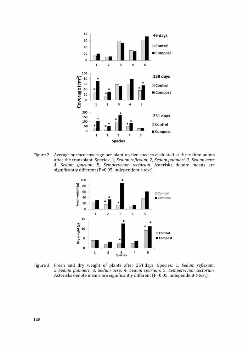
146 

Figure2. Averagesurfacecoverageperplantonfivespeciesevaluatedatthreetimepointsafterthetransplant.Species:1,Sedumreflexum;2,Sedumpalmieri;3,Sedumacre;4, Sedum spurium; 5, Sempervivum tectorum. Asterisks denote means aresignificantlydifferent(P=0.05,independentt‐test).

Figure3. Fresh and dry weight of plants after 251days. Species: 1, Sedum reflexum;2,Sedumpalmieri; 3, Sedumacre; 4, Sedum spurium; 5, Sempervivum tectorum.Asterisksdenotemeansaresignificantlydifferent(P=0.05,independentt‐test).

 

 

  147

Table2. Accumulationofnutrients(%dryweight)inplantsafter251days.

Nutrient Sedum Sempervivum

tectorum S. reflexum S. palmieri S. acre S. spurium N Control 0.56 0.42 0.45 0.64 0.25 Compost 0.87 0.53 0.50 0.87 0.36 P Control 0.17 0.20 0.24 0.25 0.18 Compost 0.35 0.29 0.22 0.35 0.30 K Control 0.61 1.05 0.56 1.10 0.62 Compost 0.60 1.30 0.39 0.77 0.93 Mg Control 0.29 0.41 0.23 0.27 0.53 Compost 0.33 0.41 0.22 0.34 0.68 Ca Control 1.68 3.22 1.43 0.93 4.23 Compost 2.96 3.50 1.33 1.49 5.10

CONCLUSIONSThe amendment of 10% compost from foodwaste on a soilless substrate for green

roofs produced a positive effect on the growth of five species of Crassulaceae under theclimaticconditionsofcentralItaly.However,thiseffectwasmoresignificantfortheSedumspeciesafter251daysandresulted ina reductionof thewinterdeclineobserved insomecases. The results agree with a previous report where an increase in plant biomass wasobservedonSedumreflexum(Biagiottietal.,2014).Thenegativeeffectofthe10%compostamendment compared to the 5% at 15weeks indicated a possible initial inhibitory effectandtheneedofmodulationofthedoseamendmentinrelationtothelengthofcultivation.Theuseofcompostisalreadyreportedasasustainablesourceoforganicmatterinsoillessmedia forhorticulture(Raviv,2014)and thisworksuggests itspotentialuse insubstratesforgreenroofsinMediterraneanareas.

ACKNOWLEDGMENTSThe work was supported by the project RDS: Eco‐green roof & vertical greenery

systemsAccordodiProgrammaENEA‐MinistryoftheEconomicDevelopmentofItaly,2012‐14.We thankDr.FabioVitali, headof the laboratoryUTAGRI‐INN,ENEA,andDr.MaurizioCoronidi,headofthelaboratoryUTAMB‐RIF,ENEA,forsupportofthisresearch.

Literaturecited

Biagiotti, D., Giagnacovo, G., Di Bonito, R., and Campiotti, C.A. (2014). Evaluation of plant species and soillesssubstrates for Mediterranean sustainable green roof installations. Paper presented at: 11th InternationalPhytotechnologiesConference(Heraklion,Crete,Greece:GrafimaPublishing).

DeKalb,C.D.,Kahn,B.A.,Dunn,B.L.,Payton,M.E.,andBarker,A.V.(2014).Substitutionofasoillessmediumwithyardwastecompostforbasiltransplantproduction.HortTechnology24,668–675.

FLL. (2008). Guideline for the Planning, Construction, and Maintenance of Green Roofing (Bonn, Germany:LandscapingandLandscapeDevelopmentResearchSocietyE.V.‐FLL).

Giagnacovo,G.,Biagiotti,D.,DiBonito,R.,Mascioli,C.,andCampiotti,C.A.(2014).SelezionediecotipispontaneidiCrassulaceae per la realizzazione di tetti verdi in ambiente mediterraneo. Paper presented at: X ConvegnoNazionalesullaBiodiversita,3‐5Sept2014(Roma,Italy:CRA‐CentrodiRicercaperloStudiodelleRelazionitraPiantaeSuolo).

Monterusso,M.A.,Rowe,D.B.,andRugh,C.L.(2005).EstablishmentandpersistenceofSedumspp.andnativetaxaforgreenroofapplications.HortScience40,391–396.

148 

Olszewski,M.W.,Holmes,M.H.,andYoung,C.A.(2010).Assessmentofphysicalpropertiesandstonecropgrowthingreenroofsubstratesamendedwithcompostandhydrogel.HortTechology20,438–444.

Ondono, S., Bastida, F., and Moreno, J.L. (2014). Microbiological and biochemical properties of artificialsubstrates:ApreliminarystudyofitsapplicationasTechnosolsorasabasisinGreenRoofSystems.Ecol.Eng.70,189–199http://dx.doi.org/10.1016/j.ecoleng.2014.05.003.

Raviv,M. (2014). Compost in growingmedia: feedstock, compostingmethods and potential applications. ActaHortic.1018,513–523http://dx.doi.org/10.17660/ActaHortic.2014.1018.56.

Restrepo,A.P.,Medina,E.,Perez‐Espinosa,A.,Agullo,E.,Bustamante,M.A.,Mininni,C.,Bernal,M.P.,andMoral,R.(2013). Substitution of peat in horticultural seedlings: suitability of digestate‐derived compost from cattlemanure and maize silage co‐digestion. Commun. Soil Sci. Plant Anal. 44 (1‐4), 668–677http://dx.doi.org/10.1080/00103624.2013.748004.

1876-6102 © 2017 The Authors. Published by Elsevier Ltd. This is an open access article under the CC BY-NC-ND license (http://creativecommons.org/licenses/by-nc-nd/4.0/).Peer-review under responsibility of the scientific committee of the International Scientific Conference “Environmental and Climate Technologies”.doi: 10.1016/j.egypro.2017.04.002

Energy Procedia 113 ( 2017 ) 1 – 8

ScienceDirect

aENEA, Via Anguillarese 301, Rome 00123, Italy bIUAV Universityof Venice, Santa Croce 191, Venezia 30135, Italy

cUniversity of Roma Tre, Via Ostiense 159, Roma 00154, Italy

Keywords:

E-mail address:

Available online at www.sciencedirect.com

© 2017 The Authors. Published by Elsevier Ltd. This is an open access article under the CC BY-NC-ND license (http://creativecommons.org/licenses/by-nc-nd/4.0/).Peer-review under responsibility of the scientific committee of the International Scientific Conference “Environmental and Climate Technologies”.

2 Michele Zinzi et al. / Energy Procedia 113 ( 2017 ) 1 – 8

Michele Zinzi et al. / Energy Procedia 113 ( 2017 ) 1 – 8 3

3.1. Optical

3.2. Thermal

4 Michele Zinzi et al. / Energy Procedia 113 ( 2017 ) 1 – 8

4.1. Estimation of the solar factor of the tested glazing unit

Winshelter V3.0

Winshelter

gei Uq

eegegi UUq

4.2. Energy performance of a commercial building

Michele Zinzi et al. / Energy Procedia 113 ( 2017 ) 1 – 8 5

5.1. Optical

6 Michele Zinzi et al. / Energy Procedia 113 ( 2017 ) 1 – 8

5.2. Thermal

Michele Zinzi et al. / Energy Procedia 113 ( 2017 ) 1 – 8 7

5.3. Solar factor

5.4. Energy performances

8 Michele Zinzi et al. / Energy Procedia 113 ( 2017 ) 1 – 8

1876-6102 © 2017 The Authors. Published by Elsevier Ltd. This is an open access article under the CC BY-NC-ND license (http://creativecommons.org/licenses/by-nc-nd/4.0/).Peer-review under responsibility of the scientific committee of the International Scientific Conference “Environmental and Climate Technologies”.doi: 10.1016/j.egypro.2017.04.003

Energy Procedia 113 ( 2017 ) 9 – 16

ScienceDirect

aUniversity of Perugia, Department of Engineering, Via G. Duranti 93, 06125 Perugia, Italy bENEA Casaccia Research Centre, Via Anguillarese 301, 00123 Rome, Italy

cUniversity of Roma Tre, Department of Engineering, Via della Vasca Navale 79/81, 00146 Rome, Italy

Keywords:

E-mail address:

Available online at www.sciencedirect.com

© 2017 The Authors. Published by Elsevier Ltd. This is an open access article under the CC BY-NC-ND license (http://creativecommons.org/licenses/by-nc-nd/4.0/).Peer-review under responsibility of the scientific committee of the International Scientific Conference “Environmental and Climate Technologies”.

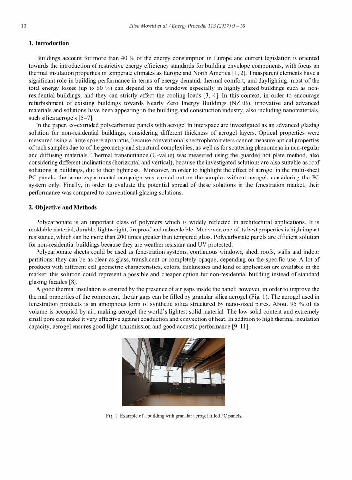
10 Elisa Moretti et al. / Energy Procedia 113 ( 2017 ) 9 – 16

Elisa Moretti et al. / Energy Procedia 113 ( 2017 ) 9 – 16 11

3.1. Optical

12 Elisa Moretti et al. / Energy Procedia 113 ( 2017 ) 9 – 16

3.2. Thermal

Elisa Moretti et al. / Energy Procedia 113 ( 2017 ) 9 – 16 13

4.1. Optical

14 Elisa Moretti et al. / Energy Procedia 113 ( 2017 ) 9 – 16

4.2. Thermal

Elisa Moretti et al. / Energy Procedia 113 ( 2017 ) 9 – 16 15

16 Elisa Moretti et al. / Energy Procedia 113 ( 2017 ) 9 – 16

buildings

Article

High Energy-Efficient Windows with Silica Aerogelfor Building Refurbishment: ExperimentalCharacterization and Preliminary Simulations inDifferent Climate ConditionsCinzia Buratti 1, Elisa Moretti 1,* and Michele Zinzi 2

1 Department of Engineering, University of Perugia, Via G. Duranti 67, 06125 Perugia, Italy;cinzia.buratti@unipg.it

2 ENEA Casaccia Research Centre, Via Anguillarese 301, 00123 Rome, Italy; michele.zinzi@enea.it* Correspondence: elisa.moretti@unipg.it; Tel.: +39-075-5853694

Academic Editor: Gianpiero EvolaReceived: 29 November 2016; Accepted: 10 January 2017; Published: 16 January 2017

Abstract: The paper deals with the potential of high energy-efficient windows with granular silicaaerogel for energy saving in building refurbishment. Different glazing systems were investigatedconsidering two kinds of granular silica aerogel and different glass layers. Thermal transmittanceand optical properties of the samples were measured and used in building simulations. The aerogelimpact on heat transfer is remarkable, allowing a thermal transmittance of 1.0–1.1 W/(m2·K) withgranular aerogel in interspace only 15 mm in thickness. A 63% reduction in U-value was achievedwhen compared to the corresponding conventional windows, together with a significant reduction(30%) in light transmittance. When assembled with a low-e glass, the U-value reduction was lower(31%), but a moderate reduction in light transmittance (about 10%) was observed for larger granules.Energy simulations for a case study in different climate conditions (hot, moderate, and cold) showeda reduction in energy demand both for heating and cooling for silica aerogel glazing systems,when compared to the conventional ones. The new glazings are a suitable solution for buildingrefurbishment, thanks to low U-values and total solar transmittance, also in warm climate conditions.

Keywords: high energy-efficient windows; nanogel windows; silica aerogel; building refurbishment;Nearly Zero Energy Buildings (NZEBs); energy saving in buildings

1. Introduction

Glass façades have an important role in buildings in terms of energy demand, thermal comfort,and daylighting: the main total energy losses (up to 60%) can depend on the windows, especially inhighly glazed buildings. In order to speed up refurbishment of existing buildings towards NearlyZero Energy Buildings (NZEBs), innovative glazing systems have been spread in the market andmight be suitable in places of conventional glazing windows, especially in cold climates [1–3]. Aerogelwindows seem to have the largest potential for improving the thermal performance and daylightingin glazing systems, because of very low thermal conductivity (about 0.020 W/m·K for translucentgranular aerogel at room temperature) and density (about 80 kg/m3), together with good opticaltransparency and acoustic insulation [4–9].

Opaque silica aerogel-based materials, such as flexible blankets and aerogel-based plasters andconcrete, have recently appeared on the market [10,11]. Silica aerogels, both in monolithic and granulartranslucent form, can be used in high-insulated nanogel windows: transparent monolithic paneswere developed 20–30 years ago, but their application in glazing systems has still not penetrated themarket, and few prototypes have been manufactured for research purposes [12,13]; for these reasons,

Buildings 2017, 7, 8; doi:10.3390/buildings7010008 www.mdpi.com/journal/buildings

Buildings 2017, 7, 8 2 of 12

building applications have focused on glazing systems with granular aerogels [14–17]. Differenttranslucent daylighting systems with granular aerogel have been emerging in the market. The mostpopular systems are multiwall polycarbonate panels for skylights, roofs, walls, structural panels forcontinuous façades, and finally insulated glass units. Many of these innovative solutions can be foundin schools, commercial and industrial buildings, airports, etc., especially in the US and in NorthernEurope [4,6,7,18]. The main application has been focusing on roof solutions [7,8], where an outsideview is usually not essential or where they can also be integrated at façade spandrels [14].

Thermal and optical properties of granular aerogel glazing systems are significantly affected byaerogel layer thickness and particle size: a significant reduction in U-value is observed by incorporatingthe aerogel granules into the cavity of double glazings (58% and 63%) [19–21]. When the aerogel layerthickness increases to 60 mm, a U-value of 0.3 W/(m2·K) can be achieved [16,22]. When compared toconventional glazings, the ones with granular aerogel also have significant benefits when used for roofsolutions, because U-values are not dependent on the tilted angle to the vertical plane, for example, ingas-filled glazings [8,22].

The paper deals with the potential of highly energy-efficient windows with silica aerogel forenergy saving in order to create Nearly Zero Energy Buildings (NZEBs) or as a strategy in buildingrefurbishment; in order to evaluate the potential spread of these solutions in the fenestration market,their performance was compared to conventional glazing solutions. The experimental characterizationof double glazing units (DGUs) with aerogel in interspace is carried out by considering differentkinds of silica granular aerogel and glass layers. Solar and light transmittance of aerogel windows areinvestigated by means of advanced instrumentation, able to measure the optical properties of diffusingand scattering materials. In this work, a large integrating sphere apparatus, designed for complextransparent and translucent systems, was used. Thermal transmittance (U-value) of DGUs is measuredusing a Heat Flux Meter in steady-state conditions. Then, the energy performance of aerogel windowsis discussed thanks to a case study: energy demand of a non-residential building is calculated bymeans of Energy Plus software by using experimental data as input data and considering differentclimate conditions (cold, moderate, and hot climates). The results are finally compared in order toevaluate the benefits of using innovative systems with aerogel instead of conventional solutions.

2. Materials and Methods

2.1. The Investigated Samples

Two prototypes of aerogel glazing units were assembled by incorporating aerogel granules intothe air space of the corresponding double glazing units, in order to investigate their optical and thermalproperties and to carry out numerical simulations on energy performance based on experimental data.

The double-glazing units with aerogel in interspace (Figure 1b) were used to realize two prototypesof windows (an aluminum frame window, Type 1 [20], and a wood frame window, Type 2) with twomobile shutters. The two windows were compared to conventional solutions with the same frame andglass, but with an air gap (Figure 1a).

Aerogel in granular form was put in a gap 15 mm thick, while external and internal layers arefloat glass 4 mm in thickness. Window Type 1 was assembled with two conventional clear float glasslayers, whereas Window Type 2 has a low-e and solar control coating on the inner side of the externalglass. During the assembly process, the glazing system was subject to mechanical vibration in order toensure a compact packing of aerogel granules between the glass layers. Two kinds of silica aerogelgranules were considered: type “A” for the window frame Type 1 and type “B” for the other window.Type “B” is the most recent aerogel, characterized by larger granules, allowing enhanced daylightingproperties, as shown in Figure 2. Table 1 shows the main characteristics of the DGU samples.

Buildings 2017, 7, 8 3 of 12

Buildings 2017, 7, 8    3 of 12 

enhanced daylighting properties, as shown in Figure 2. Table 1 shows the main characteristics of the 

DGU samples. 

 (a) (b)

Figure 1. Wood frame window prototype Type 2 (a) with conventional double glazing units (DGUs) 

and (b) with aerogel in the interspace between glass layers. 

 

Figure 2. Glazing units with aerogel: LOW‐E DGU AEROGEL with aerogel type “B” (at the top) and 

DGU‐AEROGEL with aerogel type “A” (at the bottom). 

Table 1. The investigated glazing systems: conventional DGU and DGU with aerogel. 

Name  External Layer Interspace Internal Layer  Window Frame

DGU Float clear glass   

(4 mm) Air (15 mm) 

Float clear glass   

(4 mm)  Type 1 

aluminum DGU‐AEROGEL   

Float clear glass   

(4 mm) 

Granular aerogel   

type “A” (15 mm) 

Float clear glass   

(4 mm) 

LOW‐E DGU Solar control and   

low‐e glass (4 mm) Air (15 mm) 

Float clear glass   

(4 mm) Type 2 wood 

LOW‐E DGU‐AEROGELSolar control and   

low‐e glass (4 mm) 

Granular aerogel   

type “B” (15 mm) 

Float clear glass   

(4 mm) 

 

Figure 1. Wood frame window prototype Type 2 (a) with conventional double glazing units (DGUs)and (b) with aerogel in the interspace between glass layers.

Buildings 2017, 7, 8    3 of 12 

enhanced daylighting properties, as shown in Figure 2. Table 1 shows the main characteristics of the 

DGU samples. 

 (a) (b)

Figure 1. Wood frame window prototype Type 2 (a) with conventional double glazing units (DGUs) 

and (b) with aerogel in the interspace between glass layers. 

 

Figure 2. Glazing units with aerogel: LOW‐E DGU AEROGEL with aerogel type “B” (at the top) and 

DGU‐AEROGEL with aerogel type “A” (at the bottom). 

Table 1. The investigated glazing systems: conventional DGU and DGU with aerogel. 

Name  External Layer Interspace Internal Layer  Window Frame

DGU Float clear glass   

(4 mm) Air (15 mm) 

Float clear glass   

(4 mm)  Type 1 

aluminum DGU‐AEROGEL   

Float clear glass   

(4 mm) 

Granular aerogel   

type “A” (15 mm) 

Float clear glass   

(4 mm) 

LOW‐E DGU Solar control and   

low‐e glass (4 mm) Air (15 mm) 

Float clear glass   

(4 mm) Type 2 wood 

LOW‐E DGU‐AEROGELSolar control and   

low‐e glass (4 mm) 

Granular aerogel   

type “B” (15 mm) 

Float clear glass   

(4 mm) 

 

Figure 2. Glazing units with aerogel: LOW-E DGU AEROGEL with aerogel type “B” (at the top) andDGU-AEROGEL with aerogel type “A” (at the bottom).

Buildings 2017, 7, 8 4 of 12

Table 1. The investigated glazing systems: conventional DGU and DGU with aerogel.

Name External Layer Interspace Internal Layer Window Frame

DGU Float clear glass (4 mm) Air (15 mm) Float clear glass (4 mm) Type 1 aluminumDGU-AEROGEL Float clear glass (4 mm) Granular aerogel type “A” (15 mm) Float clear glass (4 mm)

LOW-E DGU Solar control and low-e glass (4 mm) Air (15 mm) Float clear glass (4 mm) Type 2 woodLOW-E DGU-AEROGEL Solar control and low-e glass (4 mm) Granular aerogel type “B” (15 mm) Float clear glass (4 mm)

Buildings 2017, 7, 8 5 of 12

2.2. Experimental Campaign

The optical characterization of all the samples was carried out by means of a built-inspectrophotometer with a large-diameter integrating sphere (75 cm diameter, with an internal surfacemade of Spectralon, SphereOptics GmbH, Herrsching, Germany), needed to accurately characterizegeometrically complex and scattering transparent materials; a full description can be found in theliterature [23,24]. The layout of the facility can be adjusted to perform transmittance, reflectance, andabsorptance measurements, using a single beam measurement procedure (Figure 3). The near-normalincidence transmittance and reflectance were measured in the 350–2000 nm range, covering about 97%of the solar spectrum.

Buildings 2017, 7, 8    4 of 12 

2.2. Experimental Campaign 

The  optical  characterization  of  all  the  samples  was  carried  out  by  means  of  a  built‐in 

spectrophotometer  with  a  large‐diameter  integrating  sphere  (75  cm  diameter,  with  an  internal 

surface made  of  Spectralon,  SphereOptics  GmbH, Herrsching,  Germany),  needed  to  accurately 

characterize geometrically complex and scattering  transparent materials; a  full description can be 

found  in the literature [23,24]. The layout of the facility can be adjusted to perform transmittance, 

reflectance, and absorptance measurements, using a single beam measurement procedure (Figure 3). 

The near‐normal incidence transmittance and reflectance were measured in the 350–2000 nm range, 

covering about 97% of the solar spectrum. 

The thermal transmittance of the window prototypes was measured according to UNI EN ISO 

12567‐1 [25]: during the measurements, three thermofluximeters were fixed on the glazing system, in 

order to evaluate the U‐value of the glazing only in steady‐state conditions [20]. 

 

Figure 3. Optical measurements for a glazing unit with aerogel. 

2.3. Simulations 

The  energy performance  of  the  innovative glazing  systems proposed  in  the present paper was 

investigated by EnergyPlusTM software  (Version 8.4, U.S. Department of Energy’s (DOE), Washington 

DC,  USA)  [26–28].  Many  simulations  with  different  configurations  and  settings  were  performed 

considering a typical office building built in the 1990s as a reference (Figure 4). The external dimensions 

are 80 m × 20 m × 10 m, and large strip windows (window‐to‐wall ratio about 50%) are in the East 

and West walls. The mid‐floor of the building was chosen for the study so that just the façades are 

exposed to the external environment conditions (weather, sun, wind, etc.), whereas the roof and the 

floor exchange heat with zones at the same temperature. Moreover, the ground temperature has no 

effect on the performance of the chosen zone. The internal loads (people, lighting, and equipment) 

were defined as reported in Table 2. The lights are fully dimmable in order to ensure energy savings: 

artificial light is automatically reduced and switched off when the illuminance level is equal to 500 

lux.  The  heating  and  cooling  system  operating  periods  are  set  according  to  the  climatic  zone, 

considering an indoor air temperature of 20 °C and 26 °C, respectively. The office occupancy was set 

from 8:00 to 18:00, five days a week. 

The  influence of aerogel glazings on building energy performance was evaluated  in  terms of 

heating, cooling, and lighting energy demands, taking into account different climatic conditions. The 

simulations were  run  for  three  different  cities: Rome  (Italy),  characterized  by  hot  climate,  Paris 

(France), with a moderate climate, and Ottawa (Canada) with a cold climate (Figure 5). 

Figure 3. Optical measurements for a glazing unit with aerogel.

The thermal transmittance of the window prototypes was measured according to UNI EN ISO12567-1 [25]: during the measurements, three thermofluximeters were fixed on the glazing system,in order to evaluate the U-value of the glazing only in steady-state conditions [20].

2.3. Simulations

The energy performance of the innovative glazing systems proposed in the present paper wasinvestigated by EnergyPlusTM software (Version 8.4, U.S. Department of Energy’s (DOE), WashingtonDC, USA) [26–28]. Many simulations with different configurations and settings were performedconsidering a typical office building built in the 1990s as a reference (Figure 4). The external dimensionsare 80 m × 20 m × 10 m, and large strip windows (window-to-wall ratio about 50%) are in the Eastand West walls. The mid-floor of the building was chosen for the study so that just the façades areexposed to the external environment conditions (weather, sun, wind, etc.), whereas the roof and thefloor exchange heat with zones at the same temperature. Moreover, the ground temperature has noeffect on the performance of the chosen zone. The internal loads (people, lighting, and equipment)were defined as reported in Table 2. The lights are fully dimmable in order to ensure energy savings:artificial light is automatically reduced and switched off when the illuminance level is equal to 500 lux.The heating and cooling system operating periods are set according to the climatic zone, consideringan indoor air temperature of 20 ◦C and 26 ◦C, respectively. The office occupancy was set from 8:00 to18:00, five days a week.

The influence of aerogel glazings on building energy performance was evaluated in terms ofheating, cooling, and lighting energy demands, taking into account different climatic conditions. Thesimulations were run for three different cities: Rome (Italy), characterized by hot climate, Paris (France),with a moderate climate, and Ottawa (Canada) with a cold climate (Figure 5).

Buildings 2017, 7, 8 6 of 12

Buildings 2017, 7, 8    5 of 12 

 

Figure 4. The reference office building for energy simulations. 

Table 2. Simulation hypotheses.   

Internal Loads  Values Schedule 

Lighting  7 W/m2 (500 lux, fully dimmable) 8:00–18:00   

five days a week People  0.05 persons/m2 

Equipment  7 W/m2 

Operating Periods of Heating and Cooling System and schedule 

City  Heating (20 °C)  Cooling (26 °C) Schedule 

Rome  1 November–15 April    16 April–14 October   7:00–19:00   

five days a week Paris  15 October–30 April    1 May–14 October   

Ottawa  15 October–30 April    1 May–14 October   

 

Figure 5. Outdoor air temperature for the investigated cities. 

3. Results and Discussion 

3.1. Optical and Thermal Performance 

The spectral transmittance and reflectance of all the samples are reported  in Figures 6 and 7, 

respectively. By comparing empty and aerogel filled glazings, it is interesting to note a modification 

-25

-20

-15

-10

-5

0

5

10

15

20

25

30

35

Ou

tdo

or

air

tem

per

atu

re [

°C]

OTTAWA PARIS ROME

Figure 4. The reference office building for energy simulations.

Table 2. Simulation hypotheses.

Internal Loads Values Schedule

Lighting 7 W/m2 (500 lux, fully dimmable) 8:00–18:00five days a weekPeople 0.05 persons/m2

Equipment 7 W/m2

Operating Periods of Heating and Cooling System and schedule

City Heating (20 ◦C) Cooling (26 ◦C) Schedule

Rome 1 November–15 April 16 April–14 October 7:00–19:00five days a weekParis 15 October–30 April 1 May–14 October

Ottawa 15 October–30 April 1 May–14 October

Buildings 2017, 7, 8    5 of 12 

 

Figure 4. The reference office building for energy simulations. 

Table 2. Simulation hypotheses.   

Internal Loads  Values Schedule 

Lighting  7 W/m2 (500 lux, fully dimmable) 8:00–18:00   

five days a week People  0.05 persons/m2 

Equipment  7 W/m2 

Operating Periods of Heating and Cooling System and schedule 

City  Heating (20 °C)  Cooling (26 °C) Schedule 

Rome  1 November–15 April    16 April–14 October   7:00–19:00   

five days a week Paris  15 October–30 April    1 May–14 October   

Ottawa  15 October–30 April    1 May–14 October   

 

Figure 5. Outdoor air temperature for the investigated cities. 

3. Results and Discussion 

3.1. Optical and Thermal Performance 

The spectral transmittance and reflectance of all the samples are reported  in Figures 6 and 7, 

respectively. By comparing empty and aerogel filled glazings, it is interesting to note a modification 

-25

-20

-15

-10

-5

0

5

10

15

20

25

30

35

Ou

tdo

or

air

tem

per

atu

re [

°C]

OTTAWA PARIS ROME

Figure 5. Outdoor air temperature for the investigated cities.

Buildings 2017, 7, 8 7 of 12

3. Results and Discussion

3.1. Optical and Thermal Performance

The spectral transmittance and reflectance of all the samples are reported in Figures 6 and 7,respectively. By comparing empty and aerogel filled glazings, it is interesting to note a modification ofthe spectral response shape, especially in the visible range, and typical selective absorption peaks areshown in the spectral transmittance values (at about 1400 nm, 1700 nm, and 1900 nm) [20]. As known,part of the radiation is diffused and scattered when transmitted through the material [19–22,29]. Dataabout the assembled sample with float glasses and aerogel show a significant impact on the granules:the reduction is more evident in the visible range, whereas the transmittance diminishes by about 0.1in the IR range. The transmission of the samples LOW-E DGU and LOW-E DGU-AEROGEL in thenear infrared range is very low due to solar control and low-e coating, and the influence of aerogelgranules is negligible. Moreover, the reduction in the visible range due to the granular aerogel is verylow and equal to about 0.1.

Buildings 2017, 7, 8    6 of 12 

of the spectral response shape, especially in the visible range, and typical selective absorption peaks 

are shown in the spectral transmittance values (at about 1400 nm, 1700 nm, and 1900 nm) [20]. As 

known, part of the radiation is diffused and scattered when transmitted through the material [19–

21,22,29]. Data about the assembled sample with float glasses and aerogel show a significant impact 

on  the  granules:  the  reduction  is more  evident  in  the  visible  range, whereas  the  transmittance 

diminishes by about 0.1 in the IR range. The transmission of the samples LOW‐E DGU and LOW‐E 

DGU‐AEROGEL in the near infrared range is very low due to solar control and low‐e coating, and 

the influence of aerogel granules is negligible. Moreover, the reduction in the visible range due to the 

granular aerogel is very low and equal to about 0.1.   

The aerogel significantly also  influences  the reflectance spectrum (Figure 7), especially  in  the 

visible range, where the values increased up to 0.45–0.5. As expected, the reflectance trend is strictly 

linked to the glass layer type: for the samples with solar control and low‐e coating, the reflectance is 

very high in the NIR range, up to about 0.9 at 1750 nm. 

 

Figure 6. Spectral transmittance at normal incidence. 

 

Figure 7. Spectral reflectance at normal incidence.   

0

0.1

0.2

0.3

0.4

0.5

0.6

0.7

0.8

0.9

1

350 450 550 650 750 850 950 1050 1150 1250 1350 1450 1550 1650 1750 1850 1950

Sp

ectr

al t

ran

smit

tan

ce [

-]

Wavelength [nm]

DGU (4/15 Air/4) DGU AEROGEL (4/15 Aerogel /4)LOW-E DGU (4/15 Air/4 low-e) LOW-E DGU AEROGEL (4/15 Aerogel/4 low-e)

0

0.1

0.2

0.3

0.4

0.5

0.6

0.7

0.8

0.9

1

350 450 550 650 750 850 950 1050 1150 1250 1350 1450 1550 1650 1750 1850 1950

Sp

ectr

al r

efle

ctan

ce [

-]

Wavelength [nm]

DGU (4/15 Air/4)DGU AEROGEL (4/15 Aerogel/4)LOW-E DGU (4/15 Air/4 low-e)LOW-E DGU AEROGEL (4/15 Aerogel/4 low-e)

Figure 6. Spectral transmittance at normal incidence.

Buildings 2017, 7, 8    6 of 12 

of the spectral response shape, especially in the visible range, and typical selective absorption peaks 

are shown in the spectral transmittance values (at about 1400 nm, 1700 nm, and 1900 nm) [20]. As 

known, part of the radiation is diffused and scattered when transmitted through the material [19–

21,22,29]. Data about the assembled sample with float glasses and aerogel show a significant impact 

on  the  granules:  the  reduction  is more  evident  in  the  visible  range, whereas  the  transmittance 

diminishes by about 0.1 in the IR range. The transmission of the samples LOW‐E DGU and LOW‐E 

DGU‐AEROGEL in the near infrared range is very low due to solar control and low‐e coating, and 

the influence of aerogel granules is negligible. Moreover, the reduction in the visible range due to the 

granular aerogel is very low and equal to about 0.1.   

The aerogel significantly also  influences  the reflectance spectrum (Figure 7), especially  in  the 

visible range, where the values increased up to 0.45–0.5. As expected, the reflectance trend is strictly 

linked to the glass layer type: for the samples with solar control and low‐e coating, the reflectance is 

very high in the NIR range, up to about 0.9 at 1750 nm. 

 

Figure 6. Spectral transmittance at normal incidence. 

 

Figure 7. Spectral reflectance at normal incidence.   

0

0.1

0.2

0.3

0.4

0.5

0.6

0.7

0.8

0.9

1

350 450 550 650 750 850 950 1050 1150 1250 1350 1450 1550 1650 1750 1850 1950

Sp

ectr

al t

ran

smit

tan

ce [

-]

Wavelength [nm]

DGU (4/15 Air/4) DGU AEROGEL (4/15 Aerogel /4)LOW-E DGU (4/15 Air/4 low-e) LOW-E DGU AEROGEL (4/15 Aerogel/4 low-e)

0

0.1

0.2

0.3

0.4

0.5

0.6

0.7

0.8

0.9

1

350 450 550 650 750 850 950 1050 1150 1250 1350 1450 1550 1650 1750 1850 1950

Sp

ectr

al r

efle

ctan

ce [

-]

Wavelength [nm]

DGU (4/15 Air/4)DGU AEROGEL (4/15 Aerogel/4)LOW-E DGU (4/15 Air/4 low-e)LOW-E DGU AEROGEL (4/15 Aerogel/4 low-e)

Figure 7. Spectral reflectance at normal incidence.

The aerogel significantly also influences the reflectance spectrum (Figure 7), especially in thevisible range, where the values increased up to 0.45–0.5. As expected, the reflectance trend is strictly

Buildings 2017, 7, 8 8 of 12

linked to the glass layer type: for the samples with solar control and low-e coating, the reflectance isvery high in the NIR range, up to about 0.9 at 1750 nm.

In Table 3, the broadband values calculated for transmittance and reflectance in the visible andsolar spectrum are reported, according to the standard reference EN 410 [30] and the U-value of theonly glazing calculated by data measured with the thermofluximeters [20].

Table 3. Lighting, solar, and thermal performance of the samples.

AcronymLight

Transmittanceτv

LightReflectance

ρv

Direct SolarTransmittance

τe

SolarReflectance

ρe

Total SolarTransmittance

g

U–value(W/m2·K)

DGU 0.82 0.15 0.76 0.14 0.80 2.7DGU-AEROGEL 0.57 0.38 0.53 0.31 0.57 1.0

LOW-E DGU 0.63 0.27 0.39 0.43 0.41 1.6LOW-E

DGU-AEROGEL 0.57 0.32 0.35 0.46 0.36 1.1

The contribution of the innovative glazing system on thermal properties is remarkable: thethermal transmittance is 1.0–1.1 W/(m2·K) for the aerogel glazing systems, in good agreement withliterature data [7–9,14,19,31]. The U-value of the glazing depends on the thermal resistivity of eachglass layer and on the gas (convective heat transfer) and radiation conductance in the interspace, wherethe radiation heat transfer is strictly related to the emissivity of the inner side of the glasses: with alow-e coating (the emissivity is about 0.1) and air (or argon) in the interspace, a significant reductionin the radiation conductance can be observed; the U-value of LOW-E DGU is in fact 1.6 W/(m2·K)instead of 2.7 W/(m2·K). The aerogel in the interspace between the glass layers has a dual impact onthermal conductance: the convective heat transfer within the cavity becomes negligible, as reported inthe literature [18,22], and the radiative heat transfer is limited due to the transmittance of the aerogelin the infrared spectral range, which is very low [8], except in the 3500–5000 nm range. For thisreason, the low-e coating does not influence the overall heat transfer in the window when aerogel isplaced in the interspace between the glass layers (Table 3). Therefore, the thermal conductivity of silicaaerogel granules is the main responsible for the glazing U-value, and the particle size has an impact onthermal performance of the glazing, as shown in the literature [14,16,31]. In particular, small granulesallow a better performance than the larger ones: for instance, the thermal conductivity varies in the19–21 mW/mK range at 10 ◦C, when the average particle size increases [31]. For these reasons, themeasured U-value of DGU-AEROGEL is lower than the value of the glazing with the low-e coatingand larger granules of aerogel in the interspace.

The reduction of the U-value due to the aerogel in the interspace with respect to DGU and LOW-EDGU samples is about 63% and 31%, respectively. The corresponding reduction in light transmittance(τv) is about 30% and 10%, respectively, due to the improved daylighting performance of granulestype “B”.

Finally, the total solar transmittance or solar factor (g) was estimated using the methodologysuggested by the EN 410, based on the thermal properties of the samples and on the spectral reflectanceand transmittance of the glazing and of the glass layers [32] (Table 3). For both windows, the presenceof granules reduces the solar factor (12–39% reduction) due to the lower transmittance in the NIR range,reaching a value of 0.36 for the glazing with the solar control low-e glass (LOW-E DGU AEROGEL).

3.2. Energy Performance

The influence of aerogel glazings on building energy performance was evaluated in terms ofheating, cooling, and lighting energy demands, expressed in kWh/m2: ideal energy loads werecalculated by the software to meet the zone loads, without considering any equipment for heating,ventilation, and air conditioning in the simulations (Figure 8).

Buildings 2017, 7, 8 9 of 12

Buildings 2017, 7, 8    8 of 12 

especially  in  the wintertime,  the  solar  factor  reduction diminishes  the heat gain  from  the aerogel 

window, penalizing the overall result. For the same reasons, glazings with low‐e coating have the 

worst behavior than the other solutions due to the lower g‐value.   

The annual cooling energy demand for DGU‐AEROGEL decreases by a percentage from about 

18% (Rome) to 21% (Ottawa) with respect to DGU. As expected, the energy demand for cooling is 

minimum for the glazing systems with low‐e coating (LOW‐E DGU and LOW‐E DGU AEROGEL), 

due  to  the  significant  reduction  in  solar  factor  (i.e.,  0.36–0.41):  when  compared  to  DGU,  the 

reduction is in a range from 40% (Rome) to 56% (Ottawa). However, when the aerogel window is 

assembled with low‐e glass, the benefits of the translucent material in the interspace are negligible, 

and the energy demands for cooling are quite similar.   

 (a)

 (b)

Buildings 2017, 7, 8    9 of 12 

 (c)

Figure 8. Heating, cooling, and  lighting energy demand for the  investigated glazings  in Rome (a); 

Paris (b); and Ottawa (c). 

In general, for building refurbishment, granular aerogel glazing systems could be considered a 

good  solution  in  terms of  annual  energy demand  reduction with  respect  to  conventional double 

glazings,  especially  in warm  climates.  The  results  are  in  agreement with  literature  data  [33,34]: 

Huang  and Niu  evaluated  the  influence  of  translucent  aerogel  glazing  systems  on  the  energy 

performance  in  humid  subtropical  cooling‐dominant  climates  (Hong Kong). With  respect  to  the 

reference case (conventional double glazing), aerogel glazing systems reduce the total annual space 

cooling load by around 4%, and the annual cooling load reduction was almost the same as the one 

achieved by low‐e glazing, showing that silica aerogel glazings might be a suitable solution, also in 

cooling‐dominated climates. 

Finally, the energy demands for artificial lights are quite similar for all windows: the daylight 

illuminance  on  the working  plane  is  higher  than  the  recommended  value  (500  lux)  for  a  large 

amount  of  time  during  the  year,  also  for  glazing  systems  with  aerogel,  due  to  the  high 

window‐to‐wall  ratio  for  the  investigated  building,  and  the  increase  in  energy  demand  for  the 

aerogel solution is negligible. 

4. Conclusions   

Different design options  for windows have a  large  impact on  the energy efficiency  in highly 

glazed  buildings:  low  thermal  transmittance  values  can  be  crucial  to  ensure  acceptable  heating 

demand  and  low  energy  use;  at  the  same  time,  the  solar  transmittance  should  be  thoroughly 

evaluated,  especially  in  warm  climates.  Among  innovative  glazing  solutions,  windows  with 

granular  aerogel  in  interspace  seem  to  be  the  most  promising,  because  of  very  low  thermal 

transmittance, good daylight  transmittance, and a  remarkable  light weight, and some  translucent 

glazing systems are spreading in the market [7,8,18,34].   

Two innovative glazing systems with silica granular aerogel in interspace were manufactured 

and  investigated  for  building  refurbishment  by means  of  a  thermal  and  lighting  experimental 

campaign  and  energy  simulations.  Two  types  of  granular  silica  aerogel  (15 mm  thickness with 

different particle sizes) and different glass  layers (conventional float glass and solar control  low‐e 

glass) were considered, and  the  results were compared  in order  to evaluate  the benefits of using 

innovative systems with aerogel in place of conventional solutions.   

Figure 8. Heating, cooling, and lighting energy demand for the investigated glazings in Rome (a); Paris(b); and Ottawa (c).

Buildings 2017, 7, 8 10 of 12

Glazings with granular aerogel in interspace (DGU-AEROGEL) result in the most efficient systemsfor heating in all climate conditions: the reduction in energy demand is 13% for Ottawa, 24% for Paris,and 29% for Rome, when compared to the conventional glazing. The reduction is consistent with U-and g-values of the windows: in Ottawa (Figure 8c), with higher solar radiation, especially in thewintertime, the solar factor reduction diminishes the heat gain from the aerogel window, penalizingthe overall result. For the same reasons, glazings with low-e coating have the worst behavior than theother solutions due to the lower g-value.

The annual cooling energy demand for DGU-AEROGEL decreases by a percentage from about18% (Rome) to 21% (Ottawa) with respect to DGU. As expected, the energy demand for cooling isminimum for the glazing systems with low-e coating (LOW-E DGU and LOW-E DGU AEROGEL), dueto the significant reduction in solar factor (i.e., 0.36–0.41): when compared to DGU, the reduction is ina range from 40% (Rome) to 56% (Ottawa). However, when the aerogel window is assembled withlow-e glass, the benefits of the translucent material in the interspace are negligible, and the energydemands for cooling are quite similar.

In general, for building refurbishment, granular aerogel glazing systems could be considereda good solution in terms of annual energy demand reduction with respect to conventional doubleglazings, especially in warm climates. The results are in agreement with literature data [33,34]:Huang and Niu evaluated the influence of translucent aerogel glazing systems on the energyperformance in humid subtropical cooling-dominant climates (Hong Kong). With respect to thereference case (conventional double glazing), aerogel glazing systems reduce the total annual spacecooling load by around 4%, and the annual cooling load reduction was almost the same as the oneachieved by low-e glazing, showing that silica aerogel glazings might be a suitable solution, also incooling-dominated climates.

Finally, the energy demands for artificial lights are quite similar for all windows: the daylightilluminance on the working plane is higher than the recommended value (500 lux) for a large amountof time during the year, also for glazing systems with aerogel, due to the high window-to-wall ratiofor the investigated building, and the increase in energy demand for the aerogel solution is negligible.

4. Conclusions

Different design options for windows have a large impact on the energy efficiency in highlyglazed buildings: low thermal transmittance values can be crucial to ensure acceptable heatingdemand and low energy use; at the same time, the solar transmittance should be thoroughly evaluated,especially in warm climates. Among innovative glazing solutions, windows with granular aerogel ininterspace seem to be the most promising, because of very low thermal transmittance, good daylighttransmittance, and a remarkable light weight, and some translucent glazing systems are spreading inthe market [7,8,18,34].

Two innovative glazing systems with silica granular aerogel in interspace were manufactured andinvestigated for building refurbishment by means of a thermal and lighting experimental campaignand energy simulations. Two types of granular silica aerogel (15 mm thickness with different particlesizes) and different glass layers (conventional float glass and solar control low-e glass) were considered,and the results were compared in order to evaluate the benefits of using innovative systems withaerogel in place of conventional solutions.

The aerogel impact on thermal properties is remarkable: the thermal transmittance is1.0–1.1 W/(m2·K), lower than a glazing with low-e coating and a similar total thickness. With respectto the corresponding conventional windows, a 63% reduction in U-value was achieved for windowswith clear float glasses, whereas, when assembled with a low-e glass, the reduction was lower (31%).Optical measurements with a large sphere apparatus allowed for an accurate optical characterizationof the samples, which diffuse and scatter the light. When compared to conventional windows with thesame external and internal glass layers, a very modest reduction in light transmittance (about 10%)was observed for large granules, whereas the reduction is significant (30%) for the small granules;

Buildings 2017, 7, 8 11 of 12

however, the τv value is suitable for daylighting (it is equal to 0.55). For both windows, the presence ofgranules reduces the solar factor (12–39% reduction), due to the lower transmittance in the NIR range.

The results of the preliminary energy simulations for this case study showed that the new aerogelglazing systems are a suitable solution for building refurbishment, thanks to low U-values and solartransmittance, also in warm climate conditions. Moreover, they allow for significant daylightingilluminance in buildings, improving visual comfort due to light diffusing, and could have energydemands for lights very similar to those of conventional solutions, especially in buildings with a highwindow-to-wall surface ratio. In general, translucent systems such as granular aerogel filled systemsallow light to propagate uniformly within rooms, thus minimizing daylight problems, such as highcontrast zones, and preventing glare, as shown in the literature [14,15,29]. Future studies should focuson the impact of aerogel systems on indoor visual comfort and on energy consumption for artificiallights in buildings.

Acknowledgments: The authors wish to thank Francesco Cristarella Orestano and Elisa Belloni for their valuablehelp during the experimental campaign and Francesca Merli for her precious collaboration during data elaboration.

Author Contributions: The work presented in this paper is a collaborative development by all of the authors.

Conflicts of Interest: The authors declare no conflict of interest.

References

1. Jelle, B.P.; Hynd, A.; Gustavsen, A.; Arasteh, D.; Goudey, H.; Hart, R. Fenestration of today and tomorrow:A state-of-the-art review and future research opportunities. Sol. Energy Mater. Sol. Cell 2012, 96, 1–28.[CrossRef]

2. Ihara, T.; Gustavsen, A.; Jelle, B.P. Effect of facade components on energy efficiency in office buildings.Appl. Energy 2015, 158, 422–432. [CrossRef]

3. Mohammadpourkarbasi, H.; Sharples, S. The Eco-Refurbishment of a 19th Century Terraced House: Energyand Cost Performance for Current and Future UK Climates. Buildings 2013, 3, 220–244. [CrossRef]

4. Koebel, M.; Rigacci, A.; Achard, P. Aerogel-based thermal superinsulation: An overview. J. Sol-Gel Sci. Technol.2012, 63, 315–339. [CrossRef]

5. Cuce, E.; Cuce, P.M.; Wood, C.J.; Riffat, S.B. Toward aerogel based thermal superinsulation in buildings:A comprehensive review. Renew. Sustain. Energy Rev. 2014, 34, 273–299. [CrossRef]

6. Baetens, R.; Jelle, B.P.; Gustavsen, A. Aerogel insulation for building applications: A state-of-the-art review.Energy Build. 2011, 43, 761–769. [CrossRef]

7. Buratti, C.; Moretti, E. Silica nanogel for energy-efficient windows. In Nanotechnology in Eco-EfficientConstruction; Pacheco Torgal, F., Diamanti, M.V., Nazari, A., Granqvist, C.G., Eds.; Woodhead PublishingLimited: Cambridge, UK, 2013; pp. 207–235.

8. Buratti, C.; Moretti, E. Nanogel windows. In Nearly Zero Energy Building Refurbishment; Pacheco Torgal, F.,Mistretta, M., Kaklauskas, A., Granqvist, C.G., Cabeza, L.F., Eds.; Springer: Londra, UK, 2013; pp. 555–582.

9. Cotana, F.; Pisello, A.L.; Moretti, E.; Buratti, C. Multipurpose characterization of glazing systems with silicaaerogel: In-field experimental analysis of thermal-energy, lighting and acoustic performance. Build. Environ.2014, 81, 92–102. [CrossRef]

10. Buratti, C.; Moretti, E.; Belloni, E.; Agosti, F. Development of innovative aerogel based plasters: Preliminarythermal and acoustic performance evaluation. Sustainability 2014, 6, 5839–5852. [CrossRef]

11. Buratti, C.; Moretti, E.; Belloni, E. Aerogel plasters for energy building efficiency. In Nano and Biotech BasedMaterials for Energy Building Efficiency; Pacheco Torgal, F., Buratti, C., Kalaiselvam, S., Granqvist, C.G.,Ivanov, V., Eds.; Springer International Publishing AG: Basel, Switzerland, 2016; pp. 17–40.

12. Berardi, U. The development of a monolithic aerogel glazed window for an energy retrofitting project.Appl. Energy 2015, 154, 603–615. [CrossRef]

13. Bhuiya, M.M.H.; Anderson, A.M.; Carroll, M.K.; Bruno, B.A.; Ventrella, J.L.; Silberman, B.; Keramati, B.Preparation of Monolithic Silica Aerogel for Fenestration Applications: Scaling up, Reducing Cycle Time,and Improving Performance. Ind. Eng. Chem. Res. 2016, 55, 6971–6981. [CrossRef]

14. Ihara, T.; Gao, T.; Grynning, S.; Jelle, B.P.; Gustavsen, A. Aerogel granulate glazing facades and theirapplication potential from an energy saving perspective. Appl. Energy 2015, 142, 179–191. [CrossRef]

Buildings 2017, 7, 8 12 of 12

15. Gao, T.; Ihara, T.; Grynning, S.; Jelle, B.P.; Gunnarshaug Lien, A. Perspective of aerogel glazings in energyefficient buildings. Build. Environ. 2016, 95, 405–413. [CrossRef]

16. Gao, T.; Jelle, B.P.; Ihara, T.; Gustavsen, A. Insulating glazing units with silica aerogel granules: The impactof particle size. Appl. Energy 2014, 128, 27–34. [CrossRef]

17. Garnier, C.; Muneer, T.; McCauley, L. Super insulated aerogel windows: Impact on daylighting and thermalperformance. Build. Environ. 2015, 94, 231–238. [CrossRef]

18. Moretti, E.; Zinzi, M.; Carnielo, E.; Merli, F. Advanced polycarbonate transparent systems with aerogel:Preliminary characterization of optical and thermal properties. Energy Procedia 2016, in press.

19. Buratti, C.; Moretti, E. Lighting and energetic characteristics of transparent insulating materials: Experimentaldata and calculation. Indoor Built Environ. 2011, 20, 400–411. [CrossRef]

20. Buratti, C.; Moretti, E. Experimental performance evaluation of aerogel glazing systems. Appl. Energy 2012,97, 430–437. [CrossRef]

21. Buratti, C.; Moretti, E. Glazing systems with silica aerogel for energy savings in buildings. Appl. Energy 2012,98, 396–403. [CrossRef]

22. Ihara, T.; Grynning, S.; Gao, T.; Gustavsen, A.; Jelle, B.P. Impact of convection on thermal performance ofaerogel granulate glazing systems. Energy Build. 2015, 88, 165–173. [CrossRef]

23. Moretti, E.; Zinzi, M.; Belloni, E. Polycarbonate panels for buildings: Experimental investigation of thermaland optical performance. Energy Build. 2014, 70, 23–35. [CrossRef]

24. Maccari, A.; Montecchi, M.; Treppo, F.; Zinzi, M. CATRAM: An apparatus for the optical characterization ofadvanced transparent materials. Appl. Opt. 1998, 37, 5156–5161. [CrossRef] [PubMed]

25. CEN. EN 12567-1. Thermal Performance of Windows and Doors. Determination of Thermal Transmittance by theHot-Box Method. Complete Windows and Doors; International Organization for Standardization (ISO): Geneva,Switzerland, 2010.

26. Moretti, E.; Belloni, E. Evaluation of energy, thermal, and daylighting performance of solar control films fora case study in moderate climate. Build. Environ. 2015, 94, 183–195. [CrossRef]

27. Buratti, C.; Moretti, E.; Belloni, E.; Cotana, F. Unsteady simulation of energy performance and thermalcomfort in non-residential buildings. Build. Environ. 2013, 59, 482–491. [CrossRef]

28. Mujeebu, M.A.; Ashraf, N.; Alsuwayigh, A. Energy performance and economic viability of nano aerogelglazing and nano vacuum insulation panel in multi-story office building. Energy 2016, 113, 949–956.[CrossRef]

29. Huang, Y.; Niu, J. Energy and visual performance of the silica aerogel glazing system in commercial buildingsof Hong Kong. Constr. Build. Mater. 2015, 94, 57–72. [CrossRef]

30. EN 410. Glass in Building—Determination of Luminous and Solar Characteristics of Glazing; Europeen Committtefor standardization (CEN): Brussels, Belgium, 2011.

31. Moretti, E.; Merli, F.; Cuce, E.; Buratti, C. Thermal and acoustic properties of aerogels: Preliminaryinvestigation of the influence of granule size. Energy Procedia 2016, in press.

32. AGC Glass Europe. Available online: http://www.yourglass.com/configurator/tp/it/toolbox/configurator/main.html (accessed on 9 November 2016).

33. Huang, Y.; Niu, J. Application of super-insulating translucent silica aerogel glazing system on commercialbuilding envelope of humid subtropical climates: Impact on space cooling load. Energy 2015, 83, 316–325.[CrossRef]

34. Buratti, C.; Moretti, E.; Belloni, E. Nanogel windows for energy building efficiency. In Nano and BiotechBased Materials for Energy Building Efficiency; Pacheco Torgal, F., Buratti, C., Kalaiselvam, S., Granqvist, C.G.,Ivanov, V., Eds.; Springer International Publishing AG: Basel, Switzerland, 2016; pp. 41–69.

© 2017 by the authors; licensee MDPI, Basel, Switzerland. This article is an open accessarticle distributed under the terms and conditions of the Creative Commons Attribution(CC-BY) license (http://creativecommons.org/licenses/by/4.0/).

1876-6102 © 2017 The Authors. Published by Elsevier Ltd. This is an open access article under the CC BY-NC-ND license (http://creativecommons.org/licenses/by-nc-nd/4.0/).Peer-review under responsibility of the scientific committee of the 8th International Conference on Applied Energy.doi: 10.1016/j.egypro.2017.03.592

Energy Procedia 105 ( 2017 ) 2107 – 2112

ScienceDirect

The 8th International Conference on Applied Energy ICAE2016

Low order grey-box models for short-term thermal behavior prediction in buildings

Alessandro Fontia, Gabriele Comodia,*, Stefano Pizzutib, Alessia Arteconic, Lieve Helsend aUniversità Politecnica delle Marche, via Brecce Bianche 1, Ancona, 60131, Italy

bENEA, via Anguillarese 301, Rome, 00123, Italy cUniversità eCampus, via Isimbardi 10, Novendrate (CO), 22060, Italy

dKU Leuven, Celestijnenlaan 300 - bus 2421, Leuven, 3001, Belgium

Abstract

Low order grey-box models are suitable to be used in predictive controls. In real buildings in which the measured quantities are few the reliability of these models is crucial for the control performance. In this paper an identification procedure is analyzed to investigate the accuracy of different order grey-box models for short-term thermal behavior prediction in a real building, part of a living smart district. The building has a low number of zones and a single indoor temperature measuring point. The models are identified on the data acquired in 31 days during the winter 2015. The second order model shows the best performance with a root-mean-square error (RMSE) less than 0.5°C for a prediction horizon of 1-hour and a RMSE less than 1°C for a prediction horizon of 3-hours. © 2016 The Authors. Published by Elsevier Ltd. Selection and/or peer-review under responsibility of ICAE Keywords: Grey-box modeling; Reduced order models; Building energy modeling

1. Introduction

Model Predictive Control (MPC) has shown good results for achieving higher energy efficiency in buildings [1]. Such control strategy necessarily needs thermal building models [1] and the reliability of these models is crucial for the control performance [2]. Reduced order grey-box models are particularly suitable in predictive control as they combine building physics and model structure knowledge typical of the white-box approach with the parameter estimation through measured data of a black-box approach [3].

In this work an identification procedure is performed to investigate the accuracy of low order models for short-term thermal behavior prediction in a real building with a low number of zones and a single indoor temperature measuring point. The lumped element models analyzed are derived directly from Reynders et

* Corresponding author. Tel.: +39-071-220-4761; fax: +39-071-220-4770. E-mail address: g.comodi@univpm.it.

Available online at www.sciencedirect.com

© 2017 The Authors. Published by Elsevier Ltd. This is an open access article under the CC BY-NC-ND license (http://creativecommons.org/licenses/by-nc-nd/4.0/).Peer-review under responsibility of the scientific committee of the 8th International Conference on Applied Energy.

2108 Alessandro Fonti et al. / Energy Procedia 105 ( 2017 ) 2107 – 2112

al. [4], that proposed different reduced-order models, identified on simulation data obtained using Modelica IDEAS library [5]. Parameters of different order models are here identified using Matlab through measures of: indoor and outdoor air temperature, thermal and electrical load power and global horizontal irradiance. Indeed, the main contribution of the present study is the use in the identification process of data acquired in a real and living building rather than simulated data, as often done in literature. This helps to highlight practical issues, otherwise neglected, arising from the identification process in real applications.

2. Methods

A smart building that belongs to a living smart district has been considered as case study. Data obtained from sensors installed in the building are used to train and validate three grey-box models of increasing order. Different identification parameters have been analyzed to select the model that shows the best performance.

2.1. The Smart Village and the F70 building

The Smart Village is a small smart district located within the ENEA Research Centre in Rome and comprises 8 single floor buildings (progressively numbered F66÷F73) together with the thermal plant (F85). The buildings are intended for office use and are connected each other and to the common thermal plant by a heating-cooling thermal network.

Fig.1a presents an overview of the Smart Village. For every building there is a remotely controlled three-port valve which allows to control the thermal fluid flow rate. The thermal plant outlet temperature and flow rate are fixed. Each office in the building is heated by a fancoil equipped with a hysteresis thermostat and there are no fancoils in the corridors. For every building measures of corridor temperature, global thermal power, difference between inlet and outlet supply water temperature, active and reactive electric power are available.

Fig.1. The Smart Village (a) and the F70 plan (b). The F70 has a floor area of 363 m2.

The identification process carried out in this study focuses on the building F70. Fig.1b shows the F70 plan and the red asterisk indicates the position of the only temperature measuring point in the corridor. It has been assumed as hypothesis that the temperature detected along the corridor is closely related to the temperatures of the adjacent zones. This aspect will be further analyzed in the following sections.

2.2. Lumped element models

Resistance capacitance (RC) lumped element models for representing the building are here analyzed. Fig. 2 shows the three considered models and reports the parameters and the input-output quantities. It reports also the equations of the 2nd order model which is the best identified model as shown in the results.

Alessandro Fonti et al. / Energy Procedia 105 ( 2017 ) 2107 – 2112 2109

In the first order model (Fig. 2a) the entire thermal mass of the building is lumped to a single capacity and no distinction has been made between the structural mass and the indoor air mass. The 2nd order model (Fig. 2b) takes into account this difference by including a second capacity. The 3rd order model (Fig. 2c) instead, has 3 different capacities for the envelope (Cwe), the internal walls (Cwi) and the indoor air (Ci) [4].

For these models the inputs are: the outdoor air temperature (Te), solar gains (Qs), internal gains (Qu) and heating gains (Qh). The observation variable is the indoor air temperature (Ta). The indoor air temperature is obtained by the sensor installed in the corridor, the heating gains are measured through the thermal power meter and the outdoor temperature measures are retrieved by the weather station. As proposed in Reynders et. al. [4], the building electrical power is used as an alternative input for the effective user gains and the global horizontal irradiance from the weather station is used as an alternative to the effective solar gains which are difficult to obtain. For all model orders the solar gains, internal gains and heating gains are distributed over the capacities. The distribution coefficients are assumed to be constant and are identified as part of the parameter identification process.

The models in Fig. 2 are parametrized and so can be treated as grey-box models. A grey-box model consists of a set of continuous stochastic differential equations formulated in a state space form together with an output equation as follow [4,6] :

( 1 )

( 2 )

is the state vector of the dynamic system. is a vector containing the measured inputs of the system and is a Wiener process. The measured output of the system is given as a function of the states and the inputs . is the measurement error. The parameters are estimated using Matlab.

2.3. Identification process and data

The data used for the system identification process are retrieved from the Smart Village centralized database. Such database collects the sensor measurements coming from all the cluster buildings and the thermal plant with a fixed sample time of 900s. Measured data have been available since September 2014. Useful data for the identification are selected considering periods in which there were no data outliers and no missing data. From such selection two useful datasets are obtained: Train-set from 19 January 2015 to 7 February 2015 (20 days) and Test-set from 8 January 2015 to 18 January 2015 (11 days). Train-set has been used as training dataset while Test-set has been used as validation and test dataset in order to validate the identified models and to investigate a possible model overfitting.

The parameter identification procedure has been conducted using the greyest function in Matlab. This function leads to the maximum likelihood estimates and uses three different algorithms as search method

Fig. 2. Low order RC building models: (a) first order, (b) second order, (c) third order. Second order model equations (d).

2110 Alessandro Fonti et al. / Energy Procedia 105 ( 2017 ) 2107 – 2112

for the iterative parameter estimation: the Gauss-Newton direction, the Levenberg-Marquardt and the steepest descent gradient search method. At each iteration greyest chooses the search method to obtain the highest reduction in error.

After identification, the models have been validated and tested by the following parameters: the root-mean-square errors (RMSE-values) at 1 step; the RMSE-values 1 hour-ahead and 3 hours-ahead; the final prediction errors (FPE); the level of fit (FIT); the auto-correlation of the residuals.

The 1-step prediction errors correspond to the residuals obtained by the method that is used to estimate the parameters and thus indicate the goodness of fit. In addition, the RMSE-values for 1-hour and 3-hours ahead predictions on the Train-set and Test-set are useful to evaluate possible model overfitting and to quantify the uncertainty that can be expected in MPC applications. The FPE-values are Akaike's final prediction errors and measure model quality as well. According to Akaike's theory, the most accurate model has the smallest FPE [7]. FIT-values are the percent normalized root mean square errors and thus these summarize in percentage the model goodness of fit (similarly to RMSE). Finally, the level of the auto-correlation in the residuals shows if the model explains well the dynamics contained in the dataset and if some dynamics of the real process cannot be taken into account by the low order analyzed model.

3. Results

In this section the results of the system identification process are discussed. Table 1 presents the identification parameters values calculated on both training and test datasets and for each model order. The minimum value of the RMSE for the 1-step prediction on Train-set is obtained in the second and third order models. Thus increasing the model complexity beyond the second order does not produce a significant improvement in accuracy. Also analyzing the values of the same parameter calculated on the Test-set, the minimum value is reached with the second order model. Therefore the RMSE behavior indicates clearly overfitting for the third order model. Overfitting is also confirmed by the values of the FPE parameter which reaches the minimum for each dataset in the second order model. The second order model is therefore the best choice in terms of accuracy and complexity, although it can be noticed that even the simple first order model presents an accuracy not so much lower.

Table 1. Identification parameters calculated on both training and test datasets and for each model order. The values highlighted are the best values obtained. The second order model shows the best performance.

Dataset Training Dataset Test Dataset Model Order First Second Third First Second Third

RMSE 1 step (°C) 0.154 0.148 0.148 0.137 0.136 0.148 RMSE 1 hour (°C) 0.491 0.442 0.468 0.417 0.417 0.418 RMSE 3 hours (°C) 1.116 0.896 1.132 0.905 0.885 0.932

FPE (103) 23.92 22.33 22.47 - - - FIT 1 step (%) 94.24 94.46 94.46 94.31 94.38 94.37

In the following, the second order model prediction capabilities are analyzed. Fig. 3 presents a

comparison between the measured indoor temperature and the same quantity predicted by the model with a prediction horizon of 1-hour (a) and 3-hours (b) on the Test-set.

The model performance is good for the 1-hour ahead prediction with a RMSE less than 0.5°C for both the datasets and pretty good in case of longer horizon with a RMSE close to 1°C. FIT-values are also

Alessandro Fonti et al. / Energy Procedia 105 ( 2017 ) 2107 – 2112 2111

adequate since they are higher than 94% in all cases. The worst correspondence occurs during the weekends, when the thermal power is zero, and during working hours when there are temperature peaks.

Looking at Table 1, it is possible to observe a slightly better performance of all the models on the Test-set rather than on the Train-set. In a grey-box model this can happen when there are behaviors of the real process or approximations in the measurement system not taken into account in the model.

In the present identification process different reasons causing such effect can be recognized: Not predicted windows and doors opened manually by users (bad-behaviors) Sample time too wide for the thermal power measures Single point of temperature measurement may not be sufficiently representative of the adjacent zones

temperatures. In Fig. 3 indoor temperature rapid changes are indicated through black (solid) arrows and red (dotted)

arrows. The rapid changes indicated by the black arrows occur at the early morning and are due to windows and doors opening by the cleaning service. The ones indicated through red arrows are due to the same bad-behavior by users. The sample time of 900s for the thermal power may be too wide in a building equipped with fancoils. Indeed, if fancoil switching times are too fast, related measures may be affected by a major aliasing. In this case part of the thermal power dynamic is lost and this cannot be taken into account by the identified models. Moreover, a single measuring point in the corridor for the indoor temperature may not be sufficient to describe the offices thermal behavior. Further proper measures would be needed to verify if this assumption was adequate for the performed analysis. However, the lack of a wide set of sensors in real applications can frequently occur and it represents a typical practical issue to be faced during process identification in reality. Finally, Fig. 4 shows the auto-correlation of residuals for all order models calculated with a lag of 25. Dotted lines indicate a 99% limit of confidence. The autocorrelation levels in the second and third order models are closer to the confidence limit, meaning that these models describe better the building dynamics in the dataset. The autocorrelation plots for the second and third order models are pretty good. The points out of the confidence limits in these cases are related to the behaviors not represented by the models, as discussed above.

4. Conclusion and future work

In this work three lumped element grey-box models of first, second and third order have been identified and validated on measured data coming from a living building, part of a smart district. The identification process of the unknown parameters has been conducted through Matlab. The analyzed error indices point out the best accuracy of the second order model. The RMSE values are less than 0.5°C for 1-hour prediction and close to 1°C for 3-hour prediction. The second order model can be used therefore in MPC applications in which it is sufficient to have a so short-term predictive horizon and accuracy. The residual autocorrelation analysis shows that the second order model describes pretty well the building dynamics but underlines also

Fig. 3. Measured (red solid line) and predicted (blue dotted line) indoor temperature profiles by the identified second order model on a part of the Test-set. 1-hour ahead prediction (a); 3-hour ahead prediction (b).

08/01 09/01 10/01 11/01 12/01 13/01 14/01 15/01 16/01 16 18 20 22 24 26

Time - Year 2015

Indo

or T

empe

ratu

re (

°C)

8/

Measured Predicted

08/01 09/01 10/01 11/01 12/01 13/01 14/01 15/01 16/01 16

18

20

22

24

26

Time - Year 2015

Indo

or T

empe

ratu

re (

°C)

8/

Measured Predicted

(a) (b)

2112 Alessandro Fonti et al. / Energy Procedia 105 ( 2017 ) 2107 – 2112

that there are behaviors and approximations that the model cannot take into account. User bad-behaviors, measured signal aliasing and low correlation between the measured temperature and the temperatures of the represented thermal zones can make the identification difficult and even give a poor result in terms of accuracy. In order to obtain longer prediction horizon (i.e. 1-day ahead) with a good accuracy, future works will be targeted to deeply analyze and describe these sources of error. In particular, 1) it shall be evaluated the possibility of introducing new measuring points and utilize the average of these values as a reference temperature; 2) the measure sample time shall be reduced properly; 3) user bad-behaviors should be modelled and predicted. Finally the application of the studied grey-box model in an real MPC is foreseen.

Acknowledgements

The data used in this study were kindly provided by the Italian National Agency for New Technologies, Energy and Sustainable Economic Development, Casaccia Research Centre, Rome.

References

[1] Maasoumy M, Razmara M, Shahbakhti M, and Vincentelli AS. Handling model uncertainty in model predictive control for energy efficient buildings. Energy Build 2014;77:377 92.

[2] Prívara S, Cigler J, a á eková E. Building modeling as a crucial part for building predictive control. Energy Build 2013;56:8 22.

[3] De Coninck R, Magnusson F, Åkesson J, and Helsen L. Toolbox for development and validation of grey-box building models for forecasting and control. J. Build. Perform. Simul. 2015;July:1 16.

[4] Reynders G, Diriken J, Saelens D. Quality of grey-box models and identified parameters as function of the accuracy of input and observation signals. Energy Build 2014;82:263 74

[5] De Coninck R, Magnusson F, Åkesson J, Helsen L. Grey-Box Building Models for Model Order Reduction and Control. 10th Int Model Conf 2014;657 66.

[6] Madsen H. Time Series Analysis. Boca Raton (Florida): Chapman & Hall/CRC; 2007. [7] Keesman KJ. System Identification. 1st ed. London: Springer-Verlag; 2011.

Biography

Alessandro Fonti received the M.S. degree in electronic and automation engineering in 2010 and the Ph.D. degree in industrial engineering in 2016 from Università Politecnica delle Marche, Italy. Currently, he is a postdoctoral research fellow in the department of industrial engineering and mathematical sciences at Università Politecnica delle Marche.

Fig. 4. Residual autocorrelation with a lag of 25 on the Train-set. (a) First order, (b) Second order, (a) Third order model. (a)

Aut

ocor

rela

tion

0 5 10 15 20 25 0-0.5

0

0.5

1

lag (b)

0

0.5

1

-0.5 50 5 10 15 20 25 lag

(c)

1

0.5

0

-0.5 50 5 10 15 20 25 lag

1. INTRODUCTION

The European and national policies, aimed at containing

the energy product consumption and at promoting the

diffusion of renewable sources, have stimulated the search

for ways to reduce the energy demand and to boost the

efficiency in energy production. In particular, for the

residential sector, the knowledge of the consumption habits

of the families is of vital importance for achieving the goals

set by the various European directives, as well as for raising

awareness on energy consumption and for stimulating

rational behaviors on energy use by end-users.

The regulation (EC) No 1099/2008 of the European

Parliament and of the Council of 22 October 2008 on energy

statistics, and the amending Commission Regulation (EU) No

431/2014 of 24 April 2014 on energy statistics, as regards the

implementation of annual statistics on energy consumption in

households, impose an obligation on Member States to

provide annual data on energy consumption of households

for final destination and energy source. In this framework,

ISTAT in collaboration with ENEA and MiSE (Italian

Ministry of Economic Development) carried out the survey

on households energy consumption [1, 2], as part of the

Italian National Statistics Plan. The survey was conducted in

2013 for the first time in Italy, on a representative sample of

20,000 households at regional level and made it possible to

obtain information on characteristics, consumption habits,

types of plant and energy costs of Italian households,

specified by energy product (primary energy sources and

energy carriers) and end-use (heating, cooling, domestic hot

water, cooking, lighting and electrical equipment).

This paper describes the methodology used to estimate the

energy consumption for heating and the creation of monthly

load profiles for residential dwellings. For the sake of

simplicity we have chosen to present the results for the

Veneto Region and heating systems fueled by natural gas; the

calculation method remains the same for other energy

products and for the entire Italian national territory.

Furthermore, this methodology will be used in the activity

ENEA-ISTAT to estimate the energy consumption of

households for the years between two replications of the

ISTAT survey, starting from the ISTAT 2016 survey that will

be used to deliver the first data to Eurostat.

INTERNATIONAL JOURNAL OF HEAT AND TECHNOLOGY

ISSN: 0392-8764 Vol. 34, No. 3, September 2016, pp. 491-497

DOI: 10.18280/ijht.340320

Licensed under CC BY-NC 4.0

A publication of IIETA

http://www.iieta.org/Journals/IJHT

A Methodology for the Generation of Energy Consumption Profiles in the

Residential Sector

Giovanni Puglisi 1*, Fabio Zanghirella 1, Paola Ungaro 2 and Giuliano Cammarata 3

*1 ENEA (Italian National Agency for New Technologies, Energy and Sustainable Economic

Development), via Anguillarese 301, 00123 Roma, Italy 2 ISTAT (Italian National Institute of Statistics), Viale Oceano Pacifico 171, 00144, Roma, Italy

3 Università degli Studi di Catania, p.zza Università, 2, 95125 Catania, Italy

Email: giovanni.puglisi@enea.it

ABSTRACT The residential sector has been achieved in the last years more and more importance in the total energy

consumption scenario by stimulating the research for solutions to promote energy efficiency and to raise

awareness on energy consumption by end user.

The profile of an end-users energy consumption assumes a central role in finding solutions to reduce energy

demand and increase the efficiency in the production of the same energy.

European regulations impose an obligation on Member States to provide annually data on energy

consumption of households for end use and energy product. Data will be provided for Italy basing on data

collected by ISTAT Survey on energy consumption in the residential sector, appropriately processed by

ENEA and ISTAT.

In this paper it is presented a methodology that allowed to define a series of dwelling types, representative of

the entire national sample, as a function of building, family and environmental characteristics. These

dwellings, through the application of a dynamic simulation model, allowed the generation of monthly energy

consumption profiles (for heating, cooling and domestic heat water) for each cluster of dwelling types and the

evaluation of the energy consumption distribution of the residential sector for end use and energy product.

Keywords: Energy consumption, Residential sector, Dwelling types, Energy efficiency, Energy demand.

491

2. METHODOLOGY

The presented methodology is based on the processing of

the provided statistical data from the ISTAT 2013 survey on

households energy consumption, and on the identification of

dwelling-type classes representative of the entire Italian

residential building stock.

The information provided by the ISTAT 2013 survey and

used for the methodology are mainly:

dwelling characteristics (type of dwelling, year of build,

floor surface, opaque envelope type, transparent envelope

type, main exposure of the external walls);

characteristics of heating, cooling and DHW systems

(number, energy products, systems type –centralized,

individual or single device-, emission and temperature

control system, frequency of use and daily hours of use);

frequency of use of the systems;

energy cost by energy product.

The classification of the dwellings was chosen as a

function of:

period of build: before 1950, 1950-1969, 1970-1989,

from 1990;

type of dwelling: single family house, multi-family house,

ground floor apartment, middle floor apartment and top

floor apartment.

Table 1 summarizes the 20 identified dwelling-type classes

(DTC).

Table 1. Dwelling-type classes

Before

1950

1950-

1969

1970-

1989

From

1990

Single fam.

House DTC1 DTC6 DTC11 DTC16

Multi-fam.

House DTC2 DTC7 DTC12 DTC17

Ground fl. apt. DTC3 DTC8 DTC13 DTC18

Middle fl. apt. DTC4 DTC9 DTC14 DTC19

Top fl. apt. DTC5 DTC10 DTC15 DTC20

The evaluation of the energy product consumption for

heating has been carried out in different stages, as

exemplified in Figure 1:

a. determination of the thermal energy demand, in

continuous heating mode, of the dwelling-type [kWhy] by

means of a dynamic simulation software; the simulations

were performed assuming a continuous heating mode

(heating system on 24 hours a day), because the survey

answers do not allow to determine an hourly power

profile; the simulation results also provide the time profile

of the heating demand of each dwelling-type;

b. calculation of the reduction factor for intermittent heating

as a function of the average number of daily hours during

which the heating system is switched on, based on the

answers of the survey;

c. assumption of the efficiency of the different types of plant

for each dwelling-type, and estimation of the heating

consumptions per floor area [kWh/m2y];

d. estimation of the total annual energy product

consumption for heating for each class (m3, kg, l, etc.) for

a certain energy product, obtained by multiplying the

consumption per area by the total area of the dwellings,

that use that specific energy product for heating, that fall

in each dwelling-type class.

The decision to estimate the thermal energy demand for all

the dwelling-types by means of a dynamic simulation of the

dwelling, and then calculate the energy product consumption

by multiplying the heating demand calculated in continuous

mode by the reduction factor for intermittent heating and by

the average total efficiency of the heating system was related

to the information provided by survey about the type and the

characteristics of the heating systems. Clearly, the

information provided by the survey can not have a level of

detail sufficient to estimate a management profile of the

heating systems, which is instead essential to perform a

dynamic simulation of the building-plant system.

Since the energy performances of buildings are strongly

influenced by climatic conditions, the same dwelling-type

was simulated in each climate zone. For each climatic zone in

which the country is divided, the input weather data

(temperature, radiation and humidity) adopted for the

simulations were those of the chief town whose degree days

are “barycentric” with respect to the degree days interval of

the climatic zone.

3. DEFINITION OF THE DWELLING-TYPE CLASSES

Each dwelling-type class is characterized by thermo-

physical and dimensional parameters, determined on the

basis of both the information gathered from the ISTAT

survey results, appropriately processed, and the input data

required by the simulation model. Below, the main properties

that define each dwelling-type class, are listed and described.

Figure 1. Methodology scheme, for space heating and for a single energy product

….

….

….

….

…..

…..

Input

For each

Dwelling-type

Sec1, dw1

Sec1, dw2

Sec1, dwnSpace

heating

needs

Dwelling-

types

1/Sdw1

1/Sdw2

1/Sdwn

kWh, m3,…

Estimation of

the energy

consumption

per energycarrier

Heating system efficiency, dw1

Heating system efficiency, dw2

Heating system efficiency, dwn P

rim

ary

energ

yper

are

a

Space

heat.

Needs

per

are

a

For each

Dwelling-type

492

Thermal transmittance of the opaque envelope: for each

period of build a specific structure was deduced for the

exterior walls, the floor and the ceiling. The

corresponding thermal transmittance was determined,

using data from the Italian standard UNI/TR 11552:2014.

Table 2 summarizes the adopted values.

Table 2. Thermal transmittance of the opaque envelope by

period of build [kW/m2K]

Before 1950 1950-1969 1970-1989 From 1990

Walls 1.093 1.065 0.675 0.456

Floor 0.781 0.781 0.850 0.442

Roof 1.376 1.376 0.777 0.441

Thermal transmittance of the transparent envelope: the

survey provided as possible answers two types of glass

(single, double) and three types of frame (wood, metal,

PVC): for these types the average transmittance values

were calculated according to the Italian standard UNI/TR

11552: 2014 [3]; the equivalent transmittance of the glass

and of the frame for each dwelling-type, was determined

weighting the thermal transmittances corresponding to the

answers of the survey on their incidence on the total

number of dwellings that fall in the class; since the

transparent surface is not an information inferable from

the survey, a transparent surface equal to 1/8 of the floor

surface was assumed to calculate the transmittance of the

window. Table 3 summarizes the obtained values.

Table 3. Thermal trasmittance of the trasparent envelope by

period of build and type of dwelling [kW/m2K]

Before

1950

1950-

1969

1970-

1989

From

1990

S. F. House 3.320 3.490 3.280 2.450

Multi-fam.

House 3.010 3.230 2.950 2.400

Apartments 3.240 3.530 3.400 2.560

Floor surface: since the survey answers are provided for

10 m2 surface intervals, the floor area of the dwelling-

type is calculated as the average of the central values of

the surface intervals weighted on the frequency of the

answers for each surface interval (Table 4).

Table 4. Dwelling-types' heated floor surfaces [m2].

Before 1950 1950-1969 1970-1989 From 1990

S. F. House 121.5 115.0 119.9 130.3

Multi-f. House 122.0 103.7 115.9 122.6

Gr. Fl. Apt. 86.3 92.4 82.1 83.1

Mid. Fl. Apt. 90.8 83.6 89.1 92.8

Top Fl. Apt 98.5 89.6 93.4 90.8

Exposure: the survey provides information about two

main exposures (without specifying the prevailing one) of

the external walls of the dwelling. Analyzing the

frequency of all possible answers and the combinations

between them it was assumed that the multi-family

dwellings have two possible types of exposure: two

opposite sides or three adjacent sides exposed to the

outside; for apartments the types of exposure are three:

one single side, two opposite sides and two adjacent sides

exposed to the outside; for the single family house all the

4 sides are considered exposed to the outside. Table 5

summarizes all the 34 considered types of exposure,

corresponding to the simulations to be performed for each

period of build. The weight of each type of exposure is

proportional to the number of dwellings that fall in it;

Table 6 summarizes the weight of the identified types of

exposure and of their consequent simulations.

Table 5. Dwelling walls’ main exposures and consequent

simulations.

S1 S2 S3 S4 S5 S6 S7 S8 S9 S10

SFH all - - - - - - - - -

MFH N+S E+W N+E+S - - - - - - -

GFApt N E S W N+S E+W N+E N+W E+S S+W

MFApt N E S W N+S E+W N+E N+W E+S S+W

TFApt N E S W N+S E+W N+E N+W E+S S+W

Table 6. Weight of each identified type of exposure and

consequent simulation.

S1 S2 S3 S4 S5 S6 S7 S8 S9 S10

SFH 100.0% - - - - - - - - -

MFH 44.1% 23.9% 32.0% - - - - - - -

GFApt 14.2% 11.7% 12.6% 4.9% 10.5% 10.8% 7.6% 7.6% 12.4% 7.9%

MFApt 14.2% 11.7% 12.6% 4.9% 10.5% 10.8% 7.6% 7.6% 12.4% 7.9%

TFApt 14.2% 11.7% 12.6% 4.9% 10.5% 10.8% 7.6% 7.6% 12.4% 7.9%

Heat losing surfaces: the vertical heat losing surfaces are

determined in accordance with the previously identified

types of exposure, considering a square shaped floor and

assuming the height of the walls for each type of

dwelling; the total window surface, assumed to be equal

to 1/8 of the floor surface, is divided equally among the

walls exposed to the outside. For both the single and the

multi-family house, the floor and the ceiling are

considered heat losing surfaces. As far as the apartments

are concerned, the middle floor apartment has no

horizontal heat losses, the ground floor has heat losses

through the floor and the top floor apartment has heat

losses through the ceiling.

4. THE SIMULATION MODEL

Since the aim of the work is the determination of both the

energy consumption and the thermal load profiles, we chose

to use a dynamic simulation model, made by the University

of Catania, based on the equivalent resistance-capacitance

model proposed in the European standard EN ISO 13790 [4].

Dynamic models for the evaluation of energy consumption

in buildings are developed taking into account the variability

of both the external climatic conditions of the internal loads.

In general, the calculation of the heat load in summer is done

with dynamic methods that take into account the thermal

capacity and the thermal transients of the buildings.

The European standard EN ISO 13790 proposes an

electro-thermal dynamic model simplified with five thermal

493

conductance and a heat capacity, called 5R1C, shown in

Figure 2.

Figure 2. 5R1C Model Scheme

The nodes in the model scheme represent the ventilation

(sup), the outdoor air (e), the envelope mass (m), the

envelope indoor surface (s) and the indoor air (air)

temperatures. The heat transfer coefficients are: the

ventilation heat transfer coefficient (Hve), the transmission

heat transfer coefficient for windows (Htr,w), the emissive

transmission heat transfer coefficient for the opaque envelope

towards the envelope mass (Htr,em), the conductive

transmission heat transfer coefficient for the opaque envelope

towards the envelope indoor surface (Htr,ms), the coupling

conductance between the envelope indoor surface and the

indoor air (Htr,is). The heat flows are: heat flow rate from

internal and solar sources towards the envelope mass (m),

heat flow rate from internal and solar sources towards the

envelope indoor surface (st), heat flow rate from internal

sources towards indoor air (ia), heating or cooling needs

(HC,nd).

The EN ISO 13790 standard defines uniquely the heat

transfer coefficients and proposes a mode of solution refers to

the monthly average daily conditions and monthly average

daily time conditions.

The direct solution, set the temperature and the thermal

conductance, allow the calculation of the net flux exchanged, HC,nd, under changing climatic conditions. This solution

involves the solution of a differential equation related to the

heat balance to m node:

CdT

m

dt+ H

tr ,em+H

tr ,ms-H

tr ,ms

Htr ,ms

Htr ,w

+Htr ,ms

+Hsi

æ

è

çç

ö

ø

÷÷Tm =

=Fm

+Htr ,emTe+H

tr ,ms

Fsi

+Htr ,wTe+H

siTair

Htr ,w

+Htr ,ms

+Hsi

For the net flow we have:

, supHC nd ve air si air si airH T T H T T

The recursive solution based on Heun method is:

1 112 2 2

m n m n m n n n

T T TT t T t T t g t g t

where:

,

, , ,

, ,

tr ms

tr em tr ms tr ms

t w tr ms si

HH H H

H H H

C

,

, ,

, ,

si tr w e si air

m tr em e tr ms

tr w tr ms si

H T H TH T H

H H Hg

C

The calculation thus prepared is sufficient and can be

quickly implemented on Excel spreadsheet.

The input data required for the model are:

thermal transmittance of the component, W / (m².K).

participation factor (required by UN EN 13790)

total surface of each element m².

solar absorption factor for opaque walls and global solar

transmittance for transparent surfaces;

shading factor (as per UNI EN 13790).

total building height, m;

number of air changes per hour in the absence of VMC;

air flow temperature of ventilation in the case of

controlled mechanical ventilation;

ambient temperature that you want to have during the

night attenuation.

specific flow to the sky;

reference temperature for plant regulation (set equal to

20 °C in winter and 26 °C in summer);

total atmospheric pressure for the town considered;

humidity of the ventilation;

latent heat intensity for internal sources.

An important feature of the method is the ability to

customize the input vectors as a function of weather data, the

real profiles for plants and internal gains.

As output, the model provides for each day (representative

of the month) a time profile of the latent load, the total load

required, the attenuation coefficient, the indoor air

temperature and the inner surface of the walls.

5. ESTIMATION OF THE ENERGY PRODUCT

CONSUMPTION

The consumption of primary energy from the thermal

energy demand is determined according to the following

parameters:

number of hours of daily usage of the plant for each

dwelling-type, calculated as the average of the answers

and divided into climatic zones;

reduction factor, aH,red,for intermittent heating;

average overall efficiency of the heating plant.

The aH,red coefficient takes into account that the plants do

not run for all day, the solar and inner gains and the building

time constant and are calculated according to the formula

proposed in the UNI TS 11300-1 / 2014 [5]:

aH ,red =1-bH ,red

tH ,O

tæ

èç

ö

ø÷gH (1- fH ,hr )

494

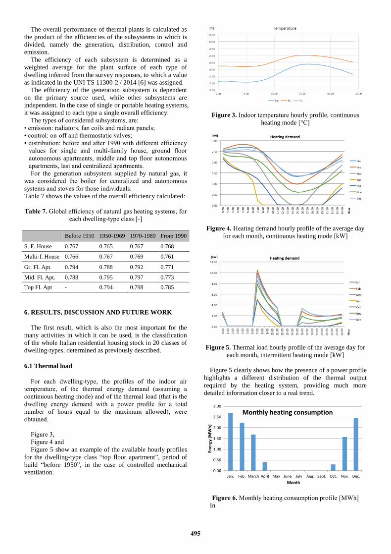
The overall performance of thermal plants is calculated as

the product of the efficiencies of the subsystems in which is

divided, namely the generation, distribution, control and

emission.

The efficiency of each subsystem is determined as a

weighted average for the plant surface of each type of

dwelling inferred from the survey responses, to which a value

as indicated in the UNI TS 11300-2 / 2014 [6] was assigned.

The efficiency of the generation subsystem is dependent

on the primary source used, while other subsystems are

independent. In the case of single or portable heating systems,

it was assigned to each type a single overall efficiency.

The types of considered subsystems, are:

• emission: radiators, fan coils and radiant panels;

• control: on-off and thermostatic valves;

• distribution: before and after 1990 with different efficiency

values for single and multi-family house, ground floor

autonomous apartments, middle and top floor autonomous

apartments, last and centralized apartments.

For the generation subsystem supplied by natural gas, it

was considered the boiler for centralized and autonomous

systems and stoves for those individuals.

Table 7 shows the values of the overall efficiency calculated:

Table 7. Global efficiency of natural gas heating systems, for

each dwelling-type class [-]

Before 1950 1950-1969 1970-1989 From 1990

S. F. House 0.767 0.765 0.767 0.768

Multi-f. House 0.766 0.767 0.769 0.761

Gr. Fl. Apt. 0.794 0.788 0.792 0.771

Mid. Fl. Apt. 0.788 0.795 0.797 0.773

Top Fl. Apt - 0.794 0.798 0.785

6. RESULTS, DISCUSSION AND FUTURE WORK

The first result, which is also the most important for the

many activities in which it can be used, is the classification

of the whole Italian residential housing stock in 20 classes of

dwelling-types, determined as previously described.

6.1 Thermal load

For each dwelling-type, the profiles of the indoor air

temperature, of the thermal energy demand (assuming a

continuous heating mode) and of the thermal load (that is the

dwelling energy demand with a power profile for a total

number of hours equal to the maximum allowed), were

obtained.

Figure 3,

Figure 4 and

Figure 5 show an example of the available hourly profiles

for the dwelling-type class “top floor apartment”, period of

build “before 1950”, in the case of controlled mechanical

ventilation.

Figure 3. Indoor temperature hourly profile, continuous

heating mode [°C]

Figure 4. Heating demand hourly profile of the average day

for each month, continuous heating mode [kW]

Figure 5. Thermal load hourly profile of the average day for

each month, intermittent heating mode [kW]

Figure 5 clearly shows how the presence of a power profile

highlights a different distribution of the thermal output

required by the heating system, providing much more

detailed information closer to a real trend.

Figure 6. Monthly heating consumption profile [MWh]

In

0.00

0.50

1.00

1.50

2.00

2.50

3.00

Jan. Feb. March April May June July Aug. Sept. Oct. Nov. Dec.

Ene

rgy

[MW

h]

Month

Monthly heating consumption

495

Figure 6 an example of a monthly consumption of thermal

energy for heating profile is plotted: it is referred to a single

simulation run of the 34 possible for each period of build and

for each climatic zone.

6.2 Energy product consumption

Starting from the results of the 34 simulations performed

for each period of build (Table 5), it is possible to obtain the

thermal energy consumption of each dwelling-type, as the

average weighted on the table of weights (Table 6) multiplied

by its corresponding reduction factor for intermittent heating,

aH,red (Table 8).

Table 8. Reduction factor for intermittent heating (aH,red)

corresponding to each simulation, period of build “before

1950”, climatic zone E [-]

S1 S2 S3 S4 S5 S6 S7 S8 S9 S10

SFH 0.70 - - - - - - - - -

MFH 0.83 0.81 0.82 - - - - - - -

GFApt 0.80 0.74 0.77 0.78 0.77 0.73 0.75 0.77 0.73 0.75

MFApt 0.71 0.62 0.66 0.67 0.72 0.68 0.70 0.73 0.67 0.70

TFApt 0.73 0.64 0.68 0.69 0.70 0.66 0.68 0.71 0.66 0.69

Since four periods of build have been identified, for each

climatic zone 136 simulations are performed, and their

results, weighted on Table 6 and multiplied by their

corresponding reduction factors for intermittent heating,

allow the calculation of the thermal energy consumption of

the 20 identified dwelling-types, as shown in Table 9.

Table 9. Heating consumption for each dwelling-type,

climatic zone E [kWhy]

Before 1950 1950-1969 1970-1989 From 1990

S. F. House 19342 18232 17957 18500

Multi-f. House 24138 21245 22979 23325

Gr. Fl. Apt. 9947 11287 9802 9704

Mid. Fl. Apt. 5832 5678 5966 6018

Top Fl. Apt 11154 9669 10774 10174

Dividing the heating consumption table of the dwelling-

types (Table 9) by the table of the dwelling-types' heated

floor surfaces (Table 4), the heating consumption per area for

each dwelling-type class, for the considered climatic zone, is

obtained (Table 10).

Table 10. Heating consumption per area for each dwelling-

type class, climatic zone E [kWh/m2y].

Before 1950 1950-1969 1970-1989 From 1990

S. F. House 159.20 158.54 149.77 141.99

Multi-f. House 197.85 204.88 198.27 190.26

Gr. Fl. Apt. 115.27 122.16 119.39 116.78

Mid. Fl. Apt. 64.24 67.93 66.96 64.86

Top Fl. Apt 113.24 107.92 115.35 112.05

The procedure described above is then applied for all

climatic zones, and a table similar to Table 10 is obtained for

each climatic zone.

For each dwelling-type class, is then possible to calculate

the weight of each climatic zone by considering the share of

floor surface of the class, falling in each zone: in the case of

the Veneto Region, for instance, the single family house class

is distributed between zone E (91.5 % of the heated floor

surface) and zone F (8.5 % of the heated floor surface).

This distribution is then summarized for each climatic

zone, as shown in Table 11 for the climatic zone E.

Table 11. % of floor surfaces of the building-type classes

falling in the climatic zone E [-]

Before 1950 1950-1969 1970-1989 From 1990

S. F. House 91.5% 95.6% 94.7% 96.6%

Multi-f. House 94.6% 93.4% 95.6% 97.2%

Gr. Fl. Apt. 100.0% 97.2% 94.5% 94.3%

Mid. Fl. Apt. 96.6% 95.6% 98.6% 100.0%

Top Fl. Apt 100.0% 95.9% 76.4% 75.8%

Weighting the simulation results of each climatic zone by

the percentage of floor falling in the zone itself, the heating

consumption per area for each dwelling-type class is

calculated. The results for the Veneto Region are summarized

in Table 12.

Table 12. Heating consumption per area for each dwelling-

type class [kWh/m2y]

Before 1950 1950-1969 1970-1989 From 1990

S. F. House 145.69 151.58 141.69 137.22

Multif. House 187.27 191.28 189.62 184.93

Gr. Fl. Apt. 115.27 118.75 112.82 110.14

Mid. Fl. Apt. 62.03 64.92 66.01 64.86

Top Fl. Apt 113.24 103.47 88.18 84.99

Multiplying the heating consumption per area by the total

area of the dwellings, that use a specific energy product for

heating (in the present example: natural gas), that fall in each

dwelling-type class (Table 13) and dividing by the respective

system’s global efficiency (Table 7), it is possible to assess

the total energy product consumption for heating of each

dwelling-type class for the specific energy product, as shown

in Table 14.

Table 13. Total floor surface of each dwelling-type class,

using Natural gas as energy product for heating [m2]

Before 1950 1950-1969 1970-1989 From 1990

S. F. House 5135 7785 11520 5665

Multi-f. House 1915 4950 6370 7865

Gr. Fl. Apt. 3340 7330 7375 3960

Mid. Fl. Apt. 720 3135 3400 2500

Top Fl. Apt 0 225 525 690

The sum of the elements of Table 14, reporting the total

annual consumption of the dwelling-type classes for the

considered energy product provides the overall annual energy

product consumption for heating of the residential building

496

stock for the considered energy product which, in the case of

the Veneto Region and of natural gas, is approx. 15,014

MWh.

Table 14. Total annual energy product consumption for

heating of each dwelling-type class, natural gas [MWhy]

Before 1950 1950-1969 1970-1989 From 1990

S. F. House 975.3 1542.9 2129.3 1011.5

Multi-f. House 468.3 1234.0 1570.6 1910.9

Gr. Fl. Apt. 484.9 1105.2 1050.0 565.4

Mid. Fl. Apt. 56.7 255.9 281.5 209.8

Top Fl. Apt 0.00 29.31 58.03 74.69

The project activity is still in progress. The present step, in

progress, is the comparison between the consumption data

calculated with the presented methodology and those

estimated by the ISTAT survey, the final results of the

comparison will be published later.

7. CONCLUSIONS

The above presented methodology has enabled, by means

of processing the data on energy consumption of Italian

families provided by the ISTAT survey and with the aid of a

dynamic simulation model, the realization of a tool able to

estimate the energy consumption and to create the thermal

load profiles of the representative dwellings of the Italian

residential sector.

In particular the methodology allowed to group the entire

national sample in 20 cluster of type dwellings, as a function

of building (dimensions, equipment, energy characteristics,

etc.), family (number of occupants, consumption habits, etc.)

and environmental (region, climatic zone, etc.)

characteristics.

The methodology is able to estimate energy consumptions

distinguished for end use (heating, cooling and domestic hot

water) and energy product.

The aim of the work is to increase knowledge of consumer

habits of end user to outline a real scenery of the buildings

consumption useful to address the choice of the most

efficient technological solutions and to provide guidance on

the policy actions of support for the dissemination of the

most promising technologies.

REFERENCES

[1] Istat, (2014, Dec. 15). “I consumi energetici delle

famiglie”, Statistiche Report, (In Italian). [Online].

Available: http://www.istat.it/it/archivio/142173.

[2] P. Ungaro, I. Bertini, (2014), “I modelli per la stima dei

consumi energetici per finalità d'uso e fonte”. [Online].

Available: http://www.istat.it/it/archivio/141193.

[3] Abaco delle strutture costituenti l'involucro opaco degli

edifici - Parametri termo fisici, UNI/TR 11552:2014

Standard, 2014.

[4] Energy performance of buildings - Calculation of energy

use for space heating and cooling, EN ISO 13790:2008

Standard, 2008.

[5] Prestazioni energetiche degli edifici. Parte 1:

Determinazione del fabbisogno di energia termica

dell’edificio per la climatizzazione estiva ed invernale.

UNI/TS 11300-1:2014.

[6] Prestazioni energetiche degli edifici. Parte 2:

Determinazione del fabbisogno di energia primaria e dei

rendimenti per la climatizzazione invernale, per la

produzione di acqua calda sanitaria, per la ventilazione e

per l'illuminazione in edifici non residenziali. UNI/TS

11300-2:2014.

497

1. INTRODUCTION

The European and national policies aimed at containing

the energy product consumption and at promoting the

diffusion of renewable sources, have stimulated the search

for ways to reduce the energy demand and to boost the

efficiency in energy production. In particular, for the

residential sector, the knowledge of the consumption habits

of the families is of vital importance for achieving the goals

set by the various European directives, as well as for raising

awareness on energy consumption and for stimulating

rational behaviors on energy use by end-users.

The regulation (EC) No 1099/2008 of the European

Parliament and of the Council of 22 October 2008 on energy

statistics, and the amending Commission Regulation (EU) No

431/2014 of 24 April 2014 on energy statistics, as regards the

implementation of annual statistics on energy consumption in

households, impose an obligation on Member States to

provide annual data on energy consumption of households

for final destination and energy source. In this framework

ISTAT in collaboration with ENEA and MiSE (Italian

Ministry of Economic Development) carried out the survey

on households energy consumption [1,2], as part of the

Italian National Statistics Plan. The survey was conducted in

2013 for the first time in Italy, on a representative sample of

20’000 households at regional level and made it possible to

obtain information on characteristics, consumption habits,

types of plant and energy costs of Italian households,

specified by energy product (primary energy sources and

energy carriers) and end-use (heating, cooling, domestic hot

water, cooking, lighting and electrical equipment).

This paper describes the methodology used to estimate the

energy consumption for heating and the creation of monthly

load profiles for residential dwellings. For the sake of

simplicity we have chosen to present the results for the

Veneto Region and heating systems fueled by natural gas; the

calculation method remains the same for other energy

products and for the entire Italian national territory.

Furthermore, this methodology will be used in the activity

ENEA-ISTAT to estimate the energy consumption of

households for the years between two replications of the

INTERNATIONAL JOURNAL OF

HEAT AND TECHNOLOGY

ISSN: 0392-8764 Vol. 34, No. 1, March, 2016, pp.

DOI:

A publication of IIETA

http://www.iieta.org/Journals/IJHT

A methodology for the generation of energy consumption profiles

in the residential sector

Giovanni Puglisi1*

, Fabio Zanghirella1, Paola Ungaro

2, Giuliano Cammarata

3

*1 ENEA (Italian National Agency for New Technologies, Energy and Sustainable Economic

Development), via Anguillarese 301, 00123 Roma, Italy 2 ISTAT (Italian National Institute of Statistics), Viale Oceano Pacifico 171, 00144, Roma, Italy

3 Università degli Studi di Catania, p.zza Università, 2, 95125 Catania, Italy

Email: giovanni.puglisi@enea.it

ABSTRACT The residential sector has been achieved in the last years more and more importance in the total energy

consumption scenario by stimulating the research for solutions to promote energy efficiency and to raise

awareness on energy consumption by end users.

The profile of a end-users energy consumption assumes a central role in finding solutions to reduce energy

demand and increase the efficiency in the production of the same energy.

European regulations impose an obligation on Member States to provide annually data on energy

consumption of households for end use and energy product. Data will be provided for Italy basing on data

collected by ISTAT Survey on energy consumption in the residential sector, appropriately processed by

ENEA and ISTAT.

In this paper it is presented a methodology that allowed to define a series of dwelling types, representative of

the entire national sample, as a function of building, family and environmental characteristics. These

dwellings, through the application of a dynamic simulation model, allowed the generation of monthly energy

consumption profiles (for heating, cooling and domestic heat water) for each cluster of dwelling types and the

evaluation of the energy consumption distribution of the residential sector for end use and energy product.

Keywords: energy consumption, residential sector, dwelling types, energy efficiency, end use, energy

demand, energy product, dynamic simulation.

ISTAT survey, starting from the ISTAT 2016 survey that will

be used to deliver the first data to Eurostat.

2. METHODOLOGY

The presented methodology is based on the processing of

the provided statistical data from the ISTAT 2013 survey on

households energy consumption, and on the identification of

dwelling-type classes representative of the entire Italian

residential building stock.

The information provided by the ISTAT 2013 survey and

used for the methodology are mainly:

dwelling characteristics (type of dwelling, year of build,

floor surface, opaque envelope type, transparent envelope

type, main exposure of the external walls);

characteristics of heating, cooling and DHW systems

(number, energy products, systems type –centralized,

individual or single device-, emission and temperature

control system, frequency of use and daily hours of use);

frequency of use of the systems;

energy cost by energy product.

The classification of the dwellings was chosen as a

function of:

period of build: before 1950, 1950-1969, 1970-1989,

from 1990;

type of dwelling: single family house, multi-family house,

ground floor apartment, middle floor apartment and top

floor apartment.

Table 1 summarizes the 20 identified dwelling-type classes

(DTC).

Table 1 – Dwelling-type classes.

Before

1950

1950-

1969

1970-

1989

From

1990

Single fam.

House DTC1 DTC6 DTC11 DTC16

Multi-fam.

House DTC2 DTC7 DTC12 DTC17

Ground fl. apt. DTC3 DTC8 DTC13 DTC18

Middle fl. apt. DTC4 DTC9 DTC14 DTC19

Top fl. apt. DTC5 DTC10 DTC15 DTC20

The evaluation of the energy product consumption for

heating has been carried out in different stages, as

exemplified in Figure 1:

a. determination of the thermal energy demand, in

continuous heating mode, of the dwelling-type [kWhy] by

means of a dynamic simulation software; the simulations

were performed assuming a continuous heating mode

(heating system on 24 hours a day), because the survey

answers do not allow to determine an hourly power

profile; the simulation results also provide the time profile

of the heating demand of each dwelling-type;

b. calculation of the reduction factor for intermittent heating

as a function of the average number of daily hours during

which the heating system is switched on, based on the

answers of the survey;

c. assumption of the efficiency of the different types of plant

for each dwelling-type, and estimation of the heating

consumptions per floor area [kWh/m2y];

d. estimation of the total annual energy product

consumption for heating for each class (m3, kg, l, etc.) for

a certain energy product, obtained by multiplying the

consumption per area by the total area of the dwellings,

that use that specific energy product for heating, that fall

in each dwelling-type class.

The decision to estimate the thermal energy demand for all

the dwelling-types by means of a dynamic simulation of the

dwelling, and then calculate the energy product consumption

by multiplying the heating demand calculated in continuous

mode by the reduction factor for intermittent heating and by

the average total efficiency of the heating system was related

to the information provided by survey about the type and the

characteristics of the heating systems. Clearly, the

information provided by the survey can’t have a detail level

sufficient to estimate a management profile of the heating

systems, which is instead essential to perform a dynamic

simulation of the building-plant system.

Since the energy performances of buildings are strongly

influenced by climatic conditions, the same dwelling-type

was simulated in each climate zone. For each climatic zone in

which the country is divided, the input weather data

(temperature, radiation and humidity) adopted for the

simulations were those of the chief town whose degree days

are "barycentric" with respect to the degree days interval of

the climatic zone.

3. DEFINITION OF THE DWELLING-TYPE CLASSES

Each dwelling-type class is characterized by thermo-

physical and dimensional parameters, determined on the

basis of the information gathered from the ISTAT survey

results, appropriately processed, and of the input data

required by the simulation model. Below the main properties

that define each dwelling-type class are listed and described.

Figure 1 - Methodology scheme, for space heating and for a single energy product.

….

….

….

….

…..

…..

Input

For each

Dwelling-type

Sec1, dw1

Sec1, dw2

Sec1, dwnSpace

heating

needs

Dwelling-

types

1/Sdw1

1/Sdw2

1/Sdwn

kWh, m3,…

Estimation of

the energy

consumption

per energycarrier

Heating system efficiency, dw1

Heating system efficiency, dw2

Heating system efficiency, dwn P

rim

ary

energ

yper

are

a

Space

heat.

Needs

per

are

a

For each

Dwelling-type

Thermal transmittance of the opaque envelope: for each

period of build a specific structure was deduced for the

exterior walls, the floor and the ceiling, the corresponding

thermal transmittance was determined, using data from

the Italian standard UNI/TR 11552:2014. Table 2

summarizes the adopted values.

Table 2 – Thermal transmittance of the opaque envelope

by period of build [kW/m2K].

Before 1950 1950-1969 1970-1989 From 1990

Walls 1.093 1.065 0.675 0.456

Floor 0.781 0.781 0.850 0.442

Roof 1.376 1.376 0.777 0.441

Thermal transmittance of the transparent envelope: the

survey provided as possible answers two types of glass

(single, double) and three types of frame (wood, metal,

PVC): for these types the average transmittance values

were calculated according to the Italian standard UNI/TR

11552: 2014 [3]; the equivalent transmittance of the glass

and of the frame for each dwelling-type, was determined

weighting the thermal transmittances corresponding to the

answers of the survey on their incidence on the total

number of dwellings that fall in the class; since the

transparent surface is not an information inferable from

the survey, a transparent surface equal to 1/8 of the floor

surface was assumed to calculate the transmittance of the

window. Table 3 summarizes the obtained values.

Table 3 – Thermal trasmittance of the trasparent

envelope by period of build and type of dwelling

[kW/m2K].

Before

1950

1950-

1969

1970-

1989

From

1990

S. F. House 3.320 3.490 3.280 2.450

Multi-fam.

House 3.010 3.230 2.950 2.400

Apartments 3.240 3.530 3.400 2.560

Floor surface: since the survey answers are provided for

10 m2 surface intervals, the floor area of the dwelling-

type is calculated as the average of the central values of

the surface intervals weighted on the frequency of the

answers for each surface interval (Table 4).

Table 4 – Dwelling-types' heated floor surfaces [m2].

Before 1950 1950-1969 1970-1989 From 1990

S. F. House 121.5 115.0 119.9 130.3

Multi-f. House 122.0 103.7 115.9 122.6

Gr. Fl. Apt. 86.3 92.4 82.1 83.1

Mid. Fl. Apt. 90.8 83.6 89.1 92.8

Top Fl. Apt 98.5 89.6 93.4 90.8

Exposure: the survey provides information about two

main exposures (without specifying the prevailing one) of

the external walls of the dwelling. Analyzing the

frequency of all possible answers and the combinations

between them it was assumed that the multi-family

dwellings have two possible types of exposure: two

opposite sides or three adjacent sides exposed to the

outside; for apartments the types of exposure are three:

one single side, two opposite sides and two adjacent sides

exposed to the outside; for the single family house all the

4 sides are considered exposed to the outside. Table 5

summarizes all the 34 considered types of exposure,

corresponding to the simulations to be performed for each

period of build. The weight of each type of exposure is

proportional to the number of dwellings that fall in it;

Table 6 summarizes the weight of the identified types of

exposure and of their consequent simulations.

Table 5 - Dwelling walls’ main exposures and consequent

simulations.

S1 S2 S3 S4 S5 S6 S7 S8 S9 S10

SFH all - - - - - - - - -

MFH N+S E+W N+E+S - - - - - - -

GFApt N E S W N+S E+W N+E N+W E+S S+W

MFApt N E S W N+S E+W N+E N+W E+S S+W

TFApt N E S W N+S E+W N+E N+W E+S S+W

Table 6 – Weight of each identified type of exposure and

consequent simulation.

S1 S2 S3 S4 S5 S6 S7 S8 S9 S10

SFH 100.0% - - - - - - - - -

MFH 44.1% 23.9% 32.0% - - - - - - -

GFApt 14.2% 11.7% 12.6% 4.9% 10.5% 10.8% 7.6% 7.6% 12.4% 7.9%

MFApt 14.2% 11.7% 12.6% 4.9% 10.5% 10.8% 7.6% 7.6% 12.4% 7.9%

TFApt 14.2% 11.7% 12.6% 4.9% 10.5% 10.8% 7.6% 7.6% 12.4% 7.9%

Heat losing surfaces: the vertical heat losing surfaces are

determined in accordance with the previously identified

types of exposure, considering a square shaped floor and

assuming the height of the walls for each type of

dwelling; the total window surface, assumed to be equal

to 1/8 of the floor surface, is divided equally among the

walls exposed to the outside. For both the single and the

multi-family house, the floor and the ceiling are

considered heat losing surfaces. As far as the apartments

are concerned, the middle floor apartment has no

horizontal heat losses, the ground floor has heat losses

through the floor and the top floor apartment has heat

losses through the ceiling.

4. THE SIMULATION MODEL

Since the aim of the work is the determination of both the

energy consumption and the thermal load profiles, we chose

to use a dynamic simulation model, made by the University of Catania, based on the equivalent resistance-capacitance

model proposed in the european standard EN ISO 13790 [4].

Dynamic models for the evaluation of energy consumption

in buildings are developed taking into account the variability

of both the external climatic conditions of the internal loads.

In general, the calculation of the heat load in summer is done

with dynamic methods that take into account the thermal

capacity and the thermal transients of the buildings The european standard EN ISO 13790 proposes an electro-

thermal dynamic model simplified with five thermal

conductance and a heat capacity, called 5R1C, shown in

Figure 2.

Figure 2 - 5R1C Model Scheme.

The nodes in the model scheme represent the ventilation

(sup), the outdoor air (e), the envelope mass (m), the

envelope indoor surface (s) and the indoor air (air)

temperatures. The heat transfer coefficients are: the

ventilation heat transfer coefficient (Hve), the transmission

heat transfer coefficient for windows (Htr,w), the emissive

transmission heat transfer coefficient for the opaque envelope

towards the envelope mass (Htr,em), the conductive

transmission heat transfer coefficient for the opaque envelope

towards the envelope indoor surface (Htr,ms), the coupling

conductance between the envelope indoor surface and the

indoor air (Htr,is). The heat flows are: heat flow rate from

internal and solar sources towards the envelope mass (m),

heat flow rate from internal and solar sources towards the

envelope indoor surface (st), heat flow rate from internal

sources towards indoor air (ia), heating or cooling needs

(HC,nd).

The EN ISO 13790 standard defines uniquely the heat

transfer coefficients and proposes a mode of solution refers to

the monthly average daily conditions and monthly average

daily time conditions.

The direct solution results in the calculation, set the

temperature and the thermal conductance, the net flux

exchanged, HC,nd, under changing climatic conditions. This

solution involves the solution of a differential equation

related to the heat balance to m node:

CdT

m

dt+ H

tr ,em+ H

tr ,ms- H

tr ,ms

Htr ,ms

Htr ,w

+ Htr ,ms

+ Hsi

æ

è

çç

ö

ø

÷÷T

m=

=Fm

+Htr ,em

Te+H

tr ,ms

Fsi

+ Htr ,w

Te+ H

siT

air

Htr ,w

+ Htr ,ms

+ Hsi

For the net flow is we have:

, supHC nd ve air si air si airH T T H T T

The recursive solution based on Heun method is:

1 112 2 2

m n m n m n n n

T T TT t T t T t g t g t

where is:

,

, , ,

, ,

tr ms

tr em tr ms tr ms

t w tr ms si

HH H H

H H H

C

,

, ,

, ,

si tr w e si air

m tr em e tr ms

tr w tr ms si

H T H TH T H

H H Hg

C

The calculation thus prepared is sufficient and can be

quickly implemented on Excel spreadsheet.

The input data required for the model are:

thermal transmittance of the component, W / (m².K).

participation factor (required by UN EN 13790)

total surface of each element m².

solar absorption factor for opaque walls and global solar

transmittance for transparent surfaces;

shading factor (as per UNI EN 13790).

total building height, m;

number of air changes per hour in the absence of VMC;

air flow temperature of ventilation in the case of

controlled mechanical ventilation;

ambient temperature that you want to have during the

night attenuation.

specific flow to the sky;

reference temperature for plant regulation (set equal to

20° C in winter and 26° C in summer);

total atmospheric pressure for the town considered;

humidity of the ventilation;

latent heat intensity for internal sources.

An important feature of the method is the ability to

customize the input vectors as a function of weather data, the

real profiles for plants and internal gains.

As output, the model provides for each day (representative

of the month) a time profile of the latent load, the total load

required, the attenuation coefficient, the indoor air

temperature and the inner surface of the walls..

5. ESTIMATION OF THE ENERGY PRODUCT

CONSUMPTION

The consumption of primary energy from the thermal

energy demand is determined according to the following parameters:

number of hours of daily usage of the plant for each

dwelling-type, calculated as the average of the answers

and divided into climatic zones;

reduction factor, aH,red,for intermittent heating;

average overall efficiency of the heating plant.

The aH,red coefficient takes into account that the plants

don’t run for all day, the solar and inner gains and the

building time constant and is calculated according to the formula proposed in the UNI TS 11300-1 / 2014 [5]:

aH ,red =1- bH ,red

t H ,O

tæ

èç

ö

ø÷gH (1- fH ,hr )

The overall performance of thermal plants is calculated as

the product of the efficiencies of the subsystems in which is

divided, namely the generation, distribution, control and

emission.

The efficiency of each subsystem is determined as a

weighted average for the plant surface of each type of

dwelling inferred from the survey responses, to which a value

as indicated in the UNI TS 11300-2 / 2014 [6] was assigned.

The efficiency of the generation subsystem is dependent

on the primary source used, while other subsystems are

independent. In the case of single or portable heating systems

it was assigned to each type a single overall efficiency.

The types of considered subsystems, are:

• emission: radiators, fan coils and radiant panels;

• control: on-off and thermostatic valves;

• distribution: before and after 1990 with different efficiency

values for single and multi-family house, ground floor

autonomous apartments, middle and top floor autonomous

apartments last and centralized apartments.

For the generation subsystem supplied by natural gas, was

considered the boiler for centralized and autonomous systems

and stoves for those individuals. Table 7 shows the values of the overall efficiency calculated:

Table 7 - Global efficiency of natural gas heating systems,

for each dwelling-type class [-].

Before 1950 1950-1969 1970-1989 From 1990

S. F. House 0.767 0.765 0.767 0.768

Multi-f. House 0.766 0.767 0.769 0.761

Gr. Fl. Apt. 0.794 0.788 0.792 0.771

Mid. Fl. Apt. 0.788 0.795 0.797 0.773

Top Fl. Apt - 0.794 0.798 0.785

6. RESULTS, DISCUSSION AND FUTURE WORK

The first result, which is also the most important for the

many activities in which it can be used, is the classification

of the whole Italian residential housing stock in 20 classes of

dwelling-types, determined as previously described.

6.1 Thermal load

For each dwelling-type, the profiles of the indoor air

temperature, of the thermal energy demand (assuming a

continuous heating mode) and of the thermal load (that is the

dwelling energy demand with a power profile for a total

number of hours equal to the maximum allowed), were

obtained. Figure 3, Figure 4 and Figure 5 show an example of the

availablehourly profiles for the dwelling-type class “top floor

apartment”, period of build “before 1950”, in the case of

controlled mechanical ventilation.

Figure 3 – Indoor temperature hourly profile, continuous

heating mode [°C].

Figure 4 - Heating demand hourly profile of the average

day for each month, continuous heating mode [kW].

Figure 5 – Thermal load hourly profile of the average day

for each month, intermittent heating mode [kW].

Figure 5 clearly shows how the presence of a power profile

highlight a different distribution of the thermal output

required to the heating system, providing much more detailed

information and close to a real trend.

Figure 6 – Monthly heating consumption profile [MWh].

In Figure 6 an example of a monthly consumption of

thermal energy for heating profile is plotted: it is referred to a

0.00

0.50

1.00

1.50

2.00

2.50

3.00

Jan. Feb. March April May June July Aug. Sept. Oct. Nov. Dec.

Ene

rgy

[MW

h]

Month

Monthly heating consumption

single simulation run of the 34 possible for each period of

build and for each climatic zone.

6.2 Energy product consumption

Starting from the results of the 34 simulations performed

for each period of build (Table 5), it is possible to obtain the

thermal energy consumption of each dwelling-type, as the

average weighted on the table of weights (Table 6) multiplied

by its corresponding reduction factor for intermittent heating,

aH,red (Table 8).

Table 8 – Reduction factor for intermittent heating (aH,red)

corresponding to each simulation, period of build “before

1950”, climatic zone E [-].

S1 S2 S3 S4 S5 S6 S7 S8 S9 S10

SFH 0.70 - - - - - - - - -

MFH 0.83 0.81 0.82 - - - - - - -

GFApt 0.80 0.74 0.77 0.78 0.77 0.73 0.75 0.77 0.73 0.75

MFApt 0.71 0.62 0.66 0.67 0.72 0.68 0.70 0.73 0.67 0.70

TFApt 0.73 0.64 0.68 0.69 0.70 0.66 0.68 0.71 0.66 0.69

Since four periods of build have been identified, for each

climatic zone 136 simulations are performed, and their

results, weighted on Table 6 and multiplied by their

corresponding reduction factors for intermittent heating,

allow the calculation of the thermal energy consumption of

the 20 identified dwelling-types, as shown in Table 9.

Table 9 - Heating consumption for each dwelling-type,

climatic zone E [kWhy].

Before 1950 1950-1969 1970-1989 From 1990

S. F. House 19342 18232 17957 18500

Multi-f. House 24138 21245 22979 23325

Gr. Fl. Apt. 9947 11287 9802 9704

Mid. Fl. Apt. 5832 5678 5966 6018

Top Fl. Apt 11154 9669 10774 10174

Dividing the heating consumption table of the dwelling-

types (Table 9) by the table of the dwelling-types' heated

floor surfaces (Table 4), the heating consumption per area for

each dwelling-type class, for the considered climatic zone, is

obtained (Table 10).

Table 10 - Heating consumption per area for each

dwelling-type class, climatic zone E [kWh/m2y].

Before 1950 1950-1969 1970-1989 From 1990

S. F. House 159.20 158.54 149.77 141.99

Multi-f. House 197.85 204.88 198.27 190.26

Gr. Fl. Apt. 115.27 122.16 119.39 116.78

Mid. Fl. Apt. 64.24 67.93 66.96 64.86

Top Fl. Apt 113.24 107.92 115.35 112.05

The procedure described above is then applied for all

climatic zones, and a table similar to Table 10 is obtained for

each climatic zone.

For each dwelling-type class, is then possible to calculate

the weight of each climatic zone by considering the share of

floor surface of the class, falling in each zone: in the case of

the Veneto Region, for instance, the single family house class

is distributed between zone E (91.5% of the heated floor

surface) and zone F (8.5% of the heated floor surface).

This distribution is then summarized for each climatic

zone, as shown in Table 11 for the climatic zone E.

Table 11 – % of floor surfaces of the building-type classes

falling in the climatic zone E [-].

Before 1950 1950-1969 1970-1989 From 1990

S. F. House 91.5% 95.6% 94.7% 96.6%

Multi-f. House 94.6% 93.4% 95.6% 97.2%

Gr. Fl. Apt. 100.0% 97.2% 94.5% 94.3%

Mid. Fl. Apt. 96.6% 95.6% 98.6% 100.0%

Top Fl. Apt 100.0% 95.9% 76.4% 75.8%

Weighting the simulation results of each climatic zone by

the percentage of floor falling in the zone itself, the heating

consumption per area for each dwelling-type class is

calculated. The results for the Veneto Region are summarized

in Table 12.

Table 12 - Heating consumption per area for each

dwelling-type class [kWh/m2y].

Before 1950 1950-1969 1970-1989 From 1990

S. F. House 145.69 151.58 141.69 137.22

Multif. House 187.27 191.28 189.62 184.93

Gr. Fl. Apt. 115.27 118.75 112.82 110.14

Mid. Fl. Apt. 62.03 64.92 66.01 64.86

Top Fl. Apt 113.24 103.47 88.18 84.99

Multiplying the heating consumption per area by the total

area of the dwellings, that use a specific energy product for

heating (in the present example: natural gas), that fall in each

dwelling-type class (Table 13) and dividing by the respective

system’s global efficiency (Table 7), it is possible to assess

the total energy product consumption for heating of each

dwelling-type class for the specific energy product, as shown

in Table 14.

Table 13 - Total floor surface of each dwelling-type class,

using Natural gas as energy product for heating [m2].

Before 1950 1950-1969 1970-1989 From 1990

S. F. House 5135 7785 11520 5665

Multi-f. House 1915 4950 6370 7865

Gr. Fl. Apt. 3340 7330 7375 3960

Mid. Fl. Apt. 720 3135 3400 2500

Top Fl. Apt 0 225 525 690

The sum of the elements of the table of the total annual

consumption of the dwelling-type classes for the considered

energy product (Table 14), provides the overall annual

energy product consumption for heating of the residential

building stock for the considered energy product which, in

the case of the Veneto Region and of natural gas, is approx.

15.014 MWh.

Table 14 - Total annual energy product consumption for

heating of each dwelling-type class, natural gas [MWhy].

Before 1950 1950-1969 1970-1989 From 1990

S. F. House 975.3 1542.9 2129.3 1011.5

Multi-f. House 468.3 1234.0 1570.6 1910.9

Gr. Fl. Apt. 484.9 1105.2 1050.0 565.4

Mid. Fl. Apt. 56.7 255.9 281.5 209.8

Top Fl. Apt 0.00 29.31 58.03 74.69

The project activity is still in progress. The present step, in

progress, is the comparison between the consumption data

calculated with the presented methodology and those

estimated by the ISTAT survey, the final results of the

comparison will be published later.

7. CONCLUSIONS

The above presented methodology has enabled, by means

of processing the data on energy consumption of Italian

families provided by the ISTAT survey and with the aid of a

dynamic simulation model, the realization of a tool able to

estimate the energy consumption and to create the thermal

load profiles of the representative dwellings of the Italian

residential sector.

In particular the methodology allowed to group the entire

national sample in 20 cluster of type dwellings, as a function

of building (dimensions, equipment, energy characteristics,

etc.), family (number of occupants, consumption habits, etc.)

and environmental (region, climatic zone, etc.)

characteristics.

The methodology is able to estimate energy consumptions

distinguished for end use (heating, cooling and domestic hot

water) and energy product.

The aim of the work is to increase knowledge of consumer

habits of end users to outline a real scenery of the buildings

consumption useful to address the choice of the most

efficient technological solutions and to provide guidance on

the policy actions of support for the dissemination of the

most promising technologies.

REFERENCES

[1] Istat, “I consumi energetici delle famiglie”, Statistiche Report,

15 dicembre 2014, 2014. (In Italian). [Online]. Available:

http://www.istat.it/it/archivio/142173.

[2] P. Ungaro, I. Bertini, "I modelli per la stima dei consumi

energetici per finalità d'uso e fonte", 2014. [Online].

Available: http://www.istat.it/it/archivio/141193.

[3] Abaco delle strutture costituenti l'involucro opaco degli

edifici - Parametri termo fisici, UNI/TR 11552:2014

Standard, 2014.

[4] Energy performance of buildings - Calculation of energy use

for space heating and cooling, EN ISO 13790:2008

Standard, 2008.

[5] Prestazioni energetiche degli edifici. Parte 1: Determinazione

del fabbisogno di energia termica dell’edificio per la

climatizzazione estiva ed invernale. UNI/TS 11300-1:2014

[6] Prestazioni energetiche degli edifici. Parte 2: Determinazione

del fabbisogno di energia primaria e dei rendimenti per la

climatizzazione invernale, per la produzione di acqua calda

sanitaria, per la ventilazione e per l'illuminazione in edifici

non residenziali. UNI/TS 11300-2:2014