
Quantitative Credit Research - QUANTLABS.NET
68
PLEASE SEE ANALYST CERTIFICATIONS AND IMPORTANT DISCLOSURES ON THE BACK COVER. Fixed Income Quantitative Credit Research Quantitative Credit Research Quarterly Volume 2007-Q1 Base Correlation Mapping........................................................................... 3 The pricing of bespoke tranches in the base correlation framework requires mapping techniques to allow correlations calibrated in the liquid tranche market to be applied to bespoke portfolios. In this article we describe methods of mapping bespoke portfolios to standard indices and investigate their impact on pricing and risk. We also compare the performance of the different methods in the pricing of a range of bespoke portfolios and discuss possible ways to price bespokes mapped to more than one index. Idiosyncratic Portfolio Risk in non-Normal Markets............................... 21 We consider security-level return factor models with a heavy-tailed idiosyncratic component. We model the portfolio-level idiosyncratic component as a t distribution. The tail index, i.e. the degrees of freedom, of this distribution is accurately modeled as a function of two inputs: first, the risk-adjusted average of the single-security tail index; second, the level of diversification in the portfolio. In order to suitably quantify diversification we introduce an entropy-based risk- adjusted measure. Trading Event Risk in Credit Markets using LEVER ............................... 30 Releveraging events have recently become a significant source of risk in credit markets. The LEVER model and the LEVER Powertool on LehmanLive have been developed to assess this risk on a systematic basis. We analyse the LEVER model as an investment framework to identify and extract alpha, and find that trades based on the LEVER framework perform well historically and that their correlation with the market and other traditional credit trading strategies is low. This finding is useful for both portfolio managers with benchmark outperformance mandates and those with absolute-return mandates. Introducing Lehman Brothers’ CMetrics Framework ............................. 42 Fundamental equity and credit analysts seek to interpret companies’ financial statements in order to identify key areas of strength and weakness with a view to making informed judgments about future prospects. Over time individual analysts have adopted and adapted a myriad of measures to gauge opportunities and risks within their coverage universe. Lehman Brothers’ CMetrics is a new financial framework aimed at improving the quality of financial analysis and valuations.
-
Upload
khangminh22 -
Category
Documents
-
view
0 -
download
0
Transcript of Quantitative Credit Research - QUANTLABS.NET

PLEASE SEE ANALYST CERTIFICATIONS AND IMPORTANT DISCLOSURES ON THE BACK COVER.
Fixed IncomeQuantitative Credit Research
Quantitative Credit Research Quarterly
Volume 2007-Q1
Base Correlation Mapping...........................................................................3 The pricing of bespoke tranches in the base correlation framework requires mapping techniques to allow correlations calibrated in the liquid tranche market to be applied to bespoke portfolios. In this article we describe methods of mapping bespoke portfolios to standard indices and investigate their impact on pricing and risk. We also compare the performance of the different methods in the pricing of a range of bespoke portfolios and discuss possible ways to price bespokes mapped to more than one index.
Idiosyncratic Portfolio Risk in non-Normal Markets...............................21 We consider security-level return factor models with a heavy-tailed idiosyncratic component. We model the portfolio-level idiosyncratic component as a t distribution. The tail index, i.e. the degrees of freedom, of this distribution is accurately modeled as a function of two inputs: first, the risk-adjusted average of the single-security tail index; second, the level of diversification in the portfolio. In order to suitably quantify diversification we introduce an entropy-based risk-adjusted measure.
Trading Event Risk in Credit Markets using LEVER...............................30 Releveraging events have recently become a significant source of risk in credit markets. The LEVER model and the LEVER Powertool on LehmanLive have been developed to assess this risk on a systematic basis. We analyse the LEVER model as an investment framework to identify and extract alpha, and find that trades based on the LEVER framework perform well historically and that their correlation with the market and other traditional credit trading strategies is low. This finding is useful for both portfolio managers with benchmark outperformance mandates and those with absolute-return mandates.
Introducing Lehman Brothers’ CMetrics Framework .............................42 Fundamental equity and credit analysts seek to interpret companies’ financial statements in order to identify key areas of strength and weakness with a view to making informed judgments about future prospects. Over time individual analysts have adopted and adapted a myriad of measures to gauge opportunities and risks within their coverage universe. Lehman Brothers’ CMetrics is a new financial framework aimed at improving the quality of financial analysis and valuations.

Lehman Brothers | Quantitative Credit Research QCR Quarterly, vol. 2007-Q1
March 7, 2007 2
CONTACTS
Quantitative Credit Research (Americas) Marco Naldi .........................................................................................................212-526-1728......................................mnaldi@lehman.com Prasun Baheti .......................................................................................................212-526-9251....................................prbaheti@lehman.com Bodhaditya Bhattacharya......................................................................................212-526-3408................................... [email protected] Ozgur Kaya ..........................................................................................................212-526-4296....................................... [email protected] Praveen Korapaty .................................................................................................212-526-0680...................................pkorapat@lehman.com Yadong Li.............................................................................................................212-526-1235.........................................yadli@lehman.com Jin Liu ..................................................................................................................212-526-3716......................................... [email protected] Claus M. Pedersen................................................................................................212-526-7775................................. [email protected] Leandro Saita .......................................................................................................212-526-4443........................................ [email protected] Minh Trinh ...........................................................................................................212-526-1712...................................... [email protected] Erik Wong ............................................................................................................212-526-3342....................................eriwong@lehman.com
Quantitative Credit Research (Europe) Lutz Schloegl .......................................................................................................44-20-7102-2113.............................. [email protected] Friedel Epple ........................................................................................................44-20-7102-5982..................................fepple@lehman.com Clive Lewis ..........................................................................................................44-20-7102-2820................................. [email protected] Sam Morgan .........................................................................................................44-20-7102-3359........................... [email protected]
Quantitative Credit Research (Asia) Hui Ou-Yang........................................................................................................81-3-6440 [email protected] ChoongOh Kang...................................................................................................81-3-6440 1511................................ [email protected] Wenjun Ruan........................................................................................................81-3-6440 [email protected]
Quantitative Market Strategies Vasant Naik..........................................................................................................44-20-7102-2813...................................vnaik@lehman.com Srivaths Balakrishnan...........................................................................................44-20-7102-2180............................... [email protected] Albert Desclee ......................................................................................................44-20-7102-2474.............................. [email protected] Mukundan Devarajan ...........................................................................................44-20-7102-9033............................mudevara@lehman.com Simon Polbennikov ..............................................................................................44-20-7102-3883.............................. [email protected] Adam Purzitsky ....................................................................................................44-20-7102-9023............................... [email protected] Jeremy Rosten ......................................................................................................44-20-7102-1020.................................jrosten@lehman.com
POINT Modeling Anthony Lazanas..................................................................................................212-526-3127................................... [email protected] Ningui Liu ............................................................................................................212-526-7536......................................... [email protected] Attilio Meucci ......................................................................................................212-526-5554................................... [email protected] Antonio Silva ......................................................................................................212-526-8880..................................... [email protected] Arne Staal.............................................................................................................212-526-6908........................................astaal@lehman.com
Additional Michael Bos ....................Global Head of Quantitative Research........................212-526-0886........................................mbos@lehman.com Prafulla Nabar .................Global Head of Enterprise Valuation ..........................212-526-6108......................................pnabar@lehman.com Michael Guarnieri ...........Global Head of Credit Research .................................212-526-3919..................................mguarnie@lehman.com Ashish Shah.....................Global Head of Credit Strategy...................................212-526-9360...................................... [email protected]

Lehman Brothers | Quantitative Credit Research QCR Quarterly, vol. 2007-Q1
March 7, 2007 3
Base Correlation Mapping The pricing of bespoke tranches in the base correlation framework requires mapping techniques to allow correlations calibrated in the liquid tranche market to be applied to bespoke portfolios. In this article we describe methods of mapping bespoke portfolios to standard indices and investigate their impact on pricing and risk. A useful quantitative test of the methods is to map one standard index to another and compare the prices with those observed in the market. We present the results of this analysis for mapping both the iTraxx S6 and CDX HY7 indices to CDX IG7 at the end of January 2007. We also compare the performance of the different methods in the pricing of a range of bespoke portfolios and discuss possible ways to price bespokes mapped to more than one index.
INTRODUCTION
The pricing of CDO tranches on bespoke portfolios depends crucially on our assumptions about the default correlations between the credits in the underlying collateral. The establishment of a liquid index tranche market means that it is now possible to obtain implied correlations for a range of standard portfolios from the observed market prices. In the current market standard approach, this is achieved by calibrating a one-factor Gaussian copula model with base correlation (BC) to the liquid indices [1]. Using mapping procedures, BCs can then be obtained for bespoke CDO tranches, allowing pricing and risk-management of these instruments. In this article, we describe a range of approaches that can be used to map bespoke portfolios to standard indices and investigate their impact on pricing and risk.
We start by defining what we mean by BC and then describe the various mapping methods that we consider in this article. A useful quantitative test of these methods is to map one standard index to another because in this case we can compare the prices and correlations with those observed or calibrated in the market. We present results from this analysis for the particular case of mapping the iTraxx S6 and CDX HY7 indices to CDX IG7 using market data from 31 January 2007. We also consider how the various mappings perform when the spread on a single-name in the iTraxx S6 portfolio widens dramatically, ultimately leading to a default. We then compare the methods for mapping a range of generic bespoke portfolios to CDX IG7. Here, judgments about the quality of the results are more subjective but we can make general observations about the range of prices produced, the relative behavior of the different methods and the various difficulties that can arise. Finally, we discuss two ways in which a bespoke portfolio can be mapped to more than one index and compare the results for a particular case.
BASE CORRELATION
To value a tranche in the one-factor Gaussian copula framework, we need to know the correlations to apply to the underlying credits so that we can build the portfolio loss distribution for a range of times up to the maturity of the trade. These correlations may depend on time, and in the simplest implementation of the BC framework they are constant across all the credits in the portfolio. The phenomenon of correlation skew means that the correlation must depend on the position in the capital structure of the particular tranche being priced if the model is to match the observed market prices. Since any tranche can be written as a combination of a long and short position in two base tranches, we can write the correlation as a function of detachment point K and time T, i.e. ρ = ρ(K,T). This BC surface gives the single correlation that should be used for all credits in the one-factor Gaussian copula model to compute the expected loss of a base tranche with detachment point K at time T.
Prasun Baheti +1 212 526 9251
Sam Morgan +44 20 7102 3359
samuel.morgan@lehman

Lehman Brothers | Quantitative Credit Research QCR Quarterly, vol. 2007-Q1
March 7, 2007 4
For standard indices, the BC surface can be obtained by calibration to the liquid tranche market using a bootstrapping algorithm. For example, consider the case of the CDX IG index, for which liquid tranches trade at strikes of 3%, 7%, 10%, 15%, and 30%, and maturities of 5Y, 7Y, and 10Y. With an assumption about the level of initial correlations and a local method to interpolate in time, we can calibrate the BC at (K,T) = (3%,5Y) by matching the market price for this tranche. With this information the correlation at (K,T) = (7%,5Y) can be obtained so that we match the price of the 3-7% tranche. Proceeding up the capital structure we obtain the BC at all the standard strikes at the 5Y maturity. For the 7Y maturity, the correlation at (K,T) = (3%,7Y) is calculated by matching the market price for the 7Y equity tranche using the previously calibrated BCs for all times before 5Y. In this way, the BC surface can be obtained out to the 10Y maturity, and for a given strike all cash flows at a fixed time horizon are priced with the same correlation regardless of the maturity of the trade. The BC at non-standard maturities or strikes can be obtained by interpolation within the BC surface.
MAPPING THE BASE CORRELATION SURFACE
Application of the BC model to tranches on bespoke portfolios requires a mapping rule to produce a BC surface for the bespoke portfolio at the strikes of interest. The general method is to associate a base tranche with detachment point KB on the bespoke portfolio, with an equivalent base tranche on a standard portfolio with strike Eq
SK . The correlation used to price the bespoke tranche is then taken to be the correlation at the equivalent standard strike, i.e. ( ) ( )TKTK Eq
SSBB ,, ρρ = . This procedure is used to generate the BCs for the bespoke portfolio at the standard maturities, and values at other times are obtained by interpolation as for the standard index.
Different mapping methods are distinguished by the way they define equivalence in this procedure. We will consider four examples in this article: No-Mapping (NM), At-The-Money (ATM), Probability Matching (PM), and Tranche-Loss-Proportion (TLP). These methods work by defining a quantity that measures the risk in a tranche and treating it as a market invariant. Calibration to the liquid indices tells us the correlation that should be used to price a particular level of risk and this value is therefore used to price bespoke tranches with the same risk. If a particular mapping rule is consistent with the market, then plots of the associated risk measure against correlation should coincide, independent of the particular portfolios we consider. We show an example of such a comparison later in this article, in Figure 4, for the PM and TLP mappings.
The mapping methods are defined in detail below, but we first consider what general characteristics a good method should have. Ideally, these would include as many as possible of the following criteria:
• It should be intuitive, in the sense that changes in the correlation should be easily attributable to changes in the market environment.
• It should have a plausible theoretical justification. • It should be sensitive only to correlation and insensitive to all other drivers of
tranche value, particularly to spread levels and spread dispersion. • It should be stable with respect to small changes in the market environment. • It should not introduce arbitrage in the bespoke where there is none in the index. • It should be easy to implement and always give a solution. • It should be able to map to a wide range of portfolios in terms of risk. • It should reflect effects of sector or spread concentration in the bespoke portfolio.

Lehman Brothers | Quantitative Credit Research QCR Quarterly, vol. 2007-Q1
March 7, 2007 5
Although none of the methods we discuss is entirely satisfactory in all these regards, we will see that some perform significantly better than others.
No-Mapping (NM)
In the NM approach, the bespoke strike BK and equivalent standard strike EqSK are
trivially related by
BEqS KK = .
Thus, in this case the invariant measure of risk is simply the tranche strike and the calibrated BC surface for the standard index is used directly to price bespokes. This approach can be considered a serious mapping rule only if one believes that the observed correlation skew should apply to all portfolios in the same sub-universe of credits, i.e. that the CDX IG skew describes all possible portfolios containing only US investment grade names, while the iTraxx skew applies to all possible portfolios containing only European investment grade names etc. In practice, we use this approach as a useful benchmark against which the other mapping methods can be measured. The difference in bespoke pricing between NM and other methods can be attributed purely to the different correlation assumptions made, as differences in the spread and dispersion of the credits between the bespoke and the index are included in the NM calculation.
At-The-Money (ATM) In the ATM mapping the bespoke and equivalent standard strikes are related by
,B
B
S
EqS
EPLK
EPLK
=
where EPL is the expected portfolio loss. The rationale behind this approach is that the EPL sets the scale for the level of risk in the portfolio and the invariant measure of risk in a tranche is therefore the strike as a fraction of this expected loss. Tranches are generally equity-like or senior-like in their correlation sensitivity depending on the position of their strikes relative to the EPL. Thus, two tranches are considered equivalent if their strikes are in the same region of the capital structure of their respective portfolios, as measured by the EPL.
The ATM mapping has some theoretical justification if we consider mapping between two portfolios with similar composition. Suppose, for example, that the bespoke portfolio contains exactly the same credits as the reference portfolio but the contract specifies a fixed recovery rate that is a constant multiple of the value for the index (here we are assuming deterministic recovery rates for simplicity). In this case, the loss on the bespoke will be a constant multiple of the loss on the index in all possible states of the world. For concreteness, suppose that the recovery rate for the index is 40% while for the bespoke it is 0%. In this case, the losses on the bespoke will always be a factor of 10/6 of those on the index and a 10% tranche on the bespoke will experience the same relative losses as a 6% tranche on the index. This behavior may be captured by the BC model only if the correlation used to price the bespoke tranche is related to that for the index by the ATM formula. In the example given, the 10% strike on the bespoke should be priced with the same correlation as the 6% strike on the index. While this example is clearly artificial, an analogous argument may be expected to hold approximately if the bespoke portfolio has a similar composition to the index in terms of spread levels and dispersion.
A clear difficulty with the ATM method, however, is that the only information about the portfolios that is used in the mapping is the EPL, which is not even a correlation-dependent quantity. The method does not take spread dispersion into account, and two

Lehman Brothers | Quantitative Credit Research QCR Quarterly, vol. 2007-Q1
March 7, 2007 6
portfolios with the same EPL but very different spread distributions will be priced with the same correlation, which is probably not reasonable.
From a practical point of view, although the numerical implementation of the ATM method is trivial, its application can be problematic. If the bespoke portfolio is much safer or much riskier than the index, then the standard equivalent strike Eq
SK can be above the maximum standard strike or below the minimum standard strike, respectively. In both cases extrapolation is required, which can produce risk numbers or valuations that are sensitive to the precise mechanism chosen. This method can also generate arbitrage in the prices for the bespoke portfolio. We present results demonstrating this fact later in the article.
Probability Matching (PM) In the PM approach, the bespoke and equivalent standard strikes are related by
( ) ( )),(,),(, TKKLPTKKLP EqSB
BT
EqS
EqS
ST ρρ ≤=≤ ,
where STL and B
TL are, respectively, the cumulative loss on the standard and bespoke portfolios at maturity T. In words, two base tranches are priced with the same correlation in this approach if they have the same probability of being wiped out, which follows from the fact that ( ) ( )KLPKLP TT ≤−=> 1 . The invariant measure of risk in this approach is therefore the probability that an investor loses his entire investment.
The PM method can be justified by noting that changing the correlation in a portfolio does not change the expected loss but rather redistributes losses around the capital structure. The effect of a change in correlation is therefore a change in the shape of the underlying loss distribution. The PM mapping method tries to capture this effect by directly comparing the loss distributions of two portfolios.
From a practical perspective, an immediate problem with this method occurs if the loss distributions are discrete, which happens, for example, if we are using deterministic recovery rates. In this case, we must smooth the cumulative loss distribution using an interpolation scheme, otherwise the equivalent strikes will be discontinuous functions of the market environment and risk calculations will not be stable. The method may not work well if the bespoke portfolio is much riskier than the index, as the equivalent strike may be below the lowest standard strike and we are sensitive to our extrapolation assumptions.
Tranche Loss Proportion (TLP) The final mapping method that we consider is the TLP approach, in which the bespoke and equivalent standard strikes are related by
( ) ( )B
EqSBB
S
EqS
EqSS
EPLTKKETL
EPLTKKETL ),(,),(, ρρ
= .
Here the expected-tranche-loss function (ETL) is defined by
( )[ ]KLEKETL T ,min),( =ρ ,
and the measure for the expectation is determined by the correlation ρ. The market invariant risk measure in this approach is therefore the fraction of the total expected portfolio loss which resides in a given base tranche.
The rationale behind the TLP mapping is similar to that behind the PM approach. The correlation skew can be seen simply as a means of adjusting the loss distributions
Lehman Brothers | Quantitative Credit Research QCR Quarterly, vol. 2007-Q1
March 7, 2007 7
implied by the one-factor Gaussian copula model to get the correct market prices. This is analogous to the volatility smile in the vanilla option market, where the wrong number is used in the wrong formula (the Black-Scholes equation) to get the right price. The TLP is a good proxy for the relative risk in a tranche so matching this quantity can be seen as a way of tracking the market-implied changes to the Gaussian copula prices.
Bespoke Equivalent Strikes The practical implementation of both the NM and ATM methods is trivial whereas the PM and TLP mappings require some numerical work. In principle, both these methods could be implemented by a root search procedure, where we guess a value for Eq
SK , read off the corresponding correlation from the calibrated BC surface, calculate the mapping parameter for the standard and bespoke portfolios and iterate until the two values coincide.
In practice, an alternative procedure may be more convenient. This involves the concept of bespoke equivalent strikes Eq
BK , which are simply strikes on the bespoke portfolio that are equivalent to the standard strikes in the sense defined by the mapping rule. Finding bespoke equivalent strikes is numerically simpler than finding standard equivalent strikes because the corresponding correlation is already known from the calibration of the index. Therefore, the bespoke loss distributions only have to be built once for each standard strike, which may be a considerable advantage if computations on the bespoke are very time-consuming relative to those on the index.
Of course, the bespoke strikes of interest in a given trade do not usually coincide with any of the equivalent strikes obtained by this procedure so interpolation in the bespoke BC surface is required after the mapping stage. A potential disadvantage of this approach is therefore that we require the mapping to be well-behaved for all (or most of) the standard strikes rather than just for one or two bespoke strikes. In addition, the method may in fact be slower than the alternative if there are a large number of standard strikes (e.g. if we are mapping from tranchelets) or if computations on the bespoke are not much more time-consuming than those on the index.
Although bespoke equivalent strikes may be more convenient for computation, the standard indices are ultimately the source of our correlation information and standard equivalent strikes are therefore more useful for developing intuition about mapping.
MAPPING STANDARD INDICES
In general, quantitative tests of mapping methods are hard to find, as there is less transparency in the prices of bespoke tranches than there is for the liquid indices. One possibility, however, is to investigate how a mapping performs for two standard indices by treating one as a bespoke and mapping it to the other. We can then compare the prices obtained from the mapping with the correct values observed in the market.
In this section, we present the results of this analysis using market data from 31 January 2007. We treat iTraxx S6 and CDX HY7 as bespoke portfolios and map them to the CDX IG7 index. The market spreads for CDX IG7 that we use are shown in Figure 1. The market and mapped prices for the standard iTraxx tranches are shown in Figure 2 and the calibrated and implied correlation skews are shown in Figure 3.
Lehman Brothers | Quantitative Credit Research QCR Quarterly, vol. 2007-Q1
March 7, 2007 8
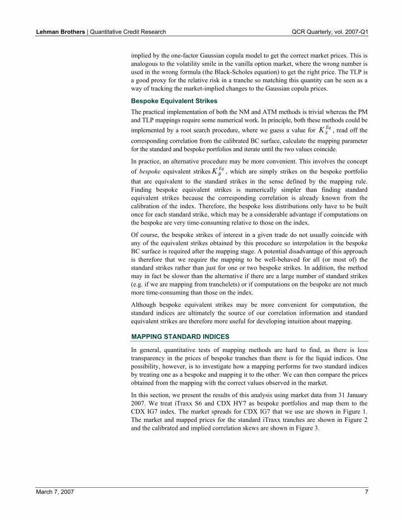
Figure 1. CDX IG7 tranche and swap quotes at close of business on 31 January 2007
Upfront Term Tranche Or Spread Swap
0-3% 20.09
3-7% 64.3 7-10% 12.3 10-15% 4.7
5Y
15-30% 2.4
31.37
0-3% 38.95 3-7% 176.9 7-10% 34.9 10-15% 15.0
7Y
15-30% 6.1
43.53
0-3% 50.51
3-7% 425.9
7-10% 92.4
10-15% 42.2
10Y
15-30% 13.7
55.81
Source: Lehman Brothers. Note: The equity tranche is quoted as an upfront percentage for a fixed 500bp running spread, while the remaining tranches are quoted in terms of a pure running spread in bp. The swap level is a reference spread in bp.
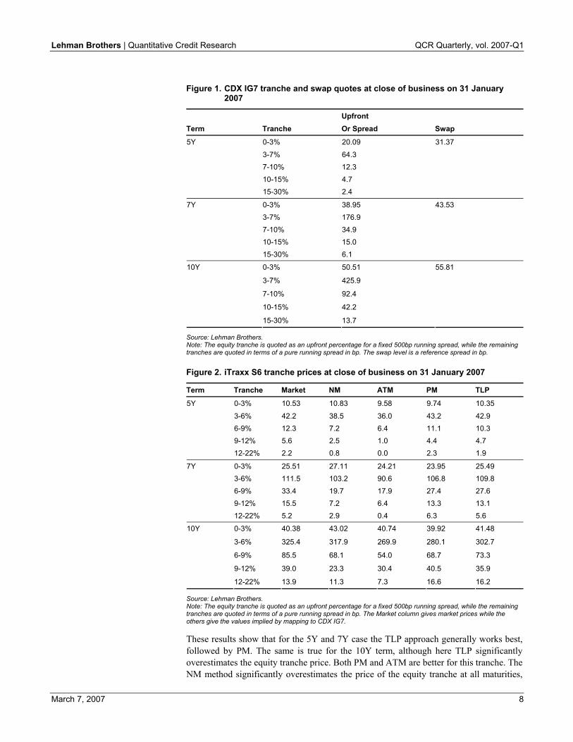
Figure 2. iTraxx S6 tranche prices at close of business on 31 January 2007
Term Tranche Market NM ATM PM TLP
0-3% 10.53 10.83 9.58 9.74 10.35
3-6% 42.2 38.5 36.0 43.2 42.9 6-9% 12.3 7.2 6.4 11.1 10.3 9-12% 5.6 2.5 1.0 4.4 4.7
5Y
12-22% 2.2 0.8 0.0 2.3 1.9
0-3% 25.51 27.11 24.21 23.95 25.49 3-6% 111.5 103.2 90.6 106.8 109.8 6-9% 33.4 19.7 17.9 27.4 27.6 9-12% 15.5 7.2 6.4 13.3 13.1
7Y
12-22% 5.2 2.9 0.4 6.3 5.6
0-3% 40.38 43.02 40.74 39.92 41.48
3-6% 325.4 317.9 269.9 280.1 302.7
6-9% 85.5 68.1 54.0 68.7 73.3
9-12% 39.0 23.3 30.4 40.5 35.9
10Y
12-22% 13.9 11.3 7.3 16.6 16.2
Source: Lehman Brothers. Note: The equity tranche is quoted as an upfront percentage for a fixed 500bp running spread, while the remaining tranches are quoted in terms of a pure running spread in bp. The Market column gives market prices while the others give the values implied by mapping to CDX IG7.
These results show that for the 5Y and 7Y case the TLP approach generally works best, followed by PM. The same is true for the 10Y term, although here TLP significantly overestimates the equity tranche price. Both PM and ATM are better for this tranche. The NM method significantly overestimates the price of the equity tranche at all maturities,

Lehman Brothers | Quantitative Credit Research QCR Quarterly, vol. 2007-Q1
March 7, 2007 9
but otherwise it seems to work better than ATM which generally gives very poor results, especially for senior tranches.
A cut through the BC surface at the 5Y time horizon is shown in Figure 3. Here we plot the correlation skew calibrated to the iTraxx S6 market prices and the values implied by mapping to CDX IG7. Consistent with our observations on the tranche prices, we see that the skew obtained from the TLP mapping is closest to the calibrated curve, followed by PM and then ATM.
To check that our results are not restricted to the particular tight spread environment existing in the market at the end of January 2007, we repeated this analysis using data from 28 September 2006 and 30 October 2006 (see Appendix for details). On both dates, the results are qualitatively the same as those presented here and we conclude in general that the TLP mapping method performs best in a comparison of the CDX IG7 and iTraxx S6 indices, followed by PM and then ATM.
Figure 3. iTraxx S6 5Y BC skew on 31 January 2007
0%
10%
20%
30%
40%
50%
60%
70%
3% 6% 9% 12% 22%Strike
Base Correlation
Calibrated ATM PM TLP
Source: Lehman Brothers. Note: The lowest curve is calibrated from the market prices while the other curves are implied by mapping to the CDX IG7 index.
Figure 4 shows plots of TLP and cumulative loss probability against calibrated correlation for both CDX IG7 and iTraxx S6. As mentioned earlier, if the TLP mapping method worked perfectly then it would be an invariant between the portfolios at a fixed correlation and the two curves would coincide. Similarly, if the PM approach was correct, plots of cumulative loss probability against correlation for two portfolios would be identical. The Figure shows that neither the TLP nor the cumulative loss is an invariant between CDX IG7 and iTraxx S6 on 31 January 2007, although the TLP curves are close for values of correlation less than about 30%, corresponding to strikes below about 8%. The PM curves are quite far apart at low correlations but they are closer than the TLP curves at higher correlations (and hence strikes).

Lehman Brothers | Quantitative Credit Research QCR Quarterly, vol. 2007-Q1
March 7, 2007 10
Figure 4. CDX IG7 and iTraxx S6 5Y TLP vs BC (left axis and lower two curves) and cumulative loss probability vs BC (right axis and upper two curves) on 31 January 2007
85%
88%
90%
93%
95%
98%
100%
13% 24% 35% 46% 57% 68%Base Correlation
TLP
85%
88%
90%
93%
95%
98%
100%Loss Probability
CDX TLP iTraxx TLP CDX PM iTraxx PM
Source: Lehman Brothers. Note: Corresponding curves should coincide if either TLP or cumulative loss is a mapping invariant.
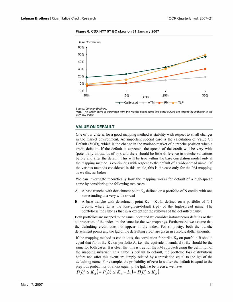
CDX IG7 and iTraxx S6 are relatively similar portfolios in terms of their expected losses and average spread levels on 31 January 2007 (although the CDX index has significantly greater spread dispersion than iTraxx). A more extreme test of the methods is obtained by mapping CDX HY7 to CDX IG7 because in this case the spread levels are very different (the 5Y expected loss on HY7 is about 11.4% compared with about 1.6% for IG7). The results of this comparison for the liquid tranche prices of the high-yield index on 31 January 2007 are shown in Figure 5 while the calibrated and implied correlation skews are shown in Figure 6. Results for 28 September 2006 and 30 October 2006 are given in the Appendix.
Figure 5. CDX HY7 5Y tranche prices at close of business on 31 January 2007
Term Tranche Market NM ATM PM TLP
0-10% 68.75 61.73 74.92 76.26 74.79
10-15% 26.07 19.31 28.85 26.26 22.78
15-25% 225.7 230.2 155.2 129.9 136.7
5Y
25-35% 56.1 134.2 21.3 27.6 28.1
Source: Lehman Brothers. Note: The first two tranches are quoted purely as an upfront percentage while the last two are quoted as a running spread in bp. The Market column gives market prices while the others give the values implied by mapping to CDX IG7.
All the mapping methods perform badly in this comparison, consistently putting too much risk in the equity tranche and too little risk in the senior part of the capital structure (NM is an exception). A possible explanation is that there is a limit to the amount a market participant would be willing to pay upfront for 5Y protection. The market therefore trades at lower levels for the high-yield equity tranches than that implied from the investment grade universe. The corresponding correlations are therefore higher than those predicted by mapping to CDX IG7, as shown in Figure 6. Since the expected portfolio loss is not a correlation-dependent quantity, the corollary of this is that the mapping methods put less risk in the senior tranches than is observed in the market.
Lehman Brothers | Quantitative Credit Research QCR Quarterly, vol. 2007-Q1
March 7, 2007 11
Figure 6. CDX HY7 5Y BC skew on 31 January 2007
0%
10%
20%
30%
40%
50%
60%
10% 15% 25% 35%Strike
Base Correlation
Calibrated ATM PM TLP
Source: Lehman Brothers. Note: The upper curve is calibrated from the market prices while the other curves are implied by mapping to the CDX IG7 index.
VALUE ON DEFAULT
One of our criteria for a good mapping method is stability with respect to small changes in the market environment. An important special case is the calculation of Value On Default (VOD), which is the change in the mark-to-market of a tranche position when a credit defaults. If the default is expected, the spread of the credit will be very wide (potentially thousands of bp), and there should be little difference in tranche valuations before and after the default. This will be true within the base correlation model only if the mapping method is continuous with respect to the default of a wide-spread name. Of the various methods considered in this article, this is the case only for the PM mapping, as we discuss below.
We can investigate theoretically how the mapping works for default of a high-spread name by considering the following two cases:
A. A base tranche with detachment point KA defined on a portfolio of N credits with one name trading at a very wide spread
B. A base tranche with detachment point KB = KA-Li defined on a portfolio of N-1 credits, where Li is the loss-given-default (lgd) of the high-spread name. The portfolio is the same as that in A except for the removal of the defaulted name.
Both portfolios are mapped to the same index and we consider instantaneous defaults so that all properties of the index are the same for the two mappings. Furthermore, we assume that the defaulting credit does not appear in the index. For simplicity, both the tranche detachment points and the lgd of the defaulting credit are given in absolute dollar amounts.
If the mapping method is continuous, the correlation for strike KB on portfolio B should equal that for strike KA on portfolio A, i.e., the equivalent standard strike should be the same for both cases. It is clear that this is true for the PM approach using the definition of the mapping invariant. If a name is certain to default, the portfolio loss distributions before and after this event are simply related by a translation equal to the lgd of the defaulting name. For example, the probability of zero loss after the default is equal to the previous probability of a loss equal to the lgd. To be precise, we have ( ) ( ) ( )B
BTiA
BTA
AT KLPLKLPKLP ≤=−≤=≤
Lehman Brothers | Quantitative Credit Research QCR Quarterly, vol. 2007-Q1
March 7, 2007 12
where ATL and B
TL are the cumulative portfolio losses at the mapping maturity (e.g. 5Y) for portfolios A and B. The expression on the left of this equation is the quantity we map to the index before the default, while the expression on the right is the corresponding quantity after the default. The equality of the two expressions ensures continuity of the mapping through the default event under the PM methodology.
In contrast, neither the ATM nor the TLP approaches are continuous when a high-spread name defaults. This event reduces the absolute tranche strike and EPL by the same dollar
amount, with the result that the ATM ratio EPL
Kdecreases for K < EPL and increases
for K > EPL. Thus, strikes below the bespoke EPL map to lower standard strikes after the default under ATM. In the usual case of an upward-sloping base correlation skew, these strikes will therefore be priced with a lower base correlation after default. The converse applies for strikes above the bespoke EPL. Only at a bespoke strike equal to the EPL is the mapping continuous in the event of default. For the case of a mezzanine tranche with attachment point below the EPL and detachment point above, the effect of the mapping will be to make the tranche safer after the default, over and above the effect coming from the removal of the high-spread name.
For TLP, the effect of the default is to reduce the absolute ETL for all surviving base tranches by the same dollar amount as the absolute EPL. Since the ratio of ETL to EPL does not exceed one, this means that the TLP decreases for all bespoke strikes and they map lower on the index, producing a discontinuous VOD. If the skew is upward-sloping, all bespoke strikes will be priced with a lower correlation after the default. The equity tranche will therefore become more risky, and its VOD, although non-zero, will have the correct sign. This is confirmed by our numerical calculations, discussed below. The same is not necessarily true for more senior tranches, however, as these depend on the slope of the base correlation skew as well as its absolute value.
We investigated the effect of a default numerically using the case of the iTraxx S6 portfolio mapped to CDX IG7 on 31 January 2007. We considered the change in the value of a 5Y, short-protection, 10MM USD position on the standard tranches of the iTraxx portfolio as the spread on a single name in that portfolio widened from its market value to 500bp, 5,000bp, 10,000bp, and finally to a level at which its survival probability for a single day was 10-6, i.e. a one-day default scenario. We compared these valuations with the case that the name had actually defaulted and was removed from the portfolio, with the tranche strikes adjusted accordingly.
Comparing the value after default with the base market we found that all the mapping methods gave negative VODs for all tranches, as one would expect for a short-protection position. The TLP and PM methods gave similar results for this case and also when the name defaulted from a spread of 500bp. However, as expected, only the PM approach gave VODs that remained negative as the name traded wider and were continuous at the point of default.
The results from ATM were generally reasonable only in the case of a sudden default of a low-spread name. For the one-day default scenario, the VOD for this method was large and positive for all tranches. Despite the fact that the equity tranche must cover the losses-on-default, a protection seller on this tranche benefits from a positive mark-to-market of about 56,000 USD from the default event under ATM. VOD was also discontinuous for the TLP mapping, with the one-day default scenario generating a change in mark-to-market of about -76,000 USD for the equity tranche. The fact that this quantity is negative is consistent with our discussion above and is a distinct improvement over ATM. The VODs for more senior tranches, however, were positive under TLP but significantly smaller than for ATM.

Lehman Brothers | Quantitative Credit Research QCR Quarterly, vol. 2007-Q1
March 7, 2007 13
Based on this analysis, we conclude that the PM mapping works best for the calculation of VOD for distressed names. For investment grade names, however, there is little to distinguish the VODs from TLP and PM, and both give reasonable results.
MAPPING BESPOKE PORTFOLIOS
In this section we discuss the results obtained from mapping a range of generic bespoke portfolios to the CDX IG7 index. Our analysis is necessarily more qualitative than before as we no longer have an absolute measure of correctness for the bespoke prices as we had for the standard indices. We consider six portfolios with low, medium and high spreads and either zero or substantial dispersion. All portfolios are priced in USD and contain 100 names trading with flat spread curves and a deterministic recovery rate of 40%. We will refer to these portfolios using the following names:
• Homogeneous 20bp: 100 names at 20bp. • Homogeneous 40bp: 100 names at 40bp. • Homogeneous 100bp: 100 names at 100bp. • Dispersed 20bp: 50 names at 10bp and 50 names at 30bp. • Dispersed 40bp: 50 names at 20bp and 50 names at 60bp. • Dispersed 100bp: 50 names at 50bp and 50 names at 150bp. The pricing results for a number of 5Y maturity tranches of the homogeneous portfolios are shown in Figure 7. A number of features of the data are of interest. First, we note that for the safe 20bp portfolio the ATM method performs very badly, putting hardly any risk in the 10-30% region and producing an arbitrage where the super senior 30-100% tranche pays a higher spread than more junior tranches. The same phenomenon is also seen for NM in this case, whereas both PM and TLP produce arbitrage-free quotes for these tranches. Overall, however, the differences between the prices generated by the various methods are smaller than we might have expected, especially for the two riskier portfolios.
Another feature of the data is that for portfolios that are riskier than the index (the 40bp and 100bp cases) the various mapping methods increase the risk in the junior part of the capital structure and decrease it in the senior, as compared with NM. This effect is clearly demonstrated in Figure 8, where we show how the protection PV is distributed across the capital structure for the 100bp portfolio. It is clear that all the methods increase the relative risk in the equity and junior mezzanine tranches at the expense of the senior tranches as compared with NM. The situation is reversed for the 20bp portfolio, which is safer than the index. Here both PM and TLP decrease the risk in the equity and increase it in more senior tranches compared with NM.
Figure 7. 5Y tranche prices for bespoke portfolios mapped to the CDX IG7 index
Homogeneous 20bp Homogeneous 40bp Homogeneous 100bp
Strikes NM ATM PM TLP NM ATM PM TLP NM ATM PM TLP
3% 7.47 5.68 6.06 6.96 28.91 30.00 29.82 30.27 63.84 68.48 69.01 69.03
7% 22.3 17.4 28.1 27.2 106.8 112.6 119.6 118.4 571.3 844.7 826.3 786.110% 2.7 0.2 6.0 6.3 22.9 22.5 25.2 23.0 176.2 203.4 187.1 180.615% 0.2 0.1 2.4 2.6 8.6 9.0 10.7 9.0 81.5 68.4 64.4 63.0 30% 0.0 0.1 2.0 1.2 3.9 3.9 4.2 2.8 35.1 16.1 16.1 13.2
100% 1.3 4.9 1.6 0.9 3.7 2.3 1.8 2.0 14.2 1.3 2.5 5.3
Source: Lehman Brothers. Note: The equity tranche is quoted as an upfront percentage for a 500bp running spread while the other tranches are quoted as a pure running spread in bp.

Lehman Brothers | Quantitative Credit Research QCR Quarterly, vol. 2007-Q1
March 7, 2007 14
Figure 8. Tranche risk allocation (% PV Protection) for the homogeneous 100bp portfolio as implied by different mappings to CDX IG7.
0%
10%
20%
30%
40%
50%
60%
0-3% 3-7% 7-10% 10-15% 15-30% 30-100%Tranche
% PV Protection
NM ATM PM TLP
Source: Lehman Brothers. Note % PV Protection is calculated as the ratio of the PVs of protection for the tranche and the portfolio.
Figure 9 shows pricing results from a similar analysis with the dispersed portfolios and many of the same comments apply here. As before, we see arbitrage in the quotes for the 20bp portfolio at senior strikes for both NM and ATM. In general, we see rather small changes in the bespoke correlations for junior tranches as we add dispersion to the portfolios and all the mapping methods are consistent with the fact that greater dispersion should increase equity tranche spreads.
Figure 9. 5Y tranche prices for bespoke portfolios mapped to the CDX IG7 index
Dispersed 20bp Dispersed 40bp Dispersed 100bp
Strikes NM ATM PM TLP NM ATM PM TLP NM ATM PM TLP
3% 7.59 5.87 6.19 7.01 29.26 30.29 30.12 30.46 64.54 68.95 69.63 69.62
7% 22.2 18.6 27.6 26.3 107.6 112.2 116.4 114.3 584.6 838.0 815.6 771.210% 3.0 0.3 5.7 6.0 23.4 22.4 24.1 21.9 180.1 195.1 176.4 171.315% 0.5 0.1 2.3 2.4 9.3 9.2 10.0 8.4 83.9 63.4 59.4 58.2 30% 0.4 0.1 1.8 1.3 4.6 4.1 3.9 2.9 36.4 14.0 14.4 12.1
100% 1.0 3.8 1.5 0.9 2.9 1.8 1.6 1.9 11.0 0.9 2.2 5.1
Source: Lehman Brothers. Note: The equity tranche is quoted as an upfront percentage for a 500bp running spread while the other tranches are quoted as a pure running spread in bp.
MAPPING BESPOKE PORTFOLIOS TO MULTIPLE INDICES
The dispersed 100bp portfolio, comprising 50 names at 50bp and 50 names at 150bp, is an example of a portfolio with clusters of names from two distinct market sectors, in this case investment grade and high yield. Intuitively, we expect that different correlations should be used for the 50bp names and the 150bp names, so it is not really sensible to price such a portfolio with a single flat correlation. Instead, we would like to use a correlation obtained from the high-yield market for the riskier names and a correlation from the investment grade market for the safer ones. The same issue arises if a portfolio contains clusters of names from different domiciles, e.g. 50% US names and 50% European names. In this case, we would like to map the US names to the CDX IG index and European names to the iTraxx index.
Lehman Brothers | Quantitative Credit Research QCR Quarterly, vol. 2007-Q1
March 7, 2007 15
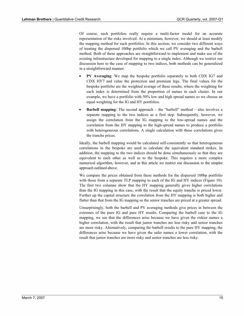
Of course, such portfolios really require a multi-factor model for an accurate representation of the risks involved. At a minimum, however, we should at least modify the mapping method for such portfolios. In this section, we consider two different ways of treating the dispersed 100bp portfolio which we call PV averaging and the barbell method. Both of these approaches are straightforward to implement and make use of the existing infrastructure developed for mapping to a single index. Although we restrict our discussion here to the case of mapping to two indices, both methods can be generalized in a straightforward manner.
• PV Averaging: We map the bespoke portfolio separately to both CDX IG7 and CDX HY7 and value the protection and premium legs. The final values for the bespoke portfolio are the weighted average of these results, where the weighting for each index is determined from the proportion of names in each cluster. In our example, we have a portfolio with 50% low and high spread names so we choose an equal weighting for the IG and HY portfolios.
• Barbell mapping: The second approach – the “barbell” method – also involves a separate mapping to the two indices as a first step. Subsequently, however, we assign the correlation from the IG mapping to the low-spread names and the correlation from the HY mapping to the high-spread names to produce a portfolio with heterogeneous correlations. A single calculation with these correlations gives the tranche prices.
Ideally, the barbell mapping would be calculated self-consistently so that heterogeneous correlations in the bespoke are used to calculate the equivalent standard strikes. In addition, the mapping to the two indices should be done simultaneously so that they are equivalent to each other as well as to the bespoke. This requires a more complex numerical algorithm, however, and in this article we restrict our discussion to the simpler approach outlined above.
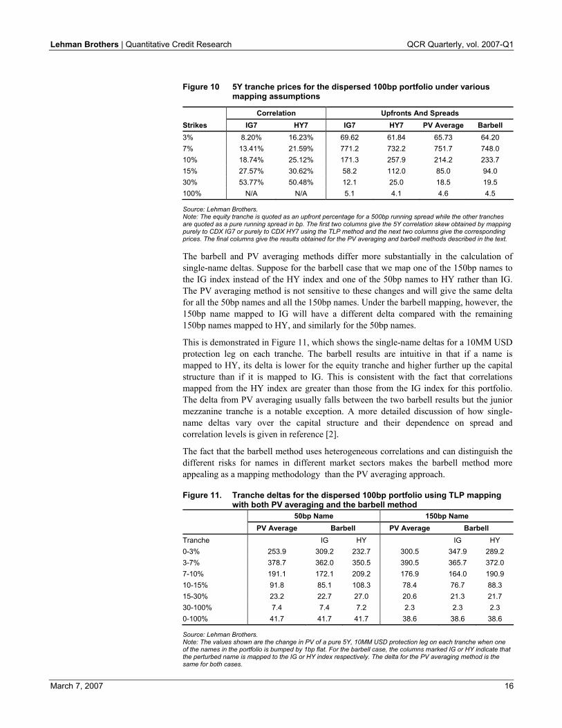
We compare the prices obtained from these methods for the dispersed 100bp portfolio with those from a separate TLP mapping to each of the IG and HY indices (Figure 10). The first two columns show that the HY mapping generally gives higher correlations than the IG mapping in this case, with the result that the equity tranche is priced lower. Further up the capital structure the correlation from the HY mapping is both higher and flatter than that from the IG mapping so the senior tranches are priced at a greater spread.
Unsurprisingly, both the barbell and PV averaging methods give prices in between the extremes of the pure IG and pure HY results. Comparing the barbell case to the IG mapping, we see that the differences arise because we have given the riskier names a higher correlation, with the result that junior tranches are less risky and senior tranches are more risky. Alternatively, comparing the barbell results to the pure HY mapping, the differences arise because we have given the safer names a lower correlation, with the result that junior tranches are more risky and senior tranches are less risky.
Lehman Brothers | Quantitative Credit Research QCR Quarterly, vol. 2007-Q1
March 7, 2007 16
Figure 10 5Y tranche prices for the dispersed 100bp portfolio under various mapping assumptions
Correlation Upfronts And Spreads Strikes IG7 HY7 IG7 HY7 PV Average Barbell 3% 8.20% 16.23% 69.62 61.84 65.73 64.20 7% 13.41% 21.59% 771.2 732.2 751.7 748.0 10% 18.74% 25.12% 171.3 257.9 214.2 233.7 15% 27.57% 30.62% 58.2 112.0 85.0 94.0 30% 53.77% 50.48% 12.1 25.0 18.5 19.5 100% N/A N/A 5.1 4.1 4.6 4.5
Source: Lehman Brothers. Note: The equity tranche is quoted as an upfront percentage for a 500bp running spread while the other tranches are quoted as a pure running spread in bp. The first two columns give the 5Y correlation skew obtained by mapping purely to CDX IG7 or purely to CDX HY7 using the TLP method and the next two columns give the corresponding prices. The final columns give the results obtained for the PV averaging and barbell methods described in the text.
The barbell and PV averaging methods differ more substantially in the calculation of single-name deltas. Suppose for the barbell case that we map one of the 150bp names to the IG index instead of the HY index and one of the 50bp names to HY rather than IG. The PV averaging method is not sensitive to these changes and will give the same delta for all the 50bp names and all the 150bp names. Under the barbell mapping, however, the 150bp name mapped to IG will have a different delta compared with the remaining 150bp names mapped to HY, and similarly for the 50bp names.
This is demonstrated in Figure 11, which shows the single-name deltas for a 10MM USD protection leg on each tranche. The barbell results are intuitive in that if a name is mapped to HY, its delta is lower for the equity tranche and higher further up the capital structure than if it is mapped to IG. This is consistent with the fact that correlations mapped from the HY index are greater than those from the IG index for this portfolio. The delta from PV averaging usually falls between the two barbell results but the junior mezzanine tranche is a notable exception. A more detailed discussion of how single-name deltas vary over the capital structure and their dependence on spread and correlation levels is given in reference [2].
The fact that the barbell method uses heterogeneous correlations and can distinguish the different risks for names in different market sectors makes the barbell method more appealing as a mapping methodology than the PV averaging approach.
Figure 11. Tranche deltas for the dispersed 100bp portfolio using TLP mapping with both PV averaging and the barbell method
50bp Name 150bp Name PV Average Barbell PV Average Barbell Tranche IG HY IG HY 0-3% 253.9 309.2 232.7 300.5 347.9 289.2 3-7% 378.7 362.0 350.5 390.5 365.7 372.0 7-10% 191.1 172.1 209.2 176.9 164.0 190.9 10-15% 91.8 85.1 108.3 78.4 76.7 88.3 15-30% 23.2 22.7 27.0 20.6 21.3 21.7 30-100% 7.4 7.4 7.2 2.3 2.3 2.3 0-100% 41.7 41.7 41.7 38.6 38.6 38.6
Source: Lehman Brothers. Note: The values shown are the change in PV of a pure 5Y, 10MM USD protection leg on each tranche when one of the names in the portfolio is bumped by 1bp flat. For the barbell case, the columns marked IG or HY indicate that the perturbed name is mapped to the IG or HY index respectively. The delta for the PV averaging method is the same for both cases.

Lehman Brothers | Quantitative Credit Research QCR Quarterly, vol. 2007-Q1
March 7, 2007 17
CONCLUSIONS
We have discussed a number of methods for obtaining BC surfaces for bespoke portfolios and tested them by mapping between standard indices and by mapping a range of generic bespoke portfolios to the CDX IG7 index. Our results for mapping iTraxx S6 to CDX IG7 show that the TLP method performs best in this case, followed by PM and then ATM. None of the methods performs satisfactorily for mapping CDX HY7 to CDX IG7, which is evidence that the high-yield and investment grade correlation markets are genuinely different from each other.
Of the various mapping methods we considered, we showed that only PM was continuous in the case of the default of a high-spread name. PM may therefore be preferable when a portfolio contains distressed credits. In the case of a sudden default of a name trading below about 500bp, however, there was little to distinguish the TLP and PM methods; both gave reasonable results. The ATM method generally performed poorly in this analysis.
For bespoke portfolios, we obtained sensible results from both TLP and PM. The ATM method, however, performed poorly, especially for mapping to low-risk portfolios, and could generate arbitrage in the quotes. We also described two approaches for treating bespokes mapped to more than one index, namely PV averaging and the barbell method. We argued that the barbell method gives more appealing results because it uses heterogeneous correlations and produces different single-name deltas for names in different market sectors.
REFERENCES
[1] O’Kane and Livesey (2004), “Base Correlation Explained”, Lehman Brothers Fixed Income Research, Quantitative Credit Research Quarterly, November 2004, pp. 3-20. [2] Schloegl and Greenberg (2003), “Understanding Deltas of Synthetic CDO Tranches”, Lehman Brothers Fixed Income Research, Quantitative Credit Research Quarterly, November 2003, pp. 45-54.
Lehman Brothers | Quantitative Credit Research QCR Quarterly, vol. 2007-Q1
March 7, 2007 18
APPENDIX
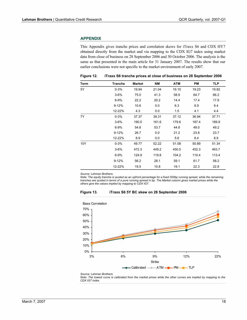
This Appendix gives tranche prices and correlation skews for iTraxx S6 and CDX HY7 obtained directly from the market and via mapping to the CDX IG7 index using market data from close of business on 28 September 2006 and 30 October 2006. The analysis is the same as that presented in the main article for 31 January 2007. The results show that our earlier conclusions were not specific to the market environment of early 2007.
Figure 12. iTraxx S6 tranche prices at close of business on 28 September 2006
Term Tranche Market NM ATM PM TLP
0-3% 19.94 21.04 19.10 19.23 19.82
3-6% 75.0 41.3 58.9 64.7 66.2 6-9% 22.2 20.2 14.4 17.4 17.8
9-12% 10.6 0.0 6.3 8.9 9.4
5Y
12-22% 4.3 0.0 1.5 4.1 4.4
0-3% 37.37 39.31 37.12 36.94 37.71 3-6% 190.0 161.6 179.6 187.4 189.9
6-9% 54.8 53.7 44.8 49.0 49.2 9-12% 26.7 0.0 21.2 23.8 23.7
7Y
12-22% 8.9 0.0 5.6 8.4 8.9
0-3% 49.77 52.22 51.08 50.89 51.34
3-6% 472.3 449.2 450.5 452.3 463.7
6-9% 124.9 119.8 104.2 110.4 113.4
9-12% 56.2 28.1 59.1 61.7 58.2
10Y
12-22% 19.5 10.8 19.1 22.3 22.8
Source: Lehman Brothers. Note: The equity tranche is quoted as an upfront percentage for a fixed 500bp running spread, while the remaining tranches are quoted in terms of a pure running spread in bp. The Market column gives market prices while the others give the values implied by mapping to CDX IG7.
Figure 13. iTraxx S6 5Y BC skew on 28 September 2006
0%
10%
20%
30%
40%
50%
60%
70%
3% 6% 9% 12% 22%Strike
Base Correlation
Calibrated ATM PM TLP
Source: Lehman Brothers. Note: The lowest curve is calibrated from the market prices while the other curves are implied by mapping to the CDX IG7 index.

Lehman Brothers | Quantitative Credit Research QCR Quarterly, vol. 2007-Q1
March 7, 2007 19
Figure 14. iTraxx S6 tranche prices at close of business on 30 October 2006
Term Tranche Market NM ATM PM TLP 0-3% 12.29 12.74 11.03 11.27 11.87 3-6% 54.7 45.7 42.6 49.1 50.1 6-9% 13.4 9.4 8.5 13.3 13.5
9-12% 5.6 3.6 1.5 5.2 6.0
5Y
12-22% 2.4 1.1 0.0 2.5 2.5 0-3% 28.75 29.62 27.07 27.01 28.01 3-6% 140.8 136.1 123.5 134.3 137.8 6-9% 40.4 30.6 31.0 36.6 36.8
9-12% 19.4 13.2 14.1 18.5 18.2
7Y
12-22% 6.9 4.9 2.3 6.8 7.1 0-3% 43.48 44.76 43.21 42.95 43.66 3-6% 375.1 377.2 335.6 341.8 356.7 6-9% 102.7 90.0 78.8 86.7 88.4
9-12% 41.6 35.0 48.4 52.6 47.9
10Y
12-22% 12.7 15.8 12.9 18.2 18.6
Source: Lehman Brothers. Note: The equity tranche is quoted as an upfront percentage for a fixed 500bp running spread, while the remaining tranches are quoted in terms of a pure running spread in bp. The Market column gives market prices while the others give the values implied by mapping to CDX IG7.
Figure 15. iTraxx S6 5Y BC skew on 30 October 2006
0%10%20%30%40%50%60%70%80%
3% 6% 9% 12% 22%
Strike
Base Correlation
Calibrated ATM PM TLP
Source: Lehman Brothers. Note: The lowest curve is calibrated from market prices while the other curves are implied by mapping to the CDX IG7 index.
Figure 16. CDX HY7 5Y tranche prices at close of business on 28 September 2006
Term Tranche Market NM ATM PM TLP 0-10% 82.97 75.31 86.50 87.78 87.13
10-15% 45.47 33.42 55.35 56.60 47.10 15-25% 392.1 390.5 374.4 297.6 281.6
5Y
25-35% 88.9 210.7 53.4 54.8 67.1
Source: Lehman Brothers. Note: The first two tranches are quoted purely as an upfront percentage while the last two are quoted as a running spread in bp. The Market column gives market prices while the others give the values implied by mapping to CDX IG7.

Lehman Brothers | Quantitative Credit Research QCR Quarterly, vol. 2007-Q1
March 7, 2007 20
Figure 17. CDX HY7 5Y BC skew on 28 September 2006
0%
10%
20%
30%
40%
50%
60%
10% 15% 25% 35%Strike
Base Correlation
Calibrated ATM PM TLP
Source: Lehman Brothers. Note: The upper curve is calibrated from the market prices while the other curves are implied by mapping to the CDX IG7 index.
Figure 18. CDX HY7 5Y prices at close of business on 30 October 2006
Term Tranche Market NM ATM PM TLP
0-10% 78.38 70.51 82.47 84.14 82.89
10-15% 37.22 27.69 44.39 43.64 36.99
15-25% 294.0 321.8 289.8 232.5 235.9
5Y
25-35% 70.0 179.7 42.6 46.4 49.5
Source: Lehman Brothers. Note: The first two tranches are quoted purely as an upfront percentage while the last two are quoted as a running spread in bp. The Market column gives market prices while the others give the values implied by mapping to CDX IG7.
Figure 19. CDX HY7 5Y BC skew on 30 October 2006
0%
10%
20%
30%
40%
50%
60%
10% 15% 25% 35%Strike
Base Correlation
Calibrated ATM PM TLP
Source: Lehman Brothers. Note: The upper curve is calibrated from the market prices while the others are implied by mapping to the CDX IG7 index.

Lehman Brothers | Quantitative Credit Research QCR Quarterly, vol. 2007-Q1
March 7, 2007 21
Idiosyncratic Portfolio Risk in non-Normal Markets We consider security-level return factor models with a heavy-tailed idiosyncratic component. We model the portfolio-level idiosyncratic component as a t distribution. The tail index, i.e. the degrees of freedom, of this distribution is accurately modeled as a function of two inputs. First, the risk-adjusted average of the single-security tail index: other things equal, portfolios of heavier-tailed securities give rise to heavier-tailed idiosyncratic terms. Second, the level of diversification in the portfolio: large and highly diversified portfolios of heavy-tailed securities give rise to quasi-normal idiosyncratic portfolio-level shocks. In order to suitably quantify diversification we introduce an entropy-based risk-adjusted measure.
1. INTRODUCTION
Consider a market of N securities, whose returns are properly modeled by a suitable factor model:
(1)
where 1, ,n N= K . In this expression X is a K-dimensional vector of systematic factors
that affect all the securities in the market; nf is a security-specific pricing function; and
nε is an idiosyncratic risk independent across securities.
This formulation is very general. Among others, it includes standard APT-like linear factor models; more complex quadratic pricing functions such as the theta-delta-gamma-vega approximation; full repricing in terms of explicit factors. More details on the above and other models can be found in Meucci (2005). For a notable example in the industry see Dynkin et al. (2005).
Consider a generic portfolio in the market (1), as represented by the portfolio weights w . Note that we do not assume that the weights sum to one: indeed, the portfolio w can represent leveraged positions as well as allocations relative to a benchmark.
The total return R on the portfolio is the weighted average of the returns of the single securities. Therefore, the total return factors into the systematic component and the
idiosyncratic component: R S I≡ + , where and the aggregate idiosyncratic term reads:
(2)
If estimating and modeling the return of a single security is an arduous task, aggregating distributions at the portfolio level is an even harder problem.
For the systematic component one can make analytically tractable assumptions that hold true in approximation, see e.g. RiskMetrics (1996). Alternatively, results can be obtained via Monte Carlo simulations, because the number of common factors is typically much less than the number of securities involved. see Glasserman (2004). Hybrid approaches are also possible, see Albanese et al. (2004).
Attilio Meucci 1-212-526-5554

Lehman Brothers | Quantitative Credit Research QCR Quarterly, vol. 2007-Q1
March 7, 2007 22
For the idiosyncratic component, the aggregation (2) of the potentially very large number of idiosyncratic shocks cannot be performed via Monte Carlo simulations in a quick and efficient way. Therefore, one needs to resort to approximate analytical results. Typically, the idiosyncratic shocks are modeled as normally distributed, where the mean is set to zero without loss of generality:
(3)
see for instance Hamilton (1994) and Campbell et al. (1997). This way the portfolio-level aggregation of idiosyncratic risk is immediate. Indeed, under the normal assumption the idiosyncratic term at the portfolio level is also normal:
(4)
The normal assumption (3) is violated in several markets: most notably, the occurrence of extreme events induces heavy tails, see e.g. Rachev (2003). This is the case, for instance, in the credit world. Nevertheless, the normal assumption (4) becomes acceptable at the aggregate portfolio level when the number of securities is large and the portfolio is not concentrated in specific securities. Indeed, under these assumptions the central limit theorem dominates and (4) becomes a very good approximation.
However, portfolio managers monitor all sorts of positions, including those that are highly concentrated in specific securities. In such cases, the portfolio-level normal assumption is no longer valid. Hyung and DeVries (2005) discuss this issue in the asymptotic limit, namely for extreme events that extend to infinity.
Here we discuss a methodology to quickly and accurately compute the whole distribution of the portfolio, including the extreme tails, also for finite, non-asymptotic, tail levels. To achieve this, we model the aggregate idiosyncratic term as a t distribution. The tail parameter of this distribution is a function of the overall tail-thickness in the market and of the level of portfolio diversification: if diversification is high, the portfolio-level distribution of idiosyncratic risk is normal, as prescribed by the central limit theorem; if diversification is low and if the market is heavy tailed, the portfolio-level idiosyncratic risk displays heavy tails. In Section 2 we introduce the rationale behind the aggregate t-model, based on a set of necessary properties that need to be satisfied; in Section 3 we model the level of diversification in the portfolio in terms of the entropy of a suitable risk-adjusted distribution; in Section 4 we calibrate the parameters of the aggregate t-model based on the overall tail-thickness of the market and on the portfolio diversification; in Section 5 we present the performance of the model in an empirical study; in Section 6 we discuss directions for further research and we conclude.
2. AGGREGATION MODEL
First of all, we generalize the security-level normal assumption for the idiosyncratic risk (3) to a flexible parametric distribution that allows for heavy tails. In particular, we choose the Student t distribution:
(5)
In this expression the degrees of freedom νn characterize the tail behavior of the idiosyncratic risk; the location parameter μn can be set to zero without loss of generality; and σ2
n represents the square dispersion parameter, which is proportional to the variance ψ2
n ≡ σ2nνn/ (νn − 2). We assume νn > 2 in such a way that the variance is defined.

Lehman Brothers | Quantitative Credit Research QCR Quarterly, vol. 2007-Q1
March 7, 2007 23
The exact distribution of the aggregate idiosyncratic term (2) under the assumption (5) cannot be computed either analytically or numerically in real time. Our plan is to approximate the exact aggregate distribution via a parsimonious parametric model. In order to implement the model, its parameters must be an analytical function of the set of market inputs (νn, μn, σ2
n) as well as of the portfolio weights . Furthermore, the aggregate model should satisfy the following properties:
(i) The aggregate must be a symmetric and bell-shaped distribution.
(ii) The expected value of the aggregate distribution must be null.
(iii) The variance of the aggregate distribution must be the weighted average of the variances of the single securities.
(iv) When the portfolio is concentrated in one position, the aggregate distribution must coincide with the security-level idiosyncratic term.
(v) When the portfolio is extremely diversified, the aggregate distribution must be normal as in (4), in accordance with the central limit theorem.
Finally, suppose that we subdivide a given portfolio into a few sub-portfolios. The model for the direct aggregation (2) of all the idiosyncratic terms in the original portfolio must equal the two-step aggregation which first computes the idiosyncratic terms in the different sub-portfolios and then combines them into one single number. In other words:
(vi) The aggregate model must be self-consistent.
We claim that for suitable parameters and the t distribution:
(6)
represents an adequate aggregate model. As we show in Section 4, the aggregate model (6) satisfies the above conditions (i)-(vi). However, a model that satisfies those conditions is not necessarily adequate. In order for a model to be adequate it must also accurately approximate the true aggregate distribution (2) in a very broad range of situations: we show this in Section 5.
3. ENTROPY-BASED DIVERSIFICATION
Intuitively, the choice of the parameters depends on the portfolio diversification. In order to quantify this concept we introduce the risk-adjusted portfolio weights:
(7)
where we used the fact that the idiosyncratic terms are independent.
Note that the risk-adjusted portfolio weights sum to one. Therefore, we can interpret them as a probability measure on the securities. We can easily establish a relationship between the diversification of the portfolio and the shape of the probability defined by the risk-adjusted portfolio weights (7) (Figure 1). When this probability density is close to uniform, i.e. each security is assigned an equal mass n ≈ 1/N, the portfolio is highly diversified. When the probability density is concentrated, i.e. a specific security is such that ≈ 1, so is the portfolio.

Lehman Brothers | Quantitative Credit Research QCR Quarterly, vol. 2007-Q1
March 7, 2007 24
Figure 1. Risk-adjusted portfolio weights as a probability measure
Source: Lehman Brothers
From the above discussion it follows that we can measure diversification in terms of the dispersion of the probability defined by the risk-adjusted portfolio weights (7). The standard measure of dispersion for a probability is its entropy:
(8)
where the limit is considered when the weight is null. In Figure 1 we display the entropy for significant cases. Note that the entropy is never negative; it reaches its minimum value ≡ 0 when the probability mass is concentrated in the single -th position ≡ 1; it increases with the dispersion of the probability; and it reaches its maximum value ≡ ln (N) when the probability density is uniform, i.e. each security is assigned an equal mass ≡ 1/N. Note that grows to infinity as the number of securities in the portfolio increases: indeed, a larger market gives rise to more diversification opportunities. On the other hand, the logarithm grows extremely slowly: indeed, the marginal diversification effect of several new securities in a well-diversified market of a few dozen securities is minimal, see e.g. Luenberger (1998) and Meucci (2005).
4. MODEL CALIBRATION
We can now proceed to calibrate the parameters and of the model (6) according to the properties (i)-(vi) discussed in Section 2.
First of all, notice that (i) and (ii) are satisfied. In order to satisfy (iii), we impose that solve:
(9)
The remaining parameter, namely the degrees of freedom , determines the tail behavior of the portfolio-level idiosyncratic term. Therefore must be a function of diversification, as represented by the entropy (8), and of the overall tail behavior of the securities (5) in the portfolio, as represented by the degrees of freedom νn. Indeed, for a given level of diversification, a portfolio of heavy-tailed securities displays heavier tails than a portfolio of normal securities, whose distribution is normal. Therefore, we introduce the average1 tail index defined as follows:
1 We consider the inverse average instead of the arithmetic or geometric average because it performs better
empirically, see Section 5.
Lehman Brothers | Quantitative Credit Research QCR Quarterly, vol. 2007-Q1
March 7, 2007 25
(10)
In particular, in the null-entropy case of a portfolio concentrated in the single -th security, the average tail index is equal to that security’s tail index ν . At the other extreme, in the maximum-entropy case of a diversified portfolio with equal risk-adjusted weights ≡ 1/N, the average tail index is properly biased toward its thick-tailed components.
To summarize, the portfolio-level tail index is determined by and . According to property (iv) in Section 2 and the above remark, must equal when the portfolio is concentrated in one single security, i.e. when the entropy is null. Furthermore, according to property (v) must grow to infinity as the entropy increases.
The simplest functional form that satisfies these criteria reads:
(11)
where g (0) ≡ 1 and g grows to infinity with . Notice that the model defined by (6), (9) and (11) also satisfies the final self-consistency property (vi). Indeed, the aggregation process always “reads” directly on the “atoms”, i.e. the individual securities. In other words, given any two sub-portfolios A and B, then A ≡ Ag ( A) and Bg ≡ Bg ( B), which clearly holds true also for the special case of a one-security portfolio. To aggregate A and B one needs to consider all the securities in A and in B and therefore obtains unequivocally the result (11).
To calibrate the functional form of g in (11) we performed an extensive study along the lines of the empirical analysis discussed in Section 5. The function g( ) ≡ 1+0.35 2 proved to provide excellent fits to the true aggregate distribution of the portfolio-level idiosyncratic term (2) under very disparate assumptions on the portfolio and the market.
5. EMPIRICAL ANALYSIS
In this section we compare the aggregate model (6) with the true distribution (2), which we generate numerically by simulating 106 Monte Carlo scenarios for each idiosyncratic shock (5).
In Figure 2 we illustrate the prototype experiment. We consider a set of N securities, N ≡ 10 in this case. We generate randomly long-short positions that are independently and standard-normally distributed. We generate randomly the variances ψn of the t-distributed idiosyncratic shocks, uniformly over a range typical of the credit market. Finally, we generate randomly the degrees of freedom νn of the t-distributed idiosyncratic shocks according to a Poisson distribution, shifted in such a way to guarantee that νn > 2.5.

Lehman Brothers | Quantitative Credit Research QCR Quarterly, vol. 2007-Q1
March 7, 2007 26
Figure 2. Portfolio-level idiosyncratic risk model
Source: Lehman Brothers
On the left-hand side in Figure 2 we display the weights ; the standard deviations ; the degrees of freedom νn; and the risk-adjusted weights (7). In the plot for the
the degrees of freedom νn we also superimpose the average tail index (10) and the portfolio tail index (11). On the right-hand side in Figure 2 we display the QQ plot of the true distribution against the approximation provided by the t model (6). To provide a comparative metric, we superimpose the QQ plot of the true distribution against the “perfect” model, i.e. the true distribution itself, which by definition is the π/4 straight line through the origin. We also superimpose the QQ plot of the true distribution against the normal approximation (4). Finally, we superimpose the QQ plot of the true distribution against a moment-matching, very heavy-tailed distribution, namely the t distribution with 2.5 degrees of freedom.
The QQ plots in Figure 2 show that the approximation provided in the above experiment by the t model (6) is excellent. To ascertain the general efficacy of the t model, we repeated the above experiment by randomizing also the number N of securities in a uniform range 1-1000. In all the experiments, the t model provides very accurate approximations of the true distribution. Below, we report a few experiments that we consider significant.
In Figure 3 we consider a prototype small credit portfolio. Three bonds of three different issuers in three different rating classes: a large long position in an AAA bond with duration of five years, standard deviation of 40bp and moderately heavy tails with 10 dof; a large short position in a high-yield bond with duration of five years, standard deviation of 390bp and heavy tails with 7 dof; and a small long position in a distressed bond which trades at price, standard deviation of 900bp and very heavy tails with 3 dof.
The QQ plots in Figure 3 show that the true distribution of the portfolio-level idiosyncratic risk is not close to normal but does not display extremely heavy tails. Instead, the true distribution is very well approximated by the t model (6) which in this case displays ≈ 8 dof. Notice that the weighted average (10) of the dof is ≈ 7. The 1 dof difference between the two numbers is due to the diversification effect induced by the portfolio entropy, see (11).

Lehman Brothers | Quantitative Credit Research QCR Quarterly, vol. 2007-Q1
March 7, 2007 27
Figure 3. Idiosyncratic risk model for a small credit portfolio
Source: Lehman Brothers
Figure 4. Idiosyncratic risk model: large diversified portfolio
Source: Lehman Brothers
In Figure 4 we consider a prototype large diversified portfolio. As expected, the QQ plots in Figure 4 show that the true distribution of the portfolio-level idiosyncratic risk is practically normal. The true distribution is very well approximated by the t model (6) which in this case displays ≈ 60 dof. Notice that the weighted average (10) of the dof
is much lower: this difference is due to the large diversification effect induced by the portfolio entropy, see (11).
In Figure 5 we consider a long-short position of two securities both with heavy tails of ≈ 3 dof each. The resulting portfolio is mildly thinner tailed. Indeed, the weighted average (10) of the dof is ≈ 3, but a small diversification effect appears in the portfolio tail index due to the non-null entropy. Indeed ≈ 4 dof.
In Figure 6 we consider the same long-short position as above, but in a market with unevenly heavy tails of ≈ 3 dof and ≈ 10 dof respectively. Again, the aggregate model performs well. Notice that the inverse scheme (10) assigns more weight to the heavier-tailed security.

Lehman Brothers | Quantitative Credit Research QCR Quarterly, vol. 2007-Q1
March 7, 2007 28
Figure 5. Idiosyncratic risk model in a homogeneously thick-tailed market
Source: Lehman Brothers
Figure 6. Idiosyncratic risk model in an unevenly thick-tailed market
Source: Lehman Brothers
6. CONCLUSIONS
We present a model for the distribution of the idiosyncratic risk of a portfolio when the security-level idiosyncratic shocks are heavy tailed. The proposed methodology relies on an entropy-based definition of portfolio diversification. Since none of the computations involved is numerical, the implementation of the proposed approach for portfolios of any size is straightforward.
The model applies to a large class of additive idiosyncratic models (1). The proposed methodology can also be extended easily to the situation where some idiosyncratic terms are correlated: this is the case for instance for same-issuer credit bonds. In this circumstance, the distribution of same-issuer bonds can be modeled as a multivariate t, in such a way that any sub-portfolio of same-issuer bonds becomes a t-distributed cluster independent of other clusters and thus it can be modeled as a single security as in (5). In future research we plan to relax the parametric t assumption at the security level, by including skewness and different tail behaviors.
The author is grateful to Anthony Lazanas, Antonio Silva and Huarong Tang for their feedback.

Lehman Brothers | Quantitative Credit Research QCR Quarterly, vol. 2007-Q1
March 7, 2007 29
REFERENCES
Albanese, C., K. Jackson, and P. Wiberg, 2004, A new Fourier transform algorithm for value at risk, Quantitative Finance 4, 328—338.
Campbell, J. Y., A. W. Lo, and A. C. MacKinlay, 1997, The Econometrics of Financial Markets (Princeton University Press).
Dynkin, L., A. Desclee, A. Gould, J. Hyman, D. Joneja, R. Kazarian, V. Naik, M. Naldi, B. Phelps, J. Rosten, A. Silva, and G. Wang, 2005, The Lehman Brothers Global Risk Model: A Portfolio Manager’s Guide (Lehman Brothers Publications).
Glasserman, P., 2004, Monte Carlo Methods in Financial Engineering (Springer).
Hamilton, J. D., 1994, Time Series Analysis (Princeton University Press).
Hyung, N., and C. G. De Vries, 2005, Portfolio diversification effects of downside risk, Journal of Financial Econometrics 3, 107—125.
Luenberger, D. G., 1998, Investment Science (Oxford University Press).
Meucci, A., 2005, Risk and Asset Allocation (Springer).
Rachev, S. T., 2003, Handbook of Heavy Tailed Distributions in Finance (Elsevier/North-Holland).
RiskMetrics, 1996, RiskMetricsTechnical Document (J.P.Morgan and Reuters Publications) 4th edn.

Lehman Brothers | Quantitative Credit Research QCR Quarterly, vol. 2007-Q1
March 7, 2007 30
Trading Event Risk in Credit Markets using LEVER1
Releveraging events have recently become a significant source of risk in credit markets. The LEVER model and the LEVER Powertool on LehmanLive have been developed to assess this risk on a systematic basis. We present a new analysis of the LEVER model as an investment framework to identify and extract alpha. Our empirical analysis shows that trades based on the LEVER framework perform well historically and that their correlation with the market and other traditional credit trading strategies is low. This finding is useful for both portfolio managers with benchmark outperformance mandates and those with absolute-return mandates.
1. INTRODUCTION
The risk of releveraging events such as LBOs and leveraged recapitalizations has been an important cause for concern among credit investors over the past two years. More specifically, 2006 saw a large number of big-ticket LBO transactions either being expected or actually going through. While this presents an opportunity for credit investors to generate outperformance using a strategy that is long protection in names that have a higher releveraging event risk, the impact of such events on credit spreads can be highly idiosyncratic.
Figure 1 presents 5-year CDS spread levels in the announcement month and in the six months before and after the announcement for the five largest LBO transactions announced in the US and Europe in 2006.
Figure 1. Spread change of largest US and European LBOs in 2006
Spread change Announcement date Target
Spread1 (bp)
6M before annmt.
Annmt. month
6M after annmt.
US Nov Equity Office Properties Trust 34 -3 -1 23 Jul HCA Inc 435 309 282 -129 May Kinder Morgan Inc 166 125 131 -38 Oct Harrah's Entertainment Inc 241 191 127 -68 Nov Clear Channel Commun Inc 271 179 -9 -74 Europe Feb BAA PLC 85 64 54 -36 Jan VNU NV 205 151 15 301 Oct AWG PLC 25 3 0 -2 Mar ITV PLC 86 -6 11 23 Mar ProSiebenSat.1 Media AG 203 114 28 -27
Source: Lehman Brothers. 1. End of announcement month.
1 The authors would like to thank Srivaths Balakrishnan, Vasant Naik and Marco Naldi for their helpful comments.
Bodha Bhattacharya+1 212-526-7907
Mukundan Devarajan+44 207-102-9033
Minh Trinh+1 212-526-1712

Lehman Brothers | Quantitative Credit Research QCR Quarterly, vol. 2007-Q1
March 7, 2007 31
Clearly, releveraging events tend to be negative for credit spreads. However, not all the above names would have contributed equally to the outperfomance of a ‘perfect-foresight’ strategy that was long protection on all these names. In addition, the fact that some of these names have wide spreads also implies that such a strategy would have been expensive in terms of carry.
Admittedly, the set of names in Figure 1 is not representative of the characteristics of LBO events in the long sample. Nevertheless the concerns mentioned above remain, and it is important to analyze whether a systematic attempt to capture risk premia embedded in credit spreads would be profitable.
Early last year, we launched our LEVER framework,2 which helps quantify this risk and acts as a tool for investors to screen a large universe of names and identify those with high or low potential risk of such events.
While LEVER is a robust framework and has shown good empirical performance both in-sample and out-of-sample, it needs to be augmented in order to be directly used by credit investors in asset selection and portfolio construction. Indeed, as it stands the LEVER model is not a complete trading tool. One needs to know for instance whether it is necessary to short all the names with a high releveraging event risk (a high score) or whether a particular credit has enough excess spread to compensate for this risk.
With a view to addressing such issues we present an extensive empirical analysis of the performance of LEVER as a trading model in the investment grade credit market. More specifically, the primary goals of the current study are:
• To analyze and document the performance of trades on credits with high and low Firm LEVER-Scores3 and to understand the time variation in the performance of these trades.
• To understand if it is useful to condition LEVER scores on the market valuation of bonds in trading releveraging risk.
Our analysis is that the LEVER framework by itself is a satisfactory predictor of bond performance – and that it shows an intuitive pattern of variation across different regimes. In addition, we find that by combining LEVER-Scores with spreads, it is possible to improve on the performance of the above trade. We also document the time variation of these trades.
On the basis of these findings, we propose a combination of two trading strategies. The first is a static trade that is intended to capture both the latent leveraging risk in the credit but also takes into account the risk premia that its bonds offer investors. The second trading strategy is a dynamic one that is attractive in regimes where the incidence of releveraging activity is more likely to be high. We find that the combination of the two strategies has performed well historically and that it has a low correlation both with the broad credit market and traditional credit trading strategies, such as that of the ESPRI model.
The rest of the article is organized as follows. In Section 2, we present a brief refresher of the LEVER framework. In Section 3 we present the performance of outright trades based on LEVER-Scores. In Section 4 we include spread levels to sharpen the information in
2 Trinh et al (2006) ‘Introducing LEVER: A Framework for Scoring LEVeraging Event Risk’ Quantitative Credit
Strategies January 9, 2006. 3 In the rest of this article, we will refer to the Firm LEVER-Score as the LEVER-Score and the Macro LEVER-
Score as such.

Lehman Brothers | Quantitative Credit Research QCR Quarterly, vol. 2007-Q1
March 7, 2007 32
the LEVER-Score. We examine the macro properties of these trades in Section 5 and present our conclusions in Section 6.
2. THE LEVER FRAMEWORK: A REFRESHER
LEVER is a quantitative framework for measuring the relative risk of releveraging events such as LBOs and leveraged recapitalizations. LEVER encapsulates key accounting and market information into two simple measures: the Firm LEVER-Score and the Macro LEVER-Score.
• The Firm LEVER-Score identifies companies that look potentially more attractive to financial sponsors. Scores range from 0 to 10, and companies that score above 7.5 are particularly at risk.
• The Macro LEVER-Score identifies market environments that are more amenable to LBOs.
In the following, we present a brief overview of the Firm and Macro LEVER Scores.
The Firm LEVER-Score The Firm LEVER-Score includes three broad categories of firm-level factors driving LBOs. The most attractive targets have below-market valuations, their operations generate adequate cash flows for servicing debt, and are likely to enjoy a smooth execution of the transaction. We list the variables used to compute these component scores and our hypothesis for the relative magnitude of these variables for LBO vs non-LBO names in Figure 2. (For example, our hypothesis is that potential LBO candidates would have a high book-to-market ratio.)
Figure 2. Components of the Firm-LEVER Score
Valuation Operation Execution
Variables Book-to-Market Ratio
EV/EBITDA Free Cash Flow Yield4
Growth of Capital Expenditure5
Cash Flow Variability6
Cash / Market Cap
Size of the Firm
Hypothesis ↑ ↓ ↑ ↓ ↓ ↑ ↓
Motivation High B/M
indicates cheap valuation
Reflects valuation vis-à-vis the
earnings capacity
Indicates the ability to generate strong cash flows
to service debt
Indicates operational
commitments
Indicates the ability to service the debt raised
Indicative of liquidity
Smaller firms are more vulnerable
Source: Lehman Brothers.
Constructing the Firm-LEVER Score
To construct the Firm LEVER-Score, we use the cross-sectional ranking of the normalized values of the variables listed in Figure 5. Each variable is divided by a normalizing factor which is the market-value weighted average of the particular variable. In the US and Europe, the average is computed over the entire universe or across the sector peer group only, depending on the variable.7 Along each normalized variable, the firms in the universe are ranked. The Valuation, Operation and Execution scores for each firm are an average of the rankings corresponding to the underlying variables. The Firm LEVER-Score is then calculated as the average of the Valuation, Operation and Execution scores.
4 The free cash flow yield is defined as the ratio of free cash flows to the market capitalization of the firm. 5 We define the growth of capital expenditure as the year-on-year percentage change in the firm’s capital expenditure. 6 We define cash flow variability as the ratio of the two-year volatility of the firm’s free cash flows to the debt of the firm. 7 For the book-to-market ratio and EV/EBITDA multiple sector variations are taken into account. The rest of the
variables are compared within the entire universe.

Lehman Brothers | Quantitative Credit Research QCR Quarterly, vol. 2007-Q1
March 7, 2007 33
The Macro LEVER-Score The Macro LEVER-Score brings together the key factors that affect LBO activity.
a. Business cycle
LBOs are more likely in expansions than in recessions. This is because revenue growth accelerates in periods of higher economic activity, making it easier for companies to take on additional debt. Several factors tell us which stage of the business cycle the economy is in, including GDP growth, changes in short-term interest rates and rate expectations.
b. Cost of capital
The level of LBO activity is affected by the cost of capital of such transactions. This could be indicated by factors such as changes in the slope of the yield curve and credit spreads.
c. Characteristics of the universe
Analysis of the broad universe of firms highlights the opportunities available to private equity firms and leveraged acquirers in general. Such factors as overall cash flow and dividend yields tend to be important signals of the broad attractiveness of the universe of firms.
d. LBO technicals
An analysis of the data shows that the level of private equity raised in the previous year has a relatively high correlation with the number of LBOs. This could explain current high levels of LBO activity, as private equity firms are raising record amounts for their funds.
3. TRADING EVENT RISK USING THE FIRM LEVER-SCORE
We have documented before that the Firm LEVER-Score performs well in predicting the actual incidence of releveraging activity (Trinh, et al 2006). From the perspective of credit investors however, it is important also to analyze the performance of the Firm LEVER-Score as an indicator for a systematic trading strategy that buys credits with low scores and sells credits with high scores. This is because it is possible that the model may accurately identify a name as being a potential releveraging target, but credit spreads may already be completely pricing in this is risk. In such a case, it would be of little use to buy credit protection on such a name. This reduces the utility of the model to credit investors.
Structure of the tests To address this concern, we perform the following exercise. We compute the Firm LEVER-Scores for all the firms in the combined universe of names that fall in the S&P 1500 Index and the Lehman US IG Corporate Index over the period 1990-2006.
We then divide the firms that fall in the Lehman IG Corporate Index (i.e. the names with bonds outstanding) into different rating and duration categories to remove any systematic bias arising from these differences between bonds. Within each rating-duration category we divide the bonds into three groups based on their Firm LEVER-Scores, as follows: the top 20%, middle 60% and bottom 20%. Based on this grouping, we go long the bonds of all names in the bottom 20% and short the bonds of those in the top 20% and hold the trade for three months.

Lehman Brothers | Quantitative Credit Research QCR Quarterly, vol. 2007-Q1
March 7, 2007 34
This exercise is repeated every month.8 In other words, in any given month there would be three portfolios outstanding. In order to compute the monthly returns of this trading strategy therefore, one needs to compute the average of the returns of the three overlapping portfolios. This back-testing methodology is very similar to that of the ESPRI model.9
Performance of the unconditional LEVER long-short trade In Figure 3, we present the performance of the above trading strategy for various rating categories. It is important to note that in Figure 3 and subsequent analyses of trading strategies, we assume zero transaction costs. We judge that this is a fair assumption in the context of a larger credit selection mechanism that also includes signals from other frameworks.
Figure 3. Performance of long-short trades based on Firm LEVER-Scores
AA A BBB 1990-2006 Average Excess Returns (bp) 1 3 5
Annualized Information Ratio 0.08 0.30 0.19 1999-2006 Average Excess Returns (bp) 3 6 9 Annualized Information Ratio 0.21 0.45 0.25 2004-2006 Average Excess Returns (bp) -0 7 16 Annualized Information Ratio -0.07 0.55 0.74
Source: Lehman Brothers.
Figure 3 presents the average excess returns of the long-short strategy and the annualized information ratio which is defined as the ratio of the average annual excess returns to the annual volatility of the strategy. In general, an annualized information ratio larger than 0.5 indicates a good trading strategy.10
We find that the trading strategy has a positive, albeit low, information ratio in the full sample for all investment-grade categories. However, we can see that in 2004-2006, when LBO activity was reasonably large, the trading strategy performs strongly.
This could be a sign that it is necessary to condition the trade based on the likelihood of the macro environment being conducive to releveraging events. In other words, risk premia for releveraging events may vary across time – and this time variation may be correlated with the variations in the macro attractiveness of the environment for such events.
Conditioning the LEVER long-short trade In order to reflect the macro behavior of releveraging risk premia, it would be valuable to condition the above trade on an indicator of the macro regime. The Macro LEVER-Score readily presents itself as one such indicator which ‘predicts’ the likelihood that the following period is one of high releveraging activity.
Investors could directly scale their trades using the Macro LEVER-Score as follows:
8 While accounting data for US corporates is available on a quarterly basis – not all corporates follow the same
reporting schedule. Therefore, it is likely that in every month some of the firms in the universe report their quarterly accounts, which alters the characteristics of the cross-section of firms each month. It is therefore possible to recompute the Firm LEVER-Scores for all issuers in the universe every month.
9 Naik et al (2002) “‘Introducing Lehman Brothers ESPRI: A Credit Selection Model using Equity Returns as Spread Indicators” Quantitative Credit Research Quarterly January 31, 2002.
10 The product of the annualized information ratio and the square root of the number of years in the sample is approximately equal to the t-statistic. In other words, given that our back-test uses 17 years of data, an information ratio of 0.58 is indicative of excess returns significantly different from zero at the 1% level.

Lehman Brothers | Quantitative Credit Research QCR Quarterly, vol. 2007-Q1
March 7, 2007 35
Score) FirmHigh - Score Firm (Low*Score Macro*0.1 Trade LEVER =
In other words, this mechanism would increase the exposure to the leveraging event risk trade in periods that are more likely to be conducive to such events and scale it down in periods that are less conducive.
Figure 4 presents the performance of the conditional LEVER long-short trade.
Figure 4. Performance of conditional long-short trades based on Firm LEVER-Scores
AA A BBB 1990-2006 Average Excess Returns (bp) 0 2 6
Annualized Information Ratio 0.03 0.34 0.39 1999-2006 Average Excess Returns (bp) 1 5 12 Annualized Information Ratio 0.18 0.50 0.54 2004-2006 Average Excess Returns (bp) -0 5 13 Annualized Information Ratio -0.07 0.54 0.78
Source: Lehman Brothers.
It is clear from Figure 4 that conditioning the trade based on the macro environment improves its performance. The excess returns of this trade have a correlation of -40% with that of the US IG Corporate Index, which is an attractive feature for both investors with benchmark outperformance mandates and those with absolute return mandates.
4. USING SPREAD LEVELS AND LEVER SCORES IN EVENT RISK TRADES
From the previous results, we see that the performance increases as we go down the rating spectrum and implicitly trade higher spread names. The trades described above do not involve any assessment of the likely magnitude of risk premia priced into the bonds of different issuers. Adjusting for variations in these risk premia should enhance the performance of these trades. In this section, we carry out such an analysis.
Conditioning LEVER-Scores on the level of spreads In order to extract and trade releveraging risk premia we therefore introduce an additional sorting based on the option adjusted spreads (OAS) of individual bonds. Among issuers with similar Firm LEVER-Scores, higher spreads could be indicative of a higher degree of releveraging risk premia priced in. As a result, as opposed to buying all names with low Firm LEVER-Scores, it would be more prudent to only buy those with low LEVER-Scores but high spread levels.
To implement this, we sort each category of LEVER-Scores (as described in Section 2) into three equal-sized buckets based on level of OAS. This gives rise to nine portfolios of issuers. The four corner portfolios have interesting economic properties, as shown in Figure 5.
Figure 5. Properties of the corner portfolios
Variables High Spread Low Spread
High LEVER-Score Cheap Bonds; High Event Risk: Defensive Short
Rich Bonds; High Event Risk: Core Short
Low LEVER-Score Cheap Bonds; Low Event Risk: Core Long
Rich Bonds; Low Event Risk: Defensive Long
Source: Lehman Brothers.

Lehman Brothers | Quantitative Credit Research QCR Quarterly, vol. 2007-Q1
March 7, 2007 36
The economic intuition about the corner portfolios is very similar to that of the ESPRI model (Naik et al, 2002). Bonds with low LEVER-Scores and high spreads are attractive core longs both from a valuation standpoint and from an event-risk perspective. Similarly bonds with high LEVER-Scores and tight spreads are attractive core shorts.
In addition, bonds whose issuers have low LEVER-Scores are attractive longs. However, if these bonds are rich to their peers, they would outperform only when market conditions are volatile and there is a flight to quality. In effect this portfolio would be good as a defensive long. A similar argument can be made about the High Spread High LEVER-Score portfolio, whereby it can be thought of as a defensive short. One would therefore put on the defensive trades only when the market is deteriorating and risk aversion is high; in normal market conditions, we would implement only the core trades.
Empirical behavior of the corner portfolios Figure 6 documents the performance (average excess returns per month in bp and annualized information ratio) of the four corner portfolios in the full sample. As before, we perform the two-way sorting (based on Firm LEVER-Scores and OAS) within rating-duration buckets. However, we report the averages across duration buckets in the interest of simplicity.
Figure 6. Performance of corner portfolios: full sample
Rating Category LL LH HH HL AA Average Excess Returns (bp) -6 10 11 -10 Annualized Information Ratio -0.80 1.17 0.85 -1.19 A Average Excess Returns (bp) -4 9 5 -8 Annualized Information Ratio -0.34 1.14 0.30 -1.17 BBB Average Excess Returns (bp) -9 6 -9 -7 Annualized Information Ratio -0.54 0.24 -0.16 -0.47
LL – Low LEVER-Score Low Spread LH – Low LEVER-Score High Spread HH – High LEVER-Score High Spread HL – High LEVER-Score Low Spread Source: Lehman Brothers.
In the full sample, we find that firms with low LEVER-Scores and wide spreads outperform, on average, while firms with high LEVER-Scores and tight spreads underperform. This is in line with the idea that firms with high releveraging event risk that has not yet been priced into bond spreads are attractive shorts, while firms with low scores and wide spreads are attractive longs.
When we compare firms with low LEVER-Scores and tight spreads (LL) with firms that have high LEVER-Scores and wide spreads (HH) in the full sample, we observe a pattern that seems counter-intuitive. In other words, we find the HH portfolio to outperform (except in the case of the BBB universe) and the LL portfolio to underperform. Thus, it is important to analyze the sub-sample performance of this portfolio. However, it is likely that this diagonal exhibits more intuitive properties in some sub-samples. We explore this in the following sections.
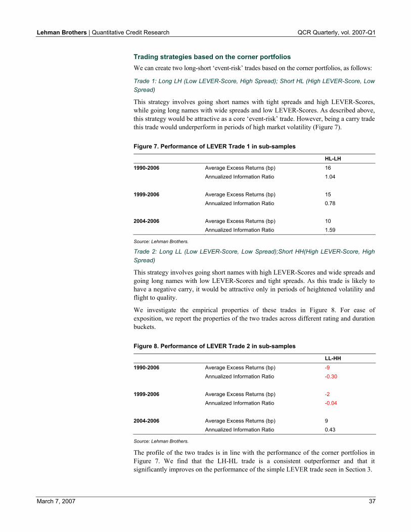
Lehman Brothers | Quantitative Credit Research QCR Quarterly, vol. 2007-Q1
March 7, 2007 37
Trading strategies based on the corner portfolios We can create two long-short ‘event-risk’ trades based on the corner portfolios, as follows:
Trade 1: Long LH (Low LEVER-Score, High Spread); Short HL (High LEVER-Score, Low Spread)
This strategy involves going short names with tight spreads and high LEVER-Scores, while going long names with wide spreads and low LEVER-Scores. As described above, this strategy would be attractive as a core ‘event-risk’ trade. However, being a carry trade this trade would underperform in periods of high market volatility (Figure 7).
Figure 7. Performance of LEVER Trade 1 in sub-samples
HL-LH 1990-2006 Average Excess Returns (bp) 16 Annualized Information Ratio 1.04 1999-2006 Average Excess Returns (bp) 15 Annualized Information Ratio 0.78 2004-2006 Average Excess Returns (bp) 10 Annualized Information Ratio 1.59
Source: Lehman Brothers.
Trade 2: Long LL (Low LEVER-Score, Low Spread);Short HH(High LEVER-Score, High Spread)
This strategy involves going short names with high LEVER-Scores and wide spreads and going long names with low LEVER-Scores and tight spreads. As this trade is likely to have a negative carry, it would be attractive only in periods of heightened volatility and flight to quality.
We investigate the empirical properties of these trades in Figure 8. For ease of exposition, we report the properties of the two trades across different rating and duration buckets.
Figure 8. Performance of LEVER Trade 2 in sub-samples
LL-HH 1990-2006 Average Excess Returns (bp) -9 Annualized Information Ratio -0.30 1999-2006 Average Excess Returns (bp) -2 Annualized Information Ratio -0.04 2004-2006 Average Excess Returns (bp) 9 Annualized Information Ratio 0.43
Source: Lehman Brothers.
The profile of the two trades is in line with the performance of the corner portfolios in Figure 7. We find that the LH-HL trade is a consistent outperformer and that it significantly improves on the performance of the simple LEVER trade seen in Section 3.
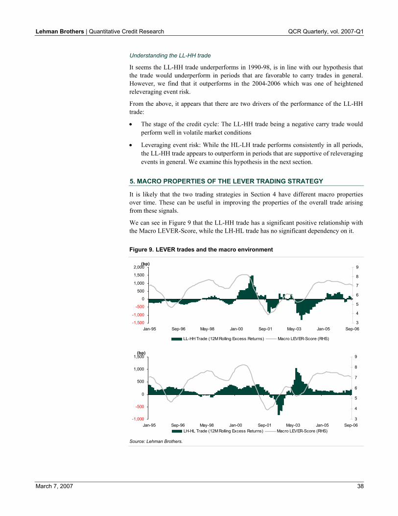
Lehman Brothers | Quantitative Credit Research QCR Quarterly, vol. 2007-Q1
March 7, 2007 38
Understanding the LL-HH trade
It seems the LL-HH trade underperforms in 1990-98, is in line with our hypothesis that the trade would underperform in periods that are favorable to carry trades in general. However, we find that it outperforms in the 2004-2006 which was one of heightened releveraging event risk.
From the above, it appears that there are two drivers of the performance of the LL-HH trade:
• The stage of the credit cycle: The LL-HH trade being a negative carry trade would perform well in volatile market conditions
• Leveraging event risk: While the HL-LH trade performs consistently in all periods, the LL-HH trade appears to outperform in periods that are supportive of releveraging events in general. We examine this hypothesis in the next section.
5. MACRO PROPERTIES OF THE LEVER TRADING STRATEGY
It is likely that the two trading strategies in Section 4 have different macro properties over time. These can be useful in improving the properties of the overall trade arising from these signals.
We can see in Figure 9 that the LL-HH trade has a significant positive relationship with the Macro LEVER-Score, while the LH-HL trade has no significant dependency on it.
Figure 9. LEVER trades and the macro environment
-1,500
-1,000
-500
0
500
1,000
1,500
2,000
Jan-95 Sep-96 May-98 Jan-00 Sep-01 May-03 Jan-05 Sep-06
(bp)
3
4
5
6
7
8
9
LL-HH Trade (12M Rolling Excess Returns) Macro LEVER-Score (RHS)
-1,000
-500
0
500
1,000
1,500
Jan-95 Sep-96 May-98 Jan-00 Sep-01 May-03 Jan-05 Sep-06
(bp)
3
4
5
6
7
8
9
LH-HL Trade (12M Rolling Excess Returns) Macro LEVER-Score (RHS)
Source: Lehman Brothers.

Lehman Brothers | Quantitative Credit Research QCR Quarterly, vol. 2007-Q1
March 7, 2007 39
To quantify this dependency, we regress the monthly returns of both the above trades on the monthly Macro LEVER-Score (Figure 10).
Figure 10. Dependency of trades on Macro LEVER-Score
LH-HL LL-HH Constant 33.1 -80.0 t-stat 2.50 -3.13 Slope -2.9 12.0 t-stat -1.33 2.88
Source: Lehman Brothers.
In summary, we find the following:
• The standard LEVER trading strategy LH-HL outperforms across regimes because it has a positive carry that enables it to enhance the degree of releveraging risk premium it extracts.
• The performance of the LL-HH trade is dependent on the macro environment – i.e. it outperforms only in periods of heightened releveraging activity, such as the current one.
Combining the two trading strategies In order therefore to optimally align our portfolio to the macro environment, we need to predict the degree of releveraging activity in the following period. The LEVER model readily allows us to do this, through the Macro LEVER-Score, which can also be used as the weight allocated to the LL-HH trade. The investor’s portfolio would be following:
(LH-HL) Trade + w*(LL-HH) Trade
where w is defined as 0.1*Macro LEVER-Score.
In other words, the portfolio consists of two components which directly reflect the macro behavior discussed above:
Component 1: The Static LEVER Trade which is long the LH portfolio and short the HL portfolio.
Component 2: The Dynamic LEVER Trade which is long the LL portfolio and short the HH portfolio. This part of the trade is scaled up in periods of high releveraging event risk.
Performance of the combined trading strategy In Figure 11 we present the performance of the combined trade in the three rating categories both in the full sample and in the sub-samples.

Lehman Brothers | Quantitative Credit Research QCR Quarterly, vol. 2007-Q1
March 7, 2007 40
Figure 11. Performance of combined trading strategy
AA A BBB Overall 1990-2006 Average Excess Returns (bp) 8 14 22 14 Annualized IR 0.51 0.73 0.55 0.90 Hit Ratio 56% 58% 53% 59% Skew 1.18 4.07 2.02 1.73 1999-2006 Average Excess Returns (bp) 8 18 34 20 Annualized IR 0.44 0.69 0.62 0.92 2004-2006 Average Excess Returns (bp) 3 18 33 18 Annualized IR 0.35 0.56 0.90 1.12
Source: Lehman Brothers.
Figure 11 shows that the trade exhibits strong performance, and that it improves on the standard trade by means of a more balanced profile across sub-samples.
To enhance our understanding, Figure 12 shows rolling 12-month cumulative returns for the combined trading strategy across all rating categories and for the US IG Corporate Index.
Figure 12. Rolling 12 month cumulative returns of combined trading strategy (bp)
-600
-200
200
600
1,000
1,400
Jan-9
1Ju
l-92
Jan-9
4Ju
l-95
Jan-9
7Ju
l-98
Jan-0
0Ju
l-01
Jan-0
3Ju
l-04
Jan-0
6
Combined Trade US IG Corporate Index
Source: Lehman Brothers.
The combined trade has a correlation of -20% with the excess returns with the Lehman US IG Corporate Index in the full sample and exhibits a stable performance profile.
Comparison of the combined LEVER trade with the ESPRI model It is also interesting to analyze the comparative performance of the combined LEVER trade with that of a model such as ESPRI – which also in part attempts to capture the risk-premia embedded in wide spread vs tight spread names.
In Figure 13 we present a comparison of the performance of the Dynamic ESPRI strategy for BBB rated long duration bonds and that of the combined LEVER trade. The in-sample correlation of the two trades is -1%, which is attractive, as it would be valuable to add the LEVER signals to a trading strategy that already includes signals from the ESPRI model.

Lehman Brothers | Quantitative Credit Research QCR Quarterly, vol. 2007-Q1
March 7, 2007 41
Figure 13. Rolling 12 month cumulative returns of combined trading strategy (bp)
-600
-200
200
600
1,000
1,400
Jan-9
1Ju
l-92
Jan-9
4Ju
l-95
Jan-9
7Ju
l-98
Jan-0
0Ju
l-01
Jan-0
3Ju
l-04
Jan-0
6
-600
0
600
1200
1800
2400
3000
Combined LEVER Trade Dynamic ESPRI (RHS)
Source: Lehman Brothers.
7. CONCLUSION
We have analyzed the performance of the LEVER model as an investment framework to identify and extract risk premia. Our empirical analysis shows that trades based on the LEVER framework perform well historically and that their correlation with the market and other traditional credit trading strategies, such as that of the ESPRI model, is low. This finding is useful for both portfolio managers with benchmark outperformance mandates and those with absolute return mandates.
REFERENCES
Trinh, Minh, Bhattacharya B., Devarajan M., Heike D., Pomper M., Wolosky J. (2006) ‘LEVER: A framework for Scoring LEVeraging Event Risk’ Quantitative Credit Research Quarterly, 2006-Q1
Naik, Vasant, Trinh M., Rennison G. (2002) ‘Introducing Lehman Brothers ESPRI: A Credit Selection Model using Equity Returns as Spread Indicators’ Quantitative Credit Research Quarterly, January 2002

Lehman Brothers | Quantitative Credit Research QCR Quarterly, vol. 2007-Q1
March 7, 2007 42
Introducing Lehman Brothers’ CMetrics Framework1
INTRODUCTION
Fundamental equity and credit analysts seek to interpret companies’ financial statements in order to identify key areas of strengths and weaknesses with a view to making informed judgments about future prospects. Over time individual analysts have adopted and adapted a myriad of measures to gauge opportunities and risks within their coverage universe. The result has often been a seemingly endless number of financial ratios that cannot be easily compared across sectors and sometimes even within the same sector. Lehman Brothers’ CMetrics is a new financial framework aimed at improving the quality of financial analysis and valuations. In particular, CMetrics provides:
• Concise, comparable and consistent financial ratios linked to Enterprise Value
• Adjusted metrics to enable cross company, cross industry comparisons
• An integrated framework that analyzes independently the three key management activities:
- Operating the core business
- Financing the enterprise
- Investing in non-core business activities
• A broad coverage of U.S. public companies
• On-line tools for Company and Industry level financial analysis
While many investors focus on earnings per share, academic and practitioner research has established a link between recurring operating return (Return on Invested Capital or “ROIC”) and long-term intrinsic value. The CMetrics Framework recognizes this relationship and offers ROIC-based performance metrics that are linked to operating performance, as well as financing and investing performance measures, so that users can evaluate how the results of management decisions and various aspects of performance drive firm value. As a result, the entire CMetrics framework is value-relevant. The Section entitled “Enterprise Valuation and Performance Measurement” discusses this in more detail.
CMetrics makes adjustments to the financial statements to enable cross comparison of companies and industries. The framework makes adjustments in order to control for differences in financial reporting, recognize unrecognized assets and liabilities, and reflect the underlying economics of the business and industry into the financial analysis and valuation of the firm. The section entitled “Adjustments” describes these adjustments in a greater detail.
1 The authors would like to acknowledge Meredith Adler, Margery Cunningham, Mathew Rothman, Sergey
Vasetnsov, Ann Gillin Lefever, Jack Malvey, Elmer Huh, and S.R. Rajan for their helpful comments and suggestions.
Mary M. Margiotta 212-526-5993
Chetan Seth
212-320-7497 [email protected]
Prafulla Nabar 212-526-6108

Lehman Brothers | Quantitative Credit Research QCR Quarterly, vol. 2007-Q1
March 7, 2007 43
ACCESS
CMetrics can be accessed on LehmanLive, keyword CMetrics. Additional information on using CMetrics is found by clicking on the CMetrics User Guide.
OVERVIEW
The aim of the management of a company is to provide maximum return for its equity holders. Even well-known recent cases of accounting scandals and fraud were primarily driven by a desire on the part of management to keep stock prices and returns from falling. While short-term market returns can be influenced by many factors, often outside the control of management, the long-term success or failure of a company is tied to the strategic operating decisions that influence the firm’s earnings and cash flows over time.
Figure 1. Firm Value and Managerial Decisions
Recurring One-Time
Operating
• Products & Markets • Cap Ex and R&D/Advertising • Credit terms • Operational improvements • HR & benefits policies
• Restructuring programs, exiting markets
• Asset sales • Changes in accounting policies
Financing
• Capital structure/leverage • Debt instruments • Near debt/hybrid capital • Changes in performance of pension
assets
• Gains/losses on debt retirement • Changes in assumptions of
pension assets/liabilities
Investing
• Investment decisions • Performance of investments
• Reclassification of investment assets (non-trading to trading)
Source: Lehman Brothers Analysis.
Figure 1 provides examples of managerial decisions classified in the operating, financing and non-operating (or investing) categories that affect firm financial performance. It also provides examples of “recurring” decisions (decisions that are part of the normal day-to-day running of the firm) and “one-time” decisions (decisions that happen with less frequency and represent a departure from the normal course of business). Financial analysts focus significant attention on understanding how the recurring operating items (the shaded items) affect performance because the long-term value of a firm is driven by recurring operations.
The aim of fundamental historical financial analysis is to gauge the impact of these past decisions on the future prospects of the firm. Performance measures such as Return on Equity (ROE) or Earnings per Share (EPS) are helpful in assessing the overall success of the management team in improving the financial return of equity holders. They are less useful in diagnosing the reason for the change in performance because they do not routinely exclude one-time items or decompose performance into the core aspects of management: (1) operation of the business, (2) financing of the enterprise, and (3) other

Lehman Brothers | Quantitative Credit Research QCR Quarterly, vol. 2007-Q1
March 7, 2007 44
non-operational investments2. The CMetrics framework addresses these concerns by decomposing company financial results into recurring vs. non-recurring items as well as distinguishing between operating, financial and non-operating investing performance.
CMetrics aims to provide a more robust framework for financial analysis with value-relevant and consistently measured financial ratios that can be readily and appropriately compared to those of their industry peers and with companies in other sectors. These metrics are made comparable by controlling for differences due to use of different accounting methods in financial reporting, reflecting unrecognized liabilities, and making the financial statement reflect the underlying economics of the business or industry.. Importantly, the measures are part of an integrated system so that investors can drill down from the financial ratios to the performance measures of various aspects of the business such as trend in inventories, receivables, fixed assets, and capital structure decisions. Users can compare these ratios across with those of individual industry competitors, with the industry or sub-industry grouping as a whole, or with non-industry peers to uncover the reasons for the improvement/deterioration in performance and gain insight about future prospects.
2 This framework is consistent with proposals made by the Joint Project of the International Accounting Standards
Board (IASB) and Financial Accounting Standards Board (FASB) on Financial Statement Presentations to improve the usefulness of financial reports.

Lehman Brothers | Quantitative Credit Research QCR Quarterly, vol. 2007-Q1
March 7, 2007 45
THE CMETRICS FRAMEWORK
The CMetrics framework summarizes firm performance into three categories: performance, market and credit risk, and valuation. Figure 2 presents the full list of CMetrics ratios.
Figure 2. CMetrics Ratios
Key Performance Metrics Adjusted EPS Sales Growth (from previous qtr) ROE Return on Invested Capital (ROIC) NOPAT Margin EBITDA Margin Depreciation Margin R&D Margin COGS Margin Other SG&A Margin Capital Intensity Working Capital Turnover AR Days AP Days Inventory Days PPE Margin Financing Return Debt to Equity Ratio Financing Spread Non-Operating Return Investment Ratio Investment Spread Non-recurring Income (Expenses) to Sales Additional Market & Credit Risk Metrics Beta WACC Interest Coverage Ratio Cash Position Operating Cash Flow Discrepancy Free Cash Flow to Sales Key Valuation Metrics P/E multiple EV/EBITDA EV/IC EV/FCF
Source: Lehman Brothers CMetrics version 1.0.
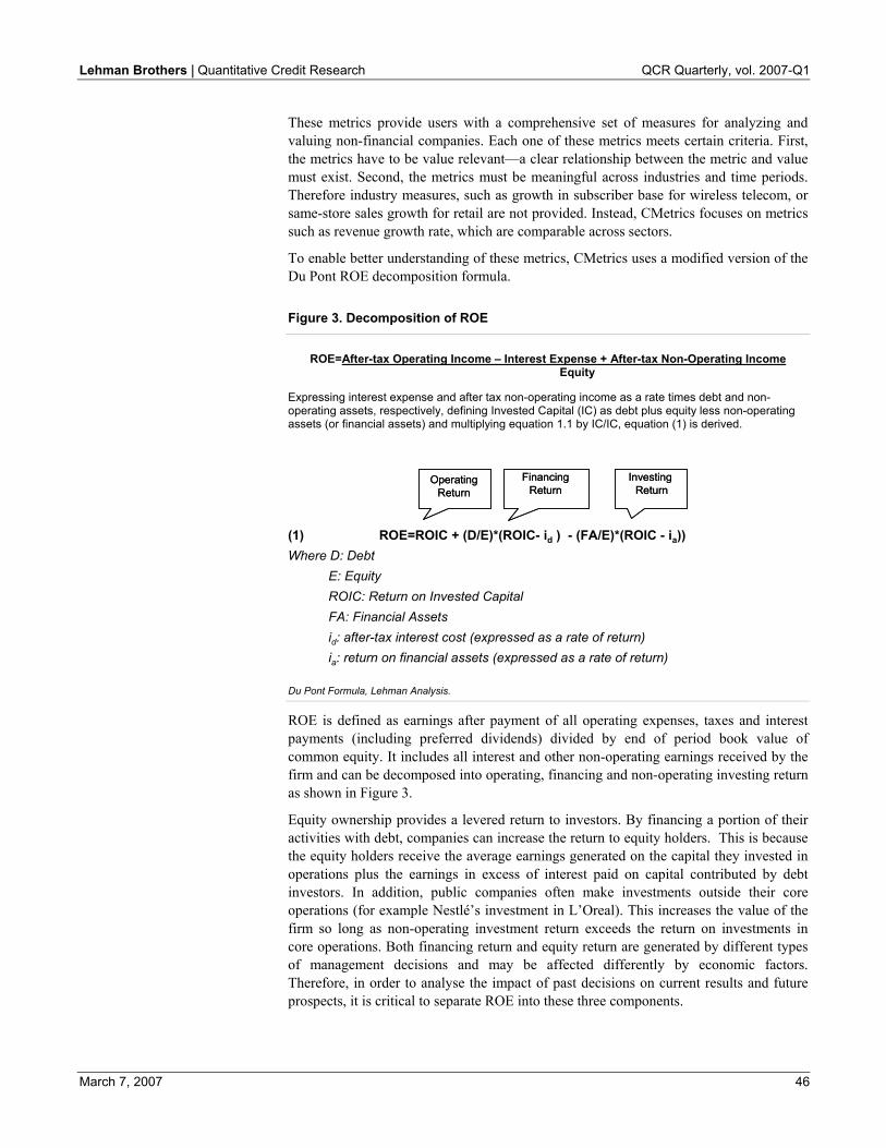
Lehman Brothers | Quantitative Credit Research QCR Quarterly, vol. 2007-Q1
March 7, 2007 46
These metrics provide users with a comprehensive set of measures for analyzing and valuing non-financial companies. Each one of these metrics meets certain criteria. First, the metrics have to be value relevant—a clear relationship between the metric and value must exist. Second, the metrics must be meaningful across industries and time periods. Therefore industry measures, such as growth in subscriber base for wireless telecom, or same-store sales growth for retail are not provided. Instead, CMetrics focuses on metrics such as revenue growth rate, which are comparable across sectors.
To enable better understanding of these metrics, CMetrics uses a modified version of the Du Pont ROE decomposition formula.
Figure 3. Decomposition of ROE
ROE=After-tax Operating Income – Interest Expense + After-tax Non-Operating Income Equity
Expressing interest expense and after tax non-operating income as a rate times debt and non-operating assets, respectively, defining Invested Capital (IC) as debt plus equity less non-operating assets (or financial assets) and multiplying equation 1.1 by IC/IC, equation (1) is derived.
(1) ROE=ROIC + (D/E)*(ROIC- id ) - (FA/E)*(ROIC - ia))Where D: Debt
E: EquityROIC: Return on Invested CapitalFA: Financial Assetsid: after-tax interest cost (expressed as a rate of return)ia: return on financial assets (expressed as a rate of return)
Operating Return
Financing Return
InvestingReturn
Operating Return
Financing Return
InvestingReturn
Du Pont Formula, Lehman Analysis.
ROE is defined as earnings after payment of all operating expenses, taxes and interest payments (including preferred dividends) divided by end of period book value of common equity. It includes all interest and other non-operating earnings received by the firm and can be decomposed into operating, financing and non-operating investing return as shown in Figure 3.
Equity ownership provides a levered return to investors. By financing a portion of their activities with debt, companies can increase the return to equity holders. This is because the equity holders receive the average earnings generated on the capital they invested in operations plus the earnings in excess of interest paid on capital contributed by debt investors. In addition, public companies often make investments outside their core operations (for example Nestlé’s investment in L’Oreal). This increases the value of the firm so long as non-operating investment return exceeds the return on investments in core operations. Both financing return and equity return are generated by different types of management decisions and may be affected differently by economic factors. Therefore, in order to analyse the impact of past decisions on current results and future prospects, it is critical to separate ROE into these three components.

Lehman Brothers | Quantitative Credit Research QCR Quarterly, vol. 2007-Q1
March 7, 2007 47
As summarized in equation (1), the factors that drive ROE are:
(1) operating return on capital employed in the core business;
(2) leverage and the firm’s ability to finance itself at a rate which is below its operating return; and
(3) the portion of equity invested in non-operating assets and the amount by which the returns from non-operations exceed those of operations.
We explain these three components of the equation below.
The Return on Invested Capital (ROIC) is net operating income after-tax (NOPAT) divided by debt and equity capital invested in the operations of the firm (Invested Capital)3. This is the profit earned by the operations of the firm on its invested capital.
The second term in equation (1) is the amount of return to equity holders from leverage; that is using debt to finance the enterprise. The firm increases its return to equity investors by taking on debt so long as the return on the firm’s operations is greater than the cost of the debt assumed. In other words, more debt can be used to support the operation (and increase the average return to equity holders) if the spread between ROIC and the cost of debt is positive. Firms with relatively lower leverage present an opportunity for improving equity returns by using additional debt.
The third term in equation (1) is the amount of ROE that can be attributed to the firm’s investments in other areas or “non-operating” assets. Companies increase their ROE when returns from non-operating assets are higher than returns from operating assets. This is difficult to do on a sustainable basis in light of the fact that investment performance is generally outside the control of management. Therefore, a company with a high percentage of ROE stemming from non-operating investments should be examined carefully for restructuring opportunities or looked at from the perspective of whether the business model is changing. Companies that hold significant amount of cash and marketable securities relative to their equity also need to be examined closely to make sure that the interest income generated by these assets exceeds that of the operating return so as to not destroy shareholder value.
The next section emphasises the importance of correctly understanding the significance of the firm’s operating performance or it’s ROIC.
ENTERPRISE VALUE AND PERFORMANCE MEASUREMENT
The value of an asset is equivalent to the aggregate value of the claims on that asset. The value of the entire business (the Enterprise Value or EV) determines the value of the claims on its assets. Thus the value of a company, which is the combined value of its tangible and intangible assets, is equal to the sum of the value of its debt and its equity. Further, assuming efficient markets, the EV equals the present value of the expected future income when adequately adjusting for the risk embedded in these earnings.
Assuming that value is equivalent to the present value of expected future cash flows (the classic Discounted Cash Flow or “DCF” model), and that a company’s cash flows grow at a constant rate, several authors4 have shown that Enterprise Value is a function of growth, ROIC and the company’s cost of capital as shown in equation (2) below.
(2) Value=ROIC*IC*(1-(g/ROIC))/(WACC-g) 3 Invested Capital includes all interest-bearing debt and debt like claims on assets plus all equity and equity like
claims in excess of non-operating assets. See Section “CMetrics Invested Capital” for further discussion of the financial line-items that are included in the Invested Capital calculations.
4 Copeland and Weston, and Koller, et al.

Lehman Brothers | Quantitative Credit Research QCR Quarterly, vol. 2007-Q1
March 7, 2007 48
In practice, market values for companies may differ from DCF estimates for many reasons that exceed the ability of a stylized model to capture. However, academic and Wall Street research has shown that over time market returns are correlated with fundamental ratios of growth, return and risk5. For this reason, CMetrics reports ROIC as its primary measure of operating performance and an indicator of future value. An analysis of ROIC by itself, however, is not informative about the reason for a change. For this, a DuPont analysis decomposition of ROIC is performed. ROIC is a function of operating margin (the amount by which the enterprise’s operating revenues exceed the operating costs) and capital turnover (the amount of invested or operating capital used by the business) relative to the size of the business. In addition, each of these metrics can be further decomposed into useful operating statistics, as shown in Figure 4, below.
Figure 4. Decomposition of ROE and ROIC
Source: Lehman Brothers Analysis.
Figure 4 details how ROIC is decomposed into the CMetrics operating drivers. Figure 4 in conjunction with equation (2) provides a valuation framework for analyzing how changes in operational drivers such as margin or working capital intensity affect ROIC and enterprise and equity valuations. In theory, these measures can be decomposed into finer and finer measures of performance. CMetrics stops at this level because further decompositions cannot be meaningfully done across sectors; moreover, the data is not available consistently across our coverage universe.
Figure 5 summarizes the ratios that are presented in CMetrics. The table contains the formula for computing each ratio, what the ratio measures, and how to interpret the observed values of these ratios. Additional information is also available in the CMetrics Glossary provided in the appendix.
5 See for example Nissim and Penman (2001) and Fairfield and Yohn (2001).

Lehman Brothers | Quantitative Credit Research QCR Quarterly, vol. 2007
March 7, 2007 49
Figure 5. CMetrics at a glance…
Performance Measure Definition What it measures Watch out for EPS Earnings Before Non Recurrings
Common shares outstanding Earnings available per equity share Significant difference from proforma EPS, diluted EPS
Sales Growth Salest – 1 * 100 Salest-1
Rate of growth in demand for company’s products / service
Acquisitions, divestitures, sustainability Sales growth exceeding industry norms may indicate aggressive accounting policies
ROE Earnings Before Extraordinary Shareholders Equity
Equity holders book return Examine leverage if ratio is high relative to peers
ROIC NOPAT Invested Capital
Profitability before financing expenses ROIC lower than WACC indicates value destruction ROIC out of line with the industry would warrant further investigation
NOPAT Margin NOPAT Net Revenues
After tax profitability of operations Declining ratio could mean greater competition or cost inefficiencies Rising ratio and rising prepaid expenses could indicate inflated earnings
EBITDA Margin EBITDA Net revenues
Profitability before financing and investing expenses
Declining ratio could mean greater competition or cost inefficiencies Rising ratio and rising prepaid expenses could indicate inflated earnings
Depreciation Margin Depreciation Net revenues
Provision for diminution in value of fixed assets as % of net revenues
Low ratio as compared to peers and a high capex / depreciation ratio could indicate insufficient provision for future capital expenditure
R&D Margin R&D Expense Net revenues
Amount invested in R&D as % of net revenues
Declining ratio with declining EBITDA margin could indicate limited growth prospects Declining ratio with rising capitalized R&D could indicate inflated earnings
COGS Margin COGS (Excl Depreciation) Net revenues
Pricing power and efficiency of manufacturing
Rising ratio could mean greater competition or cost inefficiencies Declining COGS and rising prepaid expenses could indicate inflated earnings
Other SG&A Margin SG&A Net revenues
Efficiency of selling and administrative functions
Declining ratio with declining EBITDA margin could indicate limited growth prospects or netting of one time gains
Capital Turnover Invested capital Net Revenue
Efficiency of capital utilization and whether revenue comes from core operations or additional investments
High ratio relative to peers could indicate inefficient utilization of capital or insufficient scale
Working Capital Turnover Working capital Net revenue
Efficiency of working capital management High ratio relative to peers could indicate inefficient working capital management
AR Days Trade Receivables * # of Days Net revenue
Days of credit extended to customers High ratio relative to peers may indicate channel stuffing or failure to write of bad debts
AP Days Trade Payables * # of Days Net Revenues
Days of credit obtained from suppliers Low ratio relative to peers combined with low profitability could indicate tightening credit
Inventory Days Total Inventories* # of Days Net revenues
Estimated days of sales for which inventory has been produced but is yet to be sold
Rising ratio as compared to trend or peers could indicate falling demand or failure to write of obsolete inventory
PPE Margin NPPE Net revenues
Efficiency of utilization of fixed assets Low ratio relative to peers could indicate insufficient investments or insufficient provision for depreciation
Financing Return Leverage * Financing spread ROE attributable to financing decisions Examine sustainability if contribution to ROE is significant (especially in increasing interest rate scenarios)
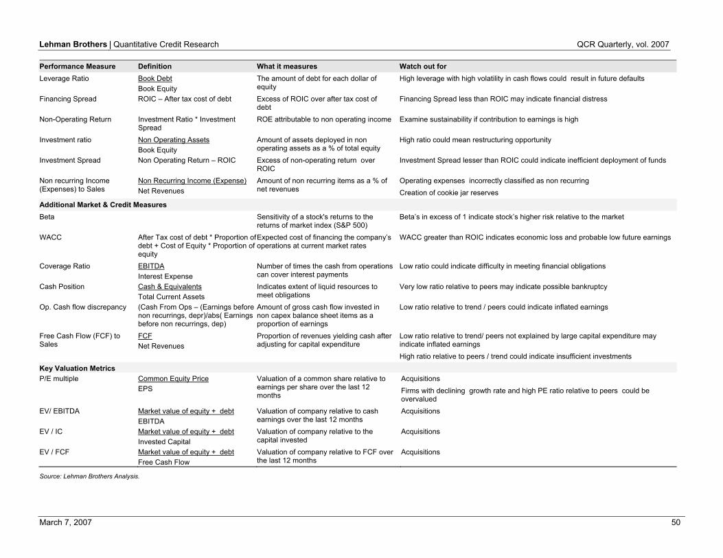
Lehman Brothers | Quantitative Credit Research QCR Quarterly, vol. 2007
March 7, 2007 50
Performance Measure Definition What it measures Watch out for Leverage Ratio Book Debt
Book Equity The amount of debt for each dollar of equity
High leverage with high volatility in cash flows could result in future defaults
Financing Spread ROIC – After tax cost of debt Excess of ROIC over after tax cost of debt
Financing Spread less than ROIC may indicate financial distress
Non-Operating Return Investment Ratio * Investment Spread
ROE attributable to non operating income Examine sustainability if contribution to earnings is high
Investment ratio Non Operating Assets Book Equity
Amount of assets deployed in non operating assets as a % of total equity
High ratio could mean restructuring opportunity
Investment Spread Non Operating Return – ROIC Excess of non-operating return over ROIC
Investment Spread lesser than ROIC could indicate inefficient deployment of funds
Non recurring Income (Expenses) to Sales
Non Recurring Income (Expense) Net Revenues
Amount of non recurring items as a % of net revenues
Operating expenses incorrectly classified as non recurring Creation of cookie jar reserves
Additional Market & Credit Measures Beta Sensitivity of a stock's returns to the
returns of market index (S&P 500) Beta’s in excess of 1 indicate stock’s higher risk relative to the market
WACC After Tax cost of debt * Proportion of debt + Cost of Equity * Proportion of equity
Expected cost of financing the company’s operations at current market rates
WACC greater than ROIC indicates economic loss and probable low future earnings
Coverage Ratio EBITDA Interest Expense
Number of times the cash from operations can cover interest payments
Low ratio could indicate difficulty in meeting financial obligations
Cash Position Cash & Equivalents Total Current Assets
Indicates extent of liquid resources to meet obligations
Very low ratio relative to peers may indicate possible bankruptcy
Op. Cash flow discrepancy (Cash From Ops – (Earnings before non recurrings, depr)/abs( Earnings before non recurrings, dep)
Amount of gross cash flow invested in non capex balance sheet items as a proportion of earnings
Low ratio relative to trend / peers could indicate inflated earnings
Free Cash Flow (FCF) to Sales
FCF Net Revenues
Proportion of revenues yielding cash after adjusting for capital expenditure
Low ratio relative to trend/ peers not explained by large capital expenditure may indicate inflated earnings High ratio relative to peers / trend could indicate insufficient investments
Key Valuation Metrics P/E multiple Common Equity Price
EPS Valuation of a common share relative to earnings per share over the last 12 months
Acquisitions Firms with declining growth rate and high PE ratio relative to peers could be overvalued
EV/ EBITDA Market value of equity + debt EBITDA
Valuation of company relative to cash earnings over the last 12 months
Acquisitions
EV / IC Market value of equity + debt Invested Capital
Valuation of company relative to the capital invested
Acquisitions
EV / FCF Market value of equity + debt Free Cash Flow
Valuation of company relative to FCF over the last 12 months
Acquisitions
Source: Lehman Brothers Analysis.
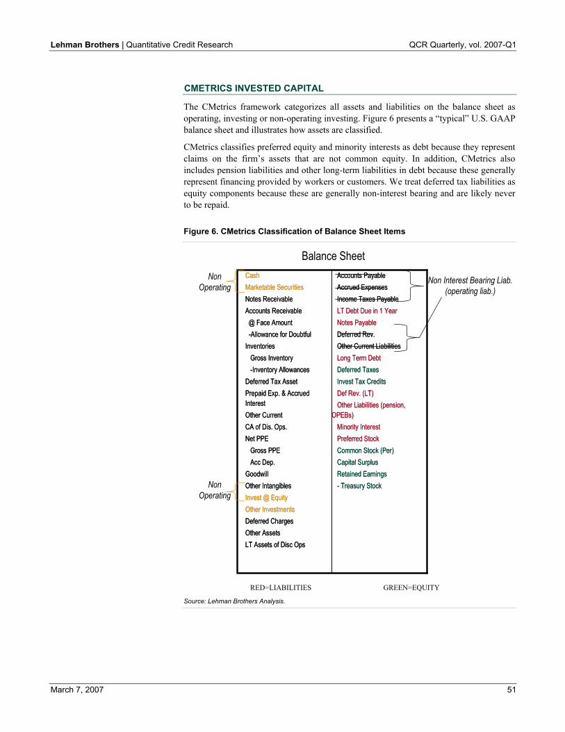
Lehman Brothers | Quantitative Credit Research QCR Quarterly, vol. 2007-Q1
March 7, 2007 51
CMETRICS INVESTED CAPITAL
The CMetrics framework categorizes all assets and liabilities on the balance sheet as operating, investing or non-operating investing. Figure 6 presents a “typical” U.S. GAAP balance sheet and illustrates how assets are classified.
CMetrics classifies preferred equity and minority interests as debt because they represent claims on the firm’s assets that are not common equity. In addition, CMetrics also includes pension liabilities and other long-term liabilities in debt because these generally represent financing provided by workers or customers. We treat deferred tax liabilities as equity components because these are generally non-interest bearing and are likely never to be repaid.
Figure 6. CMetrics Classification of Balance Sheet Items
Accounts PayableAccrued ExpensesIncome Taxes PayableLT Debt Due in 1 YearNotes PayableDeferred Rev.Other Current LiabilitiesLong Term DebtDeferred TaxesInvest Tax CreditsDef Rev. (LT)Other Liabilities (pension,
OPEBs)Minority InterestPreferred StockCommon Stock (Per)Capital SurplusRetained Earnings- Treasury Stock
CashMarketable SecuritiesNotes ReceivableAccounts Receivable@ Face Amount -Allowance for Doubtful
InventoriesGross Inventory-Inventory Allowances
Deferred Tax AssetPrepaid Exp. & Accrued InterestOther Current CA of Dis. Ops.Net PPE
Gross PPEAcc Dep.
GoodwillOther IntangiblesInvest @ EquityOther InvestmentsDeferred ChargesOther AssetsLT Assets of Disc Ops
Balance SheetNon
Operating
Non Operating
Non Interest Bearing Liab. (operating liab.)
RED=LIABILITIES GREEN=EQUITY
Source: Lehman Brothers Analysis.

Lehman Brothers | Quantitative Credit Research QCR Quarterly, vol. 2007-Q1
March 7, 2007 52
Non-operating assets include all long-term investments as well as cash and marketable securities. In some cases, long-term investments may be operational in nature (for example Coca-Cola’s investment in some of its bottlers). In general these investments are not part of the day-to-day operations of the firm and are not under the direct control of management. Therefore, we treat all such investments as non-operating.
The treatment of cash as non-operational is more controversial. It is clear that some cash is required in order to fund current operations. However, many companies have significant investments in cash. According to a recent New York Times article, U.S. public companies hold stockpiles of cash to repay all their debt and still have additional money left over.1 Because of the very high levels of cash held by companies it is hard to argue that this cash is necessary to fund current operations. For this reason, CMetrics treats all cash as a non-operational investment asset until the cash is used to purchase productive assets.
In a similar manner, CMetrics treats each income statement line item as operating, financing or non-operating investment income. Line items are allocated to these categories so as to be consistent with the treatment of the underlying assets that generate the income. For example, because cash is included in non-operating investment assets, interest income earned on that cash is included in non-operating income. Similarly, costs that are associated with the financing of assets (for example the implied interest expense on non-capitalized leases) are reclassified from operating expenses to interest expense.
ADJUSTMENTS
The CMetrics Framework includes seven standard adjustments to each company’s financials where appropriate. The adjustments were developed in order to improve comparability between companies and between industry sectors. Adjustments were designed to enable the user to control for differences in accounting standards between firms, to compare the financial statements of companies over time in a consistent manner and to recognize off-balance sheet asset and liabilities that affect company performance. In making these adjustments the guiding principle of CMetrics is to adjust financial statements to better reflect the underlying economics of the business2.
When choosing which adjustments to make and how to make them, we have been mindful of the following requirements:
• Meaningfulness/Relevance: Adjustments are only made if the failure to make such adjustments decreases the user’s ability to interpret the financial statements of the company.
• Consistency: Adjustments are only made if they can be made reliably for all companies that would be affected.
• Simplicity and Economic Rigor: The adjustments must be simple to explain, have easy interpretation and be consistent with the underlying economic conditions of the firm.
CMetrics adjustments are designed to restate the income statement and balance sheet of the company as they would appear if the company followed the adjustment for financial reporting purposes. All adjustments that affect net income have an offsetting adjustment to equity as well as the appropriate adjustments to asset and/or liability accounts. All
1 Hulbert, Mark. “Behind Those Stockpiles of Corporate Cash”, New York Times, October 22, 2006. 2 Recognizing that financial analysis is an art and that in some cases it may be appropriate to consider results
before the impact of the adjustments, CMetrics allows users the flexibility to turn on or off some or all of the adjustments.

Lehman Brothers | Quantitative Credit Research QCR Quarterly, vol. 2007-Q1
March 7, 2007 53
adjustments are tax-effected to reflect the after-tax impact of the adjustment on equity and tax liabilities.
It should be noted that financial statement analysis, especially the adjustment of financials to improve meaning and comparability is an art, not a science. In all cases, the adjustments have been designed to be as simple and transparent as possible. Also because of data limitations, some adjustments have been simplified or approximated.
The seven standard adjustments are listed below:
• Last In First Out (“LIFO”) inventories restated as First In First Out (“FIFO”)
• Adjust financial statements to reflect stock-based compensation if options were not expensed in the financial statements
• Capitalization of off-balance sheet leases
• Capitalization of R&D expenditures
• Capitalization of Advertising expenditures
• Pension and Other Post Retirement (“OPEB”) financing expenses reclassified from operating to financing (interest) expense
• Pension liabilities restated to reflect full funded status.
The remainder of this section provides details of these adjustments and examples on how these adjustments could have a significant impact on the operating performance of some of the companies. Although we believe it is important to make these adjustments when conducting a historical financial analysis, CMetrics gives the user the flexibility to apply the adjustments or not.
LIFO/FIFO For companies that follow the LIFO inventory policy, inventory values are lower, and cost of sales is higher than companies that follow FIFO or Weighted Average policies. These differences are more pronounced when commodity prices are rising and/or when inventories are rising, making it difficult to properly assess the financial health of companies. To control for this difference, inventories are restated at the level they would attain if FIFO were used, and COGS are likewise restated to the amount that would be recognized under FIFO.
Figure 7 presents an example of the LIFO/FIFO adjustment for the chemicals industry for the fourth quarter of 2005, a period of rising prices and significant changes in inventories. While the adjustment has little effect on the median ROIC, which increases from 2.19% before adjustment to 2.35% afterwards, the adjustment changes the relative ranking of Engelhard Corp. and Olin Corp. Before adjustment Engelhard Corp. has a ROIC of 3.0% and an industry ranking of 3, but after adjustment its ROIC becomes 2.6% while its ranking changes to 5. Similarly, Olin Corp. has a pre-adjustment ROIC of 2.3% and an industry rank of 5. After adjustment from LIFO to FIFO, its ROIC increases to 3.3% and the ranking becomes 2.
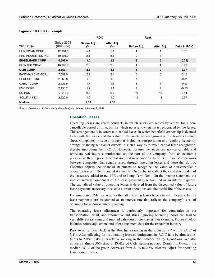
Lehman Brothers | Quantitative Credit Research QCR Quarterly, vol. 2007-Q1
March 7, 2007 54
Figure 7. LIFO/FIFO Example
ROIC Rank
2005 CQ4 Sales 2005 (USD mn)
Before Adj. (%)
After Adj. (%) Before Adj. After Adj. Delta in ROIC
HUNTSMAN CORP 12,961.6 5.1 5.4 1 1 0.38 PPG INDUSTRIES INC 10,201.0 3.1 3.1 2 3 - ENGELHARD CORP 4,597.0 3.0 2.6 3 5 (0.35) DOW CHEMICAL 46,307.0 2.8 2.9 4 4 0.08 OLIN CORP 2,357.7 2.3 3.3 5 2 0.97 EASTMAN CHEMICAL 7,059.0 2.2 2.4 6 6 0.16 HERCULES INC 2,068.8 1.9 1.6 7 8 -0.31 CABOT CORP 2,125.0 1.7 1.6 8 7 -0.03 FMC CORP 2,150.2 1.2 1.1 9 9 -0.15 DU PONT 27,516.0 0.5 0.7 10 10 0.14 SOLUTIA INC 2,825.0 (1.6) (1.0) 11 11 0.57 Median 2.19 2.35
Source: CMetrics v1.0, Lehman Brothers Analysis; data as of January 2, 2007.
Operating Leases Operating leases are rental contracts in which assets are rented by a firm for a non-cancellable period of time, but for which no asset ownership is recognized by the lessee. This arrangement is in contrast to capital leases in which beneficial ownership is deemed to be with the lessee and the value of the assets are recognized on the lessee’s balance sheet. Companies in several industries including transportation and retailing frequently arrange financing with asset owners in such a way as to avoid capital lease recognition, thereby improving their ROIC. However, because the assets are non-cancellable and represent real future commitments on the part of the company, from an economic perspective they represent capital invested in operations. In order to make comparisons between companies that acquire assets through operating leases and those that do not, CMetrics adjusts the financial statements to recognize the value of non-cancellable operating leases in the financial statements. On the balance sheet the capitalized value of the leases are added to net PPE and to Long-Term Debt. On the income statement, the implied interest component of the lease payment is reclassified as an interest expense. The capitalized value of operating leases is derived from the discounted value of future lease payments necessary to sustain current operations and the useful life of the assets.
For simplicity, CMetrics assumes that all operating leases have a term of 15 years. Future lease payments are discounted at an interest rate that reflects the company’s cost of obtaining long-term secured financing.
The operating lease adjustment is particularly important for companies in the transportation, retail, and automotive industries. Ignoring operating leases can lead to very different rankings and implied valuation of companies. For example, Figure 8 below includes before adjustment and after adjustment data for the restaurant industry.
Prior to adjustment, Jack in the Box Inc’s ranking in the industry is 7 with a ROIC of 3.1%. After adjusting for its operating lease commitments, its ROIC falls by almost one-thirds to 2.0%, making its relative ranking in the industry fall by 3 positions. We also notice an almost 50% drop in ROICs of CKE Restaurants and Domino’s. Overall, the median ROIC of the group decreases from 3.1% to 2.5% after we adjust for operating lease commitments.
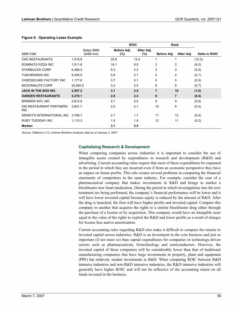
Lehman Brothers | Quantitative Credit Research QCR Quarterly, vol. 2007-Q1
March 7, 2007 55
Figure 8. Operating Lease Example
ROIC Rank
2005 CQ4 Sales 2005 (USD mn)
Before Adj. (%)
After Adj. (%) Before Adj. After Adj. Delta in ROIC
CKE RESTAURANTS 1,519.9 25.6 13.4 1 1 (12.2) DOMINO'S PIZZA INC 1,511.6 18.1 9.0 2 2 (9.2) STARBUCKS CORP 6,369.3 9.3 4.3 3 3 (5.0) YUM BRANDS INC 9,349.0 5.8 3.7 4 4 (2.1) CHEESECAKE FACTORY INC 1,177.6 3.7 3.1 5 5 (0.5) MCDONALD'S CORP 20,460.2 3.2 2.5 6 6 (0.7) JACK IN THE BOX INC 2,507.2 3.1 2.0 7 10 (1.0) DARDEN RESTAURANTS 5,278.1 2.8 2.4 8 7 (0.4) BRINKER INTL INC 3,912.9 2.7 2.0 9 9 (0.6) OSI RESTAURANT PARTNERS INC
3,601.7 2.5 2.1 10 8 (0.4)
WENDY'S INTERNATIONAL INC 3,766.7 2.1 1.7 11 12 (0.4) RUBY TUESDAY INC 1,110.3 1.9 1.8 12 11 (0.2) Median 3.1 2.5
Source: CMetrics v1.0, Lehman Brothers Analysis; data as of January 2, 2007.
Capitalizing Research & Development When comparing companies across industries it is important to consider the use of intangible assets created by expenditures in research and development (R&D) and advertising. Current accounting rules require that most of these expenditures be expensed in the period in which they are incurred even if from an economic perspective they have an impact on future profits. This rule creates several problems in comparing the financial statements of competitors in the same industry. For example, consider the case of a pharmaceutical company that makes investments in R&D and brings to market a blockbuster new heart medication. During the period in which investigations into the new treatment are being performed, the company’s financial performance will be lower and it will have lower invested capital because equity is reduced by the amount of R&D. After the drug is launched, the firm will have higher profits and invested capital. Compare this company to another that acquires the rights to a similar blockbuster drug either through the purchase of a license or by acquisition. This company would have an intangible asset equal to the value of the rights to exploit the R&D and lower profits as a result of charges for license fees and/or amortization.
Current accounting rules regarding R&D also make it difficult to compare the returns to invested capital across industries. R&D is an investment in the core business and just as important (if not more so) than capital expenditures for companies in technology-driven sectors such as pharmaceuticals, biotechnology and semiconductors. However, the invested capital of these companies will be considerably lower than that of traditional manufacturing companies that have large investments in property, plant and equipment (PPE) but relatively modest investments in R&D. When comparing ROIC between R&D intensive industries and non-R&D intensive industries, the R&D intensive industries will generally have higher ROIC and will not be reflective of the accounting return on all funds invested in the business.
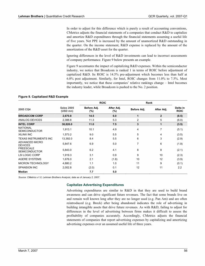
Lehman Brothers | Quantitative Credit Research QCR Quarterly, vol. 2007-Q1
March 7, 2007 56
In order to adjust for this difference which is purely a result of accounting conventions, CMetrics adjusts the financial statements of a companies that conduct R&D to capitalize and amortize R&D expenditures through the financial statements assuming a useful life of five years. Net PPE is increased by the amount of unamortized R&D outstanding in the quarter. On the income statement, R&D expense is replaced by the amount of the amortization of the R&D asset for the quarter.
Ignoring differences in the level of R&D investments can lead to incorrect assessments of company performance. Figure 9 below presents an example.
Figure 9 accentuates the impact of capitalizing R&D expenses. Within the semiconductor industry, we notice that Broadcom is ranked 1 in terms of ROIC before adjustment of capitalized R&D. Its ROIC is 14.5% pre-adjustment which becomes less than half at 6.0% post adjustment. Similarly, for Intel, ROIC changes from 11.0% to 7.5%. Most importantly, we notice that these companies’ relative rankings change – Intel becomes the industry leader, while Broadcom is pushed to the No. 2 position.
Figure 9. Capitalized R&D Example
ROIC Rank
2005 CQ4 Sales 2005 (USD mn)
Before Adj. (%)
After Adj. (%) Before Adj. After Adj. Delta in
ROIC
BROADCOM CORP 2,670.8 14.5 6.0 1 2 (8.5) ANALOG DEVICES 2,388.8 11.3 5.3 2 5 (6.0) INTEL CORP 38,826.0 11.0 7.5 3 1 (3.5) NATIONAL SEMICONDUCTOR 1,913.1 10.1 4.9 4 7 (5.1)
XILINX INC 1,573.2 9.0 5.5 5 4 (3.5) TEXAS INSTRUMENTS INC 13,392.0 8.4 5.5 6 3 (2.9) ADVANCED MICRO DEVICES 5,847.6 6.9 5.0 7 6 (1.9)
FREESCALE SEMICONDUCTOR 5,843.0 6.2 4.1 8 8 (2.1)
LSI LOGIC CORP 1,919.3 3.1 0.9 9 10 (2.3) AGERE SYSTEMS 1,676.0 2.1 (1.8) 10 12 (3.9) MICRON TECHNOLOGY 4,880.2 1.1 1.0 11 9 (0.1) SPANSION INC 2,002.8 (2.0) 0.1 12 11 2.2 Median 7.7 5.0
Source: CMetrics v1.0, Lehman Brothers Analysis; data as of January 2, 2007.
Capitalize Advertising Expenditures Advertising expenditures are similar to R&D in that they are used to build brand awareness and can drive significant future revenues. The fact that some brands live on and remain well known long after they are no longer used (e.g. Pan Am) and are often reintroduced (e.g. Breck) after being abandoned indicates the role of advertising in building intangible assets that drive future revenues. As with R&D, failing to adjust for differences in the level of advertising between firms makes it difficult to assess the profitability of companies accurately. Accordingly, CMetrics adjusts the financial statements of companies that report advertising expenses by capitalizing and amortizing advertising expenses over an assumed useful life of three years.

Lehman Brothers | Quantitative Credit Research QCR Quarterly, vol. 2007-Q1
March 7, 2007 57
Figure 10. Capitalized Advertising Expenditures Example
ROIC Rank
2005 CQ4 Sales 2005 (USD mn)
Before Adj. (%)
After Adj. (%) Before Adj. After Adj.
Delta in ROIC
REVLON INC -CL A 1,332.3 15.8 8.9 1 2 (6.9) AVON PRODUCTS 8,149.6 10.9 10.0 2 1 (0.9) LAUDER ESTEE COS 6,336.3 8.0 3.9 3 7 (4.1) HERBALIFE LTD 1,566.8 7.2 7.2 4 3 - COLGATE-PALMOLIVE CO 11,396.9 6.9 6.1 5 4 (0.8) ENERGIZER HOLDINGS INC 2,989.8 6.1 5.0 6 5 (1.2) CLOROX CO/DE 4,388.0 4.2 3.3 7 9 (0.8) NU SKIN ENTERPRISES 1,180.9 4.2 4.2 7 6 - KIMBERLY-CLARK CORP 15,902.6 4.0 3.9 9 8 (0.2) NBTY INC 1,737.2 2.5 2.6 10 10 0.0 PROCTER & GAMBLE CO 56,741.0 2.5 2.5 11 11 (0.0) SPECTRUM BRANDS INC 2,359.4 1.1 1.1 12 12 0.0 Median 5.1 4.0
Source: CMetrics v1.0, Lehman Brothers Analysis; data as of January 2, 2007.
Figure 10, presents ROIC before and after the Capitalized Advertising Expenditure adjustment for companies in the consumer packaged goods industry. Avon, ranked 2 within the industry, has a pre-adjustment ROIC of 10.9%. Its ROIC changes marginally to 10.0% after this adjustment. However, the impact of this adjustment is much larger on industry leader Revlon, whose ROIC changes to 8.9% from 15.8%. This also pushes Revlon’s ranking to No.2 behind that of Avon.
Stock-Based Compensation SFAS 123R, which is effective for companies not filing as small businesses for fiscal years beginning after December 15, 2005, requires that companies compute costs associated with stock option grants and recognize these costs over the life of the contract. Prior to SFAS 123R, companies could choose to recognize this expense in their income statement or as an adjustment to comprehensive income. Therefore, when comparing 2006 results with prior period results, or when comparing companies that expensed options with those that did not, it is necessary to adjust financial statements. CMetrics adjusts the financial statements of companies prior to the adoption of SFAS 123R to include the implied option expense for the quarter as an operating expense.
Figure 11 highlights the importance of controlling for differences in accounting treatments between firms. Prior to adjustment, Broadcom’s ROIC is 14.5% (second highest in the industry) and more than twice the industry median. After adjusting for the stock-based compensation, Broadcom’s ROIC falls by more than two-thirds to 4.3%, and its relative ranking falls to 4 – behind that of Nvidia, AMD and Freescale.

Lehman Brothers | Quantitative Credit Research QCR Quarterly, vol. 2007-Q1
March 7, 2007 58
Figure 11. Stock-Based Compensation Example
ROIC Rank
2005 CQ4 Sales 2005 (USD mn)
Before Adj. (%)
After Adj. (%) Before Adj. After Adj.
Delta in ROIC
NVIDIA CORP 2,010.0 18.5 12.9 1 1 (5.6) BROADCOM CORP 2,670.8 14.5 4.3 2 5 (10.3) TEXAS INSTRUMENTS INC 13,392.0 8.4 8.4 3 2 - AMD 5,847.6 6.9 6.4 4 3 (0.5) FREESCALE SEMICONDUCTOR INC 5,843.0 6.2 5.1 5 4 (1.1)
LSI LOGIC CORP 1,919.3 3.1 2.3 6 6 (0.9) MICRON TECHNOLOGY INC 4,880.2 1.1 1.1 7 7 - FAIRCHILD SEMICONDUCTOR INTL 1,425.1 (0.1) (0.0) 8 8 0.0
Median 6.6 4.7
Source: CMetrics v1.0, Lehman Brothers Analysis; data as of January 2, 2007.
Pension and Other Post-Employment Benefit Adjustments Pension and Other Post-Employment Benefits (OPEBs) present challenges for investors seeking to consider the financial performance and unrecognized liabilities of companies. Prior to the adoption of SFAS 158, pension and OPEB liabilities3 were not always fully recognized in the financial statements. Instead, liabilities related to the adoption of the accounting standard or changes in plans, as well as gains and losses on pension plan assets are recognized over three years. In addition, in computing the operating expenses related to pension and OPEBs, the costs of financing unfunded liabilities and the offsetting returns from plan assets, both of which are funding items, are included in pension costs, frequently resulting in very low (or negative) pension and OPEB costs. Because pension and OPEB costs are part of operating costs, this treatment has the effect of including in operating expenses costs and income that are financing in nature. In recent years, poor stock market performance over the early years of the decade has led many companies to have large financing costs and/or amortized losses included in their pension expense.
Because of the complications involved in accounting for defined benefit plans, it is difficult to assess the true liabilities incurred by firms or to make meaningful comparisons with companies that do not provide traditional defined-benefit pension plans. In order to better make these comparisons, CMetrics makes several adjustments to account for these differences. First, CMetrics reclassifies the costs associated with pension and OPEB interest costs and actual change in plan asset values as financial expenses/income. In addition, operating expenses are restated to include only the pension and OPEB service cost. Second, CMetrics reclassifies the recognized pension assets, liabilities, and minimum pension liabilities so that the net liability recognized is recognized as a single number and is reclassified as long-term debt. Further, the amount of the unrecognized pension liability (the difference between the funding status and the net amount recognized in the financial statements) is recognized in the financial statements. Figures 12 and 13 illustrate the adjustments for Delphi Corporation.
Delphi’s service cost, the cost associated with current employees’ 2005 activities, is $326 million. This number compares with the recognized expense of $668 million. The additional $340 million represents current and prior losses on plan assets, as well as financing costs. In this case, CMetrics restates pension expense at the Service Cost ($326 million) rather than the recognized pension expense of $668 million. CMetrics adds to net interest expense of -$294 million ($789 million interest expense less $1,083 million 3 SFAS 158, which was issued in September 2006, is effective for fiscal years ending after December 15, 2006.

Lehman Brothers | Quantitative Credit Research QCR Quarterly, vol. 2007-Q1
March 7, 2007 59
return on plan assets). Figure 12 highlights how large pension liabilities are for some companies, and how current treatment over- or understates operating expenses.
Figure 12. Delphi Corporation: Components of Periodic Pension Benefits
in U.S. $Million 2005 Description
Service Cost 326 Operating Current Period Interst Cost
Expected Return on Plan Assets 789
-848} Net Financing Cost
Special Termination Benefits 15 Operating Non Current Amort of Transition Amount 1 Operating Non Current Amort of Prior Service Costs 143 Operating Non Current Amort of Actuarial Losses 242 Financing Cost, Non Current Net Pension Benefit Expense 668 Note: Actual Return on Plan Assets 1083
Source: Delphi Corporation Annual Report, 2005, Lehman Brothers Analysis: data as of January 2, 2007.
Figure 13. Delphi Corporation: Funded Status and Unrecognized Liabilities
U.S. $Million 2005 Description Fair Value of Plan Assets 10511 Projected Benefit Obligation 15070 Underfunded Status -4559 Liability to Employees Unamortized Actuarial Loss 4281 Unrecognized Transition Obligation 7 Unamortized Prior Service Cost 903 Net Amt Recognized in Bal Sheet 632 Net Amount Recognized
Balance Sheet Accounts 2005 LT Prepaid Benefit Cost (Other LT Assets) 110 Asset Pension Liability (Other Liabilities) -3880 Liability Intangible Pension Asset (Intangibles) 889 Asset Acc. Other Comp. Income 3513 Deduction from Equity Net Amount Recognized 632
Net Adj. to Equity & Deferred Tax Liab. -1678 Add'l Amt Recog by Cmetrics
Source: Delphi Corporation Annual Report, 2005, Lehman Brothers Analysis; data as of January 2, 2007.
Figure 13 provides data on the funded status and the recognized pension liabilities of Delphi Corporation. As of December 2005, the Delphi pension plans had projected obligations in excess of fair value of plan assets of $4,559 million. Of this, $5.2 billion are unrecognized in the financial statements; hence Delphi has net pension assets of $632 million. CMetrics recognizes the full underfunded status as the pension liability and restates the balance sheet accounts, subtracting the asset amounts and the comprehensive income amount (associated with the Minimum Pension Liability) from the pension liability in other liabilities, reclassifying this amount from other liabilities to debt and adding to the unrecognized portion of the pension adjustment. The net effect on Delphi’s equity is a decrease of $1.678 billion. The impact on capital employed is a deduction in capital of approximately $1 billion, due to the reclassification of the pension assets as reductions in the recognized pension liability.
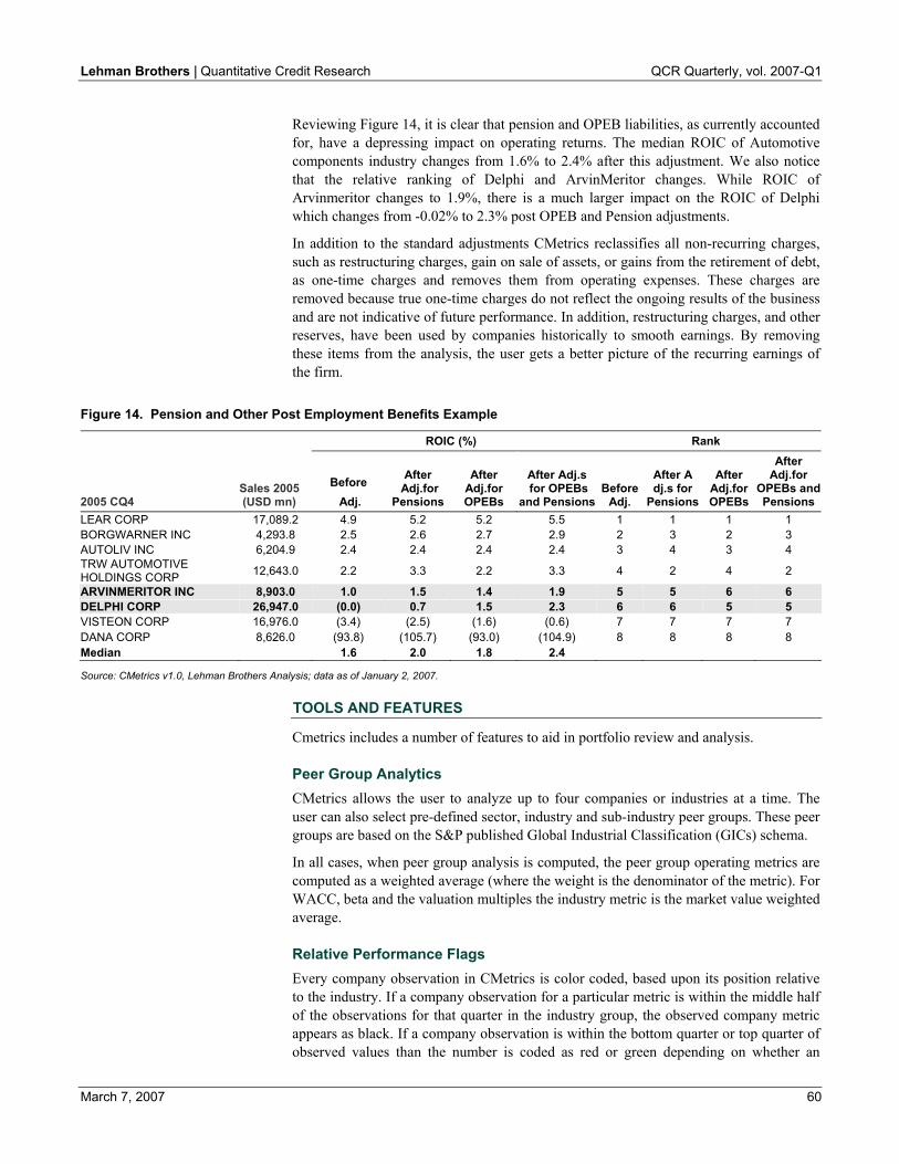
Lehman Brothers | Quantitative Credit Research QCR Quarterly, vol. 2007-Q1
March 7, 2007 60
Reviewing Figure 14, it is clear that pension and OPEB liabilities, as currently accounted for, have a depressing impact on operating returns. The median ROIC of Automotive components industry changes from 1.6% to 2.4% after this adjustment. We also notice that the relative ranking of Delphi and ArvinMeritor changes. While ROIC of Arvinmeritor changes to 1.9%, there is a much larger impact on the ROIC of Delphi which changes from -0.02% to 2.3% post OPEB and Pension adjustments.
In addition to the standard adjustments CMetrics reclassifies all non-recurring charges, such as restructuring charges, gain on sale of assets, or gains from the retirement of debt, as one-time charges and removes them from operating expenses. These charges are removed because true one-time charges do not reflect the ongoing results of the business and are not indicative of future performance. In addition, restructuring charges, and other reserves, have been used by companies historically to smooth earnings. By removing these items from the analysis, the user gets a better picture of the recurring earnings of the firm.
Figure 14. Pension and Other Post Employment Benefits Example
ROIC (%) Rank
2005 CQ4 Sales 2005 (USD mn)
Before Adj.
After Adj.for
Pensions
After Adj.for OPEBs
After Adj.s for OPEBs
and PensionsBefore
Adj.
After A dj.s for
Pensions
After Adj.for OPEBs
After Adj.for
OPEBs and Pensions
LEAR CORP 17,089.2 4.9 5.2 5.2 5.5 1 1 1 1 BORGWARNER INC 4,293.8 2.5 2.6 2.7 2.9 2 3 2 3 AUTOLIV INC 6,204.9 2.4 2.4 2.4 2.4 3 4 3 4 TRW AUTOMOTIVE HOLDINGS CORP 12,643.0 2.2 3.3 2.2 3.3 4 2 4 2
ARVINMERITOR INC 8,903.0 1.0 1.5 1.4 1.9 5 5 6 6 DELPHI CORP 26,947.0 (0.0) 0.7 1.5 2.3 6 6 5 5 VISTEON CORP 16,976.0 (3.4) (2.5) (1.6) (0.6) 7 7 7 7 DANA CORP 8,626.0 (93.8) (105.7) (93.0) (104.9) 8 8 8 8 Median 1.6 2.0 1.8 2.4
Source: CMetrics v1.0, Lehman Brothers Analysis; data as of January 2, 2007.
TOOLS AND FEATURES
Cmetrics includes a number of features to aid in portfolio review and analysis.
Peer Group Analytics CMetrics allows the user to analyze up to four companies or industries at a time. The user can also select pre-defined sector, industry and sub-industry peer groups. These peer groups are based on the S&P published Global Industrial Classification (GICs) schema.
In all cases, when peer group analysis is computed, the peer group operating metrics are computed as a weighted average (where the weight is the denominator of the metric). For WACC, beta and the valuation multiples the industry metric is the market value weighted average.
Relative Performance Flags Every company observation in CMetrics is color coded, based upon its position relative to the industry. If a company observation for a particular metric is within the middle half of the observations for that quarter in the industry group, the observed company metric appears as black. If a company observation is within the bottom quarter or top quarter of observed values than the number is coded as red or green depending on whether an

Lehman Brothers | Quantitative Credit Research QCR Quarterly, vol. 2007-Q1
March 7, 2007 61
extreme high or low value for the metric is enterprise value increasing (good) or not (bad). Figure 15 summarizes the meaning of the color-coded flags within CMetrics.
Figure 15. Performance Flags
Key Performance Above Industry Below Industry EPS Not Meaningful Not MeaningfulSales Growth Good Bad ROE Good Bad ROIC Good Bad NOPAT Margin Good Bad Depreciation Margin Bad Good R&D Margin Bad Good COGS Margin Bad Good Other SG&A Margin Bad Good Capital Turnover Bad Good Working Captial Turnover Bad Good AR Days Bad Good AP Days Good Bad Inventory Days Bad Good PPE Margin Bad Good Financing Return Good Bad Leverage Ratio Good Bad Financing Spread Good Bad Non-Operating Return Bad Good Investment Ratio Bad Good Investment Spread Bad Good Non-Recurring Income (expenses) to sales Not Meaningful Not Meaningful Additional Market & Credit Risk Measures Beta Bad Good WACC Bad Good Coverage Ratio Good Bad Cash Position Good Bad Cashflow Discrepancy Bad Good Key Valuation Metrics P/E multiple Good Bad EV/EBITDA Good Bad EV/IC Good Bad EV/FCF Good Bad
Source: CMetrics v1.0.

Lehman Brothers | Quantitative Credit Research QCR Quarterly, vol. 2007-Q1
March 7, 2007 62
Trend Flags CMetrics contains trend line flags for the current value of each metric. An up-arrow (↑) indicates the current value of the ratio is higher than the average of the ratio from four quarters and eight quarters prior4. A down-arrow (↓) indicates the opposite.
Graphics Capabilities CMetrics contains custom charts to analyze the data. CMetrics provides two standard charts. The Trend Analysis plots the selected metric for the four companies and/or industry selected. All of the CMetrics Key Performance and Additional Market and Credit Risk Measures can be plotted. As in POINT and the Time Series Plotter, a custom data tool on LehmanLive, the user can zoom in and out of the graph to get a closer view of the desired time period. The Two Metrics Time trend chart plots any two metrics over time to allow users to understand trend and correlation between metrics for one company/industry at a time. In addition, users can download data series into Microsoft Excel to create additional graphs and analysis.
User Control of Adjustments CMetrics places control of the adjustments with the user. A user can select all, one or none of the adjustments depending on the purpose of the analysis. However, because it is not meaningful to compare companies across sectors without adjustment, the default set up within CMetrics is to activate all adjustments.
COVERAGE AND DATA SOURCES
CMetrics provides consistent standardized metrics on a quarterly basis from our database of over 3,000 companies. Beta coverage is limited to U.S. companies (excluding financial institutions, insurance, and real estate companies) that have been included in the Russell 3000 index over the past five years. CMetrics ratios are constructed from quarterly data with historical data history that goes back to the first quarter of 2001. The CMetrics database is updated nightly during earnings announcement season. Outside of earnings announcement season, the database is updated weekly.
4 If the observed metric at a point in time, t, (expressed as metrict ) is less than (1/2)*(metrict-4 + metrict-8) than the
trend is considered to be decreasing and a ↓ appears. In this formula, t is the current quarter, and t-4 and t-8 reflects the result for this quarter 1 year and 2 years prior.

Lehman Brothers | Quantitative Credit Research QCR Quarterly, vol. 2007-Q1
March 7, 2007 63
APPENDIX: LEHMAN CMETRICS FINANCIAL ANALYSIS FRAMEWORK
Performance Metrics The CMetrics framework decomposes Return on Equity (ROE), the primary measure of performance, into the three key aspects of firm performance: operating performance, financing performance, and return on non-operating investments. By separating and decomposing overall performance the framework allows users to identify how managements’ operating, financing, and non-operating investments decisions influence overall performance. Importantly, decompositions into operating statistics, such as AR days and expense ratios can be useful in assessing the sustainability of current earnings levels.
In addition, two measures of overall performance, Sales Growth and Earnings per Share (EPS)), are also presented.
Overall Performance Measures
ROE is defined as earnings before extraordinary and discontinued operations divided by shareholders equity. In the CMetrics Framework, ROE is also measured before all non-recurring items (e.g. restructuring charges, gains on sale of assets, etc.). Earnings before extraordinary and discontinued operations and non-recurring items measures the income from normal business operations after all operating and financing charges; it is the profit available to pay dividends to shareholders and includes profits associated with all aspects of firm performance (operations, financing, and non-operating investments). ROE therefore is the profit margin of the firm’s equity investors as a class.
Sales Growth is computed as the quarter-on-quarter growth in Net Revenues. Equation 2 above shows that growth in cash flows (of which sales growth is a large component) is a key factor in value.
EPS is the per share profits that may be compared to share price to measure the relative value of a security. CMetrics presents the GAAP-compliant EPS, which includes all non-recurring charges that are excluded from our other metrics. EPS can only be compared overtime with care because stock splits and share buybacks will affect this number. EPS should not be compared to those of other firms, even within the same industry.
Non-Recurring Income (Expenses) to Sales is the ratio of non-recurring income and/or expenses as a percentage of sales. Companies that have an unusual number of “non-recurring” items to sales compared to their peers, especially if the company frequently declares such charges, should be examined closely for signs of aggressive accounting practices.
Performance Measures: Operating Return
ROIC is net operating profits after cash taxes (NOPAT) divided by invested capital (IC). Operating profits exclude all interest charges and non-operating income and expenses (including interest income), and all non-recurring items. NOPAT is the profits of the enterprise (excluding non-operating investments) before payment to debt or equity capital providers. IC is book value of the total capital invested in the operations of the firm, namely the debt and debt-like claim on assets and equity and equity-like claim on assets less investments in non-operating assets and non-interest bearing operating liabilities. Importantly, IC includes all book intangibles including goodwill, because these intangibles generally represents investments made by the firm in acquiring intangibles and represent a use of investors’ cash. ROIC is the profit margin of the firm’s

Lehman Brothers | Quantitative Credit Research QCR Quarterly, vol. 2007-Q1
March 7, 2007 64
debt and equity investors as a class; it measures the efficiency of the organization in exploiting its capital.
ROIC is particularly useful in comparing performance across industries, especially when examined in excess of the company’s cost of capital. Also, as seen in equation 2, ROIC is a key driver of firm value.
While ROIC is useful in assessing overall operating performance, it is less useful in identifying the reasons for that performance. However, using a variant on the du Pont analysis, ROIC is decomposed into performance statistics related to operating margins and capital intensity.
Operating Return: Margin
EBITDA Margin is earnings before interest, taxes, and depreciation and amortization divided by net revenues. EBITDA is computed before non-recurring items. EBITDA Margin is only a rough approximation of cash flows from operations as a percentage of sales. EBITDA Margin will differ from free cash flow margin by the amount of investment made in working capital and other assets and by the amount of releases from long-term liabilities. These items must be examined in detail when examining the cash flow of the business.
COGS Margin is cost of goods sold divided by net revenues. COGS is computed as company-reported Cost of Goods Sold (or Cost of Sales) less depreciation charges. COGS Margin measures the costs of producing or acquiring goods and services for sale as a percentage of sales. Changes in COGS margin should be examined closely for sustainability.
R&D to Sales, which is computed as Research and Development expenses (as reported) divided by Net Revenues, is the percentage of Net Revenues invested in the development of new products and services. Declines in R&D to sales ratio, especially in a stable or declining EBITDA margin environment, may indicate that future growth prospects for this firm are limited or that management has reduced funding future projects to meet near term profit targets.
SG&A to Sales is the ratio of non-R&D Selling, General and Administrative Costs (SG&A) to sales. This ratio (often called the expense ratio) measures the efficiency of a company’s selling and administrative functions. Comparing a company’s SG&A to sales with its peers is useful assessing the overall efficiency of the operations and in identifying areas of potential margin improvements from cost cutting measures.
Operating Return: Capital Turnover
Capital Intensity is defined as Invested Capital (IC) divided by Net Revenue. It measures the amount of capital required in the core business operations to produce $1 of revenues. Because IC includes working capital and other long term assets, as well as fixed assets (such as machinery and equipment) it is useful in assessing the efficiency of a firms’ ability to collect on its receivables as well as the degree of asset intensity of the business.
While capital turnover differs substantially across industries, a company that has capital turnover that is significantly lower than the industry is more likely to have a higher return on capital. A review of capital intensity and its decomposition can provide information to help diagnose the reason for and provide additional insights into the sustainability of current performance. The CMetrics framework provides 5 additional measures of capital intensity: Working Capital to Sales (WC/Sales), Account Receivables Days (AR Days), Accounts Payable Days (AP Days), Inventory Days, and Fixed Asset Intensity (FA Intensity).

Lehman Brothers | Quantitative Credit Research QCR Quarterly, vol. 2007-Q1
March 7, 2007 65
WC/Sales is computed as total working capital divided by net revenues; where working capital is computed as total non-cash current assets less total current liabilities, excluding debt included in current liabilities. Working Capital is the funds tied up in current operations less the short-term, operating non-interest bearing liabilities that partially finance them. Working Capital may rise because receivables and/or inventories rise (as is likely at the beginning of a recession when sales begin to lag and non-collectible receivables rise) or payables fall (as happens if, in response to perceived increase in the likelihood of non-payment, suppliers do not extend or reduce credit terms). To understand the reason for a rise or fall in Working Capital, the CMetrics framework provides data on three key components of WC/Sales: AR Days, AP Days and Inventory Days.
AR Days is the estimated number of days of sales that is not yet collected. AR Days that exceed those of competitors may indicate aggressive accounting practices such as failure to write off bad-debt or channel stuffing. Increases in AR Days may also indicate declines in demand so that more attractive financing terms may be required to induce sales.
AP Days is the estimated number of days of sales that is not yet paid to creditors. AP Days that exceed those of competitors by a large margin may indicate cash flow problems. Such rise in payables may also indicate problems to bond holders, as these claims are superior to those of the bondholders in the case of default.
Inventory Days is the estimated number of days of sales that have been produced (or acquired) that have not been sold at the end of the period. Growth in Inventory Days generally indicates that the company’s sales are falling due to decreases in demand. When Inventory Days are high relative to the industry or historic firm levels, especially while COGS margin is stable or falling, the company may be overproducing in order to reduce its per unit costs.
Fixed Asset Intensity is the ratio of Property, Plant and Equipment, net of depreciation (NPPE) to Net Revenues. Fixed Asset Intensity measures the amount of long term production assets the firm uses to produce 1 dollar of revenues. Fixed Asset Intensity varies substantially by industry and should be compared across sectors with care. Within a sector, differences in Fixed Asset Intensity can indicate that the company may lack the scale to fully utilize its fixed costs. Accordingly high Fixed Asset Intensity coupled with high growth can indicate that firm profits should increase above historic levels if sales growth continues. Fixed Asset Intensity that is low relative to peers should be reviewed with care, as this may indicate aggressive depreciation policies or lack of investment in property, plant and equipment.
Financing Return
Financing Return is the amount of ROE that is due to the capital structure and financing decisions previously made by the firm. Financing Return that is low relative to its industry peers indicates that opportunities exist to improve overall equity returns by better exploiting the capital structure. However, while it is clear that capital structure affects value, the issue of what is the optimal capital structure of a firm is extremely complex and should be analyzed in much more detail.
CMetrics also presents the two main components of Financing Return: leverage and financing spread. Leverage is computed as book debt divided by book common equity.
Leverage is positively related to the firms financing return, however, a company that has experienced increases in leverage, or one that is more highly levered than its peers, are

Lehman Brothers | Quantitative Credit Research QCR Quarterly, vol. 2007-Q1
March 7, 2007 66
also more likely to have problems making debt payments should revenues and cash flows decline.
Financing Spread is computed as ROIC less the after tax cost of debt incurred by the firm. A large financing spread increases the return from financing; however when comparing firms with high financing spreads it is important to consider whether or not the spread will continue as debt comes due and must be refinanced at higher rates.
Non-operating Investment Return
Non-operating Investment Return is the amount of ROE that results from investments in non-operating investments. It is computed as the ratio of non-operating assets (at book value) to book equity times the spread between non-operating returns and ROIC. Non-operating investments include cash and marketable securities, as well as investments in joint ventures and other unconsolidated subsidiaries, net of minority interests in the company’s operations. Non-operating return is the financial statement non-operating income less minority interest expense divided by non-operating financial assets multiplied by 1 minus the cash tax rate.
Additional Market and Credit Risk Metrics Beta is the commonly used measure of the sensitivity of a stock’s return to the market return. Betas are computed using 60 months of return data for each firm. No beta is computed unless a 60 month data history exists. The return on the S&P 500 was used as the market return. Beta is a measure of systematic stock market risk. Firms with high betas generally have more variable cash flows and higher operating risk.
Weighted Average Cost of Capital (WACC) is the expected cost of financing the company’s operations at current market rates, assuming the current capital structure. Because IC is equivalent to the debt and equity invested in the operations of the firm, companies with WACC that is greater than ROIC are making an economic loss on their economic capital and should be expected to have lower future returns.
Coverage Ratio is the ratio of EBITDA to interest expense. It is a rough approximation of the number of times by which cash from operations can pay (or “cover”) interest expense. Companies with coverage ratios higher than industry peers will, conditional on similar cash flow volatility, have a lower probability of default. Many debt covenants, especially for companies with lower debt ratings, require that the coverage ratio stay above a certain number.
Cash Position is the ratio of cash and equivalents to total current assets. Cash Position measures the cash a company has on hand. Cash Position that is low relative to peers, especially when coupled with low cash flows from operations, is associated with a higher likelihood of bankruptcy.
Cash Flow Discrepancy is the ratio of the difference between cash flows from operations and Earnings before Extraordinary Items before depreciation and amortization and other non-cash charges divided by the absolute value of cash flow from operations. Cash Flow Variance that is low relative to its peers, or relative to its historical levels is an indicator that the firms accounting may be aggressive in recognizing revenues early or expenses late. Such firms should be further examined for material weaknesses.
Free Cash Flow to Sales is the ratio of Free Cash Flow (FCF) to Net Revenues. It measures the cash provided by operations, in excess of capital expenditure, as a percentage of Net Revenues. FCF represents the cash flows derived from the business operations after capital expenditures. Declines in FCF/Sales, especially those not

Lehman Brothers | Quantitative Credit Research QCR Quarterly, vol. 2007-Q1
March 7, 2007 67
explainable by large increases in capital expenditures, should be monitored closely as an indicator of the future health of the business.
Valuation Metrics
Price to Earnings Ratio is the common equity price divided by earnings per share over the last 12 months. P/E is a common measure of market pricing and is frequently used to determine whether a company is trading high or low for its industry. PE may not be a good multiple to make comparisons when companies have significantly different capital structures.
Enterprise Value to EBITDA is the ratio of the market value of the company’s equity plus debt divided by EBITDA over the last 12 months.
Enterprise Value to Invested Capital is the ratio of the market value of the company’s equity plus debt divided by IC. It is the ratio of market value to book value of invested capital.
Enterprise Value to Free Cash Flows is the ratio of market value of the company’s equity plus debt divided by Free Cash Flows over the last 12 months.

Analyst Certification To the extent that any of the views expressed in this research report are based on the firm's quantitative research model, Lehman Brothers hereby certifies that the views expressed in this research report accurately reflect the firm's quantitative research model and that no part of its analysts compensation was, is or will be directly or indirectly related to the specific recommendations or views expressed herein. The views expressed in this report accurately reflect the personal views of Prasun Baheti, Samuel Morgan, Mukundan Devarajan, Cong Minh Trinh, Bodhaditya Bhattacharya, Attilio Meucci, Mary Margiotta, Chetan Seth and Prafulla Nabar, the primary analysts responsible for this report, about the subject securities or issuers referred to herein, and no part of such analysts' compensation was, is or will be directly or indirectly related to the specific recommendations or views expressed herein. Important Disclosures Lehman Brothers Inc. and/or an affiliate thereof (the "firm") regularly trades, generally deals as principal and generally provides liquidity (as market maker or otherwise) in the debt securities that are the subject of this research report (and related derivatives thereof). The firm's proprietary trading accounts may have either a long and / or short position in such securities and / or derivative instruments, which may pose a conflict with the interests of investing customers. Where permitted and subject to appropriate information barrier restrictions, the firm's fixed income research analysts regularly interact with its trading desk personnel to determine current prices of fixed income securities. The firm's fixed income research analyst(s) receive compensation based on various factors including, but not limited to, the quality of their work, the overall performance of the firm (including the profitability of the investment banking department), the profitability and revenues of the Fixed Income Division and the outstanding principal amount and trading value of, the profitability of, and the potential interest of the firms investing clients in research with respect to, the asset class covered by the analyst. Lehman Brothers generally does and seeks to do investment banking and other business with the companies discussed in its research reports. As a result, investors should be aware that the firm may have a conflict of interest. To the extent that any historical pricing information was obtained from Lehman Brothers trading desks, the firm makes no representation that it is accurate or complete. All levels, prices and spreads are historical and do not represent current market levels, prices or spreads, some or all of which may have changed since the publication of this document. Lehman Brothers' global policy for managing conflicts of interest in connection with investment research is available at www.lehman.com/researchconflictspolicy. To obtain copies of fixed income research reports published by Lehman Brothers please contact Valerie Monchi ([email protected]; 212-526-3173) or clients may go to https://live.lehman.com/. Legal Disclaimer This material has been prepared and/or issued by Lehman Brothers Inc., member SIPC, and/or one of its affiliates ("Lehman Brothers"). Lehman Brothers Inc. accepts responsibility for the content of this material in connection with its distribution in the United States. This material has been approved by Lehman Brothers International (Europe), authorised and regulated by the Financial Services Authority, in connection with its distribution in the European Economic Area. This material is distributed in Japan by Lehman Brothers Japan Inc., and in Hong Kong by Lehman Brothers Asia Limited. This material is distributed in Australia by Lehman Brothers Australia Pty Limited, and in Singapore by Lehman Brothers Inc., Singapore Branch ("LBIS"). Where this material is distributed by LBIS, please note that it is intended for general circulation only and the recommendations contained herein do not take into account the specific investment objectives, financial situation or particular needs of any particular person. An investor should consult his Lehman Brothers' representative regarding the suitability of the product and take into account his specific investment objectives, financial situation or particular needs before he makes a commitment to purchase the investment product. This material is distributed in Korea by Lehman Brothers International (Europe) Seoul Branch. Any U.S. person who receives this material and places an order as result of information contained herein should do so only through Lehman Brothers Inc. This document is for information purposes only and it should not be regarded as an offer to sell or as a solicitation of an offer to buy the securities or other instruments mentioned in it. With exception of the disclosures relating to Lehman Brothers, this report is based on current public information that Lehman Brothers considers reliable, but we do not represent that this information, including any third party information, is accurate or complete and it should not be relied upon as such. It is provided with the understanding that Lehman Brothers is not acting in a fiduciary capacity. Opinions expressed herein reflect the opinion of Lehman Brothers' Fixed Income Research Department and are subject to change without notice. The products mentioned in this document may not be eligible for sale in some states or countries, and they may not be suitable for all types of investors. If an investor has any doubts about product suitability, he should consult his Lehman Brothers representative. The value of and the income produced by products may fluctuate, so that an investor may get back less than he invested. Value and income may be adversely affected by exchange rates, interest rates, or other factors. Past performance is not necessarily indicative of future results. If a product is income producing, part of the capital invested may be used to pay that income. Lehman Brothers may, from time to time, perform investment banking or other services for, or solicit investment banking or other business from any company mentioned in this document. No part of this document may be reproduced in any manner without the written permission of Lehman Brothers. © 2007 Lehman Brothers. All rights reserved. Additional information is available on request. Please contact a Lehman Brothers' entity in your home jurisdiction.