Quantifying downflow through creek sediments using temperature time series: one-dimensional solution...

Journal of Hydrology

ELSEVIER

[2]

Journal of Hydrology 167 (1995) 99-119

Quantifying downflow through creek sediments using temperature time series: one-dimensional solution

incorporating measured surface temperature

Stephen E. Silliman*, Jose Ramirez 1, Raye L. McCabe 1 Department of Civil Engineering and Geological Sciences, University of Notre Dame, Notre Dame,

IN 46556, USA

Received 20 May 1994; revision accepted 1 September 1994

Abstract

Several authors have addressed the question of identifying the location of and quantifying the volume of groundwater/surface water interaction. Utilizing measurement of temperature within the sediments has been suggested as a means of estimating water flux through the sediments. A qualitative version of this method has been applied to identifying locations of communication between a creek and groundwater based upon temperature time series measurements in the water column and the sediments. The discussion presented earlier is extended to a more general solution which allows for incorporation of measured surface temperature (rather than an assumed surface temperature). The mathematical formulation presented is targeted on the quantification of flux across the sediment for conditions of one-dimensional downflow with a constant flux over periods of days to weeks. This technique, based on the assumption that the temperature of the surface water is the primary thermal influence on sediment temperature, is shown to provide an estimate of fluid flux (volume of water per area per time) for flux rates above a critical threshold. The flux threshold depends on a number of factors including thermal diffusivity of the sediments and depth of burial of the temperature measuring device. Based on use of three simple forcing functions for temperature at the surface of the sediments, it is shown that the amplitude of the temperature response in the sediments to a change in temperature in the overlying water column decreases with increasing depth and decreasing flux. Further, the timing of the peak response in the sediments becomes increasingly delayed as depth increases and flux decreases. These observations, combined with consideration of the assumption of one-dimensional flow, lead to suggesting that field design be based on relatively shallow burial (e.g. 5-15 cm) of the device to measure sediment temperatures. Based on these observations, one of the data sets presented earlier is reanalyzed to derive flux estimates. It is shown that a reasonable fit is obtained with a downflow flux of less than 0.03

* Corresponding author. Summer Interns at Notre Dame.

Elsevier Science B.V. SSDI 0022-1694(94)02613-0

100 S.E. Silliman et al. / Journal of Hydrology 167 (1995) 99-119

cm day -1 . Independent measurement of hydraulic gradient and hydraulic conductivity provide a range of flux estimates for the same site (although measured in a different year) which are consistent with this value. Based on these results, it is argued that this technique is a reasonable screening tool for use in situations where relatively inexpensive, point estimates of water flux are required within losing reaches of a creek.

1. Introduction

Quantification of groundwater interaction with surface water bodies has become an increasingly important aspect of studies involving water budgets (e.g. Carlsen, 1993), water quality (e.g. Winter, 1986; Anderson and Bowser, 1986; Kenoyer and Ander- son, 1989), and groundwater recharge. Winter demonstrated that groundwater inter- acts with surface water in a number of settings (e.g. Winter, 1986, 1978). Several authors have built upon the work of Winter to demonstrate the influence of groundwater inflows on the chemistry of surface water bodies and the sediment geochemistry underlying these waters (e.g. Cartwright et al., 1979; Lee, 1985; Anderson and Bowser, 1986; Kenoyer and Anderson, 1989).

Winter (1986) and Kenoyer and Anderson (1989) approached identification and quantification of groundwater components through characterization of the groundwater system. Each has used extensive arrays of boreholes and/or piezometers to monitor groundwater inflows to lakes. When available, such arrays can provide significant insight into the direction and rate of groundwater movement.

Several techniques have been discussed for use in the absence of significant arrays in the groundwater system. Cartwright et al. (1979) and Carlsen (1993) utilized pressure measuring devices to determine the pressure gradient within sediments in deep lakes and creeks. Several authors, including Lee (1977), have utilized seepage meters to measure the rate of groundwater inflow (outflow) to lakes. Atwell et al. (1971), Souto- Maior (1973) and Nelson (1991), and others have utilized thermal remote sensing to identify the location and area of influence of natural and forced inflows to surface water bodies.

Direct thermal methods are also showing some promise for the identification/ quantification of near-surface groundwater velocities. A number of authors have expressed interest in the general problem of utilizing thermal signatures for estimation of vertical (e.g. Stallman, 1965; Bredehoeft and Papadopulos, 1965; Silliman and Booth, 1993) and two-dimensional (e.g. Keys and Brown, 1978) groundwater velocities. Bredehoeft and Papadopulos (1965), for example, considered the steady- state distribution of temperature within confining layers subjected to vertical water flux. More appropriate to the present work, Stallman (1965) established a solution to the equation of heat flux for estimation of the vertical flux of water through a medium for which the surface temperature varied in a sinusoidal pattern. Further, Stallman suggested that this technique could be appropriate for application to estimation of seepage from a surface water body. Within this approach, both the thermal diffusivity and the average groundwater velocity were to be estimated based on a series of

S.E. Silliman et al. / Journal o f Hydrology 167 (1995) 99-119 101

temperature measurements versus depth below the surface. Stallman also argued that the accuracy of the velocity estimate was depend on the degree of accuracy with which the thermal diffusivity could be estimated. In his concluding remarks, Stallman suggested that a velocity as low as approximately 0.3 cm day -1 could be estimated with this technique.

Silliman and Booth (1993) used time series measurements of sediment temperature and water column temperature to identify reaches along a creek in northern Indiana which were gaining water from the underlying aquifer, reaches which were neutral, and reaches which were losing water to the underlying aquifer. This technique was shown to be reliable but was limited in that it did not provide an estimate of the volume of flux moving through the sediments. Further, the technique was of limited application in the presence of local infiltration/exfiltration patterns such as observed by White et al. (1987) near riffles of a northern Michigan river.

The present work is an extension of the work of Stallman (1965) based on the study of Silliman and Booth (1993). The focus of the present paper is the discussion of a general mathematical solution of the heat flux equation discussed by Stallman (1965). The solution allows estimation of seepage rates based on measured surface temperature combined with measured temperature at a specified depth within the sediments. While the extension presented is not fundamentally new (the general solution is derived from the heat flow literature), our discussion of the estimation procedure provides insight into the potential for use and limitations of this method. It is anticipated that this technique may provide an excellent screening tool to provide an order of magnitude estimate of the water flux through the sediments (averaged over time periods of days to weeks).

2. Conceptual description of method

The method described by Silliman and Booth (1993) is based on the argument that the temperature in sediments underlying a creek will be controlled (ignoring internal sources of thermal energy such as those which may be derived from biological activity) by advection of thermal energy via fluid flow and conduction of thermal energy (owing to temperature gradients either within the sediments or between the sediments and the overlying water column). As discussed by these authors, three extremes of flow can be envisioned. In the first, the creek is strongly gaining groundwater. In this case, temperature in the sediments is strongly controlled by advection from the groundwater system and will show minimal variation over time. The second case involves zero flux through the sediments. In this case, the temperature within the sediments will be driven by conduction and will vary during the day as the temperature at the surface of the sediments varies.

The third case, the one of interest for the present discussion, is represented by downflow from the creek to the subsurface. In this case, temperature in the sediments will reflect the temperature at the surface of the sediments, showing a lag in phase resulting from travel time from the surface and a reduced amplitude owing to conduction. In the absence of other sources of thermal energy (e.g. biological activity


EleclTonic Logging Device I For Recording Temperature I Time Series

• I Water Level In Creek / ~ ~ ! .......... ........... .:.:.:.:.:.:.:.:.

::::::::::::::::::::: • '.'.'.'-'-.'.'•'.'.'.:.:.:.'.'.'-'-:-".:.'." ........ Burial ':':'::::::

:::::::::::::::::::::::::::::::::::::::::::::::::::::::::::::::::::::::::::::::::::::::::::::::::::: ===================== l i?!ii i:!:!:!:i:i:!:!:!:i:::"

..::::::::i:iiiiiiiii!i!iiiiiiiii!i!i!iiiiiii!i!!!iiiiiii!!!i!iiiii!i!iiiiiii:i:.

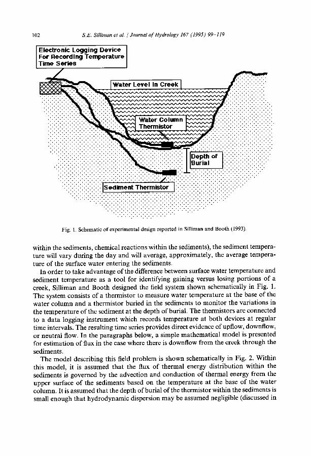
Fig. 1. Schematic of experimental design reported in Silliman and Booth (1993).

within the sediments, chemical reactions within the sediments), the sediment temperature will vary during the day and will average, approximately, the average temperature of the surface water entering the sediments•

In order to take advantage of the difference between surface water temperature and sediment temperature as a tool for identifying gaining versus losing portions of a creek, Silliman and Booth designed the field system shown schematically in Fig. 1. The system consists of a thermistor to measure water temperature at the base of the water column and a thermistor buried in the sediments to monitor the variations in the temperature of the sediment at the depth of burial. The thermistors are connected to a data logging instrument which records temperature at both devices at regular time intervals. The resulting time series provides direct evidence of upflow, downflow, or neutral flow. In the paragraphs below, a simple mathematical model is presented for estimation of flux in the case where there is downflow from the creek through the sediments.

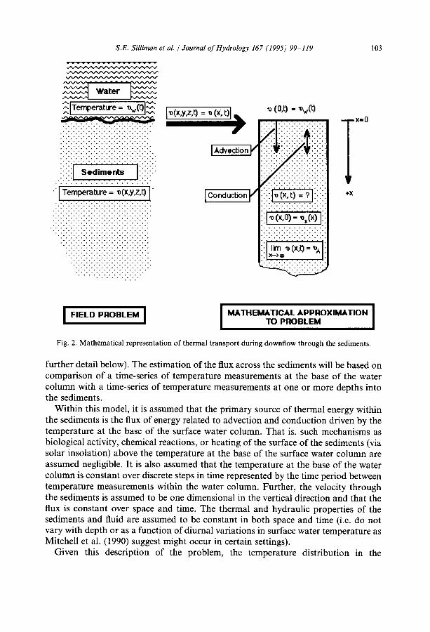
The model describing this field problem is shown schematically in Fig. 2. Within this model, it is assumed that the flux of thermal energy distribution within the sediments is governed by the advection and conduction of thermal energy from the upper surface of the sediments based on the temperature at the base of the water column. It is assumed that the depth of burial of the thermistor within the sediments is small enough that hydrodynamic dispersion may be assumed negligible (discussed in

S,E. Silliman et al. / Journal o f Hydrology 167 (1995) 99-119

~[Tempera ture = . % ( t ) J ~

, . , , , , , , , . . , . , % . , , ,

, , . , , . , , , , % , , . , , , . . , , . . , , , , , , , , , , , , , , , . . , , , %

• J romp,r~tur, = , , ( ~ , y , z , t ) I

. . . , . , . . . , , . % - . . . . ° . .

• ~ (o,t) = % ( t )

I conduction ~ i iii]~"(x,ti -?Jiiiii

:;1" : . . , , , , , , , , . , , , , , , . . . , , . : . . , . , . , , , , ; , . , , , , , ; , : , : . : , : . ' . % ' , ' , , ' , ' , % r . • •

:i ,rn ~,(x,t) "

% . . ° . , , . , , , . , . , , . .

~ . : . : . . ~

+X

103

I FIELD PROBLEM I I MATHEMATICAL APPROXIMATION I TO PROBLEM Fig. 2. Mathematical representation of thermal transport during downflow through the sediments.

further detail below). The estimation o f the flux across the sediments will be based on comparison o f a time-series o f temperature measurements at the base o f the water column with a time-series o f temperature measurements at one or more depths into the sediments.

Within this model, it is assumed that the primary source o f thermal energy within the sediments is the flux of energy related to advection a n d conduction driven by the temperature at the base o f the surface water column. That is, such mechanisms as biological activity, chemical reactions, or heating o f the surface o f the sediments (via solar insolation) above the temperature at the base o f the surface water co lumn are assumed negligible. It is also assumed that the temperature at the base o f the water co lumn is constant over discrete steps in time represented by the time period between temperature measurements within the water column. Further, the velocity through the sediments is assumed to be one dimensional in the vertical direction and that the flux is constant over space and time. The thermal and hydraulic properties of the sediments and fluid are assumed to be constant in both space and time (i.e. do not vary with depth or as a function of diurnal variations in surface water temperature as Mitchell et al. (1990) suggest might occur in certain settings).

Given this description o f the problem, the temperature distribution in the


sediments may be described through the following differential equation (Carslaw and Jaeger, 1959; Stallman, 1965)

( K e / p ' c ' ) O z u / o x 2 - (npwcw/p 'c ' ) vxOu/Ox = Ou/Ot (1)

where Ke is the thermal conductivity of the saturated sediments (Q/LTV), Pw is the density of the water (M/L3), p~ is the density of the saturated sediment (M/L3), Cw is the specific heat of water (Q/MV), c ~ is the specific heat of saturated sediment (Q/ MV), n is the porosity, v x is the average water velocity in pores of sediment (L/T), u is the temperature (V), t is the time (T), and x is the depth in the sediments below the water/sediment interface. (In the above expressions, Q represents a unit of (thermal) energy, M is a unit of mass, L is a length, T is time, and V represents a unit of temperature (notation adapted from Carslaw and Jaeger, 1959).) Note that (vxn) represents the flux through the sediments. Note further that there is no dispersion term owing to the assumption that dispersion is small as compared with conduction at shallow depths.

If a continuous record of the temperature in the water column were available, the boundary conditions assumed for the problem description would be

. ( 0 , t) = -w(t)

J i m u(x, t) = (2)

where Uw(t) is the temperature at the base of the water column at time, t, and uA is the temperature at large depth within the sediments. Note that it may be difficult to estimate u A a priori.

In application, Eq. (1) will not be solved for a continuous record of Uw(t). Rather, the variation in temperature at the base of the water column will be recorded on regular time intervals. As a result, a solution is sought for which the upper boundary condition is discretized in time. Owing to the linear nature of the differential equation, this solution is developed through superposition of a series of solutions representing the incremental change in temperature within the sediments owing to a change in temperature at the surface.

This modification of the equation leads to the following solution scheme. The predicted temperature at depth x and time t is assumed to be given by

u(x , t) = Us(X) + EBi (x , t - ti) (3)

where t; represents the ith entry in the series of N measurements of water column and sediment temperature collected prior to time, t. The summation is over these N measurements, and us(x) is a pseudo-initial condition (pseudo owing to the fact that the initial condition is only known at depth, x, and is assumed, for mathematical simplicity, to be the same at all other depths). The impact of using this pseudo-initial condition is discussed later in the paper. Bi(x , t - t i ) is the solution of the differential equation

( K e / ptct)O2 B i / Ox 2 - (npwcw/ p 'ct)vxOBi/ Ox = OBi/ O~- (4)

S.E. Silliman et al. / Journal of Hydrology 167 (1995) 99 119 105

subject to the initial condition

Bi(x, O) = o.o (5)

and the boundary conditions

n i ( o , T) = A(/]wi )

l i r n B i (x , T) = 0.0 (6)

In this expression, ~- = (t - ti) and A(uwi) represents the difference in temperature of the water column at time, ti, relative to the temperature of the water column at time, li_l~ or

A(/Twi ) = Uw(ti) -- /]w(ti_l) (7)

It is assumed that A(Uwl) = Uw(t I ) - us(x), such that the system is initially driven by the difference between the initial sediment temperature and the first observed temperature in the water column. It is noted that the combination of Eqs. (3) and (4) subject to Eqs. (5) and (6) does not satisfy Eq. (2) unless us(x) is equal to Ua. Once again, the impact of the assumed initial condition is discussed below.

Solution of Eq. (5) subject to Eqs. (6) and (7) is available from a number of sources in the literature covering chemical transport, such as Freeze and Cherry (1979). The solution takes the form

B i ( X ' 7-)/Z~(l/wi) = 1 {erfc[(x - Zt) /Z~/ - f f~]

+ e x p ( Z x / D ) e r f c [ ( x + Zt)/2~-DTT]) (8)

where Z = (pwCw/p'cf)nvx and D = (Ke/p 'c ' ) is the thermal diffusivity.

3. Behavior and sensitivity to water flux

The behavior of Eq. (3) can be investigated, particularly with respect to sensitivity to water flux, through simple numerical studies which represent extensions of the early work of Stallman (1965). In these studies, it is assumed that the following parameter values are appropriate (density and heat capacity parameters are taken from Carslaw and Jaeger, 1959)

pwCw = 1.0 calcm-3°C

p ' c ' = 0.5 calcm 3°C

K e = 0.0023 calcm-tsec-~°C -1

D = Ke/p 'c ' = 0.0046 cm2s -1

Further, the temperature measuring device is assumed (unless otherwise noted) to be at a depth of 25 cm below the contact of the sediments and the water column.

Within the following discussion, an indication of the relative magnitude of advective transport to conductive transport will be given through reference to the Peclet


number. For the present analysis, the Peclet number is given by (following, e.g. Van der Kamp and Bachu, 1987)

Pe =/3vxnl/D (9)

where l is a characteristic length of the medium, here assumed equal to the mean grain diameter (after, e.g. De Marsily, 1986) (set at 1 mm for these studies), and/3 is defined as the ratio pwCw/p'c'. As noted by Van der Kamp and Bachu (1987), the choice of the characteristic length (L) is not necessarily clear in this situation. These authors suggest that for large-scale investigations, the effective depth of the medium may be a more appropriate characteristic length. For the present study, however, there is no obvious effective depth. The only other vertical length scale unique to this system is the depth of burial of the thermistor within the sediments. This length scale is considered inappropriate as it would lead to the Peclet number being a function of the depth of measurement, rather than a function of the system. As a result, the characteristic length is chosen as the mean grain diameter.

The first study involves the situation in which the sediment is initially at zero degrees and the water column is subject to a step increase in temperature (from 0.0 to 1.0°C) at time equal to zero. Fig. 3(a) shows the temperature versus time at 25 cm depth for a range of water fluxes (3 x 10 -5 cm h -1 to 3.0 cm h -1 - - note that for a porosity of 30%, these relate to pore velocities of 10 . 4 c m h -1 t o 10.0 c m h-l) . This range of fluxes corresponds to a range of Peclet numbers of approximately 4 x 10 .7 to 4 x 10 -2. The classic 'S'-shaped curve is most clearly identifiable for the highest flux rate (largest Peclet number). For the lower fluxes, conduction of heat results in significant tailing of the late time portion of the curve. This curve leads to the observation that the advective component of the solution has little impact for fluxes below approximately 0.03 cm h -1, or Peclet numbers below approximately 2 x 10 -4. The results illustrated in this figure also indicate that the lag (in time) of the response will decrease as the flux increases.

Fig. 3(b) shows the response at a number of depths using a flux of 0.3 cm h -I (Peclet number equal to approximately 4 x 10-3). As would be expected, the magnitude of the temperature response in the sediments at a specific time following application of the pulse decreases with increasing depth below the surface of the sediments. This result implies that a response to a temperature perturbation at the surface will be most easily measured at shallow depths (e.g. the magnitude of the signal is largest at shallow depths), while the lag (in time) of the response will be greater with increasing depth. In identifying the advective component within the sediments, therefore, there will be a trade-off in experimental design between the strength of the signal (decreasing with depth) and the ability to observe a shift in the time of the response (increasing with depth).

The second study involved application of a sinusoidal temperature at the surface of the sediments (i.e. where A(uwi ) = / / w ( t i ) - tJw(t i_l) is chosen such that Uw(t) varies stepwise as a sine wave). The amplitude of the signal was 1.0 and the period was 24 h while it is assumed that temperature measurements are collected at 1 h intervals. Fig. 4(a) shows the response at 25 cm depth at different Peclet numbers. As with the result for the step input, the solution is essentially insensitive to flux when the flux is below

S.E. Silliman et al. / Journal of Hydrology 167 (1995) 99-119

i0, o/ 04 o/ 0

0.1

( a ) c j ' ~ ' ' ' ' ' ~" 50 1 O0 150 200 Time in Hours

1

0.9

0.8

0.7

0 0 . 6

~ 0.5 (1) o .

E ~ 0.4

0 .3

0.2

0.1

t i i i i

2 , ~ c m ~. ~ . . - . - ooooooooooooooooooo°°°°°°°°°°~ / - " 5 cm _oooOO°° , . , oOU ] u cm

. / ~0000 . x xXXX XXXXX;K

/ 0 0 0 u xxXXX XX'~

° o ° x x x x x x X X 2 5 cm

0 X x x x

0 X x x

0 . X x x X x

0 X x ×

× O ×

X ×

X D X

X ×

X ×

× ×

2o ( b ) 0~, x× x 1'0 2'0 30 Time in Hours

60

Fig. 3. Temperature in sediments subject to a step change in temperature within the water column. (a) Variation in temperature at 25 cm depth for four flux rates (Pe = 4 x 10-7-4 x 10-2). (b) Variation in temperature at various depths in the sediments for a flux rate of 0.3 cm h -1 (Pe = 4 x 10-3).

107


0.,

0 . 6

0 . 4

0 0.2 =

o Q .

E ~ -0.2

-0.41- - - 3 cm/hr

-0.61- xxx 0.3 cm/hr

-0.t31- "'" 0.03 cm/hr

(a ) '0 10 20 30 40 50 Time in Hours

1 I I i I I I

6 0

0 . 8

0.6

• .l 0 0 I 0 ~'~0 / 0

i.~ o ~ x x x i o • ,i o 0.,"- //.,_o xxX '~ ~. o Xx o .x~XXXx o ,, Oxxxxx,)x,o, I 0 ~ " o Xx xxxX x \ o x o : ,-, ~ x t ~ Xxx x

E \ o "~ O ~ - 0 , 2 - 2cm . o / / . o o

~. 0 i 0 ~ 0 -0.4 -,- 5 cm ~. o_ ~ ~ o .

-0.6;1- ooo 10 cm

-0.81- xxx 25 em

(b ) -1L 0 ll0 210 310 4t0 510 60 Time in Hours

Fig. 4. Temperature in sediments when the temperature in the water column varies stepwise (1 h intervals) as a sine wave with amplitude equal to 1.0 and period equal to 24 h. (a) Variation in temperature at 25 cm depth for four flux rates (Pe = 4 x 10 7-4 x 10 2). (b) Variation in temperature at various depths in the sediments for a flux rate of 0.3 cm h -I (Pe = 4 x 10-3).

S.E. Silliman et al. / Journal o f Hydrology 167 (1995) 99-119 109

I,

f l O0 0~ ~ "

0.8 / . . . - ~ /

/ 000( 0.6 ,/

./ O O

0.4 o

ii ° 0.2 x)

3 x: 0 ~ xxX

Q~

E -0 .2 - - - 2 c m

-0.4 -.- 5cm

-0.6 ooolOcm

-0.8 xxx 25 cm

! ° o o

I 0 I XXxx i kXXx 0 x ! 0 x) iO X

X X X / X X x i o x x i

0 X X [ i X X i X 0 X X

! o kRxX x li x. t 0 ~ o ~ o "~. 0 | ' ~ . 0

\ O ~ / O

\ O 0 0 \ 0 x \ O 0

. \ . O,

. I i I i

Time in Hours Fig. 5. Temperature in sediments when the temperature in the water column varies as a square wave with amplitude equal to 1.0 and period equal to 24 h. The variation in temperature is shown at various depths in the sediments for a flux rate of 0.3 cm h -1 (Pe = 4 × 10-3).

approximately 0.03 cm h -1 (Pc less than approximately 4 x 10-4). At fluxes higher than 0.03 cm h -1, an increase in flux results in an increased amplitude in the response and a decrease in the phase shift of the response. Fig. 4(b) illustrates that the amplitude of the response decreases with depth (for a flux of 0.03 cm h -1, or a Peclet of approximately 4 × 10-3). The shift in the phase of the response, however, increases with depth. As mentioned in the previous example, this implies a trade-off in terms of experimental design between our ability to resolve a temperature difference and our ability to resolve the shift in the phase of the response.

Fig. 5 shows the response at various depths to a square wave input at the surface for a flux of 0.3 cm h -1 (Pc = 4 × 10-3). The input is +1.0 degree for 12 h and then - 1 . 0 degrees for 12 h (once again, 1 h measurement intervals are utilized). The major additional piece of information gained from this case study, as shown in Fig. 5, is the loss of detail regarding the shape of the surface signal as the depth of measurement increases. It is apparent f rom this figure that the square wave pattern is clearly reflected in the shallow depth measurements (e.g. 2 cm). However, as depth increases (e.g. 10 and 25 cm), the response becomes less sensitive to the form of the forcing function at the surface, thereby reducing the need for high frequency sampling of surface temperature.

An additional consideration in understanding an analysis based on this equation is the influence of the assumed initial condition, Us(X ). Fig. 6 shows two results for a

110 S.E. Silliman et al. / Journal o f Hydrology 167 (1995) 99-119

¢3. E t-

~. T(0) = 5.0 C

\

\

\ "~.. / \

0 \ . f ~ . j " \ . ~ . \ , / \ .

T(0) = 0.0 C

I I I I

"10 50 100 1 50 200 250 Time in Hours

Fig. 6. Influence of the initial condition for case presented in Fig. 4(a).

sinusoidal input (as discussed above) with measurement at 25 cm depth and a flux o f 0.3 cm h -1 (Pe = 4 × 10-3). The solid line represents the solution discussed above in which u s (25 cm) is assumed equal to 0°C. The upper line represents the same conditions with the exception that u s (25 cm) is assumed equal to 5°C. It is apparent from this figure that although the general patterns of the two curves are similar, the upper curve differs in temperature relative to the lower curve over periods of 100- 200 h. Through similar exercises for other depths, it has been determined that the length o f time which is influenced by us(x) decreases as the depth of burial, x, decreases. For example, at 10 cm, the time o f influence is limited to the first 50 - 100 min of the solution. This discussion leads to the conclusion that our lack o f knowledge o f the true initial state o f this system leads to a loss o f predictive cap- ability within the first portion o f our time series data sets.

These observations relative to us(x) lead to two recommendations. First, owing to the reduced influence o f u s (x) at shallow depths, there is an experimental advantage in keeping the temperature measurement within the sediments at relatively shallow depths. Second, in selecting Us(X ) to utilize in the model, the magnitude of the model error is a function o f the magnitude o f the error in estimating us(x). Hence, efforts to reduce this error may provide an opportunity to utilize a larger portion o f a measurement time series in an analysis.

Finally, in considering the model selected, it will be noted that a one-dimensional model has been selected. It is anticipated that many situations will exist in which

S.E. Silliman et al. / Journal of Hydrology 167 (1995) 99-119 111

groundwater flow in the vicinity of a creek or river will exhibit strong two- dimensional or three-dimensional characteristics. Hence, the assumption of one- dimensional flow is unjustified, in most cases, except at very shallow depth in the area immediately underlying the creek or river. Within this region, the divergence of flow will be at a minimum. Even within this region, the assumption of one-dimensional flow must be carefully considered if there is a substantial horizontal component to the hydraulic gradient. As a result, the impact of the assumption of one-dimensional flow on the estimate of water flux must be analyzed for a particular field site prior to designing a field installation and/or analyzing the data generated from that installation.

Based on these simple studies, several comments can be made regarding the application of this technique in the field. First, it can be concluded that this technique will generally be limited in estimating velocities to fluxes greater than approximately 0.03 cm h -l (Pe greater than approximately 4 × 10-4), although the analysis will provide an upper bound (i.e. 0.03 cm h -l) in situations where the flux is below this value. Second, in selecting a depth of burial for the sediment thermistor, a trade-off exists between magnitude of the signal measured (which decreases with depth) and the phase shift of the signal (which increases with depth). Third, the assumed initial condition and the assumption of one-dimensional flow appear to have greatest impact at depth. Based on these various considerations, therefore, it is suggested that the depth of burial for the instrument recording sediment temperature generally be in the range of 5.0-15.0 cm. In the applications tested to date, the depths have ranged from approximately 8 to approximately 14 cm.

4. Application to a losing portion of Juday Creek

In an effort to investigate the potential for using this analysis technique, the estimation procedure was applied to Juday Creek, Indiana, USA. An introduction to the creek and local geology as well as initial efforts with temperature monitoring can be found in the paper by Silliman and Booth (1993). As discussed in that paper, Juday Creek can be separated into reaches along which the creek gains from the groundwater and reaches along which the creek loses water to the groundwater. The analysis of the losing portion of the creek is of interest as one component in an overall management study of the creek and the underlying aquifer. Of particular interest at the present time is an analysis of the rate of flux from the creek into the aquifer.

Temperatures in the creek range from the 25°-30°C in some areas of the creek during the summer to near freezing in the winter. Flow in the creek ranged from 300 to 710 1 s -1 (1.p.s.) during the summer of 1991 (a drought) although significantly higher flows were observed during heavy precipitation events in 1993. Obvious surface inflows to the creek are limited to a few small drainage ditches that enter in the upper reaches of Juday Creek, and small inflows from a small number of constructed lakes. The portion of the creek analyzed in the present paper (site C in Silliman and Booth) is well protected from direct sunlight through a dense vegetation canopy.


26

25

24

231

o 22

~ 21

E ~ 20

19

18

17

__ Water ooo Measured Sediment

I I I I I I I

1L~18 220 222 224 226 228 230 232 234 Julian Day - 1991

Fig. 7. Reproduction of temperature time series reported as Fig. 9 in Silliman and Booth (1993). 'Water ' refers to the measured temperature in the water column approximately 2 cm above the upper surface of the sediments. 'Measured sediment ' refers to the measured temperature at a depth of approximately 14 cm into the sediments.

Hence, the temperature of the water column should accurately reflect an upper boundary condition for this analysis.

Monitoring at this location was performed through installation of an automated monitoring station composed of two thermistors and one pressure transducer. Data from the pressure transducer were utilized for another analysis and are not discussed further in this paper. Both thermistors were waterproofed. One of the thermistors was buried in the sediments at a depth of approximately 14 cm. The other thermistor was placed so that it would read the water temperature in the water column approximately 2 cm above the surface of the sediments. Both thermistors were connected to a field data logger which was placed in a water tight container and buried in the bank. The field data logger allowed unattended recording at 1 h intervals over periods of up to 25 days. The data were then transferred to field portable computers and transferred to computers in the laboratory.

As discussed by Silliman and Booth, and supported by later data collected at this site, there is strong evidence that the creek is losing water to the aquifer in this reach of the creek. Support for this conclusion includes the temperature analysis reported in the previous paper, hydraulic gradient measurements collected in the sediments (Carlsen, 1993), and comparative water levels in the creek and aquifer. Prior to the


application of this analysis to this site, however, there was little available information regarding the rate of flux through the sediment at this site.

The estimation procedure was applied to the temperature time series shown in Fig. 7 (a reproduction of Fig. 9 in Silliman and Booth) and to the shorter time series shown as Fig. 10 in Silliman and Booth. Fig. 7 demonstrates the classic thermal signature of a losing stream where the sediments closely reflect the temperature of the surface water. Shallow groundwater temperature during this period was estimated at approximately 13°C. It is evident that the sediment temperatures are not repre- sentative of the groundwater temperature. In contrast, data reported by Silliman and Booth for a gaining portion of the stream showed sediment temperatures in close agreement with the groundwater temperature (Figs. 6 and 7 in Silliman and Booth).

Based on a separate modeling study of data from a region known to have zero advective flux in the vertical direction, the thermal diffusivity of the sediments was estimated to be approximately 0.005 cm 2 s -1 (the heat capacity of the saturated sediments was estimated from Carslaw and Jaeger (1959) to be approximately 0.5 cal cm -3 °C). Although not strictly necessary for this analysis, prior knowledge of the thermal diffusivity limits the estimation process to a single parameter (i.e. the water flux). Further, as noted by Stallman (1965) and others, knowledge of this parameter reduces the uncertainty in the estimate of the water flux. Fig. 8(a) shows the observed and predicted sediment temperatures for water fluxes of 0.03 cm h -1 and 0.3 cm h -1 . Owing to the influence of the initial condition, the quality of the fit between the model and the data is irrelevant for approximately 200 h into the data set. Fig. 8(b) shows an enlarged portion of this plot after the 200 h period in which the solution may be influenced by the initial condition and during a period in which relatively large temperature fluctuations were noted in the data. The solution for a flux of 0.03 cm h -l is difficult to see over much of this plot as it coincides with the data.

It is apparent from Fig. 8(b) that the lower flux rate provides the better fit to the data. As discussed earlier, the solution is relatively insensitive to flux for fluxes less than 0.03 cm h -1 . Hence, it can be concluded that the downflow from the creek at this location at this time is less than 0.03 cm h -1, a bound not previously available from other measurements collected within this creek system.

In an effort to determine whether this estimate is reasonable, we refer to work by Carlsen (1993) who measured the hydraulic gradient within the sediments of Juday Creek during 1993. It was anticipated that due to higher precipitation during 1993 (resulting in higher average creek flows during this period), the gradient in the sediments during 1993 would be greater than or equal to those which were present in 1991. The gradient estimated by Carlsen varied spatially in the immediate vicinity of this site from approximately 0.07 to approximately 0.25. One measurement of the hydraulic conductivity was conducted in the field by Carlsen. Although sub- stantially upstream from this site, the sediments at the location of this measurement were similar to (or slightly coarser than) the sediments at the field site discussed herein. The conductivity derived from that measurement was 3 x 10 -5 cm s -1. Based on this conductivity and the gradients reported above, the flux through

26

25

24

23

o 22 =

N21

E ~ 2o

1 9

18

17

24

S.E. Silliman et al. / Journal of Hydrology 167 (1995) 99-119

i i i = ! i

__ Water _._ 0.03 cm/hr

ooo Measured Sediment xxx 0.3 cm/hr

114

l ~ t i i ( a ) 18 220 222

232

I I I I I

224 226 228 230 232 234 Julian Day- 1991

__ Water

23L / ooo Measured Sediment . 0.03 cm/hr

| xxx 0.3 cm/hr !

~a. 21~ - / / /

20

19

In (b) L~26 227 228 0

Julian Day - 1991


the sediments during 1993 can be estimated to be in the range 0.008 cm h -1 to 0.027 cm h -1. It is observed that the bound on the flux derived from the thermal measurements is consistent with this gross estimate of the flux based on hydraulic measurements.

5. Discussion

In the sections above, a simple mathematical formulation has been presented which allows estimation of flux passing through creek sediments in situations where there is downflow through the sediments. The solution is an extension of the earlier work by Stallman (1965) which allows measured surface water temperature to be utilized as the driving force for temperature change within the sediments. The solution is sensitive to water velocity within the sediments for fluxes greater than approximately 0.03 cm h -1 (Pe greater than approximately 4 x 10-4). As shown in the case study, the solution remains useful for situations in which the flux is less than 0.03 cm h -1 as it provides an upper bound to the rate of seepage.

As noted in the introductory remarks within this paper, this technique is currently thought of as a screening tool or a tool to provide order of magnitude estimates of flux. The reasons, in our minds, for limiting the use to screening rather than final analysis of seepage rates are related to a number of limitations of the formulation and the application of the field method. These include the limitation to one dimension, the assumption that the water column is the only source of thermal energy, the fact that the resultant velocity estimate is a point measurement, the limited range of velocities for which the solution is sensitive to flux, the assumption that the flux is constant over time, and the need to estimate thermal and physical parameters describing the sediments.

The impact of the assumption of one-dimensional transport on field design was discussed previously in this paper. In addition to that discussion, this assumption leads to restrictions on the field conditions under which this formulation may be applied. For example, within a creek in which there is a substantial horizontal component to the velocity of water in the sediments, the simple model presented will not properly characterize the temperature distribution within the sediments. Specifically, there would exist in this case both horizontal and vertical components to the water velocity within the sediments while the driving force (in the form of the temperature at the surface of the sediments) is parallel to the upper surface of the sediments. The resulting physical problem is two-dimensional in nature such that assuming transport in only one dimension may lead to incorrect estimates of the vertical flux. One example where the horizontal component of flux was shown to

Fig. 8 (opposite). Observed sediment temperature and the predicted profiles for fluxes of 0.03 cm h -l and 0.3 cm h -j . (a) Entire time series, and (b) enlargement of typical portion of time series. (Note that the predicted curve for a flux of 0.03 cm h -1 is difficult to see in this figure as it coincides at most times with the measured data.) 'Water' refers to the measured temperature in the water column approximately 2 cm above the upper surface of the sediments. 'Measured sediment' refers to the measured temperature at a depth of approximately 14 cm into the sediments.


be significant is discussed by White et al. (1987) in their work on temperature dis- tributions near riffles in a northern Michigan river.

The assumption that the water column is the only source of thermal energy requires that additional sources of thermal energy be negligible. Hence, the sediments should not be, as a result of solar insolation, significantly warmer than the water at the base of the water column. Further, the sediments cannot receive significant input of thermal energy from microbial activity (within the sediments), chemical reactions (within the sediments), or other sources/sinks of thermal energy. It is anticipated that the most limiting of these conditions is the requirement that the sediments not be, as a result of solar insolation, significantly warmer than the base of the water column. One means of circumventing this difficulty would be to move the upper boundary of the problem into the sediments. In this case, the temperature measurement which currently takes place within the water column will be moved to a shallow depth within the sediments. Although the behavior of the sediments above this upper measurement location will not be monitored, this adjustment to the field design should allow the influence of all energy inflows/outflows at the surface of the sediments to be measured via the temperature variation in the sediments at the upper thermistor. The prediction, then, would be of the response of the thermistor at depth to the forcing function derived from the upper thermistor.

The method of measuring seepage reported in this paper is similar to the use of the seepage meter as discussed by other authors (e.g. Lee, 1977) in that the resultant estimate is essentially a point estimate. As a result, use of this procedure in systems where the seepage rate varies spatially may require multiple sets of measurements in the field. The impact of this limitation on the utility of this procedure in a particular situation will depend strongly on the application and the information sought. For example, this procedure may be impractical in a regional study where remote thermal sensing may provide a reasonable estimate of average recharge/discharge. However, in a study were estimation of local seepage is necessary (e.g. in a detailed analysis of sediment geochemistry), this procedure provides the ability to measure flux at a specific location.

While there clearly are limitations in the range of velocities which can be estimated based on this procedure, it is not anticipated that this limitation will be overly restrictive under many field situations. First, the lower limit of approximately 0.03 cm h -1 is a relative low rate of influx (for a creek with a 10 m width, this amounts to less than 1 I s -1 of water crossing the sediments per kilometer of reach of the creek). If estimates at fluxes below this amount are required, other techniques such as the seepage meter of Lee (1977) are available and may prove more effective. Second, based on our initial analysis, the sensitivity to higher velocities is a function of the experimental design (specifically the distance from the upper measurement location to the lower measurement location). Hence, the field design may be modified to provide a range of sensitivity consistent with the expected water velocities.

The resultant estimate from this analysis is a flux averaged over an extended time period. While this average will be useful in a number of situations, it may be inappropriate under conditions where the flux is expected to vary rapidly in time. It may be possible to extend this result to a time varying flux through use of a


numerical model (allowing variable flux) and measurement of creek (and, potentially, groundwater) stage. However, the details of this extension are beyond the scope of the present paper.

Perhaps the most difficult limitation of this procedure is the estimation of the properties of the sediments (combined with the assumption of homogeneity). Review of Eq. (4) demonstrates that estimates must be obtained of the thermal diffusivity of the sediments, the density and specific heat of the water, and the rate of flux through the sediments. Under normal circumstances, it is anticipated that the density and specific heat of water can be estimated with reasonable accuracy. The estimate of the flux is the final product sought in the analysis. It is therefore accepted as an unknown prior to initiating the analysis. The thermal diffusivity must be supplied a priori or estimated from the data in order to complete the analysis. Several approaches to estimating the diffusivity have been suggested. The first is to estimate values for the sediments based on published parameter values for similar materials (e.g. Carslaw and Jaeger, 1959). Examination of published values illustrates that there is a relative narrow range of parameter values, given a specific type of medium. The second approach is to follow the example of other authors such as Van der Kamp and Bachu (1987) by which the heat capacity (pc) and the thermal diffusivity are estimated from the formulas

(p'c') = npwCw + (1 - n)psC s

D = [nKw + (1 - n)Ks] / (p 'c ' )

where the subscript, s, represents a parameter describing the solids which make up the bulk material. The third is to measure the diffusivity on cores of the sediment (e.g. Sass et al., 1971). The fourth is to estimate D and the water flux from the same data set (e.g. as suggested by Stallman, 1965). Finally, one may estimate the thermal diffusivity in the field if local conditions present a situation in which it is known that there is no vertical flow in the sediments (e.g. as argued by Silliman and Booth utilizing their Fig. 8) or through planned experiments to determine these parameters (e.g. similar to the borehole measurements of Silliman and Neuzil (1990)).

In addition to the limited precision of this procedure, the procedure, as formulated, is applicable only to semi-infinite systems with advective movement of water from the upper surface of the sediments into the underlying aquifer. At present, therefore, this procedure cannot be used to estimate the rate of flux in reaches where a creek is gaining water from the groundwater. The primary difficulty in dealing with upflow is the definition of the boundary conditions appropriate to this problem. In the downflow problem, it appears realistic (within the assumptions made) to assume that the water at the upper surface of the sediments is equal in temperature to the water at the base of the water column. Further, because the measurements are limited to shallow depth, it appears reasonable to assume that the system is semi-infinite (i.e. the lower boundary does not influence the temperature at the measurement location). In the upflow problem, however, it is not clear as to what boundary conditions should be applied at the boundaries. For the lower boundary, one can circumvent this problem by placing a thermistor at depth, thereby providing a measured temperature

118 S.E. Silliman et al. /Journal of Hydrology 167 (1995) 99-119

(or first type) boundary condition in a manner similar to the downflow problem. The upper boundary, however, requires additional assumptions regarding the flow field in the immediate vicinity of the contact between the sediment and the water column. For example, if one assumed that the advective flux exiting the sediments was sufficient to create a distinct layer of water at the base of the water column which was at a different temperature than the remainder of the water column, one would need to model this boundary very differently than if the water exiting the sediments were effectively mixed into the water column. In order to reduce the influence of the uncertainty regarding the upper boundary, one might be tempted to increase the depth of burial of the measurement locations. Unfortunately, as discussed above, increasing the depth of burial leads to difficulties with respect to the assumption of one dimensional flow. The upflow problem is still being considered, but the optimal approach to experimental design and problem formulation have not been established.

Finally, as noted previously in this paper, it is assumed that hydrodynamic dispersion is insignificant. The validity of this assumption may be investigated through comparison of the parameter D/v x, as discussed in this paper, with the classic dis- persivity (the ratio of the hydrodynamic dispersion coefficient to the pore velocity). The range of D/v for the present study is approximately 2 cm (0.005 cm 2 s-l/ 10.0cmh -1) to approximately 2000 cm (0.005 cm 2 s-I/0.001 cm h-l). Given the extremely short flow distances, these values are significantly greater than the dispersivities which would be expected at this length scale except for very high velocities (e.g. Neuman, 1990). As a result, it is anticipated that, except at extremely high pore velocities, the assumption that dispersion is insignificant is justified.

This rather lengthy list of limitations may give the impression that the assumptions required are overly restrictive to allow this procedure to be applied in the field. However, proper design of the experiment can reduce the influence of many of the restrictions, including the assumption of one-dimensional flow and the limit on the range of velocities which can be estimated. It may be concluded, therefore, that under field conditions in which little is known about the properties of the sediments, this method may provide a valuable screening tool to provide order of magnitude estimates of flux. Further, the precision of the estimation procedure may improve sub- stantially under field conditions in which the thermal and physical properties of the sediments are known.

Acknowledgments

The summer stipends for Jose Ramirez and Ray Lynn MacCabe were derived from an National Science Foundation initiative supporting summer research experiences for minorities. The data discussed within this paper were derived from two projects. The first involved support from Limno-Tech, Inc. of Ann Arbor, MI, USA. The second involves continuing study of Juday Creek supported by the St. Joseph River Basin Commission, South Bend, Indiana.


References

Anderson, M.P. and Bowser, C.J., 1986. The role of groundwater in delaying lake acidification. Water Resour. Res., 22(7): 1101-1108.

Atwell, B.H., MacDonald, R.B. and Bartolucci, L.A., 1971. Thermal mapping of streams from airborne radiometric scanning. Water Resour. Bull., 7(2): 228-243.

Bredehoeft, J.D. and Papadopulos, I.S., 1965. Rates of vertical groundwater movement estimated from the earth's thermal profile. Water Resour. Res., 1(2): 325-328.

Carlsen, T.J., 1993. Groundwater and stream communication considering evapotranspiration-induced stage cycling effects at Juday Creek, Indiana. Masters Thesis, University of Notre Dame, IN.

Carslaw, H.S. and Jaeger, J.C., 1959, Conduction of Heat in Solids, 2nd edn. Oxford University, New York.

Cartwright, K., Hunt, C.S., Hughes, G.M. and Brower, R.D., 1979. Hydraulic potential in Lake Michigan bottom sediments. J. Hydrol., 43: 67-78.

De Marsily, G., 1986. Quantitative Hydrogeology. Academic, New York. Freeze, R.A. and Cherry, J.A., 1979, Groundwater. Prentice-Hall, Englewood Cliffs, NJ. Kenoyer, G.J. and Anderson, M.P., 1989. Groundwater's dynamic role in regulating acidity and chemistry

in a precipitation-dominated lake. J. Hydrol., 109: 287-306. Keys, W.S. and Brown, R.F., 1978. The use of temperature logs to trace the movement of injected water.

Ground Water, 16(1): 32-48. Lee, D.R., 1985. Method for locating sediment anomalies in lake beds that can be caused by groundwater

inflow. J. Hydrol., 79:187 193. Lee, D.R., 1977. A device for measuring seepage flux in lakes and estuaries. Limnol. Oceanogr., 22(1): 140-

147. Mitchell, K.C., James, L.G., Elger, S. and Pitts, M., 1990. Characterizing cyclic water-level fluctuations in

irrigation canals. J. Irrig. Drain. Eng., 116(2): 261-272. Nelson, J., 1991. Analysis of thermal scanning imagery and physical sampling to investigate point inflows to

surface water bodies. Master's Thesis, University of Notre Dame, IN. Neuman, S.P., 1990. Universal scaling of hydraulic conductivities and dispersivities in geologic media.

Water Resour. Res., 26(8): 1749-1758. Sass, J.H., Lachenbruch, H.A. and Munroe, R.J., 1971. Thermal conductivity of rocks from measurements

on fragments and its application to heat-flow determinations. J. Geophys. Res., 76: 3391-3401. Silliman, S.E. and Booth, D.F., 1993. Analysis of time-series measurements of sediment temperature for

identification of gaining vs. losing portions of Juday Creek, Indiana. J. Hydrol., 146:131-148. Silliman, S.E. and Neuzil, C.E., 1990. Borehole determination of formation thermal conductivity using a

thermal pulse from injected fluid. J. Geophys. Res., 95(B6): 8697-8704. Souto-Maior, J., 1973. Applications of thermal remote sensing to detailed groundwater studies. In: K.P.B.

Thomson, T.K. Lane and S.C. Csallany (Editors), Remote Sensing and Water Resources Management. Proc. Ser. No. 17, American Water Resources Association, Urbana, IL, pp. 284-299.

Stallman, R.W., 1965. Steady one-dimensional fluid flow in a semi-infinite porous medium with sinusoidal surface temperature. J. Geophys. Res., 70(12): 2821-2827.

Van der Kamp, G. and Bachu, S., 1989. Use of dimensional analysis in the study of thermal effects of various hydrogeologic regimes. In: A.E. Beck, G. Garven and L. Stegena (Editors), Hydrogeological Regimes and their Subsurface Thermal Effects. Geophysical Monogr. No. 47, American Geophysical Union, pp. 23-28.

White, D.S., C.H. Elzinga, and S.P. Hendricks, 1987. Temperature patterns within the hyporheic zone of a northern Michigan river. J. N. Am. Benthol. Soc., 6(2): 85-91.

Winter, T.C., 1978. Numerical simulation of steady-state three-dimensional groundwater flow through lakes. Water Resour. Res., 14(2): 245-254.

Winter, T.C., 1986. Effect of groundwater recharge on configuration of the water table beneath sand dunes and on seepage lakes in the sandhills of Nebraska, USA. J. Hydrol., 86: 221-237.

Quantifying downflow through creek sediments using temperature time series: one-dimensional solution...

Documents

Transcript of Quantifying downflow through creek sediments using temperature time series: one-dimensional solution...