Nelli, L., Langbein, J., Watson, P. and Putman, R. (2018) Mapping risk:

quantifying and predicting the risk of deer-vehicle collisions on major roads

in England. Mammalian Biology, 91, pp. 71-78.

(doi:10.1016/j.mambio.2018.03.013)

This is the author’s final accepted version.

There may be differences between this version and the published version.

You are advised to consult the publisher’s version if you wish to cite from

it.

http://eprints.gla.ac.uk/159796/

Deposited on: 29 March 2018

Enlighten – Research publications by members of the University of Glasgow

http://eprints.gla.ac.uk

Accepted Manuscript

Title: Mapping Risk: Quantifying and Predicting the Risk ofDeer-Vehicle Collisions on major roads in England

Authors: Luca Nelli, Jochen Langbein, Peter Watson, RoryPutman

PII: S1616-5047(17)30394-4DOI: https://doi.org/10.1016/j.mambio.2018.03.013Reference: MAMBIO 40998

To appear in:

Received date: 4-12-2017Accepted date: 24-3-2018

Please cite this article as: Nelli L, Langbein J, Watson P, Putman R, Mapping Risk:Quantifying and Predicting the Risk of Deer-Vehicle Collisions on major roads inEngland, Mammalian Biology (2010), https://doi.org/10.1016/j.mambio.2018.03.013

This is a PDF file of an unedited manuscript that has been accepted for publication.As a service to our customers we are providing this early version of the manuscript.The manuscript will undergo copyediting, typesetting, and review of the resulting proofbefore it is published in its final form. Please note that during the production processerrors may be discovered which could affect the content, and all legal disclaimers thatapply to the journal pertain.

1

Mapping Risk: Quantifying and Predicting the Risk of Deer-Vehicle Collisions on major roads in

England.

Luca Nelli1,2*, Jochen Langbein3, Peter Watson2, , Rory Putman1

1 University of Glasgow, Institute of Biodiversity, Animal Health and Comparative Medicine, Graham

Kerr Building, Glasgow G12 8QQ, UK. 2 The Deer Initiative, The Carriage House, Brynkinalt Business Centre, Chirk, Wrexham LL14 5NS, UK. 3 Langbein Wildlife Associates, Greenleas, Chapel Cleeve, Somerset TA24 6HY, UK.

*corresponding author: luca.nelli@glasgow.ac.uk.

Abstract

Wildlife-vehicle collisions are increasing across both Europe and North America, with considerable

implications for animal populations themselves, for human safety and in terms of economic cost. Deer

are generally the primary species involved in wildlife-vehicle collisions. Common mitigation measures,

such as warning signs, chemical repellent, wildlife underpasses and overpasses and roadside fencing,

have however proven to have a limited efficacy. The development of tools aimed at predicting the

real-time risk of hitting deer on a particular stretch of road can improve both human and wildlife

safety, particularly if such tools can be adopted on a large scale. We analysed data on deer-vehicle

collisions (DVCs) occurring on the major roads in England between 2008-2014, collected on behalf of

Highways England agency. Using zero-inflated regression models, we analysed the relationships

between DVCs and data on environmental, bioclimatic and traffic-related factors, on different spatial

scales and for different seasons. Traffic flow, average precipitation, and a combination of suburban

areas and broadleaved forest were generally associated with increased frequency of DVCs. We used

the results of these models to draw seasonal risk maps, which could potentially be used to target

appropriate mitigation or measures aimed at increasing driver awareness.

Key words: Deer-Vehicle Collisions, Risk maps, Road management, Wildlife management, Urban

wildlife.

ACCEPTED MANUSCRIP

T

2

INTRODUCTION

Because formal records are maintained only in relatively few countries (Langbein et al., 2011), it is

difficult to offer an accurate estimate for the total number of ungulate-vehicle collisions (UVCs)

occurring in Europe; it is evident however that collisions of motor vehicles with deer and other wild

ungulates have substantially increased over the past few decades in most European countries

(Langbein et al., 2011). The scale and recent escalation of ungulate collisions in Europe are mirrored

by figures from North America. The number of deer-vehicle collisions (hence: DVC) in the United

States during the early 1990’s was estimated as 538,000 per annum by Romin and Bissonette (1996)

and 726,000 by (Conover, 1997), although the latter suggested that even then the true figure may

well have been in excess of 1 million. Annual assessments undertaken by the US Insurance Institute

for Highway Safety confirm that DVCs in the US had risen to over 1.5 million per annum by 2004

(Insurance Institute for Highway Safety, 2004).

UVCs also lead to human fatalities and injuries as well as damage to vehicles and property. Statistics

for the United Kingdom indicate that, between 2000 and 2005, on average 12 human fatalities

occurred per year as the result of road accidents involving deer, with 100 incidents causing serious

injuries and 450 slight injuries (Langbein and Putman, 2006). There is not a great deal of comparable

data available for other countries in Europe; although it is estimated that as many as 30,000 human

injury accidents were caused each year in traffic collisions with ungulates in Europe as a whole (Groot

Bruinderink and Hazebroek, 1996). Although the majority of collisions with ungulates generally result

in only slight injury to humans, damage to cars and property can be substantial. Estimating the

economic cost of such minor incidents is complex, because in some cases only the direct costs of

damage to vehicles and property is presented (Langbein and Putman, 2006), while in other estimates

a component is added in respect of human injury and associated cost of emergency services

(Langbein, 2011).

Besides implications in terms of human injury and damage to property, collisions also may have a

major impact on ungulate populations themselves (Groot Bruinderink and Hazebroek, 1996; Niemi et

al., 2015). Such levels of mortality may have significant impact at the level of the population; in many

European countries, mortality on the roads equals or exceeds mortality imposed through hunting or

deliberate culling (Apollonio et al., 2010; Putman, 2008).

Several mitigation measures may be considered such as warning signs, chemical repellent, wildlife

underpasses and overpasses and roadside fencing. The relative efficacy of such measures has been

reviewed by for example Iuell (2004), Langbein et al. (2011), see also Found and Boyce (2011b), Grace

et al. (2015) and (Wakeling et al., 2015). The effectiveness of mitigation (and the optimum siting of

any mitigation measures attempted) can be increased with a greater understanding of the various

ACCEPTED MANUSCRIP

T

3

factors contributing to increased accident risk. It is widely recognised that accident risk changes with

season (Groot Bruinderink and Hazebroek, 1996; Hartwig, 1991; Langbein, 1985, 2011; Mysterud,

2004; Pokorny, 2006), time of day (Hothorn et al., 2012; Kušta et al., 2017; Steiner et al., 2014), traffic

speed and traffic volume (Zuberogoitia et al., 2014), presence or absence of a central barrier and road

characteristics, as well as a number of characteristics of the wider environment (association with

forest cover, landscape diversity, road visibility, presence of corridors as rivers, dry gullies or other

linear structures perpendicular to the roadway etc.) (Bashore et al., 1985; Finder et al., 1999;

Langbein et al., 2011; Malo et al., 2004; Montgomery et al., 2013; Seiler, 2004). Closer understanding

of the level of association between these factors and the frequency of UVCs, can provide valuable

insights into collision risk and collision frequency while also assisting decisions about what may be the

most effective measures of mitigation in any given instance (Malo et al., 2004).

In this context, predictive models of collisions as a function of road and landscape features, represent

a useful tool for preventing UVCs and mitigating their effects. Such models can be developed with

different methods and on different spatial scales (Gunson et al., 2011; Litvaitis and Tash, 2008).

Investigating the effect of some factors on ungulate-vehicle collisions in Sweden, Seiler (2004) focused

on the comparison between analyses conducted at national, county, district and parish level. At

higher (landscape) scales he found that the density of ungulate-vehicle collisions/100 km of public

road was affected mostly by traffic volumes, while with increased resolution, habitat factors and road

features gained greater significance in predicting the frequency of collisions. Uzal (2013) undertook

similar analyses on DVC data for England between 2003 and 2010, analysing the degree to which

density of collisions in grid squares might be affected by habitat, landscape and road features; like

Seiler (2004) he analysed different spatial scales, but found the same main factors associated with

accident frequency at increasing scale of analysis [1km x 1km, 2.5 km x 2.5km, 5km x 5km ]. While the

variables selected by the models did not change significantly at the different spatial scales however,

the explanation of the variation in density of DVCs by the same array of variables increased from

38%, when considering 1x1km squares, to 50% at 2.5x2.5km and 68% at the 5x5km spatial scale.

Hothorn et al. (2012) developed models incorporating data on climate, land use, harvest data, road

features and management strategies to estimate the risk of DVC at municipality level on the expected

number of DVC/km. The authors developed their models using administrative borders as sampling

units and used the model to draw a predictive map of the collision risk, which classified each

municipality according to an estimated index of expected deer-vehicle collisions.

Other modelling approaches are based on the prediction of the probability of DVC from the

comparison between ‘hotspots’ and ‘coldspots’. Hubbard et al. (2000) used logistic regression to

compare variables measured around each DVC hotspot in Iowa (USA) with an equal number of

random points. Similar approaches were adopted by Ng et al. (2008) and by Found and Boyce (2011a),

ACCEPTED MANUSCRIP

T

4

who compared variables describing roadside habitat and roadway characteristics, measured in

circular plot around road intersections with high DVC frequency with those measured around low DVC

frequency intersections. They subsequently used logistic regression analyses to assess how the

variables considered affected the probability of DVC occurrence. Girardet et al. (2015) have shown

that in addition to considerations of habitat composition and structure, inclusion of measures of

habitat connectivity at a regional level can improve the predictive power of models produced.

The possibility of applying the results from DVC models of this sort to supply spatially explicit tools,

such as risk maps showing differing probability of DVC risk, is potentially of great importance for road

and traffic management. The prediction of the number of possible accidents for a given road section,

obtained with a modelling approach starting from a set of actual reported accidents, can be by used

subjects in charge of road management and safety as a baseline to monitor future changes in DVC

frequency, and therefore to evaluate the success of mitigation strategies which may have been

implemented in the meantime. Furthermore, understanding where the DVC are more likely to occur

can give managers a tool for prioritizing the spatial extent of intervention measures (Meisingset et al.,

2013), particularly when resources are limited. Finally, the spatial information about the potential risk

of collision could be easily included in a global positioning system (GPS) navigation device, in order to

provide drivers with a more dynamic warning signal system, that informs about the risk in real time.

In the current study, we used DVCs data collected in England between the years 2008 to 2014 to

develop a large-scale assessment of incident frequency across the whole of the country, analysing

how landscape and road/traffic features affected the frequency of deer-vehicle collisions. In addition,

we have used our modelling approach to develop seasonal risk maps as a dynamic tool for predicting

areas of highest risk in order that efforts at mitigation may be most closely targeted on areas of

highest risk. For this modelling and analysis we have restricted assessments at present to available

DVC data for the strategic road network (motorways and A-class trunk roads) only.

Other authors have reported the effects of different environmental and traffic-related variables on

the frequency of DVCs and have assessed the relative importance of these different variables at

different spatial scales. However, researches on country-scale generally lack in the translation of

authors’ findings into spatially explicit tools such as risk maps, whereas the majority of works that

indeed provided such tools, were generally targeted only on local scales, such as provinces and

municipalities (Colino-Rabanal and Peris, 2016; Niemi et al., 2015; Uzal, 2013). Management of the

main road network in most countries is generally undertaken at provinicial or national level .

Producing tools that can be used to predict risk above a local scale is therefore a key factor in road

management, public safety and wildlife conservation. Our work represents a first attempt that take

into account both a country-scale analysis and a road-level application of the results. Although

restricted to an analysis of DVC risk in one particular country (England) it is our intention to

ACCEPTED MANUSCRIP

T

5

demonstrate an approach which might be useful for wider applications in other areas and countries,

to provide appropriate methods for determining areas of high DVC risk to road and public safety

managers, who may better be able to target limited resources in effective mitigation.

MATERIAL AND METHODS

Data collection

The Deer Collisions database for England maintained by the Deer Initiative on behalf of Highways

England provided a dataset of 57,011 geo-referenced records of DVCs within England from 2003 to

2014. Most of the records (67.9%) didn’t include the information about the species, whereas the rest

of the data were 36.6% fallow deer (Dama dama), 32.4 muntjac (Muntiacus reevesi), 28.1 roe deer

(Capreolus capreolus), 1.9 red deer (Cervus elaphus), 0.6 sika deer (Cervus Nippon), 0.6 Chinese water

deer (Hydropotes inermis). Records for this study were deliberately restricted to the Trunk Road

Network between 2008-2014, for an overall dataset of 6,139 DVCs. Data collected before 2008 were

excluded because they were not collected in a standardized and homogeneous way. For management

purposes, Highways England splits the trunk road network into several segments; the average length

of these segments is 5.5 km (± 0.10 SE). For convenience in stratifying our samples (and linking this to

ancillary information available about road character, traffic flows etc.), we assigned any reported

incident to one of these pre-defined road segments wherever possible. If insufficient locational data

was available for a given incident, we assigned it to the nearest segment within a buffer of 150m.

Data on average traffic flows and traffic volume for each segment were provided from Highways

England. In particular, we assigned to each road segment the annual average daily flow (AADT); where

direct data were not available values were interpolated from expected flow and average flow for a

given road type.

For each road segment, we assessed a number of bioclimatic variables as well as various

characteristics of the road segment itself and surrounding and habitats. For the bioclimatic variables,

we assigned values compiled within the WorldClim database (www.worldclim.org) at the maximum

available resolution, i.e. 30 arc-seconds (~ 1 km) grid, calculating the average values of cells crossed

by each road segment. Following the approach of Hothorn et al. (2012), we selected the annual mean

temperature (bio1), temperature seasonality (i.e. the coefficient of variation of annual temperature;

bio4), minimum temperature of coldest month (bio6), temperature annual range (bio7), mean

temperature of warmest quarter (bio10), mean temperature of coldest quarter (bio11), annual

precipitation (bio12), precipitation of warmest quarter (bio18) and precipitation of coldest quarter

(bio19) (Numbers cited refer to the codes assigned to each variable by worldbioclim.org).

ACCEPTED MANUSCRIP

T

6

For the road features, we considered the distance of the road segment from the closest forest or

woodland area with a minimum size of 5 ha, considering separately broadleaved and coniferous

forest. We arbitrarily chosen 5ha as a minimum size to avoid including small areas, such as

hedgerows, wrongly classified as forest by the LCM map. By calculating the ratio of the curvilinear

length and the Euclidean distance between the end points of the road, we assigned an index value

describing twistiness or sinuosity of the roadway.

Deer presence/absence was considered as another dummy variable, with value 1 if the road crossed a

cell of known deer distribution, according to established species distribution maps (Putman and

Ward, 2010; Ward, 2005; Ward et al., 2008).

Habitat descriptors were obtained from the Land Cover Map 2007 (LCM2007) (Morton et al., 2011),

with a minimum detail of 0.5 ha, and were then grouped into 8 generic variables: arable land,

broadleaf forest, coniferous forest, freshwater, heather, meadow, suburban areas and urban areas.

We subsequently calculated percentage of different cover types at different spatial scales, specifically

within zones as 100 m, 250 m, 500 m and 1 km shaped around each road segment. For each spatial

scale, using the tool Patch Analyst© for Arcgis (Rempel et al., 2012), we also calculated additional

landscape metrics : mean patch size (MPS) of each or all habitats, mean perimeter/area ratio (MPAR),

edge density (ED) and Shannon diversity index.

Data analysis

To investigate the effect of habitat and road features on the frequency of DVCs, we performed 2 main

series of analyses. In the first case, we used as the dependent variable simply the number of reported

collisions (DVC raw count) along a given road segment, averaged by year, with traffic volume included

within the explanatory variables, to predict the expected DVC/year. In a second analysis, we defined a

DVC risk index, expressed as the ratio between the average number of DVCs and the average traffic

volume, normalized by log-transformation and scaled from 0 (minimum risk) to 1 (maximum risk). In

both cases, we included the length of a given road segment as a model offset.

To select the habitat variables for inclusion in our models we first reduced multicollinearity among

predictors, based on the calculation of variance inflation factor (VIF) (Zuur et al., 2010). Starting from

the full dataset we followed a stepwise procedure, calculating the VIF of each explanatory variable.

For each step, we eliminated the variable with the highest VIF from the global model and we stopped

when all the variables in the subset had a VIF ≤ 5 (Rogerson, 2001).

Analysing the distribution of both our response variables (raw DVC and DVC risk index), we found a

clear negative binomial distribution, with a high number of zero cases. In reflection of this, we used

zero-inflated models (ZIF) to analyse the effect of predictor variables on number of DVCs or calculated

ACCEPTED MANUSCRIP

T

7

DVC risk for each segment. A ZIF model is a regression used to model count data with an excess of

zero counts (Long and Freese, 2006). Specifically, in such models, the excess of zeros is considered as

generated by a separate process from the count values and is modelled independently. Thus, a ZIF

model has generally two parts: a logit model for predicting excess of zeros and a count model, that

generally follows a Poisson or a Negative Binomial distribution. In our case, we used general mixed

effects models with binomial distribution for the zero component and a negative binomial distribution

for the count component, including the road segment ID as random effect in both cases.

Starting from the variables obtained after the VIF stepwise process we subsequently developed the

ZIF models following an information theoretic approach (Burnham and Anderson, 2002) based on the

calculation of the Quasi Akaike’s Information Criterion (QAIC) (Bolker et al., 2009). In particular, we

selected, after data dredgning, the model with the lowest QAIC as the best, ranking the following

ones by their differences from the lowest AIC (Δi). Furthermore, we measured the relative importance

of models by their Akaike weights (wi). Finally, we used model averaging using models with Δi<2 to

obtain weighted averaged coefficients and to rank them according to their predictive importance

(∑wi) (Anderson et al., 2001). All analyses (DVC/year and DVC risk index) were performed for the 4

spatial scales considered (100 m, 250 m, 500 m and 1 km). Since we didn’t have any assumption on

how the considered variables affected both the zero and the count component, these were analysed

separately, i.e. we performed the multi-model inference independently on the zero and on the count

component.

The original dataset was split into two equal subsets, randomly assigning road segment to a training

and to a test subset; models were developed using the training subset, following the information

theoretic approach as described in the previous paragraph, and validated on the test subset. In

particular, the zero-inflation component of the model was validated by calculating the correct

percentage of classification of the test subset and by calculating the area under curve (AUC) of

receiver operating characteristic (ROC) curve analysis. The count component was validated by the

coefficient, significance and R2 value of a linear regression of the observed on the fitted values in the

test subset, as predicted by the model developed on the training subset.

All analyses were first run considering the average yearly values of DVCs and DVC risk index pooled by

season. Once we chose the best spatial scale, according to the model validations, we repeated the

analysis on DVC risk index for individual seasons, with the aim of highlighting differences in the effect

of environmental variables, or in their predictive importance, in predicting risk in different seasons.

The best models were finally used to reclassify each segment of the trunk road network to create

maps of relative risk, one for each season. To build the maps we proceeded as follows. First we used

the zero component of the model to predict the probability of a zero classification. To select the

ACCEPTED MANUSCRIP

T

8

threshold at which considering the road a “zero road”, we used a prevalence approach, i.e. using the

prevalence, or frequency of occurrence of non-zeros, of the model-building data (Cramer, 2003) for its

simplicity and effectiveness (Liu et al., 2013). Once each segment was classified as zero or non-zero,

we applied the count component of the model to the non-zero roads, in order to predict the expected

number of DVC/year, and the DVC risk index (in case of both pooled and separated seasons) for each

road segment. Finally, to compare the relative risk between each season, we performed a related-

samples Friedman’s two-way analysis of variance by ranks, with pairwise comparisons.

RESULTS

Models of both DVC/year and DVC risk are split into two parts: the zero-inflation component and the

count component. In order to make the tables simpler to interpret, we have elected, in the zero

component tables, to report the inverse of the coefficient, which shows the effect of the variable on a

non-zero classification of the road segment (i.e. on the probability of having at least one collision).

The coefficients in the count model show the effects of different variables, respectively, on the

expected number of DVCs in Tables A and B and on the DVC risk index in Tables C and D of the

supplementary material.

In the expected DVC/year model (Tab. A and B), average traffic flow (AADT) was one of the most

important variables (∑w=1.00) positively affecting the probability that the road segment was classified

as a non-zero (i.e. a road segment where we expect at least one collision/year) at all the four spatial

scales considered. However, beyond predicting the likely occurrence of at least one incident, traffic

flow had no noticeable effect in determining the number of expected collisions. Another predictor

with a similar effect was annual precipitation (Bio12), showing how roads in areas with higher rainfall

are more likely to have at least one collision, although the actual amount of rain did not seem to

affect the number of collisions. The presence of deer (P_deer) showed a similar pattern. Distance

from coniferous forests was included in the most important variables in determining the non-zero

component, with a negative effect, but no effect emerged for determining the number of expected

collisions, indicating that road closer to coniferous forests had a higher chance to report a DVC, but

not a higher number of DVCs. On the contrary, the position of roads with respect to broadleaved

forests seems to have an effect mostly on the number of expected collisions.

The proportion of broadleaved forest had a positive effect on determining both the non-zero

component and the count component, indicating an effect on both non-zero classification and on the

number of expected collisions as well. This effect did not vary between the four spatial scales.

ACCEPTED MANUSCRIP

T

9

The proportion of urban areas was ranked among the most important predictors as well, but negative

coefficients in both the components of the model, for all the four spatial scales, indicate that the

presence of urbanized areas are negatively associated with both the likelihood of having at least one

collision and on the number of expected collisions. The percentage of suburban areas around the road

always had a positive effect, but in the zero component its predictive importance decreases from fine

to larger scale (∑w=1.00 at 100m, 0.48 at 250m, 0.23 at 500m, 0.20 at 1km), whereas in the count

component was always ranked among the most important variables with a ∑w=1.00.

Shannon diversity index and mean patch size (MPS) had a high predictive importance in all the

components of the model, and they indicated a high probability of having collision and a higher

number of expected collisions in landscapes characterized by small patches but with a low diversity of

habitats, in particular at 250m, 500m and 1km.

With regard to the DVC risk index on pooled seasons (Tab. C and D), the non-zero inflation component

of the model gave similar results to the expected annual DVC model. The main differences were

related to the predictive importance of some variables in determining the relative DVC risk index.

Here in fact, the percentage of broadleaved forest in the 500m strip around the road segments lose

predictive power. However, the importance of broadleaved forest in determining the count

component of the risk models, increased with the spatial scale (∑w=0.12 at 100m, 0.16 at 250m, 0.25

at 500m, 0.42 at 1km).

Among the different spatial scales considered, the zero-inflation component of the expected

DVC/year models were comparable in terms of ROC curve and percentage of correct classification of

the test subset (Tab. E in supplementary material). The AUC values varied between 0.77 and 0.78 and

the correct classifications varied between 81.1% and 82.0%. The count component of the models

showed similar predictive power. In all the considered cases in fact, the coefficient of the linear

regression of the observed on the predicted DVC values was between 0.67-0.68 and the explained

variance (R2) was between 0.518-0.561.

The validation of the risk index models showed no particular differences in both the zero-inflation and

in the count component. In the first case the AUC values were the same for each spatial scale and the

correct classifications varied between 80.4 % and 81.6 %; in the second case the coefficients varied

between 0.85 and 0.86, and the R2 varied between 0.796 and 0.826.

Since we did not find substantial differences between the four scales, we decided to build the final

maps using the model at 500 m, to compare our results with similar recent studies who used a similar

scale (Finder et al., 1999; Hubbard et al., 2000; Uzal, 2013; Zuberogoitia et al., 2014). The four

seasonal models for DVC risk index gave similar results, but some minor differences emerged with

respect of the predictive importance of some variables. Detailed results of seasonal models are

ACCEPTED MANUSCRIP

T

10

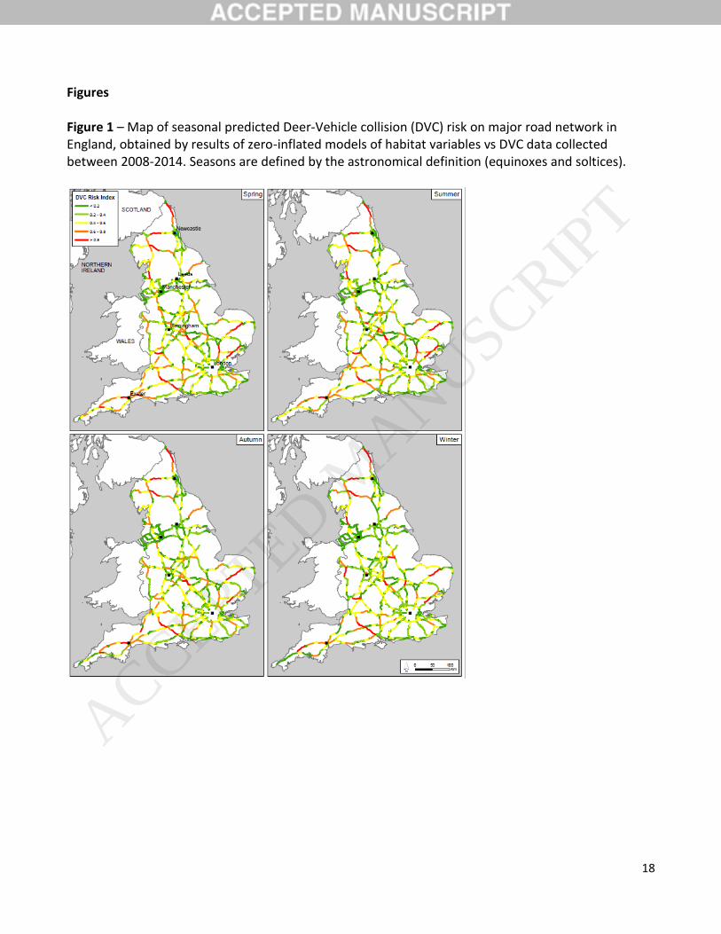
reported in the supplementary material (tables F and G). The maps of relative risk classify each road

segment into 5 different categories, according to the value of the predicted risk index (0.0 - 0.2: low

risk, 0.2 - 0.4: medium-low risk, 0.4 – 0.6: medium risk, 0.6 – 0.8: medium-high risk, 0.8 – 1.0: high

risk) (Fig. 1).

Comparison between seasonal risk maps showed overall significant differences between the seasons

(χ2 = 370.462, P < 0.001) and significant differences appeared in all pairwise comparisons except that

between autumn and winter (P = 0.536). In particular risk is predicted to be higher in spring (mean

risk = 0.158, mean rank = 2.75), followed by summer (mean risk = 0.145, mean rank = 2.54), autumn

(mean risk = 0.135, mean rank =2.34) and winter (mean risk = 0.130, mean rank = 2.37).

DISCUSSION

Modelling the frequency and the risk of DVCs as a function of landscape features, other authors have

already indicated habitat composition as one of the main factors affecting collision risk (Bashore et al.,

1985; Finder et al., 1999; Langbein et al., 2011; Malo et al., 2004; Montgomery et al., 2013; Seiler,

2004). Our findings show that DVCs are more likely to occur when roads are close to (or running

through) significant areas of woodland/forest (Hothorn et al., 2012; Malo et al., 2004; Uzal, 2013). In

particular in our models, increasing distance from areas of both coniferous and broadleaved forest

emerged as an important factor that lowers the probability of DVC occurrence, and it had a negative,

although of less importance, effect on the DVC risk index, indicating therefore that roads close to

forests are considered more at risk of collision. In the same context, we found a positive effect of the

percentage of different habitats within in the 500m strip around individual road segments comprised

of broadleaved forest.

Although in our results the percentage of urban area had generally a negative effect on the number of

expected DVCs/year, there was a clear positive effect of suburban areas. Such a finding is consistent

with observations of Langbein (2008) who showed that in England, 44% of all recorded DVCs fall

within 1 mile of built up areas. Suburban areas are characterized by a patchy mix of urban and semi-

natural habitat, thus our findings are consistent with Anderson et al. (2011) and Duarte et al. (2015)

who reported that deer would use urban areas if a forest matrix surround them. However, the effect

of suburban areas seemed to be lower in the risk model. If we consider that the urbanized areas are

characterized by a higher traffic flow, we expect an overall higher number of collisions (Valero et al.,

2015), but conversely the risk of hitting a deer will be lower, because of the relatively higher number

of cars present on each road segment. Partially confirming this, we found a clear positive effect of the

average annual daily traffic on the probability of classifying the road as a non-zero, in the model which

considers DVCs/year.

ACCEPTED MANUSCRIP

T

11

Besides habitat composition, our models also gave consideration to the effect of habitat structure.

The negative effects of Shannon diversity index in all the components of the models, together with

the negative effect of mean patch size (MPS) suggest that a more diversified landscape decreases the

number and risk of DVCs. This is inconsistent with Malo et al. (2004) and Nielsen et al. (2003), who

showed how the Shannon diversity index was positively associated with plots with high number of

DVCs, but this incongruity could be explained by the different modelling approaches used.

Habitat and landscape composition may play a different role at different spatial scales (Seiler, 2004;

Uzal, 2013). For example, the presence and abundance of forest covered areas in the immediate

vicinity of a road raises the probability of deer crossing and therefore we may expect a higher collision

risk, whereas patches of forest at higher distances play a minor role. Even if our models at the four

different spatial scales did not show particular differences in terms of predictive power, some

differences emerged in the effect and in the predictive importance of the single variables considered.

Surprisingly, proportion of forest of both broadleaf and conifer did not show differences between the

different spatial scale but the presence of open areas such as meadows lowered the probability of

having a DVC at 100m, with a high predictive importance of the variable, although its negative effect

seems to be of less importance at 1km scale. A variable that had a contrary effect at the two opposite

scales was the Shannon diversity index, with a positive effect at 100m but a negative effect at 1km.

The proportion of urbanized areas showed a similar trend as well: at fine scale it did not seem to

affect the DVCs, or it had a slightly positive effect, but on a broader extent, when considering a buffer

of 1km, the models suggested that a higher proportion of dense urban areas is associated with a

lower risk of collision.

Climate variables are known to affect deer densities in temperate forests (Latham et al., 1997;

Mysterud et al., 2008), and the use of bioclimatic variables to assess the risk of DVC, has been

recently suggested by Hothorn et al. (2012). In our models we found effects of two climatic variables

in particular: precipitation and minimum temperatures. Low winter temperature are known to affect

deer density by increasing mortality, and precipitation is generally negatively associated with deer

density, since rain can have a direct effect on reproductive success and neonatal mortality (Putman et

al., 1996). Also, the interaction between rainfall and low temperature has a general effect on car

crashes (Caliendo et al., 2007), therefore it is reasonable to expect that this can be reflected on DVCs

as well.

In our models, we could not include the effect of deer densities on frequency of DVCs because

detailed information on species densities was lacking. Available data are largely restricted to

presence/absence data for each species in each 10km2 square. While estimates of abundance for

fallow deer, roe deer, red deer and muntjac in England have been presented by Putman and Ward

(2010), their estimates were built on the basis of the potential abundance of each species, as derived

ACCEPTED MANUSCRIP

T

12

by a modelling approach. Although their models were characterized by a good predictive power, we

decided to avoid to include this information because we were more interested in the actual, and not

in the potential, abundance. Presence/absence of deer within a section affected the probability of the

road segment having at least one reported incident (non-zero component) but had no effect on

number of accidents reported or expected. This reinforces the idea that in order to have a DVC at all,

it is necessary for deer to be present in the surrounding area, but, beyond that, other factors seem to

play a more significant role. In his analyses, Uzal (2013) found environmental and road/traffic-related

variables could account for up to 70 % of the variance in accident frequency at a landscape [10km2]

scale, thus in practice leaving comparatively little to be explained by variations in ungulate density.

Seasonal patterns in the distribution of DVCs have been shown to be related to times of increased

movement, particularly in association with breeding and dispersal (Desire and Recobet, 1990; Groot

Bruinderink and Hazebroek, 1996; Hartwig, 1991; Pokorny, 2006).

Our seasonal models are partially in accordance with previous reports as they indeed show the

highest DVC risk in spring and summer but many authors report a secondary accident peak in late

autumn (Langbein, 2011) which is possibly associated with increased movement of fallow, sika or red

deer at the time of the rut. The autumn peak may alternatively be ascribed to the shorter day length

or to the change from summer time to GMT at the end of October (which suddenly brings the peak of

traffic in line with the peak of activity of deer) (Langbein, 2011). This secondary autumn peak did not

emerge in our seasonal risk models; however, distinction between these seasonal models did not

include known changes in deer behaviour at different seasons. The lack of any indication of a peak in

autumn based on our results is likely to be affected also by our model being restricted to motorways

and other major roads, some of which deer will tend to cross mostly during spring dispersal, and may

be unable to identify other seasonal peaks more apparent on smaller roads.

Identification of environmental factors associated with increased risk of DVCs also suggests possible

options for mitigation in high risk areas. Of the variables identified as associated with greater

frequency or risk of DVCs, some, as bioclimatic variables or proportion of suburban areas, are unlikely

to be artificially modified. By converse, others are potentially able to be manipulated to achieve

reduction in risk. For example, clearance of forest vegetation, that in our models had an important

effect, can decrease the risk of DVC by improving visibility for both deer and drivers (Meisingset et al.,

2014).

Deer-vehicle collision mitigation measures are generally grouped into three main categories (Groot

Bruinderink and Hazebroek, 1996; Langbein et al., 2011; Putman et al., 2004): (1) prevent or control

crossing, (2) provide safer crossing places and (3) increase driver awareness. An effective cost-benefit

analysis of the most common mitigation measures was presented by Huijser et al. (2009) and

ACCEPTED MANUSCRIP

T

13

Langbein et al. (2011) provided an extensive review of advantages and disadvantages of the most

common reported measures.

When resources are limited, especially from the economic point of view, it is important that they are

directed to actions and measures that are more likely to produce substantial results. For DVC

mitigation strategies in particular, the effort should be concentrated on road segments in which a

higher number of collisions is likely to occur. Within this framework, our expected DVC/year model

can provide road managers an important tool to prioritize the intervention measures on roads on

which we expect a higher number of collisions, and therefore to optimize cost-effectiveness of

warning or preventative measures. The information on how many DVCs are likely to occur for each

road segment, moreover, can supply a baseline for future monitoring, and to evaluate the

effectiveness of mitigation actions, such as the building of new over/underpasses, fences or wildlife

signage.

The models we present are simple and although they are characterized by good predictive power, we

acknowledge that some drawbacks and limitations prevent them from being fully applicable in all

contexts. Our models, for example, did not take into account the time of the day. In most cases our

data did include information on the time at which an incident was reported; however we recognised

that it is likely that the time the collision was reported did not necessarily coincide with the time the

collision occurred, in particular when animals which are hit at night are found dead in the following

morning. For this reason we did not include it in our analyses. If resolution of daily risk factors can be

improved, our models could be easily implemented in a GPS navigation system or on a mobile phone

application, and could give drivers an immediate information on the risk they are facing in a very

precise moment and location.

Our study was inevitably restricted in focus to consideration of one specific country (England), but we

use this as an exemplar to illustrate an approach which we believe has much wider application. The

possibility of identifying the main factors affecting accident frequency along a given road-stretch in

some, and the consequent ability to produce detailed risk maps that take into account both

environmental factors and traffic conditions, represents a substantial step towards increasing the

ability of managers to target limited resources in the most cost-effective way to increase the safety of

both humans and wildlife on roads, particularly if this can be done under standardized and shared

protocols.

With our models we considered an average value of traffic flow, but we assumed that it did not

change between the four seasons. Information on real time traffic flows is in many cases already and

easily available. Systems like Google Traffic (www.maps.google.com) for example are able to generate

a real time traffic map, by analyzing the GPS locations transmitted by a large number of mobile phone

ACCEPTED MANUSCRIP

T

14

users. The possibility to integrate our models with this real-time information would considerably

improve their effectiveness, since they could instantly give drivers the information about DVC risk

taking into account the basic models, with the effect of landscape and road features and the real-time

information on traffic and speed. This sort of real-time warning sign would have the main advantage

of having a very low cost, because it only would need a server-based system that constantly update

the model, whereas drivers could obtain the information on the actual DVC risk simply using a mobile

application. Furthermore, it could prevent drivers from habituation to the more classic warning signs,

since it would give different warnings according to precise conditions of landscape, traffic and speed.

Acknowledgement

We would like to acknowledge all of the wide range of individuals and organisations who have

contributed DVC reports to the Deer Initiative Deer Collisions database on which our modelling and

analysis has been based. We thank in particular the RSPCA, Highways England and all its road

management agents who provided the bulk of DVC data and other details specifically for the English

trunk road network. Highways England also provided lead funding for the present study. Finally, we

would like to thank T. Messmer, L. Corlatti and another anonymous reviewer, for their insightful

comments on the first version of our manuscript.

ACCEPTED MANUSCRIP

T

15

References

Anderson, C.W., Nielsen, C.K., Storm, D.J., Schauber, E.M., 2011. Modeling habitat use of deer in an exurban landscape.

Wildlife Society Bulletin 35, 235-242.

Anderson, D.R., Link, W.A., Johnson, D.H., Burnham, K.P., 2001. Suggestions for presenting the results of data analyses.

Journal of Wildlife Management 65, 373-378.

Apollonio, M., Andersen, R., Putman, R., 2010. European ungulates and their management in the 21st century. Cambridge

University Press, Cambridge, UK.

Bashore, T.L., Tzilkowski, W.M., Bellis, E.D., 1985. Analysis of deer-vehicle collision sites in Pennsylvania. The Journal

of Wildlife Management 49, 769-774.

Bolker, B.M., Brooks, M.E., Clark, C.J., Geange, S.W., Poulsen, J.R., Stevens, M.H.H., White, J.S.S., 2009. Generalized

linear mixed models: a practical guide for ecology and evolution. Trends in ecology & evolution 24, 127-135.

Burnham, K.P., Anderson, D.R., 2002. Model Selection and Multimodel Inference: A Practical Information-Theoretic

Approach. Springer-Verlag, New York.

Caliendo, C., Guida, M., Parisi, A., 2007. A crash-prediction model for multilane roads. Accident Analysis & Prevention

39, 657-670.

Colino-Rabanal, V.J., Peris, S.J., 2016. Wildlife road kills: improving knowledge about ungulate distributions? Hystrix, the

Italian Journal of Mammalogy 27, 1-8.

Conover, M.R., 1997. Monetary and intangible valuation of deer in the United States. Wildlife Society Bulletin 25, 298-305.

Cramer, J.S., 2003. Logit models from economics and other fields. Cambridge University Press, Cambridge, UK.

Desire, G., Recobet, G., 1990. Resultats de l'enquete realisee de 1984 a 1986 sur les collisions entre les vehicules at leas

grands mammiferes sauvages. Office National de la Chasse, Bulletin Mensuelle 143, 38-47.

Duarte, J., Farfán, M.A., Fa, J.E., Vargas, J.M., 2015. Deer populations inhabiting urban areas in the south of Spain: habitat

and conflicts. European Journal of Wildlife Research 61, 365-377.

Finder, R.A., Roseberry, J.L., Woolf, A., 1999. Site and landscape conditions at white-tailed deer/vehicle collision locations

in Illinois. Landscape and Urban Planning 44, 77-85.

Found, R., Boyce, M.S., 2011a. Predicting deer–vehicle collisions in an urban area. Journal of environmental management

92, 2486-2493.

Found, R., Boyce, M.S., 2011b. Warning signs mitigate deer–vehicle collisions in an urban area. Wildlife Society Bulletin

35, 291-295.

Girardet, X., Conruyt-Rogeon, G., Foltête, J.-C., 2015. Does regional landscape connectivity influence the location of roe

deer roadkill hotspots? European journal of wildlife research 61, 731-742.

Grace, M.K., Smith, D.J., Noss, R.F., 2015. Testing alternative designs for a roadside animal detection system using a

driving simulator. Nature Conservation 11, 61-77.

Groot Bruinderink, G., Hazebroek, E., 1996. Ungulate traffic collisions in Europe. Conservation Biology 10, 1059-1067.

Gunson, K.E., Mountrakis, G., Quackenbush, L.J., 2011. Spatial wildlife-vehicle collision models: A review of current work

and its application to transportation mitigation projects. Journal of Environmental Management 92, 1074-1082.

Hartwig, D., 1991. Erfassung der Verkehrsunfälle mit Wild im Jahre 1989 in Nordrhein-Westfalen im Bereich der

Polizeibehörden. Zeitschrift für Jagdwissenschaft 37, 55-62.

Hothorn, T., Brandl, R., Müller, J., 2012. Large-scale model-based assessment of deer-vehicle collision risk. PloS one 7,

e29510.

Hubbard, M.W., Danielson, B.J., Schmitz, R.A., 2000. Factors influencing the location of deer-vehicle accidents in Iowa.

The Journal of wildlife management 64, 707-713.

Huijser, M.P., Duffield, J.W., Clevenger, A.P., Ament, R.J., McGowen P.T., 2009, Cost–benefit analyses of mitigation

measures aimed at reducing collisions with large ungulates in the United States and Canada: a decision support tool.

Ecology and Society 14, 15.

Insurance Institute for Highway Safety, 2004. Lots of approaches are under way to reduce deer collisions, but few have

proven effective. Status Report 39, 5-7.

Iuell, B., 2004. Wildlife and Traffic-A European Handbook for Identifying Conflicts and Designing Solutions, Proceedinfs

of the 22nd PIARC World Road Congress.

Kušta, T., Keken, Z., Ježek, M., Holá, M., Šmíd, P., 2017. The effect of traffic intensity and animal activity on probability

of ungulate-vehicle collisions in the Czech Republic. Safety science 91, 105-113.

Langbein, J., 1985. North Staffordshire Deer Survey 1983-1985, Research and Development, Fordinbridge, UK.

ACCEPTED MANUSCRIP

T

16

Langbein, J., 2011. Monitoring reported deer road casualties and related accidents in England to 2010, Research Report

11/3. The Deer Initiative, Wrexham, UK.

Langbein, J., Putman, R., 2006. National Deer-Vehicle Collisions Project; Scotland, 2003–2005. Report to the Scottish

Executive.

Langbein, J., Putman, R., Pokorny, B., 2011. Traffic collisions involving deer and other ungulates in Europe and available

measures for mitigation, in: Putman, R., Apollonio, M., Andersen, R. (Eds.), Ungulate management in Europe: problems

and practices. Cambridge University Press, pp. 215-259.

Latham, J., Staines, B., Gorman, M., 1997. Correlations of red (Cervus elaphus) and roe (Capreolus capreolus) deer

densities in Scottish forests with environmental variables. Journal of Zoology 242, 681-704.

Litvaitis, J.A., Tash, J.P., 2008. An approach toward understanding wildlife-vehicle collisions. Environmental Management

42, 688-697.

Liu, C., White, M., Newell, G., 2013. Selecting thresholds for the prediction of species occurrence with presence-only data.

Journal of Biogeography 40, 778-789.

Long, J.S., Freese, J., 2006. Regression models for categorical dependent variables using Stata. Stata press.

Malo, J.E., Suárez, F., Diez, A., 2004. Can we mitigate animal–vehicle accidents using predictive models? Journal of

Applied Ecology 41, 701-710.

Meisingset, E.L., Loe, L.E., Brekkum, Ø., Mysterud, A., 2014. Targeting mitigation efforts: the role of speed limit and road

edge clearance for deer–vehicle collisions. The Journal of Wildlife Management 78, 679-688.

Meisingset, E.L., Loe, L.E., Brekkum, Ø., Van Moorter, B., Mysterud, A., 2013. Red deer habitat selection and movements

in relation to roads. The Journal of Wildlife Management 77, 181-191.

Montgomery, R.A., Roloff, G.J., Millspaugh, J.J., 2013. Variation in elk response to roads by season, sex, and road type.

The Journal of Wildlife Management 77, 313-325.

Morton, R.D., Rowland, C., Wood, C., Meek, L., Marston, C., Smith, G., Wadsworth, R., Simpson, I.C., 2011. Final Report

for LCM2007 - the new UK land cover map, Countryside Survey Technical Report No 11/07. NERC/Centre for Ecology

& Hydrology, p. 112.

Mysterud, A., 2004. Temporal variation in the number of car-killed red deer Cervus elaphus in Norway. Wildlife Biology

10, 203-211.

Mysterud, A., Yoccoz, N.G., Langvatn, R., Pettorelli, N., Stenseth, N.C., 2008. Hierarchical path analysis of deer responses

to direct and indirect effects of climate in northern forest. Philosophical Transactions of the Royal Society of London B:

Biological Sciences 363, 2357-2366.

Ng, J.W., Nielson, C., St Clair, C.C., 2008. Landscape and traffic factors influencing deer-vehicle collisions in an urban

enviroment. Human-Wildlife Interactions 2, 34-47.

Nielsen, C.K., Anderson, R.G., Grund, M.D., 2003. Landscape influences on deer-vehicle accident areas in an urban

environment. The Journal of wildlife management 67, 46-51.

Niemi, M., Matala, J., Melin, M., Eronen, V., Järvenpää, H., 2015. Traffic mortality of four ungulate species in southern

Finland. Nature Conservation 11, 13-28.

Pokorny, B., 2006. Roe deer-vehicle collisions in Slovenia: situation, mitigation strategy and countermeasures. Veterinarski

Arhiv 76, 177-187.

Putman, R., Langbein, J., Hewinson, A.J.M., Sharma, S., 1996. Relative roles of density‐dependent and density‐independent

factors in population dynamics of British deer. Mammal Review 26, 81-101.

Putman, R., Langbein, J., Staines, B., 2004. Deer and Road Traffic Accidents; A Review of Mitigation Measures: Costs and

Cost-Effectiveness. Report to the Deer Commission for Scotland, Contract RP 23A.

Putman, R., Ward, A., 2010. Predicting abundance and distribution of wild deer in England: suporting a vision for Natural

England, Research Report 10/2. The Deer Initiative, Wrexham, UK.

Putman, R.J., 2008. Relative roles of cull and non-cull mortality in populations of red and roe deer. Contract report for the

Deer Commission for Scotland, Inverness UK.

Rempel, R.S., Kaukinen, D., Carr, A.P., 2012. Patch Analyst and Patch Grid. Ontario Ministry of Natural Resources. Centre

for Northern Forest Ecosystem Research., Thunder Bay, Ontario.

Rogerson, P., 2001. Statistical Methods for Geography, London.

Romin, L.A., Bissonette, J.A., 1996. Deer: Vehicle Collisions: Status of State Monitoring Activities and Mitigation Efforts.

Wildlife Society Bulletin (1973-2006) 24, 276-283.

Seiler, A., 2004. Trends and spatial patterns in ungulate-vehicle collisions in Sweden. Wildlife Biology 10, 301-313.

Steiner, W., Leisch, F., Hackländer, K., 2014. A review on the temporal pattern of deer–vehicle accidents: Impact of

seasonal, diurnal and lunar effects in cervids. Accident Analysis & Prevention 66, 168-181.

ACCEPTED MANUSCRIP

T

17

Uzal, A., 2013. Reported deer road casualties and related accidents in England 2003-2010: their potential to develop an

index of deer density. The Deer Initiative, Wrexham, UK.

Valero, E., Picos, J., Álvarez, X., 2015. Road and traffic factors correlated to wildlife–vehicle collisions in Galicia (Spain).

Wildlife Research 42, 25-34.

Wakeling, B.F., Gagnon, J.W., Olson, D.D., Lutz, D.W., Keegan, T.W., Shannon, J.M., Holland, A., Lindbloom, A.,

Schroeder, C., 2015. Mule Deer and Movement Barriers, in: Group, M.D.W. (Ed.). Western Association of Fish and

Wildlife Agencies, U.S.A.

Ward, A.I., 2005. Expanding ranges of wild and feral deer in Great Britain. Mammal Review 35, 165-173.

Ward, A.I., Etherington, T., Ewald, J., 2008. Five years of change. Deer 14, 17-20.

Zuberogoitia, I., del Real, J., Torres, J.J., Rodríguez, L., Alonso, M., Zabala, J., 2014. Ungulate Vehicle Collisions in a Peri-

Urban Environment: Consequences of Transportation Infrastructures Planned Assuming the Absence of Ungulates.

PLOS ONE 9, e107713.

Zuur, A.F., Ieno, E.N., Elphick, C.S., 2010. A protocol for data exploration to avoid common statistical problems. Methods

in Ecology and Evolution 1, 3-14.

ACCEPTED MANUSCRIP

T

18

Figures Figure 1 – Map of seasonal predicted Deer-Vehicle collision (DVC) risk on major road network in England, obtained by results of zero-inflated models of habitat variables vs DVC data collected between 2008-2014. Seasons are defined by the astronomical definition (equinoxes and soltices).

ACCEPTED MANUSCRIP

T