Quantification of modeling errors in airborne TEM caused by inaccurate system description

Qb

A

eqiioe

dtaq

a

©

GEOPHYSICS, VOL. 76, NO. 1 �JANUARY-FEBRUARY 2011�; P. F43–F52, 15 FIGS., 2 TABLES.10.1190/1.3511354

uantification of modeling errors in airborne TEM causedy inaccurate system description

nders Vest Christiansen1, Esben Auken2, and Andrea Viezzoli3

ticpttdlttTsdtmtt

ABSTRACT

Being able to recover accurate and quantitative descriptions ofthe subsurface electrical conductivity structure from airborneelectromagnetic data is becoming more and more crucial in manyapplications such as hydrogeophysical and environmental map-ping, but also for mining exploration. The effect on the invertedmodels of inaccurate system description in the 1D forward mod-eling of helicopter time-domain electromagnetic �TEM� datawas studied. The most important system parameters needed foraccurate description of the subsurface conductivity were quanti-fied using a nominal airborne TEM system and three differentreference models to ensure the generality of the conclusions. Bycalculating forward responses, the effect of changing the systemtransfer function of the nominal airborne TEM system was stud-ied in detail. The data were inverted and the consequences of in-accurate modeling of the system transfer function were studied in

ocr

A

mpars

v

eived 1undwat

ail: esb

F43

Downloaded 05 Jan 2011 to 130.225.0.227. Redistribution subject to S

he model space. Errors in the description of the transfer functionnfluence the inverted model differently. The low-pass filters,urrent turn-off, and receiver-transmitter �Rx-Tx� timing issuesrimarily influenced the early time gates. The waveform repeti-ion, gate integration, altitude, and geometry mainly influencedhe late time gates. Depth of investigation is highly model depen-ent, but in general the early times hold information on the shal-ower parts of the model and the late times hold information onhe deeper parts of the model.Amplitude, gain, and current varia-ions affect the entire sounding and therefore the entire model.he results showed that all of these parameters should be mea-ured and modeled accurately during inversion of airborne TEMata. If not, the output model can differ quite dramatically fromhe true model. Layer boundaries can be inaccurate by tens of

eters, and layer resistivities by as much as an order of magni-ude. In the worst cases, the measured data simply cannot be fit-ed within noise level.

INTRODUCTION

For groundwater and environmental applications the airbornelectromagnetic �AEM� data are used quantitatively and as a conse-uence the reliability of the model parameters obtained by inversions crucial. This calls for high-quality data, accurate forward model-ng of the systems, and precise and robust inversion. Here, we focusn accurate forward modeling using synthetic models to quantify theffect of inaccuracies in the system description.

In sedimentary areas the electrical conductivity is mainly depen-ent on the salinity of the groundwater �i.e., the groundwater quali-y� and the clay content of the subsurface �i.e., the aquifer conditionsnd protection level� �Kirsch, 2006; Siemon et al., 2009�.As a conse-uence, in large-scale groundwater surveys AEM methods are most

Manuscript received by the Editor 5 February 2010; revised manuscript rec1Geological Survey of Denmark and Greenland, Department of Gro

[email protected] University, Department of Earth Sciences,Aarhus, Denmark. E-m3Aarhus GeophysicsApS,Aarhus, Denmark. E-mail: [email protected] Society of Exploration Geophysicists.All rights reserved.

ften chosen because they offer an efficient tool to investigate theonductivity structure over large areas in a reasonable time and atelatively low costs.

irborne time-domain electromagnetic systems

The application of geoelectrical and surface electromagneticethods has a long tradition in groundwater and environmental ex-

loration. However, AEM was introduced for mineral explorationnd — compared with that — airborne groundwater exploration is aelatively new application. Siemon et al. �2009� give a comprehen-ive overview ofAEM methods used for groundwater applications.

Various AEM systems are used for airborne groundwater and en-ironmental investigations, including rigid-beam helicopter-borne

7 June 2010; published online 4 January 2011.er and Quaternary Geology Mapping, Copenhagen, Denmark. E-mail:

[email protected].

EG license or copyright; see Terms of Use at http://segdl.org/

ffibvcqnpd

Hvdalmlcncwruc�tblfia

M

ttwttp

wopp

T

cktttons

alcva1sat

fmacwmme

rrtvmvialat

stmsoacre

TT

T

R

F44 Christiansen et al.

requency-domain systems, fixed-wing time-domain systems,xed-wing frequency-domain systems, and several helicopter-orne time-domain systems �Fountain, 2008�. In the last decade de-elopment has focused on the helicopter time-domain systems be-ause they have superior depth penetration compared with the fre-uency-domain systems. However, most time-domain electromag-etic �TEM� systems have less resolution in the near-surface com-ared with the frequency-domain systems. The helicopter time-omain systems are the focus of this paper.

Recently developed helicopter TEM systems are the AeroTEM,oistem, VTEM, HeliGEOTEM, and SkyTEM systems �an over-iew is presented by Allard, 2007�. These systems were originallyesigned for mineral exploration. The SkyTEM system representsn exception because it was purposely designed for mapping of geo-ogical structures in the near-surface for groundwater and environ-

ental investigations. Helicopter systems carry the transmitter �Tx�oop as a sling load beneath the helicopter. In the Tx loop an electricurrent is abruptly terminated, causing a change of the primary mag-etic field, which in turn induces currents to flow in the ground. Be-ause of ohmic loss the currents decay and, in general, diffuse down-ard and outward in the subsurface. The change over time �decay

ate� of the secondary magnetic fields from these currents is pickedp by an induction coil, typically located near the Tx frame. In mostases, two perpendicular receiver �Rx� coils pick up the inline fieldx-component� and the vertical field �z-component�. For groundwa-er exploration the vertical field holds by far most of the informationecause the geological structures are predominantly horizontal. Thearge horizontal currents induced in the ground mean that the inlineelds are small when there is only a small offset between the Tx loopnd the Rx coil.

odeling airborne TEM systems

Auken et al. �2007� showed some of the most important parame-ers that influence the system transfer function of airborne TEM sys-ems; namely, the altitude of the transmitter-receiver �Tx-Rx�, theaveform, and the Tx-Rx timing. In addition to these factors there is

he general geometry of the Tx-Rx, the waveform repetition, the in-egration of the signal over the width of the time gate, and the low-ass filters in the Rx system.

able 1. Central parameters defining a nominal airborneEM system used for the examples in this paper

ransmitter

x,y,z �m� 0, 0, �30

Turn-on 100 �s

Turn-off 3 �s

Area 500 m2

Current 1 A �normalized�

Base frequency 25 Hz, 10 ms on, 10 ms off

eceiver

x,y,z �m� 0, 0, �30

Filters None

First gate-center time 13 �s

Last gate-center time 8 ms

Gate distribution 10 gates per decade in time


Bias and leveling problems also present real and serious problemsith many airborne systems and a lot of effort is put into the removalf these effects during data collection and data processing. This pa-er will not discuss these issues and we thereby take as the startingoint that no leveling or bias issues are left with the data.

MODELING EXAMPLES

he nominal system and models

All airborne TEM system are different and they all have their ownharacteristics and design considerations. For this reason, and toeep things general, we will model the response of a nominal sys-em. The base system is a sling-load, central-loop system with the Txowed 30 m above the ground. The Tx is a 500-m2 circular loopransmitting a trapezoidal waveform in a 50% duty cycle and a turn-ff time of 3 �s. The first gate-center time is 13 �s after the begin-ing of turn-off and the last gate is at 8 ms. The nominal setup isummarized in Table 1.

We assume that there are no bias or calibration issues in the datand we do not consider data noise. Noise levels depend heavily onocal factors and a given noise model is generally wrong for specificases. We have assigned 5% uniform noise to all gates used in the in-ersion. By setting the last usable gate at 8 ms, we have indirectlyssumed a fairly low noise level. Also, the first gate is quite early at3 �s. In that sense, this system and the data can be regarded aslightly optimistic. However, many of the systems currently flyingre being developed further in the hope of achieving these parame-ers.

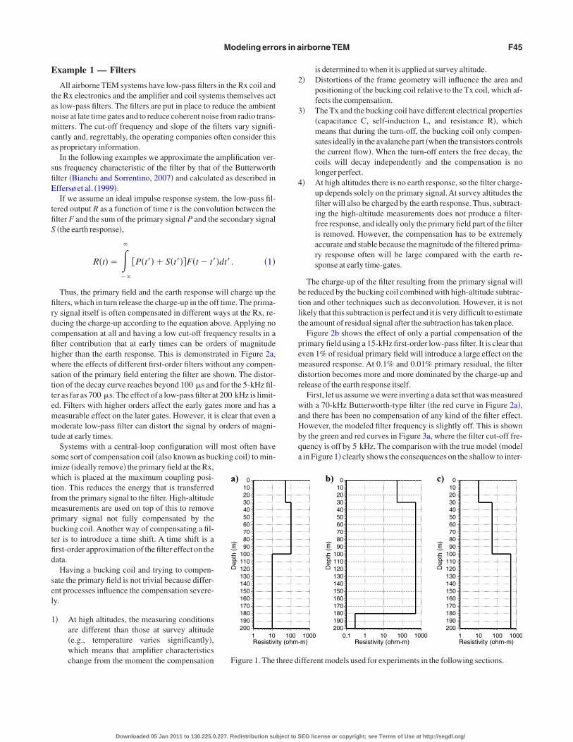
For each of the different examples we will use one of the three dif-erent models as presented in Figure 1. Model a is a low-contrastodel with a 30-m layer in the top representing till overlying an

quifer, which in turn is underlain by a clay layer. Model b has higherontrasts and the model is dominated by a very conductive last layerith higher resistivities above. This is meant to resemble an aquiferodel with salt intrusion at depth. Model c is a double ascendingodel representing clay and till overlying sands, chalk, or some oth-

r resistive bedrock.In each of the examples we will first show the effect that the pa-

ameter in question has on forward responses. Then we will assume aealistic inaccuracy on the specification of the parameter. Invertinghe data, we show the effect on the final output models. All of the in-ersions presented have been given the true model as the startingodel. The deviations are therefore the minimum changes in the in-

erted model required to fit the inaccurate forward responses. If thenversions had been started with a homogenous half-space, as is usu-lly the case with field data, the deviation from the true model wouldikely be larger. The model �a, b, or c� chosen for the individual ex-mples is the model that gives the most significant result with respecto that particular example.

Forward modeling and inversion of AEM data are not within thecope of this paper. The inversion algorithm itself is described in de-ail in Christiansen and Auken �2008�. The same algorithm imple-

ents the laterally and spatially constrained inversion concepts de-cribed in Auken et al. �2005� and Viezzoli et al. �2008�. The theoryf the forward algorithm is given in Ward and Hohmann �1988�. Thelgorithm implements a complete modeling of a piecewise linearurrent ramp, low-pass filters, gate integration, and as inversion pa-ameters the system altitude and for some systems the system geom-try.


E

tanmca

sfiE

tfiS

firdcfihwsttemmt

siwtfmpbtfid

sel

1

2

3

4

btlt

pemdr

waHbqa

Modeling errors in airborne TEM F45

xample 1 — Filters

All airborne TEM systems have low-pass filters in the Rx coil andhe Rx electronics and the amplifier and coil systems themselves acts low-pass filters. The filters are put in place to reduce the ambientoise at late time gates and to reduce coherent noise from radio trans-itters. The cut-off frequency and slope of the filters vary signifi-

antly and, regrettably, the operating companies often consider thiss proprietary information.

In the following examples we approximate the amplification ver-us frequency characteristic of the filter by that of the Butterworthlter �Bianchi and Sorrentino, 2007� and calculated as described inffersø et al. �1999�.If we assume an ideal impulse response system, the low-pass fil-

ered output R as a function of time t is the convolution between thelter F and the sum of the primary signal P and the secondary signal�the earth response�,

R�t��

�

�P�t��S�t��F�t� t��dt�. �1�

Thus, the primary field and the earth response will charge up thelters, which in turn release the charge-up in the off time. The prima-y signal itself is often compensated in different ways at the Rx, re-ucing the charge-up according to the equation above. Applying noompensation at all and having a low cut-off frequency results in alter contribution that at early times can be orders of magnitudeigher than the earth response. This is demonstrated in Figure 2a,here the effects of different first-order filters without any compen-

ation of the primary field entering the filter are shown. The distor-ion of the decay curve reaches beyond 100 �s and for the 5-kHz fil-er as far as 700 �s. The effect of a low-pass filter at 200 kHz is limit-d. Filters with higher orders affect the early gates more and has aeasurable effect on the later gates. However, it is clear that even aoderate low-pass filter can distort the signal by orders of magni-

ude at early times.Systems with a central-loop configuration will most often have

ome sort of compensation coil �also known as bucking coil� to min-mize �ideally remove� the primary field at the Rx,hich is placed at the maximum coupling posi-

ion. This reduces the energy that is transferredrom the primary signal to the filter. High-altitudeeasurements are used on top of this to remove

rimary signal not fully compensated by theucking coil. Another way of compensating a fil-er is to introduce a time shift. A time shift is arst-order approximation of the filter effect on theata.

Having a bucking coil and trying to compen-ate the primary field is not trivial because differ-nt processes influence the compensation severe-y.

� At high altitudes, the measuring conditionsare different than those at survey altitude�e.g., temperature varies significantly�,which means that amplifier characteristicschange from the moment the compensation

0102030405060708090

100110120130140150160170180190200

1 10

Dep

th(m

)

Resistivi

a)

Figure 1. The


is determined to when it is applied at survey altitude.� Distortions of the frame geometry will influence the area and

positioning of the bucking coil relative to the Tx coil, which af-fects the compensation.

� The Tx and the bucking coil have different electrical properties�capacitance C, self-induction L, and resistance R�, whichmeans that during the turn-off, the bucking coil only compen-sates ideally in the avalanche part �when the transistors controlsthe current flow�. When the turn-off enters the free decay, thecoils will decay independently and the compensation is nolonger perfect.

� At high altitudes there is no earth response, so the filter charge-up depends solely on the primary signal.At survey altitudes thefilter will also be charged by the earth response. Thus, subtract-ing the high-altitude measurements does not produce a filter-free response, and ideally only the primary field part of the filteris removed. However, the compensation has to be extremelyaccurate and stable because the magnitude of the filtered prima-ry response often will be large compared with the earth re-sponse at early time-gates.

The charge-up of the filter resulting from the primary signal wille reduced by the bucking coil combined with high-altitude subtrac-ion and other techniques such as deconvolution. However, it is notikely that this subtraction is perfect and it is very difficult to estimatehe amount of residual signal after the subtraction has taken place.

Figure 2b shows the effect of only a partial compensation of therimary field using a 15-kHz first-order low-pass filter. It is clear thatven 1% of residual primary field will introduce a large effect on theeasured response. At 0.1% and 0.01% primary residual, the filter

istortion becomes more and more dominated by the charge-up andelease of the earth response itself.

First, let us assume we were inverting a data set that was measuredith a 70-kHz Butterworth-type filter �the red curve in Figure 2a�,

nd there has been no compensation of any kind of the filter effect.owever, the modeled filter frequency is slightly off. This is showny the green and red curves in Figure 3a, where the filter cut-off fre-uency is off by 5 kHz. The comparison with the true model �modelin Figure 1� clearly shows the consequences on the shallow to inter-

1000-m) Resistivity (ohm-m) Resistivity (ohm-m)

10.1 10 100 1000

0102030405060708090

100110120130140150160170180190200

Dep

th(m

)

1 10 100 1000

0102030405060708090

100110120130140150160170180190200

Dep

th(m

)

b) c)

ifferent models used for experiments in the following sections.

100ty (ohm

three d


mtawl

fo

fismIrcn

lttido

pg

E

wcfttbtn

s�s

ipd

sftc

a

Fmttsaitrwgbm

a

Fobutipmb


ediate part of the model. Overestimating the cut-off frequency hashe most pronounced effect on the recovered model, introducing anrtificial thin shallow conductor. The overall data fit �Figure 3b� isithin the data noise, but a slightly poorer fit is noticeable for the ear-

y times where the filter effect is most pronounced.If the cut-off frequency of the low-pass filters is even more distant

rom the correct one, data cannot be fitted at all and the only way tobtain a reasonable fit is to delete the early gates.

Now, as the second filter example we will still assume a 70-kHzlter, but the primary charge-up of the filter has been fully compen-ated by the bucking coil and subtraction of high-altitude measure-ents �i.e., the orange curve in Figure 2b but with a 70-kHz filter�.

nverting this data set, assuming that no filter at all has been applied,esults in the blue model in Figure 3a. Data fits for this model �blueurve in Figure 3b� are near perfect and give no indication of an erro-eous model.

OftenAEM systems have filters of higher order than one and/or ofower cut-off frequency. To model their low-pass filter characteris-ics correctly while inverting is mandatory if quantitative informa-ion about shallow and intermediate-layer resistivity and boundariess sought. Failure to do that results in near-surface artifacts and/orata for the earlier gates that cannot possibly be fitted as well as lossf potentially valuable near-surface information.

–210

–310

–410

–510

–610

–710

–810

–910

–1010

–1110

10–5 10–4 10–3 10–2

2dB

/dt(

V/(

ms)

)

Time (s)

–210

–310

–410

–510

–610

–710

–810

–910

–1010

–1110

10–5 10–4 10–3 10–2

2dB

/dt(

V/(

ms)

)

Time (s)

) b)

5 kHz15 kHz

70 kHz200 kHzno filter

100% primary10% primary1% primary0.1% primary0.01% primaryno filter

igure 2. The effect on the forward response of low-pass filters onodel a. �a� The effect of first-order filters without any compensa-

ion of the primary signal is shown. The black curve shows no filters,he purple curve shows the effect of a 200-kHz filter, the red curvehows the effect of a 70-kHz filter, the green curve is a 15-kHz filter,nd the blue curve is a 5-kHz filter. The huge overshoot at early timess caused by the charge-up of the filter by the primary response fromhe Tx turn-off. �b� The effect of a partial compensation of the prima-y field for a 15-kHz first-order filter is shown. The purple curve isithout compensation �100% primary — same as in panel �a�, thereen curve is 10% primary left, the red curve is 1% primary left, thelue curve is 0.1% primary left, and the orange curve is 0.01% pri-ary left, and the black curve is without a filter.


Most of the airborne systems currently in operation apply low-ass filters in the range discussed above. The possible effect of auess, as qualified as it may be, is clearly seen in the above example.

xample 2 — Waveform repetition

TEM responses are often modeled using only one repetition of theaveform, but all TEM systems operate with alternating polarity of

urrent pulses, primarily to remove harmonics from the power linerequency. In practice, this means that there is less response than ac-ually modeled using only one waveform compared with modelingwo or more pulses. For high-resistivity models this is not a problemecause the effect is dominating at late times. But for deep low-resis-ive layers the effect of previous current pulses is definitely recog-izable.

In Figure 4a the red curve shows the forward response corre-ponding to model b in Figure 1 when modeling only one polarity�; 0� of the waveform, and the green curve shows the forward re-ponse when modeling the full cycle ��; 0; �; 0�.

A close look at Figure 4b at the late times shows a clear differencen forward responses �note that the error bar is 5%�. The changingolarity of the transmitted waveforms causes the earth response toecrease.

The effect of inverting the two-waveform repetition response as-uming only one repetition is seen in Figure 5. The forward datarom the inverted model fit almost perfectly to the observed data, buthe increased voltage response due to using only one waveformauses the depth to the deep good conductor to be shifted 20 m

0

10

20

30

40

50

60

70

80

90

100

110

120

130

140

150

160

170

180

190

2001 10 100 1000

Dep

th(m

)

Resistivity (ohm-m)

–310

–410

–510

–610

–710

–810

–910

–1010

–1110–510 –410 –310 –210

2dB

/dt(

V/(

ms)

)

Time (s)

) b)

No filter

75 kHz

65 kHz

True model

igure 3. The effect on the inverted models having frequency errorsn model a in Figure 1. �a� The result of the inversion, where thelack curve shows the true model. The red curve shows the effect ofnderestimating the true filter frequency �65 instead of 70 kHz�, andhe green curve is an overestimation of the true filter frequency �75nstead of 70 kHz�. The blue curve shows the inverted model if therimary charge-up of a 70-kHz filter has been fully compensated butodeled without a filter. �b� The fit to the observed data �black error

ars� is shown with the same color code.


dbm

E

eaitlc

icts

ett

tieuisefd

E

ntmcmigea2

atIetletbbvAm

ll

sip�

E

tdstbtcttGpbmau

nsdT

g1tt


ownward. The middle high-resistivity layer is also overestimated,ut this is much less important because the 500-�m layer in the trueodel is very poorly resolved in the first place.

xample 3 — Tx current turn-off

Variation in the turn-off time of the Tx current mainly affects thearly time-gates whereas the late time-gates are hardly affected atll. Two things cause the effect: first, the induction in the subsurfaces different for a different turn-off ramp; second, the distance, inime, between the first gate and the end of the ramp gets smaller forarger turn-off times. The latter effect is by far dominating and islearly seen as a raised signal level for the longer turn-off times.

The differences in the forward responses due to inaccurate model-ng of turn-off-times are seen in Figure 6. Most modern systems areapable of accurately recording the turn-off time and for some sys-ems the turn-off time is provided for each flight or even for eachounding.

Let us now assume that we model the turn-off time as 3 �s as giv-n for the nominal system description, but actually the real turn-offime for that sounding is 4 or 7 �s. The results from inverting thesewo data sets are shown in Figure 7.

The inverted model from an erroneous assumption of the turn-offime of only 1 �s is shown with blue in Figure 7a. As expected, thenverted model is only affected in the shallow part. The few percentrror of the forward response caused the first boundary to shift 6.7 mp, which can indeed be important for accurate hydrological model-ng. Resistivities are in this particular case unaffected. If the as-umed turn-off time is even further from the truth, the inverted mod-ls are affected quite heavily, introducing a thin conductor at the sur-ace to comply with the elevated response arising from the erroneousescription of the turn-off time.

xample 4 — Timing

AEM systems can also have problems with an absolute determi-ation of the relative time shift between the Tx and the Rx system orhe time shift is not properly defined. Let us now

odel the effect of not taking these shifts into ac-ount. This is shown in Figure 8. A �6-�s shifteans that the Tx pulse is moved 6 �s backward

n time �i.e., the actual gate-center time of the firstate is 6 �s later than the nominal value�. Theffect on the forward responses is very cleart early times, but it can be identified even at00–300 �s.

Let us again assume that we model the timings indicated in the nominal system, but actuallyhe measured data are shifted �3 or even �6 �s.nverting these data gives us the models present-d in Figure 9a. A timing error of just �3 �s vir-ually removes the resistivity contrast betweenayer 1 and layer 2 and we have a two-layer mod-l. On the data fit �Figure 9b� we see that there ac-ually is a small misfit to the first one or two gates,ut without any other indication that there mighte a problem with the timing, this kind of misfit isery hard to recognize at individual soundings.n error of 6 �s completely changes the outputodel by the introduction of a high-resistivity

10–5

10–6

10–7

10–8

10–9

10–10

10–11

10–12

10–5

2dB

/dt(

V/(

ms)

)

a)

Figure 4. Thedecay, �b� a clwaveform moone full cycle


ayer at the top and no clear indication of the aquifer — the 100-�mayer. Note that the data are still fitted very nicely �Figure 9b�.

A timing error superficially looks similar to a turn-off error as it iset up here. In that sense, a positive timing error would influence thenverted model in a similar way as the turn-off error described in therevious example �i.e., a conductor would be introduced at the top�Figure 7a�.

xample 5 — Gate integration

The last example in this class of errors deals with the modeling ofhe time gates of the Rx. To get a reading from a specific time win-ow the signal is integrated over a gate. This integration can be aimple box-car average or more sophisticated tapered average fil-ers. For narrow averaging kernels the gate value is well representedy the value at the gate-center time. However, especially for lateimes, some systems have very wide averaging windows and in thatase the gate-center time might not be a fair representation of the ac-ual window average. In addition, most systems give the gate-centerime as the arithmetic mean of the gate-open and gate-close times.iven that the dB/dt signal on a homogeneous half-space decaysroportional to t��5/2� �at late times�, the geometric mean is a muchetter representation of the integrated signal than the arithmeticean. Hence, if the measured integrated signal is modeled using justgate-center time, the geometric mean of the gate times should besed as the time reference.

To show the effect of the gate integration, we need to modify theominal system in Table 1. The gate integration error appears forystems with wide gates and especially at late times, to accommo-ate that, we just delete every second gate of the nominal system.his gives us the gates stated in Table 2.Using these specifications we can evaluate the effect of gate inte-

ration versus a mean value representation. This is shown in Figure0 for model c in Figure 1. The effect is not very pronounced and forhe nominal system with 10 gates per decade the effect is hardly no-iceable �not shown�.

0–3 10–2

)

10–10

10–11

10–12

10–3 10–2

2dB

/dt(

V/(

ms)

) –30 –20 –10 0 10

–30 –20

–10 0 10

Cur

rent

Time (ms)

Time (ms)

zoomin b)

1 waveform rep.

2 waveform rep.

Time (s)

Cur

rent

c)b)

n the forward response of waveform repetitions on model b. �a� Fullof the late times, and �c� a schematic drawing showing the differentused. The red curve is one waveform ��; 0� and the green curve is

; 0�.

10–4 1

Time (s

effect oose updeling��; 0; �


tmdmhti

E

otave

1ftae

attfdttFd

vBciRdtgd

FTut

a

Fmc�7


However, if we invert the gate-integrated data using a gate-centerime approach, we get the results of Figure 11. Using the arithmetic

ean as a reference point for the gate value, we get the depth to theeep boundary shifted by 10 m �red curve�. Had we used the geo-etric mean as the reference, the effect on the inverted model would

ave been very small. Had we used the nominal system of Table 1,he effect on the models would have been very small, even when us-ng the arithmetic mean.

Dep

th(m

)

Resistivity (ohm-m)

0

20

40

60

80

100

120

140

160

180

200

220

2400.1 1 10 100 1000 10000

10–5

10–6

10–7

10–8

10–9

10–10

10–11

10–12

10–5 10–4 10–3 10–2

Time (s)

dB/d

t(V

/(m

2 s))

a)

1 waveformTrue model

b)

igure 5. The effect of inverting with only one waveform repetition.he true model is shown with the black line and the inverted modelsing just one waveform is shown in red. �b� The data fit shown withhe same color code as in �a�.

10–5

10–6

10–7

10–8

10–9

10–10

10–11

10–12

10–5 10–4 10–3 10–2

dB/d

t(V

/(m

2 s))

Time (s)

zoomin b)

dB/d

t(V

/(m

2 s))

10–5

10–6

10–7

7 µs turn-off4 µs turn-off3 µs turn-off2 µs turn-off

)

10–5 10–4

Time (s)

c)

igure 6. The effect on the forward response created by a change in ditter turn-off on model a. �a� Full decay and �b� a close up of the

urve corresponds to a turn-off time of 2 �s, the black curve is a tunominal system�, the blue curve is a turn-off time of 4 �s, and the�s turn-off. �c� The turn-off times shown graphically with the same


xample 6 — Altitude

Until now we have dealt with errors originating from transmittingr receiving instruments.Another class of errors relate to the geome-ry and positioning of the system. This includes altitude errors, pitchnd roll �Tx and Rx together�, and for towed-bird systems the indi-idual pitch and roll of the Rx and spatial position of the Rx with ref-rence to the Tx as well.

We will investigate the effect of altitude errors on model b �Figureb�. The effect on the forward response of varying the height of therame �Tx and Rx� is shown in Figure 12. As expected, a higher alti-ude causes a drop in signal level. Generally, changing the altitudeffects all of the time-gates, but the early time-gates are most affect-d.

Again, let us try and invert a data set in which we assume a wrongltitude �2 m. The results are seen in Figure 13. If we do not allowhe inversion to change the altitude we see two effects: �1� the deptho the good conductor is moved upward or downward to counteractor the wrong altitude, and �2� the wrong shape of the curves intro-uced by the wrong altitude is primarily counteracted by changinghe thickness of the first layer. Assuming a 20-m altitude when therue altitude is 30 m resembles the canopy effect �orange curves inigure 13�. In this case the model errors are quite significant with theepth to the poor conductor being overestimated by more than 30 m.

However, with the altitudes we have another option — we can in-ert for the altitude itself by including it as an inversion parameter.y introducing the altitude as an inversion parameter we get, in thisase, the true model from the inversion for these noise-free data evenf the altitude and the model are not started close to the true model.esolving the altitude parameter is dependent in general on the con-uctivity of the top layers. If the top is very resistive there is no con-rast to the air and the altitude cannot be resolved, whereas deeperood conductors might still be resolved, but possibly at the wrongepth because of the wrong altitude.

Example 7 — Combined effects

Finally, we will try to simulate real-life situa-tions in which more than one effect plays a role atthe same time. In Figure 14 the effect of varia-tions in the specifications of the system transferfunction on the forward response of model b inFigure 1 are shown. We have modeled the com-bined effects of an incorrect low-pass filter esti-mation, modeling only one waveform repetition,a slightly wrong altitude, and disregarding thegate integration. From Figure 14 it is clear that thelow-pass filter effect dominates at early timeswhere it suppresses the wrong altitudes. At latetimes the effect of the waveform repetition is byfar the dominating feature. The effect of the gateintegration cannot be seen because of the narrowgates in the nominal system used here.

Again, let us try and invert the nominal data setwith these offsets in the system transfer function.To resemble real conditions we also invert for thealtitude this time. The distinctive results of thewrong assumptions are shown in Figure 15. Over-estimating the low-pass filter frequency affectsthe early times and introduces a significant under-estimation of the thickness of the first layer �blue

4 5 6 7 13

1st gate center

e (µs)

of the trans-mes. The redtime of 3 �scurve is for acoding.

0 1 2 3Tim

urationearly tirn-offgreencolor-


lsnut

mrccpcew

a

Fdib

a

Ftat

Fot�act

T

O


ine�. The missing waveform repetition affects the late times andhifts the good conductor downward �blue and red lines�. However,ote that the altitudes are also shifted significantly from the true val-e. Because variation in the altitude has a strong effect on all gates,he altitude is the parameter that tends to be changed when there is a

) 0

10

20

30

40

50

60

70

80

90

100

110

120

130

140

150

160

170

180

190

2001 10 100 1000

Dep

th(m

)

Resistivity (ohm-m)

–510

–610

–710

–810

–910

–1010

–1110

–121010–5 10–4 10–3 10–2

Time(s)

2dB

/dt(

V/(

ms)

)

b)

7 µs

True model

4 µs

igure 7. The effect on the inverted model assuming a 3-�s turn-offime when it is actually 4 or 7 �s. �a� The inverted models assuming3-�s turn-off are shown with blue �4-�s true� and red �7-�s true�;

he true model is shown in black. �b� The near-perfect data fits.

–3 0 3 6 9Time (µs)

–510

–610

–710

–810

–910

–1010

–1210

10–5 10–4 10–3 10–2

Time (s)

2dB

/dt(

V/(

ms)

)

b)a)

+6 µs+3 µs0 µs

–3 µs–6 µs

+6 µs

+3 µs0 µs

–3 µs

–6 µs

1st gate center

–1110

igure 8. The effect on the forward response of Tx-Rx timing errorsn model a. The black curve shows no timing error �nominal sys-em�, the red curve is an error of �6 �s, the blue curve is an error of

3 �s, the green curve is an error of �3 �s, and the purple curve isn error of �6 �s. Positive values mean that the current pulse isloser to the gates; negative values mean that the current pulse is fur-her from the gates.


odeling error that cannot be accounted for with one of the other pa-ameters that is being inverted for. The data fits in Figure 15b are ac-eptable, which means that these results would most likely be ac-epted and the altitude shift would be regarded as a canopy effect,itch and roll of the system, or errors associated with the altitude pro-essing. If we did not incorrectly model the filters and waveform rep-tition, the altitude would have been inverted to the correct 30 mithout any problems. Leaving out the altitude in the inversion

–510

–610

–710

–810

–910

–1010

–1110

–1210–510 10–4 10–3 10–2

2dB

/dt(

V/(

ms)

)

Time (s)

0

10

20

30

40

50

60

70

80

90

100

110

120

130

140

150

160

170

180

190

200

Dep

th(m

)

Resistivity (ohm-m)

1 10 100 1000

) b)

True mode

–3 µs–6 µs

igure 9. The effect on the inverted model having a timing error onata from model a. �a�The inverted model with a timing error of 3 �ss shown with blue and red is a timing error of 6 �s. The true model islack. �b� The data fits shown with the same color code.

able 2. Gate times in seconds for a wide-window system

pen �s� Close �s�Arithmeticcenter �s�

Geometriccenter �s�

9.741�10�6 1.544�10�5 1.259�10�5 1.226�10�5

1.544�10�5 2.447�10�5 1.995�10�5 1.943�10�5

2.447�10�5 3.878�10�5 3.162�10�5 3.080�10�5

3.878�10�5 6.146�10�5 5.012�10�5 4.882�10�5

6.146�10�5 9.741�10�5 7.943�10�5 7.737�10�5

9.741�10�5 1.544�10�4 1.259�10�4 1.226�10�4

1.544�10�4 2.447�10�4 1.995�10�4 1.944�10�4

2.447�10�4 3.878�10�4 3.162�10�4 3.080�10�4

3.878�10�4 6.146�10�4 5.012�10�4 4.882�10�4

6.146�10�4 9.741�10�4 7.943�10�4 7.737�10�4

9.741�10�4 1.544�10�3 1.259�10�3 1.226�10�3

1.544�10�3 2.447�10�3 1.995�10�3 1.943�10�3

2.447�10�3 3.878�10�3 3.162�10�3 3.080�10�3

3.878�10�3 6.146�10�3 5.012�10�3 4.882�10�3

6.146�10�3 9.741�10�3 7.943�10�3 7.737�10�3


sr

ampn

lcs

i

Fts3it

Fsad

a

Fgmw


hould not be an option because all canopy effects would migrate di-ectly to the model.

This example illustrates the difficulties associated with modelingnd inversion of AEM data. If the system transfer function is notodeled accurately, the errors introduced may migrate to the model

arameters — earth or geometry related. This points to the fact thatot only is it important to model the system transfer function correct-

–510

–610

–710

–810

–910

–1010

–1110

–1210–510 –410 –310 –210

2dB

/dt(

V/(

ms)

)

Time (s)

–910

–1010

–1110

–1210–310 –210

2dB

/dt(

V/(

ms)

)

Time (s)

a)

zoomin b)

Gate integration

Gate center

b)

igure 10. The effect on the forward response of modeling the re-ponse of model c with just the gate-center time �red curve� or withctual signal integration over the gate width �black curve�. �a� Fullecay and �b� a close up of the late times.

0

10

20

30

40

50

60

70

80

90

100

110

120

130

140

150

160

170

180

190

2001 10 100 1000Resistivity (ohm-m)

Dep

th(m

) 2dB

/dt(

V/(

ms)

)

Time (s)

10–5

10–6

10–7

10–8

10–9

10–10

10–11

10–12

10–5 10–4 10–3 10–2

) b)

Arith. mean

True mean

Geom. mean

igure 11. �a� The effect on the inverted model by modeling with aate-center time at the arithmetic mean �red curve� or the geometricean �blue curve�. The true model is black. �b� The data fits shownith the same color code.


y �obviously!�, but it is also important to always analyze the outputarefully �e.g., for systematic errors that might point to wrong filterettings or indications of other issues as discussed in this section�.

Including altitude in the inversion calls for special attention. First,t is mandatory to feed it with a feasible a priori value, typically ob-

–510

–610

–710

–810

–910

–1010

–1110

–121010–5 10–4 10–3 10–2

2dB

/dt(

V/(

ms)

)

Time (s)

–510

–610

–710–510 –410

2dB

/dt(

V/(

ms)

)

Time (s)

a) b)zoomin b) 20 m altitude

26 m altitude28 m altitude30 m altitude32 m altitude34 m altitude

Figure 12. The effect on the forward response of altitude differenceson model b. The black curve shows the nominal altitude at 30 m, theorange curve is 20 m, the red curve is 26 m, the blue curve is 28 m,the green curve is 32 m, and the purple curve is 34 m.

0

10

2030

4050

60708090

100110120

130140150

160170180

190200

0.1 1 10 100 1000

Dep

th(m

)

Resistivity (ohm-m)

–510

–610

–710

–810

–910

–1010

–1110

–1210

10–5 10–4 10–3 10–2

2dB

/dt(

V/(

ms)

)

Time (s)

a) b)

Assumed 32m

Assumed 28m

Assumed 20m

True model andaltitude inverted

igure 13. The effect on the inverted model having an assumed alti-ude error of 2 m on data from model b. �a� The inverted model as-uming 28-m altitude �true�30 m� is shown with green, assuming2 m is blue, and assuming 20 m �canopy� is orange. The true models black. By including the altitude in the inversion, we get exactly therue model �behind the black line�. �b� The almost-perfect data fits.


tiise

E

tsatlatt2tpa

vws�ao

wfsit

wHp

lialo

mnql

gf

nacsaCm

Fenttoc

FmsgsTi


ained from carefully processed data from the laser altimeters. Thent is crucial to constrain it along the flight path to resemble the record-ng conditions of slowly varying altitudes. Finally, the altitudehould only be allowed to absorb the part of the data misfit that is notasily described by resistivity structures.

DISCUSSION

rrors for actual systems

In the paragraphs above we have dealt only with a nominal sys-em. Obviously, not every effect affects the different systems in theame way because of the individual system setups and data handlingnd processing. One should also bear in mind that the severity ofhese effects is model dependent. The summarizing comments be-ow are based on our experiences with different systems. We willvoid mentioning specific names and leave it to the reader to askheir data supplier for specifications. Furthermore, many of the sys-ems have had several generations �summarized nicely by Allard,007�, and in some cases new and old generations are still in opera-ion. Our experiences are with data from systems flow in the last cou-le of years, which should reflect the latest generations of hardwarend software.

Filter effects are mostly seen with systems that use filters withery low cut-off frequencies and high order. We have seen filtersith cut-off frequencies as low as third-order 5 kHz. The fact that

ometimes operating companies do not disclose filter informationbecause it is considered proprietary information� worsens the effectnd significantly influences the interpretation of those data. As dem-nstrated, it is necessary to know to what degree the primary field

–410

–510

–610

–710

–810

–910

–1010

–1110

–121010–5 10–4 10–3 10–2

2dB

/dt(

V/(

ms)

)

Time (s)

zoomin b)

zoomin c)

10–5 10–4

–410

–510

–610

–710

2dB

/dt(

V/(

ms)

)

Time (s)

65 kHz, 28 m, 1 wave

Nominal

75 kHz, 28 m, 1 wave

10–3 10–2

–1010

–1110

2dB

/dt(

V/(

ms)

)

Time (s)

75 kHz, 28 m, 1 wave65 kHz, 28 m, 1 wave

Nominal

a) b)

c)

igure 14. The effect on the forward response of several modelingrrors on model b. The black curve shows the response from theominal altitude at 30 m with 70-kHz filtering, two waveform repe-ition, and gate integration. The red and blue curves show a combina-ion of effects. They are both modeled at an altitude of 28 m usingnly one waveform repetition and no gate integration. The blueurve has a low-pass filter of 75 kHz and the red at 65 kHz.


as compensated, primarily for systems that use filters lower than aew tens of kilohertz. Butterworth filter characteristics have been as-umed, but because other low-pass filters are in use, their details aremportant for quantitative modeling and need to be provided by con-ractors.

Waveform repetition is only a modeling issue; the information isidely available. If ignored, models from all systems are affected.owever, it is most severe at late time measurements, thereforeointing at the large-moment, low-base frequency systems.

Correct modeling of turn-off time affects data from systems with aong turn-off time in combination with high moments. The problems not the modeling itself but the fact that such systems seem to haveslight drift in the actual shape of the turn-off ramp. System drift and

eveling issues makes the quantification of possible errors with turn-ff times even more difficult.

Timing issues are mostly a problem when combining early timeeasurements with high moments, which is very desirable to get

ear-surface and deep information. This kind of error is very hard touantify; however, in our experience, many systems have this prob-em.

Gate-integration is also a pure modeling issue: the longer theates, the more severe the distortion. If ignored, all systems are af-ected.

Altitude information is available from all systems. This is theominal operating altitude, a GPS altitude of the helicopter, or thectual frame altitude obtained with laser altimeters of centimeter ac-uracy. To our knowledge, only one helicopter-based TEM systemystematically records the pitch and roll of the frame, allowing forccurate vertical corrections of the true frame height and frame area.anopy effect also frequently plays a role for all systems but canost often be dealt with by advanced filtering. Because of these dif-

–30–20–10

0102030405060708090

100110120130140150160170180190200

0.1 1 10 100 1000 10000

Dep

th(m

)

Resistivity (ohm-m)

2dB

/dt(

V/(

ms)

)

Time (s)

–410

–510

–610

–710

–810

–910

–1010

–1110

–121010–5 10–4 10–3 10–2

a) b)Altitudes

65 kHz, 28 mTrue model75 kHz, 28 m

igure 15. The effect on the inverted model having a combination ofodeling errors on data from model b. �a� The inverted model as-

uming 28-m altitude �true�30 m�, one waveform repetition, noate integration, and a 65-kHz low-pass filter is shown in red. As-uming all of the same except for a 65-kHz filter is shown in blue.he true model is black. Note that the altitude is also included in the

nversion and is shown on top of the models. �b� The decent data fits.


fidot

F

snTtrzatptnmeRlpaidns

C

tcs

teot

wtg

fl

amo

tdepMit

A

A

A

A

B

B

C

D

D

E

F

K

S

S

S

V

W


erent degrees of inaccuracies in the input altitude, a proper model-ng must incorporate all available information and solve for altitudeuring the inversion. This is obviously more crucial for systems thatnly provide nominal altitude or maybe altitudes not measured fromhe Tx frame but from the helicopter.

ixed-wing systems

This paper has dealt with a nominal, central-loop airborne TEMystem measuring only the z-component of the field. Thus, the nomi-al setup applies mainly to the many helicopter systems in operation.here is another class of systems often referred to as fixed-wing sys-

ems. They have the Tx strung around a traditional aircraft with theeceivers located in a bird towed behind. Normally, the x, y, and-components are measured. In general, the conclusions drawnbove also apply to a fixed-wing system. However, a fixed-wing sys-em has some additional issues that are not included in the analyseserformed here. In the fixed-wing system we have a bird moving inhe airspace independent of the Tx. The movements of the bird areormally not recorded, but it is well known that there are periodicovements of the bird �Smith and Annan, 1997; Smith, 2001; Davis

t al., 2006; 2009�. These movements introduce pitch and roll to thex separately from the Tx. The pitch of the Rx has an especially

arge influence on the fields received. It has been shown that it is im-ortant to include at least the pitch in the forward modeling �Brodiend Sambridge, 2006; Auken et al., 2009�, but even better to actuallynclude it as an inversion parameter similar to what was previouslyescribed with the altitude in this paper. Similarly, there can be sig-ificant errors associated with the inductive effect of the aircraft it-elf, although very little information is available on this issue.

alibration issues

In all of the examples presented here we assumed that no calibra-ion or bias-issues were present in the data. Obviously, if this is thease on top of any of the issues presented in this paper, the conclu-ions drawn potentially get worse.

CONCLUSIONS

For airborne TEM, errors are introduced in the models if the sys-em specifications used in the forward modeling are inexact. The in-xact description can come from insufficient specifications from theperating company and/or from the modeling software being unableo actually handle that information.

Using a nominal airborne TEM system on three different modelse have quantified the effect of even small errors associated with fil-

ers, Tx waveform, timing between Tx and Rx, integration overates, altitude errors, and combined effects.

In many of the cases we see layer boundaries shift more than 10 mor errors that are likely with real data. In some cases resistivities ofayers also change quite dramatically.

Needless to say, for high-accuracy modeling of, for example, an


quifer system, the model errors reported here may lead to seriousisconceptions. To avoid this, accurate system description is needed

n the operator side and on the modeling side.

ACKNOWLEDGMENTS

We thank Nikolaj Foged for his tireless work with the quantifica-ion of the effects discussed in this paper when calibrating SkyTEMata. Kurt Sørensen has also given us endless insight into instrumentngineering crucial for accurate description of the system transferarameters. An anonymous reviewer together with reviewers Jamesacnae and Richard Smith gave us very valuable suggestions for

mprovement by their insight into AEM modeling and instrumenta-ion.

REFERENCES

llard, M., 2007, On the origin of the HTEM species, in B. Milkereit, ed.,Proceedings of Exploration 07: Fifth Decennial International Conferenceon Mineral Exploration.

uken, E., A. V. Christiansen, B. H. Jacobsen, N. Foged, and K. I. Sørensen,2005, Piecewise 1D laterally constrained inversion of resistivity data:Geophysical Prospecting, 53, 497–506, doi: 10.1111/j.1365-2478.2005.00486.x.

uken, E., A. V. Christiansen, A. Viezzoli, A. Fitzpatrick, K. Cahill, T. Mun-day, and V. Berens, 2009, Investigation on the groundwater resources ofthe South Eyre Peninsula, South Australia, determined from laterally con-strained inversion of tempest data: Presented at the 20th International Geo-physical Conference and Exhibition,ASEG.

uken, E., J. A. Westergaard, A. V. Christiansen, and K. I. Sørensen, 2007,Processing and inversion of SkyTEM data for high-resolution hydrogeo-physical surveys: Presented at the 19th International Geophysical Confer-ence and Exhibition,ASEG.

ianchi, G., and R. Sorrentino, 2007, Electronic filter simulation & design:McGraw-Hill Professional.

rodie, R., and M. Sambridge, 2006, A holistic approach to inversion of fre-quency-domain airborne EM data: Geophysics, 71, no. 6, G301–G312,doi: 10.1190/1.2356112.

hristiansen, A. V., and E. Auken, 2008, Presenting a free, highly flexible in-version code: Presented at the 78thAnnual International Meeting, SEG.

avis, A., J. Macnae, and G. Hodges, 2009, Predictions of bird swing fromGPS coordinates: Geophysics, 74, no. 6, F119–F126, doi: 10.1190/1.3237143.

avis, A., J. Macnae, and T. Robb, 2006, Pendulum motion in airborne HEMsystems: Exploration Geophysics, 37, 355–362, doi: 10.1071/EG06355.

ffersø, F., E. Auken, and K. I. Sørensen, 1999, Inversion of band-limitedTEM responses: Geophysical Prospecting, 47, 551–564, doi: 10.1046/j.1365-2478.1999.00135.x.

ountain, D., 2008, 60 years of airborne EM — Focus on the last decade Pro-ceeding on AEM2008: Presented at the 5th International Conference onAirborne Electromagnetics.

irsch, R., ed., 2006, Groundwater geophysics — A tool for hydrogeology:Springer.

iemon, B., A. V. Christiansen, and E. Auken, 2009, A review of helicopter-borne electromagnetic methods for groundwater exploration: Near-Sur-face Geophysics, 7, 629–646.

mith, R. S., 2001, Tracking the transmitting-receiving offset in fixed-wingtransient EM systems: Methodology and application: Exploration Geo-physics, 32, 14–19, doi: 10.1071/EG01014.

mith, R. S., and A. P. Annan, 1997, Advances in airborne time-domain EMtechnology, in A. G. Gubins, ed., Proceedings of Exploration 97: FourthDecennial International Conference on Mineral Exploration.

iezzoli, A., A. V. Christiansen, E. Auken, and K. I. Sørensen, 2008, Quasi-3D modeling of airborne TEM data by spatially constrained inversion:Geophysics, 73, no. 3, F105–F113, doi: 10.1190/1.2895521.ard, S. H., and G. W. Hohmann, 1988, Electromagnetic theory for geophys-ical applications, in M. N. Nabighian, ed., Electromagnetic methods in ap-plied geophysics: SEG.


Quantification of modeling errors in airborne TEM caused by inaccurate system description

Documents

Transcript of Quantification of modeling errors in airborne TEM caused by inaccurate system description