Available online at www.sciencedirect.com

8 (2008) 121–129www.elsevier.com/locate/microc

Microchemical Journal 8

Application of receptor models to airborne particulate matter

P. Bruno, M. Caselli, G. de Gennaro, P. Ielpo⁎, B.E. Daresta, P.R. Dambruoso,V. Paolillo, C.M. Placentino, L. Trizio

Department of Chemistry, University of Bari, Via E. Orabona 4, 70126 Bari, Italy

Received 28 August 2007; accepted 21 November 2007Available online 5 December 2007

Abstract

The human activities in their various aspects cause a change in the natural air quality. This change results more marked in very populated andin high industrialized areas. Some pollutants emitted are typical of a particular activity. Each source of pollution is identified by its profile in thecomposition of the emissions in the environment. Multivariate receptor models can be used in order to apportion pollutants to the different sourcesassessing the contribution of each source to the total pollution.

This paper deals with the application of Absolute Principal Component Scores (APCS) receptor model to data obtained from the automaticnetwork of air quality monitoring in the city of Bari (South Italy). The parameters monitored by automatic networks, as bihourly values, are PM10,NOx, CO, Benzene, Toluene, Xilene. The data shown in this paper concerning 1 month almost of sampling in different monitoring stations of BariMunicipality during the period of time from January 2005 to April 2006. Moreover preliminary results obtained applying the APCS model to dailyPM2.5 samples collected during SITECOS PRIN project are shown. The results concerning data collected in corso Cavour (Bari) during the monthof October 2005.

The results obtained by APCS receptor model seem to suggest a poor contribution of the “vehicular traffic source” and a relevant contributionof the “secondary particulate source” to particulate matter concentrations.© 2007 Elsevier B.V. All rights reserved.

Keywords: Receptor models; APCS; PM10; PM2.5; Source apportionment

1. Introduction

Recent epidemiological studies have shown a consistent as-sociation of themass concentration of urban air thoracic particles(PM10 particles with an aerodynamic diameter smaller than10 μm), and its subfraction fine particles (PM2.5 particles with anaerodynamic diameter smaller than 2.5 μm), with mortality andmorbidity among cardio-respiratory patients [1].

In studies based on several severe air pollution episodes,correlations between high concentrations of particulate matter(PM) and SO2 pollution and acute increases in respiratory andcardiopulmonary mortality had been established beginningfrom 1970s. In these studies lung function growth was foundimpaired from long-term exposure to air pollutants and improved

⁎ Corresponding author. Tel.: +39 0805442210; fax: +39 0805442023.E-mail address: pieraielpo@chimica.uniba.it (P. Ielpo).

0026-265X/$ - see front matter © 2007 Elsevier B.V. All rights reserved.doi:10.1016/j.microc.2007.11.018

in districts where ambient air pollution had decreased [2]. Studiesperformed on a population of schoolchildren show that the re-duction of the lung function parameters per 10 μg m−3 washighest for NO2, followed by PM1, PM2.5 and PM10, whileexposure to coarse dust (PM10–PM2.5) did not change end-expiratory flow significantly [3]. Recent researches seem to in-dicate that PM10 is associate with respiratory responses and PM2.5

with cardiovascular diseases [4]. The chemical characteristics ofthe particulate fractions and biological mechanisms responsiblefor these adverse health effects are largely unknown as well as theaerosol parameters (mass, particle size, surface area, etc) involvedin the health impacts [5].

Moreover it seems that the increase in the atmospheric aero-sol burden is delaying the global warming from the increase ingreenhouse gasses (GHG: CO2, CH4, N2O, halocarbons).Whether the increase in GHGs since preindustrial times isproducing a warming of 2.4Wm−2, the overall cooling effect ofaerosols might be up to −2.5 W m−2 [6].

122 P. Bruno et al. / Microchemical Journal 88 (2008) 121–129

The United States Environmental Protection Agency (USEPA) have implemented a National Ambient Air QualityStandards (NAAQS) for PM2.5 in an attempt to reduce potentialadverse health and environmental effects [7]. Air quality man-agers at the national and local levels will soon need to char-acterize their particulate air quality problems and devise astrategy to reduce PM and air pollutants concentrations to com-ply with new standards.

Thanks to monitoring networks, air quality managers have aconsolidate cycle of testing, management and interpretation, butthis is not enough to develop effective control strategies. In factairborne particles in typical urban areas are a complex mixtureof inorganic and organic compounds that exist in either the solidand liquid state. Traditional strategy to reduce PM concentra-tions are based on reduction of the controllable emissions ofcompounds that form airborne particles. However it is worth toconsider that a variety of sources release fine primary particu-late matter to the atmosphere including combustion sources(stationary and mobile), food preparation, activities that createdust (road travel, agriculture), and natural sources such as seaspray. Moreover secondary particulate matter can also form inthe atmosphere through chemical reactions that convert gaseouspollutants (NOx, SOx, VOC) to semi-volatile products that par-tition to the particle phase. Furthermore, airborne particles withaerodynamic diameter less than 2.5 μm can stay suspended inthe atmosphere for long periods of time.

Faced with this complexity, decision makers need a setof tools that clearly show the relationship between emissionssources and airborne particle concentrations [8].

Source apportionment techniques for airborne particulatematter are generally defined as any method that quantifies thecontribution that different sources make to airborne particulatematter concentrations at receptor locations in the atmosphere.Source apportionment techniques are valuable tools that aid inthe design of effective emissions control programs to reduceparticulate air pollution. A lot of literature about different sourceapportionment techniques for airborne particulate matter isavailable [9–13].

2. Materials and methods

2.1. Receptormodel used: absolute principal component analysis

The aim of the application of the receptor models is theapportionment of the pollutant's sources. The two main ap-proaches of receptor models are Chemical Mass Balance (CMB)and multivariate factor analysis (FA). CMB gives the mostobjective source apportionment and it needs only one sample;however, it assumes knowledge of the number of sources andtheir emission pattern. On the other hand, FA attempts to ap-portion the sources and to determine their composition on thebasis of a series of observations at the receptor site only [10].Among multivariate techniques, PCA is often used as anexploratory tool to identify the major sources of air pollutantemissions [14–17]. The great advantage of using PCA as areceptor model is that there is no need for a priori knowledge ofemission inventories [18].

In our experience Factor Analysis performed by APCS(Absolute Principal Component Scores) method is the mostforceful in the reconstruction of the source profile and con-tribution matrices [19].

The mass balance equation can thus be extended to accountfor all m elements in the n samples as the sum of the contri-butions by p independent unknown sources,

Cij ¼XP

K¼1

MikAkj ð1Þ

where Cij is the ith concentration measured in the jth sample,Mik is the concentration of the ith parameter in the kth source,and Akj is the fraction of the kth source contributing to the jthsample.

In matrix form Eq. (1), taking into account the data error,becomes:

X ¼ FAþ E ð2Þ

where X (n_m) is the measured concentration matrix. F (n_p) isthe source contribution matrix. A (p_m) is the source profilematrix. E is the residue matrix, that takes in account thereconstruction error. The solution of Eq. (2) is not unique but, inany case, the solutions must be found according to a set ofphysical constraints. For example, all the terms of the matricesF and A must be non-negative numbers.

One of the most used methods to decompose the concentra-tion matrix in the product of the source pattern, and contributionmatrices is the APCS. The starting point is the matrix X(samples_parameters). In APCS the first step is the search of theEigenvalues and Eigenvectors of the data correlation matrix G.Only the most significant p Eigenvectors (or factors) are takeninto account. Generally p Eigenvectors are taken into accountuntil the sum of their Eigenvalues reaches at least 80% of thetotal variance. The p Eigenvectors are then rotated by an or-thogonal or oblique rotation. The most used rotation algorithmis Varimax, which performs orthogonal rotation of the loadings.The goal of this strategy is to obtain a clear pattern of loadings,that is, factors that are somehow clearly marked by highloadings for some variables and low loadings for others. Afterthe rotation all the components should assume positive values;small negative values are set zero. An abstract image of thesource contributions to the samples can be obtained by mul-tivariate linear regression:

Z ¼ PCS4VT ð3Þwhere Z is the scaled data matrix, PCS is the principal com-ponent scores matrix, and VT is the transposed rotated loading(Eigenvectors) matrix.

In order to pass from the abstract contributions to real ones, afictitious sample Z0, where all concentrations are zero, is built[17,20].

Using the matrix VT and the Eq. (3) the vector PCS0,corresponding to Z0, is calculated and subtracted from all thevectors that form PCS. The matrix obtained in this way is

123P. Bruno et al. / Microchemical Journal 88 (2008) 121–129

referred to as Absolute Principal Component Scores (APCS)matrix. The APCS matrix can be identified with the estimatedcontribution matrix Fr. Also in this case small negative valuesare usually set zero. Then, a regression on the data matrix Xallows to obtain the estimated source profiles matrix Ar. If theAPCS matrix is bordered with a unit column vector, the re-gression gives for each parameter also a possible contribution ofthe not explained variance.

At last the product of the matrices Fr and Ar allows torecalculate the data matrix Xr. If F and A are unknown, theagreement between X and Xr is the only assessment for theeffectiveness of their reconstruction.

An error measure that better determines the mean error on thedata is defined as:

Ef ¼ normf Xr � Xð Þnormf Xð Þ ð4Þ

where normf is the Frobenius' norm, Xr is the data matrixreconstructed and X is the data matrix, respectively.

2.2. Data collection

Bari is a town of about 350,000 inhabitants located in South-East of Italy (latitude 41°08', longitude 16°45'). It has anindustrial area with small and mean industries mostly inmechatronics. Prevailing winds are from NNW and WNW inDecember, January and February, from East in March andSeptember and from NNE and South in October and November.Raining days are 80–90 for year with maxima 40–50 mm. Theregion is characterized by an active photochemistry mostly insummer.

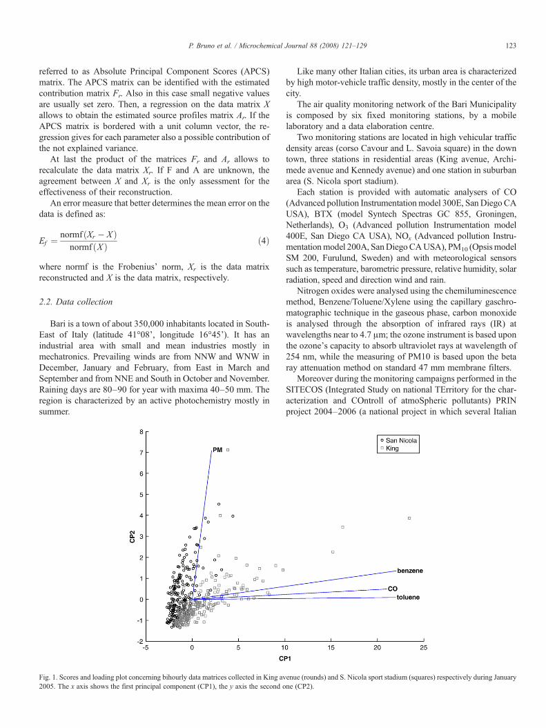
Fig. 1. Scores and loading plot concerning bihourly data matrices collected in King av2005. The x axis shows the first principal component (CP1), the y axis the second o

Like many other Italian cities, its urban area is characterizedby high motor-vehicle traffic density, mostly in the center of thecity.

The air quality monitoring network of the Bari Municipalityis composed by six fixed monitoring stations, by a mobilelaboratory and a data elaboration centre.

Two monitoring stations are located in high vehicular trafficdensity areas (corso Cavour and L. Savoia square) in the downtown, three stations in residential areas (King avenue, Archi-mede avenue and Kennedy avenue) and one station in suburbanarea (S. Nicola sport stadium).

Each station is provided with automatic analysers of CO(Advanced pollution Instrumentationmodel 300E, SanDiego CAUSA), BTX (model Syntech Spectras GC 855, Groningen,Netherlands), O3 (Advanced pollution Instrumentation model400E, San Diego CA USA), NOx (Advanced pollution Instru-mentationmodel 200A, SanDiegoCAUSA), PM10 (OpsismodelSM 200, Furulund, Sweden) and with meteorological sensorssuch as temperature, barometric pressure, relative humidity, solarradiation, speed and direction wind and rain.

Nitrogen oxides were analysed using the chemiluminescencemethod, Benzene/Toluene/Xylene using the capillary gaschro-matographic technique in the gaseous phase, carbon monoxideis analysed through the absorption of infrared rays (IR) atwavelengths near to 4.7 μm; the ozone instrument is based uponthe ozone's capacity to absorb ultraviolet rays at wavelength of254 nm, while the measuring of PM10 is based upon the betaray attenuation method on standard 47 mm membrane filters.

Moreover during the monitoring campaigns performed in theSITECOS (Integrated Study on national TErritory for the char-acterization and COntroll of atmoSpheric pollutants) PRINproject 2004–2006 (a national project in which several Italian

enue (rounds) and S. Nicola sport stadium (squares) respectively during Januaryne (CP2).

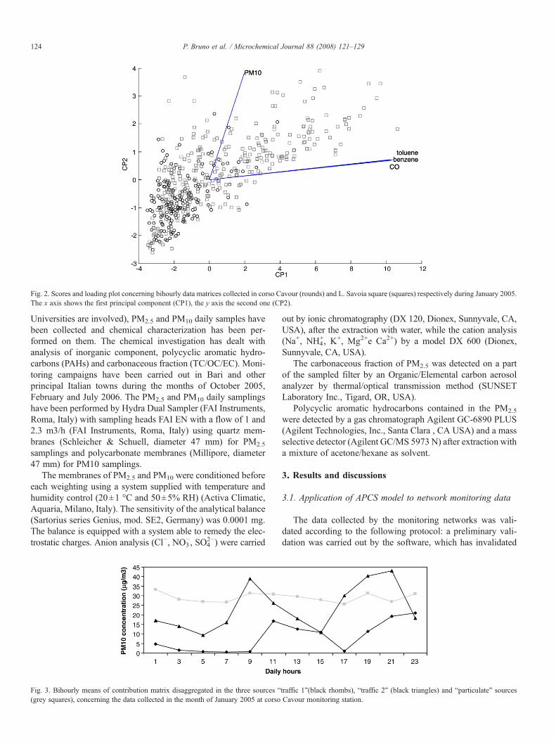
Fig. 2. Scores and loading plot concerning bihourly data matrices collected in corso Cavour (rounds) and L. Savoia square (squares) respectively during January 2005.The x axis shows the first principal component (CP1), the y axis the second one (CP2).

124 P. Bruno et al. / Microchemical Journal 88 (2008) 121–129

Universities are involved), PM2.5 and PM10 daily samples havebeen collected and chemical characterization has been per-formed on them. The chemical investigation has dealt withanalysis of inorganic component, polycyclic aromatic hydro-carbons (PAHs) and carbonaceous fraction (TC/OC/EC). Moni-toring campaigns have been carried out in Bari and otherprincipal Italian towns during the months of October 2005,February and July 2006. The PM2.5 and PM10 daily samplingshave been performed by Hydra Dual Sampler (FAI Instruments,Roma, Italy) with sampling heads FAI EN with a flow of 1 and2.3 m3/h (FAI Instruments, Roma, Italy) using quartz mem-branes (Schleicher & Schuell, diameter 47 mm) for PM2.5

samplings and polycarbonate membranes (Millipore, diameter47 mm) for PM10 samplings.

The membranes of PM2.5 and PM10 were conditioned beforeeach weighting using a system supplied with temperature andhumidity control (20±1 °C and 50±5% RH) (Activa Climatic,Aquaria, Milano, Italy). The sensitivity of the analytical balance(Sartorius series Genius, mod. SE2, Germany) was 0.0001 mg.The balance is equipped with a system able to remedy the elec-trostatic charges. Anion analysis (Cl−, NO3

−, SO42−) were carried

Fig. 3. Bihourly means of contribution matrix disaggregated in the three sources “(grey squares), concerning the data collected in the month of January 2005 at corso

out by ionic chromatography (DX 120, Dionex, Sunnyvale, CA,USA), after the extraction with water, while the cation analysis(Na+, NH4

+, K+, Mg2+e Ca2+) by a model DX 600 (Dionex,Sunnyvale, CA, USA).

The carbonaceous fraction of PM2.5 was detected on a partof the sampled filter by an Organic/Elemental carbon aerosolanalyzer by thermal/optical transmission method (SUNSETLaboratory Inc., Tigard, OR, USA).

Polycyclic aromatic hydrocarbons contained in the PM2.5

were detected by a gas chromatograph Agilent GC-6890 PLUS(Agilent Technologies, Inc., Santa Clara , CA USA) and a massselective detector (Agilent GC/MS 5973 N) after extraction witha mixture of acetone/hexane as solvent.

3. Results and discussions

3.1. Application of APCS model to network monitoring data

The data collected by the monitoring networks was vali-dated according to the following protocol: a preliminary vali-dation was carried out by the software, which has invalidated

traffic 1”(black rhombs), “traffic 2” (black triangles) and “particulate” sourcesCavour monitoring station.

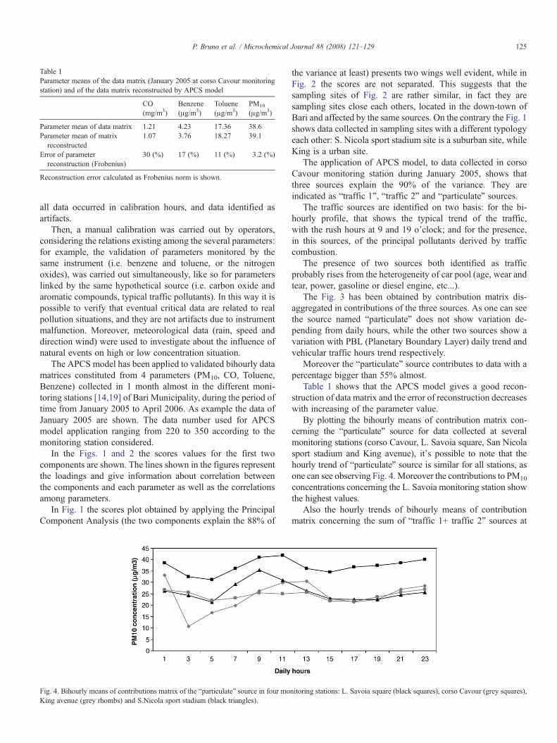
Table 1Parameter means of the data matrix (January 2005 at corso Cavour monitoringstation) and of the data matrix reconstructed by APCS model

CO(mg/m3)

Benzene(μg/m3)

Toluene(μg/m3)

PM10

(μg/m3)

Parameter mean of data matrix 1.21 4.23 17.36 38.6Parameter mean of matrix

reconstructed1.07 3.76 18.27 39.1

Error of parameterreconstruction (Frobenius)

30 (%) 17 (%) 11 (%) 3.2 (%)

Reconstruction error calculated as Frobenius norm is shown.

125P. Bruno et al. / Microchemical Journal 88 (2008) 121–129

all data occurred in calibration hours, and data identified asartifacts.

Then, a manual calibration was carried out by operators,considering the relations existing among the several parameters:for example, the validation of parameters monitored by thesame instrument (i.e. benzene and toluene, or the nitrogenoxides), was carried out simultaneously, like so for parameterslinked by the same hypothetical source (i.e. carbon oxide andaromatic compounds, typical traffic pollutants). In this way it ispossible to verify that eventual critical data are related to realpollution situations, and they are not artifacts due to instrumentmalfunction. Moreover, meteorological data (rain, speed anddirection wind) were used to investigate about the influence ofnatural events on high or low concentration situation.

The APCS model has been applied to validated bihourly datamatrices constituted from 4 parameters (PM10, CO, Toluene,Benzene) collected in 1 month almost in the different moni-toring stations [14,19] of Bari Municipality, during the period oftime from January 2005 to April 2006. As example the data ofJanuary 2005 are shown. The data number used for APCSmodel application ranging from 220 to 350 according to themonitoring station considered.

In the Figs. 1 and 2 the scores values for the first twocomponents are shown. The lines shown in the figures representthe loadings and give information about correlation betweenthe components and each parameter as well as the correlationsamong parameters.

In Fig. 1 the scores plot obtained by applying the PrincipalComponent Analysis (the two components explain the 88% of

Fig. 4. Bihourly means of contributions matrix of the “particulate” source in four moKing avenue (grey rhombs) and S.Nicola sport stadium (black triangles).

the variance at least) presents two wings well evident, while inFig. 2 the scores are not separated. This suggests that thesampling sites of Fig. 2 are rather similar, in fact they aresampling sites close each others, located in the down-town ofBari and affected by the same sources. On the contrary the Fig. 1shows data collected in sampling sites with a different typologyeach other: S. Nicola sport stadium site is a suburban site, whileKing is a urban site.

The application of APCS model, to data collected in corsoCavour monitoring station during January 2005, shows thatthree sources explain the 90% of the variance. They areindicated as “traffic 1”, “traffic 2” and “particulate” sources.

The traffic sources are identified on two basis: for the bi-hourly profile, that shows the typical trend of the traffic,with the rush hours at 9 and 19 o'clock; and for the presence,in this sources, of the principal pollutants derived by trafficcombustion.

The presence of two sources both identified as trafficprobably rises from the heterogeneity of car pool (age, wear andtear, power, gasoline or diesel engine, etc...).

The Fig. 3 has been obtained by contribution matrix dis-aggregated in contributions of the three sources. As one can seethe source named “particulate” does not show variation de-pending from daily hours, while the other two sources show avariation with PBL (Planetary Boundary Layer) daily trend andvehicular traffic hours trend respectively.

Moreover the “particulate” source contributes to data with apercentage bigger than 55% almost.

Table 1 shows that the APCS model gives a good recon-struction of data matrix and the error of reconstruction decreaseswith increasing of the parameter value.

By plotting the bihourly means of contribution matrix con-cerning the “particulate” source for data collected at severalmonitoring stations (corso Cavour, L. Savoia square, San Nicolasport stadium and King avenue), it’s possible to note that thehourly trend of “particulate” source is similar for all stations, asone can see observing Fig. 4. Moreover the contributions to PM10

concentrations concerning the L. Savoia monitoring station showthe highest values.

Also the hourly trends of bihourly means of contributionmatrix concerning the sum of “traffic 1+ traffic 2” sources at

nitoring stations: L. Savoia square (black squares), corso Cavour (grey squares),

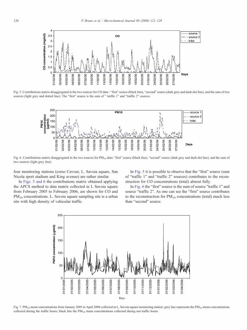
Fig. 6. Contributions matrix disaggregated in the two sources for PM10 data: “first” source (black line), “second” source (dark grey and dash-dot line), and the sum oftwo sources (light grey line).

Fig. 5. Contributions matrix disaggregated in the two sources for CO data : “first” source (black line), “second” source (dark grey and dash-dot line), and the sum of twosources (light grey and dotted line). The “first” source is the sum of ” traffic 1” and “traffic 2” sources.

126 P. Bruno et al. / Microchemical Journal 88 (2008) 121–129

four monitoring stations (corso Cavour, L. Savoia square, SanNicola sport stadium and King avenue) are rather similar.

In Figs. 5 and 6 the contributions matrix obtained applyingthe APCS method to data matrix collected in L Savoia squarefrom February 2005 to February 2006, are shown for CO andPM10 concentrations. L. Savoia square sampling site is a urbansite with high density of vehicular traffic.

Fig. 7. PM10 mean concentrations from January 2005 to April 2006 collected in L. Savcollected during the traffic hours; black line the PM10 mean concentrations collecte

In Fig. 5 it is possible to observe that the “first” source (sumof “traffic 1” and “traffic 2” sources) contributes to the recon-struction for CO concentrations (total) almost fully.

In Fig. 6 the “first” source is the sum of source ”traffic 1” andsource “traffic 2”. As one can see the “first” source contributesto the reconstruction for PM10 concentrations (total) much lessthan “second” source.

oia square monitoring station: grey line represents the PM10 mean concentrationsd during not traffic hours.

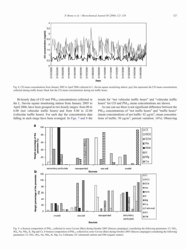
Fig. 8. CO mean concentrations from January 2005 to April 2006 collected in L. Savoia square monitoring station: grey line represents the CO mean concentrationscollected during traffic hours; black line the CO mean concentrations during not traffic hours.

127P. Bruno et al. / Microchemical Journal 88 (2008) 121–129

Bi-hourly data of CO and PM10 concentrations collected inthe L. Savoia square monitoring station from January 2005 toApril 2006, have been grouped in two hourly ranges: from 00 to6.00 (not vehicular traffic hours) and from 8.00 to 22.00(vehicular traffic hours). For each day the concentration datafalling in each range have been averaged. In Figs. 7 and 8 the

Fig. 9. a Sources composition of PM2.5 collected in corso Cavour (Bari) during OctSO4, Na, NH4, K, Mg and Ca. b Sources composition of PM2.5 collected in corso Caparameters: Cl, NO3, SO4, Na, NH4, K, Mg, Ca, Carbonate, EC (elemental carbon)

trends for “not vehicular traffic hours” and “vehicular traffichours” for CO and PM10 mean concentrations are shown.

As one can see there is not significant difference between thePM10 concentrations of “not traffic hours” and “traffic hours”(mean concentrations of not traffic: 42 μg/m3; mean concentra-tions of traffic: 50 μg/m3; percent variation: 16%). Observing

ober 2005 (Sitecos campaigns), considering the following parameters: Cl, NO3,vour (Bari) during October 2005 (Sitecos campaigns) considering the followingand OM (organic matter).

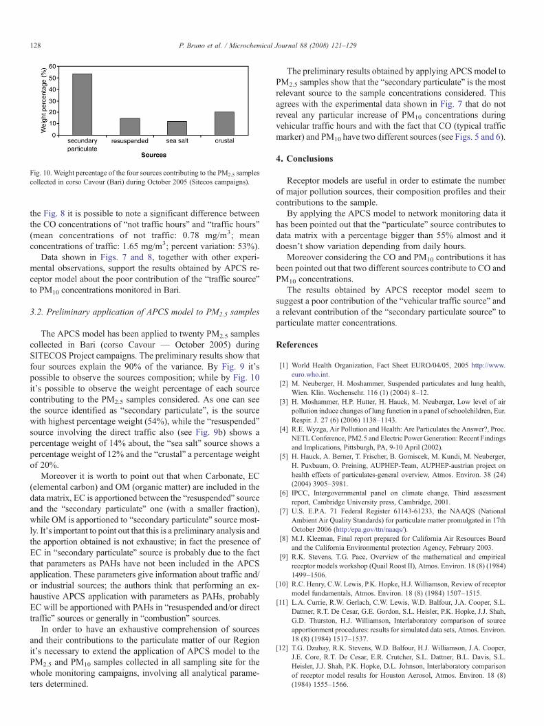
Fig. 10. Weight percentage of the four sources contributing to the PM2.5 samplescollected in corso Cavour (Bari) during October 2005 (Sitecos campaigns).

128 P. Bruno et al. / Microchemical Journal 88 (2008) 121–129

the Fig. 8 it is possible to note a significant difference betweenthe CO concentrations of “not traffic hours” and “traffic hours”(mean concentrations of not traffic: 0.78 mg/m3; meanconcentrations of traffic: 1.65 mg/m3; percent variation: 53%).

Data shown in Figs. 7 and 8, together with other experi-mental observations, support the results obtained by APCS re-ceptor model about the poor contribution of the “traffic source”to PM10 concentrations monitored in Bari.

3.2. Preliminary application of APCS model to PM2.5 samples

The APCS model has been applied to twenty PM2.5 samplescollected in Bari (corso Cavour — October 2005) duringSITECOS Project campaigns. The preliminary results show thatfour sources explain the 90% of the variance. By Fig. 9 it'spossible to observe the sources composition; while by Fig. 10it's possible to observe the weight percentage of each sourcecontributing to the PM2.5 samples considered. As one can seethe source identified as “secondary particulate”, is the sourcewith highest percentage weight (54%), while the “resuspended”source involving the direct traffic also (see Fig. 9b) shows apercentage weight of 14% about, the “sea salt” source shows apercentage weight of 12% and the “crustal” a percentage weightof 20%.

Moreover it is worth to point out that when Carbonate, EC(elemental carbon) and OM (organic matter) are included in thedata matrix, EC is apportioned between the “resuspended” sourceand the “secondary particulate” one (with a smaller fraction),while OM is apportioned to “secondary particulate” source most-ly. It's important to point out that this is a preliminary analysis andthe apportion obtained is not exhaustive; in fact the presence ofEC in “secondary particulate” source is probably due to the factthat parameters as PAHs have not been included in the APCSapplication. These parameters give information about traffic and/or industrial sources; the authors think that performing an ex-haustive APCS application with parameters as PAHs, probablyEC will be apportioned with PAHs in “resuspended and/or directtraffic” sources or generally in “combustion” sources.

In order to have an exhaustive comprehension of sourcesand their contributions to the particulate matter of our Regionit's necessary to extend the application of APCS model to thePM2.5 and PM10 samples collected in all sampling site for thewhole monitoring campaigns, involving all analytical parame-ters determined.

The preliminary results obtained by applying APCS model toPM2.5 samples show that the “secondary particulate” is the mostrelevant source to the sample concentrations considered. Thisagrees with the experimental data shown in Fig. 7 that do notreveal any particular increase of PM10 concentrations duringvehicular traffic hours and with the fact that CO (typical trafficmarker) and PM10 have two different sources (see Figs. 5 and 6).

4. Conclusions

Receptor models are useful in order to estimate the numberof major pollution sources, their composition profiles and theircontributions to the sample.

By applying the APCS model to network monitoring data ithas been pointed out that the “particulate” source contributes todata matrix with a percentage bigger than 55% almost and itdoesn’t show variation depending from daily hours.

Moreover considering the CO and PM10 contributions it hasbeen pointed out that two different sources contribute to CO andPM10 concentrations.

The results obtained by APCS receptor model seem tosuggest a poor contribution of the “vehicular traffic source” anda relevant contribution of the “secondary particulate source” toparticulate matter concentrations.

References

[1] World Health Organization, Fact Sheet EURO/04/05, 2005 http://www.euro.who.int.

[2] M. Neuberger, H. Moshammer, Suspended particulates and lung health,Wien. Klin. Wochenschr. 116 (1) (2004) 8–12.

[3] H. Moshammer, H.P. Hutter, H. Hauck, M. Neuberger, Low level of airpollution induce changes of lung function in a panel of schoolchildren, Eur.Respir. J. 27 (6) (2006) 1138–1143.

[4] R.E. Wyzga, Air Pollution and Health: Are Particulates the Answer?, Proc.NETLConference, PM2.5 and Electric Power Generation: Recent Findingsand Implications, Pittsburgh, PA, 9-10 April (2002).

[5] H. Hauck, A. Berner, T. Frischer, B. Gomiscek, M. Kundi, M. Neuberger,H. Puxbaum, O. Preining, AUPHEP-Team, AUPHEP-austrian project onhealth effects of particulates-general overview, Atmos. Environ. 38 (24)(2004) 3905–3981.

[6] IPCC, Intergovernmental panel on climate change, Third assessmentreport, Cambridge University press, Cambridge, 2001.

[7] U.S. E.P.A. 71 Federal Register 61143-61233, the NAAQS (NationalAmbient Air Quality Standards) for particulate matter promulgated in 17thOctober 2006 (http:/epa.gov/ttn/naaqs/).

[8] M.J. Kleeman, Final report prepared for California Air Resources Boardand the California Environmental protection Agency, February 2003.

[9] R.K. Stevens, T.G. Pace, Overview of the mathematical and empiricalreceptor models workshop (Quail Roost II), Atmos. Environ. 18 (8) (1984)1499–1506.

[10] R.C. Henry, C.W. Lewis, P.K. Hopke, H.J. Williamson, Review of receptormodel fundamentals, Atmos. Environ. 18 (8) (1984) 1507–1515.

[11] L.A. Currie, R.W. Gerlach, C.W. Lewis, W.D. Balfour, J.A. Cooper, S.L.Dattner, R.T. De Cesar, G.E. Gordon, S.L. Heisler, P.K. Hopke, J.J. Shah,G.D. Thurston, H.J. Williamson, Interlaboratory comparison of sourceapportionment procedures: results for simulated data sets, Atmos. Environ.18 (8) (1984) 1517–1537.

[12] T.G. Dzubay, R.K. Stevens, W.D. Balfour, H.J. Williamson, J.A. Cooper,J.E. Core, R.T. De Cesar, E.R. Crutcher, S.L. Dattner, B.L. Davis, S.L.Heisler, J.J. Shah, P.K. Hopke, D.L. Johnson, Interlaboratory comparisonof receptor model results for Houston Aerosol, Atmos. Environ. 18 (8)(1984) 1555–1566.

129P. Bruno et al. / Microchemical Journal 88 (2008) 121–129

[13] G.E. Gordon, W.R. Pierson, J.M. Daisey, P.J. Lioy, J.A. Cooper, J.G.Watson, G.R. Cass, Considerations for design of source apportionmentstudies, Atmos. Environ. 18 (8) (1984) 1567–1582.

[14] P. Bruno, M. Caselli, G. de Gennaro, A. Traini, Source apportionment ofgaseous atmospheric pollutants bymeans of an absolute principal componentscores (APCS) receptor model, Fresen. J Anal. Chem. 371 (8) (2001)1119–1123.

[15] G.M. Marcazzan, M. Ceriani, G. Valli, R. Vecchi, Source apportionment ofPM10 and PM2.5 in Milan (Italy) using receptor modelling, Sci. TotalEnviron. 317 (1-2) (2003) 137–147.

[16] H. Guo, T. Wang, P.K.K. Louie, Source apportionment of ambient non-methane hydrocarbons in Hong Kong: application of a principal com-ponent analysis/absolute principal component scores (PCA/APCS)receptor model, Environ. Pollut. 129 (3) (2004) 489–498.

[17] G.D. Thurston, J.D. Spengler, A quantitative assessment of source con-tributions to inhalable particulate matter pollution in metropolitan Boston,Atmos. Environ. 19 (1) (1985) 9–26.

[18] C.P. Chio, M.T. Cheng, C.F. Wang, Source apportionment to PM in dif-ferent air quality conditions for Taichung urban and coastal areas, Taiwan,Atmos. Environ. 38 (39) (2004) 6893–6905.

[19] M. Caselli, G. de Gennaro, P. Ielpo, A comparison between two receptormodels to determine the source apportionment of atmospheric pollutants,Environmetrics 17 (5) (2006) 507–516.

[20] P. Ielpo, Heavy Metals and Atmospheric Particulate: ChromatographicAnalysis, Electron Microscopy and Source Apportionment; Ph.D. Thesis,stored in National Public Library of Rome and Florence (BNI0013860),Italy, 2004, p. 185.