ARTICLE IN PRESS

1352-2310/$ - se

doi:10.1016/j.at

�CorrespondE-mail addr

Atmospheric Environment 40 (2006) S563–S573

www.elsevier.com/locate/atmosenv

Uncertainty in air quality model evaluation for particulatematter due to spatial variations in pollutant concentrations

Sun-Kyoung Park�, Charles Evan Cobb, Katherine Wade, James Mulholland,Yongtao Hu, Armistead G. Russell

School of Civil and Environmental Engineering, Georgia Institute of Technology, 311 Ferst Drive NW, Atlanta, GA 30332-0512, USA

Received 30 July 2005; received in revised form 25 October 2005; accepted 1 November 2005

Abstract

Air quality model performance is usually evaluated by examining the relative agreement between volume-averaged

simulations and point measurements, as volume-averaged measurements are seldom available. Because the two values have

different spatial scales, accurate model evaluation is complicated by this mismatch in areas when the pollutant gradient is

large. Uncertainty in the air quality model evaluation from the spatial variability of PM2.5 is quantitatively examined, and

how much of model error might be explained by such variability is calculated. Added uncertainty of model performance is

analyzed by comparing performance metrics between simulated concentrations and observations at one station between

simulated levels and interpolated fields from observations. Normalized differences of the performance metrics (e.g., mean

fractional error, MFE) calculated in these two ways indicate the uncertainty of the model performance due to spatial

variation. Normalized difference of MFE for PM2.5 mass is approximately 17% in July 2001 and 15% in January 2002. To

decrease the uncertainty, it has been suggested that observations be used only from spatially representative stations. When

model performance is calculated with data from spatially representative stations, uncertainty decreased, and overall model

performance improves. For example, MFE is seen to decrease up to 14% for PM2.5 mass and species concentrations,

suggesting that up to 14% of MFE can be explained by the spatial variability of PM2.5. These results indicate that

comparison between observed and simulated concentrations should not be used alone to assess performance of air quality

models. Also, spatial variability should be considered in setting model performance goals.

r 2006 Elsevier Ltd. All rights reserved.

Keywords: Model performance; Spatial variability; Representative stations

1. Introduction

Grid-based photochemical air quality models areessential tools for use in air quality managementand scientific investigation. Using these models forsuch applications with confidence necessitates thor-ough model evaluation, which traditionally is

e front matter r 2006 Elsevier Ltd. All rights reserved

mosenv.2005.11.078

ing author. Tel.: +1817 642 0850.

ess: helena@themis.ce.gatech.edu (S.-K. Park).

achieved by comparing simulated concentrationswith those observed. However, such a performanceassessment has limitations that arise from themodeling method and observations. Ideally, pre-dicted concentrations should be compared withvolume-averaged measurements, but volume-aver-aged measured concentrations are seldom available.Monitoring stations cannot be mounted densely inwide regions due to cost, and there are fewtechniques that directly provide volume-averaged

.

ARTICLE IN PRESSS.-K. Park et al. / Atmospheric Environment 40 (2006) S563–S573S564

concentrations. Thus, simulated concentrations areusually compared with concentrations measured atspecific monitoring locations, with each monitorrepresenting a point (in space) measurement. Con-centrations measured at monitoring sites can differsubstantially from average concentrations in thearea if pollutant concentration gradients are high.Therefore, model performance evaluated by com-paring between point observations and volume-averaged simulations may not represent how wellthe model actually simulates air pollution dynamics.

The implication of the spatial inhomogeneity on airquality model performance has been investigated byquantifying the spatial variability for ozone (O3),carbon monoxide (CO), and nitrogen oxide (NO)from the difference between the measurement at themonitor and the interpolated concentrations fromother monitors (McNair et al., 1996). Because theamount of spatial variability was similar to that of theair quality model error, the authors concluded thatspatial variability in observed pollutant concentra-tions should be taken into account in developingmodel performance guidelines. In a separate study, aquantitative measure for the spatial representativenessof ground level ozone concentrations is analyzed usingthe hourly ozone concentrations at 300 monitors inGermany as a means to compare modeled andmeasured data (Tilmes and Zimmermann, 1998). Thisanalysis suggested that a radius of representativness isabout 4km for ozone. The evaluation of models withgrid sizes larger than 4km may have substantial errordue to spatial variation. While there is an awarenessthat model performance depends on spatial varia-bility, there has been no effort to analyze thedependency quantitatively.

Here, observations and air quality model resultsare used to quantify spatial variability in particulatematter and how that adds uncertainty in modelevaluation for both individual PM2.5 species andtotal mass. In this paper, the amount of calculatedmodel error ‘‘error’’ that might be explained by suchvariability at the regional scale is investigated, andways to reduce added uncertainty in model perfor-mance evaluation are proposed.

2. Methods

Pollutant concentrations studied for spatial ana-lysis and model evaluation include daily PM2.5 massand various species (sulfate, nitrate, ammonium,elemental carbon, and organic carbon) with parti-cular focus on the Atlanta area for 2 years

(2002–2003) and over the continental United Statesarea for July 2001 and January 2002. The latter two1-month periods have additional observations aspart of the eastern supersite program (ESP 01/02).Monitoring data were obtained from the assessmentof spatial aerosol composition in atlanta (ASACA)project (Butler et al., 2003), the southeastern aerosolresearch and characterization (SEARCH) study(Hansen et al., 2003), the environmental protectionagency’s speciated trends network (EPA-STN)databases (Jang et al., 2004), and the interagencymonitoring of protected visual environments (IM-PROVE) network (Ames and Malm, 2001; Fig. 1).

EPA’s Models-3 was applied over a domaincovering the United States using the unified regionalplanning organization (RPO) national grid with a36 km resolution (Fig. 2). Models-3 used includesthe community multi-scale air quality (CMAQ v4.3)model (Byun and Ching, 1999), the sparse matrixoperator kernel emissions (SMOKE v1.5) (US-EPA,2004), and NCAR’s fifth generation mesoscalemodel (MM5 v3.5.3) for meteorological modeling(NCAR, 2003) (see Table 1 for details). Meteor-ological fields were evaluated with the Barnesobjective analysis scheme (Koch et al., 1983) usingthe TDL surface hourly data (UCAR, 2003), whichwere not used in the four-dimensional data assim-ilation. Mean errors (MEs) in temperature,specific humidity, and wind speed were 1.7/2.1 1C(July 2001/January 2002), 1.8/0.5 g kg�1 and 1.3/1.4m s�1, respectively (Park and Russell, 2003).These values are within the benchmarks for themetrological model evaluation (Emery et al., 2001).

Concentrations from one monitor are comparedwith the concentrations in the area surrounding themonitor to calculate the spatial inhomogeneity. In theAtlanta area, PM2.5 concentrations in the surround-ing area were calculated using the average of PM2.5

concentrations from other monitors located within120km. In the United States, some locations have lessthan four monitors within 120km, so monitors within180km were used to calculate concentrations in thesurrounding area. Average concentrations werecalculated by an inverse-distance-squared interpola-tion (McNair et al., 1996):

IðmÞ ¼

PNi¼1; iamOi

nW iPNi¼1; iamW i

, (1)

where I(m) is the interpolated pollutant concentrationfor station m, N is the number of monitoring stations,Oi is the observed pollutant concentration at station i,

ARTICLE IN PRESS

Fig. 1. (a) Horizontal and vertical structures of the air quality model domain, and PM2.5 species and mass monitors in the United States.

(b) PM2.5 species and mass monitors in Atlanta. (c) PM2.5 mass monitors in one grid of the air quality model.

S.-K. Park et al. / Atmospheric Environment 40 (2006) S563–S573 S565

ARTICLE IN PRESS

PM2.5 (Jul. 2001) PM2.5 (Jan. 2002)Sulfate (Jul. 2001) Sulfate (Jan. 2002)Nitrate (Jul. 2001) Nitrate (Jan. 2002)Ammonium (Jul. 2001) Ammonium (Jan. 2002)OC (Jul. 2001) OC (Jan. 2002)EC (Jul. 2001) EC (Jan. 2002)Soil dust (Jul. 2001) Soil dust (Jan. 2002)AQM objective*

MFE|Pred. vs. Point obs.

0

50

100

150

200

0 10 15 20

MF

E [%

]

MFE|Interp. obs. vs. Point obs.

0

50

100

150

200

0 10 15 20

(CInterp.obs. + CPoint obs.) / 2 (µg m-3)

(CPred. + CPoint obs.) / 2 (µg m-3)

MF

E [%

]

5

5

(a)

(b)

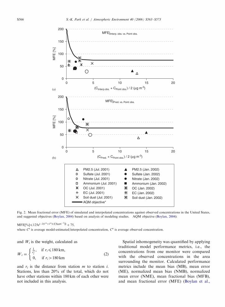
Fig. 2. Mean fractional error (MFE) of simulated and interpolated concentrations against observed concentrations in the United States,

and suggested objectives (Boylan, 2004) based on analysis of modeling studies. �AQM objective (Boylan, 2004):

MFE½%�p125e �2ðCoþCeÞð Þ= 3½mgm�3 �ð Þ þ 75,

where Ce is average model-estimated/interpolated concentration, Co is average observed concentration.

S.-K. Park et al. / Atmospheric Environment 40 (2006) S563–S573S566

and Wi is the weight, calculated as

W i ¼

1

r2i

; if rip180 km;

0; if ri4180 km

((2)

and ri is the distance from station m to station i.Stations, less than 20% of the total, which do nothave other stations within 180km of each other werenot included in this analysis.

Spatial inhomogeneity was quantified by applyingtraditional model performance metrics, i.e., theconcentrations from one monitor were comparedwith the observed concentrations in the areasurrounding the monitor. Calculated performancemetrics include the mean bias (MB), mean error(ME), normalized mean bias (NMB), normalizedmean error (NME), mean fractional bias (MFB),and mean fractional error (MFE) (Boylan et al.,

ARTICLE IN PRESS

Table 1

Detailed information of the air quality modeling system

Model Index Comments

CMAQ Chemistry SAPRC99

Chemistry solver Modified Euler backward iterative (MEBI)

Aerosol equilibrium ISORROPIA

Aerosol dynamics AERO3

Deposition veloicity AERO_DEPV2

Advection (horizontal and vertical) Piecewise parabolic method (PPM)

Cloud processing Regional acid deposition model (RADM)

SMOKE Anthropogenic

emissions

Inventory Survey from fall line air quality (FAQS) project for GA

Growth factor 1999 NEI final v2.0 for other states (0.25 was multiplied to fugitive

dust emissions)

EGAS 4.0

Hourly

emissions

Continuous emission monitoring (CEM) for major point sources

(NOx, SO2)

Spatial

surrogate

Based on the 2000 census data

Biogenic emissions Biogenic emission land cover database v3 (BELD3)

MM5 Microphysics Simple ice microphysics

Cumulus scheme Kain–Fritsch

Boundary layer Pleim–Chang

Radiation scheme Rapid radiative transfer model (RRTM)

Land surface model Pleim–Xiu

Data for four dimensional data

assimilation

NCEP ETA model outputs for the GCIP project

NCEP ADP observation data

S.-K. Park et al. / Atmospheric Environment 40 (2006) S563–S573 S567

2005). Carbon concentrations were measured bytwo different methods, thermal optical transmit-tance (TOT) and thermal optical reflectance (TOR).Sites from ASACA and STN used TOT, and thosefrom IMPROVE and SEARCH used TOR. Thus,the surrounding concentrations for organic andelemental carbon concentrations were calculatedseparately.

Uncertainty in the model performance introducedby spatial variation was quantified over the UnitedStates by comparing performance metrics betweensimulated concentrations and observations at onestation with that between simulated levels andinterpolated fields from observations at surroundingstations. The difference of the performance metricscalculated in the two different ways at each stationcorresponds to the uncertainty of the modelperformance due to spatial variation for that station.

3. Results and discussion

3.1. Spatial variability of particulate matter

Spatial variability was calculated using perfor-mance metrics that compare observed concentra-

tions at each monitor with observed concentrationsin the surrounding area of the monitor. The spatialvariability was calculated separately for the Atlantaarea using data from 2002 to 2003 (Table 2), and forthe United States using data for July 2001 andJanuary 2002 (Table 3 and Fig. 2(a)). Because theaverage observation (for Atlanta) and the inter-polated concentration (for the United States) werederived from observations in the surroundingmonitors, the bias measures (MB, NMB, MFB)are very small, and do not have important implica-tions. Spatial variability and the possible impacts oncalculated model performance can be judged basedon the error metrics (ME, NME, MFE). Spatialvariability of PM2.5 species leads to MFEs of30–59% in Atlanta (Table 2), and MFEs of28–84% in the United States for different species(Table 3 and Fig. 2(a)).

Spatial variability was higher for primary pollu-tants (e.g., elemental carbon and soil dust) andlower for secondary pollutants (e.g., sulfate, nitrateand ammonium), in general. Spatial variability indifferent species can be explained by particularemissions and formation characteristics. Sulfate hadthe lowest spatial variability among the PM2.5

ARTICLE IN PRESS

Table 3

Spatial variability of PM2.5 mass and species in the United States calculated using data in all stations

Species Period Number

of sites

Number

of obs.

Mean obs.

conc.

(mgm�3)

MB

(mgm�3)ME

(mgm�3)NMB

(%)

NME

(%)

MFB

(%)

MFE

(%)

PM2.5 total

mass

Jul. 2001 1206 14,798 13.22 0.28 2.41 2.1 18.2 5.3 20.4

Jan. 2002 1153 14,160 12.35 0.48 3.26 3.9 26.4 9.6 30.0

Sulfate Jul. 2001 189 1855 3.81 0.05 0.88 1.4 23.0 4.7 28.1

Jan. 2002 189 1695 1.60 0.06 0.43 3.4 27.1 11.0 40.8

Nitrate Jul. 2001 176 1630 0.48 0.03 0.32 5.5 67.2 12.7 52.1

Jan. 2002 171 1501 1.78 0.12 1.09 6.8 61.2 17.5 66.8

Ammonium Jul. 2001 69 863 1.64 0.00 0.58 0.3 35.5 5.4 37.3

Jan. 2002 64 654 1.49 0.03 0.47 2.0 31.5 5.1 38.3

Organic

carbon

Jul. 2001 189 1910 2.79 0.17 1.56 6.0 55.8 12.3 55.0

Jan. 2002 183 1675 2.44 0.27 1.76 11.2 72.2 22.3 72.5

Elemental

carbon

Jul. 2001 189 1907 0.43 0.04 0.25 10.2 58.0 14.6 55.6

Jan. 2002 183 1660 0.50 0.05 0.38 10.5 76.6 19.1 69.8

Soil dust Jul. 2001 59 497 4.81 0.09 2.92 1.9 60.6 6.1 61.4

Jan. 2002 55 386 2.44 0.03 1.97 1.2 80.8 5.2 83.6

Table 2

Spatial variability of PM2.5 mass and species in the Atlanta area from January 2002 to December 2003

Species Number of

obs.

Mean conc.

(mgm�3)MB

(mgm�3)ME

(mgm�3)NMB

(%)

NME

(%)

MFB

(%)

MFE

(%)

PM2.5 total mass 2903 17.50 0.09 2.20 0.5 12.6 2.0 13.2

Sulfate 2781 4.10 �0.02 1.23 �0.6 30.0 6.2 31.4

Nitrate 2732 0.91 �0.01 0.34 �0.9 37.5 8.7 38.7

Ammonium 2611 1.52 �0.02 0.50 �1.4 33.2 6.5 37.9

Organic carbon 2045 4.70 0.00 1.83 0.0 38.9 2.9 41.9

Elemental carbon 1890 0.81 0.00 0.47 0.0 58.0 4.1 59.4

Total carbon 2349 5.65 �0.06 1.54 �1.0 27.3 4.3 29.5

Soil dust 1758 5.57 0.26 2.47 4.7 44.3 13.2 46.3

S.-K. Park et al. / Atmospheric Environment 40 (2006) S563–S573S568

species. Sulfate is primarily formed either from thegas-to-particle conversion of SO2 in the atmosphereor from reactions in the aqueous phase. Because ofthe slow rates of formation and removal, sulfatebecomes relatively well mixed (Roberts and Fried-lander, 1980). Nitrate is also a secondary pollutantproduced by the oxidation of NOx (NO+NO2).The oxidation rate of NOx ranges from 5% to 50%per hour (Spicer et al., 1981), faster than that ofSO2. Also, nitric acid deposits rapidly. Thus, nitrateis spatially less homogeneously distributed thansulfate. Ammonium is also a secondary pollutantformed as ammonia (NH3) neutralizes H2SO4 andHNO3. The amount of ammonium is highlydependent on the relative amounts of H2SO4 andNH3. Spatial variability of ammonium is also

relatively small, usually being dominated by itsassociation with sulfate. Soil dust is a directemission and settles relatively rapidly, so spatialvariability of soil dust and its associated elements isvery high. Because elemental carbon is a primarypollutant, the spatial variability is relatively high.Major sources of elemental carbon include dieselengines, particularly heavy-duty trucks, wood burn-ing fireplaces and furnaces, and meat cookingcombustion process (Gray and Cass, 1998). Organiccarbon is emitted directly or formed from thecondensation of low-volatility hydrocarbons. Thus,the spatial variability of organic carbon is betweenthat of purely primary and secondary pollutants.Major primary sources of organic carbon includediesel and gasoline-burning engines, wood burning,

ARTICLE IN PRESSS.-K. Park et al. / Atmospheric Environment 40 (2006) S563–S573 S569

meat cooking operations, some industrial processes,and biogenic sources (Zheng et al., 2002).

3.2. Uncertainty of air quality model performance

due to spatial variation

The air quality model was evaluated by compar-ing the volume-averaged simulated concentrationswith the point measurements in the United States(Table 4) using six performance metrics (Boylanet al., 2005). In addition to performance metricsused to assess spatial variability, MB, NMB andMFB are included and, have important implica-tions. In particular, the MFE was compared withproposed air quality model objectives as MFE isconsidered a key indicator (Boylan et al., 2005). Allspecies except nitrate and those associated with soildust in January 2002 met the objectives (Fig. 2(b)).Nitrate is difficult to model due to its volatility andits sensitivity to temperature, relative humidity, andammonia availability (Russell et al., 1983). Soil dustemissions are uncertain (Pace, 2003). Model perfor-mance was better for secondary species, such assulfate and ammonium, than it was for primaryspecies, such as elemental carbon and soil dust.Similar to the previous study (McNair et al., 1996),model performance is compared to spatial varia-bility (Figs. 3(a) and (b)). Not surprisingly, MFEbetween simulated and observed concentrations waslarger than MFE of interpolated and observedconcentrations, though for some species, the differ-ence is remarkably small. This result also suggeststhat the added uncertainty in the model error from

Table 4

Overall air quality model performance for PM2.5 mass and species in t

Species Period MB (mgm�3) ME (mgm�3)

PM2.5 total mass Jul. 2001 0.50 4.70

Jan. 2002 5.24 8.80

Sulfate Jul. 2001 1.34 1.95

Jan. 2002 0.12 0.86

Nitrate Jul. 2001 �0.11 0.39

Jan. 2002 2.87 3.48

Ammonium Jul. 2001 0.53 0.93

Jan. 2002 1.27 1.69

Organic carbon Jul. 2001 �1.50 1.81

Jan. 2002 �1.12 1.54

Elemental carbon Jul. 2001 0.19 0.38

Jan. 2002 0.14 0.40

Soil dust Jul. 2001 �1.81 2.91

Jan. 2002 2.90 3.67

the spatial inhomogeneity should not be ignored.This issue is further examined below.

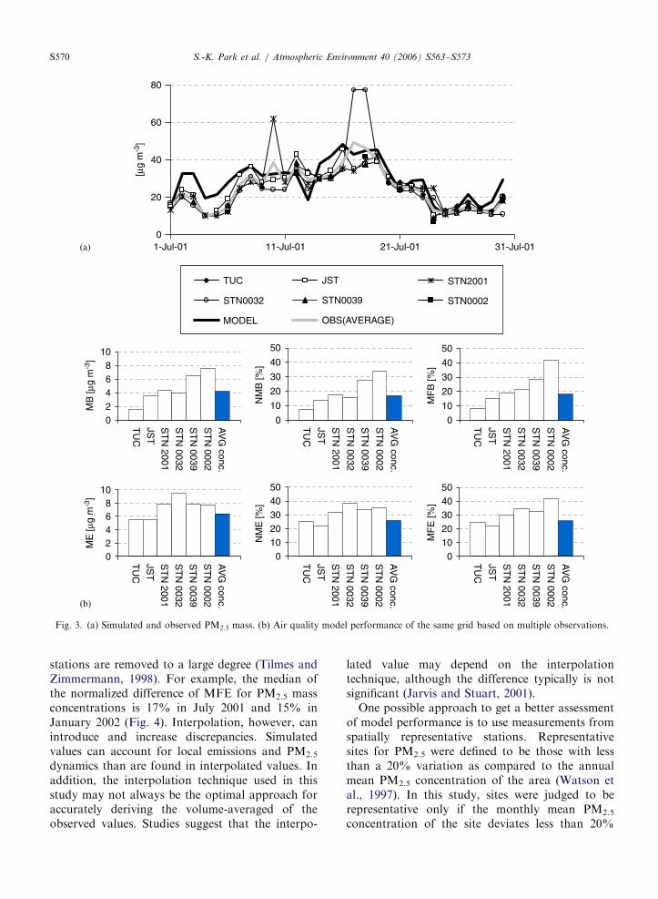
One of the model grids located over the Atlantaarea contains six PM2.5 mass monitors: FireStation 8 (STN0039), Jefferson Street (JST),E. Rivers School (STN0032), Doraville healthcenter (STN2001), Tucker (TUC), Gwinnett Tech(STN0002) (Fig. 1(c)). Although these six monitorsare located in the same grid, they have differentdaily PM2.5 total masses showing that significantspatial variability of pollutant concentrations existswithin 36 km (Fig. 3(a)). Thus, air quality modelperformance differed when observations from dif-ferent monitors are used. Also, the model perfor-mance calculated using the observation at themonitor is markedly different from that usingthe average observation. These results suggest thatthe air quality model performance evaluated usingpoint measurement includes uncertainty due topollutant gradients (Fig. 3(b)).

Uncertainty of the model performance fromspatial variation was investigated over the UnitedStates by comparing performance metrics betweensimulated concentrations and observations at onestation with those between simulated levels andinterpolated fields from observations. The normal-ized difference of the performance metrics calcu-lated in two different ways at each stationcorresponds to the added uncertainty of the modelperformance due to spatial variation for thatstation. Median, 25th and 75th percentiles of thenormalized difference from the two performancemetrics are plotted in Fig. 4. By representing 25thand 75th percentiles, effects of the varying types of

he United States calculated using data in all stations

NMB (%) NME (%) MFB (%) MFE (%)

3.8 35.5 2.7 37.6

42.4 71.2 26.2 58.1

35.2 51.4 23.2 49.0

7.2 53.8 15.8 62.6

�22.0 81.9 �80.3 112.1

160.8 195.1 74.6 109.8

32.4 56.5 31.4 58.0

85.2 113.0 51.1 77.5

�53.6 64.7 �58.0 81.4

�45.8 63.1 �30.6 78.7

43.0 87.2 9.1 63.6

26.9 80.6 �1.9 67.8

�37.5 60.4 �26.2 68.5

118.8 150.6 68.4 91.8

ARTICLE IN PRESS

02468

10

02468

10

MB

[µg

m-3

]M

E [µ

g m

-3]

TU

C

AV

G conc.

ST

N 0002

ST

N 0039

ST

N 0032

ST

N 2001

JST

TU

C

AV

G conc.

ST

N 0002

ST

N 0039

ST

N 0032

ST

N 2001

JST

TU

C

AV

G conc.

ST

N 0002

ST

N 0039

ST

N 0032

ST

N 2001

JST

TU

C

AV

G conc.

ST

N 0002

ST

N 0039

ST

N 0032

ST

N 2001

JST

TU

C

AV

G conc.

ST

N 0002

ST

N 0039

ST

N 0032

ST

N 2001

JST

TU

C

AV

G conc.

ST

N 0002

ST

N 0039

ST

N 0032

ST

N 2001

JST

0

10

20

30

40

50

NM

B [%

]

01020304050

NM

E [%

]

100

20304050

MF

E [%

]0

10

20

30

40

50

MF

B [%

]

0

20

40

60

80

1-Jul-01 11-Jul-01 21-Jul-01 31-Jul-01

[µg

m-3

]

TUC JST STN2001

STN0032 STN0039 STN0002

MODEL OBS(AVERAGE)

(a)

(b)

Fig. 3. (a) Simulated and observed PM2.5 mass. (b) Air quality model performance of the same grid based on multiple observations.

S.-K. Park et al. / Atmospheric Environment 40 (2006) S563–S573S570

stations are removed to a large degree (Tilmes andZimmermann, 1998). For example, the median ofthe normalized difference of MFE for PM2.5 massconcentrations is 17% in July 2001 and 15% inJanuary 2002 (Fig. 4). Interpolation, however, canintroduce and increase discrepancies. Simulatedvalues can account for local emissions and PM2.5

dynamics than are found in interpolated values. Inaddition, the interpolation technique used in thisstudy may not always be the optimal approach foraccurately deriving the volume-averaged of theobserved values. Studies suggest that the interpo-

lated value may depend on the interpolationtechnique, although the difference typically is notsignificant (Jarvis and Stuart, 2001).

One possible approach to get a better assessmentof model performance is to use measurements fromspatially representative stations. Representativesites for PM2.5 were defined to be those with lessthan a 20% variation as compared to the annualmean PM2.5 concentration of the area (Watson etal., 1997). In this study, sites were judged to berepresentative only if the monthly mean PM2.5

concentration of the site deviates less than 20%

ARTICLE IN PRESS

MB

0

100

200

300

400

PM2.5 SO4-2 NO3

- NH4+ OC EC Soil

[%]

NMB

0

100

200

300

[%]

NME

0

30

60

90

[%]

MFB

0

100

200

300

[%]

MFE

0

20

40

60

80

[%]

ME

0

50

100

150

[%]

July 2001

January 2002

75th percentile

median

25th percentile

PM2.5 SO4-2 NO3

- NH4+ OC EC Soil

PM2.5 SO4-2 NO3

- NH4+ OC EC Soil PM2.5 SO4

-2 NO3- NH4

+ OC EC Soil

PM2.5 SO4-2 NO3

- NH4+ OC EC Soil PM2.5 SO4

-2 NO3- NH4

+ OC EC Soil

(a)

(b)

(c)

(d)

(e)

(f)

Fig. 4. Normalized differences� in performance metrics between simulations and observations from that between simulated levels and

interpolated fields for each station in the United States. �Normalized difference of MB:

MBjprediction vs: interpolation �MBjprediction vs: observation

MBjprediction vs: observation

��������� 100 ð%Þ.

S.-K. Park et al. / Atmospheric Environment 40 (2006) S563–S573 S571

from that calculated by interpolating pollutantconcentrations from other stations located within180 km (Eqs. (1) and (2)). From 20% to 30% of thetotal stations were found to be representative forprimary species, and from 50% to 70% forsecondary species. As expected, the number ofrepresentative stations for primary species wasmuch smaller than that for secondary species.

Uncertainty in model performance from spatialvariation decreased when only spatially representa-tive stations are used to calculate model perfor-mance. For example, the median of normalized

differences of MFE for PM2.5 mass concentrationcalculated with two different methods decreasedfrom 17% to 14% in July 2001 and from 15% to10% in January 2002. In addition, overall modelperformance of PM2.5 from spatially representativestations improved when compared with the perfor-mance of PM2.5 from all stations. Among perfor-mance metrics, MFE decreased up to 14%;however, it actually increased in two cases: organiccarbon and soil dust in January 2002 (Fig. 5). Soildust was poorly simulated in this period, furthersuggesting that more basic issues are involved (e.g.,

ARTICLE IN PRESS

-16

-12

-8

-4

0

4

PM2.5total mass

Sulfate Nitrate Ammonium Organiccarbon

Elementalcarbon

Soil dust

[%]

Jul. 2001 Jan. 2002

Fig. 5. Normalized change� of mean fractional error between simulations and observations for all stations from that between simulations

and observations for representative stations. �Normalized change of MFE:

MFEjrepresentative stations �MFEjall stations

MFEjall stations

� 100 ð%Þ.

S.-K. Park et al. / Atmospheric Environment 40 (2006) S563–S573S572

an inaccurate inventory). In a separate investigation(Park et al., submitted), it was found that soil dustlevels increase with wind, which is not surprising.On the other hand, the inventory remains constantand higher winds tend to dilute the emissions moreleading to lower simulated concentrations.

The analyses performed in this paper suggest thatspatial variability contributes to uncertainty inmodel performance. However, spatial variabilityaffected the overall model performance only amoderate amount, implying that there are othersources of the model error, such as emissioninventory, meteorology, chemical mechanism para-meters, and numerical routine that contribute themodel error significantly. Further investigation ofthese sources of uncertainty should be conducted inthe future.

4. Conclusions

Air quality model performance is determined bythe relative agreement between observed andsimulated concentrations. Models predict volume-averaged concentrations, whereas monitors measureconcentrations at a single point in space. Thisintroduces uncertainty in model performance eva-luation if pollutant concentrations are spatiallyinhomogeneous. Spatial variability of PM2.5 massand species concentrations assessed by comparinginterpolated observations to point observations ledto calculated performance metrics comparable to

model error in magnitude, suggesting that spatialvariability impacts model performance. Modelperformance degradation due to spatial variationin PM2.5 is quantified by comparing model perfor-mance using interpolated observations with modelperformance using point observations. For example,the median of normalized differences of MFE forPM2.5 mass concentrations is 17% in July 2001 and15% in January 2002. When spatially representativestations are used, the median of normalizeddifferences of MFE for PM2.5 mass concentrationsis only 15% in July 2001 and 10% in January 2002.Overall MFE from representative stations generallyimproves (up to 14%). Therefore, this studysuggests that up to 14% of MFE for PM2.5 speciesand mass concentrations are due to spatial varia-bility in PM2.5. The analysis performed in this papersuggests that spatial variability degrades modelperformance moderately. However, spatial inhomo-geneity does not appear to be the major contributorto model error. Additional study for other sourcesof error should be performed in the future.

Acknowledgement

This research was supported by the US Environ-mental Protection Agency under AgreementsRD82897602, RD83107601 and RD83096001. Wethank John Jansen in the Southern Company,Eric Edgerton in the Atmospheric Research &Analysis, Inc., and researchers involved in ASACA,

ARTICLE IN PRESSS.-K. Park et al. / Atmospheric Environment 40 (2006) S563–S573 S573

EPA-STN, IMPROVE, and SEARCH projectsfor their assistance and hard work, developing thedata used.

References

Ames, R.B., Malm, W.C., 2001. Chemical species0 contributions

to the upper extremes of aerosol fine mass. Atmospheric

Environment 35, 5193–5204.

Boylan, J.W., 2004. PM model performance metrics, goals, and

criteria. In: Proceeding of 2004 Models-3 Conference,

Research Triangle, NC.

Boylan, J.W., Odman, M.T., Wilkinson, J.G., Russell, A.G.,

Doty, K.G., Norris, W.B., McNider, R.T., 2005. Integrated

assessment modeling of atmospheric pollutants in the South-

ern Appalachian Mountains. Part I: Hourly and seasonal

ozone. Journal of the Air and Waste Management Associa-

tion 55, 1019–1030.

Butler, A.J., Andrew, M.S., Russell, A.G., 2003. Daily sampling

of PM2.5 in Atlanta: results of the first year of the assessment

of spatial aerosol composition in Atlanta study. Journal of

Geophysical Research—Atmospheres 108.

Byun, D.W., Ching, J.K., 1999. Science algorithms of the EPA

Models-3 Community multiscale air qualtiy (CMAQ) model-

ing system. Atmospheric modeling division, National Ex-

posure Research Laboratory, U.S. Environmental Protection

Agency, Research Triangle Park, NC 27711.

Emery, C., Tai, E., Yarwood, G., 2001. Enhanced meteorological

modeling and performance evaluation for two texas episodes.

Report to the Texas Natural Resources Conservation

Commission, prepared by ENVIRON, International Corp,

Novato, CA.

Gray, H.A., Cass, G.R., 1998. Source contributions to atmo-

spheric fine carbon particle concentrations. Atmospheric

Environment 32, 3805–3825.

Hansen, D.A., Edgerton, E.S., Hartsell, B.E., Jansen, J.J.,

Kandasamy, N., Hidy, G.M., Blanchard, C.L., 2003. The

southeastern aerosol research and characterization study: Part

1-overview. Journal of the Air and Waste Management

Association 53, 1460–1471.

Jang, C., Phillips, S., Possiel, N., Dolwick, P.B.T., Braverman,

T.B.W.M.H., Fox, T., 2004. Annual model simulations and

evaluations of particulate matter and ozone over the

continental United States using the Models-3/CMAQ System.

In: Proceedings of the Models-3 User’s Workshop, Research

Triangle Park. NC.

Jarvis, C.H., Stuart, N., 2001. A comparison among strategies for

interpolating maximum and minimum daily air temperatures.

Part II: The interaction between number of guiding variables

and the type of interpolation method. Journal of Applied

Meteorology 40, 1075–1084.

Koch, S.E., Desjardins, M., Kocin, P.J., 1983. An Interactive

Barnes objective map analysis scheme for use with satellite

and conventional data. Journal of climate and Applied

Meteorology 22, 1487–1503.

McNair, L.A., Harley, R.A., Russell, A.G., 1996. Spatial

inhomogeneity in pollutant concentrations, and their implica-

tions for air quality model evaluation. Atmospheric Environ-

ment 30, 4291–4301.

NCAR, 2003. PSU/NCAR Mesoscale Modeling System Tutorial

Class Notes and User’s Guide: MM5 Modeling System

Version 3. Mesoscale and Microscale Meteorology Division,

National Center for Atmospheric Research.

Pace, T.G., 2003. A conceptual model to adjust fugitive dust

emissions to account for near source article removal in grid

model applications. US EPA. http://www.epa.gov/ttn/chief/

emch/invent/statusfugdustemissions_082203.pdf.

Park, S.-K., Marmur, A., Ke, L., Yan, B., Russell, A.G., Zheng,

M. Source apportionment of PM2.5: Inter-comparison be-

tween receptor and emission-based models. Environmental

Science and Technology (submitted for publication).

Park, S.-K., Russell, A.G., 2003. Sensitivity of PM2.5 to emissions

in the Southeast. In: Proceedings of the Models-3 User’s

Workshop, Research Triangle Park, NC.

Roberts, D.L., Friedlander, S.K., 1980. Sulfur-dioxide transport

through aqueous-solutions.2. Experimental results and com-

parison with theory. AICHE Journal 26, 602–610.

Russell, A.G., McRae, G.J., Cass, G.R., 1983. Mathematical-

modeling of the formation and transport of ammonium-

nitrate aerosol. Atmospheric Environment 17, 949–964.

Spicer, C.W., Koetz, J.R., Keigley, G.W., Sverdrup, G.M., Ward,

G.F., 1981. A study of nitrogen oxides reactions within urban

plumes transported over the ocean. US-EPA, Research

Triangle Park, NC.

Tilmes, S., Zimmermann, J., 1998. Investigation on the spatial

scales of the variability in measured near-ground ozone

mixing ratios. Geophysical Research Letters 25, 3827–3830.

UCAR, 2003. TDL U.S. and Canada Surface Hourly Observa-

tions. http://dss.ucar.edu/datasets/ds472.0/.

US-EPA, 2004. SMOKE User’s manual. http://cf.unc.edu/cep/

empd/products/smoke/.

Watson, J.G., Chow, J.C., Dubois, D., Green, M., Frank, N.,

Pitchford, M., 1997. Guidance for network design and

optimum site exposure for PM2.5 and PM10. U.S. Environ-

mental Protection Agency, Office of Air Quality Planning and

Standards, Research Triangle Park, NC.

Zheng, M., Cass, G.R., Schauer, J.J., Edgerton, E.S., 2002.

Source apportionment of PM2.5 in the southeastern United

States using solvent-extractable organic compounds as

tracers. Environmental Science and Technology 36,

2361–2371.

Further reading

Hu, Y., Cohan, D.S., Odman, M.T., Russell, A.G., 2003. Air

quality modeling of August 11–20, 2000 for the Fall Line Air

Quality Study (FAQS). Prepared for: Georgia Department of

Natural Resources, Environmental Protection Division—Air

Protection Branch, Atlanta, GA.

Placet, M., Mann, C.O., Gilbert, R.O., Niefer, M.J., 2000.

Emissions of ozone precursors from stationary sources: a

critical review. Atmospheric Environment 34, 2183–2204.

US-EPA, 2003. 1999 National Emission Inventory (NEI)

documentation and data. http://www.epa.gov/tth/chief/net/

1999inventory.html.