QUALITY OF LIFE MEASUREMENT AND ANALYSIS ... - DTIC

TThe US Army's Center for Strategy and Force Evaluation

MEMORANDUM REPORTrCAA-MR-96-15

QUALITY OF LIFE MEASUREMENT ANDANALYSIS

(QUAILMAN)

MARCH 1996

LC) PREPARED BYRESOURCE ANALYSIS DIVISION

US ARMY CONCEPTS ANALYSIS AGENCY8120 WOODMONT AVENUE

BETHESDA, MARYLAND 20814-2797

LC)N

c3Ar

DISCLAIMER

The findings of this report are not to be construed as anofficial Department of the Army position, policy, or decisionunless so designated by other official documentation.Comments or suggestions should be addressed to:

DirectorUS Army Concepts Analysis AgencyATTN: CSCA-RA8120 Woodmont AvenueBethesda, MD 20814-2797

CAA Memorandum Reports are used for the convenience of the sponsors or the analysts torecord substantive work done in quick reaction studies and major interactive technical supportactivities; to make available preliminary and tentative results of analyses or of working groupand panel activities; or to make a record of conferences, meetings, or briefings, or of datadeveloped in the course of an investigation. Memorandum Reports are reviewed to assure thatthey meet high standards of thoroughness, objectivity, and sound analytical methodology.

CAA-MR-96-15

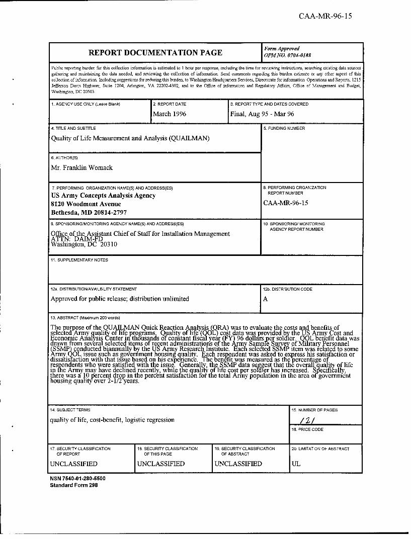
Form ApprovedREPORT DOCUMENTATION PAGE OPMNO. 0704-0188

Public reporting burden for this collection information is estimated to 1 hour per response, including the time for reviewing instructions, searching existing data sourcesgathering and maintaining the data needed, and reviewing the collection of information. Send comments regarding this burden estimate or any other aspect of thiscollection of information. Including suggestions for reducing this burden, to Washington Headquarters Services, Directorate for information Operations and Reports, 1215Jefferson Davis Highway, Suite 1204, Arlington, VA 22202-4302, and to the Office of information and Regulatory Affairs, Office of Management and Budget,Washington, DC 20503.

1. AGENCY USE ONLY (Leave Blank) 2. REPORT DATE 3. REPORT TYPE AND DATES COVERED

March 1996 Final, Aug 95 - Mar 96

4. TITLE AND SUBTITLE 5. FUNDING NUMBER

Quality of Life Measurement and Analysis (QUAILMAN)

6. AUTHOR(S)

Mr. Franklin Womack

7. PERFORMING ORGANIZATION NAME(S) AND ADDRESS(ES) 8. PERFORMING ORGANIZATION

US Army Concepts Analysis Agency REPORT NUMBER

8120 Woodmont Avenue CAA-MR-96-15Bethesda, MD 20814-2797

9. SPONSORING/MONITORING AGENCY NAME(S) AND ADDRESS(ES) 10. SPONSORING/ MONITORINGAGENCY REPORT NUMBER

Office of the Assistant Chief of Staff for Installation ManagementATTN: DAIM-FDWashington, DC 20310

11. SUPPLEMENTARY NOTES

12a. DISTRIBUTION/AVAILBILfTY STATEMENT 12b. DISTRIBUTION CODE

Approved for public release; distribution unlimited A

13. ABSTRACT (Maximum 200 words)

The purpose of the QUAILMAN Quick Reaction Analysis (ORA) was to evaluate the costs and benefits ofselected Army qualiý of life programs. Quality ofilfe (QOL) cost data was provided by the US Army Cost andEconomic Analysis C.enter in thousands of constant fiscal year (FY) 96 dollars -per soldier. QOL benefit data wasdrawn from several selected items of recent administrations of the Army Sample Survey of Military Personnel(SSMP) conducted biannually by the US Army Research Institute. Each selected SSWM item was related to someArmy QOL issue such as government housing quality. Each respondent was asked to express his satisfaction ordissatistaction with that issue based on his experence. The benefit was measured as the percentage ofrespondents who were satisfied with the issue. Generally, the SSWiP data suggest that the overall quality of lifein the Army may have declined recently, while the quality of life cost per so-ier has increased. Specifically,there was a 10 percent drop in the percent satisfaction for the total Army popalation in the area of governmenthousing quality over 2-1/2 years.

14. SUBJECT TERMS 15. NUMBER OF PAGES

quality of life, cost-benefit, logistic regression /_ _ __/

16. PRICE CODE

17. SECURITY CLASSIFICATION 18. SECURITY CLASSIFICATION 19. SECURITY CLASSIFICATION 20. LIMITATION OF ABSTRACTOF REPORT OF THIS PAGE OF ABSTRACT

UNCLASSIFIED UNCLASSIFIED UNCLASSIFIED UL

NSN 7540-01-280-5500Standard Form 298

CAA-MR-96-15

QUALITY OF LIFE MEASUREMENT AND ANALYSIS

SUMMARY

THE REASON FOR PERFORMING THE QUICK REACTION ANALYSIS(QRA) was to provide planners of the fiscal year (FY) 1998 Program Objective Memorandum(POM) build with information about recent trends in the cost and benefits of selected ArmyQuality of Life (QOL) programs.

THE QRA SPONSOR was the Office of the Assistant Chief of Staff for InstallationManagement (ACSIM).

THE QRA OBJECTIVE was to evaluate the costs and benefits of selected Army Quality of Lifeprograms in support of the FY 98 POM build.

THE SCOPE OF THE QRA will consider cost and benefit data. QOL cost data was providedin terms of cost per soldier in FY 96 current dollars by the US Army Cost and Economic AnalysisCenter (USACEAC). QOL benefit data was drawn from several selected items of recentadministrations of the Army Sample Survey of Military Personnel (SSMP) conducted biannuallyby the US Army Personnel Office of the US Army Research Institute (ARI).

THE ASSUMPTION of this QRA is that the benefit data provided by ARI can be meaningfullymatched to the cost data provided by USACEAC.

THE BASIC APPROACH was to:

(1) Estimate parameters of a standard statistical model relating cost and benefit data.

(2) Perform statistical tests of hypotheses about the parameters to determine if the parametersrelated to cost and/or time are statistically significant.

(3) Perform statistical tests of hypotheses about parameters of the model related todifferences between total population effects and subpopulation effects where the subpopulationsare selected from demographic variables collected as part of the SSMP.

(4) Present graphically some of the more important results.

THE PRINCIPAL FINDINGS AND OBSERVATIONS

(1) The SSMP data suggests that the overall quality of life in the Army may have declinedrecently, while the quality of life cost per soldier has increased.

(2) There is about a 10 percent drop in the satisfaction of the total Army population in thearea of government housing quality over 2 1/2 years.

CAA-MR-96-15

(3) It is not clear that the benefits as measured by the SSMP are totally dependent upon thecost.

(4) The Analysis Review Board, part of CAA's Total Quality Management Process,suggested that the sponsor might wish to explore conducting cost/benefit analyses at theinstallation level. For instance, there might be an increase in government housing qualitysatisfaction for an installation where housing was improved during the period.

THE QRA EFFORT was directed by Mr. Franklin Womack, Resource Analysis Division, USArmy Concepts Analysis Agency (CAA).

COMMENTS AND QUESTIONS should be sent to the Director, US Army Concepts AnalysisAgency, ATTN: CSCA-RA, 8120 Woodmont Avenue, Bethesda, MD 20814-2797.

ii

CAA-MR-96-15

CONTENTS

Page

S U M M A R Y ................................................................................................................................ i

ANNO TATED BRIEFING ....................................................................................................... 1

APPENDIX

A Request for Analytical Support .................................................................... A-1

B Contributors ................................................................................................ B-1

C Table of Cost and Benefit Data .................................................................... C-1

D QUAILM AN Statistical Analysis ................................................................. D- 1

E References .................................................................................................... E- 1

F Distribution .................................................................................................. D- 1

GLO SSARY ............................................................................................................... Glossary-1

111o~

CAA-MR-96-15

The US Army's Center for Strategy and Force Evaluation

Quality of LifeMeasurement and Analysis

(QUAILMAN)

Frank WomackPhone # (301) 295-6930Resource Analysis Division 0

This report documents the results of the Quality of Life (QOL) Measurementand Analysis (QUAILMAN) Quick Reaction Analysis (QRA).

The purpose of this QRA was to generate a report to illustrate recent trendsin costs and benefits of selected Army QOL programs. It was anticipated thatthese illustrations would be useful to planners in support of the fiscal year (FY)98 Program Objective Memorandum (POM) build.

The QRA was sponsored by the Assistant Chief of Staff for InstallationManagement (ACSIM).

This report first describes the methodology used to conduct the QRA. Thetwo main data inputs, benefits and costs, are described. Supplementaldemographic variables are described. Finally, the analysis is presented in theform of graphs depicting (1) QOL benefits by time, (2) QOL benefits by cost,and (3) differences in QOL benefit responses by demographic factors.

CAA-MR-96-15


Objective

The objective of this QRA is toevaluate the costs and benefits ofselected Army Quality of Lifeprograms (e.g., Family Housing) insupport of the FY98 POM build.

2

CAA-MR-96-15


Approach

1. Obtain benefit data from six semiannualadministrations of the Sample Survey ofMilitary Personnel (SSMP).

2. Match benefit characteristics of quality of lifemeasured on the SSMP with cost data.

3. Analyze trends in cost and benefits formatched characteristics.

4. Analyze benefits by demographic factors.

5. Illustrate results of analysis using graphs andtables.

6. Document results in a memorandum report.

0

Benefit data was obtained from the Army Research Institute (ARI) in the form ofquestionnaire results. Cost data was provided by the Army Cost and Economic Analysis Center(USACEAC).

An initial meeting was held with the sponsor in order to plan the work of the study. The rawdata for six recent surveys had been provided by ART. At this time, the form, but not thesubstance, of the cost data was provided by USACEAC. At this meeting, the sponsor selectedeight questionnaire items for use as benefit feedback variables. These eight items werematched to cost items supplied by USACEAC. Also, six demographic variables were selectedfrom the questionnaire for use in determining differences in response from varioussubpopulations. The sponsor made the point that the benefits typically lag the cost by about 2years.

The relevant benefit data was abstracted from six data bases provided by ARI and tabulated(Appendix C). Cost data were incorporated into these tables. These cost data were updated byUSACEAC several times during the course of the study.

The original intent had been to model the benefit data as a function of cost. However, thecost data were not at hand early in the study. We therefore decided to work with the data athand and to model the benefits data as a function of time and the selected demographicvariables. The binary nature of the questionnaire responses, and the ultimate desire to predictfuture response, made the logistic regression model an appropriate research tool. Significantresults from the modeling effort were graphed and appear later in this report.

As the study progressed, the final cost data update was received from USACEAC. Agraphical analysis of the benefit feedback response variables versus the cost appear in thisreport.

3

CAA-MR-96-15


Benefit Data

* QOL items selected from the SampleSurvey of Military Personnel (SSMP)administered by ARI twice each year

* Six sets of data from Spring 1992 to Fall1994

* Answers provided in form of satisfied ordissatisfied response

0

The Sample Survey of Military Personnel (SSMP) is administered by ARI twice ayear in the spring and fall. The survey gives Army personnel an opportunity to expresstheir views about the Army. The results are used to assess current and planned Armyservices, policies, and programs.

A random sample of all permanent party, Active Component Army personnel isdrawn to participate in each survey. The sample is drawn from the StandardInstallation/Division Personnel System (SIDPERS) using the final one or two digits ofsocial security numbers (SSNs).

The sample size represents about 10 percent of the officers and about 2 percent to 3percent of the enlisted personnel. In Spring 1994, the sample size was chosen suchthat one could expect a sampling error of from ± 1 to ± 3 percent. The survey wasadministered by the Personnel Survey Control Officer at each installation and overseasarea.

The data collected are weighted up to Army strength for each individual rank. TheSpring 1994 SSMP was weighted up to Army strength for end-April 1994 (based onthe Deputy Chief of Staff for Personnel (DCSPER) 46, Part 1 report). Generally thedata are weighted for gender and location (i.e., US Army Europe (USAREUR) versuselsewhere).

Items were selected for this study which seemed to relate to quality of life issues.Items selected either (1) expressed satisfaction or dissatisfaction with a particular facetof Army life based on the respondent's Army experience, or (2) expressed the rating ofsome quality of life such as high or low morale. In addition, the quality of life itemsselected for benefit analysis, six different demographic responses, were abstracted inorder to determine differences in subpopulation responses. These included rank, age,ethnicity, gender, marital status, and location.

4

CAA-MR-96-15


Items selected from SSMP to represent benefits

1. Satisfaction with Recreational Services.

2. Satisfaction with the quality of Army familyprograms.

3. Rate your current level of morale (low or high).4. Satisfaction with overall quality of Army life.

5. Satisfaction with quality of governmenthousing.

6. Satisfaction with amount of pay (basic).

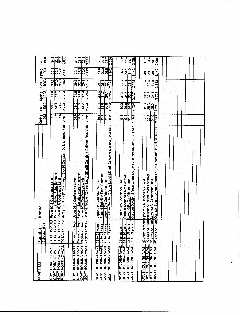
7. Satisfaction with availability of governmenthousing.

8. Satisfaction with VHA COLA.

Eight questions were chosen from the SSMP to represent benefit responses.

5

CAA-MR-96-15

The US Anny's Center for Strategy and Force Evaluation M AL,

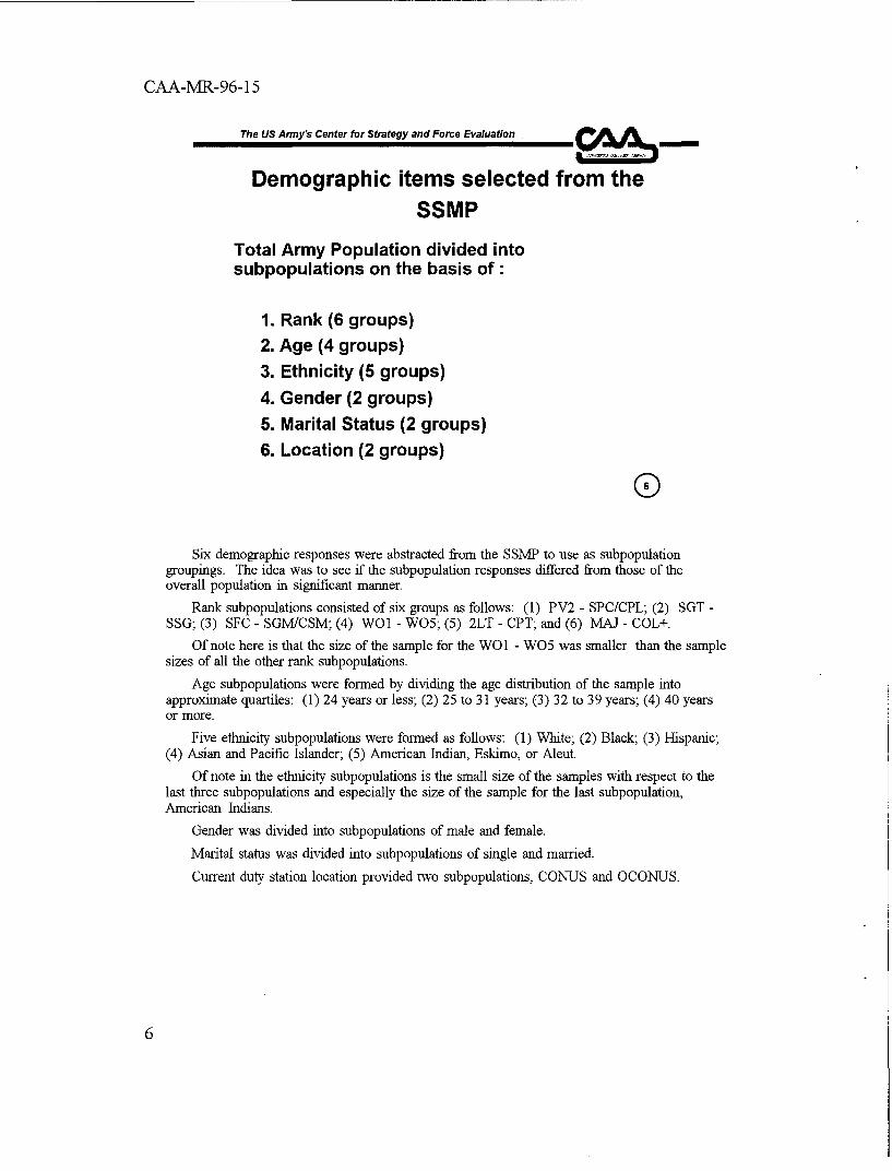
Demographic items selected from theSSMP

Total Army Population divided intosubpopulations on the basis of:

1. Rank (6 groups)

2. Age (4 groups)

3. Ethnicity (5 groups)

4. Gender (2 groups)

5. Marital Status (2 groups)

6. Location (2 groups)

0

Six demographic responses were abstracted from the SSMP to use as subpopulationgroupings. The idea was to see if the subpopulation responses differed from those of theoverall population in significant manner.

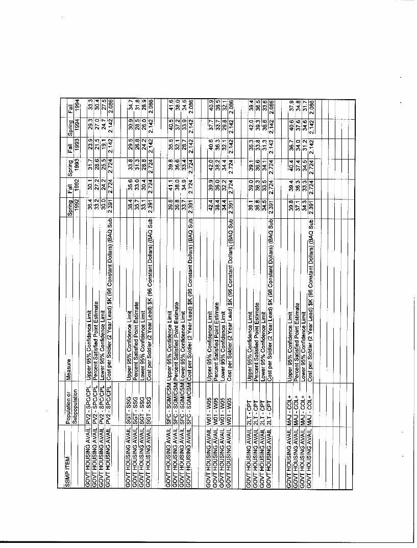
Rank subpopulations consisted of six groups as follows: (1) PV2 - SPC/CPL; (2) SGT -SSG; (3) SFC - SGM/CSM; (4) WO1 - WO5; (5) 2LT - CPT; and (6) MAJ - COL+.

Of note here is that the size of the sample for the WO 1 - W05 was smaller than the samplesizes of all the other rank subpopulations.

Age subpopulations were formed by dividing the age distribution of the sample intoapproximate quartiles: (1) 24 years or less; (2) 25 to 31 years; (3) 32 to 39 years; (4) 40 yearsor more.

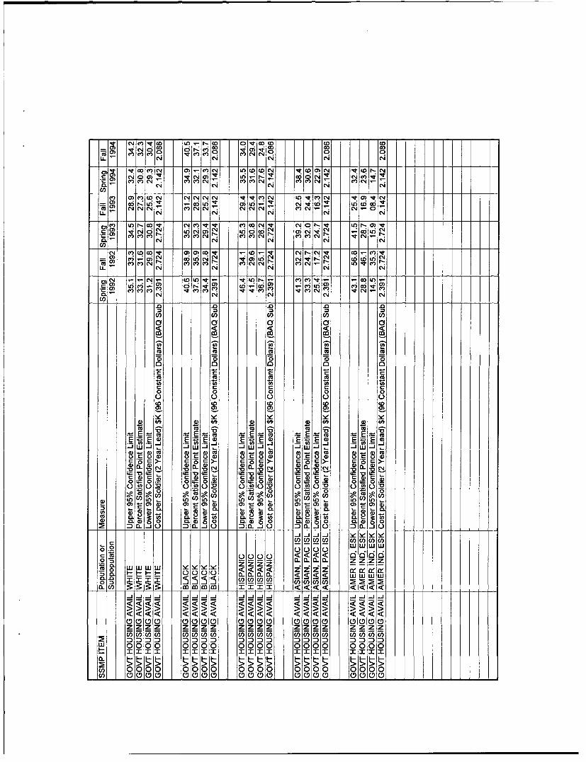
Five ethnicity subpopulations were formed as follows: (1) White; (2) Black; (3) Hispanic;(4) Asian and Pacific Islander; (5) American Indian, Eskimo, or Aleut.

Of note in the ethnicity subpopulations is the small size of the samples with respect to thelast three subpopulations and especially the size of the sample for the last subpopulation,American Indians.

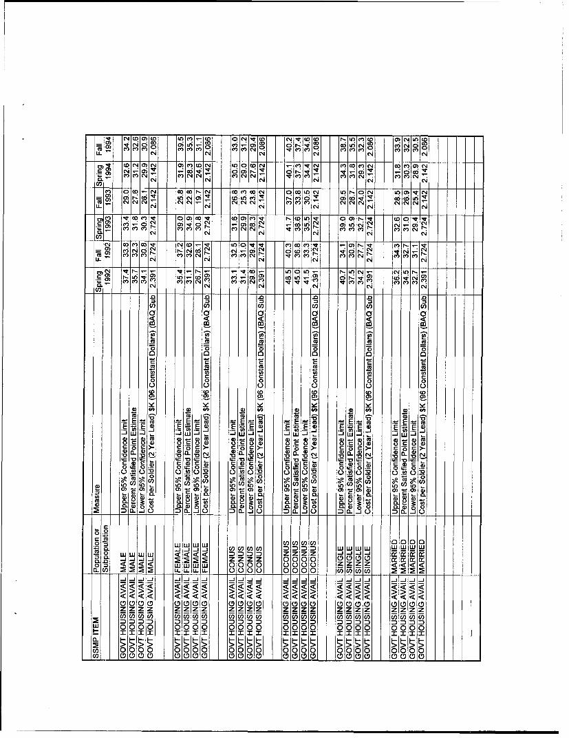
Gender was divided into subpopulations of male and female.

Marital status was divided into subpopulations of single and married.

Current duty station location provided two subpopulations, CONUS and OCONUS.

6

CAA-MR-96-15


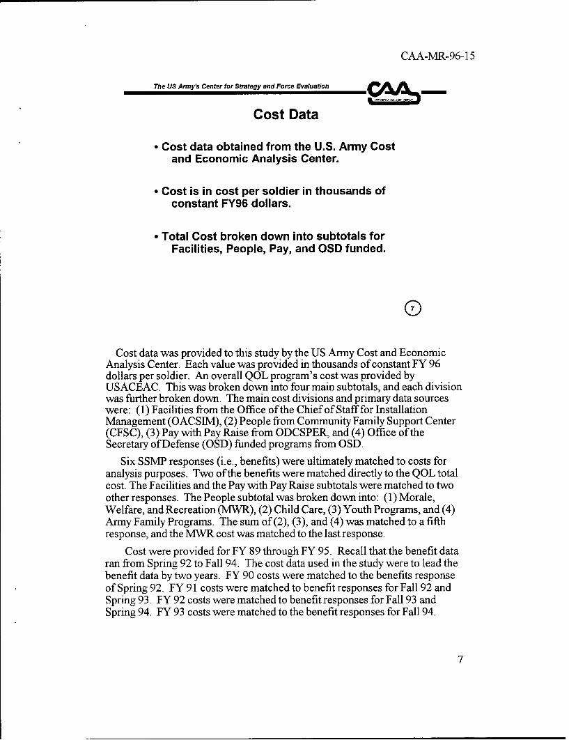
Cost Data

* Cost data obtained from the U.S. Army Costand Economic Analysis Center.

- Cost is in cost per soldier in thousands ofconstant FY96 dollars.

* Total Cost broken down into subtotals forFacilities, People, Pay, and OSD funded.

0

Cost data was provided to this study by the US Army Cost and EconomicAnalysis Center. Each value was provided in thousands of constant FY 96dollars per soldier. An overall QOL program's cost was provided byUSACEAC. This was broken down into four main subtotals, and each divisionwas further broken down. The main cost divisions and primary data sourceswere: (1) Facilities from the Office of the Chief of Staff for InstallationManagement (OACSIM), (2) People from Community Family Support Center(CFSC), (3) Pay with Pay Raise from ODCSPER, and (4) Office of theSecretary of Defense (OSD) funded programs from OSD.

Six SSMP responses (i.e., benefits) were ultimately matched to costs foranalysis purposes. Two of the benefits were matched directly to the QOL totalcost. The Facilities and the Pay with Pay Raise subtotals were matched to twoother responses. The People subtotal was broken down into: (1) Morale,Welfare, and Recreation (MWR), (2) Child Care, (3) Youth Programs, and (4)Army Family Programs. The sum of(2), (3), and (4) was matched to a fifthresponse, and the MWR cost was matched to the last response.

Cost were provided for FY 89 through FY 95. Recall that the benefit dataran from Spring 92 to Fall 94. The cost data used in the study were to lead thebenefit data by two years. FY 90 costs were matched to the benefits responseof Spring 92. FY 91 costs were matched to benefit responses for Fall 92 andSpring 93. FY 92 costs were matched to benefit responses for Fall 93 andSpring 94. FY 93 costs were matched to the benefit responses for Fall 94.

7

CAA-MR-96-15


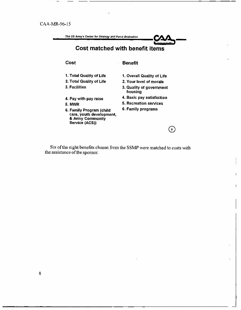
Cost matched with benefit items

Cost Benefit

1. Total Quality of Life 1. Overall Quality of Life2. Total Quality of Life 2. Your level of morale3. Facilities 3. Quality of government

housing

4. Pay with pay raise 4. Basic pay satisfaction5. MWR 5. Recreation services6. Family Program (child 6. Family programs

care, youth development,& Army CommunityService (ACS)) 0

Six of the eight benefits chosen from the SSMP were matched to costs withthe assistance of the sponsor.

8

CAA-MR-96-15

The US Army's Center for Strategy and Force Evaluation X

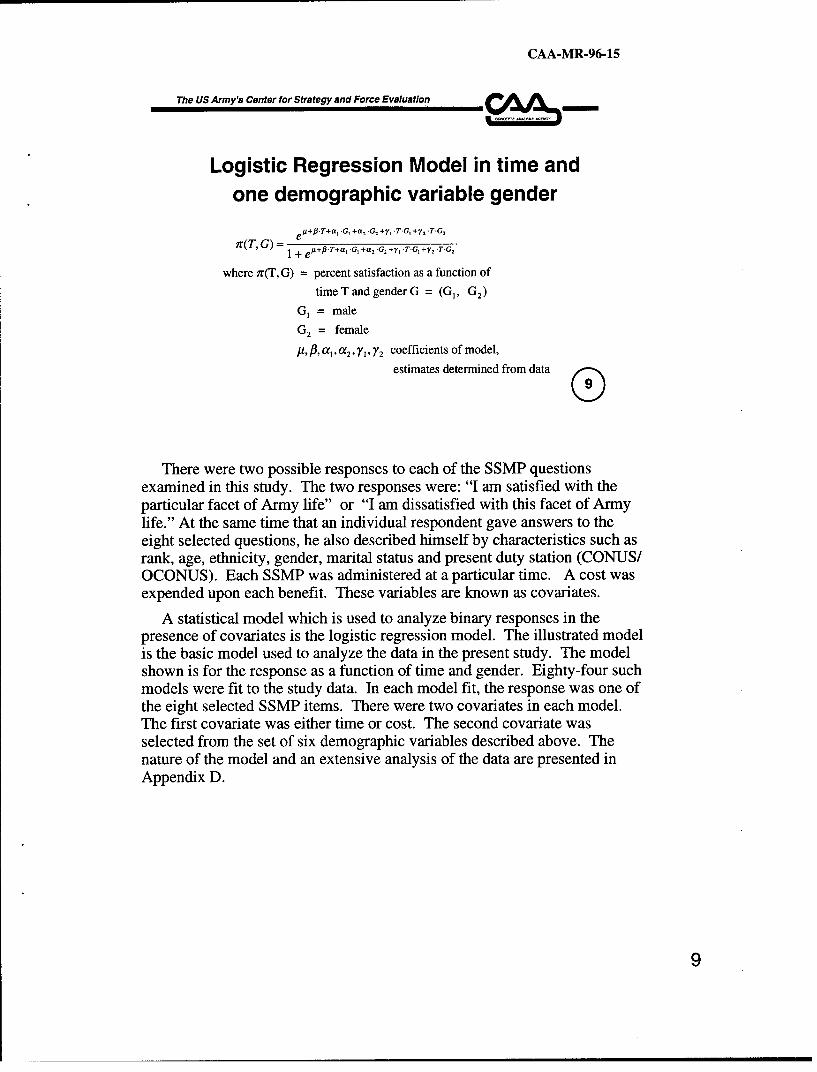
Logistic Regression Model in time and

one demographic variable gender

e+ fl.T+a .G1 +1., .G2 +yf .T-G +y2 "T'G2

r,(T, G) = 1 + eP•'T+a, .G, +a, .G, +r, .T.G, +y, "T'G2

where 7r(T,G) = percent satisfaction as a function of

time T and gender G = (G1, G2)

G, = male

G2 = female

ji, fl, ar, a 2, Y1I Y2 coefficients of model,

estimates determined from data

There were two possible responses to each of the SSMP questionsexamined in this study. The two responses were: "I am satisfied with theparticular facet of Army life" or "I am dissatisfied with this facet of Armylife." At the same time that an individual respondent gave answers to theeight selected questions, he also described himself by characteristics such asrank, age, ethnicity, gender, marital status and present duty station (CONUS/OCONUS). Each SSMP was administered at a particular time. A cost wasexpended upon each benefit. These variables are known as covariates.

A statistical model which is used to analyze binary responses in thepresence of covariates is the logistic regression model. The illustrated modelis the basic model used to analyze the data in the present study. The modelshown is for the response as a function of time and gender. Eighty-four suchmodels were fit to the study data. In each model fit, the response was one ofthe eight selected SSMP items. There were two covariates in each model.The first covariate was either time or cost. The second covariate wasselected from the set of six demographic variables described above. Thenature of the model and an extensive analysis of the data are presented inAppendix D.

9

CAA-MR-96-15


Benefits vs Time

80

so0 ---- Recreation service quality

-- -- ----- Family program quality

""0- -- Morale level highllow

- Overall quality of life

40- - Govt housing quality

...- " -Basic pay satisfaction

3 -- Govt housing availability

-Amount VHA/COLAsatisfaction

20II[ I

Spring Fall Spring Fall Spring Fall1992 1992 1993 1993 1994 1994

SSMP Administration G

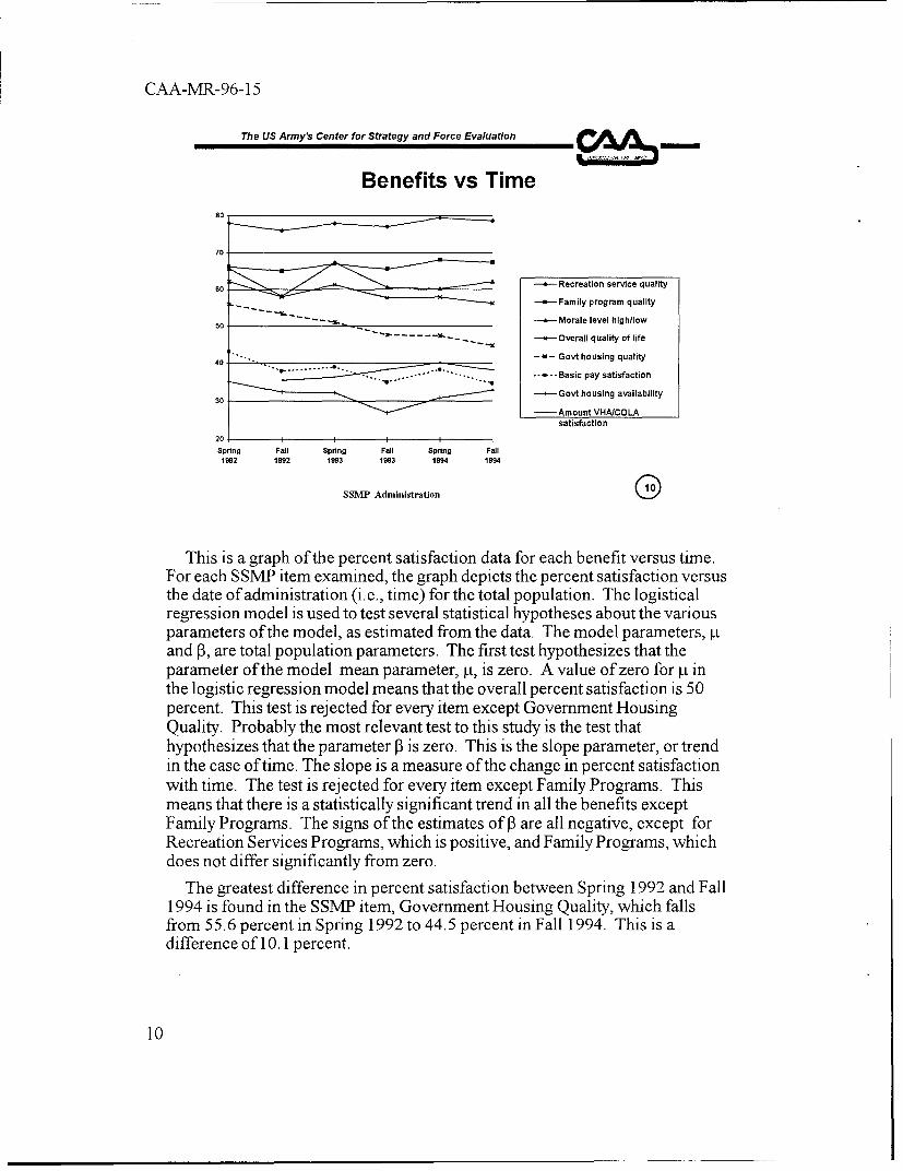
This is a graph of the percent satisfaction data for each benefit versus time.For each SSMiP item examined, the graph depicts the percent satisfaction versusthe date of administration (i.e., time) for the total population. The logisticalregression model is used to test several statistical hypotheses about the variousparameters of the model, as estimated from the data. The model parameters, .tand 03, are total population parameters. The first test hypothesizes that theparameter of the model mean parameter, [t, is zero. A value of zero for p. inthe logistic regression model means that the overall percent satisfaction is 50percent. This test is rejected for every item except Government HousingQuality. Probably the most relevant test to this study is the test thathypothesizes that the parameter 03 is zero. This is the slope parameter, or trendin the case of time. The slope is a measure of the change in percent satisfactionwith time. The test is rejected for every item except Family Programs. Thismeans that there is a statistically significant trend in all the benefits exceptFamily Programs. The signs of the estimates of P3 are all negative, except forRecreation Services Programs, which is positive, and Family Programs, whichdoes not differ significantly from zero.

The greatest difference in percent satisfaction between Spring 1992 and Fall1994 is found in the SSMIP item, Government Housing Quality, which fallsfrom 55.6 percent in Spring 1992 to 44.5 percent in Fall 1994. This is adifference of 10.1 percent.

10

CAA-MR-96-15


Quality of Life & Morale Level vs Cost

75

S70 -* MORALE LEVEL

HIGH

...... ....... OF LIFE------. LR Mode1 - Oveall

50,

45"

4021 21.5 22 22.5 23 23.5 24 24.5 25

Coal per Soldier ($409 Con.tant FYS6) (2 year Iead)

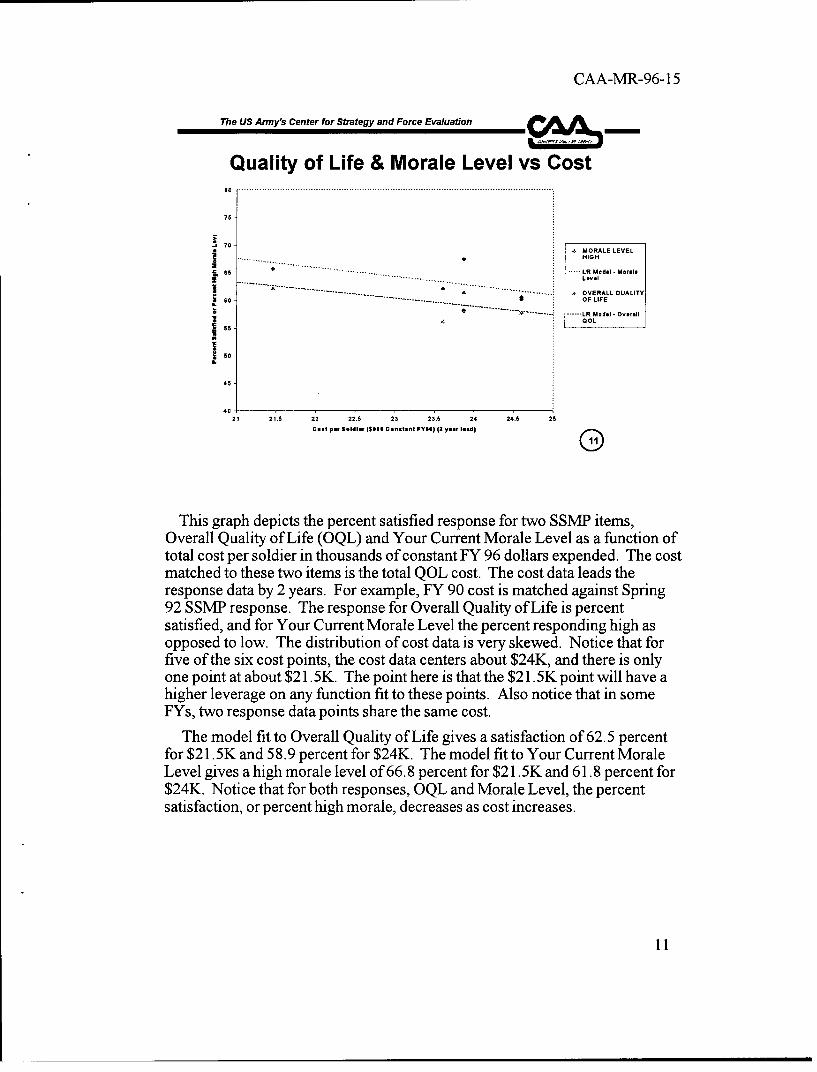
This graph depicts the percent satisfied response for two SSMP items,Overall Quality of Life (OQL) and Your Current Morale Level as a function oftotal cost per soldier in thousands of constant FY 96 dollars expended. The costmatched to these two items is the total QOL cost. The cost data leads theresponse data by 2 years. For example, FY 90 cost is matched against Spring92 SSMP response. The response for Overall Quality of Life is percentsatisfied, and for Your Current Morale Level the percent responding high asopposed to low. The distribution of cost data is very skewed. Notice that forfive of the six cost points, the cost data centers about $24K, and there is onlyone point at about $21.5K. The point here is that the $21.5K point will have ahigher leverage on any function fit to these points. Also notice that in someFYs, two response data points share the same cost.

The model fit to Overall Quality of Life gives a satisfaction of 62.5 percentfor $21.5K and 58.9 percent for $24K. The model fit to Your Current MoraleLevel gives a high morale level of 66.8 percent for $21.5K and 61.8 percent for$24K. Notice that for both responses, OQL and Morale Level, the percentsatisfaction, or percent high morale, decreases as cost increases.

11

CAA-MR-96-15


Government Housing Quality vs Facilities Cost70 ....................... ....................... ..... ................... ................... .............. ..........

65

00 . GOVr

HOUSINGQUALITY

55 ....

...... Logistic50 Z ~......Regression50 .Model

45 -

40

35

301.2 1.3 1.4 1.5 1.6 1.7 0

Facilities Cost per Soldier($000 FY96 Constant) (2 year lead)

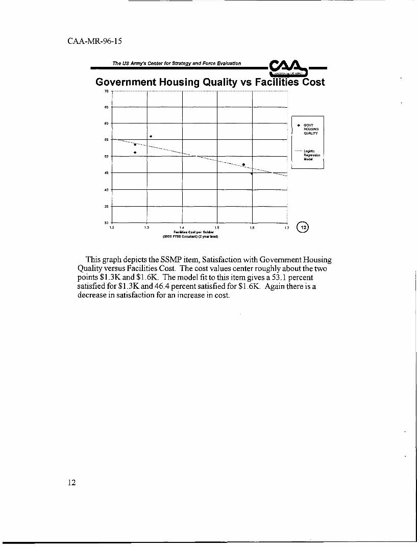
This graph depicts the SSMP item, Satisfaction with Government HousingQuality versus Facilities Cost. The cost values center roughly about the twopoints $1.3K and $1.6K. The model fitto this item gives a 53.1 percentsatisfied for $1.3K and 46.4 percent satisfied for $1.6K. Again there is adecrease in satisfaction for an increase in cost.

12

CAA-MR-96-15

The US Army's Center for Strategy and Force Evaluation • A

Family Programs Quality vs80 - --

75

70 ..... . .......... "

...... ..........

". . FAMILY' - ....... ... PROGRAMS

QUALITY

60 . LogistcRegressionModel

S5

50

45

40 -

0.16 0.18 02 0.22 024 0.26 0.28 0.3 0.32ACS, Child Care & Youlh Development Programs cost per Soldier

($000 Constant FY 20) (2 yew lead) G

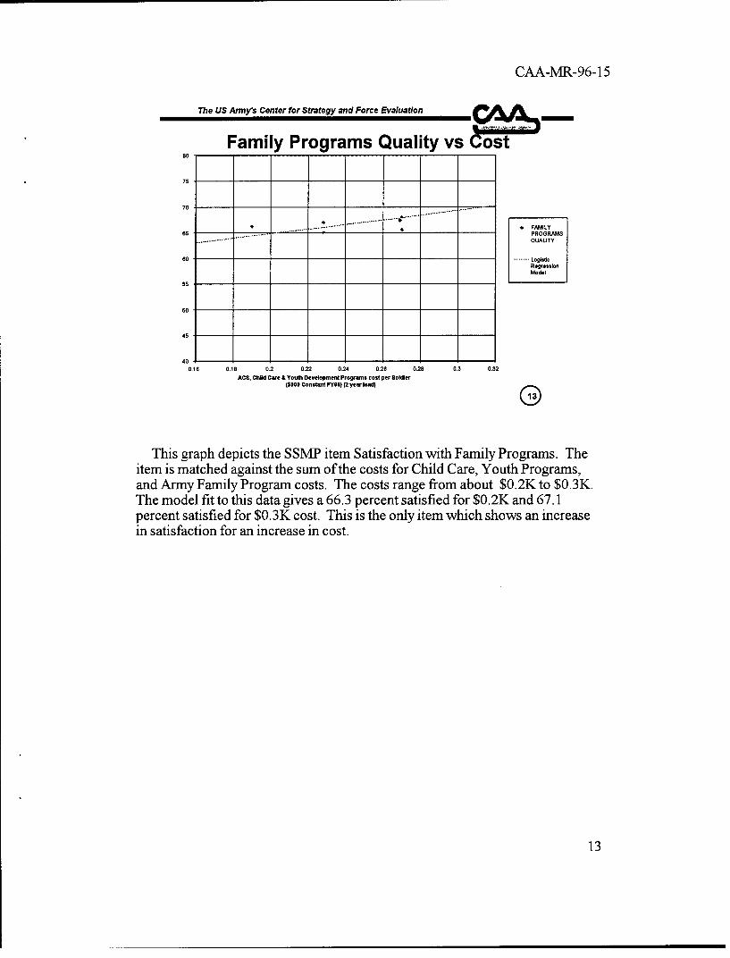
This graph depicts the SSMIP item Satisfaction with Family Programs. Theitem is matched against the sum of the costs for Child Care, Youth Programs,and Army Family Program costs. The costs range from about $0.2K to $0.3K.The model fit to this data gives a 66.3 percent satisfied for $0.2K and 67.1percent satisfied for $0.3K cost. This is the only item which shows an increasein satisfaction for an increase in cost.

13

CAA-MR-96-15

The US Army's Center for Strategy and Force Evaluation M A .

Recreation Services vs MWR100

so

86 . RECREATIONSERVICESQUALITY

s0 Logistc... .......... it R.gr-ssion Model

75

70

65

60

0.32 0.33 0.34 0.35 0.36 0.37 0.39 0.39

MWR cost per Soldier($ 0 0 0 C o n s t wn t F Y 96 ) ( 2 y e wr le a d ) G

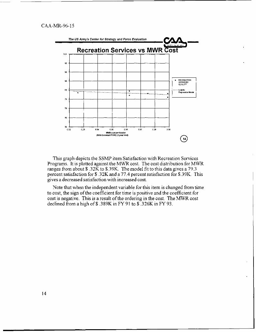
This graph depicts the SSMIP item Satisfaction with Recreation ServicesPrograms. It is plotted against the MWR cost. The cost distribution for MWRranges from about $ .32K to $.39K. The model fit to this data gives a 79.3percent satisfaction for $ .32K and a 77.4 percent satisfaction for $.39K. Thisgives a decreased satisfaction with increased cost.

Note that when the independent variable for this item is changed from timeto cost, the sign of the coefficient for time is positive and the coefficient forcost is negative. This is a result of the ordering in the cost. The MWR costdeclined from a high of$ .389K in FY 91 to $ .326K in FY 93.

14

CAA-MR-96-15


Basic Pay Satisfaction vs Pay & Pay Raise Cost60

55

50

45 BASIC PAY-.-.- .... SATISFACTION

40. ...... LogisticRegression. ......... Model

35

30

25

2019.5 20 20.5 21 21.5 22 22.5

Pay and Pay Raise cost per soldier

($000 FY96 Constantl)(2 yea lead)

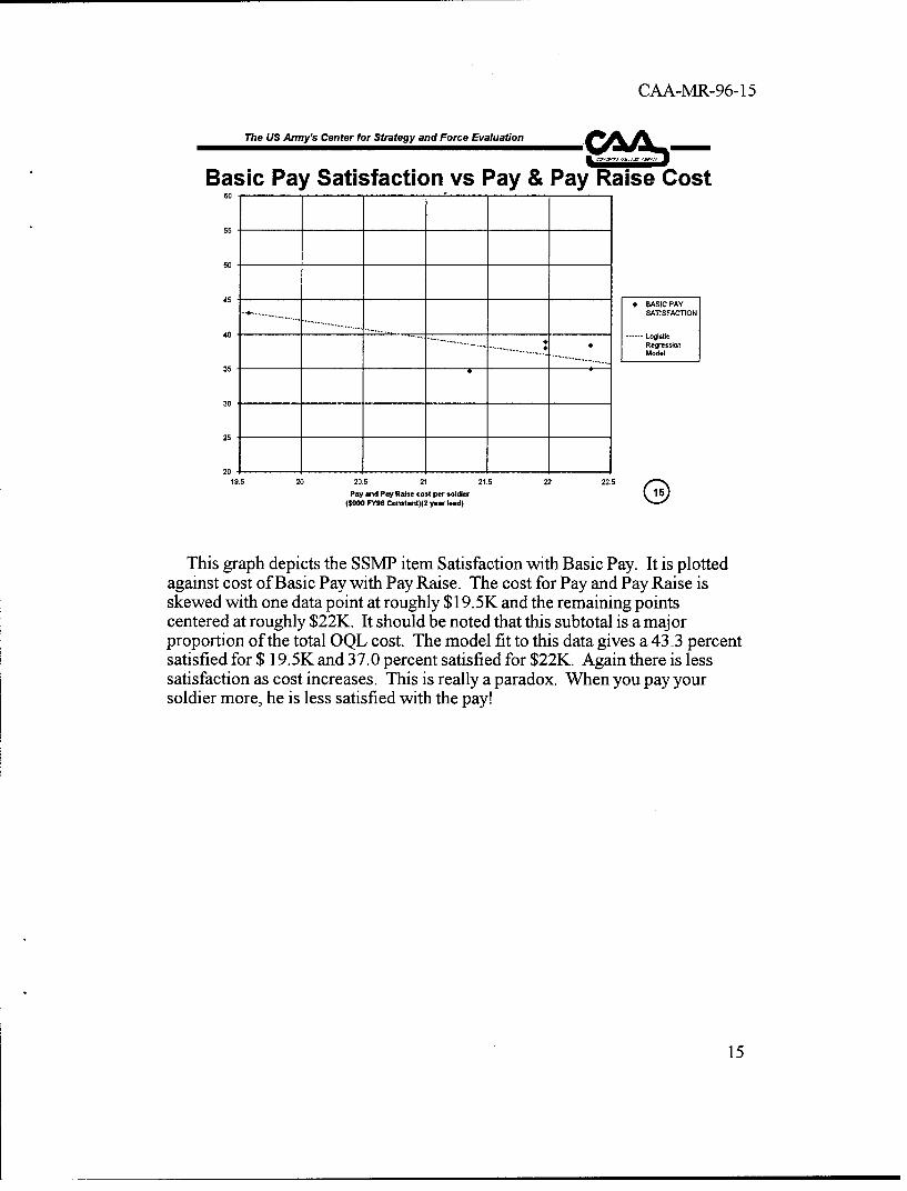
This graph depicts the SSMP item Satisfaction with Basic Pay. It is plottedagainst cost of Basic Pay with Pay Raise. The cost for Pay and Pay Raise isskewed with one data point at roughly $19.5K and the remaining pointscentered at roughly $22K. It should be noted that this subtotal is a majorproportion of the total OQL cost. The model fit to this data gives a 43.3 percentsatisfied for $ 19.5K and 37.0 percent satisfied for $22K. Again there is lesssatisfaction as cost increases. This is really a paradox. When you pay yoursoldier more, he is less satisfied with the pay!

15

CAA-MR-96-15


Summary of Cost/Benefit Results

Year of Benefit SpringF- 1 [-F Sing [F.al Sprg Fall1992J [992 1993 993 1[299• 1994J

Year of Cost FY90 FY91 FY91 FY92 FY92 FY93

SSMP ITEM

OVERALL QUALITY OF LIFE% Satisfied 62.2 58.0 61.4 67.7 57.9 56.2$000 21.46 23.87 23.87 24.60 24.60 23.61

MORALE LEVEL HIGH/LOW% High Morale 65.7 58.2 67.4 60.6 60.2 62.1

$000 21.46 23.87 23.87 24.60 24.60 23.61

BASIC PAY SATISFACTION% Satisfied 43.1 38.0 39.0 35.0 38.4 34.7

$000 19.970 21.969 21.969 22.338 22.338 21.357

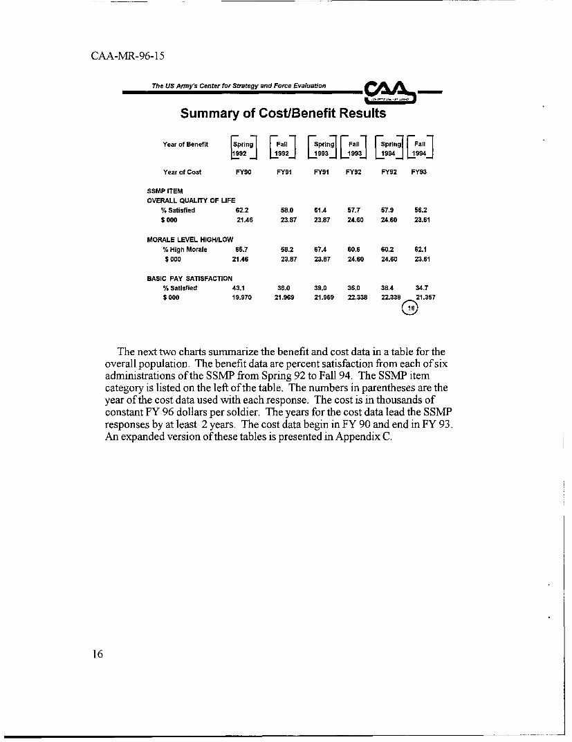
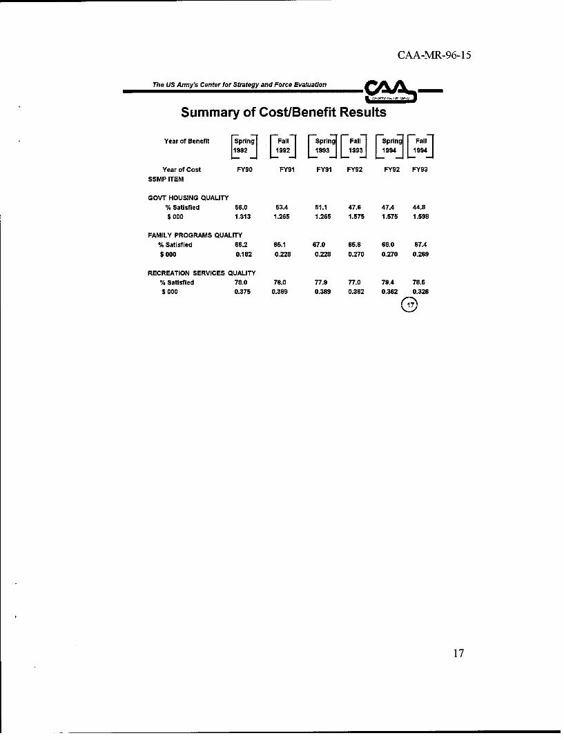
The next two charts summarize the benefit and cost data in a table for theoverall population. The benefit data are percent satisfaction from each of sixadministrations of the SSMP from Spring 92 to Fall 94. The SSMP itemcategory is listed on the left of the table. The numbers in parentheses are theyear of the cost data used with each response. The cost is in thousands ofconstant FY 96 dollars per soldier. The years for the cost data lead the SSMPresponses by at least 2 years. The cost data begin in FY 90 and end in FY 93.An expanded version of these tables is presented in Appendix C.

16

CAA-MR-96-15


Summary of Cost/Benefit ResultsYear of Benefit prin- FFa,,l Spring rFal Spring [Fall

IL82 J [Fa121 1 9 93 _ 8L Js 4 JI 9s 4 _

Year of Cost FY90 FY91 FY91 FY92 FY92 FY93

SSMP ITEM

GOVT HOUSING QUALITY

% Satisfied 56.0 53.4 51.1 47.6 47.4 44.8

$000 1.313 1.265 1.265 1.575 1.575 1.598

FAMILY PROGRAMS QUALITY

% Satisfied 66.2 65.1 67.0 65.6 68.0 67.4

$000 0.182 0.228 0.228 0.270 0.270 0.269

RECREATION SERVICES QUALITY

% Satisfied 78.0 76.0 77.9 77.0 79.4 78.6

$ 000 0.375 0.389 0.389 0.362 0.362 0.326

17

CAA-MIR-96-15

Subpopulation Analysis

Until now, we have looked at the total population. We now turn briefly to adiscussion of how subpopulations, as defined by differences in rank, age,ethnicity, gender, marital status, and present duty station (CONUS/OCONUS)might differ from the total population. The logistical regression model is usedto test several statistical hypotheses about the various parameters of the model,as estimated from the data. The model parameters a.and y. 0 =1 to m I for msubpopulations) are subpopulation parameters. The a, measure the differencebetween the level of the subpopulation and the total population. The y. measurethe difference between the slope for the subpopulation and the slope of the totalpopulation. Formal tests for these measures are fully discussed in Appendix D.In short, there were very few subpopulation slope differences which weresignificantly different from zero.

There were four significant subpopulation slope group variables (seeAppendix D) associated with the 36 cost models fit. These consisted of twoeach for the SSMP items, Family Programs and Basic Pay Satisfaction. In thecase of the Family Programs item, these two group variables involved slopedifferences in the marital status and location subpopulations. The model fit tothe Family Programs item as a function of cost and marital status showed thatover the cost range $.182K to $.270K, the satisfaction increased for marriedrespondents from 65.5 percent to 67.4 percent as cost increased. For singlerespondents over the same range, the model predicted that satisfaction woulddecrease from 67.7 percent to 64.1 percent. In the model fit to the FamilyPrograms item as a function of cost and location of duty station(CONUS/OCONUS) over the same cost range, the satisfaction for CONUSlocated respondents decreased from 67.5 percent to 66.6 percent as costincreased, but for OCONUS-located respondents, the satisfaction increasedfrom 61.3 percent to 67.6 percent as cost increased.

In the case of Basic Pay Satisfaction, there were also two slope groupvariables, ethnicity and rank, which had values significantly different fromzero. In the case of ethnicity, the negative slope with respects to cost for thewhite subpopulation was slightly less negative than for the other four ethnicgroups. In the case of ranks, the negative slope with respect to cost was slightlyless for the subpopulation of PV2 - SPC/CPL and slightly more for thesubpopulation SGT-SSG.

18

CAA-MR-96-15

The US Army's Center for Strategy and Force Evaluation • A

Basic Pay Satisfaction by Rank Group by Time

30 . .. ... : PV2 SPC/CPL

25- "SFC -SGM/CSM

20 -'-Wi1l- Wits

5 "-' 2LT-CPT

-- ""MAJ - COL.

...... ---9---....-... . . .. . . .... . .....

0 Total Population. ......... .........

-. . . . . . ....... .... "-.--- ----------..

-10

-20Spring Fall Spring Fail Spring F 111992 1992 1993 1993 1994 1994

ZSMP AdminlOtratiln

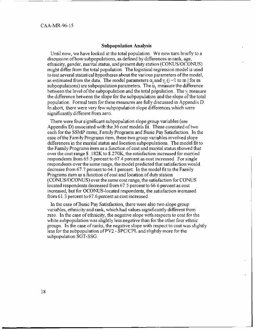
On the other hand, almost every group variable related to level differences betweensubpopulations was significantly different from zero. This means that there was a constantnonzero level difference between the subpopulations over all values of cost. In the main, thefits of the benefits versus time mirrored the fits of the benefits versus cost. The largest leveldifferences were shown in the SSMP item Satisfaction with Basic Pay. The graph plotted hereis representative of 77 out of the 84 models which had significant differences in the levels ofone or more subpopulations and the total population. In fact, this graph shows both significantlevel and slope differences. The level differences are much more pronounced and can berecognized easily. The model estimates of the mean level for the total population is 37.7percent. The model subpopulation mean levels are as follow: (1) PV2-SPC/CPL 34.1 percent,(2) SGT-SSG 31.0 percent, (3) SFC-SGM/CSM 35.0 percent, (4) WOl-WO5 44.9 percent, (5)2LT-CPT 66.5 percent, and (6) MAJ-COL+ 66.1 percent. In addition to the significant leveldifference, the model also found two slope differences in this model which were significantlydifferent from zero. The slopes of groups (2) and (5) differed from the slope of the totalpopulation for this model. The estimate of P3 (i.e., from logistic regression model) for the totalpopulation was -0.1217. The estimate of t3 + %•, the group (2) estimate, is -.02030, whichindicates a slight decrease in the slope measure and a more vigorous dissatisfaction with basicpay with increasing time from this subpopulation than from the total population. On the otherhand, the estimate of 03 + (x5 is -0.0168, which almost neutralizes the slope of the totalpopulation. Thus, group (5) is much more satisfied with the basic pay than the total population,and this satisfaction increases throughout the period of Spring 1992 to Fall 1994.

19

CAA-MR-96-15

The US Army's Center for Strategy and Force Evaluation UN .

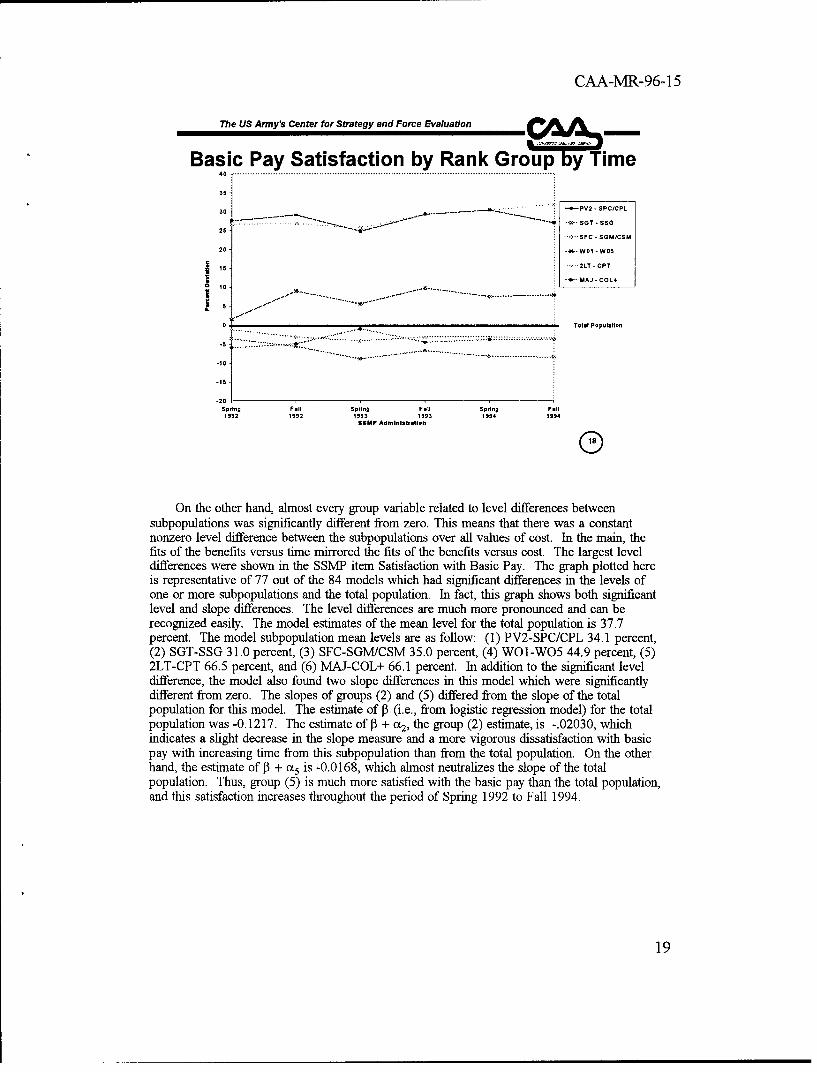
Limitations1. Benefit data spans only two and one-half years.

2. Cost data defined at a very accumulated level.

3. Manpower, resources and deployment have beenvery turbulent during this period (i.e., downsizing,redeployment to Desert Storm, etc.).

0

It is necessary that the same question be asked on consecutive admini-strations of the SSMP. The QOL questions used in this study have onlyappeared consecutively in the same form on the SSMP for the most recentadministrations of SSMP (i.e., Spring 1992 to Fall 1994). In addition tospanning only the most recent past, the benefit data is obtained at twice the rateof the cost data. Cost data is annual and benefit data is semiannual. Thiscauses two benefit data points, 6 months apart, to be matched to the same costdata point.

Cost data is defined per soldier for the total Army. If the cost data could bebroken down to the same level as the benefit data, perhaps more meaningfulinsights could be obtained. The demographic data obtained for the benefit datais at the micro level, whereas the cost data provided is at the macro level ofdetail. This is quite a mismatch.

Data was collected during a turbulent period in which many factors, besidescost, could have influenced the benefit data. Chief among these weredownsizing, redeployment to DESERT STORM, etc.

20

CAA-MR-96-15

The US Anny's Center for Strategy and Force Evaluation • .

General Findings

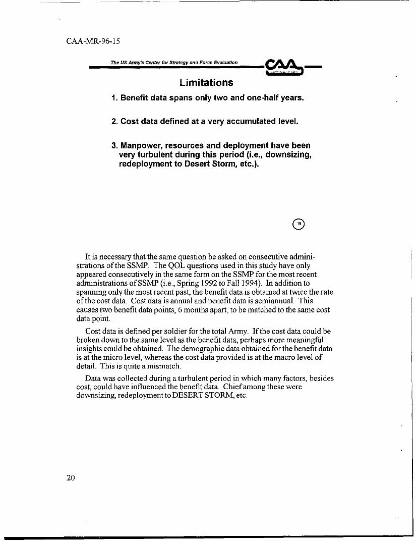
1. The SSMP data suggests that the overallquality of life in the Army may have declinedrecently, while the quality of life cost persoldier has increased.

2. There is an 11 percent drop in the satisfactionof the total Army population in the area ofgovernment housing quality over 2 112 years.

3. Overall QOL (-6%), morale level (-4%), andBasic Pay (-8%) had smaller, yet significantdecreasing time trends over the same 2 112years.

In general, the SSMIP data suggest that the overall quality of life in the Armymay have declined recently, while quality of life cost per soldier has increased.The only counterindication to this trend came in the area of Family Programs.The counterindication here occurs among married respondents who seem to behappy as time and cost increase.

The largest drop in satisfaction over the 2-1/2 year interval of the SSMIP datacame from the item about satisfaction with Government Housing. The drop forthis item was 11 percent.

Other significant changes were obtained in overall quality of life, moralelevel, and basic pay.

21

CAA-MR-96-15


General Findings

4. Recreation Services (+1%) and FamilyPrograms (+1%) show small increasingtime trends over the 2 1/2 years.

5. It is not clear that the benefits asmeasured by the SSMP are totallydependent upon the cost.

6. The Analysis Review Board suggested itmight be beneficial to the sponsor toconduct a cost/benefit analysis at theinstallation level in the future. (7)

No significant changes were obtained for Recreation Services and Family

Programs.

The Analysis Review Board convened at CAA suggested that the sponsormight wish to explore a cost/benefit analysis at the installation level. In regardto the Government Housing Satisfaction, it was felt that by looking at theinstallation level, the results might have changed for the better over someperiod in which recent housing enhancements were made at an installation.

Finally, it is not clear that the benefits as measured by the SSMP are totallydependent upon cost. Some more insight might have been gained if(1) the costdata were more detailed and (2) the SSMIP data covered a larger time interval.

22

CAA-MR-96-15

APPENDIX A

REQUEST FOR ANALYTICAL SUPPORT

A - REQ UESTFOR 4INAL YTICAL SUPPORTýR 1. Performing Directorate/ Division: RA 2. Account Number: 95147T 3. Type Effort (Enter one): S - Study 4. Tasking (Enter one):r ] Q -QRA F - Formal Directive

[Q P -Project I - InformalMode (Contract=C) R -RAA VF- I-N N"s V - Verbal

5. Title: Quality of Life Measurement and Analysis6. Acronym: QUAILMAN 7. Date Request Received: 08/01/95 8. DateDue: 10/15/95

9. Requester/Sponsor (i.e., DCSOPS): ACSIM 10. Sponsor Division (i.e., SSW, N/A) RM

11. Impact on Other Studies, QRA, Projects, RAA: N/A

12. Product Required: Memorandum & Briefing

13. Estimated Resources Required: a. Estimated PSM: 2.5 b. Estimated Funds:

c. Models Req'd: d. Other:

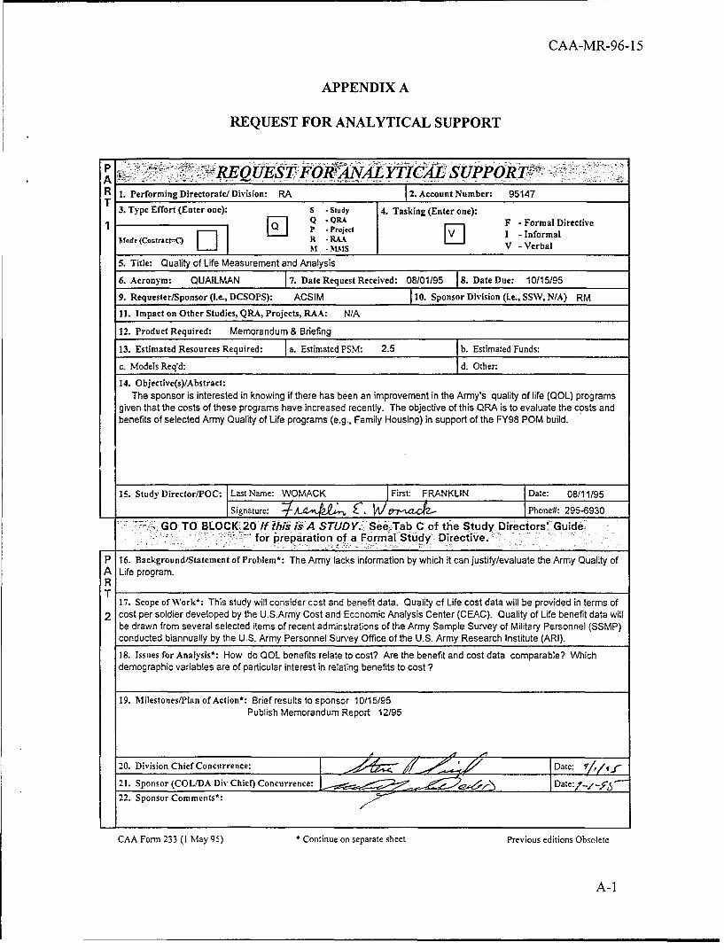
14. Objective(s)/Abstract:The sponsor is interested in knowing if there has been an improvement in the Army's quality of life (QOL) programs

given that the costs of these programs have increased recently. The objective of this QRA is to evaluate the costs andbenefits of selected Army Quality of Life programs (e.g., Family Housing) in support of the FY98 POM build.

15. Study Director/POC: Last Name: WOMACK j First: FRANKLIN Date: 08/11/95

ISignature: 7"4W.A, C. 1A/r-aT c.ý-I Phone#m: 295-6930-J GO TO BLOCK 20 If this is A STUDY:, Se'e6Tab C of the Study Directors' Guide-- for .preparation of a Formal Study' Directive.............V

P 16. Background/Statement of Problem*: The Army lacks information by which it can justify/evaluate the Army Quality ofA Life program.RT

17. Scope of Work*: This study will consider cost and benefit data. Quality of Life cost data will be provided in terms of2 cost per soldier developed by the U.S.Army Cost and Economic Analysis Center (CEAC). Quality of Life benefit data will

be drawn from several selected items of recent adminstrations of the Army Sample Survey of Military Personnel (SSMP)conducted biannually by the U.S. Army Personnel Survey Office of the U.S. Army Research Institute (ARI).

18. Issues for Analysis*: How do QOL benefits relate to cost? Are the benefit and cost data comparable? Whichdemographic variables are of particular interest in relating benefits to cost ?

19. Milestones/Plan of Action*: Brief results to sponsor 10/15/95Publish Memorandum Report 12/95

20. Division Chief Concurrence: Date: 1/,,•

21. Sponsor (COL/DA Div Chien) Concurrence: .Date

22. Sponsor Comments*:

CAA Form 233 (1 May 95) * Continue on separate sheet Previous editions Obsolete

A-1

CAA-MR-96-15

APPENDIX B

QRA CONTRIBUTORS

QRA TEAM

a. QRA Director

Mr. Franklin E. Womack, Resource Analysis Division

b. Other Contributors

Ms. Tina H. DavisMs. Nancy M. LawrenceMs. Dana Unkle

c. Product Review Board

Mr. Ronald J. lekel, Chairman

d. External Contributors

MAJ Steve Bryant (PC, DAIM-ZR)Mr. Morris Peterson (PERI-RZD)Mr. Bob Suchan (SFFM-CA-FI)

B-1

CAA-MR-96-15

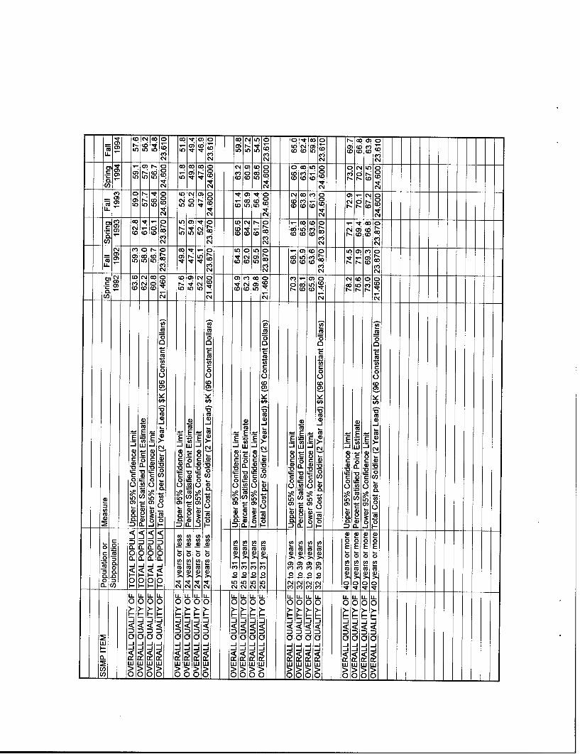
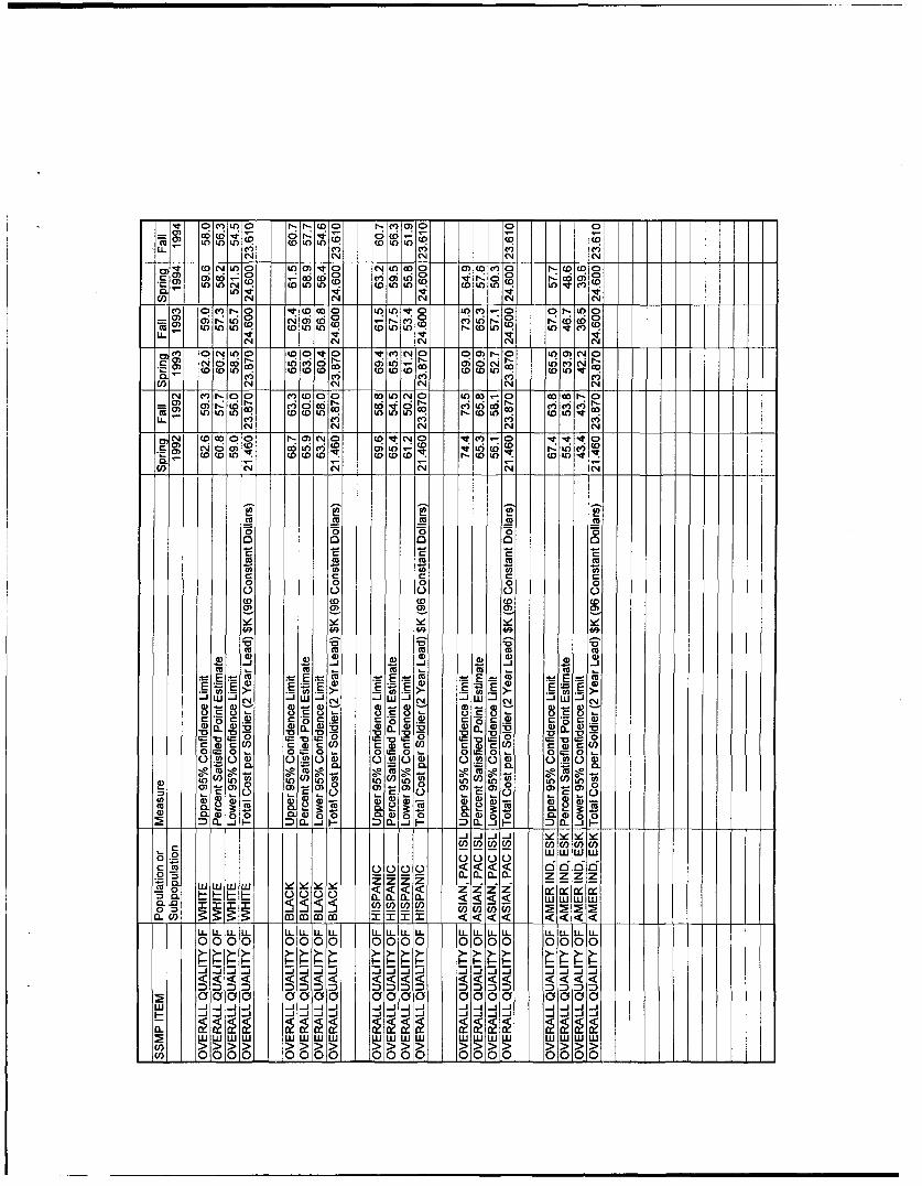
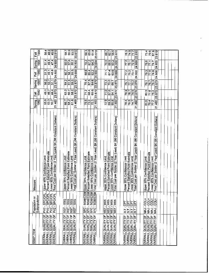
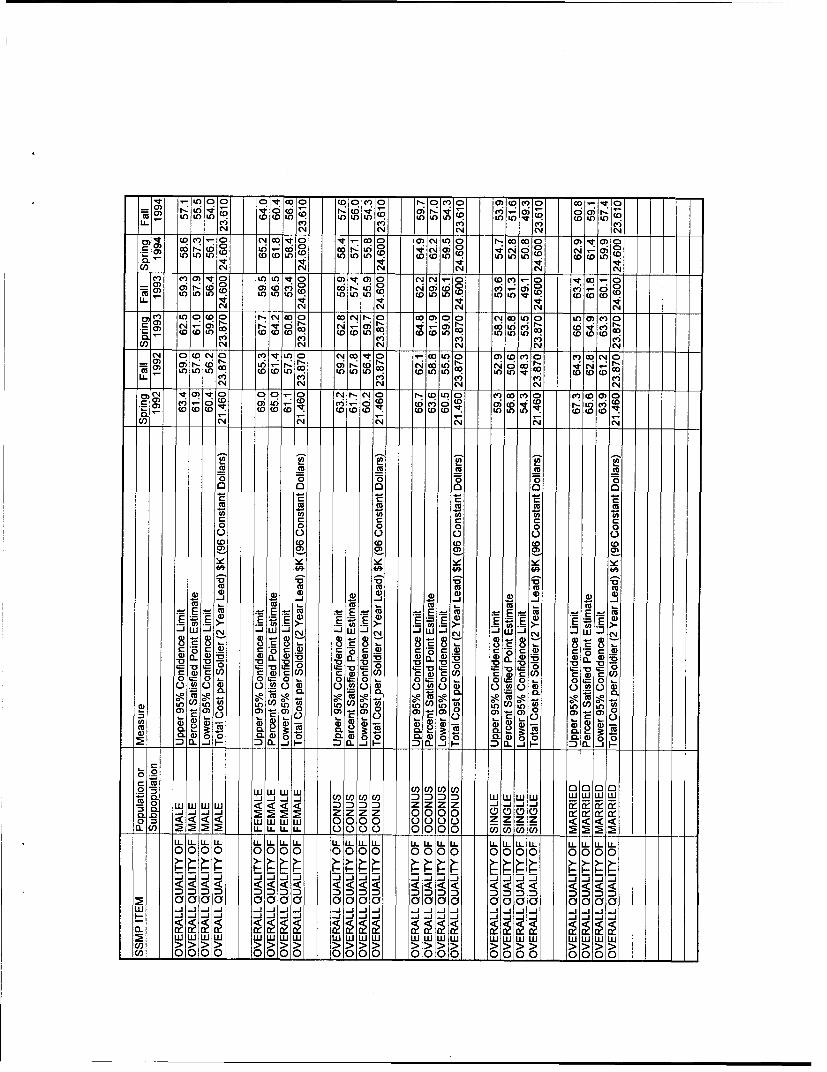
APPENDIX C

TABLE OF COST AND BENEFITS

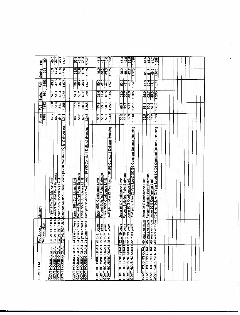
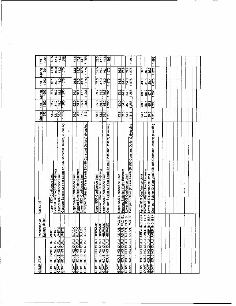
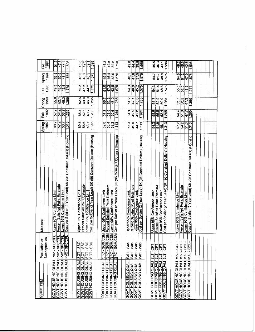
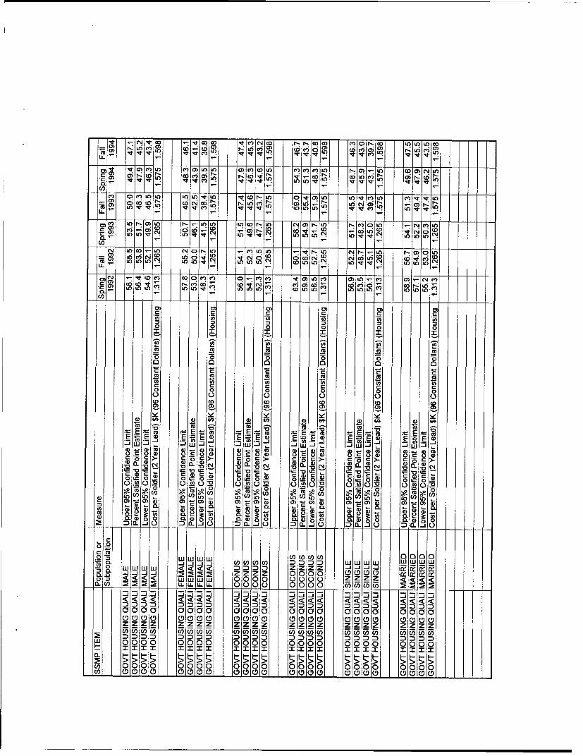
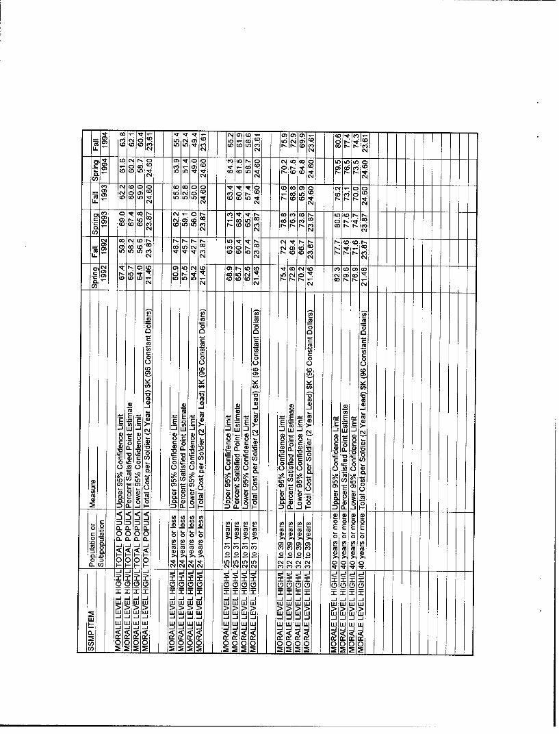
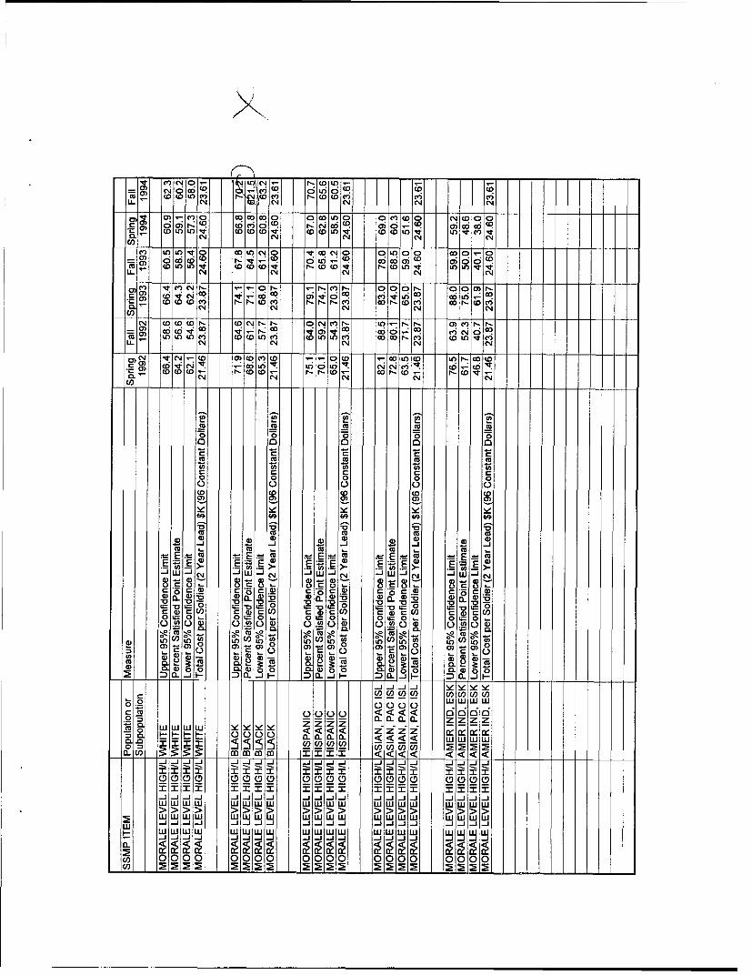
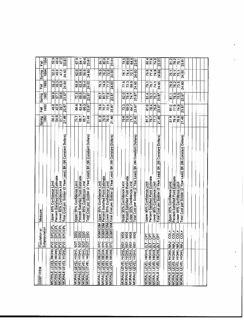
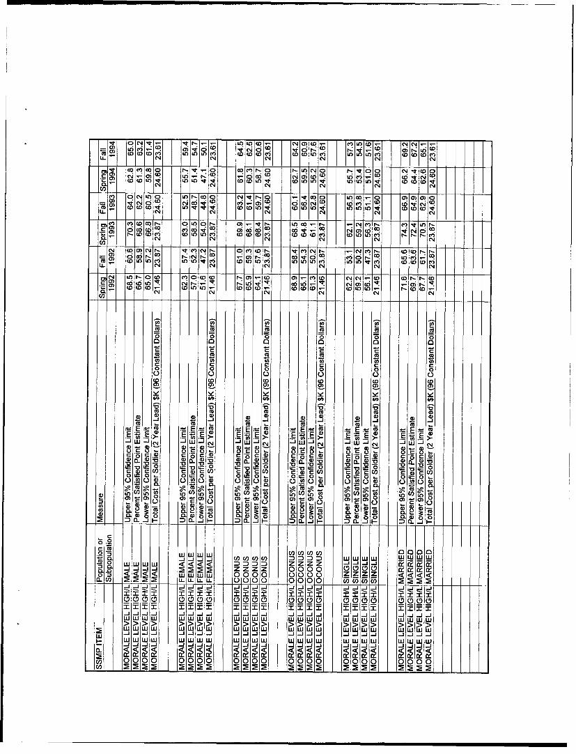
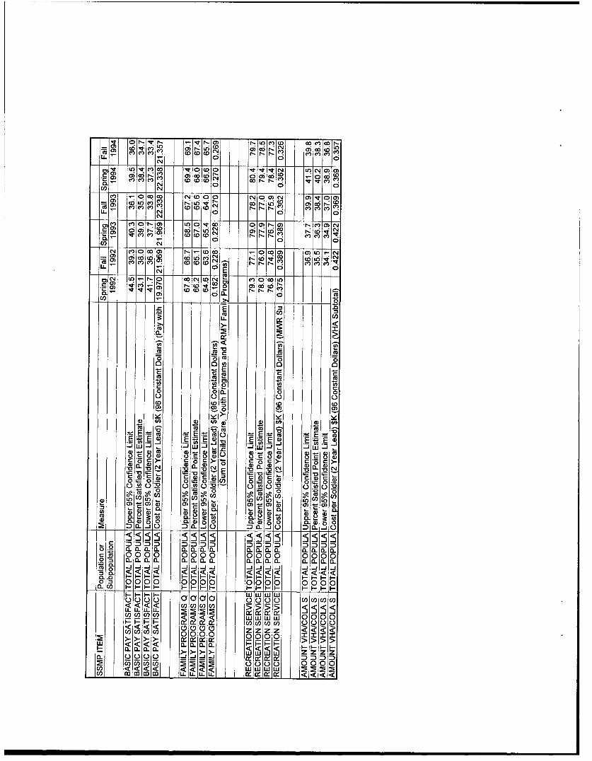
This appendix provides a complete listing of cost and benefit data for four of the SSMP items anddata for the total population only for the remaining four items studied in this QRA. Each SSMPitem is identified in the first field. The second field identifies the total population or subpopulationto which the succeeding fields relate. The third field identifies one of four types of measurements.The first three measures are the percent satisfaction for a given administration of the SSMP andits upper and lower 95 percent confidence limits. The fourth measure is the cost per soldier (2-year lead) in thousands of constant FY 96 dollars.

The last six columns give the data for one of the specific SSMP administrations (Spring 1992 toFall 1994).

C-1

(D a r (0 ( DLf ) 0) co CD.)w. LOL ,toL OL) co c t) c0N0 N C 04 CV

-E ) r - CDr- cl 0 r-cDCD 0 0C) C) .;0 l 0 t100_L Or)I D LoL o rv( o(D LO ~ co D r- r- (

_ i04 N1 CNN

*jC Uý 0 :O :co-(ý-

LO CO ) (0 US v lp (D Lo -) P c (G CD to I

N Go -ý o c U(0( 0( 0 ( r-r -C

04 N4 L N N4 Nl

N oc O NCO (NDN CDC)O C~.c D0 NC0zM PC L O L q I I -LOc

(I N N N NN

col tf U)ý (flqýq

0 0 0 00

Ci) U)COCOC

0 0 0 0 0

(0 ( (0 c0 (D

(DC D ( D 4)

*0 -- *

-JW- 4 -JLW - N uWj -J ~ C1 J J -JLJ Jc

0a* o05 )Q ). "L, 8 -- z 81 88z

L= o 70 L= io 0 v aU) ~ i CO C/ CO C)

0 0lO OCQ CCQ )U )Q OCO0 0. 0 0. = 0. " 0 0

16u -.( -a ~ ,- Cu6 , -! -e CLCCDCD

0 U) L U o n U) JLo U) Lo (0OolC

m... OL w~ CL CL R.CK

0 D.~o 0.00n 0 0.00 0.00 0 0. 0

CCU 0000 868 0000 0000 88

n0 00 0)00 0000 0000 4. 4. v L LO N N N 04 0 C)00

LL LL U- L LL U- LL LL LL LL U-LL LLILL LL L LL LLLL U-0000 0000 0000 0000 0000

D D D D M DS0000 0000 0000 0000 0000

Swuiww wwww wwww wwwo 1000 100000 0000 0000 0000

U- . LnD 0

Co Of)CD L

0Ne N 04 Nl Nl

a CDU) U)Oý OOCcc0 CD

__U) 0_ _ N 0N M

CDLJU *) mD)t CD 0UN) N N) NN N)C)r-C) ciL - l o

w U) In LO C 00 L o ( W) LoN N 0d t-) LDO -v

N' CCO 140 ID 0 L ~ O ~ ~ -

Li. to to) R CD c DcoL

N C 14 rO NO CD', UU)- ~ 4 111

CN OR N N

Cu 1 p Cu, OR CuoF n f q oco U)O - o U. 0q r oL q ( .

LL0 Ul) m Cl (04 N 04 N CN

CVC' CD (P lo o I ) c D C ClDC

0) 0) 0 0) 0

-o o co co (

C ~ ~ dCC ) C.). C5C0

(D 0)Cug~u5 CuCu -2G) ca~C CuC

E~C# E~C( m ~ CU E ~ C/ m :L-- EEC0~ =& O. ECu~ EIO. EOE E ' E ..

D ) .4) a 0. - 0. 2 0. a)00 .a) c U C D n cC

0 SC~ 0 ~ 0=0- 0 0 0=0 C 4-- 0 C -Cf u~um u C L~u

to LCu LCu LCu 0 )L OC OCu 0.)0 0.uo z.)0 0.uQ 0.

4) - ) 0000 8

C L4 00 CL0u0 0 000 CL ) 0.0

U..L~.L L~iU~. L~.ULi LU.LLLL LL LLI LLL0000 ~ ~ L 0000 000 000 00

~~~~~. 000 000 00 0 0 00 0 0

000 000 000 0000 d dzd

0)I '0 CO O cDo O M)~ Nr-CD 0~0- r(CD

04 C1 NoU 4 (DCl N to vN1

-% D0 C1 0N C'J7 r"0 C )~~0) ~-O 0 6Ru 6cr'i LOON CD 0 lr..(DC0_ N N ND N Y

,q) C'T co O r- )0 t- w o r- w(D0 rN- 0 r-r-r-r.

NC' N4 N* N N N1V:) N 0 CLO 'U D0 ('0 CD C-4-N O C -r'Cl q:q

CYO _D, N N0 tr DL N N zr iCl rý6ýv N NNc v l -No~ N n-N N~D (D.- w 0)No r-L NC')0)C',)

C') C')7P

C"0N N N CN N N4

0 N) 0)')- N N O C O O CCDO 0~) r- o - 0 CD 'q

CD Lo I-WC -1 r- r -NNF -Z

(fl Cl) Cl) ClJU)Io 0 04 0V 0 04 01

6( 0e 0 0 0 CO0 - r - ( qa Lvv C C CD CD LOC Dw( R N R G ý CR

LLCl ce) vi) Cfl ml ml04 N CN

(P 0 0 C e p0U l 0 0 T 1 00)o e 0 (D0 0 L 0 0 0 4C OC oI

co co I0VV 'tCu LO to _o Cu I. - Cu Cu W (D t_ - oNP

0 0 a 75 a. -6 a0aa

C C 0

0D CD- 0

0 0co ~ co (D - D CoCD C

Cu ~ ~ ~ D~3

6%

E2 EQa E oo EDDC( E E

CVa NNN CN 000 W '

cLC/ a- a) 4) a) COC0COa) -0 a-N (D- )( )Q .4000 00 00)00 00 000

~c a)J ~ CJ J J/..Jr_.J

0 0oi 0=c0 0000 000-0 0 = ci ooo0

CI) 0» LO » » > » (n »O»)V_ 000000 0000 ) 000 000 0 00 (D -) -

r LOO OLOD LDOC O LO C LO (D a )C ' O IT( L I0) rl L D q: a CD cc CC D

ci'

U. C r cD i .eLO,4IL CD4DU)

Cd)N N NR NN

C~~~)' CC)0N* Lt))~ a) ) 'tO 04 a- ~ C D- O LtI) LO (D ) .p LoLo Lc) lp (D ( IDC o oU) a

NT Nt NINt Nt

0) 0) ?1-CD0 0 o6c l-N~ NID 0 Ca)O C;fl W 0 0 vi ci)m D LoU) LO CDCDC .o 10 L DoUo CDCLD X) . o ULoL .v CDCDCO C

N NN NINtN O DNO C4fl IW~ ICO aCC) ~ C N0

(N G ~ -CD N vGCDfl r- c n O 6 6

CN CN Ny N N

Lo0U q C oCR )u)t * CD OC( oLoD ULo Lo .; CDCDCoce)-. G~4 C~6 ) D ~ u C9Cd) Nl N NN

CUCV CM C14 0U

CMo4":a- 0 ý -ý `o a) 0l C )U) c m aCI(0 0 0 (D'T0 - OC)E o (o C CD co (D l: cot CV )LDL tD(

CU It C C' ýicql

0 0 0 06 00

0. C0 0 C0 0 0(D CD CID CD cD (D

a) ) ) ) (D a)

cc cc w -o mE U tCU CU CU CU- cuECU c w E -- c

CU .CU i. C U4 .. CUI . CU CU

4 0 .d)15 4 -0 aE 0. 70OG O)Q.4)70 0a.OG4)a1C

0 0. 1 0.

aC)Cb rO (D =cUUr ID V0n 0 0q- 0q- 0 0j 0- 0 0-

V 0.0D00A0 a 0M 0.G~ O.Oo T-o CG)oMA 0.00

CC

CC 0 0 0 0

.275 w w w w()() )j)claccl - j- co )CflOC) U) MD WWWW U, WWW

CL ~ ~ M i i 1 22 z z zZ 0000 (ID (D 0 O0= <<<wwww 0000 0000 zzzz <<<<

)0C1)l -ý 22 L L L U -U~ 0000 0 000 CFOco __ FDFI122M2ILL -LLLLU IL L UL L LL ILL LL ILILILUL L ILLJ ILLA LALU IULLJLLILL0000 0000 0000 0000 0000 0000

MM MM MM MM~ ýn« MM

20000 000 000 aa Y0 0000C 0000 0 aaaaa00

999 M*l 99ll 991 M~luuU) ~ 0000 000111010>0> 1 0 010101 0 000 0000

~CD NCDO~ (C~0 ~ uic~a~ CuiLOto It N 00) C DLc) (DCl) D0 0'-0) C r'L t

LL co-

r o-GoN n0 Lei (7 (DM - G t 04C~ Nr-C- vUCD~ U C6 NC

0)P O0C Cl 0 r- v C0Lr'T vn -W v nv4L O IT oL

0- 0) 0D 01 DC o C) o( O0 0)

- l 0q -l 0ýqqUj :7'q n ýj0 :tOM o r-C)0 ( V)M 0 C Ol 0 co 0 iC,(in iOt no oC in LoL o nO0 oL an !

C ~ C;v CN C7- Cr_ o 0 co 0 0oL Nc )c

0 0 0. 0 0

0) 0)cn DC

00 0. 0 ~ 0cc)~~- cotococ

(D t ~o V9,~ a) 4. o 6a0o Cj O

E '5 .94) E-Z;g (D E - E ) E ;; 0) )4)g )I

0 0> 000 000a. 000 0. a.O~ (LC 0 0

0000 a r 00 )0a I4) 0. 0000 000 0 0000

m/ 00 0 00 0 00 000 0 0 0to (D(C COLOC Lo U)Lo

-C' Co L CD WCR 0)0O) LO~ U M a) CM - () 0) 0

to P U)L ' U)O c!c' .f

a~' CD-CL 0)C t lr-CDý a 0CORLO~f aCR 9~ t

I- ) (C v C'4C rui LtO LD C''0A co r-

IL) (- -- 0 DDL

CO

v vv r)Lov q ) qU)v ) (UIq cjL

oto v 0 0o 0 OL oi

N I- I*. In Iý O o w. U G) (UL o )L

N ~ 0 -~ 0 n qI I l ý

U' O 0 0Di oQ OC . 0 U)c C1 V

CM CD cm C a

C _ C Coc 0 00a

0 0 0 0 0

0) 0) 0 0) 0

0 0 A02 0?0 ~ 0

a)a~ 6a 4 t ) 1, 0) My O) 6)aca ig a cc-.-a m a& m. ~

a) 5 a 0 0) z8M 1150 aa)0 z0 o0 40)0a >-~i O.0 ,D...0 ;P- 0 ;0- J0__

0 .20 0 00a0UC 20U.o 0 .00 < 0 0i53 0 0A T 0

000 000 000 000 000

g 000 000 000 000 0000o

Co 000 0000 0000 000 00Co CC~((D ~ U) CL(C( CL(( (OD

0o)

) 0)L)qc

'r ~ 0.Lt) LOC04 MC co)L -CDLý l ~ DC~ )

C)U v~C~) CCLl 0~UU c~L) Cl Lo ) 0O0)Ui

U~) O-CD O)O C0C C\-0D N 0U) N-LDC'). ~ ~ o U'CiCD N0c D "6 N D &0C LOO C , I

0)( It. ,Mq-0 - V)N0 -

(q.qJ3 r-Nr-U culC CJ )CDX .)DA -7 U)r- ID ~ 0 LO

L6N0 D N-)( D L)N0 or 0 -f C -40( M r-(

ON. i 0 r ý0 ( l l CDC) IT 0)' Lo o 0 100-0u-)D U- OC! L)L f L) )C! L)v - -Lo U) 0 CLO v '

C,)

C Ct CDC

C0 C0 0 0 0i 0

0 05 0 0 0 0

0i 0i 0 0 0 0Q. C) L)

( to (D oo co

a) 609 a) 6.,0 0) 0., 4) 6

o00 0 0 00) 0) 0) 0) () 0)

i) io 70 N a) a. 4) 04 d) a. 4)Cc -) - CoU Cor u

o~> C0> 0=0 =0 => - 05) 05C> C5>

~~ 0.~0 0A0 0 -0 0A 0P Ae. ~0 - U )0

C2~~- U) %.!-(a.,Lo aaO 0 LO~ U)LOcoLo a..V W) U.) ) oT

00 0k0 0000

a . a -D U U' a .- ) U U

.2 7 .C La W C /U) U) c/ 000 ,., , 0 00 0C i20U)Ci) U) CO(002Q)CJ) (nl iU2C 00000L)0=- a. 0 0 0 .I I .

an a CLC4'J' i-l 0000 -

000(000 Cya0000 0 000 0000 a 0000

(/ 00 00 000 0000 0000 00

I/2 0 1 (D 0a , , (DC!2 ( D DOCDO 0 0 0DOO 0e 010 (0

t- N f ) C ) - D C D ~ )N L O C-I -D Cl 0c c )0 r o ) mD I m t ) CLL -. -,

a --- .- .

CL

*ý v:4 ý O C U)UC .CD. oCI - D NC - r f e r- Y )Le ~ y -) 1-

C0) uýra)L 1": 7U)U) U C! CD1-u) IN)1LC N-clU UC)C

-DU U) r, uci ut9

m) ?? L0))U) OinvLOL o )U Lo vo IT 04 LO oW

ojc 0 0 0' 03 0 "G o CI w e lGo W v CojC)0 oC 0I o1-L

OL ~ ~ ~ ~ ~ ~ ~ ~ ~ ~ ~ C Coo O L OvC? U )L l C L OL ' r n i)k)L l

0000 0 0

0 0 0 0 0 0Co 0 ) 0)L 0 C.)CID CD (D co (D CID

a ) 0D 01 ) 0j ) vi t4

E~E E =~ E~E E E0 E E0

~0 ~ N0 a 0 ~0a. CN 40 a. 4)0C,4a4) (L 0) 4) a.sa) a

Q: 0o =aJ 0aj 0 tr_ 0 0 O~0

CLC

S.0

75 CO/wC w www w W<DDDWW zza .WW 2222 zzzz 0000 000 wxw

0o3 <<< www 0000 0000 ZZZZ <<<<iC, 1( 1 1 -ILL LLU 10100L0 10 000101 5Co c I nF- 1 m22

0000 0000 0000 0000 0000 0000

(00000 0000 0000 0000 0000 09000

DO (D D(D D D(D D( (DO(DD :3 DDZ): = (DCD(CM (D D D

N CCJCJ 0 CN

(9 C CDN N- c')0 9 ýcyDNO l r-, l N 0C! 04

mm N 1: 0 0 1 CN 04 Nl(14 ___v__ c) -

j0) 9 (qi ? - -7 r:CO r- LO LON 0N co n mm 0 L CN )CN cm N NNN c N N m N m nN

NNN N N

U-N N N mN n r'-NCD 0u)t. CD).'. M.O) C ,l)C~

N - N CO Ný N7 NP 1 nc

oo a aaco rn co

-~0 0 00

Ci) CO Ci) lC

0 0 0 0 0

a ) 00. 0) 0e) 0)(

E~~EC 4)~EE ~ E E E~E

C5C ,- C5"C,- 0 C>- CC> C ~>-CU r--0 C r

U) 0. ~ 0.U=00 0.)0 0

__ __ _ _ M 0 0 MA0 - M 0 _

0 00.2a .,-0 05> 0 5>,X . 00>ý c

0.~~ ~~~ o o00 0 ~ U U)0 O 000 LO tDoUt . NCN 0000CD C I8 NNN NNN CC~) ) 0)

Om 000 0 00 0 0 000 000 00U) ( CDCCDC (L - 0 - -(D CD CD I - 0 D(L-L

v ~ ~ C (t.r D O'I co ID C

U'C M Cl) C D 'T c)C'M . A 'J .j 0j 0U.C 4N N

F No0 N Nf t- No0C -

CU.. c) e N C- l N C () N Cý C)C) N C l N

U) 'ýe.j6 uýo4 ýnci4 ac'i N 'au- ) Ci lpCN)~ CS C')N " 0)) V~C)' ' N.

LL C)DDI O cD'i C0.4 NN ', a Cý

r 0) 4 C- r. CL"ON~ 6)4 LO 0 Dp, G 0C C o N*Eý e Cl) MC-4) Cl)N M 04 MN ,- .0A'C4

06 LO0 N CDL N oiv1 N c Nc c

_ l j " Cr'S )Mr*: C CD-4 04 rC'Lfl coc rO) I

- N1 N4 N NVM -D N0 .D0,C

vc ~r ) L M0 N ' l C D t Md C/) l

cia Y Cy a

m m(

0 ~ 0 0 0

o 0 0 0 0

L) L)Ci C.) Ci)

co co o 0 0o

0) 0l W C.) 0) 6

aD ar ) a) E a) E a)

z1 t! a) 18d) z~ 0 G) Iwo)

0 ;- 0a) - 0 ,C>0- ;.C -

Ii) (D d 4)0U 0 0 0f 0.Cf 0.CI 0r.Cf 0 0 0

L) S2)0 0.)0 L.0)0 0.0)0 L.)00

0 "g '- 0i

a)U 00008 4 )444 000

~C.~O(~ (DC~O( (DC w (~C ~~OPDC

W 000 000 0000 0000 000

0i 000 000 000 000 00

C) C(D 0 0 0 (D 0 ( (D (D CD (DC -90 ( 9CC (D C9 D C)

a) Ce) C c f- 0C0 GoLC It)o C -CD CLD(0Co 0)DM D r- VC0G

U- (N4 (N (N CN 0N (N~~ (')Or'-(N ~ ~ 0 (7)O( LO No t-r-:~ N O'C(N (CC

04 N C(N (Ni (l VC ococý C) N (Ni M (tM Nl l

(0)

C') ai 0)t LO(N 0CD( -0 (C to6

(. CN (N (Ni 0N

(N) _(N )c l) 0 4 M( (y N (N ov 4 0 ( Nij04 0 0

a)N (Nj (j (j CN (N4

(N (N v(N: G F (o N a) (DMN MN

Lcl 0 0 04 04 0

0) t M 0co L Cl itoC) C 14 0 Y ; CY)N v0 cd)C C u) cu -)M M ) CS Cu Mu M CuM M

04 04 0 C C

Ui ) U Ui ) UC) i

o 0 0 0 0 0

0) 0) 0 0) 0) 0

0) oC~ 0 CY ) Y ~ 0 0) 4 ~ 0) l

Eu - - 4)E~~ ~E EE~EE E EE E~E

0 ;P- C5C;- 0 ;o- 0~) 0~> 0~>0).0 I) CL ) _) a.(Na 0'a -0 N 'a~ _N _c 'D v a0 l )0

c0)a)5 0 a r_ CO4) rf) U)~ cUL5

a) a')0= 0 0. = o 00=) 0

S 0) 0) 0)0.)0 0 MA)00 0.)0 U.)0 An0U0 0.0) 0

0 0 0 15 +. 0

a) 0. 0) (D S I ) IM 0 ) 0)Lo. (2((( W - 0000o

LU 0000 0L000 000 0000 0 L0 Q4)000 004)00

(L 000 000 000 000 000 000

.2-5 IL~cc (- 0- ~ c (L~o U) U)c toc

coa Cl N )G

LL 04 04 0N N~ N

'I (0Na)lý N O) 1 C!)(N U0 N C) C C)N c( l0 C')O

CD UN q( N Nl N: N

N' ' l N M N NI NývC)M l l N

.a) N D qPýC, C l-Rc4 qc *N 6C C4i LO 1-*N- ýCýq

- 1 1 N N4 N CN N40 l l l 40 4 0 N 0

N ) N Ný0 ito0 N NCNG) 0c .0 .60 c)r ' C4;

C' C ) rC/) ': V C-4 U) C n C/) UP: OR ci vl0

,ý c) e UC) M U) CN 1-U)Nr: tC) ) U): M 4mý l

U- 00 0ýN 04

o r 0f :ýV 0 - v Y0C1 C Ci 0C C. 0C

C/) CO) CliU) U) Ci)

0 0 0 0 0 0

o 0 0 0 0 0C-) -) 0) C- ) L)

OLg. EC O cc:L Eot

Ei E)a = E0) E ) E) E)a)

t! 8..~i (O z. 8 am) z.. 8 M z8Mei 8a) 8t o" ~0 0.)0 00 00- 0.a0 0.00 0.a)

0 = ~0 0 t- 0 0 0 ~ Oj &rl-0 0 = 0 0 l~0

oCaCU ) )0 000

m CL 3: v CL M 3: )C/ CL WWW CLI0= w w 0 0 0 0000a

.2 )_w W LL U .UU 00 0 o00 C/) C/UC/CU)

zzz w z<<z DDDz zzz zz zzz zzzz j ia 000 0000 000 0000 0000 00

U) 000 0000 L 0 000 000 0000 0000<<

U) (D a (D 00 (D(0DO( 0(D 0000 (D (D( ~~ C (D( CDC(DC)(9

cc ( c()0(DcPi U)L tci c LO~Q~ CD, -C It- r- D C- or l lLL' N N N N 0N

orý CD;r C=! c U -. ) Cý LOC- NCDCDO U)LALD

CY 00 N CN N 0N

(D e'iO L CD t D giNOD v~r-~ r-ou " co t r P I' '

, ~IqC CDD )UL) C) CLO NCtD Nr-

C0) s o0 ) Iq U) N-or.- l ( - (q c~c~)C uo)(DmCD CC!&0 IT r-to c - rN- P- - I

04( N NV V

CD) CV~C rLA ý

CocoCDU'CO DL L ) N. (D(D C) r.-coo~ Pr -c _PC' NI N rN Nq N~ ,q

N4 ( - i-ýi- - r.- ovv r I,-NC CDNOC '*CN9 C' CDDt-

m U' W)LO ) v t I m D (0U') Nr)r- COCD Cr.- N-P--ILN C1N 0N N 0N

0D Cfl U2 0D2 rý pC :cq ( l 02

? coc o co LO LO ( OPo- -0 -PCNC CC

020202 0 02

cc m C1

0 0 0 0 0L) Q. 0. 0

m C13 m cccc(D4 4) 4

4) .0)-

(Da. a) (D a. 4) (D CL 4) i ) a. 4) -o4)a d) i'a m. * "D 0. - 'D 0.a)

0 U ) aOJLU CID C ) a cc4 ) c c U)

0 S 0 " 0- 0S 0 - 0 0CL4) L 0.4)D C.4) m ) ) C0 0.0)00 m

0-a)o 0.4)0u

0 000 Lo~

3. CL o) o Z -)4U). n U)> 0 0 0oo 0 0 0

0u 0 000 4) (D 4) 4) NNN 0000

a) 000 000 000 000 0 000

X

CD CDUli F- CDo' N-cDC ) Cr) viclL N %I CN

~~C O'C) DC0 0CL0 0~C0 NC- D 0

0) aa) I.- (0 Cl0N0 P- 04 0 01000p cr C 06 oý1-t~~C co 6%CO LOI oCD O -CR O lOOIt(D Lo U.) CO CDC(D N C ,CD 9-D0 100pNl N N 04 04

m D? to U ) LO cococo PCDC ~ co -T'c r1-CD~ co O U)LO.L N N4 04 N CN

C Y) _ Go___c~wý,4

0O

NT -DDCN CDNN.N 4 0 CRN 10 vN-N. W)C)-NORa) co ";rr- 2 04o~ 0 ) CR cci

C2,)

co W (DCl) C-D-CD10C') r- P- Cl) c)0)N- CD ) co 10toCl)

r, N- N N N1 N-

CCY DCGo co C CD4 r- OR N ;-N-C9 00 )N Ci c rCD'-4oR

w , . - oC) c c )m C OL D c DU)I Cl)LLCu Cu4 0u CV Cui

Co ( Lo -0

o 0 0 00

o 0 0 0 0C.) 0 0) C.) C.

60 64V

G) i G) J w -J :3 5 -1 Cu Cu ::3uU

04 w0C14 0. 04 O CO 4

CL0 0 . ) a 0. -~ )( 0. -0 0.

(Dl ruC-j COCu au u w uC Cu-__~~ Oj- c S _ _ ___Cu w 0.CO 0.0 0.Cu0 0 0 0 0

L) A L)0) )CM 0 0i) Li0 . i) 0i (D ) MaC.) C)

.25 16 z50) I--II 000 . 0 zz 0

=)Ia -- -- M .CL -i - - D CL - D. CL -j-

.2 w www)L)L)w www www wwww

Cl 00 000 000 000 0000U)U U cELU M M M M Il~l :I I < <

a) 04a ) 1- V 0 V PCI-C ~ V (3DC) It-Ce iN--- V

cc 0CDrCVO CD CD CD0Ci c or Lf C6JD r- .- (Dd) co o -- r

(. (~ 4N (N

-IV No CDO"0 c ~CR(q0 Lq " OR0 vDCO: .- r)- 0 0(L00) Cýait-cq N )c o P ) D CD o oc a)~ r.-~ &c 'i ( 0 o m (qU. !F? (o VN IT (N co(NL)I -r r-V r -r - _I -I

cc t (NV V ( ( N (C t -N N VN (N (Nc t Nrl ý t rl ,rC,,_ 0__i *

(q LACO -7 riDCJ CJO) 2q0 r- C icr oO v ," C,, c qqC' 0) (D-C' - coU)CR

(N) 0N (N O(. . qi- , .N ( oN co (Nr l

V VCl) m ( DC Ce) l- r_ Cl) r oc Cl)CDN -mLL 04 0 C4 C14 C C14

t C40 lto r,- 0, r" o-C) oc (Go v 0o 0oo o'4 i 0) 0lLo L - t CO OD r , C- tCr

0 0 0 05 0 0

0 0 0 0 0 00) 0) C) 0) 0 0Q

-D 0)) 4) 4) 4cc cc - - -2 tJ mm

Cu ... Cuu CN _ u *J CuJL _J C41u 00 EC a'5 LD~C c-C aE C AEC CECC

C~0) CL(D: 4 Q a a) C ) 0 4 4Ca) -0 4) ) 0~

r_ 4)) cC~G 0U C/) C (D=c ) 0c~~ r0 a a) r0- 0. 0. 0S0 = 0. 0. W 0. 0= 0.

Lo Ci)u in U) Lo~fC Lo (ni Lo flC V U

Lo U) co C 0 o ~0.0)0 0.)0 0.)0 000 .0 0.00

03 000 +5 +0CC)000 (CL O( CL CLUCL Ct

ci~oc'C, 0o/C~ C,-lC~ 0 0 0000

0. a. (L CL U) U) co U I S

a C/ ) 0 00 CO/)OC .oIC o . . . - - ___ __

.2 7S 0- C- a. M - - - .

0- www 3!w www >WL WW 000WW

Co~( 000 00 0 00 0 0 00 0 0 0 00C', Z, _z

ca O(D (DC LALA-)LAc) C6 co co EDC vi w oCDLU) vi LAC 7, ci toC co D viCL 04 04 CM C0

N7 CN Lo - N-C!oc p ( )tol ' ) C

CD) Oc'O LANc) tIT C co.i O --t (D L O v & i LAW.- v o)O(O v

-E '7C', C C) CDLAc, ~ -'N C,

It NN N- o: Pý ý ý c J i(

(DAAC ALD~ CDLALA) ' CDLO LO v U) LoL c co (Dr,)LN CN CN 0N 0 NN') LM r-ic q )CC i'CD-( CD-C)C NN-C ON,

I--(t to - CD L U) ClA CO (D CD to.- (0(0(0 CD LO LO A. I- r-coc-

LN CN N0N N N

C,,N

6I 0j 0 00

0000 00o) L) L 0 0) 0(D C co C CD CD

64C C u uC

wn M co ocoo 0 0 0 0D

a) E D C ) ECDEEV -aE

q u Cu cg a r-L 0cu .9? Cu 6 r- LD. r- LD 275 'a ' 'D~C a.-C 'E -aC a2Cu.E

C&C ) U)W co~G U~C ) C5 G c

S01=.. 0 0. 00 0 .S.0 01=0.. 010. 01=0T.TU o0 40 ) 0T 0 a) (3In 0 ) UMnAJ 0Ld U Ae 0 0

16Cu - -L'4) 0 - 00 C-)(i aAL LAL'C5C

CDCD CDa

C0) C -)

=~ý .. C.. r) .... ti = .

0

S.=

_ CL _ o O 8 0.4a0 .400 0 0 O)oo OlD0

.275 w wu w wU 1 D... JJ aICl/C w www WWWU<<J D zz

am 2222JJ~ ZZZZ 0000 0000C ofx0 : w w wu 0 0 00 0000 ( ( Z9zZZ < << <

0-, 0 U.DL 000( D D0 0000 _D C)5 C)0 ( (

wwww wwww wwww wwww wwww wwwwIIw ~www wiwww wwwwi wwww wwwiw wwww

I- W WWW WWW WW w WWW W WW W

w, 0000 00100 0000 0000 0000 0000i, w i w L uL

v0 0 q ý0 0)0

N) 0or 3 D( 0 0Y oC

CL 0-ic N, C DC) ~C~~

wNtmM V q~0I0 U)03C 00r (3) Ncý Cl 0 0

0)N C D 06a1, L CN a) DCDc-00)0 ro IT C*~c D c) Cc DF r'- F l ceDc I

N4 (1qcqlD-N (O 0)NDL C 00 Lg)

0 0c ) mD 0ý c oc q r Nr l c)CC,, - 6

14' Cl 6 ) Dco,

:EIacCULuLC CD

0 0 M 0

0o a 0 0

to co c 0o 0ý 0

>- ýe leu

E E

0 0 0C aa.O)

0 ) 0 0 (

Ci) a) -) 0 )m0U 0..C) L 0 m 0 .

(n aa aa a)a (Da4) 0000 000 000 0 0 0aa00CL00

C '8 0000 0000 000 0 00 00.2o 75 --0 - -L M MCILa0- S.~ I_ a~-- -I -I- E

0=Ro 0000 0 00 0000 /c/c/a. C ciuu, 555> ý0/ Cj) Cl 00 000 ) U U oC

COj wwwwULULL 0000Ci ) U) U) 0 L C- 000

Ua c oc 0000 J.J

U) UOlC)C/) L) 0000 0000

CAA-MR-96-15

APPENDIX D

QUAILMAN ANALYSIS

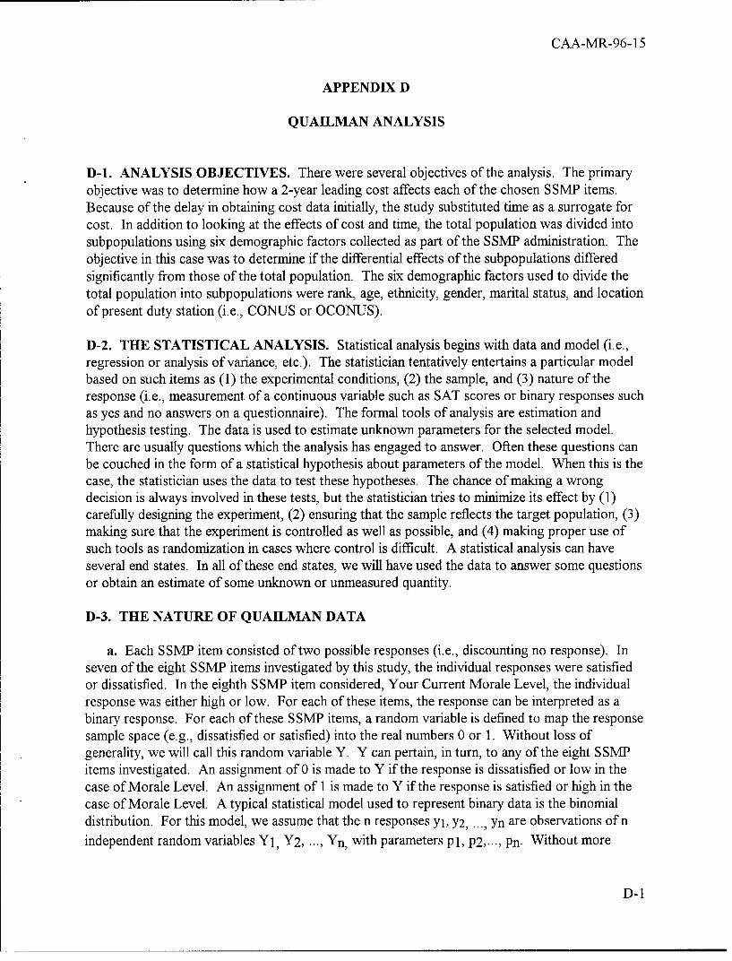
D-1. ANALYSIS OBJECTIVES. There were several objectives of the analysis. The primaryobjective was to determine how a 2-year leading cost affects each of the chosen SSMP items.Because of the delay in obtaining cost data initially, the study substituted time as a surrogate forcost. In addition to looking at the effects of cost and time, the total population was divided intosubpopulations using six demographic factors collected as part of the SSMP administration. Theobjective in this case was to determine if the differential effects of the subpopulations differedsignificantly from those of the total population. The six demographic factors used to divide thetotal population into subpopulations were rank, age, ethnicity, gender, marital status, and locationof present duty station (i.e., CONUS or OCONUS).

D-2. THE STATISTICAL ANALYSIS. Statistical analysis begins with data and model (i.e.,regression or analysis of variance, etc.). The statistician tentatively entertains a particular modelbased on such items as (1) the experimental conditions, (2) the sample, and (3) nature of theresponse (i.e., measurement of a continuous variable such as SAT scores or binary responses suchas yes and no answers on a questionnaire). The formal tools of analysis are estimation andhypothesis testing. The data is used to estimate unknown parameters for the selected model.There are usually questions which the analysis has engaged to answer. Often these questions canbe couched in the form of a statistical hypothesis about parameters of the model. When this is thecase, the statistician uses the data to test these hypotheses. The chance of making a wrongdecision is always involved in these tests, but the statistician tries to minimize its effect by (1)carefully designing the experiment, (2) ensuring that the sample reflects the target population, (3)making sure that the experiment is controlled as well as possible, and (4) making proper use ofsuch tools as randomization in cases where control is difficult. A statistical analysis can haveseveral end states. In all of these end states, we will have used the data to answer some questionsor obtain an estimate of some unknown or unmeasured quantity.

D-3. THE NATURE OF QUAILMAN DATA

a. Each SSMP item consisted of two possible responses (i.e., discounting no response). Inseven of the eight SSMP items investigated by this study, the individual responses were satisfiedor dissatisfied. In the eighth SSMP item considered, Your Current Morale Level, the individualresponse was either high or low. For each of these items, the response can be interpreted as abinary response. For each of these SSMP items, a random variable is defined to map the responsesample space (e.g., dissatisfied or satisfied) into the real numbers 0 or 1. Without loss ofgenerality, we will call this random variable Y. Y can pertain, in turn, to any of the eight SSMPitems investigated. An assignment of 0 is made to Y if the response is dissatisfied or low in thecase of Morale Level. An assignment of 1 is made to Y if the response is satisfied or high in thecase of Morale Level. A typical statistical model used to represent binary data is the binomialdistribution. For this model, we assume that the n responses Y1, y2, ..., yn are observations of n

independent random variables Y1, Y2, ... , Yn, with parameters pi, P2,..., Pn. Without more

D-1

CAA-MR-96-15

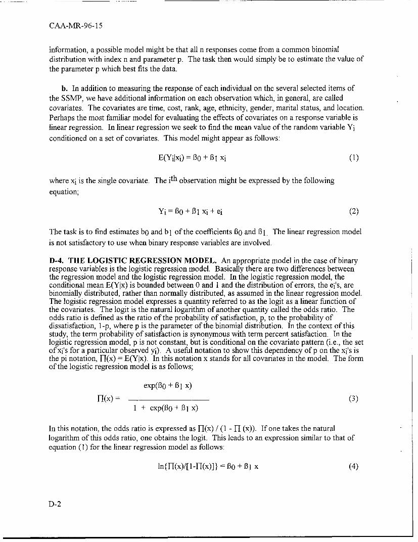
information, a possible model might be that all n responses come from a common binomialdistribution with index n and parameter p. The task then would simply be to estimate the value ofthe parameter p which best fits the data.

b. In addition to measuring the response of each individual on the several selected items ofthe SSMP, we have additional information on each observation which, in general, are calledcovariates. The covariates are time, cost, rank, age, ethnicity, gender, marital status, and location.Perhaps the most familiar model for evaluating the effects of covariates on a response variable islinear regression. In linear regression we seek to find the mean value of the random variable Yiconditioned on a set of covariates. This model might appear as follows:

E(Yilxi) = B0 + B31 xi (1)

where xi is the single covariate. The ith observation might be expressed by the followingequation;

Yi =o30+31 xi+ei (2)

The task is to find estimates bo and b 1 of the coefficients B0 and B13. The linear regression modelis not satisfactory to use when binary response variables are involved.

D-4. THE LOGISTIC REGRESSION MODEL. An appropriate model in the case of binaryresponse variables is the logistic regression model. Basically there are two differences betweenthe regression model and the logistic regression model. In the logistic regression model, theconditional mean E(YIx) is bounded between 0 and 1 and the distribution of errors, the ei's, arebinomially distributed, rather than normally distributed, as assumed in the linear regression model.The logistic regression model expresses a quantity referred to as the logit as a linear function ofthe covariates. The logit is the natural logarithm of another quantity called the odds ratio. Theodds ratio is defined as the ratio of the probability of satisfaction, p, to the probability ofdissatisfaction, l-p, where p is the parameter of the binomial distribution. In the context of thisstudy, the term probability of satisfaction is synonymous with term percent satisfaction. In thelogistic regression model, p is not constant, but is conditional on the covariate pattern (i.e., the setof xi's for a particular observed yi). A useful notation to show this dependency of p on the xi's isthe pi notation, -I(x) = E(YIx). In this notation x stands for all covariates in the model. The formof the logistic regression model is as follows;

exp(Bo + 131 x)

I(x) = (3)1 + exp(130 + 31 x)

In this notation, the odds ratio is expressed as Il(x) / (1 - H (x)). If one takes the naturallogarithm of this odds ratio, one obtains the logit. This leads to an expression similar to that ofequation (1) for the linear regression model as follows:

ln{I-H(x)/[1-I-(x)]} B3o + 131 x (4)

D-2

CAA-MR-96-15

D-5. DESCRIPTION OF THE LOGISTIC REGRESSION MODEL USED FORQUAILMAN

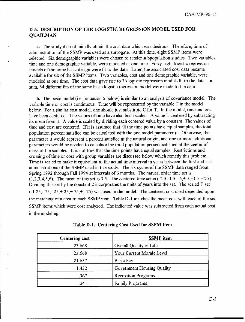
a. The study did not initially obtain the cost data which was desirous. Therefore, time ofadministration of the SSMP was used as a surrogate. At this time, eight SSMP items wereselected. Six demographic variables were chosen to render subpopulation studies. Two variables,time and one demographic variable, were modeled at one time. Forty-eight logistic regressionmodels of the same basic design were fit to the data. Later, the associated cost data becameavailable for six of the SSMP items. Two variables, cost and one demographic variable, weremodeled at one time. The cost data gave rise to 36 logistic regression models fit to the data. Insum, 84 different fits of the same basic logistic regression model were made to the data.

b. The basic model (i.e., equation 5 below) is similar to an analysis of covariance model. Thevariable time or cost is continuous. Time will be represented by the variable T in the modelbelow. For a similar cost model, one should just substitute C for T. In the model, time and costhave been centered. The values of time have also been scaled. A value is centered by subtractingits mean from it. A value is scaled by dividing each centered value by a constant. The values oftime and cost are centered. If it is assumed that all the time points have equal samples, the totalpopulation percent satisfied can be calculated with the one model parameter p.. Otherwise, theparameter pt would represent a percent satisfied at the natural origin, and one or more additionalparameters would be needed to calculate the total population percent satisfied at the center ofmass of the samples. It is not true that the time points have equal samples. Restrictions andcrossing of time or cost with group variables are discussed below which remedy this problem.Time is scaled to make it equivalent to the actual time interval in years between the first and lastadministrations of the SSMP used in this study. The six cycles of the SSMP data ranged fromSpring 1992 through Fall 1994 at intervals of 6 months. The natural order time set is(1,2,3,4,5,6). The mean of this set is 3.5. The centered time set is (-2.5,-1.5,-.5,+.5,+1.5,+2.5).Dividing this set by the constant 2 incorporates the units of years into the set. The scaled T set

(-1.25,-.75,-.25,+.25,+.75,+1.25) was used in the model. The centered cost used depended upon

the matching of a cost to each SSMP item. Table D-1 matches the mean cost with each of the six

SSMP items which were cost analyzed. The indicated value was subtracted from each actual cost

in the modeling.

Table D-1. Centering Cost Used for SSPM Item

Centering cost SSMP item

23.668 Overall Quality of Life

23.668 Your Current Morale Level

21.657 Basic Pay

1.432 Government Housing Quality

.367 Recreation Programs

.241 Family Programs

D-3

CAA-MR-96-15

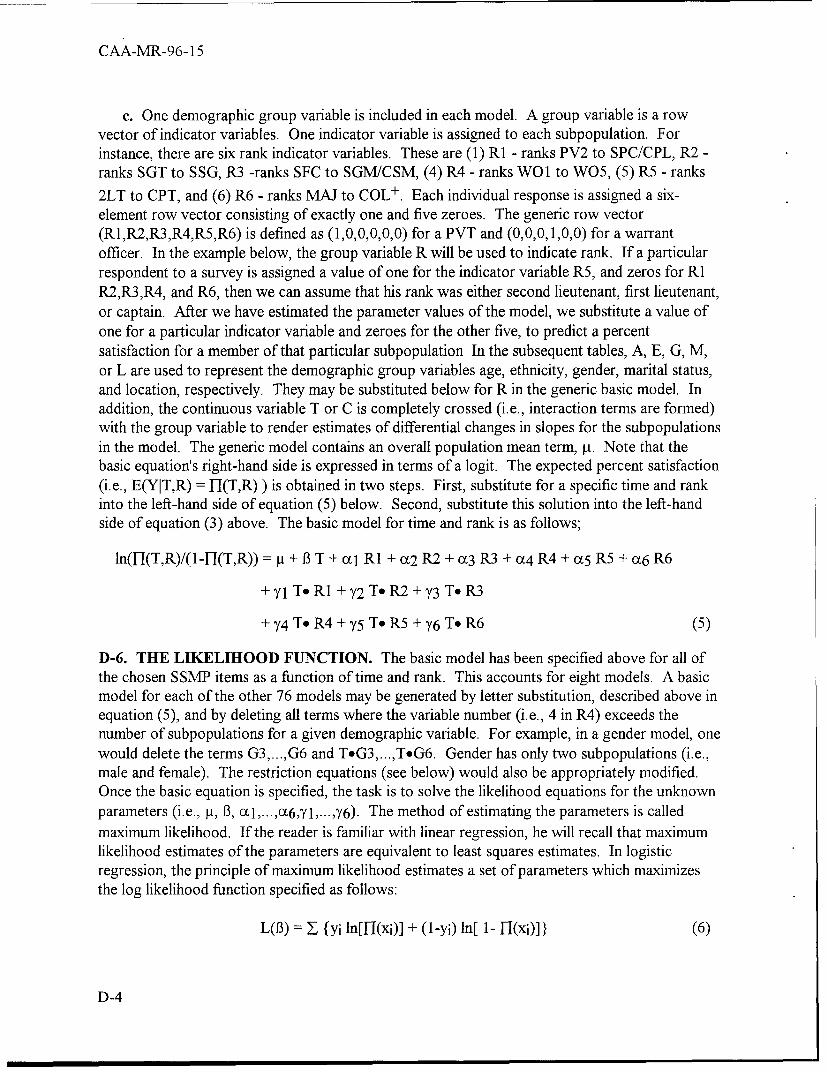
c. One demographic group variable is included in each model. A group variable is a rowvector of indicator variables. One indicator variable is assigned to each subpopulation. Forinstance, there are six rank indicator variables. These are (1) RI - ranks PV2 to SPC/CPL, R2 -ranks SGT to SSG, R3 -ranks SFC to SGM/CSM, (4) R4 - ranks WOl to WO5, (5) R5 - ranks

2LT to CPT, and (6) R6 - ranks MAJ to COL+. Each individual response is assigned a six-element row vector consisting of exactly one and five zeroes. The generic row vector(R1,R2,R3,R4,R5,R6) is defined as (1,0,0,0,0,0) for a PVT and (0,0,0,1,0,0) for a warrantofficer. In the example below, the group variable R will be used to indicate rank. If a particularrespondent to a survey is assigned a value of one for the indicator variable R5, and zeros for RIR2,R3,R4, and R6, then we can assume that his rank was either second lieutenant, first lieutenant,or captain. After we have estimated the parameter values of the model, we substitute a value ofone for a particular indicator variable and zeroes for the other five, to predict a percentsatisfaction for a member of that particular subpopulation In the subsequent tables, A, E, G, M,or L are used to represent the demographic group variables age, ethnicity, gender, marital status,and location, respectively. They may be substituted below for R in the generic basic model. Inaddition, the continuous variable T or C is completely crossed (i.e., interaction terms are formed)with the group variable to render estimates of differential changes in slopes for the subpopulationsin the model. The generic model contains an overall population mean term, it. Note that thebasic equation's right-hand side is expressed in terms of a logit. The expected percent satisfaction(i.e., E(YIT,R) = I-(T,R) ) is obtained in two steps. First, substitute for a specific time and rankinto the left-hand side of equation (5) below. Second, substitute this solution into the left-handside of equation (3) above. The basic model for time and rank is as follows;

ln(H-(T,R)/(1-H(T,R)) = p + 13 T + ccI RI + cU2 R2 + cc3 R3 + oc4 R4 + ax5 R5 + Ca6 R6

+ y1 To RI + Y2 To R2 + Y3 To R3

+ Y4 To R4 + Y5 To R5 + Y6 To R6 (5)

D-6. THE LIKELIHOOD FUNCTION. The basic model has been specified above for all ofthe chosen SSMP items as a function of time and rank. This accounts for eight models. A basicmodel for each of the other 76 models may be generated by letter substitution, described above inequation (5), and by deleting all terms where the variable number (i.e., 4 in R4) exceeds thenumber of subpopulations for a given demographic variable. For example, in a gender model, onewould delete the terms G3,...,G6 and ToG3,...,ToG6. Gender has only two subpopulations (i.e.,male and female). The restriction equations (see below) would also be appropriately modified.Once the basic equation is specified, the task is to solve the likelihood equations for the unknownparameters (i.e., [t, 3, c1,...,ca6,Y1 ,.4..,6). The method of estimating the parameters is called

maximum likelihood. If the reader is familiar with linear regression, he will recall that maximumlikelihood estimates of the parameters are equivalent to least squares estimates. In logisticregression, the principle of maximum likelihood estimates a set of parameters which maximizesthe log likelihood function specified as follows:

L(3) = Z {Yi ln[H(xi)] + (I-yi) In[ 1- -(xi)]} (6)

D-4

CAA-MR-96-15

and B in L(B) represents all of the parameters in the model (i.e., p., B, ccl,...,cc6,y1,...,Y6). The

summation is over all survey responses. The log likelihood function is maximized bydifferentiating L(B) with respect to each parameter in the model and setting the results equal tozero. The resulting likelihood equations are nonlinear in the parameters and must be solvediteratively by a Newton-Raphson type algorithm. Several commercial software packages providealgorithms to solve these equations and give estimates for the parameters p., B, c1I ,... 1,6,Y1 ,...,76.

In this study, the logistic regression procedure provided by SPSS was employed.

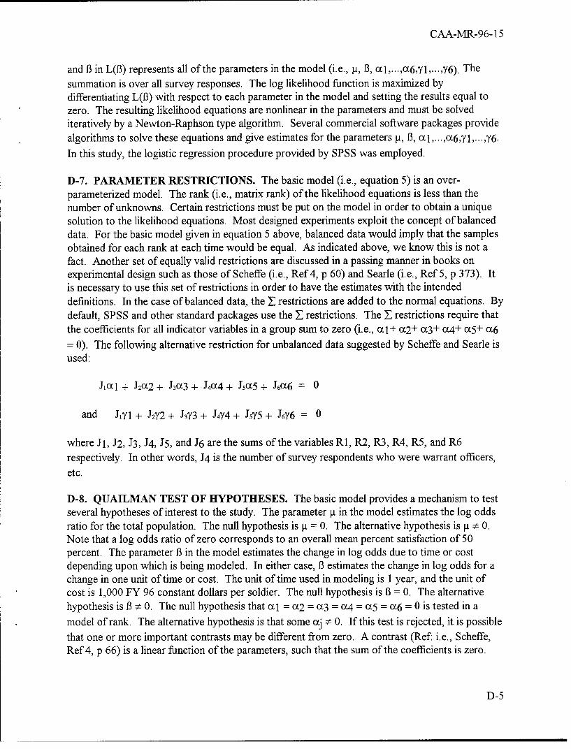
D-7. PARAMETER RESTRICTIONS. The basic model (i.e., equation 5) is an over-parameterized model. The rank (i.e., matrix rank) of the likelihood equations is less than thenumber of unknowns. Certain restrictions must be put on the model in order to obtain a uniquesolution to the likelihood equations. Most designed experiments exploit the concept of balanceddata. For the basic model given in equation 5 above, balanced data would imply that the samplesobtained for each rank at each time would be equal. As indicated above, we know this is not afact. Another set of equally valid restrictions are discussed in a passing manner in books onexperimental design such as those of Scheffe (i.e., Ref 4, p 60) and Searle (i.e., Ref 5, p 373). Itis necessary to use this set of restrictions in order to have the estimates with the intendeddefinitions. In the case of balanced data, the Z restrictions are added to the normal equations. Bydefault, SPSS and other standard packages use the YZ restrictions. The I restrictions require thatthe coefficients for all indicator variables in a group sum to zero (i.e., cl+ cC2+ cL3+ cC4+ a5+ ca6

= 0). The following alternative restriction for unbalanced data suggested by Scheffe and Searle isused:

J1 Xl + J2ox2 + J3cX3 + J4cL4 + J5oX5 + J6cx6 = 0

and J1Y1 + J2Y2 + J3Y3 + J4Y4 + J5Y5 + J6Y6 0

where J1, J2, J3, J4, J5 , and J6 are the sums of the variables R1, R2, R3, R4, R5, and R6respectively. In other words, J4 is the number of survey respondents who were warrant officers,etc.

D-8. QUAILMAN TEST OF HYPOTHESES. The basic model provides a mechanism to testseveral hypotheses of interest to the study. The parameter p. in the model estimates the log oddsratio for the total population. The null hypothesis is p = 0. The alternative hypothesis is p. # 0.Note that a log odds ratio of zero corresponds to an overall mean percent satisfaction of 50percent. The parameter B in the model estimates the change in log odds due to time or costdepending upon which is being modeled. In either case, B estimates the change in log odds for achange in one unit of time or cost. The unit of time used in modeling is 1 year, and the unit ofcost is 1,000 FY 96 constant dollars per soldier. The null hypothesis is B = 0. The alternativehypothesis is B # 0. The null hypothesis that a I c=2 = a3 = a4 = c5 = cc6 = 0 is tested in a

model of rank. The alternative hypothesis is that some cxj # 0. If this test is rejected, it is possible

that one or more important contrasts may be different from zero. A contrast (Ref: i.e., Scheffe,Ref 4, p 66) is a linear function of the parameters, such that the sum of the coefficients is zero.

D-5

CAA-MR-96-15

Certain desirable contrasts were designed into the basic model based on the set of restrictionsassumed to solve the likelihood equations. These designed contrasts measure the difference inlevel between the percent satisfaction of a subpopulation and the total population. A significantcontrast will tell us that the subpopulation percent satisfaction is significantly different from thetotal population percent satisfaction. Each significant axj estimate measures the difference in levelfor the jth rank. Note that not all of the contrasts tested will be independent, since 1 degree offreedom is lost due to the restriction on the model. The null hypothesis that 71 = Y2 = Y3 74

Y5 = Y6 = 0 is tested in a model including rank. The alternative hypothesis is that some Yj • 0.Again, if this test is rejected, certain designed contrasts can be tested. The designed contrastsmeasure the difference in trend between the subpopulation and the total population. A significantcontrast will tell us that the trend in the subpopulation is different from that in the totalpopulation. Each significant yj estimate measures the difference in trend for the jth rank.

D-9. SIGNIFICANCE AND P-VALUE. In hypothesis testing there is always the question ofpicking a significance level for the test. Formerly, this was done prior to an experiment. Somecommonly chosen significance levels are 5 percent and 1 percent. The significance level is theprobability of rejecting the null hypothesis when it is actually true (i.e., type I error). However,lately, especially with the advent of computers, it has become commonplace to quote the p valuefor a given test. The p value has essentially the same definition as the significance level exceptthat it is not preselected. Also, there is the related question of how to distribute error whenmaking a series of unplanned comparisons. In these circumstances, it is appropriate to set anexperiment-wise error rate. This is the probability of falsely rejecting at least one comparison inan experiment with multiple comparisons. Many of the tests made in this study are not necessarilyindependent tests, which is another good reason to set some kind of experiment-wise error rate.An experiment-wise error rate might well be appropriate for the group tests for both level andtrend. With this in mind, there are 21 subpopulations on which each SSMP item is beingevaluated. These are rank = 6, age = 4, ethnicity =5, gender =2, marital status =2, and location =

2, which total 21. A level difference and a trend difference are being determined for eachsubpopulation. One method of determining experiment-wise error rate is to apply the Bonferroniinequality. If one assumes a 5 percent experiment-wise error rate on these 42 comparisons andapplies the Bonferroni inequality, each individual comparison would have an adjusted significancelevel of 0.12 percent or a p-value of 0.0012. In interpreting the following analysis from each ofthe 84 regression models, this level is a suggested level as a cutoff for determining if one of thegroup comparisons or the derived contrasts should be deemed practically significant. In any case,the p-value will be reported for each test made.

D-10. THE WALD TEST AND STATISTIC. The Wald test is one test used to test thehypotheses concerning the parameters of logistic regression models for large sample sizes. It isasymptotically equivalent to the likelihood ratio test under the null hypothesis and is favored bystatistical computing packages because it is simpler to compute. For large sample sizes and acategorical variable, the distribution of the Wald statistic converges asymptotically to the chi-square distribution with in-I degrees of freedom for m categories. For continuous (i.e., time orcost) variables, where one parameter or one contrast is being evaluated, the number of degrees offreedom is 1. The results of the Wald test will be used extensively in the following tables toexplain the logistic regression models used to analyze the QUAILMAN data.

D-6

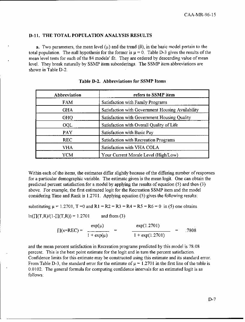
CAA-MR-96-15

D-11. THE TOTAL POPULATION ANALYSIS RESULTS

a. Two parameters, the mean level (I[) and the trend (13), in the basic model pertain to thetotal population. The null hypothesis for the former is I = 0. Table D-3 gives the results of themean level tests for each of the 84 models' fit. They are ordered by descending value of meanlevel. They break naturally by SSMP item suborderings. The SSMP item abbreviations areshown in Table D-2.

Table D-2. Abbreviations for SSMP Items

Abbreviation refers to SSMP item

FAM Satisfaction with Family Programs

GHA Satisfaction with Government Housing Availability

GHQ Satisfaction with Government Housing Quality

OQL Satisfaction with Overall Quality of Life

PAY Satisfaction with Basic Pay

REC Satisfaction with Recreation Programs

VHA Satisfaction with VHA COLA

YCM Your Current Morale Level (High/Low)

Within each of the items, the estimates differ slightly because of the differing number of responsesfor a particular demographic variable. The estimate given is the mean logit. One can obtain thepredicted percent satisfaction for a model by applying the results of equation (5) and then (3)above. For example, the first estimated logit for the Recreation SSMP item and the modelconsidering Time and Rank is 1.2701. Applying equation (5) gives the following results:

substituting [i = 1.2701, T =0 and RI = R2 = R3 = R4 = R5 = R6 = 0 in (5) one obtains

ln(H-(T,R)/(1-H-(T,R)) = 1.2701 and from (3)

exp([t) exp(1.2701)

H-(x=REC) =___ = .78081 + exp(lp) 1 + exp(1.2701)

and the mean percent satisfaction in Recreation programs predicted by this model is 78.08percent. This is the best point estimate for the logit and in turn the percent satisfaction.Confidence limits for this estimate may be constructed using this estimate and its standard error.From Table D-3, the standard error for the estimate of Vi = 1.2701 in the first line of the table is0.0102. The general formula for computing confidence intervals for an estimated logit is asfollows:

D-7

CAA-MR-96-15

9 _+ z (1 of ) x SE(ýt )(7)

Here z is the usual symbol denoting a standard normal distribution. z (1-cx/2) is the upper z (1-

ot/2) point of the random variable z if Pr(z > Z (1-c2))= ot/2. A usual value for oc is 0.05, and (1-

a) x 100 = 95 percent confidence intervals are constructed. The upper z(1-oX/2) point for a =0.05 is 1.96. Therefore, the 95 percent confidence interval on the logit in the first line of the tableis as follows:

It ± z (1-otl 2 ) x SE(ýt) = 1.2701 ± 1.96 x 0.0102 (1.2501, 1.2901)

where 1.2501 is the lower bound of the interval and 1.2901 is the upper bound. This confidenceinterval on the logit can be transformed into a 95 percent confidence interval on the percentagesatisfaction by substituting the bounds into equation (3). The lower bound is constructed asfollows:

exp(11) exp(1.2501)

r-(x=REC) =_=_ = .77731 + exp(pL) 1 + exp(1.2501)

Substituting the upper bound logit, 1.2901, one obtains .7842. Therefore, the best point estimateof the percent satisfaction of the total population in the recreation programs from this model is78.08 percent, with a 95 percent confidence interval of 77.73 percent to 78.42 percent.

b. For each of the 84 models, the standard error of the estimate is given. The Wald statisticfor a 1 degree of freedom parameter is simply the square of the ratio of the estimate to itsstandard error. Thus, in the first line of the Table D-3, the Wald statistic is approximately equal

to (1.2701/0.0102)2 = 15505.1327. This value is less precise than the one given in the tablebecause more significant figures are used when calculating the table value. The Wald statistic forthis hypothesis has an approximate chi-square distribution with one degree of freedom (df). Forthe example, in the first line, one would reject the null hypothesis that t = 0, with the probability

(p-value) of less than 5.0 x 10-5 (i.e., 0.00005) that the null hypothesis is true. Only the SSMPitem Government Housing Quality seems to have a mean which is not significantly different fromzero. As noted above, this means that the estimated mean percent satisfaction for this item isabout 50 percent.

D-8

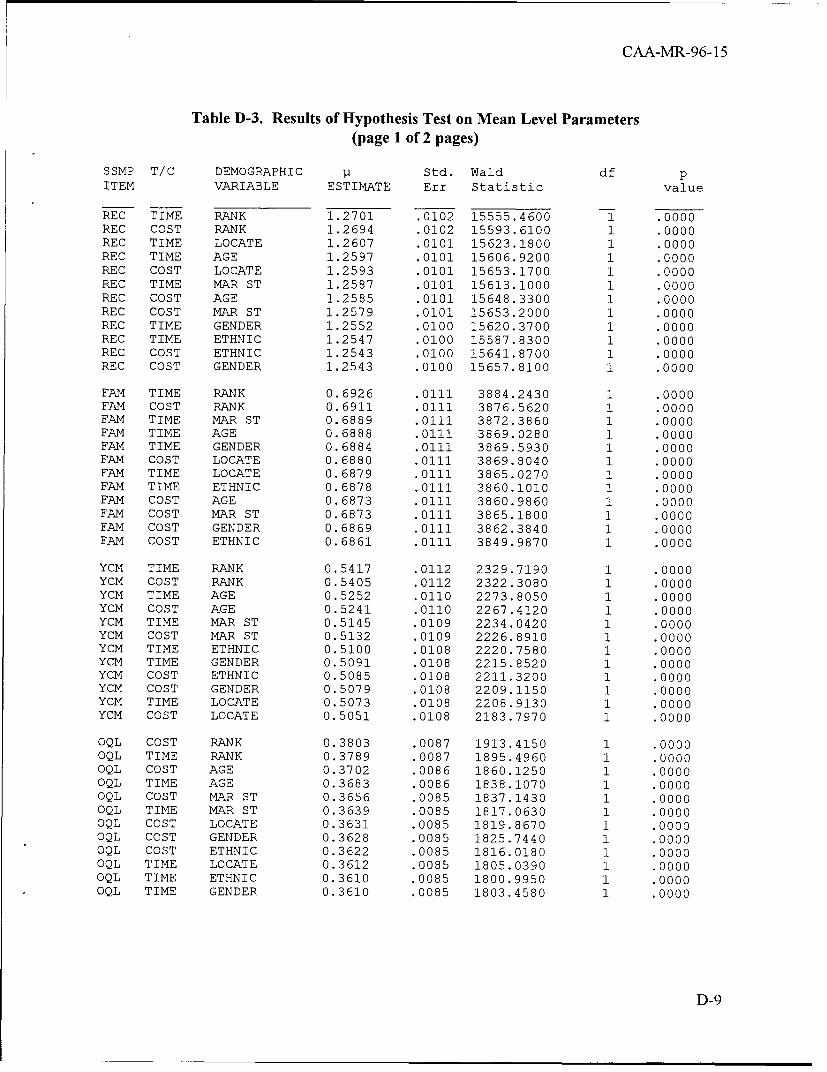
CAA-MR-96-15

Table D-3. Results of Hypothesis Test on Mean Level Parameters(page 1 of 2 pages)

SSMP T/C DEMOGRAPHIC p Std. Wald df pITEM VARIABLE ESTIMATE Err Statistic value

REC TIME RANK 1.2701 .0102 15555.4600 1 .0000REC COST RANK 1.2694 .0102 15593.6100 1 .0000REC TIME LOCATE 1.2607 .0101 15623.1800 1 .0000REC TIME AGE 1.2597 .0101 15606.9200 1 .0000REC COST LOCATE 1.2593 .0101 15653.1700 1 .0000REC TIME MAR ST 1.2587 .0101 15613.1000 1 .0000REC COST AGE 1.2585 .0101 15648.3300 1 .0000REC COST MAR ST 1.2579 .0101 15653.2000 1 .0000REC TIME GENDER 1.2552 .0100 15620.3700 1 .0000REC TIME ETHNIC 1.2547 .0100 15587.8300 1 .0000REC COST ETHNIC 1.2543 .0100 15641.8700 1 .0000REC COST GENDER 1.2543 .0100 15657.8100 1 .0000

FAM TIME RANK 0.6926 .0111 3884.2430 1 .0000FAM COST RANK 0.6911 .0111 3876.5620 1 .0000FAM TIME MAR ST 0.6889 .0111 3872.3860 1 .0000FAM TIME AGE 0.6888 .0111 3869.0280 1 .0000FAM TIME GENDER 0.6884 .0111 3869.5930 1 .0000FAM COST LOCATE 0.6880 .0111 3869.8040 1 .0000FAM TIME LOCATE 0.6879 .0111 3865.0270 1 .0000FAM TIME ETHNIC 0.6878 .0111 3860.1010 1 .0000FAM COST AGE 0.6873 .0111 3860.9860 1 .0000FAM COST MAR ST 0.6873 .0111 3865.1800 1 .0000FAM COST GENDER 0.6869 .0111 3862.3840 1 .0000FAM COST ETHNIC 0.6861 .0111 3849.9870 1 .0000

YCM TIME RANK 0.5417 .0112 2329.7190 1 .0000YCM COST RANK 0.5405 .0112 2322.3080 1 .0000YCM TIME AGE 0.5252 .0110 2273.8050 1 .0000YCM COST AGE 0.5241 .0110 2267.4120 1 .0000YCM TIME MAR ST 0.5145 .0109 2234.0420 1 .0000YCM COST MAR ST 0.5132 .0109 2226.8910 1 .0000YCM TIME ETHNIC 0.5100 .0108 2220.7580 1 .0000YCM TIME GENDER 0.5091 .0108 2215.8520 1 .0000YCM COST ETHNIC 0.5085 .0108 2211.3200 1 .0000YCM COST GENDER 0.5079 .0108 2209.1150 1 .0000YCM TIME LOCATE 0.5073 .0108 2208.9130 1 .0000YCM COST LOCATE 0.5051 .0108 2183.7970 1 .0000

OQL COST RANK 0.3803 .0087 1913.4150 1 .0000OQL TIME RANK 0.3789 .0087 1895.4960 1 .0000OQL COST AGE 0.3702 .0086 1860.1250 1 .0000OQL TIME AGE 0.3683 .0086 1838.1070 1 .0000OQL COST MAR ST 0.3656 .0085 1837.1430 1 .0000OQL TIME MAR ST 0.3639 .0085 1817.0630 1 .0000OQL COST LOCATE 0.3631 .0085 1819.8670 1 .0000OQL COST GENDER 0.3628 .0085 1825.7440 1 .0000OQL COST ETHNIC 0.3622 .0085 1816.0180 1 .0000OQL TIME LOCATE 0.3612 .0085 1805.0390 1 .0000OQL TIME ETHNIC 0.3610 .0085 1800.9950 1 .0000OQL TIME GENDER 0.3610 .0085 1803.4580 1 .0000

D-9

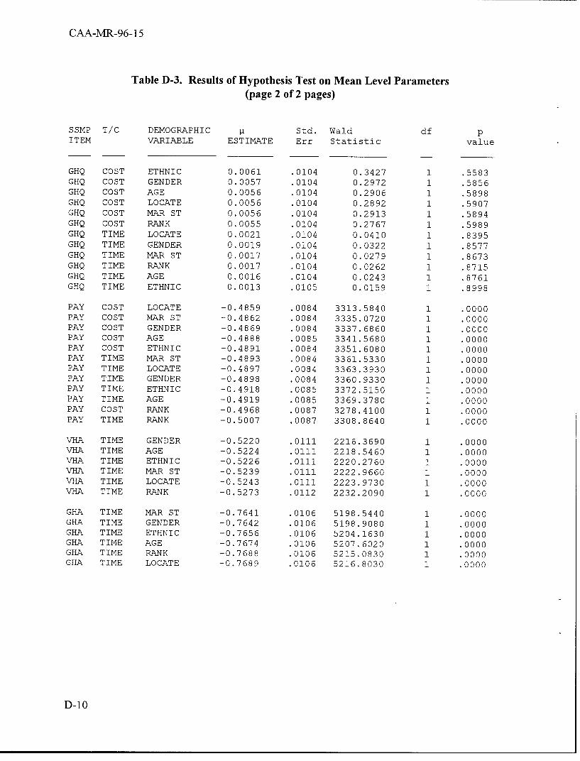
CAA-MR-96-15

Table D-3. Results of Hypothesis Test on Mean Level Parameters(page 2 of 2 pages)

SSMP T/C DEMOGRAPHIC Std. Wald df pITEM VARIABLE ESTIMATE Err Statistic value

GHQ COST ETHNIC 0.0061 .0104 0.3427 1 .5583GHQ COST GENDER 0.0057 .0104 0.2972 1 .5856GHQ COST AGE 0.0056 .0104 0.2906 1 .5898GHQ COST LOCATE 0.0056 .0104 0.2892 1 .5907GHQ COST MAR ST 0.0056 .0104 0.2913 1 .5894GHQ COST RANK 0.0055 .0104 0.2767 1 .5989GHQ TIME LOCATE 0.0021 .0104 0.0410 1 .8395GHQ TIME GENDER 0.0019 .0104 0.0322 1 .8577GHQ TIME MAR ST 0.0017 .0104 0.0279 1 .8673GHQ TIME RANK 0.0017 .0104 0.0262 1 .8715GHQ TIME AGE 0.0016 .0104 0.0243 1 .8761GHQ TIME ETHNIC 0.0013 .0105 0.0159 1 .8998

PAY COST LOCATE -0.4859 .0084 3313.5840 1 .0000PAY COST MAR ST -0.4862 .0084 3335.0720 1 .0000PAY COST GENDER -0.4869 .0084 3337.6860 1 .0000PAY COST AGE -0.4888 .0085 3341.5680 1 .0000PAY COST ETHNIC -0.4891 .0084 3351.6080 1 .0000PAY TIME MAR ST -0.4893 .0084 3361.5330 1 .0000PAY TIME LOCATE -0.4897 .0084 3363.3930 1 .0000PAY TIME GENDER -0.4898 .0084 3360.9330 1 .0000PAY TIME ETHNIC -0.4918 .0085 3372.5150 1 .0000PAY TIME AGE -0.4919 .0085 3369.3780 1 .0000PAY COST RANK -0.4968 .0087 3278.4100 1 .0000PAY TIME RANK -0.5007 .0087 3308.8640 1 .0000

VHA TIME GENDER -0.5220 .0111 2216.3690 1 .0000VHA TIME AGE -0.5224 .0111 2218.5460 1 .0000VHA TIME ETHNIC -0.5226 .0111 2220.2760 1 .0000VHA TIME MAR ST -0.5239 .0111 2222.9660 1 .0000VyA TIME LOCATE -0.5243 .0111 2223.9730 1 .0000VHA TIME RANK -0.5273 .0112 2232.2090 1 .0000

GHA TIME MAR ST -0.7641 .0106 5198.5440 1 .0000GHA TIME GENDER -0.7642 .0106 5198.9080 1 .0000GHA TIME ETHNIC -0.7656 .0106 5204.1630 1 .0000GHA TIME AGE -0.7674 .0106 5207.6020 1 .0000GHA TIME RANK -0.7688 .0106 5215.0830 1 .0000GHA TIME LOCATE -0.7689 .0106 5216.8030 1 .0000

D-10

CAA-MR-96-15

c. The second hypothesis concerning the total population has to do with the change in percentsatisfaction as a function of time. The null hypothesis is that the trend parameter 13 = 0. TableD-4 gives the results of the trend tests for each of the 84 models' fit. The table was ordered byestimated slope value. Initially after ordering, slope estimates of two items were mixed. Theordering was slightly corrected in order to segregate the list by item and the time/cost variable.Within each subordered group, the estimates differ slightly because of differing number ofresponses for different demographic variables. Probably the most evident characteristic of thecollective set of 84 trends is that 60 of them are negative. One would logically assume that if timeand especially cost were increasing, satisfaction would also be increasing. Only 10 of theremaining 24 trend coefficients are significantly different from zero. On the other hand, all but 2of the 60 negative estimates are significantly different from zero. One can obtain the predictedmean percent satisfaction for a given SSTP cycle with a time model or the mean percentsatisfaction for a given cost with a cost model by applying the results of equation (5) and then (3)above. We will continue with our example from above, the Recreation S SMP item and the modelconsidering Time and Rank. The results for this model are located in the fifth line of the thirdgroup in Table D-4. The estimate of 3 is 0.0366. This estimate has a p-value of 0.0020. It willbe noted that this value is greater than our individual comparison value of 0.0012 and thus wouldnot be considered significantly different from zero under this criteria. We might like to know themodel predicted mean percent satisfaction for the first and last S SMP cycles (i.e., Spring 1992and Fall 1994). To obtain the results for Spring 1992, and remembering that we are working witha centered time value, we will apply equation (5) to get the following results:

substituting pt = 1.2701, T = -1.25, and RI = R2 = R3 = R4 = R5 = R6 = 0 in (5) one obtains

ln(HI(T,R)/(l-H-(T,R)) = p. + 13 T = 1.2701 + 0.0366 x (-1.25) = 1.22435

Confidence limits can be constructed for this value. From Table D-3, the s.e.(g) = .0102 ands.e.(B3) = .0118. The correlation coefficient p(p.,B) = .0961. Note that correlation coefficients arecalculated for all parameters by the software but have not been presented in this text because ofthe extensive tables necessary for 84 models. However, they are available from the author if it isnecessary to calculate any extensive number of confidence limits.

The first step is to calculate the variance of the estimate as follows:

Var(ln(H1(T,R)/(1-1-(T,R))) = Var (pi + B T)

= Var(p) + T 2 Var(3) + 2Tp([,13)Var([t)l/ 2 Var(13)l/ 2

= (.0102)2 + (-1.25)2(.0118)2 + 2(-1.25)(.0961)(.0102)(.0118) = 2.92686 x 10. 4

The s.e.(ln(H-(T,R)/(1-H-(T,R))) is the square root of Var(ln(I-(T,R)/(1-H- (T,R))) which is0.0171. The 95 percent confidence interval at T -1.25 is as follows:

+ B T z (1-,/ 2 ) x s.e.(t + 13 T)

= 1.22435 ± 1.96 x 0.0171 =( 1.1908, 1.2579)

D-1l

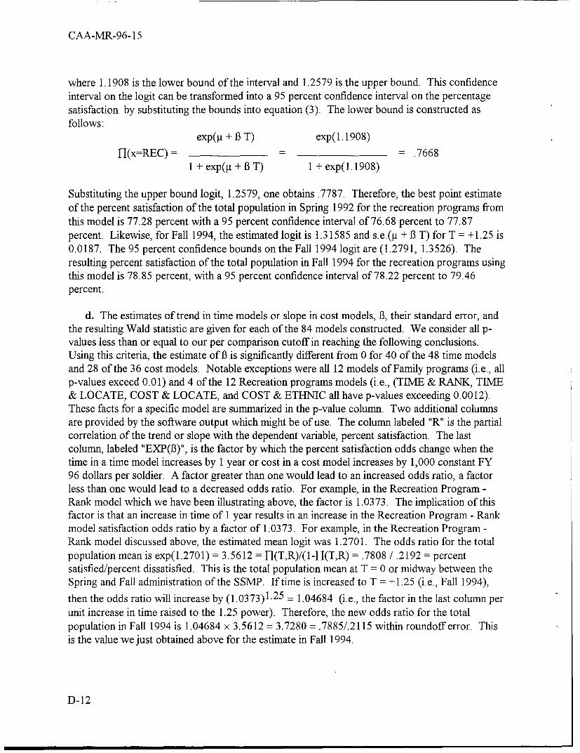
CAA-MR-96-15

where 1.1908 is the lower bound of the interval and 1.2579 is the upper bound. This confidenceinterval on the logit can be transformed into a 95 percent confidence interval on the percentagesatisfaction by substituting the bounds into equation (3). The lower bound is constructed asfollows:

exp(ýt + 13 T) exp(1.1908)

rj(x=REC) = ==- .76681 + exp([t + 3 T) 1 + exp(l.1908)

Substituting the upper bound logit, 1.2579, one obtains .7787. Therefore, the best point estimateof the percent satisfaction of the total population in Spring 1992 for the recreation programs fromthis model is 77.28 percent with a 95 percent confidence interval of 76.68 percent to 77.87percent. Likewise, for Fall 1994, the estimated logit is 1.31585 and s.e.([t + B T) for T = +1.25 is0.0187. The 95 percent confidence bounds on the Fall 1994 logit are (1.2791, 1.3526). Theresulting percent satisfaction of the total population in Fall 1994 for the recreation programs usingthis model is 78.85 percent, with a 95 percent confidence interval of 78.22 percent to 79.46percent.

d. The estimates of trend in time models or slope in cost models, B, their standard error, andthe resulting Wald statistic are given for each of the 84 models constructed. We consider all p-values less than or equal to our per comparison cutoff in reaching the following conclusions.Using this criteria, the estimate of B is significantly different from 0 for 40 of the 48 time modelsand 28 of the 36 cost models. Notable exceptions were all 12 models of Family programs (i.e., allp-values exceed 0.01) and 4 of the 12 Recreation programs models (i.e., (TIME & RANK, TIME& LOCATE, COST & LOCATE, and COST & ETHNIC all have p-values exceeding 0.0012).These facts for a specific model are summarized in the p-value column. Two additional columnsare provided by the software output which might be of use. The column labeled "R" is the partialcorrelation of the trend or slope with the dependent variable, percent satisfaction. The lastcolumn, labeled "EXP(B)", is the factor by which the percent satisfaction odds change when thetime in a time model increases by 1 year or cost in a cost model increases by 1,000 constant FY96 dollars per soldier. A factor greater than one would lead to an increased odds ratio, a factorless than one would lead to a decreased odds ratio. For example, in the Recreation Program -Rank model which we have been illustrating above, the factor is 1.0373. The implication of thisfactor is that an increase in time of 1 year results in an increase in the Recreation Program - Rankmodel satisfaction odds ratio by a factor of 1.0373. For example, in the Recreation Program -Rank model discussed above, the estimated mean logit was 1.2701. The odds ratio for the totalpopulation mean is exp(1.2701) = 3.5612 = I-(T,R)/(1-H(T,R) =.7808 /.2192 = percentsatisfied/percent dissatisfied. This is the total population mean at T = 0 or midway between theSpring and Fall administration of the SSMP. If time is increased to T = +1.25 (i.e., Fall 1994),

then the odds ratio will increase by (1.0373)1.25 = 1.04684 (i.e., the factor in the last column perunit increase in time raised to the 1.25 power). Therefore, the new odds ratio for the totalpopulation in Fall 1994 is 1.04684 x 3.5612 = 3.7280 =.7885/.2115 within roundoff error. Thisis the value we just obtained above for the estimate in Fall 1994.

D-12

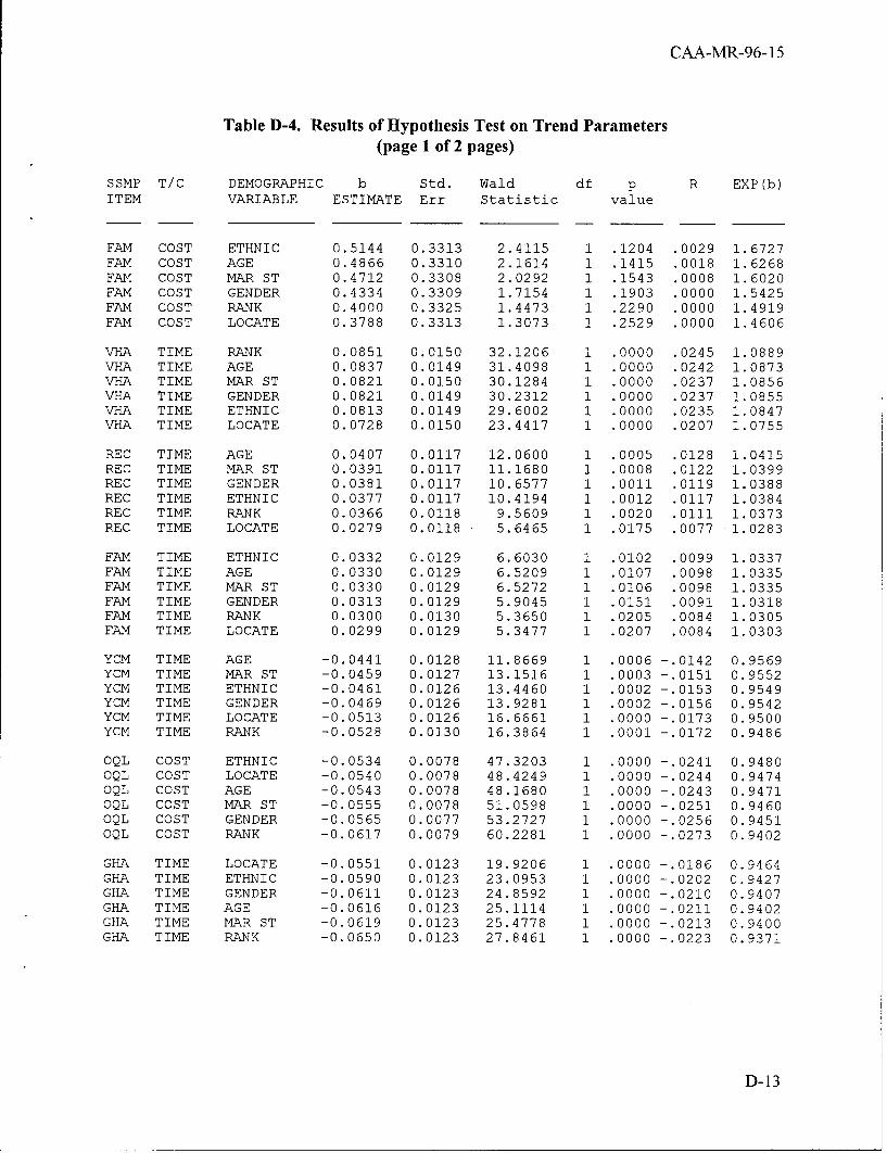
CAA-MR-96-15

Table D-4. Results of Hypothesis Test on Trend Parameters(page 1 of 2 pages)

SSMP T/C DEMOGRAPHIC b Std. Wald df p R EXP(b)ITEM VARIABLE ESTIMATE Err Statistic value

FAN COST ETHNIC 0.5144 0.3313 2.4115 1 .1204 .0029 1.6727FAN COST AGE 0.4866 0.3310 2.1614 1 .1415 .0018 1.6268FAN COST MAR ST 0.4712 0.3308 2.0292 1 .1543 .0008 1.6020FAM COST GENDER 0.4334 0.3309 1.7154 1 .1903 .0000 1.5425FAM COST RANK 0.4000 0.3325 1.4473 1 .2290 .0000 1.4919FAN COST LOCATE 0.3788 0.3313 1.3073 1 .2529 .0000 1.4606

VHA TIME RANK 0.0851 0.0150 32.1206 1 .0000 .0245 1.0889VHA TIME AGE 0.0837 0.0149 31.4098 1 .0000 .0242 1.0873VHA TIME MAR ST 0.0821 0.0150 30.1284 1 .0000 .0237 1.0856VHA TIME GENDER 0.0821 0.0149 30.2312 1 .0000 .0237 1.0855VHA TIME ETHNIC 0.0813 0.0149 29.6002 1 .0000 .0235 1.0847VHA TIME LOCATE 0.0728 0.0150 23.4417 1 .0000 .0207 1.0755

REC TIME AGE 0.0407 0.0117 12.0600 1 .0005 .0128 1.0415REC TIME MAR ST 0.0391 0.0117 11.1680 1 .0008 .0122 1.0399REC TIME GENDER 0.0381 0.0117 10.6577 1 .0011 .0119 1.0388REC TIME ETHNIC 0.0377 0.0117 10.4194 1 .0012 .0117 1.0384REC TIME RANK 0.0366 0.0118 9.5609 1 .0020 .0111 1.0373REC TIME LOCATE 0.0279 0.0118 5.6465 1 .0175 .0077 1.0283

FAN TIME ETHNIC 0.0332 0.0129 6.6030 1 .0102 .0099 1.0337FAN TIME AGE 0.0330 0.0129 6.5209 1 .0107 .0098 1.0335FAN TIME MAR ST 0.0330 0.0129 6.5272 1 .0106 .0098 1.0335FAN TIME GENDER 0.0313 0.0129 5.9045 1 .0151 .0091 1.0318FAN TIME RANK 0.0300 0.0130 5.3650 1 .0205 .0084 1.0305FAN TIME LOCATE 0.0299 0.0129 5.3477 1 .0207 .0084 1.0303

YCM TIME AGE -0.0441 0.0128 11.8669 1 .0006 -. 0142 0.9569YCM TIME MAR ST -0.0459 0.0127 13.1516 1 .0003 -. 0151 0.9552YCM TIME ETHNIC -0.0461 0.0126 13.4460 1 .0002 -. 0153 0.9549YCM TIME GENDER -0.0469 0.0126 13.9281 1 .0002 -. 0156 0.9542YCM TIME LOCATE -0.0513 0.0126 16.6661 1 .0000 -. 0173 0.9500YCM TIME RANK -0.0528 0.0130 16.3864 1 .0001 -. 0172 0.9486

OQL COST ETHNIC -0.0534 0.0078 47.3203 1 .0000 -. 0241 0.9480OQL COST LOCATE -0.0540 0.0078 48.4249 1 .0000 -. 0244 0.9474OQL COST AGE -0.0543 0.0078 48.1680 1 .0000 -. 0243 0.9471OQL COST MAR ST -0.0555 0.0078 51.0598 1 .0000 -. 0251 0.9460OQL COST GENDER -0.0565 0.0077 53.2727 1 .0000 -. 0256 0.9451OQL COST RANK -0.0617 0.0079 60.2281 1 .0000 -. 0273 0.9402

GHA TIME LOCATE -0.0551 0.0123 19.9206 1 .0000 -. 0186 0.9464GHA TIME ETHNIC -0.0590 0.0123 23.0953 1 .0000 -. 0202 0.9427GHA TIME GENDER -0.0611 0.0123 24.8592 1 .0000 -. 0210 0.9407GHA TIME AGE -0.0616 0.0123 25.1114 1 .0000 -. 0211 0.9402GHA TIME MAR ST -0.0619 0.0123 25.4778 1 .0000 -. 0213 0.9400GHA TIME RANK -0.0650 0.0123 27.8461 1 .0000 -. 0223 0.9371

D-13

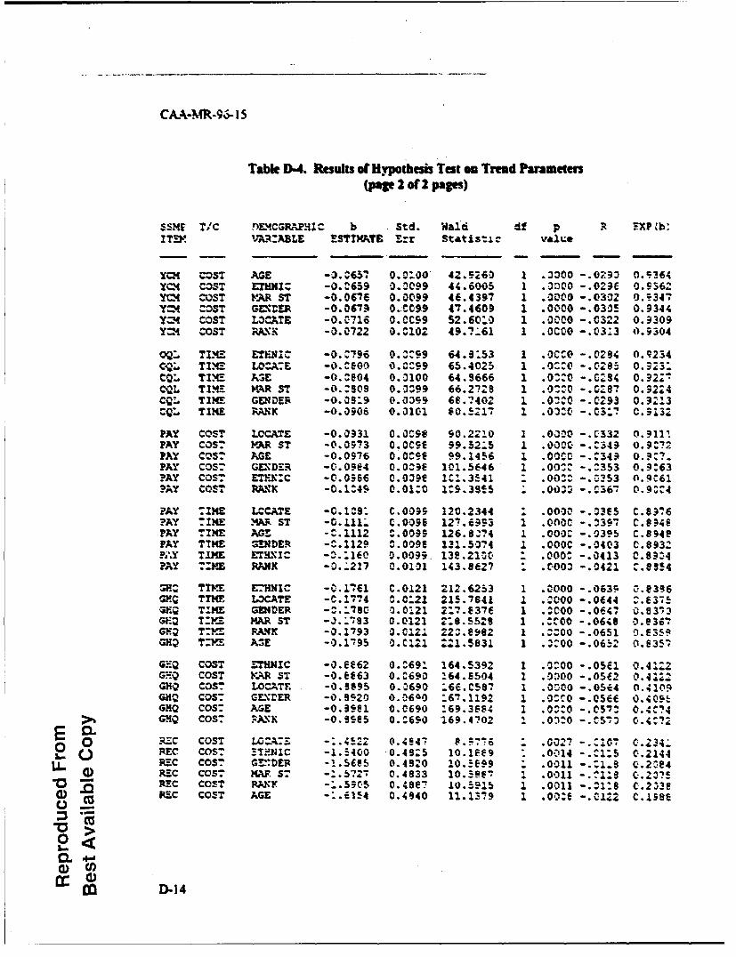
CAAAMR-95- 15

Table D-4. Resous of Hypothesis Test on Trend Parameters(page 2 o. 2 pages)

$SHE T/C ,)EMCGR..PE•IC b Std. waic df p R XP(b:ITE! VAAIALE ESTIMATE Err Statist: value

YCH COST AGE -3.^65" 0.0'00 42.5 26-3 1 .3300O -.0190 0.5364YC--4 COST ETHNIC -0.1659 0..099 44.6005 1 . x00 -. 0296 0.5362YC4 COST VAR ST -0.0676 0.0099 46.4397 1 .0000 -.0302 0.5347Y--4 COST GENDER -0.0671 0.C099 47.4609 1 .0000 -. 0305 0.9344Y-4 COST LOCATE -0.0716 0.0C99 52.60:0 1 .0000 -. 0322 0.9309Y --' COST mAx• -0.0722 0.0%02 49.7%61 1 .0C00 -. 03:3 0.9304

OQZ TIME ETFNV1 -0.^796 0.=^99 64.9.53 1 .OCCO -. 0294 0.;234CQL TIME LO.%,A: -0.e900 0.=99 65.4025 1 .0:.0 -.0295 0.223iCQ. TIM!• ASE -0.8094 0.3100 64.9666 1 .0-0 -. 0234 0.922'CWL TIME KAR ST -0.2908 0.3099 66.2!28 1 .0 0 -.oC87 0.9224CQ1 TIME GENDER -0.09:9 0.0399 68.7402 1 .02V0 -. C293 0.9213Q.L TIME RANK -0.0908 0.0101 60.5!17 1 .0320 -. 037 C.9132

PAY COST LOCATE -0.0931 0.0090 90.2210 1 .0000 -. C332 0.911.PAY COST PAR ST -0.0973 0.OC9E 99.52;5 1 .0000 -. C349 0.9:72PAY COST AGE -0.0576 0.098 99.1456 1 .0000 -. ^349 0.9'?PAY COST GL'VDER -o.09e4 0.0:96 101.5646 1 .00^. -. :353 0.9:63PAY COST ETF.:C -0.0566 0.039e 1".3541 . .002Z -. 0353 0.9U61PAY COST RANK -0.1:49 0.01:0 19.3955 .0033 -. 0367 0.924

PAY :IME LCCATE -0.129i C.009; 120.2344 . .0000 -. 0365 C.8W76?AY TIME MA$. ST -0.IIL. C.0096 121.6953 1 .000C -. 3391 C.8349PAY TIME AGS -'.1112 2.0099 126.8674 1 .0000 -. 0395 C.894ePAY TIME GENDER -C.1129 0.0096 131.5074 1 .000C -. 0403 0.893:P'Y TIPS ETVI C -_2.:160 0.0095 131.2100 " .000: -. 0413 0.89^4PAY T:m RANK -D..217 0.0101 143.8e27 :. .0003 -. 0421 2.8934

SP.Z TIRE ETHNIC -0.1761 C.0121 212.6253 1 .0000 -. 0639 0.8396GH4 TIMl LOCATE -C.1774 0.0:21 215.7841 1 .000 -. 0644 C.6375GKQ TIME GENDER -^.:780 2.0.21 227.6376 1 .^000 -. 0647 0.8313GI• T:, MAR ST -3.2783 a.Oi2z 21.B5529 1 .- o00 -. 0648 0.m36vGF2 T:?-- RAmK -0.1793 O.0121 220.6982 1 .'00 -. 0651 0.E359GHO T:?m! ACE -0.1'95 0.C21 :21.5831 1 .2:00 -. 0652 0.9357

G.uQ COST ETHNIC -0.e662 0.^69: 164.5392 1 .0^00 -. 0561 0.41Z2GiQ COST VAR ST -0.ee63 0.2690 164.SS04 1 .0;00 -. 05,2 0.412GHO COST LOCATF. -0.9695 0.0690 L,66.C587 1 .Oo00 -. o564 0.4109GHg COST GLE.ER -0.9920 O.06C!O :67.1192 1 .00E -. 056f O.409bGHQ cos: AGE -O.99el 0.0690 Z69.3684 1 .0^:0 -. 057: 0.*074GqQ COST 7-AXK -0.99e5 0.C690 169.4702 1 .010 -.I57 0.4.?2

0 0RC COST La Z4 0.4147 P.;7?6 .0027 -. C02 0.2347.,) REC COST 3T;9jIC -1.5400 0.49:5 10.1FE9 . .0014 -.^1:$ 0.2144

REC COST Gi=DER -1.5if5 0.4920 10.5e99 .0011 -. C1.6 0.2394RIC COST .MA ST -. 572• 0.4833 10.396T 1 .0011 -. ,lie 0.2;7!

V REC COST R,,K -:.5;05 0.48e! 10.591b 1 .0011 -.^1:9 C.2338REC COST AGE -:.i1!4 0.4940 11.1379 1 .00N -:V122 C.18ee

Q)Df1

D-1

CAA-MR-96-15

D-12. THE SUBPOPULATION ANALYSIS RESULTS

a. The results of the subpopulation analysis are summarized in Table D-5 for time and TableD-6 for cost. Each line of these tables refers to (1) an SSMP item, (2) a demographic variablegroup (ocj's in the basic model), or an interaction between time or cost and the demographic

variable in the model (yj's in the basic model). The lists are ordered from smallest p-value to

largest p-value. The Wald statistic, its degrees of freedom, and the p-value are given for eachdemographic group. The Wald statistic is asymptotically chi-square distributed with rn-I degreesof freedom where there are m subpopulations in the group. A significant p-value on this testindicates that there is a subpopulation difference either in level or in trend for time models, or incost for cost models, depending on the description of the group given in the second column. Itappears from these tables that level differences are much more prevalent in the data than trend andslope differences. Although the trends and slopes are in general significantly different for the totalpopulation, there does not appear to be much change in slope or trend due solely to subpopula-tions. If one uses the 0.0012 criteria proposed above as a cutoff for determining practicalsignificance, there are 8 out of 48 time by demographic interactions and 4 out of 36 cost bydemographic interactions which are significantly different from zero. The significant timeinteractions in order of increasing p-value are (1) REC-Ethnic (i.e., Table D-5, first page, fifth linefrom bottom), (2) VHA-Locate, (3) PAY-Rank, (4) PAY-Ethnic, (5) GHA- Ethnic, (6) GHQ-Rank, (7) REC-Locate, and (8) FAM-Mar St. (i.e., Table D-5, second page, fifteenth line fromtop). The significant cost interactions are (1) FAM-Locate (i.e., Table D-6, first page, tenth linefrom the bottom), (2) PAY-Rank, (3) FAM-Mar St. and (4) PAY-Ethnic (i.e., Table D-6, firstpage, bottom line). Three of the interactions, (1) PAY-Rank, (2) PAY-Ethnic, and (3) FAM-MarSt., are significant when considering either cost or time.

b. The significance of level changes due to subpopulations shows in general just the oppositepattern. Using the same 0.0012 cutoff criteria for the level changes, there are only four levelchanges in the time models and four level changes in the cost models which are not significantlydifferent from zero. The level changes which do not differ significantly from zero are for the timemodels (1) FAM-Locate (i.e., Table D-5, second page, fifteenth line from the bottom), (2) FAM-Mar St., (3) REC-Gender, (4) GHA-Gender (i.e., Table D-5, second page, bottom line) and forthe cost models (1) FAM-Mar St. (i.e., Table D-6, second page, fifth line from the top), (2) FAM-Locate, (3) PAY-Mar St., and (4) REC-Gender (i.e., Table D-6, second page, fifteenth line fromthe bottom). Three out of these four, (1) FAM- Locate, (2) FAM- Mar St., and (3) REC-Gender,are not significantly different from zero in both the time and cost models.

D-15

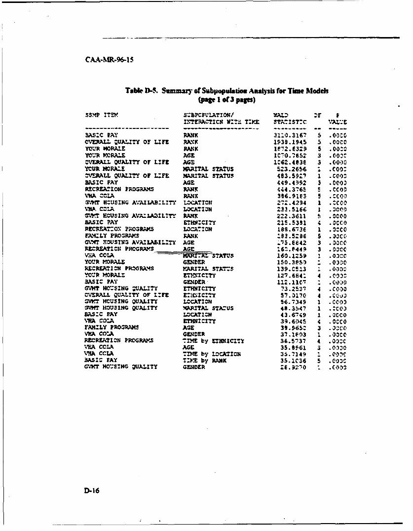
Table D-S. Summar of Subpopulation Analysis for Time Models(page I1of 3 pages)

334P ITE SPCFUfLATION/ ALFINTEVACTICS W:-; T:V.E STAT1ST:C cc

jMS:C PAY " 31`0.3167 5 00!'0OVERALL QUAL~ITY 0F LIFE RAYK 15.38.1945 5 .00%.0rOJR MORALE RANK 1F72.6329 5 .00:cYOUR ?HCRALE AGE 1c'!O.79*52 3 .C'07CZERALL QUALITY OF LIFE AGE% lCZ. 4 93e 3 .C000YCUR NORA. MARITAL STATUS 523.2656 . .COO:ZXSRALL QUALITY OF LIFE MARITAL STATUS 403.592'7 1 .COO^.BASIC PAY AGE 449.4992 3 .0C0O)RECREATION PiROZAAxS PAW 444.376! ! .CCOOVIIA -^LA RANK 366.91el & .CCOO2%r#ff HCUSING A.'AaiA3:L:TY L-'%CAT ICH ~ 272.4294 1 .^COO%Wt. CZL LOCATION 1^33.5.166 1 . 00G'.'t-T ECUSING AVA2LAZ2IL!TY- RANK 2223a c.00BASIC PAY ETHN'CxY 2415.5391 ; .OCCORZcREA7*:O~ PiROGRAI'S '-O;-:oN 189.6736 1 .o:COFA.kiLy PR0GRAV.s PANI Z$3.5286 5 .3oCC'GV?4T E!0USINS AVA1LAfiI&ITY AGE .'5.0642 3 .30C0CRECRLATI.-s PROGRAIVS_ AGE 16.P4 3 .OOCCVz~k COLA, iwff!&ALSTATvS 160.12591 2 .O3ccYOUR M~RALE GEDWER 150.3853 .030RERESATIO-N PROGRAWtS YARXTAL STATS 139.V"513 1 00C.0.1i I4ORALZ Fz17.IC!TY 127.664: 4 .0-WI.X PAY GENDER. 112.110C' .0:GVMT HO--SING QUALITY ETHIO(CITY ?3.25-11 4 .COOoCVErRALL QUALITY OF L:nE E:..%Wc."rY 57.31?0 4 C~jOWT HCUS!NG QUALITY LeCATION 56.7345 1 .CC03

vm 1 HOUSING QUALIM VMARITAL STAZUS 48.3547 1 .Cco-3A3C PAY LOCA?1N:: 43.6749 1 . oc*CO%TA CO:A ETHICIITY 39.6045 4 O0CCOFAMNLY PROGRAMS AGE 39.S.65Z 3 .3;=CVVIA COZ.A GENDER 37.1F03 1 .OOCORECRERTION ?RCGRAW'S 1!ME by ETANICITY 36.5'737 4 .03:CVHA CCLAk AGE 35.01.61 3 .0C1oCVNA CCLA. TIME by LOCATIcIC 3S.7149 I 01BAS=O FAY T:M-E by RANK 35-IC36 5 .003CGWTV~ HO-:S-NG QUALITY GENDER 26.32ioCI0

D-16

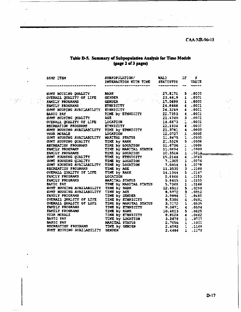
CA.,MR-96-I 3

Table D-5. Summary of Subpopulawio Analysis for Time Models(page 2 of 3 paps)

ScP :rTEH SUBPOPt•ZATION/ VAL-% :- IINTERACTICH WITH T:VE STA:TSTTC V.ALU.E

GW.T KC.':$ZNG QUALITY RAMK 27.8:71 5 .00:0OVERALL WUALIT' OF LIFE GENDER 23.4619 1 .00L. .1A..Y PROGRAMS GENDER 17.0699 1 .00..PWILY FR3GRAX4S ETHNICZTY 24.f666 4 .OOCIGwor HcUSING A%,IABTELI7Y ETHNIC:TY 24.32.69 4 .00IBASIC PAY TZME by ETMIIC:TY 22.?353 4 .00^1Gmw.ff HCnSING UALITY AGE 21.4340 3 .00,10VRALL QUALITY OF L.FE L.CATION 14.6673 " .0001RECREATION PROGRAMS ETHNICITY 22.1934 4 .00.32GVST HOUSING AMAILA3:LITY TIYE by ETHNICrTY 21.376: 4 .0003YVUR MCRALE LOCATION 12.0?21 1 .0005oV1.'T HOUSING AVALABILITY MAR:TAL STATUS 1-.9475 1 .0005W-1?!T HMUSING QUALITY TIME by RANK 2:.5528 5 .000fRECRLAT:ON PROGRAMS TIME by LOCATON 11.6736 " .0006FAMILY PROGRAM TIME by MAR:TAL STATUS 11.0f94 1 . CO09FAMILY PROGRAMS TIM1 by LOCAXION 1C.3516 1 ."OW14

,t4. H.USING QUALITY TIME by ETH;ICITY 15.2144 4 .0t434 1 HOUSING QUALMTY TIME by LOCATIO 7..3C5 1 .0016GVWT HOUSING AAILABILITY TIME by LOCATION 7.0954 1 .CC8FEOREAT:^= PRCGRAMS TIME by AGE 11.3535 3 .Z100OvERALL QUALXTY oF LIFE TIME by Pk.*K 14.1344 5 .C147FACLY PRCSRAW.S LOCATION 5.J866 1 .-.153FAICLY PRCORA-.S MAR:TAL STATUS 5.6615 1 .0155PASIC PAY TTME by )ARITAL STATUS 5.7368 1 .0166GV-tT HOUS:NG AVAI LABILITY TIME by RANK 12.451C 5 .02:-0GV.4T HOUS:NG A~.AILABILITY TIME by AGE 8.5912 3 •0352FAM1ILY PR'GRýLAMS TIME by GEN1'ER 3.9096 " .0490OVERALL OVA7.IMY OF LIFE TIME by ET*I1C:TY 9.530C 4 .0451OVERALL QUALI'TY OF LIFE TIME by MARITAL STATUS 3.7:72 1 .0539FAMfULY PRCGR.MS TIME by ETIICITY 9.3671i 4 .0594FAMILY PRZG4MMS TIME by RANK 10.4023 5 .0625YCUR MCRAL! TIME by ETHNICITY 8.90;8 4 .0ef2BASTC PAY ?ME by LOCATICN 3.26'9 1 .070?BASIC PAY MARITAL STATUS 2.?056 1 .1000RECRfEAT!O.•N PRO*RAMS TIME by GZNIER 2.4592 " .Ii:GVPWT XOUSING A%%IAEILITY GENDER 2.4464 1 . II!

D-17

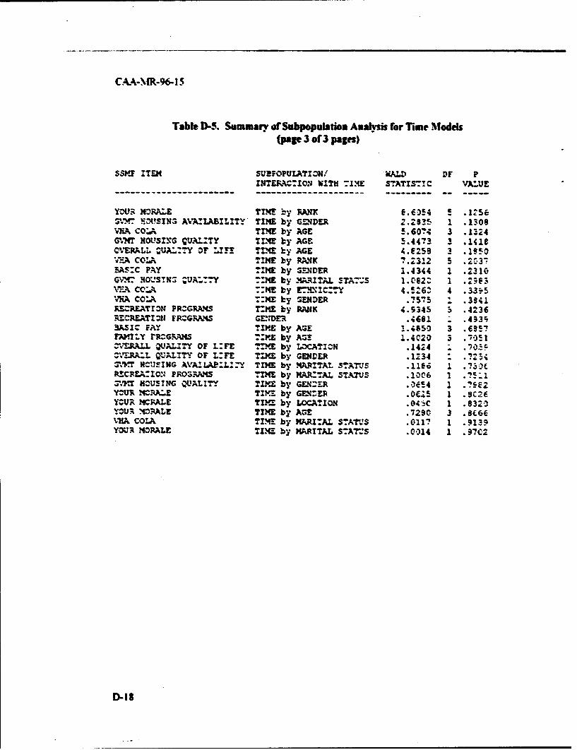
CAA-MR-96- 15

Table WIS. Summary of Ssibpopmiation Analysis for Time Models(page 3 of 3 pages)

SSMP ITEM SURFOPULATION/ W=~t DF PINTERk-c:I10J WITH I1XE STATIST1C VALUE

-------------- ---------------------------------------- -

YOUR MORALE TIM! by RAW( 6.60S4 5 .12563.'-.7 XO1?SIXS AVA'-LABILITY TIME by C-SNDER 2.2835 1 .1308V!LA CO.'^ TIME by AGE 5.6074 3 .1124G-.r HOUSING QUJALMT TIME by, AGE B.4473 3 .1419OVETRALL ;WUA=:Y Or LI!!E T M_ by AGE 4.E259 3 .19S!OV~-h CO!A TIME by RXNK ?.2312 5 .4n.3SA5S:C PAY =MNE by GENDER 1.4344 1 .2310G~vd7'r HOLS!N5 :,UAL:T-Y =MNE by IMOIA ETA:.-S 1.082: 1 .2963rr,3. C.% ::ME by Er-%IC:TY 4.!263' 4 .33;_5VKA CC:A T::E by SENDER . 75",5 : .3941IWcREATroN PR.^GXV4S ;'ME b Y PRANK 4.5345 5 .4236RECREATIMI PRO^GRAMS GENDER .;681 - .433r,3AS1C PAY TIME by AZX 1.4650 3 .0957Fr~mty rRcGrAms 7:10X by ASE 1.4020 3 .10S1COvMRALL QUALITY OF L:FE T 11- by LOCATION .1424 i.70ZOVERAL QUJALITY OF L:FE TIME by GENDER .1234 .24,a.' NVUSING 4%AVAZIAP:L:':Y TIME by MARITAL STArUS .1iE6 SO.50R'vrECRA:Io:.J PrOZRWM TIME by MAkRAL ST.X19S .1006 1 .75:i3S.V.T HCUSING OUALITY TIME by GENZER . U54 1 .7SE2YCUR MCRALE TIM!- by GFZERX .0C25 1 B C2CYCUAh NCRALE T I YE by W4CATION4 .045iC 1 .8320YOUR "1ORALE TIME by AGE .7290 3 .8t6f,VKA; CoiA TIME by MARI-IAL STAr.US .011? 1 .9139YOUR MORALE TCIE by MARITAL S7AT*US .0014 1 .97IC2

D-19

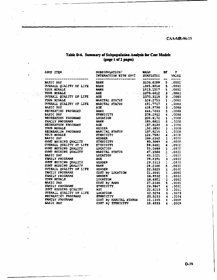
Table 0-& Summary of Subpopulaties Aiulps~ (fo Cost Models(page I of 2 pages)

SSV.F ITEM SUBFO?ULikTICN/ KAMD DT ?flITEM CTION WITH COST STMZSTIC VA:.3z

BA-Sr PAY RANX 31MQV699 5 .000^OVERXALL V~AL ITY Of LZFE PRAK i945.8014 5 .000^YCLTR NMRALE RANK 1513.151.7 5 .000.YOUR WzqLx- AG3E %1?0.4C1Z 3 .0O000OSRALL QUALMTY CF LIFE AGE TV070.3119 3 COOO3YOUR MI-RALE MARITAL STA-.US 524.2753 1 COOOOVenwLL QU.AlITy or LinE XARITAL STAZUS 491.7%7 1 .0000BASIC PAY AGE 438B.97?6 3 A.000RECRAr.:o. ?WROxWA1S RANX 446.7EiS3 S n.000BASIC PAY LETHNICITY 249.2912 4 CCOO,RECR=107IO ?;ZOGRAKS' LOCATION 236.9:72 1 ..̂CooFA.%CLY PROGRAM~S RANK 135.0611 5 .:^00REZCREATICN PAROL -IS AGE :,57.9-19i 3 0XCYOUR HozAL GEND~ER '5C.385v% I .ý00RECREAO:.'N ?RCGRAV.S xAR-:*AL STATUS 137.9:15 1 .OCCOYOU-R MORALE. ETIIN:CTTY 124.753: 4 .0:110BASIC PAY GMEDWER 103.2362 1 .0C310"M~v NO*_S:N3 OQULL:y ETIHDICITY $0.3009, 4 .0000CVERALL wUALIY OF LIFE ZF%,CITY 59.940i 4 .00ccGVM ROUSING w=ALIY LOCA: 0. 55.0468 1 .00:ý'GVX HOUSING QUALITY MARITAL STATUS 4-1.1564 :.03O^SASIC PAY LOCATION ~ 43.1C21 C~AMKILY PRCGRAMS AGE 39.E191 3 .C0OO

GwTf 80OUSING 2UALITY GUMNER 29.5113 : C1G',VMT MCUSING QUALT-Y RANK 28.2146 5 .COO!.CV!MRA,.L QuALIT oF L:Fz GENDER 22.562S 1 .COOCFAV-I1Y FROGFAMS COST by LOCATION 21.3641 1 .000^

AMI=L1. IRDGPA'45 GZHDF.Rk 16.t532 1 .0030YOU'nR MOE 1OCATION 1.81 1.Q~BASIC PAY COST by &%NK 27.2146 S I.-C0!rAY-ILY PROGRAMS £TNICZTY 24.9847 4 .'.CCQV.p~ IHUSTNG Q*:AL:TY A2-= ZC.6Z13 3 Z:CO.0VERA;,L QUALITY CF L:FE LOCATOI C 12.9294 1 .=03RECREAT::c, PROO5RAMMP EMThZCITPY 20.5153 4 . 2C04

MACLY ?ROqRGiNS COST by MARITAL STATUS 11.1315 1 .000eAM:C PAY COST by ?-lM:CITY 1E6.633 4 .0004

D-19

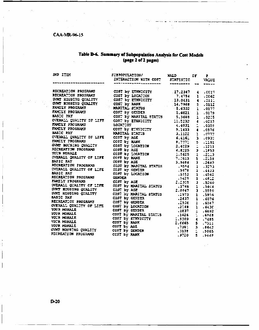
CAA-)M-96. 15

Table D-&. Summary of Subpopulation Analysis for Cost Mfodels(page 2 of 2 pages)

NlEPAC'rION WITH COST STATIS71C VAOTjr----- - - - - - - -- - ---- - -

RECREATZON PROSRAMS COST by £-THN-cITy V7.2347 4 .Ct17PrcfiEAý:ON PROS3W,5 COST by LOZA::e: .4747=.2r X- SrXG QJ.ALITY COS7 by VMINC,&Tv.3031 4.1

MM L PNOUZl Q A TYc s y RA 14.7968 5 .011:FMY RORIS3~PTA: STATUS !. 6302 1 . 01177

F.X'CLY PROZRAVS COS-. by GE-DER .5.6021 1 .0V791AS~C ?AY COST by %ARITAL STAT--S 5.3688 1 .01:501-TYAL -UA!L:Ty or :IFF COST by ETHxIC=4y :!.!232 4.01FAMLY ?.RO~fV*.S Lz-: 4.4031 -: -iFA.%aLY PROGRAY. COST by E-.-Mrc:-.y 9.1433 41 .0576sAs:c PAY MARITAL S7AT,;S 3.11^2 1 .o777Cv~lvA.-L QUAL:Ty OF LIFE COST by AGE 6.41Z. 3 .093:FAWILY PRCGVRAMS COST by RANK 8.777: 5 -1319GVHT~ Hq:S:NG QUA:.:-Y COST by '.CCATIcNj 2.4 C29 .1211Rzc-EATrou FRtcGRANs COST by AST 4. 8225 3 .1P53YC':R UVORALE CCST by ý;CAT!CN ~ 2 2.VERALL QUJALITY OF LIFE CCST by RANK 7.:613 1 259

UZI= PAY CCST by A:;E 3.;694 3 .264 ý-r-C E T O IRGX4SC S by .4ARITAL sTATUs .4 C- 1 .3213Oz'RkLL QUALITY Of LZFE C-ST by GENtE& 53R .44j33

BASIC PAY CST by LOCATION.52 1.42RECREA:7oN PRosRmS GENDER.4 1.EFAMILY FROGPA14S CCST by ASE 23. 3 .5260

ORALQ,.AL7TY OFP LFE COST by MARI:AL S:ATUS .3-46 1 .54C4ZTVT HOCUSING QUALITY COST. by AGE .0-47 3 .55503Vy-T HCUSING QUALITY COST by VRITAL STATLIS .:9'3 1 .5956BASIC ?;%Y COST by GLENDR .67 1 6

RECLACX ~R 5cost, by GENDER 456 1.616?O.&'AL:- cuA*.:TY or :ar COST by LOCATION ..9:48 1 .643CYOU 1 MORIALE COST by G !-,D~ vA e3'T .66!12YOUR MORALE C O'ST by MARITAL STXA7-.s .16F26 -. 69eeYOURI MORALE COST by EThN I C-,Y :.5309 4.'8NVO.R VORALZ COST by RANK 2.C66S5 .ZYOU.R MCOALZ COST by AG!Z .736-- 3 .0642GV14T movYs:N CuALI:y COST by GENDER .3)13e : SO965PTECREATION PP.ZG;.A2 COST by RANK .374-0 5.9-64e

D-20

CAA-MR-96-15

c. For those instances in which a group variable is significamn it is productive to imestigatewhat are called I degree of freedom contrasts. These contrasts can tell us which one of thesubpopulations is causing the difference in level or slope for a puticular group variable whoseWald test indicates that one or more subpopulation levels or slopes differ from that of the totalpopulation level or slope. These contrasts vill be described in Tables D-8 through D-21. TableD-7. a key table to Tables D-S through D-21 which shows the independent vriables, is alsoprovided. Each of the 84 models is presented. The organization ofthe models is (1) the modelswith time ard then (2) the: models with cost. Within each major group ofmodels (i.e., time orcost), the models are grouped b-y SS•fP item The lowest level of ordering is by demographicvariable.

d. The first model displayed (i.e., Table D-8) is the Overdl Quality of Life Model wthcovariates time and mrk. The baski model discussed in equation(5) above, is as follows

hkI'f(TRY)(-I(TR))- p 4 BT+al RI R. 2 - &3 R3 +ra4 R4 + IS R5 +a6R6

+ yI To Rl + -r To R2 + v3 To R3

+ y4 To R4 + "5 ToA5 -* y6 To R6 (5)

The estimates of the parameters for the Overa Qualiny ofLife model with covarnates time andnk as Wed in the table ame as follows-

i -. 3789,8-O-.09M. al m-.3778 a2 - .0172, a3 .3668, a4 -. 3440, a3 -. 7617,a6 -. 7983, yl = .0374, y2 = -. 0410, y3 = -. 0316, y4 = -. 0063. v. =.0313, Y6 = -. 0519.

In Table D-8, the group variable for Rank in the QOL model was significantly different from zero

(Cie., Wald statistic - 1938.2 with 5 df and p-value of less dma 5 x 10-5). An examination of theentry for this model in Table D" indicates that five of the six lev of rank (i e., all except 32 -SOT-to SSG) have a level sgnificantly differem from the klvd ofthe overall population. Also inTable D-5. the group variable Trne by Rzn u not signifanl different from zero using ourcutoffcriteria of 0.0012. The group variable Tume by RmA had a Wald Statistic - 14.1 with 5degrees of freedom and ap-valueofO.0147. The estimateso•fp (i.e., Table D-3. first page. lastgrop. second line) and 6 (i e. Table D-4. second page, second pmup, bottom line) in the QOLmodel with time and rank are both significamly differet from Zero, The Wald statistics are1195.5 and S0, 5 for the estimates of p and 6, respectively. Tberefoe the anal.sis of this model isas follows. The estimates of p and 1 are significantly diffen t fom zero, and the estimates of theparameters al, Q3, a4, aS, and a4i, for the rank indicator vales R 1, P3, R4, 35, anid R6 aresignifiatly different from zero. The mean levels of these sibpopations differ significantly fromthe total population mean level. The change in time of the pacent satisfaction is adequatelyexplained by the slope B.

D-2I

C.AA-MR-96-1 5

e. One should definitely look at the contrasts associated with the significant interaction termsdescribed above There were four group variables for w, hich cost interacted significantlv with ademographic group variable These were (1) FAM-Mar St.. (2) FAM-Locate, (3) PAY-Rank,and (4) PAY-Ethnic Looking at the contrasts within the Sgoup variable FAMI-Mar St , oneobserves that as the cost of the Family Programs mrmases from $ 182K to S "70K& there is amodel predicted increase of 1.9 percet in the satisfaction of married respondents from 65.5percent satisfied to 67.4 percent satisfied. On the other hand, as the cost for the Family Programsis incresed over the same range. there is a model predicted decrease in the satisfaction of singlerespondents of 2.9 percent from 67 percent satisfied to 64.1 percent satisfied Looking at thecormsts within FAM-Locate, one observs a similar interactio In the case of CON.S-locaedrespondents, there is •O.9 percent decrease from 67.5 percent satisfied to 666 percent satisfiedOver the same range of cost, there is a model predicted incaease of 6 3 percent from 61 3 satisfiedto 67.6 satisfied among OCONUS-located respondents.

E Looking .t the cost interactions with PAY-Rank, one can identit- two of the six rankindicator variables, wich have a slope significantly diffeent (i.e., at p value less than or equal to0.0012) from zero. The first rank indicator variable Rl- PV2-SPC.tCPL contrast indicates that theslope for this group is slightly !-ss negative than for the total population (- 4556 for group RI vs -4968 for the total population) The value of the contrast for R.2- SGT-SSG indicates that the

slope for this group is more negative than the slope for the total population ( -.5661 for group R2vs, -.4968 for the total population). The other four contrasts. R3. R4. R5. and R6, are notsignificantly different from zero. Looking at PAY-Ethnic cost interaction contrasts. there is onlyone significant contrast The value of the White ethnic cortrast. El. indicates that the slope forthe White subpopulation is slightl$ less negative than for the total population ( -.4571 for groupEl vs -.4891 for the total population). The other four contrasts E2, E3, E4, and ES are notsignificantly different from zero.

S. On the other hand. almost every group variable reiated to level differences betweensabpopulations was significantly difierent from zero. This means that there -as a constantnonzro level difference between the subpopulatioms over all values of cost. In the main. the fitsof the benefits versus time mirrored the fits of the benefits versus cout The largest leeldifferences %ire shown in the SSMP item Satisfaction with Basic Pay The graph plotted as slide1S in the scripted briefing section is representative ofn. out of the 84 models which hadsignificant differences in the levls of oe or more subpopulationsad the total population Infact, this graph shows both significant le•vl and slope differences The Ie• differences are muchmore pronounced and can be recognized easily. The model estimates of the mean levd for thetotal population is 37.7 percent. The model subpopulation mean levels are as follows: (I) PV2-SP•CPPL 34.1 percent. (2) SGT-SSG 31 0 percent, (3) SFC-SGI4:CSM 35 0 percent, (4) %WO1-WO5 44.9 percent, (5) 2LT-CPT 66.5 percent, and (6) MAJ-COL+ 66 1 percent In addition tothe significamt level difference, the model also found two slope differences which weresignificantly different from zero The slopes of groups (2) and (5) differed from the slope of thetotal population for this model. The estimate of b (i.e., from logistic regression model) for thetotal population was -.01217 The estimate of b + a2.the group (2) estimtate, is -.02030. which

I-22

CAA-.MR9-1- S

indicates a slight decrease in the slope measure and a more jowous dissatisfaction rih basic paywith increasing time from this ubo than from the total population On the other hand.the estimate of b + aS is -0.0168. iu-ch almost neutrlizes the sl9e of the total populationThus, group (S) is much more satisfied with the basic pay tho the total population. and thissatisfaction increases throughout the peiod of Sping 1992to Fall 1994.

L As indicated abow. nearly all of the level groWp wptds were significarly diferent from.zero indicating that there are man) leel contrasts sinififaly diferent from zero. The PAY-Rank level increases are the largest of the leel differenem Thy have bee rapicy reqpre-sented in the main body of this report. The remang lewd increases are just too manerrus todetail explicitly. Ho-*ver, Lny of the 84 models can be vAlzed in the same man by analyzingthe estimates of p (i.e., Table D-3) and B (i.e., Table D4)to determine if the estimates of leveland slope are significantly different from zero. Next, one should examine the resuhs fbr the groupvariables in Tables D-5 for time or D-6 for cost to detemine ifany single contrast is significantlydifferen from zro. Finally, if the test for either or both of the group wariables is rejeced, thenone should ecamine the contrasts in the appropriate tables peraining to a particular SSPM item.one for time and one for cost selected from Tables 1-4 through D-21 I

(THIS PAGE INTENTIONALLY LEFT BLANKC)

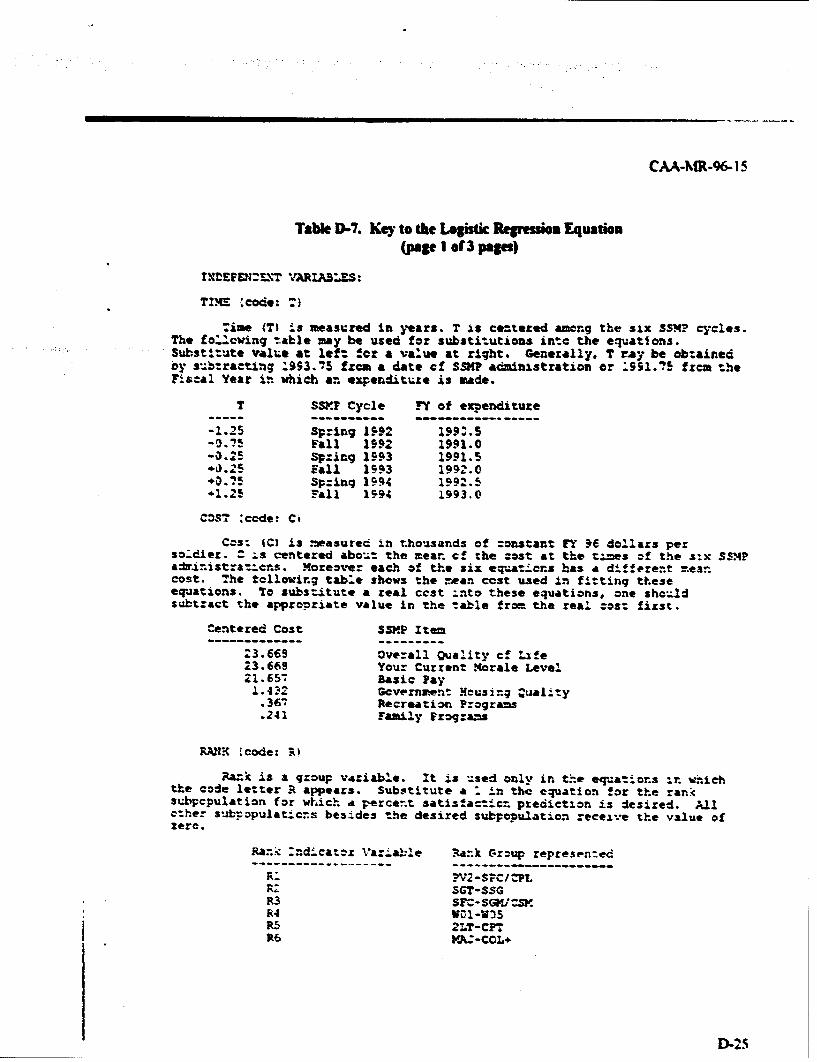
CAA-MR-96- 15

Table D-7. Key to the Logistic Regression Equation(page I of 3 pages)

TLEFPE?-L\T VARIALES:

TIME code: 7)

":ame (T is measured in years. T is ceztezed among the six SSN? cycles.The folZlwing t-able may be used for substitutions int- the equations.Substitute value at left ftr a value at right. Genezally. T ray be obtainedby sub:ractin; 2993.75 fzcm a date cf SSMP admia•stration or -S91.?5 frcm theFis:al Year in which an expendituze As made.

T SSXP Cycle FY of ezzendituze

-1.25 Spring I•92 19.M.5-0.75 Fall 1992 1991.0

Sp:ing 1593 1991.5*0. 5 Fall 1993 1992.0

Spring 1994 1992.5*1.25 Fall 1•94 1993.0

COST :code: Co

Cos: (C) is measured in thousands of =onstant FY -6 dollars perso.dier. .= s centered abo-.= the mean cf the cost at the t•.es of the six SSMPadr.-.istra-.cns. Moreover each of the six equat'ons has a di±ferent meancost. The tellowing tab:. shews the n.ean cest uZed ±n fitting theseequations. To substitute a zeal cost into these equations, one shou.dsubt:act the appropriate value in the table from the real zost fixst.

Centered Cost $SP.P Item

23.669 Overall Quality ef Life23.669 Your Cuzzent Morale Level21.657, Basic Pay1.-42 Gevernment- Housing •uality.3;6, Recreation P:ogra=s.241 Family Programs

RAIK .code: R)

Rank is a qroup variable. It is used only in the equatior.s ir. whichthe code letter R appears. Substitute a 1 in the equation !or the ranksubpcpulation for which a perce.t satis!actic, prediction is desired. Allother subpopulatlc.s bes-ides the desired subpopulation receive the value ofzero.

Rank a. nd.cat*z Va:-.able 7a-k Gozup represen:ed

R: PV2-SPCI TPLR7- SGT-SSGR3 srC-SGWCsMR4 VCl-W35R5 2LT-CPTR6 M:-CCL+

D-25

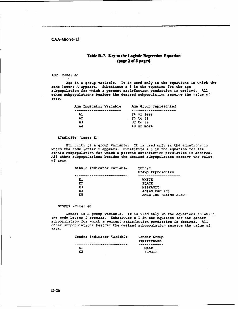
CAA-MR-96-1 S

Table D-7. Key to the Logistic Rtgrssion Equation(pag 2 of 3 pages)

AGE, I code: A.

Aqe is a qrc,.p variable. It is used only in the equations in wh-.ich thecode letter A appeazs. Substizute a 1 in the equation ! oz the ages..opopla':ion for which a percent sat-isfaction p:ed-.--tio. is des'-:ed. Allether subpcpulations besides the desized subpopulat.ion zece;'e the va-ue 'fzero.

A.e Indicator Variable Aqe Group represented

AI 24 or lessA2 25 to 31A3 32t o 39A4 44 or nmo

_rE-3:CITY (o:de: V.

Ethr.nc-tv Is a group var--ale. Zt is used crly -r. nthe eq-a:aticns :nwhich the =ode letter S appears. Substit..te a I in the equation for theethniz subh:p-ulaticn !oa which a percent satis!actior. pred:ction is des:red.All ether subpcpu-,ations besides the caes..:ed subpoep;.la--cn re-e:ve the 'a..Zee.! zero.

Etha.c Indicator Variable EthnicGroup represetted

El WMITEE: BLkCKE3 HX aNC.E4 ASIAN FAC :$Z.E5 AMER IND ESKIMN A•E1'.

CTZ ;Cc-ce: G'

Zendet -' a group va:zzab-e. It is jsed enly in the eqriatcrns in whi.hthe ccde -ettte 3 appears. Sub-stitue a 1 in the eqjat-4cn to: the ;en.ers-'.4ppFulazzcn fer w.nich a pexcent satisfactiorn predi:tion~ .2 desired. Allother subpcFulations besides the desired supbopilaticn rezeive the va-"e ofzero.

Gender Trdi±atcr Variak:*e :ender Grcup:epre-sented

G2

D-26

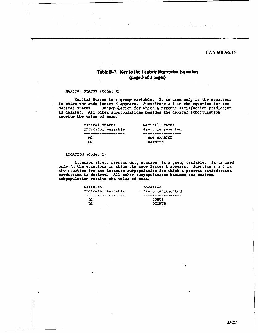
CAA.MR-96- 1 5

Table D-7. Key to the Logistic Regression Equation(page 3 of'3 paps)

%%R:TALr STATUS (Codie: V1

marital Status is a group variable. It is used only in the equationsin afih --he cod* letter K appears. Sabstitute a 1 1n the equation for themarital st.atus subpopula-.crn for which a pezcen-t sat'-sfactioz Fzedictionis desired. All othe: subpopulaticn& besides the desired subpcpulationreceive the value of zero.

Karital Status Maritaz S:atus:ndicatox variable Group represented

ml NOT APJ"!ED

L=CTION (Code: W.

Location ti.e., present duty station) is a group ;oariable. it is uredonly -.n the equations 4r. which the code letter L appears. Substitute a I inthe Equation tor the location supcpul•tion fez which a pez:en: satisfactionproedic:icr is desired. A11 other subpopulations besides the desiredsub,:ptu.ation receive the value of zero.

Lcca:-crn LocationIndicator variable Grcup represented

Ll CONUSL2 O(C=S

D-27

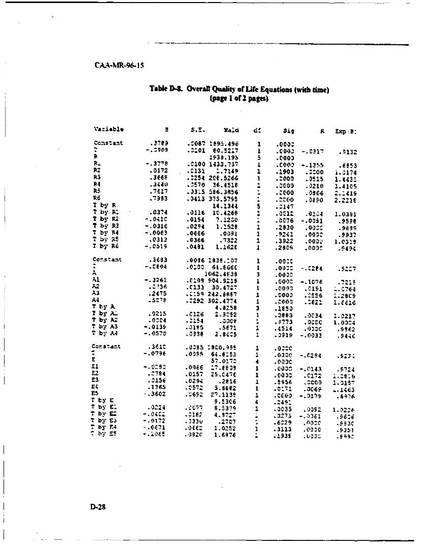
CAA-MR-96-15

Table D-. Overall Quali" of Life Equations (vmib time)(page I of 2 pages)

VaS.able $.-. Wald di Sig A LP:

Ccns:ant .37eq .CoO? 1895.496 1 .ooo:^1 9:09 -V%01 e0.52i7 I COO.' -. C317 ;132

R 1939.195 5 .000CR. -. 3718 .0100 1433.737 I .COOO -.1355 .fe53R2 .0172 .- 131 `.7149 1 .1903 .Z:00 i.!1?4R3 .3M66 .. 254 20E.5266 1 .000 .3515 1.4431R4 .3440 .1570 36.4518 .01) .0210 1.4105RS.17 .•335 BA6.3856 c. .c00 .0966 2.:419R6 .7993 .5413 373.5755 ."(10 .0E0 2.2218T by R 14.1344 5 .Z14•? by R: .03?4 .0116 1C.4268 1 .001 .0L4 1.0331T by R2 -. 041C .0154 7.12U0 " .0;76 -. 009l .95seT by R3 -. 0316 .0294 1,152e 1 .2830 .00-2 .969ST by A4 -. 00f3 .068 .0391 1 .9241 .00;: .9037

T b-: .0313 .0366 .7322 1 .3922 .002I 1.031iT by R6 -. 051; .0431 1.162C 1 .23M .0001 .549

Censtant .3603 .0036 1839.:07 1 .00:o"-."04 .0:0A 64.566 1 .00.: - ..Z84 .. :

A 1062.4F39 3 .000.Al -. 3261 .C09 904.5219 1 .000: -. 1.2A2 .736 .C133 30.4727 1 .004oo: -c1± ..:64A3 -245 C154 242.886' 1 .0000 ."E56 .29C9A4 .5CI .:292 302.4774 1 .c000 .:sz I Ze.16T by A 4.8K58 3 .ES50T by Aý .0215 CI26 2.3-2 1 .3663 .0C34 1.0217T by AZ .0:04 .. 154 .0;0P z•7?3 .OCCC 1.0'24T by A3 -.0139 .a15 .5671 1 .4514 .)33C .99f2T by A4 -. 0570 .0330 2.84.5 1 .a519 -. 0033 .94.

CorS~d~t .391- .0^55 :900.995 1 .0I^C0-.,79 .G599 64.8:53 1 .03;0 -. 0294 .923;

E 5 .01% 4 .00-3C£1 -. 0:9: .0066 I?.E52g 1 .•002 -. 0143 .5%-4Z2 .- 784 .0157 25.047C 1 .003^ .Cl#2 .ze:£3 .:156 .0294 .2816 ± .595f .-COO 1.0157X4 .1?65 .C5 2 5.66e2 1 .0:71 .006 -.1463E5 -. 3602 .L692 2-.1139 1 .cc0O -. 3119 .647FT by £ 9.5306 4 .149:T by E: .024 .5379 1 .033 .0.92 1.02,6T by M2 -. 04C: .:162 4. 5727 32"S -.3361 .96U6T b''y £E -. 0172 .433u .V7C' .629 .E:29 .933T by E4 -. 01 .Iof: 1.0252 1 .3113 . .351- b. "E .S92C 1.5376 .1939 .,0 .

D-28

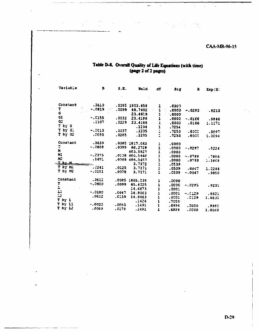
CAA-MR-96-I5

Table D-8. Overal Qualisy of Life Equations (with time)(page 2 of 2 pages)

"Varicble I S.E. Wald df S3g R Uxp 3'

CCestant .36io .0385 1803.458 1 .0007T -. 0819 .0099 68.7402 1 .000a -. 0293 .. 213G 23.4619 1 0000G1 -. C155 .0032 23.41e6 1 .0000 -. 01c6 .9e46G2 .1107 .0229 23.4186 1 .0000 .01E6 1.1171T by G .1234 1 .7254T by 3: -. Z013 .0037 .1235 1 .7253 .03^. .5e"6T by 32 .^C93 .0265 .1235 " .7253 .03ý 1.0C94

Ccnstant .3639 .0385 1817.C63 1 .COO37 -. 0809 .0399 66.2728 1 .CO03 -. 029? .9224m 4e3.59^7 1 .COOOM1 -. 2375 .0139 4S6.5460 1 .COO0 -. 0789 .7866M42 .1491 .0169 486.5457 1 .0000 .0,953 1.1cT..U- 3.7172 1 .0539by 'M_ .241 .0125 3.7171 1 .0539 .0047 I.Z244

T by H2 -.C151 .0078 3.7171 1 .C539 -. 0047 .3950

Constant .3612 .0085 1805.039 1 .CCOOT -. 09C0 .0099 65.4325 1 .0000 -. 0215 .9231

14.6673 1 .30001Ll -. 0180 .0047 14.9003 1 .0001 -. CIZ9 .9921L2 .0612 .C:59 14.9063 1 .0•01 .C129 1.0631T by L .1424 1 .7 5 9T by Li -. 0023 .0053 .1491 1 .6994 .3000 .998MT byL2 .006i .0176 .1431 1 .63-4 .000 1.0069

D-29

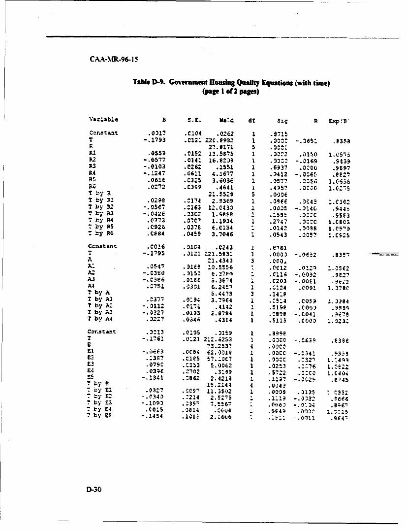
CA.A-MR-96- 15

Table D-9. Goverument Housing Quality Equations (with time)(page 1 o2 pages)

Var-'able B S.E. wa..c dt S,.q R T.xp:B

cznStant .031? .C104 .0262 1 .9715T -. 1793 .C12 22c.89s2 1 .332Z -.365: .8359R 27.6!171 5 .32 .R1 .0559 .0152 1i.5675 1 .3;72 .0150 1.C575F2 -. 05?7 .0141 16.C239 1 .133: -. 0169 .9439R3 -. 0103 .0262 .1551 1 .693? a0Q00 .9897R4 -. 1247 .061. 4.1677 1 .a412 -. 0:65 .8M2"R5 .0616 .C325 3.6036 1 .3577 .056 1.c636R 0 .0272 .C•99 .4641 1 .4957 .*0 C. .: 1 5T by R 21.5529 5 .0o300T by R 1 .0299 .- 174 2.9369 1 .09f .3C43 1.C30:T by .2 -. 0367 .. 163 12.0433 1 .00'5 -. 314C .944iT by R3 -. 042E .23C2 1. 889 1 .:5$5 .0:C .9503T by R4 .0773 .370- 1.19342% .2•47 . 3.^C 1.C203! by R5 .C926 .0378 E.C134 . .0142 .3138 1.09'D7 by R6 .Ce84 .0459 3.7046 1 .0543 .005? 1.C5:5

Ccnstan .C06 ,01C4 .C243 1 V8761-. 1795 .3121 221.563: 1 :0003 .0E2 .85

A21.4340 3 .CO0I.0547 .316e 0.556 O.CC12 .012O 1.052

-. 0360 .315^ 6.3780 " .CI16 -. 00.2 .982'A3 -. 0366 .016e 5.3e74 1 .C203 -.00kl .!O22A4.751 .0301 6.2; 1 .0124 .C091 I.378CT by A 5.4403 3 .14:8T by Al .037, .0:94 3.7964 1 .25Z4 .c059 '.3394T by AZ -. 0112 .0--4 .4142 1 .5198 .COO .99R9T by A3 -. 0327 .01a3 2.8784 1 .098s -. C041 .9678T by A4 .3227 .0346 .4314 1 .5113 .CIO? O.33

Constant .3213 .005 .3159 1 .3996T -. 1761 .0K21 212.6253 1 .COCO -. c6%9 .e3SeE $3.2537 V .00C2El -.Orc63 OCC84 62.13019 1 OOCC0 -.:34Z S93533E-- .*3-9? .C1es 51...067 1 .03^C -:321, 1 .-4 4£3 .079C ..353 5.00e2 1 .02S3 -.:?6 1. 0. 12£4 .03;E .- 702 .3:99 1 .5:22 .c 0 1.C404ES -. 1341 .4862 2.4219 1 .1197 -. 0 ..2.9 .e457 by E 15.2144 4 .U043"7 y El .03Z7 .- C5! 11.1592 1 .0038 .3135 C33."7 by E: -. 0343 . 214 2.!:'S 1.' . 911 -. '33 .36T by £3 -. 1093 .039' 7.8567 .006j -. 0134 .9;6:T by E4 .CO1S .0814 .'U4 .049 .oo 1.22157 by CS -. 1454 .103 2.1646 .15: -. 0fll .964'

D-30

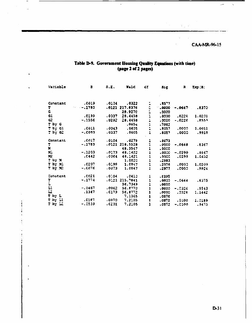
CAA-MR-96-15

Table D-9. Goverment Housing Quaqity Equations (with time)(page 2 of 2 pages)

va:iable a S.E. Wald df Sig R zx:B.

Ccnstant .019 .0104 .0322 95`7T -.2733 .0121 217.6376 . 0000 -. 064? .E3•G 28.9270 . .5000G1.01?9 .0337 28.4458 , .0030 .022f. 1.0231G. -. 155E .0292 26.4458 1 ,3000 -. 022f .855zT by G .0654 I .7982

Sby G1 .C011 .0043 .0635 . .S-5? .000c 1.0011Sby G2 -. C093 .033? .0605 .8057 .003a .9919

Constant .C1" .0104 .0279 1 .$Z73T -. 2783 .0121 218.5528 9 .OOC -. 0648 .E36 7H 46.3547 1 .00C0

.l -. 2203 .0173 4S.1422 1 .00"C -. 0299 .E66?.C442 .0064 49.1421 1 .0C .029; 1.0452

T by 4 1.032z 1 .2983T by x, .C207 .0:99 1.0847 1 .22?6 .coo: 1.0209T by .c -. C076 .0073 1.0947 1 .2977 .CO00 .594

:cOstant .C021 .0:04 .041I 1 .e395T -. 17-4 .0:21 215.-841 1 .0003 -. C644 .E375

5E.7349 1 .0000L! -. 046- .0062, sc.877 1 .0000 -. C32: .5543LZ .1347 .c017 56.0772 1 .OOO .3326 1.1442T by L 7.1365 1 .007CT by LI .CIE- .0070 7.2:05 1 .007-2 .0100 .i:1e9T 7 by LZ -.C533 .CZO1 ".2105 1 .C072 -. C103 .5475

D-31

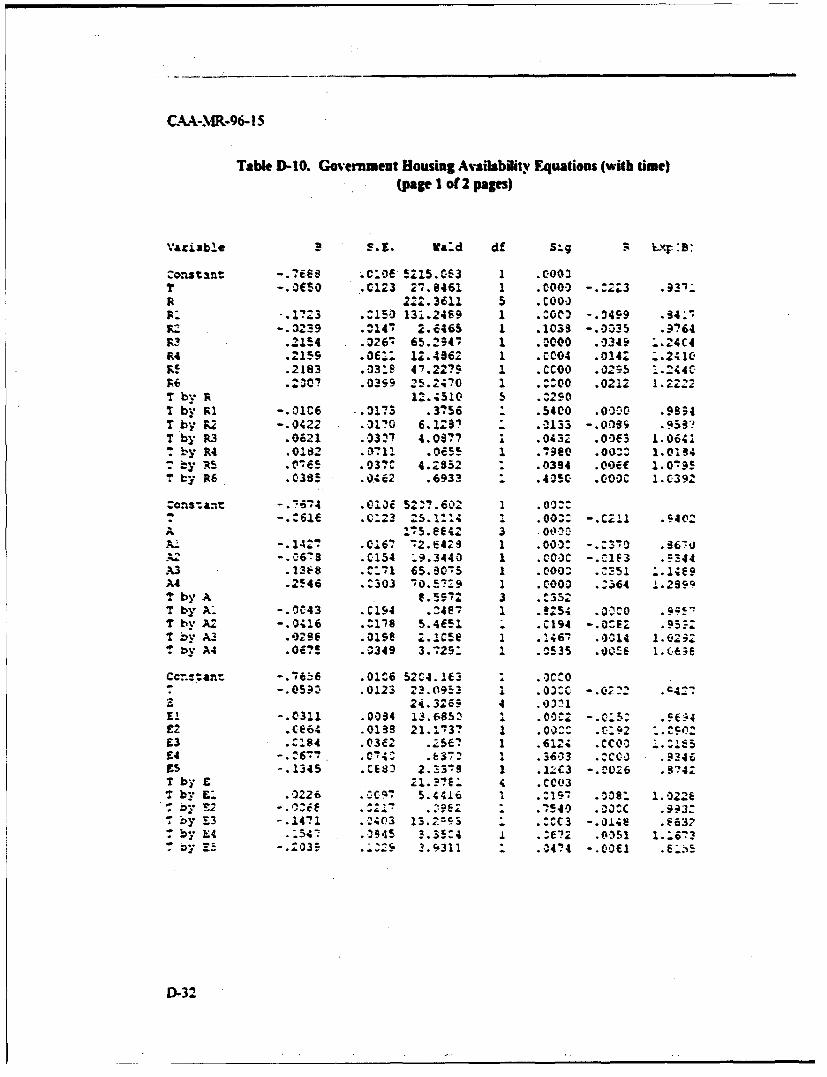
CAA-MR-96-1 5

Table D-I0. Government Housing Availability Equations (with time)(page I of 2 pages)

Vaziable 9 E.g. Va~d df S_, kgrB

constant -76 68 .C:,e 5Z15.C03 1 . 000:T -. o5 .0123 27.8461 1 . C000 -. :ZZ3 9 3,%R 222 .3611 5 .COol)A:. -. 73 C~150 131.2469 1 -COO) -. 2459 .942*

S-.3239 .'I47 2.i465 1 .103S -. 0035 .9764R3 .2154 .0267 65.2547 1 .2000 .0349 ".24C4R4 .2159 .06a.i i.4862 1 .CC04 .014Z :.2'10R! .2183 .03:S 41.227?9 1 .CCOo .029 5 1.244C96 .2007 .0399 25.2470 1 . C00 .0212 1,2222T by R 12.4510 5 .220T by Ri -. 01C6 .3173 .3756 .5400 .00!0 .93:4T by r2 -. 0422 .3170 6.123 i .0133 -. O0si .95 ?T by R3 .0621 .W03? 4.0977 1 .0432 .0063 1.064UT by R4 .0182 .0711 .055 1 .7980 .00Z 1.014T :y R5 .0 65 .037C 4.2852 " .0394 .00Q3 1.0'9!T by R6 .03;5 .0462 .6933 .405 . 000c 1.0392

Constant .67 .1010E 52 760" 1 03^". -. "61 .0:23 25.1i14 . .00W2 -. 0211 .5402

.-. 142 .C167 i 2.E42. 1 .000: -. 2970 .96.-. C154 .9.3440 1 .C%0C -. C183 .5344

A3 .1318 .C71 65.90'5 1 .000c .951 ".4l9A4 .2546 .:303 -0. 7-9 1 .000 .^364 1.29SQT by A 1.5572 3 .C352T by A' -. 0C43 .C194 .2487 1 .!256 . 030 .9; q.T by A2 -. 0416 . 118 5.4651 . .C194 -. 0282 .95tT by Az .02968 .019e :.aCse 1 .146- .0014 1.02 iT by A4 .01M5 .0349 3.729: 1 .;535 .00Z 1.663E

Ccn.:ant -. 76f6 .01C6 5204.16O 1 .C^"-.0531 .0123 23.09513 1 .0;2c -. 02 .24:

? 24.3265 4 .*i1£1 -. 0311 .0094 1.3.685Z .00~-E2 .Ce664 .0139 21.137 1 .000 .1 -92 ^.50:E3 .2.84 .03e2 .25 67 1 .612% .CCOO . 5E4 -. :6;7 .CT4 .V37. ; .3603 .ýCC, .9346Z5 -. 1345 .CE83 2.93_S 1 .12C3 -. M026 .374T by £ :I. 371 4 .CC03T by vE .0226 .nc57 5.4416 1 .29S .0081 1.0226

Z. %- 2 -. 2^6z .1. .29- ..!40 .01 .C -.) 3:b by Z3 -. 1471 ."403 13.2c-3 . .: C3 -. 014e .*632

7by L4 .i54- .09.15 3.3!:4 1 .11.051 1 i6,1r by E7 -. Z031 .2229 1 .9311 " .0474 -. 001I .6E5

D-32

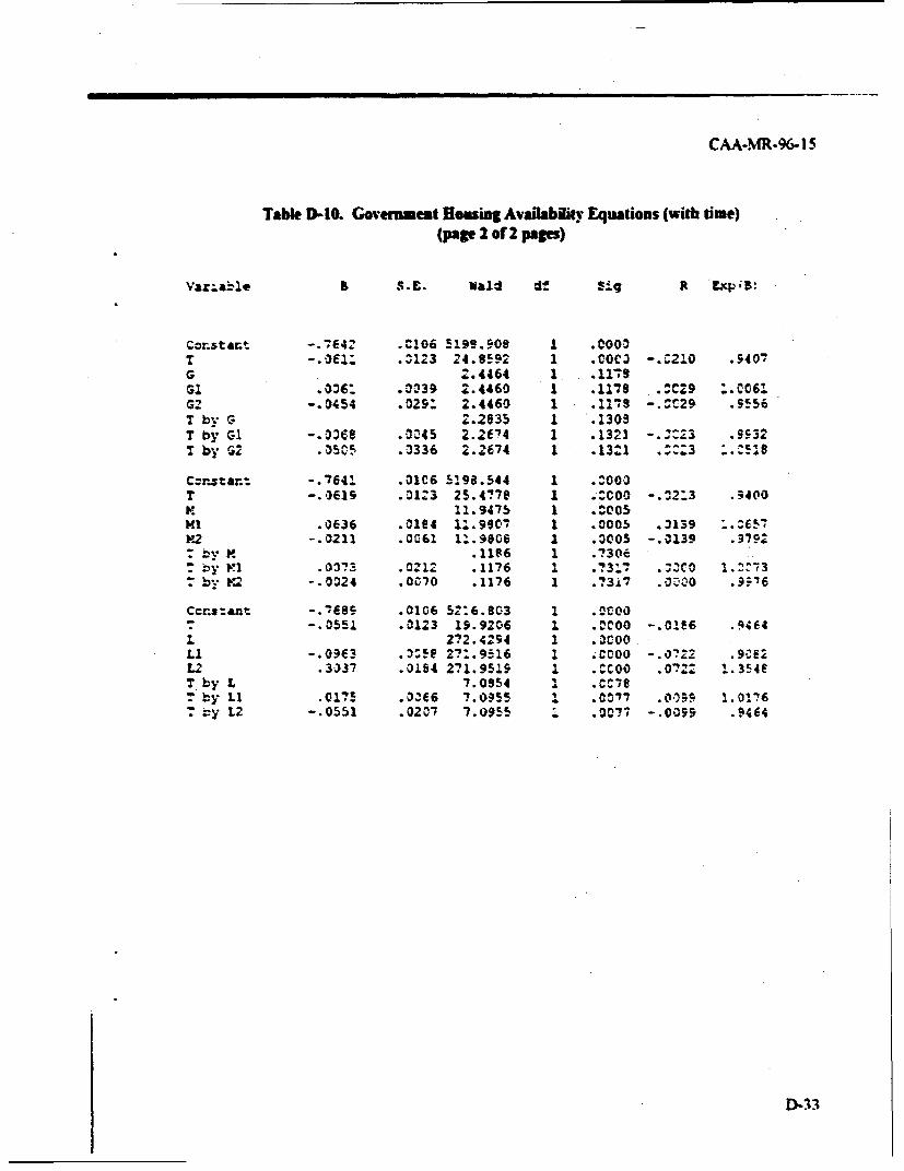
CAA-MR-96- 15

Table D-6O. Goverment Housing Availabitky Equations (with time)(page 2 of2 pages)

Vaae S.E. Wald df S.; R , xpiB:

Constant -. 7E42 .C106 5199.908 1 .000CT -. 061l .0123 24.8592 1 .C0C3 -. C210 .5407G 2.4464 1 .11.9

.036: .0039 2.4460 1 .1178 .:C29 :.C061G2 -. 0454 .029- 2.4460 1 .1179 -. 0C29 .9556T by G 2.2935 1 .1309T by G1 -. D8 .0:45 2.2E"4 1 .1321 -. 4223 .9532T by G2 .05C5 .0336 2.2674 1 .1321 .:::3 " 1

Cstar.n: -. 7641 .0106 5198.544 1 ."000T -.0615 .3123 25.477e 1 .:COO -.22:3 .;400K 11.9475 1 .t005MI .0636 .0ie4 1'.9907 1 .0005 .3139 1.05.V -. 0211 .0061 11.9006 1 .0005 -. 0139 .9792

.1106 1 .7306: by VI .0373 .0212 .1176 1 .1311 .OCO 1.:^73: b-. V.2 -. 0024 .0c.70 .1176 1 .7317 a*0 0 9Z'76

Ccr.s:ant -. 7685 .0106 52:6.603 1 .ICOOT -. 0551 .0123 19.9206 1 .00 -. 0166 .9464L 272.4254 1 .0co0Li -. 09E3 .3:5F 2?..9416 1 .CCOO -. 0722 .9CE2L2 .3337 .0154 271.9519 1 .- coo .072: 1.354FT by L 7.0954 1 .;C0eT by LI .0175 .00(6 7.0955 1 .00"T .00;; 1.01767 ."y L2 -. 0551 .0207 7.0955 i .20?7 -. 0099 .9464

D-33

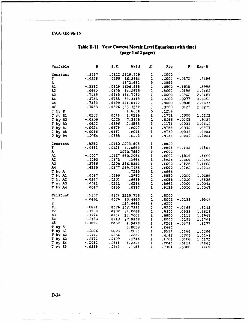
C•4A-MR-96-15

Table D-1 1. Your Curret Morale Level Equatoms (with time)(page I of 2 pages)

Vari*4le $ S.E. Wald df Sig R ExF.b!

Constan: .5;1' .1:2 2329.?:9 2 .C000T -. 0.2e .:130 16.3964 1 .Zoo: -. 3172 .74E6A 1612.E32 5 .:000Ri -. 5112 .012e 1606.95 " .ocoo -. 1915 .59s9

S• c .0275 14.2e73 ..002 .01!9 1.0e62R3 •7159 .0343 434.7Z50 1 .^COO .0=;: 2.0461R .4733 .0'55 35.3149 1 .:Q0 .0277 1.6:S"R.3 .733S .0399 336.0152 .3^00 .0930 2.0333RE .7033 .0506 :93.3290 .3:00 .0627 2•02•

9.6054 5 .1256"7 by R1 .020C .014e I•.216 1 .i..l .000c 1.02:2" by R.2 -. 0556 .02 5 ?.3945 1 .0.66 -. 0C' .543T by R3 .0621 .0396 2.4563 1 .:1i% .0031 1.064:? by N4 -. 002i 05?9 .0001 1 .9186 .031Z .€9T by R5 -. COLE .0462 .0011 1 .9130 .000ý .•994b y • .pU64 .0595 .1:; 1 .9133 .O000 I.C04

Ctnaln .5252 .oil 2273.e05 1 .0O23T -. 44 .C129 ý:.6669 1 .000e -. '142 .-951A 1070.7052 3 .0c0oAl -. 4C0T .:137 e50.2054 1 .000 -. 1319 .CcP3A: .3.^53 .21"73 .28R64 1 .5926 .co-C OCS3:AS .37P6 .2206 3136.!191 1 .t00-3 .-.82F Z.4EC:A4 .C530 .C377 299.7453 1 . ..^COO 1.921ST by A .7260 3 .566eT by Al .0:67 .160 .2-62 ! .5850 .OZO 1.0086

by A2 -. 0167 .320: .C915 .4C56 .0360 .9a35T by A3 .041 .0241 .0284 1 .8662 .ODCc 1-.341T by A4 .0047 .0435 .0117 1 .9139 .0:^c 1.0341

Ccnstant .53 .01C8 2220.758 " C 1" -.0461 .01.6 13.446 1 .00C2 -. 0153 .954QE 121.6841 4 .033CE. -. C89f .0036 133.7931 1 .033C -. e469 .5:43F2 .1509 .02:: bi.0069 1 .03^c .(333 1.16;:E3 .1'!4 .03e; 23.700c 1 .0030 .c211 1.1141E4 .S150 .0143 i?.99!9 I .000c .¢cýl 1.3'03ES -. 109ý .ceb6 4.9499 1 .C061 -. CC9 .8Z'7T by E S.ec.: 9 .C662T by E' .0 6 .CC99 ZL3! I S9551. .C^co &..^CG6T by =ý .. 254 C66- 1 .4142 .0000 1.:'-3T b £3 .E371 .3409 .4146 1 t- .6:1ICC 317:T by F4 -. 24^2 .698V 8.232E 1 .:c41 -. 3113 .!94i

I)-34-.033e .1135 l 7304

D-34

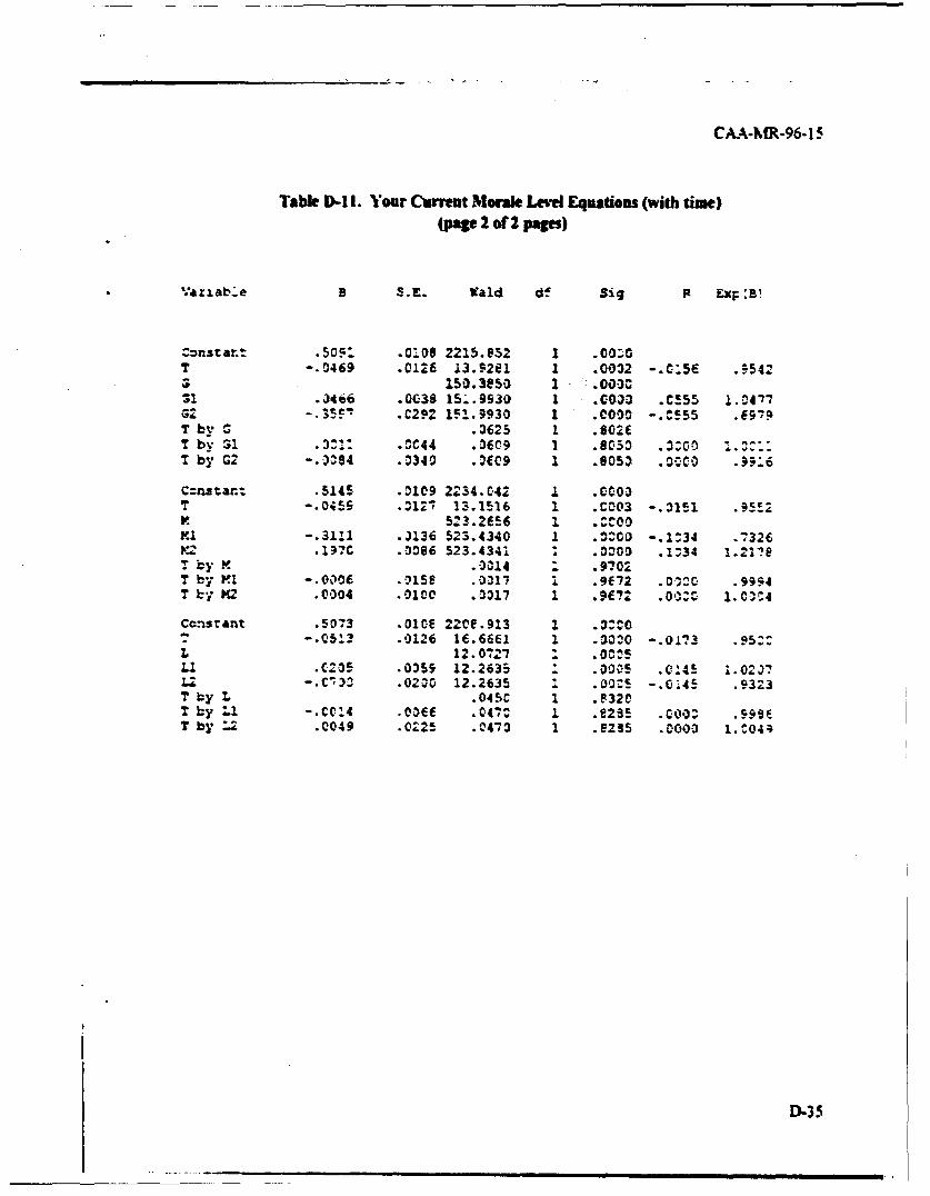
CAA-MR-96-1 5

Table D-1 I. Your Current Morale LevA Equations (with time)(pap 2of2 pages)

VBab.e B S.E. Wald df Sig P Exr B!

Constant .50K1 .0'09 2215.852 1 .00--T -. 0469 .0126 13.92el 1 .0032 -. C:56 .9542

.3406 .o03S 151.Bs30 1 .C030 .C555 1.047G2 -. 35'I .C292 151.9930 1 .eO0 -. :S55 .E975T by S .0625 1 .802OT by 31 .3^i: .OC44 .0C9 1 .8053 .3^.00 0 .CT by G2 -. 3084 .0340 .OCC9 1 .0053 .oC.0 .9..6

Crnstan: .5145 .0109 2234.-042 1 . c03T -. 045S .3121 13.1516 1 . C0Q3 -. 3151 .95E2v )523.2f!6 1 . "0mi -. 311i .3136 523.4340 1 .2300 -. 1^34 .7326Y" .197C .0386 523.4341 2 .0300 .1a34 1.2178T by M .- 014 .9702T by KI -. 0006 .1158 .0017 1 .9f72 .013c .9994T b y K2 .0004 .01CC .0317 1 .9c7• .000 1.C0C4

Ccnstant .5073 .01CE 220".913 1 .3Z•0T -. 05:2 .0126 16.6661 1 .3320 -. 0173 .9500L 12.0727 : .083L1 .C205 .0359 12.2635 .o01c5 .(U4! 1.02 3LI -. c33 .0200 12.2635 Do .ns -. 014s .9323T by L .045C 1 f32.T by Li -- CC:14 .0af6 .0473^ 1 MS25 .599ET by 12 .0049 .0225 .0473 1 .e295 .0000 1.C04

!-35

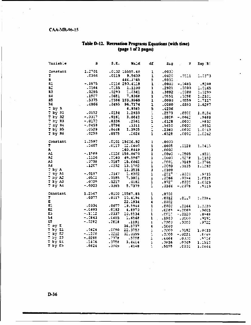
CAA-MR-961 5

Table D-12. Recreation Progran Equatioms (witb time)(page I or 2 pages)

Vaib- S. E. Va~d df S4,

T C3 .011'3 5.56031 1 .00, ni2. ~:3S444.; 7 65 5 .000:

-. 9T 29).4::9 1 .000.1 -. 8 09:01t1t6 .5 .1100 1 .2921 -So ;.v1265

3.095 .02q ".c341 1 .3092 .. :00 ý.299R4 .06e1 7.9368 I .C51 .z:9e 1.I C

.5375 .:S66 193.9M6O 1 .0000 .0559 " i117Re .0495 96.7174 1 .PCOO .0353 1.6267" by 3 4.9345 5 .4236

by 31 .0152 .01!4 1.2933 .2?73 .0C 1 1.0-54b ky R2 -. 0317 .019: 3.0f43 .0Deco -. 004' .9699

".7." 33 -. 017% .0336 .2561 1 .6128 .003: 43:7 t , 4 -. 04;3 .0"96 .3311 .SiS* .oo0o 5 5.2T by RS .0529 .0;48 1.3905 1 .2383 Q03C .•3T by R6 .0259 .0575 .1-024 1 .652E ~0 : 6

Cznstant 1.2597 .C i 15e6.92 I .0133T .407 .0:17 "Z.C601 1 .0005 .:128 I.4:.A :60.94491 3 .0C00Al -. 15e$ .C121 158.9670 1 .COo: -. z05 .3:A2 .126 .::60 49.596'? 1 6001 . ý7P 1.-12A3 .373! .01%7 .5.C462 I .1C0 .0149 C. , 6A4 .12C= .232 13.1702 1 60-3 .2135 1.2327by A 11.3535 3 .:i00- by Al -. 01i• .:14-; I. • .2•: .0o:: .9•15"by A2 .05 2 .01e5 3.39C1 S .:66 .0014 1.0515T ty A3 .0ý25. .0217 .0162 1 .Cz- .0o:3 i.c: -2T b YA -. 0.23 Oie$ 5.:379 .01ci -.CO75 .9119

astant 1.2.47 .0100 25857.93 1 .0 1t .03a'n .0117 0. 4154 1 . 001Ze3

E 22.1934 4 .00:2E: .0334 .0077 i•.S944 1 .C0O0 .^164 i. 1.39EZ -. C403 .0:32 4.693 I .Czf; -. •0E .9fC5E3 -. I" .0337 b0.E534 1 -Cc:: -. ;14 1E

-. 06643 .C655 i.656@ 1 .15-t 3 JC , .41,£5-.:2F2 .6 .1191 1 .?303 ).1Z C ~

O oy E 36.73' 4 .:CCOT b Zy .3424 .CCSO 22.375? .2CC. .i*M 1.0:1337 b E-2 . i.'339 " .1$¢0 -. 0221 .1t•

.737f .5"S .44464 OjCT by F. .24:6 .Se 3.4;4 I .U26 .0049 1.151:T by ES .0U24 .0Qt .4148 " .5155 .C 1.0644

D-36

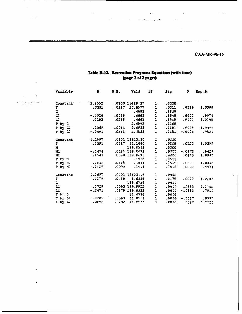
CAA-MR-96- ! .S

Table 6-12. Recreation Program Equations (,itb time)(page 2 ofZ paps)

vaztable 3 S.Z. Wald df Sig R & :a"

constant 1.2552 .0100 :5E20.37 . .0120T .0391 .0117 1C.6S? .0:1" .0119 1.0393 .4691Jsi -. C026 .0039 .46 .434S .00.4: . 5074"".! .C193 .02f6 A46M1 .494C .0):.:T by 3 2.45SQ2 .liceT by G! .C06? O .OM4 2.033 I .115: .0092 1. nT by G. -. C491 .0311 Z.4AS33 .01 -.002. .A5;2

Constant 1..557 .01 1 15613.10 1 .0.3oT .C3-?1 .0117 11.i69• " .OO0e .0122 1.0O3.•

S239.C$13 ..O0CO

M: -.. 4"r4 C.12! 13..0061 1 .0''0 -. 0473 .Ff2=.. C941 .O)33 13-;.09C 1 .00C- .04"-3 1.0 959T by v . 1 .7511T l* . .Ch4v .c". ."-1I I .s:.5 .00): 1.004C-7 by ' -. CCZ2 . .I~1i 1 .. 55 .OOJ5 .--. 1

C0z;sta.:" i.264V .C01 15E23.18 1 .0 CT.C-.1 5.6465 1 .0 .00'71 1.^:93

: 9.6-3f I .00Z:

L .C. .173 1S . e .22 1 .00t -.^553 .7!E:T by L 11.6 73E I .CO.E7 by--1 -.0205 .;06D 11.!559 1 .00!6 -.I:. .

T by :,2 . 0E .:2.02 ,l.e-58 1 .001e .'7 1. "2

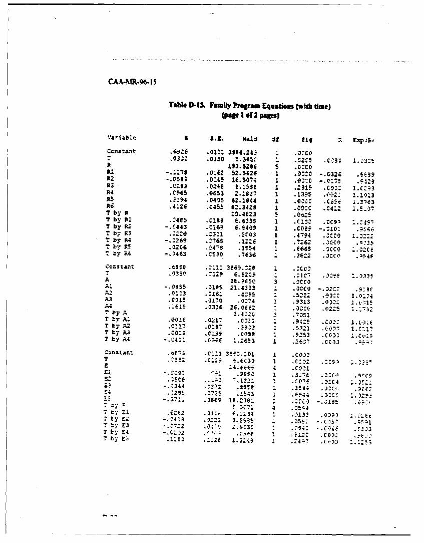
C&A-IR.96- 15

Tabe 1I-1. Family Program Equatios (wish dime)(page I of 2 pags)

""ariable B S. C. Wald df Sig 77. xp is0

constant .6926 .011: 39e4.243 .- .033: .0130 5.36c - , .. , CS; t.C3Zt

193.5:86 5 .0:co, .0.2 52.542e 1 . -3.O -. 0326 .SE90

1. S,1 .0:45 1E.504 I 0 -.C:7• .12SR3 C299 .0269 1.1591 1 .915 .M0Z: I.CZ43R4 •C.65 .0653 2.9831 1 .13=5 .*,2: I.::,:3A5 .3-94 .04'35 C2. 1044 1 .0"c .C35,E 1.313A6 .4-2f .0455 82.3429 1 .vo.c .C4:2 1.53T by P 10.4623 5 .06"25T by PI .4e5 .C193 C.6339 1 .C'39 . %C9 ".:4-T by R2 -. 1443 .CI69 e..40. .co .10 -. 102 .. 6T b7 S .R20 .:311 .!003 1 .42:Z4 . 00 1.2:2"? by 34 -. :269 .2,6 .12.6 1 .7262 .zco ."T bL- A .0206 .!%4:9 .IE54 1 .A669 .OCCO c.,2Cf.7 -.2463 .0530 .7636 , .3E22 .XC(I .7.94Fcz'.s'aa.t .c r.. 3t6w.Z:20 .z :CC

- .0333 .3229 6.52. .:9 - .32_E -.- 33A 36.•-•5c 3 .20coAl -. 0855 .OM5 21.43%3 1 .acco -. 31:2 .5:3cA3 .01-15 .0170 .nn74 I .?313 .O3Q) 1.t.:l1A4 .•El! .0316 2E,0U2 .3 Cc(I .0225 1. "S":_27 by A I.102.IOC.T b- A: .00.1 .021V .0Z .. ) 1.I.Er bY A2 .J-& .0:97 .39-3 .5321 .C,, 1.0.177 by A., .009 , .C,,9 1 .25,3 .C0) 1.C,.;.7 by A 4 -. C4A .C.3eE .z63 1 .-6 ..

onsat%. .eF, S . C::-1 3e3.:01 1 )I):!T E A. ¢. .. t..C3 3 1 .C . 32 . . : t ""

£2.S".CE ~ .2• '. 122: " .c- :' .3"-C4 . .. :

£-5 -. *7•4, .:s'9 18,sse * .asj, -. 2:,1t; .•EE"-" -'2 2A 4 .C 54

E by £2 -. 45lR .322 , .•5-? -.-7 3-•C~ ": 2. ,•-3: . •",,"- .c•,i; . :• 3I by 94 -. C32 es. "t - ..!,3 .*,ft y E2 C42 .Z 1. Ft .55S! .455 .~315' 25

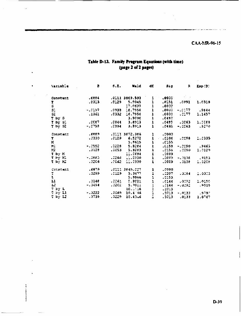
CAA-MR-96- !

Table D-13. Family Program Equaims (with time)(pae 2 of2 pages)

vaziab:t p $.E. Vald df Sig A Eap:B!

Constant .0894 .-011 3890.593 i .00.2^ "T .03*3 .0'29 5.5045 1 .0.51 .C091 1.0313

3: Ctb' .C0133 :f.7-5f 1 .0000 -.C: 17 C-E44""2 .1361 .0332 :C.IS56 1 .OOC .o:' 1.1457T by G 3.909E 1 .C49LT by G: .0Cce .6044 3.8913 I .0495 .:C63 I.:Ce9T hw 52 -. :75s .334 3.9913 1 . C43. -. Z"63 .90

Cr t ant er69 Z.::I 3F72.3E6 1 .C0O0T .3330 .0C29 6.5272 1 .C0I0 .58 :.:%35

5.9615 1 .C155- 25 23 5. 8214 1 Clss -. ::90 .?463

M2 .312S .3053 5.8263 1 .:~ .:~ .:zT by V ::.:694 1 .:009T tw M,-.3663 :2 6 C-".C330 I .OMi -. 2136 .;153T by %Z2C .:'Ci2 -:.:330 1 .:CC9 .1.13f ..̂2^.

.c::an 3E6s.c,& 1 . to00.02E .-129 5.34" 1 .020' .x4 1.33:3

L 5.9966 1 .•53LI !.9--216 1 C142.0!LZ -3454 .02c;2 5.SZ Z .144 -i0

" Li - .3222 .0:69 10.446 ..:13 -.n:33 *9'Sr.373! ."229 13.4516 .. 033 1 0! O67

D-39

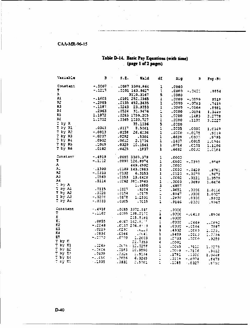
C.AA-MRfl96- 15

Table D-14. Bask Pay Equations (with time)(page I of 2 pages)

Vxa*3 S.E. Ta-'d df :.(; R 3 -I

C~astr. -5C7 C087 3304.664 1 .C003T .12 .•01 143.962" , .COol -... :: .5•4S31:0.3167 S .^000Al -. 160S .0101 252.3365 1 .:000 -.0559 9S19.2 -,.135 45423435 i .0o -.0163 .'N41R3 .:243 23.3353 1 .000 -. 0166 es3eiP; .2963 .2524 3-.,1"476 " .0c00 .01r4 I. 344

.1372 .02'3 1?59.2c5 1 .CI00 .:4e3 3 :.1R .12 .0365 1ý3 0.7 ?" 1.^00 .113! .2

S-R • 35.1:36 S .OOOY R' 1 .034; .0117 SSUI0; C.-: • •04 .oi .56 .3:35 .co;: 1.C34•

* by 32-.0813 .Oise 26.61-36 0-O .~7 91L y R3 -. 020? .0292 .5364 1 .4639 .U .7

R ;" P4 .09001 6 2.1'34 1 .14"7 .C015 .4? by R. .:049 .0329 :C.1541 1 .0c14 .c:1i 1.1:06T by R6 .0182 .0425 .1637 1 .6es: .ccJ: ^.i4

~nt ~-.4919 .0095 336z.3'!3 I Oct -T .12 .009t, 12i. 0'!4 1 .C00'-:3A 449.4992 3 tco.

-.1300 .C!09 143.C663 1 .CC321 -. 04:0 8376AZ..132 6.3153 1 C22 . ~ .

A-3 -63 .:2153 !3.E4:8 1 .Coz .312 ..3T7A4 .5114 .- 262 36:.3"3 I .2C00 .-369 I..76

b Al 0115 .:I:- .9204 .36E5 .02C 1.01ET by A2 ..0C: I* ..'1.2

£ '5* .O2S0 .01:75 1 :.Z5- I .252C .0420 .. 922

2 -.. 64 .OJ;8 1A4.7 :! I .C32C -. (E4. .!'24: *-- A; - - ." 4 .. ?.36E.0e55 Z06 E~'.3 .44 %*it '.

Ed. -.- :48 .C55 2.14.2; - .C2) -. 0.4 .-. 053 .C:;- . A 1 .433- .03 .ZZ..F-4 CE4 4 .

T by F .~.33 4 .cc00Sby E 1 : t .5 CQ5 .)I:: 1~'

li 439_ýSC .:!c .33.,-by B4 . Cý .F!6 i.324*5 .)1ic. -0374 .47

D-40

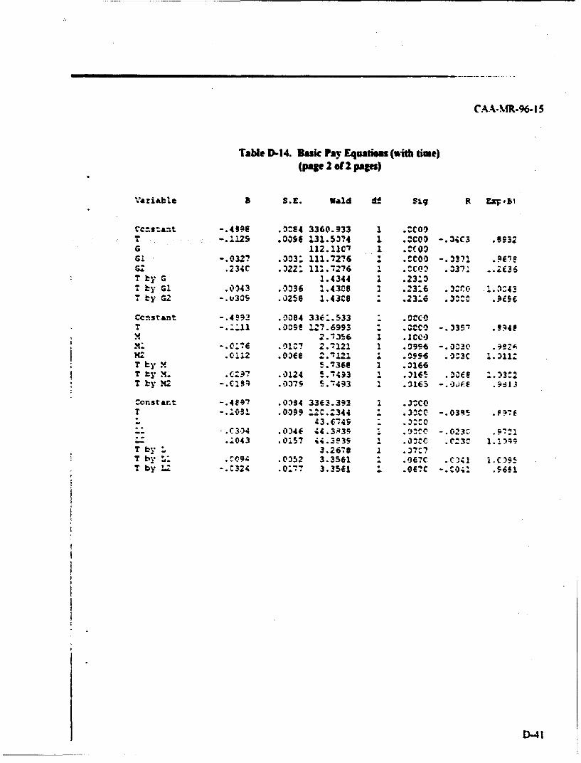
CAAAMR-96-i 5

Table D-14. Basic Pay Equatiu (with time)(page 2 of 2 pages)

Va riale $S. E. Wald d! $i; R I IFBI

0CCs:ant -. 4VE .D^.4 3360.933 1 . C0oT -. 1129 .0096 131.5074 1 . COO -. 3UC3 .8932G 112.1101 1 .Cf03

GI -. 0327 .•33 111.7276 4 .CC0 -. 3371 .PVIG. .234C .322: 11:.7276 . .CCQ, .337: .. 2C36T by G 1.4344 i .23.3T by G1 .0-343 .0336 .4 3C8 i -13'.6 - .^rCt 1. .3Z 4

I ty G2 -. 0039 .0258 1.43CO 1 .23:6 .33C C .

Ccnstant -. 4!93 .0084 336*.533 "-.:ill .009e 12?2.6993 2 3C -. 33S' .9149

M2.1356 1 .1CCO3MI2? "I 31 7 2-7121 1 .0996 a-,C'30 Q

H: .0112 .036e 2.-121 1 .3996 .03C 1.311,T b M 5.736e 1 .3166? by - .C:97 .0124 5.1493 i .1E D.~332

ST :.y M2 -.Cigq .0379 S.7493 1 .3165 -. 04F .9613

Constant -. 4897 .0394 3363.393 i .31COT .01 .0099 :2C.2344 1 .3:CC -. 03RS .Fý7f

43.E749.. C3354 .034f 44.3R35 .IDCO -. 0230 .9:1

- .1043 .0157 44.3e39 I .O33 .0:3C 1.)4T by L 3.26"8 1 .•373T b"y L .:094 .0352 3.3561 2. .O7?C .C231 1.C395T by Z -.. 324 .0:7 3.3561 2 .061C -. 0;1. .5651

D41

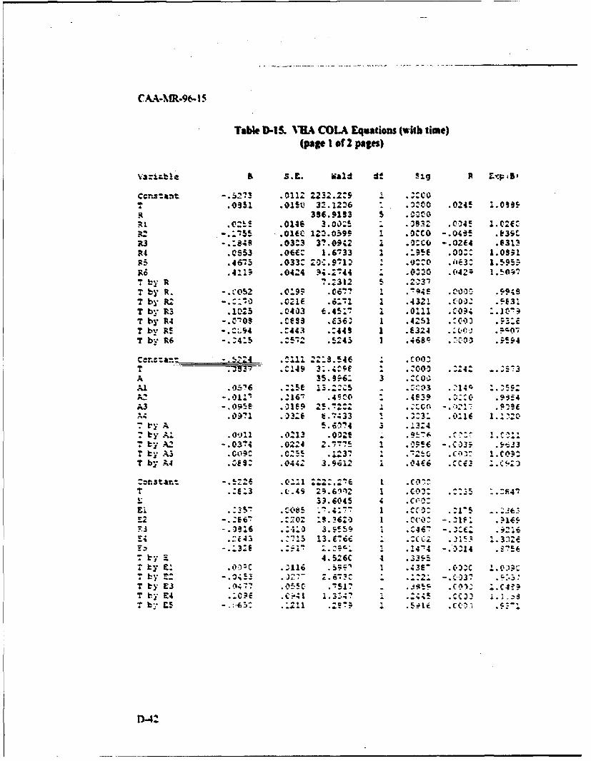
CAAAMR-96. 15

Table D-IS. VHA COLA Equations (with time)(page I of 2 pages)

a S.E. waid d! Si.g P x15

castant * 12 232. 2:9T .0951 .013U 3!.1226 - ."0 .024! 1.0os*

336.9193 5 c'R otS .0146 3.00:! .0~932 .004! 1.0^("

-.~5 .Cite 123.0595 1 OCCO -. 049S b639.R3 -. :849 .03:3 3?.0942 i .2zCO -. 02f4 .6313R4 .0S53 .OEE: 1.6733 I .:;Se .03:c 1.091;

A,.46"75 .033: 20.91 .'0J. :0 .663: 1 95.Ra .4-!i .0424 N.Z44 " .020 .(042z 1.50;'TT by Rt 7.2312 37T by Rt -."052 .0 -* 9.- :Q~46 0 0!'t .11 aT by A: -. 170 .021f .6:71 1 .4321 .C-0: .5831T by R3 .1025 ,0403 6.45'. 1 .01i .CO?4 .IVo;T by R4 -.C07 .Cess .364 1 .4251 .C.03 .T by AS -. ^94 .1443 .:449 1 .6324 VI 1 .zeonT by R6 -- 4.S .S,2 .5245 1 .468e c "1-; 94

T J .I1 3:.4CE I ..̂000 . :24^ -.Z'53A-359.46: 3 .C001)Al .0o6 .::Se 13.2X•5 .•13 .•14' - .It2A-.01: .2167 .45cc .4 #9 .•c* .91E4A3 O .095 . 19 2. "2 Z ."•C -. ý'' .•i9•

.O.3-- e E.433 i .;:3: 1016 1. 11-c.C" by -A 5.104 3 .13Z4

b by Al .00 1 06213 .002e 9E 1c:0 .c Iby A2 -. 03?4 .0224 2.7 TV 5 .5S6 -. C035 .•33

7by A 03 .c:-S .L.. 3 7 .-::c C.47- 1.c ?.~T by k4 .CE 0 .0442 3.9612 i .04f6 .CCu3 ICf- 2

=Onstarnt .- - C.c II Iz:2.: 6 i ~ iT .E.3 .C.4- 2 .6")2 I .c¢0: .:35 "S47L 33.6045 ; .Ce•0Li . 32 CX685 ' 17.C;:0 !715 -

£2 -.962 .72 :S.3620 1 .CC0 -.-IF2 .ý1E5F~3 .56 .'2~ 3.555.o i C467 -.7E. .Y2

£.4S .:715 13.E67,- .:i ..C C.37Z

T ky - 4.526C 4 .335ty. 1 .438Q .10C L.Jb4y Z: 0 .127 2.670C.

T by E3 .04?? C.05 .,7517 *O) .C~T by E4 .:CE .c;-41 1.S4 -3.'45 .cC7

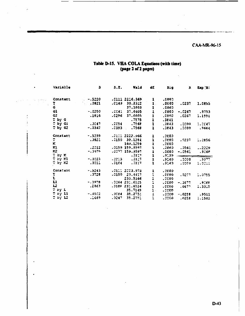
C.AA.-m-96- 1 5

Table D1-IS. VHA COLA Equatios (with time)(page 2 .t 2 pagm)

Varia~1. 3 S.E. Wald dI Sig ; EX;3

Ccrntar: -. 5220 .C1ll 22E.369 1 .C001T .0821 .C143 30.2312 1 .OC00 .023" 1.0155G 37.1E03 1 .0003GI 02!0 .CCI 37J605 1 Col C267 .9753G2 .1916 .C296 37.6605 1 .Coo0 .C267 1.11: by G .4575 I .3f41* by GI .3C47 . •54 .7568 1 .3643 .!1oo .:c47* by G2 -. 3342 .:393 .7568 1 .E 43 .Zle e

Ccr.stant -. 5239 .1 2222.!66 1 .C•OS.3821 .:150 30.12e4 I .:co0 .•237 ".:s56

K 160.1259 1 .COo!.fl.2%2 -~5 5.5 ~O ~6 .22:9

V2C~ 159 .959- 1 .^Co:).~6 .9.^6p* b* v. .•1' 1 .9:39

7 z~y KI .3Z23 Z2-3 .311- 1.:o* -. K2 .oz:1 .31C4 .Z117 1 .5.43 .::o .. :::

Constant -. '243 .CiZ 2:23.573 1 .:003.3,728 .%150 23.4417 1 .CCOO .32: :. 7E

L 233.5166 1 .COOLi .37 -0:4 23:.EzZS .3;cOO -. 3677 .:fL2 .2963 .32eF 23!.e524 1 .CCOO .001 1.33.15T ty L 35.7149 1 ^c"T •y LI -. 05z2 .04 35.275: I .4co -. 025! .9511" -L2 .:4es .024! 35.275: 1 .Z:CO .0258 1.592

D-43

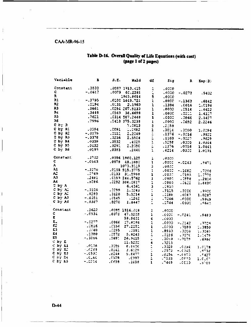
C.A-MRo96-IS

Table D-16. Overall Quality ofLife Equations (with cost)(page I of 2 pages)

Vaaiale S. E. Wild df Sig R Exp:3?

C -. 0617 .037? fC.22311 .0;:0 -. 0273 .0421i9i5.F014 5 .0.cS

.0=0• 1443.21 1 .O0: -. 1363 .6t42I,2 .ZiN .0 31 2.196-3 1 .1394 C[O16 :-i.g19R3 .3661 .0254 207.5133 1 .003 .C514 .. 4422R4 .3449 .C569 36.6699 1 .O00C .:2Z: 1.42:i

R5 .76:1 ."314 5H7.2448 1 .~00: .:e66 41.141"a6 .7?96 ..4:3 Z75.3238 1 .C000 .:612 2.2246C b- A .!U13 '1.253C by Ri .0394 .. 091 .3 .30:4 .3:00 i.0:ýz4

Sby RZ -. 07 .121 ,.136 -.Z016 .9924L by I3 -. 0374 .3236 2.55C 4 .1103 -. 0..; .qes- by RI .O33B .O532 .4C25 1 .5:5e .0320 1.044C by R5 .0;32 .0291 2.25!C .376 .0016 1.0401C by R6 .0134 .03A 3 .2440 2 .6214 .002 1.0191

Cccnst~nt 3 -- .0096 1SE0.125 tC C -I .53 .00?9 45.16s: 1 0 .032 -. CZ43 564"71A 10'2.3: :

Al ~ .0:03sis1.3~75 .004,: -.Ice: .70S.. 33 3 L 599 1 .cor . .A3 .264e I .CiS4 2 441. 562 1 .C000 . :!!E -~.29116A4 .5^66 .:292 304.eCEV: .1000 .:6:2 i..C3t: by A 6.416 3

by-9 A.2'43 0.315 .^C .94CC by A: .02?3 .11:0 5.5-ý14 1 .6 .27 .0%93?C by A3 -. 04S1 .C145 -:242 .- 246 .2: C .•4;C b, A4 -. 03V' .027" 1.844" : .Z744 .03: .'64

Cer.gt4= -1622 .00395 iS16.ci 0.1032C -. 053; .007e 47.32-3 I .v*3Z -. C241 .94e3E 5;.9431 4 .C03•

E- C 026 -. :2E2 - 6 Cbc 274.:5: 0 0C3 .16.) - MSCIE3 .40 .::55 .. 191 1 .SS33 .^C10 1.3).'-

£4 .:3co .:!72 5.924- . .. c :475£E- .6 ' 26.ý415 O3CtO -. a%? .6 49iC by E, 523.. 4 .32&3

C by Z.C6 .041 3.6'2 .. 573 -. C)45 .c3iC by E3 -. c5?: .0244 b.647 1 .o15t -. ((.3 .C42V

Z C-44 C. .C,2a .037 5 3 3 .c _:,

by4

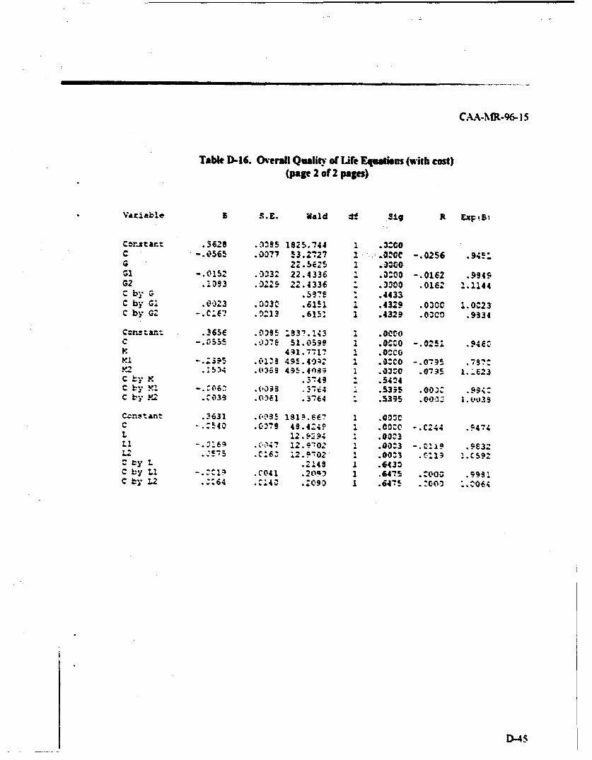
CAA.-MR-96-15

Table D-16. Overall Quality of Life Equations (with cost)(page 2 of 2 pages)

Variable 9 S.E. Wald df Sig R Expts:

C:rstant .3628 .1395 1825.744 1 .300c -.0565 .0?77 .2 7 .0:00 -.0256 .94s:G 22.5625 1 .30G0

01 -. 0152 .0032 22.4336 1 .Mo0 -. 0162 .9949G2 .2093 .0229 22.4336 .3300 .0162 1.1144C by c .537B : .4433C by G! .0023 .303C .6151 1 .4329 .030C 1.0023C by G2 -. CE? .213 .61: 1 .4329 .03CO .9334

Ccr.2 t ant 366 .~ 1933.143 1 .~c -. 5535 , S1.059e 1 .000 -. 02Si .946Cr 441.711? 1 0.O1cO

Mi-29, 1z 9!. 40;1 1 .0^Co -. 0Q:5 SI?1514 .(')DS 495.403i 1 .030 .0735 1.-623

C ty F .3-49 1 .5424C y -. .(03 .3 i4 i .535 .003C .994:C by Y.2 .039 .0361 .3764 .5395 .00U IO_33

Cc•ns•ant .- 631 .(-OR5 1B19.E 1 .OCCC -.. 540 .079 49.4240 1 .COCO -. C244 .5474L 12.-294 1 .003

iC06; ?.. 12.9•02 9 .00 3 -. C!19 .9532L2*C5.-:6 Z 2. P-02 I M083 .01 .9

Sty L .2149 1 .643aC by LI -. C1I .041 .209) 1 .6475 .:00; .999iC 1:,- 1.21 64 .4 : .2090 1

D-45

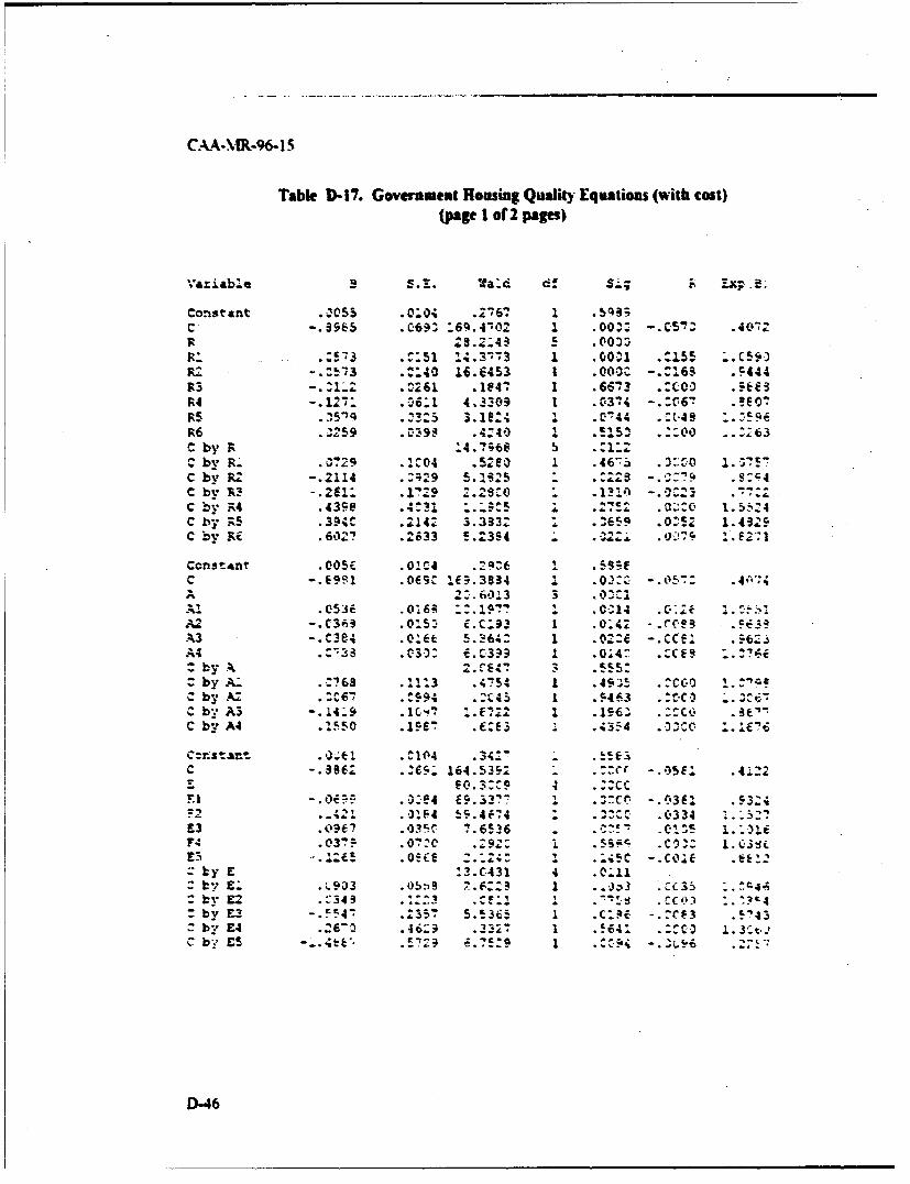
C.AA-R-96- 15

Table D-17. Government Housing Quality Equations (with cost)(page 1 of 2 pages)

Vaaiab e ... Sac c! -XR.. "

Constant .2055 .0c0; .2167 1 .53;C -. 9965 C~691 :69.4102 1 .00" -. C5,7: .40-12

28.2-4; 5 .003:.:!-13 C:51 !;.3173 1 .00-.1 ..155 :.(590

Z.:40 16.6453 1 .000, -. :169 *c444.3 -. =112 .•261 .1@41 1 .66-3 .:Coo ..6ea

R4 .6 4.3309 1 .0314 -. :067 .eEOl

R6 .2259 .•398 .4:40 1 .5152 .::e0 .. :23C by R :4.7;68 SC by RI .0?29 .1=04 .12e0 I .467 .3::010 :.!77C bV Rz -. 2114 .99 5.195 " .:zz5 -. SZ79 .8:,4C by R3 -. 261. .179 .280 " .lq -. 023 .=1.B

C bv F4 .4398 .4:31 1'?! : .2? .0 :C 1.5 4C by R5 .3C .2142 3.3332 1 .369 .O5 1.4329C by RE .6027 .2633 5.2394 l .- 21 .'JY• .8271

Ccnstant .005C .0ic4 .Z•6 1 .59C -. E91 .OM'C I.E.3534 I .0)c -. 0s7 .4,174A 2 .6013 3 .0 1AlbA .08 .13 :.495. I .44 .- C60 .A2 -,C341 .363: C.C93 1 .0:4: r.CS3 .

A3-.c3e-4 .016 5. 264: 1 .02, :6 -. Cc~elAn n.V39 .33: f . 31" .1 ;- .E9 I .Z

C by Aý 4 S 1 :O i

•2 by...:'68 .011: 5.4754 " .49J5 .C33 1. :'?

C by A2 tS9.12 .:ZC4 1 .546 .3CO. .3kC b- A3 -.14-9 .10C? .V 2 2 1 .156 -. coZC .3C"Cby A4. .1550 42567 . l43c4 .3- :.1

C:r.stjt .•41 .C104 .34- - . ."C -.36" .26'. 164.53S2 1 .. 4 .*36 1.24,

C by. 5 -,.b•'. •72 EQ.7 ' . .. 4 .,,' ' -. •C.,C

O.34 99.337 .0334 59!,E3 .07 '3 .6536 C. .i ns~ 1. I )F1I .03'!z 222.5 ~ .'3Z 1C~

Zby E 13.C431 4 O.OAC bv £. .02. 3 .05:)a 7.K I .. 3 .S: bv F- 424 ::. 2: .: CE) ý?,= by r-3 -.F!4- .:357 5.536; 1 .c:Re -.,C93 .5'43

2 y 4 .:6-0 .46-9 .3122 1 .!64. .::C-O 1. Kt,tC b.. ES -...4t9 .ý 9ý -6.7;9 .9 -G2

D-46

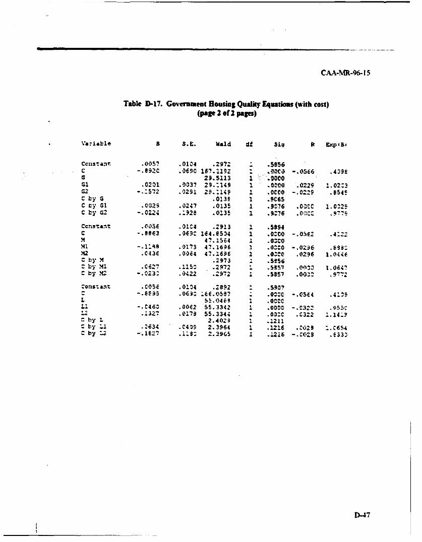
CAA-MR-96- I 5

Table D-17. Government Housing Quality Equations (with cost)(page 2 of 2 pages)

Va riable B S.E. Wald df Siq f E.p'Bt

Cc:istant .005? .0104 .29?2 .5656c -. e92c .0f90 167..192 1 ,a¢e -. 0566 .43;9G 29.5113 1 .00coGI .0201 .0037 29.:149 1 .00o .0229 1.02:3G2 -. :572 .0291 2?.:140 1 .OCcO -. 0225 .854!C by G .0138 1 .9CESC ty GI .0029 .0247 .0135 1 .9C?76 .003Cc 1.0,29C by G2 -. 022; .:92e .0135 1 .9:76 .0c .9779

Ccnstant .Cose .01C4 .2913 1 .554c -. BeE3 .069C 164.e534 1 .0:0 -. 0sE7 .4:22M 47.1564 .0:CO!1 -. 1.i8 .01?3 47.1696 1 .0=0 -. 0236 .6s9a.. C43A .00U4 47.?166 2 .0*0 .0296 1.0446C by x .2973 1 .5!56C by 41 .C627 .115C .2972 1 .5351 .0012 1.0647: by M. -. 023 .0422 .2972 1 &5357 .003 .9?2

Constant .c0se .0124 .2892 .5907-.8SS5 .063: ;66.059? OC -.CSC4 .4..-

L 5ý.0469 1 .OCCCLI -. C460 .0042 5S.3342 1 .000D -. C322 .955CT2 .i327 .0173 55.3344 i .03C .C322 1.1419C by L 2.40"; 1 .1211- by L1 .1634 .C419 2.3964 1 .1216 .C023 :.0654C by :.2 -. 1i27 .1. 2.3965 1 .1216 C. 02 e .633

D-47

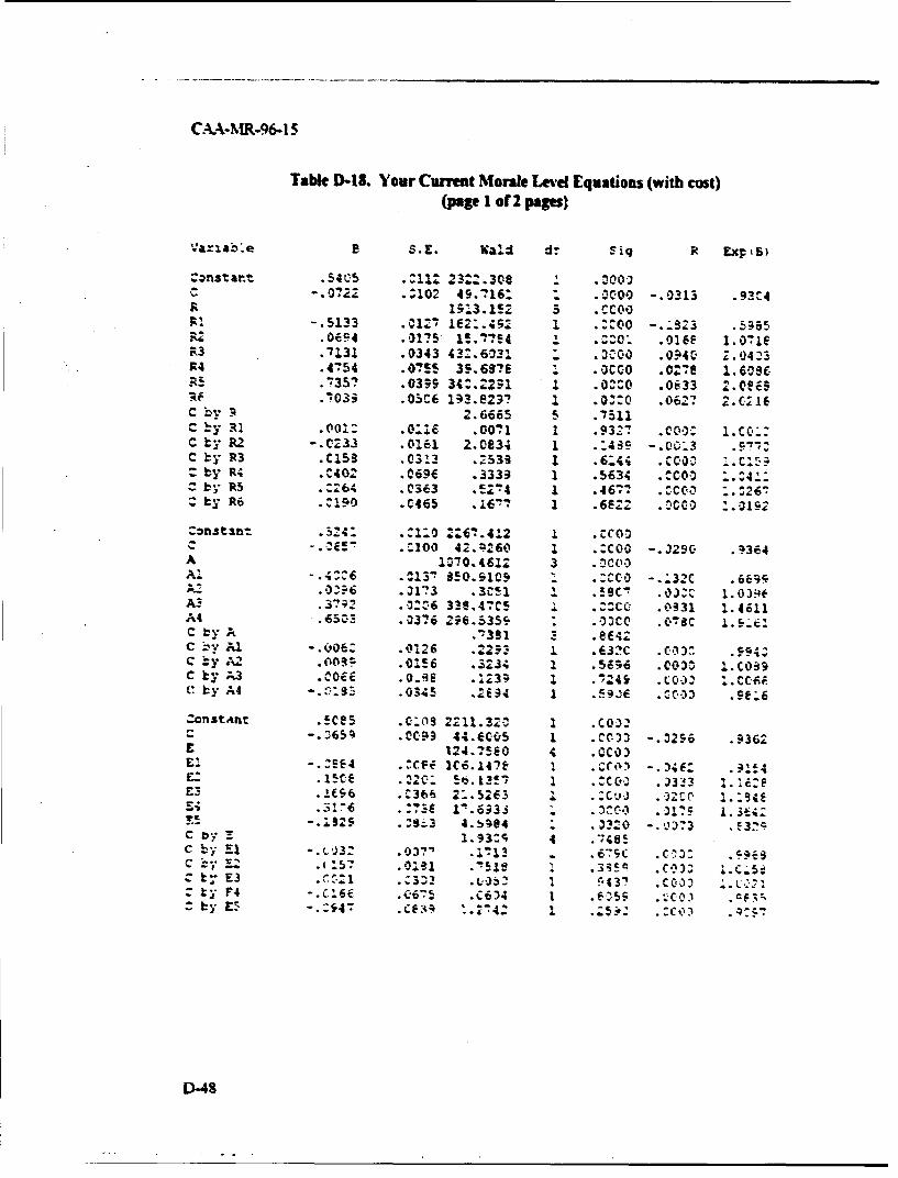
C.-A-MR-96-15

Table D-I1. Your Current Morale Level Equations (with cost)(page I of 2 pages)

Varable B S.E. Kald d Siq R ExUP5

Z:nstatt .5405 .:112 2322.308-072 .:102 49.716: 1 .0000 -. 0313 .93-43 193.152 S .CCO0

Al -. 5133 .0127 Ie2.1452 1 .:Coo -.-8:3 .595R2 .OE94 .0175 1!.??94 1 .20T .016F 1.0-LfR3 .7131 .0343 43:.6-331 L .;00 .0?40 2.042334 .4*54 .0*55 3.6S7'6 .OCCO .oU"e 1.6096

".7357 .0339 342.2251 1 .0^0 .0633 2.069s.03103 OC6 193.0413? 1 .N^1O .0627 2^.C16I

C v 1 2,6665 5 .7511c :y R1 .001: .01:6 .0071 1 .9327 .CMoo .cc,_:C ty R2 -. 0233 .0161 2.0034 1 .489 -. 00i3 .5:C by R3 .C15 .0313 -2533 1 .6144 .C0o0 2.C:5:= by R. .C402 ,069f .3339 1 .5634 ..IC0 " 411= by R5 .:264' .0363 .!2'4 1 .46-7 . CO! C . 260= by R6 .190 .0465 ,16 7 1 .6622 .- 000 -. 0152

zonstatt .524: .:1:0 267.412 1 .CCOO"C -•.200 42.;260 1 .:COO -. 3290 .ý364A 2070,461: 3 .OCQO

Al -. 13' 050.91, 9 : . CcO -. 132C .669S".. 6C173 !391 ! .59C .03:C 1.0)4(

A.0•6 330.47C5 .,:Cc .0331 1.4611A4 .6503 .0376 2O6.5359 .03C0 .0-8C 1.•1C by A .'391 3 .6642C ;y Al -. I006 .026 .2253 1. .e3!C .C03 .9942C by A2 .003I .0AI6 .3234 1 .5646 .C010 I.C099C t- A3 0 0Oi .0:-E .143; 1 L~4 .03 .ct6;b: by A4 -. 9Bs5 .0345 .,2 94 1 .5CO6 .1003 .se:6

.5¢s0 .0.09 2211.32Z 1 .C0.2C -. 0654 .O?93 44.6C, s 1 .CC33 -. 3256 .4362E 124.7'!0 4 .c03Ell -.:EE4 .106 CFIF i M iv -);IF: ill! 4E: .1509 .:20. 5d.13!7 1 .ZCoC .333 A. ,

1.1(6 .. 366 21.5263 1 .Cf.'j . 2ý) c .i4.317 6 .:7%f 1'. 6i3S 1 ^0I1 .017C 1. 3t4-:

FS-.i252 . 1S-.3 4.S8e4 )3 .30 -. )? F3.C S. 1.93:; ."4;5C by E1lL.3 .037" .1i%3 .675C .c' .ý*As;.U7 .01.1 .516 ,33 .C032 l.C.5•c k; E4 --. 1 .CE433 I .' .-C,-S .OWCCoo: ty F4 -. C.16e .407 634 I .6159 CFcK .

Z by V~ -. E-7 C3~ .4:57 2~2 .

D-48

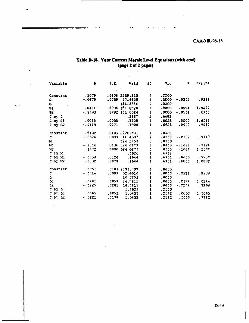
C.A-MR-96- 15

Table D-13. Your Currnt Morale Level Equations (with cost)(page 2 of 2 pages)

Va:iable S.E. ild df Sig R ExFUIB

Constant .5108 22C9.115 1 .C00C -. 0679 .0095 47.4609 1 OCCO -.03C5 .9344G 15C.3950 .0000

.046C .0036 151.6024 1 .0000 .0554 1.047732 -. 3593 .0292 151.6024 1 .0000 -. 0554 .639!by G .183? 1 .It2

Gy 01 .0015 .0035 .1909 1 .6(23 .0010 1.0015Cby G2 -. 0113 .71 .1909 1 .6f`3 0.0 1,C. .Q9S9

Cons:tat .5132 .010ý 2226.8;1 1 .0^00C -. C6066 .0059 4E.439? i .02CO - .03:1, .9347m 524.2753 " .000mi -. 3:14 .0136 524.6273 1 .00'O -. 1036 .1324.X: .1972 .0096 524.6273 1 .00I, .103f 1.2:9.:by X ..1626i 1 .AM6

C by M: -. 0045 .0124 .1644 1 .6985 .0071 .995CC by ?C .- 032 .0078 .1644 1 .695• .000 1.0032

Constant .5051 .0109 2103.797 1 .0030C-.:716 .0099 52.6010 1 .0003 -. :322 S30916I.6951 1 .0000

.241 .C059 16.7615 1 .0000 .C1T4 I.244

L2-.^.925 ..̂ 201 16.'16,5 1 OOD: -. ^14 .;)C by . 1.5625 1 .^..3C by L .065 .0052 1.,431 1 .2:42 .COO ".CO65C by ZL2 -. 3221 .:"s8 .5431 1 .2142 .!000 .•782

D-4Y

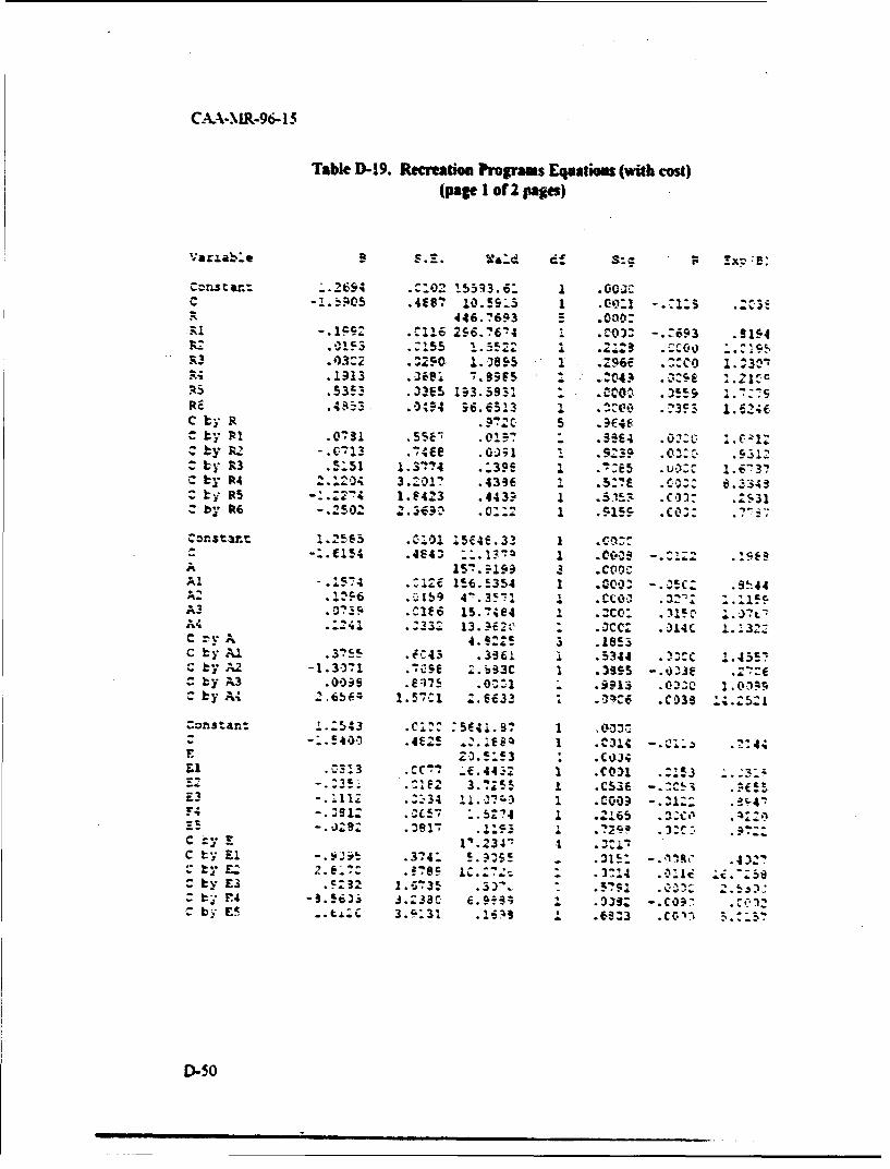
CAA-MR-96- 15

Table D-19. Recreation Programs Equatiom (with cost)

(page I of 2 pages)

varl.ab.e 3 S.E. vad C: - B

cznstarlt ý..2694 C '- 2 1-53I3.6.* 1 Go 77-c AES" 105- t C: -. ls C

A446.7653 5 .000:-. .11 26.64 I CQ): :.653 .9154

R3 .^.250 1 .8~ 31 Z96f :.^CO 1.ý30'7.1913 .39 7.99FS .200 Z-:5 2.21C.5353 .3365 1 93 .5932 1 .0 . a559 2 7

RE I-:-3 0494 M66513 I .- 7.3F3 L.626by kR &%;92 5 .4~E48~

Sby RI .0im" .5E .09 . 4 .0: i. C. Zby R -1 7.3 1 9Z .0.03 -C. .53i,

:L~ y 3 .5...51 1. 3"?4 .:356 1 .::E5 .L 3ZCC 1.6-37C by R4.~4 3.-0' . .4336 i :579 C.0 6.Z343

Ij R -9-?4 1.9423 .443ZR -3 .SMS' .c 1 .:531Zby &t6 -. 502o- 2369) :3 1 .515,c .co;:

Cnstint I .1.5 95 C .001 15C46.33 1 .Crl:-:.C15; .44 177 1 .0053 -.:i:2 .,se

A Q5 199 3 .ccOOAl ! 2 4 i 171 156.5354 1 .40C. -. ..1c sh44

6 .:.159 V! .3 F- I 3.C!O) .:Z :.159A3 079h .C1E6 15.74e4 I .2c02 .MC,~YtA4 .:,. 1 .133T 13. 31670 3C .~4 122C rvy A 4.2: 3 .153C ty Al .3?55ý I -.4 3 .3 61 1 5,144 .ý-c I.45sCC b YA2 -1.30'71 *iC5e Z.tý33C 1 .)995 -.O3~je .:-:C by A3 .00.;9 E411 5 .0:1 . .93 .0C 101

by A4 2 ~ 1. 57C,1 .66C33 I .E C039 45

4 .4 E2! Z29 ~1 -... .44

C1 .2213 .CC"7 .i.44-7 I C01 .%253 -

&- 3.-- 1 .CS36 -. :Cl53 .955E3 -. 1112 -Z34 :1.0?h 1 C.09.~ .2:-. 232 .25~25274 i 2165 3 Zc 0

C V'.234- 1C ty El j iit .374: 5995 - )i: IR .4021: by £22.9.k2 .5895 Lc.7~. .31,4 .0i E 2.

Z b-. N~ -3.56)., J.:38c f59z9 . .0)3s -. CO97 I:~b v~ ES t.LZ C 3.K.31 .16"9 .6S.23 CcM C '. i 5

D-50

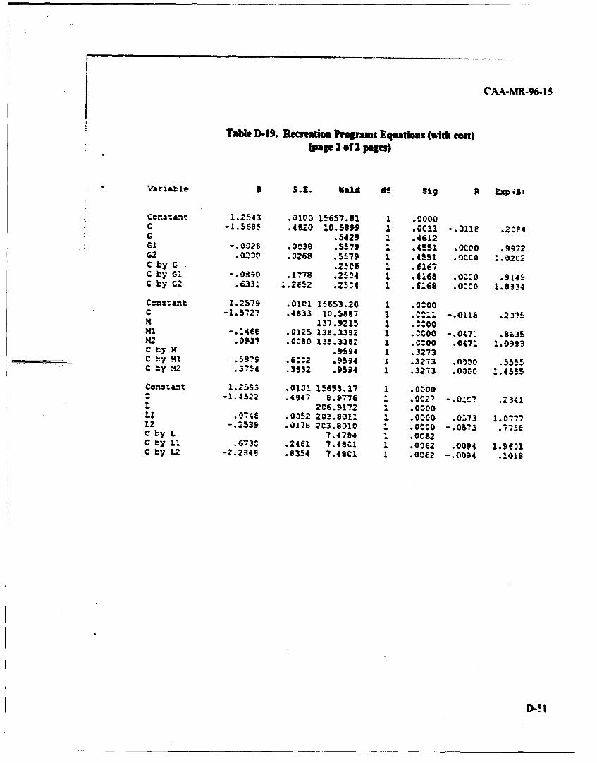
CAA-NR-96-. 15

Table D)-9. Rlecreation Pgram] Equations (with c•st)(pag 2 of2 pags)

Variable B S.E. Wald d! Sig R FxpeBI

Ccrns:an 1.2543 .0100 15657.81 1 .0000C -i.5695 .4820 10.5899 1 .CCII -. 0116 .2084G .5429 1 .4612GI -. 0026 .0038 .S579 1 .4051 .0000 .9972G2 .0230 .0268 .5579 1 .4051 .CCO '..02C2C by G .2506 1 .f167C by G1 -. 0890 .1778 .2504 1 .6168 .01:0 .9145C by G2 .633. :.2f52 .25C4 1 .6268 .01:0 1.8334

Constant 1.2579 .0101 15653.20 1 .0"0C -1.5727 .4833 10.5887 1 .c::: -. 0118 .2275m 137.9215 1 ."O00M1 -. *416 .0125 139.3392 1 .0000 -.04?: .8635M2 .0937 .0S0 13e.3382 1 .-000 .047: 1.0993C ty N .9594 1 .3273C hy M1 -.59?9 .6=2 .9594 1 .3273 .OO0D .555SC b,2 .3754 .3832 .9594 1 .3273 .0000 1.4555

Constant 1.23593 ,01t 15653.17 .00000 -1.4522 .4947 e.9776 .0027 -. 0•C? .2341L 2C6.9172 i .0000LI .0046 .0052 203.8011 1 .0000 .0ý73 1.0:7712 -. 2539 .0178 2U3.8010 1 .0CO -. 0573 .7756C by L 7.4784 1 .0C62C by Li .673' .2461 ?.43C1 1 .0062 .0034 1.9631C by ,2 -2.2349 .8354 7.48C1 1 .0^62 -. 0094 .1019

D-51

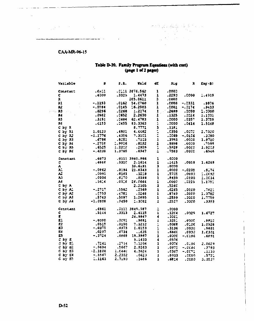
C.ALA-MR-96-1 5

TaMe D).20. Family Program Equation (wih cost)(piae I or2 pqs)

aa:.e E.g. fWald df 3:..g A ZxF )

Coracce: .?:: .. :^Z 3176.562 1 .000-C .4A00 .332i 1.4473 1 .2:93 .000 i.4=19R IS.0611 S .000A1 -. 1193 .0162 54.C760 1 . a000 -.- 331 .99?6R2 -. 0*94 .0145 :6.2903 1 .'001 Z.:174 .9433R3 .0296 .0268 1.2174 1 .2699 .i.0 .300R4 .0SE2 .C652 2.2630 1 .1325 .3:24 1.1:32R! .3191 .C404 62.4783 1 .0000 .035- 1.37*5RE .4153 .U455 e3.3363 -. D000 .0414 1.5148C by r 6.7??7 5 .1161C .y RI 1.0123 .4901 4.4462 " C350 .07: 2.352CC by R2 -1.1776 .4356 ?.31C1 : .:U69 -. 01:6 .3'90C by R3 .6796 .8CS1 .71"3 1 .3993 .^, O 1.9710C by R4 -. 275E :-916 .0192 1 .5998 .o0:0 .- 5e9C by R5 .6525 1.22.2 .295 5 .528 ,00cC. I1. 23c by? RE -.4238 1.3765 .04? 1 .7,563 .0 0 .6546

Co-'stant .6873 .0111 3960.996 1 .01c0= .4888 .331C 2.1614 1 .141s .0019 1.6269A 39.6191 3 .0-330A. -. 0L62 .0194 21.8343 1 .0000 -. C205 .974A2 C091 .0161 .32:3 I *57:5 .000 " 60CC4.A3 .0034 .0170 .0398 1 .0439 .CCOO I . C34A4 .16:4 .03:6 2E.0664 1 .COo. .Z225 1.15YC by A 2.2305 3 .52eCC by A: -. 271- .!582 .2369 1 .6265 .0a00 .7t2C by A2 .7?53 .4781 .4248 1 .8749 .3cc0 1.372C by Al .5?43 .5097 1.2695 1 .259 .3=C0 I.T759C by A4 -1.0906 .^450 :.3U62 1 .25:- .33C0 .33F3

Cctstant .6961 .Z11 364'.587 - .0000C .5144 .3313 2.4115 1 .12C4 .0129 1.61271 24.9947 4 .31Cc

£1-.005C. .3CS1 .9f91 .1 .32S.: .0003C .9p51V2 .051! .0190 7.3212 .00fe .0:10 1.0529E3 -. 0375 .0373 1.0153 Z .3136 .0031 .5631V4 .0297 .0734 .A635 I .686C .C03. I.C301E5 -. 3124 .08se 19.3997 1 .030C -. Cls6 .6F91C by E 5.1433 4 .0576= by r: .7241 ."714 7.1204 1 .007f .C04 2.062;C by F. -.51694 .!6V7 2 .92 3 1 .08%1 -. CCJ4 .3793C by E3 -2.1601 I.C44C 4.3624 1 . 367 -. CC'7 .1130C by V4 -. 5567 2.2352 .0623 1 .E033 .^C0ol .573C by E5 ".1163 2.7i9i .16E6 1 .68:4 .0003 3 03•

D-52

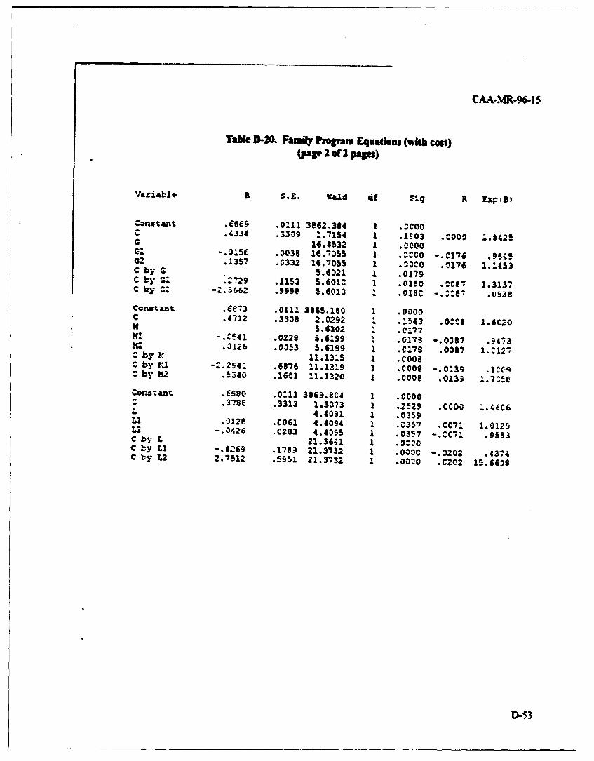
CAA-MR-96-1 5

Table D-20. Family Program Equations (with cost)(pae 2 of 2 pasa)

;aziaale S S.E. Vald af 3ig 1 1x15

Constant .Cecs .0111 3e62.304 1 .CCOOc .4334 .3309 :.7154 1 .103 .0002 1.5425G 16.8532 1 .0000GI -.0156 .0038 16.-355 1 .^C0O -. C1'6 .9945G2 .135? .0332 16. 055 1 .0:C0 .0176 1-:453C by G 5.6021 1 .0179C by G! .21*9 .1153 5.601C 1 .0180 .0CE7 1.3137C by GZ -Z.3662 .9998 5.6010 1 .0o8C -. :e' .0938

Constant .6873 .0111 3865.180 1 .0000C .4712 .3338 2.0292 1 .1543 .o0.e 1.6c20H 5.6302 . .C177H! -. C541 .0228 5.6199 .01"S -. 0397 .9473.0126 .03S3 5.6199 1 .C028 .009? 1.12 72 by V 11.13:S 1 .COOSc by r1 -2.294! .6876 11.1319 1 .COOS -.0:39 .1C09C b; .2 .5340 .1601 11.1320 1 .0008 .%,a; 1.7058

Cons:ant .6680 .0:11 3869.8C4 1 .0C00.378f .3313 1.3n73 1 .2529 .0000 ;..46C6

4.4031 1 .0359LI .012@ .C061 4.4094 1 .0357 .Cc-1 1.02291. -. 0426 .C203 4.4095 1 .0357 -.0C71 .9593C by Z. 21.3641 1 .0.^CCC by L1 -. 8V69 .1789 21.3732 1 .000C -. 0202 .43-4C by L2 2.7512 .5951 21.3732 1 .0020 .02C2 15.66;8

D-53

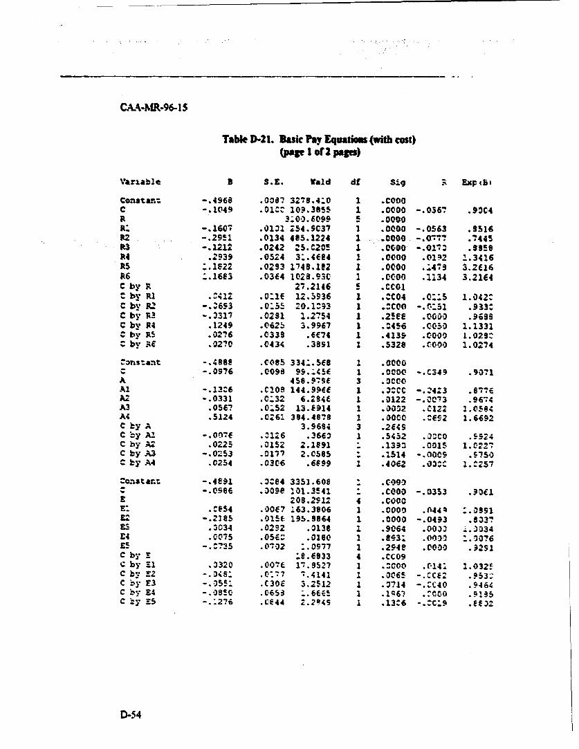
Table V-21. Basic Pay Equatios (with cost)(page i or2 pages)

Variable B S.E. Wald df S.g 9 ERpt5a

Constan: -. 4968 .0087 3278.4:0 1 .C000C -. 1049 .0100 109.3855 1 .0000 -. 0367 .93C4R 3;00.6099 5 .0000R: -. 1607 .0131 254.9C37 I .0000 -. 0563 .9516

S-.2951 .0134 485.1224 1 .A 000 -. 017? .7445R3 -. 1212 .0242 25.C20M 1 .0000 -. 017. .9958R4 .2939 .0524 3:.46e4 1 .0000 .0152 1.3416R5 ".I822 .0293 1748.182 1 .0000 .. 479 3.2616R6 ý.163 .03f4 1028.93C 1 .0I00 .2134 3.21M4C by R 2 .2146 5 .CCo0Z by R1 .^412 .0:1E 12.5936 1 .0C04 .0::5 1.042CC by R2 -.0693 .0:55 20.1093 1 .:COO -. r:51 .933^C by R3 -. 3317 .0291 1.2754 1 .2SEE .0000 .9699C by R4 .1249 .0625 3.9967 1 .2456 .0050 1.1331C by R5 .0276 .0339 .EC74 1 .4139 .0000 1.029:C by RE .02?0 .0434 .3891 1 .5328 .000 1.0274

-Onstant -. 488F .C085 334:.5E8 1 .0000-. 0976 .0098 99..456 1 .0000 -. C349 .9071

A 458.979E 3 .0000Al -. 13C6 .CI0P 144.996E 1 .30CC -. N423 .876EA2 -. 0331 .C;32 6.2946 1 .0122 -.OC73 .9674A3 .0567 .0152 13.6914 I .0002 .C122 1.05984A4 .5124 . 261 384.4878 1 .0000 .CI62 1.6692C by A 3.9684 3 .2649C *y A1 -. 00n7 .3126 .3662 1 .5452 .XCo .9924C by A2 .0225 .0152 2.1891 : .1393 .0015 1.022"C by A3 -. 0253 .0177 2.0585 1 .1514 -. 0005 .575;C by A4 .0254 .0306 .6699 1 .4062 .000 1.C257

-oistar.: -. 4691 .30e4 3351.608 : .CM3JC -. 0see .309P 201.3541 X .C000 -. 0353 .30f1E08.2512 4 .C00OEl .C854 .007 163.3906 1 .0000 .0444 :.3991£2 -. 2185 .015C 195.9864 1 .0000 -. 0433 .8337z3: .3034 .0292 .013e 1 .9064 .0033 .. 3034£4 .0075 .0536 .0180 1 .893: .00-3 .•.076£5 -. 0735 .0702 ".0977 1 .2945 .0000 .9291C by ME e.ee33 4 .oC09C by £1 .3320 .0076 1i.9527 1 ._000 .. 14: 1.032!C b s2 _-.Us: .0-77 -. 4141 1 .0065 -. CCe^ .9533C by £3 -. 055. .C306 3.2512 1 .3714 -._C40 .9464C byE4 -. 0850 .0653 .6665 1 .15V .:!Coo .9i95C :Y =S -.- 276 .CE44 2.2R49 1 .13.6 -. :C:9 .E32

D-54

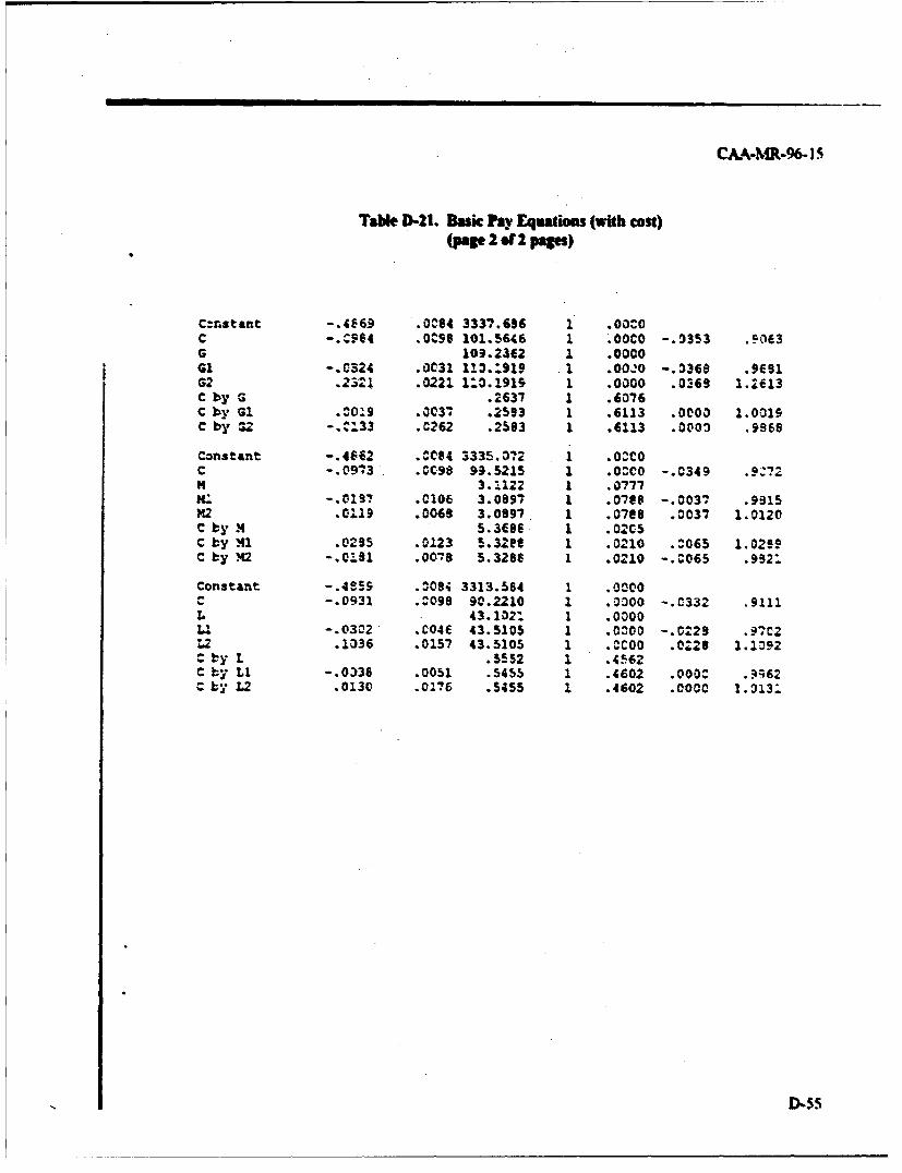
CAA-MR-96-15

Table D-21. Basic Pay Equations (with cost)(page 2 o 2 pages)

Cznstant -. 4E69 .0064 3337.696 1 .00.0C -. ^964 .0C98 101.5646 1 .OOCO -. 0353 .9063G 109.23f2 1 .0000G1 -. C324 .0031 113.:919 1 .00.0 -. 3369 .9691G2 .2321 .0221 1:0.1919 1 .0000 .0369 1.2613C by G .2637 1 .6076C by G1 .2019 .0037 .2593 1 .6113 .0000 1.0019C by 312 -. C133 .0262 .2593 1 .6113 .0003 .9868

Constant -. 4662 .0084 3335.072 1 .0O0C -. 0903 .098 99.5215 1 .O^CO -. 0349 .9272m 3.'122 1 .0777X: -. 0197 .0106 3.0897 1 .07e8 -. 0037 .9315

S.01 9 .0068 3.0897 . 1 .07e8 .0037 1.0120C by X 5.3086 1 .02C5C by Ml .0295 .0123 5.32ee 1 .0210 .M065 1.02e9C by . -.by 42 .0078 5.3286 1 .0210 -. C065 .9921

Constant -. 4059 .00894 3313.584 1 .0000C -. 0931 .0099 90.2210 1 .0000 -. C332 .9111L 43.1021 1 .00001.l -. 0302 .C04E 43.5105 1 .0300 -. 0228 .97C2L2 .1036 .0157 43.5105 1 .0000 .0:28 1.1092C by L .5552 1 .4562C by Li -. 0336 .0051 .5455 1 .4602 .000C .R62C by 2 .0130 .0176 .5455 1 .4602 .0000 1.313.

D-s5

CAA.NIR.96- IS

APPMEND E

REFEENICES

1. Edgizgton. Eugen S.. anoiain Murce Dekker, New York, 1987

2. HonDvdW WLmsoS.W e 9ikUMk onWly oNew York, 1989

3. Nowsis, Marija J, SPSS forUN1M. Adxwm dStafReleas e m5. SPSS. Inc.,

Chicago. 1993

4. Schefft. Henry. The Amblysi Of VurIance. John Wiky & Sons. New York. 19319

S. Searle, Shayie S., Linea hiodell for Unbalanc Data John Wiey & Sons, New York,1987

6. 2S SW 2d Ed., SPSS Inc..Chag

CAA-MR-96- 15

APPENDIX F

DISTRIBUTIlON

Addressee No of cpe

Deputy Chief of Staff forInstallation Manasemnt 2

Headquarters, Department of the .A"y600 Anm., PentagonATTN: bAIM-RWashington, DC 20310-0600

DirectorLS Army Cost and Economic Analysis CaterATTN: SFFM.CA-FI5611 Columbia PikeFalls Church, VA 22041

DirectorUS Army Research Institute for Beha'ioral

and Social SciencesATTN: PER1-RZD5001 Eisenhow•w AmueAlexandria, VA 223335%00

Defense Technical Information Center 2ATTN: BCP Product Management Branch8725 John L Kingman Road, STE 0944Fort Belvoir, VA 22-60-6218

Internal Distributon:

Reference celp.Uncasified Libry 2

Record copy:Originating office (CSCA-RA) 17

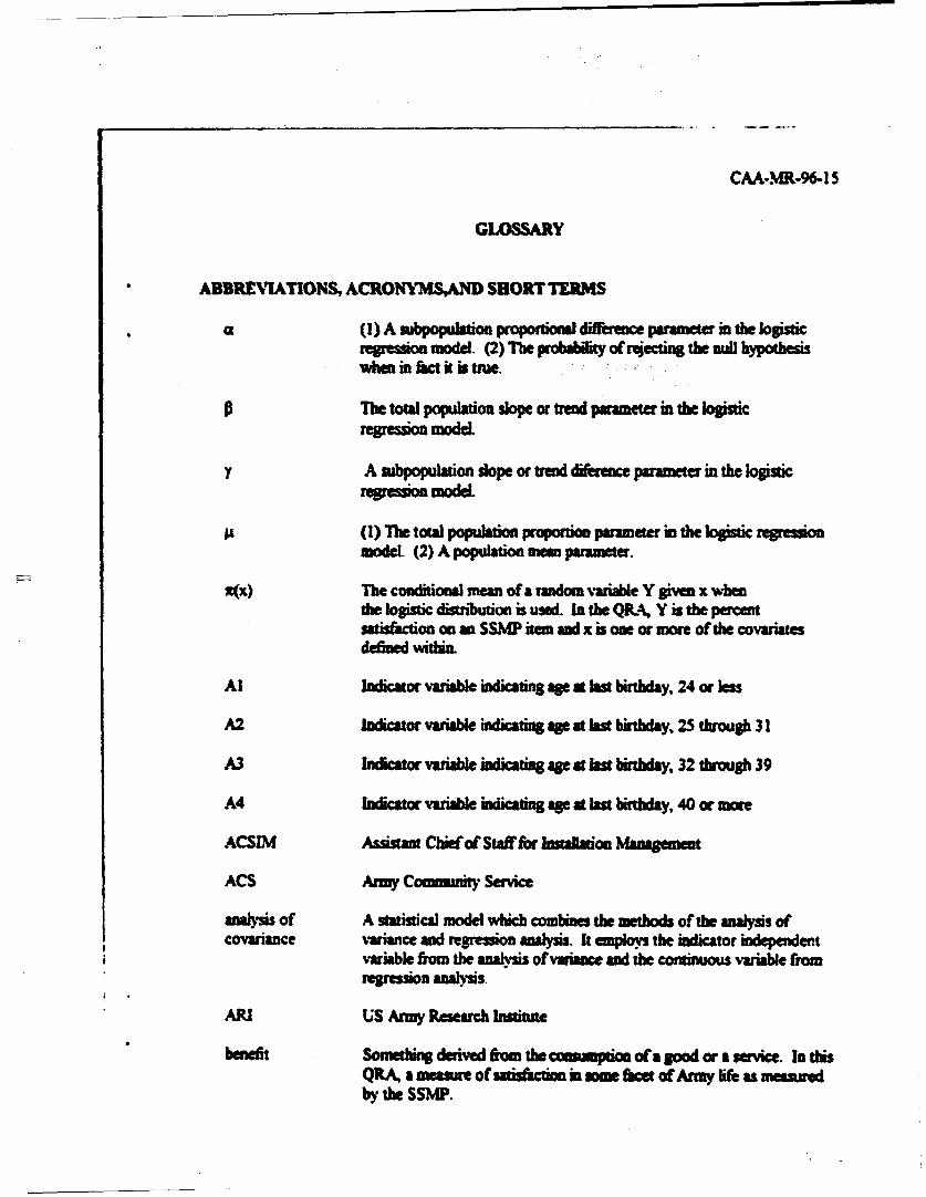
CAA-MR.96-15

GLOSSARY

ABBREVIATIONS, ACRONkMS,AND SHORT TERMS

a (I) A proportional derence parameter m the logisticrerssin model- (2) rTe pvbai ofreecting, the n hypotimsiswhe in fact it is rae.

p The toal population sdope or ftend panameter m the logistic- modd

y A sbpopumlaion slope or trend difewe parameter in the logistic- isnmode

(1) The total population proportion parameter in the logistic re imodel. (2) A population et- paameter.

z(x) The conditional mean of a rnmdom -ariable Y given x whenthe logistic distuibution is used. In the QRA- Y is the percetsatisfaction on an SS.UP itm ad x is one or more of the covariatsdeined Within.

Al Indicator variable indicating age at last birthday, 24 or less

A2 Indicazor variable indicating age at last bithday, 23 through 31

A3 Indicator variable indicating age at last birthday, 32 through 39

A4 Indicator varible indcating age at las birbday, 40 or more

ACSIM Assist Chief of Staff for Istallation Mangement

ACS Army Commnit Svice

=anayis of A statistical model which combines the methods of the analysis ofcovariance variance and regression analysis. It employs the indicator independent

variable from the analysis ofvmace mad the omuous variable fromrmes-son a•ly.sis.

ARI US Army Resrhm Insdite

benefit Somethin derived fiom the comuoption ofa good or a sevice hn thisQRA, a mawre of satisation in sme hm of Army lif as miearadby the SSMP.

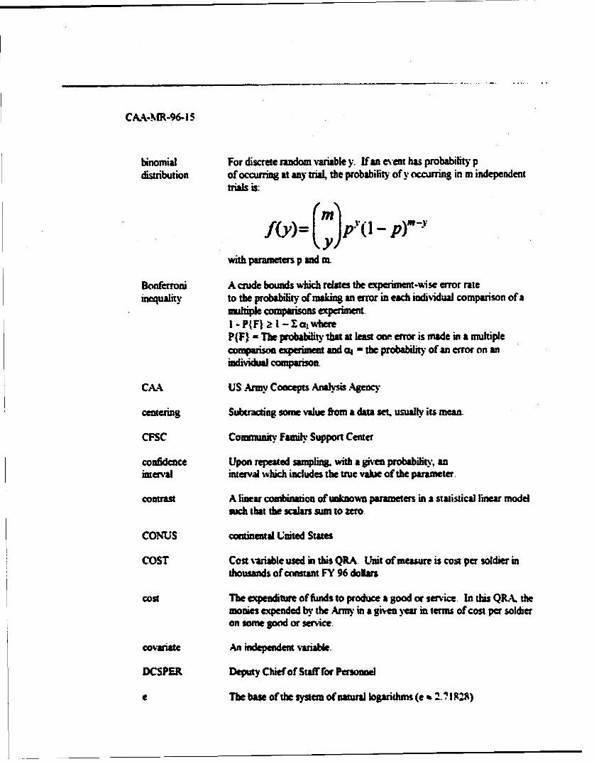
CAA-.MR-96- IS

binomial For discrete random variable y. If an event has probability pdistribution of occurring at any trial, the probability of y occurring mm independent

trials is:

f(Y)t Ri%.(0 - P) M-Y

with parameters p and sm

Bonferroni A crude bounds which relates the experiment-.ise error rateinequality to the probability of making an earo in each individual comparison of a

mulle comparisons experimentI -PMF} Z I - ZawhereP(F) - The probability that at least one error is made in a multiplecopaparisonexperiment and ck - the probability of an error on anindiial comprson

CAA US Army Concepts Analysis Agency

centering Subtracting some value from a data set, usually its mean.

CFSC Comax.nity Fami.. Support Center

confidence Upon repeated sampling, with a perobailit, aninterval interval which includes the true vawe of the parameter,

contrast A linear combinaion of unknown parameters in a statistical linear modelRich that the scalars sum to zero.

CONUS continental United States

COST Cost ariable used in this QRA. Unit of measure is cos per soldier inthousands of constant FY 96 dollars

cost The expenditure of funds to produce a good or sevice. In this QRA. themonies expended by the Army in a given )ear in terms of cosg per soldieron some good or service.

covariate An independent vaiable.

DCSPER Deputy Chief of Staff ror Personnel

e The base of the system of natural logarithms (e • 2. ? 129)

CAA-MR-96-1I

El Indicator variabl indicating white etdmiity

E2 Indiator vaiabl idicat black eftiy

E3 In"Mto variab ildiAký KiqianiC ethniCity

E4 Indicator vxiale indicatin Asian or Pacifc Islander ethnicity

ES Indicator vawiable indc American Indian, Eskimo or Aleut ethnicity

.erimit-wse The probabil of Ulsely rejecting one indidual compaison in aenrreor n multiple coMprison eriml

FAM SS Item which afst "Bsued on )yr ArM, oepence, bow sarisfiedor dissatisfied = you with the quliw y o(Anmy family proganms?"

FY fiscal year

GI Indicator vaial indicating male gander

G2 Indicator %vil indica fmule guder

HA SSMIt hem which asks "Based on your Amy vexp e, bow satsfiedor disstised ame you with the vailabiitty of goveanwit housing?"

GHQ SSMP haem utich asks, "Bnsed on your Army xpmunce how satisfiedor dissatisfied ae you with the quality ofgovaumaw houi•g"

group variable A vector coasact used a statistical watyds to tepret the cate=orS.mI I I lip of a single obseration For eam*le, guider has twocategoies (i.e., nale ad rkae). Iola Sith participated in thesamplv, he would be coded as autale by the two deemn vecor (1,0) andMary Doe would be coded as a feal, with the vector (0, 1).

hyiothesis A stadstc hyposbesis is a ypothess the parameters of aprobability distribution. The statstical h tesis under test is referredto as tie nul bypothesis An 1•am eo c specifies somevales) fr" the parameters diffm fm tose under test.

independent (I) Random variables e sta cally epd i their joint probabilitydeit, fn on =be P u q1w bthe rc of norgative f• tionsWe-" of the fMnOm vba es alonm ()A et otvectors is said to beliearly depedem if the eCs scalm nt anl aO snch that their finestconIbtiMoMaseal to Me. Ifthim dons not aem such a set, then thevectors a Vindepe

CA.A-MR-96-15

indicator vaable One elemnt of a group variable which takes on values 0 or 1. It corre-sponds to one of a finite umber of usually mutually exclusive andexhaustive categories io which a group variable can be divided. Forexample, the group ariable gender can be divided into two categories(Le., male and female). In this QRA, the indicato variable G I corre-spondstothecategoymale. IfGi takes anthe value in a panicularinstance, it may be rerring to (1) a male responden in the survey, or (2)the ubpopulaio of males whem substituted into a logistic regessonmodel. Whe the respondent is not a male or we are referring to theferule subpopulatio in a logistic regression mode, the value of G I is 0.

interacton A combined effet of two individual factors which is different from thesurm of their separate ectsc

L1 Indicator variable indicating CONUS duty stion

L2 Indica variable indicating OCONUS duty station

kCM-age In linear regresio., a point in the space of the independent variableswhich is far ftrm the rest the data. Such a point wll have a stronginfluec on eitimation of parameters.

likelihood flrnction Associated with each random variable X, them is a probability fictonP(xO where C represents the known parameers of the probabiltflmction. Given a fixed set ofobservations for a random variable, then itis appropriate to contemplate the various values of which pvc rise tothis set. The likelihood function 14JX) has the samu form a P(X14, butnow X is fxed and k is unniown.

linear regression A model ofthe random variable Y whose conditional expctation, E(Y,. - IP ,Px, Y, - 6 +Ai,x + % with e, assumed to be independemn and

identically normally distributed Aith mean zero and unknown variance a&.The unknown paramer are k, 0. and o:. The x is a fixed covriate.The parameters ., Pl, ard e are usually obtained by maximizing thelikelihood fucton which is equivalent to obtaining least squareses•mes of the paramneter

logistic A model of a discrete random variable Y which takes two valuesrepesuon (i.c, 0 and I). The conditional mean of Y give a set of covanates is

bounde by znro and one. The arr" distribution is assumed to bebinomial.

koit The natural logarithm ofthe odds ratio.

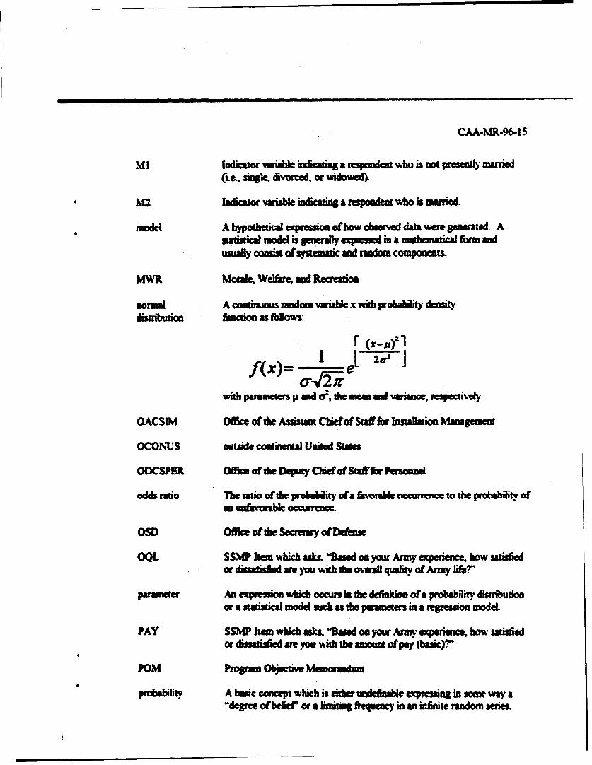
CAAA-•R-96-l 5

MI Indicator varible indicati a respondent who is not presently married(Le.. single. divorced, or wridowed).

M2 ~Indicator vuaribe indicating a respondeut Who is married.

model A hypothetical expression of how obsrved data were generated Asatistical model is Seneraly expssed in a mothematical form andusit consm of systemanc and random componets.

MUR Morale, Welfre, and Recreation

normal A condtxis random vaab x with probability densitydisulbutio. lacic as follows:

r (x-p)l

f(x)= ]

-;7N2rwith paameters p and a, the mean and variance, respecdvely.

OACSIM Offce of the Assistant Cliefof Saff for Installao Management

OCONUS outside coMninmm United Sa/

ODCSPER Office of the Deputy Chief of Staff for Personne

odds ratio The rat of the probabity ofa fvorable cuwremc, to the probability ofan umfavorb" ocowren.

DOffiv of the Smery o(fse

OQL SS.~W htem which ask&. -Bid on your Armi experence, how satisfiedor dimitsfied arm you wth the oma qualiy of Army lit?

paamer An eression which occus in the defmlkiio of a probabity disibutionor a statixtical model mach as ft paameters in a reesion model.

PAY SSMP Item which asks, "Based on your Armny expenence, bm, satisfiedor dissatifed are you with the amourn ofpay (basic)'"

POM Progrm Objectw M du

probability A btsic concept which is either w ah expessing in v m some way a"degree of beief or a limiting frequency in an infitite random siese

CAA-NfR-9& 15

QOL "sakiy of life

QRA quick reaction anaysi

QUALMAN QUafiqs of L&f Measuawmea and Azw~si

RI Indcaor variable incating ranks PVZ- through SPCICPL

R2 Indicator variabl Wnicatin ranks SGT through SSG

R3 Indicato variable indcatng ranks SFC-SGMICSM

R4 Indicatormuribloidicatn aft arravofficier ranks

RS Indcator maiable Wnicating ranks 2LT through CPT

R6 Indicator varibl indictn ranks MAI and above

random variable A quantity which may take any of the value of a spacihe set with a

REC SSUP ban which a"ks -Sued on your Army eacereneam how satsfiedor dwsatisfed am you with the recreational sernices? t

respoons A depeknda vaiab

rstriction An equaton expminig ome parameter as a howea combination of the.nin paramtters. Resrrictions are used in overperametri

systin of equaticas (i.e., snem3 with mome unknownsthan equations)to ob tain a sokation Restrictions may be. thought of as equality

sampl space The set of sample points corr esponding to AD possibe samples

SIDPE.R Standard lmmstalatow'ison Personne System

SPSS Statistica Pac~kag for the Social Scmmnes

SMe Suiple survey of Militay Personnel

CAA-MR.-96- 15

SSMP tern (~e of the 10 *Msuos hoe by this QRA as pertamag to Army*ufty ofre lism=r The riustioa seet mi be= askd sm the samfam a the sixaraia oftbe SSM? (Sprig, 1992 to Fai 1994)ausd in tis QRA. ft the swvey. (wr leves of sakeiscton (i e. xwysatids& satisied.&sA iuind very 6ssm~iAW) we und Thenerespome vm colapud ito ihe categones sotded aid dim=AWe fbrthisQRA.

SSN sca iuyime

gandad A ==Ima probabiliy distb~utio of ra ndom vwimblc zaorml dimtuibuio with p - 0 #d 1.

TEWE Ome of sk cosecazzve admi-stratioms otbe SShW ~usedfbrthis QRA(iLe. TIME -I comspomds to Spring 1992. tlwjou TME 6corresponds to FaA 1994).

USACEAC LIS Amy Cost and Econousc Analya Carna

USAREUR ULS Army Europe

V'HA (1) Veweas Hoausig Aflowwuce. (2) SSMP Item which &Ass, TMRasi onyour Army excpman how satisfid or dismifid ame you with thesmourn of VHAICOLA"P

YCM SSWP urn which adks, lThw womid you rme M awrrm leve ofmtorae* POSIWle respoma wee very bilk hWgh moderato. kr*. orvery low. For the purpom c~d ts QRA, very Lh md hih wercollapsed into a WOg clegory, low. sod very low ino a low cegory,and the wmodrte response was omtted

QUALITY OF LIFE MEASUREMENT AND ANALYSIS ... - DTIC

Documents

Transcript of QUALITY OF LIFE MEASUREMENT AND ANALYSIS ... - DTIC