Proposed methods for finding the basic acceptable solution for ...

Iraqi Journal of Statistical Science (30) 2019

pp[73-84]

Proposed methods for finding the basic acceptable solution for the

transportation problems

Asmaa Salah Alddin Sulaiman*

[email protected]

Abstract

The data tend to be centered around a certain value that can be called a

central value. In this case, the measures of central tendency are the function

used to recognize this central value to represent the data. In some cases, the

data are closing to the central value and sometimes more widespread. In

order to measure the proximity or distance of data from that central value,

measures of dispersion are used. In this research, some of these measures

are used to find the basic acceptable solution for transportation problems.

Better results are obtained by the researcher through using these measures

by taking five applications with different capacities.

Keyword: Transportation problems, Northwest-corner method, Least-cost

method , Vogel approximation method, Measures of central tendency,

Measures of dispersion.

This is an open access article under the CC BY 4.0 license

http://creativecommons.org/licenses/by/4.0/).

طرائق مقترحة إليجاد الحل األساسي المقبول لمشاكل النقل الممخص:

مركزية. في هذه الحالة ، القيمة القيمة معينة يمكن تسميتها ب حولز ركمتميل البيانات إلى الت المستخدمة لمتعرف عمى هذه القيمة المركزية لتمثيل الدالةهي ةالمركزي النزعةتكون مقاييس و

من و في بعض الحاالت تكون البيانات قريبة من القيمة المركزية وأحياًنا أكثر انتشاًرا. و البيانات. بين البيانات من تمك القيمة المركزية ، تم استخدام مقاييس التشتت. البعدقرب أو أجل قياس ال

المقبول لمشاكل النقل. األساسي إليجاد الحل المقاييساستخدام بعض هذه ، في هذا البحث تم مختمفة. بسعاتخمسة تطبيقات بأخذ المقاييسحصل الباحث عمى نتائج أفضل باستخدام هذه و

* Assistant Lecturer / Department of Mathematics / College of Basic Education / University of Telafer.

Received data 10/4/2019 Accepted data 9/6/2019 Published data 1 /21/ 2019

mailto:[email protected]

]47Iraqi Journal of Statistical Science (30) 2019 [

1. Introduction

The main problem “managers directed is how to allocate limited

resources among various activities or projects. Linear programming ( LP),

is a method of allocating sources ideally. One of the most widely used

operation research tools was decision making that helps can in almost every

manufacturing industry, in financial and service organizations. In linear

expression programming, programming refers to mathematical

programming. In this context, it refers to a process planning that allocates

resources - work, materials, machinery, capital - probably the best way to

reduce cost or to increase profits”. In LP, these sources are known as

resolution variables. Standard for selecting the best values of decision

variables (e.g., to increase profits or reduce costs), known as the objective

function. Restrictions in the form of source availability are known as

constraints. The linear word refers to that standard to select the best values

of decision variables which can be by describing a linear function of these

variables; this is a mathematical function that includes only the first powers

of variables without cross-products.

Transport problems are one of the most important and successful

applications of quantification analysis of business problems that was solved

in the physical distribution of products.

“As their purpose is to reduce the cost of shipping goods from one

location to another so that the needs of each arrival area is met and all

shipping location works within their capacity. However, quantitative

analysis has been used for many problems other than the physical

distribution of goods. for example, it was used to place employees

efficiently in some jobs within the organization”. (this application is

sometimes called assignment problem)[Reeb and Leavengood,2002]. It is

said that the transportation problem is balanced if the quantification of all

sources equals quantitative demand in all places and the so-called

imbalance in other cases[Taghrid,2009]. “The structure of the transport

problem allows us to solve it with a faster , more economical algorithm

than simplex. Problems of this kind contain thousands of variables and

constraints and can be solved in a few seconds on the computer. In fact, we

can solve a relatively large transportation problem by hand. There are some

requirements to place an LP problem in Transport problem class” [Reeb

and Leavengood,2002].

The basic “transport problem was originally developed by Hitchcock

Transport problems can be designed as standard linear programming

problem. The problem can be solved by the Simplex method. Several

heuristic techniques are available to obtain a basic initial solution, although


some heuristics can find a preliminary solution very quickly, and often the

solution you find is not very good in terms of total cost and small size. On

the other hand, some heuristics may not find a first solution quickly, but the

solution you find is often very good in terms of reducing total cost. There

are specialized algorithms for the transport problem which are more

efficient than the simple algorithm”. The best known heuristics methods are

the North west corner, Best cell method and the Vogel approximate method

[Samuel and Venkatachalapathy,2013].

2. Related Works

In 2002, AL-Sabawi and Hayawi presented a new proposal to solve the

transport model using a new method different from the previous known

methods by taking the differences between the largest cost and the lowest

cost of the transport model. They compared their method with Vogel

approximate.

The research presented by Reeb and Leavengoode in 2002 put the

problem of moving in the form of ordinary linear programming and then

solved it using the computer using Lindo program. This program solves the

problem of transport faster than the manual solution using the Simplex

method, especially if the transport problem is large. The research also

included clarifying the phenomenon of 'degeneracy' which occurs when the

number of squares occupied is not equal to the number of rows + the

number of columns -1(Sources + Destinations – 1). The researchers also

explained that the methods of solving transport problems such as the North-

West corner method and the approximate Vogel method can be used to

solve problems other than the transport problem such as the assignment

problem. In 2007, AL-Badri and Saleh reviewed the proposed new method,

which is the average method for improving, developing and evaluating the

acceptable basic solution compared with the Vogel method. The first basic

solution to the transport problem obtained from the proposed methods gave

less cost compared with the approximate Vogel method. Thus, indicating

the efficiency and possibility of this method to realize the basic solution

and therefore the best solution will not be difficult and complex.

Abdul Quddoos et al. in 2012 proposed a new method to solve the

problem of transport. The ASM method, to find the best solution for a wide

range of transport problems. This method is easy to understand and apply

even by the layman. It is also a profitable way for decision makers who

deal with restricted problems, This method gives the ideal solution as soon

as possible. Moreover, a proposed Samuel and Venkatachalapathy method

in 2013, to improve Zero Point method for finding an optimal solution

using function principle in which transportation costs are represented as

triangular fuzzy number. The methodology of “Improved Zero Point


Method (IZPM) is a simple and efficient method that is better than the

existing methods, easy to understand and can also give an optimal

solution”.

3. Transportation problems

The transportation problem is a special case of linear programming

problems. It is easy to formulate the linear programming model in its initial

and binary form after it is arranged in a format matrix, and it follows that:

m: Represents the number of sources which is S1,S2,…,Sm with capacity

supply and it is a1, a2,…, am .

n: Represents the number of destinations which is D1,D2,…,Dn with a

capacity demand and it is b1, b2,..., bn . Cij: Represents the cost of moving one unit from the source (i) to

destination (j) .

Xij: Represents the quantity or number of units to be transferred from the

source (i) to destination (j) , and that the linear programming model in its

initial form of transport problem is as follows:

∑ ∑

s.t. ∑

∑

Before the start of an acceptable basic solution and in any way the model

should have been balanced by equal or equivalent to the total required

quantities with the total quantities offered, and mathematically expressed

∑

∑

When the quantities required are greater than the quantities offered this

means that

∑

∑

Add to the decision-making matrix (transport matrix) Dummy Source ,it

works on processing the quantity in which the deficit amount is as follows:


∑

∑

Note that the cost of the Dummy source is zero and when the

quantities required are smaller than the quantities offered this means that

∑ ∑

Add to the decision-making matrix (transport matrix) Dummy Destination,

It works on processing the quantity in which the deficit amount is as

follows:

∑

∑

Note that the cost of the Dummy Destination is zero and to find

the basic solution acceptable to the transport model. There are several

different methods in terms of time and effort required to reach the initial

solution. Three most commonly used methods to obtain an acceptable basic

solution are:

1) Northwest-corner method:

This is one of the easiest ways to go, since you do not take into

account costs using any scientific logic in the distribution process

(distribution of available quantities)

2) Least-cost method:

This is a better way than the previous one, considering the cost

of transportation from the source to the center

3) Vogel's approximation method [Hamdy,2011] [Taghrid,2009].

4. Proposed Methods The methods proposed by the researcher are simple to implement

and can also be the basic solution to the problem of balance

Transportation:

1) Harmonic mean method: The following are the basic steps for

this method:

a) Calculate the harmonic mean of the costs in each row and

column according to the following equation:

∑


b) Determine the highest harmonic mean in all rows and columns

and then choose the cell containing the least cost to give the

appropriate amount of available (supply) to meet the needs

(demand).

c) Delete the row that ran out of the supply or column that was

filled in the demand so as not to enter into the harmonic mean

again.

d) Repeat steps (a-c), then calculate the total cost.

2) Quadratic mean method:

a) Calculate the Quadratic mean of the costs in each row and


√∑

b) Determine the highest Quadratic mean in all rows and

columns and then choose the cell containing the least cost to give

the appropriate amount of available (supply) to meet the needs

(demand).


filled in the demand so as not to enter into the Quadratic mean

again.


3) Median method:

a) Calculation of the median of the costs in each row and column

by ascending order ( or descending),

If the number of costs is even, the median represents the

arithmetic mean of the two values in order

and

, but if

the number of costs is odd, the median represents the value of

order

.

b) Determine the highest median in all rows and columns and

then choose the cell containing the least cost to give the


(demand).


filled in the demand so as not to enter into the median again.


4) Mean deviation method:

a) Calculate the Mean deviation of the costs in each row and



∑ | |

b) Determine the highest Mean deviation in all rows and

columns , and then choose the cell containing the least cost to

give the appropriate amount of available (supply) to meet the

needs (demand).


filled in the demand so as not to enter into the Mean

deviation again.


5) Coefficient of variation method:

a) Calculate the Coefficient of variation of the costs in each

row and column according to the following equation:

b) Determine the highest Coefficient of variation in all rows and

columns , and then choose the cell containing the least cost to

give the appropriate amount of available (supply) to meet the

needs (demand).


filled in the demand so as not to enter into the Coefficient of

variation again.


6) Mid-Range method:

a) Calculate the Mid-Range of the costs in each row and


b) Determine the highest Mid-Range in all rows and columns ,

and then choose the cell containing the least cost to give the


(demand).


filled in the demand so as not to enter into the Mid-Range

again.



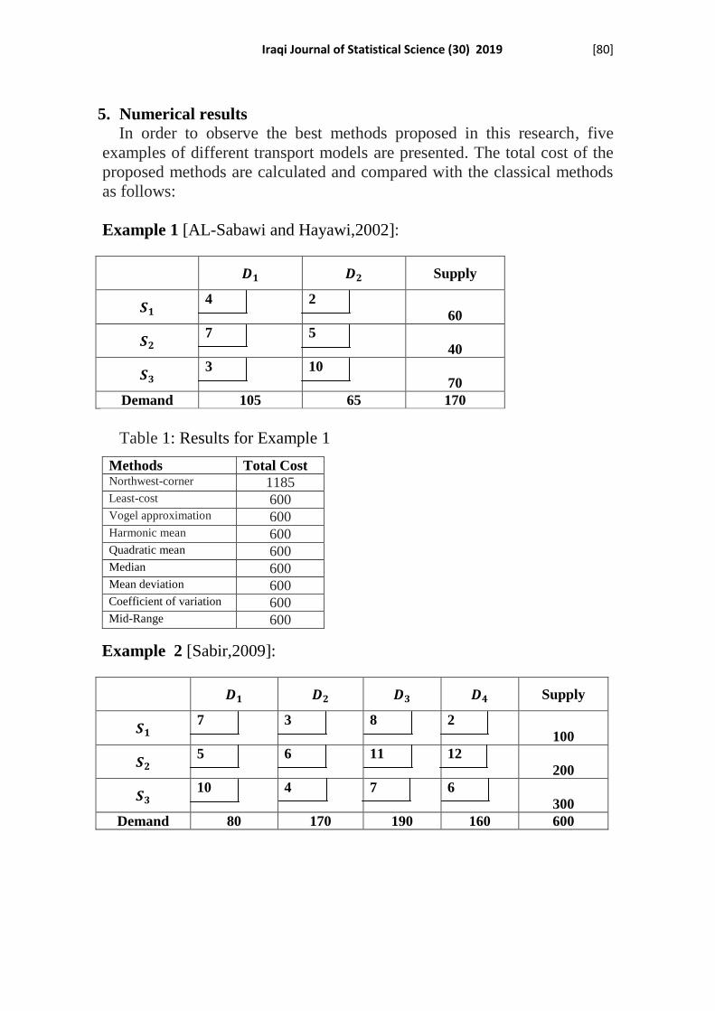
5. Numerical results

In order to observe the best methods proposed in this research, five

examples of different transport models are presented. The total cost of the

proposed methods are calculated and compared with the classical methods

as follows:

Example 1 [AL-Sabawi and Hayawi,2002]:

Supply

4 2

60

7 5

40

3 10

70

Demand 105 65 170

Table 1: Results for Example 1

Example 2 [Sabir,2009]:

Supply

7 3 8 2

100

5 6 11 12

200

10 4 7 6

300

Demand 80 170 190 160 600

Total Cost Methods

1185 Northwest-corner

600 Least-cost

600 Vogel approximation

600 Harmonic mean

600 Quadratic mean

600 Median

600 Mean deviation

600 Coefficient of variation

600 Mid-Range



Example 3 [AL-Badri and Saleh,2007] :

Supply

20 16 14 20

9

9 15 16 10

8

8 13 5 9

7

9 6 5 11

5

Demand 5 10 5 9 29


Total Cost Methods


3450 Least-cost


3210 Harmonic mean

3360 Quadratic mean

3210 Median

3210 Mean deviation


3210 Mid-Range

Total Cost Methods


308 Least-cost


306 Harmonic mean

306 Quadratic mean

306 Median

308 Mean deviation


306 Mid-Range


Example 4 [AL-Sabawi and Hayawi,2002]:

Supply

4 3 1 2 6

65

5 2 3 4 5

50

3 5 6 3 2

40

2 4 4 5 3

20

4 3 6 5 1

25

Demand 60 60 30 40 10 200


Example 5 [AL-Badri and Saleh,2007]:

Supply

5 1 2 3 4 7

400

7 2 3 1 5 6

500

9 1 9 5 2 3

300

6 5 8 4 1 4

150

8 7 11 6 4 5

600

2

5 7 5 2 1

350

Demand 300 500 700 300 250 250 2300

Total Cost Methods


420 Least-cost


505 Harmonic mean

420 Quadratic mean

420 Median

420 Mean deviation


475 Mid-Range



Table 6: shows the total cost values for the five Examples used in the

research

Mid

Range Coefficient

of variation Mean

deviation Median

Quadratic

mean Harmonic

mean Vogel

Least

cost

North

west

corner

600 600 600 600 600 600 600 600 1185 (3×2) 1

3210 3210 3210 3210 3360 3210 3210 3450 4010 (3×4) 2

306 308 308 306 306 306 308 308 392 (4×4) 3

475 420 420 420 420 505 420 420 760 (5×5) 4

6650 7100 6400 6650 6650 6650 7100 9100 11100 (6×6) 5

In the above table, when the six proposed methods and the three classic

methods are used, the results turned out to be as follows:

1) Results of the first example are similar to Least-cost and Vogel

methods due to the nature of the available data of this example.

Namely, it is the best improvement of solution (i.e. least possible

cost) because it has not given worse results than North West-corner

method.

2) Results of the second example are better than North West-corner and

Least-cost methods. However, they are equal to Vogel method. This

is due to the same reason of the first example. Yet, different results

are obtained using Quadratice mean. Still, it is better than North

West-corner and Least-cost methods despite, the fact that it is higher

in results than Vogel method.

3) Results of the third example are better than the three classic methods

except Coefficient of variation and Mean deviation methods. But, it

is better than North West-corner method and not worse than Vogel

and Least-cost methods.

4) For the same reason, results of the fourth example are better than

North West-corner method except Harmonic mean and Mid-Range

methods.

Total Cost Methods


9100 Least-cost


6650 Harmonic mean

6650 Quadratic mean

6650 Median

6400 Mean deviation


6650 Mid-Range

Methods of

solution

Application

number

Application

Capacity


5) Results of the fifth example are better than the three classic methods

except Coefficient of variation method which has given the same as

Vogel's .It is better than North West-corner and Least-Cost methods;

still not worse than Vogel's.

6. Conclusion

Statistical measures have been seen from observing and discussing

Table (6). These are either Central Tendency or Scattering Measures. They

can be used as methods to find the basic acceptable solution for

transportation problems. These methods have been proposed in the

research. Although the results are variant, they are not worse than the three

classic methods. The reason goes back to the nature of data used in the

research. In addition, it was concluded that the proposed methods are easy

to apply to all types of transport problems and are an important decision-

making tool in order to reach the basic solution of the lowest possible total

cost of goods transportation. The mathematical steps of these methods are

easy to implement in real applications.

7. References

1) Quddoos,A., S. Javaid and M.M.Khalid , 2012, A New Method for

Finding an Optimal Solution for Transportation Problems , International

Journal on Computer Science and Engineering (IJCSE), Vol. 4, No. 07,pp

1271-1274 .

2) Al-Badri, F., F.and Saleh, S., A., 2007, A Proposed Method for Finding

the Basic (acceptable) Solution to the Transportation Problem , Journal of

Economic and Administrative Sciences, Vol. 13, No. 48,pp 300-313 .

3) Al-Sabawi, A., M. and Hayawi, H., A., 2002, A Proposed Method to solve

Transportation Model , Iraqi Journal of Statistical Sciences, No. 4, pp

61-71.

4) Hamdy,A.,T., 2011, Operation Research An Introduction , Pearson

Education, Inc., Prentice hall, 9 edition, Newjersey,USA.

5) Reeb, J. And Leavengood, S., 2002, Transportation Problem: A Special

Case for Linear Prpgramming Problems , Published June © 2002 Oregon

State University.

6) Sabir, J., A., 2009, Operations Research in Accounting , Cairo University,

Egypt.

7) Samuel, A., E.and Venkatachalapathy, M., 2013, IZPM for Unbalance

Fuzzy Transportation Problems , International Journal of Pure and

Applied Mathmatics, Vol. 86, No. 4, pp 689-700 .

8) Taghrid, I., 2009, Solving Transportion Problem Using Object-Oriented

model , International Journal on Computer Science and Network Security

(IJCSNS),Vol. 9.NO. 2,pp 353-361 .

Proposed methods for finding the basic acceptable solution for ...

Documents

Transcript of Proposed methods for finding the basic acceptable solution for ...