Projector Quantum Monte Carlo Methods for Linear and Non ...
224
Projector Quantum Monte Carlo Methods for Linear and Non-linear Wavefunction Ansatzes Lauretta Rebecca Schwarz Trinity Hall University of Cambridge This dissertation is submitted for the degree of Doctor of Philosophy at the University of Cambridge October 2017
-
Upload
khangminh22 -
Category
Documents
-
view
6 -
download
0
Transcript of Projector Quantum Monte Carlo Methods for Linear and Non ...
Projector Quantum Monte CarloMethods for Linear and Non-linear
Wavefunction Ansatzes
Lauretta Rebecca Schwarz
Trinity HallUniversity of Cambridge
This dissertation is submitted for the degree ofDoctor of Philosophy
at the University of Cambridge
October 2017

Abstract
Projector Quantum Monte Carlo Methods forLinear and Non-linear Wavefunction Ansatzes
Lauretta Rebecca Schwarz
This thesis is concerned with the development of a Projector Quantum Monte Carlomethod for non-linear wavefunction ansatzes and its application to strongly correlatedmaterials. This new approach is partially inspired by a prior application of the FullConfiguration Interaction Quantum Monte Carlo (FCIQMC) method to the three-band (p− d) Hubbard model. Through repeated stochastic application of a projectorFCIQMC projects out a stochastic description of the Full Configuration Interaction(FCI) ground state wavefunction, a linear combination of Slater determinants spanningthe full Hilbert space. The study of the p− d Hubbard model demonstrates that thenature of this FCI expansion is profoundly affected by the choice of single-particle basis.In a counterintuitive manner, the effectiveness of a one-particle basis to produce asparse, compact and rapidly converging FCI expansion is not necessarily paralleled byits ability to describe the physics of the system within a single determinant. The resultssuggest that with an appropriate basis, single-reference quantum chemical approachesmay be able to describe many-body wavefunctions of strongly correlated materials.
Furthermore, this thesis presents a reformulation of the projected imaginary timeevolution of FCIQMC as a Lagrangian minimisation. This naturally allows for theoptimisation of polynomial complex wavefunction ansatzes with a polynomial ratherthan exponential scaling with system size. The proposed approach blurs the linebetween traditional Variational and Projector Quantum Monte Carlo approaches whilstinvolving developments from the field of deep-learning neural networks which can beexpressed as a modification of the projector. The ability of the developed approachto sample and optimise arbitrary non-linear wavefunctions is demonstrated withseveral classes of Tensor Network States all of which involve controlled approximationsbut still retain systematic improvability towards exactness. Thus, by applying themethod to strongly-correlated Hubbard models, as well as ab-initio systems, includinga fully periodic ab-initio graphene sheet, many-body wavefunctions and their one-and two-body static properties are obtained. The proposed approach can handle andsimultaneously optimise large numbers of variational parameters, greatly exceedingthose of alternative Variational Monte Carlo approaches.


For my parents

Preface
This dissertation contains an account of research carried out in the period betweenOctober 2013 and July 2017 in the Theoretical Sector of the Department of Chemistryin the University of Cambridge under the supervision of Prof. Ali Alavi, F.R.S. Thefollowing sections of this thesis are included in work which has either been publishedor is to be published:
Chapter 4 : L. R. Schwarz, G. H. Booth and A. Alavi, Insights into the structure ofmany-electron wave functions of Mott-insulating antiferromagnets: The three-bandHubbard model in full configuration interaction quantum Monte Carlo, PhysicalReview B, 91, 045139 (2015)
Chapter 5 and 6 : L. R. Schwarz, A. Alavi and G. H. Booth, Projector QuantumMonte Carlo Method for Nonlinear Wave Functions, Physical Review Letters,118, 176403 (2017)
Chapter 7 : In preparation.
This dissertation is the result of my own work and includes nothing which is theoutcome of work done in collaboration except where indicated otherwise. This thesisis not substantially the same as any that I have submitted, or, is being concurrentlysubmitted for a degree or diploma or other qualification at the University of Cambridgeor any other University or similar institution. I further state that no substantial partof my thesis has already been submitted, or, is being concurrently submitted for anysuch degree, diploma or other qualification at the University of Cambridge or anyother University or similar institution. This dissertation does not exceed 60, 000 wordsin length, including abstract, tables, and footnotes, but excluding table of contents,photographs, diagrams, figure captions, list of figures, list of abbreviations, bibliography,appendices and acknowledgements.
Lauretta Rebecca SchwarzOctober 2017


Acknowledgements
First, I would like to thank my supervisor, Ali Alavi, for all of his many ideas andenthusiasm. I am very grateful for the continual support that he provided, whilstgiving me the space to explore my own ideas and creating an inspiring atmosphere towork in. The many inspiring discussions with him and his wide knowledge have beeninvaluable, and I appreciate all that he has done.
Another person whom I cannot thank enough is George Booth. The huge amount ofknowledge and advice that he has passed on to me has been invaluable. I am gratefulnot only for proof-reading this thesis and the many helpful discussions, but also for hisguidance and support. I would also like to thank Charlie Scott for proof-reading partsof this thesis and Robert Thomas for many inspiring discussions, as well as the pastand present members of the Alavi group for creating such a pleasant environment towork in.
Moreover, it is a pleasure to acknowledge the Engineering and Physical SciencesResearch Council for funding this work, and the Max Planck Society for the provisionof high-performing computing facilities.
Last but not least, I would like to thank my parents for their loving support whichmeans so much to me. Their love and encouragement has continually accompaniedand helped me on my way.

Table of contents
List of figures xv
List of tables xvii
1 Introduction 1
2 Theoretical Background 92.1 Introduction . . . . . . . . . . . . . . . . . . . . . . . . . . . . . . . . . 92.2 An Alternative Formalism: Second Quantisation . . . . . . . . . . . . . 13
2.2.1 The Fock Space . . . . . . . . . . . . . . . . . . . . . . . . . . . 132.2.2 Elementary Operators . . . . . . . . . . . . . . . . . . . . . . . 15
2.3 Hartree-Fock Theory . . . . . . . . . . . . . . . . . . . . . . . . . . . . 182.4 Electron Correlation . . . . . . . . . . . . . . . . . . . . . . . . . . . . 222.5 Full Configuration Interaction . . . . . . . . . . . . . . . . . . . . . . . 252.6 Further Approximate Solution Methods . . . . . . . . . . . . . . . . . . 282.7 Beyond Traditional Quantum Chemical Methods: Tensor Network States
Approaches . . . . . . . . . . . . . . . . . . . . . . . . . . . . . . . . . 332.7.1 Entanglement Entropy and Area Laws . . . . . . . . . . . . . . 332.7.2 Decomposing the FCI Wavefunction Ansatz . . . . . . . . . . . 342.7.3 Tensor Network States in One Dimension: Matrix Product States 352.7.4 The Area Law and Efficient Approximability . . . . . . . . . . . 382.7.5 Tensor Network States in Two Dimensions: Projected Entangled
Pair States . . . . . . . . . . . . . . . . . . . . . . . . . . . . . . 412.7.6 Optimisation of MPS, PEPS, ... . . . . . . . . . . . . . . . . . . 43
3 Zero-temperature Ground State Quantum Monte Carlo Methods 473.1 Variational Quantum Monte Carlo Approaches . . . . . . . . . . . . . . 473.2 Projector Quantum Monte Carlo Approaches . . . . . . . . . . . . . . . 513.3 Full Configuration Interaction Quantum Monte Carlo: FCIQMC . . . . 55
xii Table of contents
3.3.1 Derivation of FCIQMC Equations . . . . . . . . . . . . . . . . . 563.3.2 Stochastic Implementation of FCIQMC . . . . . . . . . . . . . . 603.3.3 Energy Estimators . . . . . . . . . . . . . . . . . . . . . . . . . 623.3.4 The Fermion Sign Problem and the Importance of Annihilation 633.3.5 The Initiator Approximation . . . . . . . . . . . . . . . . . . . . 663.3.6 Non-integer Real-weight Walkers . . . . . . . . . . . . . . . . . 713.3.7 The Semi-stochastic Adaptation . . . . . . . . . . . . . . . . . . 72
3.4 Handling Stochastic Estimators . . . . . . . . . . . . . . . . . . . . . . 73
4 Application of i-FCIQMC to Strongly Correlated Systems 754.1 Model Hamiltonians . . . . . . . . . . . . . . . . . . . . . . . . . . . . 76
4.1.1 The Hubbard Model . . . . . . . . . . . . . . . . . . . . . . . . 764.1.2 The three-band (p− d) Hubbard Model . . . . . . . . . . . . . . 78
4.2 Geometries and Cluster Size . . . . . . . . . . . . . . . . . . . . . . . . 834.3 The three-band Hubbard Model in FCIQMC . . . . . . . . . . . . . . . 83
4.3.1 The Choice of Single-Particle Basis Sets . . . . . . . . . . . . . 844.3.2 An i-FCIQMC Study of the Many-Body Ground State Wave-
functions . . . . . . . . . . . . . . . . . . . . . . . . . . . . . . . 864.3.3 Orbital Occupation Numbers and Correlation Entropy . . . . . 904.3.4 Subspace Diagonalisations and CI Expansions . . . . . . . . . . 934.3.5 Conclusions . . . . . . . . . . . . . . . . . . . . . . . . . . . . . 95
5 A Projector Quantum Monte Carlo Method for Non-linear Wave-functions 975.1 Non-linear Projector Quantum Monte Carlo Method: Combining Varia-
tional and Projector Quantum Monte Carlo . . . . . . . . . . . . . . . 995.2 Derivation: Lagrangian Minimisation . . . . . . . . . . . . . . . . . . . 995.3 Sampling of the Lagrangian Gradient . . . . . . . . . . . . . . . . . . . 1015.4 Momentum Methods: Nesterov’s Accelerated Gradient Descent . . . . . 1115.5 Matrix Polynomials - Closing a Circle of Connections . . . . . . . . . . 1145.6 Step Size Adaptation: RMSprop . . . . . . . . . . . . . . . . . . . . . . 1185.7 Wavefunction Properties . . . . . . . . . . . . . . . . . . . . . . . . . . 1195.8 A Technical Point: Wavefunction Normalisation, Step Sizes and Param-
eter Updates . . . . . . . . . . . . . . . . . . . . . . . . . . . . . . . . . 1245.9 Comparison to State-of-the-art VMC Methods . . . . . . . . . . . . . . 125
Table of contents xiii
6 Applications of the Projector Quantum Monte Carlo Method forNon-linear Wavefunctions to Correlator Product State Wavefunc-tions 1276.1 The Correlator Product State Wavefunction Ansatz . . . . . . . . . . . 1296.2 Wavefunction Amplitudes and Derivatives . . . . . . . . . . . . . . . . 1316.3 2D Hubbard Model . . . . . . . . . . . . . . . . . . . . . . . . . . . . . 1326.4 1D Hubbard Model . . . . . . . . . . . . . . . . . . . . . . . . . . . . . 1366.5 Linear H50 Chain . . . . . . . . . . . . . . . . . . . . . . . . . . . . . . 1416.6 Graphene Sheet . . . . . . . . . . . . . . . . . . . . . . . . . . . . . . . 1436.7 Conclusions . . . . . . . . . . . . . . . . . . . . . . . . . . . . . . . . . 147
7 Projector Quantum Monte Carlo Method for Tensor Network States1497.1 The Computational Challenge of PEPS Wavefunctions - Can It Be
Tackled Stochastically ? . . . . . . . . . . . . . . . . . . . . . . . . . . 1517.2 The PEPS and MPS Wavefunctions Ansatz . . . . . . . . . . . . . . . 1527.3 Wavefunctions Amplitudes and Derivatives . . . . . . . . . . . . . . . . 1547.4 A Sampling Approach for Wavefunction Amplitudes and Derivatives . . 1557.5 Investigation of TNS Projection Sampling Approach . . . . . . . . . . . 1587.6 Applications for MPS and PEPS Wavefunctions . . . . . . . . . . . . . 1657.7 Conclusions . . . . . . . . . . . . . . . . . . . . . . . . . . . . . . . . . 169
8 Concluding Remarks and Continuing Directions 171
Appendix A Comparison of Lagrangian and Ritz Functional Deriva-tives 177
References 179

List of figures
2.1 Excitation level classification of configurations . . . . . . . . . . . . . . 272.2 Construction of MPS . . . . . . . . . . . . . . . . . . . . . . . . . . . . 362.3 Construction of PEPS . . . . . . . . . . . . . . . . . . . . . . . . . . . 40
3.1 An example FCIQMC calculation . . . . . . . . . . . . . . . . . . . . . 653.2 A comparison of FCIQMC and i-FCIQMC simulations . . . . . . . . . 683.3 Convergence of initiator error . . . . . . . . . . . . . . . . . . . . . . . 70
4.1 Phase conventions for three-band (p− d) Hubbard model . . . . . . . . 804.2 Clusters on 2D square lattice . . . . . . . . . . . . . . . . . . . . . . . 834.3 Convergence of ground state energy for three-band Hubbard model with
total walker number in i-FCIQMC . . . . . . . . . . . . . . . . . . . . 864.4 Spin-spin correlation function from i-FCIQMC ground state wavefunc-
tion of three-band (p− d) Hubbard model . . . . . . . . . . . . . . . . 884.5 Restricted and unrestricted Hartree-Fock band structures and density
of states for three-band Hubbard model . . . . . . . . . . . . . . . . . . 894.6 Orbital occupation numbers and mean-field orbital energies for different
single-particle basis sets . . . . . . . . . . . . . . . . . . . . . . . . . . 904.7 Illustration of selected RHF and UHF spin orbitals for three-band (p−d)
Hubbard model . . . . . . . . . . . . . . . . . . . . . . . . . . . . . . . 914.8 Magnitude of coefficients in FCI expansion with respect to determinant
energy for four different basis sets . . . . . . . . . . . . . . . . . . . . . 94
5.1 Comparison of momentum methods . . . . . . . . . . . . . . . . . . . . 1135.2 Comparison of projections . . . . . . . . . . . . . . . . . . . . . . . . . 118
6.1 Illustration of correlators . . . . . . . . . . . . . . . . . . . . . . . . . . 1336.2 Convergence of CPS wavefunction for 2D Hubbard model . . . . . . . . 1356.3 Convergence of energy of CPS wavefunctions for 1D Hubbard model . . 137
xvi List of figures
6.4 Percentage of DMRG correlation energy captured by CPS wavefunctionfor symmetric dissociation of H50 . . . . . . . . . . . . . . . . . . . . . 143
6.5 Illustration of correlators and CPS wavefunction for graphene sheet . . 1446.6 Spin correlation functions for graphene sheet . . . . . . . . . . . . . . . 146
7.1 Illustration of a PEPS network . . . . . . . . . . . . . . . . . . . . . . 1527.2 Convergence of stochastic energy estimates with number of samples . . 1607.3 Convergence of stochastic energy estimates with number of samples for
auxiliary and physical indices . . . . . . . . . . . . . . . . . . . . . . . 1637.4 Convergence of ground state energy for 1D 1× 10 Hubbard model . . . 165
List of tables
2.1 Slater-Condon rules . . . . . . . . . . . . . . . . . . . . . . . . . . . . . 28
3.1 Summary of most commonly used PMC methods . . . . . . . . . . . . 52
4.1 Parameters for three-band Hubbard model . . . . . . . . . . . . . . . . 794.2 Properties of ground state wavefunctions for three-band Hubbard model 87
6.1 Ground state energies for 2D Hubbard model . . . . . . . . . . . . . . 1346.2 Ground state energies and RDM properties for 1D Hubbard model . . 1406.3 Symmetric dissociation of H50 . . . . . . . . . . . . . . . . . . . . . . . 1426.4 Energies and RDM properties for 4× 4 graphene sheet . . . . . . . . . 145
7.1 Ground state energies for 1D 1× 10, 1× 14 and 1× 22 Hubbard model 1667.2 Ground state energy for 2D 4× 4 Hubbard model . . . . . . . . . . . . 169

Chapter 1
Introduction
It was not until the unexpected discovery of high-temperature superconductivity incuprates by J. G. Bednorz and K. A. Müller in 1986[1, 2] that the field of stronglycorrelated electrons received the attention that it deserves. Soon after their discovery, itbecame clear that in order to understand the normal state properties of these materialsand, in particular, the phenomenon of superconductivity deeper insight into the strongcorrelations that prevail in these systems is required[3–5].
In strongly correlated materials different physical interactions involving spins,charges, orbitals and the lattice of the system are strongly coupled to each other andgive rise to a variety of electronic phases[6–8] which are typically close energy, therebyleading to complex phase diagrams. The cooperation, competition, or a combinationof both, amongst these correlated electronic phases can result in unexpected electronicphenomena and non-linear responses to external fields as these systems are verysensitive to small changes in their surroundings, an observation that has been madein many experimental studies and numerous investigations of model systems[9–11].This rich variety of phenomena resulting from strong correlation effects includesnot only the high temperature superconductivity in layered copper oxides and ironpnictides, but also colossal magneto-resistance effects in manganese oxide, as well asheavy fermion phenomena in lanthanide and actinide intermetallic compounds, toname just a few[12, 13]. Typically, strongly correlated systems comprise materials inwhich transition metals, lanthanides or actinides with partially filled d- or f -shellsplay an active role. On the one hand, these electrons in open d- or f -shell arespatially localised and thus display atomic-like behaviour. On the other hand, they alsoparticipate in chemical bonding to differing extends and can act in a band-like fashionin some cases. As a consequence, they are located in an intermediate regime betweenlocalised and delocalised electrons[13] and it is this competition between localisation
2 Introduction
and delocalisation, that is between kinetic energy and electron-electron interaction,which lies at the heart of the strong correlation problem[14] and gives rise to the newlow-energy scales generated by strong correlations[3]. Usually, many of these stronglycorrelated materials consist of simple components such as transition metal oxides whichoften adopt the perovskite structure whereby a transition metal ion is surroundedby an octahedral oxygen cage. Yet, when these simple building blocks are broughttogether they interact in a highly complex manner such that their collective behaviour isdifficult to predict a priori based on their individual properties. The strong correlationsprevailing in these systems imply that the collective states cannot be understood basedon a one-electron (or even one-quasiparticle) approximation. The latter are therefore ofno use and more sophisticated approaches are needed to gain insight and rationalise theintriguing electronic phenomena and non-linear responses that emerge in these materials.Potentially, this behaviour can also form the basis for the design and development ofnovel types of electronics with new functionalities for which purpose understanding,controlling and predicting the emergent complexity of strongly correlated electronsystems is essential. Examples of these potential applications include the surface andcatalytic properties of transition metal and rare earth oxides[15], molecular magneticmaterials[16] and cathode materials of lithium batteries[17].
On the theory side, the foundations of quantum mechanics were established duringthe first half of the twentieth century. In 1926, Erwin Schrödinger rederived Bohr’ssemi-classical energy spectrum for hydrogen-like atoms within a quantum mechanicalframework[18] and concluded that each eigenstate can be uniquely labelled by threequantum numbers. In order to explain spectra of more complicated atoms, Pauliintroduced a fourth degree of freedom and stated that no two electrons can sharethe same four quantum numbers[19], a principle which is known as Pauli’s exclusionprinciple today. Whilst Uhlenbeck and Goudsmit identified this fourth quantum numberas the spin projection of the electron[20], Heisenberg introduced quantum mechanicaltreatments of many-body problems[21]. These and many other contributions andadvances of quantum mechanics lay the foundations for the development of electronicstructure theory. More generally, for any physical system, the Schrödinger equation[22]defines the allowed states of the system and their evolution in time and solving it leadsto the wavefunction which in the Copenhagen interpretation of quantum mechanicsrepresents the most complete description of a physical system. Yet, it was soon realisedthat this would only be the beginning of the problem, as Paul Dirac said in 1929[23]:
The general theory of quantum mechanics is now almost complete, theimperfections that still remain being in connection with the exact fitting
3
in of the theory with relativity ideas. These give rise to difficulties onlywhen high-speed particles are involved, and are therefore of no importancein the consideration of atomic an molecular structure and ordinary chemicalreactions, in which it is, indeed, usually sufficiently accurate if one neglectsrelativity variation of mass with velocity and assumes only Coulomb forcesbetween the various electrons and atomic nuclei. The underlying physicallaws necessary for the mathematical theory of a large part of physics andthe whole of chemistry are thus completely known, and the difficulty isonly that the exact application of these laws leads to equations much toocomplicated to be soluble. It therefore becomes desirable that approximatepractical methods of applying quantum mechanics should be developed, whichcan lead to an explanation of the main features of complex atomic systemswithout too much computation.
Nevertheless exact or approximate solutions to the corresponding equations arecrucial for understanding the collective behaviour of interacting elementary particlesand the variety of complex phenomena emerging from this. Electronic structuretheory is therefore concerned with the development of theories which attempt to findapproximate solutions to the underlying exact equations, with varying degrees ofaccuracy and associated computational cost. Over the last century, this has resultedin a huge array of methods with different levels of approximations to balance thecompeting demands of accuracy and tractable computational cost. In the realm ofstrongly correlated electrons, developments of various electronic structure approacheshave concentrated on methods which require no assumption of the explicit form of thefull many-body wavefunction since it represents a computationally expensive object.
Thus, ab-initio electronic structure calculations are dominated by density functionaltheory (DFT)[24] which is, however, a ground state theory and therefore fails, oftenqualitatively. In particular, this is the case for strongly-correlated systems where low-energy excitations need to be taken into account appropriately. This failure is inherentand independent of any approximations that are involved in the potential of the Kohn-Sham equation[3]. An example for such a failure is the local density approximation(LDA)[25] within DFT which despite its success for conventional metallic systems isinadequate for strongly correlated systems since it assumes the potential of the Kohn-Sham equations to be determined by the local density. This assumption breaks downwhen the latter has a strong spatial dependence as it is the case in strongly correlatedmaterials with their strongly fluctuating charge and spin degrees of freedom[3, 9].Qualitative failures of LDA are widely observed for the Mott insulating phase of
4 Introduction
many transition metal compounds, as well as for phases of correlated metals nearthe Mott insulator. Examples of the inability of LDA to reproduce an insulating (orsemiconducting) phase include La2CuO4, YBa2Cu3O6, NiS, NiO and MnO[9, 26, 27].Nonetheless, semi-empirical methods have had some successes like the renormalisedband-structure method[28]. Several approaches have also been proposed to incorporatestrong correlation in the LDA method such as LDA+U[29] and LDA-SIC[30]. Incontrast to LDA, both methods yield a correct antiferromagnetic insulator as groundstate for La2CuO4, but the origin of the insulating gap is not correct. Being a groundstate method, DFT is not guaranteed to reproduce excitations well which are, however,often crucial for the properties of strongly correlated systems and many cases existwhere DFT calculations involving standard approximations lead to unacceptable errors.For example, excitation energies between different states of transition metal, as well asrare earth and lanthanide atoms are often predicted poorly, differing from measuredvalues by about 2 eV[3]. Another method applied to strongly correlated electronsystems is the hybrid LDA+DMFT (Dynamical Mean Field Theory) method[31]. Inthis approach, the electron self-energy is calculated by DMFT theory in the limit ofinfinite dimension and is k-independent[10] which is why the LDA+DMFT approachprovides no viable route to the correct band dispersion. Extensions of the originalDMFT method to cluster DMFT[32] go into the right direction, but the clusters thatcan be treated are relatively small.
Since reliable ab-initio methods for strongly correlated methods are still at theirbeginning, another widely used theoretical approach is based on simplifying modelHamiltonians which seem to better capture the essence and unravel the physical effectsof correlated systems. The one most studied is the Hubbard Hamiltonian[33, 9], whichdescribes the dynamics of electrons on a lattice whereby each lattice site can at mostaccommodate two electrons of opposite spin in its associated orbitals. The complexity ofa full Hamiltonian for this system is thus reduced down to only two parameters: a kineticenergy term t which represents the hopping of electrons between nearest-neighbourlattice sites and an on-site Coulomb repulsion term U which accounts for the repulsionbetween electrons that reside on the same lattice site. The simplifications introducedby this ansatz compared to an ab-initio Hamiltonian are enormous. Nevertheless,important insight can be gained by studying Hubbard model systems, in particularat or close to half filling. A variety of techniques have been applied for the studyof Hubbard systems with emphasis on two dimensions (2D). The reason for this isthat the 2D Hubbard model is claimed to possess all the relevant physics for high-TC
superconductivity. Despite the simplicity of the model Hamiltonian, the latter is still
5
very difficult to solve accurately and many questions still remain unanswered. Anexample for this is the much studied Mott-Hubbard metal-to-insulator phase transitionat half filling when U >> t for which it is not known at which critical ratio of U
t
this phase transition occurs at T = 0[34]. For a slightly more realistic picture, theHubbard model Hamiltonians can also be refined by addition of further orbitals andparameters. This leads for example to the three-band or five-band Hubbard modelwhich act as model for Cu–O planes in high-TC cuprates. Hybrid approaches have alsobeen developed in which LDA is used to construct Wannier functions and computeparameters of a multi-band Hubbard model. The latter is treated by a generalisedtight-binding method which combines exact diagonalisation of a small cluster withperturbation treatment of the inter-cluster hopping and interactions. This approachhas been used to find the size of the gap in La2CuO4[35].
In spite of its success, DFT and its various hybrid approaches have some weaknesseswhich are difficult to amend. A general drawback is that the true exchange-correlationpotential is unknown and all results of DFT calculations depend on the choice ofapproximation to it. Any approximation to the exchange-correlation potential isessentially uncontrolled and therefore difficult to improve systematically which repre-sents a major issue for calculations of strongly correlated electrons. Because of theissues associated with DFT and its hybrid approaches there is also growing interest inwavefunction-based methods[36–38]. Initially these methods were only used to treatsmall molecules, although the studied systems increased in size. Owing to a fruitfulcombination of the advent in computer technology and methodological development,quantum chemical methods have made impressive progress and system sizes increasedto several hundred atoms[39]. In contrast to DFT, wavefunction-based methods providea rigorous framework for addressing correlation problems which avoid any uncontrolledapproximations. These approaches explicitly construct many-body wavefunctions atincreasing levels of sophistication and accuracy. However, W. Kohn put forward theargument that the many-electron wavefunction is not a legitimate concept for largesystems with large electron numbers, N ≳ 103[40, 41]. Electronic wavefunctions arethus said to face the ‘exponential wall’ problem, another formulation of the fact thatthe number of all possible classical configurations of particles grows exponentiallywith system size, and so does the Hilbert space that the exact wavefunction lives in.Yet, electronic structure methods based on many-body wavefunctions have found amultitude of ways to circumvent this ‘exponential wall’ problem. Standard quantumchemical methods provide thus an appropriate framework for a rigorous treatment ofthe ubiquitous short-range correlations and of a realistic representation of the crystalline
6 Introduction
environment. The success of these quantum chemical methods is founded on an accu-rate description in real space of the correlation hole around an electron which is of localcharacter[42, 43] apart from special cases such as marginal Fermi-liquid behaviour orsuperconductivity where the long-range part of the correlation hole becomes crucial[41].Since the correlation hole is a local object, wavefunction-based approaches can limitits description to a finite periodic cluster out of the infinite solid which is large enoughto account for crucial short-range correlations. Typically, partially filled d- or f -shellsrequire a multi-configurational wavefunction representation. This can be obtainedwith the Complete Active Space Self-Consistent Field (CASSCF) method which ingeneral provides a good description for strong correlation effects. In these treatments,the crystalline environment is described by an effective one-electron potential whichis calculated with prior Hartree-Fock evaluations for the periodic system. Althoughthe Hartree-Fock approximation is a mean-field treatment, charge distributions aredescribed quite well by it as they are relatively unaffected by correlation effects, evenwhen the latter are strong. These methods have been used to describe the groundstate of strongly correlated systems such as LaCoO3 and LiFeAs, as well as the Zhang-Rice-like electron removal band for CuO2 planes in La2CuO4[44]. Further successfulexamples include the application of the method of increments, which evaluates thecorrelation energy by decomposing it into increments[45, 46], to transition metal andrare-earth oxides[47–49].
Wavefunction-based approaches are therefore a field with high potential in the future.Although they tend to be more computationally expensive, they represent promisingalternatives to DFT-based methodologies given that all approximations are fullycontrolled and can be successively and systematically improved. In addition, many-bodywavefunctions represent the best framework to obtain deeper insight into correlationeffects of a system and a better understanding of its most important microscopicprocesses. Over the last century, developments and applications involving well-chosenand controlled approximations have yielded wavefunctions whose observables are inexcellent agreement with experimental measurements. Thus, a major motivation foradvances in electronic structure theory has been the aim to arrive at these wavefunctionsat a tractable computational cost. This has lead to a vast array of wavefunction-basedmethods at different levels of accuracy when balancing the competing demands ofcomputational cost and accuracy. A summary of those which are most relevant to thisthesis is given in Chapter 2. A set of promising techniques that may pave the way toarrive at this delicate balance are Quantum Monte Carlo (QMC) approaches[50, 51]which broadly split in two main categories, Variational and Projector Quantum Monte
7
Carlo methods. These represent an array of versatile and accurate stochastic methodswhich treat quantum many-body systems by sampling the space stochastically, asdetailed in Chapter 3 which lays the necessary groundwork for the research presentedin the later chapters. Amongst these QMC approaches, one promising emergingtechnique is the Full Configuration Interaction Quantum Monte Carlo (FCIQMC)method[52], a Projector Quantum Monte Carlo approach which samples both theprojector and the exact wavefunction in Fock space, a linear superposition of allclassical configurations. As such, FCIQMC is a high-accuracy technique and thusideally suitable for gaining a fundamental understanding of the structure and importantcomponents in the quantum many-body wavefunction of a system which then also aidsthe development of more approximate approaches. A study in this spirit is presentedin Chapter 4 for a prototypical strongly correlated system, the strongly correlatedthree-band (p− d) Hubbard model. In this investigation, FCIQMC is used to examinehow the structure of the exact wavefunction is affected by the choice of underlyingsingle-particle basis spanning the Hilbert space and what the implications for othermore approximate methods are. Even though the high accuracy of FCIQMC representsa significant advantage, the size of the Hilbert space conceals exponential complexityin the exact wavefunction ansatz and the associated computational cost can often limitthe applicability of FCIQMC, in particular when considering large systems.
This challenge has inspired the research that the remaining chapters of this thesisare concerned with: the development of a Projector Quantum Monte Carlo methodfor non-linear wavefunction ansatzes. This novel approach reformulates the projectedimaginary time evolution of FCIQMC in terms of a Lagrangian minimisation which nat-urally admits non-linear wavefunctions ansatzes. The latter more traditionally inhabitthe realm of Variational Quantum Monte Carlo approaches where their polynomialcomplexity circumvents the exponential scaling of the Hilbert space, and hence the‘exponential wall’ problem. Chapter 5 gives a thorough derivation and exposition of thisapproach which blurs the line between traditional Variational and Projector QuantumMonte Carlo methods. At the same time, it includes developments from the field ofdeep-learning neural network which can be viewed as a modification of the propagatorof the wavefunction dynamics. In addition, the dynamics of the wavefunction evolutionalso grant access to the one- and two-body static properties of the quantum many-bodywavefunction. Chapter 6 and 7 are dedicated to applications which demonstrate theability of this approach to sample and optimise arbitrary non-linear wavefunctionparameterisations with different forms of Tensor Network State ansatzes[53–55]. Thisset of powerful wavefunction parameterisations has been shown to provide efficient
8 Introduction
representations of the quantum many-body wavefunction with their success rooted intheir ability to capture the natural structure of quantum correlations. Whilst Chapter6 focuses on Correlator Product State wavefunctions, Chapter 7 considers MatrixProduct States, the underlying variational class of the highly successful Density MatrixRenormalisation Group (DMRG)[56] approach, and their generalisations to higherdimensions, Projected Entangled Pair States. All of these wavefunction ansatzes involvecontrolled approximations and retain systematic improvability towards exactness. Thus,these parameterisations are used in Chapters 6 and 7 to find many-body wavefunctionsand their one- and two-body static properties for a range of Hubbard lattice modelsand ab-initio systems. The number of variational parameters that are handled andsimultaneously optimised within these applications exceeds those of alternative state-of-the-art Variational Quantum Monte Carlo methods, again demonstrating the ability ofthis novel approach to efficiently treat and optimise arbitrary non-linear wavefunctionansatzes.
Chapter 2
Theoretical Background
2.1 Introduction
The first postulate of quantum mechanics states that all possible information on anyquantum mechanical system of interacting particles is contained within its wavefunctionΨ. The time-dependent Schrödinger equation,
iℏ∂
∂tΨ = HΨ, (2.1)
together with an appropriate set of boundary conditions entirely determines thiswavefunction, and hence the state of the system and its evolution in time. It istherefore a primary objective of molecular quantum mechanics to find a solution tothe non-relativistic time-independent Schrödinger equation [18]
HΨ = EΨ (2.2)
where H is the Hamiltonian operator for a system whose state is described by thewavefunction Ψ with total energy E . For a system of Nnuc nuclei and N electrons, thisHamiltonian (in atomic units ℏ = e = me = 4πϵ0 = 1), is given by [57]:
H = −N∑
i=1
12∇
2i −
Nnuc∑A=1
12MA
∇2A −
N∑i=1
Nnuc∑A=1
ZA
riA
+N∑
i=1
N∑j>i
1rij
+Nnuc∑A=1
Nnuc∑B>A
ZAZB
RAB
, (2.3)
where rij = |ri − rj| is the distance between electrons i and j, riA = |ri − RA| thedistance between electron i and nucleus A with mass MA and atomic number ZA,and RAB = |RA − RB| the distance between nuclei A and B. Whilst the first twoterms account for the kinetic energy of electrons and nuclei, the third term describes
10 Theoretical Background
the Coulomb attraction between electrons and nuclei. The electron-electron andnuclear-nuclear repulsion are represented by the last two terms, respectively.
Due to the large difference between nuclear and electronic masses, the electrons areexpected to adjust almost instantaneously to changes in the nuclear positions, suchthat the ∑Nnuc
A=11
2MA∇2
A term can be considered negligible. Electronic structure methodstherefore typically invoke the Born-Oppenheimer approximation [58] which decouplesthe electronic motion from the nuclear motion by expressing the total wavefunction asproduct of electronic and nuclear components,
Ψ(r,R) = Ψelec(r; R)Ψnuc(R). (2.4)
The electronic wavefunction Ψelec represents a solution to the electronic Schrödingerequation
HelecΨelec(r; R) = Eelec(R)Ψelec(r; R), (2.5)
Helec = −N∑
i=1
12∇
2i −
N∑i=1
Nnuc∑A=1
ZA
riA
+N∑
i=1
N∑j>i
1rij
+ Enuc. (2.6)
This electronic Schrödinger equation describes the motion of N electrons in a field ofNnuc fixed nuclei whose kinetic energy is neglected and whose repulsion contributes aconstant value Enuc = ∑Nnuc
A=1∑Nnuc
B>AZAZB
RABto the electronic energy Eelec. This common
approximation has been shown to produce potential energy surfaces with accuratemolecular properties. It is, however, worth noting that the approximation can breakdown in systems with closely lying electronic states due to coupling between these statesand the nuclear kinetic energy neglected in the Born-Oppenheimer approximation [59,60]. Nevertheless, the electronic Schrödinger equation is the basis of the majority ofproblems in quantum chemistry. In particular, any discussion of the Hamiltonian withinthis thesis is with respect to the Born-Oppenheimer separated electronic Hamiltonian,unless otherwise stated, and the ‘elec’ subscript is omitted from this point onwards.
In practice, it is extremely difficult to solve 2.5 for the exact Ψ and analyticalsolutions can only be found for a few simple one-electron systems such as the Hatom or the H2
+ molecule. For more complicated systems, approximations must beintroduced whilst incorporating as many of the symmetries and characteristics of theexact wavefunction as possible in the approximate wavefunction to ensure that it givesa reasonable description of the system. Many of these properties can be introducedby ensuring that the wavefunction represents an eigenfunction of the corresponding
2.1 Introduction 11
operators which commute with H such as the number operator (N ), or the total (S2)and projected spin operators (Sz) in non-relativistic theory.
One of the most fundamental characteristics which should be included at eachlevel of theory arises as a consequence of the fundamental nature of the spin thateach particle is associated with. Since the Hamiltonian is invariant to interchangeof indistinguishable particles, its eigenfunctions can be separated in two symmetryclasses: those wavefunctions which are symmetric and those which are anti-symmetricwith respect to identical particle exchange. The spin-statistics theorem [61, 62] statesthat integer spin particles, called bosons, obey Bose-Einstein statistics and half-integerspin particles, referred to as fermions, obey Fermi-Dirac statistics. Hence, for bosonsthe general many-body wavefunction is symmetric with respect to interchange of anytwo indistinguishable particles, whilst for fermions it is anti-symmetric with respect tointerchange of any two indistinguishable particles. From the anti-symmetric nature ofthe fermionic wavefunction, the Pauli exclusion principle [19, 63, 64] follows which, inits general form, states that two or more identical fermions such as electrons cannotoccupy the same (pure) quantum mechanical state. In general, writing the functionwhich completely describes a single electron i as product of a spatial and a spincomponent that depend on the spatial and spin coordinates of the electron, collectivelydenoted by:
xi = ri, σi , (2.7)
where
σ = α; β , (2.8)
the anti-symmetry and Pauli principle can thus be described as
Ψ(x1,x2, . . . ,xi, . . . ,xj, . . . ,xN) = −Ψ(x1,x2, . . . ,xj, . . . ,xi, . . . ,xN). (2.9)
The simplest, non-trivial function which satisfies this requirement is a Slater determi-nant [65]
Di = 1√N !
∣∣∣∣∣∣∣∣∣∣∣∣
ϕ1(x1) ϕ1(x2) . . . ϕ1(xN)ϕ2(x1) ϕ2(x2) . . . ϕ2(xN)
... ... . . . ...ϕn(x1) ϕn(x2) . . . ϕN(xN)
∣∣∣∣∣∣∣∣∣∣∣∣. (2.10)
12 Theoretical Background
Within this formalism interchanging the coordinates of two electrons is equivalentto interchanging two rows of the Slater determinant which changes the sign of thedeterminant as required by the anti-symmetry principle. If two electrons share thesame spin and spatial coordinates, corresponding to two identical columns in theSlater determinant, the latter vanishes. At the same time, this characteristic creates aregion of low probability for electrons with like spin at small separation distances. Thisrepresents a manifestation of Fermi correlation which is automatically incorporated intoa wavefunction written as a Slater determinant. Alternatively, the Slater determinantcan also be expressed in terms of an antisymmetrising operator A acting on a Hartreeproduct
Di = A[ϕ1(x1)ϕ2(x2) . . . ϕN(xN)], (2.11)
where
A = 1√N !
N−1∑p=0
(−1)pPp = 1√N !
1−∑i =j
Pij +∑
i =j =k
Pijk − . . .
(2.12)
with Pp the permutation operator which generates all possible permutations of pelectronic coordinates. The functions ϕi represent single particle spin orbitals whichdescribe the distribution of a single electron. Each ϕi depends on the spin and spatialcoordinates x of only one electron and is written as a product of a spatial orbital anda spin function
ϕi(x) = ϕi,s(r, σ) = ϕI(r)δs,σ. (2.13)
Whereas two spin orbitals with the same spatial function but different spin part arealways orthogonal ⟨ϕi,α(x)|ϕi,β(x)⟩ = 0, the set of spatial orbitals ϕI(r) are usuallychosen to be orthonormal ⟨ϕI(r)|ϕJ(r)⟩ = δIJ but need not necessarily be.
Since the Hamiltonian and the antisymmetrising operator are both linear operators,a linear combination of Slater determinants
Ψ =∑
iCiDi (2.14)
creates a more flexible many-body wavefunction whilst still maintaining the requiredantisymmetry properties. Wavefunctions written in the form of a single Slater deter-minant or any linear combination of Slater determinants constitute the basis of the
2.2 An Alternative Formalism: Second Quantisation 13
Hartree-Fock and Configuration Interaction methods, respectively. Working in a Slaterdeterminant basis requires keeping track of the occupations of the single particles stateswith a certain number of fermions and the appropriate sign factors arising from therespective permutation. Dirac and Fock established a formalism with this functionality,referred to as Second Quantisation [66, 67].
2.2 An Alternative Formalism: Second Quantisa-tion
The Hamiltonian in 2.5 is represented in First Quantisation, a formulation in whichobservables are represented by operators and states by functions. In the languageof Second Quantisation [37, 68–70], both wavefunctions and operators are uniquelydescribed by a single set of elementary operators. One of the major differences betweenfirst and second quantisation is that while the total number of particles is restrictedin first quantisation, second quantisation does not impose such a restriction. In itsfirst quantisation representation, the N -particle wavefunction is expanded in a basis ofvectors that span the N -particle Hilbert space HN . In the trivial case of no particles,N = 0, HN is equal to C, and in the case of a single particle N = 1, HN is spanned bythe set of single particle spin orbitals ϕi (i = 1, 2, . . .∞) with inner product ⟨ϕi|ϕj⟩ = δij .For a general N -particle system, HN is the N -fold tensor product of H1
HN = H⊗N1 . (2.15)
In the case of bosons, this tensor product is symmetrised after tensor multiplication,and in the case of fermions it is antisymmetrised, thereby implying that the fermionicHN is spanned by the set of all N -particle Slater determinants. Since this thesis isonly concerned with fermionic particles the following discussion will be restricted tofermions.
2.2.1 The Fock Space
Since in second quantisation the number of particles is not a constant, a state vectorin its second quatised form is a basis vector of an abstract linear vector space calledFock space F∞ comprising all states containing zero to infinitely many particles. This

14 Theoretical Background
Fock space is defined as the direct sum of N -particle Hilbert spaces
F∞ =∞⊕
N=0HN . (2.16)
Since F∞ may be decomposed into subspaces of N -particles Hilbert spaces which inturn are spanned by N -particle Slater determinants, the span of F∞ includes Slaterdeterminants but for all particle numbers ranging from 0 to ∞. The basis vectors ofthe Fock space are occupation number vectors defined as
|n⟩ = |n1, n2, . . .⟩ , ni =
1 ϕi occupied0 ϕi unoccupied
,∞∑
i=1ni <∞, (2.17)
which is an alternative representation for a Slater determinant constructed from the setof one-particle functions ϕi. The occupation number ni is equal to 1 if ϕi is presentin the determinant and 0 if it is absent. Spaces FN with at most N particles,
FN =N⊕
n=0Hn. (2.18)
are subspaces of the Fock space F∞ and likewise spanned by |n⟩ satisfying the constraint
∞∑i=1
ni ≤ N. (2.19)
Whilst the |n⟩ of the Fock space F∞ and its subspaces FN are created from an infiniteset of functions ϕi, in practice only finite basis set with M spin orbitals can be employed.This further restricts the space to those 2M -dimensional subspaces
FN,M =N⊕
n=0Hn,M . (2.20)
spanned by those occupation number vectors that satisfy
|n⟩ = |n1, n2, . . . , nm⟩ ,M∑
i=1ni ≤ N. (2.21)
For a given spin orbital basis, a one-to-one mapping between Slater determinants incanonical order and occupation number vectors in the Fock space exist. However, incontrast to determinants occupation number vectors have no spatial structure but are
2.2 An Alternative Formalism: Second Quantisation 15
basis vectors of an abstract vector space, representing an orthonormal and completebasis with inner product,
⟨m|n⟩ = δm,n =M∏
i=1δmi,ni
, (2.22)
and resolution of the identity defined as
I =∑
k|k⟩ ⟨k| . (2.23)
The subspace H0 with no particles contains a single basis vector, the true vacuum state
|0⟩ = |01.02, . . .⟩ = 1 ∈ C = H0 ⊂ F∞, (2.24)
which is normalised to unity ⟨0|0⟩ = 1.
2.2.2 Elementary Operators
In second quantisation, all states and operators can be constructed from the set ofelementary creation and annihilation operators. Whereas the creation operator a†pcreates a fermion in spin orbitals p, its Hermitian adjoint, the annihilation operator ap
annihilates a fermion in spin orbital p. These operators satisfy the anticommutationrules
ap, a
†q
= apa
†q + a†qap = δpq (2.25)
ap, aq =a†p, a
†q
= 0, (2.26)
from which all properties of the operators follow. These anticommutation relationsensure that, in accordance with Pauli’s exclusion principle, a single-particle state cannotbe occupied with more than one fermion, a†pa†p = −a†pa†p = 0, as well as, the antisym-metry for multiple fermions a†pa†q = −a†qa†p. Furthermore, the anticommutation rulesimply that if a creation operator a†p (annihilation operator ap) acts on an occupationnumber vector |n⟩, it populates (depopulates) the spin orbital ϕp if it is unoccupied

16 Theoretical Background
(occupied) in |n⟩
a†p |n1, . . . , np−1, np, np+1, . . .⟩ =
Γnp |n1, . . . , np−1, 1p, np+1, . . .⟩ if np = 0p
0 if np = 1p,(2.27)
ap |n1, . . . , np−1, np, np+1, . . .⟩ =
Γnp |n1, . . . , np−1, 0p, np+1, . . .⟩ if np = 1p
0 if np = 0p,(2.28)
with the phase factor
Γnp =
p−1∏q=1
(−1)nq . (2.29)
Since for a general occupation number vector the unoccupied spin orbitals can beidentified from the occupied ones, explicit reference to the former may be avoidedaltogether by writing the occupation number vector as a string of creation operators incanonical order (i.e. in the same order as in the occupation number vector) acting onthe vacuum state:
|n⟩ = ∞∏
p=1(a†p)np
|0⟩ . (2.30)
Due to the definition of the elementary creation and annihilation operators and theirrespective anticommutation relation, the antisymmetry properties of the wavefunctionare incorporated in the algebraic properties of the operators. By analogy, similarcreation b†p and annihilation bp operators can be introduced for bosons which satisfythe commutation rules [bp, b
†q] = bpb
†q − b†qbp = δpq and [bp, bq] = [b†p, b†q] = 0 to transfer
the symmetry properties of the bosonic wavefunction into the algebraic properties ofthe operator. Second quantisation allows both states and operators to be expressed interms of creation and annihilation operators in a unified way. As expectation values ofobservables are independent of the representation of operators and states, an operator inFock space can be derived by requiring its matrix elements between occupation numbervectors to be equal to the respective matrix elements between Slater determinants ofthe operator in its first quantised form. In first quantisation, the operators are exactand independent of the spin orbital basis, but explicitly depend on the number ofparticles, and the dependence on the spin orbital basis is incorporated into the Slaterdeterminants. In contrast, in the second quantisation formalism, the occupation numbervectors contain no reference to the spin orbital basis. Still, the operators are projections
2.2 An Alternative Formalism: Second Quantisation 17
of the exact operators onto the spin orbital basis, and hence basis-dependent, butindependent of the number of particles. Thus, the second-quantisation representationof the electronic Hamiltonian in 2.5 is given by [37]:
H = h+ g + Enuc =∑pq
hpqa†paq + 1
2∑pqrs
gpqrsa†pa†qasar + Enuc (2.31)
with the one- and two-particle integrals defined as
hpq = ⟨p|h|q⟩ =∫ϕ∗p(xi)
(−1
2∇2i −
Nnuc∑A=1
ZA
riA
)ϕq(xi)dxi (2.32)
gpqrs = ⟨pq|rs⟩ =∫ ∫
ϕ∗p(xi)ϕ∗q(xj)1rij
ϕr(xi)ϕs(xj)dxidxj (2.33)
Enuc =Nnuc∑A=1
Nnuc∑B>A
ZAZB
RAB
. (2.34)
Within this second-quantisation formulation, if applied to a state vector, the Hamilto-nian operator generates a linear combination of the original state and further statesconstructed by single- and double particle excitations from this state vector. Each suchexcitation is associated with an amplitude hpq and gpqrs representing the probability ofthis event occurring. In the limit of a complete set of spin orbital, the exact eigenstate Ψof the Hamiltonian can be represented by a linear expansion in terms of the occupationnumber vectors of the Fock space F∞ when no restriction with respect to particlenumber, point-group symmetry or projection of the total spin are enforced. Yet, evenif the total number of electrons is restricted to N = Nα + Nβ with Nα and Nβ thenumber of α and β spin particles, the number of terms in the linear combinationbecomes infinite due to the infinite basis set. Therefore, the approximation of a finitespin orbital basis of size M is introduced. Even within this framework, it is exceedinglydifficult in practice to solve for the exact eigenstate Ψ of the Hamiltonian since the 1
rij
term encapsulates the correlation of N interacting particles. The pursuit of accurateapproximations to the solution of the Schrödinger equation is therefore the drivingforce of development in electronic structure theory. Within the plethora of differentapproaches, many wavefunction-based methods still resort to Slater determinants asreference functions due to their favourable characteristic of enforcing antisymmetry inthe wavefunction.
18 Theoretical Background
2.3 Hartree-Fock Theory
Hartree-Fock (HF) Theory[71–73] represents a cornerstone of electronic structure theory.It is not only a useful approximation in its own right, but also often serves as startingpoint for more accurate electronic structure methods. HF theory seeks the best singleSlater determinant description of Ψ by optimising its energy with respect to variationsin the molecular (MO) spin orbitals occupying the determinant. Whilst optimisationof the HF wavefunction can be formulated as an orbital rotation problem that canbe solved using standard techniques of numerical analysis, there exists an alternativeapproach which more clearly reflects the physical contents of the HF state ΨHF:canonical Hartree-Fock theory. Since a single determinant wavefunction represents astate where each electron behaves as independent particle (subject to Fermi correlation),the optimal determinant, ΨHF, can be constructed from a set of independent-particlespin orbitals each of which represents an eigenfunction of an effective one-electronSchrödinger equation. This set of effective one-electron Schrödinger equation, knownas Hartree-Fock equations, are specified by the Fock operator
f =∑pq
fpqa†paq, (2.35)
where fpq denotes the elements of the Fock matrix. The Fock operator
f = h+ V (2.36)
retains the one-electron part h of the true Hamiltonian in 2.31, but replaces thetwo-electron part g in 2.31 by an effective one-electron potential, also referred to asFock potential
V =∑pq
∑i
(2gpiqi − gpiiq)a†paq. (2.37)
Whereas the sums over p and q run over the full set of spin orbitals, the sum over i onlyincludes occupied spatial orbitals and the Fock potential thus depends on the form ofoccupied spin orbitals. While the first term in 2.37 describes the classical Coulombinteraction of the electron with the charge distribution of the occupied spin orbitals,the second term, called exchange term, corrects the classical electrostatic interactionfor Fermi correlation. The one-electron eigenfunctions of the Fock operator
fa†p |0⟩ = ϵpa†p |0⟩ (2.38)
2.3 Hartree-Fock Theory 19
are called canonical spin orbitals and their associated eigenvalues represent the eigen-values of the Fock matrix
fpq = δpqϵp (2.39)
which is diagonal in this canonical representation. However, the canonical spin orbitalsare not only the eigenvectors of the Fock matrix, but at the same time they representthe orbitals from which the Fock matrix is constructed, thereby implying that theHartree-Fock equations constitute a set of non-linear equations that are not trueeigenvalue equations but more appropriately described as pseudo-eigenvalue equations.The HF equations can therefore only be solved in an iterative manner whereby, startingfrom an initial guess, the Fock matrix is repeatedly reconstructed and rediagonaliseduntil self-consistency is achieved and the spin orbitals from which the Fock matrixis constructed are identical to those generated by its diagonalisation. This iterativeprocedure is known as self-consistent field (SCF) method[74].
In the classical Roothaan-Hall formulation of Hartree-Fock theory[75, 37], themolecular orbitals (MO) ϕp are expanded in a finite basis of M orthonormal atomicspin orbitals (AO) χµ
ϕp =∑
µ
χµCµp. (2.40)
The expansion coefficients Cµp are treated as variational parameters for optimisationof the HF energy, the expectation value with the true Hamiltonian operator H,
EHF(C) = min ⟨ΨHF|H|ΨHF⟩ , (2.41)
which can be written as
EHF(C) =N∑i
hii + 12
N∑i
N∑j
(gijij − gijji) + Enuc, (2.42)
and the indices i and j denote occupied orbitals. Minimisation of this energy subjectto the constraint that the molecular orbitals remain orthonormal
⟨ϕi|ϕj⟩ = δij, (2.43)

20 Theoretical Background
can be reformulated by introducing the Hartree-Fock Lagrangian
L(C) = EHF(C)−∑ij
λij(⟨ϕi|ϕj⟩ − δij), (2.44)
where λij denote the set of Lagrange multipliers. The variational conditions on the HFenergy can thus be equivalently expressed in the unconstrained form
∂L(C)∂Cµk
= 0, (2.45)
which results in the conditions for the optimised HF state
fµk =∑
j
Sµjλjk, (2.46)
where Sµj represents the overlap between atomic orbital χµ and molecular orbitalϕj. Multiplication from the left by a set of molecular orbitals demonstrates that theelements of the Fock operator correspond the the Lagrange multipliers
fik = λik. (2.47)
Since the matrix λ is Hermitian, it may be diagonalised by an orthogonal transfor-mation among the occupied orbitals λ = UϵUT. The HF state is invariant to suchtransformations, and the set of occupied spin orbitals can be rotated into the basis ofcanonical spin orbitals which are defined by their diagonalisation of the Fock matrix
fik = δikϵi. (2.48)
In this canonical representation, the variational conditions in 2.46 can be expressed inthe form
∑ν
fAOµν Cνk = ϵk
∑ν
SµνCνk, (2.49)
where the elements of the AO Fock matrix may be entirely evaluated in terms of theAO basis set spin orbitals
fAOµν = hµν +
∑ρσ
DAOρσ (gµρνσ − gµρσν), (2.50)
2.3 Hartree-Fock Theory 21
with the one-electron density matrix defined as
DAOρσ =
N∑i
C∗ρiCσi. (2.51)
The eigenvalue ϵi represents the Fock energy of the respective canonical spin orbital ϕi,
ϵi = hii +N∑j
(gijij − gijji). (2.52)
The final HF wavefunction ΨHF is then constructed from the N lowest energy orbitalsof these spin orbitals, and expressing them as Slater determinant with its energy givenby the HF energy in 2.42. In this HF picture, the N electrons move independentlyof one another in an electrostatic field created by the stationary nuclei and by thecharge distributions of all the remaining electrons, appropriately modified to accountfor Fermi correlation arising from the Pauli antisymmetry principle. The occupied (ϵi)and virtual (ϵa) spin orbital energies may be interpreted as ionisation potential −ϵi
for removing an electron from the occupied spin orbital ϕi and electron affinity −ϵa
for adding an electron to the virtual spin orbital ϕa (Koopmans’ theorem). The HFvariational conditions in matrix form
fAOC = SCϵ. (2.53)
are also known as the Roothaan-Hall equations[75] within the context of RestrictedHartree-Fock (RHF) theory. The latter assumes a set of restricted spin orbitals whichimpose the constraint that the spatial functions for α and β pairs of spin orbitals ofthe same spatial orbital are the same
ϕi,α(x) = ϕI(r)α(σ) (2.54)ϕi,β(x) = ϕI(r)β(σ). (2.55)
This symmetry is broken in the Unrestricted Hartree-Fock (UHF) formalism whichuses unrestricted spin orbitals that allow different spatial functions for paired spinorbitals of the same spatial orbital
ϕi,α(x) = ϕαI (r)α(σ) (2.56)
ϕi,β(x) = ϕβI (r)β(σ). (2.57)
22 Theoretical Background
This leads to the Poble-Nesbet equations[76], a generalisation of the Roothaan-Hallequation, which must be solved simultaneously,
fAO,αCα = SCαϵα (2.58)fAO,βCβ = SCβϵβ. (2.59)
This additional flexibility may lead to a lower UHF energy compared to the RHF value.However, whilst the use of restricted spin orbitals ensures that the RHF state is alsoan eigenfunction of the total (S2) and projected spin operators (Sz), relaxation ofthis constraint in the UHF approach can introduce spin contaminations in the UHFwavefunction which is thus no longer an eigenfunction of S2.
Bearing in mind the bold approximation introduced by the effective one-bodytreatment, HF total electronic energies and properties can perform remarkably well forsome molecular systems when comparing to experimental data. Its results are bestfor weakly correlated and single reference systems where the exact wavefunction iswell approximated by a single HF determinant such as first row atoms or dimers atequilibrium geometry. However, the ability of HF theory to produce accurate, or evenonly qualitatively correct, descriptions is limited for most applications, for example,in the case of N2 the ordering of its ionisation potentials is predicted qualitativelyincorrect[57]. Furthermore, the RHF method fails to describe the dissociation ofdimers into open-shell fragments, even for the simplest case of H2 → 2 H. Whilethe UHF approach gives a qualitatively correct description in the dissociation limit,the resulting binding curves are not accurate[37]. In general, the HF wavefunctionperforms very poorly in more correlated systems due to the mean-field treatment ofinteractions between electrons. More sophisticated approaches are therefore needed forthe treatment of instantaneous electron-electron interactions, also known as electroncorrelation.
2.4 Electron Correlation
The broad term electron correlation describes the behaviour of N interacting electronsand their instantaneous electron-electron interactions in a many-body state, embodiedin the 1
rijterm in the Hamiltonian (Eq. 2.5). In other words, electron correlation effects
loosely denote corrections to the independent electron picture of the HF approximationthat are necessary to reach the limit of the exact wavefunction which is a linearcombination of all occupation number vectors (representing Slater determinants for
2.4 Electron Correlation 23
fermions) in the N -particle Hilbert space spanned by the complete single-particle basisset. As such, the theoretical concept of the correlation energy is introduced whichis defined as the difference between the exact non-relativistic electronic energy ofthe system (E0) and the HF energy (EHF) in the limit that the basis set approachescompleteness[37, 57]
Ecorr = E0 − EHF. (2.60)
In practice, the complete basis set has to be limited to a finite number of M one-particlebasis functions and the basis set correlation energy is thus defined as the differencebetween the Hartree-Fock energy in this basis and the lowest possible energy of awavefunction formed within the variational flexibility available in this incomplete basis.As the basis set approaches completeness, the basis set correlation energy tends towardsthe true correlation energy.
Since the HF state is a single Slater determinant, it is an antisymmetric superpositionof products of one-particle functions. Although this antisymmetrisation of the HFwavefunction incorporates one mode of correlation, Fermi correlation, which introducesFermi holes for electron pairs of parallel spin, ΨHF is nevertheless defined to be anuncorrelated many-particle state.
Disregarding Fermi correlation, it is conceptually convenient to distinguish betweendifferent types of electron correlation: static and dynamical correlation. Dynamicalcorrelation arises from the Coulomb repulsion and describes the instantaneous detailedcorrelated motion of the electrons due to their mutual repulsion. It is often useful toseparate long-range and short-range dynamical correlation effects. Short-range dynam-ical correlation manifests itself in the appearance of cusps in the exact wavefunctionwhen particles coincide. In this limit, the Hamiltonian in 2.5 becomes singular in theattraction terms for riA = 0 and in the repulsion term for rij = 0. These singularitiesmust be balanced by the kinetic energy of the wavefunction to ensure that the localenergy E(ri, rj) = HΨ(ri,rj)
Ψ(ri,rj) remains constant and equal to the eigenvalue E . It can beshown that the first derivative of the wavefunction must therefore satisfy[37, 77–79]
limriA→0
(∂Ψ∂riA
)= −ZAΨ(riA = 0) (2.61)
limrij→0
(∂Ψ∂rij
)= 1
2Ψ(rij = 0), (2.62)
24 Theoretical Background
The first of these conditions represents the nuclear cusp condition and describes thebehaviour of the wavefunction in the vicinity of a nucleus. Likewise, the secondcondition is referred to as (electronic) Coulomb cusp condition and establishes thebehaviour of the wavefunction when electrons coincide. Whilst Eq. 2.62 considersanti-parallel spin electrons, the case is slight different for parallel spin electrons. Forthe latter, the situation is somewhat improved since the wavefunction vanishes whenlike spin electrons coalesce due to the need to satisfy the Pauli principle. In thesecases of parallel spin electrons, the cusp condition is similar to equation 2.62 but withthe factor of 1
2 replaced by 14 . Regardless of their precise mathematical formulation,
all of these cusps in the wavefunction are difficult to approximate by means of asuperposition of Slater determinants and a good description of dynamical correlationand the wavefunction cusps is only achieved in the limit of a large expansion in Slaterdeterminant space[80]. This slowly converging expansion is therefore a limitationthat is shared by all Fock-space methods and necessitates the use of very large basissets to accurately capture dynamical correlation. In contrast, long-range dynamicalcorrelations can usually be adequately accounted for by inclusion of a relatively smallnumber of determinants.
Static correlation – also known as nondynamical or near-degeneracy correlation– arises from near-degeneracies among configurations (determinants) which interactstrongly and cannot be treated in isolation. In this case, many determinants contributesignificantly to the wavefunction and are needed for a description of the qualitativebehaviour of the system.
The two modes of correlation can be illustrated with two examples. The heliumatom represents a system where correlations are considered to be solely of dynamicalnature. Similarly, H2 at equilibrium geometry displays dynamical correlation effects.In contrast, in the molecular dissociation limit the electrons in H2 are too far apartfor significant dynamical correlation effects, yet, due to the degeneracy of the bondingand anti-bonding configurations it is regarded as static correlation problem. In theintermediate region, the linear combination of determinants serves the double purposeof describing effects of Coulomb repulsion and the near-degeneracy of configurationsand no clear distinction between the two effects can be drawn. Static correlation effectsgenerally require a multireference approach where many determinants are includedin the reference wavefunction, in contrast to single-reference methods which onlyadd correlation corrections onto a single determinant such as the HF determinant.These methods rely on the assumption that this one reference determinant provides areasonable qualitative description of the system and are therefore likely to fail in systems

2.5 Full Configuration Interaction 25
with significant static correlation. Single-reference methods are usually appropriatefor a treatment of long-range dynamical correlations whereas short-range dynamicalcorrelations are exceedingly difficult to account for and might need treatment withexplicitly correlated methods[81] which go beyond the Fock space description andmultiply the determinant expansion by a suitable correlating function γ(rij) whichimposes the correct Coulomb-cusp behaviour.
2.5 Full Configuration Interaction
The exact eigenstate of the non-relativistic, Born-Oppenheimer Hamiltonian (Eq. 2.31)for a given single-particle basis set is represented by a wavefunction expressed aslinear combination of all occupation number vectors in the direct-product basis ofsingle-particle Hilbert spaces
ΨFCI =q∑
n1n2...nm
Cn1n2...nm |n1n2 . . . nm⟩ =∑
nCn |n⟩ . (2.63)
q denotes the dimension of the local Hilbert space and assumes a value of 2 for spinorbitals corresponding to the set of unoccupied and occupied single-particle state|0⟩ , |1⟩. The sum is restricted to include only those states which conserve thenumber of alpha and beta spin electrons N = Nα + Nβ in the system such that theoccupation number vectors represent Slater determinants of the N -particle Hilbertspace. This is the wavefunction ansatz of Full Configuration Interaction (FCI) whichincludes all static and dynamical correlation exactly within the variational flexibilityafforded by the finite basis set[82–84]. The optimal set of expansion coefficients Cncan be found by variationally minimising the energy
EFCI(Cn) = min ⟨ΨFCI|H|ΨFCI⟩ (2.64)
subject to the constraint that the wavefunction remains normalised ⟨ΨFCI|ΨFCI⟩ = 1.This constraint optimisation can be performed via Lagrange’s method of undeterminedmultipliers
L[Cn] = ⟨ΨFCI|H|ΨFCI⟩ − E(⟨ΨFCI|ΨFCI⟩ − 1) (2.65)=∑mn
CmCn ⟨m|H|n⟩ − E(∑mn
CmCn ⟨m|n⟩ − 1) (2.66)
=∑mn
CmCnHmn − E(∑
nC2
n − 1). (2.67)
26 Theoretical Background
Setting the derivative with respect to an arbitrary coefficient, Ck, to zero, the stationarycondition becomes (assuming H to be a real Hermitian operator and ΨFCI to be a realwavefunction)
∂L∂Ck
=∑mCmHmk +
∑nCnHkn − 2ECk = 0 (2.68)∑
mHnmCm − ECn = 0 (2.69)
(Hnn − E)Cn +∑
m=nHnmCm = 0. (2.70)
These stationary conditions for all k can be written compactly in matrix notation as
(H− EI)C = 0 (2.71)HC = EC, (2.72)
which is a standard Hermitian eigenvalue problem for the Hamiltonian matrix H. Thus,minimisation of the expectation value of the energy by variational optimisation of theexpansion coefficients of the linear parameterisation results in the original eigenvalueformulation of the Schrödinger equation.
Exact diagonalisation of the Hamiltonian in the basis of NFCI Slater determinantsleads to the set of NFCI eigenpairs whereby the m-th eigenfunction can be identified withthe m-th state and the corresponding m-th eigenvalue with its respective energy. Dueto the linearity of the variational expansion, the m-th eigenvalue provides a rigorousupper bound to the energy of the m-th exact solution to the Schrödinger equation. Inthe limit of a complete underlying one-particle basis, the exact wavefunctions and theirenergies are recovered.
The FCI wavefunction can also be thought of as generated from a single referenceconfiguration, typically the HF state vector which tends to dominate the FCI wavefunc-tion in many systems. These generation processes create a series of occupation numbervectors by vacating states that are occupied in the reference state and occupying stateswhich are unoccupied in the reference vector instead. These generated occupationnumber vectors can thus be characterised according to how many particles in thereference state have been excited from one single-particle state to another. In thismanner, the occupation number vectors are referred to as single (S), double (D), triple
2.5 Full Configuration Interaction 27
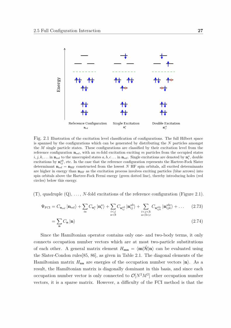
Fig. 2.1 Illustration of the excitation level classification of configurations. The full Hilbert spaceis spanned by the configurations which can be generated by distributing the N particles amongstthe M single particle states. These configurations are classified by their excitation level from thereference configuration nref , with an m-fold excitation exciting m particles from the occupied statesi, j, k, . . . in nref to the unoccupied states a, b, c . . . in nref . Single excitations are denoted by na
i , doubleexcitations by nab
ij , etc. In the case that the reference configuration represents the Hartree-Fock Slaterdeterminant nref = nHF constructed from the lowest N HF spin orbitals, all excited determinantsare higher in energy than nHF as the excitation process involves exciting particles (blue arrows) intospin orbitals above the Hartree-Fock Fermi energy (green dotted line), thereby introducing holes (redcircles) below this energy.
(T), quadruple (Q), . . . , N -fold excitations of the reference configuration (Figure 2.1).
ΨFCI = Cnref |nref⟩+∑ia
Cnai|na
i ⟩+∑i<ja<b
Cnabij|nab
ij ⟩+∑
i<j<ka<b<c
Cnabcijk|nabc
ijk⟩+ . . . (2.73)
=∑
nCn |n⟩ (2.74)
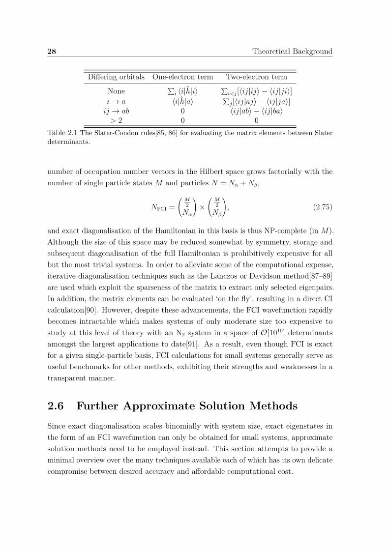
Since the Hamiltonian operator contains only one- and two-body terms, it onlyconnects occupation number vectors which are at most two-particle substitutionsof each other. A general matrix element Hmn = ⟨m|H|n⟩ can be evaluated usingthe Slater-Condon rules[85, 86], as given in Table 2.1. The diagonal elements of theHamiltonian matrix Hnn are energies of the occupation number vectors |n⟩. As aresult, the Hamiltonian matrix is diagonally dominant in this basis, and since eachoccupation number vector is only connected to O[N2M2] other occupation numbervectors, it is a sparse matrix. However, a difficulty of the FCI method is that the
28 Theoretical Background
Differing orbitals One-electron term Two-electron term
None ∑i ⟨i|h|i⟩
∑i<j[⟨ij|ij⟩ − ⟨ij|ji⟩]
i→ a ⟨i|h|a⟩ ∑j[⟨ij|aj⟩ − ⟨ij|ja⟩]
ij → ab 0 ⟨ij|ab⟩ − ⟨ij|ba⟩> 2 0 0
Table 2.1 The Slater-Condon rules[85, 86] for evaluating the matrix elements between Slaterdeterminants.
number of occupation number vectors in the Hilbert space grows factorially with thenumber of single particle states M and particles N = Nα +Nβ,
NFCI =(
M2Nα
)×(
M2Nβ
), (2.75)
and exact diagonalisation of the Hamiltonian in this basis is thus NP-complete (in M).Although the size of this space may be reduced somewhat by symmetry, storage andsubsequent diagonalisation of the full Hamiltonian is prohibitively expensive for allbut the most trivial systems. In order to alleviate some of the computational expense,iterative diagonalisation techniques such as the Lanczos or Davidson method[87–89]are used which exploit the sparseness of the matrix to extract only selected eigenpairs.In addition, the matrix elements can be evaluated ‘on the fly’, resulting in a direct CIcalculation[90]. However, despite these advancements, the FCI wavefunction rapidlybecomes intractable which makes systems of only moderate size too expensive tostudy at this level of theory with an N2 system in a space of O[1010] determinantsamongst the largest applications to date[91]. As a result, even though FCI is exactfor a given single-particle basis, FCI calculations for small systems generally serve asuseful benchmarks for other methods, exhibiting their strengths and weaknesses in atransparent manner.
2.6 Further Approximate Solution Methods
Since exact diagonalisation scales binomially with system size, exact eigenstates inthe form of an FCI wavefunction can only be obtained for small systems, approximatesolution methods need to be employed instead. This section attempts to provide aminimal overview over the many techniques available each of which has its own delicatecompromise between desired accuracy and affordable computational cost.
2.6 Further Approximate Solution Methods 29
Dynamical correlation can be captured by post Hartree-Fock methods, which startfrom the HF Slater determinant and its optimised HF orbitals and add dynamicalcorrelation onto the single configuration reference. One of the most economical postHF-methods is Møller-Plesset perturbation theory (MPx)[92] which partitions theHamiltonian into an exactly solvable reference Hamiltonian, chosen to be the Fockoperator, and a perturbing correction, the difference between the true Hamiltonianand the Fock operator. The associated energy and wavefunction of this Hamiltonianare expanded out as Taylor series and the terms can be solved for to give the x-thorder correction to the energy, whereby the HF state and energy represent the zero-order wavefunction and the sum of zero- and first-order corrections. By adding thesecond-order correction, the second-order Møller-Plesset (MP2) energy is obtained[37]
EMP2 = EHF +∑
a>b,i>j
| ⟨nHF|H|nabij ⟩ |2
ϵa + ϵb − ϵi − ϵj
, (2.76)
which provides surprisingly accurate, size-extensive, yet non-variational, correction atlow cost[93]. Higher order correction terms are costly, and the MP series does notconverge unconditionally[94]. Additionally, the dominance of the single determinantreference makes MP2 ill suited for systems with significant static correlation.
A further standard model which incorporates effects of correlation, mostly ofdynamical nature, is the Configuration Interaction (CI) method[95] which arisesnaturally from FCI ansatz by truncating the wavefunction expansion to a subset ofoccupation number vectors of the full N -electron Hilbert space. The cost limitations ofFCI are thus reduced by truncating its space at a given excitation level with respect to areference occupation number vector, typically the HF state. This results in a series of CImethods denoted by CIS, CISD, CISDT, CISDTQ . . . with a hierarchy of successivelymore accurate wavefunction by including up to single, double, triple, quadruple,. . . excitations of the reference determinant[96]. This truncation is variational, theFCI energy is approached monotonically from above and the FCI wavefunction isrecovered as the truncation level is increased to the N -th level. The advantage ofan iterative CI diagonalisation is that its cost scales polynomially with excitationlevel n as O[N2n+2]. It is interesting to note that if the HF determinant is used asreference occupation number vector the inclusion of only single-excitations has no effectdue to the zero Hamiltonian matrix elements connecting the HF occupation numbervector and its single excitations according to the Brillouin theorem[97, 98]. In general,lower order excited configurations are often more important than higher orders and forsingle-reference systems, where the reference configuration provides a good zero-order
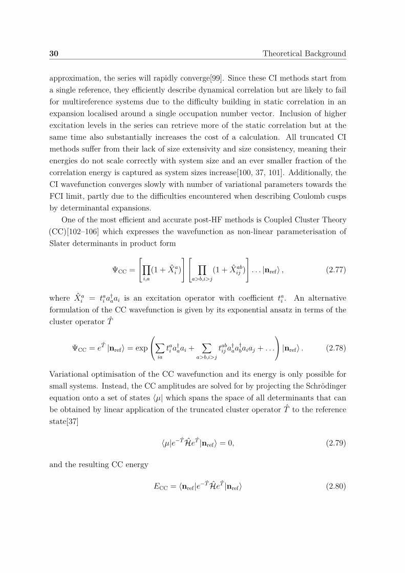
30 Theoretical Background
approximation, the series will rapidly converge[99]. Since these CI methods start froma single reference, they efficiently describe dynamical correlation but are likely to failfor multireference systems due to the difficulty building in static correlation in anexpansion localised around a single occupation number vector. Inclusion of higherexcitation levels in the series can retrieve more of the static correlation but at thesame time also substantially increases the cost of a calculation. All truncated CImethods suffer from their lack of size extensivity and size consistency, meaning theirenergies do not scale correctly with system size and an ever smaller fraction of thecorrelation energy is captured as system sizes increase[100, 37, 101]. Additionally, theCI wavefunction converges slowly with number of variational parameters towards theFCI limit, partly due to the difficulties encountered when describing Coulomb cuspsby determinantal expansions.
One of the most efficient and accurate post-HF methods is Coupled Cluster Theory(CC)[102–106] which expresses the wavefunction as non-linear parameterisation ofSlater determinants in product form
ΨCC =∏
i,a
(1 + Xai ) ∏
a>b,i>j
(1 + Xabij ) . . . |nref⟩ , (2.77)
where Xai = tai a
†aai is an excitation operator with coefficient tai . An alternative
formulation of the CC wavefunction is given by its exponential ansatz in terms of thecluster operator T
ΨCC = eT |nref⟩ = exp∑
ia
tai a†aai +
∑a>b,i>j
tabij a†aa†baiaj + . . .
|nref⟩ . (2.78)
Variational optimisation of the CC wavefunction and its energy is only possible forsmall systems. Instead, the CC amplitudes are solved for by projecting the Schrödingerequation onto a set of states ⟨µ| which spans the space of all determinants that canbe obtained by linear application of the truncated cluster operator T to the referencestate[37]
⟨µ|e−T HeT |nref⟩ = 0, (2.79)
and the resulting CC energy
ECC = ⟨nref |e−T HeT |nref⟩ (2.80)
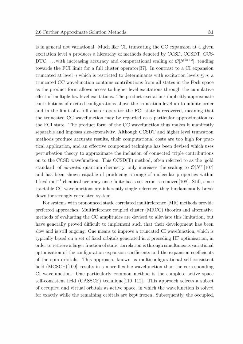
2.6 Further Approximate Solution Methods 31
is in general not variational. Much like CI, truncating the CC expansion at a givenexcitation level n produces a hierarchy of methods denoted by CCSD, CCSDT, CCS-DTC, . . . with increasing accuracy and computational scaling of O[N2n+2], tendingtowards the FCI limit for a full cluster operator[37]. In contrast to a CI expansiontruncated at level n which is restricted to determinants with excitation levels ≤ n, atruncated CC wavefunction contains contributions from all states in the Fock spaceas the product form allows access to higher level excitations through the cumulativeeffect of multiple low-level excitations. The product excitations implicitly approximatecontributions of excited configurations above the truncation level up to infinite orderand in the limit of a full cluster operator the FCI state is recovered, meaning thatthe truncated CC wavefunction may be regarded as a particular approximation tothe FCI state. The product form of the CC wavefunction thus makes it manifestlyseparable and imposes size-extensivity. Although CCSDT and higher level truncationmethods produce accurate results, their computational costs are too high for prac-tical application, and an effective compound technique has been devised which usesperturbation theory to approximate the inclusion of connected triple contributionson to the CCSD wavefunction. This CCSD(T) method, often referred to as the ‘goldstandard’ of ab-initio quantum chemistry, only increases the scaling to O[N7][107]and has been shown capable of producing a range of molecular properties within1 kcal mol−1 chemical accuracy once finite basis set error is removed[108]. Still, sincetractable CC wavefunctions are inherently single reference, they fundamentally breakdown for strongly correlated system.
For systems with pronounced static correlated multireference (MR) methods providepreferred approaches. Multireference coupled cluster (MRCC) theories and alternativemethods of evaluating the CC amplitudes are devised to alleviate this limitation, buthave generally proved difficult to implement such that their development has beenslow and is still ongoing. One means to improve a truncated CI wavefunction, which istypically based on a set of fixed orbitals generated in a preceding HF optimisation, inorder to retrieve a larger fraction of static correlation is through simultaneous variationaloptimisation of the configuration expansion coefficients and the expansion coefficientsof the spin orbitals. This approach, known as multiconfigurational self-consistentfield (MCSCF)[109], results in a more flexible wavefunction than the correspondingCI wavefunction. One particularly common method is the complete active spaceself-consistent field (CASSCF) technique[110–112]. This approach selects a subsetof occupied and virtual orbitals as active space, in which the wavefunction is solvedfor exactly while the remaining orbitals are kept frozen. Subsequently, the occupied,
32 Theoretical Background
active and virtual spaces are rotated to minimise the energy[113]. This two-stepcycle is repeated until convergence is achieved. This optimisation of the non-linearwavefunction parameterisation is more difficult and, in practice, MCSCF wavefunctionsare restricted to small determinant expansions which are adequate for the description ofstatic correlation but inadequate for the description of dynamical correlation. Dynamiccorrelation can be added on top of a MCSCF or CASSCF wavefunction by perturbationtheory (CASPT2)[114–116], a multireference CI expansion (MRCI or CASCI)[117–123]or CC theory (MRCC or CASCC)[124, 125] such as canonical transformation (CT)theory[126], an approximate scheme.
In principle all static and dynamic correlation can be captured by density functionaltheory (DFT) which is a density-based method. This approach is based on theHohenberg-Kohn theorem which states that the electron density uniquely determinesall ground state properties of a system and that a unique universal functional of theelectron density exists which can be used to find the exact electron density[24]. Themost commonly applied approach is the Kohn-Sham formalism which introduces anartificial non-interacting reference system with exactly the same electron density asthe true interacting system. The energy is thus written as functional of the electrondensity ρ and partitioned into several contributions[25]
E[ρ] = TS[ρ] +∫drρ(r)
(Vext(r) + 1
2Φ(r))
+ Exc[ρ], (2.81)
where TS[ρ] denotes the kinetic energy of the non-interacting reference system, Vext(r)the external potential, Φ(r) the classical Coulomb potential and Exc[ρ] the non-classicalexchange correlation energy. The description of electron correlation in DFT is thereforeentirely determined by the choice of the exchange-correlation functional. Unfortu-nately, the universal functional is unknown. Many approximate exchange-correlationfunctionals of various complexity have been designed. A simple proposal for definingExc[ρ] is the Local Density Approximation (LDA) which assumes the electron densityto be uniform at a local level. DFT may produce good results in some cases at littlemore computational cost than HF theory, or even lower costs with recent linear-scalingimplementations. However, each functional is limited in its applicability to only asubset of systems and DFT results have often been shown to be outside chemicalaccuracy compared to experimental data. Since the exact Exc[ρ] is unknown, currentDFT methods cannot capture all static and dynamic correlation and there is also noway of systematically improving a DFT result. It can be stated that DFT is ratherpoor at capturing static correlation[127].
2.7 Beyond Traditional Quantum Chemical Methods: Tensor Network StatesApproaches 33
2.7 Beyond Traditional Quantum Chemical Meth-ods: Tensor Network States Approaches
In addition, to conventional quantum chemical post-Hartree-Fock methods, progress inquantum information theory lead to the development of sophisticated approaches whichdecompose the full FCI tensor to obtain highly accurate and faithful representations ofthe FCI wavefunction.
2.7.1 Entanglement Entropy and Area Laws
The description of quantum many-body states in strongly correlated systems are centralto understanding a wealth of complex phenomena in condensed matter physics andquantum chemistry. A significant number of these systems are governed by localinteractions meaning interactions whose strength decays at least exponentially withdistance (beyond a distance cutoff). Naive numerical descriptions of such systemsrequire an intractably large number of parameters since the underlying Hilbert spacegrows exponentially with system size, specifically
dim(H) = O[dn] (2.82)
for a system of size n and local dimension d. As such, exact diagonalisation is henceNP-complete[128]. It has, however, emerged that ground states, and a number of otherphysical states of local Hamiltonians usually occupy a tiny submanifold of the Hilbertspace, also referred to as ‘natural corner of the Hilbert space’. States living in thistiny submanifold commonly satisfy an area law rooted in the locality of interactions.The latter not only implies a decay of two-body correlation functions but also strongerforms of locality which can be captured using concepts of entanglement in quantummany-body systems[53]. For this purpose, the von Neumann entanglement entropy isdefined[129, 130]
S(ρR) = −Tr[ρR log2 ρR], (2.83)
where ρR is the reduced density matrix of the quantum state ψR in the region R. S(ρR)represents a measure for the entanglement between the regionR and the complementaryregion R[131] which is, however, only meaningful for pure, that is non-degenerate,states. If the two regions are not entangled, S(ρR) = 0. Otherwise, the entropy will belarger, being bounded from above by its maximum value S(ρR) ≤ |R| log2(d) which
34 Theoretical Background
scales with the size |R| of the region R. For random states, this means that the entropyusually scales extensively with size S(ρR) = O[|R|][53]. It has emerged that groundstates, and a number of other physical states of local and gapped Hamiltonians satisfyan area law which states that the entanglement entropy S(ρR) for every region R obeys
S(ρR) ≤ O[∂|R|], (2.84)
where ρR is the reduced density matrix of the quantum state ψR in the region R and∂|R| is the perimeter of the region R[132, 133, 55]. Thus, the entanglement betweenthe region R and its complementary region R, as measured by the entanglemententropy, grows only like the boundary area of R and not extensively like its volume.This is a consequence of the finite correlation length[134, 135] which means thatonly subregions in the immediate vicinity of the boundary area are correlated withsubregions on the other side of the boundary. Such area laws have been proven for allgapped Hamiltonians in 1D[136–138] and it is expected that gapped local systems inhigher dimensions[132] also satisfy an area law, supported by numerical examples andtheoretical arguments[139], although a general proof for arbitrary dimensions is stilllacking. Yet, critical quantum systems with long-ranged interactions and a spectral gapshrinking to zero with system size violate area laws, albeit their logarithmic correctionsto the area law are typically small[132, 140]. In contrast to random quantum states,ground and other physical states satisfying area laws or showing only small violationsthereof display thus much less entanglement which effectively quantifies the relevantnumber of degrees of freedom that have to be taken into account[55]. This suggeststhat the exact FCI wavefunction of quantum many-body states may be efficientlyapproximated by alternative more compact representations.
2.7.2 Decomposing the FCI Wavefunction Ansatz
Any arbitrary wavefunction like eigenstates of the Hamiltonian which lives in a Hilbertspace of (Cd)⊗M can be parameterised as
|ΨFCI⟩ =d∑
n1,n2,...,nM
Cn1...nM|n1⟩ ⊗ |n2⟩ ⊗ . . .⊗ |nM⟩ (2.85)
=d∑
n1,n2,...,nM
Cn1...nM|n1n2 . . . nM⟩ , (2.86)
where d denotes the dimension of the local Hilbert space of the single-particle basisstates |ni⟩ = |1⟩ , |0⟩. The coefficients Cn1...nM
are part of the full FCI tensor C,
2.7 Beyond Traditional Quantum Chemical Methods: Tensor Network StatesApproaches 35
a rank M tensor with O[dM ] coefficients. Whilst this FCI ansatz describes |ΨFCI⟩exactly within a given single-particle basis, it grows exponentially with system sizeand is therefore a computationally inefficient description for growing system sizes.Efficient wavefunction ansatzes are therefore needed which reduce the complexity in therepresentation of |ΨFCI⟩ and allow for efficient computational treatments. The existenceof area laws, and hence, the reduced amount of entanglement which effectively quantifiesthe relevant number of degrees of freedom, suggests that physical quantum many-bodystates which usually live in the small ‘natural corner’ of the exponentially large Hilbertspace may be faithfully described by an efficient parameterisation, although there maybe limitations to this intuitive expectation for higher dimensional systems[141]. Thisconcept lies at the core of Tensor Network States (TNS) parameterisations[53–55, 142]and their powerful numerical algorithms such as the Density Matrix RenormalisationGroup approach (DMRG)[56, 143, 144] and its higher-dimensional analogues[55] whichvariationally optimise different classes of TNS[53–55, 142]. Whilst a vast array ofdifferent TNS exists, the following theoretical descriptions will focus on those whichare most relevant to this thesis.
2.7.3 Tensor Network States in One Dimension: MatrixProduct States
Ground states of gapped local Hamiltonians in one dimension are well described byMatrix Product States (MPS)[145] since both fulfil the area law. According to thelatter, the entanglement entropy, which represents a measure for the entanglementbetween a region R and its compliment, scales as the boundary of this region ∂|R|which suggests that the entanglement between R and the remainder of the systemis concentrated around the boundary between the two regions. This concept lies atthe heart of the MPS ansatz for quantum many-body systems. For the purpose ofdescribing the MPS ansatz, a one-dimensional fermionic Hubbard model with M
2 latticesites is considered where the local Hilbert space of each lattice site comprises the statesns = |00⟩ , |↑ 0⟩ , |0 ↓⟩ , |↑↓⟩. In order to construct an MPS for this one-dimensionalsystem, each site is considered to be composed of two virtual subsystems, one on theleft and one on the right (Figure 2.2). Furthermore, each of these virtual subsystems ispart of a product state of maximally entangled pairs connecting neighbouring sites,that is the right virtual subsystem of site s and the left virtual subsystem of site s+ 1
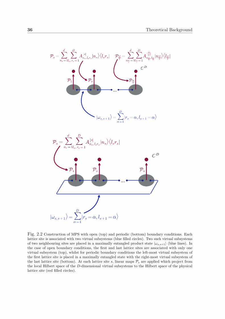
36 Theoretical Background
Fig. 2.2 Construction of MPS with open (top) and periodic (bottom) boundary conditions. Eachlattice site is associated with two virtual subsystems (blue filled circles). Two such virtual subsystemsof two neighbouring sites are placed in a maximally entangled product state |ωs,s+1⟩ (blue lines). Inthe case of open boundary conditions, the first and last lattice sites are associated with only onevirtual subsystem (top), whilst for periodic boundary conditions the left-most virtual subsystem ofthe first lattice site is placed in a maximally entangled state with the right-most virtual subsystem ofthe last lattice site (bottom). At each lattice site s, linear maps Ps are applied which project fromthe local Hilbert space of the D-dimensional virtual subsystems to the Hilbert space of the physicallattice site (red filled circles).
2.7 Beyond Traditional Quantum Chemical Methods: Tensor Network StatesApproaches 37
are in a maximally entangled state such that the state of this pair is given by
|ωs,s+1⟩ =D∑
α=1|rs = α, ls+1 = α⟩ , (2.87)
where D represents the Hilbert space of the virtual subsystems. For systems withperiodic boundary conditions the left-most subsystem of the first site is maximallyentangled with the right-most subsystem of the last M
2 -th site. In the case of openboundary conditions, the first site has only a right virtual subsystem and the lastsite only a left virtual system. The pure state |ωs,s+1⟩ is maximally entangled in thesense that the entanglement entropy of each subsystem assumes the maximum valueln(D)[53, 146]. On this system, linear maps Ps : CD ⊗ CD → Cd at each of thes = 1, . . . , M
2 lattice sites are applied which project from the Hilbert space of twoD-dimensional subsystems to the Hilbert space of the corresponding physical latticesite. The map for each lattice site s can be written as
Ps =d∑
ns=1
D∑ls,rs=1
A[s]ns;lsrs
|ns⟩ ⟨lsrs| , (2.88)
where A[s]ns;lsrs
denotes a rank-3 tensor of the lattice site s whose physical Hilbert spaceis of dimension d. For open boundary conditions the linear maps of the s = 1 ands = M
2 sites are formulated in terms of rank-2 tensors
P1 =d∑
n1=1
D∑r1=1
A[1]n1;r1 |n1⟩ ⟨r1| , PM
2=
d∑n M
2=1
D∑l M
2=1A
[ M2 ]
n M2
;l M2
|nM2⟩ ⟨lM
2| . (2.89)
Thus, for a system with open boundary conditions, the resulting state vector isparameterised as
|ΨOBC⟩ =
M2⊗
s=1Ps
M2 −1⊗s=1|ωs,s+1⟩
(2.90)
=∑
n1,n2,...,n M2
Tr[A[1]n1A
[2]n2 . . . A
[ M2 ]
n M2
] |n1n2 . . . nM2⟩ (2.91)
=∑
n1,n2,...,n M2
DαDβ ...Dω∑αβ...ω=1
A[1]n1;αA
[2]n2;αβ . . . A
[ M2 ]
n M2
;ω |n1n2 . . . nM2⟩ , (2.92)
38 Theoretical Background
where A[s]ns
represents the matrix (or vector for the first and last lattice sites) withentries A[s]
ns;αβ ≡ A[s]ns;lsrs
. Each projection onto a configuration |n1n2 . . . nM2⟩ is given
by a product of matrices, hence, the name Matrix Product State (MPS). In principle,the bond dimension, that is the dimensions of the matrices, may also vary across thesystem (Dα = Dβ = . . . = Dω). Similarly, a state vector in a system with periodicboundary conditions can be written as
|ΨPBC⟩ =
M2⊗
s=1Ps
M2⊗
s=1|ωs,s+1⟩
(2.93)
=∑
n1,n2,...,n M2
Tr[A[1]n1A
[2]n2 . . . A
[ M2 ]
n M2
] |n1n2 . . . nM2⟩ (2.94)
=∑
n1,n2,...,n M2
DαDβDγ ...Dω∑αβγ...ω=1
A[1]n1;αβA
[2]n2;βγ . . . A
[ M2 ]
n M2
;ωα |n1n2 . . . nM2⟩ , (2.95)
with |ωM2 , M
2 +1⟩ ≡ |ωM2 ,1⟩.
2.7.4 The Area Law and Efficient Approximability
It can be shown that for any subset of L consecutive lattice sites the entanglemententropy for a matrix product state is bounded from above by S(ρL) ≤ Smax = 2 log2 D,which implies that MPS satisfy an area law by construction[53, 147]. Not only is theentanglement scaling of both MPS and ground states of gapped local Hamiltoniansthe same, but also an even stronger statement can be proven: all states which fulfil anarea law, like ground states of gapped Hamiltonian[136, 132], as well as states whichviolate the area law at most logarithmically, such as critical (gapless) one-dimensionalsystems, can be efficiently approximated by an MPS[136, 148]. Strictly speaking, thisstatement follows from an area law of the Rényi entropy SR(ρR) = 1
1−αlog2(Tr[ρα
R])(α ≥ 0)[149] which in the limit of α → 1 reduces to the von Neumann entropy (forsituations where a detailed understanding has been reached, this has not been found tomake a difference[53]). Specifically, for any local Hamiltonian describing a system withM2 sites whose ground state Ψexact violates the area law at most logarithmically, an
MPS |ΨMPS(D)⟩ with bond dimension D can be found which efficiently approximatedΨexact up to an error
|| |Ψexact⟩ − |ΨMPS(D)⟩ ||2 ≤ ϵ. (2.96)
2.7 Beyond Traditional Quantum Chemical Methods: Tensor Network StatesApproaches 39
It can be proven rigorously, that in order to achieve a desired accuracy ϵ, the requiredbond dimension D scales polynomially in M
2 and 1ϵ[150, 53]. It is worth noting that
this MPS representation |ΨMPS⟩ can be obtained numerically in a time that growspolynomial with system size for ground states of gapped local Hamiltonians[151]. Owingto these properties the MPS ansatz provides an extremely accurate approximationto natural states of physical systems already at low values of D. At the same time,the O[d
M2 ] complexity of the exact FCI wavefunction ansatz is drastically reduced
to the O[M2 dD
2] complexity of an MPS wavefunction of bond dimension D[53]. Thelatter only scales linearly in system size M
2 for constant D as opposed to exponentiallyin M
2 . Whilst D = 1 yields a product state, a variant of a mean-field approach,with increasing D a larger region of the full Hilbert space is spanned by the MPSansatz which usually increases the quality of |ΨMPS⟩ as approximation to naturalstates. Allowing D to grow exponentially towards the middle of the system, (1 ×d), (d× d2), . . . , (d
M2 −1 × d
M2 ), (d
M2 × d
M2 −1) . . . , (d2 × d), (d× 1) (for open boundary
conditions), the MPS ansatz will eventually span the full Hilbert space[144, 152]. Yet,MPS are only able to describe correlation functions which decay exponentially withdistance, meaning that the correlation length of matrix product states is always finite.Thus, they cannot represent algebraically decaying correlation functions, implyingthat they cannot reproduce properties of critical or scale-invariant systems where thecorrelation length is known to diverge[54, 153]. Nevertheless, for sufficiently large bonddimensions, MPS can also efficiently approximate states with algebraically decayingcorrelation functions but other tensor network ansatzes like the Multiscale EntanglementRenormalisation Ansatz (MERA)[154] display a more favourable scaling in system sizein these cases[53, 142].
Although |ΨMPS⟩ is an efficient description of the relevant quantum many-bodystate |Ψ⟩, this is not sufficient for the MPS parameterisation to represent an effi-cient variational ansatz. Crucially, |ΨMPS⟩ also needs to allow for efficient extractionof information, usually in the form of correlation functions, expectation values ofobservables, ⟨Ψ|O|Ψ⟩, etc. For an MPS ansatz, these quantities can be efficiently eval-uated in O[M
2 d2D3] and O[M
2 d2D5] time for open and periodic boundary conditions,
respectively[55].
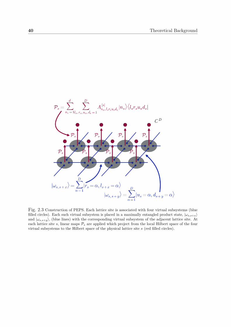
40 Theoretical Background
Fig. 2.3 Construction of PEPS. Each lattice site is associated with four virtual subsystems (bluefilled circles). Each such virtual subsystem is placed in a maximally entangled product state, |ωs,s+x⟩and |ωs,s+y⟩, (blue lines) with the corresponding virtual subsystem of the adjacent lattice site. Ateach lattice site s, linear maps Ps are applied which project from the local Hilbert space of the fourvirtual subsystems to the Hilbert space of the physical lattice site s (red filled circles).

2.7 Beyond Traditional Quantum Chemical Methods: Tensor Network StatesApproaches 41
2.7.5 Tensor Network States in Two Dimensions: ProjectedEntangled Pair States
The concept of tensor network states is not confined to one dimension but a largevariety of tensor network states, also in higher dimensional systems, exists. A naturalgeneralisation of Matrix Product States to higher-dimensional systems are ProjectedEntangled Pair States (PEPS)[53–55, 142, 155] which can be constructed in the sameway as MPS by distributing maximally entangled states between neighbouring sitesand on each site and applying linear maps from the virtual space of subsystems tothe physical Hilbert space. For concreteness, a two-dimensional square lattice withperiodic boundary conditions is considered. Each site of this lattice is thought tobe composed of four virtual D-dimensional subsystems each of which is placed ina maximally entangled state with the corresponding subsystem of the adjacent site(Figure 2.3). Thus, labelling the states of the left, right, up and down virtual systemat lattice site s by ls, rs, us and ds, respectively, the maximally entangle pairs betweentwo sites which are horizontally (+x) and vertically (+y) displaced by one unit giverise to the maximally entangled states
|ωs,s+x⟩ =D∑
α=1|rs = α, ls+x = α⟩ |ωs,s+y⟩ =
D∑α=1|us = α, ds+y = α⟩ , (2.97)
respectively. At each site of the system, linear maps Ps : CD ⊗ CD ⊗ CD ⊗ CD → Cd
are applied which project from the Hilbert space of the four virtual subsystems at sites to the physical Hilbert space of the lattice site. These local linear maps are given by
Ps =d∑
ns=1
D∑ls,rs,us,rs=1
A[s]ns;lsrsusds
|ns⟩ ⟨lsrsusds| , (2.98)
such that the resulting PEPS state vector can be written as
|ΨPEPS⟩ =
M2⊗
s=1Ps
M2⊗
s=1|ωs,s+x⟩ ⊗ |ωs,s+y⟩
(2.99)
=∑
n1n2...n M2
Tr[A[1]n1A
[2]n2 . . . A
[ M2 ]
n M2
] |n1n2 . . . nM2⟩ (2.100)
=∑
n1n2...n M2
DαDβDγDδ...Dω∑αβγδ...ω
A[1]n1;αβγωA
[2]n2;δαλη . . . A
[ M2 ]
n M2
;ϵζων |n1n2 . . . nM2⟩ , (2.101)
42 Theoretical Background
where A[s]ns
denotes the rank-4 tensor with entries A[s]ns;αβγδ ≡ A
[s]ns;lsrsusds
. Likewise, aPEPS wavefunction for systems with open boundary conditions can be constructedwith modified linear maps for the lattice sites at the edges which are obtained byreplacing the rank-5 tensor for a general lattice site by rank-4 tensors for the edges andrank-3 tensors for the corners. More generally, the outlined construction of a PEPSstate can be generalised to any lattice shape and dimension[55].
Given their analogy to MPS, PEPS share many properties with their one dimensionalcounterparts. Hence, they also obey area laws by construction since the entanglemententropy of a region R with its complement is bounded from above by O[Nbonds log2 D]where Nbonds denotes the number of bonds that the boundary ∂|R| covers[132, 53]. Byanalogy to MPS, any state can be written as a PEPS provided the bond dimensionD is large enough with the full Hilbert space being covered if D grows exponentiallyin system size[53, 54]. Moreover, PEPS can efficiently approximate ground states ofgapped local Hamiltonian provided that the density of states grows at most polynomiallywith energy[156, 157]. Unlike for MPS, a strong statement on how well PEPS canapproximate general states is lacking and ground states of non-local Hamiltoniansexist which satisfy the area law but cannot be represented efficiently by PEPS[141].Yet, numerical evidence[158] suggests that PEPS with a reasonably small and finiteD approximate low-energy states of two-dimensional quantum many-body systemswell[54]. At finite temperatures, they have also been shown to efficiently approximatethermal states[157, 159]. In contrast to MPS, PEPS can describe algebraically decayingcorrelations, a typical characteristic of critical points[148]. In principle, they aretherefore suitable to describe both, states with finite and infinite correlation lengths,that is gapped phases, as well as critical states.
Still, the extraction of information from a PEPS state is computationally muchharder. Contrary to MPS, PEPS cannot be contracted exactly in an efficient manner.Irrespective of the contraction order, the contraction will at some point involve anobject with a number of indices that is proportional to
√M2 , and hence an exponential
number of parameters. The contraction is therefore an exponentially hard problemand always requires O[exp(M
2 )] time[54]. Strictly speaking, from the point of viewof computationally complexity, the contraction of a PEPS network is contained withthe complexity class ♯P [160]. Yet, this obstacle can be overcome with approximatecontraction techniques which involve small and ideally controlled errors. One of theseapproximate contraction schemes[155] works through the network and contracts eachcolumn with the subsequent one while the bond dimensions of the new tensors areapproximated by αD2 for some α. By iterating this procedure column by column,
2.7 Beyond Traditional Quantum Chemical Methods: Tensor Network StatesApproaches 43
the whole network is contracted whilst the size of the tensors always stays bounded.Although this represents an efficient approximate contraction scheme for PEPS, thescaling with D is much less favourable than in one dimension. The most simplestapproaches display O[D12] scaling which can be improved down to O[D8]. Thisapproximate contraction method is therefore limited to much smaller bond dimensionsD in comparison the contraction of an MPS ansatz. The approximation is typically veryaccurate provided that the system is short-range correlated and the introduced error iswell controlled. In fact, the accuracy of the approach is rather limited by the bonddimension D that is needed for a good approximation to the ground state. Anotherapproximate contraction scheme[161–163] based on renormalisation ideas approximatesblock of tensors by one tensor whose bond dimension is appropriately truncated. Thisapproach relies on approximations to the environment, i.e. the remaining network.Whilst the introduced errors are less controlled and the accuracy of the approximationsare worse, the scaling in D is more favourable and allows for larger D and thuspotentially better approximations to the ground state[142].
2.7.6 Optimisation of MPS, PEPS, ...
Variationally finding the best description of the ground state in terms of a tensornetwork is equivalent to minimising
min|Ψ⟩∈TNS family
⟨Ψ|H|Ψ⟩⟨Ψ|Ψ⟩ , (2.102)
or using a Lagrange multiplier λ to ensure normalisation
min|Ψ⟩∈TNS family
(⟨Ψ|H|Ψ⟩ − λ ⟨Ψ|Ψ⟩), (2.103)
where |Ψ⟩ ∈ TNS family implies that |Ψ⟩ is parameterised as one of the class of tensornetworks states such as MPS, PEPS, . . . Since the simultaneous optimisation of allparameters amounts to a highly non-linear and non-convex global optimisation, thisminimisation problem is broken down into a sequence of linear optimisations of thetensors
A[s]
of the TNS. To this end, starting from a randomly chosen tensor at site
k, the energy is minimised with respect to A[k], whilst all other tensorsA[s]
, s = k,
are held fixed
E[k] := ⟨Ψ|H|Ψ⟩⟨Ψ|Ψ⟩ = ⟨A
[k]|K1|A[k]⟩⟨A[k]|K2|A[k]⟩
, (2.104)
44 Theoretical Background
where K1 and K2 represent the kernels of the respective quadratic forms and |A[k]⟩denotes the vectorised form of the rank-n tensor A[s]
ns;αβ... with the n indices (ns, α, β, . . .)combined into a single one. In fact, the solution to this quadratic and convex optimisa-tion problem is given by the eigenvalue problem K1 |A[k]⟩ = E[k]K2 |A[k]⟩[142, 164, 165].In this way, by iteratively sweeping back and forth through the system and sequentiallyoptimising the tensor at each site, convergence onto a state with low energy is reached.
If this minimisation is performed for an MPS with open boundary conditions, noth-ing but the extremely successful Density Matrix Renormalisation Group (DMRG)[56,166, 167] is recovered. Originally, DMRG was invented by White in the field of con-densed matter theory. Within this context, DMRG was historically formulated as arenormalisation algorithm based on keeping the states that are most relevant for theentanglement of the system and framed in the language of analysis of reduced densityoperators over subsystems of the chain. Later Östlund and Rommer discovered itsunderlying variational class, the MPS[168, 169], implying that DMRG can be reformu-lated as a variational method within the ansatz space of D-dimensional MPS. Althoughsuch a variational minimisation of an MPS can get stuck in principle[164, 165], theprocedure works extremely well in practice and generally converges onto the lowestenergy |ΨMPS⟩, essentially up to machine precision[153, 144, 55] when consideringMPS for one dimensional systems. For MPS in particular, many approaches havebeen devised in order to arrive at an efficient algorithmic realisation of the basicoptimisation method and improve upon it. Firstly, the gauge degrees of freedom of thematrix product state are exploited to arrive at an MPS representation in its canonicalform which is crucial in practical implementations in order to avoid ill-conditionedmatrices[53, 170, 144]. Secondly, each step along the sweep can involve optimising thetensors of pairs of sites, a so-called double variational site, which improves convergenceand a better control of the error[53]. In addition to MPS, this variational minimisationapproach has also been successfully applied to finite PEPS[155, 55], as well as TreeTensor Networks (TTN)[171, 172] and MERA[173].
Beyond variational optimisation, tensor network state wavefunctions can also befound with imaginary time evolution approaches whereby an initial state is evolved inimaginary time with the Hamiltonian of interest
|Ψτ ⟩ = limτ→∞
e−τH |Ψ0⟩||e−τH |Ψ0⟩ ||
, (2.105)
which results in a projection onto the ground state in the limit of τ → ∞. A largevariety of such imaginary time evolution methods for obtaining ground states exist,
2.7 Beyond Traditional Quantum Chemical Methods: Tensor Network StatesApproaches 45
including variants of the time-evolving block decimation (TEBD) approach[174–176],as well as techniques based on the time-dependent variational principle[177] andconcatenated tensor networks[178]. Even though state-of-the-art PEPS optimisationsrely on imaginary time evolution[158, 161, 179, 55] whose long imaginary time limit isrealised by applying small time steps δτ with a Trotter-Suzuki decomposition of theimaginary time operator, the considerable computational cost associated with a PEPSwavefunction means that ground state optimisations are more challenging in comparisonto their MPS analogous. In practice, additional approximations have to be introducedwhereby the PEPS bond dimensions are truncated in an approximate way after eachtime step. The truncation can be achieved with a number of different schemes[161,158, 179, 155] each of which provides its own detailed balance between accuracy andefficiency and arriving at an efficient PEPS optimisations with a good compromisebetween their competing demands still remains challenging[54]. By implementingreal time[167, 176] instead of imaginary time evolution these approaches also provideinsights into the non-equilibrium dynamics of strongly correlated quantum systems.Thus, thermal states[174, 159] are accessible, as well as time-dependent correlationfunctions and expectation values of the form ⟨Ψ|eitHOe−iHt|Ψ⟩ to study system farfrom equilibrium[176, 180, 181, 53].
Moreover, bulk systems can be studied without finite size and boundary errors withinfinite MPS (iMPS) and infinite PEPS (iPEPS)[158, 182], formulations of MPS andPEPS in the thermodynamic limit (possibly with a broken symmetry with finite period),where a finite unit cell of tensors is repeated through the infinite lattice such as in theiDMRG[183, 184] and iTEBD[158, 185] methods. Furthermore, in the case of tensornetwork classes such as MPS or PEPS, convergence with respect to the bond dimensionD has to be established in order to arrive at the true ground state energy in the infiniteD limit. Since increasing the bond dimension D results in tensor networks spanningsubspaces of the full Hilbert space which are simultaneously supersets of the previousones, the quality of the approximate tensor network state improves monotonically. Inthe limit D → ∞ the exact tensor network state representation of |Ψ⟩ is recoveredwhich allows for reliable extrapolations of the energy to the FCI limit[186–189].
Even though all of the approaches outlined above have been successfully appliedto MPS and PEPS, the latter class of tensor networks displays a worse scaling inbond dimensions D, and thus a higher computational cost, than their one dimensionalanalogues and are therefore typically restricted to smaller values of D in practicalapplication. For this reason, methods with PEPS in two dimensions often achieveworse accuracy than DMRG calculations using MPS as wavefunction ansatz whereby

46 Theoretical Background
the two dimensional system is mapped onto a one dimensional system with long-rangedinteractions. Reasonable system sizes for PEPS are therefore still roughly the same asthose which can be treated with two dimensional DMRG approaches[190, 191].
Chapter 3
Zero-temperature Ground StateQuantum Monte Carlo Methods
An alternative approach for solving the Schrödinger equation comes from QuantumMonte Carlo (QMC) methods [192–194, 50, 51, 195] which are a group of accurateand versatile stochastic techniques for treating quantum many-body systems. Theseapproaches represent efficient methods to evaluate complex integrals in the high dimen-sional space of quantum many-particle systems by sampling the integrand statisticallyand averaging the sampled values. Regardless of the dimensionality, the statisticalerror in the estimated integral decreases as N−
12
MC with the number of samples NMC, aconsequence of the central limit theorem. There are many different QMC methods ofwhich the two most commonly applied classes are Variational Quantum Monte Carlo(VMC) and various Projector Quantum Monte Carlo (PMC) methods. These QMCmethods can equally well be used for finite discrete Hilbert spaces, infinite continuousHilbert spaces or even for spaces with both continuous and discrete degrees of freedom.In the following, notation appropriate for discrete spaces (sums, matrices, etc.) willbe used interchangeably with notation appropriate for continuous spaces (integrals,integral kernels etc.).
3.1 Variational Quantum Monte Carlo Approaches
Typical VMC methods [50, 167, 51] combine the variational principle with Monte Carloevaluation of integrals by rewriting the expectation value of any general Hermitianoperator O such as the Hamiltonian H with respect to a trial wavefunction |ΨT⟩.Hence, by making use of the resolution of the identity I = ∑
n |n⟩ ⟨n| the variational
48 Zero-temperature Ground State Quantum Monte Carlo Methods
energy can be expressed as
EVMC = ⟨ΨT|H|ΨT⟩⟨ΨT|ΨT⟩
(3.1)
=∑
n ⟨ΨT|n⟩ ⟨n|H|ΨT⟩∑n ⟨ΨT|n⟩ ⟨n|ΨT⟩
(3.2)
=
∑n
⟨ΨT|n⟩ ⟨n|ΨT⟩ ⟨n|H|ΨT⟩⟨n|ΨT⟩
P [⟨n|ΨG⟩]P [⟨n|ΨG⟩]
(∑n
⟨ΨT|n⟩ ⟨n|ΨT⟩P [⟨n|ΨG⟩]
P [⟨n|ΨG⟩])−1
(3.3)
=∑
n EL(n) ⟨ΨT|n⟩⟨n|ΨT⟩P [⟨n|ΨG⟩]
P [⟨n|ΨG⟩]∑n⟨ΨT|n⟩⟨n|ΨT⟩
P [⟨n|ΨG⟩]P [⟨n|ΨG⟩]
(3.4)
≡
[1
NMC
∑NMCk=1 EL(nk) ⟨ΨT|nk⟩⟨nk|ΨT⟩
P [⟨nk|ΨG⟩]
]P [⟨n|ΨG⟩][
1NMC
∑NMCk=1
⟨ΨT|nk⟩⟨nk|ΨT⟩P [⟨nk|ΨG⟩]
]P [⟨n|ΨG⟩]
(3.5)
≡
⟨EL(nk) ⟨ΨT|nk⟩⟨nk|ΨT⟩
P [⟨nk|ΨG⟩]
⟩P [⟨n|ΨG⟩]⟨
⟨ΨT|nk⟩⟨nk|ΨT⟩P [⟨nk|ΨG⟩]
⟩P [⟨n|ΨG⟩]
, (3.6)
where the local energy EL(n) = ⟨n|H|ΨT⟩⟨n|ΨT⟩
has been introduced. The form of |ΨT⟩needs to be such that the local energy EL(n) is efficiently computable, typically inO[N3] time or even better. The notation in the last two lines indicates that the fulldeterministic sums over all states n in the Hilbert space are stochastically evaluatedby drawing NMC samples of the appropriately reweighted local energy EL(n) from thenormalised probability distribution P [⟨n|ΨG⟩] which is a suitable function of a guidingwavefunction |ΨG⟩, such as the most commonly applied probability density
P [⟨n|ΨG⟩] = | ⟨n|ΨG⟩ |2∑m | ⟨m|ΨG⟩ |2
. (3.7)
A well chosen function as probability density can significantly reduce the statisticalerror in the MC estimate [196–198], a process which is also referred to as importancesampling. In general, the requirement on |ΨG⟩ is such that the probability densityassumes a non-zero value P [⟨n|ΨG⟩] = 0 if the exact wavefunction |ΨE⟩ has ⟨n|ΨE⟩ = 0.Algorithmically, this sampling process is often realised using the Metropolis-Hastingsalgorithm [199, 200] which generates a sequence of configurations n distributedaccording to the desired probability P [⟨n|ΨG⟩]. Since the estimate of EVMC is evaluatedas the mean of the random variable EL(n) over the visited configurations, its value
3.1 Variational Quantum Monte Carlo Approaches 49
depends only on the trial wavefunction. Yet, the statistical error in this estimatedepends on both ΨT and ΨG. Although the trial and guiding wavefunction assumea different role, they are usually chosen to be the same function ΨG = ΨT. In somecircumstances, it might be beneficial to choose ΨG = ΨT. Reasons for such a choiceinclude cases when ΨT needs to be sparse for efficient evaluation of local estimatorsor when the variance in estimates of expectation values needs to be reduced. Thisapproach is very general and can be extended to any general Hermitian operator Oand its estimator ⟨O⟩, whereby the local energy is replaced by the corresponding localestimator that is analogously defined by
OL(n) = ⟨n|O|ΨT⟩⟨n|ΨT⟩
. (3.8)
An important characteristic of the probability distribution in Eq. 3.7 in the casethat ΨG = ΨT is the zero-variance property[201]. In the limit that the trial wavefunctionΨT tends towards the exact eigenstate ΨE of the Hamiltonian H, H |ΨT⟩ = EE |ΨT⟩,the local energy EL(n) is constant
EL(n) = ⟨n|H|ΨT⟩⟨n|ΨT⟩
= EE⟨n|ΨT⟩⟨n|ΨT⟩
= EE. (3.9)
and therefore independent of n. The estimator EVMC therefore coincides with the exacteigenvalue EE and its statistical error vanishes, as the variance
σ2(H) = ⟨ΨT|(H − EVMC)2|ΨT⟩⟨ΨT|ΨT⟩
= 0. (3.10)
in EL(n) is zero in the limit that |ΨT⟩ = |ΨE⟩. The energy estimator EVMC is thusalso referred to as zero-variance estimator. Likewise, expectation values of operatorsthat commute with the Hamiltonian also represent zero-variance estimators.
A typical trial wavefunction |ΨT⟩ is written in form of a Slater-Jastrow function[202,203]
|ΨT⟩ = J∑
ndnD
αnD
βn, (3.11)
where Dαn denotes a Slater determinant constructed from α spin orbitals and the
linear combination of Slater determinants determines the 3N − 1 nodal surface of the
50 Zero-temperature Ground State Quantum Monte Carlo Methods
wavefunction. The correlating Jastrow factor is given by
J = exp (f(r,p)) (3.12)
where f(r,p) consists of a set of functions which explicitly depend on the many inter-particle distances and thereby includes the cusp conditions but does not augment theoriginal nodal surface of the Slater determinants. The accuracy of the trial wavefunctionis increased by variational optimisation of the parameters p in |ΨT(p)⟩ by minimisingthe VMC energy EVMC(p) of the trial wavefunction or the variance σ2(H,p) in the localenergy EL(n)[204]. Due to the variational principle, the energy EVMC(p) will always bean upper bound to the true energy EE, but without knowledge of the exact eigenstate,it is hard to judge how accurate the variational approximation is. In contrast, thesmallest possible variance in EL(n), which is equal to zero, is known a priori andthus a good criterion for the accuracy of a trial wavefunction. Variance minimisationmethods [205–207] define a cost function that represents a linear combination of energyand variance each of which can be reweighted or unweighted
C[p] = ceEVMC(p) + cvσ2(H,p) + cewEVMC(p)w + cvwσ
2(H,p)w, (3.13)
where ce, cv, cew and cvw determine the relative weight of each cost. In this context,weighted refers to changing the relative weight of each configuration by a factor P [⟨n|Ψ′
T⟩]P [⟨n|ΨT⟩]
based on the changes of the trial wavefunction to account for changes in the probabilitydistribution. Minimisation of this cost function with any suitable algorithm locates theoptimal parameters. Current state-of-the-art wavefunction optimisation methods [208]are the Stochastic Reconfiguration (SR) [209–213] and Linear Method (LM) [214–217]which can treat large numbers of non-linear wavefunction parameters so as to minimisethe energy of the trial wavefunction. Both methods optimise the trial wavefunctionin a subspace Ω of the full Hilbert space which is the tangent space spanned by thewavefunction |ΨT(p)⟩ and its first derivatives with respect to the variational parameters
Ω = span(|Ψ0
T⟩ , |Ψ1T⟩ , |Ψ2
T⟩ , . . .)
(3.14)
where |Ψ0T⟩ ≡ |ΨT⟩ and |Ψi
T⟩ ≡∂|ΨT⟩
∂pifor i > 0. The SR method can be regarded
as approximate imaginary time evolution since it repeatedly applies the operatorT = I − τH, the first order expansion of the imaginary time evolution operatore−τH, where τ is a small number. The result of each operation with T on |ΨT⟩ isprojected into the subspace Ω to obtain a new wavefunction expanded in this subspace,

3.2 Projector Quantum Monte Carlo Approaches 51
|Ψ′T⟩ = ∑
i xi |ΨiT⟩. The expansion coefficients xi can be found by solving the system
of linear equations
⟨ΨiT|(I − τH)|ΨT⟩ =
∑j
⟨ΨiT|Ψ
jT⟩xj. (3.15)
The improved parameters are obtained p′i = pi + xi
x0, after which the subspace Ω is
redefined for the new improved wavefunction. This procedure is repeated until theenergy of the wavefunction has converged. An alternative method which optimises thewavefunction in the same subspace Ω is the Linear Method (LM) which can be viewedas an approximate Newton method with a built in stabilisation. Instead of imaginarytime propagation, the LM method optimises |ΨT⟩ in the subspace Ω by finding thelowest energy eigenstate x in Ω determined by the generalised eigenvalue problem
∑j
⟨ΨiT|H|Ψ
jT⟩xj = E
∑k
⟨ΨiT|Ψk
T⟩xk. (3.16)
After solving this generalised eigenvalue problem, the variables p are updated in thesame manner as in the SR method. If the changes to the parameters are too large,they become unphysical and need to be scaled down by a line search or rotated andscaled down by adding a diagonal shift. Efficient techniques have been developed toincrease the efficiency of the SR and LM method and their capability of treating largenumbers of parameters [208].
3.2 Projector Quantum Monte Carlo Approaches
An improvement to the VMC energy can be achieved with PMC methods whichrepresent stochastic implementations of the power method, an iterative method fordetermining the dominant eigenpair with the largest absolute eigenvalue of a matrix.These stochastic approaches are used to find expectation values of operators for thedominant eigenstate of a matrix or integral kernel that lives in a Hilbert space whichcan be discrete, infinite continuous or even contain both continuous and discretedegrees of freedom. PMC methods are useful when the Hilbert space is so large thatdeterministic iterative diagonalisation techniques are unfeasible due to their largememory requirements for storing a single vector. PMC methods drastically reduce thismemory requirement by storing only a stochastic sample of the vector elements, alsoreferred to as ensemble of walkers, and computing expectation values as a time average.The dominant eigenstate |ΨE⟩ with largest eigenvalue in magnitude E0 of a Hermitian
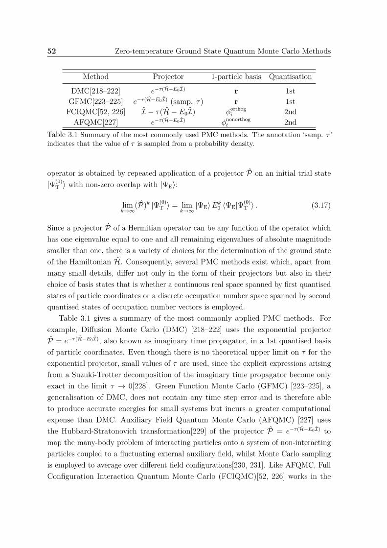
52 Zero-temperature Ground State Quantum Monte Carlo Methods
Method Projector 1-particle basis Quantisation
DMC[218–222] e−τ(H−E0I) r 1stGFMC[223–225] e−τ(H−E0I) (samp. τ) r 1st
FCIQMC[52, 226] I − τ(H − E0I) ϕorthogi 2nd
AFQMC[227] e−τ(H−E0I) ϕnonorthogi 2nd
Table 3.1 Summary of the most commonly used PMC methods. The annotation ‘samp. τ ’indicates that the value of τ is sampled from a probability density.
operator is obtained by repeated application of a projector P on an initial trial state|Ψ(0)
T ⟩ with non-zero overlap with |ΨE⟩:
limk→∞
(P)k |Ψ(0)T ⟩ = lim
k→∞|ΨE⟩Ek
0 ⟨ΨE|Ψ(0)T ⟩ . (3.17)
Since a projector P of a Hermitian operator can be any function of the operator whichhas one eigenvalue equal to one and all remaining eigenvalues of absolute magnitudesmaller than one, there is a variety of choices for the determination of the ground stateof the Hamiltonian H. Consequently, several PMC methods exist which, apart frommany small details, differ not only in the form of their projectors but also in theirchoice of basis states that is whether a continuous real space spanned by first quantisedstates of particle coordinates or a discrete occupation number space spanned by secondquantised states of occupation number vectors is employed.
Table 3.1 gives a summary of the most commonly applied PMC methods. Forexample, Diffusion Monte Carlo (DMC) [218–222] uses the exponential projectorP = e−τ(H−E0I), also known as imaginary time propagator, in a 1st quantised basisof particle coordinates. Even though there is no theoretical upper limit on τ for theexponential projector, small values of τ are used, since the explicit expressions arisingfrom a Suzuki-Trotter decomposition of the imaginary time propagator become onlyexact in the limit τ → 0[228]. Green Function Monte Carlo (GFMC) [223–225], ageneralisation of DMC, does not contain any time step error and is therefore ableto produce accurate energies for small systems but incurs a greater computationalexpense than DMC. Auxiliary Field Quantum Monte Carlo (AFQMC) [227] usesthe Hubbard-Stratonovich transformation[229] of the projector P = e−τ(H−E0I) tomap the many-body problem of interacting particles onto a system of non-interactingparticles coupled to a fluctuating external auxiliary field, whilst Monte Carlo samplingis employed to average over different field configurations[230, 231]. Like AFQMC, FullConfiguration Interaction Quantum Monte Carlo (FCIQMC)[52, 226] works in the
3.2 Projector Quantum Monte Carlo Approaches 53
2nd quantised basis of occupation number vectors, but employs the linear projectorP = I − τ(H − E0I) instead. In particular, this linear projector can only be usedfor Hamiltonians with bounded spectra given that the τ is bounded by τ < 2
(Emax−E0)with E0 and Emax being the minimum and maximum eigenvalues, respectively. Theexpectation values of the Hamiltonian and of any Hermitian operator which commuteswith the Hamiltonian are expressed as mixed estimators
⟨O⟩ = ⟨ΨE|O|ΨT⟩⟨ΨE|ΨT⟩
(3.18)
=∑
n ⟨ΨE|n⟩ ⟨n|O|ΨT⟩∑n ⟨ΨE|n⟩ ⟨n|ΨT⟩
(3.19)
=
∑n
⟨ΨE|n⟩ ⟨n|ΨT⟩ ⟨n|O|ΨT⟩⟨n|ΨT⟩
P [⟨n|ΨG⟩]P [⟨n|ΨG⟩]
(∑n
⟨ΨE|n⟩ ⟨n|ΨT⟩P [⟨n|ΨG⟩]
P [⟨n|ΨG⟩])−1
(3.20)
=∑
n OL(n) ⟨ΨE|n⟩⟨n|ΨT⟩P [⟨n|ΨG⟩]
P [⟨n|ΨG⟩]∑n⟨ΨE|n⟩⟨n|ΨT⟩
P [⟨n|ΨG⟩]P [⟨n|ΨG⟩]
(3.21)
≡
[1
NMC
∑NMCk=1 OL(nk) ⟨nk|ΨT⟩
P [⟨nk|ΨG⟩]
]P [⟨n|ΨG⟩]⟨ΨE|n⟩[
1NMC
∑NMCk=1
⟨nk|ΨT⟩P [⟨nk|ΨG⟩]
]P [⟨n|ΨG⟩]⟨ΨE|n⟩
(3.22)
≡
⟨OL(nk) ⟨nk|ΨT⟩
P [⟨nk|ΨG⟩]
⟩P [⟨n|ΨG⟩]⟨ΨE|n⟩⟨
⟨nk|ΨT⟩P [⟨nk|ΨG⟩]
⟩P [⟨n|ΨG⟩]⟨ΨE|n⟩
, (3.23)
where the factor ⟨ΨE|n⟩ has been subsumed in the probability density P [⟨n|ΨG⟩] ⟨ΨE|n⟩underlying the sampling process. Usually, the probability distribution
P [⟨n|ΨG⟩] ⟨ΨE|n⟩ = ⟨n|ΨG⟩ ⟨ΨE|n⟩∑m ⟨m|ΨG⟩ ⟨ΨE|m⟩
(3.24)
is used for the evaluation of the expectation value as average over the ensembleof walkers. Although the exact wavefunction ΨE appearing in the expressions forexpectation values is unknown, it can be sampled by repeated application of theprojector P or its importance-sampled version. Provided that no approximationsare introduced, the PMC estimate has no bias, independent of the guiding and trialwavefunction which only affect the statistical error in the MC estimate. As in the caseof VMC, if ΨG = ΨT, which is a common choice, the PMC mixed estimator represents
54 Zero-temperature Ground State Quantum Monte Carlo Methods
a zero-variance estimator in the limit ΨT → ΨE and the bias and statistical error inthe estimate vanish.
Although PMC methods are exact in principle, in practice, they all suffer from thefermion sign problem when treating fermionic and frustrated systems. The fermionsign problem is related to the fermionic nature of the wavefunction which necessitatespositive and negative (or more generally complex) wavefunction amplitudes to besampled. In all PMC methods, this means that an undesired state grows relative to thefermionic state of interest when a system is evolved by repeated stochastic applicationof a projector. As a result, the computational cost grows exponentially with system sizeand the fermion sign problem poses an NP-complete problem[128]. The sign problemmanifests itself differently in the various PMC methods. For PMC methods whichwork in the 1st quantised space of electronic coordinate the dominant state of theprojector corresponds to a nodeless bosonic solution. For projector methods workingin a 2nd quantised basis the severity of the sign problem is reduced[232]. Althoughthe intrinsic anti-symmetry of the space prevents collapse onto a bosonic solutions,the dominant state of the projector causes an exponentially decreasing signal-to-noiseratio[233]. Many PMC methods therefore employ approximation such as the fixed-node(FN) [218, 234] (or fixed-phase in the case of complex wavefunctions) approximation inDMC or the phaseless approximation [227] in AFQMC. The FN approximation imposesthe antisymmetry as constraint upon the solution in the form a 3N − 1 dimensionalnodal hypersurface on which the wavefunction is zero and across which it changes sign.The stochastic projection is thus performed subject to the constraint that the projectedstate has the same nodes as |ΨT⟩ by fixing the phase of the walkers relative to the trialstate. In most circumstances |ΨT⟩ is necessarily approximate and the nodes introduce asystematic error in the sampled wavefunction, as well as a systematic bias in expectationvalues whose quality is intrinsically limited by the quality of the trial wavefunction.In the limit that the nodal surface of the trial state is exact the exact ground statewavefunction is recovered, the bias in expectation values vanishes, and any estimator ofan operator that commutes with the Hamiltonian represents a zero-variance estimator.Since the accuracy and efficiency of approximate PMC methods depend crucially on thequality of the trail state, it is common practice to first optimise the trial wavefunction ina VMC optimisation prior to a PMC calculation. It is clear that the principal limitationfor both approximate PMC and VMC methods is this fixed-node error, which willalways raise the energy and represent a variational upper bound to the exact energy[221].It has been found difficult to improve upon this limitation, increase the accuracy of thenodal surface and retrieve more of the correlation energy in a systematic and controlled
3.3 Full Configuration Interaction Quantum Monte Carlo: FCIQMC 55
manner through techniques such as backflow corrections[235, 236] or release-nodemethods [220, 237]. These more sophisticated approaches can significantly improveenergy calculated by DMC, reducing typical systematic biases from ∼ 3kcal mol−1 towithin chemical accuracy of 1kcal mol−1[238, 239].
3.3 Full Configuration Interaction Quantum MonteCarlo: FCIQMC
Full Configuration Interaction Quantum Monte Carlo (FCIQMC)[52, 240] is a newwavefunction-based projector method which seeks the solution to the imaginary-timeSchrödinger equation. It combines the accuracy of the FCI ansatz with the computa-tional efficiency of Monte Carlo sampling of the projector and wavefunction to realisea stochastic implementation of the power method[233, 51]. The coefficients in the FCIwavefunction ansatz are stochastically represented by a set of discrete, signed walkerswithin the complete Hilbert space spanned by Slater determinants. In the limit ofa sufficiently large number of walkers, the long-time average of walker distributionis equal to the FCI wavefunction, the exact solution for a given single-particle basis.Although the choice of a finite one-particle basis introduces a finite basis set error andlimits the physical accuracy of FCIQMC, working in the intrinsically antisymmetric 2ndquantised space of occupation number vectors alleviates the Fermion sign problem[232].In contrast to many other PMC methods which introduce approximations to circumventthe sign problem that are, however, difficult to improve upon in a systematic andcontrolled manner, FCIQMC employs effective cancellation algorithms to control thesign problem instead. The exact wavefunction therefore emerges spontaneously inFCIQMC without any a priori wavefunction information. By sampling the wavefunctionand evaluating expectation values as time average over stochastic snapshots, FCIQMConly needs storage of non-zero coefficients in the FCI expansion which is often a tinyfraction of the whole Hilbert space, thereby circumventing the memory bottleneckexperienced by deterministic iterative diagonalisation techniques. FCIQMC has beenshown to reproduce FCI energies for a range of systems well within chemical accuracy.Owing to its reduced computation cost, FCIQMC is capable of treating systems manyorders of magnitude larger than those used in existing more traditional FCI approaches.FCIQMC and its variants have been found successful in studies of atomic and molecularsystems[241–244], model systems such as the homogeneous electron gas[245] and hub-bard models[246], as well as solid-state systems[247]. More recently, developments havealso enabled the extension to excited states[248–252], systems at finite temperature[248],
56 Zero-temperature Ground State Quantum Monte Carlo Methods
the calculations of molecular properties[253, 254], the use of FCIQMC as an FCI-solverin a Multi-Configurational Self-Consistent Field framework, resulting in a stochasticCASSCF approach[255, 256], as well as the application of explicitly correlated methodswhich reduce the error arising from the use of a finite basis set[257, 258]. Additionally,FCIQMC has also led to further stochastic approaches which aim at solving other typesof quantum chemical equations such as the Coupled-Cluster Monte Carlo method[259]and the Density Matrix Quantum Monte Carlo technique[260].
3.3.1 Derivation of FCIQMC Equations
The rational basis for the approach taken by many PMC methods is that the time-dependent Schrödinger equation
i∂Ψ(r, t)∂t
= HΨ(r, t) (3.25)
can also be viewed as a generalised diffusion equation. If the Hamiltonian of the systemdoes not vary with time, the solutions of the time-dependent Schrödinger equation areof the form
Ψ(r, t) =∑
i
ci(t = 0)e−iϵitψi(r), (3.26)
where ϵi and ψi(r) represent the eigenvalues and eigenfunctions of the correspondingtime-independent equation. By means of a Wick rotation[68], the time-dependentSchrödinger is transformed into the imaginary-time Schrödinger equation, with τ = it
−∂Ψ(r, τ)∂t
= HΨ(r, τ), (3.27)
thereby converting it to an ordinary differential equation whose solution is formallygiven by
Ψ(r, τ) = e−τH |Ψ(r, τ = 0)⟩ . (3.28)
The Schrödinger equation may thus be integrated in imaginary time to large values ofτ yielding a solution to the time-independent Schrödinger equation. By expanding theinitial wavefunction |Ψ(r, τ = 0)⟩ in the complete set of orthogonal eigenstates of the
3.3 Full Configuration Interaction Quantum Monte Carlo: FCIQMC 57
Hamiltonian, H |Ψi(r)⟩ = Ei |Ψi(r)⟩, such that,
|Ψ(r, τ = 0)⟩ =∑
i
Ci(τ = 0) |Ψi(r)⟩ , (3.29)
and introducing an arbitrary energy offset, Eoff , the wavefunction can be written as
Ψ(r, τ) =∑
i
Ci(τ = 0)e−τ(H−Eoff) |Ψi(r)⟩ , (3.30)
which describes the evolution of the individual eigenfunctions of the system in imaginarytime. Using the spectral expansion of the operator[50],
e−τH =∑
j
|Ψj(r)⟩ e−τEj ⟨Ψj(r)| , (3.31)
the decay of high-energy states relative to low-energy states becomes obvious
Ψ(r, τ) =∑ij
Ci(τ = 0) |Ψj(r)⟩ e−τ(Ej−Eoff) ⟨Ψj(r)|Ψi(r)⟩ (3.32)
=∑
i
Ci(τ = 0)e−τ(Ei−Eoff) |Ψi(r)⟩ . (3.33)
If Eoff is equal to the ground state energy E0, all states with energy Ei > E0 decayexponentially, with the rate of decay determined by their energy relative to the groundstate energy. In the long imaginary-time limit, the wavefunction will be dominated bythe lowest energy state
Ψ(r, τ →∞) = limτ→∞
∑i
Ci(τ = 0)e−τ(Ei−Eoff) |Ψi(r)⟩ (3.34)
= C0(τ = 0)e−τ(E0−Eoff) |Ψ0(r)⟩+O[e−τ(Ei−Eoff)], (3.35)
where |Ψ0(r)⟩ , E0 represents the lowest energy eigenpair, provided that the initialwavefunction |Ψ(r, τ = 0)⟩ has non-zero overlap with |Ψ0(r)⟩.
FCIQMC parameterises the wavefunction in the same manner as FCI which ex-pands the wavefunction in the basis of occupation number vectors representing Slaterdeterminants spanning the complete N -particle Hilbert space
Ψ =∑
nCn |n⟩ . (3.36)
58 Zero-temperature Ground State Quantum Monte Carlo Methods
Substituting this into the imaginary-time Schrödinger equation (Eq. 3.27) and in-troducing an energy offset Eoff to allow for a stationary solution in the long τ limit,gives
∑n
dCn(τ)dτ
|n⟩ = −∑
nCn(τ)(H − Eoff) |n⟩ , (3.37)
which if multiplied by ⟨m|
∑n
dCn(τ)dτ
⟨m|n⟩ = −∑
nCn(τ) ⟨m|(H − Eoff)|n⟩ , (3.38)
reduces to
dCm(τ)dτ
= −∑
n[Hmn − δmnEoff)]Cn(τ). (3.39)
In FCIQMC, the energy offset Eoff is typically split into a reference energy Eref and ashift parameter ES
dCm(τ)dτ
= −∑
n=mHmnCn(τ)
− (Hmm − Eref − ES)Cm(τ). (3.40)
In order to demonstrate the deep connection to other projector methods and thepower method, Eq. 3.40 can also be obtained through application of the projectorP = I − δτ (H − (Eref +ES)I) onto a wavefunction where δτ is viewed as a short timestep in imaginary time τ , such that the k-th application of the projector P onto anarbitrary coefficient Cm gives
C(k)m = ⟨m|Ψ(k)⟩ (3.41)
=∑
n⟨m|C(k)
n |n⟩ (3.42)
=∑
n⟨m|[I − δτ(H − (Eref + ES)I)]C(k−1)
n |n⟩ (3.43)
= ⟨m|[I − δτ(H − (Eref + ES)I)]C(k−1)m |m⟩ (3.44)
+∑
n=m⟨m|[I − δτ(H − (Eref + ES)I)]C(k−1)
n |n⟩ (3.45)
= C(k−1)m − δτHmmC
(k−1)m + δτ(Eref + ES)C(k−1)
m −∑
n=mδτHmnC
(k−1)n . (3.46)
3.3 Full Configuration Interaction Quantum Monte Carlo: FCIQMC 59
Substituting this into the derivative of the coefficient with respect to imaginary time
dCm
dτ= lim
δτ→0
C(k)m − C(k−1)
mδτ
(3.47)
gives
dCm
dτ= lim
δτ→0
1δτ
C(k−1)m − δτHmmC
(k−1)m + δτ(Eref + ES)C(k−1)
m (3.48)
−∑
n=mδτHmnC
(k−1)n − C(k−1)
m
(3.49)
= limδτ→0
−∑
n=mHmnC
(k−1)n
−HmmC(k−1)m + (Eref + ES)C(k−1)
m
(3.50)
= −∑
n=mHmnC
(k−1)n
− (Hmm − Eref − ES)C(k−1)m , (3.51)
which exactly matches Eq. 3.40. The linear projector P = I − δτ(H − (Eref + ES)I)represents the Taylor expansion of the e−δτH operator with imaginary time τ discretisedinto B time steps δτ , such that e−BδτH = e−τH. Since the imaginary time propagatore−τH represents the formal solution to the Schrödinger equation and shares the sameeigenfunctions as the linear projector, repeated application of P = I − δτ(H − (Eref +ES)I) will project out the ground state of any non-orthogonal trial state.
Once this initial state has been evolved in imaginary time for a sufficiently longperiod, corresponding to sufficiently many repeated application of the projector, thewavefunction is proportional to the dominant eigenstate of the system, at which pointthe coefficients should all be stationary and dCm
dτ= 0 ∀m and Eq. 3.40 becomes
−∑
n[Hmn − (Eref + ES)δmn]Cn = 0 (3.52)∑
nHmnCn = (Eref + ES)Cm, (3.53)
which returns the time-independent Schrödinger equation for the system in form of astandard Hermitian eigenvalue problem, where C represents the dominant eigenstateof H with energy (Eref + ES).
60 Zero-temperature Ground State Quantum Monte Carlo Methods
3.3.2 Stochastic Implementation of FCIQMC
The set of coupled differential equations in Eq. 3.40 describes the evolution of thewavefunction parameters in imaginary time which in the long-imaginary time limitprojects out the lowest energy eigenstate of the system. In FCIQMC, a stochasticalgorithm[52, 240, 261] realises a finite difference formulation of Eq. 3.40 whereby thewavefunction is represented stochastically by an ensemble of discrete signed walkerswhich live in the complete N -particle Hilbert space, and are propagated iterativelywith small time steps δτ . Each walker, α, possesses an associated sign sα = ±1 andthe instantaneous coefficients, Cn, in the wavefunction expansion is defined to beproportional to the signed sum, Nn, of the signed walkers on each Slater determinant,
Cn ∝ Nn =∑
α∈|n⟩sα (3.54)
Representing the wavefunction in this discretised form significantly compresses theinformation needed to store a stochastic snapshot of the wavefunction. The totalnumber of walkers, Nw, is given by
L1 ∝ Nw =∑
n|Nn|, (3.55)
which is thus proportional to the L1-norm of the wavefunction. Each iteration whichpropagates the walker population by a time step δτ comprises spawning and deathattempts followed by annihilation events. These processes are explained in detail inthe following.
SpawningEvery walker attempts to spawn a child from its determinant |n⟩ onto a connecteddeterminant |m⟩ which is generated with a normalised probability pgen(m|n,H).In this context, a connection between two configurations refers to a non-zeroconnecting Hamiltonian matrix element Hmn = 0. An attempt is made to spawna new child walker on |m⟩ with an acceptance probability
ps(m|n) = δτ |Hmn|pgen(m|n,H) . (3.56)
This stochastic spawning attempt necessitates the generation of a random numberr in the interval [0, 1). When ps(m|n) < 1 the spawning attempt is accepted ifps(m|n) > r. When ps(m|n) > 1, ⌊ps(m|n)⌋ walkers are spawned deterministi-
3.3 Full Configuration Interaction Quantum Monte Carlo: FCIQMC 61
cally and one further walker is created with probability ps(m|n)− ⌊ps(m|n)⌋ inthe manner described above. 1 The sign of the child walker is determined bysign(−HmnNn). The spawning step is designed to give a stochastic representationof the first term in Eq. 3.40 involving off-diagonal Hamiltonian matrix elements
dCm(τ)dτ
= −∑
n=mHmnCn(τ)
︸ ︷︷ ︸
spawning
−(Hmm − Eref − ES)Cm(τ). (3.57)
The generation of connected determinants represents an integral part that iscrucial for the efficiency of the algorithm. Whilst it is perfectly valid to use auniform distribution[261] for pgen(m|n,H) this may become rather inefficient aseach determinant is connected to O[N2M2] others. Instead, distributions whichfavour preferential generation of determinants with a strong connection |Hmn|will significantly enhance efficiency, in particular in larger spaces[262, 263].
Death / CloningEach parent walker present at the beginning of the iteration (i.e. not includingthe newly spawned child walkers) attempts to die or clone itself with probability
pd(n) = δτ(Hnn − Eref − ES). (3.58)
If pd(n) > 0, the walker dies with probability pd(n) (the attempt to die issuccessful if pd(n) > r where r is a random number in the interval [0, 1)). It isremoved from the simulation and the population on |n⟩ is reduced accordingly.If pd(n) < 0, the parent walker instead attempts to clone itself with probability|pd(n)| and the population on |n⟩ is increased if successful. Cloning attempts arerare events and usually occur in association with low energy determinants andpositive values of ES. The death step is designated to account for the secondterm in Eq. 3.40 comprising diagonal Hamilton matrix elements
dCm(τ)dτ
= −∑
n=mHmnCn(τ)
︸ ︷︷ ︸
spawning
−(Hmm − Eref − ES)Cm(τ)︸ ︷︷ ︸death/cloning
. (3.59)
AnnihilationIn the final stage of each iteration, the newly spawned child walkers and surviving
1⌊A⌋ denotes the largest integer less than or equal to A.
62 Zero-temperature Ground State Quantum Monte Carlo Methods
parent walkers are combined. All pairs of walkers with opposite sign whichreside on the same determinant annihilate each other and are removed fromthe simulation such that each determinant only retains walkers of a single sign.All walkers that survive this process form the new walker population which ispropagated further in the next iteration.
3.3.3 Energy Estimators
FCIQMC provides two independent energy estimators: the shift, ES, and the projectedenergy, Eproj. ES has been introduced as part of the energy offset which according toEq. 3.52 represents a measure of the energy of the system in the limit of a stationarysolution. The shift assumes the role of a population control parameter which, ignoringstatistical fluctuations, forces the total number of walkers Nw to remain constant,thereby allowing the system to reach a stationary solution. During an initial growthphase, ES is fixed at a specified value, typically zero, (fixed-shift mode), after whichthe value of ES is allowed to dynamically vary so as to keep Nw constant in τ (variableshift-mode). Its value is adjusted every A steps according to
ES(τ) = ES(τ − Aδτ)− ζ
Aδτln Nw(τ)Nw(τ − Aδτ) , (3.60)
where ζ is a damping parameter[222]. In this phase, Eref + ES becomes a meaningfulmeasure of the energy once the walker population has converged on the stationaryground state wavefunction.
An alternative, independent energy estimator is the projected energy Eproj, a non-variational mixed estimator, which is obtained by projecting the wavefunction onto areference state, |nref⟩
Eproj(τ) = ⟨nref |H|Ψ(τ)⟩⟨nref |Ψ(τ)⟩ (3.61)
=∑
n Cn(τ) ⟨nref |H|n⟩∑n Cn(τ) ⟨nref |n⟩
(3.62)
= ⟨nref |H|nref⟩+∑
n=nref
⟨nref |H|n⟩Cn(τ)Cnref (τ) (3.63)
= Eref +∑
n =nref
⟨nref |H|n⟩Cn(τ)Cnref (τ) (3.64)
= Eref +∑
n=nref
⟨nref |H|n⟩Nn(τ)Nnref (τ) (3.65)
3.3 Full Configuration Interaction Quantum Monte Carlo: FCIQMC 63
In the last line, the ratio of coefficients Cn(τ)Cnref (τ) has been equated to the ratio of
walker populations Nn(τ)Nnref (τ) residing on those determinants, which is true in the long
imaginary-time limit when the walker distribution is proportional to the ground stateFCI wavefunction and Eproj(τ) equal to the FCI energy. In most circumstances,the reference state, |nref⟩, is defined to be the Hartree-Fock determinant, in whichcase Eref is the HF energy. According to the Slater-Condon rules[85, 86], only theHF determinant and its doubly (and singly if another reference state is used andBrillouin’s theorem[97, 98] does not apply) excited determinants contribute to Eproj(τ).The accuracy of the projected energy is rather sensitive to the relative error in thecoefficient of the reference state and even diverges if Nnref = 0. The error in Eproj(τ) islikely to be larger for systems where the reference determinant constitutes only a smallfraction of the wavefunction, such as multireference systems. In these systems, insteadof a single determinant, the wavefunction can be projected onto a trial wavefunctionwhich is itself a linear combination of determinants[242]. These more sophisticatedtrial wavefunctions can significantly reduce the stochastic error in Eproj(τ)[264, 248],but also increase the computational expense associated with the calculation of Eproj(τ)which may become prohibitively expensive.
The availability of these two independent energy estimators is of considerable value.Whilst the projected energy depends exclusively on the walker population at the refer-ence state (or at determinants in the trial wavefunction) and its connected determinants,the shift derives from the dynamics of the entire occupied space. Agreement betweenthese two distinct measures represents therefore a useful indicator of convergence in acalculation.
3.3.4 The Fermion Sign Problem and the Importance of An-nihilation
Like all PMC methods FCIQMC needs to control the Fermion Sign problem whicharises because repeated stochastic application of the projector causes the growth ofan undesired state as the system evolves. In contrast to other PMC methods such asDMC, FCIQMC achieves this without introduction of approximations that are difficultto improve systematically and require a priori knowledge of the nodal structure of thewavefunction to be exact.
In part, this success is based on the use of the 2nd quantised basis of Slaterdeterminants spanning the complete N -particle Hilbert space. Whilst a 1st quantisedbasis allows states of various symmetry which means that the dominant state of the
64 Zero-temperature Ground State Quantum Monte Carlo Methods
projector is the physical bosonic ground state of the Hamiltonian and not its fermionicground state, a 2nd quantised basis allows only states of the correct symmetry andnoise from undesired non-fermionic states is thus prevented. However, working in a2nd quantised basis does not solve the sign problem, as different paths between twostates can contribute with opposite signs in which case they cancel and result in atotal contribution of smaller absolute magnitude, just as they would in a deterministiccalculation. Issues arise when contributions of opposite sign occur at different steps ofthe sampling process. Moreover, Ψ and −Ψ are sampled with equal probability whichfurther adds to the problem[51]. Yet, compared to a 1st quantised basis the intrinsicallyantisymmetric 2nd quantised basis reduces the severity of the sign problem[232]. Theantisymmetrised basis not only introduces the possibility of internal cancellations butis also reduced in size by a factor of N ! which increases the probability for walkers ofopposite signs to meet and cancel each other. Further, since states of symmetry otherthan fermionic are eliminated, a stable signal to noise ratio can be obtained in the limitof large walker populations. FCIQMC reaches exactly this limit with the introductionof the annihilation step which represents an efficient cancellation algorithm.
Although the annihilation process does not explicitly appear in the FCIQMC masterequations in Eq. 3.40, it is nevertheless a key element to the control of the Fermion signproblem and the success of the algorithm. In the absence of annihilation the simulationfails to converge. Only in the presence of the annihilation step, the simulation is ableto project out the ground state wavefunction with correct values for ES and Eproj
provided the total number of walkers in the simulation exceeds a system-dependentcritical value. The annihilation step is also responsible for the pattern of walker growthin a typical FCIQMC calculation. In fixed-shift mode, where ES is typically fixedat zero, the walker population initially grows exponentially. However, annihilationcauses the walker growth to spontaneously halt and enter a plateau phase before thebeginning of a second exponential growth phase. During the plateau phase the desiredwavefunction emerges and its height therefore sets the system dependent minimumrequired walker number Nw for convergence (Figure 3.1).
This minimum walker number represents the minimum amount of sampling that isrequired for sufficient annihilation events to occur such that the Fermion sign problemis controlled and a stable signal to noise ratio is obtained. Like in all other PMCmethods, noise arises from the growth of an undesired state and the severity of the signproblem is characterised by the difference in energy between the two competing states.Yet, unlike in a 1st quantised basis, where the undesired state is the physical bosonicground state of the Hamiltonian, this need not be the case in a 2nd quantised basis.
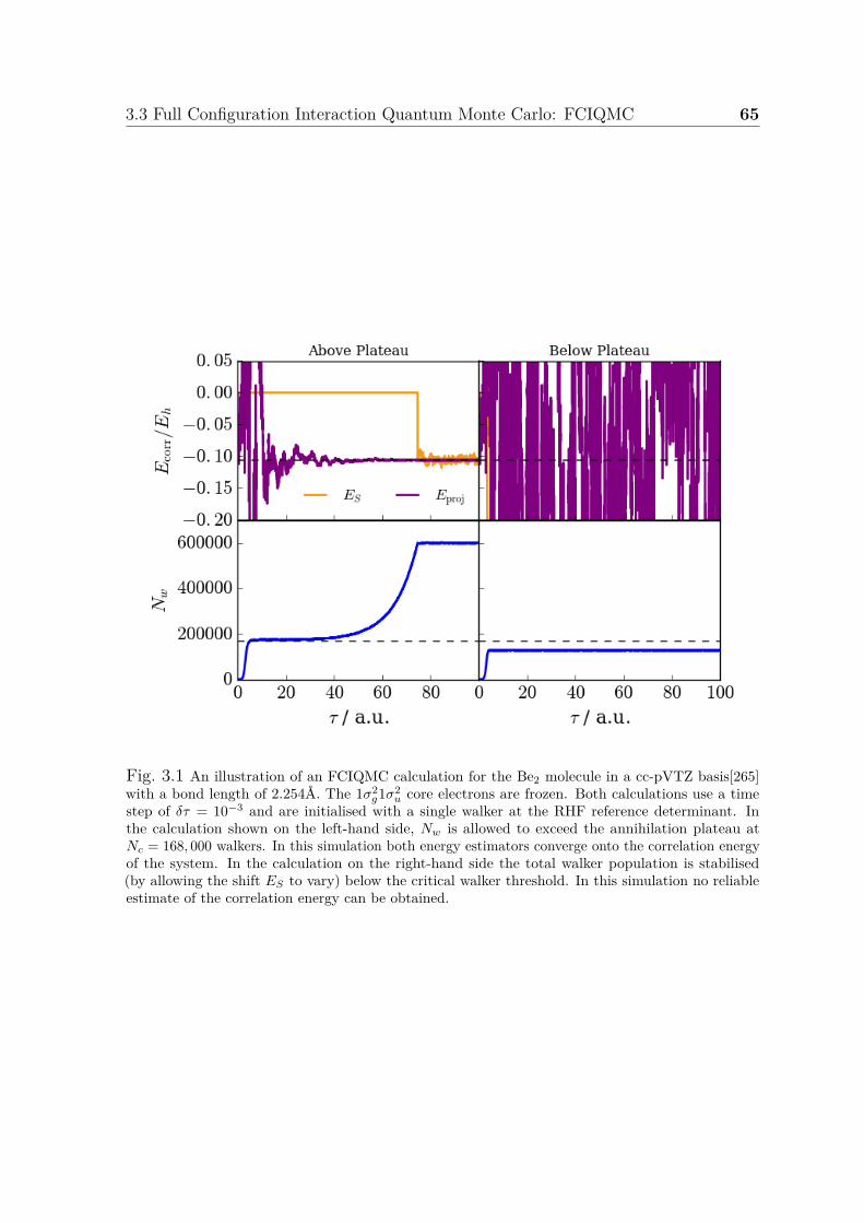
3.3 Full Configuration Interaction Quantum Monte Carlo: FCIQMC 65
Fig. 3.1 An illustration of an FCIQMC calculation for the Be2 molecule in a cc-pVTZ basis[265]with a bond length of 2.254Å. The 1σ2
g1σ2u core electrons are frozen. Both calculations use a time
step of δτ = 10−3 and are initialised with a single walker at the RHF reference determinant. Inthe calculation shown on the left-hand side, Nw is allowed to exceed the annihilation plateau atNc = 168, 000 walkers. In this simulation both energy estimators converge onto the correlation energyof the system. In the calculation on the right-hand side the total walker population is stabilised(by allowing the shift ES to vary) below the critical walker threshold. In this simulation no reliableestimate of the correlation energy can be obtained.
66 Zero-temperature Ground State Quantum Monte Carlo Methods
Instead, the undesired state represents the dominant state of the projector with alloff-diagonal elements replaced by their absolute values which is the lowest eigenfunctionof a matrix Tmn = Hmnδmn − |Hmn − Hmnδmn|[266]. The lowest eigenvalue of T isalways lower than the lowest eigenvalue of the Hamiltonian H, meaning that thisundesired solution dominates in a regime without sufficient annihilation. The differencebetween the two eigenvalues of the competing states which characterises the severityof the sign problem is always smaller than or equal to the relevant difference in a1st quantised basis, the energy gap between the fermionic and bosonic ground states.Introduction of cancellation events in the form of the annihilation step has been shownto inhibit specifically the growth of the undesired competing state and to give rise tothe spontaneous plateau phase in the walker growth, allowing the true ground statewavefunction of the Hamiltonian to emerge.
3.3.5 The Initiator Approximation
Although the FCIQMC algorithm in its form described above represents a computationalsaving over more traditional diagonalisation techniques, its computational expense stillneeds to be reduced for the treatment of larger systems, ideally without a commensurateloss of accuracy. One of the most successful developments with this aim is the initiatorapproximation[226, 267] which introduces subtle modifications to the spawning step.These alterations significantly broaden the scope of FCIQMC by removing the plateauregion from the simulation and reducing the associated minimum walker numberrequired for convergence. This initiator adaptation of FCIQMC (i-FCIQMC) has beenso successful that it is now routinely used as standard approach and all calculationspresented in this thesis use the initiator adaptation i-FCIQMC, unless otherwise stated.
The alterations introduced by i-FCIQMC start by separating the occupied Slaterdeterminants into two categories based on their instantaneous walker population relativeto a predetermined parameter, Na. Determinants with a walker population greaterthan this threshold, |Nn(τ)| > Na, are classified as initiators while determinants witha walker population less than or equal to this threshold, |Nn(τ)| ≤ Na, are classified asnon-initiators. The spaces of initiator and non-initiator determinants are dynamicallyupdated throughout the simulation to reflect the changing populations on individualdeterminants. All walkers on initiator determinants attempt to die and spawn asnormal and thus behave exactly as in FCIQMC. Walkers on non-initiator determinantsalso attempt to die as normal, but their spawning ability is restricted. In particular, ifa walker on a non-initiator attempts to spawn onto a connected determinants that isvacant and the attempt is successful, the resulting child walker is still not allowed to
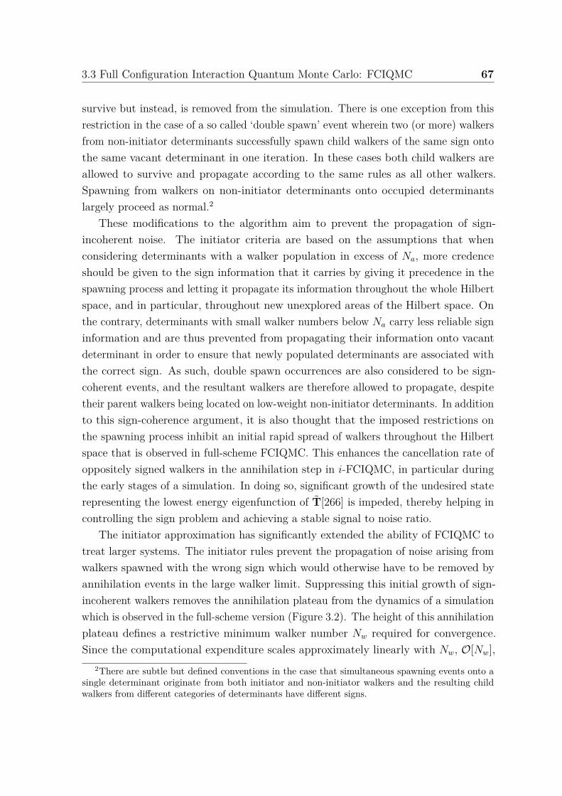
3.3 Full Configuration Interaction Quantum Monte Carlo: FCIQMC 67
survive but instead, is removed from the simulation. There is one exception from thisrestriction in the case of a so called ‘double spawn’ event wherein two (or more) walkersfrom non-initiator determinants successfully spawn child walkers of the same sign ontothe same vacant determinant in one iteration. In these cases both child walkers areallowed to survive and propagate according to the same rules as all other walkers.Spawning from walkers on non-initiator determinants onto occupied determinantslargely proceed as normal.2
These modifications to the algorithm aim to prevent the propagation of sign-incoherent noise. The initiator criteria are based on the assumptions that whenconsidering determinants with a walker population in excess of Na, more credenceshould be given to the sign information that it carries by giving it precedence in thespawning process and letting it propagate its information throughout the whole Hilbertspace, and in particular, throughout new unexplored areas of the Hilbert space. Onthe contrary, determinants with small walker numbers below Na carry less reliable signinformation and are thus prevented from propagating their information onto vacantdeterminant in order to ensure that newly populated determinants are associated withthe correct sign. As such, double spawn occurrences are also considered to be sign-coherent events, and the resultant walkers are therefore allowed to propagate, despitetheir parent walkers being located on low-weight non-initiator determinants. In additionto this sign-coherence argument, it is also thought that the imposed restrictions onthe spawning process inhibit an initial rapid spread of walkers throughout the Hilbertspace that is observed in full-scheme FCIQMC. This enhances the cancellation rate ofoppositely signed walkers in the annihilation step in i-FCIQMC, in particular duringthe early stages of a simulation. In doing so, significant growth of the undesired staterepresenting the lowest energy eigenfunction of T[266] is impeded, thereby helping incontrolling the sign problem and achieving a stable signal to noise ratio.
The initiator approximation has significantly extended the ability of FCIQMC totreat larger systems. The initiator rules prevent the propagation of noise arising fromwalkers spawned with the wrong sign which would otherwise have to be removed byannihilation events in the large walker limit. Suppressing this initial growth of sign-incoherent walkers removes the annihilation plateau from the dynamics of a simulationwhich is observed in the full-scheme version (Figure 3.2). The height of this annihilationplateau defines a restrictive minimum walker number Nw required for convergence.Since the computational expenditure scales approximately linearly with Nw, O[Nw],
2There are subtle but defined conventions in the case that simultaneous spawning events onto asingle determinant originate from both initiator and non-initiator walkers and the resulting childwalkers from different categories of determinants have different signs.
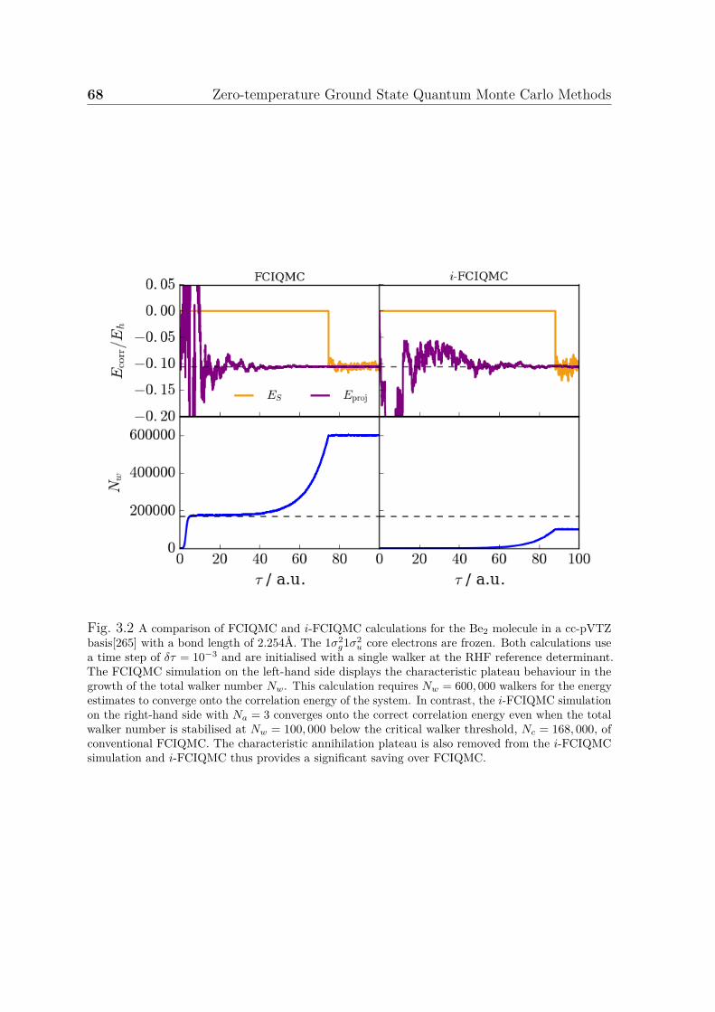
68 Zero-temperature Ground State Quantum Monte Carlo Methods
Fig. 3.2 A comparison of FCIQMC and i-FCIQMC calculations for the Be2 molecule in a cc-pVTZbasis[265] with a bond length of 2.254Å. The 1σ2
g1σ2u core electrons are frozen. Both calculations use
a time step of δτ = 10−3 and are initialised with a single walker at the RHF reference determinant.The FCIQMC simulation on the left-hand side displays the characteristic plateau behaviour in thegrowth of the total walker number Nw. This calculation requires Nw = 600, 000 walkers for the energyestimates to converge onto the correlation energy of the system. In contrast, the i-FCIQMC simulationon the right-hand side with Na = 3 converges onto the correct correlation energy even when the totalwalker number is stabilised at Nw = 100, 000 below the critical walker threshold, Nc = 168, 000, ofconventional FCIQMC. The characteristic annihilation plateau is also removed from the i-FCIQMCsimulation and i-FCIQMC thus provides a significant saving over FCIQMC.
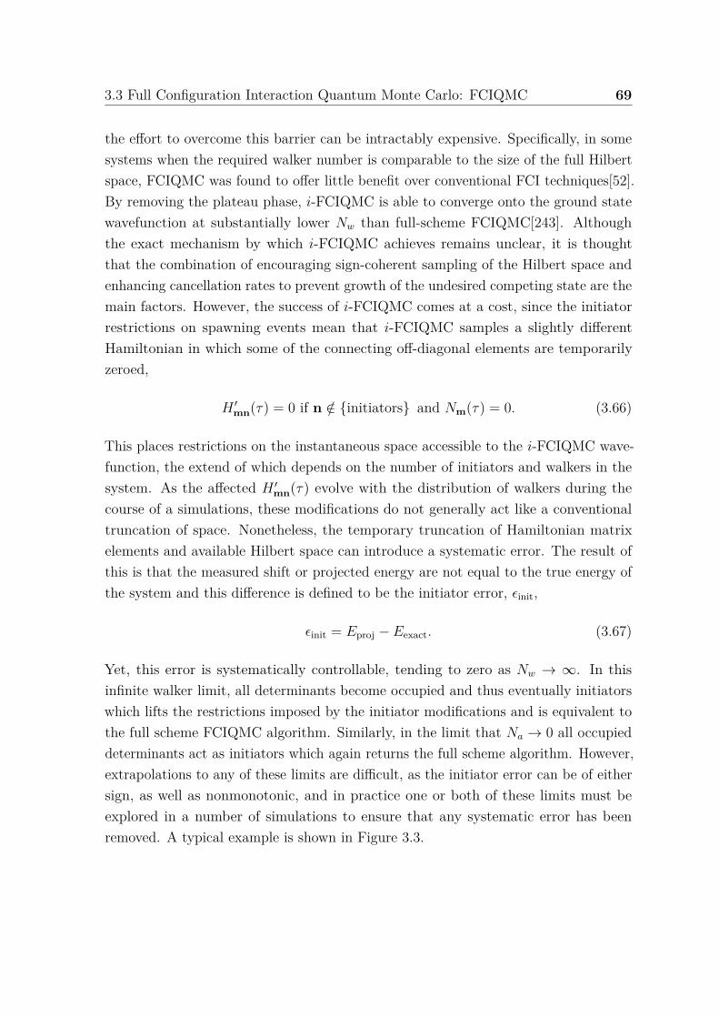
3.3 Full Configuration Interaction Quantum Monte Carlo: FCIQMC 69
the effort to overcome this barrier can be intractably expensive. Specifically, in somesystems when the required walker number is comparable to the size of the full Hilbertspace, FCIQMC was found to offer little benefit over conventional FCI techniques[52].By removing the plateau phase, i-FCIQMC is able to converge onto the ground statewavefunction at substantially lower Nw than full-scheme FCIQMC[243]. Althoughthe exact mechanism by which i-FCIQMC achieves remains unclear, it is thoughtthat the combination of encouraging sign-coherent sampling of the Hilbert space andenhancing cancellation rates to prevent growth of the undesired competing state are themain factors. However, the success of i-FCIQMC comes at a cost, since the initiatorrestrictions on spawning events mean that i-FCIQMC samples a slightly differentHamiltonian in which some of the connecting off-diagonal elements are temporarilyzeroed,
H ′mn(τ) = 0 if n /∈ initiators and Nm(τ) = 0. (3.66)
This places restrictions on the instantaneous space accessible to the i-FCIQMC wave-function, the extend of which depends on the number of initiators and walkers in thesystem. As the affected H ′mn(τ) evolve with the distribution of walkers during thecourse of a simulations, these modifications do not generally act like a conventionaltruncation of space. Nonetheless, the temporary truncation of Hamiltonian matrixelements and available Hilbert space can introduce a systematic error. The result ofthis is that the measured shift or projected energy are not equal to the true energy ofthe system and this difference is defined to be the initiator error, ϵinit,
ϵinit = Eproj − Eexact. (3.67)
Yet, this error is systematically controllable, tending to zero as Nw → ∞. In thisinfinite walker limit, all determinants become occupied and thus eventually initiatorswhich lifts the restrictions imposed by the initiator modifications and is equivalent tothe full scheme FCIQMC algorithm. Similarly, in the limit that Na → 0 all occupieddeterminants act as initiators which again returns the full scheme algorithm. However,extrapolations to any of these limits are difficult, as the initiator error can be of eithersign, as well as nonmonotonic, and in practice one or both of these limits must beexplored in a number of simulations to ensure that any systematic error has beenremoved. A typical example is shown in Figure 3.3.
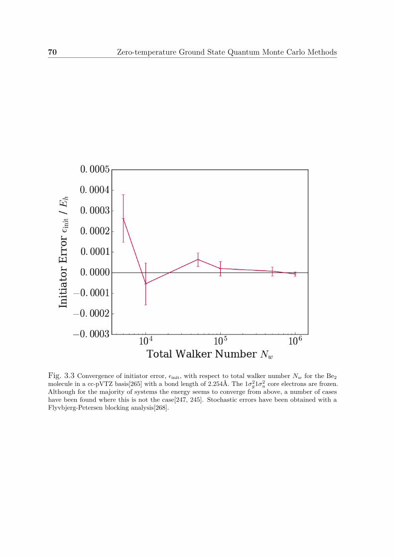
70 Zero-temperature Ground State Quantum Monte Carlo Methods
Fig. 3.3 Convergence of initiator error, ϵinit, with respect to total walker number Nw for the Be2molecule in a cc-pVTZ basis[265] with a bond length of 2.254Å. The 1σ2
g1σ2u core electrons are frozen.
Although for the majority of systems the energy seems to converge from above, a number of caseshave been found where this is not the case[247, 245]. Stochastic errors have been obtained with aFlyvbjerg-Petersen blocking analysis[268].
3.3 Full Configuration Interaction Quantum Monte Carlo: FCIQMC 71
3.3.6 Non-integer Real-weight Walkers
Although FCIQMC was originally developed with an ensemble of discrete integerweight walkers, it was found beneficial to introduce walkers with real non-integerweights[253, 269]. In the algorithm this is achieved by applying the spawning, death andannihilation process continuously, rather than discretely. In this context, continuouslymeans that weights in spawning and death events are assigned in a continuous manner,omitting the additional stochastic process to convert the weight into an integer walker.Specifically, instead of spawning a walker of integer weight ±1 from |n⟩ to |m⟩ withprobability ps(m|n), a walker of weight ps is spawned with probability 1. Similarly,a continuous death event on |n⟩ simply involves altering its walker population bypd(n) without the discretisation enforced in the integer walker algorithm. A completedefinition of this non-integer algorithm requires a discretisation of the number ofspawning attempts made from each determinant with real weight walkers. This numberof spawning events is set to be a minimum of ⌊Nn⌋ with the possibility of one additionalspawning attempt that is stochastically realised with a probability Nn−⌊Nn⌋ to ensurethat the overall number of spawning events is still proportional to Nn. Apart fromthese modifications, the remaining steps of the algorithm proceed largely in the sameway as their integer counterparts.
The continuous version of the FCIQMC algorithm removes much of the randomnumber generation in the code. At the same time, instantaneous fluctuations on eachdeterminant are reduced by allowing changes to its population by small fractions ofa walker, rather than by a whole walker at a time, which also leads to significantreductions in the stochastic error in estimates such as the projected energy. However, ascontinuous spawning events are automatically accepted, their number is substantiallyincreased. Likewise, continuous death events of fractions of a walker can lead tomany determinants being occupied by low-weight walkers. The costs in memoryand simulation time associated with non-integer walkers can thus be significant andsome means of stochastic compression of the low-weighted walkers is needed to avoidcomputational costs for these walkers which contribute little but would quickly spanmuch of the Hilbert space. Three additional parameters are therefore introduced tocontrol the computational expense of the continuous approach. First, only a subspaceof the full Hilbert space is treated with non-integer walkers whilst the remainder isdescribed in a discretised manner with integer walkers. The non-integer subspace isdefined by a given number of particle-hole excitations from the reference determinant,determined by the cutoff parameter χ which is equal to the maximum excitation level.This still preserves to a large part the minimised fluctuations in the energy estimator
72 Zero-temperature Ground State Quantum Monte Carlo Methods
as the most dominant contributions will be included in the non-integer subspace (or allcontributions with a HF reference and χ ≥ 2) and creates a hierarchy of non-integermethods which offer different compromises between high resolution and computationalcost. In addition, a minimum threshold value, κ, is introduced for a continuousspawning event. If ps > κ, ps walkers are spawned with probability 1 in a continuousprocess. If ps < κ, κ walkers a spawned with probability ps
κin a stochastic process,
otherwise 0 walkers are spawned. This approach alleviates the disproportionate costof low-weight walkers which incurs a substantial computational expense compared totheir negligible impact on the simulation. While the death step requires no additionalmodification of this kind, the annihilation process needs further considerations anda minimum occupation threshold, Nocc, is defined. After the annihilation process iscomplete, the instantaneous population of each determinant, Nn, is assessed withrespect to this threshold. If Nn < Nocc, its population is discretised to either Nocc
with probability NnNocc
or 0 with probability 1 − NnNocc
. In doing so, it is ensured thatdeterminants with low-weight walker populations do not proliferate.
It was observed that the description of at least some parts of the space in acontinuous manner was universally beneficial mostly due to the reduction in stochasticnoise[253].
3.3.7 The Semi-stochastic Adaption
A further notable development of FCIQMC which shall only be briefly mentioned is itssemi-stochastic adaption [264, 248]. This approach takes advantage of the observationthat for many system, a large proportion of the spectral weight of the ground state isconcentrated on a relatively small part of the Hilbert space. The Hilbert space HN
is therefore divided into two subspaces, a deterministic subspace D and a stochasticsubspace S, such that D ∪ S = HN and D ∩ S = ∅. Similarly, the linear projectorexpanded in the set of basis states |n⟩,
P = I − δτ(H − ESI) =∑mn
Pmn |m⟩ ⟨n| , (3.68)
whose application is performed stochastically in (i)-FCIQMC, is partitioned into adeterministic projector PD and a stochastic complement PS,
P = PD + PS, (3.69)
3.4 Handling Stochastic Estimators 73
where
PDmn =
Pmn if m,n ∈ D
0 otherwise. (3.70)
Whereas PD is applied exactly, the application of PS is realised stochastically using thenormal processes of FCIQMC. A good choice of states for the deterministic subspaceshould be of modest size whilst comprising an appreciable proportion of the groundstate wavefunction. A number of techniques of making this choice have been proposedranging from truncations based upon excitation level to iterative schemes that attemptto identify the highest weighted basis states in the wavefunction. Since a deterministicprojection has no sign problem and no statistical error, the semi-stochastic approachreduces the severity of the sign problem and the amount of stochastic noise comparedto the fully stochastic version[51].
3.4 Handling Stochastic Estimators
When using stochastic methods such as VMC or FCIQMC, estimates of quantitiesand their associated errors arising from statistical fluctuations need to be treatedappropriately. Once a simulation has converged and equilibrated statistically signif-icant data can be extracted in the form of statistical averages over the appropriateinstantaneous values of estimators collected over a series of iterations. In this process,the problem of serial correlation in the data need to be addressed, whereby consecutivedata points cannot be considered independent since the wavefunction at iteration k+ 1is closely related to that at iteration k and new information is only obtained fromdata points which are separated by the correlation time. In order to treat these issuesaccurately and remove the serial correlation from the data, the reblocking analysis ofFlyvbjerg and Petersen[268] is used which can be implemented in a computationallyconvenient and conceptionally simple algorithm. This method divides the set of datapoints x1, x2, . . . , xn of n into blocks by averaging adjacent data points,
x′i = 12(x2i−1 + x2i) (3.71)
n′ = 12n, (3.72)
and evaluating the mean m and variance σ2 of the blocks. This blocking transfor-mation is applied recursively so that the blocks contain 2k data points after the k-th
74 Zero-temperature Ground State Quantum Monte Carlo Methods
transformation. It can be shown that, under this blocking transformation
m′ = m (3.73)σ2(m′) = σ2(m) (3.74)
ζ ′t =
12ζ0 + 1
2ζ1 if t = 014ζ2t−1 + 1
2ζ2t + 14ζ2t+1 if t > 0
, (3.75)
where ζt is the covariance between two data points separated by t steps. Furtheranalysis shows that as the blocking transformations are repeatedly performed, thevariance of the data set σ2(m) emerges, since
σ2 ≥ ζ0
n(3.76)
and ζ0n
increases every time a blocking operation is performed, unless ζ1 = 0, in whichcase ζ0
nis invariant. During the reblocking process the variance initially increases until
the serial correlation has been approximately removed from the data and a plateau isreached. From this point onwards the variance remains approximately constant withincreasing block size but its error increases due to the small number of blocks. Thequantity
χ =1n(∑n
i=1 x2i )− 1
n2 (∑ni=1 xi)2
n− 1 (3.77)
acts as estimate for ζ0n
during a calculation and its value is equal to the true varianceof the data set when further blocking operations no longer change its value beyondminor fluctuations.
Chapter 4
Application of i-FCIQMC toStrongly Correlated Systems
Wavefunction-based methods represent the best approach for obtaining insight intothe characteristics of a system and its most important microscopic properties sinceall observable properties that drive the physical behaviour of the system can bedetermined directly from the wavefunction. Owing to this high potential associatedwith the knowledge of the wavefunction, there is growing interest in wavefunction-basedmethods and their application to strongly correlated systems. Whilst in quantumchemical methods wavefunctions of strongly correlated molecular systems primarilybuild on restricted single-particle bases, the general approach in condensed matterphysics is to start from qualitatively correct broken-symmetry solutions[3]. It istherefore important to investigate how the structure of a many-electron wavefunctionof a prototypical strongly correlated system depends on the representation of theone-particle basis underlying the configuration space of the system. On the faceit, such a question appears to be more of a mathematical rather than a physicalnature: a unitary transformation of a basis cannot change the physical content of thewavefunction, any more than a rotation of a Cartesian system of coordinates changesthe physical content of a tensorial quantity. Still, the choice of single-particle basis canimpact the structure of the exact FCI expansion[270] of a many-body wavefunction ina dramatic and sometimes even counterintuitive manner. In order to shed more lighton this question, the study in this chapter looks at a range of different basis sets: abroken-symmetry mean-field basis (UHF), a spin-restricted mean-field basis (RHF), aswell as restricted and unrestricted natural orbitals which are known to give a compactFCI wavefunction[271–275].
76 Application of i-FCIQMC to Strongly Correlated Systems
4.1 Model Hamiltonians
Since reliable ab-initio methods encounter many difficulties, another traditional widelyused theoretical approach is based on simplifying model Hamiltonians which take only afew relevant degrees of freedom into account. Reducing a full many-body Hamiltonianto the simplified model Hamiltonian still captures the physics of the relevant low-energydegrees of freedom, retains the essence of the physical phenomena and seems to betterunravel the physical effects of strongly correlated electron systems.
4.1.1 The Hubbard Model
One of the most studied model system is the Hubbard Hamiltonian[33, 9] which is thesimplest model of interacting electrons on a lattice
H = −t∑⟨IJ⟩,σ
a†IσaJσ + U∑
I
nI↑nI↓. (4.1)
This model associates one pair of opposite spin orbitals with each site I of the lattice.a†Iσ and aIσ represent the second quantised fermionic creation and annihilation operatorswhich create and annihilate an electron with spin σ in the orbital at lattice site I,while nI↓ = a†I↓aI↓ denotes the number operator. The first summation runs over allnearest-neighbour pairs ⟨IJ⟩. The behaviour of the correlated electrons is controlledby just two fundamental parameters. Firstly, the hopping amplitude t describes thekinetic energy arising from the hopping of electrons between nearest-neighbour latticesites. Secondly, the Hubbard repulsion coupling U represents the on-site Coulombrepulsion energy between two electrons residing at the same lattice site I. Thesetwo terms compete with each other since the kinetic energy favours mobility of theelectrons whilst the electron-electron repulsion favours localisation of the electrons ondifferent lattice sites. When the ratio U
tis small, inter-site hopping of electrons leads
to their complete delocalisation and band formation. If there is one electron per site,n = Nel
N= 1, the system will be a metal irrespective of how small the value of t is. Yet,
if the distance between lattice sites is large and t correspondingly small (and Ut
large),the electrons prefer to remain localised with one particle per site in order to minimisethe repulsion energy U . In a metallic state doubly occupied sites which increase thetotal energy of the system necessarily occur. However, for strong interactions U > t
(or rather if U > W = 2zt where W denotes the band width and z the number ofnearest-neighbours in the lattice geometry), creation of doubly occupied lattice sites isvery unfavourable as this raises the energy by the Coulomb repulsion U and lowers the
4.1 Model Hamiltonians 77
energy only by the kinetic energy ∼ t. The system will therefore remain insulating withone electron per site, a state that is referred to as Mott insulator. Since the electronsin a Mott insulator are localised, localised spins or localised magnetic moments aresimultaneously created[276]. Furthermore, the effective exchange interaction whichrepresents the main mechanism of exchange in insulators, also known as superexchange,is antiferromagnetic in nature. This is a result of the tendency to gain kinetic energydue to the partial delocalisation which is only possible if spins of neighbouring sites areanti-parallel. Consequently, undoped Mott insulators with n = 1, U >> t and simplelattices typically display an antiferromagnetic ordering of spins in the ground state.In general terms, the competition between the hopping parameter t and the on-siteCoulomb repulsion energy U leads to the Mott-Hubbard metal-to-insulator transition, ametal-insulator transition that many strongly correlated systems at half filling undergo.As a function of the ratio U
t, the system undergoes several transitions of the charge
and spin arrangements, as well as the dynamics at low temperatures. When a Mottinsulator is doped, the doped electrons or holes can move through the material and theresulting state may become metallic. However, the strong correlations can make themetal anomalous. The motion of charge carriers is hindered by the antiferromagneticorder since the movement of the additional hole or electrons leaves behind a trail ofwrong spins which in two or three dimensional systems can lead to confinement, that isthe charge carrier remains close to its original position. It is therefore often favourablefor the system to change the antiferromagnetic ordering to a ferromagnetic one whichresults in a loss of the superexchange interaction but also a gain in kinetic energywhich more than compensates for the loss. This can result not only in a ferromagnetic,or paramagnetic, metal but also in more complicated magnetic orderings for smallerdopings such as canted antiferromagnetism, a magnetic spiral or in a phase separationwhereby ferromagnetic droplets are enclosed in an antiferromagnetic matrix. This is ageneral trend that is also observed in more complicated circumstances: Mott insulatingstates often coexist with antiferromagnetic order whilst metallic states are typicallyassociated with ferromagnetism. It is also thought that the magnetic degrees of freedomand electron correlation determine the nature of superconductivity in high-TC cupratesand possibly in iron-based superconductors, although a detailed picture is still missing.
Although the simplifications introduced by model Hamiltonians compared to ab-initio systems are enormous, important insight can nevertheless be gained by studiesof Hubbard model systems. In these studies the emphasis has been on two dimensionsbecause it is claimed that the 2D Hubbard model retains all relevant physics forhigh-TC superconductivity to occur. However, despite the simplicity of the model even
78 Application of i-FCIQMC to Strongly Correlated Systems
simple properties such as the phase diagram of a strongly correlated electron system aredifficult to calculate exactly. The competition between localisation and delocalisation,between hopping term t and Coulomb repulsion U , is thus at the very heart of theelectronic many-body problem[277].
4.1.2 The three-band (p− d) Hubbard Model
The single-band Hubbard model described in the previous section is, however, an oversimplification when compounds are considered which, besides transition metal (TM)ions with their d electrons, comprise also other ions and electrons. Such compoundsinclude transition metal oxides which contain not only correlated d electrons of thetransition metal ion but also valence electrons of the s or p shells of elements such asO or F. In some cases an effective single-band model can be derived by projecting outelectrons other than the transition metal d electrons and deriving effective values forthe parameters which are determined by the interplay of all electrons in the system. Inother cases, these electrons need to be included explicitly. Specifically, this is the casefor perovskites in which the oxygen 2p levels are close in energy to that of the transitionmetal d electrons. In ideal materials, these perovskites are based on cubic lattices,where the transition metal ions are located in the centres of O6 octahedra with oxygenssitting in between the transition metal ions so that the TM–O–TM angle is ideally180°. In reality, distortions of this ideal structure occur in the form of tiling and rotationof the rigid MO6 octahedra resulting in orthorhombic or rhombohedral structures, orin the presence of orbital degeneracy in the transition metal ions Jahn-Teller effectscan lead to distortions, as well. Despite these possible distortions, the TM–O–TMangle is not far from the ideal case of 180°.
In materials such as perovskites, the important electrons which need to be includedin model Hamiltonians are the transition metal d electrons and the p electrons of theligands. The ligand p electrons have the strongest overlap with the metal d electronsand thus influence the properties of the materials strongest. In principle, the s electronsof the ligands could also be included but their inclusion rarely changes the qualitativepicture. In cases of almost filled d-shells such as cuprates based on Cu2+ (d9) ions,it is convenient to formulate the theoretical treatment not in terms of electrons butin terms of holes. In this hole picture, the Cu2+ state contains one d-hole whilst thefilled oxygen O2– 2p shells contain no holes. The simplest such theoretical model is thethree-band, or p− d, Hubbard model introduced by Emery[278–280]. This minimalmodel describes the dynamics of holes in a copper oxide plane. The CuO2 plane ismodelled by a 3dx2−y2 orbital centred on the copper site and two O 2pσ orbitals, a 2px
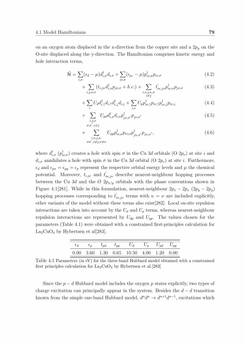
4.1 Model Hamiltonians 79
on an oxygen atom displaced in the x-direction from the copper site and a 2py on theO-site displaced along the y-direction. The Hamiltonian comprises kinetic energy andhole interaction terms,
H =∑i,σ
(ϵd − µ)d†i,σdi,σ +∑iν,σ
(ϵpν − µ)p†iν,σpiν,σ (4.2)
+∑
i,j,ν,σ
(ti,jνd†i,σpjν,σ + h.c.) +
∑i,ν,j,κ,σ
i =j
t′
iκ,jνp†iκ,σpjν,σ (4.3)
+∑
i
Udd†i,↑di,↑d
†i,↓di,↓ +
∑i,ν
Upp†iν,↑piν,↑p
†iν,↓piν,↓ (4.4)
+∑i,j,ν
σ,σ′,i =j
Updd†i,σdi,σp
†jν,σ′pjν,σ′ (4.5)
+∑
i,ν,j,κ,σσ“,i =j,ν =κ
Uppp†iν,σpiν,σp
†jκ,σ′pjκ,σ′ , (4.6)
where d†i,σ (p†iν,σ) creates a hole with spin σ in the Cu 3d orbitals (O 2pν) at site i anddi,σ annihilates a hole with spin σ in the Cu 3d orbital (O 2pν) at site i. Furthermore,ϵd and ϵpx = ϵpy = ϵp represent the respective orbital energy levels and µ the chemicalpotential. Moreover, ti,jν and t
′iκ,jν describe nearest-neighbour hopping processes
between the Cu 3d and the O 2px/y orbitals with the phase conventions shown inFigure 4.1[281]. While in this formulation, nearest-neighbour 2px − 2px (2py − 2py)hopping processes corresponding to t
′iκ,jν terms with κ = ν are included explicitly,
other variants of the model without these terms also exist[282]. Local on-site repulsioninteractions are taken into account by the Ud and Up terms, whereas nearest-neighbourrepulsion interactions are represented by Udp and Upp. The values chosen for theparameters (Table 4.1) were obtained with a constrained first-principles calculation forLa2CuO4 by Hybertsen et al[283].
ϵd ϵp tpd tpp Ud Up Upd Upp
0.00 3.60 1.30 0.65 10.50 4.00 1.20 0.00Table 4.1 Parameters (in eV) for the three-band Hubbard model obtained with a constrainedfirst principles calculation for La2CuO4 by Hybertsen et al.[283]
Since the p− d Hubbard model includes the oxygen p states explicitly, two types ofcharge excitation can principally appear in the system. Besides the d− d transitionknown from the simple one-band Hubbard model, dndn → dn+1dn−1, excitations which
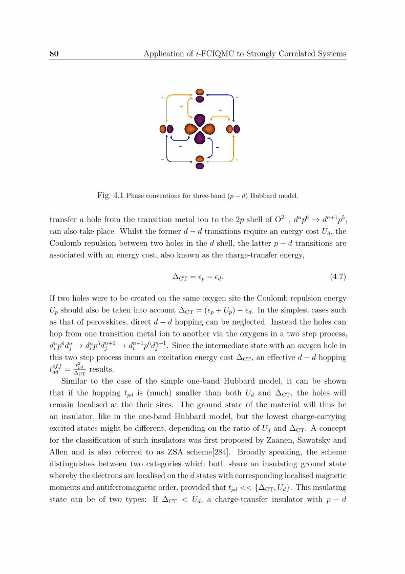
80 Application of i-FCIQMC to Strongly Correlated Systems
Fig. 4.1 Phase conventions for three-band (p− d) Hubbard model.
transfer a hole from the transition metal ion to the 2p shell of O2– , dnp6 → dn+1p5,can also take place. Whilst the former d− d transitions require an energy cost Ud, theCoulomb repulsion between two holes in the d shell, the latter p− d transitions areassociated with an energy cost, also known as the charge-transfer energy,
∆CT = ϵp − ϵd. (4.7)
If two holes were to be created on the same oxygen site the Coulomb repulsion energyUp should also be taken into account ∆CT = (ϵp + Up)− ϵd. In the simplest cases suchas that of perovskites, direct d− d hopping can be neglected. Instead the holes canhop from one transition metal ion to another via the oxygens in a two step process,dn
i p6dn
j → dni p
5dn+1j → dn−1
i p6dn+1j . Since the intermediate state with an oxygen hole in
this two step process incurs an excitation energy cost ∆CT, an effective d− d hoppingteffdd = t2
pd
∆CTresults.
Similar to the case of the simple one-band Hubbard model, it can be shownthat if the hopping tpd is (much) smaller than both Ud and ∆CT, the holes willremain localised at the their sites. The ground state of the material will thus bean insulator, like in the one-band Hubbard model, but the lowest charge-carryingexcited states might be different, depending on the ratio of Ud and ∆CT. A conceptfor the classification of such insulators was first proposed by Zaanen, Sawatsky andAllen and is also referred to as ZSA scheme[284]. Broadly speaking, the schemedistinguishes between two categories which both share an insulating ground statewhereby the electrons are localised on the d states with corresponding localised magneticmoments and antiferromagnetic order, provided that tpd << ∆CT, Ud. This insulatingstate can be of two types: If ∆CT < Ud, a charge-transfer insulator with p − d
4.1 Model Hamiltonians 81
transitions, dnp6 → dn+1p5, as lowest energy excitations and an energy gap Eg = ∆CT
results, whilst in the opposite case of ∆CT > Ud, a Mott-Hubbard insulator withd − d transitions, dndn → dn+1dn−1, as lowest energy excitations and an energy gapEg = Ud arises, yielding a schematic ZSA phase diagram[285, 276]. In both casesthe magnetic properties of the materials are largely determined by the d states onthe transition metal ions. Similarly, magnetic exchange interaction mostly involveshopping via intermediate oxygen. For materials with non-degenerate d levels andsimple lattices with TM–O–TM ∼ 180°bond angle the exchange interaction will beantiferromagnetic in nature. However, whilst in Mott-Hubbard insulators the exchangeinteraction is dominated by the standard antiferromagnetic superexchange mechanismdn
i p6dn
j1−→ dn
i p5dn+1
j2−→ dn−1
i p6dn+1j
3−→ dni p
5dn+1j
4−→ dni p
6dnj , in charge-transfer insulators
another antiferromagnetic exchange process, the semicovalent exchange, dominatesdn
i p6dn
j1−→ dn
i p5dn+1
j2−→ dn+1
i p4dn+1j
3−→ dn+1i p5dn
j4−→ dn
i p6dn
j , which involves virtualexcited states with two holes on oxygen and is therefore irrelevant in the Mott-Hubbardregime.
Most transition metal oxides belong to one of the two insulator categories and can beclassified according to which regime of the ZSA phase diagram they are likely to fall into.In general, the charge-transfer energy ∆CT decreases regularly across the 3d series fromTi to Cu. Similarly, it also decreases with increasing valency of the transition metal ionwhich becomes apparent from the values for ∆CT obtained from spectroscopic data[286].Early 3d transition metals have a relatively large ∆CT so that their correspondingmaterials such as Ti or V oxides typically fall into the Mott-Hubbard insulator regime.When the p− d hopping becomes large and the ratio Ud
tpdis reduced in this regime, the
system will sooner or later undergo a Mott transition and a metallic state results. Incontrast, heavy 3d transition metals usually belong to the charge-transfer insulatorregime as ∆CT < Ud. When the ratio ∆CT
tpdis decreased in this regime, the picture is
less clear[285]. In particular, interesting phenomena may appear for a small or evennegative charge transfer energy[287] which can occur for late 3d transition metalswith high valency like Fe4+ or Cu3+. In these circumstances, the oxygen p bandsacquire a certain number of holes since the transfer process dnp6 → dn+1p5 leads toa gain in energy. (Strictly speaking, it should be noted that the energy levels arenot single-particle energy levels of non-interacting electrons but also include effectsof Coulomb repulsion interaction.) Hence, the real electronic configuration in thesematerials involve oxygen holes with configurations of the type Fe3+L instead of Fe4+
and Cu2+L instead of Cu3+ where L denotes the ligand (here oxygen) hole. Thisphenomenon is also known as self-doping[288]: oxygen holes will spontaneously appear,
82 Application of i-FCIQMC to Strongly Correlated Systems
even for nominally undoped, stoichiometric materials which can have a strong influenceon many of their properties. Materials with small or negative charge-transfer energygaps can thus display a variety of different states, specifically when Ud remains large.They may be metals (of a heavy-fermion type, as they still contain strongly correlatedd-electrons coexisting with less correlated p-electrons of oxygen ( Ud
tpdstill >> 1)), or
they may be insulators (probably resembling Kondo insulators). They may possessdifferent magnetic properties, including ferromagnetism (CrO2[288] and (La/Sr)CoO3)or spontaneous charge disproportionation (CaFeO3[289]) may occur. It is also thoughtthat, although this is still an open question, the contribution of oxygen p holes isinstrumental for the phenomenon of high-Tc superconductivity[290, 291] since thesematerials are mostly obtained by hole-doping of CuO2-planes, as for example in thecase of La2–xSrxCuO4 where the holes will predominantly go to oxygens and statessuch as Cu2+ (d9) O– (p5) = Cu2+L instead of Cu3+ will be created.
In some situations such as hole-doped cuprates, the basis of high-Tc superconductiv-ity, the hybridisation of p and d states can lead to behaviour that resembles that of thesimple one-band Hubbard model. The objects which appear in these cases are referredto as Zhang-Rice singlets[292]. The latter represent a bound singlet state of the typed ↑ p ↓ −d ↓ p ↑ whereby the d-hole on the Cu2+ ion (S = 1
2) and the p-hole of oppositespin delocalised over the surrounding four oxygens (S = 1
2) hybridise. Coherenceeffects in the p− d hybridisation (tpd → tpd,coh. = 2tpd) strongly enhances the bindingenergy of these singlets. In effect, when an undoped cuprate with Cu2+ (d9,S = 1
2)like La2CuO4 is doped with holes as in La2–xSrxCuO4[293], each hole first localises onthe oxygen p states and then forms a singlet bound state with Cu2+, correspondingto one singlet per doped hole similar to the states created when a simple one-bandHubbard model is doped with holes. Zhang and Rice[292] therefore concluded thatfor the ground and lowest excited state in typical high-TC cuprates the p− d modelcan be reduced to a simple non-degenerate one-band Hubbard model with the holestate replaced by a Zhang-Rice singlet state. To be precise, the situation cannot bedescribed by a single-particle picture and the Coulomb repulsion between particlesneeds to be included. This will change some expressions and numerical values butthe qualitative conclusion remain the same. Although some conflicting claims andcontroversies remain[294], the Zhang-Rice picture seems to be close to reality and iswidely accepted.
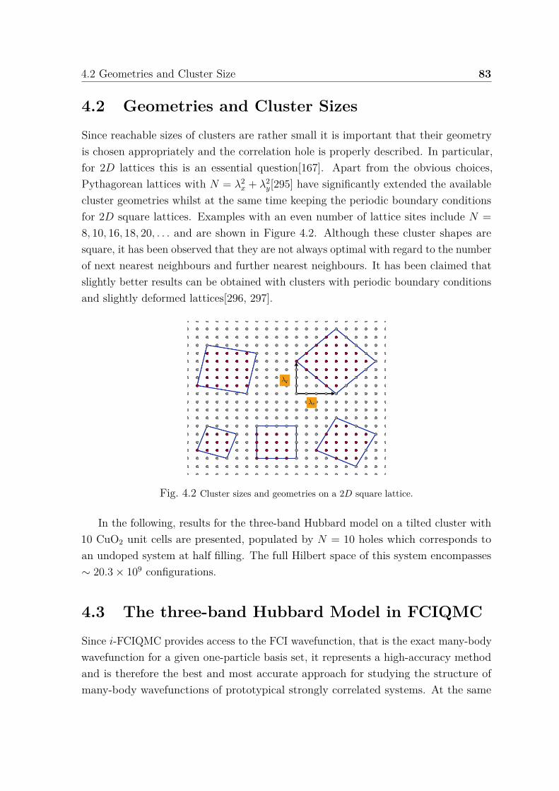
4.2 Geometries and Cluster Size 83
4.2 Geometries and Cluster Sizes
Since reachable sizes of clusters are rather small it is important that their geometryis chosen appropriately and the correlation hole is properly described. In particular,for 2D lattices this is an essential question[167]. Apart from the obvious choices,Pythagorean lattices with N = λ2
x + λ2y[295] have significantly extended the available
cluster geometries whilst at the same time keeping the periodic boundary conditionsfor 2D square lattices. Examples with an even number of lattice sites include N =8, 10, 16, 18, 20, . . . and are shown in Figure 4.2. Although these cluster shapes aresquare, it has been observed that they are not always optimal with regard to the numberof next nearest neighbours and further nearest neighbours. It has been claimed thatslightly better results can be obtained with clusters with periodic boundary conditionsand slightly deformed lattices[296, 297].
Fig. 4.2 Cluster sizes and geometries on a 2D square lattice.
In the following, results for the three-band Hubbard model on a tilted cluster with10 CuO2 unit cells are presented, populated by N = 10 holes which corresponds toan undoped system at half filling. The full Hilbert space of this system encompasses∼ 20.3× 10⁹ configurations.
4.3 The three-band Hubbard Model in FCIQMC
Since i-FCIQMC provides access to the FCI wavefunction, that is the exact many-bodywavefunction for a given one-particle basis set, it represents a high-accuracy methodand is therefore the best and most accurate approach for studying the structure ofmany-body wavefunctions of prototypical strongly correlated systems. At the same

84 Application of i-FCIQMC to Strongly Correlated Systems
time, due to its reduced computational cost, i-FCIQMC can treat systems whichare much larger than those amenable to more traditional FCI techniques. As such,i-FCIQMC can handle larger periodic clusters than conventional FCI approacheswhich helps in reducing finite size and boundary errors. Additionally, a high-accuracystudy for gaining an understanding of how the FCI representation of the wavefunctionchanges with the underlying single-particle basis set does not only enable conclusionsabout the structure of the exact wavefunction itself, but also about other wavefunctionansatzes and alternative more approximate wavefunction-based methods, as well asabout suitable directions for their further development.
4.3.1 The Choice of Single-Particle Basis Sets
Since the FCI energy is invariant to unitary transformations of the underlying single-particle basis spanning the space, it is possible to freely choose a basis set amongst thehuge variety of existing one-particle bases. The purpose of the study in this chapter is toinvestigate how this choice affects the resulting Cn coefficients in the FCI wavefunctionexpansion,
|ΨFCI⟩ =∑
nCn |n⟩ , (4.8)
where |n⟩ denotes the N -particle Slater determinant. While a good and fruitful choice ofbasis can lead to a compact and sparse FCI expansion of |Ψ⟩ which is more amenable totreatment with configuration-based methods, a poor choice of basis can result in a highlymulticonfigurational and extended wavefunction with many determinants contributingwith significant weight. A natural measure for the sparsity of a wavefunction is the L1
norm,
L1 =∑
n|Cn|. (4.9)
Within (i)-FCIQMC this L1 norm is quantified up to a normalisation constant bythe total number of walkers L1 ∝ Nw. Consequently, in this i-FCIQMC study arepresentation of |Ψ⟩ is sought in which the L1 norm and level of complexity aresmall once the energy has converged to within small error bars. For this purpose, twowidely available sources of single-particle spin orbitals are investigated, restricted andunrestricted Hartree-Fock spin orbitals (RHF, UHF) which are also compared withrestricted and unrestricted natural orbitals (RNO, UNO). Although the latter requireknowledge of the exact fully correlated wavefunction, they are known to yield rapidly
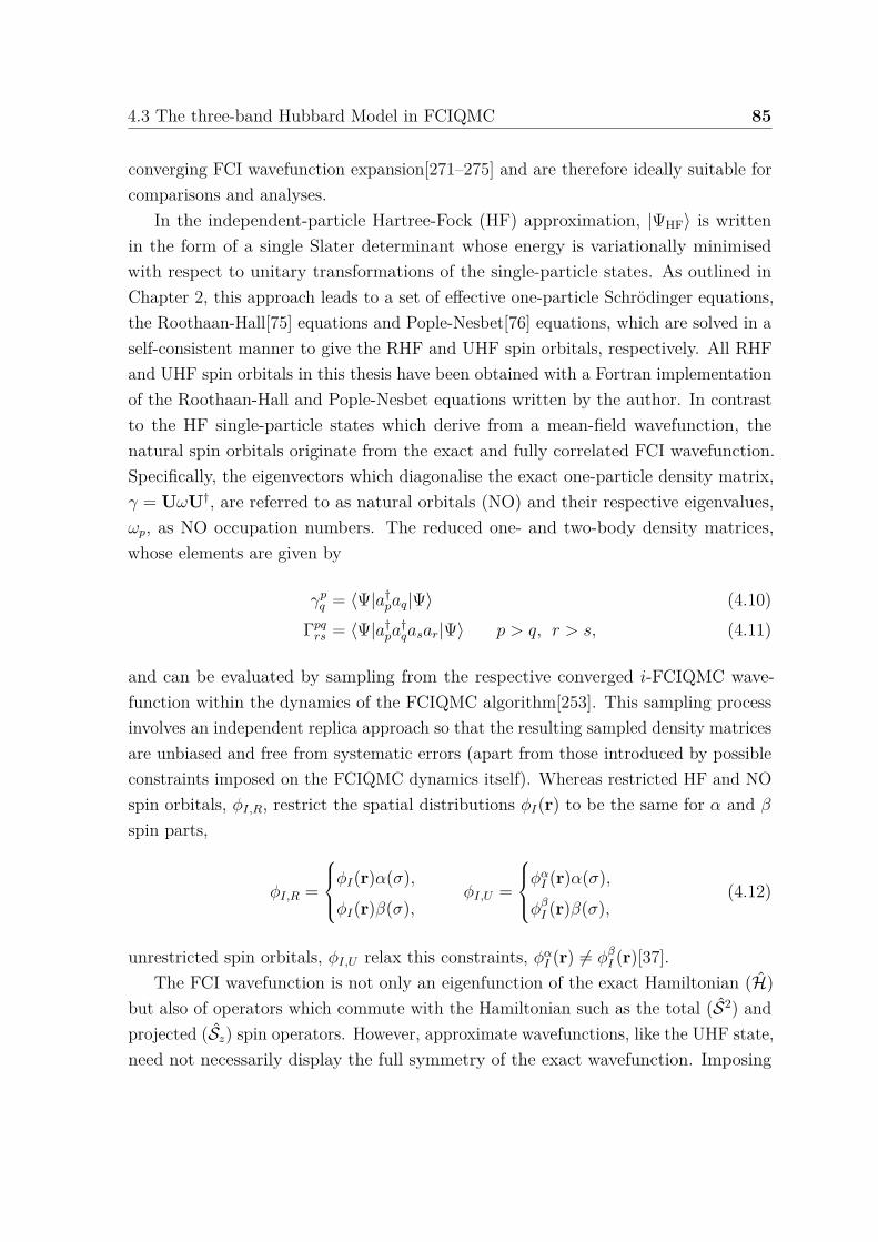
4.3 The three-band Hubbard Model in FCIQMC 85
converging FCI wavefunction expansion[271–275] and are therefore ideally suitable forcomparisons and analyses.
In the independent-particle Hartree-Fock (HF) approximation, |ΨHF⟩ is writtenin the form of a single Slater determinant whose energy is variationally minimisedwith respect to unitary transformations of the single-particle states. As outlined inChapter 2, this approach leads to a set of effective one-particle Schrödinger equations,the Roothaan-Hall[75] equations and Pople-Nesbet[76] equations, which are solved in aself-consistent manner to give the RHF and UHF spin orbitals, respectively. All RHFand UHF spin orbitals in this thesis have been obtained with a Fortran implementationof the Roothaan-Hall and Pople-Nesbet equations written by the author. In contrastto the HF single-particle states which derive from a mean-field wavefunction, thenatural spin orbitals originate from the exact and fully correlated FCI wavefunction.Specifically, the eigenvectors which diagonalise the exact one-particle density matrix,γ = UωU†, are referred to as natural orbitals (NO) and their respective eigenvalues,ωp, as NO occupation numbers. The reduced one- and two-body density matrices,whose elements are given by
γpq = ⟨Ψ|a†paq|Ψ⟩ (4.10)
Γpqrs = ⟨Ψ|a†pa†qasar|Ψ⟩ p > q, r > s, (4.11)
and can be evaluated by sampling from the respective converged i-FCIQMC wave-function within the dynamics of the FCIQMC algorithm[253]. This sampling processinvolves an independent replica approach so that the resulting sampled density matricesare unbiased and free from systematic errors (apart from those introduced by possibleconstraints imposed on the FCIQMC dynamics itself). Whereas restricted HF and NOspin orbitals, ϕI,R, restrict the spatial distributions ϕI(r) to be the same for α and β
spin parts,
ϕI,R =
ϕI(r)α(σ),ϕI(r)β(σ),
ϕI,U =
ϕαI (r)α(σ),ϕβ
I (r)β(σ),(4.12)
unrestricted spin orbitals, ϕI,U relax this constraints, ϕαI (r) = ϕβ
I (r)[37].The FCI wavefunction is not only an eigenfunction of the exact Hamiltonian (H)
but also of operators which commute with the Hamiltonian such as the total (S2) andprojected (Sz) spin operators. However, approximate wavefunctions, like the UHF state,need not necessarily display the full symmetry of the exact wavefunction. Imposing
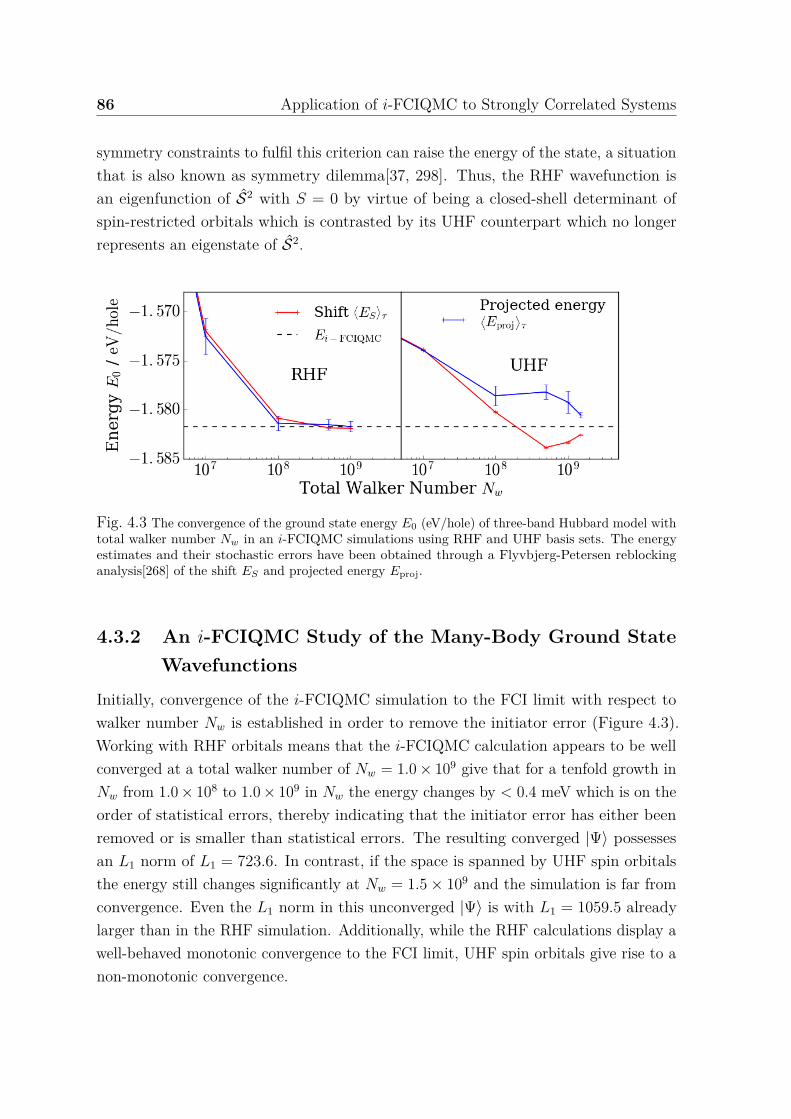
86 Application of i-FCIQMC to Strongly Correlated Systems
symmetry constraints to fulfil this criterion can raise the energy of the state, a situationthat is also known as symmetry dilemma[37, 298]. Thus, the RHF wavefunction isan eigenfunction of S2 with S = 0 by virtue of being a closed-shell determinant ofspin-restricted orbitals which is contrasted by its UHF counterpart which no longerrepresents an eigenstate of S2.
Fig. 4.3 The convergence of the ground state energy E0 (eV/hole) of three-band Hubbard model withtotal walker number Nw in an i-FCIQMC simulations using RHF and UHF basis sets. The energyestimates and their stochastic errors have been obtained through a Flyvbjerg-Petersen reblockinganalysis[268] of the shift ES and projected energy Eproj.
4.3.2 An i-FCIQMC Study of the Many-Body Ground StateWavefunctions
Initially, convergence of the i-FCIQMC simulation to the FCI limit with respect towalker number Nw is established in order to remove the initiator error (Figure 4.3).Working with RHF orbitals means that the i-FCIQMC calculation appears to be wellconverged at a total walker number of Nw = 1.0× 10⁹ give that for a tenfold growth inNw from 1.0× 10⁸ to 1.0× 10⁹ in Nw the energy changes by < 0.4 meV which is on theorder of statistical errors, thereby indicating that the initiator error has either beenremoved or is smaller than statistical errors. The resulting converged |Ψ⟩ possessesan L1 norm of L1 = 723.6. In contrast, if the space is spanned by UHF spin orbitalsthe energy still changes significantly at Nw = 1.5× 10⁹ and the simulation is far fromconvergence. Even the L1 norm in this unconverged |Ψ⟩ is with L1 = 1059.5 alreadylarger than in the RHF simulation. Additionally, while the RHF calculations display awell-behaved monotonic convergence to the FCI limit, UHF spin orbitals give rise to anon-monotonic convergence.
4.3 The three-band Hubbard Model in FCIQMC 87
Wavefunction |ΨFCI⟩ |ΨRHF⟩ |ΨUHF⟩ |ΨCAS⟩One-particle Basis RHF/UHF RHF UHF RHF UHF RNO UNO
E0 −1.5817(5) −0.9521 −1.5291 −1.3399 −1.5341 −1.5586 −1.5587ED −0.9521 −1.5291 −0.7636 −0.8350pcorr 61.6 9.5 97.2 97.0⟨nCu⟩ 0.70 0.49 0.73 0.53 0.73 0.71 0.73⟨nO⟩ 0.15 0.25 0.14 0.24 0.14 0.15 0.14⟨M2⟩ 0.118 0.000 0.113 0.056 0.130⟨S2⟩ 0.00 0.00 4.37 0.00 0.00
Table 4.2 Properties of the ground state wavefunctions for three-band Hubbard model. Ground stateenergies E0(eV/hole), energy of the lowest-energy determinant ED(eV/hole), percentage of correlationenergy pcorr(%) captured by |ΨCAS⟩, average hole densities per atom ⟨nA⟩ (holes/atom), staggeredmagnetisation
⟨M2⟩, square magnitude of spin
⟨S2⟩. Stochastic errors in the previous digit are
presented in parentheses and were estimated with a Flyvbjerg-Petersen blocking analysis[268].
In order to shed some light on the reasons behind this profound difference, thei-FCIQMC, RHF and UHF ground states are examined. As far as the total groundstate energy is concerned, the UHF approximation is able to capture ∼ 97 % of thetrue i-FCIQMC ground state energy, whereas the RHF approximation only accountsfor ∼ 60 %. A similar picture arises when comparing the average hole densities peratom for the Cu, ⟨nCu⟩, and O, ⟨nO⟩, atomic sites, defined as
⟨nA⟩ = 1NA
∑p∈A
γpp = 1
NA
∑p∈A
⟨Ψ|a†pap|Ψ⟩ , (4.13)
where the summation includes only those spin orbitals located on the respective NA
lattice sites that are associated with atoms of type A. Again, the distribution of holedensity in the system as given by the i-FCIQMC wavefunction is much more closelyapproximated by the UHF wavefunction. Whilst |ΨUHF⟩ only slightly overestimates thedegree of ionicity in the system (by a few percentages, ∼ 4− 6 %, in ⟨nCu/O⟩), |ΨRHF⟩largely overestimates the degree of covalency (by a significant percentage, ∼ 30− 66 %,in ⟨nCu/O⟩).
Like previous studies of the three band Hubbard model[284, 4, 300–304], the exacti-FCIQMC ground state establishes an antiferromagnetic long-range order across thecopper sites, as illustrated by the respective order parameter, the staggered magnetisa-tion which can be obtained from the two-body density matrix of the wavefunction,
⟨M2⟩ = 1NS
∑ij
(−1)(xi+yi)+(xj+yj) ⟨ΨFCI|Si · Sj|ΨFCI⟩ , (4.14)
where the summations over i and j run over all lattice sites with Cartesian coordinates(xi, yi) and spin operator Si giving a total of NS terms. Likewise, the local spin-spin
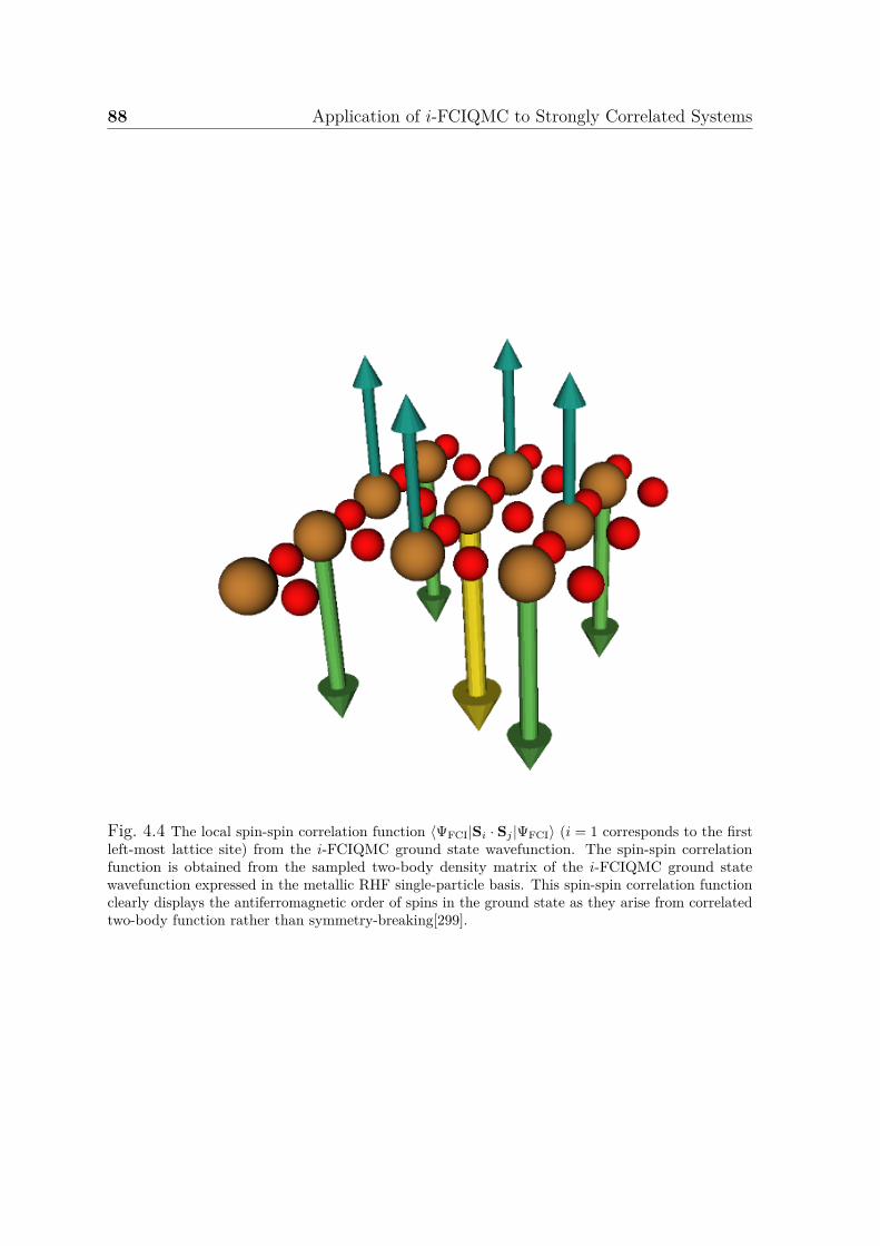
88 Application of i-FCIQMC to Strongly Correlated Systems
Fig. 4.4 The local spin-spin correlation function ⟨ΨFCI|Si · Sj |ΨFCI⟩ (i = 1 corresponds to the firstleft-most lattice site) from the i-FCIQMC ground state wavefunction. The spin-spin correlationfunction is obtained from the sampled two-body density matrix of the i-FCIQMC ground statewavefunction expressed in the metallic RHF single-particle basis. This spin-spin correlation functionclearly displays the antiferromagnetic order of spins in the ground state as they arise from correlatedtwo-body function rather than symmetry-breaking[299].
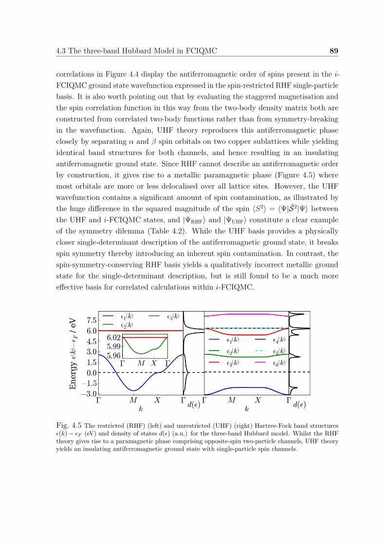
4.3 The three-band Hubbard Model in FCIQMC 89
correlations in Figure 4.4 display the antiferromagnetic order of spins present in the i-FCIQMC ground state wavefunction expressed in the spin-restricted RHF single-particlebasis. It is also worth pointing out that by evaluating the staggered magnetisation andthe spin correlation function in this way from the two-body density matrix both areconstructed from correlated two-body functions rather than from symmetry-breakingin the wavefunction. Again, UHF theory reproduces this antiferromagnetic phaseclosely by separating α and β spin orbitals on two copper sublattices while yieldingidentical band structures for both channels, and hence resulting in an insulatingantiferromagnetic ground state. Since RHF cannot describe an antiferromagnetic orderby construction, it gives rise to a metallic paramagnetic phase (Figure 4.5) wheremost orbitals are more or less delocalised over all lattice sites. However, the UHFwavefunction contains a significant amount of spin contamination, as illustrated bythe huge difference in the squared magnitude of the spin ⟨S2⟩ = ⟨Ψ|S2|Ψ⟩ betweenthe UHF and i-FCIQMC states, and |ΨRHF⟩ and |ΨUHF⟩ constitute a clear exampleof the symmetry dilemma (Table 4.2). While the UHF basis provides a physicallycloser single-determinant description of the antiferromagnetic ground state, it breaksspin symmetry thereby introducing an inherent spin contamination. In contrast, thespin-symmetry-conserving RHF basis yields a qualitatively incorrect metallic groundstate for the single-determinant description, but is still found to be a much moreeffective basis for correlated calculations within i-FCIQMC.
Fig. 4.5 The restricted (RHF) (left) and unrestricted (UHF) (right) Hartree-Fock band structuresϵ(k)− ϵF (eV) and density of states d(ϵ) (a.u.) for the three-band Hubbard model. Whilst the RHFtheory gives rise to a paramagnetic phase comprising opposite-spin two-particle channels, UHF theoryyields an insulating antiferromagnetic ground state with single-particle spin channels.
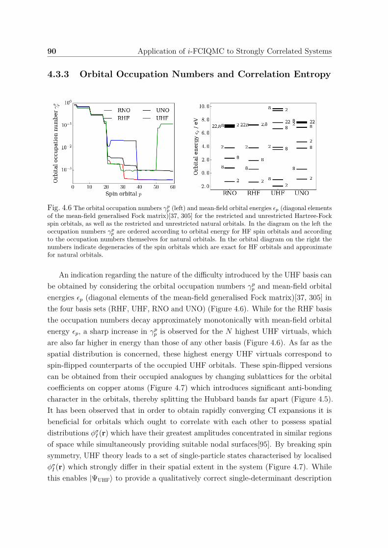
90 Application of i-FCIQMC to Strongly Correlated Systems
4.3.3 Orbital Occupation Numbers and Correlation Entropy
Fig. 4.6 The orbital occupation numbers γpp (left) and mean-field orbital energies ϵp (diagonal elements
of the mean-field generalised Fock matrix)[37, 305] for the restricted and unrestricted Hartree-Fockspin orbitals, as well as the restricted and unrestricted natural orbitals. In the diagram on the left theoccupation numbers γp
p are ordered according to orbital energy for HF spin orbitals and accordingto the occupation numbers themselves for natural orbitals. In the orbital diagram on the right thenumbers indicate degeneracies of the spin orbitals which are exact for HF orbitals and approximatefor natural orbitals.
An indication regarding the nature of the difficulty introduced by the UHF basis canbe obtained by considering the orbital occupation numbers γp
p and mean-field orbitalenergies ϵp (diagonal elements of the mean-field generalised Fock matrix)[37, 305] inthe four basis sets (RHF, UHF, RNO and UNO) (Figure 4.6). While for the RHF basisthe occupation numbers decay approximately monotonically with mean-field orbitalenergy ϵp, a sharp increase in γp
p is observed for the N highest UHF virtuals, whichare also far higher in energy than those of any other basis (Figure 4.6). As far as thespatial distribution is concerned, these highest energy UHF virtuals correspond tospin-flipped counterparts of the occupied UHF orbitals. These spin-flipped versionscan be obtained from their occupied analogues by changing sublattices for the orbitalcoefficients on copper atoms (Figure 4.7) which introduces significant anti-bondingcharacter in the orbitals, thereby splitting the Hubbard bands far apart (Figure 4.5).It has been observed that in order to obtain rapidly converging CI expansions it isbeneficial for orbitals which ought to correlate with each other to possess spatialdistributions ϕσ
I (r) which have their greatest amplitudes concentrated in similar regionsof space while simultaneously providing suitable nodal surfaces[95]. By breaking spinsymmetry, UHF theory leads to a set of single-particle states characterised by localisedϕσ
I (r) which strongly differ in their spatial extent in the system (Figure 4.7). Whilethis enables |ΨUHF⟩ to provide a qualitatively correct single-determinant description
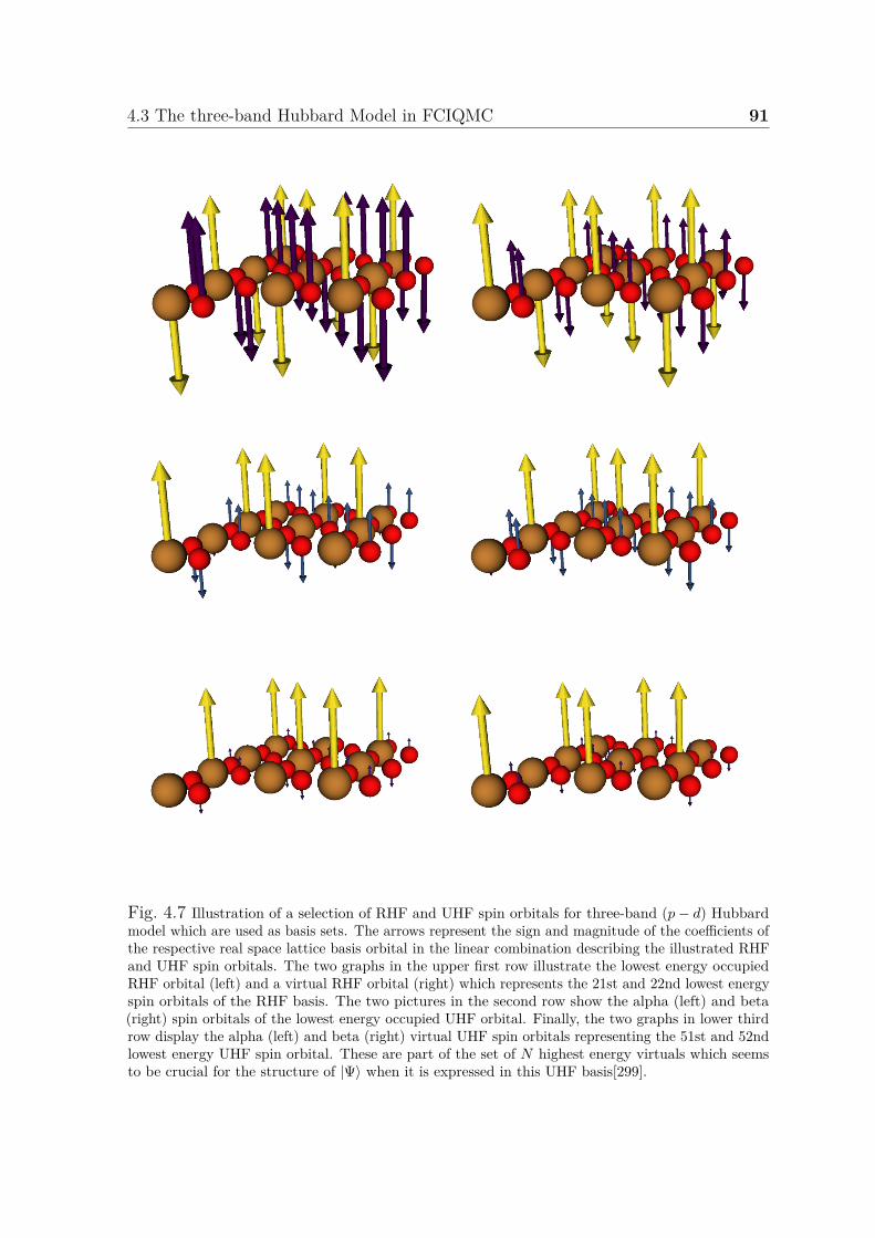
4.3 The three-band Hubbard Model in FCIQMC 91
Fig. 4.7 Illustration of a selection of RHF and UHF spin orbitals for three-band (p− d) Hubbardmodel which are used as basis sets. The arrows represent the sign and magnitude of the coefficients ofthe respective real space lattice basis orbital in the linear combination describing the illustrated RHFand UHF spin orbitals. The two graphs in the upper first row illustrate the lowest energy occupiedRHF orbital (left) and a virtual RHF orbital (right) which represents the 21st and 22nd lowest energyspin orbitals of the RHF basis. The two pictures in the second row show the alpha (left) and beta(right) spin orbitals of the lowest energy occupied UHF orbital. Finally, the two graphs in lower thirdrow display the alpha (left) and beta (right) virtual UHF spin orbitals representing the 51st and 52ndlowest energy UHF spin orbital. These are part of the set of N highest energy virtuals which seemsto be crucial for the structure of |Ψ⟩ when it is expressed in this UHF basis[299].
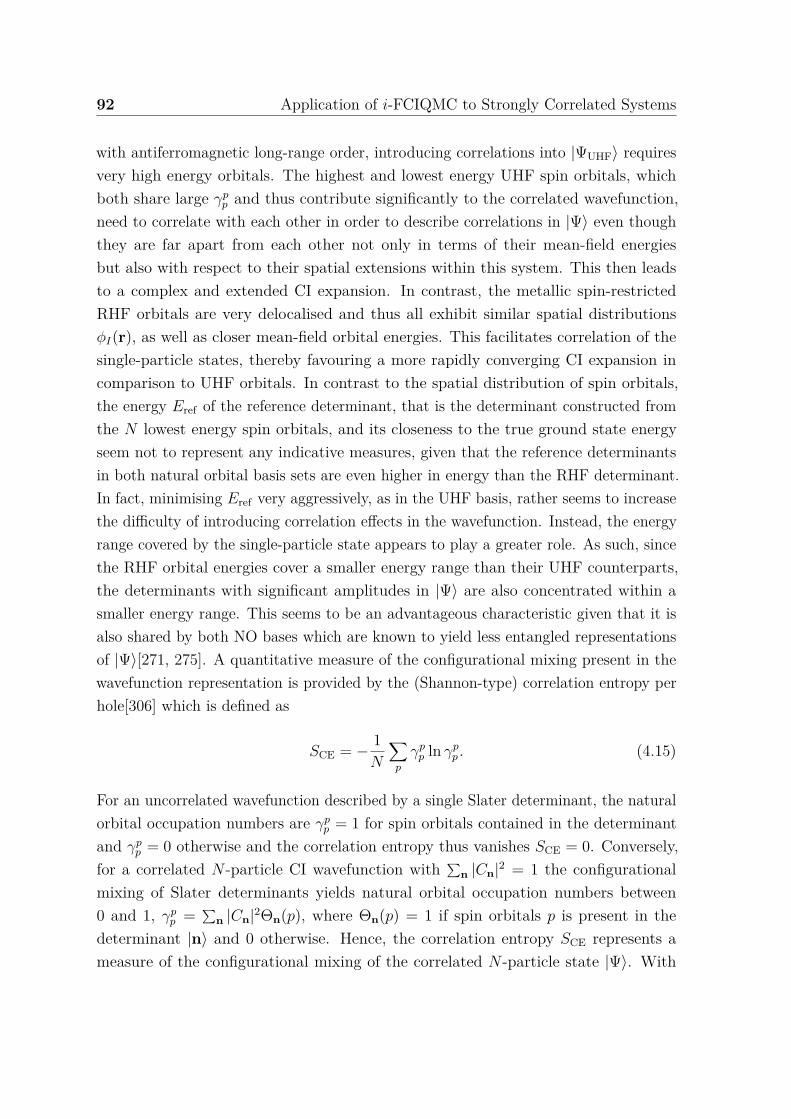
92 Application of i-FCIQMC to Strongly Correlated Systems
with antiferromagnetic long-range order, introducing correlations into |ΨUHF⟩ requiresvery high energy orbitals. The highest and lowest energy UHF spin orbitals, whichboth share large γp
p and thus contribute significantly to the correlated wavefunction,need to correlate with each other in order to describe correlations in |Ψ⟩ even thoughthey are far apart from each other not only in terms of their mean-field energiesbut also with respect to their spatial extensions within this system. This then leadsto a complex and extended CI expansion. In contrast, the metallic spin-restrictedRHF orbitals are very delocalised and thus all exhibit similar spatial distributionsϕI(r), as well as closer mean-field orbital energies. This facilitates correlation of thesingle-particle states, thereby favouring a more rapidly converging CI expansion incomparison to UHF orbitals. In contrast to the spatial distribution of spin orbitals,the energy Eref of the reference determinant, that is the determinant constructed fromthe N lowest energy spin orbitals, and its closeness to the true ground state energyseem not to represent any indicative measures, given that the reference determinantsin both natural orbital basis sets are even higher in energy than the RHF determinant.In fact, minimising Eref very aggressively, as in the UHF basis, rather seems to increasethe difficulty of introducing correlation effects in the wavefunction. Instead, the energyrange covered by the single-particle state appears to play a greater role. As such, sincethe RHF orbital energies cover a smaller energy range than their UHF counterparts,the determinants with significant amplitudes in |Ψ⟩ are also concentrated within asmaller energy range. This seems to be an advantageous characteristic given that it isalso shared by both NO bases which are known to yield less entangled representationsof |Ψ⟩[271, 275]. A quantitative measure of the configurational mixing present in thewavefunction representation is provided by the (Shannon-type) correlation entropy perhole[306] which is defined as
SCE = − 1N
∑p
γpp ln γp
p . (4.15)
For an uncorrelated wavefunction described by a single Slater determinant, the naturalorbital occupation numbers are γp
p = 1 for spin orbitals contained in the determinantand γp
p = 0 otherwise and the correlation entropy thus vanishes SCE = 0. Conversely,for a correlated N -particle CI wavefunction with ∑
n |Cn|2 = 1 the configurationalmixing of Slater determinants yields natural orbital occupation numbers between0 and 1, γp
p = ∑n |Cn|2Θn(p), where Θn(p) = 1 if spin orbitals p is present in the
determinant |n⟩ and 0 otherwise. Hence, the correlation entropy SCE represents ameasure of the configurational mixing of the correlated N -particle state |Ψ⟩. With
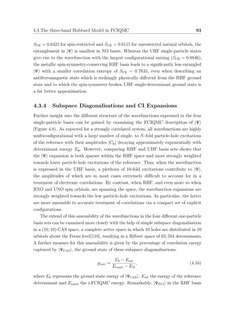
4.3 The three-band Hubbard Model in FCIQMC 93
SCE = 0.6421 for spin-restricted and SCE = 0.6115 for unrestricted natural orbitals, theentanglement in |Ψ⟩ is smallest in NO bases. Whereas the UHF single-particle statesgive rise to the wavefunction with the largest configurational mixing (SCE = 0.8846),the metallic spin-symmetry-conserving RHF basis leads to a significantly less entangled|Ψ⟩ with a smaller correlation entropy of SCE = 0.7635, even when describing anantiferromagnetic state which is strikingly physically different from the RHF groundstate and to which the spin-symmetry-broken UHF single-determinant ground state isa far better approximation.
4.3.4 Subspace Diagonalisations and CI Expansions
Further insight into the different structure of the wavefunctions expressed in the foursingle-particle bases can be gained by examining the FCIQMC description of |Ψ⟩(Figure 4.8). As expected for a strongly correlated system, all wavefunctions are highlymulticonfigurational with a large number of single- to N -fold particle-hole excitationsof the reference with their amplitudes |Cn| decaying approximately exponentially withdeterminant energy En. However, comparing RHF and UHF basis sets shows thatthe |Ψ⟩ expansion is both sparser within the RHF space and more strongly weightedtowards lower particle-hole excitations of the reference. Thus, when the wavefunctionis expressed in the UHF basis, a plethora of 10-fold excitations contribute to |Ψ⟩,the amplitudes of which are in most cases extremely difficult to account for in atreatment of electronic correlations. By contrast, when RHF, and even more so whenRNO and UNO spin orbitals, are spanning the space, the wavefunction expansions arestrongly weighted towards the low particle-hole excitations. In particular, the latterare more amenable to accurate treatment of correlations via a compact set of explicitconfigurations.
The extend of this amenability of the wavefunctions in the four different one-particlebasis sets can be examined more closely with the help of simple subspace diagonalisationin a (10, 10)-CAS space, a complete active space in which 10 holes are distributed in 10orbitals about the Fermi level[110], resulting in a Hilbert space of 63, 504 determinants.A further measure for this amenability is given by the percentage of correlation energycaptured by |ΨCAS⟩, the ground state of these subspace diagonalisations.
pcorr = E0 − Eref
Eexact − ED
, (4.16)
where E0 represents the ground state energy of |ΨCAS⟩, Eref the energy of the referencedeterminant and Eexact the i-FCIQMC energy. Remarkably, |ΨFCI⟩ in the RHF basis
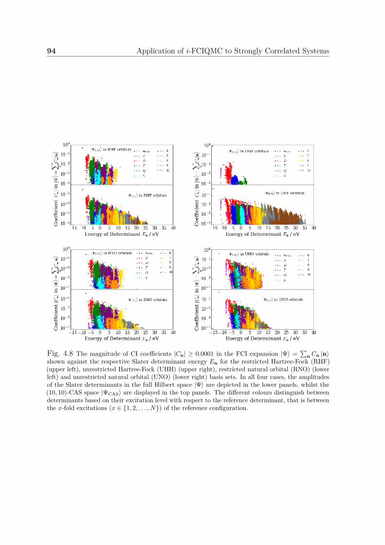
94 Application of i-FCIQMC to Strongly Correlated Systems
Fig. 4.8 The magnitude of CI coefficients |Cn| ≥ 0.0001 in the FCI expansion |Ψ⟩ =∑
n Cn |n⟩shown against the respective Slater determinant energy En for the restricted Hartree-Fock (RHF)(upper left), unrestricted Hartree-Fock (UHH) (upper right), restricted natural orbital (RNO) (lowerleft) and unrestricted natural orbital (UNO) (lower right) basis sets. In all four cases, the amplitudesof the Slater determinants in the full Hilbert space |Ψ⟩ are depicted in the lower panels, whilst the(10, 10)-CAS space |ΨCAS⟩ are displayed in the top panels. The different colours distinguish betweendeterminants based on their excitation level with respect to the reference determinant, that is betweenthe x-fold excitations (x ∈ 1, 2, . . . , N) of the reference configuration.
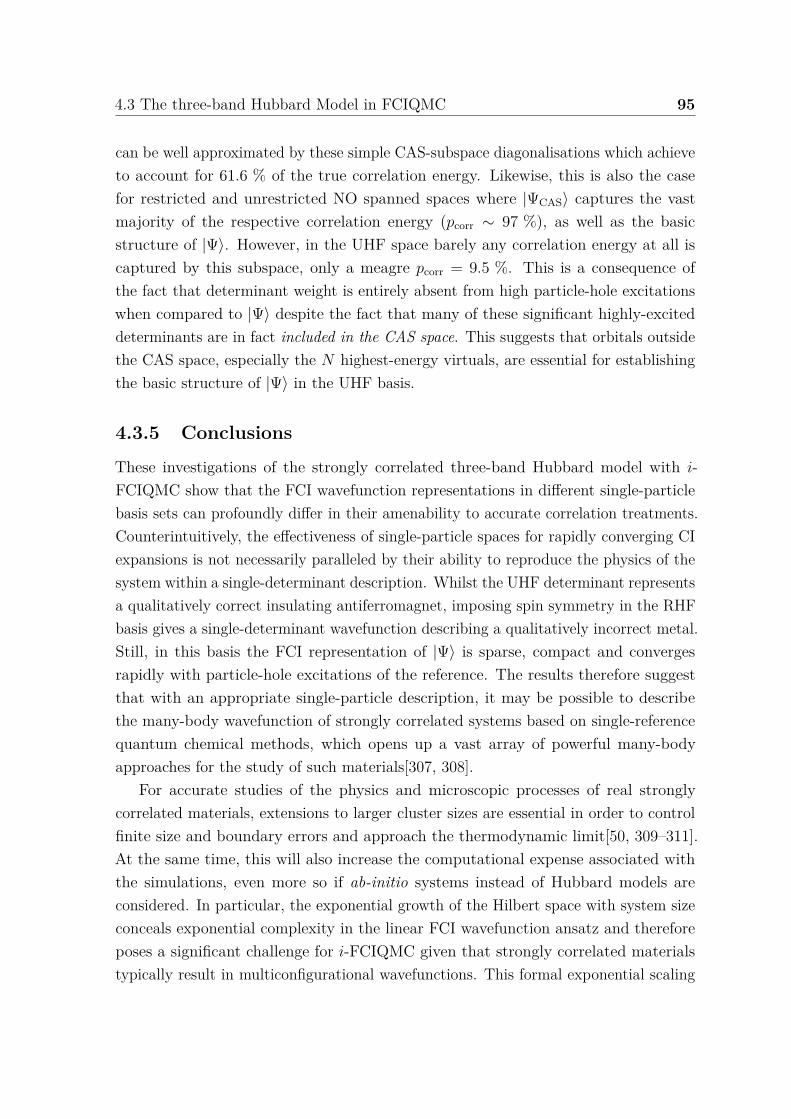
4.3 The three-band Hubbard Model in FCIQMC 95
can be well approximated by these simple CAS-subspace diagonalisations which achieveto account for 61.6 % of the true correlation energy. Likewise, this is also the casefor restricted and unrestricted NO spanned spaces where |ΨCAS⟩ captures the vastmajority of the respective correlation energy (pcorr ∼ 97 %), as well as the basicstructure of |Ψ⟩. However, in the UHF space barely any correlation energy at all iscaptured by this subspace, only a meagre pcorr = 9.5 %. This is a consequence ofthe fact that determinant weight is entirely absent from high particle-hole excitationswhen compared to |Ψ⟩ despite the fact that many of these significant highly-exciteddeterminants are in fact included in the CAS space. This suggests that orbitals outsidethe CAS space, especially the N highest-energy virtuals, are essential for establishingthe basic structure of |Ψ⟩ in the UHF basis.
4.3.5 Conclusions
These investigations of the strongly correlated three-band Hubbard model with i-FCIQMC show that the FCI wavefunction representations in different single-particlebasis sets can profoundly differ in their amenability to accurate correlation treatments.Counterintuitively, the effectiveness of single-particle spaces for rapidly converging CIexpansions is not necessarily paralleled by their ability to reproduce the physics of thesystem within a single-determinant description. Whilst the UHF determinant representsa qualitatively correct insulating antiferromagnet, imposing spin symmetry in the RHFbasis gives a single-determinant wavefunction describing a qualitatively incorrect metal.Still, in this basis the FCI representation of |Ψ⟩ is sparse, compact and convergesrapidly with particle-hole excitations of the reference. The results therefore suggestthat with an appropriate single-particle description, it may be possible to describethe many-body wavefunction of strongly correlated systems based on single-referencequantum chemical methods, which opens up a vast array of powerful many-bodyapproaches for the study of such materials[307, 308].
For accurate studies of the physics and microscopic processes of real stronglycorrelated materials, extensions to larger cluster sizes are essential in order to controlfinite size and boundary errors and approach the thermodynamic limit[50, 309–311].At the same time, this will also increase the computational expense associated withthe simulations, even more so if ab-initio systems instead of Hubbard models areconsidered. In particular, the exponential growth of the Hilbert space with system sizeconceals exponential complexity in the linear FCI wavefunction ansatz and thereforeposes a significant challenge for i-FCIQMC given that strongly correlated materialstypically result in multiconfigurational wavefunctions. This formal exponential scaling

96 Application of i-FCIQMC to Strongly Correlated Systems
of i-FCIQMC implies that larger cluster sizes can become intractable, even if anoptimal single-particle basis set is chosen. Thus, in order to circumvent the challengeposed by the exponential scaling of the Hilbert space, the development of alternativewavefunction-based methods which bear a reduced scaling with system size is vital forthe advancement to larger systems and appropriate cluster sizes of strongly correlatedmaterials.
Chapter 5
A Projector Quantum Monte CarloMethod for Non-linearWavefunctions
Conceptually, the description of quantum many-body states, which is central to under-standing a wealth of complex emergent phenomena in condensed matter physics andquantum chemistry, is straightforward and well defined: with the Hamiltonian known,the exact solution is a linear superposition of all possible classical configurations ofparticles spanning the full Hilbert space. However, this conceals exponential complexityin the wavefunction which in general prohibits both the storage and manipulation ofall of these linear coefficients.
From a methodological perspective, Quantum Monte Carlo methods provide oneapproach to deal with the exponentially large Hilbert space by sampling the spacestochastically. For studies of the ground state of quantum systems, these broadlyseparate into two categories, Variational (VMC) and Projector (PMC) Quantum MonteCarlo approaches[193, 50] which are described in detail in Chapter 3. In the first, acompact, polynomial-complex approximate wavefunction ansatz is imposed, generallywith a small number of variational parameters. State-of-the-art methods to optimisethe wavefunction involve sampling and accumulating the gradient and hessian of theenergy with respect to the parameters in the tangent space of the current wavefunction.This is done by projecting into and sampling from the exponential configurationalspace. Once a stochastic representation of these quantities is obtained, updates to thewavefunction parameters are found by a variety of iterative techniques until convergenceof this non-linear parameterisation is achieved. By contrast, in PMC approaches anoperator written as a decaying function of the Hamiltonian is continually applied
98 A Projector Quantum Monte Carlo Method for Non-linear Wavefunctions
to a stochastic representation of the full wavefunction. This projects out the higherenergy components, leaving a stochastic sampling of the dominant, (generally groundstate) eigenfunction. In particular, FCIQMC is a rather promising technique in thisspirit which stochastically samples both the wavefunction and the propagator in Fockspace[52, 247]. By exploiting sparsity inherent in the Hamiltonian, as well as in thewavefunction representations of many quantum systems essentially exact results canbe obtained with only small fractions of the Hilbert space occupied at any one time.However, despite often admitting highly accurate solutions for systems far out of reachof many alternative approaches, as demonstrated by the application of the previouschapter, the method is formally exponentially scaling with system size, albeit oftenweakly.
In order to advance to larger and condensed phase systems whilst still building onthe success of FCIQMC, one approach is to exploit the fact that electron correlationis, in general, inherently local, as well as the existence of area laws and thus thereduced amount of entanglement which effectively quantifies the relevant number ofdegrees of freedom. These facts not only imply that natural quantum many-bodystates live on a tiny submanifold of the exponentially large Hilbert space but alsosuggest that states within this relevant subspace may be faithfully described by efficientparameterisations which contain their scaling to polynomial cost, thereby circumventingthe exponential scaling of the Hilbert space. Traditionally, these wavefunctions ansatzesinhabited the domain of Variation Quantum Monte Carlo approaches, such as the LinearMethod and Stochastic Reconfiguration which represent state-of-the-art approachesfor the optimisation of large numbers of parameters. In this chapter, a new ProjectorQuantum Monte Carlo approach is proposed which naturally admits polynomialcomplex wavefunction ansatzes by combining ideas from traditional Variational andProjector Quantum Monte Carlo approaches. At the same time, developments fromthe field of deep-learning neural networks are included to arrive at a new method whichis able to handle and optimise arbitrary non-linear wavefunctions with large numbersof parameters.
5.1 Non-linear Projector Quantum Monte Carlo Method: Combining Variational andProjector Quantum Monte Carlo 99
5.1 Non-linear Projector Quantum Monte CarloMethod: Combining Variational and ProjectorQuantum Monte Carlo
The FCIQMC and some other PMC methods[51, 312] are simulated through stochasticdynamics given by
|Ψ0⟩ = limk→∞
(1− τ(H − IE0))k |ψ(0)⟩ , (5.1)
with τ chosen to be sufficiently small, where |Ψ0⟩ is the ground state of the system, andE0 is the self-consistently obtained ground state energy[52]. This can be consideredboth as a first-order approximation to imaginary-time dynamics as e−βH |ψ(0)⟩, oras a power method to project out the dominant, lowest energy eigenvector of H[51].Alternatively, a VMC perspective considers finding the variational minimum of theRitz function,
R[Ψ(Zσ)] = ⟨Ψ|H|Ψ⟩⟨Ψ|Ψ⟩ , (5.2)
through optimisation of the wavefunction parameters Zσ.
5.2 Derivation: Lagrangian Minimisation
These approaches can be shown to be analogous by considering the minimisation of apositive-definite Lagrangian
L[Ψ(Zσ)] = ⟨Ψ|H|Ψ⟩ − E0(⟨Ψ|I|Ψ⟩ − A
), (5.3)
where normalisation (up to an arbitrary constant A) is enforced by a Lagrange multiplier,which at convergence is given by E0. It is simple to show that the minimum of thisfunctional is the same as that given by the Ritz functional (Appendix A). In order tofind the wavefunction with the lowest energy, a simple gradient descent (GD)[313–315]minimisation of all variational parameters Zσ in Eq.5.3 with step size τk at iterationk is considered. Thus, for a particular parameter σ in the wavefunction this resultsin an equation which is equivalent to the finite difference approximation of imaginary
100 A Projector Quantum Monte Carlo Method for Non-linear Wavefunctions
time propagation,
Z(k+1)σ = Z(k)
σ − τk∂L[Ψ(k)(Z(k)
σ )]∂Zσ
(5.4)
= Z(k)σ − τk
[⟨∂Ψ(k)
∂Zσ
|H|Ψ(k)⟩+ ⟨Ψ(k)|H|∂Ψ(k)
∂Zσ
⟩
−E0
(⟨∂Ψ(k)
∂Zσ
|I|Ψ(k)⟩+ ⟨Ψ(k)|I|∂Ψ(k)
∂Zσ
⟩)]
(5.5)
= Z(k)σ − τk
[2 ⟨∂Ψ(k)
∂Zσ
|H|Ψ(k)⟩ − 2E0 ⟨∂Ψ(k)
∂Zσ
|I|Ψ(k)⟩]
(5.6)
= Z(k)σ − τk ⟨
∂Ψ(k)
∂Zσ
|(H − E0I)|Ψ(k)⟩ , (5.7)
where in the third line a real wavefunction and a real, symmetric Hamiltonian areassumed and in the forth line the factor of 2 is subsumed in the step size τk. Projectingthe equations into the full Hilbert space of configurations |m⟩ using the resolutionof the identity I = ∑
n |n⟩ ⟨n|, the equations
Z(k+1)σ = Z(k)
σ − τk ⟨∂Ψ(k)
∂Zσ
|(H − E(k)I)|Ψ(k)⟩ (5.8)
= Z(k)σ − τk
∑mn⟨∂Ψ(k)
∂Zσ
|m⟩ ⟨m|(H − E(k)I)|n⟩ ⟨n|Ψ(k)⟩ (5.9)
= Z(k)σ − τk
∑mn⟨∂Ψ(k)
∂Zσ
|m⟩ (⟨m|H|n⟩ − E(k) ⟨m|I|n⟩) ⟨n|Ψ(k)⟩ (5.10)
= Z(k)σ − τk
∑mn⟨∂Ψ(k)
∂Zσ
|m⟩ (Hmn − E(k)δmn) ⟨n|Ψ(k)⟩ , (5.11)
are obtained where the Lagrange multiplier E0 is replaced by the energy E(k) of thewavefunction at iteration k which at convergence is equal to E0. Similar equationscan simply be derived for complex wavefunctions and hermitian Hamiltonians. Thisapproach is very versatile and applicable to any wavefunction ansatz for which therespective derivatives exist. If the chosen wavefunction is an expansion of linearlyindependent configurations, then this will return exactly the ‘imaginary-time’ dynamicsof Eq. 5.1 and the FCIQMC master equations, demonstrating the deep connectionbetween imaginary-time propagation, gradient descent and the power method[315].
Working in the 2nd quantised basis comes with the benefit of a diagonally dominantand sparse Hamiltonian matrix. Furthermore, since the Hamiltonian is a two-bodyoperator, non-zero matrix elements, Hmn = ⟨m|H|n⟩, connect only configurations
5.3 Sampling of the Lagrangian Gradient 101
which are at most two particle-substitutions of each other (∼ O[N2M2+NM ]). Despitethe compact nature of the gradient full GD becomes unfeasible for large systems, sinceits computational cost per iteration scales linearly with the size of the exponentiallygrowing Hilbert space. In order to go beyond system sizes tractable with a deterministicgradient descent, a stochastic approach is pursued instead. In keeping with FCIQMC,the summations over configurations are replaced by random samples of both thewavefunction and Hamiltonian connections.
By replacing the deterministically evaluated gradient with its stochastic estimatethe resulting iteration cost is independent of the size of the Hilbert space which rendersthis stochastic gradient descent (SGD) approach inherently suitable for large scalesystems. A further major advantage of stochastic gradient descent over its deterministiccounterpart is that its stochastic fluctuations enable it to jump between basins ofminima. This reduces the probability of the optimisation getting trapped in oneof the abundantly present local minima which is one of the key challenges faced byminimisations of non-linear functions[316] and thus aids convergence towards the globalminimum, or at least a better local minimum with smaller error. (Dauphin et al.[317]argue that these encountered convergence difficulties are in fact not caused by localminima but rather by saddle points which are points on the surface where one dimensionslopes up and another one slopes down. These saddle points are usually surroundedby a plateau of the same error where the gradient is close to zero in all directionswhich makes it extremely difficult for SGD to escape and thus drastically slows downconvergence.)
5.3 Sampling of the Lagrangian Gradient
A key insight due to Robbins and Monro[318] was that for first order methods suchas gradient descent, the gradient does not have to be evaluated exactly to ensureconvergence towards the optimal solution. Provided that these methods use sufficientlysmall step sizes and that the gradient estimate is unbiased, the error introduced by thegradient approximation will be lifted on appropriate averaging. The stochastically eval-uated gradient of the Lagrangian for the optimisation of the wavefunction parametersat iteration k is written as
∂L[Ψ(k)(Z(k)σ )]
∂Zσ
=∑mn⟨∂Ψ(k)
∂Zσ
|m⟩ (Hmn − E(k)δmn) ⟨n|Ψ(k)⟩ , (5.12)
102 A Projector Quantum Monte Carlo Method for Non-linear Wavefunctions
where σ refers to a particular parameter in the wavefunction, m,n to a many-bodydeterminant in the configuration space, and E(k) to the current sampled energy asgiven by the density matrices and described in Section 5.7 further below. Minimisingthe statistical fluctuations in the stochastic sampling of this quantity is key to thesuccess and robustness of the algorithm. The quantities σ, n and m = n are allselected stochastically to ensure that no summation over quantities which explicitlyscale with the system size are considered. The sole exception from this is the ‘diagonal’contribution of m = n which is considered explicitly for each sample of n. Thus, thesum over n is stochastically sampled via a Metropolis Markov chain, to evaluatea stochastic representation of the wavefunction[51, 199, 200]. Similarly, a small se-lecton of configurations, m, are sampled from the set of non-zero connections viaHmn in the manner of FCIQMC, and unbiasing for the probability with a computednormalised generation probability[261, 263]. Furthermore, the derivatives ⟨∂Ψ(k)
∂Zσ|m⟩
can be efficiently evaluated from the respective wavefunction amplitudes ⟨Ψ(k)|m⟩.Further technical details on the sampling of this gradient are outlined in the followingsubsections.
Markov Chain Sampling
The selection of n is given by a Markov chain sampling of the many-body states yieldinga stochastic representation of the wavefunction Ψ(k). It is chosen to sample accordingto the probability distribution
Pmarkov(n; Ψ(k)) = | ⟨n|Ψ(k)⟩ |2∑n′ | ⟨n′|Ψ(k)⟩ |2
= | ⟨n|Ψ(k)⟩ |2
N [|Ψ(k)|2] . (5.13)
where N [|Ψ(k)|2] = ∑n′ | ⟨n′|Ψ(k)⟩ |2 represents the normalisation constant of the proba-
bility distribution. Other distributions for instance sampling according to the modulusof the wavefunction are possible and may be preferable in some instances[51]. Byrequiring the probability distribution to depend on Ψ(k), Pmarkov(n; Ψ(k)) follows theevolution of Ψ(k) and there is thus no bias originating from the choice of a (fixed) guid-ing wavefunction. Due to the difficulty of calculating the normalisation of Eq.5.13 thesampling of the set of Nsamples configurations n is performed via a Metropolis-Hastingsalgorithm[199, 200], which does not require explicit calculation of the normalisationconstant N [|Ψ(k)|2], an unfeasibly expensive operation. Instead, the algorithm gener-ates configurations ni in the Markov chain by proposing a move from ni to n′i with
5.3 Sampling of the Lagrangian Gradient 103
probability T (n′i ← ni). The move is then accepted (i.e. ni+1 = n′i) with probability
A(n′i ← ni) = min[1, T (ni ← n′i)Pmarkov(n′i; Ψ(k))T (n′i ← ni)Pmarkov(ni; Ψ(k))
], (5.14)
and otherwise rejected (i.e. ni+1 = ni). For the proposal of moves along the Markovchain only up to double electron substitutions are considered which allows for high accep-tance ratios, thereby greatly improving the efficiency of the Markov chain sampling[319].
Traditional Fock-space VMC calculations generally perform an exact summationover the possible values of m and update all σ parameters in the wavefunction.In the limit of this exact summation, a zero-variance estimator for the gradient ispossible in the case that the wavefunction Ψ(k) represents an exact eigenstate of theHamiltonian[51, 198]. However, in systems with a general two-body interaction, thisgives rise to an O[N4] step per evaluation of the gradient for a given n. Instead, thezero-variance principle is sacrificed and the set of Hamiltonian connections of n issampled via a stochastic algorithm to avoid this high cost. Hence, a small number(Ns) of configurations (m) are generated with an efficient algorithm, according to anormalised probability for each connection, Pgen(m|n; H), which can depend on theHamiltonian under consideration. Finally a single wavefunction parameter, σ is chosento be updated in the algorithm, again with a normalised probability distribution.
The evaluation of the gradient term for each sample of n, and for stochastic samplingof σ and Ns off-diagonal terms with m = n, can then be written as
∂L[Ψ(k)(Z(k)σ )]
∂Zσ offdiag=⟨ ⟨∂Ψ(k)
∂Zσ|m⟩Hmn ⟨n|Ψ(k)⟩
NsPgen(m|n; H)P (n; Ψ(k))
⟩P (n;Ψ(k))
(5.15)
where the outer brackets imply that the sampling of n is performed according to the dis-tribution given in Eq.5.13. Diagonal terms, where m = n are sampled deterministicallydue to the generally diagonally dominant nature of the Hamiltonian and contribute forevery sample of n as
∂L[Ψ(k)(Z(k)σ )]
∂Zσ diag=⟨⟨∂Ψ(k)
∂Zσ|n⟩ (Hnn − E(k)) ⟨n|Ψ(k)⟩
P (n; Ψ(k))
⟩P (n;Ψ(k))
. (5.16)
Combination of both contributions
∂L[Ψ(k)(Z(k)σ )]
∂Zσ
= ∂L[Ψ(k)(Z(k)σ )]
∂Zσ diag+ ∂L[Ψ(k)(Z(k)
σ )]∂Zσ offdiag
(5.17)

104 A Projector Quantum Monte Carlo Method for Non-linear Wavefunctions
then results in the final estimate of the gradient.
Sampling of Connected Configurations: Excitation Generation
A key to the efficiency of the algorithm is the choice of sampling distribution forPgen(m|n; H). The ideal distribution would sample each m according to a probabilityof Pgen(m|n; H) = |Hmn|(1−δmn)∑
m′ =n |Hm′n|, however, the cost of computing the denominator for
this distribution returns the algorithm to O[N4] complexity. Instead, this normaliseddistribution is approximated without requiring prohibitive computational cost. Forlattice models like the Hubbard model, only O[N ] excitations exist, all of the samemagnitude (apart from minor exception arising for particular boundary conditions),which allows for a random, uniform choice amongst the possibilities. For ab-initioHamiltonians, the distribution and magnitude of non-zero matrix elements, Hmn, ismore complex and covers a wider range, and the quality of the results is more sensitiveto the choice of distribution of excitation sampled.
Progress in this direction has recently been achieved with the ‘heat-bath’ samplingof Holmes et. al.[263], however, the memory cost of this approach precludes its use forlarge applications. Instead, borrowing techniques of ‘excitation generation’ from theFCIQMC algorithm, the excitations are considered as separable ‘single’ and ‘double’excitations depending on whether one or two electrons change occupation, and theprobabilities are split into products of normalised conditional probabilities for eachorbital substitution[261]. In the context of FCIQMC the sampling process for the set ofoff-diagonal Hamiltonian connections Hmn (m = n) between two configurations m; nin the Hilbert space is referred to as excitation generation[261, 262], a terminologythat arises since m can be constructed by vacating occupied states / spin orbitals(particles ij) in n, and filling unoccupied states / spin orbitals (holes ab) in n. Withthe Hamiltonian being a two-body operator, non-zero Hamiltonian matrix elementsHmn connect only configurations which are at most two-particle substitutions (∼O[N2M2+NM ]) of each other. The excitation generation algorithm therefore considersthe excitations as separate ‘single’ (i→ a, m = na
i ) and ‘double’ (ij → ab, m = nabij )
excitations, depending on whether one or two electrons change occupations
|n⟩ → |m⟩ (5.18)|n1, . . . , 1i, . . . , 0a, . . . , nM⟩ → |n1, . . . , 0i, . . . , 1a, . . . , nM⟩ = |na
i ⟩ (5.19)|n1, . . . , 1i, 1j, . . . , 0a, 0b, . . . , nM⟩ → |n1, . . . , 0i, 0j, . . . , 1a, 1b, . . . , nM⟩ = |nab
ij ⟩ ,(5.20)
5.3 Sampling of the Lagrangian Gradient 105
and the probabilities are split into products of normalised conditional probabilities foreach orbital substitution[261]. In addition, the concept of conditional probabilities isfurther extended so that the spin orbitals involved in the substitution are required tosatisfy particular conditions. In this respect, a number of probabilities are introduced,such as whether to generate a single, psing, or double, pdoub = 1− psing, excitation, or inthe case of a double excitation, whether a parallel, ppara, or opposite, popp = 1− ppara,spin electron pair is involved. Thus, instead of sampling from the ideal but prohibitivelyexpensive distribution Pgen(m|n; H) = |Hmn|(1−δmn)∑
m′ =n |Hm′n|, the generation probabilities are
factorised such that the probability for generating a single excitation is written as
Pgen(nai |n; H) = p(a|i)p(i)psing, (5.21)
whilst the double excitation probabilities for low and high spin pairs are given by
Pgen(nabij |n; H) = p(ab|ij)p(ij)popppdoub (5.22)
Pgen(nabij |n; H) = p(ab|ij)p(ij)pparapdoub. (5.23)
p(i) represents the probability of selecting particle i and p(a|i) denotes the probabilityof choosing hole a given that particle i has been picked. By analogy, p(ij) describes theprobability of choosing the pair of particles ij and p(ab|ij) represents the probabilityof selecting the pair of holes ab on the condition that particles ij have already beenchosen. Whilst it is perfectly valid to use uniform distributions for these selectionsprocesses, the algorithm will become very inefficient, as the number of single and doubleexcitations scales as ∼ O[N2M2 +NM ] and many m with zero or small magnitudeHmn will therefore be generated. An efficient approach thus requires more sophisticatedchoices for the probabilities such that Pgen(m|n; H) approximates the distribution ofHmn more closely.
For model systems such as the Hubbard model in the lattice-space basis thisis straightforward, since only O[N ] excitations with non-zero Hmn exist, all of thesame magnitude (apart from some minor exceptions for systems with open or anti-periodic boundary conditions), which allows for a random, uniform choice amongst thepossibilities. As such, the set of excitations available for sampling of m is restrictedto those single excitations m = na
i which satisfy the condition that a is a hole of thecorrect spin residing on a lattice site that is a nearest-neighbour to the lattice site of
106 A Projector Quantum Monte Carlo Method for Non-linear Wavefunctions
particle i, a ∈ ha←i. The appropriate probabilities are thus given by
psing = 1 (5.24)
p(i) = 1Ni
(5.25)
p(a|i) =
1
Nha(i)if a ∈ ha←i
0 otherwise, (5.26)
where Ni and Nha(i) denote the number of available particles and holes satisfyingthe restriction, respectively. In the algorithm, realisation of these distributions canbe implemented by constructing appropriate lists of allowed particles and holes inO[NNdim] time prior to the sampling process, (where Ndim is the dimensionality of thelattice).
However, for ab-initio Hamiltonians, the distribution and magnitude of non-zeromatrix elements, Hmn, is more complex and covers a wider range, and the qualityof the results is more sensitive to the choice of distribution of excitations sampled.Progress in this direction has been made with the sampling of Smart et al.[262]which optimises the individual probabilities by basing them on subsets of the exactHamiltonian matrix elements, as well as approximations to them using the Cauchy-Schwartz inequality on the magnitude of the two-electron matrix elements betweenorbitals. Their choice of probability distributions is designed to approximate the idealdistribution Pgen(m|n; H) = |Hmn|(1−δmn)∑
m′ =n |Hm′n|as closely as possible without requiring its
prohibitive computational cost. In order to reduce the complexity of the resultingalgorithm, the particles involved in any type of excitation are uniformly sampled fromthe set of allowed particles or particle pairs, thereby implying that the individualprobabilities are given by
p(i) = 1N
(5.27)
p(ij) = p(i)× p(j) = 1Nα
× 1Nβ
(5.28)
p(ij) = 1(Nα
2
)+(
Nβ
2
) , (5.29)
for single, opposite and parallel spin pair double excitations, respectively. In return, theprobability distributions that the holes of excitations are sampled from are designed tobest approximate the ideal distribution which involves the Hamiltonian matrix elementsHmn. For single excitations m = na
i , there is no simple approximation which is close
5.3 Sampling of the Lagrangian Gradient 107
enough to the Hamiltonian matrix element Hnai n = ⟨i|h|a⟩ + ∑
j[⟨ij|aj⟩ − ⟨ij|ja⟩]and the full matrix element therefore forms the basis for the probability distributionaccording to which hole a is sampled
p(a|i) = | ⟨nai |H|n⟩ |∑
h∈σn | ⟨nhi |H|n⟩ |
. (5.30)
The notation in the denominator means that the sum runs over all holes h in n withthe same spin σ as particle i, thereby requiring an order O[MN ] operation. Althoughthis is relatively expensive, in fact the single most expensive part of the excitationgeneration algorithm, the gains in efficiency with this probability distribution stilloutweigh the computational cost compared to uniform distributions or approximatedistributions which do not resemble the ideal distribution closely enough. In contrast,when considering two-particle substitutions m = nab
ij of n, whose matrix elements aregiven by Hnab
ij n = ⟨ij|ab⟩ − ⟨ij|ba⟩, good approximations in lieu of the exact Hnabij n are
required since implementations of sampling processes from distributions of exact Hnabij n
are too expensive. The Cauchy-Schwarz inequality provides a route towards obtainingthese faithful approximations. In particular, if the two picked particles have oppositespins, the exchange term is zero, ⟨ij|ba⟩ = 0 and a strict upper bound to the matrixelement can be formulated with the Cauchy-Schwarz inequality,
⟨ij|ab⟩ ≤√⟨ii|aa⟩ ⟨jj|bb⟩. (5.31)
This product form suggests that instead of picking a pair of holes holes a and b arechosen independently, p(ab|ij) = p(a|ij)p(b|ij), from the distributions
p(a|ij) =
√⟨ii|aa⟩∑
h∈σn
√⟨ii|hh⟩
(5.32)
p(b|ij) =
√⟨jj|bb⟩∑
h∈σn
√⟨jj|hh⟩
. (5.33)
If instead a parallel spin pair ij is considered, the exchange term is non-zero and afactorised Cauchy-Schwarz based upper bound to the difference provides a much lesstight upper bound to the exact matrix element
| ⟨ij|ab⟩ − ⟨ij|ba⟩ | ≤ |√⟨ii|aa⟩+
√⟨jj|aa⟩| × |
√⟨ii|bb⟩+
√⟨jj|bb⟩|. (5.34)
108 A Projector Quantum Monte Carlo Method for Non-linear Wavefunctions
This suggests that holes are sampled from the probability distributions
p(a|ij) =
√⟨ii|aa⟩+
√⟨jj|aa⟩∑
h∈σn
√⟨ii|hh⟩+
√⟨jj|hh⟩
(5.35)
p(b|a, ij) =
√⟨ii|bb⟩+
√⟨jj|bb⟩∑
h∈σn,h=a
√⟨ii|bb⟩+
√⟨jj|bb⟩
, (5.36)
where it should be noted that the sum over h in the denominator of p(b|a, ij) excludesthe term h = a to ensure that hole a is not reselected. As noted above, the Cauchy-Schwarz upper bound obtained is particularly poor for double excitations with thesame spin. Some of this can be regained by sacrificing the strict upper bound to thematrix element provided by the Cauchy-Schwarz inequality. Instead, only the first holea is selected according to the distribution p(a|ij) and the second hole b is sampled froma different probability distribution based on the exact Hamiltonian matrix elementsHnab
ij n
p(b|a, ij) =
√⟨ij|ab⟩ − ⟨ij|ba⟩∑
h∈σn,h =a
√⟨ij|ah⟩ − ⟨ij|ha⟩
. (5.37)
As such, this scheme better represents the cancellation of coulomb and exchange termin the matrix element and is thus expected to provide a better approximation to Hnab
ij n.This approach was found to lead to a much higher efficiency, specifically, in systemsdominated by local interactions where the cancellation of terms assumes a greaterimportance. Irrespective of which distribution is used, the associated computationalcost remains the same since all of them involve O[M ] operations. In addition, sinceboth particles share the same spin, the two holes can be chosen in either order which hasto be taken into account when computing the probability p(ab|ij) = p(b|a, ij)p(a|ij) +p(a|b, ij)p(b|ij). Taking all these things together, the complete expressions for thegeneration probabilities can be formulated as
Pgen(nai |n; H) = p(a|i)p(i)psing (5.38)
p(i) = 1N
(5.39)
p(a|i) = | ⟨nai |H|n⟩ |∑
h∈σn | ⟨nhi |H|n⟩ |
, (5.40)
5.3 Sampling of the Lagrangian Gradient 109
for single excitations,
Pgen(nabij |n; H) = p(ab|ij)p(ij)popppdoub (5.41)
= p(a|ij)p(b|ij)p(ij)popppdoub (5.42)
p(ij) = p(i)× p(j) = 1Nα
× 1Nβ
(5.43)
p(a|ij) =
√⟨ii|aa⟩∑
h∈σn
√⟨ii|hh⟩
(5.44)
p(b|ij) =
√⟨jj|bb⟩∑
h∈σn
√⟨jj|hh⟩
, (5.45)
for opposite spin pair and
Pgen(nabij |n; H) = p(ab|ij)p(ij)pparapdoub (5.46)
= [p(b|a, ij)p(a|ij) + p(a|b, ij)p(b|ij)]p(ij)pparapdoub (5.47)
p(ij) = 1(Nα
2
)+(
Nβ
2
) (5.48)
p(a|ij) =
√⟨ii|aa⟩+
√⟨jj|aa⟩∑
h∈σn
√⟨ii|hh⟩+
√⟨jj|hh⟩
(5.49)
p(b|a, ij) =
√⟨ij|ab⟩ − ⟨ij|ba⟩∑
h∈σn,h=a
√⟨ij|ah⟩ − ⟨ij|ha⟩
, (5.50)
for parallel spin pair double excitations. Algorithmically, sampling from these prob-ability distribution can be realised by computation and inversion of the respectivecumulative distribution function (CDF)[262]. Additionally, in order to further enhancethe efficiency of the algorithm, the probabilities psing, pdoub, popp and psame are dynami-cally updated during the course of a simulation so as to favour preferential selection ofexcitations with large magnitude Hmn. Whilst initial values for these parameters arecomputed using the relative number of excitations, better values can be obtained by
110 A Projector Quantum Monte Carlo Method for Non-linear Wavefunctions
requiring that
max[
|Hnai n|
Pgen(nai |n; H)
]sing
= max |Hnab
ij n|
Pgen(nabij |n; H)
doub
(5.51)
max |Hnab
ij n|
Pgen(nabij |n; H)
opp
= max |Hnab
ij n|
Pgen(nabij |n; H)
same
, (5.52)
where the notation max[
|Hnabij
n|
Pgen(nabij |n;H)
]doub
stands for the maximum value attained
by the ratio of matrix element and corresponding generation probability for singleexcitations and by analogy for the other types of excitations.
Selection of Wavefunction Parameter
Finally, the choice of wavefunction parameter, σ, to update is made uniformly from theset of variables which contribute to the amplitude in configuration m. If a wavefunctionansatz comprises two or more major components, e.g. a Correlator Product Statecontribution and reference state Slater determinant (as detailed in Chapter 6), aprobability is introduced with respect to the prior decision to which of these principalwavefunction components the set of parameters that σ is chosen from belongs. Thisprobability may either be fixed at a particular value or dynamically adjusted byrequiring that the L1-norm of the gradient with respect to the parameters of the firstwavefunction component (e.g. the Correlator Product State part) is approximatelyequal to the L1-norm of the gradient with respect to the parameters belonging to thesecond major component (e.g. the reference state Slater determinant). However, theprecise value of this probability was not observed to make a profound difference andan update procedure with equal probability for both sets of parameters was found togenerally perform well. Investigations were also carried out using more sophisticatedprobability distributions for the choice of σ based on the values of the parameters orthe derivatives with respect to the parameters. However, all of these schemes werefound to be less effective due to the increased computational cost associated withconstruction of the probability distributions and uniform selection of σ proved to bethe most efficient approach.
5.4 Momentum Methods: Nesterov’s Accelerated Gradient Descent 111
5.4 Momentum Methods: Nesterov’s AcceleratedGradient Descent
However, similar stochastic gradient descent (SGD) approaches have been consideredbefore with little success for large numbers of variables, due to the slow (linear)convergence of the parameters as O
(1k
+ σ√k
)where σ is the variance in the gradient
and k the number of iterations[313]. Improving on this to obtain the convergence rateof state-of-the-art quasi-second order methods involves advances in SGD methods, usedin the field of deep learning algorithms of neural networks[320–322]. Analogously, thesenetworks represent a flexible non-linear function with parameters to be optimised viaminimisation of a cost function, often achieved via SGD schemes similar to the one inEq. 5.4[323, 324].
A major role in slowing down the convergence of SGD minimisation is played byravines which typically occur around minima. Within these ravines the gradient is smallin the direction pointing towards the minimum and large in undesired directions. As aconsequence, SGD strongly oscillates around the slope of the ravine whilst progressingonly hesitantly towards to bottom of the minimum[325].
A classical technique for accelerating SGD is the momentum method[326] wherebythe addition of a ‘momentum’ implies that the update depends on not just the currentiterate, but retains a memory of previous iterations. Classical momentum approachesemploy the following pairs of equation
X(k+1)σ = µX(k)
σ − τk∂L[Ψ(k)(Z(k)
σ )]∂Zσ
(5.53)
Z(k+1)σ = Z(k)
σ +X(k+1)σ , (5.54)
where the intermediate X(k+1)σ is introduced as update for the final wavefunction
parameter Z(k+1)σ . µ is a momentum constant (or equally 1 − µ can be regarded as
friction constant) which controls over how many iterations the gradient informationpersists. Propagation thus results in the accumulation of velocity in directions oflow curvature and persistent decrease in energy, thereby accelerating the update indirections of low curvature over multiple iterations. At the same time, by combininggradients with opposite signs pointing along the same direction oscillations in directionsof high curvature but gradients with changing directions are damped, thereby reducingupdates for directions whose gradients frequently change directions. (In this sense, aphysical analogy to ball rolling down a hill can be drawn.) As a result, propagation
112 A Projector Quantum Monte Carlo Method for Non-linear Wavefunctions
of the momentum equations leads to a faster convergence and reduced oscillations,formally accelerating the convergence rate to a second-order O
(1
k2 + σ√k
).
A better version of the momentum method can be formulated as Nesterov’s ac-celerated gradient descent[327], whereby the sequence λ0 = 0, λk = 1
2 + 12
√1 + 4λ2
k−1,γk = 1−λk
λk+1is defined and starting at an initial point Z(1)
σ = Y (1)σ , the algorithm
stochastically iterates the equations[328],
Y (k+1)σ = Z(k)
σ − τk∂L[Ψ(k)(Z(k)
σ )]∂Zσ
(5.55)
Z(k+1)σ = (1− γk)Y (k+1)
σ + γkY(k)
σ , (5.56)
for k ≥ 1. The analogies and differences between classical momentum methodsand Nesterov’s accelerated gradient descent can be more clearly seen by definingX(k+1)
σ = Y (k+1)σ − Y (k)
σ and µk = −γk and rewriting the equations of Nesterov’sapproach as[329]
X(k+1)σ = µkX
(k)σ − τk
∂L[Ψ(k)(Z(k)σ + µkX
(k)σ )]
∂Zσ
(5.57)
Z(k+1)σ = Z(k)
σ +X(k+1)σ . (5.58)
Ignoring the proposed schedule for γk, the key difference between classical momentumand Nesterov’s accelerated gradient descent approaches is that classical momentummethods first compute the gradient before applying the velocity, whilst Nesterov’saccelerated gradient descent method computes the gradient after doing so[330].
This anticipatory update allows Nesterov’s accelerated gradient descent to move ina quicker and more responsive way[331], letting it behave more stably than classicalmomentum methods in many iterations. To illustrate this point, the situation isconsidered where the addition of the momentum term µkX
(k)σ undesirably increases
the energy (Figure 5.1). In Nesterov’s accelerated gradient descent, the gradient iscomputed at Z(k)
σ +µkX(k)σ , and if Z(k)
σ +µkX(k)σ is indeed a higher energy, the gradient
∂L[Ψ(k)(Z(k)σ +µkX
(k)σ )]
∂Zσwill point more strongly downwards in energy than the gradient
∂L[Ψ(k)(Z(k)σ )]
∂Zσcomputed at Z(k)
σ (which is used in classical momentum methods), therebyproviding a better and more timely correction. Whilst each iteration of Nesterov’sapproach might only be slightly more effective than classical momentum techniques,the combined effect means that Nesterov’s accelerated gradient descent performssignificantly better in many situations. Whilst this is not necessarily always the case, it
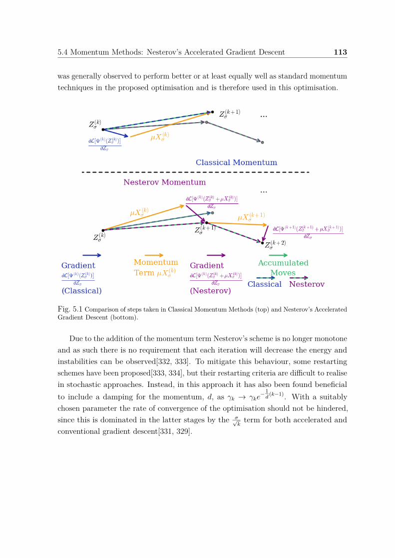
5.4 Momentum Methods: Nesterov’s Accelerated Gradient Descent 113
was generally observed to perform better or at least equally well as standard momentumtechniques in the proposed optimisation and is therefore used in this optimisation.
Fig. 5.1 Comparison of steps taken in Classical Momentum Methods (top) and Nesterov’s AcceleratedGradient Descent (bottom).
Due to the addition of the momentum term Nesterov’s scheme is no longer monotoneand as such there is no requirement that each iteration will decrease the energy andinstabilities can be observed[332, 333]. To mitigate this behaviour, some restartingschemes have been proposed[333, 334], but their restarting criteria are difficult to realisein stochastic approaches. Instead, in this approach it has also been found beneficialto include a damping for the momentum, d, as γk → γke
−1d
(k−1). With a suitablychosen parameter the rate of convergence of the optimisation should not be hindered,since this is dominated in the latter stages by the σ√
kterm for both accelerated and
conventional gradient descent[331, 329].
114 A Projector Quantum Monte Carlo Method for Non-linear Wavefunctions
5.5 Matrix Polynomials - Closing a Circle of Con-nections
Mathematically, on a more general and abstract level, projections, such as the stochasticprojection onto eigenstates of the Hamiltonian as described in Eq. 5.8, are given by amonic polynomial of the propagator of degree k[335–338], such that
Ψ(k) = pkA(A)Ψ(0), (5.59)
where pkA(A) represents a monic polynomial of the matrix A belonging to the linear
space Pk of polynomials of degree at most k. More specifically, expanding Ψ(0) =∑n−1i=0 ciΨi in the spectral basis of A with eigenpairs (λi,Ψi) ordered accordingly|λ0| ≥ |λ1| ≥ . . . ≥ |λn−1|, the projection leads to
Ψ(k) = pkA(A)Ψ(0) (5.60)
=n−1∑i=0
pkA(λi)ciΨi (5.61)
= pkA(λ0)c0Ψ0 +
n−1∑i=1
pkA(λi)ciΨi. (5.62)
If the dominant eigenpair (λ0,Ψ0) is desired, the component pkA(λ0)c0 should be much
larger than all other components pkA(λi)ci, ∀i > 0. Within this requirement, the
polynomial pkA should ideally be rescaled such that pk
A(λ0) = 1 and
Ψ(k) = c0Ψ0 +n−1∑i=1
pkA(λi)pk
A(λ0)ciΨi, (5.63)
while |pkA(λ0)| > |pk
A(λi)| ∀i > 0 and c0 = 0 are necessary conditions to project ontothe dominant eigenpair.
The most basic matrix polynomial which fulfills these requirements is P kA(A) = bkAk
with bk being an arbitrary constant. This matrix polynomial is not only constructed
5.5 Matrix Polynomials - Closing a Circle of Connections 115
during iterations of the power method[335, 337],
Ψ(k) = bkAkΨ(0) (5.64)
= bk
(c0λ
k0Ψ0 +
n−1∑i=1
ciλki Ψi
)(5.65)
= bkλk0
(c0Ψ0 +
n−1∑i=1
ciλk
i
λk0Ψi
), (5.66)
which filters out the dominant eigenstate Ψ0 and leads to a decay of contributions ofall other states provided that c0 = 0, but also during those of the Projector QuantumMonte Carlo method FCIQMC which uses the linear projector Plinear = I −τ(H−E0I).Likewise, successive iterations of the basic (S)GD method whose iterations are
Ψ(k+1) = Ψ(k) − τ ∂L[Ψ(k)]∂Ψ (5.67)
= (I− τ(H− E0I))kΨ(0) (5.68)
=(−τ
(H−
(E0 + 1
τ
)I))k
Ψ(0) (5.69)
= AkΨ(0) (5.70)
computes this polynomial with A = (I− τ(H− E0I)) = (−τ(H− (E0 + 1τ)I)). The
matrix A can be identified with the matrix representation of the linear projector Plinear
applied in FCIQMC. Essentially, both approaches, FCIQMC and (S)GD, amountto a shifted power method, thereby highlighting the deep connections between themethods (in the limit of an exact wavefunction ansatz) which are all equivalent in theirrealisation of the simple polynomial P k
A(A) = bkAk. A major drawback of this matrixpolynomial is that the decay rate for contributions from unwanted eigenpairs dependson the separation of eigenvalues. Specifically, the power method attains convergencerates of |Ψ(k) −Ψ0| = O
(|λ1|k|λ0|k
)and |λ(k) − λ0| = O
(|λ1|2k
|λ0|2k
). In general, convergence
rates for this set of methods can be extremely slow, in particular, if the two dominanteigenvalues are close to each other. The use of a shift, as employed in the projectorapproaches, may then help to either separate the desired eigenvalue from the remainingspectrum or to suppress components of close eigenvalues. Yet, this requires a prioriknowledge of the eigenvalues which is not available in practice.
A more sophisticated approach is taken by a number of methods which are commonlyreferred to as polynomial ‘filtering’ or ‘acceleration’ techniques. They accelerateconvergence by designing a polynomial pk
A(A), ideally the minimal polynomial, a
116 A Projector Quantum Monte Carlo Method for Non-linear Wavefunctions
matrix polynomial of smallest degree k ≤ n (where n represents the dimension of thematrix A) such that mk
A(A) = 0, which enhances components form desired regions ofthe spectrum and suppresses those from unwanted regions[335]. For best convergenceonto the dominant eigenpair (λ0,Ψ0), a polynomial pk
A(A) is required with pkA(λ0) = 1
and whose maximum absolute value over all λi with i > 0 is the smallest possible(Figure 5.2). However, as the eigenvalues λi are generally unknown, the problemis reformulated. Thus, relying on ideas from approximation theory, a polynomialapproximation to a continuous scalar function is sought whose value at the desiredeigenvalue λ0 of the propagator is 1 and whose maximum absolute value in a range [a, b]covering the rest of the spectrum containing all remaining eigenvalues λi is minimised
minpk
A∈Pk,pkA(λ0)=1
maxt∈[a,b]
|pkA(t)|, (5.71)
where Pk is the linear space of polynomials of degree k. Analytically, the optimal poly-nomial for this approximation problem is the shifted and scaled Chebyshev polynomialof the first kind of degree k[335, 338]
CkA(t(x)) = Ck
A(t(x))Ck
A(t(λ0))(5.72)
with
CkA(t) = cos[k cos−1(t)] for − 1 ≤ t ≤ 1, (5.73)
and t(x) providing a simple linear transformation
t(x) = 2x− (a+ b)b− a
(5.74)
to shift and scale the Chebyshev polynomials which are only defined over the range[−1, 1] to any finite range [a, b]. Additionally, these shifted and scaled Chebyshevpolynomials Ck
A(A) represent a set of orthogonal polynomials satisfying a three termrecurrence
Ck+1A (A) = 2ACk
A(A)− Ck−1A (A), (5.75)
with initial conditions C0A(A) = I and C1
A(A) = A. This recurrence relation rendersthem perfectly suitable for an enhanced projection process in the form Ψ(k) = Ck
A(A)Ψ(0)
which typically converges much faster than the power method or equivalent first-order
5.5 Matrix Polynomials - Closing a Circle of Connections 117
optimisation (Figure 5.2). The success of the Lanczos approach as a second-orderoptimisation, as well as other deterministic projections can also be rationalised in thisfashion by considering similar matrix polynomial approximations to the projection[339,340].
By analogy to Krylov space methods, convergence of GD can also be enhanced byextracting information from the state vectors Ψ(k−1) of the previous k − 1 iterations.This becomes apparent by considering the residual after k GD iterations Ψ(k) −Ψopt =Ak(Ψ(0)−Ψopt) (where Ψopt denotes the optimal state vector) and combining the statevectors Ψ(k) linearly using coefficients ak which results in[338]
i∑k=0
akΨ(k) =i∑
k=0akAk(Ψ(0) −Ψopt) +
i∑k=0
akΨopt (5.76)
= pkA(A)(Ψ(0) −Ψopt) + pk
I (I)Ψopt. (5.77)
Consequently, if pkI (I) = I is enforced, the value
min ∥pkA(A)(Ψ(0) −Ψopt)∥2 (5.78)
needs to be minimised to obtain the best approximation to Ψopt. Nesterov’s acceleratedGD achieves this by iterating the equations in 5.55 which in matrix form reads as
Ω(k+1) = Ψ(k) − τ ∂L[Ψ(k)]∂Ψ (5.79)
Ψ(k+1) = (1− γk)Ω(k+1) + γkΩ(k). (5.80)
This projection process iteratively builds a polynomial NkA(A) which satisfies Ω(0) −
Ωopt = NkA(A)(Ψ(0) − Ψopt). This implicitly constructed polynomial Nk
A(A) can beconveniently expressed as a three term recurrence relation[338]
NkA(A) = A
[(1− γk−1)Nk−1
A (A) + γk−1Nk−2(A)
](5.81)
with initial conditions N0A(A) = I and N1
A(A) = A. Whilst not being exactly equal tothe Chebyshev polynomial the polynomial Nk
A(A) of Nesterov’s accelerated approachis similar to the Chebyshev polynomial and also satisfies Nk
I = I for all k. This meansthat it filters out contributions of Ψopt and suppresses those of undesired states moreefficiently than the simple (S)GD approach, thereby accelerating convergence of theprojection. A schematic illustration of the differences in efficiency of the projection

118 A Projector Quantum Monte Carlo Method for Non-linear Wavefunctions
processes onto the desired state resulting from the various employed polynomials ofthe propagator can be seen in Figure 5.2.
Fig. 5.2 Comparison of projections of propagators onto the desired eigenvalue Emin of the Hamiltonian.The projections resulting from repeated application of the Linear Projector (SGD, FCIQMC, PowerMethod) constructing the simple polynomial Ak, of the Chebyshev Projector employing Chebyshevpolynomials Ck(A) and of the Nesterov Projector (Nesterov’s Accelerated Gradient Descent) implicitlyconstructing the polynomials Nk(A) are compared to the Optimal Projector.
5.6 Step Size Adaptation: RMSprop
The remaining arbitrariness concerns the step size (or ‘learning rate’) τk, which isnot only crucial for the efficiency of the optimisation but also affects its accuracy.Whilst decreasing the step size generally improves robustness and accuracy, it slowsconvergence and increases autocorrelation time[324, 323]. On the contrary, if too largea τk is chosen, the optimisation continually overshoots the minimum and oscillatesaround it, thereby resulting in poor accuracy, and again slow convergence, or evendivergences. A variety of different schemes, such as Adagrad[341], Adadelta[342],RMSprop[330, 343] and Adam[344] to name just a few, have been proposed in orderto avoid the use of fixed step sizes and try to address these issues. Amongst these, it

5.7 Wavefunction Properties 119
was found numerically that optimal convergence and accuracy within the acceleratedSGD approach described above is achieved with a deep-learning technique denotedRMSprop[330, 343], an adaptive step size method which dynamically estimates anindividual and independent τ (k)
Zσfor each parameter. This gives
τ(k)Zσ
= η
RMS[gZσ ](k) , (5.82)
where η is a tuned global parameter for all variables, and RMS[gZσ ](k) represents theroot mean square (RMS) of previous gradients for the variable up to the currentiteration,
RMS[gZσ ](k) =√
E[g2Zσ
](k) + ϵ, (5.83)
evaluated by accumulating an exponentially decaying average of the squared gradientsof the Lagrangian, gZσ ,
E[g2Zσ
](k) = ρE[g2Zσ
](k−1) + (1− ρ)g2(k)Zσ
. (5.84)
The small constant ϵ is added to better condition the denominator and ρ representsa decay constant. The use of the exponentially weighted average in the denominatorinstead of a simple accumulating sum which is employed in other adaptation schemessuch as Adagrad[341] avoids a continually decreasing step size which, even though beingbeneficial from an accuracy point of view, eventually shrinks to zero and thus stopsthe optimisation. This dynamically adaptive, parameter-specific step-size, acts muchlike a preconditioner for the system, and allows the optimisation to take larger stepsfor those parameters with small gradients, and vice versa. This ensures robustness ofthe algorithm to large sudden gradients due to the stochastic nature of the gradientevaluation[342].
5.7 Wavefunction Properties
In addition, the dynamics of the outlined Projector Quantum Monte Carlo methodalso provide a straightforward route to unbiased computation of the two-body reduceddensity matrix (2-RDM)[345, 253], a rank-4 tensor in the basis of spin orbitals,
Γpq,rs = ⟨Ψ|a†pa†qasar|Ψ⟩ p > q, r > s, (5.85)
120 A Projector Quantum Monte Carlo Method for Non-linear Wavefunctions
from which the 1-body reduced density matrix (1-RDM)
γpq = ⟨Ψ|a†paq|Ψ⟩ = 2N − 1
∑a
Γpa,qa, (5.86)
can be traced out with the factor of 2N−1 arising from the normalisation of the 1-
RDM and 2-RDM to N and N(N−1)2 , respectively. As such, the reduced density matrix
represents a highly compact representation of the relevant information in the N -electronwavefunction, allowing for the computation of pure expectation values. By evaluatingthe trace of the relevant 1- and 2-body operator Q with the 2-RDM
⟨Q⟩ = Tr[ΓQ], (5.87)
arbitrary 1- and 2-body static properties can be found[37]. This includes the energy,
ERDM =∑pq
hpqγpq +∑
p>q,r>s
(gpqrs − gpqsr)Γpq,rs + Enuc, (5.88)
(with hpq, gpqrs and Enuc as defined in Section 2.2.2 of Chapter 2), spin, magneticproperties and many more. In particular, the self-consistently determined energy E(k)
appearing in the gradient in Eq. 5.12 is evaluated each iteration anew from the sampledenergy as given by the density matrix E(k) = E
(k)RDM, rather than from the local energy
as it is commonly done in traditional VMC methods.In sampling the 2-RDM a similar approach to the one developed in FCIQMC[253,
269, 267] is employed which projects the 2-RDM into the full Hilbert space of configu-rations |m⟩,
Γpq,rs =∑mn⟨Ψ(k)|m⟩ ⟨m|a†pa†qasar|n⟩ ⟨n|Ψ(k)⟩ . (5.89)
Within this formulation, it is obvious that a matrix element is non-zero only whenthe configurations m and n are at most two-particle substitutions of each other, orput another way, when m is at most a double excitation of n. As such, the existingsampling processes of the Lagrangian gradient that occur throughout the dynamicsof the stochastic projection already provide all the necessary machinery required tosample the 2-RDM. Thus, entirely analogous to the sampling of the gradient, thesum over m in Eq. 5.89 is stochastically evaluated by the Metropolis Markov chain.Similarly, the off-diagonal terms in the sum over m are replaced by a small selection ofconfigurations sampled within the excitation generation process whilst the diagonalterm n = m is included deterministically for each sample in the Markov chain. It
5.7 Wavefunction Properties 121
should be noted that for an unbiased 2-RDM from which properties other than theenergy are evaluated uniform probability distributions for the orbital selections in theexcitation generation process need to be used[261] to guarantee that all contributions ofthe 2-RDM can in principal be selected in the sampling procedure. Otherwise samplingdifficulties can arise if two configurations with significant amplitude weight are onlyconnected by a very small Hamiltonian matrix element, their contribution to the RDMmay be sampled poorly, or even omitted entirely. Furthermore, both wavefunctionamplitudes
⟨Ψ(k)|m⟩ , ⟨n|Ψ(k)⟩
have already been evaluated for the calculation of the
Lagrangian gradient. As a result, stochastic evaluation of the reduced density matrixcontribution for each sample n, and for stochastic sampling of m = n can then beformulated as
Γpq,rs,offdiag =⟨
⟨Ψ(k)|m⟩ ⟨n|Ψ(k)⟩NsPgen(m|n)P (n; Ψ(k))
⟩P (n;Ψ(k))
(5.90)
where the outer brackets imply that the sampling of n is performed according to the dis-tribution given in Eq.5.13. Diagonal terms, where m = n, are sampled deterministicallyand contribute for every sample of n as
Γpq,rs,diag =⟨⟨Ψ(k)|n⟩ ⟨n|Ψ(k)⟩
P (n; Ψ(k))
⟩P (n;Ψ(k))
. (5.91)
Combination of both estimates
Γpq,rs = Γpq,rs,diag + Γpq,rs,offdiag (5.92)
then leads to the complete density matrix. At the end of the sampling process, the2-RDM is normalised to ensure that it satisfies the trace relation
∑pq
Γpq,pq = N(N − 1)2 , (5.93)
whilst the one-body RDM can be integrated out if desired. Simultaneously, hermiticityΓpq,rs = Γrs,pq is enforced in the two-body reduced density matrix by averaging therelated pairs of elements, allowing for evaluation of a hermiticity error Γpq,rs−Γrs,pq
2 foreach pair of off-diagonal elements whose maximum and mean value act as indicatorsfor the sampling quality and convergence of the RDM[269].
This sampling approach allows for an efficient stochastic evaluation of the 2-RDMduring the dynamics of the SGD algorithm with little additional computational cost.
122 A Projector Quantum Monte Carlo Method for Non-linear Wavefunctions
Part of this computational expenditure is caused by the increase in memory requirementfor storage of the 2-body reduced density matrix which scales as O[
(M(M−1)
2
)2]. The
remaining computational costs are largely associated with identification and update ofthe density matrix elements to which each pair of determinants contributes. Theseprocesses involve O[N2] operations for diagonal terms, and O[N ] or O[1] operationsfor off-diagonal terms with single- or double excitations, respectively.
Care must be taken when evaluating stochastic estimators of non-linear functions ofexpectation values such as the 2-body reduced density matrix and properties obtainedfrom it so as not to introduce a bias in the estimator. In general, for an unbiasedestimator the expectation value over the probability distribution of the wavefunctionshould satisfy (up to a normalisation constant)
E⟨ Ψ(k)
P (Ψ(k))
⟩P (Ψ(k))
= Ψ(k), (5.94)
where⟨
Ψ(k)
P (Ψ(k))
⟩Ψ(k))
denotes sampling of the exact wavefunction Ψ(k) according to theprobability distribution P (Ψ(k)). Yet, for any function f(Ψ(k)) that is nonlinear inΨ(k),
Ef⟨ Ψ(k)
P (Ψ(k))
⟩P (Ψ(k))
= f
E⟨ Ψ(k)
P (Ψ(k))
⟩P (Ψ(k))
(5.95)
holds, which implies that estimating f(Ψ(k)) by E[f(⟨
Ψ(k)
P (Ψ(k))
⟩P (Ψ(k))
)]will introduce
a bias[346, 347]. This bias was present when reduced density matrices were sam-pled in FCIQMC[269, 253], since the appropriate contributions E
[⟨⟨Ψ(k)|m⟩P (Ψ(k))
⟩P (Ψ(k))
]× E
[⟨⟨n|Ψ(k)⟩P (Ψ(k))
⟩P (Ψ(k))
]are in fact approximated by E
[⟨⟨Ψ(k)|m⟩⟨n|Ψ(k)⟩
P (Ψ(k))
⟩P (Ψ(k))
]which
neglects the (non-zero) covariance between the amplitudes and thus results in bi-ased sampling even if the E
[⟨⟨n|Ψ(k)⟩P (Ψ(k))
⟩P (Ψ(k))
]themselves are unbiased. The main
source of potential error is therefore the fact that the two amplitudes contribut-ing to the density matrix elements are correlated with the dominant error arisingfrom diagonal terms where the instantaneous amplitude projections are perfectlycorrelated and where the error is of a single sign thereby removing the possibilityof fortuitous cancellation of errors. To guarantee unbiased sampling of the densitymatrices, FCIQMC uses a replica sampling approach whereby two completely inde-pendent walker populations (replicas) are propagated simultaneously such that theamplitudes are uncorrelated between them[260, 269, 253], allowing for independent
5.7 Wavefunction Properties 123
estimates of E[⟨⟨Ψ(k)|m⟩P (Ψ(k))
⟩P (Ψ(k))
]× E
[⟨⟨n|Ψ(k)⟩P (Ψ(k))
⟩P (Ψ(k))
]as E
⟨ ⟨Ψ(k)(1) |m⟩⟨n|Ψ
(k)(2)⟩
P (Ψ(k))
⟩P (Ψ(k))
or E
⟨ ⟨Ψ(k)(2) |m⟩⟨n|Ψ
(k)(1)⟩
P (Ψ(k))
⟩P (Ψ(k))
or the appropriate average of both, where the notation
⟨Ψ(k)(1)|m⟩ denotes the wavefunction amplitude ⟨Ψ(k)|m⟩ of replica 1. In the 2-RDM
sampling procedure outlined above a similar replica approach is employed to a limitedextend. In general, because of the non-linearity of the wavefunction many solutionswith the same energy will exist. As a consequence, independent replicas will usuallyconverge to different minima with the same energy and as such, the replica approachused in FCIQMC cannot be employed while the parameters in a polynomial complexwavefunction ansatz are still optimised. Instead, contributions to the energy E(k)
RDM andthe gradient ∂L[Ψ(k)(Z(k)
σ )]∂Zσ
are simply evaluated from a single replica. Investigations weremade as to whether approaches involving two replicas for sampling of the gradient and /or energy improved optimisation behaviour. However, all approaches were found to leadto divergences due to the multitude of different wavefunctions with the same energy.Once a single replica wavefunction is converged upon the 2-RDM can be sampled byinitialising two replicas from the converged wavefunction, propagating them completelyindependently and sampling contributions to the 2-RDM and E
(k)RDM using amplitudes
from both replicas. This technique will remove as much of the correlation betweenthe wavefunction amplitudes as possible although the possibility exists that a smalldegree of correlation still remains giving the same initial starting wavefunction forthe two replicas. Similarly, concerns may be raised that a sampling of E(k)
RDM and∂L[Ψ(k)(Z(k)
σ )]∂Zσ
may be biased during the wavefunction optimisation when both amplitudesin the contribution originate from the same replica and thus introduce an error in theoptimisation. However, given the results to follow in the next chapter, it seems thatthis bias is smaller than the stochastic error in the sampling. In fact, no such errorhas so far been observed in practice and the RDM energy obtained from one replicawas usually found to be in agreement with that obtained using two replica. A similarsituation arose in an excited state approach within FCIQMC[249] where analogouslyconcerns about a similar potential sampling bias were raised. Yet, as in this SGDapproach no such bias was observed in practice despite its theoretical presence.
124 A Projector Quantum Monte Carlo Method for Non-linear Wavefunctions
5.8 A Technical Point: Wavefunction Normalisa-tion, Step Sizes and Parameter Updates
A technical yet important point regarding the efficiency of the optimisation is thedependence of estimators and parameter updates on the generally unknown normalisa-tion of the wavefunction N [|Ψ(k)|2]. In particular, updating the parameters alters thenormalisation of the wavefunction such that the parameter changes may no longer bethe optimal ones. In state-of-the-art VMC wavefunction optimisations this factor wasfound to profoundly affect the efficiency of the optimisation[217, 215] and thereforealso needs consideration in this SGD approach. All energy expressions used in thisSGD approach scale as (N [|Ψ(k)|2])0 as they ought to. By sampling the unnormalisedtwo-body reduced density matrix from the wavefunction and then explicitly normal-ising from the trace relation, there is thus no issue introduced by any change in thenormalisation of the wavefunction. Similarly, P (n,Ψ(k)) in Eq. 5.13 is a normaliseddistribution and therefore scales as (N [|Ψ(k)|2])0. However, the equations for the La-grangian in Eq. 5.15 and 5.16 include a global dependence on the normalisation of thewavefunction. A change in the normalisation of the wavefunction therefore affects theeffective magnitude of the update in each iteration, thereby resulting in a new effectivestep size, τ (k)′
Zσ, in a non-trivial manner, through the magnitude of both N [|Ψ(k)|2], as
well as ⟨∂Ψ(k)
∂Zσ| and |Ψ(k)⟩. In the case of a fixed step size, the dynamics of the non-linear
optimisation will not be invariant to this change which is in contrast to FCIQMCwith its linear ansatz where the magnitude of changes to the wavefunction would varylinearly with the L1 norm of Ψ(k). The dependence of the resultant effective step sizeon the normalisation of the wavefunction will change with both the parameterisationand the probability distribution used to sample the wavefunction in Eq. 5.13. However,for an exact parameterisation and sampling, the gradient vector will necessarily vanishas the solution is converged upon, thereby mitigating the norm dependence in theeffective step size.
It is worth considering the ramifications of the dependence of the parameter changeson the N [|Ψ(k)|2] and their relationship to other approaches in literature. In general,controlling the norm of parameter updates for non-linear wavefunctions is a difficulttask for state-of-the-art VMC methods like Stochastic Reconfiguration or the LinearMethod, as well. In these approaches, the update is rescaled, damped or a line search isperformed to search for the optimal changes in parameters[215, 211]. These measuresare not feasible for this SGD approach as they require an explicit projection intothe tangent subspace of the wavefunction, a step that is avoided at all times in the
5.9 Comparison to State-of-the-art VMC Methods 125
SGD optimisation. Yet, in practical applications, the implementation avoids potentialproblems for two reasons. Firstly, due to the shifting of the Hamiltonian by the currentestimate of the energy only small changes in the normalisation of the wavefunction occurfor all calculations attempted, even far from convergence. Secondly, the dynamicalparameter-specific step size adjustment also mitigates many of the effects of the normdependence of the effective step size. Specifically, by considering parameter-specificinformation from gradients of previous iterations and introducing an inverse dependenceon these gradients into the individual step sizes the norm dependence is mitigated anda stable and efficient optimisation is achieved. For this reason, the N [|Ψ(k)|2] term inEq. 5.15 and 5.16 are not explicitly considered in the algorithm, and its effect on theformal convergence rate is small[323].
5.9 Comparison to State-of-the-art VMC Methods
The stochastic gradient descent (SGD) of the Lagrangian described above results in aniteration cost that is independent of the size of the Hilbert space and thus renders thismethod inherently suitable for large scale systems like other Quantum Monte Carloapproaches. Yet, it also admits a number of advantages over state-of-the-art VMCoptimisation[215, 348, 213], such as the avoidance of the construction of matrices inthe tangent space of the wavefunction, whose sampling and manipulation becomes abottleneck for large numbers of parameters. Krylov subspace techniques have beenproposed to circumvent this by projecting down to more manageable space[208]. Yet,ill-conditioning can limit the efficiency of this approach although recent developmentsof the Linear Method attempt to address its memory bottleneck[349]. Furthermore,diagonalisation of the randomly sampled matrices required in some optimisations canlead to biases in the final parameters[248, 350]. Moreover, the SGD approach bearssimilarities with the Stochastic Reconfiguration method (SR)[348, 213], which canalso be considered an imaginary time propagation that differs from steepest descentin its definition of the metric in parameter space for the updates[212]. Due to this,SR requires projection of the equations into the fixed tangent space of the currentwavefunction and stabilisation of the resultant matrix equations[213]. However, theproposed matrix-free stochastic application of Eq. 5.4 describes a quasi-continuousoptimisation, where the error bar at convergence represents both the stochastic error inthe sampling, and the variation in the wavefunction as it is sampled. In addition, thedynamics of the optimisation also provide access to the two-body reduced density, andthus arbitrary 1- and 2-body static properties of the wavefunction as outlined above

126 A Projector Quantum Monte Carlo Method for Non-linear Wavefunctions
with little additional computational cost. Hence, these static properties including spinand magnetic properties, as well as the energy, are evaluated from the sampled densitymatrix, rather than from the local energy as it is commonly the case in traditional VMCapproaches. Furthermore, Quantum Monte Carlo methods working in first quantisedbasis of electron coordinates usually evaluate density matrices by sampling eitherfrom a grid or a suitable probability distribution within the configuration space whichtends to be more expensive, in particular when considering a 2-RDM expressed innon-localised basis functions[345].

Chapter 6
Applications of the ProjectorQuantum Monte Carlo Method forNon-linear Wavefunctions toCorrelator Product StateWavefunctions
In this chapter, a number of applications of the Projector Quantum Monte Carlomethod for non-linear wavefunctions are presented which demonstrate the ability ofthis approach to optimise arbitrary non-linear wavefunction ansatzes for quantum many-body systems, as well as its ability to evaluate the static properties of these wavefunctionfrom their sampled two-body reduced density matrix. These wavefunctions are soughtfor a multitude of systems, ranging from lattice Hubbard models to ab-initio systemsin one- and two-dimensions
In order to advance to larger condensed phase systems than those amenable to FCItechniques and circumvent the exponential scaling of the full Hilbert space, one approachfor designing an efficient and compact wavefunction ansatz is to exploit the fact thatelectron correlation is, in general, inherently local. Two-point correlation functions(away from criticality) will decay exponentially with distance, whilst the screening of theCoulomb interaction in bulk systems will result in local entanglement of nearby electrons,with distant electrons behaving increasingly independently[132]. The existence of thislocality of electron correlation, as well as the existence of area laws, and thereby thereduced amount of entanglement which effectively quantifies the relevant number of
128Applications of the Projector Quantum Monte Carlo Method for Non-linear
Wavefunctions to Correlator Product State Wavefunctions
degrees of freedom, suggests that quantum many-body states of strongly-correlatedmaterials may be faithfully described by an efficient parameterisation. This concept liesat the heart of powerful numerical algorithms such as the density-matrix renormalisationgroup approach (DMRG)[56, 143, 144] and its higher-dimensional analogues[55] in therealm of Tensor Network States (TNS). A further quantum many-body state ansatzwhich exploits locality to formally contain the scaling to polynomial cost is an ansatzin the form of Correlator Product States (CPS)[351–356], which explicitly correlateplaquettes of neighbouring degrees of freedom. Related wavefunctions are also referredto as entangled plaquette states[357–359] or complete graph tensor networks[360,361]) to stress their connection to higher-dimension generalisations of matrix productstates[362]. In this sense, the CPS ansatz, which can also be regarded as a class ofTensor Network States, has been introduced to extend DMRG to higher dimensionswhilst avoiding the computational cost of other higher dimensional TNS algorithms.Whereas TNS introduce auxiliary degrees of freedom in order to introduce correlationsbetween physical degrees of freedom, CPS correlate the physical degrees of freedomexplicitly. The CPS ansatz is extremely versatile, the form and size of correlatorscan be chosen to best represent the properties of the system, which also makes thewavefunction systematically improvable. A mapping between some types of CPS andTNS and vice versa can be established, however, each parameterisation form willalways only represent a subset of the states that it is mapped onto[351, 363]. Like TNS,CPS with local correlators satisfy an area law thereby suggesting that they shouldbe well suited for systems with finite correlation length. On the contrary, CPS withlong-ranged correlators are area law violating. Obeying a volume law, they are able todescribe an even higher degree of entanglement and are thus suitable for parameterisingstates of critical systems[351, 364].
Previously, the variational parameters of these CPS wavefunction have been opti-mised with a number of approaches, some of which are of deterministic nature[352, 363],whilst most of them use Variational Monte Carlo (VMC) approaches[357, 364, 208]. Inparticular, VMC methods such as the Linear Method and Stochastic Reconfigurationenabled the optimisation of large numbers of parameters. The results presented in thischapter, demonstrate that the Projector Quantum Monte Carlo method proposed inthe previous Chapter is able to optimise and handle CPS wavefunctions with muchlarger numbers of variational parameters then previous VMC optimisations.
6.1 The Correlator Product State Wavefunction Ansatz 129
6.1 The Correlator Product State WavefunctionAnsatz
The exact eigenstate of the non-relativistic time-independent electronic Schrödingerequation for an N -particle system in a discrete basis of M one-particle states assumesthe form of an FCI wavefunction ansatz, as in FCIQMC,
|ΨFCI⟩ =q∑
n1n2...nM
Xn |n1n2 . . . nM⟩ =∑
nXn |n⟩ , (6.1)
where Xn denotes the expansion coefficient of the occupation number vector |n⟩. Thefirst sum runs over the dimension q of the local Hilbert space of the single-particlebasis states |ni⟩ = |1⟩ , |0⟩ and is restricted to those occupation vectors satisfying∑M
i ni = N . Since each occupation vector is formed as a direct product of states inthe local Hilbert space |n⟩ = |n1n2 . . . nM⟩ = |n1⟩ ⊗ |n2⟩ ⊗ . . .⊗ |nM⟩, the size of thecomplete N -particle Hilbert space, and hence, of the number of variational parametersin the FCI wavefunction scales exponentially with system size[37].
Although the exactness of the FCI wavefunction for a given basis represents ahuge advantage, its exponential scaling makes it prohibitively expensive in practice,particularly for large systems, and efficient and more compact parameterisations ofthe wavefunction such as correlator product states are needed. An integral part of theCPS ansatz is the concept of a correlator which directly encodes correlations betweensingle-particle states. In general, the CPS ansatz defines ‘correlators’ as diagonaloperators which directly encode the entanglements within sets of single-particle statesas[351, 352, 357]
Cλ =∑nλ
CnλPnλ
, (6.2)
where Pnλ= |nλ⟩ ⟨nλ| is the projection operator for the single many-body state nλ in
the set of all many-body Fock states nλ in the correlator λ with correlator amplitudesCnλ
. The CPS wavefunction is then written as multi-linear product of correlatoroperators acting on a chosen reference state[351, 365]
|ΨCPS⟩ =∏λ
Cλ |Φ⟩ . (6.3)
130Applications of the Projector Quantum Monte Carlo Method for Non-linear
Wavefunctions to Correlator Product State Wavefunctions
Possible choices for the reference state include the uniform reference
|ΦU⟩ =∑
n|n⟩ , (6.4)
an equally weighted sum of all occupation number vectors which may be chosen tosatisfy symmetry constraints, as well as an Antisymmetrised Geminal Power (AGP)wavefunctions[5, 366, 212]
|ΦAGP⟩ = exp(F ) |0⟩ , (6.5)
where the pairing operator F creates a linear combination of all possible singlet pairings
of one-particle states F = ∑M2
i,j=1 fija†i↑a†j↓. Similarly, further states which can act as
reference state are a generalisation of the AGP wavefunction, the Pfaffian pairingwavefunction[367–369]
|ΦPF⟩ = exp(G) |0⟩ , (6.6)
defined in terms of a generalised pairing operator G = ∑Mi=1
∑Mj=i+1 gija
†ia†j that creates
linear combinations of all singlet and triplet pairings. Alternatively, a single Slaterdeterminant can act as reference state
|ΦD⟩ =N∏
i=1
M∑j=1
Θija†j
|0⟩ , (6.7)
where |0⟩ is the vacuum state, a†j represents the creation operator for the jth one-particle state of the basis set and Θ denotes the matrix of coefficients whose ith rowdefines the coefficient of the ith state[365, 65]. The CPS wavefunction thus provides aproduct approximation to the FCI wavefunction which for a single Slater determinantreference state, as it will be used often throughout this work, is of the explicit form
|ΨCPS⟩ =∑
n
∏λ
C(n)λ |n⟩ ⟨n|
N∏i=1
M∑j=1
Θija†j
|0⟩ , (6.8)
where ∏λ C(n)λ denotes the set of correlator amplitudes which give rise to the global
occupation defined in |n⟩. It can be shown that a number of different phases andwavefunctions can be expressed in this form, including resonating valence bond (RVB)and Laughlin wavefunctions[351]. As the number of degrees of freedom in the systemgrows, the complexity of the wavefunction grows only linearly. Additionally, this choice
6.2 Wavefunction Amplitudes and Derivatives 131
of low-rank factorisation of the wavefunction is systematically improvable in the limitof increasing correlator sizes as this recovers longer-ranged entanglement effects andincreases the number of variables in the wavefunction parameterisation. In the limitof one large correlator covering all single-particle states in the system, the exact FCIwavefunction is recovered[351, 352] and the CPS wavefunction is thus systematicallyimprovable to exactness.
6.2 Wavefunction Amplitudes and Derivatives
Projecting the CPS wavefunction into the complete Hilbert space of configurationsn, the wavefunction amplitudes are given by
⟨n|ΨCPS⟩ = ⟨n|∏λ
Cλ|n⟩ ⟨n|Φ⟩ . (6.9)
Whilst the correlator part of the CPS wavefunction makes a contribution of
⟨n|∏λ
Cλ|n⟩ = ⟨n|Ncorr∏
λ
C(n)λ |n⟩ , (6.10)
where C(n)λ denotes the set of correlator amplitudes contributing to |n⟩ and Ncorr the
number of correlators, the explicit form of the reference state contribution depends onthe nature of |Φ⟩. For a uniform reference state, its contribution to the wavefunctionamplitude is
⟨n|ΦU⟩ =∑m⟨n|m⟩ = δnm, (6.11)
while a single Slater determinant reference state results in a determinant of orbitalcoefficients
⟨n|ΦD⟩ = ⟨n|N∏
i=1
M∑j=1
Θija†j
|0⟩ , (6.12)
where Θ represents the matrix defining the orbitals in the reference Slater determinant.Similarly, in the case of an AGP reference state its respective component of the
132Applications of the Projector Quantum Monte Carlo Method for Non-linear
Wavefunctions to Correlator Product State Wavefunctions
projection onto the configuration is a determinant of the pairing matrix
⟨n|ΦAGP⟩ = 1(N2
)!⟨n|
M2∑
i,j=1fija
†i↑a†j↓
N2
|0⟩ , (6.13)
where f represents the symmetric pairing matrix (fij = −fji) describing the coefficientsof all possible singlets in the linear combination. For a general pairing function actingas reference state the contribution is given by a pfaffian of the occupied pairing matrix
⟨n|ΦPF⟩ = 1(N2
)!⟨n|
M∑i=1
M∑j=i+1
gija†ia†j
N2|0⟩ (6.14)
with g describing the occupied pairing matrix (gij = −gji) holding the coefficients ofall possible singlets and triplets in the linear combination.
Whereas the correlator part of the wavefunction amplitudes can be computed inO[Ncorr] time, the determinant and pfaffian of the reference states both require anO[N3] operation. Fast updates of the determinant based on the Sherman-Morrisonformula reduce the scaling of the computation of the determinant overlap down toO[N2], while the correlator amplitudes for a local update can similarly scale as O[1].
Derivatives with respect to the wavefunction parameters Zσ can be computed as
⟨n|∂ΨCPS
∂Cσ
⟩ = 1Cσ
⟨n|ΨCPS⟩ (6.15)
⟨n|∂ΨCPS
∂Θij
⟩ =(Θ−1
)ji⟨n|ΨCPS⟩ (6.16)
⟨n|∂ΨCPS
∂fij
⟩ =(f−1
)ji⟨n|ΨCPS⟩ (6.17)
⟨n|∂ΨCPS
∂gij
⟩ = 12(g−1
)ji⟨n|ΨCPS⟩ , (6.18)
which are thus obtainable from the respective wavefunction amplitudes ⟨n|ΨCPS⟩ inO[1] time.
6.3 2D Hubbard Model
A first example of the ability of the Projector Quantum Monte Carlo approach toconverge wavefunctions with many parameters is given by the treatment of a 98-site
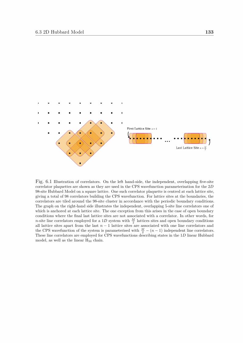
6.3 2D Hubbard Model 133
Fig. 6.1 Illustration of correlators. On the left hand-side, the independent, overlapping five-sitecorrelator plaquettes are shown as they are used in the CPS wavefunction parameterisation for the 2D98-site Hubbard Model on a square lattice. One such correlator plaquette is centred at each lattice site,giving a total of 98 correlators building the CPS wavefunction. For lattice sites at the boundaries, thecorrelators are tiled around the 98-site cluster in accordance with the periodic boundary conditions.The graph on the right-hand side illustrates the independent, overlapping 5-site line correlators one ofwhich is anchored at each lattice site. The one exception from this arises in the case of open boundaryconditions where the final last lattice sites are not associated with a correlator. In other words, forn-site line correlators employed for a 1D system with M
2 lattices sites and open boundary conditionsall lattice sites apart from the last n − 1 lattice sites are associated with one line correlators andthe CPS wavefunction of the system is parameterised with M
2 − (n− 1) independent line correlators.These line correlators are employed for CPS wavefunctions describing states in the 1D linear Hubbardmodel, as well as the linear H50 chain.
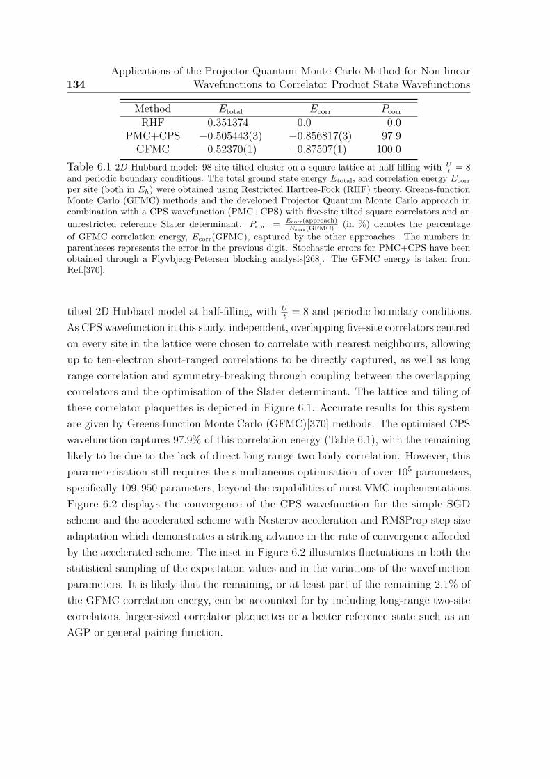
134Applications of the Projector Quantum Monte Carlo Method for Non-linear
Wavefunctions to Correlator Product State Wavefunctions
Method Etotal Ecorr PcorrRHF 0.351374 0.0 0.0
PMC+CPS −0.505443(3) −0.856817(3) 97.9GFMC −0.52370(1) −0.87507(1) 100.0
Table 6.1 2D Hubbard model: 98-site tilted cluster on a square lattice at half-filling with Ut = 8
and periodic boundary conditions. The total ground state energy Etotal, and correlation energy Ecorrper site (both in Eh) were obtained using Restricted Hartree-Fock (RHF) theory, Greens-functionMonte Carlo (GFMC) methods and the developed Projector Quantum Monte Carlo approach incombination with a CPS wavefunction (PMC+CPS) with five-site tilted square correlators and anunrestricted reference Slater determinant. Pcorr = Ecorr(approach)
Ecorr(GFMC) (in %) denotes the percentageof GFMC correlation energy, Ecorr(GFMC), captured by the other approaches. The numbers inparentheses represents the error in the previous digit. Stochastic errors for PMC+CPS have beenobtained through a Flyvbjerg-Petersen blocking analysis[268]. The GFMC energy is taken fromRef.[370].
tilted 2D Hubbard model at half-filling, with Ut
= 8 and periodic boundary conditions.As CPS wavefunction in this study, independent, overlapping five-site correlators centredon every site in the lattice were chosen to correlate with nearest neighbours, allowingup to ten-electron short-ranged correlations to be directly captured, as well as longrange correlation and symmetry-breaking through coupling between the overlappingcorrelators and the optimisation of the Slater determinant. The lattice and tiling ofthese correlator plaquettes is depicted in Figure 6.1. Accurate results for this systemare given by Greens-function Monte Carlo (GFMC)[370] methods. The optimised CPSwavefunction captures 97.9% of this correlation energy (Table 6.1), with the remaininglikely to be due to the lack of direct long-range two-body correlation. However, thisparameterisation still requires the simultaneous optimisation of over 105 parameters,specifically 109, 950 parameters, beyond the capabilities of most VMC implementations.Figure 6.2 displays the convergence of the CPS wavefunction for the simple SGDscheme and the accelerated scheme with Nesterov acceleration and RMSProp step sizeadaptation which demonstrates a striking advance in the rate of convergence affordedby the accelerated scheme. The inset in Figure 6.2 illustrates fluctuations in both thestatistical sampling of the expectation values and in the variations of the wavefunctionparameters. It is likely that the remaining, or at least part of the remaining 2.1% ofthe GFMC correlation energy, can be accounted for by including long-range two-sitecorrelators, larger-sized correlator plaquettes or a better reference state such as anAGP or general pairing function.
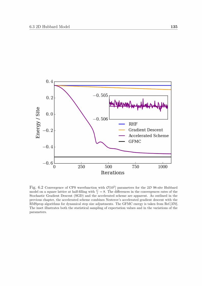
6.3 2D Hubbard Model 135
Fig. 6.2 Convergence of CPS wavefunction with O[105] parameters for the 2D 98-site Hubbardmodel on a square lattice at half-filling with U
t = 8. The differences in the convergences rates of theStochastic Gradient Descent (SGD) and the accelerated scheme are apparent. As outlined in theprevious chapter, the accelerated scheme combines Nesterov’s accelerated gradient descent with theRMSprop algorithms for dynamical step size adjustments. The GFMC energy is taken from Ref.[370].The inset illustrates both the statistical sampling of expectation values and in the variations of theparameters.
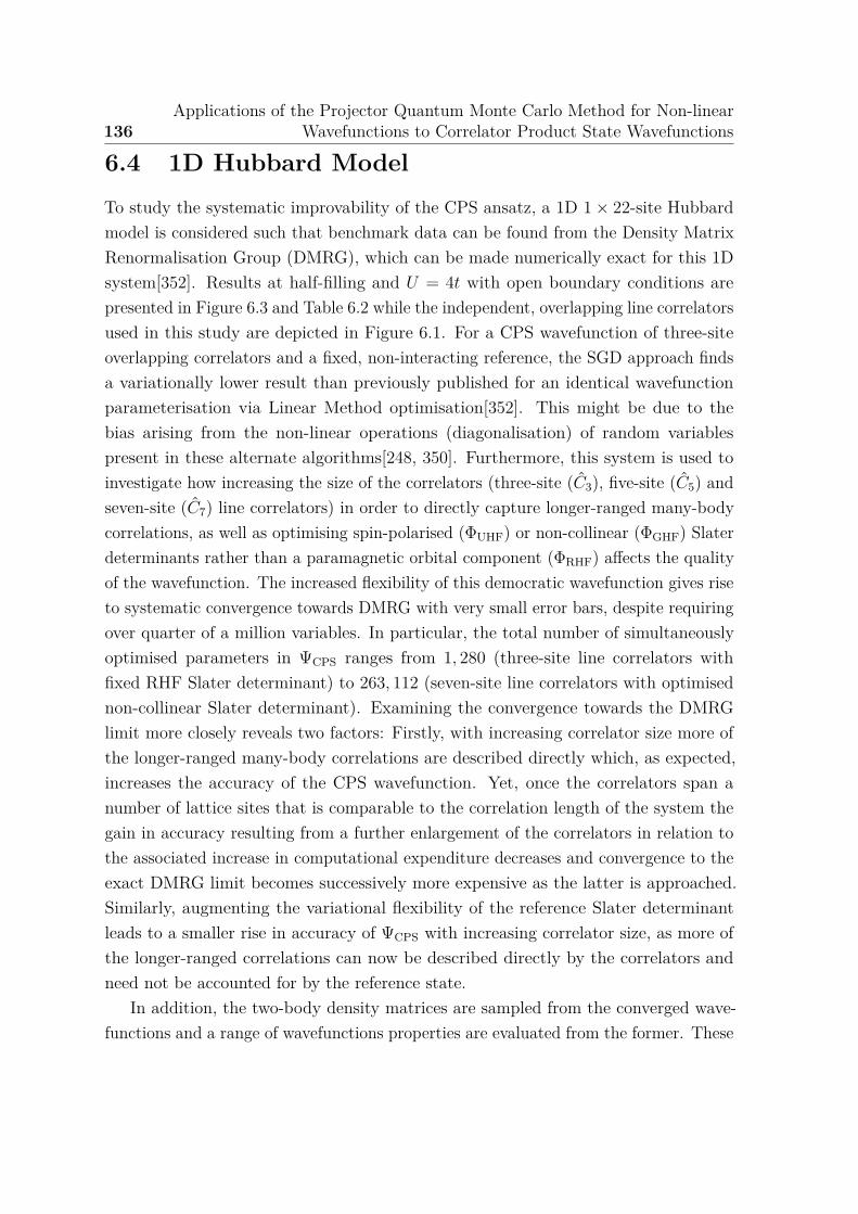
136Applications of the Projector Quantum Monte Carlo Method for Non-linear
Wavefunctions to Correlator Product State Wavefunctions
6.4 1D Hubbard Model
To study the systematic improvability of the CPS ansatz, a 1D 1× 22-site Hubbardmodel is considered such that benchmark data can be found from the Density MatrixRenormalisation Group (DMRG), which can be made numerically exact for this 1Dsystem[352]. Results at half-filling and U = 4t with open boundary conditions arepresented in Figure 6.3 and Table 6.2 while the independent, overlapping line correlatorsused in this study are depicted in Figure 6.1. For a CPS wavefunction of three-siteoverlapping correlators and a fixed, non-interacting reference, the SGD approach findsa variationally lower result than previously published for an identical wavefunctionparameterisation via Linear Method optimisation[352]. This might be due to thebias arising from the non-linear operations (diagonalisation) of random variablespresent in these alternate algorithms[248, 350]. Furthermore, this system is used toinvestigate how increasing the size of the correlators (three-site (C3), five-site (C5) andseven-site (C7) line correlators) in order to directly capture longer-ranged many-bodycorrelations, as well as optimising spin-polarised (ΦUHF) or non-collinear (ΦGHF) Slaterdeterminants rather than a paramagnetic orbital component (ΦRHF) affects the qualityof the wavefunction. The increased flexibility of this democratic wavefunction gives riseto systematic convergence towards DMRG with very small error bars, despite requiringover quarter of a million variables. In particular, the total number of simultaneouslyoptimised parameters in ΨCPS ranges from 1, 280 (three-site line correlators withfixed RHF Slater determinant) to 263, 112 (seven-site line correlators with optimisednon-collinear Slater determinant). Examining the convergence towards the DMRGlimit more closely reveals two factors: Firstly, with increasing correlator size more ofthe longer-ranged many-body correlations are described directly which, as expected,increases the accuracy of the CPS wavefunction. Yet, once the correlators span anumber of lattice sites that is comparable to the correlation length of the system thegain in accuracy resulting from a further enlargement of the correlators in relation tothe associated increase in computational expenditure decreases and convergence to theexact DMRG limit becomes successively more expensive as the latter is approached.Similarly, augmenting the variational flexibility of the reference Slater determinantleads to a smaller rise in accuracy of ΨCPS with increasing correlator size, as more ofthe longer-ranged correlations can now be described directly by the correlators andneed not be accounted for by the reference state.
In addition, the two-body density matrices are sampled from the converged wave-functions and a range of wavefunctions properties are evaluated from the former. These
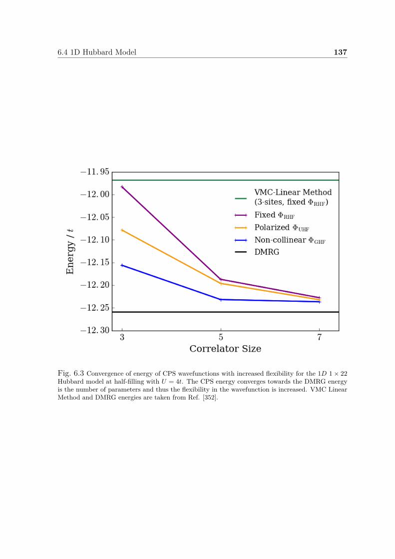
6.4 1D Hubbard Model 137
Fig. 6.3 Convergence of energy of CPS wavefunctions with increased flexibility for the 1D 1× 22Hubbard model at half-filling with U = 4t. The CPS energy converges towards the DMRG energyis the number of parameters and thus the flexibility in the wavefunction is increased. VMC LinearMethod and DMRG energies are taken from Ref. [352].
138Applications of the Projector Quantum Monte Carlo Method for Non-linear
Wavefunctions to Correlator Product State Wavefunctions
properties include the RDM energy
ERDM = Tr[ΓH] =∑pq
hpqγpq +∑
p>q,r>s
(gpqrs − gpqsr)Γpq,rs + Enuc, (6.19)
(with hpq, gpqrs and Enuc as defined in Section 2.2.2 of Chapter 2), to demonstrate thatthis estimator sampled from two replicas is in agreement with the energy estimatedduring convergence which is sampled from just one replica. Likewise, the total squaredmagnitude of the spin, S2 = S · S, is computed[37, 57]
S2 = S(S + 1) = Tr[ΓS2] (6.20)
= 14∑P Q
[ΓP αQα,P αQα + ΓP βQβ,P βQβ]− 14∑P Q
ΓP αQβ,P αQβ (6.21)
− 14∑P Q
ΓP βQα,P βQα −∑P Q
ΓP αQβ,QαP β + 34Nα + 3
4Nβ, (6.22)
where Pα refers to the α spin orbital with spatial index P . The value of S2 can alsobe taken as a measure for the accuracy of the wavefunction given that the exactwavefunction has S2 = 0. Moreover, further properties are evaluated such as the doubleoccupancy, D = 1
Nlat
∑I nI↑nI↓ = 1
Nlat
∑I a†I↑a†I↓aI↓aI↑,
D = Tr[ΓD] = 1Nlat
∑I
ΓI↑I↓,I↑I↓, (6.23)
where the sum over I includes all Nlat lattice sites, as well as the correlation entropyper electron
SCE = −Tr[γ ln γ] = − 1N
∑p
γpp ln γp
p , (6.24)
with γpp being the occupation numbers of the one-body RDM γ that is integrated out
from the 2-RDM. A last quantity which is evaluated from the density matrix is theanti-ferromagnetic order parameter, the staggered magnetisation, which is definedaccording to
M2 = 1N2
lat
∑IJ
(−1)(xI+yI)+(xJ +yI) ⟨Ψ|SI · SJ |Ψ⟩ , (6.25)
where the summations over I and J run over all Nlat lattice sites and xI and yI representthe x- and y-coordinate of the position of the lattice site I. The total spin operator
6.4 1D Hubbard Model 139
S = Sx + Sy + Sz comprises three Cartesian components which are given by
Sx = 12∑P
(a†P αaP β + a†P βaP α) (6.26)
Sy = 12i∑P
(a†P αaP β − a†P βaP α) (6.27)
Sz = 12∑P
(a†P αaP α + a†P βaP β) (6.28)
with Sz = 12(Nα −Nβ) = Mz.
The results for the properties evaluated from the sampled two-body density matrixof the differently parameterised wavefunctions are presented in Table 6.2. Firstly, agood agreement within error bars is observed between the RDM energy ERDM sampledwith one replica during the convergence of the wavefunction and ERDM evaluated fromthe density matrix sampled with two replicas. This agreement demonstrates that abias which can potentially arise when ERDM is sampled from just one replica cannotbe observed, seems to be negligible, or at least, smaller than stochastic errors and doesnot cause any issues. Secondly, the increased accuracy of ΨCPS with successively largercorrelators becomes apparent in the values of S2 which for any given reference stateconverge towards the correct value S2 = 0 of the exact wavefunction with increasingcorrelator size. However, for any given correlator size, whilst increasing the flexibilityof the reference state lowers and improves the CPS energy, the accuracy of ΨCPS doesnot necessarily improves in the same manner. This becomes obvious when consideringthe S2 values of different reference states for a fixed correlator size which shows the risein spin contamination in ΨCPS as the number of simultaneously optimised variables inthe reference state is raised when going from ΦRHF to ΦGHF.
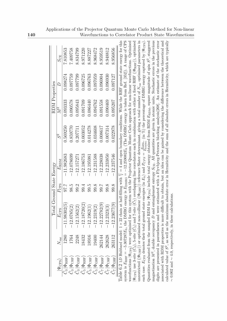
140Applications of the Projector Quantum Monte Carlo Method for Non-linear
Wavefunctions to Correlator Product State Wavefunctions
Tota
lGro
und
Stat
eEn
ergy
RD
MPr
oper
ties
|ΨC
PS⟩
Nva
rE
CP
SP
CP
SE
RD
MS
2M
2D
SC
E
C3|Φ
RH
F⟩
1280
−11.9
8302
(5)
97.7
−11.9
8268
30.
5692
500.
0933
330.
0982
747.
8108
53C
3|Φ
UH
F⟩
1764
−12.0
785(
2)98.5
−12.0
7869
90.
8597
700.
0905
780.
0977
597.
4097
58C
3|Φ
GH
F⟩
2248
−12.1
562(
2)99.2
−12.1
5727
10.
2077
110.
0958
430.
0977
998.
8347
99C
5|Φ
RH
F⟩
1843
2−
12.1
8720
(2)
99.4
−12.1
8675
30.
0030
520.
0917
090.
0967
258.
9712
20C
5|Φ
UH
F⟩
1891
6−
12.1
962(
1)99.5
−12.1
9598
10.
0142
780.
0864
400.
0967
638.
8872
27C
5|Φ
GH
F⟩
1940
0−
12.2
319(
2)99.8
−12.2
3158
80.
0346
080.
0947
620.
0970
598.
9684
72C
7|Φ
RH
F⟩
2621
44−
12.2
2782
(9)
99.7
−12.2
2803
80.
0086
170.
0915
580.
0969
048.
9595
19C
7|Φ
UH
F⟩
2626
28−
12.2
323(
3)99.8
−12.2
3385
00.
0073
140.
0904
690.
0969
308.
9488
12C
7|Φ
GH
F⟩
2631
12−
12.2
3677
(9)
99.8
−12.2
3754
60.
0229
780.
0952
070.
0971
278.
9568
56Ta
ble
6.2
1DH
ubba
rdm
odel
:1×
22ch
ain
atha
lf-fil
ling
with
U t=
4an
dop
enbo
unda
ryco
nditi
ons.
Whi
leth
eR
HF
grou
ndst
ate
ener
gyfo
rth
issy
stem
isE
RH
F=−
5.30
7287
Eh,t
heD
MR
Gen
ergy
isE
DM
RG
=−
12.2
5908
2Eh
(The
DM
RG
ener
gyis
take
nfr
omR
ef.
[352
]).A
rang
eof
CP
Swa
vefu
nctio
ns|Ψ
CP
S⟩
were
optim
ised
for
this
syst
emw
ithth
ePr
ojec
tor
Qua
ntum
Mon
teC
arlo
appr
oach
for
non-
linea
rwa
vefu
nctio
ns.
Opt
imise
d|Ψ
CP
S⟩
use
3-sit
e(C
3),5
-site
(C5)
and
7-sit
e(C
7)ov
erla
ppin
glin
eco
rrel
ator
sea
chin
com
bina
tion
with
eith
era
fixed
RH
F(|Φ
RH
F⟩)
,opt
imise
dun
rest
ricte
d(|Φ
UH
F⟩)
orop
timise
dno
n-co
lline
ar(|Φ
GH
F⟩)
refe
renc
eSl
ater
dete
rmin
ant,
givi
nga
tota
lnum
ber
ofN
var
optim
ised
para
met
ers
inea
chca
se.
EC
PS
deno
tes
thei
rto
talg
roun
dst
ate
ener
gies
(inE
h)
and
PC
PS
=E
CP
SE
DM
RG
(in%
)th
epe
rcen
tage
ofD
MR
Gen
ergy
capt
ured
by|Ψ
CP
S⟩.
Qua
ntiti
esev
alua
ted
from
the
sam
pled
RD
Mfo
r|Ψ
CP
S⟩
incl
ude
tota
lene
rgy
obta
ined
from
RD
ME
RD
M,s
quar
em
agni
tude
ofsp
inS
2 ,st
agge
red
mag
netis
atio
nM
2 ,do
uble
occu
panc
yD
and
enta
ngle
men
ten
trop
yS
CE
.A
llqu
antit
ies
are
give
nin
atom
icun
its.
Stoc
hast
icer
rors
inth
epr
evio
usdi
gits
are
pres
ente
din
pare
nthe
ses
and
wer
ees
timat
edw
itha
Flyv
bjer
g-Pe
ters
enbl
ocki
ngan
alys
is[26
8].
An
estim
ate
ofth
est
ocha
stic
erro
ras
soci
ated
with
RD
Mpr
oper
ties
ism
ore
diffi
cult
toob
tain
,but
anid
eaca
nbe
gain
edby
cons
ider
ing
the
diffe
renc
ebe
twee
nth
eth
eore
tical
and
calc
ulat
edva
lue
ofS
2 ,as
well
asth
em
axim
umab
solu
teer
ror
inH
erm
itici
tyan
dth
esu
mof
alla
bsol
ute
erro
rsin
Her
miti
city
,whi
char
ety
pica
lly∼
0.00
2an
d∼
4.0,
resp
ectiv
ely,
inth
ese
calc
ulat
ions
.
6.5 Linear H50 Chain 141
6.5 Linear H50 Chain
Ab-initio systems can also be treated in the same vein by stochastically samplingfrom both the configuration space of the wavefunction and from its O[N4] connectedconfigurations in Eq. 5.12, which are now far larger than found in the Hubbard modeldue to long-range interactions. As an example, the symmetric dissociation of H50 (ina STO-6G minimal basis[371]) is considered which represents a molecular model forstrongly-correlated systems and a non-trivial benchmark system[372] at the same time.This system has been treated not only with conventional quantum chemistry methodssuch as Coupled Cluster (CC) but also with strongly-correlated approaches includingDMFT and other embedding methods[373, 307, 374–376], due to the availability ofnumerically exact DMRG values for comparison[372]. Whilst CC methods encounterconvergence difficulties at stretched bond-lengths beyond 2.0a0, a well known anddocumented fundamental problem in CC theory[372], strongly-correlated approachescan treat all bond lengths. The CPS wavefunction is parameterised with 5-atomoverlapping correlators, and both a fixed unpolarised, or stochastically optimisedunrestricted reference determinant, leading to a total of 47, 104 or 49, 604 simultaneouslyoptimised variables. The results obtained with this ΨCPS are comparable or in somecases even better in their accuracy and closeness to DMRG results than approachesdesigned to treat strongly-correlated electrons as can be seen in the comparison inTable 6.3. At stretched bond lengths, nearly all of the DMRG correlation energy iscaptured (99.7%), as the correlation length spans few atoms, and on-site repulsiondominates (Figure 6.4). However, as the bond length decreases, a successively smallerpercentage of the DMRG correlation energy is captured, as the entanglement of theelectrons span larger numbers of atoms, which can also be seen in the larger bonddimension required of DMRG at these geometries[372]. Despite this, the correlationenergy is so small at these lengths, that the maximum error in the total energy is only1.1 kcal/mol per atom across all bond lengths.
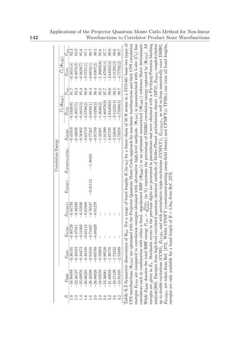
142Applications of the Projector Quantum Monte Carlo Method for Non-linear
Wavefunctions to Correlator Product State Wavefunctions
Cor
rela
tion
Ener
gyC
5|Φ
RH
F⟩
C5|Φ
UH
F⟩
RE
RH
FE
MP
2E
CC
SDE
CC
SD(T
)E
CP
MF
TE
CP
MF
T(κ
TP
SSc)
ED
MR
GE
CP
SP
corr
EC
PS
Pco
rr1.
0−
16.8
6488
−0.
3614
5−
0.40
729
−0.
4173
9−
0.41
919
−0.
3426
(8)
81.7
−0.
3451
(4)
82.3
1.2
−22.4
6127
−0.
4018
3−
0.47
011
−0.
4833
0−
0.48
638
−0.
4057
(5)
83.4
−0.
4075
(2)
83.8
1.4
−25.0
2976
−0.
4447
3−
0.54
303
−0.
5593
6−
0.56
402
−0.
4815
(3)
85.4
−0.
4829
(7)
85.6
1.6
−26.0
6225
−0.
4918
8−
0.63
118
−0.
6508
9−
0.65
719
−0.
5708
(2)
86.9
−0.
5721
(1)
87.1
1.8
−26.2
6598
−0.
5455
0−
0.74
167
−0.
7654
7−
0.21
112
−1.
3843
1−
0.77
267
−0.
6833
(1)
88.4
−0.
6853
(1)
88.7
2.0
−26.0
0820
−0.
6078
9−
0.88
329
−0.
9127
0−
0.91
789
−0.
8298
(2)
90.4
−0.
8307
(2)
90.5
2.4
−24.8
3576
−0.
7688
3−
−−
1.32
481
−1.
2646
(2)
95.5
−1.
2660
3(6)
95.6
2.8
−23.3
6081
−0.
9953
0−
−−
1.91
399
−1.
8697
8(9)
97.7
−1.
8709
1(4)
97.7
3.2
−21.8
9633
−1.
3077
8−
−−
2.67
195
−2.
6440
9(6)
99.0
−2.
6450
3(2)
99.0
3.6
−20.5
7429
−1.
7233
2−
−−
3.52
848
−3.
5122
5(4)
99.5
−3.
5129
5(3)
99.6
4.2
−18.9
5595
−2.
5589
9−
−−
4.79
376
−4.
7769
9(4)
99.7
−4.
7779
2(2)
99.7
Tabl
e6.
3Sy
mm
etric
diss
ocia
tion
ofH
50:
For
ara
nge
ofbo
ndle
ngth
sR
(ina
0)fo
ra
linea
rch
ain
of50
Hat
oms
ina
STO
-6G
basis
two
type
sof
CPS
wave
func
tions|Ψ
CP
S⟩a
reop
timise
dw
ithth
ePr
ojec
torQ
uant
umM
onte
Car
loap
proa
chfo
rnon
-line
arwa
vefu
nctio
nsan
dth
eirC
PSco
rrel
atio
nen
ergi
esE
CP
Sar
eco
mpa
red
toco
rrel
atio
nen
ergi
esob
tain
edw
ithal
tern
ativ
ehi
gh-le
velm
etho
ds.|Ψ
CP
S⟩
ispa
ram
eter
ised
with
5-sit
e(C
5)lin
eco
rrel
ator
sea
chin
com
bina
tion
with
eith
era
fixed
,unp
olar
ised
RH
F(|Φ
RH
F⟩)
oran
optim
ised
unre
stric
ted
(|ΦU
HF⟩)
refe
renc
eSl
ater
dete
rmin
ant.
Whi
leE
RH
Fde
note
sth
eto
talR
HF
ener
gyP
corr
=E
CP
SE
DM
RG
(in%
)re
pres
ents
the
perc
enta
geof
DM
RG
corr
elat
ion
ener
gyca
ptur
edby|Ψ
CP
S⟩.
All
ener
gies
are
give
nin
Eh.
Stoc
hast
icer
rors
inth
epr
evio
usdi
gits
are
pres
ente
din
pare
nthe
ses
and
were
obta
ined
with
aFl
yvbj
erg-
Pete
rsen
bloc
king
anal
ysis[
268]
.En
ergi
esfr
omhi
gh-le
velc
orre
late
dqu
antu
mch
emic
alm
etho
dsof
Møl
ler-
Ples
set
pert
urba
tion
theo
ry(M
P2),
EM
P2,
coup
led-
clus
ter
upto
doub
leex
cita
tions
(CC
SD),
EC
CSD
,and
with
pert
urba
tive
trip
leex
cita
tions
(CC
SD(T
)),E
CC
SD(T
),as
well
asfro
mnu
mer
ical
lyex
actD
MR
G,
ED
MR
G,a
reta
ken
from
Ref
.[3
72].
Whi
lstC
PM
FT(c
onst
rain
ed-p
airin
gm
ean-
field
theo
ry)
and
CP
MFT
(κT
PSS
c)ca
ntr
eat
allb
ond
leng
ths,
ener
gies
are
only
avai
labl
efo
ra
bond
leng
thof
R=
1.8a
0fr
omR
ef.
[373
].
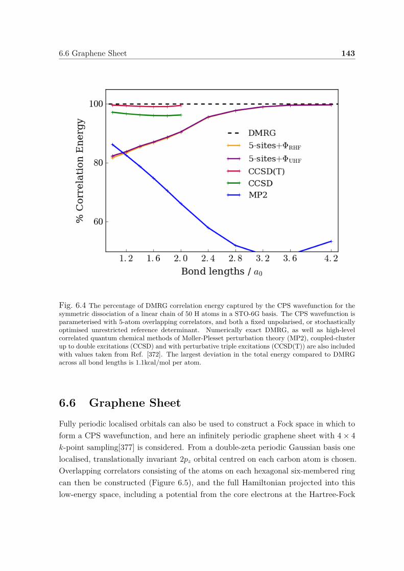
6.6 Graphene Sheet 143
Fig. 6.4 The percentage of DMRG correlation energy captured by the CPS wavefunction for thesymmetric dissociation of a linear chain of 50 H atoms in a STO-6G basis. The CPS wavefunction isparameterised with 5-atom overlapping correlators, and both a fixed unpolarised, or stochasticallyoptimised unrestricted reference determinant. Numerically exact DMRG, as well as high-levelcorrelated quantum chemical methods of Møller-Plesset perturbation theory (MP2), coupled-clusterup to double excitations (CCSD) and with perturbative triple excitations (CCSD(T)) are also includedwith values taken from Ref. [372]. The largest deviation in the total energy compared to DMRGacross all bond lengths is 1.1kcal/mol per atom.
6.6 Graphene Sheet
Fully periodic localised orbitals can also be used to construct a Fock space in which toform a CPS wavefunction, and here an infinitely periodic graphene sheet with 4× 4k-point sampling[377] is considered. From a double-zeta periodic Gaussian basis onelocalised, translationally invariant 2pz orbital centred on each carbon atom is chosen.Overlapping correlators consisting of the atoms on each hexagonal six-membered ringcan then be constructed (Figure 6.5), and the full Hamiltonian projected into thislow-energy space, including a potential from the core electrons at the Hartree-Fock
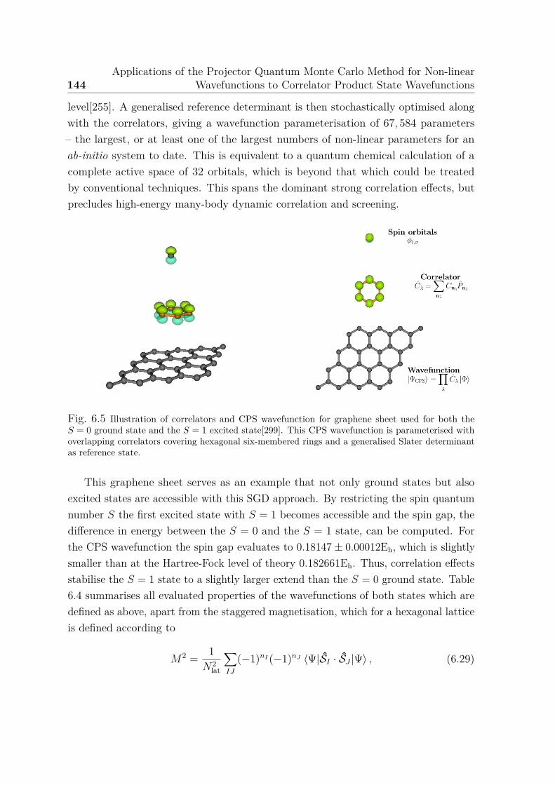
144Applications of the Projector Quantum Monte Carlo Method for Non-linear
Wavefunctions to Correlator Product State Wavefunctions
level[255]. A generalised reference determinant is then stochastically optimised alongwith the correlators, giving a wavefunction parameterisation of 67, 584 parameters– the largest, or at least one of the largest numbers of non-linear parameters for anab-initio system to date. This is equivalent to a quantum chemical calculation of acomplete active space of 32 orbitals, which is beyond that which could be treatedby conventional techniques. This spans the dominant strong correlation effects, butprecludes high-energy many-body dynamic correlation and screening.
Fig. 6.5 Illustration of correlators and CPS wavefunction for graphene sheet used for both theS = 0 ground state and the S = 1 excited state[299]. This CPS wavefunction is parameterised withoverlapping correlators covering hexagonal six-membered rings and a generalised Slater determinantas reference state.
This graphene sheet serves as an example that not only ground states but alsoexcited states are accessible with this SGD approach. By restricting the spin quantumnumber S the first excited state with S = 1 becomes accessible and the spin gap, thedifference in energy between the S = 0 and the S = 1 state, can be computed. Forthe CPS wavefunction the spin gap evaluates to 0.18147± 0.00012Eh, which is slightlysmaller than at the Hartree-Fock level of theory 0.182661Eh. Thus, correlation effectsstabilise the S = 1 state to a slightly larger extend than the S = 0 ground state. Table6.4 summarises all evaluated properties of the wavefunctions of both states which aredefined as above, apart from the staggered magnetisation, which for a hexagonal latticeis defined according to
M2 = 1N2
lat
∑IJ
(−1)nI (−1)nJ ⟨Ψ|SI · SJ |Ψ⟩ , (6.29)
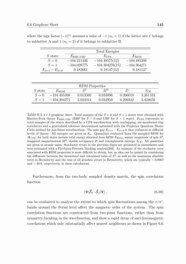
6.6 Graphene Sheet 145
where the sign factor (−1)nI assumes a value of −1 (nI = 1) if the lattice site I belongsto sublattice A and 1 (nI = 2) if it belongs to sublattice B.
Total EnergiesS state ERHF/UHF ECPS ERDMS = 0 −104.211436 −104.48575(12) −104.485398S = 1 −104.028775 −104.304276(15) −104.304271
ES=1 − ES=0 0.182661 0.18147(12) 0.181127
RDM PropertiesS state ERDM S2 M2 D SCES = 0 −104.485398 0.013560 0.033896 0.206018 3.261103S = 1 −104.304271 2.024314 0.032950 0.200342 3.424658
Table 6.4 4× 4 graphene sheet: Total energies of the S = 0 and S = 1 states were obtained withHartree-Fock theory ERHF/UHF (RHF for S = 0 and UHF for S = 1 state). ECPS represents tototal energies of the states described by a CPS wavefunction with overlapping, six-membered ringcorrelators and a generalised reference determinant optimised with the Projector Quantum MonteCarlo method for non-linear wavefunctions. The spin gap ES=1 − ES=0 is thus evaluated at differentlevels of theory. All energies are given in Eh. Quantities evaluated from the sampled RDM for|ΨCPS⟩ for both states include total energy obtained from RDM ERDM, square magnitude of spin S2,staggered magnetisation M2, double occupancy D and entanglement entropy SCE. All quantitiesare given in atomic units. Stochastic errors in the previous digits are presented in parentheses andwere estimated with a Flyvbjerg-Petersen blocking analysis[268]. An estimate of the stochastic errorassociated with RDM properties is more difficult to obtain, but an idea can be gained by consideringthe difference between the theoretical and calculated value of S2, as well as the maximum absoluteerror in Hermiticity and the sum of all absolute errors in Hermiticity, which are typically ∼ 0.0007and ∼ 40.0, respectively, in these calculations.
Furthermore, from the two-body sampled density matrix, the spin correlationfunction
⟨Ψ|SI · SJ |Ψ⟩ , (6.30)
can be evaluated to analyse the extent to which spin fluctuations among the π/π∗-bands around the Fermi level affect the magnetic order of the system. The spincorrelation functions are constructed from two-point functions, rather than fromsymmetry-breaking in the wavefunction, and show a rapid decay of anti-ferromagneticcorrelations which only substantially affect nearest neighbours as shown in Figure 6.6.
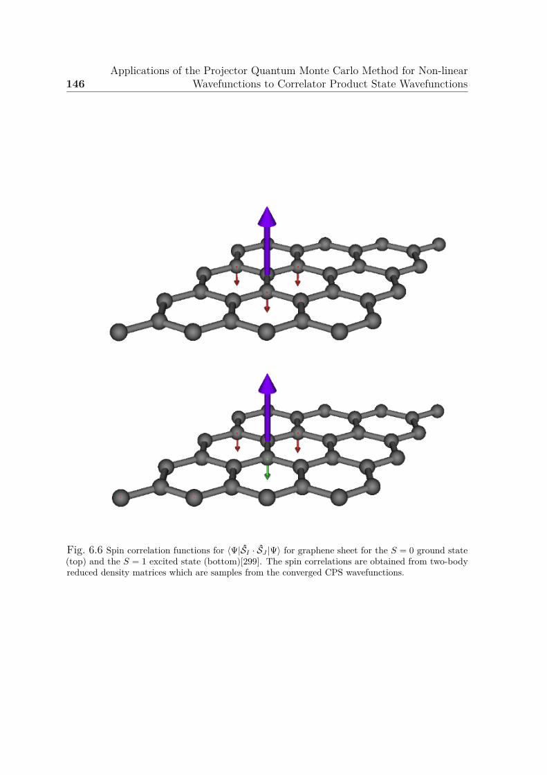
146Applications of the Projector Quantum Monte Carlo Method for Non-linear
Wavefunctions to Correlator Product State Wavefunctions
Fig. 6.6 Spin correlation functions for ⟨Ψ|SI · SJ |Ψ⟩ for graphene sheet for the S = 0 ground state(top) and the S = 1 excited state (bottom)[299]. The spin correlations are obtained from two-bodyreduced density matrices which are samples from the converged CPS wavefunctions.
6.7 Conclusions 147
6.7 Conclusions
The applications presented in this chapter demonstrate the capability of this stochasticaccelerated projector approach to handle and optimise arbitrary non-linear wavefunc-tions of quantum many-body systems. The large numbers of simultaneously optimisedparameters in the wavefunctions greatly exceeds those accessible to alternative formu-lations of Variational Quantum Monte Carlo optimisations. Systematically improvableFock-space wavefunctions have thus been found for both lattice Hubbard models andab-initio systems, as well as one- and two-body static properties of these wavefunctions.At the same time, the proposed Projector Quantum Monte Carlo method for non-linearwavefunction ansatzes blurrs the line between traditional Variational and ProjectorQuantum Monte Carlo approaches.

Chapter 7
Projector Quantum Monte CarloMethod for Tensor Network States
Many natural quantum many-body states live on a tiny submanifold of the exponentiallylarge Hilbert space. This ‘natural corner of the Hilbert space’ derives from the localityof interactions, implying that these physical states obey area laws for entanglement (orshow only small violations thereof)[132, 55, 53, 54] (as detailed in Chapter 2). Progressin quantum information theory has lead to a better understanding of entanglement inquantum many-body states and enabled the formulation of efficient parameterisationswhich directly target this relevant subspace of the Hilbert space: Tensor Network States(TNS). By efficiently describing the structure of quantum correlations and capturing theentanglement in low-energy states of a system, they satisfy area laws by constructionand are thus able to approximate physical states to a high level of accuracy with anumber of parameters that grows only polynomial with system size whilst still retainingsystematic improvability towards exactness[55, 53, 54]. Amongst the large varietyof tensor networks Matrix Product States (MPS)[170], the underlying variationalansatz of the DMRG approach, have been extremely successful in one-dimensionalsystems[136, 148]. However, the extension of their success to higher dimensions hasproved more difficult due to their one-dimensional encoding of correlations. In recentyears, Projected Entangled Pair States (PEPS)[53, 55, 54, 142, 155], the naturalgeneralisation of MPS to higher dimension, have emerged as a potential promisingalternative. This has been demonstrated by accurate results obtained for manyquantum systems including the t− J [378], the Hubbard model[189] and frustrated spinsystems[379].
However, in contrast to MPS, contraction of a PEPS network, as it is necessaryfor the extraction of information from a state vector, is a computationally hard
150 Projector Quantum Monte Carlo Method for Tensor Network States
problem in the complexity class ♯P [160] and approximate contraction schemes needto be resorted to. Despite these developments, PEPS are still much harder to handlecomputationally than their one-dimensional analogues due to the increased exponentin their polynomial scaling with system size[55, 53, 54]. Even more so, an efficientoptimisation of the variational parameters in a PEPS which give the best approximationto ground states has remained profoundly more challenging than for MPS. Since thisinvolves a highly non-linear minimisation of the energy expectation value, state-of-the-art PEPS optimisations employ imaginary time evolution which projects an initialtrial state onto the ground state |ψ0⟩ = limτ→∞ e
−τH |ψ⟩[158, 161, 179]. The limitτ → ∞ is approached with a Trotter-Suzuki decomposition by applying sufficientlysmall time steps. To arrive at an efficient algorithm with tractable cost, the PEPSbond dimensions have to be truncated in an approximate way after each time step.This truncation can be realised with a range of differing techniques each of whichprovides a different compromise between accuracy and computational cost such as thefull[158, 179], the variational[55] or the simple[161] update scheme. Whilst the fullupdate approach which takes into account the complete environment as provided by thefull PEPS wavefunction represents the most accurate procedure, even though it is notguaranteed to result in the globally optimal truncation, it is also the computationallymost expensive one[158, 179]. In contrast, the simple update scheme sacrifices partof this accuracy by using simple approximations to the environment which can beevaluated at a much reduced computational cost[161]. Yet, at both ends of the scalethe optimisation can become inefficient: whereas the computational cost of the fullupdate scheme is often too demanding, the approximate local environment of thesimple update is often a crude oversimplification of the quantum correlations. Becauseof these difficulties it is unclear whether these state-of-the-art approaches succeedin obtaining the optimal state of a given variational PEPS parameterisation whichhas also sparked the proposal of alternative optimisation approaches based on thevariational principle[380] or gradient methods[381].
As an alternative to circumvent the challenges described above, this chapter proposesan optimisation of TNS with the Projector Quantum Monte Carlo method for non-linearwavefunctions described in Chapter 5. Being formulated in a very general manner, thisapproach is applicable to any arbitrary wavefunction ansatz for which the gradient ofthe energy functional with respect to the wavefunction parameters exists. For practicalimplementations, it is also vital that projections of the wavefunction parameterisationsonto configurations in the Hilbert space, as well as projections of the respective energyderivatives onto the same configurations, are efficiently computable. For this reason
7.1 The Computational Challenge of PEPS Wavefunctions - Can It Be TackledStochastically ? 151
a novel approach for evaluating tensor network contractions stochastically is alsodeveloped in this chapter which in combination with the Projector Quantum MonteCarlo method enables the efficient optimisation of tensor network state wavefunctions.It is worth noting that the considerations outlined in this chapter are in principle alsoapplicable to many of the existing TNS categories and appropriate equations can bestraightforwardly derived. However, the main focus of this chapter are PEPS and MPS,and for brevity and clarity any equations are formulated in terms of PEPS and MPSwavefunctions only.
7.1 The Computational Challenge of PEPS Wave-functions - Can It Be Tackled Stochastically ?
Before detailing the rigorous mathematical foundations of the tensor notwork stateoptimisation developed in this chapter, it is worth giving a more intuitive and broadpicture of the challenge encountered in dealing with PEPS wavefunctions and theproposed approach to tackle it by returning to the graphical description of a PEPSwavefunction introduced in Chapter 2 (Figure 7.1). Optimisations, or even just theextraction of information, from a PEPS state require contraction of the tensor networkwhich can conceptually be split in two nested contractions: firstly, a contraction of thephysical indices (represented by the red filled circles in the graphical depiction) andsecondly, a contraction of the auxiliary indices (embodied by the blue circles and linesin the graph). Exact evaluation of these contractions is prohibitively expensive forPEPS wavefunctions and state-of-the-art PEPS calculations therefore perform thesecontractions deterministically, but in an approximate manner. This chapter proposesan alternative approach which instead of deterministically contracting the network,samples the contraction. This stochastic network contraction will also be coupled toa stochastic optimisation of the variational parameters in the PEPS state using theProjector Quantum Monte Carlo method for non-linear wavefunctions which has beenoutlined in Chapter 5. Essentially, this results in two nested stochastic processes: Theouter stochastic process realises the contraction of physical indices with a MetropolisMarkov chain just in the same way as it is outlined in Chapter 5 and used in theapplications of Chapter 6. Within this, the inner stochastic process evaluates thecontraction over auxiliary indices to obtain stochastic estimates for the projections ofwavefunction amplitudes and derivatives onto configurations in the full Hilbert spacewhich are required within the Markov chain sampling of the outer sampling procedurefor physical indices. In order to aid the stochastic contraction and avoid it suffering
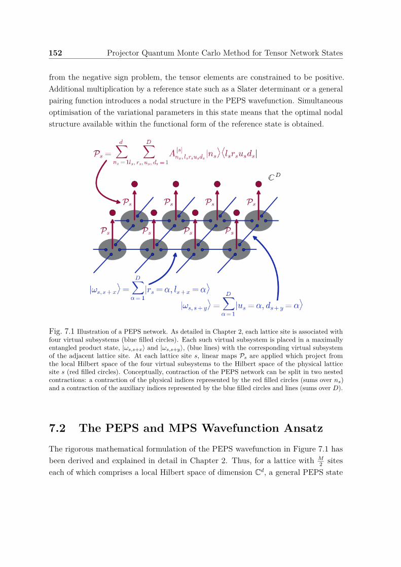
152 Projector Quantum Monte Carlo Method for Tensor Network States
from the negative sign problem, the tensor elements are constrained to be positive.Additional multiplication by a reference state such as a Slater determinant or a generalpairing function introduces a nodal structure in the PEPS wavefunction. Simultaneousoptimisation of the variational parameters in this state means that the optimal nodalstructure available within the functional form of the reference state is obtained.
Fig. 7.1 Illustration of a PEPS network. As detailed in Chapter 2, each lattice site is associated withfour virtual subsystems (blue filled circles). Each such virtual subsystem is placed in a maximallyentangled product state, |ωs,s+x⟩ and |ωs,s+y⟩, (blue lines) with the corresponding virtual subsystemof the adjacent lattice site. At each lattice site s, linear maps Ps are applied which project fromthe local Hilbert space of the four virtual subsystems to the Hilbert space of the physical latticesite s (red filled circles). Conceptually, contraction of the PEPS network can be split in two nestedcontractions: a contraction of the physical indices represented by the red filled circles (sums over ns)and a contraction of the auxiliary indices represented by the blue filled circles and lines (sums over D).
7.2 The PEPS and MPS Wavefunction Ansatz
The rigorous mathematical formulation of the PEPS wavefunction in Figure 7.1 hasbeen derived and explained in detail in Chapter 2. Thus, for a lattice with M
2 siteseach of which comprises a local Hilbert space of dimension Cd, a general PEPS state
7.2 The PEPS and MPS Wavefunctions Ansatz 153
vector in the full Hilbert space H = (Cd)⊗M2 can be written as[55, 53, 54]
|ΨPEPS⟩ =
M2⊗
s=1Ps
M2⊗
s=1
p−1⊗i=1|ωs,i⟩
(7.1)
=∑
n1n2...n M2
F(A[1]n1A
[2]n2 . . . A
[ M2 ]
n M2
) |n1n2 . . . nM2⟩ , (7.2)
where A[s]ns
denotes the rank-p tensor at lattice site s whose local configuration is ns.The rank p of the tensor is usually equal to the number of nearest-neighbours of thelattice site s and the function F(. . .) represents the contractions of tensors A[s]
nswhose
explicit form depends on the rank p of the tensors, as well as the dimension and shapeof the lattice. As explained in Chapter 2, for one dimensional systems, this formulationrecovers an MPS
|ΨMPS⟩ =
M2⊗
s=1Ps
M2⊗
s=1|ωs,s+1⟩
(7.3)
=∑
n1n2...n M2
F(f(A[1]n1)f(A[2]
n2) . . . f(A[ M2 ]
n M2
)) |n1n2 . . . nM2⟩ . (7.4)
This well known and widely used ansatz is slightly extended in order to aid thestochastic evaluation of the tensor network contraction. Hence, the fully generalisedwavefunction parameterisation can be expressed as
|ΨPEPS⟩ =
M2⊗
s=1Ps
M2⊗
s=1
p−1⊗i=1|ωs,i⟩
|Φ⟩ (7.5)
=∑
n1n2...n M2
F(f(A[1]n1)f(A[2]
n2) . . . f(A[ M2 ]
n M2
)) |n1n2 . . . nM2⟩ ⟨n1n2 . . . nM
2|Φ⟩ ,
(7.6)
where the PEPS is multiplied by a reference state |Φ⟩. Similar to the CPS wavefunctionparameterisation in Chapter 6, the uniform reference |ΦU⟩, a Slater determinant |ΦD⟩,an AGP |ΦAGP⟩ or a general pairing wavefunction |ΦPF⟩ can act as reference state.Their contributions to wavefunction amplitudes are all given in Section 6.2 of theprevious chapter. Moreover, f(. . .) represents a function of the tensor elements, suchas f(x) = x2, f(x) = |x|, f(x) = ex etc. These two extensions of the wavefunctionansatz are introduced in order to prevent the sampling approach for the tensor network
154 Projector Quantum Monte Carlo Method for Tensor Network States
contraction from suffering from the negative sign problem. Whereas the functions f(. . .)serve the purpose of constraining the tensor elements to be positive, the reference state|Φ⟩ reintroduces a nodal structure into |ΨPEPS⟩. In the limit of a uniform reference |ΦU⟩as reference state and the function f(x) = x, the original wavefunction ansatz of Eq.7.1is recovered. By analogy, for one-dimensional systems the generalised wavefunctionansatz based on MPS can be written as
|ΨMPS⟩ =
M2⊗
s=1Ps
M2⊗
s=1|ωs,s+1⟩
|Φ⟩ , (7.7)
=∑
n1n2...n M2
F(f(A[1]n1)f(A[2]
n2) . . . f(A[ M2 ]
n M2
)) |n1n2 . . . nM2⟩ ⟨n1n2 . . . nM
2|Φ⟩ . (7.8)
7.3 Wavefunction Amplitudes and Derivatives
Hence, projecting the |ΨPEPS⟩ of Eq. 7.5 into the full Hilbert space of configurations|n⟩ =
|n1n2 . . . nM
2⟩
, the wavefunction amplitudes are given by
⟨n|ΨPEPS⟩ = ⟨n|F(f(A[1]n1)f(A[2]
n2) . . . f(A[ M2 ]
n M2
))|n⟩ ⟨n|Φ⟩ . (7.9)
For an MPS, the function F representing the contraction over auxiliary indices involvesrank-2 tensors of dimensions Dα, Dβ, . . . such that
⟨n|ΨMPS,obc⟩ = ⟨n|DαDβ ...Dλ∑
αβ...λ=1f(A[1]
n1;α)f(A[2]n2;αβ) . . . f(A[ M
2 ]n M
2;λ)|n⟩ ⟨n|Φ⟩ (7.10)
⟨n|ΨMPS,pbc⟩ = ⟨n|DαDβDγ ...Dω∑
αβγ...ω=1f(A[1]
n1;ωα)f(A[2]n2;αβ) . . . f(A[ M
2 ]n M
2;λω)|n⟩ ⟨n|Φ⟩ , (7.11)
for open and periodic boundary conditions, respectively. By analogy, for a PEPS on a2D square lattice, the wavefunction amplitudes can be written as contraction of rank-4tensors of dimensions Dα, Dβ, . . .
⟨n|ΨPEPS⟩ = ⟨n|DαDβDγDδ...Dω∑
αβγδ...ω=1f(A[1]
n1;αβγω)f(A[2]n2;δαλη) . . . f(A[ M
2 ]n M
2;χζων)|n⟩ ⟨n|Φ⟩ .
(7.12)
7.4 A Sampling Approach for Wavefunction Amplitudes and Derivatives 155
From these, the appropriate derivatives of the wavefunction amplitudes with respectto a particular element of a tensor such as A[2]
n2;ij can be evaluated as
⟨n|∂ΨMPS,obc
∂A[2]n2;ij
⟩ = ⟨n|DαDβ ...Dλ∑
αβ...λ=1f(A[1]
n1;α)∂f(A[2]
n2;αβ)∂A
[2]n2;ij
δiαδjβ . . . f(A[ M2 ]
n M2
;λ)|n⟩ ⟨n|Φ⟩ (7.13)
⟨n|∂ΨMPS,pbc
∂A[2]n2;ij
⟩ = ⟨n|DαDβDγ ...Dω∑
αβγ...ω=1f(A[1]
n1;ωα)∂f(A[2]
n2;αβ)∂A
[2]n2;ij
δiαδjβ . . . f(A[ M2 ]
n M2
;λω)|n⟩ ⟨n|Φ⟩ ,
(7.14)
in the case of open and periodic boundary MPS. Likewise, the derivative of a PEPSprojection with respect to a particular tensor element A[2]
n2;ijkl can be formulated as
⟨n| ∂ΨPEPS
∂A[2]n2;ijkl
⟩ (7.15)
= ⟨n|DαDβDγDδ...Dω∑
αβγδ...ω=1f(A[1]
n1;αβγω)∂f(A[2]
n2;δαλη)∂A
[2]n2;ijkl
δiδδjαδkλδlη . . . f(A[ M2 ]
n M2
;χζων)|n⟩ ⟨n|Φ⟩ .
(7.16)
Similar expressions for wavefunction amplitudes and derivatives of PEPS states livingon lattices with other geometries, shapes and dimensionalities can be straightforwardlyderived. Furthermore, appropriate derivatives with respect to the parameters of thereference state |Φ⟩ are given by the expressions in Section 6.2 of Chapter 6.
In the case of MPS, the contractions involved in the projections amount to a series ofsimple matrix-vector (open boundary conditions) or matrix-matrix (periodic boundaryconditions) multiplications which can be computed efficiently. On the contrary, PEPScontraction involves rank-4 tensors whose exact contraction is prohibitively expensive.State-of-the-art PEPS simulations therefore rely on approximate contraction schemes.Yet, these still incur a much worse scaling with bond dimension D than their exactMPS counterparts.
7.4 A Sampling Approach for Wavefunction Am-plitudes and Derivatives
Similar to the Projector Quantum Monte Carlo method proposed in this thesis, previousapproaches have also combined PEPS contraction and Monte Carlo sampling[382–384]by replacing sums over physical indices which arise during the evaluation of expectation
156 Projector Quantum Monte Carlo Method for Tensor Network States
values by random samples. These techniques have allowed for the use of larger values ofD with the same computational resources[383, 382, 384]. Still, since even approximatecontraction schemes for PEPS projections ⟨n|ΨPEPS⟩ incur significant computationalexpenditures, a new approach is proposed in this section which employs Monte Carlosampling for the contraction of auxiliary indices. Thus, in addition to sampling of thephysical indices and nested within this first sampling process, the explicit sums overall Nauxinds auxiliary indices α, β, . . . in the PEPS projections
⟨n|ΨPEPS⟩ = Sn ⟨n|Φ⟩ (7.17)
= ⟨n|DαDβDγDδ...Dω∑
αβγδ...ω=1f(A[1]
n1;αβγω)f(A[2]n2;δαλη) . . . f(A[ M
2 ]n M
2;χζων)|n⟩ ⟨n|Φ⟩
(7.18)
⟨n| ∂ΨPEPS
∂A[2]n2;ijkl
⟩ = S′
n;n2;ijkl ⟨n|Φ⟩ (7.19)
= ⟨n|DαDβDγDδ...Dω∑
αβγδ...ω=1f(A[1]
n1;αβγω)∂f(A[2]
n2;δαλη)∂A
[2]n2;ijkl
δiδδjαδkλδlη . . . f(A[ M2 ]
n M2
;χζων)|n⟩ ⟨n|Φ⟩ ,
(7.20)
are also evaluated stochastically by drawing a few randomly sampled terms. Fora practical implementation of this sampling approach, all terms arising in the sumneed to be positive as otherwise the sampling approach is prone to suffer from thenegative sign problem. This restriction can be straightforwardly imposed with thehelp of the functions f(. . .), such as f(x) = ex, f(x) = x2, f(x) = |x|, . . ., which havebeen introduced for this sole purpose of restraining the individual tensor elements tobe positive. |ΨPEPS⟩ then retains a sign structure by multiplication by the referencestate |Φ⟩ which, likewise, has been included solely for this purpose of providing thenodal structure of the wavefunction. Similar to the CPS wavefunction optimisationin Chapter 6, the reference state is optimised simultaneously such that the optimalnodal structure available within its functional constraint is obtained at convergence.For brevity and clarity, any equations below are given for PEPS on a 2D square lattice,but similar expressions can be derived for PEPS in other dimensions and lattice shapeswith a different contraction function F such as MPS.
Instead of explicitly enumerating all terms appearing in the sum Sn, a numberof NTNS,samples terms are randomly chosen instead. Each single product term of thissampling process is picked by randomly selecting a particular value for each of theNauxinds auxiliary indices and unbiasing for the probability of the occurrence of this
7.4 A Sampling Approach for Wavefunction Amplitudes and Derivatives 157
event
Sn =DαDβDγDδ...Dω∑
αβγδ...ω=1f(A[1]
n1;αβγω)f(A[2]n2;δαλη) . . . f(A[ M
2 ]n M
2;χζων) (7.21)
≡ 1NTNS,samples
NTNS,samples∑z
⟨f(A[1]n1;abco)f(A[2]
n2;daef ) . . . f(A[ M2 ]
n M2
;ghio)
pn1n2α (a)pn1n3
β (b) . . . pn1nM/2ω (o)
⟩Pαβ...ω(z)
(7.22)
= 1NTNS,samples
NTNS,samples∑z
Tαβ...ω(z)Pαβ...ω(z) , (7.23)
where a term Tαβ...ω(z) and its respective probability Pαβ...ω(z) are given by
Tαβ...ω(z) = f(A[1]n1;abco)f(A[2]
n2;daef ) . . . f(A[ M2 ]
n M2
;ghio) (7.24)
Pαβ...ω(z) = pn1n2α (a)pn1n3
β (b) . . . pn1nM/2ω (o). (7.25)
In this notation, Greek letters α, β, γ, . . . refer to auxiliary indices and Roman lettersa, b, c, . . . to the particular values which are chosen for each auxiliary index, that isa denotes the particular value which has been picked for the auxiliary index α. Allthese picked values for the auxiliary indices are then collectively combined into onesingle index z. pn1n2
α (a) represents the normalised probability distribution from whichthe value a is sampled for auxiliary index α which connects lattice sites 1 and 2 withoccupations n1 and n2 in their local Hilbert spaces of size d. There exists a relativelylarge freedom in the choice for pn1n2
α (a) provided that it satisfies the necessary constraintthat there remains a finite probability of picking each non-zero tensor element. Thefunctional form for these probability distributions is thus chosen such that it enablespreferential selection of the most dominant terms whilst still being efficiently calculable.A good comprise was found to be
pn1n2α (a) = 1
Nnorm
∑βγω
f(A[1]n1;aβγω)
×∑
δλη
f(A[2]n2;δaλη)
, (7.26)
where Nnorm is a normalisation constant.Similar to the wavefunction amplitudes, the derivative of a PEPS projection with
respect to a particular rank-4 tensor A[2]n2 is also sampled by stochastically choosing
NTNS,samples terms in the manner described above and accumulating them in theappropriate elements of the rank-4 tensor S ′
n;n2 holding all derivatives with respect to
158 Projector Quantum Monte Carlo Method for Tensor Network States
A[2]n2 , such that a particular element S ′
n;n2,ijkl is given by
S′
n;n2,ijkl =DαDβDγDδ...Dω∑
αβγδ...ω=1f(A[1]
n1;αβγω)∂f(A[2]
n2;δαλη)∂A
[2]n2;ijkl
δiδδjαδkλδlη . . . f(A[ M2 ]
n M2
;χζων) (7.27)
≡ 1NTNS,samples
NTNS,samples∑z
⟨f(A[1]n1;abco)
f(A[2]n2;daef
)
∂A[2]n2;ijkl
δidδjaδkeδlf . . . f(A[ M2 ]
n M2
;ghio)
pn1n2α (a)pn1n3
β (b) . . . pn1nM/2ω (o)
⟩Pαβ...ω(z)
(7.28)
= 1NTNS,samples
NTNS,samples∑z
T′n2;ijkl;αβ...ω(z)Pαβ...ω(z) , (7.29)
with T′n2;ijkl;αβ...ω(z) defined as
T′
n2;ijkl;αβ...ω(z) = f(A[1]n1;abco)
f(A[2]n2;daef )
∂A[2]n2;ijkl
δidδjaδkeδlf . . . f(A[ M2 ]
n M2
;ghio). (7.30)
In the algorithm, the distributions pn1n2α are all computed at the beginning of each
iteration with O[d2NauxindsD] operations such that they follow the changes in tensorelements. Following this, sampling from these distributions can be efficiently realisedin O[1] time with the Alias method and the computation of one TNS projection onto aHilbert space configuration, as well as the evaluation of its derivatives with respect toa single tensor, therefore requires O[NTNS,samplesNauxinds] operations.
7.5 Investigation of TNS Projection Sampling Ap-proach
Prior to optimisations of arbitrary TNS wavefunctions with the proposed ProjectorQuantum Monte Carlo approach in combination with the previously outlined samplingapproach for the TNS projections, an investigation of the convergence behaviour ofthe TNS projection sampling approach is necessary to demonstrate that the latter isable to yield faithful and accurate stochastic estimates of the gradient and energy at atractable computational cost. MPS naturally lend themselves for such a rigorous studyas their exact contraction can be evaluated efficiently, thereby granting access to exactbenchmark results. For this purpose, a 1D 1×8 Hubbard model at half-filling and U
t= 2
and Ut
= 8 with open boundary conditions is considered which represents a non-trivialbenchmark system that is still small enough to allow for deterministic evaluation of the

7.5 Investigation of TNS Projection Sampling Approach 159
energy, as well as for a deterministic gradient descent optimisation of the wavefunction.The investigated MPS wavefunctions are parameterised with a general pairing functionas reference state and rank-3 tensors (rank-2 at the boundaries) (one physical andtwo (one at the boundaries) auxiliary indices) with a bond dimension of D = 10.Evaluation of the TNS projections onto configurations therefore requires contractionsover auxiliary indices whose exact computation involves Nterms = 10, 000, 000. In thefollowing, energies are evaluated for MPS wavefunctions with a fixed set of parameterswhich have either been chosen randomly or obtained by a deterministic optimisation andthe convergence of the stochastic estimates with respect towards the number of samplesfor the auxiliary, Naux, and physical, Nphys, indices towards the true deterministicvalues are studied.
Hence, in a first instance, the convergence of the energy estimate with respect tothe amount of sampling for auxiliary indices only is investigated. While the TNSprojections onto configurations are sampled, the contraction of the physical indices isrealised deterministically as represented by the full sum over all configurations n,min the Hilbert space
ETNS =∑
mn ⟨ΨTNS|m⟩Hmn ⟨n|ΨTNS⟩∑n ⟨ΨTNS|n⟩ ⟨n|ΨTNS⟩
=∑
mn Sm ⟨Φ|m⟩Hmn ⟨n|Φ⟩Sn∑n Sn ⟨Φ|n⟩ ⟨n|Φ⟩Sn
. (7.31)
It should be stressed that for each single occurrence of a particular configurationappearing in the sums over n and m a separate and independent stochastic estimate ofthe TNS projection Sn/m is sampled. In particular, this includes diagonal terms of theform Sn ⟨Φ|n⟩Hnn ⟨n|Φ⟩Sn and Sn ⟨Φ|n⟩ ⟨n|Φ⟩Sn where two independent estimates ofSn are calculated, one for the bra and one for the ket state. This repeated independentestimation of the sampled quantities Sn is vital to ensure that no bias arising froma repeated use of the same stochastic estimate with the same associated error isintroduced in the stochastic energy estimate. Unfortunately, the normalisation inthe energy estimate in Eq. 7.31 can introduce a potential unavoidable bias sincethe (∑n Sn ⟨Φ|n⟩ ⟨n|Φ⟩Sn)−1 factor represents a non-linear function of the sampledquantities Sn.
The convergences in Figure 7.2 illustrate that already at a moderate number ofsamples for the auxiliary indices (Naux ≈ 100), which represents a tiny fraction of thetotal number of terms in the contraction sum ( Naux
Nterms≈ 1 × 10⁻⁶), the errors in the
energy estimates is less than one percent in almost all cases. As expected, increasingNaux results in a general trend towards the deterministic value and agreement withinerror bars in most cases. This behaviour is more pronounced for wavefunctions with
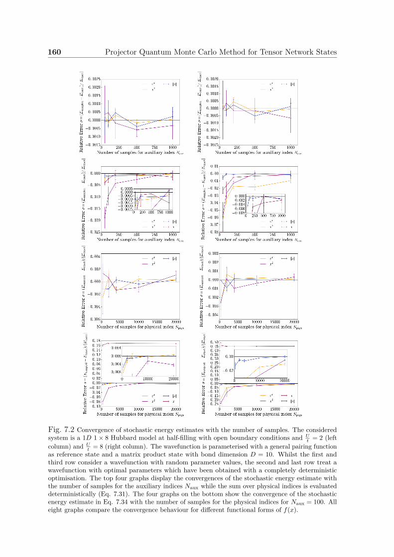
160 Projector Quantum Monte Carlo Method for Tensor Network States
Fig. 7.2 Convergence of stochastic energy estimates with the number of samples. The consideredsystem is a 1D 1× 8 Hubbard model at half-filling with open boundary conditions and U
t = 2 (leftcolumn) and U
t = 8 (right column). The wavefunction is parameterised with a general pairing functionas reference state and a matrix product state with bond dimension D = 10. Whilst the first andthird row consider a wavefunction with random parameter values, the second and last row treat awavefunction with optimal parameters which have been obtained with a completely deterministicoptimisation. The top four graphs display the convergences of the stochastic energy estimate withthe number of samples for the auxiliary indices Naux while the sum over physical indices is evaluateddeterministically (Eq. 7.31). The four graphs on the bottom show the convergence of the stochasticenergy estimate in Eq. 7.34 with the number of samples for the physical indices for Naux = 100. Alleight graphs compare the convergence behaviour for different functional forms of f(x).

7.5 Investigation of TNS Projection Sampling Approach 161
optimal parameters where the error in the estimate tends to be larger than for randomvalues. Moreover, for optimal wavefunction parameters a tendency of the energyestimates to converge from below onto the exact energy is observed. This is mostlikely an appearance of the potential bias introduced by the division of the samplednormalisation. At the same time, convergences for the three functional forms f(x) = ex,f(x) = x2 and f(x) = |x| as possible choices for the restriction function f(. . .) arecompared. These clearly demonstrate that the most efficient function is f(x) = |x|given that for the same number of samples the error is typically smaller, even by anorder of magnitude in the case of optimal wavefunction parameters.
Moreover, the convergence of the stochastic energy estimates towards its determinis-tic analogue is investigated when in addition to the contraction of auxiliary indices thecontraction of physical indices is also sampled using the techniques outlined in Section5.3 and 5.7 of Chapter 5. Thus, the energy is estimated with two nested stochasticprocesses whereby the outer sampling procedure involves a Metropolis Markov chaincomprising Nphys samples of n. Each sampled configuration n contributes a smallsampled selection of Ns off-diagonal terms with m = n,
ETNS,off−diag =⟨⟨Ψ(k)|m⟩Hmn ⟨n|Ψ(k)⟩
NsPgen(m|n; H)P (n; Ψ(k))
⟩P (n;Ψ(k))
(7.32)
where the outer brackets imply that the sampling of n is performed according to thedistribution given in Eq.5.13, as well as a diagonal term m = n which is includeddeterministically and contributes
ETNS,diag =⟨⟨Ψ(k)|n⟩Hnn ⟨n|Ψ(k)⟩
P (n; Ψ(k))
⟩P (n;Ψ(k))
, (7.33)
to the complete estimate of the energy.
ETNS = ETNS,diag + ETNS,offdiag. (7.34)
Again, two independent estimates are sampled for the bra and the ket state to removeas much of a potential bias as possible. Unfortunately, three potential sources for theintroduction of a bias in the estimate still remain in this sampling procedure. Firstly,due to the choice of probability distribution in Eq.5.13 unbiasing by the probabilityP (n; Ψ(k)) involves computation of 1
⟨n|Ψ(k)⟩ for the off-diagonal contributions whichcan potentially introduce a bias given that 1
Snrepresents a non-linear function of
the sampled quantity Sn. However, since this bias is only present in the off-diagonal
162 Projector Quantum Monte Carlo Method for Tensor Network States
terms and the diagonal terms tend to dominate the estimate, this potential bias islikely to be small. Secondly, within the Markov chain sampling process whenever amove from the configuration ni to a new configuration is proposed and rejected, nonew estimate of the TNS projection Sni
is sampled but the old estimate is reusedinstead. Many investigations were undertaken in order to arrive at an approach whichinvolves newly sampled independent estimates for each sampled n and proposed movealong the Markov chain. All of these were found to introduce too much stochasticnoise, leading to very unstable algorithms, and therefore do not provide a viable routeforward. Yet, provided that the acceptance rate of the Markov chain is high enoughall sampled configurations will be revisited, most likely several times, with differentindependently sampled estimates which thus still allows for independent stochasticestimates to represent the TNS projections for the same configuration, thereby helpingin mitigating this potential bias. Furthermore, another potential source for introductionof a potential bias is the evaluation of the acceptance ratio ⟨n
′i|Ψ
(k)⟩⟨ni|Ψ(k)⟩ itself. Again, this
involves with its 1Sni
component a non-linear function of the sampled quantity Sni
and can thus potentially lead to a bias in the decision whether to accept or reject theproposed move which implies that the distribution which is actually sampled with theMarkov chain includes a non-linear bias. Similar challenges arising from the use ofstochastic estimates within a Metropolis Markov chain have also been observed in othercontexts[385]. It has been investigated whether one of the many proposed schemesfor evaluation of a (first-order) correction of the bias in the ratio estimator can aidthe situation and remove at least part of the bias. However, these were all found toperform worse and the only viable approach to reduce this potential bias is the limit ofa sufficiently large number of samples. Fortunately, the potential biases in the ratiosrepresent O( 1
N) biases where N denotes the number of samples[347]. This means that
they will asymptotically tend to zero as the limit of an infinite number of samples isapproached. In general, there are cases where a biased estimator may be preferred toan unbiased estimator if the mean square error of the former is less than the varianceof the latter[386]. In these cases the (small) bias of the estimator is compensated bythe small mean square error such that the biased estimator still represents a moreefficient one. The sampling procedure described above seems to be such a situationwhere in the limit of a sufficiently large number of samples the bias is controlled andthe reduced mean square error implies that the biased estimator is still more efficientthan its unbiased analogue.
Initially, the convergence behaviour of this stochastic estimate is also comparedfor the three functional forms f(x) = ex, f(x) = x2 and f(x) = |x| as possible choices

7.5 Investigation of TNS Projection Sampling Approach 163
Fig. 7.3 Convergence of stochastic energy estimates with the number of samples for auxiliary andphysical indices. The considered system is a 1D 1×8 Hubbard model at half-filling with open boundaryconditions and U
t = 2 (left column) and Ut = 8 (right column). The wavefunction is parameterised
with a general pairing function as reference state and a matrix product state with bond dimensionD = 10. Whilst the first and third row consider a wavefunction with random parameter values, thesecond and last row treat a wavefunction with optimal parameters which have been obtained with acompletely deterministic optimisation. All eight graphs consider the stochastic energy estimate in Eq.7.34 which stochastically evaluates the sum over auxiliary indices with Naux random samples and thesum over physical indices with Nphys samples.
164 Projector Quantum Monte Carlo Method for Tensor Network States
for f(. . .). As with the previous estimate, the functional form f(x) = |x| is againfound to be the most effective one with errors which are often smaller than for theothers, even by an order of magnitude in the case of optimal parameters (Figure 7.2).For completeness, stochastic estimates for optimal wavefunction parameters are alsoincluded in Figure 7.2 for the function f(x) = x which means that the tensor elementscan be of either sign. The observed errors, in particular the large errors in the estimateof 7.34 which employs two nested stochastic processes, are a clear manifestation of thenegative sign problem and demonstrate the necessity to constrain the tensor elementsto be positive. Thus, all calculations considered in the following impose this constraintwith the function f(x) = |x|. As can be seen in the convergence profiles in Figure7.3, the stochastic estimates converge towards the deterministic value with increasingnumber of samples for Naux and Nphys until agreement within the estimated error barsis reached in most cases. Even for the least amount of sampling the errors in theestimates are smaller than five percent and relatively rapidly drop below one percentalready at small number of samples (Naux ≈ 100 and Nphys ≈ 2, 000). In general,in order to achieve a given error in the energy estimates, increasing the number ofsamples for the physical indices allows for the use of a smaller value for Naux andvice versa. Good choices for Naux and Nphys therefore depend on each other. Whena wavefunction with random parameters is considered, the energy estimates in theconvergence profiles oscillate around their deterministic counterpart and the potentialbiases mentioned above appear to be smaller than the stochastic noise associatedwith the estimates. However, when a wavefunction with optimal parameter values isconsidered, the stochastic estimates exhibit a tendency to converge from below ontothe exact energy. One explanation for this observation is that the above mentionedbiases become noticeable. In general, the acceptance ratio for optimal wavefunctionparameters is significantly smaller than for arbitrary values. As a consequence, theconfigurations are most likely not revisited enough to reduce the bias arising fromrepeated use of the same estimate of Sn along the Markov chain below stochasticerrors. Still, the stochastic estimates converge onto their deterministic analogue and inthe limit of a sufficient amount of sampling of Naux and Nphys the biases seem to becontrollable. It should be noted that even though many efforts are taken to removeas much as possible of any potential biases in the estimates, non-linear biases stillremain which cannot be removed exactly. Even the individual tensor elements arecorrelated, and therefore through the multiplication of several of them for a particularTNS projection, a biased distribution for the TNS projection will result which mightalso explain the tendency of the estimates to converge from below. Irrespective of
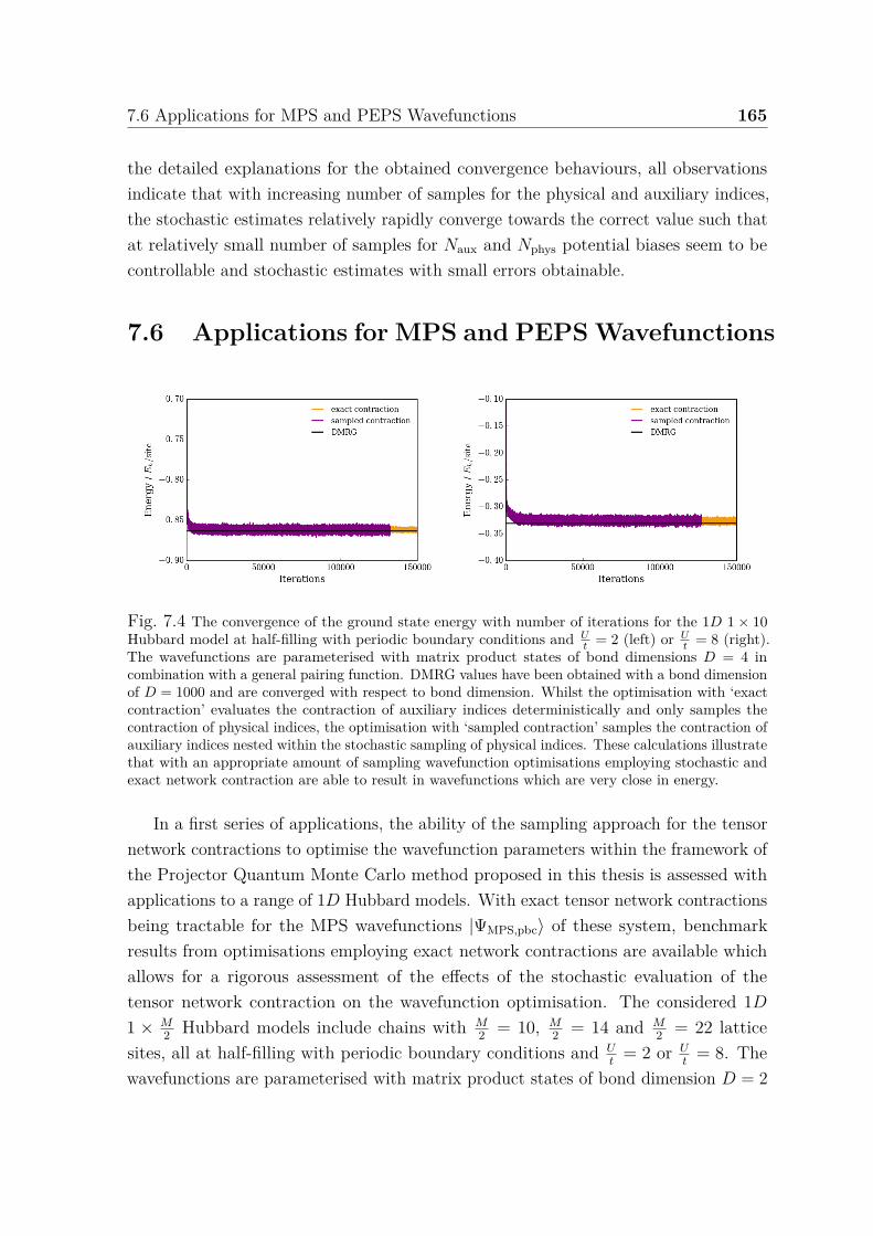
7.6 Applications for MPS and PEPS Wavefunctions 165
the detailed explanations for the obtained convergence behaviours, all observationsindicate that with increasing number of samples for the physical and auxiliary indices,the stochastic estimates relatively rapidly converge towards the correct value such thatat relatively small number of samples for Naux and Nphys potential biases seem to becontrollable and stochastic estimates with small errors obtainable.
7.6 Applications for MPS and PEPS Wavefunctions
Fig. 7.4 The convergence of the ground state energy with number of iterations for the 1D 1× 10Hubbard model at half-filling with periodic boundary conditions and U
t = 2 (left) or Ut = 8 (right).
The wavefunctions are parameterised with matrix product states of bond dimensions D = 4 incombination with a general pairing function. DMRG values have been obtained with a bond dimensionof D = 1000 and are converged with respect to bond dimension. Whilst the optimisation with ‘exactcontraction’ evaluates the contraction of auxiliary indices deterministically and only samples thecontraction of physical indices, the optimisation with ‘sampled contraction’ samples the contraction ofauxiliary indices nested within the stochastic sampling of physical indices. These calculations illustratethat with an appropriate amount of sampling wavefunction optimisations employing stochastic andexact network contraction are able to result in wavefunctions which are very close in energy.
In a first series of applications, the ability of the sampling approach for the tensornetwork contractions to optimise the wavefunction parameters within the framework ofthe Projector Quantum Monte Carlo method proposed in this thesis is assessed withapplications to a range of 1D Hubbard models. With exact tensor network contractionsbeing tractable for the MPS wavefunctions |ΨMPS,pbc⟩ of these system, benchmarkresults from optimisations employing exact network contractions are available whichallows for a rigorous assessment of the effects of the stochastic evaluation of thetensor network contraction on the wavefunction optimisation. The considered 1D1 × M
2 Hubbard models include chains with M2 = 10, M
2 = 14 and M2 = 22 lattice
sites, all at half-filling with periodic boundary conditions and Ut
= 2 or Ut
= 8. Thewavefunctions are parameterised with matrix product states of bond dimension D = 2
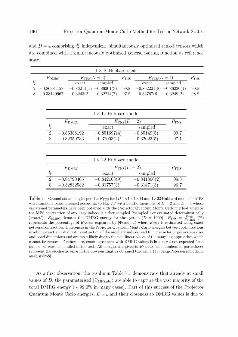
166 Projector Quantum Monte Carlo Method for Tensor Network States
and D = 4 comprising M2 independent, simultaneously optimised rank-3 tensors which
are combined with a simultaneously optimised general pairing function as referencestate.
1× 10 Hubbard modelEDMRG ETNS(D = 2) PTNS ETNS(D = 4) PTNS
Ut
exact sampled exact sampled2 −0.86384157 −0.86211(1) −0.86201(3) 99.8 −0.862221(8) −0.86230(1) 99.88 −0.33149967 −0.3243(2) −0.32214(7) 97.8 −0.32767(6) −0.3249(2) 98.8
1× 14 Hubbard modelEDMRG ETNS(D = 2) PTNS
Ut
exact sampled2 −0.85388192 −0.851697(4) −0.85149(5) 99.78 −0.32950733 −0.32003(2) −0.32023(5) 97.1
1× 22 Hubbard modelEDMRG ETNS(D = 2) PTNS
Ut
exact sampled2 −0.84790465 −0.842108(9) −0.841890(2) 99.38 −0.32832582 −0.31757(3) −0.31471(3) 96.7
Table 7.1 Ground state energies per site ETNS for 1D 1×10, 1×14 and 1×22 Hubbard model for MPSwavefunctions parameterised according to Eq. 7.7 with bond dimensions of D = 2 and D = 4 whosevariational parameters have been obtained with the Projector Quantum Monte Carlo method wherebythe MPS contraction of auxiliary indices is either sampled (‘sampled’) or evaluated deterministically(‘exact’). EDMRG denotes the DMRG energy for the system (D = 1000). PTNS = ETNS
EDMRG(%)
represents the percentage of EDMRG captured by |ΨMPS,pbc⟩ where ETNS is estimated using exactnetwork contraction. Differences in the Projector Quantum Monte Carlo energies between optimisationsinvolving exact and stochastic contraction of the auxiliary indices tend to increase for larger system sizesand bond dimensions and are most likely due to the non-linear biases of the sampling approaches whichcannot be remove. Furthermore, exact agreement with DMRG values is in general not expected for anumber of reasons detailed in the text. All energies are given in Eh/site. The numbers in parenthesesrepresent the stochastic error in the previous digit as obtained through a Flyvbjerg-Petersen reblockinganalysis[268].
As a first observation, the results in Table 7.1 demonstrate that already at smallvalues of D, the parameterised |ΨMPS,pbc⟩ are able to capture the vast majority of thetotal DMRG energy (∼ 99.0% in many cases). Part of this success of the ProjectorQuantum Monte Carlo energies, ETNS, and their closeness to DMRG values is due to

7.6 Applications for MPS and PEPS Wavefunctions 167
the optimised pairing function acting as reference state which is usually able to accountfor a large part of the correlation energy and thus allows for the use of small values ofD whilst still yielding energies close the the infinite D limit of DMRG. However, itis worth pointing out that the results obtained with the Projector Quantum MonteCarlo method for non-linear wavefunctions are in general not expected to agree exactlywith DMRG values for a number of reasons. Firstly, DMRG rigorously conservesall symmetries and quantum numbers, whereas the Projector Quantum Monte Carlooptimisation explicitly breaks symmetries and non-zero projections onto section of theHilbert space with other (e.g. spin) quantum numbers and symmetries typically remain.Secondly, by constraining the nodal structure of |ΨMPS,pbc⟩ to the variational flexibilityaffordable by the reference state, a ‘fixed-node’ error will in general be introducedapart from those cases where the nodal structure of the reference state recovers thenodal structure of the exact wavefunction. In most situations small values of D arethen sufficient to reach the wavefunction with the variational lowest energy availablewithin the given parameterisation. In contrast, DMRG energies are converged withrespect to bond dimension D in which limit they can be considered to be numericallyexact.
Moreover, the convergences displayed in Figure 7.4 demonstrate that the ProjectorQuantum Monte Carlo optimisation for non-linear wavefunctions is able to convergeonto wavefunctions whose energies largely agree with DMRG results irrespective ofwhether just one single stochastic process for sampling of the physical indices isemployed or whether two nested stochastic processes sample both the contraction ofphysical and auxiliary indices. Unfortunately, when comparing Projector QuantumMonte Carlo energies in Table 7.1 obtained with exact deterministic (one stochasticprocess) and sampled (two nested stochastic processes) contraction of auxiliary indicessmall differences persist which tend to become more pronounced when either systemsizes, bond dimensions or both increase. These deviations are most likely due to theunavoidable biases in the TNS sampling approach which have been detailed in theprevious section. Yet, given the smallness of the difference for small systems andvalues of D, this is another indication that the biases can be controlled in the limit ofsufficient sampling.
In principle, the number of samples for stochastic contraction of the auxiliary indices,Naux, as well as for stochastic contraction of the physical indices, Nphys, which arerequired for efficient wavefunction optimisations grows with the bond dimension D of thetensors and system size. In the initial stages of the optimisation, relatively small numberof samples are sufficient (e.g. Naux ∼ 100 and a total of Nphys ∼ 4× 10⁶ distributed
168 Projector Quantum Monte Carlo Method for Tensor Network States
across several processors) for all considered system sizes and bond dimensions. As theoptimisation progresses these typically have to be raised gradually to achieve a higheraccuracy with the maximum number of samples now depending on system size and bonddimension (Naux ∼ 200 and Nphy ∼ 16×106 for the 1×14 Hubbard model with D = 2).However, a precise scaling of Naux and Nphys with bond dimension and system size ismore difficult to arrive at since the appropriate values depend on each other, as well ason the step size of the optimisation and the value of U
t. It should be pointed out that in
order to ensure converged results, the optimisations aimed to substantially oversample,which results in small error bars in the calculated quantities. Since reducing errorbars in this approach by an order of magnitude represents two orders of magnitudemore computational effort, results close to convergence can already be obtained withsubstantially fewer number of samples. In terms of reducing stochastic errors, one ofthe dominant factors is the sampling of the gradient. Since the Naux samples usedto stochastically evaluate the derivatives with respect to a whole tensor S ′
n;ns, the
actual number of samples which contribute to the estimate of the derivative of a singleelement S ′
n;ns,ijkl is smaller, e.g. by approximately a factor of ∼ 1D4 for rank-4 tensors
of dimension D (assuming approximately uniform selection of the elements of S ′n;ns
forsimplicity). Whilst this approach increases the stochastic errors of the derivatives, itensures that each element S ′
n;ns,ijkl is estimated independently from all other elements inS
′n;ns
. If the elements of S ′n;ns
were not estimated independently, correlations in betweenthem will be significantly enhanced which will lead to considerable biases. Additionally,the random selection of elements of S ′
n;n2 also aids in breaking the symmetry of theindividual tensor elements in the optimisation.
Having established that sampling the tensor network also allows for efficient optimi-sation of the wavefunction parameters within the framework of the Projector QuantumMonte Carlo method proposed in this thesis, the approach is applied to PEPS wave-functions, the main aim of this chapter. Thus, a two-dimensional 4 × 4 Hubbardmodel on a square lattice at half-filling is considered with periodic boundary conditionsand U
t= 2 or U
t= 4. For these systems benchmark results from the Auxiliary Field
Quantum Monte Carlo method (AFQMC) are available[387] which can be considerednumerically exact at half-filling. While the nodal structure of the PEPS wavefunction|ΨPEPS⟩ is provided by an optimised general pairing function acting as reference state,further correlations are captured by the independent, simultaneously optimised rank-5tensors of the PEPS state (one physical index and four auxiliary indices). At a bonddimension of D = 2, the error in the total ground state energy per site of |ΨPEPS⟩ isonly ∼ 1.0% for both values of U
t.
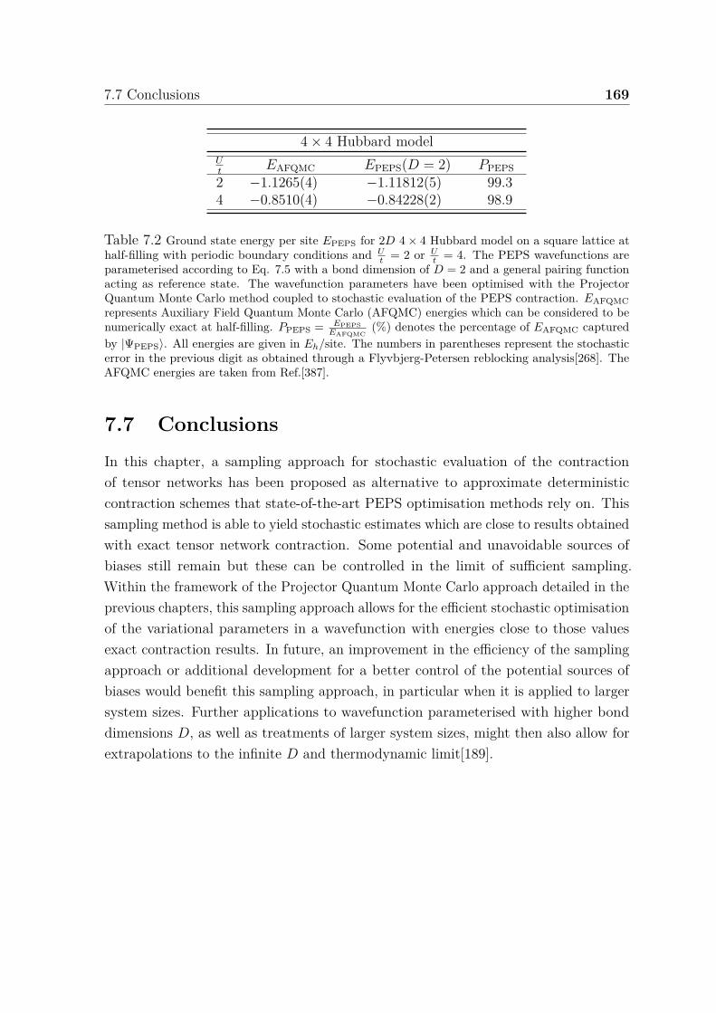
7.7 Conclusions 169
4× 4 Hubbard modelUt
EAFQMC EPEPS(D = 2) PPEPS2 −1.1265(4) −1.11812(5) 99.34 −0.8510(4) −0.84228(2) 98.9
Table 7.2 Ground state energy per site EPEPS for 2D 4× 4 Hubbard model on a square lattice athalf-filling with periodic boundary conditions and U
t = 2 or Ut = 4. The PEPS wavefunctions are
parameterised according to Eq. 7.5 with a bond dimension of D = 2 and a general pairing functionacting as reference state. The wavefunction parameters have been optimised with the ProjectorQuantum Monte Carlo method coupled to stochastic evaluation of the PEPS contraction. EAFQMCrepresents Auxiliary Field Quantum Monte Carlo (AFQMC) energies which can be considered to benumerically exact at half-filling. PPEPS = EPEPS
EAFQMC(%) denotes the percentage of EAFQMC captured
by |ΨPEPS⟩. All energies are given in Eh/site. The numbers in parentheses represent the stochasticerror in the previous digit as obtained through a Flyvbjerg-Petersen reblocking analysis[268]. TheAFQMC energies are taken from Ref.[387].
7.7 Conclusions
In this chapter, a sampling approach for stochastic evaluation of the contractionof tensor networks has been proposed as alternative to approximate deterministiccontraction schemes that state-of-the-art PEPS optimisation methods rely on. Thissampling method is able to yield stochastic estimates which are close to results obtainedwith exact tensor network contraction. Some potential and unavoidable sources ofbiases still remain but these can be controlled in the limit of sufficient sampling.Within the framework of the Projector Quantum Monte Carlo approach detailed in theprevious chapters, this sampling approach allows for the efficient stochastic optimisationof the variational parameters in a wavefunction with energies close to those valuesexact contraction results. In future, an improvement in the efficiency of the samplingapproach or additional development for a better control of the potential sources ofbiases would benefit this sampling approach, in particular when it is applied to largersystem sizes. Further applications to wavefunction parameterised with higher bonddimensions D, as well as treatments of larger system sizes, might then also allow forextrapolations to the infinite D and thermodynamic limit[189].

Chapter 8
Concluding Remarks andContinuing Directions
In this thesis, a novel Projector Quantum Monte Carlo method for non-linear wave-function ansatzes has been developed and successfully applied to a range of challengingstrongly correlated systems. The formulation of this new approach has been partiallyinspired by a prior application of the Full Configuration Interaction Quantum MonteCarlo (FCIQMC) method to a prototypical strongly correlated system. FCIQMCrepeatedly and stochastically applies a projector onto an initial trial wavefunctionparameterised as linear expansion in the basis of Slater determinants spanning thefull Hilbert space of a system. Whilst stochastic application of the propagator takesadvantage of the sparse and diagonally dominant nature of the Hamiltonian in Fockspace, sparsity inherent in the wavefunction is exploited by an ensemble of walkerswhich provides a stochastic coarse-grained description of the wavefunction. As such,FCIQMC represents a stochastic realisation of the Power Method, allowing access toessentially exact results for systems far out of reach of many traditional diagonalisationapproaches.
FCIQMC therefore naturally lends itself as a suitable method for obtaining bench-mark results and investigating the nature of the exact wavefunction. As a firstinvestigation in this spirit, an FCIQMC study of a prototypical and highly non-trivialstrongly correlated system, the three-band (p−d) Hubbard model, was conducted. Themain focus of this study was the FCI wavefunction representation expressed in differentsingle-particle basis sets and their amenability to accurate correlation treatments. Theinvestigated one-particle bases included the widely available restricted (RHF) and unre-stricted (UHF) Hartree-Fock spin orbitals which were compared with restricted (RNO)and unrestricted (UNO) natural orbitals. The latter are known to yield compact FCI
172 Concluding Remarks and Continuing Directions
expansions whose coefficients decay rapidly with increasing particle-hole excitations ofthe reference Slater determinant.
Counterintuitively, it was found in this investigation that the ability of single-particle basis sets to reproduce the physics of a system within a single-determinantdescription is not necessarily an indicator for their ability to give rise to rapidlyconverging CI expansions. Instead, it was observed that whilst a UHF determinantdescribes a qualitatively correct insulating antiferromagnet as ground state, imposingspin symmetry in the RHF basis provides a qualitatively incorrect metal as RHFdeterminant. Still, in the latter basis, and even more so in both natural orbital bases,the FCI expansion of the many-body wavefunction is sparser and converges rapidly withparticle-hole excitations of the reference determinant. These findings are of particularinterest for approaches in condensed matter physics. Whilst these typically start fromqualitatively correct symmetry-broken solutions, the findings of this FCIQMC studyindicate that these may not always be the optimal starting points and that approachesbuilding on symmetry conserving basis sets may be more successful. In addition, theresults of this investigation suggest that single-reference quantum chemical methods incombination with an appropriate single-particle descriptions may be able to treat many-body wavefunctions of strongly correlated systems. This is of great importance for thedevelopment of these single-reference approaches and their applications to stronglycorrelated materials which have so far been found to pose non-trivial challenges forthese methodologies.
Despite these findings, the challenge of an exponentially growing Hilbert space stillremains, implying that for highly multi-reference wavefunctions, as they typically occurfor strongly correlated materials, the FCI expansion will become intractable for largesystems even when expressed in an optimal single-particle basis. Thus, if progress tolarger system sizes is to be made, more compact wavefunction ansatzes need to beconsidered which scale polynomially rather than exponentially with system size, ideallywhilst still building on the success of FCIQMC. This has lead to the development of anovel Projector Quantum Monte Carlo approach through reformulation of the projectedimaginary time evolution of FCIQMC in terms of a Lagrangian minimisation. Thisnaturally admits wavefunction ansatzes with polynomial complexity which have moretraditionally inhabited the realm of Variational Quantum Monte Carlo approaches. Atthe same time, it highlights the deep connection between imaginary time evolution,the power method and (stochastic) gradient descent. However, similar approaches havepreviously had little success given the slow convergence rate of stochastic gradientdescent. Improvements on this have been made by advances in the field of deep
173
learning algorithms and neural networks. Two of these have been incorporated inthe proposed Projector Quantum Monte Carlo method resulting in a modificationof the propagator of the wavefunction dynamics. As a first advancement, Nesterov’saccelerated approach has been included which belongs to the class of ‘momentum’methods. Within these techniques the update of variational parameters retains amemory of previous updates thereby formally accelerating convergence rates to secondorder. The second improvement has been the incorporation of RMSprop which isa scheme to automatically and independently estimate an individual optimal stepsize for each individual variational parameter. This has increased the robustness ofthe optimisation, as well as accelerated its convergence by taking larger steps forparameters with small gradients and vice versa. Combining all these methods has leadto a new Projector Quantum Monte Carlo approach which represents a very versatileand general, as well as highly efficient optimisation of arbitrary non-linear wavefunctionansatzes of quantum many-body systems with large numbers of parameters.
Following the exposition of the method, it has been combined with a number ofefficient and highly accurate wavefunction ansatzes. The first of these is a parameteri-sation referred to as Correlator Product States (CPS), a form of Tensor Network Stateswhose complexity grows polynomially with system size. This CPS ansatz represents aversatile approach which, at the same time, is systematically improvable to the exactFCI limit. The capabilities of the proposed accelerated Projector Quantum MonteCarlo approach has thus been demonstrated by optimising wavefunctions of this CPSparameterisation for a number of strongly correlated systems. These applicationsinclude one and two dimensional Hubbard models, as well as ab-initio systems. Thelatter begin with the highly non-trivial benchmark system of the symmetric dissociationof H50 for whose stretching total energies have been obtained with chemical accuracyand culminate in a fully periodic ab-initio graphene sheet. In addition to optimisationof wavefunction parameters, the same dynamics also allow for sampling of the reducedone- and two-body density matrices, thereby granting access to one- and two-bodystatic properties of the investigated systems.
In a further series of applications, the developed Projector Quantum Monte Carlomethod has been applied to another wavefunction ansatz, Projected Entangled PairStates (PEPS), also a class of Tensor Network States and the natural generalisation ofthe extremely successful Matrix Product States (MPS) to higher dimensions. WhilstPEPS wavefunctions are known to yield accurate approximations to ground states,efficient optimisation of their variational parameters still poses a significant challenge.This is partly rooted in the large computational cost associated with exact contraction
174 Concluding Remarks and Continuing Directions
of a PEPS network when information in the form of expectation values and correlationfunctions is extracted from the wavefunction. Even though approximate contractionschemes improve on this, they are still relatively expensive. A new approach hastherefore been proposed in this thesis which, instead of performing the contractiondeterministically, relies on Monte Carlo sampling to obtain a stochastic estimate ofthe contraction by sampling a sufficient number of terms appearing in the sum. Withthis stochastic contraction approach, applications of the Projector Quantum MonteCarlo method for MPS and PEPS wavefunctions have been realised for a number ofHubbard models providing results close to exact energies. In the future, this approachwould benefit from improvements in the Monte Carlo sampling scheme for the PEPScontractions in the sense that fewer number of samples will lead to a more accurateestimate.
The ability of the proposed Projector Quantum Monte Carlo method for non-linear wavefunctions to treat wavefunctions with polynomial complexity allows for theconsideration of systems which are intractable for exact but exponentially complexwavefunction ansatzes, as illustrated by the many successful applications presented inthis thesis. It has been demonstrated in this thesis that this novel approach can handleand efficiently optimise large numbers of parameters, greatly exceeding those whichare amenable to state-of-the-art VMC methods where only recent developments havemade progress at extending these numbers[349]. Moreover, this optimisation approachis very versatile and general and can be applied to arbitrary wavefunction ansatzesprovided that the projections of wavefunction amplitudes, as well as the derivatives ofthe Lagrangian with respect to the variational parameters, onto configurations in thefull Hilbert space are efficiently computable.
Thus, further ansatzes which might be considered include wavefunctions param-eterised as artificial neural networks which have already been successfully appliedto spin models with state-of-the-art VMC approaches[388]. In addition to applica-tions with other wavefunction ansatzes, continuing developments can also extend thescope of the Projector Quantum Monte Carlo method. A possible direction for thesedevelopments involves the use of symmetry. So far, the Projector Quantum MonteCarlo has not made any use of symmetry but instead has explicitly broken symmetry.Thus, as an extension, symmetry may be directly enforced in order to reduce thenumber of independent variational parameters which allows for the treatment of evenlarger systems. Additionally, by imposing a specified symmetry excited states with asymmetry different to the ground state can also be converged upon. Another route to
175
excited states might be via orthogonalisation against the ground state as it has beenintroduced in FCIQMC[249].
In conclusion, the Projector Quantum Monte Carlo method formulated in this thesishas been demonstrated to provide a powerful and promising novel method for efficientoptimisation of the variational parameters in arbitrary non-linear wavefunction ansatzes.The presented results have clearly illustrated the ability of this approach to handle largenumbers of variational parameters which greatly exceed those amenable to alternativeVariational Quantum Monte Carlo techniques. Moreover, the employed non-linearwavefunction ansatzes represent efficient and accurate approximate parameterisations.At the same time, they grow only polynomially with system size and thus allow forthe treatment of much larger systems than those which are amenable to the exactwavefunction ansatz of diagonalisation approaches. Like other wavefunction-basedmethodologies, this proposed Projector Quantum Monte Carlo approach possesses twomajor advantages over DFT-based approaches which have dominated electronic struc-ture calculations, so far. Firstly, typical approximations involved in the wavefunctionparameterisation are controlled and systematically improvable toward exactness. Inaddition, many-body wavefunction descriptions of physical systems grant access to allof its properties and therefore represent one of the best frameworks to gain deeperinsight into the mechanics of quantum many-body systems,

Appendix A
Comparison of Lagrangian and RitzFunctional Derivatives
For an arbitrary wavefunction ansatz Ψ(Zσ) based on variational parameters Zσ thepositive-definite Lagrangian is given by
L[Ψ(Zσ)] = ⟨Ψ|H|Ψ⟩ − E0(⟨Ψ|I|Ψ⟩ − A
), (A.1)
where normalisation of the wavefunction Ψ(Zσ) (up to an arbitrary constant A) isenforced by a Lagrange multiplier which at convergence is equal to the self-consistentlydetermined ground state energy E0. As outlined in Chapter 5, the derivative of thisLagrangian with respect to any of the wavefunction parameters, Zσ, can be written as
∂L[Ψ(Zσ)]∂Zσ
= ⟨ ∂Ψ∂Zσ
|H|Ψ⟩+ ⟨Ψ|H| ∂Ψ∂Zσ
⟩ (A.2)
.− E0
(⟨ ∂Ψ∂Zσ
|I|Ψ⟩+ ⟨Ψ|I| ∂Ψ∂Zσ
⟩)
(A.3)
= 2 ⟨ ∂Ψ∂Zσ
|H|Ψ⟩ − 2E0 ⟨∂Ψ∂Zσ
|I|Ψ⟩ (A.4)
= 2 ⟨ ∂Ψ∂Zσ
|(H − E0I)|Ψ⟩ , (A.5)
where in the third line a real wavefunction and a real, symmetric Hamiltonian areassumed.
178 Comparison of Lagrangian and Ritz Functional Derivatives
Furthermore, when considering the same wavefunction parameterisation Ψ(Zσ), theRitz functional is defined as
R[Ψ(Zσ)] = ⟨Ψ|H|Ψ⟩⟨Ψ|Ψ⟩ , (A.6)
and its derivative with respect to any of the wavefunction parameters, Zσ, is given by
∂R[Ψ(Zσ)]∂Zσ
=2 ⟨ ∂Ψ
∂Zσ|H|Ψ⟩
⟨Ψ|Ψ⟩ −2 ⟨Ψ|H|Ψ⟩ ⟨ ∂Ψ
∂Zσ|Ψ⟩
(⟨Ψ|Ψ⟩)2 (A.7)
= 2⟨Ψ|Ψ⟩
⟨ ∂Ψ∂Zσ
|H|Ψ⟩ −⟨Ψ|H|Ψ⟩ ⟨ ∂Ψ
∂Zσ|Ψ⟩
⟨Ψ|Ψ⟩
(A.8)
= 2⟨Ψ|Ψ⟩
(⟨ ∂Ψ∂Zσ
|H|Ψ⟩ − R[Ψ(Zσ)] ⟨ ∂Ψ∂Zσ
|Ψ⟩), (A.9)
where again a real wavefunction and a real, symmetric Hamiltonian are assumed.A comparison of the Lagrangian and Ritz functional derivative leads to the conclu-
sion that both are equivalent if the following two conditions are satisfied: that is if⟨Ψ|Ψ⟩ = 1 and R[Ψ(Zσ)] = E0. These conditions are met by the Projector QuantumMonte Carlo method detailed in Chapter 5. Firstly, since the gradient employed inthis approach is sampled with the probability distribution of Eq. 5.13 in Chapter 5,normalisation is implicitly imposed such that ⟨Ψ|Ψ⟩ = 1 is ensured. Secondly, duringthe course of an optimisation the value of E0 is explicitly set to the energy of the wave-function which is given by R[Ψ(Zσ)], such that the second condition R[Ψ(Zσ)] = E0 isfulfilled, as well.
References
[1] J. G. Bednorz and K. A. Müller. Possible high Tc superconductivity inthe Ba–La–Cu–O system. Zeitschrift für Physik B Condensed Matter,64(2):189–193, 1986.
[2] J. G. Bednorz and K. A. Müller. Perovskite-type oxides—the new approach tohigh-Tc superconductivity. Reviews of Modern Physics, 60:585–600, Jul 1988.
[3] Adolfo Avella and Ferdinando Mancini. Strongly Correlated Systems: TheoreticalMethods, volume 171 of Springer Series in Solid-State Sciences. Springer Science& Business Media, 2011.
[4] E. Dagotto. Correlated electrons in high-temperature superconductors. Reviewsof Modern Physics, 66:763–840, Jul 1994.
[5] P. W. Anderson. The resonating valence bond state in La2CuO4 and supercon-ductivity. Science, 235:1196–1198, March 1987.
[6] E. Dagotto. Complexity in Strongly Correlated Electronic Systems. Science,309(5732):257–262, 2005.
[7] E. Dagotto and Y. Tokura. Strongly Correlated Electronic Materials: Presentand Future. MRS Bulletin, 33(11):1037–1045, 11 2008.
[8] Evgeny Y. Tsymbal. Multifunctional oxide heterostructures. Oxford UniversityPress, 2012.
[9] M. Imada, A. Fujimori, and Y. Tokura. Metal-insulator transitions. Reviews ofModern Physics, 70:1039–1263, Oct 1998.
[10] A. Georges, G. Kotliar, W. Krauth, and M. J. Rozenberg. Dynamical mean-fieldtheory of strongly correlated fermion systems and the limit of infinite dimensions.Reviews of Modern Physics, 68:13–125, Jan 1996.
[11] Th. Pruschke, M. Jarrell, and J.K. Freericks. Anomalous normal-state propertiesof high-Tc superconductors: intrinsic properties of strongly correlated electronsystems? Advances in Physics, 44(2):187–210, 1995.
[12] Y. Kamihara, T. Watanabe, M. Hirano, and H. Hosono. Iron-Based LayeredSuperconductor La[O1–xFx ]FeAs (x = 0.05− 0.12) with Tc = 26 K. Journal ofthe American Chemical Society, 130(11):3296–3297, 2008. PMID: 18293989.
180 References
[13] H. Jiang. First-principles approaches for strongly correlated materials: A the-oretical chemistry perspective. International Journal of Quantum Chemistry,115(11):722–730, 2015.
[14] G. Kotliar and S. Y. Savrasov. Model Hamiltonians and First Principles ElectronicStructure Calculations, page 259–301. Springer Netherlands, Dordrecht, 2001.
[15] J. Paier, C. Penschke, and J. Sauer. Oxygen Defects and Surface Chemistry ofCeria: Quantum Chemical Studies Compared to Experiment. Chemical Reviews,113(6):3949–3985, 2013. PMID: 23651311.
[16] J. P. Malrieu, R. Caballol, C. J. Calzado, C. de Graaf, and N. Guihéry. MagneticInteractions in Molecules and Highly Correlated Materials: Physical Content, An-alytical Derivation, and Rigorous Extraction of Magnetic Hamiltonians. ChemicalReviews, 114(1):429–492, 2014. PMID: 24102410.
[17] Y. S. Meng and M. E. Arroyo-de Dompablo. First principles computationalmaterials design for energy storage materials in lithium ion batteries. Energy &Environmental Science, 2:589–609, 2009.
[18] E. Schrödinger. Quantisierung als Eigenwertproblem. Annalen der Physik,385(13):437–490, 1926.
[19] W. Pauli. Über den Zusammenhang des Abschlusses der Elektronengrup-pen im Atom mit der Komplexstruktur der Spektren. Zeitschrift für Physik,31(1):765–783, 1925.
[20] G. E. Uhlenbeck and S. Goudsmit. Ersetzung der Hypothese vom unmechanischenZwang durch eine Forderung bezüglich des inneren Verhaltens jedes einzelnenElektrons. Die Naturwissenschaften, 13(47):953–954, 1925.
[21] W. Heisenberg. Mehrkörperproblem und Resonanz in der Quantenmechanik.Zeitschrift für Physik, 38(6):411–426, 1926.
[22] E. Schrödinger. An undulatory theory of the mechanics of atoms and molecules.Physical Review, 28:1049–1070, Dec 1926.
[23] P. A. M. Dirac. Quantum Mechanics of Many-Electron Systems. Proceedings ofthe Royal Society of London A: Mathematical, Physical and Engineering Sciences,123(792):714–733, 1929.
[24] P. Hohenberg and W. Kohn. Inhomogeneous electron gas. Physical Review,136:B864–B871, Nov 1964.
[25] W. Kohn and L. J. Sham. Self-consistent equations including exchange andcorrelation effects. Physical Review, 140:A1133–A1138, Nov 1965.
[26] K. Terakura, T. Oguchi, A. R. Williams, and J. Kübler. Band theory of insulatingtransition-metal monoxides: Band-structure calculations. Physical Review B,30:4734–4747, Oct 1984.

References 181
[27] W. E. Pickett. Electronic structure of the high-temperature oxide superconductors.Reviews of Modern Physics, 61:433–512, Apr 1989.
[28] G. Zwicknagl. Quasi-particles in heavy fermion systems. Advances in Physics,41(3):203–302, 1992.
[29] V. I. Anisimov, J. Zaanen, and O. K. Andersen. Band theory and mott insulators:Hubbard u instead of stoner i. Physical Review B, 44:943–954, Jul 1991.
[30] A. Svane and O. Gunnarsson. Transition-metal oxides in the self-interaction–corrected density-functional formalism. Physical Review Letters,65:1148–1151, Aug 1990.
[31] K. Held, I. A. Nekrasov, N. Blümer, V. I. Anisimov, and D. Vollhardt. Re-alistic modeling of strongly correlated electron systems: An introduction tothe LDA+DMFT approach. International Journal of Modern Physics B,15(19n20):2611–2625, 2001.
[32] Th. Maier, M. Jarrell, Th. Pruschke, and M. H. Hettler. Quantum cluster theories.Reviews of Modern Physics, 77:1027–1080, Oct 2005.
[33] J. Hubbard. Electron correlations in narrow energy bands. Proceedings ofthe Royal Society of London. Series A, Mathematical and Physical Sciences,276(1365):238–257, 1963.
[34] F. Gebhard. The Mott Metal-Insulator Transition: Models and Methods. SpringerTracts in Modern Physics. Springer Berlin Heidelberg, 1997.
[35] M. M. Korshunov, V. A. Gavrichkov, S. G. Ovchinnikov, I. A. Nekrasov, Z. V.Pchelkina, and V. I. Anisimov. Hybrid LDA and generalized tight-bindingmethod for electronic structure calculations of strongly correlated electron systems.Physical Review B, 72:165104, Oct 2005.
[36] Peter Fulde. Electron correlations in molecules and solids. Springer series insolid-state sciences. Springer-Verlag, 1991.
[37] Trygve Helgaker, Poul Jørgensen, and Jeppe Olsen. Molecular Electronic-Structure Theory. Wiley, 2014.
[38] P. Fulde. Wavefunction methods in electronic-structure theory of solids. Advancesin Physics, 51(3):909–948, 2002.
[39] Ch. Riplinger, B. Sandhoefer, A. Hansen, and F. Neese. Natural triple excitationsin local coupled cluster calculations with pair natural orbitals. The Journal ofChemical Physics, 139(13):134101, 2013.
[40] W. Kohn. Nobel lecture: Electronic structure of matter—wave functions anddensity functionals. Reviews of Modern Physics, 71:1253–1266, Oct 1999.
[41] Fulde P. Wavefunction-based electronic-structure calculations for solids. NaturePhysics, 12(2):106–107, Feb 2016.
182 References
[42] G. Stollhoff and P. Fulde. On the computation of electronic correlation energieswithin the local approach. The Journal of Chemical Physics, 73(9):4548–4561,1980.
[43] P. Pulay. Localizability of dynamic electron correlation. Chemical Physics Letters,100(2):151–154, 1983.
[44] L. Hozoi, U. Birkenheuer, H. Stoll, and P. Fulde. Spin-state transition andspin-polaron physics in cobalt oxide perovskites: ab initio approach based onquantum chemical methods. New Journal of Physics, 11(2):023023, 2009.
[45] H. Stoll. Correlation energy of diamond. Physical Review B, 46:6700–6704, Sep1992.
[46] H. Stoll, B. Paulus, and P. Fulde. On the accuracy of correlation-energy expansionsin terms of local increments. The Journal of Chemical Physics, 123(14):144108,2005.
[47] K. Doll, M. Dolg, P. Fulde, and H. Stoll. Quantum chemical approach to cohesiveproperties of NiO. Physical Review B, 55:10282–10288, Apr 1997.
[48] K. Rościszewski, K. Doll, B. Paulus, P. Fulde, and H. Stoll. Ground-stateproperties of rutile: Electron-correlation effects. Physical Review B, 57:14667–14672, Jun 1998.
[49] E. Voloshina and B. Paulus. Influence of electronic correlations on theground-state properties of cerium dioxide. The Journal of Chemical Physics,124(23):234711, 2006.
[50] W. M. C. Foulkes, L. Mitas, R. J. Needs, and G. Rajagopal. Quantum montecarlo simulations of solids. Reviews of Modern Physics, 73:33–83, Jan 2001.
[51] C. J. Umrigar. Observations on variational and projector Monte Carlo methods.The Journal of Chemical Physics, 143(16):164105, 2015.
[52] G. H. Booth, A. J. W. Thom, and A. Alavi. Fermion Monte Carlo without fixednodes: A game of life, death, and annihilation in Slater determinant space. TheJournal of Chemical Physics, 131(5):054106, 2009.
[53] J. Eisert. Entanglement and tensor network states. ArXiv e-prints, August 2013.
[54] Orús R. A practical introduction to tensor networks: Matrix product states andprojected entangled pair states. Annals of Physics, 349:117–158, oct 2014.
[55] F. Verstraete, V. Murg, and J.I. Cirac. Matrix product states, projected entangledpair states, and variational renormalization group methods for quantum spinsystems. Advances in Physics, 57(2):143–224, 2008.
[56] S. R. White. Density matrix formulation for quantum renormalization groups.Physical Review Letters, 69:2863–2866, Nov 1992.
[57] Attila Szabo and Neil S. Ostlund. Modern Quantum Chemistry: Introduction toAdvanced Electronic Structure Theory. Dover Publications, New York, 1996.
References 183
[58] M. Born and R. Oppenheimer. Zur Quantentheorie der Molekeln. Annalen derPhysik, 389(20):457–484, 1927.
[59] G. A. Worth and L. S. Cederbaum. Beyond Born-Oppenheimer: MolecularDynamics Through a Conical Intersection. Annual Review of Physical Chemistry,55(1):127–158, 2004. PMID: 15117250.
[60] T. Azumi and K. Matsuzaki. What does the term "Vibronic Coupling” mean?Photochemistry and Photobiology, 25(3):315–326, 1977.
[61] M. Fierz. Über die relativistische Theorie kräftefreier Teilchen mit beliebigemSpin. Helvetica Physica Acta, 12(3), 1939.
[62] W. Pauli. The Connection Between Spin and Statistics. Physical Review,58:716–722, Oct 1940.
[63] P. A. M. Dirac. On the Theory of Quantum Mechanics. Proceedings of theRoyal Society of London A: Mathematical, Physical and Engineering Sciences,112(762):661–677, 1926.
[64] Michela Massimi. Pauli’s Exclusion Principle: The Origin and Validation of aScientific Principle. Cambridge University Press, 2005.
[65] J. C. Slater. The Theory of Complex Spectra. Physical Review, 34:1293–1322,Nov 1929.
[66] P. A. M. Dirac. The Quantum Theory of the Emission and Absorption ofRadiation. Proceedings of the Royal Society of London A: Mathematical, Physicaland Engineering Sciences, 114(767):243–265, 1927.
[67] V. Fock. Konfigurationsraum und zweite Quantelung. Zeitschrift für Physik,75(9):622–647, 1932.
[68] Alexander L. Fetter and John Dirk Walecka. Quantum Theory of Many-particleSystems. Dover Publications, 2003.
[69] Felix Alexandrovich Berezin. The method of second quantization. Pure andapplied physics. A series of monographs and textbooks. Academic Press, 1966.
[70] Wolfgang Nolting. Grundkurs Theoretische Physik 5/2: Quantenmechanik -Methoden und Anwendungen. Springer-Lehrbuch. Springer, 2015.
[71] Vladimir Aleksandrovich Fock. V. A. Fock - Selected Works: Quantum Mechanicsand Quantum Field Theory. Chapman & Hall/CRC, Boca Raton, Fla, 2004.
[72] V. Fock. Näherungsmethode zur Lösung des quantenmechanischen Mehrkörper-problems. Zeitschrift für Physik, 61(1):126–148, 1930.
[73] D. R. Hartree. The wave mechanics of an atom with a non-coulomb centralfield. part i. theory and methods. In Mathematical Proceedings of the CambridgePhilosophical Society, volume 24, pages 89–110. Cambridge University Press,1928.
184 References
[74] D. R. Hartree, W. Hartree, and B. Swirles. Self-consistent field, including exchangeand superposition of configurations, with some results for oxygen. PhilosophicalTransactions of the Royal Socity of London. Series A, Mathematical and PhysicalSciences, 238(790):229–247, 1940.
[75] C. C. J. Roothaan. New developments in molecular orbital theory. Reviews ofModern Physics, 23(2):69–89, 1951.
[76] J.A. Pople and R.-K. Nesbet. Self-consistent orbitals for radicals. The Journalof Chemical Physics, 22(3):571–572, 1954.
[77] E. A. Hylleraas. The Schrödinger Two-Electron Atomic Problem. In P.-O. Löwdin,editor, , volume 1 of Advances in Quantum Chemistry, page 1–33. AcademicPress, 1964.
[78] T. Kato. On the eigenfunctions of many-particle systems in quantum mechanics.Communications on Pure and Applied Mathematics, 10(2):151–177, 1957.
[79] R. T. Pack and W. B. Brown. Cusp Conditions for Molecular Wavefunctions.The Journal of Chemical Physics, 45(2):556–559, 1966.
[80] D. P. Tew, W. Klopper, and T. Helgaker. Electron correlation: The many-body problem at the heart of chemistry. Journal of Computational Chemistry,28(8):1307–1320, 2007.
[81] W. Kutzelnigg and W. Klopper. Wave functions with terms linear in the inter-electronic coordinates to take care of the correlation cusp. i. general theory. TheJournal of Chemical Physics, 94(3):1985–2001, 1991.
[82] J. K. L. MacDonald. Successive approximations by the rayleigh-ritz variationmethod. Physical Review, 43:830–833, May 1933.
[83] S. F. Boys. Electronic Wave Functions. I. A General Method of Calculation for theStationary States of Any Molecular System. Proceedings of the Royal Society ofLondon A: Mathematical, Physical and Engineering Sciences, 200(1063):542–554,1950.
[84] N. C. Handy. Multi-root configuration interaction calculations. Chemical PhysicsLetters, 74(2):280–283, 1980.
[85] J. C. Slater. Molecular energy levels and valence bonds. Physical Review,38:1109–1144, Sep 1931.
[86] E. U. Condon. The theory of complex spectra. Physical Review, 36:1121–1133,Oct 1930.
[87] C. Lanczos. An iteration method for the solution of the eigenvalue problem oflinear differential and integral operators. Journal of Research of the NationalBureau of Standards, 45:225–282, 1950.
[88] R.-K. Nesbet. Algorithm for diagonalization of large matrices. The Journal ofChemical Physics, 43(1):311–312, 1965.
References 185
[89] E. R. Davidson. The iterative calculation of a few of the lowest eigenvaluesand corresponding eigenvectors of large real-symmetric matrices. Journal ofComputational Physics, 17(1):87–94, 1975.
[90] B. Roos. A new method for large-scale CI calculations. Chemical Physics Letters,15(2):153–159, 1972.
[91] E. Rossi, G. L. Bendazzoli, S. Evangelisti, and D. Maynau. A full-configurationbenchmark for the N2 molecule. Chemical Physics Letters, 310(5–6):530–536,1999.
[92] Chr. Møller and M. S. Plesset. Note on an approximation treatment for many-electron systems. Physical Review, 46:618–622, Oct 1934.
[93] M. Head-Gordon. Quantum chemistry and molecular processes. The Journal ofPhysical Chemistry, 100(31):13213–13225, 1996.
[94] M. L. Leininger, W. D. Allen, H. F. Schaefer III, and C. D. Sherrill. Is Møller-Plesset perturbation theory a convergent ab initio method? The Journal ofChemical Physics, 112(21):9213–9222, 2000.
[95] Isaiah Shavitt. The Method of Configuration Interaction, page 189–275. SpringerUS, Boston, MA, 1977.
[96] R. E. Watson. Approximate wave functions for atomic Be. Physical Review,119:170–177, Jul 1960.
[97] L. Brillouin. La méthode du champs self-consistent. Actualités Scientifiques etIndustrielles, 71, 1933.
[98] L. Brillouin. Les champs self-consistents de hartree et du fock. ActualitésScientifiques et Industrielles, 159, 1934.
[99] J. Olsen, P. Jo, H. Koch, A. Balkova, R. J. Bartlett, et al. Full configuration–interaction and state of the art correlation calculations on water in a valencedouble-zeta basis with polarization functions. The Journal of Chemical Physics,104(20):8007–8015, 1996.
[100] R. J. Bartlett. Many-body perturbation theory and coupled cluster theoryfor electron correlation in molecules. Annual Review of Physical Chemistry,32(1):359–401, 1981.
[101] Stephen R. Langhoff and Ernest R. Davidson. Configuration interaction calcula-tions on the nitrogen molecule. International Journal of Quantum Chemistry,8(1):61–72, 1974.
[102] F. Coester. Bound states of a many-particle system. Nuclear Physics, 7:421–424,August 1958.
[103] F. Coester and H. Kümmel. Short-range correlations in nuclear wave functions.Nuclear Physics, 17:477–485, July 1960.
186 References
[104] J. Čížek. On the Correlation Problem in Atomic and Molecular Systems. Calcu-lation of Wavefunction Components in Ursell-Type Expansion Using Quantum-Field Theoretical Methods. The Journal of Chemical Physics, 45:4256–4266,December 1966.
[105] J. Cizek and J. Paldus. Coupled Cluster Approach. Physica Scripta, 21(3-4):251,1980.
[106] R. J. Bartlett and M. Musiał. Coupled-cluster theory in quantum chemistry.Reviews of Modern Physics, 79:291–352, Feb 2007.
[107] G. E. Scuseria and T. J. Lee. Comparison of coupled-cluster methods whichinclude the effects of connected triple excitations. The Journal of ChemicalPhysics, 93(8):5851–5855, 1990.
[108] T. Helgaker, T. A. Ruden, P. Jørgensen, J. Olsen, and W. Klopper. A prioricalculation of molecular properties to chemical accuracy. Journal of PhysicalOrganic Chemistry, 17(11):913–933, 2004.
[109] H.-J. Werner and P. J. Knowles. A second order multiconfiguration scf procedurewith optimum convergence. The Journal of Chemical Physics, 82(11):5053–5063,1985.
[110] B. O. Roos, P. R. Taylor, and P. E.M. Siegbahn. A complete active spaceSCF method (CASSCF) using a density matrix formulated super-CI approach.Chemical Physics, 48(2):157–173, 1980.
[111] P. E. M. Siegbahn, J. Almlöf, A. Heiberg, and B. O. Roos. The complete activespace SCF (CASSCF) method in a newton–raphson formulation with applicationto the HNO molecule. The Journal of Chemical Physics, 74(4):2384–2396, 1981.
[112] B. O. Roos. The complete active space SCF method in a fock-matrix-based super-CI formulation. International Journal of Quantum Chemistry, 18(S14):175–189,1980.
[113] J. Olsen. The casscf method: A perspective and commentary. InternationalJournal of Quantum Chemistry, 111(13):3267–3272, 2011.
[114] P. A. Malmqvist, A. Rendell, and B. O. Roos. The restricted active space self-consistent-field method, implemented with a split graph unitary group approach.The Journal of Physical Chemistry, 94(14):5477–5482, 1990.
[115] K. Andersson, P. A. Malmqvist, B. O. Roos, A. J. Sadlej, and K. Wolinski.Second-order perturbation theory with a casscf reference function. The Journalof Physical Chemistry, 94(14):5483–5488, 1990.
[116] K. Andersson, P. Malmqvist, and B. O. Roos. Second-order perturbation theorywith a complete active space self-consistent field reference function. The Journalof Chemical Physics, 96(2):1218–1226, 1992.
References 187
[117] H.-J. Werner and P. J. Knowles. An efficient internally contractedmulticonfiguration–reference configuration interaction method. The Journalof Chemical Physics, 89(9):5803–5814, 1988.
[118] R. J. Buenker and S. D. Peyerimhoff. Individualized configuration selection inCI calculations with subsequent energy extrapolation. Theoretica Chimica Acta,35(1):33–58, 1974.
[119] H.-J. Werner and E.-A. Reinsch. The self-consistent electron pairs method formulticonfiguration reference state functions. The Journal of Chemical Physics,76(6):3144–3156, 1982.
[120] P. E. M. Siegbahn. Generalizations of the direct CI method based on thegraphical unitary group approach. I. Single replacements from a complete CIroot function of any spin, first order wave functions. The Journal of ChemicalPhysics, 70(12):5391–5397, 1979.
[121] P. E. M. Siegbahn. Generalizations of the direct CI method based on thegraphical unitary group approach. II. Single and double replacements from anyset of reference configurations. The Journal of Chemical Physics, 72(3):1647–1656,1980.
[122] B. R. Brooks and H. F. Schaefer III. The graphical unitary group approach tothe electron correlation problem. Methods and preliminary applications. TheJournal of Chemical Physics, 70(11):5092–5106, 1979.
[123] P. E. M. Siegbahn. Current status of the multiconfiguration-configuration in-teraction (MC-CI) method as applied to molecules containing transition-metalatoms. Faraday Symposia of the Chemical Society, 19:97–107, 1984.
[124] N. Oliphant and L. Adamowicz. The implementation of the multireferencecoupled-cluster method based on the single-reference formalism. The Journal ofChemical Physics, 96(5):3739–3744, 1992.
[125] L. Z. Stolarczyk. Complete active space coupled-cluster method. Extensionof single-reference coupled-cluster method using the CASSCF wavefunction.Chemical Physics Letters, 217(1–2):1–6, 1994.
[126] T. Yanai and G. K.-L. Chan. Canonical transformation theory for multireferenceproblems. The Journal of Chemical Physics, 124(19):194106, 2006.
[127] R. M. Dickson and A. D. Becke. Reaction barrier heights from an exact-exchange-based density-functional correlation model. The Journal of Chemical Physics,123(11):111101, 2005.
[128] M. Troyer and U.-J. Wiese. Computational complexity and fundamental limita-tions to fermionic quantum monte carlo simulations. Physical Review Letters,94:170201, May 2005.
[129] J. von Neumann. Thermodynamik quantenmechanischer gesamtheiten.Nachrichten von der Gesellschaft der Wissenschaften zu Göttingen,Mathematisch-Physikalische Klasse, 1927:273–291, 1927.
188 References
[130] John von Neumann. Mathematische Grundlagen der Quantenmechanik. Springer,1932.
[131] C. H. Bennett, D. P. DiVincenzo, J. A. Smolin, and W. K. Wootters. Mixed-stateentanglement and quantum error correction. Physical Review A, 54:3824–3851,Nov 1996.
[132] J. Eisert, M. Cramer, and M. B. Plenio. Colloquium. Reviews of Modern Physics,82:277–306, Feb 2010.
[133] M. B. Plenio, J. Eisert, J. Dreißig, and M. Cramer. Entropy, entanglement, andarea: Analytical results for harmonic lattice systems. Physical Review Letters,94:060503, Feb 2005.
[134] F. G. S. L. Brandão and M. Horodecki. An area law for entanglement fromexponential decay of correlations. Nature Physics, 9(11):721–726, nov 2013.
[135] F. G. S. L. Brandão and M. Horodecki. Exponential Decay of CorrelationsImplies Area Law. Communications in Mathematical Physics, 333(2):761–798,2015.
[136] M. B. Hastings. An area law for one-dimensional quantum systems. Journal ofStatistical Mechanics: Theory and Experiment, 2007(08):P08024, 2007.
[137] I. Arad, Z. Landau, and U. Vazirani. Improved one-dimensional area law forfrustration-free systems. Physical Review B, 85:195145, May 2012.
[138] I. Arad, A. Kitaev, Z. Landau, and U. Vazirani. An area law and sub-exponentialalgorithm for 1D systems. ArXiv e-prints, January 2013.
[139] K. Van Acoleyen, M. Mariën, and F. Verstraete. Entanglement rates and arealaws. Physical Review Letters, 111:170501, Oct 2013.
[140] G. Vidal, J. I. Latorre, E. Rico, and A. Kitaev. Entanglement in quantum criticalphenomena. Physical Review Letters, 90:227902, Jun 2003.
[141] Y. Ge and J. Eisert. Area laws and efficient descriptions of quantum many-bodystates. New Journal of Physics, 18(8):083026, 2016.
[142] N. Schuch. Condensed Matter Applications of Entanglement Theory. ArXive-prints, June 2013.
[143] S. R. White and R. L. Martin. Ab initio quantum chemistry using the density ma-trix renormalization group. The Journal of Chemical Physics, 110(9):4127–4130,1999.
[144] U. Schollwöck. The density-matrix renormalization group in the age of matrixproduct states. Annals of Physics, 326(1):96–192, 2011. January 2011 SpecialIssue.
[145] N. Schuch, M. M. Wolf, F. Verstraete, and J. I. Cirac. Entropy scaling andsimulability by matrix product states. Physical Review Letters, 100:030504, Jan2008.
References 189
[146] Ingemar Bengtsson and Karol Zyczkowskui. Geometry of Quantum States: AnIntroduction to Quantum Entanglement. Cambridge University Press, Cambridge,paperback ed. edition, 2010.
[147] T. B. Wahl. Tensor network states for the description of quantum many-bodysystems. ArXiv e-prints, September 2015.
[148] F. Verstraete, M. M. Wolf, D. Perez-Garcia, and J. I. Cirac. Criticality, the arealaw, and the computational power of projected entangled pair states. PhysicalReview Letters, 96:220601, Jun 2006.
[149] A. Rényi et al. On measures of entropy and information. In Proceedings of thefourth Berkeley symposium on mathematical statistics and probability, volume 1,pages 547–561, 1961.
[150] F. Verstraete and J. I. Cirac. Matrix product states represent ground statesfaithfully. Physical Review B, 73:094423, Mar 2006.
[151] Z. Landau, U. Vazirani, and T. Vidick. A polynomial time algorithm for theground state of one-dimensional gapped local Hamiltonians. Nature Physics,11(7):566–569, jul 2015.
[152] S. Wouters and D. Van Neck. The density matrix renormalization group for abinitio quantum chemistry. The European Physical Journal D, 68(9):272, 2014.
[153] U. Schollwöck. The density-matrix renormalization group. Reviews of ModernPhysics, 77:259–315, Apr 2005.
[154] G. Vidal. Class of quantum many-body states that can be efficiently simulated.Physical Review Letters, 101:110501, Sep 2008.
[155] F. Verstraete and J. I. Cirac. Renormalization algorithms for Quantum-ManyBody Systems in two and higher dimensions. eprint arXiv:cond-mat/0407066,July 2004.
[156] M. B. Hastings. Solving gapped hamiltonians locally. Physical Review B,73:085115, Feb 2006.
[157] M. B. Hastings. Entropy and entanglement in quantum ground states. PhysicalReview B, 76:035114, Jul 2007.
[158] J. Jordan, R. Orús, G. Vidal, F. Verstraete, and J. I. Cirac. Classical simulationof infinite-size quantum lattice systems in two spatial dimensions. PhysicalReview Letters, 101:250602, Dec 2008.
[159] A. Molnar, N. Schuch, F. Verstraete, and J. I. Cirac. Approximating gibbs statesof local hamiltonians efficiently with projected entangled pair states. PhysicalReview B, 91:045138, Jan 2015.
[160] N. Schuch, M. M. Wolf, F. Verstraete, and J. I. Cirac. Computational complexityof projected entangled pair states. Physical Review Letters, 98:140506, Apr 2007.

190 References
[161] H. C. Jiang, Z. Y. Weng, and T. Xiang. Accurate determination of tensor networkstate of quantum lattice models in two dimensions. Physical Review Letters,101:090603, Aug 2008.
[162] Z.-C. Gu, M. Levin, and X.-G. Wen. Tensor-entanglement renormalization groupapproach as a unified method for symmetry breaking and topological phasetransitions. Physical Review B, 78:205116, Nov 2008.
[163] Z. Y. Xie, H. C. Jiang, Q. N. Chen, Z. Y. Weng, and T. Xiang. Secondrenormalization of tensor-network states. Physical Review Letters, 103:160601,Oct 2009.
[164] J. Eisert. Computational difficulty of global variations in the density matrixrenormalization group. Physical Review Letters, 97:260501, Dec 2006.
[165] N. Schuch, I. Cirac, and F. Verstraete. Computational difficulty of finding matrixproduct ground states. Physical Review Letters, 100:250501, Jun 2008.
[166] S. R. White. Density-matrix algorithms for quantum renormalization groups.Physical Review B, 48:10345–10356, Oct 1993.
[167] Adolfo Avella and Ferdinando Mancini. Strongly Correlated Systems: NumericalMethods, volume 176 of Springer Series in Solid-State Sciences. Springer Science& Business Media, 2013.
[168] S. Östlund and S. Rommer. Thermodynamic limit of density matrix renormal-ization. Physical Review Letters, 75:3537–3540, Nov 1995.
[169] S. Rommer and S. Östlund. Class of ansatz wave functions for one-dimensionalspin systems and their relation to the density matrix renormalization group.Physical Review B, 55:2164–2181, Jan 1997.
[170] D. Perez-Garcia, F. Verstraete, M. M. Wolf, and J. I. Cirac. Matrix productstate representations. Quantum Information & Computation, 7(5):401–430, July2007.
[171] L. Tagliacozzo, G. Evenbly, and G. Vidal. Simulation of two-dimensional quantumsystems using a tree tensor network that exploits the entropic area law. PhysicalReview B, 80:235127, Dec 2009.
[172] V. Murg, F. Verstraete, Ö. Legeza, and R. M. Noack. Simulating stronglycorrelated quantum systems with tree tensor networks. Physical Review B,82:205105, Nov 2010.
[173] G. Vidal. Entanglement renormalization. Physical Review Letters, 99:220405,Nov 2007.
[174] G. Vidal. Efficient simulation of one-dimensional quantum many-body systems.Physical Review Letters, 93:040502, Jul 2004.
[175] A. J. Daley, C. Kollath, U. Schollwöck, and G. Vidal. Time-dependent density-matrix renormalization-group using adaptive effective Hilbert spaces. Journal ofStatistical Mechanics: Theory and Experiment, 2004(04):P04005, 2004.
References 191
[176] S. R. White and A. E. Feiguin. Real-time evolution using the density matrixrenormalization group. Physical Review Letters, 93:076401, Aug 2004.
[177] J. Haegeman, J. I. Cirac, T. J. Osborne, I. Pižorn, H. Verschelde, and F. Verstraete.Time-dependent variational principle for quantum lattices. Physical ReviewLetters, 107:070601, Aug 2011.
[178] R. Hübener, V. Nebendahl, and W. Dür. Concatenated tensor network states.New Journal of Physics, 12(2):025004, 2010.
[179] H. N. Phien, J. A. Bengua, H. D. Tuan, P. Corboz, and R. Orús. Infinite projectedentangled pair states algorithm improved: Fast full update and gauge fixing.Physical Review B, 92:035142, Jul 2015.
[180] F. Verstraete, J. J. García-Ripoll, and J. I. Cirac. Matrix product densityoperators: Simulation of finite-temperature and dissipative systems. PhysicalReview Letters, 93:207204, Nov 2004.
[181] T. Fukuhara, A. Kantian, M. Endres, M. Cheneau, P. Schausz, S. Hild, D. Bellem,U. Schollwöck, T. Giamarchi, C. Gross, I. Bloch, and S. Kuhr. Quantumdynamics of a mobile spin impurity. Nature Physics, 9(4):235–241, apr 2013.10.1038/nphys2561.
[182] R. Orús and G. Vidal. Simulation of two-dimensional quantum systems on aninfinite lattice revisited: Corner transfer matrix for tensor contraction. PhysicalReview B, 80:094403, Sep 2009.
[183] G. M. Crosswhite, A. C. Doherty, and G. Vidal. Applying matrix productoperators to model systems with long-range interactions. Physical Review B,78:035116, Jul 2008.
[184] I. P. McCulloch. Infinite size density matrix renormalization group, revisited.ArXiv e-prints, April 2008.
[185] R. Orús and G. Vidal. Infinite time-evolving block decimation algorithm beyondunitary evolution. Physical Review B, 78:155117, Oct 2008.
[186] Ö. Legeza and G. Fáth. Accuracy of the density-matrix renormalization-groupmethod. Physical Review B, 53:14349–14358, Jun 1996.
[187] Ö. Legeza, J. Röder, and B. A. Hess. Controlling the accuracy of the density-matrix renormalization-group method: The dynamical block state selectionapproach. Physical Review B, 67:125114, Mar 2003.
[188] G. K.-L. Chan and M. Head-Gordon. Highly correlated calculations with apolynomial cost algorithm: A study of the density matrix renormalization group.The Journal of Chemical Physics, 116(11):4462–4476, 2002.
[189] P. Corboz. Improved energy extrapolation with infinite projected entangled-pair states applied to the two-dimensional hubbard model. Physical Review B,93:045116, Jan 2016.
192 References
[190] S. Liang and H. Pang. Approximate diagonalization using the density matrixrenormalization-group method: A two-dimensional-systems perspective. PhysicalReview B, 49:9214–9217, Apr 1994.
[191] E.M. Stoudenmire and S. R. White. Studying Two-Dimensional Systems withthe Density Matrix Renormalization Group. Annual Review of Condensed MatterPhysics, 3(1):111–128, 2012.
[192] W. L. McMillan. Ground state of liquid He4. Physical Review, 138:A442–A451,Apr 1965.
[193] M. Peter Nightingale and Cyrus J. Umrigar. Quantum Monte Carlo methods inphysics and chemistry, volume 525 of NATO ASI Series C. Springer Science &Business Media, 1998.
[194] Malvin H. Kalos and Paula A. Whitlock. Monte Carlo Methods. Wiley-VCHVerlag GmbH, 2007.
[195] J. Kolorenč and L. Mitas. Applications of quantum Monte Carlo methods incondensed systems. Reports on Progress in Physics, 74(2):026502, 2011.
[196] J. R. Trail. Heavy-tailed random error in quantum monte carlo. Physical ReviewE, 77:016703, Jan 2008.
[197] J. R. Trail. Alternative sampling for variational quantum monte carlo. PhysicalReview E, 77:016704, Jan 2008.
[198] J. R. Trail and R. Maezono. Optimum and efficient sampling for variationalquantum Monte Carlo. The Journal of Chemical Physics, 133(17):174120, 2010.
[199] N. Metropolis, A. W. Rosenbluth, M. N. Rosenbluth, A. H. Teller, and E. Teller.Equation of State Calculations by Fast Computing Machines. The Journal ofChemical Physics, 21(6):1087–1092, 1953.
[200] W. K. Hastings. Monte Carlo sampling methods using Markov chains and theirapplications. Biometrika, 57:97–109, 1970.
[201] R. Assaraf and M. Caffarel. Zero-variance zero-bias principle for observables inquantum Monte Carlo: Application to forces. The Journal of Chemical Physics,119(20):10536–10552, 2003.
[202] R. Jastrow. Many-body problem with strong forces. Physical Review, 98:1479–1484, Jun 1955.
[203] N. D. Drummond, P. López Ríos, A. Ma, J. R. Trail, G. G. Spink, M. D. Towler,and R. J. Needs. Quantum Monte Carlo study of the Ne atom and the Ne+ ion.The Journal of Chemical Physics, 124(22):224104, 2006.
[204] C. J. Umrigar, K. G. Wilson, and J. W. Wilkins. Optimized trial wave functionsfor quantum monte carlo calculations. Physical Review Letters, 60:1719–1722,Apr 1988.
References 193
[205] C. J. Umrigar and C. Filippi. Energy and variance optimization of many-bodywave functions. Physical Review Letters, 94:150201, Apr 2005.
[206] P. R. C. Kent, R. J. Needs, and G. Rajagopal. Monte carlo energy and variance-minimization techniques for optimizing many-body wave functions. PhysicalReview B, 59:12344–12351, May 1999.
[207] C. Filippi and C. J. Umrigar. Multiconfiguration wave functions for quantumMonte Carlo calculations of first-row diatomic molecules. The Journal of ChemicalPhysics, 105(1):213–226, 1996.
[208] E. Neuscamman, C. J. Umrigar, and G. K.-L. Chan. Optimizing large parametersets in variational quantum monte carlo. Physical Review B, 85:045103, Jan 2012.
[209] S. Sorella. Green function monte carlo with stochastic reconfiguration. PhysicalReview Letters, 80:4558–4561, May 1998.
[210] S. Sorella and L. Capriotti. Green function monte carlo with stochastic re-configuration: An effective remedy for the sign problem. Physical Review B,61:2599–2612, Jan 2000.
[211] S. Sorella. Generalized lanczos algorithm for variational quantum monte carlo.Physical Review B, 64:024512, Jun 2001.
[212] M. Casula, C. Attaccalite, and S. Sorella. Correlated geminal wave functionfor molecules: An efficient resonating valence bond approach. The Journal ofChemical Physics, 121(15):7110–7126, 2004.
[213] S. Sorella, M. Casula, and D. Rocca. Weak binding between two aromatic rings:Feeling the van der Waals attraction by quantum Monte Carlo methods. TheJournal of Chemical Physics, 127(1):014105, 2007.
[214] M. P. Nightingale and V. Melik-Alaverdian. Optimization of ground- andexcited-state wave functions and van der waals clusters. Physical Review Letters,87:043401, Jul 2001.
[215] J. Toulouse and C. J. Umrigar. Optimization of quantum Monte Carlo wave func-tions by energy minimization. The Journal of Chemical Physics, 126(8):084102,2007.
[216] J. Toulouse and C. J. Umrigar. Full optimization of Jastrow–Slater wave functionswith application to the first-row atoms and homonuclear diatomic molecules. TheJournal of Chemical Physics, 128(17):174101, 2008.
[217] C. J. Umrigar, J. Toulouse, C. Filippi, S. Sorella, and R. G. Hennig. Alleviation ofthe fermion-sign problem by optimization of many-body wave functions. PhysicalReview Letters, 98:110201, Mar 2007.
[218] J. B. Anderson. Quantum chemistry by random walk. H 2P , H+3 D3h
1A′1, H23Σ+
u , H41Σ+
g , Be 1S. The Journal of Chemical Physics, 65(10):4121–4127, 1976.
194 References
[219] R.C. Grimm and R.G. Storer. Monte-Carlo solution of Schrödinger’s equation.Journal of Computational Physics, 7(1):134–156, 1971.
[220] D. M. Ceperley and B. J. Alder. Ground state of the electron gas by a stochasticmethod. Physical Review Letters, 45:566–569, Aug 1980.
[221] P. J. Reynolds, D. M. Ceperley, B. J. Alder, and William A. L. Jr. Fixed-nodequantum Monte Carlo for moleculesa) b). The Journal of Chemical Physics,77(11):5593–5603, 1982.
[222] C. J. Umrigar, M. P. Nightingale, and K. J. Runge. A diffusion Monte Carloalgorithm with very small time-step errors. The Journal of Chemical Physics,99(4):2865–2890, 1993.
[223] M. H. Kalos. Monte carlo calculations of the ground state of three- and four-bodynuclei. Physical Review, 128:1791–1795, Nov 1962.
[224] M. H. Kalos, D. Levesque, and L. Verlet. Helium at zero temperature withhard-sphere and other forces. Physical Review A, 9:2178–2195, May 1974.
[225] Kurt Binder. Monte carlo methods in statistical physics (topics in current physics7), 1979.
[226] D. Cleland, G. H. Booth, and A. Alavi. Communications: Survival of the fittest:Accelerating convergence in full configuration-interaction quantum Monte Carlo.The Journal of Chemical Physics, 132(4):041103, 2010.
[227] S. Zhang and H. Krakauer. Quantum monte carlo method using phase-freerandom walks with slater determinants. Physical Review Letters, 90:136401, Apr2003.
[228] M. Suzuki. Relationship between d-Dimensional Quantal Spin Systems and (d+1)-Dimensional Ising Systems: Equivalence, Critical Exponents and SystematicApproximants of the Partition Function and Spin Correlations. Progress ofTheoretical Physics, 56(5):1454–1469, 1976.
[229] J. Hubbard. Calculation of partition functions. Physical Review Letters, 3:77–78,Jul 1959.
[230] G. Sugiyama and S.E. Koonin. Auxiliary field Monte-Carlo for quantum many-body ground states. Annals of Physics, 168(1):1–26, 1986.
[231] W. A. Al-Saidi, S. Zhang, and H. Krakauer. Auxiliary-field quantum MonteCarlo calculations of molecular systems with a Gaussian basis. The Journal ofChemical Physics, 124(22):224101, 2006.
[232] M. H. Kolodrubetz, J. S. Spencer, B. K. Clark, and W. M.C. Foulkes. The effectof quantization on the full configuration interaction quantum Monte Carlo signproblem. The Journal of Chemical Physics, 138(2):024110, 2013.
[233] K. E. Schmidt and M. H. Kalos. Few- and Many-Fermion Problems, page 125–143.Springer Berlin Heidelberg, Berlin, Heidelberg, 1987.
References 195
[234] D. F. B. ten Haaf, H. J. M. van Bemmel, J. M. J. van Leeuwen, W. van Saarloos,and D. M. Ceperley. Proof for an upper bound in fixed-node monte carlo forlattice fermions. Physical Review B, 51:13039–13045, May 1995.
[235] Y. Kwon, D. M. Ceperley, and R. M. Martin. Effects of three-body and backflowcorrelations in the two-dimensional electron gas. Physical Review B, 48:12037–12046, Oct 1993.
[236] P. López Ríos, A. Ma, N. D. Drummond, M. D. Towler, and R. J. Needs.Inhomogeneous backflow transformations in quantum monte carlo calculations.Physical Review E, 74:066701, Dec 2006.
[237] D. M. Ceperley and B. J. Alder. Quantum Monte Carlo for molecules: Green’sfunction and nodal release. The Journal of Chemical Physics, 81(12):5833–5844,1984.
[238] Z. Bacić, M. Kennedy-Mandziuk, J. W. Moskowitz, and K. E. Schmidt. He2Cl2and He3Cl2 van der Waals clusters: A quantum Monte Carlo study. The Journalof Chemical Physics, 97(9):6472–6480, 1992.
[239] P. Seth, P. López Ríos, and R. J. Needs. Quantum Monte Carlo study of thefirst-row atoms and ions. The Journal of Chemical Physics, 134(8):084105, 2011.
[240] G. H. Booth. A novel Quantum Monte Carlo method for molecular systems. Phdthesis, University of Cambridge, 2010.
[241] G. H. Booth and A. Alavi. Approaching chemical accuracy using full configuration-interaction quantum Monte Carlo: A study of ionization potentials. The Journalof Chemical Physics, 132(17):174104, 2010.
[242] G. H. Booth, D. Cleland, A. J. W. Thom, and A. Alavi. Breaking the carbondimer: The challenges of multiple bond dissociation with full configurationinteraction quantum Monte Carlo methods. The Journal of Chemical Physics,135(8):084104, 2011.
[243] D. M. Cleland, G. H. Booth, and A. Alavi. A study of electron affinities usingthe initiator approach to full configuration interaction quantum Monte Carlo.The Journal of Chemical Physics, 134(2):024112, 2011.
[244] R. E. Thomas, G. H. Booth, and A. Alavi. Accurate Ab Initio calculation ofionization potentials of the first-row transition metals with the configuration-interaction quantum monte carlo technique. Physical Review Letters, 114:033001,Jan 2015.
[245] J. J. Shepherd, G. H. Booth, and A. Alavi. Investigation of the full configurationinteraction quantum Monte Carlo method using homogeneous electron gas models.The Journal of Chemical Physics, 136(24):244101, 2012.
[246] J. J. Shepherd, G. E. Scuseria, and J. S. Spencer. Sign problem in full config-uration interaction quantum monte carlo: Linear and sublinear representationregimes for the exact wave function. Physical Review B, 90:155130, Oct 2014.
196 References
[247] Booth G. H., Grüneis A., Kresse G., and Alavi A. Towards an exact descriptionof electronic wavefunctions in real solids. Nature, 493(7432):365–370, jan 2013.10.1038/nature11770.
[248] N. S. Blunt, A. Alavi, and G. H. Booth. Krylov-projected quantum monte carlomethod. Physical Review Letters, 115:050603, Jul 2015.
[249] N. S. Blunt, S. D. Smart, G. H. Booth, and A. Alavi. An excited-state approachwithin full configuration interaction quantum Monte Carlo. The Journal ofChemical Physics, 143(13):134117, 2015.
[250] G. H. Booth and G. K.-L. Chan. Communication: Excited states, dynamiccorrelation functions and spectral properties from full configuration interactionquantum Monte Carlo. The Journal of Chemical Physics, 137(19):191102, 2012.
[251] S. Ten-no. Stochastic determination of effective Hamiltonian for the full configu-ration interaction solution of quasi-degenerate electronic states. The Journal ofChemical Physics, 138(16):164126, 2013.
[252] A. Humeniuk and R. Mitrić. Excited states from quantum Monte Carlo in thebasis of Slater determinants. The Journal of Chemical Physics, 141(19):194104,2014.
[253] C. Overy, G. H. Booth, N. S. Blunt, J. J. Shepherd, D. Cleland, and A. Alavi.Unbiased reduced density matrices and electronic properties from full config-uration interaction quantum Monte Carlo. The Journal of Chemical Physics,141(24):244117, 2014.
[254] R. E. Thomas, D. Opalka, C. Overy, P. J. Knowles, A. Alavi, and G. H. Booth.Analytic nuclear forces and molecular properties from full configuration interac-tion quantum Monte Carlo. The Journal of Chemical Physics, 143(5):054108,2015.
[255] R. E. Thomas, Q. Sun, A. Alavi, and G. H. Booth. Stochastic MulticonfigurationalSelf-Consistent Field Theory. Journal of Chemical Theory and Computation,11(11):5316–5325, 2015.
[256] G. Li Manni, S. D. Smart, and A. Alavi. Combining the Complete ActiveSpace Self-Consistent Field Method and the Full Configuration InteractionQuantum Monte Carlo within a Super-CI Framework, with Application toChallenging Metal-Porphyrins. Journal of Chemical Theory and Computation,12(3):1245–1258, 2016. PMID: 26808894.
[257] G. H. Booth, D. Cleland, A. Alavi, and D. P. Tew. An explicitly correlatedapproach to basis set incompleteness in full configuration interaction quantumMonte Carlo. The Journal of Chemical Physics, 137(16):164112, 2012.
[258] J. A. F. Kersten, G. H. Booth, and A. Alavi. Assessment of multireferenceapproaches to explicitly correlated full configuration interaction quantum MonteCarlo. The Journal of Chemical Physics, 145(5):054117, 2016.
References 197
[259] A. J. W. Thom. Stochastic coupled cluster theory. Physical Review Letters,105:263004, Dec 2010.
[260] N. S. Blunt, T. W. Rogers, J. S. Spencer, and W. M. C. Foulkes. Density-matrixquantum monte carlo method. Physical Review B, 89:245124, Jun 2014.
[261] G. H. Booth, S. D. Smart, and A. Alavi. Linear-scaling and parallelisable algo-rithms for stochastic quantum chemistry. Molecular Physics, 112(14):1855–1869,2014.
[262] G. H. Booth, S. D. Smart, and A. Alavi. (unpublished).
[263] A. A. Holmes, H. J. Changlani, and C. J. Umrigar. Efficient Heat-Bath Samplingin Fock Space. Journal of Chemical Theory and Computation, 12(4):1561–1571,2016. PMID: 26959242.
[264] F. R. Petruzielo, A. A. Holmes, Hitesh J. Changlani, M. P. Nightingale, and C. J.Umrigar. Semistochastic projector monte carlo method. Physical Review Letters,109:230201, Dec 2012.
[265] T. H. Dunning Jr. Gaussian basis sets for use in correlated molecular calculations.I. The atoms boron through neon and hydrogen. The Journal of Chemical Physics,90(2):1007–1023, 1989.
[266] J. S. Spencer, N. S. Blunt, and W. M.C. Foulkes. The sign problem and populationdynamics in the full configuration interaction quantum Monte Carlo method.The Journal of Chemical Physics, 136(5):054110, 2012.
[267] D. Cleland. The initiator full configuration interaction quantum monte carlo method: development and applications to molecular systems. Phd thesis,University of Cambridge, 2012.
[268] H. Flyvbjerg and H. G. Petersen. Error estimates on averages of correlated data.The Journal of Chemical Physics, 91(1):461–466, 1989.
[269] C. Overy. Reduced Density Matrices and Stochastic Quantum Monte Carlo. Phdthesis, University of Cambridge, 2014.
[270] P.J. Knowles and N.C. Handy. A new determinant-based full configurationinteraction method. Chemical Physics Letters, 111(4–5):315–321, 1984.
[271] E. R. Davidson. Properties and uses of natural orbitals. Reviews of ModernPhysics, 44:451–464, Jul 1972.
[272] C. W. Bauschlicher and P. R. Taylor. Atomic natural orbital basis sets fortransition metals. Theoretica chimica acta, 86(1):13–24, 1993.
[273] C. W. Bauschlicher, S. R. Langhoff, and P. R. Taylor. Accurate QuantumChemical Calculations, page 103–161. John Wiley & Sons, Inc., 2007.
[274] J. Almlöf and P. R. Taylor. General contraction of Gaussian basis sets. II. Atomicnatural orbitals and the calculation of atomic and molecular properties. TheJournal of Chemical Physics, 92(1):551–560, 1990.
198 References
[275] R. E. Thomas, C. Overy, G. H. Booth, and A. Alavi. Symmetry Breakingand Broken Ergodicity in Full Configuration Interaction Quantum Monte Carlo.Journal of Chemical Theory and Computation, 10(5):1915–1922, 2014. PMID:26580521.
[276] Daniel I. Khomskii. Transition Metal Compounds. Cambridge University Press,2014.
[277] G. Kotliar and D. Vollhardt. Strongly Correlated Materials: Insights FromDynamical Mean-Field Theory. Physics Today, 57(3):53–59, March 2004.
[278] V. J. Emery. Theory of high-tc superconductivity in oxides. Physical ReviewLetters, 58:2794–2797, Jun 1987.
[279] O.K. Andersen, A.I. Liechtenstein, O. Jepsen, and F. Paulsen. LDA energybands, low-energy hamiltonians, t′, t”, t⊥(k), and J⊥. Journal of Physics andChemistry of Solids, 56(12):1573–1591, 1995. Proceedings of the Conference onSpectroscopies in Novel Superconductors.
[280] L. F. Mattheiss. Electronic band properties and superconductivity inLa2–yXyCuO4. Physical Review Letters, 58:1028–1030, Mar 1987.
[281] M.B. Zölfl, Th. Maier, Th. Pruschke, and J. Keller. Electronic properties ofCuO2 -planes: A DMFT study. The European Physical Journal B - CondensedMatter and Complex Systems, 13(1):47–53, 2000.
[282] X. Wang, L. de’ Medici, and A. J. Millis. Role of oxygen-oxygen hopping inthe three-band copper-oxide model: Quasiparticle weight, metal insulator andmagnetic phase boundaries, gap values, and optical conductivity. Physical ReviewB, 83:094501, Mar 2011.
[283] M. S. Hybertsen, E. B. Stechel, M. Schluter, and D. R. Jennison. Renormalizationfrom density-functional theory to strong-coupling models for electronic states inCu–O materials. Physical Review B, 41:11068–11072, Jun 1990.
[284] J. Zaanen, G. A. Sawatzky, and J. W. Allen. Band gaps and electronic structureof transition-metal compounds. Physical Review Letters, 55:418–421, Jul 1985.
[285] D. Khomskii. Unusual valence, negative charge-transfer gaps and self-doping intransition-metal compounds. eprint arXiv:cond-mat/0101164, January 2001.
[286] A. E. Bocquet, T. Mizokawa, T. Saitoh, H. Namatame, and A. Fujimori. Elec-tronic structure of 3d-transition-metal compounds by analysis of the 2p core-levelphotoemission spectra. Physical Review B, 46:3771–3784, Aug 1992.
[287] C. Weber, K. Haule, and G. Kotliar. Strength of correlations in electron- andhole-doped cuprates. Nature Physics, 6(8):574–578, aug 2010. 10.1038/nphys1706.
[288] M. A. Korotin, V. I. Anisimov, D. I. Khomskii, and G. A. Sawatzky. CrO2.Physical Review Letters, 80:4305–4308, May 1998.
References 199
[289] M. Takano, J. Kawachi, N. Nakanishi, and Y. Takeda. Valence state of the Feions in Sr1–yLayFeO3. Journal of Solid State Chemistry, 39(1):75–84, 1981.
[290] C. Weber, A. Läuchli, F. Mila, and T. Giamarchi. Orbital currents in extendedhubbard models of high-Tc cuprate superconductors. Physical Review Letters,102:017005, Jan 2009.
[291] C. Weber, K. Haule, and G. Kotliar. Apical oxygens and correlation strength inelectron- and hole-doped copper oxides. Physical Review B, 82:125107, Sep 2010.
[292] F. C. Zhang and T. M. Rice. Effective hamiltonian for the superconducting Cuoxides. Physical Review B, 37:3759–3761, Mar 1988.
[293] C. Weber, K. Haule, and G. Kotliar. Optical weights and waterfalls in dopedcharge-transfer insulators: A local density approximation and dynamical mean-field theory study of La2–xSrxCuO4. Physical Review B, 78:134519, Oct 2008.
[294] V. J. Emery and G. Reiter. Mechanism for high-temperature superconductivity.Physical Review B, 38:4547–4556, Sep 1988.
[295] J. Oitmaa and D. D. Betts. The ground state of two quantum models ofmagnetism. Canadian Journal of Physics, 56(7):897–901, 1978.
[296] D. D. Betts, H. Q. Lin, and J. S. Flynn. Improved finite-lattice estimates of theproperties of two quantum spin models on the infinite square lattice. CanadianJournal of Physics, 77:353–369, May 1999.
[297] P. R. C. Kent, M. Jarrell, T. A. Maier, and Th. Pruschke. Efficient calculationof the antiferromagnetic phase diagram of the three-dimensional hubbard model.Physical Review B, 72:060411, Aug 2005.
[298] P. Lykos and G. W. Pratt. Discussion on the hartree-fock approximation. Reviewsof Modern Physics, 35:496–501, Jul 1963.
[299] Hank Childs, Eric Brugger, Brad Whitlock, Jeremy Meredith, Sean Ahern, DavidPugmire, Kathleen Biagas, Mark Miller, Cyrus Harrison, Gunther H. Weber,Hari Krishnan, Thomas Fogal, Allen Sanderson, Christoph Garth, E. Wes Bethel,David Camp, Oliver Rübel, Marc Durant, Jean M. Favre, and Paul Navrátil.VisIt: An End-User Tool For Visualizing and Analyzing Very Large Data. InHigh Performance Visualization–Enabling Extreme-Scale Scientific Insight, pages357–372. Oct 2012.
[300] R. T. Scalettar, D. J. Scalapino, R. L. Sugar, and S. R. White. Antiferromag-netic, charge-transfer, and pairing correlations in the three-band hubbard model.Physical Review B, 44:770–781, Jul 1991.
[301] J. Dutka and A. M. Oleś. Antiferromagnetism in three-band hubbard model:Local-ansatz approach. Physical Review B, 43:5622–5633, Mar 1991.
[302] C. Weber, T. Giamarchi, and C. M. Varma. Phase diagram of a three-orbitalmodel for high-Tc cuprate superconductors. Physical Review Letters, 112:117001,Mar 2014.

200 References
[303] M. Sugihara, M. A. Ikeda, and P. Entel. Electronic structure, fermi surface, andantiferromagnetism of high-Tc cuprate materials and their doping dependence.Physical Review B, 57:11760–11768, May 1998.
[304] M. Sugihara, M. A. Ikeda, and P. Entel. Antiferromagnetism and electronicstructure of high-Tc cuprate. J Korean Phys. Soc. Suppl., 32:s11–S16, February1998.
[305] I. W. Bulik, W. Chen, and G. E. Scuseria. Electron correlation in solids viadensity embedding theory. The Journal of Chemical Physics, 141(5):054113,2014.
[306] P. Gersdorf, W. John, J. P. Perdew, and P. Ziesche. Correlation entropy of theH2 molecule. International Journal of Quantum Chemistry, 61(6):935–941, 1997.
[307] K. Boguslawski, P. Tecmer, P. W. Ayers, P. Bultinck, S. De Baerdemacker, andD. Van Neck. Efficient description of strongly correlated electrons with mean-fieldcost. Physical Review B, 89:201106, May 2014.
[308] T. Stein, T. M. Henderson, and G. E. Scuseria. Seniority zero pair coupledcluster doubles theory. The Journal of Chemical Physics, 140(21):214113, 2014.
[309] N. D. Drummond, R. J. Needs, A. Sorouri, and W. M. C. Foulkes. Finite-sizeerrors in continuum quantum monte carlo calculations. Physical Review B,78:125106, Sep 2008.
[310] S. Azadi and W. M. C. Foulkes. Systematic study of finite-size effects in quantumMonte Carlo calculations of real metallic systems. The Journal of ChemicalPhysics, 143(10):102807, 2015.
[311] M. Holzmann, R. C. Clay, M. A. Morales, N. M. Tubman, D. M. Ceperley, andC. Pierleoni. Theory of finite size effects for electronic quantum monte carlocalculations of liquids and solids. Physical Review B, 94:035126, Jul 2016.
[312] M. Casula, C. Filippi, and S. Sorella. Diffusion monte carlo method with latticeregularization. Physical Review Letters, 95:100201, Sep 2005.
[313] A. Harju, B. Barbiellini, S. Siljamäki, R. M. Nieminen, and G. Ortiz. Stochasticgradient approximation: An efficient method to optimize many-body wavefunctions. Physical Review Letters, 79:1173–1177, Aug 1997.
[314] A. Harju. Stochastic gradient approximation method applied to Hubbard model.eprint arXiv:cond-mat/0101465, January 2001.
[315] S. Bubeck. Convex Optimization: Algorithms and Complexity. ArXiv e-prints,May 2014.
[316] Sebastian R. An overview of gradient descent optimization algorithms. ComputingResearch Repository, abs/1609.04747, 2016.
References 201
[317] Y. N. Dauphin, R. Pascanu, C. Gulcehre, K. Cho, S. Ganguli, and Y. Bengio.Identifying and attacking the saddle point problem in high-dimensional non-convex optimization. In Proceedings of the 27th International Conference onNeural Information Processing Systems, NIPS’14, pages 2933–2941, Cambridge,MA, USA, 2014. MIT Press.
[318] H. Robbins and S. Monro. A stochastic approximation method. The Annals ofMathematical Statistics, 22(3):400–407, 09 1951.
[319] R. M. Lee, G. J. Conduit, N. Nemec, P. López Ríos, and N. D. Drummond.Strategies for improving the efficiency of quantum monte carlo calculations.Physical Review E, 83:066706, Jun 2011.
[320] Ian Goodfellow, Yoshua Bengio, and Aaron Courville. Deep Learning. MIT Press,2016. http://www.deeplearningbook.org.
[321] Michael A. Nielsen. Neural Networks and Deep Learning. Determination Press,2015. http://neuralnetworksanddeeplearning.com.
[322] V. Dunjko, J. M. Taylor, and H. J. Briegel. Quantum-enhanced machine learning.Physical Review Letters, 117:130501, Sep 2016.
[323] R. A. Jacobs. Increased rates of convergence through learning rate adaptation.Neural Networks, 1(4):295–307, 1988.
[324] D. R. Wilson and T. R. Martinez. The need for small learning rates on largeproblems. In Neural Networks, 2001. Proceedings. IJCNN ’01. InternationalJoint Conference on, volume 1, pages 115–119 vol.1, 2001.
[325] R. S. Sutton. Two problems with backpropagation and other steepest-descentlearning procedures for networks. In Proceedings of the Eighth Annual Conferenceof the Cognitive Science Society, 1986.
[326] N. Qian. On the momentum term in gradient descent learning algorithms. NeuralNetworks, 12(1):145–151, 1999.
[327] Y. Nesterov. A method of solving a convex programming problem with conver-gence rate O(1/k2). In Soviet Mathematics Doklady, volume 27, pages 372–376,1983.
[328] A. Beck and M. Teboulle. A Fast Iterative Shrinkage-Thresholding Algorithmfor Linear Inverse Problems. SIAM Journal on Imaging Sciences, 2(1):183–202,2009.
[329] Ilya Sutskever. Training recurrent neural networks. PhD thesis, University ofToronto, 2013.
[330] http://www.cs.toronto.edu/~tijmen/csc321/slides/lecture_slides_lec6.pdf. (Re-trieved: 16.3.2017).
202 References
[331] I. Sutskever, J. Martens, G. Dahl, and G. Hinton. On the importance of initial-ization and momentum in deep learning. In Proceedings of the 30th InternationalConference on International Conference on Machine Learning - Volume 28,ICML’13, pages III–1139–III–1147. JMLR.org, 2013.
[332] A. Beck and M. Teboulle. Fast gradient-based algorithms for constrained totalvariation image denoising and deblurring problems. IEEE Transactions on ImageProcessing, 18(11):2419–2434, Nov 2009.
[333] W. Su, S. Boyd, and E. Candès. A Differential Equation for Modeling Nes-terov’s Accelerated Gradient Method: Theory and Insights. In Z. Ghahramani,M. Welling, C. Cortes, N. D. Lawrence, and K. Q. Weinberger, editors, Advancesin Neural Information Processing Systems 27, page 2510–2518. Curran Associates,Inc., 2014.
[334] B. O’Donoghue and E. Candès. Adaptive Restart for Accelerated GradientSchemes. Foundations of Computational Mathematics, 15(3):715–732, 2015.
[335] Yousef Saad. Numerical methods for large eigenvalue problems. Society forIndustrial and Applied Mathematics, Philadelphia, rev. ed edition, 2011.
[336] Carl (Carl Dean) Meyer. Matrix Analysis and Applied Linear Algebra [electronicresource]. Society for Industrial and Applied Mathematics, Philadelphia, 2000.
[337] Lloyd N. (Lloyd Nicholas) Trefethen. Numerical linear algebra. Society forIndustrial and Applied Mathematics, Philadelphia, 1997.
[338] D. Scieur, A. d’Aspremont, and F. Bach. Regularized Nonlinear Acceleration.ArXiv e-prints, June 2016.
[339] Jane K. Cullum and Ralph A. Willoughby. Lanczos Algorithms for Large Sym-metric Eigenvalue Computations Vol II. Birkhäuser Basel, 1985.
[340] T. Zhang and F. A. Evangelista. A Deterministic Projector ConfigurationInteraction Approach for the Ground State of Quantum Many-Body Systems.Journal of Chemical Theory and Computation, 12(9):4326–4337, 2016. PMID:27464301.
[341] J. Duchi, E. Hazan, and Y. Singer. Adaptive subgradient methods for onlinelearning and stochastic optimization. The Journal of Machine Learning Research,12:2121–2159, July 2011.
[342] M. D. Zeiler. ADADELTA: an adaptive learning rate method. ComputingResearch Repository, abs/1212.5701, 2012.
[343] Y. N. Dauphin, H. de Vries, J. Chung, and Y. Bengio. Rmsprop and equili-brated adaptive learning rates for non-convex optimization. Computing ResearchRepository, abs/1502.04390, 2015.
[344] D. P. Kingma and J. Ba. Adam: A method for stochastic optimization. ComputingResearch Repository, abs/1412.6980, 2014.
References 203
[345] L. K. Wagner. Types of single particle symmetry breaking in transition metal ox-ides due to electron correlation. The Journal of Chemical Physics, 138(9):094106,2013.
[346] Ken F. Riley, Michael P. Hobson, and Stephen J. Bence. Mathematical Methodsfor Physics and Engineering: A Comprehensive Guide. Cambridge UniversityPress, 3 edition, 2006.
[347] J. Toulouse, R. Assaraf, and C. J. Umrigar. Introduction to the variational anddiffusion Monte Carlo methods. ArXiv e-prints, August 2015.
[348] S. Sorella. Wave function optimization in the variational monte carlo method.Physical Review B, 71:241103, Jun 2005.
[349] L. Zhao and E. Neuscamman. A Blocked Linear Method for Optimizing LargeParameter Sets in Variational Monte Carlo. Journal of Chemical Theory andComputation, 13(6):2604–2611, 2017. PMID: 28514597.
[350] L. Zhao and E. Neuscamman. An Efficient Variational Principle for the DirectOptimization of Excited States. Journal of Chemical Theory and Computation,12(8):3436–3440, 2016. PMID: 27379468.
[351] H. J. Changlani, J. M. Kinder, C. J. Umrigar, and G. K.-L. Chan. Approximatingstrongly correlated wave functions with correlator product states. Physical ReviewB, 80:245116, Dec 2009.
[352] E. Neuscamman, H. Changlani, J. Kinder, and G. K.-L. Chan. Nonstochastic al-gorithms for Jastrow-Slater and correlator product state wave functions. PhysicalReview B, 84:205132, Nov 2011.
[353] E. Neuscamman and G. K.-L. Chan. Correlator product state study of molecularmagnetism in the giant Keplerate Mo72Fe30. Physical Review B, 86:064402, Aug2012.
[354] M. P. Nightingale and H. W. J. Blöte. Gap of the linear spin-1 Heisenbergantiferromagnet: A Monte Carlo calculation. Physical Review B, 33:659–661, Jan1986.
[355] D. A. Huse and V. Elser. Simple variational wave functions for two-dimensionalHeisenberg Spin-½ antiferromagnets. Physical Review Letters, 60:2531–2534, Jun1988.
[356] A. Gendiar and T. Nishino. Latent heat calculation of the three-dimensionalq = 3, 4, and 5 potts models by the tensor product variational approach. PhysicalReview E, 65:046702, Apr 2002.
[357] F. Mezzacapo, N. Schuch, M. Boninsegni, and J. I. Cirac. Ground-state propertiesof quantum many-body systems: entangled-plaquette states and variationalMonte Carlo. New Journal of Physics, 11(8):083026, 2009.

204 References
[358] F. Mezzacapo and J. I. Cirac. Ground-state properties of the spin-12 antiferro-
magnetic Heisenberg model on the triangular lattice: a variational study basedon entangled-plaquette states. New Journal of Physics, 12(10):103039, 2010.
[359] F. Mezzacapo. Variational study of a mobile hole in a two-dimensional quantumantiferromagnet using entangled-plaquette states. Physical Review B, 83:115111,Mar 2011.
[360] K. H. Marti, B. Bauer, M. Reiher, M. Troyer, and F. Verstraete. Complete-graphtensor network states: a new fermionic wave function ansatz for molecules. NewJournal of Physics, 12(10):103008, 2010.
[361] A. Kovyrshin and M. Reiher. Tensor network states with three-site correlators.New Journal of Physics, 18(11):113001, 2016.
[362] K. H. Marti and M. Reiher. New electron correlation theories for transition metalchemistry. Physical Chemistry Chemical Physics, 13:6750–6759, 2011.
[363] V. Stojevic, P. Crowley, T. Ðurić, C. Grey, and A. G. Green. Time evolutionand deterministic optimization of correlator product states. Physical Review B,94:165135, Oct 2016.
[364] S. Al-Assam, S. R. Clark, C. J. Foot, and D. Jaksch. Capturing long rangecorrelations in two-dimensional quantum lattice systems using correlator productstates. Physical Review B, 84:205108, Nov 2011.
[365] Eric Neuscamman. Modeling electron correlation in quantum chemistry. Disser-tation for the degree of doctor of philosophy, Cornell University, 2011.
[366] A. J. Coleman. Structure of Fermion Density Matrices. II. AntisymmetrizedGeminal Powers. Journal of Mathematical Physics, 6(9):1425–1431, 1965.
[367] M. Bajdich, L. Mitas, G. Drobný, L. K. Wagner, and K. E. Schmidt. Pfaffianpairing wave functions in electronic-structure quantum monte carlo simulations.Physical Review Letters, 96:130201, Apr 2006.
[368] M. Bajdich, L. Mitas, L. K. Wagner, and K. E. Schmidt. Pfaffian pairing andbackflow wavefunctions for electronic structure quantum monte carlo methods.Physical Review B, 77:115112, Mar 2008.
[369] S. M. Bhattacharjee. Exact matrix representation of the RVB wavefunction.Zeitschrift für Physik B Condensed Matter, 82(3):323–324, 1991.
[370] J. P. F. LeBlanc, A. E. Antipov, F. Becca, I. W. Bulik, G. K.-L. Chan, C.-M.Chung, Y. Deng, M. Ferrero, T. M. Henderson, C. A. Jiménez-Hoyos, E. Kozik,X.-W. Liu, A. J. Millis, N. V. Prokof’ev, M. Qin, G. E. Scuseria, H. Shi, B. V.Svistunov, L. F. Tocchio, I. S. Tupitsyn, S. R. White, S. Zhang, B.-X. Zheng,Z. Zhu, and E. Gull. Solutions of the two-dimensional hubbard model: Bench-marks and results from a wide range of numerical algorithms. Physical ReviewX, 5:041041, Dec 2015.

References 205
[371] W. J. Hehre, R. F. Stewart, and J. A. Pople. Self-Consistent Molecular-OrbitalMethods. I. Use of Gaussian Expansions of Slater-Type Atomic Orbitals. TheJournal of Chemical Physics, 51(6):2657–2664, 1969.
[372] J. Hachmann, W. Cardoen, and G. K.-L. Chan. Multireference correlation inlong molecules with the quadratic scaling density matrix renormalization group.The Journal of Chemical Physics, 125(14):144101, 2006.
[373] T. Tsuchimochi and G. E. Scuseria. Strong correlations via constrained-pairingmean-field theory. The Journal of Chemical Physics, 131(12):121102, 2009.
[374] N. Lin, C. A. Marianetti, A. J. Millis, and D. R. Reichman. Dynamical mean-fieldtheory for quantum chemistry. Physical Review Letters, 106:096402, Mar 2011.
[375] K. Boguslawski and P. W. Ayers. Linearized Coupled Cluster Correction on theAntisymmetric Product of 1-Reference Orbital Geminals. Journal of ChemicalTheory and Computation, 11(11):5252–5261, 2015. PMID: 26574319.
[376] T. Nguyen Lan, A. A. Kananenka, and D. Zgid. Rigorous Ab Initio QuantumEmbedding for Quantum Chemistry Using Green’s Function Theory: ScreenedInteraction, Nonlocal Self-Energy Relaxation, Orbital Basis, and Chemical Ac-curacy. Journal of Chemical Theory and Computation, 12(10):4856–4870, 2016.PMID: 27585293.
[377] G. H. Booth, T. Tsatsoulis, G. K.-L. Chan, and A. Grüneis. From plane wavesto local Gaussians for the simulation of correlated periodic systems. The Journalof Chemical Physics, 145(8):084111, 2016.
[378] P. Corboz, T. M. Rice, and M. Troyer. Competing states in the t-j model:Uniform d-wave state versus stripe state. Physical Review Letters, 113:046402,Jul 2014.
[379] P. Nataf, M. Lajkó, P. Corboz, A. M. Läuchli, K. Penc, and F. Mila. Plaquetteorder in the su(6) heisenberg model on the honeycomb lattice. Physical ReviewB, 93:201113, May 2016.
[380] P. Corboz. Variational optimization with infinite projected entangled-pair states.Physical Review B, 94:035133, Jul 2016.
[381] L. Vanderstraeten, J. Haegeman, P. Corboz, and F. Verstraete. Gradient methodsfor variational optimization of projected entangled-pair states. Physical ReviewB, 94:155123, Oct 2016.
[382] A. W. Sandvik and G. Vidal. Variational quantum monte carlo simulations withtensor-network states. Physical Review Letters, 99:220602, Nov 2007.
[383] N. Schuch, M. M. Wolf, F. Verstraete, and J. I. Cirac. Simulation of quantummany-body systems with strings of operators and monte carlo tensor contractions.Physical Review Letters, 100:040501, Jan 2008.
[384] L. Wang, I. Pižorn, and F. Verstraete. Monte carlo simulation with tensornetwork states. Physical Review B, 83:134421, Apr 2011.

206 References
[385] D. M. Ceperley and M. Dewing. The penalty method for random walks withuncertain energies. The Journal of Chemical Physics, 110(20):9812–9820, 1999.
[386] Arjun K. Gupta and Dattatraya Govind Kabe. Theory of sample surveys. WorldScientific, 2011.
[387] M. Qin, H. Shi, and S. Zhang. Benchmark study of the two-dimensional hubbardmodel with auxiliary-field quantum monte carlo method. Physical Review B,94:085103, Aug 2016.
[388] G. Carleo and M. Troyer. Solving the quantum many-body problem with artificialneural networks. Science, 355(6325):602–606, 2017.