Monte Carlo Simulation Studies ofImaging Atmospheric Cherenkov γ RayTelescope MACE (Major Atmospheric

Cherenkov Experiment)

By

Chinmay BorwankarPHYS01201404012

Bhabha Atomic Research Center

A thesis submitted to the

Board of Studies in Physical Sciences

In partial fulfillment of requirements

for the Degree of

DOCTOR OF PHILOSOPHY

of

HOMI BHABHA NATIONAL INSTITUTE

February, 2020

Contents

List of figures vii

List of tables xi

1 Introduction 1

1.1 Scientific motivations of very high energy γ ray astronomy . . . . . . . . . . . . 1

1.2 γ ray emission mechanisms . . . . . . . . . . . . . . . . . . . . . . . . . . . . . 9

1.2.1 The γ ray emission from accelerated charged particles . . . . . . . . . . . 9

1.2.2 The γ ray emission from the decay of exotic particles . . . . . . . . . . . 14

1.3 Brief history of imaging atmospheric Cherenkov telescopes . . . . . . . . . . . . 15

1.4 Current status of the very high energy γ ray astronomy . . . . . . . . . . . . . . 18

1.4.1 Pulsar wind nebulae . . . . . . . . . . . . . . . . . . . . . . . . . . . . . 19

1.4.2 Supernova remnants . . . . . . . . . . . . . . . . . . . . . . . . . . . . 20

1.4.3 Galactic binary systems . . . . . . . . . . . . . . . . . . . . . . . . . . . 21

1.4.4 Pulsars . . . . . . . . . . . . . . . . . . . . . . . . . . . . . . . . . . . . 21

1.4.5 Galactic center . . . . . . . . . . . . . . . . . . . . . . . . . . . . . . . 22

1.4.6 Active galactic nuclei . . . . . . . . . . . . . . . . . . . . . . . . . . . . 22

1.4.7 Gamma ray bursts . . . . . . . . . . . . . . . . . . . . . . . . . . . . . . 23

1.4.8 Extragalactic background light . . . . . . . . . . . . . . . . . . . . . . . 23

1.4.9 Contributions to fundamental Physics . . . . . . . . . . . . . . . . . . . 24

2 Imaging atmospheric Cherenkov technique 27

2.1 Introduction . . . . . . . . . . . . . . . . . . . . . . . . . . . . . . . . . . . . . 27

2.2 Extensive air showers . . . . . . . . . . . . . . . . . . . . . . . . . . . . . . . . 27

2.2.1 Electromagnetic extensive air showers . . . . . . . . . . . . . . . . . . . 28

2.2.2 Hadronic extensive air showers . . . . . . . . . . . . . . . . . . . . . . . 32

2.3 Cherenkov radiation from extensive air showers . . . . . . . . . . . . . . . . . . 34

2.3.1 Cherenkov radiation . . . . . . . . . . . . . . . . . . . . . . . . . . . . 34

2.3.2 Lateral photon density distribution of atmospheric Cherenkov radiation

due to extensive air showers . . . . . . . . . . . . . . . . . . . . . . . . 36

2.3.3 Spectrum of atmospheric Cherenkov radiation from extensive air showers 39

2.3.4 Temporal structure of Cherenkov radiation from extensive air showers . . 42

2.4 Detection of the γ rays using imaging atmospheric Cherenkov technique . . . . . 43

2.5 Role of simulations in imaging atmospheric Cherenkov technique . . . . . . . . . 48

3 Major Atmospheric Cherenkov Experiment (MACE) 52

iii

3.1 Introduction . . . . . . . . . . . . . . . . . . . . . . . . . . . . . . . . . . . . . 52

3.2 Site of MACE . . . . . . . . . . . . . . . . . . . . . . . . . . . . . . . . . . . . 52

3.3 Mechanical structure . . . . . . . . . . . . . . . . . . . . . . . . . . . . . . . . 56

3.4 Light collector . . . . . . . . . . . . . . . . . . . . . . . . . . . . . . . . . . . . 58

3.5 Active mirror alignment control system . . . . . . . . . . . . . . . . . . . . . . 59

3.6 Telescope control unit . . . . . . . . . . . . . . . . . . . . . . . . . . . . . . . . 61

3.7 The MACE camera . . . . . . . . . . . . . . . . . . . . . . . . . . . . . . . . . 62

3.7.1 The photomultiplier tube array . . . . . . . . . . . . . . . . . . . . . . . 62

3.7.2 The camera housing structure . . . . . . . . . . . . . . . . . . . . . . . . 63

3.7.3 Camera electronics . . . . . . . . . . . . . . . . . . . . . . . . . . . . . 64

3.8 Calibration system . . . . . . . . . . . . . . . . . . . . . . . . . . . . . . . . . . 70

3.9 MACE console software . . . . . . . . . . . . . . . . . . . . . . . . . . . . . . 71

3.10 Data archiving system . . . . . . . . . . . . . . . . . . . . . . . . . . . . . . . . 72

3.11 Sky monitoring system . . . . . . . . . . . . . . . . . . . . . . . . . . . . . . . 72

3.12 Weather monitoring system . . . . . . . . . . . . . . . . . . . . . . . . . . . . . 72

3.13 Solar power station . . . . . . . . . . . . . . . . . . . . . . . . . . . . . . . . . 73

4 Trigger Performance Estimates for MACE 75

4.1 Introduction . . . . . . . . . . . . . . . . . . . . . . . . . . . . . . . . . . . . . 75

4.2 Simulation software . . . . . . . . . . . . . . . . . . . . . . . . . . . . . . . . . 75

4.2.1 CORSIKA (COsmic Ray SImulations for KAskade) . . . . . . . . . . . 76

4.2.2 MACE simulation program . . . . . . . . . . . . . . . . . . . . . . . . . 79

4.3 Details of simulations . . . . . . . . . . . . . . . . . . . . . . . . . . . . . . . . 81

4.3.1 Input parameters of CORSIKA . . . . . . . . . . . . . . . . . . . . . . . 81

4.3.2 Telescope parameters of simulation . . . . . . . . . . . . . . . . . . . . 82

4.3.3 Contribution of the light of night sky . . . . . . . . . . . . . . . . . . . 83

4.4 Single channel rate and chance coincidence rates of MACE . . . . . . . . . . . . 84

4.5 Data sample for estimation of trigger performance . . . . . . . . . . . . . . . . . 88

4.6 Calculation of effective area and trigger rates . . . . . . . . . . . . . . . . . . . 88

4.6.1 Effective area . . . . . . . . . . . . . . . . . . . . . . . . . . . . . . . . 89

4.6.2 Trigger rate and energy threshold . . . . . . . . . . . . . . . . . . . . . . 91

4.7 Simulation results for vertical incidence . . . . . . . . . . . . . . . . . . . . . . 93

4.8 Simulation results for different zenith angles . . . . . . . . . . . . . . . . . . . . 94

5 Sensitivity Estimates for MACE 99

5.1 Introduction . . . . . . . . . . . . . . . . . . . . . . . . . . . . . . . . . . . . . 99

5.2 Data samples and analysis . . . . . . . . . . . . . . . . . . . . . . . . . . . . . . 100

5.2.1 Data sample . . . . . . . . . . . . . . . . . . . . . . . . . . . . . . . . . 100

5.2.2 Image analysis . . . . . . . . . . . . . . . . . . . . . . . . . . . . . . . 101

5.3 Calculation of integral flux sensitivity . . . . . . . . . . . . . . . . . . . . . . . 109

5.4 Sensitivity at low zenith angle range . . . . . . . . . . . . . . . . . . . . . . . . 112

5.5 Sensitivity at zenith angle 40 . . . . . . . . . . . . . . . . . . . . . . . . . . . . 114

6 Angular and energy resolutions of the MACE 118

6.1 Introduction . . . . . . . . . . . . . . . . . . . . . . . . . . . . . . . . . . . . . 118

iv

6.2 Data sample and analysis . . . . . . . . . . . . . . . . . . . . . . . . . . . . . . 118

6.3 Reconstruction of arrival direction with single imaging atmospheric Cherenkov

telescope . . . . . . . . . . . . . . . . . . . . . . . . . . . . . . . . . . . . . . . 119

6.4 Angular resolution of the MACE telescope . . . . . . . . . . . . . . . . . . . . . 123

6.5 Integral flux sensitivity using θ 2 analysis . . . . . . . . . . . . . . . . . . . . . . 126

6.6 Energy reconstruction using single imaging atmospheric Cherenkov telescope . . 127

6.7 Energy resolution of the MACE telescope . . . . . . . . . . . . . . . . . . . . . 128

7 Summary and outlook 133

7.1 Summary . . . . . . . . . . . . . . . . . . . . . . . . . . . . . . . . . . . . . . 133

7.2 Outlook . . . . . . . . . . . . . . . . . . . . . . . . . . . . . . . . . . . . . . . 138

Appendices 141

A Random Forest I

A.1 Decision trees . . . . . . . . . . . . . . . . . . . . . . . . . . . . . . . . . . . . I

A.2 Building the decision tree . . . . . . . . . . . . . . . . . . . . . . . . . . . . . . II

A.3 Bootstrap sampling . . . . . . . . . . . . . . . . . . . . . . . . . . . . . . . . . IV

A.4 Control parameters of the Random Forest and their optimisation . . . . . . . . . V

Bibliography VII

v

DEDICATIONS

I would like to dedicate this thesis to my parents, as well as my uncle and aunt Mr. and Mrs.Phatak for supporting me throughout my education. Also to my wife Priyanka who has beenconstant source of encouragement and suport through the doctoral journey. I dedicate this workto my son Rishit who is the inspiration behind all that I do.

—— Thank you.

ACKNOWLEDGEMENTS

I take the opporunity to thank all people without whom my journey through the doctoral workcould not have been possible.

First of all, I would like to thank my supervisor Dr. R. C. Rannot for his constant encourage-ment and personal guidance throughout my doctoral journey. This thesis would not have beenpossible without his patience and guidance.

I would like to thank my Doctoral committee members Dr. A. K. Tickoo, Dr. Varsha Chitnis,previous committee chairmen Dr. A. K. Mohanty and Dr. Alok Saxena, current committeechairman Dr. B. K. Nayak for their valuable suggestions and guidance.

I wish to thank all my colleagues from Astrophysical Sciences Division for their contributions.I thank the MACE instrumentation team members Mr. Nilesh Chouhan, Mr. Venugopal, Mr.Sandeep Godiyal, Ms. Debangana for providing me various inputs required for the MACE sim-ulations. I thank Mr. Nilay Bhatt, Dr. Subir Bhattacharyya and Dr. Mridul Sharma for theircontributions in generation of simulation database and application of machine learning methods.

I am grateful to my parents, my elder brother and my uncle and aunt Mr. and Mrs. Phatakfor every possible support that they have provided throughout my life.

Finally, I want to thank my wife Priyanka Sett for her patience throughout my doctoral work,for many discussions on physics and ROOT and for her motivation and support.

CHAPTER

SEVEN

SUMMARY AND OUTLOOK

7.1 Summary

The VHE γ-ray astronomy has flourished into a vibrant branch of astronomy over the last

three decades, through which astronomers and physicists can probe many aspects of non-thermal

high energy astrophysical phenomena, CR studies, cosmology and fundamental physics. IACTs

have uplifted the VHE γ ray astronomy from a status of a small offshoot of the CR studies to

its current status of an independent branch of astronomy. Thanks to major IACT observatories

HESS, MAGIC and VERITAS, the VHE γ ray source catalogue now contains a wide variety

of the astrophysical sources like Pulsar Wind Nebula (PWN)e, SNRs, HMBs, galactic centre,

superbubble, pulsars, BL Lac objects, FSRQs, FR-I galaxies, starburst galaxies and GRBs.

ApSD BARC is in advanced stage of installing the large reflector very high altitude IACT

MACE at Hanle, India, to augment the worldwide efforts toward detail observations of more and

more VHE γ ray sources in a wide energy range of a few tens of GeV to a few tens of TeV. The

altitude of MACE is 4270 m, highest for any IACT in the world, with its reflector of diameter 21

m being the second largest in the northern hemisphere. The very high altitude and large mirror

area of the MACE will enable it to detect VHE γ rays in the full energy range of ∼ 30 GeV to ∼

133

10 TeV from various astrophysical sources spread over large zenith angles of 0 to 40.

An IACTq is an indirect technique of γ ray detection. When a VHE γ or cosmic ray enters

the atmosphere, it produces a cascade of ultrarelativistic charged particles by recurrent EM or

hadronic interactions with atmospheric molecules and nuclei, known as EAS. The ultrarelativistic

charged particles in EAS cause atmospheric Cherenkov emission which lasts for a small time inter-

val of a few nanoseconds. An IACT images EAS by focussing a Cherenkov light from EAS onto

an array of PMT placed at the focal plane of a reflector. The differences in the image properties of

the γ and cosmic ray induced EAS are used to segregate γ ray events from the huge background

CR events. The image properties are also used to reconstruct the energy and arrival direction of

the detected γ rays. In the absence of terrestrial accelerators which can provide reference beams

of γ rays with VHE energies, the Monte Carlo simulations of the CR induced EAS development

combined with the simulation of the complete response of an IACT to EAS is the only way to

estimate various performance parameters of IACTs. The data analysis of an IACT also depends

upon the simulation inputs for the γ background segregation as well as reconstruction of energy

and arrival direction. The Monte Carlo simulation studies of the MACE telescope were taken

up in this doctoral work. Various performance parameters of the MACE, namely, trigger rates,

trigger energy threshold, integral flux sensitivity, analysis energy threshold, angular and energy

resolutions were estimated in this work.

An extensive database with a total of ∼ 1.1 billion simulated EAS induced by γ rays, protons,

electrons and alpha particles was generated using CORSIKA [155], the standard EAS simulation

software in the field astroparticle physics, to evaluate the MACE performance. We have used the

standard US atmospheric model due to the lack of availability of atmospheric profile measure-

ments at MACE site. The wavelength-dependent emission and refraction of Cherenkov light in

the wavelength range of 240 nm to 650 nm were taken into account. We have used the IGRF12

model to estimate the geomagnetic field components at the MACE site, yielding values of 31.95

µT and 38.49 µT for horizontal and vertical components respectively. The IACT/ATMO exten-

sion of the CORSIKA developed by K. Bernlohr [156] was used to simulate the effects of quantum

134

efficiency, atmospheric absorption and refraction on Cherenkov light. The development of EAS

induced by γ rays in the energy range of 10 GeV to 20 TeV and background particles in the energy

range of 20 GeV to 20 TeV were simulated. The power-law distributions with spectral indices of

-2.59, -2.73, -2.64 and -3.07 were used for the energy of the primary γ , proton, alpha and electron

respectively.

I have developed C++/ROOT based software for the simulation of various components of an

IACT as a part of this work. The software includes modules for the simulation of a tessellated

light collector response, a camera geometry, LONS, image formation, topological trigger, image

cleaning and image parameterisation. It also includes the utilities for estimation of effective col-

lection area, differential and integral trigger rate, integral flux sensitivity, energy threshold, energy

resolution and angular resolutions. The auxiliary utilities for the random sampling of the database

to generate training and test samples, training of various Machine Learning (ML) models, predic-

tions using built ML models and the optimisation of the γ / hadron segregation cuts are part of the

software as well. The software has an interface to the PROOF, through which all simulation tasks

can be run in parallel over a PROOF cluster. The complete MACE response to each EAS in the

database generated by CORSIKA was simulated, and triggered images and their Hillas parameters

were saved in ROOT format over the PROOF cluster in the form of remotely browsable PROOF

datasets.

To realistically account for the contribution of the LONS in EAS images collected by the

MACE, the values of LONS photon flux in U, V, B and R bands of the visible spectrum as mea-

sured and reported by HCT observatory [134] were used. Multiplying the spectrum of LONS

photons by quantum efficiency, mirror reflectivity and FOV of a pixel of the MACE camera, the

average number of photo-electrons induced by LONS per event per pixel were estimated to be 1.47

photo-electrons. Photo-electrons following a Poisson distribution with a mean of 1.47 were added

to each pixel in each event. The SCR curves of 3 MACE PMTs with different gains measured in

the lab under conditions similar to the night sky at the MACE site were used to estimate the CCR

of the MACE for various combinations of single-channel discrimination threshold and trigger

135

configuration. It was found that the single channel discrimination threshold of 9 photo-electrons

with trigger configuration of 4 CCNN would yield the lowest trigger energy threshold while keep-

ing the SCR and CCR within permissible limits of the system. Hence, The MACE performance

parameters were evaluated only for the trigger configuration with single-channel discrimination

threshold of 9 pe and trigger condition of 4 CCNN.

The database consisting of 1 million simulated showers at each of the zenith angles of 0, 20,

40 and 60 degrees for each of the primary particles γ , proton, electron and alpha was generated to

evaluate the trigger performance of the MACE. EAS with primary axes falling within the circular

area around the telescope with a radius of 650 m were considered for the trigger study. The trigger

energy thresholds of the MACE for γ rays were estimated to be 15 GeV, 17 GeV, 34 GeV and 145

GeV for zenith angles of 0, 20, 40 and 60 respectively. The integral trigger rate varied from

∼1.1 kHz at 0 to 650 Hz at 60. Proton contribution amounts to ∼ 82% of the integral rate while

alpha particles contribute ∼ 17% of the integral rate.

Databases with a total size of ∼ 350 million simulated EASs consisting of showers induced

by γ ray, proton, electron and alpha particles, at each of the zenith angles of 5, 25 and 40, were

generated for the estimation of the integral flux sensitivity. The RFM classification algorithm

was used to segregate γ and hadron events during estimation of the integral flux sensitivity of

the MACE. The Size, Distance, Length, Width, Frac2, Asymmetry and Alpha parameters of the

cleaned triggered images were used as the inputs of the RFM classifier in the Alpha analysis. In

θ 2 analysis, the Alpha parameter was replaced by θ 2 parameter while Asymmetry parameter was

not used in the classifier training. The average of the integral flux sensitivities at the zenith angles

of 5 and 25 was used as the estimate of the MACE integral flux sensitivity for the low zenith

angle range of 0 to 30, considering the slowly varying performance of an IACT over a zenith

angle range of 0 to 30. MACE integral flux sensitivity at 40 zenith was also estimated to gain

some insight into the high-zenith performance of the MACE telescope. The MACE integral flux

sensitivity was estimated to be 24 mCrab units above the energy threshold of ∼31 GeV in the low

zenith angle range, using alpha analysis. The same was found to be 21 mCrab units above the

136

energy of ∼35 GeV using θ 2 analysis. The MACE integral flux sensitivity was estimated to be

17 mCrab units above the energy threshold of ∼ 52 GeV and 20 mCrab units above the energy

threshold of ∼ 60 GeV at the zenith angle of 40, using alpha and θ 2 analysis respectively.

A separate database consisting of EAS induced by γ rays in the energy range of 10 GeV to

20 TeV following the power-law distribution with a spectral index of -1 was simulated at zenith

angles of 5, 25 and 40, for the estimation of MACE angular and energy resolutions. The arrival

directions of the γ ray events were reconstructed using Disp procedure. The RFM regressor with

Size, Length, Width and Leakage parameters as input was applied to estimate the Disp parameter.

The Asymmetry parameter was used to resolve the source position degeneracy after reconstruct-

ing two probable positions of the source on the major axis at the distance of ’Disp’ from image

centroid. The energy of γ ray events was reconstructed using RFM regression. The Size, Length,

Width, Leakage and Frac2 served as the input parameters for the RFM regressor in case of energy

reconstruction. The angular and energy resolutions were estimated for ten logarithmic energy bins

in the range of 30 GeV to 3 TeV, at the low zenith angle range as well as at zenith angle of 40.

Two estimates for the MACE angular resolution namely, standard deviation of the 2-dimensional

Gaussian fitted to the distribution of reconstructed arrival directions, and 68% containment radius

in the camera plane for the reconstructed events were calculated. The MACE angular resolution at

low zenith angles was found to vary from 0.21 in the energy range of 30 GeV to 47 GeV to 0.07

in the range of 1.8 TeV to 3.0 TeV when estimated using Gaussian fitting. The 68% containment

radius for the γ rays was found to be 0.36 near the energy threshold while in the energy range of

1.8 TeV to 3.0 TeV it was found to be 0.09. The MACE angular resolution in the energy range

of 47 GeV to 75 GeV was estimated to be 0.19 which steadily improved reaching a value of 0.06

degrees in the energy range of 1.8 TeV to 3.0 TeV at a zenith angle of 406. The 68% containment

radius at the zenith angle of 40 in the energy range of 47 GeV to 75 GeV is 0.40. In the high

energy range of 1.8 TeV to 3.0 TeV, the same is 0.11.

The energy resolution of the MACE was evaluated based on two estimates namely, a sigma of

the 1-dimensional Gaussian fit to the distribution of the fractional deviation of the reconstructed

137

energy relative to true energy and RMS of the fractional deviation of the reconstructed energy

relative to true energy. The Gaussian energy resolution of the MACE varied from 40.5% in the

energy bin of 30 GeV to 47 GeV to 19.8% in the energy bin of 1.8 TeV to 3 TeV at the low zenith

angle range. The RMS of the fractional deviation of estimated energy at the low zenith angle

range improved from 42.4% in the energy range of 30 GeV to 47 GeV to 29.5% in high energy

bin of 1.8 TeV to 3 TeV. The MACE energy resolution does not vary much with the zenith angle.

At the zenith angle of 40, the Gaussian energy resolution varies from 37.5% in the energy range

of 47 GeV to 75 GeV to 19.3% in the energy bin of 1.8 TeV to 3 TeV. The RMS resolution at 40

zenith angle varies from 46.1% to 30.7% for respective energy bins.

7.2 Outlook

The software developed for the simulations of the MACE as a part of this PhD programme has

laid the groundwork for all future activities related to MACE simulations. The modular nature of

the framework allows the addition of new modules to study new methods of analysis. It should

be noted that the simulation framework is well integrated with the data analysis chain. All the

inputs required by the data analysis chain like effective area, RF classification models to segregate

γ /background, the optimised values of analysis cuts for various zenith angles, RF models for Disp

and energy reconstruction are generated in formats consistent with data analysis package. We are

continually expanding the simulation database by adding to it datasets of simulated air showers

induced by γ , proton, electron and alpha particles at the various zenith and azimuthal angles. The

various inputs of data analysis like effective area, training samples, optimised cuts, RF models

at various zenith angles can be generated and fetched from the database on the fly. The MAGIC

group has shown in their analysis that the use of timing information in data analysis of a single

IACT reduces the background by a factor of two [157]. The background suppression results in a

factor of 1.4 enhancement in the integral flux sensitivity. We have initiated the study to include

timing information of Cherenkov pulses in the data analysis. A study to implement the Deep

138

Neural Network methods of image recognition is also underway.

It is evident from the presented analysis of various MACE performance parameters that MACE

will collect high-quality data for a variety of VHE γ ray sources. The MACE will make detailed

spectral and temporal observations on many of the γ ray sources from 4FGL. In co-ordination with

MAGIC and VERITAS, long continuous spells of observations on transients and other sources can

be performed for the first time. The low energy threshold and high sensitivity of the MACE over a

wide zenith angle range of 0 to 40 degrees enable it to fill the spectral data gap in the energy range

of 10 GeV to 100 GeV in many sources. The Cherenkov Telescope Array (CTA) will have an order

of magnitude higher sensitivity than the current generation of IACTs and is expected to discover

many new sources [158]. The VHE γ ray source catalogue is expected to expand from its current

size of 225 sources to a few thousands of sources. With several such sources, ample opportunity

to study new astrophysical sources and phenomena in details lies ahead. The low energy threshold

of the MACE telescope is expected to be helpful specially in the studies of pulsars, detection of

GRBs, EBL estimation and DM search. MACE team hopes to make significant contributions to

the field of VHE γ ray astronomy with MACE observations.

139

SUMMARY

Imaging Atmospheric Cherenkov Technique (IACTq)-based telescopes like HESS, MAGIC and

VERITAS have revolutionised the field of Very High Energy (VHE) γ ray astronomy, emerging as

the most potent technique for the detection of γ rays in the energy range of 50 GeV - 50 TeV. The

unprecedented sensitivity and resolution of these telescopes in the detection of VHE γ rays have

allowed detection of more than 200 VHE γ ray sources with detail morphological and spectral

studies for a few of them. The IACTq based MACE telescope, being built by ApSD, BARC, is in

the final phase of the installation at a very high altitude of 4270 m in Hanle, India. MACE is the

highest altitude Imaging Atmospheric Cherenkov Telescope (IACT) with the reflector of size 21

m in diameter, second largest for any IACT in the northern hemisphere. The MACE will detect γ

rays in the wide energy range of 10 GeV - 20 TeV, allowing to bridge the observational gap in the

spectral data of many sources that exist in the energy range of 10 GeV to 100 GeV.

Monte Carlo simulations are an essential part of the operation and data analysis for any IACT.

The IACTq is an indirect technique of VHE γ ray detection where the Extensive Air Shower (EAS)

generated by VHE cosmic and γ rays are imaged onto the Photomultiplier Tube (PMT) camera at

the focal plane of a simple reflector using the EAS induced atmospheric Cherenkov light. The cor-

relations of the image properties with the type, energy and arrival direction of the primary particle

that induced the EAS are used to segregate the γ rays from the overwhelming cosmic-ray back-

ground as well as to estimate energy and arrival direction of γ rays. In the absence of terrestrial

reference beams for VHE cosmic rays, the simulation of the EAS development in the atmosphere

and the response of the IACT to EAS is the only way to extract γ ray signal and estimate en-

ergy and arrival direction of extracted γ rays. Estimation of the IACT performance parameters

through simulations also provides a guideline towards the optimum operational conditions as well

as candidate γ ray sources to be observed for the IACT. This thesis aims at the simulation study

of the MACE telescope which involves the development of the software to simulate the response

of various MACE components and using the developed software to estimate various performance

parameters of the MACE.

The C++/ROOT based software for the simulation of various MACE components like the

tessellated reflector, the PMT camera, the Light of Night Sky (LONS), the trigger system, the

image analysis was developed as a part of this work. The Monte Carlo simulation results of

the trigger and analysis performance of the MACE are presented in this thesis. The optimum

trigger configuration and single-channel discrimination threshold that is likely to yield the lowest

energy threshold achievable under the Night Sky Background (NSB) conditions of Hanle is first

estimated. The trigger performance parameters like effective collection area, differential trigger

rate, integral rates and trigger energy threshold at four zenith angle values of 0, 20, 40 and

60 for the MACE telescope were evaluated at the estimated optimum trigger configuration. The

Integral flux sensitivity as well as angular and energy resolution of the MACE telescope in the low

zenith angle range of 0 to 30 and at the zenith angle of 40 are also reported in the thesis.

xii

CHAPTER

ONE

INTRODUCTION

1.1 Scientific motivations of very high energy γ ray astronomy

Galileo Galilei systematically observed and recorded the night sky using an optical telescope

in 1609 for the first time. Astronomers observed the universe only through the visible window

of the Electromagnetic (EM) spectrum for the next three centuries. The discovery of Cosmic

Rays (CR)s by Victor Hess in 1912 [1] was the first step into the evolution of astronomy into

the multi-messenger era. Baade and Zwicky hypothesized the origin of the CR to be supernovae

in 1934 [2], linking the CR to astrophysical sources for the first time. With the detection of

first astronomical radio source by Karl Jansky in 1933 [3], the expansion of “EM astronomy”

into multi-wavelength astronomy began. The second world war halted further evolution of the

multi-wavelength astronomy for a while. However, the technologies invented during the war

and the post-war technologies related to semiconductors, space travel and computation expedited

the advancement of multi-wavelength astronomy. The combination of various ground-based and

space-based telescopes now allows the observation of the universe through multiple wavelength-

bands like radio, microwave, IR, optical, UV, X-ray, High Energy (HE) and VHE γ ray. The advent

of neutrino and Gravitational Wave (GW) detectors in the last three decades have now completed

1

the transformation of traditional astronomy into modern-day multi-messenger astronomy.

The multi-wavelength regime has allowed discovery of a large variety of classes of astro-

physical phenomena, while the GW, CR and Neutrino observations have begun contributing very

crucial insights to our understanding of these phenomena. The observed astrophysical phenomena

and the associated emission mechanisms differ from each other in several aspects like size, tem-

perature, density, chemical composition, degree of ionisation, the strength of the magnetic field.

Nevertheless, a large group of the observed astrophysical sources emit EM radiation following

the blackbody spectrum. The blackbody emission from these sources stems from the underlying

thermal population of the emitting particles with a characteristic temperature. The other category

of the astrophysical sources based on the nature of the emission spectrum is non-thermal sources.

A non-thermal emission from an astrophysical source is often a result of highly energetic pro-

cesses. Extreme environments at some astrophysical sites accelerate the part of the population

to extremely high energies, thereby disturbing the thermal equilibrium at the site. The spectrum

of the particle energies and the EM radiation detected from these sites does not have a character-

istic temperature, rendering them the title non-thermal. The power-law spectrum of the CR was

one of the first hints towards the existence of non-thermal processes at the astrophysical sites.

The observation of diffused galactic radio emission and its attribution to the Synchrotron Radia-

tion (SR) from cosmic electrons in the presence of galactic magnetic field opened the domain of

non-thermal astrophysical phenomena [4]. The non-thermal processes predominantly emit high

energy EM radiations. Thus, first HE and VHE γ ray telescopes were built with the primary goal

of exploring the non-thermal universe. However in the multi-messenger era, the γ ray astronomy

is not bound to merely studying the non-thermal universe. Since γ ray production typically suc-

ceeds the generation of neutrino, GW or CRs in most of the events in the universe, many aspects

of the fundamental physics in extreme conditions can be probed with γ ray astronomy. All the

photons above energy of 100 keV are generally termed as γ rays in astronomy. However, due to

varying cross-section of a variety of photon-matter interactions at energies above 100 keV, dif-

ferent space and ground based telescopes operate in different energy bands of the γ rays. The

2

VHE γ ray astronomy deals with the detection of the highest energy γ rays in the range of 30

GeV to a few hundreds of TeV, that astronomers have been able to detect so far. These include

detection of γ rays in the energy range of 30 GeV to a few tens of TeV by IACT observatories

like High Energetic Stereoscopic System (HESS) [5], Major Atmospheric Gamma-ray Imaging

Cherenkov Telescopes (MAGIC) [6] and Very Energetic Radiation Imaging Telescope Array Sys-

tem (VERITAS) [7] and detection of γ rays in the energy range of ∼ 100 GeV to a few hundreds

of TeV by particle array observatories like High Altitude Water Cherenkov Experiment (HAWC)

[8], MILAGRO [9] and ASγ [10]. The specific motivations behind VHE γ ray astronomy are as

follows

• Origin of CRs

More than 100 years after the discovery of CRs, many aspects of their origin and production

still need a better understanding. CRs, are observed over the vast energy range of 106 eV to

more than 1020 eV. The observed spectrum of CRs follows a power-law spectrum with varying

spectral index in different energy ranges. Fig. 1.1 shows the spectral distribution of CRs. Solar

winds modulate the magnetic field within the solar system with a period of 11 years, which in

turn modulates the flux of the low energy CRs in the range of 1 MeV to 1 GeV at Earth. The

power-law index of the CR spectrum in the energy range of 1 GeV to ∼ 4 PeV is 2.7, with

differential number flux of 1 particle m−2 sec−1 at the energy of 100 GeV. From the CR energy

of ∼ 4 PeV, also known as the knee of the CR spectrum, the CR spectrum exhibits the power-law

with a steeper index of 3.3 until the energy of ∼ 4 EeV. The energy of ∼ 4 EeV is called an ankle

point in CR spectrum since from this energy onwards the spectrum again hardens following the

power law with index 2.6. CRs being charged particles, lose the directional information during

their travel through interstellar and intergalactic magnetic fields, thereby losing the correlation

between CR flux activity at earth and their source. The charge-neutral photons and neutrinos

emitted by the CRs at their respective site are the only credible sources of information about

the astrophysical site creating CRs.

There is almost unanimous agreement among the astronomers on the galactic origin of the

3

Figure 1.1: The all particle CR spectrum from 1 GeV to more than 1020 eV. Adopted from [11]

CRs below the knee energy, where Supernova Remnant (SNR)s are believed to be the primary

sources [12]. Nevertheless, it is not clear whether middle-aged SNRs with nearby molecular

clouds which emit in GeV energy range or young TeV SNRs with harder spectra are the source

of the low energy CRs. Above the knee energy, the debate about the galactic vs extra-galactic

origin of the CRs is far from over. The Active Galactic Nucleus (AGN)s, the biggest class of

extra-galactic VHE γ ray sources by the number of observed sources, are excellent candidates

for the acceleration of the charged particles to ultra-high-energies.

4

• Particle Acceleration

Violent phenomena at astrophysical site often cause generation and propagation of shocks

through the ambient medium. These shocks in turn accelerate the charged particles to relativis-

tic energies. γ rays are produced either by direct emissions from accelerated charged particles

or subsequent interaction of accelerated particles with surrounding medium. The study of VHE

γ rays can throw light on various parameters involved in the shock acceleration of the parti-

cles. There are two competing models for the emission of γ rays, namely leptonic model and

hadronic model, which are currently debated over in high energy astrophysics. The leptonic

model involves acceleration of leptonic particles like e± to high energies and subsequent emis-

sion of photons from them via various electromagnetic interactions with surrounding medium.

The hadronic model consists of accelerated hadrons emitting high energy radiations through

decay processes. The VHE γ ray observations can be instrumental in providing the conclusive

evidence in this regard.

• Extragalactic Background Light (EBL)

γ ray photons interact with low energy photons to pair produce electrons and positrons.

γV HE + γEBL → e− + e+

The threshold energy of the low energy photon ε for the interaction with a γ ray of energy Eγ is

given by

Eγ · ε > 2(

mec2)2

where me is the electron rest mass. This interaction has an energy-dependent cross-section

given by,

σ (E(z),ε(z),x) = 1.25×10−25(

1−β 2)

[

2β(

β 2 −2)

+(

3−β 4)

ln

(

1+β

1−β

)]

cm2 (1.1a)

5

Figure 1.2: Schematic of the γ ray absorption by EBL. The emitted spectrum at the distant source

is shown by blue lines in the figure, while observed spectrum are shown by red lines. Two boxes

on the right side show cases of high or low absorption due to EBL. Higher absorption causes

the observed spectrum to be steep, while low absorption results in hard spectrum. Figure adapted

from [13]

β =

[

1−2(

mec2)2

Eεx(1+ z)2

]

12

(1.1b)

where me is electron rest mass, E is the γ ray photon energy, ε is energy of the low energy

photon, z is the redshift of the source and x = (1− cosθ).

The photon-photon pair production attenuates the γ-ray flux reaching the earth during its travel

from distant sources (See Fig. 1.2). The optical to the infrared part of the diffused EBL provides

the required low energy target photons. The flux attenuation of the γ rays is represented by the

exponential decay of the form

I(E,z) = I(E)e−τ(E,z) (1.2)

where I(E,z) is the observed intensity of γ rays at energy E for the source at redshift z, I(E)

is the intrinsic intensity of γ rays of energy E at the source site and τ is the optical depth of

the γ ray photons which depends on the energy as well as the redshift of the observed source.

6

The energy dependence of the optical depth significantly alters the intrinsic spectrum of the γ

ray source and the observed spectrum at the earth is much steeper. The optical depth constrains

the γ ray visibility of the sky and astronomers can observe the γ ray sky only up to a maximum

distance for a given energy.

The γ ray absorption, on the one hand, puts a limit on the γ ray observations while on the other

hand, it lends a way to study the Cosmic Infrared Background (CIB) part of the EBL. The

relic light from the redshifted galaxies, star-forming systems and the starlight absorbed and

re-emitted by the interstellar dust contribute to the CIB part of the EBL. The Spectral Energy

Distribution (SED) of CIB is thus the archaeological record of the galactic and star-forming

epoch of the universe. The galactic and zodiacal foreground light poses a significant challenge

in the direct measurement of the SED of CIB, inducing significant uncertainties. Using theoret-

ical models for the intrinsic spectra of the AGNs with varying redshifts, and comparing them to

their observed spectra, one can put upper limits on the SED of CIB.

• Dark Matter (DM)

Zwicky first pointed out that the rotational velocities of galaxies do not match with their ob-

served stellar mass [14], leading to speculations regarding existence of DM. Wilkinson Mi-

crowave Anisotropy Probe (WMAP) mission confirmed that non-baryonic DM constitutes ∼

25% fraction of total matter in the universe [15]. However, the direct detection and measure-

ment of physical properties of the particles that constitute the DM have eluded the physicists

and astronomers. Many exotic particle with their different properties have been hypothesized

to constitute DM, the most popular being Weakly Interacting Massive Particles (WIMP). It is

proposed that the WIMPs undergo decay processes through electroweak interactions creating

γ rays. The spectral shapes of such γ ray observations are expected to bear signatures of the

WIMP decay which will be related to the WIMP mass. Thus observation of VHE γ rays from

the regions with heightened DM density may help in ruling in or out the existence of WIMPs

as well as identifying their mass.

7

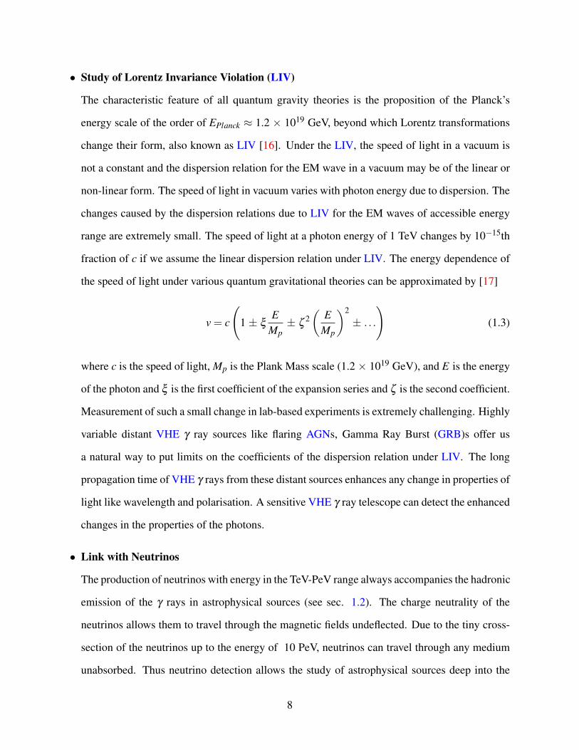
• Study of Lorentz Invariance Violation (LIV)

The characteristic feature of all quantum gravity theories is the proposition of the Planck’s

energy scale of the order of EPlanck ≈ 1.2 × 1019 GeV, beyond which Lorentz transformations

change their form, also known as LIV [16]. Under the LIV, the speed of light in a vacuum is

not a constant and the dispersion relation for the EM wave in a vacuum may be of the linear or

non-linear form. The speed of light in vacuum varies with photon energy due to dispersion. The

changes caused by the dispersion relations due to LIV for the EM waves of accessible energy

range are extremely small. The speed of light at a photon energy of 1 TeV changes by 10−15th

fraction of c if we assume the linear dispersion relation under LIV. The energy dependence of

the speed of light under various quantum gravitational theories can be approximated by [17]

v = c

(

1 ± ξE

Mp

± ζ 2

(

E

Mp

)2

± . . .

)

(1.3)

where c is the speed of light, Mp is the Plank Mass scale (1.2 × 1019 GeV), and E is the energy

of the photon and ξ is the first coefficient of the expansion series and ζ is the second coefficient.

Measurement of such a small change in lab-based experiments is extremely challenging. Highly

variable distant VHE γ ray sources like flaring AGNs, Gamma Ray Burst (GRB)s offer us

a natural way to put limits on the coefficients of the dispersion relation under LIV. The long

propagation time of VHE γ rays from these distant sources enhances any change in properties of

light like wavelength and polarisation. A sensitive VHE γ ray telescope can detect the enhanced

changes in the properties of the photons.

• Link with Neutrinos

The production of neutrinos with energy in the TeV-PeV range always accompanies the hadronic

emission of the γ rays in astrophysical sources (see sec. 1.2). The charge neutrality of the

neutrinos allows them to travel through the magnetic fields undeflected. Due to the tiny cross-

section of the neutrinos up to the energy of 10 PeV, neutrinos can travel through any medium

unabsorbed. Thus neutrino detection allows the study of astrophysical sources deep into the

8

universe; however, their detection requires arduous efforts. Nevertheless, the simultaneous /

co-ordinated observation of the neutrino and VHE γ rays can ascertain the hadronic origin of

the γ ray emission [12].

• Link with GWs

The GWs are generated in most violent events in the universe like merger of Black Hole (BH)s,

Neutron Star (NS)s, collapse of massive stars to form BHs. The electromagnetic follow-ups,

specially the γ ray follow-ups of GW would be of immense value in understanding the physics

behind these events [18].

To better appreciate how the observation of the VHE γ rays throws light on various issues de-

scribed above, understanding of the elementary mechanisms of the γ ray emission in astrophysical

environments is necessary. The next section describes the mechanisms of γ-ray emission and their

properties in brief.

1.2 γ ray emission mechanisms

There are two widely accepted scenarios for γ ray emission at astrophysical sites.

1. The γ ray emission from the population of relativistically accelerated charged particles at

astrophysical sites

2. The γ ray emission from the decay of exotic particles

We will briefly describe each of the two scenarios

1.2.1 The γ ray emission from accelerated charged particles

The thermal emission models that explain the spectra of optical and other low energy emis-

sions from astrophysical sources can not account for non-thermal spectra of γ ray emission. First

or second order Fermi shock acceleration [19, 20] mechanisms are then used to accelerate the seed

9

population of charged particles to ultra-relativistic energies. Various mechanisms of radiation by

relativistic charged particles like, synchrotron, bremsstrahlung, inverse Compton and curvature

radiation are then used to explain the γ ray emission. The first order Fermi mechanism can accel-

erate the particles to a maximum energy of Emax given by [21],

Emax ∝ Zβ

(

B

1µG

)(

L

1pc

)

PeV (1.4)

Many astrophysical sites have right combination of size, magnetic field strength and particle com-

position to allow the acceleration of charged particles to more than ultra-high energies i.e. 1 EeV.

Various radiative processes through which these accelerated particles emit and important features

of the resultant spectrum are as follows

• Synchrotron Radiation

A relativistic charged particle travelling through the magnetic field emits radiation with contin-

uum spectrum, known as SR. The Lorentz boost causes the radiation to be emitted into a cone

of angle θ = 1/γ , where γ is the Lorentz factor of the particle velocity. The energy loss rate of

a particle due to SR is given by [22],

−dE

dx=

1

c

dE

dt=

(

2e4

3m2c4

)

γ2B2 ergscm−1 (1.5)

Since the energy loss rate is ∝ 1/m4, the electron/positrons lose the energy far more efficiently

via SR compared to protons and other heavy particles. The maximum power is emitted at

critical frequency of [23]

ωc =3

2

eB

mcγ2sinθ (1.6)

The 1/m3 dependence of the peak frequency on the rest mass of the particle indicates that the

peak frequency of SR for proton is ≈ 6 × 109 times smaller than that for electron. Thus an

observation of SR from an astrophysical source is generally accredited to Leptonic nature of

emission. However, SR from electrons is not a primary source of the γ ray emission, except

10

in the astrophysical systems with very strong magnetic fields like pulsars and magnetars. The

energy of synchrotron photons emitted by an electron is given by [24],

Esync = 0.2B

10µG

(

Ee

1TeV

)2

eV (1.7)

Thus in a typical astrophysical site with an ambient magnetic field strength of a few µG, a

TeV electron emits an infrared photon while a PeV electron emits an X-ray photon through SR.

These low energy photons play a role of target photons during the γ ray production through the

Inverse Compton (IC) process. The IC process is described below.

• Inverse Compton

The high energy relativistic electrons in the medium upscatter the ambient low energy photons

to gamma-ray energies in the IC effect. The relativistic electrons in the medium transfer their

kinetic energy to low energy photons in IC scattering. The external emission from thermal

processes or synchrotron emission from non-thermal relativistic electron population provides

the low energy photons required in this process.

The energy of the scattered photon in inverse Compton process, Eγ , is given by [25]

Eγ ≃ εγ2 for γ ε ≪ mec2 (1.8a)

Eγ ≃ Ee for γ ε ≫ mec2 (1.8b)

where, γ is the Lorentz factor of an electron, ε is the energy of the photon before scattering,

and Ee is the energy of the electron. The spectrum of the γ rays produced via inverse Compton

process depends on the energy distribution of the electrons and the low energy photon density.

The energy of the electron and the scattered photon in inverse Compton are related to each other

by relation [26]

Eγ ≃ 6.5

(

Ee

1TeV

)2( ε

meV

)

GeV (1.9)

11

Thus to produce a 1 TeV γ ray by up scattering the typical microwave background photon an

electron with the energy of ∼ 17 TeV is required. On the contrary, an electron with the energy

of 1 TeV can boost the energy of photons from visible to X-ray band up to 1 TeV [25]. Given

the electron population that follows the power law distribution with index -α and the population

of low energy photons following blackbody spectrum, the resultant distribution of IC scattered

photons follows the power law distribution with index of -(α + 1)/2.

The astrophysical environments such as AGN, Pulsar Wind Nebulae (PWNe), SNR, micro-

quasars have low magnetic fields and shock accelerated population of relativistic electrons.

These environments are ideal for the Leptonic emission of γ rays. Low energy target photons

may be provided externally or they may be part of the astrophysical system that accelerates the

electrons. The ambient light from accretion disk environment in case of AGN or light from

the optical companion in case of microquasars are some of the cases where target photons are

external. The model of γ ray emission is termed as External Compton (EC) model as opposed

to Synchrotron Self Compton (SSC) model where the low energy target photons for IC are pro-

vided by the SR from the same population of shock accelerated electrons that up scatters them.

The spectral distribution of the IC boosted photons peaks in GeV - TeV energy.

• π Decay

Protons produce the π mesons on interacting with matter or radiation. Inelastic collisions be-

tween two protons produce π and π± mesons with almost equal probability. Neutral pions

have very small mean life of 0.83 × 10−16 seconds and they quickly decay into two γ rays. The

threshold kinetic energy for the production of pions in proton-proton collision is given by [27]

KEth = 2mπ c2

(

1+mπ

mp

)

(1.10)

where mπ is the rest mass of a pion, while mp is the rest mass of a proton. Thus only a

proton with minimum energy of 279.6 MeV can produce a neutral pion (mπ = 135 MeV). The

steep spectrum of CR protons with a power law index of 2.7 means that this channel of γ ray

12

production can account for only weak flux of γ rays.

A photo-production of the pions through the interaction between protons and radiation occurs

mainly through ∆+ resonance [27].

p+ γ → ∆+ → π++n,

p+ γ → ∆+ → π+ p

The hadronic origin of the γ ray production can be identified by a signature bump in the energy

spectrum of observed photons at energy of ∼ 67.5 MeV, known as pion bump. The pion bump

corresponds to half of the rest mass energy of the neutral pion.

• Curvature Radiation

Relativistic electrons and positrons moving along the curved field lines of the strong magnetic

fields emit the radiation in the direction that is tangent to the field lines. The energy loss rate of

the curvature radiation is given by [22],

dE

dt=

2e2

3c3

v⊥

R2γ4 (1.11)

where, R is the radius of the curvature of the magnetic field lines, v⊥ is the component of particle

velocity perpendicular to radius of curvature. The single particle spectrum of the curvature

radiation peaks at

ωc ≈ 0.43γ3 c

R(1.12)

The contribution from the curvature radiation is significant in astrophysical environments like

pulsars and magnetars [28]. A 10 TeV e± emits 2.5 GeV γ ray in a pulsar magnetosphere having

magnetic field curvature radius of 108 cm.

• Bremsstrahlung

The electrostatic scattering of a charged particle in the presence of other charged particle causes

13

the bremsstrahlung or breaking radiation. Classically the radiation can be explained based on

the radiation from the time-varying dipole moment of the system of charged particles dur-

ing the electrostatic scattering. Thus a system of two identical charged particle can not emit

bremsstrahlung as their dipole moment throughout the scattering is constant [22]. In astro-

physical plasmas, electrons are the primary source of bremsstrahlung due to their prominent

electrostatic deflections owing to their lower mass. The quantum effects of finite nuclear size

and screening due to the outermost electrons of ions significantly modify the classical spec-

trum of single-electron bremsstrahlung [29], in case of astrophysical plasma. The relativistic

electrons in the presence of atomic and molecular medium emit γ rays via bremsstrahlung [30].

The threshold energy of an electron to emit γ rays via bremsstrahlung is twice the energy of the

emitted γ ray [25].

1.2.2 The γ ray emission from the decay of exotic particles

The annihilation of DM candidate particles like WIMP is one possible mechanism for γ ray

production. There are two proposed modes of the WIMP decay [12]. In one of the proposition,

the WIMP pairs can annihilate through γγ or Zγ channels. These channels can produce the sharp

features related to WIMP mass in the spectrum of γ rays. The other WIMP decay mode consists

of 2 WIMP particles annihilating to form pair of quarks or leptons which can induce cascade of

secondary particles containing neutral pions. The featureless continuum spectrum of γ rays can

be produced through the decay of π. The expected γ ray flux due to annihilation of WIMPs by

any mode from any direction is given by [12]

φγ =1

4π

〈σannv〉

2m2DM

dNγ

dE

∫

∆Ω

dl(Ω)ρ2DM (1.13)

where 〈σannv〉 is annihilation rate,dNγ

dEis the γ ray differential flux per annihilation event, ρDM

is the density of the DM along the line of sight. The integration is performed over the effective

solid angle about the line of sight. The astrophysical sites like galactic center suspected to have

14

increased DM density may show the γ ray signatures of the DM thereby revealing the properties

of particles constituting them.

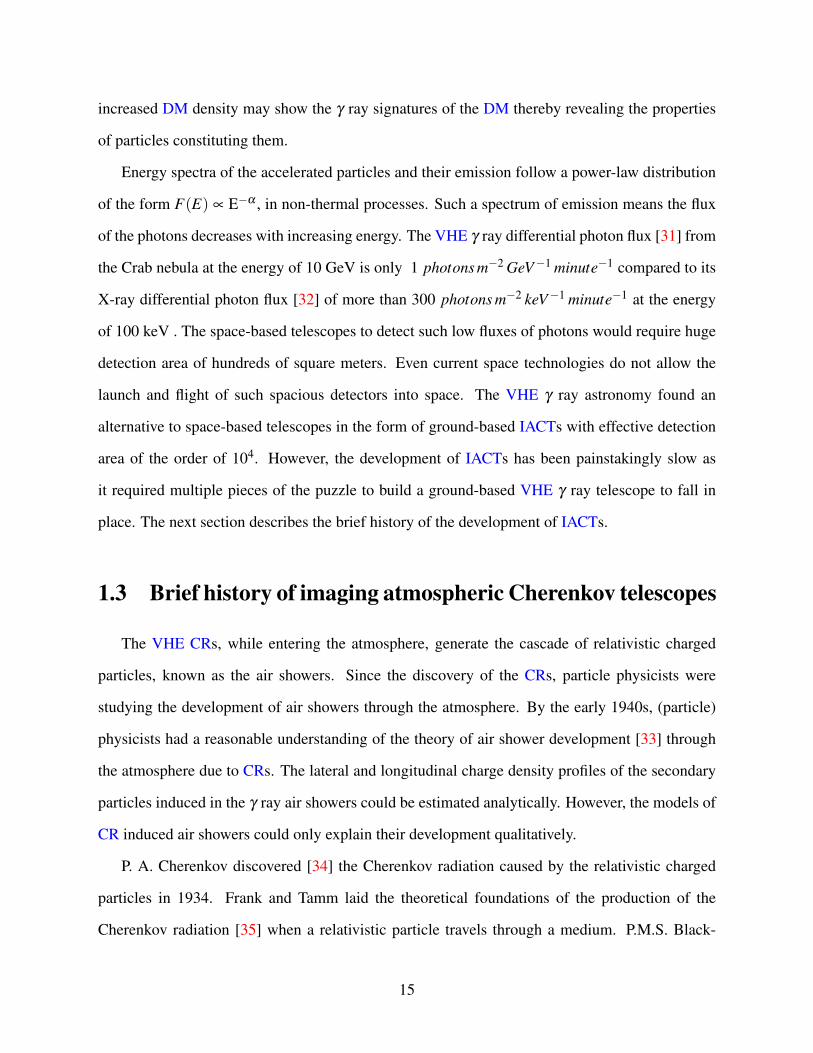
Energy spectra of the accelerated particles and their emission follow a power-law distribution

of the form F(E) ∝ E−α , in non-thermal processes. Such a spectrum of emission means the flux

of the photons decreases with increasing energy. The VHE γ ray differential photon flux [31] from

the Crab nebula at the energy of 10 GeV is only 1 photons m−2 GeV−1 minute−1 compared to its

X-ray differential photon flux [32] of more than 300 photons m−2 keV−1 minute−1 at the energy

of 100 keV . The space-based telescopes to detect such low fluxes of photons would require huge

detection area of hundreds of square meters. Even current space technologies do not allow the

launch and flight of such spacious detectors into space. The VHE γ ray astronomy found an

alternative to space-based telescopes in the form of ground-based IACTs with effective detection

area of the order of 104. However, the development of IACTs has been painstakingly slow as

it required multiple pieces of the puzzle to build a ground-based VHE γ ray telescope to fall in

place. The next section describes the brief history of the development of IACTs.

1.3 Brief history of imaging atmospheric Cherenkov telescopes

The VHE CRs, while entering the atmosphere, generate the cascade of relativistic charged

particles, known as the air showers. Since the discovery of the CRs, particle physicists were

studying the development of air showers through the atmosphere. By the early 1940s, (particle)

physicists had a reasonable understanding of the theory of air shower development [33] through

the atmosphere due to CRs. The lateral and longitudinal charge density profiles of the secondary

particles induced in the γ ray air showers could be estimated analytically. However, the models of

CR induced air showers could only explain their development qualitatively.

P. A. Cherenkov discovered [34] the Cherenkov radiation caused by the relativistic charged

particles in 1934. Frank and Tamm laid the theoretical foundations of the production of the

Cherenkov radiation [35] when a relativistic particle travels through a medium. P.M.S. Black-

15

ett [36] predicted the existence of the Cherenkov flash associated with the development of the

air showers induced by CRs. The detection of the Cherenkov emission associated with the air

showers by Galbraith and Jelly [37] in 1952, lead A. Chudakov to implement the first atmospheric

Cherenkov based calorimeter to measure the energy of the CRs detected by particle array.

G. Cocconi first proposed a way to detect astrophysical TeV γ rays [38] by detecting atmo-

spheric air showers induced by them. His proposal consisted of an array of scintillators located at

an altitude of 5.5 km above sea level, that would detect and reconstruct the arrival direction of the

CRs based on arrival time delays of the shower front. Cocconi estimated that γ rays coming from

a point source would trace back to the same location in the sky as against the isotropically dis-

tributed CR directions, allowing the statistically significant detection of TeV γ rays from sources

like Crab nebula, M87 and Sun. Zatsepin and Chudakov proposed using a Cherenkov flash of

the air showers to detect CRs while using the isotropy of the CR directions to segregate between

source γ rays and background [39]. They built first Atmospheric Cherenkov Telescope (ACT) for

the γ ray observations at Crimea in the early 1960s. However, due to the inability of the ACT

to suppress enormous CR background, a significant detection of the astrophysical γ ray source

could not be achieved. Whipple observatory in Arizona built the ACT with 10 m reflector in 1968

to pursue the research in the development of ACT-based TeV γ ray telescope. The initial design

did not consist of an imaging camera and had a single PMT at the focal plane of the reflector

instead. However by 1983, the focal plane instrumentation underwent a series of changes, ulti-

mately ending up in the imaging camera with 37 PMT pixels to capture images of the air showers

as proposed by Trevor Weekes [40]. In the meantime, the development of the computational tech-

nologies allowed Monte Carlo simulation studies of the air shower development and the response

of the telescope to Cherenkov emission from air showers for the first time. These simulation stud-

ies were instrumental in developing the understanding of the formation of Cherenkov images of

showers on the focal plane as well as differences between γ and CR induced shower images. A.

M. Hillas proposed an analysis method [41, 42] to segregate γ and CRs, based on the differences

between the γ ray and CR induced air shower images formed on the PMT camera. Whipple col-

16

laboration detected γ rays of energy above 0.7 TeV from the Crab nebula for the first time in 1989

using the IACT [43].

Since the first detection of TeV γ rays, IACTs have improved in their sensitivity, energy thresh-

old, angular and energy resolution. The construction of stereoscopic arrays has been the primary

driver of the improvement while better analysis techniques, faster electronics and pixel miniatur-

isation have also contributed. The major IACT observatories around the world today consists of

HESS, MAGIC and VERITAS. The HESS is a system of 4 IACTs with 13 m diameter reflectors

and a large IACT with 28 m diameter reflector. It is located in Khomas highlands of Namibia at

an altitude of 1800 m asl and can detect γ rays with energy less than 20 GeV [44]. The MAGIC is

an array of two 17 m diameter IACTs located at Canary islands of La Palma, Spain, at the altitude

of 2200 m. The energy threshold of the MAGIC is 50 GeV [45]. VERITAS is an array of four 12

m IACTs located at Whipple observatory, southern Arizona, USA, at an altitude of 1300 m above

asl. The VERITAS can observe γ ray in the energy range of ∼ 85 GeV to ∼ 30 TeV [46]. Over

the last three decades the imaging atmospheric Cherenkov technique has emerged as the most

powerful technique for the observations of VHE γ rays up to energy of ∼ 50 TeV.

Last few decades have also seen advent of another type of ground based VHE γ ray observa-

tories like MILAGRO, HAWC and ASγ . These observatories directly measure the arrival times

and counts of the secondary particles of EAS using array of charged particle detectors accompa-

nied with scintillation chambers (in ASγ) or Water Cherenkov detectors (in MILAGRO, HAWC).

The arrival direction and energy of primary particle is reconstructed based on the sampling of

the shower front. These observatories have advantage of ∼ 90% duty cycle and large Field of

View (FOV) of ≈ 2 sr. These features make them excellent tools for sky survey and observation

of diffused γ ray emissions specially at energies > 10 TeV. However, they have lower sensitivity

and higher energy threshold [40].

17

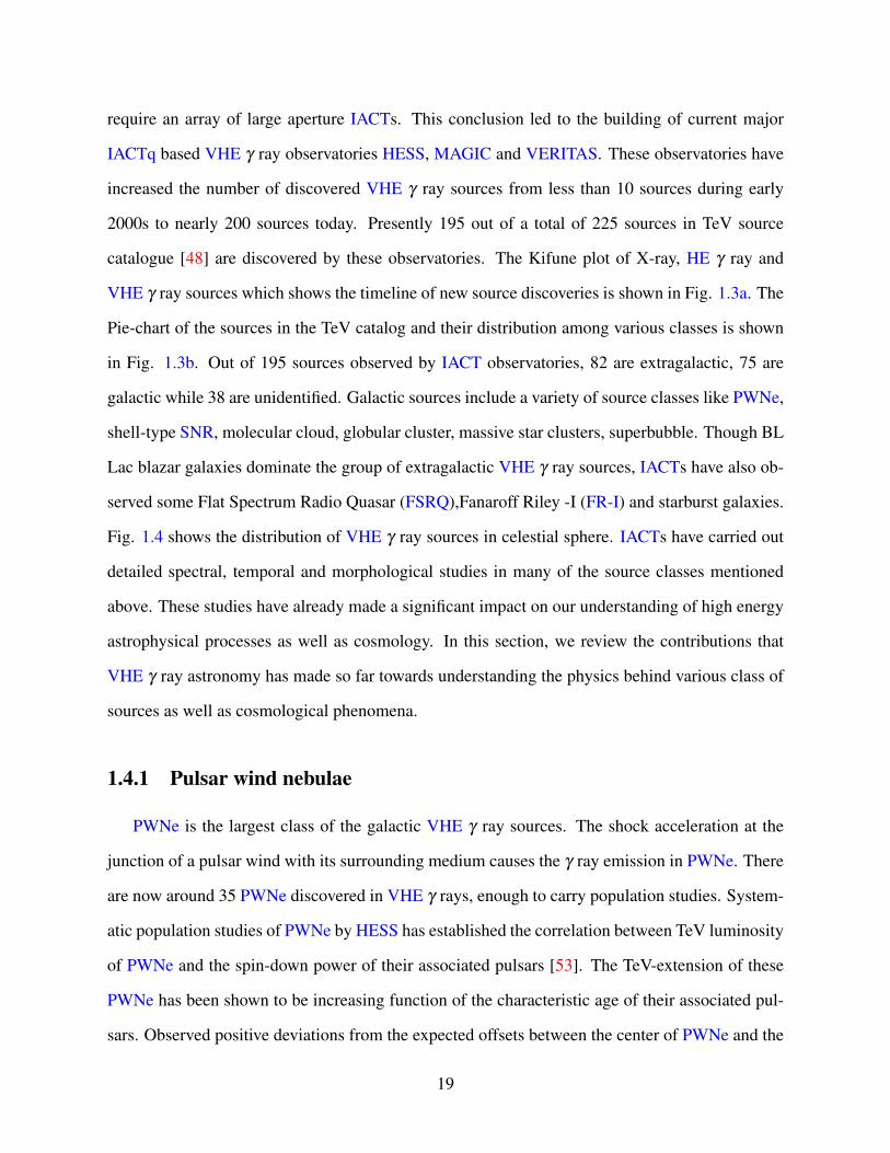
require an array of large aperture IACTs. This conclusion led to the building of current major

IACTq based VHE γ ray observatories HESS, MAGIC and VERITAS. These observatories have

increased the number of discovered VHE γ ray sources from less than 10 sources during early

2000s to nearly 200 sources today. Presently 195 out of a total of 225 sources in TeV source

catalogue [48] are discovered by these observatories. The Kifune plot of X-ray, HE γ ray and

VHE γ ray sources which shows the timeline of new source discoveries is shown in Fig. 1.3a. The

Pie-chart of the sources in the TeV catalog and their distribution among various classes is shown

in Fig. 1.3b. Out of 195 sources observed by IACT observatories, 82 are extragalactic, 75 are

galactic while 38 are unidentified. Galactic sources include a variety of source classes like PWNe,

shell-type SNR, molecular cloud, globular cluster, massive star clusters, superbubble. Though BL

Lac blazar galaxies dominate the group of extragalactic VHE γ ray sources, IACTs have also ob-

served some Flat Spectrum Radio Quasar (FSRQ),Fanaroff Riley -I (FR-I) and starburst galaxies.

Fig. 1.4 shows the distribution of VHE γ ray sources in celestial sphere. IACTs have carried out

detailed spectral, temporal and morphological studies in many of the source classes mentioned

above. These studies have already made a significant impact on our understanding of high energy

astrophysical processes as well as cosmology. In this section, we review the contributions that

VHE γ ray astronomy has made so far towards understanding the physics behind various class of

sources as well as cosmological phenomena.

1.4.1 Pulsar wind nebulae

PWNe is the largest class of the galactic VHE γ ray sources. The shock acceleration at the

junction of a pulsar wind with its surrounding medium causes the γ ray emission in PWNe. There

are now around 35 PWNe discovered in VHE γ rays, enough to carry population studies. System-

atic population studies of PWNe by HESS has established the correlation between TeV luminosity

of PWNe and the spin-down power of their associated pulsars [53]. The TeV-extension of these

PWNe has been shown to be increasing function of the characteristic age of their associated pul-

sars. Observed positive deviations from the expected offsets between the center of PWNe and the

19

current position of their associated pulsars indicate the expansion and evolution of these PWNe in

asymmetric environment. The detection of 100 to 450 TeV γ ray photons from the Crab nebula by

ASγ [54] observatory in Tibet, points at the possibility of electrons accelerated to PeV energies

at this site. A small new class of Magnetar Wind Nebulae (MWNe) seems to be emerging from

HESS detection of sources like HESS J1808-204 [55] and HESS J1834-087 [56]. These sources

have possible association with candidate magnetar sources SGR 1806-20 and Swift J1834.9-0846

respectively. Though the origin of emission from these sources is not yet clear, it is hypothesized

that magnetar’s bursting activity and their corresponding outflows power the emission from these

sources.

1.4.2 Supernova remnants

SNRs are the ejecta of the exploded star travelling through the Interstellar Medium (ISM). As

shell shaped SNRs travel through ISM, it develops the shock front, accelerating the particles by

stochastic diffusion of the particles back and forth across the shock in presence of the magnetic

field perturbations in the ISM. TeV catalogue contains 14 SNRs discovered by IACTs half of

which are shell-type SNRs while other half are composite-type SNRs.

IACTs have carried out deep observations of shell-type SNRs like Tycho, CasA. These deep

observations have led to much more accurate spectral measurements revealing the spectral breaks

previously unknown. The power law spectra of young SNRs, Cassiopeia A [57] and Vela Jr. [58]

show exponential cut-off for energy beyond 3.5 TeV and 6.7 TeV respectively. Detailed mor-

phological study of VHE emission from RX J1713-3976 using HESS, show that VHE emissions

extend farther than the X-ray emission in these regions. This is the first evidence of CR particles

escaping the shock acceleration region [59].

The hadronic nature of the γ ray emission in the middle-aged composite-type SNRs via in-

teraction of CRs with nearby molecular cloud, is gaining increasing evidence through their γ

ray observations. HESS and Fermi/LAT observations of W28 [60] have shown the spatial offset

in VHE emissions compared to SNR position which indicate existence of the site of interaction

20

between CRs escaping from W28 and nearby molecular cloud. The observation of 12CO emis-

sion lines by NANTES observatory confirms that there is a molecular cloud near W28 region.

The simultaneous Observation of composite-type SNRs like W51C, W44, IC443 and W49B by

Fermi/LAT and IACTs have shown clear breaks in their SEDs at 200 MeV and at few GeV [61].

These breaks clearly indicate that origin of γ ray emission from these SNRs is of hadronic nature.

1.4.3 Galactic binary systems

Number of binaries observed by IACTs is slowly growing. Currently TeV source catalog

contains 9 binaries. All the binaries observed by IACTs are of type High Mass Binary (HMB)

which consist of a compact object and a high mass companion star orbiting in elliptic orbit of high

(≥ 0.5) eccentricity. The emission in such system is modeled using collision between stellar wind

and a relativistic pulsar wind. For binary systems like PSR B1259-63/LS 2883, LSI +61303 and

LS 5039 IACTs have now collected data for ∼11 years [62].

1.4.4 Pulsars

The MAGIC collaboration first discovered pulsed TeV γ rays from the Crab pulsar [63] fol-

lowed by confirming detection by VERITAS. The detection of Vela pulsar in 10 - 100 GeV range

by HESS [64] implies the possibility of detection of more pulsars in VHE γ rays. The pulsar

emission models primarily rely on the synchrotron and curvature radiation from the e± plasma in

the pulsar magnetospheres. These emission models estimated the energy cut off at energy of a few

GeV in the spectrum of the pulsed emission of the pulsar. The detection of pulsed VHE γ rays

from the Crab and Vela have challenged these models and completely new models of emission

may have to be developed.

21

1.4.5 Galactic center

HESS has observed VHE gamma-ray emission from the galactic center, following power law

spectrum with index of 2.3 without any spectral cutoff up to γ ray energy of 50 TeV. This serves

as the evidence of protons of energy beyond PeV suggesting the existence of Pevatron accelerator

within 10 pc of galactic center [65]. Super-massive balck hole Sgr A* has been associated with

this Pevatron. Deep morphological observations of diffused γ ray emission around galactic center

not only has allowed the better model for diffused galactic γ ray emission but also has lead to

detection of new VHE γ ray point sources in this region.

1.4.6 Active galactic nuclei

AGNs are the first extragalactic objects discovered in VHE γ rays. It is the largest class of

VHE γ ray emitters with TeV catalogue having 78 AGNs. The AGNs are galaxies with Super

Massive Black Holes (SMBH) at the center. The galactic matter accretes around the SMBH and

eventually falls into it due to its strong gravitational pull. Conversion of the gravitational energy

to the kinetic energy of the accreting matter eventually results in the outflow of the matter in form

well-collimated relativistic jet of plasma [66]. Internal shocks or the magnetic reconnection in the

jet ejecta are the two candidates for the particle acceleration in the AGNs. A typical non-thermal

broadband EM spectrum of an AGN shows two bumps. The low energy bump is often modeled

by the synchrotron emission of the relativistic electrons in the jet. The high energy bump falling

in the GeV - TeV range is explained by the IC process either through SSC or EC.

VHE γ ray AGNs are further classified into blazars and radio galaxies on the basis of the

orientation of the jet structure relative to line of sight. The blazars are the strong VHE γ emitters

while the radio galaxies have weak emission in VHE γ rays. Out of all AGNs listed in TeV

catalogue only 4 are radio galaxies while rest of them are blazars. The blazars are further classified

based on the occurrence of the strong and broad emission lines in the spectrum. The faint VHE

γ ray sources with emission lines in the low energy part of the spectrum are termed FSRQ while

22

the rest of blazars are called BL Lacertae (BL Lac) objects. BL Lac are further divided into the

classes Low-frequency Peaked BL Lacs (LBL), Intermediate-frequency Peaked BL Lacs (IBL)

and High-frequency Peaked BL Lacs (HBL) depending upon the energy at which the second (IC)

bump occurs in their spectrum.

With recent lowering of the energy threshold after upgrades, the FSRQ PKS 1441+25 with

a very high redshift z = 0.94 has been discovered [67, 68]. Lack of evidence on internal ab-

sorption indicates the emission site to be beyond the radius of Broad Line Region (BLR) of

rBLR ≃ 1017cm(

Ldisk/1045ergs−1)1/2

. A value of H = 61 ± 7 kms−1Mpc for the Hubble con-

stant has been inferred using the detection of VHE γ rays from gravitationally lensed system

B0218+357 [69]. The high redshift observations of AGNs are also useful in estimation of the

SED of EBL.

1.4.7 Gamma ray bursts

The detection of the VHE γ rays by the HESS collaboration [70] 10 hours after the end of

the prompt emission phase of GRB180720B has surprised the astrophysical community. The

observation of VHE γ rays deep in the afterglow light curve of GRB indicates that IC mechanism

of emission would not require as much particle energy for the emissions observed at late times.

MAGIC telescope detected the GRB190114C above energy of 300 GeV with significance of >

20 sigma, in the first 20 minutes of the prompt emission [71]. With detection of prompt as well as

afterglow VHE emission from GRBs, there is a new excitement in the field of GRB studies.

1.4.8 Extragalactic background light

Fig. 1.5 shows SED of EBL using VHE observations as estimated by HESS, MAGIC and

VERITAS collaborations[72]. HESS collaboration has used nine HBL observations to estimate

the SED of EBL while MAGIC and VERITAS have reported the EBL measurements using obser-

vations of 12 and 8 blazars respectively. It is interesting to note that all the measurements agree

23

Figure 1.5: EBL SED as measured by IACTs. The blue arrows are the lower limits estimated

from the galaxy counting.The red arrows are the upper limits obtained by the direct observation

of light of night sky. The magenta squares show the HESS measurements while green and dark

violet contours show measurements by MAGIC and VERITAS respectively. Figure adapted from

[72].

well with each other and generally lie closer to estimated lower limit of EBL based on galaxy

counts.

1.4.9 Contributions to fundamental Physics

The MAGIC telescope with its long observation of dwarf Spherical satellite galaxy (dSphs)

candidate Segue 1, has set the most constraining limits on the DM annihilation cross-section for

masses above few hundred GeVs [73]. The rapid flares with doubling time of 1-2 minutes and

an order of magnitude flux variation from Markarian 501, observed by MAGIC has allowed the

physicist to constrain the lower limit on first and second order coefficients in dispersion relation

of eq. 1.3. The lower limits of LIV mass scale has been constrained to values of Mp/ξ > 5.7×

1010 GeV and Mp/ζ > 0.3× 1018 GeV [74] with observation of flares in Markarian. Using the

TeV observations from the Crab pulsar, the MAGIC collaboration has constrained the linear and

24

quadratic coefficients of dispersion relation (refer to eq. 1.3) to values of Mp/ξ > 5.5 × 1017 GeV

and Mp/ζ > 5.9 × 1010 GeV [75].

The success of IACTs in making impact on various aspects of our understanding of the uni-

verse demonstrate their potential. The VHE γ ray astronomy has matured into a vibrant branch of

astronomy and astrophysics, with major contribution from IACTs. There is an ongoing worldwide

effort toward realising the full potential of IACTs by widening the observable energy range and

increasing the sensitivity. Astrophysical Sciences Division (ApSD) of Bhabha Atomic Research

Center (BARC) is in the final phases of the commissioning of the large aperture IACT Major At-

mospheric Cherenkov Experiment (MACE) (Major Atmospheric Cherenkov Experiment) at high

altitude of 4270 m asl at Hanle, India. The altitude of the MACE is highest when compared to

existing IACTs in the world, while its reflector diameter of 21 m is the second largest among

the IACTs in northern hemisphere. The large reflector and high altitude of MACE will allow the

MACE to observe VHE γ ray universe in wide window of ∼ 30 GeV to ∼ 10 TeV.

This thesis presents the methodology and results of the Monte Carlo simulation study of the

MACE telescope. The optimum trigger multiplicity and single channel discrimination threshold

for the MACE operations to achieve lowest possible energy threshold is estimated as a part of

this work. The trigger performance of the MACE telescope at the estimated optimum trigger

configuration is then simulated for zenith angle values of 0, 20, 40 and 60. Three performance

parameters of the MACE, namely integral flux sensitivity, angular resolution and energy resolution

in the zenith angle range of 0 to 30 and at the zenith angle of 40 are presented in subsequent

chapters. The next chapter describes details of the IACTq. It depicts the working principles of

MACE and the role of simulations in IACTq.

25

CHAPTER

TWO

IMAGING ATMOSPHERIC CHERENKOV TECHNIQUE

2.1 Introduction

IACTq primarily uses the Earth’s atmosphere both as a detector and as a calorimeter for the

detection of VHE γ rays. When VHE γ and CRs enter the atmosphere, they interact with the

atmospheric nuclei, molecules and ions. These interactions produce ultrarelativistic charged par-

ticles as well as high energy photons which in turn again interact with the atmosphere. These

cyclic interactions very quickly result in cascade of charged particles and photons known as EAS.

The highly relativistic charged particles cause the emission of Cherenkov radiation in the visible

range. The IACTq based telescope detects VHE γ rays through the atmospheric Cherenkov radi-

ation produced by the energetic EAS particles. This chapter describes various aspects of IACTq.

2.2 Extensive air showers

Leptons and photons in the CRs interact with atmosphere through electromagnetic force. On

the other hand the hadronic CRs interact with atmospheric nuclei through strong force. Thus

EASs belong to two categories: electromagnetic EASs and Hadronic EASs.

27

2.2.1 Electromagnetic extensive air showers

VHE γ rays, electrons and muons initiate electromagnetic EASs. The particle multiplication

in these EASs takes place primarily through bremsstrahlung and pair production. High energy

photons undergo electron-positron pair production in the electromagnetic fields of atmospheric

nuclei and ions. The pair produced electrons and positrons further emit high energy photons by

bremsstrahlung when they get coulomb scattered by atmospheric nuclei. The distance over which

the energy of an electron becomes a factor 1/e of its initial energy due to radiation losses, is called

Radiation Length. Radiation length of electron or in general the mean interaction length for any

particle for any kind of process depends on the density of the medium. The characteristic lengths

of different interactions can be expressed independent of medium density in units of g cm−2 by

integrating medium density along path length. This quantity then gives an idea about the amount

of matter that has interacted with the primary. The radiation length of the electron is given by [33]

Xbr =[

4αr2e

NA

AZ2ln

(

183Z− 13)

]−1

gcm−2 (2.1)

where A is a mass number of the medium, Z is an atomic number of the medium, NA is the

Avogadro number, re is the classical electron radius and α = 1/137 is the fine structure constant. In

case of atmosphere average atomic number of 7 is used. The mean free path of the pair-production

for the very high energy photons which have energy hω ≫ me c02

αZ1/3 is given by [76]

Xpp =

[

4αr2e

NA

AZ2

(

28

9ln

(

183

Z1/3

)

−2

27

)

]−1

gcm−2 (2.2)

where A, Z, NA, re and α all have the same meaning as in the eq. 2.1. Thus the bremsstrahlung

radiation length and the mean free path for pair production are almost equal. The Poissonian

nature of the occurrence of these interactions mean that the probability of interaction over a path

length X can be given as

P(X) = exp(

−X

X

)

(2.3)

28

where X = Xbr ≈ Xpp. The value of X is ∼ 36.7 g cm−2 for electromagnetic showers in atmo-

sphere.

Figure 2.1: A toy model for the electromagnetic air shower development. Figure adopted from

[76]

If we set the value of probability to 0.5 in eq. 2.3 we can see that on average every interaction

in electromagnetic EAS takes place after a distance of R ≈ Xln2. This fact can be used to build a

simple toy model for the generation of electromagnetic showers due to γ-rays in the atmosphere

[77]. The VHE γ-ray photon with initial energy E entering the atmosphere undergoes pair-

production at distance of R, where electron and positron each take half of the photon’s energy.

Electron and positron each emit bremsstrahlung photons of energy E4

when they travel further

distance of R. Thus on an average at the end of the distance 2 R there are 4 particles each with

energy E4

. The repetition of these processes over the distance of nR thus creates total 2n particles

each with average energy E2n . Fig. 2.1 shows the schematic of the particle multiplication in γ

ray induced EAS. The energy losses by radiation for electrons and positrons are dominated by

ionisation losses below a critical energy of Ec ≈ 80 MeV. Hence when the average energy of

particles in the shower reaches Ec the particle multiplication stops and the number of particles

29

Figure 2.2: Number of particles in the shower as a function of the atmospheric depth according to

eq. 2.5. The atmospheric depth is scaled to the radiation length. Showers with different primary

energies are shown with blue curves. The red lines are the locus of constant shower age.

starts decreasing. This is called the shower maximum. The depth of the shower maximum in

terms of radiation lengths is then given by

nc =ln(E/Ec)

ln2(2.4)

At shower maximum there are total 2nc particles. It is clear that higher energy showers reach

deeper in the atmosphere from eq. 2.4. It should be noted that even the electron of energy 80 MeV

has the Lorentz factor of ∼ 156. Thus for most of the shower development the electrons can be

considered ultra-relativistic.

More realistic model of the electromagnetic shower development is given by [78]

Ne(t,E) =0.31

√

ln(E/Ec)exp [t (1−1.5 lns)] (2.5)

where Ne is the number of particles generated in the shower, t is atmospheric depth scaled by

30

radiation length, E is the primary energy, Ec is the critical energy and s is the dimensionless

parameter given by

s =3 t

t +2 ln(E/Ec)(2.6)

s is called the shower age. It is the quantity that indicates the stage of the shower development

independent of the primary energy and the atmospheric depth reached by the shower. The value of

s lies in the range 0 ≤ s ≤ 3 [79]. The shower age value of 0 indicates start of the shower develop-

ment, s = 1 indicates the maximum of the shower while s = 2 indicates the shower extinction. Fig.

2.2 shows the evolution of the number of shower particles in the shower as it progresses through

the atmosphere.

To a good approximation, the lateral development of the electromagnetic EAS can be treated

independent of its longitudinal development [33]. The pair-produced e± and bremsstrahlung pho-

tons in these showers have negligible deviations from the direction of their progenitors. The major

source of the transverse spread of electromagnetic EAS comes from the Coulomb scattering of the

e± in the atmosphere. The distribution of scattering angles with respect to shower axis caused by

multiple Coulomb collisions is given by ∼ exp(−θ/θ) [78, 80] . The characteristics angle θ typ-

ically is ∼ 5 [81]. However the exponential nature of the scattering angle distribution means that

lateral shower development is still fairly collimated in the direction of the primary. The Moliere’s

theory of multiple coulomb scattering [82] can be used to find the characteristic lateral spread of

the electromagnetic EAS. It is given in terms of the Moliere radius Rmol which is the radius of the

imaginary cylinder containing 90% of the secondary particles in the shower. Moliere radius is a

characteristic of the medium given by

Rmol =XEs

ρEccm (2.7)

where Es ≈ 21 MeV, Ec is the critical energy in the medium and ρ is atmospheric density. The

value of Rmol at sea level is ∼ 80 m.

The density of e± as a function of lateral distance from the shower core is given by Nishimura-

31

Kamata-Greisen (NKG) approximation as [83, 84]

ρe(r)≈Ne(t)

2ΠR2mol

Γ(4.5− s)

Γ(s)Γ(4.5−2s)

(

r

Rmol

)s−2(

1+r

Rmol

)s−4.5

(2.8)

where Ne is the given by eq. 2.5. This approximation can be used to calculate the spectrum and

lateral distribution of Cherenkov light coming from the electromagnetic EAS.

2.2.2 Hadronic extensive air showers

The hadronic CRs on interacting with atmospheric nuclei produce mesons and more nucleons.

However, π mesons constitute 90% of the collision products while rest 10% are kaons and anti-

protons [85].

h + Nucleus → mπ± + nπ (2.9)

The pion population consists of equal numbers of π, π+ and π−. The neutral pions are very

unstable and have very short lifetime of the order of 10−15 seconds in the Center of Mass (CM)

frame. They decay into 2 photons with Branching Ratio (BR) of 98.8% or 1 photon and e± pair

with BR of 1.2% [76]. In any case they initiate a electromagnetic sub-showers within the hadronic

EAS. The electromagnetic sub-showers which are main contributors to Cherenkov radiation from

hadronic EAS carry only ∼ 30% of the energy of the hadronic shower [86].

π → γ + γ (BR = 0.988)

π → γ + e± (BR = 0.012)

(2.10)

Charged pions have lifetime of the order of 10−8 seconds in CM frame. They decay to muons and

neutrinos through reaction [76]

π± → µ± + νµ (2.11)

32

The kaons have lifetime of ∼ 10−8 seconds and decay to either muons or pions through following

channels [76]

K± → µ± + νµ (BR = 0.635)

K± → π± + π (BR = 0.212)

(2.12)

The muons produced in these reactions are fairly stable particles and have decay times of the order

of microseconds in CM frame. With this lifetime and their low cross section, 1 GeV muon can

have flight distance of ∼ 10 km in the earth’s frame. Thus many muons in the hadronic EAS reach

the ground. The muons in the hadronic EAS also contribute to the Cherenkov light emission.

In the early stage of EAS development pions and kaons have much higher energy. At these

higher energies they interact with atmosphere more before they can decay. At later stage of devel-

opments, decay of pions/kaons to muons dominates the other interactions. Below 1 GeV ionisation

losses dominate all other interactions and shower starts to die out. Since only some fraction of

the primary energy goes to electromagnetic sub-showers and muons, the Cherenkov yield of the

hadronic EAS is much less as compared to showers initiated by γ / e− of same primary energy.

The secondary particles in hadronic showers have ∼ constant transverse momentum of 0.3 GeV/c.

This leads to much higher lateral spread of hadronic showers. The hadronic showers also pene-

trate much deeper compared to their electromagnetic counterparts. This is due to the large mean

interaction length of different constituent particles in the hadronic EAS. The interaction length

for proton of 1 TeV is 83 g cm−2 in the atmosphere, almost the double of mean free path of pair-

production. Pions and kaons have even higher mean interaction lengths of 107 g cm−2 and 138 g

cm−2 respectively at 1 TeV.

33

2.3 Cherenkov radiation from extensive air showers

2.3.1 Cherenkov radiation

A charged particle moving through a medium primarily loses energy through Coulomb scat-

tering and ionisation. However, when charged particles move with a constant speed that is faster

than the speed of light in the medium, the medium emits radiation in IR to UV range of the

electromagnetic spectrum. The part of energy of the particle is lost through this radiation. This

emission is known as Cherenkov radiation after its discoverer P.A. Cherenkov. He first observed

the Cherenkov radiation in the liquids due to action of γ-ray radiation [34].

Figure 2.3: Polarisation of the medium due to a moving charged particle for (a) v < c (b) v > c (c)

Cherenkov wavefront construction using Huygens principle where coherent light adds up along

conical surface with line of motion as axis. Figure adopted from [76]

The Cherenkov radiation phenomenon can be explained by analogy to the generation of the

shock wavefront by a supersonic motion of a body in a fluid medium. When a charged particle

moves through a medium it polarises nearby atoms/molecules in the medium. When speed of the

particle is slower than the light speed in the medium, the information about particle’s changing

position reaches the surrounding induced dipoles in time. Thus dipole moments of the surrounding

molecules are always directed radially inwards towards current particle position and have zero net

34

dipole moment. When the charged particle moves faster than the speed of light in the medium this

situation changes. The induced dipoles do not point radially towards the particle’s current position

and there is a net induced dipole in the direction of the particle motion. This dipole produces net

electromagnetic field at infinity seen as Cherenkov radiation. Fig. 2.3 shows the polarisation of the

medium by the charged particle in 2 cases. It also shows the Huygens construction of Cherenkov

wavefront. Theoretically, Cherenkov radiation can be appreciated by looking at retarded Lienard-

Wiechert potential in the medium of refractive index of n. It is given by [76]

φ(r, t) =1

4πεr

[ q

1− (nv · iobs )/c

]

ret(2.13)

where iobs is the unit vector along the direction of observation. It can be seen that when

vcosθ = c/n (2.14)

the potential in eq. 2.13 diverges, indicating radiation losses even in case of constant velocity of

particle.

The eq. 2.14 also gives us the minimum energy of the particle for the Cherenkov emission ECth

as

ECth = γth m c2 =

m c2

√

1 − 1/n2(2.15)

where γth is the threshold Lorentz factor of the particle. The minimum energy required for the

Cherenkov emission is known as the Cherenkov emission threshold. Since threshold energy for

Cherenkov emission depends upon the rest mass of the emitting particle, the electron has the small-

est Cherenkov emission threshold of ∼ 21 MeV at sea level. The Cherenkov emission thresholds

for muon and proton are 4.4 GeV and 39.1 GeV respectively at sea level. The Cherenkov emission

threshold energy of the particle in the atmosphere also depends on the altitude of the emission.

The atmosphere is not a homogeneous medium and its density and hence refractive index changes

with altitude. For the simplistic isothermal parallel column model of the atmosphere in the static

35

equilibrium, pressure gradient across the horizontal slab of the atmosphere balances the down-

ward gravitational pull per unit volume on the slab. This equation coupled with the ideal gas law

yields the exponential dependence of the density on the altitude as [87]

ρ = ρ exp(−h/h) (2.16)

where ρ is 0.0013 g cm−3 and h = 7250 m. The refractive index of the atmosphere at an altitude

of h can then be written as [87]

n = 1 + ηh = 1+ η exp(−h/h) (2.17)

where η = 0.00029. Using the Taylor approximation of eq. 2.17 into eq. 2.15 the ECth can be

approximated by

ECth ≈

mc2

√2ηh

(2.18)

It can be seen that, for the electron even at the altitude of the 10 km above sea level the Cherenkov

emission threshold is ∼ 42 MeV, well below the critical energy for the electromagnetic show-

ers. Thus even when shower development reaches beyond it’s maximum the electrons in the

shower can emit Cherenkov light while shower extinction continues. The muon and proton have

Cherenkov emission thresholds of 8.9 GeV and 78.8 GeV respectively at 10 km altitude from sea

level.

2.3.2 Lateral photon density distribution of atmospheric Cherenkov radia-

tion due to extensive air showers

The eq. 2.14 also gives the angle of Cherenkov emission with respect to the trajectory of the

particle. It is given as

cosθc =1

β n(2.19)

36

where β is v/c . Plugging in the eq. 2.17 in above equation dependence of Cherenkov emission

angle on the altitude can be seen.The radius of the circular intersection of the Cherenkov cone

(here onwards Cherenkov Pool Radius (CPR)) emitted at an altitude of h with the observation

level at hobs can be calculated using

Rc = ( h −hobs ) tanθc (2.20)

The variation of Cherenkov angle and CPR with emission altitude for the β = 0.999996 is

shown in Fig. 2.4. It can be seen from Fig. 2.4a that Cherenkov emission angle increases with

(a) (b)

Figure 2.4: (a): Cherenkov emission angle as a function of the altitude of the emission (b):

Cherenkov pool radius as a function of the emission altitude.

the decreasing altitude. This causes crude focussing of the Cherenkov light about the particle

trajectory. Fig. 2.4b shows this focussing effect geometrically. In the previous section we have

seen that electromagnetic shower development is collimated within ∼ 5 of the primary direction.

The electromagnetic showers are far more symmetric about the shower axis compared to their

hadronic counterparts. Thus the Cherenkov light emitted by e± in the electromagnetic showers

superimpose and give almost uniform photon density inside the Cherenkov pool around the shower

37

axis. The photon density distribution shows a small peak within the annular area around the CPR.

This hump like feature in the lateral Cherenkov photon density profile of the electromagnetic

showers can be attributed to the effect of Cherenkov focussing about particle trajectory.

(a) (b)

Figure 2.5: (a): Distribution of Cherenkov photons about the shower core for EAS initiated by

γ-ray of 50 GeV. Adapted from [88] (b): Distribution of Cherenkov photons about the shower

core for EAS initiated by proton of 200 GeV. Adapted from [88]

The Cherenkov emissions from the hadronic showers come from the electromagnetic sub-

cascades in the shower and muons. Since secondaries in the hadronic showers have much wider

lateral spread the Cherenkov emission from them don’t superimpose as effectively as electromag-

netic showers. The Cherenkov distribution on the ground due to hadronic showers looks much

scattered. It consists of multiple Cherenkov rings of individual electromagnetic sub-cascades or

muons. Fig. 2.5a and fig. 2.5b shows the scatter 2D graph of Cherenkov photon density due to

50 GeV γ ray and 200 GeV proton initiated EAS respectively [88]. Fig. 2.6 shows the difference

between the Cherenkov density profile for EAS induced by 100 GeV γ ray and 100 GeV proton.

The Cherenkov photon density for a γ ray induced EAS remains nearly constant at the value of

∼ 10 photonsm−2 up to core distance of ∼ 120 m. The focussing effect in γ ray induced EAS is

seen in form of weak bump in Cherenkov photon density around the core distance of ∼ 120 m.

The Cherenkov photon density due to proton induced EAS nearly halves from ∼ 2 photonsm−2

38

Distance from core (m) 0 20 40 60 80 100 120 140 160 180 200 220

)-2

Ph

oto

n D

ensi

ty (

ph

oto

ns

m

1−10

1

10

at 4300 mγ100 GeV

100 GeV Proton at 4300 m

Figure 2.6: Variation of Cherenkov photon density against the distance from the shower axis for

γ ray and hadron initiated showers. The focussing effect of the ACR is evident in the figure.

at shower core to ∼ 1 photonsm−2 at core distance of ∼ 120 m.

2.3.3 Spectrum of atmospheric Cherenkov radiation from extensive air show-

ers

The number of Cherenkov photons at given wavelength emitted by an electron when it tra-

verses unit path length in the atmosphere was calculated by Tamm and Franck [35] in 1937. It is

given by

d2Nph

dλ dx=

2πα

λ 2sin2θ (2.21)

Nph is the number of photons, x is the path length,α is fine structure constant, λ is the wave-

length of emitted Cherenkov light and θ is Cherenkov emission angle. The energy losses due to

Cherenkov emission per unit path length by ultra relativistic electrons is given by

dE

dX= 4π2e2 ηh

ρ

(

1

λ 21

−1

λ 22

)

(2.22)

39

(nm)Cherenkovλ200 300 400 500 600 700

)-2

m-1

( p

ho

ton

s n

mλddN

5

10

15

20

25

30

35

40

45

50, emittedγ500 GeV , absorbedγ500 GeV , emittedγ200 GeV , absorbedγ200 GeV , emittedγ100 GeV , absorbedγ100 GeV

Figure 2.7: The emitted and observed Cherenkov spectra of γ ray induced EAS of different en-

ergies at an altitude of 4270 m asl. The solid lines represent emitted spectra while dashed lines

represent the spectra after atmospheric absorption effects. The distributions generated using COR-

SIKA.

It is important to note that energy loss due to Cherenkov emission per unit path length is indepen-

dent of the height of emission as ηh/ρ = η/ρ = 0.22 cm3/gm. In ultra relativistic limits it is also

independent of the energy of the electron emitting the Cherenkov light. From eq. 2.4 the number

of radiation lengths up to which electromagnetic shower penetrates in the atmosphere roughly de-

pends only on the energy of the primary γ-ray. For most of the electromagnetic EAS development

electrons are ultra relativistic and majority of Cherenkov light in the electromagnetic EAS comes

from these electrons.Thus we can say that to the first order, energy lost through the Cherenkov

emissions by electromagnetic showers is proportional to the energy of the primary particle. Thus

by measuring the number of Cherenkov photons in the electromagnetic shower one can estimate

the energy of the primary which induced the electromagnetic EAS. The number of Cherenkov

40

photons produced per unit path length (expressed in radiation lengths) is given by,

dNph

dX= 4π α

ηh

ρ

(

1

λ 21

−1

λ 22

)

(2.23)

where α is the fine structure constant.

It can be seen from eq. 2.21 that emitted Cherenkov spectrum from the EAS does not have any

peaks. The number of photons emitted per unit path length per unit wavelength goes on increasing

with decreasing wavelength. However, atmospheric absorption and scattering effects modify the

emitted Cherenkov spectrum. The absorption and scattering processes in the atmosphere have

wavelength dependent cross sections. Fig. 2.7 shows the emitted and observed spectrum of the

ACR from EAS induced by γ rays of various energies. The extinction of the light beam while

passing through the medium is generally expressed by equation

I(x) = Ie−ε x (2.24)

where ε is called the extinction coefficient, x is the path length traversed in the medium and I is

the intensity before entering the medium. The most important of processes causing extinction of

visible light in atmosphere are [81]

• Rayleigh Scattering : This is the scattering of the light caused by the atmospheric particles

which are much smaller than the light wavelength. The extinction coefficient εR > for this

process is proportional to λ−4. This is the process for most of the Cherenkov light attenuation

and primarily occurs between 2 to 15 km of altitude.

• Mie Scattering : The light extinction caused by particles with the dimension comparable to the

light wavelength is called Mie scattering. Aerosols in the atmosphere mainly contribute to this.

The corresponding extinction coefficient varies with wavelength as λ−α where 1 < α < 1.5.

This attenuation is significant during bad sky conditions like cloudy, dusty or humid conditions.

• Absorption by ozone : UV light with λ < 330 nm breaks the ozone (O3) molecule into oxygen

41

(O2) molecule and oxygen radical (O). This results in nearly complete absorption of UV light

in the ozone layer as well as near the ground. Because of this absorption, Cherenkov spectrum

from the EAS is almost chopped off near the UV end.

Due to these effects the observed Cherenkov spectrum of the EAS has peak in the blue range of

visible spectrum. The exact position of the peak depends on the observation level. Fig. 2.7 shows

the emitted and observed Cherenkov spectra for the γ ray showers of different primary energies.

2.3.4 Temporal structure of Cherenkov radiation from extensive air show-

ers

In an ideal non-dispersive medium Cherenkov wavefronts of light with different wavelengths

coincide giving zero Cherenkov pulse width. However for a real medium like atmosphere disper-

sion will cause the wavefronts of different wavelengths to travel at different speed rendering some

finite thickness to the Cherenkov wavefront. The time lag between the blue and red wavefronts

will act as the intrinsic Cherenkov pulse width given by [89],

∆ t =r′

β c

(

tanθ rmax − tanθ b

max

)

(2.25)

where r’ is the distance from point of emission, θ rmax is maximum Cherenkov angle for longest

wavelength and θ bmax is maximum Cherenkov angle for shortest wavelength. The intrinsic width

exists even for single particle Cherenkov emission where the refractive index of the medium has

no spatial dependence but the medium is dispersive. The difference in the altitudes of the emission

of Cherenkov light in the EAS causes additional time spread given by

δ t =η h

c

(

e−h′/h − e−h/h)

(2.26)

where h’ and h are the heights of emission. Thus EAS Cherenkov radiation is emitted in form of

flash that lasts for few nanoseconds.

42

hmax ρsl ρ2.2 ρ4.3

Energy, Eγ (km) (photonm−2) (photonm−2) photonsm−2

10 GeV 12.8 2.7 × 10−1 3.6 × 10−1 9.0 × 10−1

100 GeV 10.3 4.6 × 100 7.6 × 100 1.7 × 101

1 TeV 8.4 7.4 × 101 1.3 × 102 2.0 × 102

10 TeV 6.8 1.1 × 103 1.7 × 103 2.5 × 103

Table 2.1: Typical parameter values for showers induced by different γ ray energies [90]. hmax

is the typical height of shower maximum,ρsl is the Cherenkov photon density generated at the

distance of 120 m from shower axis at the sea level, while ρ2.2 and ρ4.3 are same quantities for

altitudes of 2.2 km and 4.3 km respectively.

2.4 Detection of the γ rays using imaging atmospheric Cherenkov

technique

In sec. 2.3.2 we saw that the Cherenkov light from the EAS induced by γ ray of 100 GeV,

makes a pool of radius ∼ 120 m on the ground. The Cherenkov photons are approximately uni-

formly distributed up to the CPR beyond which density falls sharply. Thus any visible light detec-

tor placed within the Cherenkov pool would be capable of detecting the EAS from it’s Cherenkov

emission (cf Fig. 2.9a). It also means that such detector will have a very large effective detection

area of order of 105. However, there are 2 challenges in this approach :

1. Overwhelming light of night sky background in presence of which Cherenkov emission

from EAS has to be detected and

2. Overwhelming number of CR induced EAS background in presence of which a γ ray in-

duced EAS has to be detected.

Even moonless period of a clear night sky has very high amount of ambient visible light

compared to the Cherenkov emission of an EAS. This light is called LONS. The LONS has many

different sources of diffused and non-diffused type. The air glow in the upper atmosphere due

to atomic and molecular excitation by UV light from sun and interplanetary dust scattering of

sunlight are 2 main sources of diffused light. The scattering of lunar light also plays significant

role in diffused LONS. The starlight is the primary contributor to the non-diffused LONS. Fig.

43

Figure 2.8: Various sources of LONS background. Figure adapted from [90]

2.8 shows different sources of the LONS. The mean number of photons due to LONS is of the

order of 1012 photonsm−2s−1sr−1. The Cherenkov light due to ACR constitutes only a fraction

of 10−4 of the total light from the LONS [91]. It is evident that LONS poses a major challenge

in detecting EAS using their Cherenkov emission. The density of the Cherenkov photons due to

γ ray induced EAS at two different altitudes for different γ ray energies is given in Table 2.1.

It can be seen that even EAS initiated by 10 TeV γ ray produces only order of 103 Cherenkov

photonsm−2. However, a Cherenkov emission from an EAS occurs for only few nanoseconds.

A mirror with area of 1 m2 collects order of 103 LONS photons in a few nanoseconds. A PMT

placed at the focal plane of such mirror collects only ∼ few photons from LONS given that it has

FOV of 0.001 sr. On the timescale of nanoseconds, such PMT will collect ∼ 5 photons for EAS

induced by γ ray of energy 100 GeV at sea level. At higher altitudes even lower energy γ ray EAS

may produce enough number of photons at PMT. Thus A simple combination of mirror and PMT

with fast pulse counting electronics can detect EAS induced by γ rays.

However the hadronic EAS induced by isotropic CR background outnumber the γ ray induced

EAS by factor of 103 [90]. Fig. 2.10a shows that high energy CRs produce enough Cherenkov

44

(a)

(b)

Figure 2.9: (a): Schematic of EAS detection by an IACT placed within the Cherenkov light pool

of EAS [92]. (b): Schematic of the image formation of an EAS onto PMT camera placed at the

focal plane of a reflector [13].

photon density at ground to be detected by simple arrangement of mirror and PMT. The successful

detection of γ rays requires very efficient rejection of these hadronic EAS. In IACT this is achieved

by capturing images of all the EAS and the subsequent analysis of all the captured images. We

describe these steps in following

1. Image capturing of EAS :

Fig. 2.9 describe the scheme through which an IACT records images of EASs through

their ACR. An IACT based telescope contains a reflector, an array of PMTs placed at the

focal plane of the reflector and a fast electronics. The reflector collects the Cherenkov light

from an EAS and focuses it onto the focal plane. The PMT array and the electronics work

together as the camera. Due to LONS each PMT continuously detects pulses. To suppress

these false counts a discrimination threshold is set up for each PMT. The PMT generates

a trigger only when it’s pulse amplitude crosses the discrimination threshold. The value

45

of the discrimination threshold is optimised to suppress the counting of the pulses due to

LONS but to allow for the genuine pulses caused by Cherenkov emission of the EAS. The

occurrence of an EAS is detected when preset number of PMTs forming preset geometrical

pattern generate trigger within preset coincidence time interval. In such case telescope

generates the trigger signal after which the charge and timing data from all the PMTs is

recorded. The PMT array at the focal plane thus creates the ‘grey scale’ image of the EAS

in terms of counts vs position.

2. γ / hadron segregation of recorded EAS events using image characteristics :

The Fig. 2.9b shows the correlation between the shower development and its image as

captured by an IACT. The Cherenkov emission angle increases with decreasing altitude.

Thus the angle of incidence on the reflector for Cherenkov emission of an EAS increases

from top of the shower towards it’s bottom. The top of the shower is imaged closer to optic

axis while bottom is imaged away from it. Longitudinal development of the shower thus can

be mapped along the radial axis of the image on the PMT camera. The image of a shower

preserves the spatial and temporal properties of the shower. Thus differences in the spatial

and temporal properties of the γ and CR induced showers are reflected in their respective

images as well. These differences in images are useful to reject CR induced showers. A.

M. Hillas in his seminal paper in 1985 showed that by characterising the images of the EAS

recorded by Mt. Hopkins detector γ / hadron showers can be very effectively segregated.

For this purpose he proposed a set of parameters to be calculated for each IACT image

which are now known as Hillas parameters [41]. He showed in his work that distributions

of various Hillas parameters for γ and CR induced shower images peak in different regions

of phase space formed by Hillas parameters. Thus by applying cuts on values of each of

the Hillas parameters large number of CR induced showers can be rejected while retaining

significant number of γ ray induced showers. Different Hillas parameters used in γ/hadron

segregation are described in detail in sec. 5.2.2.

46

(a)

(b)

Figure 2.10: (a): The Cherenkov Yield vs Energy of the primary particle. Adapted from [88] (b):

The relation between elongation of the image and corresponding shower. The figure is adopted

from [4]

3. Reconstruction of energy and arrival direction of primary γ rays:

To investigate the physical processes occurring at astrophysical sources astronomers require

spectral and morphological data of the radiation observed. For this purpose we need to find

energy and arrival direction of the detected γ rays. Fig. 2.10a shows that the Cherenkov

yield from γ ray induced EAS is proportional to the energy of the primary γ ray. Thus it can

be used as very good estimator of the primary energy. Fig. 2.10b shows the relation between

longitudinal development of EAS and elongation of the image. The angular length of the

image is equal to the angular size of the emitting region as seen from the reflector location.

Thus showers which are farther from reflector have elongated images compared to similar

showers near to reflector. This property can be used to estimate the arrival direction of the

γ ray. The energy and arrival direction reconstruction of the γ rays in IACT is explained in

more details in sec. 6.3 and sec. 6.6

47

2.5 Role of simulations in imaging atmospheric Cherenkov tech-

nique

The IACT is an indirect technique of detecting VHE γ rays. Differences between Cherenkov

images of air showers induced by γ rays and hadrons are used for the γ / hadron segregation.

Correlations of different Hillas parameters with energy and arrival direction of primary γ ray

are used for inferring energy and arrival direction. Both methods require prior knowledge of

properties of Cherenkov images. Ideally this could be done with calibrated reference beams of

VHE γ/hadrons. Due to a lack of any such reference one has to rely on the simulation for each

aspect of IACT data analysis. The inputs from the simulations are used in each of the following

stages

• Optimum trigger configuration for telescope operation

The lowest energy which can be detected by an IACT telescope decreases on reducing the single

channel discrimination threshold of each PMT. On the other hand decrease in discrimination

threshold increases the accidental trigger rates due to LONS. The multiplicity of the trigger

configuration used may also significantly affect the energy threshold and sensitivity of the tele-

scope. The simulations can provide optimised value of trigger multiplicity and discrimination

threshold that minimizes accidental trigger rate and energy threshold.

• γ / hadron segregation

The γ/hadron are segregated based on the Hillas parameters of the images. However separation

between γ / hadron domains in Hillas parameter space is not a perfect. γ domain cuts have to be

optimized for maximum γ retention and maximum hadron rejection. One can find the optimised

domain cuts only by simulating the Hillas parameter distributions of γ and hadron initiated air

shower images. This involves simulation of air shower development for different primaries,

simulation of reflector, simulation of image formation on camera plane, simulation of PMT

response and electronics, simulation of trigger and complete data analysis chain. The machine

48

learning algorithms are routinely used for γ / hadron segregation to utilise full potential of the

Hillas parameters. These machine learning models are trained and optimised using simulated

images of γ and hadron induced EAS.

• Determination of flux

The number of γ ray events obtained after complete IACT data analysis depends on the effi-

ciency of the telescope trigger and efficiency of the γ domain cuts applied during γ / hadron

segregation. The actual number of γ rays coming from astrophysical source can be estimated

only after correcting for these efficiencies. Since, an IACT detects many EAS events falling

outside the physical collection area of the IACT all the area up to which the IACT effectively

detects γ rays of a given energy needs to be taken into account in flux calculation. Simulation

studies provide the effective collection area of the IACT at each energy to be used in flux deter-

mination along with the correction factors arising from trigger and data analysis efficiencies.

• Energy estimation

The correlations between different Hillas parameters and energy of γ ray inducing air showers

can be found out only through simulations. Machine learning methods are used for the esti-

mation of energy of an observed event using its Hillas parameters as input. These machine

learning methods need to be trained on labeled data prior to their application to observed data.

Such training is always performed on the simulated data due to lack of any other labeled sam-

ple. The energy resolution of an IACT is also estimated from the simulation study of the IACT.

The estimated energy resolution is used in choice of data binning as well as calculation of errors

in spectrum.

• Estimation of arrival direction

For the single IACT telescope the arrival direction is estimated from Disp procedure. In this

procedure correlation of image elongation with the source location is used to estimate the in

plane arrival direction of the γ ray event. The prior knowledge of correlation between image

elongation and source location can be obtained only through simulations. The angular reso-

49

lution of the IACT is estimated through simulations which are then used in generating source

maps of the extended sources.

In subsequent chapters, the work carried in this thesis, on each of above aspects of simulations

is presented. However, before moving on to the details of MACE simulation studies, the details

about the site and instrumentation of the MACE telescope are described in next chapter.

CHAPTER

THREE

MAJOR ATMOSPHERIC CHERENKOV EXPERIMENT

(MACE)

3.1 Introduction

The MACE telescope is being built as a distributed system consisting of several subsystems

functioning in independent but co-ordinated way. These subsystems include Optics, Active Mir-

ror Control System (AMCS), Telescope Control Unit (TCU), camera electronics, Light Emitting

Diode (LED) calibration, Sky Monitoring System (SkMS), Weather Monitoring System (WMS),

Data Archiving System (DArS), operator workstation and other subsystems. Each subsystem is

responsible for the different tasks related to MACE operation. The choice of high altitude site of

Hanle plays an important role in widening the energy coverage of the MACE telescope. In this

chapter we discuss the characteristics of the MACE site and various MACE subsystems in brief.

3.2 Site of MACE

The prime target of the MACE telescope is to fill the observational gap in spectral data of

VHE γ ray sources that exists in the energy range of a few GeVs to 100 GeV. As explained in sec.

52

2.4, an IACT has to detect the Cherenkov flash from the EAS above the light from NSB. Only

those EAS events which produce Cherenkov flash with large signal to noise ratio trigger the IACT

pixels. The signal content S i.e. number of photo-electrons generated by Cherenkov flash, in a

pixel of an IACT can be estimated by formula

S =

λ2∫

λ1

C(λ )ηPMT (λ )ηMirror(λ )Adλ (3.1)

where C(λ ) is the Cherenkov photon density as a function of the wavelength at the IACT obser-

vation level, ηPMT (λ ) is the quantum efficiency curve of the PMT, ηMirror(λ ) is the reflectivity

curve of the MACE mirrors, A is the area of the IACT reflector. The average number of back-

ground photo-electrons generated by LONS B in the same pixel can be estimated by

B =

λ2∫

λ1

ΦNSB(λ )ηPMT (λ )ηMirror(λ )τ AΩdλ (3.2)

where ΦNSB(λ ) is the NSB photon flux per unit solid angle per unit time per unit area, as a

function of the wavelength at the IACT observation level, τ is the integration time window of an

IACT, Ω is the FOV of the IACT. The signal to noise ratio then can be estimated as

S/N = S/B12 =

λ2∫

λ1

C(λ )

[

η(λ )A

ΦNSB(λ )τ Ω

]12

dλ (3.3)

where η(λ ) is effective efficiency of the photon to photo-electron conversion. The Cherenkov

photon density C(λ ) at the observation level of an IACT in turn is proportional to the primary en-

ergy. Thus signal to noise ratio of the Cherenkov flash generated by an EAS event is proportional

to the primary energy. Since the smallest value of the signal to noise ratio determines the smallest

detectable light pulse, the energy threshold of an IACT is inversely proportional to the signal to

53

Distance from shower core (m) 0 100 200 300

)2

Ph

oto

n D

en

sit

y

(/m

0.1

0.2

0.3

0.4

0.5

0.6

0.7

0.8

0.9 zenith°

Gamma, 10 GeV, 0

1400 m

4300 m

Figure 3.1: Lateral distributions of Cherenkov photon density for γ ray showers of energy 10 GeV,

for 0 zenith, at altitude of 1400 m and 4300 m.

noise ratio of the IACT

ET ∝1

C(λ )

[

ΦNSB(λ )τ Ω

η(λ )A

]12

(3.4)

where ET is the energy threshold of an IACT. Eq. 3.4 shows that IACT can achieve low energy

threshold by increasing the reflector area, and/or by moving to higher altitudes where photon

density due to ACR, C(λ ), of the EAS is much higher. The higher values of Cherenkov photon

density are result of smaller atmospheric attenuation of Cherenkov radiation at higher altitudes.

The variation of average Cherenkov photon density for EAS induced by γ ray of energy 10 GeV

against the distance from the shower axis, for 2 altitudes of Mount Abu and Hanle are shown in

Fig. 3.1. One can see from the figure that the Cherenkov photon density (up to core distance of ∼

100 m) increases from ∼ 0.5 photons/m2 at Mount Abu to ∼ 0.9 photons/m2 at Hanle.

The higher rate of change of Cherenkov photon density with respect to altitude for γ ray in-

duced showers as compared to hadronic showers serves as an additional advantage of high altitude

[93]. The Cherenkov yield of hadronic showers dramatically reduces below energy of 200 GeV.

The reduction causes significant difference in the Cherenkov photon density of γ ray and CR

54

Figure 3.2: World map of major IACTs. It is evident from the map that the MACE fills the

longitudinal gap between the current major IACTs in the northern hemisphere. This will allow

the continuous observations of transients and other sources in co-ordination with MAGIC and

VERITAS observatories.

showers at energies below 200 GeV [88]. As a result the energy threshold for the CR particles

does not reduce as fast as γ rays below 200 GeV. Konopelko et al. [93] has discussed various

advantages of installing an IACT at high altitudes in detail. The presented analysis indicates that

stereoscopic array of 20 m class IACTs, operating at an altitude of ∼ 5 km can yield a γ ray energy

threshold of 5 GeV. The HAGAR (High Altitude GAmma Ray) telescope at Hanle has reported

the reduction of the γ ray energy threshold to ∼ 200 GeV, from a value of ∼ 700-800 GeV for the

PACT (Panchmarhi Array of Cherenkov Telescopes) telescope installed at an altitude of ∼ 1075

m [94].

Bearing in mind advantages of a high altitude, the Hanle site with the altitude of 4270 m asl

has been chosen for the MACE telescope. The altitude of the MACE is highest for any IACT

in the world. Hanle is an excellent astronomical site with the 2 m optical Himalayan Chandra

Telescope (HCT) already operating at the place since year 2000. The exact coordinates of the

MACE site are 3246′46′′ N, 7858′35′′ E. From the world map shown in fig. 3.2, it is evident

that MACE telescope fills up the longitudinal gap between different major IACTs in the northern

hemisphere. It will be very useful to carry continuous and long observation spells of transient

55

Table 3.1: Important site characteristics of Hanle [95]

Site Characteristics

Location : 3246′46′′ N, 7858′35′′ E

Altitude : 4270 m asl

Geomagnetic field Horizontal component (North) : Bx = 31.95 µT

Vertical component (downward) : Bz = 38.49 µT

Average Temp. : −2o C (at night)

Min. Temp. : −24o C

Average Relative Humidity : 30%

Nearest Town : Leh (∼ 260 km)

Median Wind speed : 2.2 m/s (at night)

Number of photometric nights : ∼ 190 per year

Precipitable water vapour : < 2 mm between October and April

Mean Extinction values

Band U : 0.36 ± 0.07

Band B : 0.21 ± 0.04

Band V : 0.12 ± 0.04

Band R : 0.09 ± 0.04

Mean (moonless) NSB flux (magnitude/arcsec2)

Band U : 22.14 ± 0.32

Band B : 22.42 ± 0.30

Band V : 21.28 ± 0.20

Band R : 20.54 ± 0.37

sources, in co-ordination with other IACTs. Important site characteristics of the MACE site are

listed in table 3.1 [95].

3.3 Mechanical structure

The mechanical structure of the MACE telescope needs to primarily do 2 tasks :

1. support the quasi-paraboloid reflector basket of a diameter 21 m on which 356 mirror panels,

each with size 1m × 1m and weight ∼ 70 kgs, are mounted and

2. support a PMT camera structure that is held at a focal plane of a reflector basket at a distance

of 25 m from the basket.

56

Figure 3.3: Status of the MACE installation as of August 2019. All the 68 camera integrated

modules are ready for deployment in camera. 152 Mirror panels are mounted on the structure.

The telescope follows track and wheel design in which the whole telescope structure is mounted on

the fixed circular track of a diameter 27m that is built on a reinforced cement concrete foundation

through a set of wheels. The main bearing at the center of the circular track defines the azimuthal

axis of the telescope. The telescope can be rotated azimuthally through the angle of ± 270 by

moving the wheels along the circular track. The side support frames on the wheels bear the load

of the reflector basket through the telescope zenith motion of +116 to -65. The reflector basket

itself has a double layered grid structure. This structure is made up by welding together the tubular

steel elements. The tubular members of the top layer of the grid constitute the quasi-paraboloid

shape of focal length 25m. The mirror panels are mounted on the top layer of the grid. The

camera casing is held in place at 25m from the basket by four symmetrical booms which transfer

the camera weight onto the basket. The telescope structure is designed to contain the gravity-

induced deflections of the camera and the basket within a few millimeters even at large zenith

57

angles. The overall height of the telescope structure is 43 m while the overall weight including

the mirror panels and their motion control systems is ∼ 170 tons. Fig. 3.3 shows the status of the

MACE installation at Hanle site as in August 2019.

3.4 Light collector

The MACE reflector has the hybrid optical design in which the spherical mirrors of graded

focal lengths are mounted on the quasi-paraboloid basket. The paraboloid shape of the basket

minimizes the time spread of the focussing spot while spherical mirrors minimize the chromatic

and other off-axis aberrations. The telescope has a f/1.2 reflector with a diameter of 21m and the

focal length of 25m.

Spot size (cm)

2 3 4 5 6 7 8 9 10 11 12

Nu

mb

er o

f M

irro

rs

0

100

200

300

400

500

600

700

800

Spot Size (deg)

0 0.1 0.2 0.3 0.4 0.5 0.6 0.7 0.8 0.9 1

Nu

mb

er o

f M

irro

rs

0

50

100

150

200

250

300

350

400

450

Figure 3.4: Left panel shows distribution of spot size for the mirror facets while right panel shows

the distribution for the spot sizes of mirror panels when 4 facets are mounted on each panel and

aligned.

The MACE telescope reflector consists of 356 mirror panels each of size 1m × 1m. The mirror

58

panels comprise of the aluminium honeycomb structures on which metal claddings are glued using

structural adhesives (at top and bottom). On each panel 4 mirror facets, each with a dimension of

488 mm × 488mm, are mounted and aligned in such a way that they collectively act as a single

spherical reflecting surface of designated focal length. The front surface of mirror facets is made

up of 5mm thick aluminium alloy AI 6061 T6 plate while back surface is made with 1 mm thick

plate of same alloy. Metallic mirrors are used so as to avoid sagging and other gravity induced

surface deformities during the zenith movement. The required surface accuracy of λ /2 and high

reflectivity in the wavelength range of 300 - 650 nm is obtained by fabricating reflecting surface

using diamond turning procedure. Each facet is coated with a SiO2 layer for the protection from

harsh weather. All the mirror facets undergo various tests like surface flatness, form accuracy,

reflectivity, water ingress, thermal cycling etc. The mirror facets are fixed on the mirror panels

using 3 studs at the back of each facet. The facets are manually aligned on the panels using studs

so as to give collective spot with D80 ≤ 15mm for each panel with 4 mirror facets mounted on

it. The frequency distribution of D80 for the individual mirror facets as well as for the panels are

shown in fig. 3.4

The mirror panels of various focal lengths are distributed among 11 concentric annular zones

of reflector where each zone has mirror panels of same focal length. The focal length increases

from the value of 25.047 m in central zone to the value of 26.16 m at the periphery. The fig. 3.5

shows the distribution of focal lengths of mirror panels in the MACE telescope basket.

3.5 Active mirror alignment control system

When telescope is in zenith motion, reflector basket deflects due to the load of camera and

mirror panels. Due to this deflection the focal point of the paraboloid basket shifts away from

the center of the camera plane which needs insitu correction during observations. AMCS [97]

achieves this correction through slight tilting of mirror panels using a pair of brushless servo

motor driven actuators. Each of the 356 mirror panels is supported on the MACE basket by 3

59

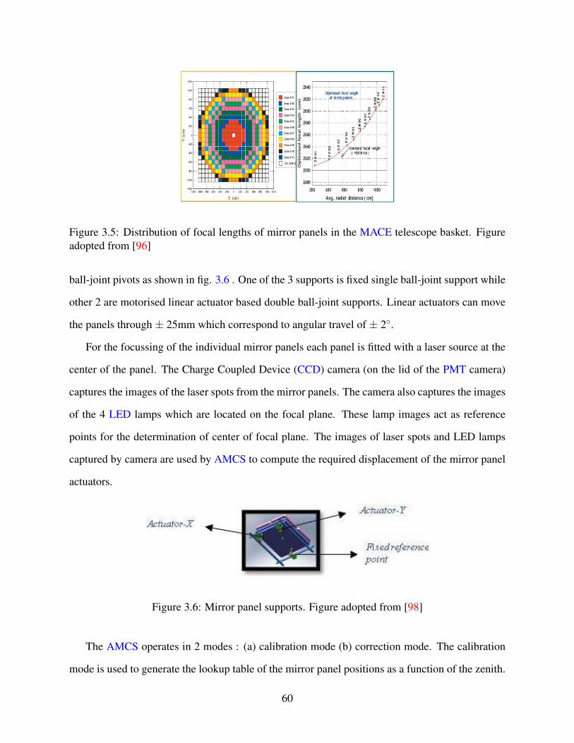
Figure 3.5: Distribution of focal lengths of mirror panels in the MACE telescope basket. Figure

adopted from [96]

ball-joint pivots as shown in fig. 3.6 . One of the 3 supports is fixed single ball-joint support while

other 2 are motorised linear actuator based double ball-joint supports. Linear actuators can move

the panels through ± 25mm which correspond to angular travel of ± 2.

For the focussing of the individual mirror panels each panel is fitted with a laser source at the

center of the panel. The Charge Coupled Device (CCD) camera (on the lid of the PMT camera)

captures the images of the laser spots from the mirror panels. The camera also captures the images

of the 4 LED lamps which are located on the focal plane. These lamp images act as reference

points for the determination of center of focal plane. The images of laser spots and LED lamps

captured by camera are used by AMCS to compute the required displacement of the mirror panel

actuators.

Figure 3.6: Mirror panel supports. Figure adopted from [98]

The AMCS operates in 2 modes : (a) calibration mode (b) correction mode. The calibration

mode is used to generate the lookup table of the mirror panel positions as a function of the zenith.

60

In this mode the telescope basket is moved through the steps of 10 zenith. At each step the re-

quired actuator displacements for all mirror panels are computed and stored in AMCS table. The

calibration will be done during the first commissioning and later periodically. AMCS operates

in correction mode during observations. In this mode, the lookup table generated during align-

ment calibration run is used by AMCS to move the mirror panel actuators to positions which are

appropriate for current zenith of the telescope basket.

3.6 Telescope control unit

The TCU [99] is responsible for providing source information, tracking, parking and camera

shutter open/close. It has a servo control that supports precision tracking of the celestial sources.

The accurate observation of a celestial source requires the telescope to steer in three modes (a)

Slew mode, (b) positioning mode and (c) tracking mode.

The TCU operates in the slew mode when switching the observation from one source to an-

other. In this case quick repositioning of the telescope is required so as to reach the new source

position rapidly. This is achieved by on the fly change in the servo drive’s transmission gear ratio.

Gear boxes of servo controller are specially designed to have support for 2 overall gear ratios. For

the high speed slew mode operation gear ratio of 6000 is used while for normal tracking operation

gear ratio of 36000 is used. The position mode is used during observational runs for pointing

calibrations. In this mode the telescope is maintained at the designated position. The wind and

other disturbances are continuously corrected for by using feedback from precision encoders. In

the tracking mode, the telescope tracks a celestial source in the sky by following the Right Angle

(RA) and Declination (Dec) of that source according to ephemeris. The tracking accuracy of the

TCU is 1 arc min at the wind speed of 30 Kmph. The tracking speed in the range of 0.5 mde-

gree/sec to 0.5 degree/sec with the tracking acceleration up to 0.02 degree/sec2 is supported by the

TCU. The telescope can be stowed to parking position under very high wind speed conditions.

61

3.7 The MACE camera

An imaging camera is the most important part of any IACT. The MACE telescope has the

imaging camera [98] consisting of 1088 PMTs at the focal plane of the basket. The detection

of Cherenkov flashes from the EAS that lasts for only ∼ 10 ns combined with few nanoseconds

pulse width of PMTs require a very fast electronics in the camera back end. For this purpose all the

components of camera like PMT HV supply unit, signal processing unit, trigger generation unit as

well as data acquisition unit have been integrated together at the same place. The complete camera

instrumentation is located behind the PMT array on the focal plane of basket. This arrangement

avoids the signal transmission delays and losses that can occur in the case where the raw PMT

signals are carried by the cables to back end electronics that is located on the ground. Only cables

connected to the MACE camera from the ground control station are power cables and optical fiber

data links for the communication and data transfer. We will describe different components of the

MACE camera in the following sections.

3.7.1 The photomultiplier tube array

The front end of the MACE camera consists of 1088 PMTs (ET Enterprises make 9117WSB)

each with diameter of 38 mm arranged in triangular pitch [98]. The Winston cone type light guide

made up of acrylic is fitted on top of each PMT to minimize the dead surface area on the camera.

The light guides have hexagonal entry aperture with pitch value (distance between parallel sides)

of 55 mm and circular exit aperture of diameter 32 mm. The effective collection efficiency of

light guides have been experimentally measured to be 85%. At the focal length of 25 m angular

size of camera pixel measures to be 0.125 . The total field of view of the camera is 4.3 × 4.0.

The inner region of the field of view 2.6 × 3.0 consisting of 576 pixels participate in the trigger

generation of the events.

62

(a) (b)

(c)

Figure 3.7: (a) : Camera housing front view with 64 light guide cups in place and shutter open

(b) : Camera housing view from back (c) : Camera cage assembly drawer where CIMs would be

placed (Mid section of the camera) Figure adopted from [98]

3.7.2 The camera housing structure

For the accurate tracking of the celestial sources stability of the camera and it’s components

in the focal plane during the observations is very crucial. For this purpose complete camera

instrumentation will be mounted inside a very rigid yet light weight camera housing [98]. The

camera will be held at the focal plane by camera mounting bracket which is attached to four

booms coming from the basket. The camera housing will be fastened to the camera bracket. The

camera housing can be divided into 3 parts.

63

1. Front: This is the part that faces the mirror basket when camera is mounted on the tele-

scope. It consists of (a) a front lid with motor,gear box and limit switches for open/close

operation (b) housing frame for light guides and (c) 8 manual latches. The front lid is made

up of 2 overlapping honeycomb panels which can be open/closed using motorised shutter

mechanism. The 2 panels of the lid can open/close with programmable angular phase dif-

ference up to 20. The maximum open angle is 109. The light guide housing frame holds

the light guides on top of PMT array in appropriate positions. Manual latches are provided

for secure clamping of front lid in parking position.

2. Mid : This part of the housing has (a) cage drawer assembly (b) Camera Integrated Modules

housings and (c) 8 pairs of clamps. The cage drawer assembly has 68 square pockets to hold

68 CIMs. Each pocket holds one CIM in place rigidly.

3. Back: The back part of housing contains (a) sliding mounts for back end electronics (b)

honeycomb lids with door stays. Sliding mounts will facilitate the removal/insertion of the

CIMs and other electronics components during maintenance. Back door is not motorised

and has to be manually opened/closed. It’s primary aim is protection of electronics from

environmental and other wear and tears.

The complete mechanical structure of the camera has dimensions of ∼ 2m × 2m × 2m. It’s total

weight including PMTs and camera electronics is 1300 kg. Fig. 3.7 shows the front, back and mid

sections of the camera housing.

3.7.3 Camera electronics

The central four units of camera electronics are a CIM, a Data Concentrator (DC), a Central

Camera Controller (CCC) and an Second Level Trigger Generator (SLTG) [100] . We briefly

describe these units in the following.

• CIM

The camera electronics of 1088 PMTs of the MACE is divided into 68 CIMs where each CIM

64

Figure 3.8: Schematic block diagram of of CIM. Figure adopted from [98]

integrates the electronics for 16 PMTs. A CIM consists of electronics blocks for power supply,

amplification, pulse shaping and discrimination, storage of output in analog memory buffers and

pulse digitisation for each PMT. Each CIM has 4 High Voltage (HV) cards where each card

provides power supply to 4 PMTs. The HV is applied to PMT through Voltage Divider Net-

work (VDN), thereby controlling the potential difference between cathode, anode and dynodes.

MACE implements low gain PMTs for a longer operational life under LONS. Two low noise

high bandwidth amplifiers placed in series at the output of each PMT amplify the PMT output.

The amplifiers have gains of 1.4 and 10 respectively. Domino Ring Sampler (DRS)s placed on

65

each CIM continuously sample pulse profiles at the output of low-gain and high-gain amplifiers

of all PMTs at the rate of 1 GSPS and store them to analog memory consisting of 1024 channels

each. Dual-channel Flash Analog to Digital Converter (FADC) with 14-bit resolution digitises

the samples in each DRS in the region of interest. Each CIM also consists of electronics for First

Level Trigger Generation (FLTG), event processing and data packet formation for the CIM. The

Field Programmable Gate Array (FPGA) unit passes the reshaped pulse profiles to FLTG unit

on the CIM where FLTG detects 3 partial or 1 full trigger with coincidence window of 5 ns. A

full trigger is when a close cluster of adjacent channels with predefined multiplicity crosses the

preprogrammed threshold. Closed clusters of adjacent trigger channels on the border of a CIM

with a multiplicity more than half the target multiplicity, half the target multiplicity or less than

half the target multiplicity constitute other 3 partial triggers respectively. Each FLTG fans out 4

binary signals each corresponding to one of four trigger conditions in the CIM described above.

An event data packet consisting of an event number, DRS stop cell number and hit-pattern is

formed for each CIM in parallel to data digitisation. The packets are stored to local First In

First Out (FIFO) memories of CIM. A process controller card mounted on each CIM monitors

different parameters of CIM like Single Channel Rate (SCR), Prompt Coincidence Rate (PCR),

Chance Coincidence Rate (CCR), board temperature, PMT anode current. It also controls PMT

HV bias and event data transmission links to DC. Fig. 3.8 shows the schematic of the CIM

electronics.

• CCC

CCC of the MACE [101] controls the camera electronics, maintains the logs of the status of

electronics components and works as the interface between the camera and operator console

at the ground station. Fig. 3.9 shows the schematic diagram of CCC. There are four blocks

in CCC, namely Single Board Computer (SBC), CCC microcontroller card, FPGA section and

power supply and I/O section. SBC is the primary interface between camera electronics and

operator console at the ground. CCC micro card and FPGA receive the control commands from

the operator console through the SBC. PC104 plus unit with 1GHz processor with 512 MB

66

Figure 3.9: Schematic block diagram of of Central Camera Controller. Figure adopted from [101]

RAM and 8GB Flash is used as SBC. The microcontroller card on CCC handles the switching

of CIMs to ON/OFF mode, other CIM controls, and status logging. The CCC collects the event

and telemetry data from DC through its FPGA sections. The power supply requirements of all

the subsystems and external units are provided by the power supply and I/O section. The CCC

also takes charge of periodically carrying out the sky and LED calibration runs as configured

before the observations. Temperature Controller (TC) on CCC maintains the CIM temperatures

by controlling the rpm of cooling fans placed behind the camera. In case of overheating, the

TC switches off a CIM and logs the status accordingly.

67

• Data Concentrator

For each triggered event each of 68 CIMs collects charge data for low and high gain channels

Figure 3.10: Flow of control signals and data to and from Data Concentrator. Figure adopted from

[98]

of its 16 PMT outputs. The pulse profile data for all the channels which cross the discrimination

threshold is also collected. The profile data consists of 31 samples of instantaneous charge data

for each pulse taken at intervals of 1 ns. The charge data amounts to 96 Bytes while full profile

data amounts to 2080 Bytes for single CIM. This adds up to 6.584 KBytes of data for single

event when only charge data is collected. If profile data is collected for hit pixels (i.e. pixels

which crossed the trigger threshold) single event data size is expected to be 13.3 KBytes. With

the 1kHz event rate at which the MACE is expected to operate, ∼ 13 MBytes of data will be

coming to DC per second. To handle this large inflow of data DC has 1 hardware FIFO for each

CIM. These FIFOs can store single CIM data of up to 32 events. The DC also attaches the time

stamp to each event so that an event data can be properly collated later. The IRIG-B00 format

time code received from the unmodulated output signal of master clock at control room is used

as an event time stamp. The master clock is synchronised with GPS and has the accuracy of 1

µsec. DC collects, compiles and transmits the data from each CIM FIFO to ground station via

1 Gbps Ethernet link. Fig. 3.10 shows the schematic diagram of working of DC

68

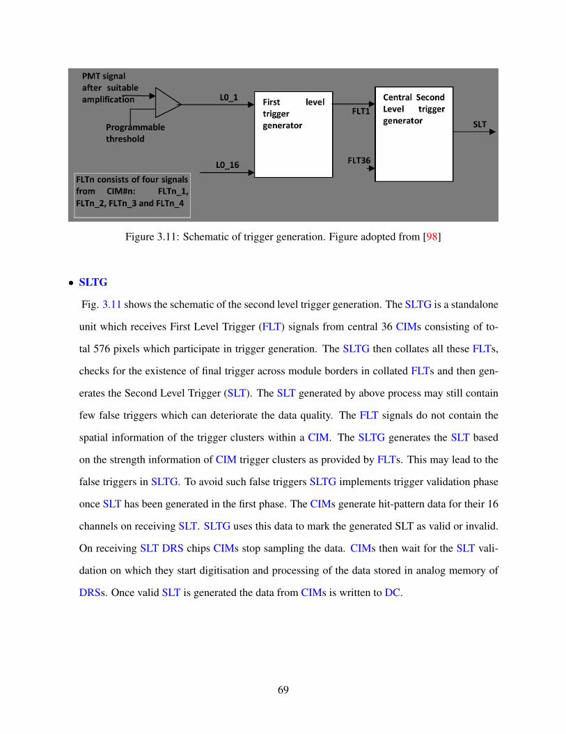
Figure 3.11: Schematic of trigger generation. Figure adopted from [98]

• SLTG

Fig. 3.11 shows the schematic of the second level trigger generation. The SLTG is a standalone

unit which receives First Level Trigger (FLT) signals from central 36 CIMs consisting of to-

tal 576 pixels which participate in trigger generation. The SLTG then collates all these FLTs,

checks for the existence of final trigger across module borders in collated FLTs and then gen-

erates the Second Level Trigger (SLT). The SLT generated by above process may still contain

few false triggers which can deteriorate the data quality. The FLT signals do not contain the

spatial information of the trigger clusters within a CIM. The SLTG generates the SLT based

on the strength information of CIM trigger clusters as provided by FLTs. This may lead to the

false triggers in SLTG. To avoid such false triggers SLTG implements trigger validation phase

once SLT has been generated in the first phase. The CIMs generate hit-pattern data for their 16

channels on receiving SLT. SLTG uses this data to mark the generated SLT as valid or invalid.

On receiving SLT DRS chips CIMs stop sampling the data. CIMs then wait for the SLT vali-

dation on which they start digitisation and processing of the data stored in analog memory of

DRSs. Once valid SLT is generated the data from CIMs is written to DC.

69

Figure 3.12: Schematic of the MACE calibration System. The pulser LED along with diffuser

uniformly illuminates 1088 pixels of the MACE camera during the relative gain calibration runs

[102].

3.8 Calibration system

The reconstruction of an event during the analysis of an IACT data requires that response

of the light detection and amplification chain be measured as accurately as possible. This is

achieved by the calibration system of the MACE telescope. Fig. 3.12 shows overall arrangements

of the calibration system [102]. It consists of an electronics pulser which drives the ultra fast

blue LEDs.A diffuser is placed on top of LEDs so that all the pixels of the camera are uniformly

illuminated. The system is placed inside the calibration box at the center of the telescope basket

facing the camera. The electronics pulser provides 5 high-speed pulses which drive the LEDs

with varying intensity. Each LED flash lasts for 8-10 ns. Relative gain calibration of the camera

PMTs can be done using the PMT data collected in response to the LED flashes. For the absolute

gain calibration, absolute gain calibrated reference PMTs are used. The number of flashes in

each calibration run (i.e. LED calibration events in one calibration run ) and the periodicity of

the calibration runs can be configured in the LED driver. This is done by LED Calibration Server

(LCS) software which interfaces between calibration hardware and the centralised MACE console

70

software.

3.9 MACE console software

The MACE Console Software [103] is a centralised software to control different subsystems

of the MACE telescope which runs on the workstations at the ground control. An operator in-

teracts with the telescope through this software. Display widgets like event data display widget,

telemetry display widget, TCU widget, SkMS widget, WMS widget are developed so as to assist

an operator in system health monitoring. A configuration utility for interactive configuration of

experimental and system parameters is also a part of MACE Console Software. The scheduler

software module gives information regarding availability of different sources given the time. The

event data retrieval module for search and retrieval of event and housekeeping data from data

archival is also provided. The data can be fetched on the basis of various parameters like run

number, source name, range of time in terms of year,month or date when data was taken etc. Fig.

3.13 shows the snapshot of the MACE console GUI.

Figure 3.13: MACE Console Software GUI. Figure adopted from [103]

71

3.10 Data archiving system

The MACE telescope uses a combination of tape Solid State Drive (SSD)s, Hard Disk Drive

(HDD)s and tape drives to realise a robust and fast DArS [104]. SSD with volume of 4 TB

constitutes the cache storage of the DArS where a raw data from the DC of the MACE telescope

will be directly sent via gigabyte Ethernet Local Area Network (LAN). The MACE observational

data generated over a fortnight assuming data generation rate of 250 GBs per day can be stored on

the SSD cache. The cached data would be transferred by two simultaneous threads to LTO-6 tape

drive storage and HDD based storage. The dual copies of the data on the tape drives and HDD

storage provides redundancy and fault tolerance.

3.11 Sky monitoring system

As the name suggests SkMS monitors the sky transparency levels. It also monitors the tracking

accuracy of the telescope. The cooled CCD camera mounted perpendicular to the telescope axis

on the basket acts as an SkMS. It periodically captures and analyses the sky images during the

observation. Sky conditions and tracking accuracy are quantified through this analysis.

3.12 Weather monitoring system

The Weather Monitoring System records the weather data to check the suitability of the

weather for the telescope operation [105] . It consists of five components namely, weather station

data logger, sky quality meter, pyrometer, anemometer and a fish eye camera. Data regarding tem-

perature, humidity, wind speed etc. are recorded by weather station data logger. It also provides

graphs and alarms. Pyrometer gives the temperature of the sky surface and gives idea about sky

clarity while sky quality meter records sky brightness. Anemometer gives an accurate value for

the wind speed. The weather packets are sent to the MACE operator console where console can

generate alerts and warnings if any of the weather parameters go out of the safe operating range.

72

3.13 Solar power station

The MACE solar power stations consists of 2 sets of Solar Photo Voltaic (SPV) panels along

with their battery banks and charge controllers [106]. Total number of SPV panels is 1400. The

lead-acid tubular stationary type batteries with positive tubular plate are used for battery bank.

The self discharge rate of these batteries is less than 3% per month. The fully charged station can

power the MACE facilities for 3 days without interruptions. The solar panels are provided with

the Schottky bypass diodes for protection against the hot spots.

The estimation of the various trigger performance parameters are presented in the next chap-

ter. This includes the estimation of optimum single channel discrimination threshold and optimum

trigger configuration for MACE operations, effective collection area, differential and integral trig-

ger rates and trigger energy threshold.

73

CHAPTER

FOUR

TRIGGER PERFORMANCE ESTIMATES FOR MACE

4.1 Introduction

The simulation studies of an IACT play an important role in finding the optimum value of

operating parameters for the telescope. An IACT must be operated in such a way that it gives

lowest possible energy threshold and highest possible sensitivity. The performance of the MACE

trigger and different aspects affecting it were studied through simulations in this doctoral work.

All these studies related to MACE trigger performance are presented in this chapter in detail.

4.2 Simulation software

A simulation study of IACTs broadly involves following tasks. 1. Simulation of Extensive

Air Showers, 2. Simulation of response of all IACT telescope components and 3. Application of

all the IACT image analysis steps on the triggered events. 4. Estimation of various performance

parameters for the IACT. Simulation of EAS has been performed using a freely available code

CORSIKA. A C++/ROOT based code to simulate an IACT response to EAS and IACT data anal-

ysis was developed for the work presented in this thesis. The details of these two softwares are

75

described in following subsections.

4.2.1 CORSIKA (COsmic Ray SImulations for KAskade)

The simulations of EAS in the entire thesis work have been performed using CORSIKA. COR-

SIKA [107, 108] is a well established code for Monte Carlo simulations of particle air showers

in the fields of astroparticle and high energy physics. It was originally written in FORTRAN 77

for the simulations of particle air showers in KASKADE [109] experiment. Particle air showers

induced by different types of primary particles like Protons, light nuclei (up to Fe56), photons,

Muons, Electrons and many other particles found in CRs can be simulated using CORSIKA. The

shower development in the atmosphere can be simulated accurately for primary particles with

energies up to 1020 eV. CORSIKA tracks each particle produced in an EAS through every inter-

action it undergoes with atmospheric nucleus. If a particle produced in an EAS is unstable then

it is tracked till its decay. The type, energy, location, direction and arrival time of all the parti-

cles produced in an EAS which reach the selected observation level is given in the output of the

CORSIKA.

Particle interactions in EAS are simulated by CORSIKA using cross-sectional data from ex-

periments wherever possible. Hadronic and electromagnetic interaction models available within

CORSIKA are as follows.

• High Energy Hadronic Interactions Models

– DPMJET (Dual Parton Model with JETs) : Two component Dual Parton Model with

soft chains and multiple mini-jets are used to describe hadron-nucleus and nucleus-nucleus

hadronic interactions at high energies in DPMJET code [110].

– HDPM : This is simple model based on the Dual Parton Model that incorporates the exper-

imental data wherever available [108]. It is optimised for speed and simplicity. However

showers induced by heavier nuclei can not be simulated realistically with this model.

76

– QGSJET (Quark Gluon String model with JETs) : The scattering amplitude of high

energy elastic collisions between hadron-nucleon are modeled using quasi-eikonal Pomeron

parameterization in QGSJET model [111, 112, 113, 114].

– SIBYLL : This model reproduces the hadronic interactions at extremely high energies using

Quantum Chromo Dynamics (QCD) mini-jets [115, 116, 117].

– VENUS (Very Energetic NUclear Scattering : In this model elastic scattering amplitudes

are modeled using Gribov-Regge theory while inelastic scattering amplitudes are expanded

in terms of topological cross sections. Ultrarelativistic heavy nuclei interactions can be de-

scribed using this model [118].

– neXus (NEXt generation of Unified Scattering approach : Features of VENUS and QGSJET

are combined along with new ideas from H1 and Zeuss data in this model [119].

– EPOS (Energy conserving quantum mechanical multi-scattering approach, based on

Partons Off-shell remnants and Splitting parton ladders): NEXUS framework with im-

provements in hard interactions, nuclear and high density effects are used in EPOS model

[120]. This model shows good agreement with RHIC data.

• Low Energy Hadronic Interaction Models

– FLUKA : FLUKA is code to simulate transport and interaction of particles and photons

within matter[121]. It can simulate propagation and interaction of 60 different particles hav-

ing energy between 1 keV up to 20 TeV through the matter.

– GHEISHA (Gamma-Hadron-Electron- Interaction SHower code): This code can treat

transport and interactions of all stable and weakly decaying particles including baryons, anti-

baryons and nuclear fragments [122]. A fragmentation mechanism is used for energies above

∼ 0.5 GeV.

– UrQMD (Ultra-relativistic Quantum Molecular Dynamics: Low energy hadron-nucleus

interactions are modeled using UrQMD [123]. It can be applied for the interactions in energy

range of Elab < 100 MeV/nucleon up to Elab > 200 GeV/nucleon.

77

Various hadronic interaction models have been compared in [124, 125].

• Electromagnetic Interaction Models

– EGS4 : The EGS4 model for the electromagnetic interactions in shower development allows

for the full Monte Carlo treatment of the electromagnetic component.[126] Such detailed

treatment is necessary for the simulation of showers when primary particles have energy

more than TeVs.

– NKG : The NKG model uses the analytical formulation provided by the NKG approxima-

tions for the calculation of the lateral electron densities as well as pseudo-age parameters[127].

A lateral grid of 80 points starting from radial distance of 100 cm up to the outer distance

as provided by the user is used for evaluation of electron densities at observation level. The

longitudinal development is sampled at each 100 gm/cm2 above the lowest observation level

for the evaluation of electron density and pseudo-age.

Many add-on packages suited for other experiments have been contributed by physicists all

over the world in 30 years since the development of CORSIKA. HEGRA collaboration developed

the routines to simulate the Cherenkov radiation of an EAS [128]. Konrad Bernlohr further devel-

oped these tools to include all the atmospheric effects on the Cherenkov radiation of EAS [129].

The IACT/ATMO extension of CORSIKA developed by Bernlohr now provide [130]

a) models of atmospheric profiles with accurate refractive indices and extinction coefficients for

different climate zones

b) a flexible interface to configure arbitrary arrays of Cherenkov detectors with uneven elevation

levels of detectors

c) a machine independent binary output format named ‘eventio’ which provides very good I/O

speed and compression. Only data of the Cherenkov photons passing the configured Cherenkov

detectors is stored in this format.

78

The simulations of EAS throughout this work has been done using CORSIKA package along with

IACT/ATMO extension. The EAS data was thus stored in ‘.evt’ files generated by IACT/ATMO

extension and used for later stages of simulation.

4.2.2 MACE simulation program

A code for general IACT simulations was developed for the thesis work. The code is written in

C++ using ROOT [131] libraries. Object oriented approach has been followed in program design

where every component of an IACT is represented by a C++ class. ROOT based command line

interface is developed through which all the tasks of the simulation can be performed. It uses

Parallel ROOT Facility (PROOF) [132] to enable parallel computations over a cluster of PCs.

Few of the important classes and their features are as follows

• MReflector : This class simulates the response of the reflector of an IACT. Simulation of

monolithic and tessellated reflector designs are supported. The reflector object can be config-

ured to hold arbitrary number of mirror facets in arbitrary shaped 2D array. The hexagonal,

circular and square pitch of mirrors are supported. The mirrors and the basket can be either

spheroidal or parabolic. The class object ray traces an incident ray onto the focal plane. The

position,wavelength and time of arrivals of the reflected rays at the focal plane is then found

out. Thus a raw image of an EAS in terms of position and arrival times at the focal plane is

formed by this object.

• MCameraLayout : This class simulates the camera geometry. It can be configured to hold arbi-

trary number of PMT pixels in arbitrary shaped 2D array. The pixels i.e. Compound Paraboloid

Concentrator (CPC) entry apertures, can be hexagonal, circular or square. This class object

receives the raw image formed by the MReflector object and finds the pixel in which each re-

flected ray falls. It discards all the rays which fall into voids in focal plane. It also takes into

account the collection efficiency of the CPCs.

The LONS contribution to an EAS image is also simulated through this class. Mean number

79

of photo-electrons (pe) due to LONS per pixel per nanosecond has to be given as an input for

this purpose. Poissonian noise with the described mean is then added to each pixel to simulate

LONS contribution. The noise can be simulated either by adding total pe due to LONS to each

pixel or by generating time of arrivals for each photo-electron induced by LONS.

• MPatternTrigger : This class simulates the topological trigger in the image formed by MCam-

eraLayout. This includes 28 different topological configurations with trigger multiplicity rang-

ing from 3 to 6. Any arbitrary shaped 2D array of pixels within camera can be configured to

be trigger region. Nearest neighboring (NN) trigger patterns as well as Closed Cluster Nearest

Neighbouring (CCNN) trigger patterns in each trigger multiplicity can be simulated. The cam-

era pixels may be divided into modules of arbitrary shapes. The triggers can be classified on the

basis of number of modules taking part in trigger formation in case pixels are divided between

many modules.

• MImageAnalyser : This class is in control of image analysis. It has a routines to perform tail

cut image cleaning and Hillas parameterisation (refer to sec. 6.2).

• MSimManagerProof : This class is an interface class for steering of simulation. It starts

the PROOF session at the provided address and manages it throughout the simulation run. It

allows the user to configure different components of an IACT through input files. It has method

‘Simulate’ to run the simulation chain with given configuration on the PROOF cluster. This

method generates the output of the simulation run and stores it to the dataset spread over the

PROOF cluster. The dataset is cataloged and can be accessed simply by an entry in the catalog

for the later processing. The class has methods to generate effective area and differential rate

curves from the given dataset. This class also provides method to randomly split any dataset

into train/test subsets. These subsets then can be retrieved to the client machine for estimation

of sensitivity.

There are many other auxiliary classes for data I/O and other functionalities.

80

4.3 Details of simulations

The Values of different general input parameters used in the simulation studies are described

in this section. This includes input parameters of CORSIKA and configurations used for different

telescope components.

4.3.1 Input parameters of CORSIKA

CORSIKAv6.735 was used to simulate development of EAS initiated by CR and γ ray pri-

maries in atmosphere. QGSJET I and FLUKA models were used for the high and low en-

ergy hadronic interaction respectively. Electromagnetic interactions were simulated using EGS4

model. The values of the geomagnetic field components were calculated using IGRF model [133]

for Hanle site. North and downward vertical components of geomagnetic fields were set at 31.95

µT and 38.49 µT respectively.

Add-on IACT/ATMO package supplied by Konrad Bernlohr [130] was used to extract the

Cherenkov photon data from the EAS data. Cherenkov photon data within a spherical detector of

radius 11 m placed at the observation level of 4270 m asl was stored for all CORSIKA runs. The

IACT/ATMO package was also used to simulate effects of atmospheric absorption of Cherenkov

photons, mirror reflectivity and quantum efficiency of the MACE PMTs. The U.S. standard at-

mospheric model as provided by IACT/ATMO package was used to simulate atmospheric density

and extinction coefficients due to non-availability of atmospheric data for the Hanle site. It should

be noted here that Cherenkov photon distributions on the ground may vary by up to ∼ 60% near

shower axis [129] depending on the atmospheric profile chosen. The variation of the mirror re-

flectivity and PMT quantum efficiency against the incident wavelength has been measured for

the MACE telescope. The effects of mirror reflectivity and quantum efficiency on the Cherenkov

photons of EAS were simulated through the CERQEF option of the CORSIKA by providing the

reflectivity and qunatum efficiency tables of the MACE. Wavelength dependence of Cherenkov

emission angles was simulated by enabling ‘CERWLEN’ routines of CORSIKA. Cherenkov pho-

81

tons in the wavelength range of (240 - 650) nm were recorded. This is in accordance with the

spectrum of Cherenkov radiation from EAS and quantum efficiency of the MACE. The bunching

of the emitted Cherenkov photons was disabled by keeping bunch size parameter 1.

4.3.2 Telescope parameters of simulation

The quasi parabolic design of the MACE reflector was configured in simulations. This includes

the parabolic basket and 356 spherical mirror panels with focal lengths varying between 25.0 m -

26.16 m depending on the zone of the reflector. The layout of the basket as set up in simulations

is shown in fig. 3.5.

X­axis (cm)

­80 ­60 ­40 ­20 0 20 40 60 80

Y­a

xis

(cm

)

­80

­60

­40

­20

0

20

40

60

80

Figure 4.1: MACE camera layout. There are total 1088 pixels, divided in 68 modules of 16

channels each. Central 576 pixels i.e. 36 modules, shown by darker grey shades, constitute the

trigger area. Representative examples of 3,4 and 5 CCNN trigger patterns are shown in red colour.

The pixel layout of the camera used in the simulations is shown in the fig. 4.1. A central

region of the camera constituted by 24 × 24 pixels is set up as the trigger region as in actual

camera. The trigger region of the camera is shown by shaded pixels. A topological trigger is

checked within the trigger region. All the results presented in the thesis work are quoted for the

82

trigger with topological pattern of 4 CCNN at single channel discrimination threshold of 9.0 pe.

The reasoning behind the choice of such trigger configuration is explained in sec. 4.3.3. For the

simulation of mirror reflectivity and PMT quantum efficiency the measured values of respective

quantities for the MACE telescope were provided in tabular form to CORSIKA. Thus CORSIKA

output thus contains the position and time of arrival of ‘pe’ at the observation level. Fig. 4.2a

shows the quantum efficiency and mirror reflectivity as function of wavelength for the MACE

telescope.

4.3.3 Contribution of the light of night sky

The raw image of an EAS collected by an IACT contains pe due to Cherenkov photons as

well as photons from LONS. Photo electrons due to LONS distort the images heavily. The

distribution of different Hillas parameters may vary significantly depending on the level of LONS

contribution and the parameter values of the cleaning algorithm used. Since Hillas parameters are

used to segregate γ / hadrons, the level of LONS indirectly affects the sensitivity of the telescope.

It may also affect the energy threshold achieved by an IACT after analysis. Realistic estimation

of the contribution from the LONS is thus very important in simulation studies.

The estimates of the LONS contribution derived from the actual measurements of the LONS

light at the nearby site of HCT (Himalayan Chandra Telescope) in Hanle are used in this thesis

work. HCT is a 2 m optical telescope operational in Hanle since August 2000. The flux due to

LONS at Hanle was measured using HCT during 2003 - 2008 [134]. The values of the night sky

brightness during moonless period as reported by [134] are given in table 3.1. These values are

converted to units of photons m−2 sec−1 sr−1 nm−1 using relations given in Leinert et al [135].

Fig. 4.2b shows the photon flux due to LONS as a function of wavelength. A parabolic fit to the

flux data of fig. 4.2b is used to estimate the LONS contribution at each wavelength. A photon

flux due to LONS is multiplied by quantum efficiency and mirror reflectivity at each wavelength

to get photo-electron contribution at each wavelength. The integration of this quantity over the

wavelength range gives the contributions of LONS in terms of mean number of pe per unit solid

83

angle per unit area per unit time. Multiplying by total reflector area and a angular size of a pixel

average number of pe generated by LONS at each pixel in unit time was obtained. ∼ 1.46 pe

are generated at each channel due to LONS in coincidence gate width of 5 ns. To simulate the

contributions of LONS to Cherenkov images random number of pe generated according to Poisson

distribution with mean value of 1.46 is added to each pixel in each image.

Wavelength (nm)

300 400 500 600

η

0

0.1

0.2

0.3

0.4

0.5

0.6

0.7

0.8

0.9

mirrorη

pmtη

(a)

Wavelength ( nm )

350 400 450 500 550 600 650

)­1

.nm

­1.s

r­1

.sec

­2F

lux (

m

0

5

10

15

20

25

910×

(b)

Figure 4.2: (a): Mirror reflectivity and quantum efficiency of PMT as used in simulations. (b):

Measured flux of Night Sky Background light at Hanle, [134]. Solid line represents the parabolic

fit.

4.4 Single channel rate and chance coincidence rates of MACE

The trigger rate of a single PMT is called SCR. It includes trigger of a PMT due to fluctuation

in LONS, afterpulsing of a PMT or genuine Cherenkov light. The false triggers of individual

neighboring channels may coincide in time to generate a false system trigger. The rate of such

false system triggers is called chance coincidence rate (CCR). CCR must be kept at a value of <

5 % of total trigger rate of an IACT for the efficient operation. The CCR depends on SCR which

in turn depends upon the single channel discrimination threshold set up during operation.

84

In absence of PMT afterpulsing discrimination threshold should be set up at a value which

minimises the false trigger due to LONS. In practice though the afterpulsing rates in PMT dictate

the single channel discrimination threshold [136]. Afterpulses are the secondary pulses with very

large amplitudes which are produced after a delay of few hundred ns from the primary pulse of

photo-electron. The inert gas in PMTs is ionised by accelerated photo-electron emitted from photo

cathode. The ions are in turn accelerated towards photo cathode which emit bunch of secondary

electrons due to colliding ions. These secondary electrons cause generation of afterpulses [137].

The discrimination threshold optimised for the suppression of LONS induced triggers still allows

for the false triggers due to afterpulses. The contribution of the afterpulse induced false triggers

to the SCR is orders of magnitude higher than the contribution of LONS induced false triggers, at

a given discrimination threshold [138].

The laboratory measurements of the single channel rates as a function of the single channel

discrimination threshold for 3 gain calibrated PMTs were taken in order to realistically determine

the single channel discrimination threshold. Typical dark night conditions of Hanle were recreated

in the laboratory dark room using LED lights. In this case intensity of LEDs was set in such a

way that PMT anode current matches the expected value of anode current in actual observation

conditions. Standard method to determine the single photo-electron peak was used to measure

the gain of the PMTs. The PMT gains were found to be ∼ 42000, ∼ 54000 and ∼ 60000 when

operated between voltage of 975 V to 1025 V. The average SCR of 3 PMTs as a function of

single channel discrimination threshold expressed in units of pe is shown in fig. 4.3. It should

be noted that same value of discrimination threshold in pe units corresponds to different actual

discrimination threshold when expressed in mV units, since different PMTs have different gains.

An event trigger in an IACT is produced when some number of neighboring pixels within

trigger region of the camera are triggered within predetermined time window of few nanoseconds.

The minimum number of pixels required to participate in the trigger, called the multiplicity of

trigger, varies between 2 to 5. CCR for the single stage trigger of multiplicity m, coincidence gate

85

Photoelectron Threshold (pe)2 4 6 8 10 12 14 16 18 20 22

Ra

te (

Hz)

­610

­510

­410

­310

­210

­110

1

10

210

310

410

510

610

710

810

910

1010

1110

1210

CCR 3CCNN

CCR 4CCNN

CCR 5CCNN

SCR

Figure 4.3: Single channel rate and CCR for different trigger configurations of (3 - 5) CCNN due

to NSB, for the MACE, as a function of the single pixel threshold [139].

width of τ and single channel photo-electron threshold of q is given by

RChance(m) = mCnm

[

Rpixel(q0)]m

τm−1 (4.1)

where RChance is CCR and Rpixel(q) is the SCR at the single channel photo electron threshold of

q and n is the number of total pixels in the trigger region.

However as seen in sec. 3.7.3 the MACE trigger is a two stage trigger. Each module of 16

pixels in trigger region generates a partial FLT with coincidence gate width of 5 ns while final

trigger is generated by collating partial FLTs from trigger modules with coincidence gate width

of 10 ns. Thus in order to estimate the CCR of the MACE for a given SCR, rates of all the partial

FLTs for the given SCR must be first calculated. The FLT rate for l-fold partial trigger within a

module is given by

FLT (l,q) = lCMl ·

[

Rpixel(q0)]m

τl−1 (4.2)

where CMl is number of l-fold partial trigger combinations that can contribute to SLT. Value of

86

τ is 5 ns for the calculation of FLT rate of l-fold partial trigger.CCR of MACE for a SLT with

multiplicity of m, will be given by addition of contribution from each combination of partial FLTs

that can generate m-fold SLT. The CCR for the m-fold SLT due to the combination of 2 partial

triggers with multiplicities l1 and l2 such that l1 + l2 = m is given by

SLT (m,q : l1, l2) =C ·FLT (l1,q) ·FLT (l2,q)τ (4.3)

where τ is the coincidence gate width for second level trigger, FLT (l1,q) and FLT (l2,q) are

the partial FLT rates for multiplicity of l1 and l2 at single channel photo-electron threshold of q

respectively and C is the number of combinations in the trigger region which can form m-fold

trigger by collation of l1 and l2 fold partial FLT triggers.

Fig. 4.3 shows the measured SCR and CCR estimated based on the measured SCR as a func-

tion of single channel photo-electron threshold [139]. CCR is calculated for trigger multiplicity of

3,4 and 5. Assuming the event trigger rate of 1 kHz CCR must be restricted to < 50 Hz in order to

keep it below 5% of prompt rate. Fig. 4.3 shows that the optimised single channel photo-electron

threshold values for the CCNN trigger configurations with multiplicity of 3,4 and 5 are ∼ 22

photo-electron , ∼ 9 photo-electron and ∼ 7.5 photo-electron respectively. The SCR values at the

single channel photo-electron thresholds of 22.5 pe, 9.0 pe and 7.5 pe are ∼ 55 kHz, ∼ 400 kHz

and ∼ 1 MHz respectively. The minimum size of the recorded events at discrimination threshold

of 22.5 pe for 3 fold CCNN trigger will be 67.5 pe. The minimum size of recorded events will be

36 pe for the trigger configuration of 4 CCNN trigger at single channel threshold of 9 pe. The 5

CCNN trigger with single channel threshold of 7.5 pe results in minimum event size of 37.5 pe.

Since low energy events are more likely to generate low size images in an IACT, 3 CCNN trigger

with single channel threshold of 22.5 pe is more likely to eliminate the low energy γ ray events at

the trigger level owing to higher minimum size of recorded events. 4 CCNN trigger with single

channel threshold of 9.0 pe and 5 CCNN trigger with single channel photo-electron threshold of

7.5 photo-electron have similar minimum size of recorded events. However 4 CCNN trigger with

87

photo-electron threshold of 9.0 pe was chosen to carry simulation studies as it is topologically

lenient compared to 5 CCNN trigger.

4.5 Data sample for estimation of trigger performance

The trigger performance of MACE at zenith angles of 0, 20, 40 and 60 was studied in

this thesis. The response of MACE trigger to showers induced by γ , Proton, Electron and Alpha

particles was considered. Thus EAS datasets generated for the study consisted of 106 showers for

each of the primary particles at each of the zenith angles described. In table 4.1, we list the energy

range, scatter radius and angular offset w.r.t. the telescope direction used for the EAS simulation

of each primary particle. The energy range for γ ray and electrons was kept 5 GeV to 10 TeV.

For Proton and Alpha particles the energy range of 10 GeV to 10 TeV was chosen. The angular

offset of the direction of primary w.r.t. telescope direction varied from 4 to 6 depending on

the zenith angle and primary particle. These simulation studies are carried out for point like γ

ray sources and hence the direction of γ rays is always kept parallel to the direction of telescope

pointing. Maximum distance of the primary from the telescope axis is kept between 400 m to 650

m depending on the type of primary and zenith angle of the dataset. All the datasets were simulated

with energy distribution following power law. The spectral index values of 2.59, 2.73, 2.64, and

3.07 were used for simulation of γ , Proton, Alpha and Electron induced EAS respectively.

4.6 Calculation of effective area and trigger rates

The EAS induced by primary axis falling up to distance of few hundred metres from an IACT

telescope have non zero probability of triggerring the telescope. Thus the effective area of detec-

tion of an IACT is weighed sum of all the area around the IACT up to which EAS can be detected.

The probability of the trigger is used as the weight in such summation. However probability of

the trigger depends on the type, energy, impact distance, offset angle w.r.t. Telescope direction

88

Primary Particle Gamma Electron

Zenith Angle 0 20 40 60 0 20 40 60

Energy Range (GeV) 5−104 5−104

Scatter Radius (m) 400 450 500 550 400 450 500 550

View Cone Angle – – – – 4 4.5 5 5.5

Primary Particle Proton α particle

Zenith Angle 0 20 40 60 0 20 40 60

Energy Range (GeV) 10−104 20−104 10−104 20−104

Scatter Radius (m) 500 550 600 650 500 550 600 650

View Cone Angle 4 4.5 5 5.5 5 5.5 5.5 6

Table 4.1: Summary of the input parameters of all the four primary particles for generating EAS

library at four different zenith angles using CORSIKA package. Million showers were generated

for each of the primaries at each zenith angle. All the showers have been generated at a fixed

azimuth angle of 0 (North direction)

and zenith angle of the primary particle inducing an EAS. The calculation of effective areas and

trigger rates is described in this section.

4.6.1 Effective area

The trigger probability for the point γ-ray source can be calculated using equation

p(R,E) =Ntriggered(R,E)

NTotal(R,E)(4.4)

where R is the impact parameter of a shower, E is the energy of the primary gamma inducing it,

Ntriggered(R,E) is the number of triggered events at core distance and energy values of R and E

respectively while NTotal(R,E) is the total number of γ ray EAS simulated with core distance and

energy values of (R,E). It should be noted here that direction of all the γ rays is parallel and hence

there is no dependence on the solid angle of the primary direction around the telescope axis. For

all the other primaries the trigger probability is given by

p(R,E,Ω) =Ntriggered(R,E,Ω)

NTotal(R,E,Ω)(4.5)

89

where Ω is the solid angle of the primary particle direction around the telescope axis. Rest of the

symbols have same meaning as in eq. 4.4. Once the trigger probabilities are known, the effective

area for the γ ray can be calculated using equation

Ae f f (E) = 2π

Rmax∫

0

R× p(R,E)dR (4.6)

where p(R,E) is the trigger probability for the given trigger configuration as a function of core

distance and primary energy, Rmax is the maximum value of an impact parameter up to which

p(R,E) is non-zero. In simulations the data of the simulated EAS is divided into fine bins of

core distance R and energy E. The trigger probability for each bin is calculated and the integral is

replaced by a summation as follows,

Ae f f (E) =n

∑i=1

π(R2i −R2

i−1)p(Rci ,E) (4.7)

where n represents number of bins along core distance, with R0 = Rmin = 0, Rn = Rmax and Rci is

the center of ith bin.

The effective area for the CR primary is given by ,

Ae f f (E) =

Rmax∫

0

2πRdR

Ωmax∫

0

p(R,E,Ω)dΩ (4.8)

where p(R,E,Ω) is the trigger probability as a function of energy, core distance and solid angle

subtended by primary direction and telescope pointing axis, Rmax is the maximum value of impact

parameter while Ωmax is maximum value of solid angle up to which p(R,E,Ω) are non-zero. The

eq. 4.8 is discretized into,

Ae f f (E) =n

∑i=1

π(R2i −R2

i−1)m

∑j=1

p(Rci ,E,Ω

cj)(Ω j −Ω j−1) (4.9)

for simulation studies where m represents the number of bins in Ω, Ω0 = Ωmin = 0, Ωm = Ωmax

90

and Ωcj is the center of jth bin. It should be noted that effective area is function of energy and it

increases with increasing energy.

4.6.2 Trigger rate and energy threshold

The number of triggered events per unit range of energy per unit time is called the differential

trigger rate of the telescope. For a given primary particle with a known differential flux dNdE

,

differential trigger rate for telescope , for that particle is given by,

dNt(E)

dE= Ae f f (E)×

dN(E)

dE(4.10)

wheredNt(E)

dEis the differential trigger rate of the telescope, while

dN(E)dE

is the differential flux of

particles. It should be noted here that for point γ ray sources dNdE

gives us the number of γ photons

coming from source per unit time per unit energy range per unit area. On the other hand for rest

of the CRs dNdE

is the number of particles per unit time per unit energy range per unit area per unit

solid angle. The distribution of CR directions is nearly isotropic.

The energy at which differential trigger rate curve for a particular progenitor particle peaks,

is the trigger energy threshold of the telescope for that particle. It is clear from the eq. 4.10 that

the differential trigger rate and the therefore energy threshold depends on the differential flux of

the particle. Crab nebula has been observed to be steady source of the VHE γ ray emissions for

long period. It is used as the standard candle of the VHE γ ray astronomy. Thus telescope perfor-

mance parameters are always quoted for the mesaured differential flux of VHE γ rays from Crab

nebula.The spectrum of VHE γ rays as measured by HEGRA and MAGIC telescopes [31, 140]

are used to estimate the trigger performance parameters for γ rays. Spectra of Protons, Electrons

and Alpha as reported in ([141, 142, 143]) are used to estimate their respective differential trigger

rates and corresponding energy thresholds. Eq. 4.11 - 4.15 give differential flux spectra used for

the γ-ray, Proton, Electron and Alpha respectively.

91

Impact Parameter(m)0 50 100 150 200 250 300 350 400

Tri

gg

er P

rob

abili

ty

0

0.2

0.4

0.6

0.8

1 5 - 10 TeV

158 - 200 GeV

100 - 125 GeV

40 - 63 GeV

16 - 25 GeV

4CCNN ,

zenith°

9.0 pe, 0

(a)

Energy (GeV) 1 10 210 310 410

)2 E

fffe

ctiv

e A

rea

(m

210

310

410

510

Gamma, 4CCNN zenith

°9.0 pe, 0

(b)

Energy (GeV) 1 10 210 310 410

)2 E

fffe

ctiv

e A

rea

(m

10

210

310

410

510

zenith°

4 CCNN, 9.0 pe, 0

Proton

Electron

Alpha

(c)

Figure 4.4: (a): Trigger probability for γ rays of different energies as a function of core distance

measured in shower plane projection from telescope axis, at trigger configuration of 4 CCNN

and single channel threshold of 9 pe, at 0 zenith (b): Effective area of γ-rays at 0 zenith, for

4 CCNN trigger configuration at 9 pe single channel threshold. Error bars correspond to 1σ

Poissonian noise on the number of triggered events within core distance bin propagated through

simulation. (c): Effective area of Proton, Alpha and Electron at 0 zenith for single pixel photo-

electron threshold of 9 pe and 4 CCNN trigger configuration.

dNγ

dE= 2.79×10−10

(

E

1TeV

)

−2.59

m−2s−1GeV−1 Power law (4.11)

dNγ

dE= 6×10−9

(

E

300GeV

)

−2.31−0.26log10( E300GeV )

m−2s−1GeV−1 Log Parabola (4.12)

dNp

dE= 1.37×104

(

E

GeV

)

−2.73

m−2sr−1s−1GeV−1 Proton (4.13)

dNe

dE= 1.849×102

(

E

1GeV

)

−3.07

m−2sr−1s−1GeV−1 Electron (4.14)

dNα

dE= 7.19×10−5

(

E

1TeV

)

−2.64

m−2sr−1s−1GeV−1 Alpha (4.15)

The integral trigger rate for any particle, is given by integrating the differential trigger rate over

an energy range detectable by the telescope.

92

4.7 Simulation results for vertical incidence

For each primary particle, we have calculated effective collection area, differential trigger

rate, energy threshold and integral rate for trigger configuration of 4 CCNN using single channel

discrimination threshold of 9 pe. In this section we present some important results regarding

trigger performance of the MACE telescope at 0 zenith.

The variation of trigger probability of the γ rays with different energies as a function of impact

parameter for the MACE telescope is shown in fig. 4.4a. It can be seen that 20 % of the total γ

rays with energy between 15 - 25 GeV and impact parameter up to 100 m from the telescope will

trigger the MACE telescope and their data will be acquired. This trigger probability translates to

an effective area of ∼ 103 m2 at this energy. At the energy of a few TeVs the trigger probability

for the γ rays is unity up to a distance of ∼ 200 m from the telescope axis. Fig. 4.4b shows the

variation of the effective area as a function of γ ray energy. The effective area sharply rises with

energy reaching the saturation value of ∼ 2 × 105 m2 around the energy of ∼ 100 GeV. Fig. 4.4c

shows the variation of the effective area against the energy of the primary for Proton, Alpha and

Electrons. The Effective area for CR particles increase slowly against the primary energy when

compared against the effective area of the γ rays. The effective area for CR particles in low energy

range of a 10 - 200 GeV is smaller than their γ ray counterpart by factors of 10 - 100.

The differential trigger rates of the MACE telescope at 0 zenith for different primaries are

shown in fig. 4.5. The differential trigger rates induced by γ rays following the power law (eq.

4.11) and the log parabola (eq. 4.12) spectrum are shown in fig. 4.5a. The 2 differential trigger

rates corresponding to the power law and the log parabola spectrum peak at the energies of ∼ 15

GeV and ∼ 30 GeV respectively. The differential trigger rates for other primaries are shown in fig.

4.5b. The differential particle spectrum given in eq. 4.13, 4.14 4.15 are used for the estimation of

differential trigger rates induced by Proton, Electron and Alpha particles respectively.

The trigger performance of the MACE was also assessed for different single channel discrim-

ination thresholds values, ranging from 6 pe to 10 pe. The PMTs with low afterpulsing rates and

93

Energy (GeV) 1 10 210 310 410

Dif

fere

nti

al R

ate(

Hz/

GeV

)

6−10

5−10

4−10

3−10

2−10

1−10Differential Trigger Rate, Gamma

~ 15 GeVth

Power Law, E

~ 30 GeVth

Log Parabola, E

(a)

Energy (GeV) 1 10 210 310 410

Dif

fere

nti

al R

ate(

Hz/

GeV

)

3−10

2−10

1−10

1

10Cosmic ray Differential Trigger Rates

~ 45 GeVth

Proton, E

~ 251 GeVth

Alpha, E

~ 25 GeVth

Electron, E

(b)

Figure 4.5: (a): Differential rate curves for γ-rays, using 4 CCNN trigger criterion with single

channel photoelectron threshold of 9 pe. We have used power law spectrum given by eq. 4.11

and log parabola spectrum given by eq. 4.12 (b): Differential rate curves for Proton, Alpha and

Electron primaries for the same trigger configuration and single channel threshold. The particle

spectra used are given by eq. (4.13)-(4.15)

/ or the operational conditions with the lower level of LONS may allow one to reduce the single

channel discrimination threshold thereby reducing the γ ray energy threshold. Fig. 4.6a shows the

variation of the γ ray energy threshold as a function of the single channel discrimination threshold.

The central value of the energy bin with maximum differential trigger rate is used as the energy

threshold while the bin width is used as the error. The power law spectrum was used to estimate

the differential trigger rate of the γ rays. The integral rates for all the primaries as well as the total

integral rate for varying single channel discrimination threshold is shown in fig. 4.6b.

4.8 Simulation results for different zenith angles

In this section we present simulation study results for various zenith angles for estimating

telescope performance in actual situations.

Fig. 4.7a shows the variation in average Cherenkov photon density against the impact param-

94

Single Channel Phot-electron Threshold (pe)6 7 8 9 10

En

erg

y T

hre

sho

ld (

GeV

)

8

10

12

14

16

18

20

22 zenith

°Gamma, 0

9.0 pe, 4 CCNN

(a)

Single Channel Photo-electron Threshold (pe)6 7 8 9 10

Inte

gra

l Rat

e (H

z)

1

10

210

310

GammaElectronAlphaProtonTotal

(b)

Figure 4.6: (a) Threshold energy as a function of single channel photoelectron threshold, for 4

CCNN trigger configurations, for vertical showers. (b) Integral rates for different primaries and

their sum as a function of single channel photoelectron threshold, with 4 CCNN trigger configu-

rations for vertical showers.

eter produced by EAS of a 30 GeV γ-ray photon arriving at five different zenith angle values of

0, 15, 30, 45, 60 for the MACE altitude. The value of photon density inside Cherenkov pool

decreases with increasing zenith angle. On the other hand the radius of the Cherenkov pool (i.e.

region of approximately constant Cherenkov photon density) increases with increasing zenith an-

gle. The primary particles entering the atmosphere at non-zero zenith angles have to travel larger

distances through the atmosphere to reach the ground. The distance between the plane perpen-

dicular to telescope axis and the point of first interaction of the primary increases with increasing

zenith angle of incidence. The larger distance between point of first interaction and the plane

perpendicular to telescope axis naturally leads to increased Cherenkov pool radius according to

eq. 2.20. On the other hand, higher distances travelled through the atmosphere lead to more ab-

sorption and scattering of Cherenkov light, reducing the photon density within the pool. These

2 effects together lead to increase in the energy threshold as well as the effective area with the

increasing zenith angles for any IACT telescope. Fig. 4.7b and 4.7c show these effects in play.

95

Core Distance (m)0 50 100 150 200 250 300 350

)­2

Ph

oto

n d

en

sit

y (

ph

oto

ns

m

0

0.2

0.4

0.6

0.8

1

1.2

1.4

1.6

1.8

2

2.2

2.4 30 GeV, Gamma, 4300 m a.s.l.

zenith°

0

zenith°

15

zenith°

30

zenith°

45

zenith°

60

(a)

Energy (GeV) 1 10 210 310 410

)2 E

fffe

ctiv

e A

rea

(m

10

210

310

410

510

610

Gamma, 9.0 pe, 4CCNN

°60

°40

°20

°0

(b)

Energy (GeV) 1 10 210 310 410

Dif

fere

nti

al R

ate(

Hz/

GeV

)

6−10

5−10

4−10

3−10

2−10

1−10Gamma, 9.0 pe, 4CCNN

~ 15 GeVth

, E°

0

~ 15 GeVth

, E°

20

~ 34 GeVth

, E°

40

~ 145 GeVth

, E°

60

(c)

Figure 4.7: (a) Lateral Cherenkov photon density distribution along core distance measured in

horizontal plane for γ ray shower of energy 30 GeV, at different zeniths from 0 to 60 in steps of

15, for altitude of 4300 m. (b) Effective area of MACE for γ ray showers, at different zeniths

from 0 to 60 in steps of 20, for 4 CCNN trigger configuration, at single channel discrimination

threshold of 9 pe. (c) Differential rate curves for γ rays, using power law spectrum given in eq.

4.11, for different zeniths from 0 to 60 in steps of 20, for 4 CCNN trigger configuration with

single channel discrimination threshold of 9 pe.

At energies more than 100 GeV, the effective area and differential trigger rate at a given energy

bin increases with the increasing zenith angle. For energies below 100 GeV, the effective area

and the differential trigger rates decrease with increasing zenith angle. This is due to decrease

in Cherenkov density within the Cherenkov pool with increasing zenith angle. The power law

spectrum is used to estimate the differential trigger rates for γ rays.

It is clear from fig. 4.7c that the energy threshold of the MACE telescope for zenith angles of

0 and 20 have same values of ∼ 15 GeV. At zenith angle of 40 the MACE will have the impres-

sive energy threshold of ∼ 34 GeV. For very high zenith observations of 60 the MACE energy

threshold lies at ∼ 145 GeV. Variations of integral rates against zenith angle, for all simulated

particles, with single channel discrimination threshold of 9.0 pe 4 CCNN trigger configuration

are shown in fig. 4.8. Integral rate remains almost constant in zenith angle range of 00−400 for

all particles after which it decreases sharply. Approximately 82 % of the events collected at each

zenith angle are due to Protons. Alpha particles contribute to ∼ 16 % of the trigger while rest of

the triggers come from electrons and γ rays.

It is evident from the presented analysis that even at the zenith angle as high as 40, the MACE

96

Zenith Angle (deg)0 10 20 30 40 50 60

Inte

gra

l Rat

e (H

z)

1

10

210

310

Integral RateGammaElectronAlphaProtonTotal

Figure 4.8: Integral rates of γ ray and hadrons as a function of zenith angle. Red solid line shows

the sum of all the components. 4 CCNN, 9 pe single channel threshold is used for this calculation.

trigger system acquires data for significant number of air showers induced by low energy γ rays

(see fig. 4.7c). The trigger energy threshold of the MACE telescope varies between the narrow

energy range of ∼ 15 GeV to ∼ 34 GeV for the wide zenith angle variation from 0 to 40. The

recorded events however contain nearly ∼ 1000 times more CR initiated events compared to γ

ray initiated events. The successful detection of VHE γ ray sources, specially at low energies,

will require not only efficient rejection of the CR initiated events but also sufficient retention of

the γ ray initiated events. The details of data analysis procedures used in IACTq to segregate

γ and hadrons and the methodology implemented to maximize the background rejection and γ

retention for the MACE are presented in the next chapter. The integral flux sensitivity of the

MACE telescope in the zenith angle range of 0 to 30 and at the zenith angle of 40 is also

presented in the same.

CHAPTER

FIVE

SENSITIVITY ESTIMATES FOR MACE

5.1 Introduction

IACT telescopes typically have small annual average duty cycle of ∼ 18 % [144]. Optimum

utilisation of the telescope time requires knowledge of the telescope sensitivity. As described

in section 2.4 an IACT telescope collects images of EAS induced by γ as well as other cosmic

rays. The collected events are then classified into γ and background categories based on the image

characteristics calculated for each image known as Hillas parameters. Though this method of γ and

background classification is by far the most efficient it is not a perfect one. Many genuine γ events

amongst the triggered events are misclassified as background and vice versa. The background

events masquerading as the γ rays and surviving the γ/ hadron segregation serve as irreducible

background over which excess γ rays have to be detected. The γ ray source is said to be detected

only if the γ ray excess exceeds the mean background level by more than 5 times the standard

deviation of background. Such detection is termed to have statistical significance of 5 σ . Integral

flux sensitivity of the telescope is a measure of the telescope’s ability to detect weak γ ray sources,

defined as minimum integral flux from the source that can be detected by an IACT in 50 hours

of observation with statistical significance of 5 sigma. To estimate the integral flux sensitivity

99

through simulations one has to

1. Simulate the γ and cosmic ray induced air showers

2. Simulate the telescope response to the air showers. This consists of simulation of reflection

of Cherenkov light by mirrors, image formation on the camera and the trigger response.

3. Perform all the image data analysis steps as in the real experiment on the triggered events.

4. Optimise the data analysis and γ / hadron segregation to estimate the best possible γ reten-

tion and background rejection

5. Estimate the minimum integral flux that can be detected in 50 hours of observation with sta-

tistical significance of 5 sigma i.e. integral flux sensitivity using the optimised data analysis

procedure and cuts.

Integral flux sensitivity, angular resolution and energy resolution of the MACE telescope is es-

timated for the low zenith angle range of 0 to 30 and at the zenith angle of 40, in this work.

Integral flux sensitivity, angular resolution and energy resolution of an IACT vary slowly up to the

zenith angle of 30. The MACE performance parameters in the low zenith angle range reported in

this work are evaluated by averaging their values at zenith angles of 5 and 25. The performance

parameters of the MACE at the zenith angle of 40 give us some insight into the MACE perfor-

mance at high zenith angles. The details of estimation process for the integral flux sensitivity and

its results will be presented in this chapter.

5.2 Data samples and analysis

5.2.1 Data sample

Datasets consisting of EAS induced by γ , Proton, Alpha and Electrons were generated for

zenith angles of 5, 25 and 40 using CORSIKA. The integral flux sensitivity for the low zenith

100

Gamma Proton Alpha Electron

5Total (× 106) 16.8 164 38.4 128

Triggered 545368 269503 223674 167285

25Total (× 106) 16.8 164 38.4 128

Triggered 460274 192466 165274 163912

40Total (× 106) 12.8 192 38.4 128

Triggered 429617 432351 203715 324992

Table 5.1: The number of events for all the simulated primaries for the 3 zenith angles

angle range was estimated using the datasets generated for zenith angles of 5 and 25. The energy

range of 10 GeV - 20 TeV was used for the γ rays while energy range of 20 GeV - 30 TeV was

used for other primaries. The maximum impact distance for the γ rays was kept at 500 m while

for other primaries it was kept at 600 m. Rest of the input parameters of the CORSIKA were

same as in the generation of dataset used for estimation of trigger performance. The details of the

CORSIKA input settings are given in section 4.3. The same section describes the simulation of

telescope response. The number of showers simulated at each zenith angle and for each primary

are given in table 5.1. The table also shows the number of triggered events. We have estimated

the sensitivity of the MACE telescope for the trigger configuration of 4 CCNN trigger with single

channel photo electron discrimination threshold of 9 pe. Section 4.3.3 describes the details of the

simulation of contribution from LONS. After simulation of camera image formation and trigger

response the image cleaning and Hillas parameterisation steps are performed on the triggered

images. The triggered images, cleaned images and the Hillas parameters are stored and used for

estimation of sensitivity.

5.2.2 Image analysis

The sensitivity of an IACT telescope is crucially dependent on the efficacy of the γ / hadron

segregation. In this section I will describe the details of the γ / hadron segregation procedure

used in estimation of sensitivity. Following steps are performed as part of data analysis in the

simulations.

101

5.2.2.1 Image cleaning

The contributions due to LONS are removed from the EAS images using the ’tail cut’ pro-

cedure [145] with little modification. Three levels of photo electron contents were fixed as the

thresholds of cleaning procedure namely core pixel threshold and boundary pixel threshold and

island cleaning threshold. During the cleaning the mean value of LONS contribution is first sub-

tracted from each PMT content. The pixels (i.e. PMT channels) which have less pe than the

boundary threshold are removed. The pixels with content more than picture threshold are re-

tained. These are called core pixels. The pixels with content more than the boundary threshold

value but less than the picture threshold value are retained only if they have at least 1 neighboring

core pixel. If some isolated core pixels remain in the cleaned image then they are retained only if

their contents are more than island threshold. Island threshold is kept much higher than the core

pixel threshold. In the simulations the core pixel threshold was chosen to be 5 standard deviations

above the mean number of pe per pixel due to LONS. The boundary threshold was selected to

be 3 standard deviations above the mean number of pe per pixel arising from LONS. The mean

number of pe contributed by LONS at each pixel is shown to be 1.47 pe in section 4.3.3 based

on the observed LONS flux in the visible light range at nearby astronomical site of HCT and the

average wavelength responses of mirrors, PMTs and CPCs of the MACE. Since we have assumed

the Poissonian nature of the LONS noise the standard deviation in the mean number of pe con-

tributed by LONS at each PMT is estimated to be√

1.47 ∼ 1.21. Thus in simulation the pixels

with total content more than 7.53 pe are core pixels, the pixels with total content between 5.11 pe

to 7.53 pe are boundary pixels if they have at least one neighboring core pixel. Contents of all the

other pixels are set to zero. The island pixel threshold was chosen to be 10 standard deviations

above the mean number of noise pe. It translates to 13.59 pe in PMT.

5.2.2.2 Hillas parameters

Once EAS images are cleaned, Hillas parameters for each of the image are calculated. As

described in section 2.4, images captured by an IACT telescope are 2 dimensional projections of

102

air showers onto the camera plane. The longitudinal development of the shower is projected along

the major axis of the image while lateral development is projected onto the minor axis. The γ ray

initiated EAS are much more compact as opposed to sparse and inhomogeneous hadron initiated

EAS. The γ ray shower images are thus somewhat elliptical in nature. The γ rays arrive along

lines which are parallel to the optical axis of the telescope in case of point sources. Thus major

axis of their images are pointed towards the source position in the camera plane. Isotropically

distributed arrival directions of the cosmic rays cause the major axis of the cosmic ray images to

be randomly oriented in the camera plane. Some of the Hillas parameters are designed to measure

the features related to shape of the image. These parameters primarily focus on measuring the

compactness and ellipticity of the shower images. Other Hillas parameters aim at quantifying

the orientation of the shower images in camera plane. All these parameters are derived from the

statistical moments of the shower images. The X-Y coordinates of an EAS image are first fitted

with a straight line using least square method. The normalised contents of the individual pixels

are used as weights in least square fits. The fitted line gives the major axis of an image while

line perpendicular to it gives the minor axis of an image. The moment analysis is then performed

on the image co-ordinates relative to reference frame comprised by major and minor axes. Since

γ ray images are much close to elliptical shape compared to hadron images, the variances along

the major and minor axes and the orientation of the major axis relative to a line joining source

position in camera with the image centroid serve as very good parameters for separation of γ and

hadron.The different moments of the image are given as follows

〈x〉 =i=N

∑i=1

wi xi and 〈y〉 =i=N

∑i=1

wi yi (5.1a)

⟨

x2⟩

=i=N

∑i=1

wi x2i and

⟨

y2⟩

=i=N

∑i=1

wi y2i (5.1b)

〈xy〉 =i=N

∑i=1

wi xi yi (5.1c)

103

Figure 5.1: Schematic depiction of the Hillas parameters. Figure adapted from [13]

var(x) =⟨

x2⟩

−〈x〉2var(y) =

⟨

y2⟩

−〈y〉2(5.1d)

covar(xy) = 〈xy〉−〈x〉 〈y〉 (5.1e)

where xi, yi are the x and y coordinates of the PMT position in camera and wi are the normalised

photo electron content of the ith pixel serving as weight. Fig. 5.1 shows the construction of the

Hillas parameters. Following different Hillas parameters are calculated for each image based on

the image moments.

• Size : Size is the sum of the photo electron content of all the PMT channels in the image. It

directly reflects the Cherenkov photon yield of the shower and is proportional to the energy of

the primary particle.

Size =i=N

∑i=1

si (5.2)

where si is the content of the pixel i, N is the number of channels in camera.

• Distance : Distance is the angular distance between image centroid and source position in the

camera. Image centroid is defined as the point in camera with XY coordinates equal to (〈x〉,

104

〈y〉) .

Distance =

√

〈x〉2 + 〈y〉2(5.3)

The distance parameters represents an angular distance of the shower maximum from the tele-

scope axis. For γ rays this parameter has excellent correlation with the core distance of the

shower.

• Frac2 : Frac2 is the ratio between the sum of contents in 2 pixels with highest number of pe

and size parameter of the image. Compact images will have higher Frac2 compared to diffused

images.

Frac2 =smax,1 + smax,2

Size(5.4)

• Length : Length represents the variance of the image along its major axis. It is given by

Length =

√

var(x)+ var(y)+ z

2(5.5a)

with

z =√

var2(y)−2var(y)var(x)+ var2(x)+4covar2(xy) (5.5b)

Since the major axis is a projection of the longitudinal development of the shower on the camera

plane the Length parameter gives an idea about the extent of the longitudinal development of

the shower.

• Width : Width represents the variance of the image along its minor axis. It is given by

Width =

√

var(x)+ var(y)− z

2(5.6)

where z is same as in eq. 5.5b. The minor axis of the image is formed by the projection of the

lateral development of the shower on the camera plane, Width parameter gives extent of lateral

development of the shower.

105

• Azwidth : The angular variance of the image in direction perpendicular to the line joining

source position in the camera and the centroid of the image is called Azwidth. Ideally for the

point source where γ rays are parallel to the optical axis telescope image major axis should

coincide with the line joining the source position in the camera with the centroid of the image.

Due to fluctuations in shower development this does not happen. However γ ray major axis

still lies making only small angle with this line. Thus azwidth simultaneously gives measure of

image elongation and orientation.

Azwidth =

√

〈x〉2 〈y2〉−2〈x〉〈y〉〈xy〉+ 〈y2〉〈x〉2

Distance(5.7)

• Miss : Miss is the perpendicular distance of the image major axis from the source position in

the camera. It is given by

Miss =u〈x〉2 + v〈y〉2

2− 2covar(xy)〈x〉〈y〉

z(5.8)

where z is same as in eq. 5.5b. u and v are given by

u = 1+var(y)− var(x)

zv = 1− var(y)− var(x)

z

Miss is an orientation parameter. It gives an estimate of the offset between orientation of the

shower axis and telescope axis.

• Alpha : Alpha is the orientation parameter. It is angle between the major axis of the image

and line joining the centroid of the image with source position in the camera plane. It is a very

powerful parameter in γ/hadron segregation.

Alpha =u〈x〉2 + v〈y〉2

2− 2covar(xy)〈x〉〈y〉

z(5.9)

106

• Asymmetry : It is a measure of the skewness in the content distribution of the image about the

mean position given by

Asymmetry =1

z(5.10)

where z is given by eq. 5.5b

• Leakage2: It is the ratio of the sum of the image content in the outer two rings of the camera

with the total content of the camera. The parameter is often simply called leakage. The leakage

parameter is an indicator of the truncation of the image due to finite camera size.

5.2.2.3 γ / hadron segregation

Length (degree)0 0.2 0.4 0.6 0.8 1 1.2 1.4

No

rmal

ised

Fre

qu

ency

0

0.05

0.1

0.15

Width (degree)0 0.2 0.4 0.6 0.8 1 1.2 1.4

No

rmal

ised

Fre

qu

ency

0

0.1

0.2

0.3

0.4

Alpha (degree)0 10 20 30 40 50 60 70 80 90

Nor

mal

ised

Fre

quen

cy

0

0.2

0.4

Frac20 0.1 0.2 0.3 0.4 0.5 0.6 0.7 0.8 0.9 1

Nor

mal

ised

Fre

quen

cy

0

0.1

0.2

Figure 5.2: Distribution of important Hillas parameters for γ and Proton images for MACE tele-

scope. Blue solid lines represent γ rays while red dashed line represent Protons.

Fig. 5.2 shows the differences between the distribution of four Hillas parameters for the γ and

Proton initiated shower images. It can be seen from the distributions that by applying simple cuts

on these parameter values one can achieve decent γ/hadron segregation. This is called static cut

analysis as the cut values do not depend upon any other parameters. In dynamic supercuts method

107

the correlations of length and width parameters with size are exploited to get better γ/hadron

segregation. Thus cuts on the length and width are linear function of log(size) and zenith hence

the name dynamic supercuts.

Correlations between many of the Hillas parameters are non linear. Thus defining the linear

or constant boundaries in Hillas parameter phase space for γ domain is not the most efficient

way to segregate γ / hadron. Machine learning methods are now routinely used to tap the full

segregation potential of Hillas parameters. Random Forest Method (RFM) classification is now

the de facto choice for γ/hadron segregation in single telescope IACT data analysis. In RFM

classification, a trained random forest model accepts the vector of Hillas parameters of an event

as an input and assigns a score which indicates the likelihood of an event to be a hadron event.

This is called hadronness score which can have value ranging from 0 to 1. Higher values indicate

higher likelihood of an event belonging to class hadron. γ and hadrons are segregated by applying

a cut on the hadronness of an event. RFM model is trained using an independent labeled data

generated from simulations. The details of RFM algorithm and its implementation in the IACT

data analysis can be found in appendix A.

Events with the leakage value >= 0.1 and Size < 50.0 pe are discarded from the analysis

Before γ/hadron segregation. This ensures the reliable reconstruction of the images chosen for

analysis. In order to train the RFM model for the γ/hadron classification, 90000 events are ran-

domly sampled from the set of triggered γ ray induced events at each zenith angle. The hadron

samples containing 90000 triggered events for the RFM training are formed at each zenith angle

by mixing the Proton, Alpha and Electron induced triggered images in ratio of their estimated

integral rates at respective zenith angles. Rest of the events are used as the test dataset at each

zenith. Six Hillas parameters namely Size, Distance, Length, Width, Frac2 and Alpha were used

to train the RFM model for classification. The number of decision trees was set to be 500 while

the number of parameters tried in random split selection was chosen to be 2. The minimum node

size before node splitting in decision trees was 10. Appendix A describes the meaning and sig-

nificance of various tuning parameters of the RFM in more details. One RFM model is trained

108

for each zenith angle and used to evaluate the hadronscore of each event in the corresponding

test dataset. γ and hadrons are segregated by applying cut on the hadronness value. This cut is

optimised for maximum separation. The optimised value is used for the estimation of sensitivity.

5.3 Calculation of integral flux sensitivity

As described in chapter 4 one can estimate the trigger rates of an IACT for a given source

spectrum by simulating the telescope response to EAS. If data analysis procedure described in

section 5.2.2 is applied on the simulated triggered data one can estimate the efficiency of the data

analysis procedure and thereby sensitivity of the telescope. After analysis effective area of γ rays

and hadrons can be calculated by introducing analysis efficiency factors into equation 4.7 and 4.9.

Thus after analysis effective area of the telescope for γ and hadrons is given by

Aanalysise f f (E) =

n

∑i=1

π(R2i −R2

i−1)p(Rci ,E)η(Rc

i ,E) γ (5.11)

Aanalysise f f (E) =

n

∑i=1

π(R2i −R2

i−1)m

∑j=1

p(Rci ,E,Ω

cj)η(Rc

i ,E,Ωcj)(Ω j −Ω j−1) hadrons (5.12)

where efficiency factor η is given by

η =Na f tercuts

Ntriggered

(5.13)

Na f tercuts and Ntriggered are the number of events retained after applying γ/hadron segregation cuts

and Ntriggered are the number of triggered events in corresponding bins respectively. After analysis

differential rates for all primaries can be obtained by multiplication of after analysis effective area

and differential spectrum of primary particle. The count rate for a primary is given by integrating

the differential rate.

Ranalysis =∫ Emax

Emin

Aanalysise f f (E)× dN(E)

dEdE (5.14)

Equation 5.14 shows that the number of γ events collected after analysis depend on the dif-

109

ferential spectrum of the source under observation. Integral flux sensitivity will thus depend on

the assumed source spectrum. However the Crab nebula has been found to be a steady source

of VHE γ rays. It is used as the standard candle in VHE γ ray astronomy. Hence integral flux

sensitivity is always quoted in units of integral Crab flux. The power law spectrum of Crab nebula

as described in eq. 4.11 has been used to estimate the after analysis γ ray count rate in this work.

The sensitivity is estimated for Crab like point source of VHE γ rays observed in ON/OFF mode.

In this observation mode the cosmic ray background from the source region of sky is estimated

by an independent run in which same region of sky is tracked in absence of source. Contributions

from Protons, Helium nuclei and Electrons are taken into account to estimate background count

rates. The particle spectra given by equations 4.13, 4.14 and 4.15 are used to estimate the after

analysis count rates of Protons, Electrons and Alpha particles respectively.

The significance of an IACT observation is given by [146]

σ =Non −α No f f

√

α (Non +No f f )(5.15)

where Non and No f f are the number of events detected after analysis in ON and OFF mode re-

spectively. α is the ratio of observation time spent in ON mode with the observation time spent in

OFF mode. In simulations Non and No f f have been assumed to be given by

Non = Nγ +Nh and No f f = Nh (5.16)

Where Nγ and Nh are the estimated number of after analysis events collected in observation time of

Tobs from γ and hadrons respectively. Nγ and Nh are obtained by multiplying count rates obtained

by eq. 5.14 by Tobs. From equations 5.14,5.15 and 5.16 the significance built in observation of

time Tobs for α = 1 is given by

σ =Rγ Tobs

√

(Rγ +2Rh)Tobs

(5.17)

where Rγ and Rh are the after analysis count rates for γ rays and hadrons obtained from equation

110

Hadron Score0 0.1 0.2 0.3 0.4 0.5 0.6 0.7 0.8 0.9 1

No

rmal

ised

Fre

qu

ency

0

0.02

0.04

0.06

0.08

0.1

0.12

0.14

0.16

0.18

0.2 Hadron Score Distribution

raysγProton

particlesαElectrons

Figure 5.3: Distribution of hadronness for γ ray, proton, alpha and electron

5.14. The γ / hadron analysis cuts can be optimised by maximising σ√Tobs

as obtained from eq.

5.17. Many iterations over the set of cut values for different parameters used to segregate γ and

hadrons is done. In each iteration efficiency η , corresponding count rates and σ√Tobs

for the set

of cut values is calculated. The set of cut values giving the maximum σ√Tobs

are chosen. After

optimising the γ / hadron segregation cuts the fraction of Crab flux which can give significance of

5 sigma in 50 hours of observation is estimated by equation

σ =µ R0

γ Tobs√

(µ R0γ +2R0

h)Tobs

(5.18)

where R0γ and R0

h are the after analysis count rates of γ and hadrons when optimised cut values are

used. By placing σ = 5 and Tobs = 50 hours in equation 5.18 a quadratic equation in µ is formed

solution of which gives the integral flux sensitivity in Crab units. Two additional constraints

namely,

1. The estimated number of γ events collected in 50 hours must be at least 10 and

2. The estimated number of γ events collected in 50 hours must be more than the 5% of esti-

111

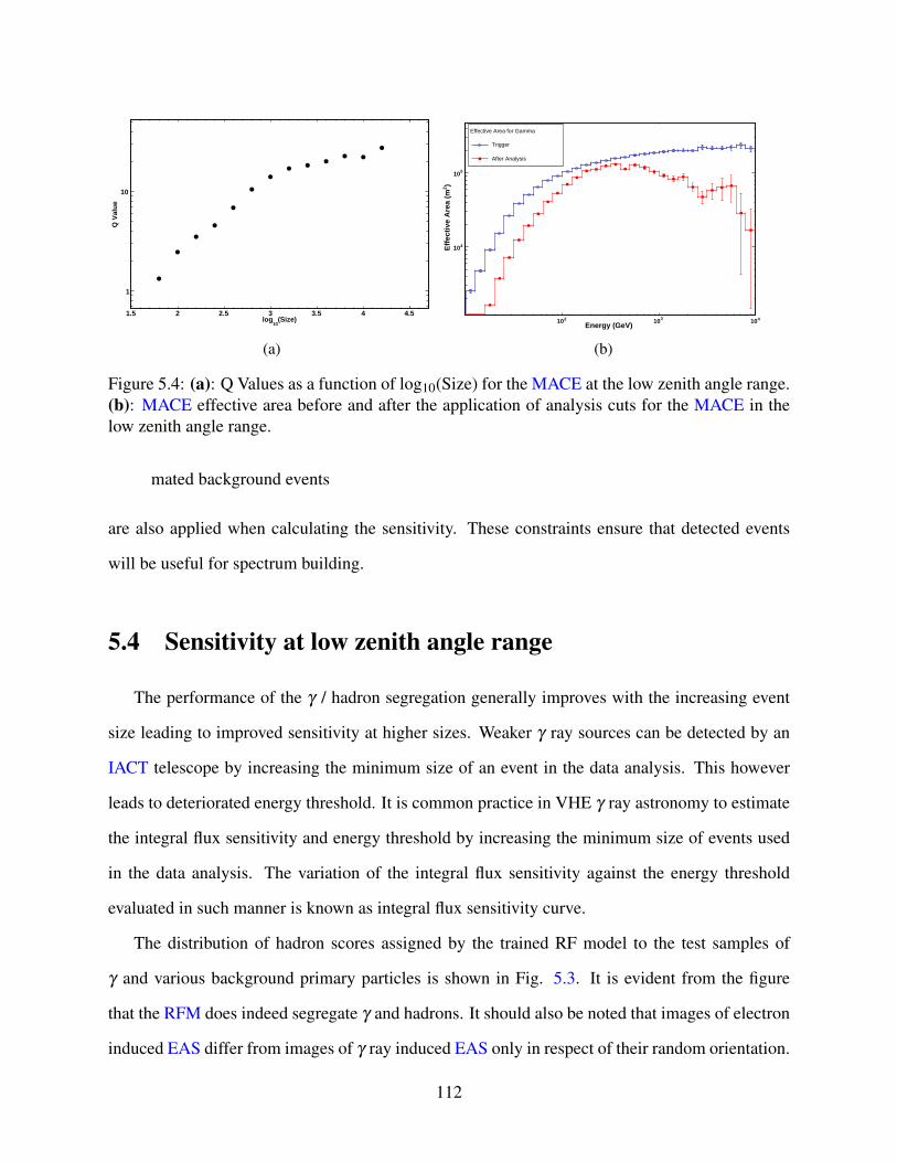
(Size)10

log1.5 2 2.5 3 3.5 4 4.5

Q V

alu

e

1

10

(a)

Energy (GeV) 210 310 410

)2

Eff

ecti

ve A

rea

(m

410

510

Effective Area for Gamma

Trigger

After Analysis

(b)

Figure 5.4: (a): Q Values as a function of log10(Size) for the MACE at the low zenith angle range.

(b): MACE effective area before and after the application of analysis cuts for the MACE in the

low zenith angle range.

mated background events

are also applied when calculating the sensitivity. These constraints ensure that detected events

will be useful for spectrum building.

5.4 Sensitivity at low zenith angle range

The performance of the γ / hadron segregation generally improves with the increasing event

size leading to improved sensitivity at higher sizes. Weaker γ ray sources can be detected by an

IACT telescope by increasing the minimum size of an event in the data analysis. This however

leads to deteriorated energy threshold. It is common practice in VHE γ ray astronomy to estimate

the integral flux sensitivity and energy threshold by increasing the minimum size of events used

in the data analysis. The variation of the integral flux sensitivity against the energy threshold

evaluated in such manner is known as integral flux sensitivity curve.

The distribution of hadron scores assigned by the trained RF model to the test samples of

γ and various background primary particles is shown in Fig. 5.3. It is evident from the figure

that the RFM does indeed segregate γ and hadrons. It should also be noted that images of electron

induced EAS differ from images of γ ray induced EAS only in respect of their random orientation.

112

Energy Threshold ( GeV)210 310

)-1

sec

-2)

(ph

oto

ns

cmth

Inte

gra

l Flu

x F

( >

E

13−10

12−10

11−10

10−10

9−10

8−10Crab flux

MACE

MAGIC-I

Figure 5.5: The integral sensitivity curve for the MACE telescope. The solid line is the sensitivity

of the MACE telescope. The dashed curve shows the sensitivity curve of the MAGIC-I [147]. The

dot-dashed line shows the integral Crab flux as the function of energy.

However RFM efficiently segregates γ rays from electron induced showers. We note here that

such may not be the case for the extended sources where γ rays may originate from the off-axis

positions in the FOV of the telescope. The Fig. 5.4a shows the variation of quality factor in

different size bins. The quality factor is defined as the ratio of γ acceptance to the square root of

the hadron acceptance when the segregation cuts are applied on the data. It should be noted that

the quality factor is calculated only for the events which pass the ‘good quality’ cuts. The Fig.

5.4b shows the effective area of the γ rays after the application of the γ / hadron segregation cuts.

It is obtained by incorporating the acceptance of the analysis cuts into the trigger effective area.

The integral sensitivity curve for the MACE telescope in the low zenith angle range of 0 -

30 is shown in Fig. 5.5. The MACE telescope has the lowest energy threshold of 31 GeV with

sensitivity of 24 mCrab. The threshold corresponds to the minimum size of the 50 pe. We see

that up to ∼ 150 GeV MACE has sensitivity comparable to that of MAGIC-I while its energy

threshold extends beyond that of MAGIC-I.

113

(Size)10

log1.5 2 2.5 3 3.5

Q V

alu

e

10

(a)

Energy (GeV) 210 310 410

)2E

ffec

tive

Are

a (m

310

410

510

Effective Area

Trigger

Minimum size = 50After Analysis

(b)

Figure 5.6: (a): Q Value as a function of log10(Size) for the MACE at the zenith angle of 40.

(b): The effective area of the MACE at the zenith angle of 40 before and after the application of

analysis cuts.

5.5 Sensitivity at zenith angle 40

It was shown in section 4.8 that the saturation value of the effective area achieved by the MACE

telescope at higher energies increases with increasing zenith angle. This leads to higher number of

γ ray induced triggers at higher energies. On the other hand the trigger energy threshold increases

with increasing zenith angle as well. Thus the number of γ ray induced triggers at low energies

reduces with increasing zenith angle. These two effects together lead to higher energy thresholds

and better sensitivities at zenith angle of 40. It should be noted here that for zenith angles > 30

the performance of an IACT changes much faster with increasing zenith and concerned studies

must be carried by sampling more zenith angle values in simulations.

The variation of quality factor and after analysis effective area of the MACE for the minimum

size of 50 pe and at the zenith angle of 40 are shown in Fig. 5.6a and 5.6b respectively. Fig. 5.7

shows the integral flux sensitivity curve for the MACE telescope for zenith of 40. The average

integral flux sensitivity of the MACE telescope for zenith less than 30 is also shown in the same

114

Energy Threshold (GeV)210 310

)-1

sec

-2) (

phot

ons

cmth

Inte

gral

Flu

x F

(>E

13−10

12−10

11−10

10−10

9−10

8−10Integral Sensitivity

zenith°

40

zenith°

< 30

Crab

Figure 5.7: The integral sensitivity curves for the MACE telescope. The dot-dashed curve shows

integral Crab flux. The dashed line shows the MACE integral flux sensitivity in the low zenith

angle range. The red solid line shows MACE sensitivity at the zenith angle of 40.

for comparison. The energy threshold of the MACE telescope at the 40 zenith is ∼ 51 GeV,

somewhat higher compared to energy threshold of ∼ 31 GeV at the low zenith range. It can also

be seen that the integral flux sensitivity is consistently better for all the energy thresholds more

than 50 GeV for the zenith angle of 40 than the low zenith range.

The estimates of the MACE integral flux sensitivity clearly show that the MACE will be able

to detect many weak VHE γ ray sources at least up to the zenith angle of 40. The after analysis

energy threshold estimates of the MACE further confirm that the images of the low energy events

that trigger the MACE telescope can be reconstructed reliably. Well formed images of the low

energy γ ray events allow the analysis chain to retain them thereby creating the possibility of

spectral studies in the energy range of 10 GeV to 100 GeV. However, the ability of an IACT to

resolve the morphology and spectrum of a VHE γ ray source is determined by the angular and

energy resolutions of the IACT respectively. The next chapter describes the procedures followed

and results obtained during the estimation of angular and energy resolutions of the MACE.

116

CHAPTER

SIX

ANGULAR AND ENERGY RESOLUTIONS OF THE MACE

6.1 Introduction

An IACT measures the arrival direction and the energy of the detected γ like event based

on their correlations with the Hillas parameters of EAS images. The details of reconstruction

procedures for arrival direction and energy and the estimated angular and energy resolutions of

the MACE telescope as a function of γ ray energy for low zenith angles and zenith angle of 40

are described in this chapter.

6.2 Data sample and analysis

A dataset consisting of γ ray induced showers with spectral index of -1 was generated at each

of the zenith angles of 5, 25 and 40 using CORSIKAv6.990. The flatter spectrum chosen for

EAS dataset generation ensured that there are enough number of showers even at high energies.

The energy range for the generation of shower was chosen from 10 GeV - 10 TeV. The dataset

for each zenith angle consisted of order of 106 events (refer to table 6.1). The maximum impact

distance for the dataset at 5 zenith angle was kept 400 m while for the rest of the datasets it was

118

Zenith Total Triggered Training Test

5 1.92 × 106 472325 105 2 × 105

25 1.92 × 106 457120 105 2 × 105

40 1.68 × 106 563121 105 2 × 105

Table 6.1: The number of total, triggered, training and test γ events at each of the 3 zenith angles.

kept 450 m. Rest of the inputs used for the CORSIKA are same as described in sec. 4.3.

The response of reflector, camera geometry, CPCs, PMT quantum efficiency and trigger was

simulated as described in sec. 4.3. The angular resolution and energy resolution for the 4 CCNN

trigger configuration with single channel discrimination threshold of 9 pe for the MACE telescope

[148] is presented in this thesis. The contribution from LONS as described in sec. 4.3.3 was

introduced in the simulation. The image cleaning and parameterisation procedures used were same

as described in sec. 5.2.2. The dataset of triggered images at each zenith angle was then divided

into training and testing subsets. Training subset was used to optimise the arrival direction / energy

estimation procedure. Test subsets were used to estimate the angular and energy resolutions at

each zenith angle. Table 6.1 shows the number of simulated triggered γ ray events along with

the number of events in training and evaluation data samples at each of the zenith. Angular and

energy resolution in the zenith angle range of 0 to 30 and at the zenith angle of 40 are presented

in this thesis. The resolutions in the zenith angle range of 0 to 330 are estimated by averaging

the respective values at 5 and 25.

6.3 Reconstruction of arrival direction with single imaging at-

mospheric Cherenkov telescope

A system of array of IACT telescopes can estimate the arrival directions of all the triggered

events by finding the intersection of the major axes of all constituent telescope images in their

common field of view. Single IACT telescope does not have any such direct way of reconstructing

the source position in the camera FOV. A significance map of an imaginary grid placed on the

119

maximum along the primary direction in the camera plane is given by centroid of an image. Thus

centroid lies on the major axis of the image as well. The angular distance between the source

position in the camera and the image centroid for an event is called Disp parameter. It is clear

from the geometry as shown in fig. 6.1 that the Disp parameter increases with increasing impact

parameter of the γ ray shower. In sec. 2.4 it was shown that for γ ray showers elongation of the

image defined as the ratio of Width to Length also increases with increasing impact parameter.

Thus the Disp parameter correlates with the elongation of the image. The Disp method exploits

correlation between Disp and image elongation to estimate Disp. The source position in the

camera is then estimated to be at angular distance of ‘Disp’ from image centroid along the major

axis.

Above procedure for the reconstruction of the source position will yield two possible source

positions in the camera plane. However the source position which is on the side of the image

which corresponds to first interaction of the shower must be the true source position. The correct

identification of the source position is done using the asymmetry parameter. The positive value of

asymmetry parameter indicates that shower head lies near the camera center while negative value

indicates otherwise. The source position in the camera is thus given by

~S =−−→COG+Disp · H (6.1)

where ~S is the vector from camera tracking position to reconstructed source position,−−→COG is

the vector from camera tracking position to image centroid and H is the unit vector along major

axis pointed towards head of the shower. The angular distance between the reconstructed source

position and the true source position in the camera i.e. magnitude of ~S in eq. 6.1, gives the error

in reconstruction of arrival direction. This distance is known as the θ parameter. It is given by

θ 2 =

d2 +Disp2−2d ×Disp× cos(α) if asym > 0

d2 +Disp2−2d ×Disp× cos(180−α) if asym < 0

(6.2)

121

where d,Disp,α and asym are the distance, Disp, alpha and asymmetry parameters respectively.

The correlation between Disp and image elongation can be treated to be linear in first approx-

imation given by [152]

Disp = ξ

(

1−Width

Length

)

(6.3)

where ξ is a scaling parameter between Disp and image elongation. The image elongation also

depends on the image size since γ rays with higher energies have higher size and penetrate deeper

in atmosphere. The longer development lengths of high energy events naturally lead to elongated

images. The events with high leakage parameters are poorly reconstructed and have poorly defined

Hillas parameters. Domingo-Santamarıa et al. [153] suggested the new empirical relation for Disp

that included the corrections for size and truncation effects. It is given by

Disp = A(Size) + B(Size)

(

Width

Length + ξ (Size)Leakage

)

(6.4)

The estimation of scaling factor ξ in eq. 6.3 or estimation of A,B and ξ in eq. 6.4 can be done

by minimising the average of θ 2 over a simulated dataset consisting of γ ray induced showers.

It can also be done by using the experimental data of a point γ ray source with precisely known

co-ordinates. Aleksic et al. [154] showed in their work that by using RFM regression for the Disp

estimation the angular resolution of the MAGIC-I could be improved by ∼ 20 - 30%. In this work

we have used RFM regression to estimate Disp and thereby source position. The details of RFM

regression can be found in appendix A and references therein. One RFM regression model to

estimate Disp was trained at each zenith angle. Size, Length, Width and Frac2 were used as inputs

to each RFM regression model. Each RFM model consisted of 500 decision trees with minimum

node size of 10 samples. The number of parameters to be used for random node splitting in trees

was set to be 2.

122

(deg)recX0.15− 0.1− 0.05− 0 0.05 0.1 0.15

(d

eg)

rec

Y

0.15−

0.1−

0.05−

0

0.05

0.1

0.15

0

100

200

300

400

500

(a)

)2 ( deg2θ0 0.5 1 1.5 2 2.5 3 3.5 4

Fre

qu

ency

3−10

2−10

1−10

1

(b)

Figure 6.2: (a): 2-dimensional distribution of the reconstructed arrival directions of γ rays for the

energy bin of (1.8 - 3.0) TeV at the low zenith angle range. Contours show the 2-dimensional

Gaussian fit to the distribution. (b): Normalised theta square distribution for γ ray events at the

low zenith angle range [148].

6.4 Angular resolution of the MACE telescope

Two estimators for the evaluation of the angular resolution of the MACE telescope were used.

A standard deviation of the 2 dimensional Gauss function fitted to 2 dimensional distribution of

the reconstructed arrival directions is used as one of the estimates of Point Spread Function (PSF)

of the MACE telescope. Additional constrain of θ 2 < 0.16 is used while fitting Gaussian. Fig.

6.2a shows the Gaussian fit to distribution of reconstructed arrival directions in the energy bin of

1.8 TeV to 3.0 TeV at the low zenith angle range. To find a model independent estimate of PSF

68 % containment value of the normalised θ 2 distribution is used. Fig. 6.2b shows the normalised

distribution of the θ 2 parameter for the γ rays at low zenith angle range. The symbols σ and σ0.68

are used to denote the Gaussian PSF and 68% containment radius respectively in this section. 5

energy bins per decade were selected in the energy range of 30 GeV - 3 TeV for the estimation of

angular PSF and energy resolution. The Gaussian PSF and 68% containment value were estimated

in each energy bin for the low zenith angle range and at the zenith angle of 40.

Fig. 6.3a shows the variation of Gaussian PSF of the MACE as a function of energy, for the

low zenith angle range well as at the zenith angle of 40. We find the angular PSF of MACE is ∼

123

Energy (GeV)210 310

PS

F (

deg

)

0.06

0.08

0.1

0.12

0.14

0.16

0.18

0.2

PSF (2D Gaussian Fits)

Zenith°

40

Low Zenith Range

(a)

Energy (GeV)210 310

(d

eg)

0.68

PS

F

0.1

0.15

0.2

0.25

0.3

0.35

0.4 )0.68σPSF (

Zenith°

40

Low Zenith Range

(b)

Figure 6.3: (a): Variation of Angular PSF as estimated by Gaussian fitting procedure at the low

zenith angle range as well as at 40 zenith. (b): The 68 % containment radius for the reconstructed

arrival directions for the MACE telescope

0.21 in the energy range of 30 GeV to 47 GeV at the low zenith angle range whereas the same for

zenith angle of 40 in the lowest energy bin of 47 GeV to 75 GeV is 0.19. These values improve

with increasing energy reaching the value of 0.06 in the highest energy bin of 1.8 TeV to 3.0 TeV

for the low zenith angle range and for the zenith angle of 40 respectively. Fig. 6.3b shows the

variation of 68% containment radius against the γ ray energy for the MACE. The red curve shows

values of 68% containment radius in different energy bins at the low zenith angle range while the

blue line shows its variation against the energy at the zenith angle of 40. The MACE has 68%

containment value of 0.36 in the lowest energy bin of 30 GeV to 47 GeV in the low zenith angle

range. It improves to 0.09 for the highest energy range of 1.8 TeV to 3.0 TeV. At the zenith angle

of 40 the 68% containment value improves from 0.41 in the energy bin of 47 GeV to 75 GeV

to 0.11 in the energy bin of 1.8 TeV to 3 TeV. Table 6.2 lists values of Gaussian PSF and 68%

containment values of the MACE telescope for the two zenith angle ranges. Values of the angular

bias along the camera x-axis and along camera y-axis are listed in table 6.3.

124

Energy Range σ (deg) σ0.68 (deg)

(TeV) 0 - 30 40 0 - 30 40

0.030 - 0.047 0.2103 ± 0.0064 - 0.3648 -

0.047 - 0.075 0.1919 ± 0.0036 0.1950 ± 0.0036 0.3130 0.4036

0.075 - 0.119 0.1565 ± 0.0029 0.1648 ± 0.0024 0.2705 0.2964

0.119 - 0.189 0.1360 ± 0.0030 0.1463 ± 0.0019 0.2240 0.2416

0.189 - 0.299 0.1214 ± 0.0017 0.1336 ± 0.0015 0.1888 0.2066

0.299 - 0.475 0.1054 ± 0.0011 0.1230 ± 0.0013 0.1565 0.1730

0.475 - 0.753 0.0881 ± 0.0011 0.1023 ± 0.0011 0.1314 0.1514

0.753 - 1.194 0.0777 ± 0.0008 0.0947 ± 0.0010 0.1117 0.1349

1.194 - 1.892 0.0654 ± 0.0009 0.0872 ± 0.0010 0.0977 0.1268

1.892 - 2.999 0.0603 ± 0.0009 0.0610 ± 0.0002 0.0950 0.1165

Table 6.2: Angular PSF as estimated by Gaussian fitting and 68% containment value in the zenith

angle range of 0 to 306 and at the zenith angle of 40 for the MACE telescope

Energy Range bias in x bias in y

µx (× 10−3 deg) µy(× 10−3 deg)

(TeV) 0 - 30 40 0 - 30 40

0.030 - 0.047 4.764 ± 3.44 - -1.119 ± 4.63 -

0.047 - 0.075 5.478 ± 1.96 7.600 ± 2.36 8.516 ± 2.94 4.940 ± 2.23

0.075 - 0.119 4.557 ± 1.60 4.631 ± 1.52 10.668 ± 2.25 6.724 ± 1.47

0.119 - 0.189 8.487 ± 1.46 8.014 ± 1.08 10.705 ± 2.06 6.163 ± 1.07

0.189 - 0.299 7.626 ± 1.09 11.629 ± 0.75 14.625 ± 1.39 12.365 ± 0.91

0.299 - 0.475 11.099 ± 0.85 13.329 ± 0.80 14.390 ± 0.98 14.077 ± 0.81

0.475 - 0.753 11.594 ± 0.85 14.195 ± 0.73 13.514 ± 0.90 13.929 ± 0.68

0.753 - 1.194 11.740 ± 0.65 16.061 ± 0.72 14.422 ± 0.71 15.163 ± 0.66

1.194 - 1.892 10.873 ± 0.74 15.985 ± 0.70 9.779 ± 0.70 14.360 ± 0.66

1.892 - 2.999 8.975 ± 0.75 6.696 ± 0.30 8.146 ± 0.64 6.607 ± 0.27

Table 6.3: Values of the Angular bias along the camera x-axis and camera y-axis in the zenith

angle range of 0 to 306 and at the zenith angle of 40 for the MACE telescope

125

Energy (GeV)210 310

)-1

sec

-2)

(ph

oto

ns

cmth

Inte

gra

l Flu

x F

(>E

13−10

12−10

11−10

10−10

analysisαLow Zenith,

analysis2θLow Zenith,

analysisα, °

40

analysis2θ, °

40

Figure 6.4: Integral flux sensitivity of the MACE using θ 2 analysis. Integral flux sensitivity using

alpha analysis is shown for the comparison as well. The red dashed lines show the MACE integral

flux sensitivity at the zenith angle of 40. The blue dot-dashed line show the variation of the

MACE integral flux sensitivity for the low zenith angle range. Hollow squares show sensitivity

estimated using θ 2 analysis. Hollow triangles are used for the MACE sensitivity using Alpha

analysis.

6.5 Integral flux sensitivity using θ 2 analysis

The θ 2 parameter is the square of the angular distance between the reconstructed source posi-

tion and the true source position. Since reconstructed source positions of γ rays peak around the

tracking position of the source in the camera for point-like γ ray source, the θ 2 distribution of γ

rays peaks at 0 deg2 for a point-like γ ray source. For background particles, the distribution of

θ 2 is much broader. The θ 2 parameter can be used as effective discriminator in place of Alpha

parameter during γ/hadron segregation, known as θ 2 analysis.

We have estimated the MACE integral flux sensitivity using θ 2 analysis for a comparative

study. The γ/hadron segregation was performed using the RFM classifier trained on Size, Dis-

tance, Length, Width, Frac2 and θ 2 parameters. All events with Size < 50.0 pe and Leakage >=

0.1 are rejected from analysis. The same training and test datasets as described in sec. 5.2.1 and

5.2.2 are used for the estimation of the MACE integral flux sensitivity using θ 2 analysis (see table

126

5.1). The γ-like events are identified by applying cut on the hadronscore of each event. Fig. 6.4

shows the variation of integral flux sensitivity against the energy threshold for two zenith angle

ranges using two analysis methods. The θ 2 analysis yields integral flux sensitivity comparable

to the Alpha analysis at both the zenith angle ranges. It however yields marginally higher energy

thresholds. The integral flux sensitivity of the MACE telescope using θ 2 analysis in the low zenith

angle range was found to be 27 mCrab units above the energy of ∼ 36 GeV. At the zenith angle of

40 the MACE can detect minimum integral flux of 20 mCrab units at the energy threshold of ∼

60 GeV. The wide angular PSF of the MACE at low energies results in the higher energy threshold

when using the θ 2 analysis.

6.6 Energy reconstruction using single imaging atmospheric

Cherenkov telescope

(Energy (GeV) )10

log1 1.5 2 2.5 3 3.5 4 4.5

( S

ize

(pe)

)10

log

1

1.5

2

2.5

3

3.5

4

4.5

5

5.5

0

100

200

300

400

500

600

700

(a)

( Energy (GeV) )10

log1 1.5 2 2.5 3 3.5 4 4.5

Len

gth

(d

egre

e)

0

0.1

0.2

0.3

0.4

0.5

0.6

0.7

0.8

0.9

1

0

100

200

300

400

500

600

700

800

900

(b)

Impact Parameter (m)0 20 40 60 80 100 120 140 160 180 200

Dis

tan

ce (

deg

)

0

0.2

0.4

0.6

0.8

1

1.2

1.4

1.6

1.8

2

0

500

1000

1500

2000

2500

3000

(c)

Figure 6.5: (a): Correlation between Size and energy of the γ ray induced shower images (b):

Correlation between the Length and energy of the γ ray induced shower images (c): Correlation

between the Distance parameter and impact parameter.

The Cherenkov photon density on the ground generated by a γ ray induced EAS is approxi-

mately constant within the Cherenkov pool of the air shower. Thus all the γ ray induced events

with the same energy those have an IACT within their respective Cherenkov pool, produce nearly

same number of Cherenkov photons at the focal plane of the telescope. Thus the size of a

127

Cherenkov image is proportional to the energy of the primary γ ray inducing it. The higher

energy showers develop deeper into the atmosphere. Thus the length of an EAS image also in-

creases with increasing energy. On the other hand, the image elongation also increases with the

increasing core distance of the shower from the telescope axis. While using the length parameter

for the estimation of energy one must take into account its correlation with core distance. For γ

rays the distance parameter of the shower images is directly proportional to the impact parameter

of the shower. This correlation can be used to take into account the effect of core distance on the

length. The correlations of the different Hillas parameter with energy and core distance are shown

in fig. 6.5

The energy of the γ rays is estimated using RFM regression. The size, length, width and

distance parameters are used as the inputs. The regression RF model with 500 trees was trained

on the training datasets described in sec. 6.2. The minimum node size before splitting was set to

be 10 while the number of trial parameters at each split was kept at 2. The number of training and

test samples at each zenith are described in table 6.1.

6.7 Energy resolution of the MACE telescope

The energy resolution was estimated in five energy bins per decade of true energy, in the range

of 30 GeV to 3 TeV. In each bin, the distribution of the fractional deviation of the estimated en-

ergy from the true energy, Eest−Etrue

Etrue, was fitted with a Gaussian function. The mean and standard

deviation of Gaussian distribution represents the bias and energy resolution of the system respec-

tively. The Root Mean Square (RMS) value of the fractional deviation of the estimated energy

with respect to true energy is also used to quantify the energy resolution in a model independent

way.

Fig. 6.6a shows the distribution of log of the estimated energy Eest against the log of the true

γ ray energy at low zenith angle range. It is clear that the estimated energy is reasonably close to

the true energies in the entire energy range, ensuring reliability of Random Forest method for the

128

GeV)est

(E10

log1 1.5 2 2.5 3 3.5 4 4.5

(G

eV))

tru

e(E

10lo

g

1

1.5

2

2.5

3

3.5

4

4.5

0

100

200

300

400

500

600

700

800

900

(a)

(GeV))est

(E10

log1 1.5 2 2.5 3 3.5 4 4.5

tru

eE

tru

e -

Ees

tE

5−

4−

3−

2−

1−

0

1

2

3

4

5

0

100

200

300

400

500

600

700

800

900

(b)

Figure 6.6: (a): True energy versus the estimated energy Eest at low zenith angle (b): Fractional

deviation of the estimated energy with respect to true energy (Eest−Etrue

Etrue) vs the log of estimated

energy (Eest) at low zenith angle

energy estimation. Fig. 6.6b shows the fractional deviation of estimated energy from true energy

as a function of log of the reconstructed energy Eest . The reconstructed energies show significant

positive bias at lower energies. The low energy showers have higher size fluctuations. These

fluctuations limit the performance of the regression for low energy γ rays.

The Fig. 6.7 shows the MACE energy resolution as a function of true energy in the low zenith

angle range of 0 to 30 and at zenith angle of 40. The Fig. 6.7a shows the variation of the

standard deviation of Gaussian fit to the distribution of fractional deviation of estimated energy

from true energy. The Gaussian energy resolution of the MACE varies from 40.5% in the low

energy bin of 30 GeV to 47 GeV to 19.8% in the energy bin of 1.8 TeV to 3 Tev for the low

zenith angle range. At the zenith angle of 40, the Gaussian energy resolution of the telescope

varies from 37.5% in the energy range of 47 GeV to 75 GeV to 19.3% in the energy bin of 1.8

TeV to 3 TeV. RMS values of the fractional deviation of estimated energy from true energy in

different energy bins are shown in the fig. 6.7b. The RMS energy resolution near the energy

threshold for the two zenith angle ranges is 42.3% and 46.1% for the low zenith angle range and

the zenith angle of 40 respectively. At the highest energy bin of 1.8 TeV to 3 TeV, the MACE

RMS resolution has values of 29.5% and 30.7% for the low zenith angle range and the zenith

129

Energy (GeV)210 310

(%

)

E E∆ σ

20

25

30

35

40

Resolution (Gauss Fit)

Zenith°

40

Low Zenith Range

(a)

Energy (GeV)210 310

(%

)

E E∆ R

MS

30

32

34

36

38

40

42

44

46 Resolution (RMS)

zenith°

40

Low Zenith Range

(b)

Figure 6.7: Energy resolution of the MACE telescope at low zenith angle range and at 40 zenith

(a): using Gaussian fit to the distribution of fractional deviation of estimated energy with respect

to true energy (b): RMS of the fractional deviation of estimated energy with respect to true energy.

Energy bias σ(∆EE) RMS(∆E

E)

Range (%) (%) (%)

(TeV) 0 - 30 40 0 - 30 40 0 - 30 40

0.03 - 0.047 36.7 ± 1.0 - 40.5 ± 1.6 - 42.37 ± 0.4 -

0.047 - 0.075 17.6 ± 0.7 23.0 ± 2.3 38.7 ± 1.0 37.5 ± 1.0 42.8 ± 0.3 46.1 ± 0.5

0.075 - 0.119 7.4 ± 0.4 15.2 ± 0.6 34.0 ± 0.5 36.8 ± 0.5 41.8 ± 0.2 42.3 ± 0.3

0.119 - 0.189 2.6 ± 0.3 9.1 ± 0.4 31.3 ± 0.3 33.3 ± 0.3 40.7 ± 0.2 40.2 ± 0.2

0.189 - 0.299 -0.5 ± 0.3 2.6 ± 0.3 29.8 ± 0.3 29.7 ± 0.3 38.0 ± 0.2 38.7 ± 0.2

0.299 - 0.475 -2.5 ± 0.3 -1.8 ± 0.3 25.9 ± 0.3 26.6 ± 0.3 36.1 ± 0.2 36.6 ± 0.2

0.475 - 0.753 -1.1 ± 0.2 -1.5 ± 0.2 23.9 ± 0.3 23.9 ± 0.3 34.0 ± 0.2 33.7 ± 0.2

0.753 - 1.194 -0.8 ± 0.2 -1.2 ± 0.2 21.7 ± 0.2 21.4 ± 0.2 31.9 ± 0.2 32.6 ± 0.2

1.194 - 1.892 -0.7 ± 0.2 -1.4 ± 0.2 20.5 ± 0.2 19.3 ± 0.2 30.6 ± 0.2 30.7 ± 0.2

1.892 - 2.999 -0.2 ± 0.2 -1.1 ± 0.2 19.8 ± 0.2 19.3 ± 0.2 29.5 ± 0.2 30.7 ± 0.2

Table 6.4: Values of the energy resolution and RMS of fractional deviation of estimated energy

from true energy at the two zenith angle ranges for the MACE telescope

angle of 40 respectively. It is clear from these figures that the energy resolution of the MACE

does not vary much with zenith angle. Table 6.4 lists the values of Gaussian energy resolution,

130

RMS energy resolution and average bias in energy estimation in each energy bin for the MACE

telescope.

It should be noted at this point that no analysis cuts are applied before estimating the MACE

angular and energy resolutions presented here. With the application of analysis cuts, the angular

and energy resolutions of the MACE are expected to improve. Addition of a second IACT element

to the MACE observatory will further improve the angular and energy resolutions of the telescope.

131

List Of Acronyms

ACR Atmospheric Cherenkov Radiation

ACT Atmospheric Cherenkov Telescope

AGN Active Galactic Nucleus

AMCS Active Mirror Control System

ApSD Astrophysical Sciences Division

BARC Bhabha Atomic Research Center

BH Black Hole

BL Lac BL Lacertae

BLR Broad Line Region

BR Branching Ratio

CCC Central Camera Controller

CCD Charge Coupled Device

CCNN Closed Cluster Nearest Neighbouring

CCR Chance Coincidence Rate

CIB Cosmic Infrared Background

CIM Camera Integrated Module

CMBR Cosmic Microwave Background Radiation

CPC Compound Paraboloid Concentrator

xii

CPR Cherenkov Pool Radius

CR Cosmic Rays

DArS Data Archiving System

DC Data Concentrator

DM Dark Matter

DRS Domino Ring Sampler

dSphs dwarf Spherical satellite galaxy

EAS Extensive Air Shower

EBL Extragalactic Background Light

EC External Compton

EM Electromagnetic

FADC Flash Analog to Digital Converter

FIFO First In First Out

FLT First Level Trigger

FLTG First Level Trigger Generation

FOV Field of View

FPGA Field Programmable Gate Array

FR-I Fanaroff Riley -I

FSRQ Flat Spectrum Radio Quasar

GRB Gamma Ray Burst

xiii

GW Gravitational Wave

HAWC High Altitude Water Cherenkov Experiment

HBL High-frequency Peaked BL Lacs

HDD Hard Disk Drive

HE High Energy

HESS High Energetic Stereoscopic System

HMB High Mass Binary

HV High Voltage

IACT Imaging Atmospheric Cherenkov Telescope

IACTq Imaging Atmospheric Cherenkov Technique

IBL Intermediate-frequency Peaked BL Lacs

IC Inverse Compton

IR Infrared

ISM Interstellar Medium

LAN Local Area Network

LBL Low-frequency Peaked BL Lacs

LED Light Emitting Diode

LIV Lorentz Invariance Violation

LONS Light of Night Sky

MACE Major Atmospheric Cherenkov Experiment

xiv

MAGIC Major Atmospheric Gamma-ray Imaging Cherenkov Telescopes

ML Machine Learning

MWNe Magnetar Wind Nebulae

NSB Night Sky Background

NS Neutron Star

PCR Prompt Coincidence Rate

pe photo-electrons

PMT Photomultiplier Tube

PROOF Parallel ROOT Facility

PSF Point Spread Function

PWNe Pulsar Wind Nebulae

PWN Pulsar Wind Nebula

QCD Quantum Chromo Dynamics

RFM Random Forest Method

RMS Root Mean Square

SBC Single Board Computer

SCR Single Channel Rate

SED Spectral Energy Distribution

SkMS Sky Monitoring System

SLTG Second Level Trigger Generator

xv

SLT Second Level Trigger

SMBH Super Massive Black Holes

SNR Supernova Remnant

SR Synchrotron Radiation

SSC Synchrotron Self Compton

SSD Solid State Drive

TC Temperature Controller

TCU Telescope Control Unit

UV Ultraviolet

VDN Voltage Divider Network

VERITAS Very Energetic Radiation Imaging Telescope Array System

VHE Very High Energy

WIMP Weakly Interacting Massive Particles

WMAP Wilkinson Microwave Anisotropy Probe

WMS Weather Monitoring System

i

APPENDIX

A

RANDOM FOREST

Leo Breiman proposed the Random Forest algorithm for classification and regression tasks

in 2001 [159]. Random Forest implements an ensemble of uncorrelated binary decision trees to

solve the classification / regression problem. The necessary details of the RFM are described in

this appendix. The details about application of RFM to IACT data analysis are nicely described

in [160].

A.1 Decision trees

The decision trees are the basic building blocks of the Random Forest algorithm. They are

flow chart like structures where each node represents the vector of feature values for an event and

branch represents the rule to be applied on vector at node. The starting node of the decision tree

is called root node. The end nodes along different paths of the decision tree are called leaf nodes.

Every leaf node of the decision tree belongs to one of the possible class defined in classification

problem. The Leaf nodes correspond to a value for the target variable in case of regression. A

feature vector of an event is first evaluated at the root node. The feature vector then traverses along

the rule branch through which it can qualify and passes to next node. This process is repeated till

I

the feature vector ends up at one of the leaf nodes. The class / value at the leaf node in which

feature vector ends is used as the outcome (decision) of the tree for the given feature vector i.e.

for the given event.

Figure A.1 shows an example of the decision tree used for the γ / hadron classification problem.

An event is described by feature vector v with components vlength, vwidth and vsize. Each branch

applies some cut on one of the vector components. Passing through the cuts an event finally

reaches one of the leaf nodes and is classified as γ or hadron. We note here that though decision

trees can be multi nodal Random Forest employs binary decision trees. Thus Every node of

decision tree in Random Forests leads to only 2 child nodes.

Figure A.1: Schematic sketch of the working of the decision tree. v is the vector of Hillas param-

eters for an event detected by an IACT telescope. Cuts applied on the components of the vector

leads us through a decision path. An event then is classified as γ or hadron. Figure adapted from

[160].

A.2 Building the decision tree

Many types of decision trees like ID3, CART, C4.5 etc. are available which differ in their

training algorithms. All the algorithms use a labeled data sample, known as training sample, to

II

build the decision trees. The Random Forest method uses binary decision trees . We will describe

only binary decision tree training here. The basic idea behind the classification tree construction is

to divide the feature phase space into the regions of maximum class homogeneity. The regression

trees divide the feature phase space into regions with minimum variance of target variable. This

is achieved in following way.

The training set consists of the feature vectors for many events along with their class labels /

target values. The root node of the binary decision tree consists of all the training samples. One

of the features is then randomly chosen and cut is applied on the chosen feature. This divides the

dataset at root node into 2 subsets belonging to 2 child nodes. Each one of the child nodes may

contain mixture of samples from different class populations. The optimum value of the feature

cut is found by maximising the purity of the subsets in the 2 child nodes. A dataset is said to be

completely pure if it contains samples of only one class. For a regression tree completely pure

dataset means a dataset where all samples have same target value thus leading to 0 variance. The

above process is repeated for each node till completely pure nodes are created or the number of

samples in the node reach the minimum value. The minimum number of samples to stop the

dataset splitting is a control parameter in this algorithm.

The optimisation of the feature cut value in node splitting requires a measure of the impurity

of the dataset. For the classification trees the Gini index or corss-entropy are used as the measures

of impurity of the dataset. If there are k classes in the training set then the Gini index and cross-

entropy for each node in the tree is given by

Gini =i=k

∑i=1

pi(1− pi) (A.1a)

Cross Entropy = −i=k

∑i=1

piln(pi) (A.1b)

where pi are the probability of occurrence for class i in the node. It is given by ratio of the number

of samples belonging to class i in the node to the number of total samples in the node. pi of 0 or 1

III

represents maximum purity of the dataset while pi = 0.5 indicates maximum impurity. As can be

seen from equation A.1 Gini index and cross entropy are minimum near 2 ends of pi range. Thus

minimising the entropy one can maximize the purity of the dataset. The variance of the target

values of the samples in the node is minimised in node splitting in regression trees. It is given by

Variance =1

N

i=N

∑i=1

(yi −〈y〉)2 (A.2)

where N is number of samples in the node, yi is the value of the target variable for the ith sample in

the node and 〈y〉 is the mean of target variable y over the samples in the node. The total Gini index,

the total cross entropy and the total variance of the 2 child nodes is minimised when splitting the

node in a decision trees.

A.3 Bootstrap sampling

The strong law of large numbers can be used to show that the generalisation error of Ran-

dom Forest converges to a limiting value provided that the decision trees are uncorrelated [159].

Bagging method is used to ensure that trees grown in forest are uncorrelated. All machine learn-

ing models are generally trained on the single training dataset. If each tree is grown on different

non-overlapping subsets of the training data then the trees will be uncorrelated. However this

will require A very big training data. Hence each tree in random forest is trained using the boot-

strapped dataset which is generated by N random draws with replacement from original training

dataset containing N samples. The bootstrap dataset generally have some duplication i.e. few

samples occur more than once. (1−1/e)×N samples in bootstrapped datasets will be from orig-

inal dataset while rest of the samples will be duplicates in limN→inf [160]. Bootstrapping allows

for the generation of independent datasets for the tree training while maintaining the statistically

identical distributions of the sample features. If kth tree Tk in random forest is trained on the

bootstrapped dataset Bk classification error for the tree Tk can be estimated on the ∼ 1e×N data

IV

samples from original dataset which were not part of Bk. This error is called out of bag error for

tree Tk. The average of out of bag errors for all the trees in random forest gives a limiting value

of the generalisation error of the random forest. Thus random forest not only provides an internal

estimate of the generalisation error it also avoids overtraining in limK→inf where K is number of

trees in random forest.

A.4 Control parameters of the Random Forest and their opti-

misation

Some of the important parameters to tune the random forest training are described in this

section.

• Number of Trees

Ideally one should have infinite number of trees in the random forest to avoid overtraining. In

practice, classification / regression error of the random forest on the independent test sample is

used to find the optimum number of trees. Multiple random forest models are trained on the

dataset using increasing number of trees in them. The variation of classification/regression error

on the test sample for each RFM model is observed as a function of number of trees. A value

for the number of trees is chosen such that gain in performance of random forest by adding one

more tree is nearly zero.

• Number of trial features in node splitting of trees

During the node splitting in the tree training is few features out of the several available are

randomly picked at each node. The split performance of each of the selected features is then

evaluated (by using gini index / or entropy). The feature which gives the best split at it’s opti-

mised value is finally chosen. The number of features randomly selected at each split,denoted

by mtry is an important variable of the random forest as it affects the strength and correlations of

the trees. If there are Npar features describing each event,√

Npar is generally very good choice

V

for mtry.

• Node Size

The node splitting in the tree training stops once the number of samples in the node reach a

minimum number. Empirically for classification trees minimum node size of 1 is chosen while

for regression trees minimum node size is kept ∼ 10.

VI

BIBLIOGRAPHY

[1] Victor Hess. On the Observations of the Penetrating Radiation during Seven Balloon

Flights. arXiv e-prints, page arXiv:1808.02927, Jul 2018. 1

[2] W. Baade and F. Zwicky. Cosmic Rays from Super-novae. Proceedings of the National

Academy of Science, 20(5):259–263, May 1934. 1

[3] Karl G. Jansky. Radio Waves from Outside the Solar System. Nature, 132(3323):66, Jul

1933. 1

[4] E. Aliu. VHE -ray observations of Northern sky pulsar wind nebulae with the MAGIC

Telescope . PhD thesis, Universitat Auteonoma de Barcelona, 2007. 2, 47

[5] J. A. Hinton and the HESS Collaboration. The status of the HESS project. New Astronomy

Reviews, 48:331–337, April 2004. 3

[6] E. Lorenz and The MAGIC Collaboration. Status of the 17 m MAGIC telescope. New

Astronomy Reviews, 48:339–344, April 2004. 3

[7] T. C. Weekes et al. VERITAS: the Very Energetic Radiation Imaging Telescope Array

System. Astroparticle Physics, 17:221–243, May 2002. 3

[8] G. Sinnis. HAWC: A Next Generation VHE All-Sky Telescope. In Felix A. Aharonian,

Heinz J. Volk, and Dieter Horns, editors, High Energy Gamma-Ray Astronomy, volume

745 of American Institute of Physics Conference Series, pages 234–245, Feb 2005. 3

[9] G. Sullivan and MILAGRO Collaboration. Status of the MILAGRO gamma ray obser-

vatory. In International Cosmic Ray Conference, volume 7 of International Cosmic Ray

Conference, page 2773, Aug 2001. 3

[10] Tibet As Gamma Collaboration, M. Amenomori, et al. Status and performance of the AS

array of the Tibet ASγ experiment. In James Matthews, editor, High Energy Gamma Ray

Astronomy, volume 220 of American Institute of Physics Conference Series, pages 257–

264, Apr 1991. 3

[11] Cosmic ray spectra of various experiments. https://www.physics.utah.edu/

~whanlon/spectrum.html. 4

VII

[12] A. De Angelis and M. Mallamaci. Gamma-ray astrophysics. European Physical Journal

Plus, 133(8):324, Aug 2018. 4, 9, 14

[13] K. K. Yadav. VHE -ray observations of Northern sky pulsar wind nebulae with the MAGIC

Telescope . PhD thesis, Universitat Auteonoma de Barcelona, 2007. 6, 45, 104

[14] F Zwicky. Die Rotverschiebung von extragalaktischen neblen. Helvetica Physica Acta,

6(8):110–127, Aug 1933. 7

[15] A. Kogut et al. Three-Year Wilkinson Microwave Anisotropy Probe (WMAP) Observa-

tions: Foreground Polarization. Astrophysical Journal, 665(1):355–362, Aug 2007. 7

[16] Joao Magueijo and Lee Smolin. Lorentz Invariance with an Invariant Energy Scale. Physi-

cal Review Letters, 88(19):190403, May 2002. 8

[17] Javier Rico. Review of fundamental physics results with the MAGIC telescopes. In 6th In-

ternational Symposium on High Energy Gamma-Ray Astronomy, volume 1792 of American

Institute of Physics Conference Series, page 060001, Jan 2017. 8

[18] I. Bartos, K. R. Corley, N. Gupte, N. Ash, Z. Marka, and S. Marka. Gravitational-wave

follow-up with CTA after the detection of GRBs in the TeV energy domain. Monthly

Notices of Royal Astronomy Society, 490(3):3476–3482, Dec 2019. 9

[19] E. Fermi. Galactic Magnetic Fields and the Origin of Cosmic Radiation. Astrophysical

Journal, 119:1, Jan 1954. 9

[20] A. R. Bell. The acceleration of cosmic rays in shock fronts - I. Monthly Notices of Royal

Astronomical Society, 182:147–156, Jan 1978. 9

[21] A. M. Hillas. Cosmic Rays: Recent Progress and some Current Questions. arXiv e-prints,

pages astro–ph/0607109, Jul 2006. 10

[22] M. Vietri. Foundations of High Energy Astrophysics. University of Chicago Press, 2008.

10, 13, 14

[23] K. R. Lang. Astrophysical formulae. Berlin : Springer, 1999. 10

[24] F. A. Aharonian, A. M. Atoyan, and T. Kifune. Inverse Compton gamma radiation of faint

synchrotron X-ray nebulae around pulsars. Monthly Notices of Royal Astronomical Society,

291(1):162–176, Oct 1997. 11

[25] P. V. Ramana Murthy and A. W. Wolfendale. Gamma-ray Astronomy. Cambridge Univer-

sity Press, 1993. 11, 12, 14

[26] Alessandro De Angelis and Mario Pimenta. Introduction to Particle and Astroparticle

Physics. Springer-Nature,Heidelberg, 2018. 11

[27] E. A. Fuste. VHE gamma-ray observations of Northern sky pulsar wind nebulae with the

MAGIC telescope. PhD thesis, Universitat Autonoma de Barcelona, 2007. 12, 13

VIII

[28] Richard N. Manchester and Joseph H. Taylor. Pulsars. Freeman, San Francisco, 1977. 13

[29] R. D. Evans. The Atomic Nucleus. Tata McGraw-Hill, 1955. 14

[30] M. Harwit. Astrophysical Concepts. Berlin:Springer, 1988. 14

[31] F. A. Aharonian et al. The Energy Spectrum of TEV Gamma Rays from the Crab Nebula as

Measured by the HEGRA System of Imaging Air Cerenkov Telescopes. ApJ, 539:317–324,

August 2000. 15, 91

[32] M. S. Strickman, W. N. Johnson, and J. D. Kurfess. The hard X-ray spectrum of the Crab

Nebula. Astrophysical Journal, Part 2 - Letters to Editor, 230:L15–L19, May 1979. 15

[33] B. Rossi and K. Greisen. Cosmic-Ray Theory. Reviews Of Modern Physics, 13:241–309,

October 1941. 15, 28, 31

[34] P. A. Cerenkov. Visible Emission of Clean Liquids by Action of γ Radiation. Doklady

Akad. Nauk SSSR, 2:451, August 1934. 15, 34

[35] I. E. Tamm and I. M. Franck. Coherent Radiation of Fast Electrons in a Medium. Doklady

Akad. Nauk SSSR, 14:107, August 1937. 15, 39

[36] P.M.S. Blackett. Emission spectra of the night sky and aurora. The Observatory, 67:121–

127, August 1947. 16

[37] W. Galbraith and J. V. Jelley. Light Pulses from the Night Sky associated with Cosmic

Rays. Nature, 171(4347):349–350, Feb 1953. 16

[38] G. Cocconi. An air shower telescope and the detection of 1012 eV photon sources. In

International Cosmic Ray Conference, volume 2 of International Cosmic Ray Conference,

page 309, Jan 1960. 16

[39] A. E. Chudakov, V. L. Dadykin, Zatsepin V. I., and Nestrova N. M. P.N. Lebedev Phys.

Inst, 26, 1965. 16

[40] N. Park. Status of ground based gamma-ray observations. In 35th International Cosmic

Ray Conference (ICRC2017), volume 301 of International Cosmic Ray Conference, page

1116, Jan 2017. 16, 17

[41] A. M. Hillas. Cerenkov Light Images of EAS Produced by Primary Gamma Rays and by

Nuclei. International Cosmic Ray Conference, 3:445, Aug 1985. 16, 46

[42] M. F. Cawley et al. Application of imaging to the atmospheric Cerenkov technique. Inter-

national Cosmic Ray Conference, 3:453–456, Aug 1985. 16

[43] T. C. Weekes et al. Observation of TeV gamma rays from the Crab nebula using the atmo-

spheric Cerenkov imaging technique. ApJ, 342:379–395, July 1989. 17

IX

[44] G. Giavitto, S. HESS Collaboration, et al. Performance of the upgraded H.E.S.S. cameras.

In 35th International Cosmic Ray Conference (ICRC2017), volume 301 of International

Cosmic Ray Conference, page 805, Jan 2017. 17

[45] J. Aleksic, MAGIC collaboration, et al. The major upgrade of the MAGIC telescopes,

Part I: The hardware improvements and the commissioning of the system. Astroparticle

Physics, 72:61–75, Jan 2016. 17

[46] N. Park and VERITAS Collaboration. Performance of the VERITAS experiment. In 34th

International Cosmic Ray Conference (ICRC2015), volume 34 of International Cosmic

Ray Conference, page 771, Jul 2015. 17

[47] Kifune plot. https://github.com/sfegan/kifune-plot/blob/master/kifune.pdf.

18

[48] Tev catalogue. http://tevcat2.uchicago.edu/labs. 18, 19

[49] A. Daum et al. First results on the performance of the HEGRA IACT array. Astroparticle

Physics, 8:1–11, December 1997. 18

[50] P. Goret and CAT Collaboration. Observation of the Crab Nebula Gamma-Ray Emission

Above 220 GeV by the CAT Cherenkov Imaging Telescope. 25 th International Cosmic

Ray Conference, Durban, South Africa, 3:173, 1997. 18

[51] H. Kubo et al. Status of the CANGAROO-III project. New Astronomy Reviews, 48:323–

329, April 2004. 18

[52] R. Koul et al. The TACTIC atmospheric Cherenkov imaging telescope. Nuclear Instru-

ments and Methods in Physics Research A, 578:548–564, August 2007. 18

[53] HESS Collaboration, H. Abdalla, et al. The population of TeV pulsar wind nebulae in the

H.E.S.S. Galactic Plane Survey. Astronomy and Astrophysics, 612:A2, Apr 2018. 19

[54] M. Amenomori, Tibet AS γ Collaboration, et al. First Detection of Photons with Energy

beyond 100 TeV from an Astrophysical Source. Physical Review Letters, 123(5):051101,

Aug 2019. 20

[55] Paul K. H. Yeung, Albert K. H. Kong, P. H. Thomas Tam, Lupin C. C. Lin, C. Y. Hui,

Chin-Ping Hu, and K. S. Cheng. Studying the SGR 1806-20/Cl* 1806-20 Region Using

the Fermi Large Area Telescope. Astrophysical Journal, 827(1):41, Aug 2016. 20

[56] Oleg Kargaltsev et al. X-Ray Observations of the New Unusual Magnetar Swift J1834.9-

0846. Astrophysical Journal, 748(1):26, Mar 2012. 20

[57] D. Guberman, J. Cortina, E. de Ona Wilhelmi, D. Galindo, A. Moralejo, and MAGIC

Collaboration. A cut-off in the TeV gamma-ray spectrum of the SNR Cassiopeia A. In 35th

International Cosmic Ray Conference (ICRC2017), volume 301 of International Cosmic

Ray Conference, page 724, Jan 2017. 20

X

[58] HESS Collaboration, H. Abdalla, et al. Deeper H.E.S.S. observations of Vela Junior (RX

J0852.0-4622): Morphology studies and resolved spectroscopy. Astronomy and Astro-

physics, 612:A7, Apr 2018. 20

[59] H. E. S. S. Collaboration, H. Abdalla, et al. H.E.S.S. observations of RX J1713.7-3946 with

improved angular and spectral resolution: Evidence for gamma-ray emission extending

beyond the X-ray emitting shell. Astronomy and Astrophysics, 612:A6, Apr 2018. 20

[60] Yudong Cui et al. Leaked GeV CRs from a Broken Shell: Explaining 9 Years of Fermi-LAT

Data of SNR W28. Astrophysical Journal, 860(1):69, Jun 2018. 20

[61] Andrea Giuliani. Hadronic emission in middle-aged SNRs. In 40th COSPAR Scientific

Assembly, volume 40, pages E1.16–13–14, Jan 2014. 21

[62] Samar Safi-Harb. Gamma2016: Highlights and summary of galactic science. In 6th Inter-

national Symposium on High Energy Gamma-Ray Astronomy, volume 1792 of American

Institute of Physics Conference Series, page 020015, Jan 2017. 21

[63] S. Ansoldi et al. Teraelectronvolt pulsed emission from the Crab Pulsar detected by

MAGIC. Astronomy and Astrophysics, 585:A133, Jan 2016. 21

[64] HESS Collaboration, H. Abdalla, et al. First ground-based measurement of sub-20 GeV

to 100 GeV γ-Rays from the Vela pulsar with H.E.S.S. II. Astronomy and Astrophysics,

620:A66, Dec 2018. 21

[65] HESS Collaboration, A. Abramowski, et al. Acceleration of petaelectronvolt protons in the

Galactic Centre. Nature, 531(7595):476–479, Mar 2016. 22

[66] Henric Krawczynski and Ezequiel Treister. Active galactic nuclei — the physics of indi-

vidual sources and the cosmic history of formation and evolution. Frontiers of Physics,

8(6):609–629, Dec 2013. 22

[67] M. L. Ahnen et al. Very High Energy γ-Rays from the Universe’s Middle Age: Detec-

tion of the z = 0.940 Blazar PKS 1441+25 with MAGIC. Astrophysical Journal Letters,

815(2):L23, Dec 2015. 23

[68] Reshmi Mukherjee. Very-high-energy gamma-ray emission from PKS 1441+25 detected

with VERITAS. The Astronomer’s Telegram, 7433:1, Apr 2015. 23

[69] T. York, N. Jackson, I. W. A. Browne, O. Wucknitz, and J. E. Skelton. The Hubble constant

from the gravitational lens CLASS B0218+357 using the Advanced Camera for Surveys.

Monthly Notices of Royal Astronomical Society, 357(1):124–134, Feb 2005. 23

[70] H. Abdalla et al. A very-high-energy component deep in the γ-ray burst afterglow. Nature,

575(7783):464–467, Nov 2019. 23

[71] Razmik Mirzoyan. First time detection of a GRB at sub-TeV energies; MAGIC detects the

GRB 190114C. The Astronomer’s Telegram, 12390:1, Jan 2019. 23

XI

[72] N. Park. Status of ground based gamma-ray observations. In 35th International Cosmic

Ray Conference (ICRC2017), volume 301 of International Cosmic Ray Conference, page

1116, Jan 2017. 23, 24

[73] J. Aleksic et al. Optimized dark matter searches in deep observations of Segue 1 with

MAGIC. Journal of Cosmology and Astroparticle Physics, 2014(2):008, Feb 2014. 24

[74] MAGIC Collaboration, J. Albert, et al. Probing quantum gravity using photons from a flare

of the active galactic nucleus Markarian 501 observed by the MAGIC telescope. Physics

Letters B, 668(4):253–257, Oct 2008. 24

[75] MAGIC Collaboration, M. L. Ahnen, et al. Constraining Lorentz Invariance Violation Us-

ing the Crab Pulsar Emission Observed up to TeV Energies by MAGIC. The Astrophysical

Journal Supplement Series, 232(1):9, Sep 2017. 25

[76] Malcolm S. Longair. High Energy Astrophysics. Cambridge University Press, 3rd edition,

2011. 28, 29, 32, 33, 34, 35

[77] W. Heitler. The qunatum theory of radiation. Oxford University Press, 1944. 29

[78] A. M. Hillas. Angular and energy distributions of charged particles in electron-photon

cascades in air. Journal of Physics G Nuclear Physics, 8:1461–1473, October 1982. 30, 31

[79] Stefan Klepser. Reconstruction of extensive air showers and measurement of the cosmic

ray energy spectrum in the range of 1 - 80 PeV at the South Pole. PhD thesis, Humboldt-

Universitt zu Berlin, Mathematisch-Naturwissenschaftliche Fakultt I, 2008. 31

[80] A. M. Hillas. The sensitivity of Cerenkov radiation pulses to the longitudinal development

of cosmic-ray showers. Journal of Physics G Nuclear Physics, 8:1475–1492, October 1982.

31

[81] F. Aharonian et al. High energy astrophysics with ground-based gamma ray detectors.

Reports on Progress in Physics, 71(9):096901, September 2008. 31, 41

[82] W.-M. Yao et al. Review of Particle Physics. Journal of Physics G Nuclear Physics, 33:1–

1232, July 2006. 31

[83] J. Nishimura and K. Kamata. On the Theory of Cascade Showers, I. Progress of Theoretical

Physics, 7:185–192, February 1952. 32

[84] P. Sokolsky. Introduction to Ultrahigh Energy Cosmic Ray Physics. Addison-Wesley, 1989.

32

[85] S. V. Godambe. Very high energy gamma ray observations of of MRK501 and

1ES2344+514 with the TACTIC telescope. PhD thesis, University of Mumbai, 2007. 32

[86] Hayashida Masaaki. Observation of very high energy gamma rays from blazars with the

MAGIC telescope. PhD thesis, 2008. 32

XII

[87] M. V. S. Rao and S. Sinha. The origin of the hump in the Cerenkov lateral distribution in

gamma-ray showers and a possible means of separating them from proton showers. Journal

of Physics G Nuclear Physics, 14(6):811–827, Jun 1988. 36

[88] R. A. Ong. Very high-energy gamma-ray astronomy. Physics Reports, 305:93–202, 1998.

38, 47, 55

[89] de la Calle Perez Ignacio. A study of the polarization of Cherenkov Radiation in Extensive

Air Showers of Energy around 1 TeV . PhD thesis, Universidad Complutense de Madrid,

1997. 42

[90] T C Weekes. Very High Energy Gamma-Ray Astronomy. Institute of Physics Publishing,

2003. 43, 44

[91] P. M. S. Blackett. A possible contribution to the night sky from the Cerenkov radiation

emitted by cosmic rays. In The Emission Spectra of the Night Sky and Aurorae, page 34,

Jan 1948. 44

[92] Robert Marcus Wagner. Measurement of very high energy gamma-ray emission from four

blazars using the MAGIC telescope and a comparative blazar study. PhD thesis, Max-

Planck-Institut fur Physik, Fohringer Ring 6, 80805 Munchen, Germany, Jan 2006. 45

[93] F. A. Aharonian, A. K. Konopelko, H. J. Volk, and H. Quintana. 5@5 - a 5 GeV energy

threshold array of imaging atmospheric Cherenkov telescopes at 5 km altitude. Astroparti-

cle Physics, 15:335–356, August 2001. 54, 55

[94] L. Saha, V. R. Chitnis, P. R. Vishwanath, S. Kale, A. Shukla, B. S. Acharya, G. C. Anupama,

P. Bhattacharjee, R. J. Britto, T. P. Prabhu, and B. B. Singh. A study of the performance

parameters of the High Altitude Gamma Ray (HAGAR) telescope system at Ladakh in

India. Astroparticle Physics, 42:33–40, February 2013. 55

[95] HIROT Team. Recent astronomical site survey at Hanle, Ladakh. Bulletin of the Astronom-

ical Society of India, 24:859, Dec 1996. 56

[96] A. K. Tickoo and V. K. Dhar. MACE Telescope Optical Surface Design. Technical report,

Bhabha Atomic Research Center. 60

[97] P. Kurup et al. Active Mirror Alignment Control System for the MACE telescope. National

Symposium on Nuclear Instrumentation, 2010. 59

[98] Abhay Kumar, Anita Behere, Nilesh Chauhan, and A. Venkateswarlu. Imaging Camera of

MACE Telescope : Critical Design Review. Technical report, Bhabha Atomic Research

Center, 2016. 60, 62, 63, 65, 68, 69

[99] P. Kurup et al. MACE telescope servo controller design. National Symposium on Nuclear

Instrumentation, 2010. 61

[100] K. Jha and Behere A. Data Transfer Scheme for High Event Rates for MACE Camera.

National Symposium on Nuclear Instrumentation, 2010. 64

XIII

[101] S. Srivastava, A. Jain, P.M. Nair, and P. Sridharan. Mace camera controller embedded soft-

ware: Redesign for robustness and maintainability. Astronomy and Computing, 30:100358,

2020. 66, 67

[102] N. Chouhan et al. Gain Calibration System for the MACE telescope. Symposium on Ad-

vances in Control & Instrumentation, 2014. 70

[103] S. Bharade et al. State Based Control Design of MACE Console System. National Sympo-

sium on Nuclear Instrumentation, 2010. 71

[104] Debangana Sarkar and Nilesh Chouhan. Mace data archival system. Technical report,

Astrophysical Sciences Division, Bhabha Atomic Research Center, 2016. 72

[105] Vantage Pro2T M Console Manual, Davis Instruments, 3465 Diablo Avenue, Hayward, CA

94545-2778 U.S.A. 72

[106] User Manual (version 1.0), Battery Management System - Wireless, Sixth Energy Tech-

nology Private Limited, #62, Sri Varada, 10th main, HMT lay out, R.T.Nagar, Bangalore,

560032, India. 73

[107] D. Heck, J. Knapp, J.N. Capdevielle, G. Schatz, and T. Thouw. Corsika: A monte carlo code

to simulate extensive air showers. Technical report, Kernforschungszentrum Karlsruhe,

1998. 51.02.03; LK 01; Wissenschaftliche Berichte, FZKA-6019 (Februar 98). 76

[108] J.N. Capdevielle, P. Gabriel, H.J. Gils, P. Grieder, D. Heck, J. Knapp, H.J. Mayer,

J. Oehlschlaeger, H. Rebel, G. Schatz, and T. Thouw. The karlsruhe extensive air shower

simulation code corsika. Technical report, Kernforschungszentrum Karlsruhe, 1992.

44.03.04; LK 01. 76

[109] H. O. Klages et al. The KASCADE Experiment. Nuclear Physics B Proceedings Supple-

ments, 52:92–102, Feb 1997. 76

[110] J. Ranft. Dual parton model at cosmic ray energies. Physics Review D, 51(1):64–84, Jan

1995. 76

[111] N. N. Kalmykov and S. S. Ostapchenko. The nucleus-nucleus interaction, nuclear fragmen-

tation, and fluctuations of extensive air showers. Physics of Atomic Nuclei, 56(3):346–353,

Mar 1993. 77

[112] N. N. Kalmykov, S. S. Ostapchenko, and A. I. Pavlov. Quark-Gluon-String Model and EAS

Simulation Problems at Ultra-High Energies. Nuclear Physics B Proceedings Supplements,

52(3):17–28, Feb 1997. 77

[113] S. Ostapchenko. QGSJET-II: towards reliable description of very high energy hadronic

interactions. Nuclear Physics B Proceedings Supplements, 151:143–146, Jan 2006. 77

[114] S. Ostapchenko. Nonlinear screening effects in high energy hadronic interactions. Physical

Review D, 74(1):014026, Jul 2006. 77

XIV

[115] R. S. Fletcher, T. K. Gaisser, Paolo Lipari, and Todor Stanev. sibyll: An event generator

for simulation of high energy cosmic ray cascades. Physical Review D, 50(9):5710–5731,

Nov 1994. 77

[116] J. Engel, T. K. Gaisser, Paolo Lipari, and Todor Stanev. Nucleus-nucleus collisions and

interpretation of cosmic-ray cascades. Physical Review D, 46(11):5013–5025, Dec 1992.

77

[117] Ralph Engel. Air Shower Calculations With the New Version of SIBYLL. In 26th Inter-

national Cosmic Ray Conference (ICRC26), Volume 1, volume 1 of International Cosmic

Ray Conference, page 415, Jan 1999. 77

[118] K. Werner. Strings, pomerons and the VENUS model of hadronic interactions at ultrarela-

tivistic energies. Physics Reports, 232(2-5):87–299, Sep 1993. 77

[119] H. J. Drescher, M. Hladik, S. Ostapchenko, T. Pierog, and K. Werner. Parton-based Gribov-

Regge theory. Physics Reports, 350(2-4):93–289, Sep 2001. 77

[120] Klaus Werner, Fu-Ming Liu, and Tanguy Pierog. Parton ladder splitting and the rapidity

dependence of transverse momentum spectra in deuteron-gold collisions at the BNL Rela-

tivistic Heavy Ion Collider. Physical Review C, 74(4):044902, Oct 2006. 77

[121] A. Fasso, A. Ferrari, J. Ranft, and P. R. Sala. Fluka : A multi particle transport code.

Technical report, European Organization for Nuclear Research (CERN), 2005. 77

[122] H. Fesefeldt. Report pitha-85/02. Technical report, RWTH Aachen, 1985. 77

[123] S. A. Bass et al. Microscopic models for ultrarelativistic heavy ion collisions. Progress in

Particle and Nuclear Physics, 41:255–369, Jan 1998. 77

[124] J. Knapp, D. Heck, and G. Schatz. Report fzka 5828. Technical report, Forschungszentrum

Karlsruhe, 1996. 78

[125] D. Heck. Low-energy hadronic interaction models. Nuclear Physics B Proceedings Sup-

plements, 151:127–134, Jan 2006. 78

[126] R. W. Nelson, H. Hirayama, and W. O. D. Rogers. Report slac 265. Technical report,

Stanford Linear Accelerator Center, 1985. 78

[127] J. N. Capdevielle and KASCADE Collaboration. Local Age Parameter and Size Estimation

in EAS. In International Cosmic Ray Conference, volume 4 of International Cosmic Ray

Conference, page 405, Aug 1991. 78

[128] S. Martinez, F. Arqueros, V. Fonseca, A. Karle, E. Lorenz, R. Plaga, and M. Rozanska.

Monte Carlo simulation of the HEGRA cosmic ray detector performance. Nuclear Instru-

ments and Methods in Physics Research A, 357:567–579, Feb 1995. 78

[129] Konrad Bernlohr. Impact of atmospheric parameters on the atmospheric Cherenkov tech-

nique*. Astroparticle Physics, 12(4):255–268, Jan 2000. 78, 81

XV

[130] Konrad Bernlohr. Simulation of imaging atmospheric Cherenkov telescopes with COR-

SIKA and sim telarray. Astroparticle Physics, 30(3):149–158, Oct 2008. 78, 81

[131] Rene Brun and Fons Rademakers. ROOT — An object oriented data analysis framework.

Nuclear Instruments and Methods in Physics Research A, 389(1):81–86, Feb 1997. 79

[132] Proof home page. https://root.cern.ch/proof. 79

[133] Erwan Thebault et al. International Geomagnetic Reference Field: the 12th generation.

Earth, Planets, and Space, 67:79, May 2015. 81

[134] C. S. Stalin, M. Hegde, D. K. Sahu, P. S. Parihar, G. C. Anupama, B. C. Bhatt, and T. P.

Prabhu. Night sky at the Indian Astronomical Observatory during 2000–2008. Bulletin of

the Astronomical Society of India, 36:111–127, September 2008. 83, 84, 135

[135] C. Leinert et al. The 1997 reference of diffuse night sky brightness. A&Ap Supplement,

127:1–99, January 1998. 83

[136] G. Hermann, C. Kohler, T. Kutter, and W. Hofmann. Triggering of Imaging Air Cherenkov

Telescopes: PMT trigger rates due to night-sky photons. ArXiv Astrophysics e-prints, Au-

gust 1995. 85

[137] R. Mirzoyan, E. Lorenz, D. Petry, and C. Prosch. On the influence of afterpulsing in

PMTs on the trigger threshold of multichannel light detectors in self-trigger mode. Nuclear

Instruments and Methods in Physics Research A, 387(1-2):74–78, Feb 1997. 85

[138] C. Kohler, G. Hermann, W. Hofmann, A. Konopelko, and A. Plyasheshnikov. Trigger

conditions and effective areas of imaging air Cherenkov telescopes. Astroparticle Physics,

6:77–85, December 1996. 85

[139] Chinmay Borwankar et al. Simulation studies of MACE-I: Trigger rates and energy thresh-

olds. Astroparticle Physics, 84:97–106, Nov 2016. 86, 87

[140] J. Albert et al. VHE γ-Ray Observation of the Crab Nebula and its Pulsar with the MAGIC

Telescope. ApJ, 674:1037–1055, February 2008. 91

[141] S. Haino et al. Measurements of primary and atmospheric cosmic-ray spectra with the

BESS-TeV spectrometer. Physics Letters B, 594:35–46, July 2004. 91

[142] M. Ackermann et al. Fermi LAT observations of cosmic-ray electrons from 7 GeV to 1

TeV. Physical Review D, 82(9):092004, November 2010. 91

[143] B. Wiebel-Sooth, P. L. Biermann, and H. Meyer. Cosmic rays. VII. Individual element

spectra: prediction and data. A&A, 330:389–398, February 1998. 91

[144] M. L. Ahnen et al. Performance of the MAGIC telescopes under moonlight. Astroparticle

Physics, 94:29–41, Sep 2017. 99

[145] J. Albert et al. VHE γ-Ray Observation of the Crab Nebula and its Pulsar with the MAGIC

Telescope. ApJ, 674:1037–1055, February 2008. 102

XVI

[146] T. P. Li and Y. Q. Ma. Analysis methods for results in gamma-ray astronomy. ApJ, 272:317–

324, Sep 1983. 110

[147] E. Carmona, P. Majumdar, A. Moralejo, F. de Sabata, V. Vitale, and MAGIC Collaboration.

Monte Carlo Studies for MAGIC-II. Astronomische Nachrichten, 328(7):616, Sep 2007.

113

[148] Chinmay Borwankar et al. Estimation of expected performance for the MACE γ-ray tele-

scope in low zenith angle range. Nuclear Instruments and Methods in Physics Research A,

953:163182, Feb 2020. 119, 123

[149] G. Vacanti et al. Gamma-Ray Observations of the Crab Nebula at TeV Energies. Astro-

physical Journal, 377:467, Aug 1991. 120

[150] V. P. Fomin, A. A. Stepanian, R. C. Lamb, D. A. Lewis, M. Punch, and T. C. Weekes. New

methods of atmospheric Cherenkov imaging for gamma-ray astronomy. I. The false source

method. Astroparticle Physics, 2:137–150, May 1994. 120

[151] J. H. Buckley et al. Constraints on cosmic-ray origin from TeV gamma-ray observations of

supernova remnants. A&A, 329:639–658, Jan 1998. 120

[152] R. W. Lessard, J. H. Buckley, V. Connaughton, and S. Le Bohec. A new analysis method for

reconstructing the arrival direction of TeV gamma rays using a single imaging atmospheric

Cherenkov telescope. Astroparticle Physics, 15(1):1–18, Mar 2001. 120, 122

[153] E. Domingo-Santamaria, J. Flix, J. Rico, V. Scalzotto, W. Wittek, and MAGIC Collabora-

tion. The DISP analysis method for point-like or extended gamma source searches/studies

with the MAGIC Telescope. In 29th International Cosmic Ray Conference (ICRC29), Vol-

ume 5, volume 5 of International Cosmic Ray Conference, page 363, Jan 2005. 122

[154] J. Aleksic et al. Search for an extended VHE γ-ray emission from Mrk 421 and Mrk 501

with the MAGIC Telescope. A&A, 524:A77, Dec 2010. 122

[155] D. Heck, T. Peirog, and J. Knapp. CORSIKA: An Air Shower Simulation Program, Febru-

ary 2012. Astrophysics Source Code Library. 134

[156] K. Bernlohr. Simulation of imaging atmospheric Cherenkov telescopes with CORSIKA

and sim telarray. Astroparticle Physics, 30:149–158, October 2008. 134

[157] E. Aliu et al. Improving the performance of the single-dish Cherenkov telescope MAGIC

through the use of signal timing. Astroparticle Physics, 30(6):293–305, Jan 2009. 138

[158] cherenkov telescope array. https://www.cta-observatory.org/. 139

[159] Leo Breiman. Random forests. Machine Learning, 45(1):5–32, Oct 2001. I, IV

[160] J. Albert et al. Implementation of the Random Forest method for the Imaging Atmospheric

Cherenkov Telescope MAGIC. Nuclear Instruments and Methods in Physics Research A,

588:424–432, April 2008. I, II, IV

XVII

List of Figures

1.1 The all particle CR spectrum from 1 GeV to more than 1020 eV. . . . . . . . . . 4

1.2 Schematic of the γ ray absorption by EBL. . . . . . . . . . . . . . . . . . . . . 6

1.3 (a) : Kifune plot of X-ray, HE and VHE γ rays. (b) : TeVCat sources (total 225)

and their class types. . . . . . . . . . . . . . . . . . . . . . . . . . . . . . . . . 18

1.4 Source map of VHE γ ray sky . . . . . . . . . . . . . . . . . . . . . . . . . . . 18

1.5 EBL SED as measured by IACTs. The blue arrows are the lower limits estimated

from the galaxy counting.The red arrows are the upper limits obtained by the direct

observation of light of night sky. The magenta squares show the HESS measure-

ments while green and dark violet contours show measurements by MAGIC and

VERITAS respectively. . . . . . . . . . . . . . . . . . . . . . . . . . . . . . . 24

2.1 A toy model for the electromagnetic air shower development . . . . . . . . . . . 29

2.2 Number of particles in the shower as a function of the atmospheric depth according

to eq. 2.5. The atmospheric depth is scaled to the radiation length. Showers with

different primary energies are shown with blue curves. The red lines are the locus

of constant shower age. . . . . . . . . . . . . . . . . . . . . . . . . . . . . . . . 30

2.3 Polarisation of the medium due to a moving charged particle for (a) v < c (b) v >

c (c) Cherenkov wavefront construction using Huygens principle where coherent

light adds up along conical surface with line of motion as axis . . . . . . . . . . 34

2.4 (a): Cherenkov emission angle as a function of the altitude of the emission (b):

Cherenkov pool radius as a function of the emission altitude. . . . . . . . . . . . 37

2.5 (a): Distribution of Cherenkov photons about the shower core for EAS initiated

by γ-ray of 50 GeV. (b): Distribution of Cherenkov photons about the shower core

for EAS initiated by proton of 200 GeV. . . . . . . . . . . . . . . . . . . . . . . 38

2.6 Variation of Cherenkov photon density against the distance from the shower axis

for γ ray and hadron initiated showers. The focussing effect of the ACR is evident

in the figure. . . . . . . . . . . . . . . . . . . . . . . . . . . . . . . . . . . . . . 39

2.7 The emitted and absorbed Cherenkov spectra of γ ray induced EAS of different

energies at an altitude of 4270 m asl. The solid lines represent emitted spectra

while dashed lines represent the spectra after atmospheric absorption effects. . . . 40

2.8 Various sources of LONS background . . . . . . . . . . . . . . . . . . . . . . . 44

2.9 (a): Schematic of EAS detection by an IACT placed within the Cherenkov light

pool of EAS. (b): Schematic of the image formation of an EAS onto PMT camera

placed at the focal plane of a reflector. . . . . . . . . . . . . . . . . . . . . . . . 45

2.10 (a): The Cherenkov yield vs Energy of the primary particle (b): The relation

between elongation of the image and corresponding shower . . . . . . . . . . . . 47

vii

3.1 Lateral distributions of Cherenkov photon density for γ ray showers of energy 10

GeV, for 0 zenith, at altitude of 1400 m and 4300 m. . . . . . . . . . . . . . . . 54

3.2 World map of major IACTs. It is evident from the map that the MACE fills the

longitudinal gap between the current major IACTs in the northern hemisphere.

This will allow the continuous observations of transients and other sources in co-

ordination with MAGIC and VERITAS observatories. . . . . . . . . . . . . . . . 55

3.3 Status of the MACE installation as of August 2019 . . . . . . . . . . . . . . . . 57

3.4 Spot size distributions of the MACE mirror facets . . . . . . . . . . . . . . . . . 58

3.5 Distribution of focal lengths of mirror panels in the MACE telescope basket . . . 60

3.6 Mirror panel supports . . . . . . . . . . . . . . . . . . . . . . . . . . . . . . . . 60

3.7 (a) : Camera housing front view with 64 light guide cups in place and shutter open

(b) : Camera housing view from back (c) : Camera cage assembly drawer where

CIMs would be placed (Mid section of the camera) . . . . . . . . . . . . . . . . 63

3.8 Schematic block diagram of of CIM . . . . . . . . . . . . . . . . . . . . . . . . 65

3.9 Schematic block diagram of of Central Camera Controller . . . . . . . . . . . . . 67

3.10 Flow of control signals and data to and from Data Concentrator . . . . . . . . . 68

3.11 Schematic of trigger generation . . . . . . . . . . . . . . . . . . . . . . . . . . 69

3.12 Schematic of the MACE calibration System. The pulser LED along with diffuser

uniformly illuminates 1088 pixels of the MACE camera during the relative gain

calibration runs. . . . . . . . . . . . . . . . . . . . . . . . . . . . . . . . . . . . 70

3.13 MACE Console Software GUI . . . . . . . . . . . . . . . . . . . . . . . . . . . 71

4.1 MACE camera layout. There are total 1088 pixels, divided in 68 modules of 16

channels each. Central 576 pixels i.e. 36 modules, shown by darker grey shades,

constitute the trigger area. Representative examples of 3,4 and 5 CCNN trigger

patterns are shown in red colour. . . . . . . . . . . . . . . . . . . . . . . . . . . 82

4.2 (a): Mirror reflectivity and quantum efficiency of PMT as used in simulations.

(b): Measured flux of Night Sky Background light at Hanle. Solid line represents

the parabolic fit. . . . . . . . . . . . . . . . . . . . . . . . . . . . . . . . . . . 84

4.3 Single channel rate and CCR for different trigger configurations of (3 - 5) CCNN

due to NSB, for the MACE, as a function of the single pixel threshold. . . . . . 86

4.4 (a): Trigger probability for γ rays of different energies as a function of core dis-

tance measured in shower plane projection from telescope axis, at trigger config-

uration of 4 CCNN and single channel threshold of 9 pe, at 0 zenith (b): Effec-

tive area of γ-rays at 0 zenith, for 4 CCNN trigger configuration at 9 pe single

channel threshold. Error bars correspond to 1σ Poissonian noise on the number

of triggered events within core distance bin propagated through simulation. (c):

Effective area of Proton, Alpha and Electron at 0 zenith for single pixel photo-

electron threshold of 9 pe and 4 CCNN trigger configuration. . . . . . . . . . . 92

4.5 (a): Differential rate curves for γ-rays, using 4 CCNN trigger criterion with single

channel photoelectron threshold of 9 pe. We have used power law spectrum given

by eq. 4.11 and log parabola spectrum given by eq. 4.12 (b): Differential rate

curves for Proton, Alpha and Electron primaries for the same trigger configuration

and single channel threshold. The particle spectra used are given by eq. (4.13)-

(4.15) . . . . . . . . . . . . . . . . . . . . . . . . . . . . . . . . . . . . . . . . 94

viii

4.6 (a) Threshold energy as a function of single channel photoelectron threshold, for 4

CCNN trigger configurations, for vertical showers. (b) Integral rates for different

primaries and their sum as a function of single channel photoelectron threshold,

with 4 CCNN trigger configurations for vertical showers. . . . . . . . . . . . . . 95

4.7 (a) Lateral Cherenkov photon density distribution along core distance measured in

horizontal plane for γ ray shower of energy 30 GeV, at different zeniths from 0 to

60 in steps of 15, for altitude of 4300 m. (b) Effective area of MACE for γ ray

showers, at different zeniths from 0 to 60 in steps of 20, for 4 CCNN trigger

configuration, at single channel discrimination threshold of 9 pe. (c) Differential

rate curves for γ rays, using power law spectrum given in eq. 4.11, for different

zeniths from 0 to 60 in steps of 20, for 4 CCNN trigger configuration with

single channel discrimination threshold of 9 pe. . . . . . . . . . . . . . . . . . . 96

4.8 Integral rates of γ ray and hadrons as a function of zenith angle. Red solid line

shows the sum of all the components. 4 CCNN, 9 pe single channel threshold is

used for this calculation. . . . . . . . . . . . . . . . . . . . . . . . . . . . . . . 97

5.1 Schematic depiction of the Hillas parameters . . . . . . . . . . . . . . . . . . . . 104

5.2 Distribution of important Hillas parameters for γ and Proton images for MACE

telescope. Blue solid lines represent γ rays while red dashed line represent Pro-

tons. . . . . . . . . . . . . . . . . . . . . . . . . . . . . . . . . . . . . . . . . . 107

5.3 Distribution of hadronness for γ ray, proton, alpha and electron . . . . . . . . . . 111

5.4 (a): Q Values as a function of log10(Size) for the MACE at the low zenith angle

range. (b): MACE effective area before and after the application of analysis cuts

for the MACE in the low zenith angle range. . . . . . . . . . . . . . . . . . . . 112

5.5 The integral sensitivity curve for the MACE telescope. The solid line is the sen-

sitivity of the MACE telescope. The dashed curve shows the sensitivity curve of

the MAGIC-I. The dot-dashed line shows the integral Crab flux as the function of

energy. . . . . . . . . . . . . . . . . . . . . . . . . . . . . . . . . . . . . . . . . 113

5.6 (a): Q Value as a function of log10(Size) for the MACE at the zenith angle of 40.

(b): The effective area of the MACE at the zenith angle of 40 before and after

the application of analysis cuts. . . . . . . . . . . . . . . . . . . . . . . . . . . 114

5.7 The integral sensitivity curves for the MACE telescope. The dot-dashed curve

shows integral Crab flux. The dashed line shows the MACE integral flux sensi-

tivity in the low zenith angle range. The red solid line shows MACE sensitivity at

the zenith angle of 40. . . . . . . . . . . . . . . . . . . . . . . . . . . . . . . . 115

6.1 Depiction of relation between the impact parameter and the Disp parameter. The

angular positions of the source in camera plane changes slowly with increasing

impact parameter, as it is the projection of the point at infinity. On the other hand,

the shower maximum projected by image centroid change their angular position

in camera very fast with increasing impact parameter due to finite distance from

camera. Effectively the Disp parameter increases with the impact parameter. . . . 120

ix

6.2 (a): 2-dimensional distribution of the reconstructed arrival directions of γ rays for

the energy bin of (1.8 - 3.0) TeV at the low zenith angle range. Contours show

the 2-dimensional Gaussian fit to the distribution. (b): Normalised theta square

distribution for γ ray events at the low zenith angle range . . . . . . . . . . . . . 123

6.3 (a): Variation of Angular PSF as estimated by Gaussian fitting procedure at the

low zenith angle range as well as at 40 zenith. (b): The 68 % containment radius

for the reconstructed arrival directions for the MACE telescope . . . . . . . . . 124

6.4 Integral flux sensitivity of the MACE using θ 2 analysis. Integral flux sensitivity

using alpha analysis is shown for the comparison as well. The red dashed lines

show the MACE integral flux sensitivity at the zenith angle of 40. The blue dot-

dashed line show the variation of the MACE integral flux sensitivity for the low

zenith angle range. Hollow squares show sensitivity estimated using θ 2 analysis.

Hollow triangles are used for the MACE sensitivity using Alpha analysis. . . . . 126

6.5 (a): Correlation between Size and energy of the γ ray induced shower images (b):

Correlation between the Length and energy of the γ ray induced shower images

(c): Correlation between the Distance parameter and impact parameter. . . . . . 127

6.6 (a): True energy versus the estimated energy Eest at low zenith angle (b): Frac-

tional deviation of the estimated energy with respect to true energy (Eest−Etrue

Etrue) vs

the log of estimated energy (Eest) at low zenith angle . . . . . . . . . . . . . . . 129

6.7 Energy resolution of the MACE telescope at low zenith angle range and at 40

zenith (a): using Gaussian fit to the distribution of fractional deviation of esti-

mated energy with respect to true energy (b): RMS of the fractional deviation of

estimated energy with respect to true energy. . . . . . . . . . . . . . . . . . . . 130

A.1 Schematic sketch of the working of the decision tree. v is the vector of Hillas

parameters for an event detected by an IACT telescope. Cuts applied on the com-

ponents of the vector leads us through a decision path. An event then is classified

as γ or hadron. . . . . . . . . . . . . . . . . . . . . . . . . . . . . . . . . . . . . II

x

List of Tables

2.1 Typical parameter values for showers induced by different γ ray energies. hmax

is the typical height of shower maximum, ρsl is the Cherenkov photon density

generated at the distance of 120 m from shower axis at the sea level, while ρ2.2

and ρ4.3 are same quantities for altitudes of 2.2 km and 4.3 km respectively . . . 43

3.1 Important site characteristics of Hanle . . . . . . . . . . . . . . . . . . . . . . . 56

4.1 Summary of the input parameters of all the four primary particles for generating

EAS library at four different zenith angles using CORSIKA package. Million

showers were generated for each of the primaries at each zenith angle. All the

showers have been generated at a fixed azimuth angle of 0 (North direction) . . 89

5.1 The number of events for all the simulated primaries for the 3 zenith angles . . . 101

6.1 The number of total, triggered, training and test γ events at each of the 3 zenith

angles. . . . . . . . . . . . . . . . . . . . . . . . . . . . . . . . . . . . . . . . 119

6.2 Angular PSF as estimated by Gaussian fitting and 68% containment value in the

zenith angle range of 0 to 306 and at the zenith angle of 40 for the MACE

telescope . . . . . . . . . . . . . . . . . . . . . . . . . . . . . . . . . . . . . . . 125

6.3 Values of the Angular bias along the camera x-axis and camera y-axis in the zenith

angle range of 0 to 306 and at the zenith angle of 40 for the MACE telescope . 125

6.4 Values of the energy resolution and RMS of fractional deviation of estimated en-

ergy from true energy at the two zenith angle ranges for the MACE telescope . . 130

xi