Efficient robust design via Monte Carlo sample reweighting

INTERNATIONAL JOURNAL FOR NUMERICAL METHODS IN ENGINEERINGInt. J. Numer. Meth. Engng 2007; 69:2279–2301Published online 9 August 2006 in Wiley InterScience (www.interscience.wiley.com). DOI: 10.1002/nme.1850

Efficient robust design via Monte Carlo sample reweighting

Jose R. Fonseca1,∗,† Michael I. Friswell2 and Arthur W. Lees1

1School of Engineering, University of Wales Swansea, Swansea SA2 8PP, U.K.2Department of Aerospace Engineering, University of Bristol, Bristol BS8 1TR, U.K.

SUMMARY

A novel probabilistic method for the optimization of robust design problems is presented. The approach isbased on an efficient variation of the Monte Carlo simulation method. By shifting most of the computationalburden to outside of the optimization loop, optimum designs can be achieved efficiently and accurately.Furthermore by reweighting an initial set of samples the objective function and constraints become smoothfunctions of changes in the probability distribution of the parameters, rather than the stochastic functionsobtained using a standard Monte Carlo method. The approach is demonstrated on a beam truss example,and the optimum designs are verified with regular Monte Carlo simulation. Copyright q 2006 John Wiley& Sons, Ltd.

Received 24 January 2006; Revised 21 June 2006; Accepted 27 June 2006

KEY WORDS: uncertainty; robust design; Monte Carlo; probabilistic

1. INTRODUCTION

The availability of well-established optimization methods, together with increasing computationalpower, has allowed the modelling and design of large and complex structures, and has pro-vided answers with fine precision. However, these answers often prove to be poor when verifiedexperimentally. This happens because there can be considerable uncertainty embedded in a model:parameters whose precise value is not known, uncontrollable external variables, and, if nothingelse, there is always some uncertainty inherent in the act of modelling itself. Furthermore, theproduct quality is desired to be high, and also consistent.

∗Correspondence to: Jose R. Fonseca, Dr. Francisco Sa Carneiro, 37, 4410-065 Serzedo, Portugal.†E-mail: j r [email protected]

Contract/grant sponsor: Portuguese Foundation for Science and Technology; contract/grant number: SFRH/BD/7065/2001Contract/grant sponsor: Engineering and Physical Sciences Research Council (U.K.); contract/grant number: GR/R34936

Copyright q 2006 John Wiley & Sons, Ltd.

2280 J. R. FONSECA, M. I. FRISWELL AND A. W. LEES

Robust design is the process of designing in the face of uncertainty. It takes into account notonly the nominal value of all input variables but also the uncertainty in those parameters whosevalue is imprecisely known or is intrinsically variable. From a mathematical point of view, robustdesign is the process of choosing the design variables while maximizing the expected objectivesand/or reducing its variance. That is, robust design aims to achieve designs which are less sensitiveto uncertainty, and hence more robust.

Section 2 summarizes the available methods of robust design, and distinguishes between meth-ods concerned with performance and those concerned with reliability. The optimum design ofdeterministic structures is considered in Section 3, so that the approach may be compared to theprobabilistic formulation of robust design given in Section 4. Robust design is not usually describedin this way, and so this background is important to understand the solution strategies proposed inSections 5 and 6. The perturbation approach of Section 5 is suitable when the response is suf-ficiently close to a linear function of the uncertain parameters. The most general approach usesMonte Carlo simulation, although this suffers from two major problems that are addressed bythe method of Section 6. The novel concept is to use a fixed set of samples and to reweight theresponses as the parameter probability density function changes. This reduces the computationalburden because only a single set of samples is calculated at the beginning of the optimization. Thesecond issue relates to the stochastic nature of the objective function and constraints when MonteCarlo sampling is used, and this may cause significant difficulty in many optimization methods.By reweighting the samples, changes in the parameter distribution characteristics produce smoothobjective functions and constraints because the weights are changed rather than the samples. InSection 7 a truss structure is used to demonstrate the method.

2. COMMON APPROACHES TO ROBUST DESIGN

A successful methodology for robust design is the Taguchi method [1, 2], which is divided into threestages: system design, parameter design, and tolerance design. System design is the developmentof a functional system under an initial set of nominal conditions. During the parameter designstage, nominal values of the various dimensions and design parameters are set to levels that makethe system less sensitive to variation. The best combination of design parameters is determinedvia an orthogonal array experiment, which requires a fraction of the number of experiments whencompared to all possible combinations [3]. The tolerance design stage is focused on reducing andcontrolling the variation in the few critical dimensions, loosening tolerances where possible andtightening where necessary.

The greatest achievement with Taguchi’s robust parameter design approach was to providea systematic and effective methodology for quality engineering. His techniques had worldwideinfluence. The main reason for the popularity of his approach is that it is simple, easy to understandand follow, and does not require a strong background in statistics and mathematics. However,Taguchi’s work was carried out in isolation from the mainstream of Western statistics, and thesolutions are often not optimal from that point of view. The loss model approach and product arrayexperimental format may lead to suboptimal solutions, information loss, efficiency loss, and lessflexible and unnecessarily expensive experiments [4].

The reliability-based design problem is another class of uncertainty-based design problemsthat is complementary to the robust design problem. In a typical robust design problem a designwith a performance measure that is relatively insensitive to uncertainty is sought, but in a typical

Copyright q 2006 John Wiley & Sons, Ltd. Int. J. Numer. Meth. Engng 2007; 69:2279–2301DOI: 10.1002/nme

EFFICIENT ROBUST DESIGN VIA MONTE CARLO SAMPLE REWEIGHTING 2281

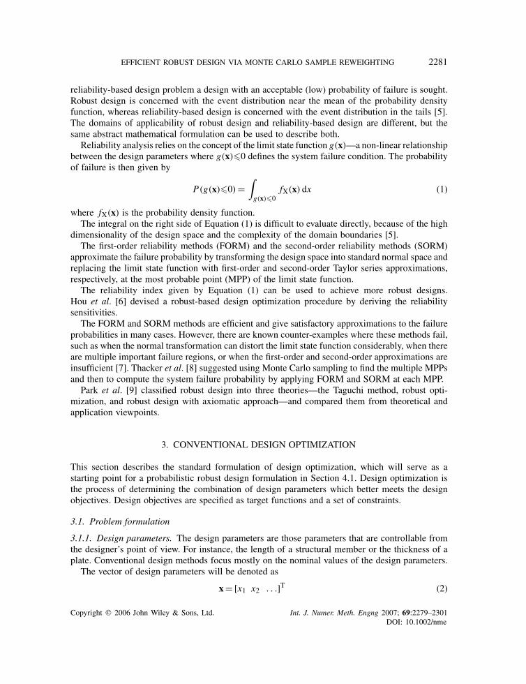
reliability-based design problem a design with an acceptable (low) probability of failure is sought.Robust design is concerned with the event distribution near the mean of the probability densityfunction, whereas reliability-based design is concerned with the event distribution in the tails [5].The domains of applicability of robust design and reliability-based design are different, but thesame abstract mathematical formulation can be used to describe both.

Reliability analysis relies on the concept of the limit state function g(x)—a non-linear relationshipbetween the design parameters where g(x)�0 defines the system failure condition. The probabilityof failure is then given by

P(g(x)�0) =∫g(x)�0

fX(x) dx (1)

where fX(x) is the probability density function.The integral on the right side of Equation (1) is difficult to evaluate directly, because of the high

dimensionality of the design space and the complexity of the domain boundaries [5].The first-order reliability methods (FORM) and the second-order reliability methods (SORM)

approximate the failure probability by transforming the design space into standard normal space andreplacing the limit state function with first-order and second-order Taylor series approximations,respectively, at the most probable point (MPP) of the limit state function.

The reliability index given by Equation (1) can be used to achieve more robust designs.Hou et al. [6] devised a robust-based design optimization procedure by deriving the reliabilitysensitivities.

The FORM and SORM methods are efficient and give satisfactory approximations to the failureprobabilities in many cases. However, there are known counter-examples where these methods fail,such as when the normal transformation can distort the limit state function considerably, when thereare multiple important failure regions, or when the first-order and second-order approximations areinsufficient [7]. Thacker et al. [8] suggested using Monte Carlo sampling to find the multiple MPPsand then to compute the system failure probability by applying FORM and SORM at each MPP.

Park et al. [9] classified robust design into three theories—the Taguchi method, robust opti-mization, and robust design with axiomatic approach—and compared them from theoretical andapplication viewpoints.

3. CONVENTIONAL DESIGN OPTIMIZATION

This section describes the standard formulation of design optimization, which will serve as astarting point for a probabilistic robust design formulation in Section 4.1. Design optimization isthe process of determining the combination of design parameters which better meets the designobjectives. Design objectives are specified as target functions and a set of constraints.

3.1. Problem formulation

3.1.1. Design parameters. The design parameters are those parameters that are controllable fromthe designer’s point of view. For instance, the length of a structural member or the thickness of aplate. Conventional design methods focus mostly on the nominal values of the design parameters.

The vector of design parameters will be denoted as

x= [x1 x2 . . .]T (2)



3.1.2. System parameters. The system parameters are those parameters that the designer eithercannot or does not want to control. They are intrinsic to the system, and because of that are oftenomitted from design considerations.

Common system parameters are modelling parameters such as damping factors, external loadsto the structure such as wind or ground motion, or noise factors in the manufacturing process.

The vector of system parameters will be denoted as

p=[p1 p2 . . .]T (3)

When system parameter values are not known precisely then their estimates must be used instead,usually taken from worst-case scenarios.

3.1.3. Objectives. An objective is a variable that is to be maximized or minimized. For example,a designer may wish to minimize production cost, maximize performance, minimize weight, min-imize FRF peaks, minimize static displacement, etc.

Objectives will be denoted by

J(x,p) =[J1(x,p) J2(x,p) . . .]T (4)

When there is more than one objective, they can either be weighted to form a single objectiveor considered simultaneously.

3.1.4. Constraints. A constraint is a formal condition that any candidate solution must observe,regardless of how well the solution performs with respect to the objectives. Common designconstraints are structural limits such as yield stress, geometric limits such as the maximum allowabledeflection or maximum overall dimensions, economic limits such as a fixed budget, etc.

Constraints can be formulated as a set of inequalities

g(x,p) =[g1(x,p) g2(x,p) . . .]T�0 (5)

Constraint inequalities can be reversed by multiplying by −1. Equality constraints can be replacedby two inequality constraints.

Constraints can either be used explicitly by the optimization algorithm, or incorporated into theobjective function [10].

3.1.5. Model. The model relates the constraints and the objectives to the design parameters andsystem parameters (Figure 1), and may be regarded as a black-box.

Figure 1. Design model.



3.2. Problem solution

3.2.1. Single objective problems. If there is a single objective, then the optimum solution is givenby

xopt = argmaxx

J(x,p) (6)

for the set of x which satisfies Equation (5). This problem can be solved using appropriateoptimization techniques, such as gradient-based algorithms or the simplex method.

3.2.2. Multiple objectives problems. If there is more than one objective then there is no uniqueoptimum solution. The multiple objective problem can be transformed into a series of single-objective problems [11], of the form

argmaxx

∑i

�isfi

Ji (x,p) (7)

where sfi is the scale factor (sfi>0) and �i is the weight of the i th objective, respectively.Weights aretypically chosen such that

∑i �i = 1 and �i�0 resulting in a convex combination of the objectives.

The set of solutions of Equation (7) forms the so called Pareto front—a set of solutions suchthat no objective can be improved further without worsening another at the same time. The finalchoice of design variables is left to the decision maker, who weights the objectives according tothe trade-offs, thereby implicitly providing an aggregated objective function.

3.3. Limitations

The main limitation of the conventional design methodology described above is that the uncer-tainty, both in the design and system parameters, is unaccounted for in the optimization. Con-ventional design also does not provide an integrated process to design tolerances along with thenominal values. This is usually done by a posterior analysis, based on the parameter sensitivities.Resorting to worst-case values or high safety factors on system parameters to compensate for theuncertainty/variability leads to over-dimensioned designs. These limitations usually lead to moreiterations of the design cycle. More experiments are required to fine tune the system parametervalues and to adjust the tolerances of the design parameters to reach an acceptable design.

4. PROBABILISTIC DESIGN OPTIMIZATION

Robust design tries overcome the limitations of conventional design by taking into account thevariability of the manufacturing process and the uncertainty in the modelling. This section describesa probabilistic approach to robust design, taking as base the formulation of conventional designgiven in Section 3.

4.1. Problem formulation

4.1.1. Design parameters. In robust design, the designer can control both the nominal values ofthe design parameters, and also their tolerances. Other design variables within the manufacturingprocess can also affect the variability in the design parameters. Generally, the designer can shapethe probability density function of the design parameters.



The design parameter vector xwill now be a realization of the design parameter random vectorX.This vector is assumed to follow a probability distribution belonging to a family of probabilitydistributions, such as

X ∼ Dx (x) (8)

where X is the design parameter random vector, Dx is the probability distribution family, and x arethe distribution parameters.

For example, when designing the length of a structural beam, the distribution family Dx couldbe a uniform distribution and the design variables x would be the nominal value and tolerance.When designing the thickness of a plate, the distribution family could be an AR(1) random field,and the design variables would be the mean thickness, the thickness standard deviation, and thesurface smoothness (the random field correlation length).

The design variables x are distinct from the design parameters x. The design variables arecontrolled by the designer, but the design parameters are fed to the model. The former shapes thelatter, but does not completely determine it—the gap between them is filled by the uncertainty dueto the manufacturing process.

4.1.2. System parameters. Similar to the design parameters, the system parameters will be refor-mulated as probability distributions in order to account for their uncertainty. The system parametervector p will be the realization of the system parameter random vector P which follows a givendistribution Dp,

P ∼ Dp (9)

Uncertainty in the system parameters can stem from a lack of knowledge. For example, dampingfactors are difficult to model precisely. Such system parameters have reducible uncertainty. Bayesianprobability theory can be used to update the parameter probability distribution Dp from experimentalmeasurements. The nature of other parameters can be truly random, such as the loading caused bywind. The uncertainty of these parameters is irreducible.

4.1.3. Constraints. In robust design, constraints can no longer be satisfied in a Boolean true orfalse sense. In general, for every combination of the design variables there is a non-zero probabilitythat either the constraint is observed or not. So, enforcing a zero probability of a constraint notbeing satisfied could narrow the set of admissible designs to the empty set. However, it is usuallyacceptable that the i th constraint is not satisfied with a probability lower than a small residualprobability �i . Thus

1 − P(gi (x,p)�0|x)��i (10)

The complement probability, 1 − �i , is referred as the confidence level or reliability.The value of �i depends on the impact of the violation of the constraint. The probability of

structural failure should be low, but the probability of structural collapse should obviously be evenlower. Thus, in general, there will be a different value �i for each constraint.



According to Equation (10), the constraints of Equation (5) are reformulated as

g(x) =

⎡⎢⎢⎢⎣1 − P(g1(x,p)�0|x) − �1

1 − P(g2(x,p)�0|x) − �2

...

⎤⎥⎥⎥⎦�0 (11)

The probability in Equation (10) is given by the integral

P(gi (x,p)�0|x) =∫ ∫

gi (x,p)�0fX(x|x) fP(p) dp dx (12)

or alternatively

P(gi (x,p)�0|x) =∫ ∫

u(−gi (x,p)) fX(x|x) fP(p) dp dx (13)

where u is the Heaviside step function.Equality constraints cannot be handled in a similar fashion to the inequality constraints, as the

probability of an equality constraint being satisfied is always zero. Instead, equality constraintsshould be seen as a decrement in number of degrees of freedom of the model. Effectively, thepresence of equality constraints implies that, for every equality constraint, the value of a parametercan be determined from all remaining parameters. Therefore, equality constraints can be hiddeninside the model and the respective dependent parameter eliminated, as viewed from outside of themodel.

4.1.4. Objectives. Like constraints, objectives can only be meet in a statistical sense. Robust designobjectives should be restated as maximizing the original objectives in a mean sense

J(x) =E(J(x,p)|x) (14)

which is given by the integral

J(x) =∫ ∫

J(x,p) fX(x|x) fP(p) dp dx (15)

Maximizing the mean implies that favourable or unfavourable scenarios are, respectively, desir-able or undesirable in an equal manner. However, the designer may wish either to maximize thewindfall likelihood or to minimize the risk instead. This can be accomplished by attributing a utilityto each possible response, by including a monotonic utility function u(·) in the objectives. This isnot usually relevant for conventional design because the position of the maximum response isunaffected by a monotonic utility function. Thus, for conventional design, the best outcomeis always the best, regardless how much better it is when compared to other designs. But forrobust design, owing to the multitude of possible outcomes considered simultaneously, the relativeimportance of each outcome does matter.

4.1.5. Model. Robust design only takes a different perspective of the same reality from conventionaldesign. Therefore the model, which describes the underlying reality, basically remains unaltered inrobust design. The difference is in the kind of inputs fed to the model and in the outputs produced by



Figure 2. Robust design model.

it. The model parameters (inputs) are now joint probability density functions, and so is the expectedresponse (output). The shift from deterministic (conventional) design optimization to probabilistic(robust) design is more a change in substance than in form (Figure 2).

Therefore, a good model for conventional design should also be good enough for robust design.When moving to robust design the only further modelling effort is to choose the appropriateprobability distributions for the design and system parameters.

Nevertheless, robust design may require more detailed parameters. Specifically, whenever anominal design parameter occurs more than once in the model a different parameter should be usedfor each instance. Imagine, for example, the diameter of a set of spot welds. Although all of thespot welds have the same nominal diameter, the actual diameter of each spot weld differs from theothers because of the variability in the welding process. So, although they can be modelled as asingle diameter parameter in the deterministic model, in the non-deterministic model there shouldbe a separate diameter parameter for each individual spot weld. This is necessary to faithfullymodel the statistical independence between parameters.

4.2. Problem solution

Since the robust design problem formulation results in a problem equivalent to conventional design,the solution procedures for conventional design described in Section 3.2 also apply to robust design.

The main difficulty is calculating the integrals of Equations (13) and (15), which can be reducedto the form ∫ ∫

h(x,p) fX(x|x) fP(p) dp dx (16)

Section 5 describes the traditional perturbation approach (similar to the techniques used forreliability analysis in Section 2) which is efficient, if the necessary conditions for its application(smooth response surface and small variations) are met. Section 6 describes a novel and generalapproach based on the Monte Carlo simulation method to evaluate these integrals. The main idea



behind both approaches is to factorize out of Equation (16) as much computation as possible [12],allowing those factors to be pre-calculated before entering the iterative loop of the optimization.

5. PERTURBATION APPROACH

The application of the perturbation uncertainty propagation method provides a fast and oftensufficiently accurate approximation to the integral of Equation (16).

This is accomplished first by changing the domain of integration from the parameter space intothe response space ∫ ∫

h(x,p) fX(x|x) fP(p) dp dx=∫

fy(y|x) dy (17)

where y = h(x,p) is the response variable. The response y is then approximated by a first-orderTaylor series in h:

y ≈ h(x0,p0) +[�h�x

(x0, p0)]

· (x − x0) +[�h�p

(x0, p0)]

· (p − p0) (18)

around point (x0,p0). If the parameters x and p follow multivariate normal distributions

X ∼ N(lx ,Rx ), P ∼ N(lp,Rp) (19)

with mean vectors lx and lp, and covariance matrices Rx and Rp, respectively, then the responsey will follow a normal distribution

Y ∼ N(�y, �y) (20)

where the mean response is

�y = h(x0,p0) +[�h�x

(x0,p0)]

· (lx − x0) +[�h�p

(x0,p0)]

· (lp − p0) (21)

and the response variance is

�2y =[�h�x

(x0,p0)]Rx

[�h�x

(x0, p0)]T

+[�h�p

(x0,p0)]Rp

[�h�p

(x0,p0)]T

(22)

In particular, Equation (15) becomes

Ji (lx ,Rx ) = �y, y = Ji (x,p) (23)

for every i th objective, and Equation (12) becomes

P(g j (x,p)�0|lx ,Rx ) = Fy(0), y = g j (x,p) (24)

for every j th constraint, where Fy is the response (Gaussian) probability distribution function.Even if the parameter distributions are not multivariate normal, they can be transformed to be

so. Random variables may be transformed into uncorrelated Gaussian variables exactly using theRosenblatt transformation, or approximately using the Nataf transformation [13, 14].



These normal space transformations have the general form

x= h(z) (25)

where z is a vector of zero mean, unit variance, uncorrelated normal variables. Since, fromEquation (8), the parameter random vector distribution X depends on the design variables x, sowill the normal space transformation

x= h(z, x) (26)

Only the first-order terms of h are relevant for the perturbation approach, therefore Equation (26)can be rewritten as

x= x0 + Jh(x) · (z − z0) (27)

where z0 is obtained by solving Equation (26) for x= x0 as

x0 = h(z0, x) (28)

and Jh(x) is the jacobian matrix of h with respect to z at the point (z0, x)

Jh(x) =[�h�z

(z0, x)]

(29)

Since the linear transformation of normal variables results in normal variables, Equation (27) isequivalent to

X ∼ N(lx ,Rx ) (30)

where

lx = x0 + Jh(x) · (lz − z0) (31)

= x0 + Jh(x) · (0 − z0) (32)

Rx = Jh(x)T · Jh(x) (33)

since lz = 0 by definition. Therefore, for every non-normal distribution, an equivalent normaldistribution can be found.

For the best approximation of the mean objectives, the linearization point (x0,p0) should be asclose as possible to the point (lx , lp). For the best approximation of the constraints observationprobability, the linearization point should be at the MPP of the constraint boundary. Both dependon the actual parameter distribution, hence x. However, the final optimum value x is unknownbeforehand since it is the final result of the optimization. Therefore an initial estimate must be usedfor x0, and if the optimum differs too much from this initial value then a further linearization andoptimization pass must be performed using the newer estimate.

The perturbation method suffers from the usual limitation, yielding inaccurate results wheneverthe response is not sufficiently linear. The Monte Carlo simulation method, on the other hand,although more computationally demanding, is generally appliable and is therefore the main focusof this work.



6. MONTE CARLO SIMULATION APPROACH

6.1. Conventional

The Monte Carlo simulation method approximates the integral of Equation (16) by sampling Nvalues of xi and pi from the Dx (x) and Dp distributions respectively, reducing the integral to asum ∫ ∫

h(x,p) fX(x|x) fP(p) dp dx≈ 1

N

N∑i=1

h(xi , pi ) (34)

Every new test value of the design variables x corresponds to a different probability distributionbeing taken from the probability distribution family, Dx (x). This, in turn, implies that a new set ofN samples of xi must be generated for every new value of x, and the respective points h(xi , pi )reevaluated. Resampling can be very time consuming, even if a meta-model is used as a surrogatefor the h function, since the number of samples needed for good accuracy in the Monte Carlomethod is usually high.

The estimates given by Equation (34) are non-deterministic, i.e. two evaluations using the samevalues of x will not necessarily give the same value, as the two sets of random samples thatare generated will be different. Furthermore, near the boundary, the constraints of Equation (11)may be satisfied for some evaluations, but not satisfied for others. This phenomena is a seriousobstacle to the employment of most optimization algorithms. The use of a pseudo-random numbersequence generator with a constant seed may reduce the problem, but that still does not guaranteethe desirable smoothness of the objective and constraint surfaces. To completely overcome thislimitation, a higher number of samples N must be generated in order to reduce the randomnessin the objective and constraint functions to below the sought precision in the design variables x.A better approach is to resort to the same reweighting technique developed for the uncertaintyquantification in [12].6.2. Reweighting

Instead of resampling for every trial of x, a single set of samples is reweighted according to thedesired distribution, as illustrated in Figure 3.

The samples xi are generated according to a different probability distribution gX(x), andEquation (34) is rewritten as

∫ ∫h(x,p) fX(x|x) fP(p) dp dx≈ 1

N

N∑i=1

wi (x)h(xi ,pi ) (35)

where

wi (x) = fX(xi |x)gX(xi )

(36)

Therefore only the weights wi depend on x, eliminating the need to resample xi or reevaluate h.

6.3. Choosing the sample distribution

The probability distribution gX should be as close as possible to the probability distribution fXthat we want to test. If they are too different then some weights will drop to zero, because of the



PDF Resampling Reweighting

Figure 3. Reweighting versus resampling—there is a different distribution for each row; the left columnshows the PDF, where the density is indicated by the shade of grey; the middle column shows samplestaken according to each PDF, represented by dots; and the right column shows a fixed set of samples,

reweighted according to each PDF, where the sample weight is indicated by the dot size.

positiveness and unit integral properties of the probability density functions. The more differentthe distributions are, the more weights will be close to zero, the effective number of samples useddrops to a small fraction of N , and the accuracy of the integral approximation will suffer.

The employment of an appropriate gX can be determined by applying a simple statistical test.Let us assume that the integrand is the unit function, h(·) = 1. Replacing this in Equation (16)



yields ∫ ∫fX(x|x) fP(p) dp dx=

∫fX(x|x) dx ·

∫fP(p) dp= 1 (37)

since both fX are fP are probability density functions. Since Equation (35) is an approximationto that integral, then

1

N

N∑i=1

wi (x) ≈ 1 (38)

which is equivalent to saying that the mean weight w ≈ 1. If a large number of samples N is taken(true for virtually all applications) then, owing to the central limit theorem, the mean weight w willapproximately follow a normal distribution with N(� =w, �2 = sw/N ), where sw is the varianceof w, given by

sw = 1

N − 1

N∑i=1

(wi − w)2 (39)

Equation (38) can be verified by the following statistical test for the mean of w [15]:w − 1√sw/N

∈ [−z(�), z(�)] (40)

where � is the desired level of confidence, and z(�) the inverse of the normal tail probability.This simple test can determine whether the given weights are effectively consistent with the w = 1statement and, therefore, if an adequate gX was chosen.

6.4. Normalizing the weights

From Equation (38) it follows that the mean weight w does not generally match unity. This is aconsequence of the number of samples being less than infinity and the samples not covering all ofthe parameter space. This can yield inaccurate results when estimating probabilities, for exampleestimating a probability outside the [0, 1] interval. To prevent this, it is advisable to normalize theweights in such circumstances. Thus, instead of Equation (35), we use

∫ ∫h(x,p) fX(x|x) fP(p) dp dx≈ 1

N

N∑i=1

wi

wh(xi ,pi ) (41)

7. A TRUSS EXAMPLE

The approach described earlier will now be demonstrated using a numerical application.

7.1. Description

7.1.1. Model. The application is a two-dimensional beam truss structure with rigid joints andcircular cross section beams (Figure 4). Each beam is modelled with four Euler–Bernoulli beamelements vibrating in the plane. Every node has three degree of freedoms consisting of displacementin the x and y directions and a rotation in the out-of-plane direction. The outer-left nodes are



Figure 4. Application—beam truss.

clamped. The beams are made of steel, with a Young’s modulus of E = 210GPa and a density of� = 7800 kg/m3.

Figure 5 shows the lower natural frequencies and respective mode shapes for a nominal valueof the beam diameter.

7.1.2. Design variables. The design parameter is the beam diameter d . Thus,

x=[d] (42)

The hypothetical metalworking lathe that will be used to cut the circular beams produces circularshapes with a deviation which follows a normal distribution with 3�d = 1mm. Beams with a desiredtolerance �d are produced by scraping those whose dimensions are outside the specification.Therefore the beam diameter follows a truncated normal distribution, with a probability densityfunction (Figure 6) given by

f (d)=

⎧⎪⎪⎪⎪⎨⎪⎪⎪⎪⎩

0 d<�d − �d

�((d − �d)/�d)

�(�d/�d) − �(−�d/�d)�d − �d�d��d + �d

0 d>�d + �d

(43)

and a cumulative probability density function given by

F(d)=

⎧⎪⎪⎪⎪⎨⎪⎪⎪⎪⎩

0 d<�d − �d

�((d − �d)/�d) − �(−�d/�d)

�(�d/�d) − �(−�d/�d)�d − �d�d��d + �d

1 d>�d + �d

(44)

where � and � are the zero mean unit variance normal probability density function and cumulativeprobability density function, respectively [16].

Since the parameter has a non-normal distribution, it has to be transformed to a normal variablebefore applying the perturbation approach. Being a single parameter, the transformation can besimply stated as

z =�−1(F(d)) (45)



(a)

(b)

(c)

(d)

Figure 5. Application—mode shapes for a nominal diameter (d = 20mm): (a) �1 = 112.81Hz;(b) �2 = 136.73Hz; (c) �3 = 137.33Hz; and (d) �4 = 148.42Hz.

The robust design variables are the beam mean diameter �d , and its tolerance �d .

x= [�d �d ]T (46)



Figure 6. Truncated normal distribution probability density functions.

0 10 20 30 40 50

Beam nominal diameter, d (mm)

0

2

4

6

8

10

Bea

m w

eigh

t, M

(kg

)

Figure 7. Application—the mass of a horizontal or vertical beam.

7.1.3. Objective. The main objective is to minimize the production cost, where only the materialcosts will be considered. The mass of a single beam of length l is

M(d)= l�d2

4� (47)

Figure 7 shows the mass associated with a horizontal or vertical beam.The design objective is then

J(x)= [M(d)] (48)

For robust design purposes, the cost will include the mass of the structure, but also the mass ofthe scrapped metal

C ∝ M × N (49)

where N is the expected number of beams which have to be produced in order to find one withinspecification.



Let p be the probability that a beam diameter is on specification. Then the probability that thefirst beam will have a diameter with the required specification is p, for the second is (1− p) × p,for the third is (1− p) × (1− p)× p, and so on. Therefore the average number of beams that haveto be produced in order to find a beam within specification is

N =∞∑i=1

i × (1 − p)i−1 × p= 1

p(50)

The probability p is given by

p=�(�d/�d) − �(−�d/�d) (51)

where � is the zero mean unit variance Gaussian cumulative probability density function.Figure 8 shows the predicted impact of the tolerance on the structure production cost given

by Equations (50) and (51). Tolerances lower than the tolerance normally given by the machineimply that a larger number of items will be scrapped. Tolerances higher than the intrinsic machinetolerance have almost no impact in the cost. Equations (50) and (47) show that the direction forlower costs is associated with lower diameters and higher tolerances.

The objective function is then

J(x) = [M(�d) × N (�d)] (52)

7.1.4. Constraints. The only constraint will be that the fundamental natural frequency of the wholestructure must lie above 100Hz. Thus

g(x) = [100 − �1(x)]�0 (53)

g(x) = [1 − P(100 − �1(x)�0) − �]�0 (54)

for � = 10%.

10-1 01

Normalized tolerance, ∆d /(3σ)

0

1

2

3

4

5

Num

ber

of b

eam

s re

quir

ed, N

Figure 8. Application—cost associated with tolerance. The vertical axis gives the expected number ofbeams that have to be produced in order to find a single beam within specification. The horizontal axis

gives the specified tolerance normalized by the three times the lathe’s standard deviation.



7.2. Procedure

The complete robust design analysis is performed in three stages of increasing complexity, startingwith a deterministic analysis, followed by a simplified robust design analysis which considers allbeam diameters to be identical, and ending with the full robust design analysis considering thebeam diameters to be independent parameters. The results from earlier stages are reused as initialdesigns for the latter stages.

7.2.1. Deterministic analysis. It is important to perform an initial deterministic analysis of themodel, to give an insight into the model response surface and its peculiarities. Furthermore, theresults from the deterministic analysis can be reused as initial estimates for the robust design. Thisis even more important since the quality of the initial design has a decisive impact on the resultsof the described methods.

Figure 9 shows the evolution of the first natural frequency of the truss, �1, with respect to thebeam diameter, d . From Equations (48) and (53) it follows that a beam diameter of d = 15.83mmwould theoretically make the first natural frequency lie exactly at �1 = 100Hz. But this value leavesno margin for variations. Considering the need for a non-zero tolerance and the monotonic natureof the response curve, this diameter value is necessarily a lower bound for the optimum designvalue.

The curvature of the response curve is negative, which means that for higher values of thediameter d the first natural frequency �1 becomes less sensitive to variations.

7.2.2. Robust design—identical parameters. For robust design Equations (52) and (54) will beused. Initially the beam diameters will be considered to be identical. Taking into account the

10 12 14 16 18 20 22 24 26 28 30

Beam diameter, d (mm)

60

70

80

90

100

110

120

130

Firs

t nat

ural

fre

quen

cy,

ω1

(Hz)

15.8

3 m

m

100 Hz

Figure 9. Application—deterministic response.



0 1 2 3 4 5 6 7 8 9 10

d1

0

(a) (b)

1

2

3

4

5

6

7

8

9

10

d 2

0 1 2 3 4 5 6 7 8 9 10

d1

0

1

2

3

4

5

6

7

8

9

10

d 2

Figure 10. Sampling of parameter space. The dots represent the samples in the first two dimensions ofthe parameter space. From the problem definition d1 and d2 are independent random variables but followthe same distribution, and therefore their probability mass will be near the d1 = d2 line. Uniform sampling(on the left) yields many points away from this line, while the suggested approach (on the right) yields amore efficient sampling while covering the same range: (a) uniform sampling; and (b) efficient sampling.

preliminary deterministic analysis in the previous section, the samples of the response curve willbe taken uniformly around and above the deterministic optimum. The results from this stage willbe used in the final stage.

7.2.3. Robust design—independent parameters. Considering all of the beam diameters to be equalis unrealistic. It is expected that the fluctuation of 15 independent parameters would sometimescancel out, resulting in less total variance due to averaging. In this second stage of robust design,the diameters of the individual beams that make up the truss will be considered independent ofeach other. Equation (42) will be replaced by

x=[d1 d2 . . . d15]T (55)

The main difficulty of this stage is the dimensionality of the parameter space, as 15 differentparameters are considered instead of just one.

The first approach used to sample the parameter space was uniform sampling. But thisattempt produced no results, as virtually all of the weights (with the exception of one or two) inEquation (36) dropped down to almost zero. Zero weights occur when the distribution used forsampling does not produce enough points on the likely subspace of the distribution being tested.It is easy to understand why this happens with this application: although all of the diameters areindependent, they all follow the same distribution. Thus the true probability distribution of theparameters will necessarily be centred on the d1 = d2 = · · · = d15 line. Points sampled from amultivariate uniform distribution will be spread over a 15-dimensional volume, instead of beingconcentrated on the identity line manifold. This is illustrated by Figure 10(a) for a two-dimensionalparameter space.

A more efficient approach in this kind of application is to sample from the distribution resultingfrom the sum of a univariate distribution and a zero centred distribution, such as a zero mean



13 14 15 16 17 18

Diameter mean, µd (mm)

10-1

1

101

Dia

met

er to

lera

nce,

∆d (

mm

)

4 kg3 kg

2 kg

1 kg

13 14 15 16 17 18

Diameter mean, µd (mm)

10-1

1

101

Dia

met

er to

lera

nce,

∆d

(mm

) 10%

5%

1%

0.1%

Figure 11. Application—objectives (above) and failure probability (below). Theoptimum design is marked with × .

normal distribution:

U(a, b) + N(0, �) (56)

where [a, b] specifies the range of interest to sample and � specifies the spread of the samplesaround the identity line, as illustrated by Figure 10(b). This distribution probability density functionis given by

f (x)=∫ b

a

1

b − afN (x − z) dz (57)



Table I. Result comparison table.

Method Stage Pass �d (mm) �d (mm) P(�0<100Hz)

Deterministic 15.83Perturbation 1 16.26 2.70 0.05% ± 0.02%Monte Carlo 1 16.26 2.11 0.04% ± 0.02%Perturbation 2 15.99 3.18 13.16% ± 0.28%Monte Carlo 2 1 16.02 2.38 8.31% ± 0.22%Monte Carlo 2 2 16.01 2.71 9.33% ± 0.24%

which can be computed without much effort using numerical integration along z. With this newdistribution there were enough samples with non-zero weights.

7.3. Results

Figure 11 shows the objectives and the estimated failure probability over the area of interest ofthe parameter space as well as the optimum design found, for the first stage. As expected, theprobability that the constraint is unobserved drops as �d increases, and this drop is steeper forlower tolerances than for higher tolerances.

Table I shows the optimum values for the design variables in each stage estimated by thedescribed approaches. Also shown for verification purposes is the failure probability obtained byrunning the straightforward Monte Carlo simulation method with the optimum values. A differentset of N = 100 000 samples was used for that verification. For each sample its value is taken asone if �0<100Hz, and zero otherwise. The probability estimate corresponds to the mean of thesamples values, and the probability error estimate corresponds to the 99% confidence interval ofthat mean.

The failure probabilities for stage 1 are well below the admissible level of 10%, corroboratingthe prediction that considering identical beam parameters would lead to over-designed solutions.In stage 2 the optimization converged to a new optimum result, with a lower nominal diameter andhigher tolerance, closer to the allowed 10%.

Two passes were performed for the stage 2 of the Monte Carlo approach. The first used thestage 1 result as initial estimate for the parameter space sampling and optimization algorithm,while the second used the estimate of the first pass.

These results could not be achieved if the optimization of the second stage was tried directly.There would be insufficient information to sample the parameter space effectively, rendering mostsample points useless; and the presented method would give no advantage over the conventionalMonte Carlo simulation method.

8. CONCLUSIONS

In this paper the concept of design and robust design was introduced. The merits and criticisms of theTaguchi robust design approach were highlighted. A novel probabilistic robust design methodologywas presented, which allows the specification of design parameters and objectives in an intuitivemanner, coping with uncertainty in both the control and noise parameters.



Numerically, the method is based on reusing the same set of samples by reweighting. Doing sois more efficient than the constant resampling performed with a straightforward application of theMonte Carlo method. Another advantage is that the resulting objective function becomes smoothand deterministic, facilitating the performance of optimization algorithms.

The method was demonstrated on an application which, albeit purely academic, includedrealistic features of cost and requirements. A staged approach to robust design was illustrated,starting with the deterministic design problem and ending with the fully fledged robust model. Thisstaged approach allows the accumulation of knowledge of the problem, ensures a successful designoptimization, and prevents the waste of computational resources.

The main disadvantage of the presented method is the requirement to know beforehand a reason-able estimate of the optimum design in order to efficiently sample the parameter space. Thereforethis method is more appropriate for rapid convergence in the neighbourhood of the optimum designsolution. If no prior estimate of the optimum design is available then a globally more convergentapproach, such as resorting to simplified models or the regular Monte Carlo simulation method,should be employed in order to get a reliable initial estimate.

A substantial improvement for the presented method would be to include adaptive sampling.Allowing the incorporation of more samples in the middle of the optimization process, as betterestimates of the optimum solution are available, would permit consideration of a wider range withinthe design space. The knowledge of a close initial estimate would then be less important, makingthe method more globally convergent.

ACKNOWLEDGEMENTS

Jose R. Fonseca acknowledges the support of the Portuguese Foundation for Science and Technologythrough the scholarship SFRH/BD/7065/2001. Michael I. Friswell and Arthur W. Lees acknowledge thesupport of the Engineering and Physical Sciences Research Council (U.K.) through grant GR/R34936.Michael I. Friswell acknowledges the support of a Royal Society-Wolfson Research Merit Award.

REFERENCES

1. Taguchi G. Introduction to Quality Engineering: Designing Quality into Products and Processes. Asian ProductivityOrganization: Tokyo, 1986.

2. Ross PJ. Taguchi Techniques for Quality Engineering (2nd edn). McGraw-Hill: New York, 1996.3. Unal R, Dean EB. Taguchi approach to design optimization for quality and cost: an overview. Proceedings of the

International Society of Parametric Analysts 13th Annual Conference, New Orleans, LA, 1991.4. Tsui KL. A critical look at Taguchi’s modelling approach for robust design. Journal of Applied Statistics 1996;

23(1):81–95.5. Zang TA, Hemsch MJ, Hilburger MW, Kenny SP, Luckring JM, Maghami P, Padula SL, Stroud WJ. Needs

and opportunities for uncertainty-based multidisciplinary design methods for aerospace vehicles. TechnicalMemorandum NASA/TM-2002-211462, NASA, Langley Research Center, Hampton, Virginia, 2002, an electronicversion can be found at http://techreports.larc.nasa.gov/ltrs/ or http://techreports.larc.nasa.gov/cgi-bin/NTRS

6. Hou GJW, Gumbert CR, Newman PA. A most probable point-based method for reliability analysis, sensitivityanalysis and design optimization. Proceedings of the 9th ASCE Specialty Conference on Probabilistic Mechanicsand Structural Reliability (PMC2004), 2004.

7. Rackwitz R. Reliability analysis—a review and some perspectives. Structural Safety 2001; 23:365–395.8. Thacker BH, Riha DS, Millwater HR, Enright MP. Errors and uncertainties in probabilistic engineering

analysis. Proceedings of the 42nd AIAA/ASME/ASCE/AHS/ASC Structures, Structural Dynamics, and MaterialsConference, AIAA 2001-1239, Seattle, WA, 2001.

9. Park GJ, Lee TH, Lee KH, Hwang KH. Robust design: an overview. AIAA Journal 2006; 44(1):181–191.



10. Wang T, Wah B. Handling inequality constraints in continuous nonlinear global optimization. Proceedings of the2nd World Conference on Integrated Design and Process Technology, vol. 1, Austin, Texas, 1996; 267–274.

11. Kim IY, de Weck OL. Adaptive weighted-sum method for bi-objective optimization: Pareto front generation.Structural and Multidisciplinary Optimization 2005; 2(29):149–158.

12. Fonseca JR, Friswell MI, Mottershead JE, Lees AW. Uncertainty identification by the maximum likelihood method.Journal of Sound and Vibration 2005; 288(3):581–599.

13. Melchers RE. Structural Reliability Analysis and Prediction. Wiley: New York, 1999.14. Worden K, Manson G, Lord TM, Friswell MI. Some observations on uncertainty propagation through a simple

nonlinear system. Journal of Sound and Vibration 2005; 288(3):601–621.15. Guimaraes RC, Cabral JAS. Estatstica. McGraw-Hill: Lisbon, 1997.16. Johnson A, Thomopoulos N. Characteristics and tables of the doubly-truncated normal distribution. Proceedings

of POM High Tech, 2002.


Efficient robust design via Monte Carlo sample reweighting

Documents

Transcript of Efficient robust design via Monte Carlo sample reweighting