On Convergence Properties of the Monte Carlo EM Algorithm

IMS Collectionsc© Institute of Mathematical Statistics,

On Convergence Properties of the Monte

Carlo EM Algorithm

Ronald C. Neath

Hunter College, City University of New York

Abstract: The Expectation-Maximization (EM) algorithm (Dempster, Lairdand Rubin, 1977) is a popular method for computing maximum likelihoodestimates (MLEs) in problems with missing data. Each iteration of the al-gorithm formally consists of an E-step: evaluate the expected complete-datalog-likelihood given the observed data, with expectation taken at current pa-rameter estimate; and an M-step: maximize the resulting expression to findthe updated estimate. Conditions that guarantee convergence of the EM se-quence to a unique MLE were found by Boyles (1983) and Wu (1983). Incomplicated models for high-dimensional data, it is common to encounter anintractable integral in the E-step. The Monte Carlo EM algorithm of Wei andTanner (1990) works around this difficulty by maximizing instead a MonteCarlo approximation to the appropriate conditional expectation. Convergenceproperties of Monte Carlo EM have been studied, most notably, by Chan andLedolter (1995) and Fort and Moulines (2003).

The goal of this review paper is to provide an accessible but rigorous in-troduction to the convergence properties of EM and Monte Carlo EM. Noprevious knowledge of the EM algorithm is assumed. We demonstrate the im-plementation of EM and Monte Carlo EM in two simple but realistic examples.We show that if the EM algorithm converges it converges to a stationary pointof the likelihood, and that the rate of convergence is linear at best. For MonteCarlo EM we present a readable proof of the main result of Chan and Ledolter(1995), and state without proof the conclusions of Fort and Moulines (2003).An important practical implication of Fort and Moulines’s (2003) result relatesto the determination of Monte Carlo sample sizes in MCEM; we provide a briefreview of the literature (Booth and Hobert, 1999; Caffo, Jank and Jones, 2005)on that problem.

1. Introduction: The Monte Carlo EM algorithm

The expectation-maximization, or EM algorithm, is an algorithm for maximizinglikelihood functions, especially in the presence of missing data. When EM works,the algorithm’s output is a sequence of parameter values that converges to themaximum likelihood estimate (MLE). The seminal paper on EM, and that whichgave the algorithm its name, is the article by Dempster, Laird and Rubin (1977).A book length treatment is given by McLachlan and Krishnan (1997).

Consider a statistical model in which the random vector (Y, U), Y ∈ RN andU ∈ Rq, has distribution given by f(y, u; θ), a density with respect to the measureλ × µ, where λ and µ are measures on RN and Rq respectively, and indexed bythe unknown parameter θ ∈ Θ. We refer to (Y,U) as the “complete data” but onlyY = y is observed; U represents the unobserved or “missing” data. The MLE of θ

Department of Mathematics and Statistics Hunter College, City University of New York e-mail:[email protected]

AMS 2000 subject classifications: Primary 62-02Keywords and phrases: Convergence, EM algorithm, Maximum likelihood, Mixed model,

Monte Carlo

1

imsart-coll ver. 2011/11/15 file: Neath.tex date: June 22, 2012

arX

iv:1

206.

4768

v1 [

mat

h.ST

] 2

1 Ju

n 20

12

http://www.imstat.org/publications/imscollections.htm

http://www.imstat.org

mailto:[email protected]

2

is the value θ which maximizes the likelihood function

(1) L(θ; y) =

∫f(y, u; θ)µ(du)

or, equivalently, the log likelihood l(θ; y) = logL(θ; y). The EM algorithm can be

used to find θ even if the integral in (1) is intractable. Define the Q-function, amapping on Θ×Θ, by

(2) Q(θ|θ; y) = E{

log f(y, U ; θ)∣∣ y; θ

},

that is, the expected value of the “complete data” log-likelihood at θ, given theobserved data, this conditional expectation evaluated under θ. Each EM iterationformally consists of an E-step, to evaluate the conditional expectation in (2), andan M-step, to maximize it. More precisely, if θ(t) is the parameter value as of thetth iteration, the update θ(t+1) is chosen such that Q(θ(t+1)|θ(t); y) ≥ Q(θ|θ(t); y)for all θ ∈ Θ. Under regularity conditions (Boyles, 1983; Wu, 1983, and see Sec-tion 3 below), and given a suitable starting value θ(0), the resulting sequence{θ(t) : t = 0, 1, . . .

}will converge to a local maximizer of L.

If the integral in (2) admits a closed form solution, the implementation of EMis straightforward (though the M-step may still require a numerical optimizationscheme such as Newton-Raphson). Suppose it does not. As noted, the evaluationof (2) requires taking an expectation with respect to the conditional distributionof the missing data U , given observed data Y = y. If one has the means to sim-ulate random draws from this target distribution, the Q-function can be approxi-mated by Monte Carlo integration. Let u(1), . . . , u(m) denote a random sample fromh(u|y; θ) = f(y, u; θ)/L(θ; y). Then a Monte Carlo approximation to (2) is given by

Qm(θ|θ; y) =1

m

m∑k=1

log f(y, u(k); θ) .

In the Monte Carlo EM algorithm (MCEM), first introduced by Wei and Tanner(1990), the update θ(t+1) is the value of θ that maximizes Qm(θ|θ(t); y).

Applications of EM and MCEM have been numerous; in this work we focus onone in particular, the two-stage hierarchical model, introduced in Section 2. We givetwo simple but realistic examples from this class of models, and demonstrate theimplementation of EM and MCEM in those two problems. In Section 3 we discussconvergence properties of the EM algorithm. Of course, the question of convergencefor MCEM is far more complicated, and an accessible discussion of the major resultsin this area is the main objective of this review paper. In Section 4 we provide arigorous but accessible review of the two seminal papers on MCEM convergence,those of Chan and Ledolter (1995) and Fort and Moulines (2003). We make someconcluding remarks in Section 5.

2. Application: The two-stage hierarchical model

Let Y = (Y1, . . . , YN )T , where each Yi is a random variable in R1, denote the ob-servable data. In a two-stage hierarchical model, the distribution of Y is specifiedconditionally on some unobservable random quantity U = (U1, . . . , Uq)

T . Specifi-cally, we assume that conditional on U = u, the Yi are independent with conditionaldensities denoted by fi(yi|ui; θ1), where θ1 ∈ Θ1 is an unknown parameter and each


Convergence of MCEM 3

fi is a density with respect to Lebesgue or counting measure. The fi may also de-pend on an observable covariate xi though this dependence is suppressed in ournotation. Define f(y|u; θ1) =

∏Ni=1 fi(yi|u; θ1), a density on RN , and this completes

specification of the first level, or stage, of the hierarchy. At the second stage wespecify a marginal distribution for U , defined by h(u; θ2), a density on Rq thatdepends on the unknown parameter θ2 ∈ Θ2. Assume the parameter spaces Θ1 andΘ2 are open subsets of Rd1 and Rd2 , respectively. Let d = d1 + d2. The unknownparameter θ = (θ1, θ2) lies in the parameter space Θ = Θ1 ×Θ2, an open subset ofRd.

Suppose we wish to compute maximum likelihood estimates (MLEs) of θ1 andθ2. Were the random effects U observable the likelihood function would be given bywhat we will call the complete data likelihood Lc(θ; y, u) = f(y|u; θ1)h(u; θ2). Butsince only the data Y are observed, the random effects must be integrated out ofLC yielding the likelihood function

(3) L(θ; y) =

∫Lc(θ; y, u)du =

∫f(y|u; θ1)h(u; θ2)du .

We wish to find the value of θ that maximizes L, that is, the MLE θ.It will most often be the case that the integral in (3) is intractable. Booth,

Hobert and Jank (2001) provide a very nice summary of numerical and MonteCarlo methods available for maximum likelihood in this problem, arriving at theconclusion that “Monte Carlo EM is generally the simplest and most efficient MonteCarlo fitting algorithm for two-stage hierarchical models.” As noted above, the EMalgorithm is a general method for maximum likelihood in the presence of missingdata; hierarchical models are cast in this light by viewing the unobserved randomeffects as “missing”.

Let lc = logLc denote the complete data log likelihood, so

lc(θ; y, u) = log f(y|u; θ1) + log h(u; θ2) .

Thus in the setting of hierarchical models, the EM update rule introduced in Section1 can be written

θ(t+1)1 = arg max E

{log f(y|U ; θ1)

∣∣ y; θ(t)},

θ(t+1)2 = arg max E

{log h(U ; θ2)

∣∣ y; θ(t)},

(4)

that is, the update of θ1 and that of θ2 can be considered separately.If one or both of the expectations in (4) is intractable, one might employ the

Monte Carlo EM algorithm. The MCEM update rule for the two-stage hierarchical

model is given here. Let θ(t) = (θ(t)1 , θ

(t)2 ) denote the current parameter value; then

θ(t+1) is found by

1. Simulate u(t,1), . . . , u(t,m), a random sample from the conditional densityh(u|y; θ(t));

2. Compute updates

θ(t+1)1 = arg max

{1

m

m∑k=1

log f(y|u(t,k); θ1)

}

θ(t+1)2 = arg max

{1

m

m∑k=1

log h(u(t,k); θ2)

}.


4

The “target density” for the Monte Carlo E-step (step 1) is the conditional densityof the random effects given the data,

(5) h(u|y; θ) ∝ f(y|u; θ1)h(u; θ2) .

If direct simulation from (5) is impossible, one might resort to a Markov chain MonteCarlo (MCMC) method such as the Metropolis-Hastings algorithm. In this casethe sample

{u(t,k) : k = 1, . . . ,m

}is an ergodic Markov chain having h(u|y; θ(t))

as its unique stationary density (see, for example, Robert and Casella, 2004). Analternative approach is to compute a quasi-Monte Carlo or randomized quasi-MonteCarlo (L’Ecuyer and Lemieux, 2002) approximation to the Q-function with the goalof reducing Monte Carlo error and hence increasing the efficiency of the algorithm.We will not consider quasi-Monte Carlo methods any further in this report; theinterested reader is referred to Jank (2004).

2.1. Example 1: A linear mixed model

Table 1 contains a data set for an experiment described by Snedecor and Cochran(1989). The experiment involved six bulls and very many cows. From each bull,some number of semen samples was taken, and each of these samples was usedin an attempt to artificially inseminate a large number of cows. Some attemptswere successful and some were not; let Yij denote the success rate (percentage ofconceptions) for sample j from bull i, for j = 1, . . . , ni and i = 1, . . . , q = 6; hereN =

∑qi=1 ni. Consider the one-way random effects model

yij = µ+ ui + eij

where µ is the overall mean, ui is the ith bull effect, and eij is a residual error term.As the six bulls were a random sample from a larger population of bulls, the ui aremodeled as independent and identically distributed (i.i.d.) random effects. Modelspecification is completed by a distribution assumption on the bull effect and errorterm; we take

ui ∼ iid Normal(0, σ2

u

); independent of eij ∼ iid Normal

(0, σ2

e

).

When there exists a conjugate relationship between f and h, as in the normal linearmixed model, the integral in (3) can be solved explicitly. The resulting log-likelihoodcan be maximized numerically (or analytically in the case of balanced data ni ≡ n);for the bulls data we obtain µ = 53.318, σ2

u = 54.821, and σ2e = 249.23.

Consider the EM algorithm. We find it more convenient to work with an equiva-lent version of the model in which yij = ui+ eij and the ui are i.i.d. Normal(µ, σ2

u).Under this reparameterization the complete data log-likelihood of θ = (µ, σ2

u, σ2e) is

lc(θ; y, u) = −N2

log(σ2e)− 1

2σ2e

q∑i=1

ni∑j=1

(yij − ui)2 − q

2log(σ2

u)− 1

2σ2u

q∑i=1

(ui − µ)2 .

Owing to the conjugacy it is straightforward to show that

(6) Ui|(Y = y; θ) i = 1, . . . , q are indep Normal

(σ2eµ+ niσ

2uyi

σ2e + niσ2

u

,σ2eσ

2u

σ2e + niσ2

u

).



Bull (i) ni Percentage of conception1 5 46, 31, 37, 62, 302 2 70, 593 7 52, 44, 57, 40, 67, 64, 704 5 47, 21, 70, 46, 145 7 42, 64, 50, 69, 77, 81, 876 9 35, 68, 59, 38, 57, 76, 57, 29, 60

Total 35Table 1

Bovine artificial insemination data of Example 1 (Snedecor and Cochran, 1989).

Denote the conditional mean and variance of Ui given Y = y by ui and Vi, respec-tively. Then the EM update rule is given by

µ(t+1) =1

q

q∑i=1

u(t)i

σ2(t+1)

u =1

q

q∑i=1

(V

(t)i +

[u

(t)i

]2)−[µ(t+1)

]2σ2(t+1)

e =1

N

q∑i=1

ni∑j=1

y2ij − 2niyiu

(t)i + ni

(V

(t)i +

[u

(t)i

]2) .

Given the existence of a closed form EM update, there is no practical reason toresort to Monte Carlo EM (indeed there was no practical need for EM, as we founda closed form expression for the likelihood as well), but we will consider MCEMfor illustration. Let u(t,1), . . . , u(t,m) denote a sequence of simulated draws fromh(u|y; θ(t)), given at (6). The MCEM update rule for θ(t+1) is

µ(t+1) =1

mq

m∑k=1

q∑i=1

u(t,k)i

σ2(t+1)

u =1

mq

m∑k=1

q∑i=1

(u

(t,k)i − µ(t+1)

)2

σ2(t+1)

e =1

mN

m∑k=1

q∑i=1

ni∑j=1

(yij − u(t,k)

i

)2

.

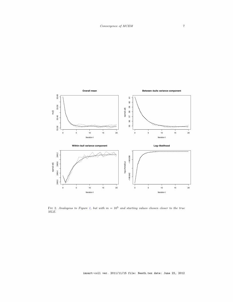
We ran three independent MCEM runs of 20 iterations each, starting at the point

(µ(0), σ2(0)

u , σ2(0)

e ) = (55, 45, 260). For each update we used Monte Carlo sample sizem = 104; results are shown in Figure 1. The three dashed lines indicate the pathsof the three MCEM runs, and the solid line shows that of ordinary (deterministic)EM. We did three more runs with starting values closer to the MLE and usingm = 105; those results are summarized in Figure 2.


6

0 5 10 15 20

53.5

54.0

54.5

55.0

Overall mean

Iteration t

mu[

t]

0 5 10 15 2046

4850

5254

Between bulls variance component

Iteration t

sigm

a2.u

[t]

0 5 10 15 20

250

252

254

256

258

260

Within bull variance component

Iteration t

sigm

a2.e

[t]

0 5 10 15 20

148.

7414

8.70

148.

66

Log likelihood

Iteration t

logL

(thet

a[t];

y)

Fig 1. Trace plots for Monte Carlo EM in Example 1, based on Monte Carlo sample size m =104 at each iteration. Top left plot is overall mean µ, top right and bottom left are variancecomponents σ2

u and σ2e , respectively. Bottom right plot shows log-likelihood evaluated at current

parameter value. The solid line is deterministic EM and the three dashed lines correspond to threeindependent runs of Monte Carlo EM.



0 5 10 15 20

53.3

053

.40

53.5

053

.60

Overall mean

Iteration t

mu[

t]

0 5 10 15 20

5556

5758

5960

61

Between bulls variance component

Iteration t

sigm

a2.u

[t]

0 5 10 15 20

248.

024

8.4

248.

824

9.2

Within bull variance component

Iteration t

sigm

a2.e

[t]

0 5 10 15 20

148.

642

148.

638

Log likelihood

Iteration t

logL

(thet

a[t];

y)

Fig 2. Analogous to Figure 1, but with m = 105 and starting values chosen closer to the trueMLE.


8

2.2. Example 2: A logit-normal generalized linear mixed model

Let Y = {Yij : j = 1, . . . , ni; i = 1, . . . , q} denote a set of binary response variables;here again one can think of Yij as the jth response for the ith subject. Let xij be acovariate (or vector of covariates) associated with the i, j observation. Conditionalon the random effects U = u ∈ Rq, the responses are independent Bernoulli(πij)where

log

(πij

1− πij

)= βxij + ui .

Let U1, . . . , Uq be independent and identically distributed as Normal(0, σ2). Thelikelihood is given by

L(β, σ2; y) =(σ2)−q/2×∫

Rq

exp

q∑i=1

ni∑j=1

[yij (βxij + ui)− log

(1 + eβxij+ui

)]− 1

2σ2

q∑i=1

u2i

du .

The above model has been used by several authors (Booth and Hobert, 1999; Caffo,Jank and Jones, 2005; McCulloch, 1997) as a benchmark for comparing Monte Carlomethods of maximum likelihood. We consider here a data set generated by Boothand Hobert (1999, Table 2) with ni = 15, q = 10, and xij = j/15 for each i, j. For

these data the MLEs are known to be (β, σ2) = (6.132, 1.766).A version of the complete data log-likelihood is given by

lc(β, σ2; y, u) = −q

2log(σ2)− 1

2σ2

q∑i=1

u2i +

q∑i=1

ni∑j=1

[βxijyij − log

(1 + eβxij+ui

)].

To apply the EM algorithm in this problem we would need to compute the (condi-tional) expectation of lc with respect to the density

(7) h(u|y; θ) ∝ exp

q∑i=1

ni∑j=1

[yijui − log

(1 + eβxij+ui

)]− 1

2σ2

q∑i=1

u2i

.

Clearly this integral will be intractable. Thus we consider a Monte Carlo EM algo-rithm, which requires the means to simulate random draws from the distributiongiven by (7). McCulloch (1997) employed a variable-at-a-time Metropolis-Hastingsindependence sampler with Normal(0, σ2) proposals, which Johnson, Jones andNeath (2011) have shown is uniformly ergodic.

Trace plots for three independent runs of MCEM are shown in the left handpanels of Figure 3. The starting values for these runs were (β(0), σ2(0)) = (2, 1), andwe ran 35 updates with Monte Carlo sample size m = 104 at each iteration. Weconducted three more runs of 25 iterations, starting at (β(0), σ2(0)) = (6, 2), withm = 105; results are shown in the right hand panels of Figure 3.



0 5 10 15 20 25 30 35

23

45

6

Monte Carlo EM trace plots for beta

Iteration t

beta

[t]

0 5 10 15 20 25

6.00

6.05

6.10

6.15

Monte Carlo EM trace plots for beta

Iteration t

beta

[t]

0 5 10 15 20 25 30 35

1.0

1.2

1.4

1.6

1.8

Monte Carlo EM trace plots for variance

Iteration t

sigm

a2[t]

0 5 10 15 20 25

1.75

1.80

1.85

1.90

1.95

2.00

Monte Carlo EM trace plots for variance

Iteration t

sigm

a2[t]

Fig 3. Monte Carlo EM trace plots for logit-normal model of Example 2. Top panels show β,bottom panels show σ2. Three dashed lines correspond to three independent runs of MCEM, withsolid horizontal line drawn at true MLE. Runs in left hand panels used Monte Carlo sample sizem = 104 at each iteration; in right hand panels we used m = 105 with starting values closer tothe true MLE.

3. Convergence properties of ordinary EM

The basic convergence properties of the EM algorithm were established by Boyles(1983) and Wu (1983). The presentation given here draws heavily from Geyer(1998). We will show that if an EM sequence converges, its limit must be a sta-tionary point of the log-likelihood. We then present conditions that guarantee theconvergence of EM, with additional conditions that guarantee convergence to theMLE. We conclude this section with a proof that the EM algorithm cannot producea superlinearly convergent sequence.

We begin by proving the ascent property of the EM algorithm, which guaranteesthat an EM update will never decrease the value of the likelihood function, that is,if{θ(t)}

is an EM sequence, then l(θ(t+1); y) ≥ l(θ(t); y) for each t.Define

R(θ|θ; y) = E{

log h(U |y; θ)∣∣ y; θ

}= E

{log f(y, U ; θ)

∣∣ y; θ}− E

{log f(y; θ)

∣∣ y; θ}

= Q(θ|θ; y)− l(θ; y) .

(8)


10

We now show that, for fixed θ, R(θ|θ; y) attains its maximum at θ = θ.

Lemma 1. For any θ ∈ Θ, R(θ|θ; y) ≥ R(θ|θ; y) for all θ.

Proof.

R(θ|θ; y)−R(θ|θ; y) = E

{log

(h(U |y; θ)

h(U |y; θ)

) ∣∣∣ y; θ

}≤ log

(E

{h(U |y; θ)

h(U |y; θ)

∣∣∣ y; θ

})by the conditional Jensen inequality (see Billingsley, 1995, page 449); now

E

{h(U |y; θ)

h(U |y; θ)

∣∣∣ y; θ

}=

∫h(u|y; θ)

h(u|y; θ)h(u|y; θ)du =

∫h(u|y; θ)du = 1

and thus R(θ|θ; y)−R(θ|θ; y) ≤ log(1) = 0.

Theorem 1. If Q(θ|θ; y) ≥ Q(θ|θ; y), then l(θ; y) ≥ l(θ; y). If Q(θ|θ; y) > Q(θ|θ; y),then l(θ; y) > l(θ; y).

Proof. By (8) and Lemma 1,

l(θ; y)− l(θ; y) = Q(θ|θ; y)−Q(θ|θ; y)−[R(θ|θ; y)−R(θ|θ; y)

]≥ Q(θ|θ; y)−Q(θ|θ; y)

The ascent property of EM follows immediately from Theorem 1: since θ(t+1) ischosen to maximize Q(θ|θ(t); y), it must be that Q(θ(t+1)|θ(t); y) ≥ Q(θ(t)|θ(t); y)and thus l(θ(t+1); y) ≥ l(θ(t); y). This is an appealing property, as it guarantees thatan EM update will never take a step in the wrong direction. Of course, this resulttells us absolutely nothing about the convergence of an EM sequence.

We now show that if an EM sequence converges, it converges to a stationarypoint of the log-likelihood. Unless otherwise noted, ∇ will denote differentiationwith respect to the first argument.

Theorem 2. Suppose the mapping (θ, θ) 7→ ∇Q(θ|θ; y) is jointly continuous. If θ∗

is the limit of an EM sequence{θ(t)}

, then ∇l(θ∗; y) = 0.

Proof. Since θ(t+1) maximizes Q(θ|θ(t); y) at each t we have ∇Q(θ(t+1)|θ(t); y) = 0at each t. By the continuity assumption∇Q(θ(t+1)|θ(t); y)→ ∇Q(θ∗|θ∗; y) as t→∞and thus ∇Q(θ∗|θ∗; y) = 0. Let R be as defined at (8), and note

∇R(θ|θ; y) =

∫ [∂

∂θlog h(u|y; θ)

]h(u|y; θ)du

=

∫ ∂∂θh(u|y; θ)

h(u|y; θ)h(u|y; θ)du

=∂

∂θ

∫h(u|y; θ)du =

∂

∂θ(1) = 0 .

It then follows from (8) that

∇l(θ∗; y) = ∇Q(θ∗|θ∗; y) = 0 .



From Theorem 2 we have that if the EM algorithm converges, it converges to astationary point of l; we as yet have no guarantee that EM converges. By the ascentproperty, the limit of an EM sequence (if it exists) cannot be a local minimum. Itcan, however, be a local but not global maximum (Wu, 1983, cites several examples)or a saddlepoint (Murray, 1977, gives an example).

We will now specify conditions that do guarantee the convergence of the EMalgorithm. We define a generalized EM sequence as one in which each update in-creases the Q-function, but does not necessarily maximize it.

Definition 1. A generalized EM (GEM) sequence is a sequence of parameter values{θ(t)}

satisfying Q(θ(t+1)|θ(t); y) ≥ Q(θ(t)|θ(t); y) for each t.

It is immediately clear from Theorem 1 that a GEM sequence enjoys the ascentproperty l(θ(t+1); y) ≥ l(θ(t); y). The conclusion of Theorem 2, that the limit of anEM sequence (if it exists) must be a stationary point of l, does not hold for GEMwithout additional assumptions.

Consider a sequence of parameter values{θ(t)}

satisfying θ(t+1) ∈ M(θ(t)) forsome point-to-set mapping M . For example, a GEM sequence can be formulated

in this manner by taking M(θ) ={θ : Q(θ|θ; y) ≥ Q(θ|θ; y)

}. We will indicate a

point-to-set mapping M in Θ by the notation M : Θ ⇒ Θ.

Definition 2. The point-to-set mapping M : Θ ⇒ Θ is outer semicontinuous if thegraph of M , {

(θ, θ) ∈ Θ×Θ : θ ∈M(θ)}

is a closed set; that is, if for any convergent sequence{

(θ(t), θ(t))}

satisfying θ(t) ∈M(θ(t)) for each t, the limit (θ∗, θ∗) satisfies θ∗ ∈M(θ∗).

The following theorem gives a set of conditions under which every cluster pointof a GEM sequence lies in a particular set Γ ⊂ Θ.

Theorem 3. Let Γ ⊂ Θ and M : Θ ⇒ Θ be such that the following conditionshold.

1. M(θ) ⊂{θ : Q(θ|θ; y) ≥ Q(θ|θ; y)

}when θ ∈ Γ.

2. M(θ) ⊂{θ : Q(θ|θ; y) > Q(θ|θ; y)

}when θ ∈ Θ \ Γ.

3. The restriction of M to Θ \ Γ is outer semicontinuous.

Further suppose that the log-likelihood l is continuous, that the level set{θ : l(θ; y) ≥ l(θ(0); y)

}is compact, and let the sequence

{θ(t) : t = 0, 1, 2, . . .

}be

such that θ(t+1) ∈M(θ(t)) for each t. Then l(θ(t); y) converges to a limit, and everycluster point of

{θ(t)}

is contained in Γ.

Proof. By assumption the log-likelihood is bounded above. Also,{θ(t)}

is a GEM

sequence, hence l(θ(t); y) is nondecreasing, so it converges to a limit λ.Suppose to get a contradiction there exists a subsequence θ(tk) → θ∗ /∈ Γ. Con-

sider the subsequence{θ(tk+1)

}. By the ascent property l(θ(tk+1); y) ≥ l(θ(0); y) for

each k, so the compactness assumption guarantees that{θ(tk+1)

}has a convergent

subsequence with limit θ∗∗. Further, θ∗∗ ∈ M(θ∗) by the outer semicontinuity ofM , and thus Q(θ∗∗|θ∗; y) > Q(θ∗|θ∗; y) and thus l(θ∗∗; y) > l(θ∗; y) by assumption2 and Theorem 1, respectively. But l(θ∗∗; y) = λ = l(θ∗; y) by continuity of l, acontradiction.

Thus all cluster points of{θ(t)}

are in Γ.


12

In the obvious application of Theorem 3 the solution set Γ is taken to be the setof stationary points of the log-likelihood. We now have a set of conditions underwhich the EM algorithm is guaranteed to converge to the unique MLE θ.

Corollary 1. If the conditions of Theorem 3 hold and the set Γ consists of a singlepoint θ, then the sequence

{θ(t)}

converges to θ.

Unfortunately, these conditions can be difficult or impossible to verify in manypractical applications. Further, the rate of convergence of the EM algorithm cannotbe superlinear, as we show here.

Definition 3. The sequence{θ(t)}

converging to θ is said to converge superlinearlyif

θ(t+1) − θ = o(||θ(t) − θ||

)as t→∞, where || · || denotes the standard Euclidean norm.

Lemma 2. Suppose the log-likelihood is twice continuously differentiable with alocal maximum at θ and suppose that ∇2l(θ; y) is nonsingular and negative def-

inite. Further supose that ∇2Q(θ|θ; y) is nonsingular and negative definite and

∇2Q(θ|θ; y)−∇2l(θ; y) is nonsingular. Define the sequence{θ(t)}

by

(9) θ(t+1) = θ(t) −[∇2Q(θ(t)|θ(t); y)

]−1

∇Q(θ(t)|θ(t); y)

and suppose that θ(t) → θ. Then the convergence is not superlinear.

Proof. Let δNR denote the Newton-Raphson update increment for the optimizationof l, that is, if

{θ′(t)

}is a Newton-Raphson sequence then θ′(t+1) = θ′(t) +δNR(θ′(t))

for each t, or

δNR(θ) = −[∇2l(θ; y)

]−1∇l(θ; y) .

Since ∇2l(θ; y) is continuous and ∇2l(θ; y) is nonsingular, it must be that ∇2l(θ; y)

is invertible in a neighborhood of θ, and thus δNR(θ(t)) is well-defined for sufficientlylarge t.

By convergence of{θ(t)}

and the continuity of ∇l, ∇l(θ(t); y) → ∇l(θ; y) = 0.Together with the continuity of ∇2l(θ; y), this guarantees that

δNR(θ(t)) = −[∇2l(θ(t); y)

]−1

∇l(θ(t); y)→[∇2l(θ; y)

]−1

· 0 = 0

as t → ∞. Now, consider the sequence{∇l(θ(t); y)/||∇l(θ(t); y)||

}. This sequence

lives on the unit sphere, a compact set, and hence has a convergent subsequence.Let {tk} denote the indices of a convergent subsequence and b its limit. Then(10)

θ(tk+1) − θ(tk)

||∇l(θ(tk); y)||=−[∇2Q(θ(tk)|θ(tk); y)

]−1∇l(θ(tk); y)

||∇l(θ(tk); y)||→ −

[∇2Q(θ|θ; y)

]−1

b

and

(11)δNR(θ(tk))

||∇l(θ(tk); y)||=−[∇2l(θ(tk); y)

]−1∇l(θ(tk); y)

||∇l(θ(tk); y)||→ −

[∇2l(θy)

]−1

b

as k → ∞. The equality in (10) follows from the fact that ∇Q(θ|θ; y) = ∇l(θ; y)for any θ.



Suppose the sequence{θ(t)}

does converge superlinearly. Then it is asymptoti-cally equivalent to Newton-Raphson by the Dennis-More characterization theorem(see, for example, Fletcher, 1987), and thus the (sub)sequences defined in (10) and

(11) must have the same limit. Then[∇2Q(θ|θ; y)

]−1

b =[∇2l(θ; y)

]−1

b = c. So[∇2Q(θ|θ; y)−∇2l(θ; y)

]c = 0

and thus c = 0 since ∇2Q(θ|θ; y)−∇2l(θ; y) is full rank. But b must be on the unitsphere, a contradiction.

Thus the convergence of{θ(t)}

to θ is not superlinear.

The algorithm defined at (9), with update rule given by a single Newton-Raphsoniteration toward the maximum of the Q-function, was first introduced by Lange(1995) and is known as the EM gradient algorithm. Details are beyond the scope ofthis report, but roughly speaking, the convergence properties of the EM algorithmare equally enjoyed by Lange’s (1995) EM gradient algorithm. Thus while Lemma2 takes the convergence of the EM gradient sequence as a given, there is no sacrificein the applicability of the result, as the EM gradient converges to a local maximumunder essentially the same conditions as does the EM algorithm.

Theorem 4. Suppose the EM sequence{θ(t)}

converges to a point θ∗ ∈ Θ, a

stationary point of the log-likelihood. Further suppose that l(θ; y), Q(θ|θ; y), andR(θ|θ; y) are twice continuously differentiable in θ and that ∇2l(θ∗; y), ∇2Q(θ∗|θ∗; y),and ∇2R(θ∗|θ∗; y) have full rank. Then the convergence cannot be superlinear.

Proof. Let δEG denote the EM gradient update increment, that is, if{θ′(t)

}is an

EM gradient sequence then θ′(t+1) = θ′(t) + δEG(θ′(t)) for each t:

δEG(θ) = −[∇2Q(θ|θ; y)

]−1∇Q(θ|θ; y) .

Define δEM analogously, so θ + δEG(θ) represents the first iteration in a Newton-Raphson routine starting at θ and converging to θ+δEM (θ). Since Newton-Raphsonconverges superlinearly in this subproblem (see, for example, Fletcher, 1987, The-orem 3.1.1), we have

θ + δEG(θ)− [θ + δEM (θ)] = o (||δEM (θ)||)

orδEG(θ) = δEM (θ) + o (||δEM (θ)||) ,

and thus the EM gradient algorithm (9) is asymptotically equivalent to the EMalgorithm. But EM gradient is not superlinearly convergent by Lemma 2, and thusneither is the EM algorithm.

4. Some convergence results for Monte Carlo EM

It seems a statement of the obvious (and an understatement at that) to point outthat the study of convergence properties of Monte Carlo EM is more complicatedthan that of ordinary EM. Even before coming to face the complexity of the math-ematical arguments, one must determine which notion of “convergence” one wishesto consider – what exactly is going to infinity? We mention here three distinctapproaches to the problem.


14

The first serious effort in establishing convergence properties of MCEM is thatof Chan and Ledolter (1995), who treat the data as fixed, and hold the Monte Carlosample size m constant across MCEM iterations. They then let m go to infinity,and study the asymptotic properties of the MCEM sequence as a Monte Carloapproximation to the ordinary EM sequence with the same starting value (whoseconvergence properties are well understood). We will discuss Chan and Ledolter’s(1995) results in considerable detail in subsection 4.1. On the other hand, unlessthe Monte Carlo sample size is allowed to increase with the iteration count, thereis no chance for convergence in the usual sense (convergence to the MLE) becauseof persistent Monte Carlo error.

In the version of MCEM considered by Sherman, Ho and Dalal (1997), the MonteCarlo E-step is carried out by running multiple (independent) Markov chains gener-ated by a Gibbs sampler. Their theoretical results are built on allowing the numberof chains, the length of each chain, and the number of EM iterations T to all tendto infinity, as does the data sample size N . They then prove

√N -consistency and

asymptotic normality of the estimator θ(T ). In other words, Sherman, Ho and Dalal(1997) found conditions under which the MCEM approximation to the MLE enjoysthe same asymptotic properties as the MLE itself. This represents yet another pos-sible notion of “convergence” of MCEM, though not one that we will pursue anyfurther in the present paper.

Fort and Moulines (2003) treat the data as fixed, the Monte Carlo sample sizeas increasing (deterministically) across MCEM iterations, and establish a.s. conver-gence of the sequence as the iteration count goes to infinity. We consider this thestrongest known result on the asymptotic properties of MCEM, as this notion ofconvergence seems the most consistent with that of ordinary (deterministic) EM.We summarize Fort and Moulines (2003) main conclusions in subsection 4.2.

4.1. A result of Chan and Ledolter (1995)

Chan and Ledolter (1995) showed that, given a suitable starting value, a sequenceof parameter values generated by the Monte Carlo EM algorithm will get arbitrarilyclose to a maximizer of the observed likelihood with high probability. Their mainresult is given as Theorem 5 below. We first establish one more convergence propertyof deterministic EM, also attributable to Chan and Ledolter (1995).

Let MEM : Θ → Θ denote the mapping given by the deterministic EM updaterule, that is, MEM (θ) = arg maxQ(θ|θ; y).

Lemma 3. (Lemma 1 of Chan and Ledolter, 1995) Suppose θ∗ is a local maximizerof the log-likelihood l(θ; y), a continous function of θ, and that there exists a neigh-borhood in which θ∗ is the only stationary point. Then for any neighborhood N ofθ∗, there exists a neigborhood N ∗ such that an EM sequence

{θ(t) : t = 0, 1, 2, . . .

}started at any θ(0) ∈ N ∗, satisfies (i) θ(t) ∈ N for all t = 1, 2, . . .; and (ii) θ(t) → θ∗

as t→∞.

Proof. Let N be a neighborhood of θ∗. There exists a compact, connected sub-neighborhood N ∗ ⊂ N such that (i) l(θ; y) attains its maximum over N ∗ at θ∗,(ii) N ∗ contains no other stationary points of l, and (ii) there exists ε > 0 suchthat l(θ; y) ≥ l(θ∗; y) − ε for all θ ∈ N ∗. It follows from these conditions thatMEM (θ) ∈ N ∗ for any θ ∈ N ∗; thus an EM sequence

{θ(t)}

with θ(0) ∈ N ∗satisfies θ(t) ∈ N ∗, and thus θ(t) ∈ N , for all t = 1, 2, . . ..



Continue to assume that θ(0) ∈ N ∗ and consider the EM sequence{θ(t)}

. Now

the sequence{l(θ(t); y)

}is nondecreasing and bounded above by l(θ∗; y), and thus

converges to a finite limit, call it λ. The sequence{θ(t)}

lives in N ∗, a compact set;

let{θ(tk)

}be a convergent subsequence and denote its limit by θ∗∗ ∈ N ∗.

Suppose θ∗∗ 6= θ∗. Then l(θ(tk+1); y)→ l(MEM (θ∗∗); y) > l(θ∗∗; y) = λ. That is,the subsequence

{l(θ(tk+1); y)

}converges to a limit greater than λ, a contradiction.

Thus any convergent subsequence of{θ(t)}

must converge to θ∗; thus{θ(t)}

converges to θ∗.

In the terminology of the stability theory of dynamical systems (see, for example,Arrowsmith and Place, 1992, section 3.5), the lemma asserts that an isolated localmaximizer θ∗ of l(θ; y) is an asymptotically stable fixed point for the EM algorithm.Practically, Lemma 3 tells us that an EM sequence with a sufficiently close startingvalue will remain arbitrarily close to θ∗ (by stability) as well as converge to θ∗.

Theorem 5. (Theorem 1 of Chan and Ledolter, 1995). Let{θ(t)}

denote a MonteCarlo EM sequence based on Monte Carlo sample sizes mt ≡ m, and supposethat the MCEM update Mm(θ) := arg maxQm(θ|θ; y) converges in probability toMEM (θ) as m→∞. Further suppose that this convergence is uniform on compactsubsets of Θ. Let θ∗ be an isolated local maximizer of l(θ; y), a continous functionof θ. Then there exists a neighborhood of θ∗ such that for any starting value θ(0) inthat neighborhood and for any ε > 0, there exists T0 such that

(12) Pr{||θ(t) − θ∗|| < ε for some t ≤ T0

}→ 1

as the Monte Carlo sample size m→∞.

Proof. Let N be the set defined as N ∗ in the proof of Lemma 3, so that N iscompact and connected, contains θ∗, and MEM (θ) ∈ N for any θ ∈ N . For anyε > 0, we will find T0 such that (12) holds for any θ(0) ∈ N .

Let ε > 0 be given. First, there exists a positive number ε1 ≤ ε such thatN1 := {θ ∈ N : ||θ − θ∗|| ≥ ε1} is nonempty; if θ ∈ N1, then MEM (θ) 6= θ. By theascent property and by continuity of l in θ there exist δ, δ1 > 0 such that for anyθ ∈ N1, if ||θ′ −MEM (θ)|| < δ, then l(θ′; y)− l(θ; y) > δ1.

By construction of N , there exists δ2 > 0 such that for any θ ∈ N , any θ′ with||θ′ −MEM (θ)|| < δ2 is also in N . Without loss of generality we can take δ2 < δ.Thus we have that for any θ ∈ N1, any θ′ with ||θ′ −MEM (θ)|| < δ2 is also in N(though not necessarily in N1) and l(θ′; y)− l(θ; y) > δ1. Let

(13) R = supθ,θ′∈N

{l(θ; y)− l(θ′; y)} <∞

and let T0 = bR/δ1c+ 1, where b·c denotes the greatest integer function.Now, suppose an element of the MCEM sequence θ(t) = θ ∈ N . Then the

probability that its MCEM update θ(t+1) =Mm(θ(t)) is also in N is

(14) Pr{θ(t+1) ∈ N

∣∣ θ(t) = θ}≥ Pr

{||θ(t+1) −MEM (θ(t))|| < δ2

∣∣ θ(t) = θ}

by the definition of δ2. Denote a lower bound on the right hand side of (14) by p =p(δ2,m) > 0 and note that (i) p can be chosen not to depend on the value of θ ∈ Nby the compactness of N and the uniformity of convergence Mm(θ) → MEM (θ)over compact subsets of Θ; and (ii) for fixed δ2, p(δ2,m)→ 1 as m→∞.


16

Consider running a Monte Carlo EM algorithm for T0 updates. For any startingvalue θ(0) ∈ N ,

Pr{θ(t) ∈ N for t = 0, 1, . . . , T0} ≥

Pr{||θ(t+1) −MEM (θ(t))|| < δ2 for t = 0, 1, . . . , T0 − 1

},

(15)

and since each Monte Carlo EM update is calculated independently, the right handside of (15) is bounded below by p(δ2,m)T0 .

Now, suppose that θ(0) ∈ N , and that ||θ(t+1) −MEM (θ(t))|| < δ2 for each t,and thus θ(t) ∈ N for each t. Suppose to get a contradiction that ||θ(t) − θ∗|| ≥ ε1,that is, that θ(t) ∈ N1 for each t = 0, 1, . . . , T0. Then l(θ(t+1); y) − l(θ(t); y) > δ1for each t = 0, 1, . . . , T0 − 1, and thus l(θ(T0); y) − l(θ(0); y) > δ1T0 > R. But thatcontradicts (13), the definition of R, since θ(0) and θ(T0) are both in N .

Thus it must be that if θ(0) ∈ N and ||θ(t+1) −MEM (θ(t))|| < δ2 for each t,then ||θ(t) − θ∗|| < ε1 ≤ ε for some t, which occurs with probability not less thanp(δ2,m)T0 , which converges to 1 as m→∞.

A couple of remarks are in order. First, we note that the assumptions of Theorem5 are slightly different than those made by Chan and Ledolter (1995) in that wherewe assumed uniform convergence of the Monte Carlo EM update, Chan and Ledolter(1995) assumed conditions on the form of the log-likelihood sufficient to guaranteeit. Secondly, the conclusion of Theorem 5, while interesting, is unsatisfying in atleast one respect: It does not guarantee the convergence of an MCEM sequencein any meaningful sense. Practically, what this theorem tells us is that if you runthe algorithm long enough (at least T0 iterations), the resulting sequence will, withhigh probability, at some point get arbitrarily close to the MLE. But to an analystexamining the output of an MCEM run, even a very long one, there is no way toknow when that has happened, if at all. A more powerful result would be one thatspecifies conditions under which the algorithm gets close to the MLE and staysthere.

4.2. A result of Fort and Moulines (2003)

Fort and Moulines (2003) used the ergodic theory of Markov chains to prove thealmost sure (a.s.) convergence of a variation of the Monte Carlo EM algorithm. Wewill state their assumptions and main conclusion; the proof is highly technical andbeyond the scope of this report.

We will state Fort and Moulines (2003) convergence result assuming that theMonte Carlo E-step is accomplished by i.i.d. sampling. In fact the result holdsmore generally under Markov chain Monte Carlo methods, assuming the underlyingMarkov transition kernel is uniformly ergodic (see, for example, Jones and Hobert,2001).

Fort and Moulines (2003) consider a variation of Monte Carlo EM they call stableMCEM, which we define here. Let {Kt : t = 0, 1, 2, . . .} be a sequence of compactsubsets of Θ satisfying

(16) Kt ⊂ Kt+1 for each t, and

∞⋃t=0

Kt = Θ .



Set p0 = 0 and choose θ(0) ∈ K0. Given θ(t) and pt, the stable MCEM update rulefor θ(t+1) and pt+1 is given by

1. Let θ′ be the ordinary MCEM update as defined in Section 1.2. If θ′ ∈ Kpt , then θ(t+1) = θ′ and pt+1 = pt.

If θ′ /∈ Kpt , then θ(t+1) = θ(0) and pt+1 = pt + 1.

Thus in stable MCEM, any time the ordinary MCEM update falls outside a specificset, the algorithm is reinitialized at the point θ(0); pt counts the cumulative numberof reinitializations as of update t. Fort and Moulines (2003) showed that underappropriate assumptions (see Theorem 6 below), {pt} is a.s. finite.

We will assume that the complete data model f(y, u; θ) is from the class of curvedexponential families: Let Y ⊂ RN denote the range of Y and U ⊂ Rq the range of U .We assume that for some integer k there exist functions φ : Θ→ R1, ψ : Θ→ Rk,and S : Y × U → S ⊂ Rk such that

lc(θ; y, u) = log f(y, u; θ) = ψ(θ)TS(y, u) + φ(θ) .

Since lc depends on (y, u) only through s = S(y, u) we can write lc(θ; s) = ψ(θ)T s+φ(θ). Note that the curved exponential families include the linear mixed model ofExample 1 in Section 2, but not the logit-normal GLMM of Example 2.

We will further assume that

1. φ and ψ are continuous on Θ, S is continuous on Y × U ;2. for all θ ∈ Θ, S(θ; y) := E {S(y, U) | y; θ} is finite and continuous on Θ;

3. there exists a continuous function θ : S → Θ such that for all s ∈ S,lc(θ(s); s) = supθ∈Θ lc(θ; s);

4. the observed data log-likelihood l(θ; y) is continuous on Θ, and for any λ, thelevel set {θ ∈ Θ : l(θ; y) ≥ λ} is compact;

5. the set of fixed points of the EM algorithm is compact.

Let Γ denote the set of fixed points of the EM algorithm; in a curved exponential

family, and using the notation introduced above, Γ ={θ ∈ Θ : θ(S(θ; y)) = θ

}.

As shown by Wu (1983, Theorem 2), under the above assumptions, if Θ is openand φ and ψ are differentiable on Θ, then l(θ; y) is differentiable on Θ and Γ ={θ ∈ Θ : ∇l(θ; y) = 0}. In other words, the set of fixed points of the EM algorithmcoincides with the set of stationary points of the log-likelihood l(θ; y); see also ourTheorem 2.

Finally, note that assumptions 4. and 5. guarantee that the set {l(θ; y) : θ ∈ Γ}is compact as well. We can now state Fort and Moulines’s (2003) main result. Wewill denote the closure of a sequence by Cl(·), so that Cl(

{θ(t)}

) represents the

union of the sequence{θ(t)}

itself with its limit points.

Theorem 6. (Theorem 3 of Fort and Moulines, 2003) Assume the complete datamodel is from the class of curved exponential families, and the model satisfies as-sumptions 1. through 6. above. Consider an implementation of the stable MCEMalgorithm using a sequence of sets {Kt} satisfying (16). Let θ(0) ∈ K0 and supposethe Monte Carlo sample sizes {mt} satisfy

∑∞t=0m

−1t <∞. Then

1. (a) limt→∞ pt < ∞ with probability 1 (w.p. 1) and lim supt→∞ ||θ(t)|| < ∞w.p. 1;

(b){l(θ(t); y)

}converges w.p. 1 to a connected component of l(Γ; y) where

Γ denotes the set of stationary points of l(θ; y) (and fixed points of theEM algorithm).


18

2. If, in addition,{l(θ; y) : θ ∈ Γ ∩ Cl(

{θ(t)}

)}

has an empty interior, then{l(θ(t); y)

}converges w.p. 1 to a point λ∗ and

{θ(t)}

converges to the set {θ : l(θ; y) = λ∗}.

It is often the case that the set Γ is made up of isolated points; the above theoremthen guarantees pointwise convergence of

{l(θ(t); y)

}to a stationary point of l(θ; y).

If Γ consists of a single point θ, the theorem guarantees that l(θ(t); y)→ l(θ; y) w.p.

1 and θ(t) → θ w.p. 1, analogous to Corollary 1.

Finally, we note that the assumption that∑m−1t <∞ can be weakened in many

instances, but is necessarily of the form∑m−pt <∞ for some p ≥ 1.

5. Remarks: Lessons for the (MC)EM practitioner

We conclude with a brief discussion of the practical implications of the convergenceresults of Sections 3 and 4. First, as we noted in our discussion following Theorem2, even when EM converges, there is no guarantee in general that it has convergedto a global maximum. In more complex settings such as mixture models, or model-based clustering, the likelihood function may have multiple optima, most of whichwill be local optima. While the EM algorithm may converge, its limit point issub-optimal. Solutions to overcome local optima can include merging the ideas ofthe EM algorithm with those of global optimization. One example is described inthe paper by Heath, Fu and Jank (2009) who combine EM with the cross-entropymethod and model reference adaptive search, two global optimization heuristics.Another example can be found in Tu, Ball and Jank (2008), who combine the EMalgorithm with the genetic algorithm to model flight delay distributions.

With respect to Monte Carlo EM, as we have previously noted, the Monte Carlosample size must be increased with the iteration count; otherwise there is no chancefor convergence in the usual sense, due to the persistence of Monte Carlo error. Theconvergence results of section 4.2 (Fort and Moulines, 2003) require

∑m−1t < ∞.

Intuitively it makes sense to start the algorithm with modest simulation sizes:when the parameter value is relatively far from the MLE, the (deterministic) EMupdate makes a substantial jump, and less precision is required for the Monte Carloapproximation to that jump. When the parameter value is close to the MLE, aswill be the case after a number of iterations, the EM update is a small step, andgreater precision is required for the Monte Carlo approximation.

Thus it is clear that mt must be an increasing function of t, though it is not at allclear what might be an appropriate form. In fact there exists a literature, beginningwith Booth and Hobert (1999), on automated Monte Carlo EM algorithms, in whichthe simulation size for each Monte Carlo E-step is determined internally to thealgorithm, based on some rule for assessing the level of precision required for theMonte Carlo approximation at hand. Other authors who have contributed to thisliterature include Levine and Casella (2001) and Caffo, Jank and Jones (2005).

One can view the Monte Carlo EM update to the parameter value θ(t) as anestimate of the deterministic EM update MEM (θ(t)). In Booth and Hobert’s (1999)algorithm, each MCEM update requires the computation of an asymptotic confi-dence region for MEM (θ(t)) in addition to the point estimate Mmt

(θ(t)). If θ(t)

falls within this confidence region, we must accept that the current parametervalue θ(t) is statistically indistinguishable from its EM update MEM (θ(t)). Thissuggests that the MCEM update was “swamped by Monte Carlo error,” and thusthe simulation size must be increased at the next iteration. The reader is referredto Booth and Hobert (1999) for details and examples. Levine and Casella (2001)



use a regeneration-based approach to Monte Carlo standard errors in computingtheir confidence region.

The Ascent-based Monte Carlo EM algorithm of Caffo, Jank and Jones (2005)seeks to prevent the MCEM update from being swamped by Monte Carlo error bysuccessively appending the Monte Carlo sample until one has a pre-specified levelof confidence that the proposed update increases the log-likelihood over the currentparameter value, that is, until we are confident that indeed l(θ(t+1); y) ≥ l(θ(t); y).Recall that this ascent property is guaranteed for ordinary EM (Theorem 1). Sincethe MCEM update maximizes an estimate of the Q-function rather than the Q-function itself, there is no ascent property for MCEM in general. But a parameterupdate computed according to the Ascent-based MCEM rule will increase the log-likelihood with high probability. Again the reader is referred to the source (Caffo,Jank and Jones, 2005) for details. Empirical comparisons between Ascent-basedMCEM and Booth and Hobert’s (1999) algorithm can be found in Caffo, Jank andJones (2005) and Neath (2006).

A second practical implication of the convergence properties of Monte CarloEM relates to convergence criteria, or stopping rules for the algorithm. At whatpoint should the MCEM iterations be terminated and the current parameter valueaccepted as the MLE? The usual stopping rules employed in a deterministic iterativealgorithm like ordinary EM terminate when it is apparent that further iterations(i) will not substantively change the approximation to the MLE, or (ii) will notsubstantively change the value of the objective (likelihood) function. For example,one might terminate at the first iteration t to satisfy

(17) maxi

{|θ(t)i − θ

(t−1)i |

|θ(t)i |+ δ

}< ε

for user-specified δ and ε, where the maximum is taken over components of theparameter vector. In Monte Carlo EM, such criteria run the risk of terminating tooearly, as (17) may be attained only because of Monte Carlo error in the update. Anobvious but inelegant solution is to terminate only after (17) is met for, say, threeconsecutive iterations. This is the stopping rule recommended by Booth and Hobert(1999). Other MCEM stopping rules considered in the literature include Chan andLedolter’s (1995) suggestion to terminate at the first iteration where l(θ(t); y) −l(θ(t−1); y) is stochastically small; in a similar vein Caffo, Jank and Jones (2005)terminate when an asymptotic upper bound on Q(θ(t)|θ(t−1); y)−Q(θ(t−1)|θ(t−1); y)falls below a pre-specified tolerance.

Finally, we note that while our focus throughout has been on finding a goodapproximation to the MLE, meaningful statistical inference requires at minimuma reliable estimate of the standard error as well. A formula in Louis (1982) ex-presses the observed Fisher Information as an expectation taken with respect tothe conditional distribution of the unobserved data given the observed data. Thusa Monte Carlo approximation to the inverse covariance matrix of the MLE is read-ily available from the simulation already conducted to compute the final MCEMupdate.

References

Arrowsmith, D. K. and Place, C. M. (1992). Dynamical Systems: DifferentialEquations, Maps and Chaotic Behavior. Chapman & Hall, London.


20

Billingsley, P. (1995). Probability and Measure, third ed. Wiley, New York.Booth, J. G. and Hobert, J. P. (1999). Maximizing generalized linear mixed

model likelihoods with an automated Monte Carlo EM algorithm. Journal of theRoyal Statistical Society, Series B 61 265–285.

Booth, J. G., Hobert, J. P. and Jank, W. (2001). A survey of Monte Carloalgorithms for maximizing the likelihood of a two-stage hierarchical model. Sta-tistical Modelling: An International Journal 1 333–349.

Boyles, R. A. (1983). On the convergence of the EM algorithm. Journal of theRoyal Statistical Society, Series B 45 47–50.

Caffo, B. S., Jank, W. and Jones, G. L. (2005). Ascent-based Monte CarloEM. Journal of the Royal Statistical Society, Series B 67 235–251.

Chan, K. S. and Ledolter, J. (1995). Monte Carlo EM estimation for time seriesinvolving counts. Journal of the American Statistical Association 90 242–252.

Dempster, A. P., Laird, N. M. and Rubin, D. B. (1977). Maximum likelihoodfrom incomplete data via the EM algorithm. Journal of the Royal StatisticalSociety, Series B 39 1–22.

Fletcher, R. (1987). Practical Methods of Optimization, Second ed. Wiley, NewYork.

Fort, G. and Moulines, E. (2003). Convergence of the Monte Carlo expectationmaximization for curved exponential families. The Annals of Statistics 31 1220–1259.

Geyer, C. J. (1998). Course notes: Inequality-constrained statistical Inference,School of Statistics, University of Minnesota.

Heath, J. W., Fu, M. C. and Jank, W. (2009). New global optimization algo-rithms for model-based clustering. Computational Statistics & Data Analysis 533999–4017.

Jank, W. (2004). Quasi-Monte Carlo sampling to improve the efficiency of MonteCarlo EM. Computational Statistics & Data Analysis 48 685–701.

Johnson, A. A., Jones, G. L. and Neath, R. C. (2011). Component-wiseMarkov chain Monte Carlo. ArXiv e-prints.

Jones, G. L. and Hobert, J. P. (2001). Honest exploration of intractable prob-ability distributions via Markov chain Monte Carlo. Statistical Science 16 312–334.

Lange, K. (1995). A gradient algorithm locally equivalent to the EM algorithm.Journal of the Royal Statistical Society, Series B 57 425–437.

L’Ecuyer, P. and Lemieux, C. (2002). Recent advances in randomized quasi-Monte Carlo methods. In Modeling Uncertainty: An Examination of StochasticTheory, Methods, and Applications (M. Dror, P. L’Ecuyer and F. Szidarovski,eds.) 419–474. Kluwer Academic Publishers, Norwell, Massachusetts.

Levine, R. A. and Casella, G. (2001). Implementations of the Monte Carlo EMalgorithm. Journal of Computational and Graphical Statistics 10 422–439.

Louis, T. A. (1982). Finding the observed information matrix when using the EMalgorithm. Journal of the Royal Statistical Society, Series B 44 226–233.

McCulloch, C. E. (1997). Maximum likelihood algorithms for generalized linearmixed models. Journal of the American Statistical Association 92 162–170.

McLachlan, G. J. and Krishnan, T. (1997). The EM Algorithm and Extensions.Wiley, New York.

Murray, G. D. (1977). Discussion of the paper by Professor Dempster et al.Journal of the Royal Statistical Society, Series B 39 27–28.

Neath, R. C. (2006). Monte Carlo methods for likelihood-based inference in hier-archical models PhD thesis, University of Minnesota, School of Statistics.



Robert, C. P. and Casella, G. (2004). Monte Carlo Statistical Methods, seconded. Springer-Verlag, New York.

Sherman, R. P., Ho, Y.-Y. K. and Dalal, S. R. (1997). Conditions for con-vergence of Monte Carlo EM sequences with an application to product diffusionmodeling. Econometrics Journal 2 248–267.

Snedecor, G. W. and Cochran, W. G. (1989). Statistical Methods, eighth ed.Iowa State University Press, Ames.

Tu, Y., Ball, M. and Jank, W. (2008). Estimating flight departure delaydistributions–a statistical approach with long-term trend and short-term pat-tern. Journal of the American Statistical Association 103 112–125.

Wei, G. C. G. and Tanner, M. A. (1990). A Monte Carlo implementation of theEM algorithm and the poor man’s data augmentation algorithms. Journal of theAmerican Statistical Association 85 699–704.

Wu, C. F. J. (1983). On the convergence properties of the EM algorithm. TheAnnals of Statistics 11 95–103.


On Convergence Properties of the Monte Carlo EM Algorithm

Documents

Transcript of On Convergence Properties of the Monte Carlo EM Algorithm