
Monte Carlo analysis of heterogeneity and core decoupling ...
173
Th ` ese de doctorat NNT : 2020UPASP045 Monte Carlo analysis of heterogeneity and core decoupling effects on reactor kinetics: Application to the EOLE critical facility Th` ese de doctorat de l’Universit´ e Paris-Saclay ´ Ecole doctorale n ◦ 576 Particules, Hadrons, ´ Energie, Noyau, Instrumentation, Imagerie, Cosmos et Simulation (PHENIICS) Sp´ ecialit´ e de doctorat: ´ Energie nucl´ eaire Unit´ e de recherche: Universit´ e Paris-Saclay, CEA, Service d’ ´ Etudes des R´ eacteurs et de Math´ ematiques Appliqu´ ees, 91191, Gif-sur-Yvette, France R´ ef´ erent : Facult´ e des sciences d’Orsay Th` ese pr´ esent´ ee et soutenue ` a Saclay, le 23 octobre 2020, par Vito Vitali Composition du Jury : Sylvain David Directeur de recherche CNRS, Universit´ e Paris-Saclay Pr´ esident Christophe Demazi` ere Professeur, Chalmers University Rapporteur Gert Van den Eynde Docteur, SCK-CEN Rapporteur Sandra Dulla Professeure, Politecnico di Torino Examinateur Patrick Blaise Directeur de recherche (HDR), CEA Cadarache Directeur de th` ese Andrea Zoia Ing´ enieur-chercheur (HDR), CEA Saclay Directeur de th` ese Alexis Jinaphanh Ing´ enieur-chercheur, CEA Saclay Encadrant Florent Chevallier Ing´ enieur-chercheur, CEA Saclay Encadrant
-
Upload
khangminh22 -
Category
Documents
-
view
3 -
download
0
Transcript of Monte Carlo analysis of heterogeneity and core decoupling ...

.
The
sede
doct
orat
NN
T:2
020U
PASP
045
Monte Carlo analysis of heterogeneity andcore decoupling effects on reactor kinetics:
Application to the EOLE critical facility
These de doctorat de l’Universite Paris-SaclayEcole doctorale n576 Particules, Hadrons, Energie, Noyau, Instrumentation, Imagerie,
Cosmos et Simulation (PHENIICS)Specialite de doctorat: Energie nucleaire
Unite de recherche: Universite Paris-Saclay, CEA, Service d’Etudes des Reacteurs et de MathematiquesAppliquees, 91191, Gif-sur-Yvette, France
Referent : Faculte des sciences d’Orsay
These presentee et soutenue a Saclay, le 23 octobre 2020, par
Vito Vitali
Composition du Jury :
Sylvain DavidDirecteur de recherche CNRS, Universite Paris-Saclay President
Christophe DemaziereProfesseur, Chalmers University Rapporteur
Gert Van den EyndeDocteur, SCK-CEN Rapporteur
Sandra DullaProfesseure, Politecnico di Torino Examinateur
Patrick BlaiseDirecteur de recherche (HDR), CEA Cadarache Directeur de these
Andrea ZoiaIngenieur-chercheur (HDR), CEA Saclay Directeur de these
Alexis JinaphanhIngenieur-chercheur, CEA Saclay Encadrant
Florent ChevallierIngenieur-chercheur, CEA Saclay Encadrant


This dissertation is dedicated to my Ph.D. director Andrea and my Ph.D. supervisor Alexis for their efforts in thiswork and for everything they taught me during these years.


Acknowledgements
I write these lines on a happy day after my thesis defense. As a student, as a friend and as a relative I am proud todedicate these acknowledgements to all those who have contributed to achieve this goal.
My first thanks go to the commission in charge of verifying and judging this manuscript: thanks to the reportersGert Van den Eynde and Christophe Demaziere for their constructive critics and to the examiners Sandra Dullaand Sylvain David for their reviews. I want to emphasize these thanks for your efforts in analyzing the thesis andparticipating to the defense despite the critical sanitary situation.
A huge thank you goes to those who have followed me professionally from the beginning until the end of thisadventure: my thesis directors Andrea and Patrick, and my advisors Alexis and Florent. During these years youhave been great guides on both professional and human levels and I hope with all my heart to always value all yourteachings. I promised that I would dedicate a statue to you, Andrea and Alexis, for the commitment, perseverance,helpfulness and expertise shown during every single day. For the time being this is not possible for me, but to youI dedicate this work and the efforts I have made to complete it. I know that it has not always been easy for you tofollow me and that I have often tested your patience: thank you for always continuing to believe in my abilitiesand for everything you have taught me!
I thank the CEA, and especially the whole SERMA, for giving me the opportunity to work on neutronics andto improve professionally in a dynamic and active research environment. Among the people with whom I have hadthe opportunity to share a lot during these years I want to sincerely thank all the friends I met during my internshipand PhD: I don’t have the courage to write all your names for fear of forgetting some, but you know very wellwho you are and how much each one of you has been a friend to me. I sincerely thank the italian team composedby Alberto, Alessandro, Andrea, Antonio, Daniele, Dominic, Laurent, Francesco, Matteo, Moira, Paolo, SimoneBleynat, Simone Guiso and Tony. You were the most beautiful piece of Italy I could hope to meet here in France.A big hug to those who are today more distant than anyone else: Gregory and Nicoleta. I will always wish you thebest and I will never have the chance to thank you enough for all the good you have spread. Thanks also to thosewho have been both professional guides and kind friends: Davide, Fausto, Simone and Igor. To all of you, I askyou to prepare the spoons for the next tiramisu!
With great pride, I want to thank the professors who inspired me in the choice of neutronics during my studiesat the Polytechnic of Turin and who remain a model to always follow: Professor Sandra Dulla and ProfessorPiero Ravetto. From my university experience I would like to thank my dear friends Giuseppe, Andrea, Vincenzo,Ortensia, Silvia, Simone and Damiano for their great support and for all the moments shared together. A specialthanks also goes to my dear friends Giuseppe and Stefano with the sincere wish to see you again soon.
Tengo a ringraziare gli amici e i luoghi in cui sono cresciuto perche credo fermamente che abbiano formatola persona che sono oggi e che abbiano quindi contribuito a farmi arrivare cosı lontano. Grazie Presicce peravermi trasmesso in egual misura il desiderio di partire e quello di tornare. Grazie a voi, amici e compagni ditante avventure : il gruppo dell’estate, i buoni compagni liceali, le nuove conoscenze e l’inseparabile compagniaincontrata in oratorio. Voglio infine dire grazie al trio Chiara, Giorgia e Giulia per tutto il sostegno e l’affettocondiviso in questi anni, nella speranza di riabbracciarvi presto.
i

Il ringraziamento piu grande va a tutta la mia famiglia. A mio padre Luciano e a mia madre Speranza, i primi ei piu importanti maestri che continuano ad insegnarmi ad essere felice. A mio fratello Simone e mia sorella Grazia,fiero della strada che hanno saputo costruirsi per il loro futuro e dei loro insegnamenti di vita. Ai miei carissiminonni Vito, Carmelo, Lidia e Donata, e a mia zia Maria, prove concrete di amore incondizionato e puro. Tutti voi,siete, e sempre sarete, il mio orgoglio piu grande.
Per ultimo, imparo in quest’occasione e per la prima volta nella mia vita, a ringraziare me stesso per nonessermi mai arreso anche nei momenti piu difficili. L’augurio e che questo traguardo mi aiuti a credere nelle miecapacita e a continuare sempre a migliorare facendo cio che amo.
Excelsior!
ii

Contents
1 Introduction 4
1.1 Plan of the thesis . . . . . . . . . . . . . . . . . . . . . . . . . . . . . . . . . . . . . . . . . . . 8
1.2 List of published material . . . . . . . . . . . . . . . . . . . . . . . . . . . . . . . . . . . . . . . 9
2 Overview of time-dependent transport and spectral analysis in reactor physics 11
2.1 Neutron interactions with matter . . . . . . . . . . . . . . . . . . . . . . . . . . . . . . . . . . . 11
2.2 General form of the transport equation . . . . . . . . . . . . . . . . . . . . . . . . . . . . . . . . 12
2.3 The integro-differential transport equations . . . . . . . . . . . . . . . . . . . . . . . . . . . . . 16
2.4 The integral formulation of the transport equations . . . . . . . . . . . . . . . . . . . . . . . . . 17
2.5 The adjoint transport equations . . . . . . . . . . . . . . . . . . . . . . . . . . . . . . . . . . . . 18
2.6 Eigenvalue problems for the transport equations . . . . . . . . . . . . . . . . . . . . . . . . . . . 20
2.7 Point kinetics . . . . . . . . . . . . . . . . . . . . . . . . . . . . . . . . . . . . . . . . . . . . . 24
3 Monte Carlo methods for reactor physics 27
3.1 Monte Carlo estimation: average and variance . . . . . . . . . . . . . . . . . . . . . . . . . . . . 27
3.2 Neutron random walks . . . . . . . . . . . . . . . . . . . . . . . . . . . . . . . . . . . . . . . . 28
3.3 Non-analog neutron random walk . . . . . . . . . . . . . . . . . . . . . . . . . . . . . . . . . . 29
3.4 Estimators for neutron histories . . . . . . . . . . . . . . . . . . . . . . . . . . . . . . . . . . . . 31
3.5 Kinetic Monte Carlo methods . . . . . . . . . . . . . . . . . . . . . . . . . . . . . . . . . . . . . 32
3.6 Monte Carlo methods for eigenvalue problems . . . . . . . . . . . . . . . . . . . . . . . . . . . . 33
3.7 Numerical simulation tools developed and used in this work . . . . . . . . . . . . . . . . . . . . 35
4 Analysis of forward and adjoint fundamental k and α-eigenfunctions 37
4.1 Introduction . . . . . . . . . . . . . . . . . . . . . . . . . . . . . . . . . . . . . . . . . . . . . . 37
4.2 Monte Carlo power iteration for k-eigenvalue problems . . . . . . . . . . . . . . . . . . . . . . . 38
1

CONTENTS
4.3 Determining the fundamental adjoint mode: the IFP method . . . . . . . . . . . . . . . . . . . . 39
4.4 The fundamental α-eigenmode . . . . . . . . . . . . . . . . . . . . . . . . . . . . . . . . . . . . 41
4.5 Adjoint α-eigenvalue equations . . . . . . . . . . . . . . . . . . . . . . . . . . . . . . . . . . . . 44
4.6 Analysis of Godiva-like benchmark configurations . . . . . . . . . . . . . . . . . . . . . . . . . 45
4.7 An application to the CROCUS reactor . . . . . . . . . . . . . . . . . . . . . . . . . . . . . . . . 55
4.8 Conclusions . . . . . . . . . . . . . . . . . . . . . . . . . . . . . . . . . . . . . . . . . . . . . . 61
5 A new matrix-filling Monte Carlo method for α-spectral analysis 63
5.1 Matrix-filling methods: the fission matrix approach . . . . . . . . . . . . . . . . . . . . . . . . . 64
5.2 A new matrix-filling method for α-eigenvalues . . . . . . . . . . . . . . . . . . . . . . . . . . . . 67
5.3 Numerical simulations . . . . . . . . . . . . . . . . . . . . . . . . . . . . . . . . . . . . . . . . 73
5.4 Discussion . . . . . . . . . . . . . . . . . . . . . . . . . . . . . . . . . . . . . . . . . . . . . . . 82
5.5 Conclusions . . . . . . . . . . . . . . . . . . . . . . . . . . . . . . . . . . . . . . . . . . . . . . 83
6 Eigenvalue separation: a numerical investigation 85
6.1 Introduction . . . . . . . . . . . . . . . . . . . . . . . . . . . . . . . . . . . . . . . . . . . . . . 85
6.2 Choice of the benchmark configurations . . . . . . . . . . . . . . . . . . . . . . . . . . . . . . . 86
6.3 Simulation settings . . . . . . . . . . . . . . . . . . . . . . . . . . . . . . . . . . . . . . . . . . 87
6.4 Homogeneous benchmark configurations . . . . . . . . . . . . . . . . . . . . . . . . . . . . . . . 88
6.5 Heterogeneous benchmark configurations . . . . . . . . . . . . . . . . . . . . . . . . . . . . . . 105
6.6 Conclusions . . . . . . . . . . . . . . . . . . . . . . . . . . . . . . . . . . . . . . . . . . . . . . 110
7 Spectral analysis of the EOLE reactor: the EPILOGUE experimental program 113
7.1 Introduction . . . . . . . . . . . . . . . . . . . . . . . . . . . . . . . . . . . . . . . . . . . . . . 113
7.2 The EPILOGUE program and the EOLE configurations . . . . . . . . . . . . . . . . . . . . . . . 114
7.3 Analysis of multi-instrumented rod-drop measurements: investigation of spatial kinetics effects . . 118
7.4 Spectral analysis of the water blade configurations . . . . . . . . . . . . . . . . . . . . . . . . . . 124
7.5 Conclusions . . . . . . . . . . . . . . . . . . . . . . . . . . . . . . . . . . . . . . . . . . . . . . 139
8 Conclusions 143
A The transient fission matrix method 147
B Derivation of the point kinetics equations 149
2

CONTENTS
C Resume en francais 151
3

Chapter 1
Introduction
Within the framework of the safety of nuclear installations, the development of predictive, reliable and fast simula-tion tools enabling the multi-physics simulation of nuclear reactor cores (including thermal-hydraulics feedbacks,in stationary and transient conditions) is the subject of a very extensive research program [106, 93, 94, 61, 30, 151].The design of new reactor configurations, which are possibly highly heterogeneous and/or decoupled, also callsfor a numerical characterization, which might complement or even replace the need for experimental facilities,especially in view of the characterization of the non-stationary neutron population behavior during operational andaccidental transients. These efforts have been capitalized in the form of the innovation agendas SNETP, NUGE-NIA and H2020. Several European projects have risen, such as NURESIM (2005-2008), NURISP (2009-2012),NURESAFE (2013-2015), HPMC (2011-2014), McSAFE (2017-2020) and its successor McSAFER (2020)1. Sim-ilar strategies have been proposed in the USA (for instance, the CESAR project2 or the CASL consortium3) and inChina. The final goal of these efforts is to pave the way towards a “numerical reactor”, allowing even extreme (i.e.,inaccessible to experimental evidence) conditions to be probed and the associated uncertainties to be quantified bysimulation.
The investigation of neutron kinetics, i.e., the time-dependent behavior of neutron transport, is predominantlyfounded on deterministic methods, ranging from extremely simplified (point kinetics) to sophisticated (transporttheory) approaches [32, 36, 31, 48, 85, 77]. For non-stationary problems, the state of the art of the current gener-ation of numerical simulation codes using deterministic methods typically relies on a “two-step” approach: a finecalculation of the neutron distribution at the lattice level in stationary conditions and in two dimensions, followedby a calculation of the time evolution of the neutron flux based on the cross sections determined in the first stepand introducing simplified models for transport (for example diffusion or SPN) with energy discretization havinga small number of groups [81]. These approximations being specific to each type of reactor, the validity of theobtained results, as well as the quantification of the uncertainties associated with the physical quantities of interest,therefore depends on the configuration under analysis. In order to overcome these issues and to be able to validatedeterministic codes in a non-stationary regime, it is primordial to develop reference calculation tools capable ofalleviating the paucity of experimental data related to transient regimes.
The Monte Carlo simulation is based on the realization of a very large number of random neutron trajecto-ries, whose probability laws are determined in agreement with the underlying physical laws: the probability ofparticle-matter interaction, post-collision angle and energy distributions, etc. Contrary to deterministic methods,no approximations are introduced for the energy variable, which is explicitly dealt with during the particle flightsand collisions; furthermore, an exact treatment of the reactor geometry is in principle possible, without resortingto discretization [96]. Therefore, the Monte Carlo simulation has been always considered as the reference methodfor neutron transport [4]. Until very recently, Monte Carlo simulation has been almost exclusively devoted to thesolution of stationary transport problems, mainly due to the large computation cost (expressed in terms of CPUand memory burden) required by the realization of the particle trajectories. This is also the case for the Tripoli-4®
1https://cordis.europa.eu/projects. McSAFER is an European project scheduled on September 2020.2https://cesar.mcs.anl.gov3https://www.casl.gov
4

code [20], developed at CEA/Saclay.
Thanks to the increasing performances of computer clusters, the availability of super-computers for scientificcalculation in the last decade and the intrinsic parallelism of Monte Carlo simulation, this stochastic method hasbegun to be applied to the investigation of non-stationary problems [88, 140, 79, 141, 142]. For this purpose, twoformidable obstacles have been identified. The first concerns the simultaneous presence of two very different timescales for particle transport, the one of neutrons and the one of delayed neutron precursors [72], which are separatedby a factor of 104 for typical light water reactors and might thus induce serious under-sampling issues [41]. Thesecond concerns the need of taking into account the effects of physical feedbacks during the transient, since theenergy released by the fissions generates changes in temperature and density, which in turn modify the crosssections and therefore the probability of neutron collisions. This calls for coupling the Monte Carlo codes withexternal tools such as thermal-hydraulics [61] and/or thermo-mechanics solvers [83]. Such challenges have beenmet by first developing specific and highly non-trivial variance-reduction techniques for the time variable (the so-called “kinetic” Monte Carlo methods) and then coupling schemes capable of exchanging information back andforth between the Monte Carlo simulation and the external feedback solvers, by taking into account subtle stabilityand convergence issues due to the stochastic nature of the Monte Carlo simulation (the so-called “dynamic” MonteCarlo methods [63, 146]). Despite having been the subject of a major research effort in recent years, kinetic anddynamic Monte Carlo methods are still in their infancy and require such massive computer resources that theirdaily use for reactor design is still beyond reach. Intensive work will be still required in the next future in order toestablish these methods as a practical tool for reactor physicists, as witnessed e.g. by the McSAFER project.
A somewhat complementary approach to reactor kinetics consists in transforming the original time-dependentneutron transport equations into a stationary form, by introducing a set of eigenvalue equations associated to theBoltzmann operator [34]. For this purpose, two main eigenbases have been historically proposed in the litera-ture: the k-eigenpairs [28], which physically correspond to decomposing the system evolution with respect to thesuccessive fission generations, and the α-eigenpairs[82], which physically correspond to decomposing the systemevolution with respect to time. For this reason, the α-eigenbasis is in particular ideally suited for time-dependentproblems. Once determined, the eigenvalues and eigenfunctions associated with each basis can be used to per-form the spectral analysis of the Boltzmann operator and reconstruct the transient behaviour by convoluting theeigenbasis with the source.
The analysis of the operator eigenvalues and eigenfunctions (i.e. spectral analysis) can provide such informa-tion as the shape of the fundamental mode, which represents the asymptotic behaviour of the neutron density withrespect to time or fission generations, depending on whether the α- or k- eigenbasis are adopted [28, 4]. Moreover,it can be used to assess the eigenvalue separation and in particular the dominance ratio between the fundamentaland the following eigenvalue, which is a measure of the degree of “tightness” of a core and thus of the responseto external perturbations: the system is said to be tightly coupled if the first two eigenvalues are separated, andloosely coupled otherwise [144, 120, 54, 113]. Finally, it can estimate the space and energy behaviour of highereigenmodes, which will shed light on the way perturbations will propagate through the reactor core [128, 126].
In this respect, a fundamental observable is provided by the eigenvalue separation E.S. [144], which for k-eigenvalue problems is defined as follows:
E.S.n(k) =1kn−
1k0≥ 0, (1.1)
for n > 0. Here kn are the n-th order k-eigenvalues 4, k0 being the fundamental eigenvalue (i.e., the multiplicationfactor). The case n = 1 plays a special role, and is frequently referred to without using the index [120], namely,
E.S.(k) = E.S.1(k) =1k1−
1k0≥ 0. (1.2)
A closely related quantity is the dominance ratio
DR =k1
k0≤ 1, (1.3)
4We are implicitly assuming here that the k-eigenvalues can be ordered, with k0 > k1 ≥ k2, · · · .
5
CHAPTER 1. INTRODUCTION
which can be monotonically mapped onto the E.S., thus sharing the same information content [37, 73]. Althoughin the mathematical literature the analogous notion of spectral gap 5 is widely used for eigenvalue problemssharing some similarity to the α-eigenvalue formulation (for instance in the context of the time-dependent diffusionequation [84, 125, 26, 2, 44]), the concept of eigenvalue separation or dominance ratio do not seem to have beendrawn much attention for α-eigenvalue, to the best of our knowledge.
Experimental and numerical investigations have shown that a small E.S. would increase the probability for asystem to propagate instabilities, thus enhancing complex space-time patterns (as opposed to systems displayinga large E.S., which behave as point-kinetics) [120]. This is especially relevant for loosely coupled cores, such asbreeders having alternating regions of highly enriched fuel and depleted blankets. By virtue of its key role in un-derstanding the system kinetics, and in particular the reactor response due to external actions such as perturbationsand tilts, the eigenvalue separation has been extensively investigated [128, 38, 3, 54, 113, 78].
For the k-eigenvalue formulation, Monte Carlo methods can determine (without approximations) the funda-mental (direct) mode and eigenvalue by the power iteration method, which will yield the asymptotic neutron fluxwithin the core [96, 95]. The stochastic version of the power iteration has a long history, and has been in usealmost since the beginning of the Monte Carlo methods [47]. The calculation of the fundamental adjoint mode, onthe contrary, has been out of reach for many years6 and has been recently made possible by a major breakthrough:the rediscovery that the fundamental adjoint mode is proportional to the neutron importance function (which canbe estimated by running a regular power iteration and recording the genealogy of each ancestor neutron) has beenkey to the development of the Iterated Fission Probability (IFP) method[42, 43, 110, 75]. By resorting to the IFP,most modern production Monte Carlo codes (including Tripoli-4®) can now provide an unbiased estimate of thefundamental adjoint mode for k-eigenvalue problems [147, 138].
The α-eigenvalue problems, although their formulation is as old as (or maybe older than) that of k-eigenvalues,has been cast in a stochastic algorithm adapted to Monte Carlo methods in later times [18]. The original methodwas flawed for sub-critical configurations (the eigenvalue search led to numerical instabilities and to abnormal ter-minations [57]) and did not include the contributions of delayed neutron precursors [115, 28, 169, 166, 162]. Sincethen, several improvements (most notably, concerning the stability for sub-critical systems) and generalizationshave been proposed and successfully tested in production Monte Carlo codes [8, 94, 170]. The most widely usedalgorithm for the fundamental (direct) α-eigenmode is based on an extension of the traditional power iteration,where the dominant α-eigenvalue is treated as a parameter and progressively adjusted until a fictitious k eigenvalueconverges to one. The characterization of the adjoint fundamental mode for the α-eigenvalue problem has beenachieved quite recently, based on a slight modification of the IFP method [147].
Once the direct and adjoint fundamental modes have been computed by Monte Carlo, the effective (i.e., adjoint-weighted) kinetics parameters of the core can be easily determined [75]: the time evolution of the reactor can thenbe expressed by solving the approximated point-kinetics equations, whose coefficients are precisely the kinetics pa-rameters. Point-kinetics equations, whose derivation is intrinsically based on collapsing the full phase-space of theBoltzmann equation into a few effective parameters (representing the whole reactor as a “point”, provided that theentire neutron population obeys the fundamental eigenmode with respect to space, angle and energy variable), arewidely used in the reactor physics community as a reliable and fast tool for the analysis of core kinetics [72, 55, 4].However, their use is deemed to be appropriate only when i) the core is sufficiently homogeneous (for the col-lapsing to a point to be a realistic approximation), and when ii) the fundamental mode of the neutron populationis sufficiently separated from higher harmonics (for the reduction to the fundamental mode to be meaningful). Ifthese conditions cannot be ensured, the analysis of higher-order eigenvalues and eigenfunctions becomes manda-tory [21].
Monte Carlo methods have been also applied to the estimation of higher-order eigenvalues and eigenfunctions,both for k- and α-eigenvalue problems [35, 68, 22, 8]. Contrary to the fundamental mode, which can be assessedby simulating particles carrying positive statistical weights, the exact determination of higher eigenmodes in prin-ciple requires weights with alternating signs, which is a daunting task for Monte Carlo methods: for k-eigenvalueproblems, some ingenuous strategies have been proposed in recent years, but most are hindered by convergenceissues and none has led so far to a practical implementation that can be transposed to production codes [12, 153].
5I.e., the distance between two consecutive eigenvalues, and most often the first and the second.6The propagation of adjoint particles is notoriously unstable [96].
6

For α-eigenvalue problems, the number of attempts is even smaller [164].
Nonetheless, a viable strategy for higher-order k-eigenvalues and eigenfunctions has been developed: the idea isto discretize the operators appearing in the eigenvalue equations and to obtain finite-size matrices, whose elementscan be filled in the course of a regular Monte Carlo power iteration [22]. It is important to stress that the resultingeigenvalues and eigenvectors are approximations, for two concurrent reasons: the matrix has a finite size, andthe neutron distribution used in order to fill the matrix element can preserve 7 at most the fundamental mode andeigenvalue. By increasing the matrix size, the eigenvalues and eigenvectors are supposed to converge to those ofthe original equation. The so-called ”fission matrix method” [152] belongs to this class of approaches and has beenin use for a long time, although it has been made popular only in recent years, when increased computer powerhas become available, and thanks to the use of sparse-matrix storage techniques [22]. Based on a similar strategy,a matrix-filling approach has been also proposed for α-eigenvalue problems, which poses specific challenges [8].
By building upon these considerations, the goal of this thesis is two-fold: on one hand, we will thoroughlycompare the Monte Carlo methods for eigenvalue problems and propose novel computational strategies for theα-eigenvalues; on the other hand, we will apply these methods to the investigation of a few relevant reactor config-urations, in order to show how pertinent information can be extracted and used in order to better grasp the featuresof the nuclear systems.
On the methodological side, in the first part of this manuscript we will begin by addressing the case of the di-rect and adjoint fundamental eigenmodes, and show that discrepancies might arise between the k- and α-eigenbasisclose to the critical point (i.e., k = 1 and α = 0). At criticality, the two fundamental modes coincide by definition,whereas for an increasing departure from criticality deviations should appear, which are enhanced by the presenceof decoupling effects and/or heterogeneities in the cores. These spatial and spectral differences in the fundamentalmodes are mirrored in the kinetics parameters (which are expressed as bilinear forms involving both the direct andadjoint modes), and thus also on the system reactivity (via the in-hour equation). It is thus of utmost importanceto ascertain whether and to which extent the estimation of the kinetics parameters is affected by the system hetero-geneities, which are conveyed in the shapes of the eigenmodes. Special attention will be paid to the contributionof the delayed neutron precursors, which has been neglected so far in previous investigations.
Concerning higher eigenmodes and eigenvalues, we will focus on the case of matrix-filling methods for α-eigenvalue problems, in view of their relevance for the time response of nuclear systems, and provide a novelMonte Carlo strategy that can overcome some of the limitations of the existing approaches. These methods,conceived and tested in a Monte Carlo code built from scratch for the purpose of exploring new algorithms, willbe implemented in Tripoli-4® to be deployed for the analysis of realistic reactor configurations.
In the second part of this manuscript, we will probe the impact of system geometry and material compositionson the reactor kinetics, via an eigenmode decomposition computed by Monte Carlo methods, in view of interpretingexperimental data coming from the EPILOGUE experiments carried out at the EOLE critical facility (formerlyoperated CEA Cadarache) [50, 51, 49]. We will first examine some simplified benchmark configurations, whichwill allow us to understand how the mechanisms of heterogeneities (and other decoupling effects, such as thesystem size) manifest themselves in the eigenvalues and eigenvectors of the k- and α-matrices. Then, we willconsider the EPILOGUE experiments, where special reactor configurations with an increased moderator fractionat selected locations (under the form of a “water blade”) have been tested. Unfortunately, the experiments for asingle water blade were not conclusive, possibly due to a poor choice of the detector locations within the core. Ournumerical simulations, carried out by using the Tripoli-4® model of the EPILOGUE configuration and the newlydeveloped α-matrix capabilities, will allow exploring details that were inaccessible in the experimental campaign.In particular, we will also consider a modified configuration where additional water blades are added: we will thusinvestigate the effects of increasing the presence of a localised moderator region on the shape of the eigenmodesand on the eigenvalues, which might shed light on the system response to perturbations such as control rods orexternal sources. In this respect, the proposed approach plays the role of a “fully numerical experiment” and mighthelp in designing new experimental campaigns in research reactors.
7i.e., yield an unbiased estimate for.
7
CHAPTER 1. INTRODUCTION
1.1 Plan of the thesis
This manuscript is organized as follows.
In Chapter 2 we will begin by providing a general overview of neutron transport problems in the context ofreactor physics. We will establish the basic notation and introduce the key quantities of interest. We will focusin particular on time-dependent transport and present the integro-differential and integral forms of the Boltzmannequations satisfied by the neutron density. The peculiar role of the delayed neutron precursors will be recalled.The adjoint transport equations will be introduced as well. We will then show how a class of eigenvalue problemformulations can be established based on the transport equation: two main classes of eigenvalue problems, namelyk-eigenvalues and α-eigenvalues, will be discussed, and their physical meaning will be emphasized. The spectralanalysis of such eigenvalue equations can provide useful information on the asymptotic behavior of the neutronpopulation, which can complement the full description stemming from the time-dependent transport equations. Wewill conclude this chapter by considering the point-kinetics approach, which provides a fast, albeit approximated,way of characterizing the time evolution of the nuclear systems.
In Chapter 3 we will recall the role and the principles of Monte Carlo simulation in the domain of reactorphysics. The basic methods will be briefly mentioned. We will in particular focus on the special role of MonteCarlo simulation as a numerical tool capable of producing reference (i.e., unbiased) solutions for nuclear systems:almost no approximations are introduced, since the energy, angle and space do not need to be discretized. We willbriefly illustrate how Monte Carlo simulation has been recently extended to kinetic (i.e., time-dependent) systems,which demands even longer computing times. The remaining part of the chapter is devoted to introducing theMonte Carlo methods specifically devoted to eigenvalue problems, which will be at the heart of the following partsof the manuscript. A short description of the Monte Carlo codes used in this thesis will be provided: Tripoli-4®,the general-purpose code developed at CEA [20], and a mock-up simplified code that was built from scratch inorder to test the algorithms, probe their stability and numerical convergence, and verify them against analyticalsolutions (where possible).
Chapter 4 will be devoted to the analysis of the behavior of the fundamental modes, both forward and adjoint,of the k- and α-eigenvalue formulations. We start by recalling the algorithms implemented in Tripoli-4® thatallow the fundamental modes to be estimated without approximations. The Iterated Fission Probability [150] andthe Generalized Iterated Fission Probability [147] methods, which have recently paved the way to the calculationof the adjoint eigenmodes, will be described at length. Our first original contribution is the investigation of thediscrepancies between the k- and α-fundamental modes close to the critical point (where the two are known tocoincide): contrary to previous works [28], we will explicitly take into account the presence of the precursor con-tributions and we will also focus on the adjoint eigenmodes. Slight, yet systematic differences will be highlightedfor a chosen set of reactor configurations, including two benchmarks based on spherical multiplying systems andthe CROCUS facility operated at the EPFL, Switzerland. The discrepancies observed for the fundamental modesmight have an impact on the calculation of derived reactor parameters, such as the effective kinetics parametersand the reactivity: a thorough discussion will be presented.
In Chapter 5 we will examine how Monte Carlo methods can be successfully used for the calculation of higher-order k- and α-eigenmodes and eigenvalues. We will first recall the basics of the fission matrix approach, amatrix-filling Monte Carlo method that can be used in order to estimate the elements of a finite-size matrix whoseeigenvectors and eigenvalues converge to those of the k- eigenvalue problem in the limit of an infinite size. Contraryto the methods used for the fundamental eigenmode and eigenvalue, the estimation of the higher eigenmodes andeigenvalues via the fission matrix is affected by a bias. Inspired by this approach, our second original contributionwill consist in conceiving a new technique designed to estimate the elements of a distinct matrix whose eigenvectorsand eigenvalues converge to those of the α-eigenvalue problem. This novel matrix-filling Monte Carlo method laysthe bases for α-spectral analysis. A thorough description of the algorithm and its practical implementation will bediscussed. A few relevant applications will be analyzed and the discrepancies between the higher α- and k-higher-order eigenmodes will be illustrated.
Chapter 6 will present some significant applications of the Monte Carlo methods for the determination of k-and α-eigenmodes and eigenvalues. The third original contribution will be to examine whether the two modalexpansions may convey different information content concerning the behavior of the systems under analysis, withspecial focus on the eigenvalue separation as defined above. In particular, we will examine how the fundamental
8

1.2. LIST OF PUBLISHED MATERIAL
and higher eigenmodes and eigenvalues behave in the presence of decoupling factors: starting from (homogeneousor heterogeneous) tightly coupled reactor configurations, we will progressively modify these systems by introduc-ing an increasingly stronger decoupling effect, either due to the system size or to the spatial heterogeneity. Forthis purpose, we will select some simple benchmark configurations where these effects can be exacerbated. Theeigenvalue separation and the shape of the eigenfunctions will be carefully examined and commented. We willexamine on the discrepancies between the k- and α-basis and show how both eigenpairs react to the presence ofthe decoupling effects.
Finally, in Chapter 7 our fourth original contribution will be to revisit the EPILOGUE experiment, carried outin the EOLE critical facility of CEA Cadarache. The EPILOGUE experiment was aimed at exploring – amongothers – the effects of the presence of a water blade with respect to the reactor response. By building on theknowledge and numerical simulation tools developed in the previous chapters, we will first run the Tripoli-4®
model corresponding to the EPILOGUE experiment and compare the effects of the water blades on the fundamentaland higher eigenmodes and eigenvalues of the k and α-bases. Then, as a way of conceiving a “thought experiment”,we will explore the effects of adding several other water blades into the core, thus increasing the decoupling effect.A physical interpretation based on the Monte Carlo simulations will be provided. The obtained results mightsuggest a better way of arranging the detector positions within the core, so as to emphasize their response, andmight thus help in conceiving a future experimental campaign in a dedicated research reactor, in view of assessingthe effects of heterogeneities with respect to the system behavior.
Conclusions will be finally drawn in Chapter 8.
1.2 List of published material
Part of the contents of this manuscript has appeared or will appear in the following peer-reviewed journals andproceedings of international conferences:
• Vitali, V., Blaise, P., Chevallier, F., Jinaphanh, A., Zoia, A., 2019. Spectral analysis by direct and adjointMonte Carlo methods. Ann. Nucl. Energy 137, 107033.
• Vitali, V., Blaise, P., Chevallier, F., Jinaphanh, A., Zoia, A., 2019. Direct and adjoint Monte Carlo methodsfor α-eigenvalue spectral analysis In Proceedings of the ICTT 2019 conference. Paris, France.
• Vitali, V., Blaise, P., Chevallier, F., Jinaphanh, A., Zoia, A., 2020. Comparison of direct and adjoint k- andα-eigenfunctions In Proceedings of the PHYSOR 2020 conference. Cambridge, UK.
• Vitali, V., Blaise, P., Chevallier, F., Jinaphanh, A., Zoia, A., 2020. Monte Carlo analysis of spectral effects:application to the EPILOGUE experiements, to be submitted to Ann. Nucl. Energy
9

CHAPTER 1. INTRODUCTION
10

Chapter 2
Overview of time-dependent transport andspectral analysis in reactor physics
The behaviour of the neutron population within a nuclear system is ruled by the Boltzmann equation, possiblycoupled with the equations describing the evolution of the delayed neutron precursors [4]. Since these equationsare key to the discussions and the development of the Monte Carlo methods presented in the following of thismanuscript, in this chapter we first provide an overview of the physical principles and the mathematical descriptionof non-stationary neutron transport, and successively show how complementary information can be extracted fromthe associated eigenvalue equations.
2.1 Neutron interactions with matter
For the energy range considered in this work, neutrons are assumed to be distinct point particles, and wave prop-erties are neglected [34]. Under these assumptions, neutrons freely travel through media and interact with thebackground, which is the primary source of randomness for particle transport. In the applications of interest innuclear reactor physics, the neutron population is much more diluted (108 n/cm3 for a full power reactor) than theone of the nuclei composing the traversed medium (roughly 1023 at/cm3) [4]. For this reason, the probability ofa neutron undergoing a collision at a generic point in phase-space is not related to the probability of encounteringother neutrons in the same position [23].
Neutron interactions are characterized by the total macroscopic cross section Σt(r,E), which represents theprobability per unit length for a neutron to undergo a collision event, at given position r and energy E [34, 23, 157].This quantity does not depend on the direction of the particle, provided that the traversed medium is isotropic. Inthe following we will assume that the physical properties of the medium are time-independent. Moreover, for ageneric nuclide A, the cross section can be expressed as the product
ΣA(r,E) = ρA(r)σA(E), (2.1)
where ρA(r) is the nuclide density and has units of the inverse of a volume, σA(E) is the microscopic cross sectionand has units of a surface. The inverse of the total macroscopic cross section is defined as the mean free path andrepresents the mean distance travelled by the neutron between any two successive collisions. This typical length isconsiderably larger than both the particle wavelength and the interaction range, so that we can consider collisionsas localized events in the phase-space.
The interactions between neutrons and the medium occur during a negligible period of time, hence particlesfreely stream up to the next collision site, where their state is randomly modified [34, 23, 24, 157]. The hypothesisof an instantaneous collision is valid for short-range interaction forces and if the emission of the particle aftersuch collision occurs in a time interval considerably shorter than the time from one collision to another. Theseconditions are typically satisfied if the particle mean free paths are much larger than the characteristic space scale
11

CHAPTER 2. OVERVIEW OF TIME-DEPENDENT TRANSPORT AND SPECTRAL ANALYSIS INREACTOR PHYSICS
over which collision events occur.
The collisions between neutrons and nuclei occur in about 10−14 s, with a correlation length of about 10−13
cm. The neutrons streaming in nuclear systems are characterized by a typical lifetime of about (10−6 −10−4 s andthe inter-collision distance exhibits values of the order of some cm [24, 157, 34]. As an example, the neutronwavelength λ expressed in cm for energy value E expressed in MeV is given by
λ =h
mn3'
2.86×10⁻⁹√
E, (2.2)
where the neutron mass mn is around 939.56 MeV, h represents the Planck constant and 3 is the speed of theneutron. By considering the typical linear size of an atom (10−10 cm), interference or diffraction phenomena forneutrons related to the wave-particle duality will only occur for energy values smaller than 10−2 eV [117].
The stochastic motion of neutrons due to their interactions with the background medium suggests a probabilis-tic approach [34, 157, 158]. Since it is not possible to predict the exact number of particles at a given position inthe phase-space, physical observables will be thus averaged over multiple particle histories in order to describe themain properties of the system.
We will assume that the phase-space is entirely defined in terms of two variables, namely the vector positionr and the vector velocity v of the particles at a given time t. In other words, we will follow a classical approach,and neglect the contributions of quantum variables (such as spin, for instance). A key physical observable is thephase-space density function n(r,v, t), here defined as
n(r,v, t)drdv, (2.3)
representing the average number of particles in the infinitesimal phase-space volume drdv located around (r,v) attime t [34, 157].
The phase-space current density J(r,v, t) can be formulated as the product of the velocity v times the phase-space density function n(r,v, t). The average number of particles that cross the infinitesimal surface dS per unittime having velocity dv around v at time t [34] is finally defined as
J(r,v, t) ·dSdv. (2.4)
2.2 General form of the transport equation
The transport equation for the particle density can be derived from a balance for the phase-space density functionn(r,v, t) [34, 157, 24]. Given a generic volume V in the phase-space, the variation of particles in the system canbe obtained by considering the leakage rate through the surface S = ∂V of V , the collision rate which randomlymodifies the velocity vector and the external source rate from a generic function Q(r,v, t). This yields the followingequation
∂
∂t
∫V
drdv n(r,v, t) = −
∫S
dS ·J(r,v, t)dv +
∫V
drdv(∂n∂t
)coll
+
∫V
drdv Q(r,v, t), (2.5)
where the term (∂tn)coll is the rate of change of n due to collisions of a generic particle with the medium. Theregion V does not depend on time. Hence, it is possible to move the time derivative inside the integral operator.Then, Gauss’ theorem can be applied in order to rewrite the leakage rate as∫
SdS ·J(r,v, t) =
∫V
dr ∇r ·J(r,v, t) =
∫V
dr v · ∇rn(r,v, t), (2.6)
where we have used ∇r · vn = v · ∇rn, since r and v are independent variables. Equation (2.5) has to be valid forany volume, hence the integrand has to be null, which yields
∂n(r,v, t)∂t
+ v · ∇rn(r,v, t) =
(∂n∂t
)coll
+ Q(r,v, t). (2.7)
12

2.2. GENERAL FORM OF THE TRANSPORT EQUATION
Equation (2.7) is the general form of the transport equation for the phase-space density n(r,v, t).
2.2.1 Collision phenomena
For neutron transport, we can justify the linearity of the collision kernel (∂tn)coll in view of the fact that the neutronpopulation is highly diluted, which implies no interactions among neutrons [34, 23].
It is customary to introduce the collision kernel C(r,v′→ v) [24]
C(r,v′→ v)dv, (2.8)
which represents the average number of particles emitted at r with velocity in dv around v, given an incomingparticle having a collision at r with velocity v′ [157]. The general form of the collision kernel is
C(r,v′→ v) =∑
A
ΣA,t(r,3′)Σt(r,3′)
∑j
σA, j(r,3′)σA,t(r,3′)
νA, j(3′) fA, j(v′→ v), (2.9)
where 3 = |v| (recall that the cross sections do not depend on the direction of the particle). The first sum of Eq. (2.9)considers all the nuclides A composing a given material, and the second considers all possible reactions j for a givennuclide A. Among the most common reactions we mention capture (the neutron is absorbed and no particles areemitted), scattering (the energy and direction of the particle are modified according to the corresponding diffusionlaw) and fission (the neutron is absorbed and a random number of fission neutrons is emitted with energy anddirection obeying the emission laws). The macroscopic cross section ΣA,t(r,3′) is the total cross section of nuclideA and Σt(r,3′) is the cross section of the entire material. Furthermore, the microscopic cross section σA, j(r,3′) isassociated to the reaction j and nuclide A and σA,t(r,3′) is the total cross section of nuclide A [82].
From inspection of this kernel, three different components can be singled out. The first is expressed by theprobability for a neutron to interact with nuclide A:
pA =ΣA,t(r,3′)Σt(r,3′)
. (2.10)
The second is the probability for a neutron to have a collision of type j with nuclide A
pA, j =σA, j(r,3′)σA,t(r,3′)
. (2.11)
The third is given by the product of the multiplicity factor νA, j(3′) and the probability density function fA, j(3′→ 3).These quantities represent the yield associated to the emitted neutrons after the collision and the distribution forthe energy and direction of such particles for collision j.
Recalling the previous definitions, the collision rate density 3Σt(r,v)n(r,v, t) represents the rate of any possibleinteraction per unit volume. Neutrons travelling with velocity v′ and creating secondary particles with velocity vare described by the collision rate density 3′Σt(r,3′)C(r,v′→ v)n(r,v′, t).
The collision term (∂tn)coll can then be expressed as(∂n∂t
)coll
=
∫4π
∫ ∞
0dv′ 3′Σt(r,3′)C(r,v′→ v)n(r,v′, t)− 3Σt(r,3)n(r,v, t). (2.12)
The linear transport equation for the phase-space density n(r,v, t) is finally expressed by coupling Eq. (2.12)with the balance from Eq. (2.7)
∂n∂t
+ v · ∇rn + 3Σt(r,3)n =
∫4π
∫ ∞
0dv′ 3′Σt(r,3′)C(r,v′→ v)n(r,v′, t) + Q(r,v, t). (2.13)
Equation (2.13) is the linear Boltzmann equation [34, 23, 24]. This is a linear integro-differential equation for thephase-space density n, where linearity stems from assuming that cross sections do not depend on n(r,v, t) and from
13

CHAPTER 2. OVERVIEW OF TIME-DEPENDENT TRANSPORT AND SPECTRAL ANALYSIS INREACTOR PHYSICS
the absence of collisions between neutrons.
The collision term can be split in order to separately consider the scattering and the fission contributions:
Σt(r,v′)C(r,v′→ v) = Σt(r,v′)Cs(r,v′→ v) +Σt(r,v′)C f (r,v′→ v), (2.14)
withCs(r,v′→ v) =
Σs(r,v′)Σt(r,v′)
νs(3′) fs(v′→ v), (2.15)
and
C f (r,v′→ v) =Σ f (r,v′)Σt(r,v′)
ν f (3′)χ f (v′→ v). (2.16)
The quantity νs(3′) is the multiplicity of the scattering interactions (as in (n, xn) reactions), whereas ν f (3′) is themultiplicity of the fission events. The average number of fission neutrons is denoted by ν f (3′) (of the order of 2.5for 235U [72]), and the associated (normalized) fission spectrum is denoted by χ f (v′→ v).
2.2.2 Precursors and delayed neutrons
In the previous paragraphs, we have implicitly assumed that there is no delay between the collision time and theemission time at collision events. Upon collision with a fissile nucleus, the neutron is absorbed, and the nucleusbecomes unstable. After a very short time lapse, the unstable nucleus may split into several fragments (typicallytwo), and sets free a variable number of other neutrons, each following an energy and angle distribution [72]. Theseneutrons are conventionally labelled as prompt. It is a good approximation to assume that fission neutrons areemitted isotropically in the laboratory system, and the energy spectrum is only weakly dependent on the incidentneutron energy, in which case we have
χp(v′→ v) =χp(3)
4π, (2.17)
where 4π is the normalization factor of the isotropic distribution [4]. The fission spectrum can be reasonably wellapproximated by a Maxwellian distribution
χp(E) ≈ χp,Maxwell(E), (2.18)
where
χp,Maxwell(E) =2√π
1kT
√E
kTe−E/kT , (2.19)
with parameter kT = 1.29. Watt has also published an analytical formula based on data fitting, which reads
χp,Watt(E) = cwe−E sinh(√
E), (2.20)
with E expressed in MeV and parameter cw = 0.484.
The fission fragments are in an excited state and decay to their fundamental state via β− nuclear reactions byemitting supplementary neutrons. Each fissile isotope leads to wide range of possible fission fragments, which arecustomarily grouped in so-called families, according to the value of their average decay times [4]. The correspond-ing decay rates are usually denoted λ j, in units of s-1, whereas the average decay time is defined as 1/λ j with j theindex of the family. The extra neutrons emitted after the decay time of the β− nuclear reactions are conventionallylabelled as delayed, as opposed to prompt neutrons. Between the fission event and the actual emission from thefission fragments by β− decay, the delayed neutrons are named precursors [72]. The average number of precur-sors of family j created per fission event is denoted by ν j
d(3′), and we typically have ν jd(3′) νp(3′). The emitted
delayed neutrons hold the same position as the associated precursors, and are emitted isotropically with an energyspectrum χ
jd(3).
For a typical light-water reactor, the average decay time of precursors is about λ−1 ≈ 10 s, which is to be com-pared with the average mean generation time (i.e., the time between a birth from fission and a death by absorption)in the reactor, which is of the order of Λ ' 20 µs. This difference is crucial for nuclear reactor control, sincethe contribution due to delayed neutrons allows the time evolution of the system due to a change in reactivity to
14

2.2. GENERAL FORM OF THE TRANSPORT EQUATION
be slowed down by a considerable amount [72]. Table 2.1 collects the values of delayed neutron yields, decayconstants and emission energies for the six precursor families associated to the 235U isotope, according to theENDF/B-VI nuclear data library [102].
family νjd[−] λ j [s-1] E j [MeV]
1 5.85 × 10⁻⁴ 1.33 × 10⁻² 4.05 × 10⁻¹
2 3.02 × 10⁻³ 3.27 × 10⁻² 4.72 × 10⁻¹
3 2.88 × 10⁻³ 1.21 × 10⁻¹ 4.43 × 10⁻¹
4 6.46 × 10⁻³ 3.03 × 10⁻¹ 5.57 × 10⁻¹
5 2.65 × 10⁻³ 8.49 × 10⁻¹ 5.18 × 10⁻¹
6 1.11 × 10⁻³ 2.85 × 10+0 5.40 × 10⁻¹
Table 2.1: 235U data from ENDF/B-VI nuclear data library: average values of delayed yields ν jd, decay constants
λ j and emission energies E j of the six precursor families.
As apparent from Tab. 2.1, another major difference in the properties of prompt and delayed neutrons concernstheir kinetic energy. In light-water reactors, fission events occur mostly at energies below 1 eV, so neutrons haveto slow down to thermal energies in order to maximise the probability of undergoing a fission event. However,prompt neutrons are emitted at a mean energy of about 2 MeV, whereas delayed neutrons are generated at energiesaround 500 keV. Thus, delayed neutrons have a larger probability of avoiding leakage and absorption during theslow-down process and are more likely to induce thermal fissions than prompt neutrons [33].
As for the transport equation, precursors are considered separately. Recalling the fission collision kernel fromEq. (2.16), the prompt fission component is expressed as
Σt(r,3′)C f ,p(r,v′→ v) = νp(3′)Σ f (r,3′)χp(3)
4π, (2.21)
where Σ f (r,3′) is the fission cross section. By taking into account the concentration of precursors c j(r, t) for familyj, it is possible to define a balance equation as it follows:
∂c j(r, t)∂t
=
∫4π
∫ ∞
0dv′ ν j
d(3′)3′Σ f (r,3′)n(r,v′, t)−λ jc j(r, t). (2.22)
Delayed neutrons are created from the decay of the precursor belonging to family j with a rate equal to λ jc j(r, t).This quantity can be derived by solving Eq. (2.22)
c j(r, t) = e−λ j(t−t0)c j(r, t0) +
∫4π
∫ ∞
0dv′
∫ t
t0dt′ ν j
d(3′)3′Σ f (r,3′)e−λ j(t−t′)n(r,v′, t′), (2.23)
where t0 is the initial time.
The total fission contribution to the collision kernel is then∫4π
∫ ∞
0dv′ Σt(r,3′)C f (r,v′→ v)3′n(r,v′, t) =
χp(3)4π
∫4π
∫ ∞
0dv′ νp(3′)Σ f (r,3′)3′n(r,v′, t) +
∑j
λ jχ
jd(3)
4πc j(r, t).
(2.24)For stationary problems (implying that precursors have reached equilibrium),
λ jc j(r) =
∫4π
∫ ∞
0dv′ ν j
d(3′)3′Σ f (r,3′)n(r,v′). (2.25)
The total fission contribution to the collision kernel for the stationary case is then
Σt(r,3′)C f (r,v′→ v) =χp(3)
4πνp(3′)Σ f (r,3′) +
∑j
χjd(3)
4πν
jd(3′)3′Σ f (r,3′). (2.26)
15

CHAPTER 2. OVERVIEW OF TIME-DEPENDENT TRANSPORT AND SPECTRAL ANALYSIS INREACTOR PHYSICS
2.2.3 Boundary and initial conditions
In order to compute solutions for the evolution of the phase-space density n(r,v, t) from Eq. (2.13), proper initialand boundary conditions are required [34, 157]. It is customary to define the initial phase-space distribution n0(r,v)as
n(r,v, t = t0) = n0(r,v). (2.27)
Different types of boundary conditions can be applied at the frontiers of the analyzed system. In particular, in thecontext of the simulations investigated in the following, leakage and reflective boundary conditions will be consid-ered. In the former case, particles cannot re-enter the system and are lost for the simulation domain. Conversely,neutrons bounce on the reflected surface, continuing their walks in the system.
2.3 The integro-differential transport equations
In transport theory, it is customary to introduce the angular neutron flux ϕ(r,v, t) [34, 157], defined as
ϕ(r,v, t) = 3n(r,v, t). (2.28)
This function can be related to the current previously defined in Eq. (2.4): J(r,v, t) = Ωϕ(r,v, t), where the unitvector Ω = v/3 denotes the neutron direction. The velocity vector can be equivalently expressed in terms ofthe direction Ω and the energy E. In view of the derivation detailed in the previous sections, the angular fluxϕ(r,Ω,E, t) obeys the Boltzmann equation, coupled with the equations for the precursor concentrations c j(r, t).The integro-differential form of this problem reads [4, 23, 24]
13(E)
∂ϕ(r,Ω,E, t)∂t
+Ω · ∇ϕ(r,Ω,E, t) +Σt(r,E)ϕ(r,Ω,E, t)−∫
4πdΩ′
∫ ∞
0dE′ Σs(r,Ω′→Ω,E′→ E)ϕ(r,Ω′,E′, t) =
χp(E)4π
∫4π
dΩ′∫ ∞
0dE′ νp(E′)Σ f (r,E′)ϕ(r,Ω′,E′, t) +
∑j
χjd(E)
4πλ jc j(r, t) + Q(r,Ω,E, t),
(2.29)∂c j(r, t)∂t
=
∫4π
dΩ′∫ ∞
0dE′ ν j
d(E′)Σ f (r,E′)ϕ(r,Ω′,E′, t)−λ jc j(r, t). (2.30)
The term Σs(r,Ω′→Ω,E′→ E) is a short-hand for the scattering kernel
Σs(r,Ω′→Ω,E′→ E) = νs(E′)Σs(r,E′) fs(Ω′→Ω,E′→ E), (2.31)
and the other notations have been previously introduced.
The system of coupled Eqs. (2.29) and (2.30) can be rewritten in a more compact form by introducing someappropriate linear transport operators. In particular, at the left-hand side of the neutron equation it is possible todefine the net disappearance operatorM as
M =L+R−S, (2.32)
where the streaming operator L, the collisional operator R and the scattering operator S are respectively definedas
L =Ω · ∇, (2.33)
R = Σt(r,E), (2.34)
S =
∫4π
dΩ′∫ ∞
0dE′ Σs(r,Ω′→Ω,E′→ E). (2.35)
The prompt fission operator Fp and the precursor production operator F jd are defined as
Fp =χp(E)
4π
∫4π
dΩ′∫ ∞
0dE′ νp(E′)Σ f (r,E′), (2.36)
16

2.4. THE INTEGRAL FORMULATION OF THE TRANSPORT EQUATIONS
Fj
d =
∫4π
dΩ′∫ ∞
0dE′ ν j
d(E′)Σ f (r,E′). (2.37)
In order to keep the notation compact, we can use a matrix form for this set of equations. First, we consider avector for the neutron flux and the precursor concentrations defined as Ψ = ϕ,c1, . . . ,cJ
T . Then, we combine thetransport operators as
13
0 · · · 00 1 · · · 0...
.... . .
...0 0 · · · 1
∂Ψ
∂t=
Fp−M λ
χ1d
4π · · · λJχJ
d4π
F 1d −λ1 · · · 0...
.... . .
...F J
d 0 · · · −λJ
Ψ+
Q0...0
, (2.38)
where J denotes the number of precursors families for the problem at hand. Finally, by introducing the linearoperators
A =
Fp−M λ1
χ1d
4π · · · λJχJ
d4π
F 1d −λ1 · · · 0...
.... . .
...F J
d 0 · · · −λJ
, (2.39)
and
V−1 =
13
0 · · · 00 1 · · · 0...
.... . .
...0 0 · · · 1
, (2.40)
Eq. (2.38) can be written as
V−1 ∂Ψ
∂t=AΨ+Q, (2.41)
where Q = Q,0, . . . ,0T is a vector representing the external source distributions for neutrons and precursors. Forthe sake of simplicity, in the following we neglect external precursor sources. The set of Eqs. (2.41) is well-posedfor suitable external source distribution, initial and boundary conditions [4, 82, 70, 157].
In general, one is interested in determining a response R at a given detector, which we express as a linearfunctional of the neutron flux:
R =
∫V
dr∫
4πdΩ
∫ ∞
0dE
∫ t f
t0dt ϕ(r,Ω,E, t)ηϕ(r,Ω,E, t), (2.42)
where ηϕ is the response function of the detector to the neutron flux (with ηϕ = 0 outside the detector region in thephase-space), t0 and t f are the initial and the final time, respectively. It is assumed that precursors do not directlycontribute to the detector response.
2.4 The integral formulation of the transport equations
It is possible to express Eqs. (2.29) and (2.30) in a more compact form by formally solving Eq. (2.30) to yield
c j(t) = c j,0e−λ j(t−t0) +
∫ t
t0dt′ F j
d ϕ(t′)e−λ j(t−t′).
where c j,0 corresponds to precursors concentration for family j at initial time t0.
Substituting this expression for c j(r, t) in Eq. (2.29) and using the formalisms introduced from Eq. (2.32) toEq. (2.41), we obtain
13
∂ϕ
∂t+Mϕ = Fpϕ+
∑j
χjd
4πλ j
∫ t
t0dt′ F j
d ϕ(t′)e−λ j(t−t′) + Q. (2.43)
17

CHAPTER 2. OVERVIEW OF TIME-DEPENDENT TRANSPORT AND SPECTRAL ANALYSIS INREACTOR PHYSICS
Equation (2.43) is amenable to an integral formulation, which is the natural framework for Monte Carlo, as dis-cussed in the next chapter. First, let P = (r,Ω,E, t) denote the coordinates of a generic point in the extendedphase-space (including time). It can be shown [100] that Eq. (2.43) can be rewritten as
ψ(P) = Tχ(P), (2.44)χ(P) = Cψ(P) + Q(P). (2.45)
Here ψ(P) = Σt(r,E)ϕ(P) is the collision density and χ(P) is the emission density in P. The flight operator T reads
Tg(P) =
∫dP′ T (P′→ P)g(P′),
where the integration over dP′ is short-hand for integration over all the coordinates of the phase-space and g(P) isany suitable function:∫
dP′ T (P′→ P)g(P′) =
∫dr′
∫dΩ′
∫dE′
∫dt′ T (r′→ r,Ω′→Ω,E′→ E, t′→ t)g(r′,Ω′,E′, t′).
The flight kernel reads
T (P′→ P) = Σt(r,E)exp−∫ |r−r′ |
0d` Σt(r + ` ·Ω,E)
·δ(Ω− r−r′
|r−r′ |
)(r− r′)2 ·δ
(t− t′−
|r− r′|v
)·δ(Ω−Ω′) ·δ(E−E′), (2.46)
where δ is a Dirac delta function.
Similarly, the collision operator C reads
Cg(P) =
∫dP′ C(P′→ P)g(P′),
where the kernel C(P′→ P) consists of a prompt and a delayed term as discussed in Section 2.2.2:
C(P′→ P) = Cp(P′→ P) +Cd(P′→ P), (2.47)
with
Cp(P′→ P) =
[νs(E′)
Σs(r,E′)Σt(r,E′)
fs(Ω′→Ω,E′→ E) + νp(E′)Σ f (r,E′)Σt(r,E′)
·χp(E)
4π
]·δ(t− t′) ·δ(r− r′), (2.48)
Cd(P′→ P) =∑
j
νjd(E′)
Σ f (r,E′)Σt(r,E′)
·χ
jd(E)
4π·λ je−λ j(t−t′) ·δ(r− r′). (2.49)
2.5 The adjoint transport equations
For a well-defined operator K associated to a kernelK(z′→ z), the adjoint operator K† associated to the kernelK†
is defined by the scalar product∫dz u(z)
∫dz′ K(z′→ z)v(z′) =
∫dz v(z)
∫dz′ K†(z′→ z)u(z′), (2.50)
for every set of suitable integrable functions u(z) and v(z). By interchanging the integration variables in Eq. (2.50),we have thus the definition of the adjoint kernel in terms of forward kernel, namely K†(z′→ z) =K(z→ z′).
18

2.5. THE ADJOINT TRANSPORT EQUATIONS
The adjoint formulation of the time-dependent transport equations reads [4, 62]
−13(E)
∂ϕ†(r,Ω,E, t)∂t
−Ω · ∇ϕ†(r,Ω,E, t) +Σt(r,E)ϕ†(r,Ω,E, t)−∫
4πdΩ′
∫ ∞
0dE′ Σs(r,Ω→Ω′,E→ E′)ϕ†(r,Ω′,E′, t) =
νp(E)Σ f (r,E)∫
4πdΩ′
∫ ∞
0dE′
χp(E′)4π
ϕ†(r,Ω′,E′, t) +∑
j
νjd(E)Σ f (r,E)λ jc
†
j (r, t) + Q†(r,Ω,E, t),
(2.51)
−∂c†j (r, t)
∂t=
∫4π
dΩ′∫ ∞
0dE′
χjd(E′)
4πϕ†(r,Ω′,E′, t)−λ jc
†
j (r, t), (2.52)
where ϕ†(r,Ω,E, t) and c†j (r, t) are the adjoint neutron flux and the adjoint precursors concentration, respectively,and Q†(r,Ω,E, t) is an arbitrary adjoint source. The physical interpretation of the adjoint flux and the precursorconcentrations will be thoroughly discussed in the next chapters. The adjoint transport operators appearing inEqs. (2.51) and (2.52) for the net disappearance, streaming, scattering and fission contributions are defined as:
M† =L†+R†−S†, (2.53)
L† = −Ω · ∇, (2.54)
R† = Σt(r,E), (2.55)
S† =
∫4π
dΩ′∫ ∞
0dE′ Σs(r,Ω→Ω′,E→ E′), (2.56)
F†p = νp(E)Σ f (r,E)
∫4π
dΩ′∫ ∞
0dE′
χp(E′)4π
, (2.57)
F†
d, j =
∫4π
dΩ′∫ ∞
0dE′
χjd(E′)
4π. (2.58)
In analogy with Eq. (2.38), it is convenient to introduce the adjoint vector Ψ† = ϕ†,c†1, . . . ,c†
JT and the adjoint
matrix form of the transport equations as
13
0 · · · 00 1 · · · 0...
.... . .
...0 0 · · · 1
∂Ψ†
∂t=
F†p −M
† ν1dΣ f · · · νJ
dΣ f
λ1F†
d,1 −λ1 · · · 0...
.... . .
...
λJF†
d,J 0 · · · −λJ
Ψ†+
Q†
0...0
. (2.59)
The final formulation of the adjoint transport equations is
V−1 ∂Ψ†
∂t=A†Ψ†+Q†, (2.60)
where we have introduced the adjoint matrix operator
A† =
F†p −M
† ν1dΣ f · · · νJ
dΣ f
λ1F†
d,1 −λ1 · · · 0...
.... . .
...
λJF†
d,J 0 · · · −λJ
, (2.61)
19

CHAPTER 2. OVERVIEW OF TIME-DEPENDENT TRANSPORT AND SPECTRAL ANALYSIS INREACTOR PHYSICS
and the vector Q† = Q†,0, . . . ,0T representing the adjoint external source for neutrons and precursors.
2.6 Eigenvalue problems for the transport equations
The coupled system of Eqs. (2.38) fully describes the time evolution of the neutron and precursor populationswithin the reactor. However, one may be interested in the solution of the stationary problem, which is tantamountto determining the asymptotic state of the system [4, 34]. Let us introduce the time-independent neutron transportequation in integro-differential form:
Ω · ∇ϕ(r,Ω,E) +Σt(r,E)ϕ(r,Ω,E) =
∫4π
dΩ′∫ ∞
0dE′ Σt(r,E′)C(r,Ω′→Ω,E′→ E)ϕ(r,Ω′,E′) + Q(r,Ω,E).
(2.62)To simplify notation, we introduce the total fission operator F as
F =χp(E)
4π
∫4π
dΩ′∫ ∞
0dE′ νp(E′)Σ f (r,E′) +
∑j
χjd(E)
4π
∫4π
dΩ′∫ ∞
0dE′ ν j
d(E′)Σ f (r,E′) = Fp +∑
j
χjd(E)
4πF
jd .
(2.63)In this way, Eq. (2.62) can be rewritten in a more compact form as
Mϕ = F ϕ+ Q. (2.64)
One of the main challenges in reactor physics is to determine whether Eq. (2.64) admits stationary bounded, non-negative and non-trivial solutions. In this context, the spectral analysis based on the eigenvalue formulation ofthe neutron and precursor transport problem can provide useful information [4]. The spectral properties of theBoltzmann operator B = F −M allow characterizing the asymptotic state of the reactor, as well as assessing howthis state is reached and whether the asymptotic state is stable with respect to external perturbations [34]. To havean idea of the extent of this subject, we briefly list a series of applications: start-up of commercial reactors [123],analysis of accelerator-driven systems [122], material control and accountability in critical assemblies [131], andpulsed neutron reactivity measurements [21]. By imposing proper assumptions, it is possible to conceive differenteigenvalue problems associated to the transport operator [154]. In the following, we detail the main eigenvalueformulations related to neutron transport.
2.6.1 The k-eigenvalue problem
Historically, the k-eigenvalue formulation stands as the possibly best-known formulation for criticality analy-sis [34]. We assume the absence of external sources (i.e. independent source-driven problem), and we seek astationary solution. For this to happen, one needs to find a combination of geometry and materials for which astationary solution is possible. Therefore, one introduces a ”fictitious” factor k that artificially reduces (k > 1) orincreases (k < 1) the fission contribution to match the losses.
We seek then a value of k that makes the operatorM−F /k singular, such that the homogeneous problem willallow a non-trivial solution (defined up to a multiplicative constant). This strategy transforms the original time-dependent problem into an eigenvalue problem. Recalling Eq. (2.64) and applying these hypotheses leads to thegeneralized eigenvalue problem
Mϕk =1kF ϕk, (2.65)
where (k,ϕk) are the k-eigenpairs, composed of the eigenvalues k and the corresponding eigenmodes ϕk(r,Ω,E).From a physical point of view, this eigenvalue problem corresponds to following the evolution of particles throughfission generations [55]. Neutrons emitted after g successive fission events are said to belong to generation g, henceEq. (2.65) can also be interpreted as a balance through generations. By inspection of Eq. (2.63), this operator carriesthe contributions of prompt and delayed neutrons.
Equation (2.65) can be reformulated by introducing the fission emission density S f ,k = F ϕk, and the operatorK as
K =M−1F , (2.66)
whereM−1 is the inverse of the net disappearance operatorM, provided that it exists. The k-eigenvalue problem
20

2.6. EIGENVALUE PROBLEMS FOR THE TRANSPORT EQUATIONS
for the S f ,k distribution can be thus defined by the following equation
KS f ,k = kS f ,k. (2.67)
In relation with the eigenvalues, there exists an eigenvalue k0, positive and simple such that k0 > |kn| for n , 0,associated to the real eigenfunction ϕk0 [1, 154].
Equation (2.65) represents a balance between the production and the disappearance of neutrons from the sys-tem. A physical interpretation of the dominant eigenvalue k0 can be obtained by integrating over the phase-space
k0 =〈F ϕk0〉
〈Mϕk0〉, (2.68)
where < · · · > represents integration over the whole phase space.
The value k0, also known as the multiplication factor, represents the ratio between the rate of neutrons producedby fission events and the rate of neutrons absorbed or leaked from the system. A critical system would be identifiedby a perfect balance between production and disappearance, hence, a ratio k0 equal to 1. For k0 < 1 the systemis sub-critical, whereas for k0 > 1 the system is super-critical. The corresponding eigenmode ϕk0 is the dominanteigenfunction, assumed to be real and non-negative [34]. The ratio k1/k0 is defined as the dominance ratio andexpresses the influence of the first excited eigenmode on the fundamental distribution [55]. The eigenvalue separa-tion related to the the fundamental and the first order eigenvalues is a key parameter for the stability of the system.In particular, it has been proved that it strongly influences the response of the system to a perturbation [46, 135].Moreover, it can also be considered as an indicator of decoupling effects present in the system [98].
This eigenvalue problem can be reformulated by following the adjoint approach, under the same assumptionspreviously introduced, which yields
M†ϕ†k =1k†F †ϕ†k , (2.69)
where F † is the adjoint total fission operator defined as
F † = νp(E)Σ f (r,E)∫
4πdΩ′
∫ ∞
0dE′
χp(E′)4π
+∑
j
νjd(E)Σ f (r,E)
∫4π
dΩ′∫ ∞
0dE′
χjd(E′)
4π. (2.70)
It can be shown that k† = k [34].
2.6.2 The α-eigenvalue problem
The k-eigenvalue formulation is intrinsically based on a decomposition of the system evolution through fissiongenerations. Although this approach is very useful in quickly ascertaining whether the system is critical, sub- orsuper-critical, one might in general be interested also in determining the asymptotic reactor behaviour with respectto time [25, 4, 34].
Assuming no delayed neutrons in the system, the most common hypotheses for the analysis of the time be-haviour of the reactor are the separation of the phase-space variables and an exponential evolution of the neutronflux with respect to time, namely
ϕ(r,Ω,E, t) = ϕα(r,Ω,E)eαt, (2.71)
where α is a suitable constant carrying the units of the inverse of a time.
In this way the so-called prompt α-eigenvalue problem is defined as
Bpϕα = αϕα, (2.72)
where the operator Bp =V(Fp −M) [34], the speed operator V is defined as the inverse of V−1 from Eq. (2.40)and we assumed the absence of the source term Q.
The spectrum associated to this operator has been thoroughly investigated [82, 80, 34]. Pioneering work in this
21

CHAPTER 2. OVERVIEW OF TIME-DEPENDENT TRANSPORT AND SPECTRAL ANALYSIS INREACTOR PHYSICS
field has concerned mono-kinetic transport in slab geometries [89, 90, 124]. In general, the eigenvalues associatedto Eq. (2.72) are complex and include discrete points, lines and possibly a continuum portion of the complexplane. The discrete and the continuum spectrum are separated into two half-planes by the so-called Corngoldlimit, defined as the smallest value of 3Σt [27]. For more complex geometries and multi-group problems [67], ithas been shown that the continuum region of the spectrum disappears. In particular, if neutrons travel through thesystem with a velocity such that no wave phenomena occur, the spectrum presents a collection of distinct points inthe phase-space. A broader overview related to the α-spectrum can be found in the references [130, 129].
Assuming the presence of a discrete set of α-eigenvalues, it has been demonstrated that this part of the spectrumcan be ordered as
Re(α∞) · · · ≤ Re(αi) · · · ≤ Re(α2) ≤ Re(αi) < α0, (2.73)
where the fundamental eigenvalue α0 exists and the corresponding fundamental eigenfunction ϕα0 is non-negativeand real [82, 80]. From a physical point of view, the absolute value of α0 represents the inverse of the asymptoticreactor period, which is the time required by the neutron flux to scale by a factor e when all the transients relatedto time constants αi shorter than α0 are over (this can be understood by inspection of the time-dependence of theflux after introducing the variable separation in Eq. (2.71)) [159]. If particle populations do not evolve during time,a value α0 = 0 is found and the system is critical. Conversely, a sub-critical system is characterized by α0 < 0,whereas a super-critical configuration is defined by α0 > 0. Moreover, since the operator Bp is real, each complexeigenvalue comes as a pair of complex conjugate values.
Let us now take into account also the delayed neutrons. If the hypothesis of separation of phase-spacevariables and exponential time behaviour is now applied to the precursor concentrations [25, 4, 34], the vectorΨ = ϕ,c1, . . . ,cJ
T readsΨ(P) = Ψα(r,Ω,E)eαt. (2.74)
By replacing Eq. (2.74) inside Eq. (2.38) the time derivative applied to the Ψ vector is equal to αΨαeαt. Dividingboth sides of Eq. (2.38) by eαt and in the absence of the source term Q, the α-eigenvalue problem is obtained as
α
13
0 · · · 00 1 · · · 0...
.... . .
...0 0 · · · 1
Ψα =
Fp−M λ
χ1d
4π · · · λJχJ
d4π
F 1d −λ1 · · · 0...
.... . .
...F J
d 0 · · · −λJ
Ψα, (2.75)
which can also be expressed in a compact form as
AΨα = αV−1Ψα, (2.76)
where the direct operators A and V−1 have been introduced in Eqs. (2.39) and (2.40), respectively. The fun-damental eigenpair (α0,Ψα0 ) physically represents the inverse of the asymptotic period of the reactor (includingdelayed contributions), and the asymptotic particle distribution. The spectral properties of the full system (2.76),including precursor contributions, have received comparatively less attention with respect to the prompt case (seefor instance [25, 55, 70] for a survey); however, these properties have recently attracted renewed attention in viewof the practical applications in reactor kinetics [139, 108, 5].
Contrary to the k-eigenvalue formulation, the delay of fission neutrons emitted from precursor decay is explic-itly taken into account, and the distributions for precursor concentrations are additional unknowns for Eq. (2.76).It is possible to recast Eq. (2.76) as an eigenvalue problem for the neutron flux alone by formally solving theprecursor distribution as
c jα =
1λ j +α
Fj
d ϕα, (2.77)
and substituting this formulation in the neutron equation. A new operator for the fission events is then defined as
Fα = Fp +∑
j
λ j
λ j +α
χjd
4πF
jd , (2.78)
22

2.6. EIGENVALUE PROBLEMS FOR THE TRANSPORT EQUATIONS
which yieldsV
[Fα−M
]ϕα = αϕα. (2.79)
Equation (2.79) is now non-linear with respect to the eigenvalues [155, 25, 55].
The adjoint formulation of the α-eigenvalue problem can be obtained recalling the definition of adjoint transportoperators. In particular, the adjoint versions of Eqs. (2.76) and (2.79) can be respectively obtained as
A†Ψ†α = α†V−1Ψ
†α, (2.80)
V[F†α −M
†]ϕ†α = αϕ†α, (2.81)
where the adjoint operator F †α is defined as
F†α = F
†p +
∑j
λ j
λ j +αν
jdΣ fF
†
d, j. (2.82)
It can be proved that α† = α [34].
Time expansion on a modal basis
Assuming the access to all eigenmodes, and that the spectrum is purely discrete, the complete temporal evolutionof a system can be determined by expanding over a complete modal basis:
Ψ(P) =
M∑m
wαm (t)Ψαm (r,Ω,E), (2.83)
where wαm and Ψαm are the coefficients of the expansion and the direct eigenmode of the m order accordingto the α-eigenvalue problem, respectively. If this expression is applied in the compact version of the transportEq. (2.41), we obtain ∑
m
wαmAΨαm +Q =∑
m
dwαm
dtV−1Ψαm . (2.84)
It can be proven that the α-eigemodes are a complete set of functions for the modal expansion [34].
The speed operatorV can be applied to both sides of Eq. (2.76) in order to recast the α-eigenvalue problem as
VAΨαm = αmΨαm . (2.85)
This relation can be exploited by multiplying the operatorA of Eq. (2.84) by the direct and the inverse of the speedoperator and introducing the eigenvalue αm of the generic m order. Then each term of this equation is multipliedby the sum of the adjoint eigenmodes Ψ
†αn , where the index n denotes the generic order of these functions. Finally,
an integration over the phase-space is performed in order to obtain the following expression∑n
∑m
[αmwαm (t)〈Ψ†αn ,V
−1Ψαm〉+ 〈Ψ†αn ,Q〉
]=
∑n
∑m
dwαm
dt〈Ψ†αn ,V
−1Ψαm〉. (2.86)
The scalar products between the adjoint eigenmodes and the inverse matrix operator applied to the direct eigen-modes can be simplified by applying a bi-orthogonality condition [34]. For the α-eigenvalue problem, such productis null in the case where the two functions have different order (m , n), hence
〈Ψ†αn ,V
−1Ψαm〉 = 0. (2.87)
Due to this property, only one summation over the modes is kept and, by dividing both sides of Eq. (2.86) by thebi-orthogonality condition, the coefficient wαm is computed as solution of the following differential equation intime [34, 21]
dwαm
dt= αmwαm +
〈Ψ†αm ,Q〉
〈Ψ†αm ,V
−1Ψαm〉, (2.88)
23

CHAPTER 2. OVERVIEW OF TIME-DEPENDENT TRANSPORT AND SPECTRAL ANALYSIS INREACTOR PHYSICS
given an initial value of wαm .
An important property coming from such expression is that the behaviour of the m-th order coefficient describ-ing the evolution of particle populations depends on the source function Q, but also on the adjoint eigenmode ofthe same order Ψ
†αm .
In reality, as discussed in Section 2.6.2, a possible continuum spectrum can arise and the number of discreteeigen-modes can be finite, say M. Therefore a residual term ζ(r,Ω,E) is introduced
Ψ(P) =
M∑m
wαm (t)Ψαm (r,Ω,E) + ζ(r,Ω,E). (2.89)
For t→∞, ζ goes to zero and the influence of higher order harmonics will die out due to the negative real partof the eigenvalues. If this is the case, the temporal behaviour of the flux is only ruled by the fundamental order.The residual associated to the continuum is smaller as compared to the other contributions of the modal expansion:even for the cases where the basis is incomplete, viable expansions can still be computed [90].
2.7 Point kinetics
The computation of the time-dependent neutron distribution requires the resolution of the Boltzmann equation: asystem of coupled integro-differential equations, depending on seven physical variables. However, if we are onlyinterested in the evolution of neutron and precursor populations with respect to time, it is possible to obtain asimplified formulation of this problem. In order to apply this methodology, the main assumption is to split theneutron flux distribution into a shape function φ(P), and an amplitude function A(t) [4, 55]:
ϕ(P) = A(t)φ(P). (2.90)
In order to ensure the uniqueness of the solution of this problem, an additional assumption for the shape functionis required. Often, it is assumed that such function has to fulfill the following property
∂
∂t
⟨ϕ†0,
13φ⟩
= 0, (2.91)
where ϕ†0 is the adjoint fundamental mode of the k-eigenvalue problem and the scalar product is applied over thewhole phase-space. The normalization is arbitrary, but this particular expression satisfies the following relation
∂
∂t
⟨ϕ†0(r,Ω,E),
13(E)
ϕ(P)⟩
=∂
∂t
(A(t)
⟨ϕ†0(r,Ω,E),
13(E)
φ(P)⟩). (2.92)
The flux factorization from Eq. (2.90) can be applied to the Boltzmann Eq. (2.41). Then, the transport operatorsare rearranged, multiplied by the weighting function ϕ†0 and integrated over the phase-space. The final formulationfor the exact point kinetics equations is expressed by
dA(t)dt
=ρ(t)−β(t)
Λ(t)A(t) +
∑j
λ jc j(t) + q(t)
dc j(t)dt
=β(t)Λ(t)
A(t)−λ jc j(t),
(2.93)
dA(t)dt
=ρ−β
ΛA(t) +
∑j
λ jc j(t) + q(t)
dc j(t)dt
=β
ΛA(t)−λ jc j(t),
(2.94)
A detailed derivation for Eq. (2.93) is given in Appendix B.
The solutions of this system are the amplitude function A and the amplitude of the rescaled precursor concen-
24

2.7. POINT KINETICS
trations c j defined as
c j(t) =1
F(t)Λ(t)
⟨ϕ†0(r,Ω,E),χ j
dc j(r, t)⟩, (2.95)
depending on the initial conditions of the problem and the source distribution q, defined as
q(t) =1
F(t)Λ(t)
⟨ϕ†0(r,Ω,E),Q(P)
⟩, (2.96)
where F is a normalization function defined as
F(t) =
⟨ϕ†0(r,Ω,E),F φ(P)
⟩. (2.97)
From a mathematical point of view, the function F has no effect on the resolution of Eqs. (2.93) and its definitionis arbitrary. Nevertheless, the specific expression in Eq. (2.97) gives a physical meaning to the other quantitiesdescribing the evolution of particles in the system: the point kinetics parameters. The reactivity ρ, the effectivedelayed fraction βeff, and the effective mean generation lifetime Λeff are defined as
ρ(t) =1
F(t)
⟨ϕ†0(r,Ω,E), [−M+F ]φ(P)
⟩, (2.98)
βjeff
(t) =1
F(t)
⟨ϕ†0(r,Ω,E),F j
d φ(P)⟩, (2.99)
βeff(t) =∑
j
βjeff
(t), (2.100)
Λeff(t) =1
F(t)
⟨ϕ†0(r,Ω,E),
13(E)
φ(P)⟩, (2.101)
where effective refers to the fact that these quantities have been weighted by the adjoint eigenmode ϕ†0 [4, 72].
The effective mean generation time Λeff is the ratio between the adjoint-weighted neutron population and theadjoint-weighted rate of emission of fission neutrons, the total effective neutron fraction βeff represents the adjoint-weighted fraction of delayed neutrons in the system.
2.7.1 Simplified k- and α-point kinetics equations
The exact point kinetics equations introduced in Section 2.7 provide a complete solution for the time-dependenceof the system. Since the real shape function φ(P) is usually not accessible, it is customary to approximate φ(P)with the direct fundamental eigenfunction from both the k- and the α-formulations, which does not depend ontime [34]. This assumption can be considered as valid if the shape function does not change significantly withrespect to time, which is the case for a system close to the critical condition, and in the absence of very localizedperturbations [55]. If the fundamental α eigenmode is chosen for the flux factorization, the weighting function iscorrespondingly taken to be the adjoint fundamental α eigenmode.
Under these hypotheses, the kinetics parameters do not depend on time and can be rewritten as
ρ(α,k) =1
F(α,k)
⟨ϕ†(α,k)(r,Ω,E), [−M+F ]ϕ(α,k)(r,Ω,E)
⟩, (2.102)
βjeff(α,k) =
1F(α,k)
⟨ϕ†(α,k)(r,Ω,E),χ j
dFj
d ϕ(α,k)(r,Ω,E)⟩, (2.103)
Λeff,(α,k) =1
F(α,k)
⟨ϕ†(α,k)(r,Ω,E),
13ϕ(α,k)(r,Ω,E)
⟩, (2.104)
where the function F(α,k) again gives a physical meaning to these quantities and is defined as
F(α,k) =
⟨ϕ†(α,k)(r,Ω,E),F ϕ(α,k)(r,Ω,E)
⟩. (2.105)
25
CHAPTER 2. OVERVIEW OF TIME-DEPENDENT TRANSPORT AND SPECTRAL ANALYSIS INREACTOR PHYSICS
In particular, by taking into account the k-eigenvalue problem, the static reactivity ρk represents the relative changein the effective multiplication factor k0. This can be proved by recalling Eq. (2.65) and substituting the net disap-pearance operatorM applied to the direct eigenfunction ϕk0 , leading to
ρk =k0−1
k0. (2.106)
In a similar fashion, the dynamic reactivity ρα [55] is obtained by considering the non-linear form of the α-eigenvalue problem
α
3(E)ϕα(r,Ω,E) =
[Fp +
∑j
λ j
λ j +αχ
jdF
jd −M
]ϕα(r,Ω,E). (2.107)
A new term is added to both sides of equation in order to recall the total fission operator F from Eq. (2.63), whichyields [
α
3(E)+
∑j
α
λ j +αχ
jdF
jd
]ϕα(r,Ω,E) =
[F −M
]ϕα(r,Ω,E), (2.108)
which can be integrated over the phase-space in order to retrieve the so called inhour equation as [148, 110]
ρα = αΛeff,α +∑ αβ
jeff,α
α+λ j. (2.109)
These definitions of reactivity depend on the approach used for the approximation of the shape function.
The kinetic parameters provide qualitative information on the time evolution of the neutron flux. In the casewhere the shape function does not change significantly over time, the kinetics parameters are considered as constantand solutions of the system (2.93) can be determined [4]. However, this could not always be the case. Moreover,the kinetics parameters are integrated over the phase-space region. If the shape function is integrated over somevery heterogeneous domain, the system could be not considered as a ”point”, hence the assumption of variableseparation between space, energy, direction and time is no longer valid. If on the contrary the system is close tothe critical condition and in the absence of very localized perturbations), the shape function can be replaced by theasymptotic distributions.
26

Chapter 3
Monte Carlo methods for reactor physics
The resolution of the Boltzmann transport equation for neutral particles requires the implementation of specificnumerical methods. In this regard, two approaches can be adopted: deterministic methods and stochastic meth-ods [95]. The first category introduces a discretization of the phase-space in order to obtain a matrix formulationof the problem, which implies an error related to the approximations of continuous variables and functions [4, 34].Furthermore, additional hypotheses are required for each specific configuration under analysis. Under these con-ditions, the main advantage related to these methods is the ”smaller” computational time for the simulations withrespect to other approaches.
The Monte Carlo method is based on a stochastic approach, involving sampling techniques for the simulationof the physical processes governing particle transport [96]. Unlike deterministic methods, Monte Carlo methodsfor particle transport do not discretize the Boltzmann equations introduced in the previous sections, but sample theunderlying physical phenomena described in nuclear data. The ensemble average of the sampled quantities tendsto the solution of the Boltzmann equation. In Monte Carlo methods, almost no approximations are introduced: thephysical laws defining particles transport and the cross sections for different materials are retrieved from the nucleardata libraries [134, 102] and are directly used for the sampling process during the simulation. The probabilisticnature of this approach implies a statistical error carried by the estimation. In order to reduce these uncertainties,a larger number of particle histories must be sampled, typically implying long simulation times. Despite thecomputational cost, Monte Carlo method stands as the ”golden standard” for the simulation of neutron transport [4].
3.1 Monte Carlo estimation: average and variance
The main algorithm related to Monte Carlo simulation for particle transport concerns the sampling process. A largeset of random samples is collected in order to compute scores of physical observables. To ensure the convergenceof these results to the quantities of interest, a sufficiently large number of samples is required. The final goal of aMonte Carlo simulation is the estimation of average quantities and the associated error [143]. The mean value mand the variance σ2 associated to the generic random variable X are defined as
m = E[X] =
∫ b
adx x fX(x) =
∫ b
adFX(x) x, (3.1)
σ2 = E[(X−m)2] =
∫ b
adx (x−m)2 fX(x) =
∫ b
adFX(x) (x−m)2, (3.2)
where fX(x) and FX(x) are the corresponding probability density function and cumulative distribution associatedto the random variable X, respectively [96]. In general, the mean value is obtained as the sample average of a setof N random variables:
m =1N
N∑i=1
xi, (3.3)
27

CHAPTER 3. MONTE CARLO METHODS FOR REACTOR PHYSICS
and the variance is consequently obtained as
σ2 =1
(N −1)
N∑i=1
(m− xi)2. (3.4)
The variance of the distribution σ2 measures the dispersion of the realizations, whereas the variance of the meanvalue σ2
σ2 =1
N(N −1)
N∑i=1
(m− xi)2. (3.5)
provides an estimation of the error associated to m with respect to its exact value, based on the Central LimitTheorem [143]. The two variances can be related since σ2 = σ2/N.
The performance of a simulation is quantified by the so-called figure of merit (FOM)
FOM =1
σ2τc, (3.6)
where τc is the required computation time, proportional to the total number of sampled variables N [143]. Thisquantity is a commonly used metric for evaluating the efficiency of a Monte Carlo calculation: the FOM increasesfor decreasing computer time and decreasing statistical uncertainty [96].
The main drawback of Monte Carlo methods is related to the fact that the uncertainty of the average resultsdecreases with the square root of the number N of sampled histories [96]. The convergence rate for deterministicmethods is typically proportional to the inverse of N2/d, where d is the dimensionality of the problem [118]. Byinspection of these rates for the two approaches, if d > 4 Monte Carlo methods allow a faster convergence to theexact solution. Variance reduction methods can be applied during a non-analog Monte Carlo simulation in orderto reduce the uncertainties related to the score of interest (see Section 3.3).
3.2 Neutron random walks
In the previous section we have briefly recalled the basics of probability distributions and sampling techniquesapplied for a generic Monte Carlo problem. In this section, we detail the implementation of such techniques forneutron transport , which is formulated in terms of random walk processes. Particle histories start according tosource distributions and propagates through the media following the transport kernels. The steps presented in thefollowing paragraphs define the rules of an analog Monte Carlo game, in the sense that the simulated neutronsobey the physical laws encoded in the transport equation [143].
3.2.1 Sampling source neutrons
Each neutron random walk starts from a generic source distribution defined as a function Q(P). An initial time t0is set and the position of particles in the phase-space is sampled from the normalized probability density function
Q(P0)∫P
dP0 Q(P0), (3.7)
where P0 represents the original coordinates and P is a phase-space region. Whenever the walker crosses thescoring region, a normalization factor equal to
∫P
dP0 Q(P0) is applied to the final score of the random walk.
3.2.2 Sampling the particle flights
The transition kernel T (P′→ P) from Eq. (2.46) is applied in order to sample particle flights. In general, neutronsmove through heterogeneous media composed of different materials, characterized by distinct total macroscopiccross sections Σt(r,E). We make the hypothesis that the system is thus composed of a collection of material regionsof arbitrary shapes, each being homogeneous in its interior. Moreover, different boundary conditions can be appliedto the geometrical domain.
28

3.3. NON-ANALOG NEUTRON RANDOM WALK
Given the initial flight position r, direction Ω and energy E, the distance lmax to the next intersection with theboundaries of the traversed material region is computed. It is possible that particles collide before reaching thisfrontier according to the following probability density function
P(l|r,Ω,E) = Σt(r + lΩ,E)e−∫ l0 dl′ Σt(r+l′Ω,E), (3.8)
which can be integrated by applying the inverse transform in order to obtain the sampled distance l as
l = −1
Σt(r,E)ln(1−ui), (3.9)
where ui is a uniform sampled number in the interval [0,1].
If l < lmax, the neutron is moved to the collision site at position r + lΩ. Otherwise, the particle is transported tothe frontier at position r+ lmaxΩ. In the case where a different material region has been reached, a new distance l issampled by using the new total macroscopic cross section [96], which is in order to be compared with an updatedvalue for lmax. If instead the particle has arrived at the boundary of the system, boundary conditions are appliedand, if it has not leaked, new distances l and lmax are computed.
3.2.3 Interactions
At the end of the flight, particles may undergo collision events, which are ruled by the collision kernel C(P→ P′)from Eq. (2.9). In particular, the interacting nuclide A, and the nuclear reaction j, are chosen with probabilitiespA(r,E′) and pA, j(r,E′) from Eqs. (2.10) and (2.11) respectively. Then, the number of emitted particles from thecollision and the corresponding energy and direction coordinates are sampled by considering the multiplicity factorνA, j(E′) and the distribution fA, j(Ω′→Ω,E′→ E), respectively.
3.2.4 Sampling from fission
As introduced in Section 2.2.2, neutrons are absorbed during fission events and the unstable nucleus splits into fis-sion fragments and a random number of fission neutrons with average ν f (E). During analog simulations, neutronsundergo fission events at collision site with probability
p f ission =Σ f (r,E)Σt(r,E)
. (3.10)
The directions of the emitted neutrons are isotropically sampled according to a uniform distribution over the solidangle 4π. Moreover, the energy related to these particles are sampled from the Maxwellian or the Watt distributionsintroduced in Eqs. (2.19) and (2.20) respectively. These distributions are representative for the emission spectrumof the prompt neutrons χp(E). The same functions can be implemented for the energy sampling of the specific jdelayed family according to the spectrum χ
jd(E) by using different constant values for kT and cw [72].
3.3 Non-analog neutron random walk
Despite Monte Carlo being suitable for parallel computing, since each history can in principle be processed byan independent computing unit, strategies aimed at reducing the computational time for a given target statisticaluncertainty have been under development since the inception of this simulation method, and go generally underthe name of non-analog Monte Carlo methods [96, 143]. The main idea is to sample particles from modifieddistributions in order to increase the number of events that contribute to the score of interest. To preserve theunbiasedness of the score estimation, particles carry a statistical weight that can be different from unity.
In particular, particles sampled from a modified generic distribution or kernel f (P′ → P) carry a correctionweight w(P′→ P) equal to
w(P′→ P) =f (P′→ P)f (P′→ P)
, (3.11)
where f (P′→ P) is the original distribution for sampling neutrons from P′ to P in the phase-space. Such modifi-
29

CHAPTER 3. MONTE CARLO METHODS FOR REACTOR PHYSICS
cations can be applied to the source function Q(P), the flight kernel T (P′→ P) or the collision kernel C(P′→ P).In the following paragraphs, further details will be given concerning the weight correction for specific variancereduction methods.
3.3.1 Implicit capture
In the case where particles are captured due to physical reactions, their histories are terminated, possibly beforethey could contribute to a detector. The implicit capture routine allows neutrons to survive captures in order toincrease the probability for the particle to reach the detector region. In order to compensate for the absence of thiscapture event, the statistical weight of the particle is reduced by the survival probability after the collision:
w′ = wΣs(r,E)Σt(r,E)
, (3.12)
where w and w′ are the statistical weights of the particle before and after the collision, respectively.
3.3.2 Forced fission
For multiplying systems, fission events can be enhanced by implementation of forced fission: if a collision with afissile nuclide occurs, fission is systematically sampled. In order to ensure an unbiased simulation, it is necessaryto either modify the number of particles emitted from fission or adjust their statistical weights. In the first case, thenumber of emitted particles n f ission is computed as
n f ission =
[ξ+ ν f (E)
Σ f (r,E)Σt(r,E)
], (3.13)
where ξ is a uniform random number in the interval [0,1], ν f (E) is the mean number of fission neutrons,Σ f (r,E)Σt(r,E) is
the probability to undergo a fission reaction.
3.3.3 Population control techniques
The implementation of the implicit capture implies that particles cannot terminate their histories at collision sites:if an infinite system is analyzed, the simulation would never end. Population control techniques are thereforeintroduced in order to avoid extreme values for the statistical weights of the particles and ensure that the historiesare terminated when needed [96, 143]. The coexistence of particles with very small and very large statisticalweights leads to a variance increase due to statistical dispersion and/or fluctuations. Population control techniquesare applied in order to balance the number of particles reaching the detector region. Specific techniques can befurther applied in order to resize a collection of particles in the simulation. Overall, these routines must preservethe average statistical weight after their application and the unbiasedness of the simulation. In the following wewill provide a brief overview.
Russian roulette
This population control technique allows terminating particle histories with small statistical weights [96, 143].Due to the implicit capture routine, the statistical weight of the particle after the collision is reduced by a factorΣs(r,E)/Σt(r,E). If the weight is below a fixed threshold wr, the Russian roulette is activated: a random number ξis uniformly sampled in the interval [0,1], if the weight of the particle is such that w < ξ, the particle survives anda new weight w′ = 1 is attributed, otherwise it is killed. This population control technique is usually applied aftereach collision. A typical value for the threshold is wr = 0.8.
Splitting
Contrary to the previous procedure, the splitting is implemented in order to avoid the presence of particles withlarge statistical weights [96, 143]. The main idea is to split the original particle into nc copies with weight w′ =
w/nc. If the weight of the particle increases beyond a general threshold ws > 1, the splitting is activated generatingan additional number of particles with smaller weights. Again, this technique is applied after a collision event. Thethreshold value is typically set at ws = 2.
30

3.4. ESTIMATORS FOR NEUTRON HISTORIES
Combing
The following technique is applied in order to change the population of K particles to M particles by preservingthe total statistical weight [11]. In particular, a set of K particles can be arranged as shown in Fig. 3.1 withcorresponding initial weights wi, with total weight:
W =
K∑i=1
wi. (3.14)
A random number ui is uniformly sampled in the interval [0,1] and multiplied by W/M, where M is the totalnumber of particles after the combing. The obtained quantity is defined as the first tooth of the comb. All thefollowing teeth Tm will be located with a step equal to W/M. These considerations can be summarized by thefollowing formula
Tm = ξWM
+ (m−1)WM, m = 1,2, . . . ,M. (3.15)
In the end, a new set of M particles will be copied from the original population, each with a statistical weight equalto W/M. The uniform random number ξ determines if j or j + 1 teeth are related to the interval of length wi, given
j ≤ wiMW≤ j + 1. (3.16)
j teeth fall in the i-th interval with probability
pi, j = j + 1−wiMW, (3.17)
whereas j + 1 teeth fall in the i-th interval with probability
pi, j+1 = wiMW− j. (3.18)
Figure 3.1: Scheme for the weight distribution of 6 particles according to the combing technique [11].
3.4 Estimators for neutron histories
Random contributions are computed in order to relate the realization of a physical process to the average value ofthe quantity of interest. As previously introduced in Eq. (2.42), it is possible to estimate a response R in a defineddetector region in the phase-space as the following integral
R =
∫P
dP ϕ(P)ηϕ(P), (3.19)
where ϕ(P) is the neutron flux and ηϕ(P) is the corresponding response function. In the following, we considerestimators related to the neutron flux, but additional estimators can also be applied by considering the emissiondensity χ(P) and the collision density ψ(P) from Eq. (2.45).
31

CHAPTER 3. MONTE CARLO METHODS FOR REACTOR PHYSICS
The response R is computed as the sample average
R =1N
N∑i=1
ωi, (3.20)
where ωi is the estimator for the i-th random walks, over a total number of N random walks. Now, we introducetwo estimators as the collision estimator ωcoll and the track-length estimator ωtrack
ωcoll =
M∑m
wm
Σt(Pm), (3.21)
ωtrack =
M∑m
wmlm, (3.22)
over M total particle tracks, where wm is the relative statistical weight and lm defined is the corresponding track-length in the detector volume. These quantities are estimated for each neutron random walk. The first estimatoris updated at each collision in the detector region, whereas the second estimator scores a realization each time aparticle travels through the region of interest.
Similarly, the current J(P) = ϕ(P)Ω can be estimated with surface estimators for each particle crossing of thedetector surface S = ∂D
ωsur f =
M∑m
wm. (3.23)
3.5 Kinetic Monte Carlo methods
The Monte Carlo methods described so far do not explicitly take into account time-dependent problems. Recently,thanks to the increasing computational capabilities and many efforts on this field [140, 141, 88, 41, 92, 107], it hasbecome possible to perform kinetic Monte Carlo simulations of realistic nuclear systems. However, such simula-tions are extremely expensive from a computational point of view. The major challenges related to time-dependentMonte Carlo methods concern the presence of two different time scales for neutron and precursor particles, and theinfluence of feedback effects during transients. The simulation of such physical problem is tantamount to solvingthe time-dependent Boltzmann system coupled to the equations defining the thermal-hydraulics effects.
The times associated to particles during their histories need to be computed, so that a score can be averagedover a proper time grid. The rate by which neutrons are converted into precursors is defined by the ratio βeff/Λeff;conversely, precursors decay into delayed neutrons following the mean decay constant λ. By considering a generalsystem at equilibrium and the ratio of these two rates (βeff/(λ×Λeff) ' 104), precursors would be much moreabundant with respect to neutrons due to their longer lifetime. In order to properly fill each time bin, specifictechniques must be then applied for variance reduction and population control.
From the beginning of the simulation, each particle stores its local time and adds each partial contributionduring flights as the ratio between the distance travelled before the next collision and the speed at the given energy.Prompt and delayed neutrons can be simulated in the same transport: the former are immediately emitted after afission and inherit the time of the parent neutron, the latter addition to their local time an additional delay related tothe precursor decay. If a critical configuration is considered, the difference in the time scales of these two particleswould prohibit an analog Monte Carlo simulation [88].
A possible solution to this problem is to apply additional population control techniques to the population ofprecursors [88, 59]. These particles will not be transported, but will provide a ”buffer” for delayed neutrons thatcan contribute to Monte Carlo scores. In particular, it is convenient to introduce a single representative (averaged)precursor, carrying the total statistical weight of all possible precursors [41]. Its decay rate is defined according tothe following function
P(t|t0) =∑
j
λ jβ j
βe−λ j(t−t0), (3.24)
32

3.6. MONTE CARLO METHODS FOR EIGENVALUE PROBLEMS
given the fraction β j/β of delayed neutrons belonging to family j, and the relative generation time t0. Then, theweight of the precursor at a generic time t is estimated as
W(t|t0) = wc
∑j
β j
βe−λ j(t−t0), (3.25)
where wc is its original weight. In order to improve the sampling of particles during the decay of the precursors,it is possible to force the decay in order to ensure a larger number of neutrons during the fission chain, leadingto an overall variance reduction [142]. In particular, it has been proposed to force this decay uniformly in eachtime bin of a specified temporal mesh from the initial time t0 up to the final time t f . Particle trajectories areMarkovian (i.e., they depend only on the particle state at the current time, and not on the past history) and thus canbe stopped and restarted at each bound of this grid preserving the ensemble averages for the physical quantities tobe computed [141].
The forced decay can be sampled uniformly over the chosen time mesh, following the distribution
pdecay =1
tq+1− tqχ(tq, tq+1), (3.26)
where χ(tq, tq+1) is a step function applied over the time interval [tq, tq+1]. The unbiased Monte Carlo simulation ispreserved by considering
Wdecay(t|t0) = (tq+1− tq)∑
j
λ jβ j
βe−λ j(t−t0)wc, (3.27)
as the statistical weight for the emitted delayed neutron [41, 142]. Energy and direction for the emitted delayedneutron are sampled from the specific spectrum of family j, which can be chosen with probability p( j, t|t0) [141],namely:
p( j, t|t0) =λ j
β jβ e−λ j(t−t0)∑
k λkβkβ e−λk(t−t0)
. (3.28)
The delayed neutron follows its history during the simulation, whereas, the precursor will be again forced to decayin the next time bin.
Regardless of the refinement chosen for the temporal mesh, the Monte Carlo score performed over a time binis a fair estimate of the integral of a generic observable averaged over the phase-space in that time interval. Eventhough the average scores are preserved for any arbitrary mesh, the variances associated to them are intimatelyrelated to the size of the bin. Moreover, population control techniques must be applied at the end of each time bin,in order to avoid a large CPU overhead caused by the application of such routines at each population size variation.
3.6 Monte Carlo methods for eigenvalue problems
Beside kinetic simulations, the assessment of the evolution of the neutron population can be usefully complementedby the spectral analysis of the Boltzmann operator [34]. For this purpose, in the following, direct and adjointformulations of k- and α-eigenvalue problems will be briefly recalled and related to specific Monte Carlo methods.A thorough description of these procedures will be further provided in Chapter 4.
The direct k-eigenvalue problem calculation
For direct k-eigenvalue calculations, the fundamental mode ϕk0 satisfying Eq. (2.65) is computed by using thestandard power iteration method [20]. The idea is to iteratively solve Eq. (2.67)
KS f ,k = kS f ,k, (3.29)
by following the distribution S f ,k at each generation g. Neutrons are transported from the initial guess sourcedistribution S (0)
f ,k until their deaths by leakage or absorption. Each fission event is considered as a promotion of the
particle to the next generation that will be sampled according to S (1)f ,k = F ϕ(0)
k . At the beginning of each cycle, a
33

CHAPTER 3. MONTE CARLO METHODS FOR REACTOR PHYSICS
proper normalization factor k(g) is applied in order to bound the particle population, computed as the ratio of twosuccessive fission emission density
k(g) =S (g+1)
f ,k
S (g)f ,k
. (3.30)
This factor provides an estimation for the fundamental eigenvalue k0 at each iteration. For these reasons, thisprocedure is also known as the successive generations method [96].
The adjoint k-eigenvalue problem calculation
Concerning the adjoint k-eigenmodes ϕ†k , which satisfy Eq. (2.69)
M†ϕ†k =1kF †ϕ†k , (3.31)
the Iterated Fission Probability (IFP) method has been recently proposed in [111, 75, 149]. The introduction ofthe IFP method has paved the way to obtaining the fundamental adjoint flux ϕ†k0
for k-eigenvalue problems in
continuous-energy Monte Carlo simulations: the adjoint flux ϕ†k0is equated to the neutron importance Ik, which
can be then estimated by running a direct calculation. The neutron importance Ik is obtained by recording thedescendants after M latent generations for an ancestor injected into the system at coordinates r,Ω,E (neutrons arepromoted to the next generation by fission events).
The direct α-eigenvalue problem calculation
For α-eigenvalue problems, in the form of Eq. (2.79)
V[Fα−M
]ϕα = αϕα. (3.32)
the fundamental mode ϕα0 can be determined by using the α-k power iteration [170]. The α-k method was orig-inally proposed for prompt eigenvalues [18] and later extended to the general case with neutrons and precur-sors [108]. The basic idea is to iteratively search for the dominant α value that makes the α-eigenvalue equationexactly critical with respect to a fictitious k-eigenvalue applied to the production terms. For positive α, a “capture”cross section α/υ is taken into account while applying a modified power iteration [28]. For negative α, the contri-bution −α/υ was originally interpreted as a “production” term. Improved algorithms have been proposed in orderto overcome the numerical instabilities of the original method and to take into account the presence of delayedneuntrons in the system [99].
The adjoint α-eigenvalue problem calculation
By building upon these ideas, a novel method has been introduced in order to compute the fundamental adjointflux ϕ†α0 for α-eigenvalue problems, which solves Eq. (2.81)
V[F†α −M
†]ϕ†α = αϕ†α, (3.33)
by resorting to a generalized version of IFP (Generalized-IFP) [147]. The fundamental adjoint flux ϕ†α0 can beagain equated to the neutron importance Iα, i.e., can be estimated by recording the descendants after M latentgenerations for an ancestor injected into the system at coordinates r,Ω,E. The only difference with respect to theregular IFP method is that for α-eigenvalue problems additional events, other than fissions, contribute to promotingthe neutrons to the next generation. For positive α, the additional term α/υ acts as a sterile capture: neutrons canthus contribute to the importance only being promoted to the next generation by prompt and delayed fission.For negative α, neutrons can contribute to importance also via the α-production term, associated to the copyoperator with cross section −α/υ. In both cases, the weight of the delayed neutrons is assigned a correction factorλ j/(λ j +α).
To sum up, the methodologies introduced in this section allow the computation of both direct and adjointfundamental eigenpairs, according to the k- and the α-eigenvalue formulations. A detailed investigation on thecomparison of these eigenpairs will be provided in Chapter 4. Regarding higher-order modes, the k-eigenvalue
34

3.7. NUMERICAL SIMULATION TOOLS DEVELOPED AND USED IN THIS WORK
problem has been extensively analyzed in literature [105, 71, 53, 152, 76, 35, 156, 22]. In particular, matrix-fillingMonte Carlo methods can be applied in order to obtain a discrete version of the operator K from Eq. (2.66) andwill be described in Chapter 5. Standard algebraic methods are then applied for the computation of the spectrumand the associated eigenfunctions. Similarly, a recent method [6, 7, 8] has suggested a similar procedure for theestimation of the α-eigenvalue problem. In view of their importance in the context of reactor physics, a major partof this thesis will be devoted to the implementation and investigation of matrix-filling Monte Carlo methods forspectral analysis. In particular, we will investigate the performance and the accuracy of these methods as appliedto benchmark and realistic core configurations.
3.7 Numerical simulation tools developed and used in this work
The Monte Carlo simulations performed for this work have been carried out by using two distinct codes.
On one hand, we have developed a stand-alone test-bed Monte Carlo code with simplified physics, in order toprobe, verify and analyse the proposed algorithms. This code will be extensively used in Chapters 5 (developmentand applications of the new alpha matrix method) and 6 (spectral analysis of benchmark configurations).
On the other hand, we have resorted to the production code Tripoli-4®, developed at CEA[20], in order toexplore more realistic configurations with continuous-energy transport and state-of-the art nuclear data. At thetime of the thesis, the code was already endowed with the possibility of computing k-weighted and α-weightedquantities, both in forward and adjoint simulations. These functionalities have been used, with minor modificationsand improvements, in Chapter 4 for the analysis of fundamental modes. For the purpose of the spectral analysis ofthe EOLE critical facility, carried out in Chapter 7, we have implemented and verified the α-matrix method in thedevelopment version of the code.
In the following, we provide a succinct description of both codes.
3.7.1 Test-bed Monte Carlo code
In order to test the methodologies analyzed in this work, a test-bed Monte Carlo code has been developed fromscratch.
This code allows particle navigation in heterogeneous geometries with multigroup cross sections in dimension1, 2 and 3. The geometries are described as a Cartesian mesh, where each cell can be associated to a differentmaterial. In order to simulate multiple materials in the same mesh, a delta-tracking method has been implementedon a mesh basis [160]. Leakage and reflective boundary conditions can be applied at the frontiers of the system.The code allows the transport of both prompt and delayed neutrons.
Criticality calculations can be performed with k- or α-eigenvalue formulations. All of these calculations rely onthe algorithms introduced in Section 2.6. It is worth noting that an additional method is also implemented to solvethe α-formulation: the α-tally method [69]. Further details will be provided in Section 4.4.1. Adjoint criticalitycalculations can be performed for both k- and α- eigenvalue problems via the implemented IFP and G-IFP methods,respectively, described in Section 4.3 and 4.5.
During particle transport, matrix-filling methods are applied in order to score the discretized version of thelinear transport operators. The idea is to obtain the matrix operators associated to the analyzed eigenvalue problem,as explained in Chapter 5. Standard linear algebra methods are then applied in order to compute the associatedeigenpairs with MATLAB® [101] by the implementation of the QZ algorithm [103]. The fission matrix methodis applied for the estimation of the k-eigenpairs during direct particle transport. An improved version of matrix-filling method for α-eigenpairs calculation is also implemented. This version allows the estimation of direct andadjoint transport operators during the Monte Carlo simulation of an eigenvalue problem, as described in Chapter 5.Moreover, it allows the estimation of both direct and adjoint α-eigenmodes from both direct (α-k power iteration,α-tally method) and adjoint (G-IFP method) calculations. The code has been applied to the investigation of thebenchmark configurations presented in Chapter 4 and of the novel α matrix-filling method discussed in Chapter 5.
35

CHAPTER 3. MONTE CARLO METHODS FOR REACTOR PHYSICS
3.7.2 Tripoli-4® Monte Carlo code
Tripoli-4® is the fourth generation of a transport Monte Carlo code developed by the Service d’Etudes desReacteurs et de Mathematiques Appliquees (SERMA) at CEA/Saclay [20]. Tripoli-4® simulates 3D continuous-energy problems and is devoted to shielding, reactor physics with depletion, criticality safety and nuclear instru-mentation for both fission and fusion systems. The code has been under development at CEA since the mid-60s, atthe Fontenay-aux-Roses center first, then at the Saclay center. Version 4 has been developed starting from the mid90s in C++ [16, 15].
For the purpose of this work, Tripoli-4® has been used for the simulations of 3D continuous-energy problemsby considering the transport of both prompt and delayed neutrons: the Godiva-like sphere geometry (Section 4.6),the CROCUS reactor (Section 4.7) and the EOLE research reactor (Section 7.4).
Tripoli-4® allows computing the direct and the adjoint fundamental eigenmode according to the k- and the α-eigenvalue formulation [150, 147, 169, 170], following the procedure introduced in Section 3.6 and detailed in theChapter 4. Moreover, a recently developed critical boron research allows iteratively adjusting the configurations ata critical state, when needed. Such calculations allow the estimation of the fundamental eigenvalues k0 and α0, aswell as the effective kinetic parameters introduced in Section 2.7.
In order to access to the higher-order modes of the eigenvalue problems, matrix filling methods are used forthe estimation of the discretized linear operators. In particular, Tripoli-4® is capable of filling the elements of thefission matrix during a k power iteration in order to compute the eigenpairs (S f ,k) related to the direct k-eigenvalueproblem. For the purpose of applying the α matrix-filling method to continuous-energy transport problems, wehave implemented new routines in order to score the matrix elements for the evaluation of the discretized linearoperators during a α-k power iteration, as shown in Chapter 7. This paves the way for the estimation of the directeigenpairs (Ψα,α) of arbitrary order for realistic configurations, as illustrated in Chapter 7 for the EOLE reactor.
36

Chapter 4
Analysis of forward and adjointfundamental k and α-eigenfunctions
4.1 Introduction
Assessing the asymptotic behaviour of a nuclear system is intimately related to computing the dominant (direct, i.e.,forward) eigenmode and the associated dominant eigenvalue of the configuration under analysis, which is central inseveral applications in reactor physics, including pulsed neutron reactivity measurements [121] and reactor periodanalysis [108, 167, 171]. Furthermore, for several key reactor coefficients, such as kinetics parameters, sensitivitiesto nuclear and material data, or perturbations, bilinear forms involving both the direct and the adjoint fundamentaleigenfunctions are required [111, 75, 150, 148, 39, 66].
The most common bases for eigenfunction expansions are those related to the k-eigenvalues and to the α-eigenvalues, respectively [34]. Calculations of dominant k- or α- eigenvalues/eigenfunctions try to assess theasymptotic reactor behaviour, each with a distinct point of view: the former basically determines the shape ofthe neutron population after a large number of fission generations, whereas the latter after a sufficiently long time.When the reactor is exactly critical, i.e., for k0 = 1 or equivalently α0 = 0, the fundamental modes of both eigenfunc-tion bases coincide, as expected on physical grounds. However, for systems far from criticality the fundamentalk- and α-eigenmodes show discrepancies and (with the possible exception of very simple cases involving single-speed transport) are not related to each other in any trivial manner [28]. Such discrepancies have been observedeven for very small deviations from criticality [147]. Since both direct and adjoint eigenmodes are involved in thecalculation of key reactor parameters, the investigation of the behaviour of the eigenfunctions might shed somelight on the behaviour of such parameters at and close to the critical point.
In the context of Monte Carlo simulation, the analysis of the prompt direct fundamental k- and α-eigenmodes(neglecting delayed neutron contributions) has been previously carried out by D. E. Cullen in a seminal workconcerning a set of sub- and super-critical systems based on homogeneous and heterogeneous Godiva-like coreswith rapid and thermal spectra [28], recently reconsidered by [153]. In this chapter, we will revisit and extendthese findings on some benchmark configurations, with a twofold aim. First, we will explicitly include the effectsof delayed neutrons, which had been originally neglected. We will thus determine whether the presence of delayedcontributions has an impact on the shape of the eigenfunctions, and in particular whether the discrepancies betweenk- and α-eigenmodes increase or decrease. Then, we will examine the behaviour of the fundamental adjointeigenmodes for both k- and α-eigenvalue problems, whose comparison has not been addressed so far, to the best ofour knowledge. For the numerical simulations presented in the following, we have used the development versionof Tripoli-4® [20].
37

CHAPTER 4. ANALYSIS OF FORWARD AND ADJOINT FUNDAMENTAL K AND α-EIGENFUNCTIONS
4.2 Monte Carlo power iteration for k-eigenvalue problems
The fundamental distribution ϕk0 and the corresponding eigenvalue k0, solutions of the k-eigenvalue problem inEq. (2.65), can be estimated by the power iteration technique [95]. This procedure, originally implemented fordeterministic methods, has been adapted to Monte Carlo simulation.
The k-eigenvalue problem can be expressed in integral form recalling the collision density ψ(P), obtained byreplacing the emission density χ(P) from Eq. (2.45) in Eq. (2.44)
ψ(P) = Kψ(P) +TQ(P), (4.1)
where the transport operator K is defined as a combination of the flight operator T from Eq. (2.4) and the collisionoperator C from Eq. (2.4), namely,
Kg(P) =
∫P′
dP′∫P′′
dP′′ C(P′→ P′′)T (P′′→ P)g(P′) =
∫P′
dP′ K(P′→ P)g(P′).
The transport kernel K(P′ → P) can be split into a scattering contribution Ks(P′ → P) and a fission contributionK f (P′→ P), defined as
Ks(P′→ P) = νs(E′)Σs(r,E′)Σt(r,E′)
fs(Ω′→Ω′′,E′→ E′′) ·δ(r− r′′)T (P′′→ P), (4.2)
K f (P′→ P) = ν f (E′)Σ f (r,E′)Σt(r,E′)
·χ f (E′′)
4π·δ(r− r′′)T (P′′→ P). (4.3)
By using the results derived in Section 2.6.1, the collision density is expressed as
ψk(r,Ω,E) = Ksψk(r,Ω,E) +1kK fψk(r,Ω,E). (4.4)
A new function ζ(r→ r′,Ω′,E′) is now introduced [96] as
ζ(r→ r′,Ω′,E′) =
∫P
dP′′ ζ(r→ r′′,Ω′′,E′′)Ks(P′′→ P′) +χ f (E)
4πT (r→ r′,Ω′,E′), (4.5)
which expresses the collision density at coordinates r′,Ω′,E′ given a fission neutron generated at position r.
Moreover, the fission density S f (r) is defined as
S f (r) =1k
∫4π
dΩ∫ ∞
0dE ν f (E)
Σ f (r,E)Σt(r,E)
ψk(r,Ω,E), (4.6)
representing the density of neutrons emerged from fission at position r. If Eq. (4.5) is multiplied by the fissiondensity S f (r) and integrated over the spatial coordinates, Eq. (4.1) is retrieved, provided that
ψk(r,Ω,E) =
∫V
dr′ ζ(r′→ r,Ω,E)S f (r′). (4.7)
The kernel Z(r′→ r) is then introduced as
Z(r′→ r) =
∫4π
dΩ∫ ∞
0dE ν f (E)
Σ f (r,E)Σt(r,E)
ζ(r′→ r,Ω,E), (4.8)
representing the density of neutrons emitted from fission at position r given an initial fission neutron generated atposition r′ [96]. These last three definitions can be combined in order to obtain the formulation of the k-eigenvalueproblem as a function of S f (r), namely, ∫
Vdr′ Z(r′→ r)S f (r′) = kS f (r). (4.9)
38
4.3. DETERMINING THE FUNDAMENTAL ADJOINT MODE: THE IFP METHOD
Two main properties can be derived from Eq. (4.9): it is expressed as an eigenvalue problem and it can be solvedby iteration. Fission density at iteration g + 1 can be defined as
S (g+1)f (r) =
∫V
dr′ Z(r′→ r)S (g)f (r′), (4.10)
and, by integrating over the spatial domain, the multiplication factor can be expressed as the ratio between twosuccessive iterations
k(g) =
∫V dr S (g+1)
f (r)∫V dr S (g)
f (r). (4.11)
An initial distribution S (0)f (r) is introduced and transported up to the next iteration according to Eq. (4.10). Particle
histories are followed during the simulation from fission events to the next ones, which suggests that each iteration(or cycle) can be interpreted as a fission generation. For this reason, this procedure is also known as the method ofsuccessive generations [96].
For a sufficient number of generations, it has been shown that this method will converge to the asymptoticdistribution. However, population control techniques are required in order to bound the particle number duringthe simulation. As an example, if a super-critical system is considered, neutron population could diverge afterfew generations, whereas particles transported in a sub-critical system could quickly disappear if not properlynormalized. For this purpose, the statistical weights of fission neutrons are divided by a factor k(g) at the end ofeach generation in order to ensure a balanced number of particles in the system at each iteration.
The method discussed here could require a large number of iterations to achieve convergence. The initialsource distribution is introduced as a guess function in the power iteration process and will thus influence theparticle distribution during the following generations. The effect of this initial function, generally affected by thehigher-order eigenfunctions, can be quantified by the dominance ratio DR(g) = k(g)
1 /k(g)0 . In particular, the closer this
value is to unit, the more the initial distribution will influence the successive generations, hence, a larger numberof iterations will be required to ensure convergence.
The fission density can be expanded over the eigenfunctions as follows [19]:
S (g+1)f (r) = S f ,0(r) + cs(DR)(g+1)S f ,1(r) + · · · , (4.12)
where cs are normalization constants defined by the modal expansion. The corresponding eigenvalue is equiva-lently expressed as
k(g+1) = k0− ck(DR)(g)(1− (DR)(g)) + . . . . (4.13)
This expansion states that the high-order eigemodes and eigenvalues are proportional to (DR)(g+1) and (DR)(g)(1−(DR)(g)), respectively. Additionally, it shows that convergence needs to be achieved with respect to both quantities:eigenvalues and eigenfunctions. For this reason, the dominance ratio plays a fundamental role in determining theconvergence rate of this method.
4.3 Determining the fundamental adjoint mode: the IFP method
The computation of bilinear-form quantities is required in several applications, such as the estimation of the kineticsparameters, perturbation theory and sensitivity analysis. The aim of these problems is to determine a generalquantity R defined as
R =〈ϕ†k ,Aϕk〉
〈ϕ†k ,Bϕk〉, (4.14)
where A and B are given operators, ϕk and ϕ†k are the solutions of the direct and adjoint k-eigenvalue problemsintroduced by Eqs. (2.65) and (2.69) respectively [4].
The k-power iteration method allows the computation of the fundamental direct distribution ϕk0 during forwardrandom walks. On the other hand, the estimation of the fundamental adjoint function ϕ†k0
by Monte Carlo methods
39

CHAPTER 4. ANALYSIS OF FORWARD AND ADJOINT FUNDAMENTAL K AND α-EIGENFUNCTIONS
requires in principle the simulation of backward transport according to the adjoint operators [96]. In this respect,a first attempt has been performed via the simulation of fixed-source problems by defining backward randomwalks of a new class of particle: the adjunctons [58]. However, serious flaws and obstacles have been foundin the simulation of continuous-energy transport problems and the normalization of the adjoint eigenmode. Forthis reason, methods involving the forward transport of particles for the estimation of the adjoint flux have beenrecently proposed. In particular, the rediscovery of the Iterated Fission Probability method has provided an exactcomputation tool for this distribution by equating it with the importance function [42, 43, 110, 75].
The importance function I(r,Ω,E) represents the average number of neutrons generated at an asymptotic gen-eration by an ancestor neutron introduced in the system at coordinates r,Ω,E [56]. All neutrons belonging to adistant generation are defined as descendants (the name progeny can also be found in literature).
By imposing a backward balance equation, it can be shown that the neutron importance at a generic point inthe phase-space satisfies [110].
Ik(r,Ω,E) = pncI(r +Ωds,Ω,E) + Qk(r +Ωds,Ω,E), (4.15)
where pnc = 1− Σtds is the probability of non-collision during the infinitesimal path ds and Qk is the averagenumber of descendants for neutrons having a collision in ds = r− r′ =Ωds.
Given the kernel qk(r+Ωds,Ω→Ω′,E→ E′) as the average number of neutrons undergoing a collision duringthe flight ds and the with incoming coordinates Ω′, E′ and defined as
qk(r +Ωds,Ω→Ω′,E→ E′) = Σs(r +Ωds,Ω→Ω′,E→ E′)ds+
1kνp(E)Σ f (r +Ωds,E)
χp(E′)4π
ds +1k
∑j
νjd(E)Σ f (r +Ωds,E)
χjd(E′)
4πds,
(4.16)
the term Qk can be expressed as
Qk(r,Ω,E) =
∫4π
dΩ′∫ ∞
0dE′qk(r,Ω→Ω′,E→ E′)Ik(r,Ω′,E′). (4.17)
Equation (4.15) can be divided by ds with ds→ 0, which yields
0 =dIk(r,Ω,E)
ds−Σt(r,E)Ik(r,Ω,E) +
Qk(r +Ωds,Ω,E)ds
. (4.18)
By developing the total derivative along ds, Eq. (4.18) can be rewritten as
0 =Ω · ∇Ik(r,Ω,E)−Σt(r,E)Ik(r,Ω,E) +
∫4π
dΩ′∫ ∞
0dE′Σs(r,Ω→Ω′,E→ E′)Ik(r,Ω′,E′)+
1kνp(E)Σ f (r,E)
∫4π
dΩ′∫ ∞
0dE′
χp(E′)4π
Ik(r,Ω′,E′) +1k
∑j
νjd(E)Σ f (r,E)
∫4π
dΩ′∫ ∞
0dE′
χjd(E′)
4πIk(r,Ω′,E′).
(4.19)By inspection of Eq. (4.19), the importance Ik satisfies Eq. (2.69) defined for the adjoint eigenfunction ϕ†k
M†Ik =1kF †Ik, (4.20)
where we have used the definitions of the adjoint operatorsM† and F † from Eqs. (2.53) and (2.70) respectively.
The next step is to obtain the number of descendants during a Monte Carlo simulation, in order to estimate theneutron importance. First, a classic k-power iteration is performed in order to obtain the effective multiplicationfactor k and to distribute the particles according to the fundamental mode ϕk0 . Once convergence has been reached,neutrons belonging to each successive generation g are tagged as ancestors. Then, a fixed-source calculation isperformed by simulating independent replicas and collecting the total statistical weight of the fission neutrons afterM + 1 generations, produced by a common ancestor generated at coordinates r0,Ω0,E0. The M generations are
40

4.4. THE FUNDAMENTAL α-EIGENMODE
defined as latent generations. In order to control the particle population, at the end of each generation a factor1/k is applied for the normalization of the total statistical weights of the new generation. In this way, the adjointflux ϕ†k0
(r0,Ω0,E0) is estimated as being proportional to the importance function I(r0,Ω0,E0) after g + M + 1generations.
The choice of the number of latent generations M used for this calculation is not trivial. In principle, a largevalue of M provides a better accuracy for the convergence of the results. On the other hand, a large value of Mcould terminate particle histories before reaching the scoring generation. Thorough considerations concerning theoptimization of the choice of the parameter M can be found in [150]. In practice, an asymptotic distribution isusually reached for values of M between 10 and 20.
The results obtained by the IFP method can be used in order to estimate the kinetics parameters as the effectivemean generation time Λeff,k from Eq. (2.104) and the effective delayed fraction β
jeff,k from Eq. (2.103). These
quantities are computed by using the fundamental direct mode ϕk0 , which is calculated during the k-power iteration,and the fundamental adjoint mode ϕ†k0
, which is proportional to the importance I computed during a fixed-sourcesimulation over the cycles of the power iteration. An index i is attributed to each fission neutron at generation g andit will be associated to all fission neutrons emitted at the following g + M + 1 generations from the same ancestor.The IFP cycle is defined as the generations in the interval [g,g + M + 1] and M + 1 is the cycle length. During thiscycle, the importance of the ancestor i is defined as (π)i and it is decomposed into (πp)i and (πd)i depending on theprompt or delayed nature of the fission event creating the ancestor.
The adjoint-weighted fission score for a given history can be estimated as
1k〈ϕ†k ,F ϕk〉history = ϕ†k,1w f 1 +ϕ†k,2w f 2 + · · · ∝
∑i
(π)i
w f iw f i =
∑(π)i, (4.21)
where w f i is the simulation weight of the fission neutron. Moreover, a factor 1/k is applied in order to take intoaccount the normalization of the particle at the end of each generation [75, 74]. Prompt and delayed contributionscan be obtained by extending the sum for (πp)i and (πd)i respectively. In a similar way, the adjoint-weightedneutron lifetime is estimated as
〈ϕ†k ,13ϕk〉history =
∑(π)iti, (4.22)
where ti is the lifetime of the ancestor i created at generation g.
4.4 The fundamental α-eigenmode
4.4.1 The α-k power iteration method
The power iteration introduced in Section 4.2 for the k-eigenvalue formulation can be generalized to solve the directα-eigenvalue: the α-k power iteration method [18] is usually performed by considering separately sub-critical andsuper-critical cases.
For both cases, the iterative procedure solves the following equation
M(g+1)α ϕ
(g+1)α =
1k(g) S (g)
f ,α, (4.23)
where the definitions of the operator M(g+1)α and the emission density S (g)
f ,α(r) depend on the critical state of theproblem. For super-critical systems, Eq. (4.23) can be balanced by considering an additional capture reaction withmacroscopic cross section
Σα(E) =α
3(E), (4.24)
defined as time absorption cross section and applied to the net disappearance operatorM in order to obtain
Mα = Σα +M. (4.25)
41

CHAPTER 4. ANALYSIS OF FORWARD AND ADJOINT FUNDAMENTAL K AND α-EIGENFUNCTIONS
The emission density S f ,α(r) is defined by the contribution of prompt and delayed fission neutrons and reads
S f ,α = Fpϕα +∑
j
w j(α)χ jdF
jd ϕα, (4.26)
where w j(α) is
w j(α) =λ j
λ j +α. (4.27)
The aim of this procedure is to find the value of α such that the system is critical with respect to k, i.e.,k0 = 1. For this purpose, a positive initial guess of α(0) is defined and neutrons are generated according to anarbitrary source distribution S (0)
f ,α. Particle histories continue until their absorption: the resulting fission particlesare recorded and moved to the next generation. At the end of each cycle, a value k(0) can be estimated by takingthe ratio of the current and the produced total weight of neutrons. This factor is used to balance the system for thenext generation, according to:
α(g+1) = α(g)k(g). (4.28)
These steps will be repeated until convergence is achieved. In particular, k will converge to unity and the funda-mental eigenpair (α0,ϕα0 ) will converge to the asymptotic values [99].
For sub-critical cases, α is negative and we cannot introduce a corresponding capture cross section. A possibleoption to overcome this problem is to promote neutrons to the next generation by a new reaction, expressed by the”copy” operator [169, 170]
Fα,η =
∫4π
dΩ′∫ ∞
0dE′ νηΣα,η(E′)δ(Ω−Ω′)δ(E−E′), (4.29)
where Σα,η(E) is a macroscopic cross section defined as
Σα,η(E) = −ηα
3(E), (4.30)
and the associated yield νη is equal to
νη =η+ 1η
> 0, (4.31)
for arbitrary η > 0.
The so called α-production term acts as a copy operator, applied in order to balance the promotion of neutronsto the next batch [169]. The expressions forMα and S f ,α(r) are then respectively reformulated as
Mα = Σα,η +M, (4.32)
S f ,α = Fα,ηϕα +Fpϕα +∑
j
w j(α)χ jdF
jd ϕα. (4.33)
The special interactions needed in the α-k algorithm can be interpreted as an absorption in the Mα kernel, andas a copy in the emission density S f ,α. The simulation of non-multiplying media is allowed, since particles arepromoted by this α-copy operation. The eigenvalue α is finally updated as
α(g+1) =α(g)
k(g+1) . (4.34)
The α-k power iteration method is considered as a reference for the evaluation of the fundamental eigenpairs ofthe α-eigenvalue problem by Monte Carlo simulation [18, 169, 170]. Nevertheless, the implementation of thisprocedure implies some drawbacks as well as limitations in the reliability of the results obtained. Singling outsub-critical and super-critical cases forces the sign of the initial guess α(0) to be constant during the simulation.This property could possibly lead to a bias if systems very close to the critical state are considered. Moreover,for deeply sub-critical systems, the α estimated at the end of each iteration could be smaller than −min(λ j). Eventhough specific routines can be applied in order to force α so that this physical limit is preserved, these operations
42

4.4. THE FUNDAMENTAL α-EIGENMODE
are somewhat delicate and could lead to wrong predictions. Finally, the variances of the results obtained by poweriteration tend to be underestimated. This is due to the correlation between generations: the update of α is obtainedby either multiplying or dividing by k. When this factor is close to unity, the generic α(g+1) can only slightly changewith respect to α(g).
The α-tally method
Some of the limitations of the traditional α-k method can be removed by a recently proposed algorithm namedα-tally method, which provides an estimation of α(g) at the end of each generation g [69]. The main idea is tocollapse the transport operators as integrals over the entire phase-space and to search for the largest real root of anon-linear equation, which is representative of the fundamental eigenvalue α0.
The α-eigenvalue problem from Eq. (2.79) is recast as
αV−1ϕα +Mϕα = Fpϕα +∑
j
λ j
λ j +α
χjd
4πF
jd ϕα. (4.35)
By expanding the net disappearance operatorM into the combination of the streaming term L, the collisional termR and the scattering term S, the previous equation is integrated over the phase-space, which yields
α〈V−1ϕα〉+ 〈Lϕα〉+ 〈Rϕα〉− 〈Sϕα〉 = 〈Fpϕα〉+∑
j
λ j
λ j +α
⟨χ jd
4πF
jd ϕα
⟩. (4.36)
These integrated quantities represent reaction rates that can be scored during a Monte Carlo simulation andEq. (4.36) is formally a polynomial as a function of α, once the coefficients appearing in the equation have beenestimated. Table 4.1 shows the distinct contributions and the physical interpretation associated to each score.
Equation (4.36) can then be solved with respect to the unknown α, obtained by bisection method as the largestreal root of the polynomial [69]. The α-tally method yields smaller correlations between successive generationsdue to the estimation of α from a polynomial equation at each cycle. Moreover, α values estimated during thesimulation can cross the critical boundary at α = 0, allowing a more precise estimation with respect to the α-kpower iteration for systems very close to criticality.
rate contribution physical interpretation
〈V−1ϕα〉 w l3
time of flight
〈Lϕα〉 w leakage from the system
〈Rϕα〉 w ΣtΣ∗t
collision rate
〈Sϕα〉 w ΣsΣ∗t
scattering rate
〈Fpϕα〉 wνpΣ fΣ∗t
prompt fission rate⟨χ
jd
4πFj
d ϕα
⟩wνdΣ fΣ∗t
delayed fission rate
Table 4.1: Estimation of the integrated transport operators for the α-tally method [69]. In particular, w it thestatistical weight, l is the length travelled by the particle and Σ∗t (r,E) is the macroscopic cross section obtained asΣt(r,E) + Σα(E) if α is positive or Σt(r,E) + Σα,η(E) if α is negative. The virtual cross sections Σα(E) and Ση,α(E),defined in Eqs. (4.24) and (4.30) respectively, take into account the additional reactions for time absorption andα-copy.
43

CHAPTER 4. ANALYSIS OF FORWARD AND ADJOINT FUNDAMENTAL K AND α-EIGENFUNCTIONS
4.5 Adjoint α-eigenvalue equations
The IFP method discussed in Section 4.3 can be generalized in order to estimate adjoint-weighted quantities ac-cording to the α-eigenvalue formulation. The main idea of the Generalized Iterated Fission probability method isto basically follow the same procedure presented in Section 4.3 and adapt it to the equations introduced for thedescription of the α-k power iteration in Section 4.4.1. For this reason, the procedure is different for positive andnegative α0. The idea is again to first relate the adjoint fundamental eigenfunction ϕ†α0 to the importance functionIα, and then to estimate such observable as the total contributions of descendants from a given ancestor.
For super-critical systems, the probability of non-collision during the infinitesimal path ds is pnc,α = 1− (Σt +
Σα)ds, with Σα defined in Eq. (4.24). The kernel qα takes into account the modifications of the delayed fissionoperators by an addition factor λ j/(λ j +α), namely
qα(r +Ωds,Ω→Ω′,E→ E′) = Σs(r +Ωds,Ω→Ω′,E→ E′)ds+
1kνp(E)Σ f (r +Ωds,E)
χp(E′)4π
ds +1k
∑j
λ j
λ j +αν
jd(E)Σ f (r +Ωds,E)
χjd(E′)
4πds,
(4.37)
with k defined as the ratio between two successive population sizes. Recalling the same procedure described inSection 4.3, the importance balance equation for sub-critical systems according to the α-eigenvalue formulationyields
0 =Ω · ∇Iα(r,Ω,E)− (Σt(r,E) +Σα(E))Iα(r,Ω,E)+∫4π
dΩ′∫ ∞
0dE′Σs(r,Ω→Ω′,E→ E′)Iα(r,Ω′,E′) +
1kνp(E)Σ f (r,E)
∫4π
dΩ′∫ ∞
0dE′
χp(E′)4π
Iα(r,Ω′,E′)+
1k
∑j
λ j
λ j +αν
jd(E)Σ f (r,E)
∫4π
dΩ′∫ ∞
0dE′
χjd(E′)
4πIα(r,Ω′,E′).
(4.38)For sub-critical systems, the probability of non-collision during the infinitesimal path ds is pnc,α,η = 1− (Σt +
Σα,η)ds, with Σα,η defined in Eq. (4.30). The kernel qα,η includes the α-copy operator from Eq. (4.29), which yields
qα,η(r +Ωds,Ω→Ω′,E→ E′) = Σs(r +Ωds,Ω→Ω′,E→ E′)ds+
1kνp(E)Σ f (r +Ωds,E)
χp(E′)4π
ds +1k
∑j
λ j
λ j +αν
jd(E)Σ f (r +Ωds,E)
χjd(E′)
4πds +
1kνηΣα,η(E)δ(Ω−Ω′)δ(E−E′)ds.
(4.39)The importance balance equation for siper-critical systems accoring to the α-eigenvalue formulation is expressedas
0 =Ω · ∇Iα(r,Ω,E)− (Σt(r,E) +Σα,η(E))Iα(r,Ω,E)+∫4π
dΩ′∫ ∞
0dE′Σs(r,Ω→Ω′,E→ E′)Iα(r,Ω′,E′) +
1kνp(E)Σ f (r,E)
∫4π
dΩ′∫ ∞
0dE′
χp(E′)4π
Iα(r,Ω′,E′)+
1k
∑j
λ j
λ j +αν
jd(E)Σ f (r,E)
∫4π
dΩ′∫ ∞
0dE′
χjd(E′)
4πIα(r,Ω′,E′) +
1kνηΣα,η(E)
∫4π
dΩ′∫ ∞
0dE′δ(Ω−Ω′)δ(E−E′)Iα(r,Ω′,E′).
(4.40)
The relation between the neutron importance Iα and the adjoint fundamental mode ϕ†α0 yields
M†α,ηIα =
1k
[F†α,η +F
†α
]Iα, (4.41)
where the operatorsM†α,η and F †α,η are respectively defined as
M†α,η =M†+Σα,η, (4.42)
44

4.6. ANALYSIS OF GODIVA-LIKE BENCHMARK CONFIGURATIONS
F†α,η = νηΣα,η. (4.43)
For sub-critical configurations, the α-copy operation acts as an additional promotion of particles to the next gener-ation.
Similarly as for the standard IFP method, the adjoint fundamental function ϕ†α0 is then estimated by collectingall statistical weights of the descendants at generation M + 1, given an ancestor born at coordinate r0,Ω0,E0.Contrary to the case of the k-eigenvalue problem, the eigenvalue α0 obtained from the direct simulation explicitlyappears in the transport operators for the importance function Iα. The general strategy is thus to first perform anα-k power iteration in order to estimate α0, and then to start a fixed-source calculations according to the kernelspreviously defined.
The generalized IFP method allows computing general bilinear forms of the kind 〈ϕ†α,Aϕα〉. At the end of theα-k power iteration, the particle population is distributed according to the direct fundamental mode ϕα0 . Then,the ancestors are defined for the successive g generations in order to compute the importance Iα up to the end ofthe IFP cycle at generation g + M + 1. The bilinear form is then estimated by multiplying the score related to theancestor by its importance.
4.6 Analysis of Godiva-like benchmark configurations
As a preliminary step in view of characterizing the behaviour of the direct and adjoint fundamental modes for k-and α-eigenvalue problems, we have selected two simple benchmark configurations, both inspired from Godiva-like test-cases previously considered in the literature [28]. The first configuration consists in a bare sphere ofuranium, whose specifications are taken from [28] (Problem I) and are very close to those of the standard Godivabenchmark [60]. In particular, the radius of the sphere is equal to 8.7407 cm and the uranium isotopic composition(normalized with respect to the uranium density) consists of 93.7695% atoms of U235, 5.2053% atoms of U238
and 1.0252% atoms of U234. The system is spatially homogeneous, and the neutron spectrum is fast. The secondconfiguration is also taken from [28] (Problem III) and corresponds to a sphere of uranium with equal radius anduranium isotopic composition, surrounded by a thick water reflector: the system is spatially heterogeneous with atotal radius of 38.7407 cm and a strong thermal component. The water density is equal to 1 g/cm3 with 2 atoms ofH1 and 1 atom of O16. For the sake of simplicity, we will call these configurations Problem I and Problem III.
4.6.1 Description of the benchmark configurations
For both cases, starting from the specifications given in [28], we have adjusted the uranium density in order toobtain slightly sub-critical and sightly super-critical configurations, with the aim of examining the effects of slightdeviations from criticality on the shape of the direct and adjoint eigenmodes. The chosen values of uranium densityfor each configuration are shown in Tab. 4.2.
configuration ρU[g/cm3]
I sub-critical 18.6836
I super-critical 18.9085
III sub-critical 13.5676
III super-critical 13.8600
Table 4.2: Uranium densities for benchmark configurations. Uranium isotopic mass fractions and water propertiesare equal to those described in the reference [28].
The simulation results displayed in the following have been obtained by resorting to Tripoli-4®. The forwardsimulations are performed via the power iteration method for the k-eigenvalue problem, and the α-k power iter-ation method for the α-eigenvalue problem. The corresponding numerical simulation parameters are presentedin Tab. 4.3. The adjoint simulations are performed via the IFP method for the k-eigenvalue problem, and the G-IFP method for the α-eigenvalue problem. The corresponding numerical simulation parameters are presented inTab. 4.4. All flux distributions have been scored into 281 energy meshes. Nuclear data for our calculations havebeen taken from the JEFF3.1.1 library, where all fissile isotopes have 8 families of precursors. [134].
45

CHAPTER 4. ANALYSIS OF FORWARD AND ADJOINT FUNDAMENTAL K AND α-EIGENFUNCTIONS
configuration active cycles inactive cycles particles
I sub-critical 5×10³ 103 105
I super-critical 5×10³ 103 105
III sub-critical 2×10³ 2×10³ 104
III super-critical 2×10³(∗) 2×10³ 104
(*) 5×10³ for the α-simulation including delayed neutron contributions
Table 4.3: Numerical simulation parameters for benchmark configurations: forward simulations.
configuration particles latent generations
I sub-critical 5×10⁷ 20
I super-critical 5×10⁷ 20
III sub-critical 5×10⁹ 5
III super-critical 5×10⁹ 5
Table 4.4: Numerical simulation parameters for benchmark configurations: adjoint simulations.
4.6.2 Analysis of the fundamental eigenmodes
Problem I
The fundamental eigenvalues k0 and α0 computed in the corresponding simulations for Problem I by including andneglecting the delayed neutron contributions are given in Tabs. 4.5 and 4.6, respectively. It is worth noting that thesuper-critical configuration in Problem I becomes sub-critical when delayed neutron contributions are neglected inthe calculations. Moreover, the fundamental eigenvalue k0 is reduced by approximately 650 pcm when the delayedcontribution is not considered. Concerning the α-eigenvalue formulation, the absolute value of α0 is smaller than1 s−1 by including delayed neutrons, whereas the absolute value of this eigenvalue is larger than 105 s−1 whenneglecting delayed neutrons. Neglecting the presence of the delayed neutrons in this fast spectrum system impliesthus a decrease of the reactor period of approximately 5 orders of magnitude.
configuration k0[−], with delayed contributions k0[−], prompt fission only
I sub-critical 0.99396±5×10⁻⁵ 0.98750±4×10⁻⁵
I super-critical 1.00389±6×10⁻⁵ 0.99740±6×10⁻⁵
Table 4.5: Fundamental eigenvalues k0 for Problem I.
configuration α0[s-1] , including precursors α0[s-1], without precursors
I sub-critical −1.1880×10⁻² ±2×10⁻⁶ −1.379×10⁶ ±1×10³
I super-critical 3.025×10⁻¹ ±3×10⁻⁴ −4.339×10⁵ ±4×10²
Table 4.6: Fundamental eigenvalues α0 for Problem I.
For illustration, the shapes of direct and adjoint eigenmodes ϕ(†)k0
and ϕ(†)α0 (with and without delayed neutron
contributions) for the sub-critical configuration and the super-critical configuration of Problem I are shown inFigs. 4.1 and 4.2, respectively. For comparison, all curves have been normalized. Deviations due to the kindof eigenfunction (either k or α) and to the presence of delayed contributions are clearly visible in the adjointdistributions.
46

4.6. ANALYSIS OF GODIVA-LIKE BENCHMARK CONFIGURATIONS
10 -4 10 -3 10 -2 10 -1 10 0 10 110 -6
10 -5
10 -4
10 -3
10 -2
10 -1
10 0
10 -9 10 -7 10 -5 10 -3 10 -1 10 1
10 -4
10 -3
10 -2
10 -1
Figure 4.1: Problem I, sub-critical configuration, direct (left) and adjoint (right) fundamental distributions accord-ing to the α- (blue) and k- (red) eigenvalue formulations, with (squares) and without (circles) delayed contributions.
10 -4 10 -3 10 -2 10 -1 10 0 10 110 -6
10 -5
10 -4
10 -3
10 -2
10 -1
10 0
10 -9 10 -7 10 -5 10 -3 10 -1 10 1
10 -4
10 -3
10 -2
10 -1
Figure 4.2: Problem I, super-critical configuration, direct (left) and adjoint (right) fundamental distributions ac-cording to the α- (blue) and k- (red) eigenvalue formulations, with (squares) and without (circles) delayed contri-butions.
In order to quantitatively assess these differences, in Figs. 4.3 and 4.4 we show the ratios between α- and k-eigenfunctions for the direct and adjoint problem, respectively. For the direct eigenfunctions, deviations are overallrather small (see Fig. 4.3). In the sub-critical configuration, we have ϕα0 < ϕk0 in the fast region and vice-versa inthe epithermal region, both with and without delayed neutrons (Fig. 4.3 left). For the super-critical configuration,the situation is different: in the fast region, we have ϕα0 < ϕk0 without delayed neutrons and ϕα0 > ϕk0 with delayedneutrons; in the epithermal region the behaviour is inverted. This is possibly due to the fact that in the super-criticalconfiguration the sign of α0 changes with or without delayed neutrons. In the thermal region, very few neutronscontribute to the direct eigenfunctions (as expected from a fast neutron spectrum system), although statisticaluncertainty prevents from drawing solid conclusions.
As for the adjoint eigenfunctions, deviations are somewhat stronger when delayed neutrons are not considered(see Fig. 4.4), especially in the resonance region. On the contrary, when delayed neutron contributions are takeninto account deviations of ϕ†k0
from ϕ†α0 become much smaller. Overall, neglecting the presence of delayed neutrons
leads to ϕ†α0 < ϕ†
k0outside the resonance region and the difference between the two distributions is larger for the
more sub-critical configuration.
Direct and adjoint eigenmodes computed by including delayed neutrons show similar distributions. In princi-ple, the absolute value of α0 drops around 10−1 s-1, therefore the term α0/3ϕα0 is significantly reduced. Moreover,the weight multiplier for both the k-delayed fission operator (1/k0) and the α-delayed fission operator (λ j/(λ j +α0))are both around the unit value. For this reason, the k- and the α- eigenvalue problems presented in Eqs. (2.65),(2.79) for the direct formulation and in Eqs. (2.69), (2.81) for the adjoint formulation would be close to each other.
47

CHAPTER 4. ANALYSIS OF FORWARD AND ADJOINT FUNDAMENTAL K AND α-EIGENFUNCTIONS
10 -3 10 -1 10 10.7
0.8
0.9
1
1.1
1.2
1.3
10 -3 10 -1 10 10.7
0.8
0.9
1
1.1
1.2
1.3
Figure 4.3: Problem I, ratios ϕα0/ϕk0 of the direct fundamental distributions, for sub-critical (left) and super-critical(right) configuration, with (red squares) and without (blue circles) delayed contributions.
10 -9 10 -7 10 -5 10 -3 10 -1 10 110 -1
10 0
10 1
10 2
10 -9 10 -7 10 -5 10 -3 10 -1 10 1
0.8
0.9
1
1.1
1.2
1.3
1.4
1.5
1.6
1.7
Figure 4.4: Problem I, ratios ϕ†α0/ϕ†
k0of the adjoint fundamental distributions, for sub-critical (left) and super-
critical (right) configuration, with (red squares) and without (blue circles) delayed contributions.
Problem III
The fundamental eigenvalues k0 and α0 computed in the corresponding simulations for Problem III with andwithout the delayed neutron contributions are given in Tabs. 4.7 and 4.8, respectively. It is worth noting thatsimilarly to Problem I the system described in Problem III is sub-critical if delayed neutron contributions areneglected in the calculations. Moreover, the fundamental eigenvalue k0 is reduced by approximately 700 pcmwhen the delayed contribution is not considered. Concerning the α-eigenvalue formulation, the absolute valueof α0 is again smaller than 1 s−1 by including delayed neutrons, whereas the absolute value of this eigenvalue isbetween 102 s−1 and 103 s−1 when neglecting delayed neutrons. Neglecting the presence of the delayed neutronsin this thermal system implies a decrease of the reactor period of approximately 3 orders of magnitude.
configuration k0[−], with delayed contributions k0[−], prompt fission only
III sub-critical 0.9927±2×10⁻⁴ 0.9858±2×10⁻⁴
III super-critical 1.0050±2×10⁻⁴ 0.9979±2×10⁻⁴
Table 4.7: Fundamental eigenvalues k0 for Problem III.
48

4.6. ANALYSIS OF GODIVA-LIKE BENCHMARK CONFIGURATIONS
configuration α0[s−1], including precursors α0[s−1], without precursors
III sub-critical −1.1686×10⁻² ±7×10⁻⁶ −9.820×10² ±9×10⁻¹
III super-critical 4.71×10⁻¹ ±1×10⁻³ −1.945×10² ±4×10⁻¹
Table 4.8: Fundamental eigenvalues α0 for Problem III.
10 -9 10 -7 10 -5 10 -3 10 -1 10 1
10 -4
10 -2
10 0
10 2
10 4
10 6
10 -9 10 -7 10 -5 10 -3 10 -1 10 110 -3
10 -2
Figure 4.5: Problem III, sub-critical configuration, direct (left) and adjoint (right) fundamental distributions accord-ing to the α- (blue) and k- (red) eigenvalue formulations, with (squares) and without (circles) delayed contributions.
10 -9 10 -7 10 -5 10 -3 10 -1 10 1
10 -4
10 -2
10 0
10 2
10 4
10 6
10 -9 10 -7 10 -5 10 -3 10 -1 10 110 -3
10 -2
Figure 4.6: Problem III, super-critical configuration, direct (left) and adjoint (right) fundamental distributionsaccording to the α- (blue) and k- (red) eigenvalue formulations, with (squares) and without (circles) delayed con-tributions.
The shapes of the direct eigenmodes ϕk0 and ϕα0 (with and without delayed neutron contributions) for thesub-critical configuration of Problem III are shown in Fig. 4.5 (left); the adjoint eigenmodes are also shown inthe same figure (right). The direct and the adjoint distributions for the super-critical configuration of the sameproblem are shown in Fig. 4.6. The behaviour of the adjoint eigenmodes shows noticeable differences with respectto what observed in spatially large systems, i.e. MOX and UOX assembly configurations [149], where the thermalcomponent was higher and the fast component was lower as compared to Problem III. The strong impact of thefast component in our example, and the milder impact of the thermal component, can be justified by the fact thatProblem III is strongly spatially heterogeneous, with a fast spectrum localized in the fissile lump and a thermalspectrum localized in the moderator. Due to normalization the amplitude of ϕ† shown in Figs. 4.5 and 4.6 issmaller in the thermal region and larger in the fast region if compared to the results obtained from MOX and UOXassembly configurations. For comparison, all curves have been normalized. Slight but significant deviations due tothe kind of eigenfunction (either k-or α-) and to the presence of delayed contributions are again visible, especiallyfor the adjoint fluxes.
The corresponding ratios for the direct and adjoint eigenfunctions are displayed in Figs. 4.7 and 4.8, respec-tively. For the direct eigenfunctions, when delayed neutron contributions are taken into account deviations arerather small (see Fig. 4.7) for both the sub- and super-critical configurations. However, it is possible to notice the
49

CHAPTER 4. ANALYSIS OF FORWARD AND ADJOINT FUNDAMENTAL K AND α-EIGENFUNCTIONS
presence of a deviation between the k- and α-eigenfunctions: for the sub-critical configuration, we have ϕα0 < ϕk0
for energy values larger than 0.6 MeV and ϕα0 > ϕk0 for energy values larger between 10 keV and 0.6 MeV; forthe super-critical configuration an opposite behaviour is noticeable in the same energy ranges. This inversion isjustified by the transition from a sub-critical to a super-critical system. For a sub-critical configuration, the k-eigenvalue formulation hardens the energy spectrum by artificially increasing the amplitude of fission operator bya factor 1/k0, whereas the α-eigenvalue formulation promotes the thermal spectrum by the term α0/3 and at thesame modifies the delayed fission operator by the factor γ = λ/(α0 + λ). Observe that we have γ > 1 for negative α0and γ < 1 for positive α0. The presence of delayed neutrons shifts the behaviour where ϕα0 < ϕk0 towards 0.6 MeVwhich is around the average emission energy for delayed neutrons [29]. According to the α-eigenvalue formula-tion, the delayed fission operator is now rescaled by a factor λ j/(λ j +α0), with λ j = β/
∑j(β j/λ j) = 0.0768±0.0006
s-1 for U235 [102]. This factor is still smaller than 1/k0, hence ϕα0 is still smaller than ϕk0 at fast energy range. Thesymmetric argument can be applied for the super-critical case.
The ratio shown for energies between 10 keV and 20 MeV for the super-critical configuration seems smallercompared to the one computed for the sub-critical configuration. This result is coherent with the former configu-ration being closer to the critical state (super-critical configuration) with respect to the latter (sub-critical configu-ration). For energy ranges smaller than 10 keV, no significant differences are visible.
10 -9 10 -7 10 -5 10 -3 10 -1 10 10.8
0.85
0.9
0.95
1
1.05
1.1
1.15
10 -9 10 -7 10 -5 10 -3 10 -1 10 10.8
0.85
0.9
0.95
1
1.05
1.1
1.15
Figure 4.7: Problem III, ratios ϕα0/ϕk0 of the direct fundamental distributions, for sub-critical (left) and super-critical (right) configuration, with (red squares) and without (blue circles) delayed contributions.
10 -9 10 -7 10 -5 10 -3 10 -1 10 10.8
0.85
0.9
0.95
1
1.05
1.1
1.15
10 -9 10 -7 10 -5 10 -3 10 -1 10 10.8
0.85
0.9
0.95
1
1.05
1.1
1.15
Figure 4.8: Problem III, ratios ϕ†α0/ϕ†
k0of the adjoint fundamental distributions, for sub-critical (left) and super-
critical (right) configuration, with (red squares) and without (blue circles) delayed contributions.
On the contrary, for the simulations excluding delayed neutrons deviations become larger: in the fast andepithermal region, we have ϕα0 < ϕk0 , whereas ϕα0 > ϕk0 in the thermal region. Again, if only prompt neutronsare considered, the fundamental eigenmode ϕk0 is shifted towards higher energies for a sub-critical system dueto the 1/k0 factor which artificially increases the number of fissions. This behaviour is smoothed in the super-critical configuration (which is sub-critical, if delayed contributions are neglected) due to the system being closerto the critical state. As for the adjoint eigenfunctions, strong deviations in the fast region (E > 0.1 MeV) are
50
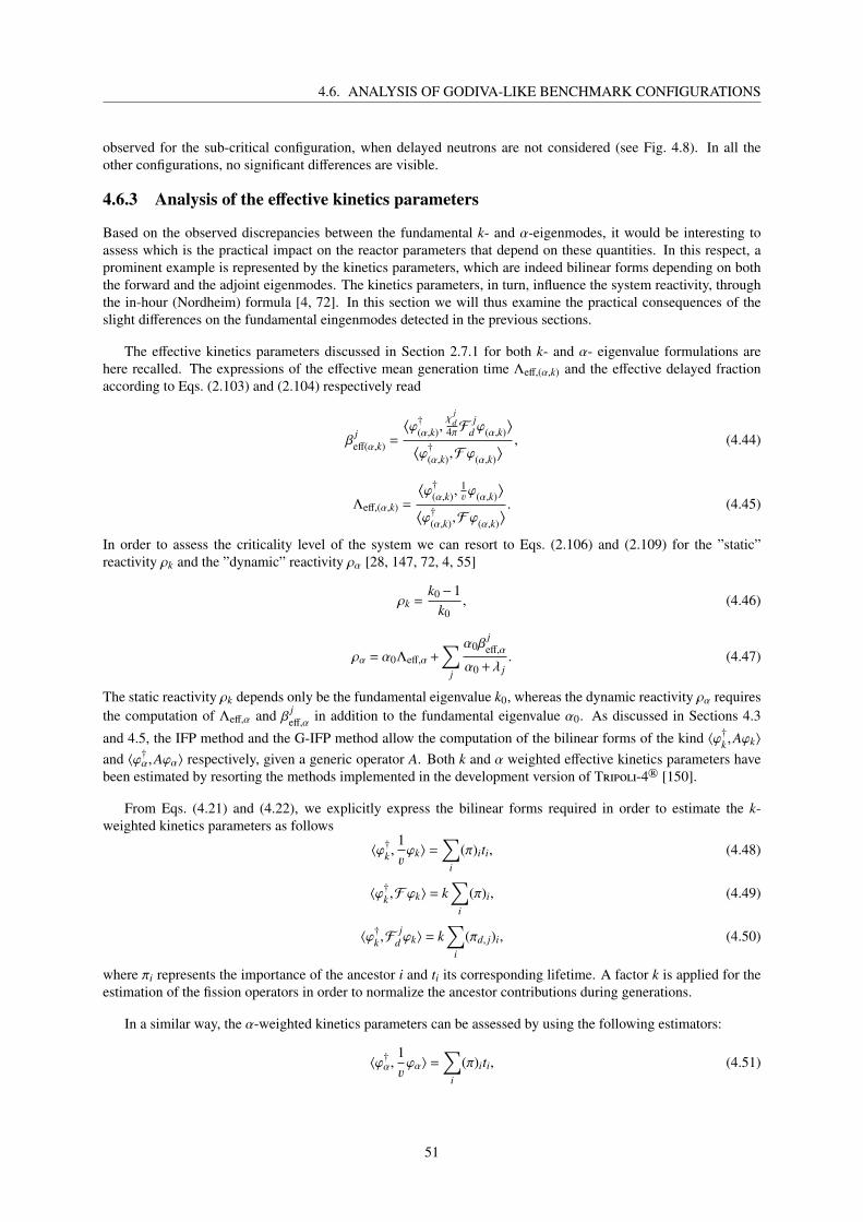
4.6. ANALYSIS OF GODIVA-LIKE BENCHMARK CONFIGURATIONS
observed for the sub-critical configuration, when delayed neutrons are not considered (see Fig. 4.8). In all theother configurations, no significant differences are visible.
4.6.3 Analysis of the effective kinetics parameters
Based on the observed discrepancies between the fundamental k- and α-eigenmodes, it would be interesting toassess which is the practical impact on the reactor parameters that depend on these quantities. In this respect, aprominent example is represented by the kinetics parameters, which are indeed bilinear forms depending on boththe forward and the adjoint eigenmodes. The kinetics parameters, in turn, influence the system reactivity, throughthe in-hour (Nordheim) formula [4, 72]. In this section we will thus examine the practical consequences of theslight differences on the fundamental eingenmodes detected in the previous sections.
The effective kinetics parameters discussed in Section 2.7.1 for both k- and α- eigenvalue formulations arehere recalled. The expressions of the effective mean generation time Λeff,(α,k) and the effective delayed fractionaccording to Eqs. (2.103) and (2.104) respectively read
βjeff(α,k) =
⟨ϕ†(α,k),
χjd
4πFj
d ϕ(α,k)⟩
⟨ϕ†(α,k),F ϕ(α,k)
⟩ , (4.44)
Λeff,(α,k) =
⟨ϕ†(α,k),
13ϕ(α,k)
⟩⟨ϕ†(α,k),F ϕ(α,k)
⟩ . (4.45)
In order to assess the criticality level of the system we can resort to Eqs. (2.106) and (2.109) for the ”static”reactivity ρk and the ”dynamic” reactivity ρα [28, 147, 72, 4, 55]
ρk =k0−1
k0, (4.46)
ρα = α0Λeff,α +∑
j
α0βjeff,α
α0 +λ j. (4.47)
The static reactivity ρk depends only be the fundamental eigenvalue k0, whereas the dynamic reactivity ρα requiresthe computation of Λeff,α and β
jeff,α
in addition to the fundamental eigenvalue α0. As discussed in Sections 4.3
and 4.5, the IFP method and the G-IFP method allow the computation of the bilinear forms of the kind 〈ϕ†k ,Aϕk〉
and 〈ϕ†α,Aϕα〉 respectively, given a generic operator A. Both k and α weighted effective kinetics parameters havebeen estimated by resorting the methods implemented in the development version of Tripoli-4® [150].
From Eqs. (4.21) and (4.22), we explicitly express the bilinear forms required in order to estimate the k-weighted kinetics parameters as follows
〈ϕ†k ,13ϕk〉 =
∑i
(π)iti, (4.48)
〈ϕ†k ,F ϕk〉 = k∑
i
(π)i, (4.49)
〈ϕ†k ,Fj
d ϕk〉 = k∑
i
(πd, j)i, (4.50)
where πi represents the importance of the ancestor i and ti its corresponding lifetime. A factor k is applied for theestimation of the fission operators in order to normalize the ancestor contributions during generations.
In a similar way, the α-weighted kinetics parameters can be assessed by using the following estimators:
〈ϕ†α,13ϕα〉 =
∑i
(π)iti, (4.51)
51

CHAPTER 4. ANALYSIS OF FORWARD AND ADJOINT FUNDAMENTAL K AND α-EIGENFUNCTIONS
〈ϕ†α,F ϕα〉 =∑
i
(π)i, (4.52)
〈ϕ†α,Fj
d ϕα〉 =λ j +α
λ j
∑i
(πd, j)i, (4.53)
recalling that the α-copy operator is not counted for the ancestors scoring during the generations. We remark thata weight multiplier equal to (λ j +α)/λ j is applied for the delayed fission operator.
The effective kinetics parameters estimated for Problem I are shown in Tabs. 4.9 and 4.10 for the sub-criticalconfiguration. Values for βeff weighted according to the k-formulation are statistically compatible to those weightedaccording to the α-formulation. Simulation parameters for the evaluation of these parameters are the same as thoseshown in Tabs. 4.3, estimated by considering 20 latent generations. A slight difference is observed in the values ofΛeff, whereas a relatively larger difference is observed between dynamic and static reactivity. The latter deviationmay be justified by the fact that the dynamic reactivity ρα depends on the eigenfunction distributions integrated forthe estimation of Λeff,α and βeff,α (Eq. (2.109)), whereas the static reactivity ρk only depends on the fundamentaleigenvalue k0. Significant differences are observed for both reactivity and effective mean generation time valueswhen only prompt neutrons are considered. In this case, the difference on the adjoint eigenmodes from Fig. 4.4(left) plays a significant role in weighting the kinetics parameters.
Parameters 〈ϕ†α,•〉 〈ϕ†k ,•〉
ρ [pcm] -669 ± 5 -608 ± 6
Λeff [ns] 5.773 ± 0.003 5.728 ± 0.002
βeff [pcm] 644 ± 2 645 ± 2
β1eff
[pcm] 23.5 ± 0.1 23.5 ± 0.4
β2eff
[pcm] 90 ± 0.7 90.9 ± 0.8
β3eff
[pcm] 66.8 ± 0.6 66.4 ± 0.7
β4eff
[pcm] 128.7 ± 0.9 128 ± 1
β5eff
[pcm] 198 ± 1 200 ± 1
β6eff
[pcm] 63.2 ± 0.7 63.1 ± 0.7
β7eff
[pcm] 58 ± 0.7 56.2 ± 0.6
β8eff
[pcm] 15.9 ± 0.4 16.6 ± 0.3
Table 4.9: Effective kinetics parameters of Problem I, sub-critical configuration with delayed contribution.
Parameters 〈ϕ†α,•〉 〈ϕ†k ,•〉
ρ [pcm] -6289 ± 50 -1266 ± 4
Λeff [ns] 45.6 ± 0.3 5.728 ± 0.002
Table 4.10: Effective kinetics parameters of Problem I, sub-critical configuration without delayed contribution.
The results obtained from the super-critical configuration of the same problem are shown in Tabs. 4.11 and 4.12.The system including delayed neutrons is super-critical and all kinetics parameters are statistically compatible.Conversely, a non negligible discrepancy is still noticeable between static and dynamic reactivities for the config-uration without delayed contributions. Overall, the differences between direct and adjoint eigenmodes accordingto the k- and the α-eigenvalue formulations are observed as discrepancies of similar amplitudes in the effectivekinetics parameters.
52

4.6. ANALYSIS OF GODIVA-LIKE BENCHMARK CONFIGURATIONS
Parameters 〈ϕ†α,•〉 〈ϕ†k ,•〉
ρ [pcm] 409 ± 9 388 ± 6
Λeff [ns] 5.654 ± 0.002 5.675 ± 0.002
βeff [pcm] 643 ± 5 644 ± 2
β1eff
[pcm] 20 ± 2 23.8 ± 0.4
β2eff
[pcm] 93 ± 3 91.1 ± 0.8
β3eff
[pcm] 68 ± 2 65.5 ± 0.7
β4eff
[pcm] 125 ± 2 128.3 ± 0.9
β5eff
[pcm] 201 ± 2 200 ± 1
β6eff
[pcm] 61.4 ± 0.8 60.9 ± 0.7
β7eff
[pcm] 57.6 ± 0.7 57 ± 0.6
β8eff
[pcm] 17.1 ± 0.4 16.9 ± 0.3
Table 4.11: Effective kinetics parameters of Problem I, super-critical configuration with delayed contribution.
Parameters 〈ϕ†α,•〉 〈ϕ†k ,•〉
ρ [pcm] -247.2 ± 0.4 -261 ± 6
Λeff [ns] 5.698 ± 0.002 5.677 ± 0.002
Table 4.12: Effective kinetics parameters of Problem I, super-critical configuration without delayed contribution.
53
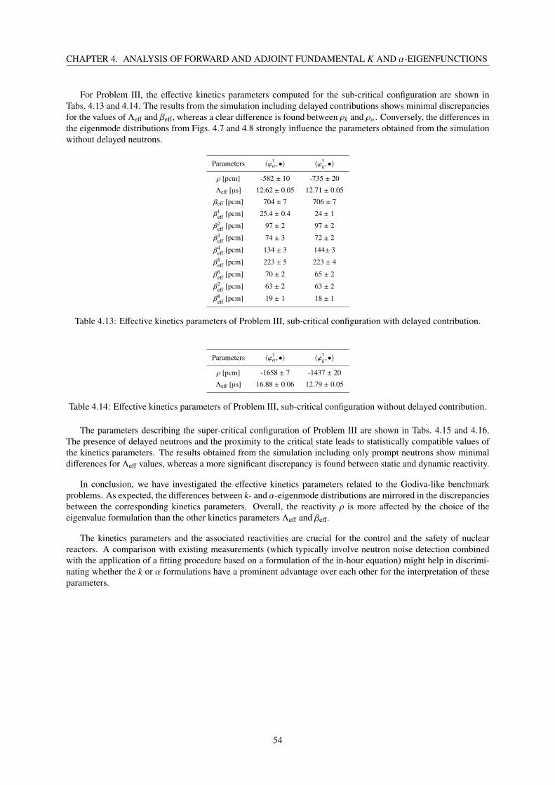
CHAPTER 4. ANALYSIS OF FORWARD AND ADJOINT FUNDAMENTAL K AND α-EIGENFUNCTIONS
For Problem III, the effective kinetics parameters computed for the sub-critical configuration are shown inTabs. 4.13 and 4.14. The results from the simulation including delayed contributions shows minimal discrepanciesfor the values of Λeff and βeff, whereas a clear difference is found between ρk and ρα. Conversely, the differences inthe eigenmode distributions from Figs. 4.7 and 4.8 strongly influence the parameters obtained from the simulationwithout delayed neutrons.
Parameters 〈ϕ†α,•〉 〈ϕ†k ,•〉
ρ [pcm] -582 ± 10 -735 ± 20
Λeff [µs] 12.62 ± 0.05 12.71 ± 0.05
βeff [pcm] 704 ± 7 706 ± 7
β1eff
[pcm] 25.4 ± 0.4 24 ± 1
β2eff
[pcm] 97 ± 2 97 ± 2
β3eff
[pcm] 74 ± 3 72 ± 2
β4eff
[pcm] 134 ± 3 144± 3
β5eff
[pcm] 223 ± 5 223 ± 4
β6eff
[pcm] 70 ± 2 65 ± 2
β7eff
[pcm] 63 ± 2 63 ± 2
β8eff
[pcm] 19 ± 1 18 ± 1
Table 4.13: Effective kinetics parameters of Problem III, sub-critical configuration with delayed contribution.
Parameters 〈ϕ†α,•〉 〈ϕ†k ,•〉
ρ [pcm] -1658 ± 7 -1437 ± 20
Λeff [µs] 16.88 ± 0.06 12.79 ± 0.05
Table 4.14: Effective kinetics parameters of Problem III, sub-critical configuration without delayed contribution.
The parameters describing the super-critical configuration of Problem III are shown in Tabs. 4.15 and 4.16.The presence of delayed neutrons and the proximity to the critical state leads to statistically compatible values ofthe kinetics parameters. The results obtained from the simulation including only prompt neutrons show minimaldifferences for Λeff values, whereas a more significant discrepancy is found between static and dynamic reactivity.
In conclusion, we have investigated the effective kinetics parameters related to the Godiva-like benchmarkproblems. As expected, the differences between k- and α-eigenmode distributions are mirrored in the discrepanciesbetween the corresponding kinetics parameters. Overall, the reactivity ρ is more affected by the choice of theeigenvalue formulation than the other kinetics parameters Λeff and βeff.
The kinetics parameters and the associated reactivities are crucial for the control and the safety of nuclearreactors. A comparison with existing measurements (which typically involve neutron noise detection combinedwith the application of a fitting procedure based on a formulation of the in-hour equation) might help in discrimi-nating whether the k or α formulations have a prominent advantage over each other for the interpretation of theseparameters.
54

4.7. AN APPLICATION TO THE CROCUS REACTOR
Parameters 〈ϕ†α,•〉 〈ϕ†k ,•〉
ρ [pcm] 478 ± 40 496 ± 20
Λeff [µs] 12.16 ± 0.04 12.21 ± 0.04
βeff [pcm] 681 ± 20 711 ± 7
β1eff
[pcm] 22 ± 7 28 ± 1
β2eff
[pcm] 92 ± 10 97 ± 2
β3eff
[pcm] 77 ± 8 73 ± 2
β4eff
[pcm] 132 ± 6 138 ± 3
β5eff
[pcm] 215 ± 6 232 ± 4
β6eff
[pcm] 65 ± 3 62 ± 2
β7eff
[pcm] 61 ± 2 62 ± 2
β8eff
[pcm] 18 ± 1 20 ± 1
Table 4.15: Effective kinetics parameters of Problem III, super-critical configuration with delayed contribution.
Parameters 〈ϕ†α,•〉 〈ϕ†k ,•〉
ρ [pcm] -252 ± 1 -213 ± 20
Λeff [µs] 12.93 ± 0.05 12.29 ± 0.05
Table 4.16: Effective kinetics parameters of Problem III, super-critical configuration without delayed contribution.
4.7 An application to the CROCUS reactor
In order to take into account a more realistic configuration, and ascertain whether the conclusions reached inthe previous section hold true for larger reactor cores, in this section we will consider two configurations of theCROCUS critical facility, operated at the Ecole Polytechnique Federale de Lausanne (EPFL), Switzerland. Thanksto its detailed description and careful measurements, the CROCUS core has been selected as an internationalbenchmark for reactivity, kinetics parameters and reactor period calculations [116, 119].
CROCUS is an open-tank type zero-power reactor, characterized by two fuel regions and moderated by lightwater. A radial section of this reactor is shown in Fig. 4.9: the outer fuel rods (green) are composed of metallicuranium at 0.947 wt% 235U/U with 2.917cm pitch, whereas the inner fuel rods (orange) are composed by UO2at 1.806 wt% 235U/U with 1.837cm pitch. Details on the number and positions of these fuel rods are given inreference [119]. The core can be modeled as a cylinder with a diameter of about 60 cm and a height of 100 cm.The critical state of the system is controlled by the level of light water filling the reactor from the bottom cadmiumplate. The critical configuration is achieved at a water level of 91.66 cm.
55

CHAPTER 4. ANALYSIS OF FORWARD AND ADJOINT FUNDAMENTAL K AND α-EIGENFUNCTIONS
Figure 4.9: Radial section of the CROCUS reactor obtained with Tripoli-4®. The inner fuel rods (UO2, orange)and the outer fuel rods (metallic U, green) are moderated by light water (blue). The red regions denotes the 14 fuelrod positions defined for the flux distribution [119].
A preliminary comparison for this facility between fundamental α-eigenpairs and time dependent calculationshas been carried out in [112]. Moreover, the kinetics parameters of the CROCUS core for the k-eigenvalue formu-lation has been previously computed in [171] and the associated reactivity was examined in [172]. In the following,we will investigate the behaviour (and possible discrepancies) of the fundamental forward and adjoint modes ofthe k and α formulations for this core, and we will then examine the impact of their respective shapes on the ki-netics parameters and on the reactivity. For this purpose, we will consider two sub-critical configurations of thereactor, both obtained by lowering the water level. Configuration H1 is characterized by a water level equal to90.8 cm, which induces a slightly sub-critical state. Configuration H2 is characterized by a water level equal to80 cm, which corresponds to a more sub-critical condition. The fundamental eigenmodes will be computed byusing Tripoli-4® over 111 energy meshes and along 14 fuel pin positions, from the core center to the outer region,denoted by the red rectangular regions in Fig. 4.9. The number of cycles and the particles per cycle simulated forthese configurations are listed in Tab. 4.17 for the forward simulations and in Tab. 4.18 for the adjoint simulations.
configuration active cycles inactive cycles particles
H1 5×10³ 5×10³ 2×10⁴
H2 5×10³ 5×10³ 2×10⁴
Table 4.17: Numerical simulation parameters for CROCUS configurations during forward simulations.
configuration particles latent generations
H1 2×10⁷ 20
H2 2×10⁷ 20
Table 4.18: Numerical simulation parameters for CROCUS configurations during adjoint simulations.
4.7.1 Analysis of the fundamental eigenmodes
The fundamental eigenvalues k0 and α0 computed in the corresponding simulations for H1 and H2 configurationsof the CROCUS reactor (with and without precursor contributions) are given in Tabs. 4.19 and 4.20, respectively.
56

4.7. AN APPLICATION TO THE CROCUS REACTOR
As expected, the computed values show a slight sub-critical level for configuration H1 and a larger sub-criticalstate for configuration H2. According to the results obtained from the k-eigenvalue formulation, the criticalitylevel of both configurations decreases by approximately 780 pcm when delayed neutrons are neglected. Concern-ing the α-eigenvalue formulation, the absolute value of α0 is smaller than 1.2× 10⁻² s-1 by including delayedneutrons, whereas the absolute value of this eigenvalue is larger than 102 s-1 for the simulation without precursorcontributions.
configuration k0[−], with delayed contributions k0[−], prompt fission only
H1 0.9995±1×10⁻⁴ 0.9918±1×10⁻⁴
H2 0.9919±1×10⁻⁴ 0.9839±1×10⁻⁴
Table 4.19: Fundamental eigenvalues k0 for H1 and H2 configurations of the CROCUS reactor.
configuration α0[s-1], including precursors α0[s-1], without precursors
H1 −5.97×10⁻³ ±2×10⁻⁵ −1.711×10² ±2×10⁻¹
H2 −1.1994×10⁻² ±3×10⁻⁶ −3.336×10² ±2×10⁻¹
Table 4.20: Fundamental eigenvalues α0 for H1 and H2 configurations of the CROCUS reactor.
The shapes of direct eigenmodes ϕk0 and ϕα0 (with and without delayed neutron contributions) are shown as afunction of energy (Fig. 4.10) and of the fuel pin position (Fig. 4.11) for H1 (left) and H2 (right) configurations. Theadjoint eigenmodes are shown as a function of the fuel pin position in Fig.4.12. All curves have been normalized.No major differences can be easily spotted in these figures, so that we have computed the ratios ϕα0/ϕk0 andϕ†α0/ϕ
†
k0in order to investigate possible discrepancies.
10 -9 10 -7 10 -5 10 -3 10 -1 10 1
10 -5
10 -3
10 -1
10 1
10 3
10 5
10 -9 10 -7 10 -5 10 -3 10 -1 10 1
10 -5
10 -3
10 -1
10 1
10 3
10 5
Figure 4.10: Direct fundamental eigenmodes of the CROCUS reactor as a function of the energy, H1 (left) and H2(right) configurations according to the α- (blue) and k- (red) eigenvalue formulations, with (squares) and without(circles) precursor contributions.
57

CHAPTER 4. ANALYSIS OF FORWARD AND ADJOINT FUNDAMENTAL K AND α-EIGENFUNCTIONS
0 5 10 15 20 25 300.02
0.03
0.04
0.05
0.06
0.07
0.08
0.09
0 5 10 15 20 25 300.02
0.03
0.04
0.05
0.06
0.07
0.08
0.09
Figure 4.11: Direct fundamental eigenmodes of the CROCUS reactor as a function of the fuel pin positions, H1(left) and H2 (right) configurations according to the α- (blue) and k- (red) eigenvalue formulations, with (squares)and without (circles) precursor contributions.
0 5 10 15 20 25 300.02
0.03
0.04
0.05
0.06
0.07
0.08
0.09
0.1
0 5 10 15 20 25 300.02
0.03
0.04
0.05
0.06
0.07
0.08
0.09
0.1
Figure 4.12: Adjoint fundamental eigenmodes of the CROCUS reactor as a function of the fuel pin positions, H1(left) and H2 (right) configurations according to the α- (blue) and k- (red) eigenvalue formulations, with (squares)and without (circles) precursor contributions.
Figure 4.13 shows the ratios of the direct fundamental eigenmodes in the energy domain. The results obtainedfor configuration H1 (left) are similar to those previously discussed for the Problem III of the benchmark config-urations. When delayed neutrons are considered, no differences are visible between ϕk0 (E) and ϕα0 (E). This ismainly due to the system reactivity being close to critical (about -50 pcm, as shown in Tab. 4.19): the k and αformulation are supposed to be very close to each other in this regime. If precursors are disregarded in the simula-tion, for this configuration the fundamental k-eigenmode is slightly different from the fundamental α-eigenmode:a shift towards high energy values is observed. The same behaviour is found for the H2 configuration (right), char-acterized by a larger effect due to a larger sub-critical level with respect to the previous case (about −1600 pcm,as shown in Tab. 4.19). The effect of precursors is clearly visible for this configuration: the k-eigenmode displayssignificant discrepancies with respect to the α-eigenmode towards high energies for this sub-critical system, butϕα0 (E) > ϕk0 (E) only for E > 0.6 MeV, which is again similar to the findings of the Problem III configuration. Pre-cursor contributions minimize the discrepancies between the two eigenvalue formulations and the delayed spectramove the threshold for ϕα0 (E) > ϕk0 (E) at higher energy.
58

4.7. AN APPLICATION TO THE CROCUS REACTOR
10 -9 10 -7 10 -5 10 -3 10 -1 10 10.85
0.9
0.95
1
1.05
1.1
1.15
10 -9 10 -7 10 -5 10 -3 10 -1 10 10.85
0.9
0.95
1
1.05
1.1
1.15
Figure 4.13: Ratios ϕα0/ϕk0 of the CROCUS reactor as a function of the energy variable, H1 (left) and H2 (right)configurations with (red squares) and without (blue circles) precursor contributions.
For the sake of completeness, we show the ratios of these eigenfunctions as a function of the fuel pin positionsin Fig. 4.14 for the direct formulation and in Fig. 4.15 for the adjoint formulation. Overall, the behaviour of thesetwo eigenmodes is similar: within uncertainty limits, no major differences can be detected with respect to thespatial coordinate.
0 5 10 15 20 25 300.99
0.995
1
1.005
1.01
0 5 10 15 20 25 300.99
0.995
1
1.005
1.01
Figure 4.14: Ratios ϕα0/ϕk0 of the CROCUS reactor as a function of the fuel pin positions, H1 (left) and H2 (right)configurations with (red squares) and without (blue circles) precursor contributions.
0 5 10 15 20 25 300.98
0.985
0.99
0.995
1
1.005
1.01
1.015
1.02
1.025
0 5 10 15 20 25 300.98
0.985
0.99
0.995
1
1.005
1.01
1.015
1.02
1.025
Figure 4.15: Ratios ϕ†α0/ϕ†
k0of the CROCUS reactor as a function of the fuel pin positions, H1 (left) and H2 (right)
configurations with (red squares) and without (blue circles) precursor contributions.
59
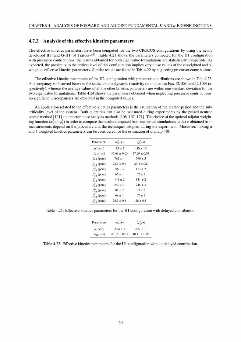
CHAPTER 4. ANALYSIS OF FORWARD AND ADJOINT FUNDAMENTAL K AND α-EIGENFUNCTIONS
4.7.2 Analysis of the effective kinetics parameters
The effective kinetics parameters have been computed for the two CROCUS configurations by using the newlydeveloped IFP and G-IFP of Tripoli-4®. Table 4.21 shows the parameters computed for the H1 configurationwith precursor contributions: the results obtained for both eigenvalue formulations are statistically compatible. Asexpected, the proximity to the critical level of this configuration implies very close values of the k-weighted and α-weighted effective kinetics parameters. Similar results are found in Tab. 4.22 by neglecting precursor contributions.
The effective kinetics parameters of the H2 configuration with precursor contributions are shown in Tab. 4.23.A discrepancy is observed between the static and the dynamic reactivity (computed as Eqs. (2.106) and (2.109) re-spectively), whereas the average values of all the other kinetics parameters are within one standard deviation for thetwo eigenvalue formulations. Table 4.24 shows the parameters obtained when neglecting precursor contributions:no significant discrepancies are observed in the computed values.
An application related to the effective kinetics parameters is the estimation of the reactor period and the sub-criticality level of the system. Both quantities can also be measured during experiments by the pulsed neutronsource method [121] and reactor noise analysis methods [108, 167, 171]. The choice of the optimal adjoint weight-ing function (ϕ†α or ϕ†k) in order to compare the results computed from numerical simulations to those obtained frommeasurements depend on the procedure and the techniques adopted during the experiment. Moreover, mixing αand k weighted kinetics parameters can be considered for the estimation of α and ρ [40].
Parameters 〈ϕ†α,•〉 〈ϕ†k ,•〉
ρ [pcm] -73 ± 2 -50 ± 10
Λeff [µs] 47.69 ± 0.03 47.69 ± 0.03
βeff [pcm] 762 ± 4 760 ± 5
β1eff
[pcm] 22.3 ± 0.6 23.4 ± 0.8
β2eff
[pcm] 109 ± 2 113 ± 2
β3eff
[pcm] 66 ± 1 62 ± 1
β4eff
[pcm] 141 ± 2 141 ± 2
β5eff
[pcm] 249 ± 3 245 ± 3
β6eff
[pcm] 81 ± 2 83 ± 2
β7eff
[pcm] 68 ± 1 67 ± 1
β8eff
[pcm] 26.5 ± 0.8 26 ± 0.8
Table 4.21: Effective kinetics parameters for the H1 configuration with delayed contribution.
Parameters 〈ϕ†α,•〉 〈ϕ†k ,•〉
ρ [pcm] -824 ± 1 -827 ± 10
Λeff [µs] 48.15 ± 0.03 48.11 ± 0.03
Table 4.22: Effective kinetics parameters for the H1 configuration without delayed contribution.
60

4.8. CONCLUSIONS
Parameters 〈ϕ†α,•〉 〈ϕ†k ,•〉
ρ [pcm] -723 ± 10 -822 ± 10
Λeff [µs] 48.06 ± 0.03 48.01 ± 0.03
βeff [pcm] 763 ± 5 766 ± 5
β1eff
[pcm] 23.2 ± 0.2 22.2 ± 0.7
β2eff
[pcm] 113 ± 2 113 ± 2
β3eff
[pcm] 64 ± 1 66 ± 1
β4eff
[pcm] 140 ± 2 143 ± 2
β5eff
[pcm] 247 ± 3 251 ± 3
β6eff
[pcm] 82 ± 2 82 ± 2
β7eff
[pcm] 68 ± 2 66 ± 1
β8eff
[pcm] 24.8 ± 0.9 24 ± 0.8
Table 4.23: Effective kinetics parameters for the H2 configuration with delayed contribution.
Parameters 〈ϕ†α,•〉 〈ϕ†k ,•〉
ρ [pcm] -1621 ± 2 -1638 ± 10
Λeff [µs] 48.59 ± 0.03 48.39 ± 0.03
Table 4.24: Effective kinetics parameters for the H2 configuration without delayed contribution.
4.8 Conclusions
Inspired by the analysis originally proposed by D. E. Cullen [28], we have applied Monte Carlo methods forthe estimation of k and α fundamental eigenmodes. We have extended the findings discussed in [28] in twodirections, by addressing the evaluation of the fundamental adjoint eigenmodes and the influence of precursorcontributions. Additional information regarding the discrepancies between the two eigenvalue formulations wasfound by assessing the effective kinetics parameters weighted by the k- or by the α-eigenmodes. We have focusedour attention on the analysis of two Godiva-like benchmark configurations and the CROCUS reactor. In thisway, we have explored thermal and fast spectra, homogeneous and heterogeneous media, simplified and realisticsystems.
Significant, albeit globally small, differences have been detected, as expected on physical grounds based onprevious investigations. In particular, we have recovered the same behaviour previously analyzed [28] in theenergy domain for the distribution of the direct fundamental eigenfunctions ϕk0 and ϕα0 , and we have foundsimilar discrepancies in the corresponding adjoint fundamental distributions ϕ†k0
and ϕ†α0 . Moreover, the presenceof precursors has a non-trivial influence on the eigenfunctions, and this impact has been carefully examined foreach configuration. Overall, the presence of precursors reduces the discrepancies between the two eigenmodes.
As a general remark, based on the configurations investigated here, it seems that the discrepancies between thek- and α-eigenfunctions are enhanced by the presence of strong spatial heterogeneities, such as those occurring ina core surrounded by a thick moderator/reflector. In this case, the system will be characterized by multiple timescales (as shown in [28]), related to the different times required by the neutrons to explore the multiplying and thediffusing region. Then, it appears that the α-eigenvalue formulation is more sensitive to these different time scalesthan the k-eigenvalue formulation, which is coherent with α being related to the time behaviour of the systemand k being related to the fission generation behavior. These discrepancies on the eigenmodes are mirrored in thekinetics parameters and on the reactivity. In this respect, it is interesting to remark that the CROCUS reactor canbe basically considered as a homogeneous system, with minimal discrepancies between the α and k formulations.
61

CHAPTER 4. ANALYSIS OF FORWARD AND ADJOINT FUNDAMENTAL K AND α-EIGENFUNCTIONS
62

Chapter 5
A new matrix-filling Monte Carlo methodfor α-spectral analysis
In the previous chapter, we have seen that Monte Carlo methods can be successfully applied to determining theforward and adjoint fundamental modes and the associated eigenvalues of both k- and α-eigenvalue problemswithout approximations, which paves the way towards reference solutions characterizing the asymptotic behaviourof nuclear systems. In view of a full spectral analysis, the fundamental modes alone might prove insufficient so as tocharacterize the systems under analysis: for instance, the shape of the first excited eigenmode can provide valuableinformation concerning the behaviour of a perturbation introduced in the core, and the eigenvalue gap (e.g., thedominance ratio DR = k1/k0) would convey the intensity of such perturbation with respect to the fundamentalmode [12, 13, 14, 161, 52, 154]. A natural question therefore arises whether the Monte Carlo methods describedin Chapter 4 can be extended and generalized to higher eigenmodes and eigenvalues.
For the case of k-eigenvalue problems, extensive work has been carried out in recent years in order to establishmodified power-iteration algorithms capable of extracting the first excited eigenmode ϕk1 and the associated eigen-value k1, and possibly also higher eigenpairs, without introducing approximations [136, 137]. Basically, all thesemethods are built upon the key idea that the eigenvalue formulation can be made local in the phase-space, so thata system of coupled eigenvalue equations emerges, each defined over a portion of the phase space: by imposingsuitable constraints on the available degrees of freedom offered by this system of equations, one may force thesolution of the power iteration to converge to several eigenpairs, namely, (k0,ϕk0 ), (k1,ϕk1 ), and so on.
In this respect, we recall the strategy from a seminal paper by Booth [12]. Let us recast the k-eigenvalueproblem from Eq. (2.65) and the operator K from Eq. (2.66) as
kϕk = [M−1F ]ϕk =Kϕk. (5.1)
Suppose that the initial guess for the power iteration is written as ϕ =∑
m wkmϕkm , where ϕkm are the eigenfunctionof order m, with m ≥ 0, and wkm are the expansion coefficients. Let us assume that the eigenvalues are ordered suchthat k0 > |k1| ≥ |k2| ≥ · · · . If wk0 , 0, by successively applying the K operator the power iteration yields
limn→∞
1kn
0Knϕ = ϕk0 , (5.2)
where n is the iteration index, and we obtain the fundamental mode. However, if we can set wk0 = 0, then we willhave
limn→∞
1kn
1Knϕ = ϕk1 , (5.3)
i.e., the power iteration will converge to the first excited mode, provided that we can remove the fundamentalmode. In order to ensure this condition, the idea is to solve the power iteration separately on two regions R+ and
63

CHAPTER 5. A NEW MATRIX-FILLING MONTE CARLO METHOD FOR α-SPECTRAL ANALYSIS
R− of the phase-space:
k1 =〈Kϕk1〉R+
〈ϕk1〉R+=〈Kϕk1〉R−
〈ϕk1〉R−(5.4)
since the eigenvalue equation (5.1) holds on every subset of the viable domain [34, 114]. The two subsets R+ andR− are not known a priori and must be progressively refined as the calculation proceeds. We can then consider twodifferent factors, k+
1 and k−1 , defined as
k+1 =〈Kϕk1〉R+
〈ϕk1〉R+, (5.5)
and
k−1 =〈Kϕk1〉R−
〈ϕk1〉R−. (5.6)
Now, if the power iteration were to be applied separately on each region, the two eigenvalue problems wouldstill converge to the fundamental mode. In order to prevent this from happening, Booth proposes to postulate anexpansion of the kind ϕ = wk0ϕk0 +wk1ϕk1 and to formally determine the conditions on the relative weight given toϕk0 and ϕk1 in order to enforce the subtraction of ϕk0 to the solution that must converge to ϕk1 and conversely thesubtraction of ϕk1 to the solution that must converge to ϕk0 . Since the first excited eigenmode is partially positiveand partially negative on the phase-space, the use of subtraction methods necessarily demands the introductionof particles carrying statistical weights of alternating signs. Furthermore, in order for the proposed method toconverge, particles having a negative/positive weight must annihilate particles having a positive/negative weightwhen meeting in the phase-space: this is called the weight cancellation procedure [14, 137].
Booth’s technique is capable of determining the eigenpair (k1,ϕk1 ) without any approximation, and as suchrepresents an ingenuous extension of the standard power iteration algorithm [12]. Several refinements of thispioneering approach have been later proposed, in particular concerning the use of more efficient or more robust(albeit approximated) methods for the weight cancellation [13, 14, 137]. Although these methods have shown agreat potential for extracting higher-order eigenmodes in k-eigenvalue problems, their use in production MonteCarlo codes is still hindered by the complexity of their implementation and most importantly by the possiblenumerical instabilities that have been met in some applications, for which investigations are still ongoing [161].
5.1 Matrix-filling methods: the fission matrix approach
Actually, the idea of extracting higher harmonics in k-eigenvalue problems by Monte Carlo methods is not new, andseveral methods have been proposed in the literature. Among these approaches, a prominent role is played by thefission matrix method, whereupon a standard Monte Carlo power iteration is used in order to estimate the elementsof a matrix that represents a discretized version of the operators appearing in the k-eigenvalue problem [22]. Theobtained matrix can be then analyzed by classical numerical methods in order to extract the full spectrum andthe associated eigenmodes: this approach is not exact, since the matrix has necessarily a finite size and thusdiscretization errors are introduced. Nonetheless, it offers a robust and reliable approach to the spectral analysisof k-eigenvalue problems for reactor physics applications: the fission matrix has a long history [105, 71, 53] andhas been extensively investigated [152, 76, 35, 156]. An extension of this approach has also been studied inliterature: the Transient Fission Matrix method [87, 86, 85]. Conversely to the original fission matrix method, theTFM approach preserves the temporal behaviour of the particles and distinguishes prompt neutrons from delayedneutrons at fission events. Further details related to this approach will be provided in Section 5.4 and in theAppendix A.
In the following we provide a short overview of the forward and adjoint forms of the standard fission matrixtreatment for k-eigenvalue problems.
5.1.1 The forward formulation
Recall the k-eigenvalue problem formulation from Eq. (2.65)
Mϕk(r,Ω,E) =1kχ f (E)
4πQ f (r), (5.7)
64

5.1. MATRIX-FILLING METHODS: THE FISSION MATRIX APPROACH
where Q f (r) is the fission neutron source defined as
Q f (r) =
∫4π
dΩ∫ ∞
0dE ν f (E)Σ f (r,E)ϕk(r,Ω,E). (5.8)
Let us now introduce the Green’s function G(r0→ r,Ω0→Ω,E0→ E) associated to the operator M, namely
MG(r0→ r,Ω0→Ω,E0→ E) = δ(r0− r)δ(Ω0−Ω)δ(E0−E), (5.9)
which physically represents the response of the system to the injection of a pulse source.
Exploiting the linearity of the problem and the superposition principle, the direct eigenmode ϕk is obtained as
ϕk(r,Ω,E) =1k
∫V
dr0
∫4π
dΩ0
∫ ∞
0dE0
χ f (E0)4π
Q f (r0)G(r0→ r,Ω0→Ω,E0→ E). (5.10)
Equation (5.10) for the eigenfunction ϕk is multiplied by ν f Σ f and integrated in energy and direction in order toexpress Q f as
Q f (r) =1k
∫V
dr0 Q f (r0)H(r0→ r), (5.11)
where H(r0 → r) is a kernel representing the Green’s function averaged on energy and direction, here explicitlyexpressed as
H(r0→ r) =
∫4π
dΩ∫ ∞
0dE
∫4π
dΩ0
∫ ∞
0dE0 ν f (E)Σ f (r,E)
χ(E0)4π
G(r0→ r,Ω0→Ω,E0→ E). (5.12)
No approximations have been introduced so far in this procedure and the averaged quantities can be estimatedduring a Monte Carlo simulation: typically, one chooses to estimate the fission matrix elements during a regularpower iteration. Then, N finite spatial regions are defined for the fission sites of neutrons of generation g, V j, andneutrons of generation g + 1, Vi, in order to express the spatially discretized version of Eq. (5.11) as
Qi =1k
N∑j=1
Ki, jQ j, (5.13)
where
Ki, j =
∫r0∈V j
dr0
∫r∈Vi
drQ f (r0)
Q jH(r0→ r), (5.14)
andQ j =
∫r′∈V j
dr′ Q f (r′). (5.15)
From a physical point of view, the element located at position (i, j) of the N×N matrix Ki, j represents the number offission neutrons born in region i stemming from one fission neutron born in region j. The matrix Ki, j in Eq. (5.14) isdefined as the fission matrix: the eigenvalue k associated to the nth eigenvector with 0 ≤ n ≤ N −1 can be obtainedfrom it and the corresponding eigenfunction is a discretized version of the neutron source distribution Q f (r) oforder n solving the k-eigenvalue problem in the form
Q f =1kKQ f . (5.16)
Fission matrix elements are associated to discrete spatial intervals mapping the geometrical domain of the system.It can be shown that the fundamental eigenvector and eigenvalue extracted from the fission matrix is exact, sincethe elements of Ki j are by construction weighted on the fundamental mode obtained by the power iteration. On thecontrary, higher-order eigenvectors and eigenvalues will have a bias due to the discretization of the phase-space,since they have been weighted by the fundamental mode instead of the corresponding higher-order eigenmode.This bias vanishes in the limit of an infinitely fine discretization [22] (i.e., when the matrix size goes to infinity).Moreover, fission matrix elements are estimated as scores during a Monte Carlo simulation and as such they areintrinsically affected by a statistical error. The uncertainty related to these estimators will be propagated into the
65

CHAPTER 5. A NEW MATRIX-FILLING MONTE CARLO METHOD FOR α-SPECTRAL ANALYSIS
computation of the eigenpairs associated to the fission matrix, as shown in Section 5.3.1.
5.1.2 The backward formulation
The same procedure can be applied to the adjoint formulation of the k-eigenvalue problem [22], now defined as
M†ϕ†k(r,Ω,E) =1kν f (E)Σ f (r,E)Q†f (r), (5.17)
where the adjoint fission neutron source Q†f (r) is introduced as
Q†f (r) =
∫4π
dΩ∫ ∞
0dE
χ f (E)4π
ϕ†k(r,Ω,E). (5.18)
The adjoint Green’s function G† is defined as:
M†G†(r0→ r,Ω0→Ω,E0→ E) = δ(r− r0)δ(Ω−Ω0)δ(E−E0). (5.19)
Similarly to the previous procedure, the adjoint eigenfunction ϕ†k is obtained as
ϕ†k(r,Ω,E) =1k
∫V
dr0
∫4π
dΩ0
∫ ∞
0dE0 ν f (E0)Σ f (r0,E0)Q f (r0)G†(r0→ r,Ω0→Ω,E0→ E). (5.20)
Then, the fission spectrum χ f (E) is multiplied and the equation is integrated in energy and direction in order toexpress the adjoint fission source Q†f , as
Q†f (r) =1k
∫V
dr0 Q†f (r0)H†(r0→ r), (5.21)
and the adjoint kernel H†(r0→ r) for the adjoint Green’s function averaged on energy and direction as
H†(r0→ r) =
∫4π
dΩ∫ ∞
0dE
∫4π
dΩ0
∫ ∞
0dE0
χ f (E)4π
ν f (E0)Σ f (r0,E0)G†(r0→ r,Ω0→Ω,E0→ E). (5.22)
The direct and the adjoint Green’s function, G and G† respectively, are related by the reciprocity theorem
G†(r0→ r,Ω0→Ω,E0→ E) = G(r→ r0,Ω→Ω0,E→ E0), (5.23)
hence, also the direct and adjoint kernels, H and H† respectively, are related as
H†(r0→ r) = H(r→ r0). (5.24)
Exploiting this property, the adjoint fission source can be expressed via the direct kernel as follows
Q†f (r) =1k
∫V
dr0 Q†f (r0)H(r→ r0). (5.25)
Finally, a spatial grid is considered in order to split N finite regions for the volumes V j and Vi, introducing adiscrete version of the problem as
Q†i =1k
N∑j=1
K†i, jQ†
j . (5.26)
where K†i, j is the adjoint fission matrix and it is defined as
K†i, j =
∫r0∈V j
dr0
∫r∈Vi
drQ†f (r0)
Q†jH(r→ r0), (5.27)
66

5.2. A NEW MATRIX-FILLING METHOD FOR α-EIGENVALUES
whereQ†j =
∫r′∈V j
dr′ Q†f (r′). (5.28)
It is possible to relate the forward and the adjoint fission matrices by considering the elements at positions (i, j)and ( j, i) respectively:
Ki, j =
∫r0∈V j
dr0
∫r∈Vi
drQ f (r0)
Q jH(r0→ r), (5.29)
K†j,i =
∫r0∈V j
dr0
∫r∈Vi
drQ†f (r)
QiH(r0→ r). (5.30)
From inspection of these definitions, two different spatial weighting functions are applied to the forward and adjointfission matrices: Q f (r0)/Q j and Q†f (r)/Qi respectively [22]. If the spatial discretization is chosen sufficiently fine,so that
Q f (r0)Q j
→1V j, (5.31)
andQ†f (r)
Q†i→
1Vi, (5.32)
the matrix element K†j,i converges to the matrix element Ki, j, hence, the adjoint fission matrix can be obtained bytransposition of the direct fission matrix.
A final remark concerns the estimation of the k-eigenmodes, which can be performed by combining the discretelinear transport operators in order to express the formulation of the k-eigenvalue problem:
Mϕk =1k
Fϕk, (5.33)
where M and F are the matrix forms of the net disappearance operator M and total fission operator F fromEqs. (2.32) and (2.63), respectively. This formulation allows the computation of the eigenmodes ϕk as a functionof the phase-space coordinates. Conversely, the fission matrix yields the emission distribution S f ,k, which onlydepends on the spatial coordinates. In principle, the implementation of matrix-form operators for the k-eigenvalueproblem allows the computation of the entire k-spectrum and of high-order eigenfunctions ϕk.
5.2 A new matrix-filling method for α-eigenvalues
Similarly to the case of k-eigenvalues, intensive work has been carried out concerning the possibility of estimatinghigher-order eigenvalue and eigenfunctions for α-eigenvalue problems.
Despite some successful attempts, generalized power iteration methods performed via Monte Carlo simulationsfor higher α-eigenvalues and eigenmodes (based on previous investigations for k-eigenvalues) have received onlylimited attention [162]. On the contrary, matrix-filling Monte Carlo methods have recently drawn much interest [6,7, 8, 153]. We remark in passing that an independent approach has been recently proposed for α-eigenvalueproblems, based on a time-discretization of the fission matrix [68]. However, it appears that such method allowsonly determining the eigenvalues but not the eigenvectors.
The matrix-filling approach proposed by Betzler [8] is very similar in spirit to the better-known fission matrixmethod for k-eigenvalues introduced in the previous section [35, 22]. Although the α-eigenvalues and eigenmodesthus estimated are generally biased because of the finite size of the matrix, this method allows obtaining a fairlyaccurate picture of the entire spectrum and thus grasping the time evolution of the system [6, 7], even for complexthree-dimensional configurations [8]. Moreover, once the α-spectrum and the associated eigenvectors have beendetermined from the matrix, the full time-dependent evolution of the neutron and precursor populations can alsobe reconstructed, at least in principle, by using the direct and adjoint matrices [8]. The idea is to compute thecoefficients wαm by solving Eq. (2.88) derived in Section 2.6.2. These coefficients preserve the time dependence of
67
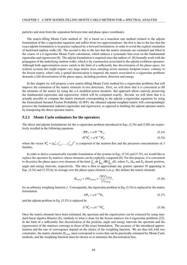
CHAPTER 5. A NEW MATRIX-FILLING MONTE CARLO METHOD FOR α-SPECTRAL ANALYSIS
particles and stem from the separation between time and phase-space coordinates.
The matrix-filling Monte Carlo method of [8] is based on a transition rate method (related to the adjointformulation of the α-eigenvalue equation) and suffers from two approximations: the first is due to the fact that theexact adjoint formulation is in practice replaced by a forward formulation, in order to avoid the explicit simulationof backward random walks [8]. The second is due to the fact that the matrix elements are estimated and filled inthe course of a k-eigenvalue Monte Carlo calculation, which induces a systematic bias even on the fundamentaleigenvalue and eigenvector [8]. The adjoint formulation is required since the authors of [8] formally work with thepropagator of the underlying random walks, which is by construction associated to the adjoint evolution operators.Although both approximation errors vanish in the limit of a sufficiently fine discretization of the phase-space, forrealistic systems this might require very large matrix sizes, entailing severe memory footprint issues: contrary tothe fission matrix, where only a spatial discretization is required, the matrix associated to α-eigenvalue problemsdemands a full discretization of the phase-space, including position, direction and energy.
In this chapter we will propose a new matrix-filling Monte Carlo method for α-eigenvalue problems that willimprove the estimation of the matrix elements in two directions. First, we will show that it is convenient to fillthe elements of the matrix by using the α-k modified power iteration: this approach allows natively preservingthe fundamental eigenvalue and eigenvector, which will be computed exactly. Second, we will show that it isactually possible to compute the matrix elements corresponding to the adjoint α-eigenvalue equations by usingthe Generalized Iterated Fission Probability (G-IFP): the obtained adjoint-weighted matrix will correspondinglypreserve the fundamental (adjoint) eigenvalue and eigenvector, as opposed to building the adjoint operator matrixby transposing the direct operator matrix.
5.2.1 Monte Carlo estimators for the operators
The direct and adjoint formulations for the α-eigenvalue problem introduced in Eqs. (2.76) and (2.80) are respec-tively recalled in the following equations
AΨα = αV−1Ψα, (5.34)
A†Ψ†α = αV−1Ψ
†α, (5.35)
where the vector Ψ†α = ϕ†α,c
†
α,1, . . . ,c†
α,JT is composed of the neutron flux and the precursor concentrations of J
families.
In order to derive a numerically tractable formulation of the systems in Eqs. (5.34) and (5.35), we would like toreplace the operators by matrices whose elements can be explicitly computed [8]. For this purpose, it is convenientto discretize the phase-space over elements of the kind
∫Vn
dr∫Ωm
dΩ∫
EgdE, where Vn, Ωm and Eg denote position,
angle and energy intervals, respectively. The idea is then to approximate any generic operator H appearing inEqs. (5.34) and (5.35) by its average over the phase-space element n,m,g: this defines the matrix elements
Hn,m,g = 〈H〉n,m,g '〈H f 〉n,m,g〈 f 〉n,m,g
, (5.36)
for an arbitrary weighting function f . Consequently, the eigenvalue problem in Eq. (5.34) is replaced by the matrixformulation
AΨα = αV−1Ψα (5.37)
and the adjoint problem in Eq. (5.35) is replaced by
A†Ψ†α = αV−1Ψ†α. (5.38)
Once the matrix elements have been estimated, the spectrum and the eigenvectors can be extracted by using stan-dard linear algebra libraries [8], similarly to what is done for the fission matrices for k-eigenvalue problems [22].In the limit of a sufficiently fine discretization of the position, angle and energy intervals the spectrum and theeigenvectors of the matrices converge to those of the exact formulation. The accuracy of the introduced approx-imation and the rate of convergence depend on the choice of the weighting function. We are thus left with twoconstraints: the matrix elements Hn,m,g must correspond to scores that can be practically estimated by Monte Carlomethods, and the weighting function must be chosen so to minimize the discretization bias.
68

5.2. A NEW MATRIX-FILLING METHOD FOR α-EIGENVALUES
5.2.2 Matrix representation of the operators
In order to fill the elements of the (direct) fission matrix corresponding to k-eigenvalue problems, the natural choiceis to use the fundamental k-eigenmode, which can be estimated by the regular power iteration method in MonteCarlo criticality calculations, previously described in Section 4.2 [22]. This approach preserves the fundamentaleigenvalue and eigenvector that can be computed from the resulting matrix, in the sense that they are unbiasedindependently of the size of the discretization intervals. This property however does not carry over to highereigenvalues and eigenvectors of the direct fission matrix, nor to the fundamental (and higher) eigenmode of thetransposed fission matrix.
By analogy, and in view of obtaining a similar unbiased estimate of the fundamental α-eigenpair, it seemsreasonable to choose the fundamental α-eigenmode as a weighting function for the forward eigenvalue problem inEq. (2.76). The fundamental eigen-pair (α0,Ψα0 ) can be determined by applying the Monte Carlo implementationof the α-k power iteration, previously described in Section 4.4. As mentioned, a few other methods exist to estimate(α0,Ψα0 ), each with distinct merits and drawbacks [170, 108, 138, 69]. Here we have chosen the α-k method, whichis relatively straightforward and can be conveniently adapted to adjoint calculations, independently of the sign ofthe system reactivity [147].
Once the discretized matrix A has been filled, the adjoint matrix A† can be in principle obtained by transposingA [8], similarly as done for the adjoint fission matrix in k-eigenvalue problems [22]. This approach would preservethe spectrum, since the eigenvalues associated to a transposed real matrix are identical to those computed fromthe original matrix. However, it would also induce a bias on the fundamental adjoint eigenvector, since the matrixelements would have been weighted by the forward fundamental eigenmode ϕα0 instead of the adjoint fundamentaleigenmode ϕ†α0 [8]. This issue is entirely analogous to what happens for the adjoint fission matrix in k-eigenvalueproblems [22]. Although this bias vanishes in the limit of sufficiently large matrices, for the sake of numericalaccuracy (and in view of reducing the memory footprint) it would be convenient to estimate the adjoint matrixelements directly. We will thoroughly examine these issues in Section 5.3.
As previously described in Section 4.5, a generalization of the Iterated Fission Probability (IFP) method hasbeen proposed in order to evaluate ϕ†α0 (and more generally bi-linear forms requiring both ϕα0 and ϕ†α0 ) by relatingthe fundamental adjoint eigenfunction to the neutron importance Iα [147], similarly to what is done for the regulark-eigenvalue IFP formulation [110, 75]. The Generalized IFP method provides estimates of the neutron impor-tance Iα in α-eigenvalue problems by recording the descendants after a given number of latent generations for anancestor neutron starting with coordinates r,Ω,E. In practice, Iα is estimated by using a fixed-source calculation,where neutrons are followed over the latent generations. Since Iα ∝ ϕ
†α0 , the importance of the ancestor neutron is
computed at the end of the latent generations as
〈ϕ†α0 Q〉 ∝∑
i
πi (5.39)
where πi is the corresponding statistical weight of the descendants of the ancestor i collected at the end of theG-IFP cycle for the neutrons initially sampled from a fixed source Q, the sum being extended over the ancestors.In this way, it is possible to estimate the elements of the adjoint matrix A† by using ϕ†α0 as weighting function. Theadjoint operators estimated in this way require a proper normalization as in Section 5.2.4.
5.2.3 Estimating the direct matrix elements
Suppose now that we partition the phase-space into N space intervals, M angle intervals and G energy intervals.The method proposed in this chapter for the direct matrices closely follows the strategy of [8], except for the choiceof ϕα and c j
α as the weighting functions and the use of the neutron flux ϕ (instead of the neutron density n) as thenormalization of the operators applied to neutrons. The corresponding matrix elements will be thus filled by usingthe following Monte Carlo estimators.
Neutrons start their flights from source sites and travel through the medium according to the streaming operatorL. In order to estimate the corresponding matrix elements, this term is first transformed by applying the Gauss
69

CHAPTER 5. A NEW MATRIX-FILLING MONTE CARLO METHOD FOR α-SPECTRAL ANALYSIS
theorem, yielding
〈Lϕα〉 = 〈Ω · ∇ϕα(r,Ω,E)〉n,m,g =
⟨∫S n
dr′Ω ·nϕα(r′,Ω,E)⟩
m,g, (5.40)
where S n is the surface enclosing the space element n and n is the normal to the surface. This term can be estimatedby computing the current of neutrons streaming in and out the surfaces of the space element n, projected over theflight direction Ω [8]. This operator acts on the spatial coordinates of the neutrons, as well as on their directions ifreflection events occurred.
At collision sites, the matrix elements associated to the inverse speed operator V−1 and the removal operatorR are respectively estimated as
〈V−1ϕα〉 =⟨ 13(E)
ϕα(r,Ω,E)⟩
n,m,g, (5.41)
〈Rϕα〉 = 〈Σt(r,E)ϕα(r,Ω,E)〉n,m,g. (5.42)
Since these operators do not act on neutron positions in the phase-space, only the diagonal elements of the corre-sponding matrices will be filled.
For fissile materials, the prompt fission operator Fp is approximated by the estimation of matrix elementsaccording to the following relation
〈Fpϕα〉 =⟨χp(E)
4π〈νp(E′)Σ f (r,E′)ϕα(r,Ω′,E′)〉m′,g′
⟩n,m,g
. (5.43)
Moreover, if precursors are considered, the matrix elements representing the precursor production operator F jd and
the delayed neutron emission χ jd can be expressed as
〈Fj
d ϕα〉 = 〈〈νjd(E′)Σ f (r,E′)ϕα(r,Ω′,E′)〉m′,g′〉n, (5.44)
⟨λ jχ
jd
4πc jα
⟩=
⟨χ jd(E)
4π〈λ jc
jα(r)〉n
⟩m,g. (5.45)
Finally, the scattering operator S is computed from the matrix elements estimated as
〈Sϕα〉 = 〈〈Σs(r,Ω′→Ω,E′→ E)ϕα(r,Ω′,E′)〉m′,g′〉n,m,g. (5.46)
All these collision operators act on the energy and the direction of neutrons according to the collision kernel laws.
The matrix elements related to operators applied to the neutron flux ϕα are normalized by
〈ϕα〉n,m,g, (5.47)
with respect to the incoming coordinates of the particle. The precursor concentration of family j is applied as anormalization for delayed neutron emission and it is estimated in its discretized form as
〈c jα〉n =
⟨ 1λ j +α
Fj
d ϕα
⟩n. (5.48)
When including the precursor contributions, the total matrix operator size is (NMG + N f J)2, where N f ≤ N is thenumber of fissile regions for which the precursor contributions must be assigned. Mainly due to the structure of thegradient operator and of the diagonal matrix associated to the precursor decay constants [8], the matrix operator ishowever considerably sparse. Assuming a Cartesian grid for the space coordinates, with Nx, Ny and Nz componentsalong each axis (N = Nx ×Ny×Nz), the maximum number of non-null matrix entries is
MG[NMG + NxNy(Nz−1) + NyNz(Nx −1) + NxNz(Ny−1)
]+ N f J
(NMG + N f J)2, (5.49)
which is an important issue when considering real-world applications.
70

5.2. A NEW MATRIX-FILLING METHOD FOR α-EIGENVALUES
For illustration, the sparsity pattern of the maximum number of non-null elements of the matrix operator Afrom Eq. (5.37) is shown in Fig. 5.1.
Figure 5.1: Sparsity pattern of the maximum number of non-null elements of the matrix operator A for the fol-lowing phase-space discretization: Nx = Ny = Nz = 4, Mx = My = Mz = 2, G = 3 and J = 1. The complete matrixsparsity pattern (left) and a zoom of the first 768 rows/columns (right) have been shown in the figure.
5.2.4 Estimating the adjoint matrix elements
For the direct matrices, the α-k power iteration ensures that particles are sampled according to the fundamentaleigenmode distribution ϕα0 and matrix elements can be constructed as regular reaction rates, as detailed above.For the adjoint matrix elements, on the contrary, the idea is to carefully select a source distribution Q such thatEq. (5.39) yields the desired adjoint matrix element. Indeed, the adjoint matrix elements illustrated in the previoussections can all be written in the form of a scalar product involving a ‘source’ weighted by the fundamental adjointmode, which can be thus estimated by computing the neutron importance function by the G-IFP method. Bearingin mind these considerations, two cases are encountered: if the source for the matrix element is a probabilitydensity function (e.g., a fission spectrum), this probability density can be straightforwardly used so as to samplethe initial coordinates of the neutron whose importance must be assessed. If the source for the matrix does notlend itself to be interpreted as a probability density function (e.g., the total cross section appearing in the adjointcollision operator R†), then an artificial uniform coordinate is sampled in the selected bin corresponding to thematrix element, and the source appearing in the expression of the matrix element will be used as a final weightingfactor for the obtained importance following from the sampled neutron. For the discretized operators, a uniformmeshing of the phase-space is preferred, since the effect of the distribution will vanish when normalizing by thebin-integrated adjoint flux 〈ϕ†α〉nmg.
The adjoint streaming matrix is expressed by applying again Gauss’ theorem in order to convert the volumeintegration into a surface integration over the boundaries of the spatial bin. This leads to
〈L†ϕ†α〉 = 〈−Ω · ∇ϕ†α(r,Ω,E)〉n,m,g = −
⟨∫S n
dr′Ω ·nϕ†α(r′,Ω,E)⟩
m,g. (5.50)
The expression in Eq. (5.50) can be given a probabilistic interpretation: the integral over the surface means thatthe starting points for the neutron ancestors must be taken uniformly over the boundaries of the spatial bins. Theangular factor Ω · n, where n is the normal vector of the surface S n, implies that the starting direction for theancestors must be sampled by respecting an isotropic incident flux on S n. In particular, the term cosθ0 = Ω0 ·nimplies that in polar coordinates ancestors starting on the surface must enter the domain with θ0 = arcsin(2ξ−1) intwo dimensions and θ0 = 1/2arccos(1−2ξ) in three dimensions, ξ being uniformly distributed in (0,1] [168]. Thiscompletely defines the source for the importance calculation associated to the streaming term.
Similarly as in the direct case, the non-trivial part of the inverse speed matrix and the adjoint removal matrix is
71
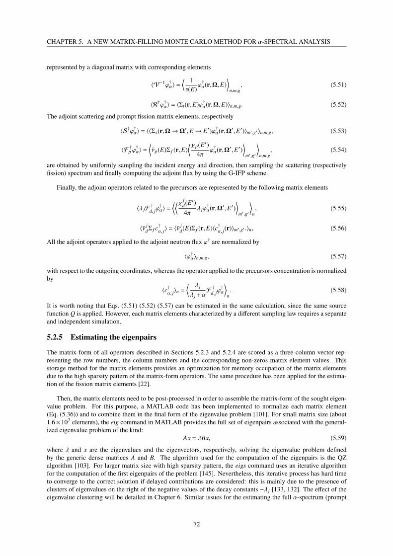
CHAPTER 5. A NEW MATRIX-FILLING MONTE CARLO METHOD FOR α-SPECTRAL ANALYSIS
represented by a diagonal matrix with corresponding elements
〈V−1ϕ†α〉 =⟨ 13(E)
ϕ†α(r,Ω,E)⟩
n,m,g, (5.51)
〈R†ϕ†α〉 = 〈Σt(r,E)ϕ†α(r,Ω,E)〉n,m,g. (5.52)
The adjoint scattering and prompt fission matrix elements, respectively
〈S†ϕ†α〉 = 〈〈Σs(r,Ω→Ω′,E→ E′)ϕ†α(r,Ω′,E′)〉m′,g′〉n,m,g, (5.53)
〈F†p ϕ†α〉 =
⟨νp(E)Σ f (r,E)
⟨χp(E′)4π
ϕ†α(r,Ω′,E′)⟩
m′,g′
⟩n,m,g
, (5.54)
are obtained by uniformly sampling the incident energy and direction, then sampling the scattering (respectivelyfission) spectrum and finally computing the adjoint flux by using the G-IFP scheme.
Finally, the adjoint operators related to the precursors are represented by the following matrix elements
〈λ jF†
d, jϕ†α〉 =
⟨⟨χ jd(E′)
4πλ jϕ
†α(r,Ω′,E′)
⟩m′,g′
⟩n, (5.55)
〈νjdΣ f c†α, j〉 = 〈ν
jd(E)Σ f (r,E)〈c†α, j(r)〉m′,g′ .〉n, (5.56)
All the adjoint operators applied to the adjoint neutron flux ϕ† are normalized by
〈ϕ†α〉n,m,g, (5.57)
with respect to the outgoing coordinates, whereas the operator applied to the precursors concentration is normalizedby
〈c†α, j〉n =
⟨ λ j
λ j +αF†
d, jϕ†α
⟩n. (5.58)
It is worth noting that Eqs. (5.51) (5.52) (5.57) can be estimated in the same calculation, since the same sourcefunction Q is applied. However, each matrix elements characterized by a different sampling law requires a separateand independent simulation.
5.2.5 Estimating the eigenpairs
The matrix-form of all operators described in Sections 5.2.3 and 5.2.4 are scored as a three-column vector rep-resenting the row numbers, the column numbers and the corresponding non-zeros matrix element values. Thisstorage method for the matrix elements provides an optimization for memory occupation of the matrix elementsdue to the high sparsity pattern of the matrix-form operators. The same procedure has been applied for the estima-tion of the fission matrix elements [22].
Then, the matrix elements need to be post-processed in order to assemble the matrix-form of the sought eigen-value problem. For this purpose, a MATLAB code has been implemented to normalize each matrix element(Eq. (5.36)) and to combine them in the final form of the eigenvalue problem [101]. For small matrix size (about1.6×107 elements), the eig command in MATLAB provides the full set of eigenpairs associated with the general-ized eigenvalue problem of the kind:
Ax = λBx, (5.59)
where λ and x are the eigenvalues and the eigenvectors, respectively, solving the eigenvalue problem definedby the generic dense matrices A and B. The algorithm used for the computation of the eigenpairs is the QZalgorithm [103]. For larger matrix size with high sparsity pattern, the eigs command uses an iterative algorithmfor the computation of the first eigenpairs of the problem [145]. Nevertheless, this iterative process has hard timeto converge to the correct solution if delayed contributions are considered: this is mainly due to the presence ofclusters of eigenvalues on the right of the negative values of the decay constants −λ j [133, 132]. The effect of theeigenvalue clustering will be detailed in Chapter 6. Similar issues for the estimating the full α-spectrum (prompt
72

5.3. NUMERICAL SIMULATIONS
and delayed contributions) for large matrices were already encountered in the reference [8] when using an iterativeeigenvalue solver [91]. In order to overcome this problem, we decided to maintain a dense structure for the matricesassociated to the transport operators and to use the QZ algorithm [103] for the computation of all eigenpairs.
5.3 Numerical simulations
In order to assess the impact of using the α-k power iteration and the G-IFP method in order to fill the matrixelements of the direct and adjoint α-matrices, respectively, we have selected some simplified benchmark con-figurations that allow more easily probing the proposed methods by comparing the obtained results to referencesolutions.
5.3.1 The rod model
The rod model is among the simplest space- and direction-dependent transport problems: neutrons move at constantspeed 3 along a line, where only two directions of flight are allowed, namely forward (Ω = +) and backward(Ω = −) [159]. We will furthermore assume that scattering and fission are isotropic. Defining ϕα(x,±) the angularflux in the positive and negative direction, the α eigenvalue equations read
±∂
∂xϕα(x,±) +
[α
3+Σt
]ϕα(x,±) =
ζα2ϕα(x), (5.60)
where we have defined ϕα(x) = ϕα(x,+) +ϕα(x,−), and
ζα = Σs + νpΣ f +
J∑j=1
λ j
λ j +αν
jdΣ f . (5.61)
Let us consider a segment [0,L], with leakage boundary conditions ϕα(0,+) = 0 and ϕα(L,−) = 0. It is possible toderive an equation for ϕα(x) alone, namely,
−Dα∂2
∂x2ϕα(x) =ζαDα−1
Dαϕα(x), (5.62)
with Robin boundary conditions ϕα(0)−Dα∂ϕα(0)/∂x = 0 and ϕα(L) + Dα∂ϕα(L)/∂x = 0, and
Dα =1
Σt + α3
. (5.63)
Taking into account the boundary conditions, the solution of Eq. (5.62) is expressed as
ϕα(x) =√ζαDα−1cos
√ζαDα−1
Dαx
+ sin
√ζαDα−1
Dαx
, (5.64)
from which we can obtain the angular flux ϕα(x,±) and the precursor concentration
c jα =
1λ j +α
νjdΣ fϕα(x) (5.65)
by observing that the particle current Pα(x) = ϕα(x,+)−ϕα(x,−) satisfies Pα(x) = −Dα∂xϕα(x). The adjoint eigen-modes satisfy the relation ϕ†α(x,±) = ϕα(x,∓). The α-eigenvalues stem from the dispersion law [170]
Λ(α) = 2√ζαDα−1cos
√ζαDα−1
DαL
− ζαDα cos
√ζαDα−1
DαL
= 0, (5.66)
which is obtained by imposing the boundary conditions on the general solutions in Eq. (5.64). The zeros ofEq. (5.66) form the discrete spectrum of the α-eigenvalues for the rod model. When the precursor contributionsare neglected, Λ(α) yields a finite number of real eigenvalues, plus a countable infinity of complex eigenvaluesassociated to oscillating modes [104]; when precursors are taken into account, J additional sets of denumerable real
73

CHAPTER 5. A NEW MATRIX-FILLING MONTE CARLO METHOD FOR α-SPECTRAL ANALYSIS
eigenvalues are introduced by the J singularities at α = −λ j, accumulating at the right of each −λ j (the ”clusters”mentioned above).
Analysis of the direct eigenpairs
We begin our analysis by considering the case of direct eigenvalues and eigenfunctions. The physical parametersfor the rod model are given in Tab. 5.1. For this example, we have chosen a deep sub-critical configuration and wehave neglected the contributions of precursors. The dominant α-eigenvalue is α0 = −0.91112 (with correspondingk-eigenvalue k0 = 0.21945). The matrix elements have been computed as described in the previous sections,based on the α-k power iteration. Since the transport model does not depend on energy and only two discretedirections are allowed, the only discretization left is with respect to the space coordinates, which makes easier theinvestigation of the convergence of the proposed methods.
3 [cm/s] Σc [cm-1] Σ f [cm-1] Σs [cm-1] νp [-] L [cm]
10 1 0.1 1 2.5 10
Table 5.1: Parameter values for the rod model.
The Monte Carlo matrix-filling calculation based on the α-k power iteration has been run with 103 inactivecycles, 103 active cycles used for scoring the matrix elements, and 105 particles per cycle. The results of thespectral analysis from the α-weighted matrices are recalled in Tab. 5.2 for a discretization of N = 1024 spatialmeshes. An excellent agreement is found between the numerical values coming from the A matrix filled by theMonte Carlo calculation and the exact reference stemming from the numerical analysis of the roots of the dispersionlaw in Eq. (5.66). Correspondingly, the first few eigenfunctions are compared in Fig. 5.2 for the same spatialdiscretization: again, an excellent agreement is found between the eigenvectors of the A matrix filled by the MonteCarlo calculation and the exact solutions stemming from Eq. (5.64).
0 1 2 3 4 5 6 7 8 9 10−0.025
−0.02
−0.015
−0.01
−0.005
0
0.005
0.01
0.015
0.02
0.025
x
ϕα(x,+)
Figure 5.2: The first few (angular) eigenmodes ϕα(x,+): the eigenvectors of the A matrix filled by the Monte Carlocalculation (symbols) are compared to the exact solutions stemming from Eq. (5.64) (solid lines). Blue circles:fundamental eigenmode ϕα0 (x,+); red squares: second eigenmode ϕα1 (x,+); green triangles: third eigenmodeϕα2 (x,+).
74

5.3. NUMERICAL SIMULATIONS
weighting function α0 [s-1] α1 [s-1] α2,3 [s-1]
exact -0.91112 -1.14021 -1.59033 ± 0.46007iα-k -0.91113 -1.14081 -1.59245± 0.45965i
Generalized IFP -0.91102 -1.14101 -1.59233± 0.45948ik -0.91104 -1.14049 -1.59232 ± 0.45890i
fixed-source -0.91135 -1.14078 -1.59273 ± 0.45864i
Table 5.2: Rod model. Comparison of the α eigenvalues obtained from the matrices filled with the method shownin the first column, for N = 1024 spatial meshes. Model parameters are shown in Tab. 5.1.
As discussed in the previous sections, an important issue concerns the convergence of the eigenvalues andeigenvectors of A with respect to the size of the matrix, i.e., the discretization of the viable phase-space. Thekey point is that the use of the α-k power iteration in order to weight the matrix elements by the fundamentaleigenfunction ϕα0 is expected to preserve the fundamental eigenvector of A for any choice of the matrix size.For the purpose of probing the behaviour of A, in addition to the α-weighted matrix we have produced two othermatrices obtained by weighting their respective elements by using the fundamental mode of the k-eigenvaluepower iteration (with 103 inactive cycles, 103 active cycles used for scoring the matrix elements, and 105 particlesper cycle) and by using the flux resulting from a fixed-source calculation starting from a uniformly distributedisotropic source within the domain (with 108 particles). In the limit of very large N, all these methods are expectedto converge to the exact limitA: for a more refined phase-space discretization, the choice of the weighting functionf introduced in Eq. (5.36) becomes less important. The corresponding numerical values are recalled in Tab. 5.2for N = 1024 spatial meshes and different weighting functions.
The convergence analysis of the α-eigenvalues as a function of the spatial discretization N and of the choice ofthe weighting function for A is shown in Fig. 5.3. As conjectured, the fundamental eigenvalue α0 resulting fromthe α-weighted matrix A is unbiased with respect to the exact reference root of the dispersion law in Eq. (5.66),independently of the discretization N (Fig. 5.3, left). On the contrary, the fundamental eigenvalues α0 resultingfrom the matrix A with the two other weighting schemes shows a bias that is progressively reduced as N increases.Even for this very simple benchmark example, it takes roughly N = 128 in order for the other schemes to convergeto the true fundamental eigenvalue, which motivates the choice of the α-weighting schemes. Concerning the secondand third eigenvalue α1 and α2, as expected the higher-order eigenfunctions are not preserved and the α-weightingmethod does not offer any specific advantage (Fig. 5.3, right). For higher-order eigenvalues the rate of convergenceof the three schemes is similar.
75

CHAPTER 5. A NEW MATRIX-FILLING MONTE CARLO METHOD FOR α-SPECTRAL ANALYSIS
101 102 103
−0.94
−0.92
−0.9
−0.88
N
α0
101 102 103−2.2
−2
−1.8
−1.6
−1.4
−1.2
−1
α2
α1
N
α
Figure 5.3: Convergence of the first few eigenvalues αi as a function of the number of spatial meshes N and of theweighting function for the matrix A. Left: the fundamental eigenvalue α0; right: α1 and Re[α2]. Black solid linescorrespond to the exact reference values from the roots of the dispersion law in Eq. (5.66). Blue circles correspondto results obtained from the α-weighted A matrix; red squares to the k-weighted A matrix; green triangles symbolsto the matrix A weighted by a fixed-source flux. Solid lines have been added to guide the eye. In addition, wedisplay with magenta diamonds the corresponding eigenvalues obtained from the adjoint matrix A† weighted bythe adjoint α-eigenfunction resulting from the Generalized IFP method.
An important issue concerns the impact of the statistical uncertainty intrinsically induced by the Monte Carlomethod on the elements of the matrices: in particular, we are interested in assessing the effects of such fluctuationson the derived spectrum and eigenvectors. For this purpose, we have performed an ensemble of independentreplicas of the α-k power iterations and we have computed the average and the dispersion of the obtained αspectrum and eigenvectors, as a function of the number of simulated particles per cycle. Numerical findingsare reported in Tab. 5.3 and show that the standard deviation of the first few eigenvalues scales roughly as 1/
√P,
P being the number of particles per cycle.
Particles per cycle α0 [s-1] α1 [s-1] Re[α2,3] [s-1] Im[α2,3] [s-1]
exact -0.911121 -1.140209 -1.590327 ± 0.460074
103 -0.91112 -1.14497 -1.60753 ± 0.45378Average 104 -0.911123 -1.14509 -1.60762 ± 0.45387
105 -0.911117 -1.145099 -1.607615 ± 0.453870
103 2 ×10⁻⁵ 5 ×10⁻⁵ 3 ×10⁻⁵ 7 ×10⁻⁵
Std 104 8 ×10⁻⁶ 1 ×10⁻⁵ 1 ×10⁻⁵ 2 ×10⁻⁵
105 2 ×10⁻⁶ 5 ×10⁻⁶ 3 ×10⁻⁶ 7 ×10⁻⁶
Table 5.3: Rod model. Comparison of the eigenvalues obtained from the matrices scored during 103 replicas ofα-k power iterations, each using 103 inactive cycles, 103 active cycles and a variable number of particles per cycle.
76

5.3. NUMERICAL SIMULATIONS
101 102 1030.54
0.55
0.56
0.57
0.58
0.59
N
R0
101 102 1030
2
4
6
8
10
12
14
R1
R2
N
R
Figure 5.4: Convergence of the first few estimators Ri as a function of the number of spatial meshes N and ofthe weighting function for the matrix A. Black solid lines correspond to the exact reference values based onEq. (5.64). Blue circles correspond to results obtained from the α-weighted A matrix; red squares correspondto the k-weighted A matrix; green triangles correspond to the matrix A weighted by a fixed-source flux. Left:the estimator R0 associated to the fundamental eigenfunction ϕα0 (x,+); right: the estimator R1 associated to thesecond eigenfunction ϕα1 (x,+) and the estimator R2 associated to the second eigenfunction ϕα2 (x,+). Solid lineshave been added to guide the eye.
In order to perform a similar analysis on the behaviour of the eigenmodes, we have introduced an estimatordefined as the normalized integral of the eigenfunction of order i over the half-domain, namely,
Ri =
|∫ L
L2
dx ϕαi (x,+)|
|∫ L
0 dx ϕαi (x,+)|, (5.67)
where L is the length of the rod. The reference value for Ri can be computed based on Eq. (5.64). The numericalvalues for the first few Ri are compared to the exact solutions in Tab. 5.4 for N = 1024 spatial meshes and differentweighting functions.
weighting function R0 [-] R1 [-] R2,3 [-]
exact 0.59054 3.04076 1.25702
α− k 0.59068 3.03938 1.26403k 0.59068 3.04243 1.26346
fixed-source 0.59039 3.05016 1.26317
Table 5.4: Rod model. Comparison of the firs few estimators Ri obtained from the matrices filled with the methodshown in the first column, for N = 1024 spatial meshes.
The convergence analysis of the estimator Ri computed by the matrix A as a function of the spatial discretizationN and of the choice of the weighting function for A is shown in Fig. 5.4. As conjectured, the estimator R0 associatedto the fundamental eigenfunction resulting from the α-weighted matrix A is unbiased with respect to the exactsolution, independently of the discretization N. On the contrary, the estimator R0 resulting from the matrix Awith the two other weighting schemes shows a bias that decreases with increasing N. It takes roughly only N = 8in order for the k-weighted scheme to converge to the true fundamental eigenvalue, which can be understood byobserving that the deviation between ϕk0 (x,+) and ϕα0 (x,+) is rather small for the parameters chosen here. For thematrix weighted on the fixed-source flux, the deviation is much larger, and convergence is achieved after N = 256.Concerning the estimators R1 and R2 associated with the second and third eigenfunction, all weighting schemesare biased, and the rate of convergence of the three schemes is similar.
77

CHAPTER 5. A NEW MATRIX-FILLING MONTE CARLO METHOD FOR α-SPECTRAL ANALYSIS
0 1 2 3 4 5 6 7 8 9 10−0.03
−0.02
−0.01
0
0.01
0.02
0.03
x
ϕ† α(x,+)
Figure 5.5: The first few (angular) adjoint eigenmodes ϕ†α(x,+): the eigenvectors of the A matrix filled by the MonteCarlo calculation (symbols) are compared to the exact solutions stemming from the equation adjoint to Eq. (5.64)(solid lines). Blue circles: fundamental adjoint eigenmode ϕ†α0 (x,+); red squares: second adjoint eigenmodeϕ†α1 (x,+); green triangles: third adjoint eigenmode ϕ†α2 (x,+).
In order to assess the impact of the statistical uncertainty induced by the Monte Carlo method on the eigenvec-tors, we have performed an ensemble of independent replicas of the α-k power iterations and we have computed theaverage and the dispersion of the obtained α-eigenvectors, as a function of the number of simulated particles percycle. Numerical findings are reported in Tab. 5.5 and show that the standard deviation of the first few estimatorsRi scales approximately as 1/
√P, P being the number of particles per cycle.
Particles per cycle R0 [-] R1 [-] R2 [-]
exact 0.590542 3.0408 1.25702
103 0.59049 3.052 1.302average 104 0.59053 3.053 1.3021
105 0.590534 3.0512 1.30201
103 7.7 ×10⁻⁵ 3.3 ×10⁻³ 2.2 ×10⁻³
Std 104 2.4 ×10⁻⁵ 1.0 ×10⁻³ 5.5 ×10⁻⁴
105 7.4 ×10⁻⁶ 3.3 ×10⁻⁴ 6.2 ×10⁻⁵
Table 5.5: Rod model. Comparison of the estimators Ri obtained from the matrices scored during 103 replicas ofα-k power iterations, each using 103 inactive cycles, 103 active cycles and a variable number of particles per cycle.
Analysis of the adjoint eigenpairs
We will now focus on the adjoint matrix A†, whose elements have been filled by using the Generalized IFP method,as detailed above. For this example, the Monte Carlo calculation has been performed with 108 particles, and 15latent generations. The α0 value needed for the Generalized IFP algorithm has been obtained from the direct cal-culations done in the previous section. The results of the spectral analysis from the adjoint α-weighted matrixare recalled in Tab. 5.2 for a discretization of N = 1024 spatial meshes. An excellent agreement is found betweenthe numerical values coming from the A† matrix filled by the Monte Carlo calculation and the exact results stem-ming from the roots of the dispersion law in Eq. (5.66). This means that the relation α† = α on the spectrum ofthe α-eigenvalues is correctly preserved when weighting A† by the fundamental eigenfunction ϕ†α0 . This prop-erty is also preserved when approximating A† by taking the transposed matrix AT (although A is weighted bythe direct fundamental eigenfunction), since by construction transposition preserves the spectrum. The first fewadjoint eigenfunctions are compared in Fig. 5.5 for the same spatial discretization: again, an excellent agreementis found between the eigenvectors of the A† matrix filled by the Generalized IFP method and the exact solutions
78

5.3. NUMERICAL SIMULATIONS
stemming from the eigenfunctions adjoint to Eq. (5.64). Observe in particular that ϕ†α satisfies ϕ†α(x,±) = ϕα(x,∓),as expected.
The convergence of the eigenvalues associated to the A† matrix is analyzed in Fig. 5.3: not surprisingly, theconvergence of the eigenvalues with respect to the matrix discretization N follows the same pattern as in the directcase. The fundamental eigenvalue α0 is similarly preserved by the matrix A†, independently of N, whereas thehigher eigenvalues are not and converge to the true values in the limit of large N.
101 102 1030.36
0.38
0.4
0.42
0.44
0.46
0.48
0.5
N
R† 0
101 102 1030.25
0.3
0.35
0.4
0.45
0.5
0.55
0.6
0.65
0.7
0.75
R†1
R†2
N
R†
Figure 5.6: Convergence of the first few estimators R†i as a function of the number of spatial meshes N. Black solidlines correspond to the exact reference values based on Eq. (5.64). Blue circles correspond to results obtained fromthe adjoint α-weighted A† matrix; red squares correspond to the direct α-weighted AT matrix. Left: the estimatorR†0 associated to the fundamental adjoint eigenfunction ϕ†α0 (x,+); right: the estimator R†1 associated to the secondadjoint eigenfunction ϕ†α1 (x,+) and the estimator R†2 associated to the second adjoint eigenfunction ϕ†α2 (x,+). Solidlines have been added to guide the eye.
Weighting function R†0 [-] R†1 [-] R†2,3 [-]
exact 0.40946 4.04076 1.65441
Generalized IFP 0.41055 4.00166 1.65293α-k and transposition 0.40982 4.03249 1.65836
Table 5.6: Rod model. Comparison of the adjoint estimators R†i obtained from the matrices filled with the methodshown in the first column, for N = 1024 spatial meshes.
In order to analyze the behaviour of the adjoint eigenmodes, we introduce the estimator
R†i =
|∫ L
L2
dx ϕ†αi (x,+)|
|∫ L
0 dx ϕ†αi (x,+)|. (5.68)
The reference value for R†i can be computed based on the adjoint eigenfunctions derived from Eq. (5.64). Numeri-cal values corresponding to the generalized IFP method and to the transposed matrix obtained from the α-k methodare recalled in Tab. 5.6 for N = 1024 spatial meshes. The convergence analysis of the estimator R†i estimated bythe matrix A† as a function of the spatial discretization N is shown in Fig. 5.6. As conjectured, the estimator R†0associated to the fundamental adjoint eigenfunction resulting from the adjoint α-weighted matrix A† is unbiasedwith respect to the exact solution, independently of the discretization N. As for the estimator R†1 associated withthe second eigenfunction, the adjoint α-weighted matrix A† yields a biased result, which converges to the exactlimit after approximatively N = 32.
In the same figure we also display the estimators of the adjoint eigenfunctions obtained by taking the transposeddirect α-weighted matrix AT in order to approximate A†. Figure 5.6 shows that this approach leads to a bias on R†i
79

CHAPTER 5. A NEW MATRIX-FILLING MONTE CARLO METHOD FOR α-SPECTRAL ANALYSIS
for the fundamental and the first eigenfunction. Although the bias vanishes as expected in the limit of large N, thisanalysis suggests that it is general preferable to compute A† rather than approximating the adjoint-weighted matrixby using the transposed matrix AT .
5.3.2 A continuous-energy transport model
We consider now a continuous-energy transport model in an infinite medium. The model includes scattering withan amnesia kernel [34], capture and fission with two precursor families. All cross sections Σr are assumed to have a1/√
E behaviour, i.e., Σr(E) = Σ0r/√
E. The scattering kernel M(E) is a Maxwell distribution with average energyEs. The prompt χp(E) and delayed χ j
d(E) fission kernels are also assumed to be Maxwellian distributions withaverage Ep and E j
d, j = 1,2, respectively. These distributions can be expressed as normalized probability densityfunctions, given the following equation
M(E) =2√π
1E3/2
√Ee−E/E , (5.69)
where E is the average energy of the corresponding distribution. The fission multiplicities are taken constant, forthe sake of simplicity.
The resulting α eigenvalue problem reads[α
3(E)+Σt(E)
]ϕα(E) = M(E)
∫ ∞
0dE′ Σs(E′)ϕα(E′) +χp(E)
∫ ∞
0dE′ νpΣ f (E′)ϕα(E′)
+∑
j
λ j
λ j +αχ
jd(E)
∫ ∞
0dE′ ν j
dΣ f (E′)ϕα(E′), (5.70)
where 3(E) =√
E. By virtue of the simple functional forms chosen for this configuration, the eigenvalues andeigenfunctions can be determined exactly. In particular, the eigenvalues are the roots of the dispersion law
Λ(α) = α+Σ0a− νpΣ0
f −∑
j
λ j
λ j +αν
jdΣ0
f = 0, (5.71)
where Σ0a = Σ0
t −Σ0s , and the eigenfunctions read
ϕα(E) =
√E
α+Σ0t
Σ0s M(E) + νpΣ0
fχp(E) +∑
j
λ j
λ j +αν
jdΣ0
fχjd(E)
, (5.72)
for the values α that satisfy the dispersion law. As for the adjoint eigenvalue problem, we have the equation[α
3(E)+Σt(E)
]ϕ†α(E) = Σs(E)
∫ ∞
0dE′ M(E′)ϕ†α(E′) + νpΣ f (E)
∫ ∞
0dE′ χp(E′)ϕ†α(E′)
+∑
j
λ j
λ j +αν
jdΣ f (E′)
∫ ∞
0dE′ χ j
d(E′)ϕ†α(E′). (5.73)
By inspection, the eigenfunctions are ϕ†α(E) = 1, independently of α, with the same associated spectrum as in thedirect problem.
80
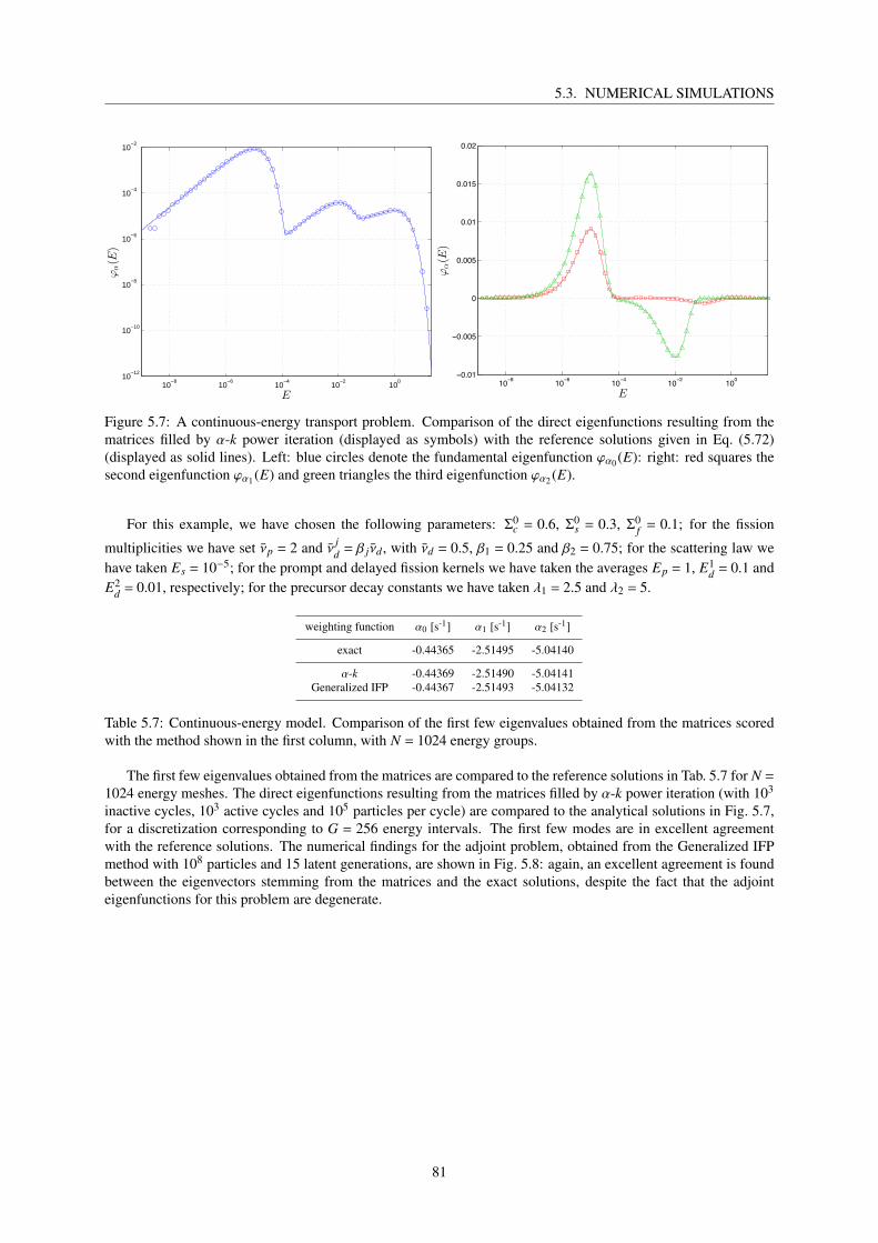
5.3. NUMERICAL SIMULATIONS
10−8
10−6
10−4
10−2
100
10−12
10−10
10−8
10−6
10−4
10−2
E
ϕα(E
)
10−8 10−6 10−4 10−2 100−0.01
−0.005
0
0.005
0.01
0.015
0.02
E
ϕα(E
)
Figure 5.7: A continuous-energy transport problem. Comparison of the direct eigenfunctions resulting from thematrices filled by α-k power iteration (displayed as symbols) with the reference solutions given in Eq. (5.72)(displayed as solid lines). Left: blue circles denote the fundamental eigenfunction ϕα0 (E): right: red squares thesecond eigenfunction ϕα1 (E) and green triangles the third eigenfunction ϕα2 (E).
For this example, we have chosen the following parameters: Σ0c = 0.6, Σ0
s = 0.3, Σ0f = 0.1; for the fission
multiplicities we have set νp = 2 and ν jd = β jνd, with νd = 0.5, β1 = 0.25 and β2 = 0.75; for the scattering law we
have taken Es = 10−5; for the prompt and delayed fission kernels we have taken the averages Ep = 1, E1d = 0.1 and
E2d = 0.01, respectively; for the precursor decay constants we have taken λ1 = 2.5 and λ2 = 5.
weighting function α0 [s-1] α1 [s-1] α2 [s-1]
exact -0.44365 -2.51495 -5.04140
α-k -0.44369 -2.51490 -5.04141Generalized IFP -0.44367 -2.51493 -5.04132
Table 5.7: Continuous-energy model. Comparison of the first few eigenvalues obtained from the matrices scoredwith the method shown in the first column, with N = 1024 energy groups.
The first few eigenvalues obtained from the matrices are compared to the reference solutions in Tab. 5.7 for N =
1024 energy meshes. The direct eigenfunctions resulting from the matrices filled by α-k power iteration (with 103
inactive cycles, 103 active cycles and 105 particles per cycle) are compared to the analytical solutions in Fig. 5.7,for a discretization corresponding to G = 256 energy intervals. The first few modes are in excellent agreementwith the reference solutions. The numerical findings for the adjoint problem, obtained from the Generalized IFPmethod with 108 particles and 15 latent generations, are shown in Fig. 5.8: again, an excellent agreement is foundbetween the eigenvectors stemming from the matrices and the exact solutions, despite the fact that the adjointeigenfunctions for this problem are degenerate.
81
CHAPTER 5. A NEW MATRIX-FILLING MONTE CARLO METHOD FOR α-SPECTRAL ANALYSIS
10−8 10−6 10−4 10−2 1000.8
0.85
0.9
0.95
1
1.05
1.1
1.15
1.2
E
ϕ† α(E
)
Figure 5.8: A continuous-energy transport problem. Comparison of the adjoint eigenfunctions resulting from thematrices filled by Generalized IFP method (displayed as symbols) with the reference solutions given in Eq. (5.72)(displayed as solid lines). Blue circles denote the fundamental adjoint eigenfunction ϕ†α0 (E); red squares the secondadjoint eigenfunction ϕ†α1 (E); green triangles the third adjoint eigenfunction ϕ†α2 (E).
5.4 Discussion
The examples discussed in the previous section are very simple and have been precisely chosen in order to comparethe obtained numerical results against reference solutions. In view of the application of the proposed methods toreal-world reactor configurations, some issues must be carefully examined and taken into account.
The first concerns the size of the matrix operators and hence the involved memory footprint. A first glanceto the involved order of magnitudes might suggest that the overall size of the matrices involved in α-eigenvalueproblems may become too large to work with for any practical case, due to the need of separately discretizingspace, direction and energy (contrary to the k-eigenvalue problem, where only a spatial discretization is typicallyrequired [35, 22]). Consider for instance a three-dimensional configuration, and assume that each variable ispartitioned into 102 bins: this would lead to a total number of 1010 bins, i.e., to a number of 1020 matrix entries.This applies to both direct and adjoint matrices. Such huge number, supposing that each entry is represented by adouble-precision floating-point number, clearly corresponds to an unaffordable memory on current machines (andon future, at least for a very long time).
In practice, however, the α-eigenvalue matrices have been already applied to realistic systems, including smallresearch reactors [8]: as discussed in Section 5.2.1, the involved matrices have a sparse nature, and the number ofnon-null entries is much smaller that the total size of the matrices (see in particular Eq. (5.49)). Furthermore, onecan often take advantage of the existing symmetries in order to reduce the dimension of the problem. Moreover,for the energy and angle variable 102 bins are probably excessive with respect to most problems of interest. Toprovide an example, for a two-dimensional representation of a reactor core, by taking Nx = Ny = 102 for the spatialmesh, M = 8 for the directions, G = 30 for the energy groups and J = 6 for the precursor families, we wouldhave ∼ 6× 10¹³ bins for the full matrix, but less than ∼ 6× 10⁸ non-null entries. Even in this case, however,and despite all the simplifications, the memory footprint would be challenging for current machines. Numericaltests of convergence should be also performed a posteriori in order to ensure that at least the spatial shape of theeigenvectors has been correctly captured. The benchmark configurations examined in this chapter clearly do notaddress these problems, since only a single dimension has been discretized and careful convergence tests were thuspossible.
The second issue concerns the applicability of these matrices to the analysis of system changes. The wholeα-eigenvalue expansion is based on the assumption that the physical properties of the system under analysis (suchas cross sections, fission spectra, multiplicities, etc.) do not evolve with time: eigenvalues and eigenvectors are
82

5.5. CONCLUSIONS
computed for a specific state. In real-world configurations, these properties naturally change, due to externalactions (control rod movements), physical feedbacks (Doppler effect, etc.), or both. In principle, once the systemchanges the computed alpha eigenvalues and eigenvectors are no longer valid and cannot be used. This leads totwo different approaches: one can either introduce (short) time steps and re-compute the required matrices at eachtime step, or use some clever interpolation between the initial and final configurations of the system. The formermethod would lead to an unreasonable memory occupation (and most probably also computation time). The lattermethod has been suggested [85] and successfully applied [87] for the Transient Fission Matrix method, and seemsthus much more promising. In particular, the application of perturbation techniques such as correlated samplinghas been shown to enhance the performances of the interpolation methods in realistic applications, including multi-physics feedbacks [86]. An overview of the Transient Fission Matrix method is provided in Appendix A.
In view of these considerations, and based on the increasing availability of direct time-dependent Monte Carlosimulations for reactor physics problems (which natively include moving geometries and physical feedbacks [141,41]), the main interest of the α-eigenvalue matrix operators seems for higher-order mode analysis rather than forreconstructing the time evolution of a system via eigenmode expansion: knowledge of the first few α-eigenvaluesand eigenfunctions for a given reactor state might help, e.g., in locating the most appropriate detector positionsfor on-line core monitoring. Nonetheless, a comparison in terms of performances and accuracy with respect toexisting matrix-based methods (using time-dependent Monte Carlo methods as a reference) for the approximationof the reactor kinetics will deserve further investigation.
5.5 Conclusions
Knowledge of the α-eigenpairs is key to several applications in reactor physics. In a series of recent works, it hasbeen proposed to use Monte Carlo methods in order to estimate the elements of the matrices that represent thediscretized formulation of the operators involved in the α-eigenvalue problem. In this chapter, we have suggestedsome strategies to overcome two possible shortcomings of the existing algorithms. We have shown that the biaspossibly appearing on the direct fundamental eigenvalue and eigenvector for smaller sizes of the discretized matrixcan be removed by using the α-k modified power iteration method as a weighing function. This correspondsto weighting the matrix elements by the fundamental mode ϕα0 , which is expected to preserve the fundamentaleigenvalue and eigenvector of the matrix, similarly to what occurs for the fission matrix in k-eigenvalue problems.We have successively shown that the matrix associated to the adjoint α-eigenvalue problem can be estimatedby using the G-IFP method, which was recently introduced as a reference Monte Carlo method to compute thefundamental adjoint α-eigenfunction. Since this approach corresponds to weighting the matrix elements by thefundamental adjoint eigenfunction, the fundamental adjoint eigenvector of the discretized matrix will be similarlypreserved.
The proposed direct and adjoint methods have been verified on two benchmark problems where exact referencesolutions were available for both the eigenvalue spectrum and the direct and adjoint eigenfunctions, and theirconvergence and accuracy have been extensively assessed. The impact of alternative weighting schemes (such asthe k-eigenvalue fundamental mode or the flux resulting from solving a fixed-source problem) and the differencesbetween the adjoint matrix and the transposed direct matrix are most probably emphasized by the choice of thebenchmark problems presented in this chapter: in the remaining parts of this manuscript, we will extensively assessthe performances and the robustness of the proposed method for more realistic configurations combining spatialand energy heterogeneities.
We conclude by observing that the strategy presented in order to fill the matrix elements of the adjoint matrix bythe G-IFP method might be easily extended to the k-eigenvalue formulation: instead of using the transposed directfission matrix, one could use the regular IFP method (which yields the importance function for the k-eigenvalueproblems) so as to produce the adjoint fission matrix, thus avoiding the bias on the fundamental adjoint eigenvector.Moreover, since the proposed method estimate the linear and adjoint transport operators, it is in principle possibleto combine the corresponding matrices in order to recast and solve eigenvalue problems different from the α-formulation.
83

CHAPTER 5. A NEW MATRIX-FILLING MONTE CARLO METHOD FOR α-SPECTRAL ANALYSIS
84
Chapter 6
Eigenvalue separation: a numericalinvestigation
6.1 Introduction
In the previous Chapter, we have successfully generalized the well-known fission matrix method so as to fillby Monte Carlo simulations the elements of matrix operators involved in the α-eigenvalue formulation, whichallows having a complete (albeit approximated) picture of the whole α-spectrum. In this Chapter, these toolswill be deployed together with the fission matrix method for the spectral analysis of a few relevant benchmarkconfigurations, for the purpose of illustrating how the higher-order k- and α-eigenvalues and eigenfunctions behaveas a function of the physical parameters. Such investigation extends the work done in Chapter 4 concerning thefundamental eigenvalues and eigenfunctions. All the simulations presented in this Chapter have been performedby using the newly implemented test-bed Monte Carlo code described in Section 3.7.1. As mentioned in Chapter 1,the tightness (or equivalently the level of decoupling) of a reactor core is typically characterized in terms of theeigenvalue separation, which for the k-eigenvalue formulation reads
E.S.n(k) =1kn−
1k0, (6.1)
with n ≥ 1 [37, 98, 144, 73, 120]. The case n = 1 plays a peculiar role, and is frequently referred to without usingthe index [120], namely,
E.S. = E.S.1(k) =1k1−
1k0. (6.2)
The system is said to be tightly coupled if the first two eigenvalues are separated, and loosely coupled otherwise.A closely related quantity is the dominance ratio
DR =k1
k0, (6.3)
which is a bounded value smaller than one and it can be monotonically mapped onto the E.S., thus sharing thesame information content.
As for the α-eigenvalues, the concept of eigenvalue separation or dominance ratio does not seem to have drawnmuch attention, to the best of our knowledge, although in the mathematical literature the analogous notion ofspectral gap is widely used for eigenvalue problems similar to the α-eigenvalue formulation (for instance in thecontext of the time-dependent diffusion equation [84, 125, 26, 2, 44]). In the same spirit as for the k-eigenvalueproblems, we can thus introduce the notion of eigenvalue separation for the α-eigenvalues, which immediatelycalls for a distinction between the formulation including the precursor contributions (usually called the “delayedeigenvalues”) and the one neglecting the precursor contributions (usually called the “prompt eigenvalues”). In thefollowing, we will denote by α the eigenvalues including the delayed contributions, whereas αp will denote the
85

CHAPTER 6. EIGENVALUE SEPARATION: A NUMERICAL INVESTIGATION
eigenvalues including only the prompt contributions. This distinction stems from the fact that, for a typical PWRreactor, the α-spectrum will have a natural ordering imposed by the fact that [72, 133, 132, 70]
νjd 1, and λ j Σt3. (6.4)
As a consequence, the α-spectrum splits into a “prompt” component and a “delayed” component, which are easilydistinguished on the complex plane [133, 132]. Numerical investigations have shown that the delayed part of theα spectrum consists of J “clusters” of real eigenvalues, with the j-th cluster, j = 1, · · · , J, being a denumerable setof eigenvalues in the interval (−λ j,−λ j−1), J being the total number of precursor families (we set λ0 to infinity).These eigenvalues are tightly regrouped at the right of each decay constant −λ j for family j on the complexplane [70, 133, 132]. The occurrence of the clustering of delayed eigenvalues had been first suggested by [45].These considerations have been previously introduced for the ”rod model” analysis in Section 5.3.1. The promptpart of the α-spectrum contains discrete eigenvalues, these latter appearing at the left of −λ j [70, 133, 132, 1] anda continuum portion (if any) at the left of the Corngold limit. In view of these considerations, it seems natural tointroduce the delayed eigenvalue separation
E.S.n(αd) = αd,n−α0, (6.5)
where αd,n is the delayed eigenvalue of order n and α0 is the fundamental eigenvalue, and the prompt eigenvalueseparation
E.S.n(αp) = αp,n−αp,0, (6.6)
where αp,n is the prompt eigenvalue of order n and αp,0 is the prompt eigenvalue with the largest real part.
Experimental and numerical investigations have shown that a small E.S.(k) would increase the probability for asystem to propagate instabilities, thus enhancing complex space-time patterns (as opposed to systems displaying alarge E.S., which behave as point-kinetics) [120]. This is especially relevant for loosely-coupled nuclear reactors,such as breeders having alternating regions of highly-enriched fuel and depleted blankets [120]. By virtue of itskey role in understanding the system kinetics, and in particular the reactor response due to external perturbationsand tilts, the k-eigenvalue separation has been extensively investigated [127, 38, 3, 54, 113, 78].
In the following, we will explore and compare the properties of E.S.n(k), E.S.n(αd) and E.S.n(αp) for a few sig-nificant configurations, and will complement this analysis by a careful investigation of the associated fundamentaland higher-order eigenmodes. In order to probe the behavior of these estimators, we have selected some simplesystems, so that we can avoid unnecessary complications and yet retain the key physical ingredients. The underly-ing idea is to ascertain whether the k and α spectral analysis can provide useful information concerning the systemresponse when a parameter related to a decoupling effect is progressively increased. The eigenpairs associatedto the eigenvalue problems discussed in this chapter have been computed with the MATLAB script mentioned inSection 5.2.5, based on the matrices estimated by the test-bed Monte Carlo code.
6.2 Choice of the benchmark configurations
In [120] it has been pointed out that homogeneous and heterogeneous systems behave quite differently with re-spect to eigenvalue separation. In homogeneous systems, small E.S.(k) can be attained only by increasing thesystem size. Under these circumstances, not only E.S.1(k), but all higher-order E.S.n(k) will be small: the physicalmeaning of this behavior is that many k-eigenmodes will be excited simultaneously. Thus, subject to local pertur-bations, the system will generally respond with complex space-dependent patterns, where several k-eigenmodesmay be present at the same time, and the fundamental eigenmode will not have a privileged role [120]. On thecontrary, in heterogeneous systems it is possible to have a small E.S.1(k), but much larger higher-order E.S.n(k):these configurations are typically obtained in loosely-coupled cores where two fissile regions are separated by asufficiently thick central moderator or absorber layer.
Based on these observations, for our numerical investigations we have selected two families of benchmarkconfigurations, respectively homogeneous and heterogeneous, whose physical parameters will be presented inSection 6.3.
The systems will be made progressively more decoupled, in the sense defined above, by acting on the overall
86

6.3. SIMULATION SETTINGS
system size (for the homogeneous configurations), and on the thickness of the layers (for the heterogeneous con-figurations): specific details will be provided in the following sections. In order to make our comparisons fair, wehave decided to make each configuration critical (i.e., k0 = 1 or equivalently α0 = 0) by adjusting a free parameter.In practice, this is achieved by adjusting the capture cross section of the fissile material: the computed k0 mustlie close to 1, within 20 pcm uncertainty. An important point is that, since we set the physical parameters so thatthe configurations are critical, the fundamental k-eigenmode will coincide with the fundamental α-eigenmode. Asa consequence, we will be allowed to use the regular k power iteration in order to weight the matrix elementsrequired for the spectral analysis, which ensures faster convergence of the Monte Carlo methods.
For both the homogeneous and heterogeneous systems, we will investigate 6 different configurations, corre-sponding to an increasing degree of decoupling. Several kinds of boundary conditions will be tested, in order toascertain their impact on the eigenvalue separation. Since the properties of the α eigenvalue separation are ratherunexplored, we have primarily used the k-eigenvalue separation to assess the degree of decoupling of the proposedconfiguration, by setting a target of at least DR = 0.95 for the most decoupled configuration of the benchmarks.For each case, we will analyze the dominance ratio from Eq. (6.3), the k-eigenvalue separation from Eq. (6.1), andthe prompt and delayed α-eigenvalue separation using Eqs. (6.6) and (6.5). Moreover, when significant, we willshow the first few k- and α-eigenmodes.
6.3 Simulation settings
The configurations analyzed in this chapter address multi-group particle transport in simplified 1D and 2D geome-tries, with reflecting and leakage boundary conditions. The energy domain is partitioned into three groups: fast,epithermal and thermal. Macroscopic cross sections, velocity, neutron yields and prompt fission emission spectrahave been taken with minimal modifications from the reference [163], where homogenized materials compatiblewith realistic configurations had been previously proposed. In particular, we have adjusted the velocities and con-sequently modified the macroscopic cross sections defined for the UO2 and H2O materials of reference [163] inorder to preserve reaction rates.
Precursor families (which were not available in [163]) are defined by using the 235U delayed data from theENDF/B-VI nuclear library [102] recalled by Cullen in [29]. The average delayed emission energy E j
d is as-sociated to a specific speed 3, which is linearly interpolated between the velocity values (31 and 32) defined inreference [163]. Emission probabilities for each delayed neutron are linearly interpolated as:
χjd1 = 1−
|3− 31|
31− 32, (6.7)
χjd2 = 1−
|3− 32|
31− 32, (6.8)
for the first and the second energy group, respectively.
According to these modifications, the materials UO2 and H2O will have the properties shown in Tabs. 6.1, 6.2and 6.3, respectively.
parameters fast group epithermal group thermal group
3(g) [cm/s] 1.66743×10⁹ 1.73734×10⁷ 3.46850×10⁵
Σc(g) [cm-1] 3.264×10⁻⁴ 9.7371×10⁻³ 2.9252×10⁻²
Σ f (g) [cm-1] 3.0586×10⁻³ 2.1579×10⁻³ 5.6928×10⁻²
Σs(1→ g) [cm-1] 2.21062×10⁻¹ 7.3843×10⁻² 0
Σs(2→ g) [cm-1] 0 7.77642×10⁻¹ 4.3803×10⁻²
Σs(3→ g) [cm-1] 0 0 1.55272
ν(g) [-] 2.4 2.4 2.4
χp(g) [-] 0.878198 0.121802 0
Table 6.1: Parameters of the fissile material for the heterogeneous configuration.
87

CHAPTER 6. EIGENVALUE SEPARATION: A NUMERICAL INVESTIGATION
parameters 1st family 2nd family 3rd family 4th family 5th family 6th family
β j [pcm] 2.275×101 1.17455×10² 1.12138×10² 2.51407×10² 1.03077×10² 4.3173×101
λ j [cm-1] 1.3336×10⁻² 3.2739×10⁻² 1.2078×10⁻¹ 3.0278×10⁻¹ 8.4949×10⁻¹ 2.8530
χjd(1) [-] 0.52296 0.56487 0.54697 0.61504 0.59265 0.60533
χjd(2) [-] 0.47704 0.43513 0.45303 0.38496 0.40735 0.39467
Table 6.2: Delayed parameters of the fissile material.
parameters fast group epithermal group thermal group
3(g) [cm/s] 1.66743×10⁹ 1.73734×10⁷ 3.46850×10⁵
Σc(g) [cm-1] 3.05×10⁻⁴ 3.699×10⁻⁴ 1.825×10⁻²
Σs(1→ g) [cm-1] 2.27125×10⁻¹ 1.0464×10⁻¹ 0
Σs(2→ g) [cm-1] 0 1.02817 9.7961×10⁻²
Σs(3→ g) [cm-1] 0 0 2.76295
Table 6.3: Parameters of the moderator material for the heterogeneous configuration.
The heterogeneous configurations described in Section 6.5 are composed of these two materials. The homo-geneous configurations analyzed in Section 6.4 are characterized by a single material obtained by summing themacroscopic cross sections of the fissile and the moderator materials. Properties and parameters of this homoge-nized material are defined in Tab. 6.4.
parameters fast group epithermal group thermal group
3(g) [cm/s] 1.66743×10⁹ 1.73734×10⁷ 3.46850×10⁵
Σc(g) [cm-1] 6.314×10⁻⁴ 1.0107×10⁻² 4.7502×10⁻²
Σ f (g) [cm-1] 3.0586×10⁻³ 2.1579×10⁻³ 5.6928×10⁻²
Σs(1→ g) [cm-1] 4.48187×10⁻¹ 1.78483×10⁻¹ 0
Σs(2→ g) [cm-1] 0 1.805812 1.41764×10⁻¹
Σs(3→ g) [cm-1] 0 0 1.55272×101
ν(g) [-] 2.4 2.4 2.4
χp(g) [-] 0.878198 0.121802 4.31567
Table 6.4: Parameters of the material for the homogeneous configurations.
6.4 Homogeneous benchmark configurations
We begin our analysis with the case of homogeneous configurations. The occurrence of decoupling effects forhomogeneous configurations can emerge for a sufficiently large size of the system with respect to the neutron mi-gration area [120]. In this section, we investigate the presence of these effects for critical 1D and 2D homogeneousconfigurations with reflective and leakage boundary conditions.
The critical state of the homogeneous configurations having reflective boundary conditions can be determinedexactly. The critical level is attained by adjusting the macroscopic capture cross sections by a factor a as follows:
Σ′c = aΣc. (6.9)
The value of a corresponding to the physical parameters given in Tab. 6.4 is equal to a = 1.49698 independentlyof the domain size. For a given parameter a, the dominance ratio will be imposed by adjusting the size of thedomain [120]. Six cases have been selected for the analysis of homogeneous systems, each defined by a character-istic length L ranging from 50 cm to 100 cm. This length corresponds to the actual length of the geometry for 1Dconfigurations and to the side of a square geometry for 2D configurations.
88

6.4. HOMOGENEOUS BENCHMARK CONFIGURATIONS
The parametric study performed for homogeneous systems with leakage boundary conditions requires an ad-ditional step, since the size of the domain L does influence the critical state of the configuration. In particular,we have started our analysis from the largest (the most decoupled) 1D and 2D configurations found for reflectiveboundary conditions. Then, we have estimated the new coefficient a in order to readjust the configuration to thecritical level after replacing reflective boundary conditions with leakage boundary conditions. This change of theboundary conditions implies that the the critical level depends on the size of the system. For this reason, we haveadjusted a second time the capture cross section by adding a factor b as follows:
Σ′c = aΣc +b3, (6.10)
for each size of the configuration under analysis.
The introduction of a second factor b/3 allows a finer adjustment with respect to the multiplicative factor a.This additional adjustment is required in order to calibrate all cases of different sizes to the critical level. Thisadjustment has been performed during a power iteration calculation that iteratively seeks the value of b whichmakes the system critical.
6.4.1 Homogeneous configurations with reflective boundary conditions
1D geometry
The first benchmark configuration analyzed in this section concerns 1D homogeneous systems of different lengthswith reflective boundary conditions. The fundamental eigenvalues k0 computed by the k power iteration are shownin the second column of Tab. 6.5. For these calculations, 5× 10⁴ particles per cycle are simulated, for a totalof 4.1× 10³ cycles (4× 10³ active, 102 inactive). During these simulations, we have activated the matrix-fillingmethods.
In order to build the matrix operators, the length of the domain has been partitioned into Nx = c×L spaceintervals along the x-axis, where c = 10 cm-1, in order to keep a constant bin width. The cosine of the particledirection with respect to the x-axis is uniformly partitioned into Mx = 4 intervals, whereas the energy groups andprecursor families are fixed at G = 3 and J = 6, respectively. The total size of the matrix defining the α-eigenvalueproblem ranges from 9.0×10³ (L = 50 cm) to 1.8×10⁴ (L = 100 cm), whereas the matrix defining the k-eigenvalueproblem ranges from 6.0×10³ to 1.2×10⁴. The eigenvalues computed from the matrix-form of the correspondingeigenvalue problem are shown in Tabs. 6.5 (k-eigenvalues), 6.6 (α-eigenvalues) and 6.7 (prompt α-eigenvalues).All fundamental eigenvalues k0 computed from the matrix of the corresponding eigenvalue problem are within 2σstandard deviation from the Monte Carlo results obtained from the k power iteration. The absolute values of thefundamental eigenvalues α0 are smaller than 2×10⁻³ s-1.
L [cm] kMC0 [-] k0 [-] k1 [-] k2 [-] k3 [-] k4 [-] k5 [-]
50 0.9999±1.0×10⁻⁴ 1.0000 0.9832 0.9356 0.8644 0.7789 0.6881
60 0.9999±1.0×10⁻⁴ 1.0000 0.9882 0.9545 0.9024 0.8369 0.7639
70 0.9999±1.0×10⁻⁴ 1.0000 0.9914 0.9661 0.9266 0.8757 0.8167
80 1.0001±1.0×10⁻⁴ 1.0001 0.9934 0.9741 0.9431 0.9025 0.8543
90 0.9999±1.0×10⁻⁴ 1.0000 0.9948 0.9793 0.9544 0.9215 0.8817
100 0.9999±1.0×10⁻⁴ 0.9999 0.9956 0.9831 0.9628 0.9355 0.9023
Table 6.5: First k-eigenvalues for the 1D homogeneous configuration with reflective boundary conditions as afunction of the size L of the system. The second column displays the fundamental eigenvalues k0 computed bythe test-bed Monte Carlo code for the k-eigenvalue problem and the corresponding standard deviations. All othereigenvalues have been computed from the matrix-form of the k-eigenvalue problem of the corresponding case.
89

CHAPTER 6. EIGENVALUE SEPARATION: A NUMERICAL INVESTIGATION
L [cm] α0 [s-1] α1 [s-1] α2 [s-1] α3 [s-1] α4 [s-1] α5 [s-1]
50 4.518×10⁻⁴ −1.315×10⁻² −1.329×10⁻² −1.332×10⁻² −1.332×10⁻² −1.333×10⁻²
60 −4.818×10⁻⁴ −1.307×10⁻² −1.327×10⁻² −1.331×10⁻² −1.332×10⁻² −1.333×10⁻²
70 −1.451×10⁻⁴ −1.296×10⁻² −1.325×10⁻² −1.330×10⁻² −1.331×10⁻² −1.333×10⁻²
80 1.771×10⁻³ −1.282×10⁻² −1.322×10⁻² −1.329×10⁻² −1.331×10⁻² −1.333×10⁻²
90 −6.398×10⁻⁴ −1.267×10⁻² −1.319×10⁻² −1.327×10⁻² −1.330×10⁻² −1.333×10⁻²
100 −1.032×10⁻³ −1.251×10⁻² −1.315×10⁻² −1.326×10⁻² −1.329×10⁻² −1.333×10⁻²
Table 6.6: First α-eigenvalues for the 1D homogeneous configuration with reflective boundary conditions as afunction of the size L of the system. These values have been computed from the matrix-form of the α-eigenvalueproblem of the corresponding case.
L αp,0 [s-1] αp,1 [s-1] αp,2 [s-1] αp,3 [s-1] αp,4 [s-1] αp,5 [s-1]
50 −3.015×10² −1.086×10³ −3.333×10³ −6.762×10³ −1.102×10⁴ −1.576×10⁴
60 −3.047×10² −8.536×10² −2.437×10³ −4.922×10³ −8.114×10³ −1.179×10⁴
70 −3.033×10² −7.049×10² −1.888×10³ −3.763×10³ −6.215×10³ −9.118×10³
80 −2.975×10² −6.087×10² −1.514×10³ −2.977×10³ −4.916×10³ −7.258×10³
90 −3.055×10² −5.481×10² −1.270×10³ −2.444×10³ −4.008×10³ −5.920×10³
100 −3.063×10² −5.059×10² −1.090×10³ −2.048×10³ −3.337×10³ −4.927×10³
Table 6.7: First prompt α-eigenvalues for the 1D homogeneous configuration with reflective boundary conditions asa function of the size L of the system. These values have been computed from the matrix-form of the α-eigenvalueproblem of the corresponding case.
For the sake of completeness, we show both the k- and the α-spectra on the complex plane in Fig. 6.1. The(very small) imaginary part of the k-spectrum is merely due to the statistical uncertainties propagated from thestochastic estimation of the matrix elements on the eigenvalues. The α-spectrum displays two circles due to thefour direction intervals chosen for the simulations: this feature is repeated for each energy group considered in thespectrum, as already pointed out in reference [8]. Figure 6.2 shows the zoom on all delayed eigenvalue clusters(left) and on the delayed eigenvalue cluster associated to the first precursor family (right). The eigenvalues areconcentrated on the right of the −λ j values, as expected from reference [133, 132]. The dominant eigenvalue α j
d,0of the j-th delayed cluster is separated from the other eigenvalues of the same precursor family [133, 132]. Thezoom of Fig. 6.2 (left) shows the gap between α j
d,0 and −λ j values for the last precursor families ( j = 4,5,6). The
computed values of α jd,0 and α j
d,1 for the last three precursor families are shown in Tab. 6.8.
Figure 6.1: Spectra of the k (left) and the α (right) eigenvalue problem for the 1D homogeneous configuration withreflective boundary conditions for the most decoupled case (L = 100 cm).
90

6.4. HOMOGENEOUS BENCHMARK CONFIGURATIONS
Figure 6.2: Zoom on the α-spectrum on the delayed region (left) and in the first delayed cluster (right) for the1D homogeneous configuration with reflective boundary conditions for the most decoupled case (L = 100 cm).Vertical lines have been added in order to indicate the values of −λ1 (blue), −λ4 (magenta), −λ5 (cyan) and −λ6(green).
L [cm] α4d,0 [s-1] α4
d,1 [s-1] α5d,0 [s-1] α5
d,1 [s-1] α6d,0 [s-1] α6
d,1 [s-1]
50 −1.914×10⁻¹ −2.693×10⁻¹ −7.383×10⁻¹ −8.139×10⁻¹ −2.684 −2.802
60 −1.921×10⁻¹ −2.596×10⁻¹ −7.393×10⁻¹ −8.049×10⁻¹ −2.686 −2.789
70 −1.919×10⁻¹ −2.505×10⁻¹ −7.390×10⁻¹ −7.960×10⁻¹ −2.685 −2.776
80 −1.904×10⁻¹ −2.420×10⁻¹ −7.371×10⁻¹ −7.882×10⁻¹ −2.683 −2.765
90 −1.923×10⁻¹ −2.353×10⁻¹ −7.392×10⁻¹ −7.821×10⁻¹ −2.686 −2.755
100 −1.926×10⁻¹ −2.300×10⁻¹ −7.400×10⁻¹ −7.776×10⁻¹ −2.686 −2.748
Table 6.8: First α-eigenvalues of the clusters associated to the last three precursor families ( j = 4,5,6) for the 1Dhomogeneous configuration with reflective boundary conditions as a function of the size L of the system. Thesevalues have been computed from the matrix-form of the α-eigenvalue problem of the corresponding case.
The k-eigenvalues computed from the matrix-form of the k-eigenvalue problem are used in order to estimate thedominance ratio DR and the eigenvalue separations E.S.n(k) of the first five orders: they are shown in Tab. 6.9 andplotted in Fig. 6.3. The values of the dominance ratio increase for increasing length of the system from DR = 0.9832up to DR = 0.9957. The values of the eigenvalue separation for these homogeneous configurations decrease forincreasing length of the system and an even faster decrease is observed for higher orders. This behaviour seems tosupport the claims previously discussed in the literature [120].
L [cm] DR [-] E.S.1(k) [-] E.S.2(k) [-] E.S.3(k) [-] E.S.4(k) [-] E.S.5(k) [-]
50 9.832×10⁻¹ 1.710×10⁻² 6.886×10⁻² 1.569×10⁻¹ 2.838×10⁻¹ 4.534×10⁻¹
60 9.882×10⁻¹ 1.190×10⁻² 4.762×10⁻² 1.081×10⁻¹ 1.949×10⁻¹ 3.091×10⁻¹
70 9.914×10⁻¹ 8.689×10⁻³ 3.503×10⁻² 7.923×10⁻² 1.420×10⁻¹ 2.245×10⁻¹
80 9.933×10⁻¹ 6.726×10⁻³ 2.671×10⁻² 6.044×10⁻² 1.081×10⁻¹ 1.707×10⁻¹
90 9.948×10⁻¹ 5.232×10⁻³ 2.108×10⁻² 4.776×10⁻² 8.520×10⁻² 1.341×10⁻¹
100 9.957×10⁻¹ 4.301×10⁻³ 1.708×10⁻² 3.861×10⁻² 6.884×10⁻² 1.082×10⁻¹
Table 6.9: Dominance ratio and E.S.n(k) eigenvalue separations of the first k-eigenvalues for the 1D homogeneousconfiguration with reflective boundary conditions as a function of the size L of the system.
91
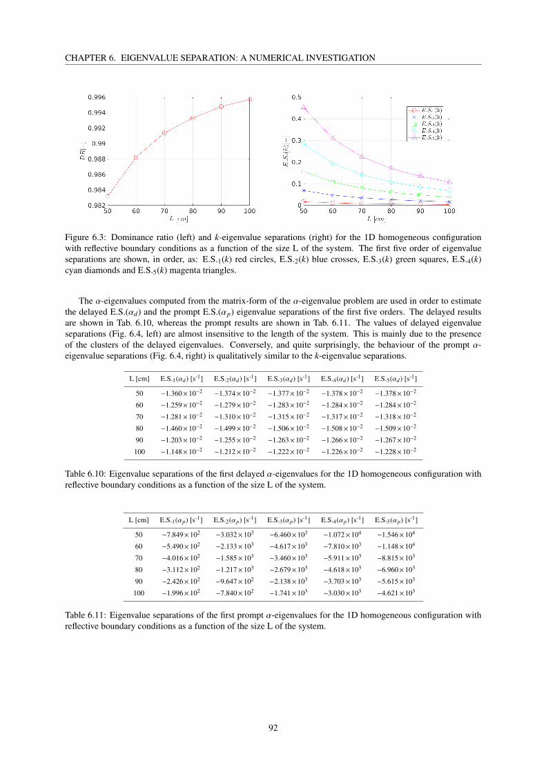
CHAPTER 6. EIGENVALUE SEPARATION: A NUMERICAL INVESTIGATION
Figure 6.3: Dominance ratio (left) and k-eigenvalue separations (right) for the 1D homogeneous configurationwith reflective boundary conditions as a function of the size L of the system. The first five order of eigenvalueseparations are shown, in order, as: E.S.1(k) red circles, E.S.2(k) blue crosses, E.S.3(k) green squares, E.S.4(k)cyan diamonds and E.S.5(k) magenta triangles.
The α-eigenvalues computed from the matrix-form of the α-eigenvalue problem are used in order to estimatethe delayed E.S.(αd) and the prompt E.S.(αp) eigenvalue separations of the first five orders. The delayed resultsare shown in Tab. 6.10, whereas the prompt results are shown in Tab. 6.11. The values of delayed eigenvalueseparations (Fig. 6.4, left) are almost insensitive to the length of the system. This is mainly due to the presenceof the clusters of the delayed eigenvalues. Conversely, and quite surprisingly, the behaviour of the prompt α-eigenvalue separations (Fig. 6.4, right) is qualitatively similar to the k-eigenvalue separations.
L [cm] E.S.1(αd) [s-1] E.S.2(αd) [s-1] E.S.3(αd) [s-1] E.S.4(αd) [s-1] E.S.5(αd) [s-1]
50 −1.360×10⁻² −1.374×10⁻² −1.377×10⁻² −1.378×10⁻² −1.378×10⁻²
60 −1.259×10⁻² −1.279×10⁻² −1.283×10⁻² −1.284×10⁻² −1.284×10⁻²
70 −1.281×10⁻² −1.310×10⁻² −1.315×10⁻² −1.317×10⁻² −1.318×10⁻²
80 −1.460×10⁻² −1.499×10⁻² −1.506×10⁻² −1.508×10⁻² −1.509×10⁻²
90 −1.203×10⁻² −1.255×10⁻² −1.263×10⁻² −1.266×10⁻² −1.267×10⁻²
100 −1.148×10⁻² −1.212×10⁻² −1.222×10⁻² −1.226×10⁻² −1.228×10⁻²
Table 6.10: Eigenvalue separations of the first delayed α-eigenvalues for the 1D homogeneous configuration withreflective boundary conditions as a function of the size L of the system.
L [cm] E.S.1(αp) [s-1] E.S.2(αp) [s-1] E.S.3(αp) [s-1] E.S.4(αp) [s-1] E.S.5(αp) [s-1]
50 −7.849×10² −3.032×10³ −6.460×10³ −1.072×10⁴ −1.546×10⁴
60 −5.490×10² −2.133×10³ −4.617×10³ −7.810×10³ −1.148×10⁴
70 −4.016×10² −1.585×10³ −3.460×10³ −5.911×10³ −8.815×10³
80 −3.112×10² −1.217×10³ −2.679×10³ −4.618×10³ −6.960×10³
90 −2.426×10² −9.647×10² −2.138×10³ −3.703×10³ −5.615×10³
100 −1.996×10² −7.840×10² −1.741×10³ −3.030×10³ −4.621×10³
Table 6.11: Eigenvalue separations of the first prompt α-eigenvalues for the 1D homogeneous configuration withreflective boundary conditions as a function of the size L of the system.
92
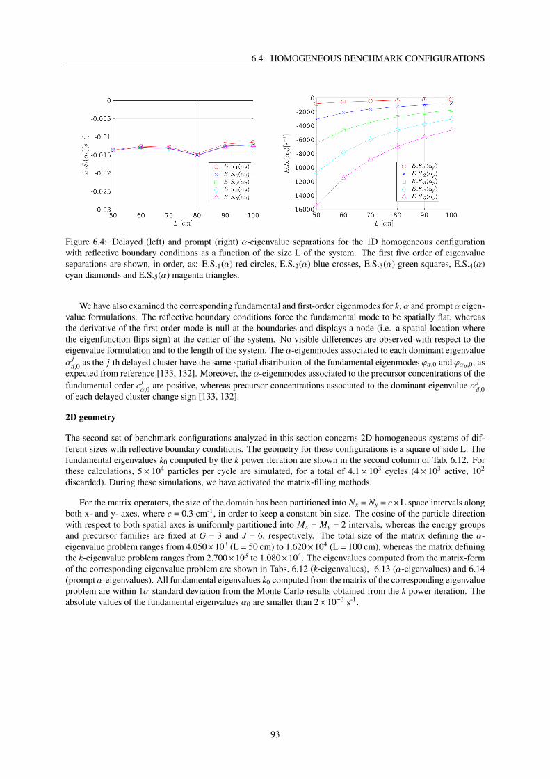
6.4. HOMOGENEOUS BENCHMARK CONFIGURATIONS
Figure 6.4: Delayed (left) and prompt (right) α-eigenvalue separations for the 1D homogeneous configurationwith reflective boundary conditions as a function of the size L of the system. The first five order of eigenvalueseparations are shown, in order, as: E.S.1(α) red circles, E.S.2(α) blue crosses, E.S.3(α) green squares, E.S.4(α)cyan diamonds and E.S.5(α) magenta triangles.
We have also examined the corresponding fundamental and first-order eigenmodes for k, α and prompt α eigen-value formulations. The reflective boundary conditions force the fundamental mode to be spatially flat, whereasthe derivative of the first-order mode is null at the boundaries and displays a node (i.e. a spatial location wherethe eigenfunction flips sign) at the center of the system. No visible differences are observed with respect to theeigenvalue formulation and to the length of the system. The α-eigenmodes associated to each dominant eigenvalueα
jd,0 as the j-th delayed cluster have the same spatial distribution of the fundamental eigenmodes ϕα,0 and ϕαp,0, as
expected from reference [133, 132]. Moreover, the α-eigenmodes associated to the precursor concentrations of thefundamental order c j
α,0 are positive, whereas precursor concentrations associated to the dominant eigenvalue α jd,0
of each delayed cluster change sign [133, 132].
2D geometry
The second set of benchmark configurations analyzed in this section concerns 2D homogeneous systems of dif-ferent sizes with reflective boundary conditions. The geometry for these configurations is a square of side L. Thefundamental eigenvalues k0 computed by the k power iteration are shown in the second column of Tab. 6.12. Forthese calculations, 5× 10⁴ particles per cycle are simulated, for a total of 4.1× 10³ cycles (4× 10³ active, 102
discarded). During these simulations, we have activated the matrix-filling methods.
For the matrix operators, the size of the domain has been partitioned into Nx = Ny = c×L space intervals alongboth x- and y- axes, where c = 0.3 cm-1, in order to keep a constant bin size. The cosine of the particle directionwith respect to both spatial axes is uniformly partitioned into Mx = My = 2 intervals, whereas the energy groupsand precursor families are fixed at G = 3 and J = 6, respectively. The total size of the matrix defining the α-eigenvalue problem ranges from 4.050×10³ (L = 50 cm) to 1.620×10⁴ (L = 100 cm), whereas the matrix definingthe k-eigenvalue problem ranges from 2.700×10³ to 1.080×10⁴. The eigenvalues computed from the matrix-formof the corresponding eigenvalue problem are shown in Tabs. 6.12 (k-eigenvalues), 6.13 (α-eigenvalues) and 6.14(prompt α-eigenvalues). All fundamental eigenvalues k0 computed from the matrix of the corresponding eigenvalueproblem are within 1σ standard deviation from the Monte Carlo results obtained from the k power iteration. Theabsolute values of the fundamental eigenvalues α0 are smaller than 2×10⁻³ s-1.
93

CHAPTER 6. EIGENVALUE SEPARATION: A NUMERICAL INVESTIGATION
L [cm] kMC0 [-] k0 [-] k1 [-] k2 [-] k3 [-] k4 [-] k5 [-]
50 0.9999±1×10⁻⁴ 1.0000 0.9320 0.9316 0.8702 0.7664 0.7661
60 0.9999±1×10⁻⁴ 0.9999 0.9522 0.9515 0.9070 0.8277 0.8274
70 0.9999±1×10⁻⁴ 0.9999 0.9642 0.9641 0.9300 0.8685 0.8683
80 1.0000±1×10⁻⁴ 1.0000 0.9726 0.9722 0.9462 0.8971 0.8963
90 0.9999±1×10⁻⁴ 0.9999 0.9781 0.9780 0.9568 0.9168 0.9167
100 1.0000±1×10⁻⁴ 1.0000 0.9824 0.9821 0.9651 0.9322 0.9316
Table 6.12: First k-eigenvalues for the 2D homogeneous configuration with reflective boundary conditions as afunction of the size L of the system. The second column displays the fundamental eigenvalues k0 computed bythe test-bed Monte Carlo code for the k-eigenvalue problem and the corresponding standard deviations. All othereigenvalues have been computed from the matrix-form of the k-eigenvalue problem of the corresponding case.
L [cm] α0 [s-1] α1 [s-1] α2 [s-1] α3 [s-1] α4 [s-1] α5 [s-1]
50 −5.026×10⁻⁴ −1.329×10⁻² −1.329×10⁻² −1.332×10⁻² −1.333×10⁻² −1.333×10⁻²
60 −1.077×10⁻³ −1.327×10⁻² −1.328×10⁻² −1.331×10⁻² −1.332×10⁻² −1.333×10⁻²
70 −1.648×10⁻³ −1.325×10⁻² −1.325×10⁻² −1.330×10⁻² −1.332×10⁻² −1.333×10⁻²
80 −7.121×10⁻⁴ −1.323×10⁻² −1.323×10⁻² −1.328×10⁻² −1.331×10⁻² −1.333×10⁻²
90 −1.350×10⁻³ −1.320×10⁻² −1.320×10⁻² −1.327×10⁻² −1.330×10⁻² −1.333×10⁻²
100 4.074×10⁻⁴ −1.316×10⁻² −1.316×10⁻² −1.325×10⁻² −1.329×10⁻² −1.333×10⁻²
Table 6.13: First α-eigenvalues for the 2D homogeneous configuration with reflective boundary conditions as afunction of the size L of the system. These values have been computed from the matrix-form of the α-eigenvalueproblem of the corresponding case.
L [cm] αp,0 [s-1] αp,1 [s-1] αp,2 [s-1] αp,3 [s-1] αp,4 [s-1] αp,5 [s-1]
50 −3.046×10² −3.556×10³ −3.576×10³ −6.672×10³ −1.232×10⁴ −1.232×10⁴
60 −3.068×10² −2.574×10³ −2.604×10³ −4.800×10³ −8.917×10³ −8.933×10³
70 −3.087×10² −1.997×10³ −2.002×10³ −3.653×10³ −6.760×10³ −6.773×10³
80 −3.058×10² −1.594×10³ −1.612×10³ −2.865×10³ −5.296×10³ −5.337×10³
90 −3.074×10² −1.334×10³ −1.335×10³ −2.349×10³ −4.305×10³ −4.311×10³
100 −3.017×10² −1.127×10³ −1.145×10³ −1.954×10³ −3.546×10³ −3.574×10³
Table 6.14: First prompt α-eigenvalues for the 2D homogeneous configuration with reflective boundary conditionsas a function of the size L of the system. These values have been computed from the matrix-form of the α-eigenvalue problem of the corresponding case.
The k- and the α-eigenvalue distributions are shown on the complex plane in Fig. 6.5. For the 2D geometry, theprompt α eigenvalues fill one circle by leaving two circular regions empty along the imaginary axis. This behaviouris repeated for the three energy groups. Figure 6.6 shows the zoom on all delayed eigenvalue clusters (left) and onthe delayed eigenvalue cluster associated to the first precursor family (right). Same comments as those presentedfor the 1D configuration can be applied to the distribution of the delayed α-eigenvalues on the complex plane. Thezoom of Fig. 6.6 (left) shows the gap between α j
d,0 and −λ j values for the last precursor families. The computed
values of α jd,0 and α j
d,1 for the last three precursor families ( j = 4,5,6) are shown in Tab. 6.15.
94

6.4. HOMOGENEOUS BENCHMARK CONFIGURATIONS
Figure 6.5: Spectra of the k (left) and the α (right) eigenvalue problem for the 2D homogeneous configuration withreflective boundary conditions for the most decoupled case (L = 100 cm).
Figure 6.6: Zoom on the α-spectrum in the delayed region (left) and on the first delayed cluster (right) for the2D homogeneous configuration with reflective boundary conditions for the most decoupled case (L = 100 cm).Vertical lines have been added in order to indicate the values of −λ1 (blue), −λ4 (magenta), −λ5 (cyan) and −λ6(green).
L [cm] α4d,0 [s-1] α4
d,1 [s-1] α5d,0 [s-1] α5
d,1 [s-1] α6d,0 [s-1] α6
d,1 [s-1]
50 −1.923×10⁻¹ −2.931×10⁻¹ −7.393×10⁻¹ −8.386×10⁻¹ −2.684 −2.838
60 −1.929×10⁻¹ −2.892×10⁻¹ −7.401×10⁻¹ −8.344×10⁻¹ −2.686 −2.832
70 −1.931×10⁻¹ −2.849×10⁻¹ −7.405×10⁻¹ −8.299×10⁻¹ −2.687 −2.825
80 −1.924×10⁻¹ −2.802×10⁻¹ −7.399×10⁻¹ −8.251×10⁻¹ −2.685 −2.818
90 −1.930×10⁻¹ −2.757×10⁻¹ −7.402×10⁻¹ −8.204×10⁻¹ −2.687 −2.812
100 −1.915×10⁻¹ −2.704×10⁻¹ −7.388×10⁻¹ −8.152×10⁻¹ −2.684 −2.804
Table 6.15: First α-eigenvalues of the clusters associated to the last three precursor families ( j = 4,5,6) for the 2Dhomogeneous configuration with reflective boundary conditions as a function of the size L of the system. Thesevalues have been computed from the matrix-form of the α-eigenvalue problem of the corresponding case.
The k-eigenvalues computed from the matrix-form of the k-eigenvalue problem are used in order to estimate thedominance ratio DR and the eigenvalue separations E.S.n(k) of the first five orders: they are shown in Tab. 6.16 andplotted in Fig. 6.7. The values of the dominance ratio increase for increasing size of the system from DR = 0.9321up to DR = 0.9824. The values of the eigenvalue separation for this homogeneous configurations decrease forincreasing size of the system and an even faster decrease is observed for higher-orders. Contrary to the case of the1D configuration, the first and second, fourth and fifth orders of eigenvalue separations are extremely close for the2D configuration: this feature is related to the symmetry properties of this system, which induces a degeneracy inthe eigenvalues.
95
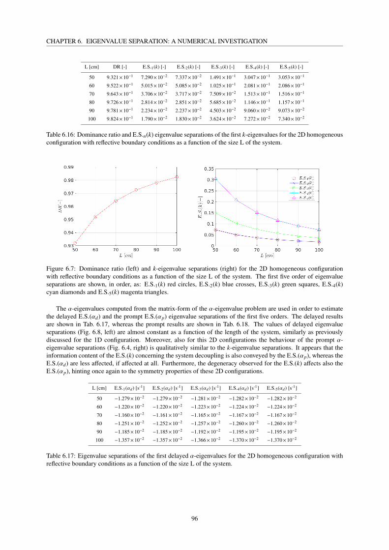
CHAPTER 6. EIGENVALUE SEPARATION: A NUMERICAL INVESTIGATION
L [cm] DR [-] E.S.1(k) [-] E.S.2(k) [-] E.S.3(k) [-] E.S.4(k) [-] E.S.5(k) [-]
50 9.321×10⁻¹ 7.290×10⁻² 7.337×10⁻² 1.491×10⁻¹ 3.047×10⁻¹ 3.053×10⁻¹
60 9.522×10⁻¹ 5.015×10⁻² 5.085×10⁻² 1.025×10⁻¹ 2.081×10⁻¹ 2.086×10⁻¹
70 9.643×10⁻¹ 3.706×10⁻² 3.717×10⁻² 7.509×10⁻² 1.513×10⁻¹ 1.516×10⁻¹
80 9.726×10⁻¹ 2.814×10⁻² 2.851×10⁻² 5.685×10⁻² 1.146×10⁻¹ 1.157×10⁻¹
90 9.781×10⁻¹ 2.234×10⁻² 2.237×10⁻² 4.503×10⁻² 9.060×10⁻² 9.073×10⁻²
100 9.824×10⁻¹ 1.790×10⁻² 1.830×10⁻² 3.624×10⁻² 7.272×10⁻² 7.340×10⁻²
Table 6.16: Dominance ratio and E.S.n(k) eigenvalue separations of the first k-eigenvalues for the 2D homogeneousconfiguration with reflective boundary conditions as a function of the size L of the system.
Figure 6.7: Dominance ratio (left) and k-eigenvalue separations (right) for the 2D homogeneous configurationwith reflective boundary conditions as a function of the size L of the system. The first five order of eigenvalueseparations are shown, in order, as: E.S.1(k) red circles, E.S.2(k) blue crosses, E.S.3(k) green squares, E.S.4(k)cyan diamonds and E.S.5(k) magenta triangles.
The α-eigenvalues computed from the matrix-form of the α-eigenvalue problem are used in order to estimatethe delayed E.S.(αd) and the prompt E.S.(αp) eigenvalue separations of the first five orders. The delayed resultsare shown in Tab. 6.17, whereas the prompt results are shown in Tab. 6.18. The values of delayed eigenvalueseparations (Fig. 6.8, left) are almost constant as a function of the length of the system, similarly as previouslydiscussed for the 1D configuration. Moreover, also for this 2D configurations the behaviour of the prompt α-eigenvalue separations (Fig. 6.4, right) is qualitatively similar to the k-eigenvalue separations. It appears that theinformation content of the E.S.(k) concerning the system decoupling is also conveyed by the E.S.(αp), whereas theE.S.(αd) are less affected, if affected at all. Furthermore, the degeneracy observed for the E.S.(k) affects also theE.S.(αp), hinting once again to the symmetry properties of these 2D configurations.
L [cm] E.S.1(αd) [s-1] E.S.2(αd) [s-1] E.S.3(αd) [s-1] E.S.4(αd) [s-1] E.S.5(αd) [s-1]
50 −1.279×10⁻² −1.279×10⁻² −1.281×10⁻² −1.282×10⁻² −1.282×10⁻²
60 −1.220×10⁻² −1.220×10⁻² −1.223×10⁻² −1.224×10⁻² −1.224×10⁻²
70 −1.160×10⁻² −1.161×10⁻² −1.165×10⁻² −1.167×10⁻² −1.167×10⁻²
80 −1.251×10⁻² −1.252×10⁻² −1.257×10⁻² −1.260×10⁻² −1.260×10⁻²
90 −1.185×10⁻² −1.185×10⁻² −1.192×10⁻² −1.195×10⁻² −1.195×10⁻²
100 −1.357×10⁻² −1.357×10⁻² −1.366×10⁻² −1.370×10⁻² −1.370×10⁻²
Table 6.17: Eigenvalue separations of the first delayed α-eigenvalues for the 2D homogeneous configuration withreflective boundary conditions as a function of the size L of the system.
96

6.4. HOMOGENEOUS BENCHMARK CONFIGURATIONS
L [cm] E.S.1(αp) [s-1] E.S.2(αp) [s-1] E.S.3(αp) [s-1] E.S.4(αp) [s-1] E.S.5(αp) [s-1]
50 −3.251×10³ −3.556×10³ −6.368×10³ −1.201×10⁴ −1.203×10⁴
60 −2.267×10³ −2.574×10³ −4.493×10³ −8.610×10³ −8.626×10³
70 −1.689×10³ −1.997×10³ −3.344×10³ −6.452×10³ −6.465×10³
80 −1.289×10³ −1.594×10³ −2.559×10³ −4.990×10³ −5.031×10³
90 −1.027×10³ −1.334×10³ −2.041×10³ −3.998×10³ −4.004×10³
100 −8.257×10² −1.127×10² −1.653×10³ −3.244×10³ −3.273×10³
Table 6.18: Eigenvalue separations of the first prompt α-eigenvalues for the 2D homogeneous configuration withreflective boundary conditions as a function of the size L of the system.
Figure 6.8: Delayed (left) and prompt (right) α-eigenvalue separations for the 2D homogeneous configurationwith reflective boundary conditions as a function of the size L of the system. The first five order of eigenvalueseparations are shown, in order, as: E.S.1(α) red circles, E.S.2(α) blue crosses, E.S.3(α) green squares, E.S.4(α)cyan diamonds and E.S.5(α) magenta triangles.
The corresponding fundamental and first-order eigenmodes have been examined for k, α and prompt α eigen-value formulations for the most decoupled case (L = 100 cm). The conclusions related to the eigenmodes describedfor the 1D configuration apply also to this 2D system.
6.4.2 Homogeneous configurations with leakage boundary conditions
Critical configuration search
We examine now 1D homogeneous systems of different lengths with leakage boundary conditions. For thesesystems the factor a has been computed for the most decoupled case (L = 100 cm) from a parametric researcharound the value computed for the reflected configurations of the previous sections. A value a = 1.4875 applied tothe macroscopic capture cross section leads to k0 = 0.9999±10−4 from a k power iteration performed with 2×10⁴
particles per cycle and a total of 6×10³ cycles (5×10³ active, 103 inactive). Then, we have considered the samelengths defined for Section 6.4.1 and we have estimated the coefficient b from Eq. (6.10) in order to readjust eachcase to the critical level. The values b have been iteratively computed by simulating 5×10⁴ particles per cycle anda total of 5×10³ cycles.
Furthermore, for 2D homogeneous systems of different sizes with leakage boundary conditions, a factora = 1.4775 has been applied to the macroscopic capture cross section. The k power iteration converges to thefundamental eigenvalue k0 = 1.0001±10−4. For this simulation we have set 2×10⁴ particles per cycle and a totalof 6×10³ cycles (5×10³ active, 103 inactive). The values b (from Eq. (6.10)) have been iteratively computed bysimulating 5×10⁴ particles per cycle and a total of 5×10³ cycles.
In the following, we will show the results computed for the 1D configurations (Section 6.4.2) and for the the2D configurations (Section 6.4.2).
97

CHAPTER 6. EIGENVALUE SEPARATION: A NUMERICAL INVESTIGATION
1D geometry
The fundamental eigenvalues k0 computed by the k power iteration are shown in the second column of Tab. 6.19.For these calculations, 105 particles per cycle are simulated, for a total of 1.2× 10³ cycles (103 active, 2× 10²
inactive).
In order to compute the matrix operators, the length of the domain has been partitioned into Nx = c×L spaceintervals along the x-axis, where c = 10 cm-1, in order to keep a constant bin width. The cosine of the parti-cle direction with respect to the x-axis is uniformly partitioned into M = 4 intervals, whereas the energy groupsand precursor families are fixed at G = 3 and J = 6, respectively. The total size of the matrix defining the α-eigenvalue problem ranges from 9.0× 10³ (L = 50 cm) to 1.8× 10⁴ (L = 100 cm), whereas the matrix definingthe k-eigenvalue problem ranges from 6.0× 10³ to 1.2× 10⁴. The eigenvalues computed from the matrix-formof the corresponding eigenvalue problem are shown in Tabs. 6.19 (k-eigenvalues), 6.20 (α-eigenvalues) and 6.21(prompt α-eigenvalues). All fundamental eigenvalues k0 computed from the matrix of the corresponding eigen-value problem are within 2σ standard deviation from the Monte Carlo results obtained from the k power iteration.The absolute values of the fundamental eigenvalues α0 are smaller than 2×10⁻³ s-1. The dominant eigenvalue α j
d,0of the j-th delayed cluster is separated from the other eigenvalues of the same precursor family [133, 132]. Thecomputed values of α j
d,0 and α jd,1 for the last three precursor families ( j = 4,5,6) are shown in Tab. 6.22.
L [cm] kMC0 [-] k0 [-] k1 [-] k2 [-] k3 [-] k4 [-] k5 [-]
50 1.0000±1×10⁻⁴ 1.0001 0.9546 0.8856 0.8019 0.7117 0.6221
60 1.0003±1×10⁻⁴ 1.0002 0.9680 0.9176 0.8539 0.7820 0.7066
70 1.0002±1×10⁻⁴ 1.0002 0.9760 0.9379 0.8881 0.8304 0.7676
80 1.0000±1×10⁻⁴ 1.0001 0.9814 0.9514 0.9118 0.8647 0.8123
90 1.0002±1×10⁻⁴ 1.0002 0.9851 0.9611 0.9289 0.8900 0.8460
100 0.9999±1×10⁻⁴ 0.9999 0.9878 0.9680 0.9414 0.9090 0.8718
Table 6.19: First k-eigenvalues for the 1D homogeneous configuration with leakage boundary conditions as afunction of the size L of the system. The second column displays the fundamental eigenvalues k0 computed bythe test-bed Monte Carlo code for the k-eigenvalue problem and the corresponding standard deviations. All othereigenvalues have been computed from the matrix-form of the k-eigenvalue problem of the corresponding case.
L [cm] α0 [s-1] α1 [s-1] α2 [s-1] α3 [s-1] α4 [s-1] α5 [s-1]
50 8.262×10⁻⁴ −1.327×10⁻² −1.331×10⁻² −1.332×10⁻² −1.333×10⁻² −1.333×10⁻²
60 2.611×10⁻³ −1.324×10⁻² −1.330×10⁻² −1.332×10⁻² −1.332×10⁻² −1.333×10⁻²
70 3.631×10⁻³ −1.321×10⁻² −1.329×10⁻² −1.331×10⁻² −1.332×10⁻² −1.333×10⁻²
80 7.799×10⁻⁴ −1.317×10⁻² −1.328×10⁻² −1.330×10⁻² −1.332×10⁻² −1.333×10⁻²
90 2.426×10⁻³ −1.313×10⁻² −1.326×10⁻² −1.330×10⁻² −1.331×10⁻² −1.333×10⁻²
100 −1.496×10⁻³ −1.308×10⁻² −1.324×10⁻² −1.329×10⁻² −1.331×10⁻² −1.333×10⁻²
Table 6.20: First α-eigenvalues for the 1D homogeneous configuration with leakage boundary conditions as afunction of the size L of the system. These values have been computed from the matrix-form of the α-eigenvalueproblem of the corresponding case.
98

6.4. HOMOGENEOUS BENCHMARK CONFIGURATIONS
L [cm] αp,0 [s-1] αp,1 [s-1] αp,2 [s-1] αp,3 [s-1] αp,4 [s-1] αp,5 [s-1]
50 −2.972×10² −2.399×10³ −5.658×10³ −9.739×10³ −1.434×10⁴ −1.921×10⁴
60 −2.926×10² −1.783×10³ −4.157×10³ −7.217×10³ −1.078×10⁴ −1.466×10⁴
70 −2.907×10² −1.416×10³ −3.206×10³ −5.573×10³ −8.386×10³ −1.153×10⁴
80 −2.995×10² −1.167×10³ −2.574×10³ −4.449×10³ −6.717×10³ −9.295×10³
90 −2.949×10² −9.951×10² −2.119×10³ −3.640×10³ −5.499×10³ −7.638×10³
100 −3.081×10² −8.681×10² −1.796×10³ −3.049×10³ −4.592×10³ −6.383×10³
Table 6.21: First prompt α-eigenvalues for the 1D homogeneous configuration with leakage boundary conditions asa function of the size L of the system. These values have been computed from the matrix-form of the α-eigenvalueproblem of the corresponding case.
L [cm] α4d,0 [s-1] α4
d,1 [s-1] α5d,0 [s-1] α5
d,1 [s-1] α6d,0 [s-1] α6
d,1 [s-1]
50 −1.910×10⁻¹ −2.883×10⁻¹ −7.378×10⁻¹ −8.334×10⁻¹ −2.683 −2.831
60 −1.900×10⁻¹ −2.830×10⁻¹ −7.370×10⁻¹ −8.281×10⁻¹ −2.681 −2.823
70 −1.893×10⁻¹ −2.775×10⁻¹ −7.356×10⁻¹ −8.223×10⁻¹ −2.680 −2.814
80 −1.912×10⁻¹ −2.717×10⁻¹ −7.383×10⁻¹ −8.166×10⁻¹ −2.683 −2.806
90 −1.902×10⁻¹ −2.661×10⁻¹ −7.367×10⁻¹ −8.110×10⁻¹ −2.680 −2.798
100 −1.931×10⁻¹ −2.605×10⁻¹ −7.404×10⁻¹ −8.055×10⁻¹ −2.687 −2.791
Table 6.22: First α-eigenvalues of the clusters associated to the last three precursor families ( j = 4,5,6) for the1D homogeneous configuration with leakage boundary conditions as a function of the size L of the system. Thesevalues have been computed from the matrix-form of the α-eigenvalue problem of the corresponding case.
The k-eigenvalues computed from the matrix-form of the k-eigenvalue problem are used in order to estimatethe dominance ratio DR and the eigenvalue separations E.S.n(k) of the first five orders: they are shown in Tab. 6.23and plotted in Fig. 6.9. The values of the dominance ratio increase for increasing length of the system fromDR = 0.9546 up to DR = 0.9879. No major differences are observed with respect to the behaviour previouslyanalyzed for the reflected system from Fig. 6.3.
L [cm] DR [-] E.S.1(k) [-] E.S.2(k) [-] E.S.3(k) [-] E.S.4(k) [-] E.S.5(k) [-]
50 9.546×10⁻¹ 4.758×10⁻² 1.292×10⁻¹ 2.471×10⁻¹ 4.051×10⁻¹ 6.076×10⁻¹
60 9.679×10⁻¹ 3.321×10⁻² 9.003×10⁻² 1.713×10⁻¹ 2.790×10⁻¹ 4.154×10⁻¹
70 9.758×10⁻¹ 2.481×10⁻² 6.650×10⁻² 1.262×10⁻¹ 2.045×10⁻¹ 3.030×10⁻¹
80 9.813×10⁻¹ 1.903×10⁻² 5.119×10⁻² 9.681×10⁻² 1.565×10⁻¹ 2.311×10⁻¹
90 9.849×10⁻¹ 1.528×10⁻² 4.067×10⁻² 7.675×10⁻² 1.238×10⁻¹ 1.822×10⁻¹
100 9.879×10⁻¹ 1.220×10⁻² 3.294×10⁻² 6.212×10⁻² 1.000×10⁻¹ 1.469×10⁻¹
Table 6.23: Dominance ratio and E.S.n(k) eigenvalue separations of the first k-eigenvalues for the 1D homogeneousconfiguration with leakage boundary conditions as a function of the size L of the system.
99

CHAPTER 6. EIGENVALUE SEPARATION: A NUMERICAL INVESTIGATION
Figure 6.9: Dominance ratio (left) and k-eigenvalue separations (right) for the 1D homogeneous configuration withleakage boundary conditions as a function of the size L of the system. The first five order of eigenvalue separationsare shown, in order, as: E.S.1(k) red circles, E.S.2(k) blue crosses, E.S.3(k) green squares, E.S.4(k) cyan diamondsand E.S.5(k) magenta triangles.
The α-eigenvalues computed from the matrix-form of the α-eigenvalue problem are used in order to estimatethe delayed E.S.(αd) and the prompt E.S.(αp) eigenvalue separations of the first five orders. The delayed results areshown in Tab. 6.24, whereas the prompt results are shown in Tab. 6.25. The eigenvalue separations E.S.(αd) andthe eigenvalue separations E.S.(αp) are shown in Fig. 6.10. The conclusions drawn from these results are similarto those drawn from the corresponding reflective case previously discussed in Section 6.4.1.
L [cm] E.S.1(αd) [s-1] E.S.2(αd) [s-1] E.S.3(αd) [s-1] E.S.4(αd) [s-1] E.S.5(αd) [s-1]
50 −1.410×10⁻² −1.414×10⁻² −1.415×10⁻² −1.415×10⁻² −1.416×10⁻²
60 −1.585×10⁻² −1.591×10⁻² −1.593×10⁻² −1.594×10⁻² −1.594×10⁻²
70 −1.684×10⁻² −1.692×10⁻² −1.694×10⁻² −1.695×10⁻² −1.696×10⁻²
80 −1.395×10⁻² −1.406×10⁻² −1.408×10⁻² −1.410×10⁻² −1.410×10⁻²
90 −1.555×10⁻² −1.569×10⁻² −1.572×10⁻² −1.574×10⁻² −1.575×10⁻²
100 −1.158×10⁻² −1.175×10⁻² −1.179×10⁻² −1.181×10⁻² −1.182×10⁻²
Table 6.24: Eigenvalue separations of the first delayed α-eigenvalues for the 1D homogeneous configuration withleakage boundary conditions as a function of the size L of the system.
L [cm] E.S.1(αp) [s-1] E.S.2(αp) [s-1] E.S.3(αp) [s-1] E.S.4(αp) [s-1] E.S.5(αp) [s-1]
50 −2.102×10³ −5.361×10³ −9.441×10³ −1.404×10⁴ −1.891×10⁴
60 −1.491×10³ −3.864×10³ −6.924×10³ −1.049×10⁴ −1.437×10⁴
70 −1.125×10³ −2.915×10³ −5.283×10³ −8.096×10³ −1.124×10⁴
80 −8.677×10² −2.274×10³ −4.150×10³ −6.417×10³ −8.995×10³
90 −7.002×10² −1.824×10³ −3.345×10³ −5.204×10³ −7.344×10³
100 −5.599×10² −1.488×10³ −2.741×10³ −4.284×10³ −6.075×10³
Table 6.25: Eigenvalue separations of the first prompt α-eigenvalues for the 1D homogeneous configuration withleakage boundary conditions as a function of the size L of the system.
100

6.4. HOMOGENEOUS BENCHMARK CONFIGURATIONS
Figure 6.10: Delayed (left) and prompt (right) α-eigenvalue separations for the 1D homogeneous configurationwith leakage boundary conditions as a function of the size L of the system. The first five order of eigenvalueseparations are shown, in order, as: E.S.1(α) red circles, E.S.2(α) blue crosses, E.S.3(α) green squares, E.S.4(α)cyan diamonds and E.S.5(α) magenta triangles.
The similar behaviour observed between the 1D homogeneous configurations with reflective and leakageboundary conditions was expected, since the length of each case has been chosen in order to enhance the de-coupling effects. The selected geometries are very large with respect to the neutron migration area, hence only asmall percentage of the simulated particles will be affected by the boundaries.
Nevertheless, the effect of the leakage boundary conditions is clearly visible for the spatial shape of the funda-mental and first-order eigenmodes of k, α and prompt α eigenvalue formulations. The usual cosine distributionsare found for the fundamental eigenfunction and a node is observed in the center of the system for the first-ordereigenfunction. No visible differences are observed with respect to the eigenvalue formulation and to the length ofthe system. Same comments as those given for the 1D configuration with reflective boundary conditions apply tothe analysis of the delayed α-eigenmodes.
2D geometry
The fundamental eigenvalues k0 computed by the k power iteration are shown in the second column of Tab. 6.26.For these calculations, 105 particles per cycle are simulated, for a total of 1.2× 10³ cycles (103 active, 2× 10²
inactive).
In order to compute the matrix operators, the size of the domain has been partitioned into Nx = Ny = c×L spaceintervals along both x- and y- axes, where c = 0.3 cm-1, in order to keep a constant bin size. The cosine of theparticle direction with respect to both spatial axes is uniformly partitioned into Mx = My = 2 intervals, whereasthe energy groups and precursor families are fixed at G = 3 and J = 6, respectively. The total size of the matrixdefining the α-eigenvalue problem ranges from 4.050× 10³ (L = 50 cm) to 1.620× 10⁴ (L = 100 cm), whereasthe matrix defining the k-eigenvalue problem ranges from 2.700× 10³ to 1.080× 10⁴. The eigenvalues computedfrom the matrix-form of the corresponding eigenvalue problem are shown in Tabs. 6.26 (k-eigenvalues), 6.27(α-eigenvalues) and 6.28 (prompt α-eigenvalues). All fundamental eigenvalues k0 computed from the matrix ofthe corresponding eigenvalue problem are within 2σ standard deviation from the Monte Carlo results obtainedfrom the k power iteration. The absolute values of the fundamental eigenvalues α0 are smaller than 2.5× 10⁻³
s-1. The dominant eigenvalue α jd,0 of the j-th delayed cluster is separated from the other eigenvalues of the same
precursor family. The computed values of α jd,0 and α j
d,1 for the last three precursor families ( j = 4,5,6) are shownin Tab. 6.29.
101

CHAPTER 6. EIGENVALUE SEPARATION: A NUMERICAL INVESTIGATION
L [cm] kMC0 [-] k0 [-] k1 [-] k2 [-] k3 [-] k4 [-] k5 [-]
50 0.9999±1×10⁻⁴ 1.0001 0.8649 0.8645 0.7540 0.6749 0.6744
60 0.9999±1×10⁻⁴ 1.0000 0.9024 0.9019 0.8174 0.7527 0.7525
70 1.0002±1×10⁻⁴ 1.0003 0.9265 0.9256 0.8597 0.8075 0.8067
80 0.9999±1×10⁻⁴ 1.0000 0.9424 0.9419 0.8894 0.8464 0.8455
90 1.0003±1×10⁻⁴ 1.0001 0.9542 0.9535 0.9107 0.8749 0.8743
100 0.9999±1×10⁻⁴ 1.0000 0.9622 0.9618 0.9263 0.8964 0.8959
Table 6.26: First k-eigenvalues for the 2D homogeneous configuration with leakage boundary conditions as afunction of the size L of the system. The second column displays mean value and standard deviation of thefundamental eigenvalues k0 computed at the end of a power iteration with the test-bed Monte Carlo code for thek-eigenvalue problem. All other eigenvalues have been computed from the matrix-form of linear transport operatorcombined for the definition of the k-eigenvalue problem.
L [cm] α0 [s-1] α1 [s-1] α2 [s-1] α3 [s-1] α4 [s-1] α5 [s-1]
50 1.376×10⁻³ −1.332×10⁻² −1.332×10⁻² −1.333×10⁻² −1.333×10⁻² −1.333×10⁻²
60 −1.466×10⁻⁴ −1.331×10⁻² −1.331×10⁻² −1.332×10⁻² −1.333×10⁻² −1.333×10⁻²
70 4.043×10⁻³ −1.330×10⁻² −1.330×10⁻² −1.332×10⁻² −1.332×10⁻² −1.333×10⁻²
80 5.862×10⁻⁴ −1.329×10⁻² −1.329×10⁻² −1.331×10⁻² −1.332×10⁻² −1.333×10⁻²
90 2.012×10⁻³ −1.327×10⁻² −1.327×10⁻² −1.330×10⁻² −1.331×10⁻² −1.333×10⁻²
100 −5.929×10⁻⁴ −1.326×10⁻² −1.326×10⁻² −1.330×10⁻² −1.331×10⁻² −1.333×10⁻²
Table 6.27: First α-eigenvalues for the 2D homogeneous configuration with leakage boundary conditions as afunction of the size L of the system. These values have been computed from the matrix-form of linear transportoperator combined for the definition of the α-eigenvalue problem.
L [cm] αp,0 [s-1] αp,1 [s-1] αp,2 [s-1] αp,3 [s-1] αp,4 [s-1] αp,5 [s-1]
50 −2.922×10² −6.768×10³ −6.788×10³ −1.269×10⁴ −1.739×10⁴ −1.742×10⁴
60 −2.991×10² −4.936×10³ −4.962×10³ −9.293×10³ −1.287×10⁴ −1.288×10⁴
70 −2.888×10² −3.778×10³ −3.823×10³ −7.115×10³ −9.880×10³ −9.917×10³
80 −2.983×10² −3.016×10³ −3.039×10³ −5.626×10³ −7.836×10³ −7.879×10³
90 −2.950×10² −2.455×10³ −2.490×10³ −4.575×10³ −6.376×10³ −6.406×10³
100 −3.033×10² −2.079×10³ −2.095×10³ −3.812×10³ −5.297×10³ −5.323×10³
Table 6.28: First prompt α-eigenvalues for the 2D homogeneous configuration with leakage boundary conditions asa function of the size L of the system. These values have been computed from the matrix-form of the α-eigenvalueproblem of the corresponding case.
102

6.4. HOMOGENEOUS BENCHMARK CONFIGURATIONS
L [cm] α4d,0 [s-1] α4
d,1 [s-1] α5d,0 [s-1] α5
d,1 [s-1] α6d,0 [s-1] α6
d,1 [s-1]
50 −1.909×10⁻¹ −2.980×10⁻¹ −7.379×10⁻¹ −8.441×10⁻¹ −2.683 −2.845
60 −1.919×10⁻¹ −2.960×10⁻¹ −7.389×10⁻¹ −8.418×10⁻¹ −2.685 −2.842
70 −1.889×10⁻¹ −2.937×10⁻¹ −7.358×10⁻¹ −8.394×10⁻¹ −2.679 −2.839
80 −1.914×10⁻¹ −2.913×10⁻¹ −7.381×10⁻¹ −8.367×10⁻¹ −2.682 −2.835
90 −1.905×10⁻¹ −2.885×10⁻¹ −7.371×10⁻¹ −8.336×10⁻¹ −2.682 −2.831
100 −1.924×10⁻¹ −2.858×10⁻¹ −7.393×10⁻¹ −8.308×10⁻¹ −2.686 −2.826
Table 6.29: First α-eigenvalues of the clusters associated to the last three precursor families ( j = 4,5,6) for the2D homogeneous configuration with leakage boundary conditions as a function of the size L of the system. Thesevalues have been computed from the matrix-form of the α-eigenvalue problem of the corresponding case.
The k-eigenvalues computed from the matrix-form of the k-eigenvalue problem are used in order to estimatethe dominance ratio DR and the eigenvalue separations E.S.n(k) of the first five orders: they are shown in Tab. 6.30and plotted in Fig. 6.11. The values of the dominance ratio increase for increasing length of the system fromDR = 0.8648 up to DR = 0.9622. No major differences are observed with respect to the behaviour previouslyanalyzed for the reflected system from Fig. 6.3. In particular, we observe that also for these 2D configurations thefirst and second, fourth and fifth orders of eigenvalue separations are extremely close. This degeneracy observedin the eigenvalues is related to the symmetry properties of the analyzed configurations.
L [cm] DR [-] E.S.1(k) [-] E.S.2(k) [-] E.S.3(k) [-] E.S.4(k) [-] E.S.5(k) [-]
50 8.648×10⁻¹ 1.563×10⁻¹ 1.568×10⁻¹ 3.264×10⁻¹ 4.817×10⁻¹ 4.829×10⁻¹
60 9.024×10⁻¹ 1.081×10⁻¹ 1.088×10⁻¹ 2.235×10⁻¹ 3.286×10⁻¹ 3.289×10⁻¹
70 9.262×10⁻¹ 7.963×10⁻² 8.069×10⁻² 1.634×10⁻¹ 2.387×10⁻¹ 2.398×10⁻¹
80 9.424×10⁻¹ 6.113×10⁻² 6.169×10⁻² 1.244×10⁻¹ 1.816×10⁻¹ 1.827×10⁻¹
90 9.541×10⁻¹ 4.809×10⁻² 4.892×10⁻² 9.822×10⁻² 1.431×10⁻¹ 1.439×10⁻¹
100 9.622×10⁻¹ 3.929×10⁻² 3.963×10⁻² 7.952×10⁻² 1.155×10⁻¹ 1.162×10⁻¹
Table 6.30: Dominance ratio and E.S.n(k) eigenvalue separations of the first k-eigenvalues for the 2D homogeneousconfiguration with leakage boundary conditions as a function of the size L of the system.
Figure 6.11: Dominance ratio (left) and k-eigenvalue separations (right) for the 2D homogeneous configurationwith leakage boundary conditions as a function of the size L of the system. The first five order of eigenvalueseparations are shown, in order, as: E.S.1(k) red circles, E.S.2(k) blue crosses, E.S.3(k) green squares, E.S.4(k)cyan diamonds and E.S.5(k) magenta triangles.
The α-eigenvalues computed from the matrix-form of the α-eigenvalue problem are used in order to estimatethe delayed E.S.(αd) and the prompt E.S.(αp) eigenvalue separations of the first five orders. The delayed resultsare shown in Tab. 6.31, whereas the prompt results are shown in Tab. 6.32. The eigenvalue separations E.S.(αd)
103

CHAPTER 6. EIGENVALUE SEPARATION: A NUMERICAL INVESTIGATION
and the eigenvalue separations E.S.(αp) are shown in Fig. 6.12. The conclusions drawn from these results areequivalent to those found for the corresponding reflective case previously discussed in Section 6.4.1.
L [cm] E.S.1(αd) [s-1] E.S.2(αd) [s-1] E.S.3(αd) [s-1] E.S.4(αd) [s-1] E.S.5(αd) [s-1]
50 −1.469×10⁻² −1.469×10⁻² −1.470×10⁻² −1.471×10⁻² −1.471×10⁻²
60 −1.316×10⁻² −1.316×10⁻² −1.318×10⁻² −1.318×10⁻² −1.318×10⁻²
70 −1.734×10⁻² −1.734×10⁻² −1.736×10⁻² −1.737×10⁻² −1.737×10⁻²
80 −1.387×10⁻² −1.387×10⁻² −1.390×10⁻² −1.391×10⁻² −1.391×10⁻²
90 −1.528×10⁻² −1.528×10⁻² −1.532×10⁻² −1.533×10⁻² −1.533×10⁻²
100 −1.267×10⁻² −1.267×10⁻² −1.271×10⁻² −1.272×10⁻² −1.272×10⁻²
Table 6.31: Eigenvalue separations of the first prompt α-eigenvalues for the 2D homogeneous configuration withreflective boundary conditions as a function of the size L of the system.
L [cm] E.S.1(αp) [s-1] E.S.2(αp) [s-1] E.S.3(αp) [s-1] E.S.4(αp) [s-1] E.S.5(αp) [s-1]
50 −6.476×10³ −6.496×10³ −1.240×10⁴ −1.710×10⁴ −1.713×10⁴
60 −4.637×10³ −4.663×10³ −8.994×10³ −1.257×10⁴ −1.258×10⁴
70 −3.490×10³ −3.534×10³ −6.827×10³ −9.591×10³ −9.628×10³
80 −2.717×10³ −2.741×10³ −5.328×10³ −7.537×10³ −7.581×10³
90 −2.160×10³ −2.195×10³ −4.280×10³ −6.081×10³ −6.111×10³
100 −1.776×10³ −1.791×10³ −3.509×10³ −4.994×10³ −5.020×10³
Table 6.32: Eigenvalue separations of the first prompt α-eigenvalues for the 2D homogeneous configuration withleakage boundary conditions as a function of the size L of the system.
Figure 6.12: Delayed (left) and prompt (right) α-eigenvalue separations for the 2D homogeneous configurationwith leakage boundary conditions as a function of the size L of the system. The first five order of eigenvalueseparations are shown, in order, as: E.S.1(α) red circles, E.S.2(α) blue crosses, E.S.3(α) green squares, E.S.4(α)cyan diamonds and E.S.5(α) magenta triangles.
The similar behaviour observed between the 2D homogeneous configurations with reflective and leakageboundary conditions was expected, since the size of each case has been chosen in order to enhance the decou-pling effects. The selected geometries are very large with respect to the neutron migration area, hence only a smallpercentage of the simulated particles will be affected by the boundaries.
Nevertheless, the effect of leakage boundary conditions is clearly visible for the spatial shape of the fundamen-tal (Fig. 6.13), first-order (Fig. 6.14) and second-order (Fig. 6.15) eigenmodes of k, α and prompt α eigenvalueformulations. The usual Bessel-like distributions are found for the fundamental eigenfunction and the presence ofa node is observed for the first-order eigenfunction. The second-order distributions are similar to the first-orderdistributions rotated by 90°: such behaviour confirms the presence of a degeneracy for higher-order eigenpairs due
104

6.5. HETEROGENEOUS BENCHMARK CONFIGURATIONS
to the symmetries of the configuration. Same comments as those presented for the 2D configuration with reflectiveboundary conditions apply to the analysis of the delayed α-eigenmodes.
Figure 6.13: Spatial distribution of the k (left), α (center) and prompt α (right) fundamental eigenmodes for the 2Dhomogeneous configuration with leakage boundary conditions for the most decoupled case (L = 100 cm).
Figure 6.14: Spatial distribution of the k (left), α (center) and prompt α (right) first-order eigenmodes for the 2Dhomogeneous configuration with leakage boundary conditions for the most decoupled case (L = 100 cm).
Figure 6.15: Spatial distribution of the k (left), α (center) and prompt α (right) second-order eigenmodes for the2D homogeneous configuration with leakage boundary conditions for the most decoupled case (L = 100 cm).
6.5 Heterogeneous benchmark configurations
The occurrence of decoupling effects for heterogeneous configurations can be observed when neutrons are localizedinto distinct regions of the system, due to the presence of strong spatial heterogeneities [120]. A perturbationinduced in a specific spatial location of the system has to overcome such heterogeneity in order to reach the otherdecoupled regions. In this section, we investigate the spectral properties induced by the presence of these effectsfor a critical 1D heterogeneous configuration with leakage boundary conditions.
In particular, we have considered a three-region slab geometry in which two fissile regions (of length Lfissile = 20cm, respectively) are separated by a progressively larger moderator region (defined by the length Lmoderator). Sixcases have been selected for our analysis, with the total length of the geometry L = 2Lfissile + Lmoderator. Thechoice of this configuration was inspired by the three-region slab geometry benchmark problem analyzed in refer-ence [165]. The parameters describing these regions have been shown in Tabs. 6.1 and 6.2 for the fissile materialand in Tab. 6.3 for the moderator material. The first step of our analysis consists in the search of a critical configu-ration by k power iteration.
The adjustment to the critical level for this first step of the parametric study has been performed by modify-ing the macroscopic capture cross section in the fissile material by a parameter a following Eq. (6.9). Then, we
105

CHAPTER 6. EIGENVALUE SEPARATION: A NUMERICAL INVESTIGATION
analyzed five additional cases by decreasing the length of the moderator region in order to increase the coupling be-tween the fissile regions. All cases have been readjusted to the critical level by an iteratively search of a coefficientb applied to the macroscopic capture cross section of the fissile material according to Eq. 6.10.
6.5.1 1D heterogeneous configurations
In order to investigate the three-region slab geometries considered in this section, we have started by consideringa configuration characterized by regions having equal width. The emergence of decoupling effect was observedfor a 20 cm long slab region in reference [165], hence the length of the system will be set to 60 cm. A valuea = 1.167 applied to the macroscopic capture cross section of the fissile regions leads to k0 = 1.0002± 4× 10⁻⁴
from a k power iteration performed with 2×10⁴ particles per cycle and a total of 6×10² cycles (5×10² active, 102
inactive). Five smaller lengths of the moderator region have been also considered: 15 cm, 10 cm, 7 cm, 5 cm and2 cm, respectively. The coefficient b from Eq. (6.10) has been iteratively computed by simulating 5×10⁴ particlesper cycle and a total of 2× 10³ cycles. The fundamental eigenvalues k0 computed by the k power iteration areshown in the second column of Tab. 6.33. For these calculations, 105 particles per cycle are simulated, for a totalof 1.2×10³ cycles (103 active, 2×10² inactive).
In order to compute the matrix operators, the length of the domain has been partitioned into Nx = c×L spaceintervals along the x-axis, where c = 20 cm-1, in order to keep a constant bin width. The cosine of the particledirection with respect to the x-axis is uniformly partitioned into Mx = 4 intervals, whereas the energy groups andprecursor families are fixed at G = 3 and J = 6, respectively. The total size of the matrix defining the α-eigenvalueproblem ranges from 1.512× 10⁴ (L = 42 cm) to 2.160× 10⁴ (L = 60 cm), whereas the matrix defining the k-eigenvalue problem ranges from 1.008× 10⁴ to 1.440× 10⁴. The eigenvalues computed from the matrix-formof the corresponding eigenvalue problem are shown in Tabs. 6.33 (k-eigenvalues), 6.34 (α-eigenvalues) and 6.35(prompt α-eigenvalues). All fundamental eigenvalues k0 computed from the matrix of the corresponding eigenvalueproblem are within 2σ standard deviation from the Monte Carlo results obtained from the k power iteration. Theabsolute values of the fundamental eigenvalues α0 are smaller than 2.5× 10⁻³ s-1. The dominant eigenvalue α j
d,0of the j-th delayed cluster is separated from the other eigenvalues of the same precursor family [133, 132]. Thecomputed values of α j
d,0 and α jd,1 for the last three precursor families ( j = 4,5,6) are shown in Tab. 6.36.
L [cm] kMC0 [-] k0 [-] k1 [-] k2 [-] k3 [-] k4 [-] k5 [-]
42 0.9997±2×10⁻⁴ 0.9999 0.7907 0.5538 0.3909 0.2600 0.1904
45 1.0003±2×10⁻⁴ 1.0001 0.8669 0.5699 0.4539 0.2726 0.2252
47 1.0000±2×10⁻⁴ 1.0001 0.9122 0.5700 0.4891 0.2750 0.2422
50 1.0002±2×10⁻⁴ 1.0001 0.9571 0.5650 0.5234 0.2747 0.2577
55 0.9996±2×10⁻⁴ 0.9998 0.9882 0.5585 0.5469 0.2725 0.2676
60 0.9999±2×10⁻⁴ 0.9998 0.9969 0.5563 0.5533 0.2716 0.2703
Table 6.33: First k-eigenvalues for the 1D heterogeneous configuration as a function of the size L of the system. Thesecond column displays mean value and standard deviation of the fundamental eigenvalues k0 computed at the endof a power iteration with the test-bed Monte Carlo code for the k-eigenvalue problem. All other eigenvalues havebeen computed from the matrix-form of linear transport operator combined for the definition of the k-eigenvalueproblem.
106

6.5. HETEROGENEOUS BENCHMARK CONFIGURATIONS
L [cm] α0 [s-1] α1 [s-1] α2 [s-1] α3 [s-1] α4 [s-1] α5 [s-1]
42 −1.973×10⁻³ −1.332×10⁻² −1.333×10⁻² −1.333×10⁻² −1.333×10⁻² −1.333×10⁻²
45 1.522×10⁻³ −1.332×10⁻² −1.333×10⁻² −1.333×10⁻² −1.333×10⁻² −1.333×10⁻²
47 6.714×10⁻⁴ −1.330×10⁻² −1.333×10⁻² −1.333×10⁻² −1.333×10⁻² −1.333×10⁻²
50 1.209×10⁻³ −1.326×10⁻² −1.333×10⁻² −1.333×10⁻² −1.333×10⁻² −1.333×10⁻²
55 −2.429×10⁻³ −1.305×10⁻² −1.333×10⁻² −1.333×10⁻² −1.333×10⁻² −1.333×10⁻²
60 −2.466×10⁻³ −1.205×10⁻² −1.333×10⁻² −1.333×10⁻² −1.333×10⁻² −1.333×10⁻²
Table 6.34: First α-eigenvalues for the 1D heterogeneous configuration as a function of the size L of the system.These values have been computed from the matrix-form of linear transport operator combined for the definition ofthe α-eigenvalue problem.
L [cm] αp,0 [s-1] αp,1 [s-1] αp,2 [s-1] αp,3 [s-1] αp,4 [s-1] αp,5 [s-1]
42 −2.419×10² −9.153×10³ −1.716×10⁴ −2.791×10⁴ −3.332×10⁴ −4.229×10⁴
45 −1.900×10² −5.471×10³ −1.211×10⁴ −2.164×10⁴ −2.708×10⁴ −3.382×10⁴
47 −1.874×10² −3.470×10³ −1.025×10⁴ −1.757×10⁴ −2.403×10⁴ −2.927×10⁴
50 −1.908×10² −1.686×10³ −8.744×10³ −1.359×10⁴ −2.017×10⁴ −2.509×10⁴
55 −2.076×10² −5.880×10² −7.671×10³ −1.051×10⁴ −1.514×10⁴ −2.035×10⁴
60 −2.115×10² −3.062×10² −7.196×10³ −9.122×10³ −1.218×10⁴ −1.635×10⁴
Table 6.35: First prompt α-eigenvalues for the 1D heterogeneous configuration as a function of the size L of thesystem. These values have been computed from the matrix-form of linear transport operator combined for thedefinition of the α-eigenvalue problem.
L [cm] α4d,0 [s-1] α4
d,1 [s-1] α5d,0 [s-1] α5
d,1 [s-1] α6d,0 [s-1] α6
d,1 [s-1]
42 −1.936×10⁻¹ −2.998×10⁻¹ −7.407×10⁻¹ −8.461×10⁻¹ −2.687 −2.848
45 −1.908×10⁻¹ −2.978×10⁻¹ −7.376×10⁻¹ −8.438×10⁻¹ −2.681 −2.845
47 −1.915×10⁻¹ −2.950×10⁻¹ −7.384×10⁻¹ −8.407×10⁻¹ −2.680 −2.841
50 −1.913×10⁻¹ −2.872×10⁻¹ −7.374×10⁻¹ −8.322×10⁻¹ −2.681 −2.829
55 −1.943×10⁻¹ −2.588×10⁻¹ −7.415×10⁻¹ −8.039×10⁻¹ −2.687 −2.787
60 −1.942×10⁻¹ −2.208×10⁻¹ −7.408×10⁻¹ −7.683×10⁻¹ −2.688 −2.733
Table 6.36: First α-eigenvalues of the clusters associated to the last three precursor families ( j = 4,5,6) for the 1Dheterogeneous configuration as a function of the size L of the system. These values have been computed from thematrix-form of the α-eigenvalue problem of the corresponding case.
The k-eigenvalues computed from the matrix-form of the k-eigenvalue problem are used in order to estimatethe dominance ratio DR and the eigenvalue separations E.S.n(k) of the first five orders: they are shown in Tab. 6.37and plotted in Fig. 6.9. The values of the dominance ratio increase for increasing length of the system fromDR = 0.7908 up to DR = 0.9971. The eigenvalue separation E.S.1(k) for this heterogeneous configuration decreasesfor increasing length of the system. Contrary to the results observed for the homogeneous configurations (Figs. 6.3and 6.9), the higher-order eigenvalue separations E.S.n(k), n > 1, are much larger than the first-order E.S.(k)1;moreover, E.S.2n+1(k) converges to E.S.2n(k) for stronger decoupling between the fissile regions (Fig. 6.9). Thisconvergence behaviour may be related to the symmetry of the system, induced by the two fissile region being ofequal length.
107

CHAPTER 6. EIGENVALUE SEPARATION: A NUMERICAL INVESTIGATION
L [cm] DR [-] E.S.1(k) [-] E.S.2(k) [-] E.S.3(k) [-] E.S.4(k) [-] E.S.5(k) [-]
42 7.908×10⁻¹ 2.646×10⁻¹ 8.056×10⁻¹ 1.558×100 2.846×100 4.253×100
45 8.668×10⁻¹ 1.537×10⁻¹ 7.549×10⁻¹ 1.203×100 2.669×100 3.440×100
47 9.122×10⁻¹ 9.628×10⁻² 7.545×10⁻¹ 1.045×100 2.637×100 3.129×100
50 9.570×10⁻¹ 4.488×10⁻² 7.700×10⁻¹ 9.108×10⁻¹ 2.640×100 2.881×100
55 9.884×10⁻¹ 1.173×10⁻² 7.903×10⁻¹ 8.285×10⁻¹ 2.669×100 2.736×100
60 9.971×10⁻¹ 2.947×10⁻³ 7.975×10⁻¹ 8.072×10⁻¹ 2.682×100 2.699×100
Table 6.37: Dominance ratio and E.S.n(k) eigenvalue separations of the first k-eigenvalues for the 1D heterogeneousconfiguration.
Figure 6.16: Dominance ratio (left) and k-eigenvalue separations (right) for the 1D heterogeneous configurationas a function of the size L of the system. The first five order of eigenvalue separations are shown, in order, as:E.S.1(k) red circles, E.S.2(k) blue crosses, E.S.3(k) green squares, E.S.4(k) cyan diamonds and E.S.5(k) magentatriangles.
The α-eigenvalues computed from the matrix-form of the α-eigenvalue problem are used in order to estimatethe delayed E.S.(αd) and the prompt E.S.(αp) eigenvalue separations of the first five orders. The delayed resultsare shown in Tab. 6.38, whereas the prompt results are shown in Tab. 6.39. The delayed eigenvalue separations(Fig. 6.17, left) are almost insensitive to the length of the system. The prompt α-eigenvalue separations (Fig. 6.17,right) have a distinct behaviour as opposed to the k-eigenvalue separations. Moreover, also E.S.(αp)2n+1 seemsto converge to E.S.(αp)2n, but a larger gap is observed between these two orders of eigenvalue separations withrespect to the k-eigenvalue separations of the corresponding orders. These results are specific to the presence of anon-fissile region for this heterogeneous configuration. Contrary to the k-eigenvalue formulation, the α-eigenvalueformulation is sensible to the time scales of the system: the moderator region subtly modifies the impact of thefissile regions of the former eigenvalue formulation with respect to the latter.
L [cm] E.S.1(αd) [s-1] E.S.2(αd) [s-1] E.S.3(αd) [s-1] E.S.4(αd) [s-1] E.S.5(αd) [s-1]
42 −1.135×10⁻² −1.136×10⁻² −1.136×10⁻² −1.136×10⁻² −1.136×10⁻²
45 −1.484×10⁻² −1.485×10⁻² −1.486×10⁻² −1.486×10⁻² −1.486×10⁻²
47 −1.397×10⁻² −1.400×10⁻² −1.400×10⁻² −1.401×10⁻² −1401×10−2
50 −1.447×10⁻² −1.454×10⁻² −1.454×10⁻² −1.454×10⁻² −1.454×10⁻²
55 −1.062×10⁻² −1.090×10⁻² −1.090×10⁻² −1.091×10⁻² −1.091×10⁻²
60 −9.583×10⁻³ −1.087×10⁻² −1.087×10⁻² −1.087×10⁻² −1.087×10⁻²
Table 6.38: Eigenvalue separations of the first delayed α-eigenvalues for the 1D homogeneous configuration withreflective boundary conditions as a function of the size L of the system.
108

6.5. HETEROGENEOUS BENCHMARK CONFIGURATIONS
L [cm] E.S.1(αp) [s-1] E.S.2(αp) [s-1] E.S.3(αp) [s-1] E.S.4(αp) [s-1] E.S.5(αp) [s-1]
42 −8.911×10³ −1.692×10⁴ −2.766×10⁴ −3.308×10⁴ −4.205×10⁴
45 −5.281×10³ −1.192×10⁴ −2.145×10⁴ −2.689×10⁴ −3.363×10⁴
47 −3.283×10³ −1.006×10⁴ −1.738×10⁴ −2.385×10⁴ −2.908×10⁴
50 −1.495×10³ −8.553×10³ −1.340×10⁴ −1.998×10⁴ −2.480×10⁴
55 −3.804×10² −7.464×10³ −1.031×10⁴ −1.493×10⁴ −2.014×10⁴
60 −9.470×101 −6.984×10³ −8.911×10³ −1.197×10⁴ −1.614×10⁴
Table 6.39: Eigenvalue separations of the first prompt α-eigenvalues for the 1D homogeneous configuration withreflective boundary conditions.
Figure 6.17: Delayed (left) and prompt (right) α-eigenvalue separations for the 1D heterogeneous configuration asa function of the size L of the system. The first five order of eigenvalue separations are shown, in order, as: E.S.1red circles, E.S.2 blue crosses, E.S.3 green squares, E.S.4 cyan diamonds and E.S.5 magenta triangles.
The corresponding fundamental (Fig. 6.18) and first-order (Fig. 6.19) eigenmodes are examined for k, α andprompt α eigenvalue formulations. By inspection of the fundamental eigenfunction, the central region of thesystem over-moderates for small length of the moderator region (from L = 42 cm, up to L = 47 cm). For largersizes of the central region, the over-moderation effects are progressively less visible, only at the frontiers withthe fissile material. The spatial shape drops in the central region by decoupling the system behaviour into twodistinct spatial regions (from L = 50 cm, up to L = 60 cm). No visible differences are observed with respectto the eigenvalue formulation and to the length of the system. Same comments as those presented for the 1Dhomogeneous configuration can be applied for the analysis of the delayed α-eigenmodes.
Figure 6.18: Spatial distribution of the k (left), α (center) and prompt α fundamental eigenmodes for the 1Dheterogeneous as a function of the size L of the system. Color legend according to the ascending order of the sizeL of the system is: L = 42 cm red, L = 45 cm blue, L = 47 cm green, L = 50 cm black, L = 55 cm cyan and L = 60cm magenta.
109

CHAPTER 6. EIGENVALUE SEPARATION: A NUMERICAL INVESTIGATION
Figure 6.19: Spatial distribution of the k (left), α (center) and prompt α first-order eigenmodes for the 1D hetero-geneous as a function of the size L of the system. Color legend according to the ascending order of the size L ofthe system is: L = 42 cm red, L = 45 cm blue, L = 47 cm green, L = 50 cm black, L = 55 cm cyan and L = 60 cmmagenta.
6.6 Conclusions
Eigenvalue separation is a convenient estimator to provide information on the degree of decoupling of a reactor corein a concise manner. In this Chapter, we have shown that the novel matrix-filling Monte Carlo methods developedin Chapter 5 can be usefully used to assess these quantities. In order to better grasp the physical meaning ofthe eigenvalue separation, which is traditionally formulated for the k-eigenvalue problems, we have extended thisanalysis to the case of α-eigenvalues, both with and without precursor contributions. For this purpose, we haveselected a series of benchmark configurations covering homogeneous and heterogeneous systems.
Our main findings are the following: homogeneous and heterogeneous system behave differently with respectto the decoupling parameter, in particular concerning higher-order eigenvalue separations, which is consistent withprevious claims appeared in the literature for the case of k-eigenvalue separations [120]. The delayed α-eigenvalueare rather insensitive to the decoupling effects, and can hardly be used as a reliable estimator to detect such effects.On the contrary, prompt eigenvalues respond to the decoupling parameter in a way that is qualitatively similar to thek-eigenvalue for the homogeneous configurations, and might be thus usefully used as a complement to the classicalk-eigenvalue separations for reactor diagnostic. Distinct behaviours were found between the prompt α-eigenvalueseparation and the k-eigenvalue separation for the heterogeneous configurations, which suggests to a differencein the response of the systems to a perturbation. In order to better apprehend the impact of these results on theway a system reacts to an external impulsion, reference kinetics simulations would be needed. This would allowdiscriminating which between the α eigenvalue separation of the k eigenvalue separation is the more pertinentapproach to the quantification of perturbations affecting the time behaviour of the neutron flux.
Our analysis has been carried out on benchmark configurations in multi-group transport, so that the validityof the obtained results should be taken with care, as it might not be easily transposable to more realistic systems.This issue will be partially dealt with in the following Chapter, where we will deploy these Monte Carlo methodsto continuous-energy transport for the investigation of the EOLE critical facility.
Despite their apparent simplicity, it should be noted that the simulations of the configurations discussed inthis chapter were time and memory consuming, due to the very nature of the matrix-filling methods. To providea rough estimate of the CPU and RAM burden involved in these calculations, in Tab. 6.40 we provide a fewsignificant examples for some representative configurations.
110

6.6. CONCLUSIONS
configuration 1D homogeneous 2D homogeneous
α-matrix size [-] 1.8×10³ 1.62×10³
k-matrix size [-] 1.2×10³ 1.08×10³
tMC [s] 6×10⁴ 3.6×10⁴
t+MC [s] 1.12×10⁵ 6.7×10⁴
α-matrix storage [MB] 7.6×100 7.0×100
k-matrix storage [MB] 7.6×100 7.0×100
teig α-matrix [s] 4.3×10³ 3.3×10³
teig k-matrix [s] 1.26×10⁴ 1.04×10⁴
Table 6.40: Computational time and memory occupation of the homogeneous configurations with leakage bound-ary conditions for the most decoupled case (L = 100 cm). The simulation times associated to the Monte Carlosimulations performed with the test-bed code including and without matrix elements estimation are expressed ast+MC and tMC, respectively.
In particular, we recall that the difference between the α- and the k-matrix size is related to the delayed con-tribution, which is collapsed for the k-formulation expressed by Eq. (2.65). However, the storage associated tothe operators in their matrix-form is exactly the same: these operators are assembled only in the post-processingMATLAB code, previously described in Section 5.2.5. Despite the smaller size of the k-matrix with respect to theα-matrix, an additional operation is required in order to compute the k-eigenpairs: the discretized form of the netleakage operator M (Eq. (2.32)) has to be inverted.
111

CHAPTER 6. EIGENVALUE SEPARATION: A NUMERICAL INVESTIGATION
112

Chapter 7
Spectral analysis of the EOLE reactor: theEPILOGUE experimental program
7.1 Introduction
In the previous chapter, we have seen that the numerical tools developed in this thesis can be successfully applied tothe analysis of multiplying systems. In particular, we have been able to perform the spectral analysis and to detectdecoupling effects in simplified benchmark configurations, based on the test-bed Monte Carlo code developed fromscratch for this purpose.
In order to extend this analysis to more realistic systems, we have successively developed the necessary routinesand algorithms in Tripoli-4®, so that we can carry out spectral analysis in continuous-energy Monte Carlo transportwith complex geometries.
In this respect, we have chosen to revisit the EPILOGUE experimental campaign, which was the last one to beperformed in the EOLE critical facility at CEA Cadarache [50, 51, 49]. The EPILOGUE campaign was especiallyconceived in order to ascertain whether heterogeneities and decoupling effects might occur in small reactor cores,in view of the investigation of similar effects in large cores of Generation III+ reactors [9].
We will focus on two experimental configurations of the EPILOGUE program: the ”low fuel bubble” exper-iment, and the ”water blade” experiment. In the former, a portion of the borated water around the fuel pins wasreplaced, which was supposed to mimic the effects of a clear water ”bubble” passing through the core; in the latter,a row and a column of fuel pins were replaced by moderator (the ”blade”), in order to induce a supposedly strongheterogeneity in the core. In both cases, the final goal was to determine to what extent these perturbations affectedthe neutron population by creating spatial effects (detectors located at different regions responding in differentmanners), as opposed to the expected point-kinetics behaviour of the EOLE facility.
Our contribution to the analysis of such experiments was twofold. On one hand, we have taken part in thepost-processing of raw data of the ”low fuel bubble” experiment (which have been finalized during a visit to theCadarache center during the first year of the thesis), and the analysis of the such findings by comparison to MonteCarlo simulations. On the other hand, we have applied the newly developed spectral analysis tools of Tripoli-4®
to the ”water blade” configuration, as an effective complement to the measurements.
This chapter is organized in three main sections. First, we describe the EOLE configurations and provide themain features of each system. Then, we present the experiments and the results obtained during rod-drop mea-surements in order to investigate the effect of perturbations and the occurrence of spatial kinetics effects inducedby reactivity insertions. Finally, we perform a spectral analysis (on both the k- and the α-modal basis) of differentconfigurations of the EOLE facility, in order to assess the decoupling effects introduced by a strong heterogene-ity. The eigenpairs associated to the eigenvalue problems discussed in this chapter have been computed with the
113

CHAPTER 7. SPECTRAL ANALYSIS OF THE EOLE REACTOR: THE EPILOGUE EXPERIMENTALPROGRAM
MATLAB code described in Section 5.2.5, based on the matrices filled with Tripoli-4®.
7.2 The EPILOGUE program and the EOLE configurations
The EPILOGUE program consists of a set of experiments performed on the EOLE zero-power facility operated atCEA/Cadarache in 2017. One of the principal goals of this program was to qualify local perturbations induced byin-core instrumentation in nuclear reactor cores of generation III+ [49]. The EOLE core has been assembled ac-cording to different configurations in order to cover a broad spectrum of situations so as to improve the knowledgeof generation III+ nuclear reactors.
For the purpose of this work, we have analyzed three of the seven different configurations examined during theEPILOGUE program:
• the reference configuration in the absence of strong spatial heterogeneities of the core,
• the low bubble fuel configuration for the analysis of reactivity variations and spatial kinetics effects resultingfrom measurements with in-core detectors,
• the water blade configuration in the presence of strong spatial heterogeneities in the core.
The reference configuration was mainly used for the calibration of the instrumentation and for the first esti-mations of reactivity insertions induced by local perturbations. During the latest days of the program, the lowfuel bubble configuration was examined in order to investigate the presence of spatial kinetics effects by analyzingefficiency variations of the in-core fission chambers. For this purpose, rod-drop experiments were performed andvarious detectors were placed in different positions of the core region. Three methods were used in order to convertdetector counting in reactivity values. Discrepancies between such values obtained at different locations of the coremay suggest the presence of spatial kinetics effects.
The main aim of the water blade configuration is to induce a local over-moderation effect in the core region. Inprinciple, the water layer substituting a section of fuel pins would separate the radial neutron flux distribution intotwo distinct regions. This decoupling effect will be analyzed via spectral analysis by resorting to the matrix-fillingmethod discussed in Chapter 5 and recently implemented in Tripoli-4®. Moreover, additional configurations of thecore are simulated in order to extract additional information on the impact of the moderator region. In particular,we will numerically explore the effects of adding two additional water blade configurations (obtained by replacingmore fuel elements with light borated water) with the aim of enhancing the decoupling of the core region.
In the following section we describe in details the core configurations of the EPILOGUE program consideredin this work. The corresponding experimental and numerical results will be analyzed in Sections 7.3 and 7.4,respectively.
7.2.1 The reference configuration
The critical core configuration is obtained with 720 fuel pins in the central region, a total of 985 UO2 fuel pinsand a Boron concentration of 302.6 ppm. A schematic rappresentation of the radial section of this configurationis shown in Fig. 7.1. The parameters measured during the first core divergence are shown in the first two partsof Tab. 7.1. The pilot rod is made of natural B4C. The moderator is borated light water, its temperature is θ =
20.0± 0.1 °C. In addition to the fission chambers monitors (positions 16-09 and 26-33), three fission chamberswere placed in the core and in the reflector region: a Ø4 mm chamber in 26-26, a Ø8 mm chamber in 01-21 anda long Ø8 mm chamber with so-called ”reduced-gap” (i.e. reduced distance between electrodes) in 36-36. Thecomputed reactivity variations and effective kinetic parameters are shown in the last part of Tab. 7.1. The reactivitymeasurements have been computed with Tripoli-4® by using JEFF-3.1.1 nuclear data libraries [134] (JEFF-3.2 forthe temperature coefficient of fuel and moderator, θ = 20.0±0.1 °C). The kinetics parameters have been computedby applying the Nauchi method [109].
The Boron concentration (CBoron of Tab. 7.1) has been determined based on the analyses performed by theSA3C/LARC (the analysis laboratory of CEA/Cadarache) and the online tracking performed by the SPEx/L2EM
114

7.2. THE EPILOGUE PROGRAM AND THE EOLE CONFIGURATIONS
(the EOLE/MINERVE operation laboratory of CEA/Cadarache) from volumetric monitoring of the moderator inthe storage tanks. The concentration is adjusted according to the value obtained by LARC, once these analyseshave been performed.
parameter value
CBoron [ppm] 303±8
τ2 [s] 37.7±0.3
ρ [pcm] 115±6
Hpilot rod [mm] 290±5
∆ρpilot rod [pcm] 160±8
∆ρ4 control rods [pcm] 7052±360
∆ρ1 control rod [pcm] 1494±84
∆ρ/∆CBoron [pcm/ppm] −14.0±0.2
∆ρ/∆θ [pcm/°C] −9.1±0.1
βeff [pcm] 782±20
Λeff [µs] 30.5±0.8
Table 7.1: Neutronics parameters computed for the reference configuration. Values reported in this table have beenextracted from reference [50, 51].
Figure 7.1: Schematic radial section of the EOLE reactor in the reference configuration. Fuel elements of enrichedUO2 at 3.7% are colored in yellow and are distinguished in monitored fuel elements (black cross, black circle andred cross). Locations for control rods (red), pilot rod (dark blue) and guide tube (white, black cross) are shown.Two fission chambers are shown: CF2268 (white, green circle) and CF2269 (white, blue circle). All the remainingelements are filled with borated light water (light grey).
7.2.2 Low fuel bubble configuration
The critical core configuration is obtained with 720 fuel pins in the central region, a total of 993 UO2 fuel pins(the 8 central guide tubes of the experimental area being replaced by fuel pins) and a Boron concentration of 275.6ppm. The 25 central pins (block of 5 by 5 pins) are held in position by a block of high density polyethylene
115

CHAPTER 7. SPECTRAL ANALYSIS OF THE EOLE REACTOR: THE EPILOGUE EXPERIMENTALPROGRAM
(HDPE) simulating a bubble of light water spreading along the pins. The height of this bubble region is 20 cm,and the bottom of this region is located at the bottom of the fuel active height (dimension 135 mm). A schematicrepresentation of the radial section of this configuration is shown in Fig. 7.2. The parameters measured duringthe first core divergence are shown in the first two parts of Tab. 7.2. The pilot rod is made of natural B4C. Themoderator is borated light water, its temperature is θ = 20.0±0.1°C. In addition to the fission chambers monitors(positions 16-09 and 26-33), three fission chambers were placed in the core and in the reflector region: a Ø4 mmchamber in 01-21, a Ø8 mm chamber in 36-06 and a long Ø8 mm chamber with so-called ”reduced gap” in 36-36.The computed reactivity variations and effective kinetic parameters are shown in the last part of Tab. 7.2. Thereactivity measurements have been computed with Tripoli-4® by using JEFF-3.1.1 nuclear data libraries [134](JEFF-3.2 for the temperature coefficient of fuel and moderator, θ = 20.0± 0.1 °C). The kinetics parameters havebeen computed by applying the Nauchi method [109].
The Boron concentration (CBoron of Tab. 7.2) has been determined based on the analyses performed by theSA3C/LARC (the analysis laboratory of CEA/Cadarache) and the online tracking performed by the SPEx/L2EM(the EOLE/MINERVE operation laboratory of CEA/Cadarache) from volumetric monitoring of the moderator inthe storage tanks. The concentration is adjusted according to the value obtained by LARC, once these analyseshave been performed.
parameter value
CBoron [ppm] 276±7
τ2 [s] 38.7±0.6
ρ [pcm] 114±6
Hpilot rod [mm] 391±5
∆ρpilot rod [pcm] 209±11
∆ρ4 control rods [pcm] 7380±381
∆ρ1 control rod [pcm] 1568±78
∆ρ/∆CBoron [pcm/ppm] −14.7±0.2
∆ρ/∆θ [pcm/°C] −9.2±0.2
βeff [pcm] 784±20
Λeff [µs] 30.6±0.8
Table 7.2: Neutronics parameters measured and computed for the low fuel bubble configuration. Values reportedin this table have been extracted from reference [50, 51].
116

7.2. THE EPILOGUE PROGRAM AND THE EOLE CONFIGURATIONS
Figure 7.2: Schematic radial section of the EOLE reactor in the low fuel bubble configuration. Fuel elements ofenriched UO2 at 3.7% are colored in yellow and are distinguished in monitored fuel elements (black cross, blackcircle and red cross). Locations for control rods (red), pilot rod (dark blue) and bubble region (dark grey) areshown. Two fission chambers are shown: CF2268 (white, green circle) and CF2269 (white, blue circle). All theremaining elements are filled with borated light water (light grey).
7.2.3 Water blade configuration
The critical core configuration is obtained with 720 fuel pins in the central region, a total of 952 UO2 fuel pins anda Boron concentration of 302.6 ppm. A row and a column of fuel pins have been removed from the central regionof the core. Moreover, 2 pins made of B4C have been placed on opposite locations with respect to the water bladein order to compensate the induced change in reactivity. A schematic representation of the radial section of thisconfiguration is shown in Fig. 7.3. The parameters measured during the first core divergence are shown in the firsttwo parts of Tab. 7.3. The pilot rod is made of natural B4C. The moderator is borated light water, its temperature isθ = 20.0±0.1°C. In addition to the fission chambers monitors (positions 16-09 and 26-33), three fission chamberswere placed in the core and in the reflector region: a Ø4 mm chamber in 00-21, a Ø8 mm chamber in 36-06 anda long Ø8 mm chamber with so-called ”reduced gap” in 36-36. The computed reactivity variations and effectivekinetic parameters are shown in the last part of Tab. 7.3. The reactivity measurements have been computed withTripoli-4® by using JEFF-3.1.1 nuclear data libraries [134] (JEFF-3.2 for the temperature coefficient of fuel andmoderator, θ = 20.0±0.1 °C). The kinetics parameters have been computed by applying the Nauchi method [109].
The Boron concentration (CBoron of Tab. 7.3) has been determined based on the analyses performed by theSA3C/LARC (the analysis laboratory of CEA/Cadarache) and the online tracking performed by the SPEx/L2EM(the EOLE/MINERVE operation laboratory of CEA/Cadarache) from volumetric monitoring of the moderator inthe storage tanks. The concentration is adjusted according to the value obtained by LARC, once these analyseshave been performed.
117
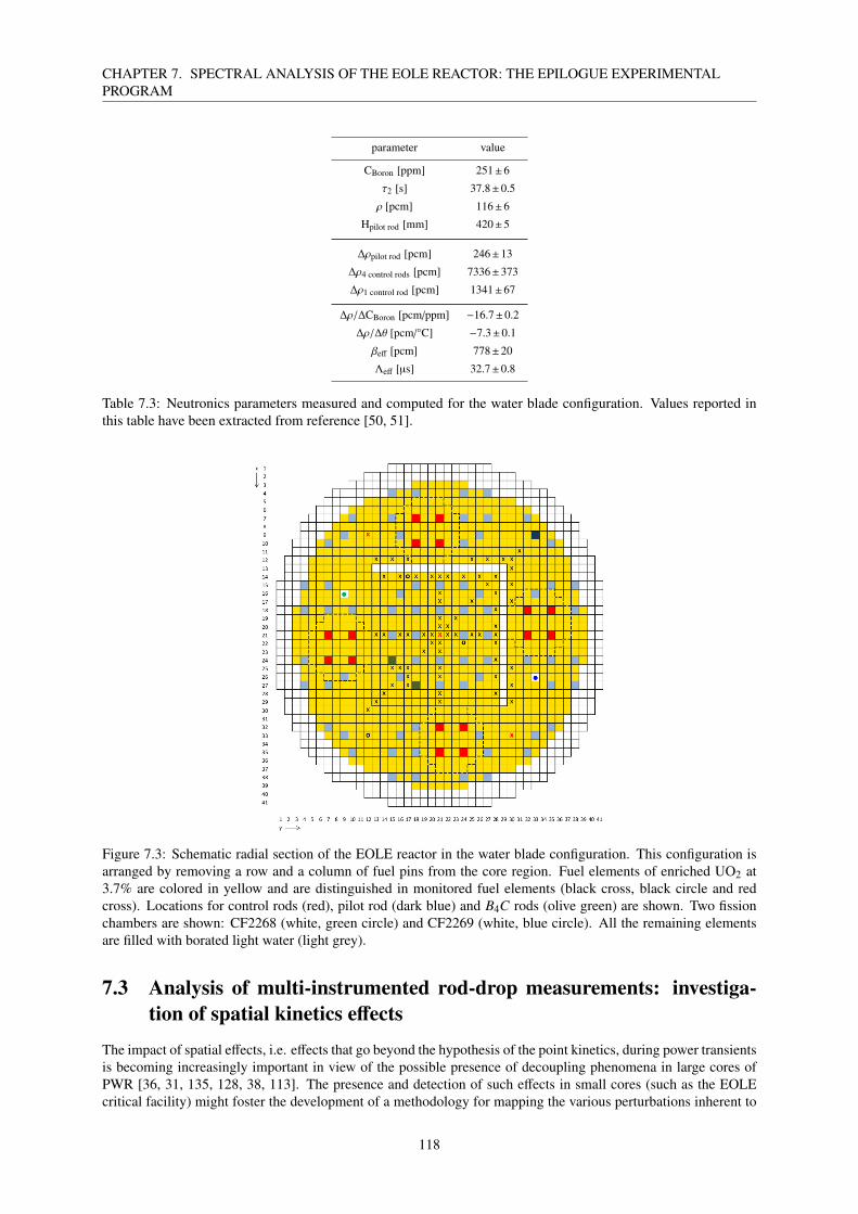
CHAPTER 7. SPECTRAL ANALYSIS OF THE EOLE REACTOR: THE EPILOGUE EXPERIMENTALPROGRAM
parameter value
CBoron [ppm] 251±6
τ2 [s] 37.8±0.5
ρ [pcm] 116±6
Hpilot rod [mm] 420±5
∆ρpilot rod [pcm] 246±13
∆ρ4 control rods [pcm] 7336±373
∆ρ1 control rod [pcm] 1341±67
∆ρ/∆CBoron [pcm/ppm] −16.7±0.2
∆ρ/∆θ [pcm/°C] −7.3±0.1
βeff [pcm] 778±20
Λeff [µs] 32.7±0.8
Table 7.3: Neutronics parameters measured and computed for the water blade configuration. Values reported inthis table have been extracted from reference [50, 51].
Figure 7.3: Schematic radial section of the EOLE reactor in the water blade configuration. This configuration isarranged by removing a row and a column of fuel pins from the core region. Fuel elements of enriched UO2 at3.7% are colored in yellow and are distinguished in monitored fuel elements (black cross, black circle and redcross). Locations for control rods (red), pilot rod (dark blue) and B4C rods (olive green) are shown. Two fissionchambers are shown: CF2268 (white, green circle) and CF2269 (white, blue circle). All the remaining elementsare filled with borated light water (light grey).
7.3 Analysis of multi-instrumented rod-drop measurements: investiga-tion of spatial kinetics effects
The impact of spatial effects, i.e. effects that go beyond the hypothesis of the point kinetics, during power transientsis becoming increasingly important in view of the possible presence of decoupling phenomena in large cores ofPWR [36, 31, 135, 128, 38, 113]. The presence and detection of such effects in small cores (such as the EOLEcritical facility) might foster the development of a methodology for mapping the various perturbations inherent to
118

7.3. ANALYSIS OF MULTI-INSTRUMENTED ROD-DROP MEASUREMENTS: INVESTIGATION OFSPATIAL KINETICS EFFECTS
the large PWR cores and for the optimization of in-core detector positions in order to cover the entire core volume.
The aim of this section is to describe the raw experimental results obtained from counting measurements from”rod-drop” experiments, performed in the course of the last sets of measurements of the EPILOGUE program [9]for the ”low fuel bubble” configuration [49], in order to highlight possible spatial kinetics effects. Different testshave been performed by using fission chambers having different sensibilities and placed in different locationsboth inside and outside the core region. These tests concern the investigation of a possible effect related to theselocations on the perturbation amplitude due to an insertion of negative reactivity caused by the pilot rod (∆ρ <βeff/2, for a fast drop) or by the control rod (∆ρ >> βeff).
7.3.1 Measurement results
Fission chamber measurements were performed in the ”low fuel bubble” configuration. The core is at a temperatureof 20°C. A schematic representation of this configuration is shown in Fig. 7.4. All fission chambers are inserted insealed aluminium sheaths and located at the core mid-plane by using aluminium shims of the appropriate length,depending on the type of chamber. Two Ø4 mm fission chambers are positioned in the core:
• CF 235U Ø4 mm (2268), located at 16-09,
• CF 239Pu Ø4 mm (2266), located at 26-33.
These two monitor detectors are connected to the MCS (Multi-Channel Scaler) measurement chain (ADS 7820and Ni-DAQ card, two channels of measurement). Five additional fission chambers are positioned in the core:
• CF 235U Ø8mm with reduced gap (2284), located at 01-21,
• CF 235U Ø8mm with long reduced gap (2296), located at 26-26,
• CF 235U Ø8mm with long reduced gap (2295), located at 07-35,
• CF 235U Ø4mm (2299), located at 21-41,
• CF 235U Ø8mm (2272), located at 36-06.
The first three chambers (2284, 2295 and 2296) are connected to fast ADS amplifiers and to the measuring systemXMODE. The last two (2272 and 2299) are connected to the traditional MP2 system (pre-amplifier + chargeamplifier). The XMODE system is capable of recording neutronic measurements as logical (32 synchronizedchannels) and analogical (8 synchronized channels) data. For the acquisition of logical signals, XMODE uses atime stamping which enables to record all detector information. This operating mode is necessary for the realisationof neutron noise experiments.
The CFUL fission chambers are traditionally used for neutron noise measurements. They are characterized by alarge usable volume and a large 235U deposit (1 g). Such large mass of fissile isotope denotes a higher sensitivity ofthe fission chambers and a larger number of counting will be detected. This large counting rate is necessary in orderto record signals in current mode, since the neutronic measuring system processes signal inputs obtained in currentmode. The measuring sleeves for the introduction of the CFUL chambers (670 and 669) are located between thecore and the vessel. The signal transmission cables (high immunity) are connected to the SPECTRON measuringsystem [64, 65]. This system is devoted to the analysis of neutron noise measurements and it has been developedat CEA/Cadarache. The high immunity of these cables allows to reduce the parasite capture contributions duringsignal acquisition in order to obtain a ”smoother” signal (lower influence of the background noise in terms ofelectromagnetic perturbations).
A summary of the measuring devices and their associated electronics is given in the table below:
119

CHAPTER 7. SPECTRAL ANALYSIS OF THE EOLE REACTOR: THE EPILOGUE EXPERIMENTALPROGRAM
CF location measuring system
2268 16−09 ADS−Ni-DAQ
2269 26−33 ADS−Ni-DAQ
CFUL 670 NO SPECTRON
CFUL 669 SE SPECTRON
2284 01−21 ADS−XMODE
2296 26−26 ADS−XMODE
2295 07−35 ADS−XMODE
2299 21−41 MP2−channel 3
2272 36−06 MP2−channel 1
Table 7.4: Detector locations and measuring systems for the rod-drop experiments.
Figure 7.4: Schematic radial section of the EOLE reactor in the low fuel bubble configuration during rod-dropexperiments. Fuel elements of enriched UO2 at 3.7% are located in the ”bubble” region (dark grey) and around it(yellow). Locations for control rods (red) and pilot rod (dark blue) are shown. The locations of fission chambers(colored circles) are shown are detailed in Tab. 7.4. All the remaining elements are filled with borated light water(white and light grey).
7.3.2 Rod-drop measurements
Two types of measurements were carried out: a rod-drop measurement of control rod (BS1 Fig. 7.4) and a rapiddescent of the pilot rod (BP Fig. 7.4), from a power level at 5 W or 10 W. The measurement protocol is thefollowing:
• reach the reactor divergence and stabilize at the target power,
• after a few minutes, required in order to ensure stabilization, start the rapid descent of the pilot rod (BP),
• when the counting rate reaches about 10 counts per second (MCS) in the chamber with the larger countingrate, start a new divergence,
• stabilize the power at 5 W,
120
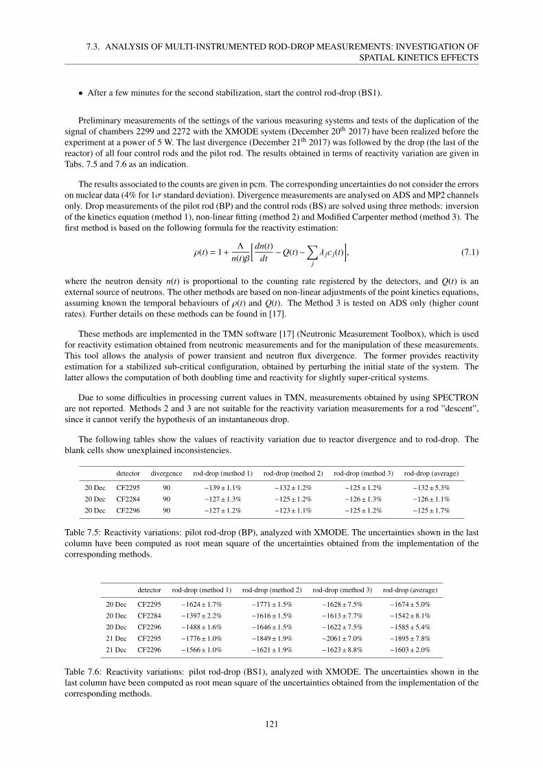
7.3. ANALYSIS OF MULTI-INSTRUMENTED ROD-DROP MEASUREMENTS: INVESTIGATION OFSPATIAL KINETICS EFFECTS
• After a few minutes for the second stabilization, start the control rod-drop (BS1).
Preliminary measurements of the settings of the various measuring systems and tests of the duplication of thesignal of chambers 2299 and 2272 with the XMODE system (December 20th 2017) have been realized before theexperiment at a power of 5 W. The last divergence (December 21th 2017) was followed by the drop (the last of thereactor) of all four control rods and the pilot rod. The results obtained in terms of reactivity variation are given inTabs. 7.5 and 7.6 as an indication.
The results associated to the counts are given in pcm. The corresponding uncertainties do not consider the errorson nuclear data (4% for 1σ standard deviation). Divergence measurements are analysed on ADS and MP2 channelsonly. Drop measurements of the pilot rod (BP) and the control rods (BS) are solved using three methods: inversionof the kinetics equation (method 1), non-linear fitting (method 2) and Modified Carpenter method (method 3). Thefirst method is based on the following formula for the reactivity estimation:
ρ(t) = 1 +Λ
n(t)β
[dn(t)dt−Q(t)−
∑j
λ jc j(t)], (7.1)
where the neutron density n(t) is proportional to the counting rate registered by the detectors, and Q(t) is anexternal source of neutrons. The other methods are based on non-linear adjustments of the point kinetics equations,assuming known the temporal behaviours of ρ(t) and Q(t). The Method 3 is tested on ADS only (higher countrates). Further details on these methods can be found in [17].
These methods are implemented in the TMN software [17] (Neutronic Measurement Toolbox), which is usedfor reactivity estimation obtained from neutronic measurements and for the manipulation of these measurements.This tool allows the analysis of power transient and neutron flux divergence. The former provides reactivityestimation for a stabilized sub-critical configuration, obtained by perturbing the initial state of the system. Thelatter allows the computation of both doubling time and reactivity for slightly super-critical systems.
Due to some difficulties in processing current values in TMN, measurements obtained by using SPECTRONare not reported. Methods 2 and 3 are not suitable for the reactivity variation measurements for a rod ”descent”,since it cannot verify the hypothesis of an instantaneous drop.
The following tables show the values of reactivity variation due to reactor divergence and to rod-drop. Theblank cells show unexplained inconsistencies.
detector divergence rod-drop (method 1) rod-drop (method 2) rod-drop (method 3) rod-drop (average)
20 Dec CF2295 90 −139±1.1% −132±1.2% −125±1.2% −132±5.3%
20 Dec CF2284 90 −127±1.3% −125±1.2% −126±1.3% −126±1.1%
20 Dec CF2296 90 −127±1.2% −123±1.1% −125±1.2% −125±1.7%
Table 7.5: Reactivity variations: pilot rod-drop (BP), analyzed with XMODE. The uncertainties shown in the lastcolumn have been computed as root mean square of the uncertainties obtained from the implementation of thecorresponding methods.
detector rod-drop (method 1) rod-drop (method 2) rod-drop (method 3) rod-drop (average)
20 Dec CF2295 −1624±1.7% −1771±1.5% −1628±7.5% −1674±5.0%
20 Dec CF2284 −1397±2.2% −1616±1.5% −1613±7.7% −1542±8.1%
20 Dec CF2296 −1488±1.6% −1646±1.5% −1622±7.5% −1585±5.4%
21 Dec CF2295 −1776±1.0% −1849±1.9% −2061±7.0% −1895±7.8%
21 Dec CF2296 −1566±1.0% −1621±1.9% −1623±8.8% −1603±2.0%
Table 7.6: Reactivity variations: pilot rod-drop (BS1), analyzed with XMODE. The uncertainties shown in thelast column have been computed as root mean square of the uncertainties obtained from the implementation of thecorresponding methods.
121

CHAPTER 7. SPECTRAL ANALYSIS OF THE EOLE REACTOR: THE EPILOGUE EXPERIMENTALPROGRAM
Small discrepancies are observed in the reactivity variations for the pilot rod-drop BP (Tab. 7.5), whereaslarger differences are observed in the reactivity variations for the control rod-drop BS1 (Tab. 7.6). In principle,such behaviour seems to suggest the possible presence of spatial effects.
The results obtained from the analysis of signal counting from MP2 channels are shown in Tab. 7.7. The corre-sponding average values (neglecting uncertainty) and the relative standard deviations of the channel measurementsare shown in Tab. 7.8.
detector rod-drop divergence rod-drop (method 1) rod-drop (method 2) rod-drop (method 3) rod-drop (average)
20 Dec CF2272 5 W−BP 96 −118±2.0% −121±1.2% −126±1.5% −122±3.1%
CF2299 5 W−BP 95 −121±4.6% −121±1.2% −123±1.3% −122±1.3%
CF2272 10 W−BS 95 −1420±1.8% −1509±1.4% - −1464±4.3%
CF2299 10 W−BS 94 -1217±2.8% −1422±1.3% - −1329±12.0%
21 Dec CF2272 BP rod-drop 90 −124±1.4% −125±1.2% −130±1.5% −127±2.7%
CF2299 BP rod-drop 87 −119±1.4% −120±1.2% −124±1.4% −121±2.3%
CF2272 BS rod-drop 88 −1244±3.0% −1501±1.4% - −1373±13.2%
CF2299 BS rod-drop 86 −1872±1.3% −1882±2.3% - −1877±0.4%
CF2272 4BS rods drop 88 −6812±1.7% −7786±1.4% - −7299±9.4%
CF2299 4BS rods drop 87 −7581±1.8% −8053±3.4% - −7817±4.3%
Table 7.7: Reactivity variations: analyzed on MP2 channels. The uncertainties shown in the last column havebeen computed as root mean square of the uncertainties obtained from the implementation of the correspondingmethods.
detector BP rod-drop BS1 rod-drop
CF2272 −124±3.4% −1418±8.7%CF2299 −121±1.7% −1603±20.5%
Table 7.8: Average reactivity variations: analyzed on MP2 channels. The uncertainties shown in the last columnhave been computed as root mean square of the uncertainties obtained from the implementation of the correspond-ing methods.
The values computed for the pilot rod-drop BP do not show any significant discrepancy. Larger reactivity de-viations are found for the control rod-drop BS1 experiment. The standard deviation corresponding to the countingof fission chamber CF2299 is rather large, which suggests a low counting rate of the detector. This behaviour canbe justified by the location of the fission chambers with respect to the position of rod BS1. The efficiency of thefission chamber CF2299 decreases after the insertion of negative reactivity, due to its proximity to the control rod.Conversely, the efficiency of fission chamber CF2272, located far from the control rod, increases, although thiseffect is less visible.
Table 7.9 shows the results obtained from ADS monitor channels. The results obtained at a power level of5 W are inconsistent and are not considered in the calculation of the corresponding average value. Converesely,small standard deviations are obtained for all the other results. The accuracy of these results is probably justifiedby the excellent performance of the ADS systems. The average values computed from these results (neglectinguncertainty) and the corresponding standard deviations are shown in Tab. 7.10.
122

7.3. ANALYSIS OF MULTI-INSTRUMENTED ROD-DROP MEASUREMENTS: INVESTIGATION OFSPATIAL KINETICS EFFECTS
detector rod-drop divergence rod-drop (method 1) rod-drop (method 2) rod-drop (method 3) rod-drop (average)
20 Dec CF2268 5 W−BP 92 −71±9.4% −114±18.9% - −93±32.2%∗
CF2269 5 W−BP 93 −95±5.6% −118±9.5% - −107±15.2%∗
CF2268 10 W−BS 93 −1521±4.9% −1358±3.3% - −1439±8.0%
CF2269 10 W−BS 94 −1785±3.6% −1674±3.8% - −1730±4.5%
21 Dec CF2268 BP rod-drop 88 −126±3.5% −125±1.7% - −125±0.4%
CF2269 BP rod-drop 89 −123±2.8% −124±4.7% - −123±0.2%
CF2268 BS rod-drop 87 −1454±4.5% −1402±3.4% - −1428±2.6%
CF2269 BS rod-drop 88 −1694±4.0% −1687±4.1% - −1690±0.3%
CF2268 4BS rods drop 87 −7309±3.4% −7204±4.0% - −7257±1.0%
CF2269 4BS rods drop 87 −7671±3.1% −7587±3.3% - −7629±0.8%
Table 7.9: Reactivity variations: analyzed on ADS monitor channels (*incoherent values, not accounted in theaverage results).
detector BP rod-drop BS1 rod-drop
CF2268 −125±1.5% −1434±4.9%
CF2269 −123±2.4% −1710±3.0%
Table 7.10: Average reactivity variations: analyzed on ADS monitor channels.
The two monitor chambers show a significant deviation of the reactivity variation related to the control rodexperiment. The corresponding mean value is −1572±195 pcm and the original values do not overlap by consid-ering 2σ standard deviations. The CF2269 fission chamber is closer to the perturbation with respect to the CF2268fission chamber and is located inside the neutron flux depression caused by the control rod-drop. Its position isresponsible for a larger measured reactivity variation.
Fission rate distributions have been calculated with Tripoli-4® for both pilot rod-drop and control rods dropin order to determine the signal variation in the detector positions. Figure 7.5 shows the variations of these fissionrates for each rod-drop experiment with respect to the unperturbed configuration.
Figure 7.5: Fission rates perturbation due to pilot rod-drop (BP, left) and control rods drop (BS1, right). Pertur-bations with respect to the unperturbed configuration ranges from -41% up to +6% due to the pilot rod-drop andfrom -61% up tp +13% due to control rods drop.
123

CHAPTER 7. SPECTRAL ANALYSIS OF THE EOLE REACTOR: THE EPILOGUE EXPERIMENTALPROGRAM
The variations in fission rates at detector locations are strongly influenced by the introduced perturbation. Thecorresponding minimum and maximum values are shown in Tab. 7.11 for the corresponding fission chamber. Asexpected, the largest variations are observed for detector located closer to the perturbation: CF2295 for the pilotrod-drop (the value for CF2268 is questionable, since this fission chamber is relatively far from the perturbationin order to observe such large variation), CF2299 and CF2269 for control rods drop. Values associated to theremaining detectors show smaller variations, except for the control rods drop experiment, where the reactivityinsertion implies a larger deformation of the neutron flux along the radial coordinate.
detector pilot rod-drop control rods drop
CFUL670 0.6% 7.8%
CFUL669 0.8% -3.2%
CF2284 -0.7% 3.1%
CF2295 -9.3% -8.0%
CF2296 -0.8% -3.1%
CF2272 2.0% 9.9%
CF2299 -0.7% -21%
CF2268 -7.2% -10.3%
CF2269 2.7% - 12.4%
Table 7.11: Fission rates variations on the detector locations.
7.3.3 Summary of the experimental results
We have illustrated the preliminary results of the rod-drop measurements carried out at the end of the experimentalcampaign in the ”low fuel bubble” configuration of the program EPILOGUE in EOLE. In addition to the fissionchambers CF2268 and CF2269, five fission chambers of different types, connected to different measuring elec-tronics, have been inserted in various core and reflector positions. The location of these detectors was intendedto identify possible spatial kinetics effects in the raw signals. The results were processed using the TMN tool,according to three methods (inversion of kinetics, flow adjustment, Carpenter’s method). The variations of thedetector efficiency as a function of the respective location suggest the presence of spatial kinetic effects in the core.
The deviations counted without detector efficiency correction are consistent with the expected deviations on thevariation in fission rates at the measurement sites. The mean values and the corresponding standard deviations ofthese measurements could be refined by a more complete calculation of the MSM (Modified Source Multiplication)factors using the new options implemented in Tripoli-4® for the adjoint calculations, which have been successfullytested on the control rod-drop measurements of CABRI [97].
7.4 Spectral analysis of the water blade configurations
The analysis of the experimental results presented in the previous section is devoted to a preliminary investigationof spatial kinetics effects during the last experiments of the EOLE reactor. In order to gain further knowledge onsuch effects, we have then analyzed the water blade configuration of the EPILOGUE program, which is character-ized by a strong spatial heterogeneity described in Section 7.2.3. Unfortunately, it was not possible to draw solidconclusions from the data collected during the experiments performed on this configuration.
Nevertheless, the effect caused by the over-moderation of the water blade has been examined by resorting tothe spectral analysis tools described in Chapter 5. In this respect, the Monte Carlo simulation has been used as a”numerical experiment”, enabling the analysis of quantities that were not easily accessible by the measurements.Monte Carlo calculations were performed with Tripoli-4® in order to deploy the matrix-filling method and thefission matrix described in Chapter 5. These numerical simulations allow estimating:
• the fundamental and higher-order eigenpairs according to the α-eigenvalue formulation,
• the fundamental and higher-order eigenpairs according to the k-eigenvalue formulation,
124

7.4. SPECTRAL ANALYSIS OF THE WATER BLADE CONFIGURATIONS
• the effective kinetics parameters.
The k- and the α- eigenpairs yield an estimation of the critical level of the system (fundamental eigenvalues andeigenmodes) and of the behaviour of particle distribution after a perturbation (higher-order eigenvalues and eigen-modes). As discussed in the previous chapter, we can exploit the dominance ratio (Eq. (6.3)) and the eigenvalueseparation (Eqs. (6.1) and (6.6)) in order to assess the degree of decoupling of the system. The spatial distributionsof the eigenmodes related to both eigenvalue formulations provide an additional tool for the investigation of the de-coupling effect caused by the water blade. Finally, the effective kinetic parameters computed for this configurationcan be usefully compared to those obtained during the experiments (Tab. 7.3).
For the purpose of enhancing the effects induced by the water blade, we have conceived additional configu-rations where the original blade has been thickened by adding extra water layers (by removing fuel pins). Forour analysis, we will consider the configuration without water blades (described in Section 7.2.1) as the reference.Then, we will remove additional fuel pins from the water blade configurations in order to artificially increase thethickness of the water in the core region. Figure 7.6 shows the radial section of the two new configurations thatwill be called for shortness ”2 water blades” configuration (left) and ”3 water blades” configuration (right). In thefollowing, by analogy we will define the (single) water blade configuration as the ”1 water blade” configuration.
Figure 7.6: Schematic radial section of the EOLE reactor in water blade configurations. The ”2 water blades”configuration (left) and the ”3 water blades” configuration (right) are arranged by removing four and six lines offuel pins from the core region. Fuel elements of enriched UO2 at 3.7% are colored in yellow and are distinguishedin monitored fuel elements (black cross, black circle and red cross). Locations for control rods (red), pilot rod(dark blue) and B4C rods (olive green) are shown. Two fission chambers are shown: CF2268 (white, green circle)and CF2269 (white, blue circle). All the remaining elements are filled with borated light water (light grey).
7.4.1 Simulation settings
All the configurations defined in the previous section have been simulated by using Tripoli-4®. Before detailingthe simulation parameters of such calculations, a preliminary step is required for the calibration allowing eachsimulated system to be critical (similarly to the procedure adopted in Chapter 6). In order to achieve this condition,we modified the Boron concentration in the moderator of each configuration. This procedure can be performedin Tripoli-4® by a recently developed critical Boron concentration research routine, which iteratively seeks amultiplier coefficient for the Boron concentration CBoron. For these calculations, 105 particles are simulated fora total of 1.5× 10³ cycles (103 active, 5× 10² discarded). Water composition and Boron concentration of themoderator for each configuration are shown in Tab. 7.12.
125

CHAPTER 7. SPECTRAL ANALYSIS OF THE EOLE REACTOR: THE EPILOGUE EXPERIMENTALPROGRAM
water blades [-] H1 [atoms/cm3] H1,H2O [atoms/cm3] O16 [atoms/cm3] B10 [atoms/cm3] B11 [atoms/cm3] CBoron [ppm]
0 4.675×10⁻⁵ 6.669×10⁻² 3.339×10⁻² 3.286×10⁻⁶ 1.323×10⁻⁵ 296.7
1 3.923×10⁻⁵ 6.670×10⁻² 3.339×10⁻² 2.708×10⁻⁶ 1.090×10⁻⁵ 244.5
2 3.923×10⁻⁵ 6.670×10⁻² 3.339×10⁻² 1.878×10⁻⁶ 7.561×10⁻⁶ 169.6
3 3.923×10⁻⁵ 6.670×10⁻² 3.339×10⁻² 7.339×10⁻⁷ 2.954×10⁻⁶ 66.3
Table 7.12: Water composition and Boron concentration (ppm) of the moderator in water blade configurations.
As already discussed in Chapter 6, setting all these configurations to the critical level leads to two main ad-vantages. The former is that the comparison of the dominance ratio and the eigenvalue separation is made easierby fixing the fundamental eigenvalues to the critical level. The latter stems from an algorithmic reason related tothe equivalence between the k- and the α-eigenvalue formulations for a critical state: this property allows us tofreely choose between the k or α-k power iteration methods as a weighting function for the matrix-filling methods.The k-power iteration is preferred with respect to the α-k power iteration method, thanks to its faster convergence.Moreover, the estimation of the elements of the matrices associated to the linear transport operators is computed byusing the same weighting function. Since the systems are at a critical level, ϕk0 ' ϕα0 , the choice of the weightingfunction becomes arbitrary.
The discretization of the phase-space variables for the EOLE configurations implies a large dimension of thematrices corresponding to the eigenvalue formulations. The trade-off required to compute the eigenpairs in areasonable time and be able to detect the effect of the moderator heterogeneity consists in primarily refining thespatial coordinates in the radial section of the reactor. By fixing the origin of the spatial reference system inthe center of the reactor, an uniform Cartesian grid is applied on the plane that divides the two coordinates inNx = Ny = 48 spatial bins from −52.8 cm to 52.8 cm. The axial coordinate is integrated over the whole height ofthe system (Nz = 1). The angle discretization is kept at Mx = My = 2 and Mz = 1. The energy domain is divided intoG = 3 groups: a fast region in the interval [20 MeV, 94.66 keV], an epithermal region [94.66 keV, 0.625 eV] anda thermal region [0.625 eV, 10-5 eV]. According to the JEFF nuclear data library [134], a total of J = 8 precursorsfamilies are considered for the fissile nuclei. The total number of elements of the matrix for the α-eigenvalueproblem is about 2×10⁹.
As for the k-eigenvalue problem, we used the estimation of the fission matrix in order to perform the spectralanalysis on the k-modal basis. According to this procedure, only the space coordinate needs to be discretized.The eigenmodes computed from the fission matrix represent fission rates and as so there is no interest in a finediscretization of the non-fissile regions of the reactor. Moreover, the linearity of this problem with respect to theeigenvalue allows combining the contributions of prompt and delayed fission operators. All these considerationsimply a significant reduction of the matrix size for the k-eigenvalue formulation. In particular, we impose acartesian grid on the radial section of the core region, specifically Nx = Ny = 74 from -23.31 cm to 23.31 cm alongboth axes. In this way, the spatial bins perfectly overlap on the square fuel pins section (1.26×1.26 cm2). The totalnumber of elements of the fission matrix is about 3×10⁷.
7.4.2 Eigenvalue analysis
The Boron concentrations shown in Tab. 7.12 are used for the criticality simulations in order to adjust each con-figuration to the critical level. All the results presented in the following paragraphs have been obtained during astandard power iteration that was used to estimate the elements of the matrices needed for the α- and k- spectralanalysis. In particular, 105 particles per cycles are simulated for a total of 2.5×10³ cycles (2×10³ active, 5×10²
discarded).
126

7.4. SPECTRAL ANALYSIS OF THE WATER BLADE CONFIGURATIONS
water blades [-] kMC0 [-] k0 [-] k1 [-] k2 [-] k3 [-] k4 [-] k5 [-]
0 0.99988±7 pcm 0.99988 0.70793 0.70552 0.48323 0.48112 0.42774
1 1.00012±7 pcm 1.00012 0.72320 0.71284 0.49605 0.49100 0.43236
2 1.00019±7 pcm 1.00019 0.73302 0.72089 0.50609 0.50061 0.44342
3 0.99997±7 pcm 0.99997 0.74483 0.73167 0.51801 0.51488 0.45587
Table 7.13: First k-eigenvalues for EOLE water blades configurations configurations. The second column displaysthe fundamental eigenvalues k0 computed by Tripoli-4® power iteration for the k-eigenvalue problem and thecorresponding standard deviations. All other eigenvalues have been computed from the fission matrix of thecorresponding configuration.
The fundamental eigenvalues obtained with these calculations are shown in the second column of Tab. 7.13.These values are less than 20 pcm from the critical state, with a standard deviation of 7 pcm for the chosen numberof particles and cycles. The other values presented in Tab. 7.13 have been computed from the fission matricesassociated to each configuration. An excellent agreement is found between the fundamental eigenvalues kMC
0(obtained by using the power iteration) and k0 (computed from the post-processed fission matrices).
During the same calculations, the discretized version of linear transport operators have been estimated andpost-processed in order to obtain the matrices of the α-eigenvalue problems. The real parts of the correspondingeigenvalues have been arranged in descending order in order to discriminate the fundamental eigenvalue, the clus-ters of delayed eigenvalues and the prompt eigenvalues. The fundamental eigenvalues α0 and the first five delayedeigenvalues are shown in Tab. 7.14. The sign and the magnitude of the fundamental α-eigenvalues are consistentwith the k0 eigenvalues from the previous table. The absolute value of the first delayed eigenvalues collapses onthe minimum decay constant equal to min(λ) = 1.247× 10⁻² s-1. Conversely, the first five prompt α-eigenvaluesshown in Tab. 7.15 exhibit significant variations as a function of the configuration and of the mode order.
water blades [-] α0 [s-1] α1 [s-1] α2 [s-1] α3 [s-1] α4 [s-1] α5 [s-1]
0 −1.122×10⁻³ −1.246×10⁻² −1.246×10⁻² −1.246×10⁻² −1.246×10⁻² −1.247×10⁻²
1 1.084×10⁻³ −1.246×10⁻² −1.246×10⁻² −1.246×10⁻² −1.246×10⁻² −1.247×10⁻²
2 2.473×10⁻³ −1.246×10⁻² −1.246×10⁻² −1.246×10⁻² −1.246×10⁻² −1.246×10⁻²
3 −5.273×10⁻⁴ −1.246×10⁻² −1.246×10⁻² −1.246×10⁻² −1.246×10⁻² −1.246×10⁻²
Table 7.14: First α-eigenvalues for EOLE water blades configurations. These values have been computed from thematrix-form of linear transport operator combined for the definition of the α-eigenvalue problem.
water blades [-] αp,0 [s-1] αp,1 [s-1] αp,2 [s-1] αp,3 [s-1] αp,4 [s-1] αp,5 [s-1]
0 −2.233×10² −4.277×10³ −4.883×10³ −5.167×10³ −6.051×10³ −6.068×10³
1 −2.010×10² −5.591×10³ −5.662×10³ −7.667×10³ −7.688×10³ −8.158×10³
2 −1.715×10² −5.000×10³ −5.088×10³ −6.252×10³ −7.000×10³ −7.022×10³
3 −1.508×10² −4.234×10³ −4.328×10³ −6.081×10³ −6.103×10³ −6.793×10³
Table 7.15: First prompt α-eigenvalues for EOLE water blades configurations. These values have been computedfrom the matrix-form of linear transport operator combined for the definition of the α-eigenvalue problem.
For the sake of completeness, we show both the k- and the α-spectra on the complex plane in Fig. 7.7. The(small) imaginary part of the k-spectrum is merely due to the statistical uncertainties propagated from the stochasticestimation of the matrix elements on the eigenvalues. Figure 7.8 shows the zoom on all delayed eigenvalue clusters(left) and on the delayed eigenvalue cluster associated to the first precursor family (right). The eigenvalues areconcentrated on the right of the −λ j values. The dominant eigenvalue α j
d,0 of the j-th delayed cluster is separated
from the other eigenvalues of the same precursor family. The zoom of Fig. 7.8 (left) shows the gap between α jd,0
and −λ j values for the last precursor families. The computed values of α jd,0 and α j
d,1 for the last three precursorfamilies ( j = 6,7,8) are shown in Tab. 7.16. Values for the −λ j shown in Fig. are: −λ1 = −1.2467× 10⁻² s−1,
127

CHAPTER 7. SPECTRAL ANALYSIS OF THE EOLE REACTOR: THE EPILOGUE EXPERIMENTALPROGRAM
−λ6 = −6.6649×10⁻¹ s−1, −λ7 = −1.6348 s−1 and −λ8 = −3.5546 s−1.
Figure 7.7: Spectra of the k (left) and the α (right) eigenvalue problem for the ”3 water blades” configuration.
Figure 7.8: Zoom on the α-spectrum on the delayed region (left) and in the first delayed cluster (right) for the”3 water blades” configuration. Vertical lines have been added in order to indicate the values of −λ1 (blue), −λ6(magenta), −λ7 (cyan) and −λ8 (green).
water blades [-] α6d,0 [s-1] α6
d,1 [s-1] α7d,0 [s-1] α7
d,1 [s-1] α8d,0 [s-1] α8
d,1 [s-1]
0 −6.079×10⁻¹ −6.653×10⁻¹ −1.506 −1.632 −3.453 −3.553
1 −6.074×10⁻¹ −6.653×10⁻¹ −1.505 −1.632 −3.453 −3.553
2 −6.069×10⁻¹ −6.652×10⁻¹ −1.503 −1.632 −3.452 −3.553
3 −6.087×10⁻¹ −6.652×10⁻¹ −1.507 −1.632 −3.455 −3.552
Table 7.16: First α-eigenvalues of the clusters associated to the last three precursor families ( j = 6,7,8) for theEOLE water blades configurations. These values have been computed from the matrix-form of linear transportoperator combined for the definition of the α-eigenvalue problem.
The eigenvalues computed for these configurations are combined in order to obtain the dominance ratio and theeigenvalue separation according to the k- and the α-formulations. These values are collected in Tabs. 7.17 and 7.19and are shown in Figs. 7.9 and 7.10.
The values of dominance ratio increase for a larger thickness of the water blade from DR = 0.7080 up toDR = 0.7449. The eigenvalue separations according to the k-formulation follow a similar behaviour as the oneobserved in the analysis of 2D systems in Chapter 6 (Figs. 6.7 and 6.11): the first and second, the third and fourthorder of the eigenvalue separations show close values. This feature might be related to the symmetry propertiesof this system, which would in turn induce a degeneracy in the eigenvalues. Conversely, all these values do notchange significantly with respect to the chosen configuration (i.e., to the number of water blades).
128

7.4. SPECTRAL ANALYSIS OF THE WATER BLADE CONFIGURATIONS
water blades [-] DR [-] E.S.1(k) [-] E.S.2(k) [-] E.S.3(k) [-] E.S.4(k) [-] E.S.5(k) [-]
0 7.080×10⁻¹ 4.125×10⁻¹ 4.173×10⁻¹ 1.069×100 1.078×100 1.338×100
1 7.231×10⁻¹ 3.829×10⁻¹ 4.030×10⁻¹ 1.016×100 1.037×100 1.313×100
2 7.329×10⁻¹ 3.644×10⁻¹ 3.874×10⁻¹ 9.761×10⁻¹ 9.977×10⁻¹ 1.255×100
3 7.449×10⁻¹ 3.426×10⁻¹ 3.667×10⁻¹ 9.304×10⁻¹ 9.422×10⁻¹ 1.194×100
Table 7.17: Dominance ratio and E.S.n(k) eigenvalue separations of the first k-eigenvalues for water blade config-urations.
Figure 7.9: Dominance ratio (left) and k-eigenvalue separations (right) for EOLE water blade configurations. Thefirst five order of eigenvalue separations are shown, in order, as: E.S.1(k) red circles, E.S.2(k) blue crosses, E.S.3(k)green squares, E.S.4(k) cyan diamonds and E.S.5(k) magenta triangles.
The α-eigenvalues computed from the matrix-form of the α-eigenvalue problem are used in order to estimatethe delayed E.S.(αd) and the prompt E.S.(αp) eigenvalue separations of the first five orders. The delayed resultsare shown in Tab. 7.18, whereas the prompt results are shown in Tab. 7.19. The values of delayed eigenvalueseparations (Fig. 6.8, left) are almost constant as a function of the water blade configuration. The prompt α-eigenvalue separations (Fig. 6.4, right) have a different behaviour with respect to the k-eigenvalue separations. Inparticular, the eigenvalue separations associated to the ”0 water blade” configuration appear to have a different trendwith respect to the results obtained from the other configurations. This stems from this configuration not havingany strong heterogeneity along the spatial coordinates. For the configurations containing the water blades, on thecontrary, we notice a similar behaviour with respect to what examined for the 2D configurations of Sections 6.4.1and 6.4.2. The proximity of the first and second, third and fourth order of the eigenvalue separations suggest againa degeneracy effect related to the symmetry of the system.
Moreover, the values of dominance ratio hint the absence of strong decoupling effects in all these configura-tions. For this reasons, no solid conclusions can be drawn relating spatial kinetics effects to the eigenvalue separa-tions of the considered configurations. Therefore, in the next section we complement this analysis by consideringthe eigenmodes.
water blades [-] E.S.1(αd) [s-1] E.S.2(αd) [s-1] E.S.3(αd) [s-1] E.S.4(αd) [s-1] E.S.5(αd) [s-1]
0 −1.134×10⁻² −1.134×10⁻² −1.134×10⁻² −1.134×10⁻² −1.134×10⁻²
1 −1.354×10⁻² −1.354×10⁻² −1.355×10⁻² −1.355×10⁻² −1.355×10⁻²
2 −1.493×10⁻² −1.493×10⁻² −1.494×10⁻² −1.494×10⁻² −1.494×10⁻²
3 −1.193×10⁻² −1.193×10⁻² −1.194×10⁻² −1.194×10⁻² −1.194×10⁻²
Table 7.18: Eigenvalue separations of the first delayed α-eigenvalues for water blade configurations.
129

CHAPTER 7. SPECTRAL ANALYSIS OF THE EOLE REACTOR: THE EPILOGUE EXPERIMENTALPROGRAM
water blades [-] E.S.1(αp) [s-1] E.S.2(αp) [s-1] E.S.3(αp) [s-1] E.S.4(αp) [s-1] E.S.5(αp) [s-1]
0 −4.054×10³ −4.660×10³ −4.943×10³ −5.827×10³ −5.844×10³
1 −5.390×10³ −5.461×10³ −7.466×10³ −7.487×10³ −7.957×10³
2 −4.828×10³ −4.916×10³ −6.080×10³ −6.828×10³ −6.851×10³
3 −4.083×10³ −4.177×10³ −5.930×10³ −5.953×10³ −6.642×10³
Table 7.19: Eigenvalue separations of the first prompt α-eigenvalues for water blade configurations.
Figure 7.10: Delayed (left) and prompt (right) α-eigenvalue separations for EOLE water blade configurations.The first five order of eigenvalue separations are shown, in order, as: E.S.1(α) red circles, E.S.2(α) blue crosses,E.S.3(α) green squares, E.S.4(α) cyan diamonds and E.S.5(α) magenta triangles.
7.4.3 Eigenmode analysis
We will now examine the eigenvectors corresponding to the k- and the α-eigenvalue formulation as a functionof the spatial coordinates in the cross-section plane of the EOLE reactor. The distributions computed from fis-sion matrices are fission rates Q f ,k(x,y) depending only on the spatial coordinates. For this reason, we applieda finer discretization in the fissile regions. Conversely, α-eigenfunctions are related to particle population (neu-trons and precursors), thus requiring the discretization of the whole phase-space, yielding distributions of the kindϕα(x,y,µx,µy,E) for neutrons and c j,α(x,y,E) for precursors.
Figures 7.11 and 7.12 show the spatial distribution of the fundamental and the first-order eigenmodes accordingto the k-formulation, respectively. As expected, since the fission rates are located only in the fissile fuel pins of thecore, the effect of the moderator region is clearly visible. Concerning the fundamental eigenmode, the distributioncorresponding to the reference configuration (top left) shows large values of the fission rates in the central region ofthe core and in its the peripheral region. The moderation caused by the borated water increases the fission rates inproximity of the non fissile regions with respect to the usual Bessel-like distribution expected for an homogeneouscore. The replacement of fuel pins in the water layer region of the ”1 water blade” configuration (top right)completely modifies the fission rates distribution in the core. Fuel pin regions over-moderated by this replacementare characterized by larger values of fission rates, whereas all the regions far from this perturbation display smallervalues with respect to the distribution of the reference configuration. Increasing the thickness of the water layer in 2(bottom left) and 3 (bottom right) water blades configurations enhance the localized behaviour of this perturbationby amplifying the fission rates of fuel pins closer to the over-moderated regions. Moreover, the absorption causedby the B4C rods placed on the other side with respect to the water layer is clearly visible, since it reduces the fissionrates in their proximity.
The adjoint distributions of the k-eigenvalue problem analyzed by transposition of the fission matrix are shownin Figs. 7.13 and 7.14 for the fundamental and the first-order eigenmodes, respectively. The presence of the strongmoderator heterogeneity appears to slightly shift the peak of the adjoint eigenfunction towards the center of thewater blade. Overall, a Bessel-like shape is observed for the four configurations.
130
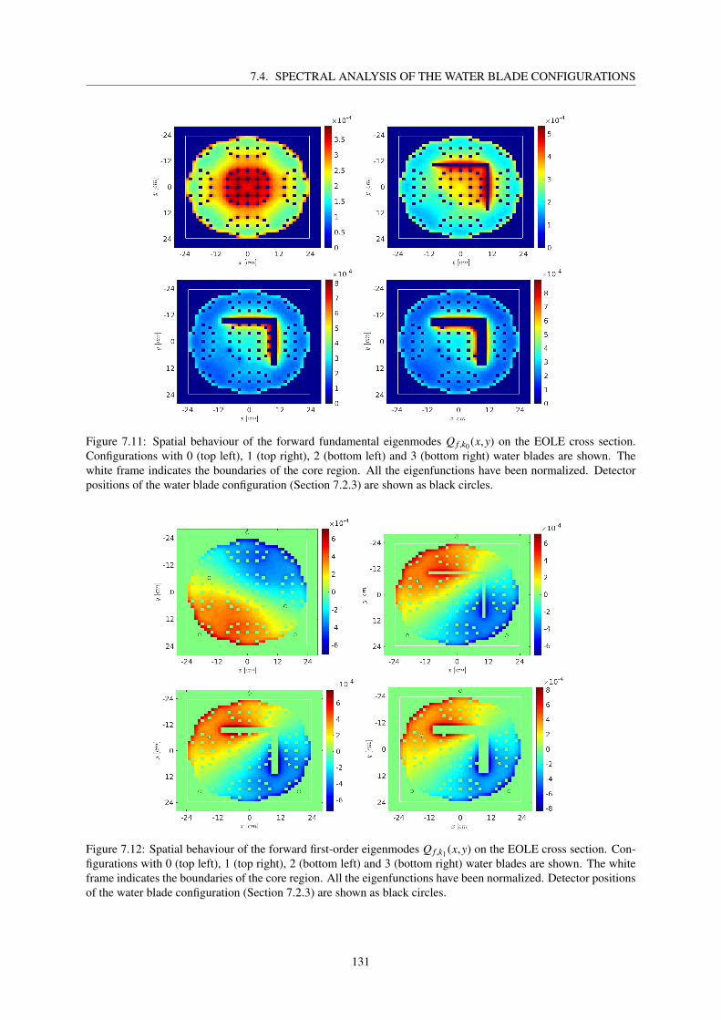
7.4. SPECTRAL ANALYSIS OF THE WATER BLADE CONFIGURATIONS
Figure 7.11: Spatial behaviour of the forward fundamental eigenmodes Q f ,k0 (x,y) on the EOLE cross section.Configurations with 0 (top left), 1 (top right), 2 (bottom left) and 3 (bottom right) water blades are shown. Thewhite frame indicates the boundaries of the core region. All the eigenfunctions have been normalized. Detectorpositions of the water blade configuration (Section 7.2.3) are shown as black circles.
Figure 7.12: Spatial behaviour of the forward first-order eigenmodes Q f ,k1 (x,y) on the EOLE cross section. Con-figurations with 0 (top left), 1 (top right), 2 (bottom left) and 3 (bottom right) water blades are shown. The whiteframe indicates the boundaries of the core region. All the eigenfunctions have been normalized. Detector positionsof the water blade configuration (Section 7.2.3) are shown as black circles.
131

CHAPTER 7. SPECTRAL ANALYSIS OF THE EOLE REACTOR: THE EPILOGUE EXPERIMENTALPROGRAM
Figure 7.13: Spatial behaviour of the adjoint fundamental eigenmodes Q†f ,k0(x,y) on the EOLE cross section.
Configurations with 0 (top left), 1 (top right), 2 (bottom left) and 3 (bottom right) water blades are shown. Thewhite frame indicates the boundaries of the core region. All the eigenfunctions have been normalized. Detectorpositions of the water blade configuration (Section 7.2.3) are shown as black circles.
Figure 7.14: Spatial behaviour of the adjoint first-order eigenmodes Q†f ,k1(x,y) on the EOLE cross section. Con-
figurations with 0 (top left), 1 (top right), 2 (bottom left) and 3 (bottom right) water blades are shown. The whiteframe indicates the boundaries of the core region. All the eigenfunctions have been normalized. Detector positionsof the water blade configuration (Section 7.2.3) are shown as black circles.
Concerning the α-eigenmodes, we resort to the discretization of the operators in energy groups by showing
132
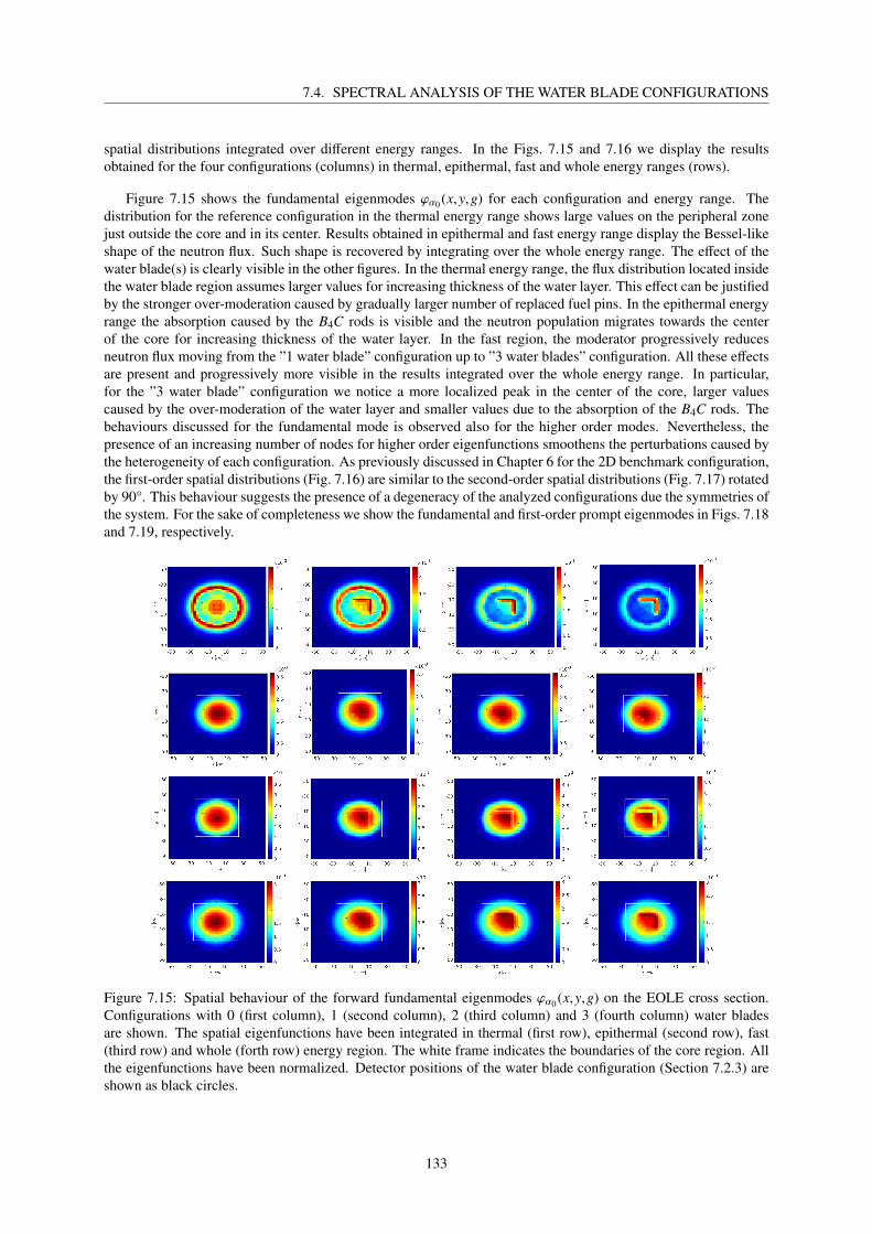
7.4. SPECTRAL ANALYSIS OF THE WATER BLADE CONFIGURATIONS
spatial distributions integrated over different energy ranges. In the Figs. 7.15 and 7.16 we display the resultsobtained for the four configurations (columns) in thermal, epithermal, fast and whole energy ranges (rows).
Figure 7.15 shows the fundamental eigenmodes ϕα0 (x,y,g) for each configuration and energy range. Thedistribution for the reference configuration in the thermal energy range shows large values on the peripheral zonejust outside the core and in its center. Results obtained in epithermal and fast energy range display the Bessel-likeshape of the neutron flux. Such shape is recovered by integrating over the whole energy range. The effect of thewater blade(s) is clearly visible in the other figures. In the thermal energy range, the flux distribution located insidethe water blade region assumes larger values for increasing thickness of the water layer. This effect can be justifiedby the stronger over-moderation caused by gradually larger number of replaced fuel pins. In the epithermal energyrange the absorption caused by the B4C rods is visible and the neutron population migrates towards the centerof the core for increasing thickness of the water layer. In the fast region, the moderator progressively reducesneutron flux moving from the ”1 water blade” configuration up to ”3 water blades” configuration. All these effectsare present and progressively more visible in the results integrated over the whole energy range. In particular,for the ”3 water blade” configuration we notice a more localized peak in the center of the core, larger valuescaused by the over-moderation of the water layer and smaller values due to the absorption of the B4C rods. Thebehaviours discussed for the fundamental mode is observed also for the higher order modes. Nevertheless, thepresence of an increasing number of nodes for higher order eigenfunctions smoothens the perturbations caused bythe heterogeneity of each configuration. As previously discussed in Chapter 6 for the 2D benchmark configuration,the first-order spatial distributions (Fig. 7.16) are similar to the second-order spatial distributions (Fig. 7.17) rotatedby 90°. This behaviour suggests the presence of a degeneracy of the analyzed configurations due the symmetries ofthe system. For the sake of completeness we show the fundamental and first-order prompt eigenmodes in Figs. 7.18and 7.19, respectively.
Figure 7.15: Spatial behaviour of the forward fundamental eigenmodes ϕα0 (x,y,g) on the EOLE cross section.Configurations with 0 (first column), 1 (second column), 2 (third column) and 3 (fourth column) water bladesare shown. The spatial eigenfunctions have been integrated in thermal (first row), epithermal (second row), fast(third row) and whole (forth row) energy region. The white frame indicates the boundaries of the core region. Allthe eigenfunctions have been normalized. Detector positions of the water blade configuration (Section 7.2.3) areshown as black circles.
133

CHAPTER 7. SPECTRAL ANALYSIS OF THE EOLE REACTOR: THE EPILOGUE EXPERIMENTALPROGRAM
Figure 7.16: Spatial behaviour of the forward first-order eigenmodes ϕα1 (x,y,g) on the EOLE cross section. Con-figurations with 0 (first column), 1 (second column), 2 (third column) and 3 (fourth column) water blades areshown. The spatial eigenfunctions have been integrated in thermal (first row), epithermal (second row), fast (thirdrow) and whole (forth row) energy region. The white frame indicates the boundaries of the core region. Allthe eigenfunctions have been normalized. Detector positions of the water blade configuration (Section 7.2.3) areshown as black circles.
134

7.4. SPECTRAL ANALYSIS OF THE WATER BLADE CONFIGURATIONS
Figure 7.17: Spatial behaviour of the forward second-order eigenmodes ϕα2 (x,y,g) on the EOLE cross section.Configurations with 0 (first column), 1 (second column), 2 (third column) and 3 (fourth column) water bladesare shown. The spatial eigenfunctions have been integrated in thermal (first row), epithermal (second row), fast(third row) and whole (forth row) energy region. The white frame indicates the boundaries of the core region. Allthe eigenfunctions have been normalized. Detector positions of the water blade configuration (Section 7.2.3) areshown as black circles.
135

CHAPTER 7. SPECTRAL ANALYSIS OF THE EOLE REACTOR: THE EPILOGUE EXPERIMENTALPROGRAM
Figure 7.18: Spatial behaviour of the forward fundamental prompt eigenmodes ϕαp,0 (x,y,g) for the ”3 blades”configuration on the EOLE cross section. The spatial eigenfunctions have been integrated in thermal (top left),epithermal (top right), fast (bottom left) and whole (bottom right) energy region. The white frame indicates theboundaries of the core region. All the eigenfunctions have been normalized. Detector positions of the water bladeconfiguration (Section 7.2.3) are shown as black circles.
Figure 7.19: Spatial behaviour of the forward first-order prompt eigenmodes ϕαp,1 (x,y,g) for the ”3 blades” config-uration on the EOLE cross section. The spatial eigenfunctions have been integrated in thermal (top left), epithermal(top right), fast (bottom left) and whole (bottom right) energy region. The white frame indicates the boundaries ofthe core region. All the eigenfunctions have been normalized. Detector positions of the water blade configuration(Section 7.2.3) are shown as black circles.
136

7.4. SPECTRAL ANALYSIS OF THE WATER BLADE CONFIGURATIONS
The adjoint distributions of the α-eigenvalue problem analyzed by transposition of the α-matrix are shownin Figs. 7.20 and 7.21 for the fundamental and the first-order eigenmodes, respectively. Similarly to the resultsanalyzed for the k-formulation, the fundamental adjoint distribution presents a Bessel-like shape. Conversely, theinfluence of the water blade region and of the control rod absorption is clearly visible in thermal and epithermalregion, respectively, for increasing thickness of the water layer.
Figure 7.20: Spatial behaviour of the adjoint fundamental eigenmodes ϕ†α0 (x,y,g) on the EOLE cross section.Configurations with 0 (first column), 1 (second column), 2 (third column) and 3 (fourth column) water bladesare shown. The spatial eigenfunctions have been integrated in thermal (first row), epithermal (second row), fast(third row) and whole (forth row) energy region. The white frame indicates the boundaries of the core region. Allthe eigenfunctions have been normalized. Detector positions of the water blade configuration (Section 7.2.3) areshown as black circles.
137

CHAPTER 7. SPECTRAL ANALYSIS OF THE EOLE REACTOR: THE EPILOGUE EXPERIMENTALPROGRAM
Figure 7.21: Spatial behaviour of the adjoint first-order eigenmodes ϕ†α1 (x,y,g) on the EOLE cross section. Config-urations with 0 (first column), 1 (second column), 2 (third column) and 3 (fourth column) water blades are shown.The spatial eigenfunctions have been integrated in thermal (first row), epithermal (second row), fast (third row)and whole (forth row) energy region. The white frame indicates the boundaries of the core region. All the eigen-functions have been normalized. Detector positions of the water blade configuration (Section 7.2.3) are shown asblack circles.
138

7.5. CONCLUSIONS
7.4.4 Analysis of kinetics parameters
During the simulations described above, the effective kinetic parameters have also been computed. Criticality k-calculations were performed, so the weighting functions applied to the bilinear forms are ϕk0 and ϕ†k0
. Since allthese systems have been adjusted to the critical level, the α- and k- fundamental eigenmodes are expected to bealmost identical. The computed values for ρ have been obtained as static reactivities according to Eq. (2.106).
The computed kinetics parameters and the corresponding reactivities parameters are shown in Tab. 7.20. Re-activity mean values and standard deviations are intimately related to the fundamental eigenvalues k0 estimatedfor each configuration and shown in Tab. 7.13. The mean generation time Λeff estimated for the ”1 water blade”configuration is smaller than the value given in Tab. 7.3 (32.7±0.8 µs), probably due to the higher Boron content inthe moderator. Due to nuclear data, the reactivity corresponding to the ”1 water blade” configuration was not zeroat the Boron concentration used in the experiment. In order to adjust the reactivity, we have artificially modifiedthe Boron content of the moderator, which in turn has slightly modified the value of the mean generation time.By inspection of the values computed for the remaining configurations, we notice that increasing the water bladethickness leads to an increase of the mean generation time. This behaviour is expected since increasing the waterlayer implies an increase in the overall moderation of the lattice. Values concerning the effective delayed fractionβeff from Tab. 7.3 (778±20 pcm) and all four simulated configurations overlap within one standard deviation.
parameters reference 1 water blade 2 water blade 3 water blade
ρ [pcm] -12 ± 7 12 ± 7 19 ± 7 -3 ± 7
Λeff [µs] 26.91 ± 0.01 29.24 ± 0.01 33.94 ± 0.02 39.63 ± 0.02
βeff [pcm] 791 ± 3 786 ± 3 775 ± 3 779 ± 3
β1eff
[pcm] 24.7 ± 0.6 23.4 ± 0.6 23.4 ± 0.6 23.8 ± 0.6
β2eff
[pcm] 112 ± 1 117 ± 1 113 ± 1 113 ± 1
β3eff
[pcm] 68.2 ± 0.9 69 ± 1 68.5 ± 0.9 70 ± 1
β4eff
[pcm] 151 ± 1 149 ± 1 144 ± 1 148 ± 1
β5eff
[pcm] 255 ± 2 252 ± 2 253 ± 2 251 ± 2
β6eff
[pcm] 83 ± 1 82 ± 1 79 ± 1 82 ± 1
β7eff
[pcm] 71 ± 1 68.1 ± 0.9 69 ± 0.9 66.8 ± 0.9
β8eff
[pcm] 25.8 ± 0.6 25.5 ± 0.6 25.2 ± 0.6 25 ± 0.6
Table 7.20: Effective kinetics parameters for water blade configurations, weighted by the adjoint fundamentalmode ϕ†k0
.
7.5 Conclusions
In order to highlight the role of the spectral analysis in the characterization of real-world nuclear systems, wehave considered different configurations of the EOLE facility. The investigation of decoupling and spatial kineticseffects analyzed by means of Monte Carlo simulation provides a useful complement of the experimental resultsobtained during the EPILOGUE program.
During the EPILOGUE program, rod-drop experiments have been performed in the ”low fuel bubble” con-figuration. The measurements collected from fission chambers located at different positions with respect to theperturbation have been post-processed in order to compute a first estimation of reactivity variations. The discrep-ancies found in the detector efficiency and reactivity variation with respect to the fission chambers position suggeststhe presence of (weak) spatial kinetics effects.
We have then chosen to consider the ”water blade” configuration in order to examine the influence of a strongheterogeneity introduced in the system. In order to investigate such effect, we have used the capabilities of thematrix-filling Monte Carlo methods for the spectral analysis according to both k- and α-eigenvalue formulation.For the study of realistic systems the procedure proposed in Chapter 5 for the estimation of high order α-eigenpairshas been implemented in the Tripoli-4® code. In addition to examining the reference configuration and the onecontaining a single water blade (which were tested in the experiment), we have used our simulation tools toconsider configurations containing 2 and 3 water blades. In this respect, we have used Monte Carlo simulation
139

CHAPTER 7. SPECTRAL ANALYSIS OF THE EOLE REACTOR: THE EPILOGUE EXPERIMENTALPROGRAM
as a numerical experiment, allowing us to explore configurations that were not accessible by experiments. Wehave thus increased our understanding of the effects induced by the water blade on the behaviour of the eigenpairsof the k- and α-eigenvalue formulation. The idea behind the ”water blade” experiment in EPILOGUE was tosearch for decoupling effects in an heterogeneous core. Unfortunately, no decoupling effects were detected fromthe experimental results. For this reason, we complemented our simulations of the ”single blade” configuration byadding further moderator layers.
The over-moderation caused by the presence of the water layer does have an impact on the higher order eigen-values k and α. Despite relatively small variations from the reference configuration, the dominance ratio and theeigenvalue separation calculated from these eigenvalues suggest the presence of a weak decoupling effect. Thisstatement is also supported by the analysis of the spatial shape of both k- and α-eigenmodes. Overall, the effectsinduced by the heterogeneity of the system are cleary detected by the spectral analysis. Nonetheless, our numer-ical findings seem to point out that the decoupling effects are rather mild and do not separate the system into twoloosely-coupled cores, not even in the rather extreme case of 3 water blades.
Effective kinetics parameters were estimated during k power iteration proving consistent values with respectto the results obtained during the experiments and shown in Tab. 7.3. This funding is an additional evidence ofthe reliability of the computation of these key parameters weighted by the fundamental adjoint eigenmode. In thisrespect, the fundamental and the first order adjoint eigenmode distributions were shown according to both k- andα-eigenvalue formulation. The importance of neutrons for the analyzed configurations shows a radially decreasingbehaviour with respect to the center of the core. This result provides a useful information for the in-core detectorlocations that would be most sensitive to the flux behaviour within the core. In this respect, our results suggest thatthe analysis of the adjoint eigenmodes would have probably helped in the phase of preparation of the measurementcampaign in EOLE.
The eigenvalue spectrum analysis described in this Chapter has been performed with the goal of complement-ing the interpretation with more traditional techniques. The experiment carried out in the EPILOGUE programwas prepared independently from the PhD, but an additional work was done afterwards in order to see whether thespectral analysis would bring valuable information on the core behaviour. Our results do bring information on corecoupling/decoupling effects. Although the EOLE facility has been closed, the know-how stemming from the spec-tral analysis methodology will be key for the future experimental programs in Zero-Power Reactors (ZPR [10]),especially in view of using forward and adjoint spectra and spatial shapes to optimize detector positions andthus enhance the detection of perturbations. This work will also profit from the PhD thesis of K. Routsonis atCEA/Cadarache (2017-2020), aimed at the optimization of detector signal response to a given perturbation (forexample a rod drop). The potential outcomes of these combined approaches are numerous, covering among othersspace-time dynamic responses for both critical and subcritical (i.e., fuel loading or ADS) systems and detectoroptimization in large Gen-III cores.
To conclude, we provide in Tab. 7.21 an estimation of the computational time and the memory occupationrequired by Tripoli-4® simulations and by MATLAB eig routine for the computation of the eigenpairs. Despitethe finer spatial discretization used for the fission matrix estimation (Nx = Ny = 76) with respect to the α-matrix(Nx = Ny = 48), the total size of the fission matrix is smaller with respect to the matrix-form of the α-eigenvalueproblem, implying a large reduction in the computational time teig required by the MATLAB function eig for thecomputation of the corresponding eigenpairs. Nevertheless, the memory occupation required for the storage of thefission matrix is much larger than the one used for the α-matrix. This is mainly due to the high sparsity pattern ofthe α-matrix, defined over the whole phase-space, whereas the discretization of the fission matrix has been chosenin order to refine only the fissile region of the system.
140

7.5. CONCLUSIONS
configuration 0 water blade 3 water blade
α-matrix size [-] 4.608×10⁴ 4.608×10⁴
fission matrix size [-] 5.776×10³ 5.776×10³
tMC [s] 3.37×10⁵ 4.04×10⁵
t+MC [s] 4.29×10⁵ 5.05×10⁵
α-matrix storage [MB] 9.6×100 9.5×100
fission matrix storage [MB] 2.35×10² 1.91×10²
teig α-matrix [s] 2.0×10⁴ 2.1×10⁴
teig fission matrix [s] 1.0×10² 9.3×101
Table 7.21: Computational time and memory occupation of the EOLE water blade configurations. The simulationtimes associated to the Monte Carlo simulations performed with Tripoli-4® including and without matrix elementsestimation are expressed as t+MC and tMC, respectively.
141

CHAPTER 7. SPECTRAL ANALYSIS OF THE EOLE REACTOR: THE EPILOGUE EXPERIMENTALPROGRAM
142
Chapter 8
Conclusions
In this thesis, we have addressed some aspects of eigenvalue problems emerging in reactor physics, and shownhow Monte Carlo methods can be successfully applied to the characterization of the spectral properties of nuclearsystems. After a general overview of time-dependent transport, the associated eigenvalue formulations (in particu-lar k and α) and an introduction to Monte Carlo methods for reactor physics, the heart of the manuscript has beendevoted to two main axes. The first axis concerns the application of Monte Carlo simulation to spectral analysis,with focus on the behavior of the fundamental modes, which provide information about the asymptotic behaviorof the neutron and precursor population. The second axis concerns the development of new Monte Carlo methodsfor the estimation of higher-order eigenpairs of the α-eigenvalue problem and the application of these novel algo-rithms to the analysis of benchmark problems and realistic reactor configurations. The newly developed methodsand the simulation results obtained in this work might provide a valuable help in the analysis of reactor cores andthe design of original reactor concepts. In the following, we briefly survey the contents and the major findings ofthis thesis.
• In Chapter 2 we have described the general framework of neutron transport problems in the context ofreactor physics, by introducing in particular the time-dependent transport formulation, which is central in theassessment of operational and accidental transient regimes. The peculiar role of delayed neutron precursorshas been mentioned. After introducing the integro-differential and integral formulations of the neutrontransport equations, we have recalled that two major families of eigenvalue equations (k and α) can beestablished: the former is related to the neutron evolution as a function of the fission generations; the latter isrelated to the neutron evolution as a function of time (and for this reason it represents the “natural” eigenvalueformulation for time-dependent problems). We have shown that useful information can be extracted fromsuch eigenvalue equations: the fundamental eigenpairs describe the asymptotic (in generations or in time)behavior of the reactor core, whereas higher-order quantities such as the eigenvalue separation or the firstand second eigenfunctions convey the details concerning the system response to an external perturbationand thus a departure from the fundamental mode. As such, the eigenvalue formulation (either k or α) canusefully complement the full description stemming from the time-dependent transport equations, which isparticularly important since the kinetics equations are often extremely demanding in terms of computerresources (time and memory).
• The basic principles of Monte Carlo simulation as applied to reactor physics have been briefly recalled inChapter 3. In particular, we have stressed the peculiar role of Monte Carlo simulation as a numerical toolcapable of producing reference (i.e., unbiased) solutions for nuclear systems: almost no approximations areintroduced, since the energy, angle and space do not need to be discretized, which comes at the expenseof a “slow” convergence. Monte Carlo methods have been recently extended to the case of time-dependentsimulations, including delayed neutron precursors: the computer time involved in this class of simulations,despite clever variance-reduction algorithms that have been proposed in order to make such calculationsfeasible, is still prohibitively large for industrial applications. New strategies for the kinetic Monte Carlosimulation have been suggested, including time-dependent CADIS methods [100]. However, in the nextfuture it seems probable that kinetic Monte Carlo simulations will be complemented, whenever possible,
143
CHAPTER 8. CONCLUSIONS
by computational tools requiring more parsimonious amounts of computer resources, at the expense ofsacrificing the target accuracy. In this respect, we have shown that the Monte Carlo methods devoted toeigenvalue problems might represent a good compromise between efficiency and unbiasedness.
• After setting the theoretical basis and describing the computational tools, in Chapter 4 we have illustrated ourfirst original contribution, concerning the analysis of the fundamental modes of the eigenvalue formulations.We have started by recalling the algorithms implemented in the Monte Carlo code Tripoli-4® that allowthe fundamental forward and adjoint modes to be estimated without approximations, for both k- and α-eigenvalue problems. In particular, we have focused on the Iterated Fission Probability and the GeneralizedIterated Fission Probability methods, which have paved the way to the calculation of the adjoint eigenmodes(until quite recently, adjoint eigenvalue calculations were not accessible by Monte Carlo methods, because ofnumerical instabilities). Our main finding is a thorough characterization of the discrepancies between the k-and α-eigenbases close to the critical point: for an exactly critical systems, the k- and α-eigenmodes coincide;on the contrary, small departures from criticality induce small, yet significant deviations in the shapes of theforward and adjoint eigenfunctions. Such discrepancies are mirrored in the key reactor parameters, whichare often expressed as ratios of bilinear forms involving the forward and adjoint fundamental modes: aprominent example is represented by the kinetics parameters. Contrary to previous works, in our analysis wehave explicitly taken into account the presence of the delayed neutron contributions and we have also focusedon the behavior of adjoint eigenmodes. Our investigation has been carried out on two sets of configurations:some simplified benchmark systems (Godiva-like spheres) proposed by D. E. Cullen in his seminal paper,and the CROCUS zero-power facility operated at the EPFL, Switzerland. In both cases, we have shownthat the effective kinetics parameters (and thus the computed reactivity, via the in-hour equation) might beaffected by the choice of the eigenbasis. These slight differences have been shown to be exacerbated by thepresence of heterogeneities in the core, such as a reflector region: for homogeneous cores, a point-kineticsbehavior is observed, without spatial effects, and the impact of the eigenbasis becomes less relevant.
• The second original contribution has been presented in Chapter 5, where we have considered Monte Carlomethods for the calculation of higher-order k- and α-eigenmodes and eigenvalues. We have first revisitedthe fission matrix approach, a matrix-filling Monte Carlo method that can be used in order to estimate theelements of a finite-size matrix whose eigenvectors and eigenvalues converge to those of the k-eigenvalueproblem in the limit of infinite size. Inspired by this approach, we have proposed and developed a novelmethod capable of estimating the elements of a matrix whose eigenvectors and eigenvalues converge tothose of the α-eigenvalue problem. This new computational strategy has paved the way towards a viablestrategy for α-spectral analysis by Monte Carlo methods. Contrary to previous attempts proposed in theliterature, our method has been shown to have two major advantages: it yields an unbiased estimate of thefundamental eigenvector (this minimizing the overall bias on the higher-order eigenvectors as well), and itcan natively take into account the adjoint eigenvalue problem without introducing an additional bias dueto matrix transposition. The developed method has been successfully tested and verified on benchmarkproblems where reference analytical solutions were available.
• In Chapter 6 we have illustrated the third original contribution, concerning the spectral analysis of bench-mark configurations where a physical parameter allows for an incremental decoupling effect. For this pur-pose, we have selected a few relevant configurations involving multi-group transport with simplified physics,in order to better apprehend the key features of these configurations without being hindered by complexconsiderations related to nuclear data and/or detailed geometries. The methods developed in Chapter 5 havebeen applied to the determination of k and α-eigenmodes and eigenvalues, in view of ascertaining whetherthe two modal expansions may convey different information content concerning the behavior of the systemsunder analysis. In particular, we have examined how the fundamental and higher-order eigenmodes andeigenvalues behave in the presence of decoupling factors. Two classes of systems have been considered:homogeneous cores, where the decoupling effect is introduced by increasing the system size, and heteroge-neous cores, where the decoupling effect is introduced by increasing the size of a central layer separating twofissile regions. These systems have been shown to behave differently: k- and α-eigenbases present distinctfeatures; furthermore, the eigenvalue separation (i.e., the estimator related to the spectral gap between con-tiguous eigenvalues) and the shape of the eigenfunctions also present discrepancies. The spectral analysis asperformed by Monte Carlo matrix-filling methods has turned out to be a useful and practical numerical toolto characterize such systems.
144

• Finally, the fourth original contribution has been discussed in Chapter 7, where we have considered an ap-plication to a realistic system: two sets of experiments carried out during the EPILOGUE program at theEOLE critical facility of CEA Cadarache. The EPILOGUE experiment was aimed at exploring – amongothers – the effects of the presence of a polyethylene region (mimicking a clear water bubble in the mod-erator) and of a water blade (with fuel rows and columns being replaced by moderator) with respect to thereactor response. The case of the polyethylene region has been examined by comparing the experimentalmeasurements obtained at several locations in the core (whose post-processing has been finalized during avisit to the Cadarache center during the first year of the thesis) to the fission rates computed by Tripoli-4®
based on the fundamental k-eigenmode. This analysis suggests that (mild) spatial effects might emerge inthe EOLE core, despite its small size. By building on the knowledge and numerical tools developed in theprevious chapters, we have then simulated the water blade configuration, in search of possibly stronger het-erogeneities and decoupling effects induced by the presence of the moderator. Instead of just interpreting thecase of single water blade, which was experimentally measured, we have used Monte Carlo simulation as a“thought experiment”: we have explored the spectral effects induced by adding several other water bladesinto the core. The obtained results might suggest a better way of arranging the detector positions within thecore, so as to emphasize their response, and might help in conceiving a future experimental campaign ina dedicated research reactor, in view of assessing the effects of heterogeneities with respect to the systembehavior.
The spectral analysis performed by the implementation of matrix-filling Monte Carlo methods provides a usefultool for the investigation of kinetics and decoupling effects. In particular, we have highlighted the discrepancies inthe fundamental eigenmode distributions and the effective kinetics parameters computed according to the k- andthe α-eigenvalue formulations. It could be interesting to extend this investigation to configurations characterized bystronger heterogeneities and different critical levels. Moreover, the fundamental distributions obtained from theseeigenvalue formulations (ϕk,0 and ϕα,0) should be compared to the asymptotic distribution of the system computedfrom a kinetic Monte Carlo simulation.
The access to high-order α-eigenpairs (forward and adjoint) allows the computation of the temporal behaviourof the system via modal expansion reconstruction. The choice of the weighting function applied for the estimationof the matrix elements for the forward formulation (ϕα,0, by α-k power iteration method) and the adjoint formula-tion (ϕ†
α,0, by G-IFP method) has removed the bias on the fundamental eigenpairs. For this reason, a more precisesignal reconstruction is expected and a comparison to kinetic Monte Carlo results could be envisaged.
145

CHAPTER 8. CONCLUSIONS
146
Appendix A
The transient fission matrix method
The following method is based on the same principle applied on the fission matrix: the aim is to define a discreteoperator representative of the k-eigenvalue problem. The generic element of this matrix is defined as the numberof fission neutrons generated in the volume I from one average fission neutron born in region J. Two additionalproperties have been considered: the distinction between prompt and delayed neutrons and the temporal behaviourof particles.
The source fission neutrons, as well as the fission neutrons produced from it, are distinguished into prompt anddelayed particles. The probability for one neutron to generate other neutrons is then split into four possibilities,hence four different matrices have been considered. Moreover, a time grid has been applied to the system in orderto take into account the time associated to each particle. For each time bin considered, a different set of the fourmatrices needs to be accounted.
Since scoring a series of these matrices requires a large amount of storage memory, an approximation of thetemporal behaviour has been introduced. In particular, a fifth matrix is considered in order to retrieve the averagetime response related to prompt neutrons generating prompt neutrons and it is defined as
Tχpνp (r′,r) =
∫t′′〉0 Gχpνp (t′′,r′,r)t′′dt′′∫
t′′〉0 Gχpνp (t′′,r′,r)dt′′, (A.1)
where Gχpνp (t′′,r′,r) is a continuous operator representing the probability that a prompt neutron born at coordinates(r′, t′) induces a prompt neutron by fission in (r, t), with t′′ = t′− t.
Each sub-matrices Gχpνp (t′′,r′,r) is then integrated over time in order to get four discrete operators of the samesize of the fission matrix
Gχp,dνp,d (r′,r) =
∫ t
−∞
dt′Gχp,dνp,d (t− t′,r′,r). (A.2)
Finally, the effective lifetime leff is computed as
leff =
!N†(r)
[Tχpνp (r′,r)Gχpνp (r′,r)
]N(r′)dr′dr!
N†(r)Gχpνp (r′,r)N(r′)dr′dr, (A.3)
where N and N† are the direct and adjoint eigenvectors associated to prompt neutron distributions, respectively.With similar reasoning, transient fission matrix has been used for the estimation of the others kinetic parame-ters [85].
From balance equations in terms of neutron production, variation and disappearance, a new set of equations
147

APPENDIX A. THE TRANSIENT FISSION MATRIX METHOD
are retrieved in order to describe the spatial distribution of particles as a function of time
dNdt
=1
leff
Gχpνp N + Gχdνp
∑j
λ jP j−1
leff
N,
dP j
dt=β
jeff
βeff
[1
leff
Gχpνd N + Gχdνp
∑j
λ jP j
]−λ jP j,
(A.4)
where N and P j are spatial and temporal distribution related to the neutron and precursor population respectively.
This method offers an hybrid approach between the fission matrix and the k point kinetics equations. For thisreason, it can be also used in order to study the evolution of the spatial distribution of particles for configurationsclose to a critical state.
148
Appendix B
Derivation of the point kinetics equations
The flux factorization from Eq. (2.90) can be applied to the Boltzmann Eq. (2.41), which yields
13(E)
∂
∂t(A(t)φ(P)) +M(A(t)φ(P)) = Fp(A(t)φ(P)) +
∑j
χjd(E)
4πλ jc j(r, t) + Q(P)
∂c j(r, t)∂t
= Fj
d (A(t)φ(P))−λ jc j(r, t).
(B.1)
The prompt fission term is replaced by the difference between the total fission operator and the delayed fission con-tribution according to Eq. (2.63). Then, the derivative rule is applied to the product Aφ and the net disappearanceoperatorM is moved to the right hand side of the neutron equation. Finally, neutron equation is divided by the am-plitude function A and the precursor equation is multiplied by the delayed neutron spectrum of the correspondingfamily, so that
13(E)
[φ(P)A(t)
∂A(t)∂t
+∂φ(P)∂t
]= [F −M]φ(P) +
∑j
[χ
jd(E)
4πF
jd φ(P) +
1A(t)
χjd(E)
4πλ jc j(r, t)
]+
1A(t)
Q(P)
χjd(E)
4π∂c j(r, t)∂t
=χ
jd(E)
4πF
jd A(t)φ(P)−
χjd(E)
4πλ jc j(r, t).
(B.2)
This set of equation is now multiplied by the adjoint fundamental mode ϕ†0 and integrated over the whole phasespace:
1A(t)
∂A(t)∂t
⟨ϕ†0(r,Ω,E),
13(E)
φ(P)⟩
+∂
∂t
⟨ϕ†0(r,Ω,E),
13(E)
φ(P)⟩
= 〈ϕ†0(r,Ω,E), [F −M]φ(P)〉
+∑
j
[⟨ϕ†0(r,Ω,E),
χjd(E)
4πF
jd φ(P)
⟩+
1A(t)
λ j
⟨ϕ†0(r,Ω,E),
χjd(E)
4πc j(r, t)
⟩]+
1A(t)〈ϕ†0(r,Ω,E),Q(P)〉
∂
∂t
⟨ϕ†0(r,Ω,E),
χjd(E)
4πc j(r, t)
⟩= A(t)
⟨ϕ†0(r,Ω,E),
χd(E) j
4πF
jd φ(P)
⟩−λ j
⟨ϕ†0(r,Ω,E),
χd(E) j
4πc j(r, t)
⟩.
(B.3)
The assumption from Eq. (2.91) can be recalled in order to neglect the specific derivative. Moreover, we introducea normalization function F as
F(t) =
⟨ϕ†0(r,Ω,E),F φ(P)
⟩, (B.4)
149

APPENDIX B. DERIVATION OF THE POINT KINETICS EQUATIONS
and we divide all terms of the previous equation by this quantity. Finally, rearranging this system yields the finalexpression for the exact point kinetics equations:
dA(t)dt
=ρ(t)−β(t)
Λ(t)A(t) +
∑j
λ jc j(t) + q(t)
dc j(t)dt
=β(t)Λ(t)
A(t)−λ jc j(t).
(B.5)
150

Appendix C
Resume en francais
Dans le cadre de la surete des installations nucleaires, le developpement des outils pour la simulation multi-physique predictive, fiable et rapide des cœurs de reacteurs nucleaires (y compris les retroactions thermo-hydrauliques,en conditions stationnaires et transitoires) fait l’objet d’un programme de recherche tres vaste. La conception denouvelles configurations de reacteurs, eventuellement tres heterogenes et/ou decouples, demande egalement unecaracterisation numerique, qui pourrait completer ou meme remplacer le besoin d’installations experimentales,notamment en vue de la caracterisation du comportement de la population de neutrons pendant les operationset les transitoires accidentels. Ces efforts ont ete capitalises sous la forme d’agendas d’innovation SNETP, NU-GENIA et H2020. Plusieurs projets europeens ont ete developpes, tels que NURESIM (2005-2008), NURISP(2009-2012), NURESAFE (2013-2015), HPMC (2011-2014), McSAFE (2017-2020) et son successeur McSAFER(2020). Egalement, des strategies ont ete proposees aux Etats-Unis (par exemple, le projet CESAR ou le consor-tium CASL) et en Chine. L’objectif final de ces efforts est d’ouvrir la voie a un reacteur numerique, permettantla simulation meme des conditions extremes (c’est-a-dire inaccessibles aux experiences) et la quantification desincertitudes associees.
L’etude de la cinetique des neutrons, c’est-a-dire le comportement du transport des neutrons en fonction dutemps, est principalement fondee sur des methodes deterministes, allant d’extremement simplifiees (cinetiqueponctuelle) a sophistiquees (theorie du transport). Pour les problemes non stationnaires, l’etat de l’art de lageneration actuelle de codes de simulation numerique utilisant des methodes deterministes repose generalementsur une approche en deux etapes : un calcul fin de la distribution des neutrons au niveau du reseau dans des con-ditions stationnaires et en deux dimensions, suivi par un calcul de l’evolution dans le temps du flux de neutronssur la base des sections efficaces determinees lors de la premiere etape et l’introduction de modeles simplifiespour le transport (par exemple la diffusion ou le SPN) avec une discretisation de l’energie ayant un petit nombrede groupes. Ces approximations etant specifiques a chaque type de reacteur, la validite des les resultats obtenus,ainsi que la quantification des incertitudes associees aux quantites physiques d’interet, depend donc de la config-uration analysee. Afin de surmonter ces problemes et de pouvoir valider les codes deterministes dans un regimenon stationnaire, il est essentiel de developper des outils de calcul de reference capables de compenser le manquede donnees experimentales en aux regime transitoire.
La simulation Monte Carlo est fondee sur la realisation d’un tres grand nombre de trajectoires aleatoires, dontles lois de probabilite sont determinees en accord avec les lois physiques : la probabilite de l’interaction neutrons-matiere, l’angle de la particule apres une collision et les distributions d’energie, etc. Contrairement aux methodesdeterministes, aucune approximation n’est introduite pour la variable energie, qui est explicitement traitee lorsdes vols de particules et les collisions ; en outre, un traitement exact de la geometrie du reacteur est en principepossible, sans recourir a la discretisation. Par consequent, la simulation Monte Carlo a toujours ete considereecomme la methode de reference pour le transport de neutrons. Jusqu’a tres recemment, la simulation Monte Carloetait presque exclusivement consacree a la solution des problemes de transport stationnaire, principalement enraison du cout de calcul eleve (exprime en termes de CPU et charge de memoire) necessaires a la realisation destrajectoires des particules. C’est egalement le cas du code TRIPOLI-4®, developpe au CEA/Saclay.
151

APPENDIX C. RESUME EN FRANCAIS
Grace aux performances croissantes des clusters de calcul, la disponibilite de superordinateurs pour la recherchescientifique de la derniere decennie et le parallelisme intrinseque de la simulation Monte Carlo, cette methodestochastique a commence a etre appliquee a l’examen des problemes non stationnaires. A cette fin, deux obstaclesformidables ont ete identifies. Le premier concerne la presence simultanee de deux temps tres differents, ceux desneutrons et ceux des precurseurs de neutrons retardes, qui sont separees par un facteur de 104 pour les reacteursa eau legere et pourraient donc induire de serieux problemes de sous-echantillonnage. Le deuxieme concernela necessite de prendre en compte les effets des retroactions physiques pendant la periode transitoire, puisquel’energie liberee par les fissions genere des changements de temperature et de densite, qui modifient a leur tourles sections efficaces et donc la probabilite de collisions de neutrons. Il faut donc coupler les codes Monte Carloavec des outils externes tels que des solveurs thermo-hydrauliques et/ou thermo-mecaniques. Ces defis demandentd’abord des techniques specifiques de reduction de la variance pour la variable temporelle, puis des schemas decouplage entre la simulation Monte Carlo et les solveurs a retroaction externe, en tenant compte de la stabilite etdes problemes de convergence dus a la nature stochastique de la simulation Monte Carlo. Bien qu’elles aient faitl’objet d’un important travail de recherche ces dernieres annees, ces methodes Monte Carlo n’en sont qu’a leursdebuts et necessitent des ressources informatiques si importantes que leur utilisation quotidienne pour la concep-tion de reacteurs est encore hors de portee. Des travaux intensifs seront encore necessaires dans un avenir procheafin de faire de ces methodes un outil pratique pour les physiciens des reacteurs, comme en temoigne par exemplele projet McSAFER.
Une approche quelque peu complementaire de la cinetique des reacteurs consiste a transformer le modele initialsous une forme stationnaire, en introduisant un ensemble d’equations aux valeurs propres associees a l’equation detransport des neutrons. A cette fin, deux bases principales ont ete historiquement proposees dans la litterature : lesvaleurs propres k, qui correspondent physiquement a la decomposition de l’evolution du systeme par rapport auxgenerations de fission successives, et les valeurs propres α, qui correspondent physiquement a la decomposition del’evolution du systeme par rapport au temps. Pour cette raison, la base α est particulierement adaptee a l’evolutiondu systeme etuide en fonction du temps. Une fois determinees, les valeurs propres et les fonctions propres associeesa chaque base peuvent etre utilisees pour effectuer l’analyse spectrale de l’operateur de Boltzmann et reconstruirele comportement transitoire en convoluant la base avec la source.
L’analyse des valeurs propres et des fonctions propres de l’operateur (c’est-a-dire l’analyse spectrale) peutfournir la forme du mode fondamental, qui represente le comportement asymptotique de la densite neutronique parrapport au temps ou aux generations de fission, selon que l’on adopte la base k ou la base α. En outre, l’analysespectrale peut etre utilisee pour evaluer la separation des valeurs propres et en particulier le rapport de dominanceentre la valeur propre fondamentale et la valeur propre suivante, qui est une mesure du degre de ”decouplage”d’un cœur et donc de la reponse aux perturbations externes : on dit que le systeme est etroitement couple si lesdeux premieres valeurs propres sont separees. Enfin, l’analyse spectrale peut estimer le comportement spatial etenergetique des harmoniques d’ordres superieurs, ce qui permettra de comprendre comment les perturbations sepropagent dans le cœur du reacteur.
A cet egard, un observable fondamental est fourni par la separation des valeurs propres E.S ., qui pour lesproblemes a valeurs propres k est definie comme suit :
E.S.n(k) =1kn−
1k0≥ 0, (C.1)
pour n > 0. Ici kn sont les valeurs propres k d’ordre n, k0 etant la valeur propre fondamentale (c’est-a-dire le facteurde multiplication). Le cas n = 1 joue un role particulier et est souvent mentionne sans utiliser l’indice, notamment,
E.S.(k) = E.S.1(k) =1k1−
1k0≥ 0. (C.2)
Une quantite etroitement liee est le rapport de dominance
DR =k1
k0≤ 1, (C.3)
qui peut etre trace de facon monotone par rapport au E.S ., partageant ainsi le meme contenu d’information. Bienque dans la litterature mathematique, la notion analogue d’ecart spectrale soit largement utilisee pour les problemes
152
aux valeurs propres, avec une certaine similitude avec la formulation de la valeur propre α (par exemple dans lecontexte de l’equation de diffusion dependant du temps), le concept de separation de valeurs propres ou de rapportde dominance ne semble pas avoir recu beaucoup d’attention pour les problemes aux valeurs propres α, a notreconnaissance.
Des etudes experimentales et numeriques ont montre qu’une petite valeur de E.S . augmenterait la probabilitequ’un systeme propage des instabilites, amenant ainsi vers des evolutions spatio-temporels complexes (par oppo-sition aux systemes affichant un grand E.S ., qui se comportent comme selon la cinetique point). Ceci est parti-culierement pertinent pour les cœurs faiblement couples. En raison de son role cle dans la comprehension de lacinetique du systeme, et en particulier de la reponse du reacteur a des actions externes telles que les perturbationset les tilts, la separation des valeurs propres a fait l’objet d’etudes approfondies.
Pour la formulation de la valeur propre k, les methodes Monte Carlo peuvent determiner (sans approximations)le mode fundamental (direct) et la valeur propre par la methode de l’iteration de puissance, qui donnera le flux deneutrons asymptotiques dans le cœur. La version stochastique de l’iteration de puissance a une longue histoire,et a ete utilisee presque depuis le debut des methodes Monte Carlo. Le calcul du mode adjoint fondamental, aucontraire, a ete hors de portee pendant de nombreuses annees et a ete recemment rendu possible par une avanceemajeure : la redecouverte que le mode adjoint fondamental est proportionnel a la fonction d’importance des neu-trons (qui peut etre estimee en enregistrant la genealogie de chaque neutron ancetre) a ete la cle du developpementde la methode de la probabilite de fission iterative (IFP). En recourant a l’IFP, la plupart des codes Monte Carlo deproduction modernes (y compris TRIPOLI-4®) peuvent desormais fournir une estimation non biaisee des modesfondamentaux adjoints.
Les problemes aux valeurs propres α, bien que leur formulation soit aussi ancienne que celle des problemes dela valeur propre k, ont donne lieu a un algorithme stochastique adapte aux methodes Monte Carlo a une epoqueulterieure. La methode originale etait inadaptee aux configurations sous-critiques (la recherche des valeurs propresa conduisant a des instabilites numeriques et a des terminaisons anormales) et n’incluait pas les contributionsdes precurseurs des neutrons retardes. Depuis lors, plusieurs ameliorations (notamment en ce qui concerne lastabilite des systemes sous-critiques) et generalisations ont ete proposees et testees avec succes dans les codesMonte Carlo. L’algorithme le plus largement utilise pour le mode propre fondamental (direct) α est fonde surune extension de l’iteration de puissance traditionnelle, ou la valeur propre dominante α est traitee comme unparametre et progressivement ajustee jusqu’a ce qu’une valeur propre fictive converge vers un. La caracterisationdu mode fondamental adjoint pour le probleme de la valeur propre α a ete realisee assez recemment, sur la based’une legere modification de la methode IFP.
Une fois que les modes fondamentaux direct et adjoint ont ete calcules par Monte Carlo, les parametrescinetiques effectifs (c’est-a-dire ponderes par l’adjoint) du cœur peuvent etre facilement determines : l’evolutiontemporelle du reacteur peut alors s’exprimer en resolvant les equations approximatives de la cinetique ponctuelle,dont les coefficients sont precisement les parametres cinetiques. Les equations de la cinetique ponctuelle, dont laderivation est intrinsequement fondee sur l’integration de la totalite de l’espace de phase de l’equation de Boltz-mann en quelques parametres effectifs (representant l’ensemble du reacteur comme un ”point”, a condition quela population entiere de neutrons obeisse au mode propre fondamental en ce qui concerne l’espace, l’angle et lavariable energetique), sont largement utilisees dans la communaute de la physique des reacteurs comme un outilfiable et rapide pour l’analyse de la cinetique du cœur. Cependant, leur utilisation n’est jugee appropriee quelorsque i) le cœur est suffisamment homogene (pour que l’approximation a un point donne soit une approximationrealiste), et lorsque ii) le mode fondamental de la population de neutrons est separe de maniere adequate des har-moniques superieures (pour que la reduction au mode fondamental soit significative). Si ces conditions ne peuventetre garanties, l’analyse des valeurs propres et des fonctions propres d’ordre superieur devient obligatoire.
Les methodes Monte Carlo ont egalement ete appliquees a l’estimation des valeurs propres d’ordre superieuret des fonctions propres, pour les problemes aux valeurs propres k et α. Contrairement au mode fondamental,qui peut etre evalue en simulant des particules portant des poids statistiques positifs, la determination exacte desmodes propres superieurs en principe necessite des poids avec des signes alternes, ce qui est une tache ardue pourles methodes Monte Carlo : pour les problemes aux valeurs propres k, certaines strategies ingenieuses ont eteproposees ces dernieres annees, mais la plupart sont entravees par des questions de convergence et aucune n’aconduit jusqu’a present a une mise en œuvre pratique qui peut etre transposee aux codes industriels. Pour lesproblemes aux valeurs propres α, le nombre de tentatives est encore plus faible.
153

APPENDIX C. RESUME EN FRANCAIS
Neanmoins, une strategie viable pour les valeurs propres d’ordre superieur et les fonctions propres a etedeveloppee : l’idee est de discretiser les operateurs apparaissant dans les equations de valeurs propres et d’obtenirdes matrices de taille finie, dont les elements peuvent etre remplis au cours d’une iteration reguliere de puissanceavec la methode Monte Carlo [22]. Il est important de souligner que les valeurs propres resultantes et les vecteurspropres sont des approximations, pour deux raisons simultanees : la matrice a une taille finie, et la distributiondes neutrons utilisee pour remplir les elements de la matrice peut tout au plus preserver le mode fondamental etla valeur propre fondamentale. En augmentant la taille de la matrice, les valeurs propres et les vecteurs propressont censes converger vers ceux de l’equation originale. La methode dite de la matrice de fission appartient a cettecategorie d’approches et est utilisee depuis longtemps, bien qu’elle n’ait ete rendue populaire que ces dernieresannees, lorsque la puissance des ordinateurs a augmente et grace a l’utilisation de techniques de stockage a matricecreuses. Sur la base d’une strategie similaire, une approche de remplissage de matrice a egalement ete proposeepour les problemes aux valeurs propres α, ce qui pose des defis specifiques.
En s’appuyant sur ces considerations, l’objectif de cette these est double : d’une part, nous comparerons lesmethodes Monte Carlo pour les problemes aux valeurs propres et proposerons de nouvelles strategies de calculpour les valeurs propres α ; d’autre part, nous appliquerons ces methodes a l’etude de quelques configurations dereacteur pertinentes, afin de montrer comment des informations peuvent etre extraites et utilisees afin de mieuxsaisir les caracteristiques des systemes nucleaires.
Sur le plan methodologique, dans la premiere partie de ce manuscrit, nous commencerons par aborder le casdes modes propres fondamentaux direct et adjoint, et nous montrerons que des divergences peuvent survenir entrela base k et α loin du point critique (c’est-a-dire k = 1 and α = 0). Au point critique, les deux modes fondamentauxco3ncident par definition, alors que pour un ecart croissant par rapport a la criticite des ecarts devraient appara3tre,qui sont renforces par la presence d’effets de decouplage et/ou d’heterogeneites dans les cœurs. Ces differencesspatiales et spectrales dans les modes fondamentaux se refletent dans les parametres cinetiques (qui sont exprimessous forme de formes bilineaires impliquant a la fois les modes direct et adjoint), et donc egalement sur la reactivitedu systeme. Il est donc de la plus haute importance de determiner si et dans quelle mesure l’estimation desparametres cinetiques est affectee par les heterogeneites du systeme, qui sont transmises dans les formes des modespropres. Une attention particuliere sera accordee a la contribution des precurseurs de neutrons retardes, qui a etenegligee jusqu’a present dans les etudes precedentes.
En ce qui concerne les modes et les valeurs propres d’ordre superieur, nous nous concentrerons sur le cas desmethodes de remplissage de matrices pour les problemes aux valeurs propres α, compte tenu de leur pertinencepour la reponse temporelle des systemes nucleaires, et nous fournirons une nouvelle strategie de Monte Carlo quipeut surmonter certaines des limites des approches existantes. Ces methodes, concues et testees dans un codeMonte Carlo construit a partir de zero dans le but d’explorer de nouveaux algorithmes, seront mises en œuvre dansTRIPOLI-4® pour etre deployees pour l’analyse de configurations de reacteurs realistes.
Dans la deuxieme partie de ce manuscrit, nous etudierons l’impact de la geometrie des systemes et de la compo-sition des materiaux sur la cinetique du reacteur, via une decomposition en modes propres calculee par les methodesMonte Carlo, en vue d’interpreter les donnees experimentales provenant des experiences EPILOGUE meneesdans l’installation critique EOLE (anciennement exploitee par le CEA a Cadarache). Nous examinerons d’abordquelques configurations de reference simplifiees, qui nous permettront de comprendre comment les mecanismesdes heterogeneites (et autres effets de decouplage, comme la taille du systeme) se manifestent dans les valeurspropres et les vecteurs propres k et α. Ensuite, nous examinerons les experiences EPILOGUE, ou des configura-tions speciales de reacteurs avec un fractionnement accru du moderateur a certains endroits (sous la forme d’unelame d’eau) ont ete testees. Malheureusement, les experiences pour une seule lame d’eau n’ont pas ete conclu-antes, peut-etre en raison d’un mauvais choix des emplacements des detecteurs dans le cœur. Des simulationsnumeriques, realisees a l’aide du modele TRIPOLI-4® de la configuration EOLE et des capacites de la nouvellemethode pour l’estimation de la matrice α, permettront d’explorer des details qui etaient inaccessibles lors de lacampagne experimentale. En particulier, nous envisagerons egalement une configuration modifiee ou des lamesd’eau supplementaires seront ajoutees : nous etudierons ainsi les effets de l’augmentation de la presence d’uneregion moderatrice localisee sur la forme des modes propres et sur les valeurs propres, ce qui pourrait eclairerla reponse du systeme aux perturbations telles que les barres de controle ou les sources externes. A cet egard,l’approche proposee joue le role d’une ”experience entierement numerique” et pourrait aider a concevoir de nou-velles campagnes experimentales dans les reacteurs de recherche.
154

Structure du manuscrit
Dans cette these, nous avons aborde certains aspects des problemes aux valeurs propres qui apparaissent dans laphysique des reacteurs, et montre comment les methodes Monte Carlo peuvent etre appliquees avec succes a lacaracterisation des proprietes spectrales des systemes nucleaires. Apres une introduction general du transport enfonction du temps, des formulations aux valeurs propres associees (en particulier k et α) et une introduction auxmethodes de Monte Carlo pour la physique des reacteurs, le cœur du manuscrit a ete divise en deux axes principaux.Le premier axe concerne l’application de la simulation Monte Carlo a l’analyse spectrale, en mettant l’accent surle comportement des modes fondamentaux, qui fournissent des informations sur le comportement asymptotiquede la population de neutrons et de precurseurs. Le second axe concerne le developpement de nouvelles methodesMonte Carlo pour l’estimation d’harmoniques d’ordre superieur du probleme aux valeurs propres α et l’applicationde ces nouveaux algorithmes a l’analyse de problemes de reference et de configurations realistes de reacteurs. Lesmethodes nouvellement developpees et les resultats de simulation obtenus dans le cadre de ce travail pourraientapporter une aide precieuse dans l’analyse des cœurs de reacteur et la conception de concepts de reacteur originaux.Dans ce qui suit, nous passons brievement en revue le contenu et les principales conclusions de cette these.
• Dans le Chapitre 2, nous avons decrit le cadre general des problemes de transport des neutrons dans le con-texte de la physique des reacteurs, en introduisant notamment la formulation du transport en fonction dutemps, qui est essentielle pour l’evaluation des regimes transitoires operationnels et accidentels. Le role par-ticulier des precurseurs de neutrons retardes a ete mentionne. Apres avoir introduit les formulations integro-differentielle et integrale des equations de transport des neutrons, nous avons rappele que deux grandesfamilles d’equations aux valeurs propres (k et α) peuvent etre etablies : la premiere est liee a l’evolution desneutrons en fonction des generations de fission ; la seconde est liee a l’evolution des neutrons en fonctiondu temps (et represente donc la formulation ”naturelle” des valeurs propres pour les problemes dependantdu temps). Nous avons montre que des informations utiles peuvent etre extraites de telles equations auxvaleurs propres : les harmoniques fondamentales decrivent le comportement asymptotique (en generationsou en temps) du cœur du reacteur, tandis que les harmoniques d’ordre superieur, ainsi que la separation desvaleurs propres, donnent des details sur la reponse du systeme a une perturbation externe, et donc sur unecart par rapport au mode fondamental. En tant que telle, la formulation aux valeurs propres (k ou α) peututilement completer la description complete decoulant des equations de transport dependantes du temps, cequi est particulierement important puisque les equations de cinetique sont souvent extremement exigeantesen termes de ressources informatiques (temps et memoire).
• Les principes de base de la simulation Monte Carlo appliques a la physique des reacteurs ont ete brievementrappeles dans le Chapitre 3. En particulier, nous avons souligne le role particulier de la simulation MonteCarlo en tant qu’outil numerique capable de produire des solutions de reference (c’est-a-dire non biaisees)pour les systemes nucleaires : presque aucune approximation n’est introduite, puisque l’energie, l’angleet l’espace n’ont pas besoin d’etre discretises, ce qui se fait au detriment d’une convergence ”lente”. Lesmethodes Monte Carlo ont recemment ete etendues au cas des simulations dependantes du temps, incluantles precurseurs de neutrons retardes : le temps de calcul necessaire a cette classe de simulations, malgreles algorithmes de reduction de la variance qui ont ete proposes pour rendre ces calculs realisables, resteprohibitif pour les applications industrielles. De nouvelles strategies pour la simulation cinetique MonteCarlo ont ete proposees, y compris des methodes CADIS dependantes du temps. Toutefois, dans l’avenirproche, il semble probable que les simulations cinetiques Monte Carlo seront completees, chaque fois quepossible par des outils de calcul necessitant des quantites plus parcimonieuses de ressources informatiques,au detriment de la precision de la cible. A cet egard, nous avons montre que les methodes Monte Carloconsacrees aux problemes aux valeurs propres pourraient representer un bon compromis entre efficacite etassence des biais.
• Apres avoir pose les bases theoriques et decrit les outils de calcul, nous avons illustre dans le Chapitre 4notre premiere contribution originale, concernant l’analyse des modes fondamentaux des formulations auxvaleurs propres. Nous avons commence par rappeler les algorithmes implementes dans le code Monte CarloTRIPOLI-4® qui permettent l’estimation des modes fondamentaux directs et adjoints sans approximation,pour les problemes aux valeurs propres k et α. Nous avons notamment mis l’accent sur les methodes IFPet GIFP. Ces methodes ont ouvert la voie au calcul des modes propres adjoints. Notre principale conclusionest une caracterisation approfondie des ecarts entre les formulations aux valeurs propres k et α au tour de
155

APPENDIX C. RESUME EN FRANCAIS
la criticite : pour un systeme exactement critique, les modes propres k et α co3ncident; au contraire, depetits ecarts par rapport a la criticite induisent des deviations faibles mais significatives dans les formes desfonctions propres directes et adjointes. Ces divergences se refletent dans les parametres cles du reacteur,qui sont souvent exprimes sous forme de rapports de formes bilineaires impliquant les modes fondamentauxdirects et adjoints : un exemple important est represente par les parametres cinetiques. Contrairement auxtravaux precedents, dans notre analyse nous avons explicitement pris en compte la presence des contributionsneutroniques retardees et nous avons egalement considere le comportement des modes propres adjoints.Notre recherche a ete menee sur deux series de configurations : certains systemes de reference simplifies(spheres de type Godiva) proposes par D. E. Cullen, et l’installation a puissance nulle CROCUS exploitee al’EPFL, en Suisse. Dans les deux cas, nous avons montre que les parametres cinetiques effectifs pourraientetre affectes par la choix de la base modale utilisee. Il a ete demontre que ces legeres differences sontexacerbees par la presence d’heterogeneites dans le cœur : pour les cœurs homogenes, un comportement decinetique ponctuelle est observe, sans effects spatiaux, et l’impact de la base modale choisie devient moinsimportant.
• La deuxieme contribution originale a ete presentee dans le Chapitre 5, ou nous avons examine la methodeMonte Carlo pour le calcul des modes propres et des valeurs propres d’ordre superieur k et α. Nous avonsd’abord reexamine l’approche de la matrice de fission, une methode Monte Carlo de remplissage de matricequi peut etre utilisee pour estimer les elements d’une matrice de taille finie dont les vecteurs et les valeurs pro-pres convergent vers ceux de la valeur propre k dans la limite d’une taille infinie. Inspires par cette approche,nous avons propose et developpe une nouvelle methode capable d’estimer les elements d’une matrice dontles vecteurs propres et les valeurs propres convergent vers celles du probleme de la valeur propre α. Cettenouvelle strategie de calcul a ouvert la voie a une strategie d’analyse spectrale par les methodes Monte Carlo.Contrairement aux tentatives precedentes proposees dans la litterature il a ete demontre que notre methodepresente deux avantages majeurs : elle donne une estimation non biaisee du vecteur propre fondamental(ce qui minimise egalement le biais global sur les vecteurs propres d’ordre superieur), et il peut prendre encompte nativement le probleme de la valeur propre adjointe sans introduire un biais supplementaire du a latransposition matricielle. La methode mise au point a ete testee et verifiee avec succes par rapport a desproblemes pour lesquels des solutions analytiques de reference etaient disponibles.
• Dans le Chapitre 6, nous avons illustre la troisieme contribution originale, concernant l’analyse spectraledes configurations de reference ou un parametre physique permet un decouplage du cœur. A cette fin,nous avons selectionne quelques configurations pertinentes impliquant un transport multigroupe avec unephysique simplifiee, afin de mieux apprehender les caracteristiques essentielles de ces configurations sansetre gene par des considerations liees aux donnees nucleaires et/ou aux geometries detaillees. Les methodesdeveloppees dans le Chapitre 5 ont a ete appliquees a la determination des modes et valeurs propres k etα, afin de verifier si les deux expansions modales peuvent vehiculer des informations differentes sur lecomportement des systemes en cours d’analyse. En particulier, nous avons examine comment les modespropres fondamentaux et les valeurs propres d’ordre superieur se comportent en presence de facteurs dedecouplage. Deux classes de systemes ont ete envisagees : les cœurs homogenes, ou l’effet de decouplageest introduit en augmentant la taille du systeme, et les cœurs heterogenes, ou l’effet de decouplage estintroduit en augmentant la taille d’une couche centrale separant deux regions fissiles. Il a ete demontre queces systemes se comportent de maniere differente : les bases k et α presentent des differences; de plus, laseparation des valeurs propres (c’est-a-dire l’estimateur lie a l’ecart spectral entre les valeurs propres) etla forme des fonctions propres presentent egalement des divergences. L’analyse spectrale realisee par lesmethodes de remplissage de matrice Monte Carlo s’est revelee etre un outil numerique utile et pratique pourcaracteriser ces systemes.
• Enfin, la quatrieme contribution originale a ete discutee dans le Chapitre 7, ou nous avons examine une ap-plication a un systeme realiste : deux series d’experiences menees dans le cadre du programme EPILOGUE al’installation critique EOLE du CEA Cadarache. L’experience EPILOGUE visait a explorer - parmi d’autres- les effets de la presence d’une region de polyethylene (imitant une bulle d’eau claire dans le moderateur) etd’une lame d’eau (les lignes et les colonnes de combustible etant remplacees par le moderateur) par rapport ala reponse du reacteur. Le cas de la region de polyethylene a ete examine en comparant les mesures obtenuesa plusieurs endroits du cœur (dont le post-traitement a ete finalise lors d’une visite du centre de Cadarachependant la premiere annee de la these) aux taux de fission calcules par TRIPOLI-4® basee sur le modepropre fondamental k. Cette analyse suggere que des effets spatiaux (legers) pourraient appara3tre dans le
156

cœur EOLE, malgre sa petite taille. En s’appuyant sur les connaissances et les outils numeriques developpesdans dans les chapitres precedents, nous avons ensuite simule la configuration des lames d’eau, a la recherched’heterogeneites eventuellement plus fortes et des effets de decouplage induits par la presence du moderateur.Au lieu de se contenter d’interpreter les cas d’une lame d’eau unique, qui a ete mesuree experimentalement,nous avons utilise la simulation Monte Carlo comme ”experience numerique” : nous avons explore les effetsspectraux induits par l’ajout de plusieurs autres lames d’eau dans le cœur. Les resultats obtenus pourraientsuggerer une meilleure facon d’organiser les positions des detecteurs dans le cœur afin de mettre l’accent surleur impact, et pourrait aider a concevoir une future campagne experimentale dans un reacteur de recherchededie, en vue d’evaluer les effets des heterogeneites par rapport au comportement du systeme.
157

APPENDIX C. RESUME EN FRANCAIS
158

Bibliography
[1] Y. Asahi. Theory of Omega-d, Modes. Journal of Science and Technology, 12:92–106, 1975.
[2] D. Bakry and Z. Qian. Some New Results on Eigenvectors via Dimension, Diameter, and Ricci Curvature.Advances in Mathematics, 155:98–153, 2000.
[3] W. D. Beckner and R. A. Rydin. Higher-order relationship between static power tilts and eigenvalue sepa-ration in nuclear-reactors. Nuclear Science and Engineering, 56:131–141, 1975.
[4] G. Bell and S. Glasstone. Nuclear Reactor Theory. Van Nordstrand Reinhold Company, 1970.
[5] B. R. Betzler. Calculating α Eigenvalues in a Continuous-Energy Infinite Medium with Monte Carlo. Tech-nical Report LA-UR-12-24472, Los Alamos National Laboratory, 2012.
[6] B. R. Betzler, W. R. Martin, B. C. Kiedrowski, and F. B. Brown. Calculating Alpha Eigenvalues of One-Dimensional Media with Monte Carlo. Journal of Computational and Theoretical Transport, 43:38–49,2014.
[7] B. R. Betzler, B. C. Kiedrowski, F. B. Brown, and W. R. Martin. Calculating Infinite-medium Alpha-eigenvalue Spectra with Monte Carlo using a Transition Rate Matrix Method. Nuclear Engineering andDesign, 295:639–644, 2015.
[8] B. R. Betzler, B. C. Kiedrowski, W. R. Martin, and F. B. Brown. Calculating Alpha Eigenvalues and Eigen-functions with a Markov Transition Rate Matrix Monte Carlo Method. Nuclear Science and Engineering,192:115–152, 2018.
[9] P. Blaise and A. Santamarina. Definition of an Experimental Program in support to theAPOLLO2.8/CEA2005v4 Validation for GEN-III+, EGERIE: Experimental program on Gamma Heatingand Response of incore Instrumentation in Eole. Technical Report NT SPRC/LEPh/10-212 ind. 0, CEACadarache, 2005.
[10] P. Blaise, B. Minot-Taioglou, P. Fougeras, K. Routsonis, C. de Saint-Jean, and D.Rochwerger. Scientificneeds for a new generation critical facility at CEA: the ZEPHYR (Zero power Experimental PHYsics Reac-tor) ZPR. In IGORR 19th - 19th Meeting of the International Group on Research Reactors, RRFM (EuropeanResearch Reactor Conference), Amman, Jordan, March 2019.
[11] T. E. Booth. A weight (charge) conserving importance-weighted comb for Monte Carlo. In Proceedings ofRadiation Protection and Shielding Division Topical Meeting conference, Falmouth, USA, 1996.
[12] T. E. Booth. Computing the Higher k-Eigenfunctions by Monte Carlo Power Iteration: A conjecture. Nu-clear Science and Engineering, 143:291–300, 2003.
[13] T. E. Booth. Power Iteration Methods for Several Largest Eigenvalue and Eigenfunctions. Nuclear Scienceand Engineering, 154:48–62, 2006.
[14] T. E. Booth and J. E. Gubernatis. Exact Regional Monte Carlo Weight Cancellation for Second Eigenfunc-tion Calculations. Nuclear Science and Engineering, 163:283–291, 2010.
[15] J. P. Both and Y. Peneliau. The Monte Carlo code Tripoli-4®and its First Benchmark Interpretations. InProceedings of Physor96: International Conference on the Physics of Reactors, Mito, Ibaraki, Japan, 1996.
[16] J. P. Both, H. Derriennic, B. Morillon, and J. C. Nimal. A survey of Tripoli-4®. In Proceedings of the 8thInternational Conference on Radiation Shielding, pages 373–380, Arlington, Texas, USA, 1994.
159
BIBLIOGRAPHY
[17] C. Bouvier. Manuel de reference de l’outil TMN. Technical Report rapport RMS N°09-0901, ind. B, CEACadarache, 2009.
[18] D. Brockway, P. Soran, and P. Whalen. Monte Carlo alpha calculations. Technical Report LA-UR-85-1224,Los Alamos National Laboratory, 1985.
[19] F. B. Brown. Fundamentals of Monte Carlo Particle Transport. Technical Report LA-UR-05-4983, LosAlamos National Laboratory, 2005.
[20] E. Brun, F. Damian, C. M. Diop, E. Dumonteil, F. X. Hugot, C. Jouanne, Y. K. Lee, F. Malvagi, A. Mazzolo,O. Petit, J. C. Trama, T. Visonneau, and A. Zoia. Tripoli-4®, CEA, EDF and AREVA reference Monte Carlocode. Annals of Nuclear Energy, 82:151–160, 2015. Joint International Conference on Supercomputing inNuclear Applications and Monte Carlo 2013, SNA + MC 2013. Pluri- and Trans-disciplinarity, TowardsNew Modeling and Numerical Simulation Paradigms.
[21] Y. Cao and J. C. Lee. Spatial Corrections for Pulsed-Neutron Reactivity Measurements. Nuclear Scienceand Engineering, 165(3):270–282, 2010.
[22] S. Carney, F. Brown, B. Kiedrowski, and W. Martin. Theory and applications of the fission matrix methodfor continuous-energy Monte Carlo. Annals of Nuclear Energy, 73:423–431, 2014.
[23] K. M. Case and P. Zweifel. Linear transport theory. Addison-Wesley, Reading, 1967.
[24] C. Cercignani. The Boltzmann equation and its applications. Springer, 1988.
[25] E. R. Cohen, D. L. Hetrick, and W. A. Horning. A survey on nuclear reactor kinetics. In Proceedings of the2nd UN conference of the peaceful uses of atomic energy 2013, Geneva, Switzerland, 1958.
[26] R. Coifman, I. Kevrekidis, S. Lafon, M. Maggioni, and A. Nadler. Diffusion Maps, Reduction Coordinates,and Low Dimensional Representation of Stochastic Systems. SIAM Journal on Multiscale Modeling andSimulation, 7:621, 2008.
[27] N. Corngold. Some Transient Phenomena in Thermalization I. Theory. Nuclear Science and Engineering,19:80–90, 1964.
[28] D. E. Cullen. Static and dynamic criticality: are they different? Technical Report UCRL-TR-201506,University of California Radiation Laboratory, 2003.
[29] D. E. Cullen. A Simple Model of Delayed Neutron Emission. Technical Report UCRL-TR-204743, Uni-versity of California, Lawrence Livermore National Laboratory, 2004.
[30] M. Daeubler, A. Ivanov, B. L. Sjenutzer, V. Sanchez, R. Stieglitz, and R. Macian-Juan. High-fidelity cou-pled Monte Carlo neutron transport and thermal-hydraulic simulations using Serpent 2/SUBCHANFLOW.Annals of Nuclear Energy, 83:352–375, 2015.
[31] F. D’Auria, A. Salah, G. Galassi, J. Vedovi, F. Reventos, A. Cuadra, J. L. Gago, A. Sjoberg, M. Yitbarek,O. Sanderv
ag, N. Garis, C. Anhert, J. M. Aragones, G. Verdu, R. Miro, D. Ginestar, A. M. Sanchez-
Hernandez, F. Maggini, J. Hadek, and D. Panayotov. Neutronics and thermal-hydraulic coupling in LWRtechnology. OECD/NEA report, 2004.
[32] T. Downar, D. Barber, R. Miller, C. H. Lee, T. Kozlowski, D. Lee, Y. Xu, J. Gan, H. Joo, J. Jin, Y. Cho,K. Lee, and A. Ulses. PARCS: Purdue advanced reactor core simulator. In Proceedings of PHYSOR 2002,Seoul, Korea, 2002.
[33] J. J. Duderstadt and L. Hamilton. Nuclear Reactor Analysis. J. Wiley and sons, New York, 1976.
[34] J. J. Duderstadt and W. R. Martin. Transport theory. J. Wiley and sons, New York, 1979.
[35] J. Dufek and W. Gudowski. Fission matrix based Monte Carlo criticality calculations. Annals of NuclearEnergy, 36:1270–1275, 2009.
[36] S. Dulla, E. H. Mund, and P. Ravetto. The quasi-static method revisited. Progress in Nuclear Energy, 50:908, 2008.
[37] E. Dumonteil and T. Courau. Dominance ratio assessment and Monte Carlo criticality simulations. NuclearTechnology, 172:120–131, 2010.
[38] D. D. Ebert, J. Clemence, and W. M. S. Jr. Interpretation of coherence function measurements in zero-power
160

BIBLIOGRAPHY
coupled-core reactors. Nuclear Science and Engineering, 55:380–386, 1974.
[39] T. Endo and A. Yamamoto. Sensitivity analysis of prompt neutron decay constant using perturbation theory.Journal of Nuclear Science and Technology, 0:1–10, 2018.
[40] T. Endo and A. Yamamoto. Conversion from prompt neutron decay constant to subcriticality using pointkinetics parameters based on α- and keff-eigenfunctions. In Proceedings of ICNC 2019, Paris, France, 2019.
[41] M. Faucher, D. Mancusi, and A. Zoia. New kinetic simulation capabilities for Tripoli-4®: methods andapplications. Annals of Nuclear Energy, 120:74–88, 2018.
[42] S. Feghhi, M. Shahriari, and H. Afarideh. Calculation of neutron importance function in fissionable assem-blies using Monte Carlo method. Annals of Nuclear Energy, 34:514–520, 2007.
[43] S. Feghhi, M. Shahriari, and H. Afarideh. Calculation of the importance-weighted neutron generation timeusing MCNIC method. Annals of Nuclear Energy, 35:1397–1402, 2008.
[44] D. Ferre, L. Herve, and J. Ledoux. Limit theorems for stationary Markov processes with L2-spectral gap.Annales de l’Institut Henri Poincare, Probabilites et Statistiques, 48:396–423, 2012.
[45] L. R. Foulke and E. P. Gyftopoulos. Application of the Natural Mode Approximation to Space-Time ReactorProblems. Nuclear Science and Engineering, 30:419–435, 1967.
[46] A. Gandini. On the standard Perturbation Theory. Nuclear Science and Engineering, 79:426–432, 1981.
[47] W. Goad and R. Johnston. A Monte Carlo Method for Criticality Problems. Nuclear Science and Engineer-ing, 5:371–375, 1959.
[48] A. M. Gomez-Torres, V. H. Sanchez-Espinoza, K. Ivanov, and R. Macian-Juan. DYNSUB: A hugh fidelitycoupled code system for the evaluation of local safety parameters - Part I: Development, implementationand verification. Annals of Nuclear Energy, 48:108–122, 2012.
[49] A. Gruel. Programme EPILOGUE Rapport d’experience. Technical Report NT SPESI/LP2E/2018-16/A,CEA Cadarache, 2018.
[50] A. Gruel and P. Blaise. Programme EPILOGUE : conception neutronique et determination des parametresde surete – Configurations ”24Gd instrumentee” et ”Grappe grise”. Technical Report NT SPEx/LPE/16-035ind. B, CEA Cadarache, 2016.
[51] A. Gruel and P. Blaise. Programme EPILOGUE : conception neutronique et determination des parametresde surete – Configurations ”Reference instrumentee”, ”Bulle d’eau claire” et ”Lame d’eau”. TechnicalReport NT SPEx/LPE/16-031 ind. D, CEA Cadarache, 2016.
[52] A. Gupta and R. S. Modak. Monte Carlo Solution of k-Eigenvalue Problem Using Subspace IterationMethod. Nuclear Science and Engineering, 194:87–103, 2019.
[53] J. M. Hammersely and D. C. Handscomb. Monte Carlo Method. Methuen & Co., Chapter 8, 1964.
[54] K. Hashimoto, T. Ohsawa, R. Miki, and T. Shibata. A practical formula for inferring eigenvalue separationfrom flux tilt measurements in nuclear-reactors. Annals of Nuclear Energy, 18(3):131–140, 1991.
[55] A. F. Henry. The Application of Inhour Modes to the Description of Non-Separable Reactor Transients.Nuclear Science and Engineering, 20:338–351, 1964.
[56] A. F. Henry. Nuclear Reactor Analysis. The MIT Press, 1975.
[57] T. R. Hill. Efficient methods for time absorption (alpha) eigenvalue calculations. Technical Report LA-9602-MS (UC-32), Los Alamos National Laboratory, 1983.
[58] J. E. Hoogenboom. Adjoint Monte Carlo methods in neutron transport calculations. PhD thesis, Delft,1977.
[59] J. E. Hoogenboom. Numerical calculation of the delayed-alpha eigenvalue using a standard criticality code.In Physor 2002, Seoul, Korea, 2002.
[60] ICSBEP. International Handbook of Evaluated Criticality Safety Benchmark Experiments.NEA/NSC/DOC(95)/03, OECD NEA, Paris, France, 2018.
[61] U. Imke and V. Sanchez. Validation of the subchannel code SUBCHANFLOW using the NUPEC PWR
161

BIBLIOGRAPHY
tests (PSBT). Technical report, Science and Technology of Nuclear Installations, 2012.
[62] D. C. Irving. The adjoint Boltzmann equation and its simulation by Monte Carlo. Nuclear Engineering andDesign, 15:273–293, 1971.
[63] A. Ivanov, V. Sanchez, and U. Imke. Development of a coupling scheme between MCNP5 and SUBCHAN-FLOW for the pin- and fuel assembly-wise simulation of LWR and innovative reactors. In Proceedings ofM&C2011 conference, Rio de Janeiro, Brazil, 2011.
[64] G. D. Izarra and C. Jammes. Qualification du systeme de mesure du bruit neutronique SPECTRON. Tech-nical Report NT SPEx/LDCI/2014-053 ind. A, CEA Cadarache, 2014.
[65] C. Jammes. Systeme de mesure neutronique pour l’estimation du beta effectif en mode fluctuation. TechnicalReport DQ SPEx/LDCI/09-29, CEA Cadarache, 2009.
[66] A. Jinaphanh and A. Zoia. Perturbation and sensitivity calculations for time eigenvalues using the General-ized Iterated Fission Probability. Annals of Nuclear Energy, 133:678–687, 2019.
[67] K. Jorgens. An Asymptotic Expansion in the Theory of Neutron Transport. Communications on Pure andApplied Mathematics, 11:219–242, 1958.
[68] C. Josey and F. Brown. Computing alpha eigenvalues using the fission matrix. In M&C 2019, Portland,Oregon, USA, 2019.
[69] C. J. Josey. General Improvements to the MCNP Alpha-Eigenvalue Solver. Technical Report LA-UR-18-22738, Los Alamos National Laboratory, 2018.
[70] H. G. Kaper. The initial-value transport problem for monoenergetic neutrons in an infinite slab with delayedneutron production. Journal of Mathematical Analysis and Applications, 19:207–230, 1967.
[71] E. L. Kaplan. Monte Carlo Methods for Equilibrium Solutions in Neutron Multiplication. Lawrence Radi-ation Laboratory, pages UCRL–5275–T, 1958.
[72] G. R. Keepin. Physics of Nuclear Kinetics. Addison-Wesley, Reading, UK, 1965.
[73] G. Kepisty and J. Cetnar. Dominance ratio evolution in large thermal reactors. Annals of Nuclear Energy,102:85–90, 2017.
[74] B. C. Kiedrowski and F. B. Brown. Adjoint-Based k-Eigenvalue Sensitivity Coefficients to Nuclear DataUsing Continuous-Energy Monte Carlo. Nuclear Science and Engineering, 174(3):227–244, 2013.
[75] B. C. Kiedrowski, F. B. Brown, and P. P. H. Wilson. Adjoint-Weighted Tallies for k-Eigenvalue Calculationswith Continuous-Energy Monte Carlo. Nuclear Science and Engineering, 168(3):226–241, 2011.
[76] T. Kitada and T. Takeda. Effective convergence of fission source distribution in Monte Carlo simulation.Nuclear Science and Technology, 38(5):324–329, 2001.
[77] M. Knebel, L. Mercatali, V. Sanchez, R. Stieglitz, and R. Macian-Juan. Validation of the Serpent 2-DYNSUB code sequence using the Special Power Excursion Reactor Test III (SPERT III). Annals of NuclearEnergy, 91:79–91, 2016.
[78] K. Kobayashi. A relation of the coupling coefficient to the eigenvalue separation in the coupled reactorstheory. Annals of Nuclear Energy, 25:189–201, 1998.
[79] J. Lappanen. Development of a Dynamic Simulation Mode in the Serpent 2 Monte Carlo Code. In Proceed-ings of M&C conference 2013, Sun Valley, USA, 2013.
[80] E. W. Larsen. The spectrum of the multigroup neutron transport operator for bounded spatial domain.Journal of Mathematical Physics, 20:1776–1782, 1979.
[81] E. W. Larsen. Physics, Fuels and Systems. In Proceedings of Frederic and Otto Hanh summer school, 2011.
[82] E. W. Larsen and P. F. Zweifel. On the spectrum of the linear transport operator. Journal of MathematicalPhysics, 15:1987–1997, 1974.
[83] K. Lassmann. TRANSURANUS: a fuel rod analysis code ready for use. Journal of Nuclear Materials, 188:295–302, 1992.
[84] R. S. Laugesen. Spectral Theory of Partial Differential Equations. Technical report, University of Illinois,
162

BIBLIOGRAPHY
USA, 2012.
[85] A. Laureau, M. Aufiero, P. Rubiolo, E. Merle-Lucotte, and D. Heuer. Transient fission matrix: kineticcalculation and kinetic parameters βe f f and Λe f f calculation. Annals of Nuclear Energy, 85:1035–1044,2015.
[86] A. Laureau, L. Buiron, B. Fontaine, and V. Pascal. Fission Matrix Interpolation for the TFM approachbased on a local correlated sampling technique for fast spectrum heterogeneous reactors. In M&C2017,Jeju, Korea, 16-20 April 2017.
[87] A. Laureau, D. Heuer, E. Merle-Lucotte, P. Rubiolo, M. Allibert, and M. Aufiero. Transient coupled calcu-lations of the Molten Salt Reactor using the Transient Fission Matrix approach. Nuclear Engineerign andDesign, 316:112–124, 2017.
[88] D. Legrady and J. E. Hoogenboom. Scouting the feasibility of Monte Carlo reactor dynamics simulations.In Proceedings of PHYSOR2008 conference, Interlaken, Switzerland, 2008.
[89] J. Lehner and G. M. Wing. On the spectrum of an unsymmetric operator arising in the transport theory ofneutrons. Communications of Pure and Applied Mathematics, 8:217–234, 1955.
[90] J. Lehner and G. M. Wing. Solution of the Linearized Boltzmann Transport Equation for the Slab Geometry.Duke Mathematical Journal, 23:125–142, 1956.
[91] R. B. Lehoucq, D. C. Sorensen, and C. Yang. ARPACK Users’ Guide: Solution of Large Scale Eigen-value Problems with Implicitly Restarted Arnoldi Methods. Society for Industrial and Applied Mathematics,Philadelphia, Pennsylvania, 1998.
[92] J. Leppanen. On the calculation of reactor time constants using the Monte Carlo method. In Proceedings ofIYNC 2008 conference, Interlaken, Switzerland, 2008.
[93] J. Leppanen, T. Viitanen, and V. Valtavirta. Multi-physics coupling scheme in the Serpent 2 Monte Carlocode. Transactions of the American Nuclear Society, 107:1165–1168, 2012.
[94] J. Leppanen, M. Pusa, T. Viitanen, V. Valtavirta, and T. Kaltiaisenaho. The Serpent Monte Carlo code:Status, development and applications in 2013. Annals of Nuclear Energy, 82:142–150, 2015.
[95] E. E. Lewis and W. F. J. Miller. Computational Methods of Neutron Transport. Wiley and sons, New York,1984.
[96] I. Lux and L. Koblinger. Monte Carlo particle transport methods: Neutrons and photon calculations. CRCPress, Boca Raton, 1991.
[97] M. Maillot. Developpement d’une Methode d’Interpretation des essais de ”Rod-Drop” dans Tripoli-4®:Application au reacteur CABRI. Technical Report NT SPRC/LPN/17-1740 ind .A, CEA Cadarache, 2017.
[98] M. Maillot, J. Tommasi, and G. Rimpault. A search for theories enabling analyses of spatial effects in highlycoupled SFR cores. In Proceedings of PHYSOR 2016, Sun valley, USA, 2016.
[99] D. Mancusi and A. Zoia. Chaos in eigenvalue search methods. Annals of Nuclear Energy, 112:354–363,2018.
[100] D. Mancusi and A. Zoia. Zero-variance schemes for kinetic Monte Carlo simulations. The EuropeanPhysical Journal Plus, 135:401, 2020.
[101] MATLAB. version 9.6.0 (R2019a). The MathWorks Inc., Natick, Massachusetts, 2019.
[102] V. McLane. Data Formats and Procedures for the Evaluated Nuclear Data File, ENDF-6. BrookhavenNational Laboratory, 2001.
[103] C. B. Moler and G. W. Stewart. An Algorithm for Generalized Matrix Eigenvalue Problems. Journal onNumerical Analysis, 10:241–256, 1971.
[104] B. Montagnini and V. Pierpaoli. The time-dependent rectilinear transport equation. Transport Theory andStatistical Physics, 1:59–75, 1971.
[105] K. W. Morton. Criticality Calculations by Monte Carlo Methods. Technical Report Report T/R-1903, UnitedKingdom Atomic Energy Research Establishment, Harwell, 1956.
[106] A. G. Mylonakis, M. Varvayanni, N. Catsaros, P. Savva, and D. G. E. Grigoriadis. Multi-physics and multi-
163
BIBLIOGRAPHY
scale methods used in nuclear reactor analysis. Annals of Nuclear Energy, 72:104–119, 2014.
[107] A. G. Mylonakis, M. Varvayanni, D. G. E. Grigoriadis, and N. Catsaros. Developing and investigating apure Monte-Carlo module for transient neutron transport analysis. Annals of Nuclear Energy, 104:103–112,2017.
[108] Y. Nauchi. Attempt to estimate reactor period by natural mode eigenvalue calculation. In Proceedings ofSNA+MC 2013, Paris, France, 2013.
[109] Y. Nauchi and T. Kameyama. Proposal of direct calculation of kinetic parameters βeff and Λeff based oncontinuous energy Monte Carlo method. Nuclear Science and Technology, 42:503–514, 2005.
[110] Y. Nauchi and T. Kameyama. Development of Calculation Technique for Iterated Fission Probability andReactor Kinetic Parameters Using Continuous-Energy Monte Carlo Method. Journal of Nuclear Scienceand Technology, 47:977–990, 2010.
[111] Y. Nauchi, A. Jinaphanh, and A. Zoia. Verification of adjoint functions of natural mode equation by General-ized Iterated Fission Probability method and by analog Monte Carlo. Proceedings of M&C 2019 conference,2019.
[112] Y. Nauchi, A. Zoia, and A. Jinaphanh. Analysis of time-eigenvalue and eigenfunctions in the CROCUSbenchmark. In Proceedings of PHYSOR 2020, Cambridge, United Kingdom, 2020.
[113] K. Nishina and M. Tokashiki. Verification of more general correspondence between eigenvalue separationand coupling coefficient. Progress in Nuclear Energy, 30:277–286, 1996.
[114] B. Noble. Applied Linear Algebra. Prentice Hall, 1969.
[115] S. D. Nolen, T. R. Adams, and J. E. Sweezy. Integral Criticality Estimators in MCATK(U). TechnicalReport LA-UR-12-25458, Los Alamos National Laboratory, 2012.
[116] OECD/NEA. Benchmark on the kinetics parameters of the CROCUS reactor. Technical Report Plutoniumrecycling, NEA 4440, 2007.
[117] R. K. Osborn and S. Yip. The foundations of neutron transport theory. Gordon and Breach, New York,1966.
[118] P. Reuss. Precis de neutronique. EDP Sciences/INSTN, Les Ulis, 2003.
[119] J. M. Paratte, R. Fruh, U. Kasemeyer, M. A. Kalugin, W. Timm, and R.Chawla. A benchmark on thecalculation of kinetic parameters based on reactivity effect experiments in the CROCUS reactor. Annals ofNuclear Energy, 33:739–748, 2006.
[120] I. Pazsit and V. Dykin. The role of the eigenvalue separation in reactor dynamics and neutron noise theory.Journal of Nuclear Science and Technology, 55(5):484–495, 2018.
[121] I. Pazsit and L. Pal. Neutron Fluctuations: A Treatise on the Physics of Branching Processes. Elsevier,Oxford, UK, 2008.
[122] C. M. Persson. Pulsed neutron source measurements in the subcritical ADS experiment YALINA-Booster.Annals of Nuclear Energy, 35:2357–2364, 2008.
[123] W. Pfeiffer, J. R. Brown, and A. C. Marshall. Fort St. Vrain startup test A-3: Pulsed-Neutron experiments.Technical Report GA-A13079, General Atomic, 1974.
[124] G. Pimbley. Solution of an Initial Value Problem for the Multi-Velocity Neutron Transport Equation with aSlab Geometry. Journal of Mathematics and Mechanics, 8:837–865, 1959.
[125] R. G. Pinsky. Comparison theorems for the spectral gap of diffusion processes and Schrodinger operatorson a interval. Journal of the London Mathematical Society, 72:621, 2005.
[126] I. Pazsit, C. Demaziere, and D. G. Cacuci. Noise techniques in nuclear systems. Handbook of nuclearengineering, 3:1631–1737, 2010.
[127] R. Y. Rubinstein and D. P. Kroese. Simulation and the Monte Carlo Method. J. Wiley and sons, New York,2007.
[128] R. A. Rydin, A. Burke, and W. E. Moore. Noise and transient kinetics experiments and calculations forloosely coupled cores. Nuclear Science and Engineering, 46:179–196, 1971.
164

BIBLIOGRAPHY
[129] D. C. Sahni. Some new results pertaining to criticality and time eigenvalue of one speed neutron transportequation. Progress in Nuclear Energy, 30:305–320, 1996.
[130] D. C. Sahni and N. G. Sjostrand. Criticality and Time Eigenvalues in One-Speed Neutron Transport.Progress in Nuclear Energy, 23:241–289, 1990.
[131] R. Sanchez and P. Jaegers. Prompt neutron decay constants and subcritical measurements for materialcontrol and accountability in SHEBA. In International conference on the physics of nuclear science andtechnology, Long Island, New York, United States, 5-8 October 1998.
[132] R. Sanchez and D. Tomatis. Analysis of alpha modes in multigroup transport. In Proceedings of the M&C2019 conference, Portland, USA, 2019.
[133] R. Sanchez, D. Tomatis, I. Zmijarevic, and H. G. Joo. Analysis of alpha modes in multigroup diffusion.Nuclear Engineering and Technology, 49:1259–1268, 2017.
[134] A. Santamarina, D. Bernard, P. Blaise, M. Coste, A. Courcelle, T. D. Huynh, C. Jouanne, P. Leconte,O. Litaize, S. Mengelle, G. Noguere, J. M. Ruggieri, O. Serot, J. Tommasi, C. Vaglio, and J. F. Vidal. TheJEFF-3.1.1 Nuclear Data Library. Technical Report JEFF Report 22, OECD-NEA Data Bank, 2009.
[135] A. Sargeni, K. W. Burn, and G. B. Bruna. Coupling effects in large reactors cores: The Impact of Heavy andConventional Reflectors on Power Distribution Perturbations. In Proceedings of Physor2014 : InternationalConference on the Physics of Reactors, Kyoto, Japan, 2014.
[136] B. Shi and B. Petrovic. Analysis of the Higher Eigenfunction Calculation Using a Modified Power IterationMethod. In Physor 2010, Pittsburgh, Pennsylvania, 2010.
[137] B. Shi and B. Petrovic. Calculating the Second Eigenpair in Criticality Calculations Using the Monte CarloMethod with Source Points Pairing as an Efficient Net-Weight (Cancellation) Algorithm. Nuclear Scienceand Engineering, 172:138–150, 2012.
[138] H. J. Shim, S. H. Jang, and S. M. Kang. Monte Carlo Alpha Iteration Algorithm for a Subcritical SystemAnalysis. Science and Technology of Nuclear Installations, 2015:859242 (7 pages), 2015.
[139] K. P. Singh, S. B. Degweker, R. S. Modak, and K. Singh. Iterative method for obtaining the prompt and thedelayed α-modes of the diffusion equation. Annals of Nuclear Energy, 38:1996–2004, 2011.
[140] B. L. Sjenitzer and J. E. Hoogenboom. A Monte Carlo method for the calculation of the dynamic behaviourof nuclear reactors. Progress in Nuclear Science and Technology, 2:716–721, 2011.
[141] B. L. Sjenitzer and J. E. Hoogenboom. Dynamic Monte Carlo Method for Nuclear Reactor Kinetics Calcu-lations. Nuclear Science and Engineering, 175:94–107, 2013.
[142] B. L. Sjenitzer, J. E. Hoogenboom, J. J. Escalante, and V. Sanchez. Coupling of dynamic Monte Carlo withthermal-hydraulic feedback. Annals of Nuclear Energy, 76:27–29, 2015.
[143] J. Spanier and E. M. Gelbard. Monte Carlo principles and neutron transport problems. Addison-Wesley,Reading, 1969.
[144] W. M. Stacey. Space-Time Nuclear Reactor Kinetics. Academic Press, New York, USA, 1969.
[145] G. W. Stewart. A Krylov-Schur Algorithm for Large Eigenproblems. SIAM Journal of Matrix Analysis andApplications, 23:601–614, 2001.
[146] V. Sanchez, L. Mercatali, F. Malvagi, P. Smith, J. Dufek, M. Seidl, L. Milisdorfer, J. Leppanen, E. Hoogen-boom, R. Vocka, S. Kliem, P. V. Uffelen, and N. Kerkar. McSAFE - High Performance Monte Carlo Meth-ods for Safety Demonstration. In 28th Symposium of AER on VVER Reactor Physics and Reactor Safety,Olomouc, Czech Republic, 2018.
[147] N. Terranova and A. Zoia. Generalized Iterated Fission Probability for Monte Carlo eigenvalue calculations.Annals of Nuclear Energy, 108:57–66, 2017.
[148] N. Terranova, D. Mancusi, and A. Zoia. New perturbation and sensitivity capabilities in Tripoli-4®. Annalsof Nuclear Energy, 121:335–349, 2018.
[149] N. Terranova, G. Truchet, I. Zmijarevic, and A. Zoia. Adjoint neutron flux calculations with Tripoli-4®:Verification and comparison to deterministic codes. Annals of Nuclear Energy, 114:136–148, 2018.
165
BIBLIOGRAPHY
[150] G. Truchet, P. Leconte, A. Santamarina, E. Brun, F. Damian, and A. Zoia. Computing adjoint-weightedkinetics parameters in Tripoli-4®. Annals of Nuclear Energy, 85:17–26, 2015.
[151] R. Tuominem, V. Valtavirta, J. Peltola, and J. Lappanen. Coupling Serpent and OpenFOAM for neutronics-CFD multiphysics calculations. In Proceedings of PHYSOR 2016, Sun Valley, Idaho, USA, 2016.
[152] T. Urbatsch. Fission Matrix Capabilities in MCNP. Technical Report TJU-92-557, Transaction of theAmerican Nuclear Society, 1992.
[153] I. Variansyah, B. R. Betzler, and W. R. Martin. Alpha-weighted transition rate matrix method. In M&C2019, Portland, Oregon, USA, 2019.
[154] G. Velarde, C. Ahnert, and J. M. Aragones. A comparison of the eigenvalue equations in kappa, α, λ and γ inreactor theory. Application to fast and thermal systems in unreflected and reflected configurations. JEN-392,9:49, 1977.
[155] A. M. Weinberg. Current Status on Nuclear Reactor Theory. American Journal of Physics, 20:401–412,1952.
[156] M. Wenner and A. Haghighat. A fission matrix based methodology for achieving an unbiased Solution foreigenvalue Monte Carlo simulations. Progress in Nuclear Science and Technology, 2:886–892, 2011.
[157] M. M. R. Williams. Mathematical Methods in Particle Transport Theory. Butterworth, 1971.
[158] M. M. R. Williams. Random processes in nuclear reactors. Pergamon Press, Oxford, 1974.
[159] G. M. Wing. An introduction to transport theory. Wiley and sons, New York, 1962.
[160] E. R. Woodcock, T. Murphy, P. J. Hemmings, and T. C. Longworth. Techniques used in the GEM code forMonte Carlo neutronics calculations in reactors and other systems of complex geometry. Technical ReportANL-7050, Argonne National Laboratory, 2018.
[161] T. Yamamoto. Convergence of the second eigenfunction in Monte Carlo power iteration. Annals of NuclearEnergy, 36:7–14, 2009.
[162] T. Yamamoto. Higher order alpha mode eigenvalue calculation by Monte Carlo power iteration. Progressin Nuclear Science and Technology, 2:826–835, 2011.
[163] T. Yamamoto and H. Sakamoto. Two-step Monte Carlo sensitivity analysis of alpha- and gamma- eigenval-ues with the differential operator sampling method. Annals of Nuclear Energy, 133:100–109, 2019.
[164] T. Yamamoto and H. Sakamoto. A Monte Carlo technique for sensitivity analysis of alpha-eigenvalue withthe differential operator sampling method. Annals of Nuclear Energy, 127:178–187, 2019.
[165] T. Y. Yamamoto and Y. Nomura. Source Convergence Benchmark 3: Three thick one-dimensional slabs.Technical report, OECD/NEA, 2001.
[166] T. Ye, C. Chen, W. Sun, B. Zhang, and D. Tian. Prompt Time Constants of a Reflected Reactor. InProceedings of the 2006 Symposium on nuclear data, Tokaimura, Japan, 2006.
[167] A. Zoia and E. Brun. Reactor physics analysis of the SPERT III E-core with Tripoli-4®. Annals of NuclearEnergy, 90:71–82, 2016.
[168] A. Zoia, E. Dumonteil, and A. Mazzolo. Properties of branching exponential flights in bounded domains.EPL, 100:40002, 2012.
[169] A. Zoia, E. Brun, and F. Malvagi. Alpha eigenvalue calculations with Tripoli-4®. Annals of Nuclear Energy,63:276–284, 2014.
[170] A. Zoia, E. Brun, F. Damian, and F. Malvagi. Monte Carlo methods for reactor period calculations. Annalsof Nuclear Energy, 75:627–634, 2015.
[171] A. Zoia, Y. Nauchi, E. Brun, and C. Jouanne. Monte Carlo analysis of the CROCUS benchmark on kineticsparameters calculation. Annals of Nuclear Energy, 96:377–388, 2016.
[172] A. Zoia, C. Jouanne, P. Sireta, P. Leconte, G. Braoudakis, and L. Wong. Analysis of dynamic reactivity byMonte Carlo methods: The impact of nuclear data. Annals of Nuclear Energy, 110:11–24, 2017.
166

Titre: Analyse des effets d’heterogeneite et de decouplage sur la cinetique des cœurs: Application a lamaquette EOLE
Mots cles: Monte-Carlo, analyse spectrale, Eole, maquette, cinetique
Resume: L’analyse de la cinetique du reacteur estun element cle pour la caracterisation du comporte-ment non-stationnaire de la population neutroniquelors de transitoires operationnels ou accidentels. Laderivation des equations de la cinetique ponctuelle estintrinsequement fondee sur le collapse de l’espace dephases associe a l’equation de Boltzmann (decrivantle transport des neutrons) en quelques parametres ef-ficaces permettant de representer le reacteur commeun ”point” , pourvu que la population neutroniqueobeisse au mode propre fondamental. La cinetiqueponctuelle est tres largement adoptee dans la com-munaute de la physique des reacteurs en tant qu’outilfiable et rapide pour l’analyse de la cinetique descœurs. Toutefois, il est connu que l’utilisationdes equations de la cinetique ponctuelle est perti-
nente seulement si le cœur est suffisamment ho-mogene (pour que le collapse en un point soit uneapproximation raisonnable) et si le mode propre fon-damental est suffisamment separe des harmoniquessuperieures (pour que la reduction au mode fonda-mental soit bien posee). L’objectif de cette these estde maitriser l’impact de la geometrie et des compo-sitions materielles du cœur sur la cinetique, en vuede la possibilite d’interpreter des donnees issues del’experience EPILOGUE (qui sera realisee dans lamaquette EOLE du CEA/Cadarache). A cette fin, uneanalyse spectrale par methodes de Monte Carlo seramise en place dans le code TRIPOLI-4 developpe auSERMA, pour determiner la separation des modespropres et des valeurs propres du reacteur en fonc-tion des caracteristiques du cœur.
Title: Monte Carlo analysis of heterogeneity and core decoupling effects on reactor kinetics: Application tothe EOLE critical facility
Keywords: Monte Carlo, spectral decomposition, Eole, experimental facility, kinetics
Abstract: The analysis of the reactor core kineticsis key for the characterization of the non-stationaryneutron population behavior during operational or ac-cidental transients. Point-kinetics equations, whosederivation is intrinsically based on collapsing the fullphase space of the Boltzmann equation into a few ef-fective parameters (representing the whole reactor asa ”point”, provided that the entire neutron populationobeys the fundamental eigen-mode), are widely usedin the reactor physics community as a reliable andfast tool for the analysis of core kinetics. However,their use is deemed to be appropriate only when thecore is sufficiently homogeneous (for the collapsingto a point to be a realistic approximation), and whenthe fundamental mode of the neutron population is
sufficiently separated from higher harmonics (for thereduction to the fundamental mode to be meaning-ful). The goal of this thesis is to investigate the im-pact of system geometry and material compositionson the reactor kinetics, via an eigen- mode decom-position, in view of interpreting experimental datacoming from the EPILOGUE experiments carried outat the EOLE critical facility (CEA/Cadarache). Tothis aim, spectral analysis techniques based on MonteCarlo methods will be implemented in the MonteCarlo code TRIPOLI-4 (developed at SERMA), soas to determine the separation between reactor eigen-modes and eigen-values as a function of the core fea-tures.
Universite Paris-Saclay
Espace Technologique / Immeuble Discovery
Route de l’Orme aux Merisiers RD 128 / 91190 Saint-Aubin, France