project report - CT ECO
43
PROJECT REPORT For the U.S. Corp of Engineers High Resolution LiDAR Data Acquisition & Processing for portions of Connecticut USACE Contract: W912P9-10-D-0534 Task Order Number: 0002 Prepared for: USDA Natural Resources Conservation Services Prepared by: Dewberry 8401 Arlington Boulevard Fairfax, VA 22031-466 Report Date: August 9, 2012
-
Upload
khangminh22 -
Category
Documents
-
view
1 -
download
0
Transcript of project report - CT ECO
PROJECT REPORT
For the
U.S. Corp of Engineers High Resolution LiDAR Data Acquisition & Processing for
portions of Connecticut
USACE Contract:
W912P9-10-D-0534
Task Order Number:
0002
Prepared for:
USDA Natural Resources Conservation Services
Prepared by: Dewberry
8401 Arlington Boulevard
Fairfax, VA 22031-466
Report Date: August 9, 2012
i
Table of Contents
Executive Summary ....................................................................................................................3
1 Project Tiling Footprint.........................................................................................................5
1.1 List of delivered tiles (1,742): ....................................................................................................................... 6
2 LiDAR Acquisition Report ................................................................................................. 17
2.1 PROJECT DESCRIPTION .................................................................................................................. 17
2.2 MISSION PLANNING ........................................................................................................................ 17
2.3 ACQUISITION.................................................................................................................................... 19
2.4 PROCESSING ...................................................................................................................................... 20
2.5 QA/QC ................................................................................................................................................. 20
2.6 Final Deliverables ................................................................................................................................ 21
3 LiDAR Processing & Qualitative Assessment ..................................................................... 21
3.1 Data Classification and Editing ............................................................................................................. 21
3.2 Qualitative Assessment ......................................................................................................................... 23
3.3 Conclusion ............................................................................................................................................ 25
4 Survey Vertical Accuracy Checkpoints ............................................................................... 26
4.1 Survey Checkpoints not used in vertical accuracy testing. ............................................................................ 27
5 LiDAR Vertical Accuracy Statistics & Analysis ................................................................. 29
5.1 Background .......................................................................................................................................... 29
5.2 Vertical Accuracy Test Procedures ........................................................................................................ 29
5.3 Vertical Accuracy Testing Steps ............................................................................................................ 30
5.4 Vertical Accuracy Results ..................................................................................................................... 31
5.5 Conclusion ............................................................................................................................................ 32
6 Breakline Production & Qualitative Assessment Report .................................................. 32
6.1 Breakline Production Methodology ....................................................................................................... 32
6.2 Breakline Qualitative Assessment.......................................................................................................... 33
6.3 Breakline Topology Rules ..................................................................................................................... 33
6.4 Breakline QA/QC Checklist .................................................................................................................. 34
6.5 Data Dictionary ..................................................................................................................................... 36
6.5.1 Horizontal and Vertical Datum ...................................................................................................... 37
6.5.2 Coordinate System and Projection ................................................................................................. 37
6.5.3 Inland Streams and Rivers ............................................................................................................. 37
Description ................................................................................................................................................... 37
Table Definition ............................................................................................................................................ 37

ii
Feature Definition ........................................................................................................................................ 37
6.5.4 Inland Ponds and Lakes ................................................................................................................. 38
Description ................................................................................................................................................... 38
Table Definition ............................................................................................................................................ 38
Feature Definition ........................................................................................................................................ 39
7 DEM Production & Qualitative Assessment........................................................................ 40
7.1 DEM Production Methodology.............................................................................................................. 40
7.2 DEM Qualitative Assessment ................................................................................................................ 41
7.3 DEM QA/QC Checklist......................................................................................................................... 41

3
Executive Summary The primary purpose of this project was to develop a consistent and accurate surface elevation dataset
derived from high-accuracy Light Detection and Ranging (LiDAR) technology for use by USDA-NRCS
Connecticut in such projects as conservation planning, floodplain mapping, dam safety assessments, and
hydrologic modeling.
The LiDAR data were processed to a bare-earth digital elevation model (DEM). Detailed breaklines, bare-
earth DEMs, and multiple LiDAR derivatives were produced for the project area. Data was formatted according to tiles with each tile covering an area of 1000 m by 1000 m. A total of 1,742 tiles were
produced for the project encompassing an area of approximately 1,703 sq. kilometers.
The Project Team Dewberry served as the prime contractor for the project. In addition to project management, Dewberry was responsible for LAS classification, all LiDAR products, breakline production, Digital Elevation
Model (DEM) production, and quality assurance.
Dewberry’s IES offices completed ground surveying for the project and delivered surveyed checkpoints. Their task was to acquire surveyed checkpoints for the project to use in independent testing of the vertical
accuracy of the LiDAR-derived surface model. They also verified the GPS base station coordinates used
during LiDAR data acquisition to ensure that the base station coordinates were accurate. Note that a separate Survey Report was created for this portion of the project.
Laser Mapping Specialist, Inc completed LiDAR data acquisition and data calibration for the project area.
Survey Area The project area addressed by this report covers portions of the Connecticut counties of Litchfield and Fairfield.
The LiDAR aerial acquisition was conducted from December 13
th, thru December 19
th, 2011.
Datum Reference Data produced for the project were delivered in the following reference system.
Horizontal Datum: The horizontal datum for the project is North American Datum of 1983
(NAD 83) Vertical Datum: The Vertical datum for the project is North American Vertical Datum of 1988
(NAVD88)
Coordinate System: UTM Zone 18N Units: Horizontal units are in meters, Vertical units are in meters.
Geoid Model: Geoid09 (Geoid 09 was used to convert ellipsoid heights to orthometric heights).
LiDAR Vertical Accuracy For the Connecticut LiDAR Project, the tested RMSEz for open terrain checkpoints equaled 0.091 m compared with the 0.0925 m specification; and the FVA computed using RMSEz x 1.9600 was equal to
0.179 m, compared with the 0.185 m specification.
4
Project Deliverables The deliverables for the project are listed below.
1. Classified Point Cloud LiDAR Data (Tiled)
2. Bare Earth LiDAR Data (Tiled)
3. First Return LiDAR Data (Tiled) 4. Last Return LiDAR Data (Tiled)
5. Model Key Point LiDAR Data (Tiled)
6. Bare Earth Surface (Raster DEM – ArcGrid Format)
7. Control & Accuracy Checkpoint Report & Points 8. Metadata
9. Project Report (Acquisition, Processing, QC)
10. Project Extents 11. Breakline Data (File GDB)
12. Intensity Imagery (GeoTIFF Format with 1m pixels)
5
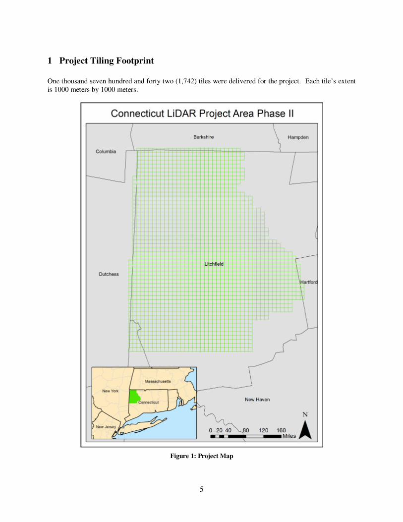
1 Project Tiling Footprint
One thousand seven hundred and forty two (1,742) tiles were delivered for the project. Each tile’s extent
is 1000 meters by 1000 meters.
Figure 1: Project Map
6
1.1 List of delivered tiles (1,742):
18TXM2306
18TXM2307
18TXM2308
18TXM2309
18TXM2310
18TXM2311
18TXM2312
18TXM2313
18TXM2314
18TXM2315
18TXM2316
18TXM2317
18TXM2318
18TXM2319
18TXM2320
18TXM2321
18TXM2322
18TXM2323
18TXM2324
18TXM2325
18TXM2326
18TXM2327
18TXM2328
18TXM2406
18TXM2407
18TXM2408
18TXM2409
18TXM2410
18TXM2411
18TXM2412
18TXM2413
18TXM2414
18TXM2415
18TXM2416
18TXM2417
18TXM2418
18TXM2419
18TXM2420
18TXM2421
18TXM2422
18TXM2423
18TXM2424
18TXM2425
18TXM2426
18TXM2427
18TXM2428
18TXM2429
18TXM2430
18TXM2431
18TXM2432
18TXM2433
18TXM2434
18TXM2435
18TXM2436
18TXM2437
18TXM2438
18TXM2439
18TXM2440
18TXM2441
18TXM2442
18TXM2443
18TXM2444
18TXM2445
18TXM2446
18TXM2447
18TXM2448
18TXM2449
18TXM2506
18TXM2507
18TXM2508
18TXM2509
18TXM2510
18TXM2511
18TXM2512
18TXM2513
18TXM2514
18TXM2515
18TXM2516
18TXM2517
18TXM2518
18TXM2519
18TXM2520
18TXM2521
18TXM2522
18TXM2523
18TXM2524
18TXM2525
18TXM2526
18TXM2527
18TXM2528
18TXM2529
18TXM2530
18TXM2531
18TXM2532
18TXM2533
18TXM2534
18TXM2535
18TXM2536
18TXM2537
18TXM2538
18TXM2539
18TXM2540
18TXM2541
18TXM2542
18TXM2543
18TXM2544
18TXM2545
18TXM2546
18TXM2547
18TXM2548
18TXM2549
18TXM2550
18TXM2551
18TXM2552
18TXM2553
18TXM2554
18TXM2555
18TXM2556
18TXM2606
18TXM2607
18TXM2608
18TXM2609
18TXM2610
18TXM2611
18TXM2612
18TXM2613
18TXM2614
18TXM2615
18TXM2616
18TXM2617
18TXM2618
18TXM2619
18TXM2620
18TXM2621
18TXM2622
18TXM2623
18TXM2624
18TXM2625
18TXM2626
18TXM2627
18TXM2628
18TXM2629
18TXM2630
18TXM2631
18TXM2632
18TXM2633
18TXM2634
18TXM2635
18TXM2636
18TXM2637
18TXM2638
18TXM2639
18TXM2640
18TXM2641
18TXM2642
18TXM2643
18TXM2644
18TXM2645
18TXM2646
18TXM2647
18TXM2648
18TXM2649
18TXM2650
18TXM2651
7
18TXM2652
18TXM2653
18TXM2654
18TXM2655
18TXM2656
18TXM2706
18TXM2707
18TXM2708
18TXM2709
18TXM2710
18TXM2711
18TXM2712
18TXM2713
18TXM2714
18TXM2715
18TXM2716
18TXM2717
18TXM2718
18TXM2719
18TXM2720
18TXM2721
18TXM2722
18TXM2723
18TXM2724
18TXM2725
18TXM2726
18TXM2727
18TXM2728
18TXM2729
18TXM2730
18TXM2731
18TXM2732
18TXM2733
18TXM2734
18TXM2735
18TXM2736
18TXM2737
18TXM2738
18TXM2739
18TXM2740
18TXM2741
18TXM2742
18TXM2743
18TXM2744
18TXM2745
18TXM2746
18TXM2747
18TXM2748
18TXM2749
18TXM2750
18TXM2751
18TXM2752
18TXM2753
18TXM2754
18TXM2755
18TXM2756
18TXM2806
18TXM2807
18TXM2808
18TXM2809
18TXM2810
18TXM2811
18TXM2812
18TXM2813
18TXM2814
18TXM2815
18TXM2816
18TXM2817
18TXM2818
18TXM2819
18TXM2820
18TXM2821
18TXM2822
18TXM2823
18TXM2824
18TXM2825
18TXM2826
18TXM2827
18TXM2828
18TXM2829
18TXM2830
18TXM2831
18TXM2832
18TXM2833
18TXM2834
18TXM2835
18TXM2836
18TXM2837
18TXM2838
18TXM2839
18TXM2840
18TXM2841
18TXM2842
18TXM2843
18TXM2844
18TXM2845
18TXM2846
18TXM2847
18TXM2848
18TXM2849
18TXM2850
18TXM2851
18TXM2852
18TXM2853
18TXM2854
18TXM2855
18TXM2856
18TXM2906
18TXM2907
18TXM2908
18TXM2909
18TXM2910
18TXM2911
18TXM2912
18TXM2913
18TXM2914
18TXM2915
18TXM2916
18TXM2917
18TXM2918
18TXM2919
18TXM2920
18TXM2921
18TXM2922
18TXM2923
18TXM2924
18TXM2925
18TXM2926
18TXM2927
18TXM2928
18TXM2929
18TXM2930
18TXM2931
18TXM2932
18TXM2933
18TXM2934
18TXM2935
18TXM2936
18TXM2937
18TXM2938
18TXM2939
18TXM2940
18TXM2941
18TXM2942
18TXM2943
18TXM2944
18TXM2945
18TXM2946
18TXM2947
18TXM2948
18TXM2949
18TXM2950
18TXM2951
18TXM2952
18TXM2953
18TXM2954
18TXM2955
18TXM2956
18TXM3006
18TXM3007
18TXM3008
18TXM3009
18TXM3010
18TXM3011
18TXM3012
18TXM3013
18TXM3014
18TXM3015
18TXM3016
18TXM3017
18TXM3018
18TXM3019
8
18TXM3020
18TXM3021
18TXM3022
18TXM3023
18TXM3024
18TXM3025
18TXM3026
18TXM3027
18TXM3028
18TXM3029
18TXM3030
18TXM3031
18TXM3032
18TXM3033
18TXM3034
18TXM3035
18TXM3036
18TXM3037
18TXM3038
18TXM3039
18TXM3040
18TXM3041
18TXM3042
18TXM3043
18TXM3044
18TXM3045
18TXM3046
18TXM3047
18TXM3048
18TXM3049
18TXM3050
18TXM3051
18TXM3052
18TXM3053
18TXM3054
18TXM3055
18TXM3056
18TXM3106
18TXM3107
18TXM3108
18TXM3109
18TXM3110
18TXM3111
18TXM3112
18TXM3113
18TXM3114
18TXM3115
18TXM3116
18TXM3117
18TXM3118
18TXM3119
18TXM3120
18TXM3121
18TXM3122
18TXM3123
18TXM3124
18TXM3125
18TXM3126
18TXM3127
18TXM3128
18TXM3129
18TXM3130
18TXM3131
18TXM3132
18TXM3133
18TXM3134
18TXM3135
18TXM3136
18TXM3137
18TXM3138
18TXM3139
18TXM3140
18TXM3141
18TXM3142
18TXM3143
18TXM3144
18TXM3145
18TXM3146
18TXM3147
18TXM3148
18TXM3149
18TXM3150
18TXM3151
18TXM3152
18TXM3153
18TXM3154
18TXM3155
18TXM3156
18TXM3206
18TXM3207
18TXM3208
18TXM3209
18TXM3210
18TXM3211
18TXM3212
18TXM3213
18TXM3214
18TXM3215
18TXM3216
18TXM3217
18TXM3218
18TXM3219
18TXM3220
18TXM3221
18TXM3222
18TXM3223
18TXM3224
18TXM3225
18TXM3226
18TXM3227
18TXM3228
18TXM3229
18TXM3230
18TXM3231
18TXM3232
18TXM3233
18TXM3234
18TXM3235
18TXM3236
18TXM3237
18TXM3238
18TXM3239
18TXM3240
18TXM3241
18TXM3242
18TXM3243
18TXM3244
18TXM3245
18TXM3246
18TXM3247
18TXM3248
18TXM3249
18TXM3250
18TXM3251
18TXM3252
18TXM3253
18TXM3254
18TXM3255
18TXM3256
18TXM3306
18TXM3307
18TXM3308
18TXM3309
18TXM3310
18TXM3311
18TXM3312
18TXM3313
18TXM3314
18TXM3315
18TXM3316
18TXM3317
18TXM3318
18TXM3319
18TXM3320
18TXM3321
18TXM3322
18TXM3323
18TXM3324
18TXM3325
18TXM3326
18TXM3327
18TXM3328
18TXM3329
18TXM3330
18TXM3331
18TXM3332
18TXM3333
18TXM3334
18TXM3335
18TXM3336
18TXM3337
18TXM3338
9
18TXM3339
18TXM3340
18TXM3341
18TXM3342
18TXM3343
18TXM3344
18TXM3345
18TXM3346
18TXM3347
18TXM3348
18TXM3349
18TXM3350
18TXM3351
18TXM3352
18TXM3353
18TXM3354
18TXM3355
18TXM3356
18TXM3406
18TXM3407
18TXM3408
18TXM3409
18TXM3410
18TXM3411
18TXM3412
18TXM3413
18TXM3414
18TXM3415
18TXM3416
18TXM3417
18TXM3418
18TXM3419
18TXM3420
18TXM3421
18TXM3422
18TXM3423
18TXM3424
18TXM3425
18TXM3426
18TXM3427
18TXM3428
18TXM3429
18TXM3430
18TXM3431
18TXM3432
18TXM3433
18TXM3434
18TXM3435
18TXM3436
18TXM3437
18TXM3438
18TXM3439
18TXM3440
18TXM3441
18TXM3442
18TXM3443
18TXM3444
18TXM3445
18TXM3446
18TXM3447
18TXM3448
18TXM3449
18TXM3450
18TXM3451
18TXM3452
18TXM3453
18TXM3454
18TXM3455
18TXM3456
18TXM3506
18TXM3507
18TXM3508
18TXM3509
18TXM3510
18TXM3511
18TXM3512
18TXM3513
18TXM3514
18TXM3515
18TXM3516
18TXM3517
18TXM3518
18TXM3519
18TXM3520
18TXM3521
18TXM3522
18TXM3523
18TXM3524
18TXM3525
18TXM3526
18TXM3527
18TXM3528
18TXM3529
18TXM3530
18TXM3531
18TXM3532
18TXM3533
18TXM3534
18TXM3535
18TXM3536
18TXM3537
18TXM3538
18TXM3539
18TXM3540
18TXM3541
18TXM3542
18TXM3543
18TXM3544
18TXM3545
18TXM3546
18TXM3547
18TXM3548
18TXM3549
18TXM3550
18TXM3551
18TXM3552
18TXM3553
18TXM3554
18TXM3555
18TXM3556
18TXM3606
18TXM3607
18TXM3608
18TXM3609
18TXM3610
18TXM3611
18TXM3612
18TXM3613
18TXM3614
18TXM3615
18TXM3616
18TXM3617
18TXM3618
18TXM3619
18TXM3620
18TXM3621
18TXM3622
18TXM3623
18TXM3624
18TXM3625
18TXM3626
18TXM3627
18TXM3628
18TXM3629
18TXM3630
18TXM3631
18TXM3632
18TXM3633
18TXM3634
18TXM3635
18TXM3636
18TXM3637
18TXM3638
18TXM3639
18TXM3640
18TXM3641
18TXM3642
18TXM3643
18TXM3644
18TXM3645
18TXM3646
18TXM3647
18TXM3648
18TXM3649
18TXM3650
18TXM3651
18TXM3652
18TXM3653
18TXM3654
18TXM3655
18TXM3656
18TXM3706
10
18TXM3707
18TXM3708
18TXM3709
18TXM3710
18TXM3711
18TXM3712
18TXM3713
18TXM3714
18TXM3715
18TXM3716
18TXM3717
18TXM3718
18TXM3719
18TXM3720
18TXM3721
18TXM3722
18TXM3723
18TXM3724
18TXM3725
18TXM3726
18TXM3727
18TXM3728
18TXM3729
18TXM3730
18TXM3731
18TXM3732
18TXM3733
18TXM3734
18TXM3735
18TXM3736
18TXM3737
18TXM3738
18TXM3739
18TXM3740
18TXM3741
18TXM3742
18TXM3743
18TXM3744
18TXM3745
18TXM3746
18TXM3747
18TXM3748
18TXM3749
18TXM3750
18TXM3751
18TXM3752
18TXM3753
18TXM3754
18TXM3755
18TXM3756
18TXM3806
18TXM3807
18TXM3808
18TXM3809
18TXM3810
18TXM3811
18TXM3812
18TXM3813
18TXM3814
18TXM3815
18TXM3816
18TXM3817
18TXM3818
18TXM3819
18TXM3820
18TXM3821
18TXM3822
18TXM3823
18TXM3824
18TXM3825
18TXM3826
18TXM3827
18TXM3828
18TXM3829
18TXM3830
18TXM3831
18TXM3832
18TXM3833
18TXM3834
18TXM3835
18TXM3836
18TXM3837
18TXM3838
18TXM3839
18TXM3840
18TXM3841
18TXM3842
18TXM3843
18TXM3844
18TXM3845
18TXM3846
18TXM3847
18TXM3848
18TXM3849
18TXM3850
18TXM3851
18TXM3852
18TXM3853
18TXM3854
18TXM3855
18TXM3856
18TXM3906
18TXM3907
18TXM3908
18TXM3909
18TXM3910
18TXM3911
18TXM3912
18TXM3913
18TXM3914
18TXM3915
18TXM3916
18TXM3917
18TXM3918
18TXM3919
18TXM3920
18TXM3921
18TXM3922
18TXM3923
18TXM3924
18TXM3925
18TXM3926
18TXM3927
18TXM3928
18TXM3929
18TXM3930
18TXM3931
18TXM3932
18TXM3933
18TXM3934
18TXM3935
18TXM3936
18TXM3937
18TXM3938
18TXM3939
18TXM3940
18TXM3941
18TXM3942
18TXM3943
18TXM3944
18TXM3945
18TXM3946
18TXM3947
18TXM3948
18TXM3949
18TXM3950
18TXM3951
18TXM3952
18TXM3953
18TXM3954
18TXM3955
18TXM3956
18TXM4006
18TXM4007
18TXM4008
18TXM4009
18TXM4010
18TXM4011
18TXM4012
18TXM4013
18TXM4014
18TXM4015
18TXM4016
18TXM4017
18TXM4018
18TXM4019
18TXM4020
18TXM4021
18TXM4022
18TXM4023
18TXM4024
18TXM4025
11
18TXM4026
18TXM4027
18TXM4028
18TXM4029
18TXM4030
18TXM4031
18TXM4032
18TXM4033
18TXM4034
18TXM4035
18TXM4036
18TXM4037
18TXM4038
18TXM4039
18TXM4040
18TXM4041
18TXM4042
18TXM4043
18TXM4044
18TXM4045
18TXM4046
18TXM4047
18TXM4048
18TXM4049
18TXM4050
18TXM4051
18TXM4052
18TXM4053
18TXM4054
18TXM4055
18TXM4056
18TXM4106
18TXM4107
18TXM4108
18TXM4109
18TXM4110
18TXM4111
18TXM4112
18TXM4113
18TXM4114
18TXM4115
18TXM4116
18TXM4117
18TXM4118
18TXM4119
18TXM4120
18TXM4121
18TXM4122
18TXM4123
18TXM4124
18TXM4125
18TXM4126
18TXM4127
18TXM4128
18TXM4129
18TXM4130
18TXM4131
18TXM4132
18TXM4133
18TXM4134
18TXM4135
18TXM4136
18TXM4137
18TXM4138
18TXM4139
18TXM4140
18TXM4141
18TXM4142
18TXM4143
18TXM4144
18TXM4145
18TXM4146
18TXM4147
18TXM4148
18TXM4149
18TXM4150
18TXM4151
18TXM4152
18TXM4153
18TXM4154
18TXM4155
18TXM4156
18TXM4206
18TXM4207
18TXM4208
18TXM4209
18TXM4210
18TXM4211
18TXM4212
18TXM4213
18TXM4214
18TXM4215
18TXM4216
18TXM4217
18TXM4218
18TXM4219
18TXM4220
18TXM4221
18TXM4222
18TXM4223
18TXM4224
18TXM4225
18TXM4226
18TXM4227
18TXM4228
18TXM4229
18TXM4230
18TXM4231
18TXM4232
18TXM4233
18TXM4234
18TXM4235
18TXM4236
18TXM4237
18TXM4238
18TXM4239
18TXM4240
18TXM4241
18TXM4242
18TXM4243
18TXM4244
18TXM4245
18TXM4246
18TXM4247
18TXM4248
18TXM4249
18TXM4250
18TXM4251
18TXM4252
18TXM4253
18TXM4254
18TXM4255
18TXM4256
18TXM4306
18TXM4307
18TXM4308
18TXM4309
18TXM4310
18TXM4311
18TXM4312
18TXM4313
18TXM4314
18TXM4315
18TXM4316
18TXM4317
18TXM4318
18TXM4319
18TXM4320
18TXM4321
18TXM4322
18TXM4323
18TXM4324
18TXM4325
18TXM4326
18TXM4327
18TXM4328
18TXM4329
18TXM4330
18TXM4331
18TXM4332
18TXM4333
18TXM4334
18TXM4335
18TXM4336
18TXM4337
18TXM4338
18TXM4339
18TXM4340
18TXM4341
18TXM4342
18TXM4343
18TXM4344
12
18TXM4345
18TXM4346
18TXM4347
18TXM4348
18TXM4349
18TXM4350
18TXM4351
18TXM4352
18TXM4353
18TXM4354
18TXM4355
18TXM4356
18TXM4406
18TXM4407
18TXM4408
18TXM4409
18TXM4410
18TXM4411
18TXM4412
18TXM4413
18TXM4414
18TXM4415
18TXM4416
18TXM4417
18TXM4418
18TXM4419
18TXM4420
18TXM4421
18TXM4422
18TXM4423
18TXM4424
18TXM4425
18TXM4426
18TXM4427
18TXM4428
18TXM4429
18TXM4430
18TXM4431
18TXM4432
18TXM4433
18TXM4434
18TXM4435
18TXM4436
18TXM4437
18TXM4438
18TXM4439
18TXM4440
18TXM4441
18TXM4442
18TXM4443
18TXM4444
18TXM4445
18TXM4446
18TXM4447
18TXM4448
18TXM4449
18TXM4450
18TXM4451
18TXM4452
18TXM4453
18TXM4454
18TXM4455
18TXM4456
18TXM4506
18TXM4507
18TXM4508
18TXM4509
18TXM4510
18TXM4511
18TXM4512
18TXM4513
18TXM4514
18TXM4515
18TXM4516
18TXM4517
18TXM4518
18TXM4519
18TXM4520
18TXM4521
18TXM4522
18TXM4523
18TXM4524
18TXM4525
18TXM4526
18TXM4527
18TXM4528
18TXM4529
18TXM4530
18TXM4531
18TXM4532
18TXM4533
18TXM4534
18TXM4535
18TXM4536
18TXM4537
18TXM4538
18TXM4539
18TXM4540
18TXM4541
18TXM4542
18TXM4543
18TXM4544
18TXM4545
18TXM4546
18TXM4547
18TXM4548
18TXM4549
18TXM4550
18TXM4551
18TXM4552
18TXM4553
18TXM4554
18TXM4555
18TXM4556
18TXM4606
18TXM4607
18TXM4608
18TXM4609
18TXM4610
18TXM4611
18TXM4612
18TXM4613
18TXM4614
18TXM4615
18TXM4616
18TXM4617
18TXM4618
18TXM4619
18TXM4620
18TXM4621
18TXM4622
18TXM4623
18TXM4624
18TXM4625
18TXM4626
18TXM4627
18TXM4628
18TXM4629
18TXM4630
18TXM4631
18TXM4632
18TXM4633
18TXM4634
18TXM4635
18TXM4636
18TXM4637
18TXM4638
18TXM4639
18TXM4640
18TXM4641
18TXM4642
18TXM4643
18TXM4644
18TXM4645
18TXM4646
18TXM4647
18TXM4648
18TXM4649
18TXM4650
18TXM4651
18TXM4652
18TXM4653
18TXM4654
18TXM4655
18TXM4656
18TXM4706
18TXM4707
18TXM4708
18TXM4709
18TXM4710
18TXM4711
18TXM4712
13
18TXM4713
18TXM4714
18TXM4715
18TXM4716
18TXM4717
18TXM4718
18TXM4719
18TXM4720
18TXM4721
18TXM4722
18TXM4723
18TXM4724
18TXM4725
18TXM4726
18TXM4727
18TXM4728
18TXM4729
18TXM4730
18TXM4731
18TXM4732
18TXM4733
18TXM4734
18TXM4735
18TXM4736
18TXM4737
18TXM4738
18TXM4739
18TXM4740
18TXM4741
18TXM4742
18TXM4743
18TXM4744
18TXM4745
18TXM4746
18TXM4747
18TXM4748
18TXM4749
18TXM4750
18TXM4751
18TXM4752
18TXM4753
18TXM4754
18TXM4755
18TXM4756
18TXM4806
18TXM4807
18TXM4808
18TXM4809
18TXM4810
18TXM4811
18TXM4812
18TXM4813
18TXM4814
18TXM4815
18TXM4816
18TXM4817
18TXM4818
18TXM4819
18TXM4820
18TXM4821
18TXM4822
18TXM4823
18TXM4824
18TXM4825
18TXM4826
18TXM4827
18TXM4828
18TXM4829
18TXM4830
18TXM4831
18TXM4832
18TXM4833
18TXM4834
18TXM4835
18TXM4836
18TXM4837
18TXM4838
18TXM4839
18TXM4840
18TXM4841
18TXM4842
18TXM4843
18TXM4844
18TXM4845
18TXM4846
18TXM4847
18TXM4848
18TXM4849
18TXM4850
18TXM4851
18TXM4852
18TXM4853
18TXM4854
18TXM4855
18TXM4856
18TXM4906
18TXM4907
18TXM4908
18TXM4909
18TXM4910
18TXM4911
18TXM4912
18TXM4913
18TXM4914
18TXM4915
18TXM4916
18TXM4917
18TXM4918
18TXM4919
18TXM4920
18TXM4921
18TXM4922
18TXM4923
18TXM4924
18TXM4925
18TXM4926
18TXM4927
18TXM4928
18TXM4929
18TXM4930
18TXM4931
18TXM4932
18TXM4933
18TXM4934
18TXM4935
18TXM4936
18TXM4937
18TXM4938
18TXM4939
18TXM4940
18TXM4941
18TXM4942
18TXM4943
18TXM4944
18TXM4945
18TXM4946
18TXM4947
18TXM4948
18TXM4949
18TXM4950
18TXM4951
18TXM4952
18TXM4953
18TXM4954
18TXM4955
18TXM4956
18TXM5006
18TXM5007
18TXM5008
18TXM5009
18TXM5010
18TXM5011
18TXM5012
18TXM5013
18TXM5014
18TXM5015
18TXM5016
18TXM5017
18TXM5018
18TXM5019
18TXM5020
18TXM5021
18TXM5022
18TXM5023
18TXM5024
18TXM5025
18TXM5026
18TXM5027
18TXM5028
18TXM5029
18TXM5030
18TXM5031
14
18TXM5032
18TXM5033
18TXM5034
18TXM5035
18TXM5036
18TXM5037
18TXM5038
18TXM5039
18TXM5040
18TXM5041
18TXM5042
18TXM5043
18TXM5044
18TXM5045
18TXM5048
18TXM5049
18TXM5050
18TXM5051
18TXM5052
18TXM5053
18TXM5054
18TXM5055
18TXM5056
18TXM5106
18TXM5107
18TXM5108
18TXM5109
18TXM5110
18TXM5111
18TXM5112
18TXM5113
18TXM5114
18TXM5115
18TXM5116
18TXM5117
18TXM5118
18TXM5119
18TXM5120
18TXM5121
18TXM5122
18TXM5123
18TXM5124
18TXM5125
18TXM5126
18TXM5127
18TXM5128
18TXM5129
18TXM5130
18TXM5131
18TXM5132
18TXM5133
18TXM5134
18TXM5135
18TXM5136
18TXM5137
18TXM5138
18TXM5139
18TXM5140
18TXM5141
18TXM5142
18TXM5143
18TXM5144
18TXM5145
18TXM5149
18TXM5150
18TXM5151
18TXM5154
18TXM5155
18TXM5206
18TXM5207
18TXM5208
18TXM5209
18TXM5210
18TXM5211
18TXM5212
18TXM5213
18TXM5214
18TXM5215
18TXM5216
18TXM5217
18TXM5218
18TXM5219
18TXM5220
18TXM5221
18TXM5222
18TXM5223
18TXM5224
18TXM5225
18TXM5226
18TXM5227
18TXM5228
18TXM5229
18TXM5230
18TXM5231
18TXM5232
18TXM5233
18TXM5234
18TXM5235
18TXM5236
18TXM5237
18TXM5238
18TXM5239
18TXM5240
18TXM5241
18TXM5242
18TXM5243
18TXM5244
18TXM5306
18TXM5307
18TXM5308
18TXM5309
18TXM5310
18TXM5311
18TXM5312
18TXM5313
18TXM5314
18TXM5315
18TXM5316
18TXM5317
18TXM5318
18TXM5319
18TXM5320
18TXM5321
18TXM5322
18TXM5323
18TXM5324
18TXM5325
18TXM5326
18TXM5327
18TXM5328
18TXM5329
18TXM5330
18TXM5331
18TXM5332
18TXM5333
18TXM5334
18TXM5335
18TXM5336
18TXM5337
18TXM5338
18TXM5339
18TXM5340
18TXM5341
18TXM5342
18TXM5343
18TXM5344
18TXM5414
18TXM5415
18TXM5416
18TXM5417
18TXM5418
18TXM5419
18TXM5420
18TXM5421
18TXM5422
18TXM5423
18TXM5424
18TXM5425
18TXM5426
18TXM5427
18TXM5428
18TXM5429
18TXM5430
18TXM5431
18TXM5432
18TXM5433
18TXM5434
18TXM5435
18TXM5436
18TXM5437
18TXM5438
18TXM5439
15
18TXM5440
18TXM5441
18TXM5514
18TXM5515
18TXM5516
18TXM5517
18TXM5518
18TXM5519
18TXM5520
18TXM5521
18TXM5522
18TXM5523
18TXM5524
18TXM5525
18TXM5526
18TXM5527
18TXM5528
18TXM5529
18TXM5530
18TXM5531
18TXM5532
18TXM5533
18TXM5534
18TXM5535
18TXM5536
18TXM5537
18TXM5538
18TXM5539
18TXM5540
18TXM5541
18TXM5614
18TXM5615
18TXM5616
18TXM5617
18TXM5618
18TXM5619
18TXM5620
18TXM5621
18TXM5622
18TXM5623
18TXM5624
18TXM5625
18TXM5626
18TXM5627
18TXM5628
18TXM5629
18TXM5630
18TXM5631
18TXM5632
18TXM5633
18TXM5634
18TXM5635
18TXM5636
18TXM5637
18TXM5638
18TXM5639
18TXM5640
18TXM5714
18TXM5715
18TXM5716
18TXM5717
18TXM5718
18TXM5719
18TXM5720
18TXM5721
18TXM5722
18TXM5723
18TXM5724
18TXM5725
18TXM5726
18TXM5727
18TXM5728
18TXM5729
18TXM5730
18TXM5731
18TXM5732
18TXM5733
18TXM5735
18TXM5736
18TXM5816
18TXM5817
18TXM5818
18TXM5819
18TXM5820
18TXM5821
18TXM5822
18TXM5823
18TXM5824
18TXM5825
18TXM5826
18TXM5827
18TXM5828
18TXM5829
18TXM5830
18TXM5831
18TXM5832
18TXM5833
18TXM5916
18TXM5917
18TXM5918
18TXM5919
18TXM5920
18TXM5921
18TXM5922
18TXM5923
18TXM5924
18TXM5925
18TXM5926
18TXM5927
18TXM5928
18TXM5929
18TXM5930
18TXM5931
18TXM5932
18TXM5933
18TXM6016
18TXM6017
18TXM6018
18TXM6019
18TXM6020
18TXM6021
18TXM6022
18TXM6023
18TXM6024
18TXM6025
18TXM6026
18TXM6027
18TXM6028
18TXM6029
18TXM6030
18TXM6031
18TXM6032
18TXM6116
18TXM6117
18TXM6118
18TXM6119
18TXM6120
18TXM6121
18TXM6122
18TXM6123
18TXM6124
18TXM6125
18TXM6126
18TXM6127
18TXM6128
18TXM6129
18TXM6130
18TXM6131
18TXM6216
18TXM6217
18TXM6218
18TXM6219
18TXM6220
18TXM6221
18TXM6222
18TXM6223
18TXM6224
18TXM6225
18TXM6226
18TXM6227
18TXM6228
18TXM6229
18TXM6230
18TXM6316
18TXM6317
18TXM6318
18TXM6319
18TXM6320
18TXM6321
18TXM6322
18TXM6323
18TXM6324
16
18TXM6325
18TXM6326
18TXM6327
18TXM6328
18TXM6329
18TXM6330
18TXM6419
18TXM6420
18TXM6421
18TXM6422
18TXM6423
18TXM6424
18TXM6425
18TXM6426
18TXM6427
18TXM6428
18TXM6429
18TXM6519
18TXM6520
18TXM6521
18TXM6522
18TXM6523
18TXM6524
18TXM6525
18TXM6526
18TXM6527
18TXM6619
18TXM6620
18TXM6621
18TXM6622
17
2 LiDAR Acquisition Report
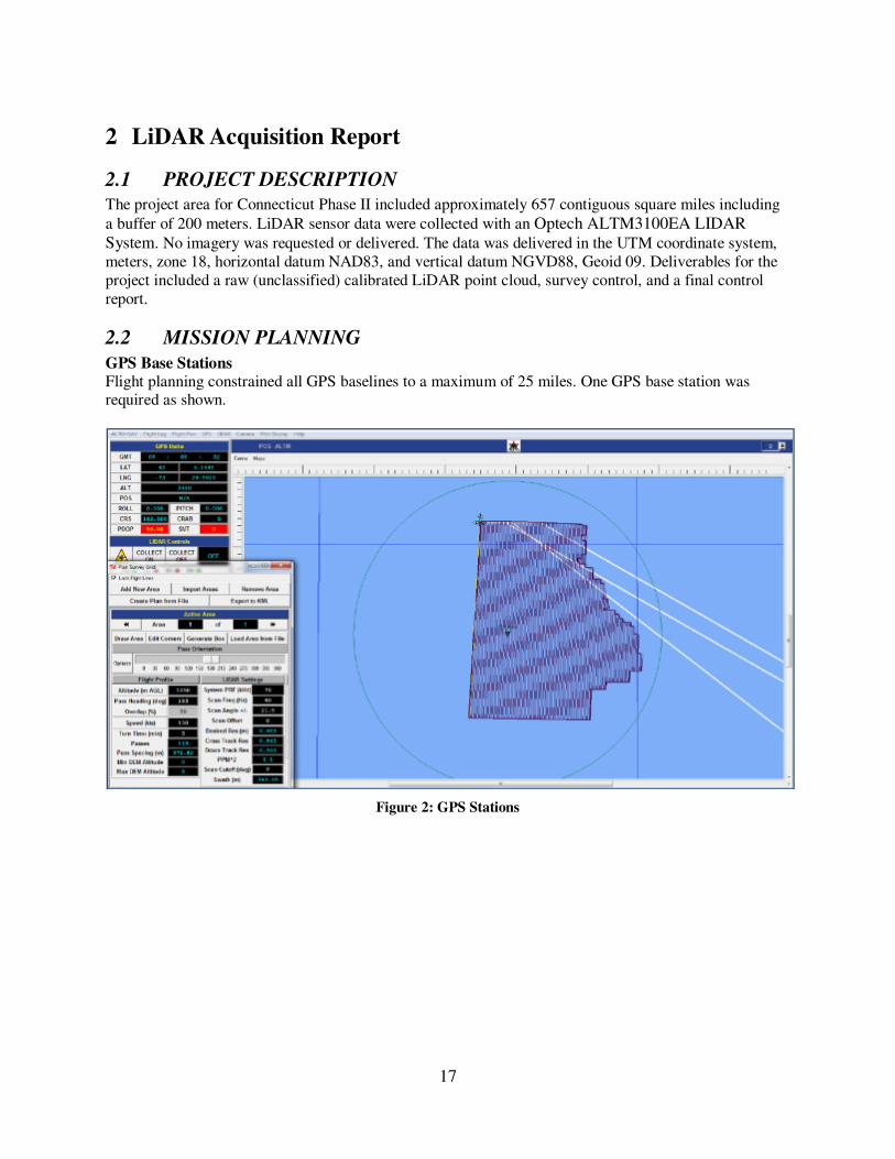
2.1 PROJECT DESCRIPTION
The project area for Connecticut Phase II included approximately 657 contiguous square miles including
a buffer of 200 meters. LiDAR sensor data were collected with an Optech ALTM3100EA LIDAR
System. No imagery was requested or delivered. The data was delivered in the UTM coordinate system,
meters, zone 18, horizontal datum NAD83, and vertical datum NGVD88, Geoid 09. Deliverables for the
project included a raw (unclassified) calibrated LiDAR point cloud, survey control, and a final control
report.
2.2 MISSION PLANNING
GPS Base Stations Flight planning constrained all GPS baselines to a maximum of 25 miles. One GPS base station was required as shown.
Figure 2: GPS Stations
18
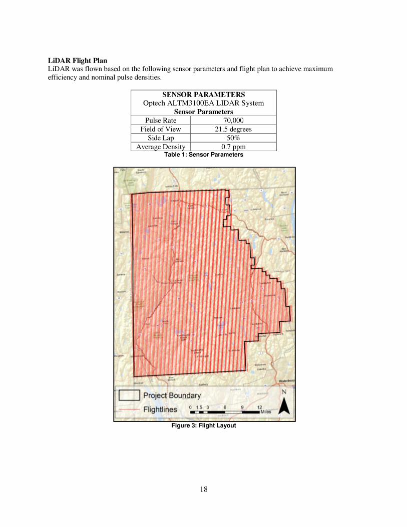
LiDAR Flight Plan LiDAR was flown based on the following sensor parameters and flight plan to achieve maximum
efficiency and nominal pulse densities.
SENSOR PARAMETERS
Optech ALTM3100EA LIDAR System
Sensor Parameters
Pulse Rate 70,000
Field of View 21.5 degrees
Side Lap 50%
Average Density 0.7 ppm Table 1: Sensor Parameters
Figure 3: Flight Layout

19
CONTROL LAYOUT A total of 7 distributed control points were planned and collected with static GPS observations as shown.
Figure 4: Control Points
2.3 ACQUISITION
Airborne LiDAR
Data acquisition commenced on December 13, 2011(Julian day 347) and was completed on
December 19, 2011(Julian day 353). 11 missions were flown to complete the acquisition. Flight lines
were flown according to the proposed flight layout with no changes. There were no unusual
occurrences and the acquisition went according to plan. The aircraft based out of Waterbury-Oxford
(KOXC) airport. NGS monument G59 was used as the primary base station for airborne missions
with an offset point set nearby as a backup GPS base station.
Survey Control Compliance with the accuracy standard was ensured through the collection of GPS ground control during the acquisition of aerial LiDAR and the establishment of a GPS base station operating at the airport. In
20
addition to the base stations, CORS bases may have been used to supplement the solutions. The following
criteria were adhered to during control point collection. 1. Each point was collected during periods of very low (<2) DOP.
2. No point was collected with a base line greater than 25 miles.
3. Each point was collected at a place of constant slope so as to minimize any errors introduced through
LiDAR triangulation. 4. Each point was collected at moderate intensity surfaces so any intensity based anomalies could be
avoided.
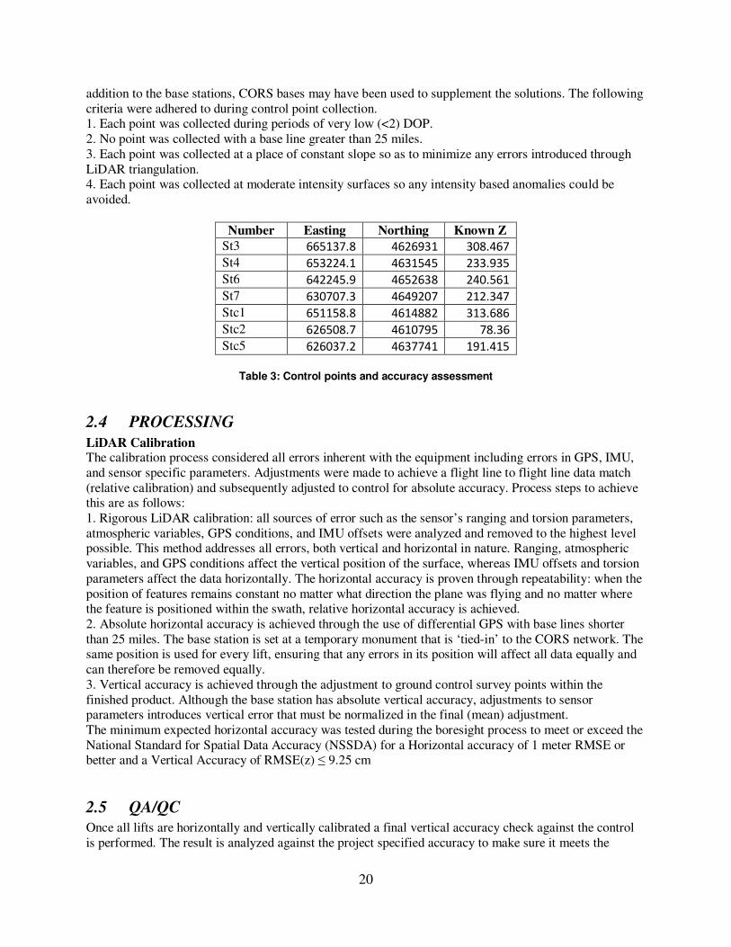
Number Easting Northing Known Z
St3 665137.8 4626931 308.467
St4 653224.1 4631545 233.935
St6 642245.9 4652638 240.561
St7 630707.3 4649207 212.347
Stc1 651158.8 4614882 313.686
Stc2 626508.7 4610795 78.36
Stc5 626037.2 4637741 191.415
Table 3: Control points and accuracy assessment
2.4 PROCESSING
LiDAR Calibration The calibration process considered all errors inherent with the equipment including errors in GPS, IMU,
and sensor specific parameters. Adjustments were made to achieve a flight line to flight line data match
(relative calibration) and subsequently adjusted to control for absolute accuracy. Process steps to achieve this are as follows:
1. Rigorous LiDAR calibration: all sources of error such as the sensor’s ranging and torsion parameters,
atmospheric variables, GPS conditions, and IMU offsets were analyzed and removed to the highest level possible. This method addresses all errors, both vertical and horizontal in nature. Ranging, atmospheric
variables, and GPS conditions affect the vertical position of the surface, whereas IMU offsets and torsion
parameters affect the data horizontally. The horizontal accuracy is proven through repeatability: when the
position of features remains constant no matter what direction the plane was flying and no matter where the feature is positioned within the swath, relative horizontal accuracy is achieved.
2. Absolute horizontal accuracy is achieved through the use of differential GPS with base lines shorter
than 25 miles. The base station is set at a temporary monument that is ‘tied-in’ to the CORS network. The same position is used for every lift, ensuring that any errors in its position will affect all data equally and
can therefore be removed equally.
3. Vertical accuracy is achieved through the adjustment to ground control survey points within the
finished product. Although the base station has absolute vertical accuracy, adjustments to sensor parameters introduces vertical error that must be normalized in the final (mean) adjustment.
The minimum expected horizontal accuracy was tested during the boresight process to meet or exceed the
National Standard for Spatial Data Accuracy (NSSDA) for a Horizontal accuracy of 1 meter RMSE or better and a Vertical Accuracy of RMSE(z) ≤ 9.25 cm
2.5 QA/QC
Once all lifts are horizontally and vertically calibrated a final vertical accuracy check against the control
is performed. The result is analyzed against the project specified accuracy to make sure it meets the

21
requirement. The final accuracy for this project yielded a 0.024 meter RMSEz @ 95% confidence level.
Following are list of all control points compared to the final calibrated LiDAR surface.
Number Easting Northing Known Z LiDAR Z Delta Z
St3 665137.8 4626931 308.467 308.47 0.003
St4 653224.1 4631545 233.935 233.94 0.005
St6 642245.9 4652638 240.561 240.56 -0.001
St7 630707.3 4649207 212.347 212.35 0.003
Stc1 651158.8 4614882 313.686 313.72 0.034
Stc2 626508.7 4610795 78.36 78.41 0.05
Stc5 626037.2 4637741 191.415 191.4 -0.015
Table 4: Final accuracy
2.6 Final Deliverables
Final project deliverables: 1. Calibrated raw (unclassified) LiDAR point clouds by flight line in las format
2. Survey Control points in excel format
3. Survey control accuracy report in excel format
4. Final Report PDF
Projections/Datums UTM coordinate system, meters, zone 18, horizontal datum NAD83, vertical datum NGVD88, Geoid 09
3 LiDAR Processing & Qualitative Assessment
3.1 Data Classification and Editing
Laser Mapping Specialist delivered LiDAR swaths to Dewberry that were calibrated and projected to project specifications. Dewberry processed the data using GeoCue and TerraScan software. The initial
step is the setup of the GeoCue project, which is done by importing a project defined tile boundary index
encompassing the entire project area. The acquired 3D laser point clouds, in LAS binary format, were imported into the GeoCue project and tiled according to the project tile grid. Once tiled, the laser points
were classified using a proprietary routine in TerraScan. This routine removes any obvious outliers from
the dataset following which the ground layer is extracted from the point cloud. The ground extraction
process encompassed in this routine takes place by building an iterative surface model.
This surface model is generated using three main parameters: building size, iteration angle and iteration
distance. The initial model is based on low points being selected by a "roaming window" with the assumption is that these are the ground points. The size of this roaming window is determined by the
building size parameter. The low points are triangulated and the remaining points are evaluated and
subsequently added to the model if they meet the iteration angle and distance constraints. This process is repeated until no additional points are added within iterations. A second critical parameter is the
maximum terrain angle constraint, which determines the maximum terrain angle allowed within the
classification model.
22
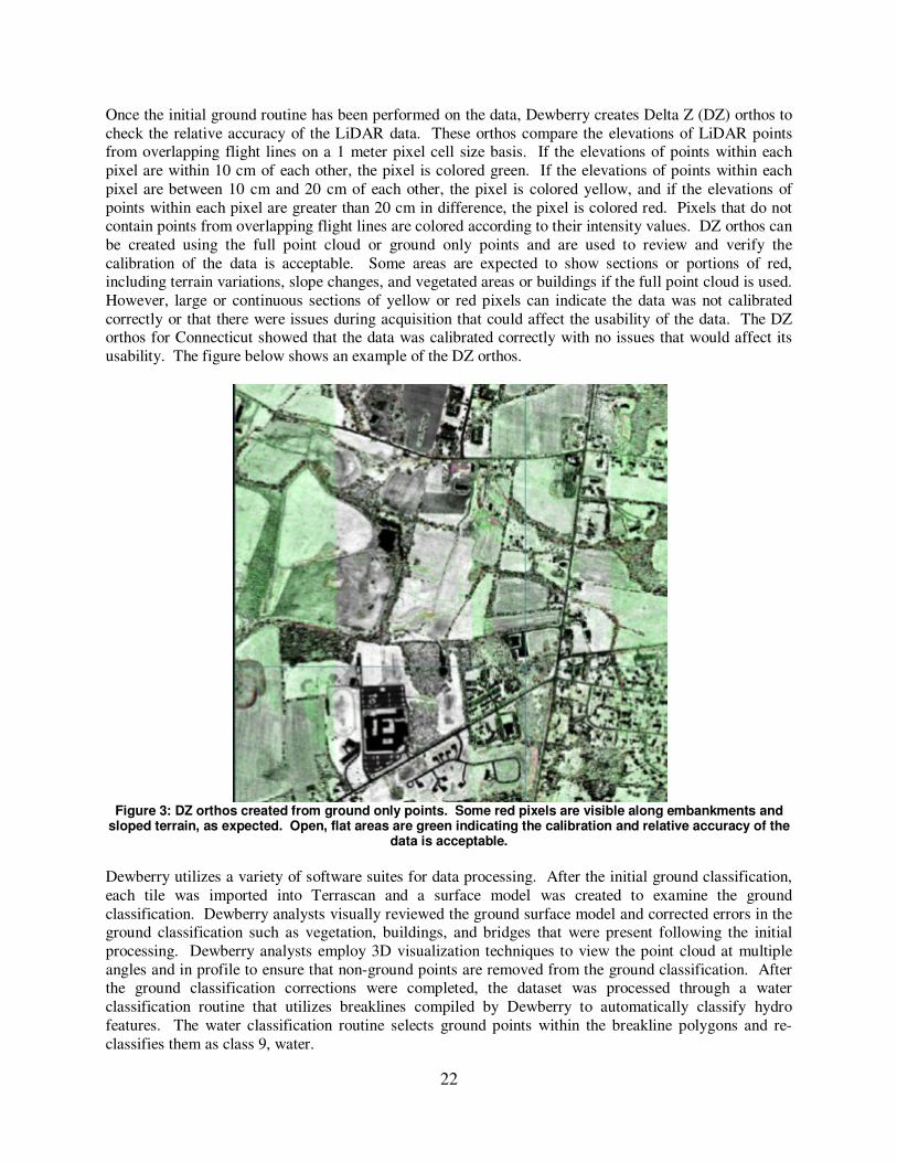
Once the initial ground routine has been performed on the data, Dewberry creates Delta Z (DZ) orthos to
check the relative accuracy of the LiDAR data. These orthos compare the elevations of LiDAR points from overlapping flight lines on a 1 meter pixel cell size basis. If the elevations of points within each
pixel are within 10 cm of each other, the pixel is colored green. If the elevations of points within each
pixel are between 10 cm and 20 cm of each other, the pixel is colored yellow, and if the elevations of
points within each pixel are greater than 20 cm in difference, the pixel is colored red. Pixels that do not contain points from overlapping flight lines are colored according to their intensity values. DZ orthos can
be created using the full point cloud or ground only points and are used to review and verify the
calibration of the data is acceptable. Some areas are expected to show sections or portions of red, including terrain variations, slope changes, and vegetated areas or buildings if the full point cloud is used.
However, large or continuous sections of yellow or red pixels can indicate the data was not calibrated
correctly or that there were issues during acquisition that could affect the usability of the data. The DZ orthos for Connecticut showed that the data was calibrated correctly with no issues that would affect its
usability. The figure below shows an example of the DZ orthos.
Figure 3: DZ orthos created from ground only points. Some red pixels are visible along embankments and
sloped terrain, as expected. Open, flat areas are green indicating the calibration and relative accuracy of the data is acceptable.
Dewberry utilizes a variety of software suites for data processing. After the initial ground classification,
each tile was imported into Terrascan and a surface model was created to examine the ground
classification. Dewberry analysts visually reviewed the ground surface model and corrected errors in the ground classification such as vegetation, buildings, and bridges that were present following the initial
processing. Dewberry analysts employ 3D visualization techniques to view the point cloud at multiple
angles and in profile to ensure that non-ground points are removed from the ground classification. After the ground classification corrections were completed, the dataset was processed through a water
classification routine that utilizes breaklines compiled by Dewberry to automatically classify hydro
features. The water classification routine selects ground points within the breakline polygons and re-
classifies them as class 9, water.
23
Terrascan was also used to create model key points. An algorithm is defined that intelligently thins bare earth ground points so that points necessary to define breaks and elevation changes in the terrain are kept
while unnecessary or redundant points are not included in the model key points. The model key points
are then written to its own file, according to the project tile grid, with all points located in class 8.
GeoCue was used to create the bare earth only LiDAR tiles, first return only LiDAR tiles, and last return
only LiDAR tiles. For bare earth only LiDAR tiles, class 2 points are filtered from the full point cloud
data and written to its own file, according to the project tile grid.
For first return and last return tiles, the desired echo return is filtered from the full point cloud and written
to its own file, according to the project tile grid. The first return and last return files include the desired return from all classes. The points for these files are located in class 1.
After all processing and classification has been completed, GeoCue software is used to update the LAS
version, projection information, creation day, and creation year of every LiDAR file.
3.2 Qualitative Assessment
Dewberry qualitative assessment utilizes a combination of statistical analysis and interpretative methodology to assess the quality of the data for a bare-earth digital elevation model (DEM). This
process looks for anomalies in the data and also identifies areas where man-made structures or vegetation
points may not have been classified properly to produce a bare-earth model.
Within this review of the LiDAR data, two fundamental questions were addressed:
• Did the LiDAR system perform to specifications?
• Did the vegetation removal process yield desirable results for the intended bare-earth terrain
product?
Mapping standards today address the quality of data by quantitative methods. If the data are tested and
found to be within the desired accuracy standard, then the data set is typically accepted. Now with the proliferation of LiDAR, new issues arise due to the vast amount of data. Unlike photogrammetrically-
derived DEMs where point spacing can be eight meters or more, LiDAR nominal point spacing for this
project is 1 point per 0.7 square meters. The end result is that millions of elevation points are measured to a level of accuracy previously unseen for traditional elevation mapping technologies and vegetated areas
are measured that would be nearly impossible to survey by other means. The downside is that with
millions of points, the dataset is statistically bound to have some errors both in the measurement process and in the artifact removal process.
As previously stated, the quantitative analysis addresses the quality of the data based on absolute
accuracy. This accuracy is directly tied to the comparison of the discreet measurement of the survey checkpoints and that of the interpolated value within the three closest LiDAR points that constitute the
vertices of a three-dimensional triangular face of the TIN. Therefore, the end result is that only a small
sample of the LiDAR data is actually tested. However there is an increased level of confidence with LiDAR data due to the relative accuracy. This relative accuracy is based on how well one LiDAR point
"fits" in comparison to the next contiguous LiDAR measurement, and is verified with DZ orthos. Once
the absolute and relative accuracy has been ascertained, the next stage is to address the cleanliness of the
data for a bare-earth DEM.

24
By using survey checkpoints to compare the data, the absolute accuracy is verified, but this also allows us
to understand if the artifact removal process was performed correctly. To reiterate the quantitative approach, if the LiDAR sensor operated correctly over open terrain areas, then it most likely operated
correctly over the vegetated areas. This does not mean that the entire bare-earth was measured; only that
the elevations surveyed are most likely accurate (including elevations of treetops, rooftops, etc.). In the
event that the LiDAR pulse filtered through the vegetation and was able to measure the true surface (as well as measurements on the surrounding vegetation) then the level of accuracy of the vegetation removal
process can be tested as a by-product.
To fully address the data for overall accuracy and quality, the level of cleanliness (or removal of above-
ground artifacts) is paramount. Since there are currently no effective automated testing procedures to
measure cleanliness, Dewberry employs a combination of statistical and visualization processes. This includes creating pseudo image products such as LiDAR orthos produced from the intensity returns,
Triangulated Irregular Network (TIN)’s, Digital Elevation Models (DEM) and 3-dimensional models. By
creating multiple images and using overlay techniques, not only can potential errors be found, but
Dewberry can also find where the data meets and exceeds expectations. This report will present representative examples where the LiDAR and post processing had issues as well as examples of where
the LiDAR performed well.
Dewberry utilizes GeoCue software as the primary geospatial process management system. GeoCue is a
three tier, multi-user architecture that uses .NET technology from Microsoft. .NET technology provides
the real-time notification system that updates users with real-time project status, regardless of who makes changes to project entities. GeoCue uses database technology for sorting project metadata. Dewberry
uses Microsoft SQL Server as the database of choice. Specific analysis is conducted in Terrascan and QT
Modeler environments.
Following the completion of LiDAR point classification, the Dewberry qualitative assessment process
flow for the Connecticut LiDAR project incorporated the following reviews:
1. Format: The LAS files are verified to meet project specifications. The LAS files conform to the
specifications outlined below.
- Format, Echos, Intensity
o LAS format 1.2, point data record format 1
o Point data record format 1
o Multiple returns (echos) per pulse
o Intensity values populated for each point
- ASPRS classification scheme
o Class 1 – unclassified
o Class 2 – ground
o Class 7 – Noise
o Class 9 – Water
- Projection
o Datum – North American Datum 1983
o Projected Coordinate System –UTM Zone 18N
o Units – Meters
o Vertical Datum – North American Vertical Datum 1988, Geoid 09
o Vertical Units - Meters
25
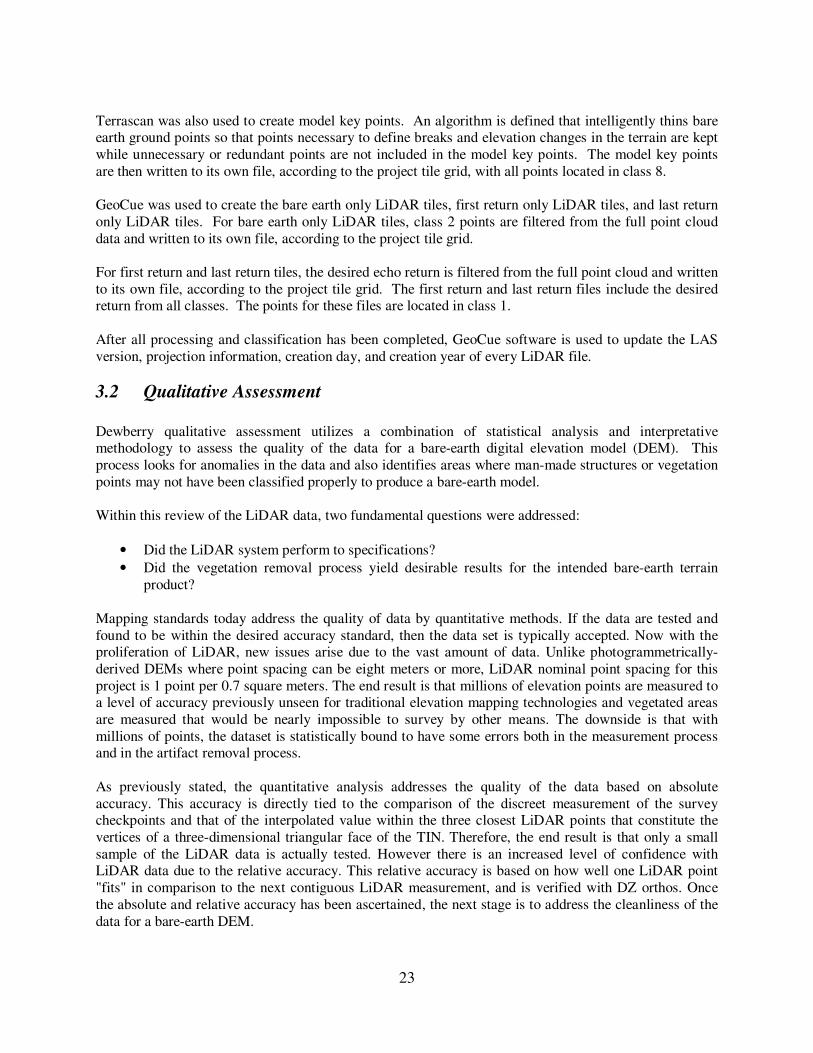
- LAS header information:
o Class (Integer)
o GPS Week Time (0.0001 seconds)
o Easting (0.01 foot)
o Northing (0.01 foot)
o Elevation (0.01 foot)
o Echo Number (Integer 1 to 4)
o Echo (Integer 1 to 4)
o Intensity (8 bit integer)
o Flight Line (Integer)
o Scan Angle (Integer degree)
2. Data density, data voids: The LAS files are used to produce Digital Elevation Models using the
commercial software package “QT Modeler” which creates a 3-dimensional data model derived
from Class 2 (ground points) in the LAS files. Grid spacing is based on the project density deliverable requirement for un-obscured areas. For the Connecticut LiDAR project it is stipulated
that the minimum post spacing in un-obscured areas should be 1 point per 0.7 square meter.
a. The Connecticut LiDAR data has full coverage. Only acceptable voids (areas with no
LiDAR returns in the LAS files) are present in the LiDAR, including voids caused by
bodies of water.
3. Bare earth quality: Dewberry reviewed the cleanliness of the bare earth to ensure the ground has
correct definition, meets the project requirements, there is correct classification of points, and there are less than 5% residual artifacts.
a. Building Removal: Large buildings, unique construction, and buildings built on sloped
terrain or built into the ground can make a noticeable impact on the bare earth DEM
once they have been removed, often in the form of large void areas with obvious
triangulation or interpolation across the area and general lack of detail in the ground
where the structure stood. Dewberry analysts verified that structures have been
removed from the ground, that areas along slopes missing definition are due to
structural or vegetation removal and not aggressive classification, and that holes or
removal of ground is accurate.
b. Flight Line Ridges: Dewberry reviewed DZ orthos to ensure acceptable calibration and
relative accuracy of the Connecticut data. No major issues were identified.
3.3 Conclusion
The dataset conforms to project specifications for format and header values. The spatial projection
information and classification of points is correct. Buildings, vegetation and other artifacts have been removed from the bare earth ground.
26
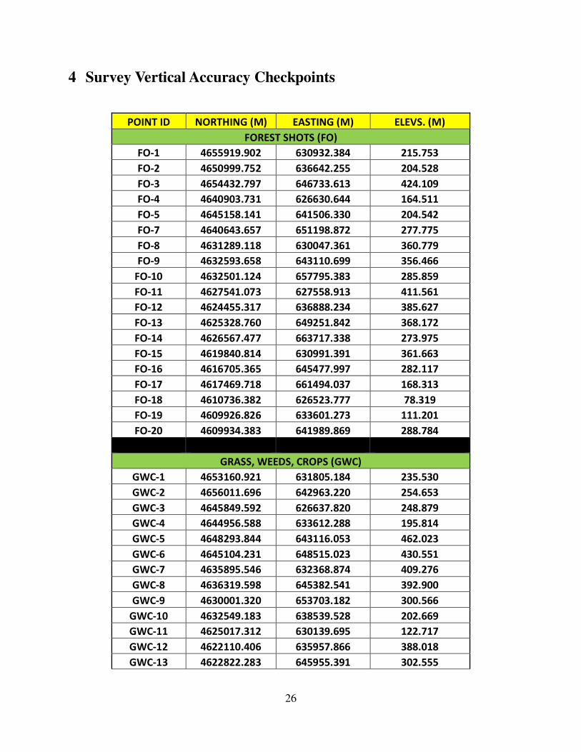
4 Survey Vertical Accuracy Checkpoints
POINT ID NORTHING (M) EASTING (M) ELEVS. (M)
FOREST SHOTS (FO)
FO-1 4655919.902 630932.384 215.753
FO-2 4650999.752 636642.255 204.528
FO-3 4654432.797 646733.613 424.109
FO-4 4640903.731 626630.644 164.511
FO-5 4645158.141 641506.330 204.542
FO-7 4640643.657 651198.872 277.775
FO-8 4631289.118 630047.361 360.779
FO-9 4632593.658 643110.699 356.466
FO-10 4632501.124 657795.383 285.859
FO-11 4627541.073 627558.913 411.561
FO-12 4624455.317 636888.234 385.627
FO-13 4625328.760 649251.842 368.172
FO-14 4626567.477 663717.338 273.975
FO-15 4619840.814 630991.391 361.663
FO-16 4616705.365 645477.997 282.117
FO-17 4617469.718 661494.037 168.313
FO-18 4610736.382 626523.777 78.319
FO-19 4609926.826 633601.273 111.201
FO-20 4609934.383 641989.869 288.784
GRASS, WEEDS, CROPS (GWC)
GWC-1 4653160.921 631805.184 235.530
GWC-2 4656011.696 642963.220 254.653
GWC-3 4645849.592 626637.820 248.879
GWC-4 4644956.588 633612.288 195.814
GWC-5 4648293.844 643116.053 462.023
GWC-6 4645104.231 648515.023 430.551
GWC-7 4635895.546 632368.874 409.276
GWC-8 4636319.598 645382.541 392.900
GWC-9 4630001.320 653703.182 300.566
GWC-10 4632549.183 638539.528 202.669
GWC-11 4625017.312 630139.695 122.717
GWC-12 4622110.406 635957.866 388.018
GWC-13 4622822.283 645955.391 302.555
27
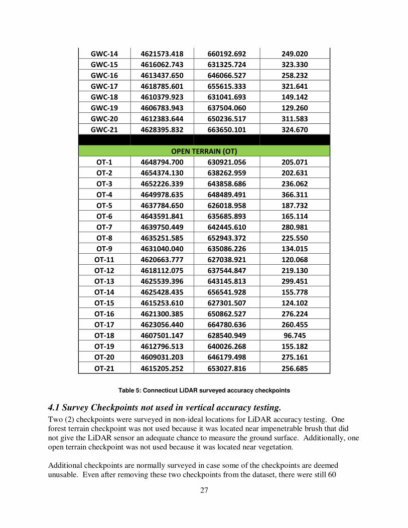
GWC-14 4621573.418 660192.692 249.020
GWC-15 4616062.743 631325.724 323.330
GWC-16 4613437.650 646066.527 258.232
GWC-17 4618785.601 655615.333 321.641
GWC-18 4610379.923 631041.693 149.142
GWC-19 4606783.943 637504.060 129.260
GWC-20 4612383.644 650236.517 311.583
GWC-21 4628395.832 663650.101 324.670
OPEN TERRAIN (OT)
OT-1 4648794.700 630921.056 205.071
OT-2 4654374.130 638262.959 202.631
OT-3 4652226.339 643858.686 236.062
OT-4 4649978.635 648489.491 366.311
OT-5 4637784.650 626018.958 187.732
OT-6 4643591.841 635685.893 165.114
OT-7 4639750.449 642445.610 280.981
OT-8 4635251.585 652943.372 225.550
OT-9 4631040.040 635086.226 134.015
OT-11 4620663.777 627038.921 120.068
OT-12 4618112.075 637544.847 219.130
OT-13 4625539.396 643145.813 299.451
OT-14 4625428.435 656541.928 155.778
OT-15 4615253.610 627301.507 124.102
OT-16 4621300.385 650862.527 276.224
OT-17 4623056.440 664780.636 260.455
OT-18 4607501.147 628540.949 96.745
OT-19 4612796.513 640026.268 155.182
OT-20 4609031.203 646179.498 275.161
OT-21 4615205.252 653027.816 256.685
Table 5: Connecticut LiDAR surveyed accuracy checkpoints
4.1 Survey Checkpoints not used in vertical accuracy testing.
Two (2) checkpoints were surveyed in non-ideal locations for LiDAR accuracy testing. One
forest terrain checkpoint was not used because it was located near impenetrable brush that did
not give the LiDAR sensor an adequate chance to measure the ground surface. Additionally, one
open terrain checkpoint was not used because it was located near vegetation.
Additional checkpoints are normally surveyed in case some of the checkpoints are deemed
unusable. Even after removing these two checkpoints from the dataset, there were still 60
28
checkpoints remaining for the vertical accuracy testing, meeting project requirements of 60 total
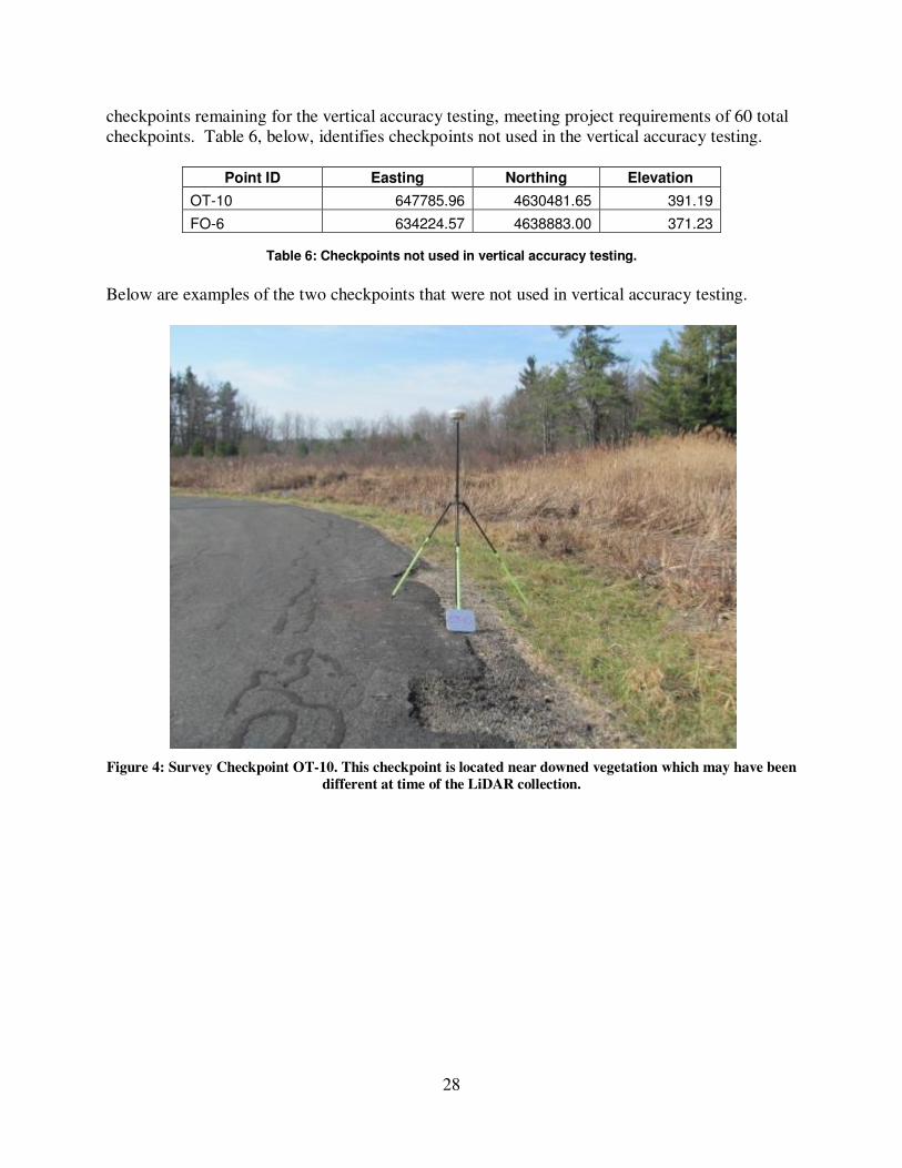
checkpoints. Table 6, below, identifies checkpoints not used in the vertical accuracy testing.
Point ID Easting Northing Elevation
OT-10 647785.96 4630481.65 391.19
FO-6 634224.57 4638883.00 371.23
Table 6: Checkpoints not used in vertical accuracy testing.
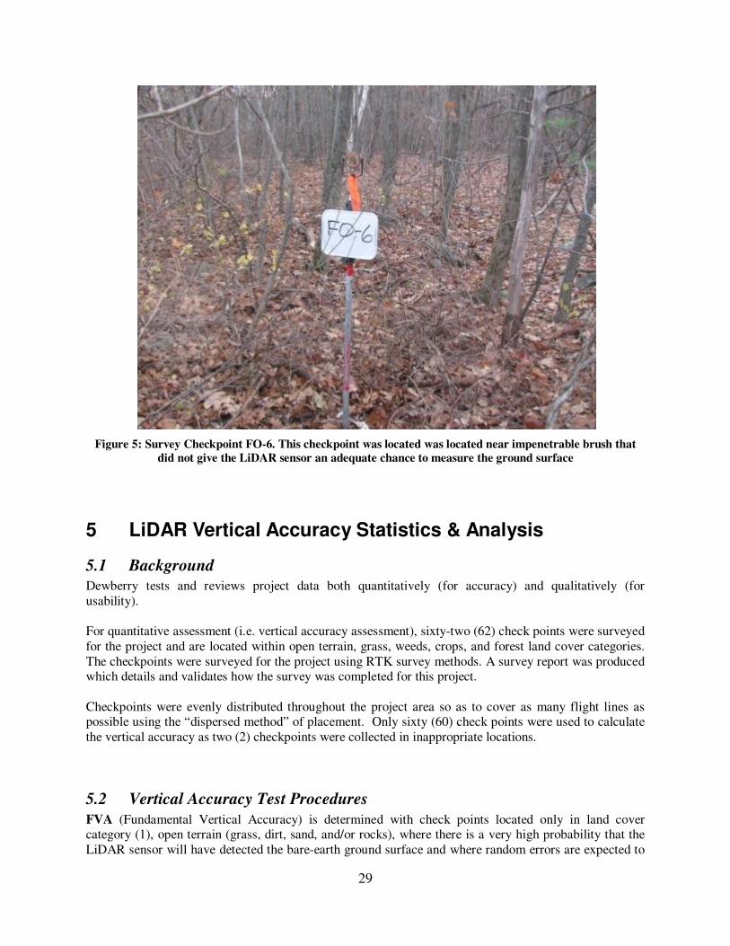
Below are examples of the two checkpoints that were not used in vertical accuracy testing.
Figure 4: Survey Checkpoint OT-10. This checkpoint is located near downed vegetation which may have been
different at time of the LiDAR collection.
29
Figure 5: Survey Checkpoint FO-6. This checkpoint was located was located near impenetrable brush that
did not give the LiDAR sensor an adequate chance to measure the ground surface
5 LiDAR Vertical Accuracy Statistics & Analysis
5.1 Background
Dewberry tests and reviews project data both quantitatively (for accuracy) and qualitatively (for
usability).
For quantitative assessment (i.e. vertical accuracy assessment), sixty-two (62) check points were surveyed
for the project and are located within open terrain, grass, weeds, crops, and forest land cover categories.
The checkpoints were surveyed for the project using RTK survey methods. A survey report was produced which details and validates how the survey was completed for this project.
Checkpoints were evenly distributed throughout the project area so as to cover as many flight lines as possible using the “dispersed method” of placement. Only sixty (60) check points were used to calculate
the vertical accuracy as two (2) checkpoints were collected in inappropriate locations.
5.2 Vertical Accuracy Test Procedures
FVA (Fundamental Vertical Accuracy) is determined with check points located only in land cover category (1), open terrain (grass, dirt, sand, and/or rocks), where there is a very high probability that the
LiDAR sensor will have detected the bare-earth ground surface and where random errors are expected to
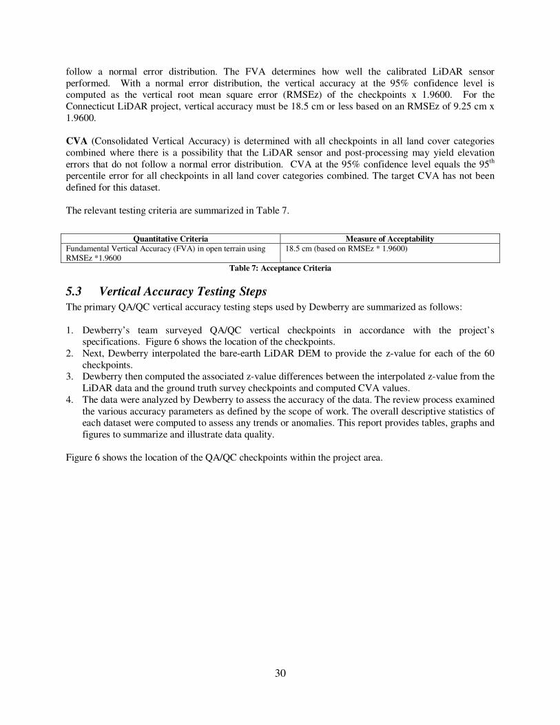
30
follow a normal error distribution. The FVA determines how well the calibrated LiDAR sensor
performed. With a normal error distribution, the vertical accuracy at the 95% confidence level is computed as the vertical root mean square error (RMSEz) of the checkpoints x 1.9600. For the
Connecticut LiDAR project, vertical accuracy must be 18.5 cm or less based on an RMSEz of 9.25 cm x
1.9600.
CVA (Consolidated Vertical Accuracy) is determined with all checkpoints in all land cover categories
combined where there is a possibility that the LiDAR sensor and post-processing may yield elevation
errors that do not follow a normal error distribution. CVA at the 95% confidence level equals the 95th
percentile error for all checkpoints in all land cover categories combined. The target CVA has not been
defined for this dataset.
The relevant testing criteria are summarized in Table 7.
Quantitative Criteria Measure of Acceptability
Fundamental Vertical Accuracy (FVA) in open terrain using RMSEz *1.9600
18.5 cm (based on RMSEz * 1.9600)
Table 7: Acceptance Criteria
5.3 Vertical Accuracy Testing Steps
The primary QA/QC vertical accuracy testing steps used by Dewberry are summarized as follows:
1. Dewberry’s team surveyed QA/QC vertical checkpoints in accordance with the project’s specifications. Figure 6 shows the location of the checkpoints.
2. Next, Dewberry interpolated the bare-earth LiDAR DEM to provide the z-value for each of the 60
checkpoints. 3. Dewberry then computed the associated z-value differences between the interpolated z-value from the
LiDAR data and the ground truth survey checkpoints and computed CVA values.
4. The data were analyzed by Dewberry to assess the accuracy of the data. The review process examined
the various accuracy parameters as defined by the scope of work. The overall descriptive statistics of each dataset were computed to assess any trends or anomalies. This report provides tables, graphs and
figures to summarize and illustrate data quality.
Figure 6 shows the location of the QA/QC checkpoints within the project area.
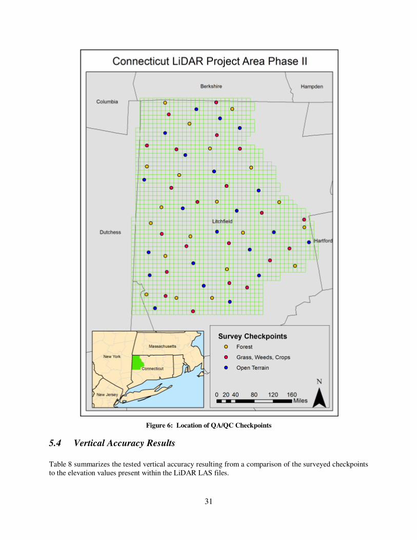
31
Figure 6: Location of QA/QC Checkpoints
5.4 Vertical Accuracy Results
Table 8 summarizes the tested vertical accuracy resulting from a comparison of the surveyed checkpoints
to the elevation values present within the LiDAR LAS files.

32
Land Cover
Category
# of
Points
FVA ― Fundamental Vertical Accuracy (RMSEz x 1.9600)
Spec=0.185 m
CVA ― Consolidated Vertical Accuracy (95th
Percentile)
SVA-Supplemental
Vertical Accuracy (95th
Percentile)
Consolidated 60 0.300
Open Terrain 20 0.179 0.176
Grass/Weeds/Crops 21 0.333
Forest 19 0.279
Table 8: FVA and CVA Vertical Accuracy at 95% Confidence Level
The RMSEz for open terrain checkpoints tested 0.091 m, within the target criteria of 0.0925 m. Compared with the 0.185 m specification, the FVA tested 0.179 m at the 95% confidence level based on RMSEz x
1.9600.
Table 10 provides overall descriptive statistics.
100 % of Totals
RMSE (m) Open
Terrain Spec=0.0925
m Mean (m)
Median (m) Skew
Std Dev (m)
# of Points
Min (m)
Max (m)
Consolidated 0.149 0.09 0.06 0.40 0.12 60 -0.16 0.35
Open Terrain 0.091 0.04 0.03 0.58 0.09 20 -0.11 0.23
Grass/Weeds/Crops 0.194 0.13 0.13 -0.18 0.15 21 -0.16 0.35
Forest 0.140 0.10 0.07 0.52 0.10 19 -0.06 0.30
Table 10: Overall Descriptive Statistics
5.5 Conclusion
Based on the vertical accuracy testing conducted by Dewberry, the LiDAR dataset for the Connecticut
LiDAR Project satisfies the project’s pre-defined vertical accuracy criteria.
6 Breakline Production & Qualitative Assessment Report
6.1 Breakline Production Methodology
Dewberry used GeoCue software to develop LiDAR stereo models of the Connecticut LiDAR Project area so the LiDAR derived data could be viewed in 3-D stereo using Socet Set softcopy photogrammetric
software. Using LiDARgrammetry procedures with LiDAR intensity imagery, Dewberry stereo-compiled
the two types of hard breaklines in accordance with the project’s Data Dictionary.
All drainage breaklines are monotonically enforced to show downhill flow. Water bodies are reviewed in
stereo and the lowest elevation is applied to the entire waterbody.

33
6.2 Breakline Qualitative Assessment
Dewberry completed breakline qualitative assessments according to a defined workflow. The following workflow diagram represents the steps taken by Dewberry to provide a thorough qualitative assessment of
the breakline data.
6.3 Breakline Topology Rules
Automated checks are applied to hydro features to validate the 3D connectivity of the feature and the
monotonicity of the hydrographic breaklines. Dewberry’s major concern was that the hydrographic breaklines have a continuous flow downhill and that breaklines do not undulate. Error points are
generated at each vertex not complying with the tested rules and these potential edit calls are then visually
validated during the visual evaluation of the data. This step also helped validate that breakline vertices did not have excessive minimum or maximum elevations and that elevations are consistent with adjacent
vertex elevations.
The next step is to compare the elevation of the breakline vertices against the elevation extracted from the
ESRI Terrain built from the LiDAR ground points, keeping in mind that a discrepancy is expected
because of the hydro-enforcement applied to the breaklines and because of the interpolated imagery used
to acquire the breaklines. A given tolerance is used to validate if the elevations do not differ too much from the LiDAR.
Dewberry’s final check for the breaklines was to perform a full qualitative analysis. Dewberry compared the breaklines against LiDAR intensity images to ensure breaklines were captured in the required
locations. The quality control steps taken by Dewberry are outlined in the QA Checklist below.
34
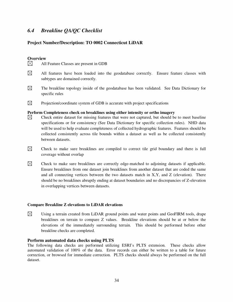
6.4 Breakline QA/QC Checklist
Project Number/Description: TO 0002 Connecticut LiDAR
Overview All Feature Classes are present in GDB
All features have been loaded into the geodatabase correctly. Ensure feature classes with
subtypes are domained correctly.
The breakline topology inside of the geodatabase has been validated. See Data Dictionary for
specific rules
Projection/coordinate system of GDB is accurate with project specifications
Perform Completeness check on breaklines using either intensity or ortho imagery Check entire dataset for missing features that were not captured, but should be to meet baseline
specifications or for consistency (See Data Dictionary for specific collection rules). NHD data
will be used to help evaluate completeness of collected hydrographic features. Features should be
collected consistently across tile bounds within a dataset as well as be collected consistently
between datasets.
Check to make sure breaklines are compiled to correct tile grid boundary and there is full
coverage without overlap
Check to make sure breaklines are correctly edge-matched to adjoining datasets if applicable.
Ensure breaklines from one dataset join breaklines from another dataset that are coded the same
and all connecting vertices between the two datasets match in X,Y, and Z (elevation). There
should be no breaklines abruptly ending at dataset boundaries and no discrepancies of Z-elevation
in overlapping vertices between datasets.
Compare Breakline Z elevations to LiDAR elevations
Using a terrain created from LiDAR ground points and water points and GeoFIRM tools, drape
breaklines on terrain to compare Z values. Breakline elevations should be at or below the
elevations of the immediately surrounding terrain. This should be performed before other
breakline checks are completed.
Perform automated data checks using PLTS The following data checks are performed utilizing ESRI’s PLTS extension. These checks allow
automated validation of 100% of the data. Error records can either be written to a table for future correction, or browsed for immediate correction. PLTS checks should always be performed on the full
dataset.
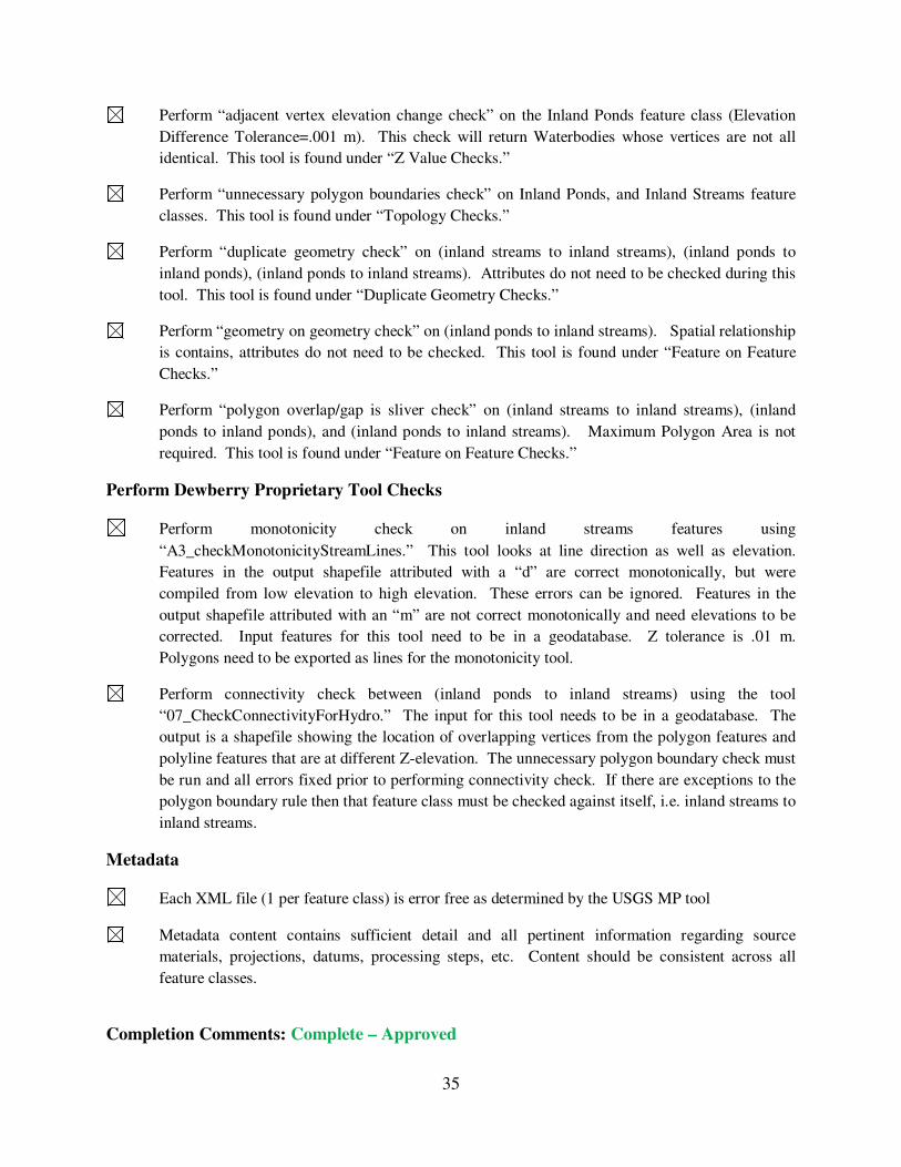
35
Perform “adjacent vertex elevation change check” on the Inland Ponds feature class (Elevation
Difference Tolerance=.001 m). This check will return Waterbodies whose vertices are not all
identical. This tool is found under “Z Value Checks.”
Perform “unnecessary polygon boundaries check” on Inland Ponds, and Inland Streams feature
classes. This tool is found under “Topology Checks.”
Perform “duplicate geometry check” on (inland streams to inland streams), (inland ponds to
inland ponds), (inland ponds to inland streams). Attributes do not need to be checked during this
tool. This tool is found under “Duplicate Geometry Checks.”
Perform “geometry on geometry check” on (inland ponds to inland streams). Spatial relationship
is contains, attributes do not need to be checked. This tool is found under “Feature on Feature
Checks.”
Perform “polygon overlap/gap is sliver check” on (inland streams to inland streams), (inland
ponds to inland ponds), and (inland ponds to inland streams). Maximum Polygon Area is not
required. This tool is found under “Feature on Feature Checks.”
Perform Dewberry Proprietary Tool Checks
Perform monotonicity check on inland streams features using
“A3_checkMonotonicityStreamLines.” This tool looks at line direction as well as elevation.
Features in the output shapefile attributed with a “d” are correct monotonically, but were
compiled from low elevation to high elevation. These errors can be ignored. Features in the
output shapefile attributed with an “m” are not correct monotonically and need elevations to be
corrected. Input features for this tool need to be in a geodatabase. Z tolerance is .01 m.
Polygons need to be exported as lines for the monotonicity tool.
Perform connectivity check between (inland ponds to inland streams) using the tool
“07_CheckConnectivityForHydro.” The input for this tool needs to be in a geodatabase. The
output is a shapefile showing the location of overlapping vertices from the polygon features and
polyline features that are at different Z-elevation. The unnecessary polygon boundary check must
be run and all errors fixed prior to performing connectivity check. If there are exceptions to the
polygon boundary rule then that feature class must be checked against itself, i.e. inland streams to
inland streams.
Metadata
Each XML file (1 per feature class) is error free as determined by the USGS MP tool
Metadata content contains sufficient detail and all pertinent information regarding source
materials, projections, datums, processing steps, etc. Content should be consistent across all
feature classes.
Completion Comments: Complete – Approved
36
6.5 Data Dictionary
LiDARgrammetry Data Dictionary
& Stereo Compilation Rules
For the Connecticut LiDAR Project
August 1, 2012
37
6.5.1 Horizontal and Vertical Datum
The horizontal datum shall be North American Datum of 1983, Units in meters. The vertical datum shall
be referenced to the North American Vertical Datum of 1988 (NAVD 88), Units in meters. Geoid09 shall
be used to convert ellipsoidal heights to orthometric heights.
6.5.2 Coordinate System and Projection All data shall be projected to UTM Zone 18N, Horizontal Units in meters and Vertical Units in meters.
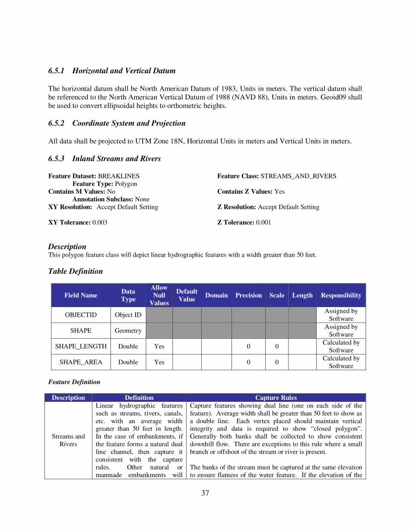
6.5.3 Inland Streams and Rivers
Feature Dataset: BREAKLINES Feature Class: STREAMS_AND_RIVERS
Feature Type: Polygon
Contains M Values: No Contains Z Values: Yes
Annotation Subclass: None
XY Resolution: Accept Default Setting Z Resolution: Accept Default Setting
XY Tolerance: 0.003 Z Tolerance: 0.001
Description This polygon feature class will depict linear hydrographic features with a width greater than 50 feet.
Table Definition
Field Name Data
Type
Allow
Null
Values
Default
Value Domain Precision Scale Length
Responsibility
OBJECTID Object ID Assigned by
Software
SHAPE Geometry Assigned by
Software
SHAPE_LENGTH Double Yes 0 0 Calculated by
Software
SHAPE_AREA Double Yes 0 0 Calculated by
Software
Feature Definition
Description Definition Capture Rules
Streams and
Rivers
Linear hydrographic features
such as streams, rivers, canals,
etc. with an average width greater than 50 feet in length.
In the case of embankments, if
the feature forms a natural dual
line channel, then capture it
consistent with the capture
rules. Other natural or
manmade embankments will
Capture features showing dual line (one on each side of the
feature). Average width shall be greater than 50 feet to show as
a double line. Each vertex placed should maintain vertical integrity and data is required to show “closed polygon”.
Generally both banks shall be collected to show consistent
downhill flow. There are exceptions to this rule where a small
branch or offshoot of the stream or river is present.
The banks of the stream must be captured at the same elevation
to ensure flatness of the water feature. If the elevation of the
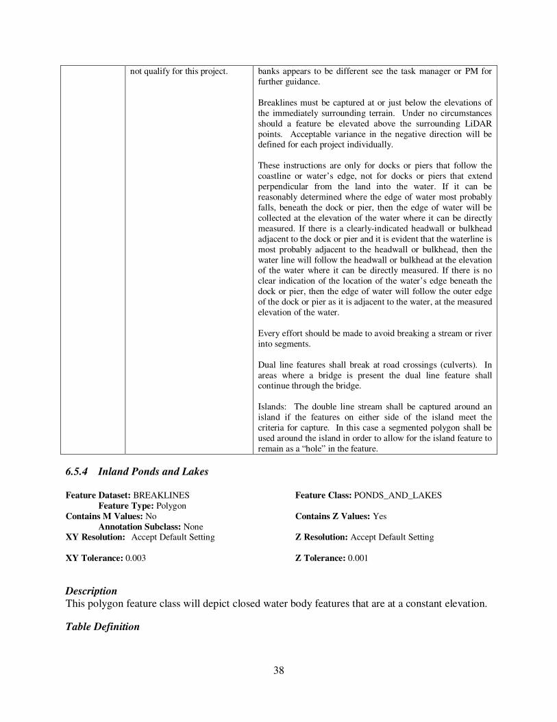
38
not qualify for this project. banks appears to be different see the task manager or PM for
further guidance.
Breaklines must be captured at or just below the elevations of
the immediately surrounding terrain. Under no circumstances
should a feature be elevated above the surrounding LiDAR
points. Acceptable variance in the negative direction will be defined for each project individually.
These instructions are only for docks or piers that follow the
coastline or water’s edge, not for docks or piers that extend
perpendicular from the land into the water. If it can be
reasonably determined where the edge of water most probably
falls, beneath the dock or pier, then the edge of water will be
collected at the elevation of the water where it can be directly
measured. If there is a clearly-indicated headwall or bulkhead
adjacent to the dock or pier and it is evident that the waterline is
most probably adjacent to the headwall or bulkhead, then the
water line will follow the headwall or bulkhead at the elevation of the water where it can be directly measured. If there is no
clear indication of the location of the water’s edge beneath the
dock or pier, then the edge of water will follow the outer edge
of the dock or pier as it is adjacent to the water, at the measured
elevation of the water.
Every effort should be made to avoid breaking a stream or river
into segments.
Dual line features shall break at road crossings (culverts). In
areas where a bridge is present the dual line feature shall continue through the bridge.
Islands: The double line stream shall be captured around an
island if the features on either side of the island meet the
criteria for capture. In this case a segmented polygon shall be
used around the island in order to allow for the island feature to
remain as a “hole” in the feature.
6.5.4 Inland Ponds and Lakes Feature Dataset: BREAKLINES Feature Class: PONDS_AND_LAKES
Feature Type: Polygon
Contains M Values: No Contains Z Values: Yes
Annotation Subclass: None XY Resolution: Accept Default Setting Z Resolution: Accept Default Setting
XY Tolerance: 0.003 Z Tolerance: 0.001
Description
This polygon feature class will depict closed water body features that are at a constant elevation.
Table Definition
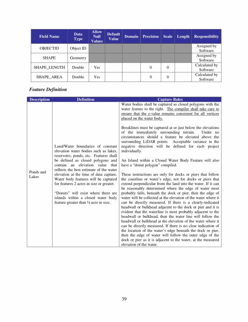
39
Field Name Data
Type
Allow
Null
Values
Default
Value Domain Precision Scale Length
Responsibility
OBJECTID Object ID Assigned by
Software
SHAPE Geometry Assigned by
Software
SHAPE_LENGTH Double Yes 0 0 Calculated by
Software
SHAPE_AREA Double Yes 0 0 Calculated by
Software
Feature Definition
Description Definition Capture Rules
Ponds and
Lakes
Land/Water boundaries of constant
elevation water bodies such as lakes,
reservoirs, ponds, etc. Features shall
be defined as closed polygons and
contain an elevation value that
reflects the best estimate of the water
elevation at the time of data capture.
Water body features will be captured for features 2 acres in size or greater.
“Donuts” will exist where there are
islands within a closed water body
feature greater than ½ acre in size.
Water bodies shall be captured as closed polygons with the
water feature to the right. The compiler shall take care to
ensure that the z-value remains consistent for all vertices
placed on the water body.
Breaklines must be captured at or just below the elevations of the immediately surrounding terrain. Under no
circumstances should a feature be elevated above the
surrounding LiDAR points. Acceptable variance in the
negative direction will be defined for each project
individually.
An Island within a Closed Water Body Feature will also
have a “donut polygon” compiled.
These instructions are only for docks or piers that follow
the coastline or water’s edge, not for docks or piers that extend perpendicular from the land into the water. If it can
be reasonably determined where the edge of water most
probably falls, beneath the dock or pier, then the edge of
water will be collected at the elevation of the water where it
can be directly measured. If there is a clearly-indicated
headwall or bulkhead adjacent to the dock or pier and it is
evident that the waterline is most probably adjacent to the
headwall or bulkhead, then the water line will follow the
headwall or bulkhead at the elevation of the water where it
can be directly measured. If there is no clear indication of
the location of the water’s edge beneath the dock or pier, then the edge of water will follow the outer edge of the
dock or pier as it is adjacent to the water, at the measured
elevation of the water.
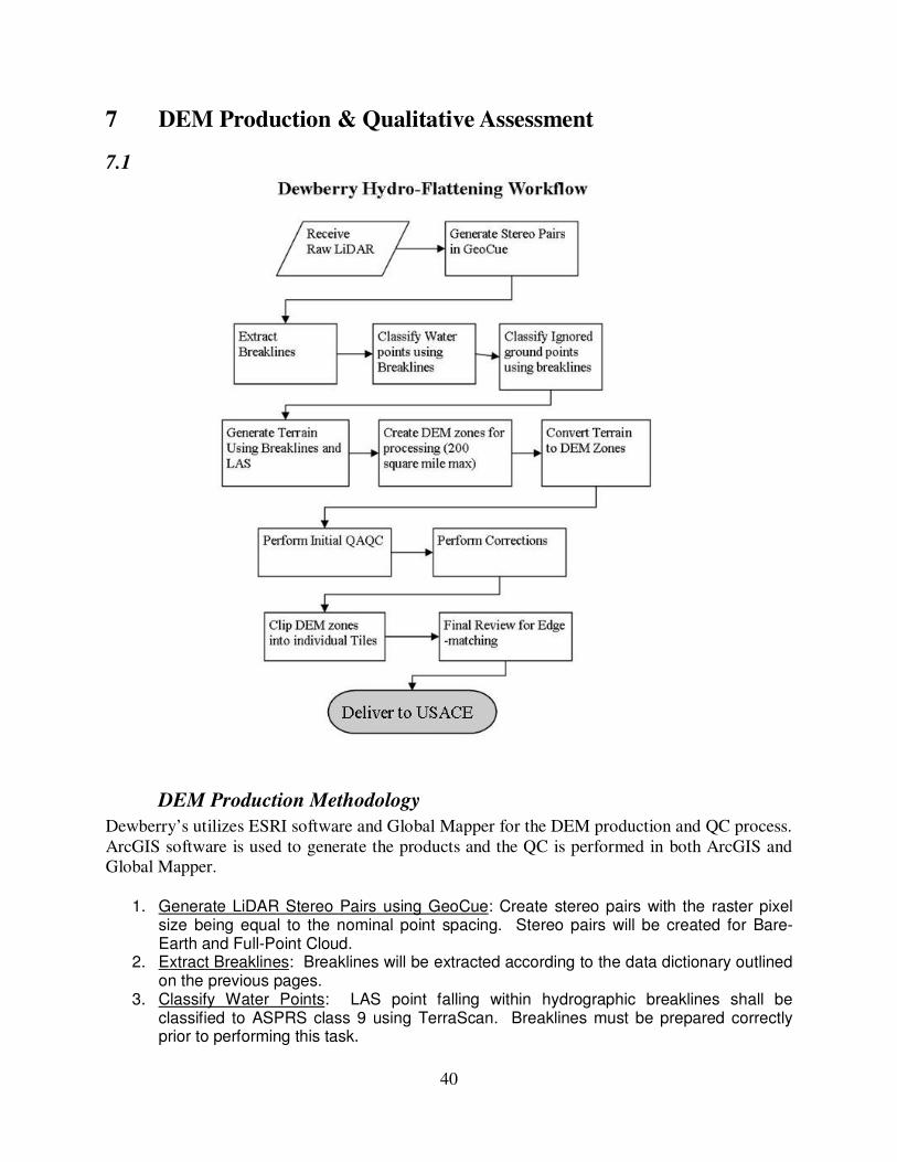
40
7 DEM Production & Qualitative Assessment
7.1
DEM Production Methodology
Dewberry’s utilizes ESRI software and Global Mapper for the DEM production and QC process.
ArcGIS software is used to generate the products and the QC is performed in both ArcGIS and
Global Mapper.
1. Generate LiDAR Stereo Pairs using GeoCue: Create stereo pairs with the raster pixel
size being equal to the nominal point spacing. Stereo pairs will be created for Bare-Earth and Full-Point Cloud.
2. Extract Breaklines: Breaklines will be extracted according to the data dictionary outlined on the previous pages.
3. Classify Water Points: LAS point falling within hydrographic breaklines shall be classified to ASPRS class 9 using TerraScan. Breaklines must be prepared correctly prior to performing this task.

41
4. Classify Ignored Ground Points: Points within a specified distance of breaklines can be removed from the ground classification and re-classified to a separate class, usually class 10. Ignored ground points were not created for the Connecticut LiDAR project.
5. Terrain Processing: A Terrain will be generated using the Breaklines and LAS data that has been imported into Arc as a Multipoint File. If the final DEMs are to be clipped to a project boundary that boundary will be used during the generation of the Terrain.
6. Create DEM Zones for Processing: Create DEM Zones that are buffered by 2 tiles around the edges. Zones should be created in a logical manner to minimize the number of zones without creating zones to large for processing. Dewberry will make zones no larger than 200 square miles (taking into account that a DEM will fill in the entire extent not just where LiDAR is present). Once the first zone is created it must be verified against the tile grid to ensure that the cells line up perfectly with the tile grid edge.
7. Convert Terrain to Raster: Convert Terrain to raster using the DEM Zones created in step 6. In the environmental properties set the extents of the raster to the buffered Zone. For each subsequent zone, the first DEM will be utilized as the snap raster to ensure that zones consistently snap to one another.
8. Perform Initial QAQC on Zones: During the initial QA process anomalies will be identified and corrective polygons will be created.
9. Correct Issues on Zones: Corrections on zones will be performed following Dewberry’s in-house correction process.
10. Extract Individual Tiles: Individual Tiles will be extracted from the zones utilizing a Dewberry proprietary tool.
11. Final QA: Final QA will be performed on the dataset to ensure that tile boundaries are seamless.
7.2 DEM Qualitative Assessment
Dewberry performed a comprehensive qualitative assessment of the DEM deliverables to ensure
that all tiled DEM products were delivered with the proper extents, were free of processing
artifacts, and contained the proper referencing information. This process was performed in
ArcGIS software with the use of a tool set Dewberry has developed to verify that the raster
extents match those of the tile grid and contain the correct projection information. The DEM
data was reviewed at a scale of 1:8000 to review for artifacts caused by the DEM generation
process and to review the hydro-flattened features. Dewberry uses Global Mapper to perform
this review. Corrections are applied in Arc Map. Dewberry creates HillShade models and
overlays a partially transparent colorized elevation model in order to perform the corrections.
The last step is to load the DEM data into Global Mapper to ensure that the corrections are
acceptable, all files are readable, and that no artifacts exist between tiles. The figure below,
illustrates the detail of the final DEMs and how the DEMs display elevation changes within
hydrographic features.
7.3 DEM QA/QC Checklist
Project Number/Description: TO 00002 Connecticut LiDAR
Overview
Correct number of files is delivered and all files are in ESRI GRID format
Verify Raster Extents

42
Verify Projection/Coordinate System
Review
Manually review bare-earth DEMs with a hillshade to check for issues with hydro- flattening process or any general anomalies that may be present. Specifically, water should be
flowing downhill, water features should NOT be floating above surrounding terrain and bridges
should NOT be present in bare-earth DEM. Hydrologic breaklines should be overlaid during review of DEMs.
DEM cell size is 1 meter
Perform final overview in Global Mapper to ensure seamless product.
Metadata Project level DEM metadata XML file is error free as determined by the USGS MP tool
Metadata content contains sufficient detail and all pertinent information regarding source
materials, projections, datums, processing steps, etc.
Completion Comments: Complete - Approved