
Product Description V16 - Intes
118
-
Upload
khangminh22 -
Category
Documents
-
view
3 -
download
0
Transcript of Product Description V16 - Intes


Product Description V16 PERMAS
© INTES GmbH, September 2016 (rev. 16.05)
The words in green colour are collected in the indexat the end of this document.
Address:
Phone:Fax:
E-mail:WWW:
INTES GmbHSchulze-Delitzsch-Str. 16
D-70565 Stuttgart
+49 711 784 99 - 0+49 711 784 99 - 10
[email protected]://www.intes.de
The finite element model of an V8 engine onthe frontpage appears by courtesy of FPT Mo-torenforschung AG in Arbon, Switzerland.
Abaqus is a registered trademark of Dassault SystèmesSimulia Corp., Providence, RI, USA.
Adams is a registered trademark of MSC.Software Cor-poration, Santa Ana, USA.
ADSTEFAN is a registered trademark of Hitachi IndustryControl & Solutions, Ltd., Ibaraki, Japan
CATIA is a registered trademark of DASSAULT SYS-TEMS, and in Canada, IBM is the registered user un-der No. RU 81167.
COMREL is a registered trademark of RCP GmbH,München, Germany .
DADS is a registered trademark of LMS CADSI,Coralville, USA.
Excite is a registered trademark of AVL List, Graz, Aus-tria.
HyperMesh, HyperView, H3D and MotionSolve are reg-istered trademarks of the Altair Engineering Inc., BigBeaver, USA.
I-DEAS is a registered trademark of SIEMENS PLM Soft-ware Inc., Plano, USA.
MEDINA and CAE-Datenschiene are registered trade-marks of the T-Systems ITS GmbH, Stuttgart, Ger-many .
MATLAB is a registered trademark of The MathworksInc., Natick, MA, USA.
MpCCI is a registered trademark of FhG SCAI, St. Au-gustin, Germany .
NASTRAN is a registered trademark of the NationalAeronautics and Space Administration (NASA).
NX is a registered trademark of Siemens PLM Software.MSC.Patran is a registered trademark of MSC Software
Corporation, Santa Ana, USA.
PERMAS is a registered trademark of INTES In-genieurgesellschaft für technische Software mbH,Stuttgart, Germany .
SIMPACK is a registered trademark of SIMPACK AG,Gilching, Germany.
STAR CD is a registered trademark of Computational Dy-namics Ltd., London, England.
VAO is a registered trademark of CDH AG, Ingolstadt,Germany .
Virtual.Lab is a registered trademark of LMS Interna-tional, Leuven, Belgium .
VisPER is a registered trademark of INTES Ingenieurge-sellschaft für technische Software mbH, Stuttgart,Germany .
The use of registered names or trademarks does not im-ply, even in the absence of further specific statements,that such names are free for general use.
Page 2 © INTES GmbH Stuttgart

PERMAS Product Description V16
ContentsPage
INTES 5Company Profile 5Services 5PERMAS 7Overview 7Introduction to PERMAS 7Benefits of PERMAS 8What’s New in PERMAS Version 16 9What’s New in VisPER Version 5 16Universal Features 18Available VisPER Modules 18Available PERMAS Modules 18Performance Aspects 19Parallelization 19Areas of Application 20Reliability 20Quality Assurance 21
Applications 23Car Body Analysis 23Engine Analysis 26Part Connections 28Brake Squeal Analysis 30Rotating Systems 32Analysis of Machine Tools 33Actively Controlled Systems 37Robust Optimum Design 38
VisPER 41The VisPER History 41VisPER – A Short Introduction 41VisPER-BAS – Basic Module 42VisPER-TOP – Topology Optimization 44VisPER-OPT – Design Optimization 45VisPER-FS – Fluid-Structure Coupling 47VisPER-CA – Contact Analysis 49Substructuring 50Evaluation of Spotwelds 51
PERMAS Basic Functions 53Substructuring 53Submodeling 53Variant Analysis 54Cyclic Symmetry 55Surface and Line Description 55Automated Coupling of Parts 56Automated Spotweld Modeling 57Local Coordinate Systems 58Kinematic Constraints 58Handling of Singularities 59Element Library 59Standard Beam Cross Sections 60
Design Elements for Optimization 61Error estimator 61Material Properties 61Sets 62Mathematical Functions 62Loads 63Model Verification 63Interfaces 64Matrix Models 66Combination of Results 66Transformation of Results 67Comparison of Results 67XY Result Data 67Cutting Forces 68Restarts 68Open Software System 68Direct Coupled Analyses 68Coupling with CFD 69
PERMAS Analysis Modules 71
PERMAS Package TM Thermo-Mechanics 71PERMAS-MQA – Model Quality Assurance 71PERMAS-LS – Linear Statics 72PERMAS-CA – Contact Analysis 72PERMAS-CAX – Extended Contact Analysis 75PERMAS-CAU – Contact Geometry Update 76PERMAS-NLS – Nonlinear Statics 77PERMAS-NLSMAT – Extended Material Laws 80PERMAS-BA – Linear Buckling 80PERMAS-HT – Heat Transfer 80PERMAS-NLHT – Nonlinear Heat Transfer 81PERMAS Package VA Vibro-Acoustics 83PERMAS-DEV – Dynamic Eigenvalues 83PERMAS-DEVX – Extended Mode Analysis 84PERMAS-MLDR – Eigenmodes with MLDR 85PERMAS-DRA – Dynamic Response 86PERMAS-DRX – Extended Dynamics 89PERMAS-FS – Fluid-Structure Acoustics 89PERMAS-NLD – Nonlinear Dynamics 91
PERMAS Package DO Design-Optimization 92PERMAS-OPT – Design Optimization 92PERMAS-TOPO – Layout Optimization 95PERMAS-AOS – Advanced Optim. Solvers 98PERMAS-RA – Reliability Analysis 100
PERMAS Special Modules 101PERMAS-LA – Laminate Analysis 101PERMAS-WLDS – Refined Weldspot Model 101PERMAS-EMS – Electro- and Magneto-Statics 101PERMAS-EMD – Electrodynamics 102PERMAS-XPU – GPU accelerator 102Interfaces 103PERMAS-MEDI – MEDINA Door 103
© INTES GmbH Stuttgart Page 3

Product Description V16 PERMAS
PERMAS-PAT – PATRAN Door 103PERMAS-ID – I-DEAS Door 103PERMAS-AD – ADAMS Interface 104PERMAS-DADS – DADS Interface 104PERMAS-EXCI – EXCITE Interface 104PERMAS-SIM – SIMPACK Interface 104PERMAS-HMS – MotionSolve Interface 105PERMAS-H3D – HYPERVIEW Interface 105PERMAS-VAO – VAO Interface 105PERMAS-VLAB – Virtual.Lab Interface 105PERMAS-ADS – ADSTEFAN Interface 105PERMAS-MAT – MATLAB Interface 105PERMAS-NAS – NASTRAN Door 105PERMAS-ABA – ABAQUS-Door 106PERMAS-CCL – MpCCI Coupling 107More Interfaces 107Installation and beyond 109Supported Hardware Platforms 109Licensing 109Maintenance and Porting 109User Support 110MEDINA + PERMAS 110Additional Tools 110Documentation 111Training 111Future Developments 112Additional Information 112Index 113
Page 4 © INTES GmbH Stuttgart

PERMAS Product Description V16
INTES
Figure 1: INTES Head Office in Stuttgart
Company Profile
INTES company was founded as an FE technol-ogy enterprise in 1984. Its competence in everyaspect of Finite Element (FE) technology is pro-vided by INTES to its clients not only through thehigh-end software system PERMAS. The full rangeof development know-how of INTES is also madeavailable to its clients by the provision of top-notchservices and expert consultancy. INTES activitiesmainly concentrate on the• development and distribution of the FE solver
PERMAS and the joint pre- and post-processorVisPER,
• development of new and efficient numerical andgraphical methods,
• development of software for new hardware ar-chitectures (such as parallel computers),
• coupling of PERMAS and VisPER with othersoftware systems (such as pre- and postproces-sors and MBS systems),
• consultancy and training of users,• consulting by analysis projects.
The international support of PERMAS clients is sup-ported in France by INTES France and in Japan byINTES Japan. In addition, partners are supportingand distributing the software in other countries.
For all of its customers, INTES wants to be a com-petent partner in all respects regarding the FiniteElement Method. Above all, satisfaction of the cus-tomers with all the software and services is of primeimportance to the company.
Services
INTES offers a number of services to its customersincluding:
• Developments for PERMAS and VisPER:– Interfaces to other software packages,– New modeling processes,– New analysis capabilities,– New finite elements,– Customer specific developments.
• Installation of PERMAS and VisPER on newhardware platforms as well as consultancy con-cerning the optimum hardware configuration,
• Software maintenance,• FEM training,• FEM research and development,• Configuration and installation of add-on soft-
ware products,• Engineering:
– modeling with VisPER, MEDINA,– simulation with PERMAS,
• Introduction of FE analysis in enterprises, con-tinuous consultation service (hotline), and sup-port on current projects.
Figure 2: Synopsis of PERMAS history
© INTES GmbH Stuttgart Page 5

Product Description V16 PERMAS
Page 6 © INTES GmbH Stuttgart

PERMAS Product Description V16
PERMAS
Overview
This product description provides information on allessential characteristics of PERMAS and its appli-cation. Therefore, the description is organized intoseven parts set forth below:
• The introduction gives some good reasonsfor the application of the Finite-Element-Method(FEM) and PERMAS. The particular benefits ofPERMAS are presented on pages 8 to 21.
• Applications using several functional modulesare illustrated on pages 23 to 39
• The features of VisPER are described on pages41 to 51.
• The universal features of PERMAS, which arenot related to a single module, are explained onpages 53 to 69.
• The available functional modules are de-scribed on pages 71 to 102.
• The interfaces are collected on pages 103 to107.
• Additional information about the installationand further aspects of PERMAS is given onpages 109 to 112.
Figure 3: Model of a chain sawAndreas Stihl AG & Co. KG, Waiblingen,Germany.
Introduction to PERMAS
PERMAS is a general purpose software system toperform complex calculations in engineering usingthe finite element method (FEM), and to optimizethe analyzed structures and models. It has beendeveloped by INTES and is available to engineersas an analysis tool worldwide.
PERMAS enables the engineer to perform compre-hensive analyses and simulations in many fields ofapplications like stiffness analysis, stress analysis,determination of natural modes, dynamic simula-tions in the time and frequency domain, determina-tion of temperature fields, acoustic fields, and elec-tromagnetic fields, analysis of anisotropic materiallike fibre-reinforced composites.
PERMAS computes a large number of results dur-ing the course of these analyses, which may beused in the assessment of the structural behaviorlike deflections, stresses and strains, natural fre-quencies and mode shapes, strain energy distribu-tion, sound vibration power density, time history andinteraction with other parts of the structure.
Independent of the area of application, these resultsprovide a lot of valuable information for the designand development process. A number of essentialbenefits can be derived from the early use of theFEM:
• Safe accomplishment of customer require-ments.
• Reduction of expensive manufacturing and test-ing of prototypes.
• Simulation of extreme conditions.• Shorter development and design cycles.• Significant suggestions for design optimization:
– topology optimization,– sizing optimization,– shape optimization,– parameter studies by sampling.
• Improvement of structural reliability.• Analysis in case of malfunction of a structure
during operation.• Long term quality improvements.
In view of today’s increasing requirements for shortdesign cycles and high quality products, the finiteelement analysis becomes an indispensible tool forthe daily development work. Moreover, complexproducts are often developed in distributed struc-
© INTES GmbH Stuttgart Page 7

Product Description V16 PERMAS
Figure 4: Model of a tractor transmissionZF Friedrichshafen AG, Friedrichshafen, Germany.
tured companies. This makes interdependenciesbetween different components of the product visi-ble in time only if they are simulated and analyzedon the computer. At the same time, the quality as-surance of analysis results is of great importance.Hence, the choice of the right analysis tool is of cru-cial significance.
Benefits of PERMAS
PERMAS is an internationally established FE anal-ysis system with users in many countries. INTEShas developed the system and, additionally, offersindividual consultation and user support and alltraining required. The consultation covers all re-quests regarding the use of the software but alsobasic questions regarding the idealization and phys-ical modeling.
The benefits arising from the use of PERMAS canbe characterized by the following points:
• As a general purpose software packagePERMAS provides for powerful capabilities ,which cover a wide range of applicationsfrom mechanics to heat transfer, fluid structureacoustics and electrodynamics.
• Integrated optimization algorithms allowPERMAS not only to analyze models but alsoto determine optimized parts which fulfil manydifferent conditions. The optimization methodsinclude topology optimization, sizing and shapeoptimization, and reliability analysis to take into
Figure 5: Turbocharger housingBorgWarner Turbo Systems Engineering GmbH,
Kirchheimbolanden, Germany.
account uncertain model parameters.• The graphical user interface VisPER supports
the user in verifying his models and in evalua-tion of the analysis results. Moreover, VisPERprovides advanced modeling features, e.g. forgeneration of fluid meshes, and for the set-up ofoptimization models in particular.
• Efficient equation solvers and optimized datastorage schemes provide PERMAS with ulti-mate computing power with low resource con-sumption. Moreover, the software is continu-ally adapted to the most advanced and powerfulcomputers.
• PERMAS, a well-proven and mature software,has been available for many years and in numer-ous structural analysis departments. There, thereliability of the software is appreciated aboveall.
On the subsequent pages all these points are spec-ified in more detail.
PERMAS is an advanced software package with up-to-date user conveniences. The PERMAS develop-ment aims to implement future-oriented functionali-ties in close cooperation with the users and to pro-vide currently most advanced algorithms. In thisway, PERMAS today faces the requirements of to-morrow.
Page 8 © INTES GmbH Stuttgart

PERMAS Product Description V16
Figure 6: Charge air coolerBehr GmbH & Co., Stuttgart, Germany.
What’s New in PERMAS Version 16
The new Version 16 of PERMAS is the resultof about 24 months of development work sincethe shipment of the predecessor version 15. Forthe regular reader of our Product Description ofPERMAS, a rough overview summarizes the mainchanges in the new version. Of course, a completeand detailed Software Release Note is available withVersion 16 in addition.
Great effort has been spent in the past years to pro-vide VisPER (i.e. Visual PERMAS) as a dedicatedtool to improve pre- and post-processing for specialPERMAS functions. The fifth regular VisPER Ver-sion 5 is released at the same time as PERMASVersion 16. The new features of VisPER Version 5will be introduced in the next section (see page 16).
PERMAS Version 16 offers again improved comput-ing performance:
• PERMAS can be invoked using a new option forusing direct I/O. If PERMAS DMS-Files are puton SSD systems, the I/O is performed directlyusing the PCI bus to these systems, which canreduce run time for I/O bound jobs significantly(see Fig. 9).
• Again improved algorithm for direct FS coupledfrequency response analysis (see Fig. 10).
• A new very fast modal frequency responsesolver (SMW-solver) has been developed (see
Figure 7: Half model of a six-cylinder Diesel engineDaimler Trucks North America in Detroit, Michigan, USA.
Fig. 8 and below on page 13).• Geometrically nonlinear analysis has been es-
sentially accelerated (see Fig. 15).
The list of major software extensions in PERMAS isas follows:
• New modules:– The new module ADS (see module ADS
on page 105) provides an interface betweenthe casting simulation software ADSTEFAN(owned by Hitachi Industry & Control Solu-tions, Ltd., see http://www.adstefan.com) andPERMAS. The interface supports the importof the temperature distribution of the castingsimulation, provided as voxel data in a csv for-mat.
• Major extensions:– Extensions to basic module (module MQA,
page 71):
* The concept of local coordinate systemshas been extended to support a largervariety of coordinate system types (seeFig. 11).
* For surfaces with quadratic elements, alinearization is available, which makesthe midside nodes linearly dependent onthe corner nodes. If these surfaces areused in contact definitions, then the sur-faces will also provide contact pressure
© INTES GmbH Stuttgart Page 9

Product Description V16 PERMAS
Figure 8: Modal frequency response analysiswith high run time savings.
results. A special export item allows tovisualize the surface definitions. Defini-tion and visualization of surfaces are fullysupported by VisPER.
* Multilinear kinematic constraints for sur-faces (by MPC conditions) provide a newprojection feature, where the dependentnode coordinates can be modified toplace them on the surface. Alternatively,a rigid lever arm will be used between thedependent nodes and the surface.
* For the PERMAS results export, a bi-nary format has been introduced basedon the widely used HDF5 library (seehttps://www.hdfgroup.org/HDF5/). Themain effect of this binary format is the re-duction of time needed to export the re-sults. In addition, a slight reduction of filesize is achieved compared to the gzip-edASCII export file format used so far.
* In previous PERMAS version, sampling
Figure 9: Direct I/O for large modelswith PCI SSD like contact analysis of engine with 56
Million DOF, 37 time steps, 2 different temperature
states, and CAS files, including GPU.
has been introduced as a method to re-peat an analysis many times with modi-fied discrete values. In order to reducethe number of samples without losing in-formation about parameter influence anew sampling method (i.e. LHC Latin Hy-percube Sampling) has been developed.
* In previous versions of PERMAS, pressfit connections have been modeled andanalyzed by contact using a negative gapwidth indicating the interference of theunconnected parts. In case, an open-ing of the gap in a press fit connectionduring operational loading is not of inter-est to the analyst, then there is a newmodeling feature for press fit connectionsavailable. This feature uses MPC cou-pling instead of contact conditions. Ex-amples show exactly the same results as
Page 10 © INTES GmbH Stuttgart

PERMAS Product Description V16
Figure 10: Direct frequency responsefor coupled fluid-structure model with 11.2 Million DOF
on 16 cores plus Tesla K20c
Figure 11: Local coordinate systems
for contact analysis (see Fig. 12). Thisnew method is a linear method and worksfor static and dynamic analysis and other
analysis types. Even substructuring withthe press fit connection in a substructureis possible with this method. Specific re-sults are available to verify, check, andevaluate press fit connections.
Figure 12: Press fit connectioncomparison of MPC and contact result
– Extensions to contact analysis (modules CA,CAX, and CAU from page 72):
* In surface-to-surface contacts, more con-tacts are taken into account than insurface-to-node contacts. More contactstypically give more accurate results butalso longer computation times. Less con-tacts does not mean that the results be-come inaccurate, but it is possible e.g. forcoarse meshes of contact surfaces. Inorder to get the best out of a contact anal-ysis by spending only moderately morecomputation time, an optional automa-tism has been developed (option COM-PLEMENT), which reduces the numberof contacts in surface-to-surface contactareas in a way that the accuracy is pre-served (see Fig. 13).
© INTES GmbH Stuttgart Page 11

Product Description V16 PERMAS
* For each contact definition with a non-zero sum of contact forces, there existsa line of action with a minimal resultanttorque due to the corresponding normaland frictional contact forces. The pointon that line of action, which lies closestto a given centroid (e.g. the center ofcontact node coordinates) is defined asthe contact’s center of pressure (COP).The coordinates of the COP and the sumof forces and moments is written to theresult file by request. This result is avail-able for all load steps performed in a lin-ear or nonlinear contact analysis.
* A new gap function has been introduced,where a given gap may be scaled by auser-defined function, which may dependon the position in space and topologicalinformation.
– Extensions to nonlinear static analysis (mod-ule NLS, page 77):
* The existing post-buckling feature hasbeen improved by enhancements of thesolid shell elements and a newly imple-mented arc length method (see Fig. 14).In addition, a linear buckling analysis canbe performed after each converged non-linear load step.
* It is now possible to switch automaticallyfrom linear shell elements to nonlinearsolid shell elements dependent on theanalysis type used.
* The performance of geometrically non-linear analysis has been improved byreducing the number of automatic loadsteps and iterations (see Fig. 15).
– Extensions to extended mode analysis (mod-ule DEVX, page 84):
* A new parallelized complex eigenvaluesolver has been developed.
– Extensions to dynamic eigenvalue analysiswith MLDR (module MLDR, page 85):
* Faster Craig-Bampton mass and damp-ing reduction.
* Temperature-dependent stiffness istaken into account.
* In order to support a subsequent re-sponse analysis, assembled situations(see page 88) and static mode shapes(see page 88) are considered. Also staticmodes due to inertia loads from iner-
Figure 13: Surface-to-surface contactwith COMPLEMENT option: Best compromise between
accuracy and computation time (von Mises nodal
stresses are shown). The numbers are taken from an
industrial application.
tia relief analysis (see page 72) can beused.
– Extensions to dynamic response analysis(module DRA, page 86):
* For models with many eigenvalues, manyexcitation frequencies, and only somedampers the computation of the fre-quency response is expensive. As longas the damping is not frequency depen-dent (only a few discrete dampers), adiagonalisation of the system is possi-ble via a singular value decomposition(complex eigenvalues). An explicit inver-sion of the resulting system matrix maybe performed, applying the Shermann-Morisson-Woodbury (SMW) formulation.The subsequent computation of each
Page 12 © INTES GmbH Stuttgart

PERMAS Product Description V16
Figure 14: Nonlinear bucklingwith post-buckling behavior for a laminated cylinder shell
frequency point is cheap. This newSMW solver is much faster than the gen-eral solver for modal frequency response
analysis.– Extensions to extended dynamics (module
DRX, page 89):
* Modal random response analysis hasnow better numerical stability and thegeneration of cross spectral densitieswas improved.
– Extensions to fluid-structure coupled analysis(module FS, page 89):
* The direct time integration for the re-sponse in time domain for fluids only isnow available.
Figure 15: Run time reductionin geometrically nonlinear analysis for a 3 Million DOF
frame structrue (in minutes)
– Extensions to design optimization (moduleOPT, page 92) for parametric optimizationmethods:
* Due to a harmonization of the optimizersnow any combination of topology, sizing,
© INTES GmbH Stuttgart Page 13

Product Description V16 PERMAS
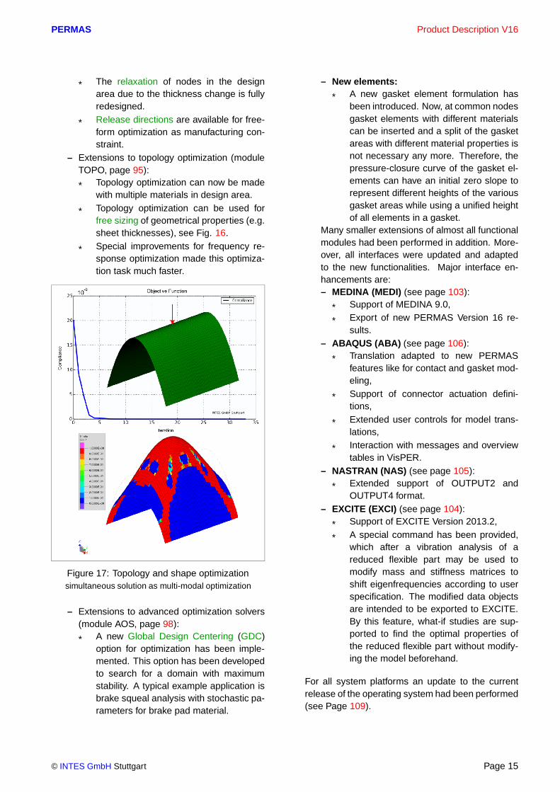
and shape optimization can be used si-multaneously in one single multi-modaloptimization (MMO). To get to this point,the mentioned optimization types are us-ing the same solver. This opens the doorto new and not yet feasible optimizationtasks (see Fig. 16 and Fig. 17).
* A new additional solver Adapted Con-vex Programming (ACP) solver has beenadded to the list of optimization solvers.This out-of-core and parallelized solveris recommended for large optimizationtasks, nonlinear behavior, and complexmanufacturing conditions.
* Optimization has been equipped with ageneral break/restart facility. To this end,a running optimization can be stoppedand restart files are prepared. So, therestart can be made at any already per-formed optimization loop. Before restart,optimization parameters can be modifiedto influence the convergence behavior ofthe optimization. The restart uses therestart file to continue the optimizationfrom the already reached status.
* The use of external tools in optimizationloops is now possible. First examples areused to calculate safety factors, whichare used as objective or constraint in afree-form optimization. To achieve that ascript has to be written, which invokes theexternal tool and provides nodal resultsin a specific PERMAS compliant format.
* Before Version 16, one design constrainthas to be selcted as design objective.Now with Version 16, an arbitrary numberof design coinstraints may be declaredas design objective. The maximum valuewill be minimized, whereas all others be-come constraints.
* For multi-objective design optimization aPareto optimization may be performedusing a suitable sampling capability.
– Extensions to design optimization (moduleOPT, page 92) for non-parametric shape op-timization:
* A new solver for the optimality criteriamethod with additional constraints hasbeen developed.
* Possible objectives or constraints areweight, stress (von Mises stress, princi-
Figure 16: Multi-modal optimizationwith topology optimization, bead optimization, and free
sizing for the sheet thicknesses.
pal stress), effective plastic strain, andnodal values generated by external tools(see above), if a local change of the partthickness influences the local value of theobjective (e.g. safety factors).
* Additional constraints could be stressesoutside the design area, displacementsor compliance as stiffness constraints orany other constraint as long as (semi-)analytic sensitivities are available.
* Of particular importance is the elementtest as additional constraint, which isused to avoid a stop of the optimizationprocess due to failing elements.
Page 14 © INTES GmbH Stuttgart
PERMAS Product Description V16
* The relaxation of nodes in the designarea due to the thickness change is fullyredesigned.
* Release directions are available for free-form optimization as manufacturing con-straint.
– Extensions to topology optimization (moduleTOPO, page 95):
* Topology optimization can now be madewith multiple materials in design area.
* Topology optimization can be used forfree sizing of geometrical properties (e.g.sheet thicknesses), see Fig. 16.
* Special improvements for frequency re-sponse optimization made this optimiza-tion task much faster.
Figure 17: Topology and shape optimizationsimultaneous solution as multi-modal optimization
– Extensions to advanced optimization solvers(module AOS, page 98):
* A new Global Design Centering (GDC)option for optimization has been imple-mented. This option has been developedto search for a domain with maximumstability. A typical example application isbrake squeal analysis with stochastic pa-rameters for brake pad material.
– New elements:
* A new gasket element formulation hasbeen introduced. Now, at common nodesgasket elements with different materialscan be inserted and a split of the gasketareas with different material properties isnot necessary any more. Therefore, thepressure-closure curve of the gasket el-ements can have an initial zero slope torepresent different heights of the variousgasket areas while using a unified heightof all elements in a gasket.
Many smaller extensions of almost all functionalmodules had been performed in addition. More-over, all interfaces were updated and adaptedto the new functionalities. Major interface en-hancements are:– MEDINA (MEDI) (see page 103):
* Support of MEDINA 9.0,
* Export of new PERMAS Version 16 re-sults.
– ABAQUS (ABA) (see page 106):
* Translation adapted to new PERMASfeatures like for contact and gasket mod-eling,
* Support of connector actuation defini-tions,
* Extended user controls for model trans-lations,
* Interaction with messages and overviewtables in VisPER.
– NASTRAN (NAS) (see page 105):
* Extended support of OUTPUT2 andOUTPUT4 format.
– EXCITE (EXCI) (see page 104):
* Support of EXCITE Version 2013.2,
* A special command has been provided,which after a vibration analysis of areduced flexible part may be used tomodify mass and stiffness matrices toshift eigenfrequencies according to userspecification. The modified data objectsare intended to be exported to EXCITE.By this feature, what-if studies are sup-ported to find the optimal properties ofthe reduced flexible part without modify-ing the model beforehand.
For all system platforms an update to the currentrelease of the operating system had been performed(see Page 109).
© INTES GmbH Stuttgart Page 15

Product Description V16 PERMAS
Figure 18: Ship engine pistonMahle GmbH, Stuttgart, Germany.
What’s New in VisPER Version 5
Great effort has been spent in the past years to pro-vide VisPER (i.e. Visual PERMAS) as a dedicatedtool to improve pre- and post-processing for specialPERMAS functions. VisPER Version 5 is releasedat the same time as PERMAS Version 16. Moreinformation on VisPER can be found on page 41.
Because the list of extensions in Version 5 is long,the following overview just lists the most importantextensions. More information can be found in theVisPER Users Manual.
The list of major software extensions in VisPER isdivided in four sections as follows:
• Model completion :– Definition of dynamic model properties:
* Linearization of contacts by locking con-tact regions according to contact results,
* Definition of damping,
* Specification of dynamic loads (like iner-tia loads and loads in frequency and timedomain),
* Definition of frequencies and rotationalspeeds, where the user wants to see re-sults.
– In case of dynamics in modal space, the defi-
Figure 19: Material reference systemfor anisotropic material
nition of additional static mode shapes is nowsupported by VisPER, too. It supports allsources of additional mode shapes like ele-ment forces, direct input of displacements orload cases, reference to already available re-sults, or displacements from an inertia reliefanalysis.
– Comprehensive extensions were made forthe handling of functions. A dedicated dia-log supports the definition of functions usingall PERMAS capabilities like library functions,tabular functions, chaining and summing upof functions, and user defined functions. Thedefined functions can be directly visualized.A referencing mechanism can show the user,where the functions have been used.
– Material reference systems for orthotropic oranisotropic materials as well as for laminatematerials are now supported (see Fig. 19).The related dialog supports the definition ofmaterial reference systems and provides in-formation on existing material reference sys-tems. The reference system and the related
Page 16 © INTES GmbH Stuttgart

PERMAS Product Description V16
structure is visualized.– All local system definitions are supported by a
special dialog. This includes all new systemtypes introduced in PERMAS like cartesian,cylindrical, conical, spherical and toroidalsystems. Special visualization facilitates theidentification of the particular system.
– A new dialogue bar has been introduced tosupport the definition of design constraintfunctions.
Figure 20: Preprocessing of brake models
• Wizards:– A new Brake Squeal Wizard allows an easy
description of complex brake models accord-ing to PERMAS brake squeal technology (seeFig. 20). See module VBAS on page 42. Thekey features of the wizard to provide modelstandardization and to ensure process stabil-ity are:
* Fast setup of brake squeal analysis,
* Guided definition of additional physics forthe dynamics of the analysis task,
* Checking of dynamic definitions and theircompatibility,
* UCI file generation after wizard comple-tion.
– The Pretension Wizard has been extended todetect holes for screw candidates.
The already existing wizards have been updatedto cover the current state of the PERMAS func-tions.
• Post-processing:– The new binary results file in PERMAS (using
HDF5 format) can be used with VisPER in or-der to reduce the time for loading the results.
– For the export of the model after model com-pletion, several selections are available: com-plete model, new items only, and one singlecomponent only. All referenced data will beexported, too.
– A new user result item has been specified,which can be postprocessed by VisPER. Thisresult item follows syntax rules of PERMASresults and is currently restricted to nodal re-sults. Several scalar values at nodes can beused. The results can be generated by anyother standard or user written software.
• Tools:– In order to reduce the complexity of the
PERMAS user control, the use of predefinedUCI templates is facilitated. A comprehensivedialogue is available to create and modify UCItemplates and to use them in the followingPERMAS runs, or to store them as new tem-plates for future use. In this way, the flexibilityin controling a PERMAS run is very much in-creased. The use of UCI templates helps tostandardize PERMAS user control and mini-mizes erroneous PERMAS runs.
– A quick exploration of model item relations issupported by a new referencing button. Bythis button, all model entities are listed, whichreference a given seed entity. From the en-tries of this list, one can directly open the re-lated GUI, or directly visualize the model en-tities, or select the model entities for furtheroperations.
© INTES GmbH Stuttgart Page 17

Product Description V16 PERMAS
Universal Features
The outstanding mostly module-independent basicfeatures of PERMAS are as follows (see pages 53to 68):
• Hierarchical substructuring, with automatic sub-component insertion (see page 53)
• Submodeling (see page 53)
• Variant analysis (see page 54)
• Cyclic symmetry (see page 55)
• Surface and Line Description (see page 58)
• Automated coupling of parts (see page 56)
• Automated spotweld modeling (see page 57)
• Local coordinate systems (see page 58)
• Multiple kinematic constraints (see page 58)
• Automatic detection of singularities (see page59)
• Same elements for different analysis types (Ele-ment library, see page 59)
• Standard beam cross sections (Seite 60)
• Design elements for optimization (page 61)
• Error estimation and refinement indicator (page61)
• General material description (see page 61)
• Node and element sets (see page 62)
• Mathematical functions (see page 62)
• All kinds of loading (see page 63)
• Model verification (see page 63)
• Integrated interfaces to pre- and post-processors (see page 64)
• Input and Output of Data Objects and matrices(see page 66)
• Combination, transformation, and comparisonof results (see page 66)
• Output of XY result data (see page 67)
• Calculation of cutting forces (see page 68)
• Restart facility (see page 68)
• Open software through Fortran and C interfaces(see page 68)
• Direct coupling of different analysis types (seepage 68)
• Coupling with CFD (see page 69)
Figure 21: Model of a transport vehiclecourtesy of Daimler AG,
Commercial Vehicle Division in Stuttgart
Available VisPER Modules
The below listed functional modules are explainedin more detail on pages 42 to 49:
• Basic module (VBAS)• Topology optimization (VTOP)• Design optimization (VOPT)• Fluid-structure coupling (VFS)• Contact analysis (VCA)
Available PERMAS Modules
The below listed functional modules are explainedin more detail on pages 71 to 107:
• Model Quality Assurance (MQA)• Linear Statics (LS)• Contact Analysis (CA)• Extended Contact Analysis (CAX)• Contact Geometry Update (CAU)• Nonlinear Statics (NLS)• Extended Nonlinear Material Laws (NLSMAT)• Buckling Analysis (BA)• Heat Transfer (HT)• Nonlinear Heat Transfer (NLHT)• Dynamic Eigenvalue Analysis (DEV)• Extended Dynamic Eigenvalue Analysis (DEVX)• Eigenmodes with MLDR (MLDR)• Dynamic Response Analysis (DRA)• Extended Dynamic Response Analysis (DRX)• Fluid-Structure Acoustics (FS)• Nonlinear Dynamics (NLD)
Page 18 © INTES GmbH Stuttgart

PERMAS Product Description V16
• Design Optimization (OPT)• Layout Optimization (TOPO)• Advanced optimization solvers (AOS)• Reliability Analysis (RA)• Laminate Analysis (LA)• Refined Weldspot Model (WLDS)• Steady-state electromagnetics (EMS)• Electrodynamics (EMD)• Use of GPU (XPU)• Interfaces to various pre-/post-processors
– MEDINA (MEDI)– PATRAN (PAT)– I-DEAS (ID)
• Interfaces to other analysis packages– ADAMS (AD)– DADS (DADS)– SIMPACK (SIM)– EXCITE (EXCI)– MOTIONSOLVE (HMS)– HYPERVIEW (H3D)– VAO (VAO)– Virtual.Lab (VLAB)– ADSTEFAN (ADS)– MATLAB (MAT)– NASTRAN (NAS)– ABAQUS (ABA)– MpCCI (CCL)
Figure 22: Machine toolINDEX-Werke GmbH & Co. KG, Esslingen, Germany
Performance Aspects
By ongoing further developments of the equationsolvers PERMAS achieves a very high computationspeed. Both, direct and iterative solvers, are contin-uously optimized.
• Very good multitasking behavior due to a highdegree of computer utilization and a low de-mand for central memory.
• The central memory size used can be freelyconfigured – without any limitation on the modelsize.
• The disk space used can be partitioned on sev-eral disks – without any logical partitioning (e.g.optimum disk utilization in a workstation net-work).
• There are practically no limits on the model sizeand no explicit limits exist within the software.Even models with many million degrees of free-dom can be handled.
• By using well-established libraries like BLASfor matrix and vector operations, PERMAS isadapted to the specific characteristics of hard-ware platforms and thus provides a very highefficiency.
• Another increase of computing power has beenachieved by an overall parallelization of the soft-ware.
• By simultaneous use of several disks (so-calleddisk striping) the I/O performance can be raisedbeyond the characteristics of the single disks.
• PERMAS can be invoked using an option for us-ing direct I/O. If PERMAS DMS-Files are put onSSD systems, the I/O is performed directly tothese systems, which can reduce run time forI/O bound jobs significantly (see Fig. 9).
• Disk I/O can be avoided at all, if large memoriesare used. The memory size may readily exceed256 GB.
Parallelization
PERMAS is also fully available for parallel com-puters. A general parallelization approach allowsthe parallel processing of all time-critical operationswithout being limited to equation solvers. There isonly one software version for both sequential andparallel computers.
© INTES GmbH Stuttgart Page 19

Product Description V16 PERMAS
PERMAS supports the parallelization on sharedmemory computers. There, the parallelization isbased on POSIX Threads, i.e. PERMAS is exe-cuted in several parallel processes, which all usethe same memory area. This avoids additional com-munication between the processors, which fully cor-responds with the overall architecture of such sys-tems.
In addition, PERMAS allows asynchronous I/O onthis architecture, which realizes better performanceby overlapping CPU and I/O times.
Parallelization does not change the sequence of nu-merical operations in PERMAS, i.e. the results of asequential analysis and a parallel analysis of thesame model on the same machine are identical(if all other parameters remain unchanged).
PERMAS is able to work with constant and pre-fixedmemory for each analysis. This also holds for a par-allel execution of PERMAS. So, several simultane-ous sequential jobs as well as several simultaneousparallel jobs or any mix of sequential and paralleljobs are possible.
The parallelization is based on a mathematical ap-proach, which allows the automatic parallelization ofsequentially programmed software. So, PERMASremains generally portable and the main goal hasbeen achieved: One single PERMAS version for allplatforms.
Parallel PERMAS is available for all platforms,where a sequential version is supported, too.
The parallelization on several cores can be ex-tended by the use of a GPU (Graphical ProcessingUnit) of Nvidia, where a Tesla K20c or better is sup-ported. For compute bound solution steps, the GPUcan essentially accelerate the analysis run (see alsomodule XPU on page 102).
The parallel execution of PERMAS is very simple.Because there are no special commands neces-sary, a sequential run of PERMAS does not differfrom a parallel one - except for the shorter run time.Only the number of parallel processes or processorsfor the PERMAS run has to be defined in advance.
Figure 23: Static analysis with 3 loading cases1.5M nodes, 176k HEXE27, 4.4M Dof
run time on Intel Boxboro
Areas of Application
Presently, PERMAS is used in the followingbranches of industry:
• Automotive industry• Aerospace industry• Ship building industry• Mechanical engineering• Offshore- and power plant engineering• Plant- and equipment engineering
Reliability
Nowadays, not all results of FE analyses can beproven by experiments. They are often directly usedin the development process. Moreover, the mod-els become more and more complex and the resultshave to be produced faster and faster. Early detec-
Page 20 © INTES GmbH Stuttgart

PERMAS Product Description V16
tion of possible modeling errors and their eliminationmeans a great challenge to the analysis software.To this end, PERMAS and VisPER make a substan-tial contribution.
• Robustness of the software : Low system er-ror rate due to advanced software engineeringmethods and intensive software testing.
• Model verification : The basic PERMAS-MQAmodule provides tools for model quality assur-ance (see page 71). Beside automatic modeltesting, many quantities and model propertiescan be exported for visualization and checkingin a postprocessor (see section Model Verifica-tion on page 63). In addition, VisPER providesa model verification environment for a growingnumber of modeling parameters (see page 42).
• Safe use : Expensive faulty runs are avoided bythe task scanning concept of PERMAS-MQA.Firstly, these give an estimation of the neces-sary computer resources, which allow for a morereliable planning of large model analyses. In ad-dition, numerous modeling deficiencies can bedetected, which directly improves the reliabilityand quality of the subsequent analysis.
• Correctness of results : The quality of results isensured by comprehensive and continuous ver-ification (using the tests of NAFEMS and SFM).
Above all, the application of well-proven algorithmsand esteemed development tools results in the highquality of the software.
Figure 24: Model of a cardan shaftVoith Turbo GmbH & Co. KG, Heidenheim, Germany.
A broad traditional PERMAS user base from differ-ent branches of industry essentially contributes tothe reliability of the software.
Quality Assurance
INTES develops high quality software und offers allrelated services. All phases of the software devel-opment are performed on the basis of establishedstandards and appropriate tools in order to achievea maximum of product quality.
Some important aspects of quality assurance are:
• Especially developed for the management andadministration of the software, a developmenttool provides for a safe software database,which includes all modifications and new sub-routines and manages them in a unique and ap-prehensible way.
• A problem report management system gathersall messages regarding software problems anddevelopment requests as well as other user re-quests together with the subsequently elabo-rated solutions and responses. A ’TechnicalNewsletter’ issued regularly informs the usersabout all inquiries made and the pertinent so-lutions.
• An ever growing library of software test runsdaily ensures the equally high quality of the soft-ware. Problem cases extracted from the prob-lem report management system lead to an ex-tension of the test library in order to preclude there-occurance of problems handled in the past.
© INTES GmbH Stuttgart Page 21

Product Description V16 PERMAS
Page 22 © INTES GmbH Stuttgart

PERMAS Product Description V16
Applications
Car Body Analysis
Finite Element Analysis of car bodies comprise abroad variety of modeling levels from BIW (body-in-white) to trimmed bodies and acoustic modelstaking into account enclosed and even surroundingair. This variety of structural variants corresponds todifferent targets from simple stiffness issues up tocomplex comfort tasks. Therefore, a lot of differentmethods are applied in car body analysis rangingfrom linear static analysis up to fluid-structure cou-pled acoustics.
A typical characteristic of car body models is the useof shell elements. Most frequently, quadrangular lin-ear shell elements are used (together with triangularshell elements). Dependent on the mesh size, upto several million shell elements are used to modelcar bodies. A car body consists of a larger num-ber of structural parts (typically 50 to 100) which arejoined by different techniques like spot welding (seepage 57 and module WLDS on page 101), bonding,laser welding. In order to generate the meshes ofall parts efficiently, incompatible meshing (see page56) is used for independent meshing.
A special feature in VisPER supports post-processing of spotwelds (see page 51) in very largebody structures.
Static analysis
For computations of static stiffness of a car body,linear static analysis is used. For some load caseslike towing or light impact calculations of inertia relief(see page 72) are applied.
To check the force flow through any structural mem-ber, cutting forces (e.g. through a column or sill, seepage 68) can easily be derived and a summary ofthe forces and moments is exported (and printed).
Dynamic analysis
It is an important issue in dynamic analysis that allmasses are taken into account. The matching ofmasses between the real structure and the simula-tion model is very important. Masses and momentsof inertia can be calculated by the simulation andcompared to the expected values.
Figure 25: Workshop example INTEScarunder torsional loading
An eigenvalue analysis is performed as a basis forsubsequent response analysis. Because cars arenot supported on ground, a free-free vibration anal-ysis has to be performed. A check on the rigid bodymodes is highly recommended and supported bycorresponding printed information. The frequencyrange for the eigenvalue analysis depends on theintended frequency range of the subsequent re-sponse analysis. A certain factor (2 to 3) on theintended frequency range is frequently applied inorder to get good response results over the full fre-quency range.
Flexible bodies are often incorporated in MBS(Multi-Body Systems) models. Usually, this is doneon the basis of modal models. PERMAS supportsa number of interfaces to export flexible bodies inspecial formats (see page 104).
Due to the cut of eigenfrequencies beyond thefrequency range, response results can be insuffi-cient in the quasi-static range (between zero fre-quency and first eigenfrequency). This quasi-staticresponse can be improved by taking relevant staticmode shapes which are computed automaticallyfrom given static load cases (see page 88).
Structural modifications of the car body (BIW) areusually done for only a few parts, e.g. the front of thecar. Then, there is no need to repeat the full anal-ysis of the car from scratch but the rear car can be
© INTES GmbH Stuttgart Page 23

Product Description V16 PERMAS
reduced by dynamic condensation (see page 84).Using dynamic condensation so-called matrix mod-els (see page 66) are generated which represent thereduced part of structure. These matrix models areused in each analysis of the remaining structure. Inthis way, run time for variants (e.g. of the front car)is reduced drastically.
For the subsequent response analysis (see page86), there are methods for the frequency domain(i.e. frequency response analysis) and for the timedomain (i.e. time-history response analysis). Thesemethods are available as modal methods (based onpreviously determined eigenfrequencies and modeshapes) and as direct methods (based on full sys-tem matrices). For realistic models, the direct meth-ods are much more time consuming than modalmethods. But the direct methods are very accurateand can be used on a case-by-case basis to checkthe accuracy of the modal models.
The dynamic loading (or excitation) can be specifiedby forces (and moments) or prescribed displace-ments (or rotations) and a frequency or time functionwhich describes the course of the excitation depen-dent on frequency or time.
• In frequency domain, the discretization of theexcitation frequency range is an important ac-curacy parameter for the resulting responsegraphs. In particular, the discretization of peaksis important and this is supported by genera-tion of clusters of excitation frequencies aroundeigenfrequencies.
• If a time function is provided by measurements,beside a time-history response an alternativeapproach is also available to get a periodic re-sponse result. An internal FFT (Fast Fouriertransformation) is available to detect the mainexcitation frequencies. For each of these fre-quencies a frequency response can be per-formed (with just one excitation frequency). Theresult of all these harmonic response results canthen be superimposed in the time domain toget the periodic response (or steady state re-sponse). Fig. 95 shows an example.
• In time domain, the sampling rate should be re-lated to the time characteristics of the excitationfunction.
For response analysis, the specification of dampingis very important. There are a lot of ways to specifydamping (see page 87). In particular, trimmed bod-
ies require a detailed and accurate modeling of alladditional springs, masses, and dampers.
The results from a frequency response analysis areany complex primary result (displacements, veloc-ities, or accelarations) and secondary result (e.g.stresses, strains, sound radiation power density) forall nodes at any excitation frequency. Frequently,so-called transfer functions are more important thanthe full fields of result quantities. Transfer functionsdescribe the relation between the excitation pointsand any target point of interest (by a unit excitation)for all excitation frequencies.
In order to reduce computational effort for responseanalysis the user can specify the requested resultsin advance. In case of requested transfer functions,the repsonse analysis can be restricted to just anode set.
Fluid-structure dynamics
Coupled simulation of structure and air is seen asnatural extension of structural dynamics. This exten-sion is needed, because noise in a car is a combina-tion of structural-borne and air-borne noise. Noiseat the driver’s ear is important for the comfort andthe acoustic quality of a car.
As a first step the interior of the car is modeled byso-called fluid elements which are classical volumeelements but with a pressure degree of freedom. Inorder to model the coupling between structure andair physically, there are additional coupling (or inter-face) elements which contain both the displacementand pressure degrees of freedom and represent thephysical compatibility condition between structureand air.
To facilitate the two modeling steps for fluid and cou-pling elements of the car interior, VisPER containsan easy-to-use wizard starting from the structuralmesh and generating the fluid mesh and the cou-pling elements step by step in an almost automaticway (see page 47). Typically, the coupling elementsare compatible with structural elements of the inte-rior surface, but the fluid elements representing theenclosed air are incompatibly meshed, because themesh for the air is usually much coarser than forthe structure. The wizard derives the appropriateelement edge length from the requested frequencyrange.
The fluid may contribute to the damping by so-called
Page 24 © INTES GmbH Stuttgart

PERMAS Product Description V16
volumetric drag which represents the absorption ina fluid volume. The coupling elements contribute tothe damping by surface absorption which representsa normal impedance of the coupling surface.
After completing the fluid-structure model, the anal-ysis steps are very similar to structural dynamics ofcars as described above (see also page 89 for morefunctional details).
• A coupled eigenvalue analysis is available toderive the coupled eigenfrequencies and modeshapes. The mode shapes consist of two corre-sponding parts, a displacement mode shape ofthe structure and a pressure mode shape of thefluid.
• Excitations can now also be specified in the fluidby a pressure signal.
• Based on coupled eigenfrequencies and modeshapes, modal frequency response analysisand modal time-history response analysis canbe performed in the same way as for the solestructure.
In addition to modal methods, also a direct fre-quency response is available for fluid-structure cou-pled analysis.
From the coupled response results, all results as de-scribed for structural response calculations can beobtained. In addition, the pressure field in the airand transfer functions from structural points to pres-sure points are available (and vice versa). Moreover,sound particle velocities (as vector field or magni-tudes) can be derived from the pressure field.
In addition to enclosed air in a car, the surroundingair can also be modeled and coupled to the struc-ture. This feature can be used to calculate noisetransition through the structure (from the road orfrom air flow induced noise to the driver’s ear).
High performance
Continuous effort is spent in improving and acceler-ating the speed of algorithms. In car body analysisemphasis is put on the following achievements:
• For large models (millions of degrees of free-dom) and many modes (thousands of modes),eigenvalue analysis is made much faster byMLDR (Multi-Level Dynamic Reduction). Detailscan be found on page 85. This method is avail-able for both structural dynamics and coupledfluid-structure dynamics.
• In frequency response analysis many differentdynamic load cases (several hundreds) are of-ten applied. So-called assembled situations(see page 88) are used to solve these loadcases simultaneously instead of one after theother.
• In frequency response analysis the equationsolving can be made much faster (for a highnumber of modes and many excitation frequen-cies) using an iterative solver.
Figure 26: Shape optimization of a sillwith transition to neighboured parts
Optimization
Supported by VisPER and PERMAS, optimizationtasks for the car body can be solved in an integratedway. So, the optimization model is part of the modeldescription and can easily use all available refer-ences to existing model parts like node and elementsets. Although all available optimization types (asdescribed on pages 92 to 100) can be used for carbodies, the most important ones are as follows:
• Sizing : This is used to optimize element prop-erties like shell thickness, beam cross section,spring stiffness, and damper properties.
• Shaping : This is used to optimize geometry ofparts by modifying node coordinates (also pos-sible with incompatible meshes).
• Bead design : This is used to position and
© INTES GmbH Stuttgart Page 25

Product Description V16 PERMAS
shape beads in shell structures (see example inFig. 27).
All these optimization types can be combined inone optimization project. Static and dynamic anal-ysis can be used simultaneously for optimizationtasks. The optimization modeling is fully supportedby VisPER (see details on page 45). Even post-processing of optimization results can be made withVisPER.
Optimization of transfer functions due to sizing,shaping, and bead design is of major importancein dynamic analysis. This frequency response opti-mization can be used with an objective transfer func-tion (i.e. a frequency dependent limit of amplitudes).
If the objective transfer function is derived from ex-perimental results, then the optimization process isnamed model updating. By this process selectedmodel parameters are modified in order to fit thesimulation transfer function to the experimental one.
Figure 27: Bead design of a platewith positioning and height of beads
Engine Analysis
Many physical effects play an important role dur-ing a mechanical analysis of combustion engines.In static analysis such effects are leak tightnessand durability under changing temperature condi-tions and in dynamic analysis there are sound ra-diation and frequency responses of complex engineassemblies. At least in static analysis the influenceof temperature requires a coupled analysis takingheat transfer into account. Modeling the mounting
of an engine requires the consideration of bolt load-ing conditions where the correct sequence of boltpre-stressing and operating loads is of major impor-tance. In addition, nonlinear material behavior hasto be considered.These and other effects are important for engineanalysis.
Figure 28: Simple engine modelDaimler AG, Commercial Vehicle Division)
Heat Transfer
Applications are e.g. the analysis of operating tem-peratures and the aging in an oil bath by simulatingthe cooling down process. The following featuresare available:
• Nonlinear material behavior with temperature-dependent conductivity and heat capacity,
• Temperature-dependent heat convection for themodeling of heat exchange with the surround-ing,
• Automatic solution method for nonlinear heattransfer with automatic step control and sev-eral convergence criteria, i.e. an automatic loadstepping for steady-state analyses and an auto-matic time stepping for transient analyses,
• Convenient and very detailed specification pos-sible for loading steps and points in time whereresults have to be obtained,
• Full coupling to subsequent static analysis(steady-state and transient),
Page 26 © INTES GmbH Stuttgart

PERMAS Product Description V16
• Heat exchange by radiation can be included, ifthis makes a relevant effect on the temperaturefield.
• If temperature fields are available for cylinderhead and engine block, then other parts maynot yet have temperatures, like gaskets or bolts.Then temperature mapping procedures usingthe submodel technique are avilable to provideall parts with proper temperatures (see submod-eling on page 53).
Figure 29: Contact status for gasket elements
Statics
Static deformations are calculated under variousloads with linear and nonlinear material behavior:
• Nonlinear material models:– plastic deformation,– nonlinear elastic,– creep,– cast iron with different material behavior un-
der tension and compression.• Gasket elements:
– for convenient simulation of sealings,– the behavior of sealings is described by mea-
sured pressure-closure curves,– input of many unloading curves possible.
• Contact analysis:– many contacts possible (> 100,000),– unrivaled short run times,– most advanced solver technology,– friction can be taken into account with transi-
tions between sticking and sliding,– bolt conditions can be applied in one step,– specification of a realistic loading history,– If an engine has many parts, which are con-
nected only by contact, the RBM assistant
in VisPER helps to avoid rigid body modesby applying compensation springs (see page43).
– contact results: contact pressure, contactstatus, contact forces, saturation, etc..
• Submodeling:– for subsequent local mesh refinements,– automatic interpolation of displacements to
get kinematic boundary conditions for a finermesh,
– then, a local analysis is performed e.g. toachieve more accurate stresses.
Figure 30: Pressure distribution at stopperover the angle
High performance
Due to typically large models in engine analysis allanalysis methods are oriented towards highest pos-sible performance. The following points can be high-lighted:
• outstanding performance through special algo-rithms for large models with nonlinear materialand contact,
• contact algorithms have been strictly designedto meet the needs of large models with manycontacts,
• unrivaled fast method for linear material andcontact.
• Gasket elements can be handled as integral partof the contact iteration instead of a feature innonlinear material analysis (i.e. CCNG analysis,Contact Controlled Nonlinear Gasket analysis).If no other material nonlinearities are presentin the model, run time reduction factors can behigher than 10 (e.g. for analysis of combustionengines with pretension, temperature loads, andcylinder pressures). In cases, where other ma-terial nonlinearities are present in the model, arun time reduction by a factor of about 2 can still
© INTES GmbH Stuttgart Page 27

Product Description V16 PERMAS
be achieved.• An additional speed-up can be obtained, if a
contact analysis is repeated. The resulting con-tact status of a contact analysis is stored in so-called contact status files. These contact sta-tus files may be used as starting point for thesubsequent contact analysis. In case of smallchanges, this will essentially reduce the run timeof the new contact analysis.
• If several temperature fields are used severaltimes in an engine analysis, e.g. to calculateseveral load cycles with different temperatureslike in a cold and hot engine, then a special al-gorithm can be used to accelerate the analysissignificantly (see Fig. ?? ).
Dynamics
By using the same software for dynamic and staticsimulations only one structural model is necessary.All dynamic methods are available for engine anal-ysis (see pages 83 to 89). Some important pointsare:
• Eigenvalues and mode shapes for large solidmodels can be calculated using MLDR (seepage 85).
• Fast dynamic condensation methods supportthe efficient analysis of engines with many at-tached parts (DEVX, see page 84).
• By using dry condensation (page 84) even fluidscan be integrated in a dynamic model withouttaking along pressure degrees of freedom (e.g.in an oil pan).
• Calculation of sound particle velocity is sup-ported for the evaluation of noise emission ofengines.
In order to facilitate the transition from static analysiswith contact to dynamic analysis, a contact lockingfeature is provided (see page 75). By using this fea-ture, the results of any loading state in static anal-ysis of an engine can be used for a subsequentdynamic analysis. A contact pressure dependentthreshold value for the locking of contacts is avail-able to fit dynamic results to experiments, if neces-sary.
Part Connections
The modeling of part connections essentially deter-mine the quality of simulation results. On the otherhand modeling of connection details is sometimescomplex and time consuming. Hence, analysts wantto have simplified models for various connectionsgiving satisfactory simulation results. Consequently,part connection is a typical modeling feature in thearea of tension between modeling effort and resultquality.
There are two different classes of part connectionswhich will be subsequently described in more detail:
• Structural connections,• Connection elements.
Structural Connections
Parts can be coupled at their surfaces in two differ-ent ways:
• Tight coupling (i.e. coupling remains underboth tension and compression). This is typicallyachieved by kinematic constraints (see page58).
• Contact (i.e. connection can open and closeduring loading). This is the topic of contact anal-ysis (see page 72).
In both cases, the surfaces of coupled parts canbe meshed compatibly or incompatibly (see the partcoupling on page 56). The latter is an advantageousfeature reducing modeling effort, because parts canbe meshed independently.
Tight coupling can be used with all analysis types(like static and dynamic analysis). But in case ofcontact, e.g. a subsequent dynamic analysis needsone additional analysis step. This step includesa contact analysis where the final contact statusis locked (i.e. contact locking, see page 75). Inthis way, a linearization of the contact problem isachieved. Fig. 31 describes the process of dy-namic analysis for engine structures under preten-sion load. Before bolt pretension is applied, theparts of an engine can vibrate separately, but af-ter bolt pretension is applied, the engine assem-bly vibrates as one single body. This behaviour isachieved by locking the contact areas where theparts are in contact. Other areas are kept uncou-pled, where no contact is in place.
Once, contact locking is applied, eigenvalue analy-
Page 28 © INTES GmbH Stuttgart

PERMAS Product Description V16
Figure 31: Dynamic analysis of an engineunder pretension load
sis and frequency response analysis can be used.Even optimization of frequency response functionscan be used, e.g. to reduce sound radiation of en-
gine. Fig. 32 shows the effect of moving the ribs onthe engine surface and the effect of increasing ribthickness to reduce sound radiation of the engineblock. The ribs are meshed incompatibly from theengine block. Hence, the ribs can easily be movedon the surface without re-meshing of engine blockand ribs. This is used by a shape optimization.
Figure 32: Optimization of rib thicknessand rib position to reduce sound radiation from engine
block surface
Connection Elements
Following features can be seen as connection ele-ments:• Bolt connections :
They are often used under pretension. So, con-tact analysis is applied to define prestressedbolts (see page 73 for more details).The thread coupling of bolts is of particular im-portance for short bolts (like in Fig. 33), because
© INTES GmbH Stuttgart Page 29

Product Description V16 PERMAS
any cut through the shaft of a short bolt will bewarped under pretension.
• Weld spot connections :Typical weld spot connections consist of an el-ement at the weld point location, which is usedto model the additional spotweld stiffness andan MPC condition which couples the elementforces to the connected flanges. These flangestypically have incompatible meshes (see page57 for more details on automated spotweld mod-eling).A refined spotweld model is also available whichshows improved stiffness representation and re-duced sensitivity against different mesh sizes atthe connected flanges (see page 101).
• Sealing connections :For convenient modeling of sealings gasket el-ements are available which define the nonlin-ear behavior in a preferential direction by force-displacement curves.Contact analysis is used to solve static sealingproblems, where the force-displacement curvesare handled as an internal contact.In dynamic analysis, the typical frequency-dependent stiffness and damping of a sealingis modeled by spring-damper systems (see nextlist item and Fig. 128).
• Spring-damper connections :In dynamic analysis, many joints have an in-fluence on stiffness and damping. Such jointsare modeled with spring-damper systems whichalso allows to model frequency dependent stiff-ness and damping properties (see Fig. 128).
Figure 33: Short bolt under pretension
Brake Squeal Analysis
Brake squeal is a known phenomenon since brakesare used, and despite intensive research for manydecades there are still coming new cars to the mar-ket which are squealing so heavily that expensivewarranty cases arise for the manufacturers. Thisholds not only for passenger cars but also for com-mercial vehicles, the same for rail cars or aircraftbrakes or even bicycles. Also, not only disk brakesbut also drum brakes are affected.
Figure 34: Brake modelby courtesy of Dr. Ing. h.c. F. Porsche AG in Stuttgart,
Germany.
There is no lack of numerical approaches to makebrake squeal computable but up to now the com-plexity of the phenomenon has prevented massivecomputations in this field due to very long comput-ing times. As long as one set of parameters for onebrake requires many hours of computing time, it ispractically impossible to study geometrical modifi-cations to get a configuration which does not exhibitsquealing under all typical operating conditions.
Brake squeal is widely understood as friction in-duced dynamic instability. Therefore, two principalapproaches are available: Transient analysis andcomplex eigenvalue analysis. Due to high computa-tional effort for transient analyses obviously stabilityis more effectively studied by a complex mode anal-ysis.
The analysis can be split up in following steps:
Page 30 © INTES GmbH Stuttgart

PERMAS Product Description V16
Figure 35: Simple brake model (1)with an unstable bending mode (m=2, n=1) at 2,54 rps
Figure 36: Simple brake model (2)with an unstable bending mode (m=3, n=1) at 3,98 rps
• A linear static analysis with contact and frictionunder brake pressure and rotation. There, slid-ing between disk and brake pad can be pre-scribed by a rigid body motion to determine thesliding velocity.
• A real vibration mode analysis using the previ-ously calculated contact status. This requiresa linear model for the contact status which isachieved by contact locking.
• A complex mode analysis with additional fric-
tional and rotational terms. Gyroscopic and stiff-ness terms are taken into account which con-sider the disk as elastic structure in an iner-tial reference system. Additional stiffness anddamping terms are derived from the frictionalcontact state perviously calculated in the con-tact analysis.
As usual instabilities are detected by a complexmode analysis if the real part of the complex eigen-value becomes positive or the effective damping ra-tio becomes negative.
Figure 37: Simple brake model (3)with an unstable bending mode (m=2, n=1) which
becomes unstable at different rotational speeds
dependent on the frictional coefficient.
A complex mode analysis is performed in one com-puting run for the full range of interesting rotationalspeeds. By this sweep all relevant points of insta-bility are obtained for one set of brake parameters.Successive computing runs are then used to studyparameter modifications in order to establish a sta-bility map for all important influencing effects.
As an example a simple brake is used which exhibitsvarious instabilities at different rotational speeds(see Fig. 35 and Fig. 36). Each of the diagramsshown was generated by one single computing run.
This analysis is repeated several times to get theinfluence of the frictional coefficient between brakedisk and brake pad (see Fig. 37).
A similar study was made to get the influence of
© INTES GmbH Stuttgart Page 31

Product Description V16 PERMAS
Young’s modulus of the brake pad. Figure 38 showsa corresponding example.
Figure 38: Simple brake model (4)with an unstable bending mode (m=3, n=1) which
becomes unstable at different rotational speeds
dependent on Young’s modulus of the brake pad.
To illustrate the required run times for such analysescorresponding computing times are given for a largeindustrial model with the following characteristics:
300 000 Elements500 000 Nodes
1.5 Million Unknowns158 Real eigenmodes316 Complex eigenfrequencies80 Rotational speeds
For this example the full elapsed run time withPERMAS Version 12 was 1 hour 10 minutes on a4-CPU Itanium machine with 8 GB memory. Therequired disk space is about 90 GB.
On a 4-CPU quad core machine the run time wasreduced to 19 minutes.
By such computing times an extensive parameterstudy of a brake will be possible in short time.
Such a parameter study can be used to generate astability map of a brake (see Fig. 39). There, allunstable modes from complex eigenvalue analysisare collected for a large number of different param-eter sets. This allows the identification of frequen-cies where squealing could occur. The information
Figure 39: Stability map of a brakefor 7110 parameter sets from rotational speeds, Young’s
modulus of disk, and frictional coefficient between disk
and pad. The total run time for this stability map was 5
hours 12 minutes.
contained can be used to detect those parts of abrake which are candidates for modification to im-prove brake squeal behaviour.
Figure 40: Campbell diagramfor the evaluation of rotor dynamics
Rotating Systems
The available static and dynamic analysis capabili-ties can be used to analyze rotating systems, whichimply additional constraints to the solution.
Fig. 41 provides an overview on the analysis capa-bilities for rotating structures. Both co-rotating andinertial reference systems can be applied.
Static Analysis
In a quasi-static analysis, which may include con-tact at the hub, the centrifugal forces due to rota-tion are taken into account. The reference system is
Page 32 © INTES GmbH Stuttgart

PERMAS Product Description V16
Figure 41: Rotor dynamics capabilities
co-rotating or inertial (with axisymmetric rotor). Thestatic analysis is possible below critical speed.
In a linear analysis, the centrifugal stiffness and thegeometric stiffness at the given rotational speed aretaken into account. In a geometrically nonlinearanalysis, an update of the centrifugal forces will takeplace.
Dynamics
In order to get the relation between eigenfrequen-cies and rotational speed an automatic procedure isavailable (see Fig. 40 and page 84) which directlygenerates all values for a Campbell diagram.
For dynamics of rotating systems, the assumption isa linearized equation of motion with constant coeffi-cients. A co-rotating or inertial reference system istaken. If rotating and non-rotating parts are present,the rotating part can be modeled as elastic body.The rotational speed is expected to be constant.
In the case of a coupling of rotating and non-rotatingparts in a co-rotating reference system , no restric-tions have to be observed for the rotating parts, butthe non-rotating parts have to provide isotropic sup-port to the rotor.
For such configuration, all direct and modal methodsin time and frequency domain can be applied in the
subcritical and overcritical frequency range. Duringresponse analysis the Coriolis matrix is taken intoaccount.
In the case of dynamics in an inertial referencesystem , no additional restrictions have to be ob-served for the non-rotating parts, but the rotatingparts have to be axisymmetric.
Also for such configuration, all direct and modalmethods in time and frequency domain can beapplied taking into account the gyroscopic matrix.Modal methods remain applicable even for the over-critical range of rotational speeds.
To determine the critical rotation speed a Campbelldiagram can be used. In the co-rotating referencesystem, the Campbell diagram will show zero eigen-values at certain rotational speed.
Rotation speed dependent stiffness and viscousdamping of rotor supports can be taken into accountduring complex eigenvalue analysis and for the gen-eration of a Campbell diagram. This feature canbe modeled by a special element (i.e. CONTROL6,siehe Abb. 125).
For dynamics modal steady-state response is ofparticular importance. There, the static stresses un-der centrifugal load are determined first. Then, withgeometrical and centrifugal stiffness, the static dis-placements are derived. On the basis of real eigen-value analysis, several modal frequency responseanalyses are performed for each harmonic. Afterback transformation to physical space, the resultsfor all harmonics and the static case are superposedin the time domain (see page 87).
Analysis of Machine Tools
For the development of machine tools, dynamic be-haviour of the complete system is of utmost impor-tance for the efficiency and precision of the ma-chines. The complete system consists of structuralparts, drives in different axes, and control. Duringmachining the interaction between workpiece andtool generates cutting forces which may cause vi-brations in the system. These vibrations have to besufficiently damped by all system components. Fi-nally, the machine tool has to provide high speedand high precision.
© INTES GmbH Stuttgart Page 33

Product Description V16 PERMAS
All dynamic analysis methods can also be usedfor machine tool analysis, like eigenmode and fre-quency response analysis, complex mode analysis,and time-history response analysis. In addition, op-timization methods can be used to propose modelmodifications which improve the characteristics ofthe machine tool like weight, static response, anddynamic response
An example of a turning machine has been pro-posed by WZL Institue in Aachen (see Fig. 42). Theparameter setting was supported by INDEX-WerkeGmbH & Co. KG in Esslingen.
Figure 42: Simplified model of a turning machineas proposed by WZL in Aachen and supported by
INDEX, Esslingen for setting suitable parameters
The following typical machine components wereused to set-up the model:
• Structural components :Machine bed, carriages, and headstock are usu-ally modeled by solid elements (see Fig. 42).
• Guide rails :They are part of structural components, but theirproper connection is modeled by spring-dampercombinations, where the spring and damperforces are connected to the solid structures tak-ing incompatible meshes properly into account.
• Ball screw drives :They are modeled by beam elements. Theirfunction is to transform a rotational motion ofthe drive to a translational motion of the car-riage. This transformation is achieved by aproper MPC condition taking the diameter of thescrew and the pitch of its thread into account.
• Spindle with workpiece :Spindle and workpiece are usually modeled withsolid elements. The coupling to the headstockis done by a special element combined with a
suitable MPC condition. The special element isused to provide rotation speed dependent stiff-ness and damping values for the spindle support(see Fig. 125).
Figure 43: Block diagram of used controller andcorresponding finite element representation
• Control :In order to include a controller in the model afinite element has been developed which repre-sents a so-called cascade controller as shown inFig. 43. This cascade controller is able to repre-sent position and velocity control beside somefilters and a current controller. This control el-ement comprises the typical control steps usedin machine tools and has been developed basedon the experience of machine tool manufactur-ers.The actuator force is applied as a moment onthe ball screw drives of both feed axes (Z axisand X axis). The sensors for relative displace-ments are located between machine bed and Zcarriage and between Z carriage and X carriagerespectively. The sensors for relative velocities(based on rotation speed sensors) are locatedat the ball screw drives.
Page 34 © INTES GmbH Stuttgart

PERMAS Product Description V16
The parameter settings have to reflect the ac-tual controller which will be used for the machinetool. So, the parameters have to be provided tothe analyst by the controller development (likeother parameters, e.g. material). Then, the an-alyst will be able to support the machine designby full system analysis.In the example model, there are two controllers,one for the translational motion parallel to thespindle axis (Z axis) and one for the motion inradial feed direction (X axis). The parameters ofthe controllers are almost the same except theparameter m which reflects the moved massesleading to higher value for the translational mo-tion.
Figure 44: Frequency response between tool andworkpiece due to excitation in Z direction for uncontrolled
(above) and controlled (below) machine
Typical methods for dynamic analysis of machinetools include:
• Eigenvalue analysis :Modal methods are often more efficient due tothe reduction of the model size. But direct meth-
ods are also available.• Modal frequency response analysis :
Fig. 44 shows the frequency response curvesfor amplitudes and phases between tool andworkpiece for an excitation in Z direction un-der uncontrolled (above) and controlled (below)conditions.
• Modal time-history response analysis :Fig. 45 shows the response to a sudden jump(above) and a smooth position change (below)of the tool in translational Z direction. It is worthmentioning that this calculation already takesthe rotation of the spindle into account (at 2000rpm).In addition, it is possible to use nonlinear sup-port conditions (like those for the spindle sup-port) in modal time-history response analysis.
Figure 45: Time-history response due to excitationin Z direction for a sudden position jump (above) and a
smooth position change (below) for the controlled
machine
• Complex mode analysis :The damping effect on the eigenfrequencies dueto guides, spindle support, and control can bedetermined using complex eigenvalue analysis
© INTES GmbH Stuttgart Page 35

Product Description V16 PERMAS
(including gyroscopic effects).• Stability analysis of process :
For the design of a machine tool, the predictionof instabilities during operation is of utmost im-portance to the manufacturer. The goal is to de-sign a machine tool which works stable with highprecision at high speed. The source of instabilityis the interaction between tool and workpiece,where the energy for selfexciting vibrations iscoming from the rotating spindle.In order to make the nonlinear turning processpredictable a cutting force model has been de-veloped. The cutting force model depends onthe cutting speed, the cutting depth, and thefeed per revolution. The cutting force model re-quires a number of coefficients which reflect thecombination of a specific turning tool with thematerial of the workpiece. These coefficientshave to be calibrated based on a few experi-ments with the same combination.On this basis a stability chart and the relatedchatter frequencies can be derived (see. Fig.46). There, one important effect of spindle ro-tation can be seen. The stability depends onthe rotating direction of the spindle. Here, coun-terclockwise rotation allows for higher cuttingdepths than clockwise rotation of the spindle.Fig. 46 also shows the time-history responsefor one point of operation (see red dot at 1300rpm) which leads to stable behaviour for coun-terclockwise spindle rotation and to instable be-haviour for clockwise spindle rotation.
Some examples of additional applications of opti-mization are:
• Topology optimization of structural parts forlighter machine tools taking control and dynamicconditions (like eigenfrequencies, frequency re-sponse) into account.
• Shape optimization for getting optimized posi-tions of supports to ground.
• Sizing optimization of controller parameters tomove eigenfrequencies and to improve fre-quency response.
Figure 46: Stability chart for longitudinal turningwith stable and instable behaviour under
counterclockwise and clockwise turning.
Page 36 © INTES GmbH Stuttgart

PERMAS Product Description V16
Figure 47: Principles of coupled analysiswith control
Actively Controlled Systems
In the past, the design of machine tools struc-tures and their control have been made separatefrom each other. Today’s drives have an essentiallyhigher dynamics and this separation of the designis no longer appropriate due to a strong couplingbetween machine and control dynamics. So, thecoupled simulation of structural dynamics and con-trol becomes a basic requirement for a successfuloverall design.
Lightweight structures tend to show higher sensibil-ity to vibrations. Sometimes, such vibrations can bedamped by active control (see example of a com-posite box girder in Fig. 48). A dynamic analysistaking control into account provides a lot of informa-tion for the design of the structures like the requireddamping forces and the related power needed.
For the analysis of controlled structures, the follow-ing features are supported:
• Linear control elements:– Three-term (PID) controller,– Various cascade controllers.Those control elements link a dynamic vibra-tional state (measured by a sensor) with a driv-ing force using classical linear control parame-ters.Linear controller elements are handled in thesame way as any other element, i.e. they are de-fined by their topology together with some prop-erty values. Of course, there may be any num-ber of controller elements in one model.An eight node controller is also available as userprogrammable element where the user has toprovide element stiffness and viscous dampingmatrices via subroutine.
Figure 48: Active damping of a compositebox girder
• Solution methods:Linear controller elements may be used only indynamic analyses, especially within the follow-ing solution methods:– Direct response analysis in frequency and
time domain.– Modal response analysis in frequency and
time domain, where the modal basis is en-hanced by static mode shapes to representthe internal state variables of the controllerelements.
– Complex eigenvalue analysis to judge the ef-fect of controllers on the dynamic behavior.
• Additional static mode shapes:Beside the representation of internal state vari-ables in modal space, static mode shapesadded to the modal basis may be used to im-prove the accuracy of results of solution meth-
© INTES GmbH Stuttgart Page 37

Product Description V16 PERMAS
ods in modal space (see page 88).
-0.06
-0.04
-0.02
0
0.02
0.04
0.06
0 0.1 0.2 0.3 0.4 0.5 0.6 0.7
Dis
plac
emen
t
Time
Active Suspension
N5, WN10, WN20, W
Figure 49: Active suspension unitu∗
aktiv between wheel M1 and body M2 as a function
f(x0, x1, x2, x1, x2) with a harmonic base excitation. The
body does not show any increase of the amplitude.
• Nonlinear control elements:In addition, for nonlinear control additional con-trol elements are available, where the depen-dency of the controller force on any result valuein the model may be described by a generalfunction, e.g. by a FORTRAN or C subroutine.Due to nonlinearities, the application of these el-ements is restricted to modal or direct transientresponse analysis.
X
Y
Z
Figure 50: Optimization of a water boxwith 18 design variables and 19 stoachstic basic
variables
Basic Optimized One StepMass: M 4.09 · 10
−43.15 · 10
−43.21 · 10
−4
Failureprobability: Pf 4.78 · 10
−66.80 · 10
−31.55 · 10
−6
Failure rate(one of): 209205 147 645161
Robust Optimum Design
In order to achieve a robust design, it is not sufficientto perform a simple optimization:
• Optimization often leads to reduced safety mar-gins.
• The optimized design may have other critical pa-rameters than the inital design.
• A “reliable” optimum may be different than a de-terministic one.
The proposed solution is a combination of optimiza-tion and reliability analysis. For this combination twodifferent approaches are available:
• Two step approach– Basic design
* FE-Analysis (e.g. static analysis)
* Reliability analysis– Optimization taking into account reliability
* Optimization
* Reliability analysis of optimized design
* If not sufficient:· Modify the design model according to
reliability results· Repeat the optimization and the reli-
ability loop• One step approach
– Combined optimization and reliability analy-sis
– Reliability as design constraint in optimization
For the one-step approach, the interplay of designvariables in optimization and basic variables in reli-ability analysis is as follows:
• Design Variables– define the design state of the structure– may be modified by the optimizer– may be assigned to one of the following
types:
* Deterministic design variable
* Deterministic mean value of a stochasticdesign variable
• Basic Variables– Basic variables define the stochastic proper-
ties of the problem– Following types of basic variables are possi-
ble:
* Stochastic properties of the structure
* Stochastic design variable with determin-istic mean value
* Load factors
Page 38 © INTES GmbH Stuttgart

PERMAS Product Description V16
* Limit state function parameter
* Parameter of another basic variable
In the one step approach, there two different statesbelong to each design point:
• Design state• Limit state
For each state one FE-analysis is necessary. There-fore, for each step during optimization at least twoFE-analyses must be performed.
The design state is the actual optimization state. Itis given by:
• Actual values of design variables• Mean values of basic variables
The objective function is evaluated for the designstate. The design constraints are evaluated for thedesign state. The final design state must fulfil thedesign constraints.
Figure 51: Optimization of PROTEUS satellitewith 28 design variables and 30 stoachstic basic
variables (Alcatel Space S.A.)
Basic Optimized One StepMass: M 324.8 308.9 312.5
Maximum stress: σ 9.6 · 107
1.2 · 108
5.5 · 106
Failureprobability: Pf 8.2 · 10
−74.2 · 10
−51.0 · 10
−6
Failure rate(one of) 1.2 Mio 23809 1 Mio.
The limit state describes for a given design state thecorresponding failure state. It is given by:
• Actual values of design variables• Actual values of basic variables
The limit state function is evaluated for the limitstate. The design constraints are meaningless for
the limit state, e.g. the limit values for the limitstate function and the limit values for the design con-straints are different.
The combined analysis gives the following results:
• Final design state– Objective function value– Design variable values– Elasticities of design variables with respect to
objective function– Probability of failure– Values of active constraints
• Final limit state– Basic variable values– Parameter sensitivities of the limit state func-
tion• Always available:
– Selected data for each iteration
© INTES GmbH Stuttgart Page 39

Product Description V16 PERMAS
Page 40 © INTES GmbH Stuttgart

PERMAS Product Description V16
VisPER
Figure 52: The logo of VisPER
The VisPER History
PERMAS as a software for numerical analysis pro-vides many functions which are not sufficiently sup-ported by available pre-processors. So, for manyyears the developers of PERMAS have looked for asuitable GUI to support PERMAS as good as pos-sible and to provide a more effective model descrip-tion.
After three years of development a new graphicaluser interface for PERMAS has been announced onthe PERMAS Users’ Conference early April 2008 inStuttgart. This product is named VisPER (for VisualPERMAS). The current version is VisPER Version 5which is available with PERMAS Version 16.
VisPER – A Short Introduction
VisPER (Visual PERMAS) is a GUI based model ed-itor. It is used to complete finite element modelsfor specific applications with PERMAS. To this endVisPER efficiently fills the gap between FE modelsgenerated by a mesher and PERMAS models whichare ready to run (see Fig. 53).
VisPER can also be used as post-processor forPERMAS. In particular, post-processing is providedfor those functions, where VisPER is used as modeleditor.
In order to demonstrate the potential of enhancedmodel editing a number of special functions are sup-ported by VisPER:
• Brake squeal analysis,• Topology optimization,• Sizing optimization,
Figure 53: Model editing with VisPER
• Shape optimization (with free-form optimiza-tion),
• Bead design,• Fluid-structure coupling,• Contact analysis (with bolt pretension).
The use of VisPER is justified, if
• a FE analysis of a supported type is to be per-formed and a mesh is already available,
• a FE model is to be inspected for checking pur-poses (e.g. loads and boundary conditions),
• a substructure model has to be created and ver-ified,
• results of a FE analysis with PERMAS shouldbe post-processed.
Some of the advantages related to the use of Vis-PER are:
• VisPER provides an easy and fast way to com-plete a model,
• The model completion represents the logicalstructure of a PERMAS model. This is aimed ata reliable and nearly error-free specification pro-cess and shortens the way to a correct model,
• Due to a recording facility and a fully integratedscripting capability (Python) VisPER is highlycustomizable,
• The model data generated in VisPER can beexported separately and used in PERMAS to-gether with the already existing model data,
• VisPER uses the same data structures and in-put facilities as PERMAS. Hence, models in bothprograms are identical without translation or in-terpretation.
Fig. 54 shows the main window of VisPER. Eachfunction can be accessed via pull down menus.Shortcuts are predefined for many functions whichmay be configured or new shortcuts may be added.The tool bar provides a fast access to frequentlyused menu functions. A dialog bar provides a rangeof commands corresponding to a selected item. The
© INTES GmbH Stuttgart Page 41

Product Description V16 PERMAS
Figure 54: Main Window of VisPER
console provides a feedback of VisPER to the user’sactions (including comments and error messages).The console and any dialog bar can be hidden tomaximize the graphics window. For frequent usethey may be pulled out of the main window to seethem permanently.
VisPER-BAS – Basic Module
This module comprises the complete VisPER infras-tructure, the graphical user interface, and all basicfunctions for pre- and post-processing.
The infrastructure includes:
• configuration of VisPER with regard to a site, auser, and the integration of user-defined docu-mentation (like tooltips),
• import and export of files (like model data andresults),
• generation and use of macros,• creation and use of PERMAS user control files
(i.e. UCI).
The graphical user interface includes:
• the menu elements like menu bar, tool bar, dia-log bar, wizards, consol panel, and informationpanel,
• the GUI elements for color definition, slider ani-mation, and font selection,
• the control of mouse, space mouse, viewer but-tons, and camera interaction,
• the interactive manipulations with the mouse,
Figure 55: VisPER Menuwith all top-level menu icons.
• the measuring of a distance between nodes orelements,
• the definition and use of shortcuts.
Fig. 55 shows the top-level menus of VisPER, whichgives a good overview on the supported PERMASfeatures.
The Brake Squeal Wizard allows an easy descrip-tion of complex brake models according to PERMASbrake squeal technology (see Fig. 20). The key fea-tures of the wizard to provide model standardizationand to ensure process stability are:
• Fast setup of brake squeal analysis,
Page 42 © INTES GmbH Stuttgart

PERMAS Product Description V16
Figure 56: Specifying single point constraints
• Guided definition of additional physics for the dy-namics of the analysis task,
• Checking of dynamic definitions and their com-patibility,
• UCI file generation after wizard completion.
Figure 57: Graphics entities for partsand element groups (select S=Show, C=Colour,
W=Wireframe, A=Active).
A RBM Assistant (Rigid Body Mode Assistant) isavailable which provides an efficient workflow togenerate elastic supports for static models. In par-ticular for contact models, compensation springscan be comfortably generated by this assistant (seepage 74).
VisPER also provides some useful tools to support
© INTES GmbH Stuttgart Page 43

Product Description V16 PERMAS
the cooperation with PERMAS, e.g.:
• A message tree is provided to summarize di-agnostics and to provide additional information(like tool tips). The dialog provides parsing of thePERMAS protocol file. There is a direct relationto model entities mentioned in the diagnostics.
• Information about the model is provided by atree view of all processed input files.
• VisPER can be configured to submit a PERMASbatch job.
• Imported results and the related post-processing model can be exported to otherformats (like MEDINA or HyperView).
Figure 58: Topology optimization of a gearwheelDefinition of cyclic symmetry and release directions,
max. stress at interface between design space and gear
rim, max. allowed weight, minimum compliance as
objective function (by courtesy of Daimler AG, Stuttgart).
VisPER-TOP – Topology Optimization
This module provides a wizard supporting the set-up of an optimization model for topology optimiza-tion tasks. The details of topology optimization inPERMAS can be found on page 95.
The wizard provides guidance through the optimiza-tion modeling by the following steps:
1. The basics contain the specification of the de-sign space and the related design elements. Forthe filling ratio a number of conditions can bespecified like initial fill, modification limit, andminimum and maximum values.
2. The manufacturing constraints contain the def-inition of release directions, filters for minimumand maximum member size, and symmetry con-ditions (see Fig. 58 as an example). A specialfunction allows the specification of a fixed moldparting line which separates opposing releasedirections.
3. Design constraints can be specified dependenton certain analysis types for various result quan-tities (like compliance, weight, displacement,frequency). One of the constraints is selectedas design objective.
In addition, post-processing of topology optimizationresults is supported by VisPER, too. Hull genera-tion, smoothing and polygon reduction can be per-formed beside the export of smoothed surface (seepage 98 for details of these results). Fig. 58 alsoshows the smoothed hull of the gear wheel body.
Figure 59: Shape optimization of a gearwheelDefinition of cyclic symmetry, max. stress, minimum
weight as objective function (by courtesy of Daimler AG,
Stuttgart).
Page 44 © INTES GmbH Stuttgart
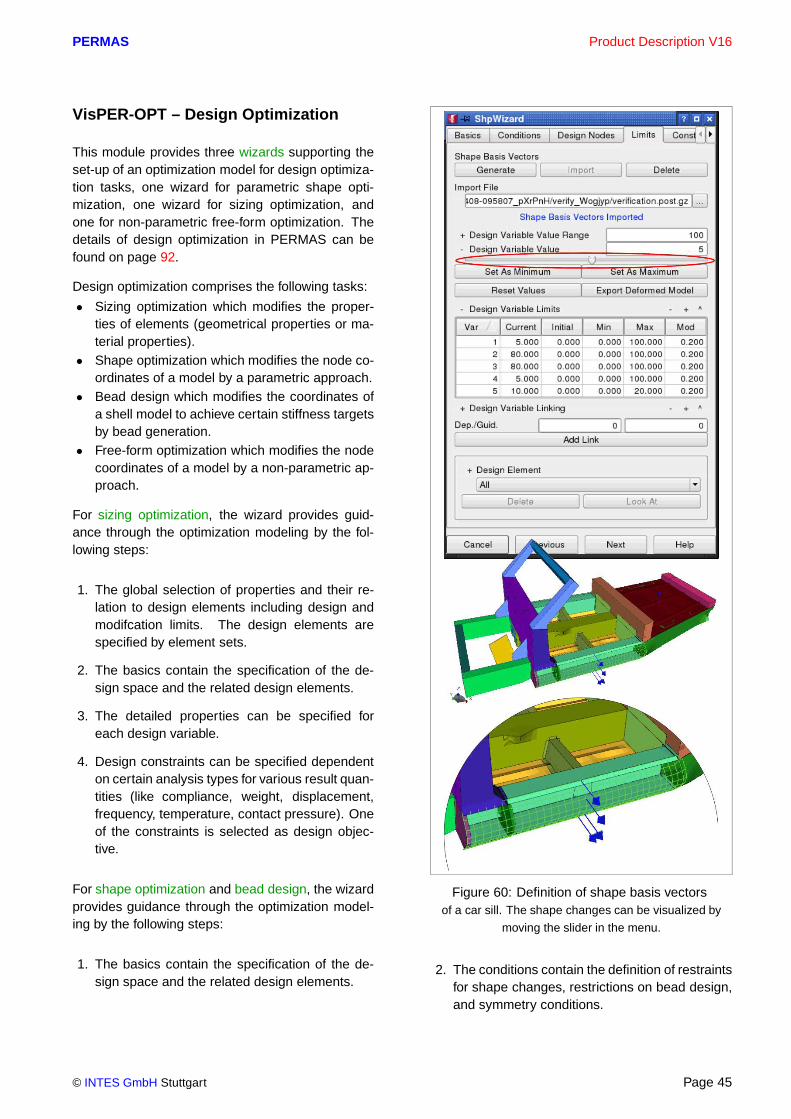
PERMAS Product Description V16
VisPER-OPT – Design Optimization
This module provides three wizards supporting theset-up of an optimization model for design optimiza-tion tasks, one wizard for parametric shape opti-mization, one wizard for sizing optimization, andone for non-parametric free-form optimization. Thedetails of design optimization in PERMAS can befound on page 92.
Design optimization comprises the following tasks:
• Sizing optimization which modifies the proper-ties of elements (geometrical properties or ma-terial properties).
• Shape optimization which modifies the node co-ordinates of a model by a parametric approach.
• Bead design which modifies the coordinates ofa shell model to achieve certain stiffness targetsby bead generation.
• Free-form optimization which modifies the nodecoordinates of a model by a non-parametric ap-proach.
For sizing optimization, the wizard provides guid-ance through the optimization modeling by the fol-lowing steps:
1. The global selection of properties and their re-lation to design elements including design andmodifcation limits. The design elements arespecified by element sets.
2. The basics contain the specification of the de-sign space and the related design elements.
3. The detailed properties can be specified foreach design variable.
4. Design constraints can be specified dependenton certain analysis types for various result quan-tities (like compliance, weight, displacement,frequency, temperature, contact pressure). Oneof the constraints is selected as design objec-tive.
For shape optimization and bead design, the wizardprovides guidance through the optimization model-ing by the following steps:
1. The basics contain the specification of the de-sign space and the related design elements.
Figure 60: Definition of shape basis vectorsof a car sill. The shape changes can be visualized by
moving the slider in the menu.
2. The conditions contain the definition of restraintsfor shape changes, restrictions on bead design,and symmetry conditions.
© INTES GmbH Stuttgart Page 45

Product Description V16 PERMAS
3. Definition of shape basis vectors (SBV) as de-sign variables and a number of conditions likeinitial values, modification limit, and minimumand maximum values. The shape basis vectorsare calculated by PERMAS and provided for vi-sualization. See Fig. 60 as example for thespecification of shape basis vectors by morph-ing.
4. Design constraints can be specified dependenton certain analysis types for various result quan-tities (like compliance, weight, displacement,frequency, temperature, contact pressure). Oneof the constraints is selected as design objec-tive.
A wizard for free-form optimization is available for aparameter-free shape optimization to reduce stressconcentrations (see Fig. 61).
In addition, post-processing of design optimizationresults is supported by VisPER, too:
• Parameters of the optimization process areavailable as XY plots for objective function his-tory, constraint history, design variable history,and max. constraint violation history. The vi-sualization of history plots allows a direct linkbetween a touched curve in the plot and a high-lighted area in the structure, e.g. a design vari-able history shows the related design elements.
• Resulting shell thicknesses can be presented.• Shape changes can be visualized by showing
the model with new coordinates.• A hull generation is supported also for the new
shape after shape optimization.
Figure 61: Pre- and post-processingfor free-form optimization:
• Initial shape with too high stresses
• Definition of surface node set to specify design area
• Automatic selection of design space in thickness di-rection
• Modified shape after free-form optimization with re-duced stresses
Page 46 © INTES GmbH Stuttgart

PERMAS Product Description V16
VisPER-FS – Fluid-Structure Coupling
This module mainly provides a wizard supportingthe semi-automatic fluid meshing of a cavity, wherethe surrounding structure is given as input. The wiz-ard supports the following steps, where the numberscorrespond to the numbers in Figs. 62 and 63:
1. A recommended mesh size is calculated basedon a frequency range for subsequent analysis.
2. Hole detection is performed automatically. Onlythose holes are detected which are larger thana defined minimum element size.
3. Due to difficult topological situations, someholes cannot be detected automatically. Then,undetected holes can be specified in addition.
4. Hole meshing is performed automatically usingelements which do not introduce any stiffness ormass (like plot elements). They are just used tospecify the topology of the hole and to limit thesubsequent cavity meshing.
Figure 62: Steps 1 to 4 of the FS wizard
© INTES GmbH Stuttgart Page 47

Product Description V16 PERMAS
5. Seed point definition is made by the user. Thisspecifies the starting point for the cavity mesh-ing.
6. Cavity meshing is performed automatically.Voxel meshing is used and leads to ahexahedra-dominant mesh. The hexahedra-dominant mesh provides a low number of pres-sure degrees of freedom compared to tetrahe-dra meshes (where the element orientation in-fluences the result, too).
7. When meshing is finished, there are some ele-ments penetrating the hull of the cavity. Thesepenetrations are resolved by a relaxation pro-cess which is performed automatically.
8. The last step automatically generates the cou-pling elements between fluid and structure.Their nodes have both pressure and displace-ment degrees of freedom.
Details of the fluid-structure acoustic simulation canbe found on page 89.
Figure 63: Steps 5 to 8 of the FS wizard
Page 48 © INTES GmbH Stuttgart

PERMAS Product Description V16
Figure 64: Contact modelingContact topology and load history definition
VisPER-CA – Contact Analysis
This module provides two wizards supporting theset-up of a contact model and bolt pretension. Thedetails of contact analysis in PERMAS can be foundon page 72.
The contact wizard provides guidance through thecontact modeling by the following steps and pro-vides a graphical check of already existing contactdefinitions:
• Definition of the contact topology with node-to-node, surface-to-node, or surface-to-surface re-lationship.
• Definition of the contact details like intial gapwidth and frictional coefficients. This informationis specified as load case dependent data.
• Definition of a load history, which specifies theactivation and deactivation for all loadcases in acontact analysis (or in a static analysis in gen-eral). See the example in Fig. 64.
• Checking of contact definitions by highlightingwhile the model is shown by contour lines.
A pretension wizard allows an easy description ofcomplex bolt definitions according to PERMAS pre-tension technology:
• Bolts are detected automatically and groupedwith respect to their length and direction.
• The coupling surfaces in the thread area areproposed and can be adjusted or confirmed af-ter visual checking.
• The wizard is capable to detect holes for screwcandidates.
© INTES GmbH Stuttgart Page 49

Product Description V16 PERMAS
Figure 65: Navigation in the component treeof a substructure model
Figure 66: Visualization of componentsof a substructure model
Substructuring
A substructure wizard has been provided to facilitatethe set-up of substructure models. This function ispart of module VBAS (see page 42).
Figure 67: Visualization of coupling nodesof a substructure model
Because VisPER uses the data structures ofPERMAS, substructure models can be directly im-ported. Substructuring is explained in more detailon page 53.
The verification of substructure models includes thefollowing points:
• Navigation through the component tree (see Fig.65).
• Visualization of single components (see Fig.66).
• Visualization of coupling nodes (see Fig. 67).• Check of element properties (see Fig. 68).• Display of mode shapes on full structure (see
Fig. 69).
Page 50 © INTES GmbH Stuttgart
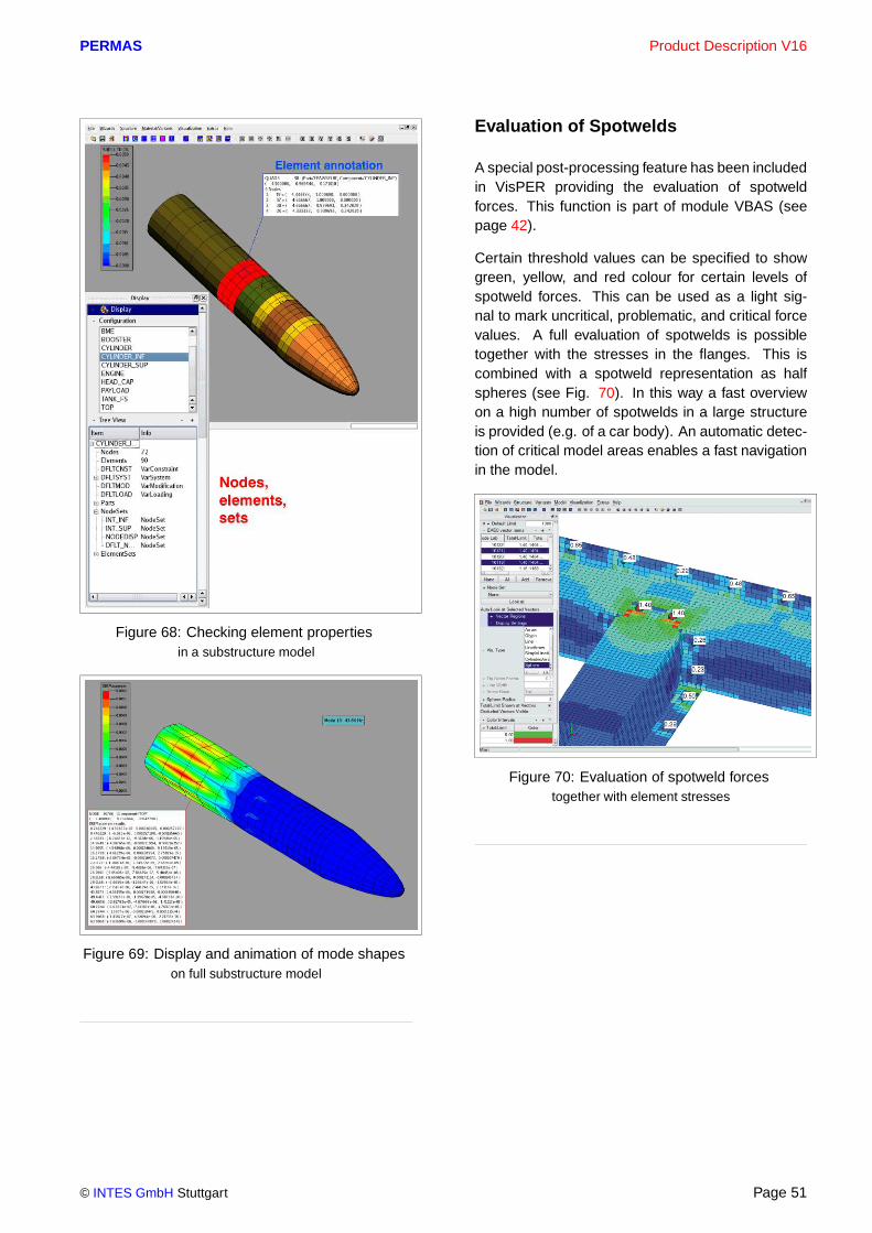
PERMAS Product Description V16
Figure 68: Checking element propertiesin a substructure model
Figure 69: Display and animation of mode shapeson full substructure model
Evaluation of Spotwelds
A special post-processing feature has been includedin VisPER providing the evaluation of spotweldforces. This function is part of module VBAS (seepage 42).
Certain threshold values can be specified to showgreen, yellow, and red colour for certain levels ofspotweld forces. This can be used as a light sig-nal to mark uncritical, problematic, and critical forcevalues. A full evaluation of spotwelds is possibletogether with the stresses in the flanges. This iscombined with a spotweld representation as halfspheres (see Fig. 70). In this way a fast overviewon a high number of spotwelds in a large structureis provided (e.g. of a car body). An automatic detec-tion of critical model areas enables a fast navigationin the model.
Figure 70: Evaluation of spotweld forcestogether with element stresses
© INTES GmbH Stuttgart Page 51

Product Description V16 PERMAS
Page 52 © INTES GmbH Stuttgart

PERMAS Product Description V16
PERMAS Basic Functions
Substructuring
PERMAS allows to decompose a model into sub-structures – the so-called Components . Like singleelements in a FEA-model, these Components maybe inserted into a superior structure – the Configu-ration .
• The number of Components is not limited andeach Component may be arbitrarily large andcomplex .
• Components and Configurations are identifiedby user defined names.
• Each Component has its own name index forelement-, node-IDs, etc.
• Each Configuration may consist of an arbitrarynumber of Component levels and each levelmay contain elements, loads and constraints.The specification of the coupling degrees offreedom in each component (the so-called ’ex-ternal’ degrees of freedom) allows the auto-matic assembly of the complete Configuration.The condensation of the components is per-formed using Guyan’s reduction.
• In addition to the static condensation usingGuyan’s reduction a dynamic condensation us-ing the Craig-Bampton method or the Mixed-Boundary Craig-Bampton method is available.
• Specific reordering concepts in conjunction withexplicit and iterative condensation schemes andautomatic selection of algorithms provide high-est solution efficiency .
Basic Components
COMP_5
COMP_4 COMP_6
COMP_1 COMP_2 COMP_3
Configuration
Top Component
Assembled Components
Figure 71: Substructuring in PERMAS
• The data base can hold an arbitrary number ofConfigurations.
• Multiple Configurations may share the sameComponents.
• Components may be extracted and saved forfuture substructuring either by their model de-scription or by the corresponding condensedmatrix models (see section Matrix Models, page66).
• Such matrix models may be forwarded to cus-tomers and suppliers in place of the real geo-metric models.
• Substructuring permits the separated modelingand verification for all parts of the structure, priorto the final assembly.
• Single FEA models from distinct modelingsources, can be easily combined.
• Areas with design variations or nonlinear prop-erties may be assembled into separate Compo-nents, thus concentrating modifications and iter-ations on this Component only. This will mea-surably cut computation time and resources.
Figure 72: Submodeling in static analysis
Submodeling
This feature supports the use of previously calcu-lated results from a coarse (global) model as bound-ary conditions for a refined mesh of a part of themodel. This enables e.g. a subsequent more pre-cise analysis of stresses (see Fig. 72).
In a static analysis the displacements at the bound-ary of the refined part are taken from the full modelas prescribed values.
For temperature fields, the interpolation on the sideof the fine mesh is usually done in 3D (see Fig. 73).
© INTES GmbH Stuttgart Page 53

Product Description V16 PERMAS
Figure 73: Mapping of temperature fields
Sometimes temperature fields have also to be ex-trapolated to nodes which do not yet have temper-atures (e.g. additional parts like gaskets or boltsin engine analysis). This extrapolation can be per-formed by the mapping or by an additional temper-ature field analysis (or both as explained by the ex-ample in Fig. 74).
Figure 74: Mapping with extrapolationof temperature fields
Variant Analysis
PERMAS offers an easy way for examining differentvariants of one FEA model. Variable model proper-ties are held within the so-called Variants :
• System Variant:– material assignment of elements,– element properties (thickness, cross section
etc.),– element local coordinate systems.
• Constraint Variant:– suppressed degrees of freedom,– prescribed degrees of freedom,– contact definitions,– coefficients of general kinematic constraints,– local coordinate systems for the degrees of
freedom at each node.• Loading Variant:
– Dynamic loads and an arbitrary number ofstatic load cases or combinations hereof.
• Result Variant:– For more detailed specification of required re-
sults, like
* load pattern combination rules,
* list of excitation frequencies for fre-quency response,
* load steps where results are requested.• Modification Variant:
– specification of design model for sensitivityanalysis and optimization.
SPC_5
Loading
Situation
ResultSystemVariantsConstraint
SV_1LOAD_4
RV_2
Variants Variants Variants
Figure 75: Variants in PERMAS
Basic properties like nodal point coordinates, ele-ment topology and global coordinate systems areinvariant.
Single Variants may be selected and examined to-gether as a so-called Situation .
• Variants and Situations are identified by user de-fined names.
• The number of Variants and Situations is not lim-ited.
• There is no restriction in combining the variantdefinitions with any substructuring feature.
• In each substructure the selection of system,constraint, loading and result Variants is inde-pendent of the selections made for other sub-structures (e.g. useful for models with symme-try/antisymmetry).
• PERMAS keeps a record of all calculation stepsalready completed. In this manner, multiple cal-
Page 54 © INTES GmbH Stuttgart

PERMAS Product Description V16
culations are avoided when using a Variant re-peatedly.
Figure 76: Cyclic symmetry of a fanBehr GmbH & Co., Stuttgart, Germany.
Cyclic Symmetry
Cyclic symmetric structures like Fig. 76 are charac-terized by a number of identical sectors each rotatedby a multiple of the sector angle around the axis ofsymmetry.
Cyclic symmetric structures can be handled directlyfor static analysis with matching cyclic symmetricloads and real eigenvalue analysis (see modules LSand DEV on pages 72 and 83). There, the analy-sis of the whole structure is replaced by a series ofanalyses for one sector with different boundary con-ditions. In addition, the number of nodal diametershas to be specified, i.e. number of waves along theperimeter.
Substructuring can be used to model a sector andthe analysis of cyclic symmetry is performed in thetop component.
In topology optimization (see module TOPO onpage 95) the result can be forced to become cyclicsymmetric.
Figure 77: Incompatible meshesCardan shaft model in sectional view
(Voith Turbo GmbH & Co. KG)
Surface and Line Description
The description of surfaces in PERMAS is used forthe specification of structural parts which have tobe coupled automatically (see next section). Thisdescription is made using one of the following meth-ods:
• by specifying element surfaces, e.g. for a set ofvolume elements (for Sets see page 62),
• by specifying geometry elements (see elementlibrary page 59).
For surfaces very accurate coordinates are fre-quently required (as e.g. for contact with incom-patible meshes), which are not available throughthe pre-processor used. Such surfaces can besmoothed internally by correction of runaways,which leads to very precise surfaces for more ac-curate analysis results.
For surfaces with quadratic elements, a linearizationis available, which makes the midside nodes linearlydependent on the corner nodes. If these surfacesare used in contact definitions, then the surfaces willalso provide contact pressure results. A special ex-port item allows to visualize the surface definitions.Definition and visualization of surfaces are fully sup-ported by VisPER.
In the same way does the description of lines serveas specification of structural parts which have to becoupled automatically along lines (see next section).This description is made using one of the followingmethods:
© INTES GmbH Stuttgart Page 55
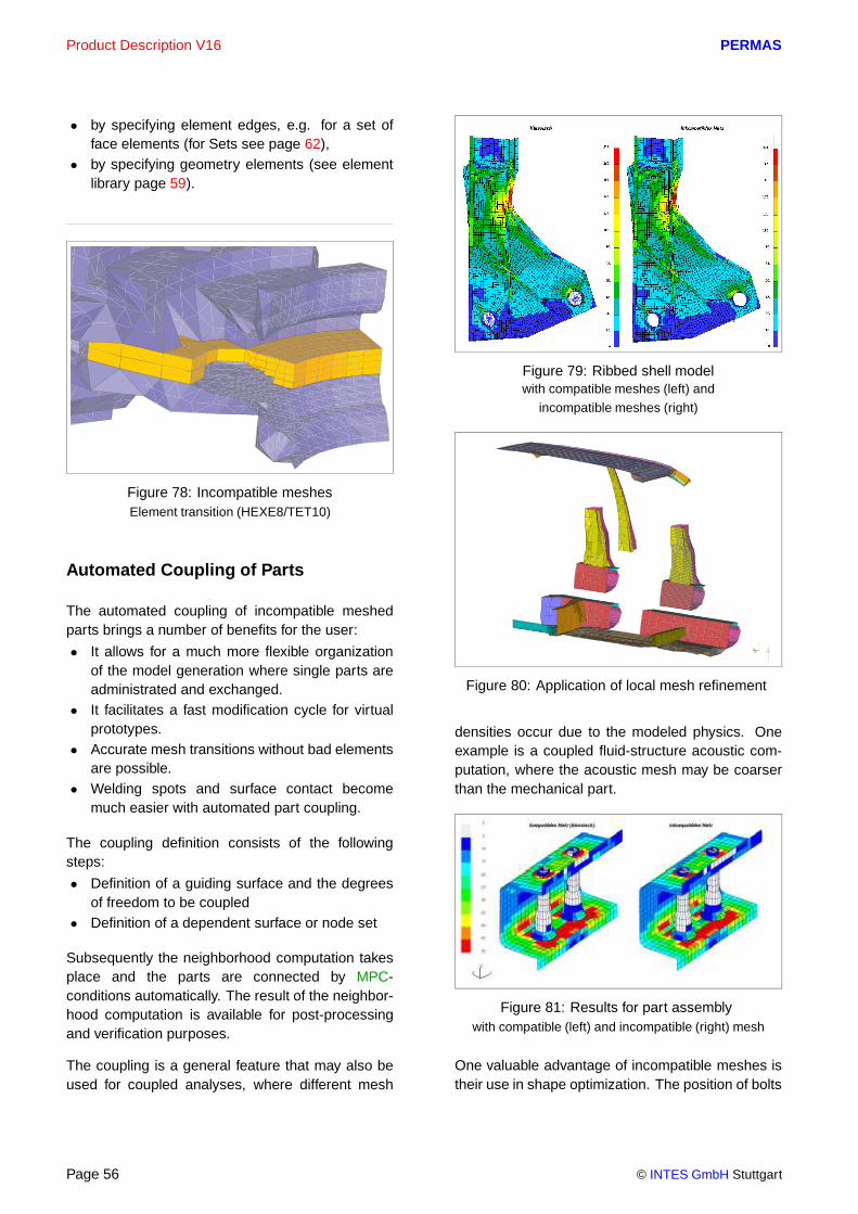
Product Description V16 PERMAS
• by specifying element edges, e.g. for a set offace elements (for Sets see page 62),
• by specifying geometry elements (see elementlibrary page 59).
Figure 78: Incompatible meshesElement transition (HEXE8/TET10)
Automated Coupling of Parts
The automated coupling of incompatible meshedparts brings a number of benefits for the user:
• It allows for a much more flexible organizationof the model generation where single parts areadministrated and exchanged.
• It facilitates a fast modification cycle for virtualprototypes.
• Accurate mesh transitions without bad elementsare possible.
• Welding spots and surface contact becomemuch easier with automated part coupling.
The coupling definition consists of the followingsteps:
• Definition of a guiding surface and the degreesof freedom to be coupled
• Definition of a dependent surface or node set
Subsequently the neighborhood computation takesplace and the parts are connected by MPC-conditions automatically. The result of the neighbor-hood computation is available for post-processingand verification purposes.
The coupling is a general feature that may also beused for coupled analyses, where different mesh
Figure 79: Ribbed shell modelwith compatible meshes (left) and
incompatible meshes (right)
XY
Z
Figure 80: Application of local mesh refinement
densities occur due to the modeled physics. Oneexample is a coupled fluid-structure acoustic com-putation, where the acoustic mesh may be coarserthan the mechanical part.
Figure 81: Results for part assemblywith compatible (left) and incompatible (right) mesh
One valuable advantage of incompatible meshes istheir use in shape optimization. The position of bolts
Page 56 © INTES GmbH Stuttgart

PERMAS Product Description V16
or ribs can be optimized in a shape optimizationwithout any remeshing of the structure. Fig. 82shows an example, where the initial position and thefinal position of the bolts are very different. Never-theless, after a number of iterations the final positionis reached which is still symmetric and shows iden-tical bolt forces for all the bolts.
Figure 82: Shape optimizationwith incompatible meshes to achieve smallest relative
displacements and identical bolt forces (top: initial
design, bottom: final design; in between: bolt forces for
each iteration)
Figure 83: Connection of spotweld forces
Automated Spotweld Modeling
For the automated modeling of spotwelds neigh-boured surfaces are connected using predefinedpoints:
• Specification of spotweld positions• Selection of (incompatible) faces
• Specification of spotweld stiffness and (option-ally) the spotweld diameter
Figure 84: Spring element at spotweld position
The spotweld stiffness is modeled by a spring ele-ment, which is coupled to the neighboured parts byautomatically generated MPC conditions (see Fig.84). Available results are the spring forces and thereaction forces at the coupling nodes of the jointparts.
Figure 85: Spotwelds and incompatible meshes
For verification purposes the topology and the con-necting vectors of the generated spotweld connec-tions can be issued for graphical post-processing(see Fig. 86).
Figure 86: Verification of spotweld connections
A more sophisticated spotweld model has been de-veloped with module WLDS (see page 101). Usingvery simple modeling it achieves best possible re-sults.
© INTES GmbH Stuttgart Page 57

Product Description V16 PERMAS
Local Coordinate Systems
Local coordinate systems are used as reference fornode coordinates or other coordinate systems to fa-cilitate the model description. Also, rotated nodebases, loads, and anisotropic materials may makereference to local coordinate systems. The types oflocal coordinate systems can be seen from Fig. 87.Local coordinate systems may be defined in a visualmanner by VisPER.
Figure 87: Local coordinate systems in VisPER
Kinematic Constraints
For the specification of single point kinematic con-straints (absolute constraints) suppressed and pre-scribed degrees of freedom are available for zero ornon-zero displacements, respectively.
Multilinear kinematic constraints (relative con-straints) between several degrees of freedom aredescribed by the use of so-called Multi Point Con-straints (MPCs).
PERMAS offers a great number of various MPCs –
all of them comfortable tools for modeling:
• Multiple degrees of freedom may be forced tohave identical freedom values by simple As-signment (for modeling swivels, hinges or slid-ing surfaces and for boundary conditions incyclic symmetry).
• Rigid Bodies allow the modeling of rigid partswithin an elastic structure. There can be one orseveral guiding degrees of freedom and one orseveral dependent degrees of freedom, too.
• Interpolation Regions may be used for meshrefinements, coupling of incompatible meshes,distributing loads, or transfer of results betweendifferent meshes:– lines with 2 or 3 guiding nodal points,– triangular and quadrilateral areas with 3 or 6
and 4, 8 or 9 guiding nodes, respectively,– Volume areas as hexahedra (with 8, 20, 27
nodes), pentahedra (with 6, 15, 18 nodes),tetrahedra (with 4, 10 nodes), pyramids (with5 nodes).
• Coupling with surfaces may be used for cou-pling of incompatible meshes. All degrees offreedom at all nodes belonging to dependentnode set, dependent surface or dependent sur-face set are forced to have displacements (ortemperatures etc.) which are determined by in-terpolation of the corresponding values at thenodes belonging to guiding surface or guidingsurface set. This coupling may be used also fora Volume-Shell Transition , i.e. the connectionof plates and shells with solid element structures(see Fig. 88). If the dependent nodes do not liein the guiding surface, then either the node isprojected onto the surface or a rigid lever arm isgenerated in order to represent the kinematicsof the coupling correctly.
Figure 88: MPC example: Volume Shell Transition
• Coupling with volumes may be used for cou-pling of incompatible meshes. All degrees offreedom at all nodes belonging to dependent
Page 58 © INTES GmbH Stuttgart

PERMAS Product Description V16
node set are forced to have displacements (ortemperatures etc.) which are determined by in-terpolation of the corresponding values at thenodes belonging to guiding volume, which esdefined by referenced elements.
• General MPCs allow any linear combination ofthe involved degrees of freedom.General MPC conditions can be used to modelPress Fits , e.g. shaft-hub connections wherethe shaft has a slightly larger outer diameterthan the inner diameter of the hub. Typically,such configurations are modeled using contact.If any change in the contact is not expected, itwould be more efficient to use a general MPCto model the interference in order to keep aproblem in the linear range instead of a nonlin-ear contact analysis. It was proven that contactanalysis and general MPC give identical resultsfor corresponding models (see Fig. 89 and Fig.12). A press fit command supports the auto-matic generation of the MPC conditions.
Figure 89: Press fit between shaft and hubIdentical stress results of MPC (above)
and contact solution (below).
The number of dependent degrees of freedom foreach MPC is not limited. Also multi-level conditions(hierarchical MPCs) may be used as long as thereis no recursive interdependence.
The coupling of single components using the sub-structure technique is defined by ’external degreesof freedom’. On the higher component’s level these
external degrees of freedom can be part of single ormultipoint constraints.
Handling of Singularities
In static analysis there are two different kinds ofsingularities, which are detected automatically andcommunicated to the user in a suitable way:
• For redundant degrees of freedom, which haveno stiffness (e.g. perpendicular to rods or mem-branes), the user gets a list on the result file.
• For rigid body degrees of freedom the re-lated displaced shapes are issued on a post-processor file. They can easily be inspectedin order to detect the missing supports or othermodeling errors.
VisPER provides an RBM Assistent (see page 43)which allows for the elimination of rigid body modesprior to analysis.
In dynamic mode analysis the rigid body modes aredetected and decoupled automatically.
In dynamic response analyses in the time or fre-quency domain the absolute response results forma superposition of the elastic and the rigid body re-sponse.
Element Library
The PERMAS elements are generally usable for dif-ferent types of physical degrees of freedom (likedisplacements, temperature, electromagnetic po-tential, etc.), beside some specific, application-dependent elements. Currently, the following ele-ments are provided:
• Solid Elements :– tetrahedra with 4 or 10 nodal points and
straight or curved edges,– pyramid element with 5 nodal points,– pentahedra with 6, 15, or 18 nodal points and
straight or curved edges,– hexahedra with 8, 20, or 27 nodal points and
straight or curved edges.– hexahedra with 8, 20, or 27 nodes, pentahe-
dra with 6, 15, or 18 nodes, tetrahedra with
© INTES GmbH Stuttgart Page 59

Product Description V16 PERMAS
4 or 10 nodes, and pyramid element with 5nodes as fluid elements.
• Flange (Rod) and Membrane Elements :– flange elements with 2 or 3 nodal points,– triangular elements with 3 or 6 nodal points
and straight or curved edges,– quadrilateral elements with 4, 8 or 9 nodal
points and straight or curved edges,– quadrilateral shear panel with 4 nodal points.
• Beam Elements with 2 nodal points, optionallywith or without rigid lever arms (offset nodes):– beams with arbitrary shaped solid cross sec-
tion,– thin-walled profiles and tubes with open or
closed cross sections,– thin-walled open or closed tubes with cross
sections tapered along the beams’ lengthaxis,
– fluid-filled or fluid-surrounded straight orcurved pipe elements.
P2
P3
P4
P5P6
t1
t3
t5
x’
y’n
P1
Figure 90: Triangular element with curved edges
• Plate and Shell Elements :– triangular or quadrilateral elements for thin
and moderately thick plates and shells.– triangular or quadrilateral elements sandwich
shells.– a thin-walled triangular plate element follow-
ing Kirchhoff’s Theory.– triangular (with 3 or 6 nodes) and quadrilat-
eral elements (with 4, 8, or 9 nodes) with 3-dimensional shell formulation for linear andnon-linear material.
– triangular and quadrilateral elements for lay-ered cross-sections (composites).
• Discrete Elements :– linear and non-linear spring elements,
– various mass elements,– linear and non-linear damper elements,– control elements,– elements with direct matrix input.
• Elements for contact analysis :– Gasket elements defined by a nonlinear
pressure-closure curve. This curve can alsoreflect an additional gap to the neighbouredpart in the unloaded initial configuration.
– Compensation springs to ground or between2 nodes with 3 translational DOF, or betweentwo nodes with 1 translational DOF.
• Scalar Elements :– spring elements between 2 degrees of free-
dom or for a support of 1 degree of freedomto ground,
– damper elements between 2 degrees of free-dom or for a connection of 1 degree of free-dom to ground,
– scalar masses for 1 or 2 nodal points,– scalar mobility element for fluid meshes.
• Load carrying membranes in form of triangularrespectively quadrilateral areas for load applica-tion and stress evaluation.
• Plot Elements in form of points, lines and trian-gular respectively quadrilateral areas for resultevaluation.
• Geometry Elements in form of lines and tri-angular respectively quadrilateral areas for lineand surface definition.
• Convectivity Elements to model the convec-tivity behavior and radiation on free surfaces inthermal analysis.
• Fluid-Structure Coupling Elements for cou-pled acoustics and surface absorption.
• Surface Wave Elements for acoustic analyses.• Semi-Infinite Elements for acoustic and elec-
tromagnetic analyses.• Radiation Boundary Condition (RBC) Ele-
ments for the modeling of acoustic radiation ef-fects.
• Axisymmetric Elements for structures, heattransfer, acoustics, and electromagnetics.
Standard Beam Cross Sections
The following standard geometries are supported forthin-walled beam cross sections:
Page 60 © INTES GmbH Stuttgart

PERMAS Product Description V16
• General thin-walled open section (see Fig. 91),• Circular cross section,• Box cross section.
Using those cross sections allows to get stress re-sults at certain points of the cross sections.
The parameters of the cross sections are directlyavailable as design parameters in an optimizationrun (see page 92).
H
t 2
W2 e2
tH
t 1
W1
e1
y’
x’G
Figure 91: General thin-walled open section
Design Elements for Optimization
For design optimization purpose (see page 92), allparts of the structure which may be modified areassigned to so-called Design Elements. They areused to define possible modifications for elementsand nodes belonging to the design element.
To facilitate shape optimization a number of addi-tional design elements are available to collect struc-tural elements belonging to one design element. Alltypes of finite elements are allowed to be part ofthese design elements:
• design element for smooth shape optimization,• design element for bead design,• design element for free-form optimization,• design element for topology optimization.
Error estimator
The element size in FE meshes influences the accu-racy of the results (in particular stress results). Butthe ’right’ element size is a local characteristic anddepends on the force flow and its gradients. Partic-ularly, notch stresses are highly dependent on ele-ment size.
With the refinement indicator pre-processors likeMEDINA may be able to perform an adaptive meshrefinement (see Fig. 92).
But this indicator can also be used to identify thosemesh regions where stresses are possibly not veryreliable.
In addition, the error estimation can also be used toimprove the stresses by a smoothing process with-out a new mesh or a repeated analysis run.
Figure 92: Example for error indicator,element stress, and smoothed element stress
Material Properties
The description of material is made independently ofthe other model data. In doing so, the needed ma-terial parameters can easily be taken from alreadyexisting data sets building a certain kind of materialdata base.
Beside isotropic material all kinds of anisotropy canbe applied in a simple and suitable way: transverse
© INTES GmbH Stuttgart Page 61

Product Description V16 PERMAS
isotropic, orthotropic, monoclinic, and general (tri-clinic) material.
Because of the application of PERMAS in differ-ent fields, different material properties can be de-fined like elasticity, density, compressibility, damp-ing, thermal expansion, heat conductivity, heat ca-pacity, absorption, volume drag, electric conductiv-ity, dielectricity, magnetic permeability. There, onlythe required data are really used, all additional ma-terial properties don’t have any effect.
For nonlinear material, additional input facilities areprovided like stress-strain curve, yield load, creepbehavior.
Almost all material properties can be specified astemperature-dependent. Following a given temper-ature field, the actual material properties are deter-mined by an interpolation from the given distributionfunction.
The definition of damping can be frequency-dependent.
Layered composites (laminates) can be defined bydifferent materials (like fibre-reinforced material) foreach layer (see page 101).
Figure 93: Mode shape of a reactor
Sets
For a lucid model description node and element setsmay be used. Such sets may be generated fromother sets using Boolean operations. In addition,
several sets can be collected in a set bin, which de-notes a set of sets.
Beside the model description such sets may beused also for the specification of result output. Forthe print output of results and the export to con-nected post-processors the amount of issued re-sults can be restricted to the relevant data by sets.In case of analyses in the time or frequency domain,the required run time and disk space can be drasti-cally reduced by the specification of sets for whichthe results are to be determined.
All interfaces preserve the sets and their identifiersfrom the pre-processing via the solver to the post-processor. An acompanying text marks a set moreprecisely.
Mathematical Functions
For the description of complex data relations a li-brary of mathematical functions is provided for:polynomes, trigonometric functions, exponentialfunctions, and discrete functions. E.g. they al-low for the definition of time-dependent loading andtemperature-dependent loads.
Beside the library functions also tabular functions oruser functions (defined by Fortran or C subroutines)may be defined and used.
On all of these functions sums, products, or chainsmay be defined in order to specify complex com-pound functions.
In VisPER, a special functions dialogue is availableto prepare, manipulate, and visualize functions (seeFig. 94).
In addition, a special function to derive theFourier coefficients of a time signal is provided.Time-dependent excitations are analyzed by aFourier transformation and the resulting frequency-dependent coefficients are used in a frequency re-sponse analysis (see Fig. 95).
Page 62 © INTES GmbH Stuttgart

PERMAS Product Description V16
Figure 94: Functions dialogue in VisPER
Loads
In static analyses the following mechanical loadsmay be used:
• Global loads:– Inertia loads,– Inertia relief (quasi-static acceleration).
• Nodal loads:– Concentrated loads,– Distributed loads,– Prescribed displacements,– Temperature loads,– State of contact.
• Element loads:– Distributed loads,– Initial strains.
• Surface loads:– Distributed loads,– Hydrostatic pressure.
For distributed surface loads, e.g. not specified atthe nodes of a mesh but a coarser grid, special loadelements (see page 60) can be used which are cou-pled to the main structure by interpolation (see page58).
In heat transfer analyses the following thermal loadsmay be used:
• Nodal loads:– Concentrated heat flows,– Distributed heat flow,– Prescribed temperatures.
• Element loads:
– Distributed heat flow.
Temperature fields may be taken directly from a pre-vious heat transfer analysis. One temperature fieldmay be used to define temperature dependent ma-terial properties, and another temperature field maybe used for initial strain calculation or as initial con-dition for a transient thermal analysis.
All distributed element loads can be defined ascoordinate-dependent.
Load case combinations may be applied to createnew loads from existing patterns.
Time-dependent loads are defined as a productof a static or thermal load and a time-dependentfunction. In addition, initial conditions for time-dependent mechanical or thermal analysis can bespecified. These can simply be taken from a previ-ous analysis.
For frequency-dependent dynamic loads it alwaysholds that they are defined as a product of a staticload and a spectrum of amplitudes and phase an-gles.
Time dependent loads of a periodic process can betransformed to frequency dependent loads by an au-tomatic Fourier analysis (see Fig. 95). Then, oneor more frequency response analyses can be per-formed. Finally, by superposition of the results in thetime domain a periodic response can be achieved.
Model Verification
With increasing complexity of models the need toverify the correctness of model descriptions in-creases. PERMAS pays attention to this point byproviding model properties in a form that they canbe post-processed like results.
It is an important principle of model description thatall quantities which can be specified can also be ex-ported for visualization and checking purposes. Inparticular, this holds for all automatically generatedquantities which facilitate model description.
Since VisPER is available, verification of PERMASmodels became much easier. It does not only pro-vide visual means to check the model, but it pro-vides also capabilities to visualize the verification
© INTES GmbH Stuttgart Page 63

Product Description V16 PERMAS
-150
-100
-50
0
50
100
150
200
0 0.5 1 1.5 2 2.5 3
Load
[N]
Time [s]
Load
0
10
20
30
40
50
60
70
0 50 100 150 200 250 300 350 400 450 500
Am
plitu
de [N
]
Frequency [Hz]
Amplitude
Figure 95: Example for the transformationof a periodic load (above in time domain,
below in frequency domain)
data generated by PERMAS (see examples below).For PERMAS models, VisPER is the recommend-able verification tool.
The following list gives a few examples of verificationaids:
• Element test results are exported for identifica-tion of erroneous elements.
• Mean element thickness at nodes can be ex-ported to check the thickness distribution in ashell structure.
• Rigid body modes detected during the analysiscan be exported for viewing in order to verifiysupport conditions.
• For MPC interpolation regions (see MPC condi-tions on page 58) the offset vectors are exportedto verify the result of the automatic interpolation.
• For spotweld connections the generated weldbase vectors are issued (see Fig. 86).
• VisPER can be used to check distributed loads(even those with a function dependent on geo-metric position).
• Element temperature loads and distributed
nodal temperature loads can be exported astemperature result for visualization.
• Initial strains are available for postprocessing.• For contact modeling a number of entities are
available for verification like contact definition,contact geometry, contact coordinate system,initial contact status, initial gap width (see Fig.96).
• For the pretension of bolts an additional num-ber of description entities can be postprocessedlike pretension definition, pretension coordinatesystem, pretension thread vectors (flank normal,downhill and pitch direction).
• For heat transfer analyses with heat exchangeby radiation the radiating surface can be coars-ened automatically. The element mesh of thecoarsened surface can be exported for check-ing.
• In fluid-structure coupled analysis the interfaceelements and their orientation can be checked.
• In optimization applications the use of design el-ements can be checked by VisPER (see pages44 and 45). Besides, the assignment of fi-nite elements to design elements can also bechecked.
For a number of input data, PERMAS can generatepostscript files using gnuplot (if gnuplot is availableon the currently used machine). It will generate gnu-plot command files, and a table with the xy-data ofthe curves will be exported to a file. Such input datainclude load history (see page 73), material curvesfor plasticity, and transient loads in timehistory re-sponse analysis.
Interfaces
The integration of PERMAS in the pre- and post-processor is of top priority for the interface devel-opment. Therefore, all interfaces are directly inte-grated without any separate software tools. Theseinterfaces are denominated as ’Doors’, which allowfor a very direct access to the original model data.Above the model description, some interfaces allowfor standard solutions, which make the working en-vironment more comfortable.
Beside its own input and output formats PERMASoffers Doors not only to various pre- and post-
Page 64 © INTES GmbH Stuttgart

PERMAS Product Description V16
Figure 96: Verification of a contact modelTop: contact normal vector
Middle: surface normal vector
Bottom: nadir vector
processors but also to model files of other FEA sys-tems:
• MEDINA (page 103)• PATRAN (page 103)• I-DEAS (page 103)• ADAMS (page 104)• DADS (page 104)• SIMPACK (page 104)• EXCITE (page 104)
• MOTIONSOLVE (page 105)• HYPERVIEW (page 105)• VAO (page 105)• Virtual.Lab (page 105)• ADSTEFAN (page 105)• MATLAB (page 105)• NASTRAN (page 105)• ABAQUS (page 106)• MpCCI (page 107)
Moreover, a growing number of extra interfaces toPERMAS are available from partner companies orINTES (see page 107).
All users with a heterogeneous environment of pre-and post-processors benefit from the excellent inter-faces to other CAE products.
During input complete FE-models are read andtranslated into autonomous PERMAS data struc-tures. If requested, any part may be combined withor completed by additional PERMAS data files.
During output the calculated results may be writ-ten in various forms (listing, xy-plot files, severalpost-processor formats). In addition, the completeFE model may be output as PERMAS model file oras post-processing model in diverse pre- and post-processor formats – independent of the kind of in-put.
The result evaluation even for very large models issupported by comprehensive selection facilities forthe exported result data. Beside the selection ofrelevant loading cases, time steps, and frequenciesthe specification of node and element sets is usedto reduce the amount of exported results.
This high-level Door concept endows a number ofadvantages :
• High comfort:– no external interface necessary,– similar command syntax for all Doors,– no intermediate files necessary.
• The translation process is very fast.• Simple input mixing :
– Several input models may be concatenated toone big model, no matter from which Door themodel files were read.
– The model description may be spread on sev-eral files, utilizing the possibilities of all Doorinput formats involved.
© INTES GmbH Stuttgart Page 65
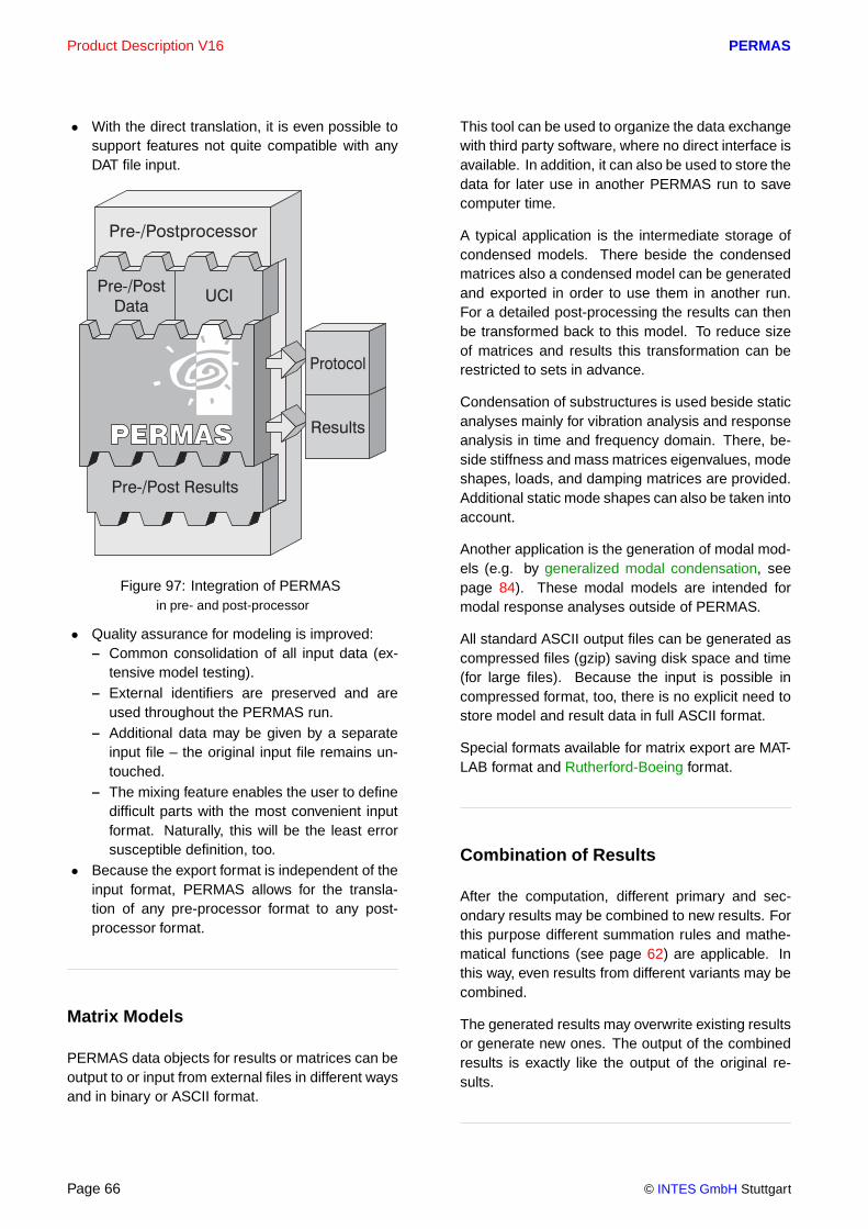
Product Description V16 PERMAS
• With the direct translation, it is even possible tosupport features not quite compatible with anyDAT file input.
Figure 97: Integration of PERMASin pre- and post-processor
• Quality assurance for modeling is improved:– Common consolidation of all input data (ex-
tensive model testing).– External identifiers are preserved and are
used throughout the PERMAS run.– Additional data may be given by a separate
input file – the original input file remains un-touched.
– The mixing feature enables the user to definedifficult parts with the most convenient inputformat. Naturally, this will be the least errorsusceptible definition, too.
• Because the export format is independent of theinput format, PERMAS allows for the transla-tion of any pre-processor format to any post-processor format.
Matrix Models
PERMAS data objects for results or matrices can beoutput to or input from external files in different waysand in binary or ASCII format.
This tool can be used to organize the data exchangewith third party software, where no direct interface isavailable. In addition, it can also be used to store thedata for later use in another PERMAS run to savecomputer time.
A typical application is the intermediate storage ofcondensed models. There beside the condensedmatrices also a condensed model can be generatedand exported in order to use them in another run.For a detailed post-processing the results can thenbe transformed back to this model. To reduce sizeof matrices and results this transformation can berestricted to sets in advance.
Condensation of substructures is used beside staticanalyses mainly for vibration analysis and responseanalysis in time and frequency domain. There, be-side stiffness and mass matrices eigenvalues, modeshapes, loads, and damping matrices are provided.Additional static mode shapes can also be taken intoaccount.
Another application is the generation of modal mod-els (e.g. by generalized modal condensation, seepage 84). These modal models are intended formodal response analyses outside of PERMAS.
All standard ASCII output files can be generated ascompressed files (gzip) saving disk space and time(for large files). Because the input is possible incompressed format, too, there is no explicit need tostore model and result data in full ASCII format.
Special formats available for matrix export are MAT-LAB format and Rutherford-Boeing format.
Combination of Results
After the computation, different primary and sec-ondary results may be combined to new results. Forthis purpose different summation rules and mathe-matical functions (see page 62) are applicable. Inthis way, even results from different variants may becombined.
The generated results may overwrite existing resultsor generate new ones. The output of the combinedresults is exactly like the output of the original re-sults.
Page 66 © INTES GmbH Stuttgart

PERMAS Product Description V16
Transformation of Results
All nodal results are calculated in the global coordi-nate system of the actual Component. From theseresults the following transformations may be per-formed:• into the displacement coordinate system of the
respective node.• into a specific coordinate system for all nodes
(cartesian, cylindric, spheric).• using a special transformation for each node.
All transformations may be performed later in back-ward direction to the Component system.
Beside the transformation of real results, complexresults of a frequency response analysis can betransformed to another coordinate system, too.
Comparison of Results
The following facilities are available for the compar-ison of dynamic analysis results between two vari-ants:• MAC (Modal Assurance Criterion):
Compares two sets of eigenvectors (with samenumber of nodes) from different situations andgets their degree of correspondence. MACfactors are computed as:
MAC =(Xt
1X2)2
diag(Xt
1X1)diag(Xt
2X2)
• CoMAC (Coordinate Modal Assurance Crite-rion):Compares two sets of eigenvectors (with samenumber of nodes) from different situations andgets their degree of correspondence. CoMACfactors are computed as:
COMAC =diag(
∑M
m=1|Xm
1 Xm
2 | )2
diag(∑
M
m=1X
m
1 )2 diag(∑
M
m=1X
m
2 )2
The result gives a measure of the correlation ofthe vector sets in each degree of freedom direc-tion.
• COF (Cross Orthogonality Factors):Compares two sets of eigenvectors (with samenumber of degrees of freedom) from differentsituations and gets their degree of correspon-dence. Cross orthogonality matrix and factorsare computed as :
COFM = Xt
1KX2; COF = COFMtCOFM.
All comparisons may be performed for two variantsof a model and the compared model parts can berestricted to specified node sets.
XY Result Data
On the basis of element and node sets, xy data canbe generated directly and issued on all connectedoutput files for graphical processing.
Usually, xy data are directly extracted from the cor-responding result item such, that the abscissa valueis given by the column (i.e. loading case, iteration)and the ordinate values are the result data. If thecolumns are associated with certain values (like fre-quencies, time, load factors), these values will beused for the abscissa.
As a special case in order to study e.g. the stiffnessbehavior of a part, it is possible to create xy data fornodal point results with the coordinate direction asabscissa. Then, the abscissa values are preparedin ascending coordinate direction for the selectednodes. A local coordinate system may be used toselect the coordinate directions.
Figure 98: Determination of elastic linefor torsional load case (displacement
for the marked nodes)
For a number of input data, PERMAS can generatepostscript files using gnuplot (if gnuplot is available
© INTES GmbH Stuttgart Page 67

Product Description V16 PERMAS
on the currently used machine). It will generate gnu-plot command files, and a table with the xy-data ofthe curves will be exported to a file. Such input datainclude load history (see page 73), material curvesfor plasticity, and transient loads in timehistory re-sponse analysis.
Within PERMAS Tools plots can be created usingPERMASgraph (see page 110 for details).
Cutting Forces
On the basis of element and node sets the cuttingforces can be determined and exported for post-processing for almost all points of a structure. Inaddition, the sum of all forces and moments over acut is calculated and printed for a previously speci-fied point in space (see Fig. 99).
Figure 99: Determination of cutting forces
Restarts
Each PERMAS run opens a data base file, whichmay be used for subsequent runs. At every restart,the latest status of the data base is always availablefrom the previous run. This includes all intermediateresults possibly obtained only by using considerablecomputation time.
In doing so, e.g. different load variants in severalruns may be processed without assembling and de-composing the stiffness matrix every time.
Open Software System
PERMAS is an open software system with respectto its capability to include user-written routines in ev-ery program execution, which may be invoked dur-ing run-time.
On the one hand, this feature is used to offer max-imum flexibility in defining data dependencies, e.g.with user-defined mathematical functions (see page62).
On the other hand, PERMAS may be used as sub-routine library in order to write own solutions or re-sult evaluations. These can be invoked at the rightplace during program execution.
The programming language is Fortran 77/90 in anycase, but on some platforms C is also available. ThePERMAS library routines are available as Fortranprograms.
Figure 100: Clutch Element, Static Displacements
Direct Coupled Analyses
PERMAS enables different coupled analyses in onerun, e.g.
• initial values for time-dependent dynamic anal-ysis may be taken from a previously performedstatic analysis.
• initial values for a transient thermal analysis maybe taken from another transient thermal analy-sis.
Page 68 © INTES GmbH Stuttgart

PERMAS Product Description V16
• a thermal stress analysis may be performed onthe basis of a previous thermal analysis.
• a thermal or mechanical analysis on the basis ofa previous electromagnetic analysis.
• a (fully) coupled fluid structure acoustics analy-sis.
• all optimizations, if different analysis types areused simultaneously (like static and eigenvalueanalysis).
For all kinds of coupled analysis the same types ofelements may be used for the different partial anal-yses. As far as appropriate, most element types areavailable for all different analysis types.
Coupling with CFD
A coupling of structural mechanics and computa-tional fluid dynamics has been realized within thescope of the CISPAR ESPRIT project by a loosecoupling approach.
Interpolation
Projection
CSM CFD
r,v,T
F,Q
MpCCI
Figure 101: Coupling of CFD and CSM
Within the project a general COupled COmmuni-cation LIBrary (COCOLIB) has been developed byFhG/SCAI, which allows for a weak coupling of astructural mechanics software (CSD) and a fluid dy-namics software (CFD). Both packages are runningsimultaneously and the data exchange is during runtime following previously defined criteria and cou-pling algorithms (Gauss-Seidel, Jacobi). This soft-ware has been further developed and is now calledMpCCI (more information at www. mpcci.org).
The transferred boundary conditions comprise ther-mal and mechanical quantities (force F or pressureresp., heat flux Q, displacement r, velocity v, tem-perature T). There the coupling library does any in-terpolation and projection necessary due to incom-patible meshes between structure and fluid.
The calls to MpCCI have been integrated intoPERMAS. So, PERMAS and any CFD code whereMpCCI is adopted, too, can be used to solveapplications in mechanical, thermal, or thermo-mechanical coupling. Module PERMAS-CCL pro-vides all necessary functions from the PERMASside to support the coupling.
© INTES GmbH Stuttgart Page 69

Product Description V16 PERMAS
Page 70 © INTES GmbH Stuttgart

PERMAS Product Description V16
PERMAS Analysis Modules
PERMAS Package TM Thermo-Mechanics
PERMAS-MQA – Model Quality Assur-ance
The PERMAS-MQA basic module builds the systemkernel for all other software modules.
Among others this system kernel contains the datamanagement system, the UCI command language,the standard input of PERMAS models, the stan-dard output of results, the model consolidation, thesubstructure technique, numerous element types,and sampling for parameter studies.
The characteristic features of PERMAS-MQA arethe concepts and tools for the quality assuranceof the analysis process and for the investigation ofdifferent model parameters by sampling .
The quality assurance of finite element models be-comes more and more important.
• Today, Finite Element calculations are used inthe product development to early assess differ-ent design variants and to accelerate the devel-opment process.
• The skill of FEA systems users changes from anexpert level to a more general background.
• The FE applications become more and morecomplex.
Design exploration by Sampling is the repeatedexecution of analyses where the values of designor basic variables are specified explicitly. Samplingworks analogous to optimization and reliability anal-ysis. An example is shown in Fig. 39. So, all possi-ble design variables (see page 92) or basic variables(see page 100) can be used for sampling and allanalysis steps supported by optimization (see page92) and reliability analysis (see page 100) can beused for sampling as well. For all desired results,sampling collects this data and prepares special XYdata for convenient post-processing. Some exam-ples for suitable variables are geometric parame-ters, Young’s modulus for stiffness considerations,or different load parameters. In order to reduce thenumber of samples without losing information about
parameter influence a special sampling method (i.e.LHC Latin Hypercube Sampling) is available.
Beside the software quality (see page 21) the relia-bility of FEA results depends on the following points:
• Model testing by VisPER:PERMAS-MQA is also the basic module of Vis-PER. So, all modell tests available in this moduleare also part of VisPER. But VisPER adds ad-ditional visualization functionality to these tests,which facilitates the understanding and the re-pair of detected problems.
• Comprehensive model testing:PERMAS performs very intensive tests of the in-put data. There are several thousands of differ-ent plain text system messages to react to com-plex inconsistencies in an appropriate way.In particular, the automatic detection of singular-ities can save much time for the user (see page59).
• Avoidance of erroneous analysis runs:In PERMAS a task scanner has been intro-duced in order to avoid faulty runs:– The analysis steps are checked in a group-
wise manner to verify the feasibility of thecomplete analysis.
– The resources in terms of CPU time and diskspace are estimated in advance.
– The input model data are checked for com-pleteness and compatibility with respect tothe analysis steps requested.
– Even the control of those PERMAS modulescan be checked which are not licensed on theactive platform.
– The model tests can be used in addition tosimilar tests of the applied pre-processor.
• Relief of the user:Cumbersome routine work can be reduced andthe overview of all model related information canbe improved by comfortable input facilities, di-rect interfaces, and all of the test tools listedabove. So, the user can concentrate on the ob-jectives of the analysis and the evaluation of theresults.In particular, comfortable interfaces allow for asmooth transfer of model data from the pre-processor (see page 64).
A comment feature supports improved communica-tion with SDM (Simulation Data Management) sys-tems. These comments provide a means to de-
© INTES GmbH Stuttgart Page 71

Product Description V16 PERMAS
scribe any entity in the model description in any de-sired level of detail. To this end, the comments canbe included in the model input file or the commentsare linked to an additional file which also can includeXML documents.
Figure 102: Model of a front axlePorsche AG, Weissach
PERMAS-LS – Linear Statics
This module allows for linear elastic calculations,based upon the assumptions of small displace-ments, small strains, and linear material behavior(isotropic or anisotropic). Therefore, this module of-ten builds the first step in Finite Element analysis.
• The following definitions of kinematic boundaryconditions are available:– Suppressed degrees of freedom,– Prescribed degrees of freedom,– Linear constraints (MPCs) (see page 58).
• For free or partially free structures a quasi-static analysis can be performed (Inertia Re-lief). There, on the basis of a rigid body de-coupling the inertia forces are computed whichare in equilibrium with the applied forces. Sub-sequently, a static analysis is performed underthe applied loads and these inertia forces.
• Different kinds of static loading are available(see page 63).
• The following primary results are calculated:– Displacements,
– Mass and moments of inertia.• From that additional results are derived:
– Reaction forces,– Stresses and stress resultants,– Strains,– Residual forces,– Strain energy density, i.e. mass- or
volume-specific strain energy.
Figure 103: Bearing housing ZF AG
PERMAS-CA – Contact Analysis
Static analyses with non-linear boundary condi-tions (contact problems) can be analyzed using thePERMAS-CA module.
Contact boundary conditions may be present be-tween elastic bodies or between elastic bodies anda rigid counterpart. The bodies may behave alsonon-linearly.
In addition self contact is supported by contact anal-ysis (see Fig. 111), i.e. contact models where asurface may get in touch with itself, e.g. due to warp-ing or other forms of large deformations, and wherecontacting regions are not known in advance.
Several methods to describe contacts are available:
• specification of contact node pairs,• specification of nodesets for each contact zone
(the node pairs are detected automatically),• assigment of nodes/nodesets to surfaces (in-
compatible meshes),
Page 72 © INTES GmbH Stuttgart

PERMAS Product Description V16
• definition of general surface-to-surface contact(incompatible meshes).
The feature to define contact with incompatiblemeshes allows the independent meshing of the con-tacting bodies. This simplifies the modeling of com-plex contact surfaces (like tooth contact betweengearwheels) essentially.
In surface-to-surface contacts, more contacts aretaken into account than in surface-to-node contacts.More contacts typically give more accurate resultsbut also longer computation times. Less contactsdoes not mean that the results become inaccurate,but it is possible e.g. for coarse meshes of contactsurfaces. In order to get the best out of a contactanalysis by spending only moderately more compu-tation time, an optional automatism has been devel-oped (option COMPLEMENT), which reduces thenumber of contacts in surface-to-surface contact ar-eas in a way that the accuracy is preserved (see Fig.13).
Figure 104: Contact with incompatible meshes
The direction of contact and the initial gap width maybe specified explicitly or determined automaticallyfrom the geometry. Any press fit is easily modeledby the specification of a negative gap width. A givengap may be scaled by a user-defined function, whichmay depend on the position in space and topologicalinformation, i.e. a gap function.
Modeling of press fit can be made with MPC condi-tions, alternatively, if the press fit will not open a gapduring loading (see page 59).
The contact analysis can handle isotropic oranisotropic frictional contact with sticking or slippingaccording to Coulomb’s law.
For large contact problems and for complex fric-
tional tasks module PERMAS-CAX provides a suit-able extension of contact analysis (see next sec-tion). Both modules together cover a wide appli-cation area for contact analysis. This combinationis complemented by module PERMAS-CAU (seesection after next section) which takes into accountlarge relative displacements of contacting bodies.
Figure 105: Representation of a load history
The specification of a load history allows the correctsimulation of assembly and working loads and anycontact situation with slipping and sticking friction.This facilitates the convenient simulation of such sit-uations in a quasi-static analysis. A postscript plotfile of the load history can be exported to view itsgraphical representation (see Fig. 105).
The load history can be amended by pretensioning(e.g. of bolts), where the contact analysis is used todescribe the pretension. In this way, the screw tight-ening torque is modeled by a known contact force inthe barrel of the bolt.
A generalized concept for bolt pretension is pro-vided. Beside the classical approach using a cut-ting plane with pretension in normal direction, a newapproach using cylindrical thread coupling with pre-tension in axial direction is available. This highly in-novative feature offers a convenient definition whichcan take into account the detailed effects of radialspreading and axial torque caused by the thread’sflank and pitch geometry without the need of model-ing the flank shape or thread line explicitly (see Fig.106).
Contacting bodies are often only supported by con-tact forces. To provide an elastic foundation tosuch bodies, a family of compensation springs (alsocalled zero force springs) can be used, where thespring force is compensated by an additional con-tact force (see Fig. 107). By this means, a force-
© INTES GmbH Stuttgart Page 73

Product Description V16 PERMAS
Figure 106: Bolt pretensionNodal point stresses and pretension forces
for deformed mid-size screws:(1) with cutting plane in bolt
(2) with radially joined thread(3) thread without radial coupling
(4) thread with flank but no pitch angle(5) thread with flank and pitch (standard M10)
(6) left-handed thread with pitch but no flank angle
guided contact is facilitated. In addition, the RBMAssistant in VisPER helps to place and properly de-fine such elements (see page 43).
Comprehensive checks allow the verification of con-tact models like type of contact, its geometry (gap-width and normal vector, see also Fig 96), and the
Figure 107: Force-guided contactwith the aid of compensation spring
contact coordinate system (for normal and frictionalforce directions). In addition, the contact status isavailable in all iteration steps for checking purposes.
For frictional contact the quality of surfaces is of ut-most importance. Therefore, PERMAS can smoothcontact surfaces in order to essentially improve fric-tional behavior.
Figure 108: Contact pressure and shear vectors
The analysis procedure uses a reduced flexibilitymodel which is derived from the set of contact de-grees of freedom. This procedure has the followingadvantages:
• The iteration is very efficient making it bestsuited for extremely large models with an arbi-trary number of contact nodes.
• The accuracy of the results is fully preserved,because no additional stiffnesses are intro-duced by the modeling of contacts.
The simultaneous analysis of an arbitrary number
Page 74 © INTES GmbH Stuttgart

PERMAS Product Description V16
of loading cases is possible. The contact parame-ters, i.e. gap width and coefficients of friction, maybe different for each loading case. The contactboundary conditions are taken into account auto-matically by the static analysis procedure. No addi-tional user request is required for a contact analysis.
For efficient calculation of successive contact vari-ants contact status files are available for easy jobrecovery and considerable run time reductions.
In addition to all results usually derived from a staticanalysis the contact analysis provides for the con-tact status, the contact forces, the contact pressure(see Fig. 108), the gap widths, and the relative gapdisplacements.
For each contact definition with a non-zero sum ofcontact forces, there exists a line of action with aminimal resultant torque due to the correspondingnormal and frictional contact forces. The point onthat line of action, which lies closest to a given cen-troid (e.g. the center of contact node coordinates) isdefined as the contact’s center of pressure (COP).The coordinates of the COP and the sum of forcesand moments is written to the result file by request.This result is available for all load steps performedin a linear or nonlinear contact analysis.
Figure 109: Temperature distributionin two contacting bodies
For subsequent analyses, contact states can belocked. This contact locking leads to linear con-straints according to the current contact state. Toachieve this, the active contacts are automaticallytransformed into kinematic constraints. With thisnew model various kinds of subsequent analysesare possible like eigenvalue analysis, heat transferanalysis (see Fig. 109), or submodeling).
PERMAS-CAX – Extended Contact Anal-ysis
This module has been designed to provide newcontact solution algorithms for ambitious slip-stickproblems and for large contact models (more than10,000 contact node pairs) in order to essentiallyaccelerate contact analysis runs again (by a factorof 3 and beyond). The module is used as an add-onto module PERMAS-CA (see preceding section).
The functionality comprises the following features:
• High performance iterative solution algorithmsto accelerate standard contact analysis with nor-mal and frictional contact.
• An additional very stable iteration method forcritical slip-stick problems (e.g. if all contactpairs get into sliding state, see Fig. 110).
Gasket elements are handled as integral part ofthe contact iteration through contact controlled non-linear gasket analysis (CCNG analysis) by default.This leads to a remarkable reduction of run timecompared to the classical solution method with non-linear material behaviour. In particular, this run timereduction will be much higher, when the nonlinearfeatures are contact and gasket elements only. Therun time reduction is still significant, if additionalnonlinearities are applied.
Figure 110: Conical press fit(slipping forces after assembly)
For sliding friction between dynamically movingparts a velocity field can be prescribed to take it intoaccount in a quasi-static contact analysis (see sec-tion Brake Squeal Analysis on page 30).
© INTES GmbH Stuttgart Page 75

Product Description V16 PERMAS
Figure 111: Self contact of a bellow
PERMAS-CAU – Contact Geometry Up-date
This module has been designed to provide newcontact solution algorithm for significant changes ofcontact geometry during loading. The contact ge-ometry is characterized by the nadir points (i.e. theprojections of the contact points of one body to thethe contact surface of the other body) and the con-tact direction (i.e. the normal to the surface at eachcontact node). The following application cases re-quire the use of contact updates:
• In case of large relative displacements of twobodies in contact, the update of the contactproperly reflects the change of the relative posi-tion of both bodies (see Fig. 112 and Fig. 113).
• If very accurate contact results are required,contact updating even reflects very smallchanges of the contact geometry which gives
Figure 112: Clip example for contact updateLarge relative motion with friction. Picture 1 shows the
model; pictures 2 show the contact pressure (above) and
the frictional shear (below) with nodal point stresses
before the bottleneck is reached; pictures 3 show the
contact pressure (above) and the frictional shear (below)
with nodal point stresses after the bottleneck is passed.
exact contact forces, displacements, stresses,etc..
The following features are supported by this module:
• Special modeling is not required. Because theupdate process changes the position of the con-tacting surfaces, the contact geometry must bespecified by surfaces (e.g. surface-to-surface orsurface-to-node). Hence, node-to-node contactand contact to ground are not updated.
Page 76 © INTES GmbH Stuttgart

PERMAS Product Description V16
Figure 113: Driven gear set
• Contact updating works with and without friction.• Contact updating works with linear and nonlin-
ear static analysis. For nonlinear applications,some modeling features are still restricted.
The geometry update is principally explained in Fig.114. Steps 1 and 2 show the typical contact pro-cedure and steps 3 and 4 show the first iterationof the updating process which will be repeated untila given number of iterations is performed or until agiven accuracy is achieved.
new CA normals
new nadir points
Load
w.r.t. updated
CA geometry
displacements r i
CA force
Updated
CA geometry
Initial
undeformed
CA geometrysmoothed surface
CA normals
nadir points
Load
w.r.t. initial
CA geometry
displacements ri
CA force
h
i
j
k
Figure 114: First steps in contact update
PERMAS-NLS – Nonlinear Statics
Geometrically nonlinear behavior
This module part enables the geometric nonlinearanalysis of models via the Co-Rotational method.Large displacements and rotations are taken intoaccount under the assumption of small strains (lin-ear strain tensor). The resulting system of nonlin-ear equations is solved efficiently by the Newton-Raphson method combined with a Line Search. Theload increments may be controlled manually or au-tomatically. The nonlinear characteristic of the so-lution path can be shown by load vs. displacementXY plots.
Nonlinear buckling problems can be analyzed withan arclength method which enables the determina-tion of the solution path beyond bifurcation and limitpoints. Again PERMAS offers an increment control,which automatically indentifies critical regions andenables an efficient solution. Examples for elasticbuckling are shown in Fig. 115 and Fig. 14, whileelastic-plastic buckling is shown in Fig. 116. In orderto determine critical points and buckling modes a lin-
© INTES GmbH Stuttgart Page 77

Product Description V16 PERMAS
ear buckling analysis may be performed after eachconverged increment based on the current stiffness.
Figure 115: Nonlinear NAFEMS Test
Linear but temperature-dependent material
When temperature is changing during a nonlin-ear load history, then the update of the stiffnessand load matrices requires a nonlinear solution ap-proach. If material and geometric nonlinearities canbe neglected, a special algorithm is available whichhas a high potential for saving run time comparedto a fully nonlinear solution. This approach can becombined with nonlinear gaskets using CCNG anal-ysis (see page 75) in particular for efficient analysisof combustion engines (see engine example in Fig.9).
Material nonlinearities
This part of the module allows the analysis of non-linear material behavior of models with small strainsunder isotropic conditions:
• Nonlinear elasticity (of Cauchy type)• Plasticity (von Mises, Tresca, Drucker-Prager,
Mohr-Coulomb)• Visco-plasticity of power-law type for von Mises
yield criterion.• Creep with
– nonlinear elasticity or
Figure 116: Elastic-plastic bucklingwith post-buckling behavior
– plasticity
The material can be defined temperature-dependent for Young’s modulus, yield stress,and the stress-strain curves. A time-dependentcharacteristic is present for creep calculations in
Page 78 © INTES GmbH Stuttgart

PERMAS Product Description V16
addition. Hardening in plasticity can be definedisotropic or kinematic or mixed.
For the use of shell elements with material nonlin-earities, an element family of elements with a 3-dimensional shell formulation is available, which isapplicable for linear analyses, too. This elementfamily (triangles and quadrangles with linear andquadratic shape functions) has been designed fornonlinear analysis with already existing shell mod-els.
For the modeling of gaskets a family of gasket el-ements is available. These elements are used todefine the nonlinear behavior in a preferential direc-tion by a measured force-displacement curve of thereal gasket.
An incremental and iterative solver strategy is basedon Newton-Raphson, Modified Newton-Raphson,and Thomas method. An automatic load step con-trol allows for an optional specification of initial loadstep and total applied load (or time). The materiallaws may be defined either in tabular form or asuser-written subroutine (Fortran or C).
Applications using inertia relief (see page 72) canalso take nonlinear material behavior into account.
Structural behavior can be influenced by any pre-treatment (like casting, rolling). The resulting inter-nal strains can be used as initial conditions (withoutdisplacements).
User defined material laws can be used. Usersubroutines allow the incorporation of own materiallaws. The subroutine does the necessary calcula-tion of stresses and strains together with the tangentmatrix associated with the material law.
Combination of material and geometrical nonlin-earities
Analyses with material nonlinearities can take intoaccount the geometrical nonlinear effects, too.There, also follower loads like pressure loads, tem-perature loads, and inertia loads can be taken intoaccount.
An application example is post-buckling of curvedshells (see Fig. 116). This allows the static analysisbeyond plastic buckling. In addition, after nonlinearanalysis a linear buckling can be performed to studyall possible buckling modes at this point of loading(see page 80).
Figure 117: Pressure of cylinder head gasket
General
In case of contact definitions the nonlinear analysistakes them into account automatically performing anonlinear contact analysis.
Initial states like for rotating structures can be takeninto account in nonlinear analyses.
The results of a nonlinear analysis may be used forsubsequent analysis like a dynamic mode analysis.
In many cases, the major part of the model is linear.This is an ideal prerequisite to apply substructuretechnique (see page 53), where the linear parts areput in subcomponents and all nonlinear parts areput in the top component. This procedure will leadto a significant reduction in run time.
If many loading cycles have to be calculated for real-istic models (e.g. with creep in engine models), thena recommendable strategy is to use submodeling toreduce the the model to the area of interest. Theresults of the global analysis are mapped to a sub-model (see section on submodeling on page 53).Then, the nonlinear analysis will be performed forthe submodel. Run times are reduced dependenton the size of the submodel and may allow for timeconsuming nonlinear analysis.
© INTES GmbH Stuttgart Page 79

Product Description V16 PERMAS
Figure 118: Impact test of a wheelwith effective plastic strain.
PERMAS-NLSMAT – Extended MaterialLaws
This module comprises a number of additional ma-terial laws to complement the standard material lawsin module NLS:
• A material law for cast-iron is available takinginto account the different behavior under tensionand compression (see Fig. 119).
• Furthermore, a nonlinear kinematic hardeningmodel (following Armstrong-Frederik) is avail-able as a model for cyclic loading.
-600
-500
-400
-300
-200
-100
0
100
200
300
-0.02 -0.015 -0.01 -0.005 0 0.005 0.01
yiel
d st
ress
effective plastic strain
Cast Iron : Uniaxial Test Data
compressiontension
Figure 119: Uniaxial test data of a cast iron material
PERMAS-BA – Linear Buckling
Based on a linear static analysis the related bucklingmodes with load factors and mode shapes can bedetermined.
The calculation of modal participation factors allowsfor the assessment of the nonlinearity of the pre-buckling behavior.
Load factors and mode shapes are available for anykind of post-processing.
PERMAS-HT – Heat Transfer
Temperature fields will be analyzed using the mod-ules PERMAS-HT and PERMAS-NLHT (see nextsection).
• The temperature field may be steady-state ortransient.
• Nonlinear material data for conductivity and heatcapacity may be specified by tabular input.
• Temperature and space-dependent convectivitycoefficients may be specified in a very generalway by functions (see page 62).
PERMAS-HT provides a complete set of convectiv-ity elements to model surface convection. In addi-tion, they allow for the determination of the surfacearea of a set of elements in order to get the drainedor injected heat through the related surface. More-over, an optional film thickness may be specified forthe convectivity elements, which allows to model theheat capacity of boundary layers in transient analy-sis.
All finite elements applicable in static analysis maybe used in heat transfer analysis. For shell elementsa temperature gradient between top and bottom sur-face is allowed.
Coupled analysis of thermo-mechanical problems isfully automatic, i.e. the resulting temperature fieldis directly used to derive the related displacements,strains and stresses. The material data for the staticanalysis (elasticity and thermal expansion data) maybe temperature-dependent.
In addition, using PERMAS-CCL convective bound-ary conditions can be imported from a CFD analysisor fully coupled analyses can be performed, respec-tively (see page 69).
A transient analysis may be continued by referenceto the results of the previous run. Among others,during the simulation of complete cycles of thermal
Page 80 © INTES GmbH Stuttgart

PERMAS Product Description V16
loads this feature easily allows for sudden changesof the surrounding conditions.
A modal analysis allows for the computation ofeigenvalues and eigenmodes for heat transfer prob-lems.
Figure 120: Transient temperatures at nodesover time
Available loads and boundary conditions:
• Stationary ’loads’ may be defined as point heatfluxes or distributed heat fluxes along lines, onsurfaces and in volumina.
• Transient ’loads’ are built conveniently by com-bination of a stationary ’load pattern’ with time-dependent functions (see page 62).
• Additional boundary conditions are prescribedtemperatures and a surrounding temperature forconvectivity elements.
Primary results of a heat transfer analysis are thetemperature field and the heat fluxes. In addition,the following derived results are available:
• the gradient of the temperature field,• the heat flux through any internal face,• arbitrarily composed element sets allow for the
output of the heat flux through a part of the sur-face in absolute or area specific values.
In addition, for transient analyses primary and de-rived results may be issued for any point in order togenerate XY plots.
PERMAS-NLHT – Nonlinear Heat Trans-fer
The methods available for nonlinear analyses inPERMAS-HT are complemented by a more ad-vanced set of algorithms to solve higher nonlinearcomputations for steady-state and transient prob-lems.
In contrary to the methods described in the previoussection an automated stepping algorithm is used forboth steady-state and transient analysis, which maybe complemented by manual selections of explicitpoints in time or load levels.
For the selection of results, load steps and particulartimes can be explicitly defined.
Figure 121: Analysis of cooling element with radia-tion
Radiation with heat exchange
Heat transfer by radiation is increasingly importantwith higher temperatures and for parts with cavitiesand self-shadowing effects like brakes, combustionengines, and cooling elements. This allows heattransfer analyses with convection and radiation cou-pled with heat conduction.
The assumptions for this function are heat exchangebetween surfaces (no radiation from within bodies),radiation of grey bodies (radiation not dependent on
© INTES GmbH Stuttgart Page 81

Product Description V16 PERMAS
wave length), and diffuse emission (radiation not de-pendent on radiating direction).
qn
et
eσ
[T4−
T4
∞]
Uncoarsed10%5%
x/l
0.4
0.5
0.6
0.7
0.8
0.9
1
φ
x
z
l
0.2 0.4 0.6 0.8 1.00
Figure 122: Heat radiation between adjoint plates
The calculation of radiation has the following char-acteristics:
• The radiation is integrated in the heat transferanalysis process.
• The convection elements are extended to modelalso radiating surfaces, i.e. all surface elementswhere radiation has to be taken into accounthave to be modeled with convection elements.
• There is a direct integration of the view factorsover the surface elements instead of averagedview factors.
• In order to accelerate the calculation of viewingfactors with a very high number of surface ele-ments an automatic (selective) coarsening pro-cedure is provided to reduce the number of sur-face elements.
• The computational efficiency is obtained by us-ing parallelization.
• The coupled solution of the nonlinear heat trans-fer equation with radiation boundary conditionsis performed in a few iteration steps either forsteady-state or transient calculations.
Page 82 © INTES GmbH Stuttgart

PERMAS Product Description V16
PERMAS Package VA Vibro-Acoustics
Figure 123: Half Model of a TurbineHalf Model of a Turbine, 8th Mode Shape with
Antisymmetric Boundary Conditions
PERMAS-DEV – Dynamic Eigenvalues
The PERMAS-DEV (Dynamics/Eigenvalues) mod-ule provides for the calculation of real eigenvaluesand mode shapes of the structure (modal analy-sis). The specification of a number of modes andan upper frequency limit is supported. The very effi-cient subspace iteration algorithm used is capable ofsolving very large eigenvalue problems. Rigid bodymodes are detected automatically or may be explic-itly defined and are decoupled prior to the subspaceiteration.
If the number of modes is increasing, one can ob-serve a disproportional increase of solution time, be-cause the last modes take more time than the firstmodes. Therefore, a shift method has been intro-duced which are used to split the frequency domainin several parts and to solve each part separately.Then, even the last modes can be solved as fast asthe first modes resulting in an overall run time reduc-tion for the complete analysis. The shift method isused automatically by PERMAS in cases, where alarge number of modes is required (> 5000 modes)
or where the standard method takes a long timeto converge. In addition, a higher accuracy of themode shapes can be expected from this method.
The stiffness matrix can be modified taking into ac-count additional stiffness effects:• Geometric stiffness for any load,• Centrifugal stiffness for rotating parts under con-
stant rotational speed referring to co-rotating ref-erence system,
• Convective stiffness for rotating parts under con-stant rotational speed referring to inertial refer-ence system,
• Pressure stiffness for shell elements and fluid-filled pipe elements under pressure.
Figure 124: Analysis of strain energy densityin element sets and for various modes
Additional tools are available for the further process-ing of modes:• Modal stresses can be derived from modal dis-
placements.• In addition, modal potential and kinematic ener-
gies can be calculated and exported.• For the evaluation of modes, e.g. with respect to
local or global mode shapes, energy balancescan be determined and exported for all sets in astructure.
• MAC (Modal Assurance Criterion) factors andother factors are available to compare modesbetween two different modal analyses (see page67).
• As a measure for the completeness of themodal model, effective masses are generatedand printed on the result file.
A generalized modal condensation is available toestablish system matrices in modal space for exter-nal applications. Export of modal models is either
© INTES GmbH Stuttgart Page 83

Product Description V16 PERMAS
supported by interfaces (e.g. to MBS systems) orby direct specification of the matrix items.
PERMAS-DEVX – Extended Mode Anal-ysis
This module provides additional methods for dy-namic eigenvalue analysis:
• Dynamic condensation• Complex mode analysis• Eigenfrequencies over rotational speed for rotat-
ing structures
Dynamic Condensation
Two methods are available for dynamic condensa-tion:
• Craig-Bampton method (CB condensation),• Mixed-Boundary Craig-Bampton method
(MBCB condensation).
Craig-Bampton method:The Craig-Bampton method uses fixed-interface vi-bration modes and the static deflections due to unitdisplacements of the interface degrees of freedomfor the dynamic reduction of substructures (CB con-densation). Like for the Guyan’s reduction, an ex-plicit and an iterative scheme is available in order toachieve good performance (see also page 53).
The functionality may be summarized as following:
• Supported solutions– Structural dynamics– Acoustics– Coupled fluid-structure acoustics
Two condensation options are available for coupledfluid-structure acoustics (see also page 89):
• “Dry” Interface– Solution of a coupled eigenvalue problem on
subcomponent level, i.e. isolation of theacoustic component. External modes arecoupled modes.
– Global solution may be a mechanical vibra-tion analysis.
• “Wet” Interface– Separate computation of mechanical and
acoustic modes on subcomponent level.– Global solution is a coupled vibration analy-
sis.
– Condensation of the fluid-structure interfacecan also be made.
Mixed-Boundary Craig-Bampton method:The method allows for free (or mixed) boundaryconditions to derive the vibration modes (MBCBcondensation). The corresponding static deflec-tions are derived using inertia relief. This methodis advantageous when the condensation is used forstructures with free boundaries, because the con-densation method can represent the boundary con-ditions. In such cases, less number of requiredmodes and a higher accuracy can be expected fromthe Mixed-Boundary Craig-Bampton method com-pared to the classical Craig-Bampton method.
The above mentioned “dry” condensation of partswith enclosed fluids also works with the Mixed-Boundary Craig-Bampton method.
Complex Mode Analysis
This includes the calculation of complex eigenval-ues and eigenvectors in modal coordinates. Thismethod is based on a previous solution of the realeigenvalue task.
The results of this analysis are as follows:
• Frequencies• Complex eigenvalues• Complex eigenfrequencies (each with damping
coefficient and circular frequency)• Equivalent viscous damping ratios• Complex mode shapes with physical and modal
representation. The modal displacements of thecomplex modes represent the modal participa-tion of the underlying real modes.
A suitable post-processor (like VisPER) can be usedto visualize and animate complex mode shapes
Eigenfrequencies of Rotating Systems
For rotational systems (see also page 32) it is oftenrequired to generate a so-called Campbell diagram,which relates the eigenfrequencies to the rotationalspeed. The values of such a diagram can be gen-erated automatically in one single run. From thesevalues all frequencies of interest can be selected fora subsequent frequency response analysis.
For rotating structures, any number of rotationalspeeds is defined in a separate input. A referencerotational velocity is used in the static pre-run. From
Page 84 © INTES GmbH Stuttgart

PERMAS Product Description V16
Figure 125: Rotorwith rotation speed dependent supports
this pre-run, additional matrices are built for the ref-erence rotational velocity. The specified rotationalvelocities are used to scale the additional matricesduring dynamic response analysis. This procedure
makes the generation of Campbell diagrams veryefficient and the response analysis of rotating struc-tures is facilitated.
Figure 126: Ariane 5 launcher modelby courtesy of ASTRIUM Space Transportation, Les
Mureaux
PERMAS-MLDR – Eigenmodes withMLDR
The calculation of eigenvalues with modules DEV(page 83) and DEVX (page 84) is complemented byanother method. This method can also be used forthe calculation of coupled fluid-structure modes.
The application of this method is advantageous inthose cases where the elapsed run times are mainlydetermined by I/O like for large models with a highnumber of modes to be calculated. The larger themodels and the larger the number of modes, thehigher is the benefit in elapsed run time through the
© INTES GmbH Stuttgart Page 85

Product Description V16 PERMAS
application of the MLDR method.
This benefit in elapsed run time can be essentiallyraised more, if there is a subsequent dynamic re-sponse analysis calculating the response behaviorjust at a small number of nodes. Then, the genera-tion of the global mode shapes can be saved result-ing in considerable computing time savings.
The MLDR method is based on an automatic parti-tioning of the model where each part does not ex-ceed a preset quantity. In addition, the coupling be-tween the parts has to be as low as possible. Theseparts are then groupwise combined as substruc-tures using dynamic condensation (see substruc-turing on page 53 and module DEVX on page 84).This procedure is hierarchically carried on until thecomplete model is represented in one component.In this component only a small number of nodesand elements remain and the dynamic behavior ismainly determined by the modes and frequenciestaken over from the substructures and combined fol-lowing the rules of dynamic condensation. Due tothis procedure the method’s name is Multi-Level Dy-namic Reduction (MLDR)
In order to support a subsequent response analysis,assembled situations (see page 88) and static modeshapes (see page 88) are considered. Also staticmodes from inertia relief analysis (see page 72) canbe used. Also temperature-dependent stiffness istaken into account.
If certain nodes and elements should be present inthe main component, the user can specify them ex-plicitly. So, selected model parts can be pushed tothe main component and any subsequent process-ing of the modes is rather beneficial due to the smallsize of the remaining matrix system. In this way, dy-namic simulation, coupling to MBS, optimization ofthe remaining system, or the consideration of non-linearities can be performed with very low comput-ing times.
Additional reductions of computing time are possibleusing multi-processor systems, because the methodhas been fully parallelized. Altogether, the use ofMLDR is a big step forward to more productivity andallows, for example, dynamic simulation in a higherfrequeny range as in the past together with a possi-ble increase in model size for more accurate results.
0
5
10
15
20
25
30
35
0 200 400 600 800 1000 1200 1400
Tim
e [h
]
Number of Modes
Elapsed Time for p1000 (950 TDofs) (Mem 1500 MB Shared 2)
ClassicMLDR (L1dim = 90)
Figure 127: Comparison of elapsed run timesfor Subspace Iteration (upper curve) and MLDR (lower
curve) with increasing number of modes (157412 Nodes,
164301 Elements (QUAD4), 944472 Unknowns)
PERMAS-DRA – Dynamic Response
The PERMAS-DRA (Dynamic Response Analysis)module allows for the determination of structural re-sponses in the time or frequency domain.
The solution of the dynamic equation is performedeither directly using physical coordinates or in modalcoordinates after a transformation into the modalspace.
• The response in the time domain (transient re-sponse) is determined by an integration of theequation of motion:– Absolute transient response with or without
rigid body response.– Direct integration of the equation of motion or
integration after a transformation to the modalspace. Available solvers are Newmark β andHHT (Hilber-Hughes-Taylor).
Local nonlinear effects are taken into account by– nonlinear spring elements,– nonlinear damper elements, and– nonlinear control elements.
Page 86 © INTES GmbH Stuttgart

PERMAS Product Description V16
• The response in the frequency domain (fre-quency response) is determined by the solutionof the linear complex equation system for eachexcitation frequency requested:– Absolute frequency response with or without
rigid body response.– Direct solution of the equation system or so-
lution after a transformation to the modalspace.
Frequency and rotation speed dependent stiff-ness and damping can be taken into accountwith CONTROL6 element (see examples in Fig.128 and Fig. 125).
• Without running through the transient phe-nomenon a calculation of the steady-state re-sponse can be performed. To achieve that,a number of frequency response analyses aresuperimposed in the time domain. In addition,a static load case can be taken into account.This is facilitated for all periodic excitations withknown harmonic composition.
By specification of a node set (see page 62) the runtime and disk space for modal superposition meth-ods can be drastically reduced when the results aredetermined for the set members only.
The features below hold for both time-history andfrequency response methods:
• The damping properties may be modeled byone of the following methods:– material or structural damping for elements,– global structural damping for components,– proportional damping (Rayleigh damping),– viscous damper elements,– modal viscous damping,– modal structural damping,– modal structural and proportional damping for
subcomponents,– direct input of modal damping matrix ,– direct input of damping matrix.For calculations in frequency domain, the struc-tural damping may be defined as a function offrequency, alternatively.Frequency-dependent viscous damping param-eters can be specified using a special element(i.e. CONTROL6 element).
• The excitation is defined by static loading casesmodulated by functions of time or frequency re-
0
50
100
150
200
250
300
0 100 200 300 400 500 6000
0.1
0.2
0.3
0.4
0.5
0.6
0.7
0.8
0.9
Re
al S
tiff
ne
ss [
N/m
m]
Da
mp
ing
Fa
cto
r
Frequency [Hz]
Frequency-Dependent Stiffness
Real StiffnessDamping Factor
0.001
0.01
0.1
1
100 150 200 250 300 350 400 450 500
Am
plit
ud
e [
mm
]
Frequency [Hz]
Displacement Amplitude at Node 100
constantfreq.dep.
z
yx
F
N120
N100
l
Figure 128: Frequency-dependent stiffnessand frequency dependent viscous damping in frequency
response analysis
spectively (see page 62). The load definitionsmay consist of:– concentrated forces or moments,– distributed loads
(loads applied to lines, surfaces or volumes),– inertia loads,– prescribed displacements.
• The primary results are:– displacements,– velocities, and– accelerations.
© INTES GmbH Stuttgart Page 87

Product Description V16 PERMAS
Figure 129: Transient responseunder contact conditions
For the drawing of XY plots, these data may beoutput as a function of time or frequency respec-tively.
• Moreover, the following results may be derived:– reaction forces,– stresses and stress resultants,– strain energy,– kinetic energy,– specific sound radiation power density.
When modal methods are applied additional func-tions are available:
Static Mode Shapes can be generated in order toenhance the modal basis. This has the following twoadvantages:
• In the low frequency range the results will be-come essentially more accurate.
• They allow to consider non-structural degrees offreedom like the internal state variables of con-trol elements.
The static mode shapes can be specified using oneof the following cases:
• directly by nodal displacements,• by external loads,• by results from another analysis,• by natural loads of specified elements (like
spring forces),• implicitly by internal degrees of freedom of con-
troller elements,• by inertia loads as generated by inertia relief
analysis.
Assembled situations can be used to highly ac-celerate frequency response analysis with many dif-ferent load cases. Instead of solving all dynamicload cases separately, a combined response anal-
ysis can be performed.
For models with many eigenvalues, many excitationfrequencies, and only some dampers the compu-tation of the frequency response is expensive. Aslong as the damping is not frequency dependent(only a few discrete dampers), a diagonalisation ofthe system is possible via a single value decompo-sition (complex eigenvalues). An explicit inversionof the resulting system matrix may be performed,applying the Shermann-Morisson-Woodbury SMWformulation. The subsequent computation of eachfrequency point is cheap. This SMW solver is muchfaster than the general solver for modal frequencyresponse analysis.
Figure 130: Modal grid participation factors
Additional tools are available for the further process-ing of modal results:
• For the evaluation of a structural responsemodal participation factors of the primary resultscan be derived and exported.
• For the evaluation of the contribution of singledegrees of freedom to a structural responsenode participation factors can be derived andexported.
• For a transient response a statistical evaluationof stresses or element forces over the time do-main can be performed, which gives the maxi-mal and effective values. These statistical val-ues can be used in durability considerations, forexample.
Page 88 © INTES GmbH Stuttgart

PERMAS Product Description V16
PERMAS-DRX – Extended Dynamics
This module comprises additional methods forstructural response analysis:
• Spectral Response Analysis (or earthquakespectral response Analysis),
• Random Response Analysis.
Spectral Response Analysis
In case of a prescribed ground motion, like in earth-quake analysis, the dynamic response behavior isdetermined by a special method, which results inmaximum response values. There, the following re-quirements have to be fulfilled:
• uni-directional and translational motion of theground,
• no other loads,• analysis can be performed in modal space,• only modal viscous damping.
After the specification of the direction of the groundmotion the load is defined by a spectrum of thetransient excitation (response spectrum). Then theanalysis is performed as follows:
• Calculation of all dynamic modes up to the high-est interesting frequency.
• Calculation of the maximum mode contributions.• Summation of the maximum contribution factors
using one of 7 available summation rules (likeCQC or 10% rule).
• Export or print of peak values.
Random Response Analysis
Frequently, vibrational loads are not predictable likefor cars on a bumpy road, for a house under windloads, or for a ship on rough sea.
Conveniently, such stochastic loads can be de-scribed by random processes. Correlations be-tween such processes and their transformation intofrequency domain are leading to the central conceptof power spectral density.
One special phenomenon is white noise which de-scribes a constant power spectral density over thefull range of frequencies.
The loads are specified as power spectral densitiesand the results are derived as RMS quantities andpower spectral densities as well.
This method is implemented as a modal method, i.e.
an eigenvalue analysis is performed first followedby the response analysis in modal space and asubsequent back transformation into physical spacewhere the results are made available for export andpost-processing.
PERMAS-FS – Fluid-Structure Acous-tics
The PERMAS-FS (Fluid-Structure Acoustics) mod-ule allows for the calculation of acoustic modes, aswell as eigenvalues of coupled fluid-structure sys-tems and the computation of coupled or uncoupledresponse in the frequency or time domain. Thiscomputation is provided either directly or in modalcoordinates. Fig. 131 shows an overview on theanalysis capabilities for fluid only and for coupledfluid and structure.
Figure 131: Overview of acoustic capabilitiesfor fluid only and for fluid coupled to a structure.
The fluid may be compressible or incompressible.All fluid absorption or damping properties are also
© INTES GmbH Stuttgart Page 89

Product Description V16 PERMAS
available for the uncoupled computation. The fluiddamping may be frequency dependent.
A number of special features is provided to modelboundary conditions:
• Surface waves are modeled by specific ele-ments.
• Special coupling elements are provided at theboundary of the fluid to the structural model.These elements are also used to model sur-face absorption. In addition, another acousticdamping facility is available through volumetricdampers (like seats in a car).
• Semi-infinite elements are provided to handle aninfinite surrounding space.
• Radiating boundary conditions (RBC) can bemodeled using special element families, one fol-lowing the theory of Bayliss-Turkel and anotherthe theory of Engquist-Majda.
For the coupling elements mentioned above the facenormal has to be oriented from the fluid to the struc-ture. This condition is checked automatically in or-der to avoid conflicts and sources of mistakes in thecoupling of fluid and structure.
Figure 132: Ship modelby courtesy of Chantiers de l’Atlantique, Saint-Nazaire
For the calculation of dynamic mode frequencies, adifference is made between the fully coupled modesand the structural modes modified by the additionalfluid mass:
• The calculation of real eigenvalues and modeshapes of the coupled structure is realized by asimultaneous vector iteration. The specificationof a number of modes and an upper frequencylimit is supported. The special formulation of thealgorithm used is capable of solving very largeeigenvalue problems in an efficient way.
• The added mass problem can be solved with thestandard structural eigenvalue solver (see page
83), where the mass of the fluid is taken intoaccount to calculate the structural modes.
The runtime for a coupled eigenvalue analysis incase of large models with a high number of modescan be drastically reduced by the MLDR method(see page 85).
For the calculation of the dynamic response behav-ior, the following methods are available:
• The response in the time domain (transient re-sponse) is determined by a modal solution of theequation of motion. Available solvers are New-mark β and HHT (Hilber-Hughes-Taylor).
• The response in the frequency domain (fre-quency response) is determined by the modalor direct solution of the linear complex systemof equations for each excitation frequency re-quested. In general, a fully populated equationsystem has to be solved. In modal space aniterative solver makes the analysis much faster.
• Additional static mode shapes can be taken intoaccount.
By specification of a node and/or element set (seepage 62) the run time for modal superposition meth-ods can be drastically reduced when the results areonly determined for the set members. The reducedresponse results in enormous disk space savings.
Figure 133: A coupled vibration mode shapeof a fluid-filled space tank with corresponding pressure
mode
Page 90 © INTES GmbH Stuttgart

PERMAS Product Description V16
The following damping features are available:
• For the structure:– viscous damping elements,– material or structural damping for elements,
also frequency dependent, if required,– global structural damping,– Rayleigh damping.
• For the fluid:– boundary absorption,– volumetric absorption (also frequency-
dependent).• For the coupled system:
– modal viscous damping (coupled system).
The excitation is defined by static loading casesmodulated by functions of frequency (see page 62).The load definitions may consist of:
• Structural loads as described for the DRA mod-ule
• prescribed pressures.
The primary results are:
• displacements,• pressures,• velocities, and• accelerations.
For the drawing of XY plots, these data may be out-put as a function of time or frequency respectively.Moreover, the following results may be derived:
• reaction forces,• stresses and stress resultants,• strain energy,• kinetic energy,• specific sound radiation power density,• sound particle velocity.
PERMAS-NLD – Nonlinear Dynamics
This module provides time integration in structuralanalysis including nonlinearities:
• Material nonlinearities like creep, nonlinear elas-ticity, plasticity, and visco-plasticity.
• Nonlinear elements like nonlinear springs orgasket elements as well as control elements.
• Large translational motions of elastic bodieshandled by updating MPC conditions (with in-compatible meshes).
Geometric nonlinear effects and contact are not yetincluded.
Time integration is done using the Newmark methodor the generalized α-method. The latter includes nu-merical damping to stabilize the integration scheme.
Different solution methods like Newton-Raphson ormodified Newton-Raphson are available. An auto-matic time stepping technique supports the use ofappropriate time steps.
Substructure technique and dynamic condensationcan be used to reduce the purely elastic parts beforethe nonlinear dynamic analysis starts.
© INTES GmbH Stuttgart Page 91

Product Description V16 PERMAS
PERMAS Package DO Design-Optimization
Figure 134: Frequency response optimizationof a body-in-white with shape and sizing parameters (see
also Fig. 137)
PERMAS-OPT – Design Optimization
Beside the pure FE modeling, PERMAS also allowsthe definition of a design model and its automaticoptimization.
The following design variables are provided:
• Sizing:– areas of cross section, inertia moments and
general functions between these propertiesfor beam elements,
– all parameters of standard beam cross sec-tions (see page 60),
– thicknesses/offsets/nonstructural mass ofmembrane and shell elements,
– stiffness and mass of spring elements,– mass of mass elements,– damping parameter of damping elements,– parameters of control elements,– convection film coefficients,– material parameters.
• Shape optimization:– node coordinates for shape optimization,– use of design elements (see page 61),– use of Shape Basis Vectors (see page 46),– use of incompatible meshes (for positioning)
without remeshing (see Fig. 82),– bead design (see Fig. 136).– Nonparametric free-form optimization (see
below on page 94).
• Design variable linking
In each optimization constraints shall limit the valuerange for design variables as well as for the re-sponse quantities like:
• displacements, velocities, accelerations,• element forces,• reaction forces,• stresses,• compliance,• weight,• contact gap widths,• contact pressure,• contact forces,• eigenfrequencies,• sound radiation power density,• temperatures,• heat fluxes,• general constraints as combination or arbi-
trary function of the above mentioned quanti-ties. Such functions include global criteria likemax/min, absmax/absmin, or RMS.
• element quality, where the PERMAS elementtest is mapped to a continuous variable with val-ues between 0. (i.e. perfect element) and 1. (i.e.erroneous element). This design constraint willhelp to avoid the failure during optimization dueto collapsing elements.
• Design constraint linking is available as power-ful tool to build constraint equations for multipleresult values.
The objective function of an optimization may be theweight or any other specified constraint. An arbi-trary number of design coinstraints may be declaredas design objective. the maximum value will beminimized, whereas all others become constraints.For multi-objective design optimization a Pareto op-timization may be performed using a suitable sam-pling capability.
Dependent nodes are also allowed for shape modifi-cations. This allows the use of incompatible meshesto realize larger modifications without the need toremesh a structure (see example in Fig. 135).
The optimization itself is performed using one of thefollowing algorithms:
• CONLIN (Linear Convex Programming): A sim-ple and robust method using analytical deriva-tives, only useful with linear analyses.
Page 92 © INTES GmbH Stuttgart

PERMAS Product Description V16
Figure 135: Frequency response optimizationfor a machine foundation where the position of the base
spring elements is optimized which are coupled to the
machine structure by interpolating surfaces. Design
optjective is the maximum flexibility of the tool center
point.
• ACP (Adapted Convex Programming): This out-of-core and parallelized solver is recommendedfor large optimization tasks, nonlinear behavior,and complex manufacturing conditions.
• OC (Optimality Criteria Method): Used for free-form optimization tasks (see below page 94).
More algorithms are available with module AOS(see below on page 98.
Optimization is equipped with a generalbreak/restart facility. To this end, a runningoptimization can be stopped and restart filesare prepared. So, the restart can be made atany already performed optimization loop. Beforerestart, optimization parameters can be modifiedto influence the convergence behavior of the
optimization. The restart uses the restart file tocontinue the optimization from the already reachedstatus.
The following solvers are available for optimization:
• Linear statics,• Inertia relief (see page 72),• Eigenvalue analysis,• Modal frequency response analysis,• Steady-state heat transfer analysis.
With the aid of module AOS (see page 98) additionalsolvers are available for Optimization:
• Contact analysis,• Nonlinear material behavior.• Complex eigenvalue analysis (including rotating
structures)
For frequency response optimization amplitudes,phases, real, and imaginary values of the abovelisted results are available for constraint or objectivedefinition. The limits for the constraints can be madedependent on frequency.
The optimization allows taking into account severalloading cases as well as different boundary condi-tions using variant analysis (see page 54.) In ad-dition, dynamic mode frequencies can also be opti-mized, where a mode tracking during the structuralchanges is performed automatically.
If a small part of a structure is optimized, substruc-turing can be used to reduce run time by separatingthe design space in the top component. So, the re-duction of the unmodified parts has to be done onlyonce.
The results of an optimization are the history of theobjective function and an overview on the validity ofthe design after each iteration. In addition, the val-ues of the design variables and the constraints areavailable as a function of the iterations performed.These functions may easily be viewed as XY plots.The export of sensitivities is also possible.
Moreover, element properties may be prepared forresult processing (i.e. thickness distribution) and ex-ported for post-processing.
The results of a shape optimization can be exportedas displacements for post-processing with the orig-inal model or as new model with identical topologyand modified coordinates.
© INTES GmbH Stuttgart Page 93

Product Description V16 PERMAS
Figure 136: Bead generation for plastic tank
Free-Form Optimization
A non-parametric optimization feature has been in-tegrated which allows a free-form shape optimiza-tion of structures for minimizing stresses by homog-enization or for limiting stresses at minimum weight(see Fig. 138). This opens the most easy way todefine shape optimization of free-form geometries.The set-up of this optimization is supported by afreeshape wizard in VisPER (see page 46).
Free-form optimization has the following features:
• Possible objectives or constraints are weight,stress (von Mises stress, principal stress), effec-tive plastic strain, and nodal values generated
Figure 137: Iteration historyof a frequency response optimization
by external tools (see above), if a local changeof the part thickness influences the local valueof the objective (e.g. safety factors).
• Additional constraints could be stresses outsidethe design area, displacements or complianceas stiffness constraints or any other constraintas long as (semi-)analytic sensitivities are avail-able.
• Of particular importance is the element test asadditional constraint, which is used to avoid astop of the optimization process due to failingelements.
• The automatic relaxation of nodes in the designarea due to the thickness change is fully sup-ported.
• Release directions are available for free-formoptimization as manufacturing constraint.
Multi-Modal Optimization
Due to a harmonization of the optimizers now anycombination of topology, sizing, and shape opti-mization can be used simultaneously in one sin-gle multi-modal optimization (MMO). To get to thispoint, the mentioned optimization types are usingthe same solver. This opens the door to a widerfield of optimization tasks (see Fig. 16 and Fig. 17).
Use of External Solvers
In optimization, the use of additional results is re-quired, which are not yet computed in PERMAS di-rectly. So, an external solver can be invoked fromwithin the optimization loop (e.g. for the calculationof safety factors). To achieve that a script has to
Page 94 © INTES GmbH Stuttgart

PERMAS Product Description V16
Figure 138: Stress homogenization of conrod
be written, which invokes the external tool and pro-vides nodal results in a specific PERMAS compliantformat.
Robust Design Optimization
Optimization for a robust design is achieved by addi-tional reliability constraints. Then, the design fulfillsall of the above mentioned constraints and it is alsoreliable regarding uncertain model parameters (seepage 38 for more details).
PERMAS-TOPO – Layout Optimization
Topology optimization is a method to find in a givenlimited part of space a finite element structure be-ing optimal relative to a user defined criterion andfulfilling a set of given conditions. For this task apart of the model, the design space, has to be filledwith finite elements. Each finite element gets its owndesign variable, the filling ratio (with values between0 and 1). It is used for the calculation of a scalefactor for the elemental stiffness. If the filling ratio isnear zero, so is the stiffness. Then the resp. finiteelement does not contribute to the mechanical be-haviour of the structure and can be neglected. Theelements with high filling ratios are the necessaryones to fulfil the given criteria. It is clear that thelayout found by this process consists of a subset ofthe elements of the design space. The finer you dis-cretize the design space the more detailed the lay-
out result can be, but the higher is the computationeffort.
Figure 139: Layout optimizationDesign space with boundary conditions and loading
(above) and the optimal material distribution (below)
This module supports the concept developmentstage by providing fully integrated topology opti-mization strategies:
• Design space specification with variable/fixedparts,
• Provide boundary conditions,• Provide loads,• Target definition with remaining volume,• Additional constraints for the optimization, if any.
For the modeling continua elements like mem-branes, shells, and solids are used and substructur-ing is supported. Additional modeling parametersare:
• Fixed/free design elements:– filling ratio per design element,– design variable limits,– design variable modification limits.
• Manufacturing constraints:– Release Directions:
For casting special constraints have to be ap-plied in order to get producible parts out ofa topology optimization. So, release direc-
© INTES GmbH Stuttgart Page 95

Product Description V16 PERMAS
Figure 140: Different results for topologywithout (above) and with (below) release directions
tions can be specified to control this kind ofmanufacturing constraint (see Fig. 140). Inaddition, a minimum residual wall thicknesscan be specified to obtain a closed structure(like housings). A fixed mold parting line canbe specified in case of opposing release di-rections.
– Symmetry conditions:Planar, axial, and cyclic symmetry conditionscan be specified to determine the final prop-erties of the layout result.
– Repetitive structures: Design element linkingis provided to get the same layout for differentparts of a structure.
– Maximum member size: In combination withrelease directions a maximum member sizeoption is available to restrict the thickness ofremaining structures.
– Minimum member size: Minimum membersizes in the remaining structure (i.e. widthsand thicknesses) can be controlled by cor-responding parameters (so-called checker-board filter).
– Frozen regions: Such regions of the designspace may not be changed during the opti-mization process.
• Design constraints and design objective:– compliance,– weight,– reaction forces,– eigenfrequency (mode range),
– displacements,– accelerations, velocities,– stress (in the non-design space),– element forces (in the non-design space),– sound radiation power density (in the non-
design space).Each design constraint can also be used as ob-jective function.Design constraint functions can be used to buildmore complex constraints out of the above listedbasic constraints.A general objective function facility can be usedto set up an objective function dependent onmultiple constraint values (like max/min, abs-max/absmin, RMS).
• Multi-Modeling– several load cases simultaneously with differ-
ent superposition options,– different design variants.
With solution options in module AOS (see page 98)maximum member size in topology optimization isexactly formulated.
Figure 141: Topology optimizationof a gearbox cover to maximize the second
eigenfrequency with release direction (by courtesy of ZF
Friedrichshafen AG)
A number of analysis options are available for theoptimization like
Page 96 © INTES GmbH Stuttgart

PERMAS Product Description V16
• Linear statics,• Contact analysis,• Dynamic mode analysis,• Modal frequency response analysis.
Figure 142: Fully converged topology
Because eigenfrequencies and mode shapeschange a lot during a topology optimization, strate-gies for the suppression of local modes are availableand of particular importance.
The optimization itself is performed using one of thefollowing algorithms:
• GCA (Global Convex Approximation)for eigenfrequencies and a combination of staticand dynamic constraints.
• PD (Primal-Dual Solution)
The iterations of an optimization can be controlledeither by the convergence of the objective function
or by a maximum number of iterations.
Topology optimization is able to provide a solutionwith clear separation of filled and void elements.So, elements will show filling ratios near 0 or near 1.This feature avoids misinterpretation of topology op-timization results and facilitates the use of the resultdirectly for further analysis and design steps (seeFig. 142).
Beside the history of the objective function, the re-sult of a layout optimization is the element fillingratio. On the basis of the filling ratio, the remain-ing structure can be visualized in the post-processoreasily.
Figure 143: Layout-Optimization of a crane hook(on the left side the primary result,
on the right side the smoothed surface)
Figure 144: Polygon reduction(on the left side the triangle mesh,
on the right side graphical representation of the surface)
The remaining structure can be further processedby one of the following means:
• Hull generation:For an automatically determined or prescribedvalue of the filling ratio the corresponding sur-
© INTES GmbH Stuttgart Page 97

Product Description V16 PERMAS
face in space is extracted as mesh out of quad-rangles and triangles.
• Smoothing:The hull is smoothed taking into considerationthe boundary of parts, loads, and kinematic con-straints.
• Polygon Reduction:The mesh is purged of too small triangles andquadrangles in order to achieve a surface de-scription as compact as possible.
• Export:The remaining triangle mesh can be exportedas FE mesh for post-processing or as geometryusing STL format.
Beside the filling ratio as design variable, topologyoptimization can also handle geometrical propertiesof elements (like shell thicknesses). This applicationis also named free sizing.
Figure 145: Optimization of contact pressurebetween piston and piston pin (Mahle GmbH, Stuttgart).
The figure shows the edge pressure between both parts
(for the optimized result see also next Fig. 146).
PERMAS-AOS – Advanced Optim.Solvers
This module provides additional optimization solverswhich essentially extend the range of applications
for the integrated optimization in PERMAS. The ex-tensions are as follows:
• By Trust Region method based local methodsadaptive stepsize control is facilitated. This ex-tends the previous static modification limit cho-sen by the user.
• Trust region methods keep track of the bestpoint. They reject points, where no improvementis achieved. This extends the previous methods,where any new point is accepted.
• Methods for derivative-free optimization andglobal optimization are available.
Using these methods, new application fields for opti-mization are opened, like contact analysis and non-linear material analysis.
The local methods include the following derivative-based methods:
• SQP (Sequential Quadratic Programming):This is a damped Newton method combinedwith an active set strategy for the optimalityequations. It is the best general purpose method(but not necessarily in structural mechanics).Second order information is available by BFGSupdate.
• SLP (Sequential Linear Programming):This method uses only linear approximation.Usually, it is slower than SQP due to missing2nd order information. It is sometimes more ro-bust than other gradient based methods (e.g. inthe case of steep gradients).
• SCP (Sequential Convex Programming):Usually, best-of-class method for classical opti-mization problems arising in structrual mechan-ics. Module OPT uses a method which belongsto SCP class of optimization methods.
When derivatives are not available, e.g in contactproblems or nonlinear material behavior, or whenthe accuracy of computed derivatives is not suffi-ciently high (like sometimes in frequency responseanalysis), then derivative-free methods can be ap-plied. The new derivative-free (local) methods com-prise the following approaches:
• Derivative-based methods using finite differ-ences (with SQP, SLP, SCP). Functions shouldbe smooth enough and the choice of the finitedifference parameter for the intervall should notbe a problem.
• Derivative-free method WLIN (Wedge con-straint, LINear approximation). There is no need
Page 98 © INTES GmbH Stuttgart

PERMAS Product Description V16
Figure 146: Optimization of contact pressurebetween piston and piston pin (Mahle GmbH, Stuttgart).
The figure shows the optimized geometry of the piston
and the reduced edge pressure.
to choose a finite difference parameter. Thismethod can be used for noisy problems.
When global minima have to be found, local meth-ods are not appropriate any more. For such globaloptimization tasks, the following approaches areavailable:
• By applying the Multi-Start method (MS) andusing random points derivative-based methodscan be used to localize minima. This is com-bined with keeping track of the best point. Thisapproach can be seen as an automatic trialmethod. A maximum number of loops is usedto terminate the analysis.
• Another method is LDR (Locally improved vari-ant of the Dividing Rectangles (DiRect) algo-rithm). Fig. 147 shows an example for thisapproach. This method has been generalizedto work with constrained problems. It could beimproved by solving local subproblems. It gen-erates a sequence of points that is dense in thedesign space and hence guarantees to approx-imate the global solution. Because this methodis slow and only useful for small models, a suit-able model reduction is highly recommended(see substructuring on page 53).
A Global Design Centering (GDC) option for opti-
Figure 147: Global optimizationof a spring-damper system with the LDR method. Top:
model with 4 design variables, Middle: 2 design variables
fixed at the optimum, objective function dependent on the
2 free variables, Bottom: course of objective function and
constraint violation during the iterations.
mization is available. This option has been devel-oped to search for a domain with maximum stability.A typical example application is brake squeal anal-ysis with stochastic parameters for brake pad mate-rial.
© INTES GmbH Stuttgart Page 99

Product Description V16 PERMAS
PERMAS-RA – Reliability Analysis
In the classical approach to structural analysis a de-terministic model is used to predict the behavior ofthe design under various loading conditions. Theresults of such calculations are compared to typicallimiting constraints such as a maximum stress or de-flection under the consideration of safety margins.This is called deterministic approach to the problemof structural safety and the Finite Element Methodhas become a widespread tool in such procedures.
In contrast to this method, the stochastic analysis ofa design assumes some properties of a structure orthe loads to be uncertain knowing only the charac-teristics of their probability distributions. The limitingconstraints on the design will usually be of the samekind as in the deterministic approach. However, theresults from the probabilistic analysis will yield theprobability of failure with respect to these constraintsand the sensitivity of this probability with respect tothe uncertain properties of the model.
This module combines the Finite Element Analy-sis with the well established COMREL program de-veloped by RCP GmbH, Munich. So, the experi-ence comprised in both software systems could bemerged in a single application simplifying the ap-proach to the Stochastic Finite Element Method.
The procedure in reliability analysis comprises thefollowing three steps:
• Definition of uncertain quantities in structuralanalysis (like geometrical or load parameters)by basic variables with an assigned distributionfunction.
• Definition of limit state functions (or failure func-tions) related to result quantities of a structuralanalysis.
• Calculation of the probability of failure for eachlimit state function.
The following quantities can be used as basic vari-ables :
• Design parameters (like geometrical data or co-ordinates)
• Load factors• Material parameters• Parameters of the limit state functions• Parameters of other basic variables
More than 20 different types of distribution functionsare available to describe the basic uncertain vari-
ables.
The stochastic analysis performs an assessmentof the failure parameters for the following analysistypes:
• Linear static analysis• Contact analysis• Dynamic eigenvalue analysis• Frequency response analysis• Complex eiegenvalue analysis (including rotat-
ing structures)
For this purpose, a number of methods are avail-able:
• Efficient sensitivity based methods asFirst/Second Order Reliability Methods(FORM/SORM)
• Response surface methods• Monte Carlo simulation using adaptive sampling• Crude Monte Carlo simulation
The reliability analysis allows to take into accountseveral loading cases as well as different boundaryconditions using different failure functions.
• The definition of Failure functions is made us-ing– General functions– Dependent on
* results (displacements, stresses, etc.)
* basic variables
* constant values• The primary Results of such an analysis are
– Probability of failure for each limit state func-tion
– Parameter sensitivites of the limit state func-tions
– Result sensitivities for basic variables (elas-ticities)
– Selected data of each iteration for MonteCarlo simulations
Page 100 © INTES GmbH Stuttgart

PERMAS Product Description V16
PERMAS Special Modules
PERMAS-LA – Laminate Analysis
The laminate analysis serves for the modeling andanalysis of multi-layered fibre-reinforced compos-ites. Therefore, PERMAS provides for 3-node and4-node shell elements.
Out of the pre-processing with MEDINA or I-DEASthe geometry, the boundary conditions and loads aswell as the material set-up of the laminate is used.From the number and sequence of layers and theirthickness, fibre orientation, and material propertiesthe usual ABD matrices are determined.
Figure 148: Laminate analysis of a girder
The analysis results in element forces, from whichthe layer stresses and strains are derived. Usingthe MEDINA post-processor, failure criteria, failureindices, and safety factors may be evaluated. Asusual, all other post-processing features may beused for composite structures in addition.
PERMAS-WLDS – Refined WeldspotModel
The modeling of weldspot connections is describedon page 57. This modeling gives a good represen-tation of the global stiffness.
But along a weld line the weldspot forces can varyvery much due to e.g. discretization effects betweenthe incompatibly meshed flanges.
Figure 149: Qualityof the refined weldspot model
This module offers a refined weldspot model whichis characterized by very low variations of theweldspot forces and by an improved stiffness rep-resentation. Among others, this is achieved by aninternal calibration of the stiffness using a volumemodel.
PERMAS-EMS – Electro- and Magneto-Statics
This module allows for steady-state electromagneticanalysis. Magnetic analyses may be based on apreviously performed calculation of the steady-statecurrent distribution. The analysis uses a scalar po-tential for the electric field and a vector potential forthe magnetic field.
Various load types are supported.
The determination and handling of singularities isanaloguous to a static analysis (see page 59).
© INTES GmbH Stuttgart Page 101

Product Description V16 PERMAS
Heat induced by an electrical field can be used fora subsequent thermal analysis (see page 80). Fromthat thermal stresses can be derived performing asubsequent static analysis (see page 72).
Figure 150: Scalar potential in an electric junction
Forces induced by a magnetic field can be used in asubsequent static analysis (see page 72).
PERMAS-EMD – Electrodynamics
A solution of Maxwell’s equations is available for dif-ferent problem cases:
• eddy currents• induction problems• resonant cavities• wave propagation• general electrodynamics
All kinds of loading may be applied in dynamics (likeprescribed potential). The specification is made bystatic loading cases and appropriate time functionslike in structural dynamics (see page 86).
PERMAS-XPU – GPU accelerator
The module XPU supports Nvidia GPU (Tesla K20cor better with CUDA Version 6) for acceleration of
compute-bound analyses by a seamless integrationin PERMAS parallelization concept. The function-ality is offered together with the S64 versions ofPERMAS (see the list of PERMAS operating modeson page 109), since an efficient use of the GPU re-quires a sufficient core memory of the host machine(≥ 32 GB). The acceleration will be most beneficialfor compute-intensive analyses, such as eigenvalueanalysis with a high number of modes, a direct fluid-structure coupled response analysis, or large nor-mal contact problems.
Page 102 © INTES GmbH Stuttgart

PERMAS Product Description V16
Interfaces
PERMAS-MEDI – MEDINA Door
This interface directly reads the model from theMEDINA data bus (.bif) and writes the results backto the data bus (.bof).
All MEDINA elements and almost all PERMASMPCs are translated (see page 58). Beside Com-ponents, different Situations with constraint and loadvariants may be specified within MEDINA (see page54).
It is a very special feature in MEDINA that PERMASelement tests have been integrated for element val-idation during pre-processing. So, if a model ischecked in MEDINA, it will likely pass the PERMAStests.
The part handling by incompatible line/surface cou-pling is supported.
The interface supports the following analysis types:
• linear and nonlinear statics• contact analysis• dynamic mode analysis• thermal analysis• fluid-structure acoustics (basic modeling and
post-processing)• electromagnetics (basic modeling and post-
processing)
The interface is continuously adapted to new ver-sions of MEDINA and extended to cover new fea-tures of PERMAS.
PERMAS-PAT – PATRAN Door
This interface reads the PATRAN database with themodel and writes the results onto PATRAN resultfiles.
The modeling is made using custom-madePERMAS preferences. Own solver menus supportstandard PERMAS solutions from within PATRAN,which may be adapted by the user himself. Thefollowing model parts are translated:
• all common elements
• all kinds of loads incl. inertia loads• all PERMAS kinematic boundary conditions• sets• specifications of substructures• variant definitions
The interface supports the following analysis types:
• linear and nonlinear statics• contact analysis• dynamic mode analysis• thermal analysis• fluid-structure acoustics
Even for other types of degrees of freedom likeelectric potential the model may be prepared withinPATRAN.
Figure 151: Exhaust SystemFrequency response analysis
PERMAS-ID – I-DEAS Door
This interface reads the model from an I-DEAS Uni-versal File:
• all common element types• axisymmetric models• all kind of loading incl. inertia loads• many linear kinematic constraints like ’rigid ele-
ment’ and ’coupled dofs’• laminate material• sets• specifications of substructures• variant definitions
© INTES GmbH Stuttgart Page 103

Product Description V16 PERMAS
The interface supports the following analysis types:
• linear and nonlinear statics• contact analysis• dynamic mode analysis• thermal analysis
Even for acoustic and electromagnetic analyses themodels can be prepared in I-DEAS.
Figure 152: Mode Shape of an Exhaust System
PERMAS-AD – ADAMS Interface
A post-processing interface for the export of modeltopology and mass-normalized vibration modeshapes. In addition, generalized stiffnesses andmasses are exported and, if needed, also staticmode shapes.
The joint orthogonalization of static and dynamicmodes can also be very efficiently performed withinPERMAS (see module DEV, page 83).
In addition, the export of statically or dynamicallycondensed models to ADAMS is possible. There,the automatic substructuring with MLDR may beused, too (see page 85).
The export is made in the format of ADAMS Version2007 r1 and up.
PERMAS-DADS – DADS Interface
A post-processing interface for the export of modeltopology and mass-normalized vibration modeshapes. In addition, generalized stiffnesses andmasses are exported and, if needed, also staticmode shapes.
• Based on single component model.• Static mode shapes defined by prescribed de-
grees of freedom.• Static analysis and dynamic eigenvalue analy-
sis.• Output based on PERMAS post file format.
PERMAS-EXCI – EXCITE Interface
Post-processing interface for export of model topol-ogy, mass-normalized vibration mode shapes andcondensed matrices. This interface was developedfor EXCITE Version 2013-2
A special fznction is available, which after a vibrationanalysis of a reduced flexible part may be used tomodify mass and stiffness matrices to shift eigenfre-quencies according to user specification. The modi-fied data objects are intended to be exported to EX-CITE. By this feature, what-if studies are supportedto find the optimal properties of the reduced flexiblepart without modifying the model beforehand.
A filtered backtransformation matrix can be ex-ported for further use after EXCITE execution.
The export can be made in zipped format (by gzip)in order to reduce the size of exchanged data.
PERMAS-SIM – SIMPACK Interface
Post-processing interface for export of model topol-ogy, mass-normalized vibration mode shapes andcondensed matrices.
• Based on substructure model.• Guyan’s reduction (static condensation) by
PERMAS.• Optional also with dynamic condensation.• Or - very interesting - with automatic substruc-
turing using MLDR (see page 85).
Page 104 © INTES GmbH Stuttgart

PERMAS Product Description V16
• Output of stiffness/mass/etc. on top componentlevel.
• Also export of geometrical stiffness matrices.• For visualization in SIMPACK the complete
model of the uncondensed structure can be ex-ported.
PERMAS-HMS – MotionSolve Interface
Post-processing interface for export of model topol-ogy, mass-normalized vibration mode shapes andcondensed matrices. This interface was developedfor HyperWorks Version 11.
PERMAS-H3D – HYPERVIEW Interface
Post-processing interface for export of model topol-ogy and results to HYPERVIEW (from Version 8 on-wards). There are formats for HYPERVIEW Version8 and 11 available.
Supported results are from statics, contact analy-sis, nonlinear statics, dynamics, acoustics, and heattransfer. The format does not support xy data.
PERMAS-VAO – VAO Interface
Post-processing interface for export of model topol-ogy, mass-normalized vibration mode shapes anddamping matrices for displacement and pressuredegrees of freedom to VAO.
PERMAS-VLAB – Virtual.Lab Interface
Post-processing interface for export of model topol-ogy and results to Virtual.Lab:
• Displacements, velocities, accelerations,• Rigid body mode shapes,• Assembled loads,• Reaction forces,• Stresses,
• Strain energy,• Kinetic energy,• Sound radiation power.
The joint orthogonalization of dynamic eigenvectorsand static mode shapes can be performed very effi-ciently in PERMAS (see module DEV, page 83).
PERMAS-ADS – ADSTEFAN Interface
Pre-processing interface for import of temperaturefields from a cast analysis using ADSTEFAN. Theinterface maps the temperature fields to the currentFE mesh. A subsequent linear or nonlinear staticanalysis will be performed to get the stresses duringthe cooling process. This interface was developedfor ADSTEFAN Version 2015.
PERMAS-MAT – MATLAB Interface
A post-processing interface for the export of modeltopology and matrices.
Often MATLAB is used for the design of controllers.In case of linear controllers the relevant parameterscan directly be used in a PERMAS model when con-trol elements are applied.
Moreover, all controllers (in particular nonlinear con-trollers) can be used in a dynamic transient analysisby providing an appropriate PERMAS user function,which is linked to the software as C or FORTRANsubroutine.
PERMAS-NAS – NASTRAN Door
The NASTRAN Door reads and checks model filescompatible to NASTRAN and translates these inputfiles directly into internal PERMAS data structures.The main capabilities of the NASTRAN-Door are:• All Bulk Data formats are supported: Small
Field, Large Field and Free Field (with all pos-sibilities for card generation).
• Executive and Case Control sections are trans-lated as well as all global usable statements.
© INTES GmbH Stuttgart Page 105

Product Description V16 PERMAS
• PERMAS Components and Situations are builtaccording to the Bulk Data model and the selec-tions made by physical Case Control requests.
• Take-over of NASTRAN identifiers, e.g.element-, node- and set-IDs survive the in-terfacing process and will be taken as PERMASidentifiers.
• Automatic label generation with labels compati-ble to those generated by NASTRAN.
• Fast Bulk Data sorting with machine indepen-dent sort sequence (i.e. equivalent sorting onASCII and EBCDIC computers).
• NASTRAN-like echo of input statements.• Extensive error tests are performed:
– All public NASTRAN statements are recog-nized and analyzed lexically.
– All supported statements are completelychecked for wrong, missing or contradictoryarguments.
• Additional features:– Calculated results may be referenced under
Subcase- or Load-ID.– Free Field comments within Fix Field state-
ments.– The INCLUDE statement supports multiple
file levels.
A remarkable specialty of the NASTRAN-Door is theability to utilize the given control data as well.
• Control input such as solution-ID, output re-quests and method selections are convertedinto task control structures, equivalent to thosemade by explicit UCI input (User Control Inter-face).
This so-called NASTRAN Task may be started byone special UCI statement.
To execute a NASTRAN-compatible run, only 4PERMAS UCI-commands are necessary (see fig-ure). Using this simple UCI input, NASTRAN deckscan be executed without the necessity of any addi-tional input.
Additional features of this NASTRAN Task are:
• Automatic re-translation of its internal task defi-nitions into plain UCI commands echoed to theuser.
• The user can choose between the automatic so-lution control (read from the given NASTRANmodel file) and an explicit UCI control.
• The user can extend the NASTRAN Task by ad-
STOP
NEWEXEC; NASTRAN Solution
Process
UCI
Door
PRO
NASTRAN
OtherExport
PERMASPrint Export
PERMAS
DAT
PERMASDataBase
post
NAS
RES
DoorPERMAS Other
Doors
Figure 153: UCI trigger for NASTRAN-Task
ditional UCI statements.• NASTRAN subcases may be selected and ex-
ecuted individually, leaving all remaining sub-cases untouched.
• Actually the following solutions are supported:– Linear Static,– Normal Modes Analysis,– Direct Frequency Response,– Direct Transient Response,– Modal Frequency Response and– Modal Transient Response.
• Supported parameters, which affect the controlflow, are also evaluated.
Finally the application of the NASTRAN Task is notrestricted to pure NASTRAN-Door input. Even ifmodel additions were made by other input Doors(e.g. DAT file input) – the user is free to executethe NASTRAN control data, automatically.
The export of limited results to certain OUTPUT2formats (i.e. as generated for PATRAN and I-DEASpost-processing). The model data comprise ele-ments, nodes, and local coordinate systems. Sup-ported results are displacements, mode shapes,rigid body mode shapes, and reaction forces.
PERMAS-ABA – ABAQUS-Door
The ABAQUS-Door reads and checks model filescompatible to ABAQUS and translates these inputfiles directly into internal PERMAS data structures.
Page 106 © INTES GmbH Stuttgart

PERMAS Product Description V16
This direct interface between two solvers has the ad-vantage that physical meaning of the Abaqus com-mands can be interpreted during translation to takethe edaquate equivalent in PERMAS. The user cancustomize the translation process by his individualdoor configurations.
The door supports a large number of model andloading data and provides important information andthematic tables to assure the quality of the transla-tion and analysis process, e.g. an overview on thestep history (see Fig. 154).
Figure 154: Overview on step history
The following analysis procedures are supported:
• linear and non-linear static analysis,• Steady-state heat transfer analysis,• Eigenvalue analysis,• Modal frequency response analysis.
Following modeling features are supported:
• Mass, beam, truss, spring, damper, 2D, 3D, gas-ket and connector elements,
• Local systems and transformations,• Various coupling conditions,• Anisotropic and temperature-dependent mate-
rial data,• Gasket properties and material data,• Many specifications for contact modeling,• Heat convection and radiation,• Static loads and boundary conditions, also cen-
trifugal and inertia loads,• Complete load history description of supported
analysis procedures,• Dynamic load definitions with real and imaginary
parts,• Support of connector actuation definitions.
For immediate visualization and inspection, VisPERcan be used to read ABAQUS input file. In caseof missing or not translated modeling features, Vis-PER may be also be used to complete the PERMASmodel.
PERMAS-CCL – MpCCI Coupling
The integration of the coupling library MpCCI allowsthe coupling of PERMAS with CFD software sys-tems as described in MpCCI section on page 69.
More Interfaces
Beside the above described interfaces a numberof additional interfaces for PERMAS are available,which have been developed by other software com-panies to couple their software to PERMAS. The fol-lowing list only contains those interfaces which be-came known to the editor before this Product De-scription was published. So, the list may be notcomplete or even not correct. In any case, theseinterfaces are not part of the PERMAS product andtheir developers have to be contacted to get moreinformation about the contained functionality.
• Animator3 (GNS, www.gns-mbh.com) : Post-processing of PERMAS results is done viaMEDINA format.
• ANSA (BETA CAE Systems, www.beta-cae.gr) : ANSA supports the PERMAS input for-mat for the model and the MEDINA format (.bif,.bof) for the result evaluation with the µETA post-processor.
• EnSight (CEI, www.ensight.com) : This post-processor takes the results directly fromPERMAS files.
• Evaluator (GNS, www.gns-mbh.com) : Thisreport generator takes the results directly fromPERMAS files.
• FE-Fatigue (nCode, www.ncode.com) : Thedata transfer is possible using MEDINA formats.
• FEGraph (von Mach Engineering,www.vonmach.de) : This software works asa comprehensive post-processor to PERMASand processes the PERMAS formats.
• FEMFAT (MAGNA POWERTRAIN,www.femfat.com) : The connection betweenPERMAS and FEMFAT is possible on the basisof the MEDINA export in PERMAS, becauseFEMFAT also supports this format.
• HyperMesh (Altair, www.altair.com) : This in-terface supports the PERMAS input format. Itcomplements the PERMAS module H3D (seepage 105) which exports the results for post-
© INTES GmbH Stuttgart Page 107

Product Description V16 PERMAS
processing with HyperView.• MAGMAlink (MAGMA, www.magmasoft.de) :
This software is a module for the transfer of cast-ing simulation results out of MAGMASOFT to FEmeshes for stress and durability analysis.
• Material data base MARLIS (M-Base, www.m-base.de) : This material data base contains ma-terial data of steel sheets and is capable to issuethe material properties as PERMAS material de-scription.
• Siemens NX (Siemens PLM Software,www.siemens.com/NX ) : FE models gener-ated with NX can be exported to PERMAS usingan interface developed by Dr. Binde Ingenieure(seewww.drbinde.de/index.php/en/leistungen-menu/produkte/178-permas).PERMAS results can be post-processed in NXafter using an interface tool provided bySiemens PLM Software and developed by VKI(seewww.vki.com/2013/Products/VdmTools.html).
• SFE CONCEPT (SFE, www.sfe-berlin.de) : Inthe concept phase of body-in-white design evenautomatic optimization with PERMAS can beapplied. SFE CONCEPT generates a PERMASmodel and reads the relevant results after theanalysis run.
• SimLab (Altair, www.altair.com) : This pre-processor provides an interface in PERMAS in-put format.
All mentioned names of products and companiesbelong to their holder. The use does not imply thatsuch names are free for general use.
Page 108 © INTES GmbH Stuttgart

PERMAS Product Description V16
Installation and beyond
Supported Hardware Platforms
For PERMAS, the following platforms are sup-ported:
Architecture Operating systemPC x86(_64) LINUX Debian 7/8,
LINUX Ubuntu 12.04/14.04/16.04,LINUX RedHat EL6/EL7,LINUX SuSE 11/12and compatibles
PC x86_64 Windows 7 64 bit
For VisPER, the following platforms are supported:
Architecture Operating systemPC x86(_64) LINUX glibc ≥ 2.5,
NVIDIA graphicsPC x86_64 Windows 7 64 bit
The supported platforms and the related operatingsystems are always subject to change due to on-going development activities and new computers onthe market. Therefore, any specific case has to beinquired using the contact address on the last pageof this document.
The functions described in this document are usu-ally available on all platforms. Nevertheless, someexceptions are certainly possible (i.e. with paral-lelization, CFD coupling, interfaces to third-partyproducts using program libraries (like H3D, VLAB),etc.). Therefore, it is recommended for any specificcase to make an inquiry using the contact addresson the last page of this document.
PERMAS fully supports 64 Bit architecture of mod-ern processors. So, the following execution modesare available:
• 64 bit operating system:– D64: Double precision floating point opera-
tions on 32 Bit machine words with a memoryusage of about 7 to 8 GB.
– S64: Single precision floating point oper-ations on 64 Bit machine words with apractically unlimited memory usage (recom-mended minimum is 16 GB).
Licensing
The following license types are available:
• Nodelock license: The execution of the soft-ware is provided for one single computing node.This license type is only available as specialfunction of a floating license.
• Floating license: The execution of the soft-ware is provided for a computer network, wherea fixed number of potential executions can bestarted on different computing nodes.
For both nodelock and floating licenses, the licensemanager is responsible for all bookkeeping of li-cense information. The following server architec-tures are supported:
• Single server: The server is acting indepen-dent from other license servers in the network.Each server has its own license equipment.
• Multi server: Three servers are needed, andtwo servers have to be availbale at least. Eachserver has the total license equipment.
For the management of the license server a WEBinterface is available.
Maintenance and Porting
PERMAS is regularly maintained and improved.Within a continual improvement process the actualsoftware version is the best one. On a daily basisnumerous software tests are performed and their re-sults are verified.
All incoming problem reports are administrated bya special management system (GNATS) and for-warded to the responsible engineer. Each resultingcorrection leads to a unique version number of thesoftware. If a problem is already solved at INTESand there is no workaround for the user, the actualand improved version of the software will be deliv-ered.
Every month a Technical Newsletter is issued, whichreports on software corrections, their reasons, andpossible workarounds. There, also frequently askedquestions are listed with important problem solu-tions. The Technical Newsletter can be accessedin a reserved section of the INTES homepage (seenext Section). The Technical Newsletter can be sub-
© INTES GmbH Stuttgart Page 109

Product Description V16 PERMAS
scribed by the users, who will receive it automati-cally via e-mail.
Usually in a 2 years period a larger developmentstep leads to a new major version of the software,which is shipped to all customers having a rentalor maintenance contract. Then, also a new versionof the user manuals is delivered. All shipments aremade within a short time span.
When new versions of the pertinent pre- and post-processor become available, an adapted version ofPERMAS is available in most cases without delay.As soon as changes of the compatibility becomeknown, the users will be notified.
User Support
PERMAS users have access to the following infor-mation sources:
• documentation,• training,• support platform on INTES internet homepage,• hotline services via phone and e-mail.
In particular, the support platform on INTES home-page contains up-to-date information on PERMASand is an increasing source for useful details:
• The Technical Newsletter contains all availableinformation on software problems, known work-arounds, and corrections.
• There is a PERMAS User and Support Forumfor the exchange of information between INTESand PERMAS users as well as between allPERMAS users.
• Downloads.• PERMAS Documentation Templates can be
used to organize the workflow and standardPERMAS analysis procedures.
• Administrative information regarding PERMASlicenses, i.e. on how to change the hardwareplatform for PERMAS.
MEDINA + PERMAS
Under a partnership agreement with T-SystemsINTES offers a package of MEDINA and PERMAS
to its customers.
The package is available for all commonly supportedplatforms and with Windows and LINUX.
Additional Tools
To support the application of PERMAS, INTES of-fers some additional tools within the PERMAS Toolswhich are only available under Linux and Windowsoperating systems. They comprise:• the integration of external management tools
(like Open Grid Engine) in PERMAS for optimumthroughput of all available computers with a min-imum of effort for administration. This facilitatesjob distribution and management, particularly incase of parallel applications with PERMAS.
• the fast and comfortable INTES-EMACS text ed-itor incl. online help, documentation for differentfile formats, and email service. Among others,this tool comprises the following features:– Identical edit environment on almost any
of the hardware platforms supported byPERMAS.
– Utilization of function keys and numerickeypad instead of control- and escape-sequences.
– Context-sensitive help functions and on-lineaccess to all PERMAS documents.
• the hotline message system OTRS for the re-porting of application problems by email.
• The PERMAS Tools comprise a number of tools:– PERMAS control center : This is a small
graphical user interface to submit a PERMASjob and to set the most common job parame-ters,
– PERMASgraph : A graphical user interface toplot XY data from PERMAS, MEDINA, andPATRAN formats.PERMASgraph supports the following file for-mats:
* PERMAS native format (.post or .post.gz)
* in MEDINA native format (.bif, .bof)
* in Patran native format
* in CSV format (as exported to PERMASto spreadsheet format; .csv)
The diagrams can be saved in different fileformats, such as:
* Portable Network Graphics (.png)
Page 110 © INTES GmbH Stuttgart

PERMAS Product Description V16
* Encapsulated PostScript (.eps)
* PostScript (.ps)
* Portable Documents Format (.pdf)
* Microsoft Excel File Format (.xls)The diagrams can also be printed on a localprinter.Additional tools are available for data manip-ulation, such as:
* Addition/Subtraction of curves
* Fourier transformationA further submenu provides special evalua-tion tools, such as:
* Analyzer for surface-to-surface coupling
* Analyzer of potential and kinetic energyof fluid-structure coupled eigenmodes
* Analyzer of modal participation factors
* Analyzer for strain and kinetic energy(see example in Fig. 124)
– PERMASmonitor : This can be used to viewthe progress of running PERMAS jobs.
Figure 155: Context-Help for UCI-Files inside Editor
The PERMAS Tools are available for all PERMASusers. In addition, INTES offers a configuration ser-vice and an adaptation to the environment at theuser’s site as well as training.
Documentation
In parallel to the development of PERMAS the doc-umentation is currently updated:
• Apart from the basic documentation– PERMAS Users Reference Manual
$MPC JOIN
2 General Description of Data Input
Pairwise Identical DisplacementsAll degrees of freedom ddof at node did are forced to have the same displacements (or temperature
etc.) as corresponding degrees of freedom at node gid. If node sets didset and gidset are given the
constraint condition is valid for pairs of corresponding nodes.$MPC JOIN DPDOFS = tuple(ddof)h
DOFTYPE = doftypei
Parameter Type Value ExplanationDPDOFS I > 0 ddof Identifiers of dependent degree(s) of freedom, separated by
commas.
DOFTYPE name doftype Degree of freedom type. Default see description of
$ENTER COMPONENT line, page 2-9, remark 5.
Data lines:
mpcid
(gid : didgidset : didset
)Item(s)
Type Explanation
mpcidI > 0 Identifier of multipoint constraint condition.
gidI > 0 Identifier of node with guiding degree(s) of freedom.
gidsetname Name of ordered set with nodes with guiding degrees of freedom.
didI > 0 Identifier of node with dependent degree(s) of freedom.
didsetname Name of ordered set with nodes with dependent degrees of freedom.
Remarks:
1. MPC identifier must be unique within one component.
2. If sets are given node pairs are formed according to the sequence of nodes in the sets. Both
sets must be ordered sets containing the same number of items.
3. Dependent degrees of freedom form an own family of physical degrees of freedom, therefore
they cannot be declared as suppressed, prescribed or external. Of course a degree of freedom
may appear only once as dependent degree of freedom, but can be used as guiding degree
of freedom in other MPC conditions.4. MPC conditions may not be recursive.
2.3.1993
2-40
User’s Reference Manual
$MPC IQUADx 2 General Description of Data Input
Quadrilateral Interpolation Surface
All degrees of freedom ddof at all nodes given by did and didset are forced to have displacements (ortemperatures etc.) which are determined by interpolation of the corresponding values at the guidingnodes gid.
$MPC
8><>:IQUAD4IQUAD8IQUAD9
9>=>; DPDOFS = tuple(ddof)h
DOFTYPE = doftypei
Parameter Type Value Explanation
IQUAD4 Bilinear interpolation, 4 guiding nodes.IQUAD8 Blended quadratic interpolation, 8 guiding nodes.IQUAD9 Biquadratic interpolation, 9 guiding nodes.DPDOFS I > 0 ddof Identifiers of dependent degree(s) of freedom, separated by
commas.DOFTYPE name doftype Degree of freedom type. Default see description of
$ENTER COMPONENT line, page 2-9, remark 5.
Data lines:
mpcid list(gid) : list(
(did
didset
))
Item(s) Type Explanationmpcid I > 0 Identifier of multipoint constraint condition.gid I > 0 Identifier of node with guiding degree(s) of freedom.did I > 0 Identifier of node with dependent degree(s) of freedom.didset name Name of set with nodes with dependent degrees of freedom.
Remarks:
1. MPC identifier must be unique within one component.
2. The coordinates of the guiding nodes define a isoparametrically curved quadrilateral surfaceas interpolation element. Dependent nodes should be located as close as possible on theinterpolation element surface, otherwise erroneous results may arise, e.g. overall imbalance ofexternal loads and reactions. In any case, the interpolation uses the normal projection of thedependent nodes onto the interpolation element.
2.3.19932-36 User’s Reference Manual
$MPC IQUADx
2 General Description of Data Input
Quadrilateral Interpolation Surface
All degrees of freedom ddof at all nodes given by did and didset are forced to have displacements (or
temperatures etc.) which are determined by interpolation of the corresponding values at the guiding
nodes gid.
$MPC
8><>:IQUAD4
IQUAD8
IQUAD9
9>=>; DPDOFS = tuple(ddof)
hDOFTYPE = doftyp
ei
Parameter Type Value Explanation
IQUAD4
Bilinear interpolation, 4 guiding nodes.
IQUAD8
Blended quadratic interpolation, 8 guiding nodes.
IQUAD9
Biquadratic interpolation, 9 guiding nodes.
DPDOFS I > 0 ddof Identifiers of dependent degree(s) of freedom, separated by
commas.
DOFTYPE name doftype Degree of freedom type. Default see description of
$ENTER COMPONENT line, page 2-9, remark 5.
Data lines:
mpcidlist(gid)
: list(
(did
didset
))
Item(s)Type Explanation
mpcidI > 0 Identifier of multipoint constraint condition.
gidI > 0 Identifier of node with guiding degree(s) of freedom.
didI > 0 Identifier of node with dependent degree(s) of freedom.
didsetname Name of set with nodes with dependent degrees of freedom.
Remarks:
1. MPC identifier must be unique within one component.
2. The coordinates of the guiding nodes define a isoparametrically curved quadrilateral surface
as interpolation element. Dependent nodes should be located as close as possible on the
interpolation element surface, otherwise erroneous results may arise, e.g. overall imbalance of
external loads and reactions. In any case, the interpolation uses the normal projection of the
dependent nodes onto the interpolation element.
2.3.1993
2-36
User’s Reference Manual
$MPC IQUADx
2 General Description of Data Input
Quadrilateral Interpolation Surface
All degrees of freedom ddof at all nodes given by did and didset are forced to have displacements (or
temperatures etc.) which are determined by interpolation of the corresponding values at the guiding
nodes gid.
$MPC
8><>:IQUAD4
IQUAD8
IQUAD9
9>=>; DPDOFS = tuple(ddof
)
hDOFTYPE = dof
type
i
ParameterType
ValueExplanation
IQUAD4
Bilinear interpolation, 4 guiding nodes.
IQUAD8
Blended quadratic interpolation, 8 guiding nodes.
IQUAD9
Biquadratic interpolation, 9 guiding nodes.
DPDOFSI >
0ddof
Identifiers of dependent degree(s) of freedom, separated by
commas.
DOFTYPEname
doftypeDegree of freedom
type.Default see description of
$ENTER COMPONENT line, page 2-9, remark 5.
Data lines:
mpcid
list(gid)
:list(
( did
didset
))
Item(s)
TypeExplanation
mpcid
I >0
Identifier of multipoint constraint condition.
gid
I >0
Identifier of node with guiding degree(s) of freedom.
did
I >0
Identifier of node with dependent degree(s) of freedom.
didset
nameName of set with nodes with dependent degrees of freedom.
Remarks:
1. MPC identifier must be unique within one component.
2. The coordinates of the guiding nodes define a isoparametrically curved quadrilateral surface
as interpolation element. Dependent nodes should be located as close as possible on the
interpolation element surface, otherwise erroneous results may arise, e.g. overall imbalance of
external loads and reactions. In any case, the interpolation uses the normal projection of the
dependent nodes onto the interpolation element.
2.3.1993
2-36
User’s Reference Manual
$MPCIQUADx
2General Description of Data Input
Quadrilateral Interpolation Surface
All degrees of freedom ddof at all nodes given by did and didset are
forced to have displacements (or
temperatures etc.) which aredeterm
ined by interpolation of the corresponding values at the guiding
nodes gid.
$MPC
8><>:IQUAD4
IQUAD8
IQUAD9
9>=>; DPDOFS = tuple(ddof
)
h DOFTYPE = doftyp
e
i
ParameterType
ValueExplanation
IQUAD4
Bilinear interpolation, 4 guiding nodes.
IQUAD8
Blended quadraticinterpolation, 8 guiding nodes.
IQUAD9
Biquadraticinterpolation, 9 guiding nodes.
DPDOFSI >
0ddof
Identifiersof dependent degree(s) of fre
edom, separatedby
commas.
DOFTYPEname
doftypeDegree
offre
edomtype.
Defaultsee
descriptionof
$ENTER COMPONENT line, page 2-9, remark 5.
Data lines:
mpcid
list(gid)
:list(
( did
didset
))
Item(s)
TypeExplanation
mpcid
I >0
Identifier of multipoint constra
int condition.
gid
I >0
Identifier of node withguiding degree(s) of fre
edom.
did
I >0
Identifier of node withdependent degree(s) of fre
edom.
didset
nameName of set with
nodes withdependent degrees of fre
edom.
Remarks:
1. MPC identifier must be unique within one component.
2. The coordinates of the guiding nodes define a isoparametrically
curved quadrilateral surfa
ce
as interpolation element.Dependent nodes should
be located as close as possibleon the
interpolation element surface, otherwise erro
neous resultsmay arise, e.g. overall imbalance of
external loads and reactions. Inany case, the interpolation uses the norm
al projection of the
dependent nodes onto the interpolation element.
2.3.1993
2-36
User’sReference Manual
Figure 156: PERMAS documentation
– PERMAS Examples Manual– VisPER Users Manual– PERMAS Programmers Manual– PERMAS Installation Manual– PERMAS Tools User Manualthe following documents are provided:– ABAQUS Door Manual,– I-DEAS Door Manual,– MEDINA Door Manual.– NASTRAN Door Manual,– PATRAN Door Manual.
• Clearly arranged layout, complete index andcross references using page numbers (evenamong distinct documents) are a matter-of-course.
For online documentation and help, all manuals areavailable as PDF files with cross references.
Training
INTES provides training courses for all applicationfields of PERMAS. Based on a three-day introduc-tory course on linear statics several one- or two-daycourses are offered on other topics like contact, heattransfer, dynamics, optimization, etc.
The latest workshop program can be downloadedfrom the INTES homepage.
© INTES GmbH Stuttgart Page 111

Product Description V16 PERMAS
Future Developments
In order to provide the FEA user community witha powerful analysis tool continuously, the PERMASand VisPER development team is intensively work-ing on the extension of already existing functionalmodules and on the development of new modulesand functionalities.
The main lines of future software development areas follows:
• Integration with CAD/CAEThis includes e.g. improved and simpler modelhandling or automatic tools for modeling and re-sult evaluation.
• More complex simulationsThis mainly includes functional extensions andcoupled analysis features.
• Higher performanceIncreasing model sizes requires a continuousimprovement of the software efficiency. Be-side algorithmic improvements, this includes theadaptation of the software to new hardware de-velopments.
• Advanced visualizationFor models and results advanced visualizationtechniques and tools are developed.
Upon your request we are ready to inform you aboutcurrent development projects and the current plan-ning status for the next major release of PERMASand VisPER.
Additional Information
For requesting more information and in case of ad-ditional questions please contact:
Marketing:
Phone:
Fax:E-mail:WWW:
Reinhard Helfrich
+49 (0)711 784 99 - 11
+49 711 784 99 - [email protected]://www.intes.de
Address: INTES GmbHSchulze-Delitzsch-Str. 16
D-70565 Stuttgart
Page 112 © INTES GmbH Stuttgart

PERMAS Product Description V16
Index
α-method, 9110% rule, 89
ACP, 14, 93active control, 37active set strategy, 98Adapted Convex Programming, 14, 93anisotropy, 61arc length method, 12architecture
64 bit, 109arclength, 77Armstrong-Frederik, 80assembled situations, 25, 88
basic variable, 100Bayliss-Turkel, 90bead design, 25, 45, 92beam elements
standard cross sections, 60BFGS, 98BIW, 23body-in-white, 23bolt pretension, 73brake squeal analysis, 30brake squeal wizard, 17, 42buckling
linear, 80nonlinear, 78
Campbell, 33, 84car body analysis, 23cascade controller, 34casting, 79Cauchy, 78CB condensation, 84CCNG analysis, 27, 75, 78center of pressure, 12, 75Co-Rotational, 77COF, 67CoMAC, 67compensation springs, 73complex eigenvalues, 84component, 53composites, 60, 101condensation, 53, 84
Craig-Bampton, 84dry, 28dynamic, 28, 53, 84, 86, 104generalized modal, 66, 83
Mixed-Boundary Craig-Bampton, 84static, 53, 104
configuration, 53CONLIN, 92constraint
kinematic, 58contact
analysis, 72locking, 28, 31, 75status files, 28wizard, 49
contact locking, 28, 31, 75contact status files, 28, 75contact wizard, 49control elements, 37convectivity elements, 80coordinate system
local, 58COP, 12, 75Coriolis matrix, 33Coulomb, 73Coulomb’s law, 73coupling
analyses, 68CFD, 69surfaces, 58volumes, 58
CQC, 89Craig-Bampton, 53, 84
mixed-boundary, 53, 84critical rotation speed, 33cutting forces, 23, 68cyclic symmetry, 55
damping, 87frequency-dependent, 87material, 87matrix, 87modal, 87proportional, 87Rayleigh, 87, 91rotation speed dependent, 33, 87structural, 87viscous, 87
design constraint function, 17, 96design constraint linking, 92DiRect, 99Dividing Rectangles, 99Drucker-Prager, 78
© INTES GmbH Stuttgart Page 113

Product Description V16 PERMAS
dynamic condensation, 91
earthquake spectral response, 89effective masses, 83eigenvalues
complex, 84real, 83
electro-statics, 101element library, 59element stress, 61
smoothed, 61elements
axisymmetric, 60beam, 60contact analysis, 60convectivity, 60, 80discrete, 60flange, 60fluid, 60fluid-structure coupling, 60gasket, 27geometry, 60load, 60, 63membrane, 60plate, 60plot, 60radiation boundary condition (RBC), 60rod, 60scalar, 60semi-infinite, 60shell, 60solid, 59surface waves, 60
engine analysis, 26Engquist-Majda, 90error estimator, 61error indicator, 61external solver, 94
failure function, 100Fast Fourier transformation, 24FFT, 24fibre-reinforced composites, 101fixed mold parting line, 44, 96floating license, 109fluid elements, 60force-guided contact, 74FORM/SORM, 100Fourier, 62, 63free sizing, 15, 98free-form optimization, 46frequency response, 87
frictionCoulomb, 73
frozen regions, 96function
design constraint, 17, 96failure, 100gap, 12, 73limit state, 100mathematical, 62
gap function, 12, 73gasket elements, 27, 75, 79GCA, 97GDC, 15, 99Global Convex Approximation, 97Global Design Centering, 15, 99gnuplot, 64, 67green, 2GUI, 41Guyan, 53, 84, 104gyroscopic matrix, 33gzip, 104
hardening, 79isotropic, 79kinematic, 79mixed, 79nonlinear kinematic, 80
HDF5, 10, 17heat transfer, 80Hilber-Hughes-Taylor, 86, 90hole detection, 47hull generation, 44, 46, 97
incompatible meshing, 23inertia relief, 12, 23, 63, 72, 79, 84, 88, 93interfaces, 64interpolation region, 58
Kirchhoff, 60
Latin Hypercube Sampling, 10, 71layout optimization, 95LDR, 99LHC, 10, 71license manager, 109limit state function, 39, 100line description, 55line of action, 12, 75Line Search, 77linear buckling, 80
MAC, 67, 83
Page 114 © INTES GmbH Stuttgart

PERMAS Product Description V16
machine tool, 33magneto-statics, 101manufacturing constraints, 44, 95material
cast-iron, 80Drucker-Prager, 78Mohr-Coulomb, 78properties, 61Tresca, 78viscoplastic, 78von Mises, 78
matrixCoriolis, 33gyroscopic, 33
matrix models, 24, 66maximum member size, 96Maxwell, 102MBCB condensation, 84MBS, 23message tree, 44minimum member size, 96MLDR, 25, 85, 86MMO, 14, 94modal analysis, 81, 83modal participation factors, 80, 88model updating, 26model verification, 63Mohr-Coulomb, 78Monte Carlo, 100morphing, 46MPC, 56 to 58, 72, 103
coupling of surfaces, 58coupling of volumes, 58general, 59interpolation region, 58rigid body, 58
MpCCI, 19, 69, 107MS, 99Multi-Body Systems, 23Multi-Level Dynamic Reduction, 25, 86multi-modal optimization, 14, 94multi-objective design optimization, 14, 92multi-start method, 99
Newmark, 86, 90, 91β, 86, 90
Newton, 98Newton-Raphson, 77, 79, 91nodelock license, 109non-parametric optimization, 94
OC, 93
optimality criteria method, 14, 93optimization
bead, 92contact pressure, 98, 99derivative-free, 98design elements, 61free-form, 92, 94frequency response, 92global, 98layout, 95non-parametric, 94positioning, 92shape, 92size, 92topology, 95trust region, 98
optimization for a robust design, 95option COMPLEMENT, 11, 73
parallelization, 19, 82, 109Pareto, 14, 92part connections, 28part coupling, 56PD, 97PERMAS Tools, 68PERMASgraph, 68, 110polygon reduction, 44, 98post-buckling, 12power spectral density, 89pre-buckling behavior, 80press fit, 10, 59, 73, 75pretension wizard, 17, 49Primal-Dual Solution, 97probability of failure, 100Python, 41
quality assurance, 71
radiation, 81random response analysis, 89Rayleigh, 87, 91RBM Assistant, 43, 74real eigenvalues, 83reduction
Guyan, 53, 84, 104reference system
co-rotating, 33inertial, 33
refinement indicator, 61relaxation, 15, 94Release directions, 15release directions, 95reliability analysis, 100
© INTES GmbH Stuttgart Page 115

Product Description V16 PERMAS
responsein frequency domain, 87in time domain, 86steady-state, 87transient, 88
response spectrum, 89response surface methods, 100restart, 68results
combination, 66comparison, 67transformation, 67xy data, 67
robust design, 38, 95rolling, 79rotating systems, 32rotor dynamics, 33Rutherford-Boeing, 66
sampling, 10, 71sandwich shells, 60SBV, 46SCP, 98SDM, 71self contact, 72sets
element sets, 62node sets, 62
Shape Basis Vectors, 92shape basis vectors, 46shape optimization, 45, 92Shermann-Morisson-Woodbury, 12, 88shift method, 83Simulation Data Management, 71situation, 54sizing, 92sizing optimization, 45SLP, 98smoothing, 44, 98SMW, 12, 88spectral repsonse analysis, 89spotweld, 57SQP, 98static mode shapes, 88, 90steady state response, 24
rotating systems, 33steady-state response, 33, 87stiffness
centrifugal, 83convective, 83frequency-dependent, 87
geometric, 83pressure, 83rotation speed dependent, 33, 87spotweld, 57
STL, 98stochastic analysis, 100submodeling, 27, 53, 75, 79subspace iteration, 83substructure technique, 59, 71, 79, 91substructure wizard, 50substructuring, 53, 54, 93, 95, 104summation rules, 89surface description, 55system kernel, 71
task scanner, 71temperature field, 80temperature mapping, 27Thomas, 79tooltips, 42topology optimization, 95transfer function, 24transient response, 86Tresca, 78trust region, 98
user defined material, 79
variant, 54variant analysis, 54view factors, 82visco-plasticity, 78VisPER, 5, 9, 16, 41volume-shell transition, 58von Mises, 78voxel, 48
wizard, 44, 45, 47, 49bead design, 45brake squeal, 17, 42contact, 49fluid-structure coupling, 47free-form optimization, 46pretension, 17, 49shape optimization, 45sizing optimization, 45substructure, 50topology optimization, 44
WLIN, 98
XML, 72
zero force springs, 73
Page 116 © INTES GmbH Stuttgart

PERMAS Product Description V16
© INTES GmbH Stuttgart Page 117

Product Description V16 PERMAS
Contact:
Phone:Fax:E-mail:WWW:
+49 (0)711 784 99 - 0+49 711 784 99 - [email protected]://www.intes.de
Address: INTES GmbH
Schulze-Delitzsch-Str. 16D-70565 Stuttgart
Page 118 © INTES GmbH Stuttgart