Process evaluation of novel CO2 capture processes for ...

www.usn.no

Faculty of Technology, Natural sciences and Maritime Sciences Campus Porsgrunn

FMH606 Master's Thesis 2021

Process Technology

Process evaluation of novel CO2 capture processes for subsea application

Roy Sømme Ommedal

www.usn.no

2

Course: FMH606 Master's Thesis, 2021

Title: Process evaluation of novel CO2 capture processes for subsea application

Number of pages: 67

Keywords: Membrane module subsea, Membrane simulation, Membrane module, Aspen Plus,

Aspen Custom modeler,

Student: Roy Sømme Ommedal

Supervisor: Lars Erik Øi

External partner: Aker Carbon Capture, Pål Helge Nøkleby ;(Aker Carbon

Capture, Zabia Marie Furre Elamin; Aker Solutions, Jostein

Kolbu)

www.usn.no

3

Summary:

With a subsea module for sweetening of natural gas, it is possible to extract natural gas

from places with a too high concentration of CO2 is too remote or both. The separated gas

containing a high amount of CO2 needs to be reinjected into the reservoir.

In this work, it is given an overview of the different alternative of what can be

implemented. Some membrane based process alternative are simulated with polymer

membranes at different specification and parameters. To lower the CO2 content down to

8 mol%, with a feed flow of 2MSm3 that contains CO2 of 80-, 50- and 20 mol% and the

rest are methane.

The membrane area required for a crossflow model were 105 000m2, 188 000m2 and 203

000m2, and for a countercurrent model 94 000m2, 176 000m2 and 200 000m2,

respectively. The crossflow model used are from an example in Aspen Custom Modeler

implemented in Aspen Plus. The countercurrent model is from literature.

For the same cases with multi components, and CO2 remains the same and other

components such as C2, C3, C4 and water are added. The membrane area for a crossflow

model was 93 000m2, 157 000m2 and 158 000m2. A case with a two stage membrane

system to bring the retentate flow to natural gas specification (2mol% CO2) with feed

content of 80mol% CO2. That case required a membrane area of 106 000m2 and 246

000m2 and a recycle compressor at 718kW. An advantage of this is that the natural gas

reaches sales specs. However, this leads to more equipment used where the focus is to

minimize equipment.

For the case with 20mol% CO2 in the feed, an estimated subsea module would cost ~62

mill. USD with operational cost annually ~1.5 mill. USD. With a potential theoretical

income of ~45 mill. USD with natural gas annually, this case seems promising.

For the case with 80mol% CO2 in the feed, an estimated subsea module would cost ~146

mill. USD with operational cost annually ~5.8 mill. USD. With a potential theoretical

income of ~10 mill. USD with natural gas annually, this is not economical in the view of

natural gas income. However, if there is a marked for CO2 enhanced oil recovery in some

nearby field, the CO2 rich gas could be sold.

Preface

4

Preface This Master thesis report is written in 4. semester to the course with subject code FMH606 at

the University of South-eastern Norway. Programs used are Microsoft Office, Aspen Plus, and

Aspen Custom modeler.

This report aims to evaluate the possibilities of cleaning CO2 from natural gas in a subsea

environment. Membrane simulations are done with equations from C.J. Geankoplis "Transport

Processes and Separation Process Principles, Fourth edition" and Aspen Custom Modeler

example simulations, "Gas Permeation Module Example".

Thanks to all supervisors for all the time that you took to share your knowledge and support.

Porsgrunn, 19.05.2021

Roy Sømme Ommedal

Contents

5

Contents

Preface ................................................................................................................... 4

Contents ................................................................................................................. 5

Nomenclature ........................................................................................................ 7

List of Figures...................................................................................................... 10

List of Tables ....................................................................................................... 11

1 Introduction ..................................................................................................... 13

2 General of Membrane CO2/CH4 Separation ................................................... 14

2.1.1 Scope ........................................................................................................................ 14 2.2 Membrane ........................................................................................................................ 14

2.2.1 Membrane classification .......................................................................................... 14 2.2.2 Transport Mechanism in Membranes ...................................................................... 15 2.2.3 Robeson upper line .................................................................................................. 15 2.2.4 The buildup of different types of membranes ......................................................... 16 2.2.5 Performance of different types ................................................................................ 19

2.3 Other separation methods .............................................................................................. 23 2.3.1 Absorption ................................................................................................................ 23 2.3.2 Adsorption ................................................................................................................ 23

3 Challenges ....................................................................................................... 24

3.1 Membrane Challenges ..................................................................................................... 24 3.1.1 Plasticization ............................................................................................................ 24 3.1.2 Membrane fouling .................................................................................................... 25 3.1.3 Membrane pretreatment ........................................................................................... 25 3.1.4 Suppliers of gas separation membranes. ............................................................... 25 3.1.5 Suited Membrane materials ..................................................................................... 26 3.1.6 Pressure drop ........................................................................................................... 28

3.2 Specifications to reach for .............................................................................................. 29 3.3 Hydrate formation and CO2 Freezeout ............................................................................ 29 3.4 Compression and Subsea ............................................................................................... 29

4 Membrane Simulations ................................................................................... 30

4.1 Different simulations models .......................................................................................... 30 4.1.1 Complete mix............................................................................................................ 30 4.1.2 Crossflow.................................................................................................................. 31 4.1.3 Countercurrent ......................................................................................................... 32

4.2 Verifying the simulation model ....................................................................................... 32 4.3 Cases ............................................................................................................................... 34

4.3.1 Base Case ................................................................................................................. 34 4.3.2 Cases with different Pressure Drop ........................................................................ 36 4.3.3 Cases with different Retentate concentration ......................................................... 39 4.3.4 Lower Permeance and selectivity ............................................................................ 43 4.3.5 Multi components ..................................................................................................... 45 4.3.6 Two Stage Compression membrane system .......................................................... 48 4.3.7 Summarize of the cases ........................................................................................... 52

5 Cost and Size .................................................................................................. 54

5.1 Compression for CO2-EOR .............................................................................................. 54

Contents

6

5.2 Potential Income .............................................................................................................. 56 5.3 Membrane ........................................................................................................................ 56

5.3.1 Size of subsea module. ............................................................................................ 58 5.4 Membrane Contactors ..................................................................................................... 58 5.5 Comparisons.................................................................................................................... 58

6 Discussion ....................................................................................................... 59

6.1 Best suited membrane .................................................................................................... 60 6.1.1 Recommendation for CO2/CH4 Separation .............................................................. 60

6.2 Future steps ..................................................................................................................... 60

7 Conclusion ...................................................................................................... 61

References ........................................................................................................... 62

Appendices .......................................................................................................... 67

Nomenclature

7

Nomenclature 6FDA 4,4'-(hexafluoroisopropylidene) dipthalic anhydride

Am Membrane Area

oC Celsius

CA Cellulose Acetate

CAPEX Capital expenditures

CC Installed compressor cost (USD)

DEA diethanolamine

EOR Enhanced oil recovery

ft3 Cubic feet

FTM Fixed transport membranes

GPU Gas permeance unit

kg Kilogram

Lf Feed flow

Lo Retentate flow

M Mega (106)

m2 Square meter

m3 Cubic meter

Mcf Mega cubic feet (Mft3)

MDA Methylenedianiline

MDEA Methyl diethanolamine

MEA Monoethanolamine

MMBtu Metric million British thermal unit

MMscfd Metric million standard cubic feet per day

Nomenclature

8

MMM Mixed matrix membrane

N Normal temperature and pressure

NG Natural gas

ODA 4,4’-Oxydianiline

OPEX Operational expenses

P'a/t Permeance of component a

PC Polycarbonates

PES Polyethersulfone

PI Polyimide

ppm Parts per million

PSf Polysulfone

PG Pressure of natural gas in MPa

ph High-pressure side of membrane

pl Low-pressure side of membrane

pr Pressure on retentate side

pp Pressure on permeate side

S (STP) Standard temperature and pressure

TEG Triethylene glycol

tG Temperature of natural gas

TR Thermal rearrange

Vp Permeate flow

Wcp,EOR Compressor energy for reinjection

Wcp,Recycle Compressor energy for recycle stream

wwater Mass of water in natural gas per Mm3

Nomenclature

9

xf,a Molar fraction in the feed

xo,a Molar fraction in the retentate

xoM Minimum reject composition

yp,a Molar fraction in the permeate

Å Ångstrøm 10-10meters

Greek symbols

ηcp Adiabatic efficiency of compressor

αa/b Selectivity between component a and b

θ Permeation cut

μ Micro (10-6)

∆P Pressure difference

0 List of Figures

10

List of Figures Figure 2.1 Membrane classification [5]. .............................................................................. 15

Figure 2.2 Presents both the prior- and present upper bound with numerous types of

membranes performances. TR (Thermal rearrange), ALPHA (selectivity). .......................... 16

Figure 2.3 illustrates the compounds permeability next to each other, glassy polymers that

relates to size and rubbery polymers relates with condensability. [3] ................................... 17

Figure 2.4 illustrate the structure of a MMM. [10] ............................................................... 18

Figure 2.5 illustrates the separation mechanics for a fixed-site-carrier membrane [11]. ........ 19

Figure 2.6 overview of membrane adsorption and -desorption that will be needed to for fill a

Gas-liquid membrane contactor.[15] ................................................................................... 22

Figure 3.1 Cellulose acetate (CA) plasticization when mixed with pure gas data and natural

gas. [18] .............................................................................................................................. 24

Figure 3.2 shows a block diagram for typical NG pretreatment for membranes. [3] ............. 25

Figure 4.1 Schematic illustration of a complete mix module with symbols [4] ..................... 30

Figure 4.2 illustration on how the materials moves within the simulated membrane. ........... 32

Figure 4.3 Schematic illustration of a countercurrent with asymmetric membrane module

with symbols ....................................................................................................................... 32

Figure 4.4 Screenshot from Aspen HYSYS ......................................................................... 45

Figure 4.5 Screenshot from Aspen plus of configuration A .................................................. 49

Figure 4.6 Screenshot from Aspen Plus of configuration B .................................................. 50

Figure 5.1 a schematic plot of recommended choice for CO2 removal. [3] ........................... 54

0 List of Tables

11

List of Tables Table 2.1 shows different types of typical Polymer membrane. [9] ...................................... 17

Table 2.2 shows different types of typical inorganic membrane. [6] .................................... 17

Table 2.3 Summary by Vinoba et al. [13] ............................................................................ 20



Table 3.1 Suppliers of membrane separation used for industrial scaled for removal of CO2 in

natural gas [3] ..................................................................................................................... 25

Table 3.2 A summary of polymer membranes with the performance. [9] ............................. 26

Table 4.1 Case used to verify the simulations. ..................................................................... 33

Table 4.2 Results from example 13.4-2 ............................................................................... 33

Table 4.3 Parameter for Base Case 1, 2, 3............................................................................ 34

Table 4.4 Results from Base Case 1, -2 and -3 ..................................................................... 35

Table 4.5 Parameter from Low pressure Case 1, -2 and -3 ................................................... 36

Table 4.6 Results from Low pressure Case 1, -2 and -3 ....................................................... 36

Table 4.7 Parameter from High pressure Case 1, -2 and -3 .................................................. 38

Table 4.8 Results from High patrial pressure Case 1, -2 and -3 ............................................ 38

Table 4.9 parameter used for Case 1, -2 and -3 with a low CO2 concentration in the retentate.

........................................................................................................................................... 39

Table 4.10 Results from low concentration of CO2 in the retentate Case 1, -2 and -3 ........... 40

Table 4.11 parameter used for Case 1, -2 and -3 with a high CO2 concentration in the

retentate. ............................................................................................................................. 41

Table 4.12 Results from high concentration of CO2 in the retentate Case 1, -2 and -3 .......... 42

Table 4.13 Parameters from Case 1, -2 and -3 with an asymmetric CA ................................ 43

Table 4.14 Results from Case 1, -2 and -3 with an asymmetric CA ...................................... 44

Table 4.15 A possible dry Natural gas compositions ............................................................ 45

Table 4.16 A possible saturated with water in Natural gas compositions.............................. 46

Table 4.17 Multi component cases with its parameters ........................................................ 46

Table 4.18 Multi component case 1, -2 and -3 ..................................................................... 48

Table 4.19 Parameter and results for Two stage Case 3 with configuration A. ..................... 49

Table 4.20 Parameter and results for Two stage Case 2 with configuration B. ..................... 50

Table 4.21 Parameter and results for Two stage Case 1 with configuration B. ..................... 51

0 List of Tables

12

Table 4.22 Summary of case 1 with CO2 inlet of 80mol%................................................... 52



Table 5.1 Compression cost for Base Case 1 to -3 with a singular compressor ..................... 55

Table 5.2 Compression cost for Base Case 1 to -3 with two compressors with a ratio outlet to

inlet pressure of 4 ................................................................................................................ 55

Table 5.3 potential income from Base Case 1, to -3 ............................................................. 56

Table 5.4 CAPEX of Base Case 1 to -3 in subsea module .................................................... 57

Table 5.5 CAPEX of Case 1 to -3 with a two stage membrane in subsea module ................. 57

Table 5.6 The Volume size needed to be put in a subsea structure. ...................................... 58

Table 5.7 Shows operation cost and utilities cost for three cases by Gutierrez et al. [52] ...... 58

1 Introduction

13

1 Introduction It is estimated 270trillion m3 of develop and undeveloped natural gas (NG) resources and

roughly half of that involves carbon dioxide at over 2% that will need further processing. With

areas around Southeast Asia, North America, North Africa and Middle East that have reservoirs

with the highest CO2 content [1]. Many of these reservoirs are undeveloped and with limited

access, that makes it hard to extract the resources. More traditional method of cleaning NG

today are amine absorption, this requires more attention and maintenance after some operation

time [2].

For remote location where supervision and maintenance are difficult, a membrane module

becomes attractive due to the minimal of operational equipment. There are several reasons why

cleaning carbon dioxide from natural gas as early as in a subsea production area is beneficial.

It reduces the weight and area on the topside of the platform. It may be a key point to develop

or continue production where CO2 are deemed too high to have production operational. For

sweeting of natural gas, membrane separation are more relevant when CO2 content are above

20% [3].

The principle for a membrane is to let through some specific gas or liquid. Membranes can be

categorized into seven different classes. This report will only be focusing on gas permeation in

a membrane. [4]

Objectives of the report is to find and utilize membrane simulation based on public information.

Evaluation for membrane materials that could be suited for a subsea facility. Study sensitivity

of variations in CO2, pressure and membrane performance.

Structure of this report starts with chapter 2 explaining different aspects of membrane used for

gas separation. Chapter 3 mention some different challenges and a list of polymer membranes.

Chapter 4 contains the simulations, along with a verification on the models used. Chapter 5

gives information about some estimation of investment and operational cost. Chapter 6 have

discussions about the report and chapter 7 have some conclusions made.

2 General of Membrane CO2/CH4 Separation

14


In this chapter it will be investigated mainly on membrane types and their functionality.

2.1.1 Scope

The scope of this report is to simulate the membrane process and look at a variety of different

parameter for membrane that would be suitable or not for a subsea application. Could be from

the membrane area to concentration on component in different streams or economical

viewpoint. What kind of factors to include when choosing a membrane type. Figure 2.1

illustrates the scope with the main purpose is the membrane box, and secondary the

compression, whilst not focusing on the pumping part.

Figure 2.1 illustrated the scope with a darker blue

2.2 Membrane

This subchapter will be presenting different factors to consider when choosing a membrane

for subsea use.

2.2.1 Membrane classification

Membranes can be divided into serval different classifications as shown in Figure 2.2. [5]


15

Figure 2.2 Membrane classification [5].

For membrane separation of natural gas, nature is synthetic. The structure could be both

symmetric and asymmetric. Geometry should be in a hollow fiber configuration as it gives the

packing density (membrane area per volume). Flat sheet configuration such as plate and frame

module gives 100- to 400m2/m3 [6]. Tubular gives a packing density of 30- to 200m2/m3

compared to hollow fibers 500- to 9,000m2/m3 [7]. Both transport mechanism is to be

considered.

2.2.2 Transport Mechanism in Membranes

How to measure the gas when permeating through a membrane, the common unites are Barrer

for permeability and GPU for permeance. The GPU can be described as component permeate

per times unit times area times pressure given in SI units it gives mole/(s·m2·pa). As for the

permeability it would need the thickness of the membrane, for an asymmetric or multi-layer it

would have added up with every layer.

2.2.3 Robeson upper line

Robeson upper line is set as a benchmark for gas permeation membranes, as most membranes

are below this line. The first mark was set in 1991, then later raised in 2008 as membranes

progress into giving better performance. Figure 2.3 shows both the prior- and present upper

bound with numerous types of membranes performances. [8]


16

Figure 2.3 Presents both the prior- and present upper bound with numerous types of membranes performances.

TR (Thermal rearrange), ALPHA (selectivity).

2.2.4 The buildup of different types of membranes

Symmetric membrane composes only one layer, while asymmetric consist of multiply layers.

2.2.4.1 Polymer membrane

For polymer membranes, there are two states to consider, glassy state and rubbery state.

"Glassy membranes generally separate using difference in size; rubbery membranes separate

using differences in condensability". Currently for commercial natural gas cleaning use, glassy

polymer membrane is used for CO2 separation, for heavier hydrocarbons (C3+) rubbery are

used. Figure 2.4 gives a visual of glassy and rubbery separation specification. [3]


17

Figure 2.4 illustrates the compounds permeability next to each other, glassy polymers that relates to size and

rubbery polymers relates with condensability. [3]

There are several different types of polymer membrane, some can be found in Table 2.2.

Table 2.1 shows different types of typical Polymer membrane. [9]

Acronym Full name

PI Polyimide

CA Cellulose Acetate

PSf Polysulfone

PES Polyethersulfone

PC Polycarbonates

2.2.4.2 Inorganic membrane

Different types of membrane can be found in Table 2.2

Table 2.2 shows different types of typical inorganic membrane. [6]

Name Usually contains


18

Zeolite Si, Al, Ca2+, Na+, K+,

Glass SiO2, B2O3, Na2O

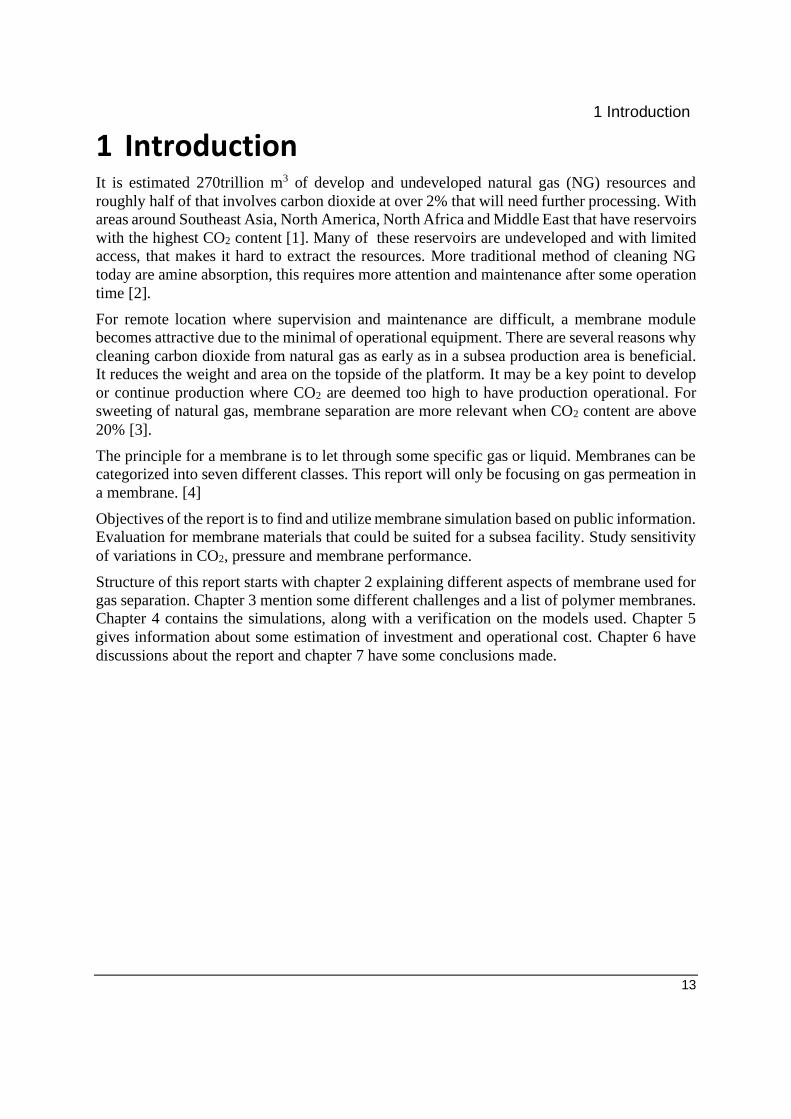
2.2.4.3 Mixed matrix membrane (MMM)

Mixed matrix membranes are a combination of both inorganic and dense polymer membranes

as shown in Figure 2.5 [10].

Figure 2.5 illustrate the structure of a MMM. [10]

2.2.4.4 Facilitated transport membranes (FTM).

With a facilitated transport membrane, it is possible to reach very high selectivity. Figure 2.6

illustrates that with the help of carriers fixed in the membrane to help the wanted gas over to

the permeate side, while the other gas has to diffuse through a polymer layer. [11]


19

Figure 2.6 illustrates the separation mechanics for a fixed-site-carrier membrane [11].

2.2.5 Performance of different types

This subchapter it is looked at how these membrane material performs.

2.2.5.1 Polymer

Polymer membrane in most cases comes with a trade-off between higher permeability and

higher selectivity described as Robeson upper bound. [9] Many are sustainable to be used with

temperature as high as 500oC. [6]

A frequent problem with polymer membrane is high plasticization when CO2, H2S, H2O, and

heavy hydrocarbons. Aging causes a reduction in gas permeability. Aging effect differently on

various types of polymer membranes. It can occur in two ways. One being the membrane

thickness comprises by letting out some free volume within the membrane. The other being

with a higher value of fractional free volume. A way to reduce aging is to strengthening the

chain packing efficiency by adding meta or para linkages such as, 6FDA, ODA, MDA and

many others. [12] Table 2.3 show some advantages and disadvantages with polymer

membranes [13].


20

Table 2.3 Summary by Vinoba et al. [13]

Membranes Advantages Disadvantages

Polymeric membranes Easy synthesis and fabrication Low chemical and thermal

stability

Low production cost Plasticization

Good mechanical stability Pore size not controllable

Easy for upscaling and making

variations in a module form

Follows the trade-off

between permeability and

selectivity

Separation mechanism:

Solution diffusion

2.2.5.2 Inorganic membranes

Inorganic membrane can usually exceed 500oC and harsh environment. Usually, consist of

multiple layers with just a thin layer for gas permeation. [6] Some inorganic membrane such

as zeolite is resistance to CO2 induced plasticization that would have led to a loss in selectivity.

Usually, higher selectivity than polymer membranes. [14] When molecular sieving carbon

membranes are dealing with impurities such as water, it might reduce performance or loss of

function due to sorption in the micropores. [15] SAPO-34 that contains Al will strongly absorb

water and possibly break the O-Al bounds that change the structure and reduces performance

[16].

With Zeolite membrane permeation and selectivity drop with impurities of heavier

hydrocarbons. The performance will be restored after the impurities are no longer present. [16]

when fabricate large scale it not uncommon that the brittleness of the material can crack some

places.

Table 2.4 show some advantages and disadvantages with inorganic membranes [13].



Inorganic Membranes Superior chemical, mechanical

and thermal stability

Brittle

Tunable pore size Expensive


21

Moderate the trade-off between

permeability and selectivity

Difficulty in scale up

Operate at harsh conditions

Separation mechanism:

Molecular sieving (<6Å),

Surface diffusion (<10-20Å),

Knudsen diffusion (<0,1µm)

2.2.5.3 Mixed matrix membranes

With MMM it is possible to surpass Robeson upper bound, Table 2.5 shows some advantages

and disadvantages with polymer membranes. [13]



Mixed matrix

membranes

Enhanced mechanical and

thermal stability

Brittle at high fraction of

fillers in polymeric matrix

Reduced plasticization Chemical and thermal

stability depends on the

polymer matrix

Lower energy requirement

Compacting at high pressure

Surpasses the trade-off between

permeability and selectivity

Enhanced separation

performance over native polymer

membranes


22

Separation followed by the

combined polymeric and

inorganic membrane principle

2.2.5.4 Facilitated transport membranes (FTM)

FTM also have a high permeability but will be limited to low CO2 partial pressure. The

separation performance will degrade over time due to evaporation and degrading of the

carrier.[9]

2.2.5.5 Gas-liquid membrane contactor

A gas-liquid membrane contactor is a combination of membranes and solvent used for

absorption and desorption. A setup with that type is illustrated in Figure 2.7 [15].

Figure 2.7 overview of membrane adsorption and -desorption that will be needed to for fill a Gas-liquid

membrane contactor.[15]


23

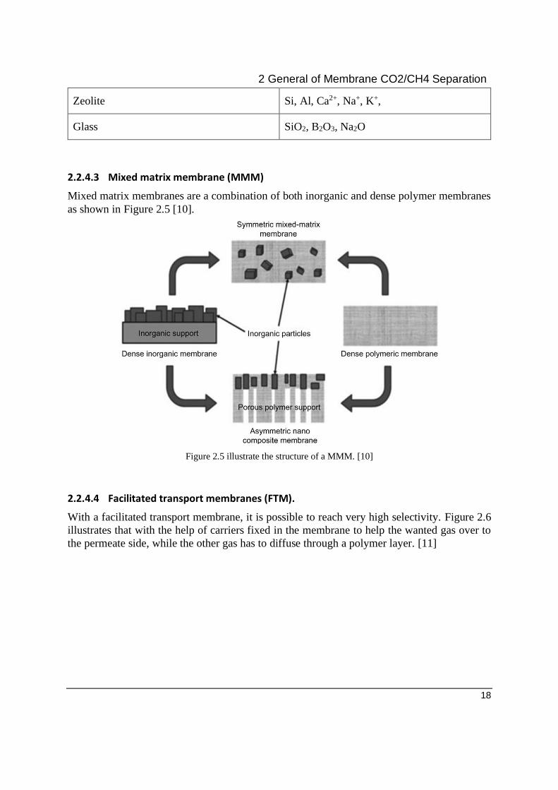
2.3 Other separation methods

2.3.1 Absorption

The most used technology for CO2 removal from natural gas is absorption processes with a

chemical solvent such as MEA, DEA or MDEA. [15] Absorption is predominantly done with

an CO2 carrier such as Methyl diethanolamine (MDEA) and Triethylene glycol (TEG) are

usually used to dehydrate the gas. Flow rate typical under 350MMscfd (9.9MSm3/day) can

have CO2 inlet conditions up to 70% and purify it down to levels as low as 50ppmv. [2]

2.3.2 Adsorption

Pressure swing adsorption (PSA) are commercial available up to 2MMscfd (0.057MSm3/day)

and does not often exceed 40mol% CO2 in inlet stream [2]. To put the flow in to context, the

Åsgard subsea compressors can handle up to 0.432MSm3/day1 per compressor [17].

1 Assumed to be gas volume at stander pressure and temperature.

3 Challenges

24

3 Challenges This chapter it will be tell about a few things to have in mind.

3.1 Membrane Challenges

By reviewing challenges which may arise with a membrane gas separation, it is possible to

understand how certain obstacles works or can be affected.

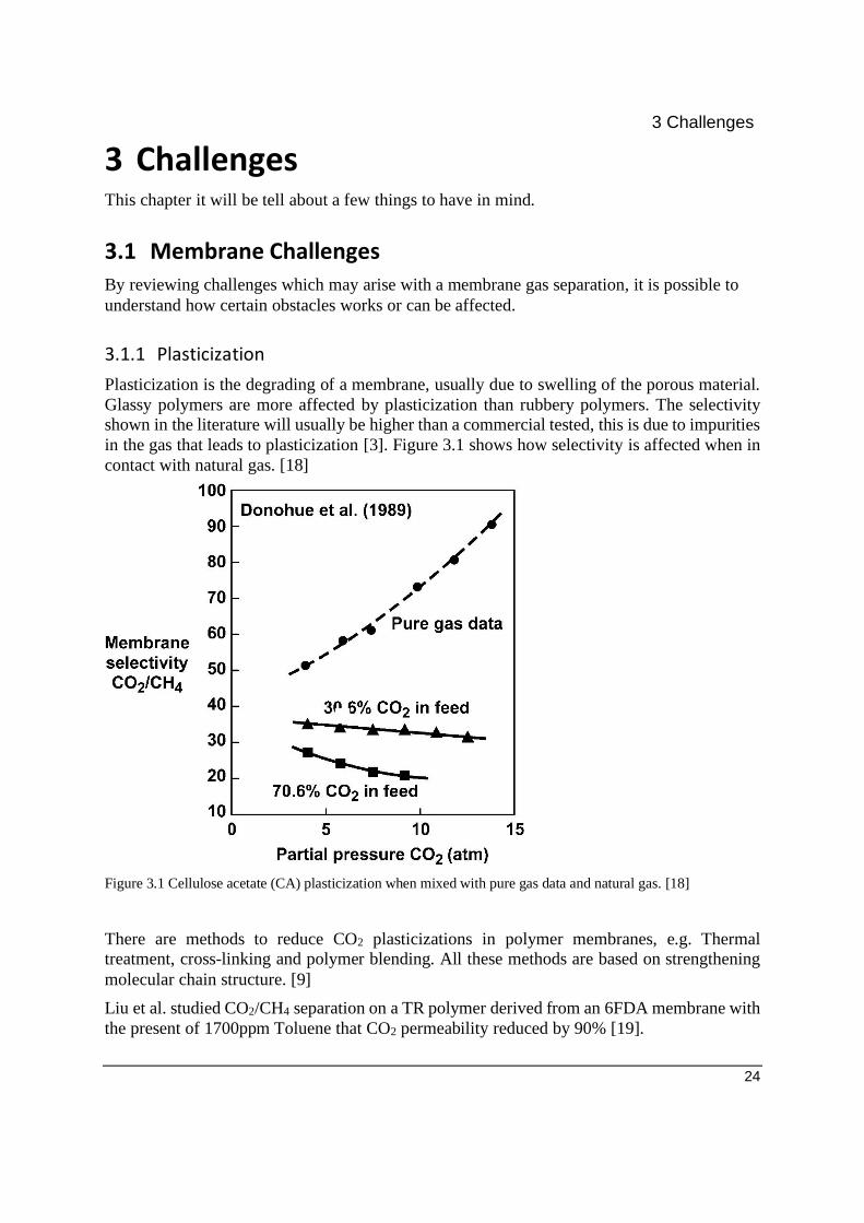
3.1.1 Plasticization

Plasticization is the degrading of a membrane, usually due to swelling of the porous material.

Glassy polymers are more affected by plasticization than rubbery polymers. The selectivity

shown in the literature will usually be higher than a commercial tested, this is due to impurities

in the gas that leads to plasticization [3]. Figure 3.1 shows how selectivity is affected when in

contact with natural gas. [18]

Figure 3.1 Cellulose acetate (CA) plasticization when mixed with pure gas data and natural gas. [18]

There are methods to reduce CO2 plasticizations in polymer membranes, e.g. Thermal

treatment, cross-linking and polymer blending. All these methods are based on strengthening

molecular chain structure. [9]

Liu et al. studied CO2/CH4 separation on a TR polymer derived from an 6FDA membrane with

the present of 1700ppm Toluene that CO2 permeability reduced by 90% [19].

3 Challenges

25

3.1.2 Membrane fouling

Membrane fouling is more common in separation processes with microfiltration, nanofiltration

and reverse osmosis compared to gas separation. Fouling is when a layer is formed on the

membrane that limits permeation. Some factors are gel layer formation, concentration

polarization, absorption and plugging of the pores. There is virtually no fouling in dense

membranes, mostly just with porous membranes. [6]

3.1.3 Membrane pretreatment

Due to particules, fouling and condensation of heavy hydrocarbons on the membrane,

pretreatment as shown in Figure 3.2 are expected on natural gas [3].

Figure 3.2 shows a block diagram for typical NG pretreatment for membranes. [3]

3.1.4 Suppliers of gas separation membranes.

Most commercial gas separation with membrane technology is based on PI and CA [9]. Table

3.1 shows a shortlist of suppliers with one of their membrane solutions for CO2 separation with

natural gas [3].

Table 3.1 Suppliers of membrane separation used for industrial scaled for removal of CO2 in natural gas [3]

Company Membrane Module Membrane material

Medal (Air Liquid) Hollow fiber Polyimide (PI)

Cynara (NATCO) Hollow fiber Cellulose acetate (CA)

3 Challenges

26

ABB/MTR Spiral-wound Perfluoro polymer silicone

rubber

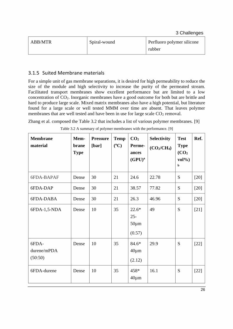
3.1.5 Suited Membrane materials

For a simple unit of gas membrane separations, it is desired for high permeability to reduce the

size of the module and high selectivity to increase the purity of the permeated stream.

Facilitated transport membranes show excellent performance but are limited to a low

concentration of CO2. Inorganic membranes have a good outcome for both but are brittle and

hard to produce large scale. Mixed matrix membranes also have a high potential, but literature

found for a large scale or well tested MMM over time are absent. That leaves polymer

membranes that are well tested and have been in use for large scale CO2 removal.

Zhang et al. composed the Table 3.2 that includes a list of various polymer membranes. [9]

Table 3.2 A summary of polymer membranes with the performance. [9]

Membrane

material

Mem-

brane

Type

Pressure

[bar]

Temp

(oC)

CO2

Perme-

ances

(GPU)a

Selectivity

(CO2/CH4)

Test

Type

(CO2

vol%)

b

Ref.

6FDA-BAPAF Dense 30 21 24.6 22.78 S [20]

6FDA-DAP Dense 30 21 38.57 77.82 S [20]

6FDA-DABA Dense 30 21 26.3 46.96 S [20]

6FDA-1,5-NDA Dense 10 35 22.6*

25-

50µm

(0.57)

49 S [21]

6FDA-

durene/mPDA

(50:50)

Dense 10 35 84.6*

40µm

(2.12)

29.9 S [22]

6FDA-durene Dense 10 35 458*

40µm

16.1 S [22]

3 Challenges

27

(11.45)

Matrimid® 5218 Dense 34.5 35 10*

30-

60µm

(0.25)

35.71 S [23]

Matrimid® 5218 Dense 1.1 20-25 28.5 50 M [24]

Matrimid® 5218

(fluorinated)

Dense 1.1 20-25 18.7 93.5 M [24]

Poly-

(dimethylsiloxane)

PDMS

Dense 2-4 23 3800*

Not

given

(95.0)

3.17 S [25]

Polycarbonate (PC) Dense 20 30 2*

Not

given

(0.05)

27.2 M

(40%)

[26]

Polyamides Dense 2 35 11*

25-

50µm

(0.28)

36.3 S [27]

DMAEMA-

PEGMEMA

Dense 2 35 24.3 12.5 S [28]

6FDA-DAT Asym-

metric

7 20 59 40 M

(40%)

[29]

6FDA-DAT Asym-

metric

2 35 55 60 M

(40%)

[30]

6FDA-DAT

(crosslinked)

Asym-

metric

2 35 32 55 M

(40%)

[30]

3 Challenges

28

PSf Asym-

metric

5 25 80.7 40.2 S [31]

Matrimid® Asym-

metric

15 20 11 67 M [32]

Matrimid®/P84

blend

Asym-

metric

8 35 11.5 35 M

(50%)

[33]

Cellulose acetate Asym-

metric

8 35 2.5 20 M

(50%)

[33]

Cross-linked

PI/PES

Dual

layer

6 23 28.3 101 S [34]

PBI/Matrimid® blen

d and PSf

Dual

layer

10 35 4.81 41.81 S [35]

Matrimid®/PES Dual

layer

10 22 9.5 40 M

(40%)

[36]

a 1 GPU = 3.35e-10 mol m-2 s-1 Pa-1

b Test type: S = Singel gas experiment; M = Mixed gas experiment

* 1 Barrer = 3.35e-16 mol m m-2 s-1 Pa-1

(xx) Calculated to GPU, Dense type, permeability is divided by 40µm to get permeance,

that represented by the membrane thickness. Membrane thickness in dense type varies

between 25-60µm. [21-23, 27]

For typical use in the industry commercial glassy polymers like PI, PSf and CA are usually

chosen. PI stands out more due to the thermal strength and mechanical properties. PI shows

satisfactory performance in pure gas permeability and selectivity ratio. PI based on the

commercially available monomer 6FDA even better performance. [37]

3.1.6 Pressure drop

To calculate the pressure drop for a laminar flow inside a pipe the Poiseullie equation can be

used.

3 Challenges

29

∆𝑃 = 8𝜋𝜇𝐿𝐿𝑝

𝐴𝑚2 (3.1)

∆P being pressure drop in pascal, μ being the average dynamic viscosity and L is the length

of the membrane. As an example, a one meter long membrane with the same specification as

Base Case 1, that gives a pressure drop of 1.177bar and 4.709bar for 2 meter long.

However, to utilize as much of the membrane area it is best to have the permeate come to the

inside of the pipes.

3.2 Specifications to reach for

Specification for transporting natural gas in the pipeline should be below 2-3% CO2 [38]. To

limit corrosion in the pipeline, CO2 content should below 8% [3]. For CO2-EOR the general

CO2 content ranges between 92- to 97vol% [39].

3.3 Hydrate formation and CO2 Freezeout

Avoid by keeping a higher temperature as well and not too high of a pressure drop. CO2

hydrates can occur with temperature at 10oC when the pressure is higher than 45bar.

3.4 Compression and Subsea

Compression is usually one of the higher costs in both CAPEX and OPEX for a membrane

system. Cost of a compressor installed in onshore (CC) can be estimated by the following

formula:

𝐶𝐶 = 𝑈𝑆𝐷8650 ×𝑊𝑐𝑝

𝜂𝑐𝑝

0.82

(3.2)

CC are the cost of an installed compressor onshore, Wcp is energy needed for the compressor

and ηcp is the efficiency. [40] To assume the cost of a multiphase compressor, it is thought it

might be similar cost as an installed regular compressor.

To be able to operate in subsea conditions a multiphase compressor is being used and can

reduce the cost of conveying around 70% of a traditional facility [41]. This is a fairly new

concept and even though Åsgard compression module operates mainly dry gas, it is the first of

its kind [42]. Another limiting factor could be ratio outlet to inlet pressure, this might cause the

need to have multiply compressors.

Due to limited access, it is favorable to minimize rotating machinery. Additional, in subsea a

challenge is that there is usually no place to direct insignificant streams also called waste

streams, this will make the pretreatment hard.

4 Membrane Simulations

30

4 Membrane Simulations Every simulation model described has some assumptions such as

• complete mixing in each cell

• isothermal conditions

• ideal gas behavior

• no pressure drop

• constant permeabilities

• Plug flow, no axial dispersion

• No flux coupling, each component permeates through the membrane with its own

permeance.

4.1 Different simulations models

Simulations models for complete mix and countercurrent in this report is from example 13.4-1

and 13.8-1, respectably, from C.J. Geankoplis "Transport Processes and Separation Process

Principles, Fourth Edition". These are modules with only two components in the stream. [4]

The crossflow module is a numerical model from Aspen Costume Modeler that can take

multiple components into account.

4.1.1 Complete mix

A complete mix module is indicated in Figure 4.1. L is the flow rate while x is mole fraction of

the nonpermeated stream, while V is the flow rate while y is mole fraction of the permeated

side. ph and pl are pressure on the high-pressure side and low-pressure side, respectively. θ

being the permeate cut fraction given as follows:

𝜃 = 𝑉𝑝

𝐿𝑓 (4.1)

The lowered font: f as feed, p as permeate, and o as outlet in the rejected stream. [4]

Figure 4.1 Schematic illustration of a complete mix module with symbols [4]


31

This method is limited to the minimum reject composition xoM that value is obtained as.

𝑥𝑜𝑀 =𝑥𝑓[1 + (𝛼 − 1)

𝑝𝑙𝑝ℎ

(1 − 𝑥𝑓 ) ]

𝛼 ∗ (1 − 𝑥𝑓) + 𝑥𝑓 (4.2)

That means the molar fraction on the rejected out xo can not be lower than the minimum reject

composition xoM. To get beyond this limit, it is possible to make an cascade system. [4]

Then a quadratic equation is used to find concentration of the permeate.

𝑦𝑝 =−𝑏 + √𝑏2 − 4𝑎𝑐

2𝑎 (4.3)

Where

𝑎 = 𝜃 + 𝑃𝑝

𝑃𝑓−

𝑃𝑝

𝑃𝑓∗ 𝜃 − 𝛼 ∗ 𝜃 − 𝛼 ∗

𝑃𝑝

𝑃𝑓+ 𝛼 ∗

𝑃𝑝

𝑃𝑓∗ 𝜃 ; b = 1− 𝜃 − 𝑥𝑝 −

𝑃𝑝

𝑃𝑓+

𝑃𝑝

𝑃𝑓∗

𝜃 + 𝛼 ∗ 𝜃 + 𝛼 ∗𝑃𝑝

𝑃𝑓− 𝛼 ∗

𝑃𝑝

𝑃𝑓∗ 𝜃 ∗ 𝛼 ∗ 𝑥𝑝 ; and c = −𝛼 ∗ 𝑥𝑝

(4.4)

Then a massbalance to give the xo:

𝑥𝑜 =𝑥𝑓 − 𝜃𝑦𝑝

(1 − 𝜃) (4.5)

Then to add it in the final equation to get the membrane area:

𝐴𝑚 =𝜃𝐿𝑓𝑦𝑝

(𝑃′𝑎/𝑡) ∗ (𝑝ℎ𝑥𝑜 − 𝑝𝑙𝑦𝑝)

(4.6)

4.1.2 Crossflow

Each component transfers into next cell on the feed/retentate side by this equation:

𝐿𝑜,(𝑘−1) ∙ 𝑥𝑜,𝑖(𝑘−1) = 𝐿𝑜,(𝑘) ∙ 𝑥𝑜,𝑖,(𝑘) + 𝑉𝑝,(𝑘) ∙ 𝑥𝑝,𝑖(𝑘) (4.7)

For the component to permeate over to the permeate side this equation is used:

𝑉𝑃 ∙ 𝑦𝑝𝑖 =𝐴𝑚 ∙ 𝑃′𝑎/𝑡 ∙ (𝑃𝑅 ∙ 𝑥𝑜,𝑖 - 𝑃𝑃 ∙ 𝑦𝑃,𝑖) (4.8)


32

Figure 4.2 illustration on how the materials moves within the simulated membrane.

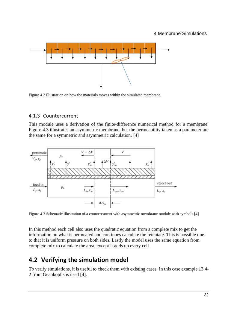
4.1.3 Countercurrent

This module uses a derivation of the finite-difference numerical method for a membrane.

Figure 4.3 illustrates an asymmetric membrane, but the permeability taken as a parameter are

the same for a symmetric and asymmetric calculation. [4]

Figure 4.3 Schematic illustration of a countercurrent with asymmetric membrane module with symbols [4]

In this method each cell also uses the quadratic equation from a complete mix to get the

information on what is permeated and continues calculate the retentate. This is possible due

to that it is uniform pressure on both sides. Lastly the model uses the same equation from

complete mix to calculate the area, except it adds up every cell.

4.2 Verifying the simulation model

To verify simulations, it is useful to check them with existing cases. In this case example 13.4-

2 from Geankoplis is used [4].


33

Table 4.1 Case used to verify the simulations.

Feed flow: Lf: 1Nm3/s = 0.0446kmole/s

Permeance:

Selectivity

P'O2/t: 0.661·10-3mole/(s·m2·bar)

P'N2/t: 0.0661·10-3mole/(s·m2·bar)

α = 10

Molar compositions in feed: xf,O2: 0.209

xf,N2: 0.791

Pressure Retentate: 2.53bar

Permeate: 0.253bar

Permeate cut fraction: θ: 0.2

(Vp: 0.00892kmole/s)

(Lo: 0.03568kmole/s)

Serval different solutions is then shown in Table 4.2.

Table 4.2 Results from example 13.4-2

Model Solution

Complete mixing model

from Geankoplis

Am: 32,300m2

yp,O2: 0.507 (Vp: 0.00892kmole/s)

xo,O2: 0.135 (Lo: 0.03568kmole/s)

Crossflow model

from Geankoplis

Am: 28,930m2

yp,O2: 0.569 (Vp: 0.00892kmole/s)

xo,O2: 0.119 (Lo: 0.03568kmole/s)

Crossflow model

from ACM done in AP

Am: 29,981m2

yp,O2: 0.598 (Vp: 0.00892kmole/s)

xo,O2: Not obtained (Lo: 0.03568kmole/s)

Countercurrent model

From Geankoplis

Am: 28,967m2

yp,O2: 0.587 (Vp: 0.00892kmole/s)


34

xo,O2: 0.119 (Lo: 0.03568kmole/s)


From MemSim2

Am: 28,967m2

yp,O2: 0.587 (Vp: 0.00892kmole/s)

xo,O2: Not given (Lo: 0.03568kmole/s)

4.3 Cases

It is chosen the membrane type 6FDA-DAP with a permeances of 38.57GPU and selectivity of

77.82 then reduce both ~20% in efficiency due to plasticization.

4.3.1 Base Case

Parameters from Base Case 1, -2 and -3 are given in Table 4.3.

Table 4.3 Parameter for Base Case 1, 2, 3.

Feed flow: Lf: 2MSm3/s = 3718kmole/h = 83333m3STP/h

Permeance:

Selectivity

P'CO2/t: 31GPU = 0.083711m3STP/(h·m2·bar)

P'CH4/t: 0.5GPU = 0.001350m3STP/ (h·m2·bar)

αCO2/CH4 = 62

Molar compositions in feed: Base Case 1

xf,CO2: 0.80

xf,CH4: 0.20

Base Case 2

xf,CO2: 0.50

xf,CH4: 0.50

Base Case 3

xf,CO2: 0.20

xf,CH4: 0.80

2 Lecture notes by Lars Erik Øi in “Membrane Technology Course” 28 November 2005.


35

Pressure Retentate: 40bar

Permeate: 8bar

Retentate: xo,CO2: 0.08

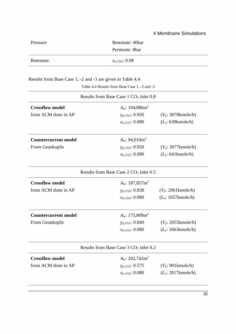
Results from Base Case 1, -2 and -3 are given in Table 4.4

Table 4.4 Results from Base Case 1, -2 and -3

Results from Base Case 1 CO2 inlet 0.8

Crossflow model

from ACM done in AP

Am: 104,886m2

yp,CO2: 0.950 (Vp: 3078kmole/h)

xo,CO2: 0.080 (Lo: 639kmole/h)


From Geankoplis

Am: 94,010m2

yp,CO2: 0.950 (Vp: 3077kmole/h)



Crossflow model

from ACM done in AP

Am: 187,857m2

yp,CO2: 0.838 (Vp: 2061kmole/h)

xo,CO2: 0.080 (Lo: 1657kmole/h)


From Geankoplis

Am: 175,809m2

yp,CO2: 0.840 (Vp: 2055kmole/h)

xo,CO2: 0.080 (Lo: 1663kmole/h)


Crossflow model

from ACM done in AP

Am: 202,742m2

yp,CO2: 0.575 (Vp: 901kmole/h)

xo,CO2: 0.080 (Lo: 2817kmole/h)


36


From Geankoplis

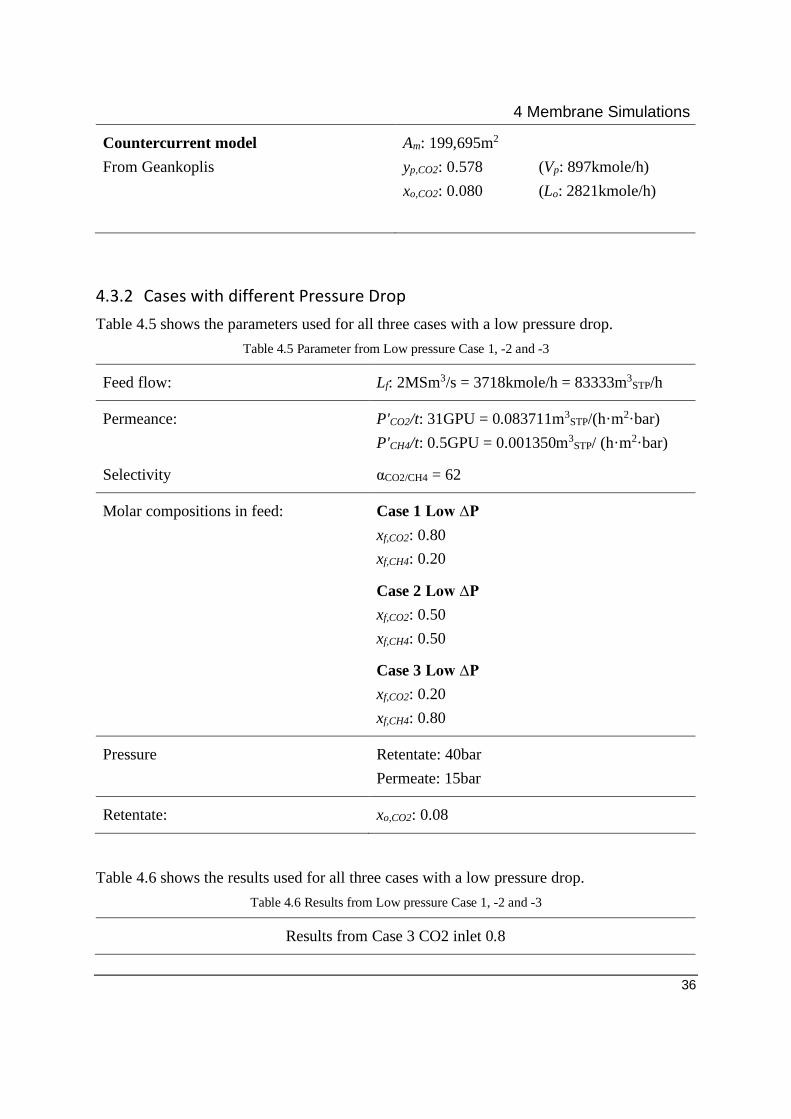
Am: 199,695m2


xo,CO2: 0.080 (Lo: 2821kmole/h)

4.3.2 Cases with different Pressure Drop

Table 4.5 shows the parameters used for all three cases with a low pressure drop.

Table 4.5 Parameter from Low pressure Case 1, -2 and -3


Permeance:

Selectivity



αCO2/CH4 = 62

Molar compositions in feed: Case 1 Low ∆P

xf,CO2: 0.80

xf,CH4: 0.20

Case 2 Low ∆P

xf,CO2: 0.50

xf,CH4: 0.50

Case 3 Low ∆P

xf,CO2: 0.20

xf,CH4: 0.80


Permeate: 15bar


Table 4.6 shows the results used for all three cases with a low pressure drop.

Table 4.6 Results from Low pressure Case 1, -2 and -3

Results from Case 3 CO2 inlet 0.8


37

Crossflow model

from ACM done in AP

Am: 292,724m2

yp,CO2: 0.882 (Vp: 3337kmole/h)



From Geankoplis

Am: 268,397m2

yp,CO2: 0.884 (Vp: 3328kmole/h)



Crossflow model

from ACM done in AP

Am: 635,554m2

yp,CO2: 0.657 (Vp: 2706kmole/h)

xo,CO2: 0.080 (Lo: 1011kmole/h)


From Geankoplis

Am: 607,814m2

yp,CO2: 0.661 (Vp: 2688kmole/h)

xo,CO2: 0.080 (Lo: 1030kmole/h)


Crossflow model

from ACM done in AP

Am: 723,467m2

yp,CO2: 0.349 (Vp: 1659kmole/h)

xo,CO2: 0.080 (Lo: 2059kmole/h)


From Geankoplis

Am: 716,134m2

yp,CO2: 0.351 (Vp: 1649kmole/h)

xo,CO2: 0.080 (Lo: 2069kmole/h)

Table 4.7 shows the parameters used for all three cases with a high pressure drop.


38

Table 4.7 Parameter from High pressure Case 1, -2 and -3


Permeance:

Selectivity



αCO2/CH4 = 62

Molar compositions in feed: Case 1 High ∆P

xf,CO2: 0.80

xf,CH4: 0.20

Case 2 High ∆P

xf,CO2: 0.50

xf,CH4: 0.50

Case 3 High ∆P

xf,CO2: 0.20

xf,CH4: 0.80


Permeate: 2bar


Table 4.8 shows the results used for all three cases with a high pressure drop.

Table 4.8 Results from High patrial pressure Case 1, -2 and -3


Crossflow model

from ACM done in AP

Am: 45,535m2

yp,CO2: 0.981 (Vp: 2972kmole/h)



From Geankoplis

Am: 44,448m2

yp,CO2: 0.980 (Vp: 2974kmole/h)



39


Crossflow model

from ACM done in AP

Am: 54,835m2

yp,CO2: 0.946 (Vp: 1804kmole/h)

xo,CO2: 0.080 (Lo: 1914kmole/h)


From Geankoplis

Am: 53,638m2

yp,CO2: 0.945 (Vp: 1805kmole/h)

xo,CO2: 0.080 (Lo: 1914kmole/h)


Crossflow model

from ACM done in AP

Am: 32,688m2


xo,CO2: 0.080 (Lo: 3147kmole/h)


From Geankoplis

Am: 37,363m2


xo,CO2: 0.080 (Lo: 3148kmole/h)

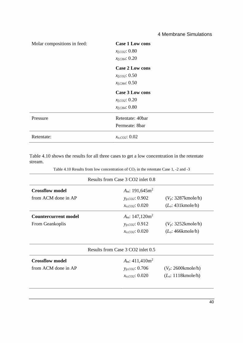
4.3.3 Cases with different Retentate concentration

Table 4.9 shows the parameter used for all three cases to get a low concentration in the

retentate stream, in this report this is the concentration needed to get a sales ready natural gas.

Table 4.9 parameter used for Case 1, -2 and -3 with a low CO2 concentration in the retentate.


Permeance:

Selectivity



αCO2/CH4 = 62


40

Molar compositions in feed: Case 1 Low cons

xf,CO2: 0.80

xf,CH4: 0.20

Case 2 Low cons

xf,CO2: 0.50

xf,CH4: 0.50

Case 3 Low cons

xf,CO2: 0.20

xf,CH4: 0.80


Permeate: 8bar


Table 4.10 shows the results for all three cases to get a low concentration in the retentate

stream.

Table 4.10 Results from low concentration of CO2 in the retentate Case 1, -2 and -3


Crossflow model

from ACM done in AP

Am: 191,645m2

yp,CO2: 0.902 (Vp: 3287kmole/h)



From Geankoplis

Am: 147,120m2

yp,CO2: 0.912 (Vp: 3252kmole/h)



Crossflow model

from ACM done in AP

Am: 411,410m2

yp,CO2: 0.706 (Vp: 2600kmole/h)

xo,CO2: 0.020 (Lo: 1118kmole/h)


41


From Geankoplis

Am: 350,273m2

yp,CO2: 0.722 (Vp: 2542kmole/h)

xo,CO2: 0.020 (Lo: 1176kmole/h)


Crossflow model

from ACM done in AP

Am: 579,394m2

yp,CO2: 0.390 (Vp: 1811kmole/h)

xo,CO2: 0.020 (Lo: 1907kmole/h)


From Geankoplis

Am: 554,077m2

yp,CO2: 0.396 (Vp: 1778kmole/h)

xo,CO2: 0.020 (Lo: 1940kmole/h)

Table 4.11 shows the parameter used for all three cases to get a high concentration of CO2 in

the retentate stream.

Table 4.11 parameter used for Case 1, -2 and -3 with a high CO2 concentration in the retentate.


Permeance:

Selectivity



αCO2/CH4 = 62

Molar compositions in feed: Case 1 High cons

xf,CO2: 0.80

xf,CH4: 0.20

Case 2 High cons

xf,CO2: 0.50

xf,CH4: 0.50

Case 3 High cons

xf,CO2: 0.20

xf,CH4: 0.80


42


Permeate: 8bar


Table 4.12 shows the results for all three cases to get a high concentration of CO2 in the

retentate stream.

Table 4.12 Results from high concentration of CO2 in the retentate Case 1, -2 and -3


Crossflow model

from ACM done in AP

Am: 69,601m2

yp,CO2: 0.970 (Vp: 2947kmole/h)



From Geankoplis

Am: 66,582m2

yp,CO2: 0.970 (Vp: 2948kmole/h)



Crossflow model

from ACM done in AP

Am: 97,292m2

yp,CO2: 0.906 (Vp: 1722kmole/h)

xo,CO2: 0.150 (Lo: 1996kmole/h)


From Geankoplis

Am: 94,376m2

yp,CO2: 0.906 (Vp: 1722kmole/h)

xo,CO2: 0.150 (Lo: 1996kmole/h)


Crossflow model

from ACM done in AP

Am: 51,021m2



43

xo,CO2: 0.150 (Lo: 3389kmole/h)


From Geankoplis

Am: 50,793m2


xo,CO2: 0.150 (Lo: 3389kmole/h)

4.3.4 Lower Permeance and selectivity

In many cases to get a well proven and tested membrane it usually has lower permeability and

selectivity. In this case it will be investigated the asymmetric cellulose acetate membrane

parameter used is given in Table 4.13.

Table 4.13 Parameters from Case 1, -2 and -3 with an asymmetric CA


Permeance:

Selectivity

P'CO2/t: 2.5GPU = 0.006751m3STP/(h·m2·bar)

P'CH4/t: 0.125GPU = 0.0003375m3STP/(h·m2·bar)

αCO2/CH4 = 20

Molar compositions in feed: Case 1

xf,CO2: 0.80

xf,CH4: 0.20

Case 2

xf,CO2: 0.50

xf,CH4: 0.50

Case 3

xf,CO2: 0.20

xf,CH4: 0.80


Permeate: 8bar



44

Table 4.14 shows the results from an asymmetric CA membrane.

Table 4.14 Results from Case 1, -2 and -3 with an asymmetric CA


Crossflow model

from ACM done in AP

Am: 891,982m2

yp,CO2: 0.912 (Vp: 3217kmole/h)



From Geankoplis

Am: 855,369m2

yp,CO2: 0.913 (Vp: 3215kmole/h)



Crossflow model

from ACM done in AP

Am: 1,348,00m2

yp,CO2: 0.753 (Vp: 2319kmole/h)

xo,CO2: 0.080 (Lo: 1399kmole/h)


From Geankoplis

Am: 1,325,126m2

yp,CO2: 0.755 (Vp: 2312kmole/h)

xo,CO2: 0.080 (Lo: 1406kmole/h)


Crossflow model

from ACM done in AP

Am: 1,220,000m2

yp,CO2: 0.487 (Vp: 1094kmole/h)

xo,CO2: 0.080 (Lo: 2624kmole/h)


From Geankoplis

Am: 1,210,793m2

yp,CO2: 0.489 (Vp: 1092kmole/h)

xo,CO2: 0.080 (Lo: 2626kmole/h)


45

4.3.5 Multi components

Saturated water content in natural gas depends on temperature and pressure, the mass in kg of

water wWater per Mm3 of natural gas, can be described as followed. [43]

𝑤𝑤𝑎𝑡𝑒𝑟 = 593.335 ∙ exp(0.05486 ∙ 𝑡𝐺) ∙ 𝑃𝐺−0.81462 (4.9)

tG are the temperature of the gas in Celsius and PG are in MPa. This gives 248kg/h with a gas

flow rate at 2Nm3 pressure of 4MPa and a temperature of 50oC.

This can also be done in Aspen HYSYS as shown in Figure 4.4, with CO2 content of 80mol%

this gives 332kg/h. With CO2 content of 20mol% that gives 257kg/h and with CO2 content of

0mol% that gives 236kg/h.

Figure 4.4 Screenshot from Aspen HYSYS

Table 4.15 shows a possibly composition of what a natural gas may contain.

Table 4.15 A possible dry Natural gas compositions

Composition (mol%)

Component Case 1 Case 2 Case 3

CO2 80.0 50.0 20.0

Methane 12.8 32.0 51.2

Ethane 3.2 8.0 12.8

Propane 3.2 8.0 12.8

C4+ 0.8 2.0 3.2

Sum 100.0 100.0 100.0


46

Table 4.16 shows the composition when it is saturated with water.

Table 4.16 A possible saturated with water in Natural gas compositions

Composition (mol%)

Component Case 1 Case 2 Case 3

CO2 79.6 49.8 19.9

Methane 12.7 31.8 51.0

Ethane 3.2 8.0 12.75

Propane 3.2 8.0 12.75

C4+ 0.8 2.0 3.2

Water 0.5 0.4 0.4

Sum 100.0 100.0 100.0

Table 4.17 gives the parameter for all three cases.

Table 4.17 Multi component cases with its parameters


Permeance:

Selectivity


P'CH4/t: 0.5GPU = 0.001350m3STP/(h·m2·bar)

P'C2H6/t: 0.89GPU = 0.002392m3STP/(h·m2·bar)

P'C3H8/t: 1.24GPU = 0.003348m3STP/(h·m2·bar)

P'C4+/t: 1.55GPU = 0.004186m3STP/(h·m2·bar)

P'H2O/t: 200GPU = 0.540007m3STP/(h·m2·bar)

αCO2/CH4 = 62

αCO2/C2H6 = 35

αCO2/C3H8 = 25


47

αCO2/C4+ = 20

αH2O/CH4 = 400 3

Molar compositions in feed: Base Case 1 Multiply Components

xf,CO2: 0.796

xf,CH4: 0.127

xf,C2H6: 0.032

xf,C3H8: 0.032

xf,C4+: 0.008

xf,H2O: 0.005

Base Case 2 Multiply Components

xf,CO2: 0.498

xf,CH4: 0.319

xf,C2H6: 0.08

xf,C3H8: 0.08

xf,C4+: 0.02

xf,H2O: 0.004

Base Case 3 Multiply Components

xf,CO2: 0.199

xf,CH4: 0.51

xf,C2H6: 0.128

xf,C3H8: 0.128

xf,C4+: 0.032

xf,H2O: 0.004


Permeate: 8bar


3 All Selectivity from C2H6 to H2O are guessed, the assumption is that this membrane will have similar ratio as

given in the literature.[44] Y. Cui, H. Kita, and K.-i. Okamoto, "Preparation and gas separation performance of

zeolite T membrane," Journal of Materials Chemistry, vol. 14, no. 5, pp. 924-932, 2004. [45] A. Kargari and H. Sanaeepur, "Application of membrane gas separation processes in petroleum industry," Advances in

petroleum engineering, vol. 1, pp. 592-622, 2015. [46] J. Liu, G. Zhang, K. Clark, and H. Lin,

"Maximizing ether oxygen content in polymers for membrane CO2 removal from natural gas," ACS applied

materials & interfaces, vol. 11, no. 11, pp. 10933-10940, 2019.


48

Table 4.18 gives the results from all multi component cases.

Table 4.18 Multi component case 1, -2 and -3

Crossflow model

from ACM done in AP

Case 1 Case 2 Case 3

Area Am: 92,407m2 Am: 157,412m2 Am: 157,672m2

Retentate Flow Lo: 606kmole/h Lo: 1596kmole/h Lo: 2776kmole/h

CO2 xo,CO2: 0.08 xo,CO2: 0.08 xo,CO2: 0.08

CH4 xo,CH4: 0.633 xo,CH4: 0.624 xo,CH4: 0.611

C2H6 xo,C2H6: 0.138 xo,C2H6: 0.140 xo,C2H6: 0.142

C3H8 xo,C3H8: 0.122 xo,C3H8: 0.126 xo,C3H8: 0.134

C4+ xo,C4+: 0.0275 xo,C4+: 0.0292 xo,C4+: 0.0319

H2O xo,H2O: 0.000024 xo,H2O: 0.00022 xo,H2O: 0.0013

Permeate Flow Vp: 3112kmole/h Vp: 2122kmole/h Vp: 942kmole/h

CO2 yp,CO2: 0.935 yp,CO2: 0.812 yp,CO2: 0.550

CH4 yp,CH4: 0.0285 yp,CH4: 0.0878 yp,CH4: 0.211

C2H6 yp,C2H6: 0.0114 yp,C2H6: 0.0352 yp,C2H6: 0.0850

C3H8 yp,C3H8: 0.0145 yp,C3H8: 0.0451 yp,C3H8: 0.1097

C4+ yp,C4+: 0.0042 yp,C4+: 0.0131 yp,C4+: 0.0322

H2O yp,H2O: 0.0060 yp,H2O: 0.0068 yp,H2O: 0.0120

4.3.6 Two Stage Compression membrane system

There are two possible configurations to have, first configuration A has a compressor for the

first permeate that goes into a second membrane as shown in Figure 4.5. This is recommended

when having a lower concentration of CO2 in the feed (>30mol%) [47]. Another purpose for


49

this is to use the recompression at a lower pressure drop in the second membrane and then not

to exceed four times the compression ratio on the compressor.

Figure 4.5 Screenshot from Aspen plus of configuration A

Table 4.19 shows Parameter and results for Two stage Case 3 with configuration A.

Table 4.19 Parameter and results for Two stage Case 3 with configuration A.


Permeance:

Selectivity



αCO2/CH4 = 62


xf,CO2: 0.20

xf,CH4: 0.80

Pressure

1. Membrane

2. Membrane

Retentate: 40bar

Permeate: 10bar

Retentate: 40bar

Permeate: 25bar

System retentate: xo,CO2: 0.08


50

Results from Crossflow Model

Area Am,1: 528,880m2

Am,2: 50,000m2

System molar fraction and flow yp,CO2: 0.929 (Vp: 526kmole/h)

xo,CO2: 0.080 (Lo: 3192kmole/h)

Compressor energy [kW]

(ηcp=100%)

Wcp,EOR: 1,020kW

Wcp,Recycle: 4,231kW

second configuration B permeate exits the system from the first membrane, in the second

membrane permeate is recycled back to the feed as shown in Figure 4.6. The compressor used

for CO2 injection exceeds the four times ratio limit and will need a secondary compressor for

that task.

Figure 4.6 Screenshot from Aspen Plus of configuration B

Table 4.20 shows parameter and results for Two stage Case 2 with configuration B.

Table 4.20 Parameter and results for Two stage Case 2 with configuration B.


Permeance:

Selectivity



αCO2/CH4 = 62


51


xf,CO2: 0.50

xf,CH4: 0.50

Pressure

1. Membrane

2. Membrane

Retentate: 40bar

Permeate: 8bar

Retentate: 40bar

Permeate: 10bar



Area Am,1: 60,829m2

Am,2: 275,115m2

System Molar fraction and flow yp,CO2: 0.950 (Vp: 1795kmole/h)

xo,CO2: 0.080 (Lo: 1923kmole/h)


(ηcp=100%)

Wcp,EOR: 4,803kW

Wcp,Recycle: 1,467kW

With the parameters from Table 4.21 it is the only case that deliver up to NG specification that

do not need more treatment.

Table 4.21 Parameter and results for Two stage Case 1 with configuration B.


Permeance:

Selectivity



αCO2/CH4 = 62


xf,CO2: 0.80

xf,CH4: 0.20

Pressure


52

1. Membrane

2. Membrane

Retentate: 40bar

Permeate: 8bar

Retentate: 40bar

Permeate: 10bar



Area Am,1: 105,682m2

Am,2: 245,519m2

System Molar fraction and flow yp,CO2: 0.950 (Vp: 3118kmole/h)



(ηcp=100%)

Wcp,EOR: 7,853kW

Wcp,Recycle: 718kW

4.3.7 Summarize of the cases

Table 4.22 summarize the results from case 1 with a CO2, inlet concentration of 80mol%.

Table 4.22 Summary of case 1 with CO2 inlet of 80mol%

Base

Case 1

Low

∆P

High

∆P

xo,CO2

=0.02

xo,CO2

=0.15

CA

mem

Multi

comp

2 stage

mem

Area 1000m2

105

293

46

192

70

892

92

352

Retentate (Lo)

(kmole/h) 641 380 746 431 771 501 606 600

xo,CH4 0.92 0.92 0.92 0.98 0.85 0.92 0.92 0.98

Permeate (Vp)

(kmole/h) 3077 3337 2972 3287 2947 3217 3112 3118

yp,co2 0.95 0.884 0.981 0.902 0.97 0.912 0.935 0.95


53



Base

Case 2

Low

∆P

High

∆P

xo,CO2

=0.02

xo,CO2

=0.15

CA

mem

Multi

comp

2 stage

mem

Area 1000m2 188 634 55 411 97 1348 157 336

Retentate (Lo)

(kmole/h) 1657 1011 1914 1118 1996 1399 1596 1923

xo,CH4 0.92 0.92 0.92 0.98 0.85 0.92 0.92 0.92

Permeate (Vp)

(kmole/h) 2061 2706 1804 2600 1722 2319 2122 1795

yp,co2 0.838 0.657 0.946 0.722 0.906 0.753 0.812 0.95



Base

Case 3

Low

∆P

High

∆P

xo,CO2

=0.02

xo,CO2

=0.15

CA

mem

Multi

comp

2 stage

mem

Area 1000m2 203 723 33 579 51 1220 158 579

Retentate (Lo)

(kmole/h) 2817 2059 3147 1907 3389 2624 2776 3192

xo,CH4 0.92 0.92 0.92 0.98 0.85 0.92 0.92 0.92

Permeate (Vp)

(kmole/h) 901 1659 570 1811 330 1094 942 526

yp,co2 0.575 0.349 0.863 0.39 0.713 0.487 0.55 0.929

5 Cost and Size

54

5 Cost and Size The schematic plot shown in Figure 5.1 gives an overview of what choice of CO2 removal

technology is generally recommended, with the given gas flow rate and CO2 concentration. [3]

In these cases, when it is 2Msm3/day that equal 70.79 MMscfd, this puts the recommendations

in a combination.

Figure 5.1 a schematic plot of recommended choice for CO2 removal. [3]

To oversimplify the CAPEX of equipment in a subsea module, e.g. the cost of the equipment

is 22% of the total cost of a subsea module [48].

5.1 Compression for CO2-EOR

In all examples it is required to inject the permeated stream into a reservoir, this requires heavy

compression. For a this report it will be compressed up to 100bar. Table 5.1 shows the result

5 Cost and Size

55

for Base Case 1 to -3, with a compressor efficiency of 100% from Aspen Plus. Table 5.2 shows

then cost for two compressors, Utility cost will be similar for both cases.

Table 5.1 Compression cost for Base Case 1 to -3 with a singular compressor

Base Case 1 Base Case 2 Base Case 3

Amount to

compress [kmol/h]

3078kmol/h 2061kmol/h 901kmol/h

Energy Wcp [hp] /

[kW] (ηcp=100%)

14,572hp/7868kW 9,182hp/4958kW 3,848hp/2078kW

Efficiency ηcp 0.8 0.8 0.8

Compressor cost

[USD]

USD 26,950,000 USD 18,454,000 USD 9,045,000

Utility cost USD0.065/kWh USD0.065/kWh USD0.065/kWh

Energy cost per

year [USD/year]

5,833,000 USD/year 3,676,000 USD/year 1,540,000 USD/year

Table 5.2 Compression cost for Base Case 1 to -3 with two compressors with a ratio outlet to inlet pressure of 4


Amount to

compress [kmol/h]

3078kmol/h 2061kmol/h 901kmol/h

Energy Wcp [hp] /

[kW]

1. 7,058hp/ 3811kW

2. 7,514hp/ 4057kW

1. 4,447hp/ 2401kW

2. 4,736hp/ 2557kW

1. 1,863hp/ 1006kW

2. 1,985hp/ 1072kW

Efficiency ηcp 0.8 0.8 0.8

Installed cost CC

[USD]

USD 30,529,000 USD 20,905,000 USD 10,245,000

As presented in Table 5.1 and Table 5.2, it is favorable to inject the least.

5 Cost and Size

56

5.2 Potential Income

Natural gas varies in price, from the last five years it ranges from 1.48- to 4.55USD/MMBtu,

but averages around 2.5- to 3.0USD/MMBtu in the US [49]. As of April 2021 the European

Union import price of natural gas was 7.147USD/MMBtu [50].Table 5.3 shows a theoretical

income from the different base cases.

Table 5.3 potential income from Base Case 1, to -3


Flow of NG at CO2

0.08mol%

14,370m3STP/h 37,265m3

STP/h 63,237m3STP/h

Theoretical NG at

CO2 0.02mol%

13,508m3STP/h 35,029m3

STP/h 59,443m3STP/h

Price of NG 2.5USD/MMBtu 2.5USD/MMBtu 2.5USD/MMBtu

1. Income/hour

2. Income/day

3. Income/year

(run time 100%)

1,163USD/h

27,920USD/d

10,191,000USD/y

3,118USD/h

74,833USD/d

27,314,000USD/y

5,120USD/h

122,869USD/d

44,847,000USD/y

Price of NG 7.147USD/MMBtu 7.147USD/MMBtu 7.147USD/MMBtu

1. Income/hour

2. Income/day

3. Income/year

(run time 100%)

3,326USD/h

79,817USD/d

29,133,000USD/y

8,914USD/h

213,933USD/d

78,086,000USD/y

14,636USD/h

351,259USD/d

125,210,000USD/y

1m3 = 35.31ft3

1MMBtu =

1MMBtu ⸱ 1.025 = Mcf =Mft3

5.3 Membrane

Hao et al. estimated polymer membranes cost with the module costed 5USD/ft2 (~18USD/m2)

back in 2002, with a lifetime of four years [40]. The cost will vary upon the membrane, some

of the more advanced membrane is likely to be higher and basic membrane could be lower.

Table 5.4 uses the membrane area from the crossflow model and a two stage compression for

CO2 reinjection.

5 Cost and Size

57

Table 5.4 CAPEX of Base Case 1 to -3 in subsea module


Area [m2] 104,886m2 187,857m2 202,742m2

Membrane Cost

[USD]

USD 1,852,000 USD 3,317,000 USD 3,580,000

Compressor Two-

Stage [USD]

USD 30,529,000 USD 20,905,000 USD 10,245,000

Installed subsea

factor [-]

4.5 4.5 4.5

Total Module cost USD 145,715,000 USD 108,999,000 USD 62,213,000

Table 5.5 CAPEX of Case 1 to -3 with a two stage membrane in subsea module

Case 1 (yp,CO2=0.8) Case 2 (yp,CO2=0.5) Case 3 (yp,CO2=0.2)

Area [m2] 352,000m2 336,000m2 579,394m2

Membrane Cost

[USD]

6,215,000USD 5,933,000USD 10,224,000USD

Recycle

Compressor [USD]

3,784,000USD 6,799,000USD 16,204,335USD

Compressor EOR

[USD]

29,907,000USD 17,980,000USD 5,047,000USD

Installed subsea

factor [-]

4.5 4.5 4.5

Total Module cost 166,083,000USD 138,201,000USD 141,636,000USD

5 Cost and Size

58

5.3.1 Size of subsea module.

Given the hollow fiber configuration of a membrane that can pack 500- to 9,000m2/m3 per

module, then assume 5,000m2/m3 are going to be used. Then assume that the membrane module

is going to take up 20% of that volume when installed. This will give the final volume of the

subsea structure of 1,000m2/m3, Table 5.6 gives the volume for the different cases.

Table 5.6 The Volume size needed to be put in a subsea structure.


Area [m2] 104,886m2 187,857m2 202,742m2

Volume per area of

membrane [m2/m3]

1,000m2/m3 1,000m2/m3 1,000m2/m3

Volume needs in

subsea structure.

[m3]

105m3 188m3 203m3

5.4 Membrane Contactors

Membrane contactors is similar to an absorption system, experiments conducted by Kværner

concluded that weight and size could be reduced by 65- to 75% compared to traditional

towers. It was reported that a run of 5000 hours was done and it showed no indication of

reduction in performance. [51]

5.5 Comparisons

Gutierrez et al. studied three different sweetening processes, two different Amine absorption

and two stage membrane, with a flow of 250Mm3/d with an CO2 content of 4mol%. [52]

Table 5.7 Shows operation cost and utilities cost for three cases by Gutierrez et al. [52]

Unit Basic Amine

(MDEA)

Two Stage Membrane

Total utilities cost USD/year 408,766 330,726

Total Operation Cost USD/year 1,750,790 2,040,820

6 Discussion

59

6 Discussion There are many different programs to simulate a gas membrane model. First to come across is

Almeesoft, a commercial software integrated with HYSYS or Unisim [53]. Another standalone

software with no technical support called MemCal was produced by Hoorfar et al. [54]. Then

a software in CAPE-OPEN that did not get further develop called MEMSIC 2.0 [55]. All these

either had to be bought or was not fully develop, and Aspen Plus had a feature to implement

models from Aspen Custom Modeler.

To start with, it was thought to use the simulation models described by Rodrigues et al. [56].

In that report, three models were used, one complete mixing, one countercurrent and one

discretized model using nodes. Considerable effort was put into these with little success in

running a working case.

Then the models made for an example in Aspen Custom Modeler was put in use. This

Crossflow model was similar to Rodrigues' countercurrent model, the difference being in

Rodrigues model, a logarithmic approached was used the same way to calculate a crossflow

model in a heat exchanger and there are cells on the permeate side. This model implemented

in Aspen Plus works well to change any parameters as well as configuration.

The countercurrent from Geankoplis is good, this model only contains ten cells compared to

the model in ACM that contains 100 cells. Drawback here is that membrane area must be

calculated and cannot be constant.

These models used all have relatively high uncertainty. As to the membrane material chosen,

it will most definitely have different permeance and selectivity if it was measured with a raw

natural gas and at different temperature and pressure.

With every simulated case it is possible to reduce the CO2 content in the stream to an acceptable

level, whether it being to satisfactory pipeline specification or to sales. Differences in

permeability, pressure and configuration plays a vital part. It all comes to different

compromises on what is sought after, whether it being sales ready natural gas, high enough

concentration of CO2 in the permeate, economically limited or just a preliminary treatment for

transport.

From every case, if the result is that the membrane area increases, that will lead to a higher

amount in the permeate stream with a lower concentration of CO2.

A drawback of the cases with high methane in the feed is that the reinject gas has a high content

of methane (yp,CH4: 0.42). This could be solved by adding a two stage membrane system,

however, this also increases the membrane area and needs a separate compressor.

as far as the potential income gets, natural gas have a history of fluctuation and gas prices will

vary depending on region.

For the correction factor used for the cost of a subsea module, is example of traditional

equipment used for subsea e.g. valve head on the well (xmas tree) and manifolds. The cost of

multiphase flow compressor is simply assumed cost of a regular installed compressor, this

might be wildly inaccurate, but gets a value based on the size of the compressor.

6 Discussion

60

All these results can not reveal anything about the effect of impurities in the stream. How the

membrane will respond to not having any pretreatment and lifetime in any regards.

Additionally, a pressure drop will have to be calculated and added manually to get a clearer

energy balance over the system.

6.1 Best suited membrane

Select a membrane material for a subsea application is a complex task, some thoughts are

given below.

• Should exceed the regular lifetime of a membrane.

• Favorable to operate at high pressure and temperature.

• The material should be easy to fabricate in a hollow fiber structure.

• High permeability and selectivity.

• Should be resistance to plasticization.

• Should tolerate impurities of higher hydrocarbons.

• Low maintenance

• It should be appropriately tested under realistic and worst case scenarios.

• Fairly low cost

A material that overcomes many of these challenges are the MMM, however, it is hard to find

large scale or even some commercially available of these in the literature.

6.1.1 Recommendation for CO2/CH4 Separation

Jeon and Lee concluded that when looking at the polymer membrane for CO2/CH4 separation

for biogas, the economic focus should be with PI, PSf and Thermal rearrange (TR) polymer

membrane [57]. Baker and Lokhandwala states in 2008 that most industrial membrane

CO2/CH4 separation is done with CA [3].

Dalane et al. suggest, based on the porous membrane contactors at National Carbon Capture

Center in USA that "membrane absorption is of interest for subsea separation" [15].

The combined effect of MMM is highly desirable for gas separation. The focus on MMM

should be on material combined and the fabrication process of the membrane. [58]

For CO2 separation in syngas, high permeability and selectivity is wanted. As for flue gas, high

CO2 permeability is more critical than high selectivity. [13]

6.2 Future steps

Permeability when induced to raw natural gas, and over time. Interesting with to look further

in MMM. furthermore, it would be interesting to look at the possibility with membrane

contactors in a subsea setting as Dalane et al. did in the report "Potential applications of

membrane separation for subsea natural gas processing: A review". [15]

7 Conclusion

61

7 Conclusion The three main goals for this report, firstly to find and utilize membrane simulation based on

available resources and public information. Second to evaluate processes suited to a subsea

system and material, thirdly to run different simulations on multiple parameters variations.

The simulations were solved by implementing an example from Aspen Custom Modeler in

Aspen Plus. Moreover, the crossflow model used is described in Geankoplis book worked to

its purpose.

The material selected was a polymer membrane of polyimides with strengthening chain

stiffness by the monomer 6FDA. However, the MMM looks attractive because it is fairly

simple to fabricate and have benefit from both organic and inorganic materials.

It showed some clear direction of what is wanted by running several simulations, higher

pressure difference had a significant impact. If a high concentration of natural gas is desired in

the retentate, this will lead to a considerable amount of natural gas loss in the reinjected stream.

An increased membrane area can not always solve concentrations in different streams, but a

two stage membrane system will be more efficient.

For the case with 20mol% CO2 in the feed, an estimated subsea module would cost ~62 mill.

USD with operational cost annually ~1.5 mill. USD. With a potential theoretical income of ~45

mill. USD with natural gas annually, this case seems promising.

For the case with 80mol% CO2 in the feed, an estimated subsea module would cost ~146 mill.

USD with operational cost annually ~5.8 mill. USD. With a potential theoretical income of ~10

mill. USD with natural gas annually. This is not economical in the view of natural gas income.

However, if there is a marked for CO2 enhanced oil recovery in some nearby field, the CO2

rich gas could be sold.

References

62

References [1] W. Burgers, P. Northrop, H. Kheshgi, and J. Valencia, "Worldwide development

potential for sour gas," Energy Procedia, vol. 4, pp. 2178-2184, 2011.

[2] T. E. Rufford et al., "The removal of CO2 and N2 from natural gas: A review of

conventional and emerging process technologies," Journal of Petroleum Science and

Engineering, vol. 94, pp. 123-154, 2012.

[3] R. W. Baker and K. Lokhandwala, "Natural gas processing with membranes: an

overview," Industrial & Engineering Chemistry Research, vol. 47, no. 7, pp. 2109-

2121, 2008.

[4] C. J. Geankoplis, Transport processes and separation process principles:(includes

unit operations). Prentice Hall Professional Technical Reference, 2003.

[5] Z. Dai, L. Ansaloni, and L. Deng, "Recent advances in multi-layer composite

polymeric membranes for CO2 separation: A review," Green Energy & Environment,

vol. 1, no. 2, pp. 102-128, 2016.

[6] M. Mulder and J. Mulder, Basic principles of membrane technology. Springer Science

& Business Media, 1996.

[7] S. Sridhar, B. Smitha, and T. Aminabhavi, "Separation of carbon dioxide from natural

gas mixtures through polymeric membranes—a review," Separation & Purification

Reviews, vol. 36, no. 2, pp. 113-174, 2007.

[8] L. M. Robeson, "The upper bound revisited," Journal of membrane science, vol. 320,

no. 1-2, pp. 390-400, 2008.

[9] Y. Zhang, J. Sunarso, S. Liu, and R. Wang, "Current status and development of

membranes for CO2/CH4 separation: A review," International Journal of Greenhouse

Gas Control, vol. 12, pp. 84-107, 2013.

[10] G. Dong, H. Li, and V. Chen, "Challenges and opportunities for mixed-matrix

membranes for gas separation," Journal of Materials Chemistry A, vol. 1, no. 15, pp.

4610-4630, 2013.

[11] T.-J. Kim, M. W. Uddin, M. Sandru, and M.-B. Hägg, "The effect of contaminants on

the composite membranes for CO2 separation and challenges in up-scaling of the

membranes," Energy Procedia, vol. 4, pp. 737-744, 2011.

[12] Y. Xiao, B. T. Low, S. S. Hosseini, T. S. Chung, and D. R. Paul, "The strategies of

molecular architecture and modification of polyimide-based membranes for CO2

removal from natural gas—A review," Progress in Polymer Science, vol. 34, no. 6,

pp. 561-580, 2009.

[13] M. Vinoba, M. Bhagiyalakshmi, Y. Alqaheem, A. A. Alomair, A. Pérez, and M. S.

Rana, "Recent progress of fillers in mixed matrix membranes for CO2 separation: A

review," Separation and Purification Technology, vol. 188, pp. 431-450, 2017.

[14] A. Bos, I. Pünt, M. Wessling, and H. Strathmann, "CO2-induced plasticization

phenomena in glassy polymers," Journal of membrane science, vol. 155, no. 1, pp.

67-78, 1999.

References

63

[15] K. Dalane, Z. Dai, G. Mogseth, M. Hillestad, and L. Deng, "Potential applications of

membrane separation for subsea natural gas processing: A review," Journal of

Natural Gas Science and Engineering, vol. 39, pp. 101-117, 2017.

[16] S. Li, G. Alvarado, R. D. Noble, and J. L. Falconer, "Effects of impurities on

CO2/CH4 separations through SAPO-34 membranes," Journal of Membrane Science,

vol. 251, no. 1-2, pp. 59-66, 2005.

[17] E. Haun, "A piece of the puzzle," OE Offshore Engineer, 2019. [Online]. Available:

https://www.oedigital.com/news/470215-a-piece-of-the-puzzle.

[18] M. Donohue, B. Minhas, and S. Lee, "Permeation behavior of carbon dioxide-

methane mixtures in cellulose acetate membranes," Journal of membrane science, vol.

42, no. 3, pp. 197-214, 1989.

[19] Q. Liu, M. Galizia, K. L. Gleason, C. A. Scholes, D. R. Paul, and B. D. Freeman,

"Influence of toluene on CO2 and CH4 gas transport properties in thermally

rearranged (TR) polymers based on 3, 3′-dihydroxy-4, 4′-diamino-biphenyl (HAB)

and 2, 2′-bis-(3, 4-dicarboxyphenyl) hexafluoropropane dianhydride (6FDA),"

Journal of Membrane Science, vol. 514, pp. 282-293, 2016.

[20] K.-J. Kim, S.-H. Park, W.-W. So, D.-J. Ahn, and S.-J. Moon, "CO2 separation

performances of composite membranes of 6FDA-based polyimides with a polar

group," Journal of membrane science, vol. 211, no. 1, pp. 41-49, 2003.

[21] R. Wang, C. Cao, and T.-S. Chung, "A critical review on diffusivity and the

characterization of diffusivity of 6FDA–6FpDA polyimide membranes for gas

separation," Journal of Membrane Science, vol. 198, no. 2, pp. 259-271, 2002.

[22] Y. Liu, M. L. Chng, T.-S. Chung, and R. Wang, "Effects of amidation on gas

permeation properties of polyimide membranes," Journal of membrane science, vol.

214, no. 1, pp. 83-92, 2003.

[23] D. Q. Vu, W. J. Koros, and S. J. Miller, "Effect of condensable impurities in

CO2/CH4 gas feeds on carbon molecular sieve hollow-fiber membranes," Industrial

& engineering chemistry research, vol. 42, no. 5, pp. 1064-1075, 2003.

[24] D. Syrtsova, A. Kharitonov, V. Teplyakov, and G.-H. Koops, "Improving gas

separation properties of polymeric membranes based on glassy polymers by gas phase

fluorination," Desalination, vol. 163, no. 1-3, pp. 273-279, 2004.

[25] N. José, L. d. A. Prado, and I. Yoshida, "Synthesis, characterization, and permeability

evaluation of hybrid organic–inorganic films," Journal of Polymer Science Part B:

Polymer Physics, vol. 42, no. 23, pp. 4281-4292, 2004.

[26] S. Sridhar, B. Smitha, S. Mayor, B. Prathab, and T. Aminabhavi, "Gas permeation

properties of polyamide membrane prepared by interfacial polymerization," Journal

of materials science, vol. 42, no. 22, pp. 9392-9401, 2007.

[27] K. Ghosal et al., "Gas separation properties of aromatic polyamides with sulfone

groups," Polymer, vol. 36, no. 4, pp. 793-800, 1995.

[28] J. Pengfei, C. Yiming, J. Xingming, and Y. Quan, "Preparation of Hollow Fiber

Composite Membrane for CO_2 Separation and Its Gas Permeation Properties,"

Petrochemical Technology, p. 09, 2010.

https://www.oedigital.com/news/470215-a-piece-of-the-puzzle

References

64

[29] C. Cao, R. Wang, T. S. Chung, and Y. Liu, "Formation of high-performance 6FDA-2,

6-DAT asymmetric composite hollow fiber membranes for CO2/CH4 separation,"

Journal of Membrane Science, vol. 209, no. 1, pp. 309-319, 2002.

[30] C. Cao, T.-S. Chung, Y. Liu, R. Wang, and K. Pramoda, "Chemical cross-linking

modification of 6FDA-2, 6-DAT hollow fiber membranes for natural gas separation,"

Journal of membrane science, vol. 216, no. 1-2, pp. 257-268, 2003.

[31] A. Ismail, S. Shilton, I. Dunkin, and S. Gallivan, "Direct measurement of

rheologically induced molecular orientation in gas separation hollow fibre membranes

and effects on selectivity," Journal of Membrane Science, vol. 126, no. 1, pp. 133-

137, 1997.

[32] G. Dong, H. Li, and V. Chen, "Factors affect defect-free Matrimid® hollow fiber gas

separation performance in natural gas purification," Journal of Membrane Science,

vol. 353, no. 1-2, pp. 17-27, 2010.

[33] T. Visser, N. Masetto, and M. Wessling, "Materials dependence of mixed gas

plasticization behavior in asymmetric membranes," Journal of Membrane Science,

vol. 306, no. 1-2, pp. 16-28, 2007.

[34] Y. Liu, T.-S. Chung, R. Wang, D. F. Li, and M. L. Chng, "Chemical cross-linking

modification of polyimide/poly (ether sulfone) dual-layer hollow-fiber membranes for

gas separation," Industrial & engineering chemistry research, vol. 42, no. 6, pp. 1190-

1195, 2003.

[35] S. S. Hosseini, N. Peng, and T. S. Chung, "Gas separation membranes developed

through integration of polymer blending and dual-layer hollow fiber spinning process

for hydrogen and natural gas enrichments," Journal of Membrane Science, vol. 349,

no. 1-2, pp. 156-166, 2010.

[36] L. Jiang, T.-S. Chung, D. F. Li, C. Cao, and S. Kulprathipanja, "Fabrication of

Matrimid/polyethersulfone dual-layer hollow fiber membranes for gas separation,"

Journal of membrane science, vol. 240, no. 1-2, pp. 91-103, 2004.

[37] G. Genduso, B. S. Ghanem, and I. Pinnau, "Experimental Mixed-Gas Permeability,

Sorption and Diffusion Polyimide of Membrane: CO2-CH4 Mixtures Unveiling in the

6FDA-mPDA Effect of Competitive Sorption on Permeability Selectivity," Gas

Transport in Glassy Polymers, vol. 9, no. 10, p. 37, 2021.

[38] E. Sanders, "BCFD-scale membrane separation systems for CO2 removal application

in oil and gas production," in 83rd GPA Annual Convention. New Orleans, LA, 2004.

[39] J. P. Meyer, "Summary of carbon dioxide enhanced oil recovery (CO2EOR) injection

well technology," American Petroleum Institute, Washington, DC, 2007.

[40] J. Hao, P. Rice, and S. Stern, "Upgrading low-quality natural gas with H2S-and CO2-

selective polymer membranes: Part I. Process design and economics of membrane

stages without recycle streams," Journal of Membrane Science, vol. 209, no. 1, pp.

177-206, 2002.

[41] F. Cao, T. Gao, S. Li, Z. Xing, and P. Shu, "Experimental analysis of pressure

distribution in a twin screw compressor for multiphase duties," Experimental Thermal

and Fluid Science, vol. 35, no. 1, pp. 219-225, 2011.

References

65

[42] Equinor. "Åsgard subsea gas compression." Equinor.

https://www.equinor.com/en/where-we-are/norway/asgard-subsea-gas-

compression.html (accessed 10/05, 2021).

[43] P. Gandhidasan, A. A. Al-Farayedhi, and A. A. Al-Mubarak, "Dehydration of natural

gas using solid desiccants," Energy, vol. 26, no. 9, pp. 855-868, 2001.

[44] Y. Cui, H. Kita, and K.-i. Okamoto, "Preparation and gas separation performance of

zeolite T membrane," Journal of Materials Chemistry, vol. 14, no. 5, pp. 924-932,

2004.

[45] A. Kargari and H. Sanaeepur, "Application of membrane gas separation processes in

petroleum industry," Advances in petroleum engineering, vol. 1, pp. 592-622, 2015.

[46] J. Liu, G. Zhang, K. Clark, and H. Lin, "Maximizing ether oxygen content in

polymers for membrane CO2 removal from natural gas," ACS applied materials &

interfaces, vol. 11, no. 11, pp. 10933-10940, 2019.

[47] A. K. Datta and P. K. Sen, "Optimization of membrane unit for removing carbon

dioxide from natural gas," Journal of Membrane Science, vol. 283, no. 1-2, pp. 291-

300, 2006.

[48] B. YONG, Subsea engineering handbook. Elsevier Science, 2010.

[49] Nasdaq. "Market activity, Natural Gas." https://www.nasdaq.com/market-

activity/commodities/ng%3Anmx (accessed 12.05, 2021).

[50] Ycharts. "European Union Natural Gas Import Price."

https://ycharts.com/indicators/europe_natural_gas_price (accessed 17.05, 2021).

[51] O. Falk-Pedersen, M. S. Grønvold, P. Nøkleby, F. Bjerve, and H. F. Svendsen, "CO2

capture with membrane contactors," International journal of green energy, vol. 2, no.

2, pp. 157-165, 2005.

[52] J. P. Gutierrez, E. L. A. Ruiz, and E. Erdmann, "Energy requirements, GHG

emissions and investment costs in natural gas sweetening processes," Journal of

Natural Gas Science and Engineering, vol. 38, pp. 187-194, 2017.

[53] Almeesoft. "Software for Calculations of Membrane Gas Separation

Join the Leading Gas Membranes Separation Companies." http://almeesoft.com/gas-

membrane_calculations.html (accessed 16.05, 2021).

[54] M. Hoorfar, Y. Alcheikhhamdon, and B. Chen, "A novel tool for the modeling,

simulation and costing of membrane based gas separation processes using Aspen

HYSYS: Optimization of the CO2/CH4 separation process," Computers & Chemical

Engineering, vol. 117, pp. 11-24, 2018.

[55] J. v. Baten, "MEMSIC 2.0: Membrane Gas Separation Simulator," 2017. [Online].

Available: https://www.colan.org/wp-

content/uploads/2017/10/Y17_COEU_MEMSIC.pdf.

[56] D. Rodrigues, D. Foglia, W. Wukovits, and A. Friedl, "Model Development of a

Membrane Gas Permeation Unit for the Separation of Hydrogen and Carbon

Dioxide," Chemical Engineering Transactions, vol. 21, pp. 1303-1308, 2010.

[57] Y.-W. Jeon and D.-H. Lee, "Gas membranes for CO2/CH4 (biogas) separation: a

review," Environmental Engineering Science, vol. 32, no. 2, pp. 71-85, 2015.

https://www.equinor.com/en/where-we-are/norway/asgard-subsea-gas-compression.html

https://www.equinor.com/en/where-we-are/norway/asgard-subsea-gas-compression.html

https://www.nasdaq.com/market-activity/commodities/ng%3Anmx

https://www.nasdaq.com/market-activity/commodities/ng%3Anmx

https://ycharts.com/indicators/europe_natural_gas_price

http://almeesoft.com/gas-membrane_calculations.html

http://almeesoft.com/gas-membrane_calculations.html

https://www.colan.org/wp-content/uploads/2017/10/Y17_COEU_MEMSIC.pdf

https://www.colan.org/wp-content/uploads/2017/10/Y17_COEU_MEMSIC.pdf

References

66

[58] D. F. Mohshim, H. b. Mukhtar, Z. Man, and R. Nasir, "Latest development on

membrane fabrication for natural gas purification: a review," Journal of Engineering,

vol. 2013, 2013.

Appendices

67

Appendices

Appendix A – Project description

Appendix B – Complete mixing model of O2 and N2

Appendix C – Crossflow model codes from ACM

Appendix D – Counter current model in Excel

Appendix E – Pressure drop by Hagen-Poiseullie equation

Appendices

68

Appendix A – Project description

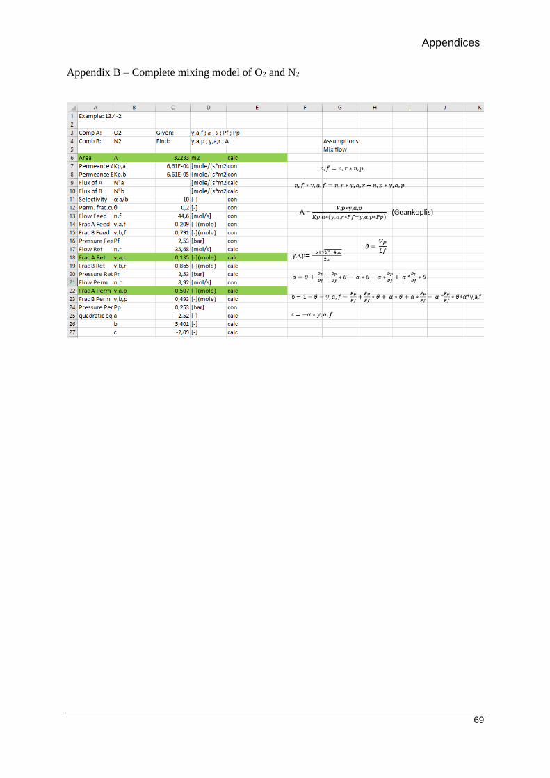
Appendices

69

Appendix B – Complete mixing model of O2 and N2

Appendices

70

Appendix C – Crossflow model codes from ACM

Appendices

71

Appendix D – Counter current model in Excel

Appendices

72

Appendix E – Pressure drop by Hagen-Poiseullie

Process evaluation of novel CO2 capture processes for ...

Documents

Transcript of Process evaluation of novel CO2 capture processes for ...