Proceedings of the 14th Field Robot Event 2016

2

Proceedings of the Field Robot Event 2016

Proceedings of the 14th Field Robot Event 2016

Gut Mariaburghausen, Haßfurt, Germany June 14th – 17th, 2016

Conducted in conjunction with the DLG‐Feldtage / DLG Field Days

Editors: M.Sc. Helga Floto Prof. Dr. Hans W. Griepentrog

Date: April 2017

Publisher: University of Hohenheim

Technology in Crop Production (440d) Stuttgart, Germany

Contact: Prof. Dr. Hans W. Griepentrog

Phone: +49‐(0)711‐459‐24550

File available on this webpage: http://www.fieldrobot.com/event

The information in these proceedings can be reproduced freely if reference is made to this proceedings bundle. Responsible for the content of team contributions are the respective authors themselves.

3


Index

Task Description …………………………………………………………………..….5

Agronaut (Finland)………………….………………………..……………………19

Beteigeuze (Germany)………………………….………………………………..67

Cornstar (Slovenia)……………………………………….………………….…...72

DTUni‐Corn (Denmark)…………………………………………………….......79

Eric (United Kingdom)……………………………………….……………….….95

Helios / FREDT (Germany)………………………………………………..….120

Plants with Benefits (The Netherlands)………………….……….……126

Soifakischtle (Germany)...……………………………………………….……131

Talos (Germany)...………………………………………………………………..137

The Great Cornholio (Germany)..………………………………………...145

Zephyr (Germany)………………………………………………………….….…154

ZukBot (Poland)………………………….………………………………….…….165

4


Sponsors

5


1. Field Robot Event 2016 ‐ Task Description

Together with the DLG‐Feldtage, 14th – 16th June 2016 at the Gut Mariaburghausen, Haßfurt, Germany

Remark: The organizers tried to describe the Tasks and assessments as good and fair as possible, but all teams should be aware of that we might need to modify the rules before or even during the contest! These ad hoc changes will always be decided by the jury members.

0. Introduction

The organizers expect that a general agreement between all participating teams is that the event is held in an “olympic manner”. The goal is a fair competition, without any technological or procedural cheating or gaining competitive advantage by not allowed technologies. The teams should even provide support to each other in all fairness.

Any observed or suspected cheating should be reported to the chair of the competition immediately.

The jury members are obliged to act as neutrals, especially when having connections to a participating team. All relevant communication will be in English. For pleasing national spectators the contest moderation could be partly in a national language.

Five tasks will be prepared to challenge different abilities of the robots in terms of sensing, navigation and actuation: Basic Navigation, Advanced Navigation, Weeding Application, Seeding Application and Free Style (option).

If teams come with more than one machine the scoring and ranking will always be machine related and not team related.

All participating teams must contribute to the event proceedings with an article describing the machine in more details and perhaps their ideas behind or development strategies.

In 2016 one of the most significant change is that NO team members are allowed to be in the inner contest area ‐ with maize plants ‐ and close to the robot during the performance of their machine. If the robot performance fails, it has to be stopped from outside with a remote switch. To enter the inner contest area is only allowed after the robot has stopped. The control switch activating team member then can go to the machine and manually correct it. When the team member has left the inner contest area only then the robot is allowed to continue its operation. This procedure shall promote the autonomous mode during the contest.

0.1. General rules

The use of a GNSS receiver is NOT allowed except for the Free Style in Task 51. The focus for the other tasks shall be on relative positioning and sensor based behaviors.

1 If you wish to use a GNSS, you must bring your own.

6


Crop plants

The crop plant in task 1 to 3 is maize (corn) or Zea Mays2. The maize plants will have a height of 20 ‐ 50 cm.

Damaged plants

A damaged plant is a maize plant that is permanently bended, broken or uprooted. The decision if a maize plant is damaged or not would be made by the jury members.

Parc fermé

During the contests, all robots have to wait in the parc fermé and no more machine modification to change the machine performance is ‐ with regard to fairness ‐ allowed. All PC connections (wired and wireless) have to be removed or switched off and an activation of a battery saving mode is recommended. This shall avoid having an advantage not being the first robot to conduct the Task. The starting order will be random. When a robot will move to the starting point, the next robot will already be asked by the parc fermé officer to prepare for starting.

Navigation

The drive paths of the robots shall be between the crop rows and not above rows. Large robots or robots which probably partly damage the field or plants will always start after the other robots, including the second chance starting robots. However, damaged plants will be replaced by spare ones, to always ensure the same operation conditions for each run.

0.2. General requirements for all robots

Autonomous mode

All robots must act autonomously in all tasks, including the freestyle. Driving by any remote controller during the task is not allowed at any time. This includes steering, motion and all features that produce movement or action at the machine.

During start, the robot is placed at the beginning of the first row. The starting line is located 1 m inwards the first path, which is marked with a white cross line. Any part of robot must not exceed the white line in start. For signaling the start and end of a task there will be a clear acoustic signal. After the start signal the robot must start within one minute. If the robot does not start within this time, it will get a second chance after all other teams finished their runs, but it must ‐ after a basic repair ‐ as soon as possible brought back into the parc fermé. If the robot fails twice, the robot will be excluded from that task.

2 Plant density 10 m‐2, row width of 0.75 m, plant spacing 0.133 m

7


Start & Stop Controller

All robots must be equipped with and connected to one wireless remote START/STOP controller. Additional remote displays are allowed but without user interaction, e.g. laptop.

Preferably, the remote controller is a device with two buttons clearly marked START and STOP. Alternatively, the coding may be done with clear green and red colors.

It is allowed to use a rocker switch with ON/OFF position with hold, if the ON and OFF are clearly marked with text in the remote controller.

Any button of the remote controller may not be touched for more than one second at time. In other words, a button, which has to be pressed all the time, is not allowed.

Remote controller may contain other buttons or controls than the required/allowed START/STOP inputs, but no other button may be used at any time during any task.

Before the start of any task, the remote controller must be placed on the table that is located at the edge of the field. One member of the team may touch the START and STOP inputs of the remote controller. Possible remote display must be placed on the same table too.

The remote controller must be presented to the Jury members before the run. A jury member will watch the use of the START/STOP remote controller during the task execution.

In each task, the robot must be started by using the remote controller START input, not pressing any buttons of the robot itself.

During any task, while the robot is stopped in the field by using the remote controller, it is allowed to use any buttons of the robot itself, e.g. to change the state of navigation system.

While the robot is STOPPED and one team member is allowed to be in the field, besides rotating the robot, the team member is allowed to touch the buttons and other input devices mounted on the robot. Other remote controllers besides START/STOP controller are strictly prohibited to be used at any time.

Implementation note: If using Logitech Cordless Gamepad or equivalent as a remote controller, the recommended practice is to paint/tape one of the push button 1 green and push button 2 red, to mark START and STOP features.

Manual correction of robot

One team member is allowed to enter the field, after the same team member has pressed the STOP button of the remote controller and the robot has completely stopped (no motion). It is recommended to install some indicator onto the robot to see that the robot is in STOP mode before entering the field in order to avoid disqualification.

The START/STOP operator is also responsible for the eventually manual robot corrections. Due to the fact that it can be difficult for him/her to monitor the robot’s behavior from a large distance, another team member can be inside the 2 m area between a red textile tape and the crop plant area (see picture 1 and 2 at the end of this

8


document). This second team member could give instructions to the operator, but this supporting person is only an observer and is NOT allowed in any case to enter the crop plant area or interact with the robot.

After leaving the remote control on the table, the operator is allowed to rotate ‐ not to move ‐ the robot in the field. The only exception for moving is within the row, where the robot may need to get back to the path if a wheel or track of the robot has collided stem of maize plant, to avoid further damage of plants. Carrying the robot is only allowed after significant navigation errors in order to bring it back (!) to the last correct position.

In the headland, only rotating of the robot is allowed, no moving or carrying is allowed at all.

0.3. Awards

The performance of the competing robots will be assessed by an independent expert jury committee. Beside measured or counted performance parameters, also creativity and originality especially in task 4 (Seeding) and task 5 (Freestyle) will be evaluated. There will be an award for the first three ranks of each task. The basic navigation (1), advanced navigation (2), weeding (3), and seeding (4) together will yield the overall competition winner. Points will be given as follows:

Rank 1 2 3 4 5 6 7 8 9 10 11 12 13 14 15 16 17 18 19 etc.

Points 30 28 26 25 24 23 22 21 20 19 18 17 16 15 14 13 12 11 10 etc.

Participating teams result in at least 1 point, not participating teams result in 0 points. If two or more teams have the same number of points for the overall ranking, the team with the better placements during all four tasks (1, 2, 3 and 4) will be ranked higher.

1. Task “Basic navigation” (1)

1.1. General description

For this task the robots are navigating autonomously. Within three minutes, the robot has to navigate through long curved rows of maize plants (picture 1 at the end of this text). The aim is to cover as much distance as possible. On the headland, the robot has to turn and return in the adjacent row. There will be no plants missing in the rows. This task is all about accuracy, smoothness and speed of the navigation operation between the rows.

At the beginning of the match it will be told whether starting is on the left side of the field (first turn is right) or on the right side (first turn is left). This is not a choice of the team but of the officials. Therefore, the robots should be able to perform for both options. A headland width of 2 meters free of obstacles (bare soil) will be available for turning.

9


1.2. Field Conditions

Random stones are placed along the path to represent a realistic field scenario. The stones are not exceeding 25 mm from the average ground level. The stones may be small pebbles (diameter <25 mm) laid in the ground and large rocks that push (max 25 mm) out from the ground, both are installed. In other words, the robot must have ground clearance of this amplitude at minimum, and the robot must be able to climb over obstacles of max 25 mm height.

A red 50 mm wide textile tape is laid in the field 2 m from the plants.

1.3. Rules for robots

For starting, the robot is placed at the beginning of the first row without exceeding the white line.

If the robot is about to deviate out from the path and hit maize plants, the team member with the remote controller must press STOP button immediately. The STOP button must be pressed before the robot damages stems of the maize plants. The team is responsible to monitor the behavior of the robot and use STOP button when necessary.

1.4. Assessment

The distance travelled in 3 minutes is measured. If the end of the field is reached in less time, this actually used time will be used to calculate a

bonus factor = total distance * 3 minutes / measured time.

The total distance includes travelled distance and the penalty values. Distance and time are measured by the jury officials.

Crop plant damage by the robot will result in a penalty of 1 meter per plant.

The task completing teams will be ranked by the results of resulting total distance values. The best 3 teams will be rewarded. This task 1, together with tasks 2, 3 and 4, contributes to the overall contest winner 2016. Points for the overall winner will be given as described under chapter 0.3 Awards.

2. Task “Advanced navigation” (2)


For this task the robots are navigating autonomously. Under real field conditions, crop plant growth is not uniform. Furthermore, sometimes the crop rows are not even parallel. We will approach these field conditions in the second task.

The rules for entering the field, moving the robot, using remote controller etc. are the same as in task 1.

No large obstacles in the field, but more challenging terrain in comparison to task 1.

10


The robots shall achieve as much distance as possible within 3 minutes while navigating between straight rows of maize plants, but the robots have to follow a certain predefined path pattern across the field (picture 2 at the end of this text). Additionally at some locations, plants will be missing (gaps) at either one or both sides with a maximum length of 1 meter. There will be no gaps at row entries.

The robot must drive the paths in given order. The code of the path pattern through the maize field is done as follows: S means START, L means LEFT hand turn, R means RIGHT hand turn and F means FINISH. The number before the L or R represents the row that has to be entered after the turn. Therefore, 2L means: Enter the second row after a left‐hand turn, 3R means: Enter the third row after a right hand turn. The code for a path pattern for example may be given as: S ‐ 3L ‐ 2L ‐ 2R ‐ 1R ‐ 5L ‐ F.

The code of the path pattern is made available to the competitors 15 minutes before putting all robots into the parc fermé. Therefore, the teams will not get the opportunity to test it in the contest field.

2.2. Field conditions

Random stones are placed along the path, to represent realistic field scenario where the robot should cope with holes etc. The stones are not exceeding the level of 35 mm from the average ground level in the neighborhood. The stones may be pebbles (diameter <35 mm) laid in the ground and large rocks that push (max 35 mm) out from the ground, both are installed. In other words, the robot must have ground clearance of this amplitude at minimum, and the robot must be able to climb over obstacles of max 35 mm high. No maize plants are intentionally missing in the end of the rows. However, due to circumstances of previous runs by other robots, it is possible that some plants in the end of the rows are damaged. The ends of the rows may not be in the same line, the maximum angle in the headland is ±15 degrees.

No large obstacles in the field and all rows are equally passable. A red 50 mm wide textile tape is laid in the field 2 m from the plants.

2.3. Assessment

The distance travelled in 3 minutes is measured. If the end of the field is reached in less time, this actually used time will be used to calculate a

bonus factor = total distance * 3 minutes / measured time.

The total distance includes travelled distance and the penalty values. Distance and time are measured by the jury officials.

Crop plant damage by the robot will result in a penalty of 1 meter per plant.

The task completing teams will be ranked by the results of resulting total distance values. The best 3 teams will be rewarded. This task 2, together with tasks 1, 3 and 4, contributes to the overall contest winner 2016. Points for the overall winner will be given as described under chapter 0.3 Awards.

Picture 2 shows an example of how the crop rows and the path tracks could look like for task 2. Be aware, the row gaps and the path pattern will be different during the contest!

11


3. Task “Weeding” (3)


For this task the robots are navigating autonomously. The robots shall detect weeds represented by pink golf balls and spray them precisely. Task 3 is conducted on the area used in task 2 with straight rows. Nevertheless, no specific path sequence will be given as in task 2 and the robot has to turn on the headland and return in the adjacent row.

The rules for entering the field, moving the robot, using remote controller etc. are the same as in task 1 and 2.


The weeds are objects represented by pink golf balls3 randomly distributed between (!) the rows in the soil that only the upper half is visible. Robots may drive across or over them without a penalty. The weeds are located in a centered band of 60 cm width between the rows. No weeds are located within rows and on headlands. A possible example is illustrated in picture 3.


Each robot has only one attempt. The maximum available time for the run is 3 minutes. The detection of a weed must be confirmed by an acoustic signal of an official siren4. All robots must use the official siren. The length of the beep may not be longer than 2 seconds.

The robot must spray only the weeds or the circular area around the golf ball with a diameter of 25 cm. Spraying outside this weed circle is counted as false positive, with no true positive scoring.

In the case that the robot is spraying or producing an acoustic signal without any reason, this is regarded as false negative.

3.4. Assessment

The Jury registers the number of true positives, false positives and false negatives:

‐ True positives (correct spraying with acoustic signal) + (plus) 6 points, ‐ True positives (correct spraying without acoustic signal) + (plus) 4 points, ‐ False positives ‐ (negative) 1 point and ‐ False negatives ‐ (negative) 2 points.

Crop plant damage by the robot will result in a penalty of 2 points per plant.

The total travelled distance will not be assessed.

The task completing teams will be ranked by the number of points as described above. The best 3 teams will be rewarded. This task 3, together with tasks 1, 2 and 4,

3 The golf balls used are “Nitro Blaster Golf Balls – Pink”. The organizer of the competition will send these to the teams after registration, but you can order your own set from Amazon.

4 “Pro Signal S130“, which is available e.g. from Farnell (order number 676550), voltage range 6 ‐ 12 V. The FRE organizer will send these to the teams after registration.

12


contributes to the overall contest winner 2016. Points for the overall winner will be given as described in chapter 0.3 Awards.

4. Task "Seeding" (4)


The robots perform a seeding operation for an area of 10 m x 1 m = 10 m2. The robots take wheat seeds from a station and sow them as even as possible on the area. How the robots realize the task is absolutely free.

From the starting point the robot goes to the filling station, stops there and asks to fill the hopper using a wireless command. A provided refill station has to be used. (Instructions given to construct your own mockup see picture 5.) The robot goes to the area and starts and ends the sowing correctly. Furthermore, the seeds need to be distributed as even as possible across the area and covered by soil as good as possible.


A bare soil area is used for this task with no plants. To provide equal conditions for every team, the soil is harrowed before every run and compacted afterwards with a light manual roller (such that is used in garden to care grass). After every run, the setup is moved to another location.

Red lines of 50 mm wide textile tape will be installed on the ground as a guiding help, see picture 4. They indicate longitudinal start and end as well as transversal center of the seed area.

The red centerline is extended to the start position of about 5 m passing the refill station. The outlet hose location of the refill station is marked with a perpendicular blue line on the ground (50 mm wide) that the robots may utilize in order to stop in the right place. The blue line is located about 3 m from the start and about 2 m from the region.

The team may install temporarily to the field also their own additional visual ground markers in the neighborhood of the blue line, to enable stopping into the accurate place for refill.

These markers must be placed in the field before the start and they may not be touched during the task.

The maximum number of additional markers is three and the maximum size of each is limited to 15 x 15 cm.

4.3. The seeds

Common wheat seeds (triticum aestivum) colored in red or blue will be used. The seeds will have a typical 1000‐seed‐weight of 30‐40 g and a bulk density of 740‐800 kg/m3.

On first day each team will get a non‐colored sample of 200 g trial seeds. More trial seeds will be available on request during the testing. During the competition the seeds will be provided.

4.4. The refill station

13


Drawings of the refill station are published well prior the competition (picture 5). Each team may build their own version for practicing, but during the competition only the provided one shall be used.

The body of refill station is located 75 cm beside the red line (picture 4 and 5). This implies the width of the robot may not exceed 75 cm including the accessories for seeding.

The hose where the seeds are delivered is adjustable, each team may adjust the height, and the side offset of the hose prior to the start. No moving of the hose during the task is allowed by any means.

The exit of hose may be adjusted 10‐60 cm from the ground level and 5‐50 cm offset from the body of the refill station. The hose outer diameter will be 50 mm at a 45 degree angle.

4.5. The seeding

The required seed rate is 500 seeds/m2. Therefore, the total number of seeds that is metered by the refill station to the hopper is 10 x 500 seeds = 5000 seeds, which equals around 150‐200 g.

How to achieve the most even distribution across the 10 m x 1 m area is up to the teams.

The seed rows may not touch the red line physically and should keep a distance of at least 5 cm from the red line.

After sowing, as many seeds as possible should be covered by soil. In other words, the seeds may not be visible on top view.

No other material besides the competition seeds may be distributed to the field.


The robot must be equipped with a hopper that can take the required amount of seeds (at least 500 ml). The hopper must be either top open or transparent, for jury members to see smooth emptying during sowing.

A robot must start from the headland, 5 m from actual field to be seeded. The starting point is illustrated in picture 4 with a green dot.

Around 3 m from the start, the refill station is located. The robot must navigate there autonomously using the red line as a reference guide path. The robot must stop there autonomously.

After stopping, the robot must send a command to the refill station, to ask material refill, by using Internet protocol. The refill station is connected to Internet with a public IP, so the team may use their own means to access it through Internet, or to use a local wireless connection. More details of the communication protocol will be announced soon.

If the refill command fails, a team member may push a manual button on the station to ask refill manually. Manual button does not score any points.

14


The station refills the hopper exactly the amount of seeds required to sow 10 m2. The refill is completed in 10 seconds from the receiving the command packet, after which the robot may continue.

After refill, the robot continues to the beginning of seeding area (which is marked with a perpendicular red line).

Robot must start sowing immediately after the red perpendicular line and sow until reaching the next red perpendicular line. In other words, the area between the two red lines needs to be sown, not beyond.

4.7. Assessment

Success in various subtasks give the score (speed does not matter as long as reasonable, max. time 6 min).

In this task, the speed is not rewarded at all. However, the maximum time to complete the task is 1+5 minutes (refill + sow).

The emphasis in scoring is more on agronomically correct operation, less on the accuracy of navigation.

In the ideal case, the resulted seeded area after each run would be 10 m2, which will result in 10 points. If the seeded area is higher or lower than the required 10 m2, the jury members will measure it. Any deviated area (in decimal m2) is subtracted from the 10 points.

One of the following achievements give 2 points each:

‐ navigating and stopping autonomously to the refill station ‐ commanding refill station to ask seed refill wirelessly ‐ correct filling of the seeds, all seeds went into the hopper ‐ navigating from refill station to region ‐ general navigation and turning

Furthermore, the jury members will assess two qualitative performance criteria by giving points from 0 (insufficient) to 10 (excellent) for each one. These two criteria are:

1. Seed spatial distribution 2. Seed soil coverage

The task completing teams will be ranked by the number of points as described above. The best 3 teams will be rewarded. This task 4, together with tasks 1, 2 and 3, contributes to the overall contest winner 2016. Points for the overall winner will be given as described in chapter 0.3 awards.

5. Task “Freestyle” (5)

5.1. Description

Teams are invited to let their robots perform a freestyle operation. Creativity and fun is required for this task as well as an application‐oriented performance. One team member has to present the idea, the realization and perhaps to comment the robot’s

15


performance to the jury and the audience. The freestyle task should be related to an agricultural application. Teams will have a time limit of five minutes for the presentation including the robot’s performance.

5.2. Assessment

The jury will assess the (i) agronomic idea, the (ii) technical complexity and the (iii) robot performance by giving points from 0 (insufficient) to 10 (excellent) for each.

The total points will be calculated using the following formula:

(agronomic idea + technical complexity) * performance.

The task 5 is optional and will be awarded separately. It will not contribute to the contest winner 2016.

16


Appendix

Picture 1 – Dimensions and row pattern for task 1.

17


Picture 2 – Dimensions and example (!) row pattern for task 2.

Picture 3 – Possible locations of the weeds for task 3.

Picture 4 – Illustration of task 4 “Seeding”.

Picture 5 – Dimensions and range of adjustment of the hose for task 4.

18


2. Robot information

19


AGRONAUT

Miika Ihonen1, Mikko Ronkainen1, Robert Wahlström1, Aleksi Turunen2, Ali Rabiei2, Robin Lönnqvist2, Mikko Perttunen3, Jori Lahti4, Aatu Heikkinen4, Timo Oksanen*,1,4, Jari

Kostamo*,2, Mikko Hakojärvi*,4, Teemu Koitto*,2, Jaakko Laine*,1

1)Aalto University, Department of Electrical Engineering and Automation, Finland 2)Aalto University, Department of Mechanical Engineering, Finland

3)Aalto University, Department of Computer Science, Finland 4)University of Helsinki, Department of Agricultural Sciences, Finland

*) Instructor and Supervisor

1. Introduction

Field Robot Event (FRE) is an annual competition for agricultural field robots. The location of the competition varies every time it is being arranged. This year, 2016, the 14th FRE was held in conjunction with DLG Feldtage exhibition in Gut Mariaburghausen, Haßfurt, Germany.

Previously, the robot for the competition was built from scratch. However, the mechanical requirements for the robot became higher and higher and, therefore, were hard to fulfill. Therefore, it was decided to use the body of the previous robot GroundBreaker [1] and focus on upgrading its weaknesses. In contrast to the mechanics, all the program code for the robot was entirely recreated and no line of program code was copied from the solutions of previous years.

The team consisted of total of nine students. Seven students were from Aalto University. Three from department of Automation and System Technology, three form Department of Engineering Design and Production and one from department of Computer Science. In addition, two team members were from University of Helsinki department of Agricultural Science.

The project lasted 10 months, which is bit over an academic year. In the autumn, the instructors had big role teaching and having meetings with the team. Part of the team members studied the tool chain and software developments, whereas, others started designing the components for the robot. In the spring, the role of the instructors became more a role of supervisor and the role of the team became independent.

The project offered for the team member a good experience of real life team project, where hard work, meetings, cooperation, deadlines etc. resulted a complete agricultural robot.

2. Mechatronics

Most of the aluminum parts of the robot Agronaut were manufactured by team members. Some of the parts were reused from the previous year’s robot GroundBreaker. During the academic year of 2015–2016 the manufacturing focus was with the axle modules of the robot as can be seen in Figure 1. Three axle modules were manufactured for the robot, two

20


for full time use and one as a spare. One requirement was that the axle modules had to compatible with the previous year’s robot.

Figure 1: Breakdown of an axle module with its main components numbered.

2.1. Components of the Axle Modules

List of parts in the axle module numbered as can be seen in Figure 1:

1. Steering knuckles manufactured by students 2. Custom motor controller VESC designed by Benjamin Vedder [2] 3. Self‐made printed circuit board to control the individual components in the axle

module and their data

21


4. Savöx SV‐0235MG digital servo that turns the wheels [3] 5. Turnigy Trackstar 17.5T sensored brushless motor with 1870KV rating [4] 6. P60 Banebots gearbox with a ratio of 26:1 [5] 7. Xray Central Differential 8. CUI AMT10 Series Incremental, capacitive modular encoder [6]

The axle modules also contained a 50 mm SUNON EB50101S2‐0000‐999 Axial Fan with a MAGLev® Motor, for cooling. It was located under the brushless DC motor.

2.2.1 Machining

The mechanical engineering students machined the axle modules in pairs. Two worked on the mill to double check measures of the parts and to practice milling, and turning with lathe.

The machining part of the project had a few setbacks and the time needed to machine the parts was exceeded by numerous hours. For example, six blocks made for the servos in the axle modules was estimated to take an hour to machine, but the actual time was three hours. Two of these blocks can be seen in Figure 1 (part 10). The time that was reserved for milling could have been doubled or even tripled. It was a learning process where students had to consider the best way of zeroing the machine, so that the required tolerances could be achieved.

Some parts were more difficult to produce than others. The cutting and drilling of the required holes for the drive axles in the modules was one the most difficult parts. Tolerances varied between the three axle modules and this variation had to be taken into consideration when manufacturing the axles that drove the wheels. The drive axle consists of six different lengths of steel rod pieces seen in Figure 2 and these had to be exactly the right length, else the axle could not be assembled. The required length was the distance between the outer planes of the two steering knuckles, which was 363 mm. The through holes in the axles were difficult as well, because they had to be exactly in the middle of the steel axle, else the wheel adaptor pins would not go through the holes on the wheel stopper nuts and thus the wheel drop off.

Figure 2 The drive axle of the axle module with the connecting universal joints and differential.

Some of the parts were ordered from our sponsor Laserle Oy, a laser cutting company that manufactured the parts in no time. For example, the sides on the axle modules with the holes for the electronics Figure 1 (part 1), were made out of 2 mm thick aluminum sheet that was cut by Laserle.

22


2.2.2 Assembly

In the assembly of the axle modules, standardized measures of screws were used to connect the walls to each other and the printed circuit boards to the walls. Screw connections were the general connection tool in this project. Table 1 has a list of screws used. Other ways of combining parts such as welding was not used.

Assembling the axle modules needed some of adjusting. The screw connections would not always align perfectly and caused the screws to be driven crooked into the work pieces. Holes needed to be made oval so that sideways movement was possible. For example, the Banebots gearbox fastening holes were not aligned with the axle module wall shown in Figure 3 that demonstrates the problem. In the actual model, all holes were aligned.

Figure 3. Banebots gearbox and axle module wall. Red circles indicate the misalignment of the holes

on wall and gearbox

2.1 Embedded Electronics for the Axle Modules

The three axle modules that were made for the robot each have printed circuit board in them that controls the VESC and electronics of the axle module. This board is used to

Screw Application

M5X25 mm Connecting the banebots to the axle module.

M5X20 mm Connections of the steering knuckle.

M5X12 mm Connection of servo to the axle module.

M4X25 mm Axle joint connections.

M4X20 mm Fan connection.

M4X12 mm Most of the connections between parts.

M4X10 mm The steering knuckle fasteners connected to the axle module walls.

Table 1: The screws of the axle modules

23


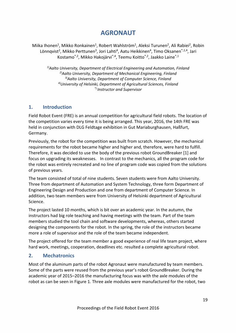
control the motors that drive the wheels, control the servo that turns the wheels and read values from thermistors that evaluate the temperature inside the axle modules. The printed circuit boards were designed using software KiCad and they were manufactured in the confines of Aalto University. The electrical components on the printed circuit board:

1. Chip45’s Crumb 128‐CAN V5.0 AVR CAN Module microcontroller [8] 2. A TOSHIBA TLP620‐4(GB) transistor output optocoupler used for galvanic isolation. 3. Molex connectors for batteries that power the actuators: servo, motor and fan. 4. 10‐pin header for ribbon cable connection with the robot’s CAN hub. 5. ON SEMICONDUCTOR MC7805BDTG Linear Voltage Regulator to lower 12 volts from

the can hub to 5 volts needed for the microcontroller. 6. MULTICOMP DIP switch with 4 circuits to set the identity of the printed circuit board. 7. Two Vishay NTCLE203E3103GB0 10K thermistors that monitor the temperature of

digital servo and the brushless dc motor. 8. INTERNATIONAL RECTIFIER IRLIZ44NPBF MOSFET Transistor N Channel for the fan

control.

2.2.1 Features of the Printed Circuit Board

Figure 4: Optocoupler annotated Opto1, power and actuator connectors

24


Figure 5: 10 pin header and voltage regulator

The axle module printed circuit board was built around the microcontroller Chip45’s Crumb 128‐CAN V5.0 AVR CAN Module that controls all the actuators and reads the value of the thermistors. The microcontroller was programmed using the universal synchronous asynchronous receiver transmitter (USART). A TOSHIBA TLP620‐4(GB) transistor output optocoupler was used to interface the high voltage to the low voltage parts of the printed circuit board, thus preventing a power surge in the actuator side from destroying the microcontroller on the other side of the optocoupler. The optocoupler with the actuator side of the circuit can be seen in figure 4. Connectors for the VESC signal, servo signal, servo power, motor batteries, and cooling fan can also be seen in figure 4. The cooling fan was controlled according to the thermistor readings and it was powered by the motor batteries located on the robot. A freewheel diode is connected between the fan and the power source to prevent inductive spikes. The power to the microcontroller is received from the CAN hub of the robot with a ribbon cable that is connected to a 10 pin header. The voltage received was 12 volts and needed to be lowered to 5 volts that the microcontroller uses. A ON SEMICONDUCTOR MC7805BDTG Linear Voltage Regulator was used drop the voltage. Figure 5 shows the schematic of the 10 pin header connector and the linear voltage regulator. Also the CAN high and low are received from the CAN hub. A MULTICOMP DIP switch with 4 circuits was used to set the identity of each axle module. The specific identities were taken into account when programming the Crumb 128‐CAN microcontroller.

2.2.2 Design of the printed circuit board

In the design process of the printed circuit board a schematic was made in KiCad seen in Figure 6. The components have been annotated and footprints have been added to each component. During the design of the printed circuit board new libraries were created and new footprints were designed. The Crumb 128‐CAN is an example component that did not have a standard footprint. The footprints of the electrical components are such, that when placing components on the printed circuit board, these footprints mark the placement of the components and the design works as reference on how much room the component takes on the printed circuit board. Other things that were considered during the printed circuit boards design was the thickness of the coppering, because of the current traveling through them. A minimum of 4 millimeters was set for the wire thickness, but it was advisable to use as thick wiring as possible. Symmetry between the pad sizes and wire thicknesses was a goal. When this symmetry was achieved, the wires could pass between the pads in optimal places while traveling to their destination. A minimum amount of through holes in the printed circuit boards was achieved when the symmetry was found. In addition, the help of zero resistors was used to remove the need of through holes. These zero resistors worked as bridges to cross over the wiring. The printed circuit board was designed as small as possible because of the limited space inside the axle modules. This space was only 70.2 mm x 140 mm x 131 mm and all the actuators, mechanical and electrical components needed to fit in this space.

25


Figure 6. Schematic of the printed circuit board for the axle modules

2.2.3 Steering Knuckles and Ackerman Angles

An integral part of the robot's motive system is the steering knuckle. It is the part to which the bearings for the wheels are attached, and which is used to turn the wheels themselves. It must, therefore be strong enough to bear what is effectively the entire weight of the robot, be able to turn under all this weight, house the joints properly and produce the correct kinds of wheel angles while turning. The last requirement is an often overlooked but integral part of steering geometry, without which the wheels must skid sideways during turns.

The knuckles used in Agronaut were custom‐designed and machined to spec by the team. During most the projects of previous years, the knuckle of choice has been one designed for large‐scale RC cars. This practice has had the advantage of a pre‐made, strong component that is widely available, and compatible with the axles and joints that were similarly chosen. This kinds of knuckles were used without problems, and they were replaced not because of any flaw in them, but because it was decided to move up to stronger axle and joint components. The RC‐spec axles had proven to be too weak, especially after cutting and remaking them to the specific length needed by the robot instead of whichever model of car they were intended to. These new knuckles needed to accept thicker axles and longer joints, and therefore had to be of a larger and sturdier construction.

The design of a steering knuckle can be broken down into the following requirements:

Physical fitting ‐ the knuckle must physically support the axles and axle joints used. It was decided to use an 8 mm axle with large and sturdy universal joints, for which the knuckles larger diameter accounts for.

Joint geometry ‐ while turning, the joint must be positioned so that it's center of turning is the same as on the knuckle, lest it cause a pulling and pushing component force as it is turned. The larger and longer joints needed an increase in the length of the joint housing for the center of turning to be correct.

26


Physical strength ‐ The knuckle must support the robot's weight and the moment of the steering system that acts on it without breaking. Due to this the knuckle was intentionally not lathed down to the bare minimums, as saving weight has a much lower priority for Agronaut than an RC racer. The steering arm was affixed with quad M3 screws, two on both sides of the arm for strength, and the turning joints as well as steering cable attachments were of the larger M4 size for the same reason.

Manufacturability ‐ There was a good reason for this joint to be able to be made with manually controlled machines instead of CNC ones ‐ the team was doing it. For this reason, it was split into two parts: the main shell with the bearings to be made mostly with a lathe, and the steering arm, which was to be milled. The lathed shell included a milled cutout for the joint during turns, and a level plane upon which the arm attaches.

Steering geometry ‐ Since the radius of turn for each wheel is different, especially during tight turns, the inner wheel must be turned proportionally more. The knuckles must cause this through their geometry, specifically through implementing the Ackermann steering geometry. This requirement needed the largest amount of design work to complete. The so‐called "Ackermann‐angles", which are the angles of the steering arms in relation to a completely straight angle, must be computed to coincide with the vehicle's turning center point, which for a four‐wheeled, two axle vehicle steered only by one set of wheels (like a normal car), would be the center of the non‐steering axle. Agronaut, however, uses symmetrical four‐wheel steering, so the center point ends up at the robot's center. This means that the angle can only be completely correct for that kind of steering, and if only one pair of wheels was turned, the angle would be wrong. Agronaut has a very short wheelbase for agility, which when coupled with the four‐wheel steering make the required angles unrealistically large. Those angles would create a massive moment arm against the steering servo with large steering inputs, so a compromise was the only choice. The angle was made larger than a 2‐wheel steering vehicle would have, but smaller than the optimal one. In this way, even though the optimum could not be reached, the angle would be improved over the RC knuckles meant for normally steered cars.

While the design of the knuckles is an overall success, there are a few difficulties associated with them. The housings of the bearings were manually done with a lathe, making it a very slow process since the tolerances are tight and must be checked individually. It also exposes them to the danger of too loose bearings, of which some examples seem to suffer from despite best efforts at avoiding this. There also appears to be some differences in the mounting holes, causing slight errors in wheel stance. Despite this, they do their work well, are strong and enable the use of more appropriate components.

3. Hardware

Most of the hardware of the robot is same as last year [1]. However, the robot was upgraded with few significant components. First of them is the local user interface and another is the motor controller VESC. Both of these new components are described in the following subsections.

27


3.1 Local User Interface (LUI)

Since the robot must be usable without a separate computer, and as relying completely on a wireless interface is risky, the robot is equipped with a local, physical user interface. This consists of a set of LED's giving feedback about the robot's status, an LCD screen and buttons for the user interface. This board is also responsible for the camera servo mounted on the mast, the buzzer function with selectable volume, and has provisions for radio communications with an XBee ‐radio.

Like all peripherals on Agronaut, the LUI is built around an Atmega 90CAN128 ‐microcontroller, and communicates through the can bus. Its main function is to be a simple interface for the robot's software running on the computers, and its tasks mainly include sending them information on what buttons are pushed, and receiving what LED's should be lit and what to show on the screen. All menus and logic is implemented outside of this device.

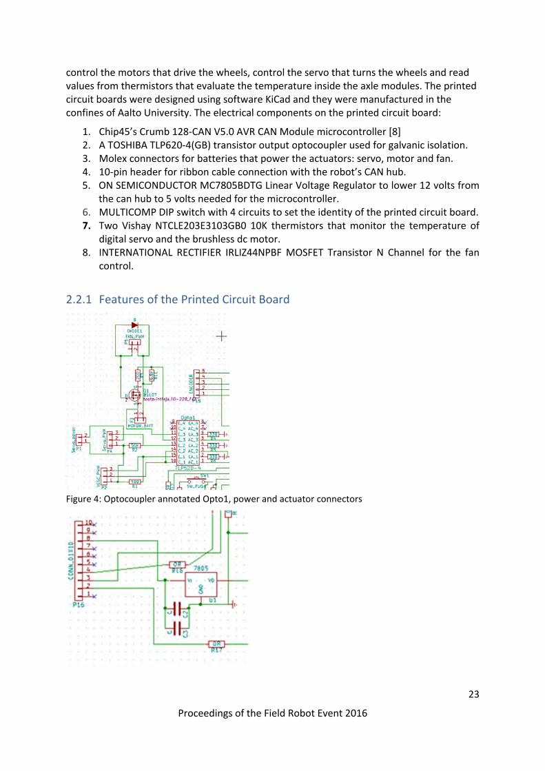
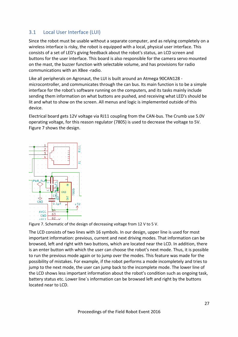
Electrical board gets 12V voltage via RJ11 coupling from the CAN‐bus. The Crumb use 5.0V operating voltage, for this reason regulator (7805) is used to decrease the voltage to 5V. Figure 7 shows the design.

Figure 7. Schematic of the design of decreasing voltage from 12 V to 5 V.

The LCD consists of two lines with 16 symbols. In our design, upper line is used for most important information: previous, current and next driving modes. That information can be browsed, left and right with two buttons, which are located near the LCD. In addition, there is an enter button with which the user can choose the robot’s next mode. Thus, it is possible to run the previous mode again or to jump over the modes. This feature was made for the possibility of mistakes. For example, if the robot performs a mode incompletely and tries to jump to the next mode, the user can jump back to the incomplete mode. The lower line of the LCD shows less important information about the robot’s condition such as ongoing task, battery status etc. Lower line`s information can be browsed left and right by the buttons located near to LCD.

28


There are three LiPo batteries in the robot and there are four orange LEDs in the UI which turn on when batteries capacity is low, one for reserve. Power on LED is green, respectively when the robot is stopped a red LED ignite on. A blue constantly flashing is robot alive LED.

In the mast there are 3 different color LED strips. Different LED strips give information about the direction of movement of the robot. The LED strips are used because of 360‐degree visibility. The upper LED strip is blue, turn right LED; in the center is green row navigation LED strip and lower LED strip is red turn left LED strip. The LED strips use 12V, the information to LED strips should go via the Crumb which uses 5V voltage. The problem is solved by using MOSFET transistors. The solution is shown in Figure 8.

Buzzer, sowing and injection are equipped with own buttons and LEDs. In addition, there is a one extra button and LED and four extra ports which go via the crumb. Switcher, which is located on the board makes possible to choose between small and big buzzer.

Weatherproofing is achieved by gluing a laser‐cut acrylic on top of the LCD, LED collars, with IP code buttons and window seals together with slanted design that allows water to flow away from the top plate and its sensitive electronics.

Figure 8. Schematic of solution.

29


3.2 Motor Controller ‐ VESC

A good motor controller, or ESC (electronic speed controller), is necessary for any electric vehicle. Its correct functioning is essential for stable power to the motors, and in more advanced cases, it also determines the behavior of the motors during starting and stopping. One such case is Agronaut, where it was decided to use brushless DC motors instead of the previously used ubiquitous brushed ones. Brushless motors provide much higher power, reliability and efficiency than brushed motors, but are more demanding to control. The main issue is that, unlike a brushed motor where one simply provides power and the motor provides torque as the mechanical brushes make sure the motor tries to turn in the right direction, a brushless one cannot work like that. It needs positional feedback, which is normally provided by back‐EMF through the motor wires and does not work while not turning. Therefore, Agronaut needed a motor controller that had not only the required power capacity and reliability, but also the ability to use some kind of motor sensors for this feedback.

The controller that was chosen is the open source VESC ‐ Vedder's ESC shown in Figure 9. It is an advanced and highly configurable controller with open hardware and software, and since it was originally intended for electric skateboards and such, it has more than the required capacity. One of its many features is the ability to use Hall‐effect sensors mounted on the motor to time the commutation even while the motor is stalled. This feature is used by Agronaut to ensure smooth starts, even with high loads. While capable of working with the much higher voltages of manned electrical vehicles, it is more than capable of running on the 3‐cell ~11.1 Volt lithium‐ion batteries used.

During our project, VESC was found to be an excellent piece of hardware. It supports a wide range of motors from large vehicular hub motors to small, fast ones such as those used in RC cars. It can be controller through an USB serial connection, the CAN‐bus, or simple servo PPM signal, all of which are configurable. It also comes with a comprehensive control suite that can tweak and tune a large array of parameters such as commutation type, use of sensors and internal limits, as well as output the current state of the controller in real time, showing current, temperature, duty cycle and even rotor position.

In Agronaut, VESC was configured to be a simple duty cycle driven speed controller, with the more advanced functions provided by the axle modules mainboard. Control is by PPM with a standard servo signal. Its abilities are such that it could easily be used as the axle module's electronics all by itself. That would have been much cleaner of a solution, but one not chosen due to our initial unfamiliarity with the VESC and its capabilities.

During installation, one of the VESC's suffered a damaged FET driver chip, which we were able to pinpoint with the VESC's own diagnostics. This circuit is fragile, since it only took a brief short of the motor leads worth hardly more than couple of mA to damage it. However, after proper installation, VESC was found to be reliable, with no recorded faults. It is capable of driving the motor smoothly at very low RPM's and does not struggle with the power required by Agronaut.

30


Figure 9. VESC, the motor controller used in the axle modules.

4. Software

The software discussed in this chapter is running on the navigation (eBox) and positioning (NUC) computers. The software of the robot contains multiple development tools, self‐made programs and algorithms. The tool‐chain described in the following consists of such programs as Microsoft Visual Studio and Matlab with Simulink. The self‐made programs were Remote User Interface (RemoteUI) and VisionTuner. The remote UI was a critical software when using the robot and the VisionTuner was made for tuning the machine vision. The software, tools and algorithms are explained more specific in the following subsections.

4.1 Toolchain

Our software tool‐chain was a combination of Windows, Matlab, Simulink, Visual Studio 2008, C, C++ and C#. Development OS was Windows 7 and of the two computers on the robot one had Windows 7 and the other had Windows CE 6.0 as the OS. All the computers and OSs were 32‐bit. Using Matlab version 2013b and its Simulink environment, a model of the software was designed graphically. We used the built‐in building blocks of Simulink in addition to custom blocks written in m‐code. The bus feature of Simulink was also extensively used. After the model had been completed the code generation feature of Simulink was used to generate C code files. The generation step required careful and extensive configuration of Simulink in addition to customized external Matlab source files.

The generated C files of the model were then incorporated into a Visual Studio 2008 C++ project. The sole purpose of this C++ project was to expose the Simulink model as a native code DLL with a simple interface. This meant that the time critical and heavy calculations were done as efficiently as possible. Also worth noting is the fact that the robot had two different computers running two different Simulink models. Their CPUs had different architectures and the DLLs were built and optimized natively for each of them.

The actual main programs on both computers were done in C#. It was chosen because it was deemed easier and faster to develop with and the performance of these parts was not that critical. We used the P/Invoke and marshalling features of the .NET platform to interface with the Simulink models inside the native C++ DLLs. The buses that were created in the Simulink model would manifest as C structures in the generated C code. These structures

31


were then identically reproduced at the C# side which allowed easy exchange of data between the C# programs and C++ DLLs.

Summarizing the work needed to get the programs running on the robot:

1. Design and implement algorithm in Simulink 2. Generate C code from the Simulink model using the code generator 3. Import generated C code to a C++ DLL project in Visual Studio 4. Import modified external files to complement the generated code 5. Inside the C++ DLL, implement minimal API to interfaces the Simulink code 6. Export that API from the DLL and find the mangled function name (using e.g. dumpbin) 7. Create C# interface for the DLL using P/Invoke and the mangled names 8. Create a C# console program that uses the C# interface to the Simulink C++ DLL 9. Make sure that the C# structs are in sync with the generated structs in the C++ DLL 10. Build a bundle containing the C# console program and necessary DLLs 11. Deploy the bundle to the robot (basically just copy files) 12. Run the executable on the robot

Not all these steps are necessary all the time. After first implementing everything and doing just simple changes in Simulink, only steps 1, 2, 9, 10, 11 and 12 are necessary to have the new code running on the robot.

4.2 RemoteUI

A custom software for managing the robot remotely (RemoteUI) was implemented from scratch. All the robot data structures were implemented in Simulink using buses when the algorithms were designed. These buses contain all the data of the robot. These buses manifest as C structures and are easy to serialize into byte buffers. Logic was implemented into the robot software to send all these buses out as UDP packets four times per second. These packets would then be received by the RemoteUI software running on laptops connected to the WLAN of the robot.

RemoteUI has multiple views to visualize the state of the robot. The most basic view which was implemented first just shows all the data. In the beginning, this was helpful to quickly start debugging the algorithms. A real‐time parameter updating functionality was also implemented. This enabled quick turn‐around when developing and adjusting the parameters of the algorithms.

32


Figure 10. The main view of the RemoteUI window. This view represents the most significant information of the state of the robot.

Later an overview screen was implemented (see Figure 10) that visually showed the state of the robot. This included e.g. the state of every subsystem, battery voltages and current consumptions, motor temperatures, CPU usage percentages and indicators for incoming UPD packets. With this view one could tell with a single glance if everything was OK with the robot. The UI could also be used to start/stop the currently activated autonomous task.

RemoteUI could also be used with different joysticks. Joystick could be used to start/stop the task and also for driving the robot manually. Logging view was implemented to help generating and managing log files. Using the UI to start the logging, a unique GUID value was created which was then also embedded into the log file names. This was helpful especially when doing multiple test runs which each generated its own set of log files. Using the GUIDs and some note taking, it was easy to later pair the log files on the robot to the specific test run. A turn sequence editor was also implemented which made testing appropriate tasks easier.

33


Figure 11. The VisionTuner software window. The VisionTuner contains all the parameters and

setting for tuning the machine vision.

4.3 Vision Tuner

The computer vision functionality was implemented with the help of the OpenCV C++ library. A separate Visual Studio C++ DLL project was created which had similar API as the Simulink C++ DLLs. A corresponding C# interface was then implemented which called the C++ DLL using P/Invoke. Using this interface, it was easy to add the vision algorithm processing alongside the Simulink model processing in the robot main program. This also meant that the heavy image processing was done in native code instead of C#.

As the vision algorithms had numerous parameters and they needed a lot of manual tuning, it was decided that a RemoteUI‐like program was necessary to help the development. VisionTuner was created from scratch which used the exact same C# interface mentioned above as the robot main program. Figure 11 shows the settings view of the VisionTuner. In the settings view all the camera settings that do not change at run‐time were editable. One notable feature here was the ability to replace the physical web camera with a video file which would then be looped over and over. One algorithm could then be selected as the active one, debug windows could be enabled and the algorithm could be stepped one frame at a time forward. In the parameters view all parameters could be adjusted live while the algorithm was running. In the output view all the output of the algorithm could also be viewed real‐time. This functionality helped the tuning of the algorithms significantly.

34


The settings and parameters could be saved into files which in turn were readable by the robot main program. Parameters were also loadable by the RemoteUI program which could upload the parameters to the robot while it was running.

4.4 Communication

The communication architecture of the robot is largely based on the designs of the previous years’ robots. They have been found to work quite well and it was determined that no big changes were necessary. Five different technologies were used for communications: USB, Ethernet, RS‐232, RS‐485 and CAN. Overview of the architecture is presented in Figure 12.

USB was mainly used for connecting the web cameras to the NUC PC. One USB hub was installed and used for both cameras. In addition, the joystick that connected directly to the robot was also using USB. All the different adapters (serial and CAN) were also USB based. All the adapters were connected straight to the PCs and did not use the USB‐hub to avoid any latency and other problems.

The Rangepack sensors were connected to a common RS‐485 based bus. This bus was driven by the NUC PC through the USB‐RS485 adapter. The NUC PC acted as the host of the bus and the Rangepack sensors were slaves. Data on the bus was exchanged using the so called Field Robot Protocol (FRP), defined in Aalto University, which is a simple messaging protocol for RS‐232/RS‐485 stream creating frames in the data stream and also for providing simple checksum checks.

In similar manner to RangePacks the cut‐offs that monitor battery voltage levels were connected to a RS‐485 bus using the FRP. The USB‐RS‐485 adapter and thus the bus itself was connected to the eBox PC. The major difference here was that the bus was driven at lower speeds compared to RangePacks. This was done because the cut‐offs were operating in somewhat noisier environment.

Gyroscope data exchange was also running on top of FRP but because it was the only device on the bus, RS‐485 was not necessary but RS‐232 was used instead. The serial connection to the NUC PC was through a USB‐RS‐232 adapter.

Major part of the robot communications was based on a CAN bus. A Kvaser USB‐CAN adapter was used to create and connect the bus to the eBox PC. A custom‐made CAN‐hub was used to connect together the adapter and all the other CAN‐based modules. Axle modules used the CAN bus to take drive commands and also for sending back status information. LocalUI used CAN bus to relay button presses and light up signal leds. The GPS module transmitted its data through the CAN bus also. The additional modules, trailer and weeder, used the CAN bus to take in activation commands.

Both of the PCs, NUC and eBox, were connected by Ethernet. A router was used to relay the messages and also to connect up a WLAN access point to the network. The PCs used exclusively UDP packets to pass data between each other. The SICK laser scanner was Ethernet‐based and was connected to this local network. The data exchange between the scanner and NUC PC was done with TCP streams. A laptop could also be connected to the local network through the WLAN access point. Both PCs would then send their status data using UDP packets to the RemoteUI program for remote status monitoring.

35


Figure 12. Overview of the communication architecture.

4.5 Algorithms and robot modelling

Many of following algorithms have basis in the kinematics of the robot. Therefore, a proper kinematic model of the robot plays a big role. The robot has a four‐wheel‐steering with Ackerman‐angles. In consequence, the steering angles of each wheel corresponding to certain control signals could not be measured in feedback manner. However, a simpler method of modeling was used instead. In the kinematic model, the robot was considered as a two‐wheeled bicycle‐typed vehicle with front and rear steering. Furthermore, the steering angles were not measured directly from the wheels. Instead, the actual steering angles were defined empirically by driving circles with different steering values. The actual steering angles were finally defined by the radius of the driven circles. In addition to the steering angles, the encoder pulses needed to be transformed into meters for completing the kinematics.

In the kinematic model formulae, the center point of the robot is considered as the origin and the robot is placed along x‐axis. The front and rear axle modules have own velocity (speed and direction). Therefore, the velocities are divided into x‐ and y‐components. Next, the x‐components and y‐components are being averaged. The averaged values are considered as true motion of the robot in the x‐y‐plane. This motion can be transferred into global coordinates if the orientation of the robot is known. The change of orientation is dependent on the steering, the distance between the axles and the longitudinal speed of the robot:

2

36


2

where the velocities are:

cos

sin

Finally, the robot kinematics in global coordinates are:

cos sin

sin cos

tantan

4.6 Positioning

The robot had two optional positioning algorithms for driving in maize field. Only one of the algorithms could be used at the time and, thus, both of the algorithms were tested in competition circumstances and the better one was chosen for usage. The first algorithm uses RangePack [1] range sensors for observing the field and the second used a laser scanner. For these algorithms, the RangePack algorithms is simple and computationally light, whereas, the laser algorithm is more complex and computationally heavy but provides usually better results. The following subsections describe the algorithms more specific.

4.6.1 RangePack based Positioning

The first positioning algorithm implemented for the robot relies on RangePack measurements. The RangePacks are range measuring units containing infrared and ultrasound measurements. The robot is assembled with four RangePacks. One in each corner directed to the sides of the robot. In addition to range measurements, estimation of the resent path of the robot is required. The path estimation is done using Euler's integration. For the Euler's integration a kinematic model of the robot is required as well as the steering and velocity of the robot.

A short log of previous 20 steps is held in robot’s memory. The log contains the pose of the robot and the measurements placed in robot’s coordinates. At the present the robot is placed in origin. Integrating backwards in time results the path of the robot and next, the measurements can be placed into robot’s coordinates. Most efficient way of computing this is keeping data in log persistent and shifting data backwards and replacing the last value with the latest data. Next, all the data is shifted among x‐axis and y‐axis based on the robot’s movement. Finally, all the data is rotated using rotation matrix corresponding to the robot’s rotation between two last steps. All the measurements are weighted since both of the sensors have reliability problems out of certain range. For infrared sensors over 0.20 m measurements are weighted as zero as well as over 0.60 m ultrasound measurements. This is how it is avoided that measurements from ground or other rows could affect the positioning of the robot.

37


Figure 13. On the left, the gray box represents the robot and the gray dots the path of the robots. RangePack measurements as aside of the robot and represented by the green dots. On the right, the measurements are moved towards the center. The red line represents the estimated center line between the rows.

Once all data is logged into robot’s coordinates. all the measurements are moved into one line. Therefore, the measurements on the right side of the robot are increased with half of a row gap and the measurements on the left side of the robot are decreased with half of a row gap. Now, it is assumed that rows are approximately in a straight line. Therefore, the center line between the rows is detected using straight fitting method called linear least squares estimation. It is computationally simple and it results coefficients b and c for line y = bx + c. The position and rotation compared of the robot compared to the center line is solved using basic geometry and trigonometry. However, the fitted line or the pose of the robot is not enough since the line could have been fitted on poor data. Therefore, a confidence factor is required. For any fitted curve a commonly used confidence factor is R‐square that is scaled from 0 to 1. Zero value means poor fit and unit value means perfect fit.

4.6.2 Laser Scanner based Positioning

Laser positioning is based on SICK 2D laser scanner. The laser scanner is placed in front of the robot above the ground level. The scanner is supposed to get hits of maize in rows. The scan results are initially in polar coordinates and, therefore, they are transformed into Cartesian coordinates where the center of the robot is the origin. Furthermore, measurements outside of approved range (from 0.1 m to 1.2 m) are disabled. Once all the approved measurements are transferred into Cartesian coordinates, the measurements are rotated several times. After each rotation a histogram of hits is formed. Additionally, variances of all the histograms are computed. After the data is rotated between feasible angular range the variances are compared. The orientation with the highest sum of variances is most likely the correct direction of the maize rows. Next, the measurement data

38


is rotated this orientation, the robot is aligned with the rows. Since, the laser sees behind the rows (sees multiple rows), a modulus of the data is computed in order to move all the measurements into one row. The histogram based rotation could be used as position data. However, it is not very accurate since the computing of histograms is not very effective and the number of calculations is limited. Therefore, a straight line is fitted to the measurement data similarly as in RangePack navigation using linear regression. The result of the line fitting is considered as the positioning data resulting the distance from the center line between rows as well as the orientation to the center line. Similarly, as previously, R‐squared is computed to evaluate the goodness of the fit.

Figure 14. The raw laser data represented in up left is being rotated (up right) and the histogram of the rotated data is seen in down right. Once the optimal rotation is being found, a modulo is taken (bottom left). The remaining data is being used to find the final estimate for the center line between the rows (the red line).

4.6.3 Kalman Filtering

The positioning algorithms have an option for filtering instead of using the raw measurement data. Since the process noise of the locomotion of the robot as well as the measurement noises of the range sensors are normally distributed, the Kalman filter provides an optimal estimate for the robot’s pose between the rows. In contrast to the raw measurements, the Kalman estimate takes into account the kinematic model of the robot and, therefore, provides more stable and realistic estimate than measurements only [7].

Using of the Kalman filter requires perceptions of the covariances of the process as well as the measurements. Partially, these covariances are defined with help of statistics from data logs. However, obtaining better estimate requires empirical tuning. That is, the tuning of the Kalman filter is weighting the measurements against the kinematics. Furthermore, since the

39


speed and steering of the robot are also measured, the Kalman filter is used as a sensor fusion method.

4.7 Navigation

Initially, the purpose was to implement several competitive algorithms for navigation as well as for positioning. However, because of the lack of time, only one algorithm was completed before the competition. The algorithm and the tuning methods are explained in the following subsections.

4.7.1 Navigation algorithm

The only row navigation algorithm was based on two parallel PID controllers. One for the distance from the center line between the rows of the robot and another for angular difference from the center line between the rows. Both of the PID controllers have an integral anti‐windup preventing undesired behavior. The outputs of the controllers were used as inputs for an inverted kinematic model of the robot. Because of the hard mathematics, the kinematic model of the robot was generated numerically and it resulted in two third order polynomials; one for front wheel steering and another for rear wheels.

The advantage of this control method is the low dependency between the PID controller. Therefore, it is possible to tune both of the controllers separately by setting another to zero and driving between the rows until the controller behavior is satisfactory.

4.7.2 Algorithm tuning

The tuning of the navigation was started in the winter before driving outdoors was possible. Therefore, an indoor test field was built of cushion board. The tuning method was mostly empirical but based on Ziegler‐Nichols method, which is known as a rule of thumb in PID tuning. First, the proportional term was increased until the controller begun to oscillate. Next, the proportional term was decreased approximately to half of the oscillation value. Finally, the integral and derivative terms were increased carefully as long as the behavior was satisfying. Once the results on the cushion board field were satisfying, a more realistic test field was built using wooden sticks with textile slides presenting maize plants.

The tuning in outdoors had two phases. First outdoor tuning was made in a field of barley provided by University of Helsinki. The barley was sowed to correspond to the circumstances of the maize field of the competition (e.g. the row spacing was 75 cm). However, the summer in Finland is short and the length of the barley was enough only for RangePack positioning. The second outdoor tuning was made at the Field robot event in the test fields. This tuning provided the most realistic results since the official competition field was very similar as the test field.

4.8 Row End Detection

Row end detection algorithms are used to determine the end of the maize field. Row end detection is required to function even when the rows contain gaps or similar distractions, which means that only relying on US and IR scanners is generally quite unreliable.

Row end detection uses measurements from the laser scanner to determine the end of the row. The laser scanner determines the x,y‐coordinates of hits inside a certain area. The hits

40


are processed to histograms that measure the number of hit points in a given direction. The histogram in driving direction is used to determine location of the row and the “strength” of the measurement. The more hits the y‐coordinate gets, the more likely it is that the coordinate contains a row. On contrast, the “weaker” the measurement, the more likely it will be that the row is about to end. The robot will enter the turn sequence when the number of hits drops below a certain threshold. The algorithm is performed in the following order:

1. Remove hits outside the Cartesian area. 2. Calculate the histogram in given direction. 3. Check if the data drops below the threshold. If so proceed to the next sequence,

otherwise repeat previous steps.

The row end detection algorithm that was used in the competition relied on UR, IR and laserscanners. Row end detection is used to trigger the transit from drive mode to turn mode.

4.9 Row Counting

In the task of advanced navigation, the robot was supposed to be capable of passing several rows in the headlands before turning back into the field. Therefore, an algorithm for keeping count of passed maize rows was required. Since the RangePacks are one‐dimensional sensors, they are useless in headland. Therefore, row counting requires using of laser scanner or machine vision. The following algorithm is based on laser scanner measurements.

When the robot is driving in the headland, it can either keep track on the rows or the row spacing. Here, tracking of the spacing is considered more reliable since the maize at the end of the row blocks the vision behind it and, therefore, it is difficult to confirm if there is a row or a false positive measurement. In contrast, when observing the spacing it would require several false negative measurements to provide wrong results, which is very unlikely. Instead of tracking just any or all spacings, the focus is on the one next to the robot’s direction. The algorithm is as follows:

When the robot has turned into the headland, its center point is in line with the row. Therefore, the first estimated place of the center of the row spacing is a half spacing ahead. Next, the measurement data of the laser scanner is rotated and shifted in several angles and positions around the robot’s origin. Meanwhile, a rectangular area is fitted into the data and the number of hits inside of the rectangle are kept in count. The direction and angle providing least hits is considered the most promising place of the row spacing. Furthermore, the algorithm is enhanced with a Kalman filter with the kinematics of the robot in order to provide more robust estimate. At the next time step, the rectangle is being fitted around the latest estimate. However, the laser scanner does not see behind the robot, a transition for tracking the next spacing is required. Therefore, when the center of the robot reaches the next estimated row line, the robot begins to keep track on the next row spacing. Finally, when the number of these transitions are one less than the number of rows to pass, the robot begins turning back into the field.

Figure 15 illustrates the algorithm in practice.

41


As well as it was with the positioning algorithms between the rows, the Kalman filter requires tuning. Testing of the algorithm proved that the odometry of the robot was far more reliable than the measurements. Weighting the measurements too high causes the robot loose the track and turn back to the field in a wrong place. However, the mud of the competition field formed a thick layer of the tires of the robot and distracted the odometry. Therefore, tuning of this algorithm was tougher to tune than the one for row positioning.

Figure 15. The blue circles represents the measurements from the laser scanner. The blue vertical line represents the level of the center of the robot. The algorithm keeps tracking the free space between the maize rows. When a row passes the level of the robot, a row is considered being passed. The algorithm begins to track the next free space. In this example the robot attempts to turn to the fourth row spacing. The impulse‐triggering robot to turn back to row is seen in the up‐left plot.

4.10 Machine Vision

Machine vision was used in three different tasks: weeding, seeding and freestyle. All three tasked relied on color detection and thresholding, but differed slightly in terms of further image processing. All image processing was done using OpenCV image processing functions in C++. The image processing is performed in several steps using a block type structure. Blocks are compiled as DLL’s which can be called by the main program. The Machine vision algorithms turned out to be slightly heavier than what was hoped for. Many of the implemented algorithms were removed in order to make the image processing more efficient.

Three different Microsoft web cameras were used for image capturing. One camera was located on the mast and the two others were located near the front. The weeding task was

42


performed using both front cameras whereas the seeding only used the front right camera. The mast camera was used for the freestyle task.

4.10.1 Algorithms

Machine vision was implemented using a block type structure, in which each block performs a specific task. Machine vision uses three types of blocks:

Sequence

Storage

Action

The sequence block is used to link the storage and the action blocks together. Storage blocks are used for retaining the camera image whereas action blocks are used for image processing.

An inverse perspective mapping is applied in order to obtain an overhead view of the field. The perspective transform in accomplished by solving and applying the transformation matrix based on the camera’s angle and position. The purpose with the perspective transform was to adjust the camera coordinates so that they match with the robot coordinates.

Figure 16. Camera view after inverse perspective mapping.

Color identification was used by transforming RGB colors into a different color space. Green colors could be detected with EGRBI (Excessive Green, Red‐Blue, Intensity) color transform. The EGRBI color transform algorithm could be generalized to detect any RGB color using the same excessive color principle [10]. The excessive color transform ECCRI (Excessive Color, Cross, Intensity) returns three quantities:

EC which measures the amount of reference color in the RGB color

CR which measures the color difference from the reference color

I which measures the intensity

43


The ECCRI Color Transform is calculated from equation (1):

∗ ∗

222

(1)

The excessive color can be solved by comparing the magnitude at which the camera RGB vector is pointing towards the reference EC according to (2):

∗ (2)

I is determined from equation (3):

√ (3)

CR is determined from the cross product between the excessive green and the intensity in equation (4):

(4)

The grayscale EC, CR and I‐images are converted to binary images with upper and lower thresholds. The thresholding operation is a simple bitwise AND/OR operation for each pixel.

Figure 17. Image without filters (but with one Hough line showing) after red ECCRI color transform

and thresholding

Three different noise filters were added to the robot’s machine vision. Either dilation, erosion or Gaussian filters could be applied to the image. Objects were detected from a binary image using OpenCV’s built‐in functions. Objects were detected by their size in the binary image.

Lines were detected using Hough line transformation. The Hough line transformation is preceded by canny edge detection using appropriate thresholds. The line detection algorithm is capable of finding multiple lines. Lines are compared using image rotation on histograms in order to find the best solution.

44


Figure 18. Image after noise filtering. Blue lines (right image) and red lines (left image) were

detected using Hough line transform.

Histograms were implemented by piling up the white pixels in the binary image. The histogram algorithm did measure the white pixel variance of each row or column. Histograms were slightly rotated in order to give a better solution. The image could contain multiple line in which case only the best fitting line was chosen.

Figure 19. Histogram of red lines before rotation. Image rotation would ideally result in a higher

“pile” and make the solution more clear.

4.10.2 Used Sequences

The machine vision in the weeding task was designed with the following steps:

1. Perspective transform

2. ECCRI‐colour transform

3. Thresholding

4. Object detection

5. Group the two front camera images together

45


6. Calculate object’s position in robot coordinates

The following sequence was designed for seeding

1. Perspective transform

2. ECCRI‐colour transform

3. Thresholding

4. Line Detection

a. Red line in driving direction

b. Red transverse lines

c. Blue transverse lines

5. Histograms

a. Histograms of red lines in driveing direction b. Histograms of red transverse lines c. Histograms of blue transverse lines

7. Compare results histogram using image rotation

8. Calculate line angles and positions in robot coordinates

5. Sprayer

5.1 Printed Circuit Board Design for Egg Collector and Sprayer

It was decided to use a common PCB for Sprayer and Freestyle tools as they share common features and are not used simultaneously. Components on the printed circuit board:

Chip45’s Crumb 128‐CAN V5.0 AVR CAN Module microcontroller.

RJ11 connector for the can bus connection.

ON SEMICONDUCTOR MC7805BDTG Linear Voltage Regulator to lower 12 volts from the can hub to 5 volts needed for the microcontroller.

2 A TOSHIBA TLP620‐4(GB) transistor output optocoupler used for Galvanic isolation.

3 INTERNATIONAL RECTIFIER IRLIZ44NPBF MOSFET Transistor to control the pump and valves.

2 Pololu A4988 Stepper Motor Driver Carrier Black Editions to control the stepper motors.

2 TEXAS INSTRUMENTS LM338T/NOPB Adjustable Linear Regulator to drop the voltage from 12 V to 6 V for the Savöx sc‐0251 High Torque Metal Gear Digital Servos.

5.1.1 The Main Printed Circuit Board

After the first task of deciding on separate or shared printed circuit board for the two devices, all the actuators and sensors used on the egg collector and weed sprayer device had to be carefully chosen. There were a few starting points that were known in advance. A

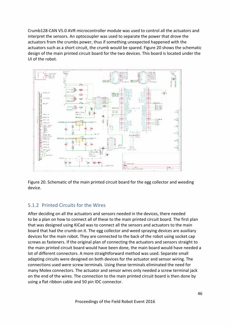
46


Crumb128‐CAN V5.0 AVR microcontroller module was used to control all the actuators and interpret the sensors. An optocoupler was used to separate the power that drove the actuators from the crumbs power, thus if something unexpected happened with the actuators such as a short circuit, the crumb would be spared. Figure 20 shows the schematic design of the main printed circuit board for the two devices. This board is located under the UI of the robot.

Figure 20. Schematic of the main printed circuit board for the egg collector and weeding device.

5.1.2 Printed Circuits for the Wires

After deciding on all the actuators and sensors needed in the devices, there needed to be a plan on how to connect all of these to the main printed circuit board. The first plan that was designed using KiCad was to connect all the sensors and actuators to the main board that had the crumb on it. The egg collector and weed spraying devices are auxiliary devices for the main robot. They are connected to the back of the robot using socket cap screws as fasteners. If the original plan of connecting the actuators and sensors straight to the main printed circuit board would have been done, the main board would have needed a lot of different connectors. A more straightforward method was used. Separate small adapting circuits were designed on both devices for the actuator and sensor wiring. The connections used were screw terminals. Using these terminals eliminated the need for many Molex connectors. The actuator and sensor wires only needed a screw terminal jack on the end of the wires. The connection to the main printed circuit board is then done by using a flat ribbon cable and 50 pin IDC connector.

47


5.1.3 The 50 Pin IDC connector

A 50 pin IDC connector is used to connect all the actuators and sensors from the small device dedicated printed circuit boards to the main egg collecting and weed spraying board located on the main robot. Table 2 describes the functions of each individual pin. Figure 21 shows the printed circuit board design of the weed spraying board with the 50 pin IDC footprint clearly visible on the top middle. A 50 IDC connector was used, because of the many different actuators and sensors and their need for more current than an individual wire on the flat ribbon cable could deliver. Some sources such as [2] were used to calculate the needed amount of wires for the actuators and sensors. Also a performance test was performed on the flat ribbon cable by short circuiting the wires and limiting the current. The current was then slowly lifted until too much heat was discovered. This performance test assured us that multiple wires of the flat ribbon cable could be used to drive the servos of the egg collector. The servos that were used in the egg collecting device were Savöx sc‐0251 High Torque Metal Gear Digital Servos and their stall current was 3200 mA [3]. The specifications of the servos can be found at [3], from where the amperage needed for the servos was checked from.

Pin number Application

1 ‐ 4 Servo number 1 power

5 ‐ 8 Servo number 2 power

9 ‐ 16 Servo ground

17 ‐ 18 Stepper motor number 1 wire 1 B

19 ‐ 20 Stepper motor number 1 wire 1 A



25 Servo signal

26 Valve ground

27 ‐ 30 Limit switches

31 5 V

32 5 V ground

33 Servo 2 signal

34 Machine ID, internal pullup resistor





43 Valve ground

45 and 47 Pump ground

44, 46 and 48 ‐ 50 12 V

Table 2: 50 pin IDC connector pins and theirapplication.

48


Figure 21. Printed circuit board design of the sprayer devices dedicated board.

5.2 Software

In order to decrease the amount of discrete circuits on the robot, it was decided to use one for both the egg‐collecting machine and the weed spraying machine. For added simplicity, both of these are interfaced through a single connector, with any possible pins reused. This means that the software running on the control board needs to effectively handle two devices, and do so safely as to not drive either one over its limits due to incorrect control signals. The communication with the robot itself is through the CAN‐bus, the activity of which is monitored by this program, with feedback given through a blinking LED. Like most of the devices, there is a dead man's switch that makes sure every hardware device stops if new commands are not received.

The logic of the control software is implemented as a state machine that make sure only the correct device is driven, and safeguards the hardware when this is not the case. The high‐level logic flow of the program is as follows.

The spray device is controlled in a trivial way; the program receives control values from Agronaut's computers and, if they match the physically connected device, writes them directly to the actuators.

The egg collector branch of the program holds the distinction of being one of the very few systems on Agronaut that has any significant logic implemented on a microcontroller. It has a set of states describing the required steps to collect an egg. During operation, it goes through these steps on the state machine and keeps the main computers appraised of the situation. If at any point a fault is detected, the hardware is driven to a safe location and kept there until the issue has been resolved.

49


Figure 22. The state machine of the egg collector and weed spraying microcontroller

In addition to the main state machine, there is a simpler, auxiliary one that acts as a driver for the egg‐collecting machine's positioning stepper motors. It receives the "reset" and "move to next position" commands from the high‐level logic, and drives the egg holder to match the desired outcome. It knows the desired positions, moves the holder independently trough them, and when required, it calibrates the position using limit switches. Whenever the egg holder is not correctly positioned, it puts up a flag telling the main logic to wait for it. This enables the egg holder to act concurrently with the rest of the program, and ensues the fastest response time that is possible with the hardware. This also allows the robot to freely move around during the procedure with the egg held securely in the lifter (acting as a buffer of like), giving full freedom of movement as the egg is "processed". To the robot's computers the egg collector is thus presented as a device that picks up an egg on command, has a flag whenever it's ready to pick a new one, and returns the number of eggs currently held. There is no need to keep track on what actions the machine needs to take, as these are all handled autonomously.

6. Seeding

In the seeding task, the robot was supposed to seed wheat. In the competition rules, the seeding method was free but the seeds should be distributed evenly and be fully covered by the soil. More specific, the seeding area was 10 m2 and the amount of the seeds was approximately 5000 seeds, which equals around 150 to 200 grams. Therefore, the resulting seed rate was 500 seeds per one square meter. The following subsections describes the selection of seeding method as well as the software and machine vision.

50


6.1. Trailer

Trailer was designed for the seeding task that was the fourth in competition. The objective was to take wheat seeds from the station and sow them in the field. Navigation and moving was done by the main robot but actions related to seeding were designed to be made by the trailer. Communication with main robot used CAN messages. Trailer had a user interface panel including various command buttons and LCD. The purpose of the user interface were debugging and observation of operation purposes.

6.1.1 Seeding method

Seeding method was chosen after calculating power and energy, which were needed for a making furrow for seeds. Our calculation showed that for small machine it would be easier to make furrow with a drilling than with a small plough. Therefore, the decision on seeding method was row drilling. However, we decided to design the trailer so that it could be later fitted with small ploughs in case the drills did not work as planned.

6.1.2 Manufacturing

Trailer was mostly made of aluminum. Transmission’s countershaft were (Figure 23, part 3.) made of iron, because trailer’s massive power was directed to countershaft first. Manufacturing started in February, when the first parts to trailer’s chassis were made. Drawings were exported from 3D modeled parts. However, parts of chassis were cut a little too long with a hacksaw and after that parts were manufactured accurately with a precise milling machine. Parts to drill holder (Figure 25, part 1) were made at the same time with a chassis. Linear actuator was used for positioning drills.

After the chassis parts, seed distribution parts were modified from old grass seeding machine from 1980s. Seeding axle was cut and centered with a lathe and it was joined to 12 V motor. Seed separator was manufactured with 3D printer. Transmission was made mostly from ready parts, only parts of countershaft were done with a milling machine.

6.1.3 Transmission

The trailer transmission was made mostly from bike parts. Transmission parts in the chassis has been shown in Figure 23 Motor (Figure 23, part 1) was an electric winch (ATV 900). The winch was controlled with a FET and its power was 625 W. The operating voltage of the motor was 12 V and current consumption was 8‐30 A when it was in operation. Wire rope was removed from the winch and it was replaced with bike’s rear hub (Figure 23, part 2) and 11T sprocket wheel. Hub and winch axle were fitted with lathe. Power was transmitted for 12 mm countershaft (Figure 23, part 3) with a single speed bicycle chain. Between the winch and the bike’s rear hub there was a countershaft delivering the power to both tires. In the countershaft (Figure 23, part 3) there was one 17T sprocket wheel (for receiving the power from the motor) and two 13T (Figure 23, part 4) sprocket wheels (for delivering the power to the tires). Tires (Figure 23, part 5) are from child bikes and are 12 inch high. Sprocket wheels were original 16T wheels. In the back tire hub there was an overrunning clutch so the main robot can drag the trailer when robot is turning. There are horizontal dropouts in the hull for straining chains (Figure 23, part 6).

51


Gear ratio was calculated with Eq. 5. With used sprocket wheels (S1‐S4 in Figure 23) the gear‐ratio was 1.90 and resulted 0.25 m/s as a trailer’s maximum speed

Gear ratio= S2

S1×S3

S4 (5)

Figure 23. 3D model from Transmission in trailer (chains not in picture) parts: part 1: motor (ATV

900), part 2: Bike’s rear hub, part 3: Countershaft, part 4: Sprocket wheel, part 5:tyre, part 6: bit for straining chains, S1‐S4 Sprocket wheels.

6.1.4 Seed distribution

Seeds were filled to a funnel (Figure 24, part 1) from the filling station. The funnel was made from plastic. Seeds flow from the funnel to a seed separator (Figure 24, part 2). Seed separator has been printed with 3D printer and transparent plastic sheet was glued to front side of separator for proving a view to the seeds and for observing the seed flow during seeding as required in the rules of Field Robot Event 2016. Seeding separator was based on the volume of seeds which was set according to the rules of the seeding task, 300 g/15 m2. Three seeding units were placed under the seed separator (Figure 24, part 3). Seeding units originated from early 1980s when manufacturer called Juko manufactured seeding machines. Seeding units have been used for seeding grass. Seeding shaft was powered with a DGO‐3512AFA 12 V DC motor (Figure 24, part 4) made by SPG Co., Ltd. and it was controlled with FET. AMT102 encoder made by CUI Inc. was placed to the seeding shaft (Figure 24, part 5) to provide information about the rotation speed. Seeds were directed

52


into the ground through a seeding pipe directing the seeds to the drilled row, immediately behind the drills.

Figure 24. 3D model for seeding system in trailers body. (Seeding pipes not shown in figure) parts:

part 1: funnel, part 2: Seed separator, part 3: Seeding units, part 4: 12 V dc motor, part 5: Encoder.

6.1.5 Chassis

The trailer’s chassis was designed to be rather simple. It was made of 8x30 mm aluminum bar. The chassis was 500 mm wide and one‐meter‐long in total with the drawbar. Due to the new drawbar height, the clearance of the chassis was only 50 mm. The chassis had two horizontal levels, where the lower level held the tires and main motor on their places. The upper level held the electronics box, seeding distribution system and the row drills. The

53


countershaft mentioned in the transmission chapter was located in the rear of the trailer chassis, on the vertical aluminum bars connecting the upper and lower levels.

6.1.6 Row drilling

We decided to use drills for making the furrows because they need less force for moving forward than ploughs. The challenge of finding the right drills for the task was the fast spindle speed due to the driving speed that was set by the task four time limit (5 minutes for seeding). After searching of different options for powering the spindles it was noticed that multi‐use rotary tools had the spindle speed required. After preliminary testing in laboratory conditions, Proxxon Micromot 50 was chosen for the task. The preliminary tests also revealed that this method also requires a “finger” which cleans the drilled row of loose soil. The drilled soil was then dragged back into the row (to cover the seeds) by a V‐shaped leveling drag following the seeding pipe. The drills were in a rig (Figure 25) where they were individually connected to a steel axle from the top part, creating the ability for each drill to float according to the ground level. The top part of the drill had a bearing unit which created the ability for the drill to move up backwards in case of too hard soil or stones. The force required for the rotation was determined by the spring installed to the mechanism allowing the drill movement. The drill rig was moved into seeding position and transport position by a linear actuator (Linak LA‐12).

´

Figure 25. 3D model showing the drill rig halfway between working and transportation stance. Parts: Part 1 Drill holder.

54


6.2 Printed Circuit Boards in the trailer

The trailer PCBs were designed with the KiCad EDA software. The schema, layout, printing and drilling maps were all done with KiCad. Double sided PCBs were used in the process. The circuits were transferred from transparent paper onto the photoresist with ultraviolet light. Natrium hydroxide was used to remove all of the excess photoresist and etching was done with hydrochloric acid. The holes were drilled on to the PCB with a CNC drill. Holes larger than 1 mm were enlarged by hand. All components were hand soldered. The trailer had three PCBs, one being the H‐bridge of the GroundBreaker’s trailer.

Figure 26. The general schema of the electrics of the trailer

6.2.1 5 V Board

A Crumb128‐CAN module with an Atmel AT90CAN128 was used as the microcontroller of the 5 V Board of the trailer. The 5 V Board had a microcontroller which was used to control the trailer’s components. It was connected to UI’s buttons, LED lights and LCD display and it communicated with the main robot through the CAN bus. The microcontroller also read its ADC to read the position of the linear actuator. It controlled the seeding shaft’s motor and the electric winch used as motor with PWM. It also controlled the H‐bridge taken from Ground Breaker’s trailer used for the linear actuator. It read the encoder data of the seeding shaft and the electric winch. It was also connected to the 12 V Board by optocouplers and controlled the 12 V main power relay and relay of the drills. The seeding shaft’s motor and the electric winch mentioned before were connected to the 12 V Board.

55


6.2.2 12 V Board

The 12 V system was isolated from 5 V by using optocouplers. The connection to the 5 V board was made with an IDC connector. The 12 V Board had fuses for all 12 V components and the whole system. It was also connected to the 12 V main power switch. It was also connected to the main power relay and relay of the drills as mentioned in 6.2.1. FETs of the seeding shaft’s motor and the electric winch were located in the 12 V Board.

6.3 Trailer Software

We had two revisions for the seed drill’s software. In the first revision the seeding machine was capable of doing everything what is needed when the main robot gives a command to seed. In this version, the trailer did the whole transition from working position to driving position. In the second revision the seed drill didn’t have any actions or sequences in it and all actions were operated by the main robot through CAN messages.

The first version of trailer software had two main state machines (Figure 27). Case 1 was not to seed and case 2 was seeding. Case 1 was a simple state machine where everything worked with pushing buttons. Case 2 had a state machine in the state machine. When seeding machine got seeding rule it tested from the linear actuator’s potentiometer if it is ready for seeding. If not, it went to case A where the trailer prepared to seed and after that the trailer went to case B where it was seeding. In case B trailer tested if the moving speed and seeding speed were right. When seeding was ordered to stop it went in case C where the trailer moves back to transportation mode.

The trailer’s software was designed to be as simple as possible. The only actual task of it was to change the trailer’s stance between transportation and seeding. In transportation, the drills were up, motor was not running and the seeding was stopped. After the trailer received the CAN message from the main robot to seed, it activated and lowered the drills, started the motor and began seeding. The software was run in the AT90CAN128, tasks of which are widely introduced in the 5 V Board topic. The software was also used for debugging in the test phase. The AT90CAN128 was programmed in C.

As the people who wrote the original code were not available towards the end of the project, a new and much simpler program was written for the trailer's microcontroller. This version was nothing more than a hardware driver, receiving commands for actuator positions and motor speeds from the robot, and driving those devices to them. It lost any state machine functionality, as this was now provided by the robot, but gained a pair of software PID‐controllers to maintain constant sowing and drive speed, and “dead man's switch” safety functionality, where the main relay is opened and all actions ceased in case of communications problems.

56


Figure 27. One of the optional state machines of the trailer software.

6.4 Robot Software

The seeding task was not completely tested before attending the FRE 2016 and, therefore, the task failed in the competition. However, the task specific software as well as the machine vision algorithm were rewritten after the competition. The seeding task was demonstrated for an audience in June 2016.

6.4.1 State flow

The seeding task differs from the first three tasks where the robot was driving between the maize rows and, therefore, a completely new state machine was implemented for this task. The state machine was created using a flow chart of Simulink software and, thus, the state machine is called here as state flow instead. The state flow contained 13 states and are described as follows:

Wait

Drive to the filling station

Fill the seeds

Driver to the field

Prepare for the first seeding

Perform the first seeding

Finish the first seeding

Headland turn

Drive back to the field

Prepare for the second seeding

57


Perform the first seeding

Finish the second seeding

Wait for user command

In the state of waiting, the robot is either performing another task or waiting for start command to begin the seeding task. In the waiting state all the task specific controls are set to initial values. Whenever the task number is set to 4 and the user of the robot gives a star command the robot transfers to state 1 and drives to filling station. In this state the robot drives forward until the transverse blue line is aligned with the trailer and goes to the next state.

At the filling station, the robot sent a message to the filling station to dispense seeds. This message could be sent either over the Internet or using a ZigBee serial connection. The internet functionality was not demonstrated due to failure to start during the actual competition; latter runs were conducted using the ZigBee method. For more information on the Internet connection configuration, see the section on egg picking. The state flow waited for 10 seconds before proceeding the next state.

After filling the robot drove to field for seeding. Once the drills passed the transverse red line the robot started preparing the seeding. In this state, the drills started to rotate and the Linak lowered the drills to the ground. Once the robot was ready, it begun the first seeding. In the seeding state, the robot drove following the longitudinal red line meanwhile the seeds were delivered to the soil. The robot continued the seeding until the drills were again aligned with a transverse red line and the seeding was ended. The robot stopped, lifted the drills and the drills stopped rotating.

Next, the robot performed a headland turn. Because of the kinematics of the robot‐trailer‐combination, the turn required a lot of space. The turning algorithm based on the gyroscope and had three steps: first the robot turned left until a defined gyroscope value was reached. Next, the robot turned right until a specific gyroscope value was reached. This value was more than 180 degrees from the value before starting the turning. Last, the robot turned again to the left until it was aligned with the row. Once the turning was finished, the seeding follows the states explained earlier. Once the second seeding was completed the robot stopped and waited for user commands.

6.4.2 Navigation

The machine vision provided information of the distance from the longitudinal red line as well as the transverse red blue lines. Because of the trailer attached to the robot, using four‐wheel‐steering was not feasible. Thus, front‐wheel‐steering was used instead. The steering was proportional considering the difference from the desired distance from the longitudinal red line. The driving speed of the robot was low and therefore set as a constant for entire task.

In addition to navigating along the longitudinal red line, the robot followed the transverse lines. The distance estimates to the transverse lines were updated whenever the machine vision provided a non‐zero distance measurement. However, the machine vision camera was in front right corner of the robot and directed forward, the lines were out of sight when the trailer was at their level. Therefore, a tracking algorithm was required. In this task, the

58


tracking algorithm was simple and based only on the mean value of the axle module encoders. Whenever, the distance to the line was not updated by the machine vision, it was cumulated by the encoder value until the estimate was at the level of the trailer and the robot transformed to the next state.

Figure 28. The robot performing the seeding task in Finland in June after the Field Robot Event. The

robot is driving to the filling station. Here, the orange tape is used instead of the red used in the competitions.

6.4.3 Machine Vision

Since the seeding task in the official competition failed, the machine vision as well as the robot software were rewritten, tested and demonstrated in Finland. The original machine vision was computationally heavy and required almost one second loop time to complete which was more or less unusable in the tasks. Whereas the original algorithm was supposed to be unerring, the new algorithm attempted to be computationally as light as possible. Therefore, the algorithm steps were reduced to minimum:

1. perspective transform 2. red and blue color transforms 3. red thresholding 4. blue thresholding 5. horizontal and vertical mean values 6. validity verification 7. transform pixels to meters

Since the camera view was not directly towards the ground, a perspective transformation was required in order to obtain an image where a pixel corresponds a metric square. Next, two new images were created, where red and blue colors were thresholded using ECCRI color transformation explained earlier in this document. The thresholded images were now black and white Boolean images.

59


Next, the algorithm finds the mass centrums in the images. These centrum coordinates are considered as the measurement results. However, the results are validated by the number of the pixels. Too low number of the pixels relate to unreliable machine vision and, thus, the measurement is disqualified. Otherwise, the pixel coordinates are transformed into metric values and set as an output of the machine vision.

Figure 29. The machine vison algorithm for the seeding task. The first image is being perspective transformed. In the center the red color is thresholded as well as the blue color in the right image. In the right, the thin white line presents the measurement result.

Figure 30. The machine vision detects the transverse red line and the estimated result is represented as the thin white line.

60


Figure 31. This figure represents the detection of the longitudinal red line. The line is skewed but the algorithm finds the mass centrum which is represented by the thin white line.

7. Freestyle Task

7.1 Mechanics

We think that every task or work in field could automate. How eggs in field are picked? We designed a machine which enable picking eggs automatically. The egg picker machine is fastened to the main robot. The main robot recognizes eggs and drive the egg picker machine to pick eggs on the ground.

The egg machine structure is very simple. Mainly it consists of two stepper motor and two servos. Machines shovel which is built up by stiff steel rod and springs enable that egg go inside shovel when the shovel striking the earth. The shovel rotates by two servos which are place in the back of machine.

The picked egg is lifted to egg cell to its right/own place. The egg cell moves to X and Y direction by stepper motors.

The egg picker machine is designed to be light structure. Principal material is 4 mm transparent acrylic sheet and aluminum. Acrylic was used as material also because of fast machinery. It was machined by laser cutter. Aluminum was used in the structure, which should take mount of load. Almost all structure for example fastening and shovel was adjustable.

7.2 Electronics

The egg picking task was designed to demonstrate the Internet capabilities of the robot, so Agronaut includes a Wi‐Fi base station that also acts as a router to provide internet connectivity over 3G. Both computers onboard are connected to the onboard network accessible by connecting to the Wi‐Fi network or over the Internet.

61


7.3 Software

To demonstrate the networking capabilities, the egg picking task implements two features: remote telemetry and processing offloading. The collection of eggs can be managed from a web application and the detection of eggs to collect is offloaded to a central server. These features, however, were not demonstrated during the actual competition, as the offloaded algorithm was deemed not to be reliable enough.

The robot communicates with the central server using JSON serialized messages encapsulated in HTTP requests. Images for egg detection are transferred as compressed JPEG images. The robot only acts as a client and thus all requests originate at the robot. The flow of data over the protocol is therefore such that with each request, the robot sends the server an update of its current state, to which the server replies with a message containing orders for the robot to execute.

The client software running on the robot is written in C# and is a part of the overall navigation software stack. It consists of two parts: one part runs on the positioning or computer vision computer and one on the navigation computer.

7.3.1 Positioning computer software

The software on the positioning computer has access to camera feeds from the cameras attached to the unit, and therefore the software running on it is responsible for transmitting images for egg detection to the offloading server in case the freestyle task is enabled.

Image acquisition and compression is implemented using the OpenCV 2.4.3 library.

By default, a 320x240 image is transferred once per second as a JPEG image. The image transmission code does not expect any results from the server; instead, results can be queried from the server asynchronously.

7.3.2 Navigation computer software

The navigation task has complete knowledge of not only the navigation parameters, but also e.g. battery status and motor status, so it is responsible for transmitting telemetry data to the central server.

During all tasks, the program running on the navigation computer transmits data including robot position to the central server once per second, so that the management interface can show this information almost in real time.

In addition, when the freestyle task is active, the central server will reply to each telemetry submission with its current estimate of the closest egg's position relative to the robot. The egg's position is sent as a three‐dimensional vector where positive X means that the egg is right of the line going ahead from the robot, Y is zero (the egg is always assumed to be on the ground) and positive Z is distance ahead from the robot's front. Additionally, the HTTP request code on the navigation computer is used during the seeding task to send the seed dispensing station the request to dispense seeds.

62


7.3.3 Server software

The server software running on the central server consists of multiple parts. The part immediately visible to the unit is the HTTP server that accepts requests from the client software running on the unit and management clients, keeping the unit's state and relaying messages. The HTTP server is also responsible for managing the separate egg detection process. The server is written in Ruby using the Sinatra micro framework and uses the Thin HTTP server during normal execution.

The second part of the server software is the management interface. The management interface is a web application that allows viewing the state of the robot connected to the HTTP server. Importantly, it acts as the information display to the freestyle task's egg collection process. The information display shows an updating image from the robot and the position of any detected egg in the image. The management interface is a single‐page web application written in the functional reactive language Elm. It communicates with the HTTP server over a Web socket interface.

The third part of the server software is the egg detection process. The role of the egg detection process is to take photos taken by the unit, detect eggs within them and generate direction vectors and distances to the visible eggs. This allows for the unit to navigate to visible eggs but also for the server software to store information about collected eggs.

The egg detection process is written in C++ using OpenCV 3.x and works similarly to the golf ball detection process used in the weed spraying task. However, since the eggs are white, ECCRI is not used for color segmentation. Instead, the image is transformed into the HSV color space and then thresholded using the saturation and value components as the white color has a relatively high value, low saturation and any value.

8. Discussion and Conclusions

In despite of having only two optional positioning algorithms and only one possible navigation algorithm, the robot performed the first two tasks well. However, the remaining tasks failed catastrophically because of failures in software and machine vision. All the software was implemented before Field Robot Event, but nothing was tested. It was known beforehand that the performance of the machine vision was not acceptable. The team attempted quick repairs at the competition fields. Nevertheless, the hard work provided no results. Similar problems occurred with the freestyle task. Luckily, hard late time decisions to change the demonstration resulted the third prize.

In addition, the mechanics could have improvements. In case of many components, the first time machining and assembling was also the only time and the results contained some small error, which had no such significant affect to the performance. Only the egg picking machine was not completed when the journey to the competition begun. The egg‐picking machine completed at the fields the night before the freestyle task. The following subsections discusses the problems and the possible effects of them.

63


8.1 Weeding

The machine vision algorithms used in the competition were mostly rewritten the night before the weeding task. Otherwise, the software was complete but untested, however. Finally, at the day of task 3 and 4 the weeding was tested before the competition. Unluckily, the software occurred to crash whenever the task parameter of the robot was set to three and start button was pushed. The short time left was not enough to find the software bug for this critical failure. It was a hard drawback for some team members to overcome. Nevertheless, it was decided to take part in the task only driving through the field knowing it would not result any points.

The software implemented for the robot would have been able to keep track on 100 weeds in a row and the machine vision were capable of recognizing up to ten weeds simultaneously. The tracked weed would have been initialized every time the robot reaches the end of the road. Therefore, after seeing the true conditions at the competition, it was obvious that the implemented weed tracking and machine vision algorithms were quite overkill and a much simpler implementation would succeed too.

Nevertheless, all of this remains just speculations since, the weed tracking and killing was not tested or demonstrated after the competition. The team was given an opportunity to demonstrate some of the machine vision tasks after the competition and the seeding task was chosen to complete instead because it seemed more straightforward to fix. The software failure in weeding task seemed difficult to debug specially because it was written as a Matlab function in Simulink and it was generated into C‐code which was glued to C#‐code. None of the debuggers in toolchain supported debugging this kind of problem. Thus, it was impossible to estimate the required time for fixing the error.

8.2 Seeding

As well as the weeding task, the seeding task failed in the competition. In contrast to the weeding, the first time the seeding was tested first time in the actual competition. We got another opportunity to attempt the task in the competition but both of them failed. After the competition, the team decided to complete the seeding task and demonstrate it to an audience at home fields.

While debugging the software for seeding, it turned out that the machine vision output was not connected with the other software of the robot and, therefore, the robot failed in the FRE. Nevertheless, the task specific software was almost completely rewritten simpler than it initially was. Originally, the software contained Kalman filters for tracking the lines for the case the machine vision would not provide reliable output. Additionally, the state flow of the task was modified and clarified. Initially, the trailer controls were distributed between the stateflow and Matlab‐function. In the remade software the purpose of the state flow was only to be aware of the current state. In contrast, the line tracking and the trailer controls were implemented in the Matlab function completely.

Finally, the seeding task was demonstrated on a real field. Luckily, we had a change to use the actual seed filling station and, therefore, the demonstration circumstances were similar to the competition (excluding the muddy field). The demonstration was a total success and

64


our team would have fair changes for winning the seeding task with this performance. After all, completing this task required only two additional days of work for two team members.

8.3 Machining

Two different methods in machining was experimented with. The first method was that a laptop was used to study the measures and 3D models of the parts simultaneously while machining them. The dimensions and shape of the part could be visualized this way. The second method was to use a machine drawing of the milled part. In this approach, all the dimensions could be read from paper without the use of a laptop at the milling station. Figure 32Error! Reference source not found. has one of the machining drawings used during the milling. The measures in the figure, helped the positioning of the mill.

Figure 32. A machine drawing used during manufacturing.

8.4 Assembly

Assembling the axle modules was more difficult than predicted. The tolerances of the machined parts were not within a perfect limit, thus the parts did not fit properly together. Holes on opposite parts were not located at same distances and the screws tended to drive crooked into the parts. Some threads needed to be removed to fit the parts together. In addition, some of the holes were not drilled deep enough for the screws that were planned to be used. The depth for the holes was set according to the screw length and the tip of the drill was not taken into account. This prevented the threading to reach the bottom of the hole. For example, only a 12 millimeter hole was drilled for a 12 millimeter screw, thus the length of the hole threading was less than 12 millimeters and the screw did not drive in all the way.

8.5 Axle module circuit board

The design process of the PCB was iterative, things needed to be changed often when ideas were revised. The PCB was manufactured three times, the third time being the final version. Some wiring had to be changed even after the first boards were manufactured when flaws were detected. The first version of PCB had a flaw in the placement and connections of the

65


field‐effect transistor (FET). The terminals of the FET were connected in a wrong order and after double‐checking the datasheet of the FET, it was realized that the terminals of the FET were in the order of gate, drain and source. The gate and drain terminals were connected in a wrong way and the problem in this PCB was fixed by twisting the pins from these terminals to the right pads on the PCB. The second version manufactured had the DB9 connectors pins

assigned to wrong ribbon cable wires. This ribbon cable connected to the CAN hub of the robot. The correct order can be seen in Table 3.

8.6 Problems with the printed circuit boards

One problem was with the VESC which had a large RC‐filter that disturbed our PWM signal from the crumb. By removing a capacitor from the VESC’s printed circuit board, the filter was removed and a nominal signal was achieved. This was a problem that took a great effort to solve. An oscilloscope was used to analyze the signal which the RC‐servo was supposed to receive. The oscilloscope gave readings that were off. The fall time of the signal was too slow for the circuit to work properly. The problem was first thought of occurring because of the size of pull‐down resistors used in the circuit. Changing the resistors had an effect on the signal but did not remove the problem. Finally, the idea of a filter was come up with and the designer of the VESC was asked about this. He then confirmed that it might be the reason causing the problems.

During the field robot competition, a few flaws were found on the printed circuit board of the egg collecting and weed spraying device. One was that if the crumb connected on the main board would have been turned 180 degrees, connecting the programming USB to the crumb would have been less cumbersome. Now the USB connection had to be made over the NUC and by twisting the USB cable in an unnatural manner. This made the programming

Ribbon 1 DB9 1

Ribbon 2 DB9 6

Ribbon 3 DB9 2

Ribbon 4 DB9 7

Ribbon 5 DB9 3

Ribbon 6 DB9 8

Ribbon 7 DB9 4

Ribbon 8 DB9 9

Ribbon 9 DB9 5

Ribbon 10Not connected

Table 3: Ribbon cable used to connect the axle module PCB to the can hub.

66


of the circuit inconvenient and it wasted precious time. The turning of the crumb on the circuit in a 180‐degree fashion would also have made it unnecessary to mill the heatsink. The heatsink was milled so that the USB could be connected to the crumb. A major problem with the printed circuit board was the current for the servos. As already mentioned the design of the board was an iterative process and some compromises had to be made. In the final version the egg collecting servos only had three wires each on the 50 pin IDC ribbon cable. It was calculated that about 1 A could be delivered per wire thus 3 amperes were possible for both servos. This was discovered to be below the required and a Hobbyking YEP 20A HV selectable voltage output was needed for these servos. During the time in Germany the first test with this device was carried out and the problem with the current was discovered. The most efficient way to fix this problem was to connect the servos to the motor batteries using a YEP [9] which would adjust the voltage for the servos. This fixed the problem though one servo burned during the testing at the Field Robot Event, because of the heavy load on the servos.

9. References

[1] http://autsys.aalto.fi/en/attach/FieldRobot2015/FinalReport_GroundBreaker.pdf

[2] https://github.com/vedderb/bldc‐hardware/blob/master/design/BLDC_4.pdf

[3] http://www.savoxusa.com/Savox_SV0235MG_Digital_Servo_p/savsv0235mg.htm

[4]

http://www.hobbyking.com/hobbyking/store/__23363__Turnigy_TrackStar_17_5T_Sensored_Brushless_Motor_1870KV.html

[5] http://www.banebots.com/category/P60.html

[6] http://www.cui.com/product/resource/amt10.pdf

[7] https://en.wikipedia.org/wiki/Kalman_filter

[8] http://download.chip45.com/Crumb128‐CAN_V5.0‐5.1_infosheet.pdf

[9]

http://www.hobbyking.com/hobbyking/store/__40274__Hobbyking_YEP_20A_HV_2_12S_SBEC_w_Selectable_Voltage_Output.html

[10] http://autsys.aalto.fi/en/attach/FieldRobot2007/FRE2007_WheelsOfCorntune.pdf

Acknowledgments

Building our robot as well as participation in the Field Robot Event 2016 in Hassfurt, Germany was made possible by our sponsors: AGCO, Valtra, Henry Ford foundation, Koneviesti, Laserle and SICK. Additionally we would like thank Aalto University and University of Helsinki for all support, teaching efforts and availability of workshops and tools to build the robot.

67


BETEIGEUZE Sebastian Blickle, Christoph Breuner, Michael Fürst, Jannik Gehringer, Philip Kiehnle,

Christian Kinzig, Tobias Loritz, Carsten Naber, Max Lukas Ritz, Christian Roth, Anton Schirg, Joachim Schönmehl*, Robert Wilbrandt

* Paper Author

Karlsruher Institut für Technologie (KIT)

HSG Kamaro Engineering e.V. (Hochschulgruppe für autonome Roboter am Kit)

The Field Robot Event (FRE) 2016 ended just like it began: deep in the mud.

From 13th to 16th of June 2016, field robotic teams from all over Europe gathered in Haßfurt, Germany to find the best among themselves in a fierce competition.

Like before in the year 2014, the 2016 FRE, also known as the unofficial world championship for autonomous field robots, was held in conjunction with the DLG‐Feldtage, a large, open air exhibition for agricultural technology where manufacturers present their newest machinery, growers their proudest cultures and chemists their most effective cocktails.

The FRE competition opens a window to the future of technology for the visitors, who are mostly farmers from all over the world.

Figure 1: Beteigeuze in the test field

68


Weeks of heavy rain above parts of Germany left their mark on the site of the Feldtage, a field next to “Gut Mariaburghausen” close to Haßfurt. The fairgrounds, access roads and most important to us, the competition field, were soaked and covered in mud ankle‐deep, while the skies kept on pouring more and more rain.

After the initial chaos, the teams quickly adopted to the situation by adding protective covers and modified wheels to their robots.

Figure 2: Beteigeuze in the mud

Day 1: Task 1 and 2

On Tuesday, the competition started almost as planned, only delayed by yet another cloudburst.

The basic tasks 1 and 2 are already well known to audiences familiar with the FRE.

The robots must drive fully autonomous through rows of young corn plants with dimensions matching exactly those of a real corn field. Points are awarded for speed and precision and penalties are subtracted for every mistake made. Common errors are collisions with plants, erratic driving behavior or manual interventions.

After 3 minutes, a score is calculated from the total distance driven minus the accumulated penalties.

69


Task 2 further complicates the matter as the rows now are bend and there are gaps in between the plants. Again, the robots must drive along the rows as fast as possible without distraction.

Kamaro Engineering entered the competition with the autonomous robotic vehicle “Beteigeuze”. An all‐wheel drive, all wheel steering chassis with off road suspension. After years of continuous development, the mechanics and electronics of the robot have matured to a very robust machine.

Even in the very rough conditions at the FRE 2016 with almost constant rain and mud often reaching up to the middle of the wheels, the robot did not suffer from traction problems or electrical failures.

Day 2: Task 3 and 4

The tasks on the second day of the competition were new and far more demanding than the well‐known basic tasks 1 and 2.

First, the robots had to detect and treat bad weeds represented by pink golf balls hidden in the field. Our robot Beteigeuze made use of a 180° fish‐eye camera, positioned on an arm in front of the robot. To “treat” the identified weeds, we build a spraying device consisting of four individually controlled nozzles on a moving bar. When a target was detected by the camera, the bar was quickly moved from side to side to place the closest nozzle directly over the target and spray. In addition, an acoustic signal was given to the jury.

Due to the bad weather conditions prior to the event, the corn plants were much smaller than we had expected, in some cases only a few centimeters high. This lead to a misinterpretation right after the robot made the turn into the second row. The robot deemed himself at the end of the row and made another turn right into the plants.

Besides this mishap, the detection was very precise and we made it to 3rd place in this weeding task. The visitors especially appreciated that the spraying action was very well visible due to the way the apparatus was moving.

In the 4th task, the robots had to proof their seeding skills.

First, the robot had to drive towards a marked position and send a signal to the automated seed dispenser to receive an amount of seeds.

The robot then had to drive along a marked route and place the seeds evenly distributed.

Our original plan was to cut four trenches behind the robot and place the seeds inside them. For this purpose, we designed a trailer with four spinning saw blades and a mechanism to release single seeds one after another.

Again, due to the weather conditions, the rules got changed a bit and we changed out our saw blade mechanism for a much simpler mechanism.

Points were awarded for the precision of the pickup procedure as well as the covered area and the distribution of the seeds.

70


Day 3: Freestyle

The freestyle task is traditionally the closing part of the event and is not included into the overall competition. The freestyle allows each team to present a unique application of autonomous machinery in agriculture. During the past couple of years, the FRE saw a large number of amazing ideas ranging from seeding machines to automated probing laboratories and of course, the occasional flamethrower.

As the Kamaro Engineering team is among the largest participating groups, we invested a considerable amount of time to present our skills in mechanical and electrical engineering.

A common problem with any mobile electric vehicle is energy storage. Lithium batteries pack quite a punch, but the trade‐off between battery life, size and weight is still an ever present problem.

With our freestyle contribution themed “charging by witchcraft” (cbw‐technology), we proposed a solution to the problem. A charging station that the robot can autonomously locate and connect to even in challenging environments like a corn field.

Figure 3: Beteigeuze at the charging station

We therefore build a working charging station with a build‐in power supply, a radio beacon and some markings for final positioning.

71


The robot was equipped with a swiveling directional antenna and two big contact brushes in addition to its usual outfit of sensors.

With the help of the swiveling antenna, the robot first located the station roughly and started moving towards it. As soon as it reached viewing distance, the optical cameras were used to precisely connect to the two contact plates.

To proof to the audience that the station was actually functional, we hot swapped batteries while the robot was connected to the charging station.

The original idea with strong relevance for practical use combined with flawless execution earned us the 1st place in the freestyle task.

The End

We will remember the FRE 2016 for a long time.

The weather conditions were extremely demanding both to men and material. Even simple routine tasks like the transport and loading of our equipment turned into energy‐sapping operations.

Even the organizers of the DLG Feldtage, who fought a battle against the weather to keep the exhibition accessible to tens of thousands of visitors could not solve every situation with professional sovereignty anymore.

Besides the difficulties, we were pleasantly surprised that our team and our equipment mastered the event with great success even in these extraordinary conditions. Even after breaking a differential (due to operator error) and loosing four‐wheel drive in the third task.

The prizes for our weeding and freestyle performances were a very welcome motivation for the new season.

We would like to thank all the participating teams and especially the organizers around Prof. Griepentrog from the University of Hohenheim.

We are looking forward to the FRE 2017!

72


CORNSTAR Peter Berk1, Peter Bernad2, Žiga Brinšek3, Matic Cebe1, Janez Cimerman3,

Jurij Rakun1, Žan Vajngerl2

1Faculty of Agriculture and Life Sciences, University of Maribor, Slovenia

2Faculty of Natural Sciences and Mathematics, University of Maribor, Slovenia

3Faculty of Electrical Engineering, University of Ljubljana, Slovenia

1. Introduction

One of the disciplines that will benefit most with future technological breakthroughs is agriculture. The progress made in recent years in the field of computer science, electronics and mechanics will make that possible. As most big food producers rely on the use of heavy machinery, this is not the case for mid‐ and small‐sized farms. There most of the work, even for big producers in some cases, still demands manual labour that is time consuming, exhausting and expensive. The thought of introducing a small army of intelligent robots to do the job quicker and more efficient seems appealing, but challenging. For one, natural uncontrolled environment poses problems with its changing conditions. A quick look (Bulanon et al, 2001, Fend et al, 2008, Thompson et al, 1991) on the subject showed that there are some potentially good solutions where authors rely on specific conditions like night time or they simply move the work to controlled environments – in green houses. Some are simply too big or too heavy to be useful at this stage.

In this work a small automated robot is presented, capable of driving between the crop rows, to find desired objects, like weeds and insects, and apply pesticides. To make this possible a robot is equipped with an on‐board LIDAR sensor, IMU unit and digital camera that all provide it with information needed to successfully navigate and observe in the surrounding environment. But readings and measurements by itself are not enough and need to be processed. This is the job for an on‐board, embedded computer based on ARM Cortex A53 processor, driven by a Linux operating system with installed ROS meta operating system (Kohlbrecher et al, 2012). Once the readings are analysed they are used to control the robot with the help of an additional expansion circuit board, where all actuators are connected and driven.

The next few sections describe the robot in greater detail. Starting with the second section, the mechanical part of the robot is described, with all the basic parts, seeding and weed mechanism. Then, the third section explains the controller architecture, with sensors, software and task strategy. The fourth section concludes the paper.

73


2. Mechanics and Power

The robot can be divided to four parts: mechanics, actuators, embedded electronics and sensors. The mechanical part is build on an RC car platform, with 4‐wheel drive, steering on all 4 wheels and suspension on front axle. The two axles enable it to turn individually by servomotors. It has an automatic gearbox with forward and backward two‐speed trasmittion and an electric motor. The actuator part includes a pressurized reservoir, two electromagnetic valves and nozzles that enable the robot to spray. The robot is powered by two batteries, one for motor (Li‐po 7.4 V, 4Ah) and one for computer, embedded circuit and actuators (lifepo4, 12V, 12Ah). Fig. 1 depicts the render of the Cornstar robot and Fig. 2 the robot in action.

Fig. 1. Render of the Constar robot.

Fig. 2. Cornstar robot while driving between the corn rows.

74


2.1 Seeding unit

We decided to make a mechanical seeding unit. It is made on principle of single grain sow machine for accurate seed placement. The measuring part of the unit is driven by a ground wheel connected to the rest of the unit by a chain. A mechanism like this is independent of speed. Seed hopper and measuring system are fixed to the robot. Seed placement system is made (almost) like on real seed drill machine. The coulter is made in the same way like Suffolk coulter. On the end it is fitted with drag tine harrow, for covering seed with soil.

2.2 Mechanical weeding unit

Mechanical weeding unit is very simple. The robot has a 3‐point hitch that is lifted with help of electro motor. The weeding unit is made of simple frame, two tines that goes under ground, to root level. Between that two tines is a metal wire that cut the roots.

3. Controller Architecture

The robot is controlled by Robotic Operating System (ROS), with multiple nodes for different purposes: the main node handles tasks, the second processes data from LIDAR, the third IMU data and the fifth sends instructions to serial interface that is used to communicate with the circuit board that controls servos for steering, main motor, electrical valves for spraying, etc.

3.1 Computer and other Hardware

The electronic part of the robot is made up of an embedded computer (Raspberry Pi 3) and a peripheral expansion board build around a AVR ATmega 128 microcontroller. The computer is based on AVR Cortex A53 quad core processor running at 1.2 GHz, with 1 GB of DRR2 memory and can reach a performance of 2458 MIPS (711 MWIPS). It offers a vast number of ports, where USB was used for camera, IMU and laser range sensors, while the UART port is used to communicate with the circuit board.

3.2 Software and strategy

The embedded computer is controlled by Ubuntu Linux operating system. In order to control low‐level hardware the mobile robot uses a Robotic Operating System (ROS), which is a meta operating system and provides a number of libraries and tools for different robotic applications; it includes hardware drivers, device drivers, visualizers, messages passing and package management. For Cornstar robot, ROS was used to provide device drivers for Sick laser scanner and the IMU unit. In order to connect the embedded computer with the mobile base an additional node for command interpretation and communication protocol was written.

The following subsection describe the basic strategy for each of the tasks. Starting with the first two tasks in the first subsection, with the description of the third and fourth following in the subsequent subsections.

75


3.2.1 Task 1 and Task 2

For Task 1 and Task 2 we basically used the same software. Going through LIDAR scans, the robot detects the nearest point which represents the nearest corn. The robot decides how much to turn, based on distance and direction from the corn. The algorithm proved to be very good because it’s very simple, and it works good enough for guiding the robot through the corn. It also automatically ignores the gaps in the rows (where corn is missing) and detects the next nearest corn.

3.2.2 Task 3

The USB camera uses an 8‐bit sensor that in general produces monochromatic images/videos. In order to record different shades of colour, the camera uses colour filters in combination with Bayer encoding (Gonzales & Woods, 2007) to produce colour images/videos. Each colour image from the camera is then converted and processed as shown by Fig. 3.

Fig. 3. Task 3 processing steps.

The camera records a small area in front of the robot in Bayer encoded format. The data is then captured by camera driver which publishes images in RGB colour format. Images are then processed by the main node that starts by converting them to HSV (Shapiro and Stockman, 2001) space for easier segmentation.

Based on empirical thresholds the images get segmented (Gonzales and Woods, 2007), by sorting each pixel into one of two groups (0 or 1), depending on the information it carries. This way the pink balls on the images get separated from the rest of the field. In case there

76


are some areas with pink pixels, the sprayer and horn get activated. Fig. 4 shows an example of colour segmentation, by looking for pink pixels.

Fig. 4. An example of colour segmentation; original image on the right and its binary representation on the left.

The area observed by the camera is divided into three different zones: the middle, left and right zone. First check is made if the ball is in the middle zone, then in the left and finally on the right. If the ball is in the middle zone, it turns the siren on along with both sprayers. If the ball appears in the left zone, it turns the siren on, but now with only the left sprayer. The same happens for the right area, but it uses the right sprayer.

The camera operates at 10 frames per second, which gives enough images to work with and efficiently recognizes pink balls on the field.

3.2.3 Task 4

For task 4 the same USB camera was used as in task 3. The difference to task 3 was that the zones are different in task 4 (horizontal and vertical) and that the algorithm is now searching for red and blue colour. For better understanding Fig. 5 summarizes the algorithm behind task 4.

The colour segmentation for red colour is applied for three different zones; left, middle and right. If red is detected in the middle line, the robot has to hold the bearing. If it is detected in right or left zone id has to adjust the bearing accordingly (left for right and right for left zone). The lower part of the image is used for the detection of blue pixels that represent a possible blue horizontal line. In case it is detected, the robot stops and gets seeds from the seed dispenser. The lower part of the image is also used to start and stop the seeding unit in case the robot detects a red horizontal line.

77


Fig. 5. Task 4 processing steps.

The three zones for the vertical red line (left, middle, right) indicate, if the robot is parallel to the red line. The algorithm in this case sends commands to the node which is responsible for movement of the robot (the node that controls the circuit board). If the line is not in the middle, the algorithm sends a value, which tells the node, if the robot has to adjust the bearing the left or right.

In case the robot reaches the blue line for the first time, the robot stops and a command is send to the seed dispenser to get the seeds. After that the robot continues onward. If the robot reaches the first or third red horizontal line, the seeding device begins to seed. The opposite happens at the second and fourth line. When the robot reaches the second red horizontal line, the robot starts making a big U turn and after the turn it starts searching for the vertical line and continues his work.

3.3 Sensors

The sensors on the robot include an industrial camera (The imaging source DBK31BU03), IMU (Phidget Spatial Precision 3/3/3) and a laser range scanner (SICK TIM 310). The laser range sensor captures distances between a sensor and an obstacle in a 270º radius from 0.05 up to 4 m distance. The sampling frequency of the laser scanner is 15 Hz with 1º resolution. It is connected to the embedded computer via USB connection. The camera captures Bayer encoded images with resolution of 1024 × 768 pixels at 30 fps. The camera is connected to the embedded computer by using an USB connection. The last is the IMU unit

78


that provides the robot with measurements regarding the readings from the 3‐axis compass, 3‐axis gyroscope and 3‐axis accelerometer.

4. Conclusion

All in all the robot performed well enough this year, but there is still a lot of room for improvement. With this robot we successfully proved, that the software should be as simple as possible, but good enough to work fast and reliably. Although we had some problems because of the robot’s large turning radius that we tried to fix with software, the robot performed well.

One of the problems we faced was the accuracy of the robot movement where the mechanical part should be replaced with a more precise one, coupled with additional sensors that would provide a feedback for better control. Furthermore, the mechanical part of the robot should be changed so the robot could turn straight to next row.

Nevertheless, with the improved version of the Cornstar field robot, we are one more step closer to building a useful small prototype robot that could serve as a small agricultural tool for various tasks. There is still a way to go, probably with a new version of the robot for the FRE2017.

5. References

Bulanon, D.M., T. Kataoka, Y. Ota, and T. Hiroma. A Machine Vision System for the Apple Harvesting Robot, Agricultural Engineering International: the CIGR Journal of Scientific Research and Development. Manuscript PM 01 006. Vol. III, 2001.

Gonzales, R. C., Woods, R. E., Digital Image Processing, 3rd edition, Upper Saddle River: Prentice Hall PTR, 3rd edition, 2007.

Guo Feng, Cao Qixin, Nagata Masateru, Fruit Detachment and Classification Method for Strawberry Harvesting Robot, International Journal of Advanced Robotic Systems, vol. 5, no. 1, 2008.

Kohlbrecher, S., Meyer, J., Peterson, K., Graber, T., Hector SLAM for robust mapping in USAR environments, ROS RoboCup Rescue Summer School Graz, 2012.

Shapiro, L., Stockman, G., Computer Vision, Prentice‐Hall, Inc. 2001.

Thompson, J. F. , Stafford, J. V., Miller, P. C. H., Potential for automatic weed detection and selective herbicide application, Crop Protection, vol. 10, pp. 254‐259, 1991.

Sponsors

A grateful thank you goes to SICK Slovenia, d.o.o. and The Imaging Source that helped us to acquire LIDAR sensor and the digital camera.

79


DTUni‐Corn Marie Claire Capolei, Adrien Gato, Christian Hoffgaard, Henning Si Høj, Jonas S. Jørgensen,

Martin A. Mellemgaard, Sigurd Engvik Rasch, José G. P. de Sousa, Oliver Topp

Department Automation and Control, Technical University of Denmark

(DTU Elektro – 31388), Kgs.Lyngby, Denmark

The DTUni‐Corn‐Team

Martin A. Mellemgaard

s133032

Jonas S. Jørgensen

s130718

José G. P. de Sousa

s130009

Sigurd Engvik Rasch

s122468

Oliver Topp

s123036

Christian Hoffgaard

s133932

Adrien Gato

s155683

Henning Si Høj

s122992

Marie Claire Capolei

s151188

80


Structure

Introduction

The DTUni‐corn

Change of robot connection

Task Solutions

Task 1

Task 2

Task 3

Task 4

The seeding mechanism

The mechanical mechanism

The arduino controller

The seeding dispenser station

Requesting seeds

Our seed dispenser for practising

Results

Task 1

Task 2

Task 3

Task 4

Suggestions for next year

Conclusion

Appendices

Appendix A ‐ Connecting with the robot

81


Introduction

This report is handed in as a completion of participating in the Field Robot Event an agricultural competition for robots in Haßfurt in Germany, held in cooperation with the DLG Feldtage. The robot was provided to the group from DTU Automation and has been to the event several years, but needed to be developed further for this year’s tasks.

The DTUni‐corn

The robot configuration used for this year’s competition is the same as last year’s. Some physical structures have been added on or adapted to the robot as part of this year’s weeding and seeding tasks. This structures will be described later on this report.

Change of robot connection

Previously the robot would connect to a local WLAN at DTU or be ethernet connection. Since Task 4 requires an internet connection, we have changed the way to connect to the robot. Firstly we put in a wifi router into the robot. To wirelessly connect to the robot, connect to the network “DTUnicorn Wifi”. Then SSH connect to the robot with its static IP 192.168.0.210. The router supports a WWAN usb dongle that can allow the robot to connect to the internet. Another option is to set up a hotspot on an android phone, with the SSID “DTU FRE Hotspot” (remember to disconnect the ethernet connection to the router). Then the robot will automatically connect to the hotspot. More details about connections details such as passwords can be found in the appendix A.

Another important issue, is that processes started from a ssh connection, should be started in the background (check the linux terminal syntax for this) so they don’t rely on the connection to the ssh connected device that started the process (running a SMR‐script, ucamserver, teamviewer etc.). Is discussed later in this report, this can cause many unpredictable problems when the wireless connection to the robot is weak.

Task Solutions

Task 1

The solution from the previous year seemed to work as desired, which meant that we did not modify the operational aspect of the code. We were experimenting with the speed of the forward and the turning. We discovered that a forward and turning speed of 1 m/s was not suitable for ensuring a successfully run. We changed the forward and turning speed to respectively 0.8 m/s and 0.5 m/s. This reduced the chances of failure, but also reduces the amount of distance covered in 3 minutes. We came to the conclusion that less speed and more accuracy was the key to this task.

We found out that the turning operation into the adjacent row was a time consumer. Instead of turning into the adjacent row the robot would drive backwards through the next row. The hypothesis was that we could save some time, resulting in covering more distance at the competition. We tried modifying the SMR‐CL code for this implementation, but we

82


discovered that the robot was too uncertain driving backwards through the rows. We did not want to use more time trying to get this implementation to work. Considering the time management at that moment we decided to drop the idea. This could be something the next year participant could invest some time into.

Task 2

The solution from the previous year was working, but needed some adjustments. We discovered during testing, that if two one meter continuous rows in both sides were missing the robot would interpret it as a free space, resulting in a turning operation. It is stated in the rules that the missing holes could not occur two meters before the end of the rows. To solve this, the constant slowdist was used in relation with the variable drivendist. If the variable drivendist was greater than the constant slowdist the robot was allowed to make a turn, otherwise the free space was ignored. This quick implementation resulted in a more autonomous and smooth driving through the rows.

Another implementation to the SMR‐CL code for task 2 was skipping rows and finding the next predefined path. If the robot was not completely perpendicular to the rows, it had trouble finding the gaps in the rows. Therefore there was added a drive command, to ensure that the robot would not get stuck in this state.

Task 3

A solution with a simple mechanic was preferred for high manoeuvrability due to the background of the designers and the time pressure. Therefore a single servo controlling the spray nozzle was chosen. That resulted in considerations on the control of the robot, because of the relative high speed of the robot makes a challenge of a spray with high accuracy. The physical setup for this task consist of a camera in front of the robot pointing towards the ground, to extend the range of vision, which detects the ball with an algorithm introduced later. The robot stops driving when a ball is detected within the spray range, then a signal is sent to a solenoid valve which opens for the waterflow provided by a 12v water pump placed in a bottle on the top of the robot. The solenoid has a hose connected to a nozzle which can be controlled in a perpendicular angle to the driving direction by a servo. The water pump is connected directly to the robot’s 12v batteries and is permanently pumping to maintain the water pressure in the system.

83


Figure 1 shows a sketch of the robot’s spraying setup without the sirene. The orange area is the spray range. The robot has to approach the ball until the ball is within this area in order to

successfully spray.

Figure 2 shows in detail the connection of the water to the nozzle (valve)

84


An algorithm is used for filtering the colors of the image, and the position of the ball is interpreted to a set of coordinates relative to the robot. The x coordinates are used to approach the robot to the ball. The y coordinates are used to point the nozzle in the ball’s direction. When the ball is under the spray mechanism a signal is given to the valve to activate the spraying. The siren is also connected to this signal in order to make a sound when the balls are sprayed.

For the detection of the pink golf balls a Microsoft Lifecam Studio webcam was used. As in the course Advanced Autonomous Robots 31388, we used an algorithm from Mobotware which finds balls in an image.

The plugin Auball plugin from Mobotware copied and slightly altered to fit the camera’s color channels with the image channels in the plugin.

Ucamserver.ini was changed to our camera settings in order to calibrate the position, the resolution, size of the ball and U and V intervals for filtering in the two camera channels. In the ucamserver.ini the webcam is set up by the auv4lgst plugin from mobotware.

The auball algorithm searches for balls in a given image, when the command “ball” is given, and it can generate debug images for viewing. The camera used had trouble detecting balls in bright sunshine due to saturation, so guvcview software was installed on the robot, in order to lower the brightness of the image.

Test of the plugin shows the debug image which draws a circle around the detected ball and another image with the pixel values changed by the filtering which sets pixels within the allowed interval, in S and V channel, to white, and other pixels to black. Below is a picture in bright sunshine which shows the detection of the pink golf ball on the two debug images.

Besides returning debug images, the plugin gives coordinates of the detected ball’s position with respect to the robot’s position, this is used to control and aim the servo.

Figure 3 shows the debug image with the detected ball

85


Figure 4 shows the debug image with the pixel values adjusted to the filter intervals

In order to pass the coordinates of the ball to the servo, a plugin to the RHD (Robot Hardware Daemon) was created to enable communication by serial port from the motherboard onboard the robot, to a mountable Arduino Uno. The plugin FREdriver was created by copying the Cruizcore plugin and replacing the variables to fit the ones needed for the task.

This RHD plugin is needed in order to communicate with the actuators (solenoid, siren and servo), from the SMR‐CL script. The plugin consists of a “Servo” a “Sirene” and a “Height” variable that can be set from the script. When the “height” variable is set according to the height of the servo (measured from the ground), the servo’s angle can be set as a value that represents the balls’s position in robot coordinates. The servo angle value is calculated in the plugin and is a trigonometric calculation to describe the detected ball’s position.

Having the ball’s location on the 70 cm stripe and the height of the servo, an angle for the servo can be calculated using:

86


Where c is the ball location relative to the robots y‐axis and a is the servo height. The angle between a and b is the servo angle needed to aim the spray towards the detected ball.

When the calculation is done, a value is send via USB to the Arduino Uno, which is then interpreted into a rotational degree of the servo that describes a place along the 70 cm stripe on the ground where the spray should aim.

The siren and solenoid are driven by a digital signal provided by the Arduino and controlled in the SMR‐CL script, in the same manner as the servo.

Task 4

To follow the red line, a new plugin was implemented. The Followline plugin first takes an image from the imagepool. Then a line of pixels across the middle of the image was extracted. The RGB values from the pixels was used in a filter that normalizes the R value with respect to the maximum red value (Filter= (R‐G) + (R‐B)). The maximum absolute value of the filter finds the most red pixel in the picture line which must be on the red line. In figure 5 there's a graphic example of the plugin. The plugin was tested several times with different backgrounds and light conditions and the maximum value was always on the red line.

The auline follow plugin can drive along a line using the difference from the center of the picture to the found maximum R value. If the difference is 0cm the robot will go straight forward. To know how many cm one pixel was we took a picture (in the right height) of a ruler and divided the cm with the pixels. With the height of the robot it was calculated that a pixel should be divided by 16 to get it in cm.

To lower the plow and to start rotating the roller in the seeder, another RHD plugin was created. This consists of a single write variable that can either be set to 1 or 0. Like the FREdriver we use this to make a communication between the SMR‐CL script to the arduino which enables a signal to the motors.

87


Figure 5 shows from the top; the R values from the extracted pixel line, the filtered R values, the maximum filtered R value pointed out in the image.

The seeding mechanism

The mechanical mechanism

The basic idea was to use three plows to dig into the soil, apply one seed at a time and finally cover the soil. The one seed at a time method was chosen in order to gain full control of the seeding rate. The initial design was made in Solidworks before the actual building started as shown in the figure beneath. The design is not identical to the final product as better solutions has been found during the building process.

88


The hopper and roller was 3‐D printed and the rack was built from aluminium in order to achieve robustness and to keep the weight at a minimum. A Piston is used to lift and lower the rack. The Piston is controlled from a Dual MC33926 Motor Driver Carrier, which again is controlled by the arduino. The piston has built in limit‐switches, so in this design it has only two states: all the way in or all the way out. A threaded shaft is attached between the piston and the rack, so that the height of the rack can be adjusted in order to achieve the desired plowing depth. The roller is driven by a DC‐motor which is controlled from the same driver as the piston.

The hopper, which contains the seeds after the refiling process, is design in order to do not obstruct the passage and the sliding of the seeds throughout the seeding process.

Its volume is larger than 500gr of common wheat, it is also provided of expansion useful during the refiling process.

In order to prevent that the seeds get stuck between the roller and the hopper some tape have been added to the holes. The tape is a more elastic material than the ABS plastic used for the 3D printing, acting as a spring it avoids the corrosion of the 3D printed edges and guarantees a smoother seed selection.

89


The roller is composed of a cylindric body where are hollowed out 4mm depths slots.

The 3mm diameter holes along the roller shaft are used to fasten the motor shaft to the roller, for future works is suggested to shape directly the roller hole with the same mould of the motor shaft in order to limit the power dissipation. It is also recommended to design a larger amount of slots.

The main challenge in the design is to avoid the seed getting stuck between the roller and the hopper. Difference in seed sizes makes the one seed at a time solution very hard to get to work properly and this method is not advisable, especially when working with 3D‐printed materials. If the task was to be repeated we would probably settle for a solution which implements a continuous flow of seeds instead.

The arduino controller

To control the mechanism from the robot SMR‐script, a arduino board combined with a simple dual motor driver were used. The robot was through SMR‐script‐commands enabled to send two commands to the arduino board through a serial connection, “On” and “Off”. These command would start and stop the mechanism, by both lowering the plov with the piston, and start the seeding wheel.

The arduino code is setup with a timer‐interrupt that sets flags at different frequencies, enabling the program to simulate several parallel processes. One of these processes is a digital PID controller for the seeding wheel. This PID controller can be optimized, and the values are mostly based on testing. The feedback of the controller is a speed measurement based on an encoder. The encoder is also handled by the arduino board. The edge changes of the pulses from the encoder, triggers interrupts that measures the states of the encoder, calculates the RPM, and finds the direction of the rotation.

The last function implemented on the arduino board, is a stuck sensing algorithm. Due to the nature of the mechanics in the seeding mechanism, seeds are often stuck in the seeding wheel. The stuck sensing algorithm checks the measured RPM compared to the desired RPM over time, and enforces at repetitive rotational direction change of the seeding wheel rotation, until the wheel again can run smoothly.

The seeding dispenser station

Requesting seeds

The seeding dispenser for the competition required a socket to make a HTTP GET request to a server using some credentials for the team.

To be very specific, we discovered that the request should have the following data to refill.fieldrobot.com:

“GET /dispense?team=DTUC&key=6z3r1l HTTP/1.1\r\nHost: refill.fieldrobot.com\r\n\r\n”

This was implemented using sockets in C, into the SMR code, so the following SMR‐commands are usable:

90


● “connectsocket” with two parameters: Establishes a socket to a IP‐address (the first

parameter as a string) with the domain name (the second parameter as a string).

Example:

connectsocket "46.101.109.151" "refill.fieldrobot.com"

● “socketget” with one or two parameters: Sends the GET request to the socket‐

connected server. The first parameter is the path. The second parameter is optional

and is set to “noresponse” if the response of the server is to be ignored and not

waited for. Example:

Socketget "dispense?team=DTUC&key=6z3r1l" "noresponse"

● “fredispense” without any parameters. This command is hardcoded for the FRE‐

competition. It tries and connect to the FRE server up to three times and the test the

connection with a ping. Then it sends the real dispense command.

Our seed dispenser for practising

To make tests more realistic we designed our own seed dispenser, like the one the competition supplies in the competition. The dispenser was 3D‐printed, and the latch was controlled by a servo motor as shown in the following renderings. The whole on the top was scaled so a bottleneck can fit inside, making a standard plastic bottle, usable as a seed funnel.

To control the serve a small PCB‐board was designed:

91


This board allows a smartphone to control the servo motor through a USB or bluetooth connection. The smartphone can then connect to the internet, and check for dispense‐request on a server.

For this a small android app where made, that can communicate with a server we set up.

Results

Task 1

To save power, the robot was not turned on until just before the start of the competition. However, when we turned it on, the robot would not boot and a last minute problem solving had to be done, which succeeded and got the robot ready just in time.

The slippery and uneven surface made it hard for the robot's odometry to function well and determine the driven distance and the orientation. There was also another unexpected issue with the communication. Even though the robot functions autonomously, a procedural error caused the robot to try to maintain a wireless connection with the computer issuing the initial command, causing a halt in the execution of its internal scripts. This issue impeded performance and was only discovered the following day, causing problems for both Task 1 and Task 2.

In spite of the connection problems and the impaired odometry, we managed to finish 4 rows and get a 6th place.

Task 2

The robot drove autonomously through the rows without hitting any maize plants. However due to the computer communication problem, it was unable to perform the correct turn,

92


when it reached the farthest point of the track from the starting position. Despite the connection problem, we still managed to get a 5th place out of 17 competitors.

Task 3

During tests at DTU campus the robot was able to spot and spray almost all the balls on the field under sun light and also under shadow/poor light conditions. After some speed and ball approach adjustments the robot was also able to stop and spray right on top of a spotted ball while completing 3 rows of 15 meters in around 2 minutes where 10 balls were placed and spotted.

At the competition the robot was able to drive almost 2.5 rows while spotting 22 out of 25 balls in 3 minutes. Unfortunately the robot sprayed many balls outside of the permitted perimeter. This was because the robot stopped too early when a ball was spotted. This error might be caused by misalignment of the camera stand while transported to the event.

Task 4

The robot had no problems following the red ling with speed up to 0.5 m/a. To be sure in the rough terrain the speed was set to 0.2 m/a until it should start to dispense. The robot followed the red line correctly until it stopped.

The dispense request were successfully tested minutes before the task started. In case the server would not respond after a socket were successfully established, this would render the robot waiting for a lost response, failing to proceed to the following parts of the task 4. To avoid this scenario, the “noresponse” were used. Sadly the dispenser did not seem to get our dispense request, during the task, and since the response were ignored, it is impossible to know what went wrong.

As we did not not have the time to implement the functionality to stop in front of the blue line, we decided to drive from odometry alone. The Robot stopped close to the correct position next to the refill station, but was off by approximately 10 cm, so it had to be moved manually. When entering the seeding field, the robot was set to drive at a very slow speed (0.1 m/a) in order to achieve the calculated seeding rate. The result was that the robot did not drive at all because of of driving in mud and the motor drivers for the wheels were unable to work at such a low speed during the field conditions. Because we drove from odometry, the robot never lowered the seeding mechanism and the roller never started as it should. This was due to the step‐by step nature of the code. Because the robot did not drive, it could not go on all the way through our code. As a result we had to abort the task.

Suggestions for next year

Save more time for testing on the real field

‐ Improve the range of the connection with the robot or make sure the connection strength becomes inconsequential.

‐ Handle bars to carry the robot more comfortably ‐ Make a new seeding mechanism that implements a continuous flow of seeds. ‐ Make a PCB for the shield between the motor driver and the arduino. ‐ Bring wheels that are more suitable for driving in mud

93


Conclusion

Our expectations before the competition were high, especially because we found our robot to be a strong contender, compared to most of the competing robots. Due to the hard weather conditions, the soil was sticky, heavy and bumpy. This caused a major difficulties and we realized, along with many other contestants that we were not sufficiently prepared for this conditions. As the competition progressed, the vast amount of unpredicted issues had us question our position in the contest. Considering the number of technical challenges we managed to overcome during the short timespan of the competition, we are satisfied with the resulting 4th place. We are more aware of the importance of testing than ever, and are certain that the experience gained from competing at the Field Robot Event 2016 would give us a huge advantage, if we were to compete again next year.

Appendices

Appendix A ‐ Connecting with the robot

Ethernet connection

ssh [email protected]

Set client (connecting PC) to static IPv4:

IP address: 192.168.0.123

Subnet mask: 255.255.255.0

Default gateway: 192.168.0.210

WLAN connection (eduroam or WaveLAN IAU)


Find IP address (on SMR)

ifconfig

Find IP address (on Client)

nmap ‐v ‐sL ‐n 192.168.0.0/24

Portable Hotspot (Android smartphones, SMR will auto‐connect)

SSID: DTU FRE Hotspot

WPA2‐PSK: WeWillWin4Sure

ssh local@xxxxxxxxx (find IP of the robot on your hotspot/phone)

Robot Wifi (TP‐Link MR3020, SMR needs ethernet, SIM may not have PIN)

SSID: DTUnicorn Wifi

WPA2‐PSK: WeWillWin4Sure

94



TeamViewer (to the robot)

Start new ssh terminal

"startx"

Start new ssh terminal

"export DISPLAY=:0"

"teamviewer"

To terminate, use Ctrl+C

Username: 369 330 988 or local IP

Password: grenen31388

For ssh from Windows, we use Putty.

95


ERIC Joseph Allin, Josh Matthews, Ali Taylor, Tom Lindley

Harper Adams University, Newport, Shropshire, England

1. Introduction

On the 14th June 2016 agricultural engineers from across the globe congregated in Haßfurt to compete in the annual Field Robotics Event. The robotic event was run in conjunction with the DLG Feldtage event, an annual agricultural show. The robotic event consisted of four individual tasks with varying difficulty:

Task 1; navigate up a 75cm wide maize row for 15 metres, turn in a 2m wide headland and then navigate down the second row and so on.

Task 2; was similar to task 1 only a sequence of rows would be provided. For instance, down one row, left turn, miss 4 rows, down the 5th row and so on.

Task 3; was a demonstration of weed detection and spraying whereby the robots would drive up and down rows as in task 1, only this time with randomly placed pink golf balls (signifying weeds) which must be sprayed.

Task 4; was the ability to drill seed into a cleared patch of ground with appropriate metering and navigation of the robot.

The aim of the event is to demonstrate the current abilities of modern electronics and sensing equipment to fulfil complex tasks appropriate to agricultural applications. This is in light of an ever growing population and the subsequent need to bring technological efficiency & effectiveness to the agricultural sector. The event therefore highlights a potential avenue to ensure global sustainability through the utilization of modern robotic technology.

This report summarises the design, testing and progress of the Harper Adams University team (of which comprises of the four authors) with their robot, Eric. Firstly the mechanical elements are discussed; vehicle, spraying and drilling. This is followed by a detailed breakdown of the sensing equipment and software used to control and navigate the robot. It should be noted that this buggy shares no resemblance or hardware from either of the previous year's teams, except for the choice of sensor.

The team would like to take the opportunity to thank our sponsor, the Douglas Bomford Trust, for their assistance in travel and accommodation to and from the event.

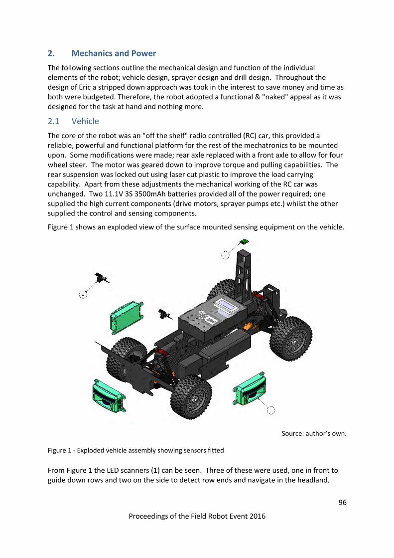
96



The following sections outline the mechanical design and function of the individual elements of the robot; vehicle design, sprayer design and drill design. Throughout the design of Eric a stripped down approach was took in the interest to save money and time as both were budgeted. Therefore, the robot adopted a functional & "naked" appeal as it was designed for the task at hand and nothing more.

2.1 Vehicle

The core of the robot was an "off the shelf" radio controlled (RC) car, this provided a reliable, powerful and functional platform for the rest of the mechatronics to be mounted upon. Some modifications were made; rear axle replaced with a front axle to allow for four wheel steer. The motor was geared down to improve torque and pulling capabilities. The rear suspension was locked out using laser cut plastic to improve the load carrying capability. Apart from these adjustments the mechanical working of the RC car was unchanged. Two 11.1V 3S 3500mAh batteries provided all of the power required; one supplied the high current components (drive motors, sprayer pumps etc.) whilst the other supplied the control and sensing components.

Figure 1 shows an exploded view of the surface mounted sensing equipment on the vehicle.

Source: author’s own.

Figure 1 ‐ Exploded vehicle assembly showing sensors fitted

From Figure 1 the LED scanners (1) can be seen. Three of these were used, one in front to guide down rows and two on the side to detect row ends and navigate in the headland.

97


Two digital imaging cameras were mounted to the front (2) which both detect weeds in task 3 and follow the red line in task 4. These were mounted on laser cut steel (1mm) and had polystyrene covers to prevent water ingress. A compass was mounted on a mast towards the rear of the vehicle (3) to indicate vehicle direction. The mast was created with laser cut plastic and lifted the compass away from interference from the primary ECU and high current electrics. The main box on top of the vehicle housed many of the electrical components. It featured a clear lid so that the screen could be read with minimal chance of water ingress throughout use. All parts added to the vehicle were designed, built and assembled at the university and were made to be easily accessible, serviceable and replaceable.

2.2 Sprayer

In the spraying task robots were required to travel up and down the rows (as in task 1) whilst detecting & spraying weeds which were represented by pink golf balls. Figure 2 shows the layout of the course.

Source: (Field Robot Event, 2016)

Figure 2 ‐ Task 3 example course layout

As can be seen in Figure , golf balls could be positioned in a number of locations within the row of maize plants.

This section describes the design and function of the sprayer unit. A number of spraying methods were considered;

� Pressurised tank – a system requiring one pneumatic pump to pressurise the tank which would then require a valve block to switch flow to individual nozzles. The pneumatic pump could have been manually operated.

� Single pump – a system requiring one pump and a valve unit to switch four individual nozzles.

� Quad pump – four pumps operating individual nozzles.

� Single pump and nozzle – whereby the nozzle moves to suit the positioning of any weed via the camera.

98


A pressurised tank or single pump with four nozzles would have both needed a complex, expensive and sizable valve system and were therefore not chosen. A single movable pump would have reduced component size and packaging, but would have increased the complexity in programming and required the development of a mobility system of which the camera and nozzle can move. The quad pump option was therefore chosen as it reduced complexity and cost. Four inexpensive pumps were specified along with four nozzles. The number of nozzles (four) was chosen after initial pilot testing whereby the nozzles were held at half the height of the buggy (an estimation made from initial sprayer design concepts) with a 45 degree angle towards the floor. Four were required to achieve an effective spray coverage with slight overlap and spanning the entire 60cm row. The nozzles themselves were also selected from a range of tested nozzles as they gave an optimum spray/mist pattern and did not spray unevenly or in jets. Figure shows the graphical work done to represent the system and ascertain nozzle coverage and height. This was done as time & cost restraints meant that multiple prototypes could not be made. The lines either side signify row width.


Figure 3 ‐ Digital prototyping to determine nozzle and camera position and angle

As seen in Figure 3, the nozzles do not quite reach the far edge of the row. This was corrected by slight angling of the outer nozzles which still allowed for a little overlap. The above view also demonstrates the highly compact design, particularly in depth to ensure significant moments were not induced on the robot due to overhanging weight. The greyed cones in Figure show the viewing areas of the cameras specified by the manufacturer. The cameras were set at just over 300mm from the ground which would provide adequate coverage and were positioned outwards from the rear of the sprayer so that the pump and nozzles would not hinder the view. However, in the final stages of development, the rear cameras were not used as testing proved that the wheel encoder was accurate enough to

99


allow the front sensor to detect the weed and accurately measure the distance to the rear of the vehicle.

The design itself is biased towards simplicity of build, small package size and weight. The downside to this system is the presence of four pumps, however, these were neatly packaged on the boom alongside the nozzles and thus, did not require a great deal of extra space. The control box was attached to the rear of the tank, which is not shown in the model. The two halves of the sprayer (top and bottom) could detach into two pieces, this is to ease assembly, fitting and removal whilst also allowing flexibility in spray height through the various hole‐compatibility. Figure shows an exploded view of the sprayer unit along with a bill of materials.


Figure 4 ‐ Exploded diagram of the sprayer unit

Figure highlights the refined design. All welded components were fitted with tabs which made manufacture extremely quick and efficient. Item 15 and 16 in the exploded view are the components of the hitch and not part of the sprayer unit (highlighted in blue).

Testing of the sprayer quickly highlighted four problems. Firstly, the water would slowly empty itself through the nozzles with the pumps switched off. This problem was solved by

100


the inclusion of pressure‐to‐open delivery valves which immediately halted leaking. The second issue was the inability of the four boom pumps to begin flow without initial priming. Therefore, the priming pump (found on the bottle) was utilised at the beginning of the spray sequence to prime the entire system with fluid before commencing. This worked extremely effectively and not once did the system stall due to air‐locks. The third issue was found that slightly weaker delivery valves could be opened by the suction of another pump; i.e. when operating nozzle one, the delivery valve would allow some amount of air into the system and therefore causing an air‐lock. This was solved through replacement of faulty valves. The final issue was slight fouling of the wheel on the end of the booms which was quickly corrected by a spacer.

All issues were overcome and the sprayer proved to be very effective in testing with good coverage of spray across the row. Figure 33 shows the final physical sprayer after the competition.


Figure 33 ‐ Actual sprayer as used at the competition

The routing of the pipework can be seen in Figure 33 along with the necessary T pieces, right angles and delivery valves. The sprayer proved successful on the day by demonstrating a simple yet well executed solution to the task at hand.

2.3 Drill

Task 4 in the Field Robotics Event 2016 involved a seeding task; where robots had to communicate with a filling station to receive seeds, and then sow them evenly in a 10m2 area where there were visual ground markers to help the robots navigate. The team decided on a methodology that used the visual markers provided, with the right mounted camera following the central red line to guide the robot up and down the drilling area. The second, left mounted camera, was then free to look for the sequence of blue and red

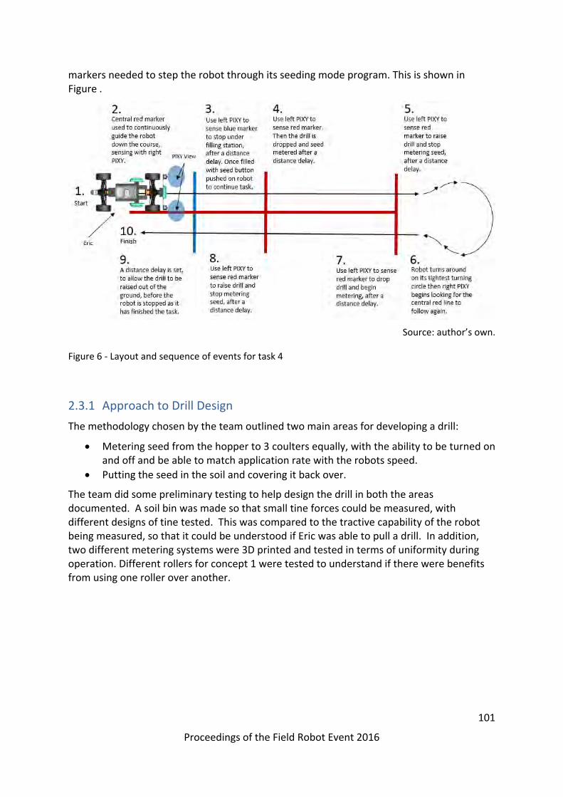
101


markers needed to step the robot through its seeding mode program. This is shown in Figure .


Figure 6 ‐ Layout and sequence of events for task 4

2.3.1 Approach to Drill Design

The methodology chosen by the team outlined two main areas for developing a drill:

Metering seed from the hopper to 3 coulters equally, with the ability to be turned on and off and be able to match application rate with the robots speed.

Putting the seed in the soil and covering it back over.

The team did some preliminary testing to help design the drill in both the areas documented. A soil bin was made so that small tine forces could be measured, with different designs of tine tested. This was compared to the tractive capability of the robot being measured, so that it could be understood if Eric was able to pull a drill. In addition, two different metering systems were 3D printed and tested in terms of uniformity during operation. Different rollers for concept 1 were tested to understand if there were benefits from using one roller over another.

102



Figure 7 ‐ Tine force and metering unit subsystem testing

The outcomes of preliminary testing influenced the final design of the drill (Figure ). The following sections describe the logic behind the design process.


Figure 8 ‐ Final digital schematics of the precision drill

103


2.3.2 Metering System Design

The main aspect of a precision drill is the metering system. Careful planning and many prototypes lead to the final design of the system. It was decided that Harper Adams's 3D printer was a perfect asset in producing a clean and aesthetically pleasing metering system. One issue found in preliminary testing was the jamming of the toothed sprocket when loaded with seeds. This could have been due to the large seeds used during testing compared to the much smaller ones supplied for the competition. However, the sponge roller soon fixed this issue with the ability to compress when put under higher loads. The schematics of the metering system can be seen in Figure 9. The included table highlights each part of the metering system, and the justification for the design.


Figure 9 ‐ Breakdown of metering system components

104


2.3.3 Drill Chassis and Soil Engagement Design

Nash and Selles (1995) suggested that it is important for a seed drill to have: means of cutting through the soil to drop seed in, means of re‐arranging soil back over the seed to facilitate water movement and compacting the soil so that adequate aeration is achieved for germination.


Figure 10 ‐ Drill with component functions detailed

Godwin (2007) outlined benefits of different tines, shown in Table 1.

Table 1 ‐ Tine angles and their effect on function


Using knowledge from Godwin (2007) and results from preliminary testing various tine types, a forward inclined tine was chosen as the final soil engaging tines as they are good at cutting soil, whilst also generating a downward force. The downward force is required in this application to pull the drill into soil, as the small weight of the implement means that it is otherwise difficult to penetrate the tines into a soil. Copper pipe was used to manufacture the tines as it simplified the overall complexity of the drill and tine design; especially in regards to tine mounting and pipe routing. Soil bin test results showed that using copper pipe tines created a draught force that Eric was able to pull in test soil from the soil hall at Harper Adams University. Actual competition soil properties were not outlined in

105


the task description so the team were unsure if Eric would actually be able to pull the drill in competition conditions.

The tines designed to fill the slot/cover seed were designed to have a vertical rake angle, as Godwin (2007) showed that this angle re‐arranges soil well. These tines are designed to run at ground level, and have lots of adjustability in type and angle to try and optimise performance in the competition soil conditions. Godwin (2007) showed that a rearward inclined tine is useful to compact soil. Rollers are a rearward inclined tine and in this setup also act as height wheels for the drill, setting the deepest position of the tines. The way the tines were mounted to the drill base plate allowed the depth setting to be adjusted, this is shown in Figure 11.


Figure 11 ‐ Justification for tine design (Drill)

The drill was designed to run in two positions: transportation position or drilling positon with a linear actuator providing the movement between the two. Transportation position was the position of the drill when being transported where tines are out of the soil so they don’t damage or get caught on task visual markers. The extended hopper has been designed to be flat in this position to benefit catching seed when filling. In drilling position, tines and the seed dispersing slot are under the ground and the metering unit has been designed to be level so that seed does not favour a coulter.

106



Figure 12 ‐ Working and transportation positions for the drill unit

2.3.4 Drill Alterations for Competition

Due to the heavy rain and appalling weather conditions during the competition, the ground preparation for the seeding task could not be carried out. Therefore, what should have been harrowed and rolled with a light garden roller ended up being large clods with much of the course underwater. The decision was made that a layer of wood chip was to be spread over the entire competition plot, and instead of the seed having to be incorporated into the soil it had to be placed on top.

This meant the drill soil engaging tines and roller packer were no longer necessary and so they were removed from the drill assembly. Instead, new hoses to the coulter mountings were cut, which allowed the seed to fall and sit on top of the woodchip. The metering system had to remain level to ensure a uniform distribution to each coulter, therefore this was the main reason for discarding the copper coulters.

In addition the wet mud stuck to the compaction rollers. The seed placed on the ground would stick to the rollers as they passed over and would make the distribution of seed uneven. In order to reduce the risk of any mud stuck to the wheels (whilst practicing at the event or whilst the robot is in parc fermé) changing the distribution of dispersed seed the drill was modified so the three compacting rollers became two transportation wheels between the three seed outlets.

The modified drill used in the competition is shown in Figure 13.

107



Figure 13‐ Drill as demonstrated in the competition


3.1 Sensors

The sensors used may be placed into three categories based on their purpose: detecting physical objects; detecting colour or navigating the vehicle. These were linked into a distributed control system which communicated via an Inter‐Integrated Circuit (i2c) bus. Finally, vehicle monitoring and control was achieved by a wireless serial link to a laptop displaying a custom human machine interface (HMI).

3.1.1 Obstacle distance

In order to determine distance, three Pepperl+Fuchs R2100 multi‐ray LED scanners were used. Mounted as shown in Figure 1, they each interfaced with an Arduino Micro via a RS232‐TTL transceiver. The R2100 was selected due to its low current consumption; durability (no moving parts as found in a traditional laser scanner); precision and capability to operate in an external environment. This sensor had also been utilised by previous teams – hence its application was proven. The detection envelope can be seen in 14 with the system representation in 15.

108


Source: adapted from (Pepperl+Fuchs, 2015)

Figure 14 ‐ Pepperl+Fuchs R2100 Field of View


Figure 15 ‐ Distance sensor system representation

The control hardware for each LED scanner was mounted onto a custom designed PCB, an example of which is shown later. This was designed such that most components were socketed, allowing for quick replacement in the case of a malfunction. Each PCB was kept separate, allowing the system as a whole to be replicated or replaced.

3.1.2 Colour

To complete tasks 3 and 4 a sensor capable of detecting colour was required. As the controllers selected did not have the power to process live video, a sensor which completed this was required. Two Pixy CMUcam5s were utilised, mounted on the front of the vehicle. They were selected for their low cost; small packaging size and ease of communication. 16 shows the sensor itself and an example detection of a coloured target.

109


Source: adapted from Charmed Labs (2011) and author’s own.

Figure 16 ‐ Pixy CMUcam5 and example detection image

As seen in Figure 1, they were mounted to the front of the vehicle, facing forward at 45°. This allowed two to cover the entire width of the vehicle and were suitably mounted for both tasks. Communication was over SPI, to the controllers mounted on each side of the vehicle.


Figure 17 ‐ Vision sensor system representation

Serial, i2c and analogue communication was also available, yet SPI offered the fastest communication rate and easiest integration.

3.1.3 Vehicle navigation

The final category of sensors used were those which provided navigational feedback and included a compass and a rotary encoder. The compass, a tilt compensated CMPS11, was mounted high on the vehicle. This ensured interference from the high current electrical systems was minimised. It was chosen for its ability to communicate over i2c and the integrated tilt compensation, of which the tilt angle could also be read. It communicated directly with the system controller through the bus.

110


Source: adapted from Robot Electronics (not dated).

Figure 18 ‐ CMPS11 and system representation

As both the Pixy CMUcam5 and the CMPS11 were vulnerable to the environment, splash‐proof covers were employed to provide a level of protection. The final sensor was an Alps 16 pulse incremental rotary encoder. The encoder’s through‐hole design allowed fitment to the driveline and also provided 16 pulses per revolution with direction. Due to the gear ratios of the differential, this provided approximately one pulse per 10mm of vehicle travel. It was fitted onto a 3D printed custom mounting flange which clamped around the driveshaft, which is shown in figure 19.


Figure 19 ‐ Rotary encoder mounting flange and mounting position

This encoder was chosen for its physical dimensions, mounting method and cost. Although it is not very durable, the mounting was designed such that it and its mounting PCB could be replaced easily. Its lack of durability was also offset by the cost. The digital signals from this were interpreted by the chassis node, as shown in figure 20.


Figure 20 ‐ Rotary encoder system representation

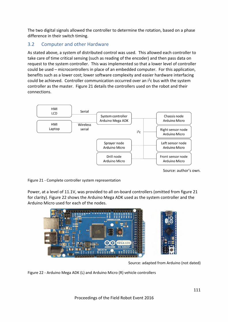
111


The two digital signals allowed the controller to determine the rotation, based on a phase difference in their switch timing.


As stated above, a system of distributed control was used. This allowed each controller to take care of time critical sensing (such as reading of the encoder) and then pass data on request to the system controller. This was implemented so that a lower level of controller could be used – microcontrollers in place of an embedded computer. For this application, benefits such as a lower cost; lower software complexity and easier hardware interfacing could be achieved. Controller communication occurred over an i2c bus with the system controller as the master. Figure 21 details the controllers used on the robot and their connections.


Figure 21 ‐ Complete controller system representation

Power, at a level of 11.1V, was provided to all on‐board controllers (omitted from figure 21 for clarity). Figure 22 shows the Arduino Mega ADK used as the system controller and the Arduino Micro used for each of the nodes.

Source: adapted from Arduino (not dated)

Figure 22 ‐ Arduino Mega ADK (L) and Arduino Micro (R) vehicle controllers

112


The Mega ADK was selected based on its processing power, program memory size and number of serial ports (4). As it would be storing the program for all four tasks, a large memory was required. The serial ports, as seen in figure 21, were required in order to communicate with the HMI elements. Processing power was not as critical as first imagined as many time critical functions had been moved. Instead, it was important for the Micro. As the code was smaller the memory size required was not as great, and physical size took greater importance. Cost for both of these types of controllers was also one, if not two, orders of magnitude less in comparison to an embedded computer.

3.2.1 Base Station

A major new requirement for this year was the ability to control start/stop from outside the test area. In order to do this, a wireless serial link was created between the robot and a laptop using a set of XBee Pro 10mW 2.4GHz RF modules. Matched with a 200mm aerial, these modules were chosen as they are capable of transmitting over a distance of 1.6km outdoors. Although over‐specified for the current application, these will hopefully provide a resilient link for future applications.

Through a USB‐serial convertor board, data could then be exchanged with the robot. A Dell Latitude XT2 tablet/ laptop ran the HMI, allowing inputs via mouse, touch or an Xbox 360 handheld controller.

3.3 Software and Strategy

In the same way that the controllers can be split, so too can the software and strategy used for the nodes and the main controller.

3.3.1 Nodes

Although the nodes completed differing tasks, the overall strategy was the same for each (figure 23).


Figure 23 ‐ Node control strategy

By completing all interfacing with the sensors and actuators and only providing the system controller with the required data, processing power and program space required was minimised. Tasks such as pulse width modulation (PWM) control of the servos and detection of the rotary encoder pulses could be maintained with a greater timing accuracy. As an example, the chassis node received four bytes of data (desired speed; desired steer angle; steer mode and speed mode) and returned three bytes (distance (two bytes) and velocity). From this, the steering servos and speed controller were set and data was returned.

113


3.3.2 Main controller

The main controller completed various functions using data from the other nodes. These functions either ran continuously or when the mode was selected and the robot was in go.

These programs, detailed below, completed communication, HMI update and diagnostics tasks along with the individual mode functions.

In addition to the explanation given in Table 2, some aspects of the program require further explanation. One of these is the link to the dash. By monitoring the time elapsed since the last message was received (on both ends), each can detect when the other is lost. This may be for a variety of reasons, but most commonly power off of the robot. As this state can be detected, the dash is able to inform the operator and the robot is able to modify its behaviour. The required mode and stop/ go state were the most important pieces of data transmitted – to ensure their integrity a checksum was calculated on each end and the data was only accepted if it matched.

Another aspect of note was the diagnostics capability of the robot. As noted in Table 2, if any of the nodes were unavailable (and should be attached in the case of the drill and sprayer), then an LED was lit and the operator was informed textually. This allowed for quick diagnosis of issues and prevented inadvertently starting a task without the required hardware available.

Finally, the method in which the modes were implemented ensured that the robot could be paused and restarted, and would return to its previous task. As the individual mode programs were not run when in stop, all variables and program position was maintained until either autonomous running was resumed or the mode was changed.

114


Table 2 ‐ Program details and functionality

Program name Call frequency Function Hardware interacted with

ReadFrontNode Every loop Request data from the node. Check the node is available.

Front node

ReadChassisNode

Every loop Request data from the node. Send commands to the node. Check the node is available.

Chassis node

ReadLeftNode Every loop Request data from the node. Check the node is available.

Left node

ReadRightNode Every loop Request data from the node. Check the node is available.

Right node

ReadCompass Every loop Request data from the node. Check the node is available.

Compass

ReadDrill Every loop Send commands to the node. Check the node is available.

Drill

ReadSprayer Every loop Send commands to the node. Check the node is available.

Sprayer

SerialDisplay 10Hz Send data to the dash. Parse data from the dash when available.

Dash

LCDDisplay Every loop Display data on the LCD, modified depending on current mode and error state of node communications

Vehicle mounted LCD

115


LidHardware Every loop Read switches to perform various functions. Set LED states dependent on error state of node communications and Go.

Vehicle mounted PTM switches and LEDs

Mode_RC Every loop when Mode = 3 and Go

Take RCSpeed and RCSteer from the dash and pass to Speed and Steer commands

‐

Mode_4 Every loop when Mode = 4 or 6 and Go

Use an array to determine required state. Call DownRow for row following or HeadlandTurn for a headland turn. Use RowEndDetection to detect row ends.

‐

Mode_5 Every loop when Mode = 5 and Go

Use a case statement to step through the sequence. Call FollowLine for line following.

‐

Mode_6 Every loop when Mode = 6 and Go

Call SprayerControl when the spray function is required ‐

DownRow Every loop of Mode_4 when the M4sequence array [x][2] = 0

Use the left and right distances to the rows (if within limits) to determine the value of Steer. Use the front distance to stop in the case of an obstacle.

‐

HeadlandTurn Every loop of Mode_4 when the M4sequence array [x][2] = 1

Perform a three point turn in the requested direction (from M4sequence array) using feedback from the compass and distance travelled.

‐

RowEndDetection

Every loop of Mode_4 when in the row

Looks at the distances to both rows, if both have not been seen for a set distance then return true.

116


FollowLine Every loop of Mode_5 when required

Uses the line position from the right camera to set the Steer command.

‐

SprayerControl Every loop of Mode_6 when required

When a weed is detected fill a line in an array with its position and sensed distance, and sound the sounder. When the set distance has elapsed since detection start spraying, after another set distance stop.

‐

CompassSteer Every loop when required

Set the Steer command based on the difference between the desired heading and actual.

‐


117


3.3.3 HMI (Dash)

As mentioned, the final part of the autonomous system was the user interface. Programmed in Processing 3, it received the serial data from the robot and displayed it for the user. Input via touch; mouse or an Xbox 360 controller was sanitised and then data was also sent to the robot, including stop/ start and mode commands.


Figure 24 ‐ HMI (Dash) as seen whilst unconnected

The box in the lower right corner provided an alternative to the Xbox 360 controller for RC navigation, by touching and dragging the small grey square, the speed and steer angle could be controlled. The mode and start/ stop was controlled and indicated by the buttons in the lower left corner, whilst error messages were displayed in the upper right. The centre displays various data from the robot, including various sensor values. Finally, information such as that from the cameras (on the right) was only displayed when in the correct mode.

4. Recommendations

Following the robot performance within testing and the competition, various shortcomings were identified. Although they did not prevent vehicle operation, implementation of solutions should ensure a higher level of performance.

For the vehicle itself, one of the major shortcomings was the turning circle. Eric was one of only two robots which required a multipoint turn on the row ends, however the longer chassis did provide stability and load capacity unmatched by the other chassis’ available to the team. A reduction in turning circle, to an outside measurement of

118


1.5m, would allow for single row end turns. Other issues with the vehicle were a lack of ingress protection beyond splash‐proof; a lack of closed loop speed control; no ground speed sensing; and a slight lack of power in some conditions. By ensuring all components were rated to IP67 and driveline modifications were introduced two of these could be solved relatively quickly. Closed loop speed control, using the rotary encoder fitted, is only a matter of programming and testing to implement (a task which the team did not have time to complete). This would identify a stall condition and be able to apply power as required. Ground speed sensing, in order to identify conditions of slip, was not as important, however in differing soil types it could quite quickly become an issue. One method of providing this feedback is an un‐driven ground wheel and encoder; or the fitment of a ground speed radar.

For this application, the control system worked adequately. However, greater programming power may allow for greater amounts of data to be processed, such as a rotating laser or further vision processing. Other improvements would be the addition of wireless programming, which would also allow ingress ratings to be maintained during testing. A degree of lag in the remote control system was also identified. This may be removed by prioritisation of the required signals or a dedicated transmitter/ receiver pair fitted.

For the drill unit, a few observations were made. The use of a parallel linkage or a change in the orientation of the metering unit would allow metering accuracy to be increased by keeping it level at all times. Driven wheels on the rear of the drill and greater lifting power (by addition of another actuator) would allow for greater draught forces to be produced and a quicker transition time between transport and work positions. Finally, a clevis hitch or ball joint for the connection would allow a greater degree of rotation around the direction of travel, an element found to be limited.

For the sprayer unit, only observations for possible improvements were made. Joining the two mounting plates would allow for easier mounting, along with a quicker method of attachment. Modification to the linkage would also allow for better positioning of the nozzles whilst bringing the tank further toward the centre of the vehicle, improving the centre of gravity. During the competition and testing it was also noted that the number of nozzles could be reduced to three, reducing complexity and cost whilst still covering the required width to the required accuracy. Cost could also be removed by changing the specification of pump which would allow for the removal of the priming pump. Finally, the package size may also be improved by fitting the boom to the underneath of the vehicle, bringing it closer to the sensing unit and protecting it from collision whilst turning.

5. Conclusion

This report has explained the robots functions with justifications for hardware, software, systems and methodologies, sensors selected and the mechanics of the robot. The team placed 2nd overall at the competition, with a 4th in task 1, 7th in task 2, 2nd in task 3 and 1st in task 4. The team hope that the future recommendations given will help any future teams to enter the Field Robot Event and compete for first place overall.

119


6. Sponsorship

The team would like to thank the Douglas Bomford Trust for their financial support with travel and accommodation for the Field Robot Event 2016.

7. References

Arduino. not dated. Arduino. [Online]. Available at: https://www.arduino.cc/ [Accessed 20th June 2016].

Charmed Labs. 2011. CMUcam5 Pixy. [Online]. Available at: http://www.cmucam.org/ [Accessed 20th June 2016].

Field Robot Event. 2016. Program Booklet. [Online]. Available at: http://www.fieldrobot.com/event/wp‐content/uploads/2016/06/Booklet_2016_complete_v5‐with‐cover.pdf [Accessed 21st June 2016].

Godwin, R. J. 2007. A review of the effect of implement geometry on soil failure and implement forces. Soil and Tillage Research, 97(2), pp. 331‐340.

Nash, H. M. and Selles, F. 1995. Seedling emergence as influenced by aggregate size, bulk density, and penetration resistance of the seedbed. Soil and Tillage Research, 34(1), pp. 61‐76.

Pepperl+Fuchs. 2015. R2100 LED Diffuse Scanner. [Online]. Available at: http://www.pepperl‐fuchs.us/usa/en/25229.htm [Accessed 20th June 2016].

Robot Electronics. not dated. CMPS11 ‐ Tilt Compensated Compass Module. [Online].

Available at: https://www.robot‐electronics.co.uk/htm/cmps11doc.htm [Accessed

20th June 2016].

120


HELIOS

Rekindling the flame that once was

Matthias Kemmerling*, Christopher Sontag*, Mohammed Alzoubi, Andrii Kostrysia, Christian Schaub*, Christopher Prange, Henrik Wulferding*, Sven von Höverling*, Tom

Schröder*, Luke Schneider*, Patrick Freitag, Michaela Pußack

* Paper Author

Institution: Technical University of Braunschweig,

Institute of Mobile Machines and Commercial Vehicles, Germany

1. Introduction

The Field Robot Event Design Team (FREDT) was founded in 2005 at the Institute of Mobile Machines and Commercial Vehicles – TU Braunschweig and participated in the Field Robot Event since 2006. Our Team members are from the areas of mechanical engineering, electronic engineering and computer science. We develop and build autonomously driving vehicles.

Helios is a self‐designed field robot and was put to use in the event since 2007. The four wheel drive and steering allow a small turning diameter of only 75 cm even on bad ground conditions. Our Robot is constantly evolving and is easily adaptable to new tasks due to its sturdiness and modular capability of the aluminum profiles. Especially for this year we built two Modules for seeding and weeding. Furthermore our software finally reached the point we worked for two years after we started a complete restructuring.

1: Helios at FRE 2016

121



The durable Helios drivetrain utilizes a permanent four‐wheel‐drive and consists of an electric motor (Dunkermotoren BG75X25CI, 250W), a set of gears and axle differentials and four wheels with equal size. The gears and differentials are separated from the rough and dusty environment through aluminum housings and the damped axle construction can easily adapt itself to very uneven ground. Therefore, the robot is ideal for use under often unpredictable field conditions. The vehicle uses an Ackermann steering concept at both axles which combines a small turning radius and smooth movement at the field headland with large vehicle stability when driving straight between the crop rows.

2: Front‐axle of Helios

For the 2016 Field Robot Event we built two Modules:

Weeding‐/ liquid‐fertilizer‐Module uses a linear bearing to enable a linear movement at a right angle to the driving direction above the plants. On this bearing are a camera and a solenoid valve with nozzle head. Additionally two tanks (each about 1.2litre) for liquid are installed between the wheels.

An electric pump transports the liquid permanently trough a choke back from one of the two tanks filled with liquid underneath Helios. This constant transport allows a quick response if the solenoid valve opens the pipe to the nozzle head.

122


3: Principle of the weeding module

Seeding Module is our first module where we used additive manufacturing technology for the upper (blue) parts.

The plough and roll alternate between a working (down) and a driving (up) position, powered by a servo.

The wheat is dispensed by a servo‐driven feed tray into three seed furrows. At the headland the servo has to stop rotating until Helios has completed the turn‐sequence.

4: Seeding Module

123


The battery we used was nickel metal hydride battery with 24 volts and 4.5 Ah. They are encased in a metal casing for easy exchange after discharge. A self‐designed energy controller distributes the energy.



For logic operations Helios has a Barebone computer produced by Gigabyte with i7‐4770R processor, 16GB RAM, 256 GB SSD.

All modules are controlled by an Arduino Uno with a motorshield and a CAN‐connection, servos are controlled by separate self‐designed servo controllers.

3.2 Software and Strategy

We are using ROS, the Robot Operating System, an open source environment for controlling robotic platforms. Its specialty is the heavy usage of the observer design pattern which, beside other techniques, decouples the need of thread and inter‐process‐communication management for the developer and leaves more room for the important parts.

Approach task 1:

Task 1, basic navigation, was aimed at an autonomic navigation of the robots through long curved rows of corn plants. At the end of each row the robots had to turn and return in the adjacent row. Therefore we implemented a simple controller. It evaluates the data from our front laser scanner which detects the distance between Helios and the plant row and initiates the necessary steering angle to correct the driving direction. So the shorter the distance to the right the bigger is the calculated steering angle to the left and vice versa.

To navigate inside the row we used a normal front wheel steering powered by servos and for the turn at the end Helios has a four‐wheel control.

Approach task 2:

Task 2, the advanced navigation, resembles task 1. The difference is that the robots have to drive through the rows in a given order. We solved the navigation through one row similarly to task 1 with our simple controller. The navigation from the end of one row into the next given row was the difficult part. We solved this by writing a mathematical function that calculates an ideal path depending on the given order. Our robot uses this function and tries to follow the path as exact as possible using its odometry.

124


5: Path in case of driving to the right

Approach task 3:

The idea of task 3, weeding, was to detect pink golf balls in a field and to spray them with a certain precision. We built a module that allowed us to move a downward facing camera and a spray nozzle in a horizontal axis over the field. When detecting a ball ahead of us with a front facing camera, the module at the back of the robot moved to the position and sprayed the ball as soon as it was detected by the rear camera.

The image detection was implemented via OpenCV and the module moves via servos and a tooth belt. Water for the spraying was supplied by pumps connected to water tanks attached to Helios.

Approach task 4:

For Task 4 we used the seeding module described in chapter 2. We installed two cameras on Helios, one on the right site looking to the red centerline. Another one, installed on the left site was looking for the perpendicular lines. The steering was controlled so that the red centerline is always in the middle of the camera view. When the left camera detects the blue line Helios send a signal via WIFI to the refill station. After detecting the red perpendicular lines with the left camera Helios start/stop seeding.

Approach task 5:

Our task 5 idea is a fertilizer with liquid fertilization which can be used on demand. A vertical 2D laser scanner detects the height of the plants and cameras can detect the state of the plant. With this data Helios decides which plants need fertilization. This happens autonomously while the robot drives through the rows as in task 2.

3.3 Sensors

Two 2D‐laserscanners (front and rear) scan the environment and enable the main orientation. As front laser scanner we used a LMS100‐10000 and as rear laser scanner a TIM310. Both were produced by SICK.

In Task 3/4 we used two RGB cameras Prosilica GC650C made by Allied Vision for the visual location of the balls and line.

125


Also in use were one IMU Analog Devices ADIS16300 with one gyroscope and three accelerometers.

4. Conclusion

Helios has been developed by our team for almost ten years now and still has a very feasible design for mastering the challenges of the Field Robot Event. It stands out in robustness and usability, since it’s a straight‐forward, simple construction which fulfills every major functionality needed.

One of the biggest benefits is that our robot is flexible. On the one hand the construction consists of item profiles. So it allows us to add every new module and construction in the same easy way. On the other hand the robot system ROS makes the same possible to the software modules.

In contrast to last year we increased the functionality of Helios enormously so now we have a good base to develop more detailed solutions.

6: FRED Team 2016

5. References

Our website

http://www.fredt.de/

Freundes‐ und Förderkreis des Instituts für mobile Maschinen und Nutzfahrzeuge e.V

https://www.tu‐braunschweig.de/imn/foerderverein/index.html

126


PLANTS WITH BENEFITS Jesse Bax, Patrick van Broeckhuijsen, Stefan Bruekers, Jarno Meijer, Stefan Sweerts,

Joris Willers

Fontys University of Applied Sciences, Tegelseweg 255, 5912 BG Venlo, The Netherlands

1. Introduction

For the Minor AgroComplex we, 3rd year mechatronic students, are going to participate in the FieldRobot event. The FieldRobot event is an annual event that takes place in a different country every year. In this event several participants from Europe take part in a competition. Students and professionals are invited to participate in the event. The contest allows for unlimited creativity as there are almost no restrictions in design and construction.

This year the competition is held at MariaburgHausen in Hassfurt, Germany. It will be held from 14 till the 16th of June.


127


Component # Description

1 The Sick Tim laser scanner, this scanner is placed in a ring that supports weight of the scanner. The cables of the scanner are going directly in the frame of the robot. There also is a protection bracket on the top side of the laser. Keep in mind that when you disassemble the laser scanner that the ring should be the first component to unscrew.

2 The PC is placed on top of the field robot. This is because the hotspot and other signals are hindered by the aluminum frame of the robot. The PC is placed under a plastic hood for protection against moisture and water. The plastic hood is painted white for protection against UV‐radiation.

3 The on/off switch is placed on the side of the robot. With this switch are also three LEDS placed. The LEDS are for the status indication of the robot.

4 The frame of the field robot is made of 2 mm aluminum. The frame is completely made at school. The aluminum is laser cutted from a DFX file.

Inside the frame we placed six batteries of 5,2 Ah (6s) which powered the whole robot.

The drone consists of three phase motors, ESCs (electronic speed controllers), propellers, flight controller, receiver and a battery of 10 Ah (6s).

128



We used LabVIEW to program the robot. The top level dataflow diagram is found below.

Every process is run parallel to each other.


Industrial PC:

I7 5600HQ

8GB 2600Mhz RAM

6x USB3.0

1x Ethernet

19.5V, 6A (120W)


All tasks use the same program. Task one navigates through the rows and switches between next row right and next row left till it finishes all rows. Task two instead sends a string including the number of rows to skip and also if the robot has to go to the left or right row. Task three is using the same program as one but in this mode it activates the camera and software to find the ball. Task four was not made before the event and was not completed before the task started.

We used LIDAR to navigate through the field, the data has to be converted before it is usable. After this conversion multiple frames of interests are divined, all other data is ignored. Two frames are for driving in the middle of the row, one frame to the left of

129


the middle and one to the right. In both frames the distance to the middle line and the angle are measured. With this information the desired direction of the robot is calculated. A third frame is divined in the middle of the robot which is about half a row wide. This frame is used to prevent collision and slowdown if the robot has to make sharp turns. The end of the row is found when all frames are empty for multiple following measurements. The same software which is used to drive in the middle of the row is used do drive alongside the rows in the headland. A new frame is used to check the amount of readings in a small frame to the left or to the right of the robot. The robot will know if it is in front of a row and can turn to drive in this row. For task two the robot can drive past it till it finds a new row and skip the desired amount of rows.

The camera is mounted on the front of the robot, we did not produce a spraying system. A RGB camera is used to detect the ball. The colour of the ball was divined and if the robot finds something whit a colour between certain thresholds it stops and produces a signal before it continues.

The software of the drone is a combination of open source software used for the flight controller and software developed by ourselves for the Raspberry Pi. We wanted to follow the robot with vision enabled software. But unfortunately this didn't work out the way we wanted. There were some problems with the communication between the flight controller and the Raspberry Pi which we used for our vision part of the task. In the end we decided to change the task a little bit. Instead of using vision to follow the field robot on the ground we fitted a GPS module and 433 MHz radio into the field robot. With this radio connected to the field robot PC, the drone and field robot PC could communicate. We used Mission Planner to accomplish the wanted behaviour. In the end we have achieved our goal to follow the field robot with the drone using GPS.

3.3 Sensors

We used the Sick TIM 551 (LiDAR) at 15Hz to scan the environment. This scanner was connected by the Ethernet bus and uses the IP/UDP protocol.

The principle of LiDAR is based on the speed of light. With a laser a small but strong beam of light is send into the air. This beam of light will partly return to the laser which is occupied with a high‐speed sensor. The returning data is a continuous signal of light‐intensity over time. Multiple returns can be processed. This enables the possibility to look through glass and plants. Based on the time aspect of the returned signal, the distance to the object which the light returned from can be calculated. Because the speed of light is always fixed at 300.000 Km/s and does not change based on the light source speed, a formula can be derived from these properties:

∗ 2

300.000.000 ∗ 2

The calculated data can be combined with other data, for example the rotational and vertical angle of the laser.

130


4. Conclusion

It was a shame that the previous group provided us with broken hardware, dangerous connections, loose wires, no working software and no documentation. This was the biggest obstacle and frustration. In the beginning we tried to work our way through the mess. But it would take too much time and we wanted to do a real project, not cleaning up after someone else. Because of this we decided to replace almost every piece of hardware and start over with the software.

Our original goals were to participate in task 1 and task 2. The intention was to try to perform the best way we could. If we had spare time, we would look into task 3 and 4. In task 5 we wanted to let the drone fly above the robot autonomously.

Overall we think the project went very successful. The original goals we set, participating in task 1 and 2, where reached, Although the tasks were not performed perfectly. It was a shame that we had no encoders, otherwise the robot would have performed better. Because of the spare time, we looked into task 3 and 4. The robot performed well during task 3, although it could be improved. We are satisfied with the 10th place, considering how we started.

5. References

We want to thank our sponsors Fontys University of Applied Science Venlo and SICK. Fontys University sponsored all equipment we needed and SICK sponsored a new laser.

List of Literature

Atmel (2016). AVRISP MKII User Guide. Obtained through: http://www.atmel.com/Images/Atmel‐42093‐ AVR‐ISP‐mkII_UserGuide.pdf. Consulted on 2‐05‐2016

FRE (2016). Field Robot Event: Program Booklet. Obtained through: http://www.fieldrobot.com/event/. Consulted on 30‐06‐16

Sick (2016). Obtained through: https://www.sick.com/nl/nl/meet‐en‐detectieoplossingen/2d‐ laserscanner/tim5xx/tim551‐2050001/p/p343045. Consulted on 29‐06‐16

131


SOIFAKISCHTLE (Soapbox Car) Use of Plywood and Epoxi Resin for Chassis assembling

Samuel Layer‐Reiss, Lukas Locher

Schülerforschungszentrum Südwürttemberg (SFZ), Standort Überlingen, Obertorstrasse16, 88696 Überlingen, locher.l@t‐online.e

1. Introduction

1.1 Institution

The aim of the german Schülerforschungszentrum Südwürttemberg, this means Students Research Center, is to build a platform for the furtherance of pupils with deeper interests in mathematics, informatics, natural science and technique. Pupils can participate in different projects to proof and train their individual skills, with the aim to participate in different contests, as for example the fieldrobot event.

1.2 Team members

The members of the Soifakischtle‐team are a mixture of pupils from different schools in a short range region of the SFZ location Überlingen. In their leisure time SFZ‐ pupils come together on Friday afternoon to do something challenging like constructing, building and programming a field robot.

1.3 Objective of the Team

The main objective of the Soifakischtle fieldrobot team is to have fun with constructing, building and programming the robot while learning a lot of things besides the curriculum of school. The students get experiences in computer aided design and manufactoring, handling different sensors, data acquisition and evaluation, microcontroller and electronics, different communication protocols, drive control and computer vision concepts. They can bring in their own ideas when programming the robot and learn a lot of object oriented concepts and many aspects of team driven software development.


2.1 Chassis

After the SFZ Überlingen participated successfully five times with their old „Idefix‐Robot”, we, a new SFZ‐fieldrobot‐team, decided to build a completely new robot base. There were several issues we want to change in our new construction. Especially the weight of about 45 kg and the huge dimension caused some (handling) problems. That's why the main focus during the construction was put on the task to keep it light. This inevitably leads to a smaller robot with a length of about 79 cm and a width of just 45 cm (wheelbase). The hole body and „chassis“ are milled with a thin layer plywood, which is often used for aviation applications, and afterwards clued with epoxy resin. For the ground plate we glued three layers of 3 mm plates together. The thickness of the outer walls is only 2 mm. With the wooden construction we could reduce our

132


weight to under 10 kg which enables us more hours of operation with a 16Ah LiPo accumulator. Furthermore the small weight increases our off‐road performance and facilitate the navigation through the muddy corn rows due to the bad weather conditions.

For higher strength we used fiberglass pads to seal the underbody and parts of the quarter panel. In addition those fiberglass pads secured the wood to soak with water or getting scratched by stones etc.

Another feature of our construction are various 3D printed parts which were used for different tasks like the affixing of sensors etc. (all green parts in the picture, except the

133


lightgreen camera housing). On the top of the robot we developed a quick‐change surface which enables us to change the special equipment for the different tasks. In the photo the „device“ for the weeding task is mounted, which consists of two cantilevers to spatter the detected weed with herbicide, a camera (mount) for weed detection, two small tanks for the herbicide and the siren.

To close the top of the robot chassis we designed a light roof. We build this roof with fibre glass sheets with 0.5 mm thickness. These thin plates were bend over a frame consisting of two curved ribs. The roof is fixed with a hook and loop fastener an can be removed within seconds.

2.2 Drive Train

The motor we use is a MAXON‐Motor which is controlled by a Maxon EPOS‐Controller, the milled mounting for this motor is made with a 6 mm carbon panel which reduces much weight compared to a normal aluminium mounting. The mounting links the motor directly to the middle‐differential‐gearbox, which is, like the two axes, not self made. We decided to buy those hardware which is often used in standard RC‐cars, because a self made version would be heavier and much more expensive. We modified the wheel suspension for higher weights by doubling the number of springs. Moreover we use two steerable front wheel suspensions for a smaller turning radius (85/2 cm). The steering is realized with two digital Dynamixel servos directly mounted to the baseplate.

134


(1): 16 Ah LiPo Accumulator, (2): Intel NUC‐Computer with Ubuntu‐Linux, (3): small fans, (4): power distributor, (5): circuit board with several fuses, (6): LiPo safer, (7): Epos‐Motorcontroller



The main control of the robot is done with a Intel NUC PC. (i7core, 8 GB‐Ram, 128 GB SSD). All sensors and actuators are attached with USB‐ connectors. On the NUC we installed Ubuntu Linux 14.04 and ROS‐ Indigo. All sensor data and actuator data is processed within the ROS‐ framework.

3.2 Sensors and actuators

Laser Scanners

Navigation is done with a Sick Tim 3xx laserscanner in the rear and a Sick Tim 5xx laserscanner in the front. Data acquisition from the scanners is done with a slightly modified ROS‐driver. With the original driver only one scanner could be accessed simultaneously.

Compass and Gyro from a Pixhawk Flight Controller

Another SFZ‐Team in Überlingen is dealing with a drone. They have experience with a Pixhawk flight controller. From this team we knew that the controller supports ROS communication with the mavros package. In this way it was very easy to get the sensor data of the magnetic field (compass), acceleration and angular velocity sensors of this flight controller.

135


Image processing

For image processing we use a Jai Go 5000 C USB 3.0 camera with a wide‐angle‐lens with a focal length of 1.8 mm. The base configuration of the camera is done with the Common Vision Blox GeniCam Browser from Stemmer Imaging. The cam configuration could be saved on the cam. For image acquisition we wrote a ROS‐Driver. The ROS driver uses the Common Vision Blox Framework (CVB) from Stemmer Imaging to acquire images from the cam. The driver delivers these images to the ROS image processing pipeline for further image processing.

Task 3 actuators

We developed a PCB with a STM32F0 microcontroller to control the switching of the two pumps for the herbicide and the siren for task 3. With the aid of the STM32‐controller we can also generate two PWM‐ signals for the control of two servos. These servos can turn the tubes in which the herbicide can flow to bring the herbicide to the right position. For the communication with the STM32F0 controllers and the Intel NUC we use a USB2UART converter. A ROS‐Node was developed to send commands to the STM32. Any other ROS‐Node can publish topics for this node to control the weeding assembly. For the configuration of the STM32‐ microcontroller we use the CubeMX‐ software from ST‐Micro. This java based software can generate projects for further C‐programming within the Eclipse development environment (equipped with the right plugin, called “system workbench for stm32” from openstm32.org). You can download cubeMX and this plugin for free and both runs on Linux (and Windows).


For the lack of time we could not test and develop a lot of new software for navigation. Mainly we tried to transfer some concepts from former SFZ‐Teams used on former fieldrobot events to the new robot.

4. Conclusion

In our opinion the use of plywood as base material for the chassis was a good decision. Despite the fact that we used screws to fix the components the chassis is build without any screw. In retrospect we were to overcautious. Now we think 6 mm thickness of the ground plate instead of 9 mm would be enough. With the experience of our first construction of this kind, we believe that we can save one or two more kilos of wight.

On the other side we were to optimistic. With the 150 W Maxon motor the robot can reach a maximum speed of 5 m/s but we could not manage to drive the robot with this speed through the rows. As we have problems with the momentum when the ground is to muddy, it makes perhaps more sense to use a higher gear reduction for lower maximum speed and better momentum.

Furthermore we are a little bit unhappy with the RC‐ car axis. There is lot of clearance within the linkage from the steering servos to the wheel. Another drawback is, that the steering servos do not have enough momentum. We suffered a lot of software truncations with “servo overpowered” error messages.

Unfortunately our USB2RS485 adapter for the communication with the steering servos got out of order just before task 3. By this means we learned another lesson: pick up enough spare parts!

136


Sponsoring

The team was supported by

the mikromakro Project of the Baden‐ Württemberg foundation,

the CLAAS‐ Foundation and

Stemmer‐ Imaging

137


TALOS David Reiser, Tobias Schleker, Max Staiger, Daniel Riehle, Hans W. Griepentrog

University of Hohenheim, Institute of Agricultural Engineering, Garbenstr. 9, D‐70599, Stuttgart, Germany, dreiser@uni‐hohenheim.de

1. Introduction

Moving in agriculture from big machines to small, autonomous machines can have a key role in solving actual challenges in crop production like soil compaction, machine transport, security or human labor costs. Competitions like the Field Robot Event are in step with actual practice on fields. Therefore, it could provide help to speed up development of mechanics and algorithms with a practical use of the systems. Detecting rows is mostly sufficient for robot navigation in semi‐structured agricultural environments, as most of the current crops are planted in row structures. Detecting line structures is topic of many researches, performed by camera images ((Marchant and Brivot, 1995),(Jiang et al., 2010)), light detection and ranging (LIDAR) laser scanner data ((Hansen et al., 2010),(Barawid et al., 2007),(Hiremath et al., 2014)), or other types of sensors. However, uncertainty in environment still makes it challenging to detect the values in noisy sensor data, like it is typical in agricultural sites (Hiremath et al., 2014) and could be seen in the Field Robot Event.

The robot described in this article used two horizontal LIDAR sensors for navigation (see Figure 1). One at the back and one mounted at the front of the robot. They were assisted by wheel encoders and an inertial measurement unit (IMU) for headland turning. Beside of just navigation, there is always a need for robotic research to show the use and ability for future applications, what was performed in the ball detection and spraying task. The whole system was programmed using ROS (Robot Operating System) (Quigley et al., 2009).

Figure 1: Robot Talos in the raw setup with open lid and Sick laser scanner attached

138



As basic vehicle, a small 4‐wheel autonomous robot with differential steering named “Talos” was used (see Fig. 1). The size of the robot platform was 500 x 600 x 1100 mm. The weight of the robot is 40 kg and it is equipped with four motors with a total power of 200 W. Maximum driving speed is 0.8 m/s and a maximum static motor torque of 4 x 2,9 Nm. For the spraying task in the field robot event, an additional implement was attached to the robot, including a water tank and three magnetic valves. They were attached at the back of the robot. For energy supply, four 12V/12Ah batteries are providing an operating time of around 4‐5 h, depending on the load torque, task and additional weight of equipment placed on the robot platform. The whole arrangement of sensors, computers, electronics, sensors and actors is shown in the following Figure 2.

Figure 2: Description of the used actors, sensors and computers

3. Sensors

As it could be seen in Figure 2, the robot was equipped with different kind of sensors. Each motor was connected to an encoder (ME22, Bühler Motor, Nürnberg, Germany) with a 1024 ticks resolution per rotation. They were attached directly to the motor controllers, which were connected to the robot computer. For estimating the initial state of the robot, an Inertial Measurement Unit (IMU) was fixed to the frame of the robot. The used IMU was a VN‐100 (VectorNav, Dallas, USA). For sensing the environment, two light detection and ranging (LIDAR) laser scanners were mounted horizontally at the front and the back of the robot at a height of 0.2 m above the ground level. The used sensors were the TiM 571 2D‐LIDARs from Sick (SICK, Waldkirch, Germany). The pink golf balls of task 3 were detected by two additional webcams, mounted at the back of the robot, looking down at the ground. The used webcams were the LogiLink UA0072 USB‐Webcam (LogiLink, Schalksmühle, Germany) with an image resolution of 640 x 480.

139



The four motors were controlled by the embedded computer with two motor controllers (Roboteq, SDC2130). This dual channel motor controller is able to power up to 30V and 2x 20 maximum, sufficient for the used motors. They were connected to the computer via USB. For the remote control and direct user interaction a standard X‐Box Joystick Logitech F710 (Logitech, Lausanne, Switzerland) was connected to the embedded computer with a Bluetooth dongle. For activating the magnetic valves and the siren, four relays were used. They were activated with the GPIOs of a Raspberry Pi 3 computer. The IMU used a RS232 protocol for communication, while the laser scanners worked with TCP/IP over Ethernet. The data flow diagram can be seen in Figure 3.

Figure 3: Signal flow diagram showing the general setup of the used robot components


The robot‐embedded computer was, equipped with i3‐Quadcore processor with 3.3 GHz, 4 GB RAM and SSD Hard drive. It runs with Ubuntu 14.04. A separate Raspberry Pi 3 (1.2 GHz ARN Cortex, 1 GB RAM, 32 GB micro SD) running Ubuntu Mate 16.04 was connected to the same network to use the advantage of the GPIOs.


For competing at the field robot event, the most important task of the robot is the autonomous row following of the system. To set up this structure a mode changer was implemented (Blackmore et al., 2002). This included one mode for navigation inside the row, and one mode for headland turning. It was possible to overwrite the autonomous mode with a user joystick input and to separate the program code to different tasks. In general, three modes were used:

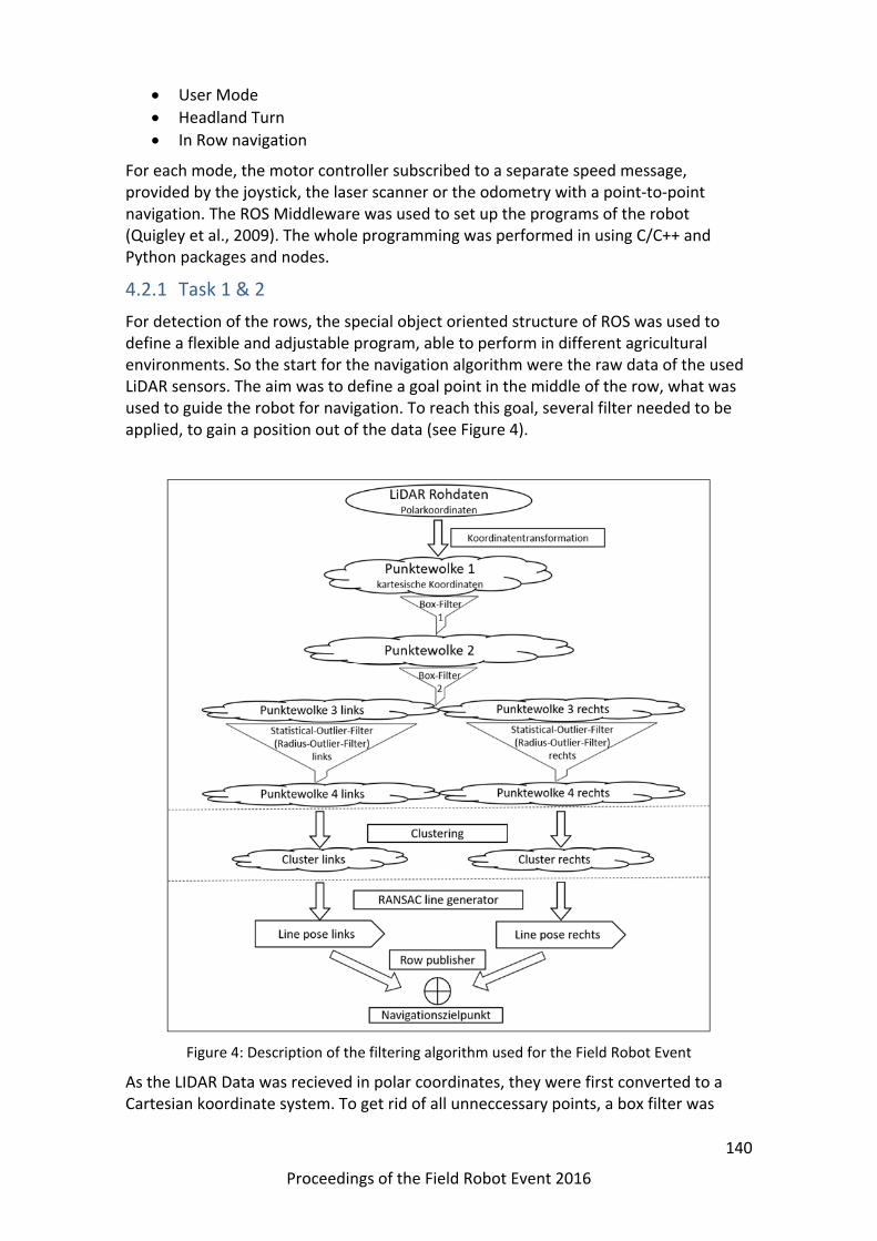
140


User Mode

Headland Turn

In Row navigation

For each mode, the motor controller subscribed to a separate speed message, provided by the joystick, the laser scanner or the odometry with a point‐to‐point navigation. The ROS Middleware was used to set up the programs of the robot (Quigley et al., 2009). The whole programming was performed in using C/C++ and Python packages and nodes.

4.2.1 Task 1 & 2

For detection of the rows, the special object oriented structure of ROS was used to define a flexible and adjustable program, able to perform in different agricultural environments. So the start for the navigation algorithm were the raw data of the used LiDAR sensors. The aim was to define a goal point in the middle of the row, what was used to guide the robot for navigation. To reach this goal, several filter needed to be applied, to gain a position out of the data (see Figure 4).

Figure 4: Description of the filtering algorithm used for the Field Robot Event

As the LIDAR Data was recieved in polar coordinates, they were first converted to a Cartesian koordinate system. To get rid of all unneccessary points, a box filter was

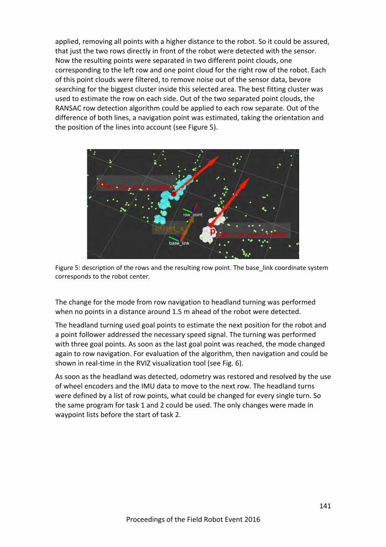
141


applied, removing all points with a higher distance to the robot. So it could be assured, that just the two rows directly in front of the robot were detected with the sensor. Now the resulting points were separated in two different point clouds, one corresponding to the left row and one point cloud for the right row of the robot. Each of this point clouds were filtered, to remove noise out of the sensor data, bevore searching for the biggest cluster inside this selected area. The best fitting cluster was used to estimate the row on each side. Out of the two separated point clouds, the RANSAC row detection algorithm could be applied to each row separate. Out of the difference of both lines, a navigation point was estimated, taking the orientation and the position of the lines into account (see Figure 5).

Figure 5: description of the rows and the resulting row point. The base_link coordinate system corresponds to the robot center.

The change for the mode from row navigation to headland turning was performed when no points in a distance around 1.5 m ahead of the robot were detected.

The headland turning used goal points to estimate the next position for the robot and a point follower addressed the necessary speed signal. The turning was performed with three goal points. As soon as the last goal point was reached, the mode changed again to row navigation. For evaluation of the algorithm, then navigation and could be shown in real‐time in the RVIZ visualization tool (see Fig. 6).

As soon as the headland was detected, odometry was restored and resolved by the use of wheel encoders and the IMU data to move to the next row. The headland turns were defined by a list of row points, what could be changed for every single turn. So the same program for task 1 and 2 could be used. The only changes were made in waypoint lists before the start of task 2.

142


Figure 6: robot model, Point clouds and resulting line directions

4.2.1 Task 3

To perform this task, the navigation algorithm from task 1 was used. Additionally the pink golf ball was detected and sprayed by a simultaneous running task. The detection of the golf balls was performed by two web‐cams, mounted at the back of the robot. They were arranged to spot the complete row, but without overlapping the pictures. For every single camera, one separated magnetic valve was used. They were mounted near the camera, so that the detection of a ball could directly be addressed to the spray valve to be activated. This helped, that the spraying system did not need any information about speed, position or other information to perform, beside a vehicle guiding it through the crop rows.

The image analysis was performed, using OpenCV. The pink golf ball was filtered with a min and max value of Hue (H), Saturation (S) and Value (V) of the color, after converting the image to the HSV‐color frame. Out of the result a binary image was generated (see Figure 6).

Figure 7: Binary image of a detected pink golf ball

143


Out of this, the best fit with a Hough circle detection algorithms was estimated. To get better results, all detected balls were checked for their radius with a minimum and maximum value to validate the result. This helped to decrease the number of false positives. As soon as the ball could be confirmed, a Boolean message was send to the relays to activate the corresponding valve.

To be more robust against sunlight, the whole aperture was shaded to minimize the influence of light changes, what could affect highly the outcome of the algorithm used for ball detection.

5 Conclusion

The proposed methods worked well under outdoor conditions and harsh field conditions at the muddy Field Robot Event 2016. The main problem for the performance of the machine were based on the size, as the Talos does not leave much space to the side of the rows. This limits the speed of the vehicle and makes it harder to perform well. The main issue in the actual software setup is the headland turning and did not performed fast enough. Anyhow, it was possible to autonomously find the next row, but the speed of the machine was not sufficient to earn a price at the event. Task 3 performed well, but was also limited by the vehicle speed and was so not able to detect all balls distributed on the field in the proposed time. Future work have to investigate in a new machine as well as changing bugs in the system, to get the overall performance more robust.

Acknowledgements: Companies SICK and MÄDLER and the University of Hohenheim sponsored the team.

6 References

Barawid,O.C.,Mizushima,A.,Ishii,K.,Noguchi,N.,2007.DevelopmentofanAutonomousNavigationSystemusingaTwo‐dimensionalLaserScannerinanOrchardApplication.Biosyst.Eng.96,139–149.doi:10.1016/j.biosystemseng.2006.10.012

Blackmore,S.,Fountas,S.,Have,H.,2002.Aproposedsystemarchitecturetoenablebehaviouralcontrolofanautonomoustractor.,in:Zhang,Q.(Ed.),AutomationTechnologyforOff‐RoadEquipment.2950NilesRoad,St.Joseph,MI49085‐9659,USA,ASAE,pp.13–23.

Griepentrog,H.W.,Blackmore,B.S.,Vougioukas,S.G.,2006.CIGRHandbookofAgriculturalEngineeringVolumeVI:InformationTechnology.AmericanSocietyofAgriculturalEngineers,Michigan.

Hansen,S.,Bayramoglu,E.,Andersen,J.C.,Ravn,O.,Andersen,N.A.,Poulsen,N.K.,2010.DerivativefreeKalmanfilteringusedfororchardnavigation,in:13thInternationalConferenceonInformationFusion.doi:10.1109/ICIF.2010.5712041

Hiremath,S.A.,vanderHeijden,G.W.A.M.,vanEvert,F.K.,Stein,A.,terBraak,C.J.F.,2014.Laserrangefindermodelforautonomousnavigationofarobotinamaizefieldusingaparticlefilter.Comput.Electron.Agric.100,41–50.doi:10.1016/j.compag.2013.10.005

Jiang,G.,Zhao,C.,Si,Y.,2010.Amachinevisionbasedcroprowsdetectionforagriculturalrobots,in:Proceedingsofthe2010InternationalConferenceon

144


WaveletAnalysisandPatternRecognition.pp.11–14.

Marchant,J.,Brivot,R.,1995.Real‐TimeTrackingofPlantRowsUsingaHoughTransform.Real‐TimeImaging1,363–371.doi:10.1006/rtim.1995.1036

Quigley,M.,Conley,K.,Gerkey,B.,Faust,J.,Foote,T.,Leibs,J.,Berger,E.,Wheeler,R.,Mg,A.,2009.ROS:anopen‐sourceRobotOperatingSystem.Icra3,5.doi:http://www.willowgarage.com/papers/ros‐open‐source‐robot‐operating‐system

145


THE GREAT CORNHOLIO

Olga Merzliakova, Ivan Zaytsev, Matthias Igelbrink, Tristan Igelbrink, Fabian Ellermann, Steffen Hellermann, Jan Roters, Aditya Kapur, Florian Wasmuth, Thomas Ludemann, Jakub Rycl, Burawich Pamornnak, Rahul Puniani, Heiko Wilms, Andreas Linz, Arno

Ruckelshausen

University of Applied Sciences Osnabrück, Engineering and Computer Sciences, Albrechtstr. 30, 49076 Osnabrück Germany

Figure 1: Field Robot, “The Great Cornholio”

1. Introduction

The following work is intended to describe the hardware and software used by students of the University of Applied Sciences Osnabrück for the 14th annual Field Robot Event. The paper begins with a general mechanical overview of the referred to entry, “The Great Cornholio”, followed by a more in‐depth description of hardware used, including specifications, and an overview of the software algorithms used to accomplish general functionality and the applicable tasks for the competition. A conclusion then follows to summarize the findings of the design process.

146


Figure 2: CAD draft of the Robot


Mechanics

''The Great Cornholio'', whose CAD draft can be seen in figure 2, has an overall size of 54x69x44cm. As it is typical for robots based on ''Volksbot'' ‐ the robot‐platform of the Fraunhofer Institute – Cornholio's case relies on item profiles, making it easy to mount sensors, motors, etc. The profiles and the cover panels are made of aluminium. As a light metal, the usage of aluminium saves weight so the robot will be able to move faster. When the top plate is removed, two claps provide fast access to the fuse‐boards and cables.

Two Maxon motors with an epicyclic gearing power the robot with a torque of 15Nm. One wheel on each side is connected to the motor shaft by a claw coupling. The other wheel is then connected to the first by a chain gear. Separating the drive sections makes it possible to control each side of the robot independent of the other as it is typical for skid drive. An advantage of skid steering is the low turn‐radius, thus optimizing manoeuvrability. This behaviour is useful in navigating through the narrow curved rows of the contest environment.

As already mentioned, the robot's case consists of item profiles. Item offers a special ball joint fitting in their profile system that we used to mount our camera. It can be slided on a horizontal line using the clamp lever to change the camera's roll‐pitch‐yaw angle. This provides great flexibility for the image processing sensor's field‐of‐view. The camera can be shifted simply by loosening the lever providing flexibility and adaptive capabilities in a changing environment (e.g. from the laboratory to field conditions) within seconds.

147


Figure 3: Inner assembly of the robot

Figure 3 shows the inner assembly of Cornholio. The robot is accessible through a PMMA lid, which is translucent. In the lid itself a PC‐fan is embedded. The fan creates a positive pressure inside the robot to keep particulate material out of it.

The inside of the robot consist of the actuating elements, controls, a sensor and the power supply system. Right below the lid on the left and right side are the fuse‐boards. Below the fan, the device server is fixed with adhesive hook‐and‐loop tape, which is connected to an aluminium plate. Just below the plate one of the motors is mounted. If there are any problems with the motor, the plate can be removed. Another plate is mounted over the second motor, which is used to fasten the IMU. The motor‐controllers are positioned right next to the motors. The battery is stationed in the middle right between the two motor‐controllers. They are held in place by aluminium brackets and plates which give a lateral bearing of the battery. This allows a fast access and replacement of the battery. The PC is placed on the left side right next to the battery. It is attached to an extra plate, which is mounted on the frame of the robot. The Ethernet‐switches are placed in the front and rear of the robot. They are mounted in an upward position, making the status LEDs observable.

Power supply

The power supply is based on two 12V lead batteries running in series to provide 24 V DC. They are directly connected to a power supply board that provides three fuse secured voltage levels ‐ 5V, 12V and 24V. The 5V and 12V voltage levels are realized by board intern step‐down converters and have a maximum current of 5A. The 24V level is able to provide 20A without conversion. Additionally, there is a buck converter connected to the 24V port of the power supply board that provides additional current to the 12V output port.

148


Fuse Board

The fuse board connects all electrical components of the robot with their corresponding operating voltages and protects them from exceeding voltage specifications as well. The fuse board supports three different voltages ‐ 5V, 12V and 24V. Every route is fused separately with easily accessible fuse holders for easy exchange.

Figure 4: PCB‐design of the fuse boards

The proper functionality of each fuse is displayed by a red LED. A working fuse bypasses the LED. The bottom side of the fuse board is moulded with epoxy resin. The advantage of this layer is the higher stability and contamination protection of the entire board. The electrical parts are connected with this board through a four‐pin connector. This allows a hard‐coded pin combination to prevent the interchange of operating voltages.

Figure 5: Fuse board



Computer:

Model: Pokini‐i

Processor: Core i7‐3517UE

RAM: 8GB DDR3 SO‐DIMM

HDD: 120GB SSD

Bluetooth integrated

Passive cooling

149


Figure 6: Pokini i PC Source: http://www.pokini.de/images/banners/pokini‐i/1_pokini‐i‐composing.png

The computer is used to control the whole robot. It is connected to all devices by Ethernet.

Motor:

Model: Maxon RE 40

Nominal voltage: 24 V

Nominal speed: 6930 rpm

Nominal torque: 170 mNm

Nominal current: 5.77 A

Stall torque: 2280 mNm

Stall current: 75.7 A

Max. efficiency: 91 %

Figure 7: Maxon motor Source: http://www.maxonmotor.com/medias/sys_master/8797180919838/RE‐40‐40‐GB‐150W‐2WE‐mTerminal‐Detail.jpg

Motor controller:

Model: Maxon Motor EPOS2 70/10

supply voltage VCC: 11…70 VDC

Max. output voltage : 0.9 • VCC

Max. output current Imax (<1sec): 25 A

Continuous output current Icont: 10 A

Switching frequency: 50 kHz

Max. efficiency: 94%

Max. speed: 100 000 rpm

Figure 8: Motor controller Source http://www.maxonmotor.com/medias/sys_master/root/8797301768222/PRODUKTBILD‐EPOS‐2‐70‐10‐375711‐Detail.jpg

For the motor‐control there are two integrated motor‐controllers used to manage the speed and position of the wheels.

150


Display:

Model: Electronic Assembly EA KIT129J‐6LWTP

Supply voltage: 5 VDC

Resolution: 128x64

Integrated touch panel

Programmable with PC

Connected by RS‐232

Figure 9: Touch display

Soure: http://www.lcd‐module.de/pdf/grafik/kit129‐6.pdf

The display with integrated touch panel generates a graphical user interface used to control the robot’s functions.

Device server:

Model: EX‐6034

Supply voltage: 5 VDC

Chip‐Set: Samsung S3C4510B

Data transfer rate Serial: 50 Baud up to 115.2KBaud

Data transfer rate Ethernet: 10/100Mbps

Figure 10: Device server Source: http://www.exsys.de/media/images/org/EX‐6034.jpg

The device server builds a connection for all serial‐connected devices to the Ethernet.

151


Digital I/O converter:

Model: EX‐6011

supply voltage: 5 VDC

Digital Input Lines: 4, CMOS/TTL Compatible

Digital Output Lines: 4, 2 non‐inverted and 2 inverted

Data transfer rate Ethernet: 10/100Mbps

Figure 11: Digital I/O converter Sourcehttp://www.exsys.de/media/images/org/EX‐6011.jpg

The digital I/O converter is used to switch loads controlled by Ethernet messages.


In order to add modularity to our system, every hardware part of the robot communicates directly or indirectly over TCP/IP protocols. This set up allows to access, test and control the system or any part of it from any computer over a simple wireless router.

The control software:

The core of the software is based on the Robot Operating System (ROS) and makes use of the built‐in state‐machine functionality to perform the main control procedures. The software initially starts the state‐machine server and decides which action is to be carried out depending on the present task and determination of the robot’s state. Each action defines a set of different parameters and instructions to be carried out in order to reach a specified goal. Once the end of the action is reached, the action returns completion data and reverts control to the state‐machine server. Examples of actions are row navigation, cease motor action and so on.

The navigation algorithm:

The employed navigation algorithm has proven reliable despite, or thanks to, its apparent simplicity. The navigation algorithm reduces the space in front of the robot into an occupancy matrix of four rows and four columns. The exact number and dimensions of the cells may change during operation to suit the current environment and task at hand. When the ranges of the laser scanner exceed a given threshold within a cell, the cell is labeled as unavailable and the robot will alter its course

152


accordingly. In the headland we use our IMU sensor to perform a 90 degree turn, drive forward for 70cm and turn back into the row with a second 90 degree turn.

Image processing

Image processing is done using the OpenCV (Open Source Computer Vision) library. Using the ros usb‐cam node, our Microsoft webcam publishes images into our controlling system. The software uses the HSV values of the actual image stream to getting rid of everything but the red line. It needs to be calibrated for the actual light conditions but it appears to be quite robust if the calibration was done. The image processing software then separates the image into a set of sections and evaluates the pose of the line. There is a previously defined section inside the image where the line should be and the current position of the line. Another software part evaluates the difference between the current position and the goal position and publishes the steering commands to match both positions.

Freestyle

Regarding the freestyle task we used our UMTS‐modem in order to send an http‐request to a second robot. This robot has been equipped with a Raspberry Pi and was in the same wireless lan as “The Great Cornholio”. After the Raspberry Pi on the commercial robot received the http‐request for starting it’s task, it controlled a relay which made the commercial robot start the loading of the pots.

3.3. Sensors

Microsoft LifeCam

In order to recognize and track the red line of the seeding task we use a Microsoft LifeCam. This webcam has a resolution of 1080p and is integrated in our system via USB 2.0. Due to the ros usb‐cam driver it can easily interact with our controlling software.

Laserscanner

For the detection of plants and obstacles there is a SICK laser scanner LMS100 placed at the front of the robot. The SICK laser scanner uses the “time of flight” method for measuring the distance between the reflecting object and the scanner. This sensor is capable of measuring the surrounding area in an arc of 270° about its vertical center axis.

IMU

The robot uses the Xsens IMU (Inertial Measurement Unit) which incorporates accelerometers, gyros and magnetometers. The sensors are used to determine the speed and position/orientation of the robot.

Incremental encoder

The motion of the motor itself is measured with an encoder which is integrated into the motor. The information of the encoder and the information from the IMU are used to increase the accuracy of the positioning.

153


4. Conclusion

Overall the robot performed well in the competition. The weather conditions on the field were really hard for all teams. Luckily our robot has quite big wheels so the mud was not a big issue. Comparing “The Great Cornholio” with last year, we put a lot of effort in improving the 90 degree turning at the end of each row which worked great this year. There is still room for improvement regarding next year: One aim is to perform faster row changes, a second idea to speed up the driving in the rows.

The seeding task appeared to be very complex. Our image processing worked quite well but unfortunately the fuse for controlling the seed distribution broke during the competition run.

All in all this year’s competition was very successful for our team and we want to defend our world‐champion title next year!

5. References

Figure 6: Pokini i PC: http://www.pokini.de/images/banners/pokini‐i/1_pokini‐i‐composing.png (Access: 11.07.2016)

Figure 7: Maxon motor: http://www.maxonmotor.com/medias/sys_master/8797180919838/RE‐40‐40‐GB‐150W‐2WE‐mTerminal‐Detail.jpg (Access: 11.07.2016)

Figure 8: Motor controller: http://www.maxonmotor.com/medias/sys_master/root/8797301768222/PRODUKTBILD‐EPOS‐2‐70‐10‐375711‐Detail.jpg (Access: 11.07.2016)

Figure 9: Touch display: http://www.lcd‐module.de/pdf/grafik/kit129‐6.pdf (Access: 11.07.2016)

Figure 10: Device server: http://www.exsys.de/media/images/org/EX‐6034.jpg (Access: 11.07.2016)

Figure 11: Digital I/O converter: http://www.exsys.de/media/images/org/EX‐6011.jpg (Access: 11.07.2016)

Team sponsors:

AMAZONEN‐Werke H. Dreyer GmbH & Co. KG

Sick AG

Xsens

iotec GmbH

Electronic Assembly GmbH

154


Sourcehttp://www.exsys.de/media/images/org/EX‐6011.jpg

ZEPHYR Jan Kunze, Simon Hardt, Sebastian Zeller, Sven Höhn, Daniel Patoka, Oliver Tiebe,

Matthias Kölsch, Klaus Dieter Kuhnert

University of Siegen, Institute of Real‐Time Learning Systems (EZLS), contact: Hölderlinstr. 3, 57076 Siegen, Germany

jan.kunze@uni‐siegen.de

Fig. 1: Team Zephyr. Matthias Kölsch, Sebastian Zeller, Oliver Tiebe, Simon Hardt, Daniel Patoka, Sven Höhn, Jan Kunze

Abstract

This year's team Zephyr of the University of Siegen was the successor of the last year's winning team. Our goal this year was to enhance last years robot to manage the new challenges presented in the Field Robot Event 2016.

1. Introduction

The 14th Field Robot Event in Haßfurt, Germany was the fourth competition for the team of the University of Siegen. After the last year’s Field Robot Event, where the Team was able to be the overall competition winner, this year we managed to be third Place in the overall competition by scoring a first place in Basic Navigation, a second place in Advanced Navigation and the Seeding Task, which was a totally new Task in this years competition.

155


This years team consists of five students, of which four students had no experience in the robotics. The students are studying computer science and electrical engineering in bachelor and master degrees.

The current robot is based on the last year’s robot platform. Our aim was to improve the robots software and hardware. The robot chassis was upgraded and made more robust to manage the additional weight of the robot. Besides our approved sensors, Zephyr had a new Camera for the Weed Detection and Seeding tasks. Additionally, the driving algorithms were improved and new object recognition algorithms were implemented.


2.1 Motors

The robot has two powerful LRP Vector K4 Brushless‐Truck motors with a maximum power of 80 watt each. They are mounted to the axles to lower the robot’s center of mass. Additionally, the motor comes with three hall‐sensors. The sensors are connected to the motor controller for precise power and throttle setting and also to the embedded board for measuring the rotational speed and direction. The motors are waterproof, fully adjustable and replaceable. [motor]

2.2 Servos

For the steering control Zephyr has a HS‐7980 TH High Voltage Ultra Torque servo by Hitec on each axle. It is controlled with pulse‐width modulation signal. Depending on the input voltage the pulling load differ between 360 Ncm and 440 Ncm with a regulating time from 0,17 sec/60° and 0,21 sec/60°. [servo]

The servos can be steered independently. Based on that the robot is capable of three different steering modes: single Ackerman mode, double Ackermann mode and crab‐steering mode.

2.3 Laser scanner protector

The main scanning step of the surrounding area of the robot is done by a laser scanner. This sensor is mounted in front of the robot for efficiency, the downside of using the laser scanner in front of the robot is that there is the danger of damaging it due to collisions. To reduce this danger we designed a special cage for this part with an adjustable mechanism to be able to adjust the position of the sensor. The cage has also a cooling function for the laser scanner and is dust proof.

2.4 Wheels

Because of new mechanical specification of the robot, we had to change the size of the wheels to have a higher efficiency. The performance of the robot had a high priority for us, so we decided to design and build our own wheels. The wheels were created with the use of CNC machines in the university's workshop.

156


Fig. 2: Custom wheel model Fig. 3: Laser scanner protector model

2.5 Chassis

Because of all new designed components, the dimension of the chassis had to be changed for mounting all the new parts on it. The new chassis has been designed and built by CNC machines, too.

Fig. 4: Robot Zephyr

157


2.6 Sprayarm and water pump with container

For the new task 3, weeding, a camera and additional attachments for spraying got mounted. The spraying attachments a watercontainer, a water pump, and a moving arm including magnetic valve and nozzle. The arm can be moved by a servo motor to the position of golf balls. These balls are detected with the camera. The water pump is connected to a DC current of 12V and squeezes water with a pressure of 1 bar to the magnetic valve. Toggling the magnetic valve controls spraying of water.

2.7 Seed spreader

To seed wheat in task 4, a seeding device got developed and mounted to the robot. As a basis we used the „WOLF‐Garten Universal‐Streuer“. The device got modified to get seeds evenly spread on a defined area. This got achieved by a polypropylen boxing to limit the spreading width. Additionally the robot is able to control the spreader. [spreader]

Fig. 5: Seed spreader

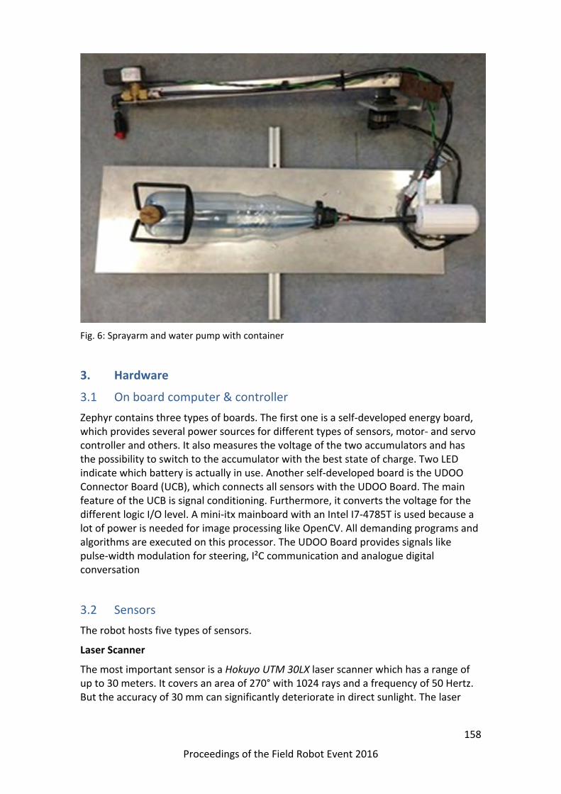
158


Fig. 6: Sprayarm and water pump with container

3. Hardware

3.1 On board computer & controller

Zephyr contains three types of boards. The first one is a self‐developed energy board, which provides several power sources for different types of sensors, motor‐ and servo controller and others. It also measures the voltage of the two accumulators and has the possibility to switch to the accumulator with the best state of charge. Two LED indicate which battery is actually in use. Another self‐developed board is the UDOO Connector Board (UCB), which connects all sensors with the UDOO Board. The main feature of the UCB is signal conditioning. Furthermore, it converts the voltage for the different logic I/O level. A mini‐itx mainboard with an Intel I7‐4785T is used because a lot of power is needed for image processing like OpenCV. All demanding programs and algorithms are executed on this processor. The UDOO Board provides signals like pulse‐width modulation for steering, I²C communication and analogue digital conversation

3.2 Sensors

The robot hosts five types of sensors.

Laser Scanner

The most important sensor is a Hokuyo UTM 30LX laser scanner which has a range of up to 30 meters. It covers an area of 270° with 1024 rays and a frequency of 50 Hertz. But the accuracy of 30 mm can significantly deteriorate in direct sunlight. The laser

159


scanner is the main sensor used in every task, for a reliable scan of the environment in front of the robot. [laserscanner]

Ultra‐sonic sensors

If the robot needs to drive backwards, two ultra‐sonic sensors at the rear assist the robot. For plants and equal structures this method works fine.

Inertia Measurement Unit and Hall sensors

Equally important is the inertia measurement board which is mounted on the top of the UCB. It provides information of positive or negative acceleration for three axes, movement directions like pitch, yaw, roll and has a magnetometer on board for orientation. At least each of the two electric motors have hall sensors to measure the motors’ speed.

OBE Sensor

At the rear bottom of the robot there is an OBE sensor. With this sensor it is possible to measure the real speed, the direction and the distance driven by the robot.

Camera

We use a SJCAM SJ4000 for detection of golf balls in task 3 as well as detection of textile tape in task 4. This camera is developed for the application of capturing outdoor sports in RGB, which comes with benefits like low weight, small size, waterproof case and a wide range white balance. We use the “PC mode”, which streams the video input from the image sensor to the robot, to lower the peak respond time. [camera]

3.3 External emergency stop

As emergency stop, we used a Futuba T10J Controller. The Controller Signals are forwarded through a micro‐controller to a Raspberry Pi 2 Model B. A ROS Node is running on this Device, which forwards Signals to the Robot via LAN. Additionally a Touchscreen is attached to the Raspberry Pi (see Fig. 7). This allows controlling the implemented state machine (Section 4.2) with a GUI, especially to change the current state in case of failure (see Fig. 8).

Fig. 7: Emergency Stop Controller

160


Fig. 8: Screenshot from the GUI of the Raspberry Pi

4. Software

4.1 ROS

The ROS (Robot Operating System) is a software framework for robots. In ROS there are packages which contain small programs, so‐called nodes. These nodes communicate with each other, by using ROS topics. A topic is a message‐bus which may contain several publishers or subscriber. The ROS‐nodes are used with all our sensors, including the laser scanner and the camera.

The ROS‐Core manages this message stream by registering those publishers and subscribers and assigns them to the respective receivers. ROS‐Messages support all standard data formats, such as strings and vectors, are predefined and provide time stamps. That ROS topics can be sent over networks, which enables easy and fast communication between individual components. With this, we are able to split the modules, so that the complex algorithms run on a powerful mainboard, while other modules (e.g. the sensor modules) run on an embedded PC. Based on this approach there are more low level modules which communicate with the sensors and actuators, either with help of libraries for the given interface or directly.

4.2 State machine

A state machine node was designed, to coordinate the execution of the other different nodes. Each node has a specified task. For example the robot has to navigate in row, or has to drive along a red line.

The state machine node represents the master of the system and communicates with the other nodes by sending messages. With these messages the state machine controls the execution of the other nodes. These nodes can be started, paused and stopped.

If a node got started by the state machine, it starts to execute the entrusted task. As soon as this task is completed, it sends back a message to the state machine. The massage contains a flag, which signals if the task was successfully completed, or failed. Depending to this flag, the state machine can respond differently. If the task completed successfully the state machine sends a stop to the current node and starts the next node with the next task. Otherwise the node failed, the current node will be stopped and the state machine starts another node with an error handling task.

161


Also all nodes can be also paused. A paused node contains the current status of the executed task. For example the driven distance of the robot. By stopping nodes these statuses are reseted.

For a better usability of the state machine we designed a GUI, to create specified states for the different tasks. The following figure (Fig. 9) shows the GUI of the designed state machine.

4.3 Dead Reckoning

The position package implements the dead reckoning. Therefore, it uses the gyroscope and the optical movement sensor to calculate the position. This is realized inside a class which can be used in every part of the system.

To calculate the position, the movement detected by the optical movement sensor is rotated around the actual angle of the robot (given through the gyroscope) and finally the result is added to the last calculated position.[reck] So we're able to keep track of the position relatively to a start position(which is usually the beginning of the calculations).

4.4 Navigation in rows

The navigation in rows in all tasks was done by the same algorithm. Navigation relied mainly on laser scanner data. A state machine switched between the different behaviors of driving in a row and change rows. Following steps are made:

Fig. 9 : Screenshot from the GUI of the state machine

162


1. Get the laser scan data as a pointcloud data type via ROS.

2. Shrink the pointcloud in direction X and Y.

3. Build clusters of the pointcloud using a density based clustering algorithm.

4. For each cluster do a line fitting and build a vector and a line equation.

5. For each cluster compute the intersections of its fitted line with the line of each other cluster; Compute the absolute value of each vector of a cluster.

6. Determine the cluster with the highest probability to be a row (of plants) regarding the distance from the robot to the intersection (higher is better), absolute value of the vector (bigger is better) and the history (more frames visible is more reliable).

7. Drive alongside the best cluster and avoid collision.

8. If no clusters are visible for some time → send a message to the state machine that the algorithm has finished successfully.

Fig. 10: Screenshot from RVIZ of in row navigation

White Dots→Pointcloud; Green Line→Cluster; Red Line→Vector from line fitting for the two best rows; Blue lines→Local coordinate system;

White lines → Global coordinate system;

4.5 Changing Rows

Changing rows also relies strongly on the laser scanner data. When triggered by the state machine the algorithm works as described below:

1. The robot steers out of the row with maximum angle of turn and stops when it is positioned orthographic to the rows.

2. The robot detects the end of the rows with the laser scanner and counts them until he passed the given number of rows. In this subtask the density based clustering is used again to detect and track the rows. The robot tracks the last row where he has to turn in and calculates the distance at which he has to turn into the row.

163


When the robot is driving along the rows the algorithm tries to drive parallel to the endpoints of the clustered rows. If the robot gets to close or to far away the robot steers accordingly.

3. When the Robot reaches the correct row it turns 90 degree into the row.

4.6 Golf ball spraying

The detection of golf balls was done using the RGB image from the SJCAM SJ4000 camera.

1. Get new image from camera.

2. Segment image based on color information to extract as less objects as possible besides golf balls.

3. Calculate features from segmented objects and apply classification to keep only golf balls.

4. Return positions to spraying node.

For spraying golf balls the circle of the spraying arm is known. If a golf ball moves into reachable positions for the spraying arm, the robot starts the pump water, stops moving, turns the arm in the right direction and sprays water on the golf ball.

4.7 Navigation along line

To navigate along a line like in task 4, the camera image was used.

1. Get new image from camera.

2. Run edge detection and walk pixel wise through the image, to extract position of a reference point. This is a imaginary point, where line pixels should be if the robots position is perfect.

3. Segment image based on color information to extract as less objects as possible besides the line.

4. Remove little objects, to keep only the long line.

5. Calculate distance from reference point to most left pixel on same height as reference point.

6. Steer according to distance.

4.8 Detection of transversal lines

Detection of transversal lines works the same way as described before in Section 4.7. The only difference is that there is no steering action. Action depends on current state and line color. Possible actions are: stop moving, start/stop seeding and turn 180°.

164


5. Conclusion

We were able to successfully adapt the old robot platform Zephyr for the new requirements of this year’s competition. For the navigation we changed the inertial measurement unit to a new unit to improve position data. Besides the inrow navigation was completely rewritten with an improved density‐based clustering algorithm. This new clustering algorithm improves the detection of plant rows. Because it works really great, it is also integrated in the outrow navigation, which results in much more stable navigation compared to last years. In the case, that the robot lose one’s way, we added a Raspberry Pi with touchscreen to be able to change the current state of the state machine. For the new tasks we added a connection for an external spray unit and the external seeding unit. With this concept it is possible to quickly change external peripheral devices to meet different requirements for different tasks. We also added a SJCAM SJ400 Camera to the robot for the computer vision tasks. However, the steering needs a better controller on the software side. In addition, the chassis frame showed some hardware weaknesses before and during the competition leading to downtimes for repairs. Supposedly the robot is too heavy for the current chassis, because it broke a part on the last day of the competition. Another problem was the rainy weather during the competition. In task 3 there was splash mud on the laserscanner, which affects the navigation. Also in task 3 the SJ4000 camera crashed, which lead to no detection of golf balls at all.

6. References

[camera] SJCAM SJ4000 Action Camera, http://sjcamhd.com/product/sjcam‐ sj4000‐action‐camera/ [22.07.16]

[laserscanner] UTM‐30LX | https://www.hokuyo‐aut.jp/02sensor/07scanner/utm_30lx.html [12.07.14]

[motor] Vector K4 Brushless Motor – Truck. https://www.lrp.cc/en/products/electric‐motors/brushless/sport/produkt/vector‐k4‐brushless‐motor‐truck/details/ [18.08.15]

[reck] Sekimori, D., Myazaki , F.: Precise dead‐reckoning for mobile robots using multiple optical mouse sensors. In: Informatics in Control, Automation and Robotics II (2007), Springer

[ros] ROS.org | Powering the world's robots. https://www.ros.org [12.08.15]

[servo] Servo HS‐7980TH. http://hitecrcd.com/products/servos/ultra‐premium‐digital‐servos/hs‐7980th‐mega‐torque‐hv‐coreless‐titanium‐gear‐servo/product [18.08.15]

[controller] Futaba, http://www.futabarc.com/systems/futk9200‐10j/ [22.07.16]

[spreader] WE‐B Universal‐Streuer, http://www.wolf‐garten.de/produkte/rasen/streugeraete‐schlauchwagen/detail/produkt/we‐b‐universal‐streuer‐889/ [22.07.16]

165


ŻUKBOT Błażej Błaszczuk, Mateusz Olszewski, Patryk Reiss, Tomasz Węsierski

Department of Automatic Control, Faculty of Electronics, Telecommunications and Informatics, Gdańsk University of Technology

1. Introduction

The aim of the project is to design and build autonomous agricultural robot ŻukBot, to participate in international tournament Field Robot Event. We decided on 4 wheel robot without pivoting wheels with 4 independent motors. We want to ensure that the vehicle was modular, allowing for further development of the structure, or a simple retraining it for other purposes. Construction has to be as narrow as to make it easier to move between the rows of plants


Chassis is built of aluminium profiles and plexi glass panels. Żukbot have four wheels whose diameter is 26cm. Every wheel is driven by a Drive‐System Europe DSMP420‐24‐024‐BFEC DC motor, with 0.95 Nm rated torque each. The power transmission system was realized using bevel gears. The main processing unit is a laptop with Robot Operating System, which is responsible for the correct functioning of Żukbot. To steer motors H‐bridges are used and a communication is done using an Arduino Uno board. To power whole rotob we used two Lithium‐Polymer Gens ace batteries 5000 mAh capacity each.

Figure 1: Concept of Żukbot

166


Figure 2: Descriptive geometry of Żukbot

3 Controller Architecture

167



Main computing power comes from Toshiba laptop with Intel i3 processor on board. This choice was made due to high computation needs to complete task three and four which were based on vision systems. In design stage we also considered using Raspberry PI as main device. It was rejected due to not enough computing power and lack of easy debug without additional wireless link to external PC. Main disadvantage of using laptop is its size. It can’t be fit into a small robot. Second problem is HDD which can be damaged due to vibrations (use of solid state drive can completely eliminate this problem).

Data from laptop was send through USB to Arduino Due board. It is arduino board based on Atsam microcontroller (Arm core). This board was used as main parallel interface to control robot movement, read encoders and gyro. Arduino UNO clone with CNC shield was used as secondary parallel interface to control all of the stepper motors. CNC shield was perfect solution to drive three StepStick stepper motor drivers.

Motor drivers were the biggest issue during development. During research we chose VNH3SP30 chips. Unfortunately to drive them 5v logic is needed. To overcome this we designed and build boards with logic level converters. Finished drivers can supply up to 30A peak current. In future projects low esr and large capacity caps must be in place to provide for current spikes.

Original in motor encoders were swapped with 12 bit Austria Microsystems magnetic incremental encoders. Choice was made due to the need of high precision odometry positioning especially when driving low speeds.

Whole robot is supplied by two Turnigy 5000mAh 3s 20C Li‐Po. Lower voltages are provided by buck converter module.


● Rows navigation Navigation was solely based on lidar readings. Point scanned were first represented in cartesian coordinate system, then points representing crops from current row were chosen. Those point where further divided into two groups representing each side of row. Resulting groups were connected into pairs based on their position relative to row and each other. For each pair a new point were calculated with its coordinates being the average of coordinates of point it was created from. Resulting sequence of points were converted into set of vectors, which made a temporary path.

● Path execution A temporary target point was chosen from points/vectors representing temporary path, based on current speed and average second derivative of discrete function, which was created by representing path points on plane where x‐axis is parallel to robot’s current vector of speed. Then appropriate engine speeds were chosen based on temporary target’s position relative to current robot’s orientation.

● Headlands At end of each row robot moved one meter forward, then rotated 90 degrees and continued onward until a specific number of rows were detected and passed (for basic navigation it was one). Then next row where entered.

168


● Weeding Markers were recognised by single camera using opencv2 library. Their position was triangulated based on set height of camera and known lens distortion. Then their position was converted to spherical coordinate system with zero at sprinkler. Resulting theta and phi angles allowed us to direct sprinkler directly at its target.

3.3 Sensors

● Sick TIM551

Field of application Outdoor

Light source Infrared (850 nm)

Laser class 1, eye‐safe (EN 60825‐1 (2007‐10))

Aperture angle 270°

Scanning frequency 15 Hz

Angular resolution 1°

Operating range 0.05 m ... 10 m

Max. range with 10 % reflectivity 8 m

● Microsoft LifeCam HD‐5000

Sensor CMOS sensor technology

Resolution Motion Video: 1280 X 720

Imaging Rate Up to 30 frames per second

Field of View 66° diagonal field of view

Imaging Features • Digital pan, digital tilt, vertical tilt, and swivel pan, and 4x digital zoom

• Auto focus, range from 6” to infinity

• Automatic image adjustment with manual override

• 16:9 widescreen

• 24‐bit color depth

169


● KAmodGYRO KAmodGYRO is a three‐axis gyroscope equipped with interfaces SPI and I2C. The module is built based upon the L3G4200D STMicroelectronics. It is used to measure the relative angular velocity of each of the three axes. The output at a resolution of 16 bit. Built‐in low‐pass and a high pass filter. The module has also high shock resistance.

● AS5045 ‐ 12 Bit Programmable Magnetic Rotary Encoder The AS5045 is a contactless magnetic rotary encoder for accurate angular measurement over a full turn of 360°. It is a system‐on‐chip, combining integrated Hall elements, analog front end and digital signal processing in a single device. The absolute angle measurement provides instant indication of the magnet’s angular position with a resolution of 0.0879° = 4096 positions per revolution. This digital data is available as a serial bit stream and as a PWM signal.

4 Conclusion

The main conclusions of the study should be presented as the outcome of the performance putting emphasis on the advantages and disadvantages of the robotic system.

5 References

The construction of the robot was supported by: DRAMIŃSKI S.A., CLAAS Foundation, Gdańsk University of Technology and Robotics Association Skalp.

Proceedings of the 14th Field Robot Event 2016

Documents

Transcript of Proceedings of the 14th Field Robot Event 2016