Procedures for the Estimation of Pavement and Bridge Preservation Costs for Fiscal Planning and...

Final Report

FHWA/IN/JTRP-2005/17

PROCEDURES FOR THE ESTIMATION OF

PAVEMENT AND BRIDGE PRESERVATION COSTS FOR FISCAL PLANNING

By

Kumares C. Sinha Olson Distinguished Professor

Samuel Labi

Visiting Assistant Professor

Marcela Rodriguez Gabriel Tine Rucci Dutta

Graduate Research Assistants

School of Civil Engineering Purdue University

Joint Transportation Research Program Project No. C-36-73W

File No.: 3-4-23 SPR-2810

Prepared in Cooperation with the Indiana Department of Transportation and

The U.S. Department of Transportation Federal Highway Administration

The contents of this report reflect the views of the authors who are responsible for the facts and the accuracy of the data presented herein. The contents do not necessarily reflect the official views of the Federal Highway Administration and the Indiana Department of Transportation. The report does not constitute a standard, a specification, or a regulation.

Purdue University West Lafayette, Indiana, 47907

July 2005

14-3 7/05 JTRP-2005/17 INDOT Division of Research West Lafayette, IN 47906

INDOT Research

TECHNICAL Summary Technology Transfer and Project Implementation Information

TRB Subject Code: 14-3 Financial Programming July 2005 Publication No.: FHWA/IN/JTRP-200517, SPR-2810 Final Report

Procedures for the Estimation of Pavement and Bridge Preservation Costs for Fiscal Planning

Introduction Facility preservation generally refers to the set of activities that are carried out to keep a facility in usable condition until the next reconstruction activity. For fiscal planning and programming, it is necessary to know the expected costs of preservation projects and how long they would last. Such information, coupled with minimum standards and facility inventory data, enables estimation of overall monetary needs for bridge and pavement

preservation, and can assist INDOT in undertaking appropriate programming and attendant financial planning over the long term. However, detailed engineering analyses are not possible every year because of the time and effort involved; therefore, simple procedures to broadly estimate annual pavement and bridge preservation needs are useful for long-term fiscal planning.

Findings The study methodology consisted of first

undertaking a full analysis based on engineering principles and detailed work in order to determine pavement and bridge needs for a period of time. Then simple procedures to estimate yearly pavement and bridge preservation costs were developed and the results were compared to the detailed engineering needs. Deterioration and cost models to establish engineering needs were developed using an array of statistical techniques including analysis of variance and regression analysis. Using the deterioration models, system inventory and minimum standards, the level of physical needs was

determined for the entire pavement and bridge network over the analysis period. Finally, using the identified physical needs and developed cost models, the monetary needs were estimated. An age-based approach (that considers fixed time intervals instead of deterioration trends and minimum standards) was used for the bridge preservation needs. Based on the historical expenditure records and the amount of work performed in the past, simple regression models were developed to estimate future annual pavement and bridge preservation needs. The results obtained proved to be consistent with the engineering analysis.

Implementation The study results are useful for long-

term planning and budgeting as INDOT’s Divisions of Policy and Fiscal Management and Planning will be able to schedule and monitor its

pavement and bridge preservation cash flows in a more effective manner than what is possible at present.

14-3 7/05 JTRP-2005/17 INDOT Division of Research West Lafayette, IN 47906

Contacts For more information: Prof. Kumares C. Sinha Principal Investigator School of Civil Engineering Purdue University West Lafayette, IN 47907-2051 Phone: (765) 494-2211 Fax: (765) 496-7996 E-mail: [email protected]

Indiana Department of Transportation Division of Research 1205 Montgomery Street P.O. Box 2279 West Lafayette, IN 47906 Phone: (765) 463-1521 Fax: (765) 497-1665 Purdue University Joint Transportation Research Program School of Civil Engineering West Lafayette, IN 47907-1284 Phone: (765) 494-9310 Fax: (765) 496-7996 E:mail: [email protected] http://www.purdue.edu/jtrp

ii

Form DOT F 1700.7 (8-69)

TECHNICAL REPORT STANDARD TITLE PAGE

1. Report No.

2. Government Accession No.

3. Recipient's Catalog No.

FHWA/IN/JTRP-2005/17

4. Title and Subtitle: Procedures for the Estimation of Pavement & Bridge preservation Costs for Fiscal Planning and Programming

Report Date: July 2005

6. Performing Organization Code 7. Author(s) Kumares C. Sinha, Samuel Labi, Marcela Rodriguez, Gabriel Tine, Rucci Dutta

8. Performing Organization Report No. FHWA/IN/JTRP-2005/17

9. Performing Organization Name and Address Joint Transportation Research Program 550 Stadium Mall Drive, Purdue University, West Lafayette, IN 47907-1284

10. Work Unit No.

11. Contract or Grant No.

SPR-2810 12. Sponsoring Agency Name and Address Indiana Department of Transportation, State Office Building, 100 N. Senate Ave. Indianapolis, IN 46204

13. Type of Report and Period Covered

Final Report 14. Sponsoring Agency Code 15. Supplementary Notes Prepared in cooperation with the Indiana Department of Transportation and Federal Highway Administration. 16. Abstract Facility preservation generally refers to the set of activities that are carried out to keep a facility in usable condition until the next reconstruction activity. For fiscal planning and programming, it is necessary to know the expected costs of preservation projects and how long they would last. Such information, coupled with minimum standards and facility inventory data enable estimation of overall monetary needs for bridge and pavement preservation, and would assist INDOT in undertaking appropriate programming and attendant financial planning over the long term. However, detailed engineering analyses are not possible every year because of the time and effort involved, therefore simple procedures to help estimate annual pavement and bridge preservation needs are useful for long-term fiscal planning. The study methodology consisted of first undertaking a full analysis based on engineering principles and detailed work in order to determine pavement and bridge needs for a period of time. Then simple procedures to estimate yearly pavement and bridge preservation costs were developed and the results were compared to the detailed engineering needs. Deterioration and cost models to establish engineering needs were developed using an array of statistical techniques including analysis of variance and regression analysis. Using the deterioration models, system inventory and minimum standards, the level of physical needs was determined for the entire pavement and bridge network over the analysis period. Finally, using the identified physical needs and developed cost models, the monetary needs were estimated. An age-based approach (that considers fixed time intervals instead of deterioration trends and minimum standards) was used for the bridge preservation needs. Based on the historical expenditure records and the amount of work performed in the past, simple regression models were developed to estimate future annual pavement and bridge preservation needs. The results obtained proved to be consistent with the engineering analysis.

17. Key Words Bridge Preservation, Pavement Preservation, Service Life, Preservation Cost, Rehabilitation, Maintenance

18. Distribution Statement No restrictions. This document is available to the public through the National Technical Information Service, Springfield, VA 22161

19. Security Classif. (of this report)

Unclassified 20. Security Classif. (of this page)

Unclassified

21. No. of Pages

11122. Price

iii

ACKNOWLEDGEMENTS

The authors wish to acknowledge the assistance provided by Messrs. Samy Noureldin, Gary

Eaton, David Holtz, Jaffar Golkhajeh, (all of INDOT) and Keith Hoernschemeyer (of FHWA), who

served on the Study Advisory Committee and provided valuable information at various stages of the

study. For the acquisition of bridge data, we appreciate the assistance provided by Messrs. Ron Scott,

Mike Jenkins, Dauda Ishola, and Bill Dittrich, all of INDOT. Regarding pavement data collection, we

acknowledge the efforts of Messrs. William Flora and Mike Yamin. The assistance of Dr. Bob

McCullouch and Aldy Haryopratomo are also acknowledged. We are also grateful to Dr. Barry

Partridge, Chief of INDOT Research Division, and Karen Hatke, JTRP Coordinator, for their

assistance in this research effort.

iv

TABLE OF CONTENTS LIST OF TABLES ...................................................................................................................................................... VII LIST OF FIGURES ......................................................................................................................................................... X CHAPTER 1 : INTRODUCTION ............................................................................................................................1

1.1 Background and Problem Statement 1 1.2 Objectives of the Study 2 1.3 Study Overview 3 1.4 Scope of the Study 3 1.5 Alternative Methodologies for Estimating Service Lives of Preservation Treatments 4

1.5.1 Estimation of Preservation Treatment Service Life Based on Time Interval 4 1.5.2 Estimation of Preservation Treatment Service Life Based on Facility erformance/Condition 5

CHAPTER 2 : LITERATURE REVIEW FOR PAVEMENT PRESERVATION NEEDS

ASSESSMENT............................................................................................................................................8 2.1 Needs Assessment Methodologies 8 2.2 Review of Pavement Performance Models 9 2.3 Pavement Rehabilitation Costs 10

CHAPTER 3 : STUDY METHODOLOGY FOR PAVEMENT NEEDS ASSESSMENT....................................12 3.1 Study Framework 12 3.2 Methodology 13

3.2.1 Defining the Jorizon Period 13 3.2.2 Establishment of Minimum Standards 13 3.2.3 Development of Pavement Deterioration Curves 13 3.2.4 Development of Preservation Cost Models 15

CHAPTER 4 : PAVEMENT SERVICE LIVES AND COST MODELS...............................................................16 4.1 Pavement Design Life 16 4.2 Pavement Condition 16

4.2.1 Pavement Deterioration Rates 17 4.2.2 Pavement Treatments 19

4.3 Pavement Preservation Cost Models 21 4.4 Unit Costs of Highway Routine Maintenance 22

v CHAPTER 5 : PAVEMENT PRESERVATION NEEDS ANALYSIS .................................................................24

5.1 Collection and Processing of Data 24 5.2 Methodology 25 5.3 Interstate Initial Pavement Condition and Treatment 27 5.4 Non-Interstate NHS Pavement Condition and Initial Treatment 32 5.5 Non-Interstate Non-NHS Pavement Condition and Initial Treatment 34 5.6 Network Analysis Results 38

CHAPTER 6 : PROCEDURE FOR EVALUATING ANNUAL PAVEMENT PRESERVATION COST...........40 6.1 Total System Size Prediction 41 6.2 Percentage of system to be treated 42 6.3 Estimation of total preservation cost using unit cost per lane mile 43 6.4 Rehabilitation and Non rehabilitation cost 45 6.5 Preservation cost by Highway Class 47

CHAPTER 7 : DEVELOPMENT OF BRIDGE PRESERVATION COST MODELS..........................................49 7.1 Introduction 49 7.2 Cost Estimation of Bridge Replacement 50

7.2.1 Slab Bridge Replacement Cost Models 50 7.2.1 Slab Bridge Replacement Cost Models 51 7.2.2 Pre-stressed Beam Bridge Replacement Cost Models 54 7.2.3 Steel Bridge Replacement Cost 58 7.2.4 Summary and Conclusions for Bridge Replacement Cost Modeling 59

7.3 Cost Estimation for Bridge Rehabilitation Activities 61 7.3.1 Deck Rehabilitation Cost Model 62 7.3.2 Deck and Superstructure Rehabilitation Cost Model 64 7.3.3 Deck Replacement Cost Model 65 7.3.4 Deck Replacement + Superstructure Rehabilitation Cost Model 67 7.3.5 Superstructure Replacement Cost Model 69 7.3.6 Superstructure Replacement + Substructure Rehabilitation Cost Models 71 7.3.7 Bridge Widening Cost Model 73 7.3.8 Summary and Conclusions for Bridge Rehabilitation Cost Models 76

7.4 Overall Summary and Conclusions for Bridge Preservation Cost Models 78 CHAPTER 8 : ESTIMATION OF BRIDGE SERVICE LIVES ............................................................................79

vi CHAPTER 9 : BRIDGE PRESERVATION EXPENDITURES ............................................................................83

9.1 Age-Based Needs 83 9.2 Estimated Needs Based on Historical Bridge Expenditures 87

9.2.1 Historical Expenditures 87 9.2.2 Projected Expenditure on the Basis of Historical Trends 88

9.3 Comparison of Age-Based Needs and Needs Based on Past Expenditure 89 CHAPTER 10 : SUMMARY AND CONCLUSIONS .............................................................................................92

10.1 Summary of Estimation Procedures 92 10.2 Conclusions 93

REFERENCES ........................................................................................................................................................95

APPENDIX A. PERFORMANCE CURVES.................................................................................................................98

APPENDIX B. COST MODELS FOR ASPHALTIC CONCRETE PAVEMENTS ...................................................101

APPENDIX C. INDOT CONTRACTS UNIT PAVEMENT TREATMENT COSTS.................................................103

APPENDIX D. AAMEX MODEL CURVES...............................................................................................................105

APPENDIX E. BRIDGE SYSTEM TYPES.................................................................................................................108

vii

LIST OF TABLES Table 4-1 Design Life of Pavement Treatments........................................................................................... 16 Table 4-2 International Roughness Index...................................................................................................... 17 Table 4-3 Terminal Pavement Serviceability Ratings ................................................................................... 17 Table 4-4 Pavement Deterioration Rates ....................................................................................................... 19 Table 4-5 Input Variables for Pavement Preservation Cost Models......................................................... 22 Table 4-6 Average Pavement Treatment Costs per Lane-Mile .................................................................. 22 Table 4-7 Average Annual Maintenance Costs per Lane-Mile ................................................................... 23 Table 5-1 Network Analysis Pavement Resurfacing Deficiency Levels ................................................... 25 Table 5-2 Network Analysis Pavement Reconstruction Deficiency Levels ............................................. 26 Table 5-3 Pavement Performance (IRI) Jumps after Treatment ............................................................... 27 Table 5-4 Interstate HMA Pavement Treatment Thresholds..................................................................... 28 Table 5-5 Interstate PCC Pavement Treatment Thresholds....................................................................... 29 Table 5-6 Interstate COMP Pavement Treatment Thresholds .................................................................. 30 Table 5-7 Non-Interstate NHS HMA Pavement Treatment Thresholds................................................. 33 Table 5-8 Non-Interstate NHS PCC Pavement Treatment Thresholds................................................... 33 Table 5-9 Non-Interstate NHS COMP Pavement Treatment Thresholds .............................................. 34 Table 5-10 Non-Interstate, Non-NHS, HMA Pavement Treatment Thresholds................................... 35 Table 5-11 Non-Interstate Non-NHS PCC Pavement Treatment Thresholds....................................... 36 Table 5-12 Non-Interstate Non-NHS COMP Pavement Treatment Thresholds .................................. 36 Table 5-13 Fifteen-year Pavement Condition Preservation Needs Scenario A....................................... 38 Table 5-14 Fifteen-year Pavement Condition Preservation Needs Scenario B ....................................... 39 Table 6-1 Comparison of actual and predicted pavement preservation costs for 2002 and 2003........ 44 Table 6-2 Percentage of money spent on different highway classes (2000 and 2001) ........................ 47 Table 6-3 2008 Pavement Preservation Costs by Highway class ............................................................... 48 Table 7-1 Summary of Superstructure Replacement Cost Models for Slab Bridges .............................. 52 Table 7-2 Details of Best Superstructure Replacement Cost Model for Slab Bridges............................ 52 Table 7-3 Summary of the Substructure Replacement Cost Models for Slab Bridges ........................... 53 Table 7-4 Details of Best Substructure Replacement Cost Model for Slab Bridges ............................... 53

viii

Table 7-5 Summary of Superstructure Replacement Cost Models for Pre-stressed Beam Bridges ..... 55 Table 7-6 Details of Best Model for Superstructure Replacement Cost of Pre-stressed Beam Bridges

..................................................................................................................................................................... 55 Table 7-7 Summary of Substructure Replacement Cost Models for Pre-stressed Beam Bridges......... 56 Table 7-8 Details of Best Substructure Replacement Cost Model for Pre-stressed Beam Bridges...... 56 Table 7-9 Summary of the Approach Cost Models for Pre-stressed Beam Bridge Replacement ........ 57 Table 7-10 Details of Best Approach Cost Model for Pre-stressed Beam Bridge Replacement .......... 57 Table 7-11 Summary of the “Other Cost” Models for Pre-stressed Beam Bridge Replacement ......... 58 Table 7-12 Details of Best “Other Cost” Model for Beam Bridge Replacement.................................... 58 Table 7-13 Descriptive Statistics of Replacement Unit Cost: for Steel Structure ................................... 59 Table 7-14 Summary of Bridge Replacement Cost for Concrete Bridges ................................................ 60 Table 7-15 Summary of Deck Rehabilitation Primary Cost Models for all Bridge Types ..................... 62 Table 7-16 Summary of “Other Cost” Models for Deck Rehabilitation Contracts................................ 62 Table 7-17 Details of Best Deck Rehabilitation Primary Cost Model for all Bridge Types .................. 63 Table 7-18 Details of Best Unit “Other Cost” Model for Deck Rehabilitation, all Bridge Types ....... 63 Table 7-19 Summary of Primary Cost Models for Deck + Superstructure Rehabilitation for all Bridge

Types........................................................................................................................................................... 64 Table 7-20 Details of the Best Primary Cost Model for Deck + Superstructure Rehabilitation for all

Bridge Types.............................................................................................................................................. 65 Table 7-21 Descriptive Statistics for Deck Replacement Total Cost ........................................................ 66 Table 7-22 Descriptive Statistics for Deck Replacement Unit Cost.......................................................... 66 Table 7-23 Descriptive Statistics for Deck Replacement + Superstructure + Substructure

Rehabilitation Cost ................................................................................................................................... 67 Table 7-24 Descriptive Statistics for Deck Replacement + Superstructure + Substructure

Rehabilitation Cost ................................................................................................................................... 67 Table 7-25 Summary of Deck Replacement + Superstructure Rehabilitation Primary Cost Models for

all Bridge Types......................................................................................................................................... 68 Table 7-26 Best Deck Replacement + Superstructure Rehabilitation Primary Cost Model for all

Bridge Types.............................................................................................................................................. 68 Table 7-27 Summary of Deck Replacement + Super Rehabilitation “Other Cost” Models for all

Bridge Types.............................................................................................................................................. 68 Table 7-28 Details of Best Deck Replacement + Super Rehabilitation “Other Cost” Model for all

Bridge Types.............................................................................................................................................. 69

ix

Table 7-29 Summary of Superstructure Replacement Primary Cost Models for all Bridge Types ...... 69 Table 7-30 Details of Best Superstructure Replacement Primary Cost Model for all Bridge Types.... 70 Table 7-31 Summary of Superstructure Replacement “Other Cost” Models for all Bridge Types...... 70 Table 7-32 Details of Best Superstructure Replacement “Other Cost” Model for all Bridge Types... 70 Table 7-33 Summary of Superstructure Replacement + Substructure Rehabilitation Primary Cost

Models for all Bridge Types .................................................................................................................... 71 Table 7-34 Details of Best Superstructure Replacement + Substructure Rehabilitation Primary Cost

Model for all Bridge Types...................................................................................................................... 71 Table 7-35 Summary of Superstructure Replacement + Substructure Rehabilitation “Other Cost”

Models ........................................................................................................................................................ 72 Table 7-36 Details of Best Superstructure Replacement + Substructure Rehabilitation “Other Cost”

Model.......................................................................................................................................................... 72 Table 7-37 Summary of Bridge Widening Primary Cost Models............................................................... 74 Table 7-38 Details of Best Bridge Widening Primary Cost Model for all Bridge Types........................ 74 Table 7-39 Summary of Bridge Widening “Other Cost” Models for all Bridge Types.......................... 75 Table 7-40 Details of Best Bridge Widening “Other Cost” Model for all Bridge Types ....................... 75 Table 7-41 Summary of Rehabilitation Activity Cost Models .................................................................... 77 Table 8-1 Results of Age-Based Physical Needs Assessment of Concrete Bridges, 2004-2015 ........... 81 Table 8-2 Results of Age-Based Physical Needs Assessment of Steel Bridges, 2004-2015................... 82 Table 9-1 Age-Based Monetary Needs for Bridge Replacement, by Year and Structure Material ....... 84 Table 9-2 Annual Deck Rehabilitation Needs by Structure Material ........................................................ 85 Table 9-3 Historical Bridge Expenditure from (1996-2003).......................................................................87 Table 9-4 Projected Bridge Expenditure from 2005 to 2015 ..................................................................... 89 Table 9-5 Comparison of Needs Based on Past Expenditures and Needs Based on Age .................... 90 Table C.0-1 Unit Pavement Treatment Costs .............................................................................................103 Table C.0-2 Unit Costs of Pavement Treatments (Continued)................................................................104

x

LIST OF FIGURES Figure 1-1 Alternative Methodologies for Service Life Determination ...................................................... 4 Figure 1-2 Estimation of Preservation Treatment Service Life based on Time Interval ......................... 5 Figure 1-3 Estimation of Preservation Treatment Service Life Based on Time-Series ............................ 6 Figure 1-4 Estimation of Preservation Treatment Service Life Based on Cross-Sectional Condition

Data............................................................................................................................................................... 7 Figure 3-1 Framework Used for Pavement Preservation Needs Assessment ......................................... 12 Figure 3-2 Pavement Deterioration Curve .................................................................................................... 14 Figure 5-1 Distribution of Interstate Pavement as of Year 2001............................................................... 28 Figure 5-2 Methodology used for Excellent, Good and Good-To-Fair Pavements .............................. 31 Figure 5-3 Distribution of Non-Interstate NHS by Pavement Condition as of Year 2001 .................. 32 Figure 5-4 Distribution of Non-Interstate Non-NHS by Pavement Condition as of Year 2001......... 35 Figure 5-5 Methodology for Poor Pavements............................................................................................... 37 Figure 6-1 Indiana’s highway system size versus time ................................................................................. 41 Figure 6-2 Percentage of system preserved versus time .............................................................................. 42 Figure 6-3 Percentage of system rehabilitated versus time ......................................................................... 45 Figure 7-1 Schematic Illustration of Typical Concrete Slab Bridge Types ............................................... 51 Figure 7-2 Schematic Illustration of Typical Pre-stressed Concrete Bridge Sections............................. 54 Figure 7-3 Comparison of Unit Cost of Bridge Replacement between Steel and Concrete Bridges ... 59 Figure 7-4 Classification of Rehabilitation Cost Models Developed in Present Study .......................... 61 Figure 7-5 Predicted and Actual Cost for Superstructure Replacement + Substructure Rehabilitation

..................................................................................................................................................................... 73 Figure 8-1 Delineation of Bridge Age ............................................................................................................ 79 Figure 9-1: Bridge Replacement Monetary Needs........................................................................................ 85 Figure 9-2 Bridge Rehabilitation Monetary Needs ....................................................................................... 86 Figure 9-3 Modeling Bridge Preservation Expenditure ............................................................................... 88 Figure 9-4 Needs Based on Age and Historical Trends .............................................................................. 91

1

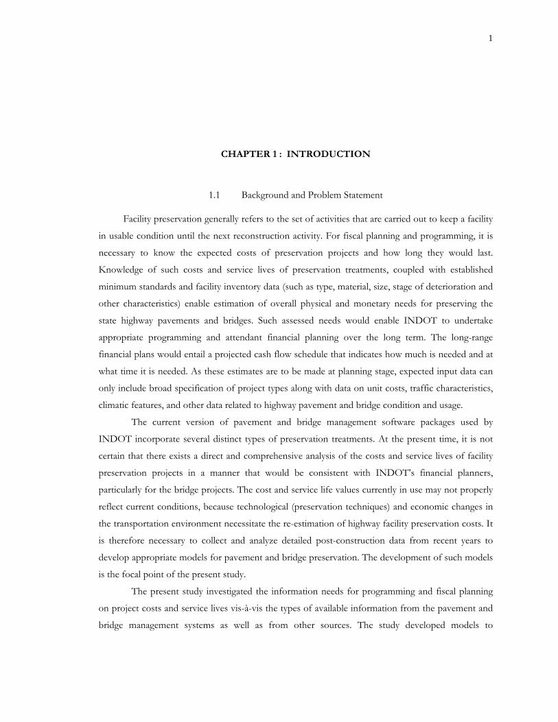
CHAPTER 1 : INTRODUCTION

1.1 Background and Problem Statement

Facility preservation generally refers to the set of activities that are carried out to keep a facility

in usable condition until the next reconstruction activity. For fiscal planning and programming, it is

necessary to know the expected costs of preservation projects and how long they would last.

Knowledge of such costs and service lives of preservation treatments, coupled with established

minimum standards and facility inventory data (such as type, material, size, stage of deterioration and

other characteristics) enable estimation of overall physical and monetary needs for preserving the

state highway pavements and bridges. Such assessed needs would enable INDOT to undertake

appropriate programming and attendant financial planning over the long term. The long-range

financial plans would entail a projected cash flow schedule that indicates how much is needed and at

what time it is needed. As these estimates are to be made at planning stage, expected input data can

only include broad specification of project types along with data on unit costs, traffic characteristics,

climatic features, and other data related to highway pavement and bridge condition and usage.

The current version of pavement and bridge management software packages used by

INDOT incorporate several distinct types of preservation treatments. At the present time, it is not

certain that there exists a direct and comprehensive analysis of the costs and service lives of facility

preservation projects in a manner that would be consistent with INDOT’s financial planners,

particularly for the bridge projects. The cost and service life values currently in use may not properly

reflect current conditions, because technological (preservation techniques) and economic changes in

the transportation environment necessitate the re-estimation of highway facility preservation costs. It

is therefore necessary to collect and analyze detailed post-construction data from recent years to

develop appropriate models for pavement and bridge preservation. The development of such models

is the focal point of the present study.

The present study investigated the information needs for programming and fiscal planning

on project costs and service lives vis-à-vis the types of available information from the pavement and

bridge management systems as well as from other sources. The study developed models to

2

estimate/predict the cost and service life of various pavement and bridge preservation activity types,

given facility characteristics such as functional class, material type, climatic region, and other

variables.

It is important to note that within each preservation life-cycle, any of several alternative

repair (maintenance and rehabilitation) strategies can be carried out. Therefore, the length of any

preservation life-cycle is not fixed, but depends on the maintenance strategy within that cycle:

generally, higher maintenance is associated with longer preservation life-cycles and vice versa.

However, beyond a certain point, increasing maintenance leads to decreasing cost-effectiveness,

therefore, for any given preservation type, there exists some optimal level of maintenance that should

be carried out within the preservation life-cycle. The present study utilizes results from an earlier

JTRP studies (Hodge et al., 2004; Rodriguez, 2004) that determined the preservation life-cycles

corresponding to different levels of life cycle repair effort.

The study product will help INDOT to schedule and monitor its preservation cash flows in

a more effective manner than what is possible at present. Also, the study provides a reliable and

simple set of procedures for estimating annual preservation costs for pavement and bridge projects.

It is expected that the study results will complement existing efforts by INDOT’s pavement and

bridge management systems in the provision of information related to preservation costs and service

lives.

1.2 Objectives of the Study

The objectives of the study were as follows:

1) To collect and collate historical records of costs and service lives of pavement preservation

and bridge replacement and rehabilitation projects,

2) To develop models for estimating service lives and costs of pavement preservation and bridge

related activities.

3) To establish a simple procedure for INDOT´s policy and fiscal management and

programming divisions for estimating annual pavement and bridge preservation costs.

3

1.3 Study Overview

The study is divided into two parts: first for pavements, and second for bridges. For each of

these two facility types, the study investigated current service lives of pavements and bridges in the

Indiana state highway system. Updated cost models were also developed to assess the financial needs

for pavement and bridge over the 2005-2020 analysis period. This was carried out on the basis of:

system size, minimum standards, deterioration trends for pavement, age for bridges and cost models.

Simple procedures to estimate annual bridge and pavement expenditure were also developed. A

comparison was made of the predicted expenditure with the estimated needs over the analysis period.

1.4 Scope of the Study

Spatial: Only pavements and bridges on the state highway system were considered. As much as

possible, pavement sections and bridges at geographically diverse locations on the state network were

included to capture any possible regional/climatic differences.

Temporal: Historical data for pavement and bridge cost and service life modeling was taken from

projects executed between the years 1990-2003. This time period provided adequate time to evaluate

the service lives of such projects. Due regard was given to the effect of changes in interest rate or

construction price indices (CPI) within this period.

Project Types: Project types and their definitions were drawn from the planning and programming

divisions and conformed to the need of the policy and fiscal management division.

Facility Material Type and Other Considerations: The study developed cost and service models for the

types of bridges found on the state highway network, such as steel and reinforced-concrete bridges,

and the types of pavements such as full-depth asphalt, rigid, and composite pavements. Also, all

major functional classes of road on the network were considered.

4

1.5 Alternative Methodologies for Estimating Service Lives of Preservation Treatments There are several approaches that can be used to estimate the service life of pavement and bridge

preservation treatments, as shown in Figure 1-1.

1.5.1 Estimation of Preservation Treatment Service Life Based on Time Interval

This approach simply involves measurement of the time interval that passes between a preservation

treatment and the next similar or higher preservation treatment (Figure 1-2).

Figure 1-1 Alternative Methodologies for Service Life Determination

Service Life Estimation using Historical Data

Estimation based on Time Interval

How much time elapsed between

“successive” preservation treatments?

Using Time-Series

Performance Data

Estimation based on Performance/Condition

How much time passed before the treated facility

reverted to the state before treatment or to a pre-

specified threshold state?

Using Cross-

Sectional

Performance Data

Using Panel

Performance Data

Pre-specified General Threshold for all

Pavements in a Given Category

Performance/Condition of

the Individual Pavement

5

Service Life at Tx, SLX = TY -TX

For each of several pavement sections or bridges that received the given preservation treatment, the

service life can thus be determined, and expressed as an average value or as a function of facility type,

traffic and weather characteristics. The advantage of this approach lies in its economy: no pavement

performance/condition data is needed to establish service lives in this manner. However, for this

approach to work, preservation treatment contract records spanning a considerable span of time

should be available for each pavement or bridge. This is generally not the case at INDOT even

though the Research Team has made earnest efforts in obtaining data of this sort.

1.5.2 Estimation of Preservation Treatment Service Life Based on Facility

Performance/Condition

In this approach, service life of a preservation treatment can be determined by estimating the amount

of time that passed before the treated facility reverted to the state before treatment or to a pre-

specified threshold state. Three separate approaches can be followed as discussed below.

Time Series: In this approach, the performance/condition of each individual facility (pavement section

or bridge) that has received a specific preservation treatment is monitored over time. The time

interval between the time of treatment and the time at which condition falls below the condition

before treatment (Figure 1-3(a)) or a pre-specified condition (Figure 1-3(b)), is measured as the

service life of the preservation treatment. If a pre-specified condition is used, the facility condition at

time of treatment may be lower than that threshold (as shown in the illustration) or may be higher

than the threshold. This approach is data intensive: facility performance/condition data is needed

over a considerable span of time for each facility.

Figure 1-2 Estimation of Preservation Treatment Service Life Based on Time Interval

TreatmentTreatment

SLX

Year TX Year TY

Time, Accumulated

6

(a) (b)

This may be repeated for several facilities that received the treatment in question, and the service

lives thus obtained can simply be processed to give an average service life for that treatment, or may

be expressed as a function of facility type, traffic, weather and other attributes, for that preservation

treatment.

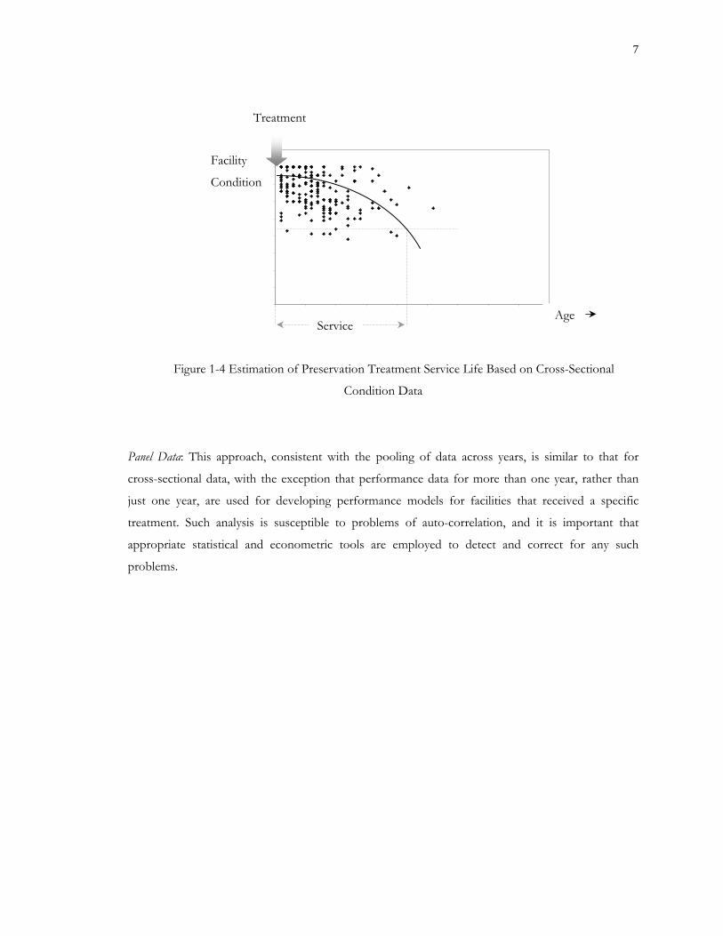
Cross Sectional: In this approach, the performance/condition (at any single given year only) of several

facilities that received a specific treatment is used. As such facilities typically have a wide range of

ages at the year in question, it is possible to obtain performance models that relate facility condition

to facility age. Using such functions, it is possible to determine the average service life associated with

the preservation treatment under investigation.

Figure 1-3 Estimation of Preservation Treatment Service Life Based on Time-Series

Treatment

Age5

6

7

8

9

0

1

0 2 4 6 8 105

6

7

8

9

0

1

0 2 4 6 8 105

6

7

8

9

0

1

0 2 4 6 8 105

6

7

8

9

0

1

0 2 4 6 8 10Service

Facility

Condition

Age

Treatment

Facility

Condition

Service

Threshold

7

Panel Data: This approach, consistent with the pooling of data across years, is similar to that for

cross-sectional data, with the exception that performance data for more than one year, rather than

just one year, are used for developing performance models for facilities that received a specific

treatment. Such analysis is susceptible to problems of auto-correlation, and it is important that

appropriate statistical and econometric tools are employed to detect and correct for any such

problems.

Figure 1-4 Estimation of Preservation Treatment Service Life Based on Cross-Sectional

Condition Data

60

65

70

75

80

85

90

95

00

05

0 10 1 20 2 30 3 40 460

65

70

75

80

85

90

95

00

05

0 10 1 20 2 30 3 40 4

Treatment

Age

Facility

Condition

Service

8

CHAPTER 2 : LITERATURE REVIEW FOR PAVEMENT PRESERVATION NEEDS ASSESSMENT

2.1 Needs Assessment Methodologies

Need can generally be attributed to investment targeted to address an identified deficiency or

maintain/operate existing facilities or transportation systems. (Hartgen, 1986). Need could be

backlog or current need and accruing or future need. This need could be physical (need to maintain

the physical condition) or monetary (cost associated with carrying out the physical needs). Physical

need arises when a pavement’s level of service falls below minimum tolerable conditions and thus

indicating a deficiency. The state and local agencies accountable for maintaining millions of miles of

the roadway pavements constantly seek tools to help them make cost-effective pavement repair

decisions. Many agencies have implemented a pavement management systems (PMS) that help them

assess and prioritize needs, and to optimize the use of available funds. From INDOT 2000-2025

Long Range Plan, it can be noted that INDOT places high priority on the preservation of the

existing road system as demonstrated by the policy planning of 1995 statewide plan (INDOT, 1999).

System preservation strategies can be developed, implemented and evaluated using the pavement

management system (PMS). INDOT’s Pavement Management System performs a pavement

performance analysis which includes an estimate of present and predicted performance for specific

pavement types and an estimation of the remaining service life of all pavements on the network. It

also carries out a network level analysis that estimates total costs to correct present and future

conditions of pavements across the network, and appropriate time periods, as determined by the

state, for these investment analyses. Thus, the PMS system at INDOT conducts pavement condition

analysis, pavement performance analysis and investment analysis to determine the needs for the

pavement network. Thus, the PMS system at INDOT conducts pavement condition analysis,

pavement performance analysis and investment analysis to determine the needs for the pavement

network. To manage this pavement system effectively, it is important to determine existing pavement

conditions and to predict remaining service life. These two aspects are some of the challenges facing

transportation agencies like INDOT.

9

The needs assessment study conducted by the Oregon Department of Transportation

(ODOT) is a recent example of such efforts (Griffith et al., 2002). In this study, the pavement

preservation methodology was based on extrapolation of historical data. In order to create the

pavement preservation projection model, some basic assumptions were made. The pavement

preservation forecast was based on the use of asphalt concrete (AC) overlays/inlays on all highways

and the use of chip seals on low volume highways. Only three existing pavement types were

considered, namely Asphalt Concrete (AC), Jointed Concrete pavement (JCP) and Continuously

Reinforced Concrete Pavement (CRCP). Different preservation options were applied based on the

existing type of pavement, traffic volumes, and urban or rural location. Preservation options, such as

overlay, chip sealing, rubblizing were identified based on the existing surface type and functional class

of the road and a predetermined value of treatment thickness was used in the model to estimate

aggregate needs. The length of each highway segment in the ODOT system, as well as corresponding

paved surface width was entered into a spreadsheet and thus by multiplying both, the surface area

was determined. Knowing the surface area and thickness of the treatment, volumetric calculations of

required paving were made for each highway segment. Thus the aggregate physical needs for

pavement preservation was determined which was converted into monetary value by multiplying the

aggregate volume for a treatment with the standard unit cost associated with each treatment. The

preservation forecast model assumed a stable paving cycle in the 15-year period and did not consider

fluctuations in funding levels from year to year. The major limitation of such approach is that needs

are based on historical expenditure data which may not reflect actual requirements to maintain a

certain level of condition.

2.2 Review of Pavement Performance Models

Pavement performance models are generally represented by condition versus age

relationships. They reflect the deterioration patterns of the pavement section and thus help assess its

present and future condition. Such models can be used to estimate the time when a pavement will

reach a specified threshold condition and thus will require a preservation activity. The year in which a

pavement section deteriorates to unacceptable levels is determined by extrapolating pavement

deterioration curves for each type of pavement to be rehabilitated. As the concept of pavement

performance curve to predict deterioration and forecast service life has been widely employed

(NCHRP Synthesis 223), it was also utilized in the present study.

10

The rationale for using the performance curve approach is simple: a consistently well

maintained pavement (a gently sloping performance curve, yielding a large area under that curve)

provides the user greater benefits than a poorly maintained pavement (a steep performance curve

having a small underlying area). Because the benefits of a well-maintained pavement are numerous

and difficult to quantify in monetary terms, the area under the performance curve could be used as a

surrogate for user benefits. Another way of measuring benefit is to estimate the extended remaining

service life by carrying out that improvement, i.e., time taken for the pavement to deteriorate to a

certain threshold level (Geoffroy, 1996; Collura, 1993; Corvi et al, 1970).

2.3 Pavement Rehabilitation Costs

Rehabilitation policies are comprised of strategies that are simply a “collection” of one or

more maintenance treatment types carried out at various points in time on a given pavement. The

costs of the treatments are a necessary input to cost-effectiveness modeling, and they provide a

quantitative measure of the cost aspect of any strategy. Rehabilitation treatment cost models are

different from rehabilitation expenditure models in that the former are treatment specific, while the

latter are specific to a pavement section. Rehabilitation treatment cost models are therefore more

appropriate for assessing the costs of treatment strategies. Typically, factors that affect rehabilitation

expenditure belong to two groups: pavement attributes (such as type, functional class, location,

condition, etc.) and work source (in-house or by-contract) (Ben Akiva et al., 1990; Carnahan et al.,

1987).

Also, it has been observed that preservation treatment unit accomplishment cost (UAC)

models typically express the cost of a treatment in terms of dollars per unit output (tons, lane-miles,

linear miles, etc.) (Feighan and Sinha, 1987). For a given rehabilitation treatment, the variation in unit

accomplishment costs are typically due to variations in pavement attributes (such as location,

condition, etc) on one hand, and treatment attributes such as type (alternative material or process),

work source (in-house or by-contract) on the other hand. Using treatment levels and annualized cost

data for various rehabilitation treatments received by pavements within a study period, models are

usually developed to estimate the unit costs of various treatments. All costs indicated are in constant

dollar of the present year but can be updated to current values using the Highway Construction and

Maintenance Cost Indices.

The present study focused on estimating the agency costs associated with pavement

preservation. Cost estimates for replacement, rehabilitation and maintenance activities are vital not

11

only for life-cycle cost analysis and ultimately for pavement repair project prioritization and selection,

but also for fiscal planning and budgeting.

In order to determine the costs for pavement preservation, equations can be developed that

model the cost of the preservation activity as a function of significant variables. Agency costs can be

obtained from historical data, either as an average value, or in the form of a model that estimates

costs as a function of the pavement type, functional class, length, width and thickness of the

preservation activity and other explanatory variables. For the identification of cost-effective

pavement projects, cost models should be developed using explanatory variables. However, for the

purpose of long range fiscal planning, procedures based on historical data may provide satisfactory

results.

12

CHAPTER 3 : STUDY METHODOLOGY FOR PAVEMENT NEEDS ASSESSMENT

3.1 Study Framework

For estimating the pavement preservation needs on actual requirements, the following methodology,

as shown in Figure 3-1, was used.

Figure 3-1 Framework Used for Pavement Preservation Needs Assessment

Develop Deterioration Models for Each Pavement Category

How fast do our facilities

deteriorate?

Determine Inventory of Pavement Network (Size, Material, etc.)

How big is our network?

Establish Minimum Standards for each Pavement Category

What is the least level of the service

we can tolerate? Determine Physical Needs Assessment for Each Pavement in Network, in the given year

Which pavements to be preserved and what kind of work,

at given year?

Determine Monetary Needs Assessment For each Pavement in Network and

For each Year in Horizon Period

How much preservation money is needed, for which pavements, and in which year?

Develop Cost Models for Various Preservation Activities

How much will it cost to carry out

each kind of pavement preservation treatment?

Determine Remaining Service Life of Each Pavement Section at given year

When will preservation be needed, for each

pavement?

Define Horizon Period

Select First Year of Horizon Period

13

3.2 Methodology

3.2.1 Defining the Jorizon Period

INDOT’s 2000-2025 long-range plan calls for the implementation of hundreds of capacity

expansion projects, with a total price tag of approximately $6.5 billion [INDOT, 1999]. This needs

assessment study can provide the information necessary to make cost-effective decisions about the

rehabilitation of the pavement network in the long term. This long term period of needs assessment

was defined in conjunction with INDOT’s long range plan, and hence the horizon period of 15

years, i.e. 2006-2020 was considered for the analysis. 2002 was considered as the base year for the

study.

3.2.2 Establishment of Minimum Standards

The use of condition triggers based on aggregate measures seems to be popular with many

agencies including INDOT. In such formulations, maintenance and rehabilitation treatments are

carried out any time the aggregate measure fall below certain thresholds or “trigger values”. An

advantage of using trigger values lies in their economy. There is no need to carry out field monitoring

of each indicator of pavement distresses. However, a disadvantage is that the aggregate measures

only give an indication of the overall pavement performance and fail to provide the distribution of

various distresses which can be used to determine the treatment types.

3.2.3 Development of Pavement Deterioration Curves

The current or most recent condition of pavement sections is reported for the Indiana state

highway system in terms of IRI and PSR. In the present study, based on the current and future

conditions, the network pavement performance trend was developed in terms of needs distribution.

The current age of the pavements was calculated by subtracting the base year from the year it was last

rehabilitated. This analysis was performed using trigger or minimum acceptable index (IRI) values.

Pavement sections with performance indices below the trigger level were identified as needs and

were recommended for rehabilitation treatments. The current age was identified on pavement

performance curve and thus the year when the pavement section would reach the minimum

threshold limit was estimated on the curve. Such determined year was an indicator of the service life

of the pavement. Thus, subtracting the current age from the service life provided the remaining

service life values. Remaining service life provided the time frame when the next rehabilitation

14

activity was due. All the forecasted preservation sections were summed up for a particular year,

which helped determine the total number of miles that need to be rehabilitated for each year for the

horizon period. This concept is explained in Figure 3-2.

The results of the analysis provide a useful tool to understand the current and future

conditions of the highway network. The remaining service lives of the pavements were also

determined by subtracting the current age of the pavements from the service (design) life values for

rehabilitated pavements given as default service life values in the Indiana Design Manual (.IDM).

This method is not very reliable because it gives a preset interval when the rehabilitation work needs

to be carried out in the future, irrespective of the condition of the pavement at that particular time

period. The pavements could deteriorate more or less depending upon the traffic and environmental

conditions. Hence the method based on conditions should be a better estimate of the remaining

service life of the rehabilitated pavements.

Figure 3-2 Pavement Deterioration Curve

(IR

I)

15

3.2.4 Development of Preservation Cost Models

Once the pavement sections that needed preservation were identified, or in other words the

total miles to be preserved each year were calculated, cost models were used for the assessment of

the monetary needs involved. The cost models were developed using unit preservation cost as the

dependent variable, as a function of various pavement preservation treatment attributes (such as road

width, new pavement thickness) and physical characteristics of the pavements (such as functional

class, age, resurfacing year, location) and other explanatory variables..

16

CHAPTER 4 : PAVEMENT SERVICE LIVES AND COST MODELS

4.1 Pavement Design Life

Pavements are typically designed for 15 to 30-year design lives (INDOT, 1998). Table 4-1

presents the typical design life of various pavement treatments as provided by INDOT.

Pavement Treatment Design Life (years) New PCCP Concrete Pavement over Existing Pavement New Full Depth HMA HMA Overlay over Rubblized PCCP HMA Overlay over Asphalt Pavement HMA Overlay over Cracked and Seated PCCP HMA Overlay over CRC Pavement HMA Overlay over Jointed Concrete, Sawed and Sealed Joints HMA Overlay over Jointed Concrete PCCP Joint Sealing Thin Mill and Resurface of Existing Asphalt Concrete Pavement Rehabilitation (CPR) Techniques Microsurface Overlay Chip Seal Asphalt Crack Sealing

30 25 20 20 15 15 15 15 12 8 8 7 6 4 3

Source: Indiana Design Manual, Chapter 52, 1998

4.2 Pavement Condition

Pavement condition influences user costs, such as vehicle operating costs, safety, and travel

time. Two measures of pavement condition were used in this research, the Pavement Serviceability

Rating (PSR) and the International Roughness Index (IRI). The Pavement Serviceability Rating

(PSR) is a subjective rating of pavement ride quality which requires visual inspection of the

pavement. According to the INDOT Design Manual (IDM) Chapter 52, the pavement is rated from

Table 4-1 Design Life of Pavement Treatments

17

0 to 5, where 0 is totally impassable or failed pavement and 5 is a pavement in excellent condition.

The manual assumes an initial serviceability index of 4.2.

IRI is a physical measure of the pavement ride quality and captures the “bumpiness” of the

pavement in terms of inches per mile. The higher the IRI value, the rougher is the ride. A review of

a set of sample data collected from INDOT suggests that a new flexible pavement would have an

initial IRI of 60 and typical new rigid pavement would have an initial IRI of 70. A summary of the

IRI index as provided by the Pavement Management Section of the Program Development Division

of INDOT is illustrated in Table 4-2.

Pavement Condition IRI Range Excellent 60 – 100

Good 100- 150 Fair 150 – 200 Poor >200

INDOT, 2000

Over time, new pavements deteriorate due to traffic loads and weather effects, and the PSR

value decreases. A pavement is considered to have reached its terminal serviceability between a PSR

of 2.5 to 2.0, depending on its functional classification. A summary of terminal serviceability ratings

for pavements is shown in Table 4-3.

Pavement Classification PSR Rural major collector and above 2.5 Rural minor collector and below 2.0

Urban arterials 2.5 Urban collectors and below 2.0

Source: INDOT Design Manual, Chapter 52, 1998

4.2.1 Pavement Deterioration Rates

Rehabilitation based on trigger values implies that a specific rehabilitation activity is carried

out anytime a selected measure of pavement condition reaches a certain threshold value. For the

measure of pavement performance, the pavement IRI values as of 2002 were considered. A

deterioration curve that depicts the rate of deterioration of pavements over time was plotted for nine

Table 4-2 International Roughness Index

Table 4-3 Terminal Pavement Serviceability Ratings

18

families of pavements, thus providing a tool with which the effective remaining service life of a

particular pavement could be predicted. The deterioration curves were plotted with age as the X-

variable and IRI as the Y-variable. The current age of the pavement was estimated by subtracting the

year when last work was done from the current year. With the knowledge of the current age of the

pavement, and the deterioration curve, the year when the pavement would reach the threshold value

could be established by extrapolating the curve. The performance curve showed IRI values varied

linearly with age. Statistical equations for the performance curves were obtained using a spreadsheet.

The trigger values for the pavement families were put in the equation and the corresponding age,

when the pavement would reach that trigger value, was obtained. This was referred as the needs year.

Thus, the current age was subtracted from the needs year to obtain the remaining service life of the

pavements. Details of the models are presented in Appendix A.

Pavement deterioration curves based on PSR (Pavement Serviceability Rating) were also

developed (Lamptey et al., 2004). The curves indicated that the average rate of deterioration for

Indiana pavements can be taken as 0.2 PSR per year. To determine the corresponding change in IRI

associated with a 0.2 PSR/year deterioration rate, Equation 4-1 (Gulen et al., 1994 and INDOT,

2000) relating IRI to PSR was used.

( )IRIPSR ×−×= 008747.00.9 ε Eq. 4-1

Using this equation, a new pavement with an initial PSR of 4.2 and a pavement deterioration

rate of 0.2 PSR/year has an equivalent change in IRI due to pavement deterioration of 6 IRI/year.

Using this method, a new pavement with a PSR of 4.2 would have a condition rating of 4.0 PSR after

one year. The pavement needs analysis for the network method is based on deterioration rates of 0.2

PSR/year and 0.3 PSR/year, which correspond to deterioration rates of 6 IRI/year and 8 IRI/year

respectively, using a PSR pf 4.2 as the starting condition. Table 4-4 illustrates the pavement

deterioration rates in terms of IRI and PSR.

19

Deterioration Rate Condition After 1 Year Initial Condition

Rating (PSR) ∆PSR/Year ∆IRI/Year PSR IRI

0.2 6 4.00 93 0.25 7 3.95 94 0.3 8 3.90 96 4.2 PSR

0.4 11 3.80 99

4.2.2 Pavement Treatments

There are many types of treatments that can be selected to improve the condition of

pavements as illustrated in Table 4-1. Descriptions of common pavement treatments as outlined in

the IDM and the April 2003 INDOT Memorandum entitled “FY-2004 Pavement Preservation

Guidance (Draft),” are discussed in the sections that follow. The terms “3R” and “4R,” when used

in a pavement treatment context, imply the following:

• 3R projects are used for rehabilitating the pavement. This is major pavement work

that will include pavement rehabilitation or reconstruction; shoulder work such as

patching and/or replacement; and limited pipe work and safety work. Work may

include curb or sidewalk work and minor realignment of the road centerline at

specific spot locations. No right-of-way acquisition is needed (INDOT, 2003).

• 4R projects are intended to replace the entire pavement structure. This is major

pavement work that generally requires the correction of all safety defects and

reconstruction of items outside the pavement structure. Work includes bringing the

road up to current geometric standards, upgrading all safety features, and upgrading

all drainage features. Work may include added travel lanes if authorized by the

INDOT LRP.

Table 4-4 Pavement Deterioration Rates

20

4.2.2.1 Preventive Maintenance Treatments

NCHRP Report 223 provides two convenient criteria for maintenance activities: urgency of

the activity and the effect of the activity. Geoffroy (1996) provided the following descriptions for

maintenance activities:

• Routine Maintenance: Day-to-day activities that are scheduled and whose timing is

within the control of maintenance personnel, such as moving and ditch cleaning.

“Routine maintenance” is a broad term often used to describe any activity that is

carried out on a routine basis, such as routine preventive maintenance, i.e., crack

sealing; routine corrective maintenance, i.e., patching; and non-pavement routine

maintenance, i.e., mowing and underdrain maintenance.

• Demand Maintenance: Urgent activities that must be done in response to an event

beyond the control of maintenance personnel, i.e., any emergency repair of a

pavement.

• Corrective Maintenance: Planned activities to repair deficiencies, i.e., shallow

patching to increase the structural capacity at a localized area.

• Preventive Maintenance: Planned activities that correct minor defects, slow down

future deterioration, and maintain and improve the functional condition of the

system while not substantially increasing the structural capacity.

Preventive Maintenance (PM) is intended to extend the life of the pavement by arresting

light deterioration, retarding progressive damage, and reducing the need for routine maintenance.

The proper time for PM is before the pavement experiences severe distress, structural problems, and

moisture or aging-related damage.

The commonly used PM treatments on asphalt surfaces include: chip sealing, crack sealing,

micro-surfacing, sand sealing, and thin hot-mix asphalt (HMA) overlays with or without milling.

Thin HMA overlays may involve a single course of 40 mm HMA. For concrete pavements, the

pavement could receive Concrete Pavement Rehabilitation (CPR) techniques, such as joint sealant

replacement, contract crack sealing, minor patching, and retrofit joint load transfer. Cleaning and

sealing of joints for PCC pavement includes inspecting contraction and longitudinal joints for loose,

missing, or depressed sealant. Defective sealants are removed and replaced. This prevents dirt and

moisture from entering the joints.

21

4.2.2.2 Pavement Rehabilitation Partial 3-R

This treatment includes a new surface placed on the existing road to improve service. The

project is not constructed to the current 3R/4R standards (which could include alignment work).

The primary intent is to restore the surface of the road by several methods. Incidental work such as

curbs, drains, shoulders, guardrail or other facility improvements also may be included. This type of

work does not widen, modernize, or significantly upgrade the facility.

4.2.2.3 Pavement Replacement/Reconstruction

This treatment replaces existing mainline pavement with new pavement. The new pavement

may be wider than the existing or have a number of lanes that is different from the original.

Incidental work, such as grading, drains, shoulders, or guard rails, for the purpose of modernizing the

facility and enhancing safety may be included.

4.3 Pavement Preservation Cost Models

Cost models were developed from contract data provided by INDOT. Preservation project

costs were converted into unit costs (dollars/square-feet). Statistical regression technique (SPSS

software) was used to develop models for estimating preservation costs, as a function of the physical

characteristics of the pavement, such as the length and width of the pavement rehabilitation section,

thickness of repair work, functional class, pavement type, and location of the pavement: north or

south, PSI, surface milling and the year of the last rehabilitation work. Three types of cost models

were developed depending upon the type of pavement, i.e., Asphaltic Concrete, Portland Cement

Concrete and Composite. The NHS and Non-NHS classification was not found to be significant

since unit rehabilitation costs were almost the same for these two categories. Table 4-5 shows the

variables included in the models and as they were found to be significant or otherwise.

22

Table 4-5 Input Variables for Pavement Preservation Cost Models

Significant Non-Significant Length Functional Class Width Year of Rehab

Thickness PSI North Factor South Factor

Surface Milling T-Statistics of each variable was used to determine the effect of each of the significant variable. The

details of the models are presented in Appendix B

Several sources were also investigated for Indiana-specific pavement treatment costs.

Average costs per lane-mile for treatments by pavement type were obtained from the JTRP project

entitled, “Life Cycle Cost Analysis for Pavement Design Procedures” (Lamptey et al., 2004). A list of

common pavement treatments and their costs per lane-mile is provided in Table 4-6. A complete

description of all of the pavement treatment costs is shown in Table C1 and Table C2 in Appendix

C.

Table 4-6 Average Pavement Treatment Costs per Lane-Mile

Treatment Flexible Pavement (HMA)

Rigid (PCC)

Composite (COMP)

Joint and Crack Sealing - $539a - Preventive Maintenance $ 72,689b - $ 72,689b

Resurfacing Partial 3-R Standards $ 297,263b $ 297,263c $ 297,263b Reconstruction/Replacement $ 1,394,329b $ 1,454,117b $ 1,394,329b

Costs are expressed in Year 2002 constant dollars. a. Labi and Sinha (2003). b. Lamptey et al. (2004). c. Assume PCC pavement is resurfaced with HMA.

4.4 Unit Costs of Highway Routine Maintenance

Average maintenance costs were obtained from models developed by Labi and Sinha (2003).

The average annual maintenance expenditure (AAMEX) models were developed for interstate and

non-interstate pavements as functions of pavement age, functional class, surface type, and other

23

pavement attributes. The models include all categories of maintenance. The expenditures were

reported in 1995 dollars per lane-mile and the average values are listed here:

• Interstate PCC – $1,093

• Interstates HMA –$1,100

• Non-Interstate HMA – $500

• Interstates COMP – $410

• Non-Interstate COMP - $590

Where two curves are provided for one road classification, the higher cost curve was used.

The average costs reflect the average of all pavement ages. The AAMEX models are illustrated in

Appendix D. The AAMEX values were adjusted to year 2002 dollars and are listed in Table 4-7.

Table 4-7 Average Annual Maintenance Costs per Lane-Mile

Facility Type Flexible Pavement (HMA)

Rigid (PCC)

Composite (COMP)

Interstate $1,335 $1,326 $497 Non Interstate $607 $1,326 $716

Labi and Sinha (2003). Costs are expressed in Year 2002 dollars.

Maintenance costs were estimated in dollars per lane-mile as a function of PSI rather than

age. Unit costs are based on parameters associated with the amount of damage to the pavement at

each PSI level and the maintenance activities included crack sealing, surface patching and deep

patching.

24

CHAPTER 5 : PAVEMENT PRESERVATION NEEDS ANALYSIS

The network needs analysis method was used to establish pavement resurfacing and

reconstruction needs. This chapter describes the data and methodology used for the network

condition analysis approach. The unit pavement treatment costs developed by Lamptey et al. (2004),

as shown in Table 4-6, and the average annual maintenance expenditure costs (Labi and Sinha, 2003),

given in Table 4-7, were used for this analysis.

Two pavement deterioration rates were used in the analysis: 6 IRI and 8 IRI per year. The

analysis used IRI pavement condition levels as a trigger to initiate specific pavement treatments based

on the pavement condition ranges established by INDOT. All lane-miles were treated with regular

annual maintenance, using the AAMEX curves developed by Labi and Sinha (2003).

The data used in the manual method did not include information on shoulders, capacity, or

alignment deficiencies, and the need estimates therefore are based solely on improvements to the

mainline pavement and do not include costs for improvements in alignments, shoulder, or capacity.

Capacity improvement needs, such as pavement widening, are based on those identified in the

INDOT LRP. Safety needs in this manual method are based on an estimate of 9.4 million dollars per

year, in year 2002 constant dollars, for road segments only (excluding intersections) as identified in

the research project by Lamptey et al. (2004), which utilized the Indiana Safety and Congestion

Management Systems Software. For the present study, the safety improvement need at intersections

was based on improvements identified in the LRP.

5.1 Collection and Processing of Data

The 2001 pavement contracts database used in t he research by Lamptey et al. (2004) was

obtained for use as a source of pavement condition data. The contracts database was sorted to group

the pavements into three main categories: HMA, PCC, and Composite (HMA over PCC). The

pavements were then separated by location: Interstate, Non-Interstate NHS (on the National

Highway System), and Non-Interstate Non-NHS. The needs analysis was conducted on the

pavements based on these categories of pavement type and location.

25

5.2 Methodology

The same pavement condition threshold levels used in HERS-ST analysis were used to

trigger pavement treatments. Tables 5-1 and 5-2 illustrate the equivalent IRI deficiency thresholds

used for resurfacing and reconstruction treatments in the manual analysis method based on the

equivalent deficiency thresholds used for HERS-ST.

Location INDOT IRIa Equivalent

HERS Deficiency b

Level (PSR) Interstate 118 3.2

Principal Arterial AADT >6000 118 3.2 Principal Arterial AADT<6000 126 3.0 Minor Arterial AADT >2000 142 2.6 Minor Arterial AADT <2000 142 2.6

Major Collector AADT >1000 151 2.4 Major Collector AADT >400 151 2.4 Major Collector AADT <400 161 2.2

Urban Interstate 111 3.4 Urban Freeway 118 3.2

Urban Principal Arterial 126 3.0 Urban Minor Arterial 142 2.6

Urban Collectors 151 2.4 a. Calculated using Gulen (1994). b. Default values from HERS-ST.

According to Table 5-1, a 3.2 PSR for a principal arterial is equivalent to 118 IRI, which

means that if a pavement condition falls below 118 IRI, then resurfacing is implemented. For urban

minor arterials, if the IRI falls below 142, then the pavement is resurfaced. Similarly, in Table 5-2, if

an urban interstate has an IRI of less than 161, it receives pavement reconstruction.

Table 5-1 Network Analysis Pavement Resurfacing Deficiency Levels

26

Location INDOT IRI Equivalent

HERS Deficiency Level (PSR)

Interstate 172 2 Principal Arterial AADT >6000 172 2 Principal Arterial AADT<6000 172 2 Minor Arterial AADT >2000 205 1.5 Minor Arterial AADT <2000 205 1.5

Major Collector AADT >1000 221 1.3 Major Collector AADT >400 221 1.3 Major Collector AADT <400 240 1.1

Urban Interstate 161 2.2 Urban Freeway 172 2

Urban Principal Arterial 184 1.8 Urban Minor Arterial 221 1.3

Urban Collector 240 1.1

After sorting the pavement data by location and pavement material type, the data was

analyzed to determine the number of lane-miles that fell within the INDOT-specified IRI ranges

from excellent to poor. The good-to-excellent category was split into an upper and lower range of

good condition to create the option for additional pavement treatments for pavements in the good-

to-excellent range. The treatment IRI ranges were:

• Excellent – Good, IRI= 60 – 100

• Good, IRI=101 –-125

• Good – Fair, IRI = 126 –-150

• Fair, IRI = 151 – 200

• Poor, IRI = > 200

The initial IRI is the condition of the pavement at the time of the pavement condition

survey in year 2001. The initial pavement IRI was compared to the established trigger values that

would indicate the need for a resurfacing project, a reconstruction project, or a “do nothing” option.

Annual maintenance was applied each year to all pavements. The research by Lamptey et al. (2004)

determined the average increase in pavement condition or “performance jump” after specific

treatments were applied based on historical data from the contracts database. Two treatments used

in the network analysis utilized the performance jumps identified by Lamptey et al., specifically, thin

overlays and cleaning and sealing of joints on portland cement concrete pavement (PCCP). The

average pavement performance jump associated with these treatments is illustrated in Table 5-3.

Table 5-2 Network Analysis Pavement Reconstruction Deficiency Levels

27

Forty-two pavement sections were used in the analysis of the pavement jump associated with HMA

overlays and 18 sections of pavement data were used to determine the pavement performance jumps

associated with cleaning and sealing of joints on concrete pavement. Based on the performance

jump information provided by Lamptey et al. (2004), the condition of the pavement should improve

by 53.3 IRI after an HMA overlay and improve by 22.7 IRI after cleaning and sealing of joints on

PCC pavement.

Treatment Type Average Jump

No. of Sections

HMA Overlay, Preventive Maintenance 53.5 42 PCCP Cleaning and Sealing Joints 22.7 18

Lamptey et al. (2004).

Pavements with less than 126 IRI at the start of the analysis were treated so as keep all of

them in that condition over the 15-year analysis period. In essence, any pavements in excellent

condition at the start of the analysis therefore would be maintained in that excellent condition

category. The trigger value for work on pavements with initial IRI of <126 was 118 IRI. Specific

treatments were selected to represent the typical treatments to be applied to pavements based on

their IRI. Flexible pavements (HMA) in good to fair condition (IRI 126 to 150) would be treated

with preventive maintenance or a thin HMA overlay specifically, while PCC pavements in good to

fair condition would be treated with joint and crack sealing. The typical treatment for pavements in

fair condition (IRI 151-200) was the Resurfacing Partial 3-R standards, while those in poor condition

would be replaced or reconstructed. Any pavement that received a Resurfacing Partial 3-R standards

or Reconstruction as the initial treatment was assumed to be returned to excellent condition,

specifically 60 IRI for HMA pavements and 70 IRI for concrete pavements, which are the accepted

IRI conditions for new pavements of those material types.

5.3 Interstate Initial Pavement Condition and Treatment

A total of 4,143 lane-miles of interstate were included in the analysis. A summary of the

initial pavement conditions, as well as the initial treatment chosen for the interstate pavement data,

are provided in Table 5-4. Approximately, 92 percent of the interstate system was in excellent

condition; 97 percent was in excellent or good condition; and there were no lane-miles on the

interstate in poor condition. Figure 5-1 illustrates the interstate pavement condition in year 2001.

Table 5-3 Pavement Performance (IRI) Jumps after Treatment

28

Figure 5-1 Distribution of Interstate Pavement as of Year 2001

Table 5-4 Interstate HMA Pavement Treatment Thresholds

Condition (IRI) Deficiency Level IRI

Existing Average IRI

Lane-miles

“Initial” Treatment (Year 2001)

Excellent-Good (IRI= 60 – 100) Trigger >118 71 658 Do Nothing

Good (IRI=101 -125) Trigger >118 106 11 Do Nothing

Good – Fair (IRI = 126 -150) Trigger >134 145 11 Preventive

Maintenance Fair

(IRI = 151 - 200) Trigger >151 155 1 Resurfacing Partial 3-R Standards

Poor (IRI = > 200) Trigger >200 - 0 Reconstruction

All Conditions n/a n/a 681 Maintenance (AAMEX)

Total=4,419 lane-miles

Fair, 1%

Good, 5%

Good - Fair, 2%

Poor, 0%

Excellent92%

Total=4,419 lane-miles

Fair, 1%

Good, 5%

Good - Fair, 2%

Poor, 0%

Excellent92%

29

In year 2001, there were no treatments applied to 669 lane-miles of highway because their

initial IRI exceeded 118 IRI (the trigger value). Eleven lane-miles in the good-fair pavement

condition range met the criteria for treatment as their average IRI was 145 with the trigger value for

treatment was an IRI greater than 134. A thin overlay preventive maintenance treatment was applied

to these sections in year 2001, thereby decreasing their IRI by 53.5 units. In separate scenarios the

pavements were simulated to deteriorate by six or eight IRI and when they again reached a condition

that exceeded 134 IRI another treatment of thin overlay was simulated, thereby keeping the

pavements in good-to-fair condition at the start of the analysis from deteriorating to the lower

condition levels such as fair or poor.

Tables 5-5 and 5-6 illustrate the initial treatments applied to the PCC and COMP interstate

pavements. The methodology used for the treatment of pavements that were initially in excellent

condition, such as the interstate pavements, as well as for the good to fair pavements is illustrated in

Figure 5-2.



Lane-miles




Good – Fair (IRI = 126 -150) Trigger >134 135 37 Joint and Crack Sealing

Fair (IRI = 151 - 200) Trigger >151 167 55 Resurfacing Partial 3-R

Standards Poor

(IRI = > 200) Trigger >200 201 5 Reconstruction


Table 5-5 Interstate PCC Pavement Treatment Thresholds

30



Lane-miles “Initial” Treatment (Year 2001)




Maintenance Fair


Poor (IRI = > 200) Trigger >200 218 2 Reconstruction


Table 5-6 Interstate COMP Pavement Treatment Thresholds

31

Figure 5-2 Methodology used for Excellent, Good and Good-To-Fair Pavements 1 Excellent and Good Pavement 2 Good-To-Fair Pavements

Compare

Initial Pavement Condition to IRI

Triggers

Initial Treatment1If IRI < 1182If IRI < 134

Do Nothing

Annual Maintenance

Apply AAMEX

2005-2020

Pavement Deterioration

6 or 8 IRI per Year

1IRI > 1182IRI > 134

1If IRI < 1182If IRI < 134

Do Nothing

HMA Pavement

Treatment Thin Overlay

PCC Pavement

Treatment Joint and Crack Sealing

Improve IRI

IRI Jump

53.5 points

Improve IRI

IRI Jump

22.7 points

Compare

Initial Pavement Condition to IRI

Triggers

Initial Treatment1If IRI < 1182If IRI < 134

Do Nothing

Annual Maintenance

Apply AAMEX

2005-2020


6 or 8 IRI per Year

1IRI > 1182IRI > 134

1If IRI < 1182If IRI < 134

Do Nothing

HMA Pavement

Treatment Thin Overlay

PCC Pavement

Treatment Joint and Crack Sealing

Improve IRI

IRI Jump

53.5 points

Improve IRI

IRI Jump

22.7 points

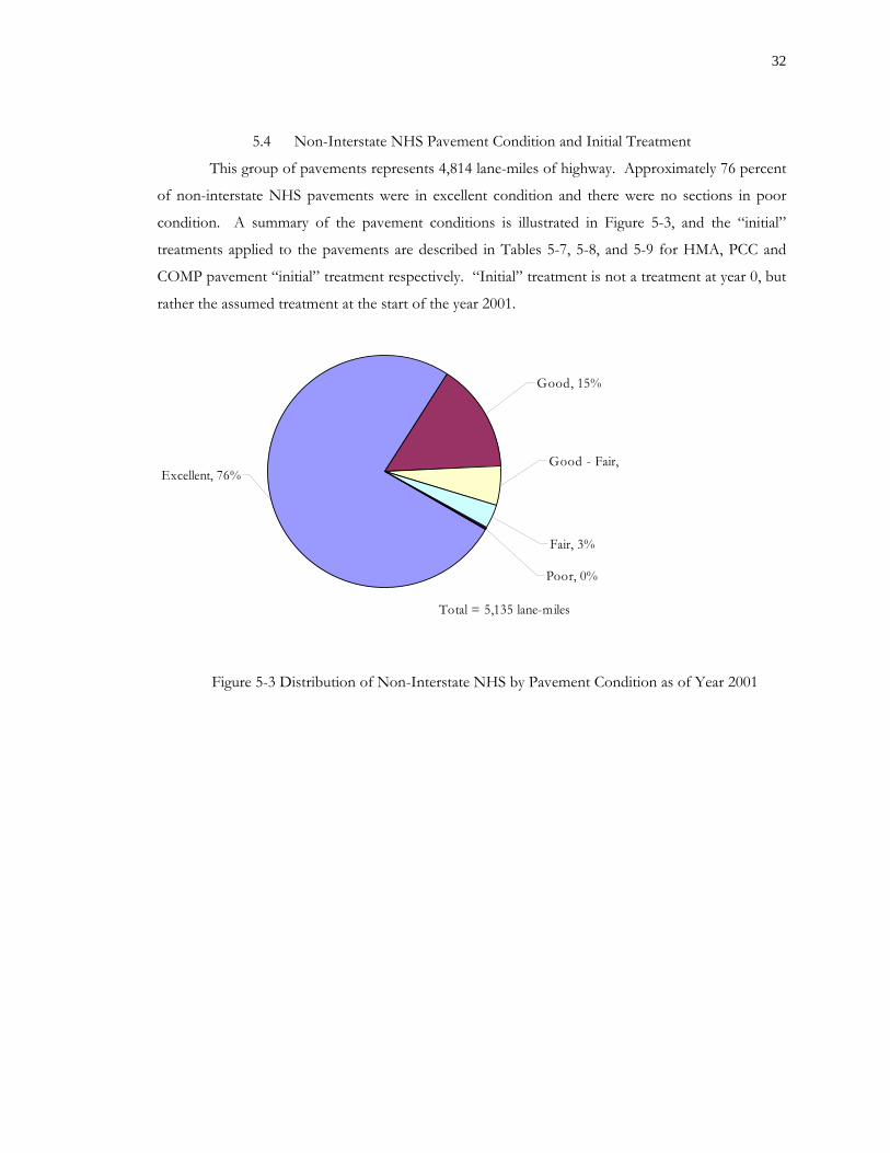
32

5.4 Non-Interstate NHS Pavement Condition and Initial Treatment

This group of pavements represents 4,814 lane-miles of highway. Approximately 76 percent

of non-interstate NHS pavements were in excellent condition and there were no sections in poor

condition. A summary of the pavement conditions is illustrated in Figure 5-3, and the “initial”

treatments applied to the pavements are described in Tables 5-7, 5-8, and 5-9 for HMA, PCC and

COMP pavement “initial” treatment respectively. “Initial” treatment is not a treatment at year 0, but

rather the assumed treatment at the start of the year 2001.

Figure 5-3 Distribution of Non-Interstate NHS by Pavement Condition as of Year 2001

Total = 5,135 lane-miles

Poor, 0%

Fair, 3%

Good - Fair,

Good, 15%

Excellent, 76%


Poor, 0%

Fair, 3%

Good - Fair,

Good, 15%

Excellent, 76%


Poor, 0%

Fair, 3%

Good - Fair,

Good, 15%

Excellent, 76%

33

Table 5-7 Non-Interstate NHS HMA Pavement Treatment Thresholds

Table 5-8 Non-Interstate NHS PCC Pavement Treatment Thresholds




Excellent-Good (IRI= 60 - 100) Trigger >118 76 3267 Do Nothing



Maintenance Fair






Lane-miles




Good – Fair (IRI = 126 -150) Trigger >134 139 108 Joint and Crack

Sealing

Fair (IRI= 151 - 200) Trigger >151 162 35 Resurfacing Partial

3-R Standards

Poor (IRI= > 200) Trigger >200 n/a 0 Reconstruction


34

5.5 Non-Interstate Non-NHS Pavement Condition and Initial Treatment

With 19,170 lane-miles, this pavement family represents the largest category in the analysis.

Sixty-six percent of pavements in this family were in excellent condition and one percent were in

poor condition. Tables 5-10, 5-11 and 5-12 present the initial conditions and initial treatments to

HMA, PCC, and COMP pavements respectively.






Good – Fair (IRI = 126 -150) Trigger >134 n/a 0 Preventive

Maintenance Fair


Poor (IRI = > 200) Trigger >200 n/a 0 Reconstruction


Table 5-9 Non-Interstate NHS COMP Pavement Treatment Thresholds

35

Figure 5-4 Distribution of Non-Interstate Non-NHS by Pavement Condition as of Year

2001



Lane-miles




Good – Fair (IRI = 126 -150) Trigger >134 136 1771 Preventive Maintenance

Fair (IRI = 151 – 200) Trigger >151 169 961 Resurfacing Partial 3-R

Standards Poor

(IRI = > 200) Trigger >200 222 184 Reconstruction


Table 5-10 Non-Interstate, Non-NHS, HMA Pavement Treatment Thresholds


Good-to-Fair, 10%

Good, 18%

Fair, 5%Poor, 1%

Excellent66%


Good-to-Fair, 10%

Good, 18%

Fair, 5%Poor, 1%

Excellent66%


Good-to-Fair, 10%

Good, 18%

Fair, 5%Poor, 1%

Excellent66%


Good-to-Fair, 10%

Good, 18%

Fair, 5%Poor, 1%

Excellent66%


Good-to-Fair, 10%

Good, 18%

Fair, 5%Poor, 1%

Excellent66%

36



Lane-miles




Good – Fair (IRI = 126 -150) Trigger >134 135 76 Joint and Crack

Sealing Fair

(IRI = 151 – 200) Trigger >151 170 61 Resurfacing Partial 3-R Standards





Lane-miles




Good – Fair (IRI = 126 -150) Trigger >134 131 21 Preventive Maintenance

Fair (IRI = 151 – 200) Trigger >151 152 1 Resurfacing Partial 3-R

Standards Poor

(IRI = > 200) Trigger >200 n/a 0 Reconstruction


The methodology used for the treatment of pavements that were initially in poor condition

is illustrated in Figure 5-5. Pavements in fair condition follow a similar process, but the analyst

compares the initial IRI to 151 and the initial treatment for pavements with IRI >151 would be

Resurfacing Partial 3-R Standards.

Table 5-11 Non-Interstate Non-NHS PCC Pavement Treatment Thresholds

Table 5-12 Non-Interstate Non-NHS COMP Pavement Treatment Thresholds

37

Figure 5-5 Methodology for Poor Pavements

Compare Initial Pavement Condition to IRI

Triggers

Annual Maintenance

Apply AAMEX

2005-2020

Initial Treatment IRI >200

Apply Pavement

Reconstruction

Improve IRI IRI Jump

53.5 points

PCC Pavement Treatment

Joint and Crack Sealing

HMA Pavement Treatment

Thin Overlay


22.7 points


6 or 8 IRI per year

IRI >118 IRI <118 Do Nothing

HMA Pavement

IRI Improved to 60

PCC Pavement

IRI Improved to 70


Triggers

Annual Maintenance

Apply AAMEX

2005-2020


Apply Pavement

Reconstruction


53.5 points




Thin Overlay


22.7 points


6 or 8 IRI per year


HMA Pavement

IRI Improved to 60

PCC Pavement

IRI Improved to 70


Triggers

Annual Maintenance

Apply AAMEX

2005-2020


Apply Pavement

Reconstruction


53.5 points




Thin Overlay


22.7 points


6 or 8 IRI per year


HMA Pavement

IRI Improved to 60

PCC Pavement

IRI Improved to 70

38

5.6 Network Analysis Results

As previously discussed, the manual condition analysis method utilizes information on

average costs per lane-mile for treatments by pavement type as described by Lamptey et al. (2004)

and average annual maintenance expenditure (AAMEX) models by Labi and Sinha (2003). The total

pavement needs included the costs to maintain the existing pavement.

Scenario A uses a pavement deterioration rate of 8.0 IRI per year, and Scenario B uses a

pavement deterioration rate of 6.0 IRI per year. The 15-year pavement preservation need for existing

roads under Scenario A for the period 2006-2020 is $5,544,222,285; while under Scenario B it is

$4,938,927,145; as shown in Tables 5-13 and 5-14. The preservation needs discussed in this section

do not include any shoulder work or added-capacity projects. The term “repairs only” applies to

those costs associated with the “initial” treatments applied in the year 2001. The 15-year need

between 2006 and 2020 was estimated by deducting the expected preservation expenditures during

2002-2005 from the 2002-2020 needs. Data from 2002 and 2003 was used to estimate preservation

expenditures during 2002-2005.

Interstate Non-Interstate NHS

Non-Interstate Non NHS

Total all Locations

Lane-Miles of Analysis 4,143 4,814 17,972 26,929 2002 Initial Repair Costs $30,152,561 $77,218,728 $729,036,542 $836,407,831

2002 AAMEX $3,507,973 $6,742,570 $25,451,291 $35,701,834 Deterioration

2003-2020 $519,055,202 $672,580,430 $2,917,184,584 $4,108,820,216

AAMEX 2003-2020 $59,635,545 $114,623,682 $432,671,952 $606,931,179 Planning & Design (9%)

(Repairs Only) $49,428,699 $67,481,924 $328,159,901 $445,070,524

Cost Overruns (10%) (Repairs Only) $56,062,154 $81,546,915 $397,305,002 $534,914,072

Subtotal 2002-2020 $717,842,134 $1,020,194,249 $4,829,809,273 $6,567,845,656 Less 2002-2005 Spendinga -$1,023,623,371

Adjusted Subtotal $5,544,222,285a. Based on FY 2002 and FY 2003 highway infrastructure spending on pavement preservation data received from the Budget and Fiscal Management Division of INDOT. Costs are expressed in Year 2002 constant dollars. The term “repairs only” applies to those costs associated with the “initial” treatment applied in the year 2001. Added-capacity improvements are not included in the costs.

Table 5-13 Fifteen-year Pavement Condition Preservation Needs Scenario A

39

Interstate Non-Interstate NHS

Non-Interstate Non NHS

Total all Locations

Lane-Miles of Analysis 4,419 5,135 19,170 28,725 2002 Initial Repair Costs $30,152,561 $77,218,728 $729,036,542 $836,407,831

2002 AAMEX $3,507,973 $6,742,570 $25,451,291 $35,701,834 Deterioration 2003-2020 $512,200,685 $617,304,103 $2,478,419,895 $3,607,924,683

AAMEX 2003-2020 $57,037,087 $113,467,786 $431,719,453 $602,224,326 Planning & Design (9%)

(Repairs Only) $48,811,792 $62,507,055 $288,671,079 $399,989,926

Cost Overruns (10%) (Repairs Only) $55,364,129 $75,527,578 $349,410,208 $480,301,916

Subtotal 2002-2020 $707,074,228 $952,767,820 $4,302,708,468 $5,962,550,516 Less 2002-2005 Spendinga -$1,023,623,371

Adjusted Subtotal $4,938,927,145a. Based on FY 2002 and FY 2003 highway infrastructure spending on pavement preservation data received from the INDOT’s Budget and Fiscal Management Division. The term “repairs only” applies to those costs associated with the “initial” treatment applied in the year 2001. Added-capacity improvements are not included in the costs. Costs are expressed in Year 2002 constant dollars.

Table 5-14 Fifteen-year Pavement Condition Preservation Needs Scenario B

40

CHAPTER 6 : PROCEDURE FOR EVALUATING ANNUAL PAVEMENT

PRESERVATION COST

For fiscal planning and programming, it is necessary to know the expected costs of

preservation projects. However, it is not certain that the current version of INDOT’s Pavement and

Bridge Management systems incorporates a direct and comprehensive analysis of the costs and

service lives in a manner that would be consistent with INDOT’s financial planners. There is a need

to develop simple and reliable procedures in order for INDOT’s planners to be able to predict

preservation costs without going through a complex modeling process. The following procedure was

developed in order to help INDOT’s Policy and Fiscal Management and Planning divisions predict

properly the dollars needed each year for pavement preservation activities. These activities do not

include new pavement construction. The developed procedure is based on the fact that there is a

correlation between time and the percentage of lane miles of the state roads that receive preservation

activities each year. Given that the rate at which the system size increases is very constant, it is

possible to predict for any given year the number of lane miles that are going to be treated. Using the

average unit costs of preservation for the preceding years (2 or 3 generally), the total preservation

cost can be derived easily. This cost can then be broken down by rehabilitation and non

rehabilitation activities, which comprise maintenance and reconstruction. Costs per functional system

can also be determined. The following categories are considered: Interstate roads, Non Interstate

roads that are on the National Highway System (NHS) and finally state roads that are not on the

NHS.

The procedure can be summarized as follows:

1. System size prediction

2. Percentage of system to be treated

3. Estimation of total preservation cost using unit cost per lane mile

4. Rehabilitation and Non-rehabilitation cost (maintenance and reconstruction)

5. Preservation cost by functional system

41

6.1 Total System Size Prediction

First, the number of lane miles in the system for each year was plotted against the years. A

statistical relation was estimated that enables the determination of the total size of Indiana’s state

highway system for any given year, as follows:

Number of lanes miles = 83.275*YEAR - 138144 (1)

The observed data and the plot are shown as Figure 6-1. Using the developed equation, the

system size of Indiana’s state highway system for each future year can be determined through

extrapolation.

Figure 6-1 Indiana’s highway system size versus time

y = 83.275x - 138144R2 = 0.9853

27400

27600

27800

28000

28200

28400

28600

1990 1992 1994 1996 1998 2000 2002

Years (since 1990)

ln-m

iles

y = 83.275x - 138144R2 = 0.9853

27400

27600

27800

28000

28200

28400

28600

1990 1992 1994 1996 1998 2000 2002

Years (since 1990)

ln-m

iles

y = 83.275x - 138144R2 = 0.9853

27400

27600

27800

28000

28200

28400

28600

1990 1992 1994 1996 1998 2000 2002

Years (since 1990)

ln-m

iles

42

Example: For the year 2008, the total number of lane-miles in the state can be estimated to be:

Number of lane miles = 83.275*2008 – 138,144 = 29,072 lane miles

6.2 Percentage of system to be treated

The percentage of lane miles in the system receiving preservation treatment each year was

plotted against the years. A time series model was then developed and the following statistical

relationship (2) that predicts the percentage of the system that will receive preservation treatment for

any given year was estimated. The data obtained is shown on Figure 6-2.

Percentage of system to be preserved = 0.0328* (# of years from 1990) ^ (0.3513) (2)

Figure 6-2 Percentage of system preserved versus time

y = 0.0328x0.3513

R2 = 0.6924

0

0.01

0.02

0.03

0.04

0.05

0.06

0.07

0.08

0.09

0 2 4 6 8 10 12 14Years (since 1990)

% o

f la

ne

mile

s tr

eate

d

y = 0.0328x0.3513

R2 = 0.6924

0

0.01

0.02

0.03

0.04

0.05

0.06

0.07

0.08

0.09

0 2 4 6 8 10 12 14Years (since 1990)

% o

f la

ne

mile

s tr

eate

d

y = 0.0328x0.3513

R2 = 0.6924

0

0.01

0.02

0.03

0.04

0.05

0.06

0.07

0.08

0.09

0 2 4 6 8 10 12 14Years (since 1990)

% o

f la

ne

mile

s tr

eate

d

y = 0.0328x0.3513

R2 = 0.6924

0

0.01

0.02

0.03

0.04

0.05

0.06

0.07

0.08

0.09

0 2 4 6 8 10 12 14Years (since 1990)

% o

f la

ne

mile

s tr

eate

d

43

Example: The percentage of the system that is going to receive a treatment in 2008 can be

determined as follows:

% of system = 0.0328*19^ (0.3513) = 0.092278

Therefore, the number of lane miles in the system on which preservation activities are going

to be performed can be derived, using the following relationship:

Number of lane miles to be treated = %percentage of system to be treated * system size (3)

In 2008, the number of lane miles that are going to receive a treatment can be estimated at:

# of lane miles to receive treatment = 0.092278 * 29072.2 = 2682.72 lane miles

6.3 Estimation of total preservation cost using unit cost per lane mile

The total preservation cost for the entire system can be obtained by multiplying the number of

lane miles to be treated by the average unit cost for preservation for the last 3 years.

Average unit cost from 1999 to 2001 = $151,375.69

Thus, the total cost to preserve the system can be estimated by multiplying the unit cost to

the total number of lane miles to be treated. The following relationship enables to estimate the total

preservation cost for pavements:

Total cost of preservation = Number of lane miles to be treated* Average unit cost for the past 3 years. (4)

Example: In 2008, the total cost to preserve the pavement in the system in 2008 will be:

Found in step 1

44

Total cost of preservation = 2682.72 *$151,375.69 = $406,098,591

Using the same procedure, the pavement preservation costs for 2002 and 2003 can be predicted and

compared to the true values as shown on Table 6-1.

The values found are consistent with the engineering needs determined in the previous chapter. The

average annual pavement preservation cost for the 15-year period 2006-2020 is estimated at $331,784

to $369,615 in the previous chapter.

Table 6-1 Comparison of Actual and Predicted Pavement Preservation Costs for

2002 and 2003

Years Actual Expenditure Predicted value Percentage difference

2002 $335,600,000 $349,306,993 + 4%

2003 $318,408,552 $359,565,218 + 13%

45

6.4 Rehabilitation and Non rehabilitation cost

- Percentage of lane miles rehabilitated The number of lane miles rehabilitated each year as a percentage of the system is plotted against the

years and a correlation was found. The following statistical relationship estimates the percentage of

the system to be rehabilitated for any given year.

% of system = 0.0248* (# of years from 1990) ^ (0.3705) (5)

The plot and the observed data are shown on Figure 6-3. The percentage of the system to be

rehabilitated can be determined through extrapolation using the developed equation.

Figure 6-3 Percentage of system rehabilitated versus time

y = 0.0248x0.3705

R2 = 0.5799

0

0.01

0.02

0.03

0.04

0.05

0.06

0.07

0.08

0 2 4 6 8 10 12 14

Years (since 1990)

% o

f sy

stem

y = 0.0248x0.3705

R2 = 0.5799

0

0.01

0.02

0.03

0.04

0.05

0.06

0.07

0.08

0 2 4 6 8 10 12 14

Years (since 1990)

% o

f sy

stem

y = 0.0248x0.3705

R2 = 0.5799

0

0.01

0.02

0.03

0.04

0.05

0.06

0.07

0.08

0 2 4 6 8 10 12 14

Years (since 1990)

% o

f sy

stem

y = 0.0248x0.3705

R2 = 0.5799

0

0.01

0.02

0.03

0.04

0.05

0.06

0.07

0.08

0 2 4 6 8 10 12 14

Years (since 1990)

% o

f sy

stem

46

Example: The percentage of the system that is going to be rehabilitated in 2008 is:

% of system = 0.0248*19^ (0.3705) = 0.0738

The number of lane miles to be rehabilitated each year can be easily derived using the following

simple relationship:

Number of lane miles to be rehabilitated = %percentage of system to be rehabilitated * system size (6)

In 2008, number of lane miles on which rehabilitation activities are going to be performed is:

Number of lane miles to be rehabilitated = 0.0738*29072.2 = 2145.52 lane miles

- Total cost of rehabilitation

The total cost of rehabilitation can be derived by using the average unit cost per lane mile calculated

for the past three years.

Average unit cost of rehabilitation for past 3 years (199-2001) = $121,851.738

Therefore, the total cost of rehabilitation activities can be estimated by the following simple and

direct relationship:

Total cost of rehabilitation = Number of lane miles to be rehabilitated * Average unit cost for the past 3 years

(7)

Example: Using the same example for the year 2008, the total cost needed to rehabilitate pavements

is estimated at:

Total cost of rehabilitation = 2145.52 *$121,851.738= $261,436,359

47

- Non-rehabilitation cost (Maintenance + Reconstruction)

Knowing the preservation cost and the rehabilitation cost, the amount to be spent on

maintenance and reconstruction can be directly determined by taking the difference.

Non Rehabilitation cost = Total preservation cost – Rehabilitation cost (8)

Example: In 2008, non rehabilitation costs can be predicted to be:

Non Rehabilitation cost = $406,098,591 - $261,436,359 = $144,662,231.4

6.5 Preservation cost by Highway Class

To estimate, the pavement preservation cost for each highway class, the percentage of money

spent on each highway class found for the last two years can be used.

For example, Table 6-2 gives the percentage of money spent on the different highway classes

in 2001 and 2000.

INT NIN NNN

2001 0.2244 0.2768 0.4987

2000 0.1632 0.3929 0.4438

* INT: Interstate roads

NIN: Non Interstate roads in the NHS (National Highway System)

NNN: State roads that are not in the NHS.

Therefore, the average can be taken and the pavement preservation cost for each highway class can

be found.

Example: If these averages are used to predict the preservation cost by highway class for 2008, the

total pavement preservation cost found above will be multiplied by the averages calculated. Thus the

pavement preservation costs in 2008 predicted for each highway class are shown on Table 6-3.

Table 6-2 Percentage of money spent on different highway classes (2000 and 2001)

48

P.C. of Cost

Average of 2000/2001

Estimated Pavement

Preservation Cost

INT 0.1938 $78,701,906

NIN 0.3348 $135,961,808

NNN 0.4712 $191,353,656

Table 6-3 2008 Pavement Preservation Costs by Highway Class

49

CHAPTER 7 : DEVELOPMENT OF BRIDGE PRESERVATION COST MODELS

7.1 Introduction The current version of the bridge management software used by INDOT incorporates up to

50 distinct project types. However, no direct and comprehensive analysis of construction costs of

these project types has been conducted to date. In the absence of recent cost analysis efforts and

models, INDOT bridge management engineers resort to the use of cost values developed several

years ago (Saito et al., 1988), duly adjusted for inflation. Although the cost estimates from the earlier

study may appear reasonable, their continued reliability has not been tested against current cost

expenditures. Also, changes in construction materials and technological advances are likely to have a

significant impact on unit costs of various bridge preservation treatments. According to NCHRP

Synthesis 227 (Thompson and Markow, 1996) lack of reliable sources for accurate cost data is a

problem faced by current bridge management systems. Uncertainties in cost analysis can lead to

incorrect decisions, particularly in selecting feasible strategies.

After an investigation of recent contracts and identification of the work performed in each

contract, it was found that the available data would allow the development of cost models for the

following activities:

1) Bridge replacement

2) Deck rehabilitation

3) Deck rehabilitation and superstructure rehabilitation

4) Deck replacement

5) Deck replacement, superstructure, and substructure rehabilitation

6) Deck replacement and superstructure rehabilitation

7) Superstructure replacement

8) Superstructure replacement and substructure rehabilitation

9) Bridge widening

50

In the present chapter, the results obtained for the different models developed are presented and the

best models for prediction are also specified.

7.2 Cost Estimation of Bridge Replacement

Bridge replacement entails a complete replacement of the entire bridge structure. Some

bridges that are replaced also may be widened. Bridge replacement costs depend on the length, width,

and height of the bridge; the number and length of individual spans; the superstructure material and

substructure material; structural type; bridge location; and feature being crossed such as a rail, or

highway or river (Hawk, 2003). The cost models were developed on the basis of 82 bridge replacement contracts during the

time period 1996 to 2002. The bridge replacement cost items were divided into four categories:

1) Superstructure Replacement Cost (SUPC),

2) Substructure Replacement Cost (SUBC),

4) Approach Cost (APPC),

3) “Other Cost” (OTHC).

Separate models were developed for these four cost components. Each of these cost

components was represented as a function of bridge characteristics and other indirect factors such as

location or weather. The total bridge replacement cost is the summation of the four cost

components. The best models were determined after validation on the basis of the Root Mean

Square Error (RMSE).

51

7.2.1 Slab Bridge Replacement Cost Models

The schematic illustration of a typical concrete slab bridge types is shown in Figure 7-1.

Deck slab structures are the simplest type of bridge superstructures. Also, slab bridges are the easiest

to construct and are frequently used for relatively short spans. The structural form of deck slabs is

very efficient at distributing point loads because of its two-way spanning ability and high torsional

strength (Gupta, 2003).

It was found that on average, the superstructure replacement cost component accounted for

24% of the total replacement cost, while the contribution of the substructure to replacement costs

was the least at 9%. Approach cost represented the largest part of the total replacement cost (almost

41%), while the share of the “other cost” component was 26%.

7.2.1.1 Superstructure Replacement Cost Model for Slab Bridges

Initial analysis showed that for slab bridges, the deck area has a strong influence on the total

superstructure cost. As expected, the larger the deck area, the higher the superstructure cost.

For modeling, several functional forms were explored, including the linear form. On Table 7-1 is

shown a summary of the Superstructure Replacement Cost Models developed for Slab Bridges.

Figure 7-1 Schematic Illustration of Typical Concrete Slab Bridge Types

Section A-A A

A

52

MODEL FORM MODEL R2

Linear SUPC = -19.451 + 1.392 * BL +1.134 * TDW + 39.585*Pre-stressed 0.417

Cobb-Douglas (1) SUPC = 0.0806*BL1.0053TDW0.814 0.545

Constrained Cobb-Douglas SUPC = 0.06045*BL0.999TDW0.841 0.535

Cobb-Douglas (2) SUPC = (0.2598+0.066*Pre-stressed)*BL0.8122*TDW0.7223 0.616

Transformed Cobb-Douglas SUPC = EXP (0.477383* BL0.3150*TDW0.250) 0.743

SUPC is the total superstructure cost in $1000’s year 2002 BL is the bridge length in feet TDW is the total deck width in feet Pre-stressed is 1 if superstructure is made of pre-stressed concrete, 0 otherwise

The models with highest R2 were chosen for validation: the Cobb-Douglas (2) and the Transformed

Cobb-Douglas model. After validation, the Cobb-Douglas (2) model, with the pre-stressed variable

included, showed the best performance. Table 7-2 shows the details of this model.

SUPC = (A + B * Pre-stressed)* BLC*TDWD

[Cobb-Douglas (2) Form]

Explanatory Variable Coefficient Standard Error t-Statistic

Constant A 0.2598 0.0921 2.8212

Pre-stressed B 0.0660 0.0382 1.7290

BL C 0.8122 0.1964 4.0839

TDW D 0.7223 0.1745 3.8926

R2 = 0.616, N = 26

Table 7-1 Summary of Superstructure Replacement Cost Models for Slab Bridges

Table 7-2 Details of Best Superstructure Replacement Cost Model for Slab Bridges

53

7.2.1.2 Substructure Replacement Cost Models for Slab Bridges

A similar analysis was performed for the substructure replacement cost for slab bridges. A

positive trend in the relationship between the total substructure replacement cost and the deck area

was also found for slab bridges. Several functional forms were investigated. A summary of the results

are presented in Table 7-3 and the details of the best model after validation are given in Table 7-4.

Although the R2 value was not high, the variables included were found to be highly significant.

MODEL FORM MODEL R2

Linear SUBC= 15.919 +3.634* SUBH 0.147

Average Cost SUBC= 5.1292* SUBH 0.149

Cobb-Douglas SUBC = 1.2603*BL 0.1124 TDW 0.3914 SUBH 0.767 0.267

Transformed Cobb-Douglass SUBC = exp (3.0449 *SUBH 0.0869) 0.327

SUBC is the total substructure replacement cost expressed in $1000’s year 2002 constant dollar SUBH is the substructure height in feet

SUBC = exp (A* SUBHB)

[Transformed Cobb-Douglas Form]


Constant A 3.0449 0.2831 10.7567

SUBH B 0.0869 0.0272 3.1988

R2 = 0.327, N = 24

7.2.1.3 Approach Replacement Cost for Slab Bridges

Data on bridge approach lengths were not available. Therefore, approach cost was modeled

in terms of other variables besides the approach length. However, due to the poor R2, even for the

Table 7-3 Summary of the Substructure Replacement Cost Models for Slab Bridges

Table 7-4 Details of Best Substructure Replacement Cost Model for Slab Bridges

54

best model, it was decided to estimate the approach replacement cost for slab bridges using an

average cost of $73.11 per square foot of deck area.

7.2.1.4 “Other Cost” for Slab Bridge Replacement

“Other cost” includes all those items related to traffic control measures, excavation,

mobilization and demobilization, and office expenses. As the R2 was poor for all models, it was

decided to use an average cost of $49.12 per square foot of deck area for estimation of the “other

cost” for slab bridge replacement cost.

7.2.2 Pre-stressed Beam Bridge Replacement Cost Models

Beam or girder superstructure types consist of a deck slab supported by longitudinal beams

or girders as illustrated in Figure 7-2. The longitudinal beam or girders may in turn be supported by

abutments, piers, bents, or floor beams (Gupta, 2003). The longitudinal beams or girders may have

any cross section, with I, T, or box sections being the most common in Indiana. These elements may

be in either reinforced or pre-stressed concrete. However, in the present dataset, bridges of this type

had only pre-stressed element sections. One characteristic of such superstructures is the use of

transverse intermediate diaphragms.

Figure 7-2 Schematic Illustration of Typical Pre-stressed Concrete Bridge Sections

55

7.2.2.1 Superstructure Replacement Cost Model for Pre-stressed Beam Bridges

A summary of the models developed for the superstructure replacement of pre-stressed

beam bridges is shown on Table 7-5. The superstructure replacement cost for pre-stressed beam

bridges was found to be independent of substructure height. After validation, the Transformed

Cobb-Douglas Form was the best model and its details are shown on Table 7-6.

MODEL FORM MODEL R2

Linear SUPC = -26.544 + 0.051 * DA 0.968

Cobb-Douglas SUPC=0.0244* BL 1.0879 * TDW 1.0424 0.972

Constrained Cobb-Douglas SUPC=0.05308* BL 1.000 * TDW 0.98236 0.967

Transformed Cobb-Douglas SUPC= exp(0.632*BL0.166*TDW0.1394) 0.977

SUPC is the superstructure replacement cost for beam bridges in $1000 (Year 2002) DA is the deck area in square feet BL is the bridge length in feet TDW is the total deck width in feet

SUPC=EXP(A* BLB*TDWC)

[Transformed Cobb-Douglas Form]


Constant A 0.6328 0.0486 2.0952

BL B 0.1667 0.0050 27.3493

TDW C 0.1395 0.0201 12.4800

R2 = 0.977, N = 32

Table 7-5 Summary of Superstructure Replacement Cost Models for Pre-stressed Beam Bridges

Table 7-6 Details of Best Model for Superstructure Replacement Cost of Pre-stressed Beam

Bridges

56

7.2.1.4 7.2.2.2 Substructure Replacement Cost Models for Pre-stressed Beam Bridges

Substructure cost was found to have a strong relationship with deck area. Various functional

forms were tested, and the best models are presented on Table 7-7. After validation, it was concluded

that the linear form was the most appropriate model for estimating substructure replacement cost for

pre-stressed beam bridges. Table 7-8 presents details of the linear model.

MODEL FORM MODEL R2

Linear SUBC = -37.848 + 0.023 * DA 0.850

Cobb-Douglas SUBC = 0.4867*BL1.1070 0.834

Constrained Cobb-Douglas SUBC = 0.9564718*BL1.000 0.826

SUBC=A+B*DA

[Linear Form]


Constant A -37.848 21.811 -1.735

DA B 0.023 0.002 13.097

R2 = 0.850, N = 32

7.2.1.5 7.2.2.3 Approach Cost for Replacement of Pre-stressed Beam Bridges

Assuming that the approach length is directly proportional to the bridge length, it is

expected that the approach cost would have a direct relationship with the bridge length. Three

models are presented in Table 7-9, and the best model was found to be the Constrained Cobb-

Douglas after validation.

Table 7-7 Summary of Substructure Replacement Cost Models for Pre-stressed Beam Bridges

Table 7-8 Details of Best Substructure Replacement Cost Model for Pre-stressed Beam Bridges

57

MODEL FORM MODEL R2

Linear APPC = -771.858+0.563 * BL +19.047 * TDW + 18.708 *SUBH 0.654

Cobb-Douglas APPC = 0.2884*BL0.2990*TDW1.1518 * SUBH 0.5517 0.742

Constrained Cobb-Douglas APPC = 0.7206*BL0.2784*TDW0.9464 * SUBH 0.5567 0.731

Transformed Cobb-Douglas APPC = exp (1.758* BL 0.084 *TDW 0.166 *SUBH 0.065) 0.699

APPC = A* BLB*TDWC* SUBH D

[Constrained Cobb Douglas Form]


Constant A 0.7206 0.6802 1.0593

BL B 0.2784 0.1165 2.3900

TDW C 0.9464 0.2195 4.3111

SUBH D 0.5567 0.2085 2.6703

R2 = 0.731, N = 32

7.2.1.6 7.2.2.4 “Other Cost” for Pre-stressed Beam Bridge Replacement

A summary of all models developed for this category is presented in Table 7-11. Upon

validation, the Constrained Cobb Douglas Model was found to be the best model; Table 7-12

presents details of the Constrained Cobb-Douglas model.

Table 7-9 Summary of the Approach Cost Models for Pre-stressed Beam Bridge Replacement

Table 7-10 Details of Best Approach Cost Model for Pre-stressed Beam Bridge Replacement

58

MODEL FORM MODEL R2

Linear OTHC = -784.420+0.682* BL + 17.425*TDW +16.373 *SUBH 0.751

Cobb-Douglas OTHC= 0.0422* BL0.4283* TDW1.3412 * SUBH 0.6577 0.847

Constrained Cobb-Douglas OTHC= 0.15008* BL0.43493* TDW1.000 * SUBH 0.65372 0.823

Transformed Cobb-Douglas OTHC= exp(1.687109* BL0.093161* TDW0.093161 * SUBH 0.1319967) 0.810

OTHC = A* BLB* SUBHC *TDW

[Cobb-Douglas Form]


Constant A 0.1501 0.0902 1.6646

BL B 0.4349 0.0943 4.6124

SUBH C 0.6537 0.1998 3.2714

R2 = 0.823, N = 32

7.2.3 Steel Bridge Replacement Cost

Due to the insufficient number of observations, it was not possible to develop steel bridge

replacement cost models. The construction types of steel bridges in the dataset were steel beam, plate

girder, and box girder bridges (Appendix E). Steel beam bridge spans ranged from 10 to 17 feet, and

are typically used for small road bridges. Plate girder bridge spans ranged from 20 to 200 feet.

Average unit costs for the replacement of the various bridge elements are presented in Table 7-13. In

comparison with those for concrete bridges, steel superstructure replacement unit costs were

relatively low. However, the approach and “other cost” per square feet of deck area for steel bridges

were higher than for concrete bridges. Finally, the total bridge replacement unit cost for steel bridges

was lower than the total unit cost for concrete bridges, as shown in Figure 7-3. The results should be

used with caution as the sample size for steel bridges was relatively small.

Table 7-11 Summary of the “Other Cost” Models for Pre-stressed Beam Bridge Replacement

Table 7-12 Details of Best “Other Cost” Model for Beam Bridge Replacement

59

Unit Cost per ft2 of Deck Area STEEL BRIDGES Number of

Observations Mean Minimum Maximum Std. Deviation

Unit Super Replacement Cost 6 56.66 52.02 67.54 7.06

Unit Sub Replacement Cost 6 17.12 10.54 31.26 9.28

Unit Approach Cost 6 56.35 33.35 102.59 32.18

Unit “Other Cost” 6 45.12 22.68 71.13 20.99

Total Unit Cost 6 176.94 122.12 248.41 53.34

Costs expressed in Year 2002 constant dollar.

$46$17

$71$54

$203

$56

$17

$56 $45

$177

$0

$50

$100

$150

$200

$250

Superstructure Substructure Approach Other Total

Uni

t Cos

t ($

per

sq. f

t. of

dec

k ar

ea)

Concrete Steel Concrete Steel Concrete Steel Concrete Steel Concrete Steel

7.2.4 Summary and Conclusions for Bridge Replacement Cost Modeling

Bridge replacement costs were analyzed for concrete and steel bridges. For concrete bridges,

sufficient data was available and models were developed. For steel bridges there was insufficient

number of observations therefore only unit cost values were estimated. The recommended models

with for prediction purposes are shown in Table 7-14.

It was found that the total bridge replacement unit cost for steel bridges was lower than for

concrete bridges and this was largely attributed to the lower approach costs and “other” unit costs

for steel bridges compared to such costs for concrete bridges. In general, it was found that approach

and “other cost” represented over 50% of the total replacement cost.

Table 7-13 Descriptive Statistics of Replacement Unit Cost: for Steel Structure

Figure 7-3 Comparison of Unit Cost of Bridge Replacement between Steel and Concrete Bridges

60

Super

Type Cost

Unit Cost

($/ft2) Bridge Replacement Cost Models R2

SUPC 43.01 SUPC = EXP (0.4774* BL0.3150*TDW0.250) 0.74

SUBC 16.26 SUBC = exp (3.0449 * SUBH 0.0869) 0.33

APPC 73.11 APPC = 53.6713 + 0.1970 * ADT 0.29

Slab

Brid

ges

OTHC 49.12 OTHC = BL 1.1273 0.30

SUPC 46.35 SUPC = exp(0.6320 * BL0.1661 * TDW0.1394) 0.98

SUBC 16.58 SUBC = exp (0.5811 * BL0.2245 * TDW0.1530 * SUBH0.1133) 0.84

APPC 70.88 APPC = 0.7206 * BL0.2784 * TDW0.9464 * SUBH 0.5567 0.73

Beam

Brid

ge

OTHC 55.08 OTHC = 0.1501 * BL0.4349 * TDW1.000 * SUBH 0.6537 0.82

SUPC 56.66 SUPC = 56.66* DA NA

SUBC 17.12 SUBC = 17.12* DA NA

APPC 56.35 APPC = 56.35* DA NA

Stee

l Brid

ge

OTHC 45.12 OTHC = 45.12* DA NA

SUPC is the superstructure replacement cost in $1000 (expressed in Year 2002 constant dollar) SUBC is the substructure replacement cost in $1000 (expressed in Year 2002 constant dollar) APPC is the approach cost in $1000 (expressed in Year 2002 constant dollar) OTHC is the “other cost” in $1000 (expressed in Year 2002 constant dollar) BL is the bridge length in feet TDW is the total deck width in feet SUBH is the substructure Height in feet ADT is the Average Daily Traffic

Table 7-14 Summary of Bridge Replacement Cost for Concrete Bridges

61

7.3 Cost Estimation for Bridge Rehabilitation Activities

Rehabilitation and repair activities are major repairs that are usually performed by

contractors. These activities include functional and structural improvements such as bridge widening,

bridge raising, lowering pavement thickness and structure strengthening. Figure 7-4 shows the

rehabilitation activities identified in the dataset after an exhaustive examination of recent INDOT

bridge contracts. The number of observations found in each category type is shown in parenthesis.

Figure 7-4 Classification of Rehabilitation Cost Models Developed in Present Study

Bridge Rehabilitation and Repair

Bridge Deck Reconstruction Cost

Superstructure Replacement Cost

Bridge Widening Cost (36 Observations)

Deck Rehabilitation Cost

Deck Replacement Cost

Cost of Superstructure Replacement (12 Observations)

Cost of Super Replacement + Sub Rehab (15 Observations)

Cost of Deck Rehab Only (66 Observations)Cost of Deck Rehab + Super Rehab (50 Observations)

Cost of Deck Replacement Only (5 Observations)

Cost of Deck Replacement + Super Rehab + Sub Rehab (4 Observations)

Cost of Deck Replacement + Super Rehab (14 Observations)

62

7.3.1 Deck Rehabilitation Cost Model

Deck rehabilitation contracts include such activities as the removal of structure railing and

deck overlay, full depth or partial deck patching, and deck overlay. Deck rehabilitation is the most

common bridge preservation activity and is typically applied to bridges approximately 20 years after

initial construction. Deck rehabilitation may also include other activities such as hydro-demolition,

deck transverse joint repair (sawing, cleaning, sealing), hole drilling, application of epoxy coating on

bars, concrete patching, and bridge railing restoration. The total rehabilitation cost for each contract

was divided into deck rehabilitation primary cost (DHC), which includes all items directly related to

the deck rehabilitation work, and “other cost” (OTHC) which are items such as traffic maintenance,

demolition, or clearing right-of-way. Summaries of the models developed to estimate primary costs

and “Other Costs” for deck rehabilitation are shown on Table 7-15 and 7-16.

MODEL FORM MODEL R2

Linear (1) DHC=0.0161*DA 0.527

Linear (1) DHC = 65.438+0.011 * DA 0.833

Cobb-Douglas DHC = 0.2110 * BL 0.6360 * TDW 0.8873 0.871

DHC is the deck rehabilitation cost in $1000’s year 2002 DA is the deck area in square feet BL is the bridge length in feet

TDW is the total deck width in feet

MODEL FORM MODEL R2

Linear (1) OTHC = 142.636 + 0.009 ADT 0.287

Linear (2) OTHUC = 52.8246 – 0.0023 DA 0.338

Inverse OTHUC= 166,103 / DA 0.739

OTHC is the total “other cost” in $1000’s year 2002 OTHUC is the unit “other cost” in $ year 2002 ADT is the Average Daily Traffic DA is the deck area in square feet

Table 7-15 Summary of Deck Rehabilitation Primary Cost Models for all Bridge Types

Table 7-16 Summary of “Other Cost” Models for Deck Rehabilitation Contracts

63

Table 7-17 and Table 7-18 present the details for the models considered best explain deck

rehabilitation primary and “other cost” respectively after validation.

DHC=A* BLB*TDWC

[Cobb-Douglas Form]

Explanatory Variable Coefficient Standard Error t-statistic

Constant A 0.2110 0.1181 1.786

BL B 0.6360 0.0358 17.746

TDW C 0.8873 0.1197 7.413

R2 = 0.871, N = 46

OTHUC=A / DA

[Inverse Form]


DA A 166103 7762.3841 21.3981

R2 = 0.739, N = 46

Table 7-17 Details of Best Deck Rehabilitation Primary Cost Model for all Bridge Types

Table 7-18 Details of Best Unit “Other Cost” Model for Deck Rehabilitation, all Bridge Types

64 7.3.2 Deck and Superstructure Rehabilitation Cost Model

The combined cost of deck and superstructure rehabilitation was modeled using deck

rehabilitation contracts where the superstructure rehabilitation cost accounted for over 5% of the

total contract cost. Those contracts had substantial superstructure rehabilitation and included such

simple items as jacking and supporting trusses or beams and cleaning and painting diaphragms as

well as more complex activities involving retrofit work, bearing assembly, beam repair, or

straightening steel beam. In deck and superstructure rehabilitation contracts, superstructure

rehabilitation items could account for 5-25% of the total cost.

Table 7-19 presents the linear models found for deck + superstructure rehabilitation primary

cost. However, no model was found appropriate to explain the “other cost.” Large variations in

“other cost” were caused by site characteristics and traffic control measures associated with the

project. Therefore, it was necessary to perform a one-way analysis of variance (ANOVA) on the deck

and superstructure rehabilitation “other cost” data with respect to the deck area. A unit “other cost”

of $31 per square foot for bridges with a deck area lower than 8,000 square feet, and $16 per square

foot above 8,000 square foot was found.

MODEL FORM MODEL R2

Linear (1) DSH = 119.571 – 0.016 * DA- 40.844 * Steel 0.671

Linear (2) DSH = 87.684 - 0.017 * DA 0.673

Linear (3) DSH = 75.606 + 93.986* NHS + 0.016 *DA 0.767

Linear (4) DSH = 103.911 + 0.015 * DA + 91.130 * NHS – 35.787 * Steel 0.784

Validation showed that the linear model 4 was the best of the models developed. Its details

are presented in Table 7-20.

Table 7-19 Summary of Primary Cost Models for Deck + Superstructure Rehabilitation for all

Bridge Types

65

DSH = A + B* DA + C*NHS + D*Steel

[Linear Form (4)]


Constant A 103.911 23.531 4.416

DA B 0.015 0.002 8.882

NHS C 91.130 23.815 3.827

Steel D -35.787 19.860 -1.802

R2 = 0.784, N = 38

DA is the deck area in square feet NHS is 1-for bridges on National Highway System, and 0- Otherwise Steel is 1- for steel bridges, 0- Otherwise

7.3.3 Deck Replacement Cost Model

Deck replacement consists of restoring bridge deck structural integrity by removal and

replacement of the existing deteriorated deck bridge. Deck replacement contracts involve not only

deck replacement but may include superstructure rehabilitation and/or substructure rehabilitation. In

the data used in the present study, only five contracts were identified to have deck replacement and

no other extra work, four contracts were identified to have substantial substructure and

superstructure rehabilitation work, and 15 contracts comprised not only deck replacement but also

superstructure rehabilitation. Due to data limitations, cost models could not be developed for deck

replacement only, and as such only average values were estimated for this category of preservation.

Deck Replacement Only

Table 7-21 presents average of the primary and “other cost” for deck replacement contracts.

Also, Table 7-22 presents the average unit cost of the primary cost and “other cost” for deck

replacement contracts. An average total unit cost of $54 per sq. ft. was found in the present study.

Table 7-20 Details of the Best Primary Cost Model for Deck + Superstructure Rehabilitation for

all Bridge Types

66

Total Cost ($1000) Deck Replacement Number of


Primary Cost 5 146.23 105.01 212.12 39.40

“Other Cost” 5 169.24 114.06 205.43 39.84

Total Cost 5 319.53 251.06 410.09 37.01

Costs are expressed in Year 2002 constant dollar

Unit Cost ($ per ft2 of deck area) Deck Replacement Number of


Unit Primary Cost 5 24.44 18.81 32.59 5.40

Unit “Other Cost” 5 29.59 16.84 43.78 11.31

Unit Total Cost 5 54.81 36.42 79.03 16.59


Deck Replacement + Superstructure + Substructure Rehabilitation

Deck replacement contracts where superstructure rehabilitation and substructure

rehabilitation each contributed over 5% to overall contract costs were considered for this category.

Only four contracts fitted this description. Tables 7-23 and 7-24 present the average total and unit

cost of the sub-components for deck replacement, superstructure and substructure rehabilitation

contracts. The average unit cost computed was $97.55 per square foot and the standard deviation

was fairly small. Among the sub-components, the superstructure cost and “other cost” were those

that varied the most. Substructure total cost and unit cost were relatively consistent among the

various contracts in this category.

Table 7-21 Descriptive Statistics for Deck Replacement Total Cost

Table 7-22 Descriptive Statistics for Deck Replacement Unit Cost

67

Total Cost ($1000) Deck Replacement, Super and Substructure Rehabilitation

Number of Observations Mean Minimum Maximum Std.

Deviation

Deck Replacement Cost 4 211.70 127.36 381.82 115.45

Superstructure Rehab Cost 4 217.78 97.65 380.36 119.73

Substructure Rehab Cost 4 66.33 33.08 95.98 33.09

“Other Cost” 4 214.28 129.54 289.51 78.13


Unit Cost ($ / ft2 of deck area) Deck Replacement, Super and Substructure Rehabilitation

Number of Observations Mean Minimum Maximum Std.

Deviation

Unit Deck Replacement Cost 4 27.50 20.07 35.09 6.19

Unit Super Rehab Cost 4 30.97 16.34 60.15 19.94

Sub Rehab Unit Cost 4 9.03 5.22 15.18 4.32

Unit “Other Cost” 4 30.04 20.48 48.45 12.52


7.3.4 Deck Replacement + Superstructure Rehabilitation Cost Model

Deck replacement + superstructure rehabilitation cost was the most common combination

among the deck replacement contracts. Replacing bridge deck typically involves complex engineering

procedures, including superstructure rehabilitation activities such as replacement of bearings and

addition or strengthening of beams.

A summary of the models developed for primary cost is shown on Table 7-25. Similarly,

Table 7-27 shows the models developed for “Other Costs” for Deck Replacement and

Superstructure Rehabilitation contracts. The best models for primary and “other cost” for are

presented in Table 7-26 and Table 7-28, respectively.

Table 7-23 Descriptive Statistics for Deck Replacement + Superstructure + Substructure

Rehabilitation Cost

Table 7-24 Descriptive Statistics for Deck Replacement + Superstructure + Substructure

Rehabilitation Cost

68

DRSH= (A+ B*NHS)+ BL C*TDW D

[Improved Cobb-Douglas Form]


Constant A -162.953 91.848 -1.774

NHS B 264.836 112.461 2.355

BL C 0.631 0.114 5.518

TDW D 0.793 0.165 4.806

R2 = 0.812, N = 15

MODEL FORM MODEL R2

Linear DRSH = - 491.708 +1.990 * BL + 10.590 *TDW+263.352*NHS 0.777

Cobb-Douglas DRSH = BL 0.7566*TDW 0.5759 0.694

Improved Cobb-Douglas DRSH= (-162.954+264.835* NHS) + BL 0.6314*TDW 0.7927 0.812

Table 7-25 Summary of Deck Replacement + Superstructure Rehabilitation Primary Cost

Models for all Bridge Types

Table 7-26 Best Deck Replacement + Superstructure Rehabilitation Primary Cost Model for all

Bridge Types

Table 7-27 Summary of Deck Replacement + Super Rehabilitation “Other Cost” Models for all

Bridge Types

MODEL FORM MODEL R2

Linear (1) OTH= -269.990 +10.040 * BL + 10.040 *TDW 0.707

Linear (2) OTH= 105421 +0.028*DA 0.592

Cobb-Douglas OTH= BL 0.3522*TDW1.0611 0.760

Constrained Cobb-Douglas OTH= BL 0.4301*TDW1.000 0.766

69

DSH= A*BLC*TDWD

[ Constrained Cobb-Douglas Form]


BL B 0.386 0.101 3.820

TDW C 1.000 0.135 7.418

R2 = 0.766, N = 15

7.3.5 Superstructure Replacement Cost Model

Superstructure replacement contracts include replacement of the bearing on an old bridge,

and replacement of steel or concrete beams and structures. In the dataset, it was found that some

superstructure replacement contracts had deck rehabilitation work but represented only up to 2% of

the total contract cost. Those contracts were categorized as superstructure-replacement-only

contracts.

Table 7-29 summarizes the various forms attempted to estimate the cost. Deck Area was

found as the most significant variable. Also, Substructure Height was found significant. The linear

form was found to be the best model for predictions.

The number of observations was not enough to carry out validation of the models. Therefore, it is

suggested that the developed models could be validated in future studies as additional data becomes

available.

MODEL FORM MODEL R2

Linear SR = -125.121 +0.080*DA + 14.650*SUBH 0.954

Cobb-Douglas SR = 0.02653 * BL 1.4235*TDW0.7545 0.976

Constrained Cobb-Douglas SR = 0.2052 * BL 1.000*TDW0.8033 0.956

Table 7-28 Details of Best Deck Replacement + Super Rehabilitation “Other Cost” Model for all

Bridge Types

Table 7-29 Summary of Superstructure Replacement Primary Cost Models for all Bridge Types

70

SR = A + B*DA + C*SUBH

[Linear Form]


Constant A -125.121 78.088 -1.602

DA B 0.080 0.007 11.974

SUBH C 14.650 7.555 1.939

R2 = 0.954, N = 12

MODEL FORM MODEL R2

Linear OTHC = 67.042 + 0.049 * DA + 824.556 * CONCRETE 0.915

Linear OTHC = 38.905 + 0.023 * ADT + 1.928 * BL 0.904

Cobb-Douglas OTHC = 0.29293 * BL 0.71388*TDW1.000. 0.857

OTHC = A + B * DA + C * CONCRETE

[Linear Form]


Constant A 67.042 30.245 2.217

DA B 0.049 0.007 7.262

CONCRETE C 824.556 131.060 6.291

R2 = 0.915, N = 12

DA is the deck area in square feet SUBH is the substructure height in feet BL is the bridge length in feet TDW is the total deck width in feet CONCRETE is 1- for concrete superstructure bridges, 0- otherwise ADT is the Average Daily Traffic

Table 7-30 Details of Best Superstructure Replacement Primary Cost Model for all Bridge Types

Table 7-31 Summary of Superstructure Replacement “Other Cost” Models for all Bridge Types

Table 7-32 Details of Best Superstructure Replacement “Other Cost” Model for all Bridge Types

71

7.3.6 Superstructure Replacement + Substructure Rehabilitation Cost Models

In superstructure replacement contracts, there are other associated activities in addition to

the main superstructure replacement activities. For instance, the substructure may be modified or

upgraded to accomplish the stability of the new superstructure system. Superstructure replacement

contracts that involve substantial substructure rehabilitation above 5% of the total contract cost were

analyzed in this section. Substructure rehabilitation can account for 6 -15% of the total contract cost.

As in the previous sections, Table 7-33 and Table 7-35 present the developed models of primary and

“other cost” for superstructure replacement and substructure rehabilitation contracts. Table 7-34 and

Table 7-36 present the best models.

MODEL FORM MODEL R2

Linear (1) SRBH = 0.088627 * DA 0.840

Linear (2) SRBH = 95.876+408.421 * DA +0.059 *NHS 0.848

Cobb-Douglas SPBH = BL1.000* TDW0.3847 0.854

SRBH = BLC * TDWD

[Cobb-Douglas Form]


BL B 1.000 0.0992 10.0767

TDW C 0.3685 0.1576 2.3387

R2 = 0.854, N = 15

Table 7-33 Summary of Superstructure Replacement + Substructure Rehabilitation Primary Cost

Models for all Bridge Types

Table 7-34 Details of Best Superstructure Replacement + Substructure Rehabilitation Primary

Cost Model for all Bridge Types

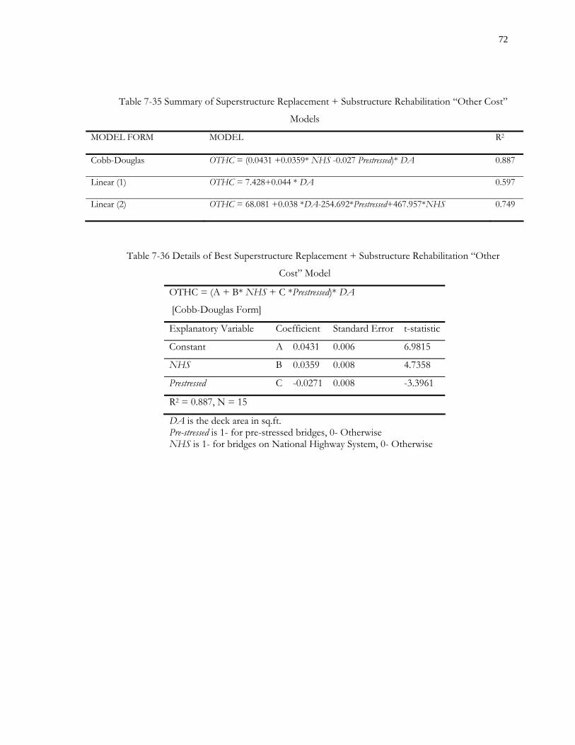
72

MODEL FORM MODEL R2

Cobb-Douglas OTHC = (0.0431 +0.0359* NHS -0.027 Prestressed)* DA 0.887

Linear (1) OTHC = 7.428+0.044 * DA 0.597

Linear (2) OTHC = 68.081 +0.038 *DA-254.692*Prestressed+467.957*NHS 0.749

OTHC = (A + B* NHS + C *Prestressed)* DA

[Cobb-Douglas Form]


Constant A 0.0431 0.006 6.9815

NHS B 0.0359 0.008 4.7358

Prestressed C -0.0271 0.008 -3.3961

R2 = 0.887, N = 15

DA is the deck area in sq.ft. Pre-stressed is 1- for pre-stressed bridges, 0- Otherwise NHS is 1- for bridges on National Highway System, 0- Otherwise

Table 7-35 Summary of Superstructure Replacement + Substructure Rehabilitation “Other Cost”

Models

Table 7-36 Details of Best Superstructure Replacement + Substructure Rehabilitation “Other

Cost” Model

73

The predicted and actual contract costs were plotted to identify the accuracy of the models

obtained. As can be seen in Figure 7-5, the models performed satisfactorily for contracts up to

$2,000,000. For contracts higher than $2,000,000, the models tended to underestimate the actual

cost.

7.3.7 Bridge Widening Cost Model

A bridge needs to be widened if it has a width deficiency or if it needs to accommodate

future increased traffic. In the dataset, such contracts involved widening up to 53 feet. Some

contracts involved construction of new piers or reinforced concrete piles, addition of beams, or

rehabilitation of the existing superstructure elements. All bridge widening contracts involved deck

rehabilitation work that ranged from one to 10% of the total cost.

Several variables were found significant. The DELTATDW variable, the difference between

the total deck width before and after the widening, was found significant. This was expected since

this variable best reflects the physical amount of work done on a bridge. Bridge widening primary

Figure 7-5 Predicted and Actual Cost for Superstructure Replacement + Substructure

Rehabilitation

0

1,000

2,000

3,000

4,000

5,000

0 1,000 2,000 3,000 4,000 5,000

Actual Superstructure Replacement + Substructure Rehabilitation Contract Cost ($1000)

Pred

icte

d ($

1000

)

0

1,000

2,000

3,000

4,000

5,000

0 1,000 2,000 3,000 4,000 5,000


Pred

icte

d ($

1000

)

0

1,000

2,000

3,000

4,000

5,000

0 1,000 2,000 3,000 4,000 5,000


Pred

icte

d ($

1000

)

0

1,000

2,000

3,000

4,000

5,000

0 1,000 2,000 3,000 4,000 5,000


Pred

icte

d ($

1000

)

74

cost models are shown in Table 7-37. For the best model, the adjusted R2 was computed as 0.934

and the details are presented in Table 7-38.

Linear models were developed and also the Cobb-Douglas model for estimating “other cost”

(Table 7-39). The Cobb-Douglas model was found to best predict bridge widening “other cost” and

is presented in Table 7-40.

BWC=A+B*TDW+C*BL+D*SUBH+E*HWY+F*DeltaTDW+G*ADT

[Linear 1]


(Constant) A -618.398 97.687 -6.330

DELTATDW B 9.922 2.863 3.466

TDW C 10.155 1.785 5.690

SUBHF D 14.606 3.356 4.353

BL E 1.565 0.231 6.784

ADT F 0.009 0.003 2.600

HWY G 183.834 56.678 3.243

R2 = 0.934, N = 28

Table 7-37 Summary of Bridge Widening Primary Cost Models

MODEL FORM MODEL R2

Linear 1 BWC = - 618.395+10.155*TDW+1.565*BL+14.606*SUBH

+183.834*HWY+9.922*DeltaTDW + 0.009*ADT 0.934

Linear 2 BWC = -172.48+0.034 * DA + 15.506*SUBH* +227.151*HWAY

+10.186*DeltaTDW + 0.008* ADT 0.925

Cobb-Douglas BWC = (0.31045 + 0.00992 * SUBH) *BL 0.636121 * TDW 1.000 0.904

Table 7-38 Details of Best Bridge Widening Primary Cost Model for all Bridge Types

75

BWC is the bridge widening primary cost in $ Year 2002

OTHC is the “other cost” in $ Year 2002 DA is the deck area in square feet BL is the bridge length in feet TDW is the total deck width in feet DeltaTDW is the difference between the total deck width before and after widening in ft NHS is 1- for bridges on National Highway System, 0- Otherwise HWY is 1- for bridges crossing highways, 0- Otherwise (rail or waterways) SUBH is substructure height in feet

OTHC= BLA*TDWB*DeltaTDWC


BL A 0.330 0.0865 3.816

TDW B 0.744 0.123 6.039

Delta TDW C 0.645 0.049 13.104

R2 = 0.945, N = 28

Table 7-39 Summary of Bridge Widening “Other Cost” Models for all Bridge Types

MODEL FORM MODEL R2

Linear OTHC =-94.975 + 39.856.725 * DeltaTDW + 0.017*DA 0.923

Linear OTHC = -353.603 + 37.644*DeltaTDW + 6.644*TDW + 0.569*BL 0.935

Cobb-Douglas OTHC = BL 0.330217 * TDW 0.743507* Delta TDW0.64523 0.945

Table 7-40 Details of Best Bridge Widening “Other Cost” Model for all Bridge Types

76

7.3.8 Summary and Conclusions for Bridge Rehabilitation Cost Models

In this section, cost models for rehabilitation activities were developed. The total contract

cost of the rehabilitation activity was divided into two cost components: one cost component

includes all items directly related to the specific rehabilitation activity, e.g., deck rehabilitation primary

cost; and the second cost component, “other cost,” included all indirect cost items. In order to

determine the best model for each cost component, several statistical parameters were considered: t-

statistic, R-square value, and standard errors of the regression coefficients. Also, whenever possible,

the models were validated to test their predictive accuracy.

Also, the model results show that the cost of bridge rehabilitation activities generally depend

on the bridge dimensions (length, deck width, or deck area). It was determined that deck and

superstructure rehabilitation costs depend not only on the deck area, but also on the bridge material

and the highway road class of the bridge. Bridge widening involves many activities and its cost was

found to depend on several factors, such as bridge size, substructure height, additional deck width,

and traffic level. In general, it was found that the “other cost” of rehabilitation costs also depends on

the bridge size. The models that best estimate the costs of various rehabilitation treatments are

presented Table 7-41.

77

BL is the bridge length in feet TDW is the total deck width in feet NHS is 1- for a bridge on NHS, 0- Otherwise DA is the deck area in square feet SUBH is the substructure height in feet HWY is 1- for bridges crossing highways, 0- Otherwise DeltaTDW is the difference in total deck width before and after bridge widening ADT is the Average Daily Traffic Concrete is 1- for concrete bridges, 0- Otherwise Steel is 1- for steel bridges, 0- Otherwise Prestressed is 1-for pre-stressed bridges, 0- Otherwise

Table 7-41 Summary of Rehabilitation Cost Models

ACTIVITY DIRECT-RELATED COST OTHER COST Deck Rehabilitation (DH)

DHC = 0.210970 * BL 0.635993 * TDW 0.8873369

OTHUC = $166,101/DA

Deck + Superstructure Rehabilitation (DSH)

DSH = 103.911 + 0.015 * DA + 91.130 * NHS – 35.787 * Steel

For DA<8000 sq. ft. $31.83* DA. For DA>8000 sq. ft. $16.01* DA.

Deck Replacement (DR)

DRUC=$24.44 * DA OTHUC = $29.59 * DA.

Deck Replacement + Super Rehabilitation (DRSH)

DRSHC = (-162.9536 + 264.835 * NHS) + BL 0.63144 * TDW0.79272

OTHC = BL 0.430053*TDW1

Deck Replacement + Super + Sub Rehabilitation (DRSBH)

DRSBHUC = $67.50* DA. OTHUC = $30.04* DA.

Superstructure Replacement (SR)

SRC = 0.2052 * BL 1 * TDW0.80330 OTHC = -89.045 + 0.066 * DA + 254.205 * Concrete

Super Replacement + Sub Rehabilitation (SRBH)

SRBHC = BL1.000* TDW0.3847 OTHC = (0.0431 +0.0359* NHS -0.027 Prestressed)* DA1.000

Bridge Widening (BW)

BWC=-618.395+10.155*TDW +1.565*BL +14.606*SUBH + 183.834*HWY + 9.922*DeltaTDW+0.009*ADT

OTHC = BL 0.330217 * TDW 0.743507

*Delta TDW0.64523

78

7.4 7.4 Overall Summary and Conclusions for Bridge Preservation Cost Models

The present chapter discussed a literature review carried out to acquire an insight into past

efforts at bridge cost modeling. The chapter also discusses the development of cost models for

bridge preservation costs, which include bridge replacement and bridge rehabilitation activities.

Various functional forms were investigated.

Bridge replacement cost was expressed as the sum of four components: superstructure

replacement cost, substructure replacement cost, approach cost, and “other cost.” After validation,

the models developed were found to predict more accurately bridge replacement costs than previous

studies. Bridge rehabilitation cost models were also developed. Bridge rehabilitation activity cost was

expressed as the sum of the primary cost and the “other cost”. Due to lack of data, it was possible to

model only eight rehabilitation activities. Also, for some activities whose costs were modeled,

validation was not possible due to the lack of additional data needed for the purpose. In general,

based on the results summarized in Table 7-14 and Table 7-41, it was found that the cost models

developed in the present study are fairly good for estimating bridge preservation costs.

For planning and budgeting, a requirement that is complementary to bridge preservation

costs is a set of models that enable bridge managers to track bridge deterioration and establish their

service lives so that the time when preservation is needed and the associated costs can be estimated.

The next chapter discusses the estimation of bridge service lives.

79

CHAPTER 8 : ESTIMATION OF BRIDGE SERVICE LIVES

Bridge age has often been considered as a representation of the combined effects of load

and weather effects and it is often used as a surrogate for these variables, especially in situations

where data is lacking. The age of a bridge deck can be expressed as a primary age (since the bridge

was constructed) or a secondary age (since the bridge was last rehabilitated). Some previous studies

have found age to be the most significant variable to explain the bridge deck deterioration (Bulusu

and Sinha, 1997; Chase et al., 2000). In Figure 8-1 is presented the delineation of bridge age. It

should be noted that the primary age of a bridge is same as the secondary age during the period of

the construction and the first rehabilitation.

Figure 8-1 Delineation of Bridge Age

Construction Repair Repair Replacement

Primary Age

Age

Deck

Condition

Rating

Secondary

Age

80

Estimates of bridge service lives are helpful for budgeting, scheduling, and programming of

rehabilitation, repair, and maintenance of bridge elements. A simple approach to determining

network level funding for bridges is to refer to service life as a measure of effectiveness and to

determine the number of bridges that are approaching the end of their service lives. The IBMS

(Indiana Bridge Management System) approximates a design life and an activity profile with

reasonable accuracy (Sinha et al. 1989). Life-cycle profiles for different types of bridges, including

concrete, steel, pre-stressed concrete, timber, and masonry, were developed. At the network level,

IBMS established that the mean age at which replacement occurs is approximately 70 years (primary

age) for most steel and concrete bridge types. Table 8-1 and Table 8-2 were developed on the

assumption that bridge replacement needs occur when bridges reach the age of 70. According to

profiles defined by INDOT, it is desirable that bridges received a major repair (deck rehabilitation,

superstructure repair, or bridge rehabilitation) every 20 or 25 years in order to extend the design life

to a service life of 70 to 80 years. For instance, for a typical concrete bridge it is suggested to have

deck rehabilitation after 20 years (secondary age) of construction and a superstructure replacement

after 15 years of the previous rehabilitation. Table 8-1 and Table 8-2 also show the number of

bridges that would need a major rehabilitation due to the fact that 20 years have passed since their

last major repair or since their construction. Current bridge replacement and rehabilitation needs are

described as “backlog.” In order to avoid double counting, it was assumed that for those bridges that

are close to the end of their life (older than 50 years), and have not had any repair in the previous 20

years in the subsequent 20 years, replacement, rather than rehabilitation, was a better option.

For the estimation of future bridge preservation needs, the software package IBMS was not used

for the following reasons:

- The data needed for the age-based analysis is not extensive and is easy to obtain. IBMS, on

the other hand, requires extensive data including age, condition, geometry, structural

deficiency, etc.

- The age of a bridge is closely related to its condition justifying the use of bridge age as a

measure of its performance

- The age based approach proved to be consistent with the historical expenditure record on

bridge preservation.

81

Year

Number of bridges

approaching the end

of service life

Cumulative number of

bridges approaching

the end of service life

Number of bridges

with more than 20

years since the last

repair

Cumulative number of

bridges with more than

20 years since the last

repair

2005 339 339 588 588

2006 32 371 115 703

2007 34 405 102 805

2008 32 437 101 906

2009 17 454 76 982

2010 15 469 53 1035

2011 23 492 94 1129

2012 35 527 85 1214

2013 7 534 138 1352

2014 3 537 127 1479

2015 4 541 94 1573

Table 8-1 Results of Age-Based Physical Needs Assessment of Concrete Bridges, 2004-2015

82

There are currently many bridges that need to be replaced and for the next 10 years the

number will increase. From the age distribution of concrete bridges, a maximum need will occur in

2007 and 2012, four and nine years from now, and the need will decline thereafter. The age

distribution of steel bridges presents a similar trend, and peak years will occur in 2007 and 2011, in

four and eight years respectively. A total of 730 bridges would need replacement because they would

be near the end of their lives in the next 10 years. In the case of bridge rehabilitation needs, it is

expected that in 2006 and 2013 there will be a need for intensive rehabilitation activity for concrete

bridges and in 2009 and 2014 for steel bridges.

Table 8-2 Results of Age-Based Physical Needs Assessment of Steel Bridges, 2004-2015

Year

Number of

bridges

approaching the

end of service life

Cumulative

number of bridges

approaching the end

of service life

Number of

bridges with more

than 20 years since

the last repair

Cumulative

number of bridges

with more than 20

years since the last

repair

2005 74 74 544 544

2006 10 84 87 631

2007 22 106 106 737

2008 13 119 102 839

2009 12 131 121 960

2010 18 149 102 1062

2011 24 173 77 1139

2012 16 189 89 1228

2013 0 189 88 1316

2014 0 189 111 1427

2015 0 189 86 1513

83

CHAPTER 9 : BRIDGE PRESERVATION EXPENDITURES

9.1 9.1 Age-Based Needs

After identifying the bridges needing replacement and rehabilitation based on their age, the

capital cost of those needs were determined on the basis of average unit costs obtained from the

recent contracts in the previous chapter. To determine the overall current replacement cost of each

structure, average unit costs for concrete and steel bridges estimated in Chapter 7 were used ($196

per square foot of deck area for concrete structures and $177 for steel structures). Similarly, average

unit cost of $54 per square foot of deck area for deck rehabilitation was used to compute the bridge

rehabilitation monetary needs. The results are summarized in Tables 9-1 and 9-2.

84

Table 9-1 Age-Based Monetary Needs for Bridge Replacement, by Year and Structure Material

Year

Concrete

Bridge Deck

Area (sq.ft.)

Concrete

Bridge

Replacement

Unit Cost

($ per sq. ft.

of deck area)

Concrete

Bridge

Replacement

Value

($millions)

Steel

Deck Area

(sq. ft.)

Steel

Bridge

Replacement

Unit Cost

($ per sq. ft.

of deck area)

Steel

Bridge

Replacement

Value

($millions)

2005 1,214,187 196 238 422,512 177 75

2006 128,097 196 25 129,018 177 23

2007 123,990 196 24 187,400 177 33

2008 103,836 196 20 93,472 177 17

2009 53,303 196 10 124,851 177 22

2010 40,410 196 8 79,931 177 14

2011 139,052 196 27 210,715 177 37

2012 130,507 196 26 130,380 177 23

2013 27,337 196 5 - 177 -

2014 23,706 196 5 - 177 -

2015 17,088 196 3 - 177 -

SUBTOTAL 2,001,512 $393 1,378,278 $244

TOTAL =$637

85

Table 9-2 Annual Deck Rehabilitation Needs by Structure Material

Year

Deck

Rehabilitation

Unit Cost

($ per sq. ft.

of deck area)

Concrete

Bridge Deck

Area (sq.ft.)

Concrete

Bridge

Rehabilitation

Value

($millions)

Steel Deck

Area (sq.

ft.)

Steel

Bridge Deck

Rehabilitation

Value

($millions)

2005 54 3,972,739 214 7,156,160 385

2006 54 644,893 35 922,400 50

2007 54 565,471 30 1,255,181 68

2008 54 554,263 30 1,244,361 67

2009 54 478,903 26 1,682,189 91

2010 54 310,300 17 1,448,352 8

2011 54 578,427 31 1,073,833 58

2012 54 540,135 29 1,140,505 61

2013 54 1,003,561 54 1,350,656 73

2014 54 815,272 44 1,376,697 74

2015 54 631,831 34 1,298,510 70

SUBTOTAL 10,095,796 $544 19,948,840 $1,075

TOTAL = $1616

Figure 9-1: Bridge Replacement Monetary Needs

-

50

100

150

200

250

300

350

2005

2007

2009

2011

2013

2015

Ann

ual B

ridge

Rep

lace

me n

Cos

t ($

M)

ConcreteSteel

-

50

100

150

200

250

300

350

2005

2007

2009

2011

2013

2015

Ann

ual B

ridge

Rep

lace

me n

Cos

t ($

M)

ConcreteSteel

86

-

100

200

300

400

500

600

700

2005

2007

2009

2011

2013

2015

Ann

ual B

ridge

Reh

abili

tatio

n C

ost (

$ M

)

ConcreteSteel

Table 9-1 and Table 9-2 present the bridge preservation needs in terms of monetary cost.

Again it is seen that the number of bridges that currently need replacement or rehabilitation is large

and translates into a substantial funding outlay. The age-based approach to needs assessment

indicated a total need of $2,256 million, corresponding to an average cost per year of $205 million

over the period 2005-2015. In Figure 9-1, yearly needs for bridge replacement are presented, while

Figure 9-2 shows the yearly needs for bridge rehabilitation. An average of $58 million per year would

be required for bridge replacement while the annual average bridge rehabilitation need would be $147

per year during 2002-2015. The total bridge preservation need can thus be expected to be $205

million per year. These engineering need estimates were compared with the historical record of

bridge preservation expenditure as discussed in the following sections.

Figure 9-2 Bridge Rehabilitation Monetary Needs

87

9.2 9.2 Estimated Needs Based on Historical Bridge Expenditures

9.2.1 Historical Expenditures

The dollars spent on bridge replacement and rehabilitation activities can be compiled from 1996

to 2003. The data is provided from the INDOT Contracts Management Division. Table 9-3 presents

the bridge expenditure from 1996 to 2003.

Year Bridge Expenditure

(current $)

Bridge

Expenditure

(2002 $)

1996 $45.1 $55.4

1997 $75.4 $85.4

1998 $61.9 $72.1

1999 $113.1 $122.6

2000 $110.9 $112.6

2001 $103.6 $105.8

2002 $124.8 $124.8

2003 $149.5 $145.9

Table 9-3 Historical Bridge Expenditure (1996-2003)

88 9.2.2 Projected Expenditure on the Basis of Historical Trends

The past bridge expenditure can be plotted against the years and a model can be developed

to predict the expenditure for any the future years. The relationship determined allows calculating the

total bridge expenditure for any given year. Figure 9-3 illustrates the data used and the results

obtained. The equation developed is as follows:

Total Bridge Expenditure = 6E+07*(# of years from 1996) ^0.4185

Using the above relationship, the bridge expenditure can be calculated for the next 10 years. Table 9-

4 shows the expected expenditure from 2005 to 2015.

Figure 9-3 Modeling Bridge Preservation Expenditure

y = 6E+07x0.4185

R2 = 0.8332

$0

$20

$40

$60

$80

$100

$120

$140

$160

0 1 2 3 4 5 6 7 8 9

Mill

ion

s

Years (1996-2001)

Pre

serv

atio

n c

ost

y = 6E+07x0.4185

R2 = 0.8332

$0

$20

$40

$60

$80

$100

$120

$140

$160

0 1 2 3 4 5 6 7 8 9

Mill

ion

s

Years (1996-2001)

Pre

serv

atio

n c

ost

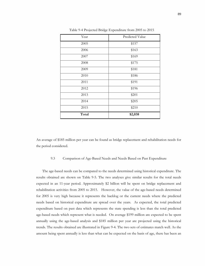
89

Year Predicted Value

2005 $157

2006 $163

2007 $169

2008 $175

2009 $181

2010 $186

2011 $191

2012 $196

2013 $201

2014 $205

2015 $210

Total $2,038

An average of $185 million per year can be found as bridge replacement and rehabilitation needs for

the period considered.

9.3 Comparison of Age-Based Needs and Needs Based on Past Expenditure

The age-based needs can be compared to the needs determined using historical expenditure. The

results obtained are shown on Table 9-5. The two analyses give similar results for the total needs

expected in an 11-year period. Approximately $2 billion will be spent on bridge replacement and

rehabilitation activities from 2005 to 2015. However, the value of the age-based needs determined

for 2005 is very high because it represents the backlog or the current needs where the predicted

needs based on historical expenditure are spread over the years. As expected, the total predicted

expenditure based on past data which represents the state spending is less than the total predicted

age-based needs which represent what is needed. On average $199 million are expected to be spent

annually using the age-based analysis and $185 million per year are projected using the historical

trends. The results obtained are illustrated in Figure 9-4. The two sets of estimates match well. As the

amount being spent annually is less than what can be expected on the basis of age, there has been an

Table 9-4 Projected Bridge Expenditure from 2005 to 2015

90

accumulation of unmet needs each year which is represented by the backlog estimated in the age-

based approach. Consequently, the simple regression model presented in Figure 9-3 can provide a

good estimate of realistic future bridge preservation needs, assuming not all needs will be met each

year.

Table 9-5 Comparison of Needs Based on Past Expenditures and Needs Based on Age

Year Predicted Value Based

Historical Trends ($Millions)

Predicted Value

Based

On Age ($Millions)

2005 $157 $912

2006 $163 $133

2007 $169 $155

2008 $175 $134

2009 $181 $149

2010 $186 $47

2011 $191 $153

2012 $196 $139

2013 $201 $132

2014 $205 $123

2015 $210 $107

Total $2,038 $2,253

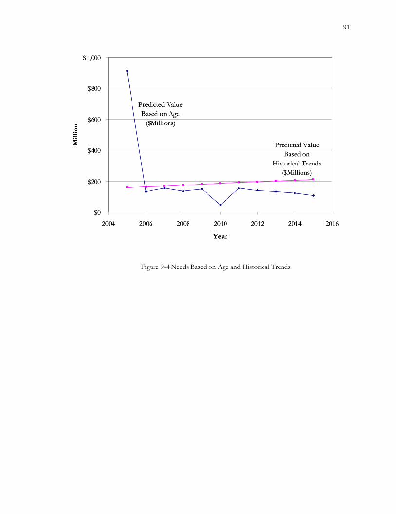
91

Figure 9-4 Needs Based on Age and Historical Trends

Predicted Value Based on Age

($Millions)

Predicted Value Based on


$0

$200

$400

$600

$800

$1,000

2004 2006 2008 2010 2012 2014 2016

Year

Mill

ion

Predicted Value Based on Age

($Millions)

Predicted Value Based on


$0

$200

$400

$600

$800

$1,000

2004 2006 2008 2010 2012 2014 2016

Year

Mill

ion

92

CHAPTER 10 : SUMMARY AND CONCLUSIONS

The purpose of the present study was to develop a simple procedure for estimating

pavement and bridge preservation needs for fiscal planning and budgeting. This was accomplished by

comparing existing technical needs based on physical condition and detailed work estimates with the

historical expenditure trends. In this chapter a summary of the estimation procedures to be used ins

presented, followed by a discussion on the highlights of the study results.

For long term fiscal planning and budgeting, it is useful to establish simple procedures in

order to estimate annual pavement and bridge preservation needs as it is time and effort consuming

to perform detailed engineering analyses each year. Therefore in the present study, simple methods to

estimate annual pavement and bridge preservation needs based on historical expenditure trends were

developed. They were then compared to technical estimates of needs established with engineering o

and were validated by engineering consuming. The procedures developed for pavements and bridges

can be summarized as follows:

10.1 Summary of Estimation Procedures

The procedure for the estimation of pavement preservation needs can be summarized as

follows:

1. Predict system size

Number of lanes miles = 83.275*YEAR - 138144 2. Estimate percentage of system to be treated

Percentage of system to be preserved = 0.0328* (# of years from 1990) ^ (0.3513)

3. Estimate total pavement preservation needs using unit cost per lane mile

Total cost of pavement preservation = Number of lane miles to be treated* Average unit cost for the past 3

years.

4. Estimate rehabilitation and non-rehabilitation needs (maintenance and

reconstruction)

% of system to be rehabilitated = 0.0248* (# of years from 1990) ^ (0.3705) Number of lane miles to be rehabilitated = %percentage of system to be rehabilitated * system size

93

Total cost of rehabilitation = Number of lane miles to be rehabilitated * Average unit cost for the past 3 years

Non Rehabilitation cost = Total preservation cost – Rehabilitation cost

5. Estimate preservation needs by functional system

Use percentages of total pavement preservation cost for on each highway class found in

recent years and multiply by the total preservation cost predicted in step 3.

Total Bridge Preservation Cost = 6E+07*(# of years from 1996) ^0.4185

Total Preservation Needs = Total Pavement Preservation Need + Total Bridge Preservation Need

10.2 Conclusions

Pavement service lives and preservation treatment costs were estimated using statistical

models developed. Models were developed for pavement deterioration rates in order to estimate

remaining service lives. Pavement preservation cost models were also implemented. Pavement

preservation needs for the period 2006-2020 were thus established using the appropriate models for

preservation costs and deterioration rates. The annual pavement preservation needs were estimated at

$354-$394 million. These needs were established based on engineering considerations. A procedure

that allows the prediction of future preservation needs on the basis of historical trends was also

developed. The procedure allows determining rehabilitation and non-rehabilitation costs for

pavements as well as preservation costs for different highway classes. Estimates based on the

procedure were compared to the amount spent on pavement preservation for 2002 and 2003 and the

results were accurate by 4% and 13% respectively.

Cost models were developed for bridge replacement and rehabilitation activities. For

replacement cost models, the cost of each component was modeled separately, and the overall cost

structure was expressed as the sum of the costs of such components. Different replacement cost

models were developed for slab bridges and beam section bridges because slab bridges are commonly

used for short bridges and preliminary data analysis showed that these two bridges exhibit different

relationships between cost and bridge characteristics. The models developed showed a significant

improvement over the models currently used in IBMS. For steel bridges, replacement cost models

94

were not developed due to an insufficient number of observations, but the average unit costs were

reported.

Cost models were developed for seven bridge rehabilitation activities. The analysis also

showed that the cost of rehabilitating bridge decks and superstructures depends not only on the deck

area but also on the bridge material and the highway functional class.

Bridge preservation costs were assessed for the period 2006-2015 using an age-based

approach. The annual average cost of preservation was estimated at $199 million. A model based on

past bridge expenditure was also developed and the results obtained for this model were consistent

with the age-based projection. The annual average cost of preservation on the basis of historical

records was estimated at $185 million. The difference is the result of the accumulation of unmet

needs each year which can be represented by the backlog determined with the age-based approach.

The study results are useful for long-term planning and budgeting as INDOT’s Division of

Policy and Fiscal Management and Planning will be able to schedule and monitor its pavement and

bridge preservation cash flows in a more effective manner than what is possible at present.

95

REFERENCES

Ben-Akiva, M. and Ramaswamy, R.., (1990) . ‘‘Estimation of highway pavement deterioration from in-service pavement data.’’ Transportation Research Record 1272, Transportation Research Board, National Research Council, Washington, D.C. Bulusu, S., and Sinha, K. C. (1997). “A Comparison of Methodologies to Predict Bridge Deterioration,” Transportation Research Record 1597. V. Carnahan, M.ASCE, W.J. Davis, M.Y. Shahin, P.L. Keane, and M.I. Wu. (1987). “Optimal Maintenance Decisions for Pavement Management,” Journal of Transportation Engineering, vol113 n5, New York: ASCE, September 1987. Chase, S. B., Small, E. P., and Nutakor, C., (2000). “An In-Depth Analysis of the National Bridge Inventory Database Utilizing Data Mining, GIS and Advanced Statistical Methods.” Transportation Research Circular No 498. Transportation Research Board, Washington D.C. Collura, J., Spring, G., and Black, K.B., (1993). “Service Lives and Costs of Local Highway Maintenance and Rehabilitation Treatments”. Transportation Research Record 1397, Transportation Research Board, National Research Council, Washington, D.C. Corvi, IE; Bullard, BG (1970). “A System of Estimating the Present Surface Condition and Remaining Service Life of Existing Pavement Sections”. Public Roads, Volume: 36, Issue: 5.

Feighan, K. J., Shahin, M. Y., and Sinha, K. C. (1987). "A dynamic programming approach to optimization for pavement management systems." Proc., 2nd North American Conf. on Managing Pavements, Toronto.

Geoffroy, D.N. (1996). “Synthesis of Highway Practice 223: Cost-effective Preventive Pavement Maintenance”. Transportation Research Board, National Research Council, Washington, D.C. Griffith, A., Wyttenberg, K., Williams, J., Lynde, M., (2002). “Aggregate Resource Inventory and Needs Forecast Study”. Final Report, SPR 314, Oregon Department of Transportation and FHWA, Washington, D.C. Gulen, S., Woods, R., Weaver, J., and Anderson, V.L.,. (1994). “Correlation of Pavement Serviceability Rating with International Roughness Index”. Transportation Research Record 1435. Hartgen, D.T., (1986). “ How Good is the Highway Performance Monitoring System? A Comparison with the State Results”. Transportation Research Record 1060, Transportation Research Board, National Research Council, Washington, D.C.

96

Hartgen, D. T. (2000). “North Carolina Highways: Performance, Needs and Funding Options”. John Locke Foundation. Hawk, H. (2003). “Bridge Life-Cycle Cost Analysis” NCHRP Report 483 Transportation Research Board, Washington D.C. Hodge, S. (2004). “An Assessment of Highway Financing Needs in Indiana”. M.S. Thesis, Purdue

University, West Lafayette, IN.

Indiana Design Manual, Chapter 52, 1998. INDOT (2000). 2000 Pavement Surface Report, December, 2000. INDOT Pavement Management Section, Program Development Division.: INDOT. INDOT (2003). I-69: Evansville to Indianapolis Tier 1 Draft Environmental Impact Statement, Summary Chapter: INDOT. Labi, S., and Sinha, K. C. (2003). “The Effectiveness of Maintenance and Its Impact on Capital Expenditures” (No. FHWA/IN/JTRP-2002/27). Joint Transportation Research Program, Purdue University. West Lafayette, IN. Lamptey, G. et al. (2004). “Life Cycle Cost Analysis for Pavement Design Procedures”. (No. FHWA/IN/JTRP-2004/28). Draft final report. Joint Transportation Research Program, Purdue University, West Lafayette, IN. Rodriguez, M. M. (2004). “An Assessment of Preservation Needs of State Highway Bridges in Indiana”. M.S. Thesis. Purdue University, West Lafayette, IN. Saito M., V.L. Anderson and Sinha K.C. (1988), “Bridge Replacement Cost Analysis”. Transportation Research Record 1180, Transportation Research Board, Washington, D.C. Sinha, K. C., Saito, M., Jiang, Y., Murthy, S., Tee, A., and Bowman, M. D.(1989), “The Development of Optimal Strategies for Maintenance, Rehabilitation and Replacement of Highway Bridges, Final Report Vol. 1: The Elements of Indiana Bridge Management System”, Joint Highway Research Project, West Lafayette, IN. Thompson P.D and Markow J, (1996). “Collecting and Managing Cost Data for Bridge Managements System”, NCHRP Synthesis 227, Transportation Research Board, National Academic Press, Washington, D.C. Tonias, D.E. (1995). “Design, Rehabilitation and Maintenance of Modern Highways Bridges.” MacGraw-Hill, Inc. New York. .

97

APPENDICES

98

Performance Curves for NHS Composite Pavements

y = 6.5558x + 65.937

R2 = 0.4233

0

50

100

150

200

250

300

0 2 4 6 8 10 12

Age

IRI

Performance Curve for NHS-AC Pavements

y = 4.0736x + 77.784R2 = 0.4611

0

50

100

150

200

250

300

350

0 2 4 6 8Age

IRI

Performance Curve for NHS-PCC Pavements

y = 3.9114x + 80.5R2 = 0.4635

020406080

100120140160180200

0 2 4 6 8Age

IRI

Appendix A. Performance Curves

99

Performance Curve for NHS Non-Interstate Composite Pavements

y = 2.2428x2 - 24.717x + 161.81R2 = 0.3192

0

50

100

150

200

250

4 5 6 7 8 9AGE

IRI

Performance Curve for Non-NHS Non-Interstate PCC Pavements

y = 88.303e0.0556x

R2 = 0.1673

050

100150200250300350400450

0 2 4 6 8 10Age

IRI

y = 69.594e0.057xR2 = 0.4458

0

50

100

150

200

250

300

350

400

450

0 2 4 6 8 10Age

IRI

Performance Curve for NHS Non-Interstate AC Pavements

100

Performance Curve for Non-NHS Composite Pavements

y = -1.2815x2 - 1.8951x + 128.63R2 = 0.2335

0

50

100

150

200

250

300

350

0 1 2 3AGE

IRI

Performance Curves for Non-NHS AC Pavements

y = 6.5558x + 65.937

R2 = 0.4233

0

50

100

150

200

250

300

0 2 4 6 8 10 12

Age

IRI

Performance Curve for Non-NHS-PCC Pavements

y = 3.9114x + 80.5R2 = 0.4635

020406080

100120140160180200

0 2 4 6 8Age

IRI

101

Appendix B. Cost Models for Asphaltic Concrete Pavements

Model Type

Models R2

Linear Cost= 8.748 - 0.356×Lngth +0.234× Nr_Lns +2.454×Thk – 0.245-N_F+0.148×S_F

0.365

Polynomial Cost=2.345-1.254×Lngth5+0.854× Nr_Lanes4+0.454×Thk3 -0.545-N_F2+1.148×S_F1

0.293

Polynomial Cost=1.726-1.254×Lngth0.25+0.854×Nr_Lanes0.24+0.454×Thk0.68 -0.545× N_F2.1

+1.148×S_F0.56

0.322

Polynomial Cost=3.26+0.954×Lngth0.55+0.854×Nr_Lanes0.74+0.146×Thk0.78 -0.721× N_F

+0.041×S_F

0.254

Logistic (Cost)0.5= 0.795 + 0.0156×Lngth +0.125×Nr_Lanes +0.454×Thk 1.245-N_F+0.5448×S_F

0.211

Cost Models for Portland Cement Concrete Pavements

Model Type

Models R2

Linear Cost= - 1.356×Lngth + 0.334× Nr_Lns +3.454×Thk – 0.215-N_F+1.240×S_F 0.315


0.219


+1.148×S_F2..56

0.302


+0.041×S_F

0.287


0.249

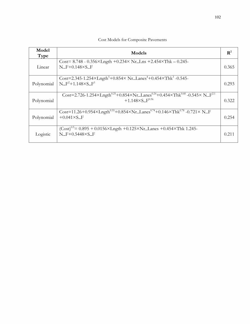
102

Cost Models for Composite Pavements

Model Type

Models R2

Linear Cost= 8.748 - 0.356×Lngth +0.234× Nr_Lns +2.454×Thk – 0.245-N_F+0.148×S_F

0.365


0.293


+1.148×S_F0.56

0.322


+0.041×S_F

0.254


0.211

103

Appendix C. INDOT Contracts Unit Pavement Treatment Costs

Mean Min. Max. Std. Dev.

Added Travel Lanes COMP 1 21798 21798 21798 0Added Travel Lanes HMA 46 2111 150 15170 2541Added Travel Lanes PCC 14 2445 236 7103 2273Added Travel Lanes, Bituminous HMA 1 263 263 263 0Added Travel Lanes, Concrete PCC 6 4628 486 16027 5689Asphalt Patching HMA 1 38 38 38 0Auxillary Lane Construction HMA 3 149 9 414 229Auxillary Lanes, Acel & Dcel HMA 1 726 726 726 0Bridge Deck Overlay HMA 1 295 295 295 0Bridge Rehabilitation Or Repair PCC 0 0 0 0 0Bridge Removal HMA 1 1067 1067 1067 0Crack & Seat Composite Pavement & HMA Overlay COMP 20 673 230 3210 735Crack & Seat PCCP & HMA Overlay PCC 5 209 2 379 188Crack & Seat PCCP & HMA Overlay (P3R) PCC 6 644 2 3356 1332Diamond Grinding PCC 0 0 0 0 0Ditch Relocation HMA 1 807 807 807 0Drainage Ditch Correction HMA 2 534 234 834 424Dual Lane Existing Route PCC 2 2065 1430 2699 897Full And Shallow Depth Patching HMA 1 31 31 31 0Full And Shallow Depth Patching PCC 1 298 298 298 0HMA Overlay, Functional COMP 17 314 7 1652 454HMA Overlay, Functional HMA 88 210 3 3086 469HMA Overlay, Functional PCC 4 129 9 406 187HMA Overlay, Preventive Maintenance COMP 1 37 37 37 0HMA Overlay, Preventive Maintenance HMA 26 73 18 296 71HMA Overlay, Structural HMA 18 236 60 1022 249Install New Guard Rail HMA 1 199 199 199 0Install New Small Structure HMA 1 80 80 80 0Interchange Modification COMP 1 1156 1156 1156 0Interchange Modification PCC 0 0 0 0 0Intersection Improvement HMA 5 234 190 301 45Intersection Improvement PCC 1 123 123 123 0Mill Full Depth And Bit Overlay COMP 3 356 17 753 372Mill Full Depth And Bit Overlay HMA 2 366 226 507 199New Br, Cont.Pres.Conc.Box Beam HMA 1 138 138 138 0New Road Construction - CRC PCC 5 2991 1244 5875 1934

Treatment Pavement Type

No.of Obs.

Cost per Lane Mile (1000s) 2002$

Source: Oware, 2004. JTRP Status Report – SPR 2810 Estimates of Costs and Service Lives of Pavement and Bridge Projects for Fiscal Planning and Programming.

Table C.0-1 Unit Pavement Treatment Costs

104

Mean Min. Max. Std. Dev.

New Road Construction, Composite COMP 1 2966 2966 2966 0New Road Construction, HMA HMA 32 2545 14 22561 4472New Road Construction, PCC PCC 31 3620 368 11010 2988New Road, HMA Paving Only HMA 2 1424 720 2127 995New Road, PCC Paving Only PCC 3 1224 484 2238 909New Sign Installation PCC 1 2760 2760 2760 0Other Methods Of Rehabing Pavement COMP 1 275 275 275 0Other Methods Of Rehabing Pavement HMA 1 272 272 272 0Other Type Project (Miscellaneous) HMA 1 994 994 994 0Patch and Rehab HMA Pavement COMP 1 8226 8226 8226 0Patch and Rehab HMA Pavement HMA 3 57 42 65 13Patch and Rehab PCC Pavement PCC 2 97 27 167 100Pavement Repair or Rehabilitation COMP 2 723 181 1265 766Pavement Repair or Rehabilitation HMA 43 311 14 2718 505Pavement Repair or Rehabilitation PCC 1 7 7 7 0Pavement Replacement, HMA HMA 3 956 23 2268 1170Pavement Replacement, New PCC COMP 1 3918 3918 3918 0Pavement Replacement, New PCC HMA 5 1394 311 2376 917Pavement Replacement, New PCC PCC 7 1454 441 2597 754PCCP Cleaning and Sealing Joints PCC 10 269 16 1828 553PCCP on Asphalt Pavement HMA 12 89 15 372 98PCCP on PCC Pavement PCC 2 1247 509 1985 1044PCCP Patching PCC 15 1145 20 10662 2717Repair PCCP & HMA Overlay PCC 7 156 10 561 217Resurface (Partial 3-R Standards) COMP 18 383 47 1960 489Resurface (Partial 3-R Standards) HMA 1405 297 8 7282 585Resurface (Partial 3-R Standards) PCC 11 826 52 3503 1110Resurface over Asphalt Pavement (Partial 3-R Standards) HMA 18 361 34 2619 719Resurface PCC Pavement (Partial 3-R Standards) PCC 2 136 134 139 3Road Reconstruction (3R/4R Standards) COMP 56 673 39 3394 749Road Reconstruction (3R/4R Standards) HMA 104 784 39 4378 956Road Reconstruction (3R/4R Standards) PCC 18 2118 128 9686 2749Rubblize PCCP & HMA Overlay PCC 18 2322 131 10789 2728Sight Distance Improvement HMA 1 505 505 505 0Small Structure, Replacement HMA 2 447 171 723 391Surface Treatment, PM HMA 10 62 8 382 114Vertical Sight Distance Correction HMA 1 906 906 906 0Wedge And Level Only HMA 65 53 2 424 83Widen Pavement and HMA Overlay HMA 6 262 25 648 230

Treatment Pavement Type

No.of Obs.

Cost per Lane Mile (1000s) 2002$

Source: Oware, 2004. JTRP Status Report – SPR 2810 Estimates of Costs and Service Lives of Pavement and Bridge Projects for Fiscal Planning and Programming.

Table C.0-2 Unit Costs of Pavement Treatments (Continued)

105

Appendix D. AAMEX Model Curves

0

400

800

1,200

1,600

2,000

0 10 20 30

Pavement Age in Years

Estim

ated

Ave

rage

Ann

ual

Mai

nten

ance

Exp

endi

ture

($/la

ne-m

ile)

Jointed UrbanInterstatesJointed RuralInterstatesContinuous UrbanInterstatesContinuous RuralInterstates

Figure D.0-1 Fitted Values for AAMEX Model, Rigid Interstate Pavements 1995$

0

400

800

1,200

1,600

0 5 10 15 20


Estim

ated

Ave

rage

Ann

ual

Mai

nten

ance

Exp

endi

ture

($/la

ne-m

ile)

Interstates, North(WSL = 0.8)Interstates, South(WSL = 0.6)Non-Interstates,North (WSL = 0.8)Non-Interstates,South (WSL = 0.6)

Figure D.0-2 Fitted Values for AAMEX Model, Rigid Interstate Pavements 1995$

106

0

100

200

300

400

500

600

0 5 10 15 20


Estim

ated

Ave

rage

Ann

ual

Mai

nten

ance

Exp

endi

ture

($/la

ne-m

ile

Urban InterstateTraditional Overlays

Rural InterstateTraditional Overlays

Urban InterstateNon-traditionalOverlaysRural Interstate Non-traditional Overlays

Figure D.0-3 Fitted Values for AAMEX Model, Interstate COMP Pavements 1995$

107

0

200

400

600

800

1,000

0 5 10 15 20


Estim

ated

Ave

rage

Ann

ual

Mai

nten

ance

Exp

endi

ture

($/la

ne-m

il eUrban Non-InterstateTraditional Overlays

Rural Non-InterstateTraditional Overlays

Urban Non-InterstateNon-traditionalOverlaysRural Non-InterstateNon-traditionalOverlays

Figure D.0-4 Fitted Values for AAMEX Model, Non-Interstate COMP Pavements 1995$

108

Appendix E. Bridge System Types

Bridge Type and Configurations Depending on the superstructure material, bridges are classified as steel or concrete. The superstructure system is defined by its material and its superstructure construction features. Steel superstructures have typical configurations of beams, girders, trusses, and arches (Petros, 1996). Concrete superstructures have common forms of slab, box beam, T-beam, stringer, prestressed girder, or segmental construction. Multi-beams and Slab on stringer structures are for short span lengths and average clearance requirements. When a span becomes excessive other forms of structures must be evaluated. Steel and concrete box girder structures are utilized when bending and torsion are major concerns, however it can represent an expensive solution (Tonias, 1995). Trusses: a truss is essentially a triangulated assembly or straight members. Trusses have two major characteristics and structural advantage: The primary member forces are axial loads, and the open-web system, accommodates a greater depth than an equivalent solid-web girder. In the past, the conventional truss bridge has been found to be economical for medium spans. However, recent advances in design and construction for both steel and concrete girders have tended to increase the economical span. Thus, truss bridges are now less favored in modern designs.

Steel Systems:

Figure A-1: Truss Systems

109

Steel I-Beam: floor systems consist of the roadway slab and the supporting rolled beams. The concrete slab is usually 7 ½ to 9 inches thick, with reinforcement perpendicular to traffic. The majority of steel I-beam bridges have some kind of continuity. Plate Girder and Box Girder Bridges: are designed with the intent to provide a more efficient arrangement and utilization of material than is possible with rolled beams. Typical floor systems consists of 1) steel grid floor resting on longitudinal stringers and main girders, 2) a concrete slab on transverse beams supported on two main girders, 3) multiple girders with or without haunches supporting a concrete slab, and 5) multiple box girders supporting a concrete slab. Through girder bridges, are structures where the main longitudinal girders extend above the roadway (Figure 2).

a) Through Girder b) Deck Girder c) I Beam

Figure 2: Steel General Bridge Type Concrete Bridges: A reinforced concrete bridge consists of deck slabs, T-beams, through and box girders, and rigid frames. Pre-stressed or pre-cast concrete structures also add other structural types and enhance bridge adaptability. Typical example of concrete bridge types are shown in Figure A and Figure A-4

110

a) Concrete Slab b) Concrete T-Beam

Figure 3: General Concrete Bridge Type (AASHTO)

Figure 4: Typical Concrete Sections

Concrete deck girder bridges are divided into three main types according to the interaction between the girder and the slab. They are: 1) girder-and-slab systems, where the slab spans transversely between longitudinal girders providing a typical T-beam action; 2) girder, floor beam, and one-way slab supported on the floor beam, and 3) girder, floor beam, and two way slab supported along four edges.

Slab

Concrete T-beam

Concrete box girder

Channel

Spread Box

Box

Procedures for the Estimation of Pavement and Bridge Preservation Costs for Fiscal Planning and...

Documents

Transcript of Procedures for the Estimation of Pavement and Bridge Preservation Costs for Fiscal Planning and...