arX

iv:1

007.

3838

v1 [

quan

t-ph

] 2

2 Ju

l 201

0

Probability and complex quantum

trajectories: Finding the missing links

Moncy V. John

Department of Physics, St. Thomas College, Kozhencherry, Kerala 689641,

India.

Abstract

It is shown that a normalisable probability density can be defined for the entirecomplex plane in the modified de Broglie-Bohm quantum mechanics, which givescomplex quantum trajectories. This work is in continuation of a previous one thatdefined a conserved probability for most of the regions in the complex space in termsof a trajectory integral, indicating a dynamical origin of quantum probability. Thereit was also shown that the quantum trajectories obtained are the same characteristiccurves that propagate information about the conserved probability density. Thoughthe probability density we now adopt for those regions left out in the previous work isnot conserved locally, the net source of probability for such regions is seen to be zeroin the example considered, allowing to make the total probability conserved. Thenew combined probability density agrees with the Born’s probability everywhere onthe real line, as required. A major fall out of the present scheme is that it explainswhy in the classical limit the imaginary parts of trajectories are not observed evenindirectly and particles are confined close to the real line.

Key words: quantum Hamilton-Jacobi equation, trajectory representation,probability axiom, complex methodsPACS: 03.65.Ca

1 Introduction

Complex quantum trajectories were first obtained [1] by modifying the deBroglie’s guiding wave approach to quantum mechanics. Here, trajectorieswere drawn for the cases of harmonic oscillator, potential step, wave packetsetc. For getting this trajectory representation, first we substitute Ψ = eiS/~ inthe Schrodinger equation, which gives the quantum Hamilton-Jacobi equation

Preprint submitted to Elsevier 23 July 2010

(QHJE) [2,3]

∂S

∂t+

1

2m

(

∂S

∂x

)2

+ V

=i~

2m

∂2S

∂x2. (1)

Then we postulate an equation of motion for the particle, similar to that usedby de Broglie:

mx ≡ ∂S

∂x=

~

i

1

Ψ

∂Ψ

∂x. (2)

The quantum trajectories x(t) were found by integrating this equation withrespect to time; in general, they lie in a complex x-plane, with x = xr + ixi.This results in a modified version of the de Broglie-Bohm (dBB) quantummechanics [4,5,6,7]. Eq. (2) was used by Leacock and Padgett [8] to obtaineigenvalues in many bound state problems, without having to solve the corre-sponding Schrodinger equation.

It shall be noted that the canonical momentum is not always the mechani-cal momentum, even in classical mechanics with Cartesian coordinates. Forinstance, when there are velocity-dependent potentials, the canonical and me-chanical momenta are different. In the case of a charged particle in a magneticfield with the vector potential A , the mechanical momentum may be writtenas

mx = ∇S − eA/c. (3)

This equation in Cartesian coordinates shall thus be the equation of motionwe adopt for charged particles in higher dimensions with electromagnetic field.

The Floyd-Faraggi-Matone (FFM) trajectory representation [9,10,11,12,13] isanother modified dBB version but with real trajectories and is based on ageneralised Hamilton-Jacobi equation equivalent to that used in dBB. Butthis representation differs from dBB quantum mechanics mainly in the use ofthe equation of motion. Here, for stationarity the equation of motion for thetrajectory time t, relative to its constant coordinate τ , is given as a functionof x by

t− τ = ∂W/∂E (4)

where W is the Hamilton’s characteristic function appearing in the generalisedHamilton-Jacobi equation and E is the energy. Carroll [11] finds that for sta-tionarity the above Jacobi’s theorem is valid, for W is a Legendre transform

2

of Hamilton’s principal function. Floyd [12] notes that as Jacobi’s theoremalso determines the equation of motion in classical mechanics, it is universaltranscending across the division between classical and quantum mechanics. Inthis way, FFM claims to be a deterministic theory.

The complex function S, which may be called the complex Hamilton’s princi-pal function in the present modified de Broglian mechanics, and the complexQHJE (1) itself are quite different from the corresponding entities in dBBor FFM representations. Moreover, probability is an integral part of the newformulation and one can also consider equation (2) as propagating probabil-ity densities. In fact, it was shown in a previous work [14] that the quan-tum trajectories obtained in this scheme are the same as the characteristiccurves propagating information about a conserved probability density. Hencewe continue to use (2), with appropriate modifications as mentioned abovewhen necessary, as the equation of motion in this modified dBB formulation.

The complex trajectory approach gives the paths in the n = 1 harmonicoscillator as shown in Fig. 1. In this case, the paths are given by (α2x2

r −α2x2

i − 1)2 + 4α4x2rx

2i = A2, a constant for each path. Here A is real and

positive, and α2 has the usual definition, equal to mω0/~. It is interesting tonote that these figures are the famous Cassinian ovals. The Jacobi lemniscate,which is the special case of these ovals, corresponds to A = 1.

Fig. 1. The complex trajectories in the n = 1 harmonic oscillator case, drawn forvarious values of A and with axes Xr ≡ αxr and Xi ≡ αxi. These are the famousCassinian ovals. The lemniscate corresponds to A = 1.

Recently, the prospects of a dynamical explanation of quantum probabilityin this scenario was explored [14]. We have shown that in this modified deBroglian mechanics, the Born’s probability along the real axis can be obtainedas an exponential function of a line integral along the real axis. Similarly inthe extended xrxi-plane, a probability density is obtained as the exponential

3

of a trajectory integral. In both these cases, integrands involve the particle’scomplex velocities, indicating a dynamical origin of quantum probability. Inthe extended case, we obtain a conserved probability, which agrees with theboundary condition (Born’s rule) along the real axis in most regions. However,for other regions (e.g., the subnests inside the lemniscate in the n = 1 harmonicoscillator case, which do not enclose any poles of x), such a definition could notbe obtained. In fact, a probability density was not proposed for such regionsin [14] and it was considered a missing link in the formalism.

Another important question faced by this trajectory representation is why thecomplex extended motion is not appreciable in the classical limit. Our every-day experience is that particle trajectories are in real space, obeying classicalrules. In this letter, we study the probability distribution of particles in thecomplex plane in detail and adopt for those regions left out in [14] an alter-native definition, first proposed in [15,16] as the probability density for theentire plane. This density satisfies the boundary condition on the real axis,though it is not a conserved one. We show that the combined probability forthe entire extended plane does not diverge and there is no difficulty in nor-malizing it, contrary to what happens in the above case. Nonconservation ofprobability points to the prospects of particle creation and destruction, a fun-damental feature of quantum phenomena. Most importantly, the new schemereveals that large part of the probability for a classical harmonic oscillator liesextremely close to the real line, thereby explaining why the complex extendedmotion does not leave any imprint in the classical limit.

We restrict ourselves to one particle stationary states in 1-dimension for sim-plicity. The paper is organized as follows. In the next section, we review theproblem with probability density faced in [14]. The third section presents thealternative definition of probability density adopted for the subnests and ob-tains a form of continuity equation obeyed by it. In section 4, the classicallimit of a harmonic oscillator in the light of our combined probability densityand its implication for complex trajectories are discussed. Section 5 comprisesour conclusion.

2 Probability from velocity field

As in the case of dBB quantum mechanics, the present modified de Broglie-Bohm mechanics too is constructed in such a way that it agrees with the resultsof standard quantum mechanics [1]. This is achieved by accepting the Born’sprobability axiom along the real line in these representations. However, we notethat one of the challenges before such a quantum trajectory representationis to explain this probability axiom. In the standard dBB approach, therewere several attempts to obtain the Ψ⋆Ψ probability distribution from more

4

fundamental assumptions [6]. (The FFM trajectory representation does notinvolve probability and is considered a deterministic description.)

In addition to that defined along the real line, it is desirable to have a proba-bility density defined everywhere in the extended complex x-plane. An earlierattempt made in [17] to define such a density was to write ρ(x) = ¯Ψ(x)Ψ(x),where ¯Ψ(x) ≡ Ψ⋆(x⋆), with x complex. With the help of time-dependentSchrodinger equation, the author shows that, in general, ∂ρ/∂t 6= j′(x, t).This arguably leads to nonconservation of probability along trajectories. Butit shall be noted that this negative result is based on the choices made in [17]for the probability density and flux. Moreover, this definition leads to com-plex probability off the real axis, which is undesirable. Another proposal is todefine probability as Ψ⋆(x)Ψ(x) itself [15,16]. Though this has the advantageof being real everywhere, it is not conserved at any point in the extendedplane. In addition, this diverges for large values of xi in many cases and is notgenerally a normalisable probability.

Using a different approach, it was shown in [14] that the complex trajectoryrepresentation is capable of explaining the quantum probability as originatingfrom dynamics itself. Here, the Born’s probability density to find the particleon the real axis around some point at x = xr0 was obtained as

Ψ⋆Ψ(xr0, 0, t) ≡ P (xr0, t) = N exp

−2m

~

xr0∫

xidxr

, (5)

where the integral is taken along the real line. In addition, an extended prob-ability density ρ(xr, xi) in the xrxi-plane for stationary states was proposedin [14] and showed, with the aid of complex-extended Schrodinger equation,that the continuity equation follows from it. The proposal was that if ρ0, theextended probability density at some point (xr0, xi0) is given, then ρ(xr, xi) atanother point that lies on the trajectory which passes through (xr0, xi0) is

ρ(xr(t), xi(t)) = ρ0 exp

−4

~

t∫

t0

Im(

1

2mx2 + V (x)

)

dt′

. (6)

Here, the integral is taken along the trajectory [xr(t′), xi(t

′)] which passesthrough (xr0, xi0). The continuity equation was shown to follow from thisaxiom by using the extended version of the Schrodinger equation. While eval-uating ρ with the help of (6) above, one should specify ρ0 at (xr0, xi0) and ifwe choose this point as (xr0, 0), the point of crossing of the trajectory on thereal line, then ρ0 can assume the Born’s value P (xr0).

However, we may note that in some regions of the complex plane, there can bedisagreement between the values of ρ and P (xr) at the points of crossing of the

5

trajectories on the real line. This happens where the complex trajectories donot enclose any poles of x, described as ‘subnests’ in [1]. Stated more clearly,the problem here is that as a particle trajectory is traversed in these regions,even while the probability ρ at one point of crossing xr0 on the real axis agreeswith P (xr0), at the other point, say the point xr1 where the trajectory againcrosses the real line, the probability calculated according to (6) happens to bedifferent from that of P (xr1).

On the other hand, if we directly solve the continuity equation for stationarystates, it is easy to see that its solution and the probability density givenby the trajectory integral (6) give identical results for regions outside thesubnests [14]. But for the subnests, the boundary condition overdeterminesthe problem and we are unable to find a solution that agrees with the Born’srule everywhere on the real line; i.e., there is complete agreement between theextended probability density ρ and the Born’s probability density only in theregions outside the subnests.

3 Probability inside the subnests

Given this situation, one can ask whether it is possible to find a probabilitydensity for the subnests that can agree with the Born’s rule on the real line,even if it is not conserved in the region. A natural choice for such a definitionis the extended probability ρ′ = Ψ⋆(x)Ψ(x), suggested in [15,16]. A trajectoryintegral form for ρ′, similar to that in Eq. (6) above, was proposed in [18]. Forstationary states, this can be written as

ρ′(xr, xi) ∝ ρ0 exp

−4

~

t∫

t0

Im(

1

2mx2

)

dt′

. (7)

We propose to adopt this as the probability density for such subnests. Herealso, the integral is to be evaluated over the trajectory of the particle. Theabsence of the potential term V (x) in the integrand marks this definition fromthat in (6). Therefore this distribution will not be conserved. Instead of thecontinuity equation, we get

∂ρ′

∂t+

∂(ρ′xr)

∂xr+

∂(ρ′xi)

∂xi=

4

~ρ′(xr, xi) Im[V (x)] (8)

Thus there are sources and sinks for probability in the subnests. However, asseen below, the net source of probability in this region for the n = 1 harmonicoscillator is zero, indicating that the total probability for the subnested regioncan remain conserved.

6

Thus instead of being ‘nonviable’, the trajectories in this region reveal an im-portant feature of quantum phenomena, namely nonconservation of particles.This indicates creation and destruction of particles in such regions. Hencewe can anticipate that the representation is capable of allowing a smoothtransition to quantum field theory. It is interesting to note that the Floyd-Farraggi-Matone trajectory representation too allows creation and destructionof particles [13].

4 Probability and classical limit

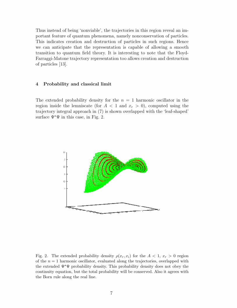
The extended probability density for the n = 1 harmonic oscillator in theregion inside the lemniscate (for A < 1 and xr > 0), computed using thetrajectory integral approach in (7) is shown overlapped with the ‘leaf-shaped’surface Ψ⋆Ψ in this case, in Fig. 2.

Fig. 2. The extended probability density ρ(xr, xi) for the A < 1, xr > 0 regionof the n = 1 harmonic oscillator, evaluated along the trajectories, overlapped withthe extended Ψ⋆Ψ probability density. This probability density does not obey thecontinuity equation, but the total probability will be conserved. Also it agrees withthe Born rule along the real line.

7

Using the above definition ρ′ ≡ Ψ⋆Ψ and the expression for x in the n = 1case, we shall see that

∂(ρ′xr)

∂xr

+∂(ρ′xi)

∂xi

∝ e−α2(x2−y2)(xrx

3i + x3

rxi). (9)

The quantity on the right hand side is the density distribution of the ‘prob-ability source’. It is positive for the first and third quadrants and negativefor the second and fourth ones. When the entire region inside the lemniscateis considered, the net source of probability is seen to be zero. Thus the totalextended probability can be normalized for the n = 1 harmonic oscillator.

It is found that the probability in the region inside the lemniscate is sub-stantial; 43.25% of the total probability lies inside this region for the n = 1harmonic oscillator. The maximum value of xi for the lemniscate (a measure ofits width) in this case is xmax

i = Xmaxi /α = 0.4858/α. This explains how classi-

cal particles are confined close to the real line. For instance, consider a classicalharmonic oscillator of mass m ∼ 1 kg and frequency ∼ 1 Hz in the n = 1 state.The maximum value of xi for its lemniscate is xmax

i ≈ 10−17/√mω0 in units

of metres. Thus 43.25% of the total probability in this case lies within thelemniscate of width ∼ 10−17 m. It may also be noted that since the extendedprobability for A > 1 decreases fast, most of the probability outside also liesclose to the real line.

For the higher energy eigenstates of the harmonic oscillator, the lemniscatesare seen to be narrower than that of the low energy ones. For example, in then = 2 case, the complex paths are described by

[

(X2r +X2

i )2 − 5(X2

r −X2i ) +

25

4

]2

(X2r +X2

i ) = constant. (10)

These are shown in Fig. (3). The Xmaxi for the 3-fold lemniscate in this case is

0.4125 and hence its xmaxi is less than that in the previous case. For n = 3, the

complex paths are described by a more detailed expression, and are shown inFig. (4). The Xmax

i for this 4-fold lemniscate is found numerically as ≈ 0.39,which is again smaller than that in the previous cases. Thus it can be assuredthat for a classical oscillator of any energy and having mass 1 kg., the width ofthe region, where the large part of probability lies, is less than or of the order of10−17/

√ω0 m. This indicates that the probable imaginary part of position for

classical particles are of extremely small size. However, we may also see that anelectron executing harmonic oscillation with frequency ω0 has to accommodaterelatively large values for xi, approximately equal to 0.01/

√ω0 m.

In summary, the probability axiom in the modified dBB quantum mechanicshelps to distinguish the classical limit of quantum harmonic oscillator as one

8

Fig. 3. The complex trajectories in the n = 2 harmonic oscillator case.

Fig. 4. The complex trajectories in the n = 3 harmonic oscillator case.

in which the oscillator is probable to be found only very close to the real axis.This result is very important for complex quantum trajectories, for it explainswhy the complex extension is not observable even indirectly in the classicallimit. We anticipate that this property is true in other problems too.

5 Conclusion

The present work is a continuation of that in [14] to obtain a probability den-sity for the entire complex x-plane, in the modified de Broglie-Bohm quantummechanics. In the earlier work, a conserved probability (6) was proposed forparticles in 1-dimensional stationary states, but only for those regions where

9

trajectories enclose poles of the velocity field. This continues to be so in thepresent framework. But for those regions where trajectories do not encloseany poles, described as subnests, a conserved probability could not be foundin [14] and it was considered a missing link in the formalism. We here adoptΨ⋆(x)Ψ(x), which is equivalent to that in (7), as the extended probability den-sity for those special regions and note that the combined probability densityhelps to find answers to many pertinent questions that arise in this context.

First of all, when compared to all other proposals for an extended probabilitydensity, the present combined probability has the important advantage thatit is normalisable in the xrxi-plane. At the same time, along the real axis inall regions, it agrees with the Born’s probability, as required. But we notethat the proposed probability for subnests does not obey a continuity equa-tion. However, it can be seen that for the entire subnested region, the netvalue of this probability is conserved. This property of local nonconservationof particles, also found in the FFM trajectory representation, is argued to becharacteristic of quantum phenomena in general and is not to be dismissed asunphysical. In addition, it explains why the imaginary part of complex trajec-tories do not leave any observable imprints in the case of classical particles.The present scheme is such that for a classical harmonic oscillator, probabilityis considerable only for those trajectories which lie extremely close to the realline, whereas for an electron in harmonic motion, trajectories have substantialprobability even when their imaginary part is appreciable. The observationthat complex trajectories with large imaginary part are least probable in theclassical limit is physically much relevant for the representation.

References

[1] M.V. John, Found. Phys. Lett. 15 (2002) 329.

[2] G. Wentzel, Z. Phys. 38 (1926) 518; W. Pauli, second ed., in: H. Geiger, K.Scheel (Ed.), Handbuch der Physik - Part 1, vol. 24, Springer, Berlin, 1933, pp.83-272; P.A.M. Dirac, The Principles of Quantum Mechanics, Oxford Univer-sity Press, London, 1958.

[3] H. Goldstein, Classical Mechanics, Addison-Wesley, Reading, MA, 1980.

[4] L. de Broglie, J. Phys. Rad., 6e serie, t. 8, (1927) 225.

[5] D. Bohm, Phys. Rev. 85 (1952) 166.

[6] D. Bohm, B.J. Hiley, The Undivided Universe, Routledge, London and NewYork, 1993; P. Holland, The Quantum Theory of Motion, Cambridge UniversityPress, Cambridge, England, 1993.

[7] G. Bacciagaluppi, A. Valentini, quant-ph/0609184v1 (2006).

10

[8] R.A. Leacock, M.J. Padgett, Phys. Rev. Lett. 50 (1983) 3; R.A. Leacock, M.J.Padgett, Phys. Rev. D 28, (1983) 2491.

[9] E.R. Floyd, Phys. Rev. D 26 (1982) 1339.

[10] A. Faraggi, M. Matone, Phys. Lett. B 450 (1999) 34.

[11] R. Carroll, J. Can. Phys. 77 (1999) 319.

[12] E.R. Floyd, Found. Phys. 37 (2007) 1386.

[13] E.R. Floyd, Phys. Essays 7 (1994) 135.

[14] M.V. John, Ann. Phys. 324 (2009) 220.

[15] C.-C. Chou, R.E. Wyatt, Phys. Rev. A 78 (2009) 044101.

[16] C.-D. Yang, Chaos, Solitons Fractals 42 (2009) 453.

[17] B. Poirier, Phys. Rev. A 77 (2008) 022114.

[18] C.-C. Chou, R.E. Wyatt, Phys. Lett. A 373 (2009) 1811.

11