Primer on Complex Analysis

Ryan D. Reece

December 17, 2006

Chapter 1

Complex Numbers

1.1 The Parts of a Complex Number

A complex number, z, is an ordered pair of real numbers similar to the pointsin the real plane, R2.

z ≡ (x, y) (1.1)

The first and second components of z is called the real and imaginary partsrespectively.

Re(z) = x, Im(z) = y (1.2)

The imaginary unit, i, is defined by

i ≡ (0, 1) (1.3)

Thus, an equivalent notation to the ordered pair, is to write a complex num-ber in terms of its components by

z = x+ iy (1.4)

with the real unit (1, 0) assumed next to the term without an i because thatterm is real.

1.2 The Complex Product

The plane of complex numbers, C, deviates from R2 in that the product oftwo complex numbers is defined by

z1 · z2 = (x1, y1) · (x2, y2) ≡ (x1x2 − y1y2, x1y2 + x2y1) (1.5)

= (x1x2 − y1y2) + i(x1y2 + x2y1) (1.6)

1

Multiplying two imaginary units, one can see why i is sometimes identifiedwith

√−1.

(0, 1) · (0, 1) = (−1, 0) (1.7)

i2 = −1 (1.8)

However, one should take caution when writing the imaginary unit as√−1,

or else one can be lead to contradicting conclusions like

− 1 = i · i =√−1 ·√−1

?=√−1 · −1 =

√1 = 1 (1.9)

One should always fall back to the definition of the imaginary unit and thecomplex product when there is confusion.

1.3 Functions

In this context, a function f takes a complex number z as its argumentand returns another complex number. The real and imaginary parts of thereturned complex number are often denoted u and v respectively.

u ≡ Re (f(z)) , v ≡ Im (f(z)) (1.10)

1.4 Euler’s Formula

Consider the exponential of an imaginary number, eiθ, where θ ∈ R.

eiθ =∞∑n=0

(iθ)2

n!(1.11)

= 1 + iθ − 1

2θ2 − i

3!θ3 +

1

4!θ4 +

i

5!θ5 . . . (1.12)

=

(1− 1

2θ2 +

1

4!θ4 − . . .

)+ i

(θ − 1

3!θ3 +

1

5!θ5 − . . .

)(1.13)

= cos θ + i sin θ (1.14)

This gives Euler’s Formula

eiθ = cos θ + i sin θ (1.15)

2

Figure 1.1: Geometric Interpretation of Euler’s Formula

Now we see that for a general complex number, η + iθ, {η, θ} ∈ R, we have

eη+iθ = eη (cos θ + i sin θ) (1.16)

Defining r ≡ eη, we see that any nonzero complex number, z, can be writtenin polar coordinates using

z = eη+iθ = r eiθ = r (cos θ + i sin θ) (1.17)

Figure 1.1 demonstrates how writing a complex number as r eiθ is a point inthe complex plane with polar coordinates (r, θ).

1.5 Argument, Magnitude, and Conjugate

When thinking of a complex number, z, in polar coordinates, it is customaryto call the angle “the argument of z,” denoted

θ = Arg(z) (1.18)

r is known as “the magnitude of z,” denoted

r = |z| (1.19)

The complex conjugate is an operation which flips the sign of the imagi-nary part of the complex number on which it acts. The complex conjugateof z is denoted z∗. For z = x+ iy = r eiθ, we have that

z∗ = x− iy = r e−iθ (1.20)

3

Figure 1.2: Geometric Interpretation of Complex Conjugate

In polar coordinates, we know that flipping the sign of the argument will flipthe sign of the imaginary part because

Im(z) = r sin θ (1.21)

andr sin (−θ) = −r sin θ = −Im(z) (1.22)

Taking the product of two complex numbers, we have

z1 z2 =(r1 e

iθ1) (r2 e

iθ2)

(1.23)

= r1 r2 ei(θ1+θ2) (1.24)

From this, we see that the geometric interpretation of the complex productis that it multiplies the magnitudes and adds the arguments.

Taking the product of a complex number with its complex conjugate, wehave

z z∗ =(r eiθ

) (r e−iθ

)(1.25)

= r2 (1.26)

= |z|2 (1.27)

giving us a relation for the magnitude of a complex number.

4

Chapter 2

Differentiation

2.1 Motivation

One might expect that we could define the complex derivative in a wayanalogous to that of the reals.

df

dz= lim

h→0

f(z + h)− f(z)

h(2.1)

But there is an additional complication because C forms a plane, and there-fore we must specify a direction to step with the differential element h whentaking the derivative, similar to a directional derivative in R2. In general,the derivative at a single point can take on many values depending on thedirection we choose to step. We will consider a subset of the complex func-tions called holomorphic functions that have a single valued derivative atevery point in some region. That is, those functions whose derivative atsome point is the same in all directions.

2.2 Cauchy-Riemann Equations

Following the expression in equation (2.1), if we pick h to be real, we get

df

dz= lim

h→0

f(x+ h+ iy)− f(x+ iy)

h(2.2)

= limh→0

f(x+ h, y)− f(x, y)

h(2.3)

=∂f

∂x(2.4)

5

If we pick h to be imaginary, h = i`, ` ∈ R, we get

df

dz= lim

`→0

f(x+ i(y + `))− f(x+ iy)

i`(2.5)

= lim`→0

f(x, y + `)− f(x, y)

i`(2.6)

=1

i

∂f

∂y(2.7)

Requiring that the derivative be the same in all directions, we have

∂f

∂x=

1

i

∂f

∂y(2.8)

∂u

∂x+ i

∂v

∂x=

1

i

(∂u

∂y+ i

∂v

∂y

)(2.9)

⇒ The Cauchy-Riemann Equations :

∂u

∂x=∂v

∂yand

∂u

∂y= −∂v

∂x(2.10)

If the partial derivatives of a function are continuous in some region andsatisfy the Cauchy-Riemann Equations in that region, then the function isholomorphic in that region.

2.3 Expressions for the Complex Derivative

Using the fact that the derivative is the same in both the x and y directions forholomorphic functions, and also using the Cauchy-Riemann Equations, onecan see that all of the following are equivalent expressions for the derivativeof a holomorphic function.

df

dz=∂f

∂x=

1

i

∂f

∂y=∂u

∂x+ i

∂v

∂x= −i∂u

∂y+∂v

∂y(2.11)

6

2.4 Conjugate Harmonic Functions

If we take the Laplacian of the real part of a holomorphic function, using theCauchy-Riemann Equations, we get

∇2u =∂2u

∂x2+∂2u

∂y2(2.12)

=∂

∂x

∂v

∂y− ∂

∂y

∂v

∂x(2.13)

= 0 (2.14)

Similarly, for the imaginary part

∇2v = 0 (2.15)

A function whose Laplacian is zero is called harmonic. Any harmonic func-tion is the real or imaginary part of some holomorphic function. A pair ofharmonic functions that are the real and imaginary parts of the same holo-morphic function are called conjugate harmonic functions.

2.5 Same Rules Apply

TODO

2.6 Examples of Holomorphic Functions

TODO

7

Chapter 3

Integration

3.1 Cauchy’s Integral Theorem

Often one is interested in evaluating integrals along closed contours. Cauchy’sIntegral Theorem shows us that if a function is holomorphic everywhere insidethe region bound by some closed contour, then the integral of that functionalong that contour is zero. In the following proof, Γ denotes a closed contourthat is the boundary of some region R. Green’s theorem is used to get fromequation (3.2) to (3.3). In equation (3.3), we recognize that the integrandsare zero using the Cauchy-Riemann Equations because we are requiring thatthe function be holomorphic everywhere in R.∮

Γ

f(z) dz =

∮Γ

(u+ iv)(dx+ i dy) (3.1)

=

∮Γ

(u dx− v dy) + i

∮Γ

(v dx+ u dy) (3.2)

= −∫∫R��

���

��*0(

∂v

∂x+∂u

∂y

)dx dy + i

∫∫R���

����*0(

∂u

∂x− ∂v

∂y

)dx dy (3.3)

= 0 (3.4)

8

∴ Cauchy’s Integral Theorem:If f(z) is holomorphic everywhere in the region bounded by Γ, then∮

Γ

f(z) dz = 0 (3.5)

3.2 The Fundamental Theorem of Calculus

TODO

3.3 The Deformation Theorem

Consider a function f(z) that is holomorphic everywhere in some regionexcept for at a point z0, where it diverges. Γ, shown in Figure 3.1(a), issome closed contour along which we want to integrate f(z). Now considera small circular contour centered at z0, denoted ΓR and shown in Figure3.1(b). By connecting these two contours, a new closed contour, Γ′, shown inFigure 3.1(c), is made that does not enclose the singular point, z0. The twoopposing segments of contour that connect Γ and ΓR can be made arbitrarilyclose together such that their contributions to the integral along Γ′ completelycancel. ∮

Γ′

f(z) dz =

∮Γ

f(z) dz −∮ΓR

f(z) dz (3.6)

Because Γ′ does not include any singularities, its integral is zero byCauchy’s Integral Theorem. Therefore,∮

Γ

f(z) dz =

∮ΓR

f(z) dz (3.7)

Because the size and shape of ΓR was arbitrary (though it is often con-venient to choose small circles), this demonstrates that a contour can becontinuously deformed to any other path enclosing the same singularitieswithout changing the value of its integral. This is the meaning of Deforma-tion Theorem.

Two contours that can continuously deformed into each other withoutcrossing any singularities are known to be homotopic to each other.

9

(a) Contour of the integral wewant to evaluate

(b) Consider a small circular con-tour

(c) Closed contour with integralzero

Figure 3.1: Demonstrating the Deformation Theorem

Figure 3.2 shows how a general contour, enclosing some multitude ofsingularities, can be broken up into several contours, each enclosing one ofthe singularities.

3.4 Cauchy’s Integral Formula

Consider the following integral, where f(z) is holomorphic everywhere in theregion integrated.

I =

∮f(z)

(z − z0)ndz (3.8)

We deform the contour to an arbitrarily small circle around the singularity,z0. Therefore, along the entire path of integration, f(z) is arbitrarily close

10

(a) Original contour (b) Deforming to small circles

(c) Contours equivalent to theoriginal

Figure 3.2: Deformation Example

to the value of f(z0) and may be pulled out of the integral.

I = f(z0)

∮1

(z − z0)ndz (3.9)

Then, we make a change of variables: z − z0 = r eiθ, dz = i r eiθ dθ.

I = f(z0)

∫ 2π

0

i r eiθ

rn eiθdθ (3.10)

= i rn−1 f(z0)

∫ 2π

0

ei(n−1)θ dθ (3.11)

∮f(z)

(z − z0)ndz =

{2πi f(z0), n = 1

0, n 6= 1(3.12)

Solving for f(z0) we get Cauchy’s Integral Formula:

f(z0) =1

2πi

∮f(z)

z − z0

dz (3.13)

11

3.5 Holomorphic = Analytic

Taking the n-th derivative of Cauchy’s Integral Formula, we have Cauchy’sDifferentiation Formula:

f (n)(z0) =n!

2πi

∮f(z)

(z − z0)n+1dz (3.14)

Because the integral on the right is well defined for any n, we conclude thatholomorphic functions are infinitely differentiable.

Consider a function f(z), for which we want to derive an expansion that isgood for values of z near some point z0. Imagine a circular contour, centeredat z0, and small enough such that f(z) is holomorphic everywhere inside thatcontour, including at the point z0. Let z be some point inside the contour,and z′, being the integration variable, is some point on the contour.

Figure 3.3: Region for Taylor Expansion

We can write f(z) using Cauchy’s Integral Formula:

f(z) =1

2πi

∮f(z′)

z′ − zdz′ (3.15)

We need to expand the denominator of the integrand in terms of (z − z0).

1

z′ − z=

1

z′ − z0 + z0 − z(3.16)

=1

(z′ − z0)(

1− z−z0z′−z0

) (3.17)

Noting that|z − z0| < |z′ − z0| (3.18)

12

we recognize a geometric series

1

1− z−z0z′−z0

=∞∑n=0

(z − z0

z′ − z0

)n(3.19)

Therefore1

z′ − z=

1

z′ − z0

∞∑n=0

(z − z0

z′ − z0

)n(3.20)

f(z) =1

2πi

∮f(z′)

z′ − z0

∞∑n=0

(z − z0

z′ − z0

)ndz′ (3.21)

=1

2πi

∞∑n=0

(z − z0)n∮

f(z′)

(z′ − z0)n+1 dz′ (3.22)

Now we recognize that the integral can be written in terms of derivatives off(z0) using Cauchy’s Differentiation Formula.

f(z) =1

��2πi

∞∑n=0

(z − z0)n��2πi f (n)(z0)

n!(3.23)

=∞∑n=0

f (n)(z0)

n!(z − z0)n (3.24)

which is the formula for the Taylor series of f(z). Therefore, every holo-morphic function has a convergent Taylor series. That is, every holomorphicfunction is analytic.

3.6 Laurent Series

We will see when we get to the calculus of residues that it is often beneficialto expand a function around a singular point. This can not be done with theTaylor series as we have derived it because the Cauchy Integral Formula weused requires that the function be analytic inside the entire region boundedby the contour one would make to use the formula. This leads us to thedevelopment of the Laurent Series as follows.

Consider a function that is analytic in some annulus centered at z0, boundby the dashed circles shown in Figure 3.4(a). The inner boundary could

13

(a) Some contour, Γ, to useCauchy’s Integral Formula

(b) The same contour deformed

(c) The integral over Γ can bewritten in terms of integrals overΓi and Γo

Figure 3.4: Deriving Laurent Series

14

enclose a single isolated singularity at z0 or a collection of singularities. Wedraw some closed contour Γ within the annulus, around a point z, with hopesof finding a way of using it for Cauchy’s Integral Formula. The contour canbe deformed within the annulus such that integration along it is equivalentto integration along the inner and outer circular contours, Γi and Γo, shownin Figure 3.4(c).

f(z) =1

2πi

∮Γ

f(ξ)

ξ − zdξ (3.25)

=1

2πi

∮Γo

f(z′)

z′ − zdz′ − 1

2πi

∮Γi

f(z′′)

z′′ − zdz′′ (3.26)

≡ 1

2πiO − 1

2πiI (3.27)

Following the same reasoning used in section 3.5, the outer integral, O,is given by

O =∞∑n=0

(z − z0)n∮Γo

f(z′)

(z′ − z0)n+1 dz′ (3.28)

But for the inner integral, I, the inequality analogous to the one we used tomake the geometric series for O is flipped the other way (compare to equation(3.18)):

|z − z0| > |z′′ − z0| (3.29)

Therefore, instead of factoring out (z′′ − z0), like we did in equation (3.17),we will factor out the point (z−z0), leading us to a suitable geometric series.

1

z′′ − z=

1

z′′ − z0 + z0 − z(3.30)

=1

(z − z0)(z′′−z0z−z0 − 1

) (3.31)

=−1

z − z0

1

1− z′′−z0z−z0

(3.32)

=−1

z − z0

∞∑n=0

(z′′ − z0

z − z0

)n(3.33)

15

I = −∮Γi

f(z′′)

z − z0

∞∑n=0

(z′′ − z0

z − z0

)ndz′′ (3.34)

= −∞∑n=0

1

(z − z0)n+1

∮Γi

f(z′′) (z′′ − z0)ndz′′ (3.35)

= −∞∑n=0

(z − z0)−n−1

∮Γi

f(z′′)

(z′′ − z0)−ndz′′ (3.36)

n→ −n− 1 (3.37)

= −−∞∑n=−1

(z − z0)n∮Γi

f(z′′)

(z′′ − z0)n+1 dz′′ (3.38)

Putting these results together, we have

f(z) =1

2πi

∞∑n=0

(z − z0)n∮Γo

f(z′)

(z′ − z0)n+1 dz′

+1

2πi

−∞∑n=−1

(z − z0)n∮Γi

f(z′′)

(z′′ − z0)n+1 dz′′ (3.39)

Lastly, we notice that the contours Γo and Γi are homotopic, and thereforewe may write the coefficients of these series in a single compact form:

an =1

2πi

∮f(z′)

(z′ − z0)n+1 dz′ (3.40)

f(z) =∞∑

n=−∞

an (z − z0)n (3.41)

Equation (3.40) is more of a formal expression for the Laurent seriescoefficients than a practical one. In chapters 4 and 5, we will see examplesof expanding a function in a Laurent series and why it is useful.

Note that if f(z) analytic in the region in the center of the annulus, thenthe inner boundary of the annulus can be completely collapsed, changing theannulus to a disk. In this case, the Laurent series of f(z) does not containany negative powers because the integrand in equation (3.40) is analytic forall negative n, giving an = 0 by Cauchy’s Integral Theorem. Therefore werecover the Taylor series as a special case of the Laurent series.

16

3.7 Classifying Singularities

Given a function, f(z) has the following Laurent series around z0

f(z) =∞∑

n=−∞

an(z − z0)n (3.42)

f(z) has the following at z0

• simple pole: if a−1 6= 0 and an = 0 for all n < −1. This is alsoknown as a pole of order 1.

• pole of order m: if there exists m < 0 such that an = 0 for all n < mand am 6= 0.

• essential singularity: if there does not exist m such that an = 0 forall n < m.

• branch point: TODO

• removable singularity: TODO

3.8 The Residue Theorem

Consider the general problem of evaluating the integral of some function, f(z)along a closed contour, Γ. We have shown by Cauchy’s Integral Theorem thatif f(z) is analytic everywhere in the region bound by Γ, the integral is zero.We are now equipped with the tools required to answer this problem in thecase where f(z) is singular at one or more isolated points in the region boundby Γ. To summarize what we needed to get here: after proving Cauchy’sIntegral Theorem, we could prove the Deformation Theorem, which allowedus to prove Cauchy’s Integral Formula, which we used to demonstrate thata function could be written as a Laurent series.

Let the singularities of f(z) inside Γ be denoted {z0, z1, z2 . . . zN}. TheDeformation Theorem tells us that the contour can be deformed to smallcircles, {Γ0,Γ1,Γ2 . . .ΓN}, surrounding each of the singularities like in Figure3.2. ∮

Γ

f(z) dz =N∑k=0

∮Γk

f(z) dz (3.43)

17

Now consider the integral along one these circular contours, Γ0. Expand-ing f(z) in a Laurent series around the singular point z0, we have∮

Γ0

f(z) dz =

∮Γ0

∞∑n=−∞

an (z − z0)n dz (3.44)

Now we need to restate equation (3.12), an important lemma we arrived atin deriving Cauchy’s Integral Formula:∮

(z − z0)n dz =

{2πi, n = −1

0, n 6= −1(3.45)

Using this we have ∮Γ0

f(z) dz = 2πi a−1 (3.46)

Seeing that the n = −1 coefficient in the Laurent series is especially impor-tant, it is customary to give a−1 as special name: the “residue of f(z) at z0.”It is denoted Res(f(z), z0).

Performing the integrals along each Γk this way, we have the ResidueTheorem: ∮

Γ

f(z) dz = 2πiN∑k=0

Res(f(z), zk) (3.47)

Therefore, we have shown that the task of evaluating the integral of a functionalong a closed contour can be reduced to finding the residues of that functionat that function’s singular points enclosed by the contour. The next sectionwill deal with how one calculates these residues.

3.9 Residue Calculus

3.9.1 Simple Pole

A function, f(z), with a simple pole at z0 can be written

f(z) =g(z)

z − z0

=1

z − z0

(g0 + g1(z − z0) + g2(z − z0)2 + . . .

)(3.48)

18

where g(z) is analytic at z0 and therefore has been expanded in a Taylorseries around z0. This expansion, including the factor of 1

z−z0 , is the Laurentseries expansion of f(z) around z0. Evidently, g0 is the residue of f(z) at z0.A direct way of calculating the residue is given by

Res(f(z), z0) =[f(z) · (z − z0)

]z=z0

(3.49)

3.9.2 Pole of Order n

The more general case is where f(z) has a pole of order n at z0, and can bewritten

f(z) =g(z)

(z − z0)n(3.50)

=1

(z − z0)n

(g0 + g1(z − z0) + . . .

+ gn−1(z − z0)n−1 + gn(z − z0)n + . . .)

(3.51)

where g(z) is analytic at z0. Evidently, gn−1 is the residue of f(z) at z0. Adirect way of calculating this residue is given by

Res(f(z), z0) =1

(n− 1)!

[(d

dz

)n−1

f(z) · (z − z0)n]z=z0

(3.52)

because

=1

(n− 1)!

[(d

dz

)n−1 (g0 + g1(z − z0) + . . .

+ gn−1(z − z0)n−1 + gn(z − z0)n + . . .)]

z=z0

(3.53)

=[gn−1 + gn(z − z0) + . . .

]z=z0

(3.54)

= gn−1 (3.55)

19

Chapter 4

Evaluating Real Integrals

The Residue Theorem and Cauchy’s Theorem sometimes can be used tocalculate real integrals that would otherwise be difficult or impossible tocalculate using methods from real analysis. The general strategy is to find away to equate the real integral to one with a closed contour in the complexplane, allowing one to use Residue Theorem or Cauchy’s Theorem (in thecase that the contour encloses no singularities) to evaluate the integral.

4.1 Example 1

I =

∫ ∞−∞

1

x2 + 1dx (4.1)

To evaluate this integral along the real axis we consider a correspondingcontour integral∮

Γ

1

z2 + 1dz =

∫ R

−R

1

x2 + 1dx+

∫ π

0

1

R2ei2θ + 1iReiθ dθ (4.2)

By the following argument, we see that the curved part of the path con-tributes nothing to the integral in the limit R→∞

limR→∞

∮Γ

1

z2 + 1dz = lim

R→∞

���

���

��*I∫ R

−R

1

x2 + 1dx+

�����

������

��:0∫ π

0

1

R2ei2θ + 1iReiθ dθ

= I (4.3)

20

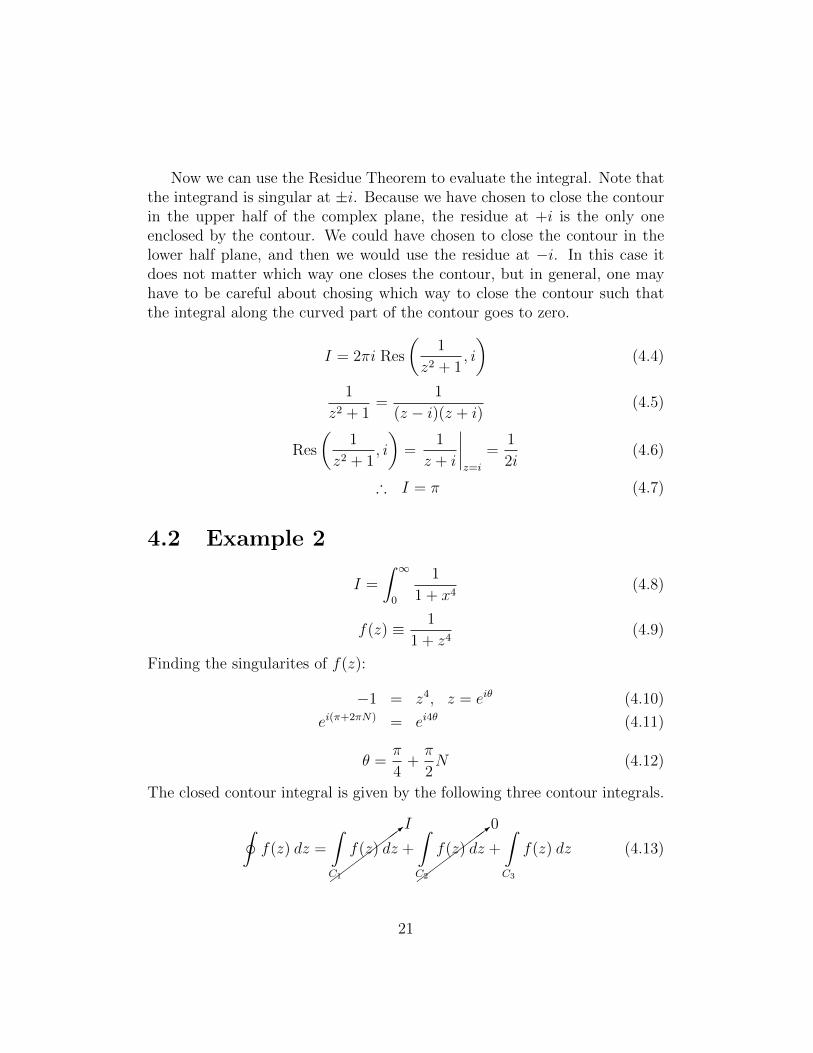
Now we can use the Residue Theorem to evaluate the integral. Note thatthe integrand is singular at ±i. Because we have chosen to close the contourin the upper half of the complex plane, the residue at +i is the only oneenclosed by the contour. We could have chosen to close the contour in thelower half plane, and then we would use the residue at −i. In this case itdoes not matter which way one closes the contour, but in general, one mayhave to be careful about chosing which way to close the contour such thatthe integral along the curved part of the contour goes to zero.

I = 2πi Res

(1

z2 + 1, i

)(4.4)

1

z2 + 1=

1

(z − i)(z + i)(4.5)

Res

(1

z2 + 1, i

)=

1

z + i

∣∣∣∣z=i

=1

2i(4.6)

∴ I = π (4.7)

4.2 Example 2

I =

∫ ∞0

1

1 + x4(4.8)

f(z) ≡ 1

1 + z4(4.9)

Finding the singularites of f(z):

−1 = z4, z = eiθ (4.10)

ei(π+2πN) = ei4θ (4.11)

θ =π

4+π

2N (4.12)

The closed contour integral is given by the following three contour integrals.

∮f(z) dz =

������>

I∫C1

f(z) dz +

������>

0∫C2

f(z) dz +

∫C3

f(z) dz (4.13)

21

We have not yet chosen which angle, θ, should be used to evaluate the integralalong C3. ∫

C3

f(z) dz =

∫ 0

∞dr eiθ

1

1 + r4ei4θ, z = r eiθ (4.14)

We can conveniently choose 4θ = 2π ⇒ θ = π2

such that ei4θ = 1.∫ 0

∞dr eiπ/2

1

1 + r4= −i

∫ ∞0

dr eiπ/21

1 + r4= −iI (4.15)

∴ 2πi Res(f(z), eiπ/4

)= I − iI = I(1− i) (4.16)

Res(f(z), eiπ/4

)=

z − eiπ/4

1 + z4

∣∣∣∣eiπ/4

(4.17)

=1

4z3

∣∣∣∣eiπ/4

(4.18)

=1

4ei3π/4(4.19)

=1

4(−1√

2+ i 1√

2

) (4.20)

=

√2

4 (i− 1)(4.21)

I(1− i) = 2πi Res(f(z), eiπ/4

)(4.22)

= 2πi

√2

4 (i− 1)(4.23)

I =πi√

2

1

(i− 1) (i− 1)(4.24)

=πi√

2

1

i− �1 + �1 + i(4.25)

=π

2√

2(4.26)

22

Chapter 5

Summing Series

5.1 Non-alternating Series

Consider the residues of cot(πz) when z is an integer, n. Take note thatcot(πz + πn) = cot(πz), and therefore it sufficent to expand cot(πz) nearz = 0 to have an expansion for cot(πz) when z is near any integer.

cot(πz) =cos(πz)

sin(πz)(5.1)

=1− 1

2(πz)2 +O[(πz)4]

πz − 16(πz)3 +O[(πz)5]

(5.2)

=1− 1

2(πz)2 +O[(πz)4]

πz(1− 1

6(πz)2 +O[(πz)4]

) (5.3)

Let x = 16(πz)2 +O[(πz)4], and use the geometric series

1

1− x= 1 + x+ x2 + . . . (5.4)

then

cot(πz) =

(1

πz− 1

2πz +O[(πz)3]

)(1 +

1

6(πz)2 +O[(πz)4]

)(5.5)

=1

πz− 1

2πz +

1

6πz +O[(πz)3] (5.6)

=1

πz− 1

3πz +O[(πz)3] (5.7)

23

⇒ Res (cot(πz), n) =1

π(5.8)

Res (π cot(πz), n) = 1 (5.9)

If we have a function g(z) that is not singular at z = n, then

Res (g(z) π cot(πz), n) = g(n) (5.10)

Thus, a summation of terms g(n) can be related to a contour integral ofthe function g(z) π cot(πz) using the Residue Theorem. This can be helpfulin summing difficult series, as will be shown in the following example.

Consider the Riemann zeta-function, ζ(s).

ζ(s) =∞∑n=1

1

ns(5.11)

Let’s say we want to evaluate ζ(2).

g(n) ≡ 1

n2, ζ(2) =

∞∑n=1

g(n) (5.12)

f(z) ≡ g(z) π cot(πz) (5.13)

1

2πi

∮f(z) dz =

−∞∑n=−1

Res (f(z), n) + Res (f(z), 0)

+∞∑n=1

Res (f(z), n) (5.14)

=−∞∑n=−1

g(n) + Res (f(z), 0) +∞∑n=1

g(n) (5.15)

=−∞∑n=−1

1

n2+ Res (f(z), 0) +

∞∑n=1

1

n2(5.16)

= Res (f(z), 0) + 2∞∑n=1

1

n2(5.17)

= Res (f(z), 0) + 2 ζ(2) (5.18)

24

Note that because g(z) is singular at z = 0, the residue of f(z) at z = 0cannot be calculated with equation 5.10. It must be calculated independently.

f(z) =π

z2cot(πz) (5.19)

=iπ

z2

eiπz + e−iπz

eiπz − e−iπz, z = R eiθ (5.20)

as R→∞

→ iπ

R2 ei2θeiπR cos θ���

��: 0

e−πR sin θ + e−iπR cos θ eπR sin θ

eiπR cos θ�����:

0

e−πR sin θ − e−iπR cos θ eπR sin θ

(5.21)

→ iπ

R2 ei2θ �����

������:−1

e−iπR cos θ eπR sin θ

−e−iπR cos θ eπR sin θ(5.22)

→ 0 (5.23)

∴∮f(z) dz = 0, as R→∞ (5.24)

∴ ζ(2) =−1

2Res (f(z), 0) (5.25)

Now we need to find the residue at z = 0.

f(z) =π

z2cot(πz) (5.26)

=π

z2

(1

πz− 1

3πz +O[(πz)3]

)(5.27)

=1

z3− π2

3z+O[π2z] (5.28)

⇒ Res (f(z), 0) =−π2

3(5.29)

∴ ζ(2) =−1

2

−π2

3=π2

6(5.30)

5.2 Alternating Series

For alternating series, instead of considering the residues of cot(πz), as wedid with non-alternating series, we will consider the residues of csc(πz) atz = n, an integer.

25

Near z = n, w ≡ z − n is near 0.

csc(πz) = csc(πw + πn) (5.31)

= (−1)n csc(πw) (5.32)

=(−1)n

sin(πw)(5.33)

=(−1)n

πw − 16(πw)3 +O[(πw)5]

(5.34)

=(−1)n

πw(1− 1

6(πw)2 +O[(πw)4]

) (5.35)

Using the geometric series,

=(−1)n

πw

(1 +

1

6(πw)2 +O[(πw)4]

)(5.36)

= (−1)n(

1

πw+

1

6πw +O[(πw)3]

)(5.37)

⇒ Res (csc(πz), n) =(−1)n

π(5.38)

Res (π csc(πz), n) = (−1)n (5.39)

If we have a function g(z) that is not singular at z = n, then

Res (g(z) π csc(πz), n) = (−1)n g(n) (5.40)

Let’s say we want to evaluate the series

∞∑n=1

(−1)n−1

n2(5.41)

26