Transp Porous Med (2011) 89:383–397DOI 10.1007/s11242-011-9776-z

Pressure Buildup During CO2 Injection into a ClosedBrine Aquifer

Simon A. Mathias · Gerardo J. González Martínez de Miguel ·Kate E. Thatcher · Robert W. Zimmerman

Received: 24 May 2010 / Accepted: 30 April 2011 / Published online: 28 May 2011© Springer Science+Business Media B.V. 2011

Abstract CO2 injected into porous formations is accommodated by reduction in thevolume of the formation fluid and enlargement of the pore space, through compression ofthe formation fluids and rock material, respectively. A critical issue is how the resulting pres-sure buildup will affect the mechanical integrity of the host formation and caprock. Buildingon an existing approximate solution for formations of infinite radial extent, this article presentsan explicit approximate solution for estimating pressure buildup due to injection of CO2 intoclosed brine aquifers of finite radial extent. The analysis is also applicable for injection into aformation containing multiple wells, in which each well acts as if it were in a quasi-circularclosed region. The approximate solution is validated by comparison with vertically averagedresults obtained using TOUGH2 with ECO2N (where many of the simplifying assumptionsare relaxed), and is shown to be very accurate over wide ranges of the relevant parameterspace. The resulting equations for the pressure distribution are explicit, and can be easilyimplemented within spreadsheet software for estimating CO2 injection capacity.

Keywords CO2 injection · Forchheimer’s equation · Closed formation · Pressure buildup

S. A. Mathias (B) · G. J. González Martínez de Miguel · K. E. ThatcherDepartment of Earth Sciences, Durham University, Durham, UKe-mail: s.a.mathias@durham.ac.uk

K. E. Thatchere-mail: kate.thatcher@durham.ac.uk

G. J. González Martínez de MiguelERC Equipoise Limited, London, UKe-mail: gerardo@ercequipoise.com

R. W. ZimmermanDepartment of Earth Science and Engineering, Imperial College London, London, UKe-mail: r.w.zimmerman@imperial.ac.uk

123

384 S. A. Mathias et al.

List of symbolsA Formation plan area [L2]b Forchheimer parameter [L−1]br Relative Forchheimer parameter [-]co Compressibility of CO2 [M−1 LT2]cr Compressibility of geological formation

[M−1 LT2]cw Compressibility of brine [M−1 LT2]h CO2 brine interface elevation [L]h D = h/H Dimensionless interface elevation [-]H Formation thickness [L]k Permeability [L2]kr Relative permeability [-]M0 Mass injection rate [MT−1]p Fluid pressure [ML−1 T−2]pD = 2π Hρokr kp/M0μo Dimensionless pressure [-]qo CO2 flux [LT−1]qoD = 2π Hrwρoqo/M0 Dimensionless CO2 flux [-]qw Brine flux [LT−1]qwD = 2π Hrwρoqw/M0 Dimensionless brine flux [-]r Radial distance [L]rc Radial extent of reservoir [L]rcD = rc/rw Dimensionless radial extent of reservoir [-]rD = r/rw Dimensionless radius [-]rw Well radius [L]Sr Residual brine saturation [-]t Time [T]tcD = αr2

cD/2.246γ Dimensionless time at which the pressuredisturbance meets the reservoir boundary [-]

tD = M0t/2π(1 − Sr )φHr2wρo Dimensionless time [-]

α = M0μo(cr + cw)/2π(1 − Sr )Hρokr k Dimensionless compressibility [-]β = M0kr kbr b/2π Hrwμo Dimensionless Forchheimer parameter [-]γ = μo/krμw Viscosity ratio [-]ε = (1 − Sr )(co − cw)/(cr + cw) Normalized fluid compressibility difference [-]μo Viscosity of CO2 [ML−1 T−1]μw Viscosity of brine [ML−1 T−1]ρo Density of CO2 [ML−3]ρw Density of brine [ML−3]σ = brρo/ρw Density ratio [-]φ Porosity [-]

1 Introduction

Carbon capture and storage is arguably one of the most promising mitigation technologiescurrently under consideration to combat CO2 emission-induced climate change. The pro-cess involves capturing CO2 at the point of generation, compressing it to a supercritical fluidstate, and sequestering it at depth within a suitable permeable geological formation. For closed

123

Pressure Buildup During CO2 Injection 385

geological formations, CO2 injected into a porous formation is accommodated by reductionin the volume of the formation fluid and enlargement of the pore space, through compressionof the formation fluids and rock material, respectively. For open formations, injected CO2

is additionally accommodated by the displacement of native formation fluids from the hostformation of concern. A critical concern is how the resulting pressure buildup will affect themechanical integrity of the host formation and caprock. In assessing the storage capacity ofa given formation, one should, therefore, verify that the estimated pressure buildup does notexceed the failure limit of the overlying cap-rock (Mathias et al. 2009a).

The calculation of pressure buildup requires simulating the injection of supercritical CO2

into the porous formation. This can be achieved using a numerical multi-phase reservoirsimulator (e.g., Rutqvist et al. 2008; Birkholzer et al. 2009). However, such models canbe expensive to acquire and computationally intensive to run. Therefore, there has been aparallel effort to develop simple semi-analytical methods. The earliest of these assumedBuckley–Leverett displacement (Saripalli and McGrail 2002). The Buckley–Leverett equa-tion describes one-dimensional, two-phase, incompressible, immiscible flow in the absenceof capillary pressure (Buckley and Leverett 1942). Nordbotten et al. (2005) took a similarapproach by assuming incompressible flow, negligible vertical pressure gradient, and negli-gible capillary pressure. Their resulting governing equations are mathematically analogousto the Buckley–Leverett equation for the special case when relative permeability is a linearfunction of fluid saturation. A major advantage of this model is that the saturation distributioncan be derived explicitly; a limitation is that calculation of the pressure distribution requiresthe specification of an arbitrary radius of influence. Zhou et al. (2008) developed an alternativemethod that accounts for the storage capacity due to formation and fluid compressibility. How-ever, an important limiting assumption in their analysis is that pressure buildup is spatiallyuniform and independent of formation permeability. More recently, Mathias et al. (2009c)improved on Nordbotten’s approach by incorporating formation and fluid compressibility,and developed accurate approximate solutions to the model equations using the method ofmatched asymptotic expansions. They also proceeded to apply the methodology of Mathiaset al. (2008) to obtain a large-time approximation that accounts for inertial effects usingthe Forchheimer (1901) equation. Inertial effects are particularly important for injection (orproduction) scenarios, due to the increase in velocity caused by the convergence of flow linesaround the injection (or production) well (Mathias et al. 2008; Mathias and Todman 2010).

The analytical solutions of Zhou et al. (2008) and Mathias et al. (2009c) represent two endmembers of the problem of concern. Zhou’s method is useful when the reservoir is small andthe permeability is large. Mathias’s method, assuming a formation of infinite radial extent, isuseful for very large reservoirs where permeability is small. In this article, the approximatesolutions of Mathias et al. (2009c) are extended to account for formations of finite radialextent, leading to an approximate analytical solution that is accurate over the entire domainof practical interest. Zhou et al. (2008) additionally account for pressure reduction due tofluid leak-off into the cap-rock. This aspect of Zhou’s work is not considered further in thisarticle.

In a recent article, Ehlig-Economides and Economides (2010) extended the heuristic func-tion (inspired by the Buckley–Leverett solution) of Burton et al. (2008) to account for aclosed outer boundary of the reservoir formation, by applying a factor of 0.472 to the radiusof influence parameter. No explanation was given as to the origin of this factor, but a detailedderivation for the case of single-phase flow can be found in Dake (1978). Although the oper-ational conclusions of Ehlig-Economides and Economides (2010) have received substantialcriticism (e.g., Chadwick et al. 2010), their fundamental idea of providing a closed boundarycondition is worthy of further consideration. The study in this article can be said to build on

123

386 S. A. Mathias et al.

the mathematical development presented by Ehlig-Economides and Economides (2010) inthe following respects: (1) a clear derivation is provided concerning the origin of the 0.472factor in the context of two-phase flow, (2) near-well non-Darcy effects are accounted forusing the Forchheimer equation, and (3) the pressure distribution is calculated explicitly with-out the need for using the Welge (1952) method for tracking the CO2 front and the heuristicfunction of Burton et al. (2008) for describing the pressure distribution within the two-phaseregion.

2 Problem Definition

Following Nordbotten et al. (2005), we assume the existence of a sharp interface located at anelevation, h [L], above the base of the formation, with CO2 and immobile brine on one sideand mobile brine on the other side. Due to CO2 generally having a lower density than brine,CO2 is assumed to exist on the upper-side of the interface. We ignore capillary pressure, andassume that the pressure, p [ML−1 T−2], is in vertical equilibrium over the entire thicknessof the confined porous formation of vertical extent H [L]. Saturation, relative permeability,and viscosity are assumed to be constant and uniform within both the CO2 and the brinezones. In order to obtain a solution for the pressure distribution, the traditional assumption ismade that the two fluids and the porous formation each have small compressibilities that donot vary with pressure (Mathias et al. 2009c). Detailed discussions concerning the theoreticalbasis of these assumptions are presented by Nordbotten et al. (2005), Dentz and Tartakovsky(2009), and Gasda et al. (2009).

From consideration of conservation of mass, the governing equations for the fluid pres-sure, p, and the interface elevation, h, can be written as

(1 − Sr )∂

∂t[φρo(H − h)] = −1

r

∂

∂r[rρo(H − h)qo] (1)

(1 − Sr )∂

∂t(φρwh) + Sr H

∂

∂t(φρw) = −1

r

∂

∂r(rρwhqw) (2)

where the fluxes, qo [LT−1] and qw [LT−1], are assumed to be related to pressure gradientby the Forchheimer equation (Forchheimer 1901), as follows:

μo

kr kqo + br bρoqo|qo| = −∂p

∂r(3)

μw

kqw + bρwqw|qw| = −∂p

∂r(4)

where Sr [-] is the residual brine saturation, t [T] is time, φ [-] is the porosity, r [L] is the radialdistance from the center of the injection well, k [L2] is absolute permeability, b [L−1] is theForchheimer parameter, and ρo [ML−3], ρw [ML−3], μo [ML−1 T−1], and μw [ML−1 T−1]are the densities and viscosities of the CO2 and brine, respectively. The factors kr [-] andbr [-] are the relative permeability and relative Forchheimer parameters, respectively, for theCO2, representing the fact that the transmissivity of the CO2 is reduced due to the presenceof the residual brine saturation, Sr (see Bennion and Bachu 2008). Relative permeability andrelative Forchheimer parameters for the brine are not required in this article, because thebrine saturation is assumed to be 1 before it is displaced by CO2.

123

Pressure Buildup During CO2 Injection 387

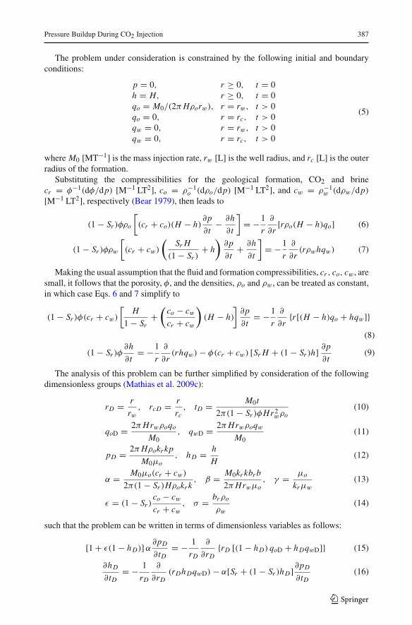
The problem under consideration is constrained by the following initial and boundaryconditions:

p = 0, r ≥ 0, t = 0h = H, r ≥ 0, t = 0qo = M0/(2π Hρorw), r = rw, t > 0qo = 0, r = rc, t > 0qw = 0, r = rw, t > 0qw = 0, r = rc, t > 0

(5)

where M0 [MT−1] is the mass injection rate, rw [L] is the well radius, and rc [L] is the outerradius of the formation.

Substituting the compressibilities for the geological formation, CO2 and brinecr = φ−1(dφ/dp) [M−1 LT2], co = ρ−1

o (dρo/dp) [M−1 LT2], and cw = ρ−1w (dρw/dp)

[M−1 LT2], respectively (Bear 1979), then leads to

(1 − Sr )φρo

[(cr + co)(H − h)

∂p

∂t− ∂h

∂t

]= −1

r

∂

∂r[rρo(H − h)qo] (6)

(1 − Sr )φρw

[(cr + cw)

(Sr H

(1 − Sr )+ h

)∂p

∂t+ ∂h

∂t

]= −1

r

∂

∂r(rρwhqw) (7)

Making the usual assumption that the fluid and formation compressibilities, cr , co, cw , aresmall, it follows that the porosity, φ, and the densities, ρo and ρw , can be treated as constant,in which case Eqs. 6 and 7 simplify to

(1 − Sr )φ(cr + cw)

[H

1 − Sr+

(co − cw

cr + cw

)(H − h)

]∂p

∂t= −1

r

∂

∂r{r [(H − h)qo + hqw]}

(8)

(1 − Sr )φ∂h

∂t= −1

r

∂

∂r(rhqw) − φ(cr + cw) [Sr H + (1 − Sr )h]

∂p

∂t(9)

The analysis of this problem can be further simplified by consideration of the followingdimensionless groups (Mathias et al. 2009c):

rD = r

rw

, rcD = r

rc, tD = M0t

2π(1 − Sr )φHr2wρo

(10)

qoD = 2π Hrwρoqo

M0, qwD = 2π Hrwρoqw

M0(11)

pD = 2π Hρokr kp

M0μo, h D = h

H(12)

α = M0μo(cr + cw)

2π(1 − Sr )Hρokr k, β = M0kr kbr b

2π Hrwμo, γ = μo

krμw

(13)

ε = (1 − Sr )co − cw

cr + cw

, σ = brρo

ρw

(14)

such that the problem can be written in terms of dimensionless variables as follows:

[1 + ε(1 − h D)] α∂pD

∂tD= − 1

rD

∂

∂rD{rD [(1 − h D) qoD + h DqwD]} (15)

∂h D

∂tD= − 1

rD

∂

∂rD(rDh DqwD) − α[Sr + (1 − Sr )h D]∂pD

∂tD(16)

123

388 S. A. Mathias et al.

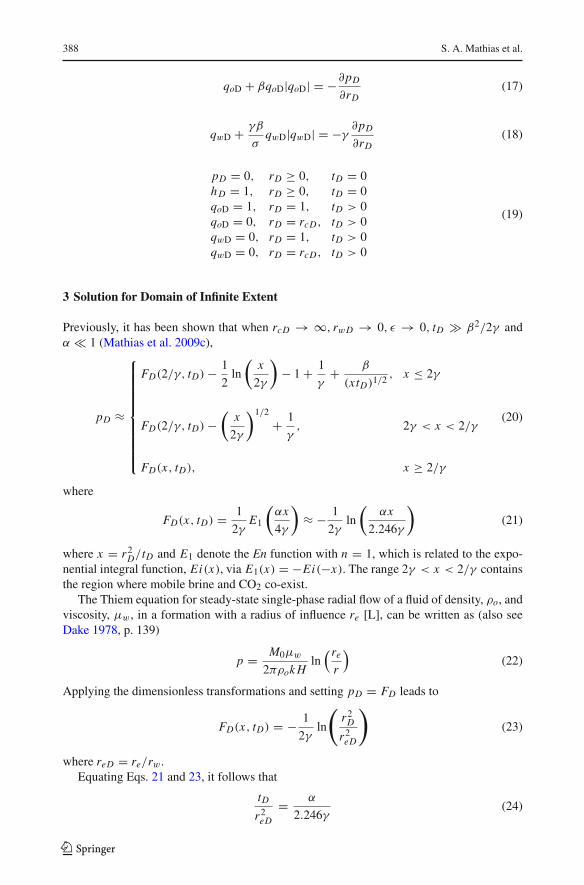
qoD + βqoD|qoD| = −∂pD

∂rD(17)

qwD + γβ

σqwD|qwD| = −γ

∂pD

∂rD(18)

pD = 0, rD ≥ 0, tD = 0h D = 1, rD ≥ 0, tD = 0qoD = 1, rD = 1, tD > 0qoD = 0, rD = rcD, tD > 0qwD = 0, rD = 1, tD > 0qwD = 0, rD = rcD, tD > 0

(19)

3 Solution for Domain of Infinite Extent

Previously, it has been shown that when rcD → ∞, rwD → 0, ε → 0, tD � β2/2γ andα � 1 (Mathias et al. 2009c),

pD ≈

⎧⎪⎪⎪⎪⎪⎪⎪⎪⎪⎨⎪⎪⎪⎪⎪⎪⎪⎪⎪⎩

FD(2/γ, tD) − 1

2ln

(x

2γ

)− 1 + 1

γ+ β

(xtD)1/2 , x ≤ 2γ

FD(2/γ, tD) −(

x

2γ

)1/2

+ 1

γ, 2γ < x < 2/γ

FD(x, tD), x ≥ 2/γ

(20)

where

FD(x, tD) = 1

2γE1

(αx

4γ

)≈ − 1

2γln

(αx

2.246γ

)(21)

where x = r2D/tD and E1 denote the En function with n = 1, which is related to the expo-

nential integral function, Ei(x), via E1(x) = −Ei(−x). The range 2γ < x < 2/γ containsthe region where mobile brine and CO2 co-exist.

The Thiem equation for steady-state single-phase radial flow of a fluid of density, ρo, andviscosity, μw , in a formation with a radius of influence re [L], can be written as (also seeDake 1978, p. 139)

p = M0μw

2πρok Hln

(re

r

)(22)

Applying the dimensionless transformations and setting pD = FD leads to

FD(x, tD) = − 1

2γln

(r2

D

r2eD

)(23)

where reD = re/rw .Equating Eqs. 21 and 23, it follows that

tD

r2eD

= α

2.246γ(24)

123

Pressure Buildup During CO2 Injection 389

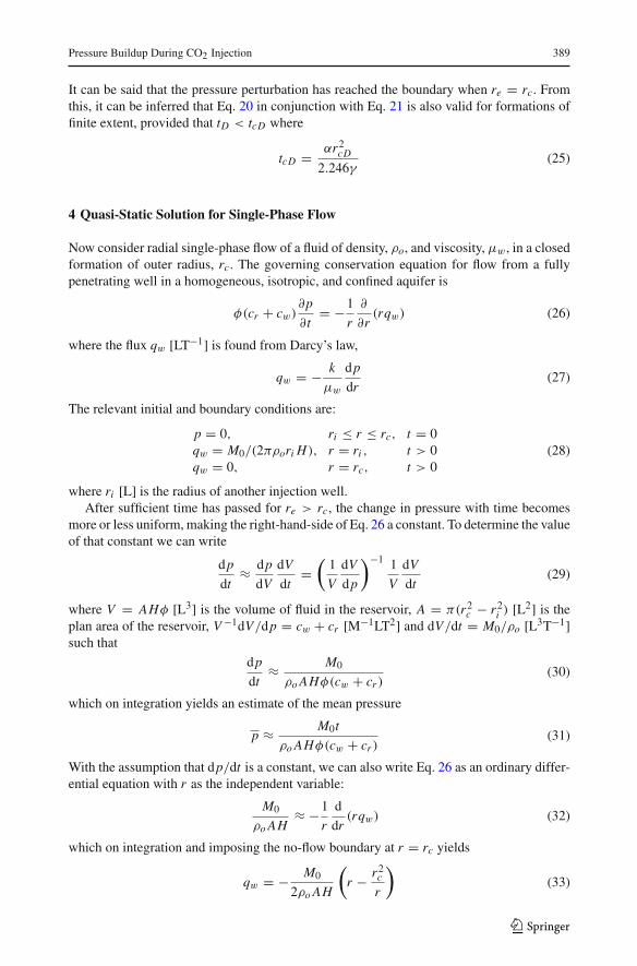
It can be said that the pressure perturbation has reached the boundary when re = rc. Fromthis, it can be inferred that Eq. 20 in conjunction with Eq. 21 is also valid for formations offinite extent, provided that tD < tcD where

tcD = αr2cD

2.246γ(25)

4 Quasi-Static Solution for Single-Phase Flow

Now consider radial single-phase flow of a fluid of density, ρo, and viscosity, μw , in a closedformation of outer radius, rc. The governing conservation equation for flow from a fullypenetrating well in a homogeneous, isotropic, and confined aquifer is

φ(cr + cw)∂p

∂t= −1

r

∂

∂r(rqw) (26)

where the flux qw [LT−1] is found from Darcy’s law,

qw = − k

μw

dp

dr(27)

The relevant initial and boundary conditions are:

p = 0, ri ≤ r ≤ rc, t = 0qw = M0/(2πρori H), r = ri , t > 0qw = 0, r = rc, t > 0

(28)

where ri [L] is the radius of another injection well.After sufficient time has passed for re > rc, the change in pressure with time becomes

more or less uniform, making the right-hand-side of Eq. 26 a constant. To determine the valueof that constant we can write

dp

dt≈ dp

dV

dV

dt=

(1

V

dV

dp

)−1 1

V

dV

dt(29)

where V = AHφ [L3] is the volume of fluid in the reservoir, A = π(r2c − r2

i ) [L2] is theplan area of the reservoir, V −1dV/dp = cw + cr [M−1LT2] and dV/dt = M0/ρo [L3T−1]such that

dp

dt≈ M0

ρo AHφ(cw + cr )(30)

which on integration yields an estimate of the mean pressure

p ≈ M0t

ρo AHφ(cw + cr )(31)

With the assumption that dp/dt is a constant, we can also write Eq. 26 as an ordinary differ-ential equation with r as the independent variable:

M0

ρo AH≈ −1

r

d

dr(rqw) (32)

which on integration and imposing the no-flow boundary at r = rc yields

qw = − M0

2ρo AH

(r − r2

c

r

)(33)

123

390 S. A. Mathias et al.

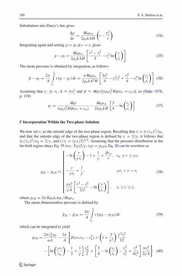
Substitution into Darcy’s law gives

dp

dr= M0μw

2ρok AH

(r − r2

c

r

)(34)

Integrating again and setting p = pi at r = ri gives

p − pi = M0μw

2ρok AH

[r2 − r2

i

2− r2

c ln

(r

ri

)](35)

The mean pressure is obtained by integration, as follows:

p − pi = 2π

A

rc∫ri

r(p − pi ) dr = π M0μw

2ρok A2 H

[3r4

c

4− r2

c r2i + r4

i

4− r4

c ln

(rc

ri

)](36)

Assuming that rc � ri , A ≈ πr2c and p ≈ M0t/[πρor2

c Hφ(cr + cw)], so (Dake 1978,p. 139)

pi = M0t

πρor2c Hφ(cr + cw)

− M0μw

2πρok H

[3

4− ln

(rc

ri

)](37)

5 Incorporation Within the Two-phase Solution

We now set ri as the outside edge of the two-phase region. Recalling that x = (r/rw)2/tD ,and that the outside edge of the two-phase region is defined by x = 2/γ , it follows that(ri/rw)2/tD = 2/γ , and r/ri = (γ x/2)1/2. Assuming that the pressure distribution in thefar-field region obeys Eq. 35 (i.e., FD(2/γ, tD) = pi D), Eq. 20 can be rewritten as

pD − pi D ≈

⎧⎪⎪⎪⎪⎪⎪⎪⎪⎪⎪⎪⎪⎨⎪⎪⎪⎪⎪⎪⎪⎪⎪⎪⎪⎪⎩

− ln

(r

γ ri

)− 1 + 1

γ+ βrw

r, rw ≤ r ≤ γ ri

− r

γ ri+ 1

γ, γ ri < r < ri

πr2c

γ A

[r2 − r2

i

2r2c

− ln

(r

ri

)], ri ≤ r ≤ rc

(38)

where pi D = 2π Hρokr kpi/M0μo.The mean dimensionless pressure is defined by

pD − pi D = 2π

A

rc∫rw

r(pD − pi D) dr (39)

which can be integrated to yield

pi D = 2πr2wtD

αA− 2π

A

{β(γ ri rw − r2

w) +(

1 + 2

γ 3

)γ 2r2

i

12

−[

ln

(γ ri

rw

)− 1

2+ 1

γ

]r2w

2+

[3

4− ln

(rc

ri

)− r2

i

r2c

+ r4i

4r4c

]πr4

c

2γ A

}(40)

123

Pressure Buildup During CO2 Injection 391

Recall from Eq. 31 that p ≈ M0t/[πρor2c Hφ(cr + cw)].

From the above, it can be said that the analogue of Eq. 21 for a closed formation is

FD(x, tD) =

⎧⎪⎪⎪⎪⎪⎨⎪⎪⎪⎪⎪⎩

1

2γE1

(αx

4γ

), tD < tcD

pi D + πr2c

A

[(γ x − 2)tD

2γ 2r2cD

− 1

2γln

(γ x

2

)], tD > tcD

(41)

where tcD is found from Eq. 25. Assuming that rc � ri (i.e., the radial extent of the CO2

plume is always much smaller than that of the formation), A = πr2c , and the above solution

reduces to

FD(x, tD) ≈

⎧⎪⎪⎪⎪⎪⎨⎪⎪⎪⎪⎪⎩

1

2γE1

(αx

4γ

), tD < tcD

2tD

αr2cD

− 1

γ

[3

4− 1

2ln

(r2

cD

xtD

)− (γ x − 2)tD

2γ r2cD

], tD > tcD

(42)

So the semi-analytical solution of Mathias et al. (2009c) (i.e., Eqs. 20 and 21) can be extendedto deal with closed formations by replacing Eq. 21 with Eq. 42. Note that 3/4 = − ln(0.472),which explains the origin of the factor 0.472 that appears in Ehlig-Economides and Econo-mides (2010).

6 Comparison with TOUGH2 ECO2N

The derivation of the approximate solution given by Eqs. 20 and 42 involves the applicationof a number of simplifying assumptions, among which the most important are: (1) verti-cal pressure equilibrium; (2) negligible capillary pressure; (3) constant fluid properties; and(4) immiscible displacement. To assess the impact of these assumptions, the approximatesolution is now compared to simulations conducted with the reservoir simulator TOUGH2(Pruess et al. 1999) using the CO2 and brine equations of state stored in the ECO2N module(Pruess 2005). The scenarios simulated were loosely based on those previously described byZhou et al. (2008).

The TOUGH2 simulations assume a fully penetrating well situated at the origin of a two-dimensional radially symmetric closed flow-field. The model assumes the van Genuchten(1980) relationship between brine effective saturation, Se [-], and capillary pressure,Pc [ML−1T−2]

Se =(

1 +∣∣∣∣ Pc

Pc,0

∣∣∣∣n)−m

, n = 1

1 − m(43)

and that brine and CO2 relative permeability are linearly related to Se and (1 − Se), respec-tively. In the absence of residual CO2 saturation, the effective brine saturation is defined bySe = (Sw − Sr )/(1− Sr ), where Sw [-] is the total brine saturation (the volumetric proportionof pore-space occupied by brine) and Sr [-] is the residual brine saturation.

The model parameters used were as follows:

Area, A = 1257 km2

Radial extent, rc = 20 km

123

392 S. A. Mathias et al.

Porosity, φ = 0.2Residual brine saturation, Sr = 0.5End-point relative permeability for CO2, kr = 0.3Well radius, rw = 0.2 mRock compressibility, cr = 4.5 × 10−10 Pa−1

Forchheimer parameter, b = 0Injection rate, M0 = 100 kg/sInitial pressure, P0 = 10 MPaTemperature, T = 40◦CSalinity, S = 0.15 kg/lvan Genuchten parameter, m = 0.46van Genuchten parameter, Pc0 = 19600 PaFormation thickness, H = 50 or 200 mPermeability, k = 10−13 or 10−12 m2

Vertically, the domain was divided into ten equally spaced layers, which corresponds to5 m/layer in the case of a 50-m thickness aquifer and 20 m/layer in the case of a 200-m thick-ness aquifer. To invoke a mean initial pressure of 10 MPa, the initial pressure distributionwas set to impose initially hydrostatic conditions with pressure along the central horizontalaxis set at 10 MPa. Horizontally, the 20- km radial extent of the model was divided into foursub-domains with boundaries located at 0.2, 10, 500, 1000, and 20,000 m from the origin.Each sub-domain was discretized in the radial direction by a set of logarithmically spacednodes. The inner zone contained two-hundred nodes, the outer zone contained fifty nodes,and the two intermediate zones contained one-hundred nodes each. The four zones werenecessary to allow sufficiently high resolution around the well without requiring an exces-sive number of grid-points. Specifically, the four sub-domains allowed the node spacing togrow from 5 mm at the well-face to 3280 m at the outer boundary using only 450 nodes in theradial direction. Such refinement was found to be necessary to ensure adequate resolutionfor accurately evaluating well pressures.

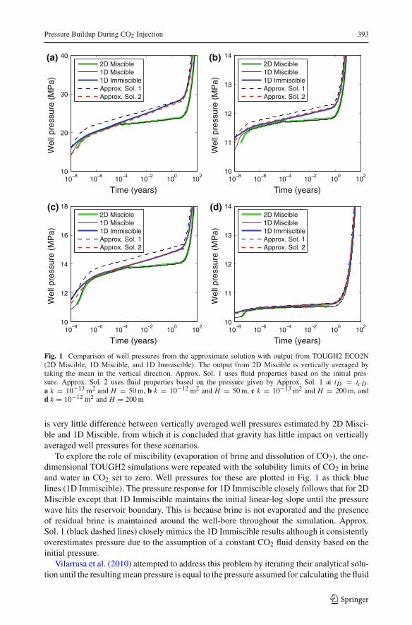
Vertically averaged (by taking the mean in the vertical direction) well pressures fromthe TOUGH2 ECO2N two-dimensional miscible radial flow simulations are presented inFig. 1 as green thick lines (2D Miscible). For the case presented in Fig. 1d (k = 10−12 m2

and H = 200 m), the TOUGH2 simulation was terminated after just less than a year dueto model convergence difficulties. Nevertheless, all four scenarios exhibit a similar pressureresponse. Pressure increases monotonically with time. After 10−6 years, the pressure increaseexhibits a constant linear-log slope until around 10−4 years beyond which pressure increasesaccording to a new reduced linear-log slope. The latter effect is due to an increase in CO2

relative permeability that develops once the residual brine is evaporated in the near-wellregion. Finally, after around 10 years, the pressure disturbance reaches the outer boundary ofthe reservoir and the well pressure increases asymptotically.

Plotted alongside, as black dashed lines (Approx. Sol. 1), are well pressures estimatedusing the approximate solution with fluid properties calculated for the initial pressure usingequations previously presented by Mathias et al. (2009a,b). Approx. Sol. 1 shows the correctinitial linear-log slope, but tends to overestimate the pressure buildup and does not predictthe reduction in slope due to brine evaporation. Nevertheless, Approx. Sol. 1 predicts similar(to TOUGH2) pressure increases once the pressure wave reaches the outer boundary.

To explore the role of gravity in pressure evolution, the TOUGH2 simulations wererepeated but with just one layer for the entire formation thickness (as opposed to ten). Wellpressures for these are plotted in Fig. 1 as thin black lines (1D Miscible). It is clear that there

123

Pressure Buildup During CO2 Injection 393

10−8

10−6

10−4

10−2

100

102

10

20

30

40

Time (years)

Wel

l pre

ssur

e (M

Pa)

10−8

10−6

10−4

10−2

100

102

10

11

12

13

14

Time (years)

Wel

l pre

ssur

e (M

Pa)

10−8

10−6

10−4

10−2

100

102

10

12

14

16

18

Time (years)

Wel

l pre

ssur

e (M

Pa)

10−8

10−6

10−4

10−2

100

102

10

11

12

13

14

Time (years)

Wel

l pre

ssur

e (M

Pa)

2D Miscible1D Miscible1D ImmiscibleApprox. Sol. 1Approx. Sol. 2

2D Miscible1D Miscible1D ImmiscibleApprox. Sol. 1Approx. Sol. 2

2D Miscible1D Miscible1D ImmiscibleApprox. Sol. 1Approx. Sol. 2

2D Miscible1D Miscible1D ImmiscibleApprox. Sol. 1Approx. Sol. 2

(a) (b)

(d) (c)

Fig. 1 Comparison of well pressures from the approximate solution with output from TOUGH2 ECO2N(2D Miscible, 1D Miscible, and 1D Immiscible). The output from 2D Miscible is vertically averaged bytaking the mean in the vertical direction. Approx. Sol. 1 uses fluid properties based on the initial pres-sure. Approx. Sol. 2 uses fluid properties based on the pressure given by Approx. Sol. 1 at tD = tcD .a k = 10−13 m2 and H = 50 m, b k = 10−12 m2 and H = 50 m, c k = 10−13 m2 and H = 200 m, andd k = 10−12 m2 and H = 200 m

is very little difference between vertically averaged well pressures estimated by 2D Misci-ble and 1D Miscible, from which it is concluded that gravity has little impact on verticallyaveraged well pressures for these scenarios.

To explore the role of miscibility (evaporation of brine and dissolution of CO2), the one-dimensional TOUGH2 simulations were repeated with the solubility limits of CO2 in brineand water in CO2 set to zero. Well pressures for these are plotted in Fig. 1 as thick bluelines (1D Immiscible). The pressure response for 1D Immiscible closely follows that for 2DMiscible except that 1D Immiscible maintains the initial linear-log slope until the pressurewave hits the reservoir boundary. This is because brine is not evaporated and the presenceof residual brine is maintained around the well-bore throughout the simulation. Approx.Sol. 1 (black dashed lines) closely mimics the 1D Immiscible results although it consistentlyoverestimates pressure due to the assumption of a constant CO2 fluid density based on theinitial pressure.

Vilarrasa et al. (2010) attempted to address this problem by iterating their analytical solu-tion until the resulting mean pressure is equal to the pressure assumed for calculating the fluid

123

394 S. A. Mathias et al.

100

101

102

103

104

10

20

30

40

Radial distance (m)

Pre

ssur

e (M

Pa)

(d)

100

101

102

103

104

0

0.2

0.4

0.6

0.8

1

Radial distance (m)

CO

2 sat

urat

ion

(−)

(a)

100

101

102

103

104

10

20

30

40

Radial distance (m)

Pre

ssur

e (M

Pa)

(c)

100

101

102

103

104

0

0.2

0.4

0.6

0.8

1

Radial distance (m)

CO

2 sat

urat

ion

(−)

(b)101 yrs

10−1 yrs

10−3 yrs

10−5 yrs

101 yrs

10−1 yrs

10−3 yrs

10−5 yrs

101 yrs

10−1 yrs

10−3 yrs

10−5 yrs

101 yrs

10−1 yrs

10−3 yrs

10−5 yrs

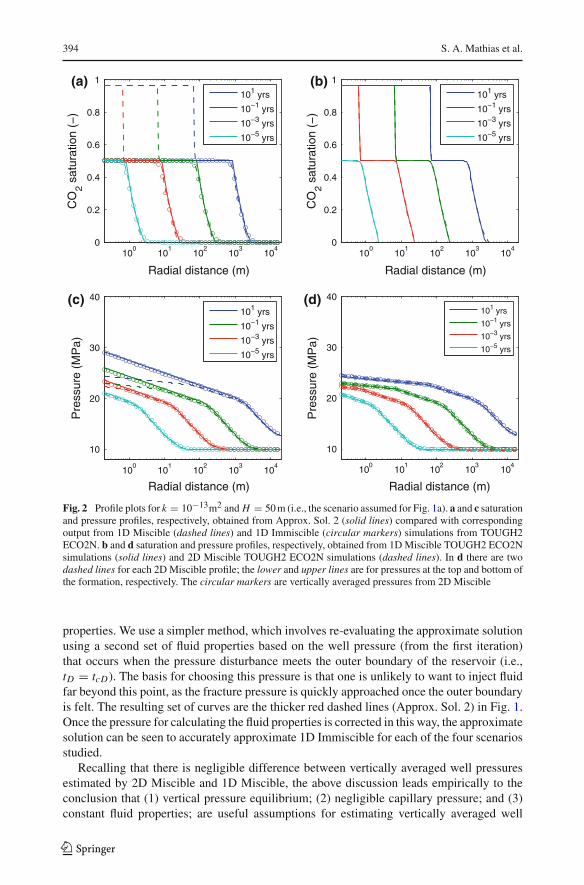
Fig. 2 Profile plots for k = 10−13m2 and H = 50 m (i.e., the scenario assumed for Fig. 1a). a and c saturationand pressure profiles, respectively, obtained from Approx. Sol. 2 (solid lines) compared with correspondingoutput from 1D Miscible (dashed lines) and 1D Immiscible (circular markers) simulations from TOUGH2ECO2N. b and d saturation and pressure profiles, respectively, obtained from 1D Miscible TOUGH2 ECO2Nsimulations (solid lines) and 2D Miscible TOUGH2 ECO2N simulations (dashed lines). In d there are twodashed lines for each 2D Miscible profile; the lower and upper lines are for pressures at the top and bottom ofthe formation, respectively. The circular markers are vertically averaged pressures from 2D Miscible

properties. We use a simpler method, which involves re-evaluating the approximate solutionusing a second set of fluid properties based on the well pressure (from the first iteration)that occurs when the pressure disturbance meets the outer boundary of the reservoir (i.e.,tD = tcD). The basis for choosing this pressure is that one is unlikely to want to inject fluidfar beyond this point, as the fracture pressure is quickly approached once the outer boundaryis felt. The resulting set of curves are the thicker red dashed lines (Approx. Sol. 2) in Fig. 1.Once the pressure for calculating the fluid properties is corrected in this way, the approximatesolution can be seen to accurately approximate 1D Immiscible for each of the four scenariosstudied.

Recalling that there is negligible difference between vertically averaged well pressuresestimated by 2D Miscible and 1D Miscible, the above discussion leads empirically to theconclusion that (1) vertical pressure equilibrium; (2) negligible capillary pressure; and (3)constant fluid properties; are useful assumptions for estimating vertically averaged well

123

Pressure Buildup During CO2 Injection 395

pressures. However, the assumption of immiscible displacement leads to an overestimate ofpressure buildup during intermediate times due to the ignoring of brine evaporation aroundthe well-bore.

Although well pressure is of primary interest in this context (Mathias et al. 2009a), it isinteresting to study the spatial distributions of pressure and CO2 predicted by the approxi-mate solution as well. Figure 2a and c presents saturation and pressure profiles, respectively,at various times for the case presented in Fig. 1a (k = 10−13m2 and H = 50 m) as pre-dicted by 1D Miscible, 1D Immiscible, and Approx. Sol. 2 (saturation profiles are obtainedusing Eq. 26 of Mathias et al. 2009c). The saturation and pressure profiles for 1D Immis-cible and Approx. Sol. 2 are virtually identical. These are also very similar to those for 1DMiscible, outside the dry-out zone (where CO2 saturation rises above (1 − Sr ) around thewell-bore). Inside the dry-out zone, 1D Miscible predicts lower pressure gradients due to

100 101 102 103 104

10

12

14

16

18

Radial distance (m)

Pre

ssur

e (M

Pa)

100

101

102

103

104

0

0.2

0.4

0.6

0.8

1

Radial distance (m)

CO

2 sat

urat

ion

(−)

(a)

100

101

102

103

104

10

12

14

16

18

Radial distance (m)

Pre

ssur

e (M

Pa)

(c)

100

101

102

103

104

0

0.2

0.4

0.6

0.8

1

Radial distance (m)

CO

2 sat

urat

ion

(−)

(b)101 yrs

10−1 yrs

10−3 yrs

10−5 yrs

101 yrs

10−1 yrs

10−3 yrs

10−5 yrs

101 yrs

10−1 yrs

10−3 yrs

10−5 yrs

101 yrs10−1 yrs10−3 yrs10−5 yrs

(d)

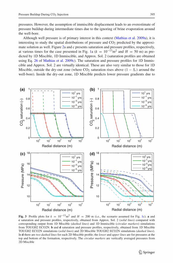
Fig. 3 Profile plots for k = 10−13m2 and H = 200 m (i.e., the scenario assumed for Fig. 1c). a andc saturation and pressure profiles, respectively, obtained from Approx. Sol. 2 (solid lines) compared withcorresponding output from 1D Miscible (dashed lines) and 1D Immiscible (circular markers) simulationsfrom TOUGH2 ECO2N. b and d saturation and pressure profiles, respectively, obtained from 1D MiscibleTOUGH2 ECO2N simulations (solid lines) and 2D Miscible TOUGH2 ECO2N simulations (dashed lines).In d there are two dashed lines for each 2D Miscible profile; the lower and upper lines are for pressures at thetop and bottom of the formation, respectively. The circular markers are vertically averaged pressures from2D Miscible

123

396 S. A. Mathias et al.

the increased availability of permeable pathways for CO2 resulting from the evaporationof the residual brine.

Figure 2b compares 1D Miscible with vertically averaged (by taking the mean in the ver-tical direction) CO2 saturations from 2D Miscible. Figure 2d compares 1D Miscible withbottom (upper dashed line), top (lower dashed line), and vertically averaged pressures (cir-cular markers) from 2D Miscible. There is negligible difference between results from 1DMiscible and 2D Miscible again verifying that the vertical equilibrium assumption is highlyappropriate for this scenario.

However, the k = 10−13m2 and H = 50 m scenario is least likely to be effected bygravity segregation due it having the smallest permeability and smallest formation thickness.Figure 3 shows the same data as Fig. 2 but for the case presented in Fig. 1c (k = 10−13m2

and H = 200 m). Again, Fig. 3a and c demonstrate the ability of Approx. Sol. 2 to accuratelyapproximate the internal states of 1D Immiscible. However, in Fig. 3b it is seen that for times> 0.1 years, there is a significant difference between the vertically averaged CO2 saturationfrom 2D Miscible and that of 1D Miscible. This is due to the effect of gravity segregation(Lu et al. 2009; Yamamoto and Doughty 2011). Figure 3d compares pressures estimated by1D Miscible and 2D Miscible. Although there is a wide variation between the upper and lowerpressures (the dashed lines), 1D Miscible again provides an accurate estimate of verticallyaveraged pressure (the circular markers). The variations between the upper and lower pres-sures are largely due to differences in elevation. Total hydrostatic pressure over the reservoirformation is (ρwgH =) 0.54 MPa when H = 50 m and 2.17 MPa when H = 200 m.

7 Summary and Conclusions

When seeking to estimate storage capacity of geological reservoirs for CO2 geo-sequestra-tion, it is necessary to be able to estimate the pressure buildup resulting from the injectionprocess. Previously, Mathias et al. (2009c) derived a semi-analytical solution for predictingpressure buildup when the formation can be assumed to be of infinite radial extent. In thisarticle, the study of Mathias et al. (2009c) is extended to account for finite outer boundaries,by invoking a quasi-static condition. The semi-analytical solution was verified by comparisonwith vertically averaged results from TOUGH2 simulations of the fully dynamic problem.This study also shows how to modify the solution presented in Mathias et al. (2009c), toaccount for residual brine saturation and the associated reduction in the effective relativepermeability of the CO2. The resulting equations remain simple to evaluate in spreadsheetsoftware, and can be easily implemented in currently available storage capacity estimationframeworks (e.g., Mathias et al. 2009a).

Acknowledgments This study was partially funded by the UK Energy Technology Institute’s (ETI) UKStorage Appraisal Project (UKSAP) and funding from both the UK Natural Environment Research Coun-cil (NERC) and the UK Technology Strategy Board (TSB) provided through the UK Knowledge TransferPartnership (KTP) scheme.

References

Bear, J.: Hydraulics of Groundwater. McGraw-Hill, New York (1979)Bennion, D.B., Bachu, S.: Drainage and imbibition relative permeability relationships for supercritical

CO2/brine and H2S/brine systems in intergranular sandstone, carbonate, shale, and annhydrite rocks.SPE Reserv. Eval. Eng. June, 487–496 (2008)

123

Pressure Buildup During CO2 Injection 397

Birkholzer, J.T., Zhou, Q., Tsang, C.F.: Large-scale impact of CO2 storage in deep saline aquifers: A sensitiv-ity study on pressure response in stratified systems. Int. J. Greenhouse Gas Control 3, 181–194 (2009).doi:10.1016/j.ijggc.2008.08.002

Buckley, S.E., Leverett, M.C.: Mechanism of fluid displacement in sands. Trans. Am. Inst. Min. Metall. Pet.Eng. 146, 107–116 (1942)

Burton, M., Kumar, N., Bryant, S.L.: Time-dependent injectvity during co2 storage in aquifers. In: SPE/DOEImproved Oil Recovery Symposium held in Tulsa, Oklahoma, USA, 19–23 April (2008). SPE 113937

Chadwick, A., Hodrien, C., Hovorka, S., Mackay, E., Mathias, S., Lovell, B., Kalaydjian, F., Sweeney, G.,Benson, S., Dooley, J., Davidson, C.: The realities of storing carbon dioxide—a response to CO2 storagecapacity issues raised by Ehlig-Economides & Economides. Technical report, Published by the EuropeanTechnology Platform for Zero Emission Fossil Fuel Power Plants (ZEP) (2010). doi:10.1038/npre.2010.4500.1

Dake, L.P.: Fundamentals of Reservoir Engineering. 17th Impression. Elsevier, Amsterdam (1978)Dentz, M., Tartakovsky, D.M.: Abrupt-interface solution for carbon dioxide injection into porous

media. Transp. Porous Media 79, 15–27 (2009). doi:10.1007/s11242-008-9268-yEhlig-Economides, C.A., Economides, M.J.: Sequestering carbon dioxide in a closed underground volume.

J. Pet. Sci. Eng. 70, 123–130 (2010). doi:10.1016/j.petrol.2009.11.002Forchheimer, P.: Wasserbewegung durch Boden. Z. Ver. Dtsch. Ing 45, 1782–1788 (1901)Gasda, S., Nordbotten, J.M., Celia, M.A.: Vertical equilibrium with sub-scale analytical methods for geological

CO2 sequestration. Comput. Geosci. 13(4), 469–481 (2009). doi:10.1007/s10596-009-9138-xLu, C., Lee, S.Y., Han, W.S., McPherson, B.J., Lichtner, P.C.: Comments on “abrupt-interface solution for

carbon dioxide injection into porous media” by M. Dentz and D. Tartakovsky. Transp. Porous Media 79,29–37 (2009). doi:10.1007/s11242-009-9362-9

Mathias, S.A., Todman, L.C.: Step-drawdown tests and the Forchheimer equation. Water Resour. Res. 46,W07514 (2010). doi:10.1029/2009WR008635

Mathias, S.A., Butler, A.P., Zhan, H.: Approximate solutions for Forchheimer flow to a well. J. Hydraul.Eng. 134(9), 1318–1325 (2008). doi:10.1061/(ASCE)0733-9429(2008)134:9(1318)

Mathias, S.A., Hardisty, P.E., Trudell, M.R., Zimmerman, R.W.: Screening and selection of sitesfor CO2 sequestration based on pressure buildup. Int. J. Greenhouse Gas Control 3, 577–585(2009a). doi:10.1016/j.ijggc.2009.05.002

Mathias, S.A., Hardisty, P.E., Trudell, M.R., Zimmerman, R.W.: Erratum to screening and selection of sitesfor CO2 sequestration based on pressure buildup [Int. J. Greenhouse Gas Control 3(5) (2009) 577–585].Int. J. Greenhouse Gas Control 4, 108–109 (2009b). doi:10.1016/j.ijggc.2009.11.004

Mathias, S.A., Hardisty, P.E., Trudell, M.R., Zimmerman, R.W.: Approximate solutions for pressure buildupduring CO2 injection in brine aquifers. Transp. Porous Media 79, 265–284 (2009c). doi:10.1007/s11242-008-9316-7

Nordbotten, J.M., Celia, M.A., Bachu, S.: Injection and storage of CO2 in deep saline aquifers: analytic solu-tion for CO2 plume evolution during injection. Transp. Porous Media 58, 339–360 (2005). doi:10.1007/s11242-004-0670-9

Pruess, K., Oldenburg, C.M., Moridis, G.: TOUGH2 user’s guide, version 2.0. Report LBNL-43134, LawrenceBerkeley National Laboratory, Berkeley, CA, USA (1999)

Pruess, K.: ECO2N: A TOUGH2 fluid property module for mixtures of water, NaCl, and CO2. Report LBNL-57952, Lawrence Berkeley National Laboratory, Berkeley, CA, USA (2005)

Rutqvist, J., Birkholzer, J.T., Tsang, C.F.: Coupled reservoir—geomechanical analysis of the potential fortensile and shear failure associated with CO2 injection in multilayered reservoir—caprock systems. Int.J. Rock Mech. Min. Sci. 45, 132–143 (2008). doi:10.1016/j.ijrmms.2007.04.006

Saripalli, P., McGrail, P.: Semi-analytical approaches to modeling deep well injection of CO2 for geologicalsequestration. Energy Convers. Manag. 43(2), 185–198 (2002)

van Genuchten, M.Th.: A closed form equation for predicting the hydraulic conductivity of unsaturatedsoils. Soil Sci. Soc. Am. J. 44, 892–898 (1980)

Vilarrasa, V., Bolster, D., Dentz, M., Olivella, S., Carrera, J.: Effects of CO2 compressibility on CO2 storagein deep saline aquifers. Transp. Porous Media 85, 619–639 (2010). doi:10.1007/s11242-010-9582-z

Welge, H.J.: A simplified method for computing oil recovery by gas or water drive. Trans. Am. Inst. Min.Metall. Pet. Eng. 195, 91–98 (1952)

Yamamoto, H., Doughty, C.: Investigation of gridding effects for numerical simulations of CO2 geologicsequestration. Int. J. Greenhouse Gas Control (2011). doi:10.1016/j.ijggc.2011.02.007

Zhou, Q., Birkholzer, J., Tsang, C., Rutqvist, J.: A method for quick assessment of CO2 storage capacity inclosed and semi-closed saline formations. Int. J. Greenhouse Gas Control 2(4), 626–639 (2008)

123