Preliminary determination of the interdependence amongstrong-motion amplitude, earthquake magnitude and hypocentraldistance for the Himalayan region

Imtiyaz A. Parvez,1,3,* Alexander A. Gusev,2 Giuliano F. Panza1,3 andAnatoly G. Petukhin4

1 Department of Earth Sciences, University of Trieste, Via E. Weiss 4, 34127 Trieste, Italy. E-mails: parvez@dst.univ.trieste.it; panza@dst.univ.trieste.it2 Institute of Volcanic Geology and Geochemistry, Russian Academy of Science, 9 Piip Boulevard, Petropavlovsk-Kamchatsky, 683006, Russia.

E-mail: gusev@emsd.iks.ru3 The Abdus Salam International Centre for Theoretical Physics, SAND Group, Trieste, Italy4 Kamchatka Experimental and Methodical Seismological Department GS RAS 9 Piip Boulevard, Petropavlovsk-Kamchatsky, 683006, Russia.

E-mail: petuhin@mail.ru

Accepted 2000 September 19. Received 2000 July 26; in original form 2000 February 6

SUMMARY

Since the installation of three limited-aperture strong-motion networks in theHimalayan region in 1986, six earthquakes with Mw=5.2±7.2 have been recorded upto 1991. The data set of horizontal peak accelerations and velocities consists of182-component data for the hypocentral distance range 10±400 km. This data set islimited in volume and coverage and, worst of all, it is highly inhomogeneous. Thus, wecould not determine regional trends for amplitudes by means of the traditional approachof empirical multiple regression. Instead, we perform the reduction of the observationsto a ®xed distance and magnitude using independently de®ned distance and magnitudetrends. To determine an appropriate magnitude-dependent distance attenuation law, weuse the spectral energy propagation/random function approach of Gusev (1983) andadjust its parameters based on the residual variance. In doing so we con®rm the known,rather gradual mode of decay of amplitudes with distance in the Himalayas; this seemsto be caused by the combination of high Qs and crustal waveguide effects for highfrequencies. The data are then reduced with respect to magnitude. The trend of peakacceleration versus magnitude cannot be determined from observations, and we assumethat it coincides with that of abundant Japanese data. For the resulting set of reducedlog10 (peak acceleration) data, the residual variance is 0.372, much above commonlyfound values. However, dividing the data into two geographical groups, western withtwo events and eastern with four events, reduces the residual variance to a more usuallevel of 0.272 (a station/site component of 0.222 and an event component of 0.162). Thiskind of data description is considered acceptable. A similar analysis is performed withvelocity data, and again we have to split the data into two subregional groups. Withour theoretically grounded attenuation laws we attempt a tentative extrapolation of ourresults to small distances and large magnitudes. Our minimum estimates of peakacceleration for the epicentral zone of Mw=7.5±8.5 events is Apeak=0.25±0.4 g for thewestern Himalayas, and as large as Apeak=1±1.6 g for the eastern Himalayas. Similarly,the expected minimum epicentral values of Vpeak for Mw=8 are 35 cm sx1 for thewestern and 112 cm sx1 for the eastern Himalayas. To understand whether our resultsre¯ect the properties of the subregions and not of a small data set, we check them againstmacroseismic intensity data for the same subregion. The presence of unusually highlevels of epicentral amplitudes for the eastern subregion agrees well with the macro-seismic evidence such as the epicentral intensity levels of X±XII for the Great Assam

* Now at: CSIR Centre for Mathematical Modelling and Computer Simulation (C-MMACS), NAL Belur Campus, Bangalore, 560037, India.

E-mail: parvez@cmmacs.ernet.in

Geophys. J. Int. (2001) 144, 577±596

# 2001 RAS 577

earthquake of 1897. Therefore, our results represent systematic regional effects, andthey may be considered as a basis for future regionalized seismic hazard assessment inthe Himalayan region. We see the location of earthquake sources/faults at a considerabledepth within the relatively drier and higher-strength shield crust as the main cause of theobserved enhanced amplitudes for the eastern Himalayas events. Western Himalayassources are shallower and occupy the tectonically highly fractured upper part of thecrust, of accretionary origin. The low attenuation common to both subregions is due tothe presence of cold, low-scattering and high-Q shield crust.

Key words: attenuation, earthquake source, Himalayan region, seismic hazard,strong-motion amplitude.

1 I N T R O D U C T I O N

The Himalayan region in India is one of the most seismically

active areas of the world. The region forms the collision plate

boundary between the Indian and Eurasian plates and has

experienced many great earthquakes (M>8) that have in¯icted

heavy casualties and economic damage. Hence, it is essential to

assess the intensity of severe ground motion in order to specify

appropriate structural design loads and to undertake other

countermeasures. The determination of ground motion relation-

ships describing peak ground acceleration and velocity as a

function of magnitude and distance may represent an important

step in solving this problem. During the last two decades,

many researchers (e.g. Trifunac 1976; Joyner & Boore 1981;

Kawashima et al. 1986; Sabetta & Pugliese 1987; Fukushima &

Tanaka 1990; Ambraseys 1995; Atkinson & Boore 1995;

Campbell 1997; Gusev et al. 1997) have studied the ground

motion attenuation relationships for various regions of the

world. Chandrasekaran (1994), Singh et al. (1996) and Sharma

(1998) proposed attenuation relations for the Himalayan region.

Most of these studies are, in essence, multiple regression models

that permit the prediction of a target parameter by means of an

empirical relationship established on the basis of the available

strong-motion data from a particular region. However, even

for regions with a long history of strong-motion observations,

data are often not suf®cient for obtaining completely reliable

average trends.

Among the studies that characterize various regions of

the territory of India, and in particular the Himalayan region,

one should ®rst mention the research on the attenuation of

macroseismic intensity, based on isoseismal maps and available

macroseismic data (e.g. Kaila & Sarkar 1977; Chandra 1980;

Gupta & Trifunac 1988). Instrumental data for strong motion

in the Himalayan region were not available before 1986, and

this impeded the determination of attenuation relationships

of peak ground motion based on local data. This is the reason

why the attenuation relationships of other regions (e.g. eastern

United States) were adopted for seismic hazard studies, in

order to estimate the expected strong ground motion ampli-

tudes (Khattri et al. 1984). In choosing a particular `analogue

region', it is required that both regions have similar attenuation

with distance of the Modi®ed Mercalli Intensity (MMI).

Gupta & Trifunac (1988) used the probabilistic relations for

the attenuation of MMI with distance in India and applied

scaling equations for strong-motion parameters in terms of site

intensity for some other regions, which have a similar de®nition

of intensity. This approach is indirect, and the availability of

even a limited instrumental data set justi®es further analysis.

Such an analysis will signi®cantly improve the reliability of the

evaluation of seismic hazard. As a ®rst step in this direction, it is

worthwhile determining region-speci®c attenuation relationships

for peak amplitudes based on locally recorded strong-motion

accelerograms.

In 1985±1986, three strong-motion arrays were installed in

the Himalayan region. Six events with Mw in the range 5.2±7.2

were recorded by these arrays during 1986±1991. Recently,

Sharma (1998) used these data to obtain the attenuation

relationship for peak ground horizontal acceleration for the

Himalayan region based on the multiple regression approach.

However, in his work he excluded two major events from

his study. This data censoring, with so small a data set, does

not seem well justi®ed. Formally, these data were excluded

because of large source depths. We will show that these events

do not differ from other events in any signi®cant respect and

essentially belong to the same population as the others. One

additional reason why these data deserve repeated study is the

unusually gradual distance decay of amplitudes found by both

Singh et al. (1996) and Sharma (1998). Such a slow decay is not

plausible from the physical viewpoint. Another less detailed

study based on this data set is that of Chandrasekaran (1994).

He also obtained a regional attenuation relationship but did

not consider it as fully reliable. The main conclusion of his

work was that a large amount of data is needed in order to

develop a suf®ciently accurate relationship.

In the present study, we analyse the strong-motion

amplitudes obtained by the Himalayan arrays following the

approach of Gusev (1983) and Gusev & Petukhin (1995,

1996). To determine the peak horizontal acceleration and

velocity relationships with magnitude and distance, we prefer

to combine the limited amount of available observations

with theoretically based attenuation laws, rather than to seek

for purely empirical relationships based on `blind' multiple

regression. Particularly dangerous in this situation is the

so-called one-step regression approach (see Joyner & Boore

1981, 1993). The general approach that has been applied to the

data includes the following steps: (1) reduction of the data to a

®xed distance; (2) reduction of the result to a ®xed magnitude;

and (3) analysis of ground, subregional and station effects.

In both reductions, a number of variants of the attenuation

laws and magnitude trends have been investigated and the

appropriate one, assumed to be near-optimal, was chosen.

After accounting for the subregional effect, we derive the

attenuation relationships for two subregions, the eastern and

western Himalayas.

578 I. A. Parvez et al.

# 2001 RAS, GJI 144, 577±596

2 S T R O N G - M O T I O N A R R A Y S A N DD A T A

The Department of Science and Technology (DST), Government

of India, under the programme of Intensi®cation of Research in

High Priority Areas has funded three strong-motion arrays in

India. The Department of Earthquake Engineering, University

of Roorkee (Chandrasekaran & Das 1992), installed these arrays

during 1985±1986. Fig. 1 gives the locations of these arrays,

namely (1) the Shillong array (in the state of Assam and

Meghalaya), (2) the Uttar Pradesh Hills (UP) array (in the west

of the state of Uttar Pradesh), and (3) the Kangra array (in the

state of Himachal Pradesh).

45 analogue strong-motion accelerographs have been installed

in the Shillong array with a spacing of 10±40 km, 50 similar

accelerographs were installed in the Kangra Array and 40 in the

UP array with a spacing of 8±30 km. The instruments are

three-component SMA-1, Kinemetrics, USA. Fig. 1 shows the

locations of stations with instruments that have been triggered

at least once. The epicentres of the recorded events are also

shown. Four events with magnitude 5.2±7.2 were recorded by

the Shillong array between 1986 and 1988 and two earthquakes

with magnitude 5.5 and 6.8 were recorded separately by the

Kangra and UP arrays in 1986 and 1991, respectively. Detailed

information about the epicentral parameters of each event is

listed in Table 1. As a measure of the source size we use the

moment magnitude Mw. Five events have been taken from the

Harvard CMT catalogue. For the event of 1986 September 10,

Mw is not reported by any agency, but ISC gives Ms=4.5, from

which we estimate Mw=5.2 (through the non-linear relation-

ship compiled by Gusev 1991). We reject the possibility of using

ML as the reference magnitude because ML determined for the

region of study is not totally reliable.

The preliminary processing and digitization of the strong-

motion records of these events was performed by Chandrasekaran

& Das (1992). They used the baseline correction and ®ltering

procedures of Lee & Trifunac (1979). The process is funda-

mentally the same as the standard processing method described

by Hudson et al. (1971). The data were sampled at a rate of

0.02 s and they were bandpass ®ltered with characteristic

frequencies of 0.17, 0.20, 25.0 and 27.0 Hz using an Ormsby

®lter. In the present study we use 138 horizontal-component

Figure 1. Generalized geological map showing the strong-motion arrays and the event locations in the Himalayas recorded by the network.

Table 1. List of events used in the study of Amax and Vmax.

No. Region Date Time (UT) Lat. (uN) Long. (uE) Depth (km) Mw

(CMT) (NEIC)

1 W. Himalayas 1986 April 26 07:35:20.0 32.17 76.28 15 33 5.5

2 1991 Oct. 19 21:23:21.6 30.73 78.79 15 10 6.8

3 E. Himalayas 1986 Sept. 10 07:50:25.6 25.42 92.08 _ 43 5.2

4 1987 May 18 01:53:59.3 25.27 94.20 75 50 6.2

5 1988 Feb. 6 14:50:43.6 24.64 91.51 31 33 5.8

6 1988 Aug. 6 00:36:37.6 25.14 95.12 101 91 7.2

Strong-motion amplitudes in the Himalayan region 579

# 2001 RAS, GJI 144, 577±596

peak accelerations and velocities (including both components)

from the events recorded by the Shillong array and 44

horizontal-component peak accelerations and velocities from

the Kangra and UP arrays. To represent relative site locations,

we use the hypocentral distance. Detailed information of site

conditions is not available. The sites of the Kangra and UP

arrays are in the High Mountain terrain, which is expected

to be devoid of thick alluvial cover, but the sites may be on

gravel sediments in river valleys or on severely fractured and

weathered rock. The site conditions of the Shillong array are

even more complicated, with mixed rock and soil types. The

altitudes of the sites of this array are much lower than the two

former arrays.

A summary of data coverage with magnitude and hypo-

central distance is shown in Fig. 2. Circles denote eastern

Himalayan events and diamonds denote western Himalayan

events. The same symbol convention is used throughout the

text. The ®gure shows that our data coverage over hypocentral

distance is very poor. Data for most events cover only a limited

distance interval and for three events out of six, there are no

data at distances below 90 km.

3 G E O L O G Y A N D T E C T O N I C S

The general geological and tectonic location of the study area

is shown in Fig. 1. For plate tectonic reviews of this area see

e.g. Gansser (1964, 1977), Evans (1964), Valdiya (1980), Wadia

(1975); a more traditional description of tectonics and seismo-

geology can be found in e.g. LeFort (1975), Mitchell (1981),

Sinha-Roy (1982), Ni & Barazangi (1984), Chen & Molnar

(1990). Based on these sources, we give here only a very brief

resume of the geology and tectonics of the region. The earth-

quakes under study occurred within two locations along a ®rst-

order tectonic feature. The two western events occurred in the

collision boundary between the Indian and Eurasian plates.

Here the Indian plate is assumed to subduct at a low angle

under Tibet, and the main Himalayan range represents the

prominent accretionary feature in this subduction system. The

eastern group of four events is located in the northeastern

region of India, which has undergone various stages of tectonic

activity. The present-day tectonics of the region is complicated

because of the interaction between active north±south con-

vergence along the Himalayas and the east±west convergence

and folding within the Indo±Burman ranges (Ni & Barazangi

1984). These four events are located about 200±250 km to the

south of the main subduction boundary.

On a smaller scale, the two western arrays of Kangra and

Uttar Pradesh Hills are located in the vicinity of two major faults,

the Main Boundary Thrust (MBT) and the Main Central

Thrust (MCT), that trace the entire length of the Himalayas.

The MBT is a series of thrusts that separates the predominantly

pre-Tertiary Lesser Himalayas from the Tertiary Siwalik belt

(Wadia 1975; Gansser 1964, 1977). This zone comprises a

mountain belt ranging in elevation from about 500±2500 m, com-

posed of fossiliferous Riphean sediments overridden by several

thrust sheets. The MCT at the base of the central crystalline

zone (Gansser 1964) dips northwards, separating the High

Himalayas from the Lesser Himalayas. Many stations of the

UP array lie along the MCT. The MBT and MCT, which dip

steeply (30u±45u) near to the surface, ¯atten out at depth and

are assumed to merge to form the interplate surface dipping to

the north at 15u. Many transverse faults and other secondary

faults cutting across the Himalayas tectonic province have also

been recognized. The famous Kangra earthquake of 1906

(M=8.1) occurred here and the Kangra array is located in its

epicentral area.

The Shillong array is located on and around the Shillong

Plateau. The Precambrian basement of the Indian shield is

exposed on the Shillong Plateau and in the Mikir Hills to the

northeast (Evans 1964), with an average elevation of 1000 m.

These crystalline rocks are almost completely surrounded by

Tertiary sedimentary rocks and Quaternary sediments of the

Bengal basin to the south, of the Assam valley to the northeast

and of the Brahmaputra valley to the north (Evans 1964;

Mitchell 1981). The eastern boundary of the Shillong Plateau

and the Mikir Hills abuts against the northern part of the

Indo±Burman ranges, which locally trends northeastwards and

joins the eastern Himalayas to form the Assam syntaxis. The

Shillong Plateau is bounded by prominent tectonic features, for

example, the Dhubri fault towards the west and the Dauki fault

towards south. The Dauki fault merges with the northeast-

trending Disang and Naga thrusts towards the east (Fig. 1).

This region has experienced some of the world's biggest

earthquakes. The `Great Assam' earthquakes occurred in the

Shillong region in 1897 (M=8.7) and in the Mishmi region in

1950 (M=8.6). The Shillong array approximately covers the

epicentral area of the 1897 event.

4 S I M P L E T H E O R Y V E R S U S E M P I R I C A LF O R M U L A E I N S T R O N G - M O T I O N D A T AA N A L Y S I S : M O D E L L I N G M A G N I T U D E -D E P E N D E N T A T T E N U A T I O N F O RS E M I - E M P I R I C A L D A T A A N A L Y S I S

Let us consider in what form we should seek the description of

the observed accelerations and velocities. In a region with a

suf®ciently large amount of recorded strong-motion data, the

average dependence of strong-motion parameters (e.g. peak

acceleration) on distance, magnitude and other parameters is

usually determined on an empirical basis by means of multiple

regression procedures. Theoretical considerations are only used,Figure 2. Distribution of processed strong-motion data over magnitude

and hypocentral distance.

580 I. A. Parvez et al.

# 2001 RAS, GJI 144, 577±596

if at all, in choosing the form of the regression formula. Such

empirical formulae (not always mutually compatible) are

then used for approximate forecasting of various parameters

of strong ground motion related to speci®c earthquake sources,

wave propagation paths and site geology. One dif®culty with

such formulae is related to the discrepancies between simple

forms of traditional empirical regression relationships for various

ground motion parameters and the actual, often non-linear,

trends that are both observed and expected from even a simple

theory. For example, until 1985 the regression coef®cient that

de®ned amplitude attenuation was almost never (even implicitly)

assumed to be magnitude-dependent, whereas such a depen-

dence is evident in the data, and it arises automatically in an

adequate theoretical calculation. The situation is frequently

aggravated by a very limited number of observations in

many poorly studied and/or low-seismicity areas. To formally

describe non-linearities or interactions between factors one

needs a considerable number of regression coef®cients, but the

data may barely be suf®cient to determine two or three. To

replace the use of formulae, we designed a simpli®ed practical

algorithm capable of determining approximate mean trends

of strong ground motion parameters. To make these trends

more reliable, we specify many properties of Earth medium

and earthquake sources (where possible) in a way that is

independent of scarce strong-motion data. The trends calcu-

lated in this manner may be used instead of formulae, both

in the analysis of observed ground motions and in the con-

struction of predictive schemes that interpolate or extrapolate

the data. This approach is particularly valuable when used

for extrapolation because it gives at least a limited guarantee

against grossly erroneous predictions. Of course, it can produce

errors but they are much more `controllable', because the

simpli®cations made in the modelling are explicit, in contrast

with the implicit assumptions made when choosing a particular

structure of an analytic formula. To implement the approach

described, a dedicated code (SSK) has been developed (Gusev

& Petukhin 1995, 1996) and a brief description of it is given

in the Appendix. In a number of aspects, our method of

data analysis follows the approaches of Trifunac (1976) and

Trifunac & Lee (1990).

The mode of data analysis described seems especially appro-

priate for the present study when the data coverage over

distance and magnitude is poor and purely empirical analysis is

hardly possible at all. Therefore, we will use a simple theoretical

model to describe the attenuation of peak acceleration and

velocity in a magnitude-dependent way. At a given magnitude,

we can determine the shape of the distance, R, dependence on a

theoretical basis and then adjust only its absolute level to the

data. In practice, an equivalent procedure has been applied:

data have been reduced to a ®xed distance and magnitude and

then averaged.

5 D E T E R M I N A T I O N O F T H E E M P I R I C A LR E G I O N A L A m a x (M w , R ) RELAT IONSH I P

5.1 Choosing the model scaling law of the sourcespectra for predicting peak acceleration trends

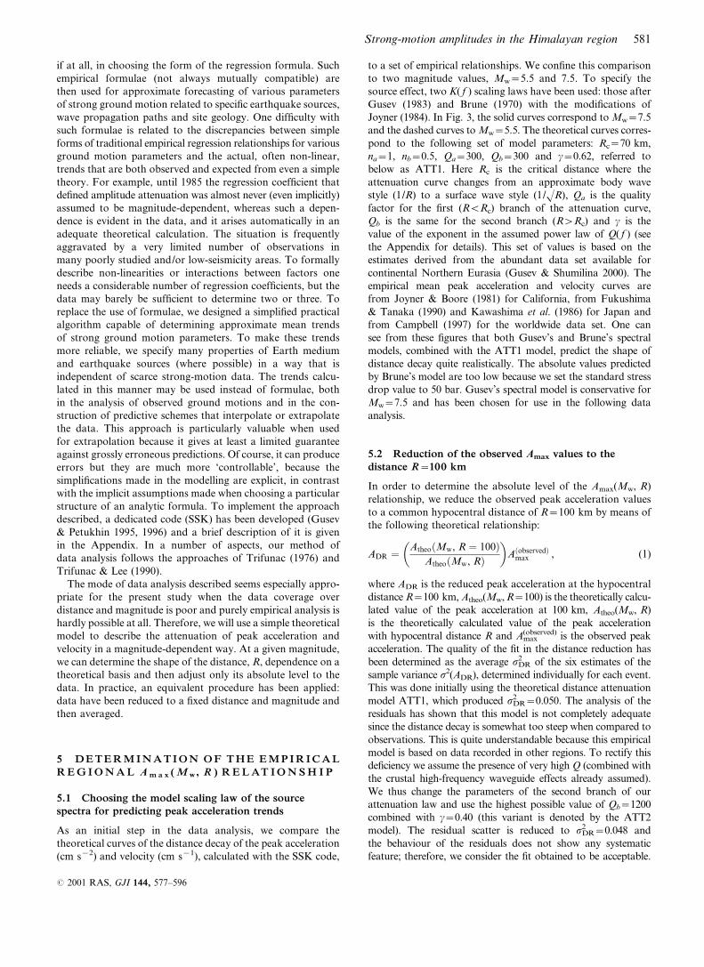
As an initial step in the data analysis, we compare the

theoretical curves of the distance decay of the peak acceleration

(cm sx2) and velocity (cm sx1), calculated with the SSK code,

to a set of empirical relationships. We con®ne this comparison

to two magnitude values, Mw=5.5 and 7.5. To specify the

source effect, two K( f ) scaling laws have been used: those after

Gusev (1983) and Brune (1970) with the modi®cations of

Joyner (1984). In Fig. 3, the solid curves correspond to Mw=7.5

and the dashed curves to Mw=5.5. The theoretical curves corres-

pond to the following set of model parameters: Rc=70 km,

na=1, nb=0.5, Qa=300, Qb=300 and c=0.62, referred to

below as ATT1. Here Rc is the critical distance where the

attenuation curve changes from an approximate body wave

style (1/R) to a surface wave style (1/dR), Qa is the quality

factor for the ®rst (R<Rc) branch of the attenuation curve,

Qb is the same for the second branch (R>Rc) and c is the

value of the exponent in the assumed power law of Q( f ) (see

the Appendix for details). This set of values is based on the

estimates derived from the abundant data set available for

continental Northern Eurasia (Gusev & Shumilina 2000). The

empirical mean peak acceleration and velocity curves are

from Joyner & Boore (1981) for California, from Fukushima

& Tanaka (1990) and Kawashima et al. (1986) for Japan and

from Campbell (1997) for the worldwide data set. One can

see from these ®gures that both Gusev's and Brune's spectral

models, combined with the ATT1 model, predict the shape of

distance decay quite realistically. The absolute values predicted

by Brune's model are too low because we set the standard stress

drop value to 50 bar. Gusev's spectral model is conservative for

Mw=7.5 and has been chosen for use in the following data

analysis.

5.2 Reduction of the observed Amax values to thedistance R=100 km

In order to determine the absolute level of the Amax(Mw, R)

relationship, we reduce the observed peak acceleration values

to a common hypocentral distance of R=100 km by means of

the following theoretical relationship:

ADR � Atheo�Mw, R � 100�Atheo�Mw, R�

� �A�observed�max , (1)

where ADR is the reduced peak acceleration at the hypocentral

distance R=100 km, Atheo(Mw, R=100) is the theoretically calcu-

lated value of the peak acceleration at 100 km, Atheo(Mw, R)

is the theoretically calculated value of the peak acceleration

with hypocentral distance R and Amax(observed) is the observed peak

acceleration. The quality of the ®t in the distance reduction has

been determined as the average s2DR of the six estimates of the

sample variance s2(ADR), determined individually for each event.

This was done initially using the theoretical distance attenuation

model ATT1, which produced s2DR=0.050. The analysis of the

residuals has shown that this model is not completely adequate

since the distance decay is somewhat too steep when compared to

observations. This is quite understandable because this empirical

model is based on data recorded in other regions. To rectify this

de®ciency we assume the presence of very high Q (combined with

the crustal high-frequency waveguide effects already assumed).

We thus change the parameters of the second branch of our

attenuation law and use the highest possible value of Qb=1200

combined with c=0.40 (this variant is denoted by the ATT2

model). The residual scatter is reduced to s2DR=0.048 and

the behaviour of the residuals does not show any systematic

feature; therefore, we consider the ®t obtained to be acceptable.

Strong-motion amplitudes in the Himalayan region 581

# 2001 RAS, GJI 144, 577±596

The reduced amplitudes are shown in Fig. 4(a). In Fig. 5, we

show the residuals of this ®t for peak acceleration and velocity.

For most of the events, the ®t is visually quite acceptable.

Nevertheless, to ensure against the possibility of the com-

plete inadequacy of our theoretical model, we perform a more

traditional and empirical regression of our data. It emulates

the ®rst step of the two-step regression (Joyner & Boore 1981,

1993). We assume a simple hyperbolic law (rxn) for the ampli-

tude decay and we estimate the value of the exponent n. Like

Sharma (1998), we use least-squares regression with dummy

variables to decouple the interfering effect of the event size, and

obtain n=1.25, which is very near to Sharma's ®gure. In this

case, the residual error is s2DR=0.047. Our ®nal choice for

the distance reduction is based on the theoretical attenuation

model ATT2.

5.3 Choice of the Amax(Mw) relationship anddetermination of the absolute level ofAmax (Mw, R) atR=100 km,Mw=7

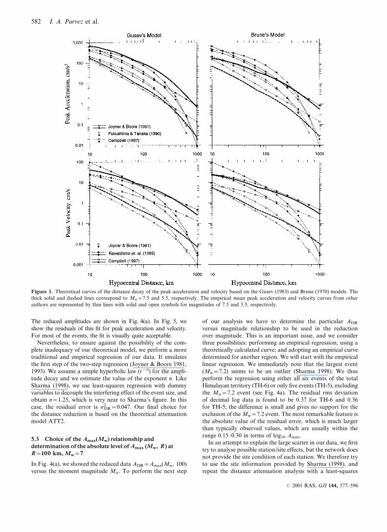
In Fig. 4(a), we showed the reduced data ADR=Amax(Mw, 100)

versus the moment magnitude Mw. To perform the next step

of our analysis we have to determine the particular ADR

versus magnitude relationship to be used in the reduction

over magnitude. This is an important issue, and we consider

three possibilities: performing an empirical regression; using a

theoretically calculated curve; and adopting an empirical curve

determined for another region. We will start with the empirical

linear regression. We immediately note that the largest event

(Mw=7.2) seems to be an outlier (Sharma 1998). We thus

perform the regression using either all six events of the total

Himalayan territory (TH-6) or only ®ve events (TH-5), excluding

the Mw=7.2 event (see Fig. 4a). The residual rms deviation

of decimal log data is found to be 0.37 for TH-6 and 0.36

for TH-5; the difference is small and gives no support for the

exclusion of the Mw=7.2 event. The most remarkable feature is

the absolute value of the residual error, which is much larger

than typically observed values, which are usually within the

range 0.15±0.30 in terms of log10 Amax.

In an attempt to explain the large scatter in our data, we ®rst

try to analyse possible station/site effects, but the network does

not provide the site condition of each station. We therefore try

to use the site information provided by Sharma (1998), and

repeat the distance attenuation analysis with a least-squares

Figure 3. Theoretical curves of the distance decay of the peak acceleration and velocity based on the Gusev (1983) and Brune (1970) models. The

thick solid and dashed lines correspond to Mw=7.5 and 5.5, respectively. The empirical mean peak acceleration and velocity curves from other

authors are represented by thin lines with solid and open symbols for magnitudes of 7.5 and 5.5, respectively.

582 I. A. Parvez et al.

# 2001 RAS, GJI 144, 577±596

regression with the additional dummy variable describing the

ground type. However, this approach does not yield satis-

factory results because (1) some of the stations are speci®ed

ambiguously, and (2) ground-type terms obtained in the

tentative regression are negligible not only for Amax but also

for Vmax, casting even more doubt on the results of such an

analysis.

However, there is another possible explanation, namely that

the data are generally non-homogeneous. To test this idea, we

divide the data into groups and process them separately. First

we group data on the basis of region. The results are shown in

Fig. 4(b), where we give the regression lines for the two regional

groupings: four eastern events (EH-4) and two western events

(WH-2). The residual rms deviations for EH-4 and WH-2 are

0.23 and 0.19, respectively. This is a radical reduction of the

scatter of data (compared to 0.37 for TH-6), and a separate

analysis of data region by region seems necessary. We also divide

the EH group into two on the basis of focal depth: two shallow

events (EH-2SL) and two deeper ones (EH-2DP) (see Table 1

for the depth values and Fig. 4b for the linear ®t). For the two

groups EH-2SL and EH-2DP, the rms deviations are 0.25 and

0.21, respectively (note that the Mw=7.2 event is included

in the EH-2DP group). Separating the data over depth does not

result in a marked effect on the ®t, and the assumption that

the Mw=7.2 event is an anomaly remains totally groundless.

Therefore, will conduct the analysis below considering two

groups of data, the eastern and western Himalayas.

In Fig. 4(a) we have plotted the Mw dependence of

mean empirical log10Amax at R=100 km from Fukushima &

Tanaka (1990), Campbell (1997) and Ambraseys (1995) for

Japan, worldwide earthquakes and Europe, respectively. One

can see from the ®gure that the slope of our linear ®t for TH-6

does not match the results obtained for the other regions; it

also contradicts theoretical estimates based on realistic spectral

scaling laws. However, the data volume (essentially six points)

is prohibitively low even for the TH6 group, where the inhomo-

geneous character of the data makes the meaning of the result

doubtful anyway. For smaller groups, the regression is evidently

meaningless. Hence, we conclude that our data are completely

inadequate for the determination of the magnitude dependence.

For this reason, we choose to use the empirical magnitude trend

(not the absolute level) from another region. In particular, we

employ the empirical shape of Fukushima & Tanaka (1990)

(F & T) as the one that is the best supported by large-

magnitude data. We also considered the use of a theoretically

calculated magnitude trend, but we rejected this option in

favour of the empirical one, considering such an approach more

conservative. There are examples when reasonable theoretical

spectral scaling laws make incorrect predictions of Amax versus

magnitude trends (see e.g. Singh et al. 1989).

Having chosen the shape of the magnitude trend, we can now

perform the second step of the analysis and reduce ADR data

along the magnitude axis to a ®xed magnitude value, Mw=7.

The magnitude reduction can be expressed by the following

formula:

AMR � Atrend,R�100�Mw � 7�Atrend,R�100�Mw�

� �ADR�Mw� : (2)

The notation is similar to eq. (1), except that this time we

reduce ADR to a ®xed magnitude Mw=7. This step is shown in

Fig. 4(c). In this ®gure, we show the F & T curves adjusted

vertically to the average reduced amplitudes ADR for TH-6,

EH-4 and WH-2, and the original F & T curve. The values of

the residual error, which now coincides with the rms deviation

of AMR, are slightly increased compared to the case of the linear

®t, and are equal to 0.40, 0.27 and 0.26, respectively.

The absolute levels of peak acceleration obtained are

of interest. The difference between the group averages is

unexpectedly large. For the western Himalayas events, the level

Figure 4. Observed log10 peak acceleration versus magnitude data,

after reduction to 100 km, using the ATT2 model (see text). Circles

correspond to the events of the eastern Himalayas and diamonds to

the events of the western Himalayas. TH-6: all six Himalayan events;

TH-5: ®ve Himalayan events excluding the largest event with Mw=7.2;

EH-4: four eastern Himalayan events; EH-2SL: two shallow eastern

Himalayan events (see Table 1 for depth values); EH-2DP: two `deep'

eastern Himalayan events; WH-2: two western Himalayan events;

F & T: Fukushima & Tanaka (1990); CAM: Campbell (1997); AMB:

Ambraseys (1995).

Strong-motion amplitudes in the Himalayan region 583

# 2001 RAS, GJI 144, 577±596

is about 62 per cent of the F & T level, whereas for the

eastern Himalayas events it is about three times this reference

value. The results obtained at this stage are essentially ®nal:

we have determined our expected Amax(Mw, R) relationship for

the western and eastern Himalayas. It is de®ned by (1) the

absolute reference values AMR=Amax(7,100)=35 and 150 Gal,

respectively, and (2) our procedure, which, applied in reverse

order, determines ®rst the Amax(Mw, 100) and then the

Amax(Mw, R) relationships tied to these `anchors'.

5.4 Amax(Mw, R) relationship as an extrapolation ofobservations to small distances and large magnitudes

We have established the semi-empirical relationship Amax(Mw, R),

and formally we could consider the analysis completed, but it is

of interest to observe what our results mean for small distances

and large magnitudes. In Fig. 6(a) we represent our results as

two families of Amax(R) curves for a set of Mw values. Thin solid

curves are our predicted values for the eastern Himalayas and

thin dashed curves are for the western Himalayas. Each event

of our very modest database is represented by its centroid (dot)

and by a segment describing the data range. All segments have

the common slope of x1.25 found in the previous section. Our

curves represent quite a reasonable description of observational

data for peak acceleration from both regions.

To make an additional check, we show in Fig. 6(b) the

result of an empirical analysis based on the assumption of the

hyperbolic law (Rx1.25) for the distance decay, with the same

reference values at R=100 km as those in Fig. 6(a). We stopped

our straight lines for Mw=7 and 8 at the level of Amax=1800

Gal because the epicentral zone corresponds roughly to the

distance range 20±60 km for the (deeper) EH events, and to

the distance range 10±30 km for the (shallower) WH events, and

we do not consider this kind of extrapolation to be reliable. We

see that even after accounting for amplitude saturation near to

the source, the eastern Himalayas earthquakes of Mw=7±8 must

be expected to regularly produce horizontal peak accelerations of

1±1.5 g in the vicinity of the seismogenic fault.

In Fig. 7 we compare our results for expected Amax versus

hypocentral distance to the results obtained by other researchers

for ®xed Mw=7 (or ML=6.7). The thick solid line represents

our results for the eastern Himalayas and the thick dashed line

our results for the western Himalayas. Solid symbols mark the

curves for the Himalayan region obtained by Chandrasekaran

Figure 5. The residuals of the log10 peak acceleration and velocity data reduced using the model ATT2 as a function of the hypocentral distance.

Different symbols are used for different events.

584 I. A. Parvez et al.

# 2001 RAS, GJI 144, 577±596

(1994), Singh et al. (1996) and Sharma (1998) on the basis of

essentially the same strong-motion data set as the one used in

the present study. Open symbols denote the results from other

parts of the world, namely Trifunac (1976) and Joyner & Boore

(1981) for the western USA, Ambraseys (1995) for Europe,

Atkinson & Boore (1995) for eastern North America and

Fukushima & Tanaka (1990) for Japan. One can see from this

®gure that our result for the eastern Himalayas is unusually high

compared to all the others except for that of Chandrasekaran

(1994), whereas our results for the western Himalayas are

Figure 6. (a) Extrapolation of the results of log10 peak acceleration for small distances and large magnitudes. The thin solid curves are the predicted

values for the eastern Himalayas and the thin dashed curves are for the western Himalayas. The thick solid and dashed lines are the segments of the

observed data with their centroids for the eastern and western Himalayas, respectively. (b) Results of the empirical analysis based on the assumption of

the hyperbolic law (Rx1.25) for distance decay, with the same reference values at R=100 km as those in (a).

Strong-motion amplitudes in the Himalayan region 585

# 2001 RAS, GJI 144, 577±596

comparable to the others. Singh et al. (1996) and Sharma

(1998) used the data from both subregions jointly; their results

for Mw=7 are close to our eastern Himalayas results for

distances above 150 km and to our western Himalayas results

for distances below 50 km. We believe that the main cause of

the differences between these results and ours is our decision to

split the data set into two groups, and we consider our results

more reliable. Our results for the western Himalayas are com-

parable to those of Ambraseys (1995) for Europe and Joyner

& Boore (1981) for California at R<100 km. However, at

R>100 km the distance attenuation curve for California decays

much faster than ours. At smaller distances, Fukushima &

Tanaka's (1990) results are slightly above ours for the western

Himalayas and lower than ours for the eastern Himalayas. The

distance decay of the Fukushima & Tanaka (1990) trend at

R>100 km is much faster than ours. The closest analogue of

our eastern Himalayas result, in terms of both level and shape

of attenuation curve, is the trend of Atkinson & Boore (1995)

for the eastern USA.

5.5 Statistical testing of the validity of theregionalization

Although the improvement of the ®t after splitting the data into

subregions is evident, some doubts may well remain because

of the very limited amount of events. We therefore checked

the validity of this splitting by analysing the variance of the

residuals. Table 2 contains all relevant input information for

Amax(7,100) (and also for velocity, used later). Formally, we ®rst

wish to demonstrate that the value of the variance for all the

data analysed together (s2TOT=0.160 when considering 182

observations, with 181 degrees of freedom, df) is signi®cantly

above the value of the variance for the data divided into the

groups EH and WH (s22=0.073 when taking the average of

the variance of the EH and WH groups considering the same

182 observations with 180 df). All quoted values are again in

log10 units. Fisher's F-ratio (the ratio of the variance of two

variables) is equal to 2.18 and it is above unity at a signi®cance

level above 10x5. Thus, the gain in the ®t is real, and the mean

values of the two groups do differ.

However, one may question the meaning of this fact

because it is possible that the particular distribution of six

events into two regions is such that the occurrence of both low-

amplitude events in the WH region is due to chance. Indeed,

the probability of the two lowest-amplitude events occupying

a particular two-event subgroup among six events is quite

considerable (2e4!/6!=1/15). We try to answer this kind of

criticism by analysing not individual station values but event

averages. We must now compare the following two variance

estimates: (1) one calculated for the average of the group of six

events taken together (0.152), and (2) the average value of the

two variance estimates calculated for the EH and WH sub-

groups (0.048). The improvement of the ®t produced by such

data splitting is drastic, with the variance reduction expressed

by an F-ratio of 3.16. Unfortunately, with as few as 5 and 4 df

this seemingly high value provides a signi®cance level that

does not even reach 10 per cent (F5, 4, 90 per cent=4.05). Thus, the

common-sense position is quite justi®ed here: despite a real,

Figure 7. Comparison of our results for expected log10 peak acceleration versus hypocentral distance with those of other authors. Our results are

shown as a thick solid line for the eastern Himalayas and a thick dashed line for the western Himalayas for Mw=7. The thin curves with solid symbols

are from the Himalayan region, while the thin curves with open symbols are from different authors for different regions of the world.

586 I. A. Parvez et al.

# 2001 RAS, GJI 144, 577±596

large difference between regional data groups, we do not have

a fully convincing proof that this fact indicates a difference

between regions as such. An additional, independent check is

crucial; it is performed below based on macroseismic data.

Having split the data into subregional groups, we obtain an

acceptable value of the residual variance s2=0.073 (or s=0.27).

We can try to split this variance value further into two com-

ponents: (1) the event-related component, rooted in variations

of the radiation capability of the events, and (2) the residual

component, which includes individual site conditions between

stations, and also some uncontrollable random ingredients that

include the effects of ray paths, purely stochastic effects and so

on. We believe that the residual component is related, to a large

extent, to individual station site effects, and we will refer to it as

the station-related effect. It is of interest to isolate these two

components of the total variance. The isolated station-related

component is given in the E column of Table 2; it is equal to

0.048 (or s=0.22). We can now ®nd the event-related component

merely by subtraction, to obtain 0.073±0.048=0.025 (or s=0.16).

For completeness, we quote the subregion-related component as

well: s2=0.160±0.073=0.087 (or s#0.29).

6 D E T E R M I N A T I O N O F T H E E M P I R I C A LR E G I O N A L V m a x (M w, R ) RELAT IONSH I P

The approach described above developed for the analysis of

Amax(Mw, R) has been applied to the peak velocity data in a

very similar way, so we will report the results very brie¯y. The

data again suggest the use of the ATT2 theoretical curves for

the distance reduction, producing a residual error of 0.22 in the

®t with the event effect excluded. The residual of this ®t can be

seen in Fig. 5. For the sake of comparison, a purely empirical

way for the determination of the attenuation has been followed,

and through a linear regression with dummy event variables we

obtain again the exponent value n=x1.18 for the hyperbolic

attenuation law, and a residual rms of 0.21.

We reduce the observed peak velocity (cm sx1) data to

R=100 km using eq. (1) and the ATT2 model, and to deter-

mine the magnitude dependence (Fig. 8a) we ®rst use the

groupings TH6 and TH5 (excluding the event with Mw=7.2,

which again appears to be an outlier). The residual rms scatter

is practically identical (0.31) for both TH-6 and TH-5. To

reduce this scatter, we split the data into groups on the basis of

the geographical region and focal depth. Fig. 8(b) shows the

linear ®t of log10Vmax(R=100 km) for EH-4, WH-2, EH-2SL

and EH-2DP. The resulting residual rms deviations are

0.21, 0.25, 0.24 and 0.19, respectively; therefore, there is a

large improvement in the results from the regional grouping

and no improvement in the results from the depth grouping.

Consequently, we decided to analyse separately the peak

velocity data for the two regions of the eastern and western

Himalayas.

The empirical log10Vmax(R=100 km) values from Kawashima

et al. (1986), Joyner & Boore (1981), Atkinson & Boore (1995)

and Campbell (1997) are shown in Fig. 8(a) for comparison. We

consider our empirical trends unreliable, and we chose to use the

empirical shape of the Mw versus Vmax relationship of Joyner &

Boore (1981). The resulting trends [`anchored' to the reduced

Vmax(7,100) value] accompanied by the original curves of Joyner

& Boore (1981) are shown in Fig. 8(c) for TH-6, EH-4 and

WH-2. The result for WH-2 is very close to that of Joyner &

Boore (1981), while for EH-4 the intercept is about three times

larger.

The established semi-empirical relationships Vmax(Mw, R)

for EH and WH are represented in Fig. 9 as two families of

Vmax(R) curves for Mw=5, 6, 7 and 8. The solid thin lines are

our expected trends for EH, and the dashed lines are those for

WH. The data centroids (dots) and the distance ranges (thick

segments) with an empirically determined slope of x1.18 are

shown in the ®gure. The differences in the absolute levels of the

expected peak velocity between regional groups are prominent,

although not as large as that for peak accelerations (Fig. 6).

The agreement between the predicted lines and the observed

peak velocity from each event is quite acceptable. We can now

compare our expected Vmax versus hypocentral distance relation-

ship with published trends for other regions (see Fig. 10, which

is the same as Fig. 7 for Amax). We believe that the ground is

rock for WH stations and mixed rock and hard soil for EH

stations, in agreement with Sharma (1998). For comparison, we

give the curves of Trifunac (1976, average for rock and medium

Table 2. Initial data used for the determination of the structure of variance for AMR and VMR*.

Individual events Regional groups Joint

data

1 2 3 4 5 6 E´ WH 2 EH 4 R"

N 18 26 50 28 36 24 44 154 198

Acceleration data, log Amax(7, 100)

m{ 1.317 1.687 2.415 2.075 2.171 2.049 1.952 1.535 2.218 1.876 2.054

s2{ 0.063 0.021 0.056 0.027 0.065 0.056 0.048 0.070 0.075 0.073 0.160

s 0.250 0.143 0.237 0.164 0.255 0.236 0.214 0.265 0.274 0.270 0.399

Velocity data, log Vmax(7, 100)

m{ 0.369 0.549 1.061 0.889 1.021 0.861 0.841 0.476 0.981 0.728 0.859

s2{ 0.060 0.039 0.048 0.012 0.048 0.072 0.047 0.054 0.051 0.053 0.099

s 0.245 0.197 0.219 0.109 0.220 0.269 0.210 0.233 0.226 0.230 0.314

* All columns except those denoted `mean' contain averages over all stations that recorded the event or the group of events. Only data for near-optimal mediummodel ATT2 (Qa=300, Qb=1200) are listed. N is the number of records in each data group.{Sample average log Amax(7, 100) or log Vmax(7, 100).{Sample variance.´ Mean over six columns for individual events." Mean over two columns for individual subregions.

Strong-motion amplitudes in the Himalayan region 587

# 2001 RAS, GJI 144, 577±596

ground) and Joyner & Boore (1981, hard soil) for the western

USA, Atkinson & Boore (1995, typically rock type) for eastern

North America, Kawashima et al. (1986, average for hard and

medium ground) for Japan, and the world average of Campbell

(1997, presumably rock). We see again that our result for

the eastern Himalayas is unusually high, above all the others

at distances in excess of 50 km, whereas our results for the

western Himalayas look quite regular.

We have also performed a statistical analysis of residuals.

The gain in the residual variance attained by splitting the data

into subregional groups is measured by a somewhat smaller

F-ratio value of 1.87, which is still signi®cant at the 10x5 level

(for 180 df). All this variance seems to be produced by station/

site effects; the event-related contribution to the variance

for velocity data is not observable. The value of the residual

rms deviation is slightly smaller than for acceleration (about

0.23, compared to 0.27). The geological conditions of the

stations have limited variations.

7 M A C R O S E I S M I C E V I D E N C E O FU N U S U A L L Y H I G H S T R O N G - M O T I O NA M P L I T U D E S I N T H E E A S T E R NH I M A L A Y A S

Macroseismic data represent an independent data source that

may help us to understand whether the large accelerations and

velocities predicted by our analysis for the eastern Himalayas

are the result of the peculiarity of our very small data set, or

whether they are a real, systematic property of large earth-

quakes in this area. To perform such an analysis we need

a measuring tool that might substitute for magnitude. It is

common knowledge that the so-called epicentral intensity I0

does not provide an ef®cient tool of this kind. Much more

useful is the parameter I100, or mean intensity at a distance of

100 km. This direct analogue of magnitude was introduced and

effectively used by Kawasumi (1951) and later by Rautian et al.

(1989). Recently, Gusev & Shumilina (2000) determined I100 for

more than 300 large earthquakes of the territory of Continental

Northern Eurasia (CNEA, i.e. former USSR with Kurile±

Kamchatka excluded). They determined a very stable I100

versus Mw (I100xMw) relationship that can easily be used as

a reference for the analysis of the macroseismic data for a

particular region.

To understand how the Indian data behave with respect to

this reference data set, we determine I100 values for a number of

earthquakes located in various parts of India and, for com-

parison, in some other regions of the world, using the published

results of Chandra (1979, 1980), Chandra et al. (1979), Tilford

et al. (1985) and Erdik et al. (1985). These authors represented

their results using the value of I0 (see Table 3), but this is not an

observable entity; instead it is a parameter that describes the

observation determined by some graphical data ®tting and thus

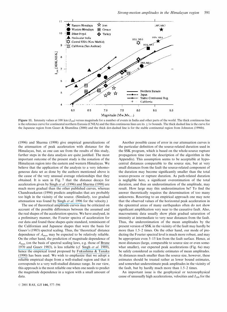
is not necessarily an integer (Chandra et al. 1979). In Fig. 11,

the three parallel curves represent the mean I100xMw trend

(thick lines)t1s (thin lines) for CNEA. The thick dashed line is

the trend determined for Japanese events compiled by Gusev &

Shumilina (2000), which matches the trend of the CNEA data

unexpectedly well. The thin line with open symbols shows

the trend of California after Lee & Trifunac (1985), but this

is valid only for magnitude less than 7. We have also plotted

the I100xMw line for `stable continental regions' derived

from Table 3 of Johnston (1996b). Large symbols denote I100

values evaluated for several events through a combination of

the published I0 values and the published empirical distance

attenuation formulae (for I0) valid for different regions such as

the eastern Himalayas, the western Himalayas, Bihar Nepal,

Peninsular India, Central USA, California, Iran, Greece and

Turkey. The detailed information about the individual events

used to obtain the I100 values is listed in Table 3. Each region is

identi®ed with a different symbol in Fig. 11. The magnitudes of

great Indian earthquakes are taken from the recent catalogue

of Abe (1981). One can see clear evidence of high values of

intensity (I100) for eastern Himalayas events and for the not

very distant Bihar Nepal event. Three out of the ®ve events of

the group show values of I100 above the CNEA average, and

two are above the+1s line. The trend of Johnston (1996b) is

Figure 8. Same as Fig. 4 but for peak velocity. J & B: Joyner & Boore

(1981).

588 I. A. Parvez et al.

# 2001 RAS, GJI 144, 577±596

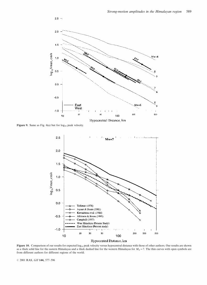
Figure 9. Same as Fig. 6(a) but for log10 peak velocity.

Figure 10. Comparison of our results for expected log10 peak velocity versus hypocentral distance with those of other authors. Our results are shown

as a thick solid line for the eastern Himalayas and a thick dashed line for the western Himalayas for Mw=7. The thin curves with open symbols are

from different authors for different regions of the world.

Strong-motion amplitudes in the Himalayan region 589

# 2001 RAS, GJI 144, 577±596

about 1.5 grades of I100 above the line for `tectonic' regions of

CNEA and somewhat overpredicts, if extrapolated, the eastern

Himalayas observations. This indicates that the East Himalayan

earthquake sources and the earthquake population studied by

Johnston may have some common properties. Of the three data

points representing the western Himalayas, one is around

+ 1s, another is near the average and the last is near x1s. This

amount of data is too small for a decisive judgement, but

suggests regular or low values of I100 for this region. Most

of the data for the other regions, viewed as a whole, agree

reasonably well with the CNEA trend. Two very pronounced

anomalies are the 1811 New Madrid series, treated as a single

event, and the Peninsular India group. These sources are

located within the old continental crust, and this kind of geo-

logical background may provide at least a partial explanation

for the anomalous eastern Himalayas data. On the whole,

the anomalous character of strong-motion amplitudes in the

eastern Himalayas is con®rmed fairly reliably by the macro-

seismic data, whereas there is no indication of anomalies for the

western Himalayas.

The macroseismic data for the Himalayan earthquakes

are indicative of speci®c, relatively gradual distance decay

(Chandra 1979, 1980; Gupta & Trifunac 1988). This fact is in

good agreement with the behaviour of the attenuation of peak

accelerations revealed in the present study (Fig. 7). Following

Gupta & Trifunac (1988), but with wider evidence, we may

conclude that in terms of the shape of the attenuation curve, the

decay of accelerations, velocities and intensities in eastern USA

represents the best-published analogy to the east Himalayan

data.

8 D I S C U S S I O N

To establish regional attenuation relationships for peak ground

acceleration and velocity is an important practical issue. With a

limited amount of data, in the present study we could obtain no

more than tentative conclusions about the behaviour of strong

ground motion amplitudes in the Himalayan region. Previous

studies of this kind by Chandrasekaran (1994), Singh et al.

Table 3. List of events used as macroseismic evidence.

No. Date Latitude Longitude Magnitude I0* I100{ Ref.´

Eastern Himalayas A

1 1897 June 12 25.9uN 91.8uE 8.7 12.27 10.32

2 1918 July 8 24.5uN 91.0uE 7.6 8.78 6.83

3 1930 July 2 25.5uN 90.0uE 7.1 9.05 7.10

4 1950 August 15 28.5uN 96.7uE 8.6 11.29 9.34

Western Himalayas A

5 1905 April 4 32.7uN 76.3uE 8.1 9.74 7.26

6 1975 January 19 32.5uN 78.4uE 6.8 8.98 6.45

7 1991 October 19 30.78uN 78.77uE 7.0 8.50 6.31

Bihar±Nepal A

8 1934 January 15 26.3uN 86.0uE 8.3 11.03 8.74

Peninsular India A

9 1900 February 8 10.8uN 76.8uE 6.0 9.34 6.15

10 1938 March 14 21.5uN 75.8uE 6.3 10.11 6.92

11 1956 July 21 23.0uN 70.0uE 6.1 8.78 5.59

12 1967 December 10 17.7uN 73.9uE 6.0 9.23 6.04

Central United States (New Madrid) B

13 1811 December 16 36.6uN 89.6uW 8.0 11.81 9.22

California (San Andreas) B

14 1952 July 21 35.0uN 119.0uW 7.7 9.97 6.64

Iran C

15 1811 September 1 36.6uN 49.8uE 7.25 9.39 5.41

16 1968 August 31 34.0uN 59.0uE 7.3 8.93 4.95

17 1972 April 10 28.4uN 52.8uE 7.1 8.92 4.93

18 1977 March 21 27.6uN 56.4uE 7.0 8.76 4.77

Greece D

19 1981 February 24 38.1uN 22.9uE 6.8 8.60 5.22

20 1981 February 25 38.1uN 23.1uE 6.4 8.50 5.12

21 1981 March 4 38.13uN 23.2uE 6.4 9.00 5.63

* Derived epicentral M.M. Intensity originally cited by different authors.{ Intensity at a distance of 100 km calculated in this paper using the original I0 values and the regionally speci®c version of the attenuation formula.´ A: Chandra (1980) except event no. 7B: Chandra (1979)C: Chandra et al. (1979)D: Tilford et al. (1985)

590 I. A. Parvez et al.

# 2001 RAS, GJI 144, 577±596

(1996) and Sharma (1998) give empirical generalizations of

the attenuation of peak acceleration with distance for the

Himalayas, but, as one can see from the results of this study,

further steps in the data analysis are quite justi®ed. The most

important outcome of the present study is the zonation of the

Himalayan region into the eastern and western Himalayas. We

believe that the application of the analysis to a very inhomo-

geneous data set as done by the authors mentioned above is

the cause of the very unusual average relationships that they

obtained. It is seen in Fig. 7 that the distance decays for

acceleration given by Singh et al. (1996) and Sharma (1998) are

much more gradual than the other published curves, whereas

Chandrasekaran (1994) predicts amplitudes that are probably

too high in the vicinity of the source. (Similarly, too gradual

attenuation was found by Singh et al. 1996 for the velocity.)

The use of theoretical amplitude curves may be criticized on

account of the possible differences between the assumed and

the real shapes of the acceleration spectra. We have analysed, in

a preliminary manner, the Fourier spectra of acceleration for

our data and found these shapes quite standard, reminiscent of

the Californian and Japanese shapes that were the basis for

Gusev's (1983) spectral scaling. Thus, the `theoretical' distance

dependence of Amax may be expected to be relatively reliable.

On the other hand, the prediction of magnitude dependence of

Amax (on the basis of spectral scaling laws, e.g. those of Brune

1970 and Gusev 1983), is less reliable (cf. Singh et al. 1989),

hence the empirical trend proposed by Fukushima & Tanaka

(1990) has been used. We wish to emphasize that we adopt a

reliable empirical shape from a well-studied region and that it

corresponds to a very well-studied distance range. In our view,

this approach is the most reliable one when one needs to predict

the magnitude dependence in a region with a small amount of

data.

Another possible cause of error in our attenuation curves is

the particular de®nition of the source-related duration used in

the SSK program, which is based on the whole-source rupture

propagation time (see the description of the algorithm in the

Appendix). This assumption seems to be acceptable at hypo-

central distances comparable to the source size, but at very

small distances from the fault the source-related component of

the duration may become signi®cantly smaller than the total

source-process or rupture duration. As path-related duration

is negligible here, a signi®cant overestimation of the total

duration, and thus an underestimation of the amplitude, may

result. How large may this underestimation be? To ®nd the

answer theoretically requires the determination of too many

unknowns. Resorting to an empirical approach one may note

that the observed values of the horizontal peak acceleration in

the epicentral areas of many earthquakes often do not show

signi®cant ampli®cation very near to the causative fault. Also,

macroseismic data usually show plain gradual saturation of

intensity at intermediate to very near distances from the fault.

Thus, the underestimation of the mean amplitudes by the

present version of SSK in the vicinity of the fault may hardly be

more than 1.5±2 times. On the other hand, our mode of pre-

dicting the Fourier spectral level is much more robust, and may

be appropriate even 5±15 km from the fault surface. Hence, at

most distances (large, comparable to source size or even some-

what smaller), our expected peak accelerations (Fig. 6a) may

be safely considered as realistic estimates of mean amplitudes.

At distances much smaller than the source size, however, these

estimates should be treated rather as lower bound estimates,

and somewhat underestimate peak amplitudes in the vicinity of

the fault, but by hardly much more than 1.5±2 times.

An important issue is the geophysical or tectonophysical

cause of unusually high accelerations, velocities and I100 for the

Figure 11. Intensity values at 100 km (I100) versus magnitude for a number of events in India and other parts of the world. The thick continuous line

is the reference curve for continental northern Eurasia (CNEA) and the thin continuous lines are its t1s bounds. The thick dashed line is the curve for

the Japanese region from Gusev & Shumilina (2000) and the thick dot-dashed line is for the stable continental region from Johnston (1996b).

Strong-motion amplitudes in the Himalayan region 591

# 2001 RAS, GJI 144, 577±596

eastern Himalayas. One possibility is the common site effect

speci®c for all stations of the Shillong array but geological data

do not provide support for this idea. Nevertheless, some

contribution of the site effects (common to the entire network)

to the observed 300 per cent increase of amplitudes cannot

be excluded, but we have no access to site geology data. An

implicit hint that site effects can hardly be large is the small site-

related variance of amplitudes, but this kind of argument is far

from being convincing. The relatively small contribution of the

site effects to the total scatter of the Himalayas data is in

prominent contrast to similar analyses applied to Kamchatka

strong-motion data (Gusev & Petukhin 1995, 1996), where the

contribution from the station terms is large or even dominating,

whereas subregion effects are dif®cult to observe (although

quite possible).

In the search for an explanation of the anomalous ampli-

tudes we consider the possible effect of an unusual anomalous

spectral shape. This possibility has been checked by direct

inspection, and it has been rejected because the spectral shapes

are of quite common appearance. Moreover, the mere fact

that an anomaly of comparable amplitude is present both for

acceleration and velocity indicates that unusual spectral shapes

can hardly be an explanation. The actual anomaly is related not

to the spectral shape but rather to its level. Hypothetically, such

kinds of anomalies may be associated with high stress drops of

the relevant earthquake faults. The high values of I100 common

to the eastern Himalayas and to the Peninsular India events

favour this possibility. Such a coincidence probably indicates

some speci®c property of old, continental crust, in agreement

with MuÈller (1978) and Panza (1980) and also with the study of

Johnston (1996a) on the earthquakes of stable continental

regions. The ®nding that I100 levels of eastern Himalayas events

are only somewhat below those expected for `stable con-

tinental' events (Fig. 10) means that eastern Himalayan events

are intrinsically intraplate events. Their location in the vicinity

of the ®rst-order plate boundary should be better speci®ed as

`active continental region' in terms of Johnston (1996a), and

the I100 levels ®t this idea. Meanwhile, the analogy between

Amax levels of the western Himalayas events and Japanese data

may be interpreted as the analogy between stress and strength

conditions in usual subduction zones and in the Himalayan

main thrust fault.

We believe, tentatively, that the property of the subregion

relevant to observed anomalies is mean fault strength, directly

manifested in the stress drop value. The critical check for this

hypothesis is its capability to explain why the phenomenon is

speci®c to the eastern Himalayas and not the western Himalayas.

We ®nd the explanation in the fact that the events from the

western Himalayas are shallower ones, so that their causative

faults are within the roots of high mountain ranges that essen-

tially represent the giant tectonic slivers of the accretionary

wedge, highly deformed, ¯uid-saturated and probably of relatively

moderate to low strength. The hypocentres of the events in

the eastern Himalayas, however, are deeper (all below 25 km

depth) and their causative faults are within the relatively drier

and higher-strength shield crust. This explanation is far from

being ®nal, but may well be of relevance.

We may become more con®dent in the proposed explanation

if it agrees with the observed character of the distance attenuation

of amplitudes. Indeed, we see anomalously low attenuation that

is common to both subregions, and this feature may well be

related to the same shield crust that is cold, low scattering and

has a high Q factor. For the eastern Himalayas, both sources

and receivers are located in such a structure, so its effect is

immediate, whereas for the western Himalayas, diving seismic

rays (characteristic of epicentral distances above 70 km) must

®rst propagate for some distance through the `tectonic' low-Q

accretionary crust and only after crossing the interplate boundary

dive into the subducted shield crust where they propagate for

most of the whole path to the receivers. Near the receivers, a

short segment of low-Q path may occur again, but this amount

cannot change the increased value of the ray-averaged, whole-

path Q. Qualitatively similar effects might be expected if the

wave propagation is treated as a surface wave phenomenon.

Therefore, the gross net effect of an unusually low attenuation

may be expected to be comparable for both subregions.

We have not used the existing strong-motion records from

Peninsular India in our study, but their use for further research

may be helpful, in particular to ®nd out whether they agree

with the macroseismic anomaly observed in that region.

To put our results, which indicate probable high accelerations

in the epicentral zones of the eastern Himalayas, in a broader

context, we describe the effects of the great Assam earthquake

of magnitude 8.7 that occurred in 1897. This unique event, with

intensity levels from X to XII (MCS) throughout the entire

epicentral area of about 150r80 km2, occurred in the eastern

Himalayas. In his classic text, Richter (1958) quoted the

impressive ®eld report by Oldham (1899) about this event.

One of the most unusual observations was that of many large

boulders thrown up and out of the ground without damaging

the rims of their former seats. This high acceleration is con-

sistent with evidence in the granite rock of Assam Hills of

widespread surface distortion and complex fracturing best charac-

terized as shattering. Richter noted that Oldham's description

of the epicentral area of the 1897 event was actually the model

case for compiling a description of grade XII of the scale.

9 C O N C L U S I O N S

In the strong-motion data analysis, instead of empirical

formulae we use a theoretical magnitude-dependent distance

attenuation in the data reduction for distance, and an empirical

acceleration versus magnitude trend, from a well-studied region,

in the data reduction for magnitude. This approach is applicable

to rather limited data sets with insuf®cient distance±magnitude

coverage and it permits us to establish conservatively the

shape and level of Amax(Mw, R) and Vmax(Mw, R) relationships

applicable to the Himalayas.

The pronounced inhomogeneity of the observed data is ascribed

to differences between the two subregions of the eastern and

western Himalayas. Of these, the western Himalayas region is

comparable, in terms of near-source amplitudes, to the Japan

region, whereas the amplitudes in the eastern Himalayas are

three times larger, and have no direct analogue amongst the

other seismic regions of the Earth that have been studied

in detail. We believe that horizontal epicentral accelerations in

excess of 1±1.5 g are typical here.

Using strong-motion records, the difference between these

two subregions can be established only on the basis of a very

limited number of events and thus it is not completely reliable;

however, a similar difference can be found in macroseismic data,

making the identi®cation of the two subregions de®nite. The

Great 1897 Assam earthquake is a particular prominent example

of an unusual, uniquely powerful eastern Himalayas event.

592 I. A. Parvez et al.

# 2001 RAS, GJI 144, 577±596

This peculiarity may be related to the fact that the sources

of the eastern group are deep-seated in relatively undisturbed

old continental lithosphere of probably high strength, whereas

the western Himalayas sources are nearer to the surface and

surrounded by highly dislocated accretionary complexes, with

relatively low strength, similar in their properties to usual

tectonic environments. The rather slow attenuation with distance

of strong-motion amplitudes and of the macroseismic intensity

indicates the presence of a high-frequency crustal waveguide

with very low attenuation. This feature seems to be common to

both subregions.

An important conclusion of our study is that the combined

use of instrumental and macroseismic data is a powerful tool

for the detailed analysis of seismic hazard. It permitted us to

check the conclusions based essentially on an insuf®cient amount

of data and to validate them by independent observations. The

presence of unusually high typical amplitudes in the eastern

Himalayas and also the slow distance decay for the entire

Himalayas should be incorporated into future seismic hazard

assessments for this region.

A C K N O W L E D G M E N T S

We thank the Department of Science and Technology,

Government of India, for making available the strong-motion

data. Constructive comments from Prof. M. D. Trifunac and

an anonymous reviewer were helpful in improving the quality

of the paper. Eugenia Guseva performed the spectral analysis

of the accelerograms. IAP is thankful to Prof. G. Furlan,

Head, Training and Research in Italian Laboratory (TRIL)

program of ICTP for providing a grant. Financial support from

CNR GNDT (contract 98.3238.PF54) is also acknowledged.

AAG acknowledges support from the Russian Foundation for

Basic Research (project 97±05±65056).

R E F E R E N C E S

Abe, K., 1981. Magnitude of large shallow earthquakes from 1904 to

1980, Phys. Earth planet. Inter., 27, 72±92.

Ambraseys, N.N., 1995. The prediction of earthquake peak ground

acceleration in Europe, Earthq. Eng. Struct. Dyn., 24, 467±490.

Atkinson, G.M. & Boore, D.M., 1995. Ground-motion relations for

eastern North America, Bull. seism. Soc. Am., 85, 17±30.

Boore, D.M., 1983. Stochastic simulation of high-frequency ground

motions based on seismological models of the radiated spectra, Bull.

seism. Soc. Am., 73, 1865±1894.

Brune, J.N., 1970. Tectonic stress and the spectra of seismic shear

waves from earthquakes, J. geophys. Res., 75, 4997±5009.

Campbell, K.W., 1997. Empirical near-source attenuation relationships

for horizontal and vertical components of peak ground acceleration,

peak ground velocity, and pseudo-absolute acceleration response

spectra, Seism. Res. Lett., 68, 154±179.

Chandra, U., McWhorter, J.G. & Nowroozi, A.M., 1979. Attenuation

of intensities in Iran, Bull. seism. Soc. Am., 69, 237±250.

Chandra, U., 1979. Attenuation of intensities in the United States, Bull.

seism. Soc. Am., 69, 2003±2024.

Chandra, U., 1980. Attenuation of intensities in India, Proc. 7th

WCEE, Vol. 2, pp. 521±524, Istanbul, Turkey.

Chandrasekaran, A.R., 1994. Evaluation of design earthquake para-

meters for a site and utilization of strong motion data, Current Sci.,

67, 353±358.

Chandrasekaran, A.R. & Das, J.D., 1992. Strong motion arrays

in India and analysis of data from Shillong array, Current Sci., 62,

233±250.

Chen, W.P. & Molnar, P., 1990. Source parameters of earthquakes and

intraplate deformation beneath the Shillong plateau and the northern

Indoburman ranges, J. geophys. Res., 95, 12 527±12 552.

Erdik, M., Doyuran, V., Akkas, N. & Gulkan, P., 1985. A probabilistic

assessment of seismic hazard in Turkey, Tectonophysics, 117, 295±344.

Evans, P., 1964. The tectonic framework of Assam, J. geol. Soc. India,

5, 80±96.

Fukushima, Y. & Tanaka, T., 1990. A new attenuation relation for

peak horizontal acceleration of strong earthquake ground motion in

Japan, Bull. seism. Soc. Am., 80, 757±783.

Gansser, A., 1964. Geology of the Himalayas, Interscience, New

York.

Gansser, A., 1977. The great suture zone between Himalaya and

Tibet: a preliminary account, in Himalaya: Sciences de la Terre,

pp. 181±192, ed. Jest, C. Colloq., Int. CNRS, 268, Ecologie et

geologie del'Himalaya, Paris.

Gupta, I.D. & Trifunac, M.D., 1988. Attenuation of intensity with

epicentral distance in India, Soil Dyn. Earthq. Eng., 7, 162±169.

Gusev, A.A., 1983. Descriptive statistical model of earthquake source

radiation and its application to an estimation of short-period strong

motion, Geophys. J. R. astr. Soc., 74, 787±808.

Gusev, A.A., 1991. Intermagnitude relationsips and asperity statistics,

Pure appl. Geophys., 136, 515±527.

Gusev, A.A., 1996. Peak factors of Mexican accelerograms: evidence

of non-Gaussian amplitude distribution, J. geophys. Res., 101,

20 083±20 090.

Gusev, A.A. & Pavlov, V.M., 1991. Deconvolution of squared velocity

waveform as applied to study of non-coherent short-period radiator

in earthquake source, Pure appl. Geophys., 136, 235±244.

Gusev, A.A. & Petukhin, A.G., 1995. An algorithm for forcasting

parameters of earthquake ground motion, Vulk. Seism., 4±5, 182±192

(in Russian).

Gusev, A.A. & Petukhin, A.G., 1996. Methods for constructing of

regional relationships among the parameters of seismic ground

motions, magnitude and distance with limited data: example of

Kamchatka maximum accelerations, Bulgarian geophys. J., 22,

40±49.

Gusev, A.A. & Shumilina, S., 2000. Modelling the intensity±

magnitude±distance relation based on the concept of an incoherent

extended earthquake source, Volc. Seism., 21, 443±463.

Gusev, A.A., Gordeev, E.I., Guseva, E.M., Petukhin, A.G. &

Chebrov, V.N., 1997. The ®rst version of the Amax(Mw, R)

relationship for Kamchatka, Pure appl. Geophys., 149, 299±312.

Hudson, D.E., Trifunac, M.D., Brady, A.G. & Vijayaraghwan, A., 1971.

Strong motion earthquake accelerograms, ii, corrected acceleration

and integrated velocity and displacement curves, Earthquake

Engineering Research Laboratory, EERL, 71±50, California Institute

of Technology, Pasadena.

Johnston, A.C., 1996a. Seismic moment assessment of earthquakes

in stable continental regionsÐI. Instrumental seismicity, Geophys. J.

Int., 124, 381±414.

Johnston, A.C., 1996b. Seismic moment assessment of earthquakes in

stable continental regionsÐII. Historical seismicity, Geophys. J. Int.,

125, 639±678.

Joyner, W.B., 1984. A scaling law for the spectra of large earthquakes,

Bull. seism. Soc. Am., 74, 1167±1188.

Joyner, W.B. & Boore, D.M., 1981. Peak horizontal acceleration and

velocity from strong-motion records including records from the 1979

Imperial Valley, California, earthquake, Bull. seism. Soc. Am., 71,

2011±2038.

Joyner, W.B. & Boore, D.M., 1993. Methods for regression analysis of

strong-motion data, Bull. seism. Soc. Am., 83, 469±487.

Kaila, K.L. & Sarkar, D., 1977. Earthquake intensity attenuation

pattern in India, Proc. Symp. Analysis of Seismicity and Seismic Risk,

173±191, Liblice, Czechoslovakia.

Kanamori, H. & Anderson, D.L., 1975. Theoretical basis of

some empirical relations in seismology, Bull. seism. Soc. Am., 65,

1073±1095.

Strong-motion amplitudes in the Himalayan region 593

# 2001 RAS, GJI 144, 577±596

Kawashima, K., Aizawa, K. & Takahashi, K., 1986. Attenuation

of peak ground acceleration, velocity and displacement based on

multiple regression analysis of Japanese strong motion records,

Earthq. Eng. Struct. Dyn., 14, 199±215.

Kawasumi, H., 1951. Measures of earthquake danger and expectancy

of intensity throughout Japan as inferred from the seismic activity in

historical times, Bull. Earthq. Res. Inst., 29, 469±482.

Khattri, K.N., Rogers, A.M., Perkins, D.M. & Algermissen, S.T., 1984.

A seismic hazard map of India and adjacent areas, Tectonophysics,

108, 93±134.

Lee, V.W. & Trifunac, M.D., 1979. Automatic Digitization and

Processing of Strong Motion Accelerograms, Part II, Computer

Processing of Accelerograms, Rept 79±15 II, Dept Civil Engineering,

University of Southern California, Los Angeles.

Lee, V.W. & Trifunac, M.D., 1985. Attenuation of Modi®ed Mercalli

Intensity for Small Epicentral Distance in California, Rept CE 85±01,

Dept Civil Engineering, University of Southern California, Los

Angeles.

LeFort, P., 1975. Himalayas: the collided range. Present knowledge of

the continental arc, Am., J. Sci., 275A, 1±44.

Mitchell, A.H.G., 1981. Phanerozoic plate boundaries in mainland SE

Asia, the Himalaya and Tibet, J. geol. Soc. Lond., 138, 109±122.

Morse, P.M. & Feshbach, H., 1953. Methods of Theoretical Physics,

McGraw-Hill, New York.

MuÈller, St., 1978. The evolution of the earth crust, in Tectonics and

Geophysics of Continental Rifts, pp. 11±28, eds Ramberg, I.B. &

Neuman, E.R., Reidel, Dordrecht.

Ni, J. & Barazangi, M., 1984. Seismotectonics of the Himalayan

collision zone: geometry of the underthrusting Indian plate beneath

the Himalaya, J. geophys. Res., 89, 1147±1163.

Ohno, S., Ohta, T., Ikerua, T. & Takemura, M., 1993. Revision of

attenuation formula considering the effect of fault size to evaluate

strong-motion spectra in near ®eld, Tectonophysics, 218, 69±81.

Oldham, H.D., 1899. Report on the great earthquake of June 12, 1897,

Mem. geol. Surv. India, 29, 1±379.

Panza, G.F., 1980. Evolution of the Earth's lithosphere, in Mechanisms

of Continental Drift and Plate Tectonics, pp. 75±87, eds Davies, P.A.

& Runcorn, S.K., Academic Press, London.

Rautian, T.G., Khalturin, V.I., Dotsev, N.T. & Sarkisyan, N.M.,

1989. Macroseismic magnitude, Voprosy Inzhenernoy Seismologii, 30,

98±109, Nauka, Moscow (in Russian).

Richter, C.F., 1958. Elementary Seismology, Freeman, San Francisco.

Sabetta, F. & Pugliese, A., 1987. Attenuation of peak horizontal

acceleration and velocity from Italian strong-motion records, Bull.

seism. Soc. Am., 77, 1491±1513.

Sharma, M.L., 1998. Attenuation relationship for estimation of peak

ground horizontal acceleration using data from strong-motion arrays

in India, Bull. seism. Soc. Am., 88, 1063±1069.

Singh, R.P., Aman, A. & Prasad, Y.J.J., 1996. Attenuation relations for

strong seismic ground motion in the Himalayan region, Pure appl.

Geophys., 147, 161±180.

Singh, S.K., Ordaz, M., Anderson, J.G., Rodriguez, M., Quaas, R.,

Mena, E., Ottaviani, M. & Almora, D., 1989. Analysis of near source

strong-motion recordings along the Mexican subduction zone, Bull.

seism. Soc. Am., 79, 1697±1717.

Sinha-Roy, S., 1982. Himalaya Main Central Thrust and its implications

for Himalayan inverted metamorphism, Tectonophysics, 84, 197±224.

Street, R.L. & Turcotte, F.T., 1977. A study of northeastern North

American spectral moments, magnitudes and intensities, Bull. seism.

Soc. Am., 67, 599±614.

Tilford, N.R., Chandra, U., Amick, D.C., Moran, R. & Snider, F.,

1985. Attenuation of intensities and effect of local site conditions on

observed intensities during the Corinth, Greece, earthquakes of 24

and 25 February and 4 March 1981, Bull. seism. Soc. Am., 75, 923±937.

Trifunac, M.D., 1976. Analysis of the peaks of strong earthquake

ground motionÐdependence of peaks on earthquake magnitude,

epicentral distance, and recording site conditions, Bull. seism. Soc.

Am., 66, 189±219.

Trifunac, M.D. & Brady, A.G., 1975. A study of the duration of strong

earthquake ground motion, Bull. seism. Soc. Am., 65, 581±626.

Trifunac, M.D. & Lee, V.W., 1990. Frequency dependent attenuation

of strong earthquake ground motion, Soil Dyn. Earthq. Eng., 9, 3±15.

Valdiya, K.S., 1980. The two intracrustal boundary thrusts of the

Himalaya, Tectonophysics, 66, 323±348.

Wadia, D.N., 1975. Geology of India, Tata McGraw-Hill, New Delhi.

A P P E N D I X A : S H O R T D E S C R I P T I O N O FT H E A L G O R I T H M O F T H E S S K C O D EF O R E S T I M A T I N G H I G H - F R E Q U E N C YS T R O N G - M O T I O N A M P L I T U D E S

The SSK code (for the initial version see Gusev & Petukhin

1995, 1996) has been written for the approximate evaluation of

high-frequency seismic strong-motion amplitudes (as well as

duration and spectra). It has been designed for practical use

in engineering seismology, to meet the need for a technique for

the fast simpli®ed forecasting of median parameters of strong

ground motion related to a speci®c earthquake source, wave

propagation path and site. The SSK algorithm reproduces the

approach of Gusev (1983) very closely.

A1 General outline of the algorithm

The ¯ow chart in Fig. A1 illustrates the principal relations

between the initial, intermediate and output quantities of the

algorithm. The main input parameters are the moment magni-

tude Mw [or seismic moment M0; log10M0=1.5(Mw+10.7)]

and the hypocentral distance R. The properties of an event of a

given Mw from a particular seismic zone are described by the

`source acceleration spectrum', K( f )=f 2|MÇ0( f )| (Gusev 1983),

where MÇ0( f ) is the Fourier spectrum of the seismic moment

rate of an equivalent point dipole. From the K( f ) spectrum,

taking into account the geometrical spreading, loss, etc., we

determine the Fourier acceleration spectrum FS( f ) for the

bedrock, which is the ®rst main intermediate parameter of the

algorithm. The distance attenuation function used combines

the point source attenuation and the saturation effect of a ®nite

source. The second main characteristic, the total signal duration

Ttotal, is found by combining the source (rupture) duration and

the duration component determined by the medium (path).

Figure A1. Diagram of the algorithm used in the Appendix.

594 I. A. Parvez et al.

# 2001 RAS, GJI 144, 577±596

Given the Fourier spectrum and the duration, another ground

motion parameter can easily be evaluated using random vibration

theory (Gusev 1983; Boore 1983).

A2 Specifying the basic reference spectrum

The acceleration source spectrum K( f ) is de®ned by the

`spectrum scaling law' function K( f, M0). This function is

either tabulated or de®ned by an analytical formula. By

default, we use the K( f, M0) table based on Gusev (1983). This

semi-empirical scaling law was derived by ®tting observational

data of many kinds using the hypothesis of source similarity

only for the lower-frequency part of the spectrum (around the

corner frequency). It can be considered as a good starting

approximation for applications in engineering seismology. As a

standard analytical model, the Brune (1970) spectral model is

used with the modi®cation of Joyner (1984) with four para-

meters: M0, stress drop Ds, corner frequency fc and acceleration

upper spectral cut-off frequency fmax. To account for the

vertical impedance gradient, spectral corrections are added

to the source spectrum. Alternatively, the reference median

smoothed FS( f ) spectrum for a ®xed (Mw, R) combination may

be speci®ed in tabular form (based for example on observations

in the target area) to be further extrapolated to other Mw and R

values.

A3 Point-source spectral amplitude attenuation

We assume that the geometrical spreading can be described as

two hyperbolic branches: a (`body wave') and b (`surface wave')

with an intersection at R=Rc (Street & Turcotte 1977). Thus,

the point-source attenuation law for FS( f ) has the form

G�R, f � �g1�R, Qa� f ��; R < Rc

C� f �g0:5�R, Qb� f ��; R > Rc

(,

where gn(R, Q) = R±nexp(xpfR/cQ), C( f ) = g1(Rc, Qa( f ))/

g0.5(Rc, Qb( f )), and c and Qa,b( f ) are the S-wave velocity and

frequency-dependent quality factor, respectively. We assume

Q( f )=Q0 f c if f>f0=1 Hz, and Q( f )=Q0 otherwise.

A4 Specifying the scaling of source parameters

The rupture duration, T, and the source length, L, are

important quantities in the calculation. They are determined

from Mw based on the concept of the approximate geometric

and kinematic similarity of earthquake sources (Kanamori &

Anderson 1975). Both T and L are assumed to grow as the

cubic root of the seismic moment. In particular, we assume

log10L= 0.5Mwx1.85+C± , where C± = dLog10L represents a

correction describing the deviation of the stress drop from its

typical value. To compute the rupture duration we then assume

that L=oT, where the default value is o=3.5 km sx1.

A5 Amplitude saturation near an extended source

The Fourier acceleration spectrum at a recording point that is

close to the surface of a ®nite source may be signi®cantly lower

than that at the same distance from a point source with the same

K( f ) spectrum because a large part of the radiating surface

is far from the receiver. In order to describe formally such

saturation effects, Gusev (1983) developed a simple theory for

the wave®eld around an incoherently radiating sur®cial source.

For a disc-shaped source, he derived a simple approximate

formula,

FS

FSpoint source

� �2

� R2

R2sloge

R2 � R2s

R2 � Rcoh

� �,

where Rs is the source radius, R is the hypocentral distance and

Rcoh is the coherence radius of the source (taken as 1 km). This

formula is applicable to spectral amplitudes at all suf®ciently

high frequencies when the source radiation can be treated as

an incoherent (noise-like, random) signal. The formula was

originally proposed for rms amplitudes, but it is directly

applicable to spectral amplitudes using Parseval's theorem

(Morse & Feshbach 1953). For practical use, we replace Rs

by the effective source radius Reff, de®ned as (S /p)0.5, where

S=LW is the source area. The formula was successfully tested

against real earthquake data by Trifunac & Lee (1990), who

compared it to three other formulae and found it superior

in describing the near-source effects contained in the western

USA accelerograms set, and by Ohno et al. (1993), who per-

formed a more detailed check against near-source data of two

well-recorded earthquakes. Recently, the SSK program was

supplemented by an alternative, more accurate procedure to

calculate the near-source saturation effect using the numerical

integration of the contributions from a rectangular source

of arbitrary aspect ratio (see Gusev & Shumilina 2000 for

details). For all but extremely elongated sources, the resulting

adjustments (averaged over azimuth) are minor.

A6 Incorporation of soil conditions

The effects of site geology are taken into account by SSK only

in a rudimentary manner: for intermediate and soft ground

categories, spectral corrections are tabulated with respect to the

bedrock, taken as a reference. These corrections are amplitude-

independent; however, to account primitively for the non-linear

enhancement of attenuation in soil, the applied corrections

correspond to a signi®cant amplitude level (peak acceleration

0.1±0.2 g on bedrock); therefore, the ground layer is treated as

a simple equivalent-linear element.

A7 Calculation of the Fourier spectrum

The Fourier spectrum for ®xed Mw and R is computed from

K( f, M0(Mw)), applying all relevant factors that account for

impedance ratio, mean S-wave radiation pattern, partition

into vectorial components, free-surface effect, geometric spread-

ing, loss (Q-factor), ®nite-source effect and ground-type/site

correction.

A8 Calculation of duration

We believe that the accelerogram duration can be estimated

by combining source/rupture-related duration and the path-

related duration. Sometimes, site-related duration is also

important, in particular for non-rock ground, but SSK ignores

this possibility. The path-related broadening of the S/Lg-

wave group, observed most frequently in records of small to

moderate earthquakes with short source duration for frequencies

above 1 Hz is a complex phenomenon that can be treated as a

Strong-motion amplitudes in the Himalayan region 595

# 2001 RAS, GJI 144, 577±596

combined effect of forward scattering, dispersion, wave con-

version and multiray propagation. We incorporate this effect

on an empirical basis. Following Trifunac & Brady (1975),

we describe this effect as a linear increase of duration with

distance: Tmedium=T1(R/R1), where T1 is an empirical constant

that depends on the region and also on the de®nition of

duration, and R1 is a ®xed reference distance, normally taken as

100 km.

In order to combine source and path contributions to the

duration we use the formal approach (see Gusev 1983; Gusev &

Pavlov 1991) based on the assumption that the time history

function for mean squared amplitude (MSA) of the recorded

incoherent wave group may be considered as a convolution of

the MSA function of the wave pulse radiated by the source

and of the MSA function that represents the pulse response

of the medium (empirical Green's function for MSA). With

this assumption, we immediately ®nd that the second central

moment, or mean square duration (MSD), of a squared record

is the sum of the MSD values of the two component functions

(source and medium components):

T2rms � T2

rms,s � T2rms,m ,

where

T2rms �

e2

e0ÿ e1

e0

� �2

,

ek ��?

0

tkAMSA�t�2dt , �k � 0, 1, 2� :

Using this approach in practice we ®rst convert, for each

component, the usual de®nitions of duration to MSD=T2rms,

and after summation, we convert the combined MSD or Trms

to the effective duration Teff, which is a measure of duration

relevant to our aims. We de®ne Teff for an arbitrary ®nite-

duration signal as the duration of a signal with a boxcar

envelope (that is, a segment of a stationary noise) that has the

same total energy and same rms amplitude as the total energy

of the reference signal and the rms amplitude of the reference

signal in the vicinity of its maximum. Usually, Teff=(1.5±3)Trms;

in SSK the default setting is Teff=2Trms. The resulting Teff value

is then used to calculate amax and omax and the response spectra.

A9 Calculation of amax and vmax

First we ®nd the rms acceleration arms using the Parseval

equation for the signal energy in the frequency and time

domains:

arms � 2

�?0

FS2�f �df =Teff :

The rms velocity, orms, is found from a similar relation in

which FS( f ) is replaced by FS( f )/2pf. We then determine the

expected value of the ratio of maximum peak acceleration to its

rms value (peak factor) using the following formula valid for a

segment of a Gaussian process:

E�amax=arms�2 � 2�1� 1=2� 1=3� . . .� 1=np�&2�loge �np� � 0:577� ,

where np=2fÃTeff is the approximate number of peaks and fÃ

is the mean signal frequency determined from FS( f ). The

Gaussian law for the amplitudes of the accelerogram assumed

in SSK is only the zero approximation to reality (Gusev 1996).

With arms and amax/arms known, the determination of amax

is now straightforward; the algorithm for calculating omax is

similar. In a similar way we then calculate the power spectrum

and the response spectrum and we estimate the macroseismic

intensity from empirical correlations.

596 I. A. Parvez et al.

# 2001 RAS, GJI 144, 577±596