ORIGINAL ARTICLE

Georgia Melagraki Æ Antreas AfantitisKalliopi Makridima Æ Haralambos Sarimveis

Olga Igglessi-Markopoulou

Prediction of toxicity using a novel RBF neural network trainingmethodology

Received: 31 March 2005 / Accepted: 25 July 2005 / Published online: 8 November 2005� Springer-Verlag 2005

Abstract A neural network methodology based on theradial basis function (RBF) architecture is introduced inorder to establish quantitative structure-toxicity rela-tionship models for the prediction of toxicity. Thedataset used consists of 221 phenols and their corre-sponding toxicity values to Tetrahymena pyriformis.Physicochemical parameters and molecular descriptorsare used to provide input information to the models. Theperformance and predictive abilities of the RBF modelsare compared to standard multiple linear regression(MLR) models. The leave-one-out cross validationprocedure and validation through an external test setproduce statistically significant R2 and RMS values forthe RBF models, which prove considerably more accu-rate than the MLR models.

Keywords RBF architecture Æ Neural network ÆQSTR Æ Toxicity Æ Tetrahymena pyriformis

Introduction

Toxicology deals with the quantitative assessment oftoxic effects to organisms in relation to the level, dura-tion and frequency of exposure. Various segments of thepopulation come in contact with toxic chemicals due tomisuse (e.g., accidental poisoning), but also throughmanufacturing, drug and food consumption. Addition-ally, people working in various jobs (e.g., painters andapplicators of pesticides) are exposed to toxic sub-stances. In general, exposure to toxic substances is to beavoided [1].

As the experimental determination of toxicologicalproperties is a costly and time-consuming process, it isessential to develop mathematical predictive relation-ships to theoretically quantify toxicity [2, 3]. Quantita-tive structure-toxicity relationship (QSTR) studies canprovide a useful tool for achieving this goal, given thesuccessful applications of quantitative structure-activityrelationships (QSARs) in several scientific areas, such aspharmacology, chemistry and environmental research.Based on a training database containing measured tox-icity potencies of compounds and a number of moleculardescriptors, QSTRs can be used to predict the toxicity ofchemical compounds that are not included in the data-base [4–6].

For the formal description of relationships betweenactivity measures and structural descriptors of com-pounds, various statistical techniques can be used.Among them the most frequently used are multiple lin-ear regression (MLR) and partial least squares (PLS).Several other statistical techniques have been used inQSAR, including discriminant analysis, principal com-ponent analysis (PCA) and factor analysis, clusteranalysis, multivariate analysis, and adaptive leastsquares [7–9]. Neural network (NN) techniques havealso been used successfully in QSAR [10–16]. The NNmethodologies are generally used when the relationshipscannot be interpreted accurately by linear functions [17].

The goal of the present study is to determine the effi-ciency of a newly introduced RBF training methodologyin predicting the toxicity of compounds. The methodol-ogy uses the innovative fuzzy-means clustering techniqueto determine the number and the locations of the hiddennode centres [18]. Compared to traditional trainingtechniques, the method employed in this work is muchfaster since it does not involve any iterative procedure,utilizes only one tuning parameter and is repetitive, i.e., itdoes not depend on a random initial selection of centres.The RBF method is applied to a data set of 221 phenolsand the results indicate that it can be used as an efficientnew technique for predicting toxicity with significantaccuracy, using appropriate descriptors as inputs.

G. Melagraki Æ A. Afantitis Æ K. Makridima Æ H. Sarimveis (&)O. Igglessi-MarkopoulouSchool of Chemical Engineering, National TechnicalUniversity of Athens, 9 Heroon Polytechniou Str.,Zografou Campus,Athens, 15780 GreeceE-mail: hsarimv@central.ntua.grTel.: +30-210-7723237Fax: +30-210-7723138

J Mol Model (2006) 12: 297–305DOI 10.1007/s00894-005-0032-8

Materials and methods

It is essential in order to obtain a successful QSTR thatall data used as part of the training and validationprocedure are of high quality. High quality data shouldderive from the same endpoint and protocol and ideallyshould be measured in the same laboratory [19]. Thedata set used in this study fulfills this criterion.

Toxicity data

This data set consists of 221 phenols and their corre-sponding toxicity data to the ciliate Tetrahymena pyri-formis in terms of log(1/IGC50) (mmol/L). The toxicityvalues were taken from the literature [20] and are shownin Table 1. The phenols are structurally heterogeneousand represent a variety of mechanisms of toxic action.The dataset consists of polar narcotics, weak acidrespiratory uncouplers, pro-electrophiles and soft elec-trophiles.

Molecular descriptors

The molecular descriptors used to derive the model weretaken from the literature [20] and include the logarithmof the octanol/water partition coefficient (log Kow),acidity constant (pKa), the energies of the highest occu-pied and lowest unoccupied molecular orbital (EHOMO

and ELUMO respectively) and the hydrogen bond donornumber (Nhdon). All these descriptors are related to thetoxicity effect of the compounds studied.

Statistical analysis (QSAR development)

In this section, we present the basic characteristics of theRBF NN architecture and the training method used todevelop the QSAR NN models.

RBF network topology and node characteristics

RBF networks consist of three layers: the input layer,the hidden layer and the output layer. The input layercollects the input information and formulates the inputvector x. The hidden layer consists of L hidden nodes,which apply nonlinear transformations to the inputvector. The output layer delivers the NN responses tothe environment. A typical hidden node l in an RBFnetwork is described by a vector xl; equal in dimensionto the input vector and a scalar width rl: The activityml(x) of the node is calculated as the Euclidean norm ofthe difference between the input vector and the nodecenter and is given by

vlðxÞ ¼ x� xlk k ð1Þ

The response of the hidden node is determined by

passing the activity through the radially symmetricGaussian function:

flðxÞ ¼ exp � vlðxÞ2

r2l

!ð2Þ

Finally, the output values of the network are computedas linear combinations of the hidden layer responses:

y ¼ gðxÞ ¼XL

l¼1flðxÞwl ð3Þ

where [w1, w2,... ,wL] is the vector of weights, whichmultiply the hidden node responses in order to calculatethe output of the network.

RBF network training methodology

Training methodologies for the RBF network architec-ture are based on a set of input–output training pairs(x(k); y(k)) (k=1, 2,...,K). The training procedure usedin this work consists of three distinct phases:

(i) Selection of the network structure and calculationof the hidden-node centers using the fuzzy-means clus-tering algorithm [18]. The algorithm is based on a fuzzypartition of the input space, which is produced bydefining a number of triangular fuzzy sets on the domainof each input variable. The centers of these fuzzy setsproduce a multidimensional grid on the input space. Arigorous selection algorithm chooses the most appro-priate knots of the grid, which are used as hidden nodecenters in the RBF network model produced. The ideabehind the selection algorithm is to place the centers inthe multidimensional input space so that there is aminimum distance between the center locations. At thesame time, the algorithm assures that for any inputexample in the training set there is at least one selectedhidden node that is close enough according to a distancecriterion. It must be emphasized that, in contrast to boththe k-means [21] and the c-means clustering [22] algo-rithms, the fuzzy-means technique does not need thenumber of clusters to be fixed before the execution of themethod. Moreover, due to the fact that it is a one-passalgorithm, it is extremely fast even if a large database ofinput–output examples is available. Furthermore, thefuzzy-means algorithm needs only one tuning parame-ter, which is the number of fuzzy sets that are used topartition each input dimension.

(ii) Following the determination of the hidden-nodecenters, the widths of the Gaussian activation functionare calculated using the P-nearest neighbor heuristic[23]:

rl ¼1

p

Xp

i¼1xl � xik k2

!1=2

ð4Þ

where x1; x2; . . . ; xp are the p nearest-node centers to thehidden node l. The parameter p is selected so that many

298

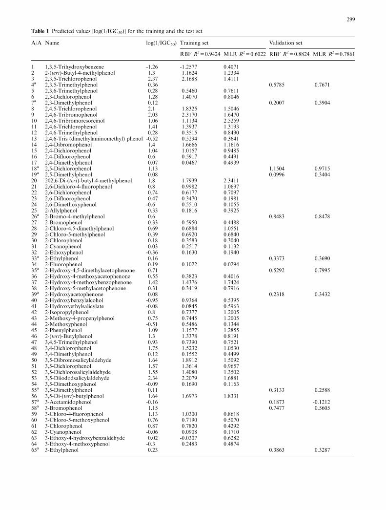
Table 1 Predicted values [log(1/IGC50)] for the training and the test set

A/A Name log(1/IGC50) Training set Validation set

RBF R2=0.9424 MLR R2=0.6022 RBF R2=0.8824 MLR R2=0.7861

1 1,3,5-Trihydroxybenzene -1.26 -1.2577 0.40712 2-(tert)-Butyl-4-methylphenol 1.3 1.1624 1.23343 2,3,5-Trichlorophenol 2.37 2.1688 1.41114a 2,3,5-Trimethylphenol 0.36 0.5785 0.76715 2,3,6-Trimethylphenol 0.28 0.5460 0.76116 2,3-Dichlorophenol 1.28 1.4070 0.80467a 2,3-Dimethylphenol 0.12 0.2007 0.39048 2,4,5-Trichlorophenol 2.1 1.8325 1.50469 2,4,6-Tribromophenol 2.03 2.3170 1.647010 2,4,6-Tribromoresorcinol 1.06 1.1134 2.525911 2,4,6-Trichlorophenol 1.41 1.3937 1.319312 2,4,6-Trimethylphenol 0.28 0.3515 0.849013 2,4,6-Tris (dimethylaminomethyl) phenol -0.52 0.5294 0.364114 2,4-Dibromophenol 1.4 1.6666 1.161615 2,4-Dichlorophenol 1.04 1.0157 0.948516 2,4-Difluorophenol 0.6 0.5917 0.449117 2,4-Dimethylphenol 0.07 0.0467 0.493918a 2,5-Dichlorophenol 1.13 1.1504 0.971519a 2,5-Dimethylphenol 0.08 0.0996 0.340420 202,6-Di-(tert)-butyl-4-methylphenol 1.8 1.7939 2.341121 2,6-Dichloro-4-fluorophenol 0.8 0.9982 1.069722 2,6-Dichlorophenol 0.74 0.6177 0.709723 2,6-Difluorophenol 0.47 0.3470 0.198124 2,6-Dimethoxyphenol -0.6 0.5510 0.105525 2-Allylphenol 0.33 0.1816 0.392526a 2-Bromo-4-methylphenol 0.6 0.8483 0.847827 2-Bromophenol 0.33 0.5950 0.448828 2-Chloro-4,5-dimethylphenol 0.69 0.6884 1.055129 2-Chloro-5-methylphenol 0.39 0.6920 0.684030 2-Chlorophenol 0.18 0.3583 0.304031 2-Cyanophenol 0.03 0.2517 0.113232 2-Ethoxyphenol -0.36 0.1630 0.194033a 2-Ethylphenol 0.16 0.3373 0.369034 2-Fluorophenol 0.19 0.1022 0.029435a 2-Hydroxy-4,5-dimethylacetophenone 0.71 0.5292 0.799536 2-Hydroxy-4-methoxyacetophenone 0.55 0.3823 0.401637 2-Hydroxy-4-methoxybenzophenone 1.42 1.4376 1.742438 2-Hydroxy-5-methylacetophenone 0.31 0.3419 0.791639a 2-Hydroxyacetophenone 0.08 0.2318 0.343240 2-Hydroxybenzylalcohol -0.95 0.9364 0.539541 2-Hydroxyethylsalicylate -0.08 0.0845 0.596342 2-Isopropylphenol 0.8 0.7377 1.200543 2-Methoxy-4-propenylphenol 0.75 0.7445 1.200544 2-Methoxyphenol -0.51 0.5486 0.134445 2-Phenylphenol 1.09 1.1577 1.285546 2-(tert)-Butylphenol 1.3 1.3378 0.819147 3,4,5-Trimethylphenol 0.93 0.7390 0.752148 3,4-Dichlorophenol 1.75 1.5232 1.053049 3,4-Dimethylphenol 0.12 0.1552 0.449950 3,5-Dibromosalicylaldehyde 1.64 1.8912 1.509251 3,5-Dichlorophenol 1.57 1.3614 0.965752 3,5-Dichlorosalicylaldehyde 1.55 1.4080 1.350253 3,5-Diiododsalicylaldehyde 2.34 2.2079 1.688154 3,5-Dimethoxyphenol -0.09 0.1690 0.116355a 3,5-Dimethylphenol 0.11 0.3133 0.258856 3,5-Di-(tert)-butylphenol 1.64 1.6973 1.833157a 3-Acetamidophenol -0.16 0.1873 -0.121258a 3-Bromophenol 1.15 0.7477 0.560559 3-Chloro-4-fluorophenol 1.13 1.0300 0.861860 3-Chloro-5-methoxyphenol 0.76 0.7190 0.507061 3-Chlorophenol 0.87 0.7820 0.429262 3-Cyanophenol -0.06 0.0908 0.171063 3-Ethoxy-4-hydroxybenzaldehyde 0.02 -0.0307 0.628264 3-Ethoxy-4-methoxyphenol -0.3 0.2483 0.487465a 3-Ethylphenol 0.23 0.3863 0.3287

299

Table 1 (contd.)

A/A Name log(1/IGC50) Training set Validation set

RBF R2=0.9424 MLR R2=0.6022 RBF R2=0.8824 MLR R2=0.7861

66 3-Fluorophenol 0.38 0.3626 0.062467a 3-Hydroxy-4-methoxybenzylalcohol -0.99 0.1893 0.290968 3-Hydroxyacetophenone -0.38 0.3606 0.210569a 3-Hydroxybenzaldehyde 0.09 0.0073 0.146470 3-Hydroxybenzoic acid -0.81 0.9606 0.527871a 3-Hydroxybenzylalcohol -1.04 0.7287 0.485472 3-Iodophenol 1.12 1.1825 0.697373 3-Isopropylphenol 0.61 0.5719 0.551974 3-Methoxyphenol -0.33 0.3633 0.031775 3-Phenylphenol 1.35 1.2389 1.293176a 3-(tert)-Butylphenol 0.73 0.9910 0.775877 4-(tert)-Octylphenol 2.1 2.0342 1.912878a 4-(tert)-Butylphenol 0.91 0.9333 0.821179 4,6-Dichlororesorcinol 0.97 0.9034 0.938580a 4-Allyl-2-methoxyphenol 0.42 0.2407 0.524781 4-Benzyloxyphenol 1.04 1.0458 1.286482a 4-Bromo-2,6-dichlorophenol 1.78 1.7768 1.381383 4-Bromo-2,6-dimethylphenol 1.17 1.3217 1.267084 4-Bromo-3,5-dimethylphenol 1.27 1.1912 1.201585 4-Bromo-6-chloro-2-cresol 1.28 1.4570 1.340686 4-Bromophenol 0.68 0.6965 0.611687a 4-Butoxyphenol 0.7 0.7779 1.097388 4-Chloro-2-isopropyl-5-methylphenol 1.85 1.7646 1.718089a 4-Chloro-2-methylphenol 0.7 0.8504 0.867590a 4-Chloro-3,5-dimethylphenol 1.2 1.2333 1.146791a 4-Chloro-3-ethylphenol 1.08 1.2658 1.123392 4-Chloro-3-methylphenol 0.8 0.7377 0.834493a 4-Chlorophenol 0.55 0.5155 0.521294 4-Chlororesorcinol 0.13 0.5804 0.471295 4-Cyanophenol 0.52 0.3434 0.097496 4-Ethoxyphenol 0.01 -0.1385 0.510597 4-Ethylphenol 0.21 0.3014 0.398198 4-Fluorophenol 0.02 -0.0708 0.252699 4-Heptyloxyphenol 2.03 2.1227 1.9979100 4-Hexyloxyphenol 1.64 1.5630 1.6922101a 4-Hexylresorcinol 1.80 1.5525 1.4144102 4-Hydroxy-2-methylacetophenone 0.19 0.1939 0.4472103 4-Hydroxy-3-methoxyacetophenone -0.12 0.1004 0.3638104 4-Hydroxy-3-methoxybenzonitrile -0.03 0.0216 0.4072105 4-Hydroxy-3-methoxybenzylalcohol -0.7 0.8639 0.4295106 4-Hydroxy-3-methoxybenzylamine -0.97 0.2649 -0.3264107a 4-Hydroxy-3-methoxyphenethylalcohol -0.18 0.1069 0.1330108 4-Hydroxyacetophenone -0.3 0.0234 0.1133109 4-Hydroxybenzaldehyde 0.27 -0.0006 0.1058110 4-Hydroxybenzamide -0.78 0.6458 0.3673111 4-Hydroxybenzoic acid -1.02 0.8670 0.3948112 4-Hydroxybenzophenone 1.02 1.0913 1.1405113 4-Hydroxybenzylcyanide -0.38 0.3997 0.4804114a 4-Hydroxyphenethylalcohol -0.83 0.6590 0.4298115 4-Hydroxyphenylacetic acid -1.5 1.5063 0.2107116a 4-Hydroxypropiophenone 0.05 0.3086 0.4059117 4-Iodophenol 0.85 0.95 0.7254118a 4-Isopropylphenol 0.47 0.6119 0.6148119 4-Methoxyphenol -0.14 0.3372 0.1976120a 4-Phenylphenol 1.39 1.2357 1.4480121a 4-Propylphenol 0.64 0.7181 0.7046122 4-(sec)-Butylphenol 0.98 1.0932 0.9117123 4-(tert)-Pentylphenol 1.23 1.3335 1.1356124 5-Bromo-2-hydroxybenzylalcohol 0.34 0.4247 0.3608125 5-Bromovanillin 0.62 0.6049 0.7279126 5-Fluoro-2-hydroxyacetophenone 0.04 0.0517 0.7771127 5-Methylresorcinol -0.39 0.4360 0.1271128 5-Pentylresorcinol 1.31 1.3376 1.3020129 6-(tert)-Butyl-2,4-dimethylphenol 1.16 1.1801 1.5907130 a,a,a-Trifluoro-4-cresol 0.62 0.6807 0.5816

300

Table 1 (contd.)

A/A Name log(1/IGC50) Training set Validation set

RBF R2=0.9424 MLR R2=0.6022 RBF R2=0.8824 MLR R2=0.7861

131 Ethyl-3-hydroxybenzoate 0.48 0.5352 0.7593132 Ethyl-4-hydroxy-3-methoxyphenylacetate 0.23 0.0891 0.2439133a Ethyl-4-hydroxybenzoate 0.57 0.7127 0.6494134 Isovanillin 0.14 0.2235 0.3669135a 3-Cresol -0.06 0.0257 0.0559136a Methyl-3-hydroxybenzoate 0.05 0.2478 0.4859137 Methyl-4-hydroxybenzoate 0.08 0.2095 0.4817138a Methyl-4-methoxysalicylate 0.62 0.6075 0.6973139 Nonylphenol 2.47 2.4674 2.4774140a 2-Cresol -0.3 0.1056 0.0954141a 2-Vanillin 0.38 0.1732 0.4571142a 4-Cresol -0.18 0.1592 0.2252143 4-Cyclopentylphenol 1.29 1.2381 0.9981144 Phenol 0.21 0.1106 0.3004145 Resorscinol 0.65 0.6311 0.2009146 Salicylaldehyde 0.42 0.4010 0.2986147 Salicylaldoxime 0.25 0.1620 0.3740148 Salicylamide 0.24 0.3046 0.0554149 Salicylhydrazide 0.18 0.1825 0.1927150 Salicylhydroxamic acid 0.38 0.3768 0.2226151 Salicylic acid 0.51 0.5072 0.7902152 Syringaldehyde 0.17 0.1762 0.3455153 Vanillin 0.03 0.0114 0.3303154 2,3,4,5-Tetrachlorophenol 2.71 2.6883 1.8520155 2,3,5,6-Tetrachlorophenol 2.22 2.2198 1.6755156 2,3,5,6-Tetrafluorophenol 1.17 1.2825 0.6360157 2,3-Dinitrophenol 0.46 0.5685 0.7861158 2,4,6-Trinitrophenol -0.16 0.1587 0.4653159 2,4-Dichloro-6-nitrophenol 1.75 1.8195 1.7045160 2,4-Dinitrophenol 1.08 0.9775 0.5527161 2,5-Dinitrophenol 0.95 0.9357 1.0017162 2,6-Dichloro-4-nitrophenol 0.63 0.6967 1.1545163 2,6-Diiodo-4-nitrophenol 1.71 1.7308 1.6515164 2,6-Dinitro-4-cresol 1.23 1.0951 1.17165 2,6-Dinitrophenol 0.54 0.6098 0.6845166 3,4,5,6-Tetrabromo-2-cresol 2.57 2.5622 2.4724167 3,4-Dinitrophenol 0.27 0.2449 0.6613168 4,6-Dinitro-2-cresol 1.72 1.8385 0.9805169 Pentabromophenol 2.66 2.6674 2.5129170 Pentachlorophenol 2.05 2.0362 2.1188171 Pentafluorophenol 1.64 1.5253 0.9301172 1,2,3-Trihydroxybenzene 0.85 0.3641 -0.4575173 1,2,4-Trihydroxybenzene 0.44 0.4386 0.1186174 2,3-Dimethylhydroquinone 1.41 2.1983 0.4201175 2,4-Diaminophenol 0.13 0.1296 -0.1773176 2-Amino-4-(tert)-butylphenol 0.37 0.3471 1.0426177 2-Aminophenol 0.94 1.0797 0.0342178 3,5-Di-(tert)-butylcatechol 2.11 2.1032 2.1321179 3-Aminophenol -0.52 0.6763 0.4105180 3-Methylcatechol 0.28 0.3889 0.2381181 4-Acetamidophenol -0.82 0.1854 0.0424182 4-Amino-2,3-dimethylphenol 1.44 1.3920 0.0618183 4-Amino-2-cresol 1.31 1.2952 0.2362184 4-Aminophenol -0.08 0.0292 0.0845185 4-Chlorocatechol 1.06 0.8653 0.7061186a 4-Methylcatechol 0.37 0.6642 0.2757187 5-Amino-2-methoxyphenol 0.45 0.4527 -0.1456188 5-Chloro-2-hydroxyaniline 0.78 0.7809 0.7450189 6-Amino-2,4-dimethylphenol 0.89 0.9603 0.4623190 Bromohydroquinone 1.68 1.7439 0.8086191a Catechol 0.75 0.2268 -0.0938192 Chlorohydroquinone 1.26 0.8143 0.3379193 Hydroquinone 0.47 0.3551 -0.0659194 Methoxyhydroquinone 2.20 0.8448 -0.0157195 Methylhydroquinone 1.86 1.5627 0.2166

301

nodes are activated when an input vector is presented tothe NN model.

(iii) The connection weights are determined usinglinear regression between the hidden-layer responses andthe corresponding output training set.

Results

In order to evaluate and compare the performance of theRBF training methodology presented in this work, thedata set was initially split into a training and a validationset in a ratio of approximately 80:20% (180 and 41compounds, respectively). For that, the Kennard andStones algorithm [24] was used. The Kennard–Stonesalgorithm has gained increasing popularity for splittingdata sets into two subsets. The algorithm starts byfinding two samples that are the farthest apart from eachother on the basis of the input variables in terms of somemetric, e.g., the Euclidean distance. These two samplesare removed from the original data set and put into thecalibration data set. The procedure described is repeateduntil the desired number of samples has been reached inthe calibration set. The advantages of this algorithm arethat the calibration samples map the measured region ofthe variable space completely with respect to the inducedmetric and that the test samples all fall inside the mea-sured region. The training and validation compoundsare clearly indicated in Table 1. Both RBF network andMLR models were developed based on exactly the same

training set. The validation set was not involved in anyway during the training phase. The results are shown inTable 1, where the predictions of the two models areshown for both the training and the external examples.The same results are shown in a graphical format inFigs. 1, 2, 3 and 4, where the experimental toxicity isplotted against the predictions of the RBF network andthe MLR model. In each figure the correspondingcoefficients of determination (R2-value) are presented,which indicate a much higher correlation betweenexperimental and predicted values using the RBF net-work methodology. The full linear equation for theprediction of toxicity is the following:

log1=IGC50¼0:5617logKowþ0:0026pKa�0:8792ELUMO

þ0:7995EHUMOþ0:2734Nhdonþ6:2044;n¼180; R2¼0:6022; RMS¼0:5352:

ð5Þ

To compare the performance of the modelingschemes further, their predictive ability was also evalu-ated by the leave-one-out (LOO) cross-validation pro-cedure. A number of modified data sets were created bydeleting in each case one object from the data. An RBFnetwork and an MLR model were developed in eachcase based on the remaining data and were validatedusing the object that had been deleted. Consequently,221 RBF networks and MLR models were built, bydeleting each time one compound from the training set.

Table 1 (contd.)

A/A Name log(1/IGC50) Training set Validation set

RBF R2=0.9424 MLR R2=0.6022 RBF R2=0.8824 MLR R2=0.7861

196 Phenylhydroquinone 2.01 2.0494 1.4188197 Tetrachlorocatechol 1.700 1.6398 2.3871198 Trimethylhydroquinone 1.34 1.0404 0.7284199 2,6-Dibromo-4-nitrophenol 1.36 1.2960 1.3558200 2-Amino-4-chloro-5-nitrophenol 1.17 1.1656 1.3096201 2-Amino-4-nitrophenol 0.48 0.5334 1.0231202 2-Chloro-4-nitrophenol 1.59 1.4875 0.8898203 2-Chloromethyl-4-nitrophenol 0.75 1.0330 0.7947204 2-Nitrophenol 0.67 0.8831 0.6586205 2-Nitroresorcinol 0.66 0.6898 1.1367206a 3-Fluoro-4-nitrophenol 0.94 0.3165 0.9997 0.4381207 3-Hydroxy-4-nitrobenzaldehyde 0.27 0.3165 0.6154208 3-Methyl-4-nitrophenol 1.73 1.3591 0.6877209 3-Nitrophenol 0.51 0.4308 0.6024210 4-Amino-2-nitrophenol 0.88 0.8491 1.0359211 4-Chloro-2-nitrophenol 2.05 2.0047 1.3347212 4-Chloro-6-nitro-3-cresol 1.64 1.5944 1.6378213 4-Hydroxy-3-nitrobenzaldehyde 0.61 0.6226 0.4118214 4-Methyl-2-nitrophenol 0.57 0.6544 1.1031215 4-Methyl-3-nitrophenol 0.74 0.7122 1.0180216 4-Nitro-3-(trifluoromethyl)-phenol 1.65 1.5893 1.0526217 4-Nitrocatechol 1.17 1.1431 0.9175218 4-Nitrophenol 1.42 1.4467 0.4263219 4-Nitrosophenol 0.65 0.5828 0.3104220 5-Fluoro-2-nitrophenol 1.13 1.2294 0.7792221 5-Hydroxy-2-nitrobenzaldehyde 0.33 0.1427 0.5858

aCompounds used in the validation set

302

Figures 5 and 6 show the experimental toxicity versusthe predictions produced by the RBF NN models andthe multiple regression technique, using the LOO crossvalidation procedure. The corresponding coefficients ofdetermination R2

CV indicate again that the models de-rived from the RBF methodology have a higher pre-dictive potential. The comparison between the RBF andthe MLR methods is summarized in Table 2. In allcases, the RBF models proved to be remarkably moreaccurate than the MLR models. The predictive abilitiesof both modeling techniques can be improved if differentmodels are developed for each one of the several dif-ferent mechanisms of action, but in this paper we con-centrated on building a single model for eachmethodology that can predict toxicity for the variety ofmechanisms that are included in the data set.

It should finally be noted that the MATLAB pro-gramming language was used to implement all thetraining and testing procedures. The computational timerequired to build the NN models in a Pentium IV 3 GHzprocessor was always less than 0.2 s. It should also beemphasized that the RBF training method has beendeveloped in-house, so no commercial packages wereused to develop the NN models. The complete QSTRmodels can be made available to the interested readers.

Discussion and conclusions

In this work, we presented a novel QSTR methodologybased on the RBF NN architecture. The method wasillustrated using a data set of 221 phenols and compared

observed toxicity

pred

icte

d to

xici

ty

R2 = 0.9424

3

2.5

2

1.5

1

0.5

0

-0.5

-1

-1.5

-2-1.5 -1 -0.5 0 0.5 1 1.5 2 2.5 3

Fig. 1 Experimental versus predicted toxicity using the RBFmethodology for the training set (180 compounds)

R2 = 0.6022

experimental toxicity

pred

icte

d to

xici

ty

-1.5 -1 -0.5 0 0.5 1 1.5 2 2.5 3

3

2.5

2

1.5

1

0.5

0

-0.5

Fig. 2 Experimental versus predicted toxicity using the MLRmethodology for the training set (180 compounds)

5 1 0.5 0 0.5 1 1.5 2

observed toxicity

R2 = 0.8824

2

1.5

1

0.5

0

-0.5

-1

pred

icte

d to

xici

ty

Fig. 3 Experimental versus predicted toxicity using the RBFmethodology for the test set (41 compounds)

-1.5 -1 -0.5 0 0.5 1 1.5 2-0.5

0

0.5

1

1.5

observed toxicity

pred

icte

d to

xici

ty

R2 = 0.7861

Fig. 4 Experimental versus predicted toxicity using the MLRmethodology for the test set (41 compounds)

303

with standard MLR. Validation of the different QSTRmethodologies was based on two evaluation procedures.In the first method the data were split into a training anda validation set and the model generated using thetraining set was used to predict toxicity in the validationset. The second method was the standard LOO cross-

validation procedure. The modeling procedures used inthis work illustrated the accuracy of the models pro-duced, not only by calculating their fitness on sets oftraining data but also by testing the predicting abilitiesof the models.

The RBF NN models were produced based on thefuzzy-means training method, which is fast and repeti-tive, in contrast to most traditional training techniques.The model generated for the data set required five de-scriptors. In terms of the R2, R2

cv and RMS values, theRBF models proved to have a significant predictivepotential. The results obtained illustrated that the RBFNN architecture can be used to derive QSTRs, which aremore accurate and have better generalization capabili-ties compared to linear regression models at the expenseof the increased complexity of the model compared to asimple structure of a linear model. The method proposedcould be a substitute to costly and time-consumingexperiments for determining toxicity.

Acknowledgements G.M. wishes to thank the Greek State Schol-arship Foundation for a doctoral assistantship.

References

1. Lu FC, Kacew S (2002) Lu’s basic toxicology. Taylor &Francis, London

2. Karcher W, Devillers J (1990) SAR and QSAR in environ-mental chemistry and toxicology: scientific tool or wishfulthinking?. In: Karcher W, Devillers J (eds) Practical applica-tions of quantitative structure-activity relationships (QSAR) inenvironmental chemistry and toxicology. Kluwer, Dordrecht,pp 1–12

3. Nendza M (1998) Structure-activity relationships in environ-mental sciences, ecotoxicology series 6. Chapman & Hall,London

4. Schultz TW, Netzeva TI, Cronin MTD (2003) SAR QSAREnviron Res 14:59–81

5. Netzeva TI, Schultz TW, Aptula AO, Cronin MTD (2003)SAR QSAR Environ Res 14:265–283

6. Zahouily M, Rhihil A, Bazoui H, Sebti S, Zakarya D (2002) JMol Model 8:168–172

7. Cronin MTD, Aptula AO, Duffy JC, Netzeva TI, Rowe PH,Valkova IV, Schultz TW (2002) Chemosphere 49:1201–1221

8. Ren S (2003) Chemosphere 53:1053–10659. Bukard U (2003) Methods for data analysis. In: Gasteiger J,

Engel Th (eds) Chemoinformatics. Wiley VCH, Weinheim, pp439–485

10. Devillers J (1996) Neural networks in QSAR and drug design.Academic Press, London

11. Afantitis A, Melagraki G, Makridima K, Alexandridis A,Sarimveis H, Iglessi-Markopoulou O (2005) J Mol Struct:Theochem 716:193–198

12. Devillers J (2004) SAR QSAR Environ Res 15:237–24913. Kaiser KLE (2003) Quant Struct-Act Relat 22:1–5

Table 2 Summary of the resultsproduced by the differentmethods

Method Training set Validation set R2train R2

pred RMS RMSpred Figure

RBF 180 41 0.9424 0.2037 1MLR 180 41 0.6022 0.5352 2RBF 180 41 0.8824 0.2398 3MLR 180 41 0.7861 0.3197 4RBF LOO 221–i 221–i 0.7203 0.4350 5MLR LOO 221–i 221–i 0.6010 0.5194 6

-1.5 -1 -0.5 0 0.5 1 1.5 2 2.5 3-1

-0.5

0

0.5

1

1.5

2

2.5

observed toxicity

pred

icte

d to

xici

ty

R2 = 0.7203

Fig. 5 Experimental versus predicted toxicity with cross validation(RBF methodology)

-1.5 -1 -0.5 0 0.5 1 1.5 2 2.5 3-1

-0.5

0

0.5

1

1.5

2

2.5

3

observed toxicity

pred

icte

d to

xici

ty

R2 = 0.6010

Fig. 6 Experimental versus predicted toxicity with cross validation(MLR methodology)

304

14. KaiserKLE (2003) J Mol Struct: Theochem 622:85–9515. Gasteiger J (2003) Handbook of chemoinformatics: from data

to knowledge, vol 3. Wiley VCH, Weinheim16. Zupan J, Gasteiger J (1999) Neural networks in chemistry and

drug design. Wiley VCH, Weinheim17. Debnath AK (2001) Quantitative structure-activity relationship

(QSAR): a versatile tool in drug design. In: Ghose AK, Vi-swanadhan VN (eds) Combinatorial library design and evalu-ation: principles, software tools, and applications in drugdiscovery. Marcel Dekker, New York, pp 73–129

18. Sarimveis H, Alexandridis A, Tsekouras G, Bafas G (2002) IndEng Chem Res 41:751–759

19. Lessigiarska I, Cronin MTD, Worth AP, Dearden JC, NetzevaTI (2004) SAR QSAR Environ Res 15:169–190

20. Aptula AO, Netzeva TI, Valkona IV, Cronin MTD, SchultzTW, Kuhne R, Schuurmann G (2002) Quant Struct-Act Relat21:12–22

21. Darken C, Moody J (1990) Fast adaptive K-means clustering:some empirical results. IEEE INNS Int Joint Conf NeuralNetw 2:233–238

22. Dunn JC (1974) J Cybernet 3:32–5723. Leonard JA, KramerMA (1991) Radial basis function networks

for classifying process faults. IEEE Control Syst 11:31–3824. Kennard RW, Stone LA (1969) Technometrics 11:137–148

305