ARTICLE IN PRESS

Prediction of thermal conductivity of rock throughphysico-mechanical properties

T.N. Singha,�, S. Sinhab, V.K. Singhb

aDepartment of Earth Sciences, Indian Institute of Technology, Bombay 400 076, IndiabInstitute of Technology, Banaras Hindu University, Varanasi 221 005, India

Abstract

The transfer of energy between two adjacent parts of rock mainly depends on its thermal conductivity. Present study supports the use

of artificial neural network (ANN) and adaptive neuro fuzzy inference system (ANFIS) in the study of thermal conductivity along with

other intrinsic properties of rock due to its increasing importance in many areas of rock engineering, agronomy and geo environmental

engineering field. In recent years, considerable effort has been made to develop techniques to determine these properties. Comparative

analysis is made to analyze the capabilities among six different models of ANN and ANFIS. ANN models are based on feedforward

backpropagation network with training functions resilient backpropagation (RP), one step secant (OSS) and Powell–Beale restarts

(CGB) and radial basis with training functions generalized regression neural network (GRNN) and more efficient design radial basis

network (NEWRB). A data set of 136 has been used for training different models and 15 were used for testing purposes. A statistical

analysis is made to show the consistency among them. ANFIS is proved to be the best among all the networks tried in this case with

average absolute percentage error of 0.03% and regression coefficient of 1, whereas best performance shown by the FFBP (RP) with

average absolute error of 2.26%. Thermal conductivity is predicted using P-wave velocity, porosity, bulk density, uniaxial compressive

strength of rock as input parameters.

Keywords: Thermal conductivity; Physico-mechanical properties of rock; Artificial neural network; Adaptive neuro fuzzy; P-wave velocity; Fuzzy

inference system

1. Introduction

Thermal conductivity of rock is studied along withdifferent physico-mechanical properties due to its increas-ing importance in the geotechnical engineering, geothermalengineering, nuclear disposal, etc. Its study is importantbecause it is main characteristic of energy transferphenomenon. Energy transfer arising from the temperaturedifference between the adjacent parts of the body is calledheat conduction. The amount of heat to be transferredthrough any body depends upon a number of factors, suchas the particle shape, porosity, temperature range, solidconstituents, moisture content, uniaxial and/or triaxialpressure exerted on the rock, etc. [1–5]. It widely influences

the energy transfer between adjacent rocks in undergroundmines and in insulation of the building by providing anenergy efficient solution. Energy saving is the importantpart of any national energy strategy and its conservationfor underdeveloped countries with inadequate resources iseven more important [5]. Thermal insulation material ismost important part of any thermal insulation system anda lower system thermal conductivity can be achieved bycombination of more thermal insulation material. Suchsystems are generally characterized by an effective thermalconductivity. The thermal conductivity is determined bythe measurements of temperature gradient in the rock andheat input [6].In general, the thermal conductivity can be calculated

using Fourier’s Law as given below:

dQ

dt¼ �kA

dT

dx½18�, (1)

0

1

2

3

0 2000 4000 6000 8000

P-Wave Velocity (m/s)

Th

erm

al

Co

nd

uct

ivit

y (W

/m.k

)

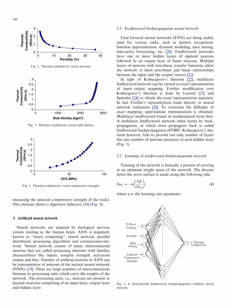
Fig. 1. Thermal conductivity versus P-wave velocity.

147

dQ

dt¼ �ðk0 þ lPnÞA

dT

dx½18�, (2)

Q ¼ �ðk0 þ lcpPncp ÞCbcpp At

dT

dx½18�, (3)

where dQ/dt is the time rate of heat transfer; A the area ofthe body whose heat is to be transferred; dT/dx thetemperature gradient, k the thermal conductivity of thematerial; k0 the thermal conductivity of the rock undernormal conditions, W/(m 1C); l and n are the rock-dependent constant parameters in uniaxial compression;P is the applied uniaxial pressure, Mpa; lcp, ncp and bcp arethe rock-dependent constant parameters in triaxial com-pression, Cp is the confining pressure, MPa. Transport andthermodynamic properties which is referred as thermo-physical properties affect the thermal conductivity of rocks.Properties like k the thermal conductivity of the materialcomes under transport properties while in thermodynamicanalysis properties like density and specific heat arecommonly used.

Considering the physical mechanism associated withconduction in general, the thermal conductivity of a solid islarger than that of a liquid, and that of liquid is larger thangas.

Knowing a greater usability of thermal property in thecivil engineering, a lot of work has been carried out to findthermal conductivity of rock and to predict by a definitesimple model for the judgment the thermal property ofrocks. Progress has been made in recent years in the abilityto predict the thermal conductivity, but the state of the artis deficient in many ways. On the basis of detailedinvestigation, a viable approach for the prediction ofthermal conductivity is necessary. An artificial intelligence(AI) comes in handy to fulfill this problem. Artificial neuralnetworks (ANNs) and adaptive neuro fuzzy inferencesystem (ANFIS) are used in the present study. ANN canbe viewed as an interesting class of statistical patternrecognition algorithm, which provides explicit facilities formodeling non-linear and non-Gaussian statistical regula-rities and proves to be strong tool to prepare an equivalentmodel by virtue of its capabilities of function approxima-tion and classification. The potential of modeling thematerial behavior using ANN was first proposed byGhaboussi et al. [7]. ANNs have been used to solve a widevariety of application in Geomechanics and Rock En-gineering [8]. In the last few years, fuzzy inference systems(FISs) began to be used in the areas of rock mechanics andengineering geology [9–12]. According to Setnes et al. [13],an interesting and perhaps the most attractive character-istics of fuzzy models compared with other conventionalmethods commonly used in geosciences. Such as instatistics, they are able to describe complex and non-linearmultivariable problems in a transparent way. Fuzzy logic isa logical system, which is an extension of multivalued logic.Fuzzy propositions are statements that posses fuzzyvariables. The concept of a fuzzy set is the basis of a fuzzylogic. A fuzzy set is a set without a crisp, clearly defined

boundary. ANFIS and ANN can be viewed as strong toolsin the statistical pattern recognition algorithm and toprepare an equivalent model by virtue of their capabilitiesof function approximation and classification. Data sets forthe analysis are taken from literature [14] based on thelaboratory experiments.

2. Input parameters

An attempt has been made to predict the thermalconductivity of rock through its physico-mechanicalproperties. There are various physical factors affectingthe thermal conductivity of rocks. Mineral compositionand constitution, structural and textural features of rocks,amount of pore water present and the condition at whichrocks are tested also affect the thermal conductivity of therocks. Physical properties like P-wave velocity, porosity,bulk density, uniaxial compressive strength has primaryaffect on thermal conductivity of the rocks [14,15].The one of the principal factors, which determines the

thermal conductivity of rocks, is P-wave velocity. P-waveinduces longitudinal oscillatory motions similar to simpleharmonic motion. It travels in any direction in a materialwhich resists compression. It is directly proportional to thethermal conductivity of rocks (Fig. 1) [14].Porosity controls thermal properties due to its depen-

dence on grain size. As the grain size increases effectivethermal conductivity decreases since more particles arenecessary for the same porosity, which means morethermal resistance between the particles [16] (Fig. 2).Other deciding parameter of thermal conductivity is bulk

density. There is a rapid increase in the thermal con-ductivity with the first increment in bulk density; however,further increase in bulk density caused only a slightincrease in thermal conductivity. Any practice or processwhich tends to cause soil compaction will increase bulkdensity and decrease porosity of a soil and hence increasesthe thermal conductivity. Thermal conductivity increaseswith increasing bulk density for all soils as a result ofparticle-contact enhancement due to decreasing porosity[17] (Fig. 3).Uniaxial compressive strength is also one of the

important factors influencing the thermal conductivity ofrocks. The thermal conductivity of the rocks increases with

0

1

2

3

0 10 20 30 40Porosity (%)

Th

erm

al

Co

nd

uct

ivit

y (W

/m.k

)

Fig. 2. Thermal conductivity versus porosity.

0

0.5

1

1.5

2

2.5

3

0 1000 2000 3000

Bulk Density (kg/m3)

Th

erm

al

Co

nd

uct

ivit

y (W

/m.k

)

Fig. 3. Thermal conductivity versus bulk density.

0

0.5

1

1.5

2

2.5

3

0 50 100

UCS (MPa)

Th

erm

al

Co

nd

uct

ivit

y (W

/m.k

)

Fig. 4. Thermal conductivity versus compressive strength.

148

increasing the uniaxial compressive strength of the rocks.This increase shows a digressive behavior [18] (Fig. 4).

Thermal conductivity

P-WaveVelocity

Porosity

BulkDensity

UniaxialCompressive

Strength

Fig. 5. A three-layered feedforward backpropogation artificial neural

network.

3. Artificial neural network

Neural networks are inspired by biological nervoussystem existing in the human brain. ANN is popularlyknown as ‘‘neuro computing’’, neural network, paralleldistributed, processing algorithms and connectionist-net-work. Neural network consist of many interconnectedneurons that are called processing elements with familiarcharacteristics like inputs, synaptic strength, activationoutput and bias. Number of artificial neurons in ANN canbe representative of neurons of the natural neural network(NNN), [19]. There are large numbers of interconnectionsbetween its processing units which carry the weights of thenetwork. The processing units, i.e., neurons are present inlayered structure comprising of an input layer, output layerand hidden layer.

3.1. Feedforward backpropagation neural network

Feed forward neural networks (FNN) are being widelyused for various tasks, such as pattern recognition,function approximation, dynamic modeling, data mining,time-series forecasting, etc. [20]. Feedforward networkshave one or more hidden layers of sigmoid neuronsfollowed by an output layer of linear neurons. Multiplelayers of neurons with non-linear transfer functions allowthe network to learn non-linear and linear relationshipsbetween the input and the output vectors [21].In light of Kolmogorov’s theorem [22], multilayer

feedforward network can be viewed as exact representationof input–output mapping. Further modification overKolmogorov’s theorem is done by Lorentz [23] andSprecher [24] to obtain the exact representation equation.In fact Frecher’s representation leads directly to neuralnetwork realization [20]. To overcome the difficulty ofexact mapping, approximate representation is obtained.Multilayer feedforward found its mathematical form here.A multilayer feedforward network when learns by back-propagation, in which error propagates back is calledfeedforward backpropagation (FFBP). Kolmogorov’s the-orem however, fails to provide not only number of layersbut also number of neurons necessary in each hidden layer(Fig. 5).

3.2. Learning of feedforward backpropagation network

Training of the network is basically a process of arrivingat an optimum weight space of the network. The descentdown the error surface is made using the following rule:

DwZ ¼ �ZqE

qwZ

� �, (4)

where Z is the learning rate parameter.

149

wZ is the weight of the connection between the ith neuronof the input layer and the jth neuron of the hidden layer.

The update of weight for the (n+1)th pattern is given as

wZðnþ 1Þ ¼ wZðnÞ þ DwZðnÞ. (5)

Similar logic applies to the connection between thehidden and the output layer.

The error E is the mean squared error and is determinedby the following relation:

E ¼X½OkðnÞ �O0kðnÞ�

2, (6)

where Ok (n) is the output determined by the network forthe nth pattern and O0kðnÞ is the corresponding output givenin the training data set.

The weight change rule is a development of theperception learning rule. Weights are changed by anamount proportional to the error at that unit times, theoutput of the unit feeding into the weight.

The output unit error is used to alter weights on theoutput units. Then, the error at the hidden nodes iscalculated (by back-propagating the error at the outputunits through the weights), and the weights on the hiddennodes altered using these values.

For each data pair to be learned a forward pass andbackward pass is performed. This is repeated over onceagain until the error is at a low enough (or is given up).

The input and the hidden layers consists of linearprocessing units as neurons, whereas, the output layerconsists of non-linear processing units as the neurons. Thenon-linear function used is the logarithmic sigmoidfunction and is defined as

f ðnetÞ ¼1

ð1þ e�netÞ, (7)

where (net) is the weighted sum of the inputs for aprocessing unit.

Thus, the outputs are determined for each epoch, themean square error calculated and the weights updatedtill a user specified error goal or epoch goal is reachedsuccessfully.

3.3. Radial basis function (RBF)

RBF networks have a static Gaussian function as thenon-linearity for the hidden layer processing elements.The Gaussian function responds only to a small region ofthe input space where the Gaussian is centered. The key toa successful implementation of these networks is to findsuitable centers for the Gaussian functions. RBF is entirelya different approach for functional approximation. Devel-opment of radial basis network traces its foundationfrom interpolation theory. RBF technique has followingform [21]:

F ðxÞ ¼XN

i¼1

W ifðjjx� ðxÞijjÞ. (8)

Function f(.) is a radial basis function in which theknown data points are taken as center. The interpolationneeds as many radial basis functions as the number ofpatterns available.The advantage of the radial basis function network is

that it finds the input to output map using localapproximators. Usually, the supervised segment is simplya linear combination of the approximators. Since linearcombiners have few weights, these networks train extre-mely fast and require fewer training samples.

3.4. Learning of RBF

RBF networks are based on sound mathematicalconcepts like theory of interpolation, regularization, kernelregression, etc. Consider the non-linear regression model as

yi ¼ f ðxiÞ þ �i; i ¼ 1; 2; 3; . . . ;N, (9)

x and y are model input and output respectively having ‘N’number of patterns. ‘N’ should be large enough. Here, f ðxiÞ

represent a regression function and �i measure of noise inthe data.

f ðxiÞ is conditional mean of y for given x, i.e., regressionof y on x:

f ðxÞ ¼

Z þ1�1

yf yðyjxÞdy, (10)

where

f yðyjxÞ ¼f x;yðx; yÞ

f xðxÞ, (11)

f ðxÞ ¼

Rþ1�1

yf x;yðx; yÞdy

f xðxÞ, (12)

where f yðyjxÞ is conditional probability density function(pdf) of y, given x; f xðxÞ is pdf of x; and f x;yðyjxÞ is jointpdf of x and y.To estimate probability density functions, a non-para-

metric estimator Parzen–Rosenblatt density estimator isused, which is as follows [25]:

f xðxÞ ¼ ð1=NhmÞXN

i¼1

kðx� xiÞ

h

� �, (13)

f x;yðx; yÞ ¼ ð1=Nhðmþ1ÞÞXN

i¼1

Kx� xi

h

� �K

y� yi

h

� �, (14)

where ‘m’ is the dimension of input vector. In light ofNadaraya Watson regression estimator approximatingfunction f ðxÞ can be written as

f ðxÞ ¼XN

i¼1

W N ;iðxÞyi, (15)

W N;iðxÞ ¼Kðx� xi=hÞP

Kðx� xi=hÞ

� �; i ¼ 1; 2; 3; . . . ;N. (16)

150

KðxÞ is a kernel function. Here, KðxÞ is chosen asmultivariate Gaussian distribution. F ðxÞ will take theform of

f ðxÞ ¼

PNi¼1yi exp ð�jjx� xijj

2=2h2ÞPN

i¼1 exp ð�jjx� xijj2=2h2

Þ. (17)

In the above equations, ‘h’ is smoothing parameterwhich is positive number; this is also called bandwidth as itcontrols the size of kernel. From Eq. (17), it is very clearthat observable values (yi) can be viewed as weights. All thepatterns are used to find out the approximating function.

4. Neuro-fuzzy model

For inference in a rule-based fuzzy model, the fuzzypropositions need to be represented by an implicationfunction called a fuzzy if-then rule or a fuzzy conditionalstatement [9]. The use of fuzzy sets to present linguisticterms enables one to represent more accurately andconsistently something which is fuzzy [26]. A linguisticvariable whose values are words, phrases or sentences arelabels of fuzzy sets [27]. In literature, many methods suchas intuition, rank ordering, angular fuzzy sets, geneticalgorithms, inductive reasoning, soft partitioning, etc. existfor the membership value assignment [28–30]. There is anincreasing interest in obtaining fuzzy models from mea-sured data [21]. An interesting and perhaps the mostattractive characteristic of fuzzy models compared withother conventional methods commonly used in geos-ciences, such as statistics, is that they are able to describecomplex and non-linear multivariable problems in atransparent way.

For utilizing the fulsome predicting power of fuzzysystems in uncertain and partially defined systems having adegree of vagueness with the purpose of getting stabilitycriteria, effective methods are needed for the optimizationof membership functions (MFs) so as to minimize theoutput error measure or to make best use of the FIS. Useof adaptive neural network techniques with FIS is one suchtool that serves as a basis for the optimization of theappropriate MFs to generate the stipulated input–outputpairs.

FISs are also known as fuzzy-rule-based systems, fuzzymodels, fuzzy associative memories (FAM), or fuzzy

Decision-mak

Input

Knowledge

Database RFuzzificationInterface

(fuzzy)

Fig. 6. Fuzzy infe

controllers when used as controllers. Basically, an FIS iscomposed of five functional blocks (Fig. 6):

1.

ing

bas

ule

ren

a rule base containing a number of fuzzy if-then rules;

2. a database which defines the MFs of the fuzzy sets used

in the fuzzy rules;

3. a decision-making unit which performs the inference

operations on the rules;

4. a fuzzification interface which transforms the crisp

inputs into degrees of match with linguistic values;

5. a defuzzification interface which transform the fuzzy

results of the inference into a crisp output [31].

4.1. Fuzzy logic

Fuzzy logic is a problem-solving control system meth-odology that lends itself to implementation in systemsranging from simple, small, embedded micro-controllers tolarge, networked, multi-channel PC or workstation-baseddata acquisition and control systems. It can be implemen-ted in hardware, software, or a combination of both. Fuzzylogic provides a simple way to arrive at a definiteconclusion based upon vague, ambiguous, imprecise, noisy,or missing input information. Fuzzy logic’s approach tocontrol problems mimics how a person would makedecisions, much faster way. Fuzzy sets describe vagueconcepts and admit the possibilities of partial membershipin it. The degree an object belongs to a fuzzy set is denotedby a membership value between 0, denoting absoluteuncertainty and 1, denoting complete certainty. An MF is acurve that defines how each point in the input space ismapped to membership value (or degree of membership)[32,33].

4.2. Adaptive neuro-fuzzy inference system

An adaptive network is a multiplayer feedforwardnetwork in which each node performs a particular functionalso known as node function on the node inputs as well as aset of parameters pertaining to this node [31]. The form forthe network functions may vary from node to node, andthe choice of each node function is optimized by theinput–output pairs. For a given adaptive network with L

layers and kth layer with# (k) nodes, the node in the ith

unit

defuzzification Interface

e

base

(fuzzy)

Output

ce system.

151

position of the kth layer by (k, I) and its node function byOk

i (Oki Both used as the node output and the node

function).As the node output depends upon the inputs and its

parameter sets

Oki ¼ Ok

i ðOk�1i ; . . . ;Ok�1

#k�1; a; b; c; . . .Þ, (18)

where a, b, c, etc. are the parameters associated with thisnode.

Assuming the given training data set has P entries, theerror measure for the pth (1pppP) entry of the trainingdata entry as the sum of squared errors:

Ep ¼X#ðlÞm¼1

ðTm;p �OLm;pÞ

2, (19)

where Tm,p is the mth component of the pth target outputvector, and Om,p is the mth component of the actual outputvector produced by the presentation of the pth inputvector.

Hence, the overall error measure is E ¼Pp

p¼1Ep.Next for the development of a learning procedure that

implements gradient descents in E over the parameterspace, the error rate

qEp

qOll;p

¼ �2ðTl;p �OLl;pÞ. (20)

For the internal node at (k,i), error rate is derived usingthe chain rule

qEp

qOki;p

¼X#ðkþ1Þm¼1

qEp

qOkþ1m;p

qOkþ1m;p

qOki;p

, (21)

where 1pkpL� 1. The error rate of an internal node canbe expressed as a linear combination of the error rates ofthe nodes in the next layer. Therefore, for all 1pkpL and1pkpðkÞ we can find qEp=qOk

i;p by (19) and (20).If a is the parameter of the given adaptive network

qEp

qa¼XO�2S

qEp

qO�qO�

qa, (22)

where S is the set of nodes whose output dependson a. Then the derivative of the overall measure with

Table 1

Statistical analysis between training and testing data set of different inputs an

P-wave velocity (m/s) Porosity (%) Bulk density (kg/m3)

Training Testing Training Testing Training Testing

Min. 1674.616 2745.315 1.499 1.528 500 1108.486

Max. 6133.383 6112.562 99.977 36.463 2690.03 2687.372

Mean 4778.998 4895.922 10.704 7.925 2330.334 2395.7

Median 5079.435 5146.255 4.045 3.798 2555.484 2564.014

Std. 1123.897 1029.694 17.009 9.687 547.274 443.239

respect to a,

qE

qa¼Xp

p¼1

qEp

qa. (23)

Accordingly, the update formula for the generic para-meter a is

Da ¼ �ZqE

@a. (24)

In which Z is a learning rate, which can be further,expressed as

Z ¼kffiffiffiffiffiffiffiffiffiffiffiffiffiffiffiffiffiffiffiffiffiffiffiffiffiffiffiP

aðqE=qaÞ2q , (25)

where k is the step size, the length of each gradienttransition in the parameter space. The method is optimizedby backpropagation (BP) of the algorithm with bar-deltarule [32].

5. The networks

The data was divided into training and testing data setsusing sorting methods, to maintain the statistical consis-tency. In the present case, about 10% of the data formedthe testing database for each network. Consequently, datafor the testing data sets were extracted at regular intervalsfrom the sorted database and the remaining 90% of thedatabase formed the training database. Same data set areused for all the networks to make a comparable analysis ofdifferent architecture. Model used for FFBP networkscontain single hidden layer of 25 neurons and run for 1500epochs. Training function chosen for modeling of BP areresilient backpropagation (RP), one step secant (OSS) andPowell–Beale conjugate gradient algorithm (CGB). Net-work used in RB are generalized regression neural network(GRNN) and more efficient design radial basis network(NEWRB) [21]. Goal and spread set for RB is 0.05 and 0.3,respectively. For the ANFIS model, rules defined are 3 andMF is 0.6. Statistical consistency is made between trainingand testing data set as shown in Tables 1 and 2. Care hasbeen taken that range of data set used for testing must besame as the range of training data set so that when data setis given to the network for testing, network should be

d output

Uniaxial compressive strength (MPa) Thermal conductivity (W/mk)

Training Testing Training Testing

3.092 22.269 0.186 0.354

82.950 82.578 2.700 2.666

58.693 60.788 1.437 0.746

64.073 65.270 1.435 1.493

20.130 18.442 0.734 0.746

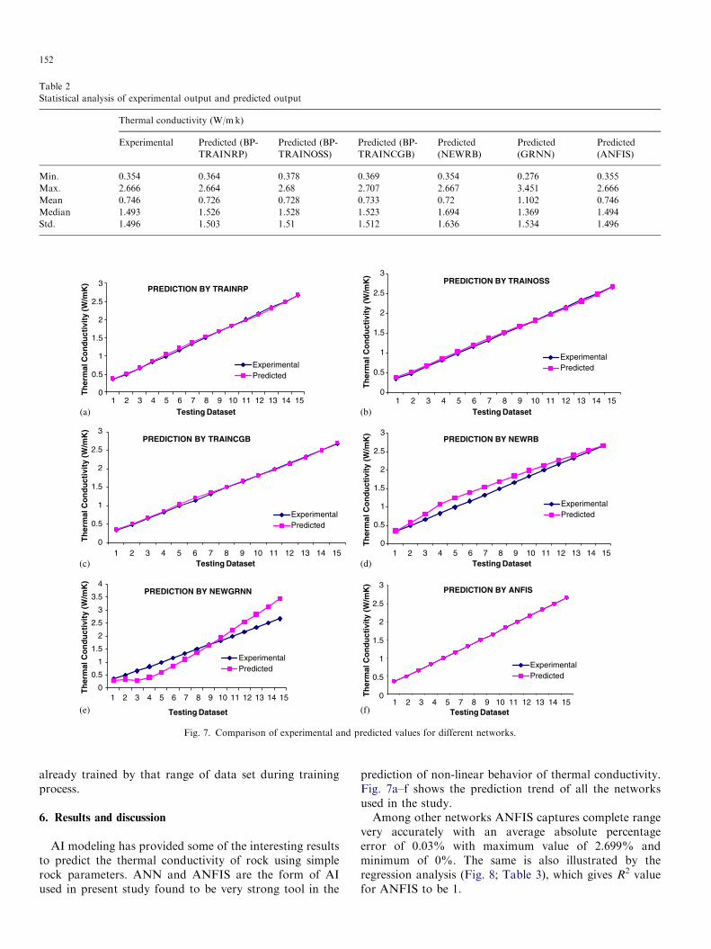
Table 2

Statistical analysis of experimental output and predicted output

Thermal conductivity (W/mk)

Experimental Predicted (BP-

TRAINRP)

Predicted (BP-

TRAINOSS)

Predicted (BP-

TRAINCGB)

Predicted

(NEWRB)

Predicted

(GRNN)

Predicted

(ANFIS)

Min. 0.354 0.364 0.378 0.369 0.354 0.276 0.355

Max. 2.666 2.664 2.68 2.707 2.667 3.451 2.666

Mean 0.746 0.726 0.728 0.733 0.72 1.102 0.746

Median 1.493 1.526 1.528 1.523 1.694 1.369 1.494

Std. 1.496 1.503 1.51 1.512 1.636 1.534 1.496

PREDICTION BY TRAINRP

0

0.5

1

1.5

2

2.5

3

1 2 3 4 5 6 7 8 9 10 11 12 13 14 15Testing Dataset

1 2 3 4 5 6 7 8 9 10 11 12 13 14 15Testing Dataset

1 2 3 4 5 6 7 8 9 10 11 12 13 14 15

Testing Dataset

1

1

2

2

3

3

4

4

5

5

6 7

7

8

8

9

9

10

10

11

11

12

12

13

13

14

14

15

15

Testing Dataset

Testing Dataset

1 2 3 4 5 6 7 8 9 10 11 12 13 14 15Testing Dataset

Th

erm

al C

on

du

ctiv

ity

(W/m

K) PREDICTION BY TRAINOSS

0

0.5

1

1.5

2

2.5

3

Th

erm

al C

on

du

ctiv

ity

(W/m

K)

Th

erm

al C

on

du

ctiv

ity

(W/m

K)

Th

erm

al C

on

du

ctiv

ity

(W/m

K)

ExperimentalPredicted

PREDICTION BY TRAINCGB

0

0.5

1

1.5

2

2.5

3

Th

erm

al C

on

du

ctiv

ity

(W/m

K)

PREDICTION BY NEWRB

0

0.5

1

1.5

2

2.5

3

0

0.5

1

1.5

2

2.5

3PREDICTION BY NEWGRNN

0

0.5

1

1.5

2

2.5

3

3.5

4

Th

erm

al C

on

du

ctiv

ity

(W/m

K)

PREDICTION BY ANFIS

ExperimentalPredicted

ExperimentalPredicted

ExperimentalPredicted

ExperimentalPredicted

ExperimentalPredicted

(a) (b)

(d)(c)

(e) (f)

Fig. 7. Comparison of experimental and predicted values for different networks.

152

already trained by that range of data set during trainingprocess.

6. Results and discussion

AI modeling has provided some of the interesting resultsto predict the thermal conductivity of rock using simplerock parameters. ANN and ANFIS are the form of AIused in present study found to be very strong tool in the

prediction of non-linear behavior of thermal conductivity.Fig. 7a–f shows the prediction trend of all the networksused in the study.Among other networks ANFIS captures complete range

very accurately with an average absolute percentageerror of 0.03% with maximum value of 2.699% andminimum of 0%. The same is also illustrated by theregression analysis (Fig. 8; Table 3), which gives R2 valuefor ANFIS to be 1.

PREDICTION BY TRAINRP

R2 = 0.999

1:10

0.51

1.52

2.53

3.5

0 0.5 1.5 2 2.5 3 3.51 0 0.5 1.5 2 2.5 3 3.51

Experimental Experimental

Pre

dic

ted

Pre

dic

ted

Pre

dic

ted

PREDICTION BY TRAINOSS

1:!0

1

2

3

4

PREDICTION BY TRAINCGB

R2 =0.9989

1:10

1

2

3

4

Experimental

Pre

dic

ted

PREDICTION BY NEWRB

R2 =0.9872

1:10

1

2

3

4

PREDICTION BY NEWGRNN

R2 = 0.9709

1:1

0

0.51

1.5

2

2.53

3.5

Pre

dic

ted

PREDICTION BY ANFIS

R2 = 1

1:10

0.51

1.52

2.53

3.5P

red

icte

d

0 0.5 1.5 2 2.5 3 3.51

Experimental0 0.5 1.5 2 2.5 3 3.51

Experimental0 0.5 1.5 2 2.5 3 3.51

Experimental0 0.5 1.5 2 2.5 3 3.51

R2 = 0.993

(a) (b)

(d)

(f)(e)

(c)

Fig. 8. Regression analysis of the networks with the comparison of 1:1 line.

Table 3

Regression analysis and average absolute percentage error of different

networks

Network used Av. absolute % error R2 value

Trainrp, FFBP 2.263 0.999

Trainoss,FFBP 2.6994 0.9993

Traincgb, FFBP 2.5832 0.9989

Radial basic functions

Newrb 12.2873 0.9872

Newgrnn 24.1524 0.9709

ANFIS 0.031 1.00

153

Radial basis network predicts with percentage error of12.28% and 24.15% by NEWRB and GRNN, respectively.Results predicted by GRNN are more nearer to experi-mental values. It is due to the fact that GRNN alwaysapproximates a function to an arbitrary accuracy. Amongall the predictions of FFBP, results of all the trainingfunctions TRAINRP, TRAINOSS and TRAINCGB arevery close to each other and best performance have shownby RP with R2 value of 0.999 and 2.263% of average error.Table 3 indicates average absolute percentage error and R2

value to make comparative analysis among differentnetworks. Tables 4 and 5 exhibit the predicted andobserved value of thermal conductivity using variouspredictors and average absolute percentage error of alltesting data set predicted by different networks, respec-tively.Ozkahraman et al. (2004) predicted thermal conducti-

vity independently with P-wave velocity, porosity, density,compressive strength and found that the thermal con-ductivity of any rock can be calculated from laboratorydetermined P-wave velocity. Thermal conductivity and P-wave velocity shows best correlation coefficient. As itdiscussed earlier thermal conductivity depends on manyother physico-mechanical properties, which affects depend-ing upon the rock type. Whereas, in present study otherinput parameters are also considered and a computa-tional model is designed to avoid complicated andcumbersome experimental setups. This can be modifieddepending upon the rock type. Table 5 indicates ofthe percentage error found by different network. Allthe networks show considerable or acceptable errorpercentage except GRNN and NEWRB. This indicatesthe prediction ability and confidence to use the networkfor future prediction of thermal conductivity of differentrock types.

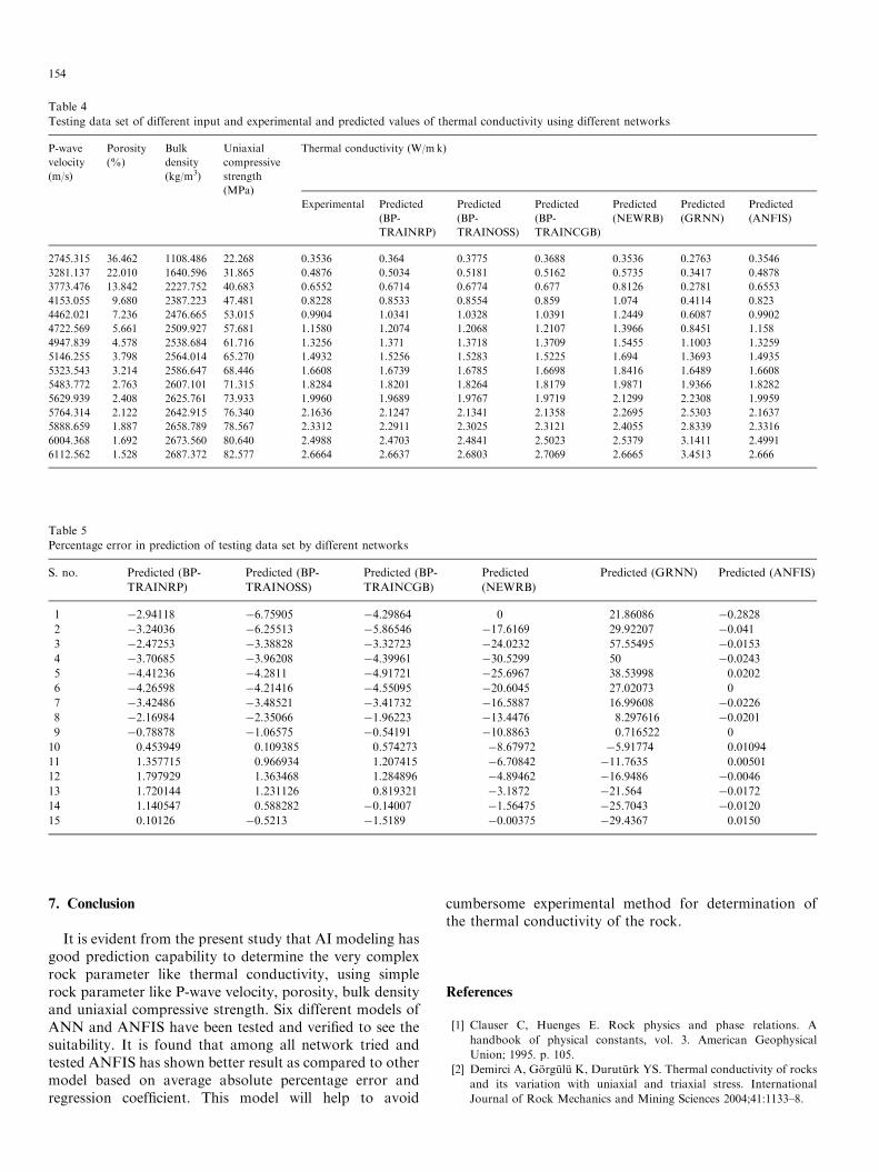
Table 4

Testing data set of different input and experimental and predicted values of thermal conductivity using different networks

P-wave

velocity

(m/s)

Porosity

(%)

Bulk

density

(kg/m3)

Uniaxial

compressive

strength

(MPa)

Thermal conductivity (W/mk)

Experimental Predicted

(BP-

TRAINRP)

Predicted

(BP-

TRAINOSS)

Predicted

(BP-

TRAINCGB)

Predicted

(NEWRB)

Predicted

(GRNN)

Predicted

(ANFIS)

2745.315 36.462 1108.486 22.268 0.3536 0.364 0.3775 0.3688 0.3536 0.2763 0.3546

3281.137 22.010 1640.596 31.865 0.4876 0.5034 0.5181 0.5162 0.5735 0.3417 0.4878

3773.476 13.842 2227.752 40.683 0.6552 0.6714 0.6774 0.677 0.8126 0.2781 0.6553

4153.055 9.680 2387.223 47.481 0.8228 0.8533 0.8554 0.859 1.074 0.4114 0.823

4462.021 7.236 2476.665 53.015 0.9904 1.0341 1.0328 1.0391 1.2449 0.6087 0.9902

4722.569 5.661 2509.927 57.681 1.1580 1.2074 1.2068 1.2107 1.3966 0.8451 1.158

4947.839 4.578 2538.684 61.716 1.3256 1.371 1.3718 1.3709 1.5455 1.1003 1.3259

5146.255 3.798 2564.014 65.270 1.4932 1.5256 1.5283 1.5225 1.694 1.3693 1.4935

5323.543 3.214 2586.647 68.446 1.6608 1.6739 1.6785 1.6698 1.8416 1.6489 1.6608

5483.772 2.763 2607.101 71.315 1.8284 1.8201 1.8264 1.8179 1.9871 1.9366 1.8282

5629.939 2.408 2625.761 73.933 1.9960 1.9689 1.9767 1.9719 2.1299 2.2308 1.9959

5764.314 2.122 2642.915 76.340 2.1636 2.1247 2.1341 2.1358 2.2695 2.5303 2.1637

5888.659 1.887 2658.789 78.567 2.3312 2.2911 2.3025 2.3121 2.4055 2.8339 2.3316

6004.368 1.692 2673.560 80.640 2.4988 2.4703 2.4841 2.5023 2.5379 3.1411 2.4991

6112.562 1.528 2687.372 82.577 2.6664 2.6637 2.6803 2.7069 2.6665 3.4513 2.666

Table 5

Percentage error in prediction of testing data set by different networks

S. no. Predicted (BP-

TRAINRP)

Predicted (BP-

TRAINOSS)

Predicted (BP-

TRAINCGB)

Predicted

(NEWRB)

Predicted (GRNN) Predicted (ANFIS)

1 �2.94118 �6.75905 �4.29864 0 21.86086 �0.2828

2 �3.24036 �6.25513 �5.86546 �17.6169 29.92207 �0.041

3 �2.47253 �3.38828 �3.32723 �24.0232 57.55495 �0.0153

4 �3.70685 �3.96208 �4.39961 �30.5299 50 �0.0243

5 �4.41236 �4.2811 �4.91721 �25.6967 38.53998 0.0202

6 �4.26598 �4.21416 �4.55095 �20.6045 27.02073 0

7 �3.42486 �3.48521 �3.41732 �16.5887 16.99608 �0.0226

8 �2.16984 �2.35066 �1.96223 �13.4476 8.297616 �0.0201

9 �0.78878 �1.06575 �0.54191 �10.8863 0.716522 0

10 0.453949 0.109385 0.574273 �8.67972 �5.91774 0.01094

11 1.357715 0.966934 1.207415 �6.70842 �11.7635 0.00501

12 1.797929 1.363468 1.284896 �4.89462 �16.9486 �0.0046

13 1.720144 1.231126 0.819321 �3.1872 �21.564 �0.0172

14 1.140547 0.588282 �0.14007 �1.56475 �25.7043 �0.0120

15 0.10126 �0.5213 �1.5189 �0.00375 �29.4367 0.0150

154

7. Conclusion

It is evident from the present study that AI modeling hasgood prediction capability to determine the very complexrock parameter like thermal conductivity, using simplerock parameter like P-wave velocity, porosity, bulk densityand uniaxial compressive strength. Six different models ofANN and ANFIS have been tested and verified to see thesuitability. It is found that among all network tried andtested ANFIS has shown better result as compared to othermodel based on average absolute percentage error andregression coefficient. This model will help to avoid

cumbersome experimental method for determination ofthe thermal conductivity of the rock.

References

[1] Clauser C, Huenges E. Rock physics and phase relations. A

handbook of physical constants, vol. 3. American Geophysical

Union; 1995. p. 105.

[2] Demirci A, Gorgulu K, Duruturk YS. Thermal conductivity of rocks

and its variation with uniaxial and triaxial stress. International

Journal of Rock Mechanics and Mining Sciences 2004;41:1133–8.

155

[3] Duruturk YS. The variation of thermal conductivity with pressure in

rocks and the investigation of its effect in underground mines. Sivas,

Turkey: Cumhuriyet University; 1999. p. 188.

[4] Duruturk YS, Demirci A, Kec-eciler A. Variation of thermal

conductivity of rocks with pressure. CIM Bulletin 2002;95:67.

[5] Hassan A. Optimising insulation thickness for building using life cost.

Applied Energy 1999;63:115–24.

[6] Clauser C, Huenges E. Thermal conductivity of rocks and minerals.

American Geophysical Union 1995:105–26.

[7] Ghaboussi J, Garrett Jr. JH, Wu X. Knowledge-based modeling of

material behavior with neural networks. Journal of Engineering

Mechanics, ASCE 1991;117(1):132–53.

[8] Ellis GW, Yao C, Zhao R. Neural network modeling of the

mechanical behavior of sand. In: Proceedings of ninth Conference.

NY: ASCE Engineering Mechanics, ASCE; 1992. p. 421–4.

[9] Alvarez Grima M. Neuro-fuzzy modeling in engineering geology.

Rotterdam: A.A. Balkema; 2000 244pp.

[10] Den Hartog MH, Babuska R, Deketh HJR, Alvarez Grima M,

Verhoef PNW, Verbruggen HB. Knowledge-based fuzzy model for

performance prediction of a rock-cutting trencher. International

Journal of Approximate Reasoning 1997;16:43–66.

[11] Finol J, Guo YK, Jing XD. A rule based fuzzy model for the

prediction of petrophysical rock parameters. Journal of Petroleum

Science and Engineering 2001;29:97–113.

[12] Gokceoglu C. A fuzzy triangular chart to predict the uniaxial

compressive strength of Ankara agglomerates from their petro-

graphic composition. Engineering Geology 2002;66:39–51.

[13] Setnes M, Babuska R, Verbruggen HB. Rule-based modeling:

precision and transparency. IEEE Transactions on Systems Man

and Cybernetics, Part C 1998;28:165–9.

[14] Ozkahraman HT, Selver R, Isik EC. Determination of the thermal

conductivity of rock from P-wave velocity. International Journal of

Rock Mechanics and Mining Sciences 2004;41:703–8.

[15] Joeleht A, Kirsimae K, Shogenova A, Sliaupa S, Kukkonen IT,

Rasteniene V, et al. Thermal conductivity of cambrian siliciclastic

rocks from the Baltic basin; Proceedings of the Estonian Academy of

Sciences. Geology 2002;51(1):5–15.

[16] Tavman IH. Effective thermal conductivity of granular porous

materials. International Communications in Heat and Mass Transfer

1996;23(2):169–76.

[17] Abu-Hamdeh NH, Reeder RC. Soil thermal conductivity-effects of

density, moisture, salt concentration, and organic matter. Soil Science

Society of America Journal, Division S-1-Soil Physics 2000;64:

1285–90.

[18] Gorgulu K. Determination of relationships between thermal con-

ductivity and material properties of rocks. Journal of University of

Science and Technology, Beijing 2004;11:297.

[19] Yegnanarayana B. Artificial neural networks. New Delhi, India:

Prentice-Hall of India Private Limited; 1999.

[20] Zurada JM. Introduction to artificial neural systems. West Publi-

shing; 1992.

[21] Demuth H, Beale M. Neural network toolbox for use with

MATLAB. Mathworks Inc; 1994. p. 158.

[22] Kolmogorov’s AN. On the representation of continuous functions of

several variables by superposition of continuous function of one

variable and addition. Duke Akademii Nauk USSR 1957;114:369–73.

[23] Lorentz GG. The 13th problem of Hillbert. In: Proceedings of the

Symposium in pure mathematics, vol. 28. 1976. p. 419–30.

[24] Sprecher DA. On the structure of continuous functions of several

variables. Transctions of American Mathematical Society 1965;115:

340–55.

[25] Haykin S. Neural network. Addition-Wesley Longman (Singapore)

Pte. Ltd.; 2001.

[26] Juang CH, Lee DH, Sheu C. Mapping slope failure potential using

fuzzy sets. Journal of Geotechnical Engineering ASCE 1992;118(3):

475–93.

[27] Zadeh LA. Outline of a new approach to the analysis of complex

systems and decision processes. IEEE Transactions on Systems Man

and Cybernetics 1973;3:28–44.

[28] Hadipriono F, Sun K. Angular fuzzy set models for linguistic values.

Civil Engineering Systems 1990;7(3):148–56.

[29] Karr CL, Gentry EJ. Fuzzy control of pH using genetic algorithims.

IEEE Transaction on Fuzzy Systems 1993;1(1):46–53.

[30] Zadeh LA. A rationale for fuzzy control. Journal of Dynamic

Systems, Measurement and Control Transaction, ASME 1972;94:

3–4.

[31] Jang JSR. ANFIS: adaptive neural based fuzzy interference system.

IEEE Transactions on Systems, Man and Cybernetics 1993;23:

665–85.

[32] Zadeh LA. In: Hayes JE, Michie D, Mikulich LI, editors. A theory of

approximate reasoning, machine intelligence. New York: Wiley;

1979.

[33] Zadeh LA. Fuzzy sets. IEEE Information and Control 1965;8:

338–53.