PREDICTION OF STOCK PRICES USING TECHNICAL ...
83
PREDICTION OF STOCK PRICES USING TECHNICAL ANALYSIS IN SELECTED COMPANIES LISTED ON THE NAIROBI SECURITIES EXCHANGE BY EMMANUEL ASUMA ONSOMU UNITED STATES INTERNATIONAL UNIVERSITY -AFRICA SUMMER 2018
-
Upload
khangminh22 -
Category
Documents
-
view
0 -
download
0
Transcript of PREDICTION OF STOCK PRICES USING TECHNICAL ...

PREDICTION OF STOCK PRICES USING TECHNICAL ANALYSIS IN
SELECTED COMPANIES LISTED ON THE NAIROBI SECURITIES
EXCHANGE
BY
EMMANUEL ASUMA ONSOMU
UNITED STATES INTERNATIONAL UNIVERSITY -AFRICA
SUMMER 2018

PREDICTION OF STOCK PRICES USING TECHNICAL ANALYSIS IN
SELECTED COMPANIES LISTED ON THE NAIROBI SECURITIES
EXCHANGE
BY
EMMANUEL ASUMA ONSOMU
A Research Project Report Submitted to the Chandaria School of Business in
Partial Fulfilment of the Requirement for the Degree on Master of Business
Administration (MBA)
UNITED STATES INTERNATIONAL UNIVERSITY -AFRICA
SUMMER 2018

ii
STUDENT’S DECLARATION
I, the undersigned, declare that this is my original work and has not been submitted to any other
college, institution or university other than the United States International University Africa for
academic credit.
Signed: ________________________ Date: _____________________
Emmanuel Asuma Onsomu (ID NO. 650014)
This project report has been presented for examination with my approval as the appointed
supervisor.
Signed: ________________________ Date: _____________________
Dr. Elizabeth Kalunda
Signed: _______________________ Date: ____________________
Dean, Chandaria School of Business

iii
COPYRIGHT
All rights reserved. No part of this project should be reproduced, stored in a retrieval system, or
transmitted in any form or by any means: electronic, mechanical, photocopying, recording or
otherwise without prior written permission of the copyright owner.
Emmanuel A. Onsomu ©2018

iv
ABSTRACT
The study aimed at determining the predictability of stock prices and their movements using
technical analysis in selected companies listed on the NSE. This research was made possible by
the following research question; to what extent does exponential moving average (EMA) predict
stock prices in the NSE? How does relative strength index (RSI) predict stock prices in the NSE?
Can parabolic stop and reverse (PSAR) predict stock prices in the NSE?
The study incorporated the use of descriptive and inferential research design to aid in predicting
stock prices. The target population for this study was 66 firms listed at the NSE however due to
other factors like the consistency of trading for the last 10 years and their existence for the same
period the study sampled only 7 firms for this study. The study entirely relied on the use of
secondary data that was readily available at the NSE cutting across from week 22 of 2008 all the
way to week 24 of 2017 to establish if moving averages, relative strength index and parabolic
stop and reverse are predictors of stock market prices. Inferential statistics was analyzed with the
help of Statistical Package for Social Sciences (SPSS) v 20.
The study findings revealed that EMA can be used to predict stock market prices as buy and sell
signals are generated to guide investors when to buy and sell to make returns. The study findings
on relative strength index (RSI) in predicting stock prices indicated that RSI cannot predict stock
prices as the mean returns on buy-signals were negative. Finally, with parabolic stop and reverse
indicator showed that it is a good predictor of stock market prices with clear buy and sell signals
to generate good returns.
The study concluded that EMA is a good predictor of stock market prices and that can generate
buy and sell signals. The study also conclude that RSI is not a good predictor given that it
presented a negative return on buy signals and a positive return on sell signals. PSAR as a
technical analysis tool has superior returns on buy signals which is best suited to predict stock
market prices. This is backed by the ability of PSAR to generate buy and sell signals.
The study recommends the need for investors and investment managers to use these indicators to
predict stock prices and get clear buy and sell signals especially EMA & PSAR. The study
further recommends the need to carry out further research on other technical analysis indicators
from EMA, RSI and PSAR to establish stock market prices and discern the behaviors so as to

v
draw a comparative analysis and also use different periods such as monthly or quarterly data
over a long period of time to get a clear picture on the use of trends.

vi
ACKNOWLEDGEMENT
I wish to take this opportunity to express my appreciation to my supervisor Dr. Elizabeth
Kalunda for her wise counsel and guidance throughout the research work. I would also like to
extend my gratitude to my family members for the overwhelming support and understanding
during my study period.

vii
DEDICATION
I dedicate this project to my family and friends, I would have not gone this far without much
sacrifices and support, may God bless you abundantly.

viii
TABLE OF CONTENTS
STUDENT’S DECLARATION ................................................................................................... ii
COPYRIGHT ............................................................................................................................... iii
ABSTRACT .................................................................................................................................. iv
ACKNOWLEDGEMENT ........................................................................................................... vi
DEDICATION............................................................................................................................. vii
TABLE OF CONTENTS .......................................................................................................... viii
LIST OF TABLES ....................................................................................................................... xi
LIST OF FIGURES .................................................................................................................... xii
ABBREVIATIONS AND ACRONYMS .................................................................................. xiii
CHAPTER ONE ........................................................................................................................... 1
1.0 INTRODUCTION................................................................................................................... 1
1.1 Background of the Study .................................................................................................. 1
1.2 Statement of the Problem ................................................................................................. 5
1.3 Purpose of the Study ........................................................................................................ 7
1.4 Research Questions .......................................................................................................... 7
1.5 Significance of the Study ................................................................................................. 7
1.6 Scope of the Study............................................................................................................ 8
1.7 Definition of Key Terms .................................................................................................. 9
1.8 Chapter Summary ............................................................................................................. 9
CHAPTER TWO ........................................................................................................................ 11
2.0 LITERATURE REVIEW .................................................................................................... 11
2.1 Introduction .................................................................................................................... 11
2.2 Moving Averages (MA) on Stock Prices ....................................................................... 11
2.3 Relative Strength Index (RSI) on Stock Prices .............................................................. 15

ix
2.4 Parabolic Stop and Reverse (PSAR) Indicator on Stock Prices ..................................... 19
2.5 Chapter Summary ........................................................................................................... 21
CHAPTER THREE .................................................................................................................... 22
3.0 RESEARCH METHODOLOGY ........................................................................................ 22
3.1 Introduction .................................................................................................................... 22
3.2 Research Design ............................................................................................................. 22
3.3 Population....................................................................................................................... 22
3.4 Sampling Design ............................................................................................................ 23
3.5 Data Collection Methods ................................................................................................ 24
3.6 Research Procedure ........................................................................................................ 24
3.7 Data Analysis Method .................................................................................................... 27
3.8 Chapter Summary ........................................................................................................... 27
CHAPTER FOUR ....................................................................................................................... 28
4.0 RESULTS AND FINDINGS ........................................................................................... 28
4.1 Introduction .................................................................................................................... 28
4.2 Exponential Moving Average and Stock Prices ................................................................. 29
4.2.1 Buy and Sell Signals for EMA......................................................................................... 29
4.3 Relative Strength Index (RSI) and Stock Prices ................................................................. 35
4.3.1 Buy and Sell Signals for RSI ........................................................................................... 35
4.3.2 Results for RSI rules ........................................................................................................ 39
4.4 Parabolic Stop and Reverse (PSAR) and Stock Prices .................................................. 40
4.5 Chapter Summary ........................................................................................................... 48
CHAPTER FIVE ........................................................................................................................ 49
5.0 DISCUSSIONS, CONCLUSIONS AND RECOMMENDATIONS ................................. 49
5.1 Introduction .................................................................................................................... 49

x
5.2 Summary of the study .................................................................................................... 49
5.3 Discussion ........................................................................................................................... 50
5.3.1 Moving Averages (MA) and Stock Prices ....................................................................... 50
5.4 Conclusions .................................................................................................................... 55
5.5 Recommendations .......................................................................................................... 55
REFERENCES ............................................................................................................................ 58
APPENDICES ............................................................................................................................. 68
Appendix I: Listed Companies at the Nairobi Securities Exchange ......................................... 68

xi
LIST OF TABLES
Table 3. 1: Population ................................................................................................................... 23
Table 4. 1 Summary Statistics for weekly returns ....................................................................... 28
Table 4. 2 Results for EMA rules ................................................................................................. 35
Table 4. 3 Results from RSI rules ................................................................................................. 40
Table 4. 4 Results from PSAR rules ............................................................................................. 48

xii
LIST OF FIGURES
Figure 4. 1 ARM Average Price vs Short (3week) EMA and Long (15week) EMA ................... 29
Figure 4. 2 KCB Average Price vs Short (3week) EMA and Long (15week) EMA .................... 30
Figure 4. 3 KenolKobil Average Price vs Short (3week) EMA and Long (15week) EMA ......... 31
Figure 4. 4 Sasini Average Price vs Short (3week) EMA and Long (15week) EMA .................. 31
Figure 4. 5 ScanGroup Average Price vs Short (3week) EMA and Long (15week) EMA .......... 32
Figure 4. 6 Safaricom Average Price vs Short (3week) EMA and Long (15week) EMA ........... 33
Figure 4. 7 Unga Average Price vs Short (3week) EMA and Long (15week) EMA ................... 33
Figure 4. 8 ARM Average Price vs RSI ....................................................................................... 36
Figure 4. 9 KCB Average Price vs RSI ........................................................................................ 36
Figure 4. 10 KenolKobil Average Price vs RSI ............................................................................ 37
Figure 4. 11 Sasini Average Price vs RSI ..................................................................................... 37
Figure 4. 12 ScanGroup Average Price vs RSI............................................................................. 38
Figure 4. 13 Safaricom Average Price vs RSI .............................................................................. 38
Figure 4. 14 Unga Average Price vs RSI ...................................................................................... 39
Figure 4. 15 ARM Average Price vs PSAR .................................................................................. 41
Figure 4. 16 KCB Average Price vs PSAR................................................................................... 42
Figure 4. 17 KenolKobil Average Price vs PSAR ........................................................................ 43
Figure 4. 18 Sasini Average Price vs PSAR ................................................................................. 44
Figure 4. 19 ScanGroup Average Price vs PSAR ......................................................................... 45
Figure 4. 20 Safaricom Average Price vs PSAR .......................................................................... 46
Figure 4. 21 Unga Average Price vs PSAR .................................................................................. 47

xiii
ABBREVIATIONS AND ACRONYMS
ADX Average Directional Index
AIMS Alternative Investments Market Segments
ATR Average True Range
BBands Bollinger Bands
CCI Commodity Channel Index
CMF Chaikin Money Flow
CMO Chande Momentum Oscillator
DEMA Double Exponential Moving Average
EMA Exponential Moving Average
MA Moving Averages
MACD Moving Average Convergence Divergence
MFI Money Flow Index
MIMS Main Investments Market Segments
NSE Nairobi Securities Exchange
PSAR Parabolic Stop and Reverse
RSI Relative Strength Index
SMA Simple Moving Average
SMI Stochastic Momentum Index
TDI Traders Dynamic Index
VHF Vertical Horizontal Filter
VWMA Volume Weighted Moving Average
WPR William’s Percent Range
WMA Weighted Moving Average

1
CHAPTER ONE
1.0 INTRODUCTION
1.1 Background of the Study
Capital market efficiency and the prediction of future stock prices are the most thought-
provoking and ferociously debated areas in finance. The followers of traditional financial theory
strongly believe that the markets are efficient in pricing the financial instruments. This view
became popular after Fama's work on the Efficient Market Hypothesis (Rahman & Mohsin,
2012).
According to Boobalan (2014), there are two methods of analyzing investment opportunities in
the stock market i.e. fundamental analysis which uses fundamental information such as financial
and non-financial company information to calculate the intrinsic value of a security and technical
analysis which focuses on actual price movements. Boobalan (2014) further states that technical
analysts assume that movement of stock prices is 90 percent psychological and 10 percent logical
and market activity is evaluated by analyzing statistics related to past prices and volume.
Kulkarni & Kulkarni (2013) indicates that fundamental analysis seeks to determine future stock
prices by understanding and measuring the objective values of the equity, whereas the study of
stock charts i.e. technical analysis dictates that the past action of the market itself will determine
the future course of the prices.
Technical analysis is a price analysis technique that claims the ability to predict the future
direction of security prices through the study of past price data. It considers only the actual price
behavior of the financial series, on the assumption that past price reflects all relevant factors
before an investor. Technical analysts extensively use certain indicators, which are typically
mathematical transformations of price or volume. These indicators are used to determine whether
the prices are trending i.e. increasing, decreasing or moving in a narrow range (Mitra, 2011).
Boobalan (2014) defines technical analysis as an art and science of forecasting future prices
based on examination of the past price movements by putting stock information like prices,
volumes and open interest on a chart and applying various patterns and indicators to it in order to
assess the future price movements.

2
Many studies have examined the benefits of conducting technical analysis on the stock market,
with mixed results. Stock price prediction is the act of determining the future price of the stock
traded on an exchange to generate profitable buy and sell signals (Abbad, Fardousi, & Abbad,
2014). According to El-Ansary and Mohssen (2017), technical analysis is a timing tool that is
being used by traders and investors in the stock markets, forex, and commodity markets,
emerging and developed markets for achieving abnormal returns. Predicting the stock market
direction or movement is a difficult task as it is based on economic factors that are influenced by
various market players such as the management, traders (Individuals and/or institutions) and
investors who can be rational or irrational (Githumbi, 2014).
Prices of securities in the securities exchange fluctuate from time to time. Investors, both
individuals and institutions, are always interested in buying at low prices and selling at higher
prices to make profits. To achieve this, they estimate the price and potentially try predicting the
direction. Historical data is used to identify patterns that predict security movements hence
violating the random walk hypothesis and weak form market efficiency (Githumbi, 2014).
Technical analysis is considered by many to be the original form of investment analysis dating
back to the 1800s (Brock, Lakonishok & LeBaron, 1992). Technical analysis can be understood
as a set of rules or charting that tends to anticipate future price shifts based on the study of
certain information, such as, for example, purchase price, selling price, and volume traded,
among others (Lin, Yang & Song, 2011; Oliveira Nobre & Zarate, 2013; Gorgulho, Neves &
Horta, 2011).
Technical analysts attempt to forecast or predict prices by the study of past prices and a few
other related summary statistics about security trading. They believe that shifts in supply and
demand can be detected in charts of market action (Brock, Lakonishok & LeBaron, 1992).
Technical analysis is a wide term that includes the usage of a range of trading strategies in
international stock markets. The strategy that technical analysts use stems its power from the
notion that upcoming stock prices are anticipated by means of the study of historical stock prices.
However, this philosophy violates the random walk hypothesis that stock prices change
independently of their historical trends and actions (Masry, 2017).
3
Technical analysis, even if deliberated by some as purely conjecture, is still generally
acknowledged as additional information to main brokerage companies. There are existent two
reasons for the achievement of technical analysis and why its success is still debated: stock
return predictability stems from efficient markets that can be analyzed by time-varying
equilibrium returns, and stock return predictability forms from prices wandering apart from their
fundamental valuations. Fundamentally, both explanations show overall market inefficiency
where investors are capable of exploiting. Therefore, technical analysis derives its importance
from its ability to train investors to take investment decision based on historical trends of
securities prices (Masry, 2017).
Technical analysis is based on the belief in which asset prices will move in trends. A technician
does not consider much about fundamental factors such as supply and demand. He or she
instead, in hopes of projecting future price movements investigates historical price changes by
examining charts, moving averages, patterns, and a wealth of indicators derived from open, high,
low and closing prices and volumes (Metghalchi, Chang & Gomez, 2012).
Menkhoff (2010) analyzed survey evidence from 692 fund managers in five countries including
the United States and finds that the share of fund managers that put at least some importance on
technical analysis is 87%. The survey indicates that technical analysis is predominantly used as a
complement to fundamental analysis; however, when the focus is shifted to forecasting horizons,
technical analysis becomes the most important forecasting tool in decision making for shorter-
term periods. In their study on technical analysis of the Jordanian Stock Exchange, Muhannad,
Atmeh & Ian (2006) concluded that the results suggested that technical analysis does help to
predict stock price changes in the ASE (Amman Stock Exchange). This evidence regarding
predictive power agrees well with results from other studies conducted in developed and
emerging markets.
Stanivuk, Skarica & Tokic (2012) analyzed the predictability of share price changes using the
momentum model on the Croatian Stock Market. They demonstrated that the shares that have
generated the highest (or lowest) returns in the period from 3 to 12 months have the tendency of
increase (or decrease) in the following 3 to 12 months. The findings are contrary to the Efficient
Market Hypothesis (EMH). This indicates predictability of stock prices. In their research to
investigate the possibility that technical rules contain significant return forecast power, Abbad,

4
Fardousi, and Abbad (2014) using simple forms of technical analysis for the Amman Stock
Exchange Index, concluded that technical analysis does have power to forecast price movements.
Njuguna (2016), in the study of the changing market efficiency of the Nairobi securities
exchange using the NSE all share index and NSE 20 share index, indicates that return
predictability is time varying thus profit opportunities exist in the market, however, since the
degree of return predictability seems to decline overtime, it means that the possibility of
identifying mispriced shares by observing past price changes is decreasing. The use of trading
systems has increased the chances of making excess returns using technical analysis. Trading
systems are set with specific rules which are strategies for predicting and increasing profitability.
According to Vanstone and Finnie (2010); Kihoro and Okango (2014) and Wanjawa (2014),
artificial neural networks can be used to generate profitable results. Giot and Petitjean (2011),
studied ten countries’ stock markets using statistical tests and found that returns are predictable
to some extent.
Pattern recognition is a major part of technical analysis and that is the major reason why
technicians are called chartists. Chart patterns can help predict or forecast stock prices by
looking for buy-sell signals. Through their new approach of identifying rounding bottoms and
resistance levels patterns and their (patterns) ability to generate buy-sell signals to forecast stock
prices, Zapranis and Tsinaslandis (2012) concluded that the patterns could not generate
particularly high returns especially if the transaction costs are taken to account. The use of high
and low past prices i.e. using past information to predict or forecast the future is important for
technicians to create stop losses and potentially let the gains run.
According to Caporin, Ranaldo and Santucci (2013) high and low prices of equity shares are
predictable and that future extreme prices can be forecasted by simply using past high and low
prices. This indicated that accurate forecasts of high and low prices can improve trading
performance and thus profitability.
There are many technical indicators that can be used to determine the predictability nature of
technical analysis. Technical analysis is a trading tool that evaluates securities and attempts to
forecast their future movement by analyzing price and volume data. Many traditional statistical
tools are available for the investors for making decision in financial market. Many technical

5
indicators such as Moving Averages (SMA, EMA, WMA, VWMA, and DEMA), Trend
Indicators (MACD, ADX, TDI, Aroon, VHF), Momentum indicators (Stochastic, RSI, SMI,
WPR, CMO, CCI), Volatility indicators (BBands, ATR, Dochain Channel) and Volume
indicators (OBV, MFI, CMF) are available to analyze the stock price movement (Vaiz &
Ramaswami, 2016). In their study on the contrarian technical trading rules: evidence from the
Nairobi Stock Index, Metghalchi, Kagochi & Hayes (2014) used exponential moving averages
(EMA), relative strength index (RSI), stochastic, parabolic stop and reverse (PSAR), moving
average convergence divergence (MACD) and directional moving system (DMS).
The Nairobi Securities Exchange (NSE) is a leading African Exchange, based in Kenya – one of
the fastest-growing economies in Sub-Saharan Africa. Founded in 1954, NSE has a six-decade
heritage in listing equity and debt securities. It offers a world class trading facility for local and
international investors looking to gain exposure to Kenya and Africa’s economic growth. NSE
demutualized and self-listed in 2014. Its Board and management team are comprised of some of
Africa’s leading capital markets professionals, who are focused on innovation, diversification
and operational excellence in the Exchange.
NSE is playing a vital role in the growth of Kenya’s economy by encouraging savings and
investment, as well as helping local and international companies’ access cost-effective capital.
NSE operates under the jurisdiction of the Capital Markets Authority of Kenya. It is an affiliate
of the World Federation of Exchange, a founder member of the African Securities Exchanges
Association (ASEA) and the East African Securities Exchanges Association (EASEA). The NSE
is a member of the Association of Futures Market and is a partner exchange in the United
Nations-led SSE initiative (NSE, 2017). The NSE has three market segments, main investments
market segment (MIMS), alternative investment market segment (AIMS) and fixed income
securities market segment (FISMS). Sectors in the NSE include basic materials, consumer goods,
consumer services, financials (banks and insurance companies), industrials, oil and gas,
telecommunications and utilities.
1.2 Statement of the Problem
Prices of securities in the securities exchange fluctuate from time to time. Investors, both
individuals and institutions, are always interested in buying at low prices and selling at higher
prices to make profits. To achieve this, they estimate the price and potentially try predicting the

6
direction. A successful prediction of stock’s future price would yield significant profit for
predictor. Predicting the stock market direction or movement is a daunting task as it is based on
factors such as economic conditions that are influenced by various market players such as the
management, traders and investors who can be rational or irrational. The ability to predict stock
price changes based on a given set of information lies behind the notion of market efficiency.
Where the market efficiency is low, predictability of the stock price movement is high (Mobarek
and Keasey, 2000). Efficient market is one in which the available information is fully reflected in
stock prices. Prediction of stock market is done by employing technical analysis. Technical
analysis aims at predicting future asset prices with the use of their historical prices, patterns and
volume traded by use of various technical indicators.
The importance of using the technical analysis method is as a result of the lack of efficiency in
the organization, the weakness of some of the legal systems of a number of markets, lack of
information, financial reports, and the extent of availability in the financial markets, in addition
to the small size of some of the financial markets, are reflected by both the capitalization of
financial market index and the number of registered companies in the market (Wafi, 2015).
The period (number of years) and length of time (hours, weeks and months) used to study
technical analysis are also important to capture the cycles in the economy. Boobalan (2014)
states that the time frame in which technical analysis is applied may range from intraday (5-
minute, 10-minutes, 15-minutes, 30-minutes or hourly), daily, weekly or monthly price data to
many years. Since cycles in our market is five years, five-year study period may not be enough
to give a clear picture of the used of patterns and other technical trading strategies. Studies have
been done on the Stock price prediction. Mutothya (2013) investigated empirically whether stock
prices at Nairobi stock exchange follow a random walk model. He employed serial correlation
tests and runs tests to analyze daily price returns for eighteen companies whose stocks
constituted the NSE 20 share over the period July 2008 to June 2011. Achieng (2013) on his
study on relationship between stock prices and trading volume used five-year data (2008-2012).
Most studies on the application of technical analysis in the NSE mostly use the Nairobi Stock
Indices (All share index, NASI & NSE 20 share index) while ignoring other technical analysis
indicators such as exponential moving averages, relative strength index and parabolic stop and
reverse. For instance, Metghalchi, Kagochi & Hayes (2014) in their study of contrarian technical

7
trading rules used daily data of the Nairobi stock index. Njuguna (2016) in testing the efficiency
of the NSE used daily and weekly index data. Moreover, Mwanyasi (2018) indicated that the all
share index and NSE 20 share index were up in 2017 and the major contributor to that was
Safaricom PLC, a single stock. This means that the market reflection, through an index will be
based on a single stock. These indices are constituted with 20 or 25 companies and yet there are
64 listed companies and therefore might not be representative in terms of looking at the technical
analysis of the NSE.
Therefore, this study seeks to fill this gap of limited studies in the use of technical analysis
indicators in predicting stock prices in selected companies listed on the NSE. This will be
realized by addressing amongst others: The use of exponential moving average (EMA) in
predicting stock prices in the NSE, how relative strength index (RSI) can predict stock prices in
the NSE and the extent to which Parabolic stop and reverse (PSAR) is used to predict stock
prices in the NSE. In this study a ten-year weekly data for individual stocks will be employed.
1.3 Purpose of the Study
The purpose of this study was to determine the predictability of stock prices using technical
analysis in selected companies listed on the NSE.
1.4 Research Questions
The study was guided by the following research questions;
1.4.1 To what extent does exponential moving average (EMA) predict stock prices in the NSE?
1.4.2 How does relative strength index (RSI) predict stock prices in the NSE?
1.4.3 Can the use of parabolic stop and reverse (PSAR) assist in predicting stock prices in the
NSE?
1.5 Significance of the Study
1.5.1 Investment Managers and Brokers
Investment managers and brokers invest on behalf of people and for themselves and need to
make returns so that they can be able to pay themselves and pass the excess returns to investors,
both individuals and institutions. This necessitates that they make good returns for their clients to

8
be happy and retain them as their advisors in relation to investments. There are various tools to
use such as technical and or fundamental analysis. Incorporating technical analysis into their
overall strategy, timing decisions can be made for stocks to predict stock prices on entry and exit
points. This will help maximize on the upside (entry) and reduce losses on the downside by
exiting the market. It can be used as a complement or in isolation to the other security analysis
methods.
1.5.2 Individual Investors
Individual investors have a wide variety of options on what to choose from when it comes to
investments. There are mutual funds, pension funds and brokerage firms who invest on behalf of
them. They sometimes choose to invest on their own account and may not have sophisticated
tools available at the discretion of institutional investor and do not have a lot of time to do
market research for decision making on buying and selling of stocks. These are people who trade
from the comfort of their homes or offices. They can therefore apply technical analysis strategies
using indicators and charts for buying and selling stocks to make a return.
1.5.3 Academicians and Researchers
Investment analysis is a wide area of study and a dynamic one because there are various products
created from time to time and technology advances are creating the need for further research for
academicians who want to increase knowledge in their area of study and researchers who want to
understand and benefit from their research. This study will be used as reference for future
researchers in the field of investment analysis in relation to technical analysis, as it indicates past
work done and increases literature for future work to be done.
1.6 Scope of the Study
The study sought to determine the predictability of stock prices using technical analysis in
selected companies listed in the NSE. The target population for this study was 66 companies
listed at the Nairobi Securities Exchange (NSE) however for this study, 7 companies which were
in operation between 2008 and 2017 were sampled. The study solely relied on secondary data
obtained from the NSE. The process involved inputting weekly price data of maximum,
minimum, and average prices obtained from the database of NSE. This study was carried out
between May 2018 and October 2018.

9
1.7 Definition of Key Terms
1.7.1 Moving Averages (MA)
Moving averages refers to a popular technical indicator which investors use to analyze price
trends (Metghalchi, Kagochi & Hayes, 2014).
1.7.2 Relative Strength Index (RSI)
Relative Strength Index is a momentum indicator that measures the magnitude of recent price
changes to analyze overbought or oversold conditions (Wilder, 1978).
1.7.3 Parabolic Stop and Reverse (PSAR)
This is a trend following indicator that is normally used to set trailing price stops. It is a stop loss
system (Metghalchi, Kagochi & Hayes, 2014).
1.7.4 Market Efficiency
Market Efficiency refers to the degree to which market prices reflect all available, relevant
information (El-Ansary & Mohssen, (2017).
1.7.5 Stock Market Prediction
Stock market prediction is the act of trying to determine the future value of a company stock or
other financial instrument traded on an exchange (Mishra, 2013).
1.7.6 Random walk Hypothesis
Random walk hypothesis is a mathematical theory where a variable does not follow an apparent
trend and moves seemingly at random (Gorgulho, Neves & Horta, 2011).
1.8 Chapter Summary
This chapter defines technical analysis and the indicators used to analyze stock prices and
volume to predict stock prices in future which is against two fundamental theories in finance, the
efficient market hypothesis (EMH) and random walk hypothesis (RWH). It further highlights the
background of the study, statement of the problem, purpose of the study, research questions,
significance of the study, scope of the study and definition of terms. Chapter two will be

10
literature review and chapter three the research methodology. Chapter four outlines the results of
the study while chapter five provides the discussion, conclusions and recommendations.

11
CHAPTER TWO
2.0 LITERATURE REVIEW
2.1 Introduction
The purpose of literature review is to outline what has been done previously as far as the
research problem being studied is concerned. The chapter will be divided into sections that
include; the use of moving averages (MA) in predicting stock prices; the use of momentum
indicators such as relative strength index (RSI) in predicting stock prices; and the use of
parabolic stop and reverse (PSAR) in predicting stock prices in the NSE. The literature reviewed
in this study will draw materials from several sources which are related to the objectives of this
specific study. The chapter finally will present the chapter summary.
2.2 Moving Averages (MA) on Stock Prices
Fundamental and technical models were adopted to predict the direction of changes in the price
of financial securities to aid in making investment decisions. Some of the studies conducted to
establish the profitability of both fundamental and technical models did not yield result instead
brought about debates by academia world and their practicalities as far as investment decision
making in the capital market is concerned. The work of the academia world is corroborated with
the argument of Endhiarto (2018), on the EMH (Efficient Market Hypothesis), opined that EMH
existed in capital market where the market price of securities has reflected all available
information. Thus, future stock price or return is unpredictable and random. Efficient Market
Hypothesis is closely related to Random Walk Hypothesis (RWH).
Endhiarto (2018) stated that in an efficient market, every effort made by investors to profit by
utilizing the available information today is a futile attempt to even make statements that forbid
technical analysis in the academic world. Technical analysis is a model predicting stock prices
by observing the pattern of price changes in the past, expecting the pattern to be repeated in the
future in hopes of generating returns exceeding the market return. Further, technical analysis
model is used as an indicator of when to buy or sell the securities. The notable used technical
analysis is the trend following indicator such as Moving Average.
Moving averages refers to a technical indicator which investors use to analyze price trends
(Metghalchi, Kagochi & Hayes, 2014). It is the most common technical analysis tool and would

12
serve to eliminate small movements in the market (Abbad, Fardousi & Abbad, 2014). There are
various moving averages used in technical analysis. The most common ones are simple moving
average (SMA) and exponential moving average (EMA). Simple Moving Average (SMA) is the
average of closing prices of the last n days. The average is moving since at the end of each
trading day, the last day is usually added, whereas the earliest day of the previous average is
dropped (Kapoor, Dey and Khurana, 2011). The major drawback associated with SMA is that all
the trading days have the same weight hence variations in the earlier day’s impact on the
accuracy of the average. EMA on the other hand assigns larger weight to the most recent day of
calculation. This causes the EMA to follow the prices more closely most of the time as compared
to SMA.
According to Pring (1991), one of the most important trend-determining techniques is based on
the crossing of two moving averages (MA) of prices because the art of technical analysis is to
identify trend changes at an early stage and to maintain an investment posture until the weight of
evidence indicates that the trend has reversed.
Brock, Lakonishok, and LeBaron (1992) analysed moving averages and trading range breakouts
on the Dow Jones Industrial Index from 1897 to 1985. They used various short and long moving
averages of prices to generate buy and sell signals. Their tests included using long moving
averages of 50, 150, and 200 days and short averages of 1, 2, and 5 days. Standard statistical
techniques were extended using bootstrap techniques with an overall support for technical
strategies. They came into a conclusion that technical rules have predictive power.
Fernando (2012) examined whether the technical trading strategies can outperform the
unconditional buy-and-hold strategy to forecast stock price movements and earn excess returns,
after adjusting transaction costs, in emerging Colombo Stock Exchange (CSE). The study used
daily market closing prices of All Share Price Index (ASPI), which is a composite index to
represent whole market, for twenty-five years from January 1985 to December 2010. Daily index
prices were converted to daily returns and moving average rules were used. The empirical
findings of the study confirmed that the moving average trading strategies have statistically
significant predictive and profitability ability in explaining the market and capable of generating
excess return to investors.

13
Faber (2007) demonstrated that a simple moving average strategy applied to broad asset class
indices would have produced superior performance compared to the buy-and-hold strategy.
Specifically, Faber (2007) documented that a 10-month simple moving average strategy applied
to the S&P 500 over a period of 100 years yielded higher annual returns and lower volatility,
resulting in improved risk adjusted performance. Even though the author reported compelling
and positive results, several weaknesses emerge. The author acknowledges that the 10-month
SMA rule was chosen due to its known performance and the results were only simulated in-
sample. In turn, this raises a legitimate “data mining” concern. In addition, the author did not
account for transaction cost and no statistical test was conducted to assess the statistical
significance of the results.
Gwilym et al. (2010) extended the study by Faber (2007) by simulating trading in-sample based
on momentum and moving average rules on international equity markets. The authors reported
statistically significant profits for the momentum rule but did not account for transaction costs.
However, the authors observed that the trading profit decreased towards the end of the sample.
Additionally, Gwilym et al. (2010) confirmed the empirical results by Faber (2007), and reported
superior risk adjusted performance for the moving average rule when compared to the buy-and-
hold strategy. Moskowitz et al. (2012) studied the effect of time-series momentum across 58
futures contracts, in the period from 1985 to 2009, for major asset classes including equity
markets, bond markets, currency markets and commodities markets. The authors were able to
document a consistent and significant time series momentum effect across every asset class
examined. More precisely, Moskowitz et al. (2012) found that returns in the last 12 months was a
positive predictor for future returns. The momentum effect was documented to persist for
approximately one year before it partially reversed.
Kilgallen (2012) replicated the influential study by Faber (2007) with some modification.
Specifically, instead of focusing on broad asset class indices, Kilgallen (2012) simulated the
same strategies separately on individual assets. The author documented consistent lower
volatility and higher annual returns for all individual assets examined. In fact, the volatility of the
simple moving average strategy for individual currencies, equity indices and commodities were
on average reported to be 27% lower than the passive benchmark. However, results are only

14
simulated in-sample, and no statistical tests were conducted to validate the significance of the
results.
Al-Shiab (2006), examined the univariate autoregressive integrated moving average (ARIMA)
Model forecasting model, using the Amman Stock Exchange (ASE) general daily index. The
model predicted the growth of the ASE. This indicates that moving averages can be used to
predict direction of stock market prices. In their study on the validation of moving average
trading rules evidenced from Hong Kong, Singapore, South Korea and Taiwan markets,
Metghalchi, Du and Ning (2009) using moving average trading rules and conducting robust tests
based on bootstrap and the related t-tests, concluded that moving averages have predictive power
and can discern recurring price patterns for profitable trading.
PhooiM’ng & Zainudin (2014) studied the predictability of Asia Pacific stock market indices
using signals from a dynamic volatility indicator, the adjustable moving average using the daily
stock market indices futures contracts’ returns from the Asia Pacific countries, namely
Australia’s SPI Futures (SPIF), Hong Kong’s Hang Seng Futures (HSF), Japan’s Nikkei 225
Futures (NikkeiF), Korea’s KOSPI Futures (KOSPIF), Malaysia’s FBMKLCI30 Futures (FKLI)
and Singapore’s SiMSCI Futures (SiMSCIF), from 2008 to 2012. There were evidences of
abnormal returns after transaction costs, above the passive buy-and-hold are found in these time
series’ returns; especially for the adjustable moving average.
Atmeh and Dobbs (2006) focused on analyzing a performance of the moving average rules in the
Amman Stock Exchange and using the time series of the Jordan Daily Market Index over the
period 1992 to 2001. The conditional returns on buy and sell signals from actual data are
examined for a range of trading rules compared with returns generated from simulated series
generated by a range of models. They clarified that technical analysis could anticipate for
changes in stock prices.
An exponential moving average (EMA) is an extension of the weighted moving average (Ord,
2004). In comparison to the simple moving average, greater emphasis is given to the most recent
data points and the resulting averaged values are closer to the actual. Exponential Moving
Average (EMA) is used to analyze and keep track of the trend changes of financial time series. It
provides an element of weighting with each previous day. Furthermore, EMA can determine that

15
a slope of financial trend is positively related with the stock price. It always decreases when
price closes below the moving average of stock price and always increases when the price is
increased (Exponential Moving Average, 2012).
Based on a research which done by Tanaka-Yamawaki, Tokuoka and Awaji (2009), they utilized
the pattern recognition approach that was combined with EMA to create the prediction model. In
the experiment, EMA was applied to recognize the pattern of uptrend and downtrend of stock
price by using a two-dimension metric format, and then utilized those patterns for EMA to
predict the price range. They had successfully improved the rate of prediction accuracy above
67%. According to the experiment done by Dzikevicius and Saranda (2010), they found that
EMA was adequate to analyze the financial trend. From their tracking signal, they concluded that
EMA was less risky to identify the direction of financial trend instead of predicting the direction.
A study on the Indian stock market, prediction from technical analysis using data of a period of
five years, Singla (2015) used the EMA and concluded that markets are predictable. There are
studies that compare technical trading strategies and buy and hold strategies. These technical
trading strategies included the use of moving averages. Masry (2017) studied the impact of
technical analysis on stock returns in an emerging capital markets (ECM’s) Country using simple
trading rules i.e. simple moving average. The results indicated that the simple moving average
beat the standard buy-and-hold strategy for the Egyptian stock exchange.
Chang, Jong and Wang (2017) evaluated the profitability of technical trading relative to buy-and-
hold (BH) strategy at firm level, controlling for firm size and trading volume using stocks listed
on the Taiwan stock exchange using a variable length moving average. The results indicated that
variable length moving average outperformed the buy-and-hold strategy. This shows that moving
averages can predict stock prices and thus the reason for profitability.
2.3 Relative Strength Index (RSI) on Stock Prices
Relative Strength Index (RSI) could be premised on Dow’s theory of stock market movements.
The theory is founded on the basis that financial markets are assumed to move in persistent ‘bull’
and ‘bear’ trends, hampered by short term deviations. These trends often result due to the human
nature of investors. Moreover, they are perceived to exert irrational behavior such as reinforcing
past price movements and thus allow bull and bear trends to arise. The relative strength index

16
(RSI), introduced by Wilder (1978), is a momentum oscillator capturing the speed of price
adjustments (momentum). Its oscillating property makes it move between 0 and 100, which
simplifies its interpretation and allows its users to determine when a security should be bought or
sold. According to the author, by relying on average values, the RSI has the additional advantage
of further eliminating erroneous erratic market movements. Regarding the implementation of the
RSI, Wilder (1978) recommends the use of a 14-day period of calculation. In subsequent work,
Achelis (2001) however argues that the period of calculation depends on the predominant cycle
of the security and that longer periods of calculation lead to less volatile values of the indicator.
Relative strength index (RSI) as technical analysis shows “overbought” and “oversold” stock
positions while momentum measures the rate of the rise or fall in stock prices. This therefore
leads to indicator being plotted between a range of zero to 100 where 100 is the highest
overbought condition and zero is the highest oversold condition. The RSI aid in measuring the
strength of a security’s recent up moves in comparison to the strength of its recent down moves.
This helps to indicate whether a security has seen more buying or selling pressure over the
trading period. The standard calculation adopts the use of 14 trading periods as the basis for the
calculation, which is often adjusted to meet the needs of the user. If the trading periods adopted
are lowered then the RSI will be more volatile and is thus adopted for shorter-term trades. RSI is
computed using the formula “RSI = 100 – 100/ 1 + RS, where RS= (Sum of the closing prices of
up days/n)/ (Sum of the closing prices of down days/n) and n=trading periods.” (Drakopoulou,
2015).
Like most indicators there are two general ways in which the indicator is used to generate signals
crossovers and divergence. In the case of the RSI, the indicator uses crossovers of its overbought,
oversold and centerline (Investor’s Business Daily, 2018). The first technique is to use
overbought and sold lines to generate buy-and-sell signals. In the RSI, the overbought line is
typically set at 70 and when the RSI is above this level the security is considered overbought.
The security is seen as oversold when the RSI is below 30. These values can be adjusted to either
increase or decrease the amount of signals that are formed by the RSI. A buy signal is generated
when the RSI breaks the oversold line in an upward direction, which means that it goes from
below the oversold line to moving above it. A sell signal is formed when the RSI breaks the
overbought line in a downward direction crossing from above the line to below the line. Setting

17
the overbought and oversold levels at 80 and 20, respectively, can use a more conservative
approach (Investor’s Business Daily, 2018).
Another crossover technique used in formulating signals is using the centerline (50). This
technique is exactly the same as using the overbought and oversold lines to formulate signals.
This technique will often form signals after a movement in the direction they are predicting but
are used more as a confirmation then a signal compared to the other techniques. A downward
trend is confirmed when the RSI crosses from above 50 to below 50. An upward trend is
confirmed when the RSI crosses above 50 (Murphy, 2018).
Drakopoulou (2015) observed that divergence can be used to form signals as well and that if RSI
is moving in an upward direction and the security is moving in a downward direction it signals to
technical traders that buying pressure is increasing and the downtrend may be coming to an end.
Divergence can also be used to signal a reversal in an upward trend where the RSI is decreasing
signaling increasing selling pressure in an upward trend. The RSI is a standard component on
any basic technical chart. The relative strength indicator focuses on the momentum underlying
the security and is a great secondary measure to be used by traders. It is important to note that the
RSI is often not used as the sole generation of buy-and-sell signals but used in conjunction with
other indicators and chart patterns.
Wilder (1978) noted that the most accurate value for value N to calculate the best RSI is 14 since
it was half of the lunar cycle. Nonetheless, depending on the market, the company and other
factors, the value 14 is not always the best value to calculate the RSI. The shorter the period set,
the more sensitive the oscillator and the wider the amplitude. RSI is perceived to work best if
fluctuation reaches the top and bottom extremes. Thus, when an investor trades in very short
time intervals and he/she wants to have more significant oscillation, it is possible to shorten the
time periods. A period is extended to have an oscillator smoother and narrower in amplitude. The
amplitude of 9-period RSI is therefore greater than that of the recommended 14-period one.
Despite 9 and 14 being the most common settings, analysts have also experimented with other
values. As noted by Murphy (1999), some analysts use a shorter interval, such as 5 or 7, to
increase volatility of the RSI line while others use 21 or 28 to smoothen RSI.

18
Turek (2008) noted that RSI is a moment indicator and despite its main usage is to show
overbought and oversold values, these values can stay irrational for a very long time. Simply
said, once RSI is used in a strong uptrend, the indicator can be expected to stay in overbought
values for a considerable part of the whole increasing movement. RSI should therefore be used
as an indicator of a future probable movement and reacted on only after the movement, not vice
versa. Once RSI is over 70, it can be thought of as if the market is overbought and that there is a
high probability of correction downwards, but it does not mean that this correction will start a
new downtrend.
Petitjean (2004) further argues that the optimal period must fit with the trading style of the
investor. The author identifies four trading style classes, each with a specific period for the
calculation of the RSI. For day trading, he recommends periods of 5 to 15 minutes. For short run
trading, periods are chosen between 60 minutes and one day. A medium-term trader would use
weekly periods. Finally, for long-run trading, the author recommends monthly periods of
calculation.
In Wong, Manzur and Chew (2003), the RSI triggers a buy or sell signal in one of the following
manners. The touch method generates a sell signal when the RSI touches the upper bound,
typically set at 70 for a 14-day RSI and generates a buy signal when the RSI touches the lower
bound, typically 30 for a 14-day RSI. The peak method sells the security when the RSI crosses
the higher bound and then turns back. By contrast, when the RSI crosses the lower bound and
turns back, it is considered a sell signal. The retracement method leads to a buy signal when the
RSI crosses the lower bound and goes back to the same lower bound or goes higher.
Similarly, it generates a sell signal when the RSI crosses the higher bound and goes back to this
one or a lower level. Finally, the 50- crossover method triggers a buy signal when the oscillator
rises above 50 and generates a sell signal when it drops under 50. These authors show that the
RSI can be used to achieve positive returns over the period from January1974 to December 1994
by trading the Singapore straits times index (STI). In the same vein, Schulmeister (2009) tests
2,580 models in the S&P 500 spot and futures markets between 1960 and 2000. The reported
evidence similarly points to the superior performance of the models based on the RSI relative to
moving average trading rules.

19
A study by Metghalchi, Chang and Garza-Gomez (2012) on the Taiwanese stock market
indicated that the best single indicator rules were based on RSI and moving average. The study
was on technical analysis of the Taiwanese stock market and various indicators were used
including PSAR and EMA. Singla (2015) studied prediction from technical analysis on the
Indian stock market using data of the period from January 2010 to December 2014. The RSI
indicator was used. The conclusion indicated that markets can be predicted using the RSI
indicator if proper and timely decisions are taken.
Chiang, Ke, Liao and Wang (2012) tested nine common trading strategies, including buy and
hold and eight technical trading strategies in their study if technical trading strategies are still
profitable in the Taiwan stock index futures market. The results show that the Relative Strength
Index (RSI) oscillator and parabolic strategies outperform the other technical trading strategies
and all the eight technical trading strategies beat the buy and hold strategy both before and after
transaction costs.
2.4 Parabolic Stop and Reverse (PSAR) Indicator on Stock Prices
Parabolic Stop and Reverse (PSAR) was developed by Wilder as a parabolic time/price system
that allows room for the market to react for the first few periods after a trade is initiated and then
the stop begins to move more rapidly. The stop is not only a function of price but is also a
function of time. SAR represent "stop and reverse" that ensures an environment for the robot to
never be outside the market. Parabolic SAR seem to work best in volatile markets with many
different trends, else there will be many signals to follow which might not generate positive
returns when accounting for transaction costs. Parabolic SAR is seen as not only being able to
provide a direction for the trend, but also provides a trailing stop loss, something useful in money
management (Wilder, 1978).
The Parabolic SAR is a “time/price reversal system” is adopted in trending markets to ensure
traders follow the upward or downward trend of the dots to assess when to reverse a position and
enter a trade in the opposed direction. The Parabolic SAR system responds highly in markets
with a dominant trend and fails despondently in sideways or non-trending markets. Wilder
created an acceleration element into the system. Occasionally the stop motions is in the direction
of the latest trend. Previously, the repositioning of the stop is correspondingly slow to enable the
trend time to validate. When the acceleration factor rises, the SAR starts to move quicker,
20
consequently catching up to the price action. A buy signal occurs when the most recent high
price of a stock has been defied imposing the SAR to be positioned at the most recent low stock
price. When the price of the stock rises, the dots will rise as well, initially slowly and then
picking up speed and accelerating with the trend. Thereafter the SAR starts to move a little faster
when the trend advances and the dots presently catch up to the price action of the stock (Paritech,
2004).
The accelerating system of SAR is seen to be profitable given that it makes it possible for the
investor to get into a trade position after the dots move closer to the price action, hence verifying
that the trend is established. Technical traders can apply “stop-loss orders” through the
evolvement of the SAR to secure gains caught on in an upward trend and traders in a bear
position can use this system to decide the time to cover their short positions. Similarly, another
lead of the Parabolic SAR trading system is that it is radically automatic and detaches all of the
human sentiments from trading enabling investors to reach a better ordered and uniform trading
pattern. The setback to this system is that most stocks do not build uniform trends hence forces
the SAR to be moving into a spasmodic way preventing the trader to enter and exit with
consistent profits (Murphy, 2018).
Wilder (1978) explains the indicator well in his book and a short summary of that is shown
below. There are a few concepts that need to be sorted out. The SAR of one period is like an
autoregressive model where the current value consists of a portion of an older value. The
computation of P-SAR even though it is complicated. LO SIP stands for low significant point
whereas HO SIP denotes high significant point in a SAR cycle. The first point in each SAR cycle
is equivalent to either the LO SIP or HI SIP of the previous SAR cycle such that the value of
starting point of each SAR cycle is equivalent to LO SIP when downward P-SAR reverses to
upward, and vice versa as given in Equation 1.
SAR1 = LO SIP Previous or HI SIP Previous ………………………1
Moreover, both Upward and Downward SAR are computed based on the aforementioned factors
separately as given in Equations 2 and 3. It is worth noting that for computing the value of the

21
rest of the SAR cycle, SIP is established by observing the same SAR pattern with respect to the
SAR situation; upward or downward.
Upward: SAR Current = SAR Previous + AF (LO SIP Previous –SAR Previous)………………2
Downward: SAR Current = SAR Previous – AF (SAR Previous – HISIP Previous)……………3
In their study of technical analysis of the Taiwanese stock market based on 9 popular technical
indicators, 13 trading models based on one indicator, 25 models based on two indicators and 28
models based on three indicators, Metghalchi, Chang and Gomez (2012) used PSAR as a single
indicator and in various trading models and concluded that it is one of the best indicators to be
used in trading models to improve trading performance.
Metghalchi, Kagochi and Hayes (2014) studied the contrarian technical trading rules on the
Nairobi stock index using daily data from 2006 to 2013 by applying several popular technical
trading rules in the normal way and in a contrarian way. PSAR was one of the indicators used
along with EMA, RSI, MACD and DMS. They established that the contrarian trading rules had
predictive powers.
According to Chiang, Ke, Lia and Wang (2012) who studied whether technical trading strategies
are still profitable in the Taiwan stock index futures market on testing nine common trading
strategies, including buy and hold (passive) and eight technical trading strategies (active). The
results showed that PSAR and RSI outperformed the other technical trading strategies and all of
the eight technical trading strategies beat the buy and hold strategy both before and after
transaction costs.
2.5 Chapter Summary
This chapter presented literature on how moving averages (MA) influenced stock market prices,
how the use of relative strength index (RSI) predicted stock prices, and lastly, how the adoption
of parabolic stop and reverse (PSAR) predicted stock prices. The next chapter outlines the
research methodology of the study.

22
CHAPTER THREE
3.0 RESEARCH METHODOLOGY
3.1 Introduction
This chapter outlines the research methodology. In specific, the chapter highlights the research
design, population, sampling design, data collection methods, research procedures and data
analysis methods.
3.2 Research Design
Chandran, (2008) described research design as to how data collection and analysis are structured
with the intended purpose of meeting the research objectives through empirical evidence,
economically. The research design method used in this study was descriptive in nature.
According to Yin (2013), descriptive design sought to find out who, what, which and how of a
population thus giving the reader a picture of the people, events or objects to which they relate
Descriptive design was adopted since it helps to establish the pertinent facts that the research
intended to establish without necessarily manipulating the variables of the study (Baxter, 2011).
The process of relating an empirical test to affirm or refute a knowledge claim involves making
decisions on the type of data required, where that data will be found, techniques used during data
collection, analysis of the collected data and interpretation. This is appropriate for this study
which sought to determine the predictability of stock price movements using technical analysis in
sector based-select companies listed on the NSE.
3.3 Population
Population is the total collection of elements upon which we wish inferences are made (Cooper
& Schindler, 2014). The target population for this study was 66 listed firms at NSE.
Nonetheless, upon considering other factors like whether all the companies had been in
existence and actively trading for the last 10 years three companies such as Britam, Home
Africa and NSE were dropped hence the study settled on 7 actively trading and had been
existence for the past 10 years. These listed firms covered the period between 2008 and 2017.
According to CMA (2016) there are 66 companies that are listed at the bourse (Appendix 2).

23
Table 3. 1: Population
Company Sector Frequency Percentage
Athi River Mining Construction & Allied 1 14.29
Kenya Commercial Bank Banking 1 14.29
Kenol Kobil Limited Energy & Petroleum 1 14.29
Sasini Limited Agricultural 1 14.29
WPP Scan Group Limited Commercial & Services 1 14.29
Safaricom Limited Telecommunication & Technology 1 14.29
Unga Group Limited Manufacturing & Allied 1 14.29
Total 7 100
3.4 Sampling Design
Kothari (2004) refers to sample design as the strategy or architecture used to select study
respondents. Sampling is favored in research due to its ability to give a representative data, ease
of accessibility of study respondents and the greater speed of data collection at minimal costs.
This method has also helped to achieve gain in precision, flexibility in the choice of the sample
design for different strata and finally one is able to get estimates of each stratum in addition to
the population estimate.
3.4.1 Sampling Frame
A sampling frame is closely related to the population and therefore is the list of elements from
which a sample is actually drawn. Ideally it is a complete and correct list of population members
only (Cooper & Schindler, 2014). For this study, the study sample comprised of 7 companies
listed at the NSE and which were consistently trading throughout the period of study (2008-
2017).
3.4.2 Sampling Technique
Ogula (2015) refers to sampling technique as the process of selecting a number of individuals for
a study that represent the entire population under study. Similarly, Kothari (2012) notes that
sampling technique is the process of selecting the study respondents. It involves selecting a sub-
group from a population in order take part in the research.

24
The study adopted a non-probability sampling method (purposive) was used to select the sample
for the study as well as convenience sampling method. Purposive sampling was used since it was
helpful in obtaining data from the select companies at the NSE and thus assisted in predicting
stock market prices hence enhancing data availability. Cooper & Schindler (2014) opined that
whereas in convenience sampling the respondents are readily available, in the case of purposive
sampling the respondents are chosen arbitrarily for their unique characteristics or their
experiences, attitudes, or perceptions.
3.4.3 Sampling Size
Mugenda and Mugenda (2013) describes a sample as a small representative unit or group that is
derived from the study population. A reasonable sample size is chosen to reflect characteristics
of the target population. Due to the bulk of the data as well as time constraint the study opted for
a sample of 7 select companies at the NSE for the purpose of this study. The companies adopted
for the study included Athi River Mining (ARM)-construction and allied, Kenya Commercial
Bank (KCB)-banking, Kenol Kobil Limited (KENO)-energy & petroleum, Sasini Limited
(SASN)-agricultural, WPP Scangroup Limited (SCAN)-commercial and services, Safaricom
Limited (SCOM)-telecommunication and technology and Unga Group Limited (UNGA)-
manufacturing and allied.
3.5 Data Collection Methods
Data was exclusively collected from a secondary source. The study relied on secondary data that
was acquired from the records at the NSE; in form of stock prices for the individual companies
that was obtained from the daily trading reports maintained at the Nairobi Securities Exchange
historical library available at the NSE offices. Data collected was for a span of 10 years i.e. from
week 22 in 2008 to week 27 in 2017. The nature of data collected was the weekly maximum,
minimum and average share prices in Kenya shillings and trade volumes for purpose of
answering the objectives.
3.6 Research Procedure
This is a sequence of clearly defined steps within a research study (Cooper & Schindler, 2014).
The popular indicators used in the study are exponential moving averages (EMA), relative
strength index (RSI) and parabolic stop and reverse (PSAR). Weekly returns were computed as

25
changes in the logarithms of the stock price adopted from a study by Abbad, Fardousi and Abbad
(2014) and Metghalchi, Kagochi and Hayes (2014). First, the study described the normal way of
using each trading rule.
The trading rules for EMA is buying (selling) the stock when the short-term EMA exceeds (is
less than) the long-term exponential moving average by a specified percentage (band). In this
study the study used long term EMA of 3, 8, and 15 weeks. This involved performing a t -test
aanalysis for exponential moving average (EMA) and stock prices, relative strength index (RSI)
and stock prices, Parabolic Stop and Reverse (PSAR) and stock prices. For EMA trading rules, a
buy signal is emitted when the short EMA breaks the long EMA from below, and a sell signal is
emitted when the short EMA breaks the long EMA from above.
EMA [Today] = (Price [Today] * K) + (EMA [Yesterday] * (1 – K)) …………..4
Where:
K = 2 / (N + 1)
N = Length of EMA
Price [Today] = the current average price
EMA [Yesterday] = the previous EMA value
EMA [Today] = the current EMA value
The second indicator used in this study was created by Wells Wilder and presented in his 1978
book, New Concepts in Technical Trading Systems. The Relative Strength Indicator (RSI)
measures the strength of a security against its history of price change by comparing up days to
down days over a period of time. If the value is below 30, the stock's price is expected to rise
shortly. Conversely, if the value is above 70, the price is expected to fall shortly. This is a simple
way of interpreting data and measuring the accuracy of RSI.
AU = Average number of weeks’ up closes
AD = Average number of weeks’ down closes
RSI = AU/ (AU + AD) * 100………………………………….5

26
The final indicator is PSAR was also created by Wells Wilder in 1978. PSAR indicates an end of
a previous trend to a new trend. It indicates the reversal of prices from an uptrend to a downtrend
and vice versa.
In an uptrend;
PSAR = Prior PSAR + Prior AF (Prior EP – Prior PSAR) ……………….6
In a down trend;
PSAR = Prior PSAR – Prior AF (Prior PSAR – Prior EP) ……………….7
Where;
EP (Extreme Point) = Highest high for an uptrend, and lowest low for a down trend
updated each time a new EP is reached.
AF (Acceleration Factor) = is one of a progression of numbers beginning at 0.02 and
ending at 0.2. It increases by 0.02 each time a new EP is reached with a maximum of
0.20.
In an uptrend market the indicator is below the price and, in a down trend, PSAR is above the
price. The normal trading rule with PSAR implies that a trader is in the market when the price is
above the PSAR value and out of the market when the index is below the PSAR value.
From the above the study had mean buy (XB) and mean sell (XS) for the indicators and for all
stocks to determine the predictability of stock prices.
XB = 1/NB ∑ RB…………………………….8
XS = 1/NS ∑ RS………………………………9
XH = 1/N ∑ RH……………………10
Where;
XB = Mean Buy

27
XS = Mean Sell
NB = Total number of buy weeks
NBW = Number of weeks ‘in the market’ on buy signal
NS = Total number of sell weeks
NSW = Number of weeks ‘out of the market’ on sell signal
N = Total number of observations (weeks)
RB = Weekly returns on buy days
RS = Weekly returns on sell days
3.7 Data Analysis Method
The collected data was sorted, classified, coded and then tabulated for easy analysis. Collected
data was analyzed using descriptive and the inferential statistics. Statistical Package for Social
Sciences v20 was used for data analysis. The study performed both descriptive as well as
inferential analysis. In descriptive statistics, the study involved use of charts. In inferential
statistics, the study used returns and means returns to infer whether exponential moving average
(EMA), relative strength index (RSI) and parabolic stop and reverse (PSAR) can predict stock
prices over the period in study.
3.8 Chapter Summary
This chapter included the research design, population and sampling that were used in the
research. It also outlines the data collection method, which was secondary data, and the data
analysis techniques that were used to draw information that can be used to determine the
findings.

28
CHAPTER FOUR
4.0 RESULTS AND FINDINGS
4.1 Introduction
This section presents the findings of the study. The study findings are arranged according to the
research questions. The study was guided by three research questions. What is the use of
exponential moving average (EMA) in predicting stock prices in the NSE? What is the use of
momentum indicators such as relative strength index (RSI) in predicting stock prices in the NSE?
What is the use of parabolic stop and reverse (PSAR) indicator in predicting stock prices in the
NSE?
4.1.1 Summary Statistics for weekly returns
First, the summary statistics for all the companies in relation to returns on table 4.1 below. The
returns are calculated logarithms of weekly price changes. None of the companies’ skewness was
zero indicating that none has a normal distribution. ARM, Britam and KenolKobil were skewed
negatively and the rest were positively skewed.
Table 4. 1 Summary Statistics for weekly returns
Company
No of
Weeks in
Study (N)
Mean
Return
Standard
Deviation Variance Skewness Kurtosis
ARM 476 -0.001 0.034 0.001 -14.339 272.588
KCB 476 0.000 0.038 0.001 4.962 127.753
KenolKobil 469 -0.002 0.050 0.002 -16.853 339.886
Sasini 476 0.001 0.022 0.000 1.496 13.186
ScanGroup 476 0.000 0.019 0.000 0.274 2.631
Safaricom 475 0.001 0.016 0.000 0.130 4.276
Unga 476 0.001 0.019 0.000 0.177 4.840
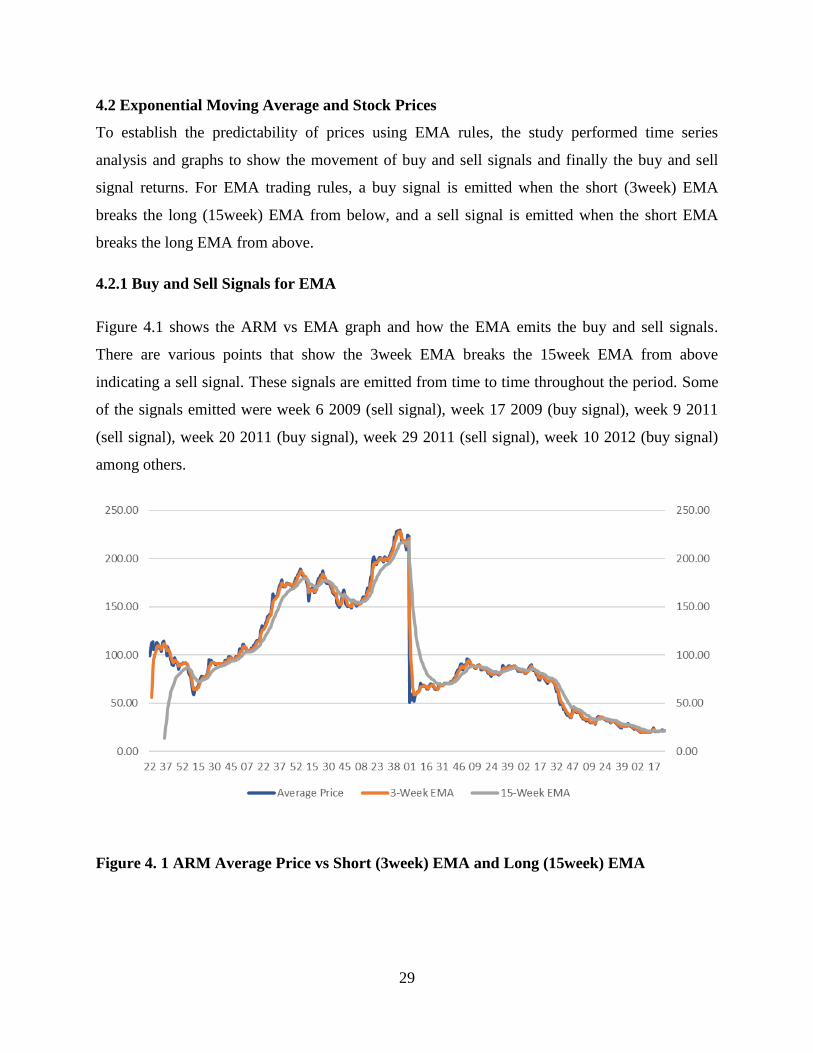
29
4.2 Exponential Moving Average and Stock Prices
To establish the predictability of prices using EMA rules, the study performed time series
analysis and graphs to show the movement of buy and sell signals and finally the buy and sell
signal returns. For EMA trading rules, a buy signal is emitted when the short (3week) EMA
breaks the long (15week) EMA from below, and a sell signal is emitted when the short EMA
breaks the long EMA from above.
4.2.1 Buy and Sell Signals for EMA
Figure 4.1 shows the ARM vs EMA graph and how the EMA emits the buy and sell signals.
There are various points that show the 3week EMA breaks the 15week EMA from above
indicating a sell signal. These signals are emitted from time to time throughout the period. Some
of the signals emitted were week 6 2009 (sell signal), week 17 2009 (buy signal), week 9 2011
(sell signal), week 20 2011 (buy signal), week 29 2011 (sell signal), week 10 2012 (buy signal)
among others.
Figure 4. 1 ARM Average Price vs Short (3week) EMA and Long (15week) EMA

30
KCB had various buy and sell signals throughout the period as per figure 4.2 below. Some of the
buy signals emitted were week 25 2009, week 34 2010, week 5 2012, week 30 2013, week 10
2014, week 11 2016 and week 9 2017. Sell signals were emitted in week 34 2009, week 19 2010,
week 25 2011, week 23 2013, week 52 2013, week 20 2015 and week 21 2016.
Figure 4. 2 KCB Average Price vs Short (3week) EMA and Long (15week) EMA
Kenol Kobil had various buy and sell signals over the period but minimal to no clear ones after
their share split in 2010. Signals included week 17 2009 (buy), week 32 2009 (sell), week 3 2010
(buy), week 22 2010 (sell), week 4 2012 (buy), week 6 2013 (sell) and week 3 2016 (buy). This
is shown in figure 4.3.

31
0.00
20.00
40.00
60.00
80.00
100.00
120.00
0.00
20.00
40.00
60.00
80.00
100.00
120.00
22 37 52 16 31 46 08 23 38 01 16 31 46 09 30 45 08 23 38 01 16 31 46 09 24 39 01 16 31 46 09 24
Average Price 3-Week EMA 15-Week EMA
Figure 4. 3 KenolKobil Average Price vs Short (3week) EMA and Long (15week) EMA
Figure 4.4 shows Sasini’s signals for buying and selling. Some of the signals emitted were week
52 2008 (buy), week 3 2009 (sell), week 16 2009 (buy) and week 35 2010 (sell). Other signals
were emitted in weeks 40 and 44 2010, weeks 19, 25 and 37 in 2011, weeks 2, 21, and 31 in
2012, week 39 2013, week 21 2014, weeks 5, 35 and 46 2015, weeks 15, 23 & 33 2016 and week
4 2017.
Figure 4. 4 Sasini Average Price vs Short (3week) EMA and Long (15week) EMA
ScanGroup had buy and sell signals throughout but beyond week 35 2013 the stock price was
trending downwards, and no buy signal was emitted. It would have been a good stock to short if

32
short selling was acceptable in the NSE. Some of the signals include week 15 2009 (buy), week
30 2009 (sell), week 49 2009 (buy), week 6 2011 (sell), week 17 2011 (buy), week 19 2011
(sell), week 5 2012 (buy), week 14 2013 (sell), week 33 2013 (buy) and week 35 2013 (sell).
This is shown below in figure 4.5.
Figure 4. 5 ScanGroup Average Price vs Short (3week) EMA and Long (15week) EMA
For the Safaricom stock figure 4.6, buy signals included week 23 2009, week 2 2012, week 46
2014, week 45 2015 and week 14 2017. Sell signals included week 32 2010, week 26 2014,
week 29 2015 and week 48 2016.

33
Figure 4. 6 Safaricom Average Price vs Short (3week) EMA and Long (15week) EMA
Some of the signals for Unga stock as per figure 4.7, include week 26 2009 (buy), week 38 2009
(sell), week 1 2010 (buy), week 41 2010 (sell), week 38 2011 (buy), week 49 2011 (sell), week
14 2012 (buy), week 49 2014 (sell), week 3 2015 (buy), week 28 2015 (sell), week 9 2016 (buy),
week 17 2016 (sell0 and week 21 2017 (buy).
Figure 4. 7 Unga Average Price vs Short (3week) EMA and Long (15week) EMA

34
4.2.2 Results for EMA Rules
To establish the predictability of prices using EMA rules, time series analysis was done for buy
and sell signals for all the 7 companies. The results as presented in Table 4.2 below shows
number of weeks in the study (N), buy (NB) and sell (NS) signals, number of weeks in the market
as generated by the buy signal (NBW) and number of weeks being out of the market sell signal
(NSW), total return on buy signal (RB) while in the market, total return on sell signal (RS) when
out of the market and mean buy returns (XB) when in the market and mean sell returns (XS) when
out of the market. Sasini had the highest number of buy signals at 20 while Safaricom had the
least number buy signals with 12 signals. This is the same with the sell signals with 19 and 11 for
Sasini and Safaricom respectively. Safaricom had the highest number of weeks in the market at
334 and the lowest number of weeks out of the market at 141. KenolKobil’s number of weeks
(231) in the market were lower than the number of weeks (238) out of the market. The rest of the
stocks had higher number of days in the market than number of days out of the market.
Returns and mean returns on buy signals were positive indicating that the stock price was in an
uptrend and the returns and mean returns on sell signals were negative indicating that the price
was in a downtrend. Returns on sell signals, in absolute terms were greater than returns on buy
signals for ARM, KenolKobil and ScanGroup while returns on sell signals, in absolute terms
were lower than returns on buy signals for KCB, Sasini, Safaricom and Unga.
The returns on buy signals were, ARM (0.671), KCB (0.778), KenolKobil (0.773), Sasini
(0.727), ScanGroup (0.741), Safaricom (0.982) and Unga (1.073) while the returns on sell
signals were, ARM (-1.332), KCB (-0.707), KenolKobil (-1.587), Sasini (-0.464), ScanGroup (-
0.941), Safaricom (-0.484) and Unga (-0.724).

35
Table 4. 2 Results for EMA rules
Company
No of Weeks
in Study
(N)
Buy Signals
(NB)
No. of weeks 'in
the market' on Buy Signal (NBW)
Return on
Buy Signal
(RB)
Mean Buy
Returns (XB)
Sell Signals
(NS)
No. of weeks 'out of
the market' on Sell Signal (NSW)
Return on Sell Signal
(RS)
Mean Sell
Returns (XS)
ARM 476 14 252 0.671 0.003 13 224 -1.332 -0.006
KCB 476 15 302 0.778 0.003 14 174 -0.707 -0.004
KenolKobil 469 19 231 0.773 0.003 18 238 -1.587 -0.007
Sasini 476 20 301 0.727 0.002 19 175 -0.464 -0.003
ScanGroup 476 16 239 0.741 0.003 15 237 -0.941 -0.004
Safaricom 475 12 334 0.982 0.003 11 141 -0.484 -0.003
Unga 476 14 299 1.073 0.004 13 177 -0.724 -0.004
4.3 Relative Strength Index (RSI) and Stock Prices
To establish the predictability of prices using RSI rules, the study performed time series analysis
and graphs to show the movement of buy and sell signals and finally the buy and sell signal
returns. For RSI rules, when the value is below 30, the stock's price is expected to rise and
conversely, if the value is above 70, the price is expected to fall.
4.3.1 Buy and Sell Signals for RSI
ARM stock had few signals to enter and exit the market i.e. the price below 30 RSI and above
70. This is shown in figure 4.8. A buy signals were emitted in week 10 2009 and week 1 2013
where the price touched and or went below RSI 30. A sell signal was emitted only once in week
31 2010.

36
Figure 4. 8 ARM Average Price vs RSI
Figure 4.9 shows average price vs RSI for KCB. Week 45 2008, week 7 and week 15 2009, week
23 and week 32 2010, week 39 2011 and week 5 2012 had RSI at or below 30 indicating buy
signals while week 18 2013 had RSI 70 which indicated a sell signal.
Figure 4. 9 KCB Average Price vs RSI
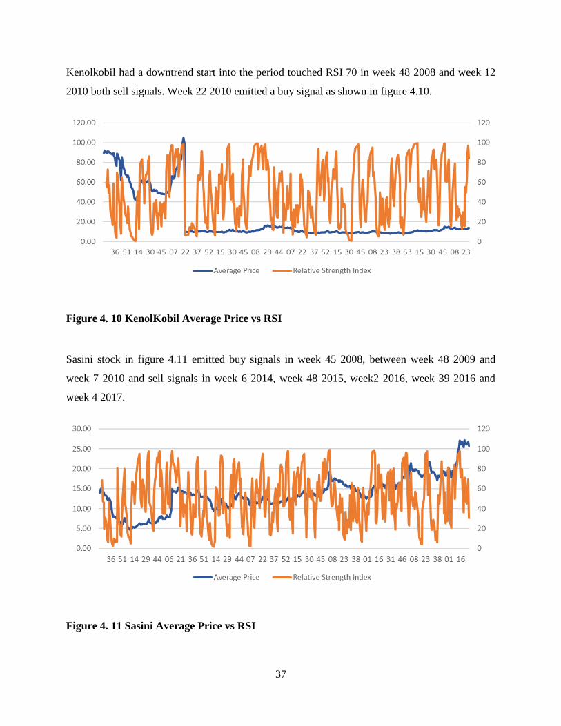
37
Kenolkobil had a downtrend start into the period touched RSI 70 in week 48 2008 and week 12
2010 both sell signals. Week 22 2010 emitted a buy signal as shown in figure 4.10.
Figure 4. 10 KenolKobil Average Price vs RSI
Sasini stock in figure 4.11 emitted buy signals in week 45 2008, between week 48 2009 and
week 7 2010 and sell signals in week 6 2014, week 48 2015, week2 2016, week 39 2016 and
week 4 2017.
Figure 4. 11 Sasini Average Price vs RSI

38
ScanGroup’s buy signals were emitted in week 8 2009, week 14 2009 and week 27 2016. Sell
signals were emitted in week 35 2010, week 12 2012, week 14 2014 and week 12 2015 (Figure
4.12).
Figure 4. 12 ScanGroup Average Price vs RSI
Figure 4.13 shows signals for Safaricom. Buy signals were emitted in weeks 35 2008, 16 and 32
2010, 10 2013 and sell signals in weeks 9 and 31 2015.
Figure 4. 13 Safaricom Average Price vs RSI

39
Figure 4.14 shows the average price vs RSI for Unga stock. The buy signals were emitted and
went above RSI 30 in week 10 2013 and sell signals were emitted in week 30 2014, week 52
2014 and week 42 2016.
Figure 4. 14 Unga Average Price vs RSI
4.3.2 Results for RSI rules
To establish the predictability of prices using RSI rules, time series analysis was done for buy
and sell signals for all the 7 companies. The results as presented in Table 4.2 below shows
number of weeks in the study (N), buy (NB) and sell (NS) signals, number of weeks in the market
as generated by the buy signal (NBW) and number of weeks being out of the market sell signal
(NSW), total return on buy signal (RB) while in the market, total return on sell signal (RS) when
out of the market and mean buy returns (XB) when in the market and mean sell returns (XS) when
out of the market.
ARM and ScanGroup had 2 buy signals each while the rest had 1 buy signal. All the 7
companies had 1 sell signal throughout the period in study.
Returns and mean returns on buy signals were negative which indicated that the stock price was
in the opposite direction of the trading rule and the returns and mean returns on sell signals were
positive which indicated that the price was in the opposite direction of the trading rules.
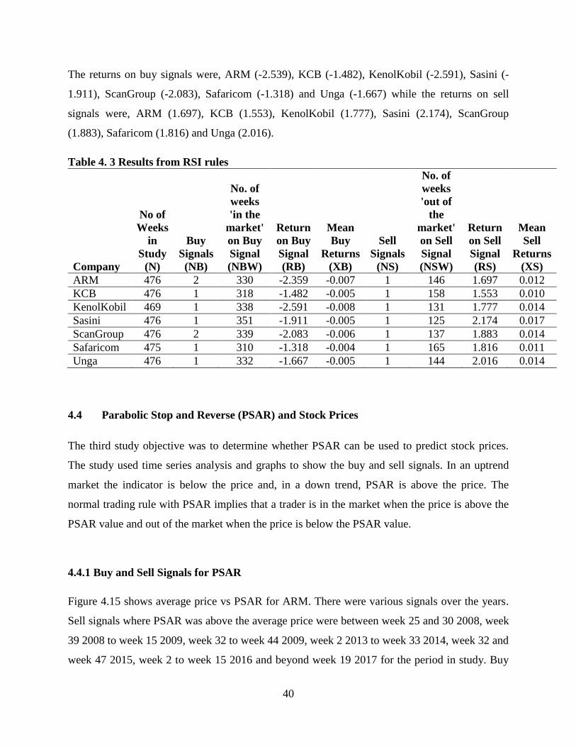
40
The returns on buy signals were, ARM (-2.539), KCB (-1.482), KenolKobil (-2.591), Sasini (-
1.911), ScanGroup (-2.083), Safaricom (-1.318) and Unga (-1.667) while the returns on sell
signals were, ARM (1.697), KCB (1.553), KenolKobil (1.777), Sasini (2.174), ScanGroup
(1.883), Safaricom (1.816) and Unga (2.016).
Table 4. 3 Results from RSI rules
Company
No of
Weeks
in
Study
(N)
Buy
Signals
(NB)
No. of
weeks
'in the
market'
on Buy
Signal
(NBW)
Return
on Buy
Signal
(RB)
Mean
Buy
Returns
(XB)
Sell
Signals
(NS)
No. of
weeks
'out of
the
market'
on Sell
Signal
(NSW)
Return
on Sell
Signal
(RS)
Mean
Sell
Returns
(XS)
ARM 476 2 330 -2.359 -0.007 1 146 1.697 0.012
KCB 476 1 318 -1.482 -0.005 1 158 1.553 0.010
KenolKobil 469 1 338 -2.591 -0.008 1 131 1.777 0.014
Sasini 476 1 351 -1.911 -0.005 1 125 2.174 0.017
ScanGroup 476 2 339 -2.083 -0.006 1 137 1.883 0.014
Safaricom 475 1 310 -1.318 -0.004 1 165 1.816 0.011
Unga 476 1 332 -1.667 -0.005 1 144 2.016 0.014
4.4 Parabolic Stop and Reverse (PSAR) and Stock Prices
The third study objective was to determine whether PSAR can be used to predict stock prices.
The study used time series analysis and graphs to show the buy and sell signals. In an uptrend
market the indicator is below the price and, in a down trend, PSAR is above the price. The
normal trading rule with PSAR implies that a trader is in the market when the price is above the
PSAR value and out of the market when the price is below the PSAR value.
4.4.1 Buy and Sell Signals for PSAR
Figure 4.15 shows average price vs PSAR for ARM. There were various signals over the years.
Sell signals where PSAR was above the average price were between week 25 and 30 2008, week
39 2008 to week 15 2009, week 32 to week 44 2009, week 2 2013 to week 33 2014, week 32 and
week 47 2015, week 2 to week 15 2016 and beyond week 19 2017 for the period in study. Buy

41
signals were emitted also throughout the period. These signals included week 30 to week 38
2008, week 15 to week 33 2009, week 13 to week 31 2010, week 20 to week 28 2011, week 11
to week 27 2012, week 34 to week 50 2014, week 7 to week 14 2015, week 16 to week 24 2016
and week 13 to week 18 2017.
Figure 4. 15 ARM Average Price vs PSAR
KCB stock had signals throughout the period as shown on figure 4.16. Week 32 2008 to week 9
2009 (Uptrend), week 10 to week 27 2009 (downtrend), week 21 to week 30 2010 (downtrend),
week 31 to week 51 2010 (uptrend), week 14 to week 25 2011 (uptrend), week 26 to week 44
2011 (downtrend), week 4 to week 17 2012 (uptrend), week 21 to week 28 2012 (downtrend),
week 52 2012 to week 12 2013 (uptrend), week 21 to week 28 2013 (downtrend), week 9 to
week 9 to week 18 2014 (uptrend), week 40 to week 47 2014 (downtrend), week 52 2014 to
week 14 2015 (uptrend), week 27 to week 43 2015 (downtrend), week 10 to week 15 2016
(uptrend), week 30 2016 to week 6 2017 (downtrend) and week 7 to week 22 2017 (uptrend).

42
Figure 4. 16 KCB Average Price vs PSAR
Figure 4.17 shows the trends for KenolKobil stock over the period. The trends which dictate
whether to be in the market (buy signals) and out of the market (sell signals) include week 22 to
week 30 2008 (uptrend), week 31 to week 40 2008 (downtrend), week 2 to week 16 2009
(downtrend), week 17 to week 32 2009 (uptrend), week 2 to week 20 2010 (uptrend), week 21
2010 to week 23 2011 (downtrend), week 24 to week 32 2011 (uptrend), week 2 to week 31
2012 (uptrend), week 32 to week 37 2012 (downtrend), week 49 2012 to week 39 2013
(downtrend), week 40 to week 47 2013 (uptrend), week 48 2013 to week 6 2014 (uptrend), week
18 to week 33 2014 (downtrend), week 3 to week 13 2015 (uptrend), week 14 to week 31 2015
(downtrend), week 52 2015 to week 15 2016 (uptrend), week 31 2016 to week 1 2017 (uptrend)
and week 2 to week 9 2017 (downtrend).

43
Figure 4. 17 KenolKobil Average Price vs PSAR
Sasini (Figure 4.18) exhibited signals in the period of study. The trends which dictate whether to
be in the market (buy signals) and out of the market (sell signals) include week 44 to week 46
2008 (uptrend), week 47 2008 to week 2 2009 (downtrend), week 6 to week 19 2009
(downtrend), week 45 2009 to week 22 2010 (uptrend), week 6 to week 20 2011 (downtrend),
week 36 2011 to week 1 2012 (uptrend), week 30 to week 44 2012 (downtrend), week 6 to week
12 2013 (downtrend), week 29 2013 to week 8 2014 (uptrend), week 34 to week 48 2014
(downtrend), week 6 to week 17 2015 (uptrend), week 33 to week 45 2015 (downtrend), week 3
to week 15 2016 (uptrend), week 33 to week 45 2016 (downtrend) and week 5 to week 17 2017
(uptrend).

44
Figure 4. 18 Sasini Average Price vs PSAR
Figure 4.19 shows average price and PSAR for ScanGroup which indicated various signals for
the period. The trends which dictate whether to be in the market (buy signals) and out of the
market (sell signals) include week 33 to week 37 2008 (uptrend), week 49 2008 to week 14 2009
(downtrend), week 15 to week 33 2009 (uptrend), week 15 to week 28 2010 (uptrend), week 46
2010 to week 15 2011 (downtrend), week 44 to week 52 2011 (uptrend), week 1 to week 9 2012
(downtrend), week 40 2012 to week 3 2013 (uptrend), week 18 to week 33 2013 (downtrend),
week 7 to week 30 2014 (downtrend), week 40 2014 to week 10 2015 (uptrend), week 18 to
week 27 2015 (downtrend), week 47 2015 to week 4 2016 (uptrend), week 17 to week 34 2016
(downtrend), week 35 to week 49 2016 (uptrend), week 50 2016 to week 7 2017 (downtrend)
and week 8 to week 18 2017 (uptrend).

45
Figure 4. 19 ScanGroup Average Price vs PSAR
Figure 4.20 shows average price and PSAR for Safaricom which indicated various signals for the
period. The trends which dictate whether to be in the market (buy signals) and out of the market
(sell signals) include week 24 to week 44 2008 (downtrend), week 45 to week 52 2008 (uptrend)
week 20 to week 38 2009 (uptrend), week 1 to week 23 2010 (uptrend), week 24 to week 40
2010 (downtrend), week 47 2010 to week 14 2011 (downtrend), week 15 to week 22 2011
(uptrend), week 15 to week 24 2012 (uptrend), week 39 to week 41 2012 (downtrend), week 42
2012 to week 13 2013 (uptrend), week 47 to week 52 2013 (downtrend), week 11 to week 26
2014 (uptrend), week 37 to week 45 2014 (downtrend), week 46 2014 to week 15 2015
(uptrend), week 19 to week 35 2015 (downtrend), week 9 to week 20 2016 (uptrend), week 35 to
week 43 2016 (downtrend), week 49 2016 to week 10 2017 (downtrend) and week 11 to week 22
2017 (uptrend).

46
Figure 4. 20 Safaricom Average Price vs PSAR
Figure 4.21 shows average price and PSAR for Unga which indicated various signals for the
period. The trends which dictate whether to be in the market (buy signals) and out of the market
(sell signals) include week 27 to week 35 2008 (downtrend), week 37 2008 to week 2 2009
(uptrend), week 15 to week 31 2009 (uptrend), week 32 to week 47 2009 (downtrend), week 7 to
week 15 2010 (uptrend), week 41 to week 52 2010 (downtrend), week 5 to week 15 2011
(downtrend), week 20 to week 30 2011 (uptrend), week 48 2011 to week 12 2012 (downtrend),
week 32 to week 39 2012 (uptrend), week 2 to week 26 2013 (uptrend), week 48 to week 52
2013 (downtrend), week 16 to week 30 2014 (uptrend), week 45 2014 to week 9 2015
(downtrend), week 10 to week 37 2015 (uptrend), week 38 2015 to week 6 2016 (downtrend),
week 9 to week 24 2016 (uptrend), week 34 2016 to week 16 2017 (downtrend) and beyond
week 17 there is an uptrend in the period of study.

47
Figure 4. 21 Unga Average Price vs PSAR
4.4.2 Results for PSAR Rules
To establish the predictability of prices using PSAR rules, time series analysis was done for buy
and sell signals for all the 7 companies. The results as presented in Table 4.2 below shows
number of weeks in the study (N), buy (NB) and sell (NS) signals, number of weeks in the market
as generated by the buy signal (NBW) and number of weeks being out of the market sell signal
(NSW), total return on buy signal (RB) while in the market, total return on sell signal (RS) when
out of the market and mean buy returns (XB) when in the market and mean sell returns (XS) when
out of the market.
Safaricom had the highest number of buy signals at 27 while KenolKobil had the least number
buy signals with 20 signals. This is the same with the sell signals with 27 and 19 for Safaricom
and KenolKobil respectively. Safaricom had the highest number of weeks in the market at 280
and the lowest number of weeks out of the market at 195. ARM, KenolKobil, Sasini, and
ScanGroup had lower number of weeks in the market than out of the market and KCB,
Safaricom and Unga had higher number of weeks in the market than out of the market.

48
Returns and mean returns on buy signals were positive indicating that the stock price was in an
uptrend and the returns and mean returns on sell signals were negative indicating that the price
was in a downtrend. Returns on sell signals, in absolute terms were greater than returns on buy
signals for ARM, KenolKobil and ScanGroup while returns on sell signals, in absolute terms
were lower than returns on buy signals for KCB, Sasini, Safaricom and Unga.
The returns on buy signals were, ARM (0.843), KCB (0.819), KenolKobil (1.190), Sasini
(1.134), ScanGroup (1.299), Safaricom (1.454) and Unga (1.311) while the returns on sell
signals were, ARM (-1.504), KCB (-0.748), KenolKobil (-2.004), Sasini (-0.871), ScanGroup (-
1.499), Safaricom (-0.956) and Unga (-0.962).
Table 4. 4 Results from PSAR rules
Company
No of
Weeks
in
Study
(N)
Buy
Signals
(NB)
No. of
weeks
'in the
market'
on Buy
Signal
(NBW)
Return
on Buy
Signal
(RB)
Mean
Buy
Returns
(XB)
Sell
Signals
(NS)
No. of
weeks
'out of
the
market'
on Sell
Signal
(NSW)
Return
on Sell
Signal
(RS)
Mean
Sell
Returns
(XS)
ARM 476 21 179 0.843 0.005 21 297 -1.504 -0.005
KCB 476 26 268 0.819 0.003 26 208 -0.748 -0.004
KenolKobil 469 20 204 1.190 0.006 19 265 -2.004 -0.008
Sasini 476 22 235 1.134 0.005 22 241 -0.871 -0.004
ScanGroup 476 26 220 1.299 0.006 25 256 -1.499 -0.006
Safaricom 475 27 280 1.454 0.005 27 195 -0.956 -0.005
Unga 476 26 255 1.311 0.005 25 221 -0.962 -0.004
4.5 Chapter Summary
This chapter presented study findings on how EMA, RSI and PSAR can be used to predict stock
prices. The next chapter presents the discussion of the study findings, conclusions and
recommendations.

49
CHAPTER FIVE
5.0 DISCUSSIONS, CONCLUSIONS AND RECOMMENDATIONS
5.1 Introduction
The purpose of this study was to establish the prediction of stock prices using technical analysis
in selected companies listed on the NSE. This chapter provides the discussions, conclusions as
well as draw conclusion for the study.
5.2 Summary of the study
The study aimed at determining whether stock prices can be predicted using technical analysis in
selected companies listed on the NSE. This research was made possible by the following
research question; to what extent does exponential moving average (EMA) predict stock prices
in the NSE? How does relative strength index (RSI) predict stock prices in the NSE? How does
parabolic stop and reverse (PSAR) predict stock prices in the NSE?
The study also incorporated the use of descriptive research design to aid in predicting stock
prices. The target population for this study was 7 firms drawn from various sectors of the
economy and are listed at the NSE. The study entirely relied on the use of secondary data that
was readily available at the NSE cutting across from week 22 of 2008 all the way to week 24 of
2017 to establish if exponential moving averages, relative strength index and parabolic stop and
reverse are predictors of stock market prices. Inferential statistics was analyzed with the help of
Statistical Package for Social Sciences (SPSS) v 20.
With regard to EMA being used to predict stock market prices, the study indicated EMA
generated returns on buy signals and an exit from the market when sell signals are triggered to
avoid losses. High negative mean return on sell signals indicated that the predicted exits reduced
losses equivalent to the negative mean returns that would have been realized if investors did not
exit the markets. The 7 companies under study overwhelmingly showed positive returns on buy
signals when in the market and high negative returns when out of the market. The buy and sell
signals were equal for most of the stocks with a differentiating factor of the number of weeks in
the market and out of the market. The mean return when in the market was positive indicating
that positive returns were realized while the mean returns when out of the market were negative

50
indicating that the decision to get out of the market when sell signals are emitted ensures that
capital is preserved, or profits are realized.
The study findings on RSI and stock market price indicated that there was a negative return on
buy signals and a positive return on sell signals. This observation painted a no clear indication of
buy and sell signals to predict stock prices which indicated that RSI is not a good predictor of
stock prices in generating buy and sell signals. Further to this, for most of the companies the
limit of buy at 30 indicating an oversold position and sell at 70 indicating an overbought position
were never reached to give the clear indication of being in the market or out of the market. The
number of weeks in the market were greater than those out of the market which meant that the
buy period was continuous even during a downtrend of the stock since the RSI value did not get
to 70 in order to trigger a sell signal.
The study indicated that PSAR generated returns on buy signals and an exit from the market
when sell signals are triggered to avoid losses. The 7 companies under study overwhelmingly
showed positive returns on buy signals when in the market and high negative returns when out of
the market. The number of weeks in the market were higher than out of the market indicating
clear entry and exit points when buy and sell signals were emitted. The buy and sell signals were
equal for most of the stocks with a differentiating factor of the number of weeks in the market
and out of the market. The mean return when in the market was positive indicating that positive
returns were realized while the mean returns when out of the market were negative indicating
that the decision to get out of the market when sell signals are emitted ensures that capital is
preserved, or profits are realized. High negative mean return on sell signals indicated that the
predicted exits reduced losses equivalent to the negative mean returns that would have been
realized if investors did not exit the markets.
5.3 Discussion
5.3.1 Moving Averages (MA) and Stock Prices
The study found out that EMA can be used to predict stock market prices as buy and sell signals,
there was a positive buy signal and a negative buy signal returns for EMA. This finding is in
agreement with the studies of Brock, Lakonishok, and LeBaron (1992) that used moving
averages to generate buy and sell signals. Their tests included using long moving averages of 50,

51
150, and 200 days and short averages of 1, 2, and 5 days. The study arrived at a conclusion that
EMA as a form of technical analysis has predictive power. This finding is further corroborated
by Fernando (2012) that opined that the use of EMA generates buy-and-sell signals that generate
stock price movements and earn excess returns, after adjusting transaction costs, in emerging
Colombo Stock Exchange (CSE). The study used daily market closing prices of All Share Price
Index (ASPI), which is a composite index to represent whole market, for twenty-five years from
January 1985 to December 2010. Daily index prices were converted to daily returns and moving
average rules were used. The empirical findings of the study confirmed that the moving average
trading strategies have statistically significant predictive and profitability ability in explaining
the market and capable of generating excess return to investors.
Similarly, Faber (2007) indicated that moving average produced superior market performance
associated with buy-and-sell signals. Specifically, Faber (2007) documented that a 10-month
simple moving average strategy applied to the S&P 500 over a period of 100 years yielded
higher annual returns and lower volatility, resulting in improved risk adjusted performance. Even
though the author reported compelling and positive results, several weaknesses emerge. The
author acknowledges that the 10-month SMA rule was chosen due to its known performance and
the results were only simulated in-sample. In turn, this raises a legitimate “data mining” concern.
In addition, the author did not account for transaction cost and no statistical test was conducted
to assess the statistical significance of the results.
The study findings established that positive buy and sell signals associated with EMA shows that
the investors are upbeat about the stock market prices. This finding is supported by the studies of
Gwilym et al. (2010) that moving average rules on international equity markets that stimulates
buy and sell signals thus trigger potential stock market prices. Similarly, PhooiM’ng & Zainudin
(2014) studied the predictability of Asia Pacific stock market indices using buy and sell signals
from a dynamic volatility indicator, the adjustable moving average using the daily stock market
indices futures contracts’ returns from the Asia Pacific countries, namely Australia’s SPI Futures
(SPIF), Hong Kong’s Hang Seng Futures (HSF), Japan’s Nikkei 225 Futures (NikkeiF), Korea’s
KOSPI Futures (KOSPIF), Malaysia’s FBMKLCI30 Futures (FKLI) and Singapore’s SiMSCI
Futures (SiMSCIF), from 2008 to 2012. There were evidences of abnormal returns after
transaction costs, above the passive buy-and-sell signals are found in these time series’ returns;
especially for the adjustable moving average.

52
Furthermore, the studies by Atmeh and Dobbs (2006) reinforced how vital EMA in predicting
stock market prices, analysis on the performance of the moving average rules in the Amman
Stock Exchange and using the time series of the Jordan Daily Market Index over the period 1992
to 2001. The conditional returns on buy and sell signals from actual data are examined for a
range of trading rules compared with returns generated from simulated series generated by a
range of models. They clarified that technical analysis could anticipate for changes in stock
prices. At the same time Ord (2004) noted that an exponential moving average (EMA) can
determine that a slope of financial trend is positively related with the stock price. It always
decreases when price closes below the moving average of stock price and always increases when
the price is increased. Tanaka-Yamawaki, Tokuoka and Awaji (2009), utilized the pattern
recognition approach that was combined with EMA to create the prediction model. In the
experiment, EMA was applied to recognize the pattern of uptrend and downtrend of stock price
by using a two-dimension metric format, and then utilized those patterns for EMA to predict the
price range. They had successfully improved the rate of prediction accuracy above 67%.
According to the experiment done by Dzikevicius and Saranda (2010), they found that EMA was
adequate to analyze the financial trend. From their tracking signal, they concluded that EMA was
less risky to identify the direction of financial trend instead of predicting the direction.
5.3.2 Relative Strength Index (RSI) and Stock Prices
The study findings pointed out that RSI is not a predictor of stock market prices. This revelation
is in line with those of Investor’s Business Daily (2008) that a sell signal is formed when the RSI
breaks the overbought line in a downward direction crossing from above the line to below the
line hence influencing stock market prices. Setting the overbought and oversold levels at 80 and
20, respectively, can use a more conservative approach. This argument is supported also by
Drakopoulou (2015) that divergence can be used to form signals as well and that if RSI is
moving in an upward direction and the security is moving in a downward direction it signals to
technical traders that buying pressure is increasing and the downtrend may be coming to an end
hence an effect on the stock market prices. Divergence can also be used to signal a reversal in an
upward trend where the RSI is decreasing signaling increasing selling pressure in an upward
trend. The RSI is a standard component on any basic technical chart. The relative strength
indicator focuses on the momentum underlying the security and is a great secondary measure to

53
be used by traders. It is important to note that the RSI is often not used as the sole generation of
buy-and-sell signals but used in conjunction with other indicators and chart patterns.
The results also noted that negative buy signal and positive sell signal associated with RSI. This
thought is supported by Investor’s Business Daily (2008) that the indicator is used to generate
signals crossovers and divergence. In the case of the RSI, the indicator uses crossovers of its
overbought, oversold and centerline which negatively influence stock market prices. The first
technique is to use overbought and sold lines to generate buy-and-sell signals. In the RSI, the
overbought line is typically set at 70 and when the RSI is above this level the security is
considered overbought. The security is seen as oversold when the RSI is below 30. These values
can be adjusted to either increase or decrease the number of signals that are formed by the RSI.
A buy signal is generated when the RSI breaks the oversold line in an upward direction, which
means that it goes from below the oversold line to moving above it. A sell signal is formed when
the RSI breaks the overbought line in a downward direction crossing from above the line to
below the line. Setting the overbought and oversold levels at 80 and 20, respectively, can use a
more conservative approach. Likewise, Murphy (2018) opined that the use of crossover
technique used in formulating signals is using the centerline (50) is exactly the same as using the
overbought and oversold lines to formulate signals. This technique will often form signals after a
movement in the direction they are predicting but are used more as a confirmation then a signal
compared to the other techniques. A downward trend is confirmed when the RSI crosses from
above 50 to below 50. An upward trend is confirmed when the RSI crosses above 50 which
greatly impact negatively on the stock market prices.
The findings further indicated that RSI has shown underperformance of the economy since it
generates negative buy signal and positive sell signal. This thought is also held by Turek (2008)
noted that RSI is a moment indicator and despite its main usage is to show overbought and
oversold values, these values can stay irrational for a very long time. Simply said, once RSI is
used in a strong uptrend, the indicator can be expected to stay in overbought values for a
considerable part of the whole increasing movement thus affecting the stock market prices. RSI
should therefore be used as an indicator of a future probable movement and reacted on only after
the movement, not vice versa. Once RSI is over 70, it can be thought of as if the market is
overbought and that there is a high probability of correction downwards, but it does not mean

54
that this correction will start a new downtrend. These findings are supported further by the works
of Wong, Manzur and Chew (2003) that opines that RSI triggers a buy or sell signal in one of the
following manners. The touch method generates a sell signal when the RSI touches the upper
bound, typically set at 70 for a 14-day RSI and generates a buy signal when the RSI touches the
lower bound, typically 30 for a 14-day RSI. The peak method sells the security when the RSI
crosses the higher bound and then turns back. By contrast, when the RSI crosses the lower bound
and turns back, it is considered a sell signal. The retracement method leads to a buy signal when
the RSI crosses the lower bound and goes back to the same lower bound or goes higher which
greatly affect stock prices negatively.
5.3.3 Parabolic Stop and Reverse (PSAR) and Stock Prices
The found out that PSAR is a predictor of stock market prices since there are clear entry (buy)
and exit (sell) signals in order to make a return. The study showed that PSAR generated a
positive buy signal and a negative sell signals. This finding is in line with Paritech (2004)
findings that a buy signal occurs when the most recent high price of a stock has been defied
imposing the SAR to be positioned at the most recent low stock price. When the price of the
stock rises, the dots will rise as well, initially slowly and then picking up speed and accelerating
with the trend. Thereafter the SAR starts to move a little faster when the trend advances and the
dots presently catch up to the price action of the stock.
Furthermore, Parabolic SAR having adopted a “time/price reversal system” in trending markets
to ensure traders follow the upward or downward trend of the dots to assess when to reverse a
position and enter a trade in the opposed direction is a good predictor of the stock market. The
Parabolic SAR system responds highly in markets with a dominant trend and fails despondently
in sideways or non-trending markets. Wilder created an acceleration element into the system.
Occasionally the stop motions are in the direction of the latest trend. Previously, the
repositioning of the stop is correspondingly slow to enable the trend time to validate. When the
acceleration factor rises, the SAR starts to move quicker, consequently catching up to the price
action.
The study findings further established that there exists a relationship between PSAR and stock
market prices. This finding is corroborated by that of Wilder (1978) that acknowledges that

55
Parabolic SAR seem to work best in volatile markets with many different trends, else there will
be many buy signals to follow which might not generate positive returns when accounting for
transaction costs which in turn affect stock market prices. Parabolic SAR is seen as not only
being able to provide a direction for the trend, but also provides a trailing stop loss, something
useful in money management in the stock market.
5.4 Conclusions
5.4.1 Moving Averages (MA) and Stock Prices
In conclusion, EMA can be used to predict stock market prices by establishing buy and sell
signals and hence returns are generated. Buy signals generated entry into the market and sell
signals emitted exit points from the market. The returns generated when being in the market were
positive and negative when out of the market. This means that entry and exit points can be
determined using the long and short EMA which prospecting investors should take advantage of
in the market to make returns.
5.4.2 Relative Strength Index (RSI) and Stock Prices
RSI is not a good predictor given that it presented a negative return on buy signals and positive
returns on sell signal. This indicates that RSI should not be used to predict stock prices to
generate buy and sell signals since these signals were few and couldn’t generate positive returns
when in the market.
5.4.3 Parabolic Stop and Reverse (PSAR) and Stock Prices
The study concludes that PSAR technical analysis tool has a superior return on buy signals
which is best suited to predict stock market prices. This is backed by the ability of PSAR to
generate a positive return on buy signals (in the market) and a negative return on sell signals (out
of the market).
5.5 Recommendations
5.5.1 Recommendations for Improvement
5.5.1.1 Moving Averages (MA) in Predicting Stock Prices

56
The study findings recommend the need for investors and investment managers to incorporate
the use of exponential moving averages in for predicting stock market prices in their strategies.
This would make it possible for investors to make informed decisions on entry and exit points to
make good returns.
5.5.1.2 Relative Strength Index (RSI) in Predicting Stock Prices
The study recommends that RSI should not be used in predicting stock prices. Investors and
investment managers should use other technical analysis tools.
5.5.1.3 Parabolic Stop and Reverse (PSAR) in Predicting Stock Prices
On the use of PSAR to predict stock market prices the study recommends the need for investors
and investment managers to adopt PSAR for predicting uptrends and downtrends and also use it
form money management as it also gives the stop and reverse signals.
5.5.2 Recommendations for Further Studies
The study recommends the need to consider using other technical analysis tools apart from
EMA, RSI and PSAR to establish stock market prices and discern the behaviors. These other
tools include other moving averages such as the simple moving average (SMA), weighted
moving average (WMA) and volume weighted moving average (VWMA), moving average
convergence divergence (MACD), average directional index (ADI), traders dynamic index
(TDI), stochastic momentum index, william’s percent range (WPR), commodity channel index
(CCI), chande momentum oscillator (CMO), Bollinger bands (BBands), average true range
(ATR), on-balance volume (OBV), money flow index (MFI) and chaikin money flow (CMF).
Further to this study, efficient marker hypothesis (EMH) and random walk hypothesis (RWH)
can also be studied to ascertain the efficiency of the stock market since technical analysis does
not support these theories in relation to the market.
The capital markets authority had not initially put in regulations or guidance on short selling
until early 2018. Such an impact can be studied in relation to predicting stock returns to compare
returns on buy and sell since now one can short a stock without owning it.

57
There is also the need to always use a combination of models to be able to arrive at more
accurate data which is verifiable and enable one to make comprehensive deduction from the data
presented.

58
REFERENCES
Abbad, J., Fardousi, B., & Abbad, M. (2014). Advantages of Using Technical Analysis to predict
Future Prices on the Amman Stock Exchange. International Journal of Business and
Management, 9(2)
Achelis, S. B. (2001.) Technical Analysis A-Z. 2nd Ed. New York, NY: McGraw Hill
Professional
Achieng G. (2013). The relationship between trading volume and stock prices of firms quoted at
the Nairobi Securities Exchange. Unpublished MBA project of the University of Nairobi,
Nairobi: KE
Almujamed, H. I, Fifield, S. & Power, D. (2013). An investigation of the role of technical
analysis in Kuwait. Qualitative Research in Financial Markets. 5(2), 43-64.
Al-Shiab M. (2006). The Predictability of the Amman Stock Exchange using the Univariate
Autoregressive Integrated Moving Average (ARIMA) Model, Journal of Economic and
Administrative Sciences, 22 (2), 17-35.
Asewe, S., Mule, R., & Ndichu, P. (2013). Determining Automation Effect on Market
Efficiency. European Scientific Journal. 9(31)
Atmeh, A. M., & Dobbs, M. I. (2006). Technical analysis and the stochastic properties of the
Jordanian stock market index return. Studies in Economics and Finance, 23, 119-140.
Bachelier, L. (1900). Theories of speculation." (Paris doctoral dissertation in mathematics),
Annales Sclentltiques deI’Ecole Normale Superleure 3, English translation by A.
J.Boness, Cootner (1964), pp. 17-78
Baxter, J. (2011). Public sector professional identities: a review of the literature. The Open
University, UK, The Open University, UK.

59
Bessembinder, H. & Seguin, P. J. (1993). Price Volatility, Trading Volume and Market Depth:
Evidence from Future Markets. Journal of Financial and Quantitative Analysis, 28 (1),
21-39.
Blume L, Easley, D & O’Hara, M. (1994). Market Statistics and Technical Analysis: The role of
volume. Journal of Finance, 49 (1), 153-181.
Boobalan C. (2014). Technical Analysis in Select Stocks of Indian Companies. International
Journal of Business Administration Research Review, 2 (4), 26.
Brock, W., Lakonishok, J., & LeBaron, B. (1992). Simple Trading Rules and the Stochastic
Properties of Stock Returns. Journal of Finance, 47(5), 1731-1764.
Carlin, B. & Robson, D. (2012). What Does Financial Literacy Training teach us? Journal of
Economic Education, 43(3), 235 – 247.
Caporin, M., Ranaldo, A., Santucci de Magistris, P., Dec 2013. On the predictability of stock
prices: A case for high and low prices. Journal of Banking & Finance. 37(12), 5132-
5146.
Chandran, E. (2008). Research Methods: A Quantitative Approach with Illustrations from
Christian Ministries. Nairobi, KE: Daystar University.
Chen, J. (2010). Essentials of technical analysis for financial markets. New Jersey, NJ: John
Wiley & Sons.
Chen, G. M, Firth, M. & Ru, OM (2001). Dynamic relation between stock returns trading
volume, and volatility. Financial Review, 36 (3), 153-174.
Chiang, Y.C., M.C. Ke, T. L. Liao & C. D. Wang, (2012). Are technical trading strategies still
profitable? Evidence from Taiwan Stock Index Futures Market, Applied Financial
Economics, 1-11.
Colby, R.W. (2003). The encyclopedia of technical market indicators. 2nd Ed. McGraw-Hill

60
Cootner, P.E. (1964). The Random Character of Stock Market Prices, Cambridge, MA: MIT
Press
Cooper, D. R., & Schindler, P. S. (2014). Business Research Methods. 9th Ed. New Delhi, India:
McGraw-Hill Publishing, Co. Ltd.
Drakopoulou V (2015). A Review of Fundamental and Technical Stock Analysis Techniques. J
Stock Forex Trad 5:163. doi:10.4172/2168-9458.1000163
Dzikevičius, A., & Šaranda, S. (2010). EMA versus SMA Usage to Forecast Stock Markets: The
Case of S&P 500 and OMX Baltic Benchmark. Business: Theory and Practice, 11(3),
248–255. doi:10.3846/btp.2010.27
Endhiarto, T (2018). The Application of Fundamental and Technical Model In the Investment
Decision Making: Empirical Study on the Companies Listed International, Journal of
Scientific & Technology Research, 7(1)
Exponential Moving Average. (2012). Incredible charts. Retrieved November 10, 2012, from
http://www.incrediblecharts.com/indicators/exponential_moving_average.php
Fama, E. (1970). Efficient Capital Markets: A review of Theory and Empirical Work. The
Journal of Finance, 25(2), 383-417.
Fama, E.F. (1965). The Behavior of Stock Market Prices. Journal of Finance, 20, 70- 87
Fama, E., (1981). Stock Returns, Real Activity, Inflation and Money„, American Economic
Review, 71, 545-565.
Fama, E.F. & Gibbons, M. (1982). Inflation, Real Returns and Capital Investment. Journal of
Monetary Economics, 9(3), 545-565.
Fama, E.F. (1991). Efficient Capital Markets: II. Journal of Finance, 46,1575-1618
Fernando, P. N. D. (2012). Profitability of Technical Trading Strategies in Emerging Sri Lankan
Stock Market. Unpublished thesis from the University of Kelaniya, Sri Lanka.

61
Giot, P. & Petitjean, M., (2010). On the statistical and economic performance of stock return
predictive regression models: an international perspective. Quantitative Finance. 11(2),
173-193.
Githumbi G. T. (2014). Relationship between Profitability of Technical Trading rules and
Central Bank Intervention on Foreign Exchange Market in Kenya. Unpublished MBA
project of the University of Nairobi. Nairobi, KE:
Gorgulho, A., Neves, R., Horta, N., (2011). Applying a GA kernel on optimizing technical
analysis rules for stock picking and portfolio composition. Expert Systems with
Applications. 38(9), 14072-14085
Gradojevic, N. & Gencay, Ramazan., (2013). Fuzzy Logic, trading uncertainty and technical
trading. Journal of Banking and Finance, 37, 578-586
Granville, J. E. (1976). New Strategy of Daily Stock Market Timing for Maximum Profit. Simon
& Schuster
Hamilton, P. (2015). The Dow Theory. Horizon publishing company
Hilliard, J., Schwartz, A., & Squire, J. (2013). A Test of Technical Analysis: Matching Time
Displaced Generalized Patterns. Journal of Financial Management, 42(2), 291-314.
Investor’s Business Daily (2018). Retrieved on 1st October 2018 from Investors.com
Jandhyala, L. S., Mbodja, M. & Kamath, R. (2010). Heteroscedasticity in stock market indicator
return data: volume versus GARCH effects. Applied Financial Economics, 6 (4), 337-
342.
Kapoor, V., Dey, S. & Khurana, A.P. (2011). Genetic Algorithm: An Application to Technical
Trading System Design. International Journal of Computer Applications, 36 (5)
Kendall, M.G. (1953). The Analysis of Economic Time Series, Part 1: Prices, Journal of the
Royal Statistical Society, 116, 11-25

62
Kulkarni G. K. & Kulkarni G. A. (2013). Fundamental vs. Technical Analysis: A Choice of
Sectoral Analysis. International Journal of Engineering and Management Sciences.
4(2), 234-246.
Kihoro J. M. & Okango E. L. (2014). Stock Market Price Prediction Using Artificial Neural
Network: An Application to the Kenyan Equity Bank Share Prices. Journal of
Agriculture, Science and Technology, 16(1).
Kothari, C. (2004). Research Methodology: Methods & Techniques. 2nd Ed. New Delhi, India:
New Age International (P) Limited, Publishers
Kothari, C.R (2012). Research Methodology: Methods & Techniques, New Delhi, ID: New age
International Publishers
Lasry, G. (1979). Valuing Common Stocks: The Power of Prudence" AMACOM Publishers
Lin, X., Yang, Z., Song, Y., (2011). Intelligent stock trading system based on improved technical
analysis and Echo State Network. Expert Systems with Applications, 38(9), 11347–
11354.
Lishenga, L. (2012). An Empirical Analysis of Momentum Profitability, Seasonality, and
Reversibility at Nairobi Stock Exchange. Journal of Finance and Investment Analysis.
1(3), 73-98.
Malkiel, B.G. (1973). A Random Walk Down Wall Street”. The best Investment Advise for the
New Century. 7th Ed. New York, NY: Norton & Co.
Masry, M. (2017). The Impact of Technical Analysis on Stock Returns in an Emerging Capital
Markets (ECM’s) Country: Theoretical & Empirical Study. International Journal of
Economics and Finance, 9(3)
Menkhoff, L., 2010. The Use of Technical Analysis by Fund Managers: International Evidence.
Journal of Banking and Finance, 34, 2573-2586.

63
Metghalchi M., Du J., & Ning Y. (2009). Validation of Moving Average Trading Rules:
Evidence from Hong Kong, Singapore, South Korea, Taiwan, Multinational
Business Review,17 (3), 101 – 122
Metghalchi M., Chang Y. H., & Gomez X. G. (2012). Technical Analysis of the Taiwanese
Stock Market. International Journal of Economics and Finance. 4(1)
Metghalchi, M., Kagochi J. & Hayes, L. (2014). Contrarian Technical Trading Rules: Evidence
from Nairobi Stock Index. The Journal of Applied Business Research. 30(3)
Mishra A. (2013) Fundamental Vs Technical Analysis. International Journal of Commerce,
Business and Management. 2(5)
Mitra S. K. (2011). How rewarding is technical analysis in the Indian stock market? Quantitative
Finance, 11(2), 287–297.
Mlambo C & Biekpe N. (2007). The Efficient Market Hypothesis: Evidence from ten African
stock Markets. Munich Personal RePEC Archive (MRPA) Paper No. 25968.
Mobarek, A. & Keasey, K. (2000). Weak-form Efficiency of An Emerging Market: Evidence
from Dhaka Stock Market of Bangladesh. A paper presented at the ENBS Conference,
Oslo, May 2000.
Moses, E. A. & Cheney, J.M. (1989). Investment. Analysis, Selection & Management" West
Publishing Company
Mugenda, O. & Mugenda, A., (2013). Research Methods: Quantitative and Qualitative
approaches, Nairobi, KE: Acts Press
Muhannad A. A & Dobbs, I.M. (2006). Technical analysis and the stochastic properties of
the Jordanian stock market index return", Studies in Economics and Finance, 23(2), 119-
140
Murphy, J. (1999). Technical Analysis of the Financial Markets. New York Institute of Finance.
New York, NY: New York Institute of Finance

64
Murphy, J. (2018). Technical Analysis of the Financial Markets. New York Institute of Finance.
New York, NY: New York Institute of Finance
Mutothya, N. M. & Muthama, N. (2013). An Empirical Investigation of the Random Walk
Hypothesis of Stock Prices on the Nairobi Stock Exchange. European Journal of
Accounting Auditing and Finance Research. 1(4), 33-59.
Mwanyasi, R. (2018). Why index Cap for big counters makes sense. Business Daily, A Nation
Media Publication. 2843, 32.
Mwlibtoolkit. (2011). Technical Analysis. code.pediapress.com.
Nairobi Securities Exchange (NSE). https://www.nse.co.ke/nse/about-nse.html
National Stock Exchange. (2010). Technical Analysis Made Easy. National Stock Exchange of
India Limited Help Documents. Mumbai.
Njuguna, J. (2016). Testing the Efficient Market Hypothesis on the Nairobi Securities Exchange.
Investment Management and Financial Innovations Journal. 13(3)
Njuguna, J. (2016). The Changing Market Efficiency of the Nairobi Securities Exchange. Banks
and Bank Systems Journal. 11(2)
Ogula, P. A. (2015). Research Methods. Nairobi, KE: CUEA Publications
Oliveira, F. A., Nobre, C. N., Zarate, L. E. (2013). Applying Artificial Neural Networks to
prediction of stock price and improvement of the directional prediction index –
Case study of PETR4, Petrobras, Brazil. Expert Systems with Applications. 40(18),
7596–7606
Olwal, J. (2013). Empirical Texting of the profitability of technical trading rules on growth and
value stocks listed at the Nairobi Securities Exchange. Unpublished MBA project of the
University of Nairobi, Nairobi, KE
Ord, K. (2004) Charles holt’ report on exponentially weighted moving averages: an introduction
and appreciation. International Journal of Forecasting, 20(1), 1 – 3

65
Osama E. & Mohssen D. (2017). Testing the Predicting Ability of Technical Analysis Classical
Patterns in the Egyptian Stock Market. Accounting and Finance Research. 6(3)
Paritech (2004). A Review of Fundamental and Technical Stock Analysis Techniques. J Stock
Forex Trad 5: 163. doi:10.4172/2168-9458.1000163
Patel N. R., Patel B. K. & Ranpura D. (2011). Testing the weak form Efficiency of Indian Stock
Markets. SS International Journal of Business and Management Research. 1(3)
PhooiM’ng J. C. & Zainudin R. (2014). Predictability of Asia Pacific Stock Market Indices
Using Signals from a Dynamic Volatility Indicator, Adjustable Moving Average.
Middle-East Journal of Scientific Research, 21(8), 1226-1231.
Pring, M. J. (1991). Technical Analysis Explained. New York, NY: McGraw Hill Co.
Rahman, H. U., & Mohsin, H. M. (2012). Momentum Effect: Empirical Evidence from Karachi
Stock Exchange. The Pakistan Development Review. 51(4), 449-461.
Regnault, J. (1863). Calcul des chances et philosophie de la bourse”, Paris: Mallet-Bachelieret
Castel.
Robert, H. V. (1959). Stock Market Patterns and Financial Analysis: Methodological
Suggestions, Journal of finance, 1-10
Ross, S. A. (1989). Information and Volatility: The No-Arbitrage Martingale Approach to
Timing and Resolution Irrelevancy. The Journal of Finance, 44(1), 1-17.
Sarbapriya, R. (2012). Revisiting the Strength of Dow Theory in Assessing Stock Price
movement. Advances in Applied Economics and Finance, 591(3), 2167- 6348.
Schulmeister, S. (2009). Profitability of technical stock trading: has it moved from daily to
intraday data? Review of Financial Economics, 18 (4), 190-201.
Singla R. (2015). Prediction from Technical Analysis- A Study of Indian Stock Market.
International Journal of Engineering Technology, Management and Applied Sciences.
3 (4), 2349-4476.

66
Stanivuk, T., Skarica, A., & Tokic, T. (2012). The Analysis of Predictability of Share Price
Changes Using the Momentum Model. Croatian Operational Research Review
(CRORR),3.
Suresh A. S. (2013). A study on fundamental and technical analysis. International journal of
Marketing, Financial Services & Management Research, 2(5)
Tanaka-Yamawaki, M., Tokuoka, S., & Awaji, K. (2009). Short-Term Price Prediction and the
Selection of Indicators. Progress of Theoretical Physics Supplement, 179, 17–25.
doi:10.1143/PTPS.179.17
Thorp, W. A. (2001). Monitoring the Smart Money by Using On-Balance Volume. Retrieved
July 11, 2014, from American Association of Individual Investors Journal:
http://www.aaii.com/journal/article/monitoring-the-smart-money-by-using-on-balance-
volume.pdf
Trochim, W. M. (2006). The Research Methods Knowledge Base, 2nd Ed. Internet WWW page,
at URL:<http://www.socialresearchmethods.net/kb/>(version current as of October 20,
2006).
Turek, L. (2008). Jak se stát traderem [Online]. Available at: http://www.czechwealth.cz/blog/
temata/materialy-zdarma. [Acessed 2018, September 6]
Vaiz, S. J. & Ramaswami, M. (2016). A Study on Technical Indicators in Stock Price Movement
Prediction Using Decision Tree Algorithms. American Journal of Engineering Research
(AJER), 5(12), 207-2012.
Vanstone, B. & Finnie, G. (2010). Enhancing stock market trading performance with ANNs.
Expert Systems with Applications. 37(9), 6602–6610.
Wafi, A. S. (2015). Profitability of technical analysis rules in emerging and developed markets:
Review. China-USA Business Review. 14(10), 495-503.

67
Wanjawa, B. W. (2014). A Neural Network Model for Predicting Stock Market Prices at the
Nairobi Securities Exchange. Unpublished MSC project of the University of Nairobi.
Nairobi, KE:
Welles Wilder, J. (1978). New Concepts in Technical Trading Systems. Greensboro: Trend
Research
Wilder, J. (1978). New concepts in technical trading systems. Greensboro, N.C.: Trend Research.
Wong, WK., Manzur, M., & Chew, BK. (2003). How rewarding is technical analysis? Evidence
from Singapore stock market. Applied Financial Economics, 13, 543-551.
Yung-Ho Chang, Chia-Ching Jong, Sin-Chong Wang, (2017) "Size, trading volume, and the
profitability of technical trading", International Journal of Managerial Finance, 13(4),
475-494.
Zapranis, A., Tsinaslanidis, P., (2012). A novel, rule-based technical pattern identification
mechanism: Identifying and evaluating saucers and resistant levels in the US stock
market. Expert Systems with Applications. 39(7), 6301–6308.

68
APPENDICES
Appendix I: Listed Companies at the Nairobi Securities Exchange
AGRICULTURAL AUTOMOBILES AND ACCESSORIES
Eaagads Ltd Car and General (K)
Kapchorua Tea Co. Sameer Africa Ltd
Kakuzi Marshalls (E.A.)
Limuru Tea Co. Ltd COMMERCIAL AND SERVICES
Rea Vipingo Plantations Express Ltd
Sasini Ltd Kenya Airways Ltd
Williamson Tea Kenya Nation Media Group
BANKING Standard Group Ltd
Barclays Bank Ltd TPS Eastern Africa (Serena)
CFC Stanbic Holdings Ltd Scangroup Ltd
I&M Holdings Ltd Uchumi Supermarket
Diamond Trust Bank Kenya Ltd Hutchings Biemer Ltd
HF Group Ltd Longhorn Publishers
KCB Group Ltd Atlas Development and Support Services
National Bank of Kenya Deacons (East Africa)
NIC Bank Ltd Nairobi Business Ventures Ltd
Standard Chartered Bank ENERGY AND PETROLEUM
Equity Group Holdings KenolKobil Ltd
The Co-operative Bank of Kenya Total Kenya Ltd
CONSTRUCTION AND ALLIED Kengen Ltd
Athi River Mining Kenya Power & Lighting Co Ltd
Bamburi Cement Ltd Umeme Ltd
Crown Berger Ltd INVESTMENT
E.A.Cables Ltd Centum Investment Co Ltd
E.A.Portland Cement Ltd Trans-Century Ltd
MANUFACTURING AND ALLIED Home Afrika Ltd

69
B.O.C Kenya Ltd Kurwitu Ventures
British American Tobacco Kenya Olympia Capital
Carbacid Investments Ltd TELECOMMUNICATION AND TECHNOLOGY
East African Breweries Ltd Safaricom Ltd
Mumias Sugar Co. Ltd Real Estate Investment Trusts
Unga Group Ltd Stanlib Fahari I-REIT
Eveready East Africa Ltd INSURANCE
Kenya Orchards Ltd Jubilee Holdings Ltd
A.Baumann CO Ltd Pan Africa Insurance Holdings Ltd
Flame Tree Group Holdings Ltd Kenya Re-Insurance Corporation Ltd
INVESTMENT SERVICES Liberty Kenya Holdings Ltd
Nairobi Securities Exchange Ltd Britam Holdings Ltd
CIC Insurance Group Ltd
(Source: NSE, 2017)