Prediction of Methane Uptake on Different Adsorbents in Adsorbed Natural Gas Technology Using a...

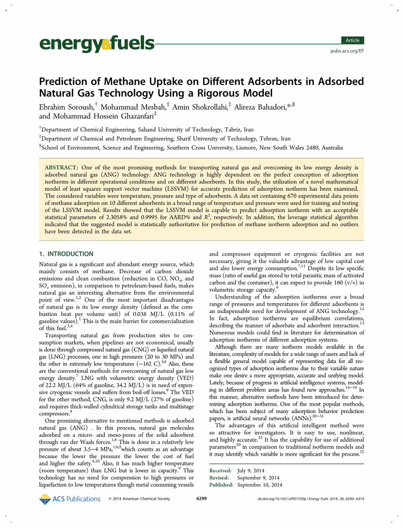
Prediction of Methane Uptake on Different Adsorbents in AdsorbedNatural Gas Technology Using a Rigorous ModelEbrahim Soroush,† Mohammad Mesbah,‡ Amin Shokrollahi,‡ Alireza Bahadori,*,§

and Mohammad Hossein Ghazanfari‡

†Department of Chemical Engineering, Sahand University of Technology, Tabriz, Iran‡Department of Chemical and Petroleum Engineering, Sharif University of Technology, Tehran, Iran§School of Environment, Science and Engineering, Southern Cross University, Lismore, New South Wales 2480, Australia

ABSTRACT: One of the most promising methods for transporting natural gas and overcoming its low energy density isadsorbed natural gas (ANG) technology. ANG technology is highly dependent on the perfect conception of adsorptionisotherms in different operational conditions and on different adsorbents. In this study, the utilization of a novel mathematicalmodel of least squares support vector machine (LSSVM) for accurate prediction of adsorption isotherm has been examined.The considered variables were temperature, pressure and type of adsorbents. A data set containing 670 experimental data pointsof methane adsorption on 10 different adsorbents in a broad range of temperature and pressure were used for training and testingof the LSSVM model. Results showed that the LSSVM model is capable to predict adsorption isotherm with an acceptablestatistical parameters of 2.3058% and 0.9995 for AARD% and R2, respectively. In addition, the leverage statistical algorithmindicated that the suggested model is statistically authoritative for prediction of methane isotherm adsorption and no outliershave been detected in the data set.

1. INTRODUCTION

Natural gas is a significant and abundant energy source, whichmainly consists of methane. Decrease of carbon dioxideemissions and clean combustion (reduction in CO, NOx, andSOx emission), in comparison to petroleum-based fuels, makesnatural gas an interesting alternative from the environmentalpoint of view.1,2 One of the most important disadvantagesof natural gas is its low energy density (defined as the com-bustion heat per volume unit) of 0.038 MJ/L (0.11% ofgasoline values).1 This is the main barrier for commercializationof this fuel.3,4

Transporting natural gas from production sites to con-sumption markets, when pipelines are not economical, usuallyis done through compressed natural gas (CNG) or liquefied naturalgas (LNG) processes, one in high pressures (20 to 30 MPa) andthe other in extremely low temperatures (−162 C).5,6 Also, theseare the conventional methods for overcoming of natural gas lowenergy density.7 LNG with volumetric energy density (VED)of 22.2 MJ/L (64% of gasoline, 34.2 MJ/L) is in need of expen-sive cryogenic vessels and suffers from boil-off losses.8 The VEDfor the other method, CNG, is only 9.2 MJ/L (27% of gasoline)and requires thick-walled cylindrical storage tanks and multistagecompressors.8

One promising alternative to mentioned methods is adsorbednatural gas (ANG) . In this process, natural gas moleculesadsorbed on a micro- and meso-pores of the solid adsorbentthrough van der Waals forces.1,8 This is done in a relatively lowpressure of about 3.5−4 MPa,1,6,9which counts as an advantagebecause the lower the pressure the lower the cost of fueland higher the safety.4,10 Also, it has much higher temperature(room temperature) than LNG but is lower in capacity.9 Thistechnology has no need for compression to high pressures orliquefaction to low temperatures though metal consuming vessels

and compressor equipment or cryogenic facilities are notnecessary, giving it the valuable advantage of low capital costand also lower energy consumption.7,11 Despite its low specificmass (ratio of useful gas stored to total parasitic mass of activatedcarbon and the container), it can expect to provide 160 (v/v) involumetric storage capacity.9

Understanding of the adsorption isotherms over a broadrange of pressures and temperatures for different adsorbents isan indispensable need for development of ANG technology.12

In fact, adsorption isotherms are equilibrium correlations,describing the manner of adsorbate and adsorbent interaction.13

Numerous models could find in literature for determination ofadsorption isotherms of different adsorption systems.Although there are many isotherm models available in the

literature, complexity of models for a wide range of users and lack ofa flexible general model capable of representing data for all rec-ognized types of adsorption isotherms due to their variable naturemake one desire a more appropriate, accurate and unifying model.Lately, because of progress in artificial intelligence systems, model-ing in different problem areas has found new approaches.14−19 Inthis manner, alternative methods have been introduced for deter-mining adsorption isotherms. One of the most popular methods,which has been subject of many adsorption behavior predictionpapers, is artificial neural networks (ANNs).20−31

The advantages of this artificial intelligent method wereso attractive for investigators. It is easy to use, nonlinear,and highly accurate.32 It has the capability for use of additionalparameters20 in comparison to traditional isotherm models andit may identify which variable is more significant for the process.22

Received: July 9, 2014Revised: September 9, 2014Published: September 10, 2014

Article

pubs.acs.org/EF

© 2014 American Chemical Society 6299 dx.doi.org/10.1021/ef501550p | Energy Fuels 2014, 28, 6299−6314

pubs.acs.org/EF

There is no need for fully detailed knowledge of the physicalphenomena22,23 and also no restriction by any processassumptions. Also, it has very good accuracy even in the case oflimited data.22 Still with all the advantages of ANNs, there are somedeficiencies for their external predictions because they may result inrandom initialization of the networks and variation of the stoppingcriteria during the optimization of the model parameters.33

For determining model parameters, precise and dependabledata are required. As a result, the experimental data shouldbe investigated with a comprehensive model, which is capableof handling various experimental techniques.In this study, a novel mathematical technique called least

square support vector machine (LSSVM) is presented forpredicting methane adsorption isotherm behavior on differentadsorbents. With use of statistical parameters, the validity of themodel will be examined. Then we will compare the network withprior isotherm models for its accuracy. For avoiding doubtful datathe statistical based Leverage approach is used.

2. LSSVM MODELCreating a mathematical relation between experimental data(temperature, pressure, type of adsorbent) and eligible output

(methane uptake) depends on finding a suitable mathematicaltool. Also, ANN-based models have presented excellent accuracyin different problems,34−40 they have a great disadvantage dueto nonreproducibility of results. This problem is because of therandom initialization of the network and stopping criteria during themodel parameter optimization process.41,42 Besides, there are otherproblems like time-consuming network training procedure (highcomputational load), tendency to over fit and high dependency onANN design parameters (number of layers, nodes, etc.), and alsoextrapolation is not recommended for ANN approach.43

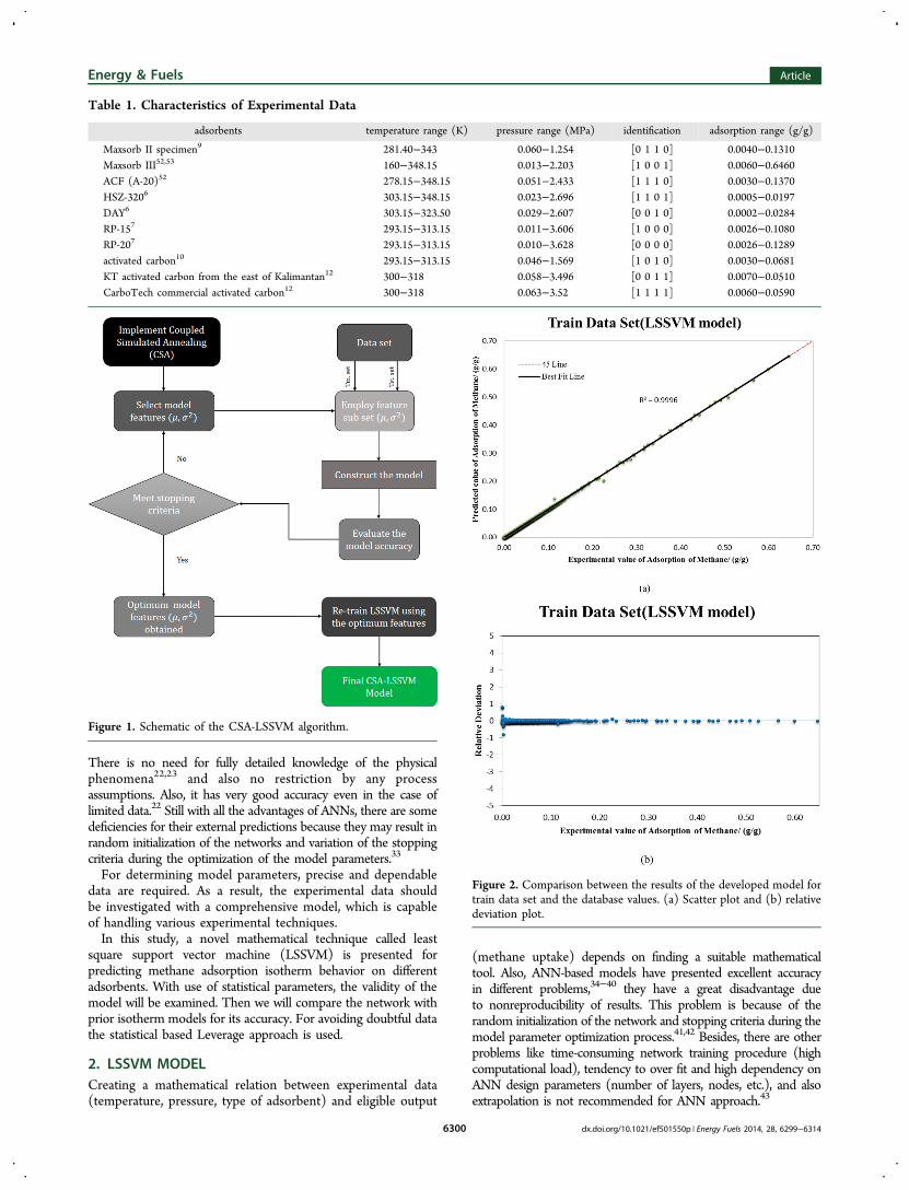
Table 1. Characteristics of Experimental Data

adsorbents temperature range (K) pressure range (MPa) identification adsorption range (g/g)

Maxsorb II specimen9 281.40−343 0.060−1.254 [0 1 1 0] 0.0040−0.1310Maxsorb III52,53 160−348.15 0.013−2.203 [1 0 0 1] 0.0060−0.6460ACF (A-20)52 278.15−348.15 0.051−2.433 [1 1 1 0] 0.0030−0.1370HSZ-3206 303.15−348.15 0.023−2.696 [1 1 0 1] 0.0005−0.0197DAY6 303.15−323.50 0.029−2.607 [0 0 1 0] 0.0002−0.0284RP-157 293.15−313.15 0.011−3.606 [1 0 0 0] 0.0026−0.1080RP-207 293.15−313.15 0.010−3.628 [0 0 0 0] 0.0026−0.1289activated carbon10 293.15−313.15 0.046−1.569 [1 0 1 0] 0.0030−0.0681KT activated carbon from the east of Kalimantan12 300−318 0.058−3.496 [0 0 1 1] 0.0070−0.0510CarboTech commercial activated carbon12 300−318 0.063−3.52 [1 1 1 1] 0.0060−0.0590

Figure 1. Schematic of the CSA-LSSVM algorithm.

Figure 2. Comparison between the results of the developed model fortrain data set and the database values. (a) Scatter plot and (b) relativedeviation plot.

Energy & Fuels Article

dx.doi.org/10.1021/ef501550p | Energy Fuels 2014, 28, 6299−63146300

Support vector machines have been introduced as powerfuland robust tools for solving a variety of complex problemsfrom pattern classification to nonlinear function approximation.Considering that the available measured data set,{(x1,y1), ...,(xn,yn)} where xi represent the input parameter and yi representthe desired output, SVM makes a nonlinear mapping ina manner that input space maps into a higher/infinitedimensional feasible space. In fact, the first goal of SVM isto find the best hyperplane that have minimum distance fromall experimental data points.44,45 The details and equationsof SVM theory can be found in previous studies.46,47 Appli-cation of SVM algorithm for regression problems or func-tion approximation results in facing a convex optimizationproblem that is subjected to inequality constraints to findsupport vectors. Consequently, employing SVM method for

regression problems has a high computational burden forapplying the constraint of the mentioned convex optimiza-tion.47 For this reason, application of an SVM algorithm in alarge scale problems data is limited due to memory and timeconsumed during optimization.47

An improved version of SVM, which called least squaressupport vector machine (LSSVM), has been developed bySuykens and Vandewalle.45 A modified version attempted toreduce the complexity and increase the speed of convergency.One of the main differences between LSSVM and SVM is thatthe inequality constraints of SVM change to equalityconstraints in LSSVM paradigm.45,47By this reformulation, thelearning process has been done through solving a set of linearequations that can be solved iteratively.45,48 Thus, in large scaleproblems with large data set in which accuracy and time areimportant, application of LSSVM algorithm is better than SVM.Generally, in LSSVM algorithm, the optimization problem isexpressed as follows:45

∑μ= || || +=

J w e w emin ( , )12

12 i

n

i2

1

2

(1)

subjected to the following linear constraints:

= ⟨ ⟩ + + =y w g x b e k n, ( ) 1, 2, ...,kt

k k (2)

In eq 1, ek signifies error variables; μ ≥ 0 denotes regulariza-tion constant; g(x) represents the mapping function, b and ware bias terms weight vectors and weight vectors, respectively,and index t represents the transpose of the weight matrix.Incorporating the linear constraint into the objective functionpreviously introduced in eq 1 provides45

∑

∑

μ

β

= || || +

− ⟨ ⟩ + +

=

=

L w e

w g x b e

12

12

{ , ( ) }

k

n

i

k

n

kt

k k

LSSVM2

1

2

1 (3)

Table 2. Details of Statistical Parameters for Proposed LSSVM, Toth, and Langmuir Models

MSE AARD% STD R2 N

LSSVM model all 3.57 × 10−06 2.3058 0.0871 0.9995 670train 3.51 × 10−06 1.8422 0.0891 0.9996 536test 3.81 × 10−06 4.1601 0.0788 0.9994 134

Toth model 3.49 × 10−05 6.6905 0.0871 0.9954 670Langmuir model 1.33 × 10−04 6.5168 0.0871 0.9828 670

Table 3. Details of LSSVM Model Statistical Parameters onEach Adsorbent

adsorbents MSE AARD% STD R2 N

Maxsorb II specimen9 1.02 × 10−06 1.3674 0.0329 0.9991 127Maxsorb III52,53 1.28 × 10−05 1.2708 0.1413 0.9994 160ACF (A-20)52 1.29 × 10−07 0.7790 0.0341 0.9999 128HSZ-3206 1.33 × 10−07 3.9300 0.0058 0.9963 36DAY6 9.1 × 10−08 7.0901 0.0087 0.9988 37RP-157 5.24 × 10−07 4.5573 0.0360 0.9996 38RP-207 1.02 × 10−06 7.8458 0.0416 0.9995 38activated carbon10 1.43 × 10−07 1.9396 0.0194 0.9996 43KT activated carbon fromthe east of Kalimantan12

4.06 × 10−06 2.6241 0.0139 0.9794 31

CarboTech commercialactivated carbon12

9.57 × 10−08 0.8846 0.0174 0.9997 32

Figure 3. Comparison between the results of the developed model fortest data set and the database values. (a) Scatter plot and (b) relativedeviation plot.



with Lagrangian multipliers βk ∈ R. Based on the method ofLagrangian multipliers, the below conditions are necessary foroptimization:

∑

∑

β

β

β

β μ

∂∂

= → =

∂∂

= → =

∂∂

= → ⟨ ⟩ + + −

=∂

∂= → = =

=

=

⎧

⎨

⎪⎪⎪⎪⎪⎪

⎩

⎪⎪⎪⎪⎪⎪

Lb

Lw

w g x

Lw g x b e y

Le

e k n

0 0

0 ( )

0 { , ( )

0

0 , ( 1, ..., )

k

n

k

k

n

k k

k

tk k k

kk k

LSSVM

1

LSSVM

1

LSSVM

LSSVM

(4)

By considering a linear regression between independent anddependent parameters of the LSSVM algorithm, the followingequation can be written:45

∑ β= +=

y x x bk

n

k kt

1 (5)

It should be mentioned that, eq 5 can only use for linearregression problems. To extend its capability for nonlinear

regression conditions, Kernel function has been contributedin eq 5 as follows:

∑ β= +=

y K x x b( , )k

n

k k1 (6)

Kernel function K(xi, x) is defined as inner product of vectorsg(x) and g(xi) as is shown below:

= ·K x x g x g x( , ) ( ) ( )k kt

(7)

There are many Kernel functions (e.g., radial basis function(RBF), polynomial, linear, sigmoid, spline, etc.) that can beused in LSSVM algorithm. Though, the most common Kernelfunctions are polynomial (eq 8) and RBF (eq 9)47

= +K x x x x c( , ) (1 / )kT

kd

(8)

σ= || − ||K x x x x( , ) exp( )k k2 2

(9)

where d is the degree of polynomial and σ2 is squaredbandwidth, which must be optimized through an optimizationalgorithm during the learning process.

3. LEVERAGE APPROACHOutlier diagnostic is necessary for constructing a mathematicalmodel.49,50 This algorithm deals with identifying secludeddata (or sets of data) that are possible to extravagant from thebulk of data.49,50 Experimental errors are the major reason for

Table 4. Maximum and Minimum Absolute Relative Deviation for Each Adsorbent in Different Models

absolute relative deviation %

LSSVM model Toth model Langmuir model

adsorbents N min max min max min max

Maxsorb II specimen9 127 1.37 × 10−02 10.85 4.92 × 10−03 18.57 2.11 × 10−02 8.19Maxsorb III52,53 160 1.97 × 10−03 20.40 2.18 × 10−01 77.82 1.16 × 10−01 66.35ACF (A-20)52 128 7.51 × 10−03 6.46 1.83 × 10−02 19.55 2.77 × 10−03 22.53HSZ-3206 36 1.42 × 10−02 44.19 2.45 × 10−01 72.74 3.13 × 10−02 16.36DAY6 37 7.44 × 10−03 81.51 2.45 × 10−01 72.74 7.81 × 10−02 148.06RP-157 38 1.54 × 10−03 81.68 2.22 × 10−02 188.72 1.53 × 10−01 24.95RP-207 38 1.95 × 10−03 198.97 1.53 × 10−02 37.72 9.81 × 10−02 48.54activated carbon10 43 7.27 × 10−03 15.50 3.97 × 10−02 39.33 1.48 × 10−01 93.39KT activated carbon from the east of Kalimantan12 31 2.37 × 10−02 21.31 3.31 × 10−02 95.97 5.19 × 10−02 18.62CarboTech commercial activated carbon12 32 3.39 × 10−02 7.76 1.75 × 10−01 5.38 2.08 × 10−01 24.33

Figure 4. Adsorption isotherms of CH4 on different adsorbents.



outliers.37 These outliers may damage the model through theintroduction of some uncertainties and lower the predictionaccuracy.36,37 The leverage approach is a strong statisticalalgorithm for outlier detection.50,51 This method is based on amatrix, which its elements are the deviation between modelpredictions and experimental values.49,50it is called Hat matrix.Here is the definition of Hat indices49,50

= −H X X X X( )t t1(10)

Where X is a matrix with n rows (each row represents a singledata) and k columns (each column as an indicator of a modelparameter). In this definition, t denotes transpose matrix. Thediagonal elements of H, presented as the Hat values.Williams plot with the use of standardized cross-validation

residuals (R) and correlation of hat indices, graphically deter-mines doubtful data.49,50 The H values are found through eq 10and are used for sketching William plot. Through the definitionof 3p/n the value of warning leverage is determined. Here, ndetermines the number of training points and p is representingthe number of correlation input parameters.49,50 As an adequate

“cut off” Leverage is generally 3, so the accepted points shouldbe in the standard deviation range of ∓3.49,50 The accumulationof data points in the range of 0 < H < H* and −3 < R < 3,proving that model is statistically valid. The points which modelcould not predict at all, are called good high leverage. Thesepoints are in the range of H ≤ H* and −3 < R < 3. Bad highleverage or outliers are in fact the suspicious data. These pointsare in the range of R < −3 or R > 3.

4. RESULT AND DISCUSSION4.1. Designing the LSSVM Model. In order to imple-

ment the LSSVM algorithm, 670 experimental data pointson the methane uptake by different adsorbents that coverwide range of pressure and temperature collected fromliterature.6,7,9,10,12,52,53 The type of adsorbent, temperature,and pressure range for these experimental data could befound in Table 1.In this communication, LSSVM modeling algorithm that

presented by Packman et al.54 and Suykens and Vandewalle41 isused to make a precise relation between methane uptake andthe adsorbent temperature, pressure, and type of adsorbent asfollows:

= f T Pmethane uptake by adsorbent ( , , type of adsorbent)(11)

It should be mentioned that interpreting the adsorbent type forthe mathematical algorithm is done by specifying each type as a

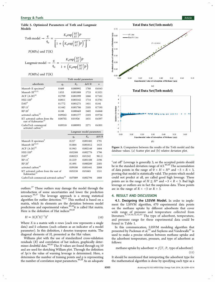
Table 5. Optimized Parameters of Toth and LangmuirModels

→ =+

Δ

Δ⎡⎣⎢

⎤⎦⎥( )

( )( )

qq

K P

K P

P T

Toth modelexp

1 exp

(MPa) and (K)

HRT

HRT

n n0

0

0

1/

→ =+

Δ

Δ( )( )

( )qq

K P

K P

P T

Langmuir modelexp

1 exp

(MPa) and (K)

HRT

HRT0

0

0

Toth model parameters

adsorbents q0 K0 ΔH/R n

Maxsorb II specimen9 0.469 0.000992 1788 0.6543Maxsorb III52,53 1.033 0.001888 1733 0.3521ACF (A-20)52 0.2709 0.001999 1666 0.7161HSZ-3206 0.0811 0.003342 1714 0.3781DAY6 0.1772 0.001275 1451 0.541RP-157 0.1442 0.001786 2105 0.7195RP-207 0.188 0.000469 2402 0.6848activated carbon10 0.09262 0.001377 2103 0.9756KT activated carbon from theeast of Kalimantan12

0.06702 0.01926 1631 0.6397

CarboTech commercialactivated carbon12

0.09318 0.000993 2271 0.6301

Langmuir model parameters

q0 K0 ΔH/R

Maxsorb II specimen9 0.257 0.001482 1791Maxsorb III52,53 0.5864 0.001812 1433ACF (A-20)52 0.1943 0.002148 1684HSZ-3206 0.02588 0.002776 1796DAY6 0.06523 0.01242 961.2RP-157 0.1219 0.001108 2196RP-207 0.1495 0.000289 2505activated carbon10 0.09106 0.001441 2088KT activated carbon from the east ofKalimantan12

0.05538 0.01665 1551

CarboTech commercial activated carbon12 0.07009 0.002794 1888

Figure 5. Comparison between the results of the Toth model and thedatabase values. (a) Scatter plot and (b) relative deviation plot.



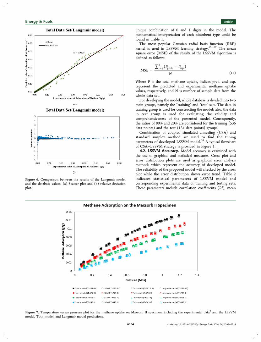
unique combination of 0 and 1 digits in the model. Themathematical interpretation of each adsorbent type could befound in Table 1.The most popular Gaussian radial basis function (RBF)

kernel is used in LSSVM learning strategy.55−57 The meansquare error (MSE) of the results of the LSSVM algorithm isdefined as follows:

=∑ −= P P

NMSE

( )i 1n

pred. exp.

(12)

Where P is the total methane uptake, indices pred. and exp.represent the predicted and experimental methane uptakevalues, respectively, and N is number of sample data from thewhole data set.For developing the model, whole database is divided into two

main groups, namely the “training” and “test” sets. The data intraining group is used for constructing the model; also, the datain test group is used for evaluating the validity andcomprehensiveness of the presented model. Consequently,the ratios of 80% and 20% are considered for the training (536data points) and the test (134 data points) groups.Combination of coupled simulated annealing (CSA) and

standard simplex method are used to find the tuningparameters of developed LSSVM model.58 A typical flowchartof CSA−LSSVM strategy is provided in Figure 1.

4.2. LSSVM Accuracy. Model accuracy is examined withthe use of graphical and statistical measures. Cross plot anderror distribution plots are used as graphical error analysismethods which represent the accuracy of developed model.The reliability of the proposed model will checked by the crossplot while the error distribution shows error trend. Table 2indicates statistical parameters of LSSVM model andcorresponding experimental data of training and testing sets.These parameters include correlation coefficients (R2), mean

Figure 6. Comparison between the results of the Langmuir modeland the database values. (a) Scatter plot and (b) relative deviationplot.

Figure 7. Temperature versus pressure plot for the methane uptake on Maxsorb II specimen, including the experimental data9 and the LSSVMmodel, Toth model, and Langmuir model predictions.



square errors (MSE), and average absolute relative deviations(AARDs). Comparison of LSSVM predictions and correspond-ing experimental data for training and testing sets are presentedin Figures 2 and 3, respectively.

Robustness of the process model is illustrated by the accu-mulation of data about the first quadrant bisector (Figures 2aand 3a). The result shows great agreement between experi-mental values and LSSVM predictions. Relative deviation plots

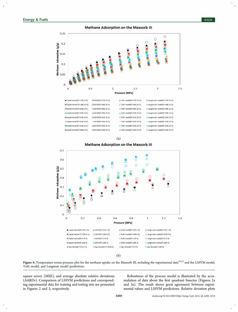
Figure 8. Temperature versus pressure plot for the methane uptake on the Maxsorb III, including the experimental data52,53 and the LSSVM model,Toth model, and Langmuir model predictions.



(Figures 2b and 3b) show a reasonable error for the wholethe data.Details on the model predictions of methane uptake

on different adsorbers in a broad range of pressure and

temperature considered in this work are shown in Tables 2and 3. In addition, maximum and minimum absolute rela-tive deviation for each adsorbent in different modelsis presented in Table 4. These tables indicate that, the

Figure 9. Temperature versus pressure plot for the methane uptake on the ACF(A-20), including the experimental data52 and the LSSVM model,Toth model, and Langmuir model predictions.

Figure 10. Temperature versus pressure plot for the methane uptake on the HSZ-320, including the experimental data6 and the LSSVM model, Tothmodel, and Langmuir model predictions.



LSSVM model is strongly capable of reproducing experimentaldata.4.3. Comparison of LSSVM with Conventional Models.

Methane uptake isotherm data for each adsorbent is graphicallypresented on a pressure−concentration−temperature plane in

Figure 4. The adsorption isotherm for all adsorbents is classifiedas Type I according to IUPAC classification, which showstypical isotherm for microporous materials with high surfacearea of over 1500 m2/g. In these adsorbents, attractive forcesbetween the adsorbate and adsorbent are much stronger than

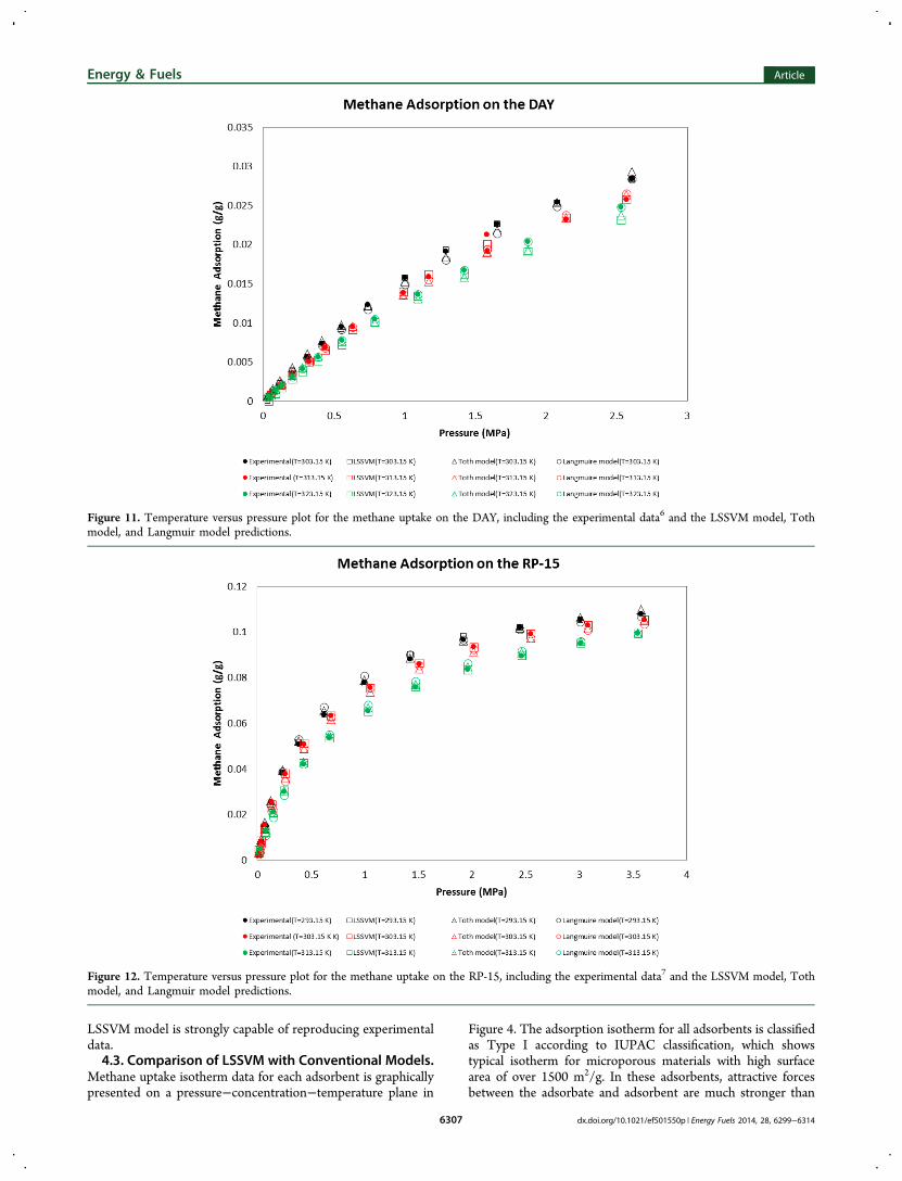
Figure 11. Temperature versus pressure plot for the methane uptake on the DAY, including the experimental data6 and the LSSVM model, Tothmodel, and Langmuir model predictions.

Figure 12. Temperature versus pressure plot for the methane uptake on the RP-15, including the experimental data7 and the LSSVM model, Tothmodel, and Langmuir model predictions.



between adsorbate molecules in the bulk state.59 It means thatthe adsorbent pore size is not much larger than the adsorbatemolecular diameter. In case of chemisorption, this type can befairly modeled by the Langmuir equation. However, this modelshows deficiencies in case of physisorption. Therefore, it seems

that the modified semiempirical models such as Sips and Tothshould be used for modeling of these data. The Toth isothermmodel has a high thermodynamic consistency, incorporates thesurface heterogeneity of the adsorbent, and also gives acceptableresults in a wide pressure range.60

Figure 13. Temperature versus pressure plot for the methane uptake on the RP-20, including the experimental data7 and the LSSVM model, Tothmodel, and Langmuir model predictions.

Figure 14. Temperature versus pressure plot for the methane uptake on the activated carbon, including the experimental data10 and the LSSVMmodel, Toth model, and Langmuir model predictions.



In this manner, for examining the quality of the pro-posed LSSVM model, three parameter Langmuir61 andToth62 equations used for modeling the whole data set. Theproblem with traditional isotherm models is that you cannotuse them for modeling of a data set combined from different

type of adsorbents. In another word, type of adsorbent isnot a variable. Therefore, for using these models, the datafrom each adsorbent modeled separately. The optimizedparameters of Toth and Langmuir models could be foundin Table 5.

Figure 15. Temperature versus pressure plot for the methane uptake on KT activated carbon from the east of Kalimantan, including theexperimental data12 and the LSSVM model, Toth model, and Langmuir model predictions.

Figure 16. Temperature versus pressure plot for the methane uptake on CarboTech commercial activated carbon, including the experimental data12

and the LSSVM model, Toth model, and Langmuir model predictions.



It is not a problem for LSSVM. As mentioned before, oneof the variables, which has been considered for LSSVM model,was the adsorbent type. In fact, the model is open to accept asmany variables as the user defines. This is an obvious advantageand means you can investigate the effect of parameters, whichmay not be considered in conventional methods.The experimental data for each adsorbent has been modeled

through a nonlinear regression approach with Toth andLangmuir isotherms. Optimized parameters of the modelsfor each adsorbent are shown in Table 5. The cross plots inFigures 5a and 6a illustrate the state of agreement betweenprediction of traditional isotherms and experimental values.In addition, relative deviation between the predicted values ofisotherm models and experimental data are shown in Figures 5band 6b. Pressure−concentration−temperature plots are drawnfor a better visual comparison between the LSSVM and conven-tional isotherm models (Figures 7−16).As is mentioned before in case of physisorption the

semiempirical models such as Sips and Toth have betterresults in comparison with Langmuir. This can be seen fromFigure 8b where the low temperature favors the physisorption.

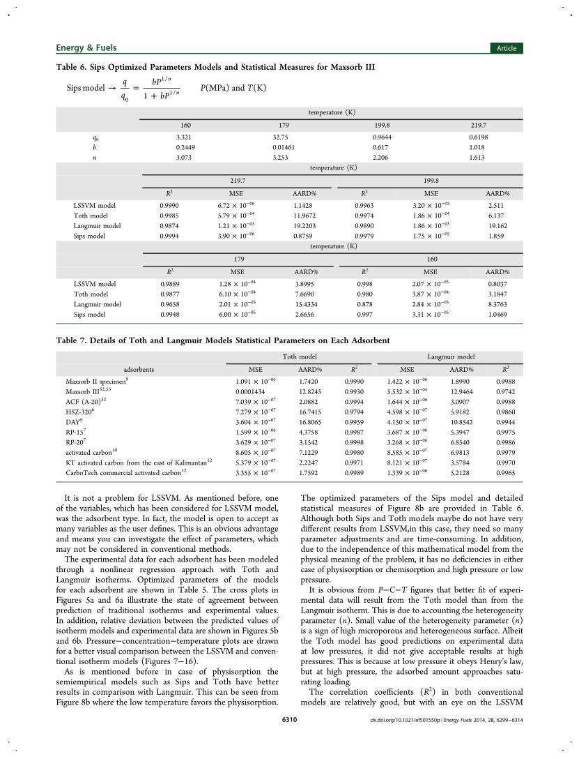
The optimized parameters of the Sips model and detailedstatistical measures of Figure 8b are provided in Table 6.Although both Sips and Toth models maybe do not have verydifferent results from LSSVM,in this case, they need so manyparameter adjustments and are time-consuming. In addition,due to the independence of this mathematical model from thephysical meaning of the problem, it has no deficiencies in eithercase of physisorption or chemisorption and high pressure or lowpressure.It is obvious from P−C−T figures that better fit of experi-

mental data will result from the Toth model than from theLangmuir isotherm. This is due to accounting the heterogeneityparameter (n). Small value of the heterogeneity parameter (n)is a sign of high microporous and heterogeneous surface. Albeitthe Toth model has good predictions on experimental dataat low pressures, it did not give acceptable results at highpressures. This is because at low pressure it obeys Henry’s law,but at high pressure, the adsorbed amount approaches satu-rating loading.The correlation coefficients (R2) in both conventional

models are relatively good, but with an eye on the LSSVM

Table 6. Sips Optimized Parameters Models and Statistical Measures for Maxsorb III

→ =+

qq

bPbP

P TSips model1

(MPa) and (K)n

n0

1/

1/

temperature (K)

160 179 199.8 219.7

q0 3.321 32.75 0.9644 0.6198b 0.2449 0.01461 0.617 1.018n 3.073 3.253 2.206 1.613

temperature (K)

219.7 199.8

R2 MSE AARD% R2 MSE AARD%

LSSVM model 0.9990 6.72 × 10−06 1.1428 0.9963 3.20 × 10−05 2.511Toth model 0.9985 5.79 × 10−04 11.9672 0.9974 1.86 × 10−04 6.137Langmuir model 0.9874 1.21 × 10−03 19.2203 0.9890 1.86 × 10−03 19.162Sips model 0.9994 3.90 × 10−06 0.8759 0.9979 1.75 × 10−05 1.859

temperature (K)

179 160

R2 MSE AARD% R2 MSE AARD%

LSSVM model 0.9889 1.28 × 10−04 3.8995 0.998 2.07 × 10−05 0.8037Toth model 0.9877 6.10 × 10−04 7.6690 0.980 3.87 × 10−04 3.1847Langmuir model 0.9658 2.01 × 10−03 15.4334 0.878 2.84 × 10−03 8.3763Sips model 0.9948 6.00 × 10−05 2.6656 0.997 3.31 × 10−05 1.0469

Table 7. Details of Toth and Langmuir Models Statistical Parameters on Each Adsorbent

Toth model Langmuir model

adsorbents MSE AARD% R2 MSE AARD% R2

Maxsorb II specimen9 1.091 × 10−06 1.7420 0.9990 1.422 × 10−06 1.8990 0.9988Maxsorb III52,53 0.0001434 12.8245 0.9930 5.532 × 10−04 12.9464 0.9742ACF (A-20)52 7.039 × 10−07 2.0882 0.9994 1.644 × 10−06 3.0907 0.9988HSZ-3206 7.279 × 10−07 16.7415 0.9794 4.598 × 10−07 5.9182 0.9860DAY6 3.604 × 10−07 16.8065 0.9959 4.150 × 10−07 10.8542 0.9944RP-157 1.599 × 10−06 4.3758 0.9987 3.687 × 10−06 5.3947 0.9975RP-207 3.629 × 10−07 3.1542 0.9998 3.268 × 10−06 6.8540 0.9986activated carbon10 8.605 × 10−07 7.1229 0.9980 8.585 × 10−07 6.9813 0.9979KT activated carbon from the east of Kalimantan12 5.379 × 10−07 2.2247 0.9971 8.121 × 10−07 3.5784 0.9970CarboTech commercial activated carbon12 3.355 × 10−07 1.7592 0.9989 1.339 × 10−06 5.2128 0.9965



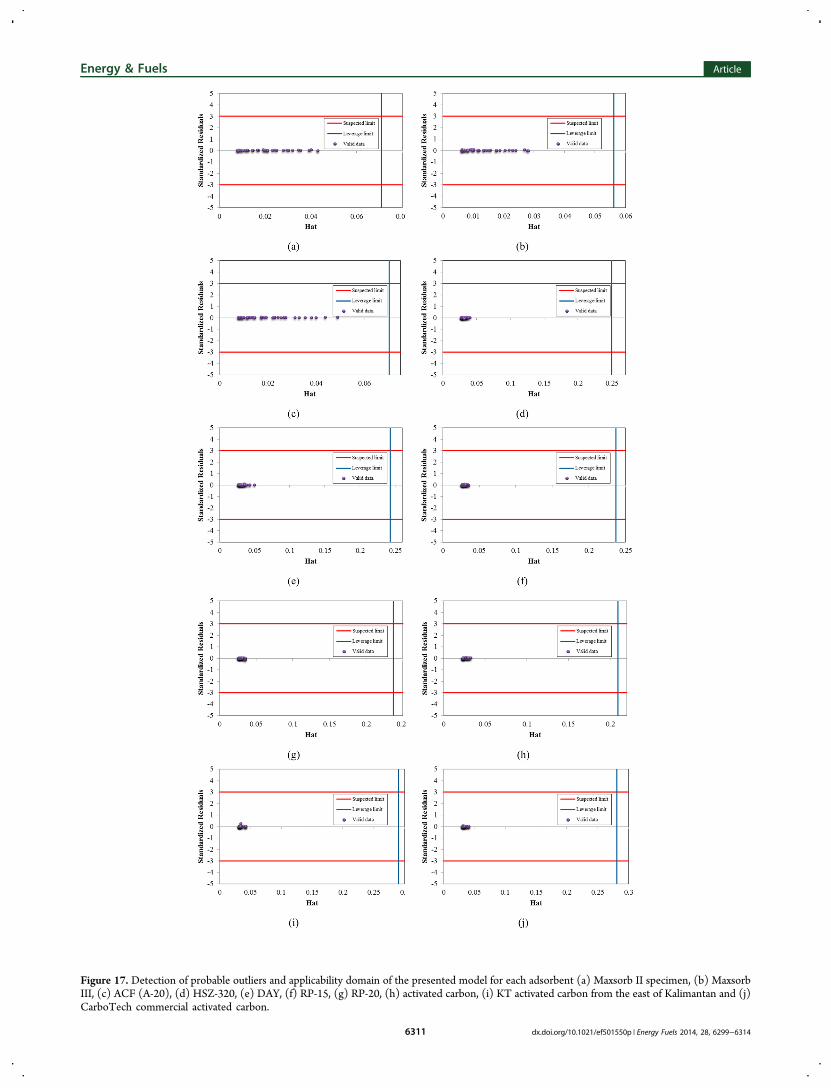
Figure 17. Detection of probable outliers and applicability domain of the presented model for each adsorbent (a) Maxsorb II specimen, (b) MaxsorbIII, (c) ACF (A-20), (d) HSZ-320, (e) DAY, (f) RP-15, (g) RP-20, (h) activated carbon, (i) KT activated carbon from the east of Kalimantan and (j)CarboTech commercial activated carbon.



outstanding correlation coefficient (R2), the supremacy of thismodel is obvious. To make an accurate statistical comparison,detailed statistical measures have been shown in Tables 2, 3,and 7. These results indicate that predictions of LSSVM modelhave a better agreement with experimental data in comparisonto those conventional isotherm models. On the basis of graphicaland statistic error analysis that performed in this study, it can beconcluded that LSSVM algorithm can be a powerful tool forprediction of adsorption isotherms.4.4. Outlier Detection. Table 2 shows that the deviation

of model predictions from experimental values is appropriatefor using the leverage algorithm. The H values have beenevaluated by eq 10, and with use of 3(p + 1)/n, warningleverages (H*) have been found. Figure 17 shows Williamsplots for each adsorbents. As the figures show, whole methaneuptake data set is in the LSSVM applicability domain. Thefigures indicate that no outliers are in the data. The qualityof the data used for modeling is different. The data with lowerH values and the lower absolute values R may be identified asmore authentic experimental data.4.5. Sensitivity Analysis. In order to investigate the

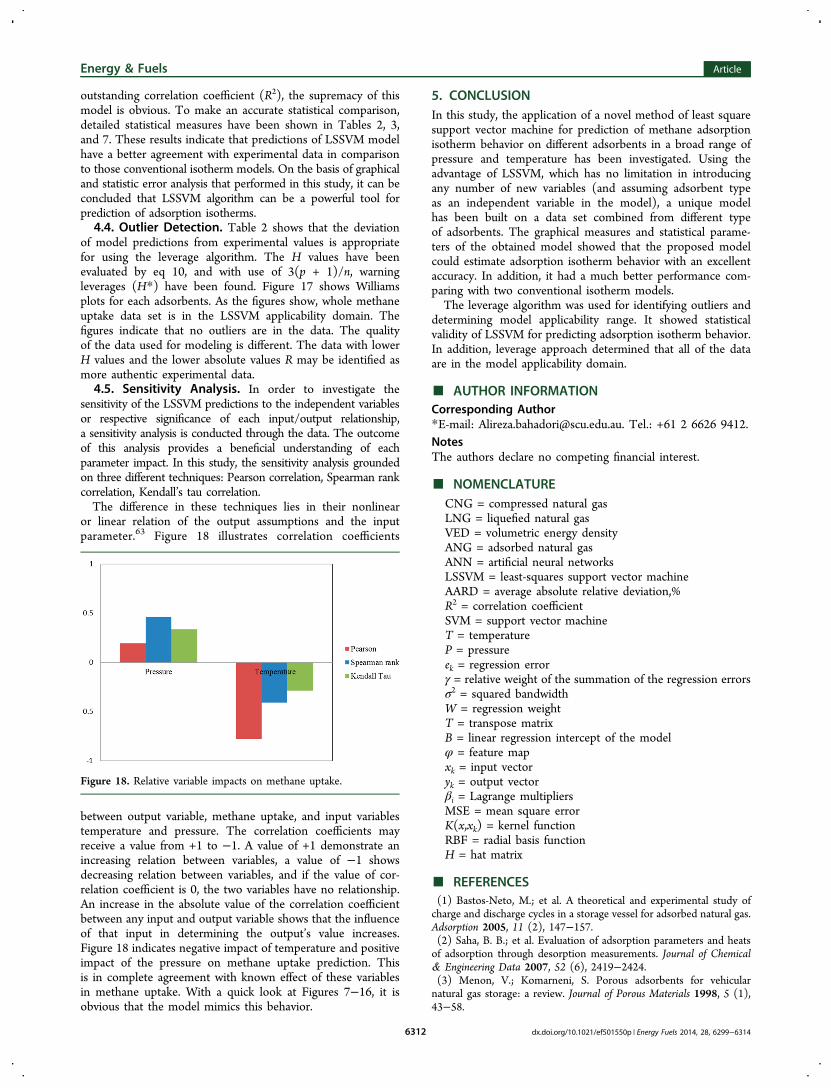
sensitivity of the LSSVM predictions to the independent variablesor respective significance of each input/output relationship,a sensitivity analysis is conducted through the data. The outcomeof this analysis provides a beneficial understanding of eachparameter impact. In this study, the sensitivity analysis groundedon three different techniques: Pearson correlation, Spearman rankcorrelation, Kendall’s tau correlation.The difference in these techniques lies in their nonlinear

or linear relation of the output assumptions and the inputparameter.63 Figure 18 illustrates correlation coefficients

between output variable, methane uptake, and input variablestemperature and pressure. The correlation coefficients mayreceive a value from +1 to −1. A value of +1 demonstrate anincreasing relation between variables, a value of −1 showsdecreasing relation between variables, and if the value of cor-relation coefficient is 0, the two variables have no relationship.An increase in the absolute value of the correlation coefficientbetween any input and output variable shows that the influenceof that input in determining the output’s value increases.Figure 18 indicates negative impact of temperature and positiveimpact of the pressure on methane uptake prediction. Thisis in complete agreement with known effect of these variablesin methane uptake. With a quick look at Figures 7−16, it isobvious that the model mimics this behavior.

5. CONCLUSIONIn this study, the application of a novel method of least squaresupport vector machine for prediction of methane adsorptionisotherm behavior on different adsorbents in a broad range ofpressure and temperature has been investigated. Using theadvantage of LSSVM, which has no limitation in introducingany number of new variables (and assuming adsorbent typeas an independent variable in the model), a unique modelhas been built on a data set combined from different typeof adsorbents. The graphical measures and statistical parame-ters of the obtained model showed that the proposed modelcould estimate adsorption isotherm behavior with an excellentaccuracy. In addition, it had a much better performance com-paring with two conventional isotherm models.The leverage algorithm was used for identifying outliers and

determining model applicability range. It showed statisticalvalidity of LSSVM for predicting adsorption isotherm behavior.In addition, leverage approach determined that all of the dataare in the model applicability domain.

■ AUTHOR INFORMATIONCorresponding Author*E-mail: [email protected]. Tel.: +61 2 6626 9412.NotesThe authors declare no competing financial interest.

■ NOMENCLATURECNG = compressed natural gasLNG = liquefied natural gasVED = volumetric energy densityANG = adsorbed natural gasANN = artificial neural networksLSSVM = least-squares support vector machineAARD = average absolute relative deviation,%R2 = correlation coefficientSVM = support vector machineT = temperatureP = pressureek = regression errorγ = relative weight of the summation of the regression errorsσ2 = squared bandwidthW = regression weightT = transpose matrixB = linear regression intercept of the modelφ = feature mapxk = input vectoryk = output vectorβi = Lagrange multipliersMSE = mean square errorK(x,xk) = kernel functionRBF = radial basis functionH = hat matrix

■ REFERENCES(1) Bastos-Neto, M.; et al. A theoretical and experimental study ofcharge and discharge cycles in a storage vessel for adsorbed natural gas.Adsorption 2005, 11 (2), 147−157.(2) Saha, B. B.; et al. Evaluation of adsorption parameters and heatsof adsorption through desorption measurements. Journal of Chemical& Engineering Data 2007, 52 (6), 2419−2424.(3) Menon, V.; Komarneni, S. Porous adsorbents for vehicularnatural gas storage: a review. Journal of Porous Materials 1998, 5 (1),43−58.

Figure 18. Relative variable impacts on methane uptake.



mailto:[email protected]

(4) Lozano-Castello, D.; et al. Advances in the study of methanestorage in porous carbonaceous materials. Fuel 2002, 81 (14), 1777−1803.(5) Thomas, S.; Dawe, R. A. Review of ways to transport natural gasenergy from countries which do not need the gas for domestic use.Energy 2003, 28 (14), 1461−1477.(6) Lee, J.-W.; et al. Methane adsorption on multi-walled carbonnanotube at (303.15, 313.15, and 323.15) K. Journal of Chemical &Engineering Data 2006, 51 (3), 963−967.(7) Lee, J.-W.; et al. Methane storage on phenol-based activatedcarbons at (293.15, 303.15, and 313.15) K. Journal of Chemical &Engineering Data 2007, 52 (1), 66−70.(8) Makal, T. A.; et al. Methane storage in advanced porousmaterials. Chem. Soc. Rev. 2012, 41 (23), 7761−7779.(9) Wang, X.; et al. Adsorption measurements of methane onactivated carbon in the temperature range (281 to 343) K andpressures to 1.2 MPa. Journal of Chemical & Engineering Data 2010, 55(8), 2700−2706.(10) Choi, B.-U.; et al. Adsorption equilibria of methane, ethane,ethylene, nitrogen, and hydrogen onto activated carbon. Journal ofChemical & Engineering Data 2003, 48 (3), 603−607.(11) Vasil’Ev, L.; et al. Adsorption systems of natural gas storage andtransportation at low pressures and temperatures. Journal of Engineer-ing Physics and Thermophysics 2003, 76 (5), 987−995.(12) Martin, A.; et al. Adsorption isotherms of CH4 on activatedcarbon from Indonesian low grade coal. Journal of Chemical &Engineering Data 2011, 56 (3), 361−367.(13) Foo, K.; Hameed, B. Insights into the modeling of adsorptionisotherm systems. Chemical Engineering Journal 2010, 156 (1), 2−10.(14) Chamkalani, A.; et al. Utilization of support vector machine tocalculate gas compressibility factor. Fluid Phase Equilibrium 2013, 358,189−202.(15) Roosta, A.; Setoodeh, P.; Jahanmiri, A. Artificial neural networkmodeling of surface tension for pure organic compounds. Industrial &Engineering Chemistry Research 2011, 51 (1), 561−566.(16) Kumar, K. V. Neural network prediction of interfacial tension atcrystal/solution interface. Industrial & Engineering Chemistry Research2009, 48 (8), 4160−4164.(17) Shafiei, A.; et al. A new screening tool for evaluation ofsteamflooding performance in Naturally Fractured CarbonateReservoirs. Fuel 2013, 108, 502−514.(18) Zendehboudi, S.; et al. Thermodynamic investigation ofasphaltene precipitation during primary oil production: laboratoryand smart technique. Industrial & Engineering Chemistry Research 2013,52 (17), 6009−6031.(19) Mesbah, M.; et al. Prediction of phase equilibrium of CO2 cycliccompound binary mixtures using a rigorous modeling approach.Journal of Supercritical Fluids 2014, 90, 110−125.(20) Myhara, R.; et al. Water sorption isotherms of dates: modelingusing GAB equation and artificial neural network approaches. LWT-Food Science and Technology 1998, 31 (7), 699−706.(21) Monneyron, P.; et al. Competitive adsorption of organicmicropollutants in the aqueous phase onto activated carbon cloth:comparison of the IAS model and neural networks in modeling data.Langmuir 2002, 18 (13), 5163−5169.(22) Carsky, M.; Do, D. Neural network modeling of adsorption ofbinary vapour mixtures. Adsorption 1999, 5 (3), 183−192.(23) Jha, S. K.; Madras, G. Neural network modeling of adsorptionequilibria of mixtures in supercritical fluids. Industrial & EngineeringChemistry Research 2005, 44 (17), 7038−7041.(24) Janjai, S.; et al. Neural network modeling of sorption isothermsof longan (Dimocarpus longan Lour.). Computers and Electronics inAgriculture 2009, 66 (2), 209−214.(25) Kumar, K. V.; et al. Neural network and principal componentanalysis for modeling of hydrogen adsorption isotherms on KOHactivated pitch-based carbons containing different heteroatoms.Chemical Engineering Journal 2010, 159 (1), 272−279.(26) Yang, Y.; et al. Biosorption of Acid Black 172 and Congo Redfrom aqueous solution by nonviable Penicillium YW 01: Kinetic study,

equilibrium isotherm and artificial neural network modeling.Bioresource Technology 2011, 102 (2), 828−834.(27) Morse, G.; et al. Neural network modelling of adsorptionisotherms. Adsorption 2011, 17 (2), 303−309.(28) Turan, N. G.; Mesci, B.; Ozgonenel, O. The use of artificialneural networks (ANN) for modeling of adsorption of Cu (II) fromindustrial leachate by pumice. Chemical Engineering Journal 2011, 171(3), 1091−1097.(29) Basu, S.; et al. Prediction of Gas-Phase Adsorption IsothermsUsing Neural Nets. Canadian Journal of Chemical Engineering 2002, 80(4), 1−7.(30) Shahryari, Z.; et al. Application of artificial neural networks forformulation and modeling of dye adsorption onto multiwalled carbonnanotubes. Research on Chemical Intermediates 2012, 1−15.(31) Asl, S. H. Artificial neural network (ANN) approach formodeling of Cr (VI) adsorption from aqueous solution by zeoliteprepared from raw fly ash (ZFA). Journal of Industrial & EngineeringChemistry 2012, 1044−1055.(32) Doherty, S. K. Control of pH in chemical processes using artificialneural networks; Liverpool John Moores University: Liverpool, U.K.,1999.(33) Eslamimanesh, A.; et al. Phase equilibrium modeling of clathratehydrates of methane, carbon dioxide, nitrogen, and hydrogen+ watersoluble organic promoters using Support Vector Machine algorithm.Fluid Phase Equilibrium 2012, 316, 34−45.(34) Chapoy, A.; Mohammadi, A.-H.; Richon, D. Predicting thehydrate stability zones of natural gases using artificial neural networks.Oil & Gas Science and Technology-Revue de l’IFP 2007, 62 (5), 701−706.(35) Soleimani, R. Experimental investigation, modeling andoptimization of membrane separation using artificial neural networkand multi-objective optimization using genetic algorithm. ChemicalEngineering Research and Design 2012, 883−903.(36) Majidi, S. M. J. Evolving an accurate model based on machinelearning approach for prediction of dew-point pressure in gascondensate reservoirs. Chemical Engineering Research and Design2013, 891−902.(37) Tatar, A.; et al. Implementing Radial Basis Function Networksfor modeling CO2-reservoir oil minimum miscibility pressure. Journalof Natural Gas Science and Engineering 2013, 15 (0), 82−92.(38) Yang, J.; Tohidi, B. Determination of Hydrate InhibitorConcentrations by Measuring Electrical Conductivity and AcousticVelocity. Energy Fuels 2013, 27 (2), 736−742.(39) Nguyen, V. D.; et al. Prediction of vapor−liquid equilibriumdata for ternary systems using artificial neural networks. Fluid PhaseEquilibria 2007, 254 (1), 188−197.(40) Rohani, A. A.; et al. Comparison between the artificial neuralnetwork system and SAFT equation in obtaining vapor pressure andliquid density of pure alcohols. Expert Systems with Applications 2011,38 (3), 1738−1747.(41) Suykens, J. A.; Vandewalle, J. Least squares support vectormachine classifiers. Neural Processing Letters 1999, 9 (3), 293−300.(42) Suykens, J. A.; et al. Weighted least squares support vectormachines: robustness and sparse approximation. Neurocomputing 2002,48 (1), 85−105.(43) Balabin, R. M.; Lomakina, E. I. Support vector machineregression (LS-SVM)an alternative to artificial neural networks(ANNs) for the analysis of quantum chemistry data? PhysicalChemistry Chemical Physics 2011, 13 (24), 11710−11718.(44) Cristianini, N. and J. Shawe-Taylor An Introduction to SupportVector Machines: and Other Kernel-Based Learning Methods; CambridgeUniversity Press: New York, 2000; 189.(45) Suykens, J. A. K.; Vandewalle, J. Least Squares Support VectorMachine Classifiers. Neural Processing Letters 1999, 9 (3), 293−300.(46) Smola, A. J.; et al. A tutorial on support vector regression.Statistics and Computing 2004, 14 (3), 199−222.(47) Haifeng, W. H. Dejin Comparison of SVM and LS-SVM forRegression. In Neural Networks and Brain; ICNN InternationalConference, 2005.



(48) Gharagheizi, F.; et al. Solubility Parameters of NonelectrolyteOrganic Compounds: Determination Using Quantitative Structure−Property Relationship Strategy. Industrial & Engineering ChemistryResearch 2011, 50 (19), 11382−11395.(49) Goodall, C. R. 13 Computation using the QR decomposition.Handbook of Statistics 1993, 9, 467−508.(50) Robust regression and outlier detection; Rousseeuw, P. J., Leroy,A.M., Eds.; John Wiley & Sons : Chichester, U. K., 2005; Vol. 589.(51) Gramatica, P. Principles of QSAR models validation: internaland external. QSAR & Combinatorial Science 2007, 26 (5), 694−701.(52) Loh, W. S.; et al. Improved isotherm data for adsorption ofmethane on activated carbons. Journal of Chemical & Engineering Data2010, 55 (8), 2840−2847.(53) Rahman, K. A.; et al. Experimental adsorption isotherm ofmethane onto activated carbon at sub-and supercritical temperatures.Journal of Chemical & Engineering Data 2010, 55 (11), 4961−4967.(54) Pelckmans, K. LS-SVMlab: a MATLAB/C toolbox for leastsquares support vector machines. Tutorial. KULeuven-ESAT. Leuven,Belgium. http://www.esat.kuleuven.be/sista/lssvmlab/old/lssvmlab_paper0.pdf (accessed June 2014).(55) Shokrollahi, A.; et al. Intelligent model for prediction of CO2 −Reservoir oil minimum miscibility pressure. Fuel 2013, 112 (0), 375−384.(56) Rafiee-Taghanaki, S.; et al. Implementation of SVM frameworkto estimate PVT properties of reservoir oil. Fluid Phase Equilibrium2013, 346 (0), 25−32.(57) Mohammadi, A. H.; et al. Gas Hydrate Phase Equilibrium inPorous Media: Mathematical Modeling and Correlation. Industrial &Engineering Chemistry Research 2011, 51 (2), 1062−1072.(58) De Brabanter, K. LS-SVMlab Toolbox User’s Guide; KatholiekeUniversiteit Leuven: Leuven-Heverlee, Belgium, 2010(59) Yang, R. T. Gas separation by adsorption processes; Butterworths:Boston, MA, 1986.(60) Do Duong, D. Adsorption analysis: equilibria and kinetics;Imperial College Press: London, U.K., 1998; Vol. 2.(61) Langmuir, I. The Constitution and Fundamental Properties ofSolids and Liquids. Part I. Solids. J. Am. Chem. Soc. 1916, 38 (11),2221−2295.(62) Toth, J. State equations of the solid-gas interface layers. ActaChimica Academiae Scientiarum Hungaricae 1971, 69 (3), 311−328.(63) Hopfe, C.; Hensen, J.; Plokker, W. Introducing uncertainty andsensitivity analysis in non-modifiable building performance software.Proceedings of the 1st International IBPSA Germany/Austria ConferenceBauSIM 2006, 3.



http://www.esat.kuleuven.be/sista/lssvmlab/old/lssvmlab_paper0.pdf

http://www.esat.kuleuven.be/sista/lssvmlab/old/lssvmlab_paper0.pdf

Prediction of Methane Uptake on Different Adsorbents in Adsorbed Natural Gas Technology Using a...

Documents

Transcript of Prediction of Methane Uptake on Different Adsorbents in Adsorbed Natural Gas Technology Using a...