Predicting the Kinetics of Heap Leaching with Unsteady-State ...

University of Nevada

Reno

/1«U5

I h i MX )5 3

Predicting the Kinetics of Heap Leaching with Unsteady-State Models

A dissertation submitted in partial fulfillment of the requirements for the degree of

Doctor of Philosophy in Metallurgical Engineering

by

David G. Dixonin

Dr. James L. Hendrix, Dissertation Advisor November 1992

The dissertation of David G. Dixon is approved:

Dtssertatissertation Advisor

jDean, Graduate School

University of Nevada Reno

November 1992

11

A bstract

An investigation has been conducted into the kinetics of heap leaching of one or

several solid reactants by a single rate-controlling reagent which is a component of the

liquid phase only, and not a dissolved gas. A particle-scale model was derived in

unsteady-state which simulates the leaching of one or more solid reactants from an inert,

porous, spherical pellet. This model was then incorporated into an unsteady-state heap-

scale model which assumes ideal plug flow for the lixiviant. Numerical solutions of the

model equations were obtained with implicit finite difference approximations. Batch and

column leaching experiments were conducted which validate both models.

The first part of the research concerned the derivation and testing of the particle-

scale leaching model. The effects of diffusion rate, chemical reaction rate, apparent

reaction order, and competition between multiple solid reactants were investigated using

the concept of the effectiveness factor. The importance of deposits of solid reactants on

the pellet surface was ascertained. It was shown that the model is capable of simulating

both "zone-wise" and "homogeneous" kinetics, depending on the choice of two

dimensionless parameters. Also, an approach was developed for simulating leaching

from particles with a distribution of sizes by using average parameters and the Gates-

Gaudin-Schuhmann distribution function. A series of batch leaching tests was performed

on manufactured ore agglomerates made of silica sand, Portland cement and pure silver

powder. Pellets of several sizes and various amounts of silver were leached continuously

with a circulating solution of sodium cyanide and sodium hydroxide. These experiments

demonstrated the usefulness of the model in general, and validated the concept of the

variable reaction order.

The second part of the research involved the derivation and testing of the heap-

scale leaching model. The effects of kinetics at the particle-scale, as well as the lixiviant

flowrate, heap height, particle size distribution and competition between multiple solid

reactants were examined using the concept of the heap effectiveness factor. It was shown

that the kinetic behavior of heaps is analogous to that of individual particles, operating

either in a zone-wise manner, or reacting throughout the heap simultaneously depending

mostly on the value of a single dimensionless parameter. Column leaching tests using

the same pellets as for the batch tests showed that the model is fundamentally correct.

However, the value of the heap-scale parameter could only be determined empirically,

depending on the degree of contact effectiveness between the ore pellets and the lixiviant

solution. A rough correlation relating the contact effectiveness with Reynolds number

was generated from the results of computer simulation of the column tests.

iii

IV

Acknowledgem ents

Many people have helped and encouraged me, both directly and indirectly, during

the course of my graduate study. I am most deeply indebted to my advisor, Dean James

L. Hendrix, for his unswerving support; technical, financial and moral. It was his

guidance, encouragement and friendship which made this work possible. I would also

like to thank the other members of my examining committee: Professors Philip Altick,

Manoranjan Misra, Ross Smith, Dhanesh Chandra, and especially John Nelson, for their

many helpful comments and suggestions, and for the painstaking care with which they

read and corrected this dissertation.

I owe a special debt of gratitude to Tom Carnahan of the U.S. Bureau of Mines.

For encouraging me to pursue a doctorate, and for having faith in me and concern for

my professional future, I will always be grateful.

For help with chemical analyses, setting up experiments, and being called upon

to take the odd inconvenient sample, I wish to thank members of the MMRRI technical

support staff, past and present: Chuck Gemmell, Mojtaba Ahmadiantehrani, Dave

Castillo, Tim Burchett, Paul Wilmot, Charles Hess, Shannon Rogan, Cindy Evans and

Dave Kashuba. One couldn’t wish for a better, more friendly bunch of people to work

with. Also, a special thanks to Jim Sjoberg and assistants at the USBM Reno Research

Center Mineralogy Lab for their efforts on my behalf.

For their intelligence, wit, good humor, and superior cnbbage skills, I wish to

thank my friends Emil Milosavljevic, Ljiljana Solujic, and Scott Rader. For moral

support, I especially wish to thank Carl Nesbitt and Bobby Varelas, whose friendship I

shall always cherish.

Lastly, I wish to express my deepest gratitude to my family. To my wonderful

parents, Joan and Nelson, for their neverending love, support and encouragement, which

words can never repay. To my parents-in-law, Jim and Betty Hulse, for making me so

much a part of their family. But most profoundly, to my beautiful wife, Jane, whose

support and self-sacrifice are deeply appreciated. With love, courage and understanding

she shared the burden of my graduate study, and it is to her that I dedicate this work.

VI

Table of Contents

ABSTRACT ............................................................................................................... ii

ACKNOWLEDGEMENTS ...................................................................................... iv

LIST OF FIGURES ................................................................................................... viii

LIST OF TABLES ..................................................................................................... xiii

INTRODUCTION

CHAPTER ONE ....................................................................................................... 4A General Model for Leaching of One or More Solid Reactants from Porous Ore Particles

I. Introduction ......................................................................II. Model Development ........................................................

a. Derivation of Model Equations ............................b. Model Equations in Dimensionless Form ...........c. Important Model Functionals ...............................

III. Experimental ...................................................................a. Experimental Procedures and Equipment ............b. Artificial Ore Preparation ....................................

IV. Results and Discussion - Theoretical ...........................a. Computer Simulation: One Solid Reactant .........b. Computer Simulation: Competing Solid Reactantsc. An Approach for Particle Size Distributions .....

V. Results and Discussion - Experimental .......................VI. Conclusions ...................................................................

477

101214141718 18 30 34 40 56

CHAPTER TWO .................................................................... . • .................. ; ...... "A Mathematical Model for Heap Leaching of One or More Solid Reactants from PorousOre Pellets

I. Introduction ......................................................................II. Model Development ........................................................

a. The Model in Dimensionless Form .....................b. Important Model Functionals ...............................

III. Experimental ............................... ....................................IV. Results and Discussion -- Theoretical ...........................

a. Computer Simulation: One Solid Reactant .........b. Computer Simulation: Competing Solid Reactants

5760636567696979

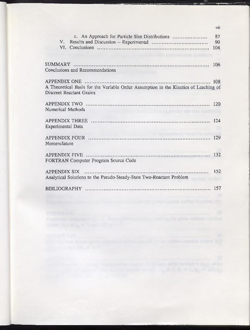
c. An Approach for Particle Size Distributions ........................... 87V. Results and Discussion — Experimental ............................................. 90VI. Conclusions ............................................................................................ 104

SUMMARY ................................................................................................................ 106Conclusions and Recommendations

APPENDIX ONE ...................................................................................................... 108A Theoretical Basis for the Variable Order Assumption in the Kinetics of Leaching of Discreet Reactant Grains

APPENDIX TWO .................................................................................................... 120Numerical Methods

APPENDIX THREE ................................................................................................ 124Experimental Data

APPENDIX FOUR ................................................................................................... 129Nomenclature

APPENDIX FIVE .................................................................................................... 132FORTRAN Computer Program Source Code

APPENDIX SIX .................................................................................................... 152Analytical Solutions to the Pseudo-Steady-State Two-Reactant Problem

vii

BIBLIOGRAPHY 157

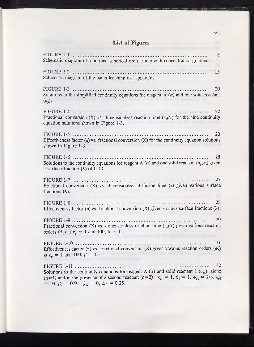
List of Figures

viii

FIGURE 1-1 ............................................................................................................ 8Schematic diagram of a porous, spherical ore particle with concentration gradients.

FIGURE 1-2 ............................................................................................................ 15Schematic diagram of the batch leaching test apparatus.

FIGURE 1-3 ............................................................................................................ 20Solutions to the simplified continuity equations for reagent A (a) and one solid reactant(O p ).

FIGURE 1-4 ............................................................................................................ 22Fractional conversion (X) vs. dimensionless reaction time (kp0t) for the nine continuity equation solutions shown in Figure 1-3.

FIGURE 1-5 ............................................................................................................ 23Effectiveness factor (rj) vs. fractional conversion (X) for the continuity equation solutions shown in Figure 1-3.

FIGURE 1-6 ...................................... ; .................................................................... 25Solutions to the continuity equations for reagent A (a) and one solid reactant (crp,ffs) given a surface fraction (X) of 0.10.

FIGURE 1-7 ............................................................................................................ 27Fractional conversion (X) vs. dimensionless diffusion time (r) given various surface fractions (X).

FIGURE 1-8 ............................................................................................................ 28Effectiveness factor (17) vs. fractional conversion (X) given various surface fractions (X).

FIGURE 1-9 ............................................................................................................. 29Fractional conversion (X) vs. dimensionless reaction time (/Cp0r) given various reaction orders (4>p) at kv = 1 and 100, 0 = 1.

FIGURE 1-10............................................................................................................. 31Effectiveness factor (rj) vs. fractional conversion (X) given various reaction orders (<f>p) at kp = 1 and 100, 0 = 1.

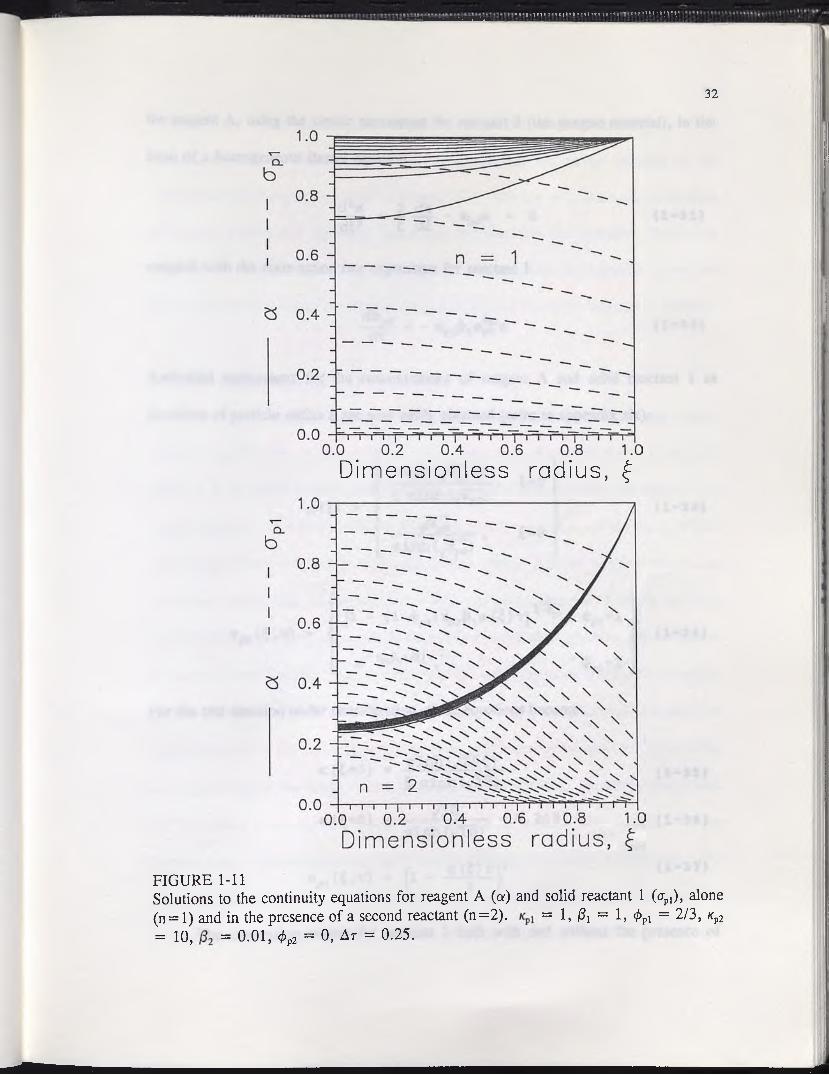
FIGURE 1-11 ............................................................................................................. 32Solutions to the continuity equations for reagent A (a) and solid reactant 1 (crpl), alone (n = l) and in the presence of a second reactant (n=2). ^ = 1, 0j = 1, <£pl = 2/3, kp2 = 10, 02 = 0.01, 0p2 = 0, Ar = 0.25.

IX

FIGURE 1-12............................................................................................................ 35Fractional conversion of solid reactant 1 (Xj) vs. dimensionless diffusion time (r) for the systems shown in Figure 1-11.

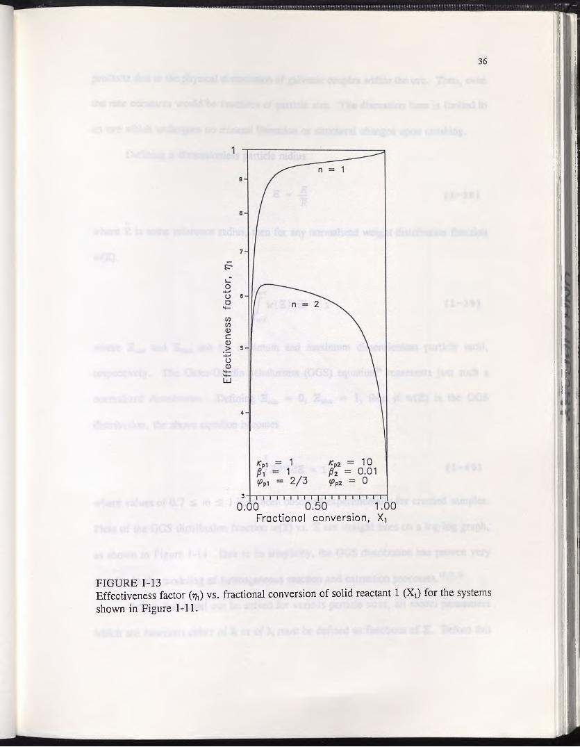
FIGURE 1-13............................................................................................................ 36Effectiveness factor fo) vs. fractional conversion of solid reactant 1 (X,) for the systems shown in Figure 1-11.

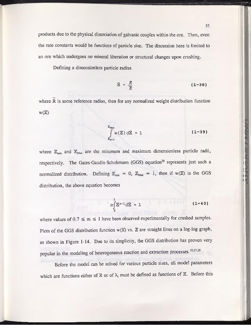
FIGURE 1-14............................................................................................................ 38The Gates-Gaudin-Schuhmann normalized weight distribution function (w(E)) vs. dimensionless particle size (S) at various values of the distribution parameter m.

FIGURE 1-15............................................................................................................ 42Fractional conversion for various particle sizes (X(E)) (solid curves), and for the entire size distribution (XT) (dotted curves) vs. reference diffusion time (7) for various values of the distribution parameter m.

FIGURE 1-16............................................................................................................ 43Effectiveness factor (77) vs. fractional conversion for various particle sizes (X(H)) at various particle sizes (S).

FIGURE 1-17................................................................................... 47Results of batch test 1.

FIGURE 1-18............................................................................................................ 48Results of batch test 2.

FIGURE 1-19............................................................................................................ 49Results of batch test 3.

FIGURE 1-20............................................................................................................. 50Results of batch test 4.

FIGURE 1-21............................................................................................................. 53Calculated effectiveness factor (77) vs. Ag conversion (X) for the batch leaching tests.

FIGURE 1-22............................................................................................................ 54Scanning electron micrograph (SEM) of pure silver powder used in the preparation of the artificial ore pellets. Magnification: lOOOx.

FIGURE 1-23 ............................................................................................................. 55Grain size distribution data from statistical image analysis of the silver powder sample shown in Figure 1-22.

FIGURE 2-1 ............................................................................................................ 61Schematic diagram of a heap.

FIGURE 2-2 ............................................................................................................ 68Schematic diagram of the experimental apparatus.

FIGURE 2-3 ............................................................................................................ 71Solutions to the simplified continuity equations for reagent A in the bulk solution (ab) and the fractional conversion (X) as functions of heap depth.

FIGURE 2-4 ............................................................................................................ 72Effluent concentration (xb(l,0)), fractional conversion (X) and extraction (E) vs. dimensionless flow time (6) given various values of /3 and co.

FIGURE 2-5 ............................................................................................................ 74Fractional conversion (X) vs. reaction time (kp(Sp<j:(6-1)/3), given various values of go.

FIGURE 2-6 ............................................................................................................. 76Heap effectiveness factor (r?) vs. fractional conversion (X) for the continuity equation solutions shown in Figure 2-3.

FIGURE 2-7 ............................................................................................................ 77Fractional conversion (X) vs. dimensionless flow time (0) given various surface fractions(X).

FIGURE 2-8 ............................................................................................................. 78Heap effectiveness factor (17) vs. dimensionless flow time (0) given various surface fractions (X).

FIGURE 2-9 ............................................................................................................. 80Fractional conversion (X) vs. dimensionless flow time (0) given various orders of reaction (</>p).

FIGURE 2-10............................................................................................................. 81Heap effectiveness factor (rj) vs. dimensionless flow time (0) given various orders of reaction (<f>p).

FIGURE 2-11 ............................................................................................................. 82Solutions to the continuity equations for reagent A (ab) and fractional conversion of reactant 1 (Xj), alone (n= l) and in the presence of a second reactant (n=2). = 1,f t = 1, </>„, = 2/3, kp2 = 10, 02 = 0.01, ^ = 0, co = 1, 1; = 1, Ad = 1.

FIGURE 2-12............................................................................................................. 85Fractional conversion of solid reactant 1 (Xj) vs. dimensionless flow time (0) for the systems shown in Figure 2-11.

XI

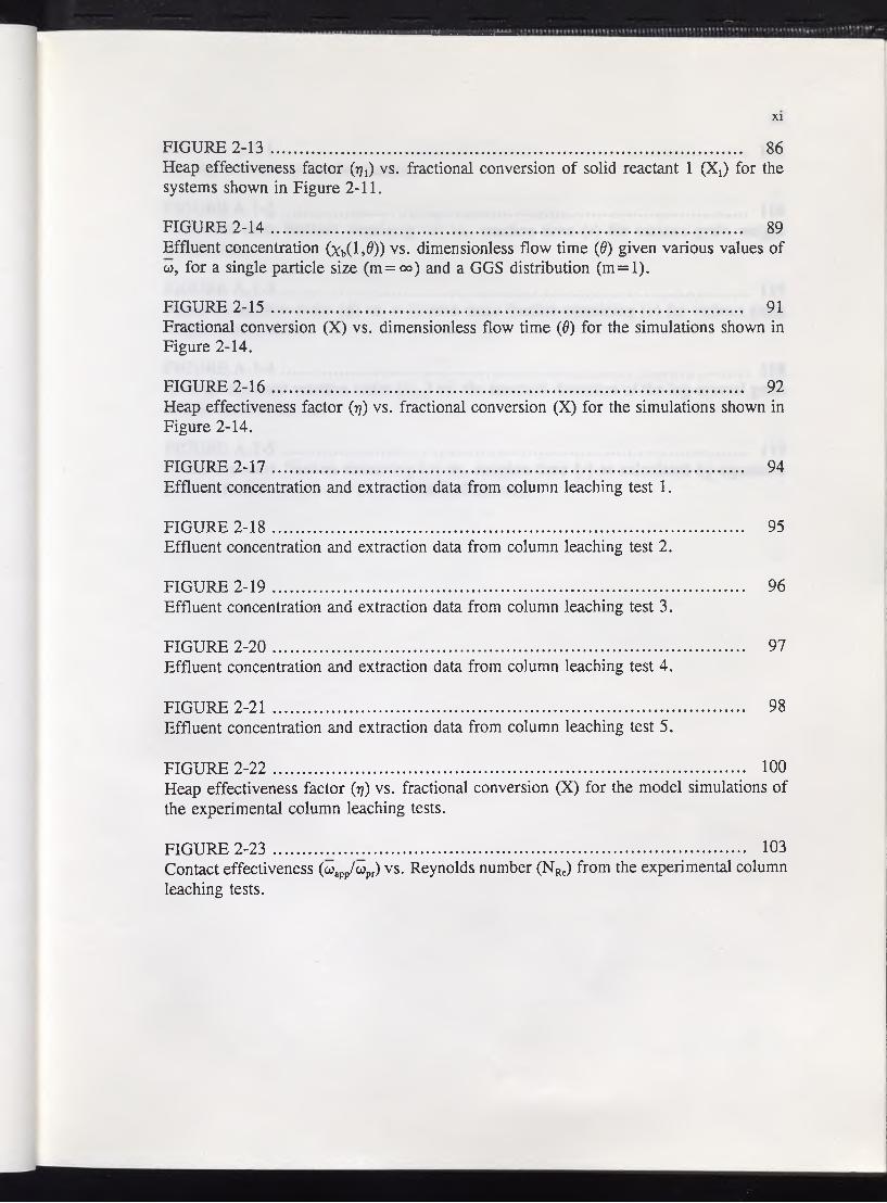
FIGURE 2-13............................................................................................................ 86Heap effectiveness factor (77,) vs. fractional conversion of solid reactant 1 (X,) for the systems shown in Figure 2-11.

FIGURE 2-14............................................................................................................ 89Effluent concentration (xb(M )) vs. dimensionless flow time (0) given various values of a), for a single particle size (m=oo) and a GGS distribution (m =l).

FIGURE 2-15............................................................................................................ 91Fractional conversion (X) vs. dimensionless flow time (6) for the simulations shown in Figure 2-14.

FIGURE 2-16............................................................................................................ 92Heap effectiveness factor (77) vs. fractional conversion (X) for the simulations shown in Figure 2-14.

FIGURE 2-17............................................................................................................ 94Effluent concentration and extraction data from column leaching test 1.


FIGURE 2-19............................................................................................................. 96Effluent concentration and extraction data from column leaching test 3.


FIGURE 2-21 ............................................................................................................. 98Effluent concentration and extraction data from column leaching test 5.

FIGURE 2-22............................................................................................................. 100Heap effectiveness factor (77) vs. fractional conversion (X) for the model simulations of the experimental column leaching tests.

FIGURE 2-23 ............................................................................................................. 103Contact effectiveness (coapp/upr) vs. Reynolds number (NRe) from the experimental column leaching tests.

FIGURE A. 1-1 .................................The log-normal distribution function.

xii

115

FIGURE A. 1 -2 ........................................................................................................... 116Collective mass fraction remaining (a) vs. reaction time (r) for various grain weight distributions.

FIGURE A. 1-3 ........................................................................................................... 117Apparent reaction order (&) vs. collective mass fraction remaining (a) for various grain weight distributions.

FIGURE A. 1-4 ........................................................................................................... 118Average apparent reaction order (<£avc) vs. the standard deviation of the log-normal grain weight distribution (s).

FIGURE A. 1-5 ........................................................................................................... 119Collective mass fraction remaining (a) vs. reaction time (r) as calculated by equations (A. 1-6) (solid curves) and (A. 1-1) (dashed curves).

List of Tables

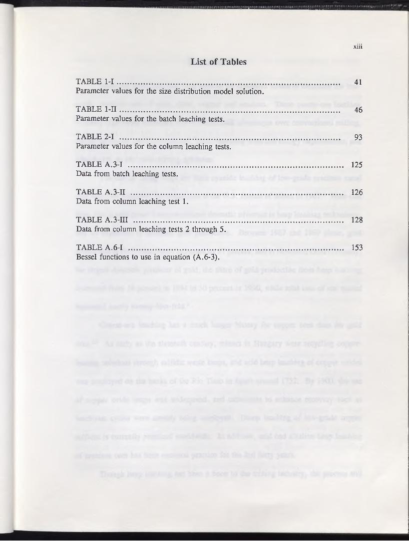
TABLE 1-1............................................................................................................... 41Parameter values for the size distribution model solution.

TABLE l - I I .............................................................................................................. 46Parameter values for the batch leaching tests.

TABLE 2-1 .............................................................................................................. 93Parameter values for the column leaching tests.

TABLE A.3-I ........................................................................................................... 125Data from batch leaching tests.

TABLE A.3-II .......................................................................................................... 126Data from column leaching test 1.

TABLE A.3-III ......................................................................................................... 128Data from column leaching tests 2 through 5.

TABLE A.6-I ........................................................................................................... 153Bessel functions to use in equation (A.6-3).

xiii

1

Introduction

Heap and dump leaching have become the dominant modes of treatment for low-

grade, oxidized ores of gold, silver, copper and uranium. These coarse-ore leaching

methods offer many economic and environmental advantages over conventional milling,

including smaller capital investment, lower operating costs and energy requirements, and

adaptability to any sized mining operation.

The idea of using heaps for basic cyanide leaching of low-grade precious metal

ores was first suggested by researchers at the U.S. Bureau of Mines in 1967.1 Since that

time, rising gold prices have precipitated dramatic advances in heap leaching technology,

and an explosion in domestic gold production. Between 1987 and 1989 alone, gold

production in the United States increased by 67 percent, and at Newmont Gold Company,

the largest domestic producer of gold, the share of gold production from heap leaching

increased from 19 percent in 1984 to 30 percent in 1990, while total tons of ore treated

increased nearly twenty-four-fold.2

Coarse-ore leaching has a much longer history for copper ores than for gold

ores.1,3 As early as the sixteenth century, miners in Hungary were recycling copper

bearing solutions through sulfidic waste heaps, and acid heap leaching of copper oxides

was employed on the banks of the Rio Tinto in Spain around 1752. By 1900, the use

of copper oxide heaps was widespread, and techniques to enhance recovery such as

leach/rest cycles were already being employed. Dump leaching of low-grade copper

sulfides is currently practiced worldwide. In addition, acid and alkaline heap leaching

of uranium ores has been common practice for the last forty years.

Though heap leaching has been a boon to the mining industry, the process still

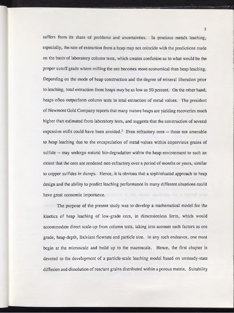
2

suffers from its share of problems and uncertainties. In precious metals leaching,

especially, the rate of extraction from a heap may not coincide with the predictions made

on the basis of laboratory column tests, which creates confusion as to what would be the

proper cutoff grade where milling the ore becomes more economical than heap leaching.

Depending on the mode of heap construction and the degree of mineral liberation prior

to leaching, total extraction from heaps may be as low as 50 percent. On the other hand,

heaps often outperform column tests in total extraction of metal values. The president

of Newmont Gold Company reports that many mature heaps are yielding recoveries much

higher than estimated from laboratory tests, and suggests that the construction of several

expensive mills could have been avoided.2 Even refractory ores — those not amenable

to heap leaching due to the encapsulation of metal values within impervious grains of

sulfide — may undergo natural bio-degradation within the heap environment to such an

extent that the ores are rendered non-refractory over a period of months or years, similar

to copper sulfides in dumps. Hence, it is obvious that a sophisticated approach to heap

design and the ability to predict leaching performance in many different situations could

have great economic importance.

The purpose of the present study was to develop a mathematical model for the

kinetics of heap leaching of low-grade ores, in dimensionless form, which would

accommodate direct scale-up from column tests, taking into account such factors as ore

grade, heap depth, lixiviant flowrate and particle size. In any such endeavor, one must

begin at the microscale and build up to the macroscale. Hence, the first chapter is

devoted to the development of a particle-scale leaching model based on unsteady-state

diffusion and dissolution of reactant grains distributed within a porous matrix. Suitability

3

of this model is shown experimentally in batch leaching tests of manufactured pellets

containing known amounts of pure silver powder.

In the second chapter, the particle leaching model is incorporated into an

unsteady-state heap-scale convection model. The results of column tests involving the

artificial ore pellets compare favorably with model simulations. An assumption

concerning the order of reaction within the model is examined in detail in the first

appendix, and a population balance model for a distribution of reactant grain sizes is

developed which clarifies the assumption.

Throughout the study, all model equations are solved with a digital computer

using numerical methods, since the complexity of those equations and the time- and

space-dependent nature of their boundary conditions generally precludes all possibility

of analytical solution. The specific mathematical techniques employed, and the

FORTRAN source code for the computer programs are reported in the second and fifth

appendices, respectively. Tabulated data from all batch and column leaching experiments

are reported in the third appendix. A full list of pertinent nomenclature is presented in

the fourth appendix. Finally, solutions to the model equations for a special case

involving the presence of a reactive gangue material are obtained in the sixth appendix.

Chapter OneA General Model for Leaching of One or More

Solid Reactants from Porous Ore Particles

I. Introduction

Many coarse-ore leaching processes involve the dissolution of one or more solid

reactants from an inert porous matrix. In recent years, the modeling of such phenomena

has received much attention, especially as it applies to the large-scale leaching processes

of copper sulfide ores. Braun et al.4 derived a model for leaching of primary sulfide ores

which assumed steady-state diffusion of dissolved oxygen as the rate controlling factor,

resulting in the formation of a narrow "reaction zone" which moves slowly toward the

center of the ore fragments, similar to the familiar "shrinking core" model for gas-solid

reactions.5 This model, which incorporates empirical rate enhancement parameters in

order to account for particle degradation under leach conditions, was shown to fit

experimental leaching data over a wide range of particle sizes and shapes,4,6 and has

subsequently been used as a basis for modeling large-scale in situ leaching processes.7

The model has recently been extended to the leaching of rocks containing more than one

copper sulfide mineral, each with its own specific rate constant.8

Models of copper sulfide leaching have not been limited to the shrinking core

type. A more general model involving the unsteady-state continuity equation for

dissolved oxygen in spherical coordinates was devised by Bartlett9 to describe the

leaching kinetics of low-grade chalcopyrite ores. In a low-grade ore, the rate of

diffusion is often fast compared to the reaction rate, so that reaction occurs

homogeneously throughout the particle. Bartlett’s model assumes a log-normal size

distribution of spherical copper sulfide grains, distributed evenly throughout the pore

4

5

structure. A modified version of this model was later verified experimentally in

autoclave leaching tests.10 A similar model, which assumes the steady-state diffusion of

ferric ion through the porous matrix to be rate controlling, was derived by Madsen and

Wadsworth,11 and included separate rate terms for a number of different copper sulfide

minerals, as well as empirical rate enhancement parameters.

While most of the attention has been focused on sulfides, several models have

been developed to describe acid leaching of copper oxide ores. Roman et al.,12 and

Shafer et al.13 were able to simulate the results of column leaching tests of a copper oxide

ore with the shrinking core model in unaltered form. More recently, Chae and

Wadsworth14 have incorporated the reaction zone model of Braun et al. into an in situ

copper oxide leaching simulation, accounting also for the consumption of acid by gangue

minerals, and the initial flushing of copper oxides from the external surfaces of ore

fragments.

Recently, Box and Prosser15 have attempted to derive a general model for the

leaching of several minerals with several reagents which requires no prior laboratory

testwork. In this model, reactions which occur at similar rates are lumped into cohesive

groups, and then each group is solved as a single reaction by the shrinking core model.

The procedure for solution of the model, however, is cumbersome, and an attempt at

simulating the experimental data of Hicban and Gray16 achieved only limited success.

Prosser17 has applied a modified version of the model to precious metal leaching with

basic cyanide solution, again with only limited success.

Bartlett18 was able to describe the leaching of oxidized gold ores with an unsteady-

state extraction model, solved by Crank in spherical coordinates,19 by assuming the actual

6

dissolution reaction to be near-instantaneous relative to the diffusion of dissolved species

out of the porous ore particle. A critical review of this and many of the other models

listed above has recently been published by Bartlett.20

In this chapter, a general model is derived which simulates the leaching of several

solid reactants from a porous particle with a common reagent. Like Bartlett’s sulfide

leaching model,9 the present model is based on the unsteady-state continuity equation for

a reagent species in spherical coordinates. Unlike Bartlett’s model, however, the

dissolution rate of each solid reactant is represented by a variable-order, power-law type

rate expression, a common practice in the modeling of non-catalytic gas-solid

reactions.21,22 Also, the model equations are made dimensionless for the purpose of

identifying the important design and scale-up parameters.

With this model it is possible to simulate not only reaction zone type, diffusion

controlled leaching, but also more homogeneous, reaction controlled leaching, as well

as those situations which fall somewhere in between, depending on the choice of

parameters. Also, any rate enhancement effects due to the presence of solid reactants

on the particle surface are easily determined, as well as the effects of different solid

reactant grain configurations, and of two or more solid reactants competing for the same

reagent.

n . Model Development

Derivation of Model Equations

Consider a porous, structurally uniform, spherical ore particle of radius R which

is submerged in a lixiviant solution, and which contains small amounts of solid reactants

evenly distributed along the pore walls, as shown in Figure 1-1. These solid reactants,

B;, are dissolved by a single reagent, A, according to the formula

7

n

A + b jB i - d i s s o l v e d p r o d u c t s ( 1- 1 )2=1

where b; are the stoichiometric numbers and n is the total number of solid reactants. At

any particle radius r, assuming that the dissolution of each solid reactant is first order in

the concentration of one rate-controlling reagent, and variable order in its own solid

concentration (see Appendix 1 for an in-depth discussion of the reasoning behind this

assumption), the rate of dissolution of solid reactant i may be expressed

d c ■pid t

= — js- r&P1 (i KpiCP2 CA ( 1- 2 )

where Cpi is the solid concentration of solid reactant i at the pore walls at particle radius

r, kpj is the reaction rate constant expressed per unit particle mass, CA is the reagent

concentration at particle radius r, and <f>pi is the reaction order in the solid concentration

of solid reactant i. Equation (1-2) has the initial condition

Cp i ( r , 0 ) = Cpi0 ( 1 - 3 )

Since every reaction within the particle involves the consumption of reagent A,

the mass balance for reagent A within the porous sphere takes the form of a continuity

8

Pore network

ore reactant deposits

O Particle radius, r R

CsO

(J)c0)r>o>Q.<X>■oOO)

Cs ‘

FIGURE 1-1Schematic diagram of a porous, spherical ore particle with concentration gradients.

9

equation with a summed consumption term

DAeP c Ad r 2

2 dC.r d r ~ P o d - e 0) £

T1 Tr-

2=1^ p i ^ p l A _ dC, 5 --- -

° a t( 1 - 4 )

where DAe is the effective diffusivity of reagent A within the particle pores, p0 is the

specific gravity of the ore matrix , and e0 is the porosity of the particle. In the interest

of simplicity, it is assumed that all of these parameters remain unchanged with time and

position. Equation (1-4) has initial and boundary conditions

CA( r , 0 )

Ca (R, t)

= 0

= c.Ab

dcAd r

(o , t) = 0

( 1 - 5 )

( 1 - 6 )

( 1 - 7 )

where CAb is the concentration of reagent A in the bulk solution external to the particle.

Most naturally occurring porous ore particles consist of tightly bound grains of

material. It is generally along the boundaries of these grains that the deposits of solid

reactants are found, and hence, these boundaries serve as the "pores" for intraparticular

diffusional processes. When ore is crushed for the purpose of exposing solid reactants

to the lixiviant solution, many of the grain boundary surfaces which would have been

accessible only via porous diffusion into the particle become accessible at the particle

surface. Therefore, it is necessary to account for the dissolution of these "surface

deposits" in addition to those within the pores of the particle. Of the previous

investigators, only Chae and Wadsworth14 have accounted for the leaching of surface

deposits in a large-scale coarse ore leaching model. However, they assumed the deposits

to be completely dissolved before any reagent enters the particle pores, i.e., that the two

10

dissolution processes (surface and intraparticular) occur in series. Here it is assumed that

the two processes occur in parallel.

Making the same assumptions concerning reaction order as for the intraparticular

reaction, the rate of dissolution of solid reactant i at the particle surface is written

dCsi 3 k r*'-1 r‘-'Ab ( 1 - 8 )d t R p0 ( i - e 0)

where Csi is the solid concentration of solid reactant i at the particle surface, is the

reaction rate constant expressed per unit particle surface area, and <£si is the reaction

order in the solid concentration of solid reactant i. Equation (1-8) has an initial condition

Cs i (0) = Csio ( 1 - 9 )

Model Equations in Dimensionless Form

For the purpose of finding the important parameters of the model, all of the above

equations are recast here in dimensionless form.

Defining the set of dimensionless variables

CA“ = CU AO b C° AO

0 • " Cpl p i r

CT . - ° s iS I (-1usiO

$ = Rx = DAet

e aR2

where CA0 is some reference reagent concentration, and recasting the model in

dimensionless terms allows one to define a set of dimensionless parameters:

11

e o^i<'A0 X -c .^SlO

Po ( l _eo) ^Eio CEio

Po( l ~ Go) kplCpf0R2 3 k gic tf0RKsi

where

c . = c . + c .

represents the total extractable solid reactant i in the ore particles, and where ft is a

dimensionless stoichiometric ratio which indicates reagent strength relative to the grade

of solid reactant i; \ is the fraction of solid reactant i residing on particle surfaces

initially; and /cpi and Ksi are the ratios of the reaction rate of solid reactant i within particle

pores and on the particle surface, respectively, to the porous diffusion rate of reagent A,

and correspond to Damkohler numbers of the second type.

The rate of dissolution of solid reactant i along the pore walls of a particle,

equation (1-2), is rewritten

do pidx

* p iP i (1 - ^ )

VPi

with initial condition

op i (Z,0) = 1

The continuity equation for reagent A, equation (1-4), becomes

( i - i o )

( i - i i )

d2a3£2

2 _8oc _ v-v$ 8$ 1=1

■pi°iiadec0X

( 1 - 1 2 )

with initial and boundary conditions

12

a ( 5 , 0 ) = 0 ( 1 - 1 3 )

a ( 1 , t ) = ( 1 - 1 4 )

I f l O . t ) = 0 ( 1 - 1 5 )

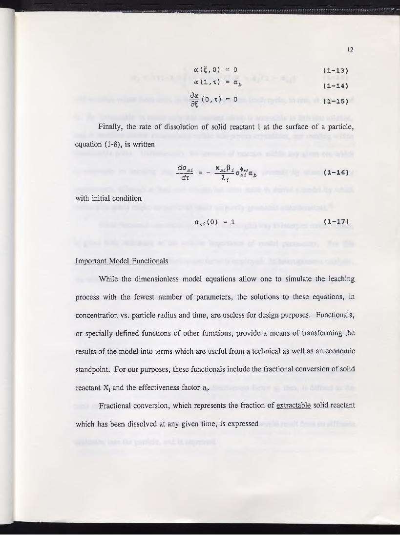
Finally, the rate of dissolution of solid reactant i at the surface of a particle,

equation (1-8), is written

d °si _ Ks i P i , A i „~ d T " " T T *

with initial condition

° Si ( 0 ) = 1

( 1 - 1 6 )

( 1 - 1 7 )

Important Model Functionals

While the dimensionless model equations allow one to simulate the leaching

process with the fewest number of parameters, the solutions to these equations, in

concentration vs. particle radius and time, are useless for design purposes. Functionals,

or specially defined functions of other functions, provide a means of transforming the

results of the model into terms which are useful from a technical as well as an economic

standpoint. For our purposes, these functionals include the fractional conversion of solid

reactant X; and the effectiveness factor 77;.

Fractional conversion, which represents the fraction of extractable solid reactant

which has been dissolved at any given time, is expressed

13

l= 3 ( 1 - A i ) f ( l - api)Vdl + ^ ( 1 - a si ) ( 1 - 1 8 )

0

and assumes values from zero, at the beginning of the leach cycle, to one, at the end of

it. By ’extractable’ is meant only that reactant which is accessible to lixiviant solution,

and is therefore neither encapsulated within non-porous crystallites, nor residing within

inaccessible pores. Unfortunately, the amount of reactant within any given ore which

is amenable to leaching may only be determined (at present) by actual leaching

experiments, although at least one attempt has been made to derive a model by which

extractable grade might be predicted based on purely geometric considerations.23

While fractional conversion provides a meaningful way to interpret model results,

it gives little indication of the relative importance of model parameters. For this

purpose, the concept of the effectiveness factor is employed. In heterogeneous catalysis,

the effectiveness factor is the total rate of reaction occurring within a catalyst particle

taken as a fraction of the "ideal" rate which would result if there were no diffusion

limitation into the particle, i.e., if the entire volume of the particle contained reagent at

the same concentration as at the surface of the particle. The effectiveness factor for non-

catalytic gas-solid reactions was introduced by Ishida and Wen.24 Here, their formulation

is extended to each solid reactant and incorporates the rates of reaction occurring along

the external surface of the particle. The effectiveness factor rit, then, is defined as the

total rate of dissolution of solid reactant i throughout the entire particle, including the

external surface, taken as a fraction of the total rate which would result from no diffusion

limitation into the particle, and is expressed

14

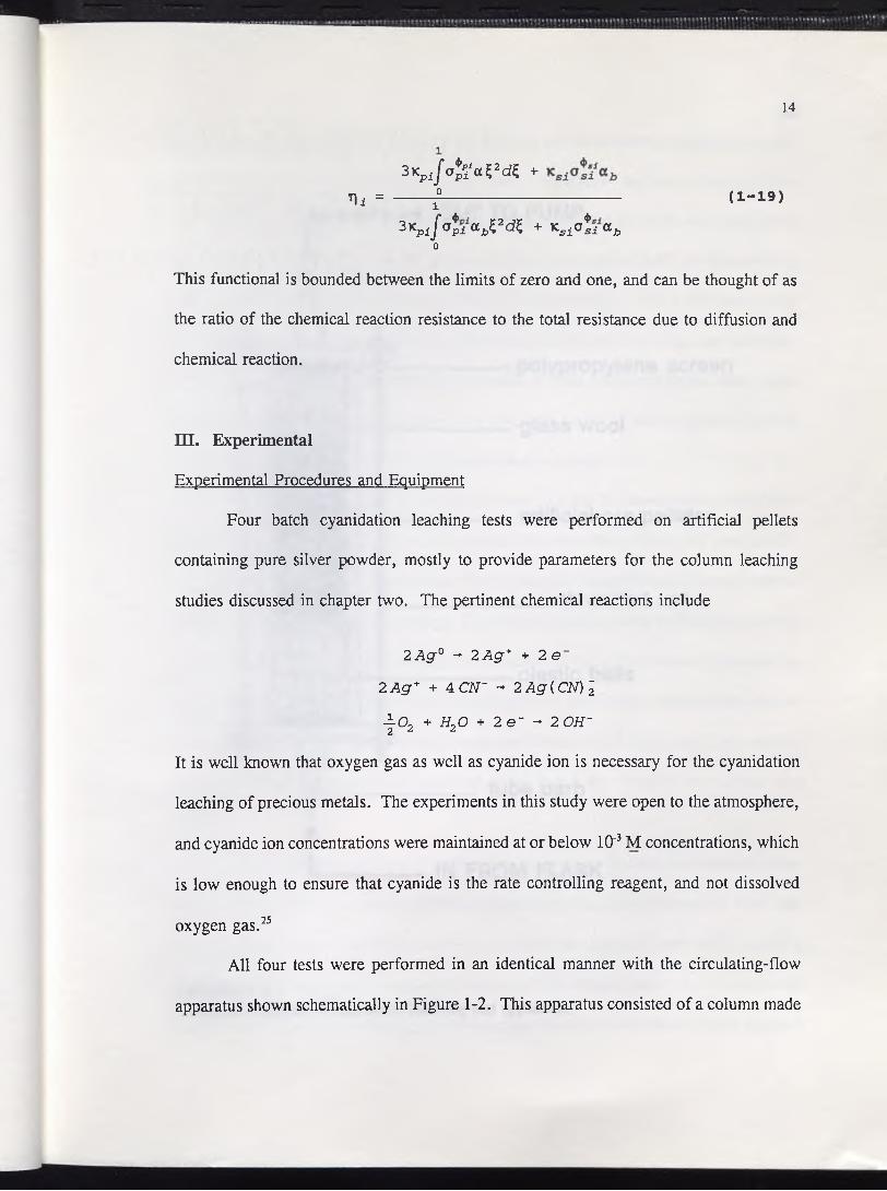
3Kp i / afeioCS2dS +T|i = ------ £------------------------------- d - 1 9 )

3 KP i f ai i “ i ,z2 d z + < s i a t i a b0

This functional is bounded between the limits of zero and one, and can be thought of as

the ratio of the chemical reaction resistance to the total resistance due to diffusion and

chemical reaction.

HI. Experimental

Experimental Procedures and Equipment

Four batch cyanidation leaching tests were performed on artificial pellets

containing pure silver powder, mostly to provide parameters for the column leaching

studies discussed in chapter two. The pertinent chemical reactions include

2 A g° - 2 A g + + 2 e "

2Ag* + 4 CN~ - 2Ag{CN)'2

- | 02 + HzO + 2 e~ - 2 OH~

It is well known that oxygen gas as well as cyanide ion is necessary for the cyanidation

leaching of precious metals. The experiments in this study were open to the atmosphere,

and cyanide ion concentrations were maintained at or below 10‘3 M concentrations, which

is low enough to ensure that cyanide is the rate controlling reagent, and not dissolved

oxygen gas.25

All four tests were performed in an identical manner with the circulating-flow

apparatus shown schematically in Figure 1-2. This apparatus consisted of a column made

► OUT TO PUMP

polypropylene screen

glass wool

artificial ore pellets

__ threaded rod

plastic balls

tube barb

IN FROM FLASK

FIGURE 1-2Schematic diagram of the batch leaching test apparatus.

16

from a 15 cm piece of transparent acrylic pipe 2.5 cm in diameter, sealed at each end

with a plexiglas plate fitted with a tube barb. The plate on the bottom end was

permanently cemented onto the end of the column, while the top plate was held tightly

in place by three threaded rods, as per the diagram. Sections of 0.95 cm Tygon tubing

were attached to the top and bottom of the column assembly. To the top section was

connected a Masterflex peristaltic pump fitted with #18 Masterflex tubing, and the bottom

section extended into a 2-liter Erlenmeyer flask. A third section of Tygon tubing went

from the flask to the pump, thus completing the circuit. A small teflon impeller operated

by an adjustable speed motor was submerged into the flask.

The column was filled in a certain manner in order to prevent the movement of

fine material through the pump, and to prevent the formation of stagnant zones within

the ore charge. First, a small circle of polypropylene screen was dropped into the

column. This was followed by enough 1 cm diameter plastic balls to fill approximately

4 cm of the column, in order to force the solution into plug flow before it reached the

ore charge. This was topped with a small patch of glass wool, followed by the ore

charge, another patch of glass wool, enough plastic balls to fill the column, and another

bit of screen to keep the plastic balls out of the exit hole. Finally, the column was

sealed.

After charging with 79 g of pellets, the column was flooded with distilled water

and allowed to drain in order to saturate the pellet pores. The Erlenmeyer flask was

filled with 2000 mL of lixiviant solution prepared from distilled water, and containing

sodium cyanide and sodium hydroxide, both at 10-3 M concentration. At time zero, the

impeller was activated, and the pump was engaged so that solution flowed from the flask

17

up through the column at a fast flowrate. The residence time of the column was only a

few seconds, and the tests were run over a period of days, so perfect mixing could be

assumed.

Samples were taken at increasing intervals over the course of each test, and

analyzed with a Perkin-Elmer Model 3100 Atomic Absorption Spectrometer (AAS).

While the readings were within the range of the prepared standard solutions, the samples

were aspirated directly to the AAS from the Erlenmeyer flask. Otherwise, 1 mL was

pipetted from the flask and diluted 10:1 in dilution tubes with stock cyanide solution.

Since only a few samples were taken from each test, no special precautions were taken

to replace the solution which was removed.

The AAS was fitted with a silver lamp under a current of 10 mA. The slit width

was 7 nm, and the wavelength was 338.3 nm, giving a linear calibration range of about

10 ppm silver. Standards used were 0 (blank), 1, 5, and 10 ppm silver, and were

prepared from a 1000 ppm silver-nitric acid standard solution and the stock cyanide

solution from the batch tests. The AAS output was set to zero for the blank standard,

and was read in Absorbance units in continuous mode. Cyanide ion concentration was

not analyzed during the experiments.

Artificial Ore Preparation

Two batches of artificial silver ore pellets were prepared from a mixture of 95

wt-% assay-grade silica sand, 2/3 left coarse and 1/3 pulverized fine; 5 wt-% Type II

Portland cement, and small amounts of 99.9% pure silver powder, supplied by Johnson-

Matthey Electronics, and measuring 4 yum to 7 /im diameter. In one batch, 34.2 g of

18

silver powder was added to 50 kg ore, resulting in a grade of 6.34 x Id 6 mol Ag/g ore,

or 20 Troy oz Ag/ton. In the other batch, 0.206 g of silver powder was added to 3 kg

ore, resulting in a grade of 6.34 x 10'7 mol Ag/g ore, or 2 Troy oz/ton.

Each batch was mixed for several hours in a cement mixer fitted with a plastic

insert, then agglomerated with tapwater on a laboratory disk pelletizer, resulting in

pellets ranging from about 0.5 to 2 cm in diameter. The wet pellets were allowed to

cure under cover for several weeks. They became strong enough not to break when

dropped on the floor, but were prone to abrasion, necessitating quite careful handling.

IV. Results and Discussion — Theoretical

Computer Simulation: One Solid Reactant

In order to examine its general behavior, the following restrictions are applied

temporarily to the model: 1) only one solid reactant (n = 1), 2) first-order rate dependence

in the solid reactant concentration (</>p = 1), 3) no surface deposits of solid reactant (A=0),

and 4) constant bulk reagent concentration (ab= l). The continuity equation for reagent

A, equation (1-12), now becomes

w = -|5-d i2 i di p p a-c(1-2 0)

and the rate expression for disappearance of the solid reactant, equation (1-10),

dap _

dx = ~ KpPapa (1-2 1 )

These equations have initial and boundary conditions

19

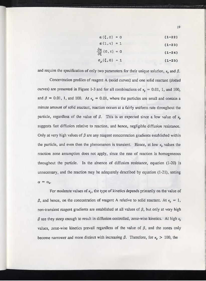
a (5,0) = 0 a ( l , x ) = 1

(1-2 2 )( 1 - 2 3 )

( 1 - 2 4 )

ap ($,0) = 1 ( 1 - 2 5 )

and require the specification of only two parameters for their unique solution, kp and (3.

Concentration profiles of reagent A (solid curves) and one solid reactant (dotted

curves) are presented in Figure 1-3 and for all combinations of ^ = 0.01, 1, and 100,

and /3 = 0.01, 1, and 100. At kp = 0.01, where the particles are small and contain a

minute amount of solid reactant, reaction occurs at a fairly uniform rate throughout the

particle, regardless of the value of /?. This is as expected since a low value of np

suggests fast diffusion relative to reaction, and hence, negligible diffusion resistance.

Only at very high values of jS are any reagent concentration gradients established within

the particle, and even then the phenomenon is transient. Hence, at low values the

reaction zone assumption does not apply, since the rate of reaction is homogeneous

throughout the particle. In the absence of diffusion resistance, equation (1-20) is

unnecessary, and the reaction may be adequately described by equation (1-21), setting

a = ab.

For moderate values of kp, the type of kinetics depends primarily on the value of

/3, and hence, on the concentration of reagent A relative to solid reactant. At ^ = 1,

non-transient reagent gradients are established at all values of 13, but only at very high

(3 are they steep enough to result in diffusion controlled, zone-wise kinetics. At high ^

values, zone-wise kinetics prevail regardless of the value of (3, and the zones only

become narrower and more distinct with increasing /?. Therefore, for kp > 100, the

20

/? = 0.01

/? = 1

jS = 100

/cp = 0.01 Ka = 1 Kp = 100

At = 100

0.0 0.2 0.4 0.6 0.8 1.0

At = 0.01

0.0 0.2 0.4 0.6 0.8 1.0

At = 0.001

FIGURE 1-3Solutions to the simplified continuity equations for reagent A (a) and one solid reactant Op)-

21

reaction zone assumption becomes valid regardless of the reagent concentration, and the

steady-state approximation may safely be applied to equation (1-20).

The parameter /3 represents the ratio of stoichiometric equivalents of reagent to

solid reactant. In a particle of given porosity, a value of ft = 1 signifies that the pores

of the particle would contain just enough reagent to dissolve all extractable solid reactant

i present in the particle, if the pores could be completely filled with reagent at

concentration a = 1. Hence, it should be noted that for most applications of interest,

/3 will assume a value less than one.

Figure 1-4 shows the relation between fractional conversion and relative reaction

time for the nine model solutions in Figure 1-3. As is expected, the relative conversion

rates are essentially identical in the chemical reaction controlled situations, but decrease

dramatically with increasing diffusion resistance.

The relative magnitudes of diffusion and reaction resistance are most conveniently

illustrated in semi-log plots of effectiveness factor vs. conversion, as shown in Figure

1-5. At kp = 0.01, rj rapidly approaches unity at all values of /3. At kp = 1, the shape

of the r?-X curve changes dramatically between /3 = 10 and j3 = 100, signifying a shift

from reaction controlled to diffusion controlled kinetics. However, all rj-X curves

approach unity near complete conversion, which is the case for all one-reactant systems.

Finally, at kp = 100, the diffusion controlled behavior is well established at all 13 values.

After attaining a peak due to the initial transient influx of reagent into the barren pores,

the effectiveness factor decreases to a minimum. This corresponds to the reaction zone

moving toward lower reagent concentrations near the center of the particle. Once the

leading edge of the reaction zone reaches the center of the particle, the tj-X curves turn

Fra

ctio

nal

conv

ersi

on

22

FIGURE 1-4Fractional conversion (X) vs. dimensionless reaction time (3t) for the nine continuity equation solutions shown in Figure 1-3.

23

FIGURE 1-5Effectiveness factor (tj) v s . fractional conversion (X) for the continuity equation solutions shown in Figure 1-3.

24

up toward unity, similar to the effectiveness factor plots reported by Ishida and Wen for

a zero-order solid-gas reaction system.24

Relaxing the restriction of no surface deposits (X^O), and also assuming first-

order rate dependence at the surface (<£s= 1), the surface rate expression, equation (1-16),

becomes

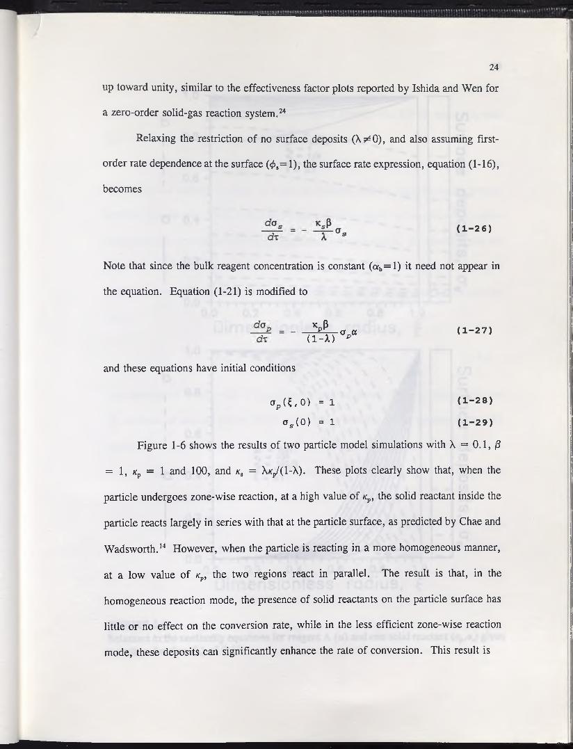
( 1 - 2 6 )

Note that since the bulk reagent concentration is constant (ab= l) it need not appear in

the equation. Equation (1-21) is modified to

«pP(l-X) a ap

and these equations have initial conditions

( 1 - 2 7 )

®p ( 5 , 0) = 1 d - 2 8 )

CTs (0 ) = 1 ( 1 - 2 9 )

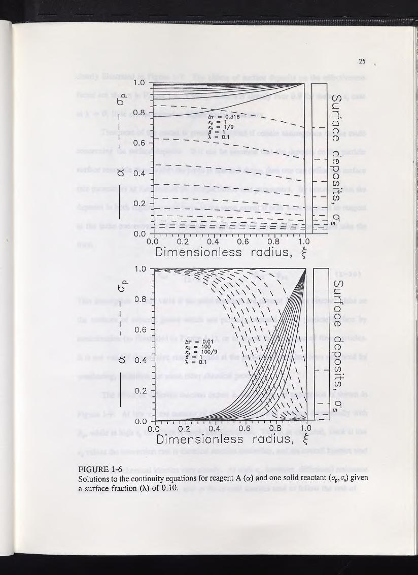
Figure 1-6 shows the results of two particle model simulations with X = 0.1, /3

= 1, kp = 1 and 100, and ks = Xkp/(1-X). These plots clearly show that, when the

particle undergoes zone-wise reaction, at a high value of kv, the solid reactant inside the

particle reacts largely in series with that at the particle surface, as predicted by Chae and

Wadsworth.14 However, when the particle is reacting in a more homogeneous manner,

at a low value of kp, the two regions react in parallel. The result is that, in the

homogeneous reaction mode, the presence of solid reactants on the particle surface has

little or no effect on the conversion rate, while in the less efficient zone-wise reaction

mode, these deposits can significantly enhance the rate of conversion. This result is

25

— - 0 3

LDc—hQOCD

Q_ CD

"O O CD ^i—HCO

b

b 0.4 -

i i i ~rp 0.0 0.2

i—i—|—rn i r 0.8 1.0

Dimensionless radius, f

FIGURE 1-6Solutions to the continuity equations for reagent A (a) and one solid reactant (ap,a^ given a surface fraction (X) of 0.10.

26

clearly illustrated in Figure 1-7. The effects of surface deposits on the effectiveness

factor are shown in Figure 1-8. Clearly, since rj is already over 0.9 for the low /cp case

at X = 0, little can be gained at higher surface fractions.

Treatment of the model is greatly simplified if certain assumptions can be made

concerning the surface deposits. If it can be assumed that the deposits on the particle

surface resemble those within the pores in size and shape, then one can define the surface

rate parameters as functions of the intraparticular rate parameters. By assuming that the

deposits in both regions would react to the same extent if both were exposed to reagent

at the same concentration for the same length of time, the surface parameters take the

form

Ksi - tsi - 4>pi ( 1 - 3 0)

This assumption is only valid if the solid reactants are present only as discreet blebs on

the surfaces of mineral grains which are partially exposed at the particle surface by

comminution (as illustrated in Figure 1-1), or in bound agglomerates of finer particles.

It is not valid if the relative reactant grade at the particle surface has been enhanced by

weathering, oxidation, or some other chemical process.

The effect of different reaction orders <£p on the rate of conversion is shown in

Figure 1-9. At low kp, the contour of the conversion curve changes dramatically with

<j) while at high Kj, the effect is much less significant. This is as expected, since at low

K values the conversion rate is chemical reaction controlled, and the overall kinetics tend

to follow the chemical kinetics very closely. At high kp, however, diffusional resistance

outweighs chemical resistance, and so the overall kinetics tend to follow the rate of

27

Dimensionless diffusion time, r

Dimensionless diffusion time, t

FIGURE 1-7Fractional conversion (X) vs. dimensionless diffusion time (r) given various surface fractions (X).

28

oocoCO<DcCD>+•>o0)

LU

FIGURE 1-8Effectiveness factor (rj) vs. fractional conversion (X) given various surface fractions (X).

29

FIGURE 1-9Fractional conversion (X) vs. dimensionless reaction time (k t) given various reaction orders (<£p) at kp = 1 and 100, 13 = 1.

30

reagent diffusion into the particle, which is far less dependent on reaction order. As

shown in Figure 1-10, at kv = 100, the shape of the tj-X curves changes with changing

4>P, but not necessarily the overall magnitude.

Computer Simulation: Competing Solid Reactants

In the presence of one or more reactants competing for reagent A, the kinetics of

conversion of a valuable mineral component can be significantly altered. Figure 1-11

shows the concentration gradients of reagent A and one solid reactant with ^ — 1, /3a

= 1, and $pl = 2/3, and no surface deposits. A value of (£pl = 2/3 implies that solid

reactant 1 is present as discreet spherical blebs of uniform size (see Appendix 1). In one

simulation the reactant is alone, and in the other it is accompanied by a reactive "gangue"

material with *p2 = 10, /?2 = 0.01, and </>p2 = 0, also with no surface deposits. At these

parameter values it is assumed that there is one hundred times more solid reactant 2 than

1, and its intrinsic reaction rate is ten times slower. Also, a value of </>p2 = 0 implies

that the gangue material forms an even coating over the pore walls of the particle, or

could even be the ore matrix material itself.

By itself, solid reactant 1 reacts effectively throughout the particle, and the

reagent concentration gradients are not significant. In the presence of solid reactant 2,

however, the reaction shifts more toward the particle surface, and the reagent gradients

are steep, with a < 0.3 at the particle center. Also, the reagent gradients do not change

significantly with time, since the reagent demand of reactant 2 does not vary over the

entire course of leaching of reactant 1. Hence, the conversion kinetics of reactant 1

could be approximately described in this special case by a steady state continuity equation

31

ooCOCOCDc0>u0

LlJ

FIGURE 1-10 . ., .Effectiveness factor ft) v s . fractional conversion (X) given various reaction orders (4>P)at kp = 1 and 100, j3 = 1.

» » . y • ? n > i * 1 1 j * »* * 1 1 \ »• * ; s • * i \ t ' .* ■ * ? * ! ' * ! \ * V

32

Dimensionless radius, £

FIGURE 1-11Solutions to the continuity equations for reagent A (a) and solid reactant 1 (apl), alone (n = l) and in the presence of a second reactant (n=2). = 1, ft = 1, <£pl = 2/3, /cp2= 10, = 0.01, </>p2 = 0, AT = 0.25.

33

for reagent A, using the kinetic parameters for reactant 2 (the gangue material), in the

form of a homogeneous Bessel equation

d 2a ciad$2 5 dl ~ *P2a 0

coupled with the mass-action rate expression for reactant 1

( 1 - 3 1 )

dadx

pi -= - K’PiPl°VplPi a ( 1 - 3 2 )

Analytical expressions for the concentrations of reagent A and solid reactant 1 as

functions of particle radius £ are now easily obtained (refer to appendix six):

a ( 0 =

s i n h ( ^ $ )£ s i n h

5=0p 2

s i n h ( y / k ^ )

( 1 - 3 3 )

api ( 5 / t ) = •

[1 - ( lHfrpjjKpiPiCC ( 5 ) X] ^ P1 , 4>p l * l

KpiP 4>pi =i

For the test situation under consideration, these equations become

( 1 - 3 4 )

a(5*0)

a (£=0)

- (i -

s i n h ( / 1 0 £ )

£ s i n h ( / T o )

y/To s i n h ( v T O )

a(£) t \ 3

= 0 . 2 6 8

( 1 - 3 5 )

( 1 - 3 6 )

( 1 - 3 7 )

The conversion curves for reactant 1 both with and without the presence of

34

reactant 2 are shown in Figure 1-12. As expected, the conversion when n = 2 is

significantly delayed relative to n = 1. The effect of the second reactant on the

effectiveness factor r\x is illustrated in Figure 1-13. When n = 2, the curve does

not approach unity near complete conversion, but does just the opposite. This is the

norm for all minor constituents of multi-reactant systems, since the reagent is maintained

at low concentrations near the center of the particle until the major reactant is depleted.

An Approach for Particle Size Distributions

In order to apply a leaching model based on the particle scale to any real coarse-

ore leaching situation, it must be solved for a distribution of particle sizes. In order to

do this it is necessary to solve the model for a number of different sizes and integrate the

results together. This may present serious difficulties because it is not always clear how

process parameters will change with particle size. Much depends on the structure and

mineralogy of the ore. If, for instance, a highly porous low-grade oxide ore has been

crushed prior to leaching, there may be little difference between the various size fractions

in terms of their leaching characteristics, and the only parameter that would change is

particle size itself. However, if the ore is not very porous, such that solid reactants are

inaccessible to the lixiviant solution, then these reactants may be liberated by crushing

to varying degrees depending on the particle size. In that case, the extractable grades

of the various solid reactants would be a function of particle size, as well. In the

extreme case, leaching chemistry itself may be a strong function of particle size. If a

copper sulfide ore consists of cemented grains of pyrite and chalcopyrite bound within

an inert gangue material, different size fractions may actually yield different reaction

Fra

ctio

nal

conv

ersi

on,

35

FIGURE 1-12Fractional conversion of solid reactant 1 (X,) vs. dimensionless diffusion time (r) for the systems shown in Figure 1-11.

36

Fractional conversion, X-[

FIGURE 1-13Effectiveness factor (17,) vs. fractional conversion of solid reactant 1 (Xj) for the systems shown in Figure 1-11.

37

products due to the physical dissociation of galvanic couples within the ore. Then, even

the rate constants would be functions of particle size. The discussion here is limited to

an ore which undergoes no mineral liberation or structural changes upon crushing.

Defining a dimensionless particle radius

where R is some reference radius, then for any normalized weight distribution function

w(E)

where Emin and EMax are the minimum and maximum dimensionless particle radii,

respectively. The Gates-Gaudin-Schuhmann (GGS) equation26 represents just such a

normalized distribution. Defining = 0, EMax = 1, then if w(E) is the GGS

distribution, the above equation becomes

where values of 0.7 < m < 1 have been observed experimentally for crushed samples.

Plots of the GGS distribution function w(E) vs. E are straight lines on a log-log graph,

as shown in Figure 1-14. Due to its simplicity, the GGS distribution has proven very

18 27 28popular in the modeling of heterogeneous reaction and extraction processes.

Before the model can be solved for various particle sizes, all model parameters

which are functions either of R or of \ must be defined as functions of E. Before this

RR

( 1 - 3 8 )

( 1 - 3 9 )

l( 1 - 4 0 )

0.01 . , ° - 1 ,Dimensionless particle size, a

FIGURE 1-14 . . . . . . . ,-vT h e G ates-G audin-Schuhm ann normalized w eig h t distribution function (w (a )) vs.dimensionless particle size (S) at various values of the distribution parameter m.

39

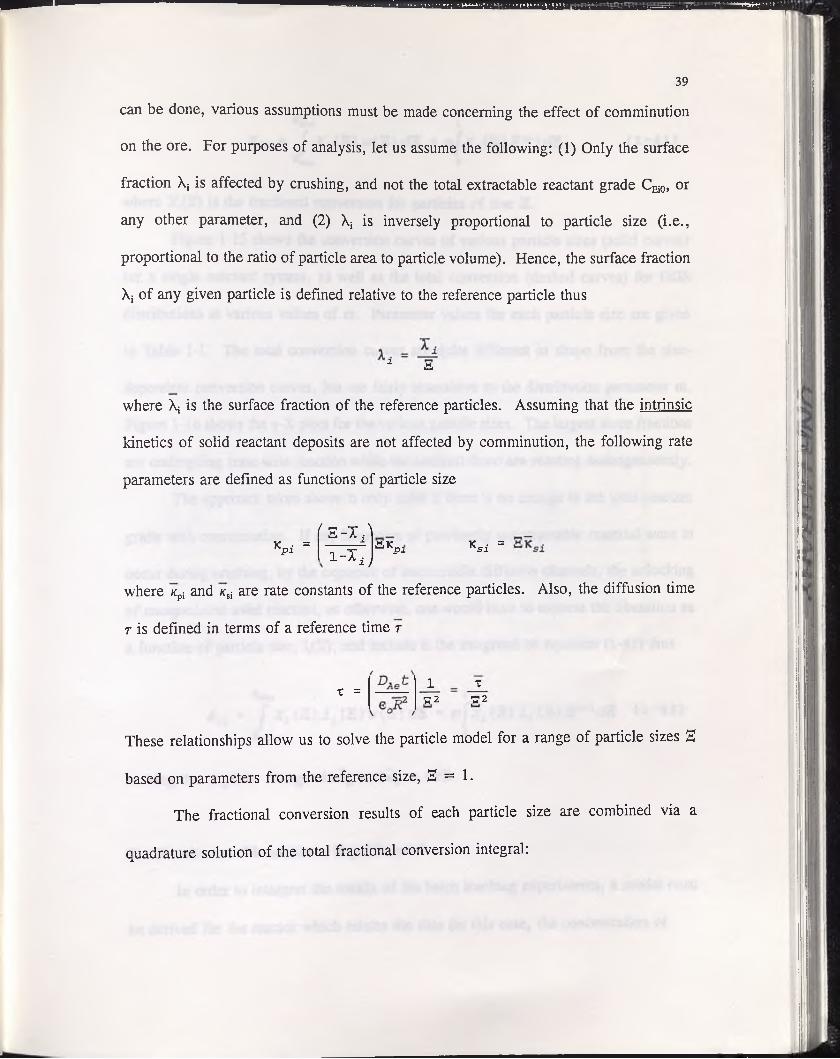
can be done, various assumptions must be made concerning the effect of comminution

on the ore. For purposes of analysis, let us assume the following: (1) Only the surface

fraction X; is affected by crushing, and not the total extractable reactant grade CEi0, or

any other parameter, and (2) X; is inversely proportional to particle size (i.e.,

proportional to the ratio of particle area to particle volume). Hence, the surface fraction

X; of any given particle is defined relative to the reference particle thus

1 a

where \ is the surface fraction of the reference particles. Assuming that the intrinsic

kinetics of solid reactant deposits are not affected by comminution, the following rate

parameters are defined as functions of particle size

Kpi =( B- Xj )

1 - * i ,iSK'Pi KSi =

where xpi and Ksi are rate constants of the reference particles. Also, the diffusion time

r is defined in terms of a reference time r

x =1T72

T■32

These relationships allow us to solve the particle model for a range of particle sizes g

based on parameters from the reference size, S = 1.

The fractional conversion results of each particle size are combined via a

quadrature solution of the total fractional conversion integral:

40

aMX 1Xn = / Xi (Z)w(E)dZ = mfxi (S)B*-1d3 ( 1 - 4 1 )

min 0

where X;(2) is the fractional conversion for particles of size 2.

Figure 1-15 shows the conversion curves of various particle sizes (solid curves)

for a single reactant system, as well as the total conversion (dashed curves) for GGS

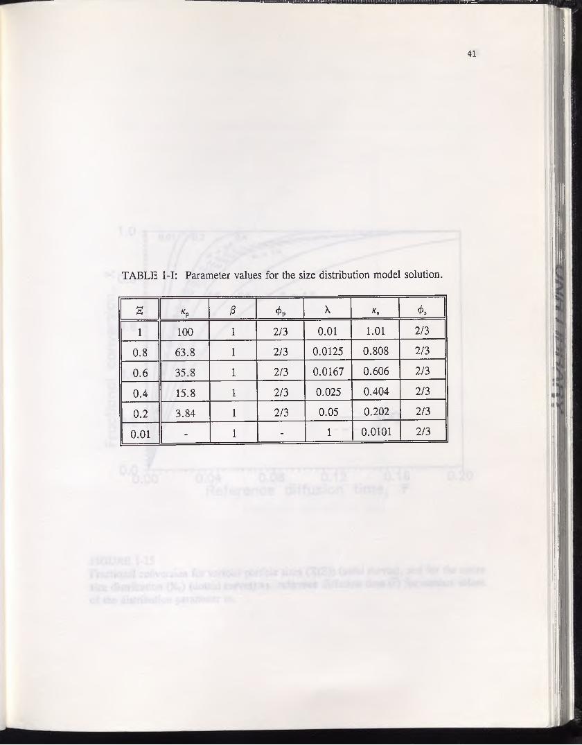
distributions at various values of m. Parameter values for each particle size are given

in Table 1-1. The total conversion curves are quite different in shape from the size-

dependent conversion curves, but are fairly insensitive to the distribution parameter m.

Figure 1-16 shows the rj-X plots for the various particle sizes. The largest three fractions

are undergoing zone-wise reaction while the smallest three are reacting homogeneously.

The approach taken above is only valid if there is no change in the total reactant

grade with comminution. If any liberation of previously unextractable material were to

occur during crushing, by the exposure of inaccessible diffusion channels, the unlocking

of encapsulated solid reactant, or otherwise, one would have to express the liberation as

a function of particle size, 1,(2), and include it the integrand of equation (1-41) thus

^ Max 1

XTi= f x I (3)l1(3)w(3)dS = mfx1(S)li (E)S--1dS ( 1 - 4 2 )

srain 0

making the requisite changes in Kpi and * si as well.

V. Results and Discussion ~ Experimental

In order to interpret the results of the batch leaching experiments, a model must

be derived for the reactor which relates the data (in this case, the concentration of

41

TABLE IT: Parameter values for the size distribution model solution.

2 *p 0 4>P X Ka &

1 100 1 2/3 0.01 1.01 2/3

0.8 63.8 1 2/3 0.0125 0.808 2/3

0.6 35.8 1 2/3 0.0167 0.606 2/3

0.4 15.8 1 2/3 0.025 0.404 2/3

0.2 3.84 1 2/3 0.05 0.202 2/3

0.01 - 1 - 1 0.0101 2/3

42

FIGURE 1-15 . . tFractional conversion for various particle sizes (X(S)) (solid curve^), and for the entire size distribution (Xx) (dotted curves) vs. reference diffusion time (t) for various values of the distribution parameter m.

43

5

oD

ww0c0>o0

UJ

FIGURE 1-16 E ffe c t iv e n e ss factor (y) v s . v a r io u s p artic le s izes ( a ) .

fractional conversion for various particle sizes (X(a)) at

, r -

dicyanoargentate ion, Ag(CN)2', in the batch lixiviant) to the general leaching model

derived in section II.

First, one needs an equation which represents the mass balance of reagent A

within the batch lixiviant: consumption by ore pellets = accumulation in batch lixiviant.

This is written, in dimensionless form

44

- 3 ( |f ) = v-3a,dx

and has an initial condition

a , ( 0 ) = l

where v is redefined thus

( 1 - 4 3 )

( 1 - 4 4 )

V =e0d “ ei)

and where eb is the ratio of the volume of batch lixiviant to the total volume of lixiviant

plus ore pellets. Since pellet sizes were kept fairly uniform in each batch leaching test,

the size distribution integral has been left out of equation (1-43).

Next, if one ignores the dissolved reactant species held up within the pellet pores

(legitimate if v is very large), then the fractional conversion may be defined in terms of

the batch lixiviant concentration of dissolved reactant species thus

* i = PivXii, ( 1 - 4 5 )

where

Xi*'ib

^i^AO —

45

and where Cib is the concentration of dissolved reactant species in the batch lixiviant.

Data from the experimental batch tests can now be simulated with the general model.

Now one can see why 79 g of pellets were used in all of the tests. It is because

this resulted in integer values for the product fiv. These values were: 2 in the high-grade

pellet tests, and 20 in the low-grade pellet test. Careful inspection will show that this

product actually represents the stoichiometric excess of rate-controlling reagent in the

batch at time zero. Thus, there was twice as much cyanide as was needed for full

conversion in the high-grade tests, and 20 times as much in the low-grade test.

Results of the batch tests are shown in Figures 1-17 through 1-20, and Table l-II

summarizes the parameters involved. The leaching tests of the high-grade particles

(Figures 1-17 through 1-19) provided an estimate of the effective diffusivity, DAe, based

on the apparently (by inspection of the datacurve shapes) diffusion-controlled kinetics of

all three situations. The low-grade ore leaching test (Figure 1-20) provided the estimate

of the variable reaction order, </>p, due to the apparently reaction-controlled kinetics

manifested in that test.

It is interesting to note that, if the effective diffusivity is assumed to obey

DjuP o (1-46)u ke T*'o

where DAB is the bulk diffusivity and r0 the tortuosity of the porous medium, then the ore

pellets have a tortuosity of r0 = 1.58. The theoretical tortuosity of a bed of packed

spheres is r0 = tt/2 = 1.57, which is ratio of the length of the shortest path around a

spherical obstacle to its diameter. The literature suggests taking a value for the tortuosity

of Tq = 2 in all leaching simulations,20 but for pellets made up of packed particles, or

46

TABLE l-II: Parameter values for the batch leaching tests. (All units cgs. Concentrations based on gmols.)

Parameters Batch test 1 Batch test 2 Batch test 3 Batch test 4

Ore mass 79 79 79 79

Soln. volume 2000 2000 2000 2000

b 0.5 0.5 0.5 0.5

n > o i o -6 IO’6 i o -6 IO'6

Cpo 6.34 -IO'7 6.34-IO'6 6.34-IO'6 6.34-IO'6

o Ae* 2.35 • IO6 2.35 • IO6 2.35-IO-6 2.35 • 10'6

k p * 3.76-107 3.76-IO7 3.76-IO7 3.76-IO7

R 0.68 0.86 0.60 0.62

0 0.094 0.0094 0.0094 0.0094

eb 0.977 0.977 0.977 0.977

e0 0.20 0.20 0.20 0.20

Kp 10 1600 780 830

V 213 213 213 213

Po 2.1 2.1 2.1 2.1

2 2 2 2

^Determined from the experimental results.* Calculated from experimentally determined values.

Convers

ion

47

FIGURE 1-17Results of batch test 1.

48


49

00

0.8 -

0.6 -

0.4 -

0 .0

—^ aa

a

/ a/ a / • Batch test 3:

/ • Kp = 780<P? = 2|S = 0.0094

i i i i i—i—i—i i n i i i i i i i i i i0 10 15 20

Dimensionless diffusion time, r


50

FIGURE 1-20 Results of batch test 4.

agglomerates of fine material, perhaps r0 = ir/2 is a more realistic assumption.

Since the pellets had a high porosity, and were known to be homogeneous, it was

assumed that no significant surface deposits were present. Thus, only the parameters kp,

4>p, and the ratio r/t had to be determined for the general leaching model, j8 and v being

given from direct measurements and the operating conditions of the tests. The ratio r/t

was obtained from matching model curves to the data from the three high-grade leaching

tests. This number was then used to non-dimensionalize the data from the low-grade

leaching test, after which kp was adjusted until the initial slopes of the model curve and

the data curve matched. Only then was <t>p adjusted until the most satisfactory fit of the

entire curve was obtained. Finally, the value of <f>p was used to calculate kp for the high-

grade tests. Thus, even though the ratio of grades between the two pellet batches was

only 1:10, since ^ is proportional to the ore grade taken to the </>p power, an order of 4>p

= 2 results in a 1:100 ratio in kp values. Of course, this increase is enough to transform

kinetics from the homogeneous regime to the zone-wise regime (refer to Figure 1-3,

above). The validity of this approach is borne out by comparing the results of the low-

grade test in Figure 1-17 to the results of the large-diameter high-grade test in Figure 1-

18, where kp was chosen strictly on the basis of the model fit of the low-grade test.

Figures 1-19 and 1-20 show the results of duplicate tests of medium-diameter

high-grade pellets. The model fits are excellent up to about X = 0.4, after which the

model overshoots the data by a consistent AX of about 0.1. This phenomenon is difficult

to explain. It may not be purely coincidental that X = 0.4 corresponds to Cb » 10 ppm,

the top of the linear calibration range, and therefore marks the spot where the samples

were no longer aspirated directly from the reactor flask, but had to be pipetted out and

52

diluted 1:10. How much error was introduced into the data as a result of dilution is,

however, impossible to ascertain. Whatever the cause, the important thing to notice from

the plots is how accurately the model simulated the rate of reaction (i.e., the slope of the

data) with time, irrespective of the dislocation in X.

Figure 1-21 shows the 73-X plots resulting from the model fits of all four batch

tests. As is expected, the low-grade pellets from test 1 react at high effectiveness while

the higher grade pellets are much less effectively leached, the largest pellets even less

so than the others.

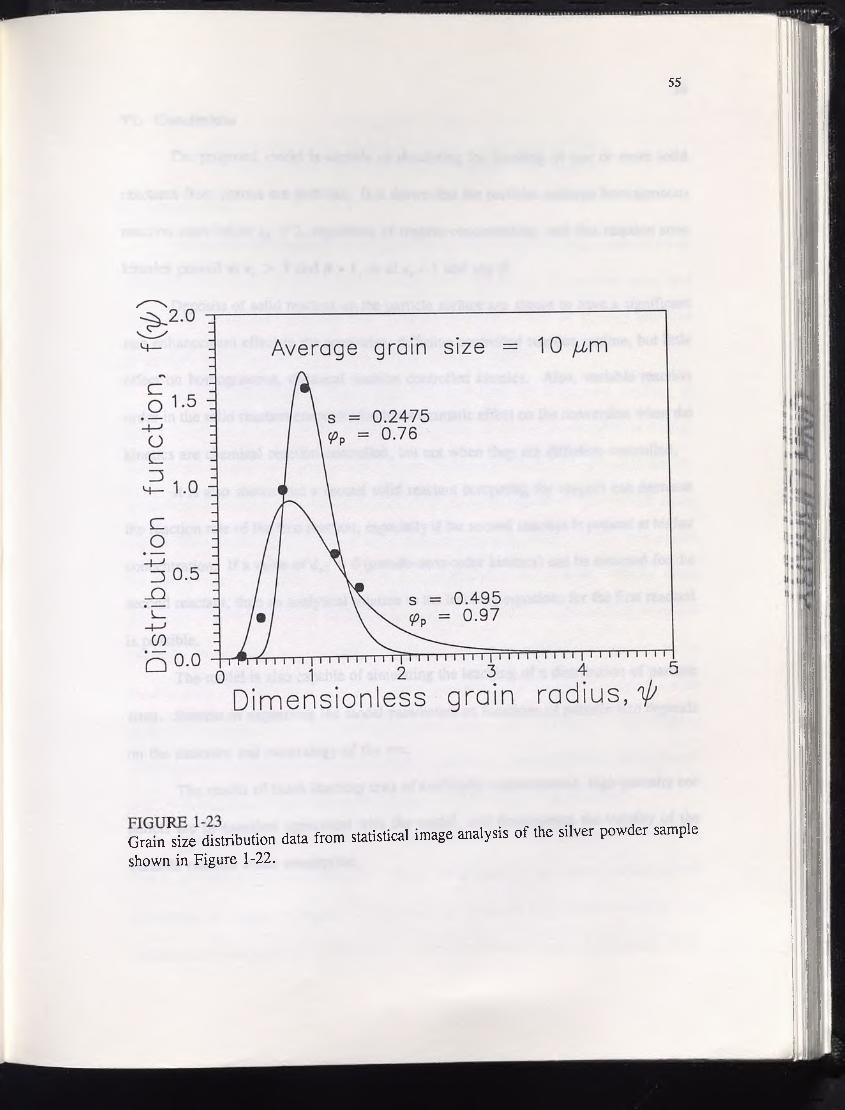
Finally, for the sake of completeness, a scanning electron micrograph (SEM) of

the silver powder used in the artificial pellets is shown in Figure 1-22, and the

corresponding size distribution from statistical image analysis is shown in Figure 1-23.

(See Appendix One for details concerning the interpretation of the Figure.) Based on the

variable order argument posed in Appendix One, one would expect the dissolution

reaction to be roughly first-order or lower. However, since the average grain size from

the image analysis (10 /xm) is more than twice that reported by the supplier of the silver

powder, and also judging from the wide variability of shapes and sizes, and especially

the degree of particle overlap apparent from the micrograph, results derived from the

statistical data from the image analysis cannot be taken as conclusive.

53

FIGURE 1-21Calculated effectiveness factor (77) vs. Ag conversion (X) for the batch leaching tests.

55

Grain^size distribution data from statistical image analysis of the silver powder sample shown in Figure 1-22.

VI. Conclusions

The proposed model is capable of simulating the leaching of one or more solid

reactants from porous ore particles. It is shown that the particles undergo homogeneous

reaction rates below kp = 1, regardless of reagent concentration, and that reaction zone

kinetics prevail at *p > 1 and j3 » 1, or at kp » 1 and any 0.

Deposits of solid reactant on the particle surface are shown to have a significant

rate enhancement effect in the zone-wise, diffusion controlled reaction regime, but little

effect on homogeneous, chemical reaction controlled kinetics. Also, variable reaction

order in the solid reactant concentration has a dramatic effect on the conversion when the

kinetics are chemical reaction controlled, but not when they are diffusion controlled.

It is also shown that a second solid reactant competing for reagent can decrease

the reaction rate of the first reactant, especially if the second reactant is present at higher

concentration. If a value of 4>p2 = 0 (pseudo-zero-order kinetics) can be assumed for the

second reactant, then an analytical solution to the leaching equations for the first reactant

is possible.

The model is also capable of simulating the leaching of a distribution of particle

sizes. Success in expressing the model parameters as functions of particle size depends

on the structure and mineralogy of the ore.

The results of batch leaching tests of artificially agglomerated, high-porosity ore

pellets are in excellent agreement with the model, and demonstrate the validity of the

variable reaction order assumption.

Chapter TwoA Mathematical Model for Heap Leaching of One or More Solid Reactants from Porous Ore Pellets

I. Introduction

There is an abundance of literature referring to the kinetics of large-scale leaching

processes, but many of the articles deal only with kinetics at the particle scale, and

completely ignore the larger process. Those which do not can be divided into two

categories: sulfide leaching models and oxide leaching models.

Several mathematical models have been developed for large-scale leaching of

coarse sulfide ores, including heap and dump leaching, as well as in-situ solution mining.

Perhaps the earliest was published in 1942 by Taylor and Whelan,29 who found that the

extraction of copper from sulfidic dumps could be described by an exponential decay

curve. Their model was of little value for scale-up, however, since it could only predict

the future recovery from a dump whose past performance was known. Nearly thirty

years later, Harris30 proposed the first truly predictive model for dump leaching of copper

sulfides. He assumed that the entire process was simply an extension of leaching at the

particle scale, the rate-controlling step being the diffusion of oxygen through the void

space of the dump. While this "pseudo-particle model" was definitely an improvement

over the earlier model, difficulty in identifying parameters from experiment and a general

lack of mathematical rigor rendered it impractical for engineering purposes.

Certainly the most rigorous, and complex, model of sulfide dump leaching to date

is that of Cathles and co-workers.31,32 Their model assumes the unsteady-state thermal

convection of oxygen through the void space of the dump to be rate-controlling, and

includes both oxygen and heat balances. While the earliest version, published in 1975,

57

58

was restricted to one-dimensional air and solution flow, this was later extended to two-

dimensional air flow with the aid of stream functions and potential flow. The model also

accounts for the presence of bacterial catalysis, intermittent solution flow, and seasonal

ambient temperature changes, and was validated experimentally in both large column

tests and small dumps.31'33

More recently, a model for in-situ solution mining of copper sulfides has been

developed by Gao, et al.,7,34 which also includes unsteady-state oxygen and heat balances

in one dimension. Unlike dump leaching, in-situ solution mining involves the forcing

of lixiviant solutions through underground cracks and fissures. As a result, the void

spaces are mostly saturated with solution, and no thermally driven convection is possible.

Thus, the variability of temperature only affects the equilibrium concentration of

dissolved oxygen in solution, and only one fluid phase need be considered.

With the exception of the earliest models, all of the large-scale sulfide leaching

models assume particle level kinetics of the shrinking-core or the reaction zone type,

as derived by Braun, et al.4 To this author’s knowledge, the unsteady-state model for

the leaching of sulfide particles derived by Bartlett9 has never been incorporated into any

simulation of a large-scale leaching operation.

Concerning the acid leaching of copper oxide ores, Roman and co-workers12,35

developed a model which accounts for the gradual consumption of sulfuric acid in the

lixiviant solution as it trickles through the heap. To achieve this end, the heap is

conceived as a number of adjacent columns, or "unit heaps" which in turn consist of

several unit volumes stacked one atop another. By solving for the acid consumption

within each unit volume, the total concentration gradient within the heap may be pieced

59

together. Chae and Wadsworth14 have recently developed a similar model for large scale

leaching of copper oxides, which is based explicitly on the "maximum gradient," or plug-

flow, reactor. Both of these models are for the one-dimensional, isothermal case, and

assume pseudo-steady-state, "shrinking-core" type kinetics at the particle level. The

latter model, however, also accounts for consumption of acid by gangue materials, and

initial enhancement of the leaching rate due to the flushing of minerals on particle

surfaces.

Much less attention has been focused on modeling the kinetics of precious metal

heap leaching. To this author’s knowledge, only one previous attempt has been

published to date, that of Prosser.17 Prosser and Box36 derived a general model for the

heap leaching of several minerals with several reagents, but assumed that transport of

reagent through the heap to the ore particles, chemical reaction, and transport of

dissolved products out of the heap all occurred very fast compared to diffusion of reagent

into the particle pores. Hence, the model was reduced to nothing more than the modified

shrinking core model of Box and Prosser15 discussed in chapter one.

In this study, a general model is derived for application to the heap leaching of

any porous, low-grade ore when the rate-controlling reagent is strictly in the aqueous

phase, as in acid leaching of copper oxides, or basic cyanide leaching of oxidized

precious metals ores. The general model fully developed in chapter one is assumed at

the particle level, and provides both intraparticular and particle surface leaching rate

terms for a global heap-scale model based on the one-dimensional, plug-flow reactor at

unsteady state. Reduction of the model to dimensionless form facilitates the identification

of important scale-up parameters, and the analysis of various leaching rate regimes.

60

II. Model Development

The heap leaching operation is a heterogeneous, non-catalytic, fixed-bed reactor

operating under unsaturated flow conditions. Lixiviant solution enters at the top of the

heap and trickles through the interstices of the ore particles. Reagents diffuse into the

pores and fissures of the ore particles, and are gradually consumed by reaction with one

or more solid reactants. These solids, in turn, are gradually dissolved throughout the

heap. Based on this physical picture, shown schematically in Figure 2-1, a global heap

model is derived with the following assumptions:

1. The heap leach reactor is essentially an unsteady-state plug flow reactor, i.e., flow of reagents and dissolved products occurs only by axial convection with no short-circuiting.

2. All physical parameters within the heap remain uniform and constant throughout the leach cycle.

3. No inhibition of diffusion into or out of the particles occurs due to dense packing or a stagnant boundary layer.

4. The heap operates isothermally.

At the particular level, the following assumptions are made:

1. The particles are spherical, and of uniform size, density and porosity.

2. All effective diffusivities are constant and uniform.

3. Reactive solids are evenly distributed throughout the pore surfaces of the particle, and their total relative volume is insignificant.

4. Dissolution reactions are irreversible, first order in the concentration of one rate-controlling reagent, and variable order in the solid concentration of the reactant.

5. Intraparticular processes are not at steady state.

These assumptions at the particle-scale result in the formulation of the general model

M E T A L D E P O S IT S :

ALONG PORE WALLS

ON PARTICLE SURFACES

FIGURE 2-1Schematic diagram of a heap.

ORE PARTICLES v = ( l - ejvh

ENTRAINED AIRV = (e„ - eJV„

BULK LIXIVLANTV = e,V*

ORE MATRIX V = (1 - t J Q - eJVh

PORE STRUCTURE V = ( 1 - eJe0V,

ON

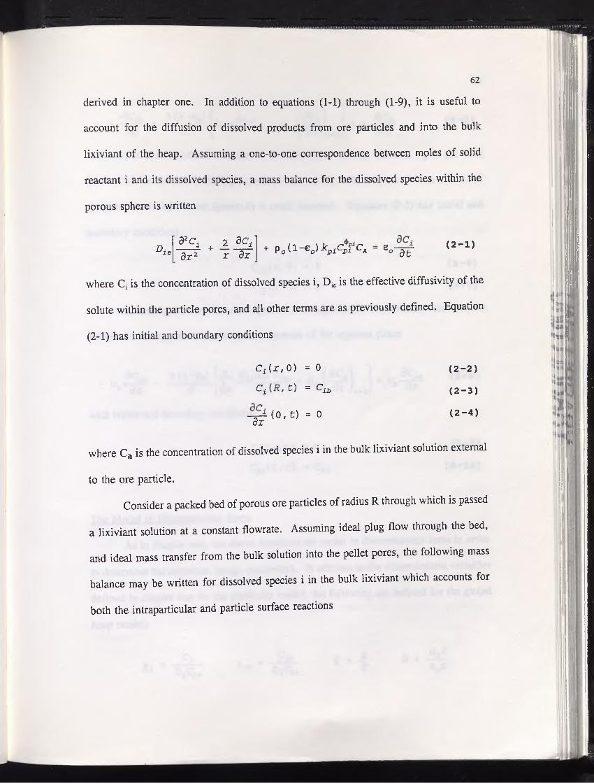
62

derived in chapter one. In addition to equations (1-1) through (1-9), it is useful to

account for the diffusion of dissolved products from ore particles and into the bulk

lixiviant of the heap. Assuming a one-to-one correspondence between moles of solid

reactant i and its dissolved species, a mass balance for the dissolved species within the

porous sphere is written

Died2C0 r :

i , 2 dCj r d r

+ p 0 ( l £0) kp icpi CA e a t(2-1)

where Q is the concentration of dissolved species i, Die is the effective diffusivity of the

solute within the particle pores, and all other terms are as previously defined. Equation

(2-1) has initial and boundary conditions

C ^ r ^ ) = 0 (2-2 )Ci t ) = Cib ( 2 - 3 )

( 0 , t ) = 0 ( 2 - 4 )d r

where Cib is the concentration of dissolved species i in the bulk lixiviant solution external

to the ore particle.

Consider a packed bed of porous ore particles of radius R through which is passed

a lixiviant solution at a constant flowrate. Assuming ideal plug flow through the bed,

and ideal mass transfer from the bulk solution into the pellet pores, the following mass

balance may be written for dissolved species i in the bulk lixiviant which accounts for

both the intraparticular and particle surface reactions

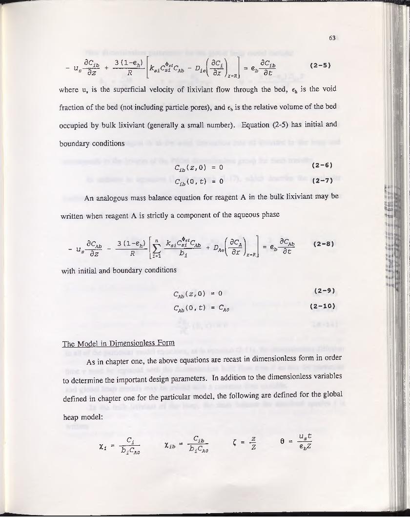
63

8C.- Ub i b 3 ( i - e „ )

dz Ry c^slC — P ‘K s i ' - s i b > ie V dr Z = R

= e. dCibd t

( 2 - 5 )

where us is the superficial velocity of lixiviant flow through the bed, eh is the void

fraction of the bed (not including particle pores), and eb is the relative volume of the bed

occupied by bulk lixiviant (generally a small number). Equation (2-5) has initial and

boundary conditions

Ci b ( z , 0) = 0 ( 2 - 6 )

Ci b ( 0 , t ) = 0 ( 2 - 7 )

An analogous mass balance equation for reagent A in the bulk lixiviant may be

written when reagent A is strictly a component of the aqueous phase

- u.dC ^ 3 ( l - e h)dz R

n v r^Biny> K si^si uAb + £>i = l b i 4 % ,

dC.= e. Ab

d t(2-8 )


0 ) = 0

^Ab ® ' t) ~ CaO

( 2 - 9 )

(2-1 0)

The Model in Dimensionless Form

As in chapter one, the above equations are recast in dimensionless form in order

to determine the important design parameters. In addition to the dimensionless variables

defined in chapter one for the particular model, the following are defined for the global

heap model:

C i - Cib C = — 0 =Z l = i Z ■ b t CMZ ebZ

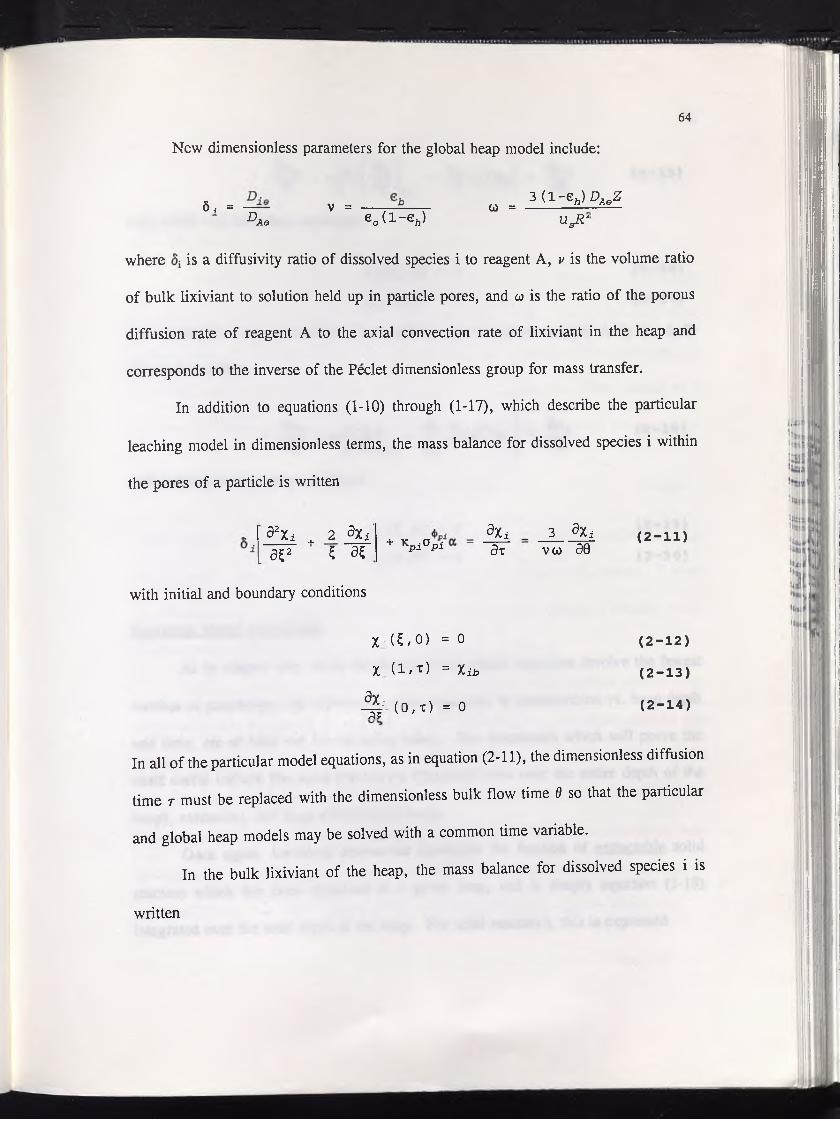
64New dimensionless parameters for the global heap model include:

6, - DV =

Ae e 0 ( l - e A)0) = 3 ( 1 - e h)DAeZ

UsR‘

where is a diffusivity ratio of dissolved species i to reagent A, v is the volume ratio

of bulk lixiviant to solution held up in particle pores, and w is the ratio of the porous

diffusion rate of reagent A to the axial convection rate of lixiviant in the heap and

corresponds to the inverse of the Peclet dimensionless group for mass transfer.

In addition to equations (1-10) through (1-17), which describe the particular

leaching model in dimensionless terms, the mass balance for dissolved species i within

the pores of a particle is written

d2Xi ^ 2 dXid ? 5 K + V ° P i

5Xi _ 3 3Xidx v o ) 5 0

( 2 - 1 1 )


X ( 5 , 0 ) = 0

X (l,r) = %ib

% (0,T) = 0

(2-1 2)( 2 - 1 3 )

( 2 - 1 4 )

In all of the particular model equations, as in equation (2-11), the dimensionless diffusion

time r must be replaced with the dimensionless bulk flow time 9 so that the particular

and global heap models may be solved with a common time variable.

In the bulk lixiviant of the heap, the mass balance for dissolved species i is

written

65

. Ks i a ^ i „ _ 5X ii ( 2 - 1 5 )_ U e 7* U , v ZT}T—


Xxb(C# 0) = 0

xijb(o,0) = 0( 2 - 1 6 )

( 2 - 1 7 )

The analogous balance equation for a strictly aqueous-phase reagent A in the bulk

lixiviant is written


Important Model Functionals

As in chapter one, while the dimensionless model equations involve the fewest

number of parameters, the solutions to these equations, in concentration vs. heap depth

and time, are of little use for designing heaps. The functionals which will prove the

most useful include fractional conversion (integrated here over the entire depth of the

heap), extraction, and heap effectiveness factor.

Once again, fractional conversion represents the fraction of extractable solid

reactant which has been dissolved at a given time, and is simply equation (1-18)

integrated over the total depth of the heap. For solid reactant i, this is expressed

a ^ C / 0) = 0

<**(0,0) = l

( 2 - 1 9 )

(2-20)

66

3 ( U i ) / ( l - opi ) ¥ d t + ^ ( 1 - a al ) dC (2-21)

As in the particle model, X; takes values from zero to one.

Extraction of reactant i from the heap represents the total fraction of extractable

reactant i which has issued from the heap at any given time. Except for very short

leaching times, or in heaps with an unusually high holdup, extraction takes approximately

the same value as conversion as a function of time, but may be written simply as a

function of the bulk concentration of dissolved species i at the bottom of the heap thus

(2-22)

Unlike conversion, extraction may be evaluated directly from chemical analysis of heap

effluent and is therefore a far more convenient measure of heap performance. It must

be re-emphasized that these functionals are based on only that amount of reactant which

can be obtained from the heap, and not the total grade of the ore.

The heap effectiveness factor is defined, analogous to the particle effectiveness

factor of chapter one, as the reaction rate of the entire heap taken as a fraction of the rate

which would obtain if there were 1) no diffusion limitation into the ore particles, and 2)

no convection limitation through the heap, i.e., if the heap were a stirred tank reactor

with reagent concentration maintained at CA0. As such, the heap effectiveness factor may

be written by simply integrating (separately) both the numerator and the denominator of

equation (1-19). For solid reactant i, the resulting expression takes the form

67

( 2 - 2 3 )

and, like the particle effectiveness factor, assumes values between zero and one.

HI. Experimental

Figure 2-2 shows a schematic diagram of the experimental leaching columns. The

tall column was comprised of six 61 cm (2 ft) sections made of transparent acrylic pipe

of 9.53 cm (3.75 in) ID, and the short column comprised only one section 30 cm (12 in)

long and 6.35 cm (2.5 in) ID. All column sections were fitted with plexiglas perforated

plates and funnels with hoses at the bottom to collect and distribute lixiviant.

Approximately two centimeters of glass wool were packed into the bottom of each

column section to prevent the movement of any fine solids from one section to another.

All column sections were open at the top. Pumping from the lixiviant tank to the

column, and from section three to section four in the tall column, was achieved with

Masterflex peristaltic pumps fitted with #13 Masterflex tubing.

Initially, the column sections were flushed with water to wash out any fine

material which may have resulted from packing the ore pellets, and to fill the pellet pores

with water. Then, water was pumped into the column, and the flowrate was adjusted to

3.8 mL/min in the tall column, and 4.1 mL/min in the short column, corresponding to

superficial velocities of 8.9 x 10r* cm/s and 2.2 x 10‘3 cm/s, respectively. Once the flow

was steady, lixiviant was introduced. The lixiviant was a solution containing 10 M

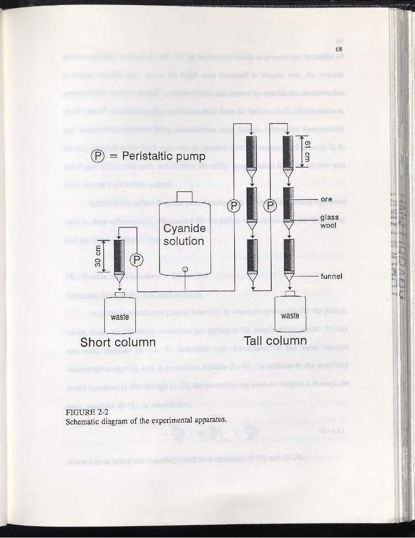
30 cm

68

= Peristaltic pump

oreglasswool

funnel

waste waste

— _____ _

Short column Tall column

FIGURE 2-2Schematic diagram of the experimental apparatus.

sodium cyanide, made basic with Id3 M sodium hydroxide to prevent the formation of

hydrogen cyanide gas. As in the batch tests discussed in chapter one, the cyanide

concentration was low enough to ensure kinetic rate control by cyanide ion concentration

at all times.25 Solution samples were taken daily from the bottom of all column sections,

and analyzed for dissolved silver concentration using Atomic Adsorption Spectrometry

(AAS), identical to the batch tests, except standard solutions containing 0 (blank), 2, 4,

and 6 ppm silver were used, and all but a few of the samples taken from the column tests

were diluted 1:10 before analysis.

Artificial ore pellets from the same batches used in the batch leaching tests were

used in these column tests. Parameters for the pellets were determined for those tests,

and are listed in chapter one.

IV. Results and Discussion -- Theoretical

Computer Simulation: One Solid Reactant

In order to examine its general behavior, as was done previously for the particle

model alone, the following restrictions are applied to the heap leaching model: 1) only

one solid reactant (n = l), 2) first-order rate dependence in the solid reactant

concentration (</>„=1), and 3) no surface deposits (\=0). In addition to the simplified

model equations (1-20) through (1-25), the convection equation for reagent A through the

heap, equation (2-18), is simplified to

( 2 - 2 4 )

which has as initial and boundary conditions equations (2-19) and (2-20).

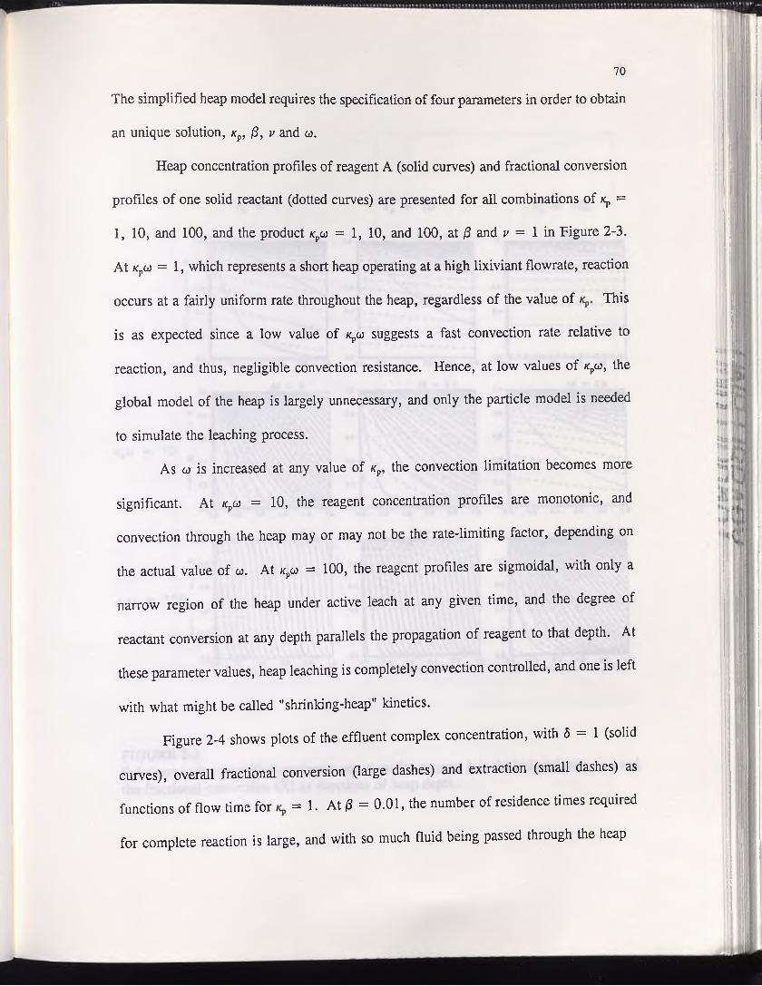
70

The simplified heap model requires the specification of four parameters in order to obtain

an unique solution, kp, fi, v and u.

Heap concentration profiles of reagent A (solid curves) and fractional conversion

profiles of one solid reactant (dotted curves) are presented for all combinations of «p =

1, 10, and 100, and the product /cpu = 1, 10, and 100, at /3 and v = 1 in Figure 2-3.

At KpW = 1, which represents a short heap operating at a high lixiviant flowrate, reaction

occurs at a fairly uniform rate throughout the heap, regardless of the value of This

is as expected since a low value of kpco suggests a fast convection rate relative to

reaction, and thus, negligible convection resistance. Hence, at low values of kpgj, the

global model of the heap is largely unnecessary, and only the particle model is needed

to simulate the leaching process.

As co is increased at any value of kp, the convection limitation becomes more

significant. At kpco = 10, the reagent concentration profiles are monotonic, and

convection through the heap may or may not be the rate-limiting factor, depending on

the actual value of co. At kpco = 100, the reagent profiles are sigmoidal, with only a

narrow region of the heap under active leach at any given time, and the degree of

reactant conversion at any depth parallels the propagation of reagent to that depth. At

these parameter values, heap leaching is completely convection controlled, and one is left

with what might be called "shrinking-heap" kinetics.

Figure 2-4 shows plots of the effluent complex concentration, with 6 = 1 (solid

curves), overall fractional conversion (large dashes) and extraction (small dashes) as

functions of flow time for k, = 1. At 0 = 0.01, the number of residence times required

for complete reaction is large, and with so much fluid being passed through the heap

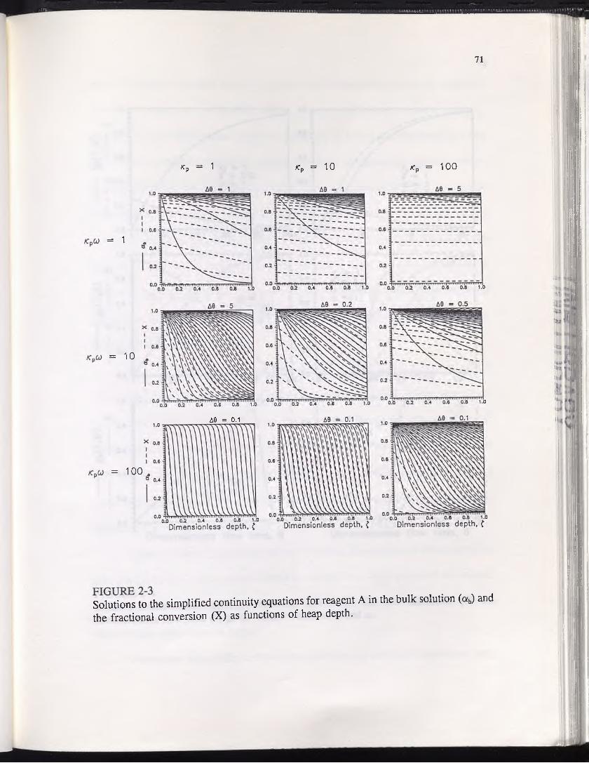
71

Kp — 1 /Cp = 10 Kp = 100

= 1

= 10

A0 = 0.1

= 100

Solutions to the simplified continuity equations for reagent A in the bulk solution (ab) and the fractional conversion (X) as functions of heap depth.

XbO

.e)

------

-Xb(

i.0)

------

-Xb(

i.e)

72

FIGURE 2-4 .Effluent concentration ( X b ( M ) ) > fractional conversion ( X )

dimensionless flow time (0) given various values of /3 and co.and extraction (E) vs.

73

over the course of the leach cycle, the total holdup of dissolved products is negligible.

Hence, the conversion and extraction curves largely coincide at all values of kp and w.

At kp(j) = 1, the effluent concentration curve consists of a short peak followed by a long

tail, and the conversion curves are roughly the shape of exponential response curves,

signifying the dominant role of particle kinetics. As kpw is increased, the Xb peak grows

taller until, at kpw = 100, it reaches its maximum value of one and flattens out. Above

a certain value of co, the dimensionless flow time for complete reaction decreases to its

limit, d = M(3v, which is simply the time required in order to feed a stoichiometric

amount of reagent to the heap. The conversion curve is a straight line, since the rate of

propagation of the reaction zone through the heap is constant at dfx/d0 ~ ftp (e.g., the

bottom left comer of Figure 2-3).

At 13 = 1, the overall flow times are much shorter, and a "chromatographic

effect" due to the high diffusion driving force at the beginning of the leach cycle results

in significant holdup. This effect, which causes the characteristic delay in attaining peak

concentration in all heap leaching operations, is only significant when the ore grade is

very low, as in precious metal leaching operations. At kpu = 100 and kp — 1, both the

conversion and extraction curves are linear, yet nearly half of the solid reactant has been

converted before any dissolved complex is seen in the heap effluent.

Figure 2-5 shows the relation between fractional conversion and relative reaction

time for the same particles at three different values of to. As is expected, the relative

conversion rate is much slower in the high to, "shrinking-heap" situation than in the

shorter heaps with faster flowrates.

The relative magnitudes of convection, diffusion and reaction resistance are most

74

FIGURE 2-5 .Fractional conversion (X) vs. reaction time (y3w(0-l)/3), given various values of w.

75

conveniently illustrated in semi-log plots of heap effectiveness factor vs. fractional

conversion, as shown in Figure 2-6. At low values of w, the heap effectiveness factor

approaches the particle effectiveness factor as a limiting value. As co is increased, the

effectiveness drops until, at about kpgo = 100, the ineffective character of the bulk flow

process dominates, obscuring any effects at the particle level. This happens irrespective

of the reagent concentration of the incoming fluid.

Relaxing the restriction of no surface deposits and also assuming first-order rate

dependence at the surface, the surface rate expression becomes

and the intraparticular rate expression becomes

Since it was already determined in chapter one that surface deposits have little or

no effect on the kinetics of particles with low Kp, only the case when this parameter is

high, and particle kinetics are diffusion controlled, will be considered here. Figure 2-7

shows the effect of various surface fractions X on the rate of reactant conversion from

the same particles in two different heap simulations. Higher surface fractions result in

much faster conversion rates at co = 0.1, but have little impact at u = 1. These results

are illustrated in the tj-X plot shown in Figure 2-8. At low u, kinetics at the particle

( 2 - 2 6 )

These equations have initial conditions

op i t , 0) = 1

os ( f , 0 ) = l

( 2 - 2 7 )

( 2 - 2 8 )

Hea

p ef

fect

iven

ess

fact

or,

m a a m sm

76

FIGURE 2-6 r vHeap effectiveness factor (rj) vs. fractional conversion (X) for the continuity equationsolutions shown in Figure 2-3.

M W W U H m iH llH IIH lU iM I

Fractional conversion (X) vs. dimensionless flow time (0) given various surface fractions(X).

78

FIGURE 2-8 „ . . ,Heap effectiveness factor (v) vs. dimensionless flow time (i9) given various surfacefractions (X).

79

level control the entire process, so the leaching rate is strongly enhanced by higher

surface fractions. At the higher u, however, the characteristic contours of the particle

kinetics all but disappear as the rate of bulk flow through the heap becomes rate

controlling.

Similar results are obtained by varying the reaction order <£p, as shown in Figure

2-9. For these plots, a low value of for the particles is assumed since reaction order

is only an important factor in systems under chemical reaction control, as shown in

chapter one. Again, the effect is greater at low values of o, especially at the beginning

of the leach cycle. However, the suppression of particle kinetics at the higher value of

cj is less pronounced since a higher reaction order tends to widen the active reaction zone

in the heap, Afx, resulting in a net increase of heap effectiveness with reaction order, as

shown in Figure 2-10.

Computer Simulation: Competing Solid Reactants

In chapter one it was shown that the presence of one or more competing reactants

within porous ore particles can significantly alter the kinetics of leaching. In particular,

computer simulation of the particle model showed how the presence of a reactive gangue

material may push the otherwise highly effective reaction of a valuable component into

a much less effective regime, and how the overall process may approach a near-steady

state. Figure 2-11 shows the concentration gradient of reagent A and the fractional

conversion of one solid reactant as functions of heap depth, for the same hypothetical

particles as in Figure 1-11, in a heap at a = 1 and v = 1. In one simulation, reactant

1 is alone, and in the other it is accompanied by the reactive gangue material, exactly as

■MM—M— n

nI t

rHi

Fractional conversion (X) vs. dimensionless flow time (0) given various orders of reaction (<£p).

1

oowwCDCCD>(JCD

M—M—CD

Q_DCD

X

0.1

In

FIGURE 2-10 . ^ „ ,Heap effectiveness factor (77) vs. dimensionless flow time (0) given various orders ofreaction (cpp).

FIGURE 2-11 J . . ,Solutions to the continuity equations for reagent A (ab) and fractional conversion ofreactant 1 (X,), alone (n = l) and in the presence of a second reactant (n=2). *pi - U j8j = 1, * pl = 2/3, *p2 = 10, |S 2 = 0 .01, </>p2 = 0, u = 1, ? = 1, ^

83

in Figure 1-11.

Alone, reactant 1 dissolves effectively throughout the heap, and the reagent

gradients are insignificant, analogous to the particle alone. In the presence of solid

reactant 2, however, the reaction shifts more toward the top of the heap, and the reagent

gradients are steep, with ab < 0.12 at the bottom. In addition, the reagent gradients

within the heap approach a steady state, just as they do within the pores of the individual

pellets. Hence, the conversion kinetics of reactant 1 could be approximately described

in this case by a steady state solution for reagent A, using only the parameters for

reactant 2. As before, the diffusion equation for reagent A becomes the Bessel equation

(1-31) coupled with the mass-action rate expression for reactant 1

An analytical expression for the concentration of reagent A as a function of particle

radius and heap depth is now easily obtained (refer to appendix six):

KpiPiVO)--- 3

( 2 - 2 9 )

Additionally, the heap convection equation for reagent A becomes

= 0 ( 2 - 3 0 )

s i n he " “ YC 5 * 0

<x(5,0 =5 sin h (^ ic^ ) ( 2 - 3 1 )

e " “ YC 5=0s in h ( 0 ^ )

where

84

= V p2 ~ t a n h ( ^ ) tanh(^ ic^)

The concentration of solid reactant 1 is expressed

o ( $ , C , 6 ) =i -

-.V PlV(J t (i,0 6a 3

W 1

4>Pi =1

( 2 - 3 2 )

For the test situation, these equations become

octC/S^O) = s i n h (yT O $ )y/T? - tanh(-y/l?) ^

tanh (%/T5)$ s i n h ( v / T o )

s i n h ( 7 l O $ ) e ~ 2 . 1 7c1 1 . 8 $

( 2 - 3 3 )

a ( C , $ =0) = yTos i n h (y T o ')

v/10 ” tanh (\/10) tanh (v/lfr) = 0 . 2 6 8 e " 2 ‘17C

«b(C=1) = ey/I? - tanh(y/l5')

tanh(v/Tff) = 0 . 1 1 4

( 2 - 3 4 )

( 2 - 3 5 )

opl ( $ , C , 0) = (1 -a ($,C) 0 \3 ( 2 - 3 6 )

The conversion curves for reactant 1 both within and without the presence of

reactant 2 are shown in Figure 2-12. As expected, the conversion when n = 2 is

significantly delayed relative to when n = 1. The effect of the second reactant on the

heap effectiveness factor of the first reactant m is illustrated in Figure 2-13. When n =

2, the curve does not approach unity near complete conversion, identical to the

particle model alone. However, in a very ineffective (high co) heap, this would not

necessarily be the case, since the second reactant would have to be depleted at every

depth before the reaction zone could move downward into fresh ore. Under these

85

Fractional conversion of solid reactant 1 (X,) vs. dimensionless flow time (0) for the systems shown in Figure 2-11.

86

FIGURE 2-13Heap effectiveness factor (j]x) vs. systems shown in Figure 2-11.

fractional conversion of solid reactant 1 (Xj) for the

87

extreme circumstances, the time for total dissolution of reactant 1 (or any other minor

constituent) would be 6 ~ 1/(32p.

Computer Simulation: An Approach for Particle Size Distributions

In chapter one, the particular leaching model was solved for a distribution of

particle sizes based on the Gates-Gaudin-Schuhmann distribution function. In this

chapter, those results are applied to the global heap model, but the discussion is limited

to ore with no significant mineral deposits exposed on external particle surfaces.

From the definition of dimensionless particle radius in equation (1-38), and the

normalized weight fraction distribution in equation (1-39), assuming the simplest case of

no mineral liberation upon comminution, as in chapter one, and also ignoring surface

deposits, then the rate constant /cpi, the diffusion time r, and the global heap parameter

co will vary as functions of particle size thus:

Kpi - - V 22 2 2

where ~icpi, r and u apply to the reference particles. Substitution of these altered

parameters into the particular leaching equations allows one to solve the particle model

for a range of particle sizes S based on the parameters from the reference size, a — 1.

In order to gauge the effect that a distribution of particles sizes will have on the heap

leaching process as a whole, the convection equations must be altered to

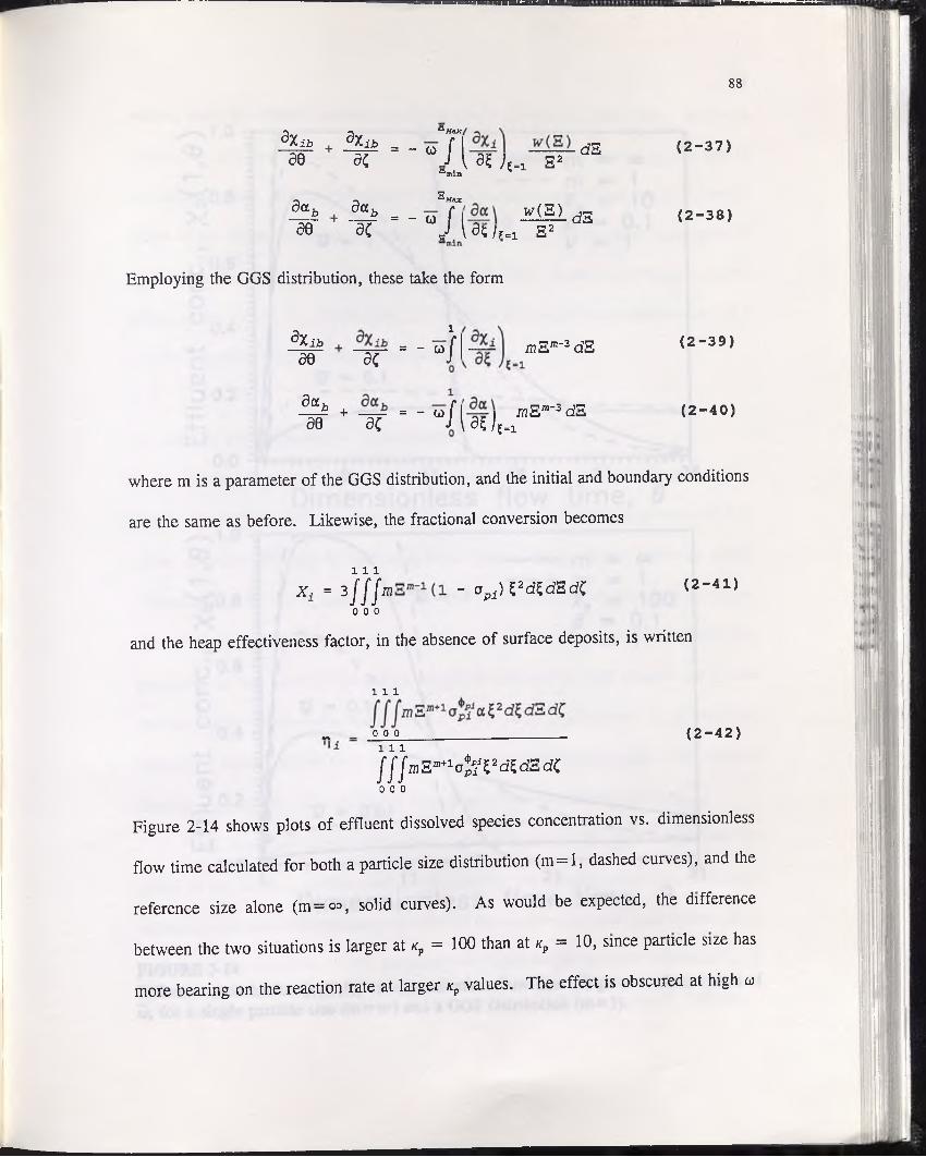
88

dxib 3X±ba HcX

‘ - “ /I dZ (2-37)30 3C l 3W?=i S 2ainin

dab dab Max

= - G> f 1 W(S) ds (2-38)30 3( J 1i 3 U ?=1 S 2

Employing the GGS distribution, these take the form

d X i b - - oil r n Z m ~2 dE (2 -39)3 0 3C J '

d a b +- - « r i m Z m ~2 d Z (2 -40)

30 3C J\\fth-1

where m is a parameter of the GGS distribution, and the initial and boundary conditions

are the same as before. Likewise, the fractional conversion becomes

i i iX. = 3 f f f w - 0piH 2d$dEdC (2-41)

0 0 0

and the heap effectiveness factor, in the absence of surface deposits, is written

i i i

„ _ 0 0 0 111

(2-42)

fffmE^olfVdtdEdC0 0 0

Figure 2-14 shows plots of effluent dissolved species concentration vs. dimensionless

flow time calculated for both a particle size distribution (m = l, dashed curves), and the

reference size alone (m=oo, solid curves). As would be expected, the difference

between the two situations is larger at kp = 100 than at xp = 10, since particle size has

more bearing on the reaction rate at larger kp values. The effect is obscured at high co

89

F IG U R E 2 -1 4 . ,E ffluent concentration (Xb( M ) ) vs. dim ensionless flow tim e (6) g iven various values o fw, for a single particle size (m=°°) and a GGS distribution (m — 1).

90

values, since the effluent concentration is already at or near its upper limit. At low w

values, the X b(M ) curves are simply a little higher in the size distributed system than in

the isometric one. The most drastic difference is at moderate u values, where the entire

shape of the effluent response may be dramatically altered. These trends are also to be

observed in the fractional conversion plots of Figure 2-15. As shown in Figure 2-16, the

effect of the particle size distribution is to increase the overall heap effectiveness, to a

greater degree at higher xp values and lower w values.

V. Results and Discussion - Experimental

Table 2-1 summarizes all of the parameters for five column leaching tests, the

results of which are shown in Figures 2-17 through 2-21. All of these parameters were

either measured directly or calculated from known values, unless otherwise noted.

Values of DAe, kp, and 4>p were known from the batch kinetics tests discussed in chapter

one. The surface fraction X was taken as zero. The value of the GGS distribution

parameter m was based on a random sample of 100 pellets from column test 2, and

assumed valid for the other tests. In all of the tests, u is treated as an empirical

parameter, chosen on the basis of the best fit of the experimental data. This value is

denoted coapp, and the value predicted from theory for comparison is denoted wpr.

The ’expected’ values of CA0 and Cp0 in Table 2-1 are the products of what was

added to the lixiviant solution and the ore pellets, respectively, while the ’observed

values are the result of integrating the effluent responses of the individual column tests.

Hence, for the model fits, 100% extraction was based on the observed values of Cp0 in

order that the extraction integrals of the data and the simulations be equal. ’Actual’

91

FIGURE 2-15Fractional conversion (X) vs. Figure 2-14.

dimensionless flow time (0) for the simulations shown in

Hea

p ef

fect

iven

ess

fact

or

93

TABLE 2-1: Parameter values for the column leaching tests. (All units cgs. Concentrations based on gmols.)

b = 0.5 eh = 0.39DAe = 2.35 • 10-6 e0 = 0.20k„ = 3.76* 107 v ■= 0.246m = 6 Po = 2.15 = 1 (assumed) eb = 0.03

4>r = 2

Parameters Column test 1

Column test 2

Column test 3

Column test 4

Column test 5

CA0-106 (exp) 1.0 1.0 1.0 1.0 1.0

CAO-106 (obs) 0.91 1.0 1.0 1.0 1.0

Cp0* 10s (exp) 6.34 6.34 6.34 6.34 0.634

Cp0* 106 (obs) 5.13 5.60 5.26 6.05 0.623

n Rc 0.117 0.288 0.358 0.218 0.288

R 0.655 0.655 0.814 0.496 0.655

us • 103 0.89 2.2 2.2 2.2 2.2

Z 366 30 30 30 30

q** 0.0106 0.0106 0.0113 0.0098 0.0955

IS ^ 930 930 1430 530 9.3

app 1.1 0.10 0.071 0.13 0.10

^pr 4.12 0.137 0.089 0.238 0.137

*Based on expected values.**Based on observed values.

Xb(

C.Q

)

94

Column test 1

............... ( = 1 / 6ooooo 1 /3■ ■ ■ ■ ■ 1 / 2□ □□□□ 2/3▲ ▲ ▲ ▲ ▲ 5/6A A A A A 1------ Model fit:

/cp = 930, p = 0.0106 p p = 2, i/ = 0.246 w = 1.1, m = 6

1.0

0.8 -

0.6 -

0.4 J

0.2 -

FIGURE 2-17Effluent concentration and extraction data from column leaching test 1.

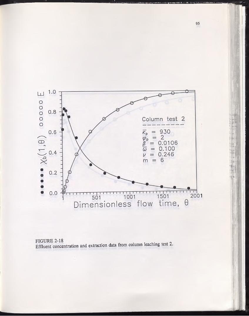
95

Effluent concentration and extraction data from column leaching test 2

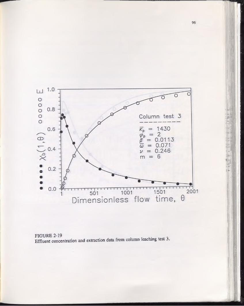
96

FIGURE 2-19 , _Effluent concentration and extraction data from column leaching test 3.

Xb

O

>0

)

97

LU

OOOoo

1.0

0.6

0.4 -

0.2

0 .0

G

__C

l

•V / o

10 \ / Co lum n te s t 4

» / /cp = 530 = 2

/3 = 0 .0098co = 0 .130 1/ = 0 .246 m = 6

•------m____ 1

501 1001 1501 2001

Dimensionless flow time, 0


Xb

O.e

)

BIIUW IUHHUHHHM HHHHW M I

98


99

extractions ranged from 80.9% in the tall column (test 1) to 98.3% in the low-grade

pellet test (test 5), and were apparent functions of pellet grade and particle size. The

parameter /3 was calculated based on the ’observed’ values, while kp was based on the

’expected’ values.

Effluent profiles from the tall column test (test 1) are shown in Figure 2-17. This

column simulates an ineffective heap (see Figure 2-22), since the effluent response is at

the maximum value of Xb(M) = 1 over most of the leach cycle. The apparent value of

u is 1.1, while the predicted value is 4.12. This large disparity is most likely due to a

combination of non-ideal flow patterns (i.e., rivulet flow, stagnant zones) within the

column, and to the blinding of pellet surfaces due to close packing. The former would

have the effect of increasing the local bulk fluid velocity in some regions, leaving others

accessible only by dispersion along pellet interstices. The latter would cause a decrease

in the effective particle size. Both would account for the observed deficiency in co,

resulting in apparently higher column effectiveness while obscuring the effects of kinetics

at the particle level.

Figures 2-18 through 2-20 show effluent response and extraction curves for three

short column tests (tests 2-4). Each involve the same grade of ore pellets as test 1, but

at three different particle sizes. As shown in Figure 2-22, these columns simulate fairly

effective heaps, based on the shape of the effluent response curves. Again, however, the

apparent values of a fall short of the predicted values, but not by as large a margin as

in the tall column test. Finally, the results of a short column test with low-grade pellets

(test 5) are shown in Figure 2-21. At the same u value as for test 2, the model fits the

data quite well, even though the kinetics within the pellets of test 5 are mostly reaction

100

FIGURE 2-22 . .Heap effectiveness factor (rj) vs. fractional conversion (X) for the model simulations ofthe experimental column leaching tests.

101

rate-controlled, while those of test 2 are diffusion-controlled. The simulated extraction

curve ends up significantly lower than the data, but this is probably as much the result

of experimental error as of any physical phenomenon.

Overall, the experimental results attest to the validity of the plug-flow modeling

approach. However, in order to predict the performance of actual heap leaching

operations from column tests, some sort of correlation between the theoretical plug-flow

model and the actual flow patterns within the heap is necessary. Roman37 modeled the

flow pattern within the heap as a collection of rivulets separated by stagnant zones across

which dispersion is the only transport mechanism. In his model, the distances from one

rivulet to the next are assumed to conform to some distribution function. This is

probably a fairly accurate picture of the flow within most heaps. Unfortunately, Roman

included no physical parameters in his model, rendering it impractical for prediction

purposes.

Assuming any correlation between convective and diffusive transport to be a

function of such factors as bulk flowrate, particle size distribution, reagent diffusivity,

surface tension, and so on, it may take the general form

o app = f ( u pI , NRe, NSclNWe, m, . . . ) ( 2 - 4 3 )

where NRe, NSc and NWe are Reynolds, Schmidt and Weber numbers, respectively, m is

a parameter of the particle size distribution, and so on. In the present study, only the

effect of Reynolds number can be accounted for, since the same ore type and reagent

species were used in all of the tests. Satterfield,38 in a review of the literature on the

performance of catalytic trickle-bed reactors, defines the ’contact effectiveness’ as the

102

ratio of the apparent to the predicted mass transfer coefficient, and suggests a

relationship, derived by Bondi,39 of the form

where the k’s are mass transfer coefficients, L is the mass flowrate, and A’ and b are

constants. Modifying this general form to accommodate the present parameters, and

defining the Reynolds number as

_ 2Rusp (2-4 5)

where p and p are the solution density and viscosity, respectively, the experimental

results may be approximated by

^JPP = 1 - 0 . 0 6 6 NrI1,15 ( 2 - 4 6 )03 p r

This result is shown graphically in Figure 2-23. Obviously, a value of one on the

ordinate represents a situation in which all of the assumptions which went into the

derivation of the global heap model are valid. Correspondingly, a heap with a serious

short-circuiting problem would approach an ordinate value of zero in Figure 2-23. Thus,

it makes sense for the curve to approach an ordinate value of one asymptotically with

increasing Reynolds number, since faster flowrates (uj coupled with smaller specific

particle area (3/R) would facilitate a more even distribution of lixiviant over particle

surfaces. While certainly, not enough data have been analyzed here to develop an

empirical correlation with a wide range of applicability, at least the method of approach

suggests an excellent avenue for future study.

103

FIGURE 2-23Contact effectiveness (coapp/wpr) vs. leaching tests.

Reynolds number (NRc) from the experimental column

104

VI. Conclusions

The proposed model is capable of simulating the heap leaching of one or more

solid reactants from porous ore particles. It is shown that the heap undergoes

homogeneous, high effectiveness kinetics for co « 1, zone-wise "shrinking-heap" kinetics

for oj » 1, and one or the other when oj ~ 1, depending on the value of *p.

Factors which affect kinetics at the particle level, such as deposits of solid

reactants on the external ore surfaces and the variable order of reaction, are shown to

have a significant effect on the rate of heap leaching only in heaps with low co values.

All kinetic resistances at the particle level are overshadowed by the bulk convection

resistance in high co heaps.

It is also shown that a second solid reactant competing for reagent can decrease

the reaction rate of the first reactant, and if a zero-order reaction may be assumed for

a major reactant (i.e., a gangue material) then an analytical, steady-state solution to the

model equations for any minor reactant is straightforward.

The model is also capable of simulating the heap leaching of particles with a

distribution of sizes. Particle size distribution has the greatest effect in heaps with low

to moderate co values, and only when the kinetics at the particle level are diffusion

controlled.

Results of experimental column leaching tests over a range of parameter values

confirm the appropriateness of the plug-flow approach to the global heap model, even

though the underlying assumptions might not be completely valid. The model provides

an excellent fit to the experimental data if to is treated as an empirical parameter. It is

shown that the apparent and predicted values of co may be correlated with Reynolds

105

number, indicating that the deviations from ideality are largely a matter of fluid

mechanics.

106

SummaryConclusions and Recommendations

I have endeavored in the first part of this work to give credence to what might

be taken as the primary maxim for anyone serious about mathematical modeling. To

paraphrase the Austrian engineer-tumed-philosopher Ludwig Wittgenstein,

"Our fundamental principle is that every question which can be decided at all by logic (mathematics) can be decided without further machinery.(And if we get into a situation where we need to answer such a problem by looking at the world, this shows that we are on a fundamentally wrong track.)"

(§5.551, Tractatus Logico-philosophicus)

Indeed, I have shown that most of the overriding dynamic factors of heap leaching can

be identified by manipulating a few basic equations of transport phenomena, without any

recourse to empirical considerations. With only mass balances, one can predict the

effects of particle size and ore grade on the rate of leaching at the particle scale, and the

corresponding effects of heap height, lixiviant flowrate, and the degree of particle size

distribution at the heap scale.

The most important aspect of such a theoretical investigation is defining the

limiting cases of a process, and how they manifest themselves in terms of certain

parameter values. It is well known that reaction systems such as heap leaching are really

several processes occurring in series. First, reagent must be transported with the bulk

solution to the particle surfaces, then it must diffuse into the particles, and only then can

it dissolve the solid reactants within the particle. Depending upon the specific resistances

of these individual steps, the rate of leaching may be controlled by any one, or to some

extent by all of them. The real value of parameters which result from the non-

dimensionalization of rate equations is that each represents an actual ratio of resistances

107

of any two interconnected processes. Thus, depending on the value of *p, particle

leaching kinetics will be either reaction controlled, diffusion controlled, or a combination

of both. By the same token, the value of w determines whether processes at the particle

scale or the convection of reagent through the heap voids will control the rate of heap

leaching.

The ultimate value of mathematical modeling is that fundamental insights about

the process are gained, even though some or all of the assumptions built into the model -

- not only to simplify the model equations, but also the interpretation of simulation

results — may not be completely valid. I have shown that the unsteady-state plug-flow

approach, coupled with an appropriate particle-scale leaching model, is adequate for

describing the kinetics of heap leaching. However, before the model can actually be

used to predict the outcome of real leaching situations, the relative validity of the model

assumptions must be determined.

In my estimation, any future research in this area should be geared toward

providing a concrete form for equation (2-43). I was able to show only crudely the

effect that Reynolds number might have on the contact efficiency between the bulk

lixiviant and the particle surfaces. However, a thorough study of the dependence of the

rate parameters on factors such as lixiviant flowrate, particle size distribution, and

especially surface tension is called for. Many processes of importance to the mining

industry, including heap pretreatment of refractory ores, heap leaching of carbonaceous

gold ores, decommissioning of spent heaps, and even the remediation of contaminated

soil, would benefit from a better knowledge of the interaction between solids and

solutions in unsaturated flow.

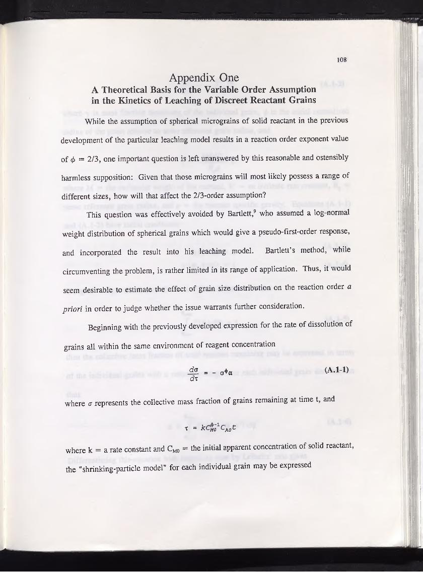
Appendix OneA Theoretical Basis for the Variable Order Assumption in the Kinetics of Leaching of Discreet Reactant Grains

While the assumption of spherical micrograins of solid reactant in the previous

development of the particular leaching model results in a reaction order exponent value

of cj) = 2/3, one important question is left unanswered by this reasonable and ostensibly

harmless supposition: Given that those micrograins will most likely possess a range of

different sizes, how will that affect the 2/3-order assumption?

This question was effectively avoided by Bartlett,9 who assumed a log-normal

weight distribution of spherical grains which would give a pseudo-first-order response,

and incorporated the result into his leaching model. Bartlett’s method, while

circumventing the problem, is rather limited in its range of application. Thus, it would

seem desirable to estimate the effect of grain size distribution on the reaction order a

priori in order to judge whether the issue warrants further consideration.

Beginning with the previously developed expression for the rate of dissolution of

grains all within the same environment of reagent concentration

do_ _ _ 0<i>a (A. 1-1)dr

where a represents the collective mass fraction of grains remaining at time t, and

X = kCtfo C-Aot

where k = a rate constant and CM0 = the initial apparent concentration of solid reactant,

the "shrinking-particle model" for each individual grain may be expressed

108

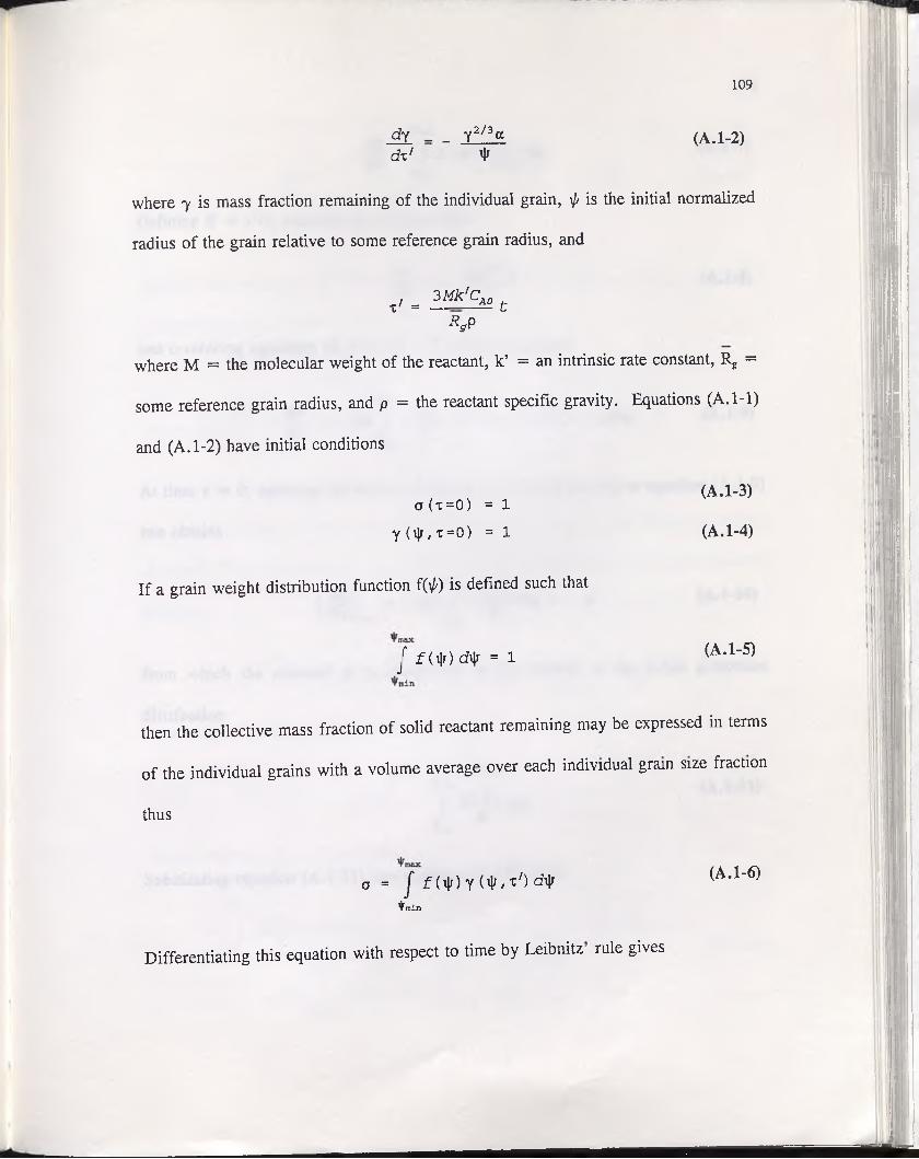
109

d y _ _ y2/3g d x ' ^

(A. 1-2)

where y is mass fraction remaining of the individual grain, \]/ is the initial normalized

radius of the grain relative to some reference grain radius, and

T/ = 2Mk'CA0 tR gP

where M = the molecular weight of the reactant, k’ = an intrinsic rate constant, Rg =

some reference grain radius, and p = the reactant specific gravity. Equations (A. 1-1)

and (A. 1-2) have initial conditions

0 (x=0) = 1 y (ijr, x=0) = 1

If a grain weight distribution function f(^) is defined such that

(A. 1-3)

(A. 1-4)

jf f (i|0 cft|r = 1 (A. 1-5)

then the collective mass fraction of solid reactant remaining may be expressed in terms

of the individual grains with a volume average over each individual grain size fraction

thus

o = | f (\|r) Y ('I'/*7) d^rnin

(A.1-6)

D ifferen tia tin g th is equation w ith resp ect to tim e b y L e ib n itz ru le g iv es

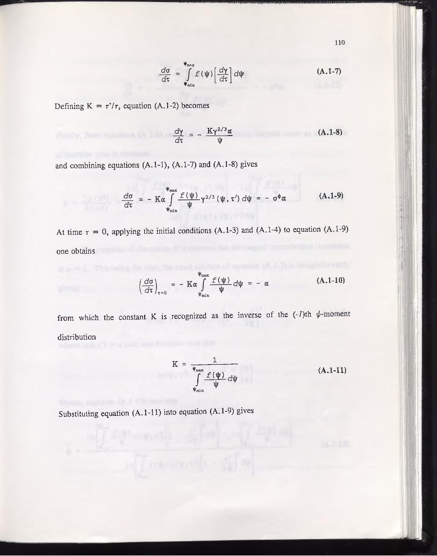
110

max

min(A. 1-7)

Defining K = t ’/t , equation (A. 1-2) becomes

dy = _ Ky2/3a (A. 1-8)d-z i|f

and combining equations (A. 1-1), (A. 1-7) and (A. 1-8) gives

(A. 1-9)

At time r = 0, applying the initial conditions (A. 1-3) and (A. 1-4) to equation (A. 1-9)

one obtains

(A. 1-10)

from which the constant K is recognized as the inverse of the (-l)th l/'-moment

distribution

K =

/f ( t )

(A.1-11)

Substituting equation (A. 1-11) into equation (A. 1-9) gives

Ill

dodr

raaxa j* ^ y2'3 (ty> t7) cfy

\|r ■“min ________max

U lL L d *min

o^a (A.1-12)

Finally, from equations (A. 1-6) and (A. 1-12) the effective reaction order as a function

of reaction time is obtained:

I n

I n ( a * )

^max

/ - ^ P - y 2/2 ( t ^ 7)^min

- I n

^max

^min

I n ( a )I n

max

J f ( i | 0 Y ( ^ / t 7) c ty^min

(A. 1-13)

For purposes of discussion, it is assumed that the reagent concentration is constant

at a = 1. This being the case, the exact solution of equation (A. 1-2) is straightforward,

giving

Y (ijf/t') 1 -

where u(\j/,T') — a unit step function such that

u (i|f, r 7)f 1 , ?7 <; 3 iJj)1 0, t' > 3\lrj

(A.1-14)

Hence, equation (A. 1-13) becomes

I n

^max / / N2

di|i - I n

^max/ m i d ,

^min<l>

I n

^max| f (v |0 u (ilr , x 7)

^min3 -

(A.1-15)

112

While the choice of a distribution function in the absence of experimental data is

an arbitrary one, the log-normal distribution40 allows easy comparison with the results

of Bartlett. In dimensionless form, this function is

f ( * , . ex p f-2 s 2

(A.1-16)v/2"rcs\|f

where s = the standard deviation of the distribution. Integrating f(i/0 between the limits

(0 < ty < o°) results in a definite integral which satisfies the criterion of equation (A. 1-5):

maxf f ( t y ) d t y

min? -1— e x p f- ( ln f - - W{ y/2nsty l 2 s 2 )

i — f e x p f - ( l n ^ 2) d ( l n t|t) ■ n s V 2 s )

(A.1-17)

y/2ns

= 1

In addition, the log-normal (-i)th ^-moment distribution is readily solved:

4*max

/minf 1 1 1 1 a y = f ----------1 — - e x p

J i|r J0 y f2 n s ty 2

^ ^ ) d t y(A.1-18)

e x p

Hence, the final expression for the reaction order as a function of reaction time is

I n

<t> =I 1

y in s ty 2

In / e x p - | u ( * , t') 1 - - U d*2 S' 3t|r,

(A. 1-19)

This equation involves only one parameter for its unique solution; namely, the standard

113

deviation, s, of the log-normal distribution.

Solutions to equation (A. 1-16) are plotted in Figure A. 1-1 for six values of the

standard deviation. These values were chosen, after Bartlett, according to

resulting in the distribution properties summarized in Table A. 1-1.

Semi-log plots of a vs. r according to equation (A. 1-6) for the six values of s are

shown in Figure A. 1-2. These curves show qualitatively how wider distributions of grain

size result in higher apparent orders of reaction. This observation is confirmed

quantitatively in Figure A. 1-3, where plots of 4> as calculated by equation (A. 1-19) are

plotted as functions of a. It should be noted that these curves are completely independent

of actual time of reaction. The dashed lines represent least-squares zero-order

polynomial fits of the 0-c curves to give "average" reaction orders which, as shown in

Figure A. 1-4, bear a near-perfect quadratic relationship to the standard deviation.

Returning to Figure A. 1-3, obviously, the range of 4> over the course of leaching

increases dramatically with increasing s. However, as shown in Figure A. 1-5, when the

values of <£ave are used in the solution of equation (A. 1-1), the results (dashed curves) fall

surprisingly close to the actual <r-r curves as calculated by equation (A. 1-6) (solid

curves), even at high s values. Thus, one may conclude that the assumption of a single

value for the overall order of reaction in the concentration of a solid reactant in equation

(A. 1-1) is acceptable over a fairly wide range of grain size distributions. Furthermore,

4> may possess a wide range of values greater than or equal to 2/3, but not less than 2/3,

when the individual reacting grains are roughly spherical.

(A.1-20)

114

TABLE A.l-I: Properties of the log-normal distributions represented in Figure A. 1-1.

Curve s '/'oW'/'o.oi '/'o.oi ’/'0.99

1 0 10° 1 1

2 0.2475 10l/2 0.562 1.78

3 0.495 101 0.316 3.16

4 0.99 102 0.1 10

5 1.485 103 0.0316 31.6

6 1.98 104 0.01 100—

115

FIGURE A. 1-1The log-normal distribution function.

116

F IG U R E A. 1-2C o llective m ass fraction remaining (cr) v s.

distributions.

reaction tim e (r) for various grain w eight

118

FIGURE A. 1-4Average apparent reaction order (<£ave) vs. weight distribution (s).

the standard deviation of the log-normal grain

119

Collective mass fraction remaining (a) vs. reaction time (r) as calculated by equations (A. 1-6) (solid curves) and (A. 1-1) (dashed curves).

120

Appendix TwoNumerical methods

The variable-order dissolution rate expressions are ordinary differential equations

which are solved by the classical four-point Runge-Kutta technique:41

dx

K =

k 2 = f ( x j + \ h , uj + \ h k j

k 2 = f ( x j + j h lUj + \ h k 2)

Jc4 = f (xj + h, Uj + hkz)

Uj+i = uj + (-^i + 2k2 + 2kz + k4.)

The particle model equations are solved numerically by fully implicit finite

difference approximations of the form42

a2; du 1 - { ( i+ l) ui+lfJtldt i ( 6 £ ) :2 J

= 6( 8 0 2

( Ul , j + 1 “ U0,J+1

du _ dx , j + 1 ~ U i . j ^

K U = KUi , j +1

where iis the particle radius index and j is the time index. Since all of the variables in

they* time level are known, and those of the (/+l)th time level are unknown, except

at the particle surface, a system of N equations for N unknowns is generated, each with

variable in each of the (i-l)th, ith, and (i+l)th radius levels. So, for the diffusionone

equation in spherical coordinates

121

3 ^ * | | H ♦ KU =d \2 l 3$ 3x

th e N a lg eb ra ic equation s form a tri-d iagon al c o e ffic ien t m atrix equation

1 *€r N. ii o 6 \ i uo,j+i ~ u 0 , j

0 ~ V i * 0 2p ~ui .3

2 r ~ V i * 0 2 r U2, j+1—

~U2.j

n-1 ^ ~ V i * 0

E Z l nn

- 2 - nn -1 r

- V i t o Un, j+1 r u n , j - ( ^ Kw h ic h is e a s ily so lv ed b y G aussian e lim in a tio n , 4 3 and w h ere

\|ri=0 = 6p - k ( 6t ) + 1

= 2 \i - k ( 8t ) + 1

and u b is th e su rface boundary con d ition for the (/ + l ) th tim e in d ex .

T h e g lo b a l heap m o d el P D E ’s are transform ed in to ordinary d ifferen tia l equation s

th rou gh th e d efin itio n o f the substantial tim e, or m aterial d er iv a tiv e , 4 4 ex p ressed in

d im e n s io n le ss coord in ates

JD_ _ _d_ + _3_D0 00 0C

T h is tran sform ation facilita tes the m athem atical treatm ent o f the g lo b a l heap m o d e l from

th e L a p la c ia n v iew p o in t, i . e . , v ia the tracking o f flu id e lem en ts (m aterial v o lu m es)

through th e h eap . S im p le backw ard fin ite d ifferen ce approxim ations are em p lo y ed to

s o lv e th e c o n v e c tio n eq u ation s e x p lic it ly .

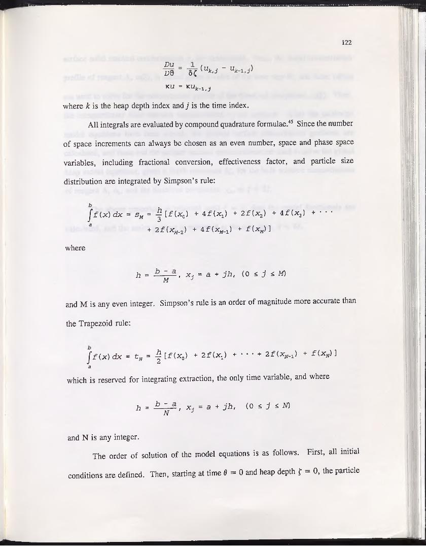
I m m m

122

DuD0 6C

(uk.j ~ U;

KU = KUJc-l.j

where £ is the heap depth index and 7 is the time index.

All integrals are evaluated by compound quadrature formulae.45 Since the number

of space increments can always be chosen as an even number, space and phase space

variables, including fractional conversion, effectiveness factor, and particle size

distribution are integrated by Simpson’s rule:

f f ( x ) d x * s M = - | [ f ( x 0) + 4 £ { x j ) + 2 f [ x 2) + 4 J f ( x 3) + • * *

+ 2 f ( x M_2) + 4 f ( x w ) + f U M) ]

where

h = —----- - f x , = a + j h , (0 <. j <■ M)M

and M is any even integer. Simpson’s rule is an order of magnitude more accurate than

the Trapezoid rule:

j*f ( x ) d x ~ t N = - | [ f ( x 0) + 2 f [ x 1) + • • • + 2 f ( x N_1) + f ( Xj j ) ]a

which is reserved for integrating extraction, the only time variable, and where

h = b ~ — , x , = a + j h , (0 <, j <■ N)N J

and N is any integer.

The order of solution of the model equations is as follows. First, all initial

conditions are defined. Then, starting at time 9 = 0 and heap depth f = 0, the particle

123

surface solid reactant concentrations crsi are determined. Next, the radial concentration

profile of reagent A, a(£), is solved given a value of the time step 59, and these values

are used to solve for the concentration profile of the dissolved complexes, Xi(£)- Then,

the intraparticular solid reactant concentrations crpi are updated. After the particular

model equations have been solved, the particle surface concentration gradients are

calculated, and these and the surface reactant concentrations are used to solve the global

heap model equations, given a depth increment 5f, for the bulk solution concentrations

of reagent A, ab, and the dissolved complexes, Xib> at f + 5f.

The above procedure is repeated until f = 1, then the model functionals are

calculated, and the entire process is reiterated at the new time, 9 + 59.

124

Appendix ThreeExperimental Data

Experimental data from the batch leaching tests are presented in Table A.3-1.

Data from column leaching test 1 are presented in Table A.3-II, and from tests 2 through

5 in Table A.3-III. Parameters and operating variables for all experimental leaching tests

are given in chapters one and two.

125

TABLE A.3-1: Data from batch leaching tests.

Batch test 1 Batch test 2 Batch test 3 Batch test 4

Time(min)

Âg |(ppm) |

Time(min)

Âg(ppm)

Time(min)

Âg |(ppm) 1

Time(min)

C-Ag(ppm)

30 0.05 15 0.20 5 0.01 30 0.87

60 0.07 30 0.48 10 0.13 60 1.79

90 0.11 60 1.04 20 0.36 90 2.72

180 0.33 130 2.16 80 2.22 120 3.42

270 0.48 220 3.35 140 3.78 240 5.23

360 0.58 360 4.68 200 4.72 410 7.03

610 0.90 600 6.16 260 5.94 770 9.38

1140 1.34 1290 9.29 360 6.98 1380 10.9

1620 1.59 1770 10.9 540 8.30 1830 12.4

2595 2.02 2910 12.8 640 9.08 2880 14.6

4080 2.22 4530 16.5 1320 11.3 4200 17.1

5460 2.39 5820 18.3 1680 12.5 5640 18.8

6900 2.52 - - 2160 14.3 - -

_ _ - 2760 15.1 - -

_ - - 3250 16.8 - -

_ - - 4200 18.2 - -

_ - - 5820 19.4 - -

. _ - 7170 20.5 - -

_ - - 8910 22.7 - -

- - - - 9960 22.6 - -

■ W M W M W I W — — — — — — — — — — — — —

126

TABLE A.3-II: Data from column leaching test 1.

Time Effluent silver concentration, CAg(Z,t) (ppm)(hr)

Z = T Z = 4’ Z = 6’ Z = 8’ Z = 10’ Z = 12’ |

6 20.7 13.4 4.9 2.3 1.7 0.4

24 33.1 34.9 29.9 24.6 18.2 12.4

48 33.5 43.0 43.3 38.7 36.0 32.1

73 38.7 47.8 44.3 43.3 42.0 39.2

96 34.6 46.8 45.4 46.2 46.0 46.5

122 28.2 45.3 49.7 47.7 46.3 47.4

145 20.5 44.7 47.5 47.6 45.7 45.6

168 22.5 46.7 47.3 47.7 47.4 47.5

191 20.7 47.1 49.2 48.1 47.9 46.7

219 17.3 45.6 48.0 49.3 49.4 49.3

241 18.4 47.7 47.8 50.7 49.9 48.9

266 13.8 43.5 48.6 48.7 49.1 49.3

291 11.7 40.1 45.9 48.3 47.5 48.3

313 10.8 35.6 45.4 46.8 46.1 47.0

340 11.2 34.9 48.5 48.9 48.6 47.8

364 12.8 29.7 46.7 48.5 47.3 48.1

384 6.2 27.2 46.9 47.7 48.0 48.3

410 4.8 21.8 46.4 48.1 47.5 48.3

434 6.1 20.5 46.5 47.6 48.3 48.5

457 4.4 15.4 44.6 48.0 48.6 48.5

481 2.6 12.5 46.4 46.6 48.2 48.1

509 3.9 11.0 41.1 47.3 47.0 47.0

533 2.6 9.1 37.1 46.9 47.5 49.3

552 4.0 7.8 36.1 46.9 47.5 48.1

580 7.1 9.0 34.2 47.4 48.6 48.5

127

Time 2’ 4’ 6’ 8’ 10’ 12’

602 1.8 5.3 30.0 45.2 48.1 48.6 1

633 5.1 6.4 24.9 43.1 47.4 47.3

652 1.8 3.8 22.0 40.9 47.7 47.2

674 1.1 3.2 22.2 42.1 46.5 47.2 1

697 1.2 2.9 20.7 37.6 50.8 50.7

723 2.8 4.0 16.5 33.8 48.4 49.8

746 1.9 3.4 16.4 32.2 49.9 50.0

769 1.1 2.3 12.6 28.6 49.0 49.2

798 1.5 2.6 9.8 25.2 49.0 49.1

821 1.8 3.4 9.1 23.7 49.7 49.3 1

842 1.7 2.9 9.6 22.4 48.8 49.0

870 1.8 2.5 8.3 21.7 50.5 51.3

889 1.3 2.3 7.4 20.0 47.4 51.2

914 1.4 2.6 6.8 17.9 45.6 50.3

938 1.2 2.3 6.1 16.5 42.1 49.8

963 0.4 1.4 4.8 17.0 39.1 48.8

984 0.6 1.5 4.1 19.6 41.5 48.6

1013 0.9 2.1 4.5 19.3 36.0 49.7

1032 0.9 1.6 4.1 17.2 34.4 48.9

1062 0.6 1.7 3.6 15.2 31.3 47.7

1108 0.2 1.2 2.6 12.8 26.6 46.0

1159 1.2 2.0 3.3 13.0 25.5 48.0

1198 0.7 1.6 2.8 11.9 21.8 45.9

1246 0.7 1.2 2.1 9.3 18.9 43.5

1300 0.6 1.3 2.0 8.3 17.0 35.3

1350 0.4 1.3 2.0 7.4 16.3 30.6

1398 0.3 0.7 1.6 6.3 11.3 24.6

i

128

TABLE A.3-III: Data from column leaching tests 2 through 5.

Column test 2 Column test 3 | Column test 4 Column test 5

Time C-Ag Time ^Ag j Time C-Ag Time ^Ag(hr) (ppm) (hr) (ppm) | (hr) (ppm) (hr) (ppm)

1 33.6 1 30.8 1 31.0 1 3.94

2 41.5 2 38.2 2 40.3 2 6.65

4 44.6 4 40.0 4 42.5 4 8.38

7 43.6 7 38.7 7 40.7 7 8.14

12 40.3 12 33.8 12 41.3 12 7.37

24 29.1 24 24.6 23 30.2 23 4.19

48 14.7 48 14.8 36 27.0 36 3.10

72 10.0 72 10.3 51 18.4 51 1.20

96 7.63 96 6.96 72 11.6 72 0.64

121 4.92 121 5.40 96 7.85 96 0.27

145 3.81 145 3.42 120 5.64 120 0.16

170 2.34 170 2.65 164 2.71 164 0.08

192 1.82 192 2.04 184 1.96 184 0.04

216 1.23 216 1.52 210 1.38 210 0.02

240 1.15 240 1.23 236 1.01 236 0.02

265 0.79 265 0.93 262 0.85 262 0.02

290 0.57 290 0.72 283 0.66 283 0.00

313 0.50 313 0.64 310 0.48 - -

342 0.35 342 0.43 335 0.31 - -

360 0.35 360 0.35 - - - -

Appendix FourNomenclature

Roman Letters

b; stoichiometry number, mol i/mol A

CA concentration of reagent A, mol A/cmf3

CAb concentration of reagent A external to particle, mol A/cmf3

CEi0 initial extractable grade of solid reactant i, mol i/g ore

q concentration of dissolved species i, mol i/cmf3

q b bulk concentration of dissolved species i, mol i/cmf3

Cpi grade of solid reactant i within particle, mol i/g ore

Cpi0 initial grade of solid reactant i within particle, mol i/g ore

Csi grade of solid reactant i on particle surface, mol i/g ore

q i0 initial grade of solid reactant i on particle surface, mol if,g ore

DAc effective pore diffusivity of reagent A, cmf3/cmp s

Die effective pore diffusivity of dissolved species i, cmf3/cmp s

E; extraction of dissolved species i, dimensionless

kpj rate constant of solid reactant i within particle, mol i/g ore s [Cpf [CA]

k*; rate constant of solid reactant i on particle surface, mol i/cny s [CJ* [CA]

1; liberation function of solid reactant i, dimensionless

m Gates-Gaudin-Schuhmann size distribution parameter, dimensionless

n number of solid reactants

NRe pellet flow Reynolds number, dimensionless

r radius, cm

130

R p artic le radius, cm

t tim e , s

u s su p erfic ia l b u lk f lo w v e lo c ity , cm f3 /cm h 2 s

w G ates-G audin-Schuhm ann size d istribution fu n ction , d im en sio n less

X; fraction a l co n v ersio n o f so lid reactant i , d im en sio n less

z dep th , cm

Z heap dep th , cm

G reek L etters

a d im en sio n less con cen tration o f reagent A

a b d im en sio n less con cen tration o f reagent A external to p article

/3 ; reagen t strength param eter relative to so lid reactant i , d im en sio n less

7 m od u lu s in stead y-sta te m odel

5 . ratio o f d iffu s iv ity o f d isso lv ed sp ec ies i to reagen t A , d im en sio n less

eb b u lk so lu tio n v o lu m e fraction

eh heap v o id fraction

eQ o re p o ro sity , cm f3 /c m p 3

f d im e n sio n less depth

,qi e ffe c tiv e n e ss factor for so lid reactant i , d im en sio n less

9 d im e n sio n le ss f lo w tim e

K D a m k o h ler II num ber fo r so lid reactant i w ith in p artic le , d im en sio n less

Ksi D am k d h ler II num ber for so lid reactant i on p artic le su rface , d im en sio n less

X; su rface fraction o f so lid reactant i, d im en sio n less

ratio o f v o lu m e o f b u lk flu id to flu id in particle p ores, d im en sio n less

d im e n sio n le ss radius

d im e n sio n le ss p artic le radius

o re d en s ity , g o re /cm 3 ore

d im e n sio n le ss grade o f so lid reactant i w ith in particle

d im e n sio n le ss grad e o f so lid reactant i on particle surface

d im e n sio n le ss d iffu s io n tim e

reaction order fo r so lid reactant i w ith in p article, d im en sio n less

rea ctio n order fo r so lid reactant i on particle surface, d im en sio n less

d im e n sio n less con cen tration o f d isso lved sp ecies i

d im e n sio n le ss b u lk concentration o f d isso lved sp ec ies i

id ea l co lu m n param eter (in verse P ec le t num ber), d im en sio n less

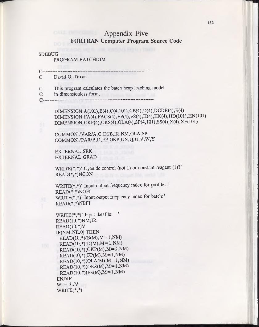
O U

A ppendix FiveFORTRAN Computer Program Source Code

$DEBUGPROGRAM BATCHDIM

David G. Dixon

C This program calculates the batch heap leaching model C in dimensionless form.C ----------------------------------------------------------------------------------------------------

D IM E N S IO N A (1 0 1 ) ,B (4 ) ,C (4 ,1 0 1 ) ,C B (4 ) ,D (4 ) ,D C D R (4 ) ,E (4 ) D IM E N S IO N F A (4 ) ,F A C S (4 ) ,F P (4 ) ,F S (4 ) ,H (4 ) ,H K (4 ) ,H D (1 0 1 ) ,H N (1 0 1 ) D IM E N S IO N O K P (4 ),O K S ( 4 ) ,O L A (4 ) ,S P (4 ,1 0 1 ) ,S S (4) ,X (4 ) ,X F (1 0 1 )

C O M M O N /V A R /A ,C ,D T B ,IR ,N M ,O L A ,S P C O M M O N /P A R /B ,D ,F P ,O K P ,O N ,Q ,U ,V ,W ,Y

E X T E R N A L SR K E X T E R N A L G R A D

W R IT E C *,*)’ C yan id e con tro l (not 1) or constan t reagen t (1 )? ’ R E A D (* ,* )N C O N

W R IT E (* ,* )’ Input output freq u en cy in d ex for p r o f ile s : ’

R E A D (* ,* )N O F IW R IT E (* ,* )’ Input output freq u en cy in d ex for b a tch :’

R E A D (* ,* )N B F I

W R IT E (* ,* )’ Input datafile: ’R E A D (1 0 ,* )N M ,I R R E A D (1 0 ,* )V IF (N M .N E .O ) T H E N

R E A D (1 0 ,’i:) (B (M ) ,M = : l ,N M )R E A D (1 0 ,* ) (D (M ) ,M = 1 ,N M )R E A D (1 0 ,* )(O K P (M ),M = 1 ,N M )R E A D (1 0 ,* ) (F P (M ) ,M = 1 ,N M )R E A D ( 1 0 ,* ) (O L A (M ) ,M = 1 , N M )R E A D (1 0 ,* ) (O K S (M ) ,M = 1 ,N M )R E A D (1 0 ,* ) (F S (M ) ,M = 1 ,N M )

E N D IF W = 3 ./V W R IT E (* ,* )

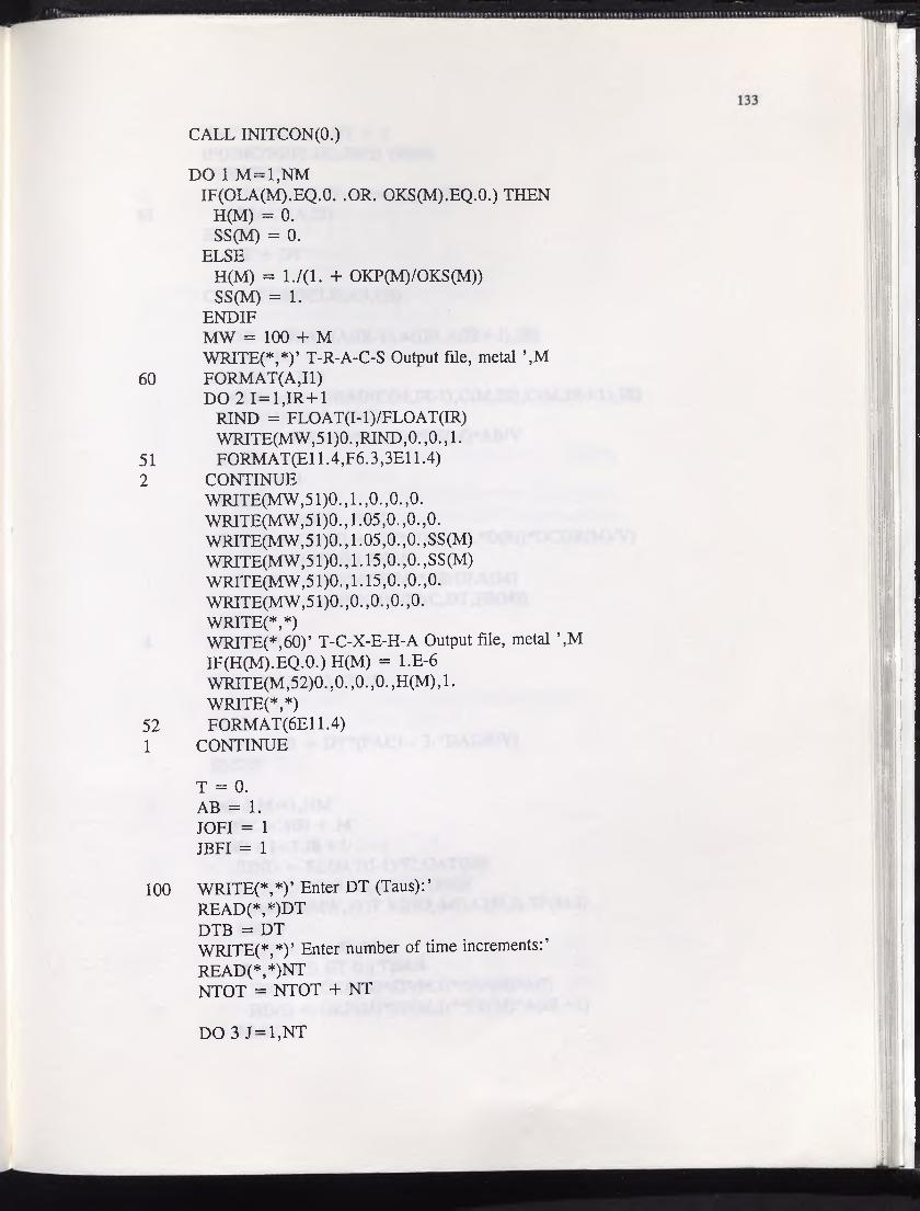
CALL INITCON(0.)

DO 1 M=1,NMIF(OLA(M).EQ.O. .OR. OKS(M).EQ.O.) THEN

H(M) = 0.SS(M) = 0.

ELSEH(M) = l ./( l . + OKP(M)/OKS(M))SS(M) = 1.

ENDIFMW = 100 + MW RITE(V)’ T-R-A-C-S Output file, metal \M

60 FORMAT(A,Il)DO 2 I=1,IR+1

RIND = FLOAT (I-1 )/FLO AT (IR)WRITE(MW,51)0.,RIND,0. ,0., 1.

51 FORMAT(E11.4,F6.3,3E11.4)2 CONTINUE

WRITE(MW,51)0., 1. ,0. ,0. ,0.WRITE(MW, 51)0., 1.05,0. ,0.,0.WRITE(MW,51)0., 1.05,0. ,0. ,SS(M)WRITE(MW,51)0., 1.15,0. ,0. ,SS(M)WRITE(MW,51)0. ,1.15,0. ,0. ,0.WRITE(MW,51)0. ,0. ,0. ,0. ,0.WRITE(*,*)WRITE(*,60)’ T-C-X-E-H-A Output file, metal ’,M IF(H(M).EQ.0.) H(M) = l.E-6 WRITE(M,52)0. ,0. ,0. ,0. ,H(M), 1.WRITE(*,*)

52 F ORM AT (6E11.4)1 CONTINUE

T = 0.AB = 1.JOFI = 1 JBFI = 1

100 WRITE(*,*)’ Enter DT (Taus): ’READ(*,*)DT DTB = DTWRITE(*,*)’ Enter number of time increments:’READ(*,*)NTNTOT = NTOT + NT

DO 3 J=1,NT

JINC = NTOT - NT + J IF(JINC/NBFI.EQ.JBFI) THEN

WRITE(*,*)WRITE(*,61)’ On increment ’,JINC

61 FORMAT(A,I5)ENDIF T = T + DT

CALL PARTICLE(AB, CB)

DADR = GRAD(A(IR-1),A(IR),A(IR+ 1),IR)FAC1 = 0.DO 4 M=1,NM

DCDR(M) = GRAD(C(M,IR-1),C(M,IR),C(M,IR+1),IR) IF(SS(M).GT.O.) THEN

FAC = OKS (M) *SS (M) * *FS (M) * AB/V ELSE

FAC = 0.ENDIFFAC1 = FAC1 - FACCB(M) = CB(M) + DT*(FAC - 3.*D(M)*DCDR(M)/V) IF(OLA(M). NE. 0.) THEN

SFAC = -OKS (M) *B (M) * AB/ OLA (M)SS(M) = SRK(SS(M),SFAC,DT,FS(M))

ENDIF4 CONTINUE

IF(NCON.EQ.l) THEN AB = 1.

ELSEAB = AB + DT*(FAC1 - 3.*DADR/V)

ENDIF

DO 5 M=1,NM MW = 100 + M DO 6 I=1,IR+1

RIND = FLOAT (I-1 )/FLO AT (IR) IF(JINC/NOFI.EQ.JOFI) THEN

WRITE(M W, 51) T, RIND ,A(I),C(M,I),SP (M, I)ENDIFXF(I) = 1. - SP(M,I)IF(SP(M,I).GT.O.) THEN

HN(I) = OKP(M)*SP(M,I)**FP(M)*A(I)HD (I) = OKP(M)*SP(M,I)**FP(M)*A(IR+1)

ELSE

135

HN(I) = 0.HD (I) = 0.

ENDIF6 CONTINUE

IF(JINC/NOFI.EQ.JOFI) THEN WRITE(MW,51)T, 1. ,0. ,0. ,0.WRITE(MW,51)T, 1.05,0. ,0. ,0.WRITE(MW,51)T, 1.05,0. ,0. ,SS(M)WRITE(MW,51)T, 1.15,0. ,0. ,SS(M)WRITE(MW,51)T, 1.15,0. ,0. ,0.WRITE(MW,51)T,0. ,0. ,0. ,0.IF(M.EQ.NM) JOFI = JOFI + 1

ENDIFCALL SIMPSON(IR,XF, 1 ,XW)CALL SIMPSON(IR,HN, 1 ,HNW)CALL SIMPSON(IR,HD, 1 ,HDW)X(M) = (1. - OLA(M))*XW + OLA(M)*(l. - SS(M)) IF(SS(M).GT.O.) THEN

HNW = HNW + OKS (M) *S S (M) * *FS (M) * A (IR +1) HDW = HDW + OKS(M)*SS(M)**FS(M)*A(IR+1)

ENDIFIF(HDW.GT.O.) THEN

H(M) = HNW/HDW ELSE

H(M) = 1.ENDIFE(M) = B(M)*V*CB(M)IF(JINC/NBFI.EQ.JBFI) THEN

WRITE(M, 52)T, CB(M), X(M) ,E(M) ,H(M), AB IF(M.EQ.NM) JBFI = JBFI + 1

ENDIF5 CONTINUE

3 CONTINUEWRITE(*,*)WRITE(*,62)’ Time (tau) = ’,T

62 FORMAT(A,F11.4)WRITE(*,*)

DO 7 M=1,NMWR1TE(*,53)’ Extraction of metal ’,M,’ = ’,E(M) WRITE(*,53)’ Conversion of metal ’,M,’ = ’,X(M) WRITE(*,53)’ Effectiveness of metal \M ,’ = ’,H(M)

53 F0RMAT(A,I2,A,F6.3)WRITE(*,*)

136

7 CONTINUE

WRITE(*,*)’ To continue, enter "1" ’ READ (*, *)NREP IF(NREP.EQ.l) GOTO 100

END

$INCLUDE: TNITCON.FOR’$INCLUDE: ’PARTICLE. FOR’$INCLUDE: ’ ASOLVE.FOR’SINCLUDE: ’CSOLVE.FOR’$INCLUDE: ’TRI.FOR’$INCLUDE: ’SPSOLVE.FOR’$INCLUDE: ’SRK.FOR’ $INCLUDE:’SIMPSON.FOR’$INCLUDE: ’GRAD.FOR’

0 U

$DEBUGPROGRAM HEAPGGS

David G. Dixon

C This program calculates the heap leaching model C in dimensionless form for a distribution of particle sizes. c --------------------------------------------------------------------

DIMENSION A(17,65,9),B(2),C(2,17,65,9),CB(2),CBOLD(2),D(2) DIMENSION E(2) ,FACS(2) ,FP(2) ,FS(2) ,H(2) ,HD(2,65) DIMENSION HN(2,65) ,HDF(17) ,HDL(65) ,HNF(17) ,HNL(65) DIMENSION HTD (2) ,HTN(2), OKP(2), OKS (2), OLA (2) DIMENSION SP(2,17,65,9),SS(2,65),WC(2),X(2,65),XF(17) DIMENSION XI(9),XL(65),XT(2)

COMMON /VAR/A,C,DTB,IR,NK,NL,NM,SP,SS COMMON /PAR/B,D,FP,FS,OKP,OKS,OLA,V,W,XI

EXTERNAL GRAD EXTERNAL SRK

WRITE(*,*)’ Enter profile output frequency index:’ READ(*,*)NOFIWRITE(*,*)’ Enter effluent output frequency index:’READ(*,*)NEFIJOFI = 0JEFI = 0

WRITE(*,*)’ Input datafile: ’READ(10,*)NM,IR,NL,NKREAD(10,*)V,W,XI(1)IF(NM.NE.O) THEN

READ(10,*)(B(M),M=1,NM)READ(10,*)(D(M),M=1,NM)READ(10,*)(OKP(M),M=1,NM)READ(10,*)(FP(M),M=1,NM)READ(10,*)(OLA(M),M=1,NM)READ (10,*) (OKS (M), M = 1, NM)READ(10,*)(FS(M),M=1,NM)

ENDIF

DZ = l./FLOAT(NL)GM = LOG (0.01 )/LOG (XI (1))

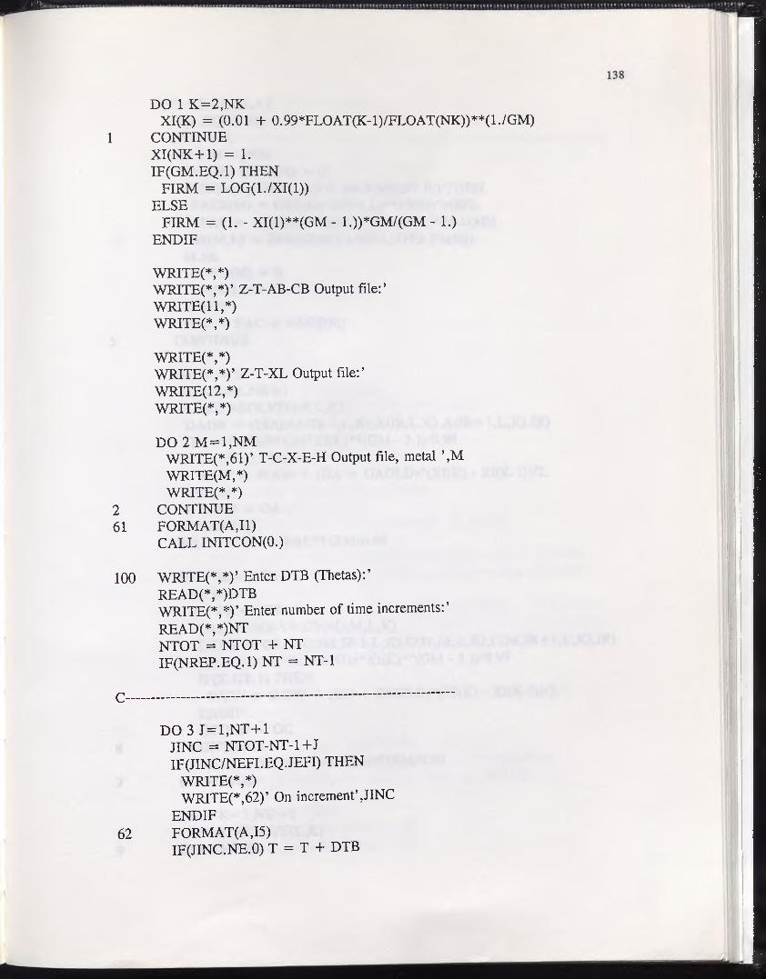
DO 1 K=2,NKXI(K) = (0.01 + 0.99 *FLO AT (K-1) /FLOAT (NK)) * * (1. / GM)

1 CONTINUE XI(NK+1) = 1.IF(GM.EQ.l) THEN

FIRM = LOG(l./XI(l))ELSE

FIRM = (1. - XI(1)**(GM - l.))*GM/(GM - 1.)ENDIF

WRITE(*,*)WRITE(*,*)’ Z-T-AB-CB Output file:’WRITE(11,*)WRITE(*,*)

WRITE(*,*)WRITER,*)’ Z-T-XL Output file:’WRITE(12,*)WRITE(*,*)

DO 2 M=1,NMWRITE(*,61)’ T-C-X-E-H Output file, metal ’,M WRITE(M,*)WRITE(*,*)

2 CONTINUE61 FORMAT(A,Il)

CALL INITCON(0.)

100 WRITE(*,*)’ Enter DTB (Thetas):’READ(*,*)DTBWRITE(*,*)’ Enter number of time increments:’READ(*,*)NTNTOT = NTOT + NTIF(NREP.EQ. 1) NT = NT-1

-------------------------------------------------------------------------------------

DO 3 J = 1,NT+1 JINC = NTOT-NT-l+J IF (JINC/NEFI. EQ. JEFI) THEN

WRITE(*,*)WRITER,62)’ On increment’,JINC

ENDIF62 FORM AT(A, 15)

IF(JINC.NE.O) T = T + DTB

139

DO 4 L =1,N L +1 IF(L.EQ.l) AB = 1.FAC = 0.DO 5 M=1,NM

IF(L.EQ.l) CB(M) = 0.IF(SS(M,L).GT.O. .AND. OLA(M).GT.O.) THEN

FACS(M) = OKS(M)*SS(M,L)**FS(M)*AB/3.SFAC = - OKS (M) *B(M) * V *W* AB/ (3. * OL A(M))SS(M,L) = SRK(SS(M,L),SFAC,DTB,FS(M))

ELSEFACS(M) = 0.SS(M,L) = 0.

ENDIFFAC = FAC + FACS(M)

5 CONTINUE

WAW = 0.DO 6 K=1,NK+1

CALL ASOLVE(AB,L,K)DADR = GRAD(A(IR-1,L,K),A(IR,L,K),A(IR+1,L,K),IR)GA = (DADR*GM*XI(K)**(GM - 3.))/0.99 IF(K.GT.l) THEN

WAW = WAW + (GA + GAOLD)*(XI(K) - XI(K-l))/2.ENDIFGAOLD = GA

6 CONTINUEWA = WAW + FAC*FIRM/0.99

DO 7 M=1,NM WCW = 0.DO 8 K=1,NK+1

CALL CSOLVE(CB(M),M,L,K)DCDR = GRAD(C(M,IR-1,L,K),C(M,IR,L,K),C(M,IR+1,L,K),IR) GC = (D(M)*DCDR*GM*XI(K)**(GM - 3.))/0.99 IF(K.GT.l) THEN

WCW = WCW + (GC + GCOLD)*(XI(K) - XI(K-l))/2.ENDIFGCOLD = GC

8 CONTINUEWC(M) = WCW - FACS (M) *FIRM/0.99

7 CONTINUE

DO 9 K=1,NK+1 CALL SSOLVE(L,K)

9 CONTINUE

140

ZL = FLOAT (L- l)/FLOAT (NL)TL = T + ZLIF(JINC/NOFI.EQ.JOFI) WRITE(11,50)ZL,TL,AB,(CB(M),M = 1 ,NM) IF(JINC/NEFI.EQ. JEFI) THEN

IF(JINC.EQ.O .OR. L.EQ.NL+1) THENWRITE(*,50)ZL,TL,AB,(CB(M),M=1,NM)

ENDIFENDIF

50 FORMAT(F6.3,F9.3,5E11.4)

DO 10 M=1,NM IF (JINC/NEFI. EQ. JEFI) THEN

X(M,L) = 0.HN(M,L) = 0.HD(M,L) = 0.DO 11 K=1,NK+1

DO 12 I=1,IR+1 XF(I) = 1. - SP(M,I,L,K)HNF(I) = SP(M,I,L,K)**FP(M)*A(I,L,K)HDF(I) = SP(M,I,L,K)**FP(M)

12 CONTINUECALL SIMPSON(IR,XF, 1 ,XW)CALL SIMPSON(IR,HNF, 1 ,HNW)CALL SIMPSON(IR,HDF, 1 ,HDW)FACK = XI(K) - OLA(M)XW = FACK*XW*GM*XI(K)**(GM - l.)/0.99 FACK = FACK/(1. - OLA(M))HNW = HNW*FACK*OKP(M)*GM*XI(K)**(GM - l.)/0.99 HDW = HDW*FACK*OKP(M)*GM*XI(K)**(GM - l.)/0.99 IF(K.NE. 1) THEN

X(M,L) = X(M,L) + (XW + XWOLD)*(XI(K) - XI(K-l))/2. HN(M,L) = HN(M,L) + (HNW + HNWO)*(XI(K)-XI(K-l))/2. HD(M,L) = HD(M,L) + (HDW + HDWO)*(XI(K)-XI(K-l))/2.

ENDIFX W O L D = X W H N W O = H N W H D W O = H D W

11 C O N T IN U EX(M,L) = X(M,L) + OLA(M)5i:(l. - SS(M,L))HN(M,L) = HN(M,L) + OKS(M)*SS(M,L)^FS(M)*AB HD(M,L) = HD(M,L) + OKS(M)*SS(M,L)**FS(M)

ENDIFIF(L.NE.NL+1) THEN

CB(M) = CB(M) - W*WC(M)*DZ IF(CB(M).LT.l.E-30) CB(M) = 0.

141

ENDIF10 CONTINUE

IF(JINC/NOFLEQJOFI)WWTE(12,50)ZL,TL,(X(M,L),M=1,NM)

IF(L.NE.NLEl) THEN AB = AB - W*WA*DZ IF(AB.LT. 1 .E-30) AB = 0.

ENDIF

4 CONTINUE

DO 13 M=1,NM IF(JINC.NE.O) THEN

E(M) = E(M) + V *B (M) * (CBOLD (M) + CB(M))*DTB/2.ELSE

E(M) = 0.ENDIF

13 CONTINUE

IF(JINC/NEFI.EQ JEFI) THEN DO 14 M=1,NM

DO 15 L=1,NL+1 XL(L) = X(M,L)HNL(L) = HN(M,L)HDL(L) = HD(M,L)

15 CONTINUECALL SIMPSON(NL,XL,0,XT(M))CALL SIMPSON(NL,HNL,0,HTN(M))CALL SIMPSON(NL,HDL,0,HTD(M))IF(HTD(M).NE.O.) THEN

H(M) = HTN (M) /HTD (M)WRITE(M,52)T +1. ,CB(M),XT(M),E(M),H(M)

ELSEWRITE(M,52)T +1. ,CB(M),XT(M),E(M)

ENDIF52 F0RMAT(F8.2,4E11.4)14 CONTINUE

JEFI = JEFI + 1ENDIF

DO 16 M=1,NM CBOLD(M) = CB(M)

16 CONTINUE

142

IF(JINC/NOFI.EQ.JOFI) THEN WRITE(11,50) 1. ,TL, 1. ,(0. ,M = 1 ,NM) WRITE(12,50)1.,TL,(0.,M=1,NM) WRITE(12,50)0. ,TL,(0. ,M = 1,NM)JOFI = JOFI + 1

ENDIF

3 CONTINUEWRITE(*,*)

DO 17 M=1,NMWRITE(*,63)’ Extraction of metal ’,M,’ = ’,E(M)

63 FORMAT(A,I2,A,F6.3)WRITER,*)

17 CONTINUE

WRITER,*)’ To continue, enter "1" ’ READ(*,*)NREP IF(NREP.EQ.l) GOTO 100

300 END

$INCLUDE: TNITCON.FOR’SINCLUDE: ’ ASOLVE.FOR’$INCLUDE:’CSOLVE.FOR’$INCLUDE: ’TRI.FOR’$INCLUDE:’SSOLVE.FOR’$INCLUDE: ’SRK.FOR’$INCLUDE: ’SIMPSON.FOR’$INCLUDE: ’GRAD.FOR’

SUBROUTINE INITCON(AO)

c ----------------------------------------------------------------------------------------------------C This subroutine sets initial conditions for all variables.c ----------------------------------------------------------------------------------------------------

DIMENSION A(17,65,9),C(2,17,65,9),SP(2,17,65,9) DIMENSION SS(2,65)

COMMON /VAR/A,C,DTB,IR,NK,NL,NM,SP,SS

DO 1 K=1,NK+1 DO 2 L=1,NL+1

DO 3 I=1,IR+1 A(I,L,K) = AO

3 CONTINUE DO 4 M=1,NM

SS(M,L) = 1.DO 5 I = 1,IR+1

SP(M,I,L,K) = 1.C(M,I,L,K) = 0.

5 CONTINUE4 CONTINUE2 CONTINUE1 CONTINUE

RETURNEND

SUBROUTINE AS OLVE(AB,L,K)

This subroutine solves the intraparticle reagent concentration profile by an iterative finite difference approximation.

D IM E N S IO N A (1 7 ,6 5 ,9 ) ,B (2 ) ,B L (1 7 ) ,B M (1 7 ) ,B R (1 7 ) ,C (2 ,1 7 ,6 5 ,9 )

D IM E N S IO N D (2 ), F P (2 ) ,F S (2 ) , O K P (2 ), O K S (2 ), O L A (2 ) ,R ( 17) D IM E N S IO N S P (2 ,1 7 ,6 5 ,9 ) ,S S (2 ,6 5 ) ,X I (9 ) ,A W (1 7 )


Ou

uu

2

144

DTR = DTB*V*W/(3.*XI(K)**2)DR = l./FLOAT(IR)DM = DTR/DR**2

DO 1 1=1,IR F = 0.DO 2 M=1,NM

IF(SP(M,I,L,K).GT.O.) THEN FXI = XI(K)*(XI(K) - OLA(M))/(l. - OLA(M))F = F + FXI*OKP(M)*SP(M,I,L,K)**FP(M)*DTR

ENDIF CONTINUE IF(I.EQ.l) THEN

BL(I) = 0.BM(I) = 6.*DM + F + 1.BR(I) = -6.*DM

ELSEBL(I) = FLOAT (1 -I) *DM/FLO AT (I)BM(I) = 2.*DM + F + 1.BR(I) = FLOAT (I) *DM/FLO AT (1 -I)

ENDIF

1R(I) = A(I,L,K)

CONTINUER(IR) = R(IR) - BR(IR)*AB

CALL TRI(IR,BL,BM,BR,R,AW)

3

DO 3 1=1,IR A(I,L,K) = AW(I)

CONTINUE A(IR+1,L,K) = AB

RETURNEND

SUBROUTINE CSOLVE(CB,M,L,K)

This subroutine solves the intraparticle complex concentration profile by an iterative finite difference approximation.

DIMENSION A(17,65,9),B(2),BL(17),BM(17),BR(17),C(2,17,65,9) DIMENSION D(2),FP(2),FS (2), OKP(2), OKS (2), OLA(2),R( 17)

noon

DIMENSION SP(2,17,65,9),SS(2,65),XI(9),CW(17)


DTR = DTB*V*W*D(M)/(3.*XI(K)**2)DR = l./FLOAT(IR)DM = DTR/DR**2

DO 1 1=1,IRFXI = XI(K)*(XI(K) - OLA(M))/(l. - OLA(M))F = FXI*OKP(M)*SP(M,I,L,K)**FP(M)*A(I,L,K)*DTR/D(M) IF(SP(M,I,L,K).LE.O.) F = 0.IF(I.EQ.l) THEN

BL(I) = 0.BM(I) = 6.*DM + 1.BR(I) = -6.*DM

ELSEBL(I) = FLOAT (1 -I) *DM/FLO AT (I)BM(I) = 2.*DM + 1.BR(I) = FLOAT (I) *DM/FLO AT (1 -I)

ENDIFR(I) = C(M,I,L,K) + F

1 CONTINUER(IR) = R(IR) - BR(IR)*CB

CALL TRI(IR,BL,BM,BR,R,CW)

DO 2 1=1,IR C(M,I,L,K) = CW(I)

2 CONTINUE C(M,IR+1,L,K) = CB

RETURNEND

SUBROUTINE TRI(N,BL,BM,BR,R,U)

This subroutine solves a tri-diagonal matrix by Gaussian elimination.

DIMENSION B L (1 0 1 ),B M (1 0 1 ),B R (1 0 1 ),R (1 0 1 ),U (1 0 1 )

0 o

u u

T r r « T i iT j - i j a a u '. r 3 r r r r r t - i w ti t i t ’

146DO 1 1=2,N

E = BL(I-1)/BM(I-1)BM(I) = BM(I) - E*BR(I-1)R(I) = R(I) - E*R(I-1)

1 CONTINUE

U(N) = R(N)/BM(N)DO 2 1=1,N-l

U(N-I) = (R(N-I) - BR(N-I)*U(N-I+ 1))/BM(N-I)2 CONTINUE

RETURNEND

SUBROUTINE SSOLVE(L,K)

This subroutine solves the intraparticle solid reactant concentration profile by a classical Runge-Kutta technique.

DIMENSION A(17,65,9),B(2),C(2,17,65,9),D(2),FP(2),FS(2) DIMENSION OKP(2),OKS(2),OLA(2),SP(2,17,65,9),SS(2,65),XI(9)


EXTERNAL SRK

DTR = DTB*V*W/3.DO 1 M=1,NM

DO 2 I=1,IR+1IF(SP(M,I,L,K).GT.O. .AND. OLA(M).LT. 1.) THEN

FAC = -OKP(M)*B(M)*A(I,L,K)/(l. - OLA(M))SP(M,I,L,K) = SRK(SP(M,I,L,K),FAC,DTR,FP(M)) IF(SP(M,I,L,K).LT.O.) SP(M,I,L,K) = 0.

ENDIF2 CONTINUE1 CONTINUE

RETURNEND

FUNCTION SRK(S,FAC,DT,F)

C ---------------------------------------------------------------------------------------------------C This function subprogram solves the solid reactant dissolution C rate expression by a classical Runge-Kutta technique.C ---------------------------------------------------------------------------------------------------

FI = FAC*S**F G = S + 0.5*DT*F1 IF(G.LT.O.) GOTO 100 F2 = FAC*G**F G = S + 0.5*DT*F2 IF(G.LT.O.) GOTO 100 F3 = FAC*G**F G = S + DT*F3 IF(G.LT.O.) GOTO 100 F4 = FAC*G**FSRK = S + DT*(F1 + 2.*F2 + 2.*F3 + F4)/6. IF(SRK.LE.0.) SRK = 0.GOTO 200

100 SRK = 0.

200 RETURN END

SUBROUTINE SIMPSON(N,X,INDEX,U)

C--------------------------------------------------------------------C This subroutine performs numerical integration by compound C quadrature techniques (Trapezoid and Simpson’s rules).C--------------------------------------------------------------------

DIMENSION X(101)N1 = N/2 N2 = N - N/2 IF(N1.NE.N2) GOTO 100

IF (INDEX. EQ.l) F = X(N+1)IF (INDEX. NE.l) F = X(l) + X(N+1)

DO 1 I=3,N-1,2IF (INDEX. EQ. 1) F = F + 2.*X(I)*(FLOAT(I-l)/FLOAT(N))**2 IF(INDEX.NE.l) F = F + 2.J,:X(I)

1 CONTINUE

nn

nn

2

148

DO 2 1=2,N,2IF (INDEX. EQ.l) F = F + 4.*X(I)*(FLOAT(I-l)/FLOAT(N))**2 IF(INDEX.NE. 1) F = F + 4.*X(I)

CONTINUE

IF(INDEX.EQ.l) U = F/FLOAT(N)IF(INDEX.NE.l) U = F/(3.*FLOAT(N))RETURN

100 IF (INDEX. EQ.l) F = X(N+1) IF(INDEX.NE. 1) F = X(l) + X(N+1)

3

C—ccc —-

DO 3 1=2,NIF(INDEX.EQ.l) F = F + 2.*X(I)*(FLOAT(I-l)/FLOAT(N))**2 IF(INDEX.NE. 1) F = F + 2.*X(I)

CONTINUE

IF(INDEX.EQ. 1) U = 3.*F/(2.*FLOAT(N))IF (INDEX. NE.l) U = F/(2.*FLOAT(N))RETURN

END

FUNCTION GRAD(F 1 ,F2 ,F3 ,IR)

This function subprogram solves the intraparticle concentration gradients at R by a three-point cubic interpolation spline.

DR = l./FLOAT(IR)C = 3.*(F3 - 2.*F2 + F1)/(4.*DR**2)B = (F3 - F2)/DR - 2.*DR*C/3.D = -C/(3.*DR)GRAD = B + 2.*C*DR + 3.*D*DR**2

RETURNEND

0 U

$LARGE$DEBUG

PROGRAM ORDER

David G. Dixon

C This program uses a log-normal grain weight distributionC function to test the variable order assumption of heterogeneousC kinetics of the dissolution of spherical mineral grains.C ----------------------------------------------------------------------------------------------------

DIMENSION PSI(2001),F(2001),FAC(2001),FACP(2001)

PI = 4.*ATAN(1.)WRITER,*)’ T-S-PHI Output file:’WRITE(1,*)0.,1.WRITE(*,*)W RITE(V)’ F-PSI Output file:’WRITE(11,*)0.,0.WRITE(*,*)WRITE(*,*)’ Enter the log-normal standard deviation:’READ(*,*)SWRITE(*,*)F(l) = 0.PSI(l) = 0.DO 1 1=2,1001

PSI(I) = FLOAT (I-1) * 1. E-3F(I) = EXP(-(LOG(PSI(I))**2/(2*S**2)))/(SQRT(2*PI)*S*PSI(I))

1 CONTINUECALL SIMPTRAP(1000,F,1,1.E-3,FI1)

100 WRITE(*,*)’ Enter psi increment to try after median:’READ(*,*)DPSI DO 2 1=1002,2001

PSI(I) = 1. + FLOAT (I-1001) *DPSIF(I) = EXP(-(LOG(PSI(I))**2/(2*S**2)))/(SQRT(2*PI)*S*PSI(I))

2 CONTINUECALL SIMPTRAP(1000,F, 1001 ,DPSI,FI2)FI = FI1 + FI2WRITE(*,*)’ Integral of f(psi) = ’,FI WRITE(*,*)WRITE(*,*)’ If this is unsatisfactory, type "1":’READ(*,*)NREP IF(NREP.EQ.l) GOTO 100 DO 3 1=2,2001

WRITE(11,*)PSI(I),F(I) 3 CONTINUE

FPIC = EXP(S**2/2)AK = l./FPIC WRITE(*,*)

200 WRITE(*,*)’ Enter DT (taus):’READ(*,*)DTWRITE(*,*)’ Enter number of time increments:’READ(*,*)NTWRITE(*,*)

DO 4 J=1,NT JTOT = JTOT + 1 WRITE(*,*)’ On increment: ’,JTOT T = T + DT TP = AK*T FAC(l) = 0.FACP(l) = 0.DO 5 1=2,2001

TFAC = 1. - TP/(3*PSI(I))IF(TFAC.LT.O.) TFAC = 0.FAC(I) = F(I)*TFAC**3 FACP(I) = F(I)*TFAC**2/PSI(I)

5 CONTINUECALL SIMPTRAP(1000,FAC, 1,1 .E-3,GI1)CALL SIMPTRAP(1000,FAC, 1001 ,DPSI,GI2)CALL SIMPTRAP(1000,FACP,1,1.E-3,GPI1)CALL SIMPTRAP(1000,FACP, 1001 ,DPSI,GPI2)H = GI1 + GI2HP = (GPI1 + GPI2)/FPICIF(H.GT.0. .AND. HP.GT.0.) PHI = LOG(HP)/LOG(H) WRITE(1,*)T,H,PHI WRITE(*,*)T,H,PHI

4 CONTINUE

W RITE(V)WRITE(*,*)’ To continue, type "1":’READ (*, *)NREP IF(NREP.EQ.l) GOTO 200

300 END

$INCLUDE: ’SIMPTRAP.FOR’

uu

uu

151

SUBROUTINE SIMPTRAP(N,X,NS,D,U)

This subroutine performs numerical integration by compound quadrature techniques for ORDER.

DIMENSION X(2001)N1 = N/2 N2 = N - N/2 IF(N1.NE.N2) GOTO 100

F = X(NS) + X(N+NS)DO 1 I=NS+2,N+NS-2,2

F = F + 2.*X(I)1 CONTINUE

DO 2 I=NS + 1,N+NS-1,2 F = F + 4.*X(I)

2 CONTINUE

U = F*D/3.RETURN

100 F = (X(NS) + X(N+NS))/2.DO 3 I=NS + 1,N+NS-1

F = F + X(I)3 CONTINUE

U = F*D RETURN

END

152

Appendix SixAnalytical Solutions to the Pseudo-Steady-State Two-Reactant Problem

The generalized differential equation

X 2 & y + X (a 2b x ' ) - & d x 2 dx ( A . 6 - 1 )

+ [c + d x 2s - b ( l - a - r ) x x + b 2x 2z] y

may be reduced to Bessel’s equation

= o

+ X *Z + ( x 2 - p 2) y = 0 d x 2 dx

( A . 6 - 2 )

by proper transformation of variables. The solution may then be obtained in terms of

Bessel functions.46 The generalized solution of equation (A.6-1) is then

y _ j r (1-a) / 2 g - ( b x 1 / r)

where

/ d X s + c,z.2 -p\yf\d

/j( A . 6 - 3 )

p = 7 N l" T -l - a \2 - c

Cl and c2 are constants, and Zp and Z p are Bessel functions of orders p and -p,

respectively. Table A.6-1 summarizes which Bessel functions are involved in the solution

depending on the conditions of the Bessel function arguments and orders.

Multiplying equation (1-31) by | 2 gives

' K*>V a ’ 0( A . 6 - 4 )

Comparing equations (A.6-4) and (A.6-1), and noting that y = a and x - £, the

following identities are observed:

153

TABLE A.6-1: Bessel functions to use in equation (A.6-3)

Conditions V'd/s is real V'd/s is imaginary

p ^ 0 or Z p = J P z P = iPan integer n Z p = J - p

Z.p — I.p

p = 0 or Zp = jn Zp = I„an integer n z.p = Yn Z.p = Kn

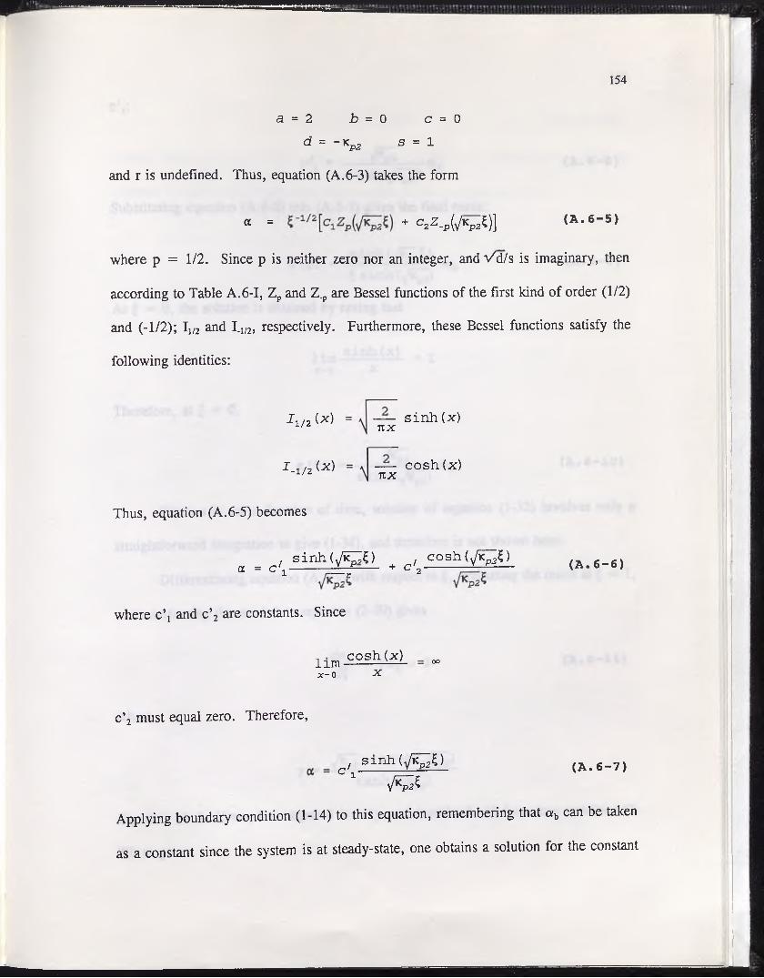
154

a = 2 £> = 0 c = 0

d = “ Kp2 s = 1

and r is undefined. Thus, equation (A.6-3) takes the form

a « + c2z .pVv 5)] <&- 6 - 5 >

where p = 1/2. Since p is neither zero nor an integer, and Vd/s is imaginary, then

according to Table A.6-1, Zp and Z.p are Bessel functions of the first kind of order (1/2)

and (-1/2); I1/2 and I.1/2, respectively. Furthermore, these Bessel functions satisfy the

following identities:

Xi/2 (x)

J - l /2 (x)

— s i n h ( x )TZ X

—— cosh(x)7 I X

Thus, equation (A.6-5) becomes

. s i n h ( ^ C C ) / c o s h ( 0 c^£) a = c \ --------- - ± r f ------ + c '2---------— —-------

where c \ and c’2 are constants. Since

( A . 6 - 6 )

cosh (x) l im ------------x-0 x

oo

c’2 must equal zero. Therefore,

c , s i n h ( 0 c ^ g ) (a . 6 - 7 )

1 ^

Applying boundary condition (1-14) to this equation, remembering that a b can be taken

as a constant since the system is at steady-state, one obtains a solution for the constant

155

c \ = -----------------absinM ^ic~)

Substituting equation (A.6-8) into (A.6-7) gives the final result:

« ( « ) ■ q ,$ sinhCyK )At £ = 0, the solution is obtained by noting that

limx-o

s i n h ( . x )x

= 1

Therefore, at £ = 0,

( A . 6 - 8 )

( A . 6 - 9 )

a (0) = --------------------ajb ( A. 6 - 1 0 )s i n h ( v/K^)

Since a is not a function of time, solution of equation (1-32) involves only a

straightforward integration to give (1-34), and therefore is not shown here.

Differentiating equation (A.6-9) with respect to £, evaluating the result at £ = 1,

and substituting the result into equation (2-30) gives

+ y « h = 0 ( A . 6 - 1 1 )dC *

where

~ t a n M ^ )Y t a n h ( ^ k^ )

Equation (A.6-11) may be integrated directly, and combined with boundary condition (2-

20) to give

a b (C) = e ~ “YC ( A . 6 - 1 2 )

which, when combined with equations (A.6-9) and (A.6-10), results in the complete

solution to the pseudo-steady-state two-reactant problem, equation (2-31).

156

Bibliography

157

1. Heinen, H.J., Peterson, D.G., and Lindstrom, R.E., "Processing Gold Ores Using Heap Leach-Carbon Adsorption Methods," (Report IC 8770, U.S. Bureau of Mines, 1978).

2. Philip, T.P., "To Mill or To Leach?," World Gold ’91. (Parkville, Victoria, Australia: The Australasian Inst. Min. Metall., 1991), pp. 1-2.

3. Dorey, R ., Van Zyl, D ., and Kiel, J ., "Overview of Heap Leaching Technology," Introduction to Evaluation. Design and Operation of Precious Metal Heap Leaching Projects, eds. Van Zyl, K., Hutchison, I., and Keil, J., (Littleton, CO: SME-AIME, 1988), pp. 3-22.

4. Braun, R.L., Lewis, A.E., and Wadsworth, M.E., "In-Place Leaching of Primary Sulfide Ores: Laboratory Leaching Data and Kinetics Model," Metall. Trans.. 5 (1974), pp. 1717-1726.

5. Levenspiel, O., Chemical Reaction Engineering. 2nd ed. (New York, NY: John Wiley & Sons, 1976), pp. 357-408.

6. Madsen, B.W., Wadsworth, M.E., and Groves, R.D., "Application of a Mixed Kinetics Model to the Leaching of Low Grade Copper Sulfide Ores," Trans. SME-AIME. 258 (1975), pp. 69-74.

7. Gao, H.W., Sohn, H.Y., and Wadsworth, M.E., "A Mathematical Model for the Solution Mining of Primary Copper Ore: Part I. Leaching by Oxygen-Saturated Solution Containing No Gas Bubbles," Metall. Trans. B. 14B (1983), pp. 541- 551.

8. Lin, H.K., and Sohn, H.Y., "Mixed-Control Kinetics of Oxygen Leaching of Chalcopyrite and Pyrite from Porous Primary Ore Fragments," Metall. Trans. B, 18B (1987), pp. 497-504.

9. Bartlett, R.W., "A Combined Pore Diffusion and Chalcopyrite Dissolution Kinetics Model for In Situ Leaching of a Fragmented Copper Porphyry," International Symposium on Hvdrometallurgy, ed. Evans , D.J.I., and Shoemaker, R.S., (New York, NY: AIME, 1973), pp. 331-374.

10. Braithwaite, J.W., (Ph. D. dissertation, University of Utah, 1976).

11. Madsen B.W., and Wadsworth, M.E., "A Mixed Kinetics Dump Leaching Model for Ores Containing a Variety of Copper Sulfide Minerals," (Report RI 8547, U.S. Bureau of Mines, 1981).

12. Roman, R.J., Benner, B.R., and Becker, G.W., "Diffusion Model for Heap Leaching and Its Application to Scale-Up," Trans. SME-ATMF,. 256 (1974), pp. 247-252.

13. Shafer, J.L., White, M.L., and Caenepeel, C.L., "Application of the Shrinking Core Model for Copper Oxide Leaching," Min. Engng.. 31 (2) (1979), pp. 165- 171.

14. Chae, D.G., and Wadsworth, M.E., "The Leaching of Dilute Copper Oxide Ore Phases," In Situ Recovery of Minerals, ed. Coyne K.R., and Hiskey, J.B., (New York, NY: Engineering Foundation, 1989), pp. 1-21.

15. Box, J.C., and Prosser, A.P., "A General Model for the Reaction of Several Minerals and Several Reagents in Heap and Dump Leaching," Hvdrometallurgy. 16 (1986), pp. 77-92.

16. Hicban, W .T., and Gray, P.M. J ., "Cost Minimization in the Extraction of Copper from an Oxide Ore," Extraction Metallurgy ’81. ed. Jones, M.J., (London: Inst. Min. Metall., 1981), pp. 165-172.

17. Prosser, A.P., "Simulation of Gold Heap Leaching as an Aid to Process Development," Precious Metals ’89. ed. Jha M.C., and Hill, S.D., (Warrendale, PA: The Minerals, Metals & Materials Society, 1988), pp. 121-135.

18. Bartlett, R.W., "Pore Diffusion-Limited Metallurgical Extraction from Ground Ore Particles," Metall. Trans.. 3 (1972), pp. 913-917.

19. Crank, J., The Mathematics of Diffusion. 2nd ed., (Oxford: Clarendon Press, 1975), p. 91.

20. Bartlett, R. W ., "Simulation of Ore Heap Leaching Using Deterministic Models," Hvdrometallurgy. 29 (1992), pp. 231-260.

21. Wen, C.Y., "Noncatalytic Heterogeneous Solid Fluid Reaction Models," Ind. Eng. Chem.. 60 (9) (1968), pp. 34-54.

22. Ramachandran, P.A., and Doraiswamy, L.K., "Modeling of Noncatalytic Gas- Solid Reactions," AIChE J .. 28 (6) (1982), pp. 881-900.

23. Roach, G.I.D., and Prosser, A.P., "Prediction of Rates of Chemical Processes for Treatment of Low-Grade Materials: Theory and Tests for Mass-Transfer Controlled Reactions," Trans. Inst. Min. Metall.. C87 (1978), pp. C129-C138.

24. Ishida, M., and Wen, C.Y., "Comparison of Kinetic and Diffusional Models for Solid-Gas Reactions," AIChE J ., 14 (2) (1968), pp. 311-317.

158

159

25. Habashi, F., "Kinetics and Mechanism of Gold and Silver Dissolution in Cyanide Solution," (Bulletin 59, Montana College of Mineral Science and Technology, 1967).

26. Schuhmann, R., "Energy Input and Size Distribution in Comminution," Trans. SME-AIME. 217 (1960), pp. 22-25.

27. Bartlett, R.W., "Conversion and Extraction Efficiencies for Ground Particles in Heterogeneous Process Reactors," Metall. Trans.. 2 (1971), pp. 2999-3006.

28. Evans, J.W., and Song, S., "A Model for the Design of Gas-Solid Reactors," Metall. Trans.. 4 (1973), pp. 1701-1707.

29. Taylor, J., and Whelan, P.T., "The Leaching of Cuprous Pyrites and the Precipitation of Copper at Rio Tinto, Spain," Inst, Min. Metall. Bull.. 457 (1942), pp. 1-36.

30. Harris, J.A., "Development of a Theoretical Approach to the Heap Leaching of Copper Sulphide Ores," Proc. Aust. Inst. Min. Metall.. 230 (1969), pp. 81-92.

31. Cathles, L.M., and Apps, J.A., "A Model of the Dump Leaching Process that Incorporates Oxygen Balance, Heat Balance, and Air Convection," Metall. Trans. B, 6B (1975), pp. 617-624.

32. Cathles, L.M., and Schlitt, W.J., "A Model of the Dump Leaching Process that Incorporates Oxygen Balance, Heat Balance, and Two Dimensional Air Convection," Leaching and Recovering Copper From As-Mined Materials, ed. Schlitt, W.J., (Littleton, CO: SME-AIME, 1980), pp. 9-27.

33. Cathles, L.M., and Murr, L.E., "Evaluation of an Experiment Involving Large Column Leaching of Low Grade Copper Sulfide Waste: A Critical Test of a Model of the Waste Leaching Process," Leaching and Recovering Copper From As-Mined Materials, ed. Schlitt, W.J., (Littleton, CO: SME-AIME, 1980), pp. 29-48.

34. Gao, H.W., Sohn, H.Y., and Wadsworth, M.E., "A Mathematical Model for the Solution Mining of Primary Copper Ore: Part II. Leaching by Solution Containing Oxygen Bubbles," Metall. Trans. B. 14B (1983), pp. 553-558.

35. Roman, R.J., and Olsen, C., "Theoretical Scale-Up of Heap Leaching," Solution Mining Symposium, ed. Apian, F.F., McKinney, W.A., and Pemichele, A.D., (New York, NY: AIME, 1974), pp. 211-229.

160

36. Prosser, A.P., and Box, J.C., "Simulation of the Mineralogical and Chemical Aspects of Heap and Dump Leaching as an Aid to Ore-Process Evaluation," Computers in Mining — 1983. (Parkville, Victoria, Australia: Australasian Inst. Min. Metall., 1983), pp. 171-178.

37. Roman, R.J., "Solution Channeling in Leach Dumps," Trans. SME-AIME. 262 (1977), pp. 73-74.

38. Satterfield, C.N., "Trickle-Bed Reactors," AIChEJ.. 21 (2) (1975), pp. 209-228.

39. Bondi, A., "Handling Kinetics from Trickle-Phase Reactors," Chem. Tech.. (3) (1971), p. 185.

40. Aitcheson, J., and Brown, J.A.C., The Lognormal Distribution. (Cambridge: Cambridge University Press, 1957).

41. Yakowitz, S., and Szidarovsky, F., An Introduction to Numerical Computations. (New York, NY: Macmillan, 1989), p. 372.

42. Crank, p. 149.

43. Smith, G.D., Numerical Solution of Partial Differential Equations. (London: Oxford University Press, 1965), pp. 17-23.

44. Bird, R.B., Stewart, W.E., and Lightfoot, E.N., Transport Phenomena. (New York, NY: John Wiley and Sons, 1960), pp. 73-74.

45. Yakowitz and Szidarovsky, pp. 197-214.

46. Mickley, H.S., Sherwood, T.K., and Reed, C.E., Applied Mathematics in Chemical Engineering. (New York, NY: McGraw-Hill Book Company, 1957), p. 174.

iM

Predicting the Kinetics of Heap Leaching with Unsteady-State ...

Documents

Transcript of Predicting the Kinetics of Heap Leaching with Unsteady-State ...