Chương 14- Chiết và Lọc ( Extraction and Leaching)

----------------------------------------------------------------------------------------------------------------------------------------------------------------------------------------------------------------------------------------------------------------------------------------------------------------------------------------------------------------------------------------------------------------------------------------------------------------- 14---------------------------------------------------------------------------------------------------------------------------------------------------------------------------------------------------------------------------------------------------------------------------------------------------------------------------------------------------------------------------------------------------------------------------------------------------------------

EXTRACTION AND LEACHING

Extraction is a process for the separation of one ormore components through intimate contact with asecond immiscible liquid called a solvent. If thecomponents in the original solution distribute

themselves differently between the two phases, separationwill occur. Separation by extraction is based on thisprinciple. When some of the original substances are solids,the process is called leaching. In a sense, the role of solventin extraction is analogous to the role of enthalpy indistillation. The solvent-rich phase is called the extract, andthe carrier-rich phase is called the raffinate. A high degree ofseparationmay be achieved with several extraction stages inseries, particularly in countercurrent flow.

Processes of separation by extraction, distillation,crystallization, or adsorption sometimes are equallypossible. Differences in solubility, and hence of separabilityby extraction, are associated with differences in chemicalstructure, whereas differences in vapor pressure are thebasis of separation by distillation. Extraction often iseffective at near-ambient temperatures, a valuable feature inthe separation of thermally unstable natural mixtures orpharmaceutical substances such as penicillin.

The simplest separation by extraction involves twoimmiscible liquids. One liquid is composed of the carrier andsolute to be extracted. The second liquid is solvent.Equilibria in such cases are represented conveniently ontriangular diagrams, either equilateral or right-angled, as forexample on Figures 14.2 and 14.3. Equivalentrepresentations on rectangular coordinates also are shown.Equilibria between any number of substances arerepresentable in terms of activity coefficient correlationssuch as the UNIQUAC or NRTL. In theory, these correlationsinvolve only parameters that are derivable frommeasurements on binary mixtures, but in practice theresulting accuracy may be poor and some multicomponentequilibrium measurements also should be used to find theparameters. Finding the parameters of these equations is acomplex enough operation to require the use of a computer.An extensive compilation of equilibrium diagrams andUNIQUAC and NRTL parameters is that of Sorensen and Arlt(1979–1980). Extensive bibliographies have been compiledby Wisniak and Tamir (1980–1981).

The highest degree of separation with a minimum ofsolvent is attained with a series of countercurrent stages.

Such an assembly of mixing and separating equipment isrepresented in Figure 14.4(a), and more schematically inFigure 14.4(b). In the laboratory, the performance of acontinuous countercurrent extractor can be simulated with aseries of batch operations in separatory funnels, as in Figure14.4(c). As the number of operations increases horizontally,the terminal concentrations E1 and R3 approachasymptotically those obtained in continuous equipment.Various kinds of more sophisticated continuous equipmentalso are widely used in laboratories; some are described byLo et al. (1983, pp. 497–506). Laboratory work is of particularimportance for complex mixtures whose equilibriumrelations are not known and for which stage requirementscannot be calculated.

In mixer-separators the contact times can be made longenough for any desired approach to equilibrium, but 80–90%efficiencies are economically justifiable. If five stages arerequired to duplicate the performance of four equilibriumstages, the stage efficiency is 80%. Since mixer-separatorassemblies take much floor space, they usually areemployed in batteries of at most four or five units. A largevariety of more compact equipment is being used. Thesimplest in concept are various kinds of tower arrangements.The relations between their dimensions, the operatingconditions, and the equivalent number of stages are the keyinformation.

Calculations of the relations between the input andoutput amounts and compositions and the number ofextraction stages are based on material balances andequilibrium relations. Knowledge of efficiencies andcapacities of the equipment then is applied to find its actualsize and configuration. Since extraction processes usuallyare performed under adiabatic and isothermal conditions,in this respect the design problem is simpler than forthermal separations where enthalpy balances also areinvolved. On the other hand, the design is complicated bythe fact that extraction is feasible only of nonideal liquidmixtures. Consequently, the activity coefficient behaviors oftwo liquid phases must be taken into account or directequilibrium data must be available. In countercurrentextraction, critical physical properties such as interfacialtension and viscosities can change dramatically through theextraction system. The variation in physical properties mustbe evaluated carefully.

14.1. INTRODUCTION

The simplest extraction system is made up of three components: the

solute (material to be extracted); the carrier, or nonsolute portion of

the feed; and the solvent, which should have a low solubility in the

carrier. Figure 14.1 illustrates a countercurrent extraction with a

light-phase solvent. The diagram can be inverted for a heavy-phase

solvent.

The carrier-rich liquid leaving the extractor is referred to as the

raffinate phase and the solvent-rich liquid leaving the extractor is

the extract phase. The solvent may be the dispersed phase or it may

be the continuous phase; the type of equipment used may determine

which phase is to be dispersed in the other phase.

In general, distillation is used to purify liquid mixtures. How-

ever, liquid extraction should be considered when the mixture

involves a:

. Low relative volatility (< 1:3)

. Removal of a nonvolatile component

. High heat of vaporization

. Thermally-sensitive components

. Dilute concentrations

481

Copyright � 2010 Elsevier Inc. All rights reserved.

DOI: 10.1016/B978-0-12-372506-6.00014-9

Liquid extraction is utilized by a wide variety of industries.

Applications include the recovery of aromatics, decaffeination of

coffee, recovery of homogeneous catalysts, manufacture of penicil-

lin, recovery of uranium and plutonium, lubricating oil extraction,

phenol removal from aqueous wastewater, and extraction of acids

from aqueous streams. New applications or refinements of solvent

extraction processes continue to be developed.

Extraction is treated as an equilibrium-stage process. Ideally,

the development of a new extraction process includes the following

steps:

. Select solvent.

. Obtain physical properties, including phase equilibria.

. Obtain material balance.

. Obtain required equilibrium stages.

. Develop preliminary design of contactor.

. Obtain pilot data and stage efficiency.

. Compare pilot data with preliminary design.

. Determine effects of scale-up and recycle.

. Obtain final design of system, including the contactor.

The ideal solvent would be easily recovered from the extract.

For example, if distillation is the method of recovery, the solvent-

solute mixture should have a high relative volatility, low heat of

vaporization of the solute, and a high equilibrium distribution

coefficient. A high distribution coefficient will translate to a low

solvent requirement and a low extract rate fed to the solvent recov-

ery column. These factors will minimize the capital and operating

costs associated with the distillation system. In addition to the

recovery aspects, the solvent should have a high selectivity (ratio

of distribution coefficients), be immiscible with the carrier, have a

low viscosity, and have a high density difference (compared to the

carrier) and a moderately low interfacial tension.

The critical physical properties that affect extractor perform-

ance include phase equilibria, interfacial tension, viscosities, den-

sities, and diffusion coefficients. In many extraction applications,

these properties may change significantly with changes in chemical

concentration. It is important that the effect of chemical concen-

tration on these physical properties be understood.

The required equilibrium stages and solvent-to-feed ratio is

determined by the phase equilibria, as discussed in Section 14.2.

The interfacial tension will affect the ease in creating drop size and

interfacial area for mass transfer. Jufu et al. (1986) provide a

reliable method for predicting the interfacial tension. It should be

noted that impurities and minor components can change the inter-

facial tension significantly.

A high density difference promotes phase settling and poten-

tially higher throughputs. High viscosities restrict throughput if the

viscous phase is continuous, and result in poor diffusion and low

mass transfer coefficients. The liquid molecular diffusion coeffi-

cient has a strong dependence on viscosity. In some applications,

increasing the operating temperature may enhance the extractor

performance.

14.2. EQUILIBRIUM RELATIONS

On a ternary equilibrium diagram like that of Figure 14.2, the limits

of mutual solubilities are marked by the binodal curve and the

compositions of phases in equilibrium by tielines. The region within

the dome is two-phase and that outside is one-phase. The most

common systems are those with one pair (Type I, Figure 14.2) and

two pairs (Type II, Figure 14.5) of partially miscible substances.

For instance, of the approximately 800 sets of data collected and

analyzed by Sorensen and Arlt (1979) andArlt et al. (1987), 75% are

Type I and 20% are Type II. The remaining small percentage of

systems exhibit a considerable variety of behaviors, a few of which

appear in Figure 14.5. As some of these examples show, the effect of

temperature on phase behavior of liquids often is very pronounced.

Both equilateral and right triangular diagrams have the prop-

erty that the compositions of mixtures of all proportions of two

mixtures appear on the straight line connecting the original mix-

tures. Moreover, the relative amounts of the original mixtures

corresponding to an overall composition may be found from ratios

of line segments. Thus, on the figure of Example 14.2, the amounts

of extract and raffinate corresponding to an overall composition

M are in the ratio E1=RN ¼ MRN=E1M.

Experimental data on only 28 quaternary systems were found

by Sorensen and Arlt (1979) and Arlt et al. (1987), and none of

more complex systems, although a few scattered measurements do

appear in the literature. Graphical representation of quaternary

systems is possible but awkward, so that their behavior usually is

analyzed with equations. To a limited degree of accuracy, the phase

behavior of complex mixtures can be predicted frommeasurements

on binary mixtures, and considerably better when some ternary

measurements also are available. The data are correlated as activity

coefficients by means of the UNIQUAC or NRTL equations. The

basic principle of application is that at equilibrium the activity of

each component is the same in both phases. In terms of activity

coefficients this condition is for component i,

gixi ¼ g�i x�i , (14:1)

where� designates the second phase. This may be rearranged into a

relation of distributions of compositions between the phases,

x�i ¼ (gi=g�i )xi ¼ Kixi, (14:2)

where Ki is the distribution coefficient. The activity coefficients are

functions of the composition of the mixture and the temperature.

Applications to the calculation of stage requirements for extraction

are described later.

The distribution coefficient Ki is the ratio of activity coeffi-

cients and may be estimated from binary infinite dilution coeffi-

cient data.

Ki ¼ g1ig�,1i

(14:3)

S+B(Extract)

A+B(Feed)

BA - CarrierB - SouteS - Solvent

S(Solvent)

A(Raffinate)

Figure 14.1. Solvent extraction process

482 EXTRACTION AND LEACHING

Binary interaction parameters (Aij) and infinite dilution

activity coefficients are available for a wide variety of binary

pairs. Therefore the ratio of the solute infinite dilution coefficient

in solvent-rich phase to that of the second phase (�) will provide anestimate of the equilibrium distribution coefficient. The method

can provide a reasonable estimate of the distribution coefficient

for dilute cases.

RT ln g1i,jn o

¼ Ai,j (14:4)

Ki ¼ g1ig�,1i

¼ eAij=RT

eA�ij=RT

(14:5)

See Example 14.1

Extraction behavior of highly complex mixtures usually can

be known only from experiment. The simplest equipment for

that purpose is the separatory funnel, but complex operations can

be simulated with proper procedures, for instance, as in Figure

14.4(c). Elaborate automatic laboratory equipment is in use. One

of them employs a 10,000–25,000 rpm mixer with a residence time

of 0.3–5.0 sec, followed by a highly efficient centrifuge and two

chromatographs for analysis of the two phases (Lo et al., 1983,

pp. 507).

Compositions of petroleum mixtures sometimes are repre-

sented adequately in terms of some physical property. Three

examples appear in Figure 14.6. Straight line combining of mix-

tures still is valid on such diagrams.

Basically, compositions of phases in equilibrium are indicated

with tielines. For convenience of interpolation and to reduce the

clutter, however, various kinds of tieline loci may be constructed,

usually as loci of intersections of projections from the two ends of

the tielines. In Figure 14.2 the projections are parallel to the base

and to the hypotenuse, whereas in Figures 14.3 and 14.7 they are

horizontal and vertical.

Several tieline correlations in equation form have been pro-

posed, of which three may be presented. They are expressed in

weight fractions identified with these subscripts:

CA solute C in diluent phase A

CS solute C in solvent phase S

SS solvent S in solvent phase S

AA diluent A in diluent phase A

AS diluent A in solvent phase S

SA solvent S in diluent phase A.

Figure 14.2. Equilibria in a ternary system, type 1, with one pair of partially miscible liquids; A ¼ 1-hexene, B ¼ tetramethylene sulfone,C ¼ benzene, at 508C (R.M. De Fre, thesis, Gent, 1976). (a) Equilateral triangular plot; point P is at 20% A, 10% B, and 70% C. (b) Righttriangular plot with tielines and tieline locus, the amount of A can be read off along the perpendicular to the hypotenuse or by difference.(c) Rectangular coordinate plot with tieline correlation below, also called Janecke and solvent-free coordinates.

14.2. EQUILIBRIUM RELATIONS 483

EXAMPLE 14.1Estimate the distribution coefficient for transferring acetonefrom water into benzene at 258C. The concentration of acetonein benzene is assumed to be dilute.

For acetone=benzene,Ai,II=RT ¼ 0:47

For acetone=water,Ai,II=RT ¼ 2:27

Ki ¼ e2:27

e0:47¼ 9:68

1:6¼ 6:05(mol=mol) ¼ 1:39(wt=wt)

Experimental values range 1.06–1.39. Distribution coefficient

data for dilute solute concentrations have been compiled by Trey-

bal in Perry’s Handbook. A sampling of the data presented by

Treybal and additional distribution coefficient data are given in

Table 14.1.

TABLE 14.1. Distribution Coefficients of Dilute Solute Systems.

Component A ¼ Carrier, component B ¼ solute, and component S ¼ extraction solvent. K1 isthe distribution coefficient (wt/wt)

Component B Component S Temp., 8C. K1 Ref.

A ¼ ethylene glycolAcetone Amyl acetate 31 1.838 38Acetone n-Butyl acetate 31 1.940 38Acetone Ethyl acetate 31 1.850 38A ¼ furfuralTrilinolein n-Heptane 30 47.5 5Triolein n-Heptane 30 95 5A ¼ n-hexaneToluene Sulfolane 25 0.336 4Xylene Sulfolane 25 0.302 4A ¼ n-octaneToluene Sulfolane 25 0.345 4Xylene Sulfolane 25 0.245 4A ¼ waterAcetaldehyde n-Amyl alcohol 18 1.43 31Acetaldehyde Furfural 16 0.967 31Acetic acid 1-Butanol 26.7 1.613 41Acetic acid Cyclohexanol 26.7 1.325 41Acetic acid Di-n-butyl ketone 25–26 0.379 32Acetic acid Diisopropyl carbinol 25–26 0.800 32Acetic acid Ethyl acetate 30 0.907 11Acetic acid Isopropyl ether 20 0.248 12Acetic acid Methyl acetate 1.273 29Acetic acid Methyl cyclohexanone 25–26 0.930 32Acetic acid Methylisobutyl ketone 25 0.657 40

25–26 0.755 32Acetic acid Toluene 25 0.0644 49Acetone n-Butyl acetate 1.127 29Acetone Chloroform 25 1.830 15

25 1.720 2Acetone Dibutyl ether 25–26 1.941 32Acetone Diethyl ether 30 1.00 19Acetone Ethyl acetate 30 1.500 46Acetone Ethyl butyrate 30 1.278 46Acetone n-Hexane 25 0.343 45Acetone Methyl acetate 30 1.153 46Acetone Methylisobutyl ketone 25–26 1.910 32Acetone Toluene 25–26 0.835 32Aniline n-Heptane 25 1.425 14

50 2.20 14Aniline Methylcyclohexane 25 2.05 14

50 3.41 14Aniline Toluene 25 12.91 43tert-Butanol Ethyl acetate 20 1.74 3Butyric acid Methyl butyrate 30 6.75 28Citric acid 25% Triisooctylamine/Chloroform 25 14.1 24Citric acid 25% Triisooctylamine/1-Octanol 25 41.5 24p-Cresol Methylnaphthalene 35 9.89 35Ethanol n-Butanol 20 3.00 10


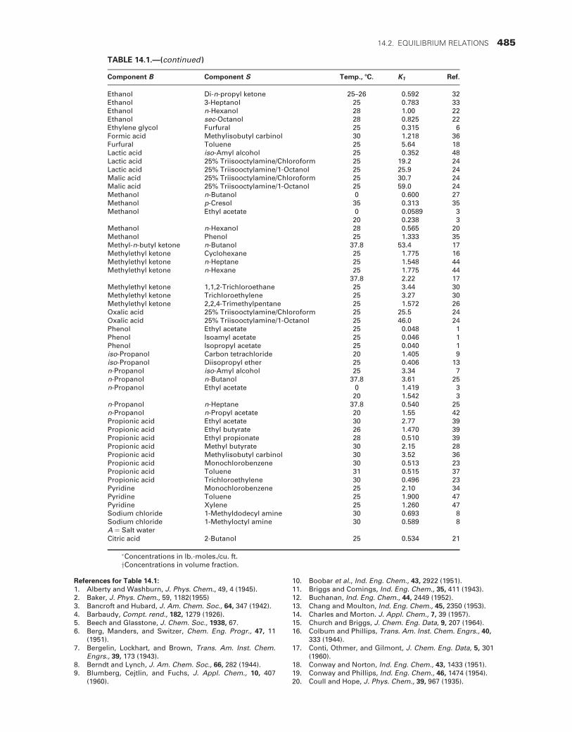
TABLE 14.1.—(continued )

Component B Component S Temp., 8C. K1 Ref.

Ethanol Di-n-propyl ketone 25–26 0.592 32Ethanol 3-Heptanol 25 0.783 33Ethanol n-Hexanol 28 1.00 22Ethanol sec-Octanol 28 0.825 22Ethylene glycol Furfural 25 0.315 6Formic acid Methylisobutyl carbinol 30 1.218 36Furfural Toluene 25 5.64 18Lactic acid iso-Amyl alcohol 25 0.352 48Lactic acid 25% Triisooctylamine/Chloroform 25 19.2 24Lactic acid 25% Triisooctylamine/1-Octanol 25 25.9 24Malic acid 25% Triisooctylamine/Chloroform 25 30.7 24Malic acid 25% Triisooctylamine/1-Octanol 25 59.0 24Methanol n-Butanol 0 0.600 27Methanol p-Cresol 35 0.313 35Methanol Ethyl acetate 0 0.0589 3

20 0.238 3Methanol n-Hexanol 28 0.565 20Methanol Phenol 25 1.333 35Methyl-n-butyl ketone n-Butanol 37.8 53.4 17Methylethyl ketone Cyclohexane 25 1.775 16Methylethyl ketone n-Heptane 25 1.548 44Methylethyl ketone n-Hexane 25 1.775 44

37.8 2.22 17Methylethyl ketone 1,1,2-Trichloroethane 25 3.44 30Methylethyl ketone Trichloroethylene 25 3.27 30Methylethyl ketone 2,2,4-Trimethylpentane 25 1.572 26Oxalic acid 25% Triisooctylamine/Chloroform 25 25.5 24Oxalic acid 25% Triisooctylamine/1-Octanol 25 46.0 24Phenol Ethyl acetate 25 0.048 1Phenol Isoamyl acetate 25 0.046 1Phenol Isopropyl acetate 25 0.040 1iso-Propanol Carbon tetrachloride 20 1.405 9iso-Propanol Diisopropyl ether 25 0.406 13n-Propanol iso-Amyl alcohol 25 3.34 7n-Propanol n-Butanol 37.8 3.61 25n-Propanol Ethyl acetate 0 1.419 3

20 1.542 3n-Propanol n-Heptane 37.8 0.540 25n-Propanol n-Propyl acetate 20 1.55 42Propionic acid Ethyl acetate 30 2.77 39Propionic acid Ethyl butyrate 26 1.470 39Propionic acid Ethyl propionate 28 0.510 39Propionic acid Methyl butyrate 30 2.15 28Propionic acid Methylisobutyl carbinol 30 3.52 36Propionic acid Monochlorobenzene 30 0.513 23Propionic acid Toluene 31 0.515 37Propionic acid Trichloroethylene 30 0.496 23Pyridine Monochlorobenzene 25 2.10 34Pyridine Toluene 25 1.900 47Pyridine Xylene 25 1.260 47Sodium chloride 1-Methyldodecyl amine 30 0.693 8Sodium chloride 1-Methyloctyl amine 30 0.589 8A ¼ Salt waterCitric acid 2-Butanol 25 0.534 21

�Concentrations in lb.-moles./cu. ft.yConcentrations in volume fraction.

References for Table 14.1:1. Alberty and Washburn, J. Phys. Chem., 49, 4 (1945).2. Baker, J. Phys. Chem., 59, 1182(1955)3. Bancroft and Hubard, J. Am. Chem. Soc., 64, 347 (1942).4. Barbaudy, Compt. rend., 182, 1279 (1926).5. Beech and Glasstone, J. Chem. Soc., 1938, 67.6. Berg, Manders, and Switzer, Chem. Eng. Progr., 47, 11

(1951).7. Bergelin, Lockhart, and Brown, Trans. Am. Inst. Chem.

Engrs., 39, 173 (1943).8. Berndt and Lynch, J. Am. Chem. Soc., 66, 282 (1944).9. Blumberg, Cejtlin, and Fuchs, J. Appl. Chem., 10, 407

(1960).

10. Boobar et al., Ind. Eng. Chem., 43, 2922 (1951).11. Briggs and Comings, Ind. Eng. Chem., 35, 411 (1943).12. Buchanan, Ind. Eng. Chem., 44, 2449 (1952).13. Chang and Moulton, Ind. Eng. Chem., 45, 2350 (1953).14. Charles and Morton. J. Appl. Chem., 7, 39 (1957).15. Church and Briggs, J. Chem. Eng. Data, 9, 207 (1964).16. Colbum and Phillips, Trans. Am. Inst. Chem. Engrs., 40,

333 (1944).17. Conti, Othmer, and Gilmont, J. Chem. Eng. Data, 5, 301

(1960).18. Conway and Norton, Ind. Eng. Chem., 43, 1433 (1951).19. Conway and Phillips, Ind. Eng. Chem., 46, 1474 (1954).20. Coull and Hope, J. Phys. Chem., 39, 967 (1935).


21. Crittenden and Hixson, Ind. Eng. Chem., 46, 265 (1954).22. Crook and Van Winkle, Ind. Eng. Chem., 46, 1474 (1954).23. Cumming and Morton, J. Appl. Chem., 3, 358 (1953).24. Davison, Smith, and Hood, J. Chem. Eng. Data, 11, 304

(1966).25. Denzler, J. Phys. Chem., 49, 358 (1945).26. Drouillon, J. chim. phys., 22, 149 (1925).27. Durandet and Gladel, Rev. Inst. Franc. Petrole, 9, 296

(1954).28. Durandet and Gladel, Rev. Inst. Franc. Petrole, 11, 811

(1956).29. Durandet, Gladel, and Graziani, Rev. Inst. Franc. Petrole,

10, 585 (1955).30. Eaglesfield, Kelly, and Short, Ind. Chemist, 29, 147, 243

(1953).31. Elgin and Browning, Trans. Am. Inst. Chem. Engrs., 31,

639 (1935).32. Fairburn, Cheney, and Chernovsky, Chem. Eng. Progr.,

43, 280 (1947).33. Forbes and Coolidge, J. Am. Chem. Soc., 41, 150 (1919).34. Fowler and Noble, J. Appl. Chem., 4, 546 (1954).35. Frere, Ind. Eng. Chem., 41, 2365 (1949).

36. Fritzsche and Stockton, Ind. Eng. Chem., 38, 737 (1946).37. Fuoss, J. Am. Chem. Soc., 62, 3183 (1940).38. Garner, Ellis, and Roy, Chem. Eng. Sci., 2, 14 (1953).39. Gladel and Lablaude, Rev. Inst. Franc. Petrole, 12, 1236

(1957).40. Griswold, Chew, and Klecka, Ind. Eng. Chem., 42, 1246

(1950).41. Griswold, Chu, and Winsauer, Ind. Eng. Chem., 41, 2352

(1949).42. Griswold, Klecka, and West, Chem. Eng. Progr., 44, 839

(1948).43. Hand, J. Phys. Chem., 34, 1961 (1930).44. Henty, McManamey, and Price, J. Appl. Chem., 14, 148

(1964).45. Hirata and Hirose, Kagalau Kogaku, 27, 407 (1963).46. Hixon and Bockelmann, Trans. Am. Inst. Chem. Engrs.,

38, 891 (1942).47. Hunter and Brown, Ind. Eng. Chem., 39, 1343 (1947).48. Jeffreys, J. Chem. Eng. Data, 8, 320 (1963).49. Johnson and Bliss, Trans. Am. Inst. Chem. Engrs., 42,

331 (1946).

Figure 14.3. Equilibria in a ternary system,type II, with two pairs of partially miscibleliquids; A ¼ hexane, B ¼ aniline, C ¼methylcyclopentane, at 34.58C [Darwentand Winkler, J. Phys. Chem. 47, 442(1943)]. (a) Equilateral triangular plot. (b)Right triangular plot with tielines and tielinelocus. (c) Rectangular coordinate plot withtieline correlation below, also called Janeckeand solvent-free coordinates.


Figure 14.4. Representation of countercurrent extraction batteries. (a) A battery of mixers and settlers (or separators). (b) Schematic of athree-stage countercurrent battery. (c) Simulation of the performance of a three-stage continuous countercurrent extraction battery with aseries of batch extractions in separatory funnels which are designated by circles on the sketch. The numbers in the circles are those of thestages. Constant amounts of feed F and solvent S are mixed at the indicated points. As the number of operations is increased horizontally,the terminal compositions E1 and R3 approach asymptotically the values obtained in continuous countercurrent extraction (Treybal, 1963,p. 360).

Figure 14.5. Less common examples of ternary equilibria and some temperature effects. (a) The system 2,2,4-trimethylpentane þnitroethane þ perfluorobutylamine at 258C; the Roman numerals designate the number of phases in that region [Vreeland and Dunlap,J. Phys. Chem. 61, 329 (1957)]. (b) Same as (a) but at 51.38C. (c) Glycolþ dodecanolþ nitroethane at 248C; 12 different regions exist at 148C[Francis, J. Phys. Chem. 60, 20 (1956)]. (d) Docosane þ furfural þ diphenylhexane at several temperatures [Varteressian and Fenske, Ind.Eng. Chem. 29, 270 (1937)]. (e) Formic acidþ benzeneþ tribromomethane at 708C; the pair formic acid/benzene is partially miscible with 15and 90% of the former at equilibrium at 258C, 43 and 80% at 708C, but completely miscible at some higher temperature. (f) Methylcyclo-hexane þ water þ -picoline at 208C, exhibiting positive and negative tieline slopes; the horizontal tieline is called solutropic (Landolt-Bornstein II2b).


Ishida, Bull. Chem. Soc. Jpn. 33, 693 (1960):

XCSXSA=XCAXSS ¼ K(XASXSA=XAAXSS)n: (14:6)

Othmer and Tobias, Ind. Eng. Chem. 34, 693 (1942):

(1� XSS)=XSS ¼ K [(1� XAA)=XAA]n: (14:7)

Hand, J. Phys. Chem. 34, 1961 (1930):

XCS=XSS ¼ K(XCA=XAA)n: (14:8)

These equations should plot linearly on log–log coordinates; they

are tested in Example 14.2.

A system of plotting both binodal and tieline data in terms of

certain ratios of concentrations was devised by Janecke and is

illustrated in Figure 14.2(c). It is analogous to the enthalpy–con-

centration or Merkel diagram that is useful in solving distillation

problems. Straight line combining of mixture compositions is valid

in this mode. Calculations for the transformation of data are made

most conveniently from tabulated tieline data. Those for Figure

14.2 are made in Example 14.3. The x–y construction shown in

Figure 14.3 is the basis for a McCabe–Thiele construction

for finding the number of extraction stages, as applied in Figure

14.8.

14.3. CALCULATION OF STAGE REQUIREMENTS

Although the most useful extraction process is with countercurrent

flow in a multistage battery, other modes have some application.

Calculations may be performed analytically or graphically. On

flowsketches for Example 14.2 and elsewhere, a single box repre-

sents an extraction stage that may be made up of an individual

mixer and separator. The performance of differential contactors

such as packed or spray towers is commonly described as the height

equivalent to a theoretical stage (HETS) in ft or m.

SINGLE STAGE EXTRACTION

The material balance is

feedþ solvent ¼ extractþ raffinate, F þ S ¼ E þ R: (14:9)

This nomenclature is shown with Example 14.4. On the triangular

diagram, the proportions of feed and solvent locate the mix point

M. The extractE and raffinateR are located on opposite ends of the

tieline that goes through M.

Figure 14.5.—(continued )


CROSSCURRENT EXTRACTION

In this process the feed and subsequently the raffinate are treated in

successive stages with fresh solvent. The sketch is with Example

14.4. With a fixed overall amount of solvent the most efficient

process is with equal solvent flow to each stage. The solution of

Example 14.4 shows that crosscurrent two stage operation is super-

ior to one stage with the same total amount of solvent.

IMMISCIBLE SOLVENTS

The distribution of a solute between two mutually immiscible solv-

ents can be represented by the simple equation,

Y ¼ K 0X , (14:10)

where

X ¼ mass of solute/mass of diluent,

Y ¼ mass of solute/mass of solvent.

When K 0 is not truly constant, some kind of mean value may

be applicable, for instance, a geometric mean, or the performance

of the extraction battery may be calculated stage by stage with a

different value ofK 0 for each. The material balance around the first

stage where the raffinate leaves and the feed enters and an inter-

mediate stage k (as in Figure 14.9, for instance) is

EYF þ RXk�1 ¼ EYk þ RXn: (14:11)

In terms of the extraction ratio,

A ¼ K(E=R), (14:12)

the material balance becomes

(A=K)YF þ Xk�1 ¼ AXk þ Xn: (14:13)

When these balances are made stage-by-stage and intermediate

compositions are eliminated, assuming constant A throughout,

Figure 14.6. Representation of solvent ex-traction behavior in terms of certain proper-ties rather than direct compositions[Dunstan et al., Sci. Pet., 1825–1855 (1938)].(a) Behavior of a naphthenic distillate ofVGC ¼ 0.874 with nitrobenzene at 108C.The viscosity-gravity constant is low for par-affins and high for naphthenes. (b) Behaviorof a kerosene with 95% ethanol at 178C. Theaniline point is low for aromatics and naph-thenes and high for paraffins. (c) Behaviorof a dewaxed crude oil with liquid propaneat 708F, with composition expressed interms of specific gravity.

14.3. CALCULATION OF STAGE REQUIREMENTS 489

the result relates the terminal compositions and the number of

stages. The expression for the fraction extracted is

f ¼ XF � Xn

XF � YS=K¼ Anþ1 � A

Anþ1 � 1: (14:14)

This is of the same form as the Kremser-Brown equation for gas

absorption and stripping and the Turner equation for leaching. The

solution for the number of stages is

n ¼ �1þ ln [(A� f)=(1� f)]lnA

: (14:15)

When A is the only unknown, it may be found by trial solution

of these equations, or the Kremser-Brown stripping chart may be

used. Example 14.5 applies these results.

Figure 14.7. Construction of points on the distribution and operating curves: Line ab is a tieline. The dashed line is the tieline locus. Point e ison the equilibrium distribution curve, obtained as the intersection of paths be and ade. Line Pfg is a random line from the difference pointP and intersecting the binodal curve in f and g. Point j is on the operating curve, obtained as the intersection of paths gj and fhj.

EXAMPLE 14.2The Equations for Tieline Data

The tieline data of the system of Example 14.2 are plotted according

to the groups of variables in the equations of Ishida, Hand, and

Othmer and Tobias with these results:

Ishida: y ¼ 1:00x0:67[Eq:(14:3)],

Hand: y ¼ 0:078x1:11[Eq:(14:5)],

Othmer and Tobias: y ¼ 0:88x0:90[Eq:(14:4)]:

The last correlation is inferior for this particular example as the

plots show.

xAA xCA xSA xAS xCS xSS

98.945 0.0 1.055 5.615 0.0 94.38592.197 6.471 1.332 5.811 3.875 90.31383.572 14.612 1.816 6.354 9.758 83.88975.356 22.277 2.367 7.131 15.365 77.50468.283 28.376 3.341 8.376 20.686 70.93960.771 34.345 4.884 9.545 26.248 64.20754.034 39.239 6.727 11.375 31.230 57.39447.748 42.849 9.403 13.505 35.020 51.47539.225 45.594 15.181 18.134 39.073 42.793

104xASxSAxAAXSS

xCSxSAxCAxSS

1

xAA� 1

1

xSS� 1 xCA=XAA xCS=xSS

6.34 0 0.0107 0.0595 0 09.30 0.0088 0.0846 0.1073 0.070 0.043

16.46 0.0129 0.1966 0.1928 0.178 0.11628.90 0.0211 0.3270 0.2903 0.296 0.19858.22 0.0343 0.4645 0.4097 0.416 0.292

119.47 0.0581 0.6455 0.5575 0.565 0.409339.77 0.0933 0.8507 0.7423 0.726 0.544516.67 0.1493 1.0943 0.9427 0.897 0.680

1640 0.3040 1.5494 1.3368 1.162 0.913


Equation 14.15 may be rewritten:

Ns ¼ln

(Xf�Ys=K0)

(Xr�Ys=K0) 1� 1A

� �þ 1A

n o

ln {A}(14:16)

where:

Xf ¼ mass (or moles) of solute in feed/mass (or moles) of

diluent

Xr ¼ mass (or moles) of solute in raffinate/mass (or moles)

of diluent

Ys ¼ mass (or moles) of solute in entering solvent/mass (or

moles) of solvent

K0 ¼ distribution coefficient, Y ¼ K0X wt/wt (or mol/mol)

E=R ¼ mass (or mole) ratio of extract to raffinate on a solute

free basis

A ¼ EK0=R

14.4. COUNTERCURRENT OPERATION

In countercurrent operation of several stages in series, feed enters

the first stage and final extract leaves it, and fresh solvent enters the

last stage and final raffinate leaves it. Several representations of

such processes are in Figure 14.4. A flowsketch of the process

together with nomenclature is shown with Example 14.6. The over-

all material balance is

F þ S ¼ E1 þ RN ¼ M (14:16)

or

F � E1 ¼ RN � S ¼ P: (14:17)

EXAMPLE 14.3Tabulated Tieline and Distribution Data for the System A ¼ 1-Hexene, B ¼ Tetramethylene Sulfone, C ¼ Benzene, Repre-sented in Figure 14.1

Experimental tieline data in mol %:

Calculated ratios for the Janecke coordinate plot of Figure 14.1:

The x� y plot like that of Figure 14.7 may be made with the tieline

data of columns 5 and 2 expressed as fractions or by projection

from the triangular diagram as shown.

Left Phase Right Phase

A C B A C B

98.945 0.0 1.055 5.615 0.0 94.38592.197 6.471 1.332 5.811 3.875 90.31383.572 14.612 1.816 6.354 9.758 83.88875.356 22.277 2.367 7.131 15.365 77.50468.283 28.376 3.341 8.376 20.686 70.93860.771 34.345 4.884 9.545 26.248 64.20754.034 39.239 6.727 11.375 31.230 57.39447.748 42.849 9.403 13.505 35.020 51.47539.225 45.594 15.181 18.134 39.073 42.793

Left Phase Right Phase

B

Aþ C

C

Aþ C

B

Aþ C

C

Aþ C

0.0108 0 16.809 00.0135 0.0656 9.932 0.40000.0185 0.1488 5.190 0.60410.0248 0.2329 3.445 0.68300.0346 0.2936 2.441 0.71180.0513 0.3625 1.794 0.73330.0721 0.4207 1.347 0.73300.1038 0.4730 1.061 0.72170.1790 0.5375 0.748 0.6830

Figure 14.8. Locations of operating points P and Q for feasible, total, and minimum extract reflux on triangular diagrams, and stagerequirements determined on rectangular distribution diagrams. (a) Stages required with feasible extract reflux. (b) Operation at total refluxand minimum number of stages. (c) Operation at minimum reflux and infinite stages.

14.4. COUNTERCURRENT OPERATION 491

The intersection of extended lines FE1 and RNS locates the operat-

ing point P. The material balance from stage 1 through k is

F þ Ekþ1 ¼ E1 þ Rk (14:18)

or

F � E1 ¼ Rk � Ekþ1 ¼ P: (14:19)

Accordingly, the raffinate from a particular stage and the extract

from a succeeding one are on a line through the operating point P.

Raffinate Rk and extract Ek streams from the same stage are

located at opposite ends of the same tieline.

The operation of finding the number of stages consists of a

number of steps:

1. Either the solvent feed ratio or the compositions E1 and RN

serve to locate the mix point M.

2. The operating point P is located as the intersection of lines FE1

and RNS.

3. When starting with E1, the raffinate R1 is located at the other

end of the tieline.

4. The line PR1 is drawn to intersect the binodal curve in E2.

The process is continued with the succeeding values

R2, E3, R3, E4, . . . until the final raffinate composition is reached.

When number of stages and only one of the terminal compo-

sitions are fixed, the other terminal composition is selected by trial

until the stepwise calculation finds the prescribed number of stages.

Example 14.7 applies this kind of calculation to find the stage

requirements for systems with Types I and II equilibria.

Evaluation of the numbers of stages also can be made on

rectangular distribution diagrams, with a McCabe–Thiele kind of

construction. Example 14.6 does this. The Janecke coordinate plots

like those of Figures 14.2 and 14.3 also are convenient when many

stages are needed, since then the triangular construction may

become crowded and difficult to execute accurately unless a very

large scale is adopted. The Janecke method was developed by

Maloney and Schubert [Trans. AIChE 36, 741 (1940)]. Several

detailed examples of this kind of calculation are worked by Treybal

(1963), Oliver (Diffusional Separation Processes, Wiley, New York,

1966), and Laddha and Degaleesan (1978).

MINIMUM SOLVENT/FEED RATIO

Both maximum and minimum limits exist of the solvent/feed ratio.

The maximum is the value that locates the mix point M on the



binodal curve near the solvent vertex, such as pointMmax on Figure

14.8(b). When an operating line coincides with a tieline, the number

of stages will be infinite and will correspond to the minimum

solvent/feed ratio. The pinch point is determined by the intersection

of some tieline with line RNS. Depending on whether the slopes of

the tielines are negative or positive, the intersection that is closest

or farthest from the solvent vertex locates the operating point for

minimum solvent. Figure 14.10 shows the two cases. Frequently,

the tieline through the feed point determines the minimum solvent

quantity, but not for the two cases shown.

For dilute solutions and a high degree of solute removal, the

minimum solvent to feed ratio (Smin=F) may be estimated from the

inverse of the distribution coefficient.

Smin

F� 1

K

EXTRACT REFLUX

Normally, the concentration of solute in the final extract is limited

to the value in equilibrium with the feed, but a countercurrent

stream that is richer than the feed is available for enrichment

of the extract. This is essentially solvent-free extract as reflux.

A flowsketch and nomenclature of such a process are given with

Example 14.8. Now there are two operating points, one for above

the feed and one for below. These points are located by the

following procedure:

1. The mix point is located by establishing the solvent/feed ratio.

2. Point Q is at the intersection of lines RNM and E1SE , where SE

refers to the solvent that is removed from the final extract, and

may or may not be of the same composition as the fresh solvent

S. Depending on the shape of the curve, point Q may be inside

the binodal curve as in Example 14.8, or outside as in Figure

14.8.

3. Point P is at the intersection of lines RNM and E1SE , where SE

refers to the solvent removed from the extract and may or may

not be the same composition as the fresh solvent S.

Determination of the stages usesQ as the operating point until

the raffinate composition Rk falls below line FQ. Then the oper-

ation is continued with operating point P until RN is reached.

EXAMPLE 14.4Single Stage and Cross Current Extraction of Acetic Acid fromMethylisobutyl Ketone with Water

The original mixture contains 35% acetic acid and 65%MIBK. It is

charged at 100 kg/hr and extracted with water.

a. In a single stage extractor water is mixed in at 100 kg/hr. On the

triangular diagram, mix point M is midway between F and S.

Extract and raffinate compositions are on the tieline throughM.

Results read off the diagram and calculated with material bal-

ance are

b. The flowsketch of the crosscurrent process is shown. Feed to the

first stage and water to both stages are at 100 kg/hr. The extract

and raffinate compositions are on the tielines passing through

mix points M1 and M2. Point M is for one stage with the same

total amount of solvent. Two stage results are:

E R

Acetic acid 0.185 0.16MIBK 0.035 0.751Water 0.78 0.089kg/hr 120 80

E1 R1 E2 R2

Acetic acid 0.185 0.160 0.077 0.058MIBK 0.035 0.751 0.018 0.902Water 0.780 0.089 0.905 0.040kg/hr 120 80 113.4 66.6

14.4. COUNTERCURRENT OPERATION 493

MINIMUM REFLUX

For a given extract composition E1, a pinch point develops when

an operating line through either P or Q coincides with a tieline.

Frequently, the tieline that passes through the feed point F deter-

mines the reflux ratio, but not on Figure 14.8(c). The tieline that

intersects lineFSE nearestpointSe locates theoperatingpointQm for

minimum reflux. In Figure 14.8(c), intersection with tieline Fcde is

further away from point SE than that with tieline abQm, which is the

one that locates the operating point for minimum reflux in this case.

MINIMUM STAGES

As the solvent/feed ratio is increased, the mix point M approaches

the solvent point S, and polesP andQ likewise do so. At total reflux

all of the points P, Q, S, SE , andM coincide; this is shown in Figure

14.8(b).

Examples of triangular and McCabe-Thiele constructions for

feasible, total, and minimum reflux are shown in Figure 14.8.

Naturally, the latter constructions are analogous to those for

distillation since their forms of equilibrium and material balances

are the same. References to the literature where similar calculations

are performed with Janecke coordinates were given earlier in this

section.

Use of reflux is most effective with Type II systems since then

essentially pure products on a solvent-free basis can be made. In

contrast to distillation, however, extraction with reflux rarely is

beneficial, and few if any practical examples are known. A related

kind of process employs a second solvent to wash the extract

countercurrently. The requirements for this solvent are that it be

Figure 14.9. Model for liquid–liquid extraction. Subscript i refersto a component: i ¼ 1, 2, . . . , c. In the commonest case, F1 is theonly feed stream and FN is the solvent, or Fk may be a reflux stream.Withdrawal streams Uk can be provided at any stage; they are notincorporated in the material balances written here.

EXAMPLE 14.5Extraction with an Immiscible Solvent

A feed containing 5% of propionic acid and 95% trichlorethylene is

to be extracted with water. Equilibrium distribution of the acid

between water (Y) and TCE (X) is represented by Y ¼ K 0X ,

K 0 ¼ 0:38. Section 14.4 is used.

a. The ratio of E/R of water to TCE needed to recover 95% of the

acid in four countercurrent stages will be found:

Xf ¼ 0:05=0:95 ¼ 0:0526

Xr ¼ 0:0025=0:95 ¼ 0:00263

Ys ¼ 0

Ns ¼ln

0:0526� 0=0:38

0:00263� 0=0:38

� �1� 1

A

� �þ 1

A

� �

ln{A}¼ 4:0

by trial and error, A ¼ 1:734

Therefore E=R ¼ 1:734=0:38 ¼ 4:56b. Determine the number of stages needed to recover 95% of the

acid with a E=R ¼ 3:5.

A ¼ (3:5)(0:38) ¼ 1:33

Ns ¼ln

0:0526� 0=0:38

0:00263� 0=0:38

� �1� 1

1:33

� �þ 1

1:33

� �

ln {1:33}¼ 6:11 stages


only slighly soluble in the extract and easily removable from the

extract and raffinate. The sulfolane process is of this type; it is

described, for example, by Treybal (1980) and in more detail by

Lo et al. (1983, pp. 541–545).

Fractional extraction involves the use of two solvents and

represents the most powerful separation means in extraction (Trey-

bal, 1963). As shown in Figure 14.11, the feed is introduced near the

middle of the countercurrent cascade consisting of nþ n0 stages.Solvent 1 is fed to the top of the cascade, while solvent 2 is fed to the

bottom of the cascade. Reflux at either or both ends of the cascade

may or may not be used. In general, one solvent is aqueous or polar

and the second solvent is a nonpolar hydrocarbon. A batch method

of simulating a continuous countercurrent six-stage fractional ex-

traction process is shown in Figure 14.11 (Treybal, 1963). Applica-

tions are shown in Table 14.2. Stage calculation methods and

additional information on fractional extraction may be found in

Treybal (1963).

14.5. LEACHING OF SOLIDS

Leaching is the removal of solutes from admixture with a solid by

contracting it with a solvent. The solution phase sometimes is called

the overflow, but here it will be called extract. The term underflow

or raffinate is applied to the solid phase plus its entrained or

occluded solution.

Equilibrium relations in leaching usually are simpler than in

liquid–liquid equilibria, or perhaps only appear so because few

measurements have been published. The solution phase normally

contains no entrained solids so its composition appears on the

hypotenuse of a triangular diagram like that of Example 14.9.

Data for the raffinate phase may be measured as the holdup of

solution by the solid, K lb solution/lb dry (oil-free) solid, as a func-

tion of the concentration of the solution, y lb oil/lb solution. The

corresponding weight fraction of oil in the raffinate or underflow is

EXAMPLE 14.6Countercurrent Extraction Represented on Triangular andRectangular Distribution Diagrams

The specified feed F and the desired extract E1 and raffinate RN

compositions are shown. The solvent/feed ratio is in the ratio of the

line segments MS/MF, where the location of point M is shown as

the intersection of lines E1RN and FS.

Phase equilibrium is represented by the tieline locus. The

equilibrium distribution curve is constructed as the locus of inter-

sections of horizontal lines drawn from the right-hand end of a

tieline with horizontals from the left-hand end of the tielines and

reflected from the 458 line.The operating curve is drawn similarly with horizontal projec-

tions from pairs of random points of intersection of the binodal

curve by lines drawn through the difference point P. Construction

of these curves also is explained with Figure 14.7.

The rectangular construction shows that slightly less than

eight stages are needed and the triangular that slightly more

than eight are needed. A larger scale and greater care in construc-

tion could bring these results closer together.

14.5. LEACHING OF SOLIDS 495

x ¼ Ky=(K þ 1): (14:20)

Since the raffinate is a mixture of the solution and dry solid,

the equilibrium value in the raffinate is on the line connecting the

origin with the corresponding solution composition y, at the value

of x given by Eq. (14.20). Such a raffinate line is constructed in

Example 14.9.

Material balance in countercurrent leaching still is represented

by Eqs. (14.17) and (14.19). Compositions Rk and Ekþ1 are on a

line through the operating point P, which is at the intersection of

lines FE1 and SRN . Similarly, equilibrium compositions Rk and Ek

are on a line through the origin. Example 14.9 evaluates stage

requirements with both triangular diagram and McCabe–Thiele

EXAMPLE 14.7Stage Requirements for the Separation of a Type I and a Type IISystem

a. The system with A ¼ heptane, B ¼ tetramethylene sulfone, and

C ¼ toluene at 508C [Triparthi, Ram, and Bhimeshwara,

J. Chem. Eng. Data 20, 261 (1975)]: The feed contains 40% C,

the extract 70% C on a TMS-free basis or 60% overall, and

raffinate 5% C. The construction shows that slightly more than

two equilibrium stages are needed for this separation. The com-

positions of the streams are read off the diagram:

The material balance on heptane is

40 ¼ 0:6E þ 0:05(100� E),

whence E ¼ 63.6 lb/100 lb feed, and the TMS/feed ratio is

0:13(63:6)þ 0:93(36:4) ¼ 42 lb=100 lb feed:

b. The type II system with A ¼ octane, B ¼ nitroethane, and C ¼2,2,4-trimethylpentane at 258C [Hwa, Techo, and Ziegler,

J. Chem. Eng. Data 8, 409 (1963)]: The feed contains 40%TMP, the extract 60% TMP, and the raffinate 5% TMP.

Again, slightly more than two stages are adequate.

Feed Extract Raffinate

Heptane 60 27 2TMS 0 13 93Toluene 40 60 5

Figure 14.10. Minimum solvent amount and maximum extract concentration. Determined by location of the intersection of extendedtielines with extended line RNS. (a) When the tielines slope down to the left, the furthest intersection is the correct one. (b) When the tielinesslope down to the right, the nearest intersection is the correct one. At maximum solvent amount, the mix pointMm is on the binodal curve.


constructions. The mode of construction of the McCabe–Thiele

diagram is described there.

These calculations are of equilibrium stages. The assumption

is made that the oil retained by the solids appears only as entrained

solution of the same composition as the bulk of the liquid phase.

In some cases the solute may be adsorbed or retained within the

interstices of the solid as solution of different concentrations. Such

deviations from the kind of equilibrium assumed will result in stage

efficiencies less than 100% and must be found experimentally.

14.6. NUMERICAL CALCULATION OF MULTICOMPONENTEXTRACTION

Extraction calculations involving more than three components

cannot be done graphically but must be done by numerical solution

of equations representing the phase equilibria and material

balances over all the stages. Since extraction processes usually are

adiabatic and nearly isothermal, enthalpy balances need not

be made. The solution of the resulting set of equations and of

the prior determination of the parameters of activity coefficient

correlations requires computer implementation. Once such pro-

grams have been developed, they also may be advantageous for

ternary extractions, particularly when the number of stages is large

or several cases must be worked out. Ternary graphical calculations

also could be done on a computer screen with a little effort and

some available software.

The notation to be used in making material balances is shown

on Figure 14.9. For generality, a feed stream Fk is shown at every

stage, and a withdrawal stream Uk also could be shown but is not

incorporated in the balances written here. The first of the double

subscripts identifies the component i and the second the stage

number k; a single subscript refers to a stage.

For each component, the condition of equilibrium is that its

activity is the same in every phase in contact. In terms of activity

coefficients and concentrations, this condition on stage k is written:

gEikyik ¼ gRikxik (14:21)

or

yik ¼ Kikxik, (14:22)

EXAMPLE 14.8Countercurrent Extraction Employing Extract Reflux

The feed F, extract E1, and raffinate RN are located on the triangu-

lar diagram. The ratio of solvent/feed is specified by the location of

the point M on line SF.

Other nomenclature is identified on the flowsketch. The sol-

vent-free reflux point R0 is located on the extension of line SE1.

Operating point Q is located at the intersection of lines SR0 and

RNM. Lines throughQ intersect the binodal curve in compositions

of raffinate and reflux related by material balance: for instance, Rn

and Enþ1. When the line QF is crossed, further constructions are

made with operating point P, which is the intersection of lines FQ

and SRN.

In this example, only one stage is needed above the feed F and

five to six stages below the feed. The ratio of solvent to feed is

S=F ¼ FM=MS ¼ 0:196,

and the external reflux ratio is

r ¼ E1R=E1P ¼ (R0S=R0E1)(QE1=SQ) ¼ 1:32:

14.6. NUMERICAL CALCULATION OF MULTICOMPONENT EXTRACTION 497

Figure 14.11. Rocha et al. (1986) provide additional descriptions of equipment options and relative costs.


EXAMPLE 14.9Leaching of an Oil-Bearing Solid in a Countercurrent Battery

Oil is to be leached from granulated halibut livers with pure ether

as solvent. Content of oil in the feed is 0.32 lb/lb dry (oil-free) solids

and 95% is to be recovered. The economic upper limit to extract

concentration is 70% oil. Ravenscroft [Ind. Eng. Chem. 28, (1934)]

measured the relation between the concentration of oil in the

solution, y, and the entrainment or occlusion of solution by

the solid phase, K lb solution/lb dry solid, which is represented

by the equation

K ¼ 0:19þ 0:126yþ 0:810y2:

The oil content in the entrained solution then is given by

x ¼ K=(K þ 1)y, wt fraction,

and some calculated values are

Points on the raffinate line of the triangular diagram are located on

lines connecting values of y on the hypotenuse (solids-free) with the

origin, at the values of x and corresponding y from the preceding

tabulation.

Feed composition is xF ¼ 0:32=1:32 ¼ 0:2424.Oil content of extract is y1 ¼ 0:7.Oil content of solvent is ys ¼ 0.

Amount of oil in the raffinate is 0.32(0.05) ¼ 0.016 lb/lb dry,

and the corresponding entrainment ratio is

KN ¼ 0:016=yN ¼ 0:19þ 0:126yN þ 0:81y2N :

Solving by trial,

yN ¼ 0:0781,

KN ¼ 0:2049,

xN ¼ 0:0133 (final raffinate composition):

The operating point P is at the intersection of lines FE1 and SRN .

The triangular diagram construction shows that six stages are

needed.

The equilibrium line of the rectangular diagram is constructed

with the preceding tabulation. Points on the material balance line

are located as intersections of random lines through P with these

results:

The McCabe–Thiele construction also shows that six stages are

needed.

Point P is at the intersection of lines E1F and SRN . Equili-

brium compositions are related on lines through the origin, pointA.

Material balance compositions are related on lines through the

operating point P.

y 0 0.1 0.2 0.3 0.4 0.5 0.6 0.7 0.8x 0 0.0174 0.0397 0.0694 0.1080 0.1565 0.2147 0.2821 0.3578

y 0 0.1 0.2 0.3 0.4 0.5 0.6 0.7x 0.013 0.043 0.079 0.120 0.171 0.229 0.295 0.368

TABLE 14.2. Applications of Fractional Extraction (Treybal 1963)

Application Solvent 1 Solvent 2

Separation of p- and o- chloronitrobenzene heptane 86.7% aqueous methanolSeparation of p- and o-methoxyphenol 50%gasoline, 50% benzene 60% aqueous ethanolSeparation of o-, m- and p-nitroaniline benzene waterSeparation of weak acids or bases Organic solvent water

14.6. NUMERICAL CALCULATION OF MULTICOMPONENT EXTRACTION 499

where

Kik ¼ gRik=gEik (14:23)

is the distribution ratio. The activity coefficients are functions of

the temperature and the composition of their respective phases:

gEik ¼ f (Tk, y1k, y2k, . . . , yck), (14:24)

gRik ¼ f (Tk, x1k, x2k, . . . , xck): (14:25)

The most useful relations of this type are the NRTL and

UNIQUAC which are shown in Table 14.3.

Around the kth stage, the material balance is

Rk�1xi,k�1 þ Ekþ1yi,kþ1 þ Fkzik � Rkxik � Ekyik ¼ 0:

(14:26)

When combined with Eq. (14.19), the material balance becomes

Rk�1xi,k�1 � (Rk þ EkKik)xik þ Ekþ1Ki,kþ1xi,kþ1 ¼ �Fkzik:

(14:27)

In the top stage, k ¼ 1 and R0 ¼ 0 so that

�(R1 þ V1Ki1)xi1 þ E2Ki2xi2 ¼ �F1zi1: (14:28)

In the bottom stage, k ¼ N and ENþ1 ¼ 0 so that

RN�1xi,N�1 � (RN þ ENKiN )xiN ¼ �FNziN : (14:29)

The overall balance from stage 1 through stage k is

Rk ¼ Ekþ1 � E1 þXk

1

Fk, (14:30)

which is used to find raffinate flows when values of the extract flows

have been estimated.

TABLE 14.3. NRTL and UNIQUAC Correlations for Activity Coefficients of Three-Component Mixturesa

NRTL

ln gi ¼t1iG1i x1 þ t2iG2i x2 þ t3iG3i x3

G1i x1 þG2i x2 þG3i x3

þ x1Gi1

x1 þG12x2 þG13x3ti1 � x2t21G21 þ x3t31G31

x1 þ x2G21 þ x3G31

�

þ x2Gi2

G12x1 þ x2 þG32x3ti2 � x1t12G12 þ x3t32G32

x1G12 þ x2 þ x3G32

�

þ x3Gi3

G13x1 þG23x2 þ x3ti3 � x1t13G13 þ x2t23G23

G13x1 þG23x2 þ x3

�

tii ¼ 0

Gii ¼ 1

UNIQUAC

ln gi ¼ lnfi

xiþ 5qi ln

yifi

þ li � fi

xi(x1l1 þ x2l2 þ x3l3)þ qi [1� ln (y1t1i þ y2t2i þ y3t3i )]

� y1ti1y1 þ y2t21 þ y3t31

� y2ti2y1t12 þ y2 þ y3t32

� y3ti3y1t13 þ y2t23 þ y3

tii ¼ 1

fi ¼rixi

r1x1 þ r2x2 þ r3x3

yi ¼ qixiq1x1 þ q2x2 þ q3x3

li ¼ 5(ri � qi )� ri þ 1

aNRTL equation: There is a pair of parameters gjk and gkj for each pair of substances in the mixture; for threesubstances, there are three pairs. The other terms of the equations are related to the basic ones by

tjk ¼ gjk=RT ,Gjk ¼ exp (� ajk tjk ):

For liquid–liquid systems usually, ajk ¼ 0:4.UNIQUAC equation: There is a pair of parameters ujk and ukj for each pair of substances in the mixture:

tjk ¼ exp (� ujk=RT ):

The terms with single subscripts are properties of the pure materials which are usually known or can be estimated.The equations are extended readily to more components.(See, for example, Walas, 1985).


For all stages for a component i, Eqs. (14.27)–(14.29) consti-

tute a tridiagonal matrix which is written

B1 C1

A2 B2 C2

Aj Bj Cj

AN�1 BN�1 CN�1

AN BN

2

66664

3

77775

xi1xi2xij

xiN�1

xiN

2

66664

3

77775¼

D1

D2

Dj

DN�1

DN

2

66664

3

77775

(14:31)

When all of the coefficients are known, this can be solved for

the concentrations of component i in every stage. A straightfor-

ward method for solving a tridiagonal matrix is known as the

Thomas algorithm to which references are made in Sec. 13.10.

‘‘Basis for Computer Evaluation of Multicomponent Separations:

Specifications.’’

INITIAL ESTIMATES

Solution of the equations is a process in which the coefficients of

Eq. (14.31) are iteratively improved. To start, estimates must be

made of the flow rates of all components in every stage. One

procedure is to assume complete removal of a ‘‘light’’ key into

the extract and of the ‘‘heavy’’ key into the raffinate, and to keep

the solvent in the extract phase throughout the system. The distri-

bution of the keys in the intermediate stages is assumed to vary

linearly, and they must be made consistent with the overall balance,

Eq. (14.30), for each component. With these estimated flowrates,

the values of xik and yik are evaluated and may be used to find the

activity coefficients and distribution ratios, Kik. This procedure is

used in Example 14.10.

PROCEDURE

The iterative calculation procedure is outlined in Figure 14.12. The

method is an adaptation to extraction by Tsuboka and Katayama

(1976) of the distillation calculation procedure of Wang and Henke

[Hydrocarb. Proc. 45(8), 155–163 (1967)]. It is also presented by

Henley and Seader (1981, pp. 586–594).

1. The initial values of the flowrates and compositions xik and yikare estimated as explained earlier.

2. The values of activity coefficients and distribution ratios are

evaluated.

3. The coefficients in the tridiagonal matrix are evaluated from

Eqs. (14.27)–(14.29). The matrix is solved once for each com-

ponent.

4. The computed values of iteration (rþ 1) are compared with

those of the preceding iteration as

t1 ¼XC

i¼1

XN

k¼1

jx(rþ1)ik � x

(r)ik j#e1 ¼ 0:01NC: (14:32)

The magnitude, 0.01NC, of the convergence criterion is arbi-

trary.

5. For succeeding evaluations of activity coefficients, the values

of the mol fractions are normalized as

(xik)normalized ¼ xikXC

i¼1

xik,

,

(yik)normalized ¼ yikXC

i¼1

yik:

,

(14:33)

6. When the values of xik have converged, a new set of yik is

calculated with

yik ¼ Kikxik: (14:34)

7. A new set of extract flow rates is calculated from

E(sþ1)k ¼ E

(s)k

XC

i¼1

yik, (14:35)

where s is the outer loop index number.

8. The criterion for convergence is

t2 ¼XN

k¼1

(1� E(s)k =E(sþ1)

k )2#e2 ¼ 0:01N: (14:36)

The magnitude, 0.01N, of the convergence criterion is arbitrary.

9. If convergence has not been attained, new values of Rk are

calculated from Eq. (14.30).

10. Distribution ratios Kik are based on normalized values of xikand yik.

11. The iteration process continues through the inner and outer

loops.

Solutions of four cases of three- and four-component systems are

presented by Tsuboka and Katayama (1976); the number of outer

loop iterations ranged from 7 to 41. The four component case

worked out by Henley and Seader (1981) is summarized in Example

14.10; they solved two cases with different water contents of the

solvent, dimethylformamide.

14.7. EQUIPMENT FOR EXTRACTION

Equipment for extraction and leaching must be capable of provid-

ing intimate contact between two phases so as to effect transfer of

solute between them and also of ultimately effecting a complete

separation of the phases. For so general an operation, naturally a

substantial variety of equipment has been devised. A very general

classification of equipment, their main characteristics and indus-

trial applications is in Table 14.4. A detailed table of comparisons

and ratings of 20 kinds of equipment on 14 characteristics has been

prepared by Pratt and Hanson (in Lo et al., 1983, p. 476). Some

comparisons of required sizes and costs are in Table 14.5. Rocha

et al. (1986) provide additional descriptions of equipment options

and relative costs.

Selected examples of the main categories of extractors are

represented in Figures 14.13 through 14.17. Their capacities and

performance will be described in general terms insofar as possible,

but sizing of liquid–liquid extraction equipment always requires

some pilot plant data or acquaintance with analogous cases. Little

detailed information about such analogous situations appears in

the open literature. Engineers familiar with particular kinds of

equipment, such as their manufacturers, usually can predict per-

formance with a minimum amount of pilot plant data.

In general, performance data published in the literature are

usually obtained from small laboratory equipment. As a result,

efficiency and flooding correlations should be used with caution.

The limits of models should be checked. For example, since most

published packed extractor data are based on small diameter

columns, the packings studied are usually small with a high specific

surface area. The extrapolation of models primarily based on such

high specific surface areas to larger packings with much lower areas

14.7. EQUIPMENT FOR EXTRACTION 501

can yield poor results. Such models can be checked by looking at

limits where the specific surface approaches zero.

Most laboratory extraction columns operate close to true

countercurrent flow. However, large diameter columns promote

significant axial mixing, which reduces the overall concentration

driving force and the apparent performance. Mixing studies at

the University of Texas at Austin confirmed that significant

continuous phase axial mixing occurred in a 42.8 cm diameter

packed column, while little axial mixing was present in 10.2 cm

diameter column with the same system and packing (Becker, 2003).

In addition, most published laboratory data are obtained

using very pure chemicals. Unfortunately, most industrial extrac-

tion systems contain impurities that are often surface active. These

impurities can greatly reduce the rate of mass transfer and can also

inhibit coalescence and settling.

With regard to equipment design, it is critically important to

work closely with equipment vendors or others experienced in

scale-up. Published models should be considered as tools for an

initial engineering design only, and a not as a replacement for pilot

testing and consulting with those experienced in extractor design.

CHOICE OF DISPERSE PHASE

Customarily the phase with the highest volumetric rate is dispersed

since a larger interfacial area results in this way with a given droplet

size. In equipment that is subject to backmixing, such as spray and

packed towers but not sieve tray towers, the disperse phase is made

the one with the smaller volumetric rate. When a substantial

difference in resistances of extract and raffinate films to mass

transfer exists, the high phase resistance should be compensated

for with increased surface by dispersion. From this point of view,

Laddha andDegaleesan (1978, pp. 194) point out that water should

be the dispersed phase in the system water þ diethylamine þtoluene. The dispersed phase should be the one that wets the

material of construction less well. Since the holdup of continuous

phase usually is greater, the phase that is less hazardous or less

expensive should be continuous. It is best usually to disperse a

highly viscous phase.

MIXER-SETTLERS

The original and in concept the simplest way of accomplishing

extractions is to mix the two phases thoroughly in one vessel and

then to allow the phases to separate in another vessel. A series of

such operations performed with series of countercurrent flows of

the phases can accomplish any desired degree of separation. Mixer-

settlers have several advantages and disadvantages, for instance:

Pros. The stages are independent, can be added to or removed

as needed, are easy to start up and shut down, are not both-

ered by suspended solids, and can be sized for high (nor-

mally 80%) efficiencies.

Cons. Emulsions can be formed by severe mixing which are

hard to break up, pumping of one or both phases between

tanks may be required, independent agitation equipment

and large floor space needs are expensive, and high holdup

EXAMPLE 14.10Trial Estimates and Converged Flow Rates and Compositions inAll Stages of an Extraction Battery for a Four-ComponentMixture

Benzene is to be recovered from a mixture with hexane using

aqueous dimethylformamide as solvent in a five-stage extraction

battery. Trial estimates of flow rates for starting a numerical solu-

tion are made by first assuming that all of the benzene and all of the

solvent ultimately appear in the extract and all of the hexane

appears in the raffinate. Then flow rates throughout the battery

are assumed to vary linearly with stage number. Table 1 shows

these estimated flowrates and Table 2 shows the corresponding mol

fractions. Tables 3 and 4 shows the converged solution made by

Henley and Seader (1981, p. 592); they do not give any details of the

solution but the algorithm of Figure 14.12 was followed.

TABLE 1. Estimated mol/hr

Extract Raffinate

Stage Total H B D W Total H B D W

0 —1 1100 0 100 750 250 400 300 100 0 02 1080 0 80 750 250 380 300 80 0 03 1060 0 60 750 250 360 300 60 0 04 1040 0 40 750 250 340 300 40 0 05 1020 0 20 750 250 320 300 20 0 0

N þ 1 1000 0 0 750 250 300 300 0 0 0

TABLE 2. Estimated Mol Fractions

Yij xij

Stage j H B D W H B D W

1 0.0 0.0909 0.6818 0.2273 0.7895 0.2105 0.0 0.02 0.0 0.0741 0.6944 0.2315 0.8333 0.1667 0.0 0.03 0.0 0.0566 0.7076 0.2359 0.8824 0.1176 0.0 0.04 0.0 0.0385 0.7211 0.2404 0.9375 0.0625 0.0 0.05 0.0 0.0196 0.7353 0.2451 1.0000 0.0 0.0 0.0

TABLE 3. Converged Mol Fractions

yij xij

Stage j H B D W H B D W

1 0.0263 0.0866 0.6626 0.2245 0.7586 0.1628 0.0777 0.00092 0.0238 0.0545 0.6952 0.2265 0.8326 0.1035 0.0633 0.00063 0.0213 0.0309 0.7131 0.2347 0.8858 0.0606 0.0532 0.00044 0.0198 0.0157 0.7246 0.2399 0.9211 0.0315 0.0471 0.00035 0.0190 0.0062 0.7316 0.2432 0.9438 0.0125 0.0434 0.0003

TABLE 4. Converged mol/hr

Extract Raffinate

Hexane 29.3 270.7Benzene 96.4 3.6DMF 737.5 12.5Water 249.0 0.1

Total 1113.1 286.9


of valuable or hazardous solvents exists particularly in the

settlers.

Some examples of more or less compact arrangements of

mixers and settlers are in Figures 14.13 and 14.16(c). Mixing equip-

ment is described in Chapter 10 where rules for sizing, blending,

mixing intensity, and power requirements are covered, for instance

Figure 10.3 for blend times in stirred tanks. Mixing with impellers

in tanks is most common, but also is accomplished with pumps, jet

mixers [Fig. 14.13(b)], line mixers and static mixers. Capacities of

line mixers are fond in Section 10.12, Pipeline Mixers, and of static

mixers are stated in manufacturers catalogs. A procedure for esti-

mating mixing efficiencies from basic correlations is illustrated by

Laddha and Degaleesan (1978, p. 424).

Separation of the mixed phases is accomplished by gravity

settling or less commonly by centrifugation. It can be enhanced

by inducing coalescence with packing or electrically, or by

shortening the distance of fall to a coalesced phase. Figures

14.13(d), 18.2, and 18.3 are some examples. Chapter 18 deals with

some aspects of the separation of liquid phases.

A common basis for the design of settlers is an assumed

droplet size of 150�m, which is the basis of the standard API design

method for oil–water separators. Stokes law is applied to find the

settling time. In open vessels, residence times of 30–60min or

superficial velocities of 0.5–1.5 ft/min commonly are provided.

Longitudinal baffles can cut the residence time to 5–10min. Co-

alescence with packing or wire mesh or electrically cut these

times substantially. A chart for determining separation of droplets

of water with a plate pack of 3/4 in. spacing is reproduced by

Hooper and Jacobs (in Schweitzer, 1979, 1.343–1.358). Numerical

examples of settler design also are given in that work. For especially

difficult separations or for space saving, centrifuges are applied.

Liquid hydrocyclones individually have low efficiencies, but a

number in series can attain 80–85% efficiency overall. Electrical

coalescence is used commonly for separation of brine from

crude oil; the subject is treated by Waterman (Chem. Eng. Prog.

61(10), 51 1965).

A control system for a mixer-settler is represented by Figure

3.19.

SPRAY TOWERS

These are empty vessels with provisions for introducing the liquids

as dispersed or continuous phases and for removing them. Figure

14.14(a) shows both phases dispersed, which may be demanded

when substantial changes in volumetric or physical properties

result from solute transfer. Capacities of spray towers are high

because of their openness, and they are not bothered by suspended

solids. Backmixing is severe in towers of more than a few inches in

diameter. Without operating experience to the contrary, even

Figure 14.12. Algorithm for computing flows and compositions inan extraction battery of a specified number of stages (after Henleyand Seader, 1981).

TABLE 14.4. Features and Industrial Applications of Liquid–Liquid Extractors

Types ofExtractor General Features

Fields ofIndustrialApplication

Unagitatedcolumns

Low capital costLow operating and

maintenance cost

PetrochemicalChemical

Simplicity in constructionHandles corrosive material

Mixer-settlers High-stage efficiency PetrochemicalHandles wide solvent ratios NuclearHigh capacity FertilizerGood flexibility MetallurgicalReliable scale-upHandles liquids with high

viscosityPulsed columns Low HETS Nuclear

No internal moving parts PetrochemicalMany stages possible Metallurgical

Rotary-agitationcolumns

Reasonable capacityReasonable HETSMany stages possibleReasonable construction costLow operating and

maintenance cost

PetrochemicalMetallurgicalPharmaceuticalFertilizer

Reciprocating-platecolumns

High throughputLow HETSGreat versatility and flexibilitySimplicity in constructionHandles liquids containing

suspended solidsHandles mixtures with

emulsifying tendencies

PharmaceuticalPetrochemicalMetallurgicalChemical

Centrifugalextractors

Short contacting timefor unstable material

PharmaceuticalNuclear

Limited space required PetrochemicalHandles easily emulsified

materialHandles systems with little

liquid density difference

(Reprinted by permission from T. C. Lo, Recent Developments inCommercial Extractors, Engineering Foundation Conference onMixing Research, Rindge, N.H., 1975).


towers 20–40 ft high cannot be depended upon to function as more

than single stages.

Commercially, spray towers are suitable for liquid-liquid pro-

cesses in which rapid, irreversible chemical reactions occur, as in

neutralization of waste acids. The substantial literature of flooding,

holdup, mass transfer and axial mixing in small spray towers is

reviewed by Laddha and Degaleesan (1978, pp. 221–255) and more

briefly by Cavers (in Lo et al., 1983, pp. 320–328).

PACKED TOWERS

Since mass transfer in packed or spray towers occurs differentially

rather than stagewise, their performance should be expressed in

terms of the number of transfer units (NTU) rather than the

number of theoretical stages (NTS). For dilute systems, the number

of transfer units is given in terms of the terminal concentrations and

the equilibrium relation by

NTU ¼Z x2

x1

dx

x� xequilib: (14:37)

In order to permit sizing a tower, data must be available of the

height of a transfer unit (HTU). This term often is used inter-

changeably with the height equivalent to a theoretical stage

(HETS), but strictly they are equal only for dilute solutions when

the ratio of the extract and raffinate flow rates, E/R, equals the

distribution coefficient, K ¼ xE=xR (Treybal, 1963, p. 350). Ex-

tractor performance also is expressible in terms of mass transfer

coefficients, for instance, KEa, which is related to the number and

height of transfer units by

KEaDC

E=S¼ NTU

Z¼ 1

HTU, (14:38)

where E/S is the extract flow rate per unit cross section and DCis mean concentration difference of the solute. Correlations of

this quantity based on data from towers of 1–2 in. dia have

been made, for example, by Laddha and Degaleesan (1978). They

may be of qualitative value in predicting performance of commer-

cial equipment when combined with some direct pilot plant

information. In commercial packed towers, an HETS of 3–5 ft is

possible. However, large-scale packed columns are susceptible to

axial mixing. As a result, bed heights should be limited to 5–10 ft

and frequent redistribution is recommended. The redistributor

allows re-formation of drops and limits axial mixing.

The University of Texas at Austin has performed extensive

testing of commercial scale packing using a 42.8-cm diameter

column (Seibert et al., 1990; Becker, 2003). Rigorous mechanistic

models have been developed that compare well with larger-

scale data. An approximation of the rigorous design method is

given here. The approximation is based on extraction factors near

unity.

HETP ¼ f1 þ f2 (14:39)

f1 ¼ A .BUc

Ud

� 0:8s2

effiffiffiffiap

pDr

� 0:25m0:5d m0:35

c ��(14:40)

f2 ¼ Zp 1� exp �CD

42

� �0:3m0:5c

ap

� �Ud

Uc

� �( )" #

(14:41)

Where

A ¼ 60 for mass transfer c ! d

¼ 85 for mass transfer d ! c

ap ¼ specific surface of the packing, cm2=cm3

B ¼ 1 for clean chemical system, no surface active

impurities

¼ 1.5 for chemical system with surface active

impurities

C ¼ 0.1 for structured packing with intermediate

dualflow trays

¼ 0.2 for structured packing with no plate

¼ 0.3 for random packing

D ¼ column diameter, cm

Uc ¼ superficial velocity of the continuous phase, cm/s

Ud ¼ superficial velocity of the dispersed phase, cm/s

Zp ¼ packed height between distributors

s ¼ interfacial tension, dynes/cm

Dr ¼ density difference, g=cm3

rc ¼ density of the continuous phase, g=cm3

md ¼ viscosity of the dispersed phase, cP

mc ¼ viscosity of the continuous phase, cP

TABLE 14.5. Comparisons of Performance and Costs ofExtraction Equipment

(a) Some Comparisons and Other Performance Data

Total Flow Capacity(Imp. gal/hrft2)

System Equipment Pilot Plant Plant

Co–Ni–D2EHPA Mixco agitated (4 in.) 300 (60 in.) 170H2SO4 Karr reciprocating (3 in.) 900

sieve plate pulse (2 in.) 900Zr–Hf–TBP Mixco agitated (30 in.) 184

HNO3 sieve plate pulse(steel)

(2 in.) 500

sieve plate pulse(Teflon)

(2 in.) 1345 (10 in.) 1345

RDC (30 in.) 135Hf–Zr–MIBK spray column (4 in.) 2450

SCN�

Rare earths–D2EHPAH2SO4

Podbielniakcentrifuge

(4 feed dia)30,000 gal/hr

U–amine–solvent-in-pulp H2SO4

sieve plate pulse (2 in.) 600 (10 in.) 900

Cu–Lix 64N mixer settlers 60–120H2SO4

Cu–Ni–amine HCI mixer settlers 60–120

(b) Cost Comparison, 1970 Prices, for Extraction of 150gpmof Aqueous Feed Containing 5g/L of Cu with 100 gpmSolvent, Recovering 99% of the Copper

Equipment Required

Contactor No.Dia.(ft)

Length(ft)

Equip.Cost

$ � 1000

Totalcost

$ � 1000

Mixer settler 2 — — 60 151.2Mixco 3 5 16 100 246.7Pulse 1 5 60 160 261.5Kenics 3 2 28 230 336.1Podbielniak 3–D36 — 300 378.0Graesser 15 5 3.0 88 308.0

a Mixers have 150gal capacity, settlers are 150 sqft by 4 ft deepwith 9 in. solvent layer.

(Ritcey and Ashbrook, 1979, Vol. II).


Figure 14.13. Some types and arrangements of mixers and settlers. (a) Kemira mixer-settler (Mattila, Proc. Solvent Extraction Conference,ISEC 74, Inst. Chem. Eng., London, 1974); (b) Injection mixer and settler (Ziolkowski, 1961). (c) Gravity settler; ‘‘rag’’ is foreign materialthat collects at the interface. (d) Provisions for improving rate of settling: (top) with packing or wire mesh; (bottom) with a nest of plates. (e)Compact arrangement of pump mixers and settlers [Coplan et al., Chem. Eng. Prog. 50, 403 (1954)]. (f) Vertical arrangement of a battery ofsettlers and external mixers (Lurgi Gesellschaften).


Packed towers are best employed when 3–6 equilibrium stages

suffice, there is an interfacial tension of 15 dynes/cm or less, and the

desired dispersed-to-continuous phase ratio is between 0.3 and 3.

Packed columns provide the advantages of excellent interface con-

trol, low dispersed phase hold-up, and potentially high capacity.

Published data indicate that it is best that the continuous phase

preferentially wets the packing surface, which allows the dispersed

phase to travel through the column as drops. In general, a metal or

ceramic packing material should be used with a continuous aque-

ous phase, whereas a thermoplastic material should be used with an

organic continuous phase.

In recent years, high performance random packings and struc-

tured packings have been utilized in extraction. These packings are

similar to those used in distillation service, such as Pall rings and

IMTP. Structured packings are also popular. In some cases, dual-

flow plates are placed between elements of structured packings for

the purpose of enhancing flow distribution and reducing axial

mixing.

Figure 14.14. Tower extractors without agitation. (a) Spray tower with both phases dispersed. (b) Two-section packed tower with lightphase dispersed. (c) Sieve tray tower with light phase dispersed. (d) Sieve tray construction for light phase dispersed (left) and heavy phasedispersed (right). (e) Redistributor for packed tower with light phase dispersed (Treybal, 1963).


1

Ucf

¼ 5:63

eUso

þ 5:21 Udf Ucf

� �

eUso cos2pz4

� � (14:42)

z ¼ ap � dvs2

(14:43)

The equilibrium Sauter mean drop diameter (dvs) is estimated:

dvs ¼ 1:15Zffiffiffiffiffiffiffiffis

Drg

r(14:44)

Where:

n ¼ 1:0 for mass transfer c ! d or no mass transfer

¼ 1:4 for mass transfer d ! c



g ¼ 980 cm=s2

Figure 14.15. Towers with reciprocating trays or with pulsing action. (a) Assembly of a 36 in. Karr reciprocating tray column (Chem. Pro.Co.). (b) Sieve trays used in reciprocating trays columns; (left) large opening trays for the Karr column; (middle) countermotion trays withcutouts; (right) countermotion trays with downpipes for heavy phase. (c) Rotary valve pulsator, consisting of a variable speed pump and arotary valve that alternately links the column with pairs of suction and discharge vessels. (d) Sieve tray tower with a pneumatic pulser [Proc.Int. Solv. Extr. Conf. 2, 1571 (1974)]. (e) A pulser with a cam-operated bellows.


The empirical model of Grace et al. (1976) is recommended for

estimating the characteristic drop velocity (Uso).

NRe

P0:149¼ 0:94H0:757 � 0:857 H#59:3 (14:45)

NRe

P0:149¼ 3:42H0:441 � 0:857 H > 59:3 (14:46)

where the dimensionless groups are defined as:

P ¼ r2cs3

m4cgDr

(14:47)

H ¼ 4d2vsgDr

3s

� mw

mc

� 0:14P0:149 (14:48)

Figure 14.16. Tower extractors with rotary agitators. (a) RDC (rotating disk contactor) extraction tower (Escher B.V., Holland).(b) Oldshue–Rushton extractor with turbine impellers and stator rings (Mixing Equip. Co.). (c) ARD (asymmetric rotating disk) extractor:(1) rotating disk rotor; (2) mixing zone; (3) settling zone (Luwa A.G.). (d) Kuhni extractor, employing turbine impellers and perforatedpartitions (Kuhni Ltd.). (e) EC (enhanced coalescing) extractor [Fischer et al., Chem. Ing. Tech., 228 (Mar. 1983)]. (f) Model of Scheibelextractor employing baffled mixing stages and wire mesh separating zones (E.G. Scheibel Inc.). (g) Model of Scheibel extractor employingshrouded turbine impellers and flat stators, suited for larger diameter columns (E.G. Scheibel Inc.).


NRe ¼ dvsrcUso

mc

(14:49)

and

mc ¼ viscosity of the continuous phase, g=cm-s( ¼ cP=100)mw ¼ reference viscosity ¼ 0:009, g=cm-s

In the absence of packing, equation 14.42 can be rewritten to

predict flooding in a spray column:

1

Ucf

¼ 5:63

Uso

þ 5:21 Udf=Ucfð ÞUso

(14:50)

Ucf ¼ 0:178Uso

1þ 0:925 Udf=Ucf Þð (14:51)

where Ucf and Udf are the superficial velocities for the continuous

and dispersed phases at the flooding point.

Dispersed phase loadings should not exceed 25 gal/min-ft2. For

most packed column applications, the maximum dispersed phase

loadings will range 10 to 20 gal/min-ft2. Dispersion is best accom-

plished with perforated plates with a hole size range of 3/16 to 1/4 in.

Velocities though the holes should not exceed 0.8 ft/s, but if short

riser tubes are employed, the velocities can be as high as 1.5 ft/s.

SIEVE TRAY TOWERS

Sieve tray extractors are popular in the chemical and petrochemical

industries. The trays minimize axial mixing, which results in good

scale-up from laboratory data. The dispersed phase drops re-form

at the each perforation, rise (or fall) near their terminal velocity,

and then coalesce underneath (or above) the tray, as shown in

Figure 14.14(d). The coalesced layer is important to prevent axial

mixing of the continuous phase and to allow re-formation of the

drops, which enhances mass transfer. The continuous phase passes

through the downcomer (or upcomer) and across the sieve

tray. The height of the coalesced layer depends on the combined

pressure drop of the dispersed phase through the perforations

and the continuous phase through the downcomer (or upcomer).

In commercial sieve tray extractors, the height of the coalesced

layer should be designed for 1 to 2 inches. In general, the pressure

drop should be balanced between the downcomer and orifice.

In some cases, the inlet area of the downcomer is larger than

the outlet to minimize entrainment of dispersed phase into the

downcomer.

h ¼ DPo þ DPdow

gDr(14:52)

The orifice pressure dropmay be calculated using the predicted

model of Pilhofer and Goedl (1977).

DPo ¼ 1

21� 0:71

logRe

� ��2

rdU2o þ 3:2

d2ogDr

s

� �0:2s

do(14:53)

The downcomer pressure drop may be estimated:

where:

DPdow ¼ 4:5rcU2dow

2(14:54)

do ¼ hole diameter, cm

g ¼ acceleration due to gravity, cm=s2

Uo ¼ average hole velocity, cm/s

Udow ¼ average velocity in downcomer, cm/s

Re ¼ orifice Reynolds number, ( ¼ doUord=md)

DPo ¼ orifice pressure drop, g=cm-s2

DPdow ¼ downcomer pressure drop, g=cm-s2




rd ¼ density of the dispersed phase, g=cm3


md ¼ viscosity of the dispersed phase, g/cm-s ( ¼ cP/100)

Hole diameters are generally smaller than for vapor-liquid

contacting, being 3–8mm, usually on a triangular pitch of 2–3

hole diameters, and occupy 4–15% of the available tray area. The

area at a downcomer or riser is not perforated, nor is the area at the

support ring, which may be 1 to 2 inches wide. Velocities through

the holes are kept below 25 cm/s to minimize formation of small

drops. Likewise, the average drop velocity should be sufficient to

ensure complete operation of holes. Eldridge (1986) confirmed the

Weber number (We) of at least 2 is required to have complete hole

operation.

We ¼ pdU2odo

s> 2 (14:55)

Diameter of the Tower. The cross section of the tower must be

large enough to accommodate the downcomer and the perforated

zone. The ultimate capacity of a sieve tray tower should approach

that of a spray column. The capacity of an existing tower can also

be limited by the total pressure drop through the perforated zone

and downcomer. In addition, for applications of high dispersed-to-

continuous phase flow ratios, the maximum capacity may be

limited by inadequate drop coalescence at the main operating

interface. In such cases, a structured packing that is preferentially

wetted by the dispersed phase may be added to the region of the

main operating interface. In large diameter sieve tray extractors,

the crossflow velocity may be large enough to slow the vertical rise

(or fall) of the drops. In this case, multiple downcomer (or upco-

mer) trays may be used to reduce the radial velocity of the contin-

uous phase and increase the column capacity by 10 to 15% (Seibert

et al., 2002).

Tray Efficiency. A rough correlation for tray efficiency is due

to Treybal (1963); as modified by Krishnamurty and Rao [Ind. Eng.

Chem. Process. Des. Dev. 7, 166 (1968)] it has the form

E ¼ (0:35Z0:5T =sd0:35

0 )(VD=VC)0:42, (14:56)

Figure 14.17. A horizontal rotating extractor and two kinds of centrifugal extractors. (a) The RTL (formerly Graesser raining bucket)horizontal rotating extractor; both phases are dispersed at some portion of the rotation (RTL S. A., London). (b) Operating principle of thePodbielniak centrifugal extractor; it is made up of several concentric perforated cylinders (Baker–Perkins Co.). (c) The Luwesta centrifugalextractor (schematic diagram) (Luwa Corp.).


where the interfacial tension s is in dyn/cm and the tray spacing ZT

and hole diameter d0 are in ft. Efficiencies and capacities of several

kinds of extractors are summarized in Figure 14.18.

Application of the rules given here for sizing extraction towers

without mechanical agitation is made in Example 14.11. The results

probably are valid within only about 25%. The need for some pilot

plant information of the particular system is essential.

The sieve tray extractor is amenable to mechanistic modeling.

Seibert and Fair (1993) provide a rigorous model for the prediction

of efficiency.

Other Static Extractors. Baffle trays are also utilized in ex-

traction for the processing when significant solids are present. In

general, short tray spacings are used (4–6 inches). The baffles are

generally segmental with a side-to-side arrangement. The capacity

and efficiency are dependent on the available open area. In general,

the dispersed phase flows as a stream across the tray. In some cases,

drops are also present. These trays are best suited for processing

slurries and with systems that have a low interfacial tension.

The application of hollow fiber extractor technology to extrac-

tion is relatively new. These contactors resemble a shell- and-tube

heat exchanger and are comprised of bundles of microporous

hollow fibers, usually made of polyethylene or polypropylene.

Since a liquid-liquid interface can be immobilized within the large

pores of the fiber walls, a very large area for mass transfer is

available. These devices are best suited for very high distribution

coefficient systems where solute transfer is into the organic phase.

The organic solvent should be chemically compatible with the

device, feed should not contain solids, and only a few equilibrium

stages of separation are required.

PULSED PACKED AND SIEVE TRAY TOWERS

A rapid reciprocating motion imparted to the liquid in a tower

results in improved mass transfer. This action can be accomplished

without parts and bearings in contact with the process liquids and

consequently has found favor for handling hazardous and corro-

sive liquids as in nuclear energy applications. Most of the applica-

tions still are in that industry, but several other installations are

listed by Lo et al. (1983, pp. 345, 366). Packed columns up to 3m

dia and 10m high with throughputs in excess of 200m3/hr are in use.

Both packed and perforated plate towers are in use. The most

commonly used packing is 1 in. Raschig rings. A ‘‘standard’’ geom-

etry for the plates is 3mm dia holes on triangular spacing to give

23% open area, plate thickness of 2mm, and plate spacing of

50mm. Reissinger and Schroter (1978) favor 2mm holes and

100mm plate spacing. The action of the plates is to disperse the

heavy phase on the upstroke and the light phase on the down

stroke.

Pulsing is uniform across the cross section, and accordingly the

height needed to achieve a required extraction is substantially

independent of the diameter as long as hydrodynamic similarity is

preserved. Although correlations for flooding, holdup, and HTU

are not well generalized, a major correlating factor is the product of

frequency f and amplitude Ap; in practical applications fAp is in the

range of 20–60mm/sec.

One large user has standardized on a frequency of 90 cycles/

min and amplitudes of vibration of 6–25mm. Three kinds of puls-

ing modes are shown in Figures 14.15(c)–(e). The rotary valve

pulsator consists of two reservoirs each on the suction and dis-

charge of a variable speed centifugal pump and hooked to a rotat-

ing valve. Pneumatic and reciprocating pump pulsers also are

popular.

Extraction efficiency can be preserved over a wide range of

throughputs by adjusting the product fAp. A comparison of several

correlations of HTU made by Logsdail and Slater (in Lo et al.,

1983, pp. 364) shows a four- to five-fold range, but a rough conser-

vative rule can be deduced from these data, namely

HTU ¼ 3:7=(fAp)1=3, 20#fA0#60mm=sec, (14:57)

which gives an HTU of 1m at fPp ¼ 50mm/sec. In small diameter

extractors, data for HETS of 0.2–0.5m or less have been found, as

appear in Figure 14.18.

Flooding, holdup, and mass transfer rates are highly interde-

pendent and are not simply related. Reissinger and Schroter (1978)

state that tray towers in comparison with other types have good

efficiencies at 60m3=m2hr at frequencies of 60–90/min and ampli-

tudes of 10mm. Packed towers have about 2/3 the capacities of tray

towers. Also in comparison with unagitated towers, which are

limited to interfacial tensions below 10 dyn/cm, pulsed towers are

not limited by interfacial tension up to 30–40 dyn/cm. Some further

comparisons are made in Tables 14.5 and 14.6 and Figure 14.18.

RECIPROCATING TRAY TOWERS

Desirable motion can be imparted to the liquids by reciprocating

motion of the plates rather than by pulsing the entire liquid mass.

This mode employs much less power and provides equally good

extraction efficiency. A 30 in. dia tower 20 ft high is sufficiently

agitated with a 1.5 HP motor. Some arrangements of such extrac-

tors are shown in Figure 14.15.

The holes of reciprocating plates are much larger than those of

pulsed ones. Typical specifications of such extractors are: Holes are

9/16 in. dia, open area is 50–60%, stroke length 0.5–1.0 in., 100–150

strokes/min at 0.75 in. stroke length, plate spacing normally 2 in.

but may vary from 1–6 in. when the physical properties vary

significantly in different parts of the tower. In towers about 30 in.

dia, HETS is 20–25 in. and throughputs are up to 40m3=m2 hr

(2000 gal/hr sqft). Scaleup formulas for HETS and reciprocating

speed, fAp, are stated by the manufacturer, Chem Pro Corp.:

Figure 14.18. Efficiency and capacity range of small diameter ex-tractors, 50–150mm dia. Acetone extracted from water with tolu-ene as the disperse phase, Vd=Vc ¼ 1:5. Code: AC ¼ agitated cell;PPC ¼ pulsed packed column; PST ¼ pulsed sieve tray; RDC ¼rotating disk contactor; PC ¼ packed column; MS ¼ mixer-settler; ST ¼ sieve tray [Stichlmair, Chem. Ing. Tech. 52(3),253–255 (1980)].


EXAMPLE 14.11Sizing of Spray, Packed, or Sieve Tray Towers

Determine the capacity and efficiency of the tower, given the

following:

Qd ¼ 600 ft3=hr ¼ 4,719 cm3=sQc ¼ 500 ft3=hr ¼ 3,933 cm3=srd ¼ 50 lb=ft3 ¼ 0:80 g=cm3

rc ¼ 60 lb=ft3 ¼ 0:96 g=cm3

md ¼ 0:5 cPmc ¼ 1:0 cPs ¼ 10 dyne=cmdo ¼ 0:25 in ¼ 0:635 cm (hole diameter for sieve tray case)

dvs ¼ 0:41 cm (Sauter mean drop diameter)

Characteristic drop velocity: Use method of Grace et al. (Eqs

14.45–14.49)

P ¼ r2cs3

m4cgDr

� ¼ (0:96)2(10)3

(0:01)4(981)(0:16)¼ 5:87.108

H ¼ 4(0:41)2(981)(0:16)

3(10)

" #0:009

0:01

� 0:14(5:87.108)0:149 ¼ 70:2

H ¼ 70:2 > 59:3

NRe

P0:149¼ 3:42H0:441 � 0:857H > 59:3

NRE ¼ 3:42 (70:2)0:441 � 0:857� �

5:87.108� �0:149

NRE ¼ 434

Uso ¼ 434mc

dvsrc

Uso ¼ 434(0:01)

(0:41)(0:96)

Uso ¼ 11:0 cm=s (Characteristic Drop Velocity)

Spray tower: The flooding velocity is found from Equation 14.51.

Ucf ¼ 0:178(11:0)

1þ 0:925(4719=3933)¼ 0:928 cm=s

Designing for 60% of flood, Uc ¼ (0:6)(0:928) ¼ 0:56 cm=sRequired Area ¼ 3933=0:56 ¼ 7023 cm2

Required Diameter ¼ffiffiffiffiffiffiffiffiffiffiffi4(7023)

p

q¼ 94:6 cm(3:1 ft)

To accommodate four stages, a total height of 100 ft. or so would be

needed. Two towers each 3.1 ft dia by 50 ft high may be suitable.

Packed Tower: Flooding velocity is obtained using Equations

14.42–14.43. For one inch metal Pall rings,

ap ¼ 2:07 cm2=cm3,e ¼ 0:94

z ¼ 2:07 � 0:412

¼ 0:42

1

Ucf

¼ 5:63

(0:94)(11:0)þ 5:21(4719=3933)

(0:94)(11:0) cos2 p(0:42)4

. 180p

� ¼ 1:21

Ucf ¼ 0:82 cm=s

Designing for 60% of flood, Uc ¼ (0:6)(0:82) ¼ 0:49 cm=s

Required Area ¼ 3933=0:49 ¼ 8027 cm2

Required Diameter ¼ffiffiffiffiffiffiffiffiffiffiffiffiffiffiffiffi4(8027)

p

r

¼ 101 cm(3:3 ft)

The HETS is calculated from Equations 14.39–14.41. A bed height

of 10 ft (between redistributors) is used.

HETP ¼ f1 þ f2

f1 ¼ 60 . 1:50:49

0:59

� 0:8102

(e2:07)(0:16)

� 0:25(0:50:5)(1:0)0:35� � ¼ 163 cm

f2 ¼ 305 1� exp �0:3101

42

� �0:3(1:0)0:5

2:07

!0:59

0:49

� �( )" #

¼ 62 cm

HETP ¼ 163þ 62 ¼ 225 cm(7:4 ft)

Therefore three beds will provide approximately 4 stages. The

tower will be 3.4 ft in diameter with three beds (total of 30 ft of

packing), two redistributors (6 ft), and two settling zones on ends of

column (8 ft each); height will be 52 ft.

Sieve tray tower: Design is based on a coalesced layer of 1 inch

(h ¼ 2:54 cm) with 50% of pressure drop through perforations and

50% through downcomer. An 18-inch tray spacing is used.

Therefore, the orifice pressure drop is calculated using equation

14.53.

DPo ¼ (0:5)(2:54)(981)(0:16) ¼ 199 g=cm-s2

199 ¼ 1

21� 0:71

log(0:8)(0:635)(Uo)

0:005

� �

0

BB@

1

CCA

�2

(0:8)U2o

þ3:2(0:635)2(981)(0:16)

10

!0:210

0:635

by trial and error, Uo ¼ 13:8 cm=sArea required for perforations ¼ 4719=13:8 ¼ 342 cm2

Number of perforations ¼ 342p4(0:635)2

¼ 1080

Weber Number ¼ (0:635)(13:82)(0:8)

10¼ 9:7 > 2

(Therefore all perforations will be active.)

The downcomer pressure drop is calculated using equation

14.55.

199 ¼ 4:5(0:96)U2

dow

2Udow ¼ 9:5 cm=s

Therefore the downcomer area ¼ 3933=9:5 ¼ 414 cm2.

The tray will be designed so that the flooding velocity within

the active area approaches the ultimate capacity ( spray column).

The total active area required for 60% of flood ¼ 7023 cm2.

The total area occupied by the downcomer region ¼ 2(414)

¼ 828 cm2.

Therefore the total column area ¼ 7023þ 828 ¼ 7851 cm2.

Required Column Diameter ¼ffiffiffiffiffiffiffiffiffiffiffiffiffiffiffiffi4(7851)

p

r

¼ 100 cm(3:3 ft):

The tray efficiency is calculated from Equation (14.57):

E ¼ 0:35(1:5)0:5

10(0:0208)0:35(4719=3933)0:42 ¼ 0:18 ¼ 18%

Number of trays ¼ 4/0.18 ¼ 22 trays

The tower will be 3.3 ft in diameter with 22 sieve trays, con-

tacting height of 33 ft and two settling zones on ends of column (8 ft

each), yielding a total height of 49 ft.

Summary:

Height, ft Diameter, ft

Spray� 100 3.1Packed 52 3.3Sieve Tray 49 3.3

�Two towers in series may berequired.


(HETS)2=(HETS)1 ¼ (D2=D1)0:36, (14:58)

(fAp)2=(fAp)1 ¼ (D1=D2)0:14: (14:59)

The performance of a reciprocating tower is compared with several

other small extractors in Figure 14.18.

An extractor with countermotion of alternate plates is known

as the VPE (vibrating plate extractor). Figure 14.15(c) shows the

arrangement. This model also is constructed with segmented plates

or with downcomers for passage of the continuous phase. At least

during some portion of the cycle, the light phase coalesces and is

trapped below the tray, just as in static tray extractors. The capacity

of these units is greater than of those with full trays and the

efficiency remains high. Some data (Lo et al., 1984, p. 386) indicate

that some commercial extractions are completed satisfactorily in

towers 4–8m high at rates of 35---100m3=m2 hr.

ROTATING DISK CONTACTOR (RDC)

The concept of arranging a battery of mixer-settlers in a vertical line

in a single shell has been implemented in a variety of ways. In the

RDC (Rotary Disk Contractor) extractor, the impellers are flat

disks, the mixing zones are separated by partial diametral baffles

called stators, but distinct settling zones are not provided. Figure

14.16(a) is a sketch. Because of its geometrical simplicity and its

effectiveness, the RDC is one of the most widely employed of

agitated extractors. The situations in which it may not be suitable

are when only a few stages are needed, in which case mixer-settlers

will be satisfactory and cheaper; or when their large holdup and

long residence times may be harmful to unstable substances; or for

systems with low interfacial tensions and low density differences

because then stable emulsions may be formed by the intense

agitation.

According to the comparisons of small units in Figure 14.18,

the RDC is intermediate in stage efficiency and throughput. The

value of HETS ¼ 0:3m from this figure compares roughly with

the HTU ¼ 0:4 or 0.75, depending on which phase is dispersed, of

the pilot plant data of Example 14.12.

The design procedure used by Kosters, of Shell Oil Co., who

developed this equipment, requires pilot plant measurements on the

particular system of HTU and slip velocity as functions of power

input. The procedure for scaleup is summarized in Table 14.5, and

results of a typical design worked out by Kosters (in Lo et al., 1983,

pp. 391–405) are summarized in Example 14.12. Scale-up by this

method is said to be reliable in going from 64mm dia to 4–4.5m

dia. The data of Figure 14.19 are used in this study.

OTHER ROTARY AGITATED TOWERS

One of the first agitated tower extractors was developed by Scheibel

(AIChE. J. 44, 681, 1948). The original design, like Figure 14.16(f),

employed settling zones packed with wire mesh, but these were

found unnecessary in most cases and now flat partitions between

mixing zones are used. The Mixco [Figure 14.16(b)] and Scheibel–

York [Figure 14.14(g)] units differ primarily in the turbine impel-

lers, the Mixco being open and the other shrouded. In spite of the

similarity of their equipment, the manufacturers have possibly

different ranges of experience. Since extractor selection is not on

an entirely rational basis, a particular body of experience may be

critical for fine tuning.

Enhanced coalescing between stages is provided in the designs

of Figure 14.16(e). The Kuhni extractor of Figure 14.16(d) employs

shrouded turbine impellers and perforated plate partitions between

compartments and extending over the entire cross section. The

ARD (asymmetric rotating disk) extractor has lateral spaces for

settling between agitation zones.

Some performance data are cited for the Kuhni by Ritcey and

Ashbrook (1979, p. 102):

Although not all equipment is compared, Figure 14.18 shows the

Kuhni to have a high efficiency but somewhat lower capacity than

the RDC and other units.

Most of these types of equipment have at least several hundred

installations. The sizing of full scale equipment still requires pilot

planting of particular systems. The scaleup procedures require

geometrical and hydrodynamic similarities between the pilot and

full scale plants. Hydrodynamic similarity implies equalities of

droplet diameters, fractional holdups, and linear superficial veloci-

ties. Also preserved are the specific radial discharge rates, defined

by Q/DH ¼ (volumetric flow rate)/(vessel dia) (compartment

height).

A detailed design of an ARD extractor based on pilot plant

work is presented by Misek and Marek (in Lo et al., 1983, pp. 407–

417). The design and operating parameters of the ARD extractor

are related to the vessel diameter D (mm); thus:

Free cross section ¼ 25%Disk diameter ¼ 0:49D.

Chamber height ¼ 1:3D0:67.

Agitator rpm ¼ 15,000=D0:78.

A manufacturer’s bulletin on a 150mm dia ARD extractor gives

HETS ¼ 0:4m and capacity 15m3=m2 hr.

Less specific information about the other kinds of extractors

mentioned here is presented by Lo et al. (1983, pp. 419–448) but

no integrated examples. The information perhaps could be run

down in the abundant literature cited there, or best from the

manufacturers.

OTHER KINDS OF EXTRACTORS

Some novel types and variations of basic types of extractors have

been developed, most of which have not found wide acceptance, for

instance pulsed rotary towers. The literature of a few of them is

listed by Baird (in Lo et al., 1983, pp. 453–457). Here the extractors

illustrated in Figure 14.17 will be described.

Graesser Raining Bucket Contactor. The Graesser ‘‘raining

bucket’’ contactor consists of a horizontal rotating shell with a

shaft that carries a number of diametral partitions extending to

the wall. Between the partitions are buckets that carry the liquid

and cascade it through each phase. No attempt is made to effect

dispersion beyond simply emptying the buckets. The light and

heavy phases are alternately both dispersed. They are introduced

and withdrawn at opposite ends. The speed of rotation can vary

between 0.25–40 rpm depending on the Graesser diameter and

viscosities of the phases. The performance will vary depending on

the physical properties of the extraction system.

A commercial unit 5 ft dia by 18 ft long has 26� 7-in. wide

compartments each with 16� 8-in. buckets and provides six theor-

etical stages. A unit 12 in. dia by 3 ft long has a capacity of 30 gal/hr

at 8 rpm. A unit 6 ft dia has a capacity of 6000 gal/hr at 1.4 rpm.

Centrifugal Contactors. These devices have large capacities

per unit, short residence times, and small holdup. They can handle

systems that emulsify easily or have small density differences or

large interfacial tensions or need large ratios of solvent to feed.

Some types are employed as separators of mixtures made in other

% Free Cross Section m3=m2hr HETS (m)

10 10 0.0840 50 0.20


equipment, others as bothmixers and settlers, and some as differen-

tial contactors.

The Podbielniak contactor is a differential type. It is con-

structed of several perforated concentric cylinders and is shown

schematically in Figure 14.17(b). Input and removal of the phases

at each section are accomplished through radial tubes. The flow is

countercurrent with alternate mixing and separating occurring re-

spectively at the perforations and between the bands. The position

of the interface is controlled by the back pressure applied on the

light phase outlet.

TABLE 14.6. Maximum Loads and Diameters of Extractors

Column TypeMaximum Load(m3=(m2) (h))

Maximum ColumnDiameter (m)

MaximumThroughput (m3=h)

Graesser contactor <10 7.0 380Scheibel <20 1.0 16Asymmetric rotating-disk �25 3.2–5.0 200Lurgi tower �30 8.0 1500Pulsed packed �40 2.8 250Rotating-disk contactor �40 4.0 500Kuhni �50 3.0 350Pulsed sieve-tray extractor �60 3.0 420Karr 80–100 1.0 <80

These data apply at a high interfacial tension (30–40 dyn/cm), a viscosity similar to water, an inlet ratio ofthe phases of 1:1 parts by volume, and a density difference of approximately 0.6 g=cm3.

(Reissinger and Schroter, 1978).

EXAMPLE 14.12Design of a Rotating Disk Contactor

A hydrocarbon mixture containing 10% aromatics and at the rate

of 55:5m3=hr is to be treated with a solvent at the rate of

173:6m3=hr. Ten stages are needed for the extraction. Pilot plant

data are available for the HTU and the slip velocity; they are shown

on the graphs for solvent either continuous or dispersed. The

procedure of Table 14.7 was applied by Kosters (in Lo et al.,

1983, pp. 391–405) with the following results:

Solvent Continuous Solvent Dispersed

Vessel dia (m) 2.1 1.7Stator dia (m) 1.47 1.19Rotor dia (m) 1.26 1.02HTU (m) 0.41 0.75(HTU)off (m) 0.663 1.107Number of compartments 40 81Compartment height (m) 0.20 0.17Total height (m) 10.4 15.7Rotor speed (rpm) 15–60 15–70Power (theoretical kW) 4.6 2.8


TABLE 14.7. Formulas for Sizing and RDC

1. Stator opening diameter, S ¼ 0:7D, where D is vessel diameter2. Rotor diameter, R ¼ 0:6D3. Height to diameter ratio of a compartment:

4. Power input, Figure 14.20(a)5. Fractional holdup at flooding, hf , from Figure 14.20(b)6. Slip velocity Vs preferably is obtained experimentally,

but is given approximately by Figure 14.20(c)7. Superficial velocity of the continuous phase at flooding,

VCf ¼ Vs exp (� hf )

VD=VChf þ 1=(1� hf ),

where VC and VD are the superficial velocities of the continuousand dispersed phases

8. Holdup h at an operating velocity VC 0 say 70–80% of flooding,

VC ¼ Vs exp (� h)

VD=VChþ 1=(1� h);

solve by trial for h when other quantities are specified

(W.C.G. Kosters, Shell Oil Co.).

D (m) 0.5–1.0 1.0–1.5 1.5–2.5 2.5H/D 0.15 0.12 0.1 0.08–0.1

9. Effective height of a transfer unit,

(HTU)off ¼ (HTU)pilot plant þ HDU

in terms of a value obtained in a pilot plant and a calculatedheight of a diffusion unit (HDU)

10. Height of a diffusion unit, HDU ¼ H(1=PeC þ 1=PeD )11. Factors EC and ED for evaluating the Peclet numbers,

EC ¼ 0:5VCH þ 0:012RNH(S=D)2

ED ¼ EC [4:2(105)(VD=h)

3:3=D2];

when the correction in brackets is less than unity, make EDE¼ EC

12. The Peclet numbers are

1=PeC ¼ EC (1� h)=HVC ,

1=PeD ¼ EDh=HVD

13. Final expression for height of a diffusion unit is

HDU ¼ Ec (1� h)=VC þ Edh=VD

Figure 14.19. Holdup at flooding, power input, and slip velocity in an RDC (Kosters, in Lo, Baird, and Hanson, 1983). (a) Fractional holdupat flooding, hf , as a function of flow ratio of the phases. (b) Power input to one rotor as a function of rotation speedN and radius R. (c) Slipvelocity versus power input group for density difference of 0.15 g/mL, at the indicated surface tensions (dyn/cm).


Residence time can be as short as 10 sec. One 750 gpm unit is

said to have a total liquid holdup of 200 gal. From 3–10 stages per

unit have been reported, although Table 14.8 shows a range of 1.8–

7.7. A 65 in. dia casing can accommodate throughputs up to

25,000 gal/hr. An economic comparison of a Podbielniak with

other extractors is made in Table 14.5(b). Although its basic cost

is high, it requires few auxiliaries so that the overall cost of an

extraction plant is not drastically out of line in every instance.

Nevertheless, this equipment is used primarily when short residence

time and other characteristic features are indispensable.

Other kinds of centrifugals also are used widely. Some are

described by Hafez (in Lo et al., 1983, pp. 459–474) and perform-

ance data are presented in Table 14.8. Characteristics of centrifu-

gals that are used primarily for removal of solids from slurries are

summarized in Table 11.18.

LEACHING EQUIPMENT

In leaching processes, finely divided solids are contacted with solv-

ents to remove soluble constituents. Usually some kind of multi-

stage and countercurrent operation is desirable. The most

bothersome aspect is handling of the wet solids.

In the leaching battery of Figure 14.20(a), the solids are trans-

ported between vessels with slurry pumps and are mixed in line with

countercurrent solution from the next stage. For the process to be

effective, the solids must settle freely. The tanks have sloped

TABLE 14.8. Performance of Centrifugal Extractors

SPECIFICATIONSa

Extractor Model Volume, m3 Capacity, m3/hr rpmMotor

MountingMotor

Power, kW Diameter, m

Podbielniak E 48 0.925 113.5 1,600 Side 24 1.2Quadronic Hiatchi 4848 0.9 72 1,500 Side 55 1.2a-Laval ABE 216 0.07 21 6,000 Top 30UPV 6 1,400 Bottom 14Luwesta EG 10006 5 4,500 BottomRobatel SGN LX6 70NL 0.072 3.5 1,600 Top, side 1.3Robatel BXP BXP 800 0.220 50 1,000 Top 15 0.8Westfalia TA 15007 0.028 30 3,500 Top 63 0.7SRL/ANL 0.003 0.05 3,500 Top 0.1MEAB SMCS-10 0.00012 0.3 22,000 Bottom

aOperating pressures are in the range 300–1750 kPa; operating temperatures cover a very wide range; operating flow ratios cover the range101 � 1

10 easily.

PERFORMANCE

Operating Variables

Number ofTheoretical

Extractor System rpm R ¼ Qh=Ql Qt , m3=hr Flooding, % Stages

PodbielniakB-10 Kerosene-NBAa-water 3000 0.5 5.1 73 6–6.5D-18 Kerosene-NBA-water 2000 0.5 11.1 58 5–5.5A-1 Oil-aromatics-phenolb 5000 3.5 0.01–0.02 33–66 5–7.79000 Broth-penicillin B-pentacetate 2900 4.4 7.5 1.8

2900 3.4 7.5 2.042900 2.4 7.5 2.21

9500 Some system 2900 3.5 7.5 2.042700 3.5 7.5 2.192500 3.5 7.5 2.302300 3.5 7.5 2.36

Oil-aromatics-furfural 2000 4.0 12.0 90 3–6A-1 IAAc-boric acid-water 5000 1–0.3 0.01–0.03 44–95 3.5–7.7

3000 1.0 0.01 44 2.34075 1.0 0.01 44 2.84600 1.0 0.01 44 2.96

UPV Oil-aromatics-phenolb 1400 0.8–1.2 6 75 2–5.8Robatel SGN

LX-168N Uranyl nitrate-30% TBP 1500 1–0.2 2.1–4.5 7LX-324 Some system 3100 1.6 24–63 3.4–3.9

SRL single stage Uranyl nitrate-Ultrasene 1790 0.5–1.5 6.4–12 33–96 0.92–0.99ANL single stage Uranyl nitrate-TBP/dodacane 3500 0.3–4 0.8–1.6 50 0.97–1

a Normal butyl amine.b Containing 1.7–5% water.c Isoamyl alcohol.d Number of theoretical and actual stages.

(M. Hafez, in Lo et al., 1983, pp. 459–474).


bottoms and slowly moving rakes that scrape the solids towards the

center discharge. Units employed for treating ores, for example, are

very large, 100–200 ft dia. A few performance data of settlers are in

Table 14.9.

Solids being extracted remain fixed in the cells of the battery of

Figure 14.21(b). Fresh solvent is charged to the cell that is most

nearly exhausted and next to be taken off stream, then solution

proceeds through the other cells in series and leaves as finished

extract from the cell that has been charged most recently. For sugar

beet extraction a battery normally consists of 10–14 cells. Cells have

volumes ranging from 4–12 m3 and height to diameter ratios as

high as 1.5. Since leaching is faster at elevated temperatures, the

Figure 14.20. Continuous leaching equipment. (a) A battery of thickeners of the type shown, for example, in Figure 13.9(a), used incountercurrent leaching. The slurry is pumped between stages counter to the liquid flow: (A) mixing line for slurry and solution; (B) scraperarms; (C) ¼ slurry pumps. (b) A bucket elevator with perforated buckets used for continuous extraction, named the Bollmann or Hansa–Muehle system [Goss, J. Am. Oil Chem. Soc. 23, 348 (1946)]. (c) A countercurrent leaching system in which the solid transport is with screwconveyors; a similar system is namedHildebrandt. (d) The Bonottomulti-tray tower extractor. The trays rotate while the solid is scraped anddischarged from tray to tray. The solid transport action is similar to that of the rotary tray dryer of Figure 9.8(a) [Goss, J. Am. Oil Chem.Soc. 23, 348 (1946)]. (e) Rotocel extractor, which consists of about 18 wedge-shaped cells in a rotating shell. Fresh solvent is charged to thelast cell and the drained solutions are pumped countercurrently to each cell in series (Blaw-Knox Co.).


solutions are heated between cells. Leaching time is 60–100min.

The amount of solution made is 110 kg/100 kg beets and contains

13–16% sugar. Various kinds of barks and seeds also are extracted

in this kind of equipment. Further details of the equipment ar-

rangement are given by Badger andMcCabe (Elements of Chemical

Engineering, McGraw-Hill, New York, 1936).

Continuous transport of the solids against the solution is

employed in several kinds of equipment, including screw, perfor-

ated belt, and bucket conveyors. One operation carries a bed of

seeds 3–4 ft thick on a perforated belt that moves only a few feet per

minute. Fresh solvent is applied 1/5 to 1/3 of the distance from the

discharge, percolates downward, is collected in pans, and is redis-

tributed by pumps countercurrently to the travel of the material.

The vertical bucket elevator extractor of Figure 14.20(b)

stands 40–60 ft high and can handle as much as 50 tons/hr with

1–2HP. The buckets have perforated bottoms. As they start to

descend, they are filled with fresh flaked material and sprayed

with dilute intermediate extract. The solution percolates downward

from bucket to bucket. As the travel turns upward, the buckets are

subjected to countercurrent extraction with solution from fresh

solvent that is charged about 1/3 the distance from the top. There

is sufficient travel time for drainage before discharge of the spent

flakes.

Countercurrent action is obtained in the Bonotto extractor of

Figure 14.20(d). It has a number of trays arranged in vertical line

and provided with scrapers to discharge solids through staggered

openings in the trays. The principle of this mode of solid transport

is similar to that of Figure 9.8(b). Solvent is charged at the bottom

of the tower and leaves at the top, and the spent solid is removed

with a screw conveyor.


TABLE 14.9. Performance of Settling Tanks

No. Size (ft) Slurry Mesh

Rate ofFeed

(tons/day)

Solidsin

Feed

Solids inUnder-flow

(%) Remarks

4 6 � 5 Paint pigment 300 39 5.7% 33 Solubles washed out3 16 � 8 Iron oxide 300 162 10 33 C.C.D. washing1 20 � 8 Zinc, copper, lead ore 99.5% 400 20 40

�2002 25 � 10 Calcium carbonate 200 450 each 10 38 Feed is 148Be caustic liquor1 40 � 10 Flotation tailings 65% 800 20 55 To recover the water

�2001 40 � 12 Flotation mill concentrates 1050 25 56

(Hardinge Co.).


Few performance data of leaching equipment have found their

way into the open literature, but since these processes have long

been exploited, a large body of information must be in the files of

manufacturers and users of such equipment.

14.8. PILOT-TESTING

It is highly recommend that all new extraction processes be pilot-

tested before commercialization. Design models are especially

useful when coupled with experimental verification. Use pilot

tests to address four critical issues:

1. Demonstrate the full separation process.

2. Detect the effects of impurity buildup in the extraction loop.

3. Carefully analyze pilot data and evaluate scale-up of the con-

tacting device (e.g., the packing material).

4. Evaluate solvent recovery.

In general, an extraction process involves an extractor and a

solvent-recovery operation. The recovered solvent is recycled back

to the extractor, making an extraction loop necessary. The feasibi-

lity of the loop must be demonstrated. This is especially important

for chemical systems with complex and poorly understood phase

equilibria. For example, a systems where the slope of the equilib-

rium line changes significantly with solute concentration may be

prone to pinching.

If the solvent is nonvolatile, it can cause accumulation of heavy

impurities in an extraction loop that are surface-active. Even in

trace concentrations, these culprits can have a devastating effect on

extractor performance. They can reduce the coalescing rates of

drops—and thus reduce column capacity. Since most flooding

models are based on pure-component tests, these models tend to

be overly optimistic. Relative to a clean system, the presence of

impurities can lower column capacity by 20% or more and effi-

ciency by as much as 60%.

Pilot-testing of the extractor is useful for detecting other un-

foreseen problems. One should create an experimental design using

available mass-transfer and hydraulic models, and then use an

experimental vessel that permits viewing, if at all possible. Tests

should vary the design solvent-to-feed ratio at a variety of loadings.

In particular, the mechanisms and location of the flooding condi-

tion should be noted.

After successful completion of the pilot tests, the data should

be analyzed carefully and compared against those predicted by the

models. All deviations should be address carefully and then re-

solved before the commercial system is designed. For column-type

extractors, the designer should not fail to allow for axial mixing

effects. Axial mixing will reduce the concentration difference be-

tween the phases, and as a result, reduce the apparent efficiency of

the contacting device. Axial mixing can be especially critical in the

design of commercial-scale columns. Vendors of extraction equip-

ment can be especially helpful regarding scale-up of their devices.

REFERENCES

W. Arlt, M. Macedo, P. Rasmussen, and J.M. Sorensen, Liquid-Liquid

Equilibrium Data Collection, vol. V, Parts 1–4, DECHEMA Chemistry

Data Series, Frankfurt, 1987.

P.J. Bailes, C. Hanson, M.A. Hughes, and M.W.T. Pratt, Extraction,

liquid–liquid, Encycl. Chem. Process. Des. 21, 19–125 (1984).

O. Becker, Chemical Engineering and Technology, 26(1), 3 (2003).

S.W. Briggs and E.W. Comings, Ind. Chem., 35(4), 1943.

A.E. Dunstan et al. (Eds.), in Science of Petroleum, Solvent extraction

methods of refining, 1817–1929, Oxford University Press, Oxford, 1938,

Section 28.

R.B. Eldridge, Ph.D. Dissertation, The University of Texas at Austin, 1986.

J.R. Grace, T. Wairegi, and T.H. Nguyen, Trans. Instn. Chem. Engrs. 54,

167 (1976).

C. Hanson (Ed.), Recent Advances in Liquid–Liquid Extraction, Pergamon,

New York, 1971.

E.J. Henley and J.D. Seader, Equilibrium-Stage Separation Operations in

Chemical Engineering, Wiley, New York, 1981.

F. Jufu, L. Buqiang, and W. Zihao, Chemical Engineering Science, 41(10),

2673 (1986).

A.E. Karr, Design scale up and application of the reciprocating plate

extraction column, Sep. Sci. Technol. 15, 877–905 (1980).

G.S. Laddha and T.E. Degaleesan, Transport Phenomena in Liquid Extrac-

tion, Tata McGraw-Hill, New York, 1978.

Figure 14.21. Single tank and battery of tanks as equipment for batch leaching. (a) A single tank extractor of the type used for recovering theoil from seeds. (b) Principle of the leaching battery. Cells are charged with solid and solvent is pumped through heaters and cells in series. Inthe figure, cell 1 has been exhausted and is being taken off stream and cell 3 has just been charged. (Badger and McCabe, Elements ofChemical Engineering, McGraw-Hill, New York, 1936.)

14.8. PILOT-TESTING 519

T.C. Lo, M.H.I. Baird, and C. Hanson, Eds., Handbook of Solvent Extrac-

tion, Wiley, New York, 1983.

T. Pilhofer and R. Goedl, Chem. Eng. Tech. 49, 431 (1977).

K.H. Reissinger and J. Schroter, Selection criteria for liquid–liquid extrac-

tors,Chem. Eng., 109–118 (6 Nov. 1978); also Encycl. Chem. Process. Des.

21, 125–149 (1984).

G.M. Ritcey and A.W. Ashbrook, Solvent Extraction with Applications to

Process Metallurgy, Elsevier, New York, 1979, Parts I, II.

L.A. Robbins, Liquid–liquid extraction, in Ref. 13, pp. 1.256–1.282;

in Chemical Engineers’ Handbook, McGraw-Hill, New York, 1984,

pp. 15.1–15.20, 21.56–21.83.

J.A. Rocha, J.R. Fair, and J.L. Humphrey, Ind. Eng. Chem. Proc. Des. Dev.

25, 862 (1986).

H. Sawistowski and W. Smith, Mass Transfer Process Calculations, Wiley,

New York, 1963.

P.A. Schweitzer, Ed., Handbook of Separation Techniques for Chemical

Engineers, McGraw-Hill, New York, 1979.

A.F. Seibert and J.R. Fair, Ind. Eng. Chem. Res., 32, 2213 (1993).

A.F. Seibert, J.R. Fair, and J.L. Bravo, ISEC2002 Proceedings, Vol. 2, 1328

(2002).

A.F. Seibert, B.E. Reeves, and J.R. Fair, Ind. Eng. Chem. Res., 29(9), 1901

(1990).

J.M. Sorensen and W. Arlt, Liquid–Liquid Equilibrium Data Collection,

DECHEMA, Frankfurt/Main, Germany, 1979–1980.

R.E. Treybal, Liquid Extraction, McGraw-Hill, New York, 1951, 1963.

R.E. Treybal, Mass Transfer Operations, McGraw-Hill, New York, 1980.

T. Tsuboka and T. Katayama, Design algorithm for liquid-liquid separation

processes, J. Chem. Eng. Jpn. 9, 40–45 (1976).

S.M. Walas, Phase Equilibria in Chemical Engineering, Butterworths, Stone-

ham, MA, 1985.

J. Wisniak and A. Tamir, Liquid–Liquid Equilibrium and Extraction Bibliog-

raphy, Elsevier, New York, 1980.

J. Wisniak and A. Tamir, Phase Diagrams: A Literature Source Book, Else-

vier, New York, 1981.

Z. Ziolkowski, Liquid Extraction in the Chemical Industry (in Polish), PWT,

Warsaw, 1961.


Chương 14- Chiết và Lọc ( Extraction and Leaching)

Documents

Transcript of Chương 14- Chiết và Lọc ( Extraction and Leaching)