23

Heap Models, Composition and Control

Jan Komenda, Sébastien Lahaye* & Jean-Louis Boimond* Institute of Mathematics, Czech Academy of Sciences, Zizkova 22, Brno

Czech Republic *LISA, Université d' Angers, 62, Av. Notre Dame du Lac, Angers

France

1. Introduction

This chapter deals with modelling and control of discrete event systems. Discrete event systems (DES) are event driven man made systems whose evolution is guided by occurrences of asynchronous events as opposed to classical time driven discrete or continuous systems. DES are modelled by tools from computer science like automata, Petri nets and process algebras. There are two major streams in control theory of DES. The first stream, known as supervisory control theory, has been introduced by Wonham and Ramadge for logical automata, e.g. (Ramadge & Wonham,1989). The second stream, more specialized, which uses the class of timed Petri nets, called timed event graphs is based on linear representation in the (max,+) algebra. It is of large interest to make a bridge between both approaches while generalizing both of them at the same time. Being inspired by papers on (max,+) automata (e.g. (Gaubert & Mairesse, 1999); (Gaubert, 1995), which generalize both logical automata and (max,+)-linear systems, it is interesting to develop a control method for (max,+) automata by considering supervisory control approach. The time semantics of the parallel composition operation (called supervised product) we have proposed for control of (max,+) automata in (Komenda et al, 2007) are different from the standard time semantics for timed automata or timed Petri nets. One has to increase the number of clocks in order to define a synchronous product of (max,+) automata viewed as 1-clock timed automata. This goes in general beyond the class of (max,+) automata and makes powerful algebraic results for (max,+) automata difficult to use. The results of (Gaubert & Mairesse, 1999) suggest however an alternative for the subclass of (max,+) automata corresponding to safe timed Petri nets, where synchronous product is standard composition of subnets through shared (synchronization) transitions. The intermediate formalism of heap models enables a letter driven (max,+)-linear representation of 1-safe timed Petri nets. Therefore it is interesting to work with heaps of pieces instead of (max,+)-automata and introduce a synchronous composition of heap models that yields essentially reduced nondeterministic (max,+)- automata representation of synchronous

New Developments in Robotics, Automation and Control

428

composition of corresponding (max,+)-automata. This way we obtain representations allowing for use of powerful dioid algebras techniques and the reduced dimension of concurrent systems at the same time: the dimension of synchronous product of two heap models is the sum of each models dimensions, while the dimension of supervised product of (max,+)-automata is the product of the individual dimensions, which causes an exponential blow up of the number of states in the number of components. The extension of supervisory control to timed DES represented by timed automata is mostly based on abstraction methods (for instance region construction turning a timed automaton into a logical one). On the other hand abstraction methods are not suitable for (max,+) or heap automata, because their timed semantics (when weights of transitions are interpreted as their minimal durations) are based on the earliest possible behavior similarly as for timed Petri nets. The method we propose avoids any abstraction and works with timed DES (TDES) represented by heap models. Similarly as for logical DES our approach to supervisory control is based on the parallel composition (synchronous product) of the system with the supervisor (another heap model). Our research is motivated by applying supervisory control on heap models, which are appropriate to model 1-safe timed Petri nets. This is realized by using the synchronous product: the controlled system is the synchronous product of the system with its controller (another heap model). The algebraization of the synchronous product that is translated into idempotent sum of suitable block matrices together with a linear representation of composed heap models using its decomposed morphism matrix is then applied to the control problem for heap models. This research work is organized as follows. Algebraic preliminaries needed throughout this chapter are recalled in Section 2. In Section 3 are introduced heap models together with their synchronous product and their modelling by fixed-point equations in the dioid of formal power series. Section 4 is devoted to the study of properties of synchronous product of heap models that will be applied in Section 5 to supervisory control of heap models using residuation theory. Section 6 is devoted to an example illustrating the proposed approach. The conclusion is given and future extensions of our approach are discussed in Section 7.

2. Preliminaries on dioid algebras.

In this section we recall some fundamental algebraic notions needed in the next sections. An idempotent semigroup is a set M equipped with a commutative, associative operation ⊕ that has a unit element ε that satisfies the idempotency condition aaa =⊕ for each

Ma∈ . There is a naturally defined partial order p on any idempotent semigroup, namely, ba p if and only if bba =⊕ .

An idempotent semigroup is called idempotent semiring or dioid if it is equipped with another associative operation ⊗ that has a unit element e, distributes over ⊕ on the left and on the right.

Heap Models, Composition and Control

429

An idempotent semiring is said to be commutative if the multiplication is commutative. A dioid D is called to be complete if any nonempty subset has an infimum and a supremum with respect to the order generated by ⊕ and the distributivity axioms extend to infinite sums. In the context of complete dioids, the star operation has been introduced by

ii

aa∞

=⊕=

0* , where by convention ea =0 . Let us recall the notation i

iaa

∞

=

+ ⊕=1

, i.e. ∗+ =⊕ aae

and the well know properties +∗ = aaa and ∗+∗ =⊕ aaa Moreover, the infimum of each non empty subset A of D always exists and it is denoted by xa

Ax∧∈

= .

Elementary examples of dioids are number dioids such as the semiring

{ } ) max, ,-(Rmax +∞∪=R endowed with maximum (denoted additively) and the usual addition (denoted multiplicatively). The zero element of maxR is −∞=ε , the unity is e = 0.

The complete version of maxR is denoted by { }( )+±∞∪= max,,max RR . 2.1 Fixed point equations and residuation Two powerful tools have been developed for complete dioids: fixed-point theorems and the residuation theory. Residuation theory generalizes the concept of inversion for mappings that do not necessarily admit an inversion, in particular those among ordered sets. If

DCf →: is a mapping between two dioids, in most cases there does not exist a solution to the equation ( ) bxf = . Instead of solutions to this equation, the greatest solution to the inequality ( ) bxf ≤ or the least solution to the inequality ( ) bxf ≥ are considered. In the case these exist for all Db∈ , the mapping f is called residuated, and dually residuated, respectively. The notation proposed in (Baccelli et al., 1992) is used in this paper. Concretely, the residual mapping of a residuated mapping f will be denoted by #f . It is

defined by the formula: { } y f(x) :max)(# pxyf = . The residual of the right multiplication by an element Da∈ in a commutative dioid will be denoted through ax / , i.e.

( )xayaxDy

≤⊗=∈

max/ . Similarly, the residual of the left multiplication is denoted by

( )xyaxaDy

≤⊗=∈

max\ .

Finally, residuation of matrix multiplication will be needed. In this paper only residuated mappings of matrix multiplication are used. The residuated mapping of the left matrix multiplication, i.e. the greatest solution to the inequality BAX ≤ is denoted by BA \ . Similarly, the residuated mapping of the right matrix multiplication, i.e. the greatest solution to the inequality BXA ≤ is denoted by AB/ . Recall from (Gaubert 1992) that for

matrices nmDA ×∈ , pmDB ×∈ , and pnDC ×∈ over a complete dioid D pn\ ×∈DBA is given

by ( ) lj1B\B\ li

m

lij AA=∧= and nm×∈DC/B is given by ( ) jk1

CC /B/B ikp

kij=∧= .

Now fixed point equations in complete dioids are recalled (see Baccelli et al. 1992).

New Developments in Robotics, Automation and Control

430

Theorem 1. Let D be a complete dioid, and bxax ⊕⊗= be a linear equation of the fixed-point type. The least solution to this equation exists and is given by ba=x ⊗∗ . The following Lemma will be needed. Lemma 1. Let D be a complete dioid, Db,a ∈ . Then ( ) ( ) ( ) ( ) ( )∗∗∗∗∗∗∗∗ ====⊕ ***** bbaaba ababbaba . (1)

2.2 Formal power series and their properties Now we recall formal power series, which include both formal languages and dater functions from R to maxR and their properties. Formal power series in the noncommutative variables from and coefficients from maxR form a dioid called dioid of formal power series.

The standard notation *A is used for the free monoid of finite sequences (words) from A . The empty word is denoted by 1.

Formal power series form a dioid denoted )A(Rmax , where addition and (Cauchy or convolution) multiplication are defined as follows. For any )A(R's,s max∈

)v('s)u(s)w)('ss()w('s)w(s)w)('ss(

wuv⊕⊕=⊗

⊕=⊕

= (2)

This dioid is isomorphic to the dioid of generalized dater functions from *A to maxR similarly as the dioid ( )γmaxZ used to study Timed Event Graphs (TEG), is isomorphic to the dioid of daters Z to maxZ . The isomorphism associates to any

maxR:y →*A the formal power series ( ) )A(Rwwy maxAw *

∈⊕∈

. The zero and identity series are respectively denoted ε and e. It will always be clear from the context whether these elements are meant for a number dioid or a dioid of formal power series.

Let us recall −∞=∈∀ )w(Aw * ε , and ⎩⎨⎧

≠∞−=

=110

ww

)w(e .

We consider in the sequel the complete version of )A(Rmax with coefficients in maxR .

An order relation on )A(Rmax will be needed for introduction and study of control problems in Section 5. Let us recall the natural order relation on formal power series from

)A(Rmax . For )A(R's,s max∈ we put 'ss ≤ iff ( ) ( )wsws:Aw * ≤∈∀ , where in the latter inequality usual order on maxR that coincides with the natural order is used.

Heap Models, Composition and Control

431

3. Heap models and their synchronous products

In this section heap models together with their basic poperties are first recalled. Then synchronous product of heap models is proposed as a mechanism to build large heap models out of smaller ones. 3.1 Basic properties of heap models Let us first recall the definition of time extension of heap models, also called task-resource systems (Gaubert & Mairesse, 1999), which model an important class of TDES exhibiting both synchronization and resource sharing phenomena. Definition 1. (Heap model) A heap model is the structure ( )u,l,r,P,A=ℜ , where • A is a finite set of pieces (also called tasks) • P is a finite set of slots (also called resources) • Pwr(P)A →:r determines the subset of resources required by a task. It is always

assumed that ∅≠∈∀ r(a) :Aa . • maxRPA →×:l is a function such that ( )p,al determines the height of the lower

contour of piece a at the slot p . • maxRPA →×:u is function such that ( )p,au determines the height of the upper

contour of piece a at the slot p . By convention, lu ≤ , ( ) ( ) −∞== p,aup,al if r(a)p∉ , and

( )( ) 0=

∈p,almin

arp.

Any sequence of pieces (tasks) is called a heap, i.e. heaps are just words of the free monoid *A . There is a nice geometrical interpretation of heaps.

The dynamics of heap models is described by row vectors of generalized dater function ( ) Pp;wx p ∈ corresponding to the height of the heap naaw K1= on individual slots Pp∈ .

It has been shown in (Gaubert & Mairesse, 1999) that the upper contour of a heap w , denoted by )w(x , and the overall height of the heap w , denoted )w(y , are given by the following letter driven (max,+)-linear equations in terms of generalized dater functions x and y .

( ) ( )( ) ( ) ( )( ) ( ) ( )Twxw y

aμwxwax1x

00

00

K

K

=

==

with the so called morphism matrix associated to the heap model and given by:

( )[ ]( )

( ) ( ) ( ) ( )⎪⎩

⎪⎨

⎧

∞∈∈−

∉=

-arq andarp sa,lqa,u

arq=p 0aμ pq

otherwiseif

if (3)

New Developments in Robotics, Automation and Control

432

It is called the morphism matrix associated to the heap model ( )u,l,r,P,A=ℜ . In fact; it is shown in (Gaubert & Mairesse, 1999) that heap models are special

(max,+)-automata with input and output functions as row, resp. column vectors of zeros, i.e. (max,+) identity elements, and the morphism matrix defined above. The (max,+)-automaton ( ) ( )βμα ,,A =ℜ given by the triple input function ( )00K=α , output function

( )T00K=β , and the morphism matrix μ recalled above is then called heap automaton. Therefore one may view heap models as special (max,+)-automata called heap automata. On one hand the upper contour (height) of heap models is recognized by (max,+) automata and are considered as a subclass of (max,+) automata , but on the other hand it is known from (Gaubert & Mairesse, 1999) that heap models have a strong expressive power in terms of Timed Petri Nets (TPN), a very important tool in the study of Timed DES. Let us recall at this point few basic facts about TPNs. Definition 2. (Timed Petri Net ) A Timed Petri Net (TPN) is a valued bipartite graph represented by a 5-tuple

)t,M,W,T,P(N p= . The finite sets P and T are called the set of places and the set of

transitions, respectively. TPNW ×∈ is the Boolean incidence matrix, -ij

+ij WWW −=ij , where

+ijW equals 1 iff there exists an edge going from the transition jT to the place iP and

similarly +ijW equals 1 iff there exists an edge going from iP to jT . Otherwise the

corresponding values of +ijW and -

ijW are 0. The vector PNM∈ denotes the distribution of

the initial marking in the places. The vector PN∈Pt is formed by the sojourn times associated to the places of the net. A place may contain tokens (called marking), which move from place to place according to the following (earliest functioning) firing rule. A transition jT fires as soon as all the places

iP upstream jT contain at least one available token. A token entering a place iP is

considered available after having sojourned iPt units of time. A Timed Event Graph (TEG)

is a TPN such that each place has exactly one upstream and one downstream transition. Although heap models similarly as Petri nets already support the concurrency phenomenon, it is useful for control purposes to introduce explicit concurrency by defining synchronous product of heap models. DES are typically composed of large number of components and the compositionality, i.e. building of large system out of smaller ones and inversely analysis or control synthesis based on decomposition into elementary components are very efficient techniques. So we will consider two levels of concurrency: "local" (or implicit) concurrency that is inside each heap model given by "local" tasks that do not share any resource and the "global" (or explicit) concurrency between tasks of two component heap models that are not common to both heaps, but belong only to one component. This is is given by the distribution of tasks in the definition of synchronous composition below. We then speak about private and shared tasks of two heap models.

Heap Models, Composition and Control

433

The situation is similar to logical automata, where there can be two levels of concurrency (an explicit one using synchronous composition and an implicit one inside individual automata that may have "hidden concurrency"). We assume in the definition of synchronous product below that there are no shared resources between two heap models. Otherwise stated: resources are shared only by tasks within individual heap models. This requirement is best understood if one considers safe timed Petri nets (which can be viewed (Gaubert & Mairesse, 1999) as particular heap models), where synchronous compositions of subnets is realized by synchronizing shared transitions (in heap models tasks), while the set of places (in heap models resources) of the individual subnets are disjoint. Definition 3. (Synchronous product of heap models) Let ( ) 1,2=i ,u,l,r,P,A iiiiii =ℜ be two heap models with ∅=∩ 21 PP . Their synchronous product is the heap model ( ) 212121 ,u,l,r,PP,AA|| ∪∪=ℜℜ where

( ) ( )( )( )⎪

⎩

⎪⎨

⎧

∈∈

∩∈∪=

122

211

2121

Aa ifAa ifAa if

A\arA\arAarar

)a(r ,

( ) ( )( )⎩

⎨⎧

∈∈

=22

11 if if

Ppp,alPpp,al

p,al , and ( ) ( )( )⎩

⎨⎧

∈∈

=22

11 if if

Ppp,auPpp,au

p,au .

Since the slots (resources) of component heaps are disjoint, l and u are well defined: even though in ∅=∩ 21 AA for any Pp∈ there is only one { }21,i∈ , namely i such that iPp∈ , with ( )p,ali and ( )p,aui being defined. Similarly as in the supervisory control of (logical) automata the purpose of synchronous product is twofold. Firstly, explicitly concurrent heap models ( cf. concurrent or modular automata) are heap models built by the synchronous product of "local" heap models, whence the interest in studying the properties of synchronous composition of heap models. Secondly, synchronous product is used to describe the action of the supervisor, i.e. interaction of the supervisor with the system cf. (Kumar & Heymann, 2000). Let us remark that if the above definition is used for control purposes, it is symmetric with respect to both the plant heap (say 1ℜ ) and the controller (say 2ℜ ). We then implicitly assume in the above definition that the supervisor is complete, i.e. that it never tries to disable an uncontrollable task. This is always true in the special case, where all tasks are controllable. Now (max,+)-linear representation of heap models will be used for the study of the morphism matrix of the synchronous product of two heap models. An approach for just in time control of flexible manufacturing systems based on Petri net and heap models, that builds upon the approach of (Menguy, 1997), has been developped in (Al Saba et al., 2006).

New Developments in Robotics, Automation and Control

434

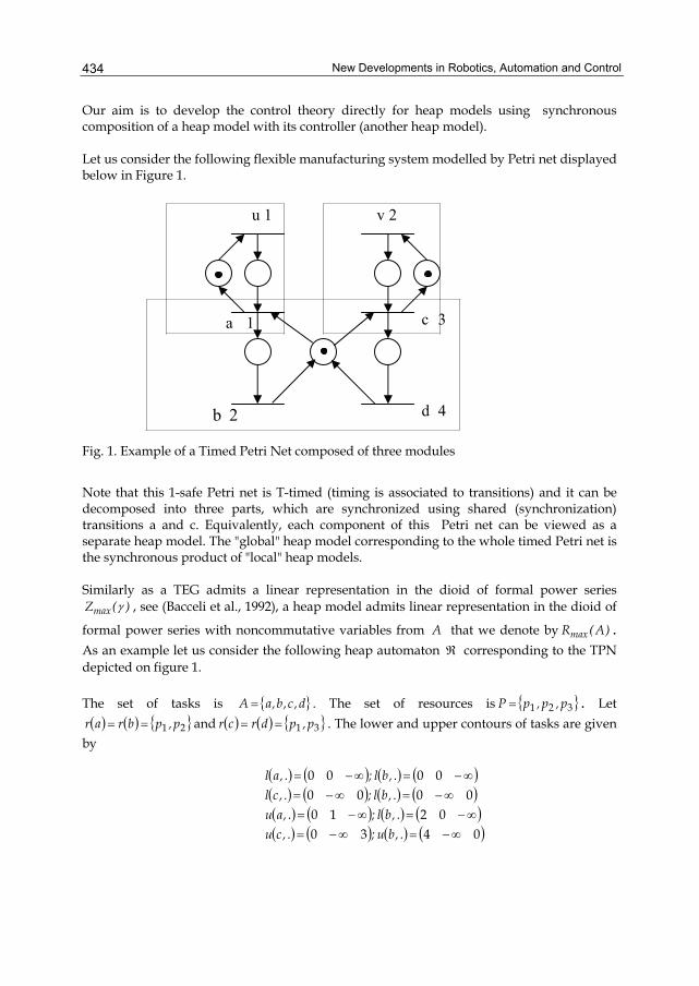
Our aim is to develop the control theory directly for heap models using synchronous composition of a heap model with its controller (another heap model). Let us consider the following flexible manufacturing system modelled by Petri net displayed below in Figure 1. Fig. 1. Example of a Timed Petri Net composed of three modules

Note that this 1-safe Petri net is T-timed (timing is associated to transitions) and it can be decomposed into three parts, which are synchronized using shared (synchronization) transitions a and c. Equivalently, each component of this Petri net can be viewed as a separate heap model. The "global" heap model corresponding to the whole timed Petri net is the synchronous product of "local" heap models. Similarly as a TEG admits a linear representation in the dioid of formal power series

)(Zmax γ , see (Bacceli et al., 1992), a heap model admits linear representation in the dioid of

formal power series with noncommutative variables from A that we denote by )A(Rmax . As an example let us consider the following heap automaton ℜ corresponding to the TPN depicted on figure 1. The set of tasks is { }d,c,b,aA = . The set of resources is { }321 p,p,pP = . Let ( ) ( ) { }21 p,pbrar == and ( ) ( ) { }31 p,pdrcr == . The lower and upper contours of tasks are given

by

( ) ( ) ( ) ( )( ) ( ) ( ) ( )( ) ( ) ( ) ( )( ) ( ) ( ) ( )04 30

02 10 00 00

00 00

∞−=∞−=∞−=∞−=

∞−=∞−=∞−=∞−=

.,bu;.,cu.,bl;.,au

.,bl;.,cl

.,bl;.,al

a 1

b 2 d 4

v 2

c 3

u 1

Heap Models, Composition and Control

435

It has been shown in (Gaubert & Mairesse, 1999) that any heap model is a special (max,+)-automaton with the morphism matrix defined in equation (3). The graphical interpretation of the morphism matrix is given in terms of transition weights:

( )[ ] ka ij =μ means that there is a transition labelled by Aa∈ from state i to state j with

weight k provided −∞≠k , while in the case −∞=k there is no transition from state i to state j. Note that the morphism matrix μ of a heap model can be also considered as

element of RRmax )A(R × , and by extending the definition of μ from letters Aa∈ to

sequences (words) *Aw∈ using the morphism property ( ) ( ) ( )nn aaaa μμμ KK 11 = and

hence we can even write ( )ww*Awμμ

∈⊕= .

However, μ has an important property of being finitely generated, because it is completely determined by its values on A : ( ) Aa,a ∈ μ . For this reason we have in fact

( )*

Aa* aa ⎟

⎠⎞

⎜⎝⎛ ⊕=∈

μμ . Since we are interested in behaviors of heap models that are given in

terms of *μ (more precisely by βαμ* ) we abuse the notation and write simply ( )aa

Aaμμ

∈⊕= .

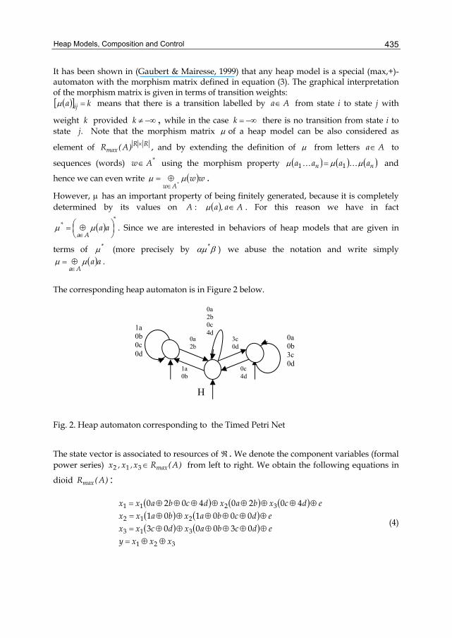
The corresponding heap automaton is in Figure 2 below. Fig. 2. Heap automaton corresponding to the Timed Petri Net

The state vector is associated to resources of ℜ . We denote the component variables (formal power series) )A(Rx,x,x max∈312 from left to right. We obtain the following equations in

dioid )A(Rmax :

( ) ( ) ( )( ) ( )( ) ( )

321

313

212

3211

030003000101

40204020

xxxyedcbaxdcxxedcbaxbaxx

edcxbaxdcbaxx

⊕⊕=⊕⊕⊕⊕⊕⊕=⊕⊕⊕⊕⊕⊕=

⊕⊕⊕⊕⊕⊕⊕⊕=

(4)

0a 0b 3c 0d

1a 0b 0c 0d

H

3c0d

1a0b

0c4d

0a2b

0a 2b 0c 4d

New Developments in Robotics, Automation and Control

436

The corresponding matrix form of system of equations (4) is

βαμ

xxx=

⊕= y

with ( ),xxxx 321 = ( ),0 0 0 =α , ( ) ,T0 0 0 =β and finally

⎟⎟⎟

⎠

⎞

⎜⎜⎜

⎝

⎛

⊕⊕⊕⊕⊕⊕⊕⊕

⊕⊕⊕⊕⊕=

dcbadcdcbaba

dcbadcba

430040000120

03014020

εεμ . (5)

It is now easy to see that in general we always have the following linear description of (max,+) automata in the dioid )A(Rmax of formal power series:

βαμ

xxx=

⊕= y with ( )aa

Aaμμ

∈⊕= the so called morphism matrix.

Let us recall from Theorem 1 that the least solution to this equation is βαμ*=y . 4. Linear representation of synchronous product

Since we introduce supervisory control of heap models using the synchronous product of the plant heap model with the controller heap model, it is important to study properties of the synchronous product. In this section the behavior of a synchronous product of two heap models will be represented in terms of morphism matrix of the synchronous product. According to the definition of synchronous product, the dimension (here number of resources) of the synchronous product of subsystems is the sum of dimensions of each subsystem. It should be intuitively clear that morphism matrices of synchronous products are block matrices, where the blocks are formed according to dimensions (number of resources) of the component heap models. In order to simplify the approach we require that ( ) 0pa,l = whenever ( )arp∈ . This is a reasonable assumption that simply means that pieces are on the ground in all slots. Thus, the upper contour gives information about the duration of tasks for different resources used. We recall at this point that ( ) −∞=pa,l whenever ( )arp∉ . Let 1ℜ and 2ℜ be two heap models with morphism matrices denoted by 1μ and 2μ , respectively. Their dimensions, i.e. the number of resources of 1ℜ and 2ℜ are 1m and

2m , respectively. The Booleans morphism matrices of underlying Boolean automata are denoted by 1B and 2B , respectively. Let us recall from (Komenda et al, 2007) that

( )[ ]( )( )⎪⎩

⎪⎨⎧

=≠

= εμεεμ

ij

ijij a

aeaB

1

11 if

if

Let 1,2=, ji,ijε be the rectangular matrices of (max,+) zeros of dimensions ji mm × and 1,2=i ,Ei the square (max,+)-identity matrices of dimensions ii mm × .

Heap Models, Composition and Control

437

It will be shown that the morphism matrix of the parallel composition admits an interesting decomposition into blocks. Indeed, the following block form of ( )aℜμ depending on 21 AAAa ∪=∈ is now claimed. Theorem 2. The morphism matrix of 21 ℜℜ=ℜ || admits the following decomposition:

• if 21 AAa ∩∈ then ( ) ( ) ( )( ) ( )⎟⎟⎠

⎞⎜⎜⎝

⎛=ℜ aa

aaa

21

21μμμμ

μ , where

( ) ( ) ( ) ( )( )⎩

⎨⎧

∉∞−∈∈

=aaar k,a

a kjij

2

2111 ri if

ri ifarbitrary μμ (6)

and similarly, ( ) ( ) ( ) ( )

( )⎩⎨⎧

∉∞−∈∈

=aaarl,a

a ljij

1

1222 ri if

ri ifarbitrary μμ

• if 21 A\Aa∈ then ( ) ( )⎟⎟⎠

⎞⎜⎜⎝

⎛=ℜ

221

121E

aa

εεμ

μ (7)

• if 12 A\Aa∈ then ( ) ( )( ) ( ) ⎟⎟⎠

⎞⎜⎜⎝

⎛=ℜ aa

aEa

221

121μεε

μ (8)

Proof. This result can be obtained from the form of the morphism matrix in equation (3). In accordance with the definition of morphism matrix of heap models for 21 AAAa ∪=∈ three cases are to be distinguished. Let us start with the most complicated case, where

21 AAa ∩∈ is a shared task. It should be clear that for resources q,p from 21 PPP ∪= there are four possibilities depending on whether p and q belong to 1P or 2P , whence the block

form of ( )aℜμ . At this point we recall our assumption that ∅=∩ 21 PP . It is then straightforward to see that in the diagonal blocks the individual morphism matrices appear. Also, the remaining non diagonal terms according to the definition of the morphism matrix of heap automata are equal to:

( ) ( ) ( ) ( ) ( ) ( ) ( ) ( )( ) ( )⎩

⎨⎧

∉∉∞−∈∈=−=−

=ar jariarjar ij,aui,alj,aui,alj,au

a ij12

121211 or if

and ifμ (9)

Note that any such element above in the lower left block must satisfy 2Pi∈ and 1Pj∈ , hence ( ) ( )j,auj,au 1= , ( ) ( )i,ali,al 2= , and ( ) 02 =i,al for ( )ari 2∈ according to our assumption and similarly for elements in the right upper block of ( )aℜμ we get:

New Developments in Robotics, Automation and Control

438

( ) ( ) ( ) ( ) ( ) ( ) ( ) ( )( ) ( )⎩

⎨⎧

∉∉∞−∈∈=−=−

=arjariarjar ij,aui,alj,aui,alj,au

a ij21

212122 or if

and ifμ (10)

Since ( )ija1μ equals either ( )j,au1 (for ( ) ( )arjari 12 and ∈∈ ) or to (max,+) zero otherwise,

we can see that the rows corresponding ( ) 2 ari∈ of ( )a1μ , i.e. ( )( ).,ia

1μ are the same as the

rows ( )( ).,ka

1μ for ( ) 2 ark∈ , which are all the same.

Thus, the corresponding entry does not depend on j anymore. Similar arguments can show that ( )a2μ is of the form above. The morphism matrix ( )aℜμ of the composed heap has then the claimed form for 21 AAa ∩∈ . In much easier situation when 21 A\Aa∈ it is sufficient to notice that no resource from 2P is used by a . It is easily seen that ( )aℜμ has again the claimed form. Finally, the case 12 A\Aa∈ is symmetric to the previous one. Theorem on decomposition can be generalized to the case of n component heaps, where morphism matrix of synchronous product are matrices with nn× blocks. This is useful for decentralized control, but in this paper we only need synchronous product of the system with its controller, i.e. the case 2=n . The algebraization of synchronous product presented in this section will be useful for control purposes in the next section.

5. Application to supervisory control

In this section supervisory control of heap models is studied. The aim is to satisfy a behavioral specification given by a formal power series. The closed-loop system is represented by parallel composition (synchronous product) of the plant with a supervisor to be found, which is itself represented by a heap model. In general a supervisor acts on both timing and logical properties of the plant's behavior under supervision. In this section we focus mainly on timing aspects, when the supervisor does not disable, but only delay the execution of tasks corresponding to transitions in underlying timed Petri nets. This is similar to control of TEG in the maxplus algebra, where input transitions are added in order to delay the timed behavior of a TEG (Cottenceau et al, 2000). Note that adding input transitions to a TEG corresponds to synchronization of the TEG with a TEG of the controller that has predefined structure given by the graph topology of input transitions. This way control of TEG can be seen in this sense as a special case of supervisory control, where the supervisor has a predefined fixed structure (logical behavior) and only output values (timing) of transitions are to be determined such that a specified behavior is met. Note however that such a methodology enables only to consider periodic inputs without a transient regime, which would require to either consider a controller,

Heap Models, Composition and Control

439

where weights are time depending or equivalently to use a unfolding (max,+) automaton representation of the controller, which would have much more states. Now we apply Theorem 2 to the control of heap models. The synchronous product of heap models ( )ggggg u,l,r,P,AG = and ( )ccccc u,l,r,P,AC = of dimensions m and n

(respectively) corresponds to the controlled (closed-loop) system. The event alphabets of G and C are denoted by gA and cA , respectively. The event alphabet of the controlled

system is denoted by A . According to definition of synchronous product, we then have cg AAA ∪= . Let us denote the morphism matrices of G and C by gμ and cμ ,

respectively. Now let us return to the description of behaviors of heap models in the dioid of formal power series ( )ARmax . The vector of formal power series from ( )ARmax associated

to generalized dater functions nmmaxG Rx +→*

C || A : satisfies the following equations:

β

αμ

⊗=

⊕⊗=

C || C ||

C || C || C ||

GG

GGG

xyxx

(11)

where C || Gμ the morphism matrix of C || G , α , and β are row, resp. column, vectors of

zeros of dimension nm+ , i.e. ( ),e...e=α and ( ) .e...e T=β First of all, according to Theorem 1 the greatest solutions to equations above are

βαμ

αμ*

GG

*GG

y

x

C || C ||

C || C ||

=

= (12)

whence an interest in studying properties of *

G C || μ . Given a specification behavior (e.g. language or formal power series), the goal in supervisory control of DES is to find a supervisor that achieves this specification as the behavior of the controlled system. In a first approach we assume, similarly as in control of TEG, that the structure of the controller is given, which means here that the controller heap model only delays executions of different tasks in the plant. This is done by the choice of upper contour functions (i.e. duration of controller's tasks) from ( ) c Au,uc ∈μ . The delaying effect of the controller is naturally realized via its tasks (transitions of the corresponding heap automaton) shared with the plant heap. The morphism matrix of the composed system is given by

( ) ( ) ( ) ( )aaaauuaa GA\Au

GAAa

GA\Au

GAa

Gcggcgc

C || C || C || C || C || μμμμμ∈∩∈∈∈⊕⊕⊕⊕⊕=⊕= . (13)

New Developments in Robotics, Automation and Control

440

In order to simplify the approach our attention is from now on limited to the case gA=cA .

This is a standard assumption in the supervisory control with complete observations. Since state vector in equation (12) is associated to resources, it can be written as ( )uxxG =C || , where the first component corresponds to the (uncontrolled) plant (heap G ) and the second to the controller heap C . Owing to Theorem 2 we have:

( ) ( ) ( ) ( )( ) ( )

( ) 21 αα⊕⎥⎥⎦

⎤

⎢⎢⎣

⎡⎟⎟⎠

⎞⎜⎜⎝

⎛=

∈⊕

aaFaaHaaFaaHuxux

Aa, (14)

where 1α and 2α are vectors of zeros of corresponding dimensions, for any Aa∈ ( )agμ is

for convenience denoted by ( )aH , i.e. ( )aH denotes ( )agμ . Similarly, ( )aF is the notation

for ( )acμ , i.e. ( )aF denotes ( )acμ This way we obtain

( ) ( ) ( )21 αα⊕⎟⎟⎠

⎞⎜⎜⎝

⎛=

FHFHuxux ,

where ( ) aaHH

Aa

∈⊕= and similarly ( ) aaFF

Aa

∈⊕= , ( ) aaHH

Aa

∈⊕= , and ( ) aaFF

Aa

∈⊕= .

Hence,

2

1

α

α

⊕⊕=

⊕⊕=

uFFxu

HuxHx

According to Theorem 1 the least solution of the second equation is ( ) *FFxu 2α⊕= . The above equation gives us the expression of the closed-loop system transfer, where the matrix F plays the role of a feedback. It is worth to notice that there is a significant difference from standard feedback control: unlike classical control theory the control variables have their inner dynamics. This is caused by adopting a supervisory control approach, where a controller is itself a dynamical system of the same kind as the uncontrolled system: a heap automaton. Therefore, our F , which plays the role of feedback mapping, is determined by inner dynamics of the controller given by its morphism matrix F . The substitution into the first equation then yields

( )[ ] 12 αα ⊕⊕⊕= HFFxxHx *

Another application of Theorem 1 leads to the least solution given by

( )( )*** HFFHHFx ⊕⊕= 12 αα .

Heap Models, Composition and Control

441

From a different viewpoint, there is a strong analogy with the feedback approach for control of TEG, see (Cottenceau et al, 2000), which should not be surprising, because supervisory control (realized here by synchronous product) is based on a feedback control architecture. In supervisory control the control specification (as counterpart of reference output from control of TEG using dioid algebras) are given in terms of behaviors of (max,+) automata (i.e. formal power series). In fact, for a reference output refy we are interested in the greatest

feedback F such that the output of the closed-loop system y is less or equal to the specification refy : refyy ≤ .We obtain in our situation:

( )( ) ref*** yHFFHHF ≤⊕⊕ βαα 12 . (15)

And ( ) ( ) βαα /y\HFHFFH ref

***12 ⊕≤⊕ , where ( ) βαα /y\HF ref

*12 ⊕ is a matrix playing

the role of reference model in (Cottenceau et al, 2000). An application of Lemma 1 leads to:

( ) ( ) ( ) βαα /y\HFHHFFHHFFH ref*******

12 ⊕≤=⊕ . (16)

Note that all operations involved in the description above, i.e. ⊗⊕ , , and the Kleene star, are lower semicontinuous and residuated when the image is suitably constrained. Hence, using residuation theory (see Section 2) it should be possible to obtain the greatest series F corresponding to the "controller part" of the morphism matrix. Moreover, as follows from Theorem 2 that F can simply be expressed using F . Hence, there is a hope that at least in some special cases residuation theory (see Section 2) can be applied to obtain the greatest series F corresponding to the "controller part" of the morphism matrix C || Gμ such C || Gy satisfies a given specification (e.g. it is less than or equal to a given reference output series refy ).

We aim at obtaining the greatest ∗FF such that inequality (16) is satisfied. This is far from being an easy problem. The situation is much simpler in case FF = and HH = . This is satisfied if we assume that the controller heap model has the same number of resources as the uncontrolled heap model and the logical structure of the controller (given by

)P(PwrA:r cc → mimics the logical structure of the plant (given by )P(PwrA:r gg → ).

Formally stated it is required that there exists an isomorphism between cP and gP such that

cr and gr are equal up to this isomorphism.

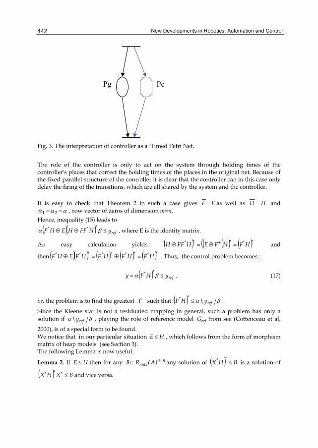
In terms of Petri nets this can be interpreted as having a controller net with the same net topology (i.e. logical structure as the uncontrolled net). This means that in the closed-loop system there are always parallel places of the controller corresponding to places of the uncontrolled net.

New Developments in Robotics, Automation and Control

442

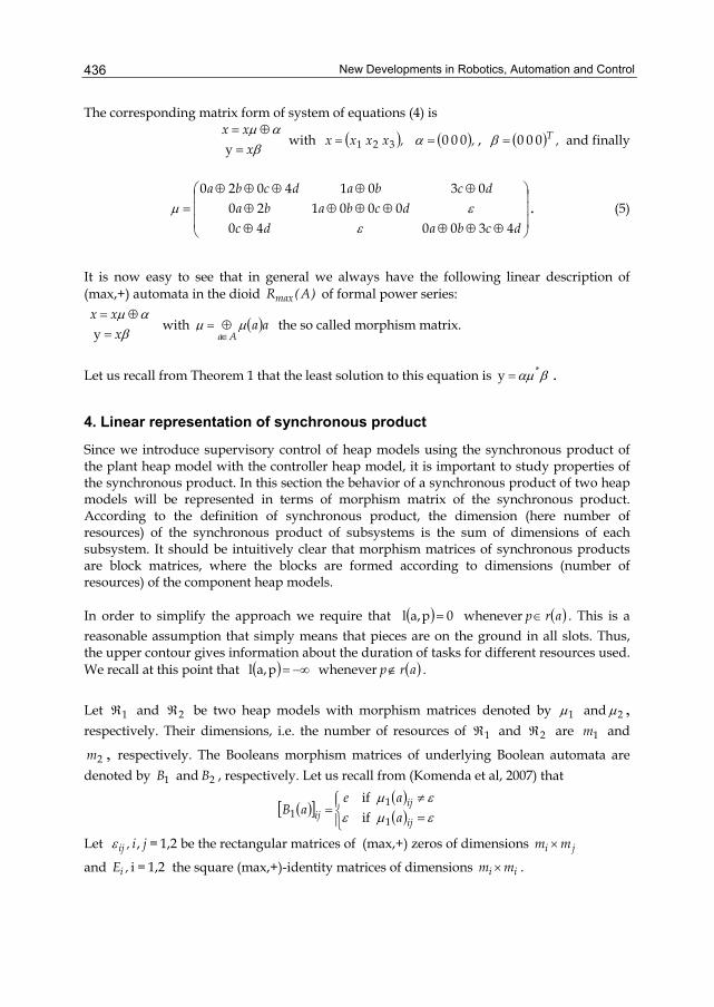
Fig. 3. The interpretation of controller as a Timed Petri Net.

The role of the controller is only to act on the system through holding times of the controller's places that correct the holding times of the places in the original net. Because of the fixed parallel structure of the controller it is clear that the controller can in this case only delay the firing of the transitions, which are all shared by the system and the controller. It is easy to check that Theorem 2 in such a case gives FF = as well as HH = and

ααα == 21 , row vector of zeros of dimension m=n. Hence, inequality (15) leads to

( )( ) ref*** yHFFHEHF ≤⊕⊕ βα , where E is the identity matrix.

An easy calculation yields ( ) ( )( ) ( )∗∗+∗=⊕=⊕ HFHFEHFFH ** and

then ( )( ) ( ) ( ) ( )∗∗+∗=⊕=⊕ HFHFHFHFEHF ***** . Thus, the control problem becomes :

( ) ref** yHFy ≤= βα . (17)

i.e. the problem is to find the greatest F such that ( ) βα ref

** y\HF ≤ .

Since the Kleene star is not a residuated mapping in general, such a problem has only a solution if βα refy\ , playing the role of reference model refG from see (Cottenceau et al,

2000), is of a special form to be found. We notice that in our particular situation HE ≤ , which follows from the form of morphism matrix of heap models (see Section 3). The following Lemma is now useful.

Lemma 2. If HE ≤ then for any nnmax )A(RB ×∈ any solution of ( ) BHX

** ≤ is a solution of

( ) BXHX ≤∗∗∗ and vice versa.

Pc Pg

Heap Models, Composition and Control

443

Proof. If X a solution of ( ) BHX** ≤ , then ( ) ( ) BHXEHX *** ≤⊕=

+, hence also ( ) BHX* ≤

+.

Therefore,

( ) ( ) ( ) ( ) BHXHXHXEXHXXHX *** ≤=≤=+∗∗∗∗∗∗∗ ,

where the first inequality follows from isotony of multiplication and the assumption HE ≤ .

Conversely, if X is a solution of ( ) BXHX ≤∗∗∗ , then

( ) ( ) ( ) BXHXEHXHX ≤≤= ∗∗∗∗∗∗∗

as follows from isotony of multiplication and the assumption that ∗≤ XE , a general and very well known property of the Kleene star. Using Lemma 2 (with F playing the role of X ) our problem is equivalently formulated as

follows : find the greatest solution in F of ( ) βα refy\FHF ≤∗∗∗ . It follows from Lemma 1

that ( ) ( )*FHH)FH(FHF ∗∗∗∗∗∗ =⊕= , thus we get formally the same problem as the one

solved in (Cottenceau et al, 2000) with ∗H playing the role of transfer function H in the TEG setting. The following result adapted from Proposition 3 in (Cottenceau et al, 2000) is useful: If there exists a matrix nn

max )A(RD ×∈ such that ∗∗= DHy\ ref βα or there exists nn

max )A(RD~ ×∈ such that ∗∗= HD~y\ ref βα then there exists the greatest F such that

( ) βα ref*

y\FHH ≤∗∗ , namely

( ) ( )βα ∗∗= Hy\HF ref

opt . (18)

Let us note that it is very difficult to compute the optimal feedback according to formula (18), although the formula is similar to the corresponding one used in feedback control of timed event graphs. In fact, dealing with formal power series in several non commutative variables from A is much more difficult than handling formal power series from )(Zmax γ . Similar simplificaton rules, the one proposed in (Benveniste et al, 1998a) and (Benveniste et al, 1998b), should be used in the computation according to formula (18). These simplificaton rules correspond to the fact that nondecreasing series are useful for practical computation. In the special case we have restricted attention to, our methods yields the gretest feedback such that timing specification given by refy is satisfied, provided refy is of one of the above

special forms. In our case of a controller with fixed logical structure only timed behavior is under control. At this point it is not clear yet how to leave the restriction on the form of

refy . In timed event graphs this has been done by using the concept of compensator

borrowed (extended) from the classical control theory. However there is no similar structure

New Developments in Robotics, Automation and Control

444

for heap models, because there is no input function and we use another heap model as a controller. If we are interested in manufacturing systems, where specificatons are given in terms of Petri nets, the reference output is not typically required to be met for all sequences of tasks, but only those having a real interpretation. These are given by the correponding (logical) Petri net language, say L . Thus, the problem is to find the greatest F , such that

( ) ( ) ( )LcharLchar ref*

yFHH ≤∗∗ βα ,

where ( ) w.e

Lw∈⊕=Lchar is the series with Boolean coefficients, i.e. the formal series of

language L . Let us recall (Gaubert & Mairesse, 1997) that such a restriction is formally realized by the tensor product (residuable operation) of the heap automaton with the logical (marking) automaton recognizing the Petri net language L , which is compatible with Theorem 4.1 of (Komenda et al, 2007). Note that specifications based on (multivariable) formal power series are not easy to obtain in many practical problems, in particular those coming from production systems, often represented by Petri nets. In fact, given a reference output series amounts to solve a scheduling problem. A formal power series specification is not given, but it is to be found: e.g. using Jackson rule (Jacson, 1955).

6. Example

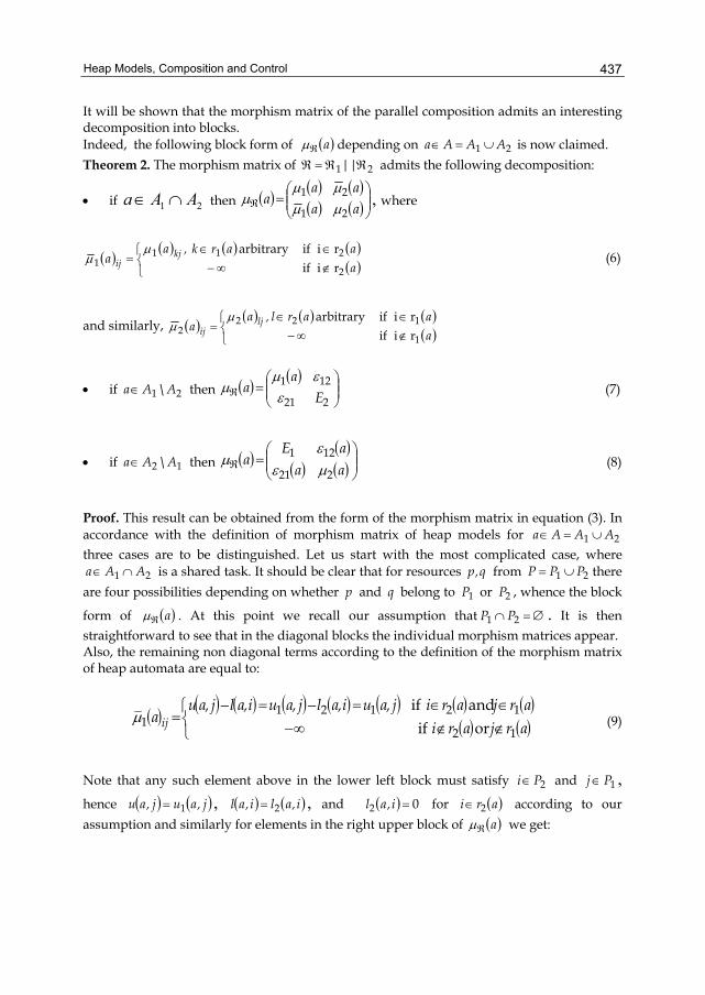
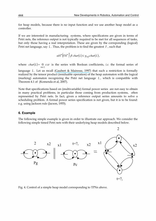
The following simple example is given in order to illustrate our approach. We consider the following simple timed Petri nets with their underlying heap models described below. Fig. 4. Control of a simple heap model corresponding to TPNs above.

x2 x2x1

2

t=?,

x1 x2 2 t=?,

Pg Pc

Heap Models, Composition and Control

445

In the timed Petri nets above the timing (holdig time) of places Pg and Pc are 2 and t, respectively. In the controller net the value t is the control parameter. The heap model G corresponding to the above simplest possible timed Petri nets with resource sharing is given below togetherwith its controller C. ( )ggggg u,l,r,P,AG = and ( )ccccc u,l,r,P,AC = with { }21 x,xAAA gc === , { }PgPg = ,

{ }PcPc = , { }Pg)x(r)x(r gg == 21 , { }Pc)x(r)x(r cc == 21 , ε=)Pg,x(l ig for { }21,i∈ ,

ε=)Pc,x(l ic for { }21,i∈ , )Pg,x(u)Pg,x(u gg 21 2 == , and finally )Pc,x(ut)Pc,x(u cc 21 == .

αμαμ

⊕⊗=⊕⊗=

CCC

GGGxxxx

,

where 21G 22 xx ⊕=μ and 21C txtx ⊕=μ are morphism matrices (here scalars of dimension 1).

In accordance with Theorem 2 we obtain

β

αμμμ

μμμ

⊗=

⊕⎥⎦

⎤⎢⎣

⎡=

=⊗=

C || C ||

C || C ||

GG

CGG

CCGGG

xy

xx

with

.)xx(t)xx()xx(t)xx(

G ⎥⎦

⎤⎢⎣

⎡⊕⊕⊕⊕

=2121

2121C || 2

2μ

Let us choose the control reference (specification) as ( ) .xxy ∗⊕= 21ref 44 This specification is of the form

( ) ( ) .DHxxxxyy\ refref∗∗∗∗ =⊕⊕== 2121 4422βα

We compute

( ) ( ) ( ) .44\\ 21∗∗∗∗∗ ⊕=== xxHyHHyHF refref

opt βα Indeed, by definition

{ } ( ) ( ){ } ( )∗∗∗∗∗ ⊕=⊕≤⊕=≤= 212121 44 4422 max max\ xxxxxxxyxHyHx

refx

ref ,

and similarly ( ) ( ) ,4444 2121

∗∗∗ ⊕=⊕ xxHxx whence the expected result. In the above computation we use the simple fact that for two series (here polynomial) s and t with ts ≤ ,

es ≥ , and et ≥ we have ∗∗∗ = tts .

New Developments in Robotics, Automation and Control

446

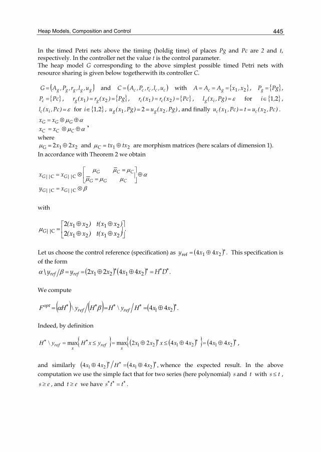
Let us remark that if one would choose some different specification, e.g. ( )∗⊕= 21ref 43 xxy , then this specification is not compatible with the system, because there is only one place, where the timing is a control parameter. In order to achieve such a specification one would need a heap model corresponding to the following net structure. Fig. 5. Another TPN corresponding to a heap model allowing for more general specifications.

7. Concluding remarks

It has been shown how methods of dioid algebras can be used in supervisory control of heap models. We have proposed a synchronous product of heap models. The structure of the morphism matrix of synchronous product of two heap models is derived and applied to control of heap models. The present reseach is a preliminary step in control of heap automata. We have limited our attention to a particular type of synchronous composition. In this work we have assumed that all events were controllable, i.e. any event may be delayed and even disabled (prevented from happening) by a suitable controller heap automaton. This assumption is however often unrealistic in practice: for instance one can hardly imagine that different kinds of system failures can always be avoided. Another restriction is the one we have imposed on the form of the reference input refy (in supervisory control also called control

specification) . One possible way of leaving this restriction is to formulate heap automata in terms of input output automata and use the concept of precompensator from the classical control theory. Let us recall that recently different types of automata (e.g. classical automata, timed automata, stochastic automata) have been formulated in an equivalent way using explicit input and output functions as input output automata (e.g. IO timed automata and IO stochastic automata). It seems therefore interesting to work with IO (max,+) automata in order to extend the techniques based on precompensator from timed event graphs to our setting of heap automata. Of potential interest is also supervisory control with partial controllability and partial observations or decentralized control of heap automata. Modular control of (explicitly)

x2 2

Pg

x1

P2 P1

Heap Models, Composition and Control

447

concurrent heap automata that are formed as synchronous compositions of heap models is particularly worthy to investigate.

8. Acknowledgement KJB100190609, of the French-Czech bilateral project Barrande N. 14235XG and of the Academy of Sciences of the Czech Republic, Institutional Research Plan No. AV0Z10190503 are gratefully acknowledged.

9. References

Al Saba, M.; Boimond J.L &. Lahaye, S (2006). On just in time control of flexible manufacturing systems via dioid algebra. Proceedings of INCOM'06, Vol.2, pp. 137-142, Saint-Etienne, France.

Baccelli, F.; Cohen, G.; Olsder, G.J. & Quadrat, J.P. (1992). Synchronization and linearity. An algebra for discrete event systems, John Wiley & Son, New York.

Benveniste A. ; Jard C &. Gaubert S (1998a). Algebraic techniques for timed systems. Proceedings of CONCUR'98, International Conference on Concurrency Theory, 1998. Benveniste A. ; Jard C &. Gaubert S (1998b). Monotone rational series and max-plus

algebraic models of real-time systems. Proceedings of the 4th Workshop on Discrete Event Systems, WODES'98, Cagliari, Italy, august 1998.

Cottenceau, B.; Hardouin, L.; Boimond J.L &. Ferrier, J.L. (2001). Model Reference Control for Timed Event Graphs in Dioids. Automatica, Vol. 37, pp. 1451-1458.

Gaubert, S. (1992). Theorie des systèmes linéaires dans les dioïdes. Thèse de doctorat, Ecole des Mines de Paris, 1992.

Gaubert, S. (1995). Performance evaluation of (max,+) automata. IEEE Transactions on Automatic Control, Vol. 40, N12, pp. 2014-2025.

Gaubert, S. & Mairesse, J. (1997). Task resource models and (max,+) automata, In J. Gunawardena, Editor: Idempotency. Cambridge University Press, 1997.

Gaubert, S. & Mairesse, J. (1999). Modeling and analysis of timed Petri nets using heaps of pieces. IEEE Transactions on Automatic Control, Vol. 44, N4, pp. 683-698.

Jackson, J.R. (1955). Scheduling a Production Line to Minimize Maximum Tardiness. Research report 43. University of California Los Angeles. Management Science Research Project.

Komenda, J.; Al Saba, M. & Boimond, J.L. (2007). Supervisory Control of Maxplus Automata: Timing Aspects. In Proceedings of the European Control Conference (ECC) 2007, Kos (Greece).

Kumar, R. & Heymann, M. (2000). Masked prioritized synchronization for interaction and control of discrete-event systems. IEEE Transaction Automatic Control 45, 1970-1982, 2000.

Lin, F. & Wonham, W.M. (1998). On Observability of Discrete-Event Systems. Information Sciences, Vol. 44, pp. 173-198.

Menguy, E. (1997). Contribution à la commande des systèmes linéaires dans les dioïdes. Thèse de doctorat, Université d'Angers.

Ramadge, P.J. & Wonham, W.M. (1989). The Control of Discrete-Event Systems. Proceedings of IEEE, Vol. 77, pp. 81-98, 1989.

New Developments in Robotics, Automation and Control

448

Sifakis, J. & Yovine, S. (1996). Compositional specification of timed systems. Proceedings of the 13th Symposium on Theoretical Aspects of Computer Science, STACS'96, pp. 347-359, . LNCS 1046.