Supplementary Information:

Predicting Malaria Control Endpoints and Timelines

David L. Smith, Simon I. Hay, Abdisalan M. Noor, Robert W. Snow

Changes in malaria endemicity under scaled-up ITN coverage in Africa can

be predicted by combining a malaria transmission model and a control model

that relates ITN coverage levels to a transmission effect size, defined here as a

proportional reduction in the reproductive number: R0/RC(φ). A previously

published ITN control model describes a non-linear relationship between ITN

coverage and the effect size on transmission 1. The malaria transmission model

describes a non-linear relationship between the equilibrium PfPR, PfEIR, and

PfR02,3. An analogous queuing model describes the timelines 4. These models

are described again here.

ITN control Model The ITN effect size on transmission follows the model

previously published by Le Menac’h et al.1. The feeding-cycle model for ITNs

assumes that φ represents the proportion of encounters between humans and

mosquitoes that are altered by the presence of a net. This is called effective cov-

erage, and it is usefully approximated by ownership multiplied by the frequency

of use. The model predicts changes in vectorial capacity, which is directly pro-

portional to R0 or RC(φ). The effect size, R0/RC(φ) is a function of effective

coverage, φ, which is illustrated graphically in Figure 1b.

The reductions in vectorial capacity depend on two parameters that describe

what happens when a mosquito encounters a human protected by a net, the

fraction that end in a mosquito being killed (δ) or repelled (ζ). The reductions

in vectorial capacity also depend on the bionomics of the vector at the baseline,

when there is no ITN coverage (denoted by the subscript 0), including the lifespan

(1/g0), the proportion of bites on humans (Q0), the length of the feeding cycle

(f0), and the time to sporogony (n).

1

Given estimates of these six parameters, we can predict the effect size achieved

by ITNs as they scale up over time, φ(t). Four species have been characterized1,5. The benchmark results depend on one particular set of parameters and

the parameters for one vector (see Table S1). That vector was chosen as the

benchmark because it was an important African vector, and also because the

effect size was approximately equal to the geometric mean response of two An.

gambiae species from different places (Figure 1b). The assessment of uncertainty

is based on the distributions in Table S1, and the associated variability in effect

size is illustrated in Figure S1.

Malaria Transmission Model The following summarizes previously pub-

lished descriptions and analysis of a malaria transmission model 2–4,6. The nota-

tion and parameters are described in those publications, and tables of the terms

and parameters are described in Box S1 and Box S2.

Steady States: The following model describes a population where PfPR is

stratified by exposure. PfEIR (denoted E in equations) defines the population av-

erage exposure, but each population stratum has a distribution of biting weights,

ω, such that the malaria exposure within a stratum is ωE . Clearance follows the

assumption of Dietz, et al.7. The prevalence of malaria in a risk stratum is Xω,

and the dynamics are described by the equation:

Xω = bωE(1−Xω)− bωEebωE/r − 1

Xω (1)

It is assumed that ω is Gamma distributed with a mean of 1 and a variance α, so

that exposure is also Gamma distributed with a mean E and a squared coefficient

of variation of α. The population prevalence integrates over all risk strata:

X =∫ ∞

0Γ(ω|α)Xωdω. (2)

At the steady state:

X = 1−(

1 +bEαr

)−1/α

(3)

This equation fits the relationship between PfEIR and PfPR in children for b/r ≈0.45/yr and α ≈ 4.2 8.

The dynamics of infections in mosquitoes generally follow the classical as-

2

sumptions 6, except that the rate of infection is modified to consider heteroge-

neous biting 3. The probability that a mosquito becomes infected after biting a

human is defined by the formula:

X =∫ ∞

0ωc(ωE)Γ(ω|α)dω (4)

Following Smith, et al.3:

R0 =bc0

rE S + X

X(1 + α) (5)

If no estimate of E is available, then it can be inferred from X using Eq. 3:

E =r((

1− X)−α− 1

)bα

(6)

which gives a relationship between R0 and X:

R0 =1 + α

α

((1− X

)−α− 1

)c0

(1 +

S

X

)(7)

The formula is mainly a function of the PfPR and the degree of heterogeneous bit-

ing (α). Other parameters that modify the expression are the baseline infectivity

c0, and the stability index (Box S2).

The benchmark approximation was made by assuming that that c(ωE) = c0,

so that:

X = c0

(1−

(1− X

)(1+α)/α2)(8)

This formula tends to underestimate R0 if there is transmission blocking im-

munity. To estimate PfR0 from PfPR for some assumption about transmission

blocking immunity, we use Eq. 6, along with Eq. 7 to get X as a function of only

X, and the atomic parameters b/r (which always appear together) and c0 = 0.5

and the index S = 1.

The functions can be used to describe changes in the steady state relationships

under malaria control. Given a reduction in vectorial capacity as a function of

ITN coverage, V (φ), we can predict the change in steady state under malaria

3

control, starting from a population without malaria control, using the formulas:

X(φ = 0)F⇀↽ R0

V (φ)⇀↽ RC(φ)

F−1

⇀↽ X(φ) (9)

The functions describing the algorithm for predicting the steady state PfPR in

the presence and absence of control (X(φ) and X0, respectively) are given on top

of the directional arrow. The functions can be inverted, and this also makes it

possible to predict the changes in PfPR at the steady state starting from one

level of malaria control (φ′) and improving (or relaxing) to another φ:

X(φ′)F⇀↽ RC(φ′)

V −1(φ′)⇀↽ R0

V (φ)⇀↽ RC(φ)

F−1

⇀↽ X(φ) (10)

R-code is freely available upon request, and a demonstration version is available

at http://www.map.ox.ac.uk.

Timelines: To compute the timelines, a different set of equations is required;

these have described in detail elsewhere, and are repeated here 4. Minor differ-

ences between the steady state of these equations and of the equation above are

introduced because the risk strata are subdivided into a finite number of com-

partments. The equations are analogous, in the sense that they make the same

assumptions about the biology, and they have the same steady states in a limiting

case on the mesh of compartments.

Let j subscripts denote a subpopulation with biting weight ωj that comprises

a fraction Wj of the whole population. Let xm,j denote the fraction of that

subpopulation with a given MOI, m. Thus,∑m xm,j = 1, for all j. The changes

in the proportion uninfected within the jth population stratum is:

x0,j = −h0x0,j + rx1,j

xm,j = −(hj + ρm)xm,j + ρm+1xm+1 + hjxm−1,j;(11)

Here, we have taken ρm = rm, and hj = bE . The parasite rate is defined to be

X =∑j

Wj(1− x0,j). (12)

The probability that a mosquito becomes infected after biting a human, denoted

4

X and called net infectivity, is given by the formula:

X =∑j

cωjWj(1− x0,j). (13)

The dynamic of infections in mosquitoes follow the same logic as above 3, such

that PfEIR is given by the equation:

E = R0rX

1 + sX(14)

The biting weights were given by a Gamma-like distribution, as described

elsewhere 4. Simulated timelines were produced by letting the equilibrium come

to a specified equilibrium determined by the vectorial capacity, then instituting

control. ITN coverage was simulated by changing the vectorial capacity, according

to a model.

A. Sensitivity Analysis

Variability in the ITN effect size is realted to vector bionomics, as described else-

where 1. Another source of heterogeneity in the outcome the translation from

PfPR back to PfEIR, which is largely ascribed to differences in the degree of biting

heterogeneity. Taken together, baseline endemicity and uncertainty about het-

erogeneous biting, immunity, and vector bionomics suggest highly unpredictable

endpoints after reaching universal coverage, as prescribed by RBM. Monitoring

and evaluation across the transmission spectrum and across the range of dom-

inant vector species should aim to establish context-specific expectations and

goals. Figure 2b is based on the parameter values and distributions reported in

Table S1, we have also generated a predicted effect size distribution (Figure S1).

The relationship between the PfPR, the PfEIR, and the PfR0 is strongly

affected by the degree of heterogeneous biting, described by α 4,9, and illustrated

in Figure 1a. The fitted model describes α = 4.2 as an average degree of biting

heterogeneity, but the degree of biting heterogeneity can vary among populations,

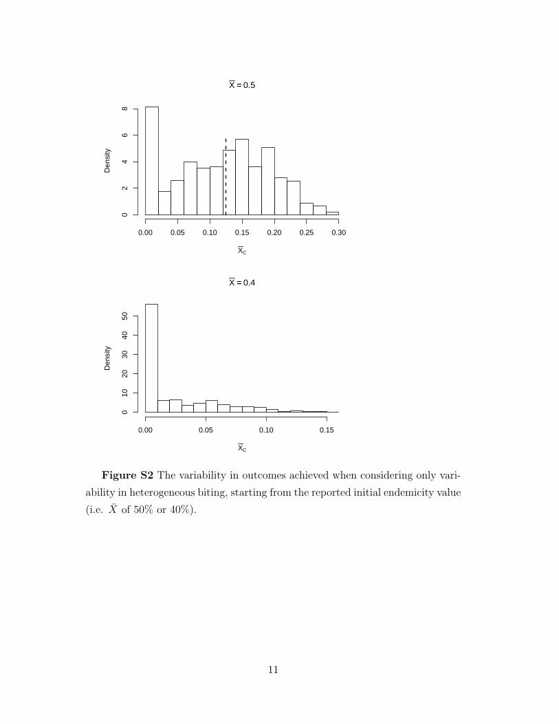
depending on context. Here, α is assumed to be drawn from a normal distribution

with mean 4.2 and variance 1. Variability associated only with the distribution of

α are illustrated in (Figure S2). Similarly, two populations with the same PfEIR

5

but different values of PfPR, malaria would be more difficult to eliminate in the

population with the lower PfPR, because biting is more intense on a smaller

fraction of the population.

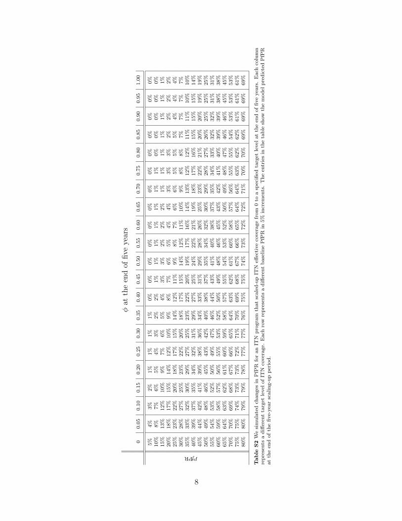
Finally, because the relationship between ITN effective control and the ITN

effect size is greater than log-linear, as illustrated in Figure 1b. This implies that

if ITNs are scaled-up steadily over a period of time, then the greatest effects will

not be realized until effective coverage is near the target maximum. This leads

to different estimates of the PfPR over time. To illustrate these differences, two

tables were created by simulating a steady scaling up of ITN effective coverage

over a five-year period (Tables S2 & S3).

With variability in vector bionomics and heterogeneous biting, the variable

outcome is shown in Figure S3. Differences between the benchmark prediction

and some actual outcome can also occur because of other reasons: Our analysis

also assumes that there has been no major change in any other important factors,

such as drought or contemporary changes in other modes of malaria control, such

as a change in drug policy. If there has been a change, these must be taken into

account when assessing the effects that are attributable to ITNs.

6

Parameter 1 2 3∗ 4 Sensitivity

p0 = e−g0 0.83 0.9 0.94 0.86 TR(0.7,0.9, 0.95)

t0 = 1/f0 2.7 d 2 d 3 d 2.3 d TR(2,3,5)

Q0 0.95 0.9 0.75 0.72 TR(0.7,0.9,0.95)

n 10.7 11.6 10.3 9 TR(8,10,13)

δ 0.3 TR(0.05, 0.3, 0.5)

ζ 0.1 TR(0.05, 0.1, 0.3)

α 4.2 normal(4.2, 1)

c 0.5 0.5

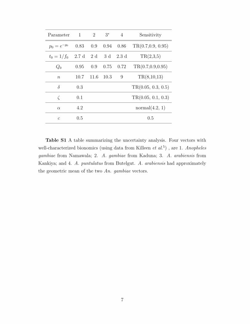
Table S1 A table summarizing the uncertainty analysis. Four vectors with

well-characterized bionomics (using data from Killeen et al.5) , are 1. Anopheles

gambiae from Namawala; 2. A. gambiae from Kaduna; 3. A. arabiensis from

Kankiya; and 4. A. puntulatus from Butelgut. A. arabiensis had approximately

the geometric mean of the two An. gambiae vectors.

7

φat

the

end

offive

year

s

00.0

50.1

00.1

50.2

00.2

50.3

00.3

50.4

00.4

50.5

00.5

50.6

00.6

50.7

00.7

50.8

00.8

50.9

00.9

51.0

0

PfPR

5%

4%

3%

2%

1%

1%

1%

1%

0%

0%

0%

0%

0%

0%

0%

0%

0%

0%

0%

0%

0%

10%

8%

7%

6%

5%

4%

3%

2%

2%

1%

1%

1%

1%

1%

1%

1%

0%

0%

0%

0%

0%

15%

13%

12%

10%

9%

7%

6%

5%

4%

3%

3%

2%

2%

2%

1%

1%

1%

1%

1%

1%

1%

20%

18%

17%

15%

14%

12%

10%

9%

8%

7%

6%

5%

4%

4%

3%

3%

3%

2%

2%

2%

2%

25%

23%

22%

20%

18%

17%

15%

14%

12%

11%

9%

8%

7%

6%

6%

5%

5%

5%

4%

4%

4%

30%

28%

27%

25%

23%

22%

20%

18%

17%

15%

14%

12%

11%

10%

9%

8%

8%

7%

7%

7%

7%

35%

33%

32%

30%

29%

27%

25%

23%

22%

20%

19%

17%

16%

14%

13%

12%

12%

11%

11%

10%

10%

40%

39%

37%

35%

34%

32%

31%

29%

27%

25%

24%

22%

21%

19%

18%

17%

16%

15%

15%

15%

14%

45%

44%

42%

41%

39%

38%

36%

34%

33%

31%

29%

28%

26%

25%

23%

22%

21%

20%

20%

19%

19%

50%

49%

48%

46%

45%

43%

42%

40%

38%

37%

35%

34%

32%

30%

29%

28%

27%

26%

25%

25%

25%

55%

54%

53%

52%

50%

49%

47%

46%

44%

43%

41%

40%

38%

37%

35%

34%

33%

32%

32%

31%

31%

60%

59%

58%

57%

56%

55%

53%

52%

50%

49%

48%

46%

45%

43%

42%

41%

40%

39%

39%

38%

38%

65%

64%

63%

62%

61%

60%

59%

58%

57%

55%

54%

53%

52%

50%

49%

48%

47%

46%

46%

45%

45%

70%

70%

69%

68%

67%

66%

65%

64%

63%

62%

61%

60%

58%

57%

56%

55%

55%

54%

53%

53%

53%

75%

75%

74%

73%

73%

72%

71%

70%

69%

68%

67%

66%

65%

64%

64%

63%

62%

62%

61%

61%

61%

80%

80%

79%

79%

78%

77%

77%

76%

75%

75%

74%

73%

72%

72%

71%

70%

70%

69%

69%

69%

69%

Table

S2

We

sim

ula

ted

chan

ges

inP

fPR

for

an

ITN

pro

gra

mth

at

scale

d-u

pIT

Neff

ecti

ve

cover

age

from

0to

asp

ecifi

edta

rget

level

at

the

end

of

five

yea

rs.

Each

colu

mn

rep

rese

nts

ad

iffer

ent

targ

etle

vel

of

ITN

cover

age.

Each

row

rep

rese

nts

ad

iffer

ent

base

lin

eP

fPR

in5%

incr

emen

ts.

Th

een

trie

sin

the

tab

lesh

ow

the

mod

elp

red

icte

dP

fPR

at

the

end

of

the

five-

yea

rsc

alin

g-u

pp

erio

d.

8

φat

the

end

offive

year

s

PfP

R0.0

50.1

00.1

50.2

00.2

50.3

00.3

50.4

00.4

50.5

00.5

50.6

00.6

50.7

00.7

50.8

00.8

50.9

00.9

51.0

0

5%

10.5

13.1

12.8

10.5

8.5

7.4

6.7

6.2

5.9

5.7

5.5

5.4

5.3

5.2

5.2

5.1

55

55

YearstoReachEndpoint

10%

7.1

911.4

13.4

13.3

11.4

9.4

8.2

7.5

76.6

6.4

6.2

66

5.9

5.8

5.8

5.8

5.8

15%

6.1

7.2

8.2

9.8

12

13.6

13.3

11.2

9.4

8.3

7.7

7.2

6.9

6.7

6.6

6.5

6.4

6.3

6.2

6.2

20%

5.8

6.4

77.7

8.5

9.9

12

13.8

13.4

11.3

9.5

8.5

7.9

7.5

7.2

76.9

6.8

6.7

6.7

25%

5.6

6.2

6.6

7.1

7.6

8.2

9.2

10.8

13.1

13.9

12.4

10.2

8.9

8.2

7.8

7.5

7.3

7.2

7.1

7.1

30%

5.5

66.4

6.7

77.4

7.8

8.5

9.5

11.3

13.6

13.8

11.5

9.6

8.7

8.2

7.8

7.6

7.5

7.4

35%

5.4

5.9

6.3

6.6

6.8

7.1

7.4

7.8

8.3

9.1

10.5

13

14

12.1

9.9

8.9

8.3

87.8

7.7

40%

5.4

5.9

6.2

6.5

6.7

6.9

7.1

7.4

7.7

8.1

8.7

9.6

11.5

13.9

13.2

10.5

9.2

8.5

8.2

8.1

45%

5.3

5.8

6.1

6.4

6.6

6.8

77.2

7.5

7.7

8.1

8.5

9.4

11

13.8

13.4

10.5

9.2

8.6

8.3

50%

5.3

5.8

66.3

6.5

6.7

6.9

7.1

7.3

7.6

7.8

8.1

8.5

9.2

10.7

13.6

13.4

10.4

9.2

8.7

55%

5.2

5.6

66.2

6.4

6.6

6.8

77.2

7.4

7.6

7.8

8.1

8.4

910

12.8

13.8

10.5

9.3

60%

5.2

5.6

5.9

6.1

6.4

6.5

6.7

6.9

7.1

7.3

7.5

7.7

7.9

8.2

8.5

910

13

13.3

10.1

65%

5.1

5.5

5.8

6.1

6.2

6.5

6.6

6.8

77.2

7.3

7.6

7.8

8.1

8.3

8.7

9.2

10.1

13.5

12.1

70%

55.4

5.8

66.2

6.4

6.5

6.7

6.9

7.1

7.2

7.5

7.7

7.9

8.2

8.4

8.8

9.4

10.4

14.3

75%

4.9

5.4

5.6

5.9

6.1

6.3

6.5

6.6

6.8

77.2

7.3

7.6

7.8

8.1

8.3

8.7

9.1

9.7

11.4

80%

4.8

5.3

5.5

5.8

66.1

6.4

6.5

6.7

6.8

7.1

7.2

7.5

7.7

7.9

8.2

8.5

8.9

9.4

10.1

Table

S3

We

sim

ula

ted

chan

ges

inP

fPR

for

an

ITN

pro

gra

mth

at

scale

d-u

pIT

Neff

ecti

ve

cover

age

from

0to

asp

ecifi

edta

rget

level

at

the

end

of

five

yea

rs.

We

exte

nd

edth

esi

mu

lati

on

sso

that

aft

erfi

ve

yea

rs,

the

maxim

um

level

of

ITN

effec

tive

cover

age

was

sust

ain

edin

defi

nit

ely.

Each

colu

mn

rep

rese

nts

ad

iffer

ent

targ

etle

vel

of

ITN

cover

age,

an

dea

chro

wre

pre

sents

ad

iffer

ent

base

lin

eP

fPR

in5%

incr

emen

ts.

Th

enu

mb

ers

rep

ort

the

nu

mb

erof

yea

rsel

ap

sed

,co

unti

ng

from

the

start

of

the

pro

gra

m,

bef

ore

PfP

Ris

wit

hin

1%

of

its

end

poin

t.

9

ITN Effect Size

log(Effect Size)

Den

sity

1 2 3 4

0.0

0.2

0.4

0.6

0.8

ITN Effect Size

Effect Size

Den

sity

0 20 40 60 80

0.00

0.05

0.10

0.15

Figure S1 The variability in the predicted effect size achieved with 60%

effective coverage, or 80% coverage and 75% use. These represent 10,000 monte

carlo sample from the distributions reported in Table S1, the log effect size is

Gamma distributed with shape parameter, a ≈ 13.4 and scale paramater s ≈0.14.

10

X == 0.5

XC

Den

sity

0.00 0.05 0.10 0.15 0.20 0.25 0.30

02

46

8

X == 0.4

XC

Den

sity

0.00 0.05 0.10 0.15

010

2030

4050

Figure S2 The variability in outcomes achieved when considering only vari-

ability in heterogeneous biting, starting from the reported initial endemicity value

(i.e. X of 50% or 40%).

11

X == 0.5

XC

Den

sity

0.0 0.1 0.2 0.3 0.4

01

23

45

6

X == 0.4

XC

Den

sity

0.00 0.05 0.10 0.15 0.20 0.25 0.30 0.35

05

1015

Figure S3

The variability in outcomes achieved when considering both the variability in

heteroeneous biting and effect size, using the distributions reported in Table S1.

12

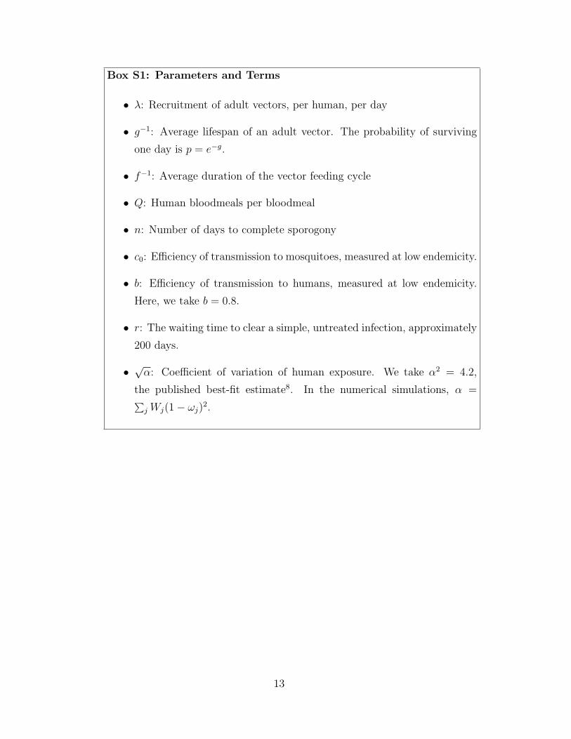
Box S1: Parameters and Terms

• λ: Recruitment of adult vectors, per human, per day

• g−1: Average lifespan of an adult vector. The probability of surviving

one day is p = e−g.

• f−1: Average duration of the vector feeding cycle

• Q: Human bloodmeals per bloodmeal

• n: Number of days to complete sporogony

• c0: Efficiency of transmission to mosquitoes, measured at low endemicity.

• b: Efficiency of transmission to humans, measured at low endemicity.

Here, we take b = 0.8.

• r: The waiting time to clear a simple, untreated infection, approximately

200 days.

•√α: Coefficient of variation of human exposure. We take α2 = 4.2,

the published best-fit estimate8. In the numerical simulations, α =∑jWj(1− ωj)2.

13

Box S2: Indices of Transmission Intensity

• s: The stability index (fQ/g)

• h: The force of infection. In these models h = bE .

• X: Net human infectiousness, the probability a mosquito becomes in-

fected after biting a human. Here, we use X =∫∞

0 ωc(ωE)Γ(ω|α)dω for

steady states and X =∑j ωjWj(1−X0,j) for timelines.

• V : Vectorial capacity. λs2e−gn = ma2e−gn/g.

• E : Entomological inoculation rate, E = V X/(1 + sX).

• X: Standard PfPR at the steady state

• R0: The basic reproductive number, bcV (1 + α)/r.

14

REFERENCES

1. Le Menach, A, Takala, S, McKenzie, F. E, Perisse, A, Harris, A, Flahault, A,

& Smith, D. L. (2007) Malar J 6, 10.

2. Smith, D. L, Dushoff, J, & McKenzie, F. E. (2004) PLoS Biol 2, e368.

3. Smith, D. L, McKenzie, F. E, Snow, R. W, & Hay, S. I. (2007) PLoS Biol 5,

e42.

4. Smith, D. L & Hay, S. I. (2009) Malar J 8, 87.

5. Killeen, G. F, McKenzie, F. E, Foy, B. D, Schieffelin, C, Billingsley, P. F, &

Beier, J. C. (2000) Am J Trop Med Hyg 62, 535–544.

6. Smith, D. L & McKenzie, F. E. (2004) Malar J 3, 13.

7. Dietz, K, Molineaux, L, & Thomas, A. (1974) Bull. Wld. Hlth. Org. 50,

347–357.

8. Smith, D. L, Dushoff, J, Snow, R. W, & Hay, S. I. (2005) Nature 438, 492–495.

9. Dietz, K. (1988) in Principles and Practice of Malaria, eds. Wernsdorfer, W

& McGregor, I. (Churchill Livingstone, Edinburgh, UK), pp. 1091–1133.

15