Preconditioning Newton–Krylov methods in

nonconvex large scale optimization

Giovanni Fasano1,2 and Massimo Roma2

1 Universita Ca’ Foscari di VeneziaCa’ Dolfin Dorsoduro, 3825/E30123 Venezia, ITALYE-mail: fasano@unive.it

2 Dipartimento di Informatica e Sistemistica “A. Ruberti”SAPIENZA, Universita di Romavia Ariosto, 2500185 Roma, ITALYE-mail: (fasano,roma)@dis.uniroma1.it

Abstract

We consider an iterative preconditioning technique for largescale optimization, where the objective function is possiblynon-convex. First, we refer to the solution of a generic indef-inite linear system by means of a Krylov subspace method,and describe the iterative construction of the preconditionerwhich does not involve matrices products or matrix stor-age. The set of directions generated by the Krylov sub-space method is also used, as by product, to provide anapproximate inverse of the system matrix. Then, we ex-perience our method within Truncated Newton schemes forlarge scale unconstrained optimization, in order to speedup the solution of the Newton equation. Actually, we use aKrylov subspace method to approximately solve the New-ton equation at current iterate (where the Hessian matrixis possibly indefinite) and to construct the preconditionerto be used at the current outer iteration. An extensive nu-merical experience show that the preconditioning strategyproposed leads to a significant reduction of the overall inneriterations on most of the test problems considered.

1

Keywords : Large Scale Optimization, Non–convex problems,Krylov subspace methods, Newton–Krylov methods, Precondi-tioning.

1 Introduction

In this paper we deal with a preconditioning strategy to be usedfor the efficient solution of the large scale linear systems, whicharise very frequently in large scale nonlinear optimization. Aswell known, there are many and different contexts of nonlinearoptimization in which the iterative solution of sequences of lin-ear systems is required. Some examples are Truncated Newtonmethods in unconstrained optimization, equality and/or inequal-ity constrained problems, KKT systems, interior point methods,PDE constrained optimization and many others.

Krylov subspace methods are usually used for iteratively solv-ing such linear systems by means of “matrix–free” implementa-tions. Some of the most commonly used are the Conjugate Gradi-ent methods for symmetric positive definite systems, the Lanczosalgorithm for symmetric systems, GMRES, Bi-CGSTAB, QMRmethods for unsymmetric systems.

In this work we consider symmetric indefinite linear systemsand focus on the possibility of constructing good preconditionersfor Krylov subspace methods. In particular, our aim is to con-struct a preconditioner by using an iterative decomposition of thesystem matrix, commonly obtained as by product of the Krylovsubspace methods (see, e.g. [22, 10]) and without requiring a sig-nificant additional computational effort. Firstly, we state the leastrequirements that a Krylov subspace method must satisfy to besuited to this aim. Then we define the preconditioner with refer-ence to a generic Krylov subspace method and prove interestingproperties of such a preconditioner. Finally, we focus on a partic-ular Krylov subspace method, a version of the planar ConjugateGradient (CG) method, which is an extension of the well knownstandard CG method. In particular, we refer to the planar CGalgorithm FLR [6, 9]. We consider this algorithm since it pre-vents from pivot breakdowns of the standard CG algorithm when

2

the system matrix is not positive definite. As a consequence weperform a number of iterations enough to generate a good approx-imation of the inverse of the system matrix, to be used for buildingthe preconditioner. We show how the construction of such a pre-conditioner is performed without storing any n×n matrix (wheren is the dimension of the vector of the variables) or computingmatrices products or explicit matrices inverse. Actually, we as-sume that the entries of the system matrix are not known andthe only information of the system matrix is gained by means of aroutine, which provides the product of the matrix times a vector.This routine is available for free, since already required by anyimplementation of a Krylov subspace method.

We use our preconditioner within a nonlinear optimizationframework, namely in solving nonconvex large scale unconstrainedproblems. In particular, we focus on the so called Newton–Krylovmethods, also called Truncated Newton (TN) methods (see [18]for a survey). TN methods are implementations of the Newtonmethods, in which a Krylov subspace method is used for approx-imately solving the linear system arising in computing the searchdirection. In this context, all we need to compute our precondi-tioner is already available, as by product of the inner iterationsperformed for computing the search direction.

Notwithstanding Truncated Newton methods have been widelystudied and extensively tested, it is largely recognized (see, e.g.[20]) that, especially in dealing with large scale problems, two keyaspects for the overall efficiency of the method can be still con-sidered worthwhile to be investigated: the first one regards theformulation and handling of a preconditioner which enables to ac-celerate the convergence of the iterates. In fact, for TruncatedNewton methods, preconditioning is today considered an essentialtool for achieving a good efficiency and robustness, especially inthe large scale setting. The second one concerns the possibilityto tackle nonconvex problems and hence to handle the indefinitecase for Newton’s equation. In these paper we try to tackle boththese aspects in the large scale setting. As regards the first issue,we embed our preconditioner within the inner iterations of the TNmethods, according to a suited strategy. Numerical results show

3

that this leads to an overall reduction of the number of CG inneriterations, needed in most of the test problems considered. Asregards the possibility to handle nonconvex problems, we adoptthe planar CG method FRL for constructing the preconditioner,instead of the standard CG methods, in order to avoid pivot break-down. Moreover, drawing our inspirations from [12], in computingthe search direction by the preconditioned CG, we adopt a strat-egy which allows us to overcome the usual drawbacks in dealingwith indefinite problems, namely the untimely termination of theinner iterations.

The paper is organized as follows: in Section 2, we consider theproblem of constructing a preconditioner for an indefinite linearsystem, by using a generic Krylov subspace method. In Section 3,we focus on a particular Krylov subspace method which allow usto tackle indefinite systems, the planar CG algorithm FLR, whichis first recalled for sake of completeness. In Section 4 an itera-tive matrix decomposition is obtained for the preconditioned CG.In Section 5, we focus on Truncated Newton methods for uncon-strained optimization and define a new preconditioning strategyfor the class of preconditioned Truncated Newton methods. More-over, we describe the strategy we adopt in order to efficiently tack-ling large scale indefinite problems. Finally, in Section 6 we reportthe results of an extensive numerical testing for the resulting Trun-cated Newton method, on a selection of large scale unconstrainedtest problems. We show that the approach we propose in thispaper is reliable and enables a significant reduction of the num-ber of the inner iterations, in solving both convex and nonconvexproblems.

2 Iterative matrix decomposition and the

new preconditioner

In this section we consider a general symmetric linear system,which is solved by using a Krylov subspace method. We describethe conditions which should be satisfied by the Krylov subspacemethod, in order to iteratively obtaining a decomposition of thesystem matrix, for constructing the preconditioner we propose. To

4

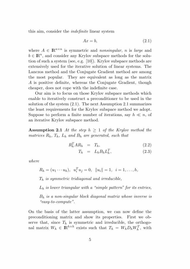
this aim, consider the indefinite linear system

Ax = b, (2.1)

where A ∈ IRn×n is symmetric and nonsingular, n is large andb ∈ IRn, and consider any Krylov subspace methods for the solu-tion of such a system (see, e.g. [10]). Krylov subspace methods areextensively used for the iterative solution of linear systems. TheLanczos method and the Conjugate Gradient method are amongthe most popular. They are equivalent as long as the matrixA is positive definite, whereas the Conjugate Gradient, thoughcheaper, does not cope with the indefinite case.

Our aim is to focus on those Krylov subspace methods whichenable to iteratively construct a preconditioner to be used in thesolution of the system (2.1). The next Assumption 2.1 summarizesthe least requirements for the Krylov subspace method we adopt.Suppose to perform a finite number of iterations, say h ≪ n, ofan iterative Krylov subspace method.

Assumption 2.1 At the step h ≥ 1 of the Krylov method thematrices Rh, Th, Lh and Bh are generated, such that

RTh ARh = Th, (2.2)

Th = LhBhLTh , (2.3)

where

Rh = (u1 · · ·uh), uTi uj = 0, ‖ui‖ = 1, i = 1, . . . , h,

Th is symmetric tridiagonal and irreducible,

Lh is lower triangular with a “simple pattern” for its entries,

Bh is a non-singular block diagonal matrix whose inverse is“easy-to-compute”.

On the basis of the latter assumption, we can now define thepreconditioning matrix and show its properties. First we ob-serve that, since Th is symmetric and irreducible, the orthogo-nal matrix Wh ∈ IRh×h exists such that Th = WhDhW T

h , with

5

Dh = diag1≤i≤h{di} non-singular. Then, we can define the matrix|Dh| = diag1≤i≤h{|di|} and, accordingly, the matrix |Th|

|Th| = Wh|Dh|W Th .

Let us now introduce the following matrix

Mh = (I − RhRTh ) + Rh|Th|RT

h , (2.4)

where Rh and Th satisfy relation (2.2).

Theorem 2.1 Consider any Krylov subspace method to solve (2.1)and suppose it performs a number h ≪ n of iterations, and thatAssumption 2.1 holds. Then we have:

a) Mh is symmetric and nonsingular;

b) M−1h = (I − RhRT

h ) + Rh|Th|−1RTh ;

c) Mh is positive definite and its spectrum Λ(Mh) is given by

Λ(Mh) = Λ(|Th|) ∪ Λ(In−h),

where Λ(In−h) is the set of the n− h unit eigenvalues of theidentity matrix In−h;

d) Λ(M−1h A) = Λ(AM−1

h ) and contains at least h eigenvaluesin the set {−1, +1}.

Proof: As regards a), the symmetry trivially follows from thesymmetry of Th. Moreover, since A in (2.1) is symmetric, thematrix Rn,h exists such that RT

n,hRn,h = In−h and the columns of

the matrix [Rh... Rn,h] are an orthogonal basis of IRn. Thus, for

any v ∈ IRn we can write v = Rhv1 + Rn,hv2, with v1 ∈ IRh andv2 ∈ IRn−h. Now, to prove Mh is invertible, we show that Mhv = 0implies v = 0. In fact,

Mhv = Rn,hv2 + Rh|Th|v1 =

[Rh|Th|

... Rn,h

] [v1

v2

]= 0,

6

if and only of (vT1 vT

2 )T = 0, since from Assumption 2.1 the matrix|Th| is nonsingular.

As regards b), recalling that RTh Rh = I and |Th| is nonsingular

from Assumption 2.1, a direct computation yields the result.As concerns item c), since I −RhRT

h = Rn,hRTn,h, we can write

Mk = [Rh Rn,h]

[|Th| 00 In−h

] [RT

h

RTn,h

]

which gives the results, since Th is irreducible and thus |Th| ispositive definite.

Item d) may be proved by considering that the matrices M−1h A

and AM−1h are similar to the matrix M

−1/2h AM

−1/2h and hence

Λ(M−1h A) = Λ(M

−1/2h AM

−1/2h ) = Λ(AM−1

h ). Moreover, we have

M−1/2h =

[Rh

... Rn,h

] [ |Th|−1/2 0

0 In−h

] [RT

h

RTn,h

],

and henceM

−1/2h AM

−1/2h =

=

[Rh

... Rn,h

] [ |Th|−1/2 0

0 In−h

] [RT

h ARh RTh ARn,h

RTn,hARh RT

n,hARn,h

]

[|Th|−1/2 0

0 In−h

] [RT

h

RTn,h

].

Recalling that ARh = RhTh, we have

RTh ARn,h = (RT

n,hARh)T = (RTn,hRhTh)T = 0,

and from (2.2) we obtain

M−1/2h AM

−1/2h =

[Rh

... Rn,h

] [Ih 0

0 RTn,hARn,h

] [RT

h

RTn,h

].

which proves that at least h eigenvalues of M−1/2h AM

−1/2h are in

the set {−1, +1} and this completes the proof.

7

Our aim is to use the matrix Mh, with h ≪ n, as preconditioner,as we will describe in the sequel, in order to use information gath-ered during the iteration of the Krylov subspace method. Notethat this is not the first attempt in literature to use a precondi-tioner of this form. In fact, a similar approach has been consideredin the context of GMRES methods (see [4, 1, 14]). However, it isvery important to note that GMRES information is given in theform of Hessenberg decomposition of the matrix A, and not as atridiagonal one, as in our approach. However, the main distin-guishing feature of the approach we propose consists of the choiceof the particular Krylov subspace method we adopt. Indeed ourchoice allows us to construct and use the preconditioner withoutstoring any n×n matrix and without any explicit matrix inversion.In particular, as described in Section 3, to perform the precondi-tioned method it will suffice to store h ≪ n n-dimensional vectors,the diagonal elements of a h×h diagonal matrix and the subdiago-nal elements of a lower bidiagonal h×h matrix. All the entries areavailable as by product from the iterates of the Krylov method.In the next section we will describe the method we chose to adopt.

3 Computing the new preconditioner via

the Planar-CG algorithm FLR

The Krylov subspace method we propose to use in this paper is theConjugate Gradient-type method FLR introduced in [7]. Unlikethe Conjugate Gradient, it copes with the indefinite case too. Itis an iterative method for solving indefinite linear systems, and isa modification of the standard CG algorithm [13]. Now we reporta scheme of this method.

8

Algorithm FLR

Step 1 : k = 1, s1 = 0, r1 = b. If r1 = 0 then STOP,else compute p1 = r1.

Step k : Compute σk = pTk Apk.

If | σk | ≥ ǫk‖pk‖2 then go to Step kA

else go to Step kB

– Step kA (standard CG step) :Set sk+1 = sk + akpk, rk+1 = rk − akApk ,

where ak =rTk pk

σk=

‖rk‖2

σk.

If rk+1 = 0 then STOPelse compute pk+1 = rk+1 + βkpk

with βk =−pT

k Ark+1

σk=

‖rk+1‖2

‖rk‖2.

Set k = k + 1 and go to Step k.

– Step kB (planar CG step) :If k = 1 then compute the vector qk = Apk,else compute the vector

qk =

Apk + bk−1pk−1, if the previous step isStep (k − 1)A

Apk +bk−2

∆k−2(σk−2qk−2 − δk−2pk−2) ,

if the previous step is Step (k − 2)B

where bk−1 = −(Apk−1)T Apk/σk−1 and

bk−2 = −(Aqk−2)T Apk.

9

Compute ck = rTk pk, δk = pT

k Aqk, ek = qTk Aqk,

∆k = σkek − δ2k and ck = (ckek − δkq

Tk rk)/∆k,

σk = (σkqTk rk − δkck)/∆k.

Set sk+2 = sk + ckpk + σkqk andrk+2 = rk − ckApk − σkAqk.

If rk+2 = 0 then STOP

else compute pk+2 = rk+2 +βk

∆k(σkqk − δkpk),

with βk = −qTk Ark+2.

Set k = k + 2 and go to Step k.

Further details on the FLR algorithm can be found in [7, 6]; herewe simply consider some relevant results, which are used in orderto obtain relations (2.2)-(2.3).

First observe that as long as at Step k the planar CG Step kB isnot performed, the FLR algorithm reduces to the standard CG andhence, at Step kA the algorithm detects the solution of (2.1) alongthe conjugate direction pk. On the contrary, if a pivot breakdownoccurs at Step k (i.e. pT

k Apk ≈ 0), the FLR algorithm generatesanother direction at Step kB (namely qk). Then, it performs asearch for the system solution on the 2-dimensional linear manifoldsk + span{pk, qk}, and generates the new point sk+2. In additionit can be easily proved (see [7]) that, if the indefinite matrix A isnonsingular and at Step k we have rk 6= 0, then the FLR algorithmcan always perform either Step kA or Step kB. As concerns theassessment of the parameter ǫk at the Step k, some proposalswhere considered in [8, 9], in order to avoid possible instabilities.

For sake of completeness, now we report the tridiagonalizationprocedure proposed in the paper [9], which will be at the basis ofthe construction of the matrices Rh, Th and Bh mentioned in theAssumption 2.1.

10

Let us consider the Algorithm FLR at a generic Step k andlet us introduce the following notation: if at Step k of the FLR

algorithm the condition |pTk Apk| ≥ ǫk‖pk‖2 is satisfied, then we set

wk = pk (standard CG step); otherwise we set wk = pk and wk+1 =qk (planar CG step). According with the latter positions, thesequence {wi} represents the sequence of directions generated bythe Algorithms FLR which contains, at most, pairs of consecutivenon–conjugate directions.

As regards the sequence {ri} of the residuals generated by thealgorithm FLR up to Step k, if a planar CG Step kB occurs, wehave two directions (wk and wk+1) and only one residual rk. Toovercome this drawback, if the Step k is the planar Step kB, weintroduce a “dummy” residual rk+1, which completes the sequenceof orthogonal vectors {r1, . . . , rk, rk+1} [2, 5]. The possible choicesfor rk+1 in order to satisfy the conditions rk+1 ∈ Kk(A, r1) andrk+1 6∈ Kk−1(A, r1) and to preserve the orthogonality conditionsrTk+1pk = rT

k+1rk are:

rk+1 = ± [αkrk + (1 + αk) sgn(σk)Apk] , (3.1)

with αk = − |σk|‖rk‖2 + |σk|

.

Therefore, after h ≤ n steps of the FLR algorithm the followingmatrices can be defined:

Rh =

(r1

‖r1‖· · · rh

‖rh‖

)∈ IRn×h, Ph =

(w1

‖r1‖· · · wh

‖rh‖

)∈ IRn×h.

In the remainder of this section we give evidence that the Al-gorithm FLR can also provide the matrices Lh and Bh mentionedin the Assumption 2.1, such that (2.2) and (2.3) hold. To this aimwe report the statement of Theorem 2.1 in [9].

Theorem 3.1 Consider the FLR algorithm where A is symmetric,indefinite and nonsingular. Suppose ǫk > 0 and let ‖ri‖ 6= 0,i ≤ h. Assume the only one planar CG step performed by the FLR

11

algorithm is Step kB < h. Then the following relations hold:

PhLTh = Rh, (3.2)

APh =

(Rh

...rh+1

‖rh+1‖

)(Lh

lh+1,heTh

)Dh, h < n, (3.3)

ARh =

(Rh

...rh+1

‖rh+1‖

)(Th

th+1,heTh

), h < n, (3.4)

where

Lh =

1

−√

β1 ·

· 1

−√

βk−1 1 0

α1 α2

α3 α4 1

0 −√

βk+2 ·

· 1

−√

βh−1 1

(3.5)with (βk = ‖rk+1‖2/‖rk‖2, βk+1 = ‖rk+2‖2/‖rk+1‖2)

α1 =αk√βk

, α2 = (1 + αk) sgn(σk),

α3 =βkδk

∆k

√βk+1βk

, α4 = − βk σk

∆k

√βk+1

,(3.6)

12

Dh =

1

a1·

1

ak−10

1

ξk1

ξk+1

01

ak+2

·1

ah

, (3.7)

Lh =

1

−√

β1 ·

· 1 0

−√

βk−1 α1 α3

α2 α4

α5 1

0 −√

βk+2 ·

· 1

−√

βh−1 1

.

(3.8)

The coefficients ξk and ξk+1 are independent arbitrary non-zero

13

parameters, and αi, i = 1, . . . , 5, have the following values:

α1 =σk

‖rk‖2ξk, α2 =

√βk

[sgn(σk) +

σk

‖rk‖2

]ξk,

α3 =ξk+1√βkσk

[1 − σk

‖rk‖2ck

], α4 = − ckξk+1

σk(1 + αk) sgn(σk),

α5 = −ξk+1

σk

√βk+1.

Finally, Th is an irreducible symmetric tridiagonal matrix definedby (

Th

0 · · · 0 th+1,h

)=

(Lh

0 · · · 0 lh+1,h

)DhLT

h , (3.9)

where lh+1,h and th+1,h are the element (h + 1, h) of the matrixLh+1 and Th+1, respectively.

Moreover, since both Lh and Lh are nonsingular from Theo-rem 3.1 the following result can be obtained (see [9]).

Proposition 3.2 Consider the FLR algorithm where ǫk > 0 andlet ‖ri‖ 6= 0, i ≤ h. Suppose the only one planar CG step per-formed by the FLR Algorithm is Step kB < h. Then, the nonsin-gular matrix Qh ∈ IRh×h exists such that

Lh = LhQh, (3.10)

where

Qh =

1. . . 0

1πk,k πk,k+1

πk+1,k πk+1,k+1

1

0. . .

1

, (3.11)

14

with

πk,k = α1, πk,k+1 = α3,

πk+1,k =α2 − α1α1

α2, πk+1,k+1 =

α4 − α3α1

α2.

(3.12)

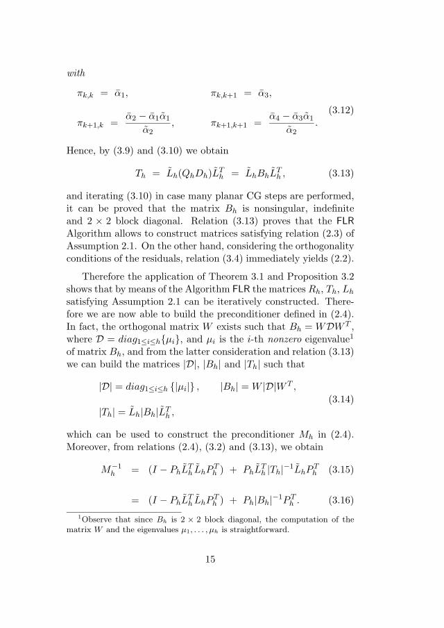
Hence, by (3.9) and (3.10) we obtain

Th = Lh(QhDh)LTh = LhBhLT

h , (3.13)

and iterating (3.10) in case many planar CG steps are performed,it can be proved that the matrix Bh is nonsingular, indefiniteand 2 × 2 block diagonal. Relation (3.13) proves that the FLR

Algorithm allows to construct matrices satisfying relation (2.3) ofAssumption 2.1. On the other hand, considering the orthogonalityconditions of the residuals, relation (3.4) immediately yields (2.2).

Therefore the application of Theorem 3.1 and Proposition 3.2shows that by means of the Algorithm FLR the matrices Rh, Th, Lh

satisfying Assumption 2.1 can be iteratively constructed. There-fore we are now able to build the preconditioner defined in (2.4).In fact, the orthogonal matrix W exists such that Bh = WDW T ,where D = diag1≤i≤h{µi}, and µi is the i-th nonzero eigenvalue1

of matrix Bh, and from the latter consideration and relation (3.13)we can build the matrices |D|, |Bh| and |Th| such that

|D| = diag1≤i≤h {|µi|} , |Bh| = W |D|W T ,

|Th| = Lh|Bh|LTh ,

(3.14)

which can be used to construct the preconditioner Mh in (2.4).Moreover, from relations (2.4), (3.2) and (3.13), we obtain

M−1h = (I − PhLT

h LhP Th ) + PhLT

h |Th|−1LhP Th (3.15)

= (I − PhLTh LhP T

h ) + Ph|Bh|−1P Th . (3.16)

1Observe that since Bh is 2 × 2 block diagonal, the computation of the

matrix W and the eigenvalues µ1, . . . , µh is straightforward.

15

It is fundamental to notice that the construction of the precondi-tioner by the Algorithm FLR does not require any matrix inversion(apart from |Bh|−1 which is a 2×2 block diagonal matrix). In par-ticular, relation (3.16) reveals that the storage of the matrices Ph

(in place of the matrix Rh) and Lh suffices to compute the precon-ditioned residual M−1

h rk. Finally, observe that Ph should be fullystored, however Lh is sparse and has the very simple structure in(3.5).

An alternative way to construct the preconditioner could bebased on the use of the Lanczos algorithm. It is well known that,in the positive definite case, the standard CG and the Lanczosmethods are equivalent (see, e.g., [22]). Moreover, as regards theAssumption 2.1, at step h, the Lanczos method provides the matri-ces Rh and Th such that the equality (2.2) holds. Indeed it sufficesto take as matrix Rh the matrix whose columns are the Lanczosvectors ui, i = 1, . . . , h, i.e. the matrix Uh = (u1 · · · uh). More-

over if we denote by T(L)h the tridiagonal matrix generated by the

Lanczos algorithm, if A is positive definite, the matrix T(L)h is pos-

itive definite too and can be stably decomposed in the form (2.3),where Lh is a unit lower bidiagonal matrix and Bh is simply diag-onal. Moreover the Lanczos algorithm can be used also in dealingwith the indefinite case, thus overcoming the drawback of the stan-dard CG due to possible pivot breakdown. Moreover, the relationsbetween standard CG and Lanczos algorithm in the definite caseare well known (see. e.g. [22]). The correspondence between theplanar-CG FLR method and the Lanczos method in the indefinitecase has been studied in [8] (see, in particular Theorem 4.3 in [8]).

Now we show how the Lanczos algorithm can be used to deter-mine the matrix Mh in (2.4). However, at the same time here weshow that the Algorithm FLR should be preferred not only for itscompetitive computational burden, but also because it yields for-mulae (3.15)–(3.16) which avoid the computation of the inverse ofa tridiagonal matrix. In fact, the construction of the matrix (2.4)via the Lanczos algorithm, can be immediately derived similarlyto the description in [1, 14], as a particular case of the Arnoldi

16

decomposition used therein, i.e. it results

Mh = (I − UhUTh ) + Uh

∣∣∣T (L)h

∣∣∣UTh .

Here, the tridiagonal matrix∣∣∣T (L)

h

∣∣∣ is defined analogously to |Th|in (2.4). Moreover,

M−1h = (I − UhUT

h ) + Uh

∣∣∣T (L)h

∣∣∣−1

UTh . (3.17)

Thus, Mh may be obtained either by the Algorithm FLR or theLanczos algorithm, without formally modifying its expression in(2.4). However, the implementation of the preconditioned iterativemethod in hand, for solving system (2.1), claims for an efficientcomputation, at each iteration i, of the preconditioned residual,i.e. of the product M−1

h ri. Thus, the computational cost of thepreconditioner cannot include the full inversion of the tridiagonalmatrix |Th|−1. The latter drawback may be overcome by usingthe Algorithm FLR by means of (3.15)-(3.16). The latter result isnot immediately available for the Lanczos algorithm, i.e. the com-putation of the preconditioned residual by means of the Lanczos

algorithm requires the calculation of the dense matrix |T (L)h |−1.

4 Iterative matrix decomposition for

preconditioned CG

In this section we analyze some properties of the preconditionedCG algorithm. We aim at carrying out formulae similar to (3.2)-(3.4) of Section 3, which were obtained with the unpreconditionedCG algorithm FLR. For sake of completeness, we now report thescheme of the algorithm Prec-CG which is a standard precondi-tioned CG scheme. Our aim is to obtain suitable formulae inorder to exploit a decomposition of the matrix A.

17

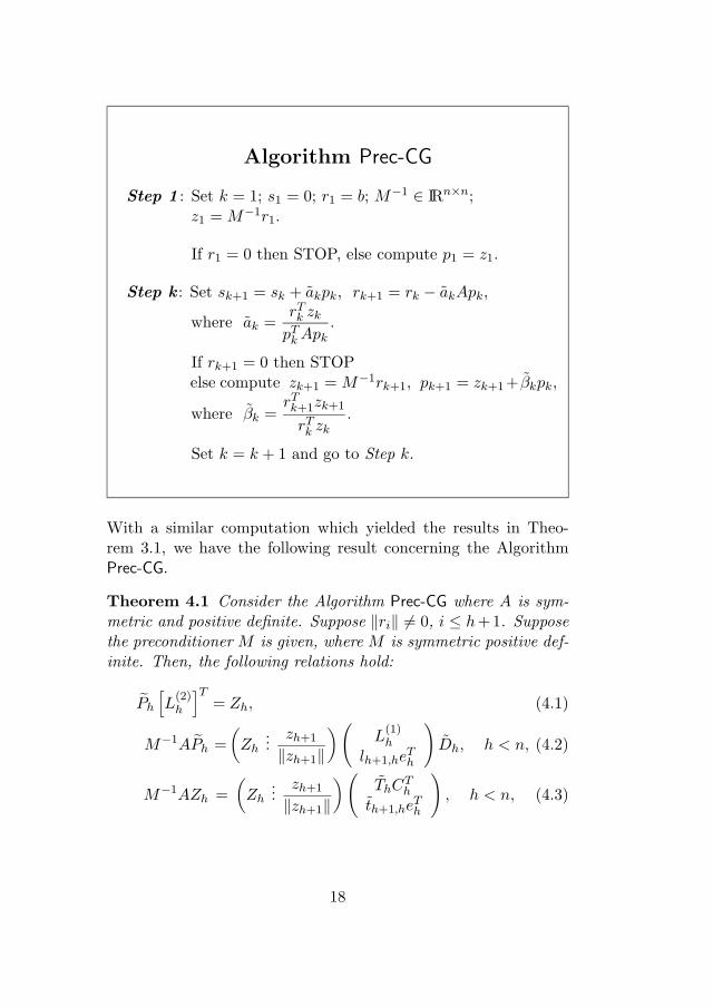
Algorithm Prec-CG

Step 1 : Set k = 1; s1 = 0; r1 = b; M−1 ∈ IRn×n;z1 = M−1r1.

If r1 = 0 then STOP, else compute p1 = z1.

Step k : Set sk+1 = sk + akpk, rk+1 = rk − akApk,

where ak =rTk zk

pTk Apk

.

If rk+1 = 0 then STOPelse compute zk+1 = M−1rk+1, pk+1 = zk+1+ βkpk,

where βk =rTk+1zk+1

rTk zk

.

Set k = k + 1 and go to Step k.

With a similar computation which yielded the results in Theo-rem 3.1, we have the following result concerning the AlgorithmPrec-CG.

Theorem 4.1 Consider the Algorithm Prec-CG where A is sym-metric and positive definite. Suppose ‖ri‖ 6= 0, i ≤ h+1. Supposethe preconditioner M is given, where M is symmetric positive def-inite. Then, the following relations hold:

Ph

[L

(2)h

]T= Zh, (4.1)

M−1APh =

(Zh

...zh+1

‖zh+1‖

)(L

(1)h

lh+1,heTh

)Dh, h < n, (4.2)

M−1AZh =

(Zh

...zh+1

‖zh+1‖

)(ThCT

h

th+1,heTh

), h < n, (4.3)

18

where Ph = (p1/‖z1‖ · · · ph/‖zk‖) and Zh = (z1/‖z1‖ · · · zh/‖zh‖),

L(2)h =

1

−β1‖z1‖‖z2‖

1

· 1

· 1

−βh−1‖zh−1‖‖zh‖

1

, (4.4)

Dh =

1

a1·

··

1

ah

, (4.5)

L(1)h =

1

−‖z2‖‖z1‖

1

· 1

· 1

− ‖zh‖‖zh−1‖

1

, (4.6)

and Ch = {chi,j} is given by

19

chi,j =

0, i < j,

(−1)i+j−1Πh

k=jγk

Πhl=i−1γl

(βi−1

γi−1− γi−1

), i > j,

1, i = j(4.7)

with γi = −‖zi+1‖/‖zi‖. Finally, Th is an irreducible symmetrictridiagonal matrix defined by

Th = L(1)h Dh

[L

(1)h

]T, (4.8)

and

th+1,h = − 1

ah

‖zh+1‖‖zh‖

.

Proof: Relation (4.1) follows observing that by the precondi-tioned CG we have

p1

‖z1‖=

z1

‖z1‖p2

‖z2‖=

z2

‖z2‖+

β1

‖z2‖‖z1‖

p1

‖z1‖...

ph

‖zh‖=

zh

‖zh‖+

βh−1

‖zh‖‖zh−1‖

ph−1

‖zh−1‖.

Similarly, if zh+1 = 0 we obtain

M−1Ap1

‖z1‖=

1

α1

(z1

‖z1‖− ‖z2‖

‖z1‖z2

‖z2‖

)

M−1Ap2

‖z2‖=

1

α2

(z2

‖z2‖− ‖z3‖

‖z2‖z3

‖z3‖

)

...

M−1Aph

‖zh‖=

1

αh

(zh

‖zh‖

),

20

which yield relation M−1APh = ZhL(1)h Dh. On the other hand,

if zh+1 6= 0, the latter relation yields M−1APh = Zh+1L(1)h+1Dh,

where

L(1)h+1 =

L(1)h

−‖zh+1‖‖zh‖

eTh

.

Thus, (4.2) holds with lh+1,h = −‖zh+1‖/‖zh‖ and

Zh+1 = (Zh... zh+1/‖zh+1‖).

Finally, after some manipulations from (4.7) it follows

L(2)h = ChL

(1)h . (4.9)

Then, by multiplying relation APh = Zh+1L(1)h+1Dh by the non-

singular matrix [L(2)h+1]

T , and recalling relations (4.1) and (4.9) weobtain (4.3).

Now, we consider a preconditioned version of the algorithmFLR planar CG algorithm. We soon realize that, unfortunately, inthis case the full storage of the preconditioner is required. Indeed,unlike the coefficients in the Algorithm Prec-CG, in a precondi-tioned version of the Algorithm FLR, the coefficients ‘bk−1’ and‘bk−2’ at Step kB still depend on the preconditioner, which impliesthat a preconditioned Algorithm FLR may be hardly obtained forlarge scale problems.This implies that the Algorithm FLR may be used only for buildingand providing the preconditioner, as described previously.

21

5 Preconditioning Truncated Newton

methods

In the previous sections we described how to iteratively constructa preconditioner. Even if this preconditioner can be exploited indifferent contexts involving the solution of large scale linear sys-tems, our main interest is to fruitfully use it within the frameworkof Truncated Newton methods, for large scale optimization. Ofcourse, both unconstrained and constrained nonlinear optimiza-tion problems are of interest. Here we investigate the use ofthe preconditioner within Truncated Newton methods for uncon-strained optimization, namely for solving the problem

minx∈IRn

f(x),

where f : IRn → IR is a twice continuously differentiable functionand n is large. In particular we aim at defining some precondi-tioning strategies based on the preconditioner we introduced inthe previous sections, which lead an improvement of the overallefficiency of the method.

The structure of any Truncated Newton method for uncon-strained optimization is well known (see e.g. [18]). It is basedon two nested loops: the iterations of the Newton method (outeriterations) and the iterations of the solvers used, at each outeriteration j, to approximately solving the Newton system (inneriterations)

Hj s = −gj , (5.1)

where Hj = ∇2f(xj) and gj = ∇f(xj). Thus, since a sequence oflinear systems must be solved, in many cases, it is crucial to haveat one’s disposal a preconditioning strategy, which should enablea considerable computational saving in terms of number of inneriterations. This motives the fact that to define general purposepreconditioning strategies within Truncated Newton methods isusually still considered one the main issues which is worthwhileinvestigating, especially in dealing with large scale problems. Aswell known, the main difficulty in this context relies on the factthat, in the large scale setting, the Hessian matrix can not be

22

stored or handled. Hence, any Truncated Newton implementationgains information on the Hessian matrix by means of a routine,which provides the product of the Hessian matrix times a vec-tor. This prevents from using any preconditioner based on theknowledge of the actual elements of the Hessian matrix. Unfortu-nately, few preconditioners have been proposed up to now whichdo not require the full Hessian matrix. The first proposal of such apreconditioner is in [17], where a diagonal scaling which uses a di-agonal approximation of the Hessian obtained by means of BFGSupdating is introduced. Afterwards, in [15, 16] an automatic pre-conditioning based on m–step limited memory quasi–Newton up-dating has been proposed without requiring the knowledge of theHessian matrix. More recently, a preconditioning strategy basedon a diagonal scaling, which only gains the information of theHessian matrix by means of the product of the Hessian times avector has been proposed in [21]. The other preconditioners up tonow proposed, usually require the knowledge of the entries of theHessian matrix and hence are not suited to be used in large scalesetting.

The preconditioner we defined in Section 2, actually is gener-ated during the iterations of the solver, gaining the informationon the Hessian matrix as by product of the iterates of the method.Moreover, as already noticed in Section 3, its application does notrequire to store any n × n matrix.

5.1 Our preconditioning strategy

The strategy we adopt in solving the sequence of the linear systems(5.1) is based on an adaptive rule for deciding when the applicationof the preconditioner is fruitful, that is the preconditioned methodshould be effective, or not. In fact, it is well known that theeffectiveness of a preconditioner is problem dependent. Hence,whenever the application of a preconditioner is expected to ledto a worsening of the performance, it should be desirable to usean unpreconditioned method. Of course, the key point is how toformulate an adaptive rule for deciding that. The adaptive schemewe adopt at each outer iteration can be summarized as follows:

23

1. Perform a number h ≤ 10 of iterations of the unprecon-ditioned algorithm FLR and store Ph, Lh and Bh.

2. Restart the CG iterations and perform h iterations of thepreconditioned CG method.

3. On the basis of the information gained decide how toproceed:

– if the preconditioner should be used, continue thepreconditioned CG iterations,

– otherwise continue the unpreconditioned iterates.

Observe that, if during the first h iterations of the algorithm FLR

at point 1 the termination criterion is satisfied before performingh iterations, of course the inner iterations are stopped and nopreconditioner is considered. Analogously, while performing thepreconditioned CG iterates at point 2, if the termination criterionis satisfied before performing h iterations, the inner iterates arestopped.

Whenever the selection rule indicates to proceed with the un-preconditioned iterates, the standard unpreconditioned CG me-thod FLR is simply continued until a termination criterion is sat-isfied. Otherwise, the standard preconditioned CG algorithm isused. Note that the planar CG algorithm FLR can not be precon-ditioned since a preconditioned version of this algorithm wouldneed the storage of the full matrix Mh. This is due to the factthat in the Step kB of the FLR algorithm, the coefficients bk−1 andbk−2 depend on Mh.

Remark 5.1 One of the most relevant point of such a strategyis the fact that, at the j-th outer iteration (i.e. when we aresolving the j-th system of the sequence (5.1)) the preconditioner

24

is computed on the basis of the information on the actual Hessianmatrix Hj . On the opposite, the strategies usually adopted (see,e.g. [15]) compute the preconditioner, to be used in the j-th outeriteration, during the inner CG iterations used at the previous outeriteration. This means that the preconditioner is computed on thebasis of Hj−1, that is on the Hessian matrix at the previous outeriteration and in general, this could be a serious drawback in casethe Hessian matrix should drastically change from xj−1 to xj .

5.2 The search direction

In this section we describe how the search direction is computedat each outer iteration of the Truncated Newton method. We referto the application of the algorithm Prec-CG to solve the Newtonsystem (5.1), assuming that the preconditioner Mh was alreadybeen computed after h planar CG iterates (of course this alsoapplies to the case when unpreconditioned CG is used, settingMh = I). We recall that we are dealing with the indefinite case,so that particular safeguard is needed in computing the searchdirection whenever a negative curvature is encountered, namely adirection p such that pT Hjp < 0. Getting our inspiration fromthe strategy proposed in [12], we do not terminate the CG inneriterations whenever a negative curvature direction is encountered,provided that

|pTk Hjpk| > ǫ‖pk‖2,

where ǫ > 0 is a suitable parameter. Observe that, if pTk Hjpk < 0

for some k, the approximate solution sk+1 generated at the k-th CG iteration, could be no longer a descent direction for thequadratic model

Qj(s) =1

2sT Hjs + gT

j s.

To overcome this drawback, which arises in dealing with non-convex problems, we proceed as follows. Let us consider a generick-th iteration of the preconditioned CG, and define the followingindex sets

25

I+k =

{i ∈ {1, k} : pT

i Hjpi > ǫi‖pi‖2}

,

I−k ={i ∈ {1, k} : pT

i Hjpi < −ǫi‖pi‖2}

where |I+k |+ |I−k | = k, (|C| is the cardinality of the set C) and the

following vectors

sPk =

∑

i∈I+

k

aipi =∑

i∈I+

k

rTi M−1

h ri

pTi Hjpi

pi,

sNk = −

∑

i∈I−k

aipi = −∑

i∈I−k

riM−1h ri

pTi Hjpi

pi.

The direction sPk can be viewed as the minimizer of Qj(s) over the

(positive) subspace generated by the vectors pi with i ∈ I+k , and

sNk is a negative curvature direction. Then, at each preconditioned

CG iterate we define the vector sk = sPk + sN

k . With this choicewe guarantee the monotonic decrease of {Qj(sk)} as k increase.In fact the following result holds.

Proposition 5.1 Suppose that the preconditioned CG algorithm(Prec-CG) is applied for solving the system (5.1). At each iterationk consider the following vector

sk = sPk + sN

k .

Then the sequence {Qj(sk)}k=1,2,... is strictly decreasing, i.e.

Qj(sk+1) < Qj(sk), k = 1, 2, . . . .

Proof: By definition, we have

sk = sPk + sN

k =k∑

i=1

|ai|pi = sk−1 + |ak|pk.

Now, using the fact that r1 = −gj and rT1 pk = rT

k M−1rk we obtain

Qj(sk)=1

2[sk−1 + |ak|pk]

T Hj [sk−1 + |ak|pk] + gTj [sk−1 + |ak|pk]

26

=1

2

[sTk−1Hjsk−1 + a2

hpTk Hjpk

]+ |ak|pT

k Hjsk−1

+ gTj sk−1 + |ak|gT

j pk

= Q(sk−1) +1

2sgn(pT

k Hjpk)(rT

k M−1h rk)

2

|pTk Hjpk|

− rTk M−1

h rk

|pTk Hjpk|

rT1 pk

= Qj(sk−1) +

(1

2sgn(pT

k Hjpk) − 1

)(rT

k M−1h rk)

2

|pTk Hjpk|

< Qj(sk−1).

The property stated in Proposition 5.1 plays a fundamental ruleconcerning the choice of the stopping criterion for the precondi-tioned CG iterates. In fact, this property allows us to use, also inthe preconditioned CG iterates, the standard stopping rule basedon the comparison of the reduction in the quadratic model withthe average reduction per iteration [19]. Therefore, at the outeriteration j, the inner preconditioned CG iterations are terminatedwhenever

Qj(sk) − Qj(sk−1)

Qj(sk)/k≤ α (5.2)

where α is a suited parameter. Observe that setting Mh = I,i.e. in the unpreconditioned case, sk coincides with the choiceof the Newton–type direction in [12]. Note that Proposition 5.1,ensuring the monotonic decrease of the quadratic model, enablesto extend the use of the stopping criterion (5.2) to the nonconvexcases. Hence, criterion (5.2) may be fruitfully used alternativelyto the residual–based standard criterion ‖rj‖/‖gj‖ ≤ ηj , whereηj → 0 as j → ∞.

5.3 Preconditioned Newton step

Now we aim at proving that the application of the preconditionerdefined in Section 3 leads to an interesting property. In the follow-ing proposition, we prove that one iteration of the preconditionedCG improves the quadratic model not less than h iterations of thealgorithm FLR. For sake of simplicity we assume that no planar

27

steps are performed in the h unpreconditioned iterations neededfor computing the preconditioner.

Proposition 5.2 Let Mh be the preconditioner in (2.4), computedafter h iterations of the FLR algorithm where no planar stepsare performed. Let p1, . . . , ph the CG directions generated, withpT

ℓ Hjpm = 0, 1 ≤ ℓ 6= m ≤ h, and p1 = −gj. Consider the vectors

sUNh = s1 +

h∑

i=1

aipi =h∑

i=1

aipi

sPR2 = s1 + |a1|p1 = |a1|M−1

h r1

then we haveQ(sPR

2 ) ≤ Q(sh) ≤ Q(sUNh ).

Proof: From the definition of M−1h , we have

M−1h r1 =

[(I − RhRT

h ) + Rh|T |−1RTh

]r1

= r1 − Rh

‖r1‖0...0

+ Rh[Lh|Dh|LTh ]−1

‖r1‖0...0

= RhL−Th |Dh|−1L−1

h

‖r1‖0...0

= RhL−Th diag1≤i≤h{|ai|}

1√β1...√

β1 · · · ·βh−1

‖r1‖

= Phdiag1≤i≤h

{‖ri‖2

|pTi Hjpi|

}

‖r1‖‖r2‖

...‖rh‖

28

=

(p1

‖r1‖p2

‖r2‖· · · ph

‖rh‖

)

|a1|. . .

|ah|

‖r1‖‖r2‖

...‖rh‖

=h∑

i=1

|ai|pi. (5.3)

The latter relation proves that if a1 = 1, the directions sh and sPR2

coincide. Now, by definition we have

Q(sUNh ) =

1

2

(sUNh

)THj

(sUNh

)+ gT sUN

h

=1

2

(h∑

i=1

aipi

)T

Hj

(h∑

i=1

aipi

)− rT

1

(h∑

i=1

aipi

)

=1

2

h∑

i=1

a2i p

Ti Hjpi −

h∑

i=1

ai‖ri‖2

=h∑

i=1

[1

2ai‖ri‖2 − ai‖ri‖2

]

= −1

2

h∑

i=1

ai‖ri‖2. (5.4)

Q(sh) =1

2sTh Hjsh + gT sh

=1

2

(h∑

i=1

|ai|pi

)T

Hj

(h∑

i=1

|ai|pi

)− rT

1

(h∑

i=1

|ai|pi

)

=1

2

h∑

i=1

a2i p

Ti Hjpi −

h∑

i=1

|ai|‖ri‖2

=h∑

i=1

[1

2ai‖ri‖2 − |ai|‖ri‖2

]

=h∑

i=1

[1

2sgn(pT

i Hjpi) − 1

]|ai|‖ri‖2. (5.5)

29

Moreover, from (5.3)

|a1| =

∣∣∣∣∣rT1 z1

pT1 Hj p1

∣∣∣∣∣ =

∣∣∣∣∣rT1 M−1

h r1

zT1 Hjz1

∣∣∣∣∣

=

∣∣∣∣∣∣∣

rT1

(∑hi=1 |ai|pi

)

(∑hi=1 |ai|pi

)THj

(∑hi=1 |ai|pi

)

∣∣∣∣∣∣∣=

∣∣∣∣∣∣∣∣∣∣∣

h∑

i=1

|ai|‖ri‖2

h∑

i=1

a2i p

Ti Hpi

∣∣∣∣∣∣∣∣∣∣∣

=

∑hi=1 |ai|‖ri‖2

∣∣∣∑h

i=1 a2i p

Ti Hjpi

∣∣∣;

thus, we have also

Q(sPR2 ) =

1

2

( ∑hi=1 |ai|‖ri‖2

∑hi=1 a2

i pTi Hjpi

)2( h∑

i=1

|ai|pi

)T

Hj

(h∑

i=1

|ai|pi

)

−∑h

i=1 |ai|‖ri‖2

∣∣∣∑h

i=1 a2i p

Ti Hjpi

∣∣∣rT1

(h∑

i=1

|ai|pi

)

=1

2

[∑hi=1 |ai|‖ri‖2

]2

∑hi=1 a2

i pTi Hjpi

−

[∑hi=1 |ai|‖ri‖2

]2∣∣∣∑h

i=1 a2i p

Ti Hjpi

∣∣∣

=1

2

[∑hi=1 |ai|‖ri‖2

]2

∑hi=1 ai‖ri‖2

−

[∑hi=1 |ai|‖ri‖2

]2∣∣∣∑h

i=1 ai‖ri‖2∣∣∣

. (5.6)

From (5.4) and (5.5), considering that

h∑

i=1

[−1

2sgn(pT

i Hjpi) −(

1

2sgn(pT

i Hjpi) − 1

)]|ai|‖ri‖2 ≥ 0

we easily obtainQ(sh) ≤ Q(sUN

h ).

Moreover, observe that Q(sPR2 ) ≤ Q(sh) if and only if

1

2

[∑hi=1 |ai|‖ri‖2

]2

∑hi=1 ai‖ri‖2

−

[∑hi=1 |ai|‖ri‖2

]2∣∣∣∑h

i=1 ai‖ri‖2∣∣∣

≤ 1

2

h∑

i=1

ai‖ri‖2−h∑

i=1

|ai|‖ri‖2,

30

or equivalently

12

[∑hi=1 |ai|‖ri‖2

]2− sgn

(∑hi=1 ai‖ri‖2

) [∑hi=1 |ai|‖ri‖2

]2

∑hi=1 ai‖ri‖2

≤ 1

2

h∑

i=1

ai‖ri‖2 −h∑

i=1

|ai|‖ri‖2. (5.7)

To prove the latter relation we separately consider two cases: thecase

∑hi=1 ai‖ri‖2 > 0 and the case

∑hi=1 ai‖ri‖2 < 0. In the first

case the relation (5.7) holds if and only if

1

2

[h∑

i=1

|ai|‖ri‖2

]2

− sgn

(h∑

i=1

ai‖ri‖2

)[h∑

i=1

|ai|‖ri‖2

]2

≤ 1

2

[h∑

i=1

ai‖ri‖2

]2

−[

h∑

i=1

|ai|‖ri‖2

]h∑

i=1

ai‖ri‖2

or equivalently if and only if

−1

2

[h∑

i=1

|ai|‖ri‖2

]2

≤[1

2

h∑

i=1

ai‖ri‖2 −h∑

i=1

|ai|‖ri‖2

]h∑

i=1

ai‖ri‖2,

and the latter inequality holds since

−1

2

(

h∑

i=1

|ai|‖ri‖2

)2

+

(h∑

i=1

ai‖ri‖2

)2+

h∑

i=1

|ai|‖ri‖2h∑

i=1

ai‖ri‖2 ≤ 0.

In the second case the relation (5.7) is equivalent to

3

2

[h∑

i=1

|ai|‖ri‖2

]2

≥ 1

2

[h∑

i=1

ai‖ri‖2

]2

+

∣∣∣∣∣

h∑

i=1

ai‖ri‖2

∣∣∣∣∣

h∑

i=1

|ai|‖ri‖2,

which holds since

3

2

[h∑

i=1

|ai|‖ri‖2

]2

=1

2

[h∑

i=1

|ai|‖ri‖2

]2

+

∣∣∣∣∣

h∑

i=1

|ai|‖ri‖2

∣∣∣∣∣

h∑

i=1

|ai|‖ri‖2

≥ 1

2

[h∑

i=1

ai‖ri‖2

]2

+

∣∣∣∣∣

h∑

i=1

ai‖ri‖2

∣∣∣∣∣

h∑

i=1

|ai|‖ri‖2.

31

This proves that

Q(sPR2 ) ≤ Q(sh) ≤ Q(sUN

h ).

6 Numerical Results

In this section we report the results of a preliminar numericalinvestigation obtained by embedding the new preconditioner ina linesearch based Truncated Newton method for unconstrainedoptimization. In particular, we performed a standard implemen-tation of a Truncated Newton method which uses the planar CGalgorithm FLR as a tool for constructing the preconditioner. Thenthe standard preconditioned CG algorithm is used as precondi-tioned scheme for the inner iteration.

The aim of our numerical investigation is, firstly, to assess ifthe preconditioning strategy proposed is reliable. The key pointis to check if the use of the preconditioner leads to a computa-tional savings in terms of overall inner iterations, with respect tothe unpreconditioned case. Therefore, to this aim, in this prelim-inary testing we do not use any adaptive criterion for choosing ifthe preconditioner should be used or not at each outer iterationof the method. We simply always use the preconditioned CG forsolving the sequence of Newton systems (5.1) whenever the pre-conditioner has been computed. We recall that the preconditioneris computed whenever at least h iterations of the unpreconditionedFLR algorithm have been performed.

As regards the test problems, we used all the unconstrainedlarge problems contained in the CUTEr collection [11]. All thealgorithms were coded in FORTRAN 90 compiled under CompaqVisual Fortran 6.6. All the runs were performed on a PC Pen-tium 4 – 3.2GHz with 1Gb RAM. The results are reported in termsof number of iterations, number of function evaluations, number ofCG-inner iterations and CPU time needed to solve each problem.In Tables 6.1, 6.2 and 6.3 we report the complete results for theunpreconditioned Truncated Newton method. In Tables 6.4, 6.5

32

and 6.6 we report the complete results for the preconditioned ver-sion of the same algorithm. As regards the parameter h, we trieddifferent values ranging from 5 to 10 and h = 7 is a value whichseems to be a good trade–off between the computational burdenrequired to compute the preconditioner and its effectiveness.

By comparing these results obtained by means of the precondi-tioned algorithm with respect to those obtained without using anypreconditioner, it is very clear that in most cases the use of thepreconditioner is beneficial, since it enables a significant reductionof the inner iterations needed to solve the problems. In particular,in terms of number of inner iterations, on 36 test problems the pre-conditioned algorithm performs better than the unpreconditionedone, and only on 10 problems it performs worse. On the remainingtest problems the two algorithms led to the same results or (on 8problems) they converge to different minimizers.

The performances of the two algorithms, in terms of number ofinner iterations, are also compared by means of the performanceprofiles [3]. In particular, in Figure 6.1 we drew the performanceprofiles relative to the results reported in the previous tables. Alsofrom these figures it is clear that the preconditioned algorithmperforms the best in terms of number of inner iterations. However,it is important to note that the preconditioned algorithm leads to6 additional failures with respect to the unpreconditioned one, dueto an excessive number of outer iterations (> 10000) of CPU time(> 900 seconds). This evidences the fact that, in some cases, theapplication of the preconditioner is not beneficial and even leadsto a severe worsening. Hence the necessity to define an adaptivecriterion which enables to assess whenever it is fruitful to use thepreconditioner or not.

33

7 Conclusions

In this paper we propose a new preconditioning technique for effi-ciently solving symmetric indefinite linear systems arising in largescale optimization, within the framework of Newton–type meth-ods. Krylov subspace methods are considered for the iterativesolution of the linear systems, and the construction of the precon-ditioner is obtained as by product of the Krylov methods iterates.In fact, the preconditioner is built by means of an iterative matrixdecomposition of the system matrix, without requiring to store orhandle the system matrix. The only information on this matrix isgained by means of a routine which computes the product of thematrix times a vector. The use of a planar version of the Con-jugate Gradient algorithm also enables to tackle indefinite linearsystems arising from nonconvex optimization problems. In orderto assess if the preconditioning strategy proposed is reliable, weembed it within a linesearch based Truncated Newton method forunconstrained optimization. The results obtained showed thatthe proposed strategy is efficient, enabling a significant computa-tional saving in terms of number of inner iterations need to solvethe problems. Unfortunately, few additional failures are obtainedby using the preconditioned algorithm. This should be due to thenecessity of an adaptive criterion, which enables to decide when-ever the preconditioner is beneficial and hence worthwhile to beapplied or not. This will be the subject of future work.

Acknowledgement

The first author wishes to thank the “Programma Ricerche IN-SEAN 2007-2009”.

34

1 1.2 1.4 1.6 1.8 20.55

0.6

0.65

0.7

0.75

0.8

0.85

0.9

0.95

UnpreconditionedPreconditioned

τ

1 1.5 2 2.5 3 3.50.55

0.6

0.65

0.7

0.75

0.8

0.85

0.9

0.95

UnpreconditionedPreconditioned

τ

Figure 6.1: Performance Profile w.r.t. inner iterations.

35

References

[1] J. Baglama, D. Calvetti, G. Golub, and L. Reichel,Adaptively preconditioned GMRES algorithms, SIAM Journalon Scientific Computing, 20 (1998), pp. 243–269.

[2] R. Bank and T. Chan, A composite step bi-conjugate gra-dient algorithm for nonsymmetric linear systems, NumericalAlgorithms, 7 (1994), pp. 1–16.

[3] E. D. Dolan and J. More, Benchmarking optimizationsoftware with performance profiles, Mathematical Program-ming, 91 (2002), pp. 201–213.

[4] J. Erhel, K. Burrage, and B. Pohl, Restarted GMRESpreconditioned by deflation, Journal of Computational andApplied Mathematics, 69 (1996), pp. 303–318.

[5] G. Fasano, Use of conjugate directions inside Newton–typealgorithms for large scale unconstrained optimization, PhDthesis, Universita di Roma “La Sapienza”, Rome, Italy, 2001.

[6] G. Fasano, Planar–conjugate gradient algorithm for large–scale unconstrained optimization, Part 2: Application, Jour-nal of Optimization Theory and Applications, 125 (2005),pp. 543–558.

[7] G. Fasano, Planar–conjugate gradient algorithm for large–scale unconstrained optimization, Part 1: Theory, Journal ofOptimization Theory and Applications, 125 (2005), pp. 523–541.

[8] G. Fasano, Lanczos-conjugate gradient method and pseu-doinverse computation, in unconstrained optimization, Jour-nal of Optimization Theory and Applications, 132 (2006),pp. 267–285.

[9] G. Fasano and M. Roma, Iterative computation of nega-tive curvature directions in large scale optimization, Compu-tational Optimization and Applications, 38 (2007), pp. 81–104.

36

[10] G. Golub and C. Van Loan, Matrix Computations, TheJohn Hopkins Press, Baltimore, 1996. Third edition.

[11] N. I. M. Gould, D. Orban, and P. L. Toint, CUTE

(and sifdec), a constrained and unconstrained testing environ-ment, revised, ACM Transaction on Mathematical Software,29 (2003), pp. 373–394.

[12] L. Grippo, F. Lampariello, and S. Lucidi, A trun-cated Newton method with nonmonotone linesearch for uncon-strained optimization, Journal of Optimization Theory andApplications, 60 (1989), pp. 401–419.

[13] M. Hestenes, Conjugate Direction Methods in Optimiza-tion, Springer Verlag, New York, 1980.

[14] L. Loghin, D. Ruiz, and A. Touhami, Adaptive precondi-tioners for nonlinear systems of equations, Journal of Compu-tational and Applied Mathematics, 189 (2006), pp. 362–374.

[15] J. Morales and J. Nocedal, Automatic preconditioningby limited memory quasi–Newton updating, SIAM Journal onOptimization, 10 (2000), pp. 1079–1096.

[16] J. L. Morales and J. Nocedal, Algorithm PREQN: For-tran 77 subroutine for preconditioning the conjugate gradi-ent method, ACM Transaction on Mathematical Software, 27(2001), pp. 83–91.

[17] S. Nash, Preconditioning of truncated-Newton methods,SIAM Journal on Scientific and Statistical Computing, 6(1985), pp. 599–616.

[18] S. Nash, A survey of truncated-Newton methods, Journalof Computational and Applied Mathematics, 124 (2000),pp. 45–59.

[19] S. Nash and A. Sofer, Assessing a search direction withina truncated-Newton method, Operations Research Letter, 9(1990), pp. 219–221.

37

[20] J. Nocedal, Large scale unconstrained optimization, in Thestate of the art in Numerical Analysis, A. Watson and I. Duff,eds., Oxford, 1997, Oxford University Press, pp. 311–338.

[21] M. Roma, A dynamic scaling based preconditioning for trun-cated newton methods in large scale unconstrained optimiza-tion, Optimization Methods and Software, 20 (2005), pp. 693–713.

[22] J. Stoer, Solution of large linear systems of equations byconjugate gradient type methods, in Mathematical Program-ming. The State of the Art, A. Bachem, M.Grotschel, andB. Korte, eds., Berlin Heidelberg, 1983, Springer-Verlag,pp. 540–565.

38

PROBLEM n ITER FUNCT CG-it F. VALUE TIMEARWHEAD 1000 34 364 37 0.000000D+00 0.08ARWHEAD 10000 10 102 11 1.332134D-11 0.22BDQRTIC 1000 50 297 103 3.983818D+03 0.11BDQRTIC 10000 461 **** 2244 4.003431D+04 41.27BROYDN7D 1000 449 1972 2686 3.823419D+00 2.52BROYDN7D 10000 884 4058 4575 3.711778D+03 54.77BRYBND 1000 21 65 29 9.588198D-14 0.02BRYBND 10000 21 65 29 8.686026D-14 0.42CHAINWOO 1000 262 440 1004 1.000000D+00 0.64CHAINWOO 10000 287 823 911 1.000000D+00 8.78COSINE 1000 22 64 40 -9.990000D+02 0.03COSINE 10000 19 65 32 -9.999000D+03 0.27CRAGGLVY 1000 46 213 110 3.364231D+02 0.14CRAGGLVY 10000 115 775 177 3.377956D+03 3.45CURLY10 1000 151 438 7638 -1.003163D+05 2.94CURLY10 10000 135 1295 55801 -1.003163D+06 318.88CURLY20 1000 267 470 7670 -1.001379D+05 4.91CURLY20 10000 162 994 64081 -1.001313D+06 510.39CURLY30 1000 >10000 - - - -DIXMAANA 1500 8 13 9 1.000000D+00 0.00DIXMAANA 3000 8 14 8 1.000000D+00 0.02DIXMAANB 1500 5 10 6 1.000000D+00 0.02DIXMAANB 3000 5 10 6 1.000000D+00 0.02DIXMAANC 1500 5 11 6 1.000000D+00 0.00DIXMAANC 3000 5 11 6 1.000000D+00 0.05DIXMAAND 1500 5 8 5 1.000000D+00 0.00DIXMAAND 3000 5 8 5 1.000000D+00 0.00DIXMAANE 1500 63 66 204 1.000000D+00 0.23DIXMAANE 3000 88 91 277 1.000000D+00 0.70DIXMAANF 1500 33 38 198 1.000000D+00 0.23DIXMAANF 3000 32 37 238 1.000000D+00 0.58DIXMAANG 1500 41 80 223 1.000000D+00 0.25DIXMAANG 3000 65 133 400 1.000000D+00 1.09DIXMAANH 1500 26 28 194 1.000000D+00 0.19DIXMAANH 3000 28 30 256 1.000000D+00 0.66DIXMAANI 1500 60 63 1997 1.000000D+00 1.81DIXMAANI 3000 83 86 2585 1.000000D+00 5.23DIXMAANJ 1500 58 118 213 1.089260D+00 0.22DIXMAANJ 3000 63 135 291 1.176995D+00 0.75DIXMAANK 1500 24 38 335 1.000000D+00 0.34DIXMAANK 3000 28 41 333 1.000000D+00 0.78DIXMAANL 1500 34 36 1648 1.000000D+00 1.59DIXMAANL 3000 30 32 282 1.000000D+00 0.67

Table 6.1: The results for the unpreconditioned Truncated Newtonmethod. Part A

39

PROBLEM n ITER FUNCT CG-it F. VALUE TIMEDQDRTIC 1000 33 274 34 7.461713D-26 0.06DQDRTIC 10000 102 868 103 2.426640D-27 2.02DQRTIC 1000 22 81 40 2.784985D-02 0.00DQRTIC 10000 31 111 60 4.932478D-01 0.28EDENSCH 1000 21 89 27 6.003285D+03 0.00EDENSCH 10000 18 85 23 6.000328D+04 0.42ENGVAL1 1000 11 34 16 1.108195D+03 0.02ENGVAL1 10000 12 36 19 1.109926D+04 0.22FLETCBV2 1000 1 1 1 -5.013384D-01 0.00FLETCBV2 10000 1 1 1 -5.001341D-01 0.02FLETCBV3 1000 11 11 33 -4.050270D+04 0.02FLETCBV3 10000 183 183 398 -3.519402D+09 5.34FLETCHCR 1000 50 342 116 6.392434D-10 0.14FLETCHCR 10000 116 1085 179 3.525524D-11 3.81FMINSURF 1024 32 88 1193 1.000000D+00 1.44FMINSURF 5625 29 122 5062 1.000000D+00 32.72FREUROTH 1000 38 300 50 1.214697D+05 0.08FREUROTH 10000 107 1052 119 1.216521D+06 3.89GENHUMPS 1000 829 3041 5090 6.634813D-11 6.06GENHUMPS 10000 4682 20484 37195 2.053170D-10 422.52GENROSE 1000 838 2978 6209 1.000000D+00 4.11GENROSE 10000 8114 28447 62732 1.000000D+00 569.25LIARWHD 1000 42 251 61 8.352643D-19 0.08LIARWHD 10000 112 1107 133 1.455368D-20 2.78MOREBV 1000 6 6 70 9.088088D-09 0.03MOREBV 10000 2 2 7 2.428066D-09 0.06MSQRTALS 1024 178 549 6074 3.676555D-07 52.75MSQRTBLS 1024 176 560 4545 1.281827D-07 39.78NONCVXUN 1000 180 664 6040 2.325913D+03 5.27NONCVXUN 10000 2173 10978 16270 2.323860D+04 185.31NONCVXU2 1000 191 878 2028 2.317579D+03 1.98NONCVXU2 10000 1869 9496 11198 2.316937D+04 131.89NONDIA 1000 22 256 27 6.680969D-21 0.11NONDIA 10000 78 1515 82 5.507180D-13 7.19NONDQUAR 1000 43 112 215 1.135243D-04 0.08NONDQUAR 10000 50 182 208 1.745194D-04 1.06PENALTY1 1000 31 32 59 9.686175D-03 0.03PENALTY1 10000 54 81 121 9.900151D-02 0.95POWELLSG 1000 46 257 86 1.992056D-08 0.06POWELLSG 10000 114 783 151 7.735314D-08 1.09POWER 1000 56 180 221 2.472989D-09 0.08POWER 10000 139 797 683 2.426355D-09 3.22QUARTC 1000 22 81 40 2.784985D-02 0.03QUARTC 10000 31 111 60 4.932478D-01 0.36SCHMVETT 1000 14 35 37 -2.994000D+03 0.08SCHMVETT 10000 19 69 38 -2.999400D+04 0.91

Table 6.2: The results for the unpreconditioned Truncated Newtonmethod. Part B

40

PROBLEM n ITER FUNCT CG-it F. VALUE TIMESINQUAD 1000 37 310 49 -2.942505D+05 0.06SINQUAD 10000 104 1517 111 -2.642315D+07 3.61SPARSINE 1000 110 586 2942 2.759912D-04 3.02SPARSINE 10000 412 2303 52888 3.740182D-03 739.14SPARSQUR 1000 22 66 34 6.266490D-09 0.05SPARSQUR 10000 22 67 39 1.069594D-08 0.91SPMSRTLS 1000 56 219 211 6.219291D+00 0.20SPMSRTLS 10000 5333 5796 62357 5.697109D+01 809.02SROSENBR 1000 35 309 40 2.842418D-22 0.03SROSENBR 10000 104 920 108 9.421397D-12 1.20TESTQUAD 1000 174 723 2823 7.538349D-13 1.06TOINTGSS 1000 2 3 1 1.001002D+01 0.00TOINTGSS 10000 2 3 1 1.000100D+01 0.03TQUARTIC 1000 21 185 27 3.767509D-10 0.03TQUARTIC 10000 14 144 18 1.145916D-11 0.27TRIDIA 1000 68 459 927 1.141528D-13 0.34TRIDIA 10000 176 1803 3756 7.993474D-14 14.91VARDIM 1000 37 37 72 1.058565D-20 0.05VARDIM 10000 >10000 - - - -VAREIGVL 1000 20 45 167 3.903597D-10 0.17VAREIGVL 10000 21 179 22 3.924839D-16 1.05WOODS 1000 64 377 141 3.857513D-08 0.12WOODS 10000 139 1095 223 5.031534D-08 2.67

Table 6.3: The results for the unpreconditioned Truncated Newtonmethod. Part C

41

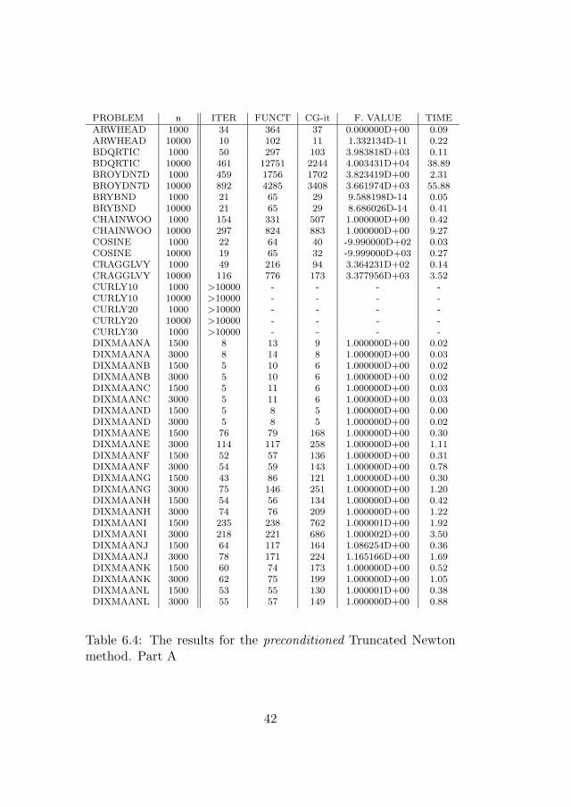
PROBLEM n ITER FUNCT CG-it F. VALUE TIMEARWHEAD 1000 34 364 37 0.000000D+00 0.09ARWHEAD 10000 10 102 11 1.332134D-11 0.22BDQRTIC 1000 50 297 103 3.983818D+03 0.11BDQRTIC 10000 461 12751 2244 4.003431D+04 38.89BROYDN7D 1000 459 1756 1702 3.823419D+00 2.31BROYDN7D 10000 892 4285 3408 3.661974D+03 55.88BRYBND 1000 21 65 29 9.588198D-14 0.05BRYBND 10000 21 65 29 8.686026D-14 0.41CHAINWOO 1000 154 331 507 1.000000D+00 0.42CHAINWOO 10000 297 824 883 1.000000D+00 9.27COSINE 1000 22 64 40 -9.990000D+02 0.03COSINE 10000 19 65 32 -9.999000D+03 0.27CRAGGLVY 1000 49 216 94 3.364231D+02 0.14CRAGGLVY 10000 116 776 173 3.377956D+03 3.52CURLY10 1000 >10000 - - - -CURLY10 10000 >10000 - - - -CURLY20 1000 >10000 - - - -CURLY20 10000 >10000 - - - -CURLY30 1000 >10000 - - - -DIXMAANA 1500 8 13 9 1.000000D+00 0.02DIXMAANA 3000 8 14 8 1.000000D+00 0.03DIXMAANB 1500 5 10 6 1.000000D+00 0.02DIXMAANB 3000 5 10 6 1.000000D+00 0.02DIXMAANC 1500 5 11 6 1.000000D+00 0.03DIXMAANC 3000 5 11 6 1.000000D+00 0.03DIXMAAND 1500 5 8 5 1.000000D+00 0.00DIXMAAND 3000 5 8 5 1.000000D+00 0.02DIXMAANE 1500 76 79 168 1.000000D+00 0.30DIXMAANE 3000 114 117 258 1.000000D+00 1.11DIXMAANF 1500 52 57 136 1.000000D+00 0.31DIXMAANF 3000 54 59 143 1.000000D+00 0.78DIXMAANG 1500 43 86 121 1.000000D+00 0.30DIXMAANG 3000 75 146 251 1.000000D+00 1.20DIXMAANH 1500 54 56 134 1.000000D+00 0.42DIXMAANH 3000 74 76 209 1.000000D+00 1.22DIXMAANI 1500 235 238 762 1.000001D+00 1.92DIXMAANI 3000 218 221 686 1.000002D+00 3.50DIXMAANJ 1500 64 117 164 1.086254D+00 0.36DIXMAANJ 3000 78 171 224 1.165166D+00 1.69DIXMAANK 1500 60 74 173 1.000000D+00 0.52DIXMAANK 3000 62 75 199 1.000000D+00 1.05DIXMAANL 1500 53 55 130 1.000001D+00 0.38DIXMAANL 3000 55 57 149 1.000000D+00 0.88

Table 6.4: The results for the preconditioned Truncated Newtonmethod. Part A

42

PROBLEM n ITER FUNCT CG-it F. VALUE TIMEDQDRTIC 1000 33 274 34 7.461713D-26 0.05DQDRTIC 10000 102 868 103 2.426640D-27 1.98DQRTIC 1000 22 81 40 2.784985D-02 0.02DQRTIC 10000 31 111 60 4.932478D-01 0.34EDENSCH 1000 21 89 27 6.003285D+03 0.05EDENSCH 10000 18 85 23 6.000328D+04 0.41ENGVAL1 1000 11 34 16 1.108195D+03 0.02ENGVAL1 10000 12 36 19 1.109926D+04 0.28FLETCBV2 1000 1 1 1 -5.013384D-01 0.00FLETCBV2 10000 1 1 1 -5.001341D-01 0.00FLETCBV3 1000 9 9 22 -8.470587D+04 0.02FLETCBV3 10000 111 111 132 -6.590391D+09 1.39FLETCHCR 1000 58 350 105 1.153703D-09 0.14FLETCHCR 10000 123 1091 161 2.483558D-08 3.16FMINSURF 1024 68 172 210 1.000000D+00 0.56FMINSURF 5625 209 556 664 1.000000D+00 11.98FREUROTH 1000 38 300 50 1.214697D+05 0.08FREUROTH 10000 107 1052 119 1.216521D+06 3.27GENHUMPS 1000 801 2848 2894 1.715389D-11 5.61GENHUMPS 10000 5318 9264 15635 1.282590D-13 390.52GENROSE 1000 849 2596 2608 1.000000D+00 4.38GENROSE 10000 8090 24307 24913 1.000000D+00 524.05LIARWHD 1000 42 251 61 8.352643D-19 0.09LIARWHD 10000 112 1107 133 1.455368D-20 2.55MOREBV 1000 8 8 28 2.148161D-08 0.03MOREBV 10000 2 2 7 2.428066D-09 0.06MSQRTALS 1024 4726 4955 16550 3.407724D-05 342.20MSQRTBLS 1024 3110 3337 10724 1.119480D-05 229.73NONCVXUN 1000 676 1245 2279 2.327300D+03 5.22NONCVXUN 10000 2765 12132 11297 2.330632D+04 195.00NONCVXU2 1000 462 1176 1674 2.319022D+03 3.34NONCVXU2 10000 2176 10275 8905 2.319615D+04 146.28NONDIA 1000 22 256 27 6.680969D-21 0.12NONDIA 10000 78 1515 82 5.507180D-13 6.62NONDQUAR 1000 45 111 111 1.425631D-04 0.08NONDQUAR 10000 46 175 98 3.744366D-04 0.94PENALTY1 1000 31 32 59 9.686175D-03 0.05PENALTY1 10000 54 81 121 9.900151D-02 0.94POWELLSG 1000 46 257 86 1.992056D-08 0.05POWELLSG 10000 114 783 151 7.735314D-08 1.17POWER 1000 65 189 142 5.912729D-09 0.16POWER 10000 243 901 616 7.784205D-09 6.06QUARTC 1000 22 81 40 2.784985D-02 0.03QUARTC 10000 31 111 60 4.932478D-01 0.36SCHMVETT 1000 14 35 37 -2.994000D+03 0.06SCHMVETT 10000 19 69 38 -2.999400D+04 0.86

Table 6.5: The results for the preconditioned Truncated Newtonmethod. Part B

43

PROBLEM n ITER FUNCT CG-it F. VALUE TIMESINQUAD 1000 37 310 49 -2.942505D+05 0.11SINQUAD 10000 104 1517 111 -2.642315D+07 3.55SPARSINE 1000 2718 3138 9243 1.271332D-02 27.39SPARSINE 10000 - - - - >900SPARSQUR 1000 22 66 34 6.266490D-09 0.06SPARSQUR 10000 22 67 39 1.069594D-08 0.89SPMSRTLS 1000 62 218 132 6.219291D+00 0.25SPMSRTLS 10000 - - - - >900SROSENBR 1000 35 309 40 2.842418D-22 0.03SROSENBR 10000 104 920 108 9.421397D-12 1.38TESTQUAD 1000 >10000 - - - -TOINTGSS 1000 2 3 1 1.001002D+01 0.00TOINTGSS 10000 2 3 1 1.000100D+01 0.05TQUARTIC 1000 21 185 27 3.767509D-10 0.03TQUARTIC 10000 14 144 18 1.145916D-11 0.28TRIDIA 1000 431 822 1416 8.189019D-12 1.55TRIDIA 10000 3618 5245 12146 1.026049D-11 142.69VARDIM 1000 37 37 72 1.058565D-20 0.06VARDIM 10000 >10000 - - - -VAREIGVL 1000 39 64 127 1.491460D-09 0.30VAREIGVL 10000 21 179 22 3.924839D-16 1.09WOODS 1000 64 377 141 3.857513D-08 0.16WOODS 10000 139 1095 223 5.031534D-08 2.81

Table 6.6: The results for the preconditioned Truncated Newtonmethod. Part C

44