Computing the Success Factors in Consistent Acquisition and Recognition of Objects in Color Digital...

The Journal of Supercomputing, 30, 179–198, 2004C© 2004 Kluwer Academic Publishers. Manufactured in The Netherlands.

Computing the Success Factors in ConsistentAcquisition and Recognition of Objects in Color DigitalImages by Explicit Preconditioning

ILIAS G. MAGLOGIANNIS [email protected] of Information and Communication Systems Engineering, University of the Aegean,GR 83200 Karlovasi, Samos, Greece

ELIAS P. ZAFIROPOULOS [email protected] of Electrical and Computer Engineering, National Technical University of Athens,GR 15773 Iroon Polytechneiou 9, Athens, Greece

AGAPIOS N. PLATIS [email protected] of Information and Communication Systems Engineering, University of the Aegean,GR 83200 Karlovasi, Samos, Greece

GEORGE A. GRAVVANIS [email protected] of Computer Science, Hellenic Open University, Patras, Greece

Abstract. The paper studies the factors influencing the consistent acquisition and recognition of object’s colorand border features in digital imaging. The proposed image acquisition process is utilized by a computer supportedimaging system implementing the acquisition and analysis of skin lesion images supporting medical diagnosis.In addition the same approach may be used for several problems requiring reliable color measurement and objectidentification. Two methodologies are adopted: The Bayesian Networks, which provide an efficient way of rea-soning under uncertainty and are used to incorporate the expert judgement into the estimation of the probabilityof successful operation, and a Markov chain approach, which is generally used for the dynamic modeling of thesystem behavior. The Markov chain model requires asymptotically the solution of sparse linear systems. Explicitpreconditioned methods are used for the efficient solution of the derived sparse linear system, and the parallelimplementation of the dominant computational part is exploited.

Keywords: digital image acquisition, camera calibration, color measurement, reproducibility, computer vision,Bayesian networks, Markov modeling, Markov Reward Models, approximate inverses, preconditioning, parallelcomputations

1. Introduction

The acquisition of reliable and reproducible color images has been a major challenge forengineers during the last decades. The wide applications of image processing and patternrecognition in several scientific areas, such as biomedical engineering, robotics, securityand safety systems, have increased the need for the development of image analysis systemsthat would diminish the equipment and environmental constraints of noise, low image

180 MAGLOGIANNIS ET AL.

resolution, illumination reflections and be able to measure reliably and with reproducibilitycolor [1, 19, 32].

The many influencing factors that characterize the image acquisition and recognitionprocess and the severity of the effects in most application areas of these systems (medicine,robotics etc.) have shown the need for studying all the parameters concerning the reliability,and availability of the process for reproducible image acquisition [5, 27].

Computer vision usually suffers from the problem of non-reproducibility in image acqui-sition and representation. Basically, each digital imaging system has its own varying colorspace, depending among others on the spectral sensitivities of its sensors, the performance ofits hardware and software, its settings and the environmental illumination conditions duringimage acquisition. It is possible to calibrate such an imaging system by controlling its set-tings and determining the relationship between its unknown device-dependent color spaceand some device-independent color space, an issue which has been extensively covered inthe literature [6, 8, 17, 33]. However the external factors affecting the camera calibrationand the image reproducibility during acquisition have not been studied thoroughly.

The paper introduces a method for acquiring reliable colour images and studies all thefactors influencing the reproducibility in image acquisition, color representation and thusthe recognition process of objects in color digital imaging.

Several modelling approaches may be used for the proposed process, which are groupedin two categories: combinatorial [4] and state space [21, 24, 26]. The combinatorial modeltypes include reliability block diagrams, Bayesian networks and fault trees. The state spacemodel types include Markov chains and petri-net based models. In the present paper, theBayesian networks and the Markov models in conjunction with Markov Reward Models areadopted for studying the proposed image acquisition and classification system providingcomplementary results. The Bayesian networks were selected, as they incorporate uncer-tainty among the influential factors and the process stages, they accommodate multi-statevariables and they allow a backward diagnostic analysis providing significant criticalitymeasures for each influential factor. Furthermore the Markov models [21, 26] have beenused, in order to take into account the dynamic behavior of the image acquisition andclassification process, using alternative scenarios for the utilization of the implementedsystem.

The Markov chain model requires asymptotically the solution of sparse arrow-structuredlinear systems. Direct methods such as Gaussian elimination may be used, with a majordisadvantage of replacing a sparse matrix by a full matrix. Preconditioning methods, basedon various forms of the preconditioner derived either from splitting techniques or incom-plete factorization techniques (modifications of Gaussian Elimination) have been presented,but are difficult to be implemented on parallel systems. Recently sparse approximate in-verses, by minimizing the Frobenious norm of the error, have been presented and can beimplemented on parallel systems. The solution of ergodic Markov chains with large num-ber of states by preconditioned Krylov subspace methods has also been studied by otherresearchers [3, 31, 35]. Explicit preconditioned conjugate gradient-type methods are usedfor the efficient solution of the sparse arrow-structured linear system [11–14], and the par-allel implementation of the dominant computational part is explored on multiprocessorsystems.

CONSISTENT ACQUISITION AND RECOGNITION OF OBJECTS 181

The rest paper is organized as follows: In Section 2, the color acquisition limitationsand errors in digital imaging are provided and the proposed acquisition process along withthe implemented system is described. In Section 3, the image acquisition and classificationprocedure is modeled considering all the process stages and the respective influential factors.In Sections 4 and 5 the proposed image acquisition and classification system is studied usingthe Bayesian networks and the Markov chain models and complementary results about thesystem behavior are provided. Furthermore in Section 6, explicit preconditioned conjugategradient methods, based on approximate inverses, are presented for the efficient solutionof sparse linear systems. In Section 7, the applicability and effectiveness of the modelingtechniques is examined and the results are discussed and finally, in Section 8 the paper isconcluded.

2. Color acquisition limitations and the proposed acquisition process

Commercially available photographic cameras, although their characteristics have beenconsiderably improved recently, are incapable of measuring objectively color. The mainreason is their inability to compensate or eliminate the effects of environmental lighting[22]. The objective and reproducible color measurement in digital imaging requires realtime and automated color calibration of the camera. The calibration procedure is a rathercomplex and very sensitive task, which is not expected to be incorporated as a full functionin future commercial models. Color calibration refers to the adjustments and correctionsthat are necessary, so as the camera works within its dynamic range and measures alwaysthe same color regardless the lighting conditions of the targeted item or the surroundingenvironment.

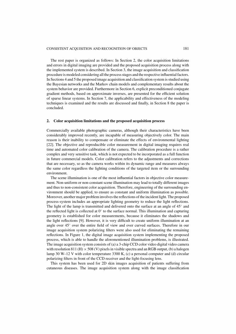
The scene illumination is one of the most influential factors in objective color measure-ment. Non-uniform or non-constant scene illumination may lead to totally different imagesand thus to non-consistent color acquisition. Therefore, engineering of the surrounding en-vironment should be applied, to ensure as constant and uniform illumination as possible.Moreover, another major problem involves the reflections of the incident light. The proposedprocess-system includes an appropriate lighting geometry to reduce the light reflections.The light of the lamp is transmitted and delivered onto the surface at an angle of 45◦ andthe reflected light is collected at 0◦ to the surface normal. This illumination and capturinggeometry is established for color measurements, because it eliminates the shadows andthe light reflections [9]. However, it is very difficult to create uniform illumination at anangle over 45◦ over the entire field of view and over curved surfaces. Therefore in ourimage acquisition system polarizing filters were also used for eliminating the remainingreflections. In Figure 1, the digital image acquisition system implementing the proposedprocess, which is able to handle the aforementioned illumination problems, is illustrated.The image acquisition system consists of (a) a 3-chip CCD color video digital video camerawith resolution 811 (H) × 508 (V) pixels in visible spectra and an RGB output, (b) a halogenlamp 30 W–12 V with color temperature 3300 K, (c) a personal computer and (d) circularpolarizing filters in front of the CCD receiver and the light-focusing lens.

This system has been used for 2D skin images acquisition of patients suffering fromcutaneous diseases. The image acquisition system along with the image classification


Figure 1. The lighting geometry of the image acquisition system consisting of a color video camera, two focusinglenses (mounted on an articulated arm), a light source that sends lights to the lenses through fiber optics and apersonal computer.

software has been used for diagnostic purposes. The expert knowledge acquired duringthe application of the system has been collected and coded in cause effect relationships soas to examine the success factors of the image acquisition and recognition process using aBayesian and a Markovian approach.

Before the system is able to acquire reproducible images, the camera has to be calibrated.Color calibration refers to two types of software corrections: Calibration to Black and White,and Shading Compensation. The Calibration to Black and White includes comparing cameraresponse to black and white standards with their known values. This procedure requires thecapturing of two images—BLACK and WHITE (three-dimensional arrays of pixel values).Covering the lens of the CCD camera generates the BLACK image. The WHITE image isgenerated by capturing the image of a perfect diffuser (BaSO4). During the Black and WhiteCalibration it should be ensured that the CCD camera is functioning in its dynamic rangeand is not saturated. Shading is a typical problem in image acquisition systems, needed tobe resolved, as the image might be bright in the center and decrease in brightness as onegoes to the edge of the field-of-view. In the implemented system for shading correctionwe use the image of the perfect diffuser that was previously captured. Shading correctionis performed by division of an image with all pixels having R = G = B = 255 by theimage of the perfect diffuser and then multiplying a captured image with the look-up tablegenerated by the division.

Following the calibration procedure, the digital image is acquired and processed. Mostof the image analysis systems require the extraction of border and color-based features,which are used for the characterization and the classification of the digital images. To assistcolor identification Median or Low Pass Filtering for noise reduction was performed ina preprocessing stage. The image noise is mainly attributed to limitations of the image


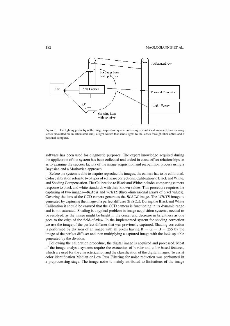
Figure 2. The process for the color image acquisition and recognition.

acquisition hardware (sensor elements, digitizer) that cause the pixel values to fluctuatewithin some limits (color values). Cross talking between neighboring pixels is also a factorthat contributes in noise. The measured color is adversely affected by noise thus leading tounreliable results concerning its value. Particles of variable geometric characteristics on thetargeted item such as dirt or dust may cause additional noise. This type of noise is eliminatedthrough appropriate morphological filtering [10].

Although the filtering procedure ends in blurring the image, it assists the analysis, as itremoves noise. The values for the border and color features of the images are entered intothe classification computer program, which is based on a neural network algorithm trainedto classify the input cases into different categories. The training of the neural networks hasbeen executed previously and the satisfactory performance of the classification computerprogram has been assured. The complete process of image acquisition and recognitionprocedure as described above is shown in Figure 2.

3. Influential factors in object recognition

The image acquisition and classification process (cf. Figure 2), presented in the previoussection comprises of six basic stages. The performance of each stage is influenced by severalfactors. The characteristics of each factor have been identified and their possible states,with respect to the corresponding identified characteristic, are quantified depending on theoperating environment. Each stage has two states, “successful” and “degraded-failed”, i.e.


the success or failure of the desired function, with a certain probability of occurrence. Thedependency issues for the image acquisition and classification process are as follows:

1. Calibration: The analyzed factors influencing the calibration procedure performanceare:

(a) Artificial lighting: The two lighting bulbs produce the artificial lighting and theattribute that affects the performance of the calibration procedure is light uniformity,resulting in two states “uniform” and “non-uniform”.

(b) Physical lighting: It is described by the following four states: “stable with lowintensity”, “stable with high intensity”, “variable with low intensity”, “variable withhigh intensity”. The probabilities of occurrence for each state are highly dependenton the environment that the system is operating.

(c) Calibration software: The software used for the calibration procedure is consideredhighly reliable, with two states “success” and “fail”.

(d) Circular polarizers: The polarizing filters are characterized by the two states “oper-ating” and “degraded-failed”. The “degraded-failed” state incorporates all the factorsinfluencing the polarizer performance, such as failures due to material degradation,dirt and dust.

(e) CCD camera: The states of the camera’s operation are characterized as “operating”and “degraded-failed”.

(f) Human interaction: The human factor is incorporated in all the processes that requirethe human interaction [25]. The reliability of the process is also affected significantlyby the personnel executing the detailed calibration procedure, resulting in two states“correct handling” and “mishandling”.

2. Image acquisition: The “Artificial Lighting”, the “Physical Lighting”, the “CircularPolarizers” and the “CCD camera” affect the image acquisition procedure as well. Ad-ditionally, “Human Interaction in Image Acquisition”, “Image Acquisition Software”,the “Calibration” stage and the “Changes in Lighting Conditions” stage i.e. “identicalto calibration” or “different from calibration” lighting condition during acquisition arethe remaining factors influencing the “Image Acquisition” stage.

3. The status of the software based stages “Image Filtering”, “Border Features Extraction”,“Color Features Extraction” and “Image Classification” are influenced by the success ofthe image acquisition stage, the performance of the respective software and the followinginterrelations:

(a) “Color features Extraction” is influenced by “Image Filtering”(a) “Image Classification” by “Border Features” and “Color Features Extraction”.

4. Bayesian network modeling

Bayesian networks are a set of methods used for graphical representation and probabilisticcalculation for most problems which are characterized by uncertainty. The Bayesian net-works provide a framework for graphically representing the logical relationships between


discrete or continuous random variables and capturing the uncertainty in the dependencybetween these variables using conditional probabilities. A Bayesian network consists of:a set of variables and a set of directed edges between variables. Each variable has a finiteset of mutually exclusive states. To each variable Xi with parents B1, B2, . . . , Bn(n ≥ 1)there is attached a conditional probability table P(Xi |B1, B2, . . . , Bn). For the variablesX1, X2, . . . , Xn of a Bayesian network the probability of the joint event X1 ∧ X2 ∧· · ·∧ Xn

is given by:

P(X1, X2, . . . Xn) =n∏

i=1

P[Xi |Parent(Xi )] (1)

where Parent (Xi ) is the set of parent variables of the variable Xi .Building and using a Bayesian network is essentially a three-stage process. The first stage

includes the determination of the variables and their cause-effect relationships, while thesecond stage includes the specification of each variable state conditional probability, giventhe state of the parent variables. The third stage is inference, during which the input datais introduced to the Bayesian network model and the probabilities for all network nodesare calculated according to their corresponding cause-effect relationships. Furthermore,Bayesian inference includes the calculation of posterior probabilities for the variable statesgiven a system fault or a certain combination of events, the joint probability of combinationof variable states and the determination of the most probable combination of variable states.The image acquisition and classification process (cf. Figure 2), has been modelled in aBayesian Network shown in Figure 3, where the root factors are designated with a boldborder. The root factors influence the successful completion of the image acquisition andrecognition system stages and they are not influenced by any other factor. Moreover, there arecertain influences among the system stages. For example, the “border features extraction”stage is influenced by the “border features extraction software” and the “image acquisition”stage. All the influences among the different factors are designated with arcs.

5. Markovian modeling

The Markovian modeling is a stochastic modeling technique that provides flexibility bymaking the analysis of complex operational scenarios possible [21, 26, 29]. It is generallyused for the dynamic modeling of a process or a system behavior while Bayesian networksare considered for a static modeling. This alternative modeling technique permits to obtainadditional results, such as the evaluation of different procedure policies.

The same influential factors and the corresponding interrelations, described in Section 3,were incorporated in the Markov model. Since all of the process stages are supposedwith predefined time duration, the system is modeled with a Discrete Time Markov Chain(DTMC) generally used for phased-mission systems. The state transition diagram of theprocess is depicted in Figure 4, where the calibration procedure state is an aggregated statecorresponding to the six variables affecting calibration and their 256 combinations of failureand operational states. The Image Acquisition procedure state is also an aggregated statecorresponding to the seven variables affecting acquisition and their 500 combinations of


Figure 3. The Bayesian network model of the process depicted in Figure 2.

Figure 4. State transition diagram of the different stages of the process.

failure and operational states. The final four independent phases correspond to the 8 fail-ure and operational states leading to a state transition diagram with 764 total number ofstates. The transition probabilities are the probabilities of failure or success of every com-ponent of the system and the transition probabilities from the classification software states


to the calibration and image acquisition aggregated states depend on the procedure policyadopted.

The computation of the steady-state probability distribution of the Markovian systemallows obtaining the probability distribution of the different failures of the image acquisitionprocedure. An additional interesting aspect is the comparison of different procedure policiesand their effect on the probability distribution of the different failures. For instance, afterthe conclusion of capturing an image, a new calibration can be executed (Policy 1). Thispolicy is however too constraining since the duration of each calibration lasts for at least10 minutes. Alternative policies are after 2 image acquisitions to make a new calibration(Policy 2) or after 4 image acquisitions to perform a new calibration (Policy 3).

In order to evaluate the best policy, the Markov Reward Models (MRMs) are introduced,[28, 29, 30, 34], which consist in calculating the following random variable, called cumu-lative reward on a time interval [N , N + T ]:

WN ,T =N+T −1∑

k=N

g(Xk), (2)

where Xk is the DTMC modeling the system (with E = {1, 2 . . . n} its state space and p itstransition probability matrix) and g(.) a reward function defined as follows: g(CalibrationState)=R1, g(Image Acquisition state)=R2 and g(·)=0 for any other state. The asymptoticnormalized mean value of the cumulative reward is given as follows:

EW =n∑

i=1

g(i)π (i),

where π is the steady state probability distribution.Since the major interest is the long run behavior of the system, the computation of the

steady state probability distribution is needed. For an irreducible, aperiodic, finite stateMarkov chain, the steady-state probability distribution π is given by the equation:

πp = π, (3)

where p is the transition probability matrix. The equation πp = π gives multiple solutions,as a consequence the constraint

∑1≤i≤n π (i) = 1 is used in order to obtain the uniqueness

of the solution. The resulting equation is therefore:

Aπ = en, (4)

where A is the transposition of the matrix (p − I ) with its last line the unit vector (a linecontaining ones) and en the last vector of the orthonormal base (i.e. an n-dimensional vectorcontaining the unit as the last element and zeros for the remaining elements). The coefficient


matrix A is a sparse arrow-structure type (n × n) matrix of the following form:

(5)

Modeling systems with a large number of states requires the solution of large sparselinear systems. Recently, explicit preconditioned conjugate gradient type methods, basedon various classes of explicit approximate inverse matrix techniques, have been derived forsolving efficiently arrow-structured systems [11, 12, 14], exploiting the structure of suchsystems.

6. Explicit approximate inverse preconditioning

In this section we present explicit preconditioned conjugate gradient-type methods, basedon approximate LU-type factorization and approximate inverses [11–14], for solving ingeneral sparse linear system, i.e.,

Au = s. (6)

The elements of the L and U decomposition factors can be computed by the DODALUFAalgorithm [12]. The elements of the optimised approximate inverse Mδl,δu ≡ (µi, j ), i ∈[1, n], j ∈ [max(1, i−δl + 1), min(n, i + δu)], of the coefficient matrix A, by retaining onlyδl elements in the lower part and δu elements in the upper part of the inverse and by usinga moving window shifted from bottom to top, can be computed by the ODODGAIM algo-rithm [12]. The memory requirements of the ODODGAIM algorithm are ≈[n × (δl + δu)]words and the computational work involved is ≈ O[(�1 + �2 + 1)(δl + δu)]n multiplicativeoperations [12]. It should be noted that if �1 = 0 and �2 = 1, cf. (4), then the DO-DALUFA and ODODGAIM algorithms are reduced to ALUFA and OAIAM algorithmsrespectively [14]. The Explicit Preconditioned Biconjugate Conjugate Gradient-STAB


(EPBICG-STAB) method, based on the approximate inverse Mδl,δu , can be expressedby the following compact algorithmic scheme:

Let u0 be an arbitrary initial approximation to the solution vector u. Then,

set u0 = 0, compute r0 = s − Au0, (7)

set r ′0 = r0, ρ0 = α = ω0 = 1 and v0 = p0 = 0. (8)

Then, for i = 0, 1, . . . , (until convergence) compute the vectors ui , ri and the scalarquantities α, β, ωi as follows:

calculate ρi = (r ′0, ri−1) and β = (ρi/ρi−1)/(α/ωi−1), (9)

compute pi = ri−1 + β (pi−1 − ωi−1vi−1) , (10)

form yi = Mδl,δu pi , vi = Ayi and α = ρi/(r ′0, vi ), (11)

compute xi = ri−1 − αvi , form zi = Mδl,δu xi and ti = Azi , (12)

set ωi = (Mδl,δuti , Mδl,δu xi )/(Mδl,δuti , Mδl,δuti ), (13)

compute ui = ui−1 + αyi + ωi zi and ri = xi − ωi ti (14)

The computational complexity of the EPBICG-STAB method is ≈O[(3δl + 3δu + 4�1 +4�2 +12)n mults +6n adds]ν operations, where ν denotes the number of iterations requiredfor convergence to a predetermined tolerance level.

The effectiveness of the explicit preconditioned conjugate gradient–type method, usingthe ODODGAIM algorithm, is related to the fact that the approximate inverse exhibits asimilar “fuzzy” structure and is a close approximant to the coefficient matrix A [12–15].The convergence analysis of similar explicit approximate inverse preconditioning has beenpresented in [11, 15].

It is evident that the dominant computational part in the Explicit Preconditioning Conju-gate Gradient-type methods is the approximate inverse matrix–vector product which whenthe “retention” parameter is chosen as δl = 1 reduces to a vector-vector (inner) product.

7. Case study application for the recognition of skin lesions

The cause-effect dependencies among process stages and the influencing factors for theproposed process model as depicted in Figure 3 are incorporated in a Bayesian network,in which the corresponding conditional probabilities are quantified. The prior probabilitiesof occurrence of the factors states differ in different environmental conditions. The effectsof the influencing factors in the calibration process and the image acquisition processare summarized in Table 1. Regarding the rest of the process stages, there is an AND-typedependency among the influential factors and the process stage, thus if any of the influencing(parent) nodes is in the “degraded” or “failed” state, then the affected (child) node is in the“degraded” or “failed” state. The HUGIN software has been used for the implementation ofthe Bayesian network [16]. All the probabilities for the root variables states are estimated


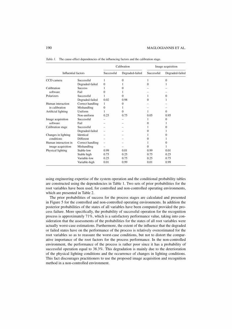
Table 1. The cause-effect dependencies of the influencing factors and the calibration stage.

Calibration Image acquisition

Influential factors Successful Degraded-failed Successful Degraded-failed

CCD camera Successful 1 0 1 0Degraded-failed 0 1 0 1

Calibration Success 1 0 – –software Fail 0 1 – –

Polarizers Successful 1 0 1 0Degraded-failed 0.02 0.98 0 1

Human interaction Correct handling 1 0 – –in calibration Mishandling 0 1 – –

Artificial lighting Uniform 1 0 1 0Non-uniform 0.25 0.75 0.05 0.95

Image acquisition Successful – – 1 0software Fail – – 0 1

Calibration stage Successful – – 1 0Degraded-failed – – 0 1

Changes in lighting Identical – – 1 0conditions Different – – 0 1

Human interaction in Correct handling – – 1 0image acquisition Mishandling – – 0 1

Physical lighting Stable-low 0.99 0.01 0.99 0.01Stable high 0.75 0.25 0.75 0.25Variable-low 0.25 0.75 0.25 0.75Variable-high 0.01 0.99 0.01 0.99

using engineering expertise of the system operation and the conditional probability tablesare constructed using the dependencies in Table 1. Two sets of prior probabilities for theroot variables have been used, for controlled and non-controlled operating environments,which are presented in Table 2.

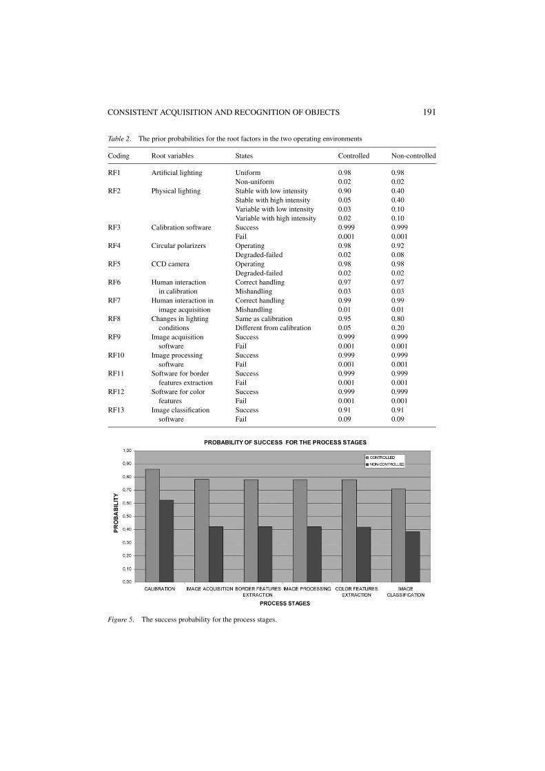
The prior probabilities of success for the process stages are calculated and presentedin Figure 5 for the controlled and non-controlled operating environments. In addition theposterior probabilities of the states of all variables have been computed provided the pro-cess failure. More specifically, the probability of successful operation for the recognitionprocess is approximately 71%, which is a satisfactory performance value, taking into con-sideration that the assessments of the probabilities for the states of all root variables wereactually worst-case estimations. Furthermore, the extent of the influence that the degradedor failed states have on the performance of the process is relatively overestimated for theroot variables so as to reassure the worst-case conditions, but not to distort the compar-ative importance of the root factors for the process performance. In the non-controlledenvironment, the performance of the process is rather poor since it has a probability ofsuccessful operation equal to 38.3%. This degradation is mainly due to the deteriorationof the physical lighting conditions and the occurrence of changes in lighting conditions.This fact discourages practitioners to use the proposed image acquisition and recognitionmethod in a non-controlled environment.


Table 2. The prior probabilities for the root factors in the two operating environments

Coding Root variables States Controlled Non-controlled

RF1 Artificial lighting Uniform 0.98 0.98Non-uniform 0.02 0.02

RF2 Physical lighting Stable with low intensity 0.90 0.40Stable with high intensity 0.05 0.40Variable with low intensity 0.03 0.10Variable with high intensity 0.02 0.10

RF3 Calibration software Success 0.999 0.999Fail 0.001 0.001

RF4 Circular polarizers Operating 0.98 0.92Degraded-failed 0.02 0.08

RF5 CCD camera Operating 0.98 0.98Degraded-failed 0.02 0.02

RF6 Human interaction Correct handling 0.97 0.97in calibration Mishandling 0.03 0.03

RF7 Human interaction in Correct handling 0.99 0.99image acquisition Mishandling 0.01 0.01

RF8 Changes in lighting Same as calibration 0.95 0.80conditions Different from calibration 0.05 0.20

RF9 Image acquisition Success 0.999 0.999software Fail 0.001 0.001

RF10 Image processing Success 0.999 0.999software Fail 0.001 0.001

RF11 Software for border Success 0.999 0.999features extraction Fail 0.001 0.001

RF12 Software for color Success 0.999 0.999features Fail 0.001 0.001

RF13 Image classification Success 0.91 0.91software Fail 0.09 0.09

Figure 5. The success probability for the process stages.


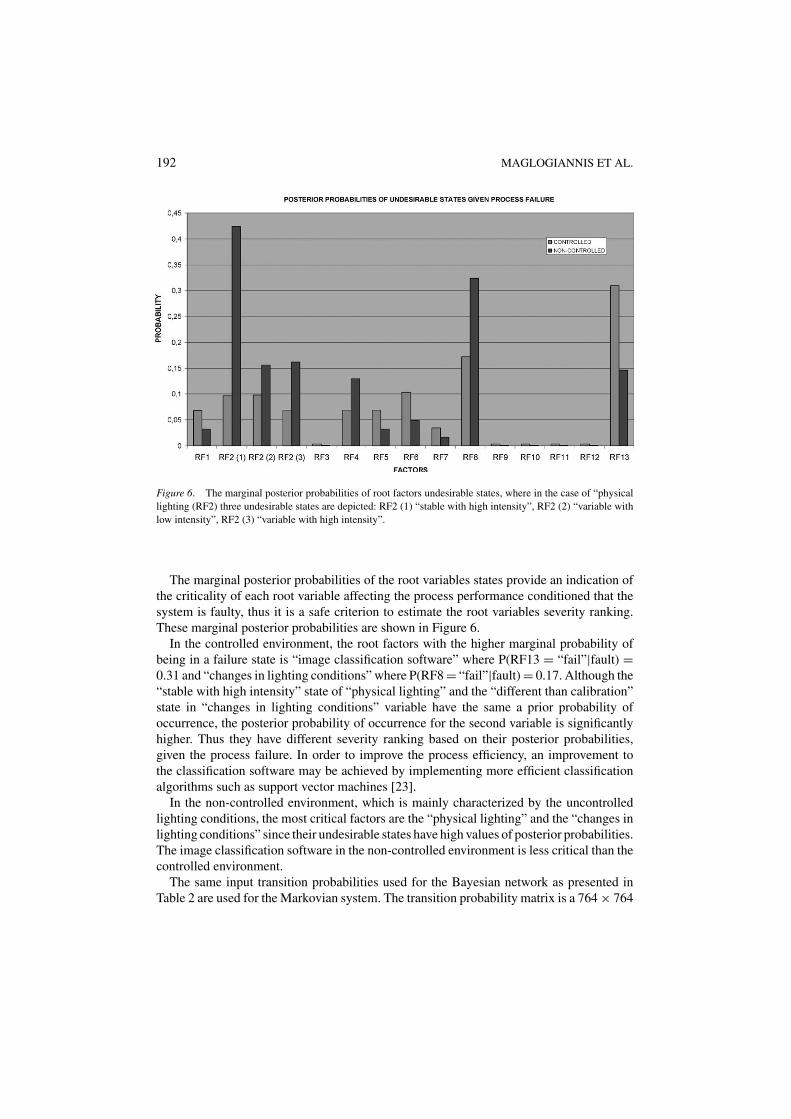
Figure 6. The marginal posterior probabilities of root factors undesirable states, where in the case of “physicallighting (RF2) three undesirable states are depicted: RF2 (1) “stable with high intensity”, RF2 (2) “variable withlow intensity”, RF2 (3) “variable with high intensity”.

The marginal posterior probabilities of the root variables states provide an indication ofthe criticality of each root variable affecting the process performance conditioned that thesystem is faulty, thus it is a safe criterion to estimate the root variables severity ranking.These marginal posterior probabilities are shown in Figure 6.

In the controlled environment, the root factors with the higher marginal probability ofbeing in a failure state is “image classification software” where P(RF13 = “fail”|fault) =0.31 and “changes in lighting conditions” where P(RF8 = “fail”|fault) = 0.17. Although the“stable with high intensity” state of “physical lighting” and the “different than calibration”state in “changes in lighting conditions” variable have the same a prior probability ofoccurrence, the posterior probability of occurrence for the second variable is significantlyhigher. Thus they have different severity ranking based on their posterior probabilities,given the process failure. In order to improve the process efficiency, an improvement tothe classification software may be achieved by implementing more efficient classificationalgorithms such as support vector machines [23].

In the non-controlled environment, which is mainly characterized by the uncontrolledlighting conditions, the most critical factors are the “physical lighting” and the “changes inlighting conditions” since their undesirable states have high values of posterior probabilities.The image classification software in the non-controlled environment is less critical than thecontrolled environment.

The same input transition probabilities used for the Bayesian network as presented inTable 2 are used for the Markovian system. The transition probability matrix is a 764 × 764


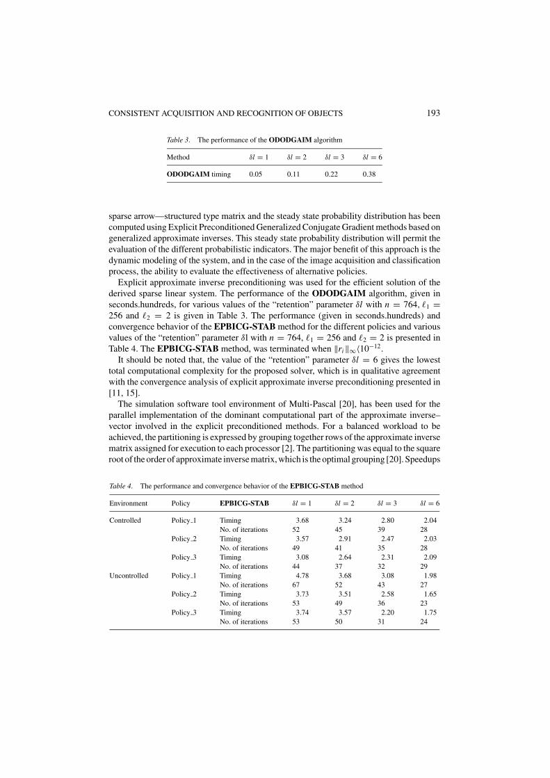
Table 3. The performance of the ODODGAIM algorithm

Method δl = 1 δl = 2 δl = 3 δl = 6

ODODGAIM timing 0.05 0.11 0.22 0.38

sparse arrow—structured type matrix and the steady state probability distribution has beencomputed using Explicit Preconditioned Generalized Conjugate Gradient methods based ongeneralized approximate inverses. This steady state probability distribution will permit theevaluation of the different probabilistic indicators. The major benefit of this approach is thedynamic modeling of the system, and in the case of the image acquisition and classificationprocess, the ability to evaluate the effectiveness of alternative policies.

Explicit approximate inverse preconditioning was used for the efficient solution of thederived sparse linear system. The performance of the ODODGAIM algorithm, given inseconds.hundreds, for various values of the “retention” parameter δl with n = 764, �1 =256 and �2 = 2 is given in Table 3. The performance (given in seconds.hundreds) andconvergence behavior of the EPBICG-STAB method for the different policies and variousvalues of the “retention” parameter δl with n = 764, �1 = 256 and �2 = 2 is presented inTable 4. The EPBICG-STAB method, was terminated when ‖ri‖∞〈10−12.

It should be noted that, the value of the “retention” parameter δl = 6 gives the lowesttotal computational complexity for the proposed solver, which is in qualitative agreementwith the convergence analysis of explicit approximate inverse preconditioning presented in[11, 15].

The simulation software tool environment of Multi-Pascal [20], has been used for theparallel implementation of the dominant computational part of the approximate inverse–vector involved in the explicit preconditioned methods. For a balanced workload to beachieved, the partitioning is expressed by grouping together rows of the approximate inversematrix assigned for execution to each processor [2]. The partitioning was equal to the squareroot of the order of approximate inverse matrix, which is the optimal grouping [20]. Speedups

Table 4. The performance and convergence behavior of the EPBICG-STAB method

Environment Policy EPBICG-STAB δl = 1 δl = 2 δl = 3 δl = 6

Controlled Policy 1 Timing 3.68 3.24 2.80 2.04No. of iterations 52 45 39 28

Policy 2 Timing 3.57 2.91 2.47 2.03No. of iterations 49 41 35 28


Uncontrolled Policy 1 Timing 4.78 3.68 3.08 1.98No. of iterations 67 52 43 27




Table 5. Speedups and processorsallocated for several values of δl

δl Speedup No. of proc.

1 20.325 302 26.462 303 26.972 306 27.485 30

and processors allocated for several values of the “retention” parameter δl with n = 764are presented in Table 5. Further, an alternative approach will be to synthesize optimaltime-processor systolic configurations as presented in [7].

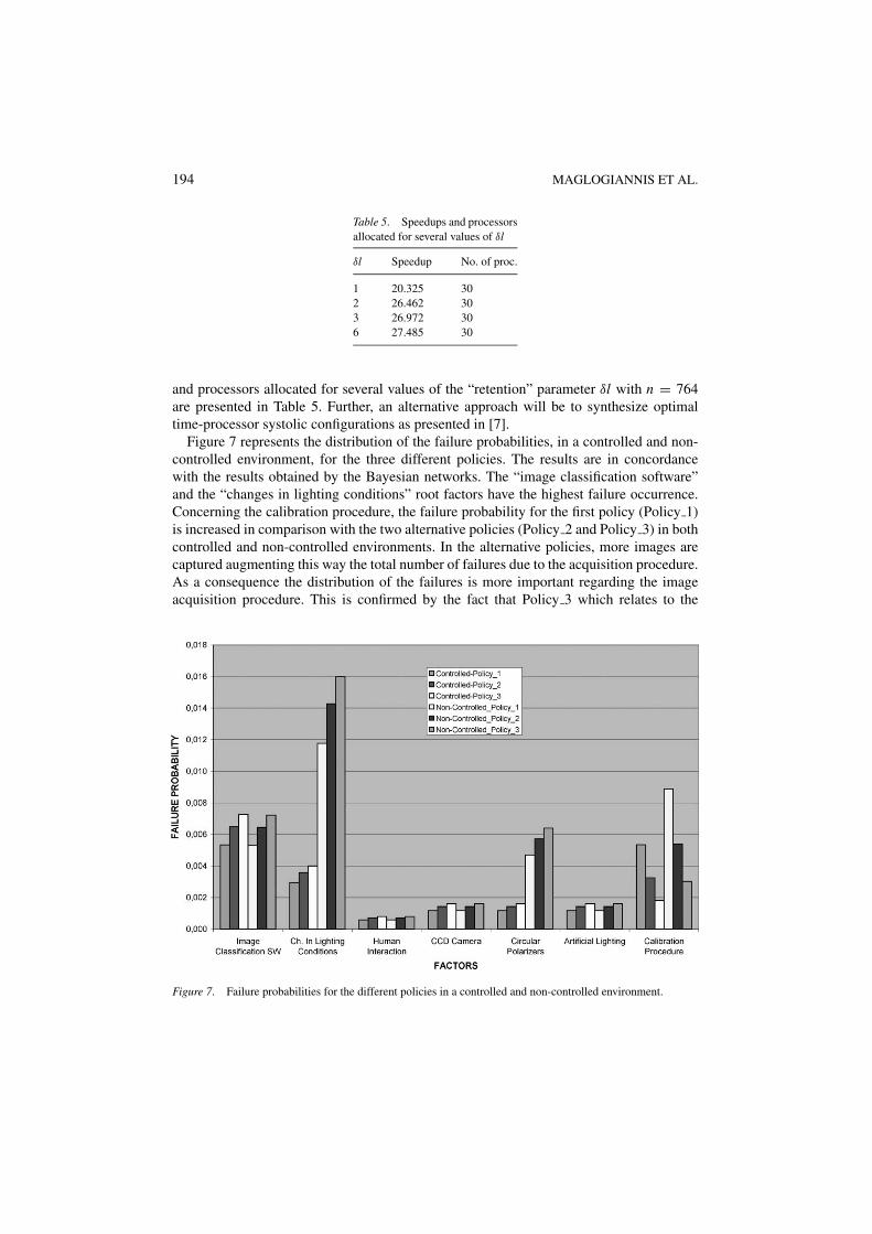
Figure 7 represents the distribution of the failure probabilities, in a controlled and non-controlled environment, for the three different policies. The results are in concordancewith the results obtained by the Bayesian networks. The “image classification software”and the “changes in lighting conditions” root factors have the highest failure occurrence.Concerning the calibration procedure, the failure probability for the first policy (Policy 1)is increased in comparison with the two alternative policies (Policy 2 and Policy 3) in bothcontrolled and non-controlled environments. In the alternative policies, more images arecaptured augmenting this way the total number of failures due to the acquisition procedure.As a consequence the distribution of the failures is more important regarding the imageacquisition procedure. This is confirmed by the fact that Policy 3 which relates to the

Figure 7. Failure probabilities for the different policies in a controlled and non-controlled environment.


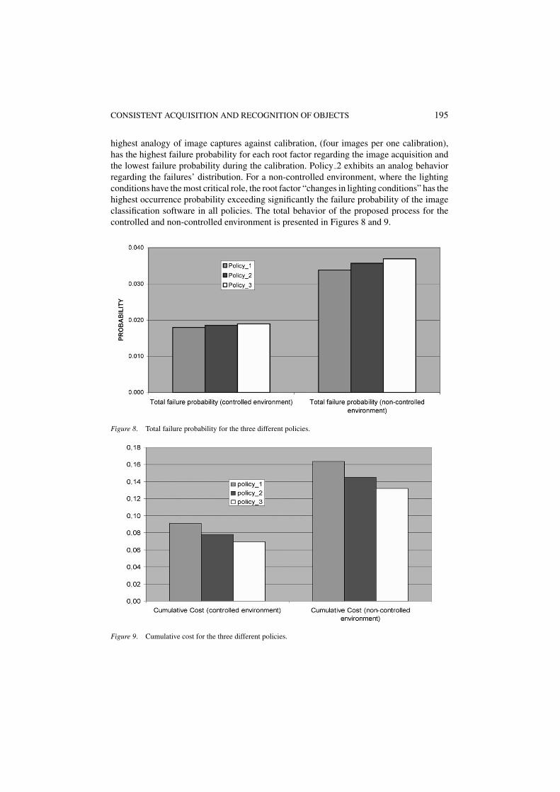
highest analogy of image captures against calibration, (four images per one calibration),has the highest failure probability for each root factor regarding the image acquisition andthe lowest failure probability during the calibration. Policy 2 exhibits an analog behaviorregarding the failures’ distribution. For a non-controlled environment, where the lightingconditions have the most critical role, the root factor “changes in lighting conditions” has thehighest occurrence probability exceeding significantly the failure probability of the imageclassification software in all policies. The total behavior of the proposed process for thecontrolled and non-controlled environment is presented in Figures 8 and 9.

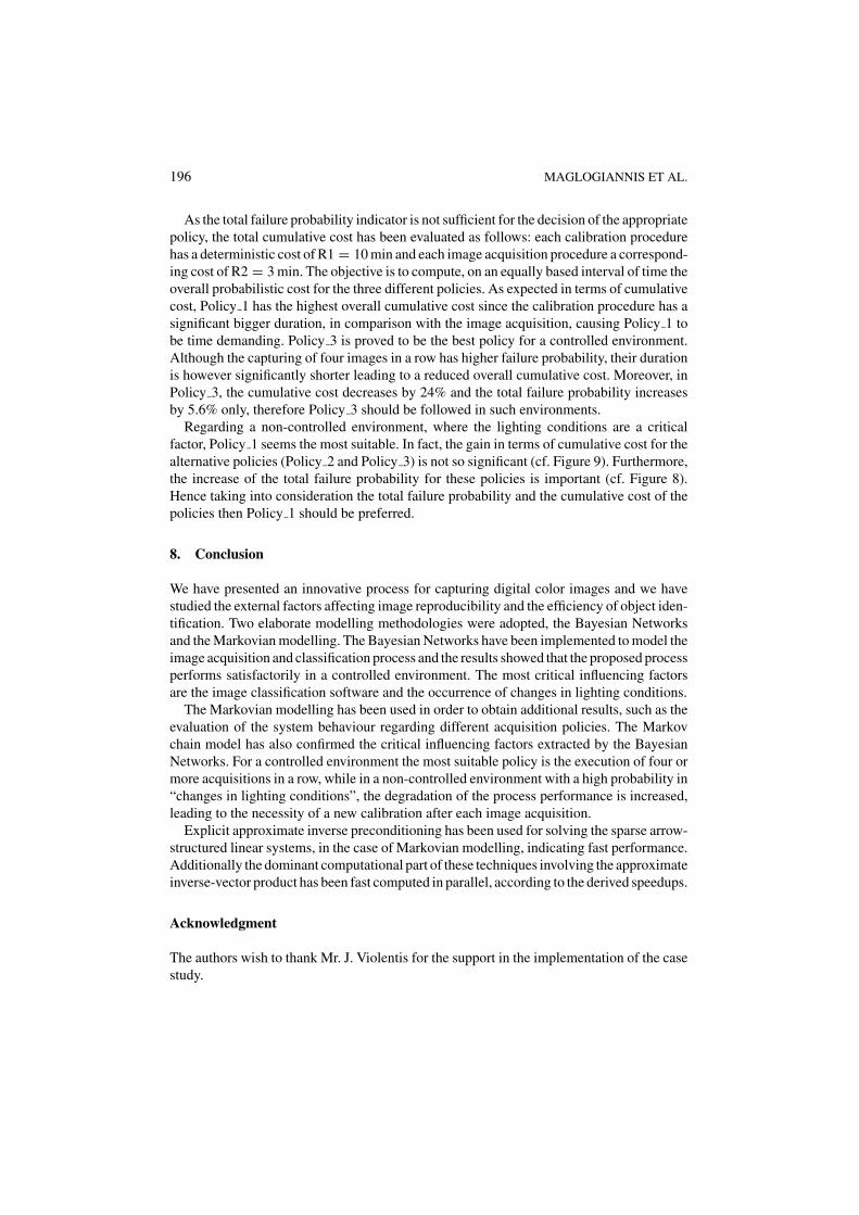
Figure 8. Total failure probability for the three different policies.

Figure 9. Cumulative cost for the three different policies.


As the total failure probability indicator is not sufficient for the decision of the appropriatepolicy, the total cumulative cost has been evaluated as follows: each calibration procedurehas a deterministic cost of R1 = 10 min and each image acquisition procedure a correspond-ing cost of R2 = 3 min. The objective is to compute, on an equally based interval of time theoverall probabilistic cost for the three different policies. As expected in terms of cumulativecost, Policy 1 has the highest overall cumulative cost since the calibration procedure has asignificant bigger duration, in comparison with the image acquisition, causing Policy 1 tobe time demanding. Policy 3 is proved to be the best policy for a controlled environment.Although the capturing of four images in a row has higher failure probability, their durationis however significantly shorter leading to a reduced overall cumulative cost. Moreover, inPolicy 3, the cumulative cost decreases by 24% and the total failure probability increasesby 5.6% only, therefore Policy 3 should be followed in such environments.

Regarding a non-controlled environment, where the lighting conditions are a criticalfactor, Policy 1 seems the most suitable. In fact, the gain in terms of cumulative cost for thealternative policies (Policy 2 and Policy 3) is not so significant (cf. Figure 9). Furthermore,the increase of the total failure probability for these policies is important (cf. Figure 8).Hence taking into consideration the total failure probability and the cumulative cost of thepolicies then Policy 1 should be preferred.

8. Conclusion

We have presented an innovative process for capturing digital color images and we havestudied the external factors affecting image reproducibility and the efficiency of object iden-tification. Two elaborate modelling methodologies were adopted, the Bayesian Networksand the Markovian modelling. The Bayesian Networks have been implemented to model theimage acquisition and classification process and the results showed that the proposed processperforms satisfactorily in a controlled environment. The most critical influencing factorsare the image classification software and the occurrence of changes in lighting conditions.

The Markovian modelling has been used in order to obtain additional results, such as theevaluation of the system behaviour regarding different acquisition policies. The Markovchain model has also confirmed the critical influencing factors extracted by the BayesianNetworks. For a controlled environment the most suitable policy is the execution of four ormore acquisitions in a row, while in a non-controlled environment with a high probability in“changes in lighting conditions”, the degradation of the process performance is increased,leading to the necessity of a new calibration after each image acquisition.

Explicit approximate inverse preconditioning has been used for solving the sparse arrow-structured linear systems, in the case of Markovian modelling, indicating fast performance.Additionally the dominant computational part of these techniques involving the approximateinverse-vector product has been fast computed in parallel, according to the derived speedups.

Acknowledgment

The authors wish to thank Mr. J. Violentis for the support in the implementation of the casestudy.


References

1. J. F. Aitken, J. Pfitzner, D. Battistutta, P. K. O’Rourke, A. C. Green, and N. G. Martin. Reliability of computerimage analysis of pigmented skin lesions of Australian adolescents. Cancer, 78(2):252–257, 1996.

2. M. P. Bekakos and O. B. Efremides. An efficient parallel approach to reduce sparse matrices with invari-ant entries. In C.A. Brebbia and H. Power, eds., Fourth International Conference on Applications of HighPerformance Computing in Engineering, pp. 11–18. Computational Mechanics Publications, 1995.

3. M. Benzi and M. Tuma. A parallel solver for large-scale Markov chains. Applied Numerical Mathematics,41:135–153, 2002.

4. A. Bobbio, L. Portinale, M. Minichino, and E. Ciancarmela. Improving the analysis of dependable systemsby mapping fault trees into Bayesian networks. Reliability Engineering and System Safety, 71(3):249–260,2001.

5. S. Bologna, E. Giancamerla, M. Minichino, A. Bobbio, G. Franceschinis, L. Portinale, and R. Gaeta. Com-parison of methodologies for the safety and dependability assessment of an industrial programmable logiccontroller. In N. Piccinini and E. Zio, eds., European Safety Dependability Conference (ESREL2001), pp.411–418, A. A. Balkema Publications, 2001.

6. Y. C. Chang and J. F. Reid. RGB calibration for color image analysis in machine vision. IEEE TransactionsImage Processing, 5:1414–1422, 1996.

7. O. B. Efremides and M. P. Bekakos. Designing processor-time optimal systolic configurations. In M. P.Bekakos, ed., Highly Parallel Computations: Algorithms and Applications, Series: Advances in High Perfor-mance Computing, 5:339–364. WIT Press, 2001.

8. G. Finlayson. Color in perspective. IEEE Trans. Pattern Anal. Machine Intell., 18:1034–1038, 1996.9. G. Goldon and G. Nuckols. Interior Lighting for Designers. John Wiley, 1995.

10. C. R. Gonzalez and E. R. Woods. Digital Image Processing. Addison Wesley, 1995.11. G. A. Gravvanis. Explicit preconditioned domain decomposition schemes. Inter. J. Computational and Nu-

merical Analysis and Applications, 2(1):19–36, 2002.12. G. A. Gravvanis. Explicit preconditioned generalized domain decomposition methods. Inter. J. Applied Math-

ematics, 4(1):57–71, 2000.13. G. A. Gravvanis. Approximate inverse banded matrix techniques. Engineering Computations, 16(3):337–346,

1999.14. G. A. Gravvanis. An approximate inverse matrix technique for arrowhead matrices. Inter. J. Comp. Math.,

70:35–45, 1998.15. G. A. Gravvanis. The rate of convergence of explicit approximate inverse preconditioning. Inter. J. Comp.

Math., 60:77–89, 1996.16. V. Jensen Finn. An Introduction to Bayesian Networks. UCL Press, 1996.17. H. Kang. Color Technology for Electronic Imaging Devices. SPIE Opt. Eng. Press, 1997.18. J. E. Kaufman. Lighting Handbook Application Volume. Illuminating Engineering Society of North America,

1987.19. V. Leemans, H. Magein, and M. -F. Destain. AE—automation and emerging technologies: On-line fruit grading

according to their external quality using machine vision, Biosystems Engineering, 83(4):397–404, 2002.20. B. P. Lester. The Art of Parallel Programming. Prentice-Hall Int. Inc., 1993.21. N. Limnios and G. Oprisan. Semi-Markov Processes and Reliability, Birkhauser, 2001.22. I. Maglogiannis. A digital image acquisition system for skin lesions. In D. Chakraborty and E. Krupinski,

eds., SPIE International Conference on Medical Imaging, pp. 337–346. SPIE Press 2003.23. I. Maglogiannis and E. Zafiropoulos. Characterization of dermatological images using support vector ma-

chines. In H. Arabnia, eds., International Conference on Parallel and Distributed Processing Techniques andApplications (PDPTA), pp. 1293–1297. CSREA Press, 2003.

24. M. Malhotra and K. Trivedi. Dependability modeling using Petri nets. IEEE Transactions on Reliability,44(3):428–439, 1995.

25. M. Modarres, M. Kaminskiy, and V. Kritvtsov. Reliability engineering and risk Analysis. Marcel Dekker Inc.,1999.

26. A. Pages and M. Gondran. Fiabilite des Systemes. Eyrolles, 1980.27. M. Pecht. Product Reliability, Maintainability, and Supportability Handbook. CRC Press, 1995.


28. A. N. Platis. An extension of the Performability measure and application in system reliability. Inter. J. Com-putational and Numerical Analysis and Applications, 2(1):87–101, 2002.

29. A. N. Platis and G. A. Gravvanis. Dependability evaluation using explicit approximate inverse preconditioning.Inter. J. Computational and Numerical Analysis and Applications, 2(1):71–86, 2002.

30. A. N. Platis, N. Limnios, and M. Le Du. Dependability analysis of systems modeled by non-homogeneousMarkov chains. Reliability Engineering and System Safety, 61(3):235–249, 1998.

31. Y. Saad. Preconditioned Krylov subspace methods for the numerical solution of Markov chains. In W. J.Stewart, eds., Computations with Markov Chains, pp. 49–64. Kluwer Academic, 1995.

32. S. Seidenari, M. Burroni, G. Dell’Eva, P. Pepe, and B. Belletti. Computerized evaluation of pigmented skinlesion images recorded by a videomicroscope: Comparison between polarizing mode observation and oil/slidemode observation. Skin Res. Technol., 1:187–191, 1995.

33. D. Slater and G. Healey. The illumination-invariant recognition of 3d objects using local color invariants.IEEE Trans. Pattern Anal. Machine Intell., 18:206–210, 1996.

34. R. M. Smith, K. S. Trivedi, and A. Ramesh. Performability analysis: Measures, an algorithm and a case study.IEEE Transactions on Computers, C-37(4):406–417, 1988.

35. W. J. Stewart, Introduction to the Numerical Solution of Markov Chains, Princeton University Press, 1994.

Computing the Success Factors in Consistent Acquisition and Recognition of Objects in Color Digital...

Documents

Transcript of Computing the Success Factors in Consistent Acquisition and Recognition of Objects in Color Digital...