Precipitation and Deposition of Asphaltenes in Production Systems: A Flow Assurance Overview
44
23 Precipitation and Deposition of Asphaltenes in Production Systems: A Flow Assurance Overview Ahmed Hammami and John Ratulowski 1. Introduction The movement of production systems to deepwater and subsea environ- ments in recent years has increased the importance of fluid property related flow assurance issues. Asphaltene precipitation and deposition is one of these potential problems. While not as common as wax or scale, the impact of asphaltene is often catastrophic. Asphaltene can cause reservoir impairment, plugging of wells and flowlines through deposition, separation difficulties, and fouling in facilities. Off- shore, the cost of remediating an unexpected asphaltene problem is excessive. It is imperative that the behavior of asphaltenes in an offshore production system be understood in the design stage of the project. Proper control and remediation strate- gies must be built into the system from the beginning. In this chapter, we will review the current process of sampling and analysis that provide the initial assessment of asphaltene stability in the reservoir fluid. We will relate these measurements in the laboratory to expected behavior in the field and address uncertainties. We will then discuss how improved characterization and deposition measurements will decrease uncertainty and allow less conservative design and operation strategies. Finally, we will briefly review the types of asphaltene precipitation models and discuss their respective underlying assumptions. Land-based sources of conventional crude oil and gas have been decreasing for the last couple of decades. As a result, the petroleum industry has turned to explore, develop, and produce hydrocarbon fluids from more challenging fields in- cluding deep and ultra deep offshore areas such as the North Sea, Gulf of Mexico, West Africa, and East coast Canada. 1 Productions in these regions are under ex- treme conditions where temperature can be near freezing point, and pressure drops from reservoir to production facility are quite large. These conditions often lead to Ahmed Hammami • Schlumberger Oilfield Services, Edmonton, Alberta, Canada, and John Ratulowski • Schlumberger Well Completion and Productivity Subsea-Flow Assurance, Rosharon, Texas, USA 617
-
Upload
independent -
Category
Documents
-
view
0 -
download
0
Transcript of Precipitation and Deposition of Asphaltenes in Production Systems: A Flow Assurance Overview
23Precipitation and Deposition of
Asphaltenes in Production Systems:
A Flow Assurance Overview
Ahmed Hammami and John Ratulowski
1. Introduction
The movement of production systems to deepwater and subsea environ-ments in recent years has increased the importance of fluid property related flowassurance issues. Asphaltene precipitation and deposition is one of these potentialproblems. While not as common as wax or scale, the impact of asphaltene is oftencatastrophic. Asphaltene can cause reservoir impairment, plugging of wells andflowlines through deposition, separation difficulties, and fouling in facilities. Off-shore, the cost of remediating an unexpected asphaltene problem is excessive. Itis imperative that the behavior of asphaltenes in an offshore production system beunderstood in the design stage of the project. Proper control and remediation strate-gies must be built into the system from the beginning. In this chapter, we will reviewthe current process of sampling and analysis that provide the initial assessmentof asphaltene stability in the reservoir fluid. We will relate these measurements inthe laboratory to expected behavior in the field and address uncertainties. We willthen discuss how improved characterization and deposition measurements willdecrease uncertainty and allow less conservative design and operation strategies.Finally, we will briefly review the types of asphaltene precipitation models anddiscuss their respective underlying assumptions.
Land-based sources of conventional crude oil and gas have been decreasingfor the last couple of decades. As a result, the petroleum industry has turned toexplore, develop, and produce hydrocarbon fluids from more challenging fields in-cluding deep and ultra deep offshore areas such as the North Sea, Gulf of Mexico,West Africa, and East coast Canada.1 Productions in these regions are under ex-treme conditions where temperature can be near freezing point, and pressure dropsfrom reservoir to production facility are quite large. These conditions often lead to
Ahmed Hammami • Schlumberger Oilfield Services, Edmonton, Alberta, Canada, andJohn Ratulowski • Schlumberger Well Completion and Productivity Subsea-Flow Assurance,Rosharon, Texas, USA
617
618 Ahmed Hammami and John Ratulowski
0
4000
8000
12000
16000
0 50 100 150 200 250
Temperature (oF)
Pre
ssu
re (
psi
a) ReservoirReservoir
FlowlineFlowline
300
Bubble point
Wax
Hyd
rate
0
Asphaltene
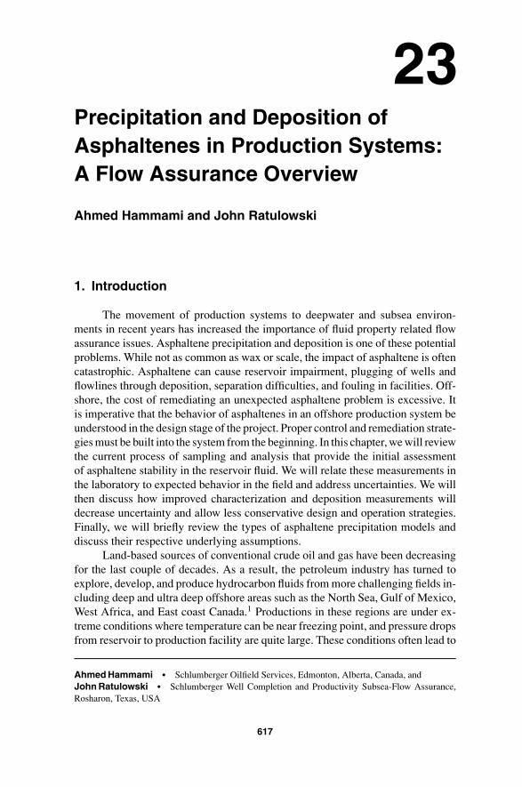
Figure 23.1. Gulf of Mexico black oil phase diagram.2
the precipitation and deposition of common organic solids (i.e., waxes, asphaltenes,and hydrates) and inorganic scales. Some less common solids include diamondoids,elemental sulfur, and naphtenates.2
Depending on the design and operation of the production system, some orall of the solid phase boundaries may be crossed as the fluid moves from thereservoir through the flow line to arrival conditions at the host facility. Figure 23.1shows a phase diagram for typical Gulf of Mexico deepwater black oils.2 Pre-cipitation and, more importantly, deposition of these solids can have detrimentaleffects on the profitability of production systems, especially in offshore oper-ations. These solids may deposit on surfaces, collect in low-energy regions orincrease the effective viscosity of the flowing fluid. The net effect is an increasein pressure drop for a given rate through reduction in flowing area or viscositychange. In some cases the system may be completely blocked. It is, therefore,imperative that the potential for and severity of organic solids deposition problemsbe assessed early in the design process.3−5 If deposition is likely, provisions forcontrol and remediation must be incorporated into both the system design andoperating strategy at an early stage. The risk and cost of these measures can in-fluence the decision to proceed with the development of a prospect. Therefore,this decision must be based on sound laboratory data obtained from representativesamples.3
Flow assurance is a self-descriptive term. The discipline of flow assuranceaddresses a variety of fluid property related issues that impact the flow of oil, gas,and water through production systems. The goal of the flow assurance engineeris to assure that fluids flow through the system as designed. For all aspects ofpetroleum production, transportation, and processing, it is necessary to understandthe properties and the behavior of petroleum fluids under consideration. Due to thediverse heterogeneous nature of petroleum products, composition, and operating
Precipitation and Deposition of Asphaltenes in Production Systems 619
conditions of temperature and pressure, it is essential to comprehend the behaviorof complex mixtures of components with wide ranges of physical and chemicalproperties. The ability to measure a minimum number of these properties in thelaboratory and subsequently predict other properties based on the measured datais of vital economic importance to the petroleum industry.
Prior to addressing the details of petroleum fluid phase behavior and relatedflow assurance studies, it is useful to provide an overview of petroleum fluid chem-istry and the current understanding of the key parameters affecting the stability oforganic solids in general and asphaltenes in particular.
2. Chemistry of Petroleum Fluids
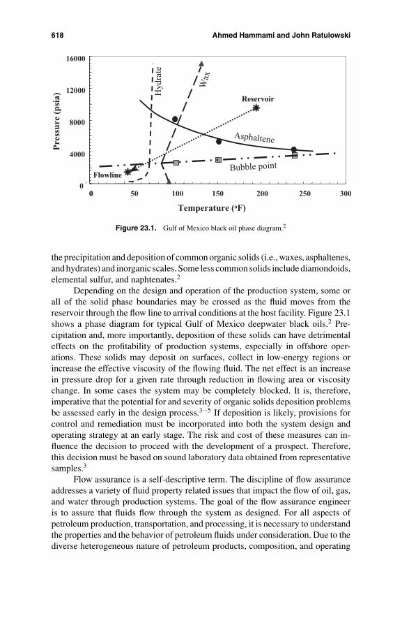
Petroleum is a mixture of mainly hydrocarbons plus organic compounds ofsulfur, nitrogen, and oxygen as well as compounds containing metallic elementsincluding vanadium, nickel, and iron. Hydrocarbon contents may range from ashigh as 97% in lighter paraffinic oils or as low as 50% in heavy, asphalteniccrudes. Despite this bulk characterization, the nonhydrocarbon molecules in thecrude are usually in the form of large hydrocarbon structures with only one or twosubstituted heteroatoms. Therefore, heavy crudes with as little as 50% hydrocarboncomponents are still assumed to retain most of the essential characteristics ofhydrocarbons.6 Of the data available in the literature, it appears that the proportionsof elements in petroleum sources vary only slightly despite the highly differingnature of their sources and overall characteristics.7,8 This consistency is shown inTable 23.1.
The isolation of pure hydrocarbon constituents from crude oils began inearnest in the 1930s with the separation of light paraffinic molecules.9 It soonbecame obvious, however, that the resolution of heavier, individual paraffinmolecules from crudes was impossible due to the increasing numbers of iso-mers that exist. For example, while there is only one possible structure formethane, ethane, and propane, two structures may exist for butane: straight-chainnormal butane, and branched-chain isobutane. As is shown in Table 23.2, thenumber of possible structures increases phenomenally with increasing carbonnumber.
Two other difficulties in the characterization and property prediction arisefrom the immense numbers of isomers of petroleum molecules. First, molecules
Table 23.1. Ultimate Elemental CompositionRanges of Crude Oils
Carbon 83.0–87.0%Hydrogen 10.0–14.0%Nitrogen 0.1–2.0%Oxygen 0.05–1.5%Sulfur 0.05–6.0%
620 Ahmed Hammami and John Ratulowski
n-Pentane (Tbp = 36°C)
iso-Pentane (Tbp = 28°C)
neo-Pentane (Tbp = 10°C) C
CH3
CH3
CH3
C
CHCH3
CH3 CH3
CH3
CH3
CH2
CH2 CH2 CH2 CH3
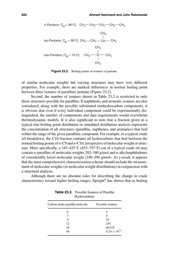
Figure 23.2. Boiling points of isomers of pentane.
of similar molecular weights but varying structures may have very differentproperties. For example, there are marked differences in normal boiling pointbetween three isomers of paraffinic pentane (Figure 23.2).
Second, the number of isomers shown in Table 23.2 is restricted to onlythose structures possible for paraffins. If naphthenic and aromatic isomers are alsoconsidered, along with the possible substituted nonhydrocarbon components, itis obvious that even if every individual component could be experimentally dis-tinguished, the number of components and data requirements would overwhelmthermodynamic models. It is also significant to note that a fraction given in atypical true boiling point distillation or simulated distillation analysis representsthe concentration of all structures (paraffins, napthenes, and aromatics) that boilwithin the range of the given paraffinic compound. For example, in a typical crudeoil breakdown, the C10 fraction contains all hydrocarbons that boil between thenormal boiling points of n-C9 and n-C10, irrespective of molecular weight or struc-ture. More specifically, a 345–425◦C (653–797◦F) cut of a typical crude oil maycontain n-paraffins of molecular weights 282–380 g/mol and n-alkylnaphthalenesof considerably lower molecular weight (240–296 g/mol). As a result, it appearsthat the most comprehensive characterization scheme should include the measure-ment of molecular weights (or molecular weight distributions) in conjunction witha structural analysis.
Although there are no absolute rules for describing the change in crudecharacteristics toward higher boiling ranges, Speight9 has shown that as boiling
Table 23.2. Possible Isomers of ParaffinHydrocarbons
Carbon atoms paraffin molecule Possible isomers
6 57 99 3512 35518 60,52340 6.24 × 10¹³
Precipitation and Deposition of Asphaltenes in Production Systems 621
ranges (or proportionally molecular weights) increase in a petroleum sample, theconcentration of paraffinic molecules decreases. This reduction is paralleled by anincrease in polynuclear aromatics and polycycloparaffins (polynaphthenes).
In subsequent sections, a very general classification scheme is used to definethe various components typically found in petroleum fluids. The scheme is specif-ically designed to address special phase behavior and solid deposition issues. Ingeneral, petroleum constituents are classified under two major groups, namelythe well-defined and volatile C6- fraction and the poorly defined and relativelynonvolatile C6+ fraction.
The C6- fraction consists of all pure hydrocarbon components (andnonhydrocarbons) with carbon numbers up to C5. These include all isomers ineach carbon number range; the physical properties of each of the pure componentspecies are well understood and recorded in the literature. The C6+ fraction, on theother hand, is far more complex due to the multiple isomer combinations availableto hydrocarbons with increasing chain length.8 This group of components is clas-sified as paraffins (P), naphthenes (N), aromatics (A), resins (R), and asphaltenes(A). The combined fraction of paraffins and naphthenes is also termed the saturate(S) fraction.
2.1. Saturates
Saturates are nonpolar and consist of normal alkanes (n-paraffins), branchedalkanes (iso-paraffins) and cyclo-alkanes (also known as naphthenes). Examples ofeach of these classes of chemicals along with the aromatics, resins, and asphalteneshave been reported elsewhere.10−12 Saturates are the largest single source of hy-drocarbon or petroleum waxes, which are generally classified as paraffin wax,microcrystalline wax, and/or petrolatum.13 Of these, the paraffin wax is the majorconstituent of most solid deposits from crude oils.
2.2. Aromatics
Aromatics are hydrocarbons, which are chemically and physically very dif-ferent from the paraffins and naphthenes. They contain one or more ring structuressimilar to benzene. The atoms are connected by aromatic double bonds.
2.3. Resins
Resins are thought to be molecular precursors of the asphaltenes. The po-lar heads of the resins surround the asphaltenes, while the aliphatic tails extendinto the oil. Resins may act to stabilize the dispersion of asphaltene particlesand can be converted to asphaltenes by oxidation. Unlike asphaltenes, however,resins are assumed soluble in the petroleum fluid. Pure resins are heavy liquids orsticky (amorphous) solids and are as volatile as the hydrocarbons of the same size.Petroleum fluids with high-resin content are relatively stable.
622 Ahmed Hammami and John Ratulowski
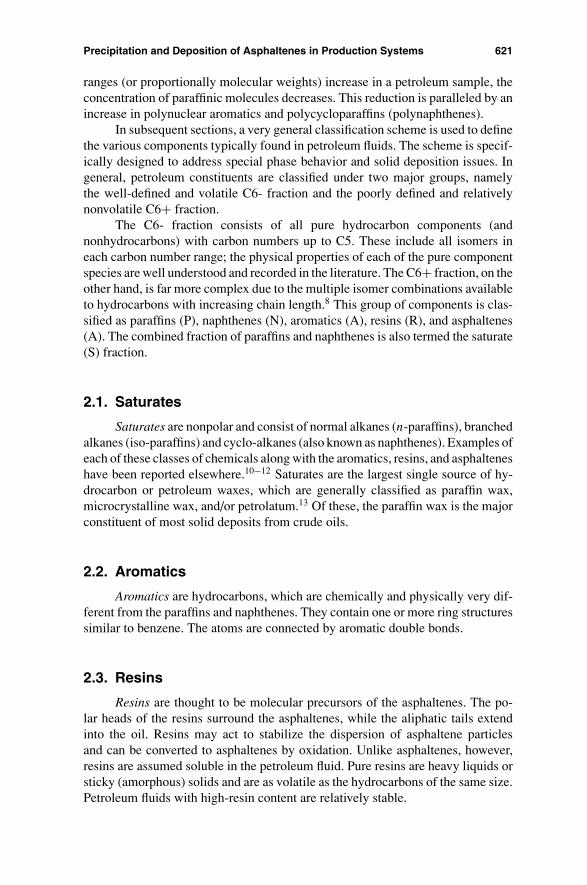
Pentane Induced CO2 InducedPres & Tres
Pressure InducedPsat & Tres
Figure 23.3. Variation of asphaltene texture and character with destabilization method and/orconditions.
2.4. Asphaltenes
Asphaltenes are arbitrarily defined as a solubility class of petroleum that isinsoluble in light alkanes but soluble in toluene or dichloromethane.1,5,10 They arecomposed of aromatic polycyclic clusters variably substituted with alkyl groupand contain heteroatoms (N, S, O) and trace metals (e.g., Ni, V, Fe). The actualchemical structure of asphaltenes is difficult to define using existing analyticaltools, and it remains the subject of ongoing research and contentious debates.15−21
Creek8 has recently argued that structure is important provided it is related tofunction and reactivity. He suggests an ensemble approach be considered, ratherthan a stylized “molecule” for asphaltenes.
It is often assumed that asphaltenes do not dissolve in petroleum but are dis-persed/suspended in the fluid as colloids (evidence of this is mixed). The amount,chemical constituency, and physical structure of asphaltenes precipitated vary withprecipitant type, pressure and temperature (Figure 23.3). Pure asphaltenes are blackdry powders and are nonvolatile; they tend to crack before boiling.
3. Petroleum Precipitates and Deposits
Solid materials precipitating from hydrocarbon systems in the field willrarely be composed of components derived from one of the above general compo-nent groups. To the contrary, hydrocarbon precipitates are most often mixtures ofcomponents from the different fractions. As a result, the following subclassifica-tions have been developed to address the solids precipitation issues.
3.1. Petroleum Waxes
Petroleum waxes refined from crude oils are generally classified as paraffinwax, microcrystalline wax, and petrolatum (wax and oil). The commonly reportedcrystal habits of petroleum waxes are needles, plates, and malcrystalline masses.
Precipitation and Deposition of Asphaltenes in Production Systems 623
Such differing crystal structures and compositions provide waxes with a widerange of properties.
In field operations, asphaltenes and residual oil components can coprecipitatewith the waxes and result in varying appearance (color) and texture to the precipi-tated solids. As would be expected, waxes from condensates and wet gases tend tobe cleaner and more pure than those from heavier crudes. The predominately waxycharacter of the solid can only be defined based on analysis of the solid and theremedial techniques that can be used to redissolve such a solid. In general, onlysmall amounts of aromatic components coprecipitate with waxes and the solidmaterial usually melts by applying heat.22
3.2. Asphaltene Deposits
Our experience indicates that field asphaltene deposits consist of a widerange of components from all the groups outlined previously. The definition ofa predominately asphaltenic deposit must be based on the analysis of the solidand the remedial techniques required to redissolve the material. In general, signif-icant quantities of wax, aromatics, and resins can coprecipitate with asphaltenes,however, the majority of the solid does not melt upon the application of heat.
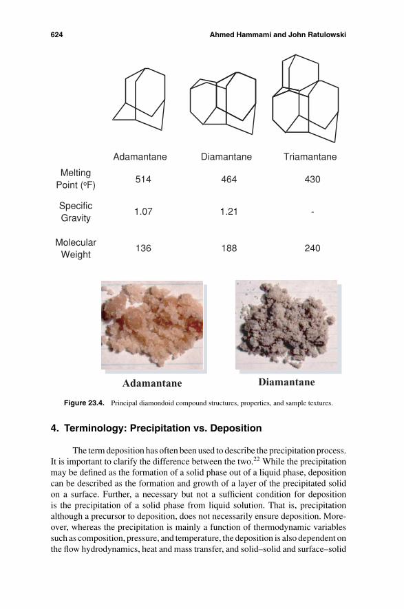
3.3. Diamondoids
Diamondoids are very stable solid compounds, which usually precipitatedirectly from the gas phase. Diamondoid solids often precipitate from gases thathave undergone thermochemical sulfate reduction. These gases tend to be sourand very dry and are associated with high temperatures and carbonate structurescontaining anhydrite. They contain principally saturated, cyclic hydrocarbon com-pounds with a diamond structure; hence the name diamondoids. The molecularweights of diamondoids range from 136 to more than 270 g/mol. The carbonskeleton chemical structures of the three major solid-forming compounds, namelyadamantane, diamantane, and triamantane are shown in Figure 23.4.
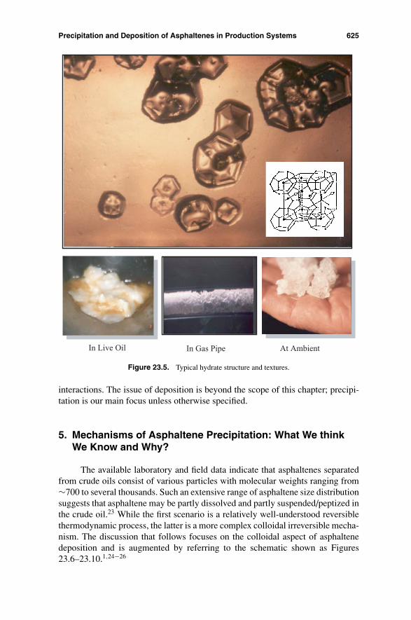
3.4. Gas Hydrates
Hydrates are a common problem in hydrocarbon production and trans-portation systems where free water is present and in contact with the C6-components of the hydrocarbon fluid under certain conditions of temperatureand pressure. Under the proper conditions, the C6- hydrocarbon molecules canoccupy the geometric lattices of the water molecules in the aqueous phase. Whenthese lattices are filled with the light hydrocarbon compounds, a semistable solidcompound similar to ice forms at temperatures far in excess of 0◦C (32◦F). Hydratescan be identified in the field by their behavior. Without sufficient pressure to main-tain the hydrocarbon molecules in the water lattices, the hydrate structures willdecompose into water and gas. This behavior can be easily identified in practice.Examples of typical gas hydrate structure and textures are provided in Figure 23.5.
624 Ahmed Hammami and John Ratulowski
Adamantane Diamantane Triamantane
Melting514 464 430
Point (oF)
Specific1.07 1.21 -
Gravity
Molecular136 188 240
Weight
Adamantane Diamantane
Figure 23.4. Principal diamondoid compound structures, properties, and sample textures.
4. Terminology: Precipitation vs. Deposition
The term deposition has often been used to describe the precipitation process.It is important to clarify the difference between the two.22 While the precipitationmay be defined as the formation of a solid phase out of a liquid phase, depositioncan be described as the formation and growth of a layer of the precipitated solidon a surface. Further, a necessary but not a sufficient condition for depositionis the precipitation of a solid phase from liquid solution. That is, precipitationalthough a precursor to deposition, does not necessarily ensure deposition. More-over, whereas the precipitation is mainly a function of thermodynamic variablessuch as composition, pressure, and temperature, the deposition is also dependent onthe flow hydrodynamics, heat and mass transfer, and solid–solid and surface–solid
Precipitation and Deposition of Asphaltenes in Production Systems 625
In Gas PipeIn Live Oil At Ambient
Figure 23.5. Typical hydrate structure and textures.
interactions. The issue of deposition is beyond the scope of this chapter; precipi-tation is our main focus unless otherwise specified.
5. Mechanisms of Asphaltene Precipitation: What We thinkWe Know and Why?
The available laboratory and field data indicate that asphaltenes separatedfrom crude oils consist of various particles with molecular weights ranging from∼700 to several thousands. Such an extensive range of asphaltene size distributionsuggests that asphaltene may be partly dissolved and partly suspended/peptized inthe crude oil.23 While the first scenario is a relatively well-understood reversiblethermodynamic process, the latter is a more complex colloidal irreversible mecha-nism. The discussion that follows focuses on the colloidal aspect of asphaltenedeposition and is augmented by referring to the schematic shown as Figures23.6–23.10.1,24−26
626 Ahmed Hammami and John Ratulowski
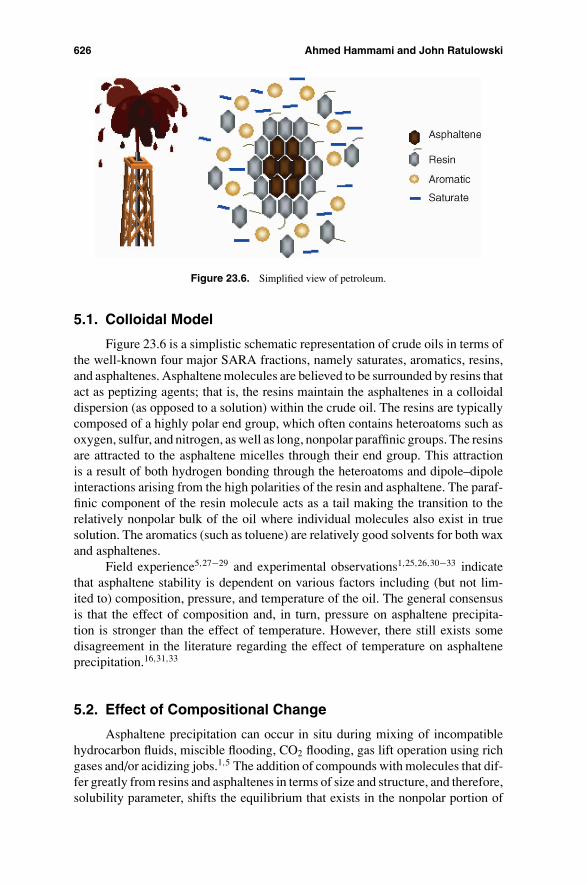
Figure 23.6. Simplified view of petroleum.
5.1. Colloidal Model
Figure 23.6 is a simplistic schematic representation of crude oils in terms ofthe well-known four major SARA fractions, namely saturates, aromatics, resins,and asphaltenes. Asphaltene molecules are believed to be surrounded by resins thatact as peptizing agents; that is, the resins maintain the asphaltenes in a colloidaldispersion (as opposed to a solution) within the crude oil. The resins are typicallycomposed of a highly polar end group, which often contains heteroatoms such asoxygen, sulfur, and nitrogen, as well as long, nonpolar paraffinic groups. The resinsare attracted to the asphaltene micelles through their end group. This attractionis a result of both hydrogen bonding through the heteroatoms and dipole–dipoleinteractions arising from the high polarities of the resin and asphaltene. The paraf-finic component of the resin molecule acts as a tail making the transition to therelatively nonpolar bulk of the oil where individual molecules also exist in truesolution. The aromatics (such as toluene) are relatively good solvents for both waxand asphaltenes.
Field experience5,27−29 and experimental observations1,25,26,30−33 indicatethat asphaltene stability is dependent on various factors including (but not lim-ited to) composition, pressure, and temperature of the oil. The general consensusis that the effect of composition and, in turn, pressure on asphaltene precipita-tion is stronger than the effect of temperature. However, there still exists somedisagreement in the literature regarding the effect of temperature on asphalteneprecipitation.16,31,33
5.2. Effect of Compositional Change
Asphaltene precipitation can occur in situ during mixing of incompatiblehydrocarbon fluids, miscible flooding, CO2 flooding, gas lift operation using richgases and/or acidizing jobs.1,5 The addition of compounds with molecules that dif-fer greatly from resins and asphaltenes in terms of size and structure, and therefore,solubility parameter, shifts the equilibrium that exists in the nonpolar portion of
Precipitation and Deposition of Asphaltenes in Production Systems 627
Asphaltene
Resin
Aromatic
Saturate
Titration with C5
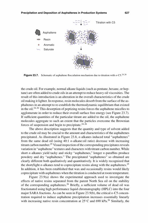
Figure 23.7. Schematic of asphaltene flocculation mechanism due to titration with n-C5.24,26
the crude oil. For example, normal alkane liquids (such as pentane, hexane, or hep-tane) are often added to crude oils in an attempt to reduce heavy oil viscosities. Theresult of this introduction is an alteration in the overall characteristics of the crudeoil making it lighter. In response, resin molecules desorb from the surface of the as-phaltenes in an attempt to re-establish the thermodynamic equilibrium that existedin the oil.24,26 This desorption of peptizing resins forces the asphaltene micelles toagglomerate in order to reduce their overall surface free energy (see Figure 23.7).If sufficient quantities of the particular titrant are added to the oil, the asphaltenemolecules aggregate to such an extent that the particles overcome the Brownianforces of suspension and begin to precipitate.24,26
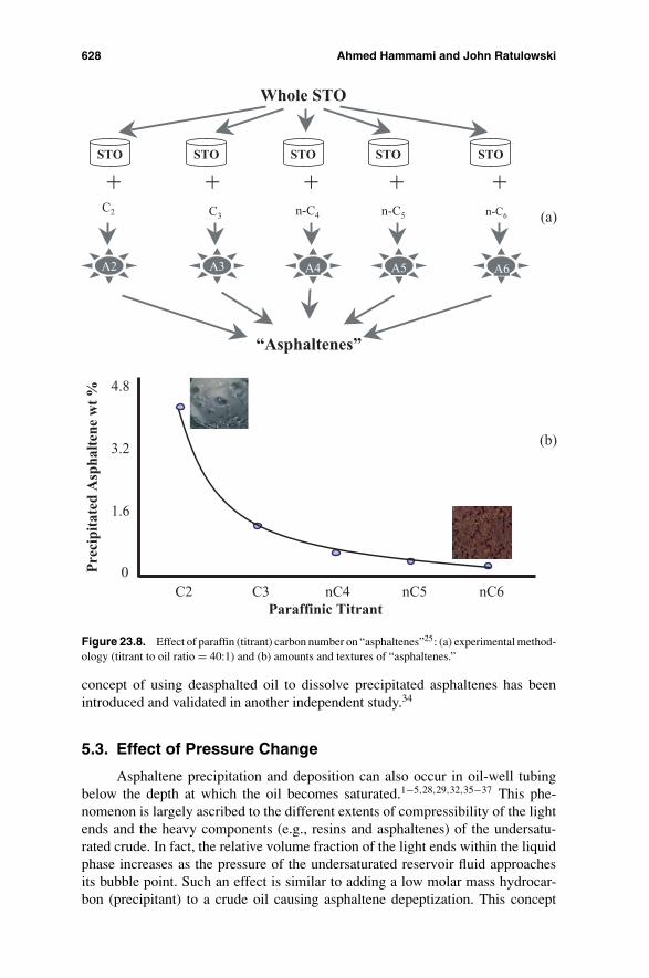
The above description suggests that the quantity and type of solvent addedto the crude oil may be crucial to the amount and characteristics of the asphaltenesprecipitated. As illustrated in Figure 23.8, n-alkanes induced total “asphaltenes”from the same dead oil (using 40:1 n-alkane:oil ratio) decrease with increasingtitrant carbon number.25 Visual inspection of the corresponding precipitates revealsvariation in “asphaltene” textures and characters with titrant carbon number. Whileshort n-alkanes yield tacky and sticky “asphaltenes,” longer n-paraffins producepowdery and dry “asphaltenes.” The precipitated “asphaltenes” so obtained areclearly different both qualitatively and quantitatively. It is widely recognized thatthe short/light n-alkanes tend to coprecipitate resins along with the asphaltenes.25
In addition, it has been established that wax and occasionally resins would likelycoprecipitate with asphaltenes when the titration is conducted at room temperature.
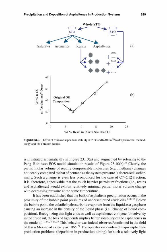
Figure 23.9(a) shows the experimental approach used to investigate theeffects of native resins separated from the parent North Sea oil on the stabilityof the corresponding asphaltenes.26 Briefly, a sufficient volume of dead oil wasfractionated using high performance liquid chromatography (HPLC) into the fourmajor SARA fractions. As can be seen in Figure 23.9(b), the critical n-C5 concen-tration required to induce asphaltene precipitation increases essentially linearlywith increasing native resin concentration at 25◦C and 690 kPa.26 Similarly, the
628 Ahmed Hammami and John Ratulowski
“Asphaltenes”
Whole STO
STO STO STO STO STO
C2 C3 n-C4 n-C5 n-C6
A2 A3 A4 A6A5
+ + + + +
C2 C3 nC4 nC5 nC6Paraffinic Titrant
0
1.6
3.2
4.8
Pre
cipi
tate
d A
spha
lten
e w
t %
(a)
(b)
Figure 23.8. Effect of paraffin (titrant) carbon number on “asphaltenes”25: (a) experimental method-ology (titrant to oil ratio = 40:1) and (b) amounts and textures of “asphaltenes.”
concept of using deasphalted oil to dissolve precipitated asphaltenes has beenintroduced and validated in another independent study.34
5.3. Effect of Pressure Change
Asphaltene precipitation and deposition can also occur in oil-well tubingbelow the depth at which the oil becomes saturated.1−5,28,29,32,35−37 This phe-nomenon is largely ascribed to the different extents of compressibility of the lightends and the heavy components (e.g., resins and asphaltenes) of the undersatu-rated crude. In fact, the relative volume fraction of the light ends within the liquidphase increases as the pressure of the undersaturated reservoir fluid approachesits bubble point. Such an effect is similar to adding a low molar mass hydrocar-bon (precipitant) to a crude oil causing asphaltene depeptization. This concept
Precipitation and Deposition of Asphaltenes in Production Systems 629
(a)
(b)
Whole STO
Saturates Aromatics Resins Asphaltenes
STO STO
+++
54
57
60
63
66
0 5 10 15 20 25
Wt % Resin in North Sea Dead Oil
Wt
% n
-C5
at "
Asp
halt
ene"
On
set
Original OilComposition
Figure 23.9. Effect of resins on asphaltene stability at 25◦C and 690 kPa.26 (a) Experimental method-ology and (b) Titration results.
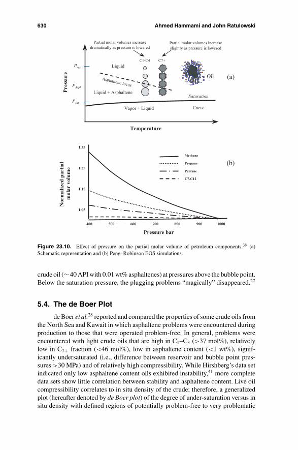
is illustrated schematically in Figure 23.10(a) and augmented by referring to thePeng–Robinson EOS model simulation results of Figure 23.10(b).38 Clearly, thepartial molar volume of readily compressible molecules (e.g., methane) changesnoticeably compared to that of pentane as the system pressure is decreased isother-mally. Such a change is even less pronounced for the case of C7–C12 fraction.It is, therefore, conceivable that the much heavier petroleum fractions (i.e., resinsand asphaltenes) would exhibit relatively minimal partial molar volume changewith decreasing pressure at the same temperature.
It has been established that the bulk of asphaltene precipitation occurs in theproximity of the bubble point pressures of undersaturated crude oils.1,28,35 Belowthe bubble point, the volatile hydrocarbons evaporate from the liquid as a gas phasecausing an increase in the density of the liquid phase (i.e., change of liquid com-position). Recognizing that light ends as well as asphaltenes compete for solvencyin the crude oil, the loss of light ends implies better solubility of the asphaltenes inthe crude oil.1,24,28,29,35 This behavior was indeed observed/confirmed in the fieldof Hassi Messaoud as early as 1965.27 The operator encountered major asphalteneproduction problems (deposition in production tubing) for such a relatively light
630 Ahmed Hammami and John Ratulowski
Liquid
Vapor + Liquid
Pres
Psat
C7+
Partial molar volumes increaseslightly as pressure is lowered
C1-C4
Partial molar volumes increasedramatically as pressure is lowered
Temperature
Pre
ssu
re
Saturation
Curve
Oil
PAsph
Liquid + Asphaltene
Asphaltene locus
(a)
(b)
1.05
1.15
1.25
1.35
400 500 600 700 800 900 1000
Pressure bar
Nor
mal
ized
par
tial
m
olar
vol
ume
Methane
Propane
Pentane
C7-C12
Figure 23.10. Effect of pressure on the partial molar volume of petroleum components.38 (a)Schematic representation and (b) Peng–Robinson EOS simulations.
crude oil (∼ 40 API with 0.01 wt% asphaltenes) at pressures above the bubble point.Below the saturation pressure, the plugging problems “magically” disappeared.27
5.4. The de Boer Plot
de Boer et al.28 reported and compared the properties of some crude oils fromthe North Sea and Kuwait in which asphaltene problems were encountered duringproduction to those that were operated problem-free. In general, problems wereencountered with light crude oils that are high in C1–C3 (>37 mol%), relativelylow in C7+ fraction (<46 mol%), low in asphaltene content (<1 wt%), signif-icantly undersaturated (i.e., difference between reservoir and bubble point pres-sures >30 MPa) and of relatively high compressibility. While Hirshberg’s data setindicated only low asphaltene content oils exhibited instability,41 more completedata sets show little correlation between stability and asphaltene content. Live oilcompressibility correlates to in situ density of the crude; therefore, a generalizedplot (hereafter denoted by de Boer plot) of the degree of under-saturation versus insitu density with defined regions of potentially problem-free to very problematic
Precipitation and Deposition of Asphaltenes in Production Systems 631
crude oils was proposed.28 Accordingly, the lighter the prospect crude oil is, thegreater its tendency to precipitate asphaltenes during production will be.1 The deBoer plot is generally considered a conservative screen that is best used to identifynonproblematic oils.
5.5. Reversibility of Asphaltene Precipitation
Many researchers believed that asphaltene precipitation is not reversiblemainly due to experimental observation of the colloidal behavior of asphaltenesuspensions.39 Hotier and Robin40 have argued that the results from titrationexperiments show that asphaltene precipitated by the addition of a precipitantcan be redissolved by the addition of a solvent. This is, however, no firm indica-tion for reversibility because the addition of a solvent is not the reverse processof the addition of a precipitant. Hirschberg et al.41 have assumed that asphalteneprecipitation is reversible but is likely very slow. Fotland32 and Wang et al.33 havespeculated that asphaltene precipitation is less likely to be reversible for crude oilssubjected to conditions well beyond those of the onset.
It is noteworthy to point out that most of the experimental techniques em-ployed to study asphaltenes before 1995 were limited in pressure rating; hence,conclusions were generally overextrapolated to live oil conditions based on deadoil analyses. It was difficult to test for asphaltene reversibility based on dead oilexperiments whereby the sample composition appeared to be altered irreversibly.
Following the development of high-pressure high-temperature laser-basedlight transmittance technique in 1995, Hammami et al.1 were the first to establishand report a strong tendency for pressure-induced apshaltenes to redissolve inundersaturated Gulf of Mexico reservoir fluids upon increasing the system pressureabove the saturation pressures at corresponding reservoir temperatures. These testswere performed over typical production conditions of composition, pressure, andtemperature. Evidence of asphaltene precipitation above and redissolution belowthe saturation pressure was also observed. That is, a pressure range for asphalteneinstability was measured at constant temperatures. Such an observation is indeedin agreement with the reported Hassi Messaoud field experience first reported inmid 1960s.27
6. Sampling
Flow assurance measurements have led to a new awareness of the need tohave representative samples. Changes in pressure and temperature can cause phasechanges that lead to sample alteration. The test fluid in any laboratory investigationmust be reasonably representative of the reservoir fluid if the data are to have anypractical application. Therefore, prior to initiating any laboratory fluid propertymeasurement, it is imperative that the appropriate time, effort, and money beinvested wisely so as to insure that the utmost appropriate fluid sampling and fluidpreparation procedures are followed for a given petroleum fluid.
632 Ahmed Hammami and John Ratulowski
Bottom hole sampling from hydrocarbon reservoirs is essential to understandthe fluids to be produced. Fluid samples are also acquired at later stages in the lifeof the reservoir to evaluate the conditions of the fluids at a certain point of timeor after some production activities; however, the point of comparison is alwaysthe original fluid properties. Thus, it is important to acquire quality, representativefluid samples and to manage this data.
Introduction of contaminates during the sample acquisition process can alsoalter the fluid composition. The most common source of contamination is fromdrilling fluids. Oil-based mud (OBM) is commonly used in drilling operations.OBM filtrates often invade the formation due to overbalance pressure in the mudcolumn and, in turn, can contaminate adjacent formation fluids. The extent ofcontamination depends on the OBM type as well as the penetration depth (layer)in the formation. This leads to problems and challenges in sampling representativereservoir fluids. In that, the presence of even small concentration of OBM filtrate inthe collected sample could significantly alter the phase behavior and fluid propertiesof the formation fluid.42
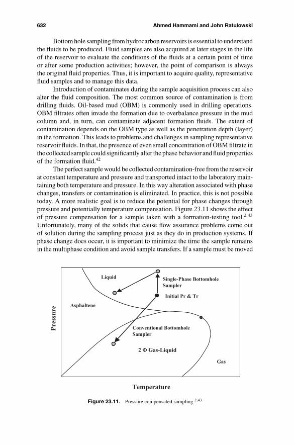
The perfect sample would be collected contamination-free from the reservoirat constant temperature and pressure and transported intact to the laboratory main-taining both temperature and pressure. In this way alteration associated with phasechanges, transfers or contamination is eliminated. In practice, this is not possibletoday. A more realistic goal is to reduce the potential for phase changes throughpressure and potentially temperature compensation. Figure 23.11 shows the effectof pressure compensation for a sample taken with a formation-testing tool.2,43
Unfortunately, many of the solids that cause flow assurance problems come outof solution during the sampling process just as they do in production systems. Ifphase change does occur, it is important to minimize the time the sample remainsin the multiphase condition and avoid sample transfers. If a sample must be moved
Liquid
Gas
Asphaltene
2 Φ Gas-Liquid
Initial Pr & Tr
Temperature
Pre
ssu
re
Conventional BottomholeSampler
Single-Phase BottomholeSampler
Figure 23.11. Pressure compensated sampling.2,43
Precipitation and Deposition of Asphaltenes in Production Systems 633
Pow
er o
f T
rans
mit
ted
Lig
ht
Pressure
Sample 2
Sample 1
Sample 3Asphaltene
Precipitation Onset10,000 psi
Asphaltene Precipitation Onset
7,800 psi
Asphaltene Precipitation Onset
7,800 psi
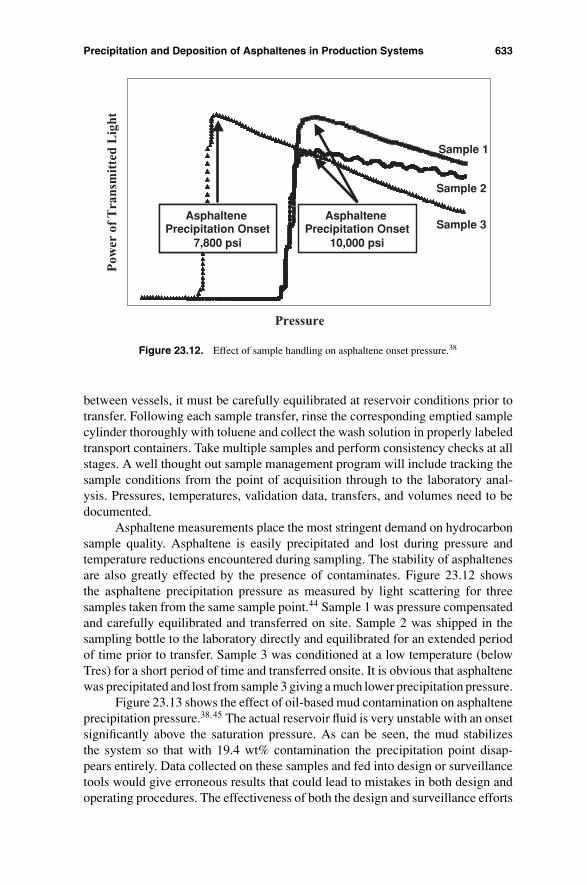
Figure 23.12. Effect of sample handling on asphaltene onset pressure.38
between vessels, it must be carefully equilibrated at reservoir conditions prior totransfer. Following each sample transfer, rinse the corresponding emptied samplecylinder thoroughly with toluene and collect the wash solution in properly labeledtransport containers. Take multiple samples and perform consistency checks at allstages. A well thought out sample management program will include tracking thesample conditions from the point of acquisition through to the laboratory anal-ysis. Pressures, temperatures, validation data, transfers, and volumes need to bedocumented.
Asphaltene measurements place the most stringent demand on hydrocarbonsample quality. Asphaltene is easily precipitated and lost during pressure andtemperature reductions encountered during sampling. The stability of asphaltenesare also greatly effected by the presence of contaminates. Figure 23.12 showsthe asphaltene precipitation pressure as measured by light scattering for threesamples taken from the same sample point.44 Sample 1 was pressure compensatedand carefully equilibrated and transferred on site. Sample 2 was shipped in thesampling bottle to the laboratory directly and equilibrated for an extended periodof time prior to transfer. Sample 3 was conditioned at a low temperature (belowTres) for a short period of time and transferred onsite. It is obvious that asphaltenewas precipitated and lost from sample 3 giving a much lower precipitation pressure.
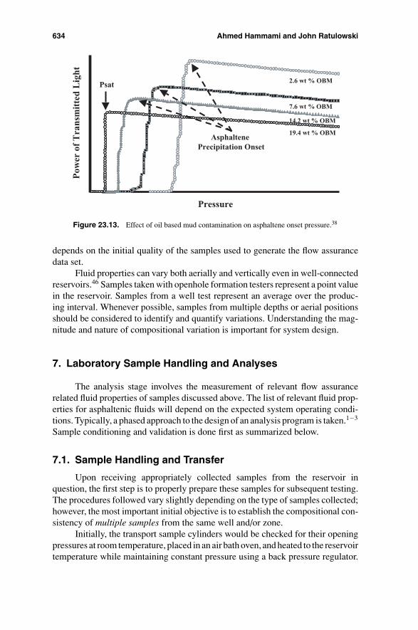
Figure 23.13 shows the effect of oil-based mud contamination on asphalteneprecipitation pressure.38,45 The actual reservoir fluid is very unstable with an onsetsignificantly above the saturation pressure. As can be seen, the mud stabilizesthe system so that with 19.4 wt% contamination the precipitation point disap-pears entirely. Data collected on these samples and fed into design or surveillancetools would give erroneous results that could lead to mistakes in both design andoperating procedures. The effectiveness of both the design and surveillance efforts
634 Ahmed Hammami and John Ratulowski
Pow
er o
f T
ran
smit
ted
Lig
ht
Pressure
2.6 wt % OBM
7.6 wt % OBM
14.2 wt % OBM
19.4 wt % OBMAsphaltene
Precipitation Onset
Psat
Figure 23.13. Effect of oil based mud contamination on asphaltene onset pressure.38
depends on the initial quality of the samples used to generate the flow assurancedata set.
Fluid properties can vary both aerially and vertically even in well-connectedreservoirs.46 Samples taken with openhole formation testers represent a point valuein the reservoir. Samples from a well test represent an average over the produc-ing interval. Whenever possible, samples from multiple depths or aerial positionsshould be considered to identify and quantify variations. Understanding the mag-nitude and nature of compositional variation is important for system design.
7. Laboratory Sample Handling and Analyses
The analysis stage involves the measurement of relevant flow assurancerelated fluid properties of samples discussed above. The list of relevant fluid prop-erties for asphaltenic fluids will depend on the expected system operating condi-tions. Typically, a phased approach to the design of an analysis program is taken.1−3
Sample conditioning and validation is done first as summarized below.
7.1. Sample Handling and Transfer
Upon receiving appropriately collected samples from the reservoir inquestion, the first step is to properly prepare these samples for subsequent testing.The procedures followed vary slightly depending on the type of samples collected;however, the most important initial objective is to establish the compositional con-sistency of multiple samples from the same well and/or zone.
Initially, the transport sample cylinders would be checked for their openingpressures at room temperature, placed in an air bath oven, and heated to the reservoirtemperature while maintaining constant pressure using a back pressure regulator.
Precipitation and Deposition of Asphaltenes in Production Systems 635
Following a minimum of 5 days stabilization period under continuous rocking,an isobaric and isothermal transfer to a suitable high-pressure high-temperaturecylinder would take place. This transfer involves the following steps.
First, a clean pistoned lab cylinder would be evacuated and filled with dis-placement fluid below the piston. The lab cylinder would then be connected to theshipping cylinder with a sight glass and high-pressure tubing. To begin the transfer,one pump would be used to displace the oil out of the shipping cylinder into the labcylinder, while a second pump would be used to withdraw the displacement fluidfrom the lab cylinder. In the process, the transfer pressure is maintained well abovesaturation and likely asphaltene onset pressures. It is strongly recommended thatthe differential pressure between the two cylinders does not exceed 200 psi duringthe sample transfer. Following this, each emptied cylinder would be thoroughlyrinsed with a sufficient amount of toluene to dissolve any organic deposit if any,and clean the transport cylinder. The corresponding toluene rinses are recoveredin suitable pre-labeled containers.
Finally, each of the toluene rinses of the sampling chambers is subjectedto compositional analyses up to C30+ (for waxy crudes) and/or rotoevaporationfollowed by asphaltene content of the resulting residues (for asphaltenic crudes).In the case of waxy crudes, the C30+ composition of the rinses is then comparedto those of the corresponding dead oils on a toluene-free basis. The quality assur-ance/quality control (QA/QC) of onsite sample conditioning and transfer will bedeemed acceptable provided the C30+ compositions of the rinses on a toluene-freebasis and/or the asphaltene contents of the residues are confirmed to be reasonablysimilar to those of the parent oils.
7.2. Compositional Analyses
Subsamples of the reconditioned fluids are analyzed for composition(tyically up to C30+) by a flash procedure.47 In this technique, an accurately mea-sured volume of fluid is isobarically and isothermally displaced into a preweighedempty pycnometer where its density and mass are evaluated. The pycnometer isthen connected to a gas–oil ratio (GOR) single stage flash apparatus where thefluid is flashed to ambient pressure and temperature conditions. Subsequently, theevolved gas phase is circulated through the residual liquid for a period of time toachieve equilibrium between phases. Following circulation, the volume of equi-librium vapor and the mass of liquid remaining in the pycnometer are measured.The vapor phase is resolved to C5 by natural gas chromatograph (GC), while thevapor C5+ fraction and the residual liquids are analyzed to C30+ using liquid GC.From the measured composition and total mass of each phase, the composition ofthe original live fluid may be calculated by mass balance.
7.3. Oil-Based Mud (OBM) Contamination Quantification
The most common technique used to quantify OBM concentrationsin reservoir fluids is gas chromatography.42 Gas chromatography provides a
636 Ahmed Hammami and John Ratulowski
OBM Contamination (wt %)
1
10
100
CO
2
C1
C3
N-C
4N
-C5
C7
C9
C11
C13
C15
C17
C19
C21
C23
C25
C27
C29
Con
cent
rati
on
1008 5
0
Component
OBM Contamination (wt %)
C11
Figure 23.14. OBM contamination analysis by gas chromatography.
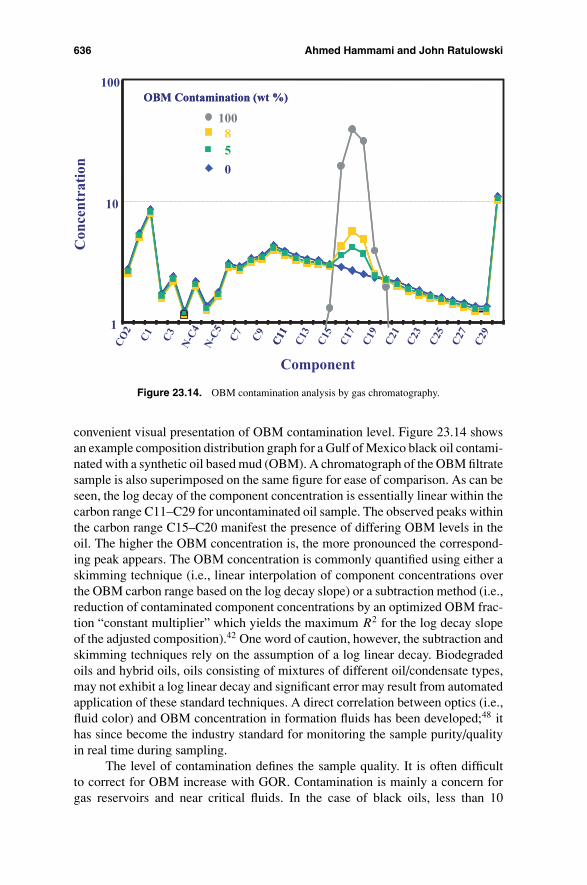
convenient visual presentation of OBM contamination level. Figure 23.14 showsan example composition distribution graph for a Gulf of Mexico black oil contami-nated with a synthetic oil based mud (OBM). A chromatograph of the OBM filtratesample is also superimposed on the same figure for ease of comparison. As can beseen, the log decay of the component concentration is essentially linear within thecarbon range C11–C29 for uncontaminated oil sample. The observed peaks withinthe carbon range C15–C20 manifest the presence of differing OBM levels in theoil. The higher the OBM concentration is, the more pronounced the correspond-ing peak appears. The OBM concentration is commonly quantified using either askimming technique (i.e., linear interpolation of component concentrations overthe OBM carbon range based on the log decay slope) or a subtraction method (i.e.,reduction of contaminated component concentrations by an optimized OBM frac-tion “constant multiplier” which yields the maximum R2 for the log decay slopeof the adjusted composition).42 One word of caution, however, the subtraction andskimming techniques rely on the assumption of a log linear decay. Biodegradedoils and hybrid oils, oils consisting of mixtures of different oil/condensate types,may not exhibit a log linear decay and significant error may result from automatedapplication of these standard techniques. A direct correlation between optics (i.e.,fluid color) and OBM concentration in formation fluids has been developed;48 ithas since become the industry standard for monitoring the sample purity/qualityin real time during sampling.
The level of contamination defines the sample quality. It is often difficultto correct for OBM increase with GOR. Contamination is mainly a concern forgas reservoirs and near critical fluids. In the case of black oils, less than 10
Precipitation and Deposition of Asphaltenes in Production Systems 637
wt% OBM is usually considered acceptable for PVT but not for flow assurancestudies.2,37,38,49
7.4. Dead Oil Characterization
Once duplicate bottom hole samples are verified to have similar C30+ com-position, density, OBM concentration and GOR, a subsample (∼100 cm3) of oneof the fluids (randomly selected) is flashed to ambient conditions. The resultingdead oil is then subjected to a suite of screening tests using different analyticaltechniques as detailed below.
Analytical methods have been available for some time for the separationand characterization of asphaltenes in heavy crudes and bitumens, and of waxesin waxy crudes.13 Both of these component types can give rise to production,transportation, and processing problems related to the crudes or their products.Good data characterizing the asphaltenes in terms of their content and stability,and waxes in terms of their content and carbon number distribution, are usuallyrequired to help solve these problems. Increasingly both asphaltenes and waxes arebeing found in the same crudes, and the established methods for their separationare often not applicable. Improved separation techniques have been described,and their applicability to different crude types discussed.13,50 Examples are givenbelow for the types of characterization, which may be carried out on the separatedasphaltenes, maltenes, waxes, and oils.
7.4.1. SARA Analysis
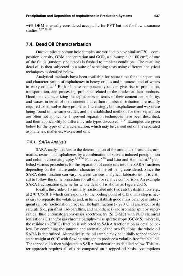
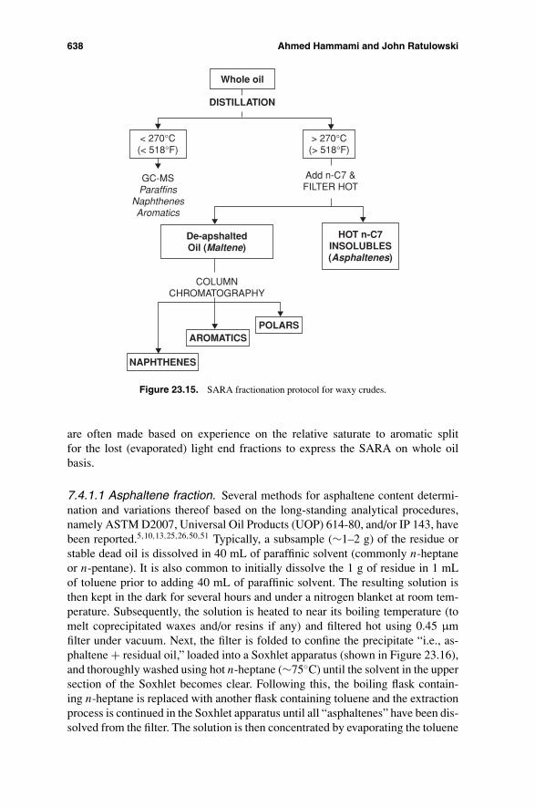
SARA analysis refers to the determination of the amounts of saturates, aro-matics, resins, and asphaltenes by a combination of solvent induced precipitationand column chromatography.5,13,50 Fuhr et al.50 and Lira and Hammami.13 pub-lished various procedures for the separation of crude oils into the SARA fractionsdepending on the nature and/or character of the oil being considered. Since theSARA determination can vary between various analytical laboratories, it is criti-cal to follow the same procedure for all oils for relative comparison. An exampleSARA fractionation scheme for whole dead oil is shown as Figure 23.15.
Ideally, the crude oil is initially fractionated into two cuts by distillation (e.g.,at 270◦C/518◦F which corresponds to the boiling point of C15). This step is nec-essary to separate the volatiles and, in turn, establish good mass balance in subse-quent sample fractionation process. The light fraction (<270◦C) is analyzed for itssaturate (i.e., paraffins, iso-paraffins, and naphthenes) and aromatic split by super-critical fluid chromatography-mass spectrometry (SFC-MS) with N2O chemicalionization (Cl) and/or gas chromatography-mass spectroscopy (GC-MS); whereas,the residue (>270◦C) fraction is subjected to SARA fractionation as detailed be-low. By combining the saturate and aromatic of the two fractions, the whole oilSARA is determined. Alternatively, the oil sample may be initially topped to con-stant weight at 60◦C with flowing nitrogen to produce a volatile-free “stable” oil.The topped oil is then subjected to SARA fractionation as detailed below. This lat-ter approach requires all oils be compared on a topped-oil basis. Assumptions
638 Ahmed Hammami and John Ratulowski
Whole oil
DISTILLATION
NAPHTHENES
AROMATICSPOLARS
COLUMNCHROMATOGRAPHY
De-apshaltedOil (Maltene)
HOT n-C7INSOLUBLES(Asphaltenes)
Add n-C7 &FILTER HOT
GC-MSParaffins
NaphthenesAromatics
< 270°C(< 518°F)
> 270°C(> 518°F)
Figure 23.15. SARA fractionation protocol for waxy crudes.
are often made based on experience on the relative saturate to aromatic splitfor the lost (evaporated) light end fractions to express the SARA on whole oilbasis.
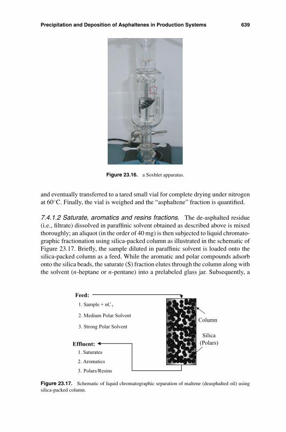
7.4.1.1 Asphaltene fraction. Several methods for asphaltene content determi-nation and variations thereof based on the long-standing analytical procedures,namely ASTM D2007, Universal Oil Products (UOP) 614-80, and/or IP 143, havebeen reported.5,10,13,25,26,50,51 Typically, a subsample (∼1–2 g) of the residue orstable dead oil is dissolved in 40 mL of paraffinic solvent (commonly n-heptaneor n-pentane). It is also common to initially dissolve the 1 g of residue in 1 mLof toluene prior to adding 40 mL of paraffinic solvent. The resulting solution isthen kept in the dark for several hours and under a nitrogen blanket at room tem-perature. Subsequently, the solution is heated to near its boiling temperature (tomelt coprecipitated waxes and/or resins if any) and filtered hot using 0.45 μmfilter under vacuum. Next, the filter is folded to confine the precipitate “i.e., as-phaltene + residual oil,” loaded into a Soxhlet apparatus (shown in Figure 23.16),and thoroughly washed using hot n-heptane (∼75◦C) until the solvent in the uppersection of the Soxhlet becomes clear. Following this, the boiling flask contain-ing n-heptane is replaced with another flask containing toluene and the extractionprocess is continued in the Soxhlet apparatus until all “asphaltenes” have been dis-solved from the filter. The solution is then concentrated by evaporating the toluene
Precipitation and Deposition of Asphaltenes in Production Systems 639
16.24
Figure 23.16. a Soxhlet apparatus.
and eventually transferred to a tared small vial for complete drying under nitrogenat 60◦C. Finally, the vial is weighed and the “asphaltene” fraction is quantified.
7.4.1.2 Saturate, aromatics and resins fractions. The de-asphalted residue(i.e., filtrate) dissolved in paraffinic solvent obtained as described above is mixedthoroughly; an aliquot (in the order of 40 mg) is then subjected to liquid chromato-graphic fractionation using silica-packed column as illustrated in the schematic ofFigure 23.17. Briefly, the sample diluted in paraffinic solvent is loaded onto thesilica-packed column as a feed. While the aromatic and polar compounds adsorbonto the silica beads, the saturate (S) fraction elutes through the column along withthe solvent (n-heptane or n-pentane) into a prelabeled glass jar. Subsequently, a
Feed:
1. Sample + nC7
2. Medium Polar Solvent
3. Strong Polar Solvent
Effluent:1. Saturates
2. Aromatics
3. Polars/Resins
Silica (Polars)
Column
Figure 23.17. Schematic of liquid chromatographic separation of maltene (deasphalted oil) usingsilica-packed column.
640 Ahmed Hammami and John Ratulowski
medium polar solvent and a strong polar solvent are loaded onto the same packedcolumn (one at a time) to recover/elute the aromatic (A) and resin (R) fractions,respectively. The corresponding effluents are collected in separate glass jars. Eachsolution is then subjected to roto-evaporation under nitrogen atmosphere to removethe respective solvents. The saturate fraction so obtained is observed to be whiteand opaque just like candle wax; whereas, the aromatic and polar fractions appearto be brownish and very dark, respectively.
7.5. Dead Oil Asphaltene Stability Tests
Various techniques and approaches are used to assess asphaltene stability ofdead crude oils. In general, these include SARA screens and titration tests usingn-pentane, n-hexane, or n-heptane.
7.5.1. SARA Screens
The reader is reminded that there are many variations of SARA fractionationmethod and procedures of crude oils. Hence, the SARA screens described hereinmust be used with caution. In other words, one must ensure the SARA fractionsare obtained by strictly following the same experimental procedures and analyticaltechniques described by the developer of the SARA screen method in question.
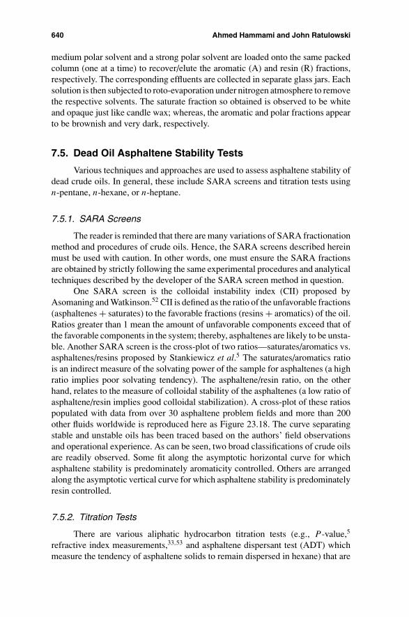
One SARA screen is the colloidal instability index (CII) proposed byAsomaning and Watkinson.52 CII is defined as the ratio of the unfavorable fractions(asphaltenes + saturates) to the favorable fractions (resins + aromatics) of the oil.Ratios greater than 1 mean the amount of unfavorable components exceed that ofthe favorable components in the system; thereby, asphaltenes are likely to be unsta-ble. Another SARA screen is the cross-plot of two ratios—saturates/aromatics vs.asphaltenes/resins proposed by Stankiewicz et al.5 The saturates/aromatics ratiois an indirect measure of the solvating power of the sample for asphaltenes (a highratio implies poor solvating tendency). The asphaltene/resin ratio, on the otherhand, relates to the measure of colloidal stability of the asphaltenes (a low ratio ofasphaltene/resin implies good colloidal stabilization). A cross-plot of these ratiospopulated with data from over 30 asphaltene problem fields and more than 200other fluids worldwide is reproduced here as Figure 23.18. The curve separatingstable and unstable oils has been traced based on the authors’ field observationsand operational experience. As can be seen, two broad classifications of crude oilsare readily observed. Some fit along the asymptotic horizontal curve for whichasphaltene stability is predominately aromaticity controlled. Others are arrangedalong the asymptotic vertical curve for which asphaltene stability is predominatelyresin controlled.
7.5.2. Titration Tests
There are various aliphatic hydrocarbon titration tests (e.g., P-value,5
refractive index measurements,33,53 and asphaltene dispersant test (ADT) whichmeasure the tendency of asphaltene solids to remain dispersed in hexane) that are
Precipitation and Deposition of Asphaltenes in Production Systems 641
Asphaltene/Resin
0.00 0.20 0.40 0.60 0.80 1.00 1.20 1.40 1.600.00
0.50
1.00
1.50
2.00
2.50
3.00
3.50
4.00
4.50
5.00
Unstable
Stable
UnstableMarginalStable
Satu
rate
/Aro
mat
ic
Resin Controlled
Aromaticity Controlled
Figure 23.18. Shell’s SARA cross plot stability screen.5
used to assess the stability of asphaltenes in dead crude oils. The general procedureinvolves either continuous (fast) or discrete (slow intermittent) addition of aliphatictitrant to the crude oil sample.
7.5.2.1 Continuous Titrations. In the case of continuous titration, the samplemixture is vigorously stirred and simultaneously monitored for asphaltene floccu-lation onset using typically near-infrared laser transmittance probes. The exper-imental technique used for this test is commonly referred to as the flocculationpoint apparatus (FPA). This system is analogous to the laser-based light transmit-tance solid detection system (SDS) described by Hammami and Raines.47 As thetitrant (typically heptane or pentane) concentration increases in the oil sample,the resulting mixture optical density decreases and, in turn, the light transmittancethrough the sample increases. At certain critical titrant concentration, however,asphaltenes flocs begin to appear; the corresponding light transmittance signalexhibits a maximum and begins to drop dramatically. Typically, the titrant con-centration that corresponds to the maximum in the transmittance trace is deemedthe FPA number, which is defined as the ratio of the volume of titrant to the initialmass of crude oil.4,5 Figure 23.19 shows an example titration curve obtained usingthe infrared light transmittance probe.
The true asphaltene onset concentration, however, is almost always lowerthan the value, which corresponds to the observed maximum in light transmittancecurve. This is because of the two simultaneous competing (counter) effects ofthe decrease in optical density vs. size and amount of precipitated asphalteneflocs with increasing titrant concentration. While the decrease in optical densityleads to increase in light transmittance, the precipitation of asphaltenes resultsin a decrease of light transmittance. The asphaltene flocs must therefore reach acritical size and/or concentration before the light transmittance attains a maximum

642 Ahmed Hammami and John Ratulowski
0 0.2 0.4 0.6 0.8
Mass Fraction n-C5
Asphaltene Onset
0
10
20
30
40
Pow
er o
f T
rans
mit
ted
Lig
ht (
mW
)
Figure 23.19. Typical light transmittance titration curve at constant temperature and pressure.
as a net effect of the two competing factors. Beyond the observed maximum inlight transmittance, the effects of asphaltenes become stronger than those of thetitrant dilution; thereby, light transmittance continues to drop with increasing titrantconcentration.
7.5.2.2 Discrete Titrations. Discrete titrations account for slow kinetics of as-phaltene instability and, thus, provide for better approximation of equilibriummeasurements. Often the kinetics of titrant-induced asphaltene precipitation havebeen reported to be quite fast (on the order of few seconds) at relatively high-dilution rates.24,54 At low-dilution rates, however, Wang55 observed that the timerequired for a reasonable approximation to equilibrium for asphaltene precipitationwith aliphatic titrant at ambient temperature is on the order of 24 hr. Anderson56
reported solution formation to be time dependent, which is indicative of very slowkinetics in particle formation and reorganization. Long and coworkers57 reportedthe precipitation of asphaltene from bitumen, induced by addition of aliphaticsolvents, occurs in two distinct stages. The first stage entails fast and massiveasphaltene flocculation after bitumen is contacted with the aliphatic solvent. Thesecond stage is the continued slow precipitation of asphaltene with no further ad-dition of aliphatic solvent. The asphaltene precipitation during the second stagewas reported to undergo three phases, namely induction (slow nucleation), rapidgrowth, and fractal formation.
Wang and Buckley57 and Buckely et al.58,59 used refractive index mea-surements along with microscopic observations to evaluate various crude oils di-luted with incremental proportions of aliphatic solvents at ambient temperatures.According to their refractive index screening approach, crude oils with refractiveindices well above 1.45 at ambient temperature are generally quite stable withrespect to asphaltene precipitation.
Precipitation and Deposition of Asphaltenes in Production Systems 643
8. Live Oil Asphaltene Stability Techniques
The area of flow assurance measurements is still a developing field with newtechnologies becoming available regularly. This has both positive and negativeconsequences. On the positive side, our ability to measure and interpret changesin fluid behavior is continually improving. This leads to a better design that bothoptimizes performance and reduces flow assurance risks. However, the dynamicnature of the measurement technology has led to a lack of standardization andinconsistencies between measurements and modeling. Below we will discuss threeestablished new technologies for flow assurance measurements that have beenintroduced in the past 10 years.
8.1. Light Transmittance (Optical) Techniques
The first is the laser-based light transmittance technique (also commonly re-ferred to as solids detection system “SDS”). The SDS has gained wide acceptancein the late 1990s and became the industry standard for screening asphaltene sta-bility in live formation fluids.1−5,35−38,47,60,61 Details about this technique andcorresponding measurement principles have been described elsewhere.1,47 To thisend, it is useful to summarize some of the main factors known to influence lighttransmittance (LT)1:
� LT is inversely proportional to density; hence, if the density decreases thenLT increases. Density is proportional to pressure (above bubble point);hence, if the pressure decreases then LT increases.
� LT is inversely proportional to particle size (PS); hence, if the PS increasesthen LT decreases.
� LT is inversely proportional to the nucleation density of solids (NDS);hence, if the NDS increases then the LT decreases.
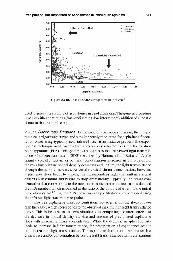
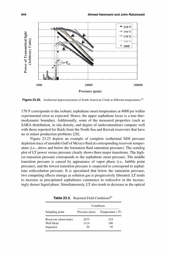
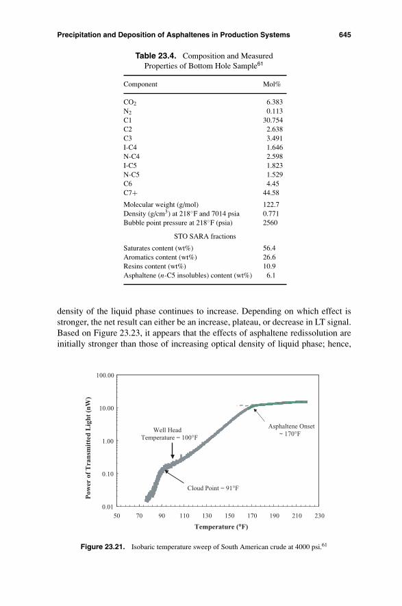
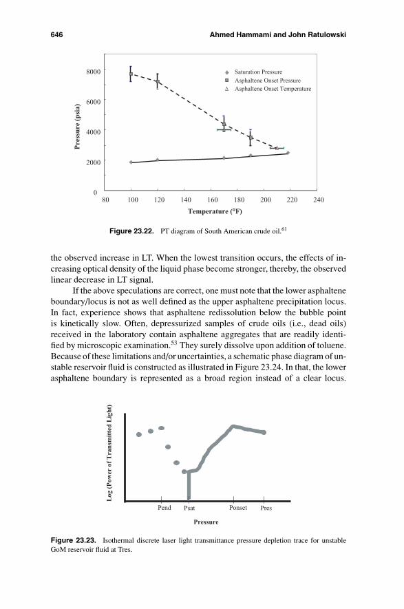
The suitability of this technique for measuring upper asphaltene precipita-tion locus and corresponding saturation curve is demonstrated through exampleFigure 23.20, which shows isothermal light transmittance traces measured forSouth American live oil. The corresponding sampling conditions and formationfluid properties are listed in Tables 23.3 and 23.4, respectively.61 The South Amer-ican crude is barely undersaturated at reservoir conditions. It is deemed to be blackoil as characterized by the C7+ fraction (∼44 mol%) and single stage GOR (∼ 540scf/STB). This fluid is not likely to precipitate asphaltenes during pressure de-pletion at reservoir temperature (i.e., 218◦F). It is, however, prone to precipitateasphaltenes during isobaric temperature sweeps (Figure 23.21) and/or isothermalpressure depletions at lower temperatures. The onset pressure of asphaltene precipi-tation is observed to increase with decreasing temperature. The corresponding SDSdepressurization traces are qualitatively similar to Gulf of Mexico reservoir flu-ids with minor asphaltene precipitation problems. The corresponding PT diagramis provided as Figure 23.22.1,61 Note the isothermal asphaltene onset pressure at
644 Ahmed Hammami and John Ratulowski
1000 10000 100000
Pressure (psia)
Pow
er o
f T
rans
mit
ted
ligh
t(A
rbit
rary
Uni
ts)
218°F
190°F
170°F
120°F
100F
Psat
Figure 23.20. Isothermal depressurization of South American Crude at different temperatures.61
170◦F corresponds to the isobaric asphaltene onset temperature at 4000 psi withinexperimental error as expected. Hence, the upper asphaltene locus is a true ther-modynamic boundary. Additionally, some of the measured properties (such asSARA distribution, in situ density, and degree of undersaturation) compare wellwith those reported for fluids from the North Sea and Kuwait reservoirs that haveno or minor production problems [28].
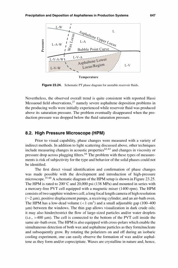
Figure 23.23 depicts an example of complete isothermal SDS pressuredepletion trace of unstable Gulf of Mexico fluid at corresponding reservoir temper-ature (i.e., above and below the formation fluid saturation pressure). The semilogplot of LT power versus pressure clearly shows three major transitions. The high-est transition pressure corresponds to the asphaltene onset pressure. The middletransition pressure is caused by appearance of vapor phase (i.e., bubble pointpressure), and the lowest transition pressure is suspected to correspond to asphal-tene redissolution pressure. It is speculated that below the saturation pressure,two competing effects emerge as solution gas is progressively liberated. LT tendsto increase as precipitated asphaltenes commence to redissolve in the increas-ingly denser liquid phase. Simultaneously, LT also tends to decrease as the optical
Table 23.3. Reported Field Conditions61
Conditions
Sampling point Pressure (psia) Temperature (◦F)
Reservoir (down hole) 2673 218Well Head 1114 100Separator 59 95
Precipitation and Deposition of Asphaltenes in Production Systems 645
Table 23.4. Composition and MeasuredProperties of Bottom Hole Sample61
Component Mol%
CO2 6.383N2 0.113C1 30.754C2 2.638C3 3.491I-C4 1.646N-C4 2.598I-C5 1.823N-C5 1.529C6 4.45C7+ 44.58
Molecular weight (g/mol) 122.7Density (g/cm3) at 218◦F and 7014 psia 0.771Bubble point pressure at 218◦F (psia) 2560
STO SARA fractions
Saturates content (wt%) 56.4Aromatics content (wt%) 26.6Resins content (wt%) 10.9Asphaltene (n-C5 insolubles) content (wt%) 6.1
density of the liquid phase continues to increase. Depending on which effect isstronger, the net result can either be an increase, plateau, or decrease in LT signal.Based on Figure 23.23, it appears that the effects of asphaltene redissolution areinitially stronger than those of increasing optical density of liquid phase; hence,
0.01
0.10
1.00
10.00
100.00
50 70 90 110 130 150 170 190 210 230
Temperature (∞F)
Pow
er o
f T
ran
smit
ted
Lig
ht (
nW)
Cloud Point = 91°F
Well Head Temperature = 100°F
Asphaltene Onset ~ 170°F
Figure 23.21. Isobaric temperature sweep of South American crude at 4000 psi.61
646 Ahmed Hammami and John Ratulowski
0
2000
4000
6000
8000
80 100 120 140 160 180 200 220 240
Temperature (∞F)
Pre
ssur
e (p
sia)
Saturation Pressure
Asphaltene Onset PressureAsphaltene Onset Temperature
Figure 23.22. PT diagram of South American crude oil.61
the observed increase in LT. When the lowest transition occurs, the effects of in-creasing optical density of the liquid phase become stronger, thereby, the observedlinear decrease in LT signal.
If the above speculations are correct, one must note that the lower asphalteneboundary/locus is not as well defined as the upper asphaltene precipitation locus.In fact, experience shows that asphaltene redissolution below the bubble pointis kinetically slow. Often, depressurized samples of crude oils (i.e., dead oils)received in the laboratory contain asphaltene aggregates that are readily identi-fied by microscopic examination.53 They surely dissolve upon addition of toluene.Because of these limitations and/or uncertainties, a schematic phase diagram of un-stable reservoir fluid is constructed as illustrated in Figure 23.24. In that, the lowerasphaltene boundary is represented as a broad region instead of a clear locus.
Log
(P
ower
of
Tra
nsm
itte
d L
ight
)
Pressure
PresPsatPend Ponset
Figure 23.23. Isothermal discrete laser light transmittance pressure depletion trace for unstableGoM reservoir fluid at Tres.
Precipitation and Deposition of Asphaltenes in Production Systems 647
Pre
ssu
re
L-V
L
L-A
L-V-A
L-V-W
L-V-A-W
L-A-W
L-W
Wax
Loc
us
Asphaltene Upper LocusBubble Point Curve
Asphaltene Lower
Locus/Region
Temperature
Figure 23.24. Schematic PT phase diagram for unstable reservoir fluids.
Nevertheless, the observed overall trend is quite consistent with reported HassiMessaoud field observations,27 namely severe asphaltene deposition problems inthe producing wells were initially experienced while reservoir fluid was producedabove its saturation pressure. The problem eventually disappeared when the pro-duction pressure was dropped below the fluid saturation pressure.
8.2. High Pressure Microscope (HPM)
Prior to visual capability, phase changes were measured with a variety ofindirect methods. In addition to light scattering discussed above, other techniquesinclude measuring changes in acoustic properties62,63 and changes in viscosity orpressure drop across plugging filters.64 The problem with these types of measure-ments is risk of subjectivity for the type and behavior of the solid phases could notbe identified.
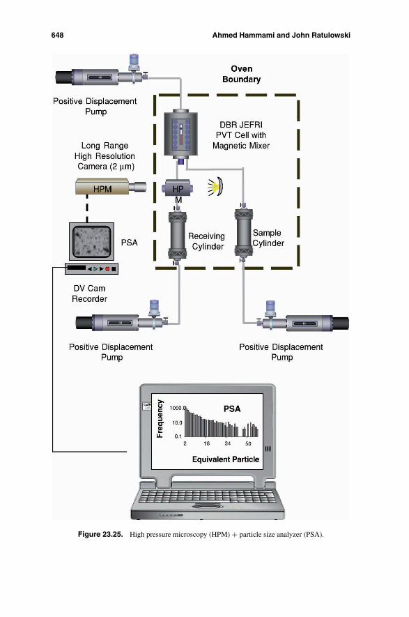
The first direct visual identification and confirmation of phase changeswas made possible with the development and introduction of high-pressuremicroscope.35,60 A schematic diagram of the HPM setup is shown in Figure 23.25.The HPM is rated to 200◦C and 20,000 psi (138 MPa) and mounted in series witha mercury-free PVT cell equipped with a magnetic mixer (1400 rpm). The HPMconsists of two sapphire windows cell, a long focal length camera of high resolution(∼2 μm), positive displacement pumps, a receiving cylinder, and an air-bath oven.The HPM has a low-dead volume (<1 cm3) and a small adjustable gap (100–400μm) between the windows. The thin gap allows visualization in dark crude oils;it may also hinder/restrict the flow of large-sized particles and/or water droplets(i.e., >400 μm). The cell is connected to the bottom of the PVT cell inside thesame air–bath oven. The HPM is also equipped with cross-polars which enable thesimultaneous detection of both wax and asphaltene particles as they form/nucleateand subsequently grow. By rotating the polarizers on and off during an isobariccooling experiment, one can easily observe the formation of wax and/or asphal-tene as they form and/or coprecipitate. Waxes are crystalline in nature and, hence,
648 Ahmed Hammami and John Ratulowski
Figure 23.25. High pressure microscopy (HPM) + particle size analyzer (PSA).
Precipitation and Deposition of Asphaltenes in Production Systems 649
110
1001000
1
100
10000
110
1001000
10000
1 11 21 31 41 51 61 71 81 91 101 111 121
110
1001000
1
100
100001
100
10000
100
100001
100
10000C
ount
Size (μm)
P = 6500 psi
P = 6000 psi
P = 5500 psi
P = 5250 psi
P = 5000 psi
P = 4500 psi
P = 4000 psi
P = 3500 psi
1
Figure 23.26. Sample PSA histograms for a discrete depressurization experiment.
are clearly visible under polarized light; whereas, asphaltene are predominantlyamorphous and visible under normal light mode.
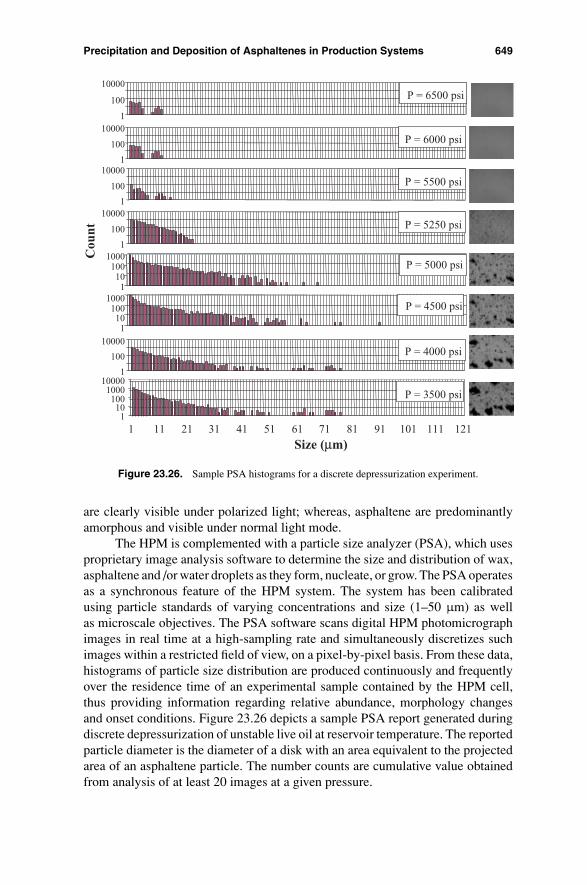
The HPM is complemented with a particle size analyzer (PSA), which usesproprietary image analysis software to determine the size and distribution of wax,asphaltene and /or water droplets as they form, nucleate, or grow. The PSA operatesas a synchronous feature of the HPM system. The system has been calibratedusing particle standards of varying concentrations and size (1–50 μm) as wellas microscale objectives. The PSA software scans digital HPM photomicrographimages in real time at a high-sampling rate and simultaneously discretizes suchimages within a restricted field of view, on a pixel-by-pixel basis. From these data,histograms of particle size distribution are produced continuously and frequentlyover the residence time of an experimental sample contained by the HPM cell,thus providing information regarding relative abundance, morphology changesand onset conditions. Figure 23.26 depicts a sample PSA report generated duringdiscrete depressurization of unstable live oil at reservoir temperature. The reportedparticle diameter is the diameter of a disk with an area equivalent to the projectedarea of an asphaltene particle. The number counts are cumulative value obtainedfrom analysis of at least 20 images at a given pressure.
650 Ahmed Hammami and John Ratulowski
0
50
100
150
200
250
300
1000 3000 5000 7000 9000 11000 13000
Pressure (psia)
Pow
er o
f T
rans
mit
ted
Lig
ht (
pW)
Psat2050 psia
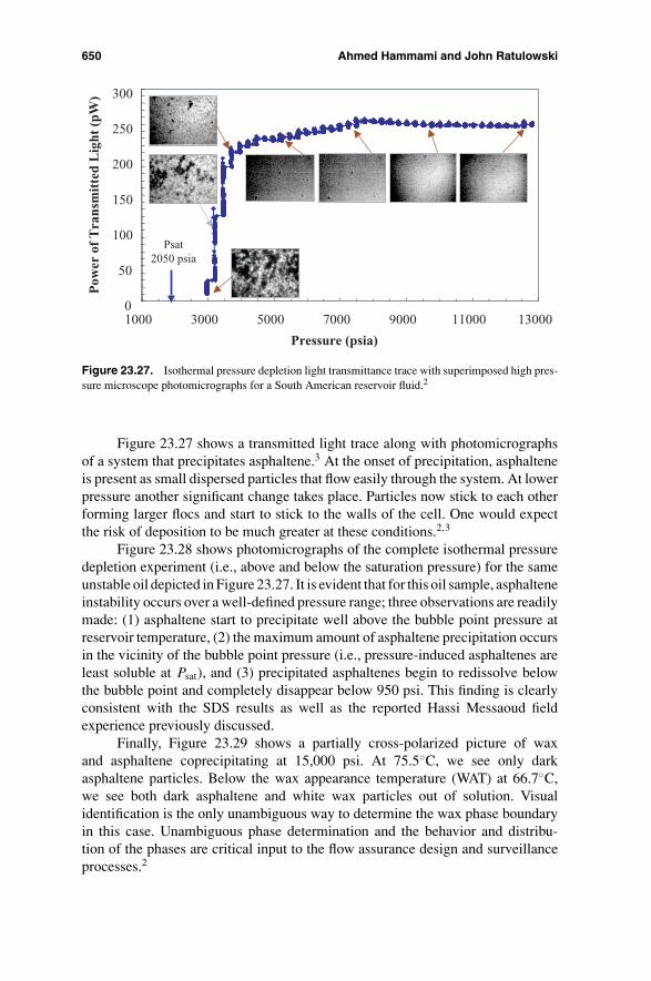
Figure 23.27. Isothermal pressure depletion light transmittance trace with superimposed high pres-sure microscope photomicrographs for a South American reservoir fluid.2
Figure 23.27 shows a transmitted light trace along with photomicrographsof a system that precipitates asphaltene.3 At the onset of precipitation, asphalteneis present as small dispersed particles that flow easily through the system. At lowerpressure another significant change takes place. Particles now stick to each otherforming larger flocs and start to stick to the walls of the cell. One would expectthe risk of deposition to be much greater at these conditions.2,3
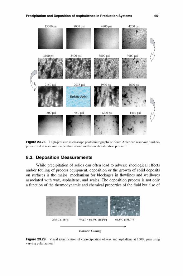
Figure 23.28 shows photomicrographs of the complete isothermal pressuredepletion experiment (i.e., above and below the saturation pressure) for the sameunstable oil depicted in Figure 23.27. It is evident that for this oil sample, asphalteneinstability occurs over a well-defined pressure range; three observations are readilymade: (1) asphaltene start to precipitate well above the bubble point pressure atreservoir temperature, (2) the maximum amount of asphaltene precipitation occursin the vicinity of the bubble point pressure (i.e., pressure-induced asphaltenes areleast soluble at Psat), and (3) precipitated asphaltenes begin to redissolve belowthe bubble point and completely disappear below 950 psi. This finding is clearlyconsistent with the SDS results as well as the reported Hassi Messaoud fieldexperience previously discussed.
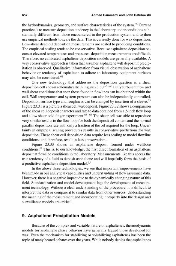
Finally, Figure 23.29 shows a partially cross-polarized picture of waxand asphaltene coprecipitating at 15,000 psi. At 75.5◦C, we see only darkasphaltene particles. Below the wax appearance temperature (WAT) at 66.7◦C,we see both dark asphaltene and white wax particles out of solution. Visualidentification is the only unambiguous way to determine the wax phase boundaryin this case. Unambiguous phase determination and the behavior and distribu-tion of the phases are critical input to the flow assurance design and surveillanceprocesses.2
Precipitation and Deposition of Asphaltenes in Production Systems 651
Bubble Point
13000 psi 8000 psi 4900 psi 4200 psi
3900 psi3600 psi3400 psi3100 psi
2150 psi 1900 psi 1600 psi
1400 psi1200 psi950 psi800 psi
2035 psi
Figure 23.28. High-pressure microscope photomicrographs of South American reservoir fluid de-pressurized at reservoir temperature above and below its saturation pressure.
8.3. Deposition Measurements
While precipitation of solids can often lead to adverse rheological effectsand/or fouling of process equipment, deposition or the growth of solid depositson surfaces is the major mechanism for blockages in flowlines and wellboresassociated with wax, asphaltene, and scales. The deposition process is not onlya function of the thermodynamic and chemical properties of the fluid but also of
75.5 C (168∞F) WAT = 66.7∞C (152∞F) 66.5∞C (151.7∞F)
Isobaric Cooling
Figure 23.29. Visual identification of coprecipitation of wax and asphaltene at 15000 psia usingvarying polarization.2
652 Ahmed Hammami and John Ratulowski
the hydrodynamics, geometry, and surface characteristics of the system.35 Currentpractice is to measure deposition tendency in the laboratory under conditions sub-stantially different from those encountered in the production system and to thenuse empirical methods to scale the data. This is currently done for wax deposition.Low-shear dead oil deposition measurements are scaled to producing conditions.The empirical scaling tends to be conservative. Because asphaltene deposition oc-curs at elevated temperatures and pressures, deposition measurements are difficult.Therefore, no calibrated asphaltene deposition models are generally available. Avery conservative approach is taken that assumes asphaltene will deposit if precip-itation is observed. Qualitative information from visual observation of asphaltenebehavior or tendency of asphaltene to adhere to laboratory equipment surfacesmay also be considered.61
One new technology that addresses the deposition question is a sheardeposition cell shown schematically in Figure 23.30.65−68 Fully turbulent flow andwall shear conditions that span those found in flowlines can be obtained within thecell. Wall temperature and system pressure can also be independently controlled.Deposition surface type and roughness can be changed by insertion of a sleeve.65
Figure 23.31 is a picture a shear cell wax deposit. Figure 23.32 shows a comparisonof the shear cell deposit character and rate to data obtained from a 2-inch flow loopand a low shear cold finger experiment.65−67 The shear cell was able to reproducevery similar results to the flow loop for both the deposit oil content and the normalparaffin deposition rate with only a fraction of the oil required for the loop. Uncer-tainty in empirical scaling procedures results in conservative predictions for waxdeposition. These shear cell deposition data require less scaling to model flowlineconditions; and therefore, result in less conservatism.
Figure 23.33 shows an asphaltene deposit formed under wellboreconditions.68 This is, to our knowledge, the first direct formation of an asphaltenedeposit at flowline conditions in the laboratory. Measurements like this access thetrue tendency of a fluid to deposit asphaltene and will hopefully form the basis ofa predictive asphaltene deposition model.65
In the above three technologies, we see that important improvements havebeen made in our analytical capabilities and understanding of flow assurance data.However, there is a negative impact due to the dynamically changing nature of thisfield. Standardization and model development lags the development of measure-ment technology. Without a clear understanding of the procedure, it is difficult tointerpret the data or compare it to similar data from other sources. Understandingthe meaning of the measurement and incorporating it properly into the design andsurveillance models are critical.
9. Asphaltene Precipitation Models
Because of the complex and variable nature of asphaltenes, thermodynamicmodels for asphaltene phase behavior have generally lagged those developed forwax. Even the mechanism for stabilizing or solubilizing asphaltenes has been thetopic of many heated debates over the years. While nobody denies that asphaltenes
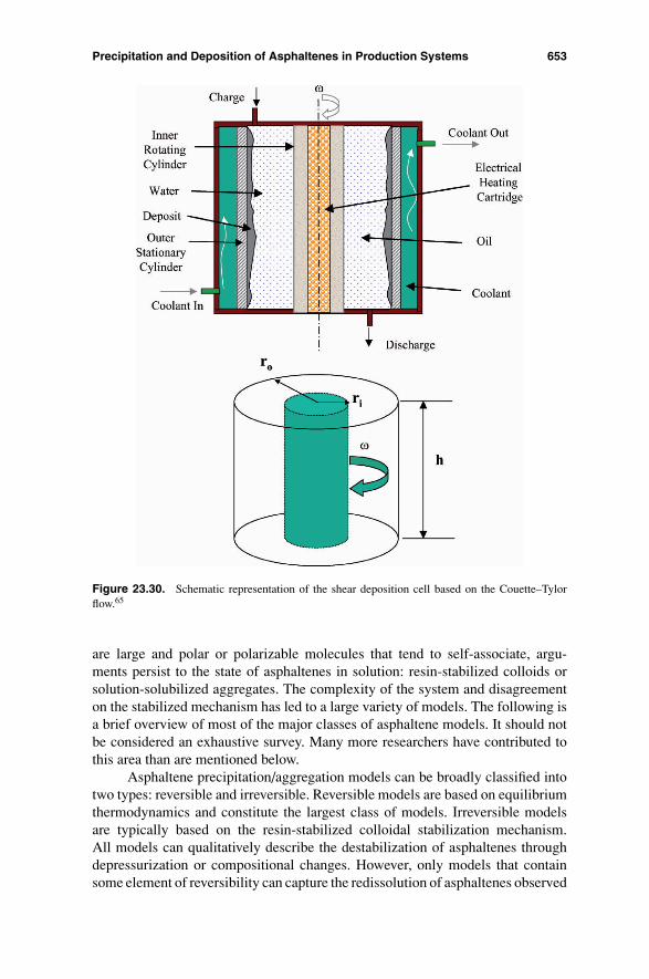
Precipitation and Deposition of Asphaltenes in Production Systems 653
Figure 23.30. Schematic representation of the shear deposition cell based on the Couette–Tylorflow.65
are large and polar or polarizable molecules that tend to self-associate, argu-ments persist to the state of asphaltenes in solution: resin-stabilized colloids orsolution-solubilized aggregates. The complexity of the system and disagreementon the stabilized mechanism has led to a large variety of models. The following isa brief overview of most of the major classes of asphaltene models. It should notbe considered an exhaustive survey. Many more researchers have contributed tothis area than are mentioned below.
Asphaltene precipitation/aggregation models can be broadly classified intotwo types: reversible and irreversible. Reversible models are based on equilibriumthermodynamics and constitute the largest class of models. Irreversible modelsare typically based on the resin-stabilized colloidal stabilization mechanism.All models can qualitatively describe the destabilization of asphaltenes throughdepressurization or compositional changes. However, only models that containsome element of reversibility can capture the redissolution of asphaltenes observed
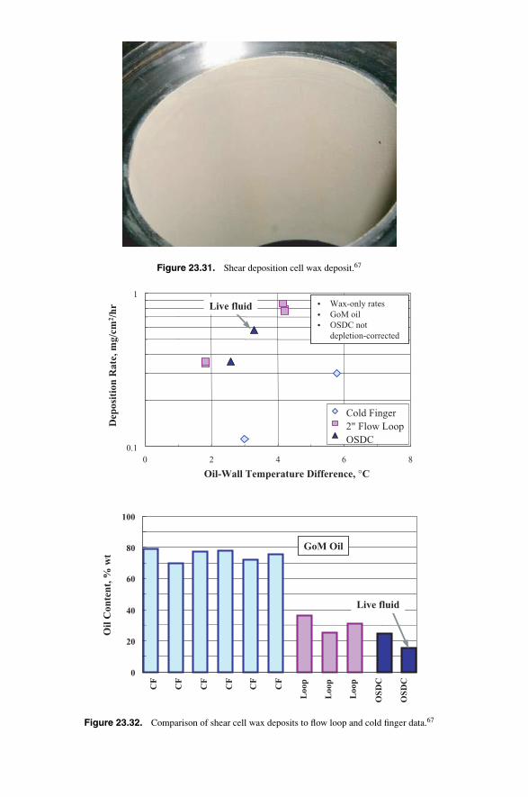
Figure 23.31. Shear deposition cell wax deposit.67
Dep
osit
ion
Rat
e, m
g/cm
2 /hr
Cold Finger2" Flow LoopOSDC
...Wax-only ratesGoM oilOSDC not depletion-corrected
Live fluid1
0.10 2 4 6 8
Oil-Wall Temperature Difference, °C
0
20
40
60
80
100
CF
CF
CF
CF
CF
CF
Loo
p
Loo
p
Loo
p
OSD
C
OSD
C
Oil
Con
tent
, % w
t
GoM Oil
Live fluid
Figure 23.32. Comparison of shear cell wax deposits to flow loop and cold finger data.67
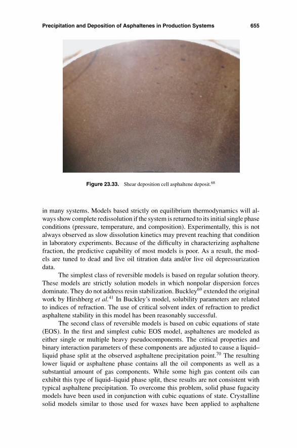
Precipitation and Deposition of Asphaltenes in Production Systems 655
Figure 23.33. Shear deposition cell asphaltene deposit.68
in many systems. Models based strictly on equilibrium thermodynamics will al-ways show complete redissolution if the system is returned to its initial single phaseconditions (pressure, temperature, and composition). Experimentally, this is notalways observed as slow dissolution kinetics may prevent reaching that conditionin laboratory experiments. Because of the difficulty in characterizing asphaltenefraction, the predictive capability of most models is poor. As a result, the mod-els are tuned to dead and live oil titration data and/or live oil depressurizationdata.
The simplest class of reversible models is based on regular solution theory.These models are strictly solution models in which nonpolar dispersion forcesdominate. They do not address resin stabilization. Buckley69 extended the originalwork by Hirshberg et al.41 In Buckley’s model, solubility parameters are relatedto indices of refraction. The use of critical solvent index of refraction to predictasphaltene stability in this model has been reasonably successful.
The second class of reversible models is based on cubic equations of state(EOS). In the first and simplest cubic EOS model, asphaltenes are modeled aseither single or multiple heavy pseudocomponents. The critical properties andbinary interaction parameters of these components are adjusted to cause a liquid–liquid phase split at the observed asphaltene precipitation point.70 The resultinglower liquid or asphaltene phase contains all the oil components as well as asubstantial amount of gas components. While some high gas content oils canexhibit this type of liquid–liquid phase split, these results are not consistent withtypical asphaltene precipitation. To overcome this problem, solid phase fugacitymodels have been used in conjunction with cubic equations of state. Crystallinesolid models similar to those used for waxes have been applied to asphaltene
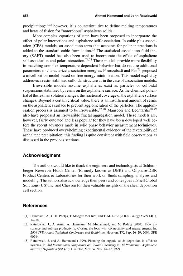
656 Ahmed Hammami and John Ratulowski
precipitation;71,72 however, it is counterintuitive to define melting temperaturesand heats of fusion for “amorphous” asphaltene solids.
More complex equations of state have been proposed to incorporate theeffect of polar interactions and asphaltene self-association. In cubic plus associ-ation (CPA) models, an association term that accounts for polar interactions isadded to the standard cubic formulation.73 The statistical association fluid the-ory (SAFT) model has also been used to incorporate the effect of asphalteneself-association and polar interaction.74,75 These models provide more flexibilityin matching complex temperature-dependent behavior but do require additionalparameters to characterize association energies. Firoozabadi and Pan76 proposeda micellization model based on free energy minimization. This model explicitlyaddresses a resin-stabilized colloidal structure as in the case of association models.
Irreversible models assume asphaltenes exist as particles or colloidalsuspensions stabilized by resins on the asphaltene surface. As the chemical poten-tial of the resin in solution changes, the fractional coverage of the asphaltene surfacechanges. Beyond a certain critical value, there is an insufficient amount of resinson the asphaltenes surface to prevent agglomeration of the particles. The agglom-eration process is assumed to be irreversible.77,78 Mansoori and Leontaritis78,79
also have proposed an irreversible fractal aggregation model. These models are,however, fairly outdated and less popular for they have been developed well be-fore the recent advances made in solid phase behavior measurement techniques.These have produced overwhelming experimental evidence of the reversibility ofasphaltene precipitation; this finding is quite consistent with field observations asdiscussed in the previous sections.
Acknowledgment
The authors would like to thank the engineers and technologists at Schlum-berger Reservoir Fluids Center (formerly known as DBR) and Oilphase-DBRProduct Centers & Laboratories for their work on fluids sampling, analyses andmodeling. The authors also acknowledge their peers and colleagues at Shell GlobalSolutions (US) Inc. and Chevron for their valuable insights on the shear depositioncell section.
References
[1] Hammami, A., C. H. Phelps, T. Monger-McClure, and T. M. Little (2000). Energy Fuels 14(1),14–18.
[2] Ratulowski, J., A. Amin, A. Hammami, M. Muhammad, and M. Riding (2004). Flow as-surance and sub-sea productivity: Closing the loop with connectivity and measurements. In:2004 SPE Annual Technical Conference and Exhibition, Houston, TX, Sept 26–29, 2004, SPE90244.
[3] Ratulowski, J. and A. Hammami (1999). Planning for organic solids deposition in offshoresystems. In: 3rd International Symposium on Colloid Chemistry in Oil Production. Asphalteneand Wax Deposition (ISCOP), Huatelco, Mexico, Nov. 14–17, 1999.
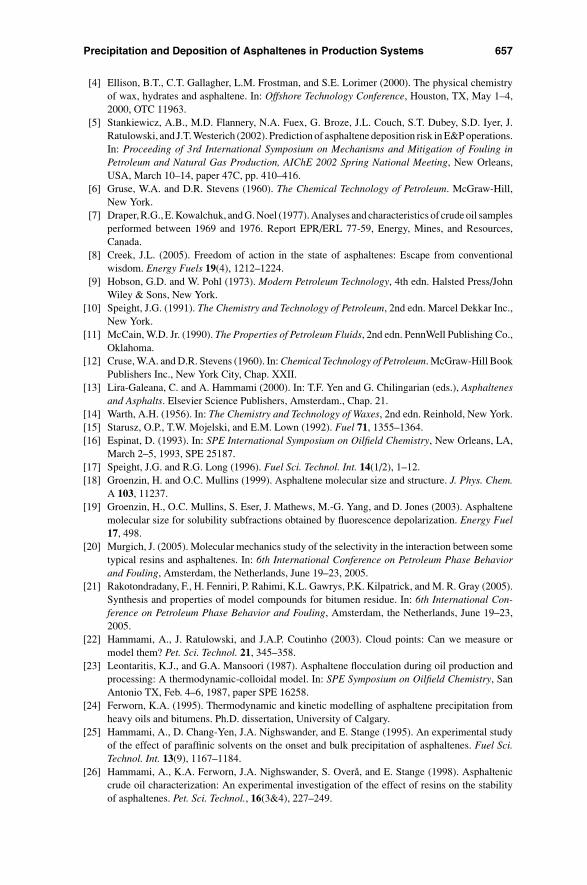
Precipitation and Deposition of Asphaltenes in Production Systems 657
[4] Ellison, B.T., C.T. Gallagher, L.M. Frostman, and S.E. Lorimer (2000). The physical chemistryof wax, hydrates and asphaltene. In: Offshore Technology Conference, Houston, TX, May 1–4,2000, OTC 11963.
[5] Stankiewicz, A.B., M.D. Flannery, N.A. Fuex, G. Broze, J.L. Couch, S.T. Dubey, S.D. Iyer, J.Ratulowski, and J.T. Westerich (2002). Prediction of asphaltene deposition risk in E&P operations.In: Proceeding of 3rd International Symposium on Mechanisms and Mitigation of Fouling inPetroleum and Natural Gas Production, AIChE 2002 Spring National Meeting, New Orleans,USA, March 10–14, paper 47C, pp. 410–416.
[6] Gruse, W.A. and D.R. Stevens (1960). The Chemical Technology of Petroleum. McGraw-Hill,New York.
[7] Draper, R.G., E. Kowalchuk, and G. Noel (1977). Analyses and characteristics of crude oil samplesperformed between 1969 and 1976. Report EPR/ERL 77-59, Energy, Mines, and Resources,Canada.
[8] Creek, J.L. (2005). Freedom of action in the state of asphaltenes: Escape from conventionalwisdom. Energy Fuels 19(4), 1212–1224.
[9] Hobson, G.D. and W. Pohl (1973). Modern Petroleum Technology, 4th edn. Halsted Press/JohnWiley & Sons, New York.
[10] Speight, J.G. (1991). The Chemistry and Technology of Petroleum, 2nd edn. Marcel Dekkar Inc.,New York.
[11] McCain, W.D. Jr. (1990). The Properties of Petroleum Fluids, 2nd edn. PennWell Publishing Co.,Oklahoma.
[12] Cruse, W.A. and D.R. Stevens (1960). In: Chemical Technology of Petroleum. McGraw-Hill BookPublishers Inc., New York City, Chap. XXII.
[13] Lira-Galeana, C. and A. Hammami (2000). In: T.F. Yen and G. Chilingarian (eds.), Asphaltenesand Asphalts. Elsevier Science Publishers, Amsterdam., Chap. 21.
[14] Warth, A.H. (1956). In: The Chemistry and Technology of Waxes, 2nd edn. Reinhold, New York.[15] Starusz, O.P., T.W. Mojelski, and E.M. Lown (1992). Fuel 71, 1355–1364.[16] Espinat, D. (1993). In: SPE International Symposium on Oilfield Chemistry, New Orleans, LA,
March 2–5, 1993, SPE 25187.[17] Speight, J.G. and R.G. Long (1996). Fuel Sci. Technol. Int. 14(1/2), 1–12.[18] Groenzin, H. and O.C. Mullins (1999). Asphaltene molecular size and structure. J. Phys. Chem.
A 103, 11237.[19] Groenzin, H., O.C. Mullins, S. Eser, J. Mathews, M.-G. Yang, and D. Jones (2003). Asphaltene
molecular size for solubility subfractions obtained by fluorescence depolarization. Energy Fuel17, 498.
[20] Murgich, J. (2005). Molecular mechanics study of the selectivity in the interaction between sometypical resins and asphaltenes. In: 6th International Conference on Petroleum Phase Behaviorand Fouling, Amsterdam, the Netherlands, June 19–23, 2005.
[21] Rakotondradany, F., H. Fenniri, P. Rahimi, K.L. Gawrys, P.K. Kilpatrick, and M. R. Gray (2005).Synthesis and properties of model compounds for bitumen residue. In: 6th International Con-ference on Petroleum Phase Behavior and Fouling, Amsterdam, the Netherlands, June 19–23,2005.
[22] Hammami, A., J. Ratulowski, and J.A.P. Coutinho (2003). Cloud points: Can we measure ormodel them? Pet. Sci. Technol. 21, 345–358.
[23] Leontaritis, K.J., and G.A. Mansoori (1987). Asphaltene flocculation during oil production andprocessing: A thermodynamic-colloidal model. In: SPE Symposium on Oilfield Chemistry, SanAntonio TX, Feb. 4–6, 1987, paper SPE 16258.
[24] Ferworn, K.A. (1995). Thermodynamic and kinetic modelling of asphaltene precipitation fromheavy oils and bitumens. Ph.D. dissertation, University of Calgary.
[25] Hammami, A., D. Chang-Yen, J.A. Nighswander, and E. Stange (1995). An experimental studyof the effect of paraffinic solvents on the onset and bulk precipitation of asphaltenes. Fuel Sci.Technol. Int. 13(9), 1167–1184.
[26] Hammami, A., K.A. Ferworn, J.A. Nighswander, S. Overa, and E. Stange (1998). Asphalteniccrude oil characterization: An experimental investigation of the effect of resins on the stabilityof asphaltenes. Pet. Sci. Technol., 16(3&4), 227–249.
658 Ahmed Hammami and John Ratulowski
[27] Haskett, C.E. and M. Tartera (1965). A practical solution to the problem of asphaltene deposits—Hassi Messaoud Field, Algeria. J. Pet. Technol., April 387–391.
[28] de Boer, R.B., K. Leerlooyer, M.R.P. Eigner, and A.R.D. van Bergen (1995). Screening of crudeoils for asphalt precipitation: Theory, practice and the selection of inhibitors. SPE Prod. Facil.,Feb., 55–61.
[29] Kokal, S.L. and S.G. Sayegh (1995). Asphaltenes: The cholesterol of petroleum. In: SPE MiddleEast Oil Show, Bahrain, March 11–14, 1995, paper SPE 29787.
[30] Fuhr, B.J., C. Cathrea, L. Coates, H. Kalra, and A.I. Majeed (1991). Fuel 70, 1293–1297.[31] Andersen, S.I. (1994). Fuel Sci. Technol. Int. 12(1), 51–74.[32] Fotland, P. (1996). Fuel Sci. Technol. Int. 14(1/2), 313–325.[33] Wang, J.X., K.R. Brower, and J.S. Buckley (1999). In: SPE International Symposium on Oilfield
Chemistry, Houston, TX, Feb. 16–19, 1999, SPE 50745.[34] Jamaluddin, A.K.M., T.W. Nazarko, S. Sills, and B.J. Fuhr (1996). Deasphalted oil: A natural
asphaltene solvent. SPE J. Prod. Facil. 11(3), 161–165.[35] Karan, K., A. Hammami, M. Flannery, and A. Stankiewicz (2003). Systematic evaluation of
asphaltene instability and control during production of live oils: A flow assurance study. Pet. Sci.Technol. 21, 629–645.
[36] Joshi, N.B., O.C. Mullins, A. Jamaluddin, J. Creek, and J. McFadden (2001). Asphaltene precip-itation from live crude oils. Energy Fuels 15, 979.
[37] Joshi, N.B., M. Muhammad, J. Creek, and J. McFadden (2003). Flow assurance: A challengingpath to well completions and productivity. In: Offshore Technology Conference, Houston, TX,May 5–8, 2003, OTC 15185.
[38] Ratulowski, J., A. Hammami, M. Muhammad, and J. Creek (1999). Considerations for deter-mination of asphaltene stability and control—Effect of oil bases drilling fluid on the asphalteneprecipitation onset pressure of live reservoir fluids. In. IBC Forum Controlling Hydrates Waxesand Asphaltenes, Aberdeen, UK, Oct. 28–29, 1999.
[39] Pfieffer, J.P. and R.N.J. Saal (1940). J. Phys. Chem. 44, 139–149.[40] Hotier, G. and M. Robin (1983). Rev. L’institut Fr. Pet. 38, 101–120.[41] Hirshberg, A., L.N.J. deJong, B.A. Schipper, and J.G. Meijer (1984). Influence of temperature
and pressure on asphaltene flocculation. SPE J., June, 283–293.[42] Gozalpour, F., A. Danesh, D.-H. Tehrani, A.C. Todd, and B. Tohidi (1999). Predicting reservoir
fluid phase and volumetric behaviour from samples contaminated with oil-based mud. Society ofPetroleum Engineers # 56747, Houston, TX.
[43] Jamaluddin, A.K.M., B. Ross, D. Calder, J. Brown, and M. Hashem (2002). Single-phase bot-tomhole sampling technology. JCPT 41(7), 25–30.
[44] Muhammad, M., M. McFadden, and J. Creek (2003). Asphaltene precipitation from reservoirfluids: Asphaltene solubility and particle size vs. pressure. SPE International Symposium onOilfield Chemistry, Houston, TX, Feb. 5–8, 2003, SPE 80263.
[45] Muhammad, M. et al. (2004). Effect of oil based mud on live fluid asphaltene precipitation pres-sure. In: 5th International Conference on Petroleum Phase Behavior & Fouling, Banff, Alberta,Canada, June 13–17, 2004.
[46] Ratulowski, F.A., J.T. Westrich, and J.J. Sieler (2003). Theoretical and experimental investigationof isothermal compositional grading. In: SPEREE, June, 2003, SPE 84777.
[47] Hammami, A. and M.A. Raines (1999). Paraffin deposition from crude oils: Comparison oflaboratory results to field data. SPE J. 4, 1–10.
[48] Andrews, R.J., G. Beck, K. Castelijns, A. Chen, M.E. Cribbs, F.H. Fadness, J. Irvine-Fortescue,S. Williams, M. Hashem, A. Jamaluddin, A. Kurkjian, B. Sass, O.C. Mullins, E. Rylander, andA. Van Dusen (2001). Quantifying contamination using color of crude and condensate. OilfieldRev. Autumn, 24–43.
[49] Hashem, M.N., E.C. Thomas, R.I. McNeil, and O.C. Mullins (1997). Determination of produciblehydrocarbon type and oil quality in wells drilled with synthetic oil-based muds. Society ofPetroleum Engineers #39093, San Antonio, TX.
[50] Fuhr, B.J., L.R. Holloway, and A. Hammami (1999). Analytical considerations related to as-phaltenes and waxes in the same crudes. Energy Fuels 13, 336–339.
Precipitation and Deposition of Asphaltenes in Production Systems 659
[51] Kaminski, T., H.S. Fogler, N. Wolf, P. Wattana, and A. Mairal (2004). Classification of asphlatenesvia fractionation and the effect of heteroatom content on dissolution kinetics. Energy Fuel 14,25–30.
[52] Asomaning, S. and A.P. Watkinson (1998). Petroleum stability and heteroatom species effects infouling of heat exchangers by asphaltenes. In: AIChE Spring National Meeting 1998, Preprint.
[53] Buckley, J.S. (1996). Microscopic investigation of the onset of asphaltene precipitation. Fuel Sci.Technol. Int. 14, 55–74.
[54] Ferworn, K.A., A.K. Mehrotra, and W.Y. Svrcek (1993). Measurement of asphaltene ag-glomeration from Cold Lake bitumen diluted with n-alkanes. Can. J. Chem. Eng. 71, 699–703.
[55] Wang, J. (2000). Predicting asphaltene flocculation in crude oils. Ph.D. dissertation. New MexicoInstitute of Mining and Technology, Socorro, NM.
[56] Anderson, S.I. (2003). The state of asphaltenes in the region we called CMC! In: 4th InternationalConference on Petroleum Phase Behavior and Fouling, Trondheim, Norway, June 2003.
[57] Long, Y., T. Dabros, H. Hamza, and W.J. Power (2001). Continued slow precipitation of asphaltenefrom aliphatic solvent-diluted bitumen solutions. In: Symposium on Stability and Compatibilityduring Production, Transportation and Refining of Petroleum, Calgary, Alberta, Canada, Sept.17–18, 2001.
[58] Wang, J. and J.S. Buckley (2003). Asphaltene stability in crude oil and aromatic solvent—Theinfluence of oil composition. Energy Fuels 17(6), 1445–1451.
[59] Buckley, J.S., G.H. Hirasaki, Y. Liu, V. Drasek, J. Wang, and B.S. Gill (1998). Asphalteneprecipitation and solvent properties of crude oils. Pet. Sci. Technol. 16(3&4), 251–285.
[60] Karan, K., J. Ratulowski, and P. German (2000). Measurement of waxy crude properties usingnovel laboratory techniques. In: Annual Technical Conference of Society of Petroleum Engineers,Dallas, TX, Oct. 1–4, 2000, SPE paper 62945.
[61] Allenson, S.J., A. Hammami, H. Maeda, and K. Ohno (1999). Control of asphaltene deposition:Laboratory screening and evaluation of asphaltene inhibitors. In: 3rd International Symposiumon Colloid Chemistry in Oil Production. Asphaltene & Wax Deposition (ISCOP’99), Huatelco,Mexico, Nov. 14–17, 1999.
[62] Sivaraman, A., Y.F. Hu, F.B. Thomas, D.B. Bennion, A.K.M. Jamaluddin, and Y.F. Hu (1997).Acoustic resonance: An emerging technology to identify wax and asphaltene precipitation onsetconditions in reservoir fluids. In: 48th Annual Technical Meeting of the Petroleum Society of CIM,Calgary, Alberta, Canada, June 8–11, 1997.
[63] Kabir, C.S. and A.K.M. Jamaluddin (2002). Asphaltene characterization and mitigation in southKuwait’s Marrat reservoir. SPE J. 17(4), 251–258.
[64] Aquino, O., B.E. Gonzales, S.I. Andersen, and C.L. Gaeana (2001). Investigation of inhibitionof asphaltene pressure using bottomhole samples. Energy Fuels 15, 236–240.
[65] Zougari, M., S. Jacobs, A. Hammami, G. Broze, M. Flannery, J. Ratulowski, and A. Stankiewicz(2006). Novel organic solid deposition and control device for live oils: Design and application.Accepted for publication in Energy & Fuels.
[66] Zougari, M., S. Jacobs, A. Hammami, G. Broze, and N. Fuex (2005). Live oils novel organicsolid deposition and control device: Wax deposition validation. In: 14th SPIE Middle East Oil &Gas Show and Conference, Bahrain, March 12–15, 2005, SPE 93558.
[67] Broze, G., P. Cornelisse, M. Zougari, S. Jacobs, A. Hammami, and J. Ratulowski (2003). A com-parison of wax deposition under live and stock-tank conditions. In: 4th International Conferenceon Petroleum Phase Behavior and Fouling, Trondheim, Norway, June 23–26, 2003.
[68] Flannery, M., P. Cornelisse, M. Zougari, and A. Hammami (2003). Asphaltene precipitationand deposition under live oil conditions in a novel experimental device. In: 4th Interna-tional Conference on Petroleum Phase Behavior and Fouling, Trondheim, Norway, June 23–26,2003.
[69] Buckley, J.S. (1999). Predicting the onset of asphaltene precipitation from refractive index mea-surements. Energy Fuels 13, 328–332.
[70] Rydhal, A.K., K.S. Pedersen, and H.P. Hjermstad (1997). In: AICHE Spring National Meeting,Houston, TX, March 1997.
660 Ahmed Hammami and John Ratulowski
[71] MacMillan, D.J., J.E. Tackett Jr., M.A. Jessee, and T.G. Monger-McClure (1995). A unified ap-proach to asphaltene precipitation: Laboratory measurement and modeling. In: SPE InternationalSymposium on Oilfield Chemistry, San Antonio, TX, Feb. 14–17, 1995, SPE paper 28990.
[72] Chung, T-H. Thermodynamic modeling for organic solid precipitation. In: SPE Annual TechnicalConference and Exhibition, Washington, D.C. Oct. 4–7, 1992, SPE 24851.
[73] Edmonds, B., R.A.S. Moorwood, R. Szczepanski, X. Zhang, M. Heyward, and R. Hurle (1999).Measurement and prediction of asphaltene precipitation from live oils. In: 3rd International Sym-posium on Colloid Chemistry in Oil Production, Asphaltenes and Waxes Deposition (ISCOP’99),Mexico, Nov. 1999.
[74] Wu, J., J.M. Prausnitz, and A. Firoozabadi (1998). AIChE J. 44, 1188.[75] Ting P.D., G.J. Hirasaki, and W.G. Chapman (2003). Modeling of asphaltene phase behavior with
the SAFT equation of state. Pet. Sci. Technol. 21, 647–661.[76] Pan, H. and A. Firoozabadi. Thermodynamic micellization model for asphaltene precipitation
from reservoir crudes at high pressures and temperatures. In: SPE Annual Technical Conferenceand Exhibition, Oct. 5–8, 1997, San Antonio, TX, SPE 38857.
[77] Takhar, S., P.D. Ravenscroft, and D.C.A. Nicholl (1995). Prediction of asphaltene deposition dur-ing production—Model description and experimental details. In: European Formation DamageConference, The Hague, Netherlands, May 15–16, 1995, SPE 30108.
[78] Mansoori, G.A. (1994). The occurrance of asphaltene throughout production cycle: A com-prehensive description of mechanism and factors influencing heavy organic deposition. In: 6thInternational Petroleum Exhibition and Conference, Abu Dhabi, Oct. 16–19, 1994, paper ADSPE# 2. pp. 282–292.
[79] Leontaritis, K.J. and G.A. Mansoori (1987). Asphaltene flocculation during Oil production andprocessing: A thermodynamic-colloidal model. In: SPE International Symposium on OilfieldChemistry, San Antonio, TX, Feb. 4–6, 1987, paper SPE 16258.