�����������������

Citation: Rodriguez-Sotelo, D.;

Rodriguez-Licea, M.A.; Araujo-Vargas,

I.; Prado-Olivarez, J.; Barranco-

Gutierrez, A.-I.; Perez-Pinal, F.J. Power

Losses Models for Magnetic Cores: A

Review. Micromachines 2022, 13, 418.

https://doi.org/10.3390/mi13030418

Academic Editor: Jürgen J. Brandner

Received: 3 February 2022

Accepted: 25 February 2022

Published: 7 March 2022

Publisher’s Note: MDPI stays neutral

with regard to jurisdictional claims in

published maps and institutional affil-

iations.

Copyright: © 2022 by the authors.

Licensee MDPI, Basel, Switzerland.

This article is an open access article

distributed under the terms and

conditions of the Creative Commons

Attribution (CC BY) license (https://

creativecommons.org/licenses/by/

4.0/).

micromachines

Review

Power Losses Models for Magnetic Cores: A ReviewDaniela Rodriguez-Sotelo 1,† , Martin A. Rodriguez-Licea 2,† , Ismael Araujo-Vargas 3 , Juan Prado-Olivarez 1 ,Alejandro-Israel Barranco-Gutiérrez 1 and Francisco J. Perez-Pinal 1,*,†

1 Tecnológico Nacional de México, Instituto Tecnológico de Celaya, Antonio García Cubas Pte. 600,Celaya 38010, Mexico; d1903002@itcelaya.edu.mx (D.R.-S.); juan.prado@itcelaya.edu.mx (J.P.-O.);israel.barranco@itcelaya.edu.mx (A.-I.B.-G.)

2 CONACYT, Tecnológico Nacional de México, Instituto Tecnológico de Celaya, Antonio García Cubas Pte. 600,Celaya 38010, Mexico; martin.rodriguez@itcelaya.edu.mx

3 Escuela Superior de Ingeniería Mecánica y Eléctrica (ESIME), Unidad Culhuacán, Instituto PolitécnicoNacional, Mexico City 04260, Mexico; iaraujo@ipn.mx

* Correspondence: francisco.perez@itcelaya.edu.mx† These authors contributed equally to this work.

Abstract: In power electronics, magnetic components are fundamental, and, unfortunately, representone of the greatest challenges for designers because they are some of the components that lead theopposition to miniaturization and the main source of losses (both electrical and thermal). The useof ferromagnetic materials as substitutes for ferrite, in the core of magnetic components, has beenproposed as a solution to this problem, and with them, a new perspective and methodology inthe calculation of power losses open the way to new design proposals and challenges to overcome.Achieving a core losses model that combines all the parameters (electric, magnetic, thermal) neededin power electronic applications is a challenge. The main objective of this work is to position thereader in state-of-the-art for core losses models. This last provides, in one source, tools and techniquesto develop magnetic solutions towards miniaturization applications. Details about new proposals,materials used, design steps, software tools, and miniaturization examples are provided.

Keywords: core losses methods; power losses; ferromagnetic material; inductors; transformers

1. Introduction

It is a fact that magnetic components are an essential part of our lives. We can find themin almost anything of quotidian use, from simple things such as cell phone charges [1] toTVs and home appliances. However, they have become more relevant in the developmentof electric and hybrid vehicles, electric machines [2], renewable energy systems [3–6],and recently in implanted electronics [7,8] to open the possibility to micro-scale neuralinterfaces [9]. Inside these devices and systems, a power stage is conformed by magneticand electronic components.

A few years ago, these power stages used to be bigger and heavier, and they hadconsiderable energy losses making them less efficient. Nowadays, silicon carbide (SiC) andgallium nitride (GaN) switching devices have improved power electronics, making themsmaller and faster [10,11]. Notwithstanding, magnetic components oppose miniaturization;these remain stubbornly large and lossy [12]. In a modern power converter, magneticsare approximately half of the volume and weight , and they are the main source of powerlosses [13,14].

The trend in power electronics has two explicit purposes for the design of magneticcomponents. The former is to make maximum use of magnetics capabilities, achievingmultiple functions from a single component [12]. The latter consists of minimizing thesize of magnetic components substituting ferrite (the leading material in their fabrication)with ferromagnetic materials [15]. Those materials have a higher saturation point thanferrite, high permeability and are based on iron (Fe) and metallic elements (Si, Ni, Cr, and

Micromachines 2022, 13, 418. https://doi.org/10.3390/mi13030418 https://www.mdpi.com/journal/micromachines

Micromachines 2022, 13, 418 2 of 27

Co). Some examples of these kinds of material are Fe-Si alloys, powder cores, amorphousmaterials, and nanocrystal material [16–18].

The design of magnetic components is the key to achieving two purposes. The designparameters are intimately dependent on geometric structure, excitation conditions, andmagnetic properties such as power losses that determine if a core magnetic is suitable to bepart of a magnetic component [19]. Power losses in magnetic components are importantdesign parameters; which limit many high-frequency designs.

Power losses in a magnetic component are divided into two core power losses andwinding power losses. Core power losses are related to the selection of the material to makethe core of inductors and transformers; in this case, parameters such as frequency operatingrange, geometric shape, volume, weight, temperature operating range, magnetic saturationpoint, and relative permeability must be considered [20]. On the other hand, windinglosses are related to phenomena such as skin effect, direct current (DC) and alternatingcurrent(AC) resistance in a conductor, and proximity effect [19,21,22]. Those phenomenaincrease the volume of a winding structure [23]. One way to overcome this kind of loss isby using Litz wire [24].

Nowadays, there are several models for studying, predicting, and analyzing the powerlosses in the ferromagnetic cores of magnetic components. However, many of them havebeen developed to work in a limited frequency range , temperature and low magneticflux [25]. Usually, the ferromagnetic cores’ manufacturers provide the graphs of the corelosses in their datasheets, which it is commonly obtained with sinusoidal signal tests andfor specific values of frequency ( f ) and magnetic flux (B) [26].

There are many ways to calculate the power losses in magnetic materials. The originalSteinmetz equation is one of them; however, to the best of the author’s knowledge, it is notalways the best option. In the author’s opinion, selecting a method to calculate power corelosses must be based on its versatility to vary their measurement’s parameters [27].

This document aims to provide the reader with a general panorama about the corepower losses in ferromagnetic materials, emphasising the diverse models found in the liter-ature, announcing their characteristics, advantages, and limitations. Besides, it will presenta relationship about magnetic materials and tested models. Any magnetic componentdesigner must know the basic methods, core losses’ models, the conditions at which theyare valid, and their mathematical fundamentals. Magnetic and thermal losses, calculusand modelling are open research areas due to the non-linear features of ferromagneticmaterials, the complexity of developing a unique power core losses model for the overallferromagnetic materials, and their respective validations.

The organization of this work consists of the following sections. In Section 2, the readerwill find information about the characteristics of each ferromagnetic material. Losses inmagnetic components are reviewed in Section 3. In Section 4, general core losses models arementioned as empirical core losses proposals. Features of Finite Element Method softwareare given in Section 5. The design process of a magnetic component is discussed in Section 6;on the other hand, the importance of the core losses methods in miniaturization of magneticdevices is summarized in Section 7. The discussion of this work is presented in Section 8,and finally, in Section 9, conclusions are provided.

2. Ferromagnetic Alloys

Ferromagnetic materials are exciting materials, where several of their physical proper-ties and chemical micro-structure allow being controlled. Susceptibilities, permeabilities,the shape of the hysteresis loop, power loss, coercivity, remanence, and magnetic inductionare some examples of no intrinsic properties [18]. The saturation magnetization and theCurie temperature are the only intrinsic properties [17,18].

The magnetic behavior is ruled by the dipole moments’ interaction of their atomswithin an external magnetic field [28]. Ferromagnetic materials have strong magneticproperties due to their magnetic moments that tend to line up easily along an outwardmagnetic field direction [29]. These materials also have the property of remaining partially

Micromachines 2022, 13, 418 3 of 27

magnetized even when the external magnetic field is removed; this means that they canquickly change their magnetic polarization by applying a small field. Ferromagneticmaterials are also profitable materials due to being composed by Fe, one of the eight moreabundant elements on Earth [30].

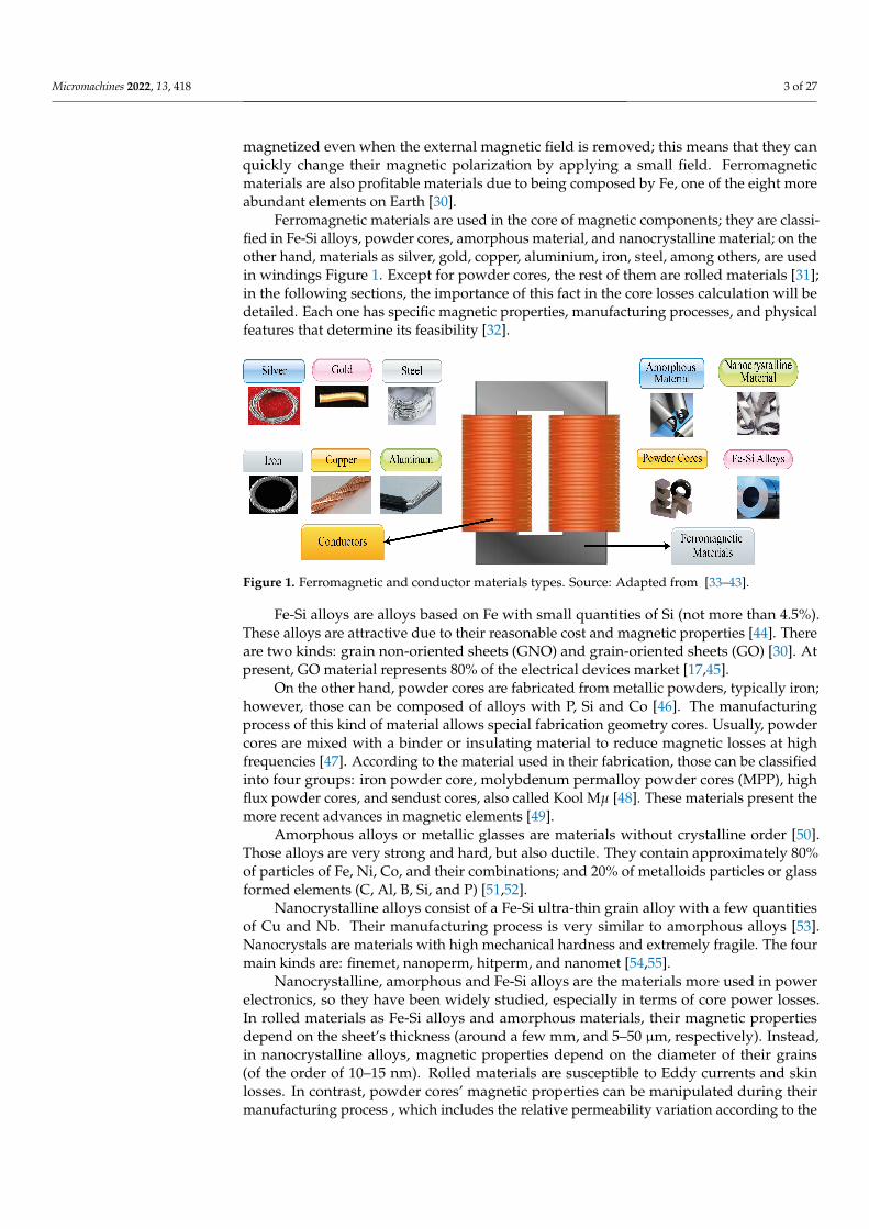
Ferromagnetic materials are used in the core of magnetic components; they are classi-fied in Fe-Si alloys, powder cores, amorphous material, and nanocrystalline material; on theother hand, materials as silver, gold, copper, aluminium, iron, steel, among others, are usedin windings Figure 1. Except for powder cores, the rest of them are rolled materials [31];in the following sections, the importance of this fact in the core losses calculation will bedetailed. Each one has specific magnetic properties, manufacturing processes, and physicalfeatures that determine its feasibility [32].

Figure 1. Ferromagnetic and conductor materials types. Source: Adapted from [33–43].

Fe-Si alloys are alloys based on Fe with small quantities of Si (not more than 4.5%).These alloys are attractive due to their reasonable cost and magnetic properties [44]. Thereare two kinds: grain non-oriented sheets (GNO) and grain-oriented sheets (GO) [30]. Atpresent, GO material represents 80% of the electrical devices market [17,45].

On the other hand, powder cores are fabricated from metallic powders, typically iron;however, those can be composed of alloys with P, Si and Co [46]. The manufacturingprocess of this kind of material allows special fabrication geometry cores. Usually, powdercores are mixed with a binder or insulating material to reduce magnetic losses at highfrequencies [47]. According to the material used in their fabrication, those can be classifiedinto four groups: iron powder core, molybdenum permalloy powder cores (MPP), highflux powder cores, and sendust cores, also called Kool Mµ [48]. These materials present themore recent advances in magnetic elements [49].

Amorphous alloys or metallic glasses are materials without crystalline order [50].Those alloys are very strong and hard, but also ductile. They contain approximately 80%of particles of Fe, Ni, Co, and their combinations; and 20% of metalloids particles or glassformed elements (C, Al, B, Si, and P) [51,52].

Nanocrystalline alloys consist of a Fe-Si ultra-thin grain alloy with a few quantitiesof Cu and Nb. Their manufacturing process is very similar to amorphous alloys [53].Nanocrystals are materials with high mechanical hardness and extremely fragile. The fourmain kinds are: finemet, nanoperm, hitperm, and nanomet [54,55].

Nanocrystalline, amorphous and Fe-Si alloys are the materials more used in powerelectronics, so they have been widely studied, especially in terms of core power losses.In rolled materials as Fe-Si alloys and amorphous materials, their magnetic propertiesdepend on the sheet’s thickness (around a few mm, and 5–50 µm, respectively). Instead,in nanocrystalline alloys, magnetic properties depend on the diameter of their grains(of the order of 10–15 nm). Rolled materials are susceptible to Eddy currents and skinlosses. In contrast, powder cores’ magnetic properties can be manipulated during theirmanufacturing process , which includes the relative permeability variation according to the

Micromachines 2022, 13, 418 4 of 27

magnetic field intensity, high saturation point, fringing flux elimination, soft saturation,among others.

3. Losses in Magnetic Components

To any magnetic component designer, a real challenge to overcome is getting a mag-netic component with high efficiency, small size, low cost, convenience, and low losses [56].Usually, losses are the common factor in all requirements announced before; losses are themost difficult challenges to beat in a magnetic component.

Losses in a magnetic component are divided in two groups: core losses and windinglosses (also called copper losses), [57]. Figure 2 shows each one of them, as well as theircausing phenomena, methods, models, techniques and elements associated with them;nonetheless, phenomena such as the fringing effect and the flux linkage many times are notconsidered in the losses model. Still, they are necessary to achieve a complete losses modelin any magnetic component.

Figure 2. Types and classification of losses presented on magnetic components. Source: Adaptedfrom [58].

Current windings generate the flux linkage density; therefore, it is the sum of theflux enclosed of each one of the turns wound around the core, the flux linkage linkedthem [50,59]. Flux linkage depends on the conductor’s geometry and the quantity of fluxcontained in it. In the gap between windings is the maximum flux linkage [60–62].

Otherwise, the fringing effect is the counterpart of flux linkage; this is, the fringingeffect is presented around the air gap instead of the windings of the magnetic component.This phenomenon depends on core geometry and core permeability, to higher permeabilitythe fringing effect is low [50].

The copper losses are caused by the flow of DC and AC through the windings of amagnetic component, where losses always are more significant for AC than DC [63,64].The circulating current in the windings generates Eddy phenomena as Eddy currents, skineffect loss and, proximity effect loss.

The skin effect and the proximity effect loss are linked to the conductor size, frequency,permeability and distance between winding wires. For the first of them, the currentdistribution trough the cross-area of the wire will define the current density in it. The skineffect and the proximity effect loss are linked to the winding wires. For the first of them,the current distribution through the cross-area of the wire will define the current densityin it. It means that the conductor will have a uniform distribution for DC, higher on itssurface and lower in its center for AC distribution [65].

Micromachines 2022, 13, 418 5 of 27

The proximity effect is similar to the skin effect, but in this case, it is generated by thecurrent carried nearby conductors [50,65]. Eddy currents are induced in a wire in this kindof loss due to a variant magnetic field in the vicinity of conductors at high frequency [46,66].

The Litz wire and interleaved windings help minimize winding losses in magneticcomponents, both are widely used currently. Indeed, interleaved windings are very efficientin high-frequency planar magnetics [67,68].

On the other hand, core losses directly depend on the intrinsic and extrinsic corematerials’ characteristics. Core losses are related to hysteresis loop, Eddy currents, andanomalous or residual losses. Without matter, the core losses model chosen by the magneticcomponent designer will be based on those three primary losses; core loss models willbe detailed in the next section. Besides, core losses depend on the core’s geometry andthe core intrinsic properties’ such as permeability, flux density, Curie temperature, amongothers [69–71]. Many methods and models have been developed; all of them have thepredominant interest in studying, analyzing and understanding those kinds of losses toimprove the magnetic components’ performance.

4. General Core Losses Models

In a magnetic component, the core is the key to determine its magnetic properties andperformance [72]. So to achieve an optimal magnetic component’s performance, the corelosses effects must be characterized [73].

Core loss depends on many aspects that must be considered [74,75]:

• Relative permeability.• Magnetic saturation point.• Temperature operation range.• AC excitation frequency and amplitude.• Voltages’ waveform.• DC bias.• Magnetization process.• Peak-to-peak value of magnetic flux density.

In the case of the magnetization process, some factors are instantaneous values andtime variation values. While to waveform’s topic, the duty ratio of the excitation waveformalso influence the core loss [76,77].

Generally, the core loss is provided at a specific frequency and a maximum fluxdensity [78]. The variation frequency effect in ferromagnetic materials is related to Eddycurrents and the wall-domain displacement [72].

Core losses in ferrimagnetic and ferromagnetic materials are similar. Both have lossesdue to Eddy currents, hysteresis, and anomalous; however, there are differences concerningflux density, magnetization process, and hysteresis loop shape that define the magneticbehavior of each one.

The hysteresis is one of the principal features of ferromagnetic materials; it describesthe internal magnetization of magnetic components as a function of external magnetizingforce and magnetization history [79]. The source of hysteresis loss is the domain wallmovement and the magnetic domains’ reorientations [80,81].

The hysteresis loss is defined as power loss in each cycle of magnetization and demag-netization into a ferromagnetic material [82]. If a magnetic sample is excited from zero tothe maximum field value and later comes back at the initial field’s value, it will be observedthat the power returned is lower than the supplied it [83,84].

The loss is proportional to the area surrounded by the upper and lower traces of thehysteresis curve; it represents the per cycle loss and it is proportional to f · B2 [82]. However,if the curve’s shape remains equal for each successive excitation, the loss power will be theproduct of the core’s area and the applied frequency [80,82].

The hysteresis loops give a lot of information about the magnetic properties [72]. Anaccurate way to calculate core loss is by measuring the full hysteresis curve [85].

Micromachines 2022, 13, 418 6 of 27

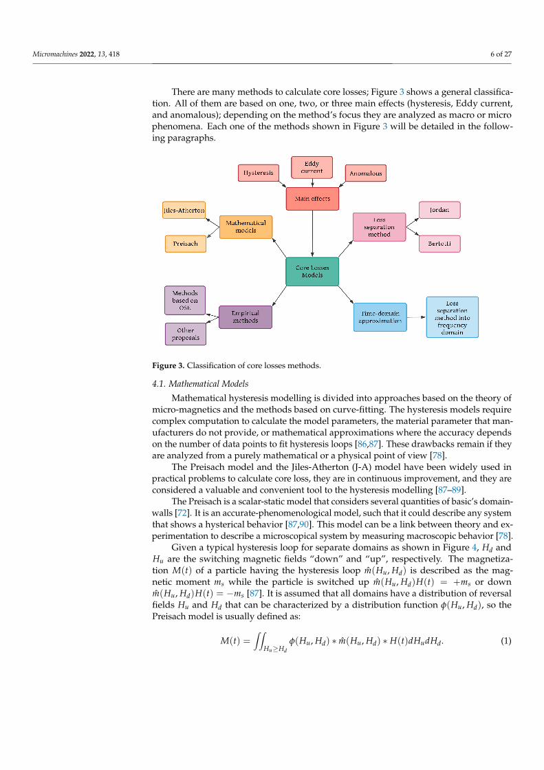
There are many methods to calculate core losses; Figure 3 shows a general classifica-tion. All of them are based on one, two, or three main effects (hysteresis, Eddy current,and anomalous); depending on the method’s focus they are analyzed as macro or microphenomena. Each one of the methods shown in Figure 3 will be detailed in the follow-ing paragraphs.

Figure 3. Classification of core losses methods.

4.1. Mathematical Models

Mathematical hysteresis modelling is divided into approaches based on the theory ofmicro-magnetics and the methods based on curve-fitting. The hysteresis models requirecomplex computation to calculate the model parameters, the material parameter that man-ufacturers do not provide, or mathematical approximations where the accuracy dependson the number of data points to fit hysteresis loops [86,87]. These drawbacks remain if theyare analyzed from a purely mathematical or a physical point of view [78].

The Preisach model and the Jiles-Atherton (J-A) model have been widely used inpractical problems to calculate core loss, they are in continuous improvement, and they areconsidered a valuable and convenient tool to the hysteresis modelling [87–89].

The Preisach is a scalar-static model that considers several quantities of basic’s domain-walls [72]. It is an accurate-phenomenological model, such that it could describe any systemthat shows a hysterical behavior [87,90]. This model can be a link between theory and ex-perimentation to describe a microscopical system by measuring macroscopic behavior [78].

Given a typical hysteresis loop for separate domains as shown in Figure 4, Hd andHu are the switching magnetic fields “down” and “up”, respectively. The magnetiza-tion M(t) of a particle having the hysteresis loop m(Hu, Hd) is described as the mag-netic moment ms while the particle is switched up m(Hu, Hd)H(t) = +ms or downm(Hu, Hd)H(t) = −ms [87]. It is assumed that all domains have a distribution of reversalfields Hu and Hd that can be characterized by a distribution function φ(Hu, Hd), so thePreisach model is usually defined as:

M(t) =∫∫

Hu≥Hd

φ(Hu, Hd) ∗ m(Hu, Hd) ∗ H(t)dHudHd. (1)

Micromachines 2022, 13, 418 7 of 27

Figure 4. Hysteresis loop of (a) an oriented magnetic domain, (b) a multidomain particle of a 3C90Epcos ferrite core at 500 Hz and 28.5 ◦C. Source: Adapted from [91].

A drawback of the Preisach model is the several measurement data to adapt it tothe B-H environment’s changes [72]. Nonetheless, it can track complex magnetizationprocesses and minor loops [78].

On the other hand, the J-A model requires solving a strongly non-linear system ofequations, with five scalar parameters, which are determined in an experimental way; thisis, measuring the hysteresis loop [92]. This model predicts the major hysteresis loops underquasi-static conditions, besides there is a dynamic conditions version in which eddy currentloss, DC-bias fields, anisotropy, and minor loops are included [86,93].

The J-A model is described as the sum of reversible Mrev and irreversible Mirr magne-tizations, hence, the total magnetization M is:

M = Mirr + Mrev (2)

dMrev

dH= c(

dMan

dH− dMirr

dH

)(3)

dMirrdH

=Man −Mirr

δx/µ0 − αic(Man −Mirr)(4)

Man = Ms

(coth

He f f

as− as

He f f

)(5)

He f f = H + αic M. (6)

In these equations, c is the reversibility coefficient, αic is the inter-domain coupling, δindicates the direction for magnetizing field (δ = 1 for the increasing field, and δ = −1 fordecreasing field), x is the Steinmetz loss coefficient, Ms is the saturation magnetization, Manis anhysteretic magnetization, He f f is the effective field, H is the magnetic field, µ0 is thepermeability in free-space, and as is the shape parameter for anhysteretic magnetization [73].A drawback of the J-A model is the computing time and the computing resources to solve astrongly non-linear system.

On the other hand, Eddy’s losses are produced due to changing magnetic fields insidethe analyzed core. These fast changes generate circulating peak currents into it, in the formof loops, generating losses measured in joules [94].

These losses depend on the actual signal shape instead of only the maximum valueof the density flux. The power loss is proportional to the area of the measured loops andinversely proportional to the resistivity of the core material [50,94].

Eddy currents are perpendicular to the magnetic field axis and domain at high-frequency, as well, they are proportional to the frequency. This phenomenon can be

Micromachines 2022, 13, 418 8 of 27

treated as a three-dimensional character or in a simplified way [95]. In a magnetic circuit,Eddy currents cause flux density changes in specific points of its cross-section [96].

One way to describe the Eddy currents distribution is based on Maxwell’s equa-tions [95,97]. In practice, especially on higher frequencies, there is a difference in themeasured total loss between the sum of the hysteresis loss and the Eddy current loss; thisdifference is known as anomalous or residual losses [13]. The effect of temperature and therelaxation phenomena are enclosed in this category [82].

4.2. Time-Domain Approximation Models

For the time-domain model, the loss separation method is used in the frequencydomain, using Fast Fourier Transform (FFT) [13].

Time-domain approximation (TDA) can be used for sinusoidal and non-sinusoidalmagnetic flux density; however, it is only valid for linear systems [98]. The losses arecalculated considering each frequency, separately, and adding them later [85,98].

Pc =∞

∑n=1

π( f n)BnHn sin φn. (7)

According to Equation (7), time-domain approximation is a function of the fundamen-tal frequency f , the peak values of the nth harmonic of the magnetic field H and magneticflux density B, and φn the angle between Bn and Hn.

When a pulse width modulation (PWM) is induced in a magnetic component madewith non-linear material, a non-sinusoidal ripple is generated [93]. Fourier’s core lossdecomposition accuracy is not acceptable for non-sinusoidal flux densities and it is limitedfor frequencies > 400 Hz, as it was reported in [99].

4.3. Loss Separation Models

The loss separation method (LSM) is well-known, accurate and straightforward inmany applications [94]. It defines the core loss (PC) under a dynamic magnetic excitationas the sum of three components: the hysteresis loss (Ph), the Eddy current loss (Peddy) andthe residual or anomalous loss (Panom) [82] is given by:

Pc = Ph + Peddy + Panom. (8)

According to Equation (8), the power loss per unit volume is the sum of a hysteresisand dynamic contribution; Eddy currents and residual loss are part of the latest one [100].

The loss separation method was proposed in 1924 by Jordan, which describes thecore losses as the sum of the hysteresis loss (or static loss) and the Eddy loss (or dynamicloss) [98]

Pc = kh f Bs + keddy f 2B2s . (9)

Years later, Bertotti extended Jordan’s proposal, adding an extra term to calculateresidual losses. G. Bertotti is the maximum exponent in the loss separation methods; histheory provides a solid physical background. The total power loss can be calculated atany magnetizing frequency as the sum of three components [44]. This is show in thefollowing equation

Pc = kh f Bxs + keddy f 2B2

s + kanom f 1.5B1.5s , (10)

where kh, kc, kanom are the hysteresis, Eddy currents, and anomalous coefficients, respec-tively. The hysteresis coefficient decreases if the magnetic permeability increase. Thefrequency is represented by f , while x is the Steinmetz coefficient and has values between1.5 and 2.5, according to the permeability of the material. Finally, Bs is the peak value of theflux density amplitude [23,100].

Micromachines 2022, 13, 418 9 of 27

From Equation (10), Bertotti defined eddy currents and anomalous losses inEquations (11) and (12), respectively, for lamination materials.

Peddy =π2d2 f 2B2

sρβ

(11)

Panom = 8

√GAV0

ρB1.5

s√

f , (12)

where G is about 0.2, ρ is the electrical resistivity, d is the lamination thickness, A isthe cross sectional area of the lamination, β is the magnetic induction exponent, G isa dimensionless coefficient of Eddy current, and V0 is a parameter that characterizesthe statistical distribution of the magnetic objects responsible for the anomalous eddycurrents [101]. However, this method only provides average information, so it is not ableto calculate core loss under harmonic excitation [94]. Still, it can calculate core loss undersquare waveforms considering DC bias [102].

4.4. Empirical Models

A big group of empirical models is based on a simple power-law equation, whichwas proposed in 1982 by Charles Steinmetz to calculate hysteresis loss without includingthe frequency relation [103]. This equation is known as the Steinmetz equation or originalSteinmetz equation (OSE),

POSE = k f αBβs , (13)

where POSE is the time-average core loss per unit volume, Bs the peak induction of thesinusoidal excitation, k is a material parameter, α, and β are the frequency and magneticinduction exponents, respectively, often referred to as Steinmetz parameters [76]. Typicallyα is a number between 1 and 2, and β is typically between 1.5 and 3 [104].

The Steinmetz parameters can be determined from a double logarithm plot by lin-ear curve fitting of the measured core loss data. Therefore Equation (13) assumes onlysinusoidal flux densities with no DC bias [76,77,98,105].

In modern power electronics applications, sinusoidal-wave voltage excitation is notpractical because many of them, like power converters, require square-wave voltage excita-tion [106]. Therefore, a square waveform’s core loss can be lower than the sinusoidal-wave’slosses for the same peak flux density and the same frequency [76,107].

To overcome the aforementioned situation, modifications to OSE have been made.The result was the developing Modified Steinmetz Equation(MSE) [108], General Stein-metz Equation (GSE) [109], Doubly Improved Steinmetz Equation (Improved-ImprovedSteinmetz Equation, i2GSE) [110], Natural Steinmetz Equation (NSE) [85], and Waveform-Coefficient Steinmetz Equation (WcSE) [111]. It is important to mention that the OSEs’sconstants α, β, and k remain in those expressions.

Modified Steinmetz Equation was the first modification proposed to calculate core losswith non-sinusoidal excitation, incorporating into OSE the influence of a magnetizationrate. MSE is proposed in [112] as follows

PMSE = (k f α−1eq Bβ

s ) fr (14)

feq =2

∆B2π2

∫ T

0

(dB(t)

dt

)2

dt,

where fr is the periodic waveform fundamental frequency, feq is the frequency equivalent,∆B is the magnetic induction peak to peak, and dB(t)/dt is the core loss magnetization rate.

A drawback of Equation (14) is that its accuracy decreases with the increasing of wave-form harmonics, and for waveforms with a small fundamental frequency part [77,85,113].

Micromachines 2022, 13, 418 10 of 27

Another modification of OSE is the Generalized Steinmetz Equation to overcome thedrawbacks of OSE and MSE for sinusoidal excitations, whose expression is:

PGSE =k1

T

∫ T

0

∣∣∣∣dB(t)dt

∣∣∣∣α|B(t)|β−αdt (15)

k1 =k

2β−α(2π)α−1∫ 2π

0 |cos θ|α|sin θ|(β−α)dθ.

In this equation, the current value of flux is considered additional to the instantaneousvalue of dB(t)/dt, B(t), T is the waveform period, and θ is the sinusoidal waveform phaseangle. The main GSE’s advantage is it DC-bias sensitivity. However, its accuracy is limitedif a higher harmonic part of the flux density becomes significant [85,98].

The Improved Generalized Steinmetz Equation is considered one of the best methodsbecause it is a practical and accurate [114]. It is defined as follows:

PiGSE =kiT

∫ T

0

∣∣∣∣dB(t)dt

∣∣∣∣α|∆B|β−αdt (16)

ki =k

2β−α(2π)α−1∫ 2π

0 |cos θ|αdθ.

Unlike GSE, which uses the instantaneous value B(t), iGSE considers its peak-to-peakvalue ∆B. Any excitation waveform can be calculated by it; therefore, it has better accuracywith waveforms that contained strong harmonics [114–117].

The Natural Steinmetz Extension is similar approach to the iGSE; this means that ∆Bwas also taken into account [85,118]. It is written as:

PNSE =

(∆B2

)β−α kNT

∫ T

0

∣∣∣∣dB(t)dt

∣∣∣∣αdt (17)

kN =k

(2π)α−1∫ 2π

0 |cos θ|αdθ.

The NSE focuses on the impact of rectangular switching waveform like PWM, soEquation (17) can be modelled for a square waveform with duty ratio D by:

PNSE = kN(2 f )αBs

[D1−α + (1− D)1−α

]. (18)

The Improved–Improved Generalized Steinmetz Equation (i2GSE) considers the re-laxation phenomena effect in the magnetic material used due to a transition to zero vol-tage [115]. The i2GSE was developed to work with any waveform but its main applicationis with trapezoidal magnetic flux waveform [110]. For a trapezoidal waveform, i2GSE isdescribed as follows:

Pi2GSE =1T

∫ T

0ki

∣∣∣∣dB(t)dt

∣∣∣∣α(∆B)(β−α)dt +n

∑l=1

Qrl Prl (19)

Prl =kr

T

∣∣∣∣ ddt

B(t−)∣∣∣∣αr

(∆B)βr (1− e−t1τ )

Qrl = e−qr

∣∣∣ dB(t+)/dtdB(t−)/dt

∣∣∣.Note that Prl and Qrl calculate the variation of each voltage change and the voltage

change, respectively. However, to use the i2GSE requires additional coefficients as canbe seen in Equation (19) where kr, αr, βr, τ and qr are material parameters and they haveto be measured experimentally; given that, they are not provided by manufacturers and

Micromachines 2022, 13, 418 11 of 27

the steps to extract the model parameters are detailed in [119]. The expression given byEquation (19) can also be rewritten by a triangular waveform.

Finally, the Waveform-Coefficient Steinmetz Equation (WcSE) was proposed in [111]to include the resonant phenomena , and it applies only at situations with certain loss char-acteristics. This empirical equation is used in high-power, and high-frequency applications,where resonant operations are adopted to reduce switching losses. The WcSE is a simplemethod that correlates a non-sinusoidal wave with a sinusoidal one with the same peakflux density; the waveform coefficient (FWC) is the ratio between the average value of bothtypes of signals [119,120]. WcSE can be written as follows:

PWcSE = FWCk f αBβs . (20)

The most important characteristics of each approximation based on the Steinmetzequation are listed in Table 1.

Table 1. Details of Steinmetz’s equations.

Steinmetz’s Equation Characteristics

OSEOnly for sinusoidal signals.Hysteresis losses proportional to f .Eddy current losses proportional to f 2.The values for α and β are between 1 and 3.

Equivalent f calculus.MSE Considers Bs in the core losses.

Its accuracy decreases with harmonics increment.

Considers Bs variation and its instantaneous value.GSE Compensates the mathematical error between OSE and GSE for sinusoidal excitations.

Considers the DC-level in the signal.

Takes the peak to peak value of Bs .iGSE Accurate with a high number of harmonics.

Core losses calculus with frequencies and duty cycles variables.

It can be used for rectangular signals.NSE The second and third harmonic are dominants at moderate values of D.

For extreme values of D (∼95%) a high alpha value will give a better adjustment.

i2GSECharacteristics similar to iGSE.Applications with trapezoidal Bs .Takes into account the material relaxation effect.Require parameters not provided by the materials manufacturers.

WcSE Proposed to correlate a not sinusoidal signal with a sinusoidal with the same measuredvalue of Bs .

In addition to the methods listed before, in [110] the authors provided several graphsfor different materials at different operating temperatures making use of the Steinmetz Pre-magnetization Graph (SPG), which is a simple form to show the dependency of Steinmetz’sparameters on premagnetization to calculate the core losses under bias conditions.

Using the SPG, the changes of Steinmetz in iGSE can be considered; it is also possibleto calculate the core loss under any density flux waveform [19,74].

Empirical Core Losses Proposals

The primary purpose of this section is to show a few empirical core losses modelsproposals to emphasize the diversity of parameters that are taken into account: voltagewaveforms, temperature effect, and the versatility of using them to calculate core losses.

Generally, square waveforms are used in power electronic applications resultingin triangular waveform induction and flux density; therefore, core losses models mustcontemplate this waveform. However, a sinusoidal approximation for a duty rate of 50% isvalid [121].

Curve fitting is used to approximate and characterize the model’s core losses parame-ters. Nonetheless, curve fitting by polynomials are unstable with minor changes at entry,resulting in a big variation on coefficients, so the designer must be meticulous in selectingthe model as the curve fitting method and logarithm curve [121].

The Composite Waveform Hypothesis (CHW) was proposed in 2010; it is basedon a hypothesis that establishes that if a rectangular waveform given is decomposed in

Micromachines 2022, 13, 418 12 of 27

two pulses, total core losses are the sum of the losses generated by each one of the twopulses [26,122]. This method is described by

PCHW =1T

[Psqr

(V1

N, t)

t1 + Psqr

(V2

N, t)

t2

], (21)

where Psqr is the power losses of a rectangular waveform with the parameters given, V1/Nand V2/N are the voltage by turn in time t1 and t2, respectively.

Villar’s proposal [120,123] calculates core losses for three-level voltage profiles througha lineal model by parts. Villar takes the models based on Steinmetz equations and modifiesthem by a linear model by parts (22)–(24); this includes a duty ratio parameter in the originalequations, getting expressions to calculate core losses for three-level voltage profiles.

PVillarOSE = k f αBβs Dβ (22)

PVillarIGSE = 2α+βki f αBβs Dβ−α+1 (23)

PVillarWcSE =π

4

(1 +

ω

π

)k f αBβ

s Dβ. (24)

In Equation (24) the parameter ω is the duration of zero-voltage period this is, powerelectronics converters’ switching devices take a short time to start their conduction mode;therefore, Villar includes this effect in its model by the flux density’s equation as follows:

Bs =12

UNAe f f

(T2− Tω

), Tω = ω

T2π

, (25)

where U is a DC constant voltage, Ae f f is the core’s area effective, and Tω is the length ofzero-voltage period.

Villar’s proposal also is applied to the equivalent elliptical loop (EEL); however, theproposal does not include thermal parameters.

Another alternative is the model proposed by Gorécki given by Equation (26) in [124,125],which includes 20 parameters. Those are divided into three groups: electrical parameters,magnetic parameters, and thermal parameters. At the same time, the magnetic parameters’are subdivided into three groups: core material parameters, geometrical parameters, andferromagnetic material parameters corresponding to power losses. The model parameterscan be obtained by the datasheets of the cores and experimental way when the inductor istested under specific conditions, which is called local estimation.

PGorecki = Pv0 f αBβs (2π)α

[1 + αp(TR − TM)2

][0.6336− 0.1892 ln(α)] (26)

Pv0 = αexp(− f + f0

f3

)+ a1(TR − TM) + a2exp

(f − f2

f1

)

β

2[1− exp

(− TR

αT

)]+ 1.5 if exp

(−TRαT

)> 0

1.5 if exp(−TRαT

)< 0

.

In these equations, TR is the core temperature, TM is the core temperature at which thecore has a minor loss, αp is the losses’ temperature coefficient in ferromagnetic material, a,a1, a2, f0, f1, f2, f3, and αT are material parameters.

Gorecki’s model is also valid for the triangular waveform following Equation (27),where D is the duty ratio of the waveform.

PGorecki = Pv0 f αBβs (2π)α

[1 + αp(TR − TM)2

][D(1−α) + (1 + D)(1−α)

]. (27)

The main drawback of Gorecki’s model is to find the overall parameters mentionedbefore, and solving the equations related to the power core losses.

Micromachines 2022, 13, 418 13 of 27

5. Simulation Software

Several core loss models have been reviewed; they are the base for developing a seriesof numerical and theoretical models that are useful for designing magnetic components.Nonetheless, they fail to predict dynamic magnetic behaviors. Usually, the calculation ofthe core parameters’ losses in a dynamic situation is complicated (specially with complexgeometries), and it requires a rigorous numerical treatment [126].

Several methods are used in the simulation and calculation of core and wire windings.However, the finite element method (FEM) is the most widely used for designs in 2-D and3-D [22].

In 1960 Clough introduced the name of Finite Element Method (FEM), which continuesto these days [127]. FEM is a computational method whose basic idea consists on finding acomplicated problem and replacing it with a simpler one. It is always possible to improvethe approximation solution spending more computational effort [127,128].

To find the solution of a region, the FEM considers that it is built of many small,interconnected subregions called elements [128], and the global solution is obtained fromthe union of individual solutions on these regions [129].

The FEM is a tool for solving problems with partial differential equations that are partof physics problems [130]. FEM has quite benefits of using it; some of them is the freedomthat it offers in the discretization’s selection, and its well developed theoretical base thatallows valid error estimates for the numerical model equations, and its flexibility to beadapted to a wide range of numerical problems [129,131].

The FEM was originally developed to solve problems in solid-state mechanics. Still, itsversatility, excellent simulation technique, availability to optimize the mesh size, and accu-racy have been implemented in a wide variety of applied science and engineering [127,129].

Mathematical models are discretized by FEM, resulting in numerical models. To solvethe discretized equations, Finite Element Analysis (FEA) is used [131,132].

There are many FEM software developers in the market; however, Ansys® is theleader so far. Ansys, Inc. (Canonsburg, PA, USA) was founded in 1970s, and since then, ithas developed, commercialized and brought support at several range of physics throughengineering simulation software. The Ansys® catalogue includes simulation software forsemiconductors, structures, materials, fluids, and electronics.

An exciting tool that Ansys has developed in recent years is Twin Builder®, a multi-technology platform to create digital representations simulations, recollected real-time datainformation through sensor inputs asset with real-world [133]. Twin Builder® is a powerfuland robust multi-domain system modelling compatible with a series of standard languagesand formats as SPICE, Python, C/C++, simplorer modelling language (SML), among others.It can be used to develop basic simulation experiments and advanced simulation studies,from 2-D and 3-D physics simulations . Inclusive the functional mock-up interface (FMIstandard) can import and export models as available mockup units (FMU). An exampleof an electromagnetic digital twin is shown in Figure 5. Twin Builder® only is compatiblewith Ansys software and its main application is in the industry as virtual laboratory to testany kind of system.

Figure 5. Twin Builder example.

Micromachines 2022, 13, 418 14 of 27

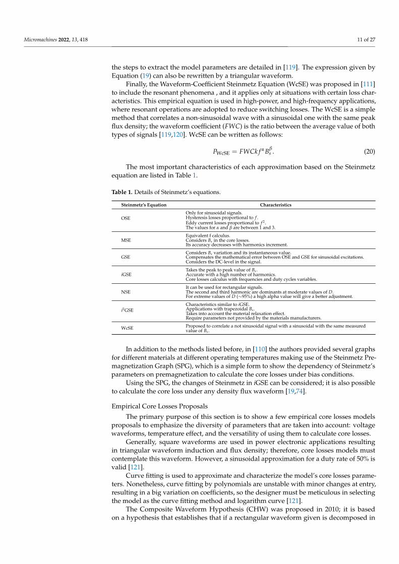
Added to these FEM software developers, there is Comsol Multiphysics®, which is apowerful software tool for developing and simulating modelling designs in all fields of en-gineering, manufacturing, and scientific research [134]. This software was founded in 1986.Its main characteristic is its friendly graphical user interface. The Comsol Multiphysics®

community is more significant than the other software. In Figure 6, two simulations areprovided. Comsol Multiphysics® can import designs in CAD and export final designsto Simulink®, given that both belong to the MathWorks® family. Comsol Multiphysics®

is oriented to students and academic researchers, it is not complex to learn and it is anexcellent option to start with for FEM software.

Figure 6. Examples of magnetic flux density simulations’ in Comsol Multiphysics for a powder corewith shape: (a) toroidal , and (b) “E”.

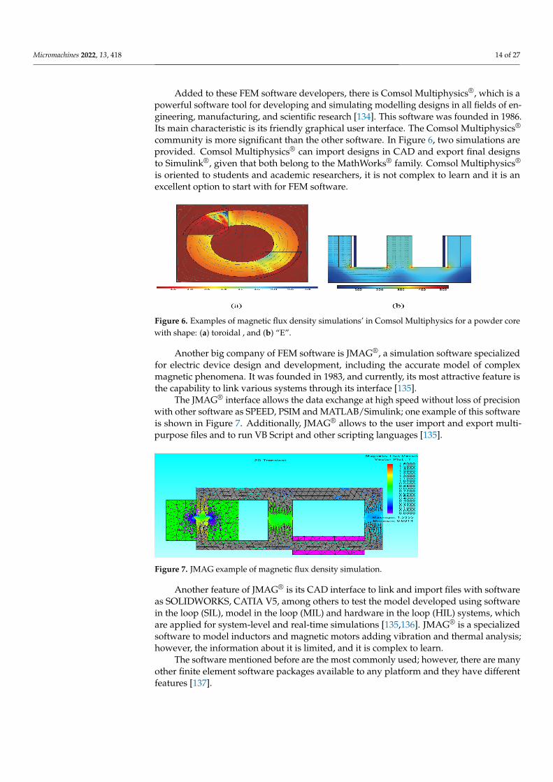
Another big company of FEM software is JMAG®, a simulation software specializedfor electric device design and development, including the accurate model of complexmagnetic phenomena. It was founded in 1983, and currently, its most attractive feature isthe capability to link various systems through its interface [135].

The JMAG® interface allows the data exchange at high speed without loss of precisionwith other software as SPEED, PSIM and MATLAB/Simulink; one example of this softwareis shown in Figure 7. Additionally, JMAG® allows to the user import and export multi-purpose files and to run VB Script and other scripting languages [135].

Figure 7. JMAG example of magnetic flux density simulation.

Another feature of JMAG® is its CAD interface to link and import files with softwareas SOLIDWORKS, CATIA V5, among others to test the model developed using softwarein the loop (SIL), model in the loop (MIL) and hardware in the loop (HIL) systems, whichare applied for system-level and real-time simulations [135,136]. JMAG® is a specializedsoftware to model inductors and magnetic motors adding vibration and thermal analysis;however, the information about it is limited, and it is complex to learn.

The software mentioned before are the most commonly used; however, there are manyother finite element software packages available to any platform and they have differentfeatures [137].

Micromachines 2022, 13, 418 15 of 27

6. Magnetic Components Design Process

In general, the design process of a magnetic component consists of four steps: design,simulate, implement, and evaluate Figure 8.

Figure 8. Steps to design a magnetic component. Source: Adapted from [138].

The design step can completely follow the diagram shown in Figure 8, where theapplication specifications will determine the selection core material up to the copper losses,the core losses model, and the high-frequency effects according to [139,140].

It is worth to mention, that there are some intermediate steps, which are related to corephysical and magnetic parameters such as the cross section of the core, section of the core,length of it, effective relative permeability, peak to peak density ripple, among others [141].In the same way, choosing a gapped core (a core with a concentrated air gap) instead of adistributed air gap core will impact its behavior and parameters to calculate; for the firstone, gap parameters as length are a priority. For the second one, permeability parameterswill be taken into account [142].

As applications specifications as selection core material are fundamental to selector design a core losses model, both will establish the minimum parameters to calculatepower losses.

The simulate step is the masterpiece to validate the magnetic component designed,but at the same time, it will be a problematic step if the designer is not careful; FEMsoftware always will give a solution but does not mean that it is correct. In a general way,simulation steps can be subdivided into three parts: data analysis, finite element method,and simulation of applications.

From the design steps depending on the models selected to calculate power losses,core physical parameters, and data related to the windings, many formulas are involved,and sometimes some depend on others; software such as Mathcad® and Matlab® are ofgreat help in these cases. FEM is a big world, as it was explained in the section before.Once the magnetic component’s design is complete (windings and core parameters) andvalidated in FEM; the next step consists in exporting the final FEM design to software like

Micromachines 2022, 13, 418 16 of 27

Simulink® or Twin Builder®, PSIM®, to simulate it in a specific application and corroborateits correct performance [59,143–146].

The implementation step tests the simulated application through the interconnectionof different sorts of software and platforms (MCU hardware, LabVIEW®, Typhoon HIL,among others) to simulate it with high fidelity, in similar conditions to real [147]. TyphoonHIL is a feasible example of this, as it can see in Figure 8. The reader interested in magneticcomponent testing is referred to [148–153] and the references therein.

The last one is to evaluate, that is, physically build the magnetic component designedand tested in the steps before and implement it in a circuit. Technically speaking, the testsobtained in the implementation step must coincide with the physical circuit measurementswith a minimal error percentage. If the magnetic component behavior is not satisfactory,the steps must be repeated, modifying the necessary parameters until the desired resultsare obtained.

7. Magnetic Devices and Miniaturization

Transportation, electrification, medical applications, micromachines, wireless com-munication and wireless charging are some areas demanding new technology to developcompact and high performance applications; and the manufacturing of low losses magneticcomponents is key [154].

Magnetic components exhibit design difficulties when power conversion systemsrequire low power levels and high frequencies due to the nonlinear behavior of magneticmaterials, thermal limits, and the exponential increase of losses under these conditions.

Core data and core losses models are critical to design magnetic components properlyand select the size of magnetic devices. According to core selection material differentprocedures may be applied [155].

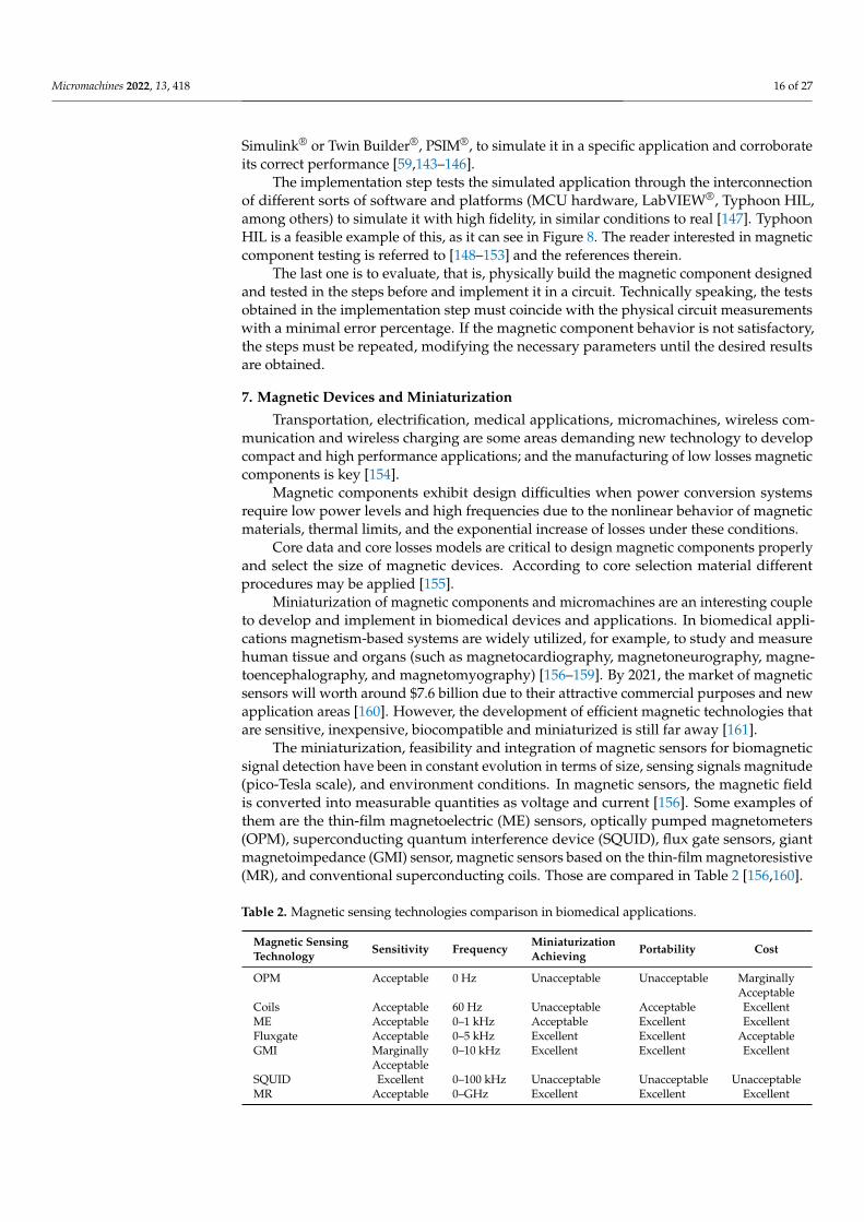
Miniaturization of magnetic components and micromachines are an interesting coupleto develop and implement in biomedical devices and applications. In biomedical appli-cations magnetism-based systems are widely utilized, for example, to study and measurehuman tissue and organs (such as magnetocardiography, magnetoneurography, magne-toencephalography, and magnetomyography) [156–159]. By 2021, the market of magneticsensors will worth around $7.6 billion due to their attractive commercial purposes and newapplication areas [160]. However, the development of efficient magnetic technologies thatare sensitive, inexpensive, biocompatible and miniaturized is still far away [161].

The miniaturization, feasibility and integration of magnetic sensors for biomagneticsignal detection have been in constant evolution in terms of size, sensing signals magnitude(pico-Tesla scale), and environment conditions. In magnetic sensors, the magnetic fieldis converted into measurable quantities as voltage and current [156]. Some examples ofthem are the thin-film magnetoelectric (ME) sensors, optically pumped magnetometers(OPM), superconducting quantum interference device (SQUID), flux gate sensors, giantmagnetoimpedance (GMI) sensor, magnetic sensors based on the thin-film magnetoresistive(MR), and conventional superconducting coils. Those are compared in Table 2 [156,160].

Table 2. Magnetic sensing technologies comparison in biomedical applications.

Magnetic SensingSensitivity Frequency

MiniaturizationPortability Cost

Technology Achieving

OPM Acceptable 0 Hz Unacceptable Unacceptable MarginallyAcceptable

Coils Acceptable 60 Hz Unacceptable Acceptable ExcellentME Acceptable 0–1 kHz Acceptable Excellent ExcellentFluxgate Acceptable 0–5 kHz Excellent Excellent AcceptableGMI Marginally 0–10 kHz Excellent Excellent Excellent

AcceptableSQUID Excellent 0–100 kHz Unacceptable Unacceptable UnacceptableMR Acceptable 0–GHz Excellent Excellent Excellent

Micromachines 2022, 13, 418 17 of 27

In [162], a GMI miniaturized magnetic sensor fabricated with a Co-based amorphousby Micro-Electro-Mechanical System (MEMS) technology wire is described, achieving asize of 5.6 × 1.5 × 1.1 mm3. Co-based amorphous wire is selected for its high impedancechange rate, increasing the sensitive of the GMI sensor, it is used to fabricated a pick-upcoil of 200 turns and diameter of 200 µm.

A common problem in biomagnetic sensors is the noise at low frequencies, specificallybetween 10 and 100 Hz due to the small magnitude of measured signals. A set of bi-planar electromagnetic coils is a recent technique to cancelling the Earth’s noise nearby themagnetic sensors and improving their sensitivity [156].

Magnetic signal detection including portable and handled devices in the point-of-care testing (POCT) including mini magnetic induction coils and electromagnets to dothe devices more portable, flexible and with high detection capabilities. In [163] severalexamples of these applications are described, where magnetic devices have dimensions incentimeters scale and those consider other POCT techniques for their favorable accuracy,high reliability, innovation and novelty, although their cost might increase.

Portable and small size, or even single handled devices that provide rapid and accuratedetection have potential application of POCT [163]. Portable and wearable biosensors arethe future of healthcare sensor technologies. Those have demonstrated their utility indisease diagnosis with accurate prediction. Their incorporation with mobile phones isknown as digital health or mobile health, which promises reduce the frequency of clinicalvisits, prevent health problems and revolutionary the demand of micro and wearablesensors technology [164–166].

The emerge of microrobots and the use of a magnetic resonance imaging help toimprove diagnostic capabilities by minimally invasive procedures. A microrobot is arobot on a microscale that can perform high-precision operations. Microrobots’ actuationsystem require input energy to act it, which usually requires special materials (soft andhard magnetic materials) or structural design (arrangement of coils) [167,168]. While thepropulsion of microrobots, ferromagnetic cores and magnetic structures can be used togenerate an image of many sites in the human body [169–171].

In [172], microcoils with a diameter <1 mm are used to harvest electromagneticenergy wirelessly by inductive coupling in the on-board energy robots, achieving severalmilliwatts of power, capable of controlled motion and actuation with a maximum efficiencyof 40%. This has been a recent development to controlled and powered remotely a system-engineered miniaturized robot (SEMER).

To increase the adaptability and robustness of robotic systems in challenging envi-ronments, and inter disciplinary research is needed, including material science, biology,control, among others [172]. Magnetic materials and magnetoelectric concepts of micro andnanorobots in magnetic applications are detailed in [173].

In this authors opinion the versatility, scalability, and flexibility of developing a powercore loss model to analyze and allowing a better comprehension of the magnetic phenomenain ferromagnetic materials, will be the first step to the miniaturization of magnetic devicesand power conversion systems at any scale [174,175].

8. Discussion

Nowadays , there are several models for studying, predicting, and analyzing the powerlosses in the ferromagnetic cores of magnetic components. Usually, these models considera series of parameters based on magnetic units and frequency to predict and calculatepower losses. Figure 9 illustrates a comparison between core losses models dependingseveral features.

Micromachines 2022, 13, 418 18 of 27

Figure 9. Power core losses models’ comparison depending on the size of the phenomena analyzed,kind of losses to calculate and ferromagnetic materials. Features of mathematical models, time-domain approximations, loss separation, and empirical methods are in color yellow, blue, pink, andpurple, respectively.

Nevertheless, one main application of magnetic components is in power electronics,where the measurement units are electric, which in many cases cause inexactness whiledesigning a magnetic element. A common idea in the literature is that in a magnetic com-ponent with high operating frequency, its losses and size will be lower; however, this is notalways true. There are many factors involved (kind of material, core losses, copper losses,among others) to determine the integrity of this expression. Although the last years’ powerelectronic researchers have been working hard to find and develop numerous techniques toachieve better performance from magnetic components, the way is still long. For instance,the future design of magnetic components should take advantage of all capabilities ofthe final application (support multiple input/outputs, multiple voltage/current domains,characterization of the material, losses’ reduction, among others), with the option to workin parallel with switches at high frequency [12,176].

On the other hand, the industry of FEM software is more versatile each year; severalapplications and tools are added to these, improving accuracy, functionality, scenariosto apply it, and user friendly environments. Nonetheless, a common point is a lack ofcompatibility among those, limiting the use of platforms to validate and complement thefinal design. This lack of compatibility motivates users to know different packages to solvea unique problem.

This is translated into a monetary cost to purchase different licenses and increasecomputer resources. Therefore, to motivate and improve the FEM designs, in this authorsopinion, a standard format type should be implemented in the following years betweenthose kinds of software to take advantage of each characteristic and unify all FEM files.

In the literature, static or dynamic core losses models can be found, depending on thedesigner choice, the loses calculus could be as complex as the model chosen [177]. So, the

Micromachines 2022, 13, 418 19 of 27

model selection in function of the material and the requirements’ application of a magneticcomponent’s design process are fundamental to achieving an accurate core losses calculus.

Table 3 illustrates a comparison between power core losses models, ferromagneticmaterials, and accuracy. It is essential to mention that ferrite is the start point to validate anypower core losses model, so this is not listed. Nonetheless, to the best authors knowledge,not all models had been tested in all ferromagnetic materials, or those are not suitable tocalculate their power core losses.

Table 3. Comparison between empiric core losses models. The sinusoidal and non-sinusoidalwaveform are indicated with light yellow and light green, respectively.

Loss Steinmetz’s Additional FerromagneticCharacteristics Accuracy

Model Parameters Data MaterialsPreisach No Yes All unless powder cores Based on domains movements Computing cost,

and B-H loop approximationsMany additional data.

J-A No Yes All unless powder cores Non-linear equations systems. Computing cost,Based on magnetization core process. approximationsMany additional data.

LSM No Yes All unless powder core Suitable only for lineal systems. GoodVery accuracy for laminar materials.

TDA No No All unless powder cores Suitable only for lineal systems. GoodValid for PWM signals <400 Hz.

OSE Yes No All Base of empiric loss models. LowMSE Yes No All Not suitable for signals with many harmonics. Mα−2

GSE Yes No All Consider CD-level in the signal. <iGSEiGSE Yes No All Signals with strong harmonics. Same as i2GSENSE Yes No No reported A similar version of GSE. No reported

i2GSE Yes Yes All Consider the relaxation effect. Same as iGSESignals with strong harmonics.

WcSE Yes Yes Nanocrystal, amorphous Physical base not verified. D < 0.5and powder core A practical and direct method.

CHW No Yes Nanocrystal, amorphous Square waveform as the sum of its components. Goodand powder core

Villar Yes No Amorphous material Core loss calculus implemented a piecewise linear Goodmodel (PWL).

Górecki Yes No Nanocrystal, amorphous Considers thermal, electrical and magnetic Same asand powder core effects manufacturers

Designers can use the information mentioned in Table 3 and Figure 9 to improve someof the power core loss models listed before or propose their model, always keeping in mindthat any design parameter will be sacrificed to improve another one; magnetic componentssize will be reduced with frequency increment.

Due to the high energy consumption worldwide, renewable energy sources and energyefficiency have accelerated research in energy applications, conversion, transportation,and telecommunication [178]. Magnetic materials are the key piece of those researchfields, mainly for their potential for energy efficiency and their impact on consumptionpower [179]. Materials’ demand as electric steel, iron, and cobalt will be exponential growthfor 2026. Studies on the effect of magnetic materials in renewable energy have to be apriority to guarantee the supply chain, options for recycling, the footprint impact, theblueprint impact, and the socio-economical impact of their extraction [180,181].

9. Conclusions

In the literature, many core-losses models are available to select. Researchers continuedeveloping new core losses models with specific features (core material, waveform, densityflux, application, frequency range, among others), but the majority are not easy to replicate.

To develop a power core losses model that involves electrical, magnetic, thermal effects,suitable for all kinds of ferromagnetic materials, and also competent to power electronic isfundamental. Not only for advantages to calculate power core losses accurately but not toreach optimal magnetic components. The challenge is to understand the comportment of

Micromachines 2022, 13, 418 20 of 27

the magnetic materials and model them differently than ferrite magnetic elements because,until now, both are very similar, although their behaviour is quite different.

Each of the core losses models in this document is a point of start for researchers.Despite promising results using Steinmetz’s equations, those are not enough to calculatethe core losses accuracy according to the need for the power electronic community. FEMsoftware is indispensable nowadays to validate the power losses model as the magneticcomponent design. At the same time, virtual laboratories are promising to be the trend in afew years, allowing a reduction of the cost of a physical test bench to that of a virtual one andgetting good approximations of the magnetic component behavior in a real environment.In addition, the option to interconnect different kinds of software to implement completepower electronics systems in platforms such as HIL, SIL, and MIL, makes the capability ofdesign more versatile.

Author Contributions: Conceptualization, D.R.-S. and F.J.P.-P.; methodology, M.A.R.-L.; software,I.A.-V.; validation, J.P.-O., A.-I.B.-G. and F.J.P.-P.; formal analysis, M.A.R.-L.; investigation, D.R.-S.;resources, F.J.P.-P. and A.-I.B.-G.; data curation, J.P.-O.; writing original draft preparation, D.R.-S.;writing—review and editing, D.R.-S., M.A.R.-L., J.P.-O. and F.J.P.-P.; visualization, D.R.-S.; supervision,I.A.-V.; project administration, A.-I.B.-G.; funding acquisition, F.J.P.-P. and I.A.-V. All authors haveread and agreed to the published version of the manuscript.

Funding: The authors thank Tecnológico Nacional de México, Instituto Tecnológico de Celaya. Thework of Daniela Rodriguez-Sotelo was supported by CONACYT through a Ph.D. grant.

Acknowledgments: The authors thank IPN, Tecnológico Nacional de México, Instituto Tecnológicode Celaya and CONACYT.

Conflicts of Interest: The authors declare no conflict of interest.

AbbreviationsThe following abbreviations are used in this manuscript:

Pc Core loss Ph Hysteresis or static lossPeddy Eddy current loss Panom Anomalous or residual losskh Hysteresis coefficient keddy Eddy currents coefficientkanom Anomalous coefficient f Fundamental frequencyB Magnetic flux density φn Angle between Bn and Hn

BnMagnetic flux density of the nth

HnMagnetic field of the nth

harmonic harmonicBs Magnetic induction peak x Steinmetz coefficientd Lamination thickness ρ Electrical resistivityA Cross-sectional area lamination feq Equivalent frequencyMan Anhysteretic magnetization αic Inter-domain coupling∆B Magnetic induction peak to peak dB(t)/dt Core loss magnetization rateβ Magnetic induction exponent α Frequency exponentδ Magnetizing field direction fr Fundamental frequencyθ Sinusoidal waveform phase angle T Waveform periodD Duty ratio N Number of turnsFWC Waveform coefficient V1, V2 Voltaget Time ω Zero-voltage period durationU DC constant voltage Tω Length of zero-voltage periodTM Core temperature with smallest losses TR Core temperatureM Total magnetization H Magnetic fieldHe f f Effective magnetic field µ0 Free-space permeabilityMirr Irreversible magnetization Mrev Reversible magnetizationAe f f Effective core area αp Losses temperature coefficientB(t) Instantaneous value of core V0 Magnetic objects statistical

loss magnetization rate distributionG Eddy current dimensionless as Anhysteretic magnetization

coefficient shape parameter

Micromachines 2022, 13, 418 21 of 27

M(t) Instantaneous magnetization Ms Saturation magnetizationms Magnetic moment H(t) Instantaneous magnetic fieldPsqr Rectangular waveform power losses c Reversibility coefficientkr ,αr , βr , τ, qra, a1,a2, f0, f1, Material parametersf2, f3, αT , k

References1. Lee, H.; Jung, S.; Huh, Y.; Lee, J.; Bae, C.; Kim, S.J. An implantable wireless charger system with ×8.91 Increased charging power

using smartphone and relay coil. In Proceedings of the IEEE Wireless Power Transfer Conference (WPTC), San Diego, CA, USA,1–4 June 2021; pp. 1–4. [CrossRef]

2. Yu, W.; Hua, W.; Zhang, Z. High-frequency core loss analysis of high-speed flux-switching permanent magnet machines.Electronics 2021, 10, 1076. [CrossRef]

3. Pérez, E.; Espiñeira, P.; Ferreiro, A. Instrumentación Electrónica; Acceso Rápido; Marcombo: Barcelona, Spain, 1995.4. Chitode, J.; Bakshi, U. Power Devices and Machines; Technical Publications: Maharashtra, India, 2009.5. López-Fernández, X.; Ertan, H.; Turowski, J. Transformers: Analysis, Design, and Measurement; CRC Press: Boca Raton, FL,

USA, 2017.6. Muttaqi, K.M.; Islam, M.R.; Sutanto, D. Future power distribution grids: Integration of renewable energy, energy storage, electric

vehicles, superconductor, and magnetic bus. IEEE Trans. Appl. Supercond. 2019, 29, 3800305. [CrossRef]7. Phan, H.P. Implanted flexible electronics: Set device lifetime with smart nanomaterials. Micromachines 2021, 12, 157. [CrossRef]

[PubMed]8. Ivanov, A.; Lahiri, A.; Baldzhiev, V.; Trych-Wildner, A. Suggested research trends in the area of micro-EDM—Study of some

parameters affecting micro-EDM. Micromachines 2021, 12, 1184. [CrossRef]9. Kozai, T.D.Y. The history and horizons of microscale neural interfaces. Micromachines 2018, 9, 445. [CrossRef]10. Rashid, M.H. Power Electronics Handbook; Elsevier: Amsterdam, The Netherlands, 2018; p. 1510. [CrossRef]11. Matallana, A.; Ibarra, E.; López, I.; Andreu, J.; Garate, J.; Jordà, X.; Rebollo, J. Power module electronics in HEV/EV applications:

New trends in wide-bandgap semiconductor technologies and design aspects. Renew. Sustain. Energy Rev. 2019, 113, 109264.[CrossRef]

12. Hanson, A.J.; Perreault, D.J. Modeling the magnetic behavior of n-winding components: Approaches for unshackling switchingsuperheroes. IEEE Power Electron. Mag. 2020, 7, 35–45. [CrossRef]

13. Bahmani, A. Core loss evaluation of high-frequency transformers in high-power DC-DC converters. In Proceedings of theThirteenth International Conference on Ecological Vehicles and Renewable Energies (EVER), Monte Carlo, Monaco, 10–12 April2018; pp. 1–7. [CrossRef]

14. Hossain, M.Z.; Rahim, N.A.; Selvaraj, J. Recent progress and development on power DC-DC converter topology, control, designand applications: A review. Renew. Sustain. Energy Rev. 2018, 81, 205–230. [CrossRef]

15. Silveyra, J.M.; Ferrara, E.; Huber, D.L.; Monson, T.C. Soft magnetic materials for a sustainable and electrified world. Science 2018,362, eaao0195. [CrossRef]

16. Zurek, S. Characterisation of Soft Magnetic Materials under Rotational Magnetisation; CRC Press: Boca Raton, FL, USA, 2017; p. 568.17. Cullity, B.; Graham, C. Soft magnetic materials. In Introduction to Magnetic Materials; John Wiley & Sons, Ltd.: Hoboken, NJ, USA,

2008; Chapter 13, pp. 439–476. [CrossRef]18. Krishnan, K.M. Fundamentals and Applications of Magnetic Materials; Oxford University Press: Oxford, UK, 2016; p. 816. [CrossRef]19. Islam, M.R.; Rahman, M.A.; Sarker, P.C.; Muttaqi, K.M.; Sutanto, D. Investigation of the magnetic response of a nanocrystalline

high-frequency magnetic link with multi-input excitations. IEEE Trans. Appl. Supercond. 2019, 29, 0602205. [CrossRef]20. Dobrzanski, L.A.; Drak, M.; Zieboqicz, B. Materials with specific magnetic properties. J. Achiev. Mater. Manuf. Eng. 2006, 17, 37.21. Duppalli, V.S. Design Methodology for a High-Frequency Transformer in an Isolating DC-DC Converter. Ph.D. Thesis, Purdue

University, West Lafayette, IN, USA, 2018.22. Liu, X.; Wang, Y.; Zhu, J.; Guo, Y.; Lei, G.; Liu, C. Calculation of core loss and copper loss in amorphous/nanocrystalline

core-based high-frequency transformer. AIP Adv. 2016, 6, 055927. [CrossRef]23. Balci, S.; Sefa, I.; Bayram, M.B. Core material investigation of medium-frequency power transformers. In Proceedings of the 2014

16th International Power Electronics and Motion Control Conference and Exposition, Antalya, Turkey, 21–24 September 2014;pp. 861–866.

24. de Sevilla Galán, J.F. Mejora del Cálculo de las Pérdidas por el Efecto Proximidad en alta Frecuencia Para Devanados de Hilos deLitz. Available online: https://oa.upm.es/56807/1/TFG_JAVIER_FERNANDEZ_DE_SEVILLA_GALAN.pdf (accessed on 24February 2022).

25. Herbert, E. User-Friendly Data for Magnetic Core Loss Calculations. Technical Report 4. 2008. Available online: https://www.psma.com/coreloss/eh1.pdf (accessed on 24 February 2022).

26. Sullivan, C.R.; Harris, J.H.; Herbert, E. Testing Core Loss for Rectangular Waveforms the Power Sources ManufacturersAssociation. Technical Report 973. 2010. Available online: https://www.psma.com/coreloss/phase2.pdf (accessed on 24February 2022).

Micromachines 2022, 13, 418 22 of 27

27. Tacca, H.; Sullivan, C. Extended Steinmetz Equation; Report of Posdoctoral Research; Thayer School of Engineering: Hanover, NH,USA, 2002.

28. Ulaby, F.T. Fundamentos de Aplicaciones en Electromagnetismo; Pearson: London, UK, 2007.29. Cheng, D. Fundamentos de Electromagnetismo para Ingeniería; Mexicana, A., Ed.; 1997. Available online: https://www.academia.e

du/36682331/Fundamentos_de_Electromagnetismo_para_Ingenieria_David_K_Cheng (accessed on 24 February 2022).30. Coey, J.M.D. Magnetism and Magnetic Materials; Cambridge University Press: Cambridge, UK, 2010. [CrossRef]31. Goldman, A. Handbook of Modern Ferromagnetic Materials; Springer: Boston, MA, USA, 1999. [CrossRef]32. Gupta, K.; Gupta, N. Magnetic Materials: Types and Applications. In Advanced Electrical and Electronics Materials; John Wiley &

Sons, Ltd.: Hoboken, NJ, USA, 2015; Chapter 12, pp. 423–448. [CrossRef]33. Hitachi. Nanocrystalline Material Properties; Hitachi: Tokyo, Japan, 2019.34. County Council, K.; Richardson, A. Silver Wire Ring. 2017. [image/JPEG]. Available online: https://www.academia.edu

/2306387/With_Dickinson_T_M_and_Richardson_A_Early_Anglo_Saxon_Eastry_Archaeological_Evidence_for_the_Beginnings_of_a_District_Centre_in_the_Kingdom_of_Kent_Anglo_Saxon_Studies_in_Archaeology_and_History_17 (accessed on24 February 2022).

35. Alisdojo. Detail of an Enamelled Litz Wire. 2011. [image/JPEG]. Available online: https://commons.wikimedia.org/wiki/File:Enamelled_litz_copper_wire.JPG (accessed on 24 February 2022).

36. Magnetics. Powder Cores Properties; Magnetics: Pittsburgh, PA, USA, 2019.37. Laboratory, N.E.T. FINEMET Properties. 2018. Available online: https://www.hitachi-metals.co.jp/e/products/elec/tel/p02_2

1.html#:~:text=FINEMET%C2%AE%20has%20high%20saturation,and%20electronics%20devices%20as%20well (accessed on24 February 2022).

38. CATECH®. Amorphous and Nanocrystalline Core; CATECH: Singapore, 2022.39. Soon, H. Wire. 2017. [image/JPEG]. Available online: https://iopscience.iop.org/article/10.1088/1742-6596/871/1/012098/pdf

(accessed on 24 February 2022).40. Aluminium Wire, 16 mm2. 2012. [image/JPEG]. Available online: https://ceb.lk/front_img/specifications/1540801489P.V_.C_._

INSULATED_ALUMINIUM_SERVICE_MAIN_WIRE-FINISHED_PRODUCT_.pdf (accessed on 24 February 2022).41. County Council, K.; Richardson, A. Length of Gold Wire, Ringlemere. 2017. [image/JPEG]. Available online: https://www.sa

chsensymposion.org/wp-content/uploads/2012/04/68th-International-Sachsensymposion-Canterbury.pdf (accessed on 24February 2022).

42. SpinningSpark. Transformer Core. 2012. [image/JPEG]. Available online: https://commons.wikimedia.org/wiki/File:Transformer_winding_formats.jpg (accessed on 24 February 2022).

43. TheDigitalArtist. coil-gd137ed32f-1920. 2015. [image/JPEG]. Available online: https://plato.stanford.edu/entries/digital-art/(accessed on 24 February 2022).

44. Fiorillo, F.; Bertotti, G.; Appino, C.; Pasquale, M., Soft magnetic materials. In Wiley Encyclopedia of Electrical and ElectronicsEngineering; American Cancer Society: Atlanta, GA, USA, 2016; pp. 1–42. [CrossRef]

45. Aguglia, D.; Neuhaus, M. Laminated magnetic materials losses analysis under non-sinusoidal flux waveforms in powerelectronics systems. In Proceedings of the 15th European Conference on Power Electronics and Applications (EPE), Lille, France,2–6 September 2013; pp. 1–8. [CrossRef]

46. McLyman, C. Transformer and Inductor Design Handbook, 3rd ed.; Taylor & Francis: Abingdon-on-Thames, UK, 2004.47. Tsepelev, V.; Starodubtsev, Y.; Konashkov, V.; Belozerov, V. Thermomagnetic analysis of soft magnetic nanocrystalline alloys.

J. Alloys Compd. 2017, 707, 210–213. [CrossRef]48. Ouyang, G.; Chen, X.; Liang, Y.; Macziewski, C.; Cui, J. Review of Fe-6.5 wt% silicon steel-a promising soft magnetic material for

sub-kHz application. J. Magn. Magn. Mater. 2019, 481, 234–250. [CrossRef]49. Yuan, W.; Wang, Y.; Liu, D.; Deng, F.; Chen, Z. Impacts of inductor nonlinear characteristic in multi-converter microgrids:

Modelling, analysis and mitigation. IEEE J. Emerg. Sel. Top. Power Electron. 2020, 8, 3333–3347. [CrossRef]50. Kazimierczuk, M. High-Frequency Magnetic Components, 2nd ed.; John Wiley & Sons, Ltd.: Hoboken, NJ, USA, 2013. [CrossRef]51. Tumanski, S. Handbook of Magnetic Measurements; Series in Sensors; CRC Press: Boca Raton, FL, USA, 2016.52. Goldman, A. Magnetic Components for Power Electronics; Springer: Berlin/Heidelberg, Germany, 2012.53. Wang, Y.; Calderon-Lopez, G.; Forsyth, A. Thermal management of compact nanocrystalline inductors for power dense converters.

In Proceedings of the IEEE Applied Power Electronics Conference and Exposition (APEC), San Antonio, TX, USA, 4–8 March2018; pp. 2696–2703. [CrossRef]

54. Conde, C.; Blázquez, J.; Conde, A. Nanocrystallization process of the Hitperm Fe-Co-Nb-B alloys. In Properties and Appli-cations of Nanocrystalline Alloys from Amorphous Precursors; Idzikowski, B., Švec, P., Miglierini, M., Eds.; Springer: Dordrecht,The Netherlands, 2005; pp. 111–121.

55. Tsepelev, V.S.; Starodubtsev, Y.N. Nanocrystalline soft magnetic iron-based materials from liquid state to ready product.Nanomaterials 2021, 11, 108. [CrossRef]

56. Lidow, A. Accelerating adoption of magnetic resonant wireless power based on the AirFuel, 2021. IEEE Wirel. Power Week 2021.Available online: https://airfuel.org/wireless-power-week-2021-highlights/ (accessed on 24 February 2022).

57. Jafari, M.; Malekjamshidi, Z.; Zhu, J. Copper loss analysis of a multiwinding high-frequency transformer for a magnetically-coupled residential microgrid. IEEE Trans. Ind. Appl. 2019, 55, 283–297. [CrossRef]

Micromachines 2022, 13, 418 23 of 27

58. Slionnnnnn. The Prototype of the Balanced Twisted Winding CM Choke. 2017. [image/JPEG]. Available online: https://en.wikipedia.org/wiki/File:4ffffss123.jpg (accessed on 24 February 2022).

59. Corti, F.; Reatti, A.; Lozito, G.M.; Cardelli, E.; Laudani, A. Influence of non-linearity in losses estimation of magnetic componentsfor DC-DC converters. Energies 2021, 14, 6498. [CrossRef]

60. Zhu, F.; Yang, B. Power Transformer Design Practices; CRC Press: Boca Raton, FL, USA, 2021.61. Glisson, T. Introduction to Circuit Analysis and Design; Springer: Berlin/Heidelberg, Germany, 2011.62. Wang, W.; Nysveen, A.; Magnusson, N. The influence of multidirectional leakage flux on transformer core losses. J. Magn. Magn.

Mater. 2021, 539, 168370. [CrossRef]63. Kulkarni, S.; Khaparde, S. Transformer Engineering: Design, Technology, and Diagnostics, 2nd ed.; Taylor & Francis: Abingdon-on-

Thames, UK, 2012.64. Tian, H.; Wei, Z.; Vaisambhayana, S.; Thevar, M.P.; Tripathi, A.; Kjær, P.C. Calculation and experimental validation on leakage

inductance of a medium frequency transformer. In Proceedings of the IEEE 4th Southern Power Electronics Conference (SPEC),Singapore, 10–13 December 2018; pp. 1–6. [CrossRef]

65. Kothari, D.; Nagrath, I. Modern Power System Analysis; Tata McGraw-Hill Publishing Company: New York, NK, USA, 2003.66. Barg, S.; Alam, M.F.; Bertilsson, K. Optimization of high frequency magnetic devices with consideration of the effects of the

magnetic material, the core geometry and the switching frequency. In Proceedings of the 22nd European Conference on PowerElectronics and Applications (EPE’20 ECCE Europe), Lyon, France, 7–11 September 2020; pp. 1–8. [CrossRef]

67. Ouyang, Z. High Frequency Planar Magnetics for Power Converters; Presentation; ECPE Online Tutorial: Nuremberg, Germany, 2021.68. Barrios, E.L.; Ursúa, A.; Marroyo, L.; Sanchis, P. Analytical design methodology for Litz-wired high-frequency power transformers.

IEEE Trans. Ind. Electron. 2015, 62, 2103–2113. [CrossRef]69. Brighenti, L.L.; Martins, D.C.; Dos Santos, W.M. Study of magnetic core geometries for coupling systems through a magnetic bus.

In Proceedings of the IEEE 10th International Symposium on Power Electronics for Distributed Generation Systems (PEDG),Xi’an, China, 3–6 June 2019; pp. 29–36. [CrossRef]

70. Rodriguez-Sotelo, D.; Rodriguez-Licea, M.A.; Soriano-Sanchez, A.G.; Espinosa-Calderon, A.; Perez-Pinal, F.J. Advancedferromagnetic materials in power electronic converters: A state of the art. IEEE Access 2020, 8, 56238–56252. [CrossRef]

71. Detka, K.; Górecki, K. Influence of the size and shape of magnetic core on thermal parameters of the inductor. Energies 2020, 13,3842. [CrossRef]

72. Jiandong, D.; Yang, L.; Hao, L. Research on ferromagnetic components J-A model—A review. In Proceedings of the InternationalConference on Power System Technology (POWERCON), Guangzhou, China, 6–8 November 2018; pp. 3288–3294.

73. Saeed, S.; Georgious, R.; Garcia, J. Modeling of magnetic elements including losses-application to variable inductor. Energies2020, 13, 1865. [CrossRef]

74. Ishikura, Y.; Imaoka, J.; Noah, M.; Yamamoto, M. Core loss evaluation in powder cores: A comparative comparison betweenelectrical and calorimetric methods. In Proceedings of the International Power Electronics Conference (IPEC-Niigata 2018-ECCEAsia), Niigata, Japan, 20–24 May 2018; pp. 1087–1094.

75. Hanif, A. Measurement of Core Losses in Toroidal Inductors with Different Magnetic Materials. Master’s Thesis, TampereUniversity of Technology, Tampere, Finland, 2017.

76. Wang, Y. Modelling and Characterisation of Losses in Nanocrystalline Cores. Ph.D. Thesis, The University of Manchester,Manchester, UK, 2015.

77. Yue, S.; Li, Y.; Yang, Q.; Yu, X.; Zhang, C. Comparative analysis of core loss calculation methods for magnetic materials undernonsinusoidal excitations. IEEE Trans. Magn. 2018, 54, 6300605. [CrossRef]

78. Bi, S. Charakterisieren und Modellieren der Ferromagnetischen Hysterese. Ph.D. Thesis, Friedrich-Alexander-UniversitätErlangen-Nürnberg (FAU), Erlangen, Germany, 2014.

79. Iniewski, K. Advanced Circuits for Emerging Technologies; Wiley: Hoboken, NJ, USA, 2012.80. Sudhoff, S. Power Magnetic Devices: A Multi-Objective Design Approach; IEEE Press Series on Power Engineering; Wiley: Hoboken,

NJ, USA, 2014.81. Spaldin, N. Magnetic Materials: Fundamentals and Applications; Cambridge University Press: Cambridge, UK, 2010.82. Dong Tan, F.; Vollin, J.L.; Cuk, S.M. A practical approach for magnetic core-loss characterization. IEEE Trans. Power Electron. 1995,

10, 124–130. [CrossRef]83. Fiorillo, F.; Mayergoyz, I. Characterization and Measurement of Magnetic Materials; Elsevier: Amsterdam, The Netherlands, 2004.84. O’Handley, R. Modern Magnetic Materials: Principles and Applications; Wiley: Hoboken, NJ, USA, 1999.85. Krings, A.; Soulard, J. Overview and comparison of iron loss models for electrical machines. J. Electr. Eng. Elektrotechnicky Cas.

2010, 10, 162–169.86. Sai Ram, B.; Kulkarni, S. An isoparametric approach to model ferromagnetic hysteresis including anisotropy and symmetric

minor loops. J. Magn. Magn. Mater. 2019, 474, 574–584. [CrossRef]87. Mayergoyz, I. Mathematical Models of Hysteresis and Their Applications, 2nd ed.; Elsevier: Amsterdam, The Netherlands, 2003.88. Zhao, X.; Liu, X.; Zhao, Z.; Zou, X.; Xiao, Y.; Li, G. Measurement and modeling of hysteresis characteristics in ferromagnetic

materials under DC magnetizations. AIP Adv. 2019, 9, 025111. [CrossRef]89. Jiles, D.; Atherton, D. Theory of ferromagnetic hysteresis. J. Magn. Magn. Mater. 1986, 61, 48–60. [CrossRef]

Micromachines 2022, 13, 418 24 of 27

90. Bernard, Y.; Mendes, E.; Bouillault, F. Dynamic hysteresis modeling based on Preisach model. IEEE Trans. Magn. 2002, 38, 885–888.[CrossRef]

91. Magnetic, M. Jiles-Atherton Model of Magnetic Hysteresis Loops of Mn-Zn Ferrite. 2016. [image/PNG]. Available online: https://commons.wikimedia.org/wiki/File:Jiles-Atherton_model_of_magnetic_hysteresis_loops_of_Mn-Zn_ferrite.png (accessed on24 February 2022) .

92. Aboura, F.; Touhami, O. Modeling and analyzing energetic hysteresis classical model. In Proceedings of the InternationalConference on Electrical Sciences and Technologies in Maghreb (CISTEM), Algiers, Algeria, 28–31 October 2018; pp. 1–5.

93. Chang, L.; Jahns, T.M.; Blissenbach, R. Characterization and modeling of soft magnetic materials for improved estimation ofPWM-induced iron loss. IEEE Trans. Ind. Appl. 2020, 56, 287–300. [CrossRef]

94. Ducharne, B.; Tsafack, P.; Tene Deffo, Y.; Zhang, B.; Sebald, G. Anomalous fractional magnetic field diffusion through cross-sectionof a massive toroidal ferromagnetic core. Commun. Nonlinear Sci. Numer. Simul. 2021, 92, 105450. [CrossRef]

95. Szular, Z.; Mazgaj, W. Calculations of eddy currents in electrical steel sheets taking into account their magnetic hysteresis.COMPEL—Int. J. Comput. Math. Electr. Electron. Eng. 2019, 38, 1263–1273. [CrossRef]

96. Yu, Q.; Chu, S.; Li, W.; Tian, L.; Wang, X.; Cheng, Y. Electromagnetic shielding analysis of a canned permanent magnet motor.IEEE Trans. Ind. Electron. 2020, 67, 8123–8130. [CrossRef]

97. Marchenkov, Y.; Khvostov, A.; Slavinskaya, A.; Zhgut, A.; Chernov, V. The eddy current diagnostics method for the plasticallydeformed area sizes evaluation in non-magnetic metals. J. Appl. Eng. Sci. 2020, 18, 92–97. [CrossRef]

98. Müller, S.; Keller, M.; Maier, M.; Parspour, N. Comparison of iron loss calculation methods for soft magnetic composite. InProceedings of the Brazilian Power Electronics Conference (COBEP), Juiz de Fora, Brazil, 19–22 November 2017; pp. 1–6.

99. Ionel, D.M.; Popescu, M.; McGilp, M.I.; Miller, T.J.E.; Dellinger, S.J.; Heideman, R.J. Computation of Core Losses in ElectricalMachines Using Improved Models for Laminated Steel. IEEE Trans. Ind. Appl. 2007, 43, 1554–1564. [CrossRef]

100. Bertotti, G. General properties of power losses in soft ferromagnetic materials. IEEE Trans. Magn. 1988, 24, 621–630. [CrossRef]101. Mehboob, N. Hysteresis Properties of Soft Magnetic Materials. Ph.D. Thesis, University of Vienna, Wien, Austria, 2012.102. Sun, H.; Li, Y.; Lin, Z.; Zhang, C.; Yue, S. Core loss separation model under square voltage considering DC bias excitation. AIP

Adv. 2020, 10, 015229. [CrossRef]103. Steinmetz, C.P. On the law of hysteresis. Trans. Am. Inst. Electr. Eng. 1892, IX, 1–64. [CrossRef]104. Mu, M. High Frequency Magnetic Core Loss Study. 2013. Available online: https://vtechworks.lib.vt.edu/bitstream/handle/1

0919/19296/Mu_M_D_2013.pdf (accessed on 24 February 2022).105. Zhou, T.; Zhou, G.; Ombach, G.; Gong, X.; Wang, Y.; Shen, J. Improvement of Steinmetz’s parameters fitting formula for ferrite

soft magnetic materials. In Proceedings of the IEEE Student Conference on Electric Machines and Systems, Huzhou, China, 14–16December 2018; pp. 1–4.

106. Erickson, R.; Maksimovic, D. Fundamentals of Power Electronics; Springer International Publishing AG: Berlin/Heidelberg,Germany, 2020.

107. Chen, D.Y. Comparisons of high frequency magnetic core losses under two different driving conditions: A sinusoidal voltage anda square-wave voltage. In Proceedings of the IEEE Power Electronics Specialists Conference, Syracuse, NY, USA, 13–15 June 1978;pp. 237–241.

108. Mulder, S.A. Fit formula for power loss in ferrites and their use in transformer design. In Proceedings of the 26th InternationalConference on Power Conversion, PCIM, Orlando, FL, USA, 1983; pp. 345–359.

109. Venkatachalam, K.; Sullivan, C.R.; Abdallah, T.; Tacca, H. Accurate prediction of ferrite core loss with nonsinusoidal waveformsusing only Steinmetz parameters. In Proceedings of the 2002 IEEE Workshop on Computers in Power Electronics, Mayaguez, PR,USA, 3–4 June 2002; pp. 36–41. [CrossRef]

110. Muhlethaler, J.; Biela, J.; Kolar, J.W.; Ecklebe, A. Improved core-loss calculation for magnetic components employed in powerelectronic systems. IEEE Trans. Power Electron. 2012, 27, 964–973. [CrossRef]

111. Shen, W.; Wang, F.; Boroyevich, D.; Tipton, C.W. Loss Characterization and calculation of nanocrystalline cores for high-frequencymagnetics applications. In Proceedings of the APEC 07—Twenty-Second Annual IEEE Applied Power Electronics Conferenceand Exposition, Anaheim, CA, USA, 25 February–1 March 2007; pp. 90–96.

112. Reinert, J.; Brockmeyer, A.; De Doncker, R.W.A.A. Calculation of losses in ferro- and ferrimagnetic materials based on themodified Steinmetz equation. IEEE Trans. Ind. Appl. 2001, 37, 1055–1061. [CrossRef]

113. Yu, X.; Li, Y.; Yang, Q.; Yue, S.; Zhang, C. Loss characteristics and model verification of soft magnetic composites undernon-sinusoidal excitation. IEEE Trans. Magn. 2019, 55, 6100204. [CrossRef]

114. Yue, S.; Yang, Q.; Li, Y.; Zhang, C. Core loss calculation for magnetic materials employed in SMPS under rectangular voltageexcitations. AIP Adv. 2018, 8, 056121. [CrossRef]

115. Yue, S.; Yang, Q.; Li, Y.; Zhang, C.; Xu, G. Core loss calculation of the soft ferrite cores in high frequency transformer undernon-sinusoidal excitations. In Proceedings of the 2017 20th International Conference on Electrical Machines and Systems (ICEMS),Sydney, Australia, 11–14 August 2017; pp. 1–5.

116. Karthikeyan, V.; Rajasekar, S.; Pragaspathy, S.; Blaabjerg, F. Core loss estimation of magnetic links in DAB converter operatedin high-frequency non-sinusoidal flux waveforms. In Proceedings of the IEEE International Conference on Power Electronics,Drives and Energy Systems (PEDES), Chennai, India, 18–21 December 2018; pp. 1–5.

Micromachines 2022, 13, 418 25 of 27

117. Marin-Hurtado, A.J.; Rave-Restrepo, S.; Escobar-Mejía, A. Calculation of core losses in magnetic materials under nonsinusoidalexcitation. In Proceedings of the 2016 13th International Conference on Power Electronics (CIEP), Guanajuato, Mexico, 20–23June 2016; pp. 87–91.

118. Valchev, V.; Van den Bossche, A. Inductors and Transformers for Power Electronics; CRC Press; Boca Raton, FL, USA, 2018.119. Barg, S.; Ammous, K.; Mejbri, H.; Ammous, A. An improved empirical formulation for magnetic core losses estimation under

nonsinusoidal induction. IEEE Trans. Power Electron. 2017, 32, 2146–2154. [CrossRef]120. Villar, I.; Rufer, A.; Viscarret, U.; Zurkinden, F.; Etxeberria-Otadui, I. Analysis of empirical core loss evaluation methods for

non-sinusoidally fed medium frequency power transformers. In Proceedings of the IEEE International Symposium on IndustrialElectronics, Cambridge, UK, 30 June–2 July 2008; pp. 208–213. [CrossRef]

121. Ridley, R.; Nace, A. Modeling ferrite core losses. Switch. Power Mag. 2006, 3 , 1–7.122. Bar, S.; Tabrikian, J. Adaptive waveform design for target detection with sequential composite hypothesis testing. In Proceedings

of the IEEE Statistical Signal Processing Workshop (SSP), Palma de Mallorca, Spain, 26–29 June 2016; pp. 1–5. [CrossRef]123. Villar, I.; Viscarret, U.; Etxeberria-Otadui, I.; Rufer, A. Global loss evaluation methods for nonsinusoidally fed medium-frequency

power transformers. IEEE Trans. Ind. Electron. 2009, 56, 4132–4140. [CrossRef]124. Górecki, K.; Detka, K. The Parameter Estimation of the Electrothermal Model of Inductors. 2015. Available online: http:

//www.midem-drustvo.si/Journal%20papers/MIDEM_45(2015)1p29.pdf (accessed on 24 February 2022).125. Górecki, K.; Detka, K. Influence of power losses in the inductor core on characteristics of selected DC–DC converters. Energies

2019, 12, 1991. [CrossRef]126. Dlala, E. Comparison of models for estimating magnetic core losses in electrical machines using the finite-element method. IEEE

Trans. Magn. 2009, 45, 716–725. [CrossRef]127. Pradhan, K.K.; Chakraverty, S. Chapter four—Finite element method. In Computational Structural Mechanics; Pradhan, K.K.,

Chakraverty, S., Eds.; Academic Press: Cambridge, MA, USA, 2019; pp. 25–28.128. Peyton, A. 3—Electromagnetic induction tomography. In Industrial Tomography; Wang, M., Ed.; Woodhead Publishing Series in

Electronic and Optical Materials; Woodhead Publishing: Sawston, UK, 2015; pp. 61–107. [CrossRef]129. Rapp, B.E. Chapter 32—Finite Element Method. In Microfluidics: Modelling, Mechanics and Mathematics; Rapp, B.E., Ed.; Micro and

Nano Technologies; Elsevier: Oxford, UK, 2017; pp. 655—678. [CrossRef]130. Meunier, G. The Finite Element Method for Electromagnetic Modeling; ISTE, Wiley: Hoboken, NJ, USA, 2010.131. Multiphysics, C. The Finite Element Method (FEM). 2017. Available online: https://www.comsol.com/multiphysics/finite-elem

ent-method (accessed on 24 February 2022).132. Calderon-Lopez, G.; Wang, Y.; Forsyth, A.J. Mitigation of gap losses in nanocrystalline tape-wound cores. IEEE Trans. Power

Electron. 2019, 34, 4656–4664. [CrossRef]133. Ansys, I. Ansys Twin Builder Digital Twin: Simulation-Based & Hybrid Analytics. 2021. Available online: https://www.ansys.co

m/products/digital-twin/ansys-twin-builder (accessed on 24 February 2022).134. COMSOL Inc. Comsol Multiphysics; COMSOL Inc.: Burlington, MA, USA, 2021.135. JDJ Co. JMAG Products Catalog; JDJ Co.: Singapore, 2020.136. Hansen, N.; Wiechowski, N.; Kugler, A.; Kowalewski, S.; Rambow, T.; Busch, R. Model-in-the-loop and software-in-the-loop

testing of closed-loop automotive software with arttest. In Informatik 2017; Eibl, M., Gaedke, M., Eds.; Gesellschaft für Informatik:Bonn, Germany, 2017; pp. 1537–1549. [CrossRef]

137. Wikipedia. List of Finite Element Software Packages. 2021. Available online: https://en.wikipedia.org/wiki/List_of_finite_element_software_packages (accessed on 24 February 2022).

138. Haase, H. Forward Converter ATX PC Power Supply. 2013. [image/JPEG]. Available online: https://commons.wikimedia.org/wiki/File:Forward_Converter_ATX_PC_Power_Supply_IMG_1092.jpg (accessed on 24 February 2022).

139. Hurley, W.G. Passives in Power Electroics: Magnetic Component Design and Simulation; Presentation; ECPE Online Tutorial:Nuremberg, Germany, 2021.

140. Ionita, V.; Cazacu, E.; Petrescu, L. Effect of voltage harmonics on iron losses in magnetic cores with hysteresis. In Proceedingsof the 2018 18th International Conference on Harmonics and Quality of Power (ICHQP), Ljubljana, Slovenia, 13–16 May 2018;pp. 1–5. [CrossRef]

141. Ruiz-Robles, D.; Figueroa-Barrera, C.; Moreno-Goytia, E.L.; Venegas-Rebollar, V. An experimental comparison of the effectsof nanocrystalline core geometry on the performance and dispersion inductance of the MFTs applied in DC-DC converters.Electronics 2020, 9, 453. [CrossRef]

142. Jiang, C.; Li, X.; Ghosh, S.; Zhao, H.; Shen, Y.; Long, T. Nanocrystalline powder cores for high-power high-frequency applications.IEEE Trans. Power Electron. 2020, 35, 10821–10830. [CrossRef]

143. Islam, M.R.; Farrok, O.; Rahman, M.A.; Kiran, M.R.; Muttaqi, K.M.; Sutanto, D. Design and characterisation of advancedmagnetic material-based core for isolated power converters used in wave energy generation systems. IET Electr. Power Appl.2020, 14, 733–741. [CrossRef]

144. Bolsi, P.C.; Sartori, H.C.; Pinheiro, J.R. Comparison of core technologies applied to power inductors. In Proceedings of the 13thIEEE International Conference on Industry Applications (INDUSCON), Sao Paulo, Brazil, 12–14 November 2018; pp. 1100–1106.[CrossRef]

Micromachines 2022, 13, 418 26 of 27

145. Imaoka, J.; Yu-Hsin, W.; Shigematsu, K.; Aoki, T.; Noah, M.; Yamamoto, M. Effects of high-frequency operation on magneticcomponents in power converters. In Proceedings of the IEEE 12th Energy Conversion Congress Exposition—Asia (ECCE-Asia),Singapore, 24–27 May 2021; pp. 978–984. [CrossRef]

146. Delgado, A.; Oliver, J.A.; Cobos, J.A.; Rodriguez-Moreno, J. Macroscopic modeling of magnetic microwires for finite elementsimulations of inductive components. IEEE Trans. Power Electron. 2020, 35, 8452–8459. [CrossRef]

147. Abourida, S.; Dufour, C.; Belanger, J.; Yamada, T.; Arasawa, T. Hardware-in-the-loop simulation of finite-element based motordrives with RT-LAB and JMAG. In Proceedings of the IEEE International Symposium on Industrial Electronics, Montreal, QC,Canada, 9–13 July 2006; Volume 3, pp. 2462–2466. [CrossRef]

148. Bjørheim, F.; Siriwardane, S.C.; Pavlou, D. A review of fatigue damage detection and measurement techniques. Int. J. Fatigue2022, 154, 106556. [CrossRef]

149. Faba, A.; Quondam Antonio, S. An Overview of Non-Destructive Testing of Goss Texture in Grain-Oriented Magnetic Steels.Mathematics 2021, 9, 1539. [CrossRef]

150. Ibrahim, M.; Singh, S.; Barman, D.; Bernier, F.; Lamarre, J.M.; Grenier, S.; Pillay, P. Selection of Soft Magnetic Composite Materialfor Electrical Machines using 3D FEA Simulations. In Proceedings of the 2021 IEEE Energy Conversion Congress and Exposition(ECCE), Vancouver, BC, Canada, 10–14 October 2021; pp. 3860–3865. [CrossRef]

151. Xie, S.; Zhang, L.; Zhao, Y.; Wang, X.; Kong, Y.; Ma, Q.; Chen, Z.; Uchimoto, T.; Takagi, T. Features extraction and discussion in anovel frequency-band-selecting pulsed eddy current testing method for the detection of a certain depth range of defects. NDT EInt. 2020, 111, 102211. [CrossRef]

152. Li, E.; Chen, Y.; Chen, X.; Wu, J. Defect Width Assessment Based on the Near-Field Magnetic Flux Leakage Method. Sensors 2021,21, 5424. [CrossRef]

153. Galluzzi, R.; Amati, N.; Tonoli, A. Modeling, Design, and Validation of Magnetic Hysteresis Motors. IEEE Trans. Ind. Electron.2020, 67, 1171–1179. [CrossRef]

154. Kang, S.G.; Song, M.S.; Kim, J.W.; Lee, J.W.; Kim, J. Near-Field Communication in Biomedical Applications. Sensors 2021, 21, 703.[CrossRef]

155. Calderon-Lopez, G.; Todd, R.; Forsyth, A.J.; Wang, J.; Wang, W.; Yuan, X.; Aldhaher, S.; Kwan, C.; Yates, D.; Mitcheson, P.D.Towards Lightweight Magnetic Components for Converters with Wide-bandgap Devices. In Proceedings of the 2020 IEEE 9thInternational Power Electronics and Motion Control Conference (IPEMC2020-ECCE Asia), Nanjing, China, 29 November–2December 2020; pp. 3149–3155. [CrossRef]

156. Zuo, S.; Heidari, H.; Farina, D.; Nazarpour, K. Miniaturized Magnetic Sensors for Implantable Magnetomyography. Adv. Mater.Technol. 2020, 5, 2000185. [CrossRef]

157. Trohman, R.G.; Huang, H.D.; Sharma, P.S. The Miniaturization of Cardiac Implantable Electronic Devices: Advances in Diagnosticand Therapeutic Modalities. Micromachines 2019, 10, 633. [CrossRef] [PubMed]

158. Murzin, D.; Mapps, D.J.; Levada, K.; Belyaev, V.; Omelyanchik, A.; Panina, L.; Rodionova, V. Ultrasensitive Magnetic FieldSensors for Biomedical Applications. Sensors 2020, 20, 1569. [CrossRef] [PubMed]

159. Jeon, S.; Park, S.H.; Kim, E.; Kim, J.y.; Kim, S.W.; Choi, H. A Magnetically Powered Stem Cell-Based Microrobot for MinimallyInvasive Stem Cell Delivery via the Intranasal Pathway in a Mouse Brain. Adv. Healthc. Mater. 2021, 10, 2100801. [CrossRef]

160. Khan, M.A.; Sun, J.; Li, B.; Przybysz, A.; Kosel, J. Magnetic sensors-A review and recent technologies. Eng. Res. Express 2021,3, 022005. [CrossRef]

161. Sharma, A.; Jain, V.; Gupta, D.; Babbar, A. A Review Study on Miniaturization : A Boon or Curse. In Advanced Manufacturing andProcessing Technology; CRC Press: Boca Raton, FL, USA, 2020; pp. 111–131. [CrossRef]

162. Chen, J.; Li, J.; Li, Y.; Chen, Y.; Xu, L. Design and Fabrication of a Miniaturized GMI Magnetic Sensor Based on Amorphous Wireby MEMS Technology. Sensors 2018, 18, 732. [CrossRef]

163. Yang, J.; Wang, K.; Xu, H.; Yan, W.; Jin, Q.; Cui, D. Detection platforms for point-of-care testing based on colorimetric, luminescentand magnetic assays: A review. Talanta 2019, 202, 96–110. [CrossRef] [PubMed]

164. Tu, J.; Torrente-Rodríguez, R.M.; Wang, M.; Gao, W. The Era of Digital Health: A Review of Portable and Wearable AffinityBiosensors. Adv. Funct. Mater. 2020, 30, 1906713. [CrossRef]

165. Purohit, B.; Kumar, A.; Mahato, K.; Chandra, P. Smartphone-assisted personalized diagnostic devices and wearable sensors. Curr.Opin. Biomed. Eng. 2020, 13, 42–50. [CrossRef]

166. Dinis, H.; Mendes, P. A comprehensive review of powering methods used in state-of-the-art miniaturized implantable electronicdevices. Biosens. Bioelectron. 2021, 172, 112781. [CrossRef]

167. Sitti, M.; Wiersma, D.S. Pros and Cons: Magnetic versus Optical Microrobots. Adv. Mater. 2020, 32, 1906766 . [CrossRef]168. Zhou, H.; Mayorga-Martinez, C.C.; Pané, S.; Zhang, L.; Pumera, M. Magnetically Driven Micro and Nanorobots. Chem. Rev. 2021,

121, 4999–5041. [CrossRef] [PubMed]169. Mathieu, J.B.; Beaudoin, G.; Martel, S. Method of propulsion of a ferromagnetic core in the cardiovascular system through

magnetic gradients generated by an MRI system. IEEE Trans. Biomed. Eng. 2006, 53, 292–299. [CrossRef] [PubMed]170. Vitol, E.A.; Novosad, V.; Rozhkova, E.A. Microfabricated magnetic structures for future medicine: From sensors to cell actuators.

Nanomedicine 2012, 7, 1611–1624 . [CrossRef] [PubMed]171. Li, Z.; Li, C.; Dong, L.; Zhao, J. A Review of Microrobot’s System: Towards System Integration for Autonomous Actuation In

Vivo. Micromachines 2021, 12, 1249. [CrossRef]

Micromachines 2022, 13, 418 27 of 27

172. Bandari, V.K.; Schmidt, O.G. System-Engineered Miniaturized Robots: From Structure to Intelligence. Adv. Intell. Syst. 2021,3, 2000284 . [CrossRef]

173. Xu, K.; Xu, S.; Wei, F. Recent progress in magnetic applications for micro- and nanorobots. Beilstein J. Nanotechnol. 2021,12, 744–755. [CrossRef]

174. Hein, H.; Li, Y.; Yue, S.; Sun, H. Core Losses Analysis for Soft Magnetic Materials under SPWM Excitations. Int. J. Electromagn.Appl. 2020, 10, 1–6.

175. Sundaria, R.; Nair, D.G.; Lehikoinen, A.; Arkkio, A.; Belahcen, A. Effect of Laser Cutting on Core Losses in Electrical Ma-chines—Measurements and Modeling. IEEE Trans. Ind. Electron. 2020, 67, 7354–7363. [CrossRef]

176. Lu, K.; Liu, X.; Wang, J.; Yang, T.; Xu, J. Simultaneous improvements of effective magnetic permeability, core losses andtemperature characteristics of Fe-Si soft magnetic composites induced by annealing treatment. J. Alloys Compd. 2022, 892, 162100.[CrossRef]

177. Corti, F.; Reatti, A.; Cardelli, E.; Faba, A.; Rimal, H. Improved Spice simulation of dynamic core losses for ferrites with nonuniformfield and its experimental validation. IEEE Trans. Ind. Electron. 2020, 68, 12069–12078. [CrossRef]

178. Gutfleisch, O. Magnetic Materials in Sustainable Energy. 2012. Available online: https://www.jst.go.jp/sicp/ws2011_eu/presentation/presentation_04.pdf (accessed on 24 February 2022).

179. Group, H.M. Examples of Products That Help Realize a Sustainable Society. 2020. Available online: https://www.hitachi-metals.co.jp/e/ir/pdf/ar/2020/2020_17.pdf (accessed on 24 February 2022).

180. Research, A.M. Soft Magnetic Materials Market Outlook—2026. 2019. Available online: https://www.alliedmarketresearch.com/soft-magnetic-materials-market#:~:text=Soft (accessed on 24 February 2022).

181. Matizamhuka, W. The impact of magnetic materials in renewable energy-related technologies in the 21st century industrialrevolution: The case of South Africa. Adv. Mater. Sci. Eng. 2018, 2018, 3149412. [CrossRef]