
Power Flow Analysis
39
POWER FLOW ANALYSIS Power Flow Study Faruk DILSIZ 2014 International University of Sarajevo Faculty of Engineering and Natural Sciences
Transcript of Power Flow Analysis
POWER FLOW ANALYSISPower Flow Study
Faruk DILSIZ
2014
International University of SarajevoFaculty of Engineering and Natural Sciences
DeanProf. Dr. Fuat GURCAN
RefereesAssist. Professor Dr. Emir KARAMEHMEDOVICProfessor Dr. Migdat HODZIC
Date of the graduation2014 (Fall Semester)

To my family and lover.

Contents
Abstract 1
1 Introduction 3
2 The Power Flow Problem and Its Solution 52.1 Power Flow (Load Flow) Study . . . . . . . . . . . . . . . . . . . . . 52.2 Focusing on Power Flow . . . . . . . . . . . . . . . . . . . . . . . . . 62.3 The Power Flow Problem on a Direct Current Network . . . . . . . . 7
3 Gauss Sidel Method 113.1 Case (a): Systems with PQ buses only . . . . . . . . . . . . . . . . . 113.2 Case (b): Systems with PV buses : . . . . . . . . . . . . . . . . . . . 133.3 Case (c): Systems with PV buses with reactive power generation
limits specified: . . . . . . . . . . . . . . . . . . . . . . . . . . . . . . 133.3.1 Acceleration of convergence . . . . . . . . . . . . . . . . . . . 14
4 The Per-Unit System 194.1 Overview . . . . . . . . . . . . . . . . . . . . . . . . . . . . . . . . . . 19
5 Conclusion 27
Acknowledgments 29
Bibliography 31
Nomenclature 33
i

Abstract
In this research,a practical method is given for solving the power flow problemwith control variables such as active and reactive power and transformer ratiosautomatically adjusted to minimize instantaneous costs or losses. The solution isfeasible with respect to constraints on control variables and dependent variables suchas load voltages, reactive sources, and tie line power angles. The method is based onpower flow solution by applying the Per-Unit System and Gauss-Sidel Method forobtaining the minimum and penalty functions to account for dependent constraints.
Key Words : Active Power,Reactive Rower,Load voltages,Reactive Sources,TieLine Power Angles,Gauss-Seidel,Per-Unit.
1

1 Introduction
Under normal conditions,electrical transmission systems operate in their steady-state mode and the basic calculation required to determined the characteristics ofthis state is called power flow.The object of power-flow calculations is to determinethe steady-state operating characteristics of the power generation system for a givenset of loads.[1] Power flow calculations provide active and reactive power flows andbus voltage magnitude and their phase angle at all the buses for a specified powersystem configuration. Loads are normally specified by their constant active and re-active power requirement,assume unaffected by the small variations of voltage andfrequency expected during normal steady-state operation.The power flow solution isconsisted of two steps.The first one is to find the complex voltage at all busses.Thesecond step of computing current,active and reactive power flow.The solution hasto be obtained for ill-conditioned problems,in outage studies and for real time ap-plication.The mathematical formulation of power flow problem results in a systemof algebraic nonlinear equations which must be solved by iterative techniques.Thepurpose of power flow studies is to plan ahead and account for various hypotheticalsituations. The basic steps involved in power flow studies are:
1. Determine element values for passive network components.2. Determine locations and values of all complex power loads.3. Determine generation specifications and constraints.4. Develop a mathematical model describing power flow in the network.5. Solve for the voltage profile of the network.6. Solve for the power flows and losses in the network.7. Check for constraint violations.
3

2 The Power Flow Problem and ItsSolution
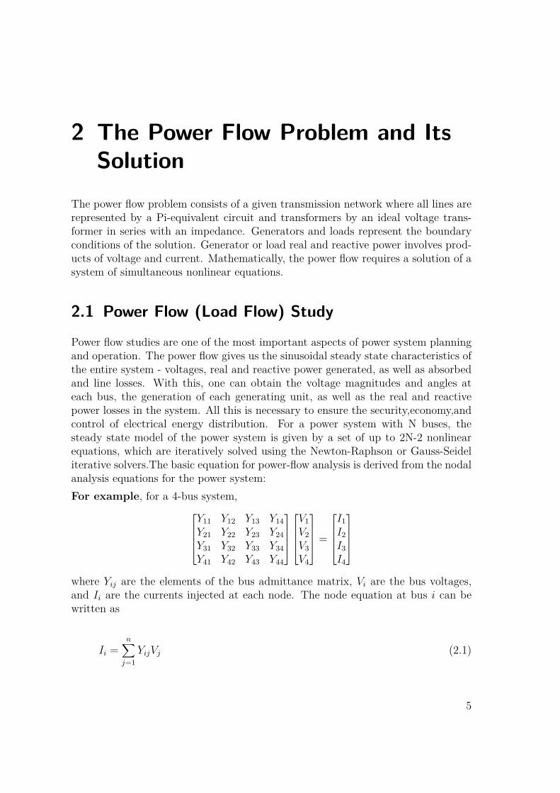
The power flow problem consists of a given transmission network where all lines arerepresented by a Pi-equivalent circuit and transformers by an ideal voltage trans-former in series with an impedance. Generators and loads represent the boundaryconditions of the solution. Generator or load real and reactive power involves prod-ucts of voltage and current. Mathematically, the power flow requires a solution of asystem of simultaneous nonlinear equations.
2.1 Power Flow (Load Flow) Study
Power flow studies are one of the most important aspects of power system planningand operation. The power flow gives us the sinusoidal steady state characteristics ofthe entire system - voltages, real and reactive power generated, as well as absorbedand line losses. With this, one can obtain the voltage magnitudes and angles ateach bus, the generation of each generating unit, as well as the real and reactivepower losses in the system. All this is necessary to ensure the security,economy,andcontrol of electrical energy distribution. For a power system with N buses, thesteady state model of the power system is given by a set of up to 2N-2 nonlinearequations, which are iteratively solved using the Newton-Raphson or Gauss-Seideliterative solvers.The basic equation for power-flow analysis is derived from the nodalanalysis equations for the power system:For example, for a 4-bus system,
Y11 Y12 Y13 Y14Y21 Y22 Y23 Y24Y31 Y32 Y33 Y34Y41 Y42 Y43 Y44
V1V2V3V4
=
I1I2I3I4
where Yij are the elements of the bus admittance matrix, Vi are the bus voltages,and Ii are the currents injected at each node. The node equation at bus i can bewritten as
Ii =n∑
j=1YijVj (2.1)
5
Chapter 2 The Power Flow Problem and Its Solution
Relationship between per-unit real and reactive power supplied to the system at busi and the per-unit current injected into the system at that bus:
Si = ViI∗i = Pi + jQi (2.2)
whereVi is the per-unit voltage at the bus. I∗
i is a complex conjugate of the per-unit current: injected at the bus.Pi and Qi are per-unit real and reactive powers.Therefore,
I∗i = Pi + jQi
Vi
⇒ Ii = Pi − jQi
V ∗i
⇒ Pi − jQi = V ∗i
n∑j=1
YijVj =n∑
j=1YijVjV
∗i (2.3)
LetYij =
∣∣∣Yij
∣∣∣∠θijand Vi =∣∣∣Vi
∣∣∣∠δiThenPi − jQi = ∑n
j=1
∣∣∣Yij
∣∣∣ ∣∣∣Vj
∣∣∣ ∣∣∣Vi
∣∣∣∠(θij + δj − δi)HencePi = ∑n
j=1
∣∣∣Yij
∣∣∣ ∣∣∣Vj
∣∣∣ ∣∣∣Vi
∣∣∣ cos(θij + δj − δi)AndQi = −∑n
j=1
∣∣∣Yij
∣∣∣ ∣∣∣Vj
∣∣∣ ∣∣∣Vi
∣∣∣ sin(θij + δj − δi)[2]
2.2 Focusing on Power Flow
There are four variables that are associated with each bus:1. P2. Q3. V4. δ
Meanwhile, there are two power flow equations associated with each bus. In a powerflow study, two of the four variables are defined and the other two are unknown.That way, we have the same number of equations as the number of unknown. Theknown and unknown variables depend on the type of bus. Each bus in a powersystem can be classified as one of three types:
6
2.3 The Power Flow Problem on a Direct Current Network
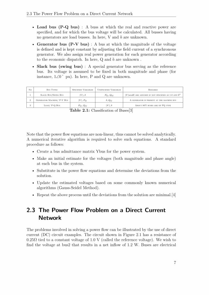
• Load bus (P-Q bus) : A buss at which the real and reactive power arespecified, and for which the bus voltage will be calculated. All busses havingno generators are load busses. In here, V and δ are unknown.
• Generator bus (P-V bus) : A bus at which the magnitude of the voltageis defined and is kept constant by adjusting the field current of a synchronousgenerator. We also assign real power generation for each generator accordingto the economic dispatch. In here, Q and δ are unknown .
• Slack bus (swing bus) : A special generator bus serving as the referencebus. Its voltage is assumed to be fixed in both magnitude and phase (forinstance, 1∠0˚ pu). In here, P and Q are unknown.
No Bus Types Specified Variables Unspecified Variables Remarks
1 Slack Bus/Swing Bus |V |, δ PG, QG |V |andδ are assumed if not specified as 1.0 and 0
2 Generator Machine/ P-V Bus |V |, PG δ,QG A generator is present at the machine bus
3 Load/ P-Q Bus PG, QG |V |, δ About 80% buses are of PQ type
Table 2.1: Classification of Buses[3]
Note that the power flow equations are non-linear, thus cannot be solved analytically.A numerical iterative algorithm is required to solve such equations. A standardprocedure as follows:
• Create a bus admittance matrix Ybus for the power system.• Make an initial estimate for the voltages (both magnitude and phase angle)
at each bus in the system.• Substitute in the power flow equations and determine the deviations from the
solution.• Update the estimated voltages based on some commonly known numerical
algorithms (Gauss-Seidel Method).• Repeat the above process until the deviations from the solution are minimal.[4]
2.3 The Power Flow Problem on a Direct CurrentNetwork
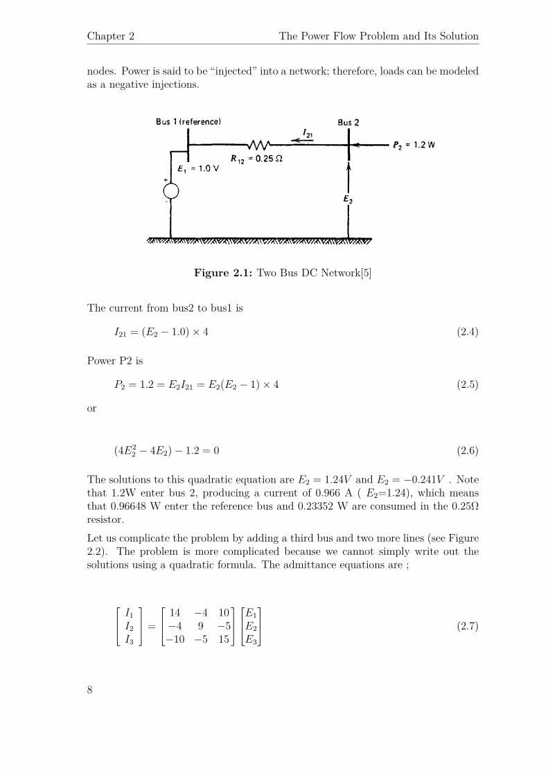
The problems involved in solving a power flow can be illustrated by the use of directcurrent (DC) circuit examples. The circuit shown in Figure 2.1 has a resistance of0.25Ω tied to a constant voltage of 1.0 V (called the reference voltage). We wish tofind the voltage at bus2 that results in a net inflow of 1.2 W. Buses are electrical
7
Chapter 2 The Power Flow Problem and Its Solution
nodes. Power is said to be “injected” into a network; therefore, loads can be modeledas a negative injections.
Figure 2.1: Two Bus DC Network[5]
The current from bus2 to bus1 is
I21 = (E2 − 1.0)× 4 (2.4)
Power P2 is
P2 = 1.2 = E2I21 = E2(E2 − 1)× 4 (2.5)
or
(4E22 − 4E2)− 1.2 = 0 (2.6)
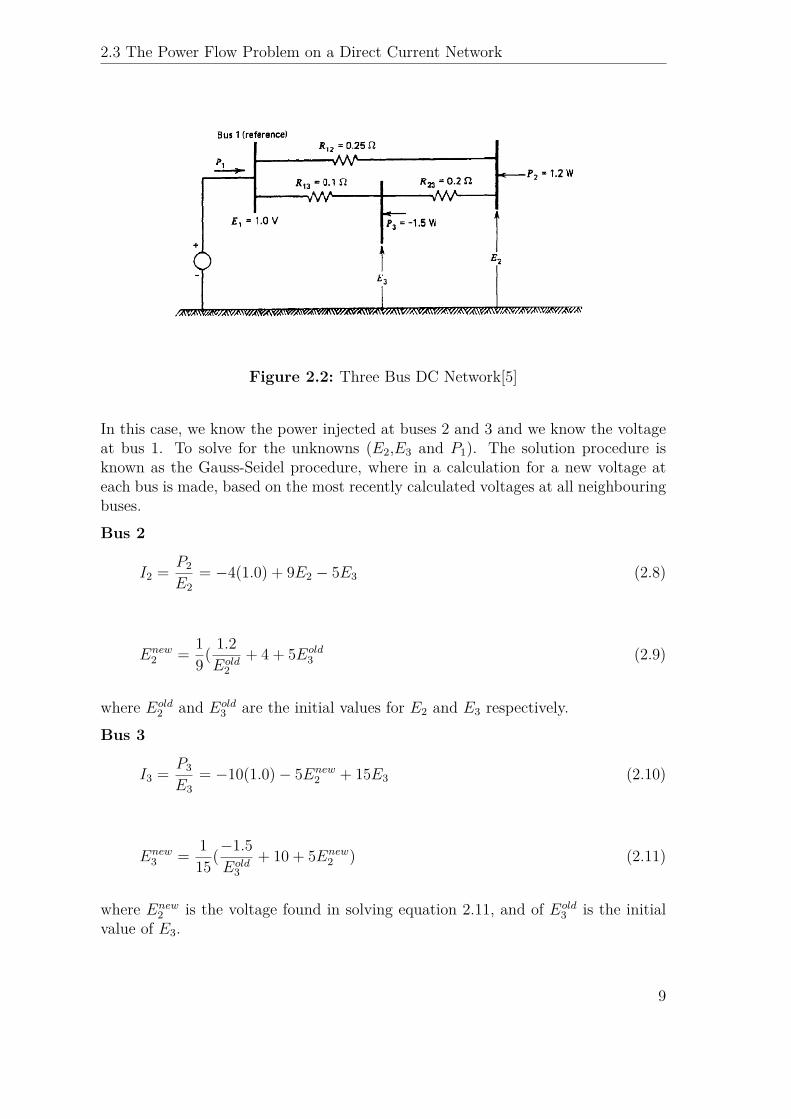
The solutions to this quadratic equation are E2 = 1.24V and E2 = −0.241V . Notethat 1.2W enter bus 2, producing a current of 0.966 A ( E2=1.24), which meansthat 0.96648 W enter the reference bus and 0.23352 W are consumed in the 0.25Ωresistor.Let us complicate the problem by adding a third bus and two more lines (see Figure2.2). The problem is more complicated because we cannot simply write out thesolutions using a quadratic formula. The admittance equations are ;
I1I2I3
=
14 −4 10−4 9 −5−10 −5 15
E1E2E3
(2.7)
8
2.3 The Power Flow Problem on a Direct Current Network
Figure 2.2: Three Bus DC Network[5]
In this case, we know the power injected at buses 2 and 3 and we know the voltageat bus 1. To solve for the unknowns (E2,E3 and P1). The solution procedure isknown as the Gauss-Seidel procedure, where in a calculation for a new voltage ateach bus is made, based on the most recently calculated voltages at all neighbouringbuses.Bus 2
I2 = P2
E2= −4(1.0) + 9E2 − 5E3 (2.8)
Enew2 = 1
9( 1.2Eold
2+ 4 + 5Eold
3 (2.9)
where Eold2 and Eold
3 are the initial values for E2 and E3 respectively.Bus 3
I3 = P3
E3= −10(1.0)− 5Enew
2 + 15E3 (2.10)
Enew3 = 1
15(−1.5Eold
3+ 10 + 5Enew
2 ) (2.11)
where Enew2 is the voltage found in solving equation 2.11, and of Eold
3 is the initialvalue of E3.
9
Chapter 2 The Power Flow Problem and Its Solution
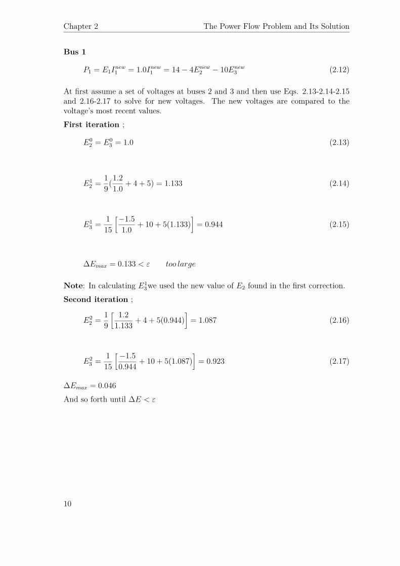
Bus 1
P1 = E1Inew1 = 1.0Inew
1 = 14− 4Enew2 − 10Enew
3 (2.12)
At first assume a set of voltages at buses 2 and 3 and then use Eqs. 2.13-2.14-2.15and 2.16-2.17 to solve for new voltages. The new voltages are compared to thevoltage’s most recent values.First iteration ;
E02 = E0
3 = 1.0 (2.13)
E12 = 1
9(1.21.0 + 4 + 5) = 1.133 (2.14)
E13 = 1
15
[−1.51.0 + 10 + 5(1.133)
]= 0.944 (2.15)
∆Emax = 0.133 < ε too large
Note: In calculating E13we used the new value of E2 found in the first correction.
Second iteration ;
E22 = 1
9
[ 1.21.133 + 4 + 5(0.944)
]= 1.087 (2.16)
E23 = 1
15
[−1.50.944 + 10 + 5(1.087)
]= 0.923 (2.17)
∆Emax = 0.046And so forth until ∆E < ε
10
3 Gauss Sidel Method
In power system, we usually need to solve the bus voltages in a power load flow.The Gauss-Seidel method is an iterative algorithm for solving non linear algebraicequations. An initial solution vector is assumed, chosen from past experiences,statistical data or from practical considerations. At every subsequent iteration, thesolution is updated until convergence is reached. The Gauss-Seidel method appliedto power flow problem is as discussed below.
3.1 Case (a): Systems with PQ buses only
Initially assume all buses to be PQ type buses, except the slack bus. This meansthat (n–1) complex bus voltages have to be determined.Consider the expression forthe complex power at bus-i asSi = Vi(
∑nj=1 YijVj)∗
This can be written as,S∗
i = V ∗i
[∑nj=1 YijVj
]Since,S∗
i = Pi − jQi
we get,
Pi − jQi
V ∗i
=n∑
j=1YijVj (3.1)
So that,
Pi − jQi
V ∗i
= YiiVi +n∑
j=1YijVj (3.2)
Rearranging the terms, we get,
Vi = 1Yii
Pi − jQi
V ∗i
−n∑
j=1YijVj
∀ i = 1, 2, 3.....n (3.3)
11
Chapter 3 Gauss Sidel Method
Equation (3.3) is an implicit equation since the unknown variable, appears on bothsides of the equation. Hence, it needs to be solved by an iterative technique.One iteration of the method involves computation of all the bus voltages.In Gauss–Seidel method, the value of the updated voltages are used in the compu-tation of subsequent voltages in the same iteration, thus speeding up convergence.Iterations are carried out till the magnitudes of all bus voltages do not change bymore than the tolerance value.Thus the algorithm for Gauss–Seidel method is as under:
1. Prepare data for the given system as required.2. Formulate the bus admittance matrix Ybus. This is generally done by the rule
of inspection.3. Assume initial voltages for all buses, (2,3,. . . n). In practical power systems,
the magnitude of the bus voltages is close to 1.0 p.u. Hence, the complex busvoltages at all (n-1) buses (except slack bus) are taken to be 1.0∠0 This isnormally refered as the flat start solution.
4. Update the voltages. In any (k+1)st iteration, from (3) the voltages are givenby
V(k+1)
i = 1Yii
Pi − jQi
(V ki )∗ −
i−1∑j=1
YijV(k+1)
j −n∑
j=1+i
YijV(k)
j
∀ i = 1, 2, 3.....n (3.4)
Here note that when computation is carried out for bus-i, updated values arealready available for buses 2,3. . . .(i-1) in the current (k+ 1)stiteration. Hencethese values are used. For buses (i+1). . . ..n, values from previous, kth iterationare used.
5. Continue iterations untill
|∆V (k+1)i | = |V (k+1)
i − V (k)i | < ε ∀ i = 1, 2, 3.....n (3.5)
Where ε is the tolerance value. Generally it is customary to use a value of0.0001 pu.
6. Compute slack bus power after voltages have converged using (1) [assumingbus 1 is slack bus].
S∗1 = P1 − jQ1 = V ∗
1
n∑j=1
Y1jVj
(3.6)
7. Compute all line flows.8. The complex power loss in the line is given by (Sik + Ski). The total loss in
the system is calculated by summing the loss over all the lines.[6]These steps will be illustrated with giving example at the following pages.
12
3.2 Case (b): Systems with PV buses :
3.2 Case (b): Systems with PV buses :
At PV buses, the magnitude of voltage and not the reactive power is specified.Hence, it is needed to first make an estimate of Qi to be used in (3.4).From (3.1) we have
Qi = −Im
V ∗1
n∑j=1
YijVj
Where Im stands for the imaginary part.At any (k+1)st iteration, at the PV bus-i,
Q(k+1)i = −Im
(V (k)i )∗
i−1∑j=1
YijV(k+1)
j + (V (k)i )∗
n∑j=1
YijV(k)
j
(3.7)
The steps for ith PV bus are as follows:1. Compute Q(k+1)
i using (24)
2. Calculate V i using (21) with Qi = Q(k+1)i
3. Since,|Vi| is specified at the PV bus, the magnitude of Vi obtained in step 2 has to bemodified and set to the specified value |Vi,sp|.Therefore,
V(k+1)
i = |Vi,sp|∠δ(k+1)i (3.8)
The voltage computation for PQ buses does not change.[7]
3.3 Case (c): Systems with PV buses with reactivepower generation limits specified:
In the previous algorithm if the Q limit at the voltage controlled bus is violatedduring any iteration, i.e (Q(k+1)
i ) computed using (3.7) is either less than Qi,min orgreater than Qi,max , it means that the voltage cannot be maintained at the specifiedvalue due to lack of reactive power support. This bus is then treated as a PQ busin the (k+1)st iteration and the voltage is calculated with the value of Qi set asfollows:
13
Chapter 3 Gauss Sidel Method
If Qi < Qi,min If Qi > Qi,max
then Qi = Qi,min then Qi = Qi,max (3.9)
If in the subsequent iteration, if Qi falls within the limits, then the bus can beswitched back to PV status.[8]
3.3.1 Acceleration of convergence
It is found that in Gauss-Seidel method of load flow, the number of iterations increasewith increase in the size of the system. The number of iterations required can bereduced if the correction in voltage at each bus is accelerated, by multiplying witha constant α, called the acceleration factor. In the (k + 1)st iteration we can let
V(k+1)
i (accelerate, d) = V(k)
i + α(V (k+1)i − V (k)
i ) (3.10)
where is a α real number.
When
α = 1
the value of V (k+1)i is the computed value.
If
1 < α < 2
then the value computed is extrapolated.
Generally α is taken between 1.2 to 1.6 for Gauss-Seidel load flow procedure. AtPQ buses (pure load buses) if the voltage magnitude violates the limit, it simplymeans that the specified reactive power demand cannot be supplied, with the voltagemaintained within acceptable limits.[9]
14
3.3 Case (c): Systems with PV buses with reactive power generation limitsspecified:
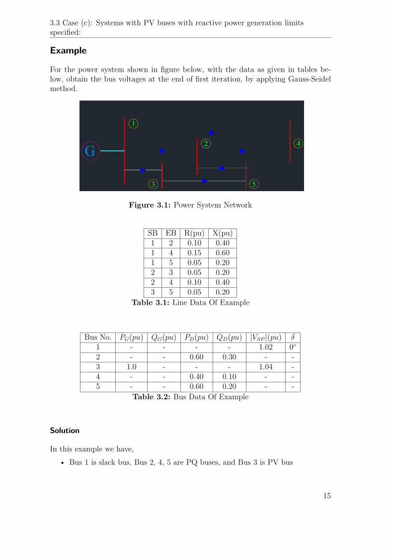
Example
For the power system shown in figure below, with the data as given in tables be-low, obtain the bus voltages at the end of first iteration, by applying Gauss-Seidelmethod.
Figure 3.1: Power System Network
SB EB R(pu) X(pu)1 2 0.10 0.401 4 0.15 0.601 5 0.05 0.202 3 0.05 0.202 4 0.10 0.403 5 0.05 0.20
Table 3.1: Line Data Of Example
Bus No. PG(pu) QG(pu) PD(pu) QD(pu) |VSP |(pu) δ1 - - - - 1.02 0
2 - - 0.60 0.30 - -3 1.0 - - - 1.04 -4 - - 0.40 0.10 - -5 - - 0.60 0.20 - -
Table 3.2: Bus Data Of Example
Solution
In this example we have,• Bus 1 is slack bus, Bus 2, 4, 5 are PQ buses, and Bus 3 is PV bus
15
Chapter 3 Gauss Sidel Method
• The lines do not have half line charging admittances
P2 + jQ2 = PG2 + jQG2–(PD2 + jQD2) = –0.6–j0.3
P3 + jQ3 = PG3 + jQG3–(PD3 + jQD3) = 1.0 + jQG3
Similarly,
P4 + jQ4 = −0.4− j0.1
P5 + jQ5 = −0.6− j0.2
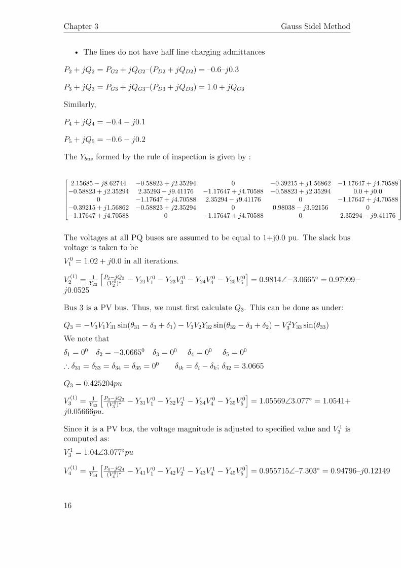
The Ybus formed by the rule of inspection is given by :
2.15685− j8.62744 −0.58823 + j2.35294 0 −0.39215 + j1.56862 −1.17647 + j4.70588−0.58823 + j2.35294 2.35293− j9.41176 −1.17647 + j4.70588 −0.58823 + j2.35294 0.0 + j0.0
0 −1.17647 + j4.70588 2.35294− j9.41176 0 −1.17647 + j4.70588−0.39215 + j1.56862 −0.58823 + j2.35294 0 0.98038− j3.92156 0−1.17647 + j4.70588 0 −1.17647 + j4.70588 0 2.35294− j9.41176
The voltages at all PQ buses are assumed to be equal to 1+j0.0 pu. The slack busvoltage is taken to beV 0
1 = 1.02 + j0.0 in all iterations.
V(1)
2 = 1Y22
[P2−jQ2
(V 02 )∗ − Y21V
01 − Y23V
03 − Y24V
04 − Y25V
05
]= 0.9814∠−3.0665 = 0.97999−
j0.0525
Bus 3 is a PV bus. Thus, we must first calculate Q3. This can be done as under:
Q3 = −V3V1Y31 sin(θ31 − δ3 + δ1)− V3V2Y32 sin(θ32 − δ3 + δ2)− V 23 Y33 sin(θ33)
We note thatδ1 = 00 δ2 = −3.06650 δ3 = 00 δ4 = 00 δ5 = 00
∴ δ31 = δ33 = δ34 = δ35 = 00 δik = δi − δk; δ32 = 3.0665
Q3 = 0.425204pu
V(1)
3 = 1Y33
[P3−jQ3
(V 03 )∗ − Y31V
01 − Y32V
12 − Y34V
04 − Y35V
05
]= 1.05569∠3.077 = 1.0541+
j0.05666pu.
Since it is a PV bus, the voltage magnitude is adjusted to specified value and V 13 is
computed as:V 1
3 = 1.04∠3.077pu
V(1)
4 = 1Y44
[P4−jQ4
(V 04 )∗ − Y41V
01 − Y42V
12 − Y43V
14 − Y45V
05
]= 0.955715∠–7.303 = 0.94796–j0.12149
16
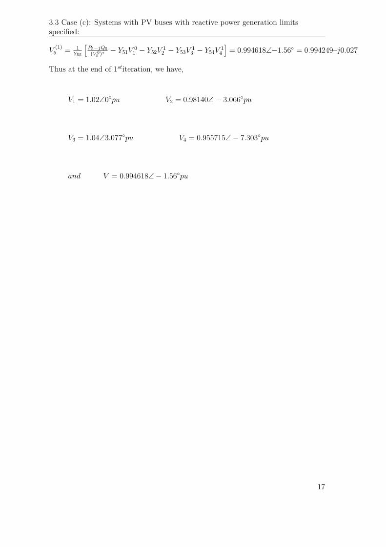
3.3 Case (c): Systems with PV buses with reactive power generation limitsspecified:
V(1)
5 = 1Y55
[P5−jQ5
(V 05 )∗ − Y51V
01 − Y52V
12 − Y53V
13 − Y54V
14
]= 0.994618∠−1.56 = 0.994249–j0.027
Thus at the end of 1stiteration, we have,
V1 = 1.02∠0pu V2 = 0.98140∠− 3.066pu
V3 = 1.04∠3.077pu V4 = 0.955715∠− 7.303pu
and V = 0.994618∠− 1.56pu
17

4 The Per-Unit System
An interconnected power system typically consists of many different voltage levelsgiven a system containing several transformers and/or rotating machines. The per-unit system simplifies the analysis of complex power systems by choosing a commonset of base parameters in terms of which, all systems quantities are defined. The dif-ferent voltage levels disappear and the overall system reduces to a set of impedances.[10]
4.1 Overview
The primary advantages of the per-unit system are:1. The per-unit values for transformer impedance, voltage and current are identi-
cal when referred to the primary and secondary (no need to reflect impedancesfrom one side of the transformer to the other, the transformer is a singleimpedance).
2. The per-unit values for various components lie within a narrow range regardlessof the equipment rating.
3. The per-unit values clearly represent the relative values of the circuit quanti-ties. Many of the ubiquitous scaling constants are eliminated.
4. Ideal for computer simulations. The complete characterization of a per-unitsystem requires that all four base values be defined. Given the four base values,the per-unit quantities are defined as
Vpu = V
Vbase
(4.1)
Ipu = I
Ibase
(4.2)
Zpu = Z
Zbase
(4.3)
Spu = S
Sbase
(4.4)
19
Chapter 4 The Per-Unit System
Note that the numerator terms in the previous equations are in general complexwhile the base values are real-valued. Once any two of the four base values (Vbase,Ibase, Sbase, and Zbase) are defined, the remaining two base values can be determinedaccording their fundamental circuit relationships. Usually the base values of powerand voltage are selected and the base values of current and impedance are determinedaccording to
Ibase = Sbase
Vbase
(4.5)
Zbase = Vbase
Ibase
= V 2base
Sbase
(4.6)
If we also assume that:• The value of Sbase is constant for all points in the power system• the ratio of voltage bases on either side of a transformer is chosen to equal
the ratio of the transformer voltage ratings, then the transformer per-unitimpedance remains unchanged when referred from one side of a transformerto the other.
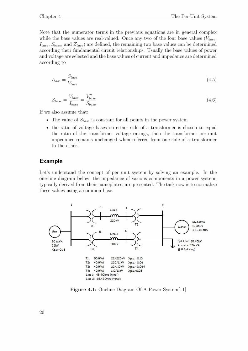
Example
Let’s understand the concept of per unit system by solving an example. In theone-line diagram below, the impedance of various components in a power system,typically derived from their nameplates, are presented. The task now is to normalizethese values using a common base.
Figure 4.1: Oneline Diagram Of A Power System[11]
20
4.1 Overview
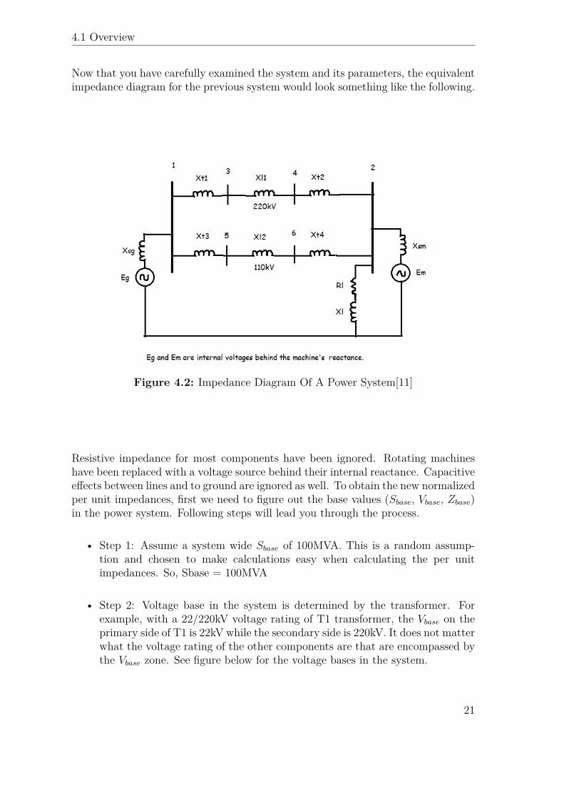
Now that you have carefully examined the system and its parameters, the equivalentimpedance diagram for the previous system would look something like the following.
Figure 4.2: Impedance Diagram Of A Power System[11]
Resistive impedance for most components have been ignored. Rotating machineshave been replaced with a voltage source behind their internal reactance. Capacitiveeffects between lines and to ground are ignored as well. To obtain the new normalizedper unit impedances, first we need to figure out the base values (Sbase, Vbase, Zbase)in the power system. Following steps will lead you through the process.
• Step 1: Assume a system wide Sbase of 100MVA. This is a random assump-tion and chosen to make calculations easy when calculating the per unitimpedances. So, Sbase = 100MVA
• Step 2: Voltage base in the system is determined by the transformer. Forexample, with a 22/220kV voltage rating of T1 transformer, the Vbase on theprimary side of T1 is 22kV while the secondary side is 220kV. It does not matterwhat the voltage rating of the other components are that are encompassed bythe Vbase zone. See figure below for the voltage bases in the system.
21
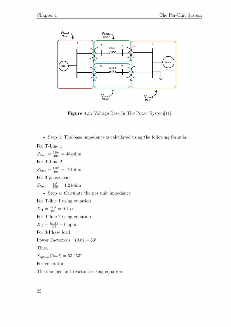
Chapter 4 The Per-Unit System
Figure 4.3: Voltage Base In The Power System[11]
• Step 3: The base impedance is calculated using the following formula:
For T-Line 1Zbase = 2202
100 = 484ohmFor T-Line 2Zbase = 1102
100 = 121ohmFor 3-phase loadZbase = 112
100 = 1.21ohm• Step 4: Calculate the per unit impedance
For T-line 1 using equationXt1 = 48.4
484 = 0.1p.uFor T-line 2 using equationXt2 = 65.43
121 = 0.5p.uFor 3-Phase loadPower Factor:cos−1(0.6) = 53
Thus,S3phase(load) = 53∠53
For generatorThe new per unit reactance using equation
22
4.1 Overview
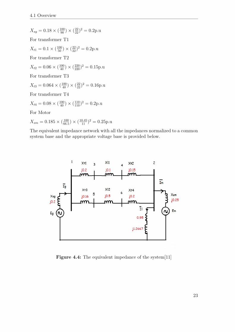
Xsg = 0.18× (10090 )× (22
22)2 = 0.2p.u
For transformer T1
Xt1 = 0.1× (10050 )× (22
22)2 = 0.2p.u
For transformer T2
Xt2 = 0.06× (10040 )× (220
220)2 = 0.15p.u
For transformer T3
Xt3 = 0.064× (10040 )× (22
22)2 = 0.16p.u
For transformer T4
Xt4 = 0.08× (10040 )× (110
110)2 = 0.2p.u
For Motor
Xsm = 0.185× ( 10066.5)× (10.45
11 )2 = 0.25p.u
The equivalent impedance network with all the impedances normalized to a commonsystem base and the appropriate voltage base is provided below.
Figure 4.4: The equivalent impedance of the system[11]
23
Chapter 4 The Per-Unit System
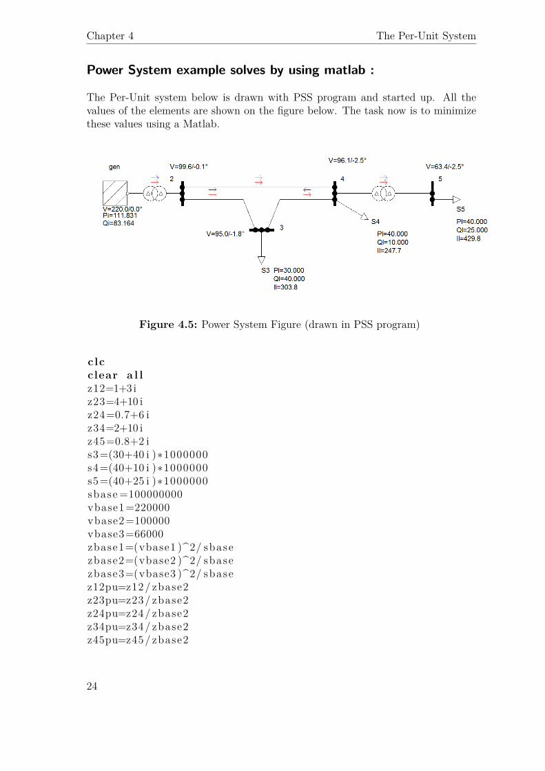
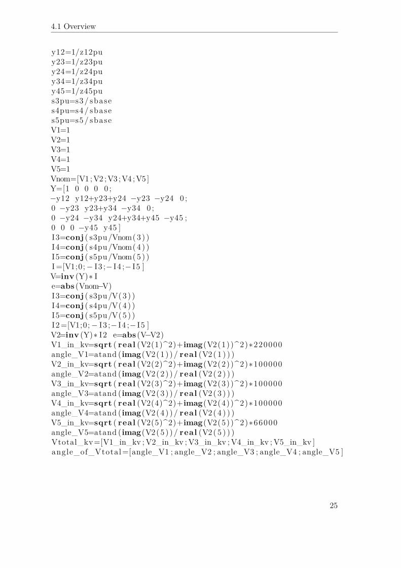
Power System example solves by using matlab :
The Per-Unit system below is drawn with PSS program and started up. All thevalues of the elements are shown on the figure below. The task now is to minimizethese values using a Matlab.
Figure 4.5: Power System Figure (drawn in PSS program)
clcclear a l lz12=1+3 iz23=4+10 iz24=0.7+6 iz34=2+10 iz45=0.8+2 is3=(30+40 i )∗1000000s4=(40+10 i )∗1000000s5=(40+25 i )∗1000000sbase =100000000vbase1=220000vbase2=100000vbase3=66000zbase1=(vbase1 )^2/ sbasezbase2=(vbase2 )^2/ sbasezbase3=(vbase3 )^2/ sbasez12pu=z12/ zbase2z23pu=z23/ zbase2z24pu=z24/ zbase2z34pu=z34/ zbase2z45pu=z45/ zbase2
24
4.1 Overview
y12=1/z12puy23=1/z23puy24=1/z24puy34=1/z34puy45=1/z45pus3pu=s3 / sbases4pu=s4 / sbases5pu=s5 / sbaseV1=1V2=1V3=1V4=1V5=1Vnom=[V1 ;V2 ;V3 ;V4 ;V5 ]Y=[1 0 0 0 0 ;−y12 y12+y23+y24 −y23 −y24 0 ;0 −y23 y23+y34 −y34 0 ;0 −y24 −y34 y24+y34+y45 −y45 ;0 0 0 −y45 y45 ]I3=conj ( s3pu/Vnom(3 ) )I4=conj ( s4pu/Vnom(4 ) )I5=conj ( s5pu/Vnom(5 ) )I=[V1;0;− I3 ;− I4 ;− I5 ]V=inv (Y)∗ Ie=abs (Vnom−V)I3=conj ( s3pu/V(3 ) )I4=conj ( s4pu/V(4 ) )I5=conj ( s5pu/V(5 ) )I2=[V1;0;− I3 ;− I4 ;− I5 ]V2=inv (Y)∗ I2 e=abs (V−V2)V1_in_kv=sqrt ( real (V2(1)^2)+imag(V2(1))^2)∗220000angle_V1=atand ( imag(V2(1 ) ) / real (V2 ( 1 ) ) )V2_in_kv=sqrt ( real (V2(2)^2)+imag(V2(2))^2)∗100000angle_V2=atand ( imag(V2(2 ) ) / real (V2 ( 2 ) ) )V3_in_kv=sqrt ( real (V2(3)^2)+imag(V2(3))^2)∗100000angle_V3=atand ( imag(V2(3 ) ) / real (V2 ( 3 ) ) )V4_in_kv=sqrt ( real (V2(4)^2)+imag(V2(4))^2)∗100000angle_V4=atand ( imag(V2(4 ) ) / real (V2 ( 4 ) ) )V5_in_kv=sqrt ( real (V2(5)^2)+imag(V2(5))^2)∗66000angle_V5=atand ( imag(V2(5 ) ) / real (V2 ( 5 ) ) )Vtotal_kv=[V1_in_kv ; V2_in_kv ; V3_in_kv ; V4_in_kv ; V5_in_kv ]angle_of_Vtotal=[angle_V1 ; angle_V2 ; angle_V3 ; angle_V4 ; angle_V5 ]
25

5 Conclusion
In this study, the load flow problem, also called as the power flow problem, has beenconsidered in detail. The load flow solution gives the complex voltages at all thebuses and the complex power flows in the lines. Though, algorithms are availableusing the impedance form of the equations, the sparsity of the bus admittance matrixand the ease of building the bus admittance matrix, have made algorithms using theadmittance form of equations more popular.The most popular method is the Gauss-Seidel method. This method have been discussed in detail with illustrative examples.In smaller systems, the ease of programming and the memory requirements makeGauss-Seidel method attractive.
27

Acknowledgments
I would like to express my utmost gratitude to Assoc. Prof. Dr. Izudin Dzafic forhis supports ,valuable guidance and suggestions throughout the study. I would liketo thank Mesut OZ and Alimert Vuran for their suggestions during my project.Iwould also like to thank my family for their continuous support. Lastly, I want tothank all who gave a hand during my project.
29

Bibliography
[1] I. Dzafic, E. Halilovic, and E. Karamehmedovic, “Power system analysis,” inIntroduction to Power System Analysis,International University of Sarayevo,january 2013, pp. 103–114.
[2] D. McCalley, in The Power Flow Problem, Lowa State University, June 2004,pp. 10–22.
[3] H. Chowdhury, in Load Flow Analysis in Power System,Universty of Missouri,february 2006, pp. 140–190.
[4] J. Grainger and W. Stevenson, “Power flow,” in Power System Analysis.McGraw-hill, New York, Martch 1994.
[5] J. A. Wood and F. B. Wollenberg, “Power technologies,” in Power Genera-tion,Operation and Control, Second Edition, University of Minnesota, April2007, pp. 105–130.
[6] Y. Liang, “Improved gauss seidel method on power network,” in Gauss SeidelMethod,University of Florida, January 2004.
[7] Y. Saad, in Iterative Methods,Second Edition. Society for industrial and appliedmathematics, February 2003.
[8] A. Keyhani, “Keyhani lecture,www.mty.itsm.mx,” in Gauss-Seidel Method,OhioState University, 2008.
[9] A. G. Tcheslavski, “Power system representations and equations,” in PowerSystem,www.ee.lamar.edu, 2009.
[10] S. Kouro, “Per-unit system,” in Power Conversion, September 2011.[11] “Per unit system-practice problem solved for easy understanding,” in Per Unit
System,www.peguru.com, June 2001.
31

Nomenclature
SG complex power generation
δ bus voltage angle
E synchronous machine-generated voltage
P real bus power
PD real power demand
PG real power generation
Q reactive bus power
QD reactive power demand
QG reactive power generation
R resistance
S complex bus power
SD complex power demand
X reactance
Y admitance
Ybus bus admittance matrix
Yii driving point admittance at bus i
Yij transfer admittance between busses i and j
Z impedance
33