University of Windsor University of Windsor

Scholarship at UWindsor Scholarship at UWindsor

Electrical and Computer Engineering Publications

Department of Electrical and Computer Engineering

6-1-2020

Optimal power flow incorporating facts devices and stochastic Optimal power flow incorporating facts devices and stochastic

wind power generation using krill herd algorithm wind power generation using krill herd algorithm

Arsalan Abdollahi Payam‐e‐Golpayegan Higher Education Institute

Ali Asghar Ghadimi Arak University, Iran

Mohammad Reza Miveh University of Tafresh

Fazel Mohammadi University of Windsor

Francisco Jurado Universidad de Jaen

Follow this and additional works at: https://scholar.uwindsor.ca/electricalengpub

Part of the Electrical and Computer Engineering Commons

Recommended Citation Recommended Citation Abdollahi, Arsalan; Ghadimi, Ali Asghar; Miveh, Mohammad Reza; Mohammadi, Fazel; and Jurado, Francisco. (2020). Optimal power flow incorporating facts devices and stochastic wind power generation using krill herd algorithm. Electronics (Switzerland), 9 (6), 1-18. https://scholar.uwindsor.ca/electricalengpub/15

This Article is brought to you for free and open access by the Department of Electrical and Computer Engineering at Scholarship at UWindsor. It has been accepted for inclusion in Electrical and Computer Engineering Publications by an authorized administrator of Scholarship at UWindsor. For more information, please contact scholarship@uwindsor.ca.

electronics

Article

Optimal Power Flow Incorporating FACTS Devicesand Stochastic Wind Power Generation Using KrillHerd Algorithm

Arsalan Abdollahi 1, Ali Asghar Ghadimi 2, Mohammad Reza Miveh 3, Fazel Mohammadi 4,* andFrancisco Jurado 5

1 Faculty of Electrical and Computer Engineering, Payam-e-Golpayegan Higher Education Institute,Golpayegan, Iran; arsalan.abdoollahi@gmail.com

2 Department of Electrical Engineering, Faculty of Engineering, Arak University, Arak 38156-8-8349, Iran;a-ghadimi@araku.ac.ir

3 Department of Electrical Engineering, Tafresh University, Tafresh 39518-79611, Iran; miveh@tafreshu.ac.ir4 Electrical and Computer Engineering (ECE) Department, University of Windsor, Windsor, ON N9B 1K3, Canada5 Department of Electrical Engineering, University of Jaen, 23700 Linares, Spain; fjurado@ujaen.es* Correspondence: fazel@uwindsor.ca or fazel.mohammadi@ieee.org

Received: 26 May 2020; Accepted: 19 June 2020; Published: 24 June 2020�����������������

Abstract: This paper deals with investigating the Optimal Power Flow (OPF) solution of powersystems considering Flexible AC Transmission Systems (FACTS) devices and wind power generationunder uncertainty. The Krill Herd Algorithm (KHA), as a new meta-heuristic approach, is employedto cope with the OPF problem of power systems, incorporating FACTS devices and stochastic windpower generation. The wind power uncertainty is included in the optimization problem using Weibullprobability density function modeling to determine the optimal values of decision variables. Variousobjective functions, including minimization of fuel cost, active power losses across transmission lines,emission, and Combined Economic and Environmental Costs (CEEC), are separately formulated tosolve the OPF considering FACTS devices and stochastic wind power generation. The effectivenessof the KHA approach is investigated on modified IEEE-30 bus and IEEE-57 bus test systems andcompared with other conventional methods available in the literature.

Keywords: flexible AC transmission systems (FACTS) devices; krill herd algorithm (KHA); optimalpower flow (OPF); stochastic wind power generation

1. Introduction

Optimal Power Flow (OPF) plays a significant role in power systems operation and control.The OPF mainly aims to optimize a certain objective function, such as minimizing the generationfuel cost and at the same time, satisfying the load balance constraints and bound constraints [1,2].Under normal conditions, all devices in power systems should operate within their pre-determinedrange. Such constraints include the maximum and minimum active and reactive power of thegeneration units, voltage levels, loadability of power transmission lines, and transformers tap settings.Minimizing the operating costs and increasing the reliability of power systems are two main objectivesfrom the power companies and utilities’ point of view. Basically, the power flow problem focuses on theeconomic aspect of operating the power systems due to the fact that a slight change in power flow maysignificantly increase the operating costs of power systems. To do so, an objective function is optimizedconsidering various equality and inequality constraints. Solving the OPF problem precisely leads toproper control, planning, and protection of power systems. The OPF problem can be divided intotwo major problems: (1) the optimal active power flow problem, and (2) the optimal reactive power

Electronics 2020, 9, 1043; doi:10.3390/electronics9061043 www.mdpi.com/journal/electronics

Electronics 2020, 9, 1043 2 of 18

flow problem. Numerous papers have investigated the OPF problem using conventional optimizationmethods, such as the Newton Raphson (NR) method, and evolutionary optimization techniques,such as particle swarm optimization (PSO) and artificial bee colony (ABC) optimization algorithms.

Increasing the load demand over the last few decades has created different problems in powersystems in terms of power transmission congestion and constraints. Those limitations are mainly dueto maintaining the stability and maintaining the voltage range of the power system at its permissiblelevel [3,4]. Distributed Generations (DGs) are one of the best solutions to prevent congestion in thetransmission lines [5]. DGs have several advantages, such as reducing energy costs, improving powerquality and reliability, and preventing environmental pollutions. Among different DGs, wind power isone of the most popular power generations. However, wind behavior is often unpredictable, as it is astochastic phenomenon, thereby, needing proper uncertainty modeling. To cope with this challenge,many research studies in the literature have investigated different methods to model the randombehavior of the wind power generation, as depicted in Table 1.

Table 1. Different methods to model the random behavior of wind power generations.

Reference Uncertainty Model Solution Method Objective Functions

[6] Weibull distribution function Sequential quadraticprogramming PSO

Minimizing the total operating costsand minimizing emission

[7] Incomplete gamma function Imperialist CompetitiveAlgorithm (ICA) Minimizing the fuel cost function

[8] Weibull probability density function Gbest Guided-ABC Minimizing the total operating costs

[9] Weibull probability density function PSO Minimizing the total operating andcongestion costs

Another way to enhance the capacity of the transmission systems is by employing Flexible ACTransmission System (FACTS) devices [10]. FACTS devices play a crucial role in improving theflexibility of power transmission and guaranteeing the stability of power systems. FACTS devicesare used for improving power flow regardless of the costs of generating power. Two primary goalsof using FACTS devices are (1) increasing capacity of transmission systems by controlling somecharacteristics, such as series/shunt impedances and phase angle; (2) transmitting power through thedesired paths. Table 2 shows a summary of the previous research studies related to the FACTS devices.Therefore, the conventional OPF problem, integrated with FACTS devices can open new opportunitiesfor controlling the active and reactive power flow.

To date, numerous papers on the OPF problem with various optimization techniques have beenpublished. However, previous studies have not dealt with the OPF incorporating FACTS devicesand stochastic wind power generation at the same time. In this regard, this paper proposes an OPFsolution of power system considering FACTS devices and stochastic wind power generation usingthe krill herd algorithm (KHA). The wind power uncertainty is modeled in the optimization problemusing the Weibull probability density function. Minimization of fuel cost, active power losses acrossthe transmission lines, emission, and combined economic and environmental costs (CEEC) are theobjective functions.

To the best of the authors’ knowledge, solving the OPF problem considering the minimization offuel cost, active power losses across transmission lines, emission, and CEEC, incorporating FACTSdevices and dealing with the stochastic behavior of wind power generation has not been investigatedbefore. Compared with the other techniques, the proposed method has better performance andachieves more accurate results.

Electronics 2020, 9, 1043 3 of 18

Table 2. Different methods to model the random behavior of wind power generations.

Reference Method Objective Functions FACTS Devices

[7] Micro-genetic algorithm andhybrid method

Minimizing the fuel cost and powerlosses, Optimal location of FACTS devices TCSC, TCPAR, UPFC, SVC

[8] PSAT software analysis Improving voltage profile, Minimizingpower losses SVC

[9] Dimensional algorithm using NRload flow

Improving voltage profile, Minimizingpower losses and fuel costs TCSC, TCPR, SVC, STATCOM

[11]Genetic Algorithm (GA) and

Differential EvolutionAlgorithm (DEA)

Minimizing the fuel cost and powerlosses, Optimal location of FACTS devices UPFC, SVC, TCSC

[12] Dimensional algorithm Heat control, Minimizing power losses,Improving power systems stability UPFC

[13] GA and DEA Minimizing the fuel cost and power losses UPFC

[14] Artificial Immune Systems (AIS) Minimizing the fuel cost TCPS, TCSC

[15] GA Minimizing the fuel cost and power losses TCSC, TCPAR, UPFC

[16] DEAMaximizing the loadability of

transmission lines, Reducing thetransmission lines losses

STATCOM

[17] Combined Tabu Search (TS) andSimulated Annealing (SA) method Minimizing the total fuel cost TCSC, TCPS

[18] GA Minimizing the total fuel costs undersecurity constraints UPFC

[19] PSO Reducing the FACTS devices installationcosts, Reducing overload TCSC, UPFC, SVC, TCVR

The followings are the major contributions of this research study:

• Modeling and including the stochastic nature of wind power generation in the problem formulation.• Unlike the other research studies, in this paper, the OPF problem incorporating FACTS devices

and stochastic wind power generation at the same time is solved.• The KHA is used to minimize the fuel cost, active power losses across the transmission lines,

emission, and CEEC, as the objective functions.

This paper is divided into four sections. In Section 2, the problem formulation is given. The resultsare presented in Section 3. Finally, the conclusions are presented.

2. Problem Formulation

In this part, the OPF problem formulation in the presence of FACTS devices, including thyristorcontrolled phase shifter (TCPS) as well as thyristor-controlled series compensator (TCSC), and stochasticwind power generation is presented. The frequency distribution is one of the most essential tools forplanning and operating in power systems, and its general structure is divided into two parts of theobjective function and constraints.

2.1. General Formulation

The general formulation for the constrained optimization problem in this paper is as follows:

min f (u, v) (1)

subject to: {g(u, v) = 0h(u, v) ≤ 0

(2)

where f is the objective function that should be minimized, g(u, v) is the set of equality constraints,and h(u, v) is the set of inequality constraints. It should be noted that for N number of components

Electronics 2020, 9, 1043 4 of 18

in power systems, u is the vector of dependent variables that contains the active power of the slack

generator, voltage of the loads(VL1 , . . . , VLNPQ

), reactive power generation by the generation units(

QG1 , . . . , QGNPV

), and the lines loadability

(SL1 , . . . , SLNL

). Also, v is the vector of independent

variables that contains active power generation by the generation unit except for the slack bus(PG1 , . . . , PGNPV

), voltage of the generators

(VG1 , . . . , VGNPV

), transformers tap settings

(T1, . . . , TNT

),

and the injected reactive power by the FACTS devices(QC1 , . . . , QCNC

). It should be noted that NPQ,

NPV, NL, NT, and NC show the maximum number of generation buses, load buses, transmission lines,transformer tap settings, and FACTS devices, respectively.

The constraints of the OPF problem include active and reactive power of the generation units,transformer tap settings, and the loading of the power transmission lines.

2.2. FACTS Devices Modeling

2.2.1. TCSC Modeling

Figure 1 shows the static of a TCSC connected between bus p and q [20,21].

Electronics 2020, 9, x FOR PEER REVIEW 4 of 18

2. Problem Formulation

In this part, the OPF problem formulation in the presence of FACTS devices, including thyristor controlled phase shifter (TCPS) as well as thyristor-controlled series compensator (TCSC), and stochastic wind power generation is presented. The frequency distribution is one of the most essential tools for planning and operating in power systems, and its general structure is divided into two parts of the objective function and constraints.

2.1. General Formulation

The general formulation for the constrained optimization problem in this paper is as follows: min ( , ) (1)

subject to: ( , ) = 0ℎ( , ) ≤ 0 (2)

where is the objective function that should be minimized, ( , ) is the set of equality constraints, and ℎ( , ) is the set of inequality constraints. It should be noted that for number of components in power systems, is the vector of dependent variables that contains the active power of the slack generator, voltage of the loads ( , … , ), reactive power generation by the generation units ( , … , ), and the lines loadability ( , … , ). Also, is the vector of independent variables that contains active power generation by the generation unit except for the slack bus ( , … , ), voltage of the generators ( , … , ) , transformers tap settings ( , … , ) , and the injected reactive power by the FACTS devices ( , … , ). It should be noted that , , , , and

show the maximum number of generation buses, load buses, transmission lines, transformer tap settings, and FACTS devices, respectively.

The constraints of the OPF problem include active and reactive power of the generation units, transformer tap settings, and the loading of the power transmission lines.

2.2. FACTS Devices Modeling

2.2.1. TCSC Modeling

Figure 1 shows the static of a TCSC connected between bus and [20,21].

Figure 1. Model of TCSC connected between bus and bus.

The power flow equations from bus to bus , including TCSC, are as follows [21]: = − cos − − sin − (3) = − − sin − + cos − (4)

where

Figure 1. Model of TCSC connected between pth bus and qth bus.

The power flow equations from bus p to bus q, including TCSC, are as follows [21]:

Ppq = V2pGpq −VpVqGpq cos

(δp − δq

)−VpVqBpq sin

(δp − δq

)(3)

Qpq = −V2pBpq −VpVqGpq sin

(δp − δq

)+ VpVqBpq cos

(δp − δq

)(4)

where

Gpq =Rpq

R2pq + (Xpq −XCpq)

2 (5)

Bpq =Rpq

R2pq + (Xpq −XCpq)

2 (6)

where Ppq and Qpq are the active and reactive power flow from bus p to bus q with TCPS, respectively,Gpq and Bpq are the conductance and susceptance of transmission line between bus p and bus q,respectively, δp and δq are the voltage angles at the pth bus and qth bus, respectively, Rpq and Xpq denotethe resistance and reactance of the transmission line between bus p and bus q, respectively, and lastly,XCpq represents the reactance of the TCSC located in the transmission line between bus p and bus q.

Similarity, the power flow equations from bus q to bus p, including TCSC, are as follows:

Pqp = V2q Gpq −VpVqGpq cos

(δp − δq

)+ VpVqBpq sin

(δp − δq

)(7)

Qqp = −V2q Bpq + VpVqGpq sin

(δp − δq

)+ VpVqBpq cos

(δp − δq

)(8)

Electronics 2020, 9, 1043 5 of 18

where Pqp and Qqp are the active and reactive power flow from bus q to bus p with TCPS, respectively.

2.2.2. TCPS Modeling

Figure 2 demonstrates the static of a TCPS connected between bus p and q, having a complextaping ratio of 1 : 1∠ϕ and series admittance of Ypq = Gpq − jBpq [20].

Electronics 2020, 9, x FOR PEER REVIEW 5 of 18

= + ( − ) (5)

= + ( − ) (6)

where and are the active and reactive power flow from bus to bus with TCPS, respectively, and are the conductance and susceptance of transmission line between bus and bus , respectively, and are the voltage angles at the bus and bus, respectively,

and denote the resistance and reactance of the transmission line between bus and bus , respectively, and lastly, represents the reactance of the TCSC located in the transmission line between bus and bus .

Similarity, the power flow equations from bus to bus , including TCSC, are as follows: = − cos − + sin − (7) = − + sin − + cos − (8)

where and are the active and reactive power flow from bus to bus with TCPS, respectively.

2.2.2. TCPS Modeling

Figure 2 demonstrates the static of a TCPS connected between bus and , having a complex taping ratio of 1: 1∠ and series admittance of = − [20].

Figure 2. TCPS model connected between bus and bus.

The power flow equations from bus to bus , including the TCPS, are as follows: = cos ( ) − cos( ) cos − + + sin − + (9)

= − cos ( ) − cos( ) sin − + − cos − + (10)

where and are the active and reactive power flow from bus to bus with TCPS, respectively. In addition, shows the phase shift angle of TCPS.

Likewise, the power flow equations from bus to bus , including the TCPS, are as follows: = − cos( ) cos − + − sin − + (11)

= − + cos( ) sin − + + cos − + (12)

Figure 2. TCPS model connected between pth bus and qth bus.

The power flow equations from bus p to bus q, including the TCPS, are as follows:

Ppq =V2

pGpq

cos2(ϕ)−

VpVq

cos(ϕ)

[Gpq cos

(δp − δq + ϕ

)+ Bpq sin

(δp − δq + ϕ

)](9)

Qpq = −V2

pBpq

cos2(ϕ)−

VpVq

cos(ϕ)

[Gpq sin

(δp − δq + ϕ

)− Bpq cos

(δp − δq + ϕ

)](10)

where Ppq and Qpq are the active and reactive power flow from bus p to bus q with TCPS, respectively.In addition, ϕ shows the phase shift angle of TCPS.

Likewise, the power flow equations from bus q to bus p, including the TCPS, are as follows:

Pqp = V2pGpq −

VpVq

cos(ϕ)

[Gpq cos

(δp − δq + ϕ

)− Bpq sin

(δp − δq + ϕ

)](11)

Qqp = −V2q Bpq +

VpVq

cos(ϕ)

[Gpq sin

(δp − δq + ϕ

)+ Bpq cos

(δp − δq + ϕ

)](12)

where Pqp and Qqp are the active and reactive power flow from bus q to bus p with TCPS, respectively.

2.3. Wind Power Generation Modeling

The technology of wind turbines to generate electricity from wind can be divided into two majorgroups: (1) constant speed wind turbine, and (2) variable speed wind turbine. Fixed speed windturbines are easy to install, more durable, and more affordable, while variable speed wind turbinesshould be installed according to the strategic and geographical conditions. Figure 3 shows the outputpower curve of a typical wind turbine. In Figure 3, vci and vci are the cut-in wind speed and cut-outwind speed, respectively, vr is the rated wind speed, and vw is the wind speed flowing into thewind turbine.

Electronics 2020, 9, 1043 6 of 18

Electronics 2020, 9, x FOR PEER REVIEW 6 of 18

where and are the active and reactive power flow from bus to bus with TCPS, respectively.

2.3. Wind Power Generation Modeling

The technology of wind turbines to generate electricity from wind can be divided into two major groups: (1) constant speed wind turbine, and (2) variable speed wind turbine. Fixed speed wind turbines are easy to install, more durable, and more affordable, while variable speed wind turbines should be installed according to the strategic and geographical conditions. Figure 3 shows the output power curve of a typical wind turbine. In Figure 3, and are the cut-in wind speed and cut-out wind speed, respectively, is the rated wind speed, and is the wind speed flowing into the wind turbine.

Figure 3. The output power curve of a typical wind turbine.

Since the wind speed is variable, the Weibull distribution is often considered as the probability density function that can be used to approximately model the behavior of the wind with a reasonable error. The Weibull distribution function to calculate the probability of the wind speed is as follows [22,23]: ( ) = ( )( ) ( ) (13)

where shows the wind speed, and (shape factor) and (scale factor) are the wind speed parameters that vary depending on the region in which the wind blows.

It should be noted that to evaluate the power output of wind power, the problem has a general wind scenario, which initially generates a random number of wind speeds. Then, based on the Weibull distribution function considering the shape factor and scale factor, the probability of occurrence of those wind speeds is determined. Next, a certain number of wind speeds that most probably occur is selected. Finally, the average power of the wind farm is calculated.

2.4. Objective Functions

In this section, four different objective functions are presented.

2.4.1. Minimization of Fuel Cost

Fuel cost minimization with a quadratic function is considered as the first objective function, as follows [24]:

min = + + (14)

where is the total fuel cost of the generation units in ($/h), , , and are the fuel cost coefficients of the generation unit, shows the total number of generation units, and denotes the generated active power by the generation unit.

Figure 3. The output power curve of a typical wind turbine.

Since the wind speed is variable, the Weibull distribution is often considered as the probabilitydensity function that can be used to approximately model the behavior of the wind with a reasonable error.The Weibull distribution function to calculate the probability of the wind speed is as follows [22,23]:

f (v) =(

kc

)(vc

)k−1e−(

vc )

k(13)

where v shows the wind speed, and k (shape factor) and c (scale factor) are the wind speed parametersthat vary depending on the region in which the wind blows.

It should be noted that to evaluate the power output of wind power, the problem has a generalwind scenario, which initially generates a random number of wind speeds. Then, based on the Weibulldistribution function considering the shape factor and scale factor, the probability of occurrence ofthose wind speeds is determined. Next, a certain number of wind speeds that most probably occur isselected. Finally, the average power of the wind farm is calculated.

2.4. Objective Functions

In this section, four different objective functions are presented.

2.4.1. Minimization of Fuel Cost

Fuel cost minimization with a quadratic function is considered as the first objective function, asfollows [24]:

minFC =

NPV∑p=1

(ap + bpPGp + cpP2

Gp

)(14)

where FC is the total fuel cost of the generation units in ($/h), ap, bp, and cp are the fuel cost coefficients ofthe pth generation unit, NPV shows the total number of generation units, and PGp denotes the generatedactive power by the pth generation unit.

Considering the valve-point effect, Equation (15) can be rewritten as follows:

minFC =

NPV∑p=1

(ap + bpPGp + cpP2

Gp

)+

∣∣∣∣∣dp sin(ep

(Pmin

Gp− PGp

))∣∣∣∣∣ (15)

where dp and ep are the fuel cost coefficients to model the valve-point effect, and PminGp

denotes the

minimum active power generated by the pth generation unit.

Electronics 2020, 9, 1043 7 of 18

2.4.2. Minimization of Active Power Losses across the Transmission Lines

This objective function can be formulated as follows:

minPLoss =

NL∑k=1

(Gk

[V2

p + V2q − 2VpVq cos

(δp − δq

)])(16)

where PLoss is the total active power losses across the transmission lines in (MW), Gk is the conductanceof the kth transmission line connected between bus p and bus q, NL is the total number of transmissionlines, Vp and Vq are the voltage magnitudes of bus p and bus q, respectively, and δp and δq are thevoltage angles of bus p and bus q, respectively.

2.4.3. Minimization of Emission

The third objective function is to minimize the total emission, which is formulated as follows:

minE(PG) =

NPV∑k=1

[10−2

(αp + βpPGp + γpP2

Gp+ ηpeλpPGp

)](17)

where E(PG) is the total emission due to the generation of the pth generation unit in (ton/h), and αp, βp,γp, ηp, and λp are the emission coefficients of the pth generation unit.

2.4.4. Minimization of the Combined Economic and Environmental Costs

The last objective function is to minimize the CEEC according to Equations (15) and (17):

minCEEC = FC + Φ.E(PG) =

NPV∑p=1

(ap + bpPGp + cpP2

Gp

)+

∣∣∣∣∣dp sin(ep

(Pmin

Gp− PGp

))∣∣∣∣∣+ ΦNPV∑k=1

(αp + βpPGp + γpP2

Gp+ ηpeλpPGp

)(18)

where CEEC denotes the combined economic and environmental costs, and Φp is the penalty factor,and can be obtained as follows:

Φ =ap

(Pmax

Gp

)2+ bpPmax

Gp+ cp

αp

(Pmax

Gp

)2+ βpPmax

Gp+ γp

(19)

The pollution charge coefficient for each unit is defined as the amount of fuel cost divided by theamount of pollution at its maximum output active power (Pmax

Gp).

2.5. Constraints

In this section, different constraints are defined [24].

2.5.1. Load Flow Constraints

Pwt +

NB∑p=1

(PGp − PLp

)+

NTPCS∑p=1

Ppk =

NB∑p=1

NB∑q=1

∣∣∣∣∣∣∣∣Vp∣∣∣∣∣∣Vq

∣∣∣Ypq∣∣∣ cos

(θpq + δp − δq

)(20)

NB∑p=1

(QGp − PLp

)+

NTPCS∑p=1

Qpk = −

NB∑p=1

NB∑q=1

∣∣∣∣∣∣∣∣Vp∣∣∣∣∣∣Vq

∣∣∣Ypq∣∣∣ sin

(θpq + δp − δq

)(21)

where PGp and QGp are the generated active and reactive power at bus p, respectively, PLp and QLp arethe consumed active and reactive power at bus p, respectively, Ppk and Qpk are the injected active and

Electronics 2020, 9, 1043 8 of 18

reactive power by the TCPSs at bus p, respectively, Pwt indicates the generated active power by thewind turbine,

∣∣∣Ypq∣∣∣ and θpq are the magnitude and phase of the admittance of the transmission line

between bus p and bus q, NB shows the total number of buses, and NTPCS denotes the total numberof TCPSs.

2.5.2. Active and Reactive Power of the Generation Units

PminGp≤ PGp ≤ Pmax

Gp(22)

QminGp≤ QGp ≤ Qmax

Gp(23)

where for p = 1, . . . , NPV (NPV is the total number of generators), PminGp

and PmaxGp

are the minimum

and maximum limits of the active power of the pth generator, respectively, and QminGp

and QmaxGp

are the

minimum and maximum limits of the reactive power of the pth generator, respectively.

2.5.3. Voltage at Each Bus

VminLp≤ VLp ≤ Vmax

Lp(24)

where for p = 1, . . . , NPQ (NPQ is the total number of loads), VminLp

and VmaxLp

are the minimum and

maximum level of the voltage at the pth load center, respectively.

2.5.4. Transformer Tap Settings

Tminp ≤ Tp ≤ Tmax

p (25)

where for p = 1, . . . , NT (NT is the total number of transformers), Tminp and Tmax

p are the minimum andmaximum tap settings limits of the pth transformer, respectively.

2.5.5. Transmission Lines Loading

SLp ≤ SmaxLp

(26)

where for p = 1, . . . , NL (NL is the total number of transmission lines), SLp and SmaxLp

are the apparent

power flow and maximum apparent power flow of the pth transmission line, respectively.

2.5.6. TCSC Reactance Constraints

XminTp≤ XTp ≤ Xmax

Tp(27)

where for p = 1, . . . , NTCSC (NTCSC is the total number of TCSCs), XminTp

and XmaxTp

are the minimum and

maximum reactance of the pth TCSC, respectively.

2.5.7. TCPS Phase Shift

ϕminTp≤ ϕTp ≤ ϕ

maxTp

(28)

where for p = 1, . . . , NTCPS (NTCPS is the total number of TCPSs), ϕminTp

and ϕmaxTp

are the minimum and

maximum phase shift angle of the pth TCPS, respectively.

Electronics 2020, 9, 1043 9 of 18

2.6. Solution Method

The KHA is based on the herding behavior of krill swarms in response to the specific biological andenvironmental processes [25]. In this paper, the KHA is used to solve the OPF problem incorporatingstochastic wind power generation and FACTS devices considering uncertainty. The followings are thesteps to implement the KHA.

Step 1: Start

Step 2: Check the data structure

Step 3: Initialization

Step 4: Fitness evaluation and check for constraints

Step 5: Motion calculationInduced motionForaging motionPhysical diffusion

Step 6: Implementation of the genetic operator

Step 7: Check the results based on updating the krill individual position in the search space

Step 8: If the best results are achieved thenGo to Step 9OtherwiseGo to Step 4

Step 9: End

3. Simulation Results

To demonstrate the applicability and validity of the proposed method, two different test systems,(1) IEEE 30-bus test system, and (2) IEEE 57-bus test system are analyzed [26,27]. In addition, a windfarm consisting of 20 × 2 MW wind turbines is considered. It should be noted that the number ofiterations for all simulated cases is set to 500. The highlighted rows in all tables show the correspondingvalues for the specific objective functions.

3.1. Case 1: IEEE 30-Bus Test System

The IEEE 30-bus test system consists of 21 load centers with an overall power consumption of4283 MW. It has six generators at buses 1, 2, 5, 8, 11, and 13. Totally, nine reactive power control devicesare located at buses 10, 12, 15, 17, 20, 21, 23, 24, and 29. In addition, the range of voltage in this casestudy is considered between 0.95 and 1.05 p.u. There are 41 transmission lines. The tap changers arelocated in transmission lines 6–9, 6–10, 4–12, and 28–27. According to [13], two TCSCs are installed intransmission lines 3–4, 19–20 with 50% (minimum) and 100% (maximum) series line reactances, andtwo TCPS are also placed on transmission lines 5–7 and 10–22 with –5◦ (minimum) and +5◦ (maximum)phase shift angles. In addition, the wind farm is placed on bus 22 [27]. In this section, two case studies,considering the wind farm in power systems and neglecting it are carried out.

3.1.1. Minimization of Fuel Cost

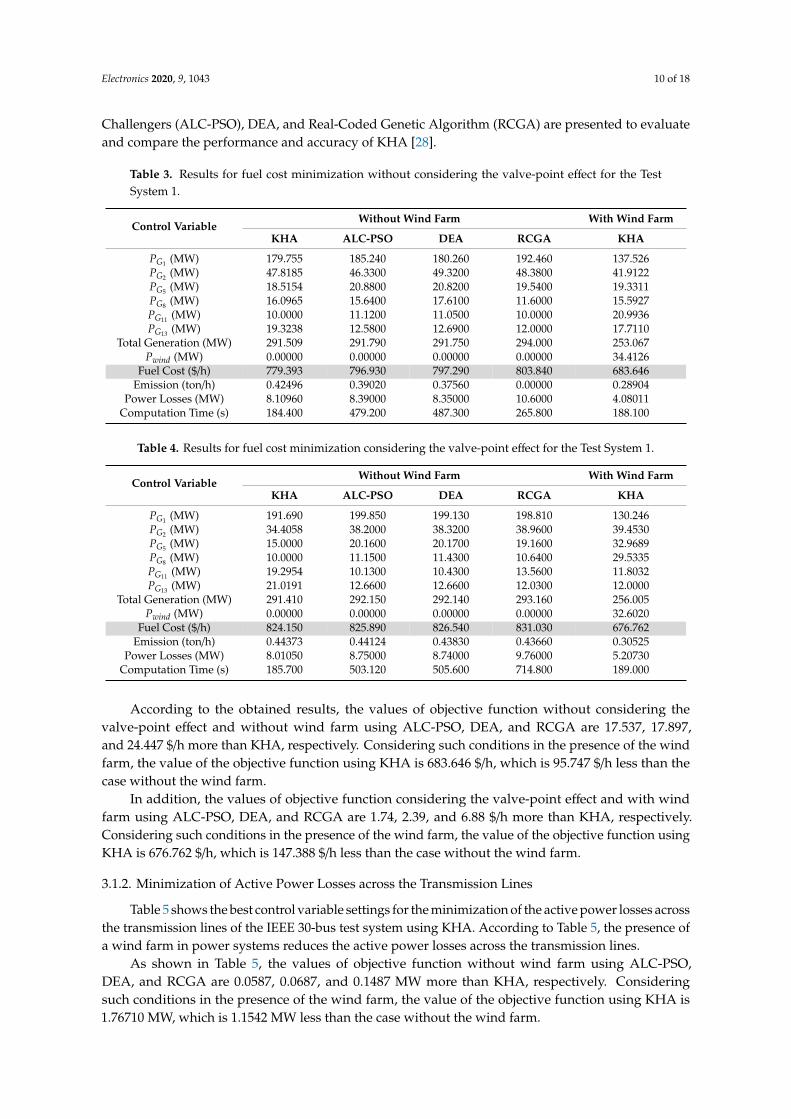
The simulation results without considering the valve-point effect, with and without wind farm (asindicated by Pwind), are provided in Table 3. The simulation results considering the valve-point effect,with and without wind farm, are also given in Table 4. Tables 3 and 4 show that the presence of a windfarm in the case study reduces the generation capacity of other generation units and decreases the fuelcosts and emission. Additionally, the results of Particle Swarm Optimization with Aging Leader and

Electronics 2020, 9, 1043 10 of 18

Challengers (ALC-PSO), DEA, and Real-Coded Genetic Algorithm (RCGA) are presented to evaluateand compare the performance and accuracy of KHA [28].

Table 3. Results for fuel cost minimization without considering the valve-point effect for the TestSystem 1.

Control VariableWithout Wind Farm With Wind Farm

KHA ALC-PSO DEA RCGA KHA

PG1 (MW) 179.755 185.240 180.260 192.460 137.526PG2 (MW) 47.8185 46.3300 49.3200 48.3800 41.9122PG5 (MW) 18.5154 20.8800 20.8200 19.5400 19.3311PG8 (MW) 16.0965 15.6400 17.6100 11.6000 15.5927PG11 (MW) 10.0000 11.1200 11.0500 10.0000 20.9936PG13 (MW) 19.3238 12.5800 12.6900 12.0000 17.7110

Total Generation (MW) 291.509 291.790 291.750 294.000 253.067Pwind (MW) 0.00000 0.00000 0.00000 0.00000 34.4126

Fuel Cost ($/h) 779.393 796.930 797.290 803.840 683.646Emission (ton/h) 0.42496 0.39020 0.37560 0.00000 0.28904

Power Losses (MW) 8.10960 8.39000 8.35000 10.6000 4.08011Computation Time (s) 184.400 479.200 487.300 265.800 188.100

Table 4. Results for fuel cost minimization considering the valve-point effect for the Test System 1.

Control VariableWithout Wind Farm With Wind Farm

KHA ALC-PSO DEA RCGA KHA

PG1 (MW) 191.690 199.850 199.130 198.810 130.246PG2 (MW) 34.4058 38.2000 38.3200 38.9600 39.4530PG5 (MW) 15.0000 20.1600 20.1700 19.1600 32.9689PG8 (MW) 10.0000 11.1500 11.4300 10.6400 29.5335PG11 (MW) 19.2954 10.1300 10.4300 13.5600 11.8032PG13 (MW) 21.0191 12.6600 12.6600 12.0300 12.0000

Total Generation (MW) 291.410 292.150 292.140 293.160 256.005Pwind (MW) 0.00000 0.00000 0.00000 0.00000 32.6020

Fuel Cost ($/h) 824.150 825.890 826.540 831.030 676.762Emission (ton/h) 0.44373 0.44124 0.43830 0.43660 0.30525

Power Losses (MW) 8.01050 8.75000 8.74000 9.76000 5.20730Computation Time (s) 185.700 503.120 505.600 714.800 189.000

According to the obtained results, the values of objective function without considering thevalve-point effect and without wind farm using ALC-PSO, DEA, and RCGA are 17.537, 17.897,and 24.447 $/h more than KHA, respectively. Considering such conditions in the presence of the windfarm, the value of the objective function using KHA is 683.646 $/h, which is 95.747 $/h less than thecase without the wind farm.

In addition, the values of objective function considering the valve-point effect and with windfarm using ALC-PSO, DEA, and RCGA are 1.74, 2.39, and 6.88 $/h more than KHA, respectively.Considering such conditions in the presence of the wind farm, the value of the objective function usingKHA is 676.762 $/h, which is 147.388 $/h less than the case without the wind farm.

3.1.2. Minimization of Active Power Losses across the Transmission Lines

Table 5 shows the best control variable settings for the minimization of the active power losses acrossthe transmission lines of the IEEE 30-bus test system using KHA. According to Table 5, the presence ofa wind farm in power systems reduces the active power losses across the transmission lines.

As shown in Table 5, the values of objective function without wind farm using ALC-PSO,DEA, and RCGA are 0.0587, 0.0687, and 0.1487 MW more than KHA, respectively. Consideringsuch conditions in the presence of the wind farm, the value of the objective function using KHA is1.76710 MW, which is 1.1542 MW less than the case without the wind farm.

Electronics 2020, 9, 1043 11 of 18

Table 5. Results for minimizing the active power losses across the transmission lines for the TestSystem 1.

Control VariableWithout Wind Farm With Wind Farm

KHA ALC-PSO DEA RCGA KHA

PG1 (MW) 98.0937 74.6900 77.5900 77.5800 15.7459PG2 (MW) 53.5641 67.3000 67.3000 69.5800 80.0000PG5 (MW) 50.0000 50.0000 50.0000 49.9800 50.0000PG8 (MW) 35.0000 34.6600 34.8500 34.9600 35.0000PG11 (MW) 16.5549 27.2600 27.0400 23.6900 30.0000PG13 (MW) 32.8586 32.2200 32.3600 30.4300 40.0000

Total Generation (MW) 286.071 286.130 285.140 286.220 250.745Pwind (MW) 0.00000 0.00000 0.00000 0.00000 34.4212

Fuel Cost ($/h) 992.050 992.180 992.300 985.210 918.639Emission (ton/h) 0.21091 0.21090 0.21090 0.21440 0.21031

Power Losses (MW) 2.92130 2.98000 2.99000 3.07000 1.76710Computation Time (s) 170.150 482.100 497.400 711.700 174.300

3.1.3. Minimization of Active Power Losses across the Transmission Lines

Table 6 shows the best control variable settings for the emission minimization of the IEEE 30-bustest systems using KHA. Table 6 shows that the presence of a wind farm in power systems decreasesthe emission.

Table 6. Results for emission minimization for the Test System 1.

Control VariableWithout Wind Farm With Wind Farm

KHA ALC-PSO DEA RCGA KHA

PG1 (MW) 51.3924 64.5200 63.5000 63.9800 45.9204PG2 (MW) 80.0000 66.9000 67.9200 67.7500 51.6969PG5 (MW) 50.0000 50.0000 50.0000 50.0000 50.0000PG8 (MW) 35.0000 35.0000 35.0000 35.0000 35.0000PG11 (MW) 30.0000 30.0000 30.0000 29.9600 30.0000PG13 (MW) 40.0000 40.0000 40.0000 40.0000 40.0000

Total Generation (MW) 286.392 286.420 286.420 286.690 252.617Pwind (MW) 0.00000 0.00000 0.00000 0.00000 33.3285

Fuel Cost ($/h) 1012.75 1014.24 1015.10 1015.80 906.068Emission (ton/h) 0.20469 0.20475 0.20480 0.20490 0.19587

Power Losses (MW) 2.99240 3.02000 3.02000 3.29000 2.54580Computation Time (s) 169.140 506.100 511.300 706.000 173.180

According to the obtained results, the values of objective function without wind farm usingALC-PSO, DEA, and RCGA are 0.00006, 0.00011, and 0.00021 ton/h more than KHA, respectively.Considering such conditions in the presence of the wind farm, the value of the objective function usingKHA is 0.19587 ton/h, which is 0.00882 ton/h less than the case without the wind farm.

3.1.4. Minimization of Combined Economic and Environmental Costs

Table 7 demonstrates the best control variable settings for the CEEC minimization of the IEEE30-bus test systems using KHA. According to the obtained results, the presence of a wind farm inpower systems decreases the CEEC.

As shown in Table 7, the values of objective function without wind farm using ALC-PSO andDEA are 1.64 and 5.29 more than KHA, respectively. Considering such conditions in the presence ofthe wind farm, the value of the objective function using KHA is 1095.72, which is 137.08 less than thecase without the wind farm.

Electronics 2020, 9, 1043 12 of 18

Table 7. Results for emission minimization for the Test System 1.

Control VariableWithout Wind Farm With Wind Farm

KHA ALC-PSO DEA KHA

PG1 (MW) 126.476 115.230 107.980 110.376PG2 (MW) 66.4293 56.5700 58.5700 63.8014PG5 (MW) 29.8519 31.8800 32.3800 23.7588PG8 (MW) 27.9298 27.5400 27.6100 17.1252PG11 (MW) 18.0473 23.8900 29.5100 16.7590PG13 (MW) 19.8514 34.2300 33.2700 23.6716

Total Generation (MW) 288.585 289.330 289.320 255.492Pwind (MW) 0.00000 0.00000 0.00000 32.3655

Fuel Cost ($/h) 897.430 907.170 922.360 784.653Emission (ton/h) 0.23990 0.24302 0.23640 0.22423

Power Losses (MW) 5.18590 5.92000 5.93000 4.45820CEEC 1232.80 1234.44 1238.09 1095.72

Computation Time (s) 189.140 515.100 521.300 189.180

Figures 4–7 show the convergence curves of the defined objective functions for the Test System 1after 500 iterations.

Electronics 2020, 9, x FOR PEER REVIEW 12 of 18

Table 7. Results for emission minimization for the Test System 1.

Control Variable Without Wind Farm With Wind Farm

KHA ALC-PSO DEA KHA (MW) 126.476 115.230 107.980 110.376 (MW) 66.4293 56.5700 58.5700 63.8014 (MW) 29.8519 31.8800 32.3800 23.7588 (MW) 27.9298 27.5400 27.6100 17.1252 (MW) 18.0473 23.8900 29.5100 16.7590 (MW) 19.8514 34.2300 33.2700 23.6716

Total Generation (MW) 288.585 289.330 289.320 255.492 (MW) 0.00000 0.00000 0.00000 32.3655

Fuel Cost ($/h) 897.430 907.170 922.360 784.653 Emission (ton/h) 0.23990 0.24302 0.23640 0.22423

Power Losses (MW) 5.18590 5.92000 5.93000 4.45820 CEEC 1232.80 1234.44 1238.09 1095.72

Computation Time (s) 189.140 515.100 521.300 189.180

As shown in Table 7, the values of objective function without wind farm using ALC-PSO and DEA are 1.64 and 5.29 more than KHA, respectively. Considering such conditions in the presence of the wind farm, the value of the objective function using KHA is 1095.72, which is 137.08 less than the case without the wind farm.

Figures 4–7 show the convergence curves of the defined objective functions for the Test System 1 after 500 iterations.

Figure 4. The convergence curves for the fuel cost minimization considering and neglecting the valve-point effect for the Test System 1.

Figure 4. The convergence curves for the fuel cost minimization considering and neglecting thevalve-point effect for the Test System 1.Electronics 2020, 9, x FOR PEER REVIEW 13 of 18

Figure 5. The convergence curves for the minimization of power losses across the transmission lines for the Test System 1.

Figure 6. The convergence curves for emission minimization for the Test System 1.

Figure 7. The convergence curves for CEEC minimization for the Test System 1.

Figure 5. The convergence curves for the minimization of power losses across the transmission linesfor the Test System 1.

Electronics 2020, 9, 1043 13 of 18

Electronics 2020, 9, x FOR PEER REVIEW 13 of 18

Figure 5. The convergence curves for the minimization of power losses across the transmission lines for the Test System 1.

Figure 6. The convergence curves for emission minimization for the Test System 1.

Figure 7. The convergence curves for CEEC minimization for the Test System 1.

Figure 6. The convergence curves for emission minimization for the Test System 1.

Electronics 2020, 9, x FOR PEER REVIEW 13 of 18

Figure 5. The convergence curves for the minimization of power losses across the transmission lines for the Test System 1.

Figure 6. The convergence curves for emission minimization for the Test System 1.

Figure 7. The convergence curves for CEEC minimization for the Test System 1. Figure 7. The convergence curves for CEEC minimization for the Test System 1.

3.2. Case 2: IEEE 57-Bus Test System

The IEEE 57-bus test system, which consists of 7 generators located at the buses 1, 2, 3, 6, 8, 9,and 12 with 15 transformers under load tap settings, is chosen as test system 2. Three reactive powersources are taken at buses 18, 25, and 53. In this paper, TCSCs are located in transmission lines 18–19,31–32, 34–32, 40–56, and 39–57. TCPSs are also installed in transmission lines 4–5, 5–6, 26–27, 41–43,and 53–54. The wind farm is placed at bus 52 [27]. The same as the previous section, two case studies,considering the wind farm in power systems and neglecting it, are carried out. Tables 8–11 show thebest control variable settings for different objective functions of the IEEE 57-bus test system using KHA.

According to the obtained results from Tables 8–11, considering wind farm in power system causea significant reduction on power losses across the transmission lines, emission, and CEEC.

Electronics 2020, 9, 1043 14 of 18

Table 8. Results for fuel cost minimization without considering the valve-point effect for the TestSystem 2.

Control VariableWithout Wind Farm With Wind Farm

KHA ALC-PSO DEA RCGA KHA

PG1 (MW) 584.6750 514.2600 520.0900 517.4500 422.6630PG2 (MW) 0.000000 0.000000 0.000000 0.000000 105.4910PG5 (MW) 75.16610 123.5300 103.7400 94.81000 161.5274PG6 (MW) 0.000000 0.000000 0.000000 0.000000 182.3932PG8 (MW) 166.0264 159.6700 175.6300 181.7500 0.00000PG9 (MW) 253.7019 0.000000 0.000000 0.000000 125.9095PG12 (MW) 211.8802 486.8900 485.2300 489.7700 256.8480

Total Generation (MW) 1291.449 1284.350 1284.690 1283.780 1254.832Pwind (MW) 0.000000 0.000000 0.000000 0.000000 36.37860

Fuel Cost ($/h) 7768.000 8103.180 8309.270 8413.430 6748.000Emission (ton/h) 2.379500 2.397820 2.433300 2.433100 2.018000

Power Losses (MW) 40.64980 33.55000 33.89000 32.98000 40.41060Computation Time (s) 678.9000 680.1200 689.9000 847.9000 714.7000

Table 9. Results for minimizing the active power losses across the transmission lines for the TestSystem 2.

Control VariableWithout Wind Farm With Wind Farm

KHA ALC-PSO DEA RCGA KHA

PG1 (MW) 192.3159 303.2400 318.5800 311.3400 176.1450PG2 (MW) 0.000000 0.000000 0.000000 0.000000 16.85120PG5 (MW) 34.34410 63.19000 45.90000 60.61300 156.9747PG6 (MW) 134.0298 0.000000 0.000000 0.000000 58.62480PG8 (MW) 469.7929 400.7500 407.6500 400.0600 158.5790PG9 (MW) 0.000000 0.000000 0.000000 0.000000 290.1441PG12 (MW) 436.1565 500.0000 495.0300 495.1400 371.8631

Total Generation (MW) 1266.639 1267.180 1267.160 1267.153 1229.181Pwind (MW) 0.000000 0.000000 0.000000 0.000000 35.46800

Fuel Cost ($/h) 15,354.40 15,423.88 15,691.30 15,348.11 13,078.79Emission (ton/h) 1.916836 1.906545 1.966905 1.917299 1.507600

Power Losses (MW) 21.93910 22.48000 22.46000 22.46300 21.11000Computation Time (s) 670.2000 881.3000 701.7000 691.0450 715.0000

Table 10. Results for minimizing the active power losses across the transmission lines for the TestSystem 2.

Control VariableWithout Wind Farm With Wind Farm

KHA ALC-PSO DEA RCGA KHA

PG1 (MW) 333.585 341.910 298.12 300.23 143.311PG2 (MW) 0.00000 0.00000 0.00000 0.00000 149.200PG5 (MW) 170.617 91.9000 83.24 91.43 158.020PG6 (MW) 0.00000 0.00000 0.00000 0.00000 161.346PG8 (MW) 311.707 419.250 413.63 406.26 220.977PG9 (MW) 0.00000 0.00000 0.00000 0.00000 173.139PG12 (MW) 453.292 418.450 474.14 472.08 228.994

Total Generation (MW) 1269.20 1271.51 1269.13 1270 1234.99Pwind (MW) 0.00000 0.00000 0.00000 0.00000 34.2539

Fuel Cost ($/h) 15,667.9 15,856.1 15,914.3 15,577.3 15,202.6Emission (ton/h) 1.82129 1.88918 1.85870 1.83871 1.72090

Power Losses (MW) 18.4031 20.7100 18.3300 19.2000 18.4442Computation Time (s) 690.100 878.700 694.200 690.140 705.510

Electronics 2020, 9, 1043 15 of 18

Table 11. Results for CEEC minimization for the Test System 2.

Control VariableWithout Wind Farm With Wind Farm

KHA ALC-PSO DEA KHA

PG1 (MW) 346.8868 480.9300 475.6800 92.82350PG2 (MW) 0.000000 0.000000 0.000000 286.8995PG5 (MW) 173.0854 80.14000 80.64000 89.87540PG6 (MW) 0.000000 0.000000 0.000000 193.2463PG8 (MW) 157.0796 270.4200 276.0300 13.55130PG9 (MW) 0.000000 0.000000 0.000000 89.01440PG12 (MW) 583.2398 446.0400 447.2000 459.5085

Total Generation (MW) 1260.291 1279.530 1279.550 1224.918Pwind (MW) 0.000000 0.000000 0.000000 36.18200

Fuel Cost ($/h) 9917.870 10,237.79 10,408.49 8481.851Emission (ton/h) 2.200089 2.227447 2.211635 1.620300

Power Losses (MW) 9.491500 28.73000 28.75000 10.30090CEEC 11,410.00 13,032.56 13,183.42 10,060.00

Computation Time (s) 690.1000 700.1400 702.2000 717.5100

In addition, Figures 8–11 show the convergence curves of the defined objective functions for theTest System 2 after 500 iterations.

Electronics 2020, 9, x FOR PEER REVIEW 15 of 18

Table 10. Results for minimizing the active power losses across the transmission lines for the Test System 2.

Control Variable Without Wind Farm With Wind Farm

KHA ALC-PSO DEA RCGA KHA (MW) 333.585 341.910 298.12 300.23 143.311 (MW) 0.00000 0.00000 0.00000 0.00000 149.200 (MW) 170.617 91.9000 83.24 91.43 158.020 (MW) 0.00000 0.00000 0.00000 0.00000 161.346 (MW) 311.707 419.250 413.63 406.26 220.977 (MW) 0.00000 0.00000 0.00000 0.00000 173.139 (MW) 453.292 418.450 474.14 472.08 228.994

Total Generation (MW) 1269.20 1271.51 1269.13 1270 1234.99 (MW) 0.00000 0.00000 0.00000 0.00000 34.2539

Fuel Cost ($/h) 15667.9 15856.1 15914.3 15577.3 15202.6 Emission (ton/h) 1.82129 1.88918 1.85870 1.83871 1.72090

Power Losses (MW) 18.4031 20.7100 18.3300 19.2000 18.4442 Computation Time (s) 690.100 878.700 694.200 690.140 705.510

Table 11. Results for CEEC minimization for the Test System 2.

Control Variable Without Wind Farm With Wind Farm

KHA ALC-PSO DEA KHA (MW) 346.8868 480.9300 475.6800 92.82350 (MW) 0.000000 0.000000 0.000000 286.8995 (MW) 173.0854 80.14000 80.64000 89.87540 (MW) 0.000000 0.000000 0.000000 193.2463 (MW) 157.0796 270.4200 276.0300 13.55130 (MW) 0.000000 0.000000 0.000000 89.01440 (MW) 583.2398 446.0400 447.2000 459.5085

Total Generation (MW) 1260.291 1279.530 1279.550 1224.918 (MW) 0.000000 0.000000 0.000000 36.18200

Fuel Cost ($/h) 9917.870 10237.79 10408.49 8481.851 Emission (ton/h) 2.200089 2.227447 2.211635 1.620300

Power Losses (MW) 9.491500 28.73000 28.75000 10.30090 CEEC 11410.00 13032.56 13183.42 10060.00

Computation Time (s) 690.1000 700.1400 702.2000 717.5100

In addition, Figures 8–11 show the convergence curves of the defined objective functions for the Test System 2 after 500 iterations.

Figure 8. The convergence curves for the fuel cost minimization considering and neglecting the valve-point effect for the Test System 2.

Figure 8. The convergence curves for the fuel cost minimization considering and neglecting thevalve-point effect for the Test System 2.

Electronics 2020, 9, x FOR PEER REVIEW 16 of 18

Figure 9. The convergence curves for the minimization of power losses across the transmission lines for the Test System 2.

Figure 10. The convergence curves for emission minimization for the Test System 2.

Figure 11. The convergence curves for CEEC minimization for the Test System 2.

4. Conclusions

Figure 9. The convergence curves for the minimization of power losses across the transmission linesfor the Test System 2.

Electronics 2020, 9, 1043 16 of 18

Electronics 2020, 9, x FOR PEER REVIEW 16 of 18

Figure 9. The convergence curves for the minimization of power losses across the transmission lines for the Test System 2.

Figure 10. The convergence curves for emission minimization for the Test System 2.

Figure 11. The convergence curves for CEEC minimization for the Test System 2.

4. Conclusions

Figure 10. The convergence curves for emission minimization for the Test System 2.

Electronics 2020, 9, x FOR PEER REVIEW 16 of 18

Figure 9. The convergence curves for the minimization of power losses across the transmission lines for the Test System 2.

Figure 10. The convergence curves for emission minimization for the Test System 2.

Figure 11. The convergence curves for CEEC minimization for the Test System 2.

4. Conclusions

Figure 11. The convergence curves for CEEC minimization for the Test System 2.

4. Conclusions

A new meta-heuristic algorithm is proposed in this paper to cope with the Optimal Power Flow(OPF) problem of power systems incorporated with wind farm and FACTS devices. Four differentobjective functions, including minimization of fuel cost, minimization of power losses across thetransmission line, emission reduction, and combined economic and environmental cost minimizationare formulated separately in this paper. To show the effectiveness of the proposed approach, the IEEE30-bus test system and the IEEE 57-bus test system with the installation of thyristor controlled phaseshifter (TCPS) and thyristor-controlled series compensator (TCSC) and a wind farm are simulated.Based on numerical results, it is observed that the krill herd algorithm (KHA) has great capability toachieve an optimal solution in the target functions with less computation time. The proposed methodindicates an improved convergence performance to optimal solutions than other heuristic techniquesand can be applied to cope with complex optimization problems in modern power systems. It canefficiently deal with the uncertainties in wind power generation. In addition, it is shown that thepresence of the wind farm in power systems minimizes the d the generation capacity of the othergenerating unit, which reduces the dependency on conventional power plants, thus, reducing powerlosses across the transmission lines and reducing emission as well as the combined economic andenvironmental costs (CEEC).

Electronics 2020, 9, 1043 17 of 18

Author Contributions: All authors have contributed equally to this work. All authors have read and agreed tothe published version of the manuscript.

Funding: This research received no external funding.

Conflicts of Interest: The authors declare no conflict of interest.

References

1. Kahourzade, S.; Mahmoudi, A.; Mokhlis, H.B. A Comparative Study of Multi-Objective Optimal Power FlowBased on Particle Swarm, Evolutionary Programming, and Genetic Algorithm. Electr. Eng. 2015, 97, 1–12.[CrossRef]

2. Viafora, N.; Delikaraoglou, S.; Pinson, P.; Holbøll, J. Chance-Constrained Optimal Power Flow withNon-Parametric Probability Distributions of Dynamic Line Ratings. Int. J. Electr. Power Energy Syst. 2020,114, 105389. [CrossRef]

3. Dong, X.; Zhang, R.; Wang, M.; Wang, J.; Wang, C.; Wang, Y.; Wang, P. Capacity Assessment for Wind PowerIntegration Considering Transmission Line Electro-Thermal Inertia. Int. J. Electr. Power Energy Syst. 2020,118, 105724. [CrossRef]

4. Miveh, M.R.; Rahmat, M.F.; Ghadimi, A.A.; Mustafa, M.W. Control Techniques for Three-Phase Four-LegVoltage Source Inverters in Autonomous Microgrids: A Review. Renew. Sustain. Energy Rev. 2016, 54,1592–1610. [CrossRef]

5. Heideier, R.; Bajay, S.V.; Jannuzzi, G.M.; Gomes, R.D.M.; Guanais, L.; Ribeiro, I.; Paccola, A. Impacts ofPhotovoltaic Distributed Generation and Energy Efficiency Measures on the Electricity Market of ThreeRepresentative Brazilian Distribution Utilities. Energy Sustain. Dev. 2020, 54, 60–71. [CrossRef]

6. Zhang, Y.; Yao, F.; Iu, H.H.-C.; Fernando, T.; Wong, K.P. Sequential Quadratic Programming Particle SwarmOptimization for Wind Power System Operations Considering Emissions. J. Mod. Power Syst. Clean Energy2013, 1, 231–240. [CrossRef]

7. Baskaran, J.; Palanisamy, V. Optimal Location of FACTS Devices in a Power System Solved by a HybridApproach. Nonlinear Anal. Theory Methods Appl. 2006, 65, 2094–2102. [CrossRef]

8. Roy, R.; Jadhav, H.T. Optimal Power Flow Solution of Power System Incorporating Stochastic Wind PowerUsing Gbest Guided Artificial Bee Colony Algorithm. Int. J. Electr. Power Energy Syst. 2015, 64, 562–578.[CrossRef]

9. Gotham, D.J.; Heydt, G.T. Power Flow Control and Power Flow Studies for Systems with FACTS Devices.IEEE Trans. Power Syst. 1998, 13, 60–65. [CrossRef]

10. Bhattacharyya, B.; Gupta, V.K.; Kumar, S. UPFC with Series and Shunt FACTS Controllers for the EconomicOperation of a Power System. Ain Shams Eng. J. 2014, 5, 775–787. [CrossRef]

11. Noroozian, M.; Angquist, L.; Ghandhari, M.; Andersson, G. Use of UPFC for Optimal Power Flow Control.IEEE Trans. Power Deliv. 1997, 12, 1629–1634. [CrossRef]

12. Behshad, M.; Lashkarara, A.; Rahmani, A.H. Optimal Location of UPFC Device Considering SystemLoadability, Total Fuel Cost, Power Losses and Cost of Installation. In Proceedings of the 2ndInternational Conference on Power Electronics and Intelligent Transportation System, Shenzhen, China,19–20 December 2009.

13. Basu, M. Multi-Objective Optimal Power Flow with FACTS Devices. Energy Convers. Manag. 2011, 52,903–910. [CrossRef]

14. Pattanaik, J.K.; Basu, M.; Dash, D.P. Optimal Power Flow with FACTS Devices Using Artificial ImmuneSystems. In Proceedings of the International Conference on Technological Advancements in Power andEnergy, Kollam, India, 21–23 December 2017.

15. Vanitha, R.; Baskaran, J.; Sudhakaran, M. Multi Objective Optimal Power Flow with STATCOM Using DE inWAFGP. Indian J. Sci. Technol. 2015, 8, 191. [CrossRef]

16. Ongsakul, W.; Bhasaputra, P. Optimal Power Flow with FACTS Devices by Hybrid TS/SA Approach. Int. J.Electr. Power Energy Syst. 2002, 24, 851–857. [CrossRef]

17. Leung, H.C.; Chung, T.S. Optimal Power Flow with a Versatile FACTS Controller by Genetic AlgorithmApproach. In Proceedings of the 5th International Conference on Advances in Power System Control,Operation and Management, Hong Kong, China, 30 October–1 November 2000.

Electronics 2020, 9, 1043 18 of 18

18. Easwaramoorthy, N.K.; Dhanasekaran, R. Solution of Optimal Power Flow Problem Incorporating VariousFACTS Devices. Int. J. Comput. Appl. Technol. 2012, 55, 38–44.

19. Singh, B.; Kumar, R. A Comprehensive Survey on Enhancement of System Performances by Using DifferentTypes of FACTS Controllers in Power Systems with Static and Realistic Load Models. Energy Rep. 2020, 6,55–79. [CrossRef]

20. Singh, R.P.; Mukherjee, V.; Ghoshal, S.P. Particle Swarm Optimization with an Aging Leader and ChallengersAlgorithm for Optimal Power Flow Problem with FACTS Devices. Int. J. Electr. Power Energy Syst. 2015, 64,1185–1196. [CrossRef]

21. Nguyen, T.T.; Mohammadi, F. Optimal Placement of TCSC for Congestion Management and Power LossReduction Using Multi-Objective Genetic Algorithm. Sustainability 2020, 12, 2813. [CrossRef]

22. Nguyen, T.T.; Pham, L.H.; Mohammadi, F.; Kien, L.C. Optimal Scheduling of Large-ScaleWind-Hydro-Thermal Systems with Fixed-Head Short-Term Model. Appl. Sci. 2020, 10, 2964. [CrossRef]

23. Saeed, M.A.; Ahmed, Z.; Yang, J.; Zhang, W. An Optimal Approach of Wind Power Assessment UsingChebyshev Metric for Determining the Weibull Distribution Parameters. Sustain. Energy Technol. Assess.2020, 37, 100612. [CrossRef]

24. Shaw, B.; Mukherjee, V.; Ghoshal, S.P. A Novel Opposition-Based Gravitational Search Algorithm forCombined Economic and Emission Dispatch Problems of Power Systems. Int. J. Electr. Power Energy Syst.2012, 35, 21–33. [CrossRef]

25. Gandomi, A.H.; Alavi, A.H. Krill Herd: A New Bio-Inspired Optimization Algorithm. Commun. NonlinearSci. Numer. Simul. 2012, 17, 4831–4845. [CrossRef]

26. Mishra, C.; Singh, S.P.; Rokadia, J. Optimal Power Flow in the Presence of Wind Power Using ModifiedCuckoo Search. IET Gener. Transm. Distrib. 2015, 9, 615–626. [CrossRef]

27. Mohseni-Bonab, S.M.; Rabiee, A.; Mohammadi-Ivatloo, B. Voltage Stability Constrained Multi-ObjectiveOptimal Reactive Power Dispatch Under Load and Wind Power Uncertainties: A Stochastic Approach.Renew. Energy 2016, 85, 598–609. [CrossRef]

28. Mukherjee, A.; Mukherjee, V. Solution of Optimal Power Flow with FACTS Devices Using a NovelOppositional Krill Herd Algorithm. Int. J. Electr. Power Energy Syst. 2016, 78, 700–714. [CrossRef]

© 2020 by the authors. Licensee MDPI, Basel, Switzerland. This article is an open accessarticle distributed under the terms and conditions of the Creative Commons Attribution(CC BY) license (http://creativecommons.org/licenses/by/4.0/).