Method for analysing multi-path power flow transmissions

A Study of Genetic Algorithm Evolution on the Lipophilicity ofPolychlorinated Biphenyls

Lorentz J�ntschia)b)c), Sorana D. Bolboaca*a)b)c), and Radu E. Sestrasc)

a) Technical University of Cluj-Napoca, 103-105 Muncii Bvd, RO-400641 Cluj-Napoca(phone: þ40-264-431697; fax: þ40-264-593847; e-mail: [email protected])

b) �Iuliu Hatieganu� University of Medicine and Pharmacy Cluj-Napoca, 13 Emil Isac,RO-400023 Cluj-Napoca

c) University of Agricultural Sciences and Veterinary Medicine Cluj-Napoca, 3-5 Manastur,RO-400372 Cluj-Napoca

The search for multivariate linear regression (MLR) in quantitative structure–property relation-ships (QSPR) is a hard problem, due to the dimension of the entire search space. A genetic algorithm(GA) was developed and assessed, to select proper descriptors for predicting the octan-1-ol/H2Opartition coefficient of polychlorinated biphenyls. The GA was implemented as a Windows basedFreePascal application with MySQL connectivity for fetching the data. An outcome study based on 30runs was done keeping all parameters constant: sample size, 8; number of variables in the MLR, 2;adaptation-imposed requirements; maximum number of generations, 1000; selection strategy, propor-tional; probability of mutation, 0.05; number of genes implied in mutation, 2; optimization parameter, r2 ;optimization score, minimum in sample; and optimization objective, maximum. The results revealed thatthe number of evolutions followed the Poisson distribution with the sample size as parameter. Theaverage of the determination coefficient is higher than 98% of the determination coefficient obtainedthrough complete search, and follows the Gaussian distribution. The correlation coefficients obtained bythe best performing GA-MLR models proved not to be statistically different from the correlationcoefficient of the QSPR model obtained by complete search.

Introduction. – Genetic algorithms (GAs) are derived from observations of naturalphenomena and simulations of the artificial selection of organisms with multiple locicontrolling a measurable trait [1] [2]. GAs have evolved into complex and stronginformatics tools able to deal with hard problems of decision, classification,optimization, and simulation [3]. GAs have also been used in drug design [4 –7].

The structure – property/activity relationships (SP/ARs) establish functional linksbetween the structure of chemical compounds and the associated physical and chemicalproperties (SPRs) or the biological activities (SARs) [8]. A huge variety of potentialdescriptors is available nowadays [9]. The computer is used to reduce the dimension-ality of the descriptor space, to select those descriptors that have the highestcontribution to the activity/property [10 – 12]. A series of techniques are used to select asubset of the most relevant descriptors: cluster analysis [13] [14], principal componentanalysis [15], discriminate analysis [16] [17], multiple linear regressions [18], partialleast squares regression [19], factor analysis [20], GAs [21], machine learning [5] [22],self-organizing-maps [23] [24], and neural networks [25].

CHEMISTRY & BIODIVERSITY – Vol. 7 (2010)1978

� 2010 Verlag Helvetica Chimica Acta AG, Z�rich

The molecular descriptors family (MDF) approach [26] has been introduced andproved its abilities to identify the structure – activity/property relationships of severalclasses of compounds [27 – 29]. The aim of the present paper was to develop,implement, and assess the performances of a GA used to select the MDF subset withthe highest explanation capacity for the octan-1-ol/H2O partition coefficients of asample of polychlorinated biphenyls (PCBs).

Results and Discussion. – The 60 descriptors presented in Table 1 were identified asbeing used by the genetic algorithm-based multivariate linear regression (GA-MLR)models with a high determination coefficient.

A summary of the performances obtained in each run, expressed as the minimumand maximum values of the determination coefficient, the minimum and maximumvalues of the sum of residuals in the estimate, and the generation (out of 1000) in whichthe maximum value of the correlation coefficient was obtained, are presented inTable 2.

The analysis of the alive regressions in cultivar revealed the followings:* The minimum value varied from 2 (Runs 9, 11, and 15) to 66 (Run 26) with a mean

of 20 (95% CI (15 – 26)) and a standard error of 2.75.* The most frequent minimum number of alive regressions was 12 (Runs 2, 19, 23, and

25).* The maximum number of alive regressions varied from 80 (Run 11) to 288 (Run 22)

with a mean of 172 (95% CI (151– 194)) and a standard error of 10.48.* The most frequent value of the maximum number of alive regressions was 128

(Runs 2, 3, 24, and 30).* The range between the maximum and minimum of alive regressions on a run varied

from 78 (Run 11) to 244 (Run 22) with a mean of 152 (95% CI (133 – 171)) and astandard error of 9.41. The minimum value of the range was obtained in a run, inwhich both the minimum and maximum values of alive regressions in cultivar wereminimum (Run 11). The maximum range was obtained in Run 22, in which thevalue of the number of alive regressions in cultivar was maximum.

CHEMISTRY & BIODIVERSITY – Vol. 7 (2010) 1979

Table 1. Descriptors of the Molecular Descriptors Family Selected by Genetic Algorithms

Type Descriptors

Geometrical IhMrFMg, isDdTCg, iADrVGg, lFmdlCg, IBDmlHg, isDRKHg, isDddHg,iamdlMg, IHmmkHg, ismmFEg, iHPRSMg, iHDrjMg, isMmVGg, isMDFGg,IbMrVGg, iammkEg, iimmkMg, ISPmjGg, iHDrkGg, IbmrWGg, ISDrsGg,IaDdQEg, IbMdlHg, IbMdqGg, IbMdoMg, lfMmkEg, lbmmfHg, iimmfHg,IBMdLHg, lBMmtHg, iimdSHg, ImDdQEg, ImMdlEg

Topological INPRLCt, ISPRWCt, INPRKGt, iAmdSEt, inmMlHt, IMPdQHt, IHmmkHt,lMmRFGt, iSPRsEt, ISmRPEt, ABMMJQt, INMMJCt, iBDRsEt, IBPRoEt,inMRjGt, IbDrkGt, inmRVGt, iSPRsGt, ImDrTGg, iSPDFCt, ihmDFMt,IbMdoMt, IaDDDCt, iSDRFEt, ImMDJGt, ImPDKGt, ImMMKCt

The evolution of the GA in terms of determination coefficients in the runs for theminimum and maximum numbers of alive regressions in cultivar is presented in Fig. 1.Note that the minimum number of alive regressions usually comes from the firstgeneration (correlates with the initial solution), while the maximum number of aliveregressions comes from the most populated generation.

As expected, it was observed that when the GA was run 30 times, 30 different QSPRmodels were identified for the investigated PCBs (see Table 2). The GA-MLR model


Table 2. Summary of Genetic Algorithm Performances According to the Run

Run r2min

a) r2max

b) Evolc) Parameters of the optimum solution

Alive Gend) r (95% CI)e) Sef) trg) Hrh)

1 0.2608 0.8764 6 118 488 0.9362 (0.9168–0.9511) 17.49 62.91 0.5402 0.7126 0.8779 6 56 908 0.9370 (0.9178–0.9517) 17.27 �139.82 0.5353 0.4276 0.8770 7 90 690 0.9365 (0.9171–0.9513) 17.40 �323.91 0.5384 0.7191 0.8724 6 104 33 0.9340 (0.9139–0.9494) 18.06 27.71 0.5515 0.2621 0.8792 12 124 846 0.9377 (0.9187–0.9523) 17.09 107.37 0.5326 0.4434 0.8737 5 88 77 0.9347 (0.9148–0.9499) 17.88 �120.01 0.5477 0.5782 0.8807 8 94 676 0.9385 (0.9197–0.9529) 16.88 �134.84 0.5278 0.7141 0.8747 3 80 5 0.9353 (0.9156–0.9504) 17.73 �129.25 0.5449 0.7802 0.8745 15 66 936 0.9351 (0.9153–0.9503) 17.76 �21.34 0.545

10 0.4528 0.8784 12 74 937 0.9372 (0.9180–0.9519) 17.20 �120.27 0.53411 0.8153 0.8756 9 46 381 0.9358 (0.9162–0.9508) 17.60 39.91 0.54212 0.3071 0.8793 6 78 908 0.9377 (0.9187–0.9523) 17.17 �513.91 0.53113 0.1659 0.8796 7 182 104 0.9379 (0.9190–0.9524) 17.03 �226.42 0.53014 0.5126 0.8778 10 88 724 0.9369 (0.9177–0.9516) 17.29 104.39 0.53615 0.3628 0.8733 13 26 692 0.9345 (0.9146–0.9498) 17.93 975.79 0.54816 0.2858 0.8684 9 64 297 0.9319 (0.9112–0.9478) 18.61 29.51 0.56217 0.4694 0.8791 6 82 118 0.9376 (0.9186–0.9522) 17.11 98.87 0.53218 0.7995 0.8739 10 56 961 0.9348 (0.9150–0.9500) 17.85 119.86 0.54719 0.6931 0.8773 5 80 889 0.9366 (0.9173–0.9514) 17.36 114.80 0.53720 0.4480 0.8790 6 106 19 0.9375 (0.9184–0.9521) 17.12 170.24 0.53221 0.8092 0.8748 8 84 869 0.9353 (0.9156–0.9504) 17.71 118.77 0.54422 0.3788 0.8719 7 82 485 0.9338 (0.9137–0.9493) 18.12 �54.23 0.55223 0.3796 0.8781 10 88 424 0.9371 (0.9179–0.9518) 17.25 178.88 0.53524 0.7933 0.8704 6 118 814 0.9330 (0.9126–0.9486) 18.33 461.09 0.55625 0.7629 0.8771 7 190 126 0.9365 (0.9171–0.9513) 17.39 �1166.71 0.53826 0.7617 0.8745 10 138 117 0.9351 (0.9153–0.9503) 17.76 �82.76 0.54527 0.3518 0.8742 14 142 571 0.9350 (0.9152–0.9502) 17.80 696.11 0.54628 0.8551 0.8751 8 118 565 0.9355 (0.9159–0.9506) 17.67 �27.33 0.54329 0.4619 0.8746 13 128 650 0.9352 (0.9155–0.9503) 17.74 �44.25 0.54530 0.6486 0.8767 5 68 157 0.9363 (0.9169–0.9512) 17.44 �200.80 0.539

a) r2min¼Minimum determination coefficient. b) r2

max¼Maximum determination coefficient. c) Evol¼Evolution (number of iterations in which an improvement of r2 was obtained). d) Gen¼Generation (outof 1000) in which the optimum was obtained. e) r (95% CI)¼Correlation coefficient of the QSPR modelwith 95% confidence intervals associated to the correlation coefficient in parentheses. f) Se¼Sum ofresiduals in the estimate. g) tr¼Geometric mean of evolution. h) Hr¼Entropy of determination orundetermination event.

with the highest determination coefficient was obtained in Run 7. The characteristics ofthis model are:

YGA-MLR¼1.139(�0.917)�0.237(�0.079) · ImPdQHt þ 0.217(�0.019) · iAmdlMg

r¼0.9384 (95% CI (0.9196�0.9528))

r2¼0.8807, sest¼0.29, Fest (pest)¼749 (1.93 ·10�94)

r2cv-loo¼0.8763, sloo¼0.29, Fpred (ppred)¼719 (2.17 · 10�93)

where YGA-MLR is the estimated octan-1-ol/H2O partition coefficient (GA-MLR),ImPdQHt and iAmdlMg are molecular descriptors, and r is the correlation coefficient,r2 the determination coefficient, sest the standard error of estimate, Fest (pest) the F-valueand associated probability, r2

cv-loo the cross-validation leave-one-out score, sloo thestandard error of predicted, and Fpred (ppred) the F-value and associated significance inthe leave-one-out analysis, respectively. The descriptors used in this model and theassociated residuals are available as Supplementary Material1). The graphicalrepresentations of the best performing GA-MLR search vs. the complete MLR searchis presented in Fig. 2.

In terms of GA scores, the optimum scores were obtained in the run, in which thehighest determination coefficient was obtained (see Table 2). Thus, in Run 7, three outof four GA scores, represented by the minimum value of the sum of residuals inestimate, the maximum value of the determination coefficient, and the minimum valueof the determination or undetermination entropy, were optimum. The analysis of thegeometric mean of evolution revealed that the minimum value of �1166.71 wasobtained in Run 25, while the maximum value of 975.79 was obtained in Run 15 (the


Fig. 1. Evolution of the coefficient of determination (r2): minimum (Runs 9, 11, and 15) vs. maximum(Run 22) number of alive regressions

1) Supplementary Material may be obtained upon request from the authors.

absolute minimum value of 21.34 was obtained in Run 9, the absolute maximum valueof 1166.71 was obtained in Run 25). The value of the geometric mean of evolutionseems to be the score that is not related with the other imposed scores in the evaluationof GA performances.

Three criteria were used to assess the GA performance: i) the evolution (number ofgenerations in which the determination coefficient improved), ii) the generation forwhich the determination coefficient has not changed until the end, and iii) thedetermination coefficient. The main statistical characteristics of these criteria arepresented in Table 3.

The following were revealed to be true, when the distribution of the investigatedcriteria was analyzed:* The evolution distribution proved to be Poisson (number of categories¼12, l¼

8.00, df (degree of freedom)¼2, Kolmogorov – Smirnov statistics¼0.136, Chi-square statistics¼1.446, and p¼0.485).

* The maximum frequency distribution (for ten classes) of the number of generationsin which the maximum value was obtained was observed in the following classes:


Fig. 2. Experimental log POW as a function of the best estimated log POW: GA-MLR search vs. MLRcomplete search

Table 3. Statistical Characteristics of the Genetic Algorithm Assessment

Criterion Minimum Maximum Mean Median Mode

Evola) 3 15 8 7.5 6Genmax

b) 5 961 516 568 908r2c) 0.8684 0.8807 0.8759 0.8760 n.a.d)

a) Evol¼Evolution (number of iteration in which r2 improved). b) Genmax¼Generation in which r2

reaches the maximum value. c) r2¼Determination coefficient. d) n.a.¼Not available.

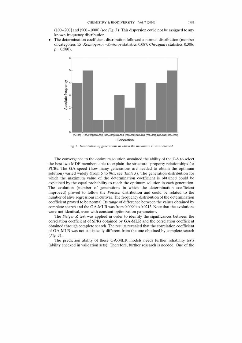
(100– 200] and (900– 1000] (see Fig. 3). This dispersion could not be assigned to anyknown frequency distribution.

* The determination coefficient distribution followed a normal distribution (numberof categories, 15; Kolmogorov – Smirnov statistics, 0.087; Chi-square statistics, 0.306;p¼0.580).

The convergence to the optimum solution sustained the ability of the GA to selectthe best two MDF members able to explain the structure – property relationships forPCBs. The GA speed (how many generations are needed to obtain the optimumsolution) varied widely (from 5 to 961, see Table 3). The generation distribution forwhich the maximum value of the determination coefficient is obtained could beexplained by the equal probability to reach the optimum solution in each generation.The evolution (number of generations in which the determination coefficientimproved) proved to follow the Poisson distribution and could be related to thenumber of alive regressions in cultivar. The frequency distribution of the determinationcoefficient proved to be normal. Its range of difference between the values obtained bycomplete search and the GA-MLR was from 0.0090 to 0.0213. Note that the evolutionswere not identical, even with constant optimization parameters.

The Steiger Z test was applied in order to identify the significances between thecorrelation coefficient of SPRs obtained by GA-MLR and the correlation coefficientobtained through complete search. The results revealed that the correlation coefficientof GA-MLR was not statistically different from the one obtained by complete search(Fig. 4).

The prediction ability of these GA-MLR models needs further reliability tests(ability checked in validation sets). Therefore, further research is needed. One of the


Fig. 3. Distribution of generations in which the maximum r2 was obtained

main advantages of the GA is given by its ability to identify more models with highdetermination coefficients. Thus, for a sample of compounds, more models with similarperformances in terms of the determination coefficient are available. Some of thesemodels are able to characterize the relationship between structure and property by thesame compound characteristics than the model identified through complete search(e.g., geometry, cardinality, etc.).

Conclusions. – The implemented GA was able to select two MDF descriptors ableto explain the relationships between the structure of PCBs and lipophilicity. Thirtyindependent runs were investigated. The results showed that although each rungenerated a different optimum solution, these solutions were not statistically differentfrom the solution obtained by complete search. The highest value of the determinationcoefficient, the minimum value of the sum of residuals in estimate, and the minimumvalue of entropy were the three criteria used to identify the best runs.

Financial support is gratefully acknowledged to CNCSIS-UEFISCSU Romania (project PNII-IDEI1051/202/2007).

Experimental Part

Compound Set and Complete Search. A sample of 206 polychlorinated biphenyls (PCBs) was studied[30]. The octan-1-ol/H2O partition coefficient was the subject of SPR analyses; the experimental valueswere taken from previously published articles [31–39]. The generic structure of the compounds,abbreviations, and measured octan-1-ol/H2O partition coefficients are available as Supplementary


Fig. 4. Distribution of Steiger Z values: comparison of the r obtained by GA-MLR search in each run withthe r obtained by complete search

Material1). The experimental data proved to be normally distributed at a significance level of 5%(Kolmogorov–Smirnov statistic, 0.0335 (p¼0.9691); Chi-square statistic, 11 (p¼0.1386, df¼7), mean,6.58; and standard deviation 0.83).

The MDF, comprising a total number of 787968 members, was applied [26] on PCBs and SPR modelswere obtained. The complete search for pairs of two descriptors (310446390528 candidate solutions)provided the following model:

YMDF-2D¼3.121(�0.347)�0.441(�0.064) · IIDDKGg þ 0.045(�0.002) · IHDRKEg

r¼0.9433 (95% CI (0.9259 –0.9566))

r2¼0.8897, sest¼0.28, Fest (pest)¼819 (6.36 ·10�98)

r2cv-loo¼0.8854, sloo¼0.28; Fpred (ppred)¼784 (9.33 ·10�97)

where YMDF-2D is the estimated octan-1-ol/H2O partition coefficient (according to the MDF model withtwo descriptors), IIDDKGg and IHDRKEg are molecular descriptors (members of MDF), and r is thecorrelation coefficient, r2 the determination coefficient, sest the standard error of estimate, Fest (pest) the F-value and the associated probability, r2

cv-loo the cross-validation leave-one-out score, sloo the standard errorof predicted, and Fpred (ppred) the F-value and the p-value in the leave-one-out analysis, resp.

Genetic Algorithms (GA). The search in the MDF pool for descriptors to be used in MLR for SPRcould be regarded as a hard problem (HP). Two types of information are available for a sample ofchemical compounds, a pool of molecular descriptors (structural information obtained from moleculartopology and geometry-based models of quantum and molecular physics) and an observed property.Therefore, the question is: �which SPR is best able to describe the property as function of the compounds�structure?�

The search for MLR with MDF is a HP because the search space increases exponentially with theincrease in the number of descriptors. Moreover, the execution time is out of a real-time for MLR withmore than three descriptors.

The implementation and use of a GA offer the advantage of a heuristic search, compared to acomplete search that implies the exploration of all possible combinations to identify the MLR model.

The molecular structure of the PCBs was drawn using the HyperChem program [40], and the 3Dgeometry was optimized. Partial charges were calc. using the semi-empirical extended H�ckel model(single point approach) [41], and the geometry of the compounds was optimized by applying the Austinmethod (AM1) [42]. The obtained outputs stored information on the topology, geometry, and chargedistribution of the PCBs and served as primary data for generating the MDF [43].

The GA designed is described below (see Fig. 5):* Step 0 (search space): definition of the genetic representation of the feature selection applied to

select proper descriptors for the MLR problem of the property predicted by SPR.* Step 1 (initial sample): generation (random selection) of the initial sample of the MDF members

calc. for PCBs (�Create tables� and �Insert MDF and property�, see Fig. 5). This contains thecandidate solutions. The genetic representation of the MDF was defined; a molecular descriptorrepresents a genotype described by the following genes:* �d� Gene: encodes the distance operator and could take two values, �g� for geometrical distance

and �t� for topological distance.* �p� Gene: encodes the atomic property used to construct the phenotype and could take six values:

�M� (relative atomic mass), �Q� (atomic partial charge, semi-empirical extended H�ckel model,single point approach), �C� (cardinality, trivial atomic property; its value for any atom is equal to1), �E� (atomic electronegativity, i.e., the relative value on the Sanderson electronegativity scale),�G� (group electronegativity, i.e., the value obtained by calculating the geometric mean ofelectronegativity associated with the group of atoms that are neighbors of the investigatedatom), and � H� (number of H-atoms that are neighbors of the investigated atom).

* �I� Gene: encodes the interaction descriptor and could take one of the following 22 values (where�d� is the distance operator and �p� is the atomic property): �D(d)�, �d(1/d)�, �O(p1)�, �o(1/p1)�,


�P(p1p2)�, �p(1/p1p2)�, �Q(p

p1p2)�, �q(1/p

p1p2)�, �J(p1d)�, �j(1/p1d)�, �K(p1p2d)�, �k(1/p1p2d)�,�L(dp

p1p2)�, �l(1/dp

p1p2)�, �V(p1/d)�, �E(p1/d2)�, �W(p12/d)�, �w(p1p2/d)�, �F(p1

2/d2)�, �f(p1p2/d2)�,�S(p1

2/d3)�, �s(p1p2/d3)�, �T(p12/d4)�, �t(p1p2/d4)�.

* �O� Gene: encodes the overlapping interactions. Six values were implemented, two for themodels with sporadic and distant interactions (�R� and �r�, resp.), two for the models withfrequent and distant interactions (�M� and �m�, resp.), and two for the models with frequent andclosed interactions (�D� and �d�, resp.).

* �f� Gene: encodes the algorithm of molecular fragmentation on pairs of atoms and could take oneof the following values: �P� (fragmentation based on paths), �D� (fragmentation based ondistances), �M� (fragmentation in maximal fragments), and �m� (fragmentation in minimalfragments, trivial fragments with one atom).

* �M� Gene: encodes the global overlapping of fragment interactions and could take one of thefollowing 19 values classified into four groups: i) values� group (�m�, minimum value; �M�,maximum value; �n�, lowest absolute value; �N�, highest absolute value), ii) means� group (�S�,sum; �A�, arithmetic mean of the number of fragments� properties; �a�, arithmetic mean of thenumber of fragments; �B�, arithmetic mean of the number of atoms; �b�, arithmetic mean of thenumber of bonds), iii) geometrics� group (�P�, multiplication; �G�, geometric mean of the numberof fragments� properties; �g�, geometric mean of the number of fragments; �F�, geometric mean ofthe number of atoms; �f�, geometric mean of the number of bonds), and iv) harmonics� group (�s�,harmonic sum; �H�, harmonic mean of the number of fragments� properties; �h�, harmonic meanof the number of fragments; �I�, harmonic mean of the number of atoms; �i�, harmonic mean ofthe number of bonds).

* �L� Gene: encodes one of the following six linearization operators: �I� (identity), �i� (inverse), �A�(absolute value), �a� (inverse of absolute value), �L� (logarithm of absolute value), and �l�(logarithm). One of these operators is applied during the evaluation of the fittest for everydescriptor of the sample.


Fig. 5. Steps in the genetic algorithm selection of molecular descriptors family members for PCBs

The entire population is of 131328 molecular descriptors (excluding the six above cited linearizationoperators from the multiplication). A small number are included in the sample, which contains a fixednumber of genotypes. Eight were used for this experiment.* Step 2 (adaptation): transformation of the genotypes into phenotypes by checking their values in the

environment given by the experimental (measured) data and by applying the linearization operator.The following were applied to the adaptation of each phenotype:* For the minimum absolute variance (a ratio of measured data variance), 0.1 was used.* For the maximum Jarque –Bera value (no higher than the value of a Jarque–Bera ratio on the

measured data [44]), 1.0 was used.* For the minimum determination coefficient with experimental data (higher than a ratio), 0.1 was

used.* Step 3 (fittest): the fittest score of an individual was defined as the minimum determination

coefficient obtained in MLR with all the other individuals in the sample.* Step 4 (phenotyping): the fittest score of an individual can be defined using different expressions;

every expression characterizes the individual in one way; a series of other fittest scores are calculated(as given in Table 4) for analysis purpose and an output is given for each generation.

* Step 5 (selection): selects pairs of individuals from the sample for reproduction. The proportionalselection method is used (the frequencies of selection are proportional to the fittest scores). Theselected individuals are subjects of genotype crossover and mutation. The equation used for theselection was pi¼ fi/Sifi (where pi¼probability used for the selection, fi¼ fittest score).

* Step 6 (crossover and mutation): crossovers the selected individuals to generate offspring. If thegenotypes are given by: Genotype1¼d1p1I1O1f1M1 and Genotype2¼d2p2I2O2f2M2, then two numbers(acting as crossover boundaries) are randomly generated within the 0 to 5 range (e.g., 2 and 4), andthe crossover genotypes generate offspring (e.g., Child1¼d1p1I2O2f2M1 and Child2¼d2p2I1O1f1M2). Ifa mutation is decided (with a low probability; 0.05 was used), one of two individuals is chosen(randomly) and the mutation is applied. Mutation implies the random selection of a gene that will bemutated and the random mutation of that gene.

* Step 7 (survival): offspring replace two individuals in the sample in the following order: dead,parents, others. At the end of this step, an evolution cycle is complete and a new generation of thesample is generated.


Table 4. Scores for the Genetic Algorithms

Score (i¼1..2) Significance Objective Remarks

Se¼S j Yi�Yi j p Sum of residuals inthe estimate (Se)

Minimum pa) is frequent equal with 1.0

r2¼ (r2(Y,Y))p Coefficient ofdetermination (r2)

Maximum Y¼b0þSbi ·Pheni; p frequentequal with 2.0

tr¼min(ti) Geometric mean ofevolution (tr)

Maximum Y¼b0þSbi ·Pheni;ti

b)¼ j t(bi) j p; i=0; p frequentequal with 1.0

Hr¼H(r2, 1� r2, p) Entropy ofdetermination orundetermination event(Hr)

Minimum It takes a value of 1 (maximum)when the determination is maximumor when the undetermination is minimum.It takes a value of 0 (minimum) whenthe determination is equal to theundetermination (r2¼0.5)

a) p¼a constant defined by the user. b) ti¼Student�s t-parameter associated to the coefficients ofregression.

* Step 8 (evolution): the GA continues with Step 2 again, unless a number of generations wasexhausted (1000 was used) or an imposed value of the best (or worst) fittest score was obtained.

The objective of the GA was to obtain the MLR with two MDF members having the highestdetermination coefficient. The GA was implemented as Widows based FreePascal application withMySQL connectivity for fetching the data. The application was run 30 times on PCBs, to assess thealgorithm performance in terms of speed and its ability to identify the optimum solution. The imposedmaximum number of generations was equal to 1000. The optimization criterion used in this search was tomaximize the minimum value of determination coefficient obtained from GA-MLR.

The Steiger�s Z test was used to compare the GA-MLR correlation coefficient obtained with thatidentified in the complete search (H0 hypothesis: the correlation coefficient obtained in GA-MLR is notdifferent from the correlation coefficient obtained in the complete search) [45]. The Z critical value for asignificance level of 5% was equal to 1.96 (Zcalc.2 (�1 , 1.96] [ [1.96, þ1 ), then the H0 is rejected).Statistica 8.0 was used to investigate the type of distribution on each investigated criterion.

REFERENCES

[1] A. S. Fraser, Aust. J. Biol. Sci. 1957, 10, 484.[2] A. S. Fraser, Aust. J. Biol. Sci. 1957, 10, 492.[3] E. Falkenauer, �Genetic Algorithms and Grouping Problems�, Wiley, New York, 1998.[4] M. H. J. Seifert, M. Lang, Mini-Rev. Med. Chem. 2008, 8, 63.[5] W. Duch, K. Swaminathan, J. Meller, Curr. Pharm. Des. 2007, 13, 1497.[6] A. Z. Dudek, T. Arodz, J. Galvez, Comb. Chem. High Throughput Screening 2006, 9, 213.[7] J. Shen, Y. Du, Y. Zhao, G. Liu, Y. Tang, QSAR Comb. Sci. 2008, 27, 704.[8] L. P. Hammett, Chem. Rev. 1935, 17, 125.[9] R. Todeschini, V. Consonni, � Handbook of Molecular Descriptors�, Wiley-VCH, Weinheim,

Germany, 2000.[10] Z. R. Li, L. Y. Han, Y. Xue, C. W. Yap, H. Li, L. Jiang, Y. Z. Chen, Biotechnol. Bioeng. 2007, 97, 389.[11] I. V. Tetko, J. Gasteiger, R. Todeschini, A. Mauri, D. Livingstone, P. Ertl, V. A. Palyulin, E. V.

Radchenko, N. S. Zefirov, A. S. Makarenko, V. Y. Tanchuk, V. V. Prokopenko, J. Comput.-AidedMol. Des. 2005, 19, 453.

[12] C. Kibbey, A. Calvet, J. Chem. Inf. Model. 2005, 45, 523.[13] D. K. Agrafiotis, D. Bandyopadhyay, M. Farnum, J. Chem. Inf. Model. 2007, 47, 69.[14] A. Strehl, J. Ghosh, INFORMS J. Comput. 2003, 15, 208.[15] B. Hemmateenejad, M. Akhond, R. Miri, M. Shamsipur, J. Chem. Inf. Comput. Sci. 2003, 43, 1328.[16] M. A. Demel, A. G. K. Janecek, K.-M. Thai, G. F. Ecker, W. N. Gansterer, Curr. Comput.-Aided

Drug Des. 2008, 4, 91.[17] E. Molina, E. Estrada, D. Nodarse, L. A. Torres, H. Gonzalez, E. Uriarte, Int. J. Quantum Chem.

2008, 108, 1856.[18] A. Afantitis, G. Melagraki, H. Sarimveis, P. A. Koutentis, J. Markopoulos, O. Igglessi-Markopoulou,

Mol. Diversity 2006, 10, 405.[19] P. P. Roy, K. Roy, QSAR Comb. Sci. 2008, 27, 302.[20] S. Ray, K. De, C. Sengupta, K. Roy, Indian J. Biochem. Biophys. 2008, 45, 198.[21] S. Riahi, E. Pourbasheer, R. Dinarvand, M. R. Ganjali, P. Norouzi, Chem. Biol. Drug Des. 2008, 72,

575.[22] M. Fernandez, J. Caballero, Chem. Biol. Drug Des. 2006, 68, 201.[23] D. P. Hristozov, T. I. Oprea, J. Gasteiger, J. Comput.-Aided Mol. Des. 2007, 21, 617.[24] D. K. Agrafiotis, M. Shemanarev, P. J. Connolly, M. Farnum, V. S. Lobanov, J. Med. Chem. 2007, 50,

5926.[25] I. I. Baskin, V. A. Palyulin, N. S. Zefirov, Methods Mol. Biol. 2008, 458, 137.[26] L. J�ntschi, S. D. Bolboaca, Leonardo Electron. J. Pract. Technol. 2006, 8, 71.[27] L. J�ntschi, S. D. Bolboaca, Int. J. Mol. Sci. 2007, 8, 189.


[28] S. D. Bolboaca, L. J�ntschi, MATCH Commun. Math. Comput. Chem. 2008, 60, 1021.[29] S. D. Bolboaca, L. J�ntschi, Chem. Biol. Drug Des. 2008, 71, 173.[30] R. Eisler, A. A. Belisle, in �Contaminant Hazard Reviews�, U.S. Department of the Interior,

Maryland, 1996, pp. 1–96.[31] K. Ballschmiter, M. Zell, Fresenius� J. Anal. Chem. 1980, 302, 20.[32] B. McDuffie, Chemosphere 1981, 10, 73.[33] W. A. Bruggeman, J. Van Der Steen, O. Hutzinger, J. Chromatogr., A 1982, 238, 335.[34] M. D. Mullins, C. M. Pochini, S. McCrindle, M. Romkes, S. H. Safe, L. M. Safe, Environ. Sci.

Technol. 1984, 18, 468.[35] S. H. Yalkowsky, S. C. Valvani, D. MacKay, Residue Rev. 1983, 85, 43.[36] R. A. Rapaport, S. J. Eisenreich, Environ. Sci. Technol. 1984, 18, 163.[37] W. Y. Shiu, D. Mackay, J. Phys. Chem. Ref. Data 1986, 15, 911.[38] K. B. Woodburn, W. J. Doucette, A. W. Andren, Environ. Sci. Technol. 1984, 18, 457.[39] D. W. Hawker, D. W. Connell, Environ. Sci. Technol. 1988, 22, 382.[40] HyperChem, Molecular Modelling System software, Hypercube, Inc., 2003, available from http://

www.hyper.com/.[41] R. Hoffmann, J. Chem. Phys. 1963, 39, 1397.[42] M. J. S. Dewar, E. G. Zoebisch, E. F. Healy, J. J. P. Stewart, J. Am. Chem. Soc. 1985, 107, 3902.[43] L. J�ntschi, Leonardo Electron. J. Pract. Technol. 2005, 4, 76.[44] C. M. Jarque, A. K. Bera, Econ. Lett. 1980, 6, 255.[45] J. H. Steiger, Psychol. Bull. 1980, 87, 245.

Received October 27, 2009


Method for analysing multi-path power flow transmissions

Documents

Transcript of Method for analysing multi-path power flow transmissions