Model-based calibration of automated transmissions
165
Advances in Automaon Engineering Band 2 Editor: Clemens Gühmann Hua Huang Model-based Calibraon of Automated Transmissions Universitätsverlag der TU Berlin
-
Upload
khangminh22 -
Category
Documents
-
view
1 -
download
0
Transcript of Model-based calibration of automated transmissions
Advances in Automation Engineering Band 2
Editor: Clemens Gühmann
Hua Huang
Model-based Calibration of Automated Transmissions
Universitätsverlag der TU Berlin


Hua HuangModel-based Calibration of Automated Transmissions

The scientific serie Advances in Automation Engineering is edited by Prof.-Dr.-Ing. Clemens Gühmann.
Advances in Automation Engineering | 2
Hua Huang
Model-based Calibration of Automated Transmissions
Universitätsverlag der TU Berlin
Bibliographic information published by the Deutsche NationalbibliothekThe Deutsche Nationalbibliothek lists this publication in the Deutsche Nationalbibliografie; detailed bibliographic data are available on the Internet at http://dnb.dnb.de.
Universitätsverlag der TU Berlin, 2016http://verlag.tu-berlin.de
Fasanenstr. 88, 10623 BerlinTel.: +49 (0)30 314 76131 / Fax: -76133E-Mail: [email protected]
Zugl.: Berlin, Techn. Univ., Diss., 2016Gutachter: Prof. Dr.-Ing. Clemens GühmannGutachter: Prof. Dr.-Ing. Christian BohnGutachter: Prof. Dr.-Ing. Steffen MüllerDie Arbeit wurde am 18. Mai 2016 an der Fakultät IV unter Vorsitz von Prof. Dr.-Ing. Jörg Raisch erfolgreich verteidigt.
This work – except for quotes, figures and where otherwise noted – is licensed under the Creatice Commons Licence CC BY 4.0 http://creativecommons.org/licenses/by/4.0/
Cover image: Sebastian Nowoisky | Gear set of a transmission | 2009
Print: docupoint GmbHLayout/Typesetting: Hua Huang
ISBN 978-3-7983-2858-7 (print) ISBN 978-3-7983-2859-4 (online)
ISSN 2509-8950 (print)ISSN 2509-8969 (online)
Published online on the institutional Repository of the Technische Universität Berlin:DOI 10.14279/depositonce-5461http://dx.doi.org/10.14279/depositonce-5461
Acknowledgements
This work was created during my stay at Technische Universität Berlin as a research assistantto the Chair of Electronic Measurement and Diagnostic Technology, Department of Energy andAutomation Technology.
I am most grateful to Prof. Dr.-Ing. Clemens Gühmann, head of the Chair, who has not onlygranted me the precious chance to be his doctoral student but kept giving me invaluable guidanceon my project for the whole period of five long years. I owe so much to his unswerving encour-agement, which has brought my initiatives into full swing to reach effective fruition and guidedme through my doctoral studies.
Prof. Dr.-Ing. Christian Bohn, head of the Institute of Electrical Information Technology at Tech-nische Universität Clausthal, and Prof. Dr.-Ing. Steffen Müller, head of the Department of Auto-motive Engineering at Technische Universität Berlin, are definitely on my appreciation list. Theyspared their precious time to examine my dissertation and gave valuable comments and sugges-tions, in addition to finding time to attend the evaluation committee as panel members. Moreover,I am also extremely grateful to Prof. Dr.-Ing. Jörg Raisch, head of the Control Systems Group atTechnische Universität Berlin, for presiding over my dissertation defense.
I owe my speedy fitting into the laboratory environment and better comprehension of the outcomeof my research to the support of all my colleagues, especially Dr.-Ing Sebastian Nowoisky andDr.-Ing René Knoblich.
Here I am also expressing my appreciation to my students, Mr. Di Di, Ms. Dongyue Chen,Mr. Jian Ye and Mr. Ying Zhu, to name just a few. You have helped me in taking my studiesto delve into a deeper level.
My special thanks are to QTronic GmbH, the generous supplier and trustworthy technical sup-porter of the software Silver®.
I remember vividly the guidance I received while a graduate student at Beijing Institute ofTechnology from Profs. Huiyan Chen and Junqiang Xi. Their teachings on vehicle transmis-sion among other knowledge and know-how have laid a solid foundation for my work here inGermany.
Last but not least, hearty thanks to my parents for their unlimited spiritual support as well as myupbringing.
Berlin, 10th August 2015 ———————————————————————– Hua Huang
I

Contents
Acknowledgements I
List of Figures VII
List of Tables XI
List of Abbreviations and Symbols XIII
Abstract XXI
1 Introduction 11.1 Motivations and Objectives . . . . . . . . . . . . . . . . . . . . . . . . . . . . 21.2 State of the Art . . . . . . . . . . . . . . . . . . . . . . . . . . . . . . . . . . 2
1.2.1 Fundamentals of Automated Transmissions . . . . . . . . . . . . . . . 31.2.2 Function Structure of TCUs . . . . . . . . . . . . . . . . . . . . . . . 41.2.3 Software Development . . . . . . . . . . . . . . . . . . . . . . . . . . 51.2.4 Modeling Types . . . . . . . . . . . . . . . . . . . . . . . . . . . . . . 71.2.5 Fundamental of Optimization . . . . . . . . . . . . . . . . . . . . . . . 81.2.6 Multi-objective Optimization Methods . . . . . . . . . . . . . . . . . . 101.2.7 Shift Quality Calibration . . . . . . . . . . . . . . . . . . . . . . . . . 12
1.3 Scope and Structure . . . . . . . . . . . . . . . . . . . . . . . . . . . . . . . . 13
2 Modeling of an Automated Transmission 172.1 Gearbox Model . . . . . . . . . . . . . . . . . . . . . . . . . . . . . . . . . . 18
2.1.1 Hydraulic Components . . . . . . . . . . . . . . . . . . . . . . . . . . 192.1.2 Mechanical Components . . . . . . . . . . . . . . . . . . . . . . . . . 24
2.2 Clutch Model . . . . . . . . . . . . . . . . . . . . . . . . . . . . . . . . . . . 302.2.1 Hydraulic Components . . . . . . . . . . . . . . . . . . . . . . . . . . 312.2.2 Mechanical Components . . . . . . . . . . . . . . . . . . . . . . . . . 31
2.3 System Simulation and Validation . . . . . . . . . . . . . . . . . . . . . . . . . 372.4 Conclusion . . . . . . . . . . . . . . . . . . . . . . . . . . . . . . . . . . . . 40
3 Development of a Gear Shifting Controller 433.1 Position Trajectory . . . . . . . . . . . . . . . . . . . . . . . . . . . . . . . . 433.2 Development of a Gear Shifting Control Algorithm . . . . . . . . . . . . . . . . 46
III
IV Contents
3.2.1 Sliding-mode Control . . . . . . . . . . . . . . . . . . . . . . . . . . . 483.2.2 Fuzzy Logic Algorithm . . . . . . . . . . . . . . . . . . . . . . . . . . 51
3.3 Genetic Algorithm-based Parameter Optimization . . . . . . . . . . . . . . . . 533.3.1 Genetic Algorithm Implementation Procedures . . . . . . . . . . . . . 543.3.2 Realization of Control Parameter Optimization . . . . . . . . . . . . . . 58
3.4 Simulation . . . . . . . . . . . . . . . . . . . . . . . . . . . . . . . . . . . . . 613.4.1 Tracking Performance . . . . . . . . . . . . . . . . . . . . . . . . . . 623.4.2 Adaptability and Robustness . . . . . . . . . . . . . . . . . . . . . . . 643.4.3 Practicability and Real-time Capability . . . . . . . . . . . . . . . . . . 65
3.5 Conclusion . . . . . . . . . . . . . . . . . . . . . . . . . . . . . . . . . . . . 68
4 Objective Evaluation of Shift Quality 694.1 Criteria of Comfort . . . . . . . . . . . . . . . . . . . . . . . . . . . . . . . . 694.2 Criterion of Sportiness . . . . . . . . . . . . . . . . . . . . . . . . . . . . . . 734.3 Criterion of Wear . . . . . . . . . . . . . . . . . . . . . . . . . . . . . . . . . 734.4 Criterion of Sound . . . . . . . . . . . . . . . . . . . . . . . . . . . . . . . . . 734.5 Implementation Method . . . . . . . . . . . . . . . . . . . . . . . . . . . . . . 734.6 Conclusion . . . . . . . . . . . . . . . . . . . . . . . . . . . . . . . . . . . . 75
5 Model-based Optimization of Shift Quality 775.1 Optimization using Multi-objective Lamarckian Immune Algorithm . . . . . . . 78
5.1.1 Related Terms of Immunology . . . . . . . . . . . . . . . . . . . . . . 795.1.2 Procedures of the Implementation . . . . . . . . . . . . . . . . . . . . 805.1.3 Proportional Cloning . . . . . . . . . . . . . . . . . . . . . . . . . . . 815.1.4 Lamarkian Learning Operator . . . . . . . . . . . . . . . . . . . . . . 825.1.5 Hybrid Mutation . . . . . . . . . . . . . . . . . . . . . . . . . . . . . 855.1.6 Termination Condition . . . . . . . . . . . . . . . . . . . . . . . . . . 88
5.2 Evaluation of Effectiveness . . . . . . . . . . . . . . . . . . . . . . . . . . . . 905.3 Optimization results . . . . . . . . . . . . . . . . . . . . . . . . . . . . . . . . 925.4 Conclusion . . . . . . . . . . . . . . . . . . . . . . . . . . . . . . . . . . . . 95
6 Verification 976.1 Test Bench Design . . . . . . . . . . . . . . . . . . . . . . . . . . . . . . . . . 976.2 Testing . . . . . . . . . . . . . . . . . . . . . . . . . . . . . . . . . . . . . . . 100
6.2.1 Gear Shifting Testing . . . . . . . . . . . . . . . . . . . . . . . . . . . 1006.2.2 Feasibility of Gear Shifting and Vehicle Start Simulation . . . . . . . . 101
6.3 Verification of Optimized Shift Quality on Test Bench . . . . . . . . . . . . . . 1026.4 Conclusion . . . . . . . . . . . . . . . . . . . . . . . . . . . . . . . . . . . . 106
7 Summary and Outlook 107
References 108
Contents V
Appendix 123A.1 Volkswagen Lupo AMT System . . . . . . . . . . . . . . . . . . . . . . . . . . 123A.2 Pressure Control Valve . . . . . . . . . . . . . . . . . . . . . . . . . . . . . . 124A.3 Synchronizer . . . . . . . . . . . . . . . . . . . . . . . . . . . . . . . . . . . 125A.4 System for Measuring Clutch Spring Force . . . . . . . . . . . . . . . . . . . . 125A.5 Clutch Model Parameters . . . . . . . . . . . . . . . . . . . . . . . . . . . . . 126A.6 Modelica® based AMT Model . . . . . . . . . . . . . . . . . . . . . . . . . . 127A.7 Real Passenger Vehicle Validation . . . . . . . . . . . . . . . . . . . . . . . . 127A.8 Modelica® based Vehicle Model . . . . . . . . . . . . . . . . . . . . . . . . . 128A.9 AMT Platform based on Rapid Control Prototyping . . . . . . . . . . . . . . . 129A.10 SMC Verification on Clutch System based on Rapid Control Prototyping . . . . 130A.11 Acceleration Sensor . . . . . . . . . . . . . . . . . . . . . . . . . . . . . . . . 130A.12 Simulink® based TCU Program . . . . . . . . . . . . . . . . . . . . . . . . . . 131A.13 Silver® based Vehicle Virtual Platform . . . . . . . . . . . . . . . . . . . . . . 132A.14 Measuring Microphone . . . . . . . . . . . . . . . . . . . . . . . . . . . . . . 132A.15 Torque Sensor . . . . . . . . . . . . . . . . . . . . . . . . . . . . . . . . . . . 133A.16 LabVIEW® based Front Panel for the Test Bench Control . . . . . . . . . . . . 133A.17 Transmission Test Bench . . . . . . . . . . . . . . . . . . . . . . . . . . . . . 134

List of Figures
Figure 1.1: Powertrain - transmission outlook from PwC Autofacts® . . . . . . . . . 1Figure 1.2: Model-based shift quality optimization process . . . . . . . . . . . . . . 3Figure 1.3: Traction characteristic curve of an internal combustion engine . . . . . . 3Figure 1.4: Schematic diagram of automated transmissions . . . . . . . . . . . . . . 4Figure 1.5: Overview of typical function and software structure of an electronic trans-
mission control unit . . . . . . . . . . . . . . . . . . . . . . . . . . . . 5Figure 1.6: V-model of software development process for automobile application . . . 6Figure 1.7: Schematic diagram of the different modeling types . . . . . . . . . . . . 7Figure 1.8: Transformation process from decision space to criteria space . . . . . . . 9Figure 1.9: Dominance-based individual evaluation in criteria space . . . . . . . . . 9Figure 1.10: Pareto-optimal solution set and mapped Pareto-optimal front . . . . . . . 10Figure 1.11: Principle process of evolutionary algorithm . . . . . . . . . . . . . . . . 11Figure 1.12: Model-based shift quality implementation method . . . . . . . . . . . . . 15Figure 1.13: Structure of the research topic . . . . . . . . . . . . . . . . . . . . . . . 16
Figure 2.1: Schematic diagram of a 5-speed AMT . . . . . . . . . . . . . . . . . . . 18Figure 2.2: Hydraulic system plan . . . . . . . . . . . . . . . . . . . . . . . . . . . 19Figure 2.3: Dynamic module of the hydraulic pump system . . . . . . . . . . . . . . 20Figure 2.4: Comparison result of the pump pressure . . . . . . . . . . . . . . . . . . 20Figure 2.5: Schematic diagram of the pressure control valve . . . . . . . . . . . . . . 21Figure 2.6: Dynamic module of the pressure control valve . . . . . . . . . . . . . . . 23Figure 2.7: Simulation results of the pressure control valve . . . . . . . . . . . . . . 23Figure 2.8: Schematic diagram of gear shifting . . . . . . . . . . . . . . . . . . . . 24Figure 2.9: Draft of a synchronizer . . . . . . . . . . . . . . . . . . . . . . . . . . . 24Figure 2.10: Simplified force diagram of shift actuators . . . . . . . . . . . . . . . . . 25Figure 2.11: Resulting pattern of detent pin forces . . . . . . . . . . . . . . . . . . . 26Figure 2.12: Force characteristic of the detent pin . . . . . . . . . . . . . . . . . . . . 26Figure 2.13: Synchronizing process . . . . . . . . . . . . . . . . . . . . . . . . . . . 27Figure 2.14: Schematic diagram of a synchronizer . . . . . . . . . . . . . . . . . . . 28Figure 2.15: Dynamic module of the synchronizer . . . . . . . . . . . . . . . . . . . 28Figure 2.16: Simulation results of the synchronization process under a constant gearshift-
ing force . . . . . . . . . . . . . . . . . . . . . . . . . . . . . . . . . . 29Figure 2.17: Comparison results of the synchronization process . . . . . . . . . . . . 29Figure 2.18: Dynamic module of the shaft . . . . . . . . . . . . . . . . . . . . . . . . 29
VII
VIII List of Figures
Figure 2.19: Schematic diagram of driveline . . . . . . . . . . . . . . . . . . . . . . 30Figure 2.20: Schematic diagram of a clutch . . . . . . . . . . . . . . . . . . . . . . . 30Figure 2.21: Schematic diagram of the proportional valve . . . . . . . . . . . . . . . 31Figure 2.22: Force diagram of the clutch plate . . . . . . . . . . . . . . . . . . . . . 32Figure 2.23: Structure diagram of a coat spring . . . . . . . . . . . . . . . . . . . . . 33Figure 2.24: Comparison of clutch plate characteristic curve with measurements . . . . 33Figure 2.25: Spring forces on the big end of the disk spring . . . . . . . . . . . . . . . 34Figure 2.26: Structure diagram of a disk spring . . . . . . . . . . . . . . . . . . . . . 34Figure 2.27: Comparison of simulated disk spring force with measurements . . . . . . 35Figure 2.28: Comparison of simulated clutch release force with measurements . . . . . 36Figure 2.29: Torsion damping system . . . . . . . . . . . . . . . . . . . . . . . . . . 36Figure 2.30: Dynamic module of the clutch system . . . . . . . . . . . . . . . . . . . 37Figure 2.31: Structure diagram of the Modelica® hydro-mechanical AMT system . . . 38Figure 2.32: Comparison of shifting process with measurements from test bench . . . 38Figure 2.33: Comparison of shifting process with measurements: power upshift 1st to
2nd . . . . . . . . . . . . . . . . . . . . . . . . . . . . . . . . . . . . . 40
Figure 3.1: Synchronizer position trajectory . . . . . . . . . . . . . . . . . . . . . . 44Figure 3.2: Real object photo of worn gearshift sleeve toothing . . . . . . . . . . . . 44Figure 3.3: Synchronization behavior with different time duration t1 . . . . . . . . . 44Figure 3.4: Synchronization behavior with different time duration t2 . . . . . . . . . 45Figure 3.5: Synchronization behavior with different time duration t3 . . . . . . . . . 45Figure 3.6: Schematic diagram of the synchronizer adaptive sliding-mode controller . 47Figure 3.7: Schematic diagram of a speed difference trajectory during gear upshifting 47Figure 3.8: Schematic diagram of the fuzzy sliding-mode control . . . . . . . . . . . 48Figure 3.9: Phase plot of a super twisting sliding-mode . . . . . . . . . . . . . . . . 50Figure 3.10: Block scheme of PI and super twisting controllers . . . . . . . . . . . . . 50Figure 3.11: Schematic of a fuzzy logic algorithm . . . . . . . . . . . . . . . . . . . 52Figure 3.12: Membership function of input s . . . . . . . . . . . . . . . . . . . . . . 52Figure 3.13: Defuzzification schematic of COG . . . . . . . . . . . . . . . . . . . . . 53Figure 3.14: An example of a binary encoded chromosome . . . . . . . . . . . . . . . 54Figure 3.15: Schematic diagram of the roulette wheel generation based on rank and
fitness . . . . . . . . . . . . . . . . . . . . . . . . . . . . . . . . . . . 56Figure 3.16: Example of the individual selection on rank-based roulette wheel . . . . . 57Figure 3.17: Examples of crossover operators . . . . . . . . . . . . . . . . . . . . . . 57Figure 3.18: Examples of random mutation . . . . . . . . . . . . . . . . . . . . . . . 58Figure 3.19: Schematic diagram of the 2nd selection for a new population . . . . . . . 58Figure 3.20: Schematic of the GA-based SMC parameters optimization . . . . . . . . 60Figure 3.21: Schematic of the GA-based fuzzy rule base optimization . . . . . . . . . 60Figure 3.22: Fitness evolution during GA training . . . . . . . . . . . . . . . . . . . . 61Figure 3.23: Results of trajectory tracking simulation . . . . . . . . . . . . . . . . . . 62Figure 3.24: Comparison tracking results of proposed algorithm with/without fuzzy
control/SMPC . . . . . . . . . . . . . . . . . . . . . . . . . . . . . . . 63
List of Figures IX
Figure 3.25: Comparison among PI controller, ASMC without/with GA optimization . 63Figure 3.26: Position tracking results with different t3 . . . . . . . . . . . . . . . . . 64Figure 3.27: Speed difference tracking results under different t2 . . . . . . . . . . . . 64Figure 3.28: Noise signals of the gear position and the characteristic analysis . . . . . 65Figure 3.29: Synchronizer trajectory tracking results with added environmental noise . 66Figure 3.30: Schematic diagram of the verification platform for sliding-mode controller 66Figure 3.31: Schematic diagram of the cascade control for position trajectory tracking . 67Figure 3.32: Schematic diagram of the H-bridge circuit . . . . . . . . . . . . . . . . . 67Figure 3.33: Sliding-mode based position tracking control results of the synchronizer
through rapid control prototyping . . . . . . . . . . . . . . . . . . . . . 68
Figure 4.1: Schematic digram of a simplified transmission system . . . . . . . . . . . 69Figure 4.2: Objective evaluation criteria for synchronizer . . . . . . . . . . . . . . . 70Figure 4.3: Synchronization behavior vs. synchronizer point s2 . . . . . . . . . . . . 72Figure 4.4: Sound pressure changes during gear shifting process . . . . . . . . . . . 74Figure 4.5: Screenshot of the objective evaluation system for synchronizer shift qual-
ity optimization . . . . . . . . . . . . . . . . . . . . . . . . . . . . . . 74
Figure 5.1: Correlation among synchronizer shift quality criteria . . . . . . . . . . . 77Figure 5.2: Structure of a canonical memetic algorithm . . . . . . . . . . . . . . . . 78Figure 5.3: Crowding-distance for antibody d based on its neighbors . . . . . . . . . 80Figure 5.4: Evolution process of MLIA . . . . . . . . . . . . . . . . . . . . . . . . 81Figure 5.5: Illustration of proportional cloning . . . . . . . . . . . . . . . . . . . . . 82Figure 5.6: Illustration of Chebyshev approach . . . . . . . . . . . . . . . . . . . . 83Figure 5.7: Flowchart of Lamarckian learning for a single individual in clone population 84Figure 5.8: Schematic diagram of linear search for finding hollow niched region near
a clone-individual . . . . . . . . . . . . . . . . . . . . . . . . . . . . . 85Figure 5.9: Flowchart of Powell search . . . . . . . . . . . . . . . . . . . . . . . . . 86Figure 5.10: δm distribution . . . . . . . . . . . . . . . . . . . . . . . . . . . . . . . 87Figure 5.11: Schematic diagram of aspi distribution . . . . . . . . . . . . . . . . . . 88Figure 5.12: Coverage metric tendency of MLIA in 30 generations . . . . . . . . . . . 89Figure 5.13: Last generation optimization results of NSGAII, SPEA2, NNIA, MLIA
(original) and MLIA (GP-HM) . . . . . . . . . . . . . . . . . . . . . . . 91Figure 5.14: Convergence trend chart of five multi-objective optimization algorithms . 92Figure 5.15: Schematic diagram of MiL simulation . . . . . . . . . . . . . . . . . . . 93Figure 5.16: Evolution procedure of MLIA . . . . . . . . . . . . . . . . . . . . . . . 94Figure 5.17: Optimization results for the power upshift from 1st to 2nd . . . . . . . . 95
Figure 6.1: Structure of the test bench . . . . . . . . . . . . . . . . . . . . . . . . . 97Figure 6.2: Schematic structure of the real-time control system . . . . . . . . . . . . 98Figure 6.3: Structure of the model-based test bench control . . . . . . . . . . . . . . 99Figure 6.4: Synchronization process with different actuation currents . . . . . . . . . 101Figure 6.5: Control results of vehicle start . . . . . . . . . . . . . . . . . . . . . . . 101Figure 6.6: Control results of gear shifting . . . . . . . . . . . . . . . . . . . . . . . 102
X List of Figures
Figure 6.7: Verification of optimal control parameters of gear shifting at test bench . . 103Figure 6.8: Shift quality criteria comparison . . . . . . . . . . . . . . . . . . . . . . 105Figure 6.9: Spectrogram of gear shifting sound . . . . . . . . . . . . . . . . . . . . 105Figure 6.10: Comparison of shift quality with referenced and random trajectories at
test bench . . . . . . . . . . . . . . . . . . . . . . . . . . . . . . . . . . 106
Figure A.1: Structure of the 5-speed transmission gear . . . . . . . . . . . . . . . . . 123Figure A.2: Exploded view of the pressure control valve . . . . . . . . . . . . . . . . 124Figure A.3: Photos of the synchronizer . . . . . . . . . . . . . . . . . . . . . . . . . 125Figure A.4: Photo of the system to measure clutch spring forces . . . . . . . . . . . . 125Figure A.5: Screenshot of the Modelica® based AMT model . . . . . . . . . . . . . . 127Figure A.6: Photos of real vehicle validation . . . . . . . . . . . . . . . . . . . . . . 127Figure A.7: Screenshot of the Modelica® based vehicle model . . . . . . . . . . . . . 128Figure A.8: Real object photos of the AMT platform . . . . . . . . . . . . . . . . . . 129Figure A.9: Results of the sliding-mode based clutch position tracking control . . . . 130Figure A.10: Screenshot of the Simulink® based TCU program . . . . . . . . . . . . . 131Figure A.11: Screenshot of the Silver® based vehicle virtual platform . . . . . . . . . . 132Figure A.12: Real object photo of the measuring microphone with amplifier . . . . . . 132Figure A.13: Screenshot of the front panel of the test bench control . . . . . . . . . . . 133Figure A.14: Real object photo of the test bench . . . . . . . . . . . . . . . . . . . . . 134Figure A.15: Real object photo of the sealed differential . . . . . . . . . . . . . . . . . 134
List of Tables
Table 1.1: Evaluation table for shift quality . . . . . . . . . . . . . . . . . . . . . . 2
Table 2.1: Schedule of the 5-speed AMT . . . . . . . . . . . . . . . . . . . . . . . 19Table 2.2: Numbers of friction surfaces . . . . . . . . . . . . . . . . . . . . . . . . 27Table 2.3: Comparison results with measurements from transmission test bench . . . 39Table 2.4: Comparison results with measurements from real vehicle . . . . . . . . . 40
Table 3.1: Example of scaled rank with different SP values . . . . . . . . . . . . . . 56Table 3.2: Configuration of GA-based control parameters . . . . . . . . . . . . . . 59Table 3.3: Elapsed time during optimization . . . . . . . . . . . . . . . . . . . . . 59Table 3.4: Example of a fuzzy rule base . . . . . . . . . . . . . . . . . . . . . . . . 60Table 3.5: Defined and needed generations of GA optimization . . . . . . . . . . . 61Table 3.6: Comparison tracking results of proposed algorithm with/without fuzzy
control/SMPC . . . . . . . . . . . . . . . . . . . . . . . . . . . . . . . 62Table 3.7: Comparison among PI controller, ASMC without/with GA optimization . 64
Table 5.1: Parameter setting for multi-objective optimization algorithm . . . . . . . 90Table 5.2: Elapsed time on MiL optimization . . . . . . . . . . . . . . . . . . . . . 92
Table 6.1: Detailed technical data of three-phase asynchronous motors . . . . . . . . 98Table 6.2: Motor control modes in different situations . . . . . . . . . . . . . . . . 99Table 6.3: Detailed comparison among objective evaluation criteria of shift quality
from different trajectories . . . . . . . . . . . . . . . . . . . . . . . . . 104
Table A.1: Gear tooth count . . . . . . . . . . . . . . . . . . . . . . . . . . . . . . 123Table A.2: Pressure control valve parameters . . . . . . . . . . . . . . . . . . . . . 124Table A.3: Coat spring parameters . . . . . . . . . . . . . . . . . . . . . . . . . . . 126Table A.4: Disk spring parameters . . . . . . . . . . . . . . . . . . . . . . . . . . . 126Table A.5: Technical data of the passenger vehicle . . . . . . . . . . . . . . . . . . 128Table A.6: Technical data of the acceleration sensor . . . . . . . . . . . . . . . . . . 130Table A.7: Technical data of the measuring microphone . . . . . . . . . . . . . . . . 133Table A.8: Technical data of the torque sensor . . . . . . . . . . . . . . . . . . . . . 133Table A.9: Road resistance parameters . . . . . . . . . . . . . . . . . . . . . . . . 134
XI

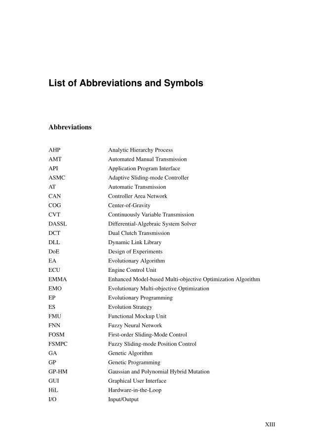
List of Abbreviations and Symbols
Abbreviations
AHP Analytic Hierarchy Process
AMT Automated Manual Transmission
API Application Program Interface
ASMC Adaptive Sliding-mode Controller
AT Automatic Transmission
CAN Controller Area Network
COG Center-of-Gravity
CVT Continuously Variable Transmission
DASSL Differential-Algebraic System Solver
DCT Dual Clutch Transmission
DLL Dynamic Link Library
DoE Design of Experiments
EA Evolutionary Algorithm
ECU Engine Control Unit
EMMA Enhanced Model-based Multi-objective Optimization Algorithm
EMO Evolutionary Multi-objective Optimization
EP Evolutionary Programming
ES Evolution Strategy
FMU Functional Mockup Unit
FNN Fuzzy Neural Network
FOSM First-order Sliding-Mode Control
FSMPC Fuzzy Sliding-mode Position Control
GA Genetic Algorithm
GP Genetic Programming
GP-HM Gaussian and Polynomial Hybrid Mutation
GUI Graphical User Interface
HiL Hardware-in-the-Loop
I/O Input/Output
XIII
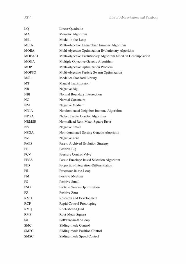
XIV List of Abbreviations and Symbols
LQ Linear Quadratic
MA Memetic Algorithm
MiL Model-in-the-Loop
MLIA Multi-objective Lamarckian Immune Algorithm
MOEA Multi-objective Optimization Evolutionary Algorithm
MOEA/D Multi-objective Evolutionary Algorithm based on Decomposition
MOGA Multiple Objective Genetic Algorithm
MOP Multi-objective Optimization Problem
MOPSO Multi-objective Particle Swarm Optimization
MSL Modelica Standard Library
MT Manual Transmission
NB Negative Big
NBI Normal Boundary Intersection
NC Normal Constraint
NM Negative Medium
NNIA Nondominated Neighbor Immune Algorithm
NPGA Niched Pareto Genetic Algorithm
NRMSE Normalized Root-Mean-Square Error
NS Negative Small
NSGA Non-dominated Sorting Genetic Algorithm
NZ Negative Zero
PAES Pareto Archived Evolution Strategy
PB Positive Big
PCV Pressure Control Valve
PESA Pareto Envelope-based Selection Algorithm
PID Proportion-Integration-Differentiation
PiL Processor-in-the-Loop
PM Positive Medium
PS Positive Small
PSO Particle Swarm Optimization
PZ Positive Zero
R&D Research and Development
RCP Rapid Control Prototyping
RMQ Root-Mean-Quad
RMS Root-Mean-Square
SiL Software-in-the-Loop
SMC Sliding-mode Control
SMPC Sliding-mode Position Control
SMSC Sliding-mode Speed Control
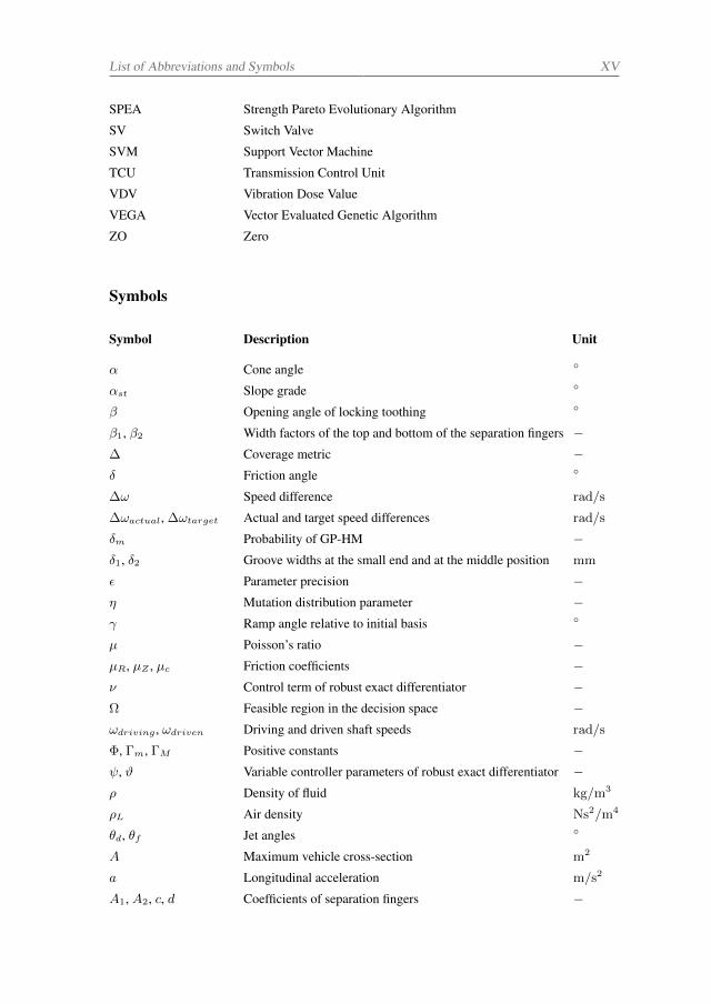
List of Abbreviations and Symbols XV
SPEA Strength Pareto Evolutionary Algorithm
SV Switch Valve
SVM Support Vector Machine
TCU Transmission Control Unit
VDV Vibration Dose Value
VEGA Vector Evaluated Genetic Algorithm
ZO Zero
Symbols
Symbol Description Unit
α Cone angle
αst Slope grade
β Opening angle of locking toothing
β1, β2 Width factors of the top and bottom of the separation fingers −∆ Coverage metric −δ Friction angle
∆ω Speed difference rad/s
∆ωactual, ∆ωtarget Actual and target speed differences rad/s
δm Probability of GP-HM −δ1, δ2 Groove widths at the small end and at the middle position mm
ϵ Parameter precision −η Mutation distribution parameter −γ Ramp angle relative to initial basis
µ Poisson’s ratio −µR, µZ , µc Friction coefficients −ν Control term of robust exact differentiator −Ω Feasible region in the decision space −ωdriving , ωdriven Driving and driven shaft speeds rad/s
Φ, Γm, ΓM Positive constants −ψ, ϑ Variable controller parameters of robust exact differentiator −ρ Density of fluid kg/m3
ρL Air density Ns2/m4
θd, θf Jet angles
A Maximum vehicle cross-section m2
a Longitudinal acceleration m/s2
A1, A2, c, d Coefficients of separation fingers −
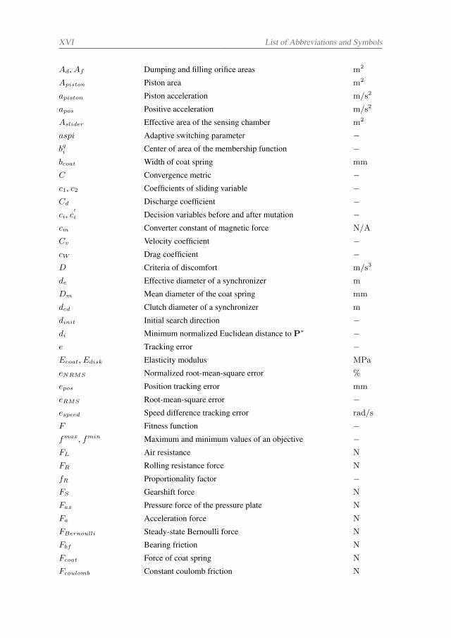
XVI List of Abbreviations and Symbols
Ad, Af Dumping and filling orifice areas m2
Apiston Piston area m2
apiston Piston acceleration m/s2
apos Positive acceleration m/s2
Aslider Effective area of the sensing chamber m2
aspi Adaptive switching parameter −bqi Center of area of the membership function −bcoat Width of coat spring mm
C Convergence metric −c1, c2 Coefficients of sliding variable −Cd Discharge coefficient −ci, c
′i Decision variables before and after mutation −
cm Converter constant of magnetic force N/A
Cv Velocity coefficient −cW Drag coefficient −D Criteria of discomfort m/s3
de Effective diameter of a synchronizer m
Dm Mean diameter of the coat spring mm
dcd Clutch diameter of a synchronizer m
dinit Initial search direction −di Minimum normalized Euclidean distance to P∗ −e Tracking error −Ecoat, Edisk Elasticity modulus MPa
eNRMS Normalized root-mean-square error %
epos Position tracking error mm
eRMS Root-mean-square error −espeed Speed difference tracking error rad/s
F Fitness function −fmax, fmin Maximum and minimum values of an objective −FL Air resistance N
FR Rolling resistance force N
fR Proportionality factor −FS Gearshift force N
Fax Pressure force of the pressure plate N
Fa Acceleration force N
FBernoulli Steady-state Bernoulli force N
Fbf Bearing friction N
Fcoat Force of coat spring N
Fcoulomb Constant coulomb friction N
List of Abbreviations and Symbols XVII
Fcounter Release bearing counterforce N
Fcylinder Shifting force from the hydraulic cylinder N
Fdisk Force of disk spring N
Fd Force from the release bearing N
Ffriction Friction force N
Flining Force of friction lining N
Flocking Locking force from the detent pin N
Fmagnetic0 Magnetic force induced by current i0 N
Fmagnetic Magnetic force induced by current i N
Fpre Preloading force N
Fprop Speed-proportional friction force N
Fspring0 Initial spring force N
Fspring Spring force N
Fstribeck Stribeck friction N
Fst Gradient resistance N
fit Fitness value of an antibody −G Current iteration count −g Acceleration of gravity m/s2
gj Inequality constraint −Gmax Maximum number of generations −h Step length for local search −hk Equality constraint −hc Height of the truncated cone mm
I Crowding-distance −i(t) Current A
i0 Initial current A
i1todriven, i2todriving Gear ratios −J , K Numbers of the inequality and equality constraints −Jin, Jout Moments of inertia kgm2
jneg Negative jerk m/s3
jpos Positive jerk m/s3
Kc Compressibility modulus Pa
kfork, kdisk Lever ratios −Ki Correction factor −ks, klining Spring stiffness N/m
Lc Length of a binary encoded chromosome −lp Length of a control parameter −Lcoil Coil inductance H
Ld, ld Radii of pressure plate and loading point of supporting ring mm
XVIII List of Abbreviations and Symbols
mv Vehicle’s mass kg
mpiston Piston mass kg
mplgr Plunger mass kg
minpm Minimal mutation probability −N Number of the compared data −n Number of individuals in the population −n1, n2 Transmission input and output rotational speeds 1/min
nA Maximum size of active population −nc Maximum size of clone population −nD Maximum size of dominant population −nf Number of separation fingers −Nw Number of waves −p Mutation scale −Pc Cylinder pressure Pa
pi Decision parameter −Po Output pressure Pa
Pr Release pressure Pa
Ps Supply pressure Pa
pm Dynamic mutation probability −Pos Position of an individual in the population −qi Self-adaptive parameter of proportional cloning −qPCV , qPV Flow rate m3/s
re Inner radius on the small end mm
ri Random number −rv Radius of the tire m
Rd, rd Outer and inner radii of the disk spring mm
rfu number of the fuzzy rules −rf Radius of the loading point at the small end mm
ro, ri Outer and inner friction surface radii of a friction plate m
s Sliding variable −s0 Boundary layer around sliding surface −s2 Displacement on the disk spring’s small end mm
scoat Displacement of coat spring mm
sdisk Displacement of disk spring mm
slining Compressed displacement of friction lining m
ssynactual, ssyntarget
Actual and target synchronizer positions mm
SP Selective pressure −s2
′ Rigid displacement on the disk spring’s small end mm
s2′′ Elastic deformation mm
List of Abbreviations and Symbols XIX
t Generation −t1, t2, t3 Time duration of synchronization ms
TR Friction torque Nm
TZ Gearing torque Nm
tbegin, tend Beginning and ending time of synchronization ms
Tbrake Brake torque Nm
Tci Clutch transfered torque Nm
tcoat Section thickness mm
Tc Clutch capacity Nm
tdisk Section thickness of disk spring mm
Te Controlled torque of the drive motor Nm
Tloss Torque of losses N
Tres Road resistance torque Nm
Tstatic Maximum static friction torque Nm
u Control input −u1, u2 Control terms of super twisting algorithm −v Vehicle speed m/s
V0 Offset volume m3
vplgr Plunger speed m/s
W , λ, ρ Variable controller parameters of super twisting algorithm −Wear Criteria of wear J
xm, ym Gaussian mutation probabilities −xLi , xUi Lower and upper variable bounds −xplgr Plunger position m
yq Crisp output of defuzzification −ymeasure Measurement data −ysim Simulation data −yu, yd Upper and low boundaries −zs, zc Numbers of friction surfaces −λ Self-adaptive weight vector −A Active population −a Active antibody −B Antibody population −b Antibody −C Clone population −c Clone antibody −D Dominant population −d, d
′, d
′′Dominant antibodies −
F Criteria vector −

XX List of Abbreviations and Symbols
L Lamarckian learning operation −PF∗ Pareto-optimal front −p Decision vector −P∗ Pareto-optimal solution set −R Fuzzy rules −TC Proportional cloning −x Decision vector −x∗ Pareto-optimal solution −Xi
p, Bi Linguistic variables of the ith fuzzy set −z∗ Objective value of a reference individual −
Abstract
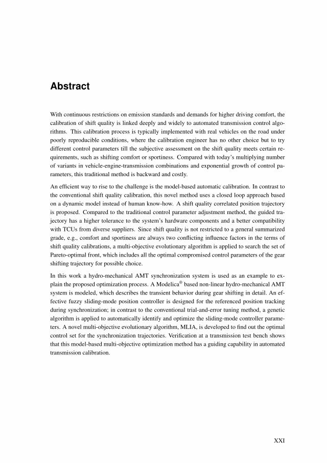
With continuous restrictions on emission standards and demands for higher driving comfort, thecalibration of shift quality is linked deeply and widely to automated transmission control algo-rithms. This calibration process is typically implemented with real vehicles on the road underpoorly reproducible conditions, where the calibration engineer has no other choice but to trydifferent control parameters till the subjective assessment on the shift quality meets certain re-quirements, such as shifting comfort or sportiness. Compared with today’s multiplying numberof variants in vehicle-engine-transmission combinations and exponential growth of control pa-rameters, this traditional method is backward and costly.
An efficient way to rise to the challenge is the model-based automatic calibration. In contrast tothe conventional shift quality calibration, this novel method uses a closed loop approach basedon a dynamic model instead of human know-how. A shift quality correlated position trajectoryis proposed. Compared to the traditional control parameter adjustment method, the guided tra-jectory has a higher tolerance to the system’s hardware components and a better compatibilitywith TCUs from diverse suppliers. Since shift quality is not restricted to a general summarizedgrade, e.g., comfort and sportiness are always two conflicting influence factors in the terms ofshift quality calibrations, a multi-objective evolutionary algorithm is applied to search the set ofPareto-optimal front, which includes all the optimal compromised control parameters of the gearshifting trajectory for possible choice.
In this work a hydro-mechanical AMT synchronization system is used as an example to ex-plain the proposed optimization process. A Modelica® based non-linear hydro-mechanical AMTsystem is modeled, which describes the transient behavior during gear shifting in detail. An ef-fective fuzzy sliding-mode position controller is designed for the referenced position trackingduring synchronization; in contrast to the conventional trial-and-error tuning method, a geneticalgorithm is applied to automatically identify and optimize the sliding-mode controller parame-ters. A novel multi-objective evolutionary algorithm, MLIA, is developed to find out the optimalcontrol set for the synchronization trajectories. Verification at a transmission test bench showsthat this model-based multi-objective optimization method has a guiding capability in automatedtransmission calibration.
XXI

Kurzfassung
Mit deutlich strengeren gesetzlichen Anforderungen hinsichtlich der Abgasemissionen und einerzunehmend anspruchsvolleren Nachfrage bezüglich des Fahrkomforts, rückt die Frage nach derSchaltqualität stärker in den Fokus der Getriebeentwicklung. Die Kalibrierung (umgangssprach-lich die Applikation) ist deshalb ein Schwerpunkt bei der Entwicklung von Algorithmen fürdie Schaltqualität von automatisierten Getriebesteuerungen.sDer Kalibrierungsprozess wird inder Regel im Fahrzeugversuch auf der Straße durchgeführt.sDer Applikationsingenieur versuchtunter diesen nicht reproduzierbaren Bedingungen verschiedene Steuerparameter zu adaptieren.Dies wird für eine Schaltung solange durchgeführt bis die subjektive Beurteilung der Schaltqual-ität und die zugehörigen Eigenschaften, wie zum Beispiel Schaltkomfort und Sportlichkeit, er-füllt sind. Dieser beschriebene Prozess ist zeit- und personalaufwendig, was mit dem aktuellenAngebot an Fahrzeug-Motor-Getriebevarianten kaum bewältigt werden kann. Als weitere Her-ausforderung steigt die Anzahl der kalibrierbaren Parameter der Regler- und Steuerungsmetho-den stetig um die Kundenbedürfnisse zu befriedigen, weshalb auch aus Kostensicht ein bessererProzess gefunden werden muss.
Eine effiziente Möglichkeit zur Lösung der skizzierten Problemstellungen ist die modellbasierteautomatische Kalibrierung. Im Gegensatz zu der herkömmlich auf Fahrversuche basierendeKalibrierung der Schaltqualität verwendet dieses neue Verfahren ein dynamisches Modell ineiner geschlossenen Schleife. Anstelle des Applikationsingenieurs für die Fahrvorgaben werdenin der Schleife ein Fahrerregler und ein Optimierungsalgorithmus verwendet, um so eine hoheReproduzierbarkeit des Schaltereignisses sicherzustellen. Es wird vorgeschlagen, die Position-strajektorie des Gangstellers zu optimieren, da diese mit der Schaltqualität korreliert. Diametralsteht dem die allgemein übliche Regleranpassung verschiedener Parameter für die Synchronisa-tion gegenüber. Die vorgeschlagene Methode der geführten Schaltbewegung weist eine deutlichhöhere Toleranz gegenüber der Varianz an Hardwarekomponenten und damit eine bessere Kom-patibilität zu den Getriebesteuergeräten (TCUs) verschiedener Lieferanten auf. Die Schaltqualitätlässt sich nicht auf ein subjektives Kriterium zusammenfassen, es werden immer unterschiedlicheFaktoren wie z.B. Komfort und Sportlichkeit den Schaltvorgang bestimmen. Deshalb wird fürdie Optimierung des Schaltvorgangs eine mehrkriterieller evolutionärer Algorithmus angewandt,um die Paretofront zu identifizieren, was alle Kompromisse der Schaltbewegungsregelung ein-schließt.
Es wird ein Modell eines hydromechanischen Synchronisationssystems für ein automatisiertesGetriebe als Beispielanwendung benutzt, um den vorgeschlagenen Optimierungsprozess zu dem-onstrieren. Das nichtlineare hydromechanische Synchronisationssystem wird mit der objekto-rientierten Sprache Modelica® modelliert. Mit dem Modell werden Schaltvorgänge detailliertbeschrieben. Ein Fuzzy-Sliding-Mode-Regler wird für die jeweilige Bewegung der Schaltung
XXIII

XXIV
während der Synchronisation benutzt. Im Gegensatz zur herkömmlichen empirischen Anpas-sung der Reglerparameter wird ein genetischer Algorithmus angewendet, um die automatischeErkennung und Bewertung der Parameter vom Fuzzy-Sliding-Mode-Regler zu optimieren. Einneuartiger evolutionärer mehrkriterieller Algorithmus (MLIA) wurde angewandt, um eine opti-male Bewegung der Schaltstellung während der Synchronisierung zu finden. Die Validierung amGetriebeprüfstand zeigt, dass diese modellbasierte Methode der mehrkriteriellen Optimierung inder automatisierten Getriebekalibrierung eine deutliche Verbesserung darstellt.
1 Introduction
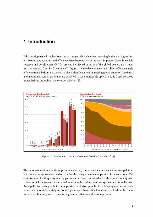
With developments in technology, the passenger vehicle has been reaching higher and higher lev-els. Nowadays, economy and efficiency have become two of the most important facets in vehicleresearch and development (R&D). As can be viewed in terms of the global powertrain - trans-mission outlook from PwC Autofacts® (figure 1.1), the development and rollout of increasinglyefficient transmissions is expected to play a significant role in meeting global emission standards,and mature markets in particular are expected to see a noticeable uptick in 7, 8, 9 and 10-speedtransmissions throughout the forecast window [1].
AMT Electric DCT CVT Auto Manual
2005 2010 2015 2020
0.7
%0.
8%
1.2
%1.
2%
0.7
%1.
2%
0.2
% 1.7
%6.
9% 9.2
%
3.4
%8.
2% 11.6
%12.5
%
44.6
%35.2
%33.3
%30.0
%
51.0
% 54.1
%46.3
%46.1
%
0 %
10 %
20 %
30 %
40 %
50 %
60 %
Transmission Type Snapshot2005,2010,2015,2020 (percentage share)
Transmission Gear Count2005-2020 (percentage share)
2005
2006
2007
2008
2009
2010
2011
2012
2013
2014
2015
2016
2017
2018
2019
2020
3 4 5 6 7 8 9 10 CVT Electric
0 %
10 %
20 %
30 %
40 %
50 %
60 %
70 %
80 %
90 %
100 %
Figure 1.1: Powertrain - transmission outlook from PwC Autofacts® [1]
The automation of gear shifting processes not only improves the convenience in manipulation,but it is also an appropriate method to solve the rising structure complexity of transmissions. Theoptimization of shift quality is a key part in automation control, which is the core to comply withstricter vehicle emission standards and to meet higher riding comfort expectations. Actually, withthe rapidly increasing technical complexity, explosive growth of vehicle-engine-transmission-related variants and multiplying control parameters have placed an excessive load on the trans-mission calibration process, thus forcing a more effective calibration process.
1
2 1.1 Motivations and Objectives
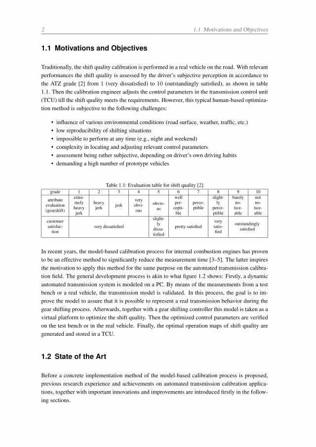
1.1 Motivations and Objectives
Traditionally, the shift quality calibration is performed in a real vehicle on the road. With relevantperformances the shift quality is assessed by the driver’s subjective perception in accordance tothe ATZ grade [2] from 1 (very dissatisfied) to 10 (outstandingly satisfied), as shown in table1.1. Then the calibration engineer adjusts the control parameters in the transmission control unit(TCU) till the shift quality meets the requirements. However, this typical human-based optimiza-tion method is subjective to the following challenges:
• influence of various environmental conditions (road surface, weather, traffic, etc.)• low reproducibility of shifting situations• impossible to perform at any time (e.g., night and weekend)• complexity in locating and adjusting relevant control parameters• assessment being rather subjective, depending on driver’s own driving habits• demanding a high number of prototype vehicles
Table 1.1: Evaluation table for shift quality [2]grade 1 2 3 4 5 6 7 8 9 10
attributeevaluation(gearshift)
extre-melyheavyjerk
heavyjerk jerk
veryobvi-ous
obvio-us
wellper-
cepti-ble
perce-ptible
slight-ly
perce-ptible
barelyno-tice-able
notno-tice-able
customersatisfac-
tionvery dissatisfied
slight-ly
dissa-tisfied
pretty satisfiedverysatis-fied
outstandinglysatisfied
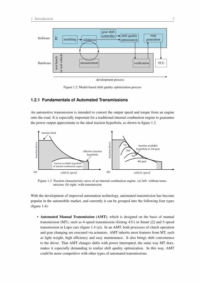
In recent years, the model-based calibration process for internal combustion engines has provento be an effective method to significantly reduce the measurement time [3–5]. The latter inspiresthe motivation to apply this method for the same purpose on the automated transmission calibra-tion field. The general development process is akin to what figure 1.2 shows: Firstly, a dynamicautomated transmission system is modeled on a PC. By means of the measurements from a testbench or a real vehicle, the transmission model is validated. In this process, the goal is to im-prove the model to assure that it is possible to represent a real transmission behavior during thegear shifting process. Afterwards, together with a gear shifting controller this model is taken as avirtual platform to optimize the shift quality. Then the optimized control parameters are verifiedon the test bench or in the real vehicle. Finally, the optimal operation maps of shift quality aregenerated and stored in a TCU.
1.2 State of the Art
Before a concrete implementation method of the model-based calibration process is proposed,previous research experience and achievements on automated transmission calibration applica-tions, together with important innovations and improvements are introduced firstly in the follow-ing sections.
1 Introduction 3
modelingPCte
stbe
nch
orre
alve
hicl
e
shift qualityoptimization
verificationmeasurement TCUHardware
Software
development process
validationmap
generation
gear shiftcontroller
Figure 1.2: Model-based shift quality optimization process
1.2.1 Fundamentals of Automated Transmissions
An automotive transmission is intended to convert the output speed and torque from an engineonto the road. It is especially important for a traditional internal combustion engine to guaranteethe power output approximate to the ideal traction hyperbola, as shown in figure 1.3.
vehicle speed
trac
tion
forc
e
traction limit
effective traction hyperbola
traction available hyperbola of internal combustion engine
vehicle speed
trac
tion
forc
e
1st
2nd
3rd
4th gear
traction available hyperbola in 3rd gear
(a) (b)
Figure 1.3: Traction characteristic curve of an internal combustion engine. (a) left: without trans-mission, (b) right: with transmission
With the development of improved automation technology, automated transmission has becomepopular in the automobile market, and currently it can be grouped into the following four types(figure 1.4):
• Automated Manual Transmission (AMT), which is designed on the basis of manualtransmission (MT), such as 6-speed transmission (Getrag 431) in Smart [2] and 5-speedtransmission in Lupo cars (figure 1.4 (a)). In an AMT, both processes of clutch operationand gear changing are executed via actuators. AMT inherits most features from MT, suchas light weight, high efficiency and easy maintenance. It also brings shift convenienceto the driver. That AMT changes shifts with power interrupted, the same way MT does,makes it especially demanding to realize shift quality optimization. In this way, AMTcould be more competitive with other types of automated transmissions.
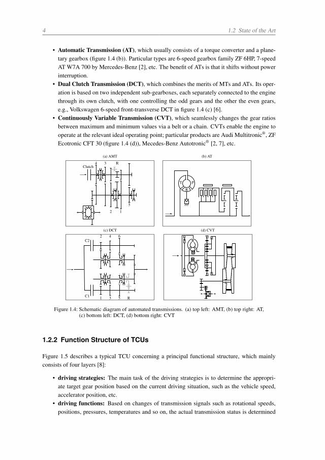
4 1.2 State of the Art
• Automatic Transmission (AT), which usually consists of a torque converter and a plane-tary gearbox (figure 1.4 (b)). Particular types are 6-speed gearbox family ZF 6HP, 7-speedAT W7A 700 by Mercedes-Benz [2], etc. The benefit of ATs is that it shifts without powerinterruption.
• Dual Clutch Transmission (DCT), which combines the merits of MTs and ATs. Its oper-ation is based on two independent sub-gearboxes, each separately connected to the enginethrough its own clutch, with one controlling the odd gears and the other the even gears,e.g., Volkswagen 6-speed front-transverse DCT in figure 1.4 (c) [6].
• Continuously Variable Transmission (CVT), which seamlessly changes the gear ratiosbetween maximum and minimum values via a belt or a chain. CVTs enable the engine tooperate at the relevant ideal operating point; particular products are Audi Multitronic®, ZFEcotronic CFT 30 (figure 1.4 (d)), Mecedes-Benz Autotronic® [2, 7], etc.
(a) AMT (b) AT
(c) DCT (d) CVT
C2
C1
4 3
12
5
RClutch
1 3 5 R
2 4 6
T P
R
Figure 1.4: Schematic diagram of automated transmissions. (a) top left: AMT, (b) top right: AT,(c) bottom left: DCT, (d) bottom right: CVT
1.2.2 Function Structure of TCUs
Figure 1.5 describes a typical TCU concerning a principal functional structure, which mainlyconsists of four layers [8]:
• driving strategies: The main task of the driving strategies is to determine the appropri-ate target gear position based on the current driving situation, such as the vehicle speed,accelerator position, etc.
• driving functions: Based on changes of transmission signals such as rotational speeds,positions, pressures, temperatures and so on, the actual transmission status is determined
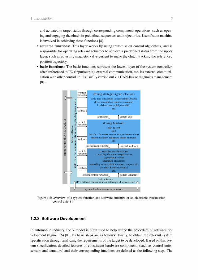
1 Introduction 5
and actuated to target status through corresponding components operations, such as open-ing and engaging the clutch in predefined sequences and trajectories. Use of state machineis involved in achieving these functions [8].
• actuator functions: This layer works by using transmission control algorithms, and isresponsible for operating relevant actuators to achieve a predefined status from the upperlayer, such as adjusting magnetic valve current to make the clutch tracking the referencedposition trajectory.
• basic functions: The basic functions represent the lowest layer of the system controller,often referenced to I/O (input/output), external communication, etc. Its external communi-cation with other control unit is usually carried out via CAN-bus or diagnosis management[8].
transmission functionsconverting the torque requirements
(open/close clutch)adaptation algorithms
controlling valves, electric motors, magnets etc.position- & current control
etc.
static gear calculation (characteristics based)driver recognition (sport/economical)
load detection (uphill/downhill)etc.
driving strategies (gear selection)
driving functionsstart & stop
shiftinterface for motor control (torque intervention)
determination of requested clutch momentsetc.
system hardware (sensors, actuators...)
basic software
basi
cso
ftw
are
(I/O
,ext
erna
lcom
mun
icat
ion,
inte
rrup
ts,d
iagn
osis
,etc
.)
(mot
orco
ntro
l,A
BS,
CA
N,..
.)
(I/O, external communication, interrupts, diagnosis, etc.)
target gear current gear
internal requirements internal feedback
system control variables system variables
feedback
feedback
feedback
vehiclevariables
vehiclevariables
vehiclevariables
Figure 1.5: Overview of a typical function and software structure of an electronic transmissioncontrol unit [8]
1.2.3 Software Development
In automobile industry, the V-model is often used to help define the procedure of software de-velopment (figure 1.6) [8]. Its basic steps are as follows: Firstly, to obtain the relevant systemspecification through analyzing the requirements of the target to be developed. Based on this sys-tem specification, detailed features of constituent hardware components (such as control units,sensors and actuators) and their corresponding functions are defined as the following step. The
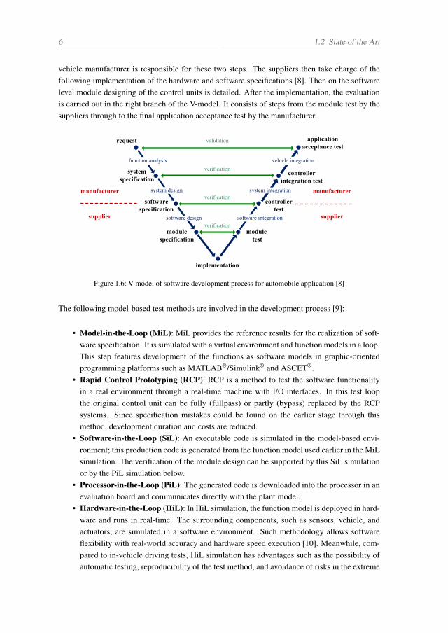
6 1.2 State of the Art
vehicle manufacturer is responsible for these two steps. The suppliers then take charge of thefollowing implementation of the hardware and software specifications [8]. Then on the softwarelevel module designing of the control units is detailed. After the implementation, the evaluationis carried out in the right branch of the V-model. It consists of steps from the module test by thesuppliers through to the final application acceptance test by the manufacturer.
request
system specification
software specification
module specification
implementation
moduletest
controller test
controller integration test
application acceptance test
validation
verification
verification
function analysis
system design
software design software integration
system integration
verification
vehicle integration
manufacturer
supplier
manufacturer
supplier
Figure 1.6: V-model of software development process for automobile application [8]
The following model-based test methods are involved in the development process [9]:
• Model-in-the-Loop (MiL): MiL provides the reference results for the realization of soft-ware specification. It is simulated with a virtual environment and function models in a loop.This step features development of the functions as software models in graphic-orientedprogramming platforms such as MATLAB®/Simulink® and ASCET®.
• Rapid Control Prototyping (RCP): RCP is a method to test the software functionalityin a real environment through a real-time machine with I/O interfaces. In this test loopthe original control unit can be fully (fullpass) or partly (bypass) replaced by the RCPsystems. Since specification mistakes could be found on the earlier stage through thismethod, development duration and costs are reduced.
• Software-in-the-Loop (SiL): An executable code is simulated in the model-based envi-ronment; this production code is generated from the function model used earlier in the MiLsimulation. The verification of the module design can be supported by this SiL simulationor by the PiL simulation below.
• Processor-in-the-Loop (PiL): The generated code is downloaded into the processor in anevaluation board and communicates directly with the plant model.
• Hardware-in-the-Loop (HiL): In HiL simulation, the function model is deployed in hard-ware and runs in real-time. The surrounding components, such as sensors, vehicle, andactuators, are simulated in a software environment. Such methodology allows softwareflexibility with real-world accuracy and hardware speed execution [10]. Meanwhile, com-pared to in-vehicle driving tests, HiL simulation has advantages such as the possibility ofautomatic testing, reproducibility of the test method, and avoidance of risks in the extreme
1 Introduction 7
cases tests [8]. The verification during the controller test, integration test, system test andeven the calibration of control units can be supported by HiL simulation [9].
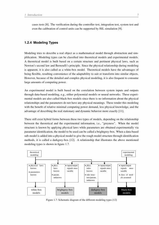
1.2.4 Modeling Types
Modeling tries to describe a real object as a mathematical model through abstraction and sim-plification. Modeling types can be classified into theoretical models and experimental models.A theoretical model is built based on a certain structure and pertinent physical laws, such asNewton’s second law and Bernoulli’s principle. Since the physical relationship during modelingis apparent, it is also called as a white-box model. Theoretical models have the advantages ofbeing flexible, resulting convenience of the adaptability to suit or transform into similar objects.However, because of the detailed and complex physical modeling, it is also frequent to consumelarge amounts of computing power.
An experimental model is built based on the correlation between system inputs and outputsthrough data-based modeling, e.g., either polynomial models or neural networks. These experi-mental models are also called black-box models since there is no information about the physicalrelationships and the parameters do not have any physical meanings. These render this modelingwith the benefit of relative minimal computing power demand, less physical knowledge, and theadvantage of describing the real stationary and dynamic behavior more exactly [11].
There still exist hybrid forms between these two types of models, depending on the relationshipbetween the theoretical and the experimental information, i.e., “greyness”. When the modelstructure is known by applying physical laws while parameters are obtained experimentally viaparameter identification, the model to be used can be called a brightgrey-box. When a data-basedsub-model is added into a physical model to give the rough model structure through identificationmethods, it is called a darkgrey-box [12]. A relationship that illustrates the above mentionedmodeling types is shown in figure 1.7.
• physical lawsknown
• parametersknown
• phys.lawsknown
• param.unknown
• input/outputsignals mea-surable
• input/outputsignals mea-surable
• class of mod-els assumed
• phys.rulesknown
• rule struc-ture/param.unknown
• input/outputsignals mea-surable
theoreticalmodeling
darkgrey-boxmodels
black-boxmodels
brightgrey-boxmodels
white-boxmodels
experimentalmodeling
Figure 1.7: Schematic diagram of the different modeling types [12]
8 1.2 State of the Art
1.2.5 Fundamental of Optimization
An optimization issue can be divided into a single-objective optimization task and a multi-objective optimization problem (MOP). If only one objective function is needed to be optimized,it is called a single-objective optimization [13]. Generally speaking, single-objective optimiza-tion that aims to optimize one objective with n decision parameters can be expressed as in equa-tion (1.1) [13, 14]:
⎧⎪⎪⎪⎨⎪⎪⎪⎩min f(x), x ∈ Ω
gj(x) ≤ 0, j = 1, 2, · · · Jhk(x) = 0, k = 1, 2, · · ·KxLi ≤ xi ≤ xUi , i = 1, 2, · · · , n
(1.1)
where x is called a n decision vector, x = (x1, x2, · · · , xn)T. Ω is the feasible region in thedecision space. gj(x) is inequality constraints and hk(x) is equality constraints. J and K arerespectively number of the inequality- and equality constraints. xLi and xUi are relevant lowerand upper variable bounds restricting each decision variable xi.
The optimization can cope with not only for minimization issues but also maximization oneswhen the maximization of the objective function F is reformulated from the minimization casesmentioned above, i.e.,
max f(x) = min −f(x) (1.2)
Actually, many real life problems have several objectives that need simultaneously optimized, andthis is known as multi-objective optimization. Different from the single-objective optimization,which turns out a unique solution, multi-objective optimization tries to find all the good trade-offsolutions which are considered equivalent in the absence of information concerning the relevanceof each objective relative to the others [14].
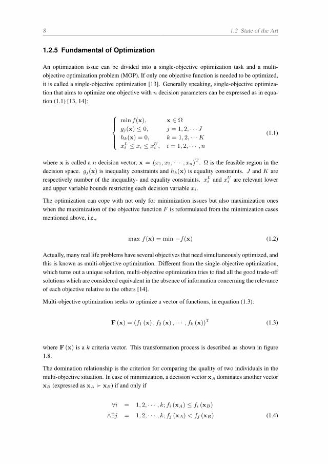
Multi-objective optimization seeks to optimize a vector of functions, in equation (1.3):
F (x) = (f1 (x) , f2 (x) , · · · , fk (x))T (1.3)
where F (x) is a k criteria vector. This transformation process is described as shown in figure1.8.
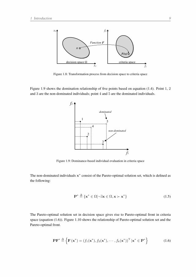
The domination relationship is the criterion for comparing the quality of two individuals in themulti-objective situation. In case of minimization, a decision vector xA dominates another vectorxB (expressed as xA ≻ xB) if and only if
∀i = 1, 2, · · · , k; fi (xA) ≤ fi (xB)
∧∃j = 1, 2, · · · , k; fj (xA) < fj (xB) (1.4)
1 Introduction 9
x2
x1 f1
f2
Function
Figure 1.8: Transformation process from decision space to criteria space
Figure 1.9 shows the domination relationship of five points based on equation (1.4). Point 1, 2and 3 are the non-dominated individuals; point 4 and 5 are the dominated individuals.
1
2
dominated
non-dominated
Figure 1.9: Dominance-based individual evaluation in criteria space
The non-dominated individuals x∗ consist of the Pareto-optimal solution set, which is defined asthe following:
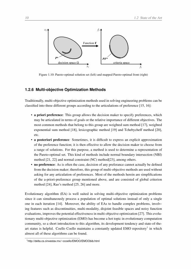
P∗ ∆= x∗ ∈ Ω|¬∃x ∈ Ω,x ≻ x∗ (1.5)
The Pareto-optimal solution set in decision space gives rise to Pareto-optimal front in criteriaspace (equation (1.6)). Figure 1.10 shows the relationship of Pareto-optimal solution set and thePareto-optimal front.
PF∗ ∆=F (x∗) = (f1(x
∗), f2(x∗), · · · , fk(x∗))
T |x∗ ∈ P∗
(1.6)
10 1.2 State of the Art
x2
x1
decision space ΩP*
f1
criteria space
f2
Function F
PF*
Figure 1.10: Pareto-optimal solution set (left) and mapped Pareto-optimal front (right)
1.2.6 Multi-objective Optimization Methods
Traditionally, multi-objective optimization methods used in solving engineering problems can beclassified into three different groups according to the articulations of preference [15, 16]:
• a priori preference: This group allows the decision maker to specify preferences, whichmay be articulated in terms of goals or the relative importance of different objectives. Themost common methods that belong to this group are weighted sum method [17], weightedexponential sum method [18], lexicographic method [19] and Tchebycheff method [20],etc.
• a posteriori preference: Sometimes, it is difficult to express an explicit approximationof the preference function; it is then effective to allow the decision maker to choose froma range of solutions. For this purpose, a method is used to determine a representation ofthe Pareto-optimal set. This kind of methods include normal boundary intersection (NBI)method [21, 22] and normal constraint (NC) method[23], among others.
• no preference: As is often the case, decision of any preferance cannot actually be definedfrom the decision maker; therefore, this group of multi-objective methods are used withoutasking for any articulation of preferences. Most of the methods herein are simplificationsof the a-priori-preference group mentioned above, and are consisted of global criterionmethod [24], Rao’s method [25, 26] and more.
Evolutionary algorithm (EA) is well suited in solving multi-objective optimization problemssince it can simultaneously process a population of optimal solutions instead of only a singleone in each iteration [14]. Moreover, the ability of EAs to handle complex problems, involv-ing features such as discontinuities, multi-modality, disjoint feasible spaces and noisy functionevaluations, improves the potential effectiveness in multi-objective optimization [27]. This evolu-tionary multi-objective optimization (EMO) has become a hot topic in evolutionary computationcommunity, so a short introduction to this algorithm, its development tendency and state-of-the-art status is helpful. Coello Coello maintains a constantly updated EMO repository1 in whichalmost all of these algorithms can be found.
1http://delta.cs.cinvestav.mx/~ccoello/EMOO/EMOObib.html
1 Introduction 11
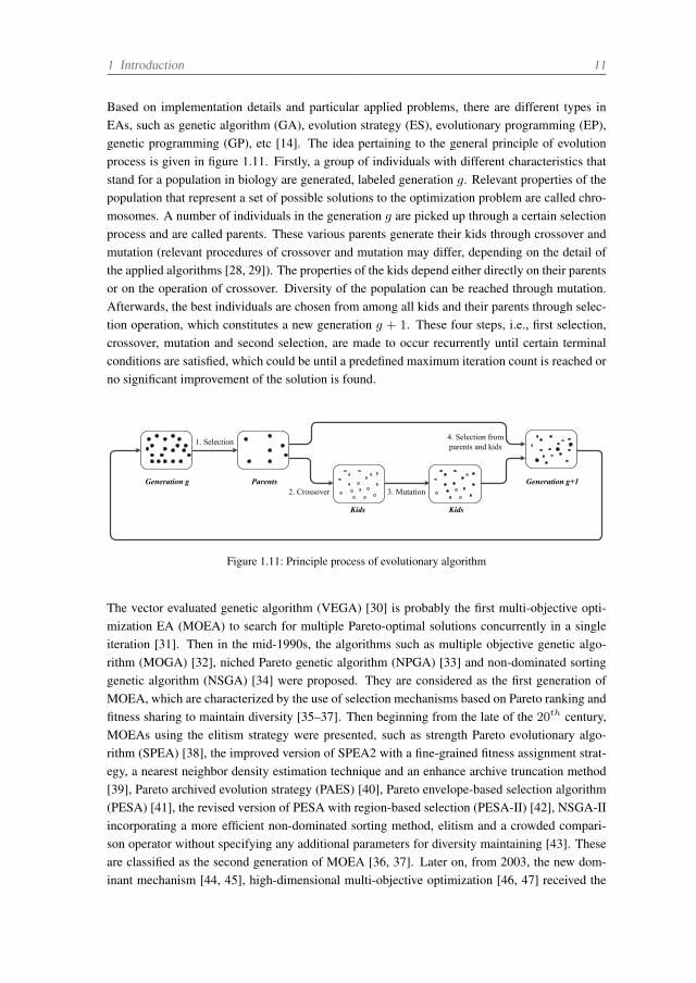
Based on implementation details and particular applied problems, there are different types inEAs, such as genetic algorithm (GA), evolution strategy (ES), evolutionary programming (EP),genetic programming (GP), etc [14]. The idea pertaining to the general principle of evolutionprocess is given in figure 1.11. Firstly, a group of individuals with different characteristics thatstand for a population in biology are generated, labeled generation g. Relevant properties of thepopulation that represent a set of possible solutions to the optimization problem are called chro-mosomes. A number of individuals in the generation g are picked up through a certain selectionprocess and are called parents. These various parents generate their kids through crossover andmutation (relevant procedures of crossover and mutation may differ, depending on the detail ofthe applied algorithms [28, 29]). The properties of the kids depend either directly on their parentsor on the operation of crossover. Diversity of the population can be reached through mutation.Afterwards, the best individuals are chosen from among all kids and their parents through selec-tion operation, which constitutes a new generation g + 1. These four steps, i.e., first selection,crossover, mutation and second selection, are made to occur recurrently until certain terminalconditions are satisfied, which could be until a predefined maximum iteration count is reached orno significant improvement of the solution is found.
Generation g Parents Generation g+1
1. Selection
2. Crossover 3. Mutation
4. Selection from parents and kids
KidsKids
Figure 1.11: Principle process of evolutionary algorithm
The vector evaluated genetic algorithm (VEGA) [30] is probably the first multi-objective opti-mization EA (MOEA) to search for multiple Pareto-optimal solutions concurrently in a singleiteration [31]. Then in the mid-1990s, the algorithms such as multiple objective genetic algo-rithm (MOGA) [32], niched Pareto genetic algorithm (NPGA) [33] and non-dominated sortinggenetic algorithm (NSGA) [34] were proposed. They are considered as the first generation ofMOEA, which are characterized by the use of selection mechanisms based on Pareto ranking andfitness sharing to maintain diversity [35–37]. Then beginning from the late of the 20th century,MOEAs using the elitism strategy were presented, such as strength Pareto evolutionary algo-rithm (SPEA) [38], the improved version of SPEA2 with a fine-grained fitness assignment strat-egy, a nearest neighbor density estimation technique and an enhance archive truncation method[39], Pareto archived evolution strategy (PAES) [40], Pareto envelope-based selection algorithm(PESA) [41], the revised version of PESA with region-based selection (PESA-II) [42], NSGA-IIincorporating a more efficient non-dominated sorting method, elitism and a crowded compari-son operator without specifying any additional parameters for diversity maintaining [43]. Theseare classified as the second generation of MOEA [36, 37]. Later on, from 2003, the new dom-inant mechanism [44, 45], high-dimensional multi-objective optimization [46, 47] received the
12 1.2 State of the Art
research foci. Meanwhile, some new evolution paradigms have been introduced into the fieldof EMO; among them are multi-objective particle swarm optimization (MOPSO) [48], multi-objective evolutionary algorithm based on decomposition (MOEA/D) [49] and non-dominatedneighbor immune algorithm (NNIA) [31], etc. Moreover, memetic algorithms (MAs) [50], anarea of population-based meta-heuristic search approaches, regarded as hybrid algorithms be-tween global search and local improvement procedures have also found wide usage in the MOPs.Here, a MA based multi-objective optimization has been developed for model-based shift qualityin automated transmissions. Its detailed discussion is presented in chapter 5.
1.2.7 Shift Quality Calibration
Calibration is defined as the adaption of the transmission properties to the dynamics and behaviorof the entire vehicle by inputting data into the transmission software [2]. The shifting process iscalibrated with regard to following aspects [2]:
• driving comfort: shifting quality, vibrations and load change behavior• driving behavior: spontaneity, consumption/emissions• driving safety: functional reliability and durability of transmission
The main focus here is on the calibration of gear shifting quality. As mentioned in section 1.1,the traditional method of shift quality evaluation is subjective, thus has a lot of drawbacks and isnot fit for the increasing market share of vehicles with automated transmission; hence, pushingobjective evaluation and automatic optimization under limelight.
Major steps in shift quality calibration based on objective criteria are given below:
1) Criteria for Shift Quality Objective Evaluation
Shifting comfort as felt by the driver stands in direct correlation with the characteristics of thetransmission output torque and thus with vehicle acceleration during shifting [2]. So the vehiclelongitudinal acceleration is often used as its characteristic parameter. To be specific, its root-mean-square (RMS) value [51] and vibration dose value (VDV) [52] are often used to describeits mean value during gear shifting [51, 53–56]. The time derivative (also called jerk) and thepeak-to-peak value of acceleration are also imported to define the vibration difference [57]. Ithas been shown that the most strongly felt frequencies are in a range between 2 and 9Hz [57],so a 10Hz low pass filter is valid in perceiving the gear shifting comfort. Moreover, some otherinformation, such as overshoot/undershoot of engine speed when the clutch disengages/engagesand decrease/increase of the engine speed when upshifting/downshifting, are also cited as criteriato assess the shifting quality [58].
For shifting sportiness, shifting time, shift delay time and delay time of engine speed are oftenused [53, 55, 58]. Last but not least, some references on clutch friction work, power [55, 59],difference of sound pressure level, and fuel economy data [60] are also taken into shift qualityconsideration.
1 Introduction 13
2) Shift Quality Evaluation Methods
An objective grade model, which describes the correlation between objective criteria based onthe measurements and the subjective ratings from driver’s perception, is developed through cor-relation analysis [51], regression analysis [51, 53, 57], artificial neural networks [61, 62], fuzzylogic [62] (for the gear shifting sportiness), or support vector machine (SVM) [60].
The subjective evaluation results of shift quality acquired from diverse drivers are aggregatedbased on evidence theory, which makes subjective evaluation input more reliable and more jus-tified; afterwards, the objective evaluation metrics are trained through a fuzzy neural network(FNN) [63].
Multi-objective optimization algorithm is also applied to the development of the objective eval-uation system for shift quality. For example, in [58, 64] a linear weighted method is defined totransform multi-objective assessment criteria into a single level, which the weights of assessmentcriteria are either assigned by the expert advice [58] or through the analytic hierarchy process(AHP) of the evaluation system [64]. Moreover, a Pareto-optimal front is generated in which allthe compromised optimal evaluation criteria includes [55, 65, 66].
Several industry-standard tools for objective analysis and quality control on vehicle driveabilityhave been developed. The AVL-DRIVE™2, for one, captures various driveability-related sensorsand CAN-bus signals, such as longitudinal acceleration, engine speed, vehicle velocity, acceler-ator position, and vibration. Then a conclusion is reached on the objective ratings for drivingevents, including a quality ranking of vehicle characteristics [61, 67–69].
3) Shift Quality Optimization Methods
Based on the developed objective grade model, a fuzzy logic strategy based model [53, 57] ora neuro-fuzzy-system [62], in which the inputs are the objective characteristic parameters (shiftquality criteria) and the outputs are the control parameters, is applied on-line on the shift pointoptimization in a chassis dynamometer. And in [51, 62] an artificial neural network, whosedevelopment is based on the design of experiments (DoE) test plan, is applied on the off-lineoptimization through an evolutionary algorithm.
For the multi-objective optimization, the optimal compromised control parameters are foundthrough a multi-objective genetic algorithm, such as NSGA-II [55, 65], model-based multi-objective optimization algorithm (EMMA) [55, 66], or directly through a relevant commercialsoftware like iSIGHT™ [58].
1.3 Scope and Structure
The aim of this dissertation is to develop a complete framework for a model-based calibrationfor automated transmissions, with the main focus on control parameter optimization during thegear shifting process. A hydro-mechanical AMT synchronizer equipped in a Volkswagen Lupo
2https://www.avl.com/html/static/emag/e-pdf_folder_Drive/index.html [Retrieved 1st June 2015]
14 1.3 Scope and Structure
vehicle is used as the research object. As for the model-based optimization of the clutch controlparameters, a detailed process can be found in [70].
The contributions of this dissertation can be summarized as follows:
• A new model-based calibration method in automated transmission application: Thiscalibration method is newly introduced from the internal combustion engine to transmis-sion application. A virtual vehicle is developed to simulate the gear shifting in the MiLenvironment, and shift quality is optimized automatically based on this virtual platform. Incontrast to the on-line optimization, i.e., real vehicle, dynamometer and test bench basedcalibration, a vehicle model based off-line optimization is easier to implement and incursless expenses.
• A detailed non-linear dynamic model of the hydro-mechanical AMT system (Chap-ter 2): Gear shifting is a non-linear, dynamic process caused by the actuator’s movement.In order to correctly describe this transient behavior for shift quality research, a dynamicmodel is needed. Compared with a black-box model generated through measurements,e.g., the DoE test plan, a brightgrey-box model is easier to understand for the developerand more flexible for other similar product applications. Moreover, since the performanceof the gear shifting is highly influenced by all the components in a system, a detailed modelis necessary. However, the related research results of automated transmission modelingare rare and scattered, so in this dissertation the modeling process of the hydro-mechanicalAMT is systematically described; and all the components—even the actuators—are at-tempted to be developed in a detailed way, e.g., the magnetic valve’s dynamic characteris-tics and kinematic status are both modeled. The synchronization process is represented inpre-synchronizing, locking, unlocking, meshing and engaging stages. Characteristic clutchcurves of a disk spring and a coat spring are also described. Additionally, flexible shaftsand torsion damping systems are considered. At the end, the model validation is carriedout based on the measurements from both the transmission test bench and the real vehicle.
• A position trajectory based shift quality optimization (Chapter 3): Gear shifting qual-ity is optimized traditionally based on the correlation between the TCU control parame-ters and the evaluation criteria. However, this direct optimization approach is limited byworking experience, manufacturing tolerance of transmissions, etc. Gear shifting positiontrajectory based calibration is proposed here, which has the advantages of clearer visual-ization and better adaptability.
• A genetic algorithm optimized fuzzy logic sliding-mode position controller (Chapter3): In order to find out the correlation of shifting position trajectory and shift quality, amore accurate and rapid controller for tracking a referenced position trajectory is needed.Compared with other popular control algorithms, a fuzzy logic sliding-mode position con-troller is developed here considering the implementation complexity. Moreover, a geneticalgorithm is applied to optimize the controller parameters automatically rather than thetraditional trial-and-error tuning.
• Definition of multi-objective evaluation criteria (Chapter 4): The objective evaluationof shift quality is the precondition for the model-based automatic optimization. Here theobjective criteria are well chosen among the state-of-the-art research achievements. Corre-
1 Introduction 15
lation among these criteria is also analyzed afterwards to reduce the computational burdenduring the multi-objective optimization.
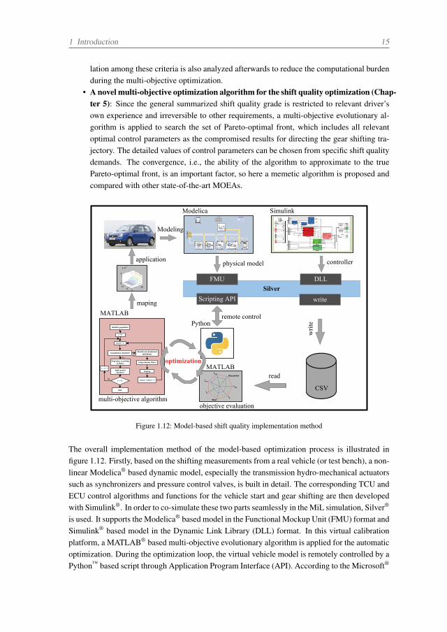
• A novel multi-objective optimization algorithm for the shift quality optimization (Chap-ter 5): Since the general summarized shift quality grade is restricted to relevant driver’sown experience and irreversible to other requirements, a multi-objective evolutionary al-gorithm is applied to search the set of Pareto-optimal front, which includes all relevantoptimal control parameters as the compromised results for directing the gear shifting tra-jectory. The detailed values of control parameters can be chosen from specific shift qualitydemands. The convergence, i.e., the ability of the algorithm to approximate to the truePareto-optimal front, is an important factor, so here a memetic algorithm is proposed andcompared with other state-of-the-art MOEAs.
Silver
FMU DLL
Scripting API
engine transmi Driveline
resist
brakes
w orld
x
yroad atmosp
driver
co
ntro
lBu
s
Modelica Simulink
Pythonremote control
write
CSV
MATLABread
MATLAB
objective evaluationmulti-objective algorithm
optimization
maping
Initialize population
t = 0
Layer = 1
Is population classified?Identify non-dominated
individuals
Reproduce according to fitness
Apply genetic operators
End
Assign dummy fitness
sharing
Layer = Layer + 1
t = t + 1
t > T?
NoYes
No
050
1214
0
5
x 10-4
physical model controllerapplication
ModelingAMT
wri
te
tsyn
Discomfort
js-p
js-n
t3
Wear
t2
Figure 1.12: Model-based shift quality implementation method
The overall implementation method of the model-based optimization process is illustrated infigure 1.12. Firstly, based on the shifting measurements from a real vehicle (or test bench), a non-linear Modelica® based dynamic model, especially the transmission hydro-mechanical actuatorssuch as synchronizers and pressure control valves, is built in detail. The corresponding TCU andECU control algorithms and functions for the vehicle start and gear shifting are then developedwith Simulink®. In order to co-simulate these two parts seamlessly in the MiL simulation, Silver®
is used. It supports the Modelica® based model in the Functional Mockup Unit (FMU) format andSimulink® based model in the Dynamic Link Library (DLL) format. In this virtual calibrationplatform, a MATLAB® based multi-objective evolutionary algorithm is applied for the automaticoptimization. During the optimization loop, the virtual vehicle model is remotely controlled by aPython™ based script through Application Program Interface (API). According to the Microsoft®
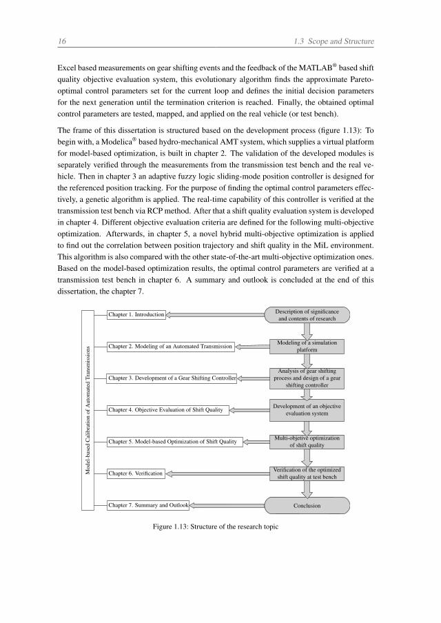
16 1.3 Scope and Structure
Excel based measurements on gear shifting events and the feedback of the MATLAB® based shiftquality objective evaluation system, this evolutionary algorithm finds the approximate Pareto-optimal control parameters set for the current loop and defines the initial decision parametersfor the next generation until the termination criterion is reached. Finally, the obtained optimalcontrol parameters are tested, mapped, and applied on the real vehicle (or test bench).
The frame of this dissertation is structured based on the development process (figure 1.13): Tobegin with, a Modelica® based hydro-mechanical AMT system, which supplies a virtual platformfor model-based optimization, is built in chapter 2. The validation of the developed modules isseparately verified through the measurements from the transmission test bench and the real ve-hicle. Then in chapter 3 an adaptive fuzzy logic sliding-mode position controller is designed forthe referenced position tracking. For the purpose of finding the optimal control parameters effec-tively, a genetic algorithm is applied. The real-time capability of this controller is verified at thetransmission test bench via RCP method. After that a shift quality evaluation system is developedin chapter 4. Different objective evaluation criteria are defined for the following multi-objectiveoptimization. Afterwards, in chapter 5, a novel hybrid multi-objective optimization is appliedto find out the correlation between position trajectory and shift quality in the MiL environment.This algorithm is also compared with the other state-of-the-art multi-objective optimization ones.Based on the model-based optimization results, the optimal control parameters are verified at atransmission test bench in chapter 6. A summary and outlook is concluded at the end of thisdissertation, the chapter 7.
Conclusion
Mod
el-b
ased
Cal
ibra
tion
ofA
utom
ated
Tran
smis
sion
s
Modeling of a simulationplatform
Chapter 6. VerificationVerification of the optimized
shift quality at test bench
Chapter 2. Modeling of an Automated Transmission
Chapter 3. Development of a Gear Shifting Controller
Chapter 4. Objective Evaluation of Shift Quality
Chapter 5. Model-based Optimization of Shift Quality
Description of significanceand contents of research
Analysis of gear shiftingprocess and design of a gear
shifting controller
Development of an objectiveevaluation system
Multi-objetive optimizationof shift quality
Chapter 1. Introduction
Chapter 7. Summary and Outlook
Figure 1.13: Structure of the research topic
2 Modeling of an Automated Transmission
An automated transmission model should ideally represent the similar transient dynamic behaviorof the real object, such as the shaft rotational speed oscillation and the longitudinal accelerationchanges during gear shifting. However, these requirements bring complexity to the transmissionmodeling, especially for a multi-domain system.
To cope with these problems, research has been conducted to obtain detailed transmission mod-els. In [71] a four degree-of-freedom and a 15 degree-of-freedom DCT mechanical models areseparately developed to compare their shift transient difference, and it concludes that the lowerorder model can only capture the 6Hz shuffle mode response because other components of vi-bration response have not been described. But in [71] the torque is used as a source input and thedetailed relationship between the hydraulic pressure and the mechanical force is not described.The successive gear shifting process can be distinguished by different stages through the relativepositions of the synchronizer parts and the characteristic points such as the synchronized angularvelocity. The number of stages depends on the purpose of the study and on the type of modelformulated for the gear shifting process. For example, eight main stages of the synchronizer be-havior are defined in [72], especially the phenomena of stick-slip and second bump. In [73] thesynchronization process is modeled as 11 stages to evaluate the shifting force transmitted to thedriver’s hand. Based on these conclusions, a hydro-mechanical synchronizer with five dynamicstages in the synchronization procedure is represented here, i.e., pre-synchronizing, locking, un-locking, meshing and engaging. In [74] the emphasis is given to hydro-mechanical actuator dy-namics. Based on the steady-state characteristics of the actuator and assuming dither signalsapplied to the command current, a reduced-ordered electro-hydraulic AMT actuator model is de-rived to accurately reproduce the system response during gear shifting. However, a low ordermodel is only suitable for the control application. For the dynamic transient research of shiftquality during gear shifting, a more accurate model is suited.
Meanwhile, different modeling methods have been put to use. MATLAB®/Simulink® is a clas-sical modeling software [75–77]. Some other softwares, such as AMESim [78–80], bond graph[81, 82], and Modelica® [83, 84] are also widely used these years. Especially Modelica®, aunified object-oriented, general equation based language for modeling of multi-domain physi-cal systems, helps model developers to look at modeling from a physical perspective instead ofmere mathematical one [85, 86]. However, references covering Modelica® based modeling de-velopment in vehicle automated transmission field are relatively rare and simple. For example,Zhang et al. [83] uses Modelica® to model the dynamics and control of the DCT during gearshift process, but the pressure profiles for the clutch torque control is based on a lookup tableand, for simplicity, the synchronizer is modeled as power flow switches. Although in [84] a
17
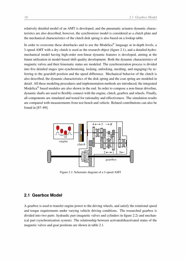
18 2.1 Gearbox Model
relatively detailed model of an AMT is developed, and the pneumatic actuator dynamic charac-teristics are also described, however, the synchronizer model is considered as a clutch plate andthe mechanical characteristics of the clutch disk spring is also based on a lookup table.
In order to overcome these drawbacks and to use the Modelica® language at in-depth levels, a5-speed AMT with a dry clutch is used as the research object (figure 2.1), and a detailed hydro-mechanical model having high-order non-linear dynamic features is developed, aiming at thefuture utilization in model-based shift quality development. Both the dynamic characteristics ofmagnetic valves and their kinematic status are modeled. The synchronization process is dividedinto five detailed stages (pre-synchronizing, locking, unlocking, meshing, and engaging) by re-ferring to the gearshift position and the speed difference. Mechanical behavior of the clutch isalso described, the dynamic characteristics of the disk spring and the coat spring are modeled indetail. All these modeling procedures and implementation methods are introduced, the integratedModelica® based modules are also shown in the end. In order to compose a non-linear driveline,dynamic shafts are used to flexibly connect with the engine, clutch, gearbox and wheels. Finally,all components are simulated and tested for rationality and effectiveness. The simulation resultsare compared with measurements from test bench and vehicle. Related contributions can also befound in [87–89].
R
gearbox
4 3
52 1
engineclutch
Figure 2.1: Schematic diagram of a 5-speed AMT
2.1 Gearbox Model
A gearbox is used to transfer engine power to the driving wheels, and satisfy the rotational speedand torque requirements under varying vehicle driving conditions. The researched gearbox isdivided into two parts: hydraulic part (magnetic valves and cylinders in figure 2.2) and mechan-ical part (synchronization system). The relationship between activated/deactivated status of themagnetic valves and gear positions are shown in table 2.1.
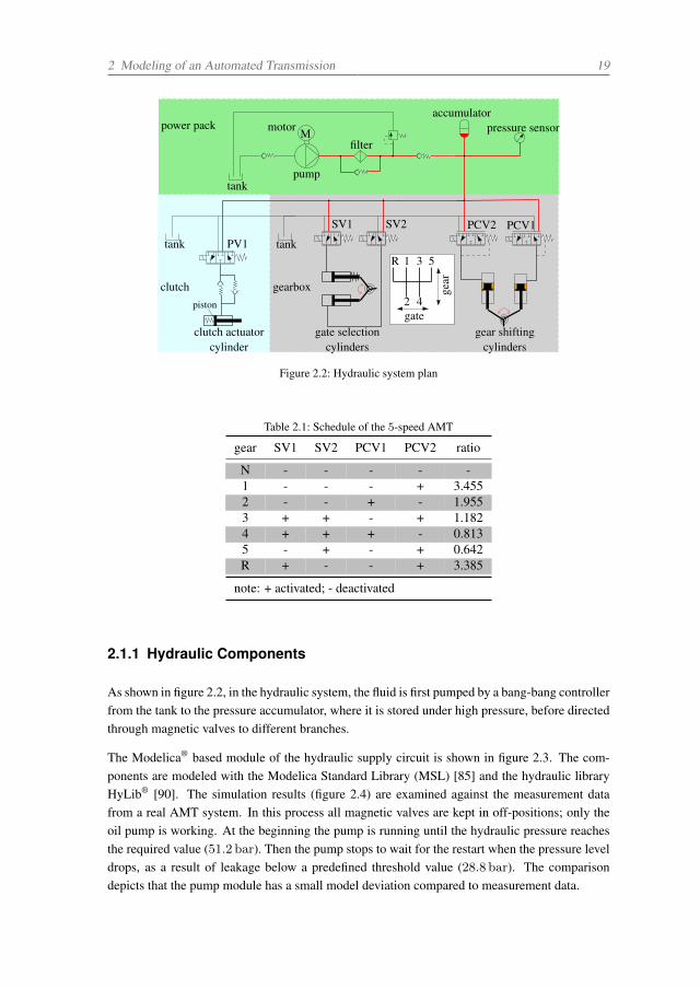
2 Modeling of an Automated Transmission 19
pump
motor Mfilter
tank
accumulatorpressure sensor
PCV1PCV2SV2
gate selectioncylinders
clutch actuatorcylinder
clutch gearbox
power pack
SV1
tank tank
gear shiftingcylinders
PV153
4
1
2
R
gate
gear
piston
Figure 2.2: Hydraulic system plan
Table 2.1: Schedule of the 5-speed AMT
gear SV1 SV2 PCV1 PCV2 ratio
N - - - - -1 - - - + 3.4552 - - + - 1.9553 + + - + 1.1824 + + + - 0.8135 - + - + 0.642R + - - + 3.385
note: + activated; - deactivated
2.1.1 Hydraulic Components
As shown in figure 2.2, in the hydraulic system, the fluid is first pumped by a bang-bang controllerfrom the tank to the pressure accumulator, where it is stored under high pressure, before directedthrough magnetic valves to different branches.
The Modelica® based module of the hydraulic supply circuit is shown in figure 2.3. The com-ponents are modeled with the Modelica Standard Library (MSL) [85] and the hydraulic libraryHyLib® [90]. The simulation results (figure 2.4) are examined against the measurement datafrom a real AMT system. In this process all magnetic valves are kept in off-positions; only theoil pump is working. At the beginning the pump is running until the hydraulic pressure reachesthe required value (51.2 bar). Then the pump stops to wait for the restart when the pressure leveldrops, as a result of leakage below a predefined threshold value (28.8 bar). The comparisondepicts that the pump module has a small model deviation compared to measurement data.
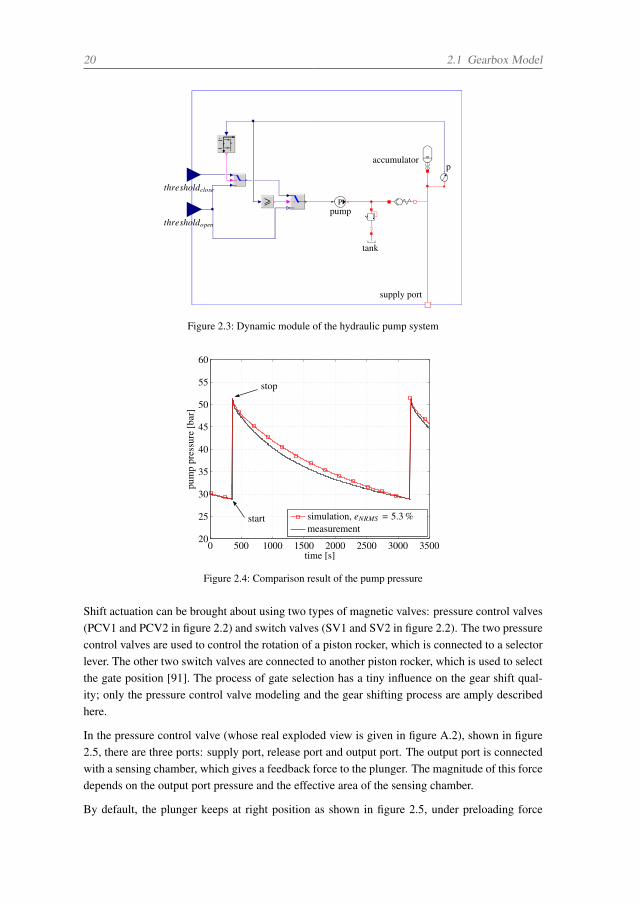
20 2.1 Gearbox Model
>pump
P
tank
accumulatorp
thresholdclose
thresholdopen
supply port
-11
Figure 2.3: Dynamic module of the hydraulic pump system
0 500 1000 1500 2000 2500 3000 350020
25
30
35
40
45
50
55
60
time [s]
pum
ppr
essu
re[b
ar]
simulation, eNRMS = 5.3 %measurement
start
stop
Figure 2.4: Comparison result of the pump pressure
Shift actuation can be brought about using two types of magnetic valves: pressure control valves(PCV1 and PCV2 in figure 2.2) and switch valves (SV1 and SV2 in figure 2.2). The two pressurecontrol valves are used to control the rotation of a piston rocker, which is connected to a selectorlever. The other two switch valves are connected to another piston rocker, which is used to selectthe gate position [91]. The process of gate selection has a tiny influence on the gear shift qual-ity; only the pressure control valve modeling and the gear shifting process are amply describedhere.
In the pressure control valve (whose real exploded view is given in figure A.2), shown in figure2.5, there are three ports: supply port, release port and output port. The output port is connectedwith a sensing chamber, which gives a feedback force to the plunger. The magnitude of this forcedepends on the output port pressure and the effective area of the sensing chamber.
By default, the plunger keeps at right position as shown in figure 2.5, under preloading force
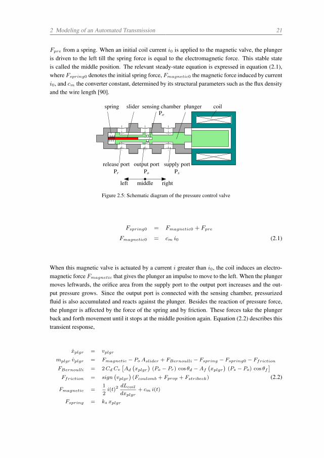
2 Modeling of an Automated Transmission 21
Fpre from a spring. When an initial coil current i0 is applied to the magnetic valve, the plungeris driven to the left till the spring force is equal to the electromagnetic force. This stable stateis called the middle position. The relevant steady-state equation is expressed in equation (2.1),whereFspring0 denotes the initial spring force, Fmagnetic0 the magnetic force induced by currenti0, and cm the converter constant, determined by its structural parameters such as the flux densityand the wire length [90].
spring coil
release port output port supply port
sensing chamberslider plunger
Pr Po Ps
Po
left rightmiddle
Figure 2.5: Schematic diagram of the pressure control valve
Fspring0 = Fmagnetic0 + Fpre
Fmagnetic0 = cm i0 (2.1)
When this magnetic valve is actuated by a current i greater than i0, the coil induces an electro-magnetic force Fmagnetic that gives the plunger an impulse to move to the left. When the plungermoves leftwards, the orifice area from the supply port to the output port increases and the out-put pressure grows. Since the output port is connected with the sensing chamber, pressurizedfluid is also accumulated and reacts against the plunger. Besides the reaction of pressure force,the plunger is affected by the force of the spring and by friction. These forces take the plungerback and forth movement until it stops at the middle position again. Equation (2.2) describes thistransient response,
xplgr = vplgr
mplgr vplgr = Fmagnetic − Po Aslider + FBernoulli − Fspring − Fspring0 − Ffriction
FBernoulli = 2Cd Cv[Ad
(xplgr
)(Po − Pr) cos θd −Af
(xplgr
)(Ps − Po) cos θf
]Ffriction = sign
(vplgr
)(Fcoulomb + Fprop + Fstribeck) (2.2)
Fmagnetic =1
2i(t)2
dLcoil
dxplgr+ cm i(t)
Fspring = ks xplgr
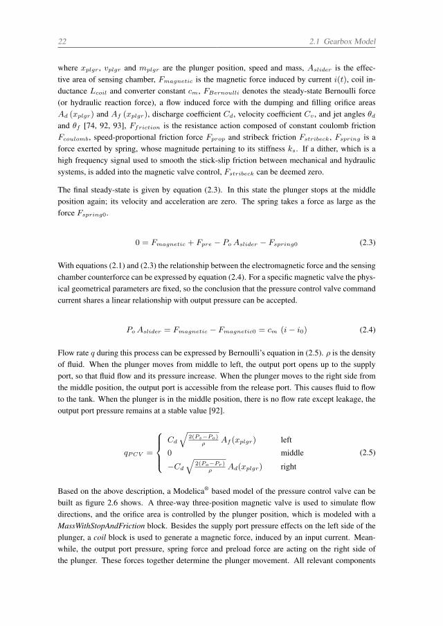
22 2.1 Gearbox Model
where xplgr , vplgr and mplgr are the plunger position, speed and mass, Aslider is the effec-tive area of sensing chamber, Fmagnetic is the magnetic force induced by current i(t), coil in-ductance Lcoil and converter constant cm, FBernoulli denotes the steady-state Bernoulli force(or hydraulic reaction force), a flow induced force with the dumping and filling orifice areasAd (xplgr) and Af (xplgr), discharge coefficient Cd, velocity coefficient Cv , and jet angles θdand θf [74, 92, 93], Ffriction is the resistance action composed of constant coulomb frictionFcoulomb, speed-proportional friction force Fprop and stribeck friction Fstribeck, Fspring is aforce exerted by spring, whose magnitude pertaining to its stiffness ks. If a dither, which is ahigh frequency signal used to smooth the stick-slip friction between mechanical and hydraulicsystems, is added into the magnetic valve control, Fstribeck can be deemed zero.
The final steady-state is given by equation (2.3). In this state the plunger stops at the middleposition again; its velocity and acceleration are zero. The spring takes a force as large as theforce Fspring0.
0 = Fmagnetic + Fpre − PoAslider − Fspring0 (2.3)
With equations (2.1) and (2.3) the relationship between the electromagnetic force and the sensingchamber counterforce can be expressed by equation (2.4). For a specific magnetic valve the phys-ical geometrical parameters are fixed, so the conclusion that the pressure control valve commandcurrent shares a linear relationship with output pressure can be accepted.
PoAslider = Fmagnetic − Fmagnetic0 = cm (i− i0) (2.4)
Flow rate q during this process can be expressed by Bernoulli’s equation in (2.5). ρ is the densityof fluid. When the plunger moves from middle to left, the output port opens up to the supplyport, so that fluid flow and its pressure increase. When the plunger moves to the right side fromthe middle position, the output port is accessible from the release port. This causes fluid to flowto the tank. When the plunger is in the middle position, there is no flow rate except leakage, theoutput port pressure remains at a stable value [92].
qPCV =
⎧⎪⎪⎨⎪⎪⎩Cd
√2(Ps−Po)
ρAf (xplgr) left
0 middle
−Cd
√2(Po−Pr)
ρAd(xplgr) right
(2.5)
Based on the above description, a Modelica® based model of the pressure control valve can bebuilt as figure 2.6 shows. A three-way three-position magnetic valve is used to simulate flowdirections, and the orifice area is controlled by the plunger position, which is modeled with aMassWithStopAndFriction block. Besides the supply port pressure effects on the left side of theplunger, a coil block is used to generate a magnetic force, induced by an input current. Mean-while, the output port pressure, spring force and preload force are acting on the right side ofthe plunger. These forces together determine the plunger movement. All relevant components
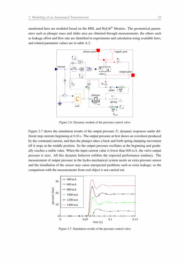
2 Modeling of an Automated Transmission 23
mentioned here are modeled based on the MSL and HyLib® libraries. The geometrical param-eters such as plunger mass and slider area are obtained through measurements, the others suchas leakage effort and flow rate are identified in experiments and calculation using available laws,and related parameter values are in table A.2.
release port supply port
plunger
coil
slider
spring
Fpre
current
output port
+ cf
>
++1
+1
f
Ps
Pos
R
A
a
valve
Figure 2.6: Dynamic module of the pressure control valve
Figure 2.7 shows the simulation results of the output pressure Po dynamic responses under dif-ferent step currents beginning at 0.05 s. The output pressure at first shows an overshoot producedby the command current, and then the plunger takes a back and forth spring-damping movementtill it stops at the middle position. So the output pressure oscillates at the beginning and gradu-ally reaches a stable value. When the input current value is lower than 600mA, the valve outputpressure is zero. All this dynamic behavior exhibits the expected performance tendency. Themeasurement of output pressure in the hydro-mechanical system needs an extra pressure sensorand the installation of the sensor may cause unexpected problems such as extra leakage; so thecomparison with the measurements from real object is not carried out.
0 0.05 0.10
10
20
30
pres
sure
[bar
]
time [s]
400 mA
600 mA
800 mA
1000 mA
1200 mA
1400 mA
0.15
Figure 2.7: Simulation results of the pressure control valve
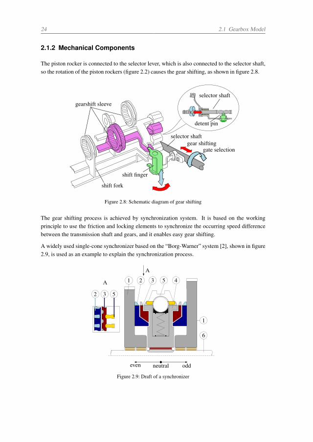
24 2.1 Gearbox Model
2.1.2 Mechanical Components
The piston rocker is connected to the selector lever, which is also connected to the selector shaft,so the rotation of the piston rockers (figure 2.2) causes the gear shifting, as shown in figure 2.8.
gearshift sleeve
selector shaftgear shifting
gate selection
shift finger
shift fork
selector shaft
detent pin
Figure 2.8: Schematic diagram of gear shifting
The gear shifting process is achieved by synchronization system. It is based on the workingprinciple to use the friction and locking elements to synchronize the occurring speed differencebetween the transmission shaft and gears, and it enables easy gear shifting.
A widely used single-cone synchronizer based on the “Borg-Warner” system [2], shown in figure2.9, is used as an example to explain the synchronization process.
1
6
532
A
A 1 2 3 5 4
oddeven neutral
Figure 2.9: Draft of a synchronizer
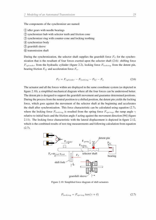
2 Modeling of an Automated Transmission 25
The components of the synchronizer are named:
1 idler gears with needle bearings2 synchronizer hub with selector teeth and friction cone3 synchronizer ring with counter-cone and locking toothing4 synchronizer body5 gearshift sleeve6 transmission shaft
During the synchronization, the selector shaft supplies the gearshift force FS for the synchro-nization that is the resultant of four forces exerted upon the selector shaft (2.6): shifting forceFcylinder from the hydraulic cylinder (figure 2.2), locking force Flocking from the detent pin,bearing friction Fbf and acceleration force Fa.
FS = Fcylinder − Flocking − Fbf − Fa (2.6)
The actuator and all the forces within are displayed in the same coordinate system (as depicted infigure 2.10), a simplified mechanical diagram where all the four forces can be understood better.The detent pin is designed to support the gearshift movement and guarantee determined positions.During the process from the neutral position to a shifted position, the detent pin yields the lockingforce, which goes against the movement of the selector shaft at the beginning and acceleratesthe shaft after synchronization. This force characteristic can be calculated using equation (2.7),where the locking force Flocking is resulted from the spring force Fspring , the ramp angle γrelative to initial basis and the friction angle δ acting against the movement direction [94] (figure2.11). The locking force characteristic with the lateral displacement is depicted in figure 2.12,which is the combined results of test ring measurements and following calculation from equation(2.7).
Fcylinder Fspring
FlockingFb f
FSFa=m f ork a f ork
detent pin
bearing
x
selector shaft
shift fork
gearshift sleeve
Figure 2.10: Simplified force diagram of shift actuators
Flocking = Fspring tan(γ + δ) (2.7)
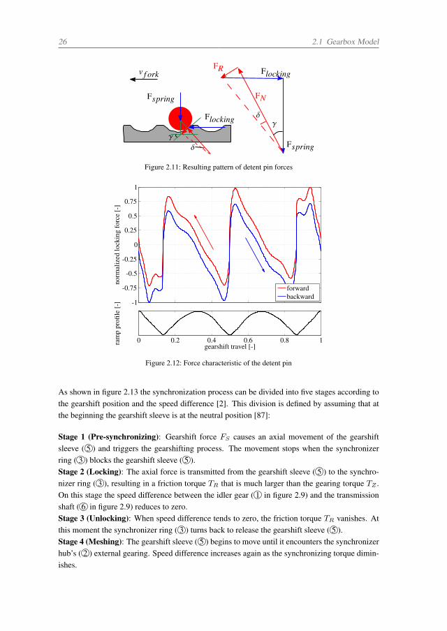
26 2.1 Gearbox Model
Fspring
δ
Flocking
γ
δ
Flocking
Fspring
FR
FN
γ
v f ork
Figure 2.11: Resulting pattern of detent pin forces
0 0.2 0.4 0.6 0.8 1gearshift travel [-]ra
mp
profi
le[-
] -1
-0.75
-0.5
-0.25
0
0.25
0.5
0.75
1
norm
aliz
edlo
ckin
gfo
rce
[-]
forwardbackward
Figure 2.12: Force characteristic of the detent pin
As shown in figure 2.13 the synchronization process can be divided into five stages according tothe gearshift position and the speed difference [2]. This division is defined by assuming that atthe beginning the gearshift sleeve is at the neutral position [87]:
Stage 1 (Pre-synchronizing): Gearshift force FS causes an axial movement of the gearshiftsleeve ( 5 ) and triggers the gearshifting process. The movement stops when the synchronizerring ( 3 ) blocks the gearshift sleeve ( 5 ).Stage 2 (Locking): The axial force is transmitted from the gearshift sleeve ( 5 ) to the synchro-nizer ring ( 3 ), resulting in a friction torque TR that is much larger than the gearing torque TZ .On this stage the speed difference between the idler gear ( 1 in figure 2.9) and the transmissionshaft ( 6 in figure 2.9) reduces to zero.Stage 3 (Unlocking): When speed difference tends to zero, the friction torque TR vanishes. Atthis moment the synchronizer ring ( 3 ) turns back to release the gearshift sleeve ( 5 ).Stage 4 (Meshing): The gearshift sleeve ( 5 ) begins to move until it encounters the synchronizerhub’s ( 2 ) external gearing. Speed difference increases again as the synchronizing torque dimin-ishes.
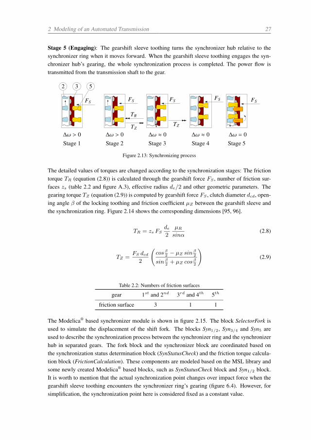
2 Modeling of an Automated Transmission 27
Stage 5 (Engaging): The gearshift sleeve toothing turns the synchronizer hub relative to thesynchronizer ring when it moves forward. When the gearshift sleeve toothing engages the syn-chronizer hub’s gearing, the whole synchronization process is completed. The power flow istransmitted from the transmission shaft to the gear.
Stage 1 Stage 2 Stage 4 Stage 5Stage 3∆ω > 0 ∆ω ≈ 0∆ω > 0 ∆ω ≈ 0 ∆ω = 0
FS FS
TR
TZ
FS
TZ
FS FS
2 3 5
Figure 2.13: Synchronizing process
The detailed values of torques are changed according to the synchronization stages: The frictiontorque TR (equation (2.8)) is calculated through the gearshift force FS , number of friction sur-faces zs (table 2.2 and figure A.3), effective radius de/2 and other geometric parameters. Thegearing torque TZ (equation (2.9)) is computed by gearshift force FS , clutch diameter dcd, open-ing angle β of the locking toothing and friction coefficient µZ between the gearshift sleeve andthe synchronization ring. Figure 2.14 shows the corresponding dimensions [95, 96].
TR = zs FSde2
µR
sinα(2.8)
TZ =FS dcd
2
(cosβ
2− µZ sin
β2
sinβ2+ µZ cos
β2
)(2.9)
Table 2.2: Numbers of friction surfaces
gear 1st and 2nd 3rd and 4th 5th
friction surface 3 1 1
The Modelica® based synchronizer module is shown in figure 2.15. The block SelectorFork isused to simulate the displacement of the shift fork. The blocks Syn1/2, Syn3/4 and Syn5 areused to describe the synchronization process between the synchronizer ring and the synchronizerhub in separated gears. The fork block and the synchronizer block are coordinated based onthe synchronization status determination block (SynStatusCheck) and the friction torque calcula-tion block (FrictionCalculation). These components are modeled based on the MSL library andsome newly created Modelica® based blocks, such as SynStatusCheck block and Syn1/2 block.It is worth to mention that the actual synchronization point changes over impact force when thegearshift sleeve toothing encounters the synchronizer ring’s gearing (figure 6.4). However, forsimplification, the synchronization point here is considered fixed as a constant value.
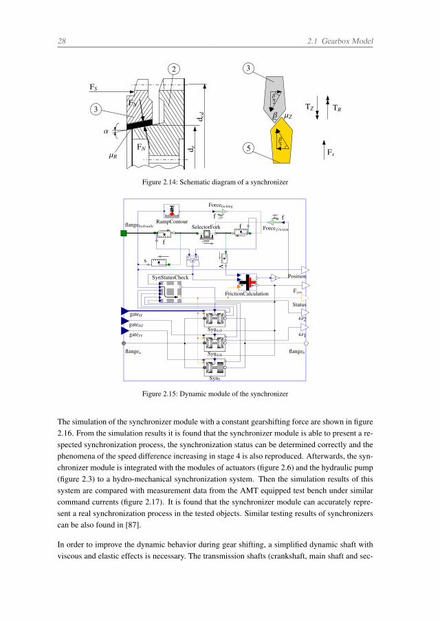
28 2.1 Gearbox Model
FS
FN
α
3
β2
β2
β
µR
d ed c
d
FN
µZ
TZ TR
2
Fs
3
5
Figure 2.14: Schematic diagram of a synchronizer
flangehydraulic
Forcelocking
Force f rictionSelectorForkRampContour
flangea flangeb
Position
Status
ω1
ω2
f
−1
s
f
fv
SynStatusCheck
f
+
+1 +1
FrictionCalculation
Syn1/2
Syn3/4
Syn5
gateII
gateIII
gateIV
Fsyn
Figure 2.15: Dynamic module of the synchronizer
The simulation of the synchronizer module with a constant gearshifting force are shown in figure2.16. From the simulation results it is found that the synchronizer module is able to present a re-spected synchronization process, the synchronization status can be determined correctly and thephenomena of the speed difference increasing in stage 4 is also reproduced. Afterwards, the syn-chronizer module is integrated with the modules of actuators (figure 2.6) and the hydraulic pump(figure 2.3) to a hydro-mechanical synchronization system. Then the simulation results of thissystem are compared with measurement data from the AMT equipped test bench under similarcommand currents (figure 2.17). It is found that the synchronizer module can accurately repre-sent a real synchronization process in the tested objects. Similar testing results of synchronizerscan be also found in [87].
In order to improve the dynamic behavior during gear shifting, a simplified dynamic shaft withviscous and elastic effects is necessary. The transmission shafts (crankshaft, main shaft and sec-
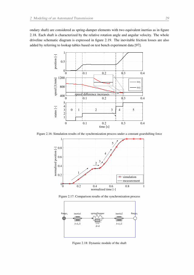
2 Modeling of an Automated Transmission 29
ondary shaft) are considered as spring-damper elements with two equivalent inertias as in figure2.18. Each shaft is characterized by the relative rotation angle and angular velocity. The wholedriveline schematic diagram is expressed in figure 2.19. The inevitable friction losses are alsoadded by referring to lookup tables based on test bench experiment data [97].
0 0.1 0.2 0.3 0.40
0.5
1po
sitio
n[-
]
0 0.1 0.2 0.3 0.4400
800
1200
spee
d[1
/min
]
ω1
ω2
0 0.1 0.2 0.3 0.4
12345
time [s]
stat
us[-
]
speed difference increases
0 1 2 3 4 5
Figure 2.16: Simulation results of the synchronization process under a constant gearshifting force
0 0.2 0.4 0.6 0.8 10
0.2
0.4
0.6
0.8
1
normalized time [-]
norm
aliz
edpo
sitio
n[-
]
simulationmeasurement
1
2 3
4
5
Figure 2.17: Comparison results of the synchronization process
springDamperinertia1 inertia2
c=cd=d
J=Js/2 J=Js/2
flangea flangeb
Figure 2.18: Dynamic module of the shaft
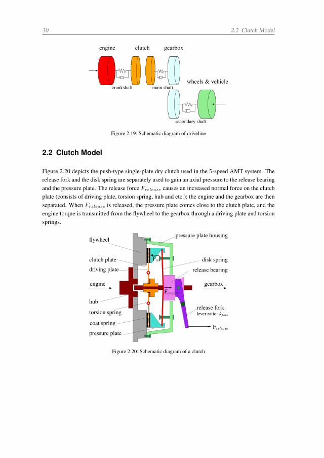
30 2.2 Clutch Model
engine clutch gearbox
wheels & vehiclecrankshaft main shaft
secondary shaft
Figure 2.19: Schematic diagram of driveline
2.2 Clutch Model
Figure 2.20 depicts the push-type single-plate dry clutch used in the 5-speed AMT system. Therelease fork and the disk spring are separately used to gain an axial pressure to the release bearingand the pressure plate. The release force Frelease causes an increased normal force on the clutchplate (consists of driving plate, torsion spring, hub and etc.); the engine and the gearbox are thenseparated. When Frelease is released, the pressure plate comes close to the clutch plate, and theengine torque is transmitted from the flywheel to the gearbox through a driving plate and torsionsprings.
flywheel
pressure plate
disk spring
release fork
release bearing
pressure plate housing
clutch plate
torsion spring
engine gearbox
Frelease
hub
driving plate
Fax
Fcounter
coat spring
lever ratio: k f ork
Figure 2.20: Schematic diagram of a clutch
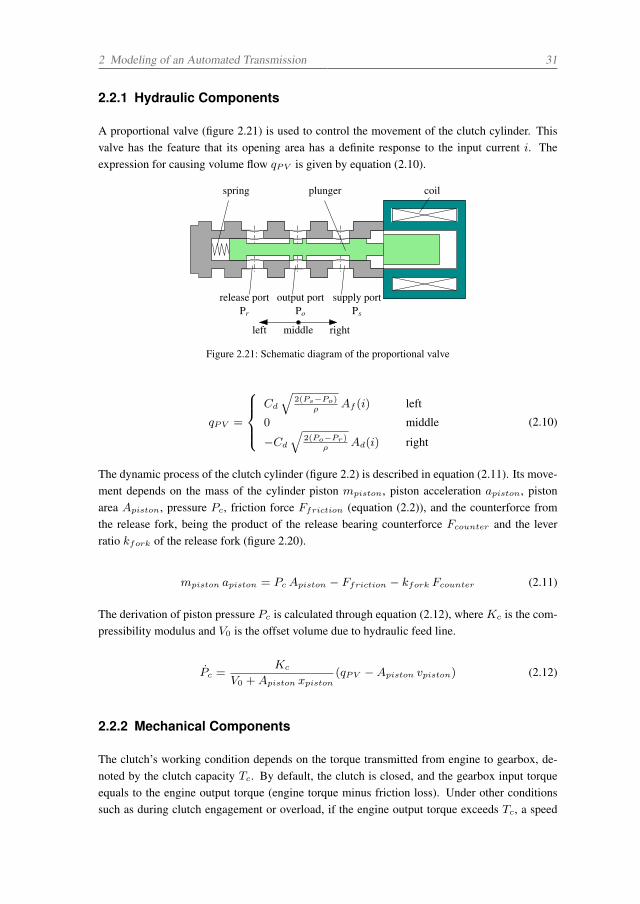
2 Modeling of an Automated Transmission 31
2.2.1 Hydraulic Components
A proportional valve (figure 2.21) is used to control the movement of the clutch cylinder. Thisvalve has the feature that its opening area has a definite response to the input current i. Theexpression for causing volume flow qPV is given by equation (2.10).
spring coil
release port output port supply port
plunger
Pr Po Ps
left rightmiddle
Figure 2.21: Schematic diagram of the proportional valve
qPV =
⎧⎪⎪⎨⎪⎪⎩Cd
√2(Ps−Po)
ρAf (i) left
0 middle
−Cd
√2(Po−Pr)
ρAd(i) right
(2.10)
The dynamic process of the clutch cylinder (figure 2.2) is described in equation (2.11). Its move-ment depends on the mass of the cylinder piston mpiston, piston acceleration apiston, pistonarea Apiston, pressure Pc, friction force Ffriction (equation (2.2)), and the counterforce fromthe release fork, being the product of the release bearing counterforce Fcounter and the leverratio kfork of the release fork (figure 2.20).
mpiston apiston = PcApiston − Ffriction − kfork Fcounter (2.11)
The derivation of piston pressure Pc is calculated through equation (2.12), where Kc is the com-pressibility modulus and V0 is the offset volume due to hydraulic feed line.
Pc =Kc
V0 +Apiston xpiston(qPV −Apiston vpiston) (2.12)
2.2.2 Mechanical Components
The clutch’s working condition depends on the torque transmitted from engine to gearbox, de-noted by the clutch capacity Tc. By default, the clutch is closed, and the gearbox input torqueequals to the engine output torque (engine torque minus friction loss). Under other conditionssuch as during clutch engagement or overload, if the engine output torque exceeds Tc, a speed
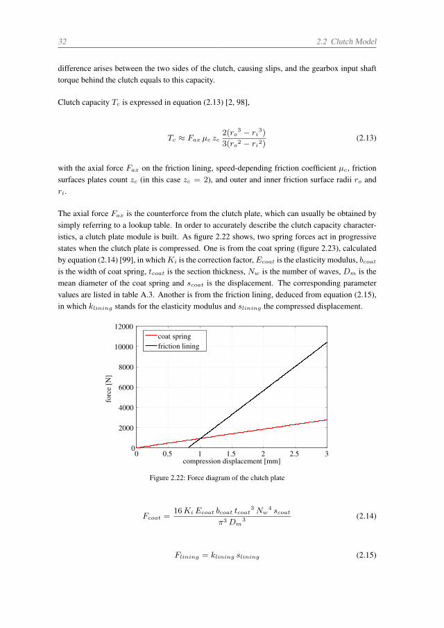
32 2.2 Clutch Model
difference arises between the two sides of the clutch, causing slips, and the gearbox input shafttorque behind the clutch equals to this capacity.
Clutch capacity Tc is expressed in equation (2.13) [2, 98],
Tc ≈ Fax µc zc2(ro
3 − ri3)
3(ro2 − ri2)(2.13)
with the axial force Fax on the friction lining, speed-depending friction coefficient µc, frictionsurfaces plates count zc (in this case zc = 2), and outer and inner friction surface radii ro andri.
The axial force Fax is the counterforce from the clutch plate, which can usually be obtained bysimply referring to a lookup table. In order to accurately describe the clutch capacity character-istics, a clutch plate module is built. As figure 2.22 shows, two spring forces act in progressivestates when the clutch plate is compressed. One is from the coat spring (figure 2.23), calculatedby equation (2.14) [99], in whichKi is the correction factor,Ecoat is the elasticity modulus, bcoatis the width of coat spring, tcoat is the section thickness, Nw is the number of waves, Dm is themean diameter of the coat spring and scoat is the displacement. The corresponding parametervalues are listed in table A.3. Another is from the friction lining, deduced from equation (2.15),in which klining stands for the elasticity modulus and slining the compressed displacement.
0 0.5 1 1.5 2 2.5 30
2000
4000
6000
8000
10000
12000
compression displacement [mm]
forc
e[N
]
coat springfriction lining
Figure 2.22: Force diagram of the clutch plate
Fcoat =16KiEcoat bcoat tcoat
3Nw4 scoat
π3Dm3 (2.14)
Flining = klining slining (2.15)
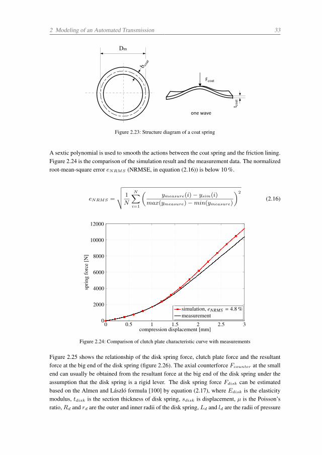
2 Modeling of an Automated Transmission 33
Dm
b coat
t coa
t
one wave
Fcoat
Figure 2.23: Structure diagram of a coat spring
A sextic polynomial is used to smooth the actions between the coat spring and the friction lining.Figure 2.24 is the comparison of the simulation result and the measurement data. The normalizedroot-mean-square error eNRMS (NRMSE, in equation (2.16)) is below 10 %.
eNRMS =
√ 1
N
N∑i=1
(ymeasure(i)− ysim(i)
max(ymeasure)−min(ymeasure)
)2
(2.16)
0 0.5 1 1.5 2 2.5 30
2000
4000
6000
8000
10000
12000
compression displacement [mm]
spri
ngfo
rce
[N]
simulation, eNRMS = 4.8 %measurement
Figure 2.24: Comparison of clutch plate characteristic curve with measurements
Figure 2.25 shows the relationship of the disk spring force, clutch plate force and the resultantforce at the big end of the disk spring (figure 2.26). The axial counterforce Fcounter at the smallend can usually be obtained from the resultant force at the big end of the disk spring under theassumption that the disk spring is a rigid lever. The disk spring force Fdisk can be estimatedbased on the Almen and László formula [100] by equation (2.17), where Edisk is the elasticitymodulus, tdisk is the section thickness of disk spring, sdisk is displacement, µ is the Poisson’sratio,Rd and rd are the outer and inner radii of the disk spring, Ld and ld are the radii of pressure
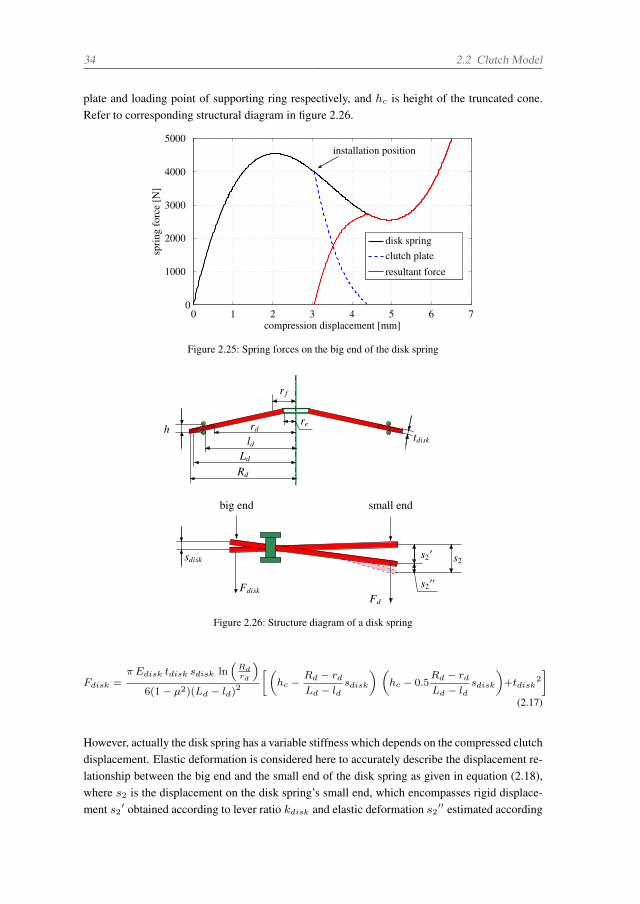
34 2.2 Clutch Model
plate and loading point of supporting ring respectively, and hc is height of the truncated cone.Refer to corresponding structural diagram in figure 2.26.
0 1 2 3 4 5 6 70
1000
2000
3000
4000
5000
compression displacement [mm]
spri
ngfo
rce
[N]
disk springclutch plate
resultant force
installation position
Figure 2.25: Spring forces on the big end of the disk spring
sdisk s2′
s2′′
s2
Fd
htdiskld
Rd
r f
re
Fdisk
big end small end
rd
Ld
Figure 2.26: Structure diagram of a disk spring
Fdisk =π Edisk tdisk sdisk ln
(Rdrd
)6(1− µ2)(Ld − ld)
2
[(hc −
Rd − rd
Ld − ldsdisk
) (hc − 0.5
Rd − rd
Ld − ldsdisk
)+tdisk
2
](2.17)
However, actually the disk spring has a variable stiffness which depends on the compressed clutchdisplacement. Elastic deformation is considered here to accurately describe the displacement re-lationship between the big end and the small end of the disk spring as given in equation (2.18),where s2 is the displacement on the disk spring’s small end, which encompasses rigid displace-ment s2′ obtained according to lever ratio kdisk and elastic deformation s2′′ estimated according
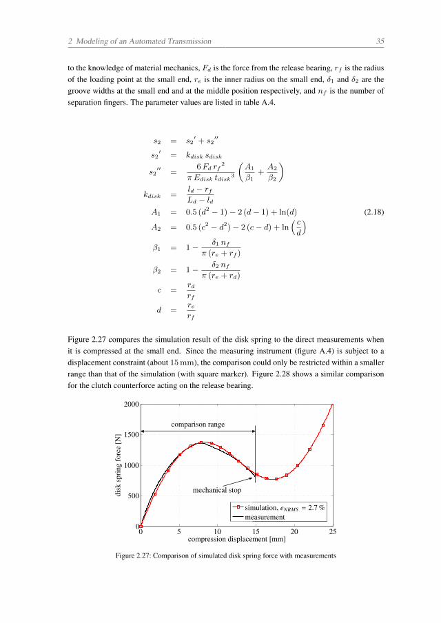
2 Modeling of an Automated Transmission 35
to the knowledge of material mechanics, Fd is the force from the release bearing, rf is the radiusof the loading point at the small end, re is the inner radius on the small end, δ1 and δ2 are thegroove widths at the small end and at the middle position respectively, and nf is the number ofseparation fingers. The parameter values are listed in table A.4.
s2 = s2′ + s2
′′
s2′ = kdisk sdisk
s2′′ =
6Fd rf2
π Edisk tdisk3
(A1
β1+A2
β2
)kdisk =
ld − rfLd − ld
A1 = 0.5 (d2 − 1)− 2 (d− 1) + ln(d) (2.18)
A2 = 0.5 (c2 − d2)− 2 (c− d) + ln( cd
)β1 = 1− δ1 nf
π (re + rf )
β2 = 1− δ2 nf
π (re + rd)
c =rdrf
d =rerf
Figure 2.27 compares the simulation result of the disk spring to the direct measurements whenit is compressed at the small end. Since the measuring instrument (figure A.4) is subject to adisplacement constraint (about 15mm), the comparison could only be restricted within a smallerrange than that of the simulation (with square marker). Figure 2.28 shows a similar comparisonfor the clutch counterforce acting on the release bearing.
0 5 10 15 20 250
500
1000
1500
2000
compression displacement [mm]
disk
spri
ngfo
rce
[N]
simulation, eNRMS = 2.7 %measurement
mechanical stop
comparison range
Figure 2.27: Comparison of simulated disk spring force with measurements
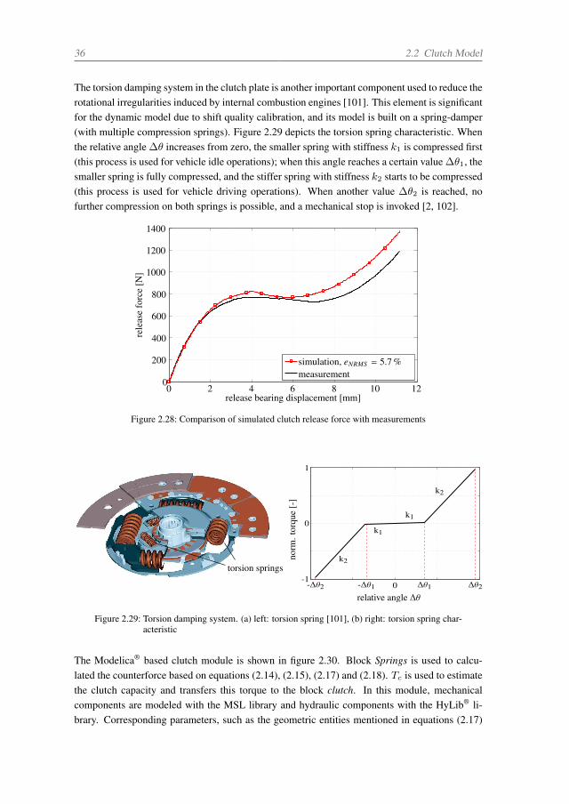
36 2.2 Clutch Model
The torsion damping system in the clutch plate is another important component used to reduce therotational irregularities induced by internal combustion engines [101]. This element is significantfor the dynamic model due to shift quality calibration, and its model is built on a spring-damper(with multiple compression springs). Figure 2.29 depicts the torsion spring characteristic. Whenthe relative angle ∆θ increases from zero, the smaller spring with stiffness k1 is compressed first(this process is used for vehicle idle operations); when this angle reaches a certain value ∆θ1, thesmaller spring is fully compressed, and the stiffer spring with stiffness k2 starts to be compressed(this process is used for vehicle driving operations). When another value ∆θ2 is reached, nofurther compression on both springs is possible, and a mechanical stop is invoked [2, 102].
0 2 4 6 8 10 120
200
400
600
800
1000
1200
1400
release bearing displacement [mm]
rele
ase
forc
e[N
]
simulation, eNRMS = 5.7 %measurement
Figure 2.28: Comparison of simulated clutch release force with measurements
blabla
relative angle ∆θ
norm
.tor
que
[-]
-1
0
1
k1
k1
k2
k2
∆θ1 ∆θ2-∆θ2 -∆θ1 0
torsion springs
Figure 2.29: Torsion damping system. (a) left: torsion spring [101], (b) right: torsion spring char-acteristic
The Modelica® based clutch module is shown in figure 2.30. Block Springs is used to calcu-lated the counterforce based on equations (2.14), (2.15), (2.17) and (2.18). Tc is used to estimatethe clutch capacity and transfers this torque to the block clutch. In this module, mechanicalcomponents are modeled with the MSL library and hydraulic components with the HyLib® li-brary. Corresponding parameters, such as the geometric entities mentioned in equations (2.17)
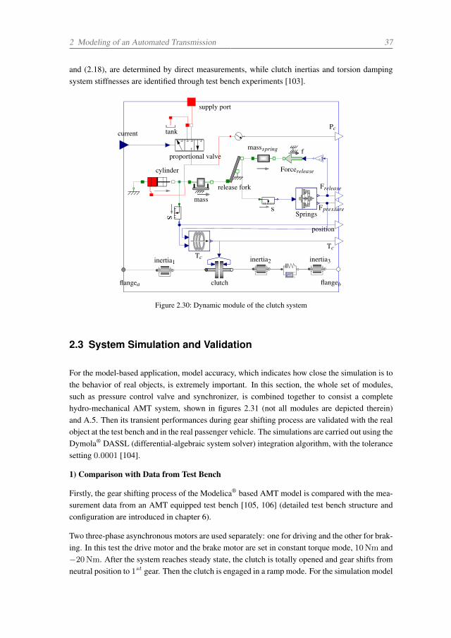
2 Modeling of an Automated Transmission 37
and (2.18), are determined by direct measurements, while clutch inertias and torsion dampingsystem stiffnesses are identified through test bench experiments [103].
f
supply port
tankcurrent
cylinder
release fork
massspring
flangea flangeb
inertia2 inertia3
clutch
Forcerelease
Tc
mass
proportional valve -1
ss
inertia1
Springs
Pc
Frelease
Fpressure
position
Tc
Figure 2.30: Dynamic module of the clutch system
2.3 System Simulation and Validation
For the model-based application, model accuracy, which indicates how close the simulation is tothe behavior of real objects, is extremely important. In this section, the whole set of modules,such as pressure control valve and synchronizer, is combined together to consist a completehydro-mechanical AMT system, shown in figures 2.31 (not all modules are depicted therein)and A.5. Then its transient performances during gear shifting process are validated with the realobject at the test bench and in the real passenger vehicle. The simulations are carried out using theDymola® DASSL (differential-algebraic system solver) integration algorithm, with the tolerancesetting 0.0001 [104].
1) Comparison with Data from Test Bench
Firstly, the gear shifting process of the Modelica® based AMT model is compared with the mea-surement data from an AMT equipped test bench [105, 106] (detailed test bench structure andconfiguration are introduced in chapter 6).
Two three-phase asynchronous motors are used separately: one for driving and the other for brak-ing. In this test the drive motor and the brake motor are set in constant torque mode, 10Nm and−20Nm. After the system reaches steady state, the clutch is totally opened and gear shifts fromneutral position to 1st gear. Then the clutch is engaged in a ramp mode. For the simulation model
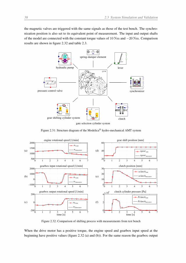
38 2.3 System Simulation and Validation
the magnetic valves are triggered with the same signals as those of the test bench. The synchro-nization position is also set to its equivalent point of measurement. The input and output shaftsof the model are connected with the constant torque values of 10Nm and −20Nm. Comparisonresults are shown in figure 2.32 and table 2.3.
hydraulic pump
pressure control valve synchronizer
spring-damper element
lever
gate selection cylinder system
gear shifting cylinder system
c©VW
clutch
Figure 2.31: Structure diagram of the Modelica® hydro-mechanical AMT system
0 1 2 3 4 5 6 7500
1000
1500
2000
(a)
engine rotational speed [1/min]
nesim
nemeasure
0 1 2 3 4 5 6 720
40
60
(d)
gear shift position [mm]
sgearsim
sgearmeasure
0 1 2 3 4 5 6 7-1000
0
1000
2000
(b)
gearbox input rotational speed [1/min]
n1sim
n1measure
0 1 2 3 4 5 6 70
10
20
30
(e)
clutch position [mm]
sclutchsim
sclutchmeasure
0 1 2 3 4 5 6 7-200
0
200
time [s]
(c)
gearbox output rotational speed [1/min]
n2sim
n2measure
0 1 2 3 4 5 6 70
2
4 x 10⁶
time [s]
(f)
clutch cylinder pressure [Pa]
Pclutchsim
Pclutchmeasure
Figure 2.32: Comparison of shifting process with measurements from test bench
When the drive motor has a positive torque, the engine speed and gearbox input speed at thebeginning have positive values (figure 2.32 (a) and (b)). For the same reason the gearbox output
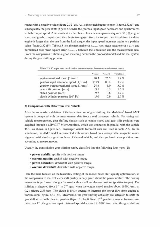
2 Modeling of an Automated Transmission 39
rotates with a negative value (figure 2.32 (c)). At 1 s the clutch begins to open (figure 2.32 (e)) andsubsequently the gear shifts (figure 2.32 (d)), the gearbox input speed decreases and synchronizeswith the output speed. Afterwards, at 2 s the clutch closes in a ramp mode (figure 2.32 (e)), enginespeed and gearbox input speed then begin to engage. Since the torque transferred from the driveengine is larger than the one from the load torque, the input speed increases again to a positivevalue (figure 2.32 (b)). Table 2.3 lists the maximal error emax, root-mean-square error eRMS andnormalized root-mean-square error eNRMS between the simulation and the measurement data.From the comparison it shows a good matching between the proposed model and the real systemduring the gear shifting process.
Table 2.3: Comparison results with measurements from transmission test bench
emax eRMS eNRMS
engine rotational speed [1/min] 40.5 23.5 1.8 %gearbox input rotational speed [1/min] 363.9 80.4 3.9 %gearbox output rotational speed [1/min] 24.4 5.0 3.0 %gear shift position [mm] 3.1 0.3 1.5 %clutch position [mm] 9.2 0.8 3.7 %clutch cylinder pressure [105 Pa] 5.0 0.9 2.9 %
2) Comparison with Data from Real Vehicle
After the successful validation of the basic function of gear shifting, the Modelica® based AMTsystem is compared with the measurement data from a real passenger vehicle. For taking realvehicle measurements, gear shifting signals such as engine speed and gear shift position wereacquired through a dSPACE® MicroAutoBox, which was connected in parallel with the vehicleTCU, as shown in figure A.6. Passenger vehicle technical data are listed in table A.5. In thesimulation, the AMT model is connected with torques based on a lookup table, magnetic valuestriggered with similar signals to those of the real vehicle, and the synchronization position resetaccording to measurements.
Usually the transmission gear shifting can be classified into the following four types [2]:
• power upshift: upshift with positive torque• overrun upshift: upshift with negative torque• power downshift: downshift with positive torque• overrun downshift: downshift with negative torque
Here the main focus is on the feasibility testing of the model-based shift quality optimization, sothe comparison to real vehicle’s shift quality is only given about the power upshift. The drivingmaneuver is performed along a flat road with a small accelerator position (positive torque). Theshifting is triggered from 1st to 2nd gear when the engine speed reaches about 1650 1/min at0.2 s (figure 2.33 (a)). The clutch is firstly opened to interrupt the power flow from engine totransmission (figure 2.33 (d)). Meanwhile, the gear shifting actuators are activated to shift thegearshift sleeve to the desired position (figure 2.33 (c)). Since 2nd gear has a smaller transmissionratio than 1st, the gearbox input rotational speed decreased to 920 1/min after this gear shifting
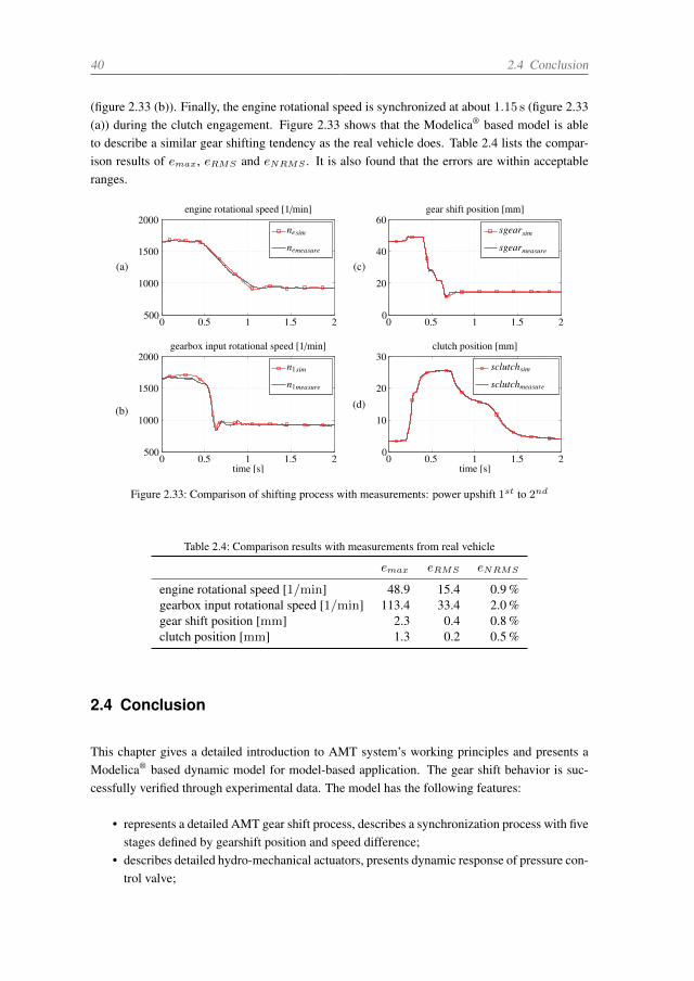
40 2.4 Conclusion
(figure 2.33 (b)). Finally, the engine rotational speed is synchronized at about 1.15 s (figure 2.33(a)) during the clutch engagement. Figure 2.33 shows that the Modelica® based model is ableto describe a similar gear shifting tendency as the real vehicle does. Table 2.4 lists the compar-ison results of emax, eRMS and eNRMS . It is also found that the errors are within acceptableranges.
0 0.5 1 1.5 2500
1000
1500
2000engine rotational speed [1/min]
nesim
nemeasure
0 0.5 1 1.5 20
20
40
60gear shift position [mm]
sgearsim
sgearmeasure
0 0.5 1 1.5 2500
1000
1500
2000
time [s]
gearbox input rotational speed [1/min]
n1sim
n1measure
0 0.5 1 1.5 20
10
20
30
time [s]
clutch position [mm]
sclutchsim
sclutchmeasure
(a)
(b)
(c)
(d)
Figure 2.33: Comparison of shifting process with measurements: power upshift 1st to 2nd
Table 2.4: Comparison results with measurements from real vehicle
emax eRMS eNRMS
engine rotational speed [1/min] 48.9 15.4 0.9 %gearbox input rotational speed [1/min] 113.4 33.4 2.0 %gear shift position [mm] 2.3 0.4 0.8 %clutch position [mm] 1.3 0.2 0.5 %
2.4 Conclusion
This chapter gives a detailed introduction to AMT system’s working principles and presents aModelica® based dynamic model for model-based application. The gear shift behavior is suc-cessfully verified through experimental data. The model has the following features:
• represents a detailed AMT gear shift process, describes a synchronization process with fivestages defined by gearshift position and speed difference;
• describes detailed hydro-mechanical actuators, presents dynamic response of pressure con-trol valve;
2 Modeling of an Automated Transmission 41
• introduces in detail the clutch disk and coat springs displacement-force characteristics,improves model behavior;
• models torsion damping system in clutch and spring-damping system in the driveline,which makes speed oscillation during torque changes possible. This improvement drawsthe developed model closer to real case;
• the model is developed based on Modelica®, it describes the system in a physical per-spective. This makes it easier for other co-developers to understand the relevant physicalmeaning.
After combined with other physical models (e.g., engine model, driveline model, driving systemand resistance model [107]), and created definitions of input interfaces for the control signals(e.g., magnetic valve current and accelerator position) and output interfaces for the feedback (e.g.,clutch position and vehicle speed), a complete Modelica® based passenger vehicle is available asshown in figure A.7. Due to space restriction, they are not discussed here.
Based on this dynamic non-linear model, now comes the next step: development of a suitablecontroller for gear shiftings.

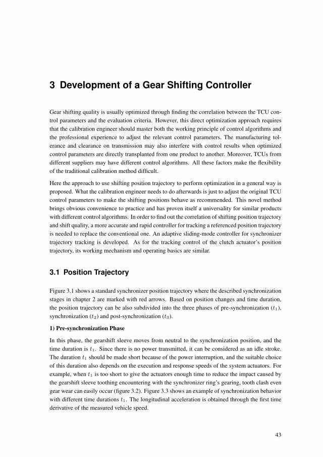
3 Development of a Gear Shifting Controller
Gear shifting quality is usually optimized through finding the correlation between the TCU con-trol parameters and the evaluation criteria. However, this direct optimization approach requiresthat the calibration engineer should master both the working principle of control algorithms andthe professional experience to adjust the relevant control parameters. The manufacturing tol-erance and clearance on transmission may also interfere with control results when optimizedcontrol parameters are directly transplanted from one product to another. Moreover, TCUs fromdifferent suppliers may have different control algorithms. All these factors make the flexibilityof the traditional calibration method difficult.
Here the approach to use shifting position trajectory to perform optimization in a general way isproposed. What the calibration engineer needs to do afterwards is just to adjust the original TCUcontrol parameters to make the shifting positions behave as recommended. This novel methodbrings obvious convenience to practice and has proven itself a universality for similar productswith different control algorithms. In order to find out the correlation of shifting position trajectoryand shift quality, a more accurate and rapid controller for tracking a referenced position trajectoryis needed to replace the conventional one. An adaptive sliding-mode controller for synchronizertrajectory tracking is developed. As for the tracking control of the clutch actuator’s positiontrajectory, its working mechanism and operating basics are similar.
3.1 Position Trajectory
Figure 3.1 shows a standard synchronizer position trajectory where the described synchronizationstages in chapter 2 are marked with red arrows. Based on position changes and time duration,the position trajectory can be also subdivided into the three phases of pre-synchronization (t1),synchronization (t2) and post-synchronization (t3).
1) Pre-synchronization Phase
In this phase, the gearshift sleeve moves from neutral to the synchronization position, and thetime duration is t1. Since there is no power transmitted, it can be considered as an idle stroke.The duration t1 should be made short because of the power interruption, and the suitable choiceof this duration also depends on the execution and response speeds of the system actuators. Forexample, when t1 is too short to give the actuators enough time to reduce the impact caused bythe gearshift sleeve toothing encountering with the synchronizer ring’s gearing, tooth clash evengear wear can easily occur (figure 3.2). Figure 3.3 shows an example of synchronization behaviorwith different time durations t1. The longitudinal acceleration is obtained through the first timederivative of the measured vehicle speed.
43
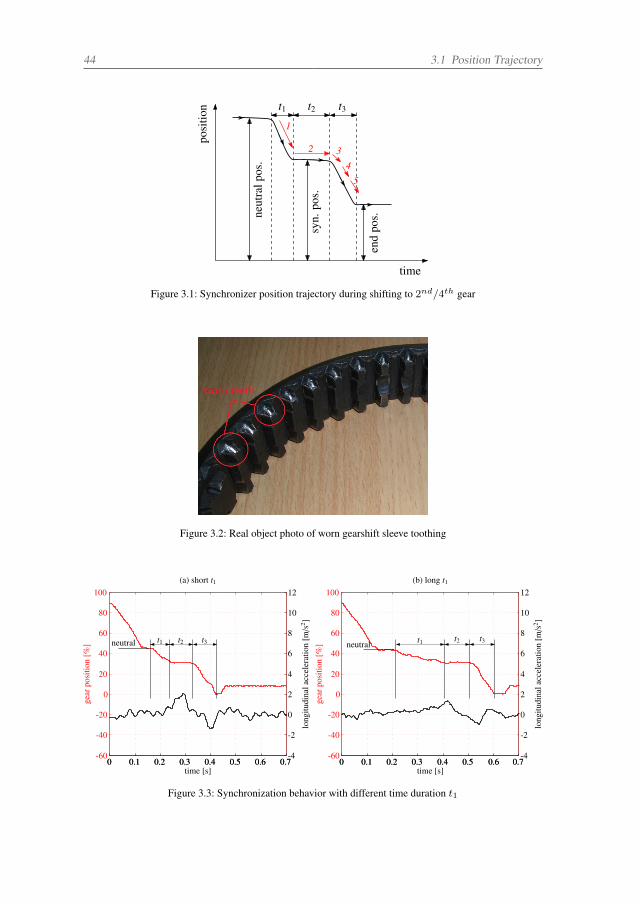
44 3.1 Position Trajectory
posi
tion
time
t1 t2 t3
neut
ralp
os.
syn.
pos.
end
pos.
1
2 34
5
Figure 3.1: Synchronizer position trajectory during shifting to 2nd/4th gear
Figure 3.2: Real object photo of worn gearshift sleeve toothing
0 0.1 0.2 0.3 0.4 0.5 0.6 0.7-60
-40
-20
0
20
40
60
80
100(a) short t1
time [s]
gear
posi
tion
[%]
0 0.1 0.2 0.3 0.4 0.5 0.6 0.7-4
-2
0
2
4
6
8
10
12
long
itudi
nala
ccel
erat
ion
[m/s
2 ]
0 0.1 0.2 0.3 0.4 0.5 0.6 0.7-60
-40
-20
0
20
40
60
80
100(b) long t1
time [s]
gear
posi
tion
[%]
0 0.1 0.2 0.3 0.4 0.5 0.6 0.7-4
-2
0
2
4
6
8
10
12
long
itudi
nala
ccel
erat
ion
[m/s
2 ]
neutralt2 t3t1neutral t2 t3t1
Figure 3.3: Synchronization behavior with different time duration t1
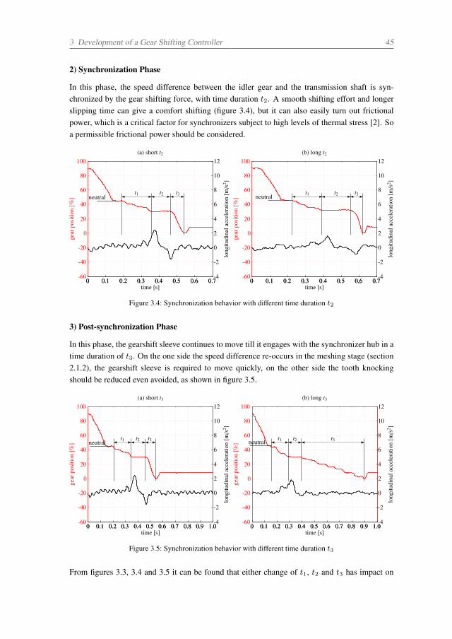
3 Development of a Gear Shifting Controller 45
2) Synchronization Phase
In this phase, the speed difference between the idler gear and the transmission shaft is syn-chronized by the gear shifting force, with time duration t2.sA smooth shifting effort and longerslipping time can give a comfort shifting (figure 3.4), but it can also easily turn out frictionalpower, which is a critical factor for synchronizers subject to high levels of thermal stress [2]. Soa permissible frictional power should be considered.
0 0.1 0.2 0.3 0.4 0.5 0.6 0.7-60
-40
-20
0
20
40
60
80
100(a) short t2
time [s]
gear
posi
tion
[%]
0 0.1 0.2 0.3 0.4 0.5 0.6 0.7-4
-2
0
2
4
6
8
10
12
long
itudi
nala
ccel
erat
ion
[m/s
2 ]
0 0.1 0.2 0.3 0.4 0.5 0,6 0.7-60
-40
-20
0
20
40
60
80
100(b) long t2
time [s]
gear
posi
tion
[%]
0 0.1 0.2 0.3 0.4 0.5 0,6 0.7-4
-2
0
2
4
6
8
10
12
long
itudi
nala
ccel
erat
ion
[m/s
2 ]
neutralt2 t3t1
neutralt2 t3t1
Figure 3.4: Synchronization behavior with different time duration t2
3) Post-synchronization Phase
In this phase, the gearshift sleeve continues to move till it engages with the synchronizer hub in atime duration of t3. On the one side the speed difference re-occurs in the meshing stage (section2.1.2), the gearshift sleeve is required to move quickly, on the other side the tooth knockingshould be reduced even avoided, as shown in figure 3.5.
0 0.1 0.2 0.3 0.4 0.5 0.6 0.7 0.8 0.9 1.0-60
-40
-20
0
20
40
60
80
100(a) short t3
time [s]
gear
posi
tion
[%]
0 0.1 0.2 0.3 0.4 0.5 0.6 0.7 0.8 0.9 1.0-4
-2
0
2
4
6
8
10
12
long
itudi
nala
ccel
erat
ion
[m/s
2 ]
0 0.1 0.2 0.3 0.4 0.5 0.6 0.7 0.8 0.9 1.0-60
-40
-20
0
20
40
60
80
100(b) long t3
time [s]
gear
posi
tion
[%]
0 0.1 0.2 0.3 0.4 0.5 0.6 0.7 0.8 0.9 1.0-4
-2
0
2
4
6
8
10
12
long
itudi
nala
ccel
erat
ion
[m/s
2 ]
neutralt2 t3t1 neutral
t2 t3t1
Figure 3.5: Synchronization behavior with different time duration t3
From figures 3.3, 3.4 and 3.5 it can be found that either change of t1, t2 and t3 has impact on
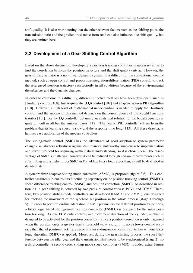
46 3.2 Development of a Gear Shifting Control Algorithm
shift quality. It is also worth noting that the other relevant factors such as the shifting point, thetransmission ratio and the gradient resistance from road can also influence the shift quality, butthey are omitted here.
3.2 Development of a Gear Shifting Control Algorithm
Based on the above discussion, developing a position tracking controller is necessary so as tofind the correlation between the position trajectory and the shift quality criteria. However, thegear shifting actuator is a non-linear dynamic system. It is difficult for the conventional controlmethod, such as open control and proportion-integration-differentiation (PID) control, to trackthe referenced position trajectory satisfactorily in all conditions because of the environmentaldisturbances and the dynamic changes.
In order to overcome this difficulty, different effective methods have been developed, such asH-infinity control [108], linear quadratic (LQ) control [109] and adaptive neuron PID algorithm[110]. However, a high level of mathematical understanding is needed to apply the H-infinitycontrol, and the success of this method depends on the correct choice of the weight functionstransfer [111]. For the LQ controller obtaining an analytical solution for the Ricatti equation isquite difficult in all but the simplest cases [112]. The neuron PID controller suffers from theproblem that its learning speed is slow and the response time long [113]. All these drawbackshamper easy application of the modern controllers.
The sliding-mode control (SMC) has the advantages of good adaption to system parameterchanges, satisfactory robustness against disturbances, noteworthy simpleness to implementationand lower threshold for acquiring mathematical understanding, so it is chosen here. The disad-vantage of SMC is chattering; however, it can be reduced through certain improvements such assubstituting into a higher order SMC and/or adding fuzzy logic algorithm, as will be described indetailed later.
A synchronizer adaptive sliding-mode controller (ASMC) is proposed (figure 3.6). This con-troller has three sub-controllers functioning separately on the position tracking control (FSMPC),speed difference tracking control (SMSC) and position correction (SMPC). As described in sec-tion 2.1, a gear shifting is actuated by two pressure control valves: PCV1 and PCV2. There-fore, two position sliding-mode controllers are developed (FSMPC and SMPC), one designedfor tracking the movement of the synchronizer position in the whole process (stage 1 through5). In order to perform on-line adaptation to SMC parameters for different position trajectories,a fuzzy logic based sliding-mode position controller (FSMPC) is designed for the main posi-tion tracking. As one PCV only controls one movement direction of the cylinder, another isdesigned to be activated for the position correction. Since a position correction is only triggeredwhen the position error is greater than a threshold value strigger , it needs lower control accu-racy than that of position tracking, a second-order sliding-mode position controller without fuzzylogic algorithm (SMPC) is applied. Moreover, during the gear shifting process, the speed dif-ference between the idler gear and the transmission shaft needs to be synchronized (stage 2); soa third controller, a second-order sliding-mode speed controller (SMSC) is added extra. Figure
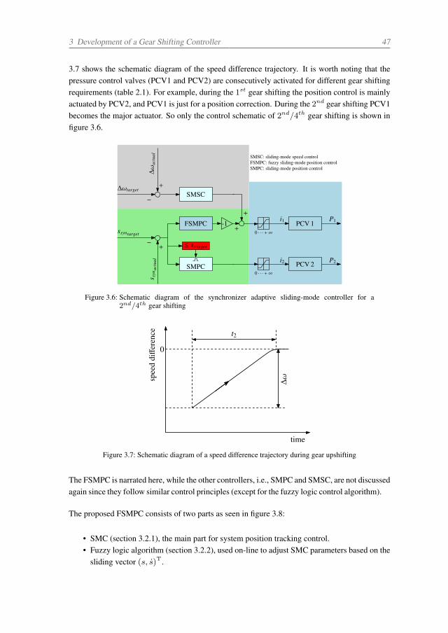
3 Development of a Gear Shifting Controller 47
3.7 shows the schematic diagram of the speed difference trajectory. It is worth noting that thepressure control valves (PCV1 and PCV2) are consecutively activated for different gear shiftingrequirements (table 2.1). For example, during the 1st gear shifting the position control is mainlyactuated by PCV2, and PCV1 is just for a position correction. During the 2nd gear shifting PCV1becomes the major actuator. So only the control schematic of 2nd/4th gear shifting is shown infigure 3.6.
FSMPC
SMPC
PCV 1
PCV 2
0 · · · +∞
0 · · · +∞
SMSC
i1
i2
+
+
P1
P2
ssyntarget
∆ωtarget
−
−
+
+
∆ω
actu
als s
ynac
tual
≤ strigger
SMSC: sliding-mode speed controlFSMPC: fuzzy sliding-mode position controlSMPC: sliding-mode position control
-1
Figure 3.6: Schematic diagram of the synchronizer adaptive sliding-mode controller for a2nd/4th gear shifting
spee
ddiff
eren
ce
time
t2
∆ω
0
Figure 3.7: Schematic diagram of a speed difference trajectory during gear upshifting
The FSMPC is narrated here, while the other controllers, i.e., SMPC and SMSC, are not discussedagain since they follow similar control principles (except for the fuzzy logic control algorithm).
The proposed FSMPC consists of two parts as seen in figure 3.8:
• SMC (section 3.2.1), the main part for system position tracking control.• Fuzzy logic algorithm (section 3.2.2), used on-line to adjust SMC parameters based on the
sliding vector (s, s)T.
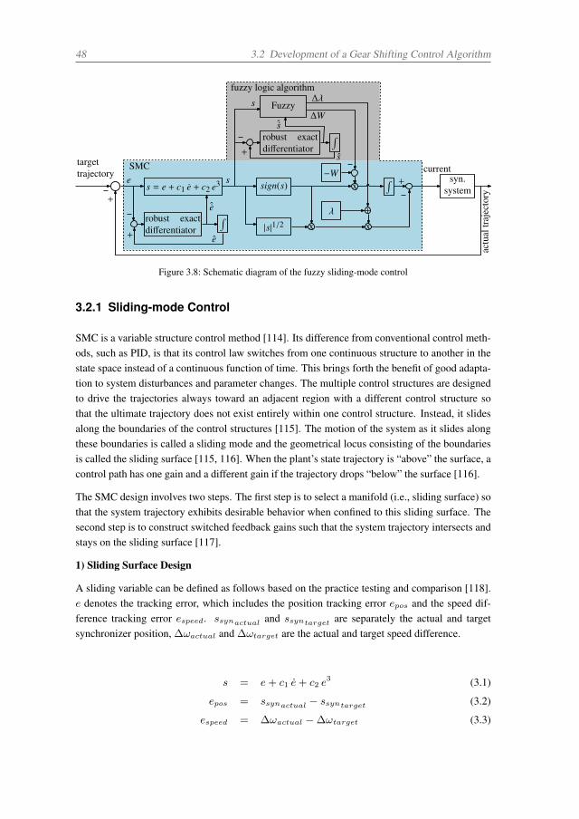
48 3.2 Development of a Gear Shifting Control Algorithm
+
actu
altr
ajec
tory
current
ˆs
e
ˆe
ssign(s)
|s|1/2
Fuzzys
+
x
x
+
∆W
∆λ
x
−W
λ
∫targettrajectory syn.
systems = e + c1 e + c2 e3
SMC
fuzzy logic algorithm
robust exactdifferentiator
∫
+ e
robust exactdifferentiator
∫
s+
Figure 3.8: Schematic diagram of the fuzzy sliding-mode control
3.2.1 Sliding-mode Control
SMC is a variable structure control method [114]. Its difference from conventional control meth-ods, such as PID, is that its control law switches from one continuous structure to another in thestate space instead of a continuous function of time. This brings forth the benefit of good adapta-tion to system disturbances and parameter changes. The multiple control structures are designedto drive the trajectories always toward an adjacent region with a different control structure sothat the ultimate trajectory does not exist entirely within one control structure. Instead, it slidesalong the boundaries of the control structures [115]. The motion of the system as it slides alongthese boundaries is called a sliding mode and the geometrical locus consisting of the boundariesis called the sliding surface [115, 116]. When the plant’s state trajectory is “above” the surface, acontrol path has one gain and a different gain if the trajectory drops “below” the surface [116].
The SMC design involves two steps. The first step is to select a manifold (i.e., sliding surface) sothat the system trajectory exhibits desirable behavior when confined to this sliding surface. Thesecond step is to construct switched feedback gains such that the system trajectory intersects andstays on the sliding surface [117].
1) Sliding Surface Design
A sliding variable can be defined as follows based on the practice testing and comparison [118].e denotes the tracking error, which includes the position tracking error epos and the speed dif-ference tracking error espeed. ssynactual and ssyntarget are separately the actual and targetsynchronizer position, ∆ωactual and ∆ωtarget are the actual and target speed difference.
s = e+ c1 e+ c2 e3 (3.1)
epos = ssynactual − ssyntarget (3.2)
espeed = ∆ωactual −∆ωtarget (3.3)
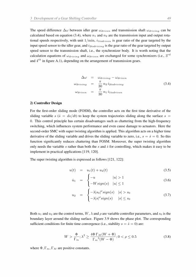
3 Development of a Gear Shifting Controller 49
The speed difference ∆ω between idler gear ωdriven and transmission shaft ωdriving can becalculated based on equation (3.4), where n1 and n2 are the transmission input and output rota-tional speeds respectively, with unit 1/min, i1todriven is gear ratio of the gear targeted by theinput speed sensor to the idler gear, and i2todriving is the gear ratio of the gear targeted by outputspeed sensor to the transmission shaft, i.e., the synchronizer body. It is worth noting that thecalculation equations of ωdriving and ωdriven are exchanged for some synchronizers (i.e., 3rd
and 4th in figure A.1), depending on the arrangement of transmission gears.
∆ω = ωdriving − ωdriven
ωdriving =π
30n2 i2todriving (3.4)
ωdriven =π
30n1 i1todriven
2) Controller Design
For the first-order sliding mode (FOSM), the controller acts on the first time derivative of thesliding variable s (s = ds/dt) to keep the system trajectories sliding along the surface s =
0. This control principle has certain disadvantages such as chattering from the high-frequencyswitching, which influences system performance and even cause damage to actuators. Here thesecond-order SMC with super twisting algorithm is applied. This algorithm acts on a higher timederivative of the sliding variable and drives the sliding variable to zero, i.e., s = s = 0. So thisfunction significantly reduces chattering than FOSM. Moreover, the super twisting algorithmonly needs the variable s rather than both the s and s for controlling, which makes it easy to beimplement in practical applications [119, 120].
The super twisting algorithm is expressed as follows [121, 122]:
u(t) = u1(t) + u2(t) (3.5)
u1 =
⎧⎨⎩−u |u| > 1
−Wsign(s) |u| ≤ 1(3.6)
u2 =
⎧⎨⎩−λ|s0|ρsign(s) |s| > s0
−λ|s|ρsign(s) |s| ≤ s0(3.7)
Both u1 and u2 are the control terms,W , λ and ρ are variable controller parameters, and s0 is theboundary layer around the sliding surface. Figure 3.9 shows the phase plot. The correspondingsufficient conditions for finite time convergence (i.e., stability s = s = 0) are:
W >Φ
Γm;λ2 ≥ 4ΦΓM (W +Φ)
Γm3(W − Φ)
; 0 < ρ ≤ 0.5 (3.8)
where Φ,Γm,ΓM are positive constants.
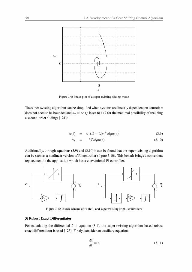
50 3.2 Development of a Gear Shifting Control Algorithm
0
0
s
s
Figure 3.9: Phase plot of a super twisting sliding-mode
The super twisting algorithm can be simplified when systems are linearly dependent on control; udoes not need to be bounded and s0 = ∞ (ρ is set to 1/2 for the maximal possibility of realizinga second-order sliding) [121]:
u(t) = u1(t)− λ|s|12 sign(s) (3.9)
u1 = −Wsign(s) (3.10)
Additionally, through equations (3.9) and (3.10) it can be found that the super twisting algorithmcan be seen as a nonlinear version of PI controller (figure 3.10). This benefit brings a convenientreplacement in the application which has a conventional PI controller.
e u
∫kI
+
+
s u
∫W
-
-
Figure 3.10: Block scheme of PI (left) and super twisting (right) controllers
3) Robust Exact Differentiator
For calculating the differential e in equation (3.1), the super-twisting-algorithm based robustexact differentiator is used [123]. Firstly, consider an auxiliary equation:
de
dt= ˆe (3.11)
3 Development of a Gear Shifting Controller 51
Assume that a controller auxiliary equation output e perfectly tracks the speed error e:
ϵ := e− e = 0 (3.12)
then ˆe equals to the time derivative of e. And e, ˆe can be considered as the approximations ofcorresponding state variables e, e. The super twisting algorithm (equations (3.9) and (3.10)) isused for the tracking task, where ψ and ϑ are positive constants:
ˆe = ν − ϑ|ϵ|12 sign(ϵ) (3.13)
ν = −ψsign(ϵ) (3.14)
3.2.2 Fuzzy Logic Algorithm
Due to two contradicting factors, rapid reaching to the sliding surface and steady sliding alongthe surface, it is difficult to find optimal parameters during SMC implementation. Convention-ally, the controller parameters are first bounded based on the control-Lyapunov function, and thenidentified through the trial-and-error method [119]. However, this kind of tuning method is time-consuming and parameters thus found cannot guarantee to achieve optimal tracking performanceunder different matching conditions. In order to solve this problem, different research has beenmade. In [124, 125], an observer-based SMC is applied to dynamically adapt the parameters. Butthe effectiveness of the control performance depends on the accuracy of the observer modelingand professional knowledge on the working principle of the controlled object; it is complicatedto implement in a non-linear system with higher-order. In [126], a neural network is applied toon-line estimate the SMC parameters. However, the neural-network based control scheme needslonger time to detect all possible interaction between the predictor variables before achievingoptimal control performance [127]. Recently, SMC with adaptive algorithm, which aims to elim-inate overestimation of the control gains and reduce chattering, has been developed [128, 129].While this adaptive algorithm forecasts control parameters based on current state, it causes anadjusting performance delay and results in a bad dynamic behavior [117]. Thus, fuzzy logicalgorithm [130], whose intrinsic rules makes fast response possible, is applied here to on-lineadjust the sliding-mode controller parameters.
Fuzzy logic algorithm exploits linguistic rules in IF-THEN format to control or model complexand high-order non-linear systems without mathematical descriptions [131]. Since it does notrequire precise and perturbation-free inputs, this algorithm is known as a robust control approachand has been combined with sliding mode control in applications [132–134].
In a fuzzy logic algorithm there are three main components (figure 3.11): a fuzzification, whichis obtained via membership functions; an inference engine, which calculates the fuzzy outputsbased on the inputs and linguistic rules; and a defuzzification, which computes the crisp out-puts.
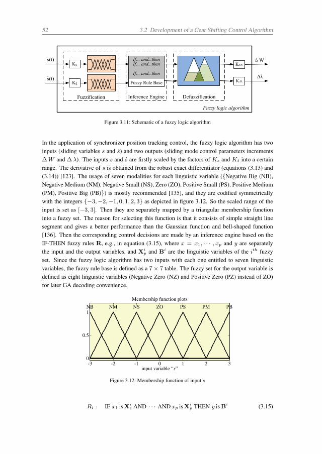
52 3.2 Development of a Gear Shifting Control Algorithm
KΔW
KS
KS
KΔλ
Fuzzification
If… and...thenIf… and...then
If… and...then
Fuzzy Rule Base
Inference Engine Defuzzification
s(t) ΔW
Δλs(t)
Fuzzy logic algorithm
Figure 3.11: Schematic of a fuzzy logic algorithm
In the application of synchronizer position tracking control, the fuzzy logic algorithm has twoinputs (sliding variables s and s) and two outputs (sliding mode control parameters increments∆W and ∆λ). The inputs s and s are firstly scaled by the factors of Ks and Ks into a certainrange. The derivative of s is obtained from the robust exact differentiator (equations (3.13) and(3.14)) [123]. The usage of seven modalities for each linguistic variable (Negative Big (NB),Negative Medium (NM), Negative Small (NS), Zero (ZO), Positive Small (PS), Positive Medium(PM), Positive Big (PB)) is mostly recommended [135], and they are codified symmetricallywith the integers −3,−2,−1, 0, 1, 2, 3 as depicted in figure 3.12. So the scaled range of theinput is set as [−3, 3]. Then they are separately mapped by a triangular membership functioninto a fuzzy set. The reason for selecting this function is that it consists of simple straight linesegment and gives a better performance than the Gaussian function and bell-shaped function[136]. Then the corresponding control decisions are made by an inference engine based on theIF-THEN fuzzy rules R, e.g., in equation (3.15), where x = x1, · · · , xp and y are separatelythe input and the output variables, and Xi
p and Bi are the linguistic variables of the ith fuzzyset. Since the fuzzy logic algorithm has two inputs with each one entitled to seven linguisticvariables, the fuzzy rule base is defined as a 7× 7 table. The fuzzy set for the output variable isdefined as eight linguistic variables (Negative Zero (NZ) and Positive Zero (PZ) instead of ZO)for later GA decoding convenience.
-3 -2 -1 0 1 2 30
0.5
1
Membership function plots
input variable “s”
NB NM NS ZO PS PM PB
Figure 3.12: Membership function of input s
Ri : IF x1 isXi1 AND · · · ANDxp isXi
p THEN y isBi (3.15)
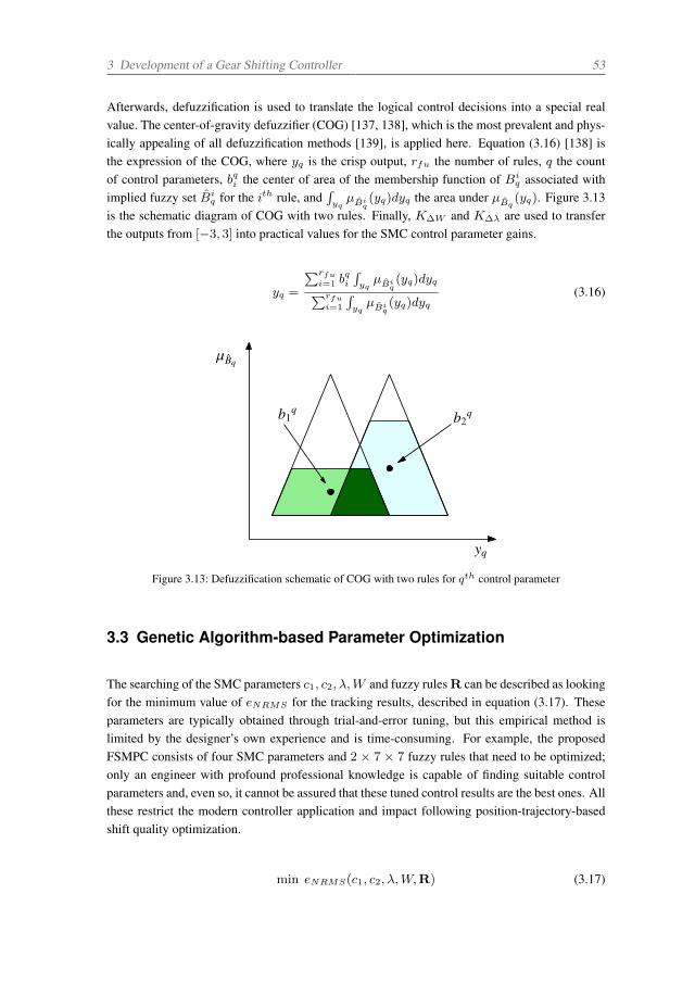
3 Development of a Gear Shifting Controller 53
Afterwards, defuzzification is used to translate the logical control decisions into a special realvalue. The center-of-gravity defuzzifier (COG) [137, 138], which is the most prevalent and phys-ically appealing of all defuzzification methods [139], is applied here. Equation (3.16) [138] isthe expression of the COG, where yq is the crisp output, rfu the number of rules, q the countof control parameters, bqi the center of area of the membership function of Bi
q associated withimplied fuzzy set Bi
q for the ith rule, and∫yqµBi
q(yq)dyq the area under µBq
(yq). Figure 3.13is the schematic diagram of COG with two rules. Finally, K∆W and K∆λ are used to transferthe outputs from [−3, 3] into practical values for the SMC control parameter gains.
yq =
∑rfu
i=1 bqi
∫yqµBi
q(yq)dyq∑rfu
i=1
∫yqµBi
q(yq)dyq
(3.16)
µBq
yq
b2qb1
q
Figure 3.13: Defuzzification schematic of COG with two rules for qth control parameter
3.3 Genetic Algorithm-based Parameter Optimization
The searching of the SMC parameters c1, c2, λ,W and fuzzy rules R can be described as lookingfor the minimum value of eNRMS for the tracking results, described in equation (3.17). Theseparameters are typically obtained through trial-and-error tuning, but this empirical method islimited by the designer’s own experience and is time-consuming. For example, the proposedFSMPC consists of four SMC parameters and 2 × 7 × 7 fuzzy rules that need to be optimized;only an engineer with profound professional knowledge is capable of finding suitable controlparameters and, even so, it cannot be assured that these tuned control results are the best ones. Allthese restrict the modern controller application and impact following position-trajectory-basedshift quality optimization.
min eNRMS(c1, c2, λ,W,R) (3.17)
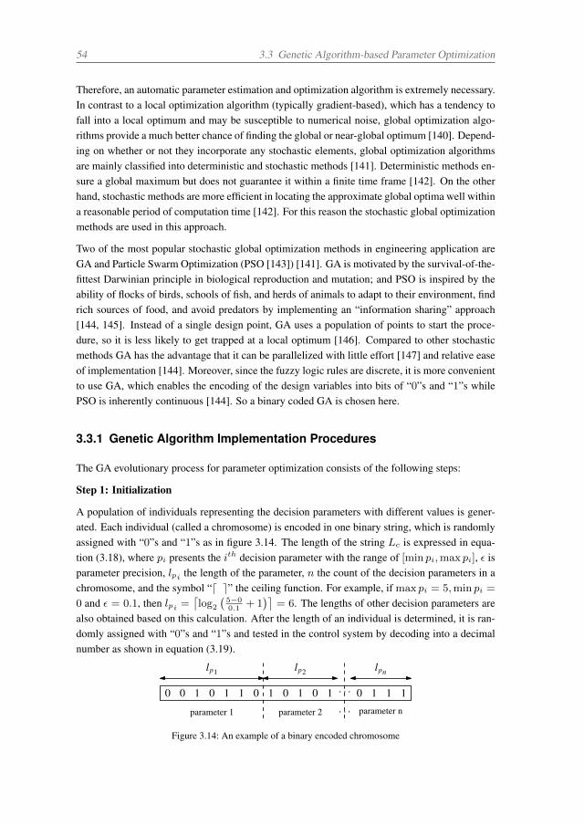
54 3.3 Genetic Algorithm-based Parameter Optimization
Therefore, an automatic parameter estimation and optimization algorithm is extremely necessary.In contrast to a local optimization algorithm (typically gradient-based), which has a tendency tofall into a local optimum and may be susceptible to numerical noise, global optimization algo-rithms provide a much better chance of finding the global or near-global optimum [140]. Depend-ing on whether or not they incorporate any stochastic elements, global optimization algorithmsare mainly classified into deterministic and stochastic methods [141]. Deterministic methods en-sure a global maximum but does not guarantee it within a finite time frame [142]. On the otherhand, stochastic methods are more efficient in locating the approximate global optima well withina reasonable period of computation time [142]. For this reason the stochastic global optimizationmethods are used in this approach.
Two of the most popular stochastic global optimization methods in engineering application areGA and Particle Swarm Optimization (PSO [143]) [141]. GA is motivated by the survival-of-the-fittest Darwinian principle in biological reproduction and mutation; and PSO is inspired by theability of flocks of birds, schools of fish, and herds of animals to adapt to their environment, findrich sources of food, and avoid predators by implementing an “information sharing” approach[144, 145]. Instead of a single design point, GA uses a population of points to start the proce-dure, so it is less likely to get trapped at a local optimum [146]. Compared to other stochasticmethods GA has the advantage that it can be parallelized with little effort [147] and relative easeof implementation [144]. Moreover, since the fuzzy logic rules are discrete, it is more convenientto use GA, which enables the encoding of the design variables into bits of “0”s and “1”s whilePSO is inherently continuous [144]. So a binary coded GA is chosen here.
3.3.1 Genetic Algorithm Implementation Procedures
The GA evolutionary process for parameter optimization consists of the following steps:
Step 1: Initialization
A population of individuals representing the decision parameters with different values is gener-ated. Each individual (called a chromosome) is encoded in one binary string, which is randomlyassigned with “0”s and “1”s as in figure 3.14. The length of the string Lc is expressed in equa-tion (3.18), where pi presents the ith decision parameter with the range of [min pi,max pi], ϵ isparameter precision, lpi the length of the parameter, n the count of the decision parameters in achromosome, and the symbol “⌈a⌉” the ceiling function. For example, if max pi = 5,min pi =
0 and ϵ = 0.1, then lpi =⌈log2
(5−00.1
+ 1)⌉
= 6. The lengths of other decision parameters arealso obtained based on this calculation. After the length of an individual is determined, it is ran-domly assigned with “0”s and “1”s and tested in the control system by decoding into a decimalnumber as shown in equation (3.19).
0 00 0 0 0 01 1 1 1 1 1 1· · ·lp1 lp2 lpn
parameter 1 parameter 2 parameter n
11
· · ·
Figure 3.14: An example of a binary encoded chromosome
3 Development of a Gear Shifting Controller 55
begin hereLc =
n∑i=1
lpi
lpi =
⌈log2
(max pi −min pi
ϵi+ 1
)⌉(3.18)
pi = min pi +
lpi∑j=1
2j−1 max pi −min pi
2lpi − 1(3.19)
Step 2: Fitness Evaluation
Fitness function F is a computation to evaluate the quality of each individual as a solution to aparticular problem [148]. In a maximization issue the higher the fitness value of an individual isthe better the control performance of the system behaves. Since multi-objective criteria fitnesshas the weighted distribution problem and the practical testing showing that it does not havean obvious improvement over the single-objective criteria fitness for the synchronizer trajectoryoptimization problem [149], here only the latter one is applied (equations (3.20) and (3.21)). It isworth mentioning that in speed difference control ssyn is replaced by ∆ω.
eNRMS =
√ 1
N
N∑i=1
(ssyntarget − ssynactual
max(ssyntarget)−min(ssyntarget)
)2
(3.20)
F =1
1 + eNRMS(3.21)
Step 3: 1st Selection
According to the fitness values, certain individuals are selected to participate in the reproductionfor the next population (called parents). The selection exploits the information represented withinthe population, and the term selective pressure is used to characterize the emphasis of selectionon the best individuals [150]. A strong selective pressure may cause the algorithm to convergeto a local optimum, while a low selection pressure may cause the GA to get random resultsthat differ from one run to another [151]. There are several methods to implement the selectionoperation: roulette wheel selection [152], rank-based roulette wheel selection [153], stochasticuniversal sampling [154], the tournament selection [155], etc.
Since rank-based roulette wheel selection can avoid premature convergence due to super indi-vidual and eliminate the need to scale fitness values [153], it is chosen in the 1st Selection. Theselection strategy of rank-based roulette wheel selection applied here is that the individuals beingselected is based on its fitness rank relative to the entire population. Firstly, the individuals aresorted in descending order by their fitness, then the selection probabilities are computed basedon the fitness rank, i.e., rank divided the population count.
The rank of an individual can be scaled using equation (3.22) for a linear-rank-based selection[153, 156]:
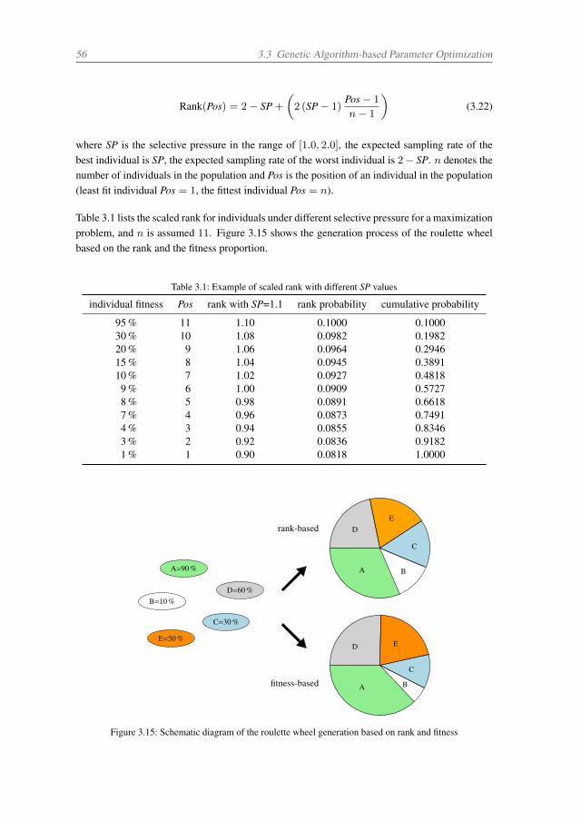
56 3.3 Genetic Algorithm-based Parameter Optimization
Rank(Pos) = 2− SP +
(2 (SP − 1)
Pos − 1
n− 1
)(3.22)
where SP is the selective pressure in the range of [1.0, 2.0], the expected sampling rate of thebest individual is SP, the expected sampling rate of the worst individual is 2− SP. n denotes thenumber of individuals in the population and Pos is the position of an individual in the population(least fit individual Pos = 1, the fittest individual Pos = n).
Table 3.1 lists the scaled rank for individuals under different selective pressure for a maximizationproblem, and n is assumed 11. Figure 3.15 shows the generation process of the roulette wheelbased on the rank and the fitness proportion. 0
Table 3.1: Example of scaled rank with different SP values
individual fitness Pos rank with SP=1.1 rank probability cumulative probability
95 % 11 1.10 0.1000 0.100030 % 10 1.08 0.0982 0.198220 % 09 1.06 0.0964 0.294615 % 08 1.04 0.0945 0.389110 % 07 1.02 0.0927 0.481809 % 06 1.00 0.0909 0.572708 % 05 0.98 0.0891 0.661807 % 04 0.96 0.0873 0.749104 % 03 0.94 0.0855 0.834603 % 02 0.92 0.0836 0.918201 % 01 0.90 0.0818 1.0000
A=90 %
D=60 %B=10 %
C=30 %
E=50 %
A
DE
C
B
A
D E
C
Bfitness-based
rank-based
Figure 3.15: Schematic diagram of the roulette wheel generation based on rank and fitness
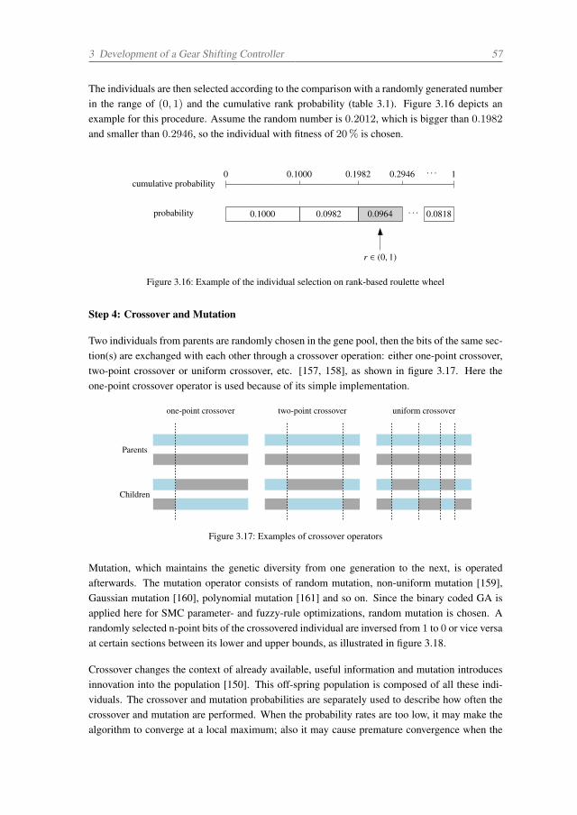
3 Development of a Gear Shifting Controller 57
The individuals are then selected according to the comparison with a randomly generated numberin the range of (0, 1) and the cumulative rank probability (table 3.1). Figure 3.16 depicts anexample for this procedure. Assume the random number is 0.2012, which is bigger than 0.1982
and smaller than 0.2946, so the individual with fitness of 20% is chosen.
probability
10
0.1000 0.0964 · · ·0.0982 0.0818
0.1000 0.1982 0.2946 · · ·
r ∈ (0, 1)
cumulative probability
Figure 3.16: Example of the individual selection on rank-based roulette wheel
Step 4: Crossover and Mutation
Two individuals from parents are randomly chosen in the gene pool, then the bits of the same sec-tion(s) are exchanged with each other through a crossover operation: either one-point crossover,two-point crossover or uniform crossover, etc. [157, 158], as shown in figure 3.17. Here theone-point crossover operator is used because of its simple implementation.
Parents
Children
one-point crossover two-point crossover uniform crossover
Figure 3.17: Examples of crossover operators
Mutation, which maintains the genetic diversity from one generation to the next, is operatedafterwards. The mutation operator consists of random mutation, non-uniform mutation [159],Gaussian mutation [160], polynomial mutation [161] and so on. Since the binary coded GA isapplied here for SMC parameter- and fuzzy-rule optimizations, random mutation is chosen. Arandomly selected n-point bits of the crossovered individual are inversed from 1 to 0 or vice versaat certain sections between its lower and upper bounds, as illustrated in figure 3.18.
Crossover changes the context of already available, useful information and mutation introducesinnovation into the population [150]. This off-spring population is composed of all these indi-viduals. The crossover and mutation probabilities are separately used to describe how often thecrossover and mutation are performed. When the probability rates are too low, it may make thealgorithm to converge at a local maximum; also it may cause premature convergence when the
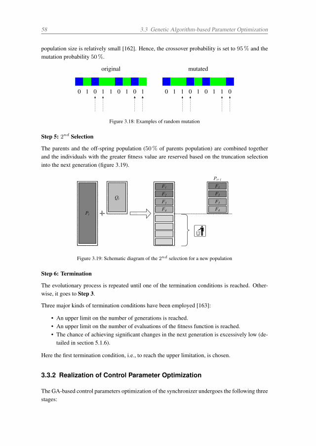
58 3.3 Genetic Algorithm-based Parameter Optimization
population size is relatively small [162]. Hence, the crossover probability is set to 95% and themutation probability 50%.
0
original mutated
0 0 0 0 0 0 01 1 1 1 1 1 1 1 1 1
Figure 3.18: Examples of random mutation
Step 5: 2nd Selection
The parents and the off-spring population (50% of parents population) are combined togetherand the individuals with the greater fitness value are reserved based on the truncation selectioninto the next generation (figure 3.19).
Qt
F1
Pt+1
Pt
F2
F3
F4
F1
F2
F3
F4
Figure 3.19: Schematic diagram of the 2nd selection for a new population
Step 6: Termination
The evolutionary process is repeated until one of the termination conditions is reached. Other-wise, it goes to Step 3.
Three major kinds of termination conditions have been employed [163]:
• An upper limit on the number of generations is reached.• An upper limit on the number of evaluations of the fitness function is reached.• The chance of achieving significant changes in the next generation is excessively low (de-
tailed in section 5.1.6).
Here the first termination condition, i.e., to reach the upper limitation, is chosen.
3.3.2 Realization of Control Parameter Optimization
The GA-based control parameters optimization of the synchronizer undergoes the following threestages:
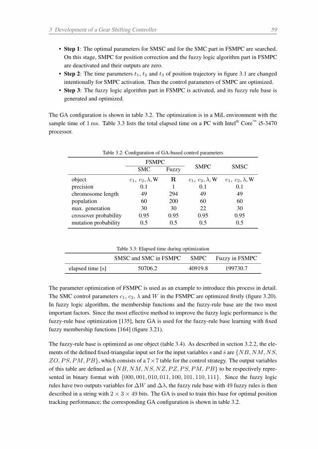
3 Development of a Gear Shifting Controller 59
• Step 1: The optimal parameters for SMSC and for the SMC part in FSMPC are searched.On this stage, SMPC for position correction and the fuzzy logic algorithm part in FSMPCare deactivated and their outputs are zero.
• Step 2: The time parameters t1, t2 and t3 of position trajectory in figure 3.1 are changedintentionally for SMPC activation. Then the control parameters of SMPC are optimized.
• Step 3: The fuzzy logic algorithm part in FSMPC is activated, and its fuzzy rule base isgenerated and optimized.
The GA configuration is shown in table 3.2. The optimization is in a MiL environment with thesample time of 1ms. Table 3.3 lists the total elapsed time on a PC with Intel® Core™ i5-3470processor.
Table 3.2: Configuration of GA-based control parameters
FSMPCSMPC SMSCSMC Fuzzy
object c1, c2,λ, W R c1, c2,λ, W c1, c2,λ, Wprecision 0.1 1 0.1 0.1chromosome length 49 294 49 49population 60 200 60 60max. generation 30 30 22 30crossover probability 0.95 0.95 0.95 0.95mutation probability 0.5 0.5 0.5 0.5
Table 3.3: Elapsed time during optimization
SMSC and SMC in FSMPC SMPC Fuzzy in FSMPC
elapsed time [s] 50706.2 40919.8 199730.7
The parameter optimization of FSMPC is used as an example to introduce this process in detail.The SMC control parameters c1, c2, λ and W in the FSMPC are optimized firstly (figure 3.20).In fuzzy logic algorithm, the membership functions and the fuzzy-rule base are the two mostimportant factors. Since the most effective method to improve the fuzzy logic performance is thefuzzy-rule base optimization [135], here GA is used for the fuzzy-rule base learning with fixedfuzzy membership functions [164] (figure 3.21).
The fuzzy-rule base is optimized as one object (table 3.4). As described in section 3.2.2, the ele-ments of the defined fixed-triangular input set for the input variables s and s are NB,NM,NS,
ZO,PS, PM,PB, which consists of a 7×7 table for the control strategy. The output variablesof this table are defined as NB,NM,NS,NZ, PZ, PS, PM, PB to be respectively repre-sented in binary format with 000, 001, 010, 011, 100, 101, 110, 111. Since the fuzzy logicrules have two outputs variables for ∆W and ∆λ, the fuzzy rule base with 49 fuzzy rules is thendescribed in a string with 2× 3× 49 bits. The GA is used to train this base for optimal positiontracking performance; the corresponding GA configuration is shown in table 3.2.
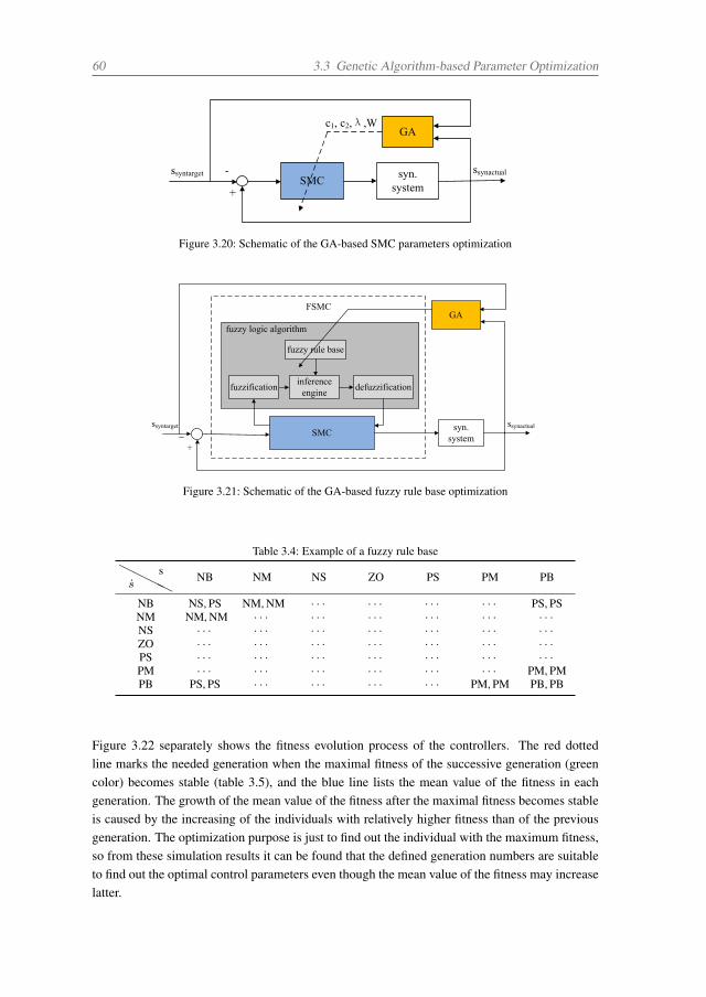
60 3.3 Genetic Algorithm-based Parameter Optimization
syntarget synactual
1 2 λ
Figure 3.20: Schematic of the GA-based SMC parameters optimization
ssyntargetSMC syn.
system+
GA
ssynactual
FSMC
fuzzification
fuzzy logic algorithm
fuzzy rule base
inference engine defuzzification
Figure 3.21: Schematic of the GA-based fuzzy rule base optimization
Table 3.4: Example of a fuzzy rule base
ss NB NM NS ZO PS PM PB
NB NS, PS NM, NM · · · · · · · · · · · · PS, PSNM NM, NM · · · · · · · · · · · · · · · · · ·NS · · · · · · · · · · · · · · · · · · · · ·ZO · · · · · · · · · · · · · · · · · · · · ·PS · · · · · · · · · · · · · · · · · · · · ·PM · · · · · · · · · · · · · · · · · · PM, PMPB PS, PS · · · · · · · · · · · · PM, PM PB, PB
Figure 3.22 separately shows the fitness evolution process of the controllers. The red dottedline marks the needed generation when the maximal fitness of the successive generation (greencolor) becomes stable (table 3.5), and the blue line lists the mean value of the fitness in eachgeneration. The growth of the mean value of the fitness after the maximal fitness becomes stableis caused by the increasing of the individuals with relatively higher fitness than of the previousgeneration. The optimization purpose is just to find out the individual with the maximum fitness,so from these simulation results it can be found that the defined generation numbers are suitableto find out the optimal control parameters even though the mean value of the fitness may increaselatter.
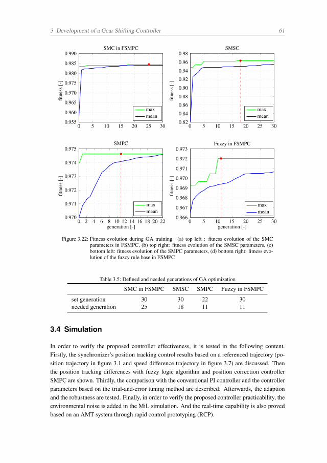
3 Development of a Gear Shifting Controller 61
0 5 10 15 20 25 300.955
0.960
0.965
0.970
0.975
0.980
0.985
0.990fit
ness
[-]
SMC in FSMPC
maxmean
0 5 10 15 20 25 300.82
0.84
0.86
0.88
0.90
0.92
0.94
0.96
0.98
fitne
ss[-
]
SMSC
maxmean
0 2 4 6 8 10 12 14 16 18 20 220.970
0.971
0.972
0.973
0.974
0.975
generation [-]
fitne
ss[-
]
SMPC
maxmean
0 5 10 15 20 25 300.966
0.967
0.968
0.969
0.970
0.971
0.972
0.973
generation [-]
fitne
ss[-
]
Fuzzy in FSMPC
maxmean
Figure 3.22: Fitness evolution during GA training. (a) top left : fitness evolution of the SMCparameters in FSMPC, (b) top right: fitness evolution of the SMSC parameters, (c)bottom left: fitness evolution of the SMPC parameters, (d) bottom right: fitness evo-lution of the fuzzy rule base in FSMPC
Table 3.5: Defined and needed generations of GA optimization
SMC in FSMPC SMSC SMPC Fuzzy in FSMPC
set generation 30 30 22 30needed generation 25 18 11 11
3.4 Simulation
In order to verify the proposed controller effectiveness, it is tested in the following content.Firstly, the synchronizer’s position tracking control results based on a referenced trajectory (po-sition trajectory in figure 3.1 and speed difference trajectory in figure 3.7) are discussed. Thenthe position tracking differences with fuzzy logic algorithm and position correction controllerSMPC are shown. Thirdly, the comparison with the conventional PI controller and the controllerparameters based on the trial-and-error tuning method are described. Afterwards, the adaptionand the robustness are tested. Finally, in order to verify the proposed controller practicability, theenvironmental noise is added in the MiL simulation. And the real-time capability is also provedbased on an AMT system through rapid control prototyping (RCP).
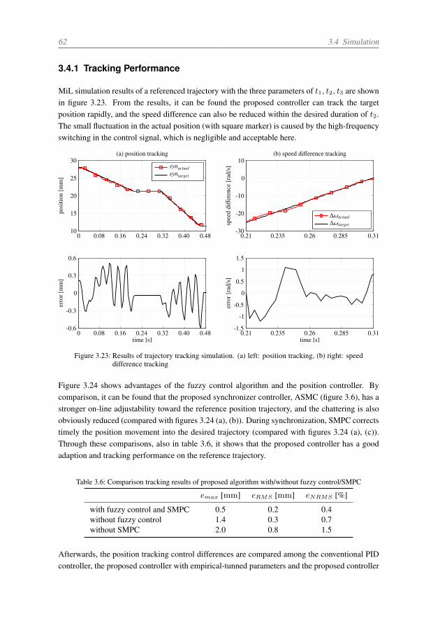
62 3.4 Simulation
3.4.1 Tracking Performance
MiL simulation results of a referenced trajectory with the three parameters of t1, t2, t3 are shownin figure 3.23. From the results, it can be found the proposed controller can track the targetposition rapidly, and the speed difference can also be reduced within the desired duration of t2.The small fluctuation in the actual position (with square marker) is caused by the high-frequencyswitching in the control signal, which is negligible and acceptable here.
0 0.08 0.16 0.24 0.32 0.40 0.4810
15
20
25
30
posi
tion
[mm
]
(a) position tracking
synactualsyntarget
0.21 0.235 0.26 0.285 0.31-30
-20
-10
0
10
spee
ddi
ffer
ence
[rad
/s]
(b) speed difference tracking
∆ωactual∆ωtarget
0 0.08 0.16 0.24 0.32 0.40 0.48-0.6
-0.3
0
0.3
0.6
time [s]
erro
r[m
m]
0.21 0.235 0.26 0.285 0.31-1.5
-1
-0.5
0
0.5
1
1.5
time [s]
erro
r[ra
d/s]
Figure 3.23: Results of trajectory tracking simulation. (a) left: position tracking, (b) right: speeddifference tracking
Figure 3.24 shows advantages of the fuzzy control algorithm and the position controller. Bycomparison, it can be found that the proposed synchronizer controller, ASMC (figure 3.6), has astronger on-line adjustability toward the reference position trajectory, and the chattering is alsoobviously reduced (compared with figures 3.24 (a), (b)). During synchronization, SMPC correctstimely the position movement into the desired trajectory (compared with figures 3.24 (a), (c)).Through these comparisons, also in table 3.6, it shows that the proposed controller has a goodadaption and tracking performance on the reference trajectory.
Table 3.6: Comparison tracking results of proposed algorithm with/without fuzzy control/SMPC
emax [mm] eRMS [mm] eNRMS [%]
with fuzzy control and SMPC 0.5 0.2 0.4without fuzzy control 1.4 0.3 0.7without SMPC 2.0 0.8 1.5
Afterwards, the position tracking control differences are compared among the conventional PIDcontroller, the proposed controller with empirical-tunned parameters and the proposed controller
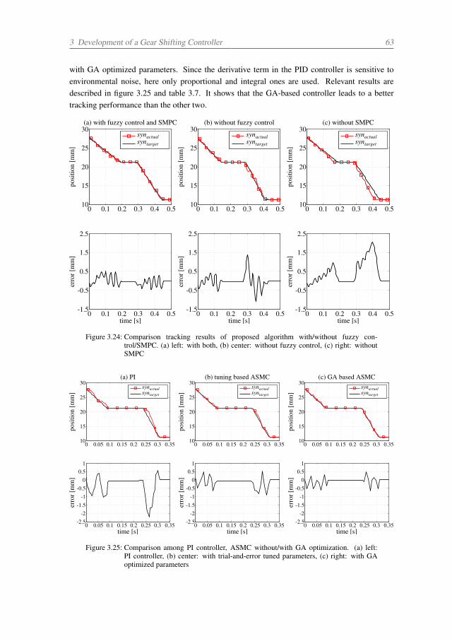
3 Development of a Gear Shifting Controller 63
with GA optimized parameters. Since the derivative term in the PID controller is sensitive toenvironmental noise, here only proportional and integral ones are used. Relevant results aredescribed in figure 3.25 and table 3.7. It shows that the GA-based controller leads to a bettertracking performance than the other two.
0 0.1 0.2 0.3 0.4 0.510
15
20
25
30
posi
tion
[mm
]
(a) with fuzzy control and SMPC
synactualsyntarget
0 0.1 0.2 0.3 0.4 0.510
15
20
25
30
posi
tion
[mm
]
(b) without fuzzy control
0 0.1 0.2 0.3 0.4 0.510
15
20
25
30
posi
tion
[mm
]
(c) without SMPC
0 0.1 0.2 0.3 0.4 0.5-1.5
-0.5
0.5
1.5
2.5
time [s]
erro
r[m
m]
0 0.1 0.2 0.3 0.4 0.5-1.5
-0.5
0.5
1.5
2.5
time [s]
erro
r[m
m]
0 0.1 0.2 0.3 0.4 0.5-1.5
-0.5
0.5
1.5
2.5
time [s]
erro
r[m
m]
synactualsyntarget
synactualsyntarget
Figure 3.24: Comparison tracking results of proposed algorithm with/without fuzzy con-trol/SMPC. (a) left: with both, (b) center: without fuzzy control, (c) right: withoutSMPC
0 0.05 0.1 0.15 0.2 0.25 0.3 0.3510
15
20
25
30
posi
tion
[mm
]
(a) PIsynactualsyntarget
0 0.05 0.1 0.15 0.2 0.25 0.3 0.3510
15
20
25
30
posi
tion
[mm
]
(b) tuning based ASMC
0 0.05 0.1 0.15 0.2 0.25 0.3 0.3510
15
20
25
30
posi
tion
[mm
]
(c) GA based ASMC
0 0.05 0.1 0.15 0.2 0.25 0.3 0.35-2.5
-2-1.5
-1-0.5
00.5
1
time [s]
erro
r[m
m]
0 0.05 0.1 0.15 0.2 0.25 0.3 0.35-2.5
-2-1.5
-1-0.5
00.5
1
time [s]
erro
r[m
m]
0 0.05 0.1 0.15 0.2 0.25 0.3 0.35-2.5
-2-1.5
-1-0.5
00.5
1
time [s]
erro
r[m
m]
synactualsyntarget syntarget
synactual
Figure 3.25: Comparison among PI controller, ASMC without/with GA optimization. (a) left:PI controller, (b) center: with trial-and-error tuned parameters, (c) right: with GAoptimized parameters
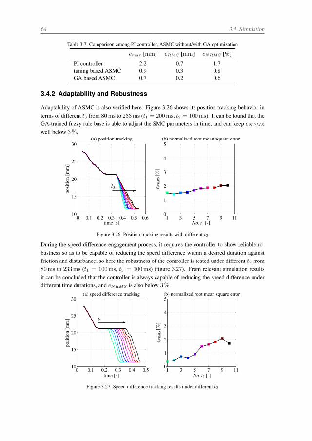
64 3.4 Simulation
begin hereTable 3.7: Comparison among PI controller, ASMC without/with GA optimization
emax [mm] eRMS [mm] eNRMS [%]
PI controller 2.2 0.7 1.7tuning based ASMC 0.9 0.3 0.8GA based ASMC 0.7 0.2 0.6
3.4.2 Adaptability and Robustness
Adaptability of ASMC is also verified here. Figure 3.26 shows its position tracking behavior interms of different t3 from 80ms to 233ms (t1 = 200ms, t2 = 100ms). It can be found that theGA-trained fuzzy rule base is able to adjust the SMC parameters in time, and can keep eNRMS
well below 3%.
0 0.1 0.2 0.3 0.4 0.5 0.610
15
20
25
30
posi
tion
[mm
]
time [s]
(a) position tracking
1 3 5 7 9 110
1
2
3
4
5
e NR
MS[%
]
No. t3 [-]
(b) normalized root mean square error
t3
Figure 3.26: Position tracking results with different t3
During the speed difference engagement process, it requires the controller to show reliable ro-bustness so as to be capable of reducing the speed difference within a desired duration againstfriction and disturbance; so here the robustness of the controller is tested under different t2 from80ms to 233ms (t1 = 100ms, t3 = 100ms) (figure 3.27). From relevant simulation resultsit can be concluded that the controller is always capable of reducing the speed difference underdifferent time durations, and eNRMS is also below 3%.
0 0.1 0.2 0.3 0.4 0.510
15
20
25
30
posi
tion
[mm
]
time [s]
(a) speed difference tracking
1 3 5 7 9 110
1
2
3
4
5
e NR
MS[%
]
No. t2 [-]
(b) normalized root mean square error
t2
Figure 3.27: Speed difference tracking results under different t2
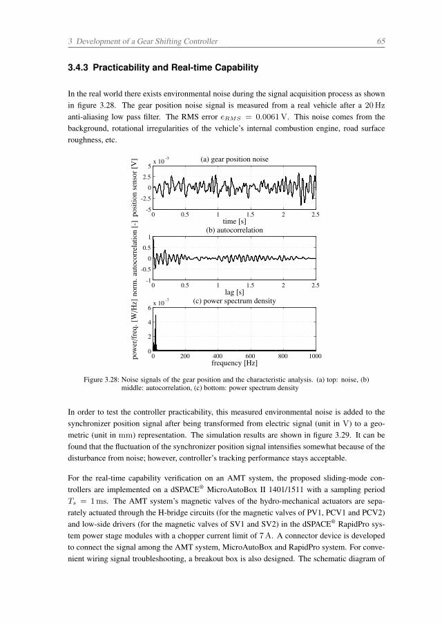
3 Development of a Gear Shifting Controller 65
3.4.3 Practicability and Real-time Capability
In the real world there exists environmental noise during the signal acquisition process as shownin figure 3.28. The gear position noise signal is measured from a real vehicle after a 20Hz
anti-aliasing low pass filter. The RMS error eRMS = 0.0061V. This noise comes from thebackground, rotational irregularities of the vehicle’s internal combustion engine, road surfaceroughness, etc.
0 0.5 1 1.5 2 2.5-5
-2.5
0
2.5
5x 10
-3
time [s]
posi
tion
sens
or[V
] (a) gear position noise
0 0.5 1 1.5 2 2.5-1
-0.5
0
0.5
1
lag [s]norm
.aut
ocor
rela
tion
[-]
(b) autocorrelation
0 200 400 600 800 10000
2
4
6x 10
-7 (c) power spectrum density
frequency [Hz]
pow
er/f
req.
[W/H
z]
Figure 3.28: Noise signals of the gear position and the characteristic analysis. (a) top: noise, (b)middle: autocorrelation, (c) bottom: power spectrum density
In order to test the controller practicability, this measured environmental noise is added to thesynchronizer position signal after being transformed from electric signal (unit in V) to a geo-metric (unit in mm) representation. The simulation results are shown in figure 3.29. It can befound that the fluctuation of the synchronizer position signal intensifies somewhat because of thedisturbance from noise; however, controller’s tracking performance stays acceptable.
For the real-time capability verification on an AMT system, the proposed sliding-mode con-trollers are implemented on a dSPACE® MicroAutoBox II 1401/1511 with a sampling periodTs = 1ms. The AMT system’s magnetic valves of the hydro-mechanical actuators are sepa-rately actuated through the H-bridge circuits (for the magnetic valves of PV1, PCV1 and PCV2)and low-side drivers (for the magnetic valves of SV1 and SV2) in the dSPACE® RapidPro sys-tem power stage modules with a chopper current limit of 7A. A connector device is developedto connect the signal among the AMT system, MicroAutoBox and RapidPro system. For conve-nient wiring signal troubleshooting, a breakout box is also designed. The schematic diagram of
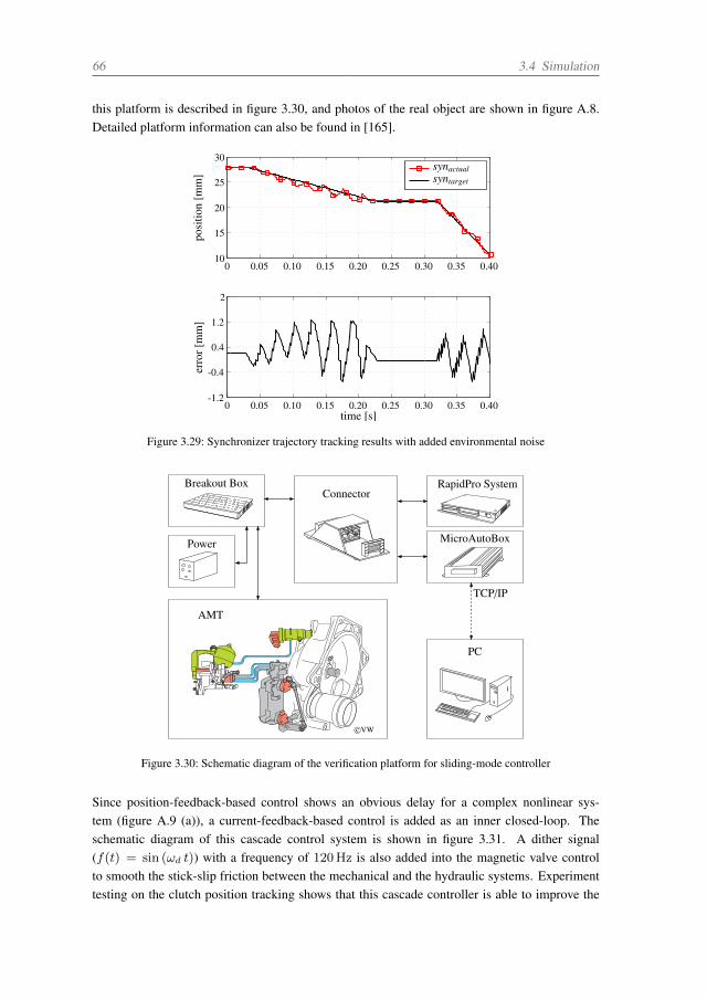
66 3.4 Simulation
this platform is described in figure 3.30, and photos of the real object are shown in figure A.8.Detailed platform information can also be found in [165].
0 0.05 0.10 0.15 0.20 0.25 0.30 0.35 0.4010
15
20
25
30
posi
tion
[mm
]
synactualsyntarget
0 0.05 0.10 0.15 0.20 0.25 0.30 0.35 0.40-1.2
-0.4
0.4
1.2
2
time [s]
erro
r[m
m]
Figure 3.29: Synchronizer trajectory tracking results with added environmental noise
TCP/IP
Breakout BoxConnector
RapidPro System
MicroAutoBox
PC
AMT
c©VW
Power
Figure 3.30: Schematic diagram of the verification platform for sliding-mode controller
Since position-feedback-based control shows an obvious delay for a complex nonlinear sys-tem (figure A.9 (a)), a current-feedback-based control is added as an inner closed-loop. Theschematic diagram of this cascade control system is shown in figure 3.31. A dither signal(f(t) = sin (ωd t)) with a frequency of 120Hz is also added into the magnetic valve controlto smooth the stick-slip friction between the mechanical and the hydraulic systems. Experimenttesting on the clutch position tracking shows that this cascade controller is able to improve the
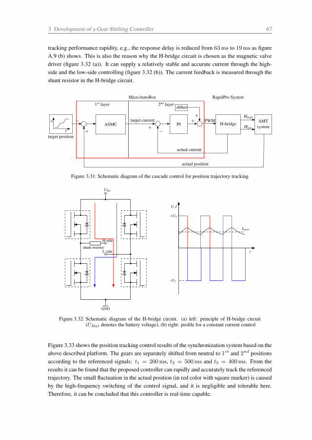
3 Development of a Gear Shifting Controller 67
tracking performance rapidity, e.g., the response delay is reduced from 63ms to 19ms as figureA.9 (b) shows. This is also the reason why the H-bridge circuit is chosen as the magnetic valvedriver (figure 3.32 (a)). It can supply a relatively stable and accurate current through the high-side and the low-side controlling (figure 3.32 (b)). The current feedback is measured through theshunt resistor in the H-bridge circuit.
actual current
actual position
Hhigh
Hlow
RapidPro SystemMicroAutoBox
1st layer 2nd layer
target positiont
s
ASMC PItarget current
dither
PWMH-bridge
AMTsystem
Figure 3.31: Schematic diagram of the cascade control for position trajectory tracking
UBat
GND
shunt resistor
H-side
L-side t
+U1
-U2
Imean
U, I
Figure 3.32: Schematic diagram of the H-bridge circuit. (a) left: principle of H-bridge circuit(UBat denotes the battery voltage), (b) right: profile for a constant current control
Figure 3.33 shows the position tracking control results of the synchronization system based on theabove described platform. The gears are separately shifted from neutral to 1st and 2nd positionsaccording to the referenced signals: t1 = 200ms, t2 = 500ms and t3 = 400ms. From theresults it can be found that the proposed controller can rapidly and accurately track the referencedtrajectory. The small fluctuation in the actual position (in red color with square marker) is causedby the high-frequency switching of the control signal, and it is negligible and tolerable here.Therefore, it can be concluded that this controller is real-time capable.
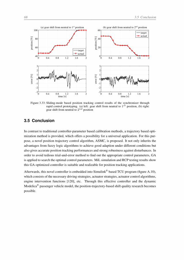
68 3.5 Conclusion
0 0.4 0.8 1.2 1.6 240
60
80
100(a) gear shift from neutral to 1st position
posi
tion
[%]
targetactual
0 0.4 0.8 1.2 1.6 2-3
-2
-1
0
1
2
3
time [s]
erro
r[%
]
0 0.4 0.8 1.2 1.6 20
20
40
60(b) gear shift from neutral to 2nd position
posi
tion
[%]
targetactual
0 0.4 0.8 1.2 1.6 2-3
-2
-1
0
1
2
3
time [s]er
ror[
%]
Figure 3.33: Sliding-mode based position tracking control results of the synchronizer throughrapid control prototyping. (a) left: gear shift from neutral to 1st position, (b) right:gear shift from neutral to 2nd position
3.5 Conclusion
In contrast to traditional controller-parameter based calibration methods, a trajectory based opti-mization method is provided, which offers a possibility for a universal application. For this pur-pose, a novel position trajectory control algorithm, ASMC, is proposed. It not only inherits theadvantages from fuzzy logic algorithms to achieve good adaption under different conditions butalso gives accurate position tracking performances and strong robustness against disturbances. Inorder to avoid tedious trial-and-error method to find out the appropriate control parameters, GAis applied to search the optimal control parameters. MiL simulation and RCP testing results showthis GA optimized controller is suitable and realizable for position tracking applications.
Afterwards, this novel controller is embedded into Simulink® based TCU program (figure A.10),which consists of the necessary driving strategies, actuator strategies, actuator control algorithms,engine intervention functions [120], etc. Through this effective controller and the dynamicModelica® passenger vehicle model, the position-trajectory-based shift quality research becomespossible.
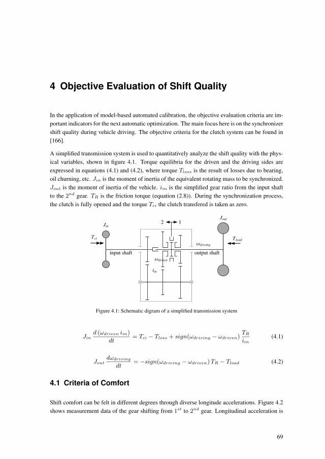
4 Objective Evaluation of Shift Quality
In the application of model-based automated calibration, the objective evaluation criteria are im-portant indicators for the next automatic optimization. The main focus here is on the synchronizershift quality during vehicle driving. The objective criteria for the clutch system can be found in[166].
A simplified transmission system is used to quantitatively analyze the shift quality with the phys-ical variables, shown in figure 4.1. Torque equilibria for the driven and the driving sides areexpressed in equations (4.1) and (4.2), where torque Tloss is the result of losses due to bearing,oil churning, etc. Jin is the moment of inertia of the equivalent rotating mass to be synchronized.Jout is the moment of inertia of the vehicle. iin is the simplified gear ratio from the input shaftto the 2nd gear. TR is the friction torque (equation (2.8)). During the synchronization process,the clutch is fully opened and the torque Tci the clutch transfered is taken as zero.
2 1
input shaft output shaft
Jin
Jout
Tci
iin
ωdriving
ωdriven
Tload
Figure 4.1: Schematic digram of a simplified transmission system
Jind (ωdriven iin)
dt= Tci − Tloss + sign(ωdriving − ωdriven)
TR
iin(4.1)
Joutdωdriving
dt= −sign(ωdriving − ωdriven)TR − Tload (4.2)
4.1 Criteria of Comfort
Shift comfort can be felt in different degrees through diverse longitude accelerations. Figure 4.2shows measurement data of the gear shifting from 1st to 2nd gear. Longitudinal acceleration is
69
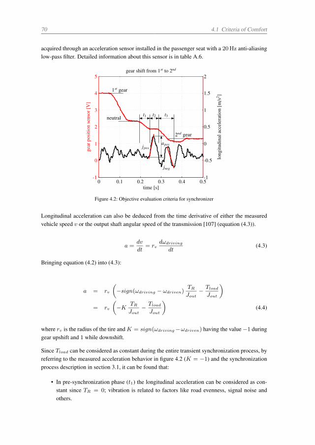
70 4.1 Criteria of Comfort
acquired through an acceleration sensor installed in the passenger seat with a 20Hz anti-aliasinglow-pass filter. Detailed information about this sensor is in table A.6.
0.1 0.2 0.3 0.4 0.5-1
0
1
2
3
4
5gear shift from 1st to 2nd
time [s]
gear
posi
tion
sens
or[V
]
0-1
-0.5
0
0.5
1
1.5
2
long
itudi
nala
ccel
erat
ion
[m/s
2 ]
1st gear
neutral
2nd gear
t1 t2 t3
jpos
jneg
apos
Figure 4.2: Objective evaluation criteria for synchronizer
Longitudinal acceleration can also be deduced from the time derivative of either the measuredvehicle speed v or the output shaft angular speed of the transmission [107] (equation (4.3)).
a =dv
dt= rv
dωdriving
dt(4.3)
Bringing equation (4.2) into (4.3):
a = rv
(−sign(ωdriving − ωdriven)
TR
Jout− Tload
Jout
)= rv
(−K TR
Jout− Tload
Jout
)(4.4)
where rv is the radius of the tire andK = sign(ωdriving−ωdriven) having the value −1 duringgear upshift and 1 while downshift.
Since Tload can be considered as constant during the entire transient synchronization process, byreferring to the measured acceleration behavior in figure 4.2 (K = −1) and the synchronizationprocess description in section 3.1, it can be found that:
• In pre-synchronization phase (t1) the longitudinal acceleration can be considered as con-stant since TR = 0; vibration is related to factors like road evenness, signal noise andothers.
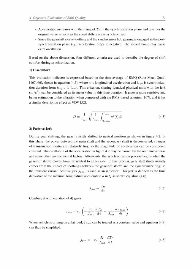
4 Objective Evaluation of Shift Quality 71
• Acceleration increases with the rising of TR in the synchronization phase and resumes theoriginal value as soon as the speed difference is synchronized.
• Since the gearshift sleeve toothing and the synchronizer hub gearing is engaged in the post-synchronization phase (t3), acceleration drops to negative. The second bump may causeextra oscillation.
Based on the above discussion, four different criteria are used to describe the degree of shiftcomfort during synchronization.
1) Discomfort
This evaluation indicator is expressed based on the time average of RMQ (Root-Mean-Quad)[167, 66], shown in equation (4.5), where a is longitudinal acceleration and tsyn is synchroniza-tion duration from tbegin to tend. This criterion, sharing identical physical units with the jerk(m/s3), can be considered as its mean value in this time duration. It gives a more sensitive andbetter estimation to the vibration when compared with the RMS-based criterion [167], and it hasa similar description effect as VDV [52].
D =1
tsyn4
√1
tsyn
∫ tend
tbegin
a4(t)dt (4.5)
2) Positive Jerk
During gear shifting, the gear is firstly shifted to neutral position as shown in figure 4.2. Inthis phase, the power between the main shaft and the secondary shaft is disconnected; changesof transmission inertia are relatively tiny, so the magnitude of acceleration can be consideredconstant. The oscillation of the acceleration in figure 4.2 may be caused by the road unevennessand some other environmental factors. Afterwards, the synchronization process begins when thegearshift sleeve moves from the neutral to either side. In this process, gear shift shock usuallycomes from the impact of toothings between the gearshift sleeve and the synchronizer ring; sothe transient variant, positive jerk jpos, is used as an indicator. This jerk is defined as the timederivative of the maximal longitudinal acceleration a in t2 as shown equation (4.6).
jpos =d a
d t(4.6)
Combing it with equation (4.4) gives:
jpos = rv
(− K
Jout
d TR
d t− 1
Jout
d Tload
dt
)(4.7)
When vehicle is driving on a flat road, Tload can be treated as a constant value and equation (4.7)can thus be simplified:
jpos = −rvK
Jout
d TR
d t(4.8)
72 4.1 Criteria of Comfort
This equation (4.8) shows that the magnitude of jpos is very much linked to the time derivativeof TR. It is affected by the length of duration t2 and the definition of synchronization point s2 int2. If t2 is too short and s2 is too low, the value of jpos will be relatively great and the toothingclash is obvious, so the positive jerk jpos can be conclude as equation (4.9) shows. For example,figure 4.3 describes a synchronizer’s behavior when the synchronizer point s2 varies. It can befound that in a lower position the jpos is relatively larger and the peak value of acceleration isreached a littler bit earlier, meaning that the speed difference is synchronized quicker.
jpos = f(t2, s2) (4.9)
0 0.1 0.2 0.3 0.4 0.5 0.6-100
-60
-20
20
60
100(a) with a deeper syn. point s2
time [s]
gear
posi
tion
[%]
0 0.1 0.2 0.3 0.4 0.5 0.6-1.4
0
1.4
2.8
4.2
5.6
0 0.1 0.2 0.3 0.4 0.5 0.6-100
-60
-20
20
60
100(b) with an appropriate syn. point s2
time [s]0 0.1 0.2 0.3 0.4 0.5 0.6
-1.4
0
1.4
2.8
4.2
5.6
long
itudi
nala
ccel
erat
ion
[m/s
2 ]t1 t2 t3 t1 t2 t3lo
ngitu
dina
lacc
eler
atio
n[m/s
2 ]
gear
posi
tion
[%]
Figure 4.3: Synchronization behavior vs. synchronizer point s2
3) Positive Acceleration
In the speed difference synchronization phase (t2), the magnitude of acceleration apos is alsoconsidered as an indicator. During a certain gear shifting process, such as gear shifting from 1st
to 2nd gear along a flat road, the shift point is pre-determined. Speed difference ∆ω can thenbe deemed constant, so the magnitude of apos has an inverse proportional relationship with t2.It is worth noting that apos may also be affected by the synchronizer point s2. For example, infigure 4.3, if the synchronizer point is lower, apos will have an obvious large value, and the speedsynchronization will also complete somewhat earlier. For the downshift, the signs of jpos andapos are both reversed as upshift.
4) Negative Jerk
When the gearshift sleeve toothing engages with the synchronizer hub gearing, it causes a nega-tive acceleration change jneg . Since the distance from the synchronizer point to the synchronizerhub can be considered constant, the magnitude of jneg depends on the duration of t3, given byequation (4.10). If t3 is too short, the transmission knocking and the second bump are obvious,as shown in figure 4.3.
jneg = f(t3) (4.10)
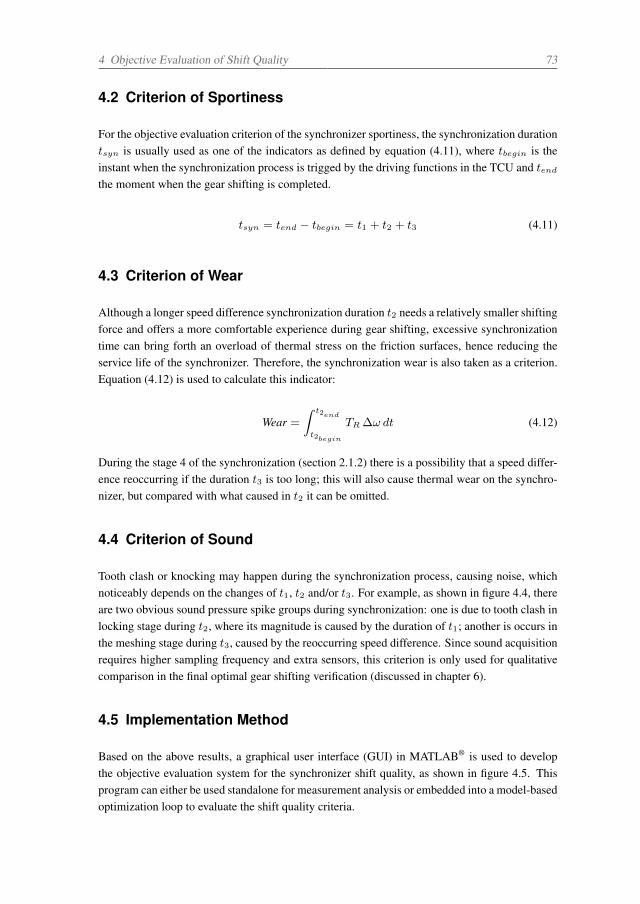
4 Objective Evaluation of Shift Quality 73
4.2 Criterion of Sportiness
For the objective evaluation criterion of the synchronizer sportiness, the synchronization durationtsyn is usually used as one of the indicators as defined by equation (4.11), where tbegin is theinstant when the synchronization process is trigged by the driving functions in the TCU and tend
the moment when the gear shifting is completed.
tsyn = tend − tbegin = t1 + t2 + t3 (4.11)
4.3 Criterion of Wear
Although a longer speed difference synchronization duration t2 needs a relatively smaller shiftingforce and offers a more comfortable experience during gear shifting, excessive synchronizationtime can bring forth an overload of thermal stress on the friction surfaces, hence reducing theservice life of the synchronizer. Therefore, the synchronization wear is also taken as a criterion.Equation (4.12) is used to calculate this indicator:
Wear =∫ t2end
t2begin
TR ∆ω dt (4.12)
During the stage 4 of the synchronization (section 2.1.2) there is a possibility that a speed differ-ence reoccurring if the duration t3 is too long; this will also cause thermal wear on the synchro-nizer, but compared with what caused in t2 it can be omitted.
4.4 Criterion of Sound
Tooth clash or knocking may happen during the synchronization process, causing noise, whichnoticeably depends on the changes of t1, t2 and/or t3. For example, as shown in figure 4.4, thereare two obvious sound pressure spike groups during synchronization: one is due to tooth clash inlocking stage during t2, where its magnitude is caused by the duration of t1; another is occurs inthe meshing stage during t3, caused by the reoccurring speed difference. Since sound acquisitionrequires higher sampling frequency and extra sensors, this criterion is only used for qualitativecomparison in the final optimal gear shifting verification (discussed in chapter 6).
4.5 Implementation Method
Based on the above results, a graphical user interface (GUI) in MATLAB® is used to developthe objective evaluation system for the synchronizer shift quality, as shown in figure 4.5. Thisprogram can either be used standalone for measurement analysis or embedded into a model-basedoptimization loop to evaluate the shift quality criteria.
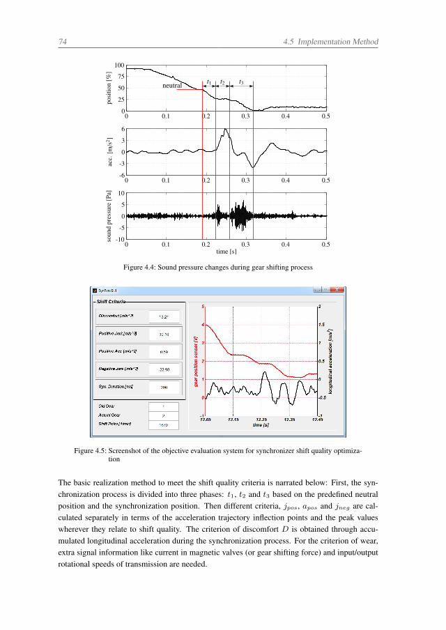
74 4.5 Implementation Method
0 0.1 0.2 0.3 0.4 0.50
25
50
75
100
posi
tion
[%]
0 0.1 0.2 0.3 0.4 0.5-6
-3
0
3
6
acc.
[m/s
2 ]
0 0.1 0.2 0.3 0.4 0.5-10
-5
0
5
10
soun
dpr
essu
re[P
a]
time [s]
neutral t1 t2 t3
Figure 4.4: Sound pressure changes during gear shifting process
Figure 4.5: Screenshot of the objective evaluation system for synchronizer shift quality optimiza-tion
The basic realization method to meet the shift quality criteria is narrated below: First, the syn-chronization process is divided into three phases: t1, t2 and t3 based on the predefined neutralposition and the synchronization position. Then different criteria, jpos, apos and jneg are cal-culated separately in terms of the acceleration trajectory inflection points and the peak valueswherever they relate to shift quality. The criterion of discomfort D is obtained through accu-mulated longitudinal acceleration during the synchronization process. For the criterion of wear,extra signal information like current in magnetic valves (or gear shifting force) and input/outputrotational speeds of transmission are needed.

4 Objective Evaluation of Shift Quality 75
4.6 Conclusion
In order to supply an objective evaluation system for the following model-based shift quality op-timization, relevant evaluation criteria are discussed and a program is developed for data analysis,thus making automatic optimization loop possible.

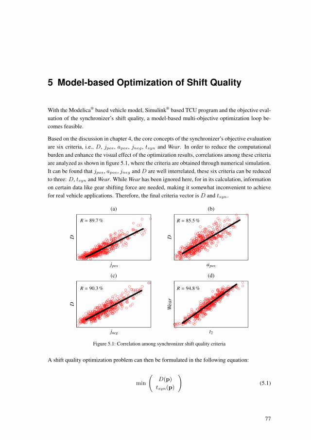
5 Model-based Optimization of Shift Quality
With the Modelica® based vehicle model, Simulink® based TCU program and the objective eval-uation of the synchronizer’s shift quality, a model-based multi-objective optimization loop be-comes feasible.
Based on the discussion in chapter 4, the core concepts of the synchronizer’s objective evaluationare six criteria, i.e., D, jpos, apos, jneg , tsyn and Wear. In order to reduce the computationalburden and enhance the visual effect of the optimization results, correlations among these criteriaare analyzed as shown in figure 5.1, where the criteria are obtained through numerical simulation.It can be found that jpos, apos, jneg and D are well interrelated, these six criteria can be reducedto three: D, tsyn and Wear. While Wear has been ignored here, for in its calculation, informationon certain data like gear shifting force are needed, making it somewhat inconvenient to achievefor real vehicle applications. Therefore, the final criteria vector is D and tsyn.
(a)
jpos
D
(c)
jneg
D
(d)
t2
Wea
r
(b)
apos
D
R = 89.7 %
R = 90.3 % R = 94.8 %
R = 85.5 %
Figure 5.1: Correlation among synchronizer shift quality criteria
A shift quality optimization problem can then be formulated in the following equation:
min
(D(p)
tsyn(p)
)(5.1)
77
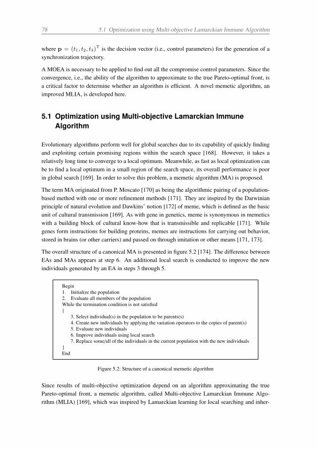
78 5.1 Optimization using Multi-objective Lamarckian Immune Algorithm
where p = (t1, t2, t3)T is the decision vector (i.e., control parameters) for the generation of a
synchronization trajectory.
A MOEA is necessary to be applied to find out all the compromise control parameters. Since theconvergence, i.e., the ability of the algorithm to approximate to the true Pareto-optimal front, isa critical factor to determine whether an algorithm is efficient. A novel memetic algorithm, animproved MLIA, is developed here.
5.1 Optimization using Multi-objective Lamarckian ImmuneAlgorithm
Evolutionary algorithms perform well for global searches due to its capability of quickly findingand exploiting certain promising regions within the search space [168]. However, it takes arelatively long time to converge to a local optimum. Meanwhile, as fast as local optimization canbe to find a local optimum in a small region of the search space, its overall performance is poorin global search [169]. In order to solve this problem, a memetic algorithm (MA) is proposed.
The term MA originated from P. Moscato [170] as being the algorithmic pairing of a population-based method with one or more refinement methods [171]. They are inspired by the Darwinianprinciple of natural evolution and Dawkins’ notion [172] of meme, which is defined as the basicunit of cultural transmission [169]. As with gene in genetics, meme is synonymous in memeticswith a building block of cultural know-how that is transmissible and replicable [171]. Whilegenes form instructions for building proteins, memes are instructions for carrying out behavior,stored in brains (or other carriers) and passed on through imitation or other means [171, 173].
The overall structure of a canonical MA is presented in figure 5.2 [174]. The difference betweenEAs and MAs appears at step 6. An additional local search is conducted to improve the newindividuals generated by an EA in steps 3 through 5.
Begin1. Initialize the population2. Evaluate all members of the populationWhile the termination condition is not satisfieda 3. Select individual(s) in the population to be parents(s)a 4. Create new individuals by applying the variation operators to the copies of parent(s)a 5. Evaluate new individualsa 6. Improve individuals using local searcha 7. Replace some/all of the individuals in the current population with the new individualsEnd
Figure 5.2: Structure of a canonical memetic algorithm
Since results of multi-objective optimization depend on an algorithm approximating the truePareto-optimal front, a memetic algorithm, called Multi-objective Lamarckian Immune Algo-rithm (MLIA) [169], which was inspired by Lamarckian learning for local searching and inher-
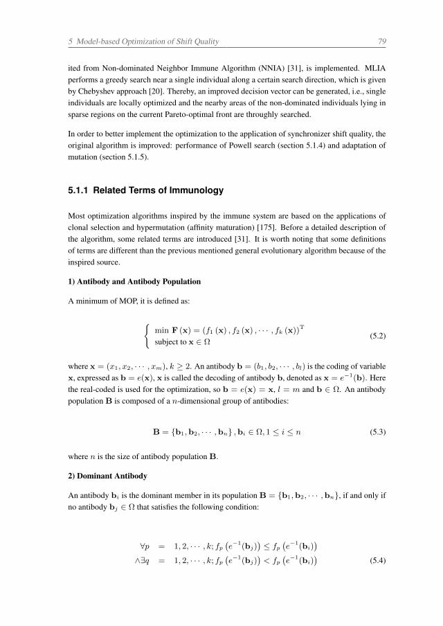
5 Model-based Optimization of Shift Quality 79
ited from Non-dominated Neighbor Immune Algorithm (NNIA) [31], is implemented. MLIAperforms a greedy search near a single individual along a certain search direction, which is givenby Chebyshev approach [20]. Thereby, an improved decision vector can be generated, i.e., singleindividuals are locally optimized and the nearby areas of the non-dominated individuals lying insparse regions on the current Pareto-optimal front are throughly searched.
In order to better implement the optimization to the application of synchronizer shift quality, theoriginal algorithm is improved: performance of Powell search (section 5.1.4) and adaptation ofmutation (section 5.1.5).
5.1.1 Related Terms of Immunology
Most optimization algorithms inspired by the immune system are based on the applications ofclonal selection and hypermutation (affinity maturation) [175]. Before a detailed description ofthe algorithm, some related terms are introduced [31]. It is worth noting that some definitionsof terms are different than the previous mentioned general evolutionary algorithm because of theinspired source.
1) Antibody and Antibody Population
A minimum of MOP, it is defined as:
min F (x) = (f1 (x) , f2 (x) , · · · , fk (x))T
subject to x ∈ Ω(5.2)
where x = (x1, x2, · · · , xm), k ≥ 2. An antibody b = (b1, b2, · · · , bl) is the coding of variablex, expressed as b = e(x), x is called the decoding of antibody b, denoted as x = e−1(b). Herethe real-coded is used for the optimization, so b = e(x) = x, l = m and b ∈ Ω. An antibodypopulation B is composed of a n-dimensional group of antibodies:
B = b1,b2, · · · ,bn ,bi ∈ Ω, 1 ≤ i ≤ n (5.3)
where n is the size of antibody population B.
2) Dominant Antibody
An antibody bi is the dominant member in its population B = b1,b2, · · · ,bn, if and only ifno antibody bj ∈ Ω that satisfies the following condition:
∀p = 1, 2, · · · , k; fp(e−1(bj)
)≤ fp
(e−1(bi)
)∧∃q = 1, 2, · · · , k; fp
(e−1(bj)
)< fp
(e−1(bi)
)(5.4)
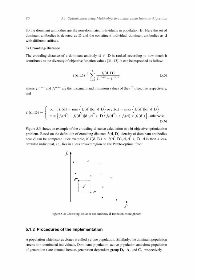
80 5.1 Optimization using Multi-objective Lamarckian Immune Algorithm
So the dominant antibodies are the non-dominated individuals in population B. Here the set ofdominant antibodies is denoted as D and the constituent individual dominant antibodies as d
with different suffixes.
3) Crowding-Distance
The crowding-distance of a dominant antibody d ∈ D is ranked according to how much itcontributes to the diversity of objective function values [31, 43]; it can be expressed as follow:
I(d,D)∆=
k∑i=1
Ii(d,D)
fimax − fi
min(5.5)
where fimax and fimin are the maximum and minimum values of the ith objective respectively,and
Ii(d,D) =
⎧⎨⎩ ∞, if fi(d) = minfi(d
′)|d
′∈ D
or fi(d) = max
fi(d
′)|d
′∈ D
min
fi(d
′)− fi(d
′′)|d
′,d
′′∈ D : fi(d
′′) < fi(d) < fi(d
′), otherwise
(5.6)
Figure 5.3 shows an example of the crowding-distance calculation in a bi-objective optimizationproblem. Based on the definition of crowding-distance I(d,D), density of dominant antibodiesnear d can be compared. For example, if I(d,D) > I(d
′,D),d,d
′∈ D, d is then a less-
crowded individual, i.e., lies in a less crowed region on the Pareto-optimal front.
f1
f2
d”
d’
d
Figure 5.3: Crowding-distance for antibody d based on its neighbors
5.1.2 Procedures of the Implementation
A population which stores clones is called a clone population. Similarly, the dominant populationstocks non-dominated individuals. Dominant population, active population and clone populationof generation t are denoted here as generation-dependent group Dt, At and Ct, respectively.
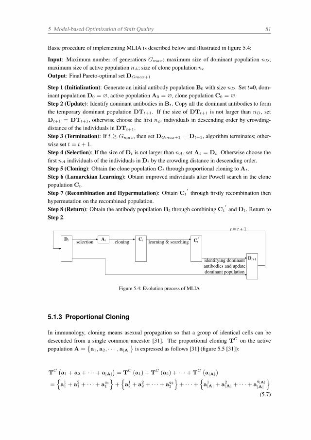
5 Model-based Optimization of Shift Quality 81
Basic procedure of implementing MLIA is described below and illustrated in figure 5.4:
Input: Maximum number of generations Gmax; maximum size of dominant population nD;maximum size of active population nA; size of clone population nc
Output: Final Pareto-optimal set DGmax+1
Step 1 (Initialization): Generate an initial antibody population B0 with size nD . Set t=0, dom-inant population D0 = ∅, active population A0 = ∅, clone population C0 = ∅.Step 2 (Update): Identify dominant antibodies in Bt. Copy all the dominant antibodies to formthe temporary dominant population DTt+1. If the size of DTt+1 is not larger than nD , setDt+1 = DTt+1, otherwise choose the first nD individuals in descending order by crowding-distance of the individuals in DTt+1.Step 3 (Termination): If t ≥ Gmax, then set DGmax+1 = Dt+1, algorithm terminates; other-wise set t = t+ 1.Step 4 (Selection): If the size of Dt is not larger than nA, set At = Dt. Otherwise choose thefirst nA individuals of the individuals in Dt by the crowding distance in descending order.Step 5 (Cloning): Obtain the clone population Ct through proportional cloning to At.Step 6 (Lamarckian Learning): Obtain improved individuals after Powell search in the clonepopulation Ct.Step 7 (Recombination and Hypermutation): Obtain Ct
′through firstly recombination then
hypermutation on the recombined population.Step 8 (Return): Obtain the antibody population Bt through combining Ct
′and Dt. Return to
Step 2.
At Ct Ct′
cloning learning & searching
t = t + 1
identifying dominantantibodies and updatedominant population
Dt+1
selectionDt
Figure 5.4: Evolution process of MLIA
5.1.3 Proportional Cloning
In immunology, cloning means asexual propagation so that a group of identical cells can bedescended from a single common ancestor [31]. The proportional cloning TC on the activepopulation A =
a1,a2, · · · ,a|A|
is expressed as follows [31] (figure 5.5 [31]):
TC (a1 + a2 + · · ·+ a|A|)= TC (a1) +TC (a2) + · · ·+TC (a|A|
)=a11 + a2
1 + · · ·+ aq11
+a12 + a2
2 + · · ·+ aq22
+ · · ·+
a1|A| + a2
|A| + · · ·+ aq|A||A|
(5.7)
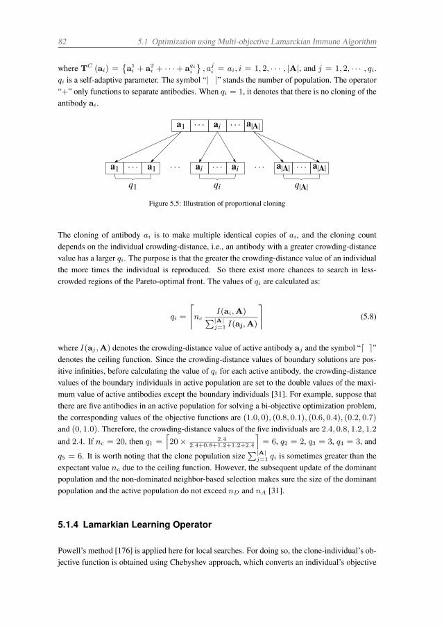
82 5.1 Optimization using Multi-objective Lamarckian Immune Algorithm
where TC (ai) =a1i + a2
i + · · ·+ aqii
, aji = ai, i = 1, 2, · · · , |A|, and j = 1, 2, · · · , qi.
qi is a self-adaptive parameter. The symbol “|A|” stands the number of population. The operator“+” only functions to separate antibodies. When qi = 1, it denotes that there is no cloning of theantibody ai.
a1 · · · ai · · · a|A|
ai · · · ai a|A| · · · a|A|a1 · · · a1
q1 qi q|A|
· · · · · ·
Figure 5.5: Illustration of proportional cloning
The cloning of antibody ai is to make multiple identical copies of ai, and the cloning countdepends on the individual crowding-distance, i.e., an antibody with a greater crowding-distancevalue has a larger qi. The purpose is that the greater the crowding-distance value of an individualthe more times the individual is reproduced. So there exist more chances to search in less-crowded regions of the Pareto-optimal front. The values of qi are calculated as:
qi =
⌈nc
I(ai,A)∑|A|j=1 I(aj,A)
⌉(5.8)
where I(aj ,A) denotes the crowding-distance value of active antibody aj and the symbol “⌈a⌉”denotes the ceiling function. Since the crowding-distance values of boundary solutions are pos-itive infinities, before calculating the value of qi for each active antibody, the crowding-distancevalues of the boundary individuals in active population are set to the double values of the maxi-mum value of active antibodies except the boundary individuals [31]. For example, suppose thatthere are five antibodies in an active population for solving a bi-objective optimization problem,the corresponding values of the objective functions are (1.0, 0), (0.8, 0.1), (0.6, 0.4), (0.2, 0.7)
and (0, 1.0). Therefore, the crowding-distance values of the five individuals are 2.4, 0.8, 1.2, 1.2
and 2.4. If nc = 20, then q1 =⌈20× 2.4
2.4+0.8+1.2+1.2+2.4
⌉= 6, q2 = 2, q3 = 3, q4 = 3, and
q5 = 6. It is worth noting that the clone population size∑|A|
j=1 qi is sometimes greater than theexpectant value nc due to the ceiling function. However, the subsequent update of the dominantpopulation and the non-dominated neighbor-based selection makes sure the size of the dominantpopulation and the active population do not exceed nD and nA [31].
5.1.4 Lamarkian Learning Operator
Powell’s method [176] is applied here for local searches. For doing so, the clone-individual’s ob-jective function is obtained using Chebyshev approach, which converts an individual’s objective
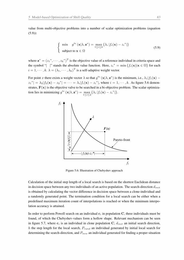
5 Model-based Optimization of Shift Quality 83
value from multi-objective problems into a number of scalar optimization problems (equation(5.9)):
min gte (x|λ, z∗) = max
1≤i≤kλi |fi(x)− zi
∗|
subject to x ∈ Ω(5.9)
where z∗ = (z1∗, · · · , zk∗)T is the objective value of a reference individual in criteria space and
the symbol “|A|” stands the absolute value function. Here, zi∗ = min fi(x)|x ∈ Ω for eachi = 1, · · · , k. λ = (λ1, · · · , λk)
T is a self-adaptive weight vector.
For point x there exists a weight vector λ so that gte (x|λ, z∗) is the minimum, i.e., λ1|f1(x)−z1
∗| = λ2|f2(x) − z2∗| = · · · = λi|fi(x) − zi
∗|, where i = 1, · · · , k. As figure 5.6 demon-strates, F(x) is the objective valve to be searched in a bi-objective problem. The scalar optimiza-tion lies in minimizing gte (x|λ, z∗) = max
1≤i≤2λi |fi(x)− zi
∗|.
f1
f2
Pareto-front
| f1(x)-z1*|
|f2 (x)-z2 *|
F(x)
Figure 5.6: Illustration of Chebyshev approach
Calculation of the initial step length of a local search is based on the shortest Euclidean distancein decision space between any two individuals of an active population. The search-direction dinit
is obtained by calculating the vector difference in decision space between a clone-individual anda randomly generated point. The termination condition for a local search can be either when apredefined maximum iteration count of interpolations is reached or when the minimum interpo-lation accuracy is attained.
In order to perform Powell search on an individual ci in population C, three individuals must befound, of which the Chebyshev-values form a hollow shape. Relevant mechanism can be seenin figure 5.7, where ci is an individual in clone population C, dinit an initial search direction,h the step length for the local search, Prand an individual generated by initial local search fordetermining the search-direction, and Pnew an individual generated for finding a proper situation
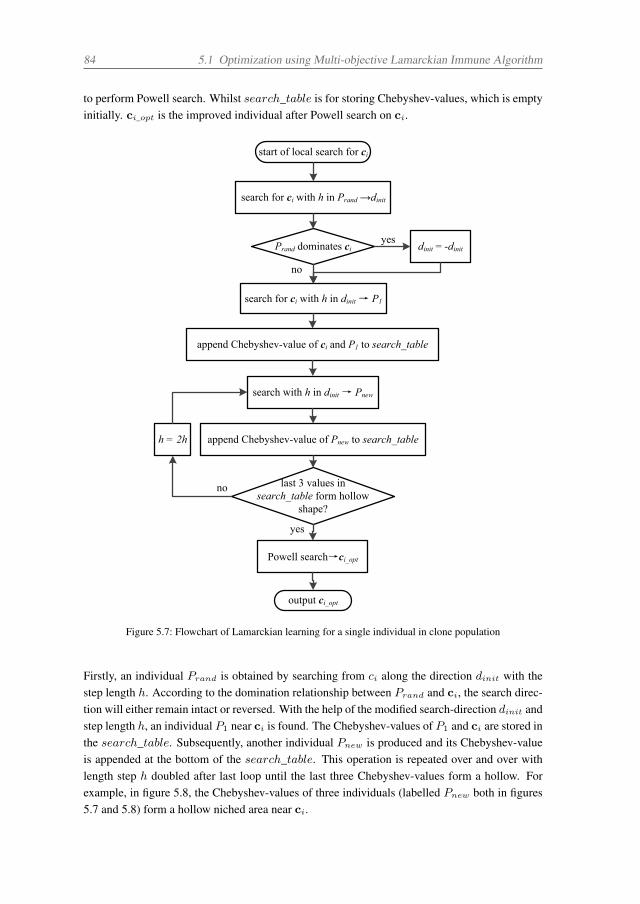
84 5.1 Optimization using Multi-objective Lamarckian Immune Algorithm
to perform Powell search. Whilst search_table is for storing Chebyshev-values, which is emptyinitially. ci_opt is the improved individual after Powell search on ci.
search for ci with h in Prand →dinit
append Chebyshev-value of ci and P1 to search_table
Prand dominates ciyes
no
dinit = -dinit
search for ci with h in dinit → P1
search with h in dinit → Pnew
append Chebyshev-value of Pnew to search_table
last 3 values in search_table form hollow
shape?
yes
no
start of local search for ci
Powell search→ci_opt
output ci_opt
h = 2h
Figure 5.7: Flowchart of Lamarckian learning for a single individual in clone population
Firstly, an individual Prand is obtained by searching from ci along the direction dinit with thestep length h. According to the domination relationship between Prand and ci, the search direc-tion will either remain intact or reversed. With the help of the modified search-direction dinit andstep length h, an individual P1 near ci is found. The Chebyshev-values of P1 and ci are stored inthe search_table. Subsequently, another individual Pnew is produced and its Chebyshev-valueis appended at the bottom of the search_table. This operation is repeated over and over withlength step h doubled after last loop until the last three Chebyshev-values form a hollow. Forexample, in figure 5.8, the Chebyshev-values of three individuals (labelled Pnew both in figures5.7 and 5.8) form a hollow niched area near ci.
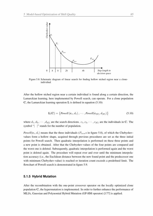
5 Model-based Optimization of Shift Quality 85
Step length in decision space
Che
bysh
ev-v
alue
h0 h 2h 4h
ci
P1
Pnew
Pnew
Pnew
Figure 5.8: Schematic diagram of linear search for finding hollow niched region near a clone-individual
After the hollow niched region near a certain individual is found along a certain direction, theLamarckian learning, here implemented by Powell search, can operate. For a clone populationC, the Lamarckian learning operation L is defined in equation (5.10):
L(C) =
Powell (c1, d1) , · · · ,Powell(c|C|, d|C|)
(5.10)
where d1, d2, · · · , d|C| are the search directions. c1, c2, · · · , c|C| are the individuals in C. Thesymbol “|A|” stands for the number of population.
Powell(ci, di) means that the three individuals (Pnews in figure 5.8), of which the Chebyshev-values form a hollow shape, acquired through previous procedures are set as the three initialpoints for Powell search. Then quadratic interpolation is performed on these three points anda new point is obtained. After that the Chebyshev-values of the four points are compared andthe worst one is deleted. Subsequently, quadratic interpolation is performed again and the worstpoint is deleted again. The procedure will repeat over and over until the minimum interpola-tion accuracy (i.e., the Euclidean distance between the new found point and the predecessor onewith minimum Chebyshev-value) is reached or iteration count exceeds a predefined limit. Theflowchart of Powell search is demonstrated in figure 5.9.
5.1.5 Hybrid Mutation
After the recombination with the one-point crossover operator on the locally optimized clonepopulation C, the hypermutation is implemented. In order to further enhance the performance ofMLIA, Gaussian and Polynomial Hybrid Mutation (GP-HM operator) [177] is applied.
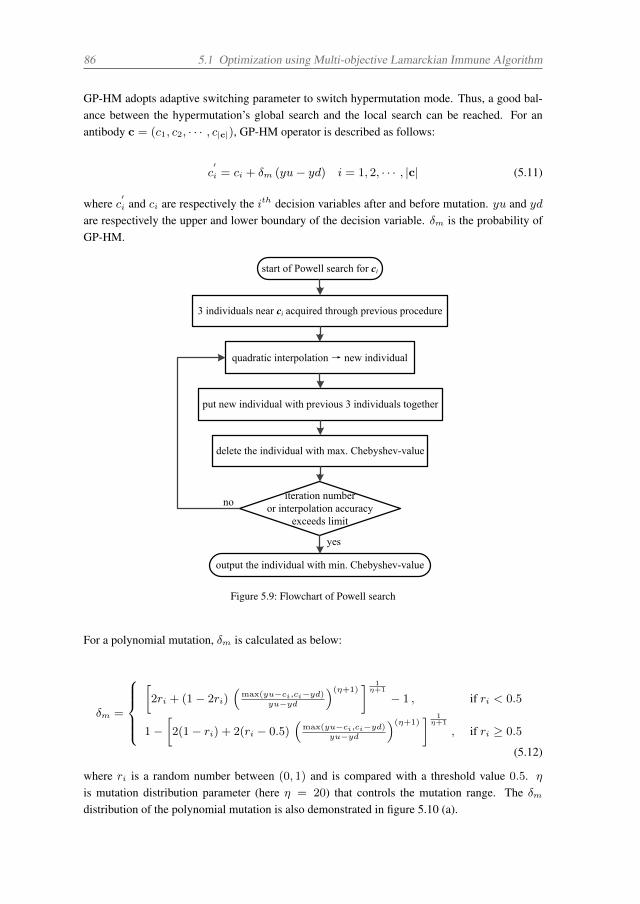
86 5.1 Optimization using Multi-objective Lamarckian Immune Algorithm
GP-HM adopts adaptive switching parameter to switch hypermutation mode. Thus, a good bal-ance between the hypermutation’s global search and the local search can be reached. For anantibody c = (c1, c2, · · · , c|c|), GP-HM operator is described as follows:
c′i = ci + δm (yu− yd) i = 1, 2, · · · , |c| (5.11)
where c′i and ci are respectively the ith decision variables after and before mutation. yu and yd
are respectively the upper and lower boundary of the decision variable. δm is the probability ofGP-HM.
start of Powell search for ci
3 individuals near ci acquired through previous procedure
quadratic interpolation → new individual
put new individual with previous 3 individuals together
delete the individual with max. Chebyshev-value
iteration number or interpolation accuracy
exceeds limit
output the individual with min. Chebyshev-value
yes
no
Figure 5.9: Flowchart of Powell search
For a polynomial mutation, δm is calculated as below:
δm =
⎧⎪⎪⎪⎨⎪⎪⎪⎩[2ri + (1− 2ri)
(max(yu−ci,ci−yd)
yu−yd
)(η+1)] 1
η+1
− 1 , if ri < 0.5
1−[2(1− ri) + 2(ri − 0.5)
(max(yu−ci,ci−yd)
yu−yd
)(η+1)] 1
η+1
, if ri ≥ 0.5
(5.12)
where ri is a random number between (0, 1) and is compared with a threshold value 0.5. η
is mutation distribution parameter (here η = 20) that controls the mutation range. The δmdistribution of the polynomial mutation is also demonstrated in figure 5.10 (a).
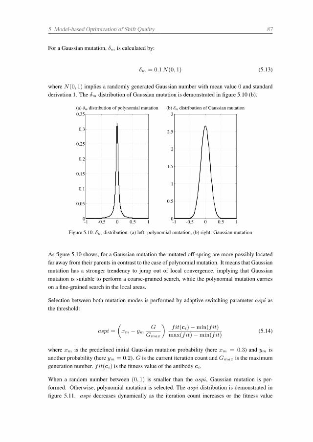
5 Model-based Optimization of Shift Quality 87
For a Gaussian mutation, δm is calculated by:
δm = 0.1N(0, 1) (5.13)
where N(0, 1) implies a randomly generated Gaussian number with mean value 0 and standardderivation 1. The δm distribution of Gaussian mutation is demonstrated in figure 5.10 (b).
-1 -0.5 0 0.5 10
0.05
0.1
0.15
0.2
0.25
0.3
0.35(a) δm distribution of polynomial mutation
-1 -0.5 0 0.5 10
0.5
1
1.5
2
2.5
3(b) δm distribution of Gaussian mutation
Figure 5.10: δm distribution. (a) left: polynomial mutation, (b) right: Gaussian mutation
As figure 5.10 shows, for a Gaussian mutation the mutated off-spring are more possibly locatedfar away from their parents in contrast to the case of polynomial mutation. It means that Gaussianmutation has a stronger trendency to jump out of local convergence, implying that Gaussianmutation is suitable to perform a coarse-grained search, while the polynomial mutation carrieson a fine-grained search in the local areas.
Selection between both mutation modes is performed by adaptive switching parameter aspi asthe threshold:
aspi =
(xm − ym
G
Gmax
)fit(ci)−min(fit)
max(fit)−min(fit)(5.14)
where xm is the predefined initial Gaussian mutation probability (here xm = 0.3) and ym isanother probability (here ym = 0.2). G is the current iteration count and Gmax is the maximumgeneration number. fit(ci) is the fitness value of the antibody ci.
When a random number between (0, 1) is smaller than the aspi, Gaussian mutation is per-formed. Otherwise, polynomial mutation is selected. The aspi distribution is demonstrated infigure 5.11. aspi decreases dynamically as the iteration count increases or the fitness value
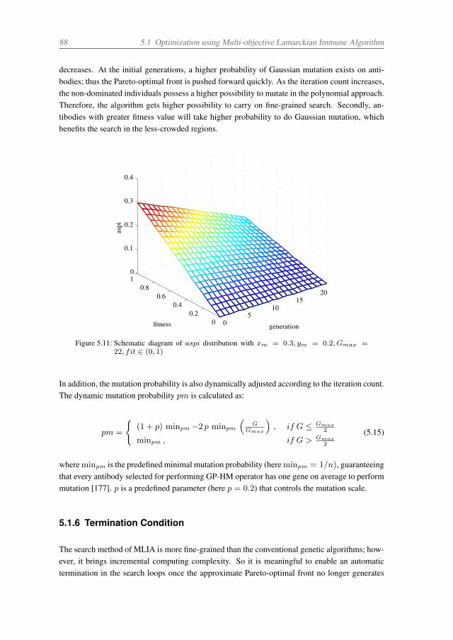
88 5.1 Optimization using Multi-objective Lamarckian Immune Algorithm
decreases. At the initial generations, a higher probability of Gaussian mutation exists on anti-bodies; thus the Pareto-optimal front is pushed forward quickly. As the iteration count increases,the non-dominated individuals possess a higher possibility to mutate in the polynomial approach.Therefore, the algorithm gets higher possibility to carry on fine-grained search. Secondly, an-tibodies with greater fitness value will take higher probability to do Gaussian mutation, whichbenefits the search in the less-crowded regions.
05
1015
20
00.2
0.40.6
0.810
0.1
0.2
0.3
0.4
generationfitness
aspi
Figure 5.11: Schematic diagram of aspi distribution with xm = 0.3, ym = 0.2, Gmax =22, fit ∈ (0, 1)
In addition, the mutation probability is also dynamically adjusted according to the iteration count.The dynamic mutation probability pm is calculated as:
pm =
(1 + p) minpm −2 p minpm
(G
Gmax
), if G ≤ Gmax
2
minpm , if G > Gmax2
(5.15)
where minpm is the predefined minimal mutation probability (here minpm = 1/n), guaranteeingthat every antibody selected for performing GP-HM operator has one gene on average to performmutation [177]. p is a predefined parameter (here p = 0.2) that controls the mutation scale.
5.1.6 Termination Condition
The search method of MLIA is more fine-grained than the conventional genetic algorithms; how-ever, it brings incremental computing complexity. So it is meaningful to enable an automatictermination in the search loops once the approximate Pareto-optimal front no longer generates
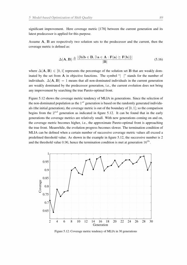
5 Model-based Optimization of Shift Quality 89
significant improvement. Here coverage metric [178] between the current generation and itslatest predecessor is applied for this purpose.
Assume A, B are respectively two solution sets to the predecessor and the current, then thecoverage metric is defined as:
∆(A,B)∆=
|b|b ∈ B,∃a ∈ A : F(a) ≽ F(b)||B| (5.16)
where ∆(A,B) ∈ [0, 1] represents the percentage of the solution set B that are weakly dom-inated by the set from A in objective functions. The symbol “|A|” stands for the number ofindividuals. ∆(A,B) = 1 means that all non-dominated individuals in the current generationare weakly dominated by the predecessor generation, i.e., the current evolution does not bringany improvement by searching the true Pareto-optimal front.
Figure 5.12 shows the coverage metric tendency of MLIA in generations. Since the selection ofthe non-dominated population as the 1st generation is based on the randomly generated individu-als (the initial generation), the coverage metric is out of the boundary of [0, 1]; so the comparisonbegins from the 2nd generation as indicated in figure 5.12. It can be found that in the earlygenerations the coverage metrics are relatively small. With new generations coming on and on,the coverage metric becomes higher, i.e., the approximate Pareto-optimal front is approachingthe true front. Meanwhile, the evolution progress becomes slower. The termination condition ofMLIA can be defined when a certain number of successive coverage metric values all exceed apredefined threshold value. As shown in the example in figure 5.12, the successive number is 2and the threshold value 0.96, hence the termination condition is met at generation 16th.
2 4 6 8 10 12 14 16 18 20 22 24 26 28 30
0.65
0.7
0.75
0.8
0.85
0.9
0.95
1
Generation
Cov
erag
e
Figure 5.12: Coverage metric tendency of MLIA in 30 generations
90 5.2 Evaluation of Effectiveness
5.2 Evaluation of Effectiveness
The multi-objective optimization effectiveness depends on the approximation degree of used al-gorithm(s) to the true Pareto-optimal front. Here four other state-of-the-art multi-objective opti-mization algorithms, NSGA-II, SPEA2, NNIA and original MLIA, are used to compare with theenhanced MLIA (aided by GP-HM). Their implementation methods for synchronizer shift qual-ity optimization can also be found in [179]. All simulations were run on a PC with Intel® Core™
i5-3470 processor. The tuned parameter values for the enhanced MLIA with GP-HM, originalMLIA, NNIA, SPEA2 and NSGA-II are listed in table 5.1. The ranges of decision vector p aret1 ∈ [75ms, 250ms], t2 ∈ [75ms, 250ms], and t3 ∈ [75ms, 250ms]. For NNIA, the maxi-mum size of the dominant population nD = 220, that of the active population nA = 44, andthe size of clone population nC = 220. For MLIA (both original and with GP-HM), in additionto identical parameter values to their counterparts in NNIA, its step ratio of local search is 0.02,local search step length h is the product of step ratio and the minimum Euclidean distance amongall decision variables in the active population, maximum iteration count for one-direction searchis 10, maximum local search iteration count is 5, and the smallest local search step length is0.001. For MLIA with GP-HM, the mutation distribution parameter η = 20, Gaussian mutationprobabilities are xm = 0.3 and ym = 0.2, mutation probability minpm = 1/3, and the mutationscale parameter p = 0.2.
Table 5.1: Parameter setting for multi-objective optimization algorithm
parameter enhanced MLIA original MLIA NNIA SPEA2 NSGA-II
generation 22 22 22 22 22population 220 220 220 220 220crossover probability 1 1 1 0.9 0.9mutation probability GP-HM 1/3 1/3 0.1 0.1decision variables 3 3 3 3 3criteria variables 2 2 2 2 2
As figure 5.13 shows that almost all the points obtained by MLIA with GP-HM lie on the lowerleft curve, suggesting that this algorithm holds the best convergence ability among the five. Forexample, the MLIA (GP-HM) point at 0.7 along with D axis (unit in m/s3) takes approximately4ms less in tsyn than the SPEA2 point along the same horizontal axis.
The convergence metric (equation (5.18)) [31] is used to describe the ability of the algorithmto approximate to the true Pareto-optimal front. The lower the convergence metric value is thebetter the convergence ability it has.
Firstly, define that P∗ =(p1,p2, · · · ,p|P∗|
)is the solution set of all non-dominated individuals
from the optimization results. A =(a1,a2, · · · ,a|A|
)is the non-dominated solution set through
a certain algorithm. For each individual ai in solution set A, the minimum normalized Euclideandistance to P∗ is expressed as:
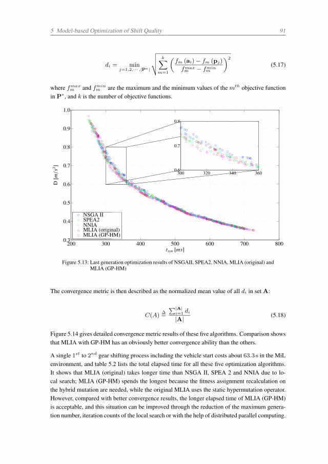
5 Model-based Optimization of Shift Quality 91
di = minj=1,2,··· ,|P∗|
√ k∑m=1
(fm (ai)− fm (pj)
fmaxm − fmin
m
)2
(5.17)
where fmaxm and fmin
m are the maximum and the minimum values of the mth objective functionin P∗, and k is the number of objective functions.
200 300 400 500 600 700 8000.3
0.4
0.5
0.6
0.7
0.8
0.9
1.0
tsyn [ms]
D[m/s3 ]
NSGA IISPEA2NNIAMLIA (original)MLIA (GP-HM)
300 320 340 3600.6
0.7
0.8
Figure 5.13: Last generation optimization results of NSGAII, SPEA2, NNIA, MLIA (original) andMLIA (GP-HM)
The convergence metric is then described as the normalized mean value of all di in set A:
C(A)∆=
∑|A|i=1 di
|A| (5.18)
Figure 5.14 gives detailed convergence metric results of these five algorithms. Comparison showsthat MLIA with GP-HM has an obviously better convergence ability than the others.
A single 1st to 2nd gear shifting process including the vehicle start costs about 63.3 s in the MiLenvironment, and table 5.2 lists the total elapsed time for all these five optimization algorithms.It shows that MLIA (original) takes longer time than NSGA II, SPEA 2 and NNIA due to lo-cal search; MLIA (GP-HM) spends the longest because the fitness assignment recalculation onthe hybrid mutation are needed, while the original MLIA uses the static hypermutation operator.However, compared with better convergence results, the longer elapsed time of MLIA (GP-HM)is acceptable, and this situation can be improved through the reduction of the maximum genera-tion number, iteration counts of the local search or with the help of distributed parallel computing.
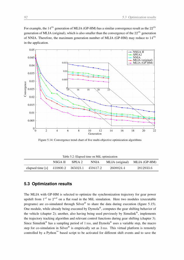
92 5.3 Optimization results
For example, the 14th generation of MLIA (GP-HM) has a similar convergence result as the 22th
generation of MLIA (original), which is also smaller than the convergence of the 22th generationof NNIA. Therefore, the maximum generation number of MLIA (GP-HM) may reduce to 14th
in the application.
0 2 4 6 8 10 12 14 16 18 20 220
0.005
0.01
0.015
0.02
0.025
0.03
0.035
0.04
0.045
0.05
Generation
Con
verg
ence
NSGA IISPEA2NNIAMLIA (original)MLIA (GP-HM)
14 16 18 20 220
0.005
0.01
0.015
Figure 5.14: Convergence trend chart of five multi-objective optimization algorithms
Table 5.2: Elapsed time on MiL optimization
NSGA II SPEA 2 NNIA MLIA (original) MLIA (GP-HM)
elapsed time [s] 410800.2 365023.1 459417.2 2608824.4 2812933.6
5.3 Optimization results
The MLIA with GP-HM is selected to optimize the synchronization trajectory for gear powerupshift from 1st to 2nd on a flat road in the MiL simulation. Here two modules (executableprograms) are co-simulated through Silver® to share the data during execution (figure 5.15).One module, while already being executed by Dymola®, computes the gear shifting behavior ofthe vehicle (chapter 2); another, also having being used previously by Simulink®, implementsthe trajectory tracking algorithm and relevant control functions during gear shifting (chapter 3).Since Simulink® has a sampling period of 1ms, and Dymola® uses a variable step, the macrostep for co-simulation in Silver® is empirically set as 3ms. This virtual platform is remotelycontrolled by a Python™ based script to be activated for different shift events and to save the
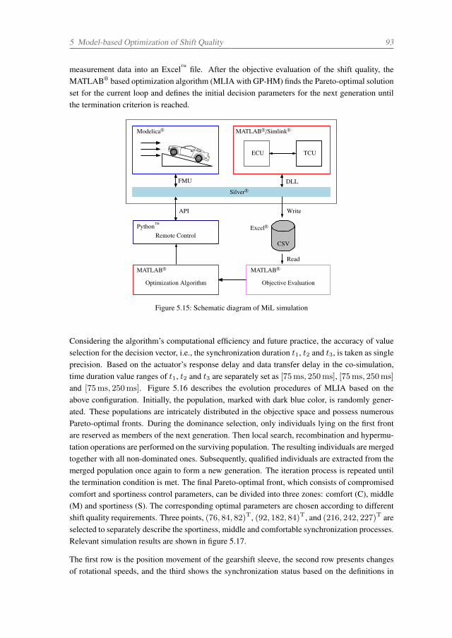
5 Model-based Optimization of Shift Quality 93
measurement data into an Excel™ file. After the objective evaluation of the shift quality, theMATLAB® based optimization algorithm (MLIA with GP-HM) finds the Pareto-optimal solutionset for the current loop and defines the initial decision parameters for the next generation untilthe termination criterion is reached.
PythonTM
Remote Control
FMU DLL
Silver R©
ECU TCU
MATLAB R©/Simlink R©Modelica R©
MATLAB R©
Optimization Algorithm
MATLAB R©
Objective Evaluation
API Write
CSV
Read
Excel R©
Figure 5.15: Schematic diagram of MiL simulation
Considering the algorithm’s computational efficiency and future practice, the accuracy of valueselection for the decision vector, i.e., the synchronization duration t1, t2 and t3, is taken as singleprecision. Based on the actuator’s response delay and data transfer delay in the co-simulation,time duration value ranges of t1, t2 and t3 are separately set as [75ms, 250ms], [75ms, 250ms]
and [75ms, 250ms]. Figure 5.16 describes the evolution procedures of MLIA based on theabove configuration. Initially, the population, marked with dark blue color, is randomly gener-ated. These populations are intricately distributed in the objective space and possess numerousPareto-optimal fronts. During the dominance selection, only individuals lying on the first frontare reserved as members of the next generation. Then local search, recombination and hypermu-tation operations are performed on the surviving population. The resulting individuals are mergedtogether with all non-dominated ones. Subsequently, qualified individuals are extracted from themerged population once again to form a new generation. The iteration process is repeated untilthe termination condition is met. The final Pareto-optimal front, which consists of compromisedcomfort and sportiness control parameters, can be divided into three zones: comfort (C), middle(M) and sportiness (S). The corresponding optimal parameters are chosen according to differentshift quality requirements. Three points, (76, 84, 82)T, (92, 182, 84)T, and (216, 242, 227)T areselected to separately describe the sportiness, middle and comfortable synchronization processes.Relevant simulation results are shown in figure 5.17.
The first row is the position movement of the gearshift sleeve, the second row presents changesof rotational speeds, and the third shows the synchronization status based on the definitions in
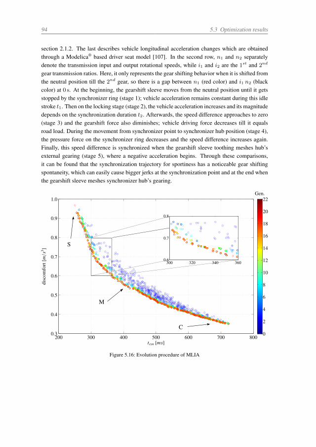
94 5.3 Optimization results
section 2.1.2. The last describes vehicle longitudinal acceleration changes which are obtainedthrough a Modelica® based driver seat model [107]. In the second row, n1 and n2 separatelydenote the transmission input and output rotational speeds, while i1 and i2 are the 1st and 2nd
gear transmission ratios. Here, it only represents the gear shifting behavior when it is shifted fromthe neutral position till the 2nd gear, so there is a gap between n1 (red color) and i1 n2 (blackcolor) at 0 s. At the beginning, the gearshift sleeve moves from the neutral position until it getsstopped by the synchronizer ring (stage 1); vehicle acceleration remains constant during this idlestroke t1. Then on the locking stage (stage 2), the vehicle acceleration increases and its magnitudedepends on the synchronization duration t2. Afterwards, the speed difference approaches to zero(stage 3) and the gearshift force also diminishes; vehicle driving force decreases till it equalsroad load. During the movement from synchronizer point to synchronizer hub position (stage 4),the pressure force on the synchronizer ring decreases and the speed difference increases again.Finally, this speed difference is synchronized when the gearshift sleeve toothing meshes hub’sexternal gearing (stage 5), where a negative acceleration begins. Through these comparisons,it can be found that the synchronization trajectory for sportiness has a noticeable gear shiftingspontaneity, which can easily cause bigger jerks at the synchronization point and at the end whenthe gearshift sleeve meshes synchronizer hub’s gearing.
200 300 400 500 600 700 8000.3
0.4
0.5
0.6
0.7
0.8
0.9
1.0
tsyn [ms]
disc
omfo
rt[m/s3 ]
0
2
4
6
8
10
12
14
16
18
20
22
300 320 340 3600.6
0.7
0.8
Gen.
S
M
C
Figure 5.16: Evolution procedure of MLIA
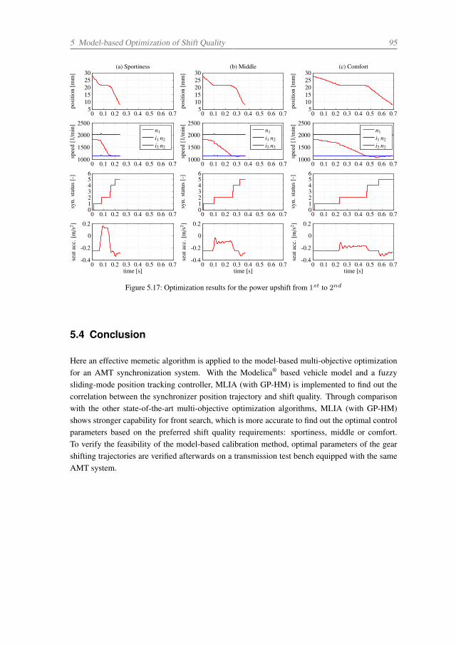
5 Model-based Optimization of Shift Quality 95
0 0.1 0.2 0.3 0.4 0.5 0.6 0.75
1015202530
posi
tion
[mm
](a) Sportiness
0 0.1 0.2 0.3 0.4 0.5 0.6 0.71000
1500
2000
2500
spee
d[1/m
in]
n1
i1 n2
i2 n2
0 0.1 0.2 0.3 0.4 0.5 0.6 0.70123456
syn.
stat
us[-
]
0 0.1 0.2 0.3 0.4 0.5 0.6 0.7-0.4
-0.2
0
0.2
time [s]
seat
acc.
[m/s
2 ]
0 0.1 0.2 0.3 0.4 0.5 0.6 0.75
1015202530
posi
tion
[mm
]
(b) Middle
0 0.1 0.2 0.3 0.4 0.5 0.6 0.71000
1500
2000
2500
spee
d[1/m
in]
n1
i1 n2
i2 n2
0 0.1 0.2 0.3 0.4 0.5 0.6 0.70123456
syn.
stat
us[-
]
0 0.1 0.2 0.3 0.4 0.5 0.6 0.7-0.4
-0.2
0
0.2
time [s]
seat
acc.
[m/s
2 ]
0 0.1 0.2 0.3 0.4 0.5 0.6 0.75
1015202530
posi
tion
[mm
]
(c) Comfort
0 0.1 0.2 0.3 0.4 0.5 0.6 0.71000
1500
2000
2500
spee
d[1/m
in]
n1
i1 n2
i2 n2
0 0.1 0.2 0.3 0.4 0.5 0.6 0.70123456
syn.
stat
us[-
]
0 0.1 0.2 0.3 0.4 0.5 0.6 0.7-0.4
-0.2
0
0.2
time [s]
seat
acc.
[m/s
2 ]Figure 5.17: Optimization results for the power upshift from 1st to 2nd
5.4 Conclusion
Here an effective memetic algorithm is applied to the model-based multi-objective optimizationfor an AMT synchronization system. With the Modelica® based vehicle model and a fuzzysliding-mode position tracking controller, MLIA (with GP-HM) is implemented to find out thecorrelation between the synchronizer position trajectory and shift quality. Through comparisonwith the other state-of-the-art multi-objective optimization algorithms, MLIA (with GP-HM)shows stronger capability for front search, which is more accurate to find out the optimal controlparameters based on the preferred shift quality requirements: sportiness, middle or comfort.To verify the feasibility of the model-based calibration method, optimal parameters of the gearshifting trajectories are verified afterwards on a transmission test bench equipped with the sameAMT system.

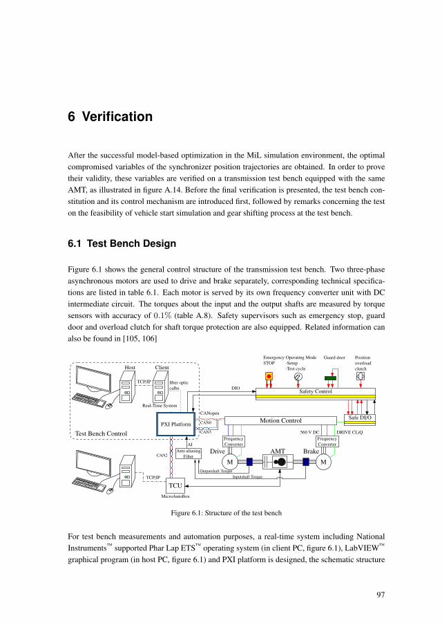
6 Verification
After the successful model-based optimization in the MiL simulation environment, the optimalcompromised variables of the synchronizer position trajectories are obtained. In order to provetheir validity, these variables are verified on a transmission test bench equipped with the sameAMT, as illustrated in figure A.14. Before the final verification is presented, the test bench con-stitution and its control mechanism are introduced first, followed by remarks concerning the teston the feasibility of vehicle start simulation and gear shifting process at the test bench.
6.1 Test Bench Design
Figure 6.1 shows the general control structure of the transmission test bench. Two three-phaseasynchronous motors are used to drive and brake separately, corresponding technical specifica-tions are listed in table 6.1. Each motor is served by its own frequency converter unit with DCintermediate circuit. The torques about the input and the output shafts are measured by torquesensors with accuracy of 0.1% (table A.8). Safety supervisors such as emergency stop, guarddoor and overload clutch for shaft torque protection are also equipped. Related information canalso be found in [105, 106]
Motion Control Safe DI/O
AMT
CANopen
TCP/IP
560 V DC
ClientHost
Drive Brake
DIO
CAN2
CAN0
CAN3Test Bench Control DRIVE CLiQ
Positionoverloadclutch
Safety Control
Operating Mode·Setup·Test cycle
Guard doorEmergencySTOP
M M
TCU
PXI Platform
TCP/IP
MicroAutoBox
AI
Real-Time System
Outputshaft TorqueInputshaft Torque
Anti-aliasingFilter
FrequencyConverter
FrequencyConverter
fiber opticcalbe
Figure 6.1: Structure of the test bench
For test bench measurements and automation purposes, a real-time system including NationalInstruments™ supported Phar Lap ETS™ operating system (in client PC, figure 6.1), LabVIEW™
graphical program (in host PC, figure 6.1) and PXI platform is designed, the schematic structure
97
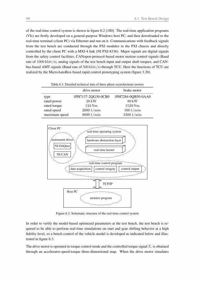
98 6.1 Test Bench Design
of the real-time control system is shown in figure 6.2 [180]. The real-time application programs(VIs) are firstly developed on a general-purpose Windows host PC, and then downloaded to thereal-time terminal (client PC) via Ethernet and run on it. Communications with feedback signalsfrom the test bench are conducted through the PXI modules in the PXI chassis and directlycontrolled by the client PC with a MXI-4 link (NI PXI-8336). Major signals are digital signalsfrom the safety control facilities, CANopen-protocol-based motor motion control signals (Baudrate of 1000 kbit/s), analog signals of the test bench input and output shaft torques, and CAN-bus-based AMT signals (Baud rate of 500 kbit/s) through TCU. Here the functions of TCU arerealized by the MicroAutoBox-based rapid control prototyping system (figure 3.30).
Table 6.1: Detailed technical data of three-phase asynchronous motors
drive motor brake motor
type 1PH7137-2QG30-0CB0 1PH7284-0QB50-0AA0rated power 28 kW 80 kWrated torque 134Nm 1529Nmrated speed 2000 1/min 500 1/minmaximum speed 8000 1/min 3300 1/min
real-time control program
real-time operating system
hardware abstraction layer
real-time kernelNI-DAQmx
NI-CAN
instrument driver
Client PC
TCP/IP
data acquisition control stragety control output
monitor program
Host PC
Figure 6.2: Schematic structure of the real-time control system
In order to verify the model-based optimized parameters at the test bench, the test bench is re-quired to be able to perform real-time simulations on start and gear shifting behavior at a highfidelity level, so a bench control of the vehicle model is developed as indicated below and illus-trated in figure 6.3.
The drive motor is operated in torque control mode and the controlled torque signal Te is obtainedthrough an accelerator-speed-torque three-dimensional map. When the drive motor simulates
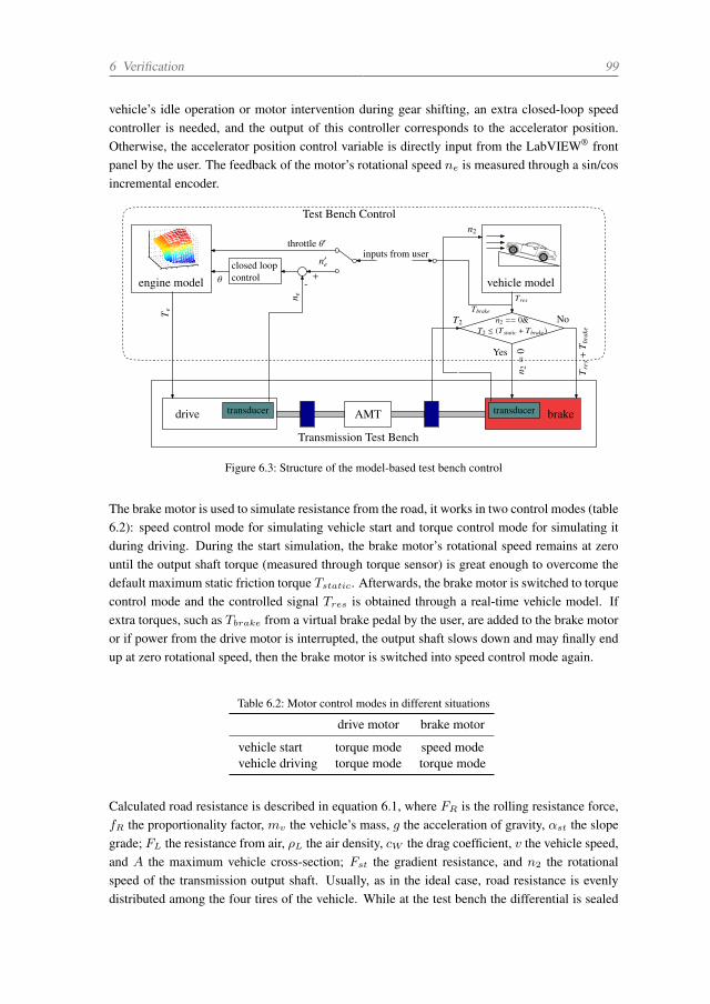
6 Verification 99
vehicle’s idle operation or motor intervention during gear shifting, an extra closed-loop speedcontroller is needed, and the output of this controller corresponds to the accelerator position.Otherwise, the accelerator position control variable is directly input from the LabVIEW® frontpanel by the user. The feedback of the motor’s rotational speed ne is measured through a sin/cosincremental encoder.
Transmission Test Bench
engine modelclosed loopcontrol
drive transducer
throttle θ′
n′e
Te
n e
+-θ
n2
AMT braketransducer
n 2=
0Yes
No
Tre
s+
T bra
ke
Tres
T2
Test Bench Control
vehicle modelrotate speed
throttle
torq
ue
inputs from user
n2 == 0&T2 ≤ (Tstatic + Tbrake)
Tbrake
Figure 6.3: Structure of the model-based test bench control
The brake motor is used to simulate resistance from the road, it works in two control modes (table6.2): speed control mode for simulating vehicle start and torque control mode for simulating itduring driving. During the start simulation, the brake motor’s rotational speed remains at zerountil the output shaft torque (measured through torque sensor) is great enough to overcome thedefault maximum static friction torque Tstatic. Afterwards, the brake motor is switched to torquecontrol mode and the controlled signal Tres is obtained through a real-time vehicle model. Ifextra torques, such as Tbrake from a virtual brake pedal by the user, are added to the brake motoror if power from the drive motor is interrupted, the output shaft slows down and may finally endup at zero rotational speed, then the brake motor is switched into speed control mode again.
Table 6.2: Motor control modes in different situations
drive motor brake motor
vehicle start torque mode speed modevehicle driving torque mode torque mode
Calculated road resistance is described in equation 6.1, where FR is the rolling resistance force,fR the proportionality factor, mv the vehicle’s mass, g the acceleration of gravity, αst the slopegrade; FL the resistance from air, ρL the air density, cW the drag coefficient, v the vehicle speed,and A the maximum vehicle cross-section; Fst the gradient resistance, and n2 the rotationalspeed of the transmission output shaft. Usually, as in the ideal case, road resistance is evenlydistributed among the four tires of the vehicle. While at the test bench the differential is sealed
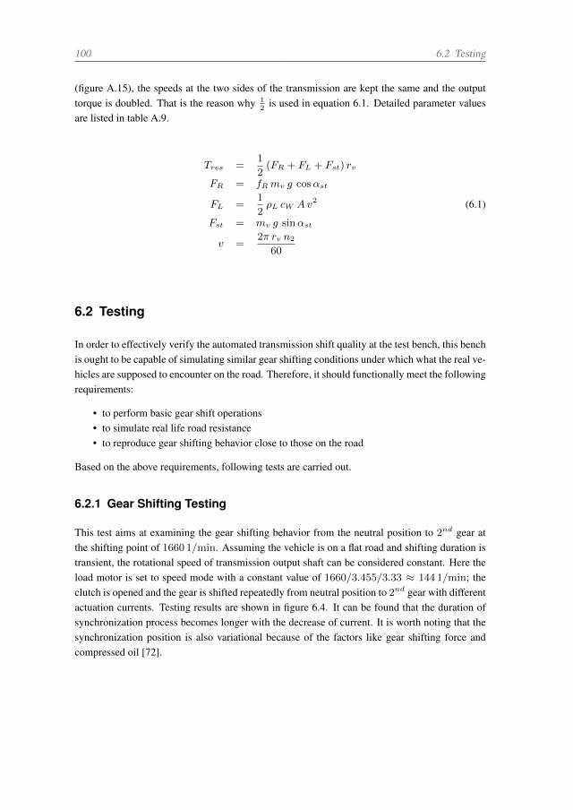
100 6.2 Testing
(figure A.15), the speeds at the two sides of the transmission are kept the same and the outputtorque is doubled. That is the reason why 1
2is used in equation 6.1. Detailed parameter values
are listed in table A.9.
Tres =1
2(FR + FL + Fst) rv
FR = fRmv g cosαst
FL =1
2ρL cW Av2 (6.1)
Fst = mv g sinαst
v =2π rv n2
60
6.2 Testing
In order to effectively verify the automated transmission shift quality at the test bench, this benchis ought to be capable of simulating similar gear shifting conditions under which what the real ve-hicles are supposed to encounter on the road. Therefore, it should functionally meet the followingrequirements:
• to perform basic gear shift operations• to simulate real life road resistance• to reproduce gear shifting behavior close to those on the road
Based on the above requirements, following tests are carried out.
6.2.1 Gear Shifting Testing
This test aims at examining the gear shifting behavior from the neutral position to 2nd gear atthe shifting point of 1660 1/min. Assuming the vehicle is on a flat road and shifting duration istransient, the rotational speed of transmission output shaft can be considered constant. Here theload motor is set to speed mode with a constant value of 1660/3.455/3.33 ≈ 144 1/min; theclutch is opened and the gear is shifted repeatedly from neutral position to 2nd gear with differentactuation currents. Testing results are shown in figure 6.4. It can be found that the duration ofsynchronization process becomes longer with the decrease of current. It is worth noting that thesynchronization position is also variational because of the factors like gear shifting force andcompressed oil [72].
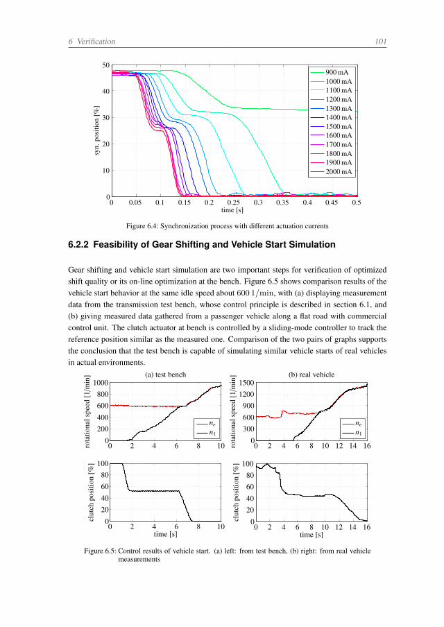
6 Verification 101
0 0.05 0.1 0.15 0.2 0.25 0.3 0.35 0.4 0.45 0.50
10
20
30
40
50
syn.
posi
tion
[%]
time [s]
900 mA1000 mA1100 mA1200 mA1300 mA1400 mA1500 mA1600 mA1700 mA1800 mA1900 mA2000 mA
Figure 6.4: Synchronization process with different actuation currents
6.2.2 Feasibility of Gear Shifting and Vehicle Start Simulation
Gear shifting and vehicle start simulation are two important steps for verification of optimizedshift quality or its on-line optimization at the bench. Figure 6.5 shows comparison results of thevehicle start behavior at the same idle speed about 600 1/min, with (a) displaying measurementdata from the transmission test bench, whose control principle is described in section 6.1, and(b) giving measured data gathered from a passenger vehicle along a flat road with commercialcontrol unit. The clutch actuator at bench is controlled by a sliding-mode controller to track thereference position similar as the measured one. Comparison of the two pairs of graphs supportsthe conclusion that the test bench is capable of simulating similar vehicle starts of real vehiclesin actual environments.
0 2 4 6 8 100
200400
600800
1000(a) test bench
rota
tiona
lspe
ed[1/m
in]
ne
n1
0 2 4 6 8 100
2040
6080
100
clut
chpo
sitio
n[%
]
time [s]
0 2 4 6 8 10 12 14 160
300600
90012001500
rota
tiona
lspe
ed[1/m
in] (b) real vehicle
ne
n1
0 2 4 6 8 10 12 14 160
2040
6080
100
time [s]
clut
chpo
sitio
n[%
]
Figure 6.5: Control results of vehicle start. (a) left: from test bench, (b) right: from real vehiclemeasurements
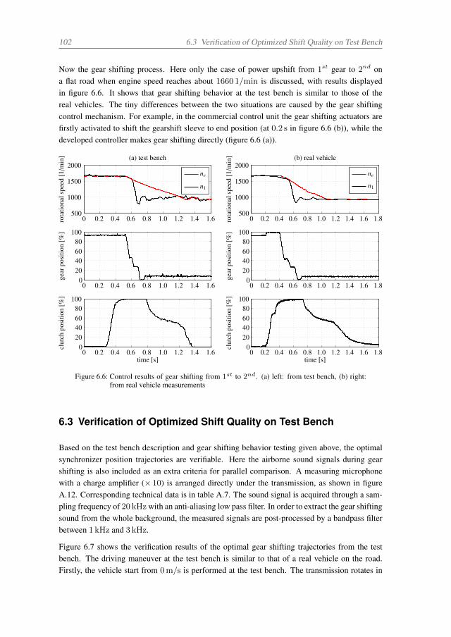
102 6.3 Verification of Optimized Shift Quality on Test Bench
Now the gear shifting process. Here only the case of power upshift from 1st gear to 2nd ona flat road when engine speed reaches about 1660 1/min is discussed, with results displayedin figure 6.6. It shows that gear shifting behavior at the test bench is similar to those of thereal vehicles. The tiny differences between the two situations are caused by the gear shiftingcontrol mechanism. For example, in the commercial control unit the gear shifting actuators arefirstly activated to shift the gearshift sleeve to end position (at 0.2 s in figure 6.6 (b)), while thedeveloped controller makes gear shifting directly (figure 6.6 (a)).
0 0.2 0.4 0.6 0.8 1.0 1.2 1.4 1.6500
1000
1500
2000
rota
tiona
lspe
ed[1/m
in] (a) test bench
ne
n1
0 0.2 0.4 0.6 0.8 1.0 1.2 1.4 1.60
20406080
100
gear
posi
tion
[%]
0 0.2 0.4 0.6 0.8 1.0 1.2 1.4 1.60
20406080
100
clut
chpo
sitio
n[%
]
time [s]
0 0.2 0.4 0.6 0.8 1.0 1.2 1.4 1.6 1.8500
1000
1500
2000
rota
tiona
lspe
ed[1/m
in] (b) real vehicle
ne
n1
0 0.2 0.4 0.6 0.8 1.0 1.2 1.4 1.6 1.80
20406080
100
clut
chpo
sitio
n[%
]
time [s]
0 0.2 0.4 0.6 0.8 1.0 1.2 1.4 1.6 1.80
20406080
100ge
arpo
sitio
n[%
]
Figure 6.6: Control results of gear shifting from 1st to 2nd. (a) left: from test bench, (b) right:from real vehicle measurements
6.3 Verification of Optimized Shift Quality on Test Bench
Based on the test bench description and gear shifting behavior testing given above, the optimalsynchronizer position trajectories are verifiable. Here the airborne sound signals during gearshifting is also included as an extra criteria for parallel comparison. A measuring microphonewith a charge amplifier (× 10) is arranged directly under the transmission, as shown in figureA.12. Corresponding technical data is in table A.7. The sound signal is acquired through a sam-pling frequency of 20 kHz with an anti-aliasing low pass filter. In order to extract the gear shiftingsound from the whole background, the measured signals are post-processed by a bandpass filterbetween 1 kHz and 3 kHz.
Figure 6.7 shows the verification results of the optimal gear shifting trajectories from the testbench. The driving maneuver at the test bench is similar to that of a real vehicle on the road.Firstly, the vehicle start from 0m/s is performed at the test bench. The transmission rotates in
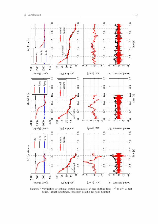
6 Verification 103
00.
20.
40.
60.
81.
050
0
1000
1500
2000
speed[1/min]
(a)S
port
ines
s
n 1 i 1n 2
i 2n 2
00.
20.
40.
60.
81.
00255075100
position[%]
actu
alde
sire
00.
20.
40.
60.
81.
0-2-10123
acc.[m/s2]
00.
20.
40.
60.
81.
0-4-2024
soundpressure[Pa]
time
[s]
00.
20.
40.
60.
81.
050
0
1000
1500
2000
speed[1/min]
(b)M
iddl
e
n 1 i 1n 2
i 2n 2
00.
20.
40.
60.
81.
00255075100
position[%]
00.
20.
40.
60.
81.
0-2-10123
acc.[m/s2]
00.
20.
40.
60.
81.
0-4-2024
soundpressure[Pa]
time
[s]
00.
20.
40.
60.
81.
050
0
1000
1500
2000
speed[1/min]
(c)C
omfo
rt
00.
20.
40.
60.
81.
00255075100
position[%]
00.
20.
40.
60.
81.
0-2-10123
acc.[m/s2]
00.
20.
40.
60.
81.
0-4-2024
soundpressure[Pa]
time
[s]
activ
ated
activ
ated
activ
ated
actu
alde
sire
actu
alde
sire
n 1 i 1n 2
i 2n 2
Figure 6.7: Verification of optimal control parameters of gear shifting from 1st to 2nd at testbench. (a) left: Sportiness, (b) center: Middle, (c) right: Comfort
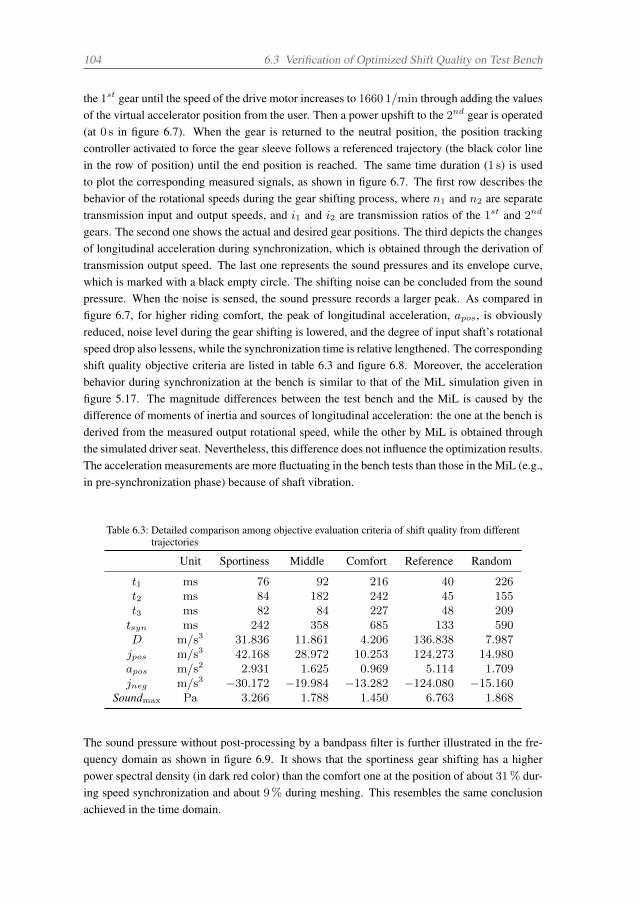
104 6.3 Verification of Optimized Shift Quality on Test Bench
the 1st gear until the speed of the drive motor increases to 1660 1/min through adding the valuesof the virtual accelerator position from the user. Then a power upshift to the 2nd gear is operated(at 0 s in figure 6.7). When the gear is returned to the neutral position, the position trackingcontroller activated to force the gear sleeve follows a referenced trajectory (the black color linein the row of position) until the end position is reached. The same time duration (1 s) is usedto plot the corresponding measured signals, as shown in figure 6.7. The first row describes thebehavior of the rotational speeds during the gear shifting process, where n1 and n2 are separatetransmission input and output speeds, and i1 and i2 are transmission ratios of the 1st and 2nd
gears. The second one shows the actual and desired gear positions. The third depicts the changesof longitudinal acceleration during synchronization, which is obtained through the derivation oftransmission output speed. The last one represents the sound pressures and its envelope curve,which is marked with a black empty circle. The shifting noise can be concluded from the soundpressure. When the noise is sensed, the sound pressure records a larger peak. As compared infigure 6.7, for higher riding comfort, the peak of longitudinal acceleration, apos, is obviouslyreduced, noise level during the gear shifting is lowered, and the degree of input shaft’s rotationalspeed drop also lessens, while the synchronization time is relative lengthened. The correspondingshift quality objective criteria are listed in table 6.3 and figure 6.8. Moreover, the accelerationbehavior during synchronization at the bench is similar to that of the MiL simulation given infigure 5.17. The magnitude differences between the test bench and the MiL is caused by thedifference of moments of inertia and sources of longitudinal acceleration: the one at the bench isderived from the measured output rotational speed, while the other by MiL is obtained throughthe simulated driver seat. Nevertheless, this difference does not influence the optimization results.The acceleration measurements are more fluctuating in the bench tests than those in the MiL (e.g.,in pre-synchronization phase) because of shaft vibration.
Table 6.3: Detailed comparison among objective evaluation criteria of shift quality from differenttrajectories
Unit Sportiness Middle Comfort Reference Random
t1 ms 76 92 216 40 226t2 ms 84 182 242 45 155t3 ms 82 84 227 48 209tsyn ms 242 358 685 133 590D m/s3 31.836 11.861 4.206 136.838 7.987jpos m/s3 42.168 28.972 10.253 124.273 14.980apos m/s2 002.931 1.625 0.969 5.114 1.709jneg m/s3 −30.172 −19.984 −13.282 −124.080 −15.160
Soundmax Pa 3.266 1.788 1.450 6.763 1.868
The sound pressure without post-processing by a bandpass filter is further illustrated in the fre-quency domain as shown in figure 6.9. It shows that the sportiness gear shifting has a higherpower spectral density (in dark red color) than the comfort one at the position of about 31% dur-ing speed synchronization and about 9% during meshing. This resembles the same conclusionachieved in the time domain.
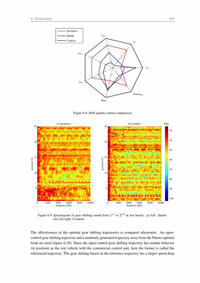
6 Verification 105
tsyn
D
jpos
apos
jneg
Wear
Soundmax
Sportiness
Middle
Comfort
Figure 6.8: Shift quality criteria comparison
posi
tion
[%]
9
27
36
45
18
(a) Sportiness (b) Comfort
posi
tion
[%]
9
27
36
45
18
frequency [Hz]0 2000 4000 6000 8000 10000
frequency [Hz]0 2000 4000 6000 8000 10000
PSD
-30
-40
-50
-60
-70
-80
-90
-100
Figure 6.9: Spectrogram of gear shifting sound from 1st to 2nd at test bench. (a) left: Sporti-ness,(b) right: Comfort
The effectiveness of the optimal gear shifting trajectories is compared afterwards. An open-control gear shifting trajectory and a randomly generated trajectory away from the Pareto-optimalfront are used (figure 6.10). Since the open-control gear shifting trajectory has similar behavior(in position) as the real vehicle with the commercial control unit, here the former is called thereferenced trajectory. The gear shifting based on the reference trajectory has a larger speed drop
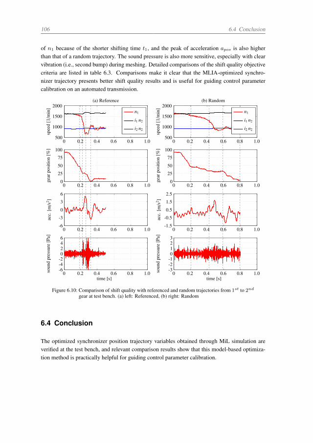
106 6.4 Conclusion
of n1 because of the shorter shifting time t1, and the peak of acceleration apos is also higherthan that of a random trajectory. The sound pressure is also more sensitive, especially with clearvibration (i.e., second bump) during meshing. Detailed comparisons of the shift quality objectivecriteria are listed in table 6.3. Comparisons make it clear that the MLIA-optimized synchro-nizer trajectory presents better shift quality results and is useful for guiding control parametercalibration on an automated transmission.
0 0.2 0.4 0.6 0.8 1.0500
1000
1500
2000
spee
d[1/m
in]
(a) Reference
n1
i1 n2
i2 n2
0 0.2 0.4 0.6 0.8 1.00
25
50
75
100
gear
posi
tion
[%]
0 0.2 0.4 0.6 0.8 1.0-6
-3
0
3
6
acc.
[m/s
2 ]
0 0.2 0.4 0.6 0.8 1.0-6-4-20246
soun
dpr
essu
re[P
a]
time [s]
0 0.2 0.4 0.6 0.8 1.0500
1000
1500
2000
spee
d[1/m
in]
(b) Random
0 0.2 0.4 0.6 0.8 1.00
25
50
75
100
gear
posi
tion
[%]
0 0.2 0.4 0.6 0.8 1.0-1.5
-0.5
0.5
1.5
2.5
acc.
[m/s
2 ]
0 0.2 0.4 0.6 0.8 1.0-3-2-10123
soun
dpr
essu
re[P
a]
time [s]
n1
i1 n2
i2 n2
Figure 6.10: Comparison of shift quality with referenced and random trajectories from 1st to 2nd
gear at test bench. (a) left: Referenced, (b) right: Random
6.4 Conclusion
The optimized synchronizer position trajectory variables obtained through MiL simulation areverified at the test bench, and relevant comparison results show that this model-based optimiza-tion method is practically helpful for guiding control parameter calibration.
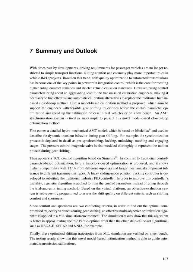
7 Summary and Outlook
With times past by developments, driving requirements for passenger vehicles are no longer re-stricted to simple transport functions. Riding comfort and economy play more important roles invehicle R&D projects. Based on this trend, shift quality optimization to automated transmissionshas become one of the key points in powertrain integration control, which is the core for meetinghigher riding comfort demands and stricter vehicle emission standards. However, rising controlparameters bring about an aggravating load to the transmission calibration engineers, making itnecessary to find effective and automatic calibration alternatives to replace the traditional human-based closed-loop method. Here a model-based calibration method is proposed, which aims tosupport the engineers with feasible gear shifting trajectories before the control parameter op-timization and speed up the calibration process in real vehicles or on a test bench. An AMTsynchronization system is used as an example to present this novel model-based closed-loopoptimization method.
First comes a detailed hydro-mechanical AMT model, which is based on Modelica® and used todescribe the dynamic transient behavior during gear shifting. For example, the synchronizationprocess is depicted in detail as pre-synchronizing, locking, unlocking, meshing and engagingstages. The pressure control magnetic valve is also modeled thoroughly to represent the motionprocess during gear shifting.
Then appears a TCU control algorithm based on Simulink®. In contrast to traditional control-parameter-based optimization, here a trajectory-based optimization is proposed, and it showshigher compatibility with TCUs from different suppliers and larger mechanical component tol-erance to different transmissions types. A fuzzy sliding-mode position tracking controller is de-veloped to substitute the traditional industry PID controller. In order to improve this controller’susability, a genetic algorithm is applied to train the control parameters instead of going throughthe trial-and-error tuning method. Based on the virtual platform, an objective evaluation sys-tem is subsequently programmed to assess the shift quality on different criteria such as shiftingcomfort and sportiness.
Since comfort and sportiness are two conflicting criteria, in order to find out the optimal com-promised trajectory variances during gear shifting, an effective multi-objective optimization algo-rithm is applied in a MiL simulation environment. The simulation results show that this algorithmis better in approximating the true Pareto-optimal front than the other state-of-the-art algorithms,such as NSGA-II, SPEA2 and NNIA, for example.
Finally, these optimized shifting trajectories from MiL simulation are verified on a test bench.The testing results show that this novel model-based optimization method is able to guide auto-mated transmission calibrations.
107
108
The proposed model-based optimization method for synchronizer shift quality can be introducedto other applications, e.g., clutch control during vehicle start. The multi-objective optimizationalgorithm can also be used on-line for test benches or real vehicles. Since the memetic algo-rithm consists of both global and local optimizations, experiment time may lengthen, so localoptimization can also be activated in the last generations alone.
The following improvements are expected in future research:
• temperature influence during modeling process can be brought in because the characteris-tics of certain system components do depend on this factor;
• distributed parallel computing should also be introduced to improve computational effi-ciency;
• alternative number of evolution generations and/or size of algorithm population couldbring the possibility of higher efficiency, especially in on-line applications;
• many-objective optimization (more than five criteria) might open up new space in shiftquality optimization;
• if more than three criteria are involved, method of selecting compromised optimal controlparameters should be considered further;
• using objective indicators such as accelerator position and its changes to bring drivinghabits into shift quality selection might be more driver-friendly;
• last but not least, the verification of the optimized position trajectories needs to be furthertested on a real vehicle.
References
[1] Global Analyst Briefing. Tech. rep. USA: PwC Autofacts, 2014 (cit. on p. 1).
[2] H. Naunheimer, B. Bertsche, J. Ryborz, and W. Novak. Automotive Transmissions: Fun-damentals, Selection, Design and Application. 2nd. Germany: Springer-Verlag BerlinHeidelberg, 2011 (cit. on pp. 2–4, 12, 24, 26, 32, 36, 39, 45).
[3] C. Atkinson and G. Mott. “Dynamic Model-based Calibration Optimization: An Intro-duction and Application to Diesel Engines.” In: SAE Technical Paper. USA, 2005 (cit.on p. 2).
[4] C. Atkinson, M. Allain, and H. Zhang. “Using Model-Based Rapid Transient Calibra-tion to Reduce Fuel Consumption and Emissions in Diesel Engines.” In: SAE TechnicalPaper. UAS, 2008 (cit. on p. 2).
[5] C. Atkinson. “Fuel Efficiency Optimization using Rapid Transient Engine Calibration.”In: SAE Technical Paper. USA, 2014 (cit. on p. 2).
[6] W. Schreiber, F. Rudolph, and V. Becker. “Das neue Doppelkupplungsgetriebe von Volk-swagen.” In: ATZ - Automobiltechnische Zeitschrift vol. 11 (2003) (cit. on p. 4).
[7] A. English. “CVT: Hochwertig und Leistungsstark.” In: Schaeffler Kolloquium. Ger-many, 2010, pp. 138–151 (cit. on p. 4).
[8] K. R. Henning Wallentowitz, ed. Handbuch Kraftfahrzeugelektronik: Grundlagen - Kom-ponenten - Systeme - Anwendungen. 2nd. Germany: Vieweg+Teubner Verlag, 2011 (cit.on pp. 4–7).
[9] C. Gühmann. “Model-Based Testing of Automotive Electronic Control Units.” In: 3rdInternational Conference on Materials Testing: Test 2005. Germany, 2005 (cit. on pp. 6–7).
[10] Hardware in the Loop for the MATLAB/Simulink Environment. Tech. rep. USA: AlteraCorporation, 2013 (cit. on p. 6).
[11] R. Isermann. Engine Modeling and Control: Modeling and Electronic Management ofInternal Combustion Engines. Germany: Springer Berlin Heidelberg, 2014 (cit. on p. 7).
[12] R. Isermann. Mechatronische Systeme: Grundlagen. 2nd. Germany: Springer BerlinHeidelberg, 2008 (cit. on p. 7).
[13] A. Schumacher. Optimierung mechanischer Strukturen, Grundlagen und industrielleAnwendungen. Germany: Springer Berlin Heidelberg, 2005 (cit. on p. 8).
[14] K. Deb. Multi-Objective Optimization using Evolutionary Algorithms. England: JohnWiley & Sons, Ltd, 2001 (cit. on pp. 8, 10–11).
109
110 References
[15] R. T. Marler and J. S. Arora. “Survey of Multi-objective Optimization Methods forEngineering.” In: Structural and Multidisciplinary Optimization vol. 26, no. 6 (2004),pp. 369–395 (cit. on p. 10).
[16] G. O. Odu and O. E. Charles-Owaba. “Review of Multi-criteria Optimization Methods -Theory and Applications.” In: IOSR Journal of Engineering vol. 3, no. 10 (2013), pp. 1–14 (cit. on p. 10).
[17] H. Eschenauer, J. Koski, and A. Osyczka, eds. Multicriteria Design Optimization: Pro-cedures and Application. Germany: Springer Berlin Heidelberg, 1990 (cit. on p. 10).
[18] T. W. Athan and P. Y. Papalambros. “A Note on Weighted Criteria Methods for Compro-mise Solutions in Multi-objective Optimization.” In: Engineering Optimization vol. 27,no. 2 (1996), pp. 155–176 (cit. on p. 10).
[19] W. Stadler. “Fundamentals of Multicriteria Optimization.” In: Multicriteria Optimizationin Engineering and in the Sciences. Ed. by W. Stadler. Vol. 37. Mathematical Conceptsand Methods in Science and Engineering. USA: Springer US, 1988, pp. 1–25 (cit. onp. 10).
[20] K. M. Miettinen. Nonlinear Multiobjective Optimization. USA: Kluwer Academic, 1999(cit. on pp. 10, 79).
[21] I. Das. “An Improved Technique for Choosing Parameters for Pareto Surface Genera-tion using Normal-boundary Intersection.” In: Third World Congress of Structural andMultidisciplinary Optimization. Vol. 2. New York, 1999, pp. 411–413 (cit. on p. 10).
[22] I. Das and J. E. Dennis. “Normal-Boundary Intersection: A New Method for Generatingthe Pareto Surface in Nonlinear Multicriteria Optimization Problems.” In: SIAM Journalon Optimization vol. 8, no. 3 (1998), pp. 631–657 (cit. on p. 10).
[23] A. Messac, A. Ismail-Yahaya, and C. Mattson. “The Normalized Normal ConstraintMethod for Generating the Pareto Frontier.” In: Structural and Multidisciplinary Opti-mization vol. 25, no. 2 (2003), pp. 86–98 (cit. on p. 10).
[24] A. Osyczka. “An Approach to Multicriterion Optimization Problems for EngineeringDesign.” In: Computer Methods in Applied Mechanics and Engineering vol. 15, no. 3(1978), pp. 309–333 (cit. on p. 10).
[25] S. S. Rao. “Game Theory Approach for Multiobjective Structural Optimization.” In:Computers & Structures vol. 25, no. 1 (1987), pp. 119–127 (cit. on p. 10).
[26] S. S. Rao and T. I. Freiheit. “A Modified Game Theory Approach to MultiobjectiveOptimization.” In: Journal of Mechanical Design vol. 113, no. 3 (1991), pp. 286–291(cit. on p. 10).
[27] C. M. Fonseca and P. J. Fleming. “An Overview of Evolutionary Algorithms in Multi-objective Optimization.” In: Evolutionary Computation vol. 3, no. 1 (1995), pp. 1–16(cit. on p. 10).
[28] H. Aguirre, K. Tanaka, and T. Sugimura. “Cooperative Model for Genetic Operators toImprove GAs.” In: Proceedings 1999 International Conference on Information Intelli-gence and Systems. USA, 10/1999, pp. 98–106 (cit. on p. 11).
References 111
[29] H. E. Aguirre and K. Tanaka. “Parallel Varying Mutation Genetic Algorithms.” In:Proceedings of the 2002 Congress on Evolutionary Computation. CEC ’02. Vol. 1. USA,05/2002, pp. 795–800 (cit. on p. 11).
[30] J. D. Schaffer. “Multiple Objective Optimization with Vector Evaluated Genetic Algo-rithms.” Dissertation. USA: Department of Electrical Engineering, Vanderbilt University,1984 (cit. on p. 11).
[31] M. Gong, L. Jiao, H. Du, and L. Bo. “Multiobjective Immune Algorithm with Nondom-inated Neighbor-based Selection.” In: Evolutionary Computation vol. 16, no. 2 (2008),pp. 225–255 (cit. on pp. 11–12, 79–82, 90).
[32] C. M. Fonseca and P. J. Fleming. “Genetic Algorithm for Multiobjective Optimization:Formulation, Discussion and Generation.” In: Proceedings of the 5th International Con-ference on Genetic Algorithms. USA, 1993, pp. 416–423 (cit. on p. 11).
[33] J. Horn, N. Nafpliotis, and D. Goldberg. “A Niched Pareto Genetic Algorithm for Multi-objective Optimization.” In: Proceedings of the First IEEE Conference on EvolutionaryComputation. IEEE World Congress on Computational Intelligence. USA, 06/1994, 82–87 vol.1 (cit. on p. 11).
[34] N. Srinivas and K. Deb. “Multiobjective Optimization using Nondominated Sorting inGenetic Algorithms.” In: Evolutionary Computation vol. 2, no. 3 (1994), pp. 221–248(cit. on p. 11).
[35] C. A. Coello Coello. “Recent Trends in Evolutionary Multiobjective Optimization.” In:Evolutionary Multiobjective Optimization. Advanced Information and Knowledge Pro-cessing. London: Springer, 2005, pp. 7–32 (cit. on p. 11).
[36] C. A. Coello Coello. “20 Years of Evolutionary Multi-Objective Optimization: WhatHas Been Done and What Remains To Be Done.” In: Computational Intelligence: Prin-ciples and Practice. Ed. by G. Y. Yen and D. B. Fogel. Canada: IEEE ComputationalIntelligence Society, 2006. Chap. 4, pp. 73–88 (cit. on p. 11).
[37] C. A. Coello Coello. “Evolutionary Multi-objective Optimization: a Historical Viewof the Field.” In: IEEE Computational Intelligence Magazine vol. 1, no. 1 (02/2006),pp. 28–36 (cit. on p. 11).
[38] E. Zitzler and L. Thiele. “Multiobjective Evolutionary Algorithms: a Comparative CaseStudy and the Strength Pareto Approach.” In: IEEE Transactions on Evolutionary Com-putation vol. 3, no. 4 (11/1999), pp. 257–271 (cit. on p. 11).
[39] E. Zitzler, M. Laumanns, and L. Thiele. “SPEA2: Improving the Strength Pareto Evo-lutionary Algorithm for Multiobjective Optimization.” In: Evolutionary Methods forDesign, Optimisation, and Control. Spain: CIMNE, Barcelona, Spain, 2002, pp. 95–100(cit. on p. 11).
[40] J. D. Knowles and D. W. Corne. “Approximating the Nondominated Front using thePareto Archived Evolution Strategy.” In: Evolutionary Computation vol. 8, no. 2 (2000),pp. 149–172 (cit. on p. 11).
112 References
[41] D. W. Corne, J. D. Knowles, and M. J. Oates. “The Pareto Envelope-based SelectionAlgorithm for Multiobjective Optimization.” In: Parallel Problem Solving from NaturePPSN VI. Vol. 1917. Lecture Notes in Computer Science. Germany: Springer BerlinHeidelberg, 2000, pp. 839–848 (cit. on p. 11).
[42] D. W. Corne, N. R. Jerram, J. D. Knowles, and M. J. Oates. “PESA-II: Region-basedSelection in Evolutionary Multiobjective Optimization.” In: Proceedings of the Geneticand Evolutionary Computation Conference (GECCO ’2001). USA, 2001, pp. 283–290(cit. on p. 11).
[43] K. Deb, A. Pratap, S. Agarwal, and T. Meyarivan. “A Fast and Elitist MultiobjectiveGenetic Algorithm: NSGA-II.” In: IEEE Transactions on Evolutionary Computationvol. 6, no. 2 (04/2002), pp. 182–197 (cit. on pp. 11, 80).
[44] P. Koduru, S. Das, and S. M. Welch. “Multi-objective Hybrid PSO using µ-fuzzy Dom-inance.” In: Proceedings of the 9th Annual Conference on Genetic and EvolutionaryComputation. GECCO ’07. London, England: ACM, 2007, pp. 853–860 (cit. on p. 11).
[45] A. G. Hernández-Díaz, L. V. Santana-Quintero, C. A. Coello Coello, and J. Molina.“Pareto-adaptive ϵ-dominance.” In: Evolutionary Computation vol. 15, no. 4 (2007),pp. 493–517 (cit. on p. 11).
[46] A. Lotov, V. A. Bushenkov, and G. K. Kamenev. Interactive Decision Maps: Approxi-mation and Visualization of Pareto Frontier. USA: Kluwer Academic Publishers, 2004(cit. on p. 11).
[47] J. B. Tenenbaum, V. de Silva, and J. C. Langford. “A Global Geometric Framework forNonlinear Dimensionality Reduction.” In: Science vol. 290, no. 5500 (2000), pp. 2319–2323 (cit. on p. 11).
[48] C. A. Coello Coello, G. Pulido, and M. Lechuga. “Handling Multiple Objectives withParticle Swarm Optimization.” In: IEEE Transactions on Evolutionary Computationvol. 8, no. 3 (06/2004), pp. 256–279 (cit. on p. 12).
[49] Q. Zhang and H. Li. “MOEA/D: A Multiobjective Evolutionary Algorithm Based onDecomposition.” In: IEEE Transactions on Evolutionary Computation vol. 11, no. 6(12/2007), pp. 712–731 (cit. on p. 12).
[50] J. E. Smith. “Coevolving Memetic Algorithms: A Review and Progress Report.” In:IEEE Transactions on Systems, Man, and Cybernetics, Part B: Cybernetics vol. 37, no. 1(02/2007), pp. 6–17 (cit. on p. 12).
[51] G. Alvermann. “Virtuelle Getriebeabstimmung.” Dissertation. Germany: Instituts fürFahrzeugtechnik, Technische Universität Braunschweig, 2009 (cit. on pp. 12–13).
[52] Verein Deutscher Ingenieure. Einwirkungen mechanischer Schwingungen auf den Men-schen - Ganzkörper - Schwingungen. Düsseldorf, 2002 (cit. on pp. 12, 71).
[53] A. Hagerodt. “Automatisierte Optimierung des Schaltkomforts von Automatikgetrieben.”Dissertation. Germany: Instituts für Fahrzeugtechnik, Technische Universität Braunschweig,2003 (cit. on pp. 12–13).
References 113
[54] E.-J. Hurard. “Kundenorientierte Objektiverung des Schaltkomforts zur Anwendung inder Simulation.” Dissertation. Germany: Instituts für Fahrzeugtechnik, Technischen Uni-versität Braunschweig, 2009 (cit. on p. 12).
[55] S. Kahlbau. “Mehrkriterielle Optimierung des Schaltablaufs von Automatikgetriebe.”Dissertation. Germany: Fakultät für Maschinenbau, Elektrotechnik und Wirtschaftsinge-nieurwesen, Brandenburgischen Technischen Universität, 2013 (cit. on pp. 12–13).
[56] J.-M. Birkhold. “Komfortobjektivierung und funktionale Bewertung als Methoden zurUnterstützung der Entwicklung des Wiederstartsystems in parallelen Hybridantrieben.”Dissertation. Germany: Fakultät für Maschinenbau, Karlsruher Institut für Technologie,2013 (cit. on p. 12).
[57] A. Hagerodt, J. Boehl, G. Alvermann, and F. Küçükay. “Automated Calibration of theShifting Comfort for Automatic Transmissions.” In: FISITA World Automotive Congress.Barcelona, 23-27 May/2004, pp. 1–25 (cit. on pp. 12–13).
[58] H. Liu, Y. Lei, J. Zhang, J. Qiu, et al. “Shift Quality Optimization Based on AssessmentSystem for Dual Clutch Transmission.” In: SAE Technical Paper. USA, 2012 (cit. onpp. 12–13).
[59] Y. Fu, Y. Lei, S. Shaohua, H. Zeng, et al. “Shift Quality Evaluation of DCT Based onTOPSIS Model.” In: SAE Technical Paper. USA, 2014 (cit. on p. 12).
[60] W. Jian, G. Konghui, L. Y. Lei, and T. Hua. “Support Vector Machine Theory basedShift Quality Assessment for Automated Mechanical Transmission (AMT).” In: SAETechnical Paper. USA, 04/2007 (cit. on pp. 12–13).
[61] P. Schoeggl and E. Ramschak. “Vehicle Driveability Assessment using Neural Networksfor Development, Calibration and Quality Tests.” In: SAE Technical Paper. USA, 2000(cit. on p. 13).
[62] J. Böhl. “Effiziente Abstimmung von Automatikgetrieben.” Dissertation. Germany: In-stituts für Fahrzeugtechnik, Technische Universität Braunschweig, 2007 (cit. on p. 13).
[63] G. Chen, W. Zhang, Z. Gong, and W. Sun. “Evaluation Model for Vehicle Shift QualityBased on Evidence Theory and FNN.” In: Pacific-Asia Workshop on ComputationalIntelligence and Industrial Application, 2008. PACIIA ’08. Vol. 1. China, 12/2008,pp. 837–841 (cit. on p. 13).
[64] H. Zeng, Y. Lei, Y. Fu, and Y. Li. “Analysis of a Shift Quality Metric for a Dual ClutchTransmission.” In: SAE International Journal of Passenger Cars- Mechanical Systemsvol. 6, no. 2 (2013), pp. 798–804 (cit. on p. 13).
[65] T.-M. Wolter, S. Kahlbau, D. Bestle, and T. Liebezeit. “Guided Transmission Calibra-tion using the Example of AT.” In: 10th Internationales CTI Symposium für InnovativeFahrzeug-Getriebe und Hybrid Elektro-Antriebe. Berlin, 12/2011, pp. 445–454 (cit. onp. 13).
[66] A. Wurm, T.-M. Wolter, and S. Kahlbau. “New Approach for Transmission Calibration- Model-based Multi-objective Optimization via SIL.” In: 7th International CTI Sympo-sium and Exhibition. USA, 05/2013 (cit. on pp. 13, 71).
114 References
[67] H. O. List and P. Schoeggl. “Objective Evaluation of Vehicle Driveability.” In: SAETechnical Paper. USA, 1998 (cit. on p. 13).
[68] M. Nybacka, D. Holmlund, and C. Danner. AVL-DRIVE Pre-study Report. Tech. rep.Sweden: Department of Applied Physics and Mechanical Engineering, Division of Func-tional Product Development, Luleå University of Technology, 09/2009 (cit. on p. 13).
[69] G. Kokalj, J. Lewis, C. Zach, and R. Ekachaiworasin. “INNOVATION - Significant Re-duction of Powertrain Calibration Effort in Production Programs: Automated Calibrationof Driveability on Chassis Dyno and Powertrain Testbed.” In: 8th International Confer-ence on Automotive Engineering (ICAE-8). Thailand, 04/2012 (cit. on p. 13).
[70] H. Huang, D. Di, Y. Chu, and C. Gühmann. “Model-Based Optimization for an AMTClutch Control during the Vehicle Starting.” In: SAE International Journal of PassengerCars - Electronic and Electrical Systems vol. 8, no. 1 (2015), pp. 90–98 (cit. on p. 14).
[71] P. D. Walker and N. Zhang. “Modelling of Dual Clutch Transmission Equipped Pow-ertrains for Shift Transient Simulations.” In: Mechanism and Machine Theory vol. 60(2013), pp. 47–59 (cit. on p. 17).
[72] L. Lovas, D. Play, J. Marialigeti, and J. F. Rigal. “Mechanical Behaviour Simulationfor Synchromesh Mechanism Improvements.” In: Proceedings of the Institution of Me-chanical Engineers, Part D: Journal of Automobile Engineering vol. 220, no. 7 (2006),pp. 919–945 (cit. on pp. 17, 100).
[73] J. Kim, D. Sung, C. Seok, H. Kim, et al. “Development of Shift Feeling Simulator for aManual Transmission.” In: SAE Technical Paper. USA, 2002 (cit. on p. 17).
[74] G. Lucente, M. Montanari, and C. Rossi. “Modelling of an Automated Manual Trans-mission System.” In: Mechatronics vol. 17, no. 2-3 (2007), pp. 73–91 (cit. on pp. 17,22).
[75] M. Zoppi, C. Cervone, G. Tiso, and F. Vasca. “Software in the Loop Model and Decou-pling Control for Dual Clutch Automotive Transmissions.” In: 3rd International Confer-ence on Systems and Control (ICSC). Algiers, 10/2013 (cit. on p. 17).
[76] E. Galvagno, M. Velardocchia, and A. Vigliani. “Dynamic and Kinematic Model of aDual Clutch Transmission.” In: Mechanism and Machine Theory vol. 46, no. 6 (2011),pp. 794–805 (cit. on p. 17).
[77] X.-Y. Song, Z.-X. Sun, X.-J. Yang, and G.-M. Zhu. “Modelling, Control, and Hardware-in-the-Loop Simulation of an Automated Manual Transmission.” In: Proceedings ofthe Institution of Mechanical Engineers, Part D: Journal of Automobile Engineeringvol. 224, no. 2 (2010), pp. 143–160 (cit. on p. 17).
[78] M.-V. Bataus and N. Vasiliu. “Modeling of a Dual Clutch Transmission for Real-timeSimulation.” In: Scientific Bulletin vol. 74, no. 2 (2012), pp. 251–264 (cit. on p. 17).
[79] G. Tao, T. Zhang, and H. Chen. “Modeling of Shift Hydraulic System for AutomaticTransmission.” In: International Conference on Consumer Electronics, Communicationsand Networks (CECNet). China, 04/2011, pp. 474–477 (cit. on p. 17).
References 115
[80] R. Amari, M. Alamir, and P. Tona. “Unified MPC Strategy for Idle-speed Control, Vehi-cle Start-up and Gearing Applied to an Automated Manual Transmission.” In: Proceed-ings of the 17th IFAC World Congress. Seoul, Korea, 07/2008, pp. 7079–7085 (cit. onp. 17).
[81] M. Cipek, J. Deur, and J. Petric. “Bond Graph Analysis of Power Flow in Series-parallelHybrid Electric Vehicle Transmissions.” In: UKACC International Conference on Con-trol. Coventry, 2010, pp. 1–7 (cit. on p. 17).
[82] J.-H. Kim and D.-i. Cho. “An Automatic Transmission Model for Vehicle Control.” In:IEEE Conference on Intelligent Transportation System, 1997. ITSC ’97. Boston, MA,1997, pp. 759–764 (cit. on p. 17).
[83] Y. Zhang, X. Zhang, H. Jiang, X. Chen, et al. “Dynamic Modeling and Simulation ofa Dual-clutch Automated Lay-shaft Transmission.” In: Journal of Mechanical Designvol. 127, no. 2 (2005), pp. 302–307 (cit. on p. 17).
[84] M. Jiang, W. Chen, Y. Zhang, and L. Chen. “Multi-domain Modeling and Simulation ofAMT Based on Modelica.” In: SAE Technical Paper. 2011 (cit. on p. 17).
[85] Modelica Standard Library (2008), version 3.1. Product Help. Modelica Association,2008 (cit. on pp. 17, 19).
[86] M. M. Tiller. Introduction to Physical Modeling with Modelica. USA: Kluwer Academic,2004 (cit. on p. 17).
[87] H. Huang, S. Nowoisky, R. Knoblich, and C. Gühmann. “Modeling and Testing of theHydro-Mechanical Synchronization System for a Double Clutch Transmission.” In: Pro-ceedings of the 9th International Modelica Conference. Linköping Electronic ConferenceProceedings 76. Munich, Germany, 09/2012, pp. 284–294 (cit. on pp. 18, 26, 28).
[88] H. Huang, S. Nowoisky, R. Knoblich, and C. Gühmann. “Modeling and Simulation ofan Automated Manual Transmission System.” In: Proceedings of the 7th InternationalConference on Integrated Modeling and Analysis in Applied Control and Automation(IMAACA). Athens, Greece, 25-27. September/2013, pp. 44–51 (cit. on p. 18).
[89] H. Huang, S. Nowoisky, R. Knoblich, and C. Gühmann. “Multi-domain Modelling andSimulation of an Automated Manual Transmission System based on Modelica.” In: In-ternational Journal of Simulation and Process Modelling vol. 10, no. 3 (2015), pp. 253–264 (cit. on p. 18).
[90] HyLib (2009), version 2.7. Product Help. Modelon, 2009 (cit. on pp. 19, 21).
[91] Volkswagen. Self-study Programme 221: Electronic Manual Gearbox, Design and Func-tion. Volkswagen AG. Germany, 1999 (cit. on p. 20).
[92] H. E. Merritt. Hydraulic Control Systems. USA: John Wiley & Sons, Inc., 06/1967 (cit.on p. 22).
[93] M. Montanari, F. Ronchi, C. Rossi, A. Tilli, et al. “Control and Performance Evaluationof a Clutch Servo System with Hydraulic Actuation.” In: Control Engineering Practicevol. 12, no. 11 (2004), pp. 1369–1379 (cit. on p. 22).
[94] INA. Automotive Product Information API 14: Detent Pins for Automotive Transmis-sions. Schaeffler Technologies AG & Co. KG. Germany, 8/2007 (cit. on p. 25).
116 References
[95] E. Kirchner. Leistungsübertragung in Fahrzeuggetrieben. Germany: Springer-VerlagBerlin Heidelberg, 2007 (cit. on p. 27).
[96] INA. Automotive Product Information API 06: Intermediate Rings for Multi-Cone Syn-chronizer Systems. Schaeffler Technologies AG & Co. KG. Germany, 8/2007 (cit. onp. 27).
[97] S. Nowoisky and C. Gühmann. “Automated Parameter Identification for Nonlinear Com-ponents of an Automated Transmission.” In: Design of Experiments (DoE) in EngineDevelopment. Germany, 2013, pp. 306–317 (cit. on p. 29).
[98] H. Scherf. Modellbildung und Simulation dynamischer Systeme: Eine Sammlung vonSimulink-Beispielen. 4th. Germany: Oldenbourg Wissenschaftsverlag, 2010 (cit. onp. 32).
[99] J. Lei and L. Li. “The Structure Design and Application of the Waveform Spring.” Chi-nese. In: Heavy Machinery Science and Technology vol. 02 (1999), pp. 9–11 (cit. onp. 32).
[100] J. O. Alemen and A. László. “The Uniform-section Disk Spring.” In: Trans. ASMEvol. 58, no. 10 (1936), pp. 305–314 (cit. on p. 33).
[101] Luk. Luk Clutch Course: An Introduction to Clutch Technology for Passenger Cars,Schaeffler Automotive Aftermarket GmbH & Co. KG. Germany, 05/2012 (cit. on p. 36).
[102] H.-J. Drexl. Kraftfahrzeugkupplungen: Function und Auslegung. Germany, 1997 (cit. onp. 36).
[103] S. Nowoisky and C. Gühmann. “Automated Parameter Identification for a Dry Clutch.”In: 10th International Multi-Conference on Systems, Signals and Devices (SSD). Ham-mamet, Tunesien, 18-21. March/2013, pp. 978–984 (cit. on p. 37).
[104] Dymola (2010), version 7.4. Product Help. Dynasim AB, 2010 (cit. on p. 37).
[105] R. Knoblich, C. Gühmann, and J. Beilharz. “Modellbasierte Steuergeräteentwicklung fürKfz-Getriebesysteme am Prüfstand.” In: Tagungsband Mechatronik. Dresden, 31. March- 1.April/2011 (cit. on pp. 37, 97).
[106] S. Nowoisky, R. Knoblich, and C. Gühmann. “Prüfstand für die Identifikation und denFunktionstest an automatisierten Schaltgetrieben.” In: Virtuelle Instrumente in der Praxis2012; Begleitband zum 17. VIP-Kongress. XIV. Germany: VDE-Verlag, 2012, pp. 150–156 (cit. on pp. 37, 97).
[107] Y. Zhu. “Model-based Development and Validation of the Traveling System for a Passen-ger Vehicle.” Master Thesis. Germany: Chair of Electronic Measurement and DiagnosticTechnology, Department of Energy and Automation Technology, Technische UniversitätBerlin, 2014 (cit. on pp. 41, 70, 94).
[108] J. Oh, J. Kim, and S. Choi. “Robust Feedback Tracking Controller Design for Self-Energizing Clutch Actuator of Automated Manual Transmission.” In: SAE Int. J. Pas-seng. Cars - Mech. Syst. Vol. 6, no. 3 (2013), pp. 1510–1517 (cit. on p. 46).
[109] F. Garofalo, L. Glielmo, L. Iannelli, and F. Vasca. “Optimal Tracking for Automotive DryClutch Engagement.” In: 15th IFAC World Congress. Barcelona, Spain, 2002 (cit. onp. 46).
References 117
[110] X. Wang, X. Xie, X. Wu, and T. Yu. “Precise Position Tracking Control based on Adap-tive Neuron PID Algorithm for Automatic Clutch Driven by DC Motor.” In: IEEE VehiclePower and Propulsion Conference. Harbin, 09/2008, pp. 1–4 (cit. on p. 46).
[111] X. C. M. Cubillos and L. C. G. de Souza. “Using of H-Infinity Control Method in AttitudeControl System of Rigid-Flexible Satellite.” In: Mathematical Problems in Engineeringvol. 2009 (2009), pp. 1–9 (cit. on p. 46).
[112] H. M. L. Gabasa. “LQR Controller Tuning by using Particle Swarm Optimization.” Mas-ter Thesis. Malaysia: Faculty of Electrical Engineering, Universiti Teknologi Malaysia,2009 (cit. on p. 46).
[113] T.-T. Hu, Y.-F. Zhuang, and J. Yu. “An Improved Single Neuron Adaptive PID ControllerBased on Levenberg-Marquardt Algorithm.” In: Advances in Brain Inspired CognitiveSystems. Vol. 7366. Lecture Notes in Computer Science. Germany: Springer BerlinHeidelberg, 2012, pp. 288–295 (cit. on p. 46).
[114] R. DeCarlo, S. Zak, and G. Matthews. “Variable Structure Control of Nonlinear Multi-variable Systems: a Tutorial.” In: Proceedings of the IEEE vol. 76, no. 3 (1988), pp. 212–232 (cit. on p. 48).
[115] Information Resources Management Association. Research Methods: Concepts, Method-ologies, Tools, and Applications. USA: IGI Global, 2015 (cit. on p. 48).
[116] J. Liu and X. Wang. Advanced Sliding Mode Control for Mechanical Systems: Design,Analysis and MATLAB Simulation. Germany: Springer-Verlag Berlin Heidelberg, 2011(cit. on p. 48).
[117] A. T. Azar and Q. Zhu, eds. Advances and Applications in Sliding Mode Control Systems.Switzerland: Springer International Publishing, 2015 (cit. on pp. 48, 51).
[118] P. Jagiello. “Model-based Development of Sliding Mode Position Control for a DryClutch System.” Bachelor Thesis. Germany: Chair of Electronic Measurement and Di-agnostic Technology, Department of Energy and Automation Technology, TechnischeUniversität Berlin, 2014 (cit. on p. 48).
[119] K. B. Goh, S. K. Spurgeon, and N. B. Jones. “Higher-order Sliding Mode Control of aDiesel Generator Set.” In: Proceedings of the Institution of Mechanical Engineers, PartI: Journal of Systems and Control Engineering vol. 217, no. 3 (2003), pp. 229–241 (cit.on pp. 49, 51).
[120] H. Huang, C. Gühmann, and Y. Yu. “Second-order Sliding Mode Control of the EngineSpeed for an Automated Manual Transmission during Gear Shifting Process.” In: 11thInternational Multi-Conference on Systems, Signals and Devices (SSD). Castelldefels-Barcelona, Spain, 11-14, February/2014 (cit. on pp. 49, 68).
[121] W. Perruquetti and J. P. Barbot, eds. Sliding Mode Control in Engineering. New York,USA: Marcel Dekker, Inc., 2002 (cit. on pp. 49–50).
[122] A. LEVANT. “Sliding Order and Sliding Accuracy in Sliding Mode Control.” In: Inter-national Journal of Control vol. 58, no. 6 (1993), pp. 1247–1263 (cit. on p. 49).
[123] A. Levant. “Robust Exact Differentiation via Sliding Mode Technique.” In: Automaticavol. 34, no. 3 (1998), pp. 379–384 (cit. on pp. 50, 52).
118 References
[124] Y. Yasui, K. Shimojo, M. Saito, and Y. Tamagawa. “Rapid Engine Speed Control forAMT using Two-degree-of-freedom Sliding Mode Algorithm.” In: SAE Technical Paper.USA, 2005 (cit. on p. 51).
[125] K. Nakano, U. Sawut, K. Higuchi, and Y. Okajima. “Modelling and Observer-basedSliding-Mode Control of Electronic Throttle Systems.” In: ECTI Transactions on Elec-trical Eng., Electronics, and Communications vol. 4, no. 1 (02/2006), pp. 22–28 (cit. onp. 51).
[126] M. Baric, I. Petrovic, and N. Peric. “Neural Network-based Sliding Mode Control ofElectronic Throttle.” In: Engineering Applications of Artificial Intelligence vol. 18, no. 8(2005), pp. 951–961 (cit. on p. 51).
[127] J. V. Tu. “Advantages and Disadvantages of using Artificial Neural Networks versusLogistic Regression for Predicting Medical Outcomes.” In: Journal of Clinical Epidemi-ology vol. 49, no. 11 (1996), pp. 1225–1231 (cit. on p. 51).
[128] F. Plestan, Y. Shtessel, V. Brégeault, and A. Poznyak. “New Methodologies for Adap-tive Sliding Mode Control.” In: International Journal of Control vol. 83, no. 9 (2010),pp. 1907–1919 (cit. on p. 51).
[129] F. Plestan, Y. Shtessel, V. Brégeault, and A. Poznyak. “Sliding Mode Control withGain Adaptation-Application to an Electropneumatic Actuator.” In: Control EngineeringPractice vol. 21, no. 5 (2013), pp. 679–688 (cit. on p. 51).
[130] A. Kareem and M. F. Azzem. “A Novel Fuzzy Logic Based Adaptive Super-twistingSliding Mode Control Algorithm for Dynamic Uncertain Systems.” In: InternationalJournal of Artificial Intelligence & Applications vol. 3, no. 4 (07/2012), pp. 21–34 (cit.on p. 51).
[131] G. Chen and T. T. Pham. Introduction to Fuzzy Sets, Fuzzy Logic, and Fuzzy ControlSystems. USA: CRC Press, 2000 (cit. on p. 51).
[132] S.-J. Huang and W.-C. Lin. “Adaptive Fuzzy Controller with Sliding Surface for VehicleSuspension Control.” In: IEEE Transactions on Fuzzy Systems vol. 11, no. 4 (08/2003),pp. 550–559 (cit. on p. 51).
[133] S.-J. Huang and H.-Y. Chen. “Adaptive Sliding Controller with Self-tuning Fuzzy Com-pensation for Vehicle Suspension Control.” In: Mechatronics vol. 16, no. 10 (2006),pp. 607–622 (cit. on p. 51).
[134] J. Lin, R.-J. Lian, C.-N. Huang, and W.-T. Sie. “Enhanced Fuzzy Sliding Mode Controllerfor Active Suspension Systems.” In: Mechatronics vol. 19, no. 7 (2009). Special Issueon Hardware-in-the-Loop Simulation, pp. 1178–1190 (cit. on p. 51).
[135] J. RAGOT and M. LAMOTTE. “Fuzzy Logic Control.” In: International Journal ofSystems Science vol. 24, no. 10 (1993), pp. 1825–1848 (cit. on pp. 52, 59).
[136] J. Zhao and B. Bose. “Evaluation of Membership Functions for Fuzzy Logic ControlledInduction Motor Drive.” In: 28th Annual Conference of IEEE Industrial ElectronicsSociety. Vol. 1. Spain, 11/2002, pp. 229–234 (cit. on p. 52).
[137] N. K. Kasabov. Foundations of Neural Networks, Fuzzy Systems, and Knowledge Engi-neering. USA: The MIT Press, 1998 (cit. on p. 53).
References 119
[138] W. S. Levine, ed. The Control Handbook. 2nd. USA: CRC Press, 2010 (cit. on p. 53).
[139] T. J. Ross. Fuzzy Logic with Engineering Application. 3rd. USA: John Wiley & Sons,Ltd, 2010 (cit. on p. 53).
[140] G. Venter. “Review of Optimization Techniques.” In: Encyclopedia of Aerospace Engi-neering. John Wiley & Sons, Ltd, 2010 (cit. on p. 54).
[141] J. S. Arora, O. Elwakeil, and A. Chahande. “Global Optimization Methods for Engineer-ing Application: A Review.” In: Structural Optimization vol. 9, no. 3-4 (1995), pp. 137–159 (cit. on p. 54).
[142] S. M. Baker, K. Schallau, and B. H. Junker. “Comparison of Different Algorithms forSimultaneous Estimation of Multiple Parameters in Kinetic Metabolic Models.” In: Jour-nal of Integrative Bioinformatics vol. 7, no. 3 (2010), pp. 1–9 (cit. on p. 54).
[143] J. Kennedy and R. Eberhart. “Particle Swarm Optimization.” In: Neural Networks, 1995.Proceedings., IEEE International Conference on. Vol. 4. Perth, WA, 11/1995, pp. 1942–1948 (cit. on p. 54).
[144] R. Hassan, B. Cohanim, O. de Weck, and G. Venter. “A Copmarison of Particle SwarmOptimization and the Genetic Algorithm.” In: 46th AIAA/ASME/ASCE/AHS/ASC Struc-tures, Structural Dynamics and Materials Conference. Austlin, Texas, 04/2005, pp. 1–13(cit. on p. 54).
[145] S. Panda and N. P. Padhy. “Comparison of Particle Swarm Optimization and GeneticAlgorithm for FACTS-based Controller Design.” In: Applied Soft Computing vol. 8,no. 4 (2008). Soft Computing for Dynamic Data Mining, pp. 1418–1427 (cit. on p. 54).
[146] S. S. Rao. Engineering Optimization: Theory and Practice. USA: John Wiley & Sons,Inc., 1996 (cit. on p. 54).
[147] R. Rojas. Neural Networks: A Systematic Introduction. Germany: Springer Berlin Hei-delberg, 1996 (cit. on p. 54).
[148] J. McCall. “Genetic Algorithms for Modelling and Optimisation.” In: Journal of Compu-tational and Applied Mathematics vol. 184, no. 1 (2005). Special Issue on MathematicsApplied to Immunology, pp. 205–222 (cit. on p. 55).
[149] D. Chen. “Optimization of an Adaptive Fuzzy Sliding-mode Position Control for anAMT System based on Genetic Algorithms.” Master Thesis. Germany: Chair of Elec-tronic Measurement and Diagnostic Technology, Department of Energy and AutomationTechnology, Technische Universität Berlin, 2014 (cit. on p. 55).
[150] T. Bäck. “Selective Pressure in Evolutionary Algorithms: A Characterization of SelectionMechanisms.” In: Proceedings of the First IEEE Conference on Evolutionary Computa-tion. IEEE World Congress on Computational Intelligence. Orlando, FL, 1994, 57–62vol.1 (cit. on pp. 55, 57).
[151] K. Jebari and M. Madiafi. “Selection Methods for Genetic Algorithm.” In: InternationalJournal of Emerging Sciences vol. 3, no. 4 (12/2013), pp. 333–344 (cit. on p. 55).
[152] J. H. Holland. Adaptation in Natural and Artificial Systems: An Introductory Analysiswith Applications to Biology, Control and Artificial Intelligence. USA: The MIT Press,1992 (cit. on p. 55).
120 References
[153] N. M. Razali and J. Geraghty. “Genetic Algorithm Performance with Different SelectionStrategies in Solving TSP.” In: Proceeding of the World Congress on Engineering 2011Vol. II. London, UK, 6-8 July/2011 (cit. on p. 55).
[154] J. E. Baker. “Reducing Bias and Inefficiency in the Selection Algorithm.” In: Proceed-ings of the 2nd International Conference on Genetic Algorithms on Genetic Algorithmsand Their Application. Cambridge, Massachusetts, USA: L. Erlbaum Associates Inc.,1987, pp. 14–21 (cit. on p. 55).
[155] B. L. Miller and D. E. Goldberg. “Genetic Algorithms, Tournament Selection, and theEffects of Noise.” In: Complex Systems vol. 9, no. 3 (1995), pp. 193–212 (cit. on p. 55).
[156] O. Findik, M. S. Kiran, and I. Babaoglu. “Investigation Effects of Selection Mecha-nisms for Gravitational Search Algorithm.” In: Journal of Computer and Communica-tions vol. 2, no. 4 (2014), pp. 117–126 (cit. on p. 55).
[157] D. Vrajitoru. “Crossover Improvement for the Genetic Algorithm in Information Re-trieval.” In: Information Processing & Management vol. 34, no. 4 (1998), pp. 405–415(cit. on p. 57).
[158] J. Magalhães-Mendes. “A Comparative Study of Crossover Operators for Genetic Algo-rithm to Solver the Job Shop Scheduling Problem.” In: WSEAS Transactions on Com-puters vol. 12, no. 4 (04/2013), pp. 164–173 (cit. on p. 57).
[159] Z. Michalewicz. Genetic Algorithms + Data Structures = Evolution Programs. 3rd, rev.and extended edition. Germany: Springer-Verlag Berlin Heidelberg, 1996 (cit. on p. 57).
[160] R. Hinterding. “Gaussian Mutation and Self-adaption for Numeric Genetic Algorithms.”In: IEEE International Conference on Evolutionary Computation. Vol. 1. Australia,11/1995, pp. 384–389 (cit. on p. 57).
[161] K. Deb and R. B. Agrawal. “Simulated Binary Crossover for Continuous Search Space.”In: Complex Systems vol. 9, no. 2 (1995), pp. 115–148 (cit. on p. 57).
[162] C. Hang and Y. Cheung. “Using a GA Adaptor in Multi-applications.” In: ComputationalScience - ICCS 2003. Vol. 2660. Lecture Notes in Computer Science. Melbourne,Australia and St. Petersburg, Russia: Springer Berlin Heidelberg, 2003, pp. 839–848(cit. on p. 58).
[163] M. Safe, J. Carballido, I. Ponzoni, and N. Brignole. “On Stopping Criteria for GeneticAlgorithms.” In: Advances in Artificial Intelligence - SBIA 2004. Ed. by A. Bazzanand S. Labidi. Vol. 3171. Lecture Notes in Computer Science. Brazil: Springer BerlinHeidelberg, 2004, pp. 405–413 (cit. on p. 58).
[164] T.-P. Hong and C.-Y. Lee. “Induction of Fuzzy Rules and Membership Functions fromTraining Examples.” In: Fuzzy Sets and Systems vol. 84 (1996), pp. 33–47 (cit. on p. 59).
[165] J. Ye. “Entwicklung eines Rapid Prototype Systems für die Softwareentwicklung vonautomatisierten Getrieben.” Master Thesis. Germany: Chair of Electronic Measurementand Diagnostic Technology, Department of Energy and Automation Technology, Tech-nische Universität Berlin, 2014 (cit. on p. 66).
References 121
[166] Y. Chu. “Model-based Development of the AMT Shift Quality Objective EvaluationSystem.” Master Thesis. Germany: Chair of Electronic Measurement and DiagnosticTechnology, Department of Energy and Automation Technology, Technische UniversitätBerlin, 2014 (cit. on p. 69).
[167] O. Thuong and M. J. Griffin. “The Vibration Discomfort of Standing Persons: Evaluationof Random and Transient Motions.” In: Ergonomics vol. 54, no. 12 (2011), pp. 1228–1239 (cit. on p. 71).
[168] F. Tao, L. Zhang, and Y. Laili. Configurable Intelligent Optimization Algorithm: Designand Practice in Manufacturing. Springer Series in Advanced Manufacturing. Switzer-land: Springer International Publishing, 2015 (cit. on p. 78).
[169] M. Gong, C. Liu, L. Jiao, and G. Cheng. “Hybrid Immune Algorithm with LamarckianLocal Search for Multi-objective Optimization.” In: Memetic Computing vol. 2, no. 1(2010), pp. 47–67 (cit. on p. 78).
[170] P. Moscato. On Evolution, Search, Optimization, Genetic Algorithms and Martial Arts:Towards Memetic Algorithms. Tech. rep. 826. USA: Caltech Concurrent ComputationProgram 158-79, California Institute of Technology, 1989 (cit. on p. 78).
[171] X. Chen, Y.-S. Ong, M.-H. Lim, and K. C. Tan. “A Multi-Facet Survey on Memetic Com-putation.” In: IEEE Transactions on Evolutionary Computation vol. 15, no. 5 (10/2011),pp. 591–607 (cit. on p. 78).
[172] R. Dawkins. The Selfish Gene. Oxford, UK: Oxford University Press, 2006 (cit. onp. 78).
[173] S. Blackmore. The Meme Machine. New York: Oxford University Press, 1999 (cit. onp. 78).
[174] R. Kicinger and T. Arciszewski. “Empirical Analysis of Memetic Algorithms for Con-ceptual Design of Steel Structural Systems in Tall Buildings.” In: Advances in Engineer-ing Structures, Mechanics & Construction. Vol. 140. Solid Mechanics and Its Applica-tions. Dordrecht: Springer Netherlands, 2006, pp. 277–288 (cit. on p. 78).
[175] E. Hart and J. Timmis. “Application Areas of AIS: The Past, the Present and the Future.”In: Artificial Immune Systems. Ed. by C. Jacob, M. Pilat, P. Bentley, and J. Timmis.Vol. 3627. Lecture Notes in Computer Science. Germany: Springer Berlin Heidelberg,2005, pp. 483–497 (cit. on p. 79).
[176] M. J. D. Powell. “An Efficient Method for Finding the Minimum of a Function of Sev-eral Variables without Calculating Derivatives.” In: The Computer Journal vol. 7, no. 2(1964), pp. 155–162 (cit. on p. 82).
[177] J. Chen, Q. Lin, and Z. Ji. “A Hybrid Immune Multiobjective Optimization Algorithm.”In: European Journal of Operational Research vol. 204, no. 2 (2010), pp. 294–302 (cit.on pp. 85, 88).
[178] A. Zhou, Y. Jin, Q. Zhang, B. Sendhoff, et al. “Combining Model-based and Genetics-based Offspring Generation for Multi-objective Optimization Using a Convergence Crite-rion.” In: IEEE Congress on Evolutionary Computation (CEC). Canada, 2006, pp. 892–899 (cit. on p. 89).

122 References
[179] D. Di. “Multi-objective Optimization of the AMT Shift Quality during the Gear ShiftingProcess.” Master Thesis. Germany: Chair of Electronic Measurement and DiagnosticTechnology, Department of Energy and Automation Technology, Technische UniversitätBerlin, 2014 (cit. on p. 90).
[180] Z. Jin, M. Ouyang, Q. Lu, and D. Gao. “Development of Simulation and Real timeConrol Platform for Fuel Cell Powertrain.” In: China Mechanical Engineering vol. 19,no. 15 (2008), pp. 1879–1882 (cit. on p. 98).
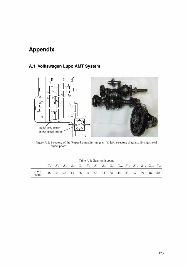
Appendix
A.1 Volkswagen Lupo AMT System
43
1 25
R
Z1Z2
Z3Z6
Z7
Z4
Z8
Z9 Z10Z11 Z12 Z13
Z14
Z15
Z5
input speed sensoroutput speed sensor
Figure A.1: Structure of the 5-speed transmission gear. (a) left: structure diagram, (b) right: realobject photo
Table A.1: Gear tooth count
Z1 Z2 Z3 Z4 Z5 Z6 Z7 Z8 Z9 Z10 Z11 Z12 Z13 Z14 Z15
toothcount 48 33 22 13 28 11 53 34 38 44 43 39 39 18 60
123
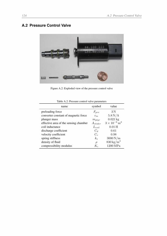
124 A.2 Pressure Control Valve
A.2 Pressure Control Valve
Figure A.2: Exploded view of the pressure control valve
Table A.2: Pressure control valve parameters
name symbol value
preloading force Fpre 3Nconverter constant of magnetic force cm 5.8N/Aplunger mass mplgr 0.021 kgeffective area of the sensing chamber Aslider 3× 10⁻⁶ m2
coil inductance Lcoil 0.01Hdischarge coefficient Cd 0.61velocity coefficient Cv 0.98spring stiffness ks 3000N/mdensity of fluid ρ 830 kg/m3
compressibility modulus Kc 1200MPa
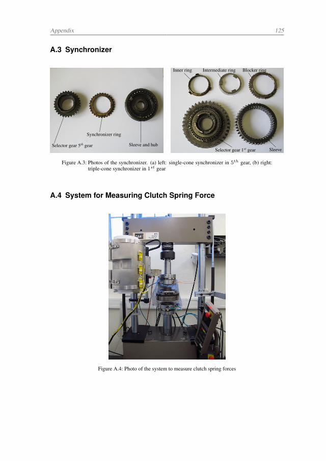
Appendix 125
A.3 Synchronizer
Inner ring Intermediate ring Blocker ring
Selector gear 1st gearSelector gear 5th gear
Synchronizer ring
Sleeve and hubSleeve
Figure A.3: Photos of the synchronizer. (a) left: single-cone synchronizer in 5th gear, (b) right:triple-cone synchronizer in 1st gear
A.4 System for Measuring Clutch Spring Force
Figure A.4: Photo of the system to measure clutch spring forces
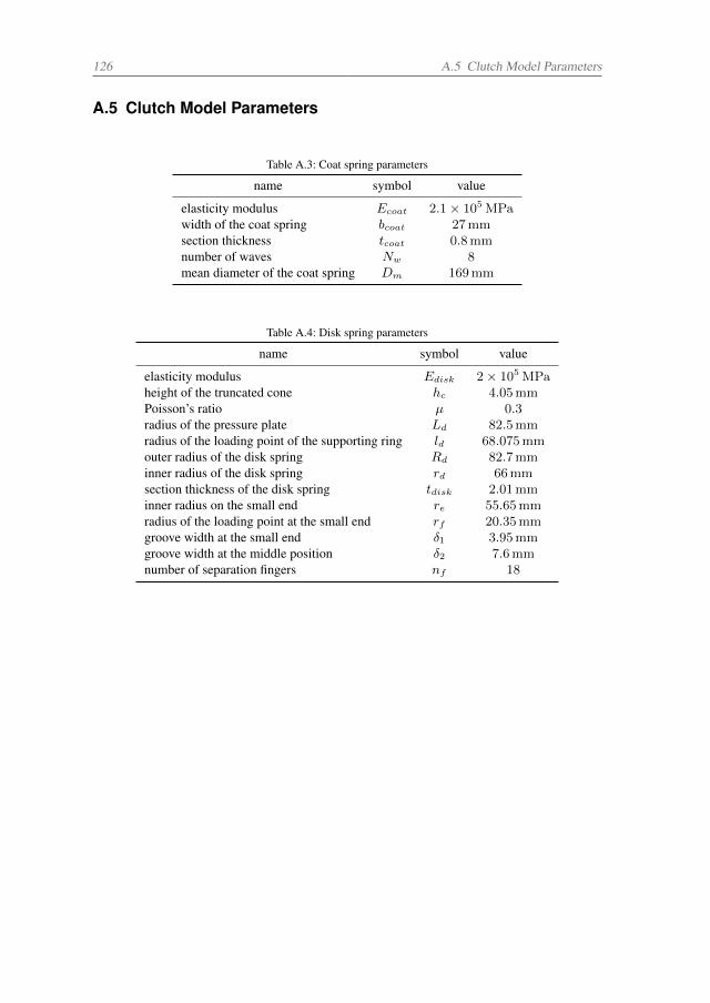
126 A.5 Clutch Model Parameters
A.5 Clutch Model Parameters
Table A.3: Coat spring parameters
name symbol value
elasticity modulus Ecoat 2.1× 10⁵ MPawidth of the coat spring bcoat 27mmsection thickness tcoat 0.8mmnumber of waves Nw 8mean diameter of the coat spring Dm 169mm
Table A.4: Disk spring parameters
name symbol value
elasticity modulus Edisk 2× 10⁵ MPaheight of the truncated cone hc 4.05mmPoisson’s ratio µ 0.3radius of the pressure plate Ld 82.5mmradius of the loading point of the supporting ring ld 68.075mmouter radius of the disk spring Rd 82.7mminner radius of the disk spring rd 66mmsection thickness of the disk spring tdisk 2.01mminner radius on the small end re 55.65mmradius of the loading point at the small end rf 20.35mmgroove width at the small end δ1 3.95mmgroove width at the middle position δ2 7.6mmnumber of separation fingers nf 18
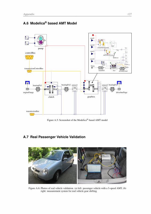
Appendix 127
A.6 Modelica® based AMT Model
controlBus
transmissionControlBus
engineFlange drivelineFlage
transmissionBus
clutch gearbox
sensor1 sensor2bearingFri1 bearingFri2 bearingFri3
pump
?.
signal1
signal2
signal3
signal4
flangeaflangeb
check
shiftValveSystem
switchValveSystemGate
shiftlever
mainShaft secondaryshaftSyn
s3
sgate
sgear
ω2
ω1
Fsyn
S tatussyn
Figure A.5: Screenshot of the Modelica® based AMT model
A.7 Real Passenger Vehicle Validation
Figure A.6: Photos of real vehicle validation. (a) left: passenger vehicle with a 5-speed AMT, (b)right: measurement system for real vehicle gear shifting
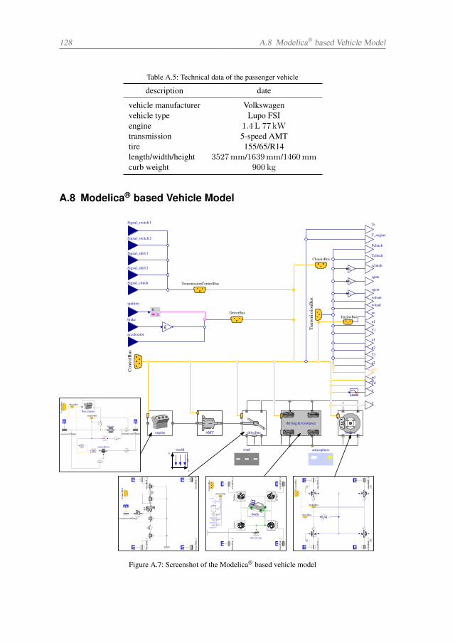
128 A.8 Modelica® based Vehicle Model
Table A.5: Technical data of the passenger vehicle
description date
vehicle manufacturer Volkswagenvehicle type Lupo FSIengine 1.4L 77 kWtransmission 5-speed AMTtire 155/65/R14length/width/height 3527mm/1639mm/1460mmcurb weight 900 kg
A.8 Modelica® based Vehicle Model
x
y
_m/s
km/h
R
B
Con
trol
Bus
Tran
smis
sion
Bus
Signal_switch 1
Signal_switch 2
Signal_shift 1
Signal_shift 2
Signal_clutch
ignition
brake
accelerator
k
TransmissionControlBus
DriverBus
ChassisBus
engine AMT driveline brakes
world road atmosphere
k2
k2
k2
EngineBus
Te
T_engine
Pclutch
Tclutch
sclutch
sgate
wfront
wload
ne
n1
T1
a1
n2
T2
a2
syn
ndTd
v
a
sgear
driving & resistance
w
w
w
w
Con
trol
Bus
whe
elH
ub_1
whe
elH
ub_2
whe
elH
ub_3
whe
elH
ub_4
1/4driverBus
brakesBus
<
and
rad/s
1/min w
tau
tau
Con
trol
Bus
Base_Engine
JEngine
tau
accessoryFlange transmissionFlange
starterMotor
driverBus
engineBus
d= dc= c
d =d
c =c
Con
trol
Bus
transmissionFlange
whe
elH
ub_1
whe
elH
ub_2
whe
elH
ub_3
whe
elH
ub_4
diff
.
Con
trol
Bus
chassisBus
chassisLong.
whe
elH
ub_1
whe
elH
ub_2
whe
elH
ub_3
whe
elH
ub_4
bodys
vehicleDis tancev_x
vehicleVelocity
a_x
vehicleAccel
yawRate
k=0
v_x_s tart
y1
y2
y3
y4
whe
el1
whe
el3
wheel2
wheel4
Figure A.7: Screenshot of the Modelica® based vehicle model
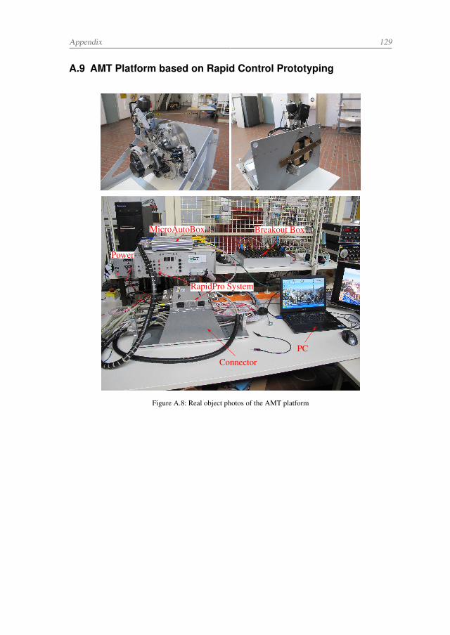
Appendix 129
A.9 AMT Platform based on Rapid Control Prototyping
Connector
PC
MicroAutoBox Breakout Box
RapidPro System
Power
Figure A.8: Real object photos of the AMT platform
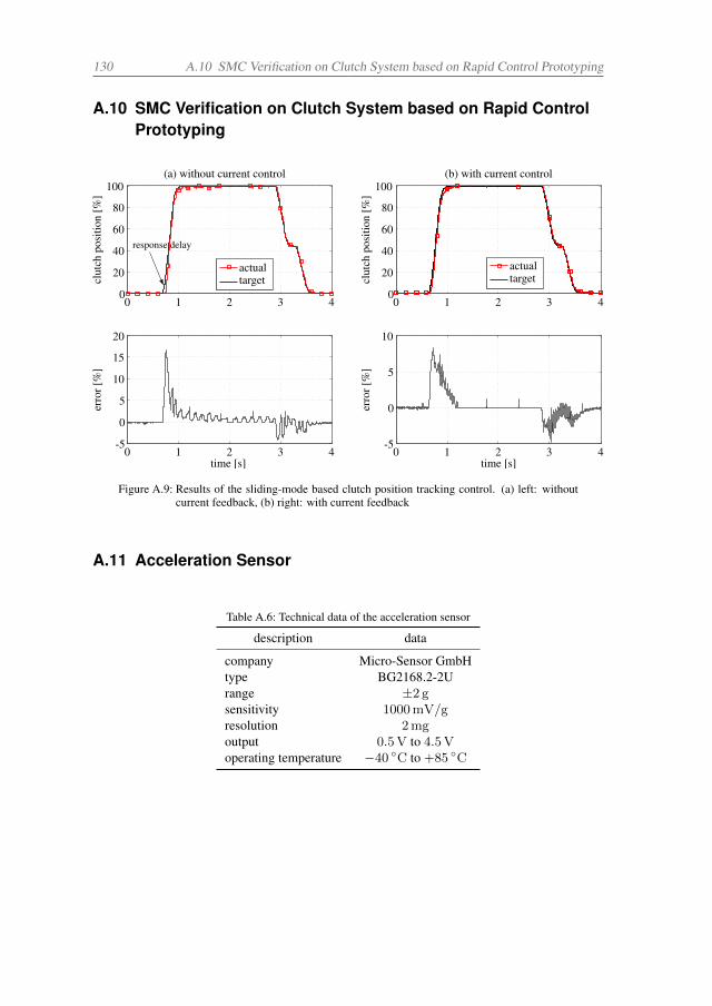
130 A.10 SMC Verification on Clutch System based on Rapid Control Prototyping
A.10 SMC Verification on Clutch System based on Rapid ControlPrototyping
0 1 2 3 40
20
40
60
80
100
clut
chpo
sitio
n[%
]
(a) without current control
actualtarget
0 1 2 3 4-5
0
5
10
15
20
time [s]
erro
r[%
]
0 1 2 3 40
20
40
60
80
100
clut
chpo
sitio
n[%
]
(b) with current control
0 1 2 3 4-5
0
5
10
time [s]
erro
r[%
]
actualtarget
response delay
Figure A.9: Results of the sliding-mode based clutch position tracking control. (a) left: withoutcurrent feedback, (b) right: with current feedback
A.11 Acceleration Sensor
Table A.6: Technical data of the acceleration sensor
description data
company Micro-Sensor GmbHtype BG2168.2-2Urange ±2 gsensitivity 1000mV/gresolution 2mgoutput 0.5V to 4.5Voperating temperature −40 C to +85 C
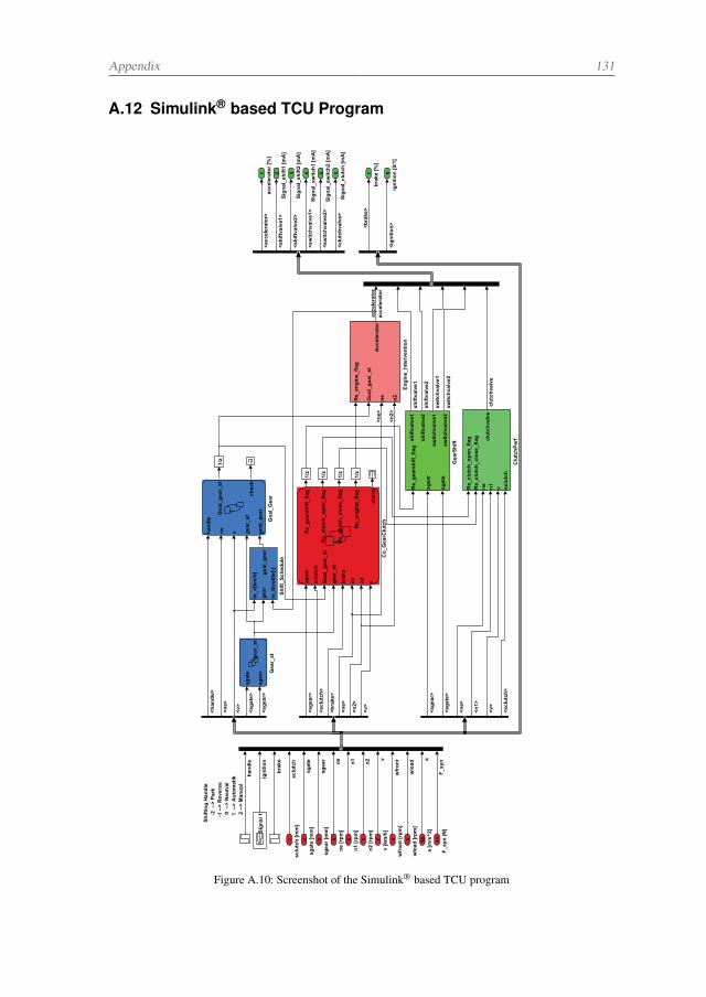
Appendix 131
A.12 Simulink® based TCU Program
Figure A.10: Screenshot of the Simulink® based TCU program
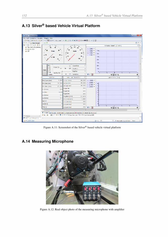
132 A.13 Silver® based Vehicle Virtual Platform
A.13 Silver® based Vehicle Virtual Platform
Figure A.11: Screenshot of the Silver® based vehicle virtual platform
A.14 Measuring Microphone
Figure A.12: Real object photo of the measuring microphone with amplifier
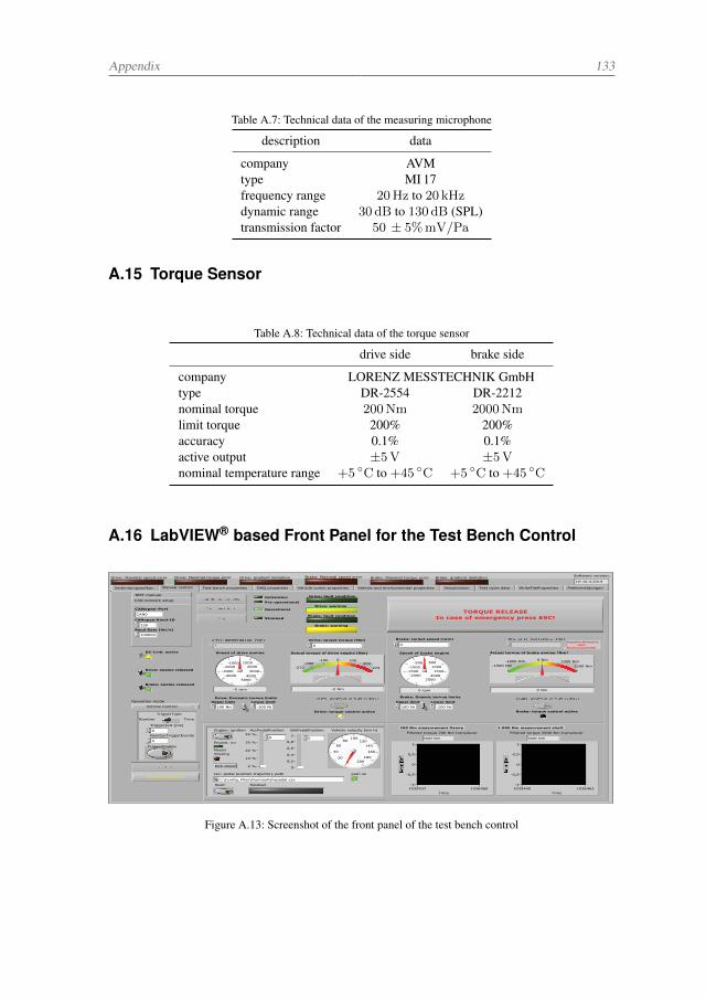
Appendix 133
Table A.7: Technical data of the measuring microphone
description data
company AVMtype MI 17frequency range 20Hz to 20 kHzdynamic range 30 dB to 130 dB (SPL)transmission factor 50 ± 5%mV/Pa
A.15 Torque Sensor
Table A.8: Technical data of the torque sensor
drive side brake side
company LORENZ MESSTECHNIK GmbHtype DR-2554 DR-2212nominal torque 200Nm 2000Nmlimit torque 200% 200%accuracy 0.1% 0.1%active output ±5V ±5Vnominal temperature range +5 C to +45 C +5 C to +45 C
A.16 LabVIEW® based Front Panel for the Test Bench Control
Figure A.13: Screenshot of the front panel of the test bench control
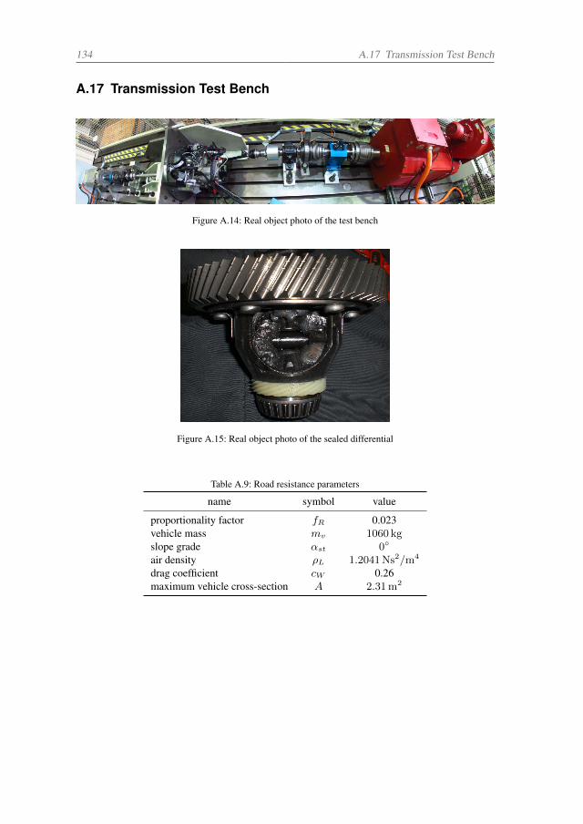
134 A.17 Transmission Test Bench
A.17 Transmission Test Bench
Figure A.14: Real object photo of the test bench
Figure A.15: Real object photo of the sealed differential
Table A.9: Road resistance parameters
name symbol value
proportionality factor fR 0.023vehicle mass mv 1060 kgslope grade αst 0
air density ρL 1.2041Ns2/m4
drag coefficient cW 0.26maximum vehicle cross-section A 2.31m2
Mod
el-b
ased
Cal
ibra
tion
of A
utom
ated
Tra
nsm
issi
ons
Universitätsverlag der TU Berlin
Advances in Automation Engineering Band 2
The shift quality calibration is typically performed in real vehicles on the road, where the calibration engineers try different control parameters till the subjective assessment on the shift quality meets certain requirements, such as shifting comfort or sportiness. Howe-ver, compared with today‘s multiplying number of variants in vehicle-engine-transmission combinations and exponential growth of control parameters, this traditional method is becoming backward and costly. An efficient way to rise to the challenge is the model-based automatic calibration. In contrast to the conventional shift quality calibration, this method uses a closed loop approach based on a dynamic model instead of human know-how. In this work a hydro-mechanical synchronization system in an automated manual transmission is used as an example, and a position-trajectory-based shift quality optimi-zation process is presented. A non-linear dynamic transmission model is built to describe the transient behavior during gear shifting in detail. A fuzzy sliding-mode controller is de-signed for the tracking of gear shifting positions. A multi-objective evolutionary algorithm is developed to find out the optimal set of control parameters. In the end the optimized parameters are verified at a transmission test bench.
Hu
a Hu
ang
2
Model-based Calibration of Automated Transmissions
Editor: Clemens Gühmann
Universitätsverlag der TU Berlin
I S B N 9 7 8 - 3 - 7 9 8 3 - 2 8 5 8 - 79 783798 328587
ISBN 978-3-7983-2858-7 (print)ISBN 978-3-7983-2859-4 (online)
http://verlag.tu-berlin.de
Hua Huang
Model-based Calibration of Automated Transmissions
Umschlag_17x24_huang.indd 1 07.10.2016 12:10:46