Kindermann et al. Carbon Balance andManagement 2013, 8:2http://www.cbmjournal.com/content/8/1/2

RESEARCH Open Access

Potential stocks and increments of woodybiomass in the European Union underdifferent management and climate scenariosGeorg E Kindermann1*, Stefan Schorghuber2, Tapio Linkosalo3, Anabel Sanchez4, Werner Rammer2,Rupert Seidl2 and Manfred J Lexer2

Abstract

Background: Forests play an important role in the global carbon flow. They can store carbon and can also providewood which can substitute other materials. In EU27 the standing biomass is steadily increasing. Increments andharvests seem to have reached a plateau between 2005 and 2010. One reason for reaching this plateau will be thecircumstance that the forests are getting older. High ages have the advantage that they typical show high carbonconcentration and the disadvantage that the increment rates are decreasing. It should be investigated how biomassstock, harvests and increments will develop under different climate scenarios and two management scenarios whereone is forcing to store high biomass amounts in forests and the other tries to have high increment rates and muchharvested wood.

Results: A management which is maximising standing biomass will raise the stem wood carbon stocks from 30 tC/hato 50 tC/ha until 2100. A management which is maximising increments will lower the stock to 20 tC/ha until 2100. Theestimates for the climate scenarios A1b, B1 and E1 are different but there is much more effect by the managementtarget than by the climate scenario. By maximising increments the harvests are 0.4 tC/ha/year higher than in themanagement which maximises the standing biomass. The increments until 2040 are close together but around 2100the increments when maximising standing biomass are approximately 50% lower than those when maximisingincrements. Cold regions will benefit from the climate changes in the climate scenarios by showing higher increments.

Conclusions: The results of this study suggest that forest management should maximise increments, not stocks to bemore efficient in sense of climate change mitigation. This is true especially for regions which have already high carbonstocks in forests, what is the case in many regions in Europe. During the time span 2010–2100 the forests of EU27 willabsorb additional 1750 million tC if they are managed to maximise increments compared if they are managed tomaximise standing biomass. Incentives which will increase the standing biomass beyond the increment optimalbiomass should therefore be avoided. Mechanisms which will maximise increments and sustainable harvests need tobe developed to have substantial amounts of wood which can be used as substitution of non sustainable materials.

BackgroundForests play an important role in the global carbon flow.They can be used to store carbon and can also pro-vide wood which can substitute non sustainable fossilfuel based energy sources or used e.g. for constructionand furniture. Carbon storage and wood production arepossible at the same time but they are also competing. If

*Correspondence: kinder@iiasa.ac.at1International Institute for Applied Systems Analysis (IIASA), Schlossplatz 1,A-2361 Laxenburg, AustriaFull list of author information is available at the end of the article

the management target is set to produce as much woodas is sustainable possible, which can be used as construc-tion wood or for biofuel, will result in forests which areyounger and have less standing biomass than a manage-ment target which is maximising the standing biomass.Both targets will help in climate mitigation. One by stor-ing carbon in the forest the other by substituting fossilmaterials and storing the carbon in the not used fossils.Forests also need to adapt to climate changes. Climate

change will lead to increment changes and shifts in com-petition between tree species [1]. One practical way to

© 2013 Kindermann et al.; licensee BioMed Central Ltd. This is an Open Access article distributed under the terms of the CreativeCommons Attribution License (http://creativecommons.org/licenses/by/2.0), which permits unrestricted use, distribution, andreproduction in any medium, provided the original work is properly cited.

Kindermann et al. Carbon Balance andManagement 2013, 8:2 Page 2 of 20http://www.cbmjournal.com/content/8/1/2

make this adaptation is to select during reforestation treespecies suitable to the new site conditions. This adap-tation needs one rotation time to change from one toanother species. The rotation times in forest manage-ment systems maximising the standing biomass are muchlonger than those maximising increments. [2] showedthat an increasing growth trend can be observed in mostcases, apart from some specific sites in Europe. [3] givenet annual increment for EU27 with 550.6 mill.m3 (1990),597.8 mill.m3 (2000), 619.5 mill.m3 (2005) and 608.9mill.m3 (2010). It looks like that the annual incrementshave reached a peak around the year 2005 especially ifit is taken into account that the forest area is increas-ing from 146.1 mill.ha (1990), 152.8 mill.ha (2000), 154.7mill.ha (2005) to 157.2 mill.ha (2010). This incrementtrend reversal can be caused by many reasons. One obvi-ous reason will be found in the increasing share of oldforests in EU27. Forests show a typical increment pat-tern over age [4]. Young forests show low increments perhectare and year which are increasing with age until acertain age where the increment is culminating and a fur-ther increasing age shows a decreasing increment. Thispattern is e.g. site, species and stand density depending.The standing biomass is increasing with an increasingage until the age of the climax phase and will declinein the following disaggregation phase. Those growth andbiomass developments can be interrupted by several dis-asters. [3] show that the carbon in forests (above andbelow ground) is increasing from 7 806 MtC (1990),8 782 MtC (2000), 9 317 MtC (2005) to 9 901 MtC(2010). This trend of increasing carbon stock is not onlycaused by the increasing forest area. It is also causedby higher average carbon stocks per hectare. This trenddoes currently not show to reach a peak. A decliningincrement rate and a constantly increasing biomass stockcan only be realised by a reduction in harvests, andexactly this has been reported by [3] with 325.5 mill.m3

(1990), 378.1 mill.m3 (2000), 408.5 mill.m3(2005) and387.6 mill.m3 (2010). The harvest pattern is following theincrement pattern. Assuming a balanced age–site distri-bution this correlation between increment and harvestsseems perfect for sustainable forest management. But thegap between increments and harvests cause an increasingaverage age and biomass and at certain point a decreas-ing wood increment. [5] showed the development of thistrend until 2030 with an estimated marginal increas-ing wood demand for the time span 2005–2030. Theyalso showed that the estimated increments are slowlydecreasing until 2030. Beside the age and stand den-sity with the current species composition, the incrementtrend is also affected by site factors. In the past environ-ment pollution will have lowered the site productivity.Nowadays a changing climate and CO2 concentrationshow influence.

Most of the climate mitigation literature so far hasassessed the potential contribution of purposeful man-agement of terrestrial ecosystemmanagement in terms ofdelivery of carbon neutral biomass for energy productionwhere the overall terrestrial sink was assumed to stay con-stant over time [6]. [7] and all yield tables and most forestgrowth models which have been produced and used inforestry since that time, showed that using forests as car-bon storage and for biomass production at the same timecan not maximise both. If a forest has high incrementsit has medium standing biomass, if it has high standingbiomass it has low increments. Both management targets(maximise increment – maximise standing biomass) arecompeting against each other. To show the effect of cli-mate and management, forest growthmodels can be used.They can show the effect of climate change on site andits productivity rate. They can also show the effect of dif-ferent management targets. Here we use a combination ofplot and large scale forest growth models and couple cli-mate scenarios with one management scenario which isincreasing biomass stock and another which is increas-ing the increment rates. This allows showing the effect onstanding biomass, harvests and increments and giving arecommendation which of those management targets willbe better in respect of climate mitigation.

Results and discussionDifferent climate and management scenarios show a typ-ical development of the standing biomass over time.Figure 1 shows the development of the average standingstem carbon in EU27 assuming that the current forestarea stays constant. The effect of the chosen manage-ment target has much more influence on the standingbiomass than the different climate scenarios. The cur-rently standing ≈30 tC/ha can be raised to ≈50 tC/hawithin the next 60 years. The total forest area of EU27is around 155 million hectares what makes a total car-bon storage increase of around 3100 million tC until 2070where the potential of carbon storage by choosing a longrotation time is reached. Of the climate scenarios E1 hasthe lowest potential. A1b and B1 show higher carbon stor-age potentials compared to the baseline but at the end ofthe century they loose some standing biomass and comevery close together with the baseline scenario. The man-agement which is maximising the increment decreasesthe currently standing stem biomass from ≈30 tC/ha to20 tC/ha in 2100. This decrease is not caused by unsus-tainable usage or forest degradation. It is caused by thefact, that a forest, which is managed to produce optimalincrements, has a certain stand density and also a cer-tain rotation time which determines the standing biomass[8]. Starting from forests which have low stand density,very short rotation times or low standing biomass wouldshow an increasing biomass with a increment optimising

Kindermann et al. Carbon Balance andManagement 2013, 8:2 Page 3 of 20http://www.cbmjournal.com/content/8/1/2

2020 2040 2060 2080 2100

2025

3035

4045

50

Year

Sto

ckin

g S

tem

Car

bon

[tC/h

a]

BaselineA1bB1E1

MaxIncMaxBmMaxInc + Change Species

Figure 1 Stem carbon development under conditions of baseline and three climate change scenarios (A1b, B1 and E1) and threemanagement scenarios (maximise stocking biomass, maximise increments with and without change of species).

management regime. Reasons why the forest owners don’tuse their increment potential can be that harvests of largerand older trees are most of the time cheaper [9], highharvest amounts will lower market prices of wood as itcan be seen e.g. after large wind throws or the harvest-ing costs are higher than the wood price. Also the timberprice depends on the tree dimensions. So an economicharvest decision will minimise harvesting costs and max-imise timber prices by having high harvest amount. In thismanagement scenario the E1 scenario shows also the low-est standing biomass and A1b and B1 are slightly abovebaseline but come in the year 2090 very close together.By allowing a change of tree species groups the standingbiomass is at the end of this century about 3 tC/ha higherthan the scenario that keeps the same species. In total thismakes a carbon loss at around 1550 million tC until 2100.Comparing both management scenarios the one whichis maximising biomass will store in 2100 approximately4650 million tC more than the management-option that ismaximising increments.Figure 2 shows the amount of removed stem wood per

hectare and year. The amount of removed stem woodincludes planned harvests but also unplanned mortality.Here the picture is contrary to the standing stem car-bon (Figure 1) by having high amounts of harvest whenmaximising increment and low harvest amounts whenmaximising the standing stem carbon. By maximisingincrements harvests amounts are around 0.4 tC/ha/yearhigher than in the management that maximises the stand-ing biomass. For B1 in the time span 2010–2100 thismakes additional harvests of 40 tC/ha when maximisingincrement compared to maximising standing carbon. ForEU27 in the time span 2010–2100 this makes in total10 200 million tC stem wood harvests in the scenariomaximising standing biomass but 16 600 million tC whenmaximising increments.

The scenario with and without species change showfor this time range nearly the same values as the newplanted species are mainly used by thinning. Some ofthose trees which are planted in the beginning of the sim-ulation period can reach in the end of the simulation anage suitable for final harvest. The change from one toanother species shows in the years until 2070 lower andafterwards higher harvest rates and it looks like that thisnew species are superior in the years after 2070. This indi-cates that decisions which are made today have a positiveeffect only in the long run. This is true especially for thespecies selection under changing environment.If someone has to select a species today for regenera-

tion someone can choose those species which are suitablefor the current conditions or for the conditions expectedin the future. The species selected for current conditionswill be adapted to the current conditions but might haveproblems with future conditions, if selecting it for futureconditions it might not survive until the time when theconditions fit. Also it is vague how the site conditions willbe in the future. A risk reduction can be found in usingseveral species for regeneration. They can be planted inpure stands but also in mixed forests. Mixed forests canbut need not increase the increment rate compared to apure stand [10,11]. If one species is suffering in a mixedstand the other species can make use the growing spaceof the suffering species and keep the total increment rateon a high level. In mixed stands one species can e.g.increase the water stress of another species [12] and alsothe regulation on the competition on light will need anincreased management effort compared with pure stands.The species selection has also an effect on rotation time.Assuming there are two species showing the same poten-tial of increment and are in all other concerns equivalentbut have a different growth pattern which one should bepreferred. Tomake it more illustrative let’s say one species

Kindermann et al. Carbon Balance andManagement 2013, 8:2 Page 4 of 20http://www.cbmjournal.com/content/8/1/2

2020 2040 2060 2080 2100

0.4

0.6

0.8

1.0

1.2

1.4

Year

Har

vest

ed S

tem

Car

bon

[tC/h

a/Ye

ar] Baseline A1b B1 E1

MaxInc MaxBm MaxInc + Change Species

Figure 2 Removed stem wood under conditions of baseline and three climate change scenarios (A1b, B1 and E1) and three managementscenarios (maximise stocking biomass, maximise increments with and without change of species).

is robinia, the other one oak. Oak shows in young ageslow increments and is increasing slowly but is keeping theincrement rate in old ages on a high level what results inapplying long rotation times. Robinia shows a fast raiseof increments in young ages but also a fast decrease inolder ages what results in applying short rotation times.The long rotation times will cause high standing biomassbut causes also a long time to change from one species toanother. The short rotation will show the opposite. A rec-ommendation in species selection will not be easy but acombination of short and long rotation will increase thenumber of species what spreads the risk. A combination ofshort and long rotation in the same stand can be realisedwith middle forest (coppice with standards), plenter andfemel systembut not with clear cut. Those silviculture sys-tems will at least increase the management and harvestingcosts and can cause different wood qualities. Using forestsin very short rotation will have the disadvantages that thesize of the trees might be small and can not be used assawn wood what causes low wood prices. Also the car-bon storage and the increments are reduced. A reductionof biomass opens the possibility to use for a short timemore wood than is growing again. This amount of har-vests will be increased for a short time in many regionsof EU27 if the rotation time is reduced to an incrementoptimal rotation time for current species. If the replantedspecies have a shorter increment optimal rotation timeand with this a lower standing biomass, this short timeharvest amount is further increased. This opens the pos-sibility to substitute now more fossil fuels and developin the meanwhile efficient technologies which allow areduction of energy use int the future. These increasedharvests must not exceed the point where an additionalreduction of the standing biomass causes a reduction offorest increment.

In E1 harvest shows a peak near 2070 which is causedby increasedmortality caused by a climate situation whichstresses the trees. It can also be seen, that the forests whichare maximising biomass show more mortality (peaks inharvest amount) than those maximising increments. [3]shows also an increasing damage from 1990 to 2005. Onthe one hand this higher mortality is caused by the higherstanding biomass on the other hand by the increased sen-sitivity of older trees against stress. If the damaged woodremains in the stand, the carbon will be stored there forsome time, and especially wood of larger dimensions tendto decompose much slower than fine litter and will alsoincrease the soil carbon. On the other hand this damagedand left wood can not be used for substitution and canincrease the risk that the remaining trees are also dam-aged. In scenario A1b and B1 the harvests since 2050are slowly decreasing when maximising increments andkeeping the same species but they are increasing whenmaximising biomass. This is caused by a decreasing sitesuitability of the trees. This reduces the increments andso the model reduces the harvests but this reduction isovercompensated by mortality in the scenario which ismaximising biomass. It can also bee seen, that the levelof harvests could be more or less held constant duringthe simulation period in the management scenario whichchanges tress species. The deviation in the baseline sce-nario is caused by a climate pattern and the age structureof the forests. Comparing bothmanagement scenarios theone which is maximising increment will harvest in thetime span 2010–2100 approximately 6400million tCmorethan the management which is maximising biomass.To complete the picture the increment for the climate

and management scenarios are given in Figure 3 whichneed to be consistent with the already shown standingstem wood and removals in the respect that a change in

Kindermann et al. Carbon Balance andManagement 2013, 8:2 Page 5 of 20http://www.cbmjournal.com/content/8/1/2

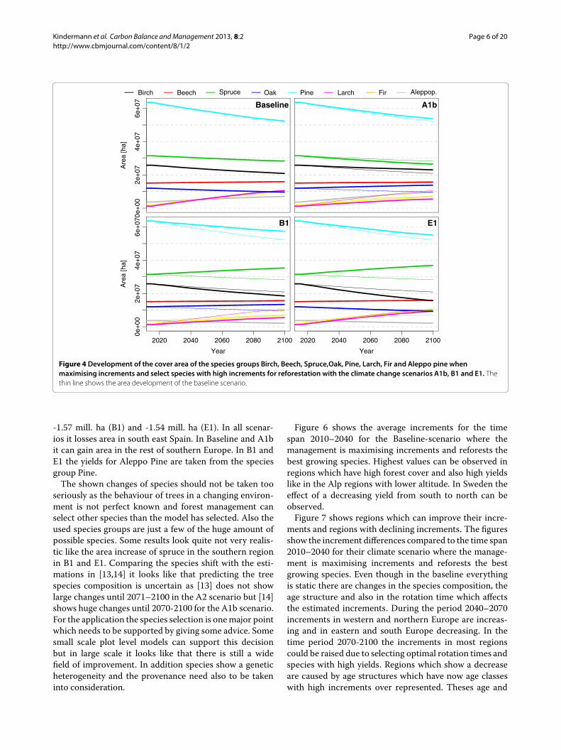
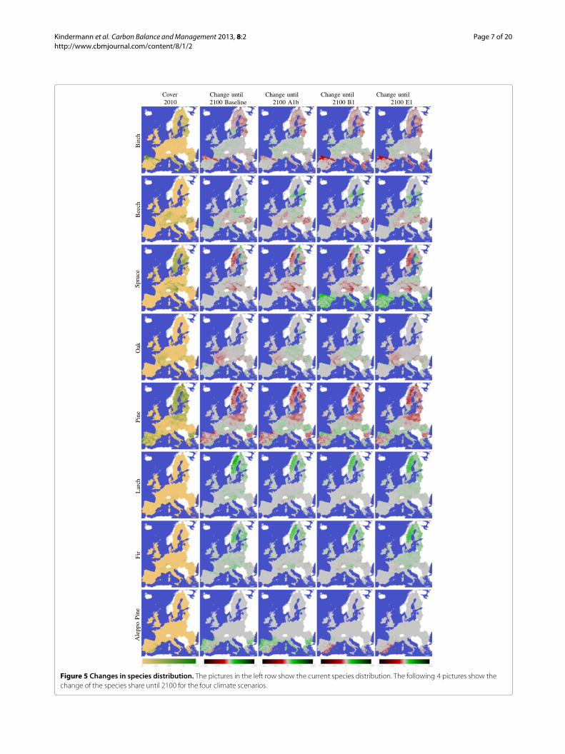
the standing biomass is equivalent to the difference ofincrements and removals. In the first years there is not toomuch difference between the two management scenariosas a complete change of forest structure and age distri-bution needs typical one rotation time which is in manycase 100 years and more. In the beginning the manage-ment whichmaximises the standing biomass shows higherincrements than the one which maximises increments.On a first look this sounds counter intuitive. The reasonfor this is that the model does not maximize the incre-ments in a short run. It starts to decrease the rotation timeby increasing the harvests. Heavy harvests produce largeareas which needs to be afforested and those young standsobviously show a lower productivity than the old standswhich have been there previously. But the growth curvesshow that this short time disadvantage is turning someyears later into higher increments than those that the oldtrees would be able to produce. The increments of thebiomass maximising management is decreasing over thetime. That means that the capacity of sequestrating car-bon is getting lost with this strategy. For sure this capacityof sequestrating carbon can be increased again but thiswill need time and the lost increments can never be caughtup. Changing to productive species will further increasethe increment potential in the long run. Also in the base-line run the increment could be increased by changing thespecies.Figure 4 shows how the area of the 8 species groups

is developing in the scenario which is maximising incre-ments and selecting species with high increments forreforestation with the four climate scenarios. Figure 5shows where the species are located and the regions oftheir changes until 2100 under the different climate sce-narios. From the total forest area of 155 million hectare16.7% (25.8 mill. ha) is covered by Birch, 9.74% (15.1 mill.

ha) by Beech, 20.33% (31.5 mill. ha) by Spruce, 7.75%(12.0mill. ha) by Oak, 41.1% (63.6mill. ha) by Pine, 0.79%(1.2 mill. ha) by Larch, 1.25% (1.9 mill. ha) by Fir and2.38% (3.7 mill. ha) by Aleppo Pine in the year 2010. Untilthe year 2100 the total area of Birch is reduced in all sce-narios. The area is changed by -4.95 mill. ha (Baseline),-2.77 mill. ha (A1b), -7.33 mill. ha (B1), -10.19 mill. ha(E1) where birch looses area in the north and south andgains some share in central Europe. Beech is increasingits area by 0.82 mill. ha (Baseline), 0.51 mill. ha (A1b),0.50 mill. ha (B1) and 0.82 mill. ha (E1). Beech loses partlyin central Europe and gains in northern Spain and northeast Europe. Spruce is changing its area by -3.15 mill. ha(Baseline), -5.06 mill. ha (A1b), +3.83 mill. ha (B1) and+5.42 mill. ha (E1). Spruce looses in central and northEurope and gains in the very north regions. In the sce-narios B1 and E1 it also gains areas in south Europe. Oakchanges its area by -2.38 mill. ha (Baseline), +1.82 mill. ha(A1b), +1.38 mill. ha (B1) and -2.66 mill. ha (E1). In Base-line it looses in central Europe and gains in south Europe.In A1b and B1 Oak looses in western Europe and gains incentral, east and north Europe. The most present speciesgroup pine losses -11.26 mill. ha (Baseline), -9.80 mill. ha(A1b), -6.20 mill. ha (B1) and -8.51 mill. ha (E1). Pinelooses in north and south and gains in central Europe.Larch is increasing its area by 9.39 mill. ha (Baseline),4.27mill. ha (A1b), 4.27mill. ha (B1) and 8.10mill. ha (E1).Larch has very small areas in 2010 and is loosing a little bitof its share in the alpine region and gains areas in northEurope. Fir is increasing its area by 8.15mill. ha (Baseline),5.10 mill. ha (A1b), 5.10 mill. ha (B1) and 8.55 mill. ha(E1). Also Fir has small forest areas and is loosing onlyvery few of them. Fir can increase little in central Europeand substantial in north Europe. Aleppo Pine is changingits area by +3.37 mill. ha (Baseline), +5.91 mill. ha (A1b),

2020 2040 2060 2080 2100

0.4

0.6

0.8

1.0

1.2

Year

Ste

m C

arbo

n In

crem

ent [

tC/h

a/Ye

ar]

BaselineA1bB1E1

MaxIncMaxBmMaxInc + Change Species

Figure 3 Increment development under conditions of baseline and three climate change scenarios (A1b, B1 and E1) and threemanagement scenarios (maximise stocking biomass, maximise increments with and without change of species).

Kindermann et al. Carbon Balance andManagement 2013, 8:2 Page 6 of 20http://www.cbmjournal.com/content/8/1/2

Are

a [h

a]

0e+

002e

+07

4e+

076e

+07 Baseline

Year

2020 2040 2060 2080 2100

E1

A1b

Birch Beech Spruce Oak Pine Larch Fir Aleppop.

2020 2040 2060 2080 2100

0e+

002e

+07

4e+

076e

+07

Year

Are

a [h

a]

B1

Figure 4 Development of the cover area of the species groups Birch, Beech, Spruce,Oak, Pine, Larch, Fir and Aleppo pine whenmaximising increments and select species with high increments for reforestation with the climate change scenarios A1b, B1 and E1. Thethin line shows the area development of the baseline scenario.

-1.57 mill. ha (B1) and -1.54 mill. ha (E1). In all scenar-ios it losses area in south east Spain. In Baseline and A1bit can gain area in the rest of southern Europe. In B1 andE1 the yields for Aleppo Pine are taken from the speciesgroup Pine.The shown changes of species should not be taken too

seriously as the behaviour of trees in a changing environ-ment is not perfect known and forest management canselect other species than the model has selected. Also theused species groups are just a few of the huge amount ofpossible species. Some results look quite not very realis-tic like the area increase of spruce in the southern regionin B1 and E1. Comparing the species shift with the esti-mations in [13,14] it looks like that predicting the treespecies composition is uncertain as [13] does not showlarge changes until 2071–2100 in the A2 scenario but [14]shows huge changes until 2070-2100 for the A1b scenario.For the application the species selection is onemajor pointwhich needs to be supported by giving some advice. Somesmall scale plot level models can support this decisionbut in large scale it looks like that there is still a widefield of improvement. In addition species show a geneticheterogeneity and the provenance need also to be takeninto consideration.

Figure 6 shows the average increments for the timespan 2010–2040 for the Baseline-scenario where themanagement is maximising increments and reforests thebest growing species. Highest values can be observed inregions which have high forest cover and also high yieldslike in the Alp regions with lower altitude. In Sweden theeffect of a decreasing yield from south to north can beobserved.Figure 7 shows regions which can improve their incre-

ments and regions with declining increments. The figuresshow the increment differences compared to the time span2010–2040 for their climate scenario where the manage-ment is maximising increments and reforests the bestgrowing species. Even though in the baseline everythingis static there are changes in the species composition, theage structure and also in the rotation time which affectsthe estimated increments. During the period 2040–2070increments in western and northern Europe are increas-ing and in eastern and south Europe decreasing. In thetime period 2070-2100 the increments in most regionscould be raised due to selecting optimal rotation times andspecies with high yields. Regions which show a decreaseare caused by age structures which have now age classeswith high increments over represented. Theses age and

Kindermann et al. Carbon Balance andManagement 2013, 8:2 Page 7 of 20http://www.cbmjournal.com/content/8/1/2

Cover Change until Change until Change until Change until2010 2100 Baseline 2100 A1b 2100 B1 2100 E1

Bir

chB

eech

Spru

ceO

akPi

neL

arch

Fir

Ale

ppo

Pine

Figure 5 Changes in species distribution. The pictures in the left row show the current species distribution. The following 4 pictures show thechange of the species share until 2100 for the four climate scenarios.

Kindermann et al. Carbon Balance andManagement 2013, 8:2 Page 8 of 20http://www.cbmjournal.com/content/8/1/2

Figure 6 Average stem wood increments in baseline scenarioduring the period 2010–2040. Values are in tC/ha/Year × forestshare.

species effects are also present in the climate scenarios buthere is in addition a change of the environment. In A1bmany regions show higher increments in the time span2040–2070 than in the 30 years before but in the time span2070–2100 only cold regions show increased yields mostother regions show a declining increment. B1 looks simi-lar like A1b but some regions in Spain show an increasedincrement. E1 looks also similar to A1b but the incrementincreases in cold regions are not as high as in A1b and theincrement reduction on the remaining regions are lowerthan in A1b.

ConclusionsStocks and increments of the woody biomass are muchmore sensitive to forest management targets than to theclimate change scenarios.Adaption of forests to climate change is done during

regeneration by choosing appropriate species. To reducerisk, mixed forests should be established. Regeneration isdone after a final cut and a final cut is done in Europeanforestry typical in the range of every 100 years. Thisrotation time needs to be increased if forests are man-aged to store high carbon amounts what reduces theability of adaptation during regeneration. The absolutechange of temperature or precipitation will be larger dur-ing long rotation times than during short rotation times.

1E1Bb1AenilesaB

2040

-207

020

70-2

100

Figure 7 Changes of stem wood increments for the time periods 2040–2070 and 2070–2100 and the four climate scenarios (Baseline,A1b, B1 and E1) shown as the difference to the increments of the time period 2010–2040 in Figure 6. Differences related to time period2010-2040 in tC/ha/Year × forest share.

Kindermann et al. Carbon Balance andManagement 2013, 8:2 Page 9 of 20http://www.cbmjournal.com/content/8/1/2

Therefore tree species for storing high biomass in a chang-ing environment need to have a wide ecophysiologialspectrum, what will limit the number of possible treespecies.A policy focusing on storing high amounts of carbon

in forests has to increase the rotation time and this willreduce in the long run the annual wood increments whatwill e.g. reduce the substitution of fossil fuels. Low woodincrements will diminish forests ability in climate changemitigation. The model results indicate, that in EU27the standing wood biomass is higher than the expectedbiomass in forest which are managed to maximise incre-ments. A strategy which is using forests for storing carbonby increasing their biomass stock could be economicalattractive for a short time but this strategy will decreasethe amount of carbon fixation in forest in the longrun to zero. The estimates show that in total (standingbiomass and harvests) maximising increments is absorb-ing 1750 million tC more in the time span 2010–2100in EU27 than the management which is maximising thestanding biomass. This suggests avoiding any incentivewhich will increase the standing biomass beyond theincrement optimal biomass and hinder a decrease of thestanding biomass in many regions of EU27.

MethodsTo examine the development of

• standing stem carbon,• increments and• harvests

in the forests of the EuropeanUnion (Figure 8) we used theglobal forest growth model (g4gm). The forest area andits location are not changed in the simulations, what willresult in some underestimation as [3] showed a forest areaincrease for EU27 from 146 mill. ha in 1990 to 157 mill. hain 2010 and this trend seems to continue. These threeforest values of interest are influenced by site conditionsand management. The site conditions are described bysoil texture, slope, altitude, temperature and precipitation.The development of temperature and precipitation areestimated on a daily basis until 2100 by the REMO [15]model for the scenarios

• Baseline,• A1b,• B1 and• E1 (like A1b but limit to 450-ppm CO2 equivalent).

The plot level models Prelued, Picus and Gotilwa+ usedthe site information to estimate the potential productivityof forests. This productivity was used by the g4gm to pre-dict the development of standing stem carbon, increments

Figure 8 Forest cover map in EU27 in the year 2010.

and harvests until the end of this century where forestmanagement target is either to

• maximise increments and keep current species• maximise standing volume and keep current species• maximise increments and select species with high

increments for reforestation.

The scenario which changes species selects those specieswhich have show at least 70% of the average increment ofthe best growing species where the model looks 80 yearsinto the future to make an increment ranking. The rota-tion time of all present species is set to the incrementoptimal rotation time but species who don’t reach these70% of increment their rotation time is limited tomaximal70 years what will result that these species are exchangedwithin the next 70 years.

Aggregating to homogeneous response unitsAll data, beside the climate data, was available on a reso-lution of 1 × 1 km. The climate data was at a resolutionof 25 × 25 km. This makes for the 27 member states ofthe European Union 4 304 383 grids on land with a size of1 km2. Many of this grids show huge similarities in theresite conditions. To reduce calculation time those gridshave been merged to homogeneous groups. In the firststep all grids which have the same

• Country,• Elevation category,• Slope category and• Soil texture.

Kindermann et al. Carbon Balance andManagement 2013, 8:2 Page 10 of 20http://www.cbmjournal.com/content/8/1/2

are joined together to 2454 homogeneous groups. Wherethe categories are:

Country: Austria, Belgium, Bulgaria, Cyprus, CzechRepublic, Denmark, Estonia, Finland, France,Germany, Greece, Hungary, Ireland, Italy, Latvia,Lithuania, Luxembourg, Malta, Netherlands, Poland,Portugal, Romania, Slovakia, Slovenia, Spain, Sweden,United KingdomElevation category: < 300m, 300–600m,600–1100m, 1100–1600m, 1600–2100m and> 2100mSlope category: 0–3%, 3–6%, 6–10%, 10–15%,15–30%, 30–50% and > 50%Soil texture: Coarse, Medium, Medium-fine, Fine,Very fine and Peat

In order to reduce the climatic variability within the indi-vidual response units, these 2454 regions have been splitup into 14 168 sub-regions of similar climate. The split-ting utilized k–means clustering based on the absolutevariability of annual temperature, annual and summerprecipitation, and temperature amplitude within responseunits. For each sub-region, average soil conditions weredetermined from the EU27 data grids.The area of EU27 was allocated to the responsibility

of on specific plot level model. Figure 9 shows that Pre-lued was responsible for the northern (orange), Picus forthe central (green) and Gotilwa+ for the southern (red)region. Adjoining models are responsible for the overlap-ping area (grey). This division was cancelled if one modelwas not able to make estimates of a specific species group(see Table 1).

Estimating yieldsFor each of the previously build homogeneous responseunits a yield level is estimated. As the site conditions arechanging also this yield is changing from year to year.The yield estimates have been done by the tree plot levelmodels:

Prelued: Yield estimates for the boreal zone wereproduced with a simple model of Gross PrimaryProduction (GPP), described in detail in [16]. Themodel is based on light use efficiency (LUE) models[17], further modified by factors downscaling thephotosynthesis due to low humidity (in air or soil),low temperatures or phenology. The potential GPPwas calculated based on daily meteorologicalparameters, while soil water conditions weresimulated with a simple dynamic model [16]. GPPwas converted into NPP by subtracting therespiration as in [18] and equations from the“summary model” by [19] as well as yield tables from

Figure 9 The tree modelregions indicating the main applicationof the used plot level models. Prelued was responsible for thenorthern (orange), Picus for the central (green) and Gotilwa+ for thesouthern (red) region. Adjoining models are responsible for theoverlapping area (grey).

[20] where then used to produce the maximumMeanAnnual Increment from the NPP estimates.

Picus: The aim of PICUS3G is to provide aphysiology–based, climate–sensitive estimate offorest NPP based on a parsimonious set of input dataavailable at continental scales. PICUS3G is based onthe production sub–module of the hybrid forest gapmodel PICUS v1.4 [21], and is a descendant of thegeneralized productivity model 3-PG [22]. GPP iscalculated on a monthly time step using a light use

Table 1 Modelregions

Region North Central South

Birch Prelued Prelued Prelued

Beech Picus Picus Picus

Spruce Prelued Picus Picus

Oak Picus Picus Picus

Pine Prelued Picus Gotilwa+1

Larch Picus Picus Picus

Fir Picus Picus Picus

Aleppo Pine Gotilwa+2 Gotilwa+2 Gotilwa+2

1For B1 and E1 the estimates come from Picus.2For B1 and E1 the values of Pine were used.

Kindermann et al. Carbon Balance andManagement 2013, 8:2 Page 11 of 20http://www.cbmjournal.com/content/8/1/2

efficiency approach. The fraction of the absorbedradiation in the canopy that is utilizable forphotosynthesis is determined by limitingenvironmental factors, i.e., temperature, soil wateravailability, and vapor pressure deficit [21]. Thequantum use efficiency is modified by the CO2concentration in the atmosphere and by availablenitrogen as a proxy for soil nutrient supply. NPP isderived from GPP using a constant respirationfraction, and is split into above- and belowgroundfractions based on environmental conditions,assuming that a more favourable environment resultin a higher share of aboveground allocation [22].PICUS3G requires plant-available nitrogen (kg/ha)and water holding capacity (mm) as well astemperature, precipitation, vapor pressure deficit, andradiation data at monthly resolution as model drivers.For the current contribution NPP was calculated forfully stocked, monospecific stands using the leaf areaindex (LAI) of even-aged stands at peak productivity.Simulations were conducted for beech, oak, fir, pine,spruce and larch (Table 1). G4gm used the NPPestimates generated by PICUS3G as a yield levelindicator and scaling factor to adjust its empiricallyaggregated stand growth function. This modellinkage thus allows an estimation of productivitybased on physiological principles and environmentaldrivers (PICUS3G) while efficiently consideringmanagement in the subsequent application of theempirical model G4M.

Gotilwa+: Results of the process-based forest growthmodel Gotilwa+ [23-27] are computed for DBHclasses and integrated at the stand level. Although thepresent study has been carried out for even agedforests, most of Mediterranean forests are unevenaged. Information from National Forest Inventoriesdo not include age as a measured variable and in factsome more detailed studies carried out in local forestinventories show that, in most cases, no relationshipcan be established between dominant tree height andage or between DBH and age in this water limitedand with intense competition forest ecosystems [28].That is part of the reason why Gotilwa+ does notinclude age as an explicit variable in the model. Asg4gm model needed yield estimates at a determinateage of the forest, the Gotilwa+ model calculationswere performed in such a way that the simulationstarted with a tree plantation and so the year of thesimulation was assumed to be the age of the foresttoo. Climate files were reorganized in 50-year fileswith a 25-year overlapping, so that for eachsimulation unit there were 4 runs with an initial25-year simulation to get a forest of 25 years of age

and the rest of the results were used by g4gm tocalculate the MAI. The output variable that wasprovided to g4gm was annual stem wood increment(tC/ha/year).

The g4gm model will use the mean annual stem-woodincrement at increment optimal rotation time (MAI) inunits of ton carbon per hectare and per year [tC/ha/year]as a yield descriptor. None of the three plot level modelwas able to provide their yield estimate inMAI. It was alsonot possible to find another yield description which allthree plot level models could provide. So it was necessaryto transfer three individual yield estimates with differentdefinitions to one definition. For this task the growth func-tions of g4gm are used (equation 1) but the parametersto estimate the shape (factor k in equation 4 describesif increments in young or old ages are high or low), thehighest age of increment (tmax equation 5) and maxi-mum total carbon production of stemwood per hectare(TCPmax equation 6) are estimated individually for eachplot level model and each species using several growthestimates from the plot level model itself for each of theirspecies on a range of poor to very productive sites. Thecoefficients are in Table 2 where the growth curves forthe Prelued model where calculated by using estimatesform the PipeQual model [29] and a finish yield table [20].The yield tables from [30,31] are used to compare Pinussylvestris and Pinus halepensis with growth patterns fromGotilwa+.The shapes of the growth curves of the northern region

are shown in Figure 10. PipeQual [29] simulations (Pineand Spruce) weremade from full stockedmanaged forests,the tables from [20] (Birch) are for natural forest. On pro-ductive sites Birch is culminating very fast followed byPine and ending with Spruce. On average and on lessproductive sites Pine and Birch are showing similar pat-terns and spruce shows a slowly starting increment butthe increment level is kept high in old stands. Specieson productive sites show a distinctly earlier culminationthan the low productive sites. Note that these curvesdon’t show the growth pattern of the species for a spe-cific stand. They show the growth for the species if theiryield level, expressed as the highest mean annual incre-ment, is at a specific level and there is no need thatthis yield level is equal for different tree species on thesame site.The shapes of the growth curves of the central region

are shown in Figure 11. On productive and average sitesthe growth pattern of coniferous trees are very similar.Oak and beech show a later culmination and afterwards avery slow growth decrease. On low productive sites Pineand Larch are similar and show an early, spruce and fir aresimilar and show an average and Oak and Beech are sim-ilar and show a late growth culmination. There are spares

Kindermann et al. Carbon Balance andManagement 2013, 8:2 Page 12 of 20http://www.cbmjournal.com/content/8/1/2

Table 2 Growth curve coefficients estimatedwith growth data from the plot level models and yield tables

Source species c0 c1 c2 c3 c4 c5 c6 c7 Figure

PipeQual Spruce -0.2 -0.4 -0.1220 1.8345 350 100 0 0.776 10

PipeQual Pine -0.2 -0.5 -0.6361 1.1998 200 300 1.816 -1.246 10

Ilvessalo Birch -0.1 -0.5560 -0.1365 -2.0064 400 -325.070 4.985 -3.5 10

Picus Beech -0.2671 -0.2334 -3.8842 -1.8490 474.789 655.717 -7.068 4.402 11

Picus Spruce -0.3641 -52.7111 -6.1741 0.2943 -646.403 945.370 -1.643 -1.468 11

Picus Oak -0.1781 -1.0421 -3.7204 1.0574 300 1512.405 2.885 -3.722 11

Picus Pine -0.2523 -0.3219 -14.8589 -2.8190 261.892 323.775 -9.763 4.875 11

Picus Larch -2.936e-01 -4.020e-02 -2.855e+06 -1.247e+01 285.788 116.032 -17.287 5.248 11

Picus Fir -0.3449 -1.3433 -3.4040 0.6076 186.619 142.930 1.337 -3.258 11

Gotilwa+ Pine 1.246963 -1.097645 0.172259 -0.006605 3000 1400 2.875 -2 12

Gotilwa+ Aleppo Pine -0.08 0.02212 -0.05967 -1.37455 2600 1200 1.491 -2 12

Abejon Pine 0 -0.54 -0.3369 0.5073 225 65 16.69 -21.22 12

Montero Aleppo Pine -0.3 -0.306 -2.052 1.673 150 130 1.898 -1.141 12

differences in the age of growth culmination between highand low productive sites.The shapes of the growth curves in the southern region

are shown in Figure 12. Those from Gotilwa+ look quitedifferent compared to those of the other two plot levelmodels. Yield tables from the southern region show sim-ilar growth patterns with the other plot level models butnot like those from Gotilwa+. In Gotilwa+ the incrementis decreasing monotonously when the age is increasing.

This difference will not make to much problems as thosegrowth curves from the regional plot models will only beused to convert their yield estimates to the yield estimateusable by g4gm. Growth curves like those from Gotilwa+will recommend a rotation time of one year for foreststo maximise the average increment what will not be torealistic. Also the total increment until a specific rotationtime will show huge differences between the incrementsof Gotilwa+ and the local yield table for the same MAI.

0 50 100 150

0.0

0.5

1.0

1.5

2.0

2.5

3.0

3.5

Age [Years]

Cur

rent

ann

ual i

ncre

men

t [tC

/ha/

Year

]

BirchSprucePine

MAI=2.5tC/HaMAI=1.5tC/HaMAI=0.5tC/Ha

Figure 10 Growth curves of the northern region form the PipeQual model [29] and a finish yield table [20].

Kindermann et al. Carbon Balance andManagement 2013, 8:2 Page 13 of 20http://www.cbmjournal.com/content/8/1/2

0 50 100 150

0.0

0.5

1.0

1.5

2.0

2.5

3.0

Age [Years]

Cur

rent

ann

ual i

ncre

men

t [tC

/ha/

Year

]

BeechSpruceOakPineLarchFir

MAI=2.5tC/Ha MAI=1.5tC/Ha MAI=0.5tC/Ha

Figure 11 Growth curves of the central region from the Picus model.

0 50 100 150

0.0

0.5

1.0

1.5

2.0

2.5

3.0

Age [Years]

Cur

rent

ann

ual i

ncre

men

t [tC

/ha/

Year

]

Pine (Gotilwa)Aleppo Pine (Gotilwa)Pine (Table)Aleppo Pine (Table)

MAI=2.5tC/HaMAI=1.5tC/HaMAI=0.5tC/Ha

Figure 12 Growth curves of the southern region from the from Gotilwa+ model and yield tables from [30,31].

Kindermann et al. Carbon Balance andManagement 2013, 8:2 Page 14 of 20http://www.cbmjournal.com/content/8/1/2

How is this yield estimate conversion done? Preluedestimates the highest stem wood productivity in one yearat a specific, but not given, age. For example it says that thehighest stem wood increment of Birch is 3.5 tC/Ha/Year.With this information g4gmwill have a look on the growthcurves in Figure 10 and see that this maximum incre-ment of 3.5 tC/Ha/Year are corresponding an MAI of2.5 tC/Ha/Year. So this transformation is quite simple.There is just a need of one table showing the maxi-mum increment and the corresponding MAI by using theproper growth curves.Picus estimates the net primary productivity at an age of

50 Years (NPP50). The first step is to convert the NPP50to stem wood increment also at age 50 in tC/ha/year. Thisis done by using estimates directly from Picus showingthe ratio of how much of the NPP is stored in the stem.In Picus the assumption was made that this ratio is inde-pendent of site, age and productivity what will result ina species specific constant conversion factor. This factorwill convert the NPP50, given in tC/ha/year, to stem woodincrement, given in m3/ha/year (see Table 3). This factorincludes beside the share of increment which is stored inthe stem, a conversion from tC to m3 by using wood den-sity and carbon content of wood. The carbon content ofwood was assumed to be for all species 0.5 tC for 1 t drywoody biomass. The transformation from wood volumeto weight typical is done by using the volume of wet woodand the weight of absolutely dry wood. The wood densityρ0 need to be corrected by the degree of wood shrink-ing. The wood density is varying between species, sitesand others and is even not homogeneous within a tree. Asthe conversation was done internally in Picus from weightto volume there will not arise any error if the conversa-tion from this estimated volume back to weight is done byusing the same coefficient which can be found in Table 3.After the first step converts the NPP50 to stem wood

increment at age 50 in tC/ha/year this stem wood incre-ments is converted into MAI by using the extractedgrowth curves fromPicus. If e.g. the stemwood increment

Table 3 Coefficients from Picus to convert NPP to stemincrement

Species Stem/NPP Wood density ρ0

Beech 1.24579 680

Spruce 1.92055 430

Oak 1.24576 650

Pine 1.787301 490

Larch 1.64733 550

Fir 1.93735 430

NPP . . .net primary productivity at age of 50 Years [tC/ha/year], Stem . . . stemwood increment [m3/ha/year], Wood density . . .Wood density of oven dry wood[kg/m3].

at age 50 is 2.8 tC/ha/year for Oak it can be seenin Figure 11 that this is equivalent to an MAI of2.5 tC/ha/year. For this conversion there is a need for onetable which shows the stem wood increment at age 50 andthe MAI. Such a table can be created by using the growthcurves. There might arise one problem during this con-version if there are two different MAI’s for one NPP50.In this case the lower MAI is used. Also it will be possi-ble that there exists no MAI for a given NPP50 but thiscase did never appear in this study. Another problem isthat the size and leave area of the trees at age 50, which isneeded in Picus, for a specific yield is currently not knownin advance so they were set to an average constant value.As long as the Picus model is not sensitive to tree sizes theexpected bias in the predictions will be low.Gotilwa+ estimates the stem wood increment at an

increasing age with a tree size according to cumulativeincrements of the previous years. If the yield of the pre-vious years is comparable the tree size will be correct, ifthere is a changing yield the tree size will not fit perfectto the age and yield combination. As long as the Gotilwa+model is not very sensitive to tree sizes this will causean acceptable bias in the predictions. The transformationfrom stem wood increment at a given age to MAI worksthe same way like for Prelued and for Picus by lookingon the growth curves. E.g. if Gotilwa+ estimates an incre-ment of 0.5 tC/ha/year for Pine with an age of 30 yearsit will be equivalent with an MAI of 2.5 tC/ha/year bymaking the conversion with the curves of Gitilwa+ inFigure 12. To make yield estimates Gotilwa+ plants treesand let them grow for 50 years. The values of the first25 years are only used to create up forests with an age of25 years. The following 25 years, where the forest has anage of 25 to 50 years, are used to estimate the yield. For thetransformation to MAI 25 tables (one for each age class)for each species are needed which show the combinationof stem wood increment and MAI.The estimated yields of the climate scenarios are not

identical for the starting year 2010. To let the simulationsstart at the same point the yield estimates for the first5 year period are set to those of the baseline scenario.

Creating initial forest conditionsAfter knowing the yields it is necessary to have realis-tic forest information where the simulation can start on.Therefore the following information will be needed:

• Forest area• Species share• Age class distribution

In addition also the stand density of a forest will have aninfluence on the standing biomass and the increment. Forthis investigation the starting stand density is set to a yieldtable stocking degree of one.

Kindermann et al. Carbon Balance andManagement 2013, 8:2 Page 15 of 20http://www.cbmjournal.com/content/8/1/2

The forest area was taken from the European Commis-sion Joint Research Centre (JRC) Institute for Environ-ment and Sustainability. There we select the forest covermap of the year 2006 where the map was indicated tobe in the beta stadium. This map has a spatial resolu-tion of 25 × 25m. This map indicates that a grid is oris not covered by forest. A grid which is indicated to becovered by forest is treated as 100% forest coverage andthose which are indicated to be not covered by forest aretreated to have 0% forest cover. This map was aggregatedto a 1 × 1 km map, which is congruent with the mapwhich was used for the homogeneous response units, andgives now the information which share of this area is cov-ered by forests. In the next step the tree species maps,also from the JRC Institute for Environment and Sustain-ability, which have a resolution of 1 × 1 km showing theshare of the species in the year 2000 are used. These mapsdistinguish between 118 different species (groups). Herewe will aggregate them into the following eight speciesgroups:

Beech: Acer campestre, Acer monspessulanum, Aceropalus, Acer platanoides, Acer pseudoplatanus,Carpinus betulus, Carpinus orientalis, Castanea sativa(C. vesca), Eucalyptus sp., Fagus moesiaca, Fagusorientalis, Fagus sylvatica, Fraxinus angustifolia spp.oxycarpa (F. oxyphylla), Fraxinus excelsior, Fraxinusornus, Ostrya carpinifolia, Platanus orientalis, Tiliacordata, Tilia platyphyllos, Ulmus glabra (U. scabra,U. scaba, U. montana), Ulmus laevis (U. effusa),Ulmus minor (U. campestris, U. carpinifolia), Arbutusunedo), Arbutus andrachne, Other broadleaves

Birch: Alnus cordata, Alnus glutinosa, Alnus incana,Alnus viridis, Betula pendula, Betula pubescens,Buxus sempervirens, Corylus avellana, Ilexaquifolium, Populus alba, Populus canescens, Populushybrides, Populus nigra, Populus tremula, Salix alba,Salix caprea, Salix cinerea, Salix eleagnos, Salixfragilis, Salix sp., Sorbus aria, Sorbus aucuparia,Sorbus domestica, Sorbus torminalis, Erica arborea,Erica scoparia, Erica manipuliflora, Phillyrea latifolia,Pistacia lentiscus, Pistacia terebinthus, Crataegusmonogyna

Oak: Juglans nigra, Juglans regia, Malus domestica, Oleaeuropaea, Prunus avium, Prunus padus, Prunusserotina, Pyrus coomunis, Quercus cerris, Quercuscoccifera (Q. calliprinos), Quercus faginea, Quercusfrainetto (Q. conferta), Quercus fruticosa (Q.lusitanica), Quercus ilex, Quercus macrolepis (Q.aegilops), Quercus petraea, Quercus pubescens,Quercus pyrenaica (Q. toza), Quercus robur (Q.pedunculata), Quercus rotundifolia, Quercus rubra,

Quercus suber, Quercus trojana, Robiniapseudoacacia, Ceratonia siliqua, Cercis siliquastrum

Aleppo Pine: Pinus halepensis

Fir: Abies alba Abies borisii-regis Abies cephalonica Abiesgrandis Taxus baccata

Larch: Larix decidua Larix kaempferi (L.leptolepis)

Pine: Cedrus atlantica, Cedrus deodara, Cupressuslusitanica, Cupressus sempervirens, Juniperuscommunis, Juniperus oxycedrus, Juniperusphoenicea, Juniperus thurifera, Pinus brutia, Pinuscanariensis, Pinus cembra, Pinus contorta, Pinusleucodermis, Pinus mugo (P. montana), Pinus nigra,Pinus pinaster, Pinus pinea, Pinus radiata (P.insignis),Pinus strobus, Pinus sylvestris, Pinus uncinata

Spruce: Picea abies (P. excelsa), Picea omorika, Piceasichensis, Pseudotsuga menziesii, Thuya sp., Tsugasp., Other conifers

The aggregated species maps have been merged with thecorresponding yield estimate form the plot level models.All grids where the yield estimate for a species in the years2000-2010 show at least one year with zero increment areset to not occupied with this species. With this proce-dure the original area of birch was reduced by 1%, beech34%, spruce 8%, oak 56%, pine 11%, larch 23%, fir 47%and aleppo pine by 39%. This reduction is partly compen-sated as the remaining species get the area of the removedspecies. On grids indicating they are covered by forest butthere is now no species present are set to show no for-est. This reduces the original total forest area by 6.7%.The next task is to bring the total forest area of a coun-try to the given values in [32]. This is done by summingup the forest area of the grids belonging to a certain coun-try and transforming the forest share, which can have arange from 0 (no forest) to 1 (grid is full covered withforest), by an exponent. So the forest area is calculatedwith: forest area = ∑

(gridSize × forestSharex) where theexponent x is chosen for each country individually thatthe calculated Forest area is equivalent with the forestarea of the country statistics (Figure 8). In addition it ispossible, that the origin forest shares are overlaid with arandom deviation. This will help e. g. to affect also gridswhich show no forest cover or are full covered with for-est and also will avoid that the distance between forestcover classes is changing so that some classes are overrepresented and others are empty. As we have currently1600 forest cover classes with equal distance, an over-lay of a random number was not done. The share of thespecies groups was adjusted the same way like the forestshares but the adjustment was not done for the species

Kindermann et al. Carbon Balance andManagement 2013, 8:2 Page 16 of 20http://www.cbmjournal.com/content/8/1/2

groups itself, instead it was done for broad leafed andneedle trees. The country statistics of the broad leafed andneedle trees shares are taken from [33] where the groupmixed forests is added to the coniferous and broad leavedgroup where 25%–75% of the mixed forest area is addedto broad leaved or coniferous choosing the share to havelow shifts of the starting assumptions.These forest area shares by different species can be

divided into different age classes. Therefore the incre-ment optimal rotation time (topt) individually for eachregion and species using the average MAI for the years2000–2010 is estimated using equation (2). This rotationtime is increased depending on the slope by multiplyingit with the following factors: 1 (slope 0–6%), 1.04 (6–15%), 1.37 (15–30%), 1.61 (30–50%), 1.13 (> 50%). E. g.when the increment optimal rotation time is estimatedwith 100 years and the forest is located on a site witha slope of 20% the typical age of harvest is estimatedwith 137 years. These factors are estimated by using alaser scanner biomass map of Vorarlberg and take intoaccount, that harvest is postponed if the slope is increas-ing. Until topt× slope factor each age class has the samearea share. Ages beyond topt× slope factor get the rightwing of normal distribution area share where the stan-dard deviation of this normal distribution is calculatedwith 0.2 × topt× slope factor. These areas are summed upper country and age class separate for broad leaved andconiferous trees. With this you have an age class distribu-tion which can be brought to those from [33]. The givenarea of the age class “unknown” in [33] is shared pro-portional to each known age class. The used age classesare 1–10, 11–20, 21–40, 41–60, 61–80, 81–100, 101–120,121–140 and > 140 years. The mixed forest age classarea is divided according to the previous made divisionto broad leaved and needle trees. The previous createdspecies groups are aggregated also into broad leaved andneedle trees. To bring the initial estimated age struc-ture to the observed age structure those estimates areincreased or decreased with iterativemodifiedmultipliers.These multipliers for each age class needs to be appliedfor each region, slope class and species group (needleor broad leaved) and the total area needs to stay thesame in each of theses groups after this multiplication.This means that if only one multiplier of one age class ischanged also all other age classes are affected. Keeping theareas constant after multiplication is done by multiplyingthe new area of each age class with

∑Area∑

Area after multiplicationwhere the sums are build for each region. The multi-pliers are iterative updated by setting new multiplier =old multiplier × target age class share

current age class share . This allows creatingstarting conditions for the model which are close to givenforest area, species distribution and age distribution fromcountry statistics.

Forest development estimates with the global forestgrowth modelIncrement FunctionsThe increment functions are able to describe the (1) totalcarbon production of stemwood per hectare (TCP) atincrement optimal stand density (SDopt) depending onlyon age, (2) estimate the managed stand density and (3)the maximum possible stand density, estimate (4) the treesize (DBH, height) and (5) the influence of stand den-sity on TCP and DBH increment. All coefficients of thegrowthmodel are in Table 4. The coefficients are found byapplying regressions on the yield tables of [31,34].

Total carbon production The total stemwood carbonproduction per hectare (TCP) at a certain stand age (t) canbe described with equation (1) where TCPt is the TCP atstand age t, TCPmax is the maximum TCP which will bereached at stand age tmax and k is a factor describing theshape of the increment curve.

TCPt = TCPmax · ek·ln2(t/tmax) (1)

This curve can be fitted to values from a yield table, fieldobservations or model results. The curve fit allows esti-mating the maximum of the total carbon production andalso the forest age, when this maximum is reached. Thecoefficient k allows describing how the increment is dis-tributed over age. The estimated values may be differentfor different yield levels.By knowing k and tmax the increment optimal harvest-

ing time topt can be calculated with equation (2).

topt = tmax × e0.5/k (2)

By dividing the TCP at time topt with topt the high-est mean annual increment (MAI) can be calculated(equation 3). This MAI is used in the g4g-model todescribe the yield level.

MAI = TCPtopttopt

(3)

Typical TCPmax, k and tmax are changing for differ-ent yield levels and so their values needs to be esti-mated depending on yield. The relation of MAI with theshape factor (k), the highest age until increment happens(tmax) and maximum TCP (TCPmax) are described withequation (4), 5 and 6.

k = c0 + c1 × ec2×MAIc3 (4)

tmax = c4 + c51 + e(c6+c7×MAI) (5)

TCPmax = MAI × tmax × e0.25/k (6)

Maximum stand density The biomass of forests withlow thinning (removal of dead trees) at a specific age isthe TCPt subtracted by the biomass of dead and removed

Kindermann et al. Carbon Balance andManagement 2013, 8:2 Page 17 of 20http://www.cbmjournal.com/content/8/1/2

Table 4 Coefficients of the growthmodel (equation (1)–(12))

Pine Beech Birch Fir Larch Oak Spruce P.Halep.

c0 -0.3835 0 0 -0.4562 0 0 0 -0.3

c1 -0.2416 -0.5998 -0.7422 -0.7403 -0.388 -0.6 -0.9082 -0.306

c2 -1.7576 -0.2467 -0.54 -1.0772 -0.01226 -0.4419 -0.2728 -2.052

c3 1.1638 0.7674 0.5719 1.4803 0.8593 0.3179 0.6483 1.673

c4 170 245.6 137 0.6713 195.4 16.67 209.7 150

c5 114.3 100 100 300 600 300 300 130

c6 -2.804 2.6345 0.2972 -0.2151 0.9883 -0.6066 1.8536 1.898

c7 1.044 -0.8978 -0.7543 -0.9929 1.0784 -1.1243 0.4811 -1.141

c8 0 0.69135 0 0.5 0 0.7 0 0.92

c9 0.9 0 0.9 0.2 0.9 0.3 0.9 0.07

c10 -0.8242 0 -0.953 -0.7642 -2.1347 -0.4339 -0.143 -4.25

c11 -0.4273 0 -0.9236 0.3156 -0.3437 0.5288 -0.5915 6.168

c12 -0.4 -0.03177 -0.4 -0.4 -0.4 -0.4 -0.4 -0.4

c13 -1.476 0 1.052 0.4468 1.3238 2.0156 0.4507 0.9324

c14 4.283 0 0.108 0.1425 0.4061 -0.07354 0.3713 -0.00468

c15 -0.3 0 0 0 0 0 0 0

c16 3.61 0 0 0 0 0 0 0

c17 -1.071 0 0 0 0 0 0 0

c18 0.1 -0.875 0.1 0.25 0.1 0.1 0.1 0.25

c19 1.127 2 1.082 -0.865 1.082 1.03 1.135 -0.865

c20 -0.3028 0 -0.4 -0.5 -0.3 0.3 -0.3 -0.5

c21 0.5 0.5 0.5 0.5 0.5 0.5 0.5 0.5

c22 22.09 21.29 23.24 24.83 23.63 21.26 22.59 26.59

c23 0.6207 0.4872 0.4455 0.6071 0.5028 0.5199 0.6168 0.6284

c24 -0.0197 -0.0197 -0.0249 -0.0212 -0.0156 -0.019 -0.021 -0.0202

c25 1.5061 1.8148 1.3697 2.4131 1.162 1.3408 2.4176 1.0595

c26 -0.2535 -0.2914 -0.4294 -0.4825 -0.1867 -0.1098 -0.3582 -0.0349

c27 22.7 30.71 13.61 16.11 25.2 -7.511 16.11 18.73

c28 16.56 7.008 10.69 17.78 9.118 41.69 17.78 46.38

c29 -0.0107 -0.0105 -0.0269 -0.0144 -0.0138 -0.022 -0.0144 -0.2643

c30 0.248 -0.198 0.242 0.374 0.646 0.581 0.374 14.143

c31 -1.814 0.298 -0.702 -1.524 -0.799 1.725 -1.524 -0.637

c32 1.095 1.423 1.337 2.282 1.082 3.676 2.282 0.895

c33 0.1 1.025 0.071 1.272 0.167 1.754 1.272 0

c34 -1.603 -16.85 -2.151 -0.771 -0.941 0.326 -0.771 -4.963

c35 1.6 1.6 1.6 1.6 1.6 1.6 1.6 1.6

c36 1.5 1.5 1.5 1.5 1.5 1.5 1.5 1.5

c37 150 300 150 150 150 150 150 150

c38 0.01 0.01 0.01 0.01 0.01 0.01 0.01 0.01

c39 0.5 0.5 0.5 0.5 0.5 0.5 0.5 0.5

c40 0.5 0.5 0.5 0.5 0.5 0.5 0.5 0.5

c41 0.8 0.8 0.8 0.8 0.8 0.8 0.8 0.8

c42 0.002 0.001 0.002 0.002 0.002 0.002 0.002 0.002

Kindermann et al. Carbon Balance andManagement 2013, 8:2 Page 18 of 20http://www.cbmjournal.com/content/8/1/2

Table 4 Coefficients of the growth model (equation (1)–(12)) (continued)

c43 2 2 2 2 2 2 2 2

c44 0.01 0.01 0.01 0.01 0.01 0.01 0.01 0.01

c45 0.5 0.5 0.5 0.5 0.5 0.5 0.5 0.5

trees until this age. The fraction of carbon in the livingbiomass (CMaxt) compared to the TCP is described withequation (7).

CMaxtTCPt

= (cc0 + cc1 × ln(t

topt)) × (1 − cc2 × t

topt)c21

(7)

cc0 = c8 + c91 + e(c10+c11×MAI)

cc1 = c121 + e(c13+c14×MAI) + c15

1 + e(c16+c17×MAI)

cc2 = c18 + c19 × e(c20×MAI)

The cc2 × ttopt defines the age where all the biomass of a

forest has been died. If the estimated fraction of CMaxtTCPt is

lower than 0 it is set to 0 (age is beyond the age where alltrees have died) and if it’s higher than 1 it is set to 1 (youngstands where maximum density is not reached).

Managed stand density The managed stand densitydepends on the thinning regime. Here the managed standdensity is defined as the density where 95% of the incre-ment of a full stocked stand is produced. This point canbe estimated using equation (12) describing the incrementdepending on stand density.

Tree size The tree size has an influence on the harvestingcosts and share of wood which can be used as sawn wood.The height development (h) over age (t) is described inequation (8)

h = c22 × MAIc23 × (1 − e(c24×t))c25×MAIc26 (8)

Typical the height growth is not affected by the standdensity as long as the tree does not belong to the sup-pressed trees which are here not considered. Differentthinning methods (removing high trees versus removingsmall trees) can influence the average height, which is alsonot considered in this equation.The calculation of the age until the height of 1.3m is

reached (th1.3) can be done with equation (9).

th1.3 = ln(1 − 1.3c22×MAIc23

1c25×MAIc26 )

c24(9)

Until this age the diameter, which is typical measured atbreast height (1.3m above ground), is zero. At older agesthe average diameter of a full stocked stand (dfs) will becalculated with equation (10).

dfs = cc3 × (1 − e(cc4×(t−th1.3)))cc5 (10)cc3 = c27 + c28 × MAIcc4 = c29/(1 + c30 × MAIc31)cc5 = c32/(1 + c33 × MAIc34)

Stand density dependency Diameter and volume incre-ment per hectare depend on stand density. The diameterestimation in equation (10) describes the diameter devel-opment over time at full stocked stands. At lower stockingdegrees the DBH will be larger. Open grown trees havetwice diameter compared to trees with the same agegrown in full stocked stands [35]. Also thinning will influ-ence the average diameter of a stand if smaller or largertrees are removed compared to those left in the stand[36] but these effects are not taken into consideration inthis calculations. In the g4g–model the diameter of a treegrown permanently under other than full stocked standdensities (sd) can be calculated with equation (11) wheresd = 0 for open grown trees and sd = 1 for full stockedstands.

dsddfs

= 2 − sdc35 (11)

Also the increment per hectare depends on the actualstand density (sd). In the model this increment reactionis calculated with equation (12) which describes the rela-tion of the increment at a specific stand density (TCPsd)and the increment at increment optimal stand density(TCPopt). The equation uses stand density (sd) yield (MAI)and forest age (t).

TCPsdTCPopt

= cc11 − cccc611cc9

(12)

cc6 = 1 + tc36c37

× 1c38 + c39 × MAIc40

cc7 = 1 + c411 + c42 × tc43 × 1

c44+MAIc45

cc8 = (1cc6

)1

cc6−1

Kindermann et al. Carbon Balance andManagement 2013, 8:2 Page 19 of 20http://www.cbmjournal.com/content/8/1/2

cc9 = cc8 − cccc68

cc10 = cc8 × cc7

cc11 ={cc8 : cc8 ≤ sd × cc10sd × cc10 : cc8 > sd × cc10

Both stand density adaptors work if the stand densitystays constant over the whole rotation time. If the standdensity is changing over time, these equations can alsobe used. But then is the question either to use the standage or the actual tree size or something in between. Thesame is valid for the increment functions for changes inthe yield. For themade calculations the stand age was usedbut with the current model structure it will also be pos-sible to calculate a theoretical age of a tree e.g. by usingthe current tree height and calculating the years a treewill need under the current yield to reach this height likeit was done in [37]. [8] describes sites where the incre-ment in not full stocked stands is slightly higher than infull stocked stands. This effect is small and observed onlyon some sites with low productivity and is currently notreproduced by the model.

Competing interestsThe authors declare that they have no competing interest.

Authors’ contributionsGK has made all calculations regarding the g4g–model and the results in thispaper. He has also written the main part of the manuscript. SS has made theyield calculations with PICUS3G and has written the description of thiscalculations together with mjl and rs and reviewed the main article. TL hasmade the yield calculations with Prelued and has written the description ofthis calculations and reviewed the main article. AS has made the yieldcalculations with Gotilwa+ and has written the description of this calculationsand reviewed the main article. WR has prepared and described the simulationdatabase (soil, climate), implemented the PICUS3G model, and reviewed themain article. RS has developed and implemented the PICUS3G model, and has,together with mjl and ss, written the PICUS3G section. MJL has furthermorecontributed to the design of the model linking approach and to design andimplementation of the simulation data base of the three stand level models.All authors read and approved the final manuscript.

AcknowledgementsThe research leading to these results has received funding from the EuropeanCommunity’s Seventh Framework Programme (FP7) under grant agreementno 226364, Earth Observation for monitoring and assessment of theenvironmental impact of energy use (EnerGEO) www.energeo-project.eu andgrant agreement no 282746, Quantifying projected impacts under 2°Cwarming (IMPACT2C) and grant agreement no 212535, Climate Change –Terrestrial Adaptation and Mitigation in Europe (CC-TAME), www.cctame.eu(see Article II.30. of the Grant Agreement).We would graceful thank Carlos Gracia, Annikki Makela, Raisa Makipaa,Rastislav Skalsky, Juraj Balkovic, Swantje Preuschmann, Claas Teichmann,Michael Obersteiner, Florian Kraxner, Hannes Bottcher and three reviewers fortheir help.

Author details1International Institute for Applied Systems Analysis (IIASA), Schlossplatz 1,A-2361 Laxenburg, Austria. 2University of Natural Resources and Life Sciences(BOKU), Gregor Mendel Straße 33, A-1180 Wien, Osterreich. 3The Finnish ForestResearch Institute, PL 18, FI-01301 Vantaa, Finland. 4Centre for EcologicalResearch and Forestry Applications (CREAF), Edifici C Campus de Bellaterra(UAB), 08193 Cerdanyola del Valles, Barcelona, Spain.

Received: 12 November 2012 Accepted: 11 December 2012Published: 1 February 2013

References1. Pretzsch H, Dursky J: Growth reaction of Norway spruce (Picea abies

(L.) Karst) and European beech (Fagus silvatica L.) to possibleclimatic changes in Germany. A sensitivity study[Wachstumsreaktionen von Fichte (Picea abies (L.) Karst.) undRotbuche (Fagus silvatica L.) auf mogliche klimaveranderungen inDeustchland. Eine sensitivitatsanalyse]. ForstwissenschaftlichesCentralblatt 2002, 121:145–154.

2. Spiecker H, Mielikainen K, Kohl M, Skovsgaard JP: Growth Trends inEuropean Forests. European Forest Institute Research Report:Springer-Verlag; 1996.

3. Ministerial Conference on the Protection of Forests in Europe (FORESTEUROPE) and United Nations and Economic Commission for Europe(UNECE) and Food and Agriculture Organization of the United Nations(FAO): State of Europe’s forests 2011: Status and Trends in Sustainable ForestManagement in Europe.Ministerial Conference on the Protection ofForests in Europe, Oslo, Norway; 2011. [http://www.foresteurope.org/filestore/foresteurope/Publications/pdf/State of Europes Forests 2011 Report.pdf]

4. Krauss F: Die Ermittelung des nachhaltigen Ertrags der Walder: H. Hotop,Cassel; 1848.

5. Bottcher H, Verkerk PJ, Gusti M, HavlIk P, Grassi G: Projection of thefuture EU forest CO2 sink as affected by recent bioenergy policiesusing two advanced forest managementmodels. GCB Bioenergy 2011.[http://dx.doi.org/10.1111/j.1757-1707.2011.01152.x]

6. Obersteiner M, Bottcher H, Yamagata Y: Terrestrial ecosystemmanagement for climate changemitigation. Curr Opin EnvironmenSustainability 2010, 2(4):271–276. [http://www.sciencedirect.com/science/article/pii/S1877343510000382]

7. Paulsen J: Kurze praktische Anweisung zum Forstwesen, Georg FerdinandFuhrer, Detmold; 1797.

8. Assmann E:Waldertragskunde: organische Produktion, Struktur, Zuwachsund Ertrag vonWaldbestanden. Munchen: BLV Verl.-Ges.; 1961.

9. Speidel G: Das Stuckmassegesetz und seine Bedeutung fur denInternationalen Leistungsvergleich bei der Forstarbeit: Diss. IFFA Nr. 5,Reinbek/Hamburg; 1952.

10. Mitscherlich G:Wald, Wachstum und Umwelt. 1. Form undWachstum vonBaum und Bestand. Bd. 1, Sauerlander; 1970.

11. Pretzsch H, Block J, Dieler J, Dong PH, Kohnle U, Nagel J, Spellmann H,Zingg A: Comparison between the productivity of pure andmixedstands of Norway spruce and European beech along an ecologicalgradient. Ann For Sci 2010, 67(7):712. [http://dx.doi.org/10.1051/forest/2010037]

12. Sterba H, Blab A, Katzensteiner K: Adapting an individual tree growthmodel for Norway spruce (Picea abies L. Karst.) in pure andmixedspecies stands. Forest EcolManage 2002, 159(1-2):101–110.

13. Hickler T, Vohland K, Feehan J, Miller PA, Smith B, Costa L, Giesecke T,Fronzek S, Carter TR, Cramer W, Kuhn I, Sykes MT: Projecting the futuredistribution of European potential natural vegetation zones with ageneralized, tree species-based dynamic vegetation model. GlobEcol Biogeography 2012, 21:50–63. [http://dx.doi.org/10.1111/j.1466-8238.2010.00613.x]

14. Hanewinkel M, Cullmann DA, Schelhaas MJ, Nabuurs GJ, ZimmermannNE: Climate changemay cause severe loss in the economic value ofEuropean forest land. Nature Climate Change 2012. [http://www.nature.com/nclimate/journal/vaop/ncurrent/full/nclimate1687.html]

15. Jacob D, Van den Hurk BJJM, Andræ U, Elgered G, Fortelius C, Graham LP,Jackson SD, Karstens U, Kopken C, Lindau R, Podzun R, Rockel B, Rubel F,Sass BH, Smith RNB, Yang X: A comprehensive modelinter-comparison study investigating thewater budget during theBALTEX-PIDCAP period.Meteorol Atmos Phys 2001, 77:19–43. [http://dx.doi.org/10.1007/s007030170015]

16. Linkosalo T, Kolari P, Makipaa R, Pumpanen J, Makela A: Response ofboreal forests to increased temperature and CO2 concentrationsimulating different climate change scenarios. Submitted toEcological Modelling 2013.

17. Makela A, Pulkkinen M, Kolari P, Lagergren F, Berbigier P, Lindroth A,Loustau D, Nikinmaa E, Vesala T, Hari P, Developing an empirical model of

Kindermann et al. Carbon Balance andManagement 2013, 8:2 Page 20 of 20http://www.cbmjournal.com/content/8/1/2

stand GPP with the LUE approach: Analysis of eddy covariance data atfive contrasting conifer sites in Europe. Glob Change Biol 2008, 14:92–108.

18. Makela A, Valentine H: The ratio of NPP to GPP: Evidence of changeover the course of stand development. Tree Physiol 2001,21(14):1015–1030.

19. Harkonen S, Pulkkinen M, Duursma R, Makela A: Estimating annual GPP,NPP and stem growth in Finland using summarymodels. Forest EcolManage 2010, 259(3):524–533.

20. Ilvessalo Y, Ilvessalo M: Suomenmetsatyypit metsikoiden luontaisenkehitys- ja puuntuottokyvyn valossa (The forest types of Finland inthe light of natural development and yield capacity of foreststands). Acta Forestalia Fennica 1975, 144:1–101.

21. Seidl R, Lexer MJ, Jager D, Honninger K: Evaluating the accuracy andgenerality of a hybrid patchmodel. Tree Physiol 2005, 25(7):939–951.[http://www.biomedsearch.com/nih/Evaluating-accuracy-generality-hybrid-patch/15870060.html]

22. Landsberg J, Waring R: A generalised model of forest productivityusing simplified concepts of radiation-use efficiency, carbonbalance and partitioning. Forest Ecol Manage 1997, 95(3):209–228.[http://linkinghub.elsevier.com/retrieve/pii/S0378112797000261]

23. Gracia C, Sabate S, Keenan T: Carbon pools in Mediterranean forests :comparing eddy covariance and GOTILWA+model results. SlovenianForestry Institute (SFI), Ljubljana, Slovenia, 2007, 1–18.

24. Keenan T, Garcıa R, Sabate S, Gracia C: Process based forest modeling:A thorough validation and future prospects for mediterraneanforests in a changingworld. Cuad Soc Esp Cienc For 2007, 23:81–92.

25. Keenan T, Sabate S, Gracia C: Forest ecophysiological models andcarbon sequestration. InManaging Forest Ecosystems: The Challenge ofClimate Change. Edited by Bravo F, LeMay V, Jandl R, Gadow K.Netherlands: Springer; 2008:82–102.

26. Keenan T, Serra MJ, Lloret F, Ninyerola M, Sabate S: Predicting the futureof forests in the Mediterranean under climate change, with niche-and process-basedmodels: CO2matters!. Glob Change Biol 2011,17:565–579. [http://doi.wiley.com/10.1111/j.1365-2486.2010.02254.x]

27. Sabate S, Gracia CA, Sanchez A: Likely effects of climate change ongrowth of Quercus ilex, Pinus halepensis, Pinus pinaster, Pinussylvestris and Fagus sylvatica forests in the Mediterranean region.Forest Ecol Manage 2002, 162:23–37. [http://www.sciencedirect.com/science/article/pii/S0378112702000488]

28. Gracia C, Burriel JA, Mata T, Vayreda J: Inventari Ecologic i Forestal deCatalunya: Centre de Recerca Ecologica i Aplicacions Forestals. 108 pp.ISBN 84-931323-0-6 2000-2004.

29. Makela A: A carbon balancemodel of growth and self-pruning intrees based on structural relationships. Forest Sci 1997, 43:7–24.[http://www.ingentaconnect.com/content/saf/fs/1997/00000043/00000001/art00004]

30. Abejon GJ: Tablas de Produccion de densidad variable para Pinus sylvestris L.en el Sistema Pirenaico. No. 43 in Recursos Naturales, Madrid:Comunicaciones INIA; 1981.

31. Montero G, Canellas I, Ruız-Peinado R: Growth and Yield Model for Pinushalepensis Mill., Volume 10. Investigacion Agraria: Sistemas y RecursosForestales; 2001.

32. Food and Agriculture Organization of the United Nations (FAO): GlobalForest Resources Assessment 2010. Rome: FAO; 2010.

33. MCPFE Liaison Unit Warsaw, United Nations Economic Commission forEurope and Food and Agriculture Organization of the United Nations:State of Europe’s Forests 2007. TheMCPFE report on sustainable forestmanagement in Europe: Ministerial Conference on the Protection ofForests in Europe; 2007.

34. Shvidenko AZ, Schepashchenko DG, Nilsson S, Sukachev YBV (Eds): TablesandModels of Growth and Productivity of Forests of Major Forest FormingSpecies of Northern Eurasia. Ministry of natural resources of the russianfederation, Federal agency of forest Management, International institutefor applied system analysis, Moscow 2006.

35. Sterba H: Assmanns Theorie der Grundflachenhaltungund die“Competition-Density-Rule” der Japaner Kira, Ando und Tadaki.Cetralblatt fur das Gesamte Forstwesen 1975, 92:46–62.

36. Biber P:Wachstum und rechnerische Verschiebung desMitteldurchmessers in selbstdurchforsteten Bestanden. InTagungsband 2010, Deutscher Verband Forstlicher Forschungsanstalten,Sektion Ertragskunde, ISSN 1432-2609. Edited by Nagel J; 2010:181–189.

37. Hasenauer H: Ein Einzelbaumwachstumssimulator fur ungleichaltrigeFichten-Kiefern- und Buchen- Fichtenmischbestande. ForstlicheSchriftenreihe Universitat fur Bodenkultur, Wien, OsterreichischeGesellschaft fur Waldokosystmforschung und experimentelleBaumforschung 1994.

doi:10.1186/1750-0680-8-2Cite this article as: Kindermann et al.: Potential stocks and increments ofwoody biomass in the European Union under different management andclimate scenarios. Carbon Balance andManagement 2013 8:2.

Submit your next manuscript to BioMed Centraland take full advantage of:

• Convenient online submission

• Thorough peer review

• No space constraints or color figure charges

• Immediate publication on acceptance

• Inclusion in PubMed, CAS, Scopus and Google Scholar

• Research which is freely available for redistribution

Submit your manuscript at www.biomedcentral.com/submit