Why Stocks May Disappoint

��

��

��

��

��

�!�� "��##$%

&��"'((��)�*��)!��("�"��+(�##$%

��,��,��-��

./0/��++�1&�+��+��2��

��3*� ��4��/5.%$

��67�5///

��

�� !��"�� #�� #��$�� %� ��%�� &��

'�� (� �)� ��'�� *��&�� $� ��* ��

�� *��(� �� '�� +��,�� -% ��

�� (�� .�� +

/�0111�� !��2�� #�+�� !�� +�� -��

�-�� %� �! �%��3�� -%��%� ��% �� !�/

��!�� +

�&7� �!1�+��7�� +�""! ��

��4��4��

��!�� "��!)�##$%

��67�5///

��

��1��67�3�1&� "�!��++� &�+� *��3�� 2�6!" �� !"� 3�6� "!��8!6 !� 1&! 1��3!��6+

�11!3!�� 3�92��7 ��!""!�� 7� +��+4� *�� 6�++� �2�+�!�+� ��+!��*67� � +�� 2��+�4

!"� 3�6�&!6� ��+� �16��+!��*67�6��:� �7�"!+ � !�+)��+!�� +��&��3!+��+�� +��++�3�

�2�+�!�+�*�&�2��+��;"�1�� 6 �7�3�; 3 <��+�� &�"!�� 6 �7)��& +�� 16�4��"�!2 ��

8!�3�6��3��!8�*!�&�+�� 1��7��3 1�"!��8!6 !�1&! 1��+ ��&�� +�""! ��3��2��+ !�

"��8��1�+�!8��6�=.>>.?)��& 6�� 88��8�!3��&��&��3��9�2��+�7�=.>#>?�6!++��2��+ !�� 6 �74

�&�+��"��8��1�+� 3"67��+733�� 1��2��+ !�� !�� +�2��+�+� 6!++�+��1!�+ +�� &� �&�

��17�!8�+!3��"�!"6��!�6 ��6!��79�7"��3*6�+�*�� +6 ��+�!1�� 92�+�3��+)��7�1�6 *��

��3*��!8�� "�!1�++�+��!��1��6�, ��!��+�!1��*!��+4��8 ��2��7

��+!��*6��"!��8!6 !+�8!��3!��67�� +�""! ��3��2��+�� 2�+�!�+�� &�� 6 �7�8��1� !�+��;& * � ��

6!��1��2��)�� +�""! ��3��2��+ !��"��8��1�+��88�1�� 3"!��6�&�� 3��+��&�

+��"��1��!8��++��66!1�� !�� +�1&��7��+��!��!��*��"6 1�*6��*7�+��;"�1�� 6 �7

8��1� !�+�� &� & �&�� 1��2��)� -��&��3!��4� �� +� ��+7� �!� ��1!�1 6�� &�� 6�� :� �7� "��3 �3

!*+��2�� &�� &� � +�""! ��3�� 2��+ !�� 6 �7� !8� 6!�� 1��2�� +!��*6�

� +�""! ��3��2��+ !�)

�� ! 2��

2 �� 2 ��

&��'�� &��'��

4100�� 5617�' �� 4100�� 5610�' ��

(� �)� ��()�81109 (� �)� ��()�81109

��:81;��+�� (�.�

!�0<8;��+��

��#�

��

'&#�

<17��!� ��

#��!��&��=11=7

��;�� +��+��

1 Introduction

Several authors demonstrate that only a minority of American households actually hold stocks.1

Overall, the portfolios of US investors including pension funds and endowments are fairly bal-

anced across stocks and bonds/cash, most estimates yielding a 60%-40% mix of equity and

bonds. Given that we observe a large equity premium in US data (Mehra and Prescott (1985)),

standard portfolio choice models predict large equity positions for most investors. Recently,

much progress has been made in developing optimal portfolio choice models under more realis-

tic data generating process (DGP’s) for returns (see Campbell and Viceira (1999, 1998) and Liu

(1999)), but unless investors are unreasonably risk-averse, optimal holdings under these DGP’s

continue to include large equity positions. For example, in Campbell and Viceira (1998) an

investor with risk aversion equal to 2, the value often considered to be normal, actually invests

over 200% of her wealth in the stock market at unconditional mean levels of stock returns and

dividend yields.

Benartzi and Thaler (1995) provide an interesting perspective on these observations. They

argue that investors display “myopic loss aversion”, and that this explains both the observed

portfolio holdings and the large equity premium. They model an aversion to loss using the

framework of Kahneman and Tversky (1979) where the utility function is defined asymmet-

rically over gains and losses. They add the feature that investors evaluate gains and losses

frequently, even though their investment objectives are long-term. Put together they find that

most investors are largely indifferent between bonds and stocks even in the presence of the large

equity premium.

In this article, we provide a formal treatment of portfolio choice in the presence of loss

aversion, but rather than relying on Kahneman and Tversky (1979)’s prospect theory, we use

the Disappointment Aversion (DA) framework of Gul (1991). These preferences are a one

parameter extension of standard iso-elastic preferences in the usual expected utility framework

and have the characteristic that good outcomes - outcomes above the certainty equivalent - are

downweighted relative to bad outcomes. The larger weight given to outcomes which are bad

in a relative sense gives rise to the name “disappointment-averse” preferences, but as we show

they imply a sharp aversion to losses.

DA utility displays first order risk aversion, where the risk premium, the amount that makes

an investor indifferent between the status quo and accepting a lottery, is proportional to volatil-

ity. In contrast, with expected utility the risk premium is proportional to variance. This feature

helps DA utility to account for the phenomenon that individuals are risk averse with respect to1See Heaton and Lucas (1999, 1996), Vissing-Jørgensen (1997) and Mankiw and Zeldes (1991).

1

gambles which yield a large loss with small probability (for example a stock investment) but

risk-loving with respect to gambles that involve winning a large prize with small probability

(as in lottery gambles). DA utility also accommodates the violation of the independence axiom

commonly observed in experiments (the Allais paradox) as shown by Gul (1991).

DA utility has a number of advantages over prospect theory while still capturing the asym-

metry between losses and gains. First, in prospect theory there is no guidance about how to

choose and update the reference point to which gains and losses are compared. Moreover, the

portfolio weights implied by prospect theory depend very sensitively on the choice of the ref-

erence point. Benartzi and Thaler (1995) choose current wealth as the reference point, while

Barberis, Huang and Santos (1999) use current wealth times the risk-free rate. In DA utility

the reference point is endogenous, and can be updated over time without having to make an

arbitrary exogenous choice.

The second advantage of DA utility over loss aversion is that DA utility is axiomatic (Gul

(1991)) and is a normative theory. Hence formal techniques like dynamic programming can

be consistently applied rather than being ad hoc adapted to a descriptive theory. We show

how optimal asset allocations can be computed both in a static and dynamic framework, where

investors with DA preferences maximize end-of-period wealth subject to an exogenous return

process. We generalize DA preferences to a multi-period dynamic asset allocation set-up, which

includes dynamic constant relative risk aversion (CRRA) utility as a special case.

While Kahneman and Tversky (1979)’s prospect theory differs in a myriad of ways from

the standard expected utility framework, DA preferences are very closely related to the standard

CRRA expected utility preferences that are prevalent in mainstream portfolio theory. In fact,

standard preferences are a special case of DA preferences with the loss aversion parameter put

equal to one. We consider this closeness to be the major advantage of our proposed framework:

we can capture many of the asymmetric effects of loss aversion without resorting to behavioral

theory. This makes our results directly comparable to the large body of empirical work that

has accumulated on dynamic asset allocation. We illustrate the connection in this article, by

considering a DGP where stock returns are predictable.

The sensitivity of intertemporal hedging demands to different forms of stock return pre-

dictability has been the focus of much of the recent dynamic asset allocation literature. Whereas

some (Brennan, Schwartz and Lagnado (1997), Barberis (2000), Campbell and Viceira (1998)

and Liu (1999)) find hedging demands to be large, others (Brandt (1999), and Ang and Bekaert

(1999)) find them to be small. Our results strongly suggest that the proper specification of an

investor’s utility function matters as much as, if not more than, the proper specification of the

stochastic environment. Given weaker evidence on the predictability of excess returns with

2

more recent data, especially using traditional instruments such as dividend yields (See Ang

and Bekaert (2000) and Amit and Goyal (1999)), this may hopefully re-focus the direction the

literature takes.

Although DA preferences are promising, it remains to be seen whether they are a viable

alternative to a more exotic theory. There are two ways in which they could fail. First, DA

preferences may simply be not flexible enough to generate realistic portfolio allocations. In

that case, our results add to the body of work that calls for changing our standard preferences

paradigm. Second, DA preferences are of little use if we can obtain the same results with a stan-

dard utility function at higher risk aversion. In this article, we will clearly demonstrate that DA

preferences yield predictions that cannot be obtained by scaling up risk aversion, because they

generate asset allocations which exhibit different intertemporal hedging and state dependence

than what is implied by standard CRRA preferences.

Finally, we mention a growing literature analyzing the effects of loss or disappointment

aversion. In equilibrium settings, Epstein and Zin (1991) consider embedding a number of

alternative preferences, including DA preferences into an infinite horizon consumption model

with recursive preferences. Bekaert, Hodrick and Marshall (1997) consider asset return pre-

dictability in the context of an international consumption model with DA preferences. Barberis,

Huang and Santos (1999) use prospect theory in an infinite horizon consumption problem. To

do this, they have to make a number of non-standard auxiliary assumptions about how prospect

theory can be generalized to a dynamic setting, and how to specify and update the reference

point. Other authors have used loss aversion or DA utility in partial equilibrium settings. Gomes

(2000) completely characterizes stock holdings of loss aversion under two state lotteries for the

stock return, and Berkelaar and Kouwenberg (2000) derive closed-form solutions for optimal

loss aversion portfolio choice under more general return distributions. Benartzi and Thaler

(1995) use loss aversion to try to explain the equity premium with different rebalancing hori-

zons. All these papers are conceptually different from our dynamic asset allocation set-up with

an exogenous DGP and end-of-period utility wealth optimization.2

This article is organized as follows. In Section 2 we contrast the basic DA preference frame-

work both with standard CRRA preferences and with loss aversion in the context of a number

of simple realistic gamble examples. In Section 3, we introduce the formal asset allocation

framework and show how to solve for optimal asset weights for a particular DGP. We discuss

static CRRA and DA problems and generalize DA to a dynamic long horizon case. The fourth2A different treatment of an investor’s asymmetric response to gains and losses is given by Roy (1952), Maen-

hout (1999), and Stutzer (1999). These authors model agents who first minimize the possibility of undesirable

outcomes.

3

section delivers optimal asset allocation under two different DGP’s, estimated from US data on

stocks and interest rates, including one that embeds predictability of equity returns. We also

consider what equity premiums are required to make investors hold the observed mix of equity

and risk free assets. Section 5 looks at the robustness of our results by considering a DGP in-

corporating inflation as a state variable, and a DGP estimated on more recent data that shows

stronger pedictability. Section 6 concludes.

2 Why Stocks May Disappoint

In this Section, we introduce DA preferences and compare them to standard CRRA and loss-

aversion preferences in the context of simple two-state atemporal gambles. First, we show that

while DA investors may choose to accept lottery-type gambles but decline stock gambles, risk-

averse CRRA agents will reject both gambles. Second, we show that the unrealistic risk aversion

over large stakes implied by CRRA utility (Rabin (1999)) is not shared by DA utility. These

examples show that DA preferences are more realistic approximations of investor’s preferences

than standard expected utility.

2.1 Lotteries versus Stocks

Many people do not invest in stocks but have no qualms buying lottery tickets. To investigate

the consistency of such behavior with various preferences, we consider two different gambles,

S and L, where S stands for “stocks” and L denotes “lottery”. We use quarterly data on US

stock returns and the quarterly T-bill rate to calibrate the stock gamble. Initial wealth is set at

1, 000×(1+0.0103), where 0.0103 is the average quarterly 3 month T-bill rate over 1941-1998.

There is a 50% probability of realizing 1, 000× (1 + µ+ σ) and a 50% probability of realizing

1, 000(1 + µ − σ), where µ = 0.0358 and σ = 0.0749, the mean and standard deviation of

quarterly US simple stock returns over the same period. We represent the S gamble by:

1,010.30��0.5

960.90

@@@@

0.51,110.70

Stock Gamble S

4

For the lottery-type payoff, we assume that the investor, with initial wealth also equal to 1,000

dollars, either loses 2.5 dollars, reflecting the small cost of lottery tickets, but has a one in a

100,000 chance of winning $10,000,000. Hence:

1,000 ��0.99999

997.5

@@@@

0.0000110,001,000

Lottery Gamble L

For our two gambles, we assume that the relevant benchmark is either initial wealth scaled up

with the risk free rate for the stock gamble or simply initial wealth for the lottery-type gamble.3

That many people will reject the first gamble but accept the second is puzzling from the per-

spective of standard expected utility, especially given the enormous positive expected return on

the lottery-type gamble. To see this, consider standard CRRA preferences, where risk aversion

is characterized by risk aversion γ. That is, the utility function over random wealth W is given

by:

U(W ) =W 1−γ

1− γ(1)

To determine whether investors with different risk aversions will accept or reject the S or

L gambles, we compute the “willingness-to-pay” (to avoid the gamble) for both gambles. The

willingness-to-pay is the difference between the certain wealth the investors have available by

not taking on the gamble minus the certainty equivalent of the gamble. The certainty equiv-

alent is the certain level of wealth that generates the same utility as the gamble, hence the3We have to assume a positive expected value to the lottery, which we interpret as the agent gaining utility

above purely potential monetary gains. In reality, the physical distribution has negative expected returns in lottery

or casino gambles. However, the lottery buyer may “feel lucky” or gamblers may feel that they are “better than

average” so the expected returns using their subjective probability distribution may be positive. Following Benartzi

and Thaler (1995) and Barberis, Huang and Santos (1999), we do not consider subjective transformations of the

physical distribution, but work directly with the physical distribution which is assumed to be known by the agent.

A third way to explain why people take negative expected return gambles is to assume that those people are risk

seeking at very low wealth levels. In Kahneman and Tversky (1979), the utility function may be convex (risk

seeking) in the loss region. Both Benartzi and Thaler (1995) and Barberis, Huang and Santos (1999) ignore the

risk-seeking areas in the loss region.

5

certainty equivalent associated with different gambles can be used to represent the utility func-

tion. We denote the certainty equivalent for CRRA utility as µCRRAW = E[U(W )](1/(1−γ)). If

the willingness-to-pay is negative, rational agents would accept the gamble. The top plot of

Figure (1) shows willingness-to-pay dollar amounts for S and L in the case of CRRA utility. In

Figure (1) we divide the plots into different areas:

Area lottery L stock S

A likes likes

B dislikes likes

C dislikes dislikes

D likes dislikes

The puzzle is very apparent. Only investors with γ’s higher than 10 would reject the stock

gamble. But such agents would never invest in lotteries; only agents close to risk neutral find

the lottery payoff attractive and they also like stocks.

Although this puzzle has to our knowledge not been offered as a motivation for the use

of loss aversion, we now demonstrate that Kahneman and Tversky (1979)’s prospect theory

as applied by Benartzi and Thaler (1995) can be used to resolve this puzzle. This preference

framework is very different from standard expected utility. First, utility is defined over gains

and losses relative to a reference point, rather than wealth levels. We choose the reference level

to be initial wealth as Benartzi and Thaler do. Second, the utility is asymmetric over these gains

and losses. With χ representing a gain or loss relative to a reference point, the loss aversion

(LA) utility of Kahneman and Tversky (1979) is given by:

−λE[(−χ)(1−γ1)1{χ≤0}] + E[χ(1−γ2)1{χ>0}], (2)

where 1 is an indicator variable, χ = W − B0 is the gain or loss of final wealth W relative

to a benchmark B0. Kahneman and Tversky estimated λ = 2.25, so losses are weighted 2.25

times as much as gains, and γ1 = γ2 = 0.12, implying the same amount of curvature across

gains and losses. The felicity function (−λ(−χ)1−γ11{χ≤0} + χ(1−γ2)1{χ>0}), is monotone in χ

if 0 ≤ γ1 < 1 and 0 ≤ γ2 < 1.4

In Kahneman and Tversky (1979), the expectation in the above equation is taken with a

subjective probability distribution transformed from the objective probability distribution, as

Kahneman and Tversky allow for the possibility for individuals to transform objective prob-

abilities into “decision weights”. However, Benartzi and Thaler (1995)’s results are robust to4Note that the utility function gives different preferences if χ is expressed in different units unless γ 1 = γ2 or

the difference between γ1 and γ2 is very small. Expressing χ in returns (so χ has no dimension) circumvents this

problem.

6

this transformation. Barberis, Huang and Santos (1999) also use objective probabilities. The

parameter λ governs the additional weight on losses. Benartzi and Thaler set λ = 2.25, γ1 = 0

and γ2 = 0, so they use a bilinear model.

Although the LA utility in equation (2) is defined over gains and losses, it is possible to

calculate a certainty equivalent of wealth of LA for most parameter values. Since gains and

losses are always evaluated relative to a benchmark, wealth is implicitly given as the gain or

loss plus the reference point. Denoting the LA utility in equation (2) as ULA, the certainty

equivalent of LA, µLAW , is defined by:

µLAW =

U1

1−γ2LA +B0 if ULA > 0,

− (−ULAλ

) 11−γ1 +B0 if ULA ≤ 0

(3)

where B0 is the benchmark of the gamble, which is initial wealth in our case. The middle plot

of Figure (1) graphs the willingness-to-pay for LA utility for γ = 0.12 and various λ values.

Individuals with small λ both like stock gambles and lotteries, but when λ increases to 2.5, the

stock gamble is no longer attractive but the lottery gamble remains desirable.

It is not necessary to deviate so dramatically from expected utility to obtain such results.

Consider the following implicitly defined utility function, which defines DA utility:

U(µW ) =1

K

(∫ µW−∞

U(W )dF (W ) + A

∫ ∞µW

U(W )dF (W )

)(4)

where U(·) represents power utility (CRRA), that is U(W ) = W (1−γ)/(1 − γ), A ≤ 1 is the

coefficient of disappointment aversion, F (·) is the cumulative distribution function for wealth,

and

K = Pr(W ≤ µW ) + APr(W > µW ). (5)

If 0 ≤ A < 1 the outcomes below the certainty equivalent are weighted more heavily than

outcomes above the certainty equivalent. Note that these preferences are outside the standard

expected utiltiy framework because the level of utility at the optimum (or the certainty equiva-

lent of wealth) appears on the right hand side. Although this is a non-expected utility function,

CRRA preferences are a special case for A = 1. Moreover, this utility function can easily

embed aversion to losses by letting A → 0. When A is zero, individuals derive no utility at all

from gains but worry only about losses.

The bottom plot of Figure (1) shows willingness-to-pay for γ = 0.12 and various A values.

Clearly, this utility function resolves the stock/lottery puzzle. The fairly small losses the lottery

gamble generates deter disappointment averse investors only slightly given the possibility of a

7

very large payoff should they win the lottery. As long as A remains above approximately 0.1

the lottery payoff generates positive utility. Stocks, however, are only attractive when people

are not too disappointment averse. When A drops below 0.5, the individual does not invest in

the stock market anymore fearing the loss, but does accept the lottery gamble.

2.2 Rabin Gambles

In a recent article, Rabin (1999) shows that within the expected-utility framework, anything but

virtual risk neutrality over modest stakes implies manifestly unrealistic risk aversion over large

stakes. His “calibration theorem” is best illustrated with an example. Suppose that for some

ranges of wealth (or for all wealth levels), a person turns down gambles where she loses $100

or gains $110, each with equal probability. Then she will turn down 50%-50% bets of losing

$1,000 or gaining ANY sum of money. We will call such a gamble a “Rabin gamble”. Since

DA preferences do not fall into the expected utility category, they do not necessarily suffer from

the Rabin-gamble problem.

Figure (2) illustrates this. Imagine an investor with $10,000 wealth. If he has CRRA prefer-

ences, a γ = 10 makes him reject the initial 100/110 gamble. The graph shows both his utility

and willingness-to-pay relative to the Rabin gamble of losing 1,000 and gaining the amount on

the x-axis. The last amount on the right hand side of the x-axis represents $25,000. It is appar-

ent from the top graph that the marginal utility of additional wealth becomes virtually zero very

fast. The willingness to pay to avoid the gamble asymptotes to about $280, even if the poten-

tial gain is over $1,000,000. The extreme curvature in the utility function drives the continued

rejection of the second gamble even as the possible amount of money to be gained increases to

infinity.

With DA preferences, an investor need not display an extremely concave utility function

to dislike the original 100/110 gamble, because he hates to lose $100. In fact, an investor with

γ = 0 but A = 0.9will reject the original gamble, since she puts 1/0.9 = 1.11 times more weight

on the loss than on the gain. Of course, this particular investor’s willingness-to-pay to avoid the

gamble will be very small, but he will nonetheless reject it. However, such an investor loves the

Rabin gambles. Since there is no curvature in the utility function, the utility and willingness to

pay are linear in the gain and increase (decrease) monotonically. For example, our DA investor

would be willing to pay $10,000 to enter a bet where he can gain $25,000 but may lose $1,000

with equal probability. From introspection, this seems a much more reasonable attitude towards

risk.

8

3 Asset Allocation under Disappointment Aversion

In Sections 3.1 and 3.2 we first consider a simple one-period asset allocation problem for CRRA

and DA preferences, then extend to consider the dynamic case in Sections 3.3 and 3.4.

3.1 Static CRRA Utility

The investment opportunity set of an investor with initial wealth W0 consists of a risky asset and

a riskless bond. The bond yields a certain return of rf and the risky asset yields an uncertain

return of y. The investor chooses the proportion of his initial wealth to invest in the risky asset

α, to maximize the expected utility of end-of-period wealth W , which is uncertain. Formally,

the problem is:

maxαE[U(W )] (6)

where W is given by

W = αW0(exp(y)− exp(rf)) +W0 exp(rf). (7)

Since CRRA utility is homogenous in wealth, we set W0 = 1.

The first-order condition (FOC) of equation (6) is solved by choosing α to equate:∫ ∞−∞

W−γ(exp(y)− exp(rf))dF (y) = 0 (8)

where F (·) is the cumulative density function of the risky asset return. This expectation can be

computed by numerical quadrature as described in Tauchen and Hussey (1991). This procedure

involves replacing the integral with a probability-weighted sum:

N∑s=1

psW−γs (exp(ys)− exp(rf)) = 0. (9)

The N values of the risky asset return ({ys}Ns=1}) and the associated probabilities ({ps}Ns=1}) are

chosen by an optimal quadrature rule. Ws represents the investor’s terminal wealth when the

risky asset return is ys. In the case of normally distributed asset returns, Gaussian quadrature

can be used to determine the abscissae and the associated probability weights. Moreover, the

approximation is very accurate with as few as five points. Quadrature approaches to asset

allocation problems have been used by Ang and Bekaert (1999), Balduzzi and Lynch (1999),

and Campbell and Viceira (1999), among others.

9

3.2 Static DA Utility

For the non-expected utility case of DA preferences, the optimization problem becomes:

maxα

U(µW ) (10)

where the certainty equivalent is defined in equation (4) and end of period wealth W is given by

equation (7). For U(·) given by power utility, optimal utility remains homogenous in wealth and

we set W0 = 1. The implicit definition of µW makes the optimization problem non-trivial, and

we relegate a rigorous treatment to the Appendix (See also Epstein and Zin (1989, 1991)). Here,

we offer an intuitive derivation of the FOC’s. To do so, we introduce an alternative preference

function:

V (W ) =

U(W ) if W > µW ,

U(W )− ( 1A− 1)[U(µW )− U(W )] if W ≤ µW

(11)

Note that U(µW ) = E[V (W )]. Equation (11) clearly shows the penalty associated with disap-

pointing outcomes (those that are worse than expectations). The lower A, the larger the penalty

and when A = 1, the penalty is zero and expected utility results.

As equation (11) demonstrates, in DA utility, the reference point defining elating outcomes

(“gains”), versus disappointing outcomes (“losses”) is endogenous. In contrast, for standard

loss aversion preferences, the reference point is arbitrarily defined. For example, suppose χ in

the loss aversion utility in equation (2) is end of period wealth, so the reference point B0 is zero.

If 0 ≤ α ≤ 1, wealth is then always positive and the loss aversion utility function reduces to

E[χ(1−γ2)] which are standard CRRA preferences. Barberis, Huang and Santos (1999) choose

to set the reference point at current wealth times the risk-free return. In this case, the gain or

loss χ in equation (2) is given by χ = α(exp(y) − exp(rf)). If xe denotes the excess return

(exp(y)− exp(rf)) the loss aversion utility can be written as:

E[−λ(−αxe)

(1−γ1)1{αxe≤0} + (αxe)(1−γ2)1{αxe>0}

]. (12)

In the case of γ1 = γ2 = γ, as in Kahneman and Tversky (1979), the loss aversion utility

simplifies to E[k(α)(1−γ)(|xe|)(1−γ)], where k is a constant, which is a homogenous function in

the excess return. The formal solution to this asset allocation problem is a corner solution where

α is either zero or infinity. DA utility does not suffer from such problems as the reference point

is endogenous.

The DA investor’s problem can be solved by maximizing E[V (W )] over α, where heuristi-

10

cally we ignore the constant U(µW ):

maxαE[V (W )] = max

α

(E[U(W )|W > µW ]Pr(W > µW )

+ 1AE[U(W )|W ≤ µW ]Pr(W ≤ µW )

)(13)

The FOC for this problem is:

E

[∂U(W )

∂W

(exp(y)− exp(rf)) ∣∣∣W > µW

]Pr(W > µW )

+1

AE

[∂U(W )

∂W

(exp(y)− exp(rf)) ∣∣∣W ≤ µW

]Pr(W ≤ µW ) = 0 (14)

If µW were known, equation (14) could be solved for α in the same way as in the standard

expected utility framework. The only difference is that for states below µW , the original utilities

have to be scaled up by 1/A. However, µW is itself a function of the outcome of optimization

(that is, µW is a function of α). Hence, equation (14) must be solved simultaneously with

equation (11) which defines µW .

To solve these equations numerically, we can use quadrature to approximate the definition

of µW in equation (11) by:

µ1−γW =∑

s:Ws>µW

psW1−γs +

∑s:Ws≤µW

ps

(W 1−γs − ( 1

A− 1)[µ1−γW −W 1−γ

s ]

), (15)

and the FOC in equation (14) by:∑s:Ws>µW

psW−γs (exp(ys)− exp(rf)) +

∑s:Ws≤µW

psW−γs

A(exp(ys)− exp(rf)) = 0 (16)

Equations (15) and (16) are solved simultaneously to yield the portfolio weight α that max-

imizes the utility of this disappointment-averse investor. The exact discretization procedure

used depends on the DGP for returns and is discussed in detail in the Appendix.

The closeness between standard expected utility and DA preferences suggests another al-

gorithm to obtain the optimal asset allocation for a discrete state space. Let xe = (exp(y) −exp(rf)) denote the excess stock return. With N quadrature points there are N outcomes for

xe, {xes}Ns=1, with probability weights {ps}Ns=1. Without loss of generality we can order xe from

low to high across states s. The utility equivalent µ∗W corresponding to the optimal portfolio

weight α∗ can be in any of N intervals:

[ exp(rf) + α∗xe1, exp(rf) + α∗xe2 ),

[ exp(rf) + α∗xe2, exp(rf) + α∗xe2 ),

11

...

[ exp(rf) + α∗xe,N−1, exp(rf) + α∗xeN ).

Suppose µ∗W lies in [ exp(rf) + α∗xei, exp(rf) + α∗xe,i+1 ) for some state i. Then α∗ solves∑s:Ws>exp(rf )+α∗xe,i+1

ps(W∗s )−γxes +

∑s:Ws≤exp(rf )+α∗xe,i

psA(W ∗s )−γxes = 0 (17)

where W ∗s = exp(r

f)+α∗xes. Equation (17) is a CRRA maximization problem with a changed

probability distribution πi = {πis}Ns=1, where the probabilities above the certainty equivalent

are downweighted, that is:

πi ≡ (p1, ..., pi, Api+1, ..., ApN)′

(p1 + ...+ pi) + A(pi+1 + ...+ pN ). (18)

Our algorithm is as follows. We start with a state i and solve the CRRA problem with

probability distribution πi. Then we calculate the certainty equivalent µ∗Wi given by:

µ∗Wi =

(N∑s=1

(W ∗s )1−γπis

) 11−γ

(19)

Then we check if in this state the following is true:

µWi ∈ [ exp(rf) + α∗ixei, exp(rf) + α∗ixe,i+1). (20)

If this is true for i = i∗ then α∗ = α∗i and µ∗W = µ∗Wi. As the states are ordered in increasing

wealth across states for a given portfolio weight, it is easy to do a bisection search algorithm

(with intermediate CRRA optimizations) to obtain the DA portfolios. If we start our search for

i∗ at the midpoint of the N states and find that µWi > (<) exp(rf) + α∗ixe,i+1, then we begin a

search in the upper (lower) half of the state space.5

3.3 Dynamic CRRA Utility

When the return distribution is independent and identically distributed (IID) over time, we know

from Samuelson (1969) that there are no hedging demands in a standard expected utility frame-

work with CRRA preferences. However, once returns are not IID, intertemporal hedging de-

mands for CRRA utility appear. In the empirical section, we consider a DGP in which the5A similar algorithm is given in Gul (1991)’s appendix. Both our algorithm and Gul’s require the solution of an

optimization problem in each discrete state. The difference is that in our algorithm we solve a simple smooth CRRA

problem, whereas Gul requires a non-linear maximization involving an indicator function. For his optimization

problem, gradient-based search algorithms cannot be used, and thus our algorithm is numerically more tractable.

12

interest rate predicts equity returns and solve the dynamic asset allocation problem under this

setting.

Our problem for dynamic CRRA utility is to find a series of portfolio weights α = {αt}T−1t=0

to maximize:

maxα0,...,αT−1

E0[U(WT )] (21)

where α0, . . . , αT−1 are the portfolio weights at time 0 (with T periods left), . . . , to time T − 1(with 1 period left), and U(W ) = W 1−γ/(1 − γ). Wealth Wt at time t is given by Wt =

Rt(αt−1)Wt−1 with given by

Rt(αt−1) = αt−1(exp(yt)− exp(rft−1)) + exp(rft−1).

As in the static case, since CRRA utility is homogenous in wealth, we set W0 = 1.

Using dynamic programming we can obtain the portfolio weights at each horizon t by using

the (scaled) indirect utility:

α∗t = argmaxαtEt[Qt+1,TW

1−γt+1 ] (22)

where Qt+1,T = Et+1[(RT (α

∗T−1) . . .Rt+2(α

∗t+1))

1−γ] , and QT,T = 1. The variable Qt+1,T is

the investor’s (scaled) indirect utility. The FOC’s of the investor’s problem are:

Et[Qt+1,TR−γt+1(αt)xe,t+1] = 0, (23)

where xe,t+1 = (exp(yt+1)− exp(rft )) are the excess returns at time t+1. This expectation can

be solved using quadrature in a similar manner to the static problem. For N quadrature points

there will be N values of Qt+1,T to keep track at each horizon. At each horizon there will also

be N portfolio weights, corresponding to each state.

In equation (22), if (yt+1, rt+1) is independent of (yt, rt) for all t, then Qt+1,T is independent

of Wt+1 ≡ R1−γt+1 (αt), so equation (22) becomes

Et[Qt+1,TW1−γt+1 ] = Et[Qt+1,T ]Et[R

1−γt+1 (αt)] (24)

Since Et[Qt+1,T ] does not depend on αt the objective function for the optimization problem

at time t is equivalently Et[R1−γt+1 (αt)]. Thus the problem has been reduced to a single-period

problem and there will be no intertemporal hedging component.

3.4 Dynamic DA Utility

The DA utility defined in equation (4) is atemporal. We generalize DA to a multi-period setting,

which has dynamic CRRA utility as a special case. We will show that in our multi-period

13

version of DA utility, the portfolio weights will also be constant across investment horizon

when returns are IID. The generalization of DA utility to multiple periods is less trivial than it

may seem. Therefore, we first explore a two-period example, before discussing our dynamic

programming algorithm.

3.4.1 Two Period Example

Suppose there are three dates t = 0, 1, 2 and two states u, d for the excess equity return at dates

t = 1, 2. Without loss of generality we take the risk-free rate to be zero. The distribution is

independent across time. In this special setting Rt(αt−1) is given by 1 + αt−1u in state u and

1 + αt−1d in state d. The agent chooses optimal portfolios at dates 0 and 1.

At t = 1 an agent will maximize µ1 in each state u and d given by:

K1µ1−γ1 = AE[R1−γ2 (α1)1{R2(α1)>µ1}] + E[R

1−γ2 (α1)1{R2(α1)≤µ1}], (25)

to get the optimal portfolio weight α1 and the corresponding optimal utility µ∗1. The constant

K1 = Pr(R2(α1) ≤ µ1) + APr(R2(α1) > µ1). Since the distribution is IID, µ∗1 is the same

across states, that is µ∗1(u) = µ∗1(d).

Suppose at t = 0 the agent defines the DA utility as:

K0µ1−γ0 = AE0[(R1(α0)R2(α

∗1))1−γ1{R1(α0)R2(α∗1)>µ0}]

+ E0[(R1(α0)R2(α∗1))1−γ1{R1(α0)R2(α∗1)≤µ0}], (26)

where K0 = Pr(R1(α0)R2(α∗1) ≤ µ1) + APr(R1(α0)R2(α

∗1) > µ1). That is, he computes

the certainty equivalent of end-of-period wealth, given his current information. There are four

states {uu, ud, du, dd} with portfolio returns {(1 + α0u)(1 + α∗1u),(1 + α0u)(1 + α∗1d),(1 +

α0d)(1 + α∗1u), (1 + α0d)(1 + α∗1d)}. Note that the returns are not necessarily recombining

(the ud return can be different from the du return) using this definition of DA utility. We must

track both the return states both at t = 1 and t = 0. As a result, the number of states increases

exponentially with the number of periods. Moreover, the optimization is time-dependent, so

portfolio weights will depend on the horizon even when the returns are IID.

An alternative way to compute the certainty equivalent at t = 0 is to use the certainty

equivalent at t = 1 rather than actual returns:

K0µ1−γ0 = AE0[(R1(α0)µ

∗1)1−γ1{R1(α0)µ∗1>µ0}] + E0[(R1(α0)µ

∗1)1−γ1{R1(α0)µ∗1≤µ0}], (27)

where K0 is now defined as K0 = Pr(R1(α0) ≤ µ0)+APr(R1(α0) > µ0). In this formulation

there are only two states {u, d}, and we only need to track {(1 + α0u)µ∗1, (1 + α0d)µ

∗1}. This

14

agent uses the next period’s indirect utility µ∗1 to form the DA utility this period as in a dynamic

programming problem. The endogenous reference point also updates itself and depends on the

future optimal return. This generalization of DA utility to a dynamic setting not only preserves

computational feasibility but also preserves the property that the CRRA dynamic program (us-

ing the CRRA indirect utility) is a special case for A = 1. Like CRRA utility, the DA portfolio

weights in this generalization of DA utility to a dynamic setting will not exhibit intertemporal

hedging demands if the return DGP is IID.

3.4.2 Dynamic DA Algorithm

Building on the DA utility defined in equation (27) we present an algorithm for solving dynamic

DA utility. Our problem is similar to the problem described in equation (21), but utility is now

disappointment aversion. We start the dynamic program at horizon t = T − 1. We solve:

maxαT−1

µT−1(αT−1) (28)

where µT−1 is defined by:

KT−1µ1−γT−1 ≡ AET−1[R

1−γT (αT−1)1{RT (αT−1)>µT−1}]

+ ET−1[R1−γT (αT−1)1{RT (αT−1)≤µT−1}], (29)

with KT−1 = Pr(RT (αT−1) ≤ µT−1) + APr(RT (αT−1) > µT−1). We denote the optimal

portfolio weight α∗T−1, with corresponding µ∗T−1, which can be solved as in the one-period

problem. At this horizon, this problem is equivalent to the static problem, except it is solved for

each quadrature state. The optimal utility equivalent µ∗T−1 will differ in each state.

At horizon t = T − 2 we solve:

maxαT−2

µT−2(αT−2) (30)

where µT−2 is defined by:

KT−2µ1−γT−2 ≡ AET−2[R

1−γT−1(αT−2)(µ

∗T−1)

1−γ1{RT−1(αT−2)µ∗T−1>µT−2}]

+ ET−2[R1−γT−1(αT−2)(µ

∗T−1)

1−γ1{{RT−1(αT−2)µ∗T−1≤µT−2}], (31)

with KT−2 = Pr(RT−1(αT−2) ≤ µT−2) + APr(RT−1(αT−2) > µT−2). In this definition we

need to keep track of only the states at T − 1 for µ∗T−1 to solve for optimal α∗T−2 and µ∗T−2. We

continue this process for t = T − 3 until t = 0.

If A = 1, then at horizon t = T − 2 the DA utility reduces to:

µ1−γT−2 = ET−2[R1−γT−1(αT−2)(µ

∗T−1)

1−γ ] = ET−2[R1−γT−1(αT−2)QT−1,T ] (32)

15

which is the standard CRRA problem. Note that if returns are IID, then at each horizon, exactly

the same DA problem will be solved and the portfolio weights are independent of the horizon.

To solve the DA problem at each horizon, we can solve simultaneously the maximization

problem and the definition of the utility equivalent, as in the static DA problem where equations

(11) and (14) are solved simultaneously. In the case where µt is increasing across states, it is

possible to extend the bisection algorithm given in Section 3.2 to the dynamic case. This is

done by defining normalized wealth Ws = Wsµs,t at horizon t for state s in equation (17).6 If

the states are not able to be ordered in increasing wealth for a given portfolio weight, then a

bisection algorithm is not possible, but at most N − 1 steps are required to find the optimal DA

portfolio weight for N quadrature states at each horizon.

4 Disappointment Aversion and Stock Holdings

4.1 Data and DGP’s

To examine portfolio choice under realistic DGP’s, we use US data on stock returns and Trea-

sury bills. Most of our results use nominal quarterly data from 1926 to 1998, but we also check

robustness for the post 1940 period. The use of nominal data makes our study comparable to the

empirical work in Benartzi and Thaler (1995) but it does make T-bills unrealistically attractive

for disappointment averse agents (unless they truly exhibit money illusion). Hence, in Section

5, we estimate a DGP using real stock return data and real T-bill returns.

Table (1) summarizes some properties of the stock return and Treasury bill data, most of

them well-known. The equity premium is about 6.55% (in logs) over the whole period but about

a percent higher post 1940, although the average interest rate is higher then. Equity volatility is

lower post 1940, but the decrease is primarily due to the exclusion of the 1929 crash. Generally,

stocks look more attractive post 1940. In real terms, the average annual post-1940 real return

on T-bills is 1.2%, whereas on stocks it is 8.7%. Volatility of real stock returns and real T-bill

returns are higher than their nominal counterparts: 16% (5%) real versus 15% (4%) nominal for

stock (bond) returns. Whereas interest rates are generally persistent processes, the persistence

of the ex-post real rate (0.56) is much lower than that of nominal interest rates (0.92).

We use two main DGP’s in this paper that largely conform to what has been used in the

extensive literature on dynamic asset allocation.7 In our first model, stock returns are IID over6If Ws is increasing across states for a given portfolio weight, and µ ts is also increasing across states for a

given portfolio weight, then Ws will also be increasing across states.7See for example Barberis (2000), Campbell and Viceira (1999, 1998), Balduzzi and Lynch (1999), and Kandel

16

time and the interest rate follows a first-order autoregressive system. This is slightly more

general than Benartzi and Thaler (1995) who consider only IID returns. Following most of the

dynamic asset allocation literature, we consider only one possible predictor of stock returns and

consider a system where an instrument linearly predicts stock returns in the conditional mean

of equity returns. Whereas many authors have focussed on yield variables, we use the interest

rate itself. This has the advantage of reducing the state space and introduces an interesting

dynamic since the predictor itself is the return on an investable asset. We are also unlikely to

lose much predictive power, since Ang and Bekaert (2000) find that the short rate is the most

robust predictor of international stock return data, including the US. Goyal and Welch (1999)

and Ang and Bekaert (2000) demonstrate that the dividend yield, which has been previously

used by many authors to forecast returns, has no forecasting power when data of the late 1990’s

are added to the sample.

Our two DGP’s for nominal data are special cases of a bivariate VAR on stock returns and

interest rates:

Xt = c+ ΦXt−1 + Σ12 εt, (33)

where Xt = (yt rft )′, yt = yt − rft−1 is the continuously compounded excess equity return and

rft is the risk-free rate, and εt ∼ N(0, I).

The “No Predictability” model imposes all elements of Φ to equal zero except Φ22, and the

“Predictability” model constrains all elements of Φ except Φ12 and Φ22 to be zero. Estimates

for these DGP’s are reported in Table (2). In both systems, note the negative contemporaneous

correlation between shocks to short rates and stock returns. The predictability system reveals

the short rate to be a significant predictor of stock returns only in the post-1941 period. We will

look at sensitivity with respect to the Φ12 parameter in Section 5.

We now proceed to derive optimal asset allocations for various parameter configurations

under the two DGP’s. Since the DGP’s are first-order Markov processes, they lend themselves

easily to discretization (See the Appendix). In the last sub-section, we consider a different

exercise. We attempt to infer what equity premium is necessary to obtain a 60% optimal asset

weight for equities. Benartzi and Thaler (1995) find that loss aversion utility, where losses are

weighted 2.5 times more heavily than gains and where updating happens annually, results in a

60% optimal equity position, at the historical equity premium.

and Stambaugh (1996).

17

4.2 No Predictability Case

In this system, the excess premium is constant and IID, while short rates are autoregressive and

negatively correlated with equity returns. For a given risk aversion, portfolio allocations in this

system depend on the horizon, but they do not depend on the level of the short rate (as we will

show later). In Figure (3) we see that moderately risk averse CRRA agents (γ = 2) should put

close to 100% of their portfolio in equities.8 More realistic equity allocations start to appear at

γ’s between 3 and 4, which is lower than is found in some recent literature (see further below).

However, even for γ’s equalling 10, a corner solution of no equity holdings is still quite far

away. Figure (3) appears to suggest there are hedging demands in that the equity proportion is

larger for longer horizons and hence agents gradually decrease their equity proportions as they

age, but the effect is very slight.

As we will confirm later in Figure (5), in the no predictability system the intertemporal

hedging demand does not depend on the short rate but depends only on the horizon. This is not

surprising given that our set-up is similar to that of Liu (1999). Liu proves this result analytically

in a continuous-time problem with the short rate following a Vasicek (1977) model. Under the

Vasicek term structure model, excess returns of bonds have a constant risk premium, constant

volatilities, and are perfectly correlated with the short rate. Similarly, in our no-predictability

system the excess returns of stocks have a constant risk premium and a constant volatility.

Although in our setting the correlation between equities and the short rate is not unity, Liu’s

results obtain. However, Liu’s results will not generalize to our predictable system, where short

rates predict the conditional mean of stock returns.

The horizon effect in the no predictability system arises from the persistence of the short

rate, and the correlation of short rate shocks with shocks to the excess returns. It is well known,

from Samuelson (1991) and others, that processes with positive persistence will exhibit neg-

ative hedging demands (they are “riskier” over longer periods), whereas negatively correlated

processes will exhibit positive hedging demands.

In our no predictability system, if the correlation between short rates and stock returns is

zero then the stock return is IID and independent of the short rate. In this case, we are back in the

Samuelson (1969) world and portfolio weights will be constant across all horizons. However, in

our empirical estimates, shocks to stock returns and short rates are slightly negatively correlated

8Note that if (yt, rft ) is normally distributed, DA utility (which includes CRRA utility) may not be strictly

defined for any leveraged portfolio. In this case, the formal solution is a corner solution of 100% equity. This is

because wealth has a possibility of going negative in some states of the world, and the utility may not be defined

for these states. In our model, leveraged positions occur when investors are not very risk averse, for example when

risk aversion is less than log.

18

(−0.0474). As Campbell and Viceira (1999) note, as the number of periods increases, the total

portfolio becomes less volatile because of the negative correlation, and this enables an investor

to hold a greater proportion of stocks as the horizon increases.

Figure (4) compares optimal asset allocation under DA preferences with CRRA preferences.

We focus on the 3 month horizon here since intertemporal hedging demands are very small. An

explicit discussion of hedging demands in the no predictability case versus the predictability

case is deferred to the next Section. The various lines in the top panel of Figure (4) correspond

to different γ’s, with higher γ’s leading to lower equity proportions. Going from left to right, we

decrease A from 1 (which is CRRA utility) to 0.85, which represents very modest disappoint-

ment aversion. For γ = 2, dropping A to 0.85 is sufficient to bring the equity allocation close

to 0.60. The effect on asset allocation of lower A is less dramatic for higher γ. This is most

clearly illustrated in the bottom panel, where, for each γ, the equity proportions for different

A’s are depicted. As γ increases, risk-aversion, which diminishes the attractiveness of stocks, is

more and more driven by the curvature in the utility function rather than the additional distaste

of disappointing outcomes.

4.3 Predictability Case

Figure (5) contrasts portfolio allocation in the no predictability case with the predictable system

under CRRA preferences. In the predictable system, asset demand is a function of the interest

rate. Hence, we graph optimal asset weights for various horizons as a function of the interest

rate. The top panels consider γ = 2, and the bottom panel γ = 5. The equity premium is

a negative function of the interest rate in this model, so the higher the interest rate, the lower

the equity allocation. The effect is quite pronounced. For example, for γ = 5, optimal equity

proportions decrease from around 40% for a 4% interest rate to around 15% for a 12% interest

rate. This elasticity is primarily driven by the Φ12 parameter in equation (33). Note that the

hedging demands are larger at higher interest rates, but similar to the no predictability case they

are small. Like the no predictability system, portfolio weights increase with investment horizon

in the predictability case because the shocks to stock returns and short rates are negatively

correlated (ρ = −0.0475).Figure (6) focuses on DA preferences. In the left column we see that, like CRRA utility,

hedging demands are small. Graphs in the right column illustrate the state dependence for the

three month horizons at γ equal to 2 and 5 for various A. The A = 1 case is the CRRA case.

As with CRRA preferences, the curves slope down but at a lower level. Figure (6) shows that,

similar to CRRA preferences the hedging demands are positive due to the negative correlation

19

of the shocks. Second, as the disappointment aversion increases (A decreases), investors hold a

smaller equity position as more emphasis is placed on avoiding disappointing outcomes.

The graphs in Figure (6) prompt two questions. First, is the state dependence for DA pref-

erences any different than for CRRA preferences? The graph suggests it may not be, with the

shape of the lines looking very similar for A = 1 and A = 0.9. If this is the case, we may find

DA outcomes using CRRA utility with a higher risk aversion coefficient. However, Figure (6)

is indeed deceptive. Figure (7) vividly illustrates. For each short rate, we start from the opti-

mal equity weight at a horizon of one quarter for a DA investor with γ = 5 and A = 0.95 or

A = 0.90. We then find a CRRA investor, characterized by γ, that chooses the same portfolio.

If the above claim were true, we should find a horizontal line. In contrast, the line starts out

relatively flat but then ratchets upward non-linearly for higher short rates, so the aversion of the

DA investor to stocks increases non-linearly with higher interest rates. As a consequence, the

state dependence of DA preferences cannot be captured by a CRRA utility function. For lower

A, the effect is very dramatic, as the bottom graph in Figure (7) illustrates. The intuition behind

the shape of the plots in Figure (7) is that the equity return is lower for higher short rates. The

higher the short rate the more stocks can disappoint, leading to lower equity holdings for DA

investors relative to CRRA preferences and consequently higher implied CRRA risk aversions.

Second, comparing Figures (5) and (6), the hedging demands also look similar across CRRA

and DA preferences. Again this is deceptive. Table (3) shows that the intertemporal hedging

demands delivered by DA preferences cannot be mimicked by a CRRA utility function. The

table presents the CRRA risk aversion parameter that would yield the same optimal equity

demand for each horizon as is true for a particular DA investor. For the portfolio weights

implied by DA utility with γ = 5 and A = 0.95 or A = 0.85, we find the γ a CRRA investor

must have to choose the same portfolio at a 3 month horizon. The exercise is repeated for a 1

year horizon, rebalancing quarterly, and then a 5 and 10 year horizon. The longer the horizon,

the less CRRA risk aversion is required to match the DA asset demand. For example, for DA

utility with γ = 5 and A = 0.85, a γ of 7.39 is required to produce the DA portfolio weight

at a 3 month horizon, but at a 10 year horizon, the required γ drops to 6.89. The intuition

behind these results is that as the horizon increases, mean reversion allows the total portfolio to

become less volatile. As stocks have less room to disappoint with increasing horizon, this leads

to smaller implied CRRA risk aversion.

Overall, the effect of DA preferences on intertemporal hedging demands seems small com-

pared to its direct effect on asset allocation, which would apply in a model with a constant

investment opportunity set as well. Whereas the typical γ = 2 investor puts over 90% of his

wealth in stocks (See Figure (4)), a mildly disappointment averse investor with γ = 2 and

20

A = 0.85 decreases his allocation to little over 60%. Despite the large equity premium, stocks

may disappoint! Whereas the primary focus of the recent literature has been on the effects

of predictability on portfolio choice, our results suggest the importance of understanding the

investor’s attitude towards risk. Consequently, it is encouraging to see related work such as

Barberis, Huang and Santos (1999) who embed prospect theory in a dynamic portfolio choice

model with consumption, or Campbell and Viceira (1999) who investigate the portfolio choice

implications disentangling risk aversion from intertemporal substition in an Epstein-Zin (1989)

framework. Given that some researchers find much stronger intertemporal hedging demands

than we document here (See Brennan, Schwartz and Lagnado (1997), Barberis (2000), Camp-

bell and Viceira (1998, 1999), and Balduzzi and Lynch (1999)), we revisit this issue in Section

5 with a DGP exhibiting more pronounced predictability than the system we examined so far.

4.4 Disappointment Aversion and the Equity Premium

Our paper started out wondering why many rational people do not invest in the equity market.

Empirically, institutional investors hold about 50% to 60% of their portfolios in equity. Suppose

we want the optimal asset allocation weight between the equities and the one period bond to be

60%-40%, what is the equity premium that delivers this outcome for different utility functions

and parameters? We focus on the post-1940 period and look at both one-period quarterly and

annual horizons.9 The latter data frequency is used in Benartzi and Thaler (1995) and Gomes

(2000) in a similar exercise. The equity premiums required to a hold a 60%-40% portfolio are

given in Figure (8). Given the substantial sampling error in estimating the equity premium,

95% confidence bands of the empirical equity premium stretch from less than 5%, almost 4%,

to somewhat less than 12%. Under CRRA preferences, a γ of 4 is enough to just make the

lower boundary (annual data) or to just barely miss it (quarterly data). That is, such investors

require a premium of about 4% to invest 60% of their wealth in equity. Investors with relative

risk aversion coefficients between 6 and 7, require a premium of about the same as observed in

the data (8%) to invest 60% of their wealth in the stock market. Note that these results are for

the no predictability case. Predictability typically makes equities more attractive at low interest

rates.10

In the bottom row of Figure (8), we focus on DA utility with very low curvature, setting γ

either equal to 1 (log-utility) or 2. For the quarterly horizon, even moderately disappointment9VAR’s are fitted separately for each horizon. For quarterly horizon estimates see Table (2).

10It is important to realize that this is not to be understood as an “explanation” for the equity premium, as

Benartzi and Thaler (1995) do. We simply try to understand portfolio behavior in the presence of a large equity

premium, and try to make inferences about risk preferences

21

averse investors (with A = 0.75) limit their equity investments to 60%, even when the equity

premium is as large as observed in the data, or larger. The results for the annual horizon are

somewhat weaker. Again, only modest disappoinment aversion is required for a 60% equity

investment to be consistent with an equity premium in the 95% confidence interval. However,

for investors to require a premium close to 8%, the observed value A must be somewhat lower

than 0.5. This result is very much consistent with Benartzi and Thaler (1995) who find investors

to require the observed equity premium with losses being weighted 2.25 times as much as

gains. Although our utility functions are not directly comparable, the discrete solution algorithm

discussed in Section 3.2 shows that DA utility implicitly over-weights disappointing outcomes

by 1A

, implying that an informal translation of Benartzi and Thaler’s 2.25 parameter is A =12.25= 0.44.

5 Robustness

Agents who face practical portfolio allocation problems must confront the problem of inflation,

which becomes a significant factor over long horizons. In this Section we first consider the case

where agents care about returns after inflation. This introduces another state variable, inflation,

into our analysis and makes the return of both stocks and bonds conditionally stochastic, where

in the nominal setting only the stock return was stochastic. We also look at the case where

predictability in returns is stronger than over the full 1926-1998 sample. The predictability

coefficient (Φ12 in the VAR in equation (33)) using data from 1941-1998 is much more negative

and more significant than over the full sample (-1.3167 versus -0.6049). In both these cases, the

qualitative effects of DA as compared to CRRA utility are the same as in our main analysis.

5.1 Inflation

To incorporate inflation we estimate a VAR of the following form:yt

rt

pt

= c+

0 0 0

0 Φ22 0

0 0 Φ33

yt−1rt−1pt−1

+ Σ 12 εt (34)

where yt = yt − rft is the nominal (or real) excess return of stocks, rt = rft−1 − pt are real

bond returns and pt is inflation. All variables are continuously compounded. This system is

comparable to the nominal no predictability system because it retains constant excess returns of

equity. The real return on equity is given by (yt + rt). Estimates of the system using quarterly

22

data from 1928-1998 are given in Table (4). Real bond returns are much less persistent than

their nominal counterparts (autocorrelation of 0.56), and inflation has an autocorrelation of

0.57. Excess stock returns show almost identical slight negative correlation with real bond

return shocks as they did with nominal interest rate shocks (See Table (2)). Shocks to real bond

returns and inflation are strongly negatively correlated (-0.92). The negative relationship of

asset returns with inflation has been documented by several authors (See Hess and Lee (1999),

and Boudoukh, Richardson and Whitelaw (1994) for recent summaries).

We look at optimal portfolio holdings over a one quarter horizon for the problem:

maxα

U(µW ),

where µW , the certainty equivalent for real wealth, is defined as in equation (4). End of period

real wealth W is given by

W = αW0(exp(yt+1 + rt+1)− exp(rt+1)) + W0 exp(rt+1).

where α is the equity portfolio weight. Both the real stock (yt+1+rt+1) and real bond return rt+1

are now stochastic whereas in the problem with nominal returns, the bond return was known at

time t. We solve for α by simultaneously solving for the FOC’s and the definition of DA utility

(equations (15) and (16)) using a discretization method outlined in the Appendix.11

The optimal portfolio weights for CRRA and DA utility are presented in Table (5) under the

headings “real weights”. Under the heading “nominal weights” we list optimal equity holdings

for the nominal no-predictability system discussed in Section 4.2. The portfolio weights do not

depend on the level of inflation or real interest rates as in the no-predictability nominal system.

We first focus on CRRA utility. It is no surprise that inflation risk in both stocks and bonds

increases the relative attractiveness of equity compared to the nominal system where bonds are

risk-free. Table (5) shows that at γ = 1, an investor levers up to obtain an equity position larger

than 100% of his wealth. Nevertheless, at γ = 3, we obtain a reasonable 64% equity position,

compared to a 62% equity position in the nominal system. There is only a small difference

(around 2%) between the nominal and the real positions.

The DA utility results confirm our previous findings, making equity less attractive as dis-

appointment aversion increases. However, increasing disappointment aversion (lowering A)

reduces equity holdings at a slower rate than was the case in the nominal system. Since bond

returns can now also disappoint, equity is relatively more attractive. For example, when γ = 1,

we need to decrease A to 0.70 before we obtain an optimal equity allocation around 70% for the11The bi-section algorithm presented in Section 3.2 cannot be used as there are now two stochastic assets.

23

real system. If the investor maximizes nominal wealth, she will hold an equity position around

55% at the same risk aversion and disappointment aversion. For γ = 2, a DA-investor with A

equal to 0.75 will invest around 50% in the equity market taking into account inflation, whereas

she will invest around 40% in the nominal system. Although the inflation effects decrease the

impact of DA on equity allocation, our main results appear robust. It remains true that only

modest amounts of disappointment aversion are required to substantially lower equity holdings

for the same level of curvature in the utility function.

5.2 Stronger Predictability

Table (2) shows several differences between the coefficients of the quarterly predictability VAR

over the full sample 1926-1998 compared to more recent 1941-1998 sample. First, conditional

volatility for the excess returns is lower with more recent data (0.0750 versus 0.1094), and stock

and bond returns are more negatively correlated (-0.17 versus -0.05). There has been a large

change in the significance and magnitude of the predictability coefficient Φ12 from -0.6 to -1.3.

This strong evidence of short-rate predictability using more recent data has been noted by many

authors (See Patelis (1997), for example). The predictability of returns using the short rate

decreases with horizon, and in the last column of the bottom panel of Table (2) we see that it is

not significant using annual data.

Using the estimates of the quarterly VAR from 1941-1998 produces severely leveraged port-

folios at low and high interest rates, similar to the highly leveraged positions found by authors

who considered DGP’s with strong predictability.12 At low interest rates, excess returns are very

high and agents want to short bonds and go long equity. At high interest rates, excess returns

can be negative, so agents short equity and lever into bonds.

In Table (6) we present quarterly horizon portfolio weights for DA utility at the interest rate

state corresponding to the unconditional mean of short rates over 1941-1998 (0.0487 annual-

ized). At this short rate, excess returns are sufficiently attractive for investors with low γ to short

bonds and go long equity. For γ = 2, a CRRA investor invests more than 200% of her portfolio

in equity. Only for γ = 7 do we obtain an equity allocation of 60%. To obtain a 60% equity

allocation, for a DA investor with γ = 2, now requires dropping A below 0.60. Nevertheless,12Many of these authors use the dividend yield, over sample periods where dividend yield predictability was

much stronger than what it is using more recent data. See Barberis (2000), Campbell and Viceira (1999, 1998),

Kandel and Stambaugh (1996) and others. See the comments by Goyal and Welch (1999) on dividend predictability

in more recent periods. Equity holdings using the dividend yield as a predictor also have much larger hedging

demands than using the short rate as a predictor as in this study because of the large negative correlation between

stock returns and the dividend yield.

24

the decreases in wealth allocated to equity as A is decreased, very much follow the pattern of

Figure (4), but starting from a much higher initial CRRA allocation. Again our main results

appear robust to stronger predictability.

6 Conclusions

In this article, we have used the disappointment aversion (DA) preference framework developed

by Gul (1991) to look at the portfolio choice of US investors. Although DA preferences are very

much related to loss aversion in that they treat gains and losses asymmetrically, they are fully

axiomatically motivated and admit easy comparison with standard expected utility. From the

perspective of the smooth concave nature of constant relative risk averse (CRRA) preferences,

the behavior of many investors often appears puzzling. For example, the tendency of people to

happily accept bets with small but almost certain losses, but a very small probability of very

large gains (as in a lottery), but at the same time not to invest in the stock market is not con-

sistent with standard preferences. By increasing the relative weight of bad outcomes by 1/A,

DA preferences can resolve this puzzle. DA investors may find lottery-type payoffs very attrac-

tive and stock market investments rather disappointing. Also, the curvature of CRRA utility

makes investors unrealistically risk averse over large stakes, as discussed by Rabin (1999). This

behavior can likewise be resolved by DA preferences.

By calibrating a number of data generating processes to actual US data on stock and bond

returns, we find very reasonable portfolios for moderately disappointment averse investors with

utility functions exhibiting quite low curvature. DA preferences affect intertemporal hedging

demands and the state dependence of asset allocation in such a way as to not be replicable by a

CRRA utility function with higher curvature. Furthermore, it is easy using these preferences as

the benchmark to reconcile the large equity premium with a typical asset allocation to equities

of about 60%. Our results are robust to considering stronger predictability over a more recent

subsample of our data, and to incorporating inflation as another state variable.

There are a number of interesting avenues for future work. Disappointment averse agents

will dislike negative skewness much more than standard CRRA agents. Hence, the regular oc-

currence of equity market crashes inducing such skewness may further scare investors away

from equity investments or it may induce them to buy (costly) insurance against such crashes.

This may account for the recent popularity of put-protected products which seem to have lured

many investors into the stock market. In an international context, the occurrence of correlated

bear markets (See Ang and Bekaert (1999), Longin and Solnik (1999), and Das and Uppal

25

(1999)) may induce home bias in asset preferences for disappointment averse investors. Dis-

appointment aversion may help account for equity market non-participation if agents are very

disappointment averse, and cross-sectional variation in portfolio holdings (See Heaton and Lu-

cas (1999)). Although DA preferences yield portfolio allocations promisingly close to actual

holdings, we must ultimately investigate whether DA preferences can be accommodated in an

equilibrium model of risk.

26

A Appendix

A.1 First Order Conditions for DA Utility

We derive the FOC for the static DA utility problem. Given a random outcome W , the utility µ for DA preferences

is defined by the following equation:

µ1−γ =1

K

(AE(W 1−γ1{W>µ}) + E(W 1−γ1{W≤µ})

), (A-1)

where 1 is an indicator function and the normalization constant K is given by:

K = AE(1{W>µ}) + E(1{W≤µ}) = APr(W > µ) + Pr(W ≤ µ).

For the portfolio problem studied in this paper, the random outcome is wealth W given by:

W = exp(rf ) + α(exp(y)− exp(rf )) ≡ Rf + αxe,

where xe = (exp(y)− exp(rf )) represents the stochastic excess return on equity, rf is the constant risk-free rate,

and Rf = exp(rf ). Although we restrict attention to one risky asset, the analysis can easily be generalized to

multiple assets. The formal static portfolio problem is:

maxα

µ.

Taking the derivative with respect to α of both sides of equation (A-1) we have:

(1− γ)µ−γ∂µ

∂α=1

K

(A

∂

∂αE(W 1−γ1{W>µ}) +

∂

∂αE(W 1−γ1{W≤µ})

)− AE(W 1−γ1{W>µ}) + E(W 1−γ1{W≤µ})

K2

(A

∂

∂αE(1{W>µ}) +

∂

∂αE(1{W≤µ})

)=1

K

(A

∂

∂αE(W 1−γ1{W>µ}) +

∂

∂αE(W 1−γ1{W≤µ})

)− µ1−γ

K

(A

∂

∂αE(1{W>µ}) +

∂

∂αE(1{W≤µ})

). (A-2)

Note that by definition we have:

E(W 1−γ1{W>µ}) =∫W>µ

f(xe)(Rf + αxe)1−γdxe,

E(W 1−γ1{W≤µ}) =∫W≤µ

f(xe)(Rf + αxe)1−γdxe,

E(1{W>µ}) =∫W>µ

f(xe)dxe,

E(1{W≤µ}) =∫W≤µ

f(xe)dxe, (A-3)

where f(xe) is the probability density function of xe.

27

This implies:

∂

∂αE(W 1−γ1{W>µ}) = (1− γ)

∫ ∞µ−Rfα

f(xe)(Rf + αxe)−γxedxe − f

(µ−Rf

α

)µ1−γ

∂

∂α

µ−Rf

α

= (1− γ)E(W−γ1{W>µ})− f

(µ−Rf

α

)µ1−γ

∂

∂α

µ−Rf

α

∂

∂αE(W 1−γ1{W≤µ}) = (1− γ)

∫ µ−Rfα

∞f(xe)(Rf + αxe)

−γxedxe + f

(µ−Rf

α

)µ1−γ

∂

∂α

µ−Rf

α

= (1− γ)E(W−γ1{W≤µ}) + f

(µ−Rf

α

)µ1−γ

∂

∂α

µ−Rf

α

∂

∂αE(1{W>µ}) = −f

(µ− Rf

α

)µ1−γ

∂

∂α

µ−Rf

α

∂

∂αE(1{W≤µ}) = f

(µ−Rf

α

)µ1−γ

∂

∂α

µ−Rf

α(A-4)

Note that the f((µ − Rf )/α) terms in the above equations come from the taking the derivative of the limit of the

integrals.

Using equations (A-3) and (A-4) we have:(A

∂

∂αE(W 1−γ1{W>µ}) +

∂

∂αE(W 1−γ1{W≤µ})

)= (1− γ)

(AE(W−γxe1{W>µ}) + E(W−γxe1{W≤µ})

)+ (A− 1)f

(µ−Rf

α

)µ1−γ

∂

∂α

µ−Rf

α, (A-5)

and (A

∂

∂αE(1{W>µ}) +

∂

∂αE(1{W≤µ})

)= (A− 1)f

(µ−Rf

α

)∂

∂α

µ−Rf

α. (A-6)

Using the above two equations and equation (A-2), the FOC can be written as:

1

K

(AE(W−γxe1{W>µ}) + E(W−γxe1{W≤µ})

)+1

K(A− 1)µ1−γf

(µ−Rf

α

)∂

∂α

µ−Rf

α− 1

K(A− 1)µ1−γf

(µ−Rf

α

)∂

∂α

µ−Rf

α= 0

or,

1

K

(AE(W−γxe1{W>µ}) + E(W−γWe1{W≤µ})

)= 0. (A-7)

Therefore, in the FOC, we can ignore the α dependence in the indicator functions, both in the numerator and

in the denominator. The intuition for this is clear. From the definition of the utility equivalent

µ1−γ =AE(W 1−γ1{W>µ}) + E(W 1−γ1{W≤µ})

AE(1{W>µ}) + E(1{W≤µ}),

we see that if W were constant, µ would be a constant. When taking the derivative with respect to the indicator

function, it is zero except at W = µ. So when taking the derivative of the indicator functions in the numerator

with respect to α, we can treat W as if it were a constant. Hence all the derivatives with respect to the indicator

functions add up to zero.

28

A.2 Estimation of Data Generating Processes

We estimate the following Vector Autoregression (VAR):

Xt = c+ΦXt−1 + ut (A-8)

where ut IID N(0,Σ). For the nominal systems Xt = (yt rt) where yt = yt − rft−1 is the (real or nominal) equity

excess return, and rt is the short rate. For the real systems with inflation Xt = (yt rt pt) where yt is the real equity

excess return, rt = rft−1 − pt is the real bond return and pt is the inflation rate. We discuss the estimation for the

nominal systems, as the real system estimation is similar.13

The system without predictability has Φ =

(0 0

0 ρ

)and with predictability Φ =

(0 b

0 ρ

).

Equation (A-8) can be written in compact form as:

X = B ∗ Z + U (A-9)

where X = (X1 . . . XT ) (2 × T ), B = [cΦ] (2 × 3), U = (u1 . . . uT ) (2 × T ), Z = (z0 . . . zT−1) (3 × T )

with zt = [1X′t]′ (3 × 1). The restrictions are written as Rβ = r with β = vec(B). The unrestricted maximum

likelihood estimator, where Φ is unconstrained is given by:

β = ((ZZ ′)−1Z ⊗ I)Y,

where Y = vec(X). The restricted maximum likelihood estimator is given by:

βc = β +((ZZ ′)−1 ⊗ I

)R′(R((ZZ ′)−1 ⊗ I)R′

)−1(r −Rβ). (A-10)

and B = devec(βc), as in Lutkepohl (1993).

The estimate of Σ is given by Σ = 1/T (U ′U), where U = X− BZ . The estimated covariance of βc is given

by:

cov(βc) = Γ⊗ Σ− (Γ⊗ Σ)R′(R(Γ⊗ Σ)R′

)−1R(Γ⊗ Σ) (A-11)

where Γ = (ZZ ′)−1. The estimated covariance of vech(Σ) is given by:

cov(vech(Σ)) =2

TD−1

(Σ⊗ Σ

)(D−1)′ (A-12)

where D−1 is the Moore-Penrose inverse of D, the duplication matrix which makes vec(C) = D vech(C) for a

symmetric matrix C.

A.3 Discretization of VAR’s

We construct an approximate discrete Markov chain to the VAR in equation (A-8) using the quadrature-based

methods of Tauchen (1990) and Tauchen and Hussey (1991). We first detail the Markov discretization for the

nominal systems (with excess equity return and short rates), and then discuss the extension to the real systems

(which also include inflation).

For the system for Xt = (yt rt), with yt = yt − rft−1 the excess equity return and rft the short rate, yt may be

dependent on lagged rft but not vice-versa, so rft is the driving variable in the system. We choose N = 50 points

for the short rate over a uniform grid and denote these as {r fi }. The short rate is very persistent, so many points

13The optimal lag choice in all systems by the Bayesian Information Criteria (BIC) is 1 lag.

29

are necessary for an accurate approximation (See Tauchen and Hussey (1991)). We use a uniform grid because

points chosen by Gaussian-Hermite quadrature perform poorly in optimization as they are too widely spaced. We

construct the transition probabilities Πr (N × N) for going from state rfi to rfj , 1 ≤ i, j ≤ N by evaluating the

conditional density of rfj (which is conditionally Normal) and then normalizing the densities so that they sum to

unity. This is the driving process of the discretized system.

We choose M = 30 discrete states for yt. These states are chosen using Gaussian-Hermite points approxi-

mating the unconditional distribution of y t implied by equation (A-8). To include y t in the discretization we note

that for each state rfi , an N ×M vector πi can be constructed giving the transition probabilities going from state

rfi (1 ≤ j ≤ N) to (rfj , yj) (1 ≤ j ≤ N ×M). The distribution of yt conditional on rfi is Normal, and con-

structed by evaluating the distribution of y t conditional on rfi for going from state rfi to state (rfj , yj). A Choleski

decomposition is used to take account of the contemporaneously correlated error terms u t in equation (A-8). The

vectors πi can be stacked to give a N ×NM probability transition matrix Πry giving the probabilities from {rfi },1 ≤ i ≤ N to {rfj , yj}, 1 ≤ j ≤ NM . The Markov chain constructed this way matches first and second moments

of the VAR in equation (A-8) to 3-4 significant figures. It is possible to also construct a square Π matrix, but this

matrix will have repeated rows.

For the inflation systems, our state variables are the real bond return r t and the inflation rate pt. We choose

N = 20 points for each of rt and pt to construct a N 2×N2 transition matrixΠrp for the states {ri pi}, 1 ≤ i ≤ N2,

in a similar manner to Πr above. These points are each chosen on a uniform grid. We choose M = 5 discrete

points for the real equity return yt using Gaussian quadrature. Then a N 2 ×N2M transition matrix Πrpy can be

constructed similar to Πry .

30

References[1] Ang, A., and G. Bekaert, 2000, “Stock Return Predictability - Does it Exist?”, working paper.

[2] Ang, A., and G. Bekaert, 1999, “International Asset Allocation with Time-Varying Correlations”, NBER

working paper 7056.

[3] Balduzzi, P., and A. W. Lynch, 1999, “Transaction Costs and Predictability: Some Utility Cost Calculations”,

Journal of Financial Economics, 52, 47-78.

[4] Barberis, N., 2000, “Investing for the Long Run when Returns are Predictable”, Journal of Finance, 55, 1,

225-264.

[5] Barberis, N., M. Huang, and J. Santos, 1999, “Prospect Theory and Asset Prices”, NBER working paper

7220.

[6] Bekaert, G., R. J. Hodrick, and D. A. Marshall, 1997, “The Implications of First-Order Risk Aversion for

Asset Market Risk Premiums”, Journal of Monetary Economics, 40, 3-39.

[7] Benartzi, S., and R. Thaler, 1995, “Myopic Loss Aversion and the Equity Premium Puzzle”, Quarterly Jour-

nal of Economics, 110, 73-92.

[8] Berkelaar, A., and R. Kouwenberg, 2000, “Optimal Portfolio Choice Under Loss Aversion”, working paper.

[9] Boudoukh, J., M. Richardson, and R. F. Whitelaw, 1994, “Industry Returns and the Fisher Effect”, Journal

of Finance, 49, 1595-1615.

[10] Brandt, M., 1999, “Estimating Portfolio and Consumption Choice: A Conditional Euler Equations Ap-

proach”, Journal of Finance, 64, 5, 1609-1645.

[11] Brennan, M. J., E. S. Schwartz, and R. Lagnado, 1997, “Strategic Asset Allocation”, Journal of Economic

Dynamics and Control, 21, 1377-1403.

[12] Campbell, J. Y., and L. M. Viceira, 1999, “Consumption and Portfolio Decisions When Expected Returns are

Time Varying”, forthcoming Quarterly Journal of Economics.

[13] Campbell, J. Y., and L. M. Viceira, 1998, “Who Should Buy Long-Term Bonds?”, working paper.

[14] Das, S. J., and R. Uppal, 1999, “The Effect of Systemic Risk on International Portfolio Choice”, working

paper.

[15] Epstein, L. G., and S. E. Zin, 1991, “The Independence Axiom and Asset Returns”, NBER Technical Working

Paper 109.

[16] Epstein, L. G., and S. E. Zin, 1990, “ ‘First-Order’ Risk Aversion and the Equity Premium Puzzle”, Journal

of Monetary Economics, 387-407.

[17] Epstein, L. G., and S. E. Zin, 1989, “Substitution, Risk Aversion and the Temporal Behavior of Consumption

and Asset Returns”, Econometrica, 57, 937-969.

[18] Gomes, F. J., 2000, “Loss Aversion and the Demand for Risky Assets”, working paper.

[19] Goyal, A., and I. Welch, 1999, “The Myth of Predictability: Does the Dividend Yield Forecast the Equity

Premium?”, working paper.

[20] Gul, F., 1991, “A Theory of Disappointment Aversion”, Econometrica, 59, 3, 667-686.

[21] Heaton, J., and D. J. Lucas, 1999, “Portfolio Choice in the Presence of Background Risk,” working paper.

31

[22] Heaton, J., and D. J. Lucas, 1996, “Evaluating the Effects of Incomplete Markets on Risk Sharing and Asset

Pricing”, Journal of Political Economy, 104, 31, 443-487.

[23] Hess, P. J., and B. S. Lee, 1999, “Stock Returns and Inflation with Supply and Demand Disturbances”, Review

of Financial Studies, 12, 5, 1203-1218.

[24] Kahneman, D., and A. Tversky, 1979, “Prospect Theory: An Analysis of Decision Under Risk”, Economet-

rica, 47, 263-291.

[25] Kandel, S., and R. F. Stambaugh, 1996, “On the Predictability of Stock Returns: An Asset-Allocation Per-

spective”, Journal of Finance, 51, 2, 385-424.

[26] Liu, J., 1999, “Portfolio Selection in Stochastic Environments”, working paper.

[27] Longin, F., and B. Solnik, 1999, “Correlation Structure of International Equity Markets During Extremely

Volatile Periods”, working paper.

[28] Lutkepohl, H., 1993, Introduction to Time Series Analysis, 2nd edition.

[29] Maenhout, P. J., 1999, “Robust Portfolio Rules and Asset Pricing”, working paper.

[30] Mankiw, N. G., and S. P. Zeldes, 1991, “The Consumption of Stockholders and Nonstockholders”, Journal

of Financial Economics, 29, 1, 97-112.

[31] Mehra, R., and E. C. Prescott, 1985, “The Equity Premium: A Puzzle”, Journal of Monetary Economics,

145-61.

[32] Patelis, A. D., 1997, “Stock Return Predictability and the Role of Monetary Policy”, Journal of Finance, 52,

5, 1951-72.

[33] Rabin, M., 1999, “Risk Averion and Expected Utility Theory: A Calibration Theorm”, working paper.

[34] Roy, A. D., 1952, “Safety First and the Holding of Assets”, Econometrica, 20, 431-449.

[35] Samuelson, P. A., 1969, “Lifetime Portfolio Selection by Dynamic Stochastic Programming”, Review of

Economics and Statistics, 51, 3, 239-246.

[36] Samuelson, P. A., 1991, “Long-Run Risk Tolerance When Equity Returns are Mean Regressing: Pseudopara-

doxes and Vindication of Businessmen’s Risk”, in Brainard, W. C., W. D. Nordhaus, and H. W. Watts, eds.,

Money, Macroeconomics and Economic Policy, MIT Press, 181-200.

[37] Stutzer, M. A., 1999, “A Portfolio Performance Index and its Implications”, working paper.

[38] Tauchen, G., and R. Hussey, 1991, “Quadrature-Based Methods for Obtaining Approximate Solutions to

Nonlinear Asset Pricing Models”, Econometrica, 59, 2, 371-396.

[39] Vasicek, O., 1977, “An Equilibrium Characterization of the Term Structure”, Journal of Financial Economics,

5, 177-188.

[40] Vissing-Jørgensen, A., 1997, “Limited Stock Market Participation,” working paper.

32

Table 1: Summary Statistics of Data

Nominal Data

stock bond excessmean 0.1063 0.0408 0.0655

1926-1998 std 0.2193 0.0173 0.2197ρ -0.0575 0.9273 -0.0532mean 0.1299 0.0487 0.0812

1941-1998 std 0.1494 0.0170 0.1520ρ 0.0861 0.9191 0.1142

Real Data

real realstock bond inflation

mean 0.0758 0.0103 0.03051926-1998 std 0.2205 0.0273 0.0273

ρ -0.0060 0.5613 0.5742

All data is quarterly. Stock data is S&P 500 returns, with dividends. The bonddata are 90 day bond returns and 1 year bond returns, both from CRSP. Nominalexcess returns refer to stock returns in excess of bond returns. Inflation is changesin CPI. All returns (and inflation) are compounded logarithmic price changes. Thedata is annualized by multiplying the mean by 4, the standard deviation by 2. Thefirst autocorrelation is denoted by ρ.

33

Table 2: VAR Estimates

No Predictability System1926-1998 1941-1998

c1 0.0161 0.0202(0.0064) (0.0087)

c2 0.0008 0.0011(0.0003) (0.0004)

Φ22 0.9273 0.9156(0.0219) (0.0257)

σ1 0.1095 0.0758(0.0032) (0.0033)

σ2 0.0015 0.0010(0.0000) (0.0000)

ρ -0.0474 -0.1674(0.0585) (0.0645)

Predictability System1926-1998 1941-1998

c1 0.0223 0.0362(0.0099) (0.0087)

c2 0.0008 0.0011(0.0003) (0.0004)

Φ12 -0.6049 -1.3167(0.7416) (0.5867)

Φ22 0.9273 0.9156(0.0219) (0.0261)

σ1 0.1094 0.0750(0.0032) (0.0033)

σ2 0.0015 0.0010(0.0000) (0.0000)

ρ -0.0475 -0.1693(0.0585) (0.0645)

The model is:Xt = µ+ΦXt−1 +Σ

12 εt

with Xt = (yt rt)′, yt the excess one-period return, and rt the short rate. All elements

of Φ are constrained to be zero except for Φ22 in the No Predictability System. In thePredictability System Φ11 and Φ21 are constrained to be zero. The correlation between theerrors of yt and rt is denoted ρ.

34

Table 3: Implied CRRA Risk Aversion for DA Hedging Demands

DA γ = 5Horizon A = 0.95 A = 0.803 months 5.57 7.391 year 5.51 7.215 years 5.36 6.9210 years 5.33 6.89

Implied CRRA risk aversion for DA with γ = 5 and various A for the system with nopredictability. The optimal T horizon portfolio weights for dynamically rebalanced DAutility are calcuated, and then we solve for the implied CRRA risk aversion to give thesame portfolio weight as the DA utility.

Table 4: Inflation System VAR Estimates

Estimate SEc1 0.0161 0.0064c2 0.0011 0.0007c3 0.0033 0.0007Φ22 0.5608 0.0279Φ33 0.5735 0.0276σ1 0.1095 0.0015σ2 0.0113 0.0000σ3 0.0112 0.0000ρ12 -0.0375 0.0585ρ13 0.0110 0.0586ρ23 -0.9203 0.0090

The model is:Xt = c+ΦXt−1 +Σ

12 εt

with Xt = (yt rt pt)′, yt the nominal excess equity return, and rt the real bond return and

pt the inflation rate. All elements of Φ are constrained to be zero except for Φ 22 and Φ33(so there is no predictability of equity). The correlation between the errors of variable i andj is denoted ρij .

35

Table 5: Portfolio Weights: Nominal versus Inflation

CRRA Utilityreal nominal

γ weight weight1 1.8835 1.82742 0.9580 0.92703 0.6402 0.61814 0.4807 0.46325 0.3851 0.37036 0.3214 0.30847 0.2759 0.2642

DA Utilityγ = 1 γ = 2 γ = 3

A Real Nominal Real Nominal Real Nominal1.00 1.8835 1.8274 0.9580 0.9270 0.6402 0.61810.95 1.7244 1.6510 0.8757 0.8331 0.5868 0.55500.90 1.5539 1.4608 0.7888 0.7337 0.5268 0.48840.85 1.3709 1.2559 0.6970 0.6283 0.4655 0.41810.80 1.1747 1.0354 0.5998 0.5165 0.4007 0.34360.75 0.9641 0.7984 0.4966 0.3976 0.3320 0.26450.70 0.7382 0.5443 0.3867 0.2710 0.2594 0.1803

We present the proportion of the investor’s portfolio invested in equity for the system with real equityand real bond returns (Table (4)). These are presented as “real weights”. We compare these weightswith the weights from a nominal system (with non-stochastic bond returns) for the system in Table(2). These are referred to as “nominal weights”. The investment horizon is one quarter in both cases.

Table 6: Portfolio Weights with Stronger Predictability

A γ = 1 γ = 2 γ = 3 γ = 4 γ = 5 γ = 6 γ = 7 γ = 81 3.8325 2.0319 1.3649 1.0254 0.8207 0.6839 0.5861 0.5128

0.9 3.3975 1.7674 1.18300.8 2.8712 1.4656 0.97810.7 2.2223 1.1182 0.74460.6 1.4317 0.7140 0.47500.5 0.4771 0.2378 0.1583

We present DA portfolio weights for the period 1941-1998 using quarterly data at a short rate stateequal to the unconditional mean of T-bill returns over this period (0.0487). Our horizon is onequarter. The case of CRRA is given with A = 1.

36

0 5 10 15 20 25 30−100

−80

−60

−40

−20

0

20

40

Pa

yme

nt

to A

void

Ga

mb

le

Risk Aversion γ

Willingness to pay − CRRA

A B C

Stock Lotteryx−axis

0 0.5 1 1.5 2 2.5 3 3.5 4 4.5−30

−25

−20

−15

−10

−5

0

5

10

Pa

yme

nt

to A

void

Ga

mb

le

Over−weighting of losses λ

Willingness to Pay − LA γ = 0.12

A D


0 0.1 0.2 0.3 0.4 0.5 0.6 0.7 0.8 0.9 1−40

−30

−20

−10

0

10

20

30

40

50

Disappointment Weighting 1−A

Pay

men

t to

Avo

id G

ambl

e

Willingness to pay − DA γ = 0.12

A D C


Willingness-to-pay amounts for CRRA (top plot) as a function of risk aversion γ, for loss aversion (LA)(middle plot) with γ = 0.12 as a function of loss weight λ, and for disappointment aversion (DA) (bottomplot) with γ = 0.12 as a function of disappointment level A. The willingness to pay (to avoid the stock orlottery gamble) is the difference between the certain wealth the investors have available by not taking on thegamble minus the certainty equivalent of the gamble. We divide the graphs into 4 possible areas: Area Ais where agents like lotteries and stocks, Area B is where agents dislike lotteries but like stocks, Area C iswhere agents dislike both lotteries and stocks, and Area D is where agents like lotteries and dislike stocks.

Figure 1: Willingness to Pay

37

0 0.5 1 1.5 2 2.5

x 104

−1.7

−1.65

−1.6

−1.55

−1.5

−1.45

−1.4

−1.35x 10

−37 CRRA γ = 10 Utility level

Payoff

Util

ity le

vel

0 0.5 1 1.5 2 2.5

x 104

1

1.1

1.2

1.3

1.4

1.5

1.6

1.7

1.8

1.9

2x 10

4 Disappointment Aversion γ = 0, A = 0.90 Utility level

Payoff

Util

ity le

vel

0 0.5 1 1.5 2 2.5

x 104

260

280

300

320

340

360

380

400

420

440CRRA γ = 10 Willingness to pay

Payoff

Paym

ent to

Avo

id G

am

ble

0 0.5 1 1.5 2 2.5

x 104

−10000

−8000

−6000

−4000

−2000

0

2000Disappointment Aversion γ = 0, A = 0.90 Willingness to pay

Payoff

Paym

ent to

Avo

id G

am

ble

Utility levels (top row) and willingness to pay (bottom row) for a gamble with the following characteristics:an initial wealth of $10,000, a 50% probability of a loss of $1000 and a 50% probability of a gain representedon the x-axis. The left side considers CRRA utility with γ = 10, and the right side DA utility with γ = 0 andA = 0.90.

Figure 2: Rabin Gambles

38

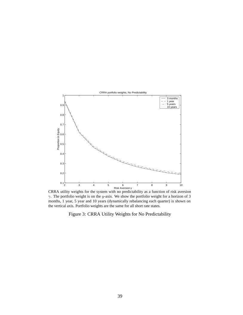
2 3 4 5 6 7 8 9 100.1

0.2

0.3

0.4

0.5

0.6

0.7

0.8

0.9

1

Risk Aversion γ

Pro

port

ion

in E

quity

CRRA portfolio weights, No Predictability

3 months1 year 5 years 10 years

CRRA utility weights for the system with no predictability as a function of risk aversionγ. The portfolio weight is on the y-axis. We show the portfolio weight for a horizon of 3months, 1 year, 5 year and 10 years (dynamically rebalancing each quarter) is shown onthe vertical axis. Portfolio weights are the same for all short rate states.

Figure 3: CRRA Utility Weights for No Predictability

39

0 0.05 0.1 0.150.1

0.2

0.3

0.4

0.5

0.6

0.7

0.8

0.9

1

Disappointment weighting 1−A

Por

tfolio

wei

ght

Myopic DA portfolio weights, No Predictability

γ = 2γ = 3γ = 4γ = 5γ = 6

1.5 2 2.5 3 3.5 4 4.5 5 5.5 6 6.50.1

0.2

0.3

0.4

0.5

0.6

0.7

0.8

0.9

1

Risk Aversion γ

Por

tfolio

wei

ght

Myopic DA portfolio weights, No Predictability

A = 1.00A = 0.95A = 0.90A = 0.85

Quarterly myopic DA utility weights for the system with no predictability. In the top plotportfolio weights appear as a function of disappointment level A with various γ. The bot-tom plot shows the portfolio weights as a function risk aversion γ with various A. Portfolioweights are the same for all short rate states. The case of A = 1 corresponds to CRRAutility.

Figure 4: Myopic DA Utility Portfolio Weights

40

0.02 0.04 0.06 0.08 0.1 0.12 0.14

0.86

0.88

0.9

0.92

0.94

0.96

0.98

Short rate (annualized)

Po

rtfo

lio w

eig

ht

in e

qu

ity

CRRA utility, No predictability, γ = 2


0.02 0.04 0.06 0.08 0.1 0.12 0.14

0.3

0.4

0.5

0.6

0.7

0.8

0.9

1


Por

tfolio

wei

ght i

n eq

uity

CRRA utility, Linear predictability, γ = 2


0.02 0.04 0.06 0.08 0.1 0.12 0.14

0.34

0.35

0.36

0.37

0.38

0.39

0.4


Po

rtfo

lio w

eig

ht

in e

qu

ity

CRRA utility, No predictability, γ = 5


0.02 0.04 0.06 0.08 0.1 0.12 0.14

0.15

0.2

0.25

0.3

0.35

0.4


Po

rtfo

lio w

eig

ht

in e

qu

ity

CRRA utility, Linear predictability, γ = 5


Portfolio weights for CRRA Utility for the system without predictability (left column) andwith short rate predictability (right column), as a function of the short rate. We dynamicallyrebalance every quarter.

Figure 5: CRRA Portfolio Weights

41

0 0.05 0.1 0.15

0.74

0.76

0.78

0.8

0.82

0.84

0.86

0.88

0.9

Short rate

Po

rtfo

lio w

eig

ht

in e

qu

ity

DA utility, No predictability, γ = 2 A = 0.95


0.02 0.04 0.06 0.08 0.1 0.12 0.140

0.1

0.2

0.3

0.4

0.5

0.6

0.7

0.8

0.9

1

short rate

equi

ty w

eigh

t

DA utility, Linear predictability, γ = 2, Myopic Horizon

A=1.00A=0.98A=0.95A=0.90

0.02 0.04 0.06 0.08 0.1 0.12 0.14

0.2

0.3

0.4

0.5

0.6

0.7

0.8

0.9

Short rate

Por

tfolio

wei

ght i

n eq

uity

DA utility, Linear predictability, γ = 2 A = 0.95


0.02 0.04 0.06 0.08 0.1 0.12 0.140

0.05

0.1

0.15

0.2

0.25

0.3

0.35

0.4

short rate

eq

uity

we

igh

t

DA utility, Linear predictability, γ = 5, Myopic Horizon

A=1.00A=0.98A=0.95A=0.90

Consider DA utility for the predictable system with γ = 5 and A = 0.95 in the top plot andA = 0.90 in the bottom plot. The graph shows the γ that yields the same optimal equityallocation when utility is CRRA. The x-axis shows (annualized) short rates, and the y-axisshows the implied CRRA. We work with a quarterly horizon. We dynamically rebalanceevery quarter.

Figure 6: DA Utility Portfolio Weights

42

0 0.05 0.1 0.155

5.5

6

6.5

7

7.5

8Implied γ for CRRA for DA with γ = 5, A = 0.95

short rate (annualized)

Impl

ied

CR

RA

ris

k av

ersi

on

0 0.05 0.1 0.156

8

10

12

14

16

18Implied γ for CRRA for DA with γ = 5, A = 0.90

short rate (annualized)

Impl

ied

CR

RA

ris

k av

ersi

on

For the predictable system we plot the implied CRRA risk aversion γ which correspondsto the same portfolio weight for DA utility. The horizon is one quarter. On the x-axis weshow (annualized) short rates, and on the y-axis implied CRRA γ.

Figure 7: Implied CRRA Risk Aversion of DA Utility

43

1 2 3 4 5 6 7 80

2

4

6

8

10

12CRRA Utility Quarterly Horizon

Risk Aversion γ

Required E

quity

Pre

miu

m

CRRA utilityEquity Prem 95% SE

1 2 3 4 5 6 7 80

2

4

6

8

10

12CRRA Utility Annual Horizon

Risk Aversion γ

Required E

quity

Pre

miu

m

CRRA utilityEquity Prem 95% SE

0.1 0.2 0.3 0.4 0.5 0.6 0.70

2

4

6

8

10

12

14

16

18DA Utility Quarterly Horizon


Required E

quity

Pre

miu

m

γ = 1 γ = 2 Equity Prem95% SE

0.1 0.2 0.3 0.4 0.5 0.6 0.70

2

4

6

8

10

12

14

16

18DA Utility Annual Horizon


Required E

quity

Pre

miu

m

γ = 1 γ = 2 Equity Prem95% SE

Equity premium required to hold a 60% weight in equities with a VAR without predictabil-ity (1941-1998). The historical equity premium is given by the straight line, with 95% SEbounds in dotted lines. The left hand column displays the required equity premium usinga quarterly horizon, the right hand column using an annual horizon. The top row showsCRRA utility, with risk averision γ on the x-axis. The bottom row shows DA utility, withγ = 1 and γ = 2, with disappointment weight 1 − A on the x-axis. The required equitypremium is presented as an annualized figure.

Figure 8: Required Equity Premium for 60% Equity

44

Why Stocks May Disappoint

Documents

Transcript of Why Stocks May Disappoint