Style Investing: Incorporating Growth Characteristics in Value Stocks

Parvez Ahmed, Ph.D.* Sudhir Nanda, Ph.D., CFA

Pennsylvania State University at Harrisburg

August 2000 * Corresponding author Address: Pennsylvania State University at Harrisburg School of Business Administration Middletown, PA 17057-4898 Parvez Ahmed, Assistant Professor of Finance Tel: (717) 948-6162; Fax: (717) 948-6456; email: pahmed@psu.edu Sudhir Nanda, Assistant Professor of Finance Tel: (717) 948-6161; Fax: (717) 948-6456; email: snanda@psu.edu Keywords: Value and Growth Investing; Style Investing JEL Classification: G1

Style Investing: Incorporating Growth Characteristics in Value Stocks

ABSTRACT Several empirical studies show a systematic relationship between stock characteristics (size, earning yield, dividend yield, etc.) and stock returns. The previous studies, that show stocks with high earnings yield produce superior returns use univariate measures (such as E/P or B/P) to classify stocks into value or growth stocks. This paper shows that the traditional method of classification ignores instances when value and growth investing strategies instead of being mutually exclusive can complement each other in selecting superior performing stocks. Growth in EPS provides a more meaningful way to capture growth than using a measure of low E/P ratio. A strategy focusing on investing in stocks that have the dual characteristics of a high E/P ratio and high growth in EPS outperforms a strategy of high E/P alone. The study also documents some evidence of persistence in performance for stocks having the dual characteristic of high growth in EPS and high E/P ratio. Keywords: Value and Growth Investing; Style Investing JEL Classification: G1

1

Style Investing: Incorporating Growth Characteristics in Value Stocks

Institutional investors often employ multiple domestic equity managers and select

managers that provide superior performance within a particular “style” category. Sharpe [1992]

shows that such style allocation decision as the key to successful portfolio management. Style

investing refers to a manager's adherence to some pre-defined and specific asset allocation

strategy. The popularity of style investing is seen in the proliferation of many style indexes. For

example, Wilshire Associates has a large selection of indexes that are designed to "track the

style-oriented investment products."1 However, most indexes and mutual fund evaluation

agencies such as Morningstar use a univariate definition such as high earnings yield (E/P) or

book-to-price ratio (B/P) to characterize value stocks.2 This univariate approach treats value and

growth as mutually exclusive investment styles. Studies by Michaud [1998], and Brown and

Mott [1997] suggest that there are significant measurement and performance benefits in

incorporating multiple dimensions when constructing style indexes or portfolios.

The finance literature generally classifies a stock as value or growth using a univariate

dimension such as earnings yield or book-to-price ratio. Studies by Fama and French [1992,

1993], and Capaul, Rowley and Sharpe [1993] present evidence that over the long-term value

stocks outperform growth stocks for both U.S. and foreign markets. Loughran (1997) contends

that the success of B/P ratio in explaining expected returns is primarily limited to small-cap

stocks, and the observed effectiveness of B/P ratio is explained by the presence of a strong

January effect. Similarly, Knez and Ready (1997) doubt the systematic relationship between

stock returns and B/P or size by showing the dependence of the Fama and French [1992] results

on “1% extreme observations.” Several other papers like Arnott [1992], Bernstein [1995] and

2

Kao and Shumaker [1999] posit that the success from investing in value and growth strategies is

conditional upon aggregate business and economic conditions. In contrast, Asness, Friedman,

Krail and Liew [2000] criticize this approach as being susceptible to spurious ex-post

relationship that may be artifacts of the data. They advocate using stock characteristics such as

spread in earnings yields and earnings growth rates between value and growth firms as indicators

of the attractiveness of a particular style strategy.

We examine an approach to style investing that conditions the selection of value

portfolios on their growth characteristics. Thus, value and growth, instead of being mutually

exclusive strategies can be complementary to each other. The intent is to illustrate a simple

strategy that provides superior returns over different investment horizons. While the idea of

incorporating growth characteristics in value portfolios may be old, it has not been empirically

tested over recent time periods. Results from a period that spans 1982 to 1997 indicate that the

incorporation of growth characteristics allows investors to enhance returns over a pure value

strategy, which were shown to be successful in several previous studies.3

To provide a more robust measure of the efficacy of our style portfolios, we evaluate

their risk and return characteristics over varying investment horizons. The terminal wealth

(TW) over their holding period and the variability in ending-period wealth may be of more

interest to long-term investors than the time series averages of annual returns (O'Neal 1997).

Finally, we analyze turnover in the style portfolios and illustrate a method of stock selection

based on momentum in earnings-per-share. Stratifying style portfolios on rate of change in

earnings indicates the efficacy of using information on momentum to further enhance portfolio

returns. Our results show that stocks that lie at the intersection of value and growth have the

highest returns and these stocks continue to outperform those in other style portfolios even in the

3

second year after their inclusion in a style portfolio. The consistency of this strategy over

different investing horizons and at different time periods shows that all value stocks may not be

equal; some are more equal than others.

PERSPECTIVES ON INCORPORATING GROWTH CHARACTERISTICS IN SELECTING VALUE STOCKS

Several studies show a systematic link between growth rates (historical or forecasted) and

stock returns. Harris and Marston [1994] report that B/P ratios are negatively correlated with

forecasts of future growth in earnings. This indicates that expectation of high growth increases

the price of the stock, which in turn lowers its B/P ratio. They find that portfolios of growth

stocks (low B/P or high growth in earnings per share) have similar return and risk and suggest

that to understand the effect of book-to-market ratios on stock returns one should incorporate

measures of future growth prospects. They use data from 1982-1989 and constrain their sample

to firms for which IBES had five-year growth forecasts. Their inability to find stocks that have

low B/P and low EPS growth (or high B/P and high EPS growth) and their overall results may be

driven by analysts' bias in projecting earnings growth, which is well documented in several

studies.4

Which variable proxies for growth? Lakonishok, Shleifer, and Vishny [1994] believe

that investor expectations are based on extrapolation of recent past performance. De Bondt and

Thaler [1987] suggest that investors overreact to recent stock market events. Dreman and Berry

[1995] support this contention by showing that analysts overreact to recent events, so subsequent

disappointments in EPS adversely affect the market price of growth stocks (low E/P) more than

value stocks (high E/P). Bauman and Miller (1997) examine four-year EPS growth rates and do

not find higher returns to higher growth stocks. They also find a negative correlation between

4

earnings surprise and past growth rates, and suggest that the EPS of higher growth stock is

overestimated to a greater extent than that of lower growth stocks.

Scott, Stumpp and Xu (1999) use a theoretical framework to show that earnings yield

alone do not capture all the growth characteristics of stocks. In the traditional dividend growth

model, the stock prices of low growth companies will be more dependent on the normalized

earnings; while for high growth companies, the growth opportunities will have a larger influence

on price. Borrowing from the behavioral theory of Kahneman and Tvesky [1979] and De Bondt

and Thaler [1985] they assert that cognitive biases can affect the estimates of both normalized

earnings and earnings growth. They imply that current valuation measures like E/P may be well

suited for characterizing value stocks but they have little meaning for growth stocks. As a result,

growth managers must seek out cheap growth stocks. Furthermore, because investors react

slowly to news, growth stock managers should ride winners and look for good news. In contrast,

they suggest that value investors should index or emphasize 'dogs' (stocks with low past earnings

growth rates, and low future expected EPS growth rates).

The previous literature gives us sufficient hint to explore the role of growth rates in style

investing. The studies that incorporate growth in earning per share to characterize growth stocks

use either analysts forecasts or long-term past growth rates. However, there is evidence to

suggest biases in earning forecast (De Bondt and Thaler, 1987) and mean reversions in long-term

growth rates (Rouwenhorst, 1998). Further, Lakonishok, Shleifer, and Vishny [1994] use only

NYSE/AMEX firms that have at least five-year's data, which limits the scope of their study.5 In

this paper, we define growth stocks as those having a high rate of growth in historical EPS and

evaluate the returns to portfolios that lie at the intersection of value and growth styles. We use

two-year average growth rate in EPS and use all firms on NYSE/AMEX and NASDAQ. This

5

ensures that we have a large enough sample to study the effect of superimposing growth

characteristics on value stocks. Given the evidence of mean reversions in long-term growth

rates, our definition of growth rate is more consistent with strategies followed by several money

managers.6

CREATING STYLE PORTFOLIOS AND SIMULATING TERMINAL WEALTH

Style portfolios are constructed using all firms in the Center for Research in Security

Prices (CRSP) and COMPUSTAT databases over the period 1982-1997. We use monthly stock

returns from CRSP, while E/P and growth in EPS, g, are from COMPUSTAT. The EPS growth

rate, g, is the annualized two-year growth rate. Following Fama and French [1995], we construct

portfolios by independently ranking firms on the basis of their earnings yield and g.7 We first

divide stocks into five groups based on g. Within each of these quintiles, stocks are assigned to

five portfolios based on their earnings yield. Stocks are reassigned to one of 25 portfolios in July

of each year. In addition to the full sample, we also formed similar portfolios for large and small

cap stocks. Stocks were divided into cap categories by dividing the full sample into two equal

sub-samples. These sub-samples allow us to study if style portfolio returns differ by market cap.

For each stock in our sample, the annual buy and hold return over year t is calculated by

compounding the monthly returns from July of year t to June of year t+1. The annual buy-and-

hold returns are cumulated over different holding periods to calculate terminal wealth from

investing $100 in each style portfolio.

Market values for calculating E/P are as of June. This allows us to avoid year-end

seasonality. To allow full dissemination of accounting information before assigning a firm to a

portfolio, the accounting variables such as earnings and growth in earnings are as of the previous

6

December. We exclude firms with negative earnings and all financial firms. Studies by Basu

[1977] and Dowen and Bauman [1986] find that excluding firms with negative earnings has no

effect on rankings of portfolio returns. Firms that were delisted during a year remained in the

sample for the time period they traded. To obtain the greatest separation between style

portfolios, we exclude portfolios that are in the middle E/P and g quintiles. Using the remaining

sixteen portfolios, we create the following style classes: low-growth and low-earnings yield

(LGLE), high-growth and low-earnings yield (HGLE), low-growth and high-earnings yield

(LGHE) and high-growth and high-earnings yield (HGHE). Thus, the LGLE portfolio includes

firms in the two lowest growth in EPS and two lowest E/P quintiles, while the HGHE portfolio

consists of firms at the intersection of the two highest growth and the two highest E/P quintiles.

To simulate terminal wealth, we randomly select two portfolios from the four portfolios

in each style class. This process is repeated 1,000 times. The return of each style portfolio is the

arithmetic mean of the returns for the two randomly selected portfolios.8 The selection process

used in this study in essence simulates a random selection of approximately 150 stocks for each

style portfolio from a universe of 300 stocks within that style class. However, the selection of

two portfolios from a basket of four implies that there will be only six unique combinations of

portfolios. While this may seem like an apparent limitation, it does not diminish the general

implication of the results. The simulations simply confirm the results obtained from using actual

returns and additionally allow comparison of risks across the four style classifications. For most

investors, risk as measured by standard deviation of a portfolio’s time-series returns is far less

important than variability in end-of-period wealth. Following Radcliffe [1994], we use mean

terminal wealth (MTW) and its standard deviation (TWSD) to measure the reward and risk from

the various investment strategies. These simulations will provide a test of robustness of

7

performance within each style. If only a handful of stocks drive differential performance across

style portfolios, our simulation should be able to highlight outliers.

CHARACTERISTICS OF STYLE PORTFOLIOS

Table 1 shows the summary characteristics of the 25 portfolios stratified by value and

growth. Each of the 25 portfolios on average consists of 75 stocks with an average monthly

trading volume of around 1.5 million shares. The style portfolios in our study are distinguishable

only by their E/P and g and do not have any systematic relationship with other market variables.

The growth rate in EPS, g, increases as we go across the columns with column 5 representing the

highest growth portfolios. The earnings yield increases as we go down the rows with row 5

representing the highest value portfolios. In Panels A, B and C of Table 1, we report the mean

E/P, g, and annual return from July of year t to June of year t+1 averaged across all 15 years.

Panel D provides the terminal wealth in June 1997 of $100 invested in July 1982.

The mean growth rates in the first two EPS growth quintiles are negative for all 10

portfolios. The growth rates in the fifth quintile averages 98%. The firms in the highest growth

quintile are obviously in a high growth phase, which may not be sustainable over long time

periods. As outliers may drive the means, we also examine the median growth rates for each

quintile. The highest growth quintile has a median growth rate of 59.5% and the lowest growth

quintile has a median growth rate of -40.5%.

The average E/P (P/E) ratio for lowest value quintile portfolios was 0.03 (33.33) and for

the highest value quintile was 2.23 (0.44). Out of concern that a few outliers could skew the

results, especially in the extreme portfolios, we also computed the median values of E/P (P/E).

The median E/P (P/E) values for the lowest and highest E/P quintiles were 0.03 (33.33) and 0.15

8

(6.66) respectively. The median E/P ratio for the highest value quintile indicates that its mean

value was indeed affected by some extreme observations.9

Panel D of Table 1 shows that as growth increases across the columns, the average annual

return and terminal wealth continue to increase up to the fourth growth quintile and decrease

thereafter. However, the returns in the highest growth quintile, on average, remain above those

of the two lowest growth quintiles. We observe that portfolios with the lowest growth rates

(column 1) consistently underperform all other portfolios. The likely cause is that the lowest

growth portfolios may represent severely underperforming firms with an average two-year

growth rate of -36.2%. Going down the rows we observe that the returns monotonically increase

with increasing E/P. High earnings yield stocks consistently outperform stocks with low

earnings yield.

Considering the interaction between value and growth characteristic of each portfolio

shows that portfolios, which lie at the intersection of the two highest E/P (value) and the two

highest growth quintiles outperform most other portfolios. The cumulative average return for the

four portfolios in the highest growth and highest value quintiles is $1,555. A passive strategy of

investing in the Wilshire 5000 index would have yielded $1,198 during the same time period

(average annual return of 19%). These high growth and high earnings yield portfolios also

outperform the Wilshire All Value Index that over the same time period had a return of $1,278.

In contrast, the high earnings yield and low growth stocks underperform the Wilshire 5000 index

with a cumulative average return of $887. Thus, stratifying the value portfolios on their growth

in EPS characteristics allows us to identify stocks that outperform a passive index strategy.

[Table 1 here]

9

In Figure 1 we present the cumulative returns for the low (E/P) value portfolios (both

high and low growth) and the Wilshire All Growth Index. The 15-year cumulative return for the

portfolios HGLE, LGLE and the Wilshire All Growth Index are $552, $520 and $1,145

respectively. Similarly, in Figure 2 we compare the two high earnings yield portfolios with the

Wilshire Value Index. The 15-year cumulative return for the portfolios HGHE, LGHE and the

Wilshire All Value Index are $1,555, $887 and $1,278 respectively. The annual return for the

HGHE portfolio exceeded that of the other three style portfolios in 10 out of the 15 years studied.

These results show that passive indexing may be a better strategy when investing in stocks with

low earnings yield, but value investors are better off selecting stocks that in addition to a high

earnings yield also have high growth rate in EPS.

[Figure 1 and Figure 2 here]

SIMULATING RETURNS FROM INVESTMENT IN STYLE PORTFOLIOS

We simulate investing in value/growth portfolios by randomly selecting two portfolios

from a choice of the four portfolios within each style class (HGHE, HGLE, LGLE, LGHE). This

process is repeated 1,000 times to yield many different combinations of portfolios. These

portfolios are rebalanced every year for the next 15 years. For example, in simulation 1 we

select two portfolios from the four that belong to the HGHE style class and in July of the

following year we select two new portfolios from this style class. The terminal wealth of HGHE

style portfolio is then the cumulative return from these random selections made in July of each

year.

For the 1,000 randomly selected portfolios, we calculate the mean terminal wealth

(MTW) and the standard deviation (TWSD) of terminal wealth over different holding periods.

10

For example, for a 3-year holding period, we compute the TW for the three years from July 1982

to June 1985. Thereafter, another year is added while dropping the first one. In Table 2 we

report the performance of each style portfolio by reporting their MTW, TWSD, the 5th, 25th, 75th

and 95th percentile TW. Each statistic is reported over 3, 5, 10 and 15-year holding periods.

Results in Table 2 show that the HGHE portfolio outperforms all other style portfolios. The

extent of its superior performance increases with longer holding periods. For 10- and 15-year

holding periods the 5th percentile TW of HGHE exceeds the 95th percentile TW of all other

portfolios. For 3- and 5-year holding periods the HGHE portfolio is clearly superior to others

with its 25th percentile value exceeding the 95th percentile value of all other style portfolios

except LGHE.

For every holding period, the risk (as measured by TWSD) of portfolio LGHE is the

lowest. Thus, this portfolio has the highest reward-to-risk ratio (MTW/TWSD). The best

performing portfolio, HGHE, also has the highest standard deviation of terminal values.

However, the extent of its larger terminal wealth suggests that even after accounting for risk, the

high growth and high earnings yield strategy is superior to other strategies. In general, the 25th

percentile TW of HGHE exceeds the 75th percentile TW of other style portfolios.

[Table 2 here]

We also evaluate the performance of our value-growth portfolios against a benchmark

index. Figure 3 shows that the difference in the mean TW of the four style portfolios and the

returns to the corresponding indexes. The portfolios with low earnings yield were compared

with the Wilshire All Growth Index while those with high earnings yield were compared with the

Wilshire All Value Index. All style portfolios except HGHE underperform their respective

indexes. Only the HGHE style portfolio outperforms its benchmark index over every holding

11

period. For a $100 investment, the HGHE portfolio earns $11, $23, $49 and $509 more than the

Wilshire All Value Index over the 3, 5, 10 and 15-year holding periods respectively.

[Figure 3 here]

We next evaluate the effectiveness of our style portfolios in sub-samples stratified by

market cap. Table 3 reports the 15-year TW for each style portfolio stratified by market cap.10

The HGHE portfolio is again the clear winner with its 5th percentile TW ($1,108.70 for small

caps and $1,149.46 for large caps) exceeding the 95th percentile TW of all other style portfolios

except HGLE in the large cap universe. Also, a year-by-year comparison of the annual (July-

June) returns shows that the HGHE portfolio has the highest return in 10 out of 15 years for

small-cap stocks and in 8 out of 15 years for large-cap stocks. The strategy of investing in

HGHE stocks seems to work better for small cap stocks. However, the HGHE portfolios provide

the highest cumulative return among all other style portfolios regardless of market cap.

[Table 3 here]

The terminal wealth calculations use annual rebalancing in July of each year. This may

lead to large transactions cost if many firms get re-classified each year. To examine the practical

use of these value-growth strategies we evaluate the extent of stock turnover in our style

portfolios. Table 4 shows that only 28% of firms in the HGHE portfolio remain in the same

style class in the year following their classification. This average is similar for other style

portfolios. Moreover, the majority of firms that drift out of their style class bounce between the

high and low earnings yield classes. For example, 17% of the firms in HGHE move to HGLE

next year while only 3% move to LGHE. Thus, very rarely (average of 6%) do firms move from

one growth class to another. The drift in and out of value classes is attributable to the change in

price of the stocks. High earnings yield stocks perform well and move into low earnings yield

12

classifications while low earnings yield stocks perform poorly and become earnings yield

portfolios.

One way to reduce transaction costs associated with high portfolio turnover will be to

rebalance the style portfolios less frequently. Figure 4 shows the MTW of all style portfolios

when rebalancing occurs every two years. For example, firms that enter a certain style portfolio

in July of 1982 are kept in that particular style portfolio until June 1984. In July 1984, a new set

of firms belonging the same style classification is chosen. This process is repeated every two

years. Results show that the HGHE portfolio again outperforms the other style portfolios. The

extent of its superior performance increases over longer investment horizons.

[Figure 4 here]

Evidence from the momentum literature shows stock returns have a systematic

relationship with rate of change in their growth rates.11 The growth rate, g, in our study is a two

year average. These averages by themselves do not provide information on change in the

direction of growth over the past two years. By stratifying the sample on growth characteristics,

we evaluate the role momentum plays in the performance of the stocks (portfolios). Our results

show that stocks with increasing momentum (negative growth rate followed by positive growth

rate or increasing positive growth rate) in general outperform those with decreasing momentum

(positive growth rate followed by negative growth rate or increasing negative growth rate).

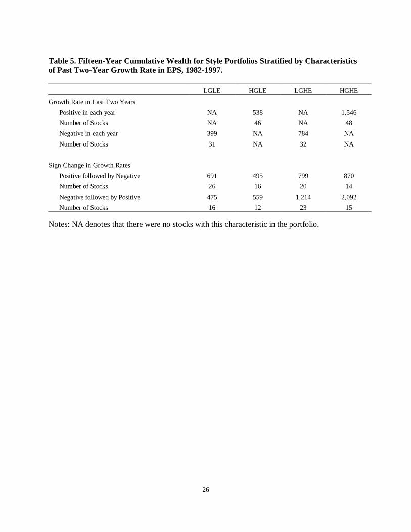
Table 5 reports the performance of the four style portfolios segmented by characteristics

of the growth rate in the previous two years. Results show that firms with positive growth rates

in each of the past two years outperform firms with negative growth rates. Also, there is strong

evidence in support of momentum investing. Stocks that have increasing momentum outperform

those with decreasing momentum within each style class except LGLE. The hidden gems in the

13

HGHE style class are firms that have an overall positive growth rate but their growth rate in year

t-1 changes to positive after being negative in year t-2. This group of stocks outperforms the

Wilshire 5000 and the Wilshire All Value indexes by a significant margin.

IMPLICATIONS FOR INVESTORS

The popularity of style investing is reflected in the plethora of mutual funds that are

categorized as value or growth by classification agencies such as Morningstar, Lipper etc.

This dichotomy, placing funds in one of the two categories, suggests value and growth investing

are mutually exclusive. These agencies use a univariate scale (such as E/P or B/P) to define

value and growth. The practice of placing a portfolio or stock into value or growth category has

usually been accomplished by using arbitrary measures. For instance, Morningstar classifies all

funds with average price-to-earnings and price-to-book ratios 12.5% below those of the S&P 500

Index as ‘value’ funds.

In this paper, we show empirical evidence that can allow investors to enhance returns

from a value strategy. Value and growth may not be mutually exclusive. Specifically, all firms

that do not meet the high earnings yield criterion need not be automatically labeled growth

stocks. By using the historical growth rate in earnings to distinguish growth stocks, we examine

an investment process where value and growth strategies may complement each other. Our

results show that stocks at the intersection of high earnings yield and growth outperform all other

stocks.

To achieve superior results from investing in high earnings yield and growth stocks, an

investor will have to rebalance their portfolio every year. With only 30% of stocks remaining

within the style this rebalancing can lead to significant transactions costs.12 However, we find

14

that the performance of high earnings yield and high growth stocks persists in the second year

following their classification to their style class, with a higher two-year return than other style

portfolios.

Results from this study also show support for momentum investing strategies. Stocks

that either exhibited a reversal in growth rates from negative to positive or had sequentially

increasing positive growth rates over the past two years, significantly outperformed other

subsamples of stocks. Approximately 40% of the stocks in the high earnings yield and high

growth style category exhibited this trend in growth rates. This evidence has important

implications for fund managers and pension sponsors.

15

REFERENCES Arnott, R. "Style Management: The Missing Element in Equity Portfolios." Journal of Investing, Summer 1992. Arshanapalli, B. T., D. Coggin, and J. Doukas." Multifactor Asset Pricing Analysis of International Value Investment Strategies." The Journal of Portfolio Management, Summer 1998, 24 (4) pp. 10-23. Asness, C.S., J.A. Friedman, R.J. Krail, and J.M. Liew. "Style Timing: Value versus Growth." Journal of Portfolio Management, 2000, 26(3), pp. 50-60. Basu, S. "Investment Performance of Common Stocks in Relation to their Price-Earnings Ratios: A Test of the Efficient Market Hypothesis." Journal of Finance, June 1977, 32( 3), pp. 663-682. Bauman, W. S. and R. E. Miller. "Investor Expectations and the Performance of Value Stocks versus Growth Stocks." The Journal of Portfolio Management, Spring 1997, 23(3) pp. 57-68. Bernstien, R., "Style Investing: Unique Insight into Equity Management," New York, John Wiley & Sons. Brown, M.R., and C.E. Mott. "Understanding the Differences and Similarities of Equity Style Indexes." 1977, in T.D. Coggin, F. Fabozzi and R. Arnott, eds.., The Handbook of Equity Style Management, Fabozzi and Associates Publishing. Capaul, C., I. Rowley, and W. F. Sharpe. "International Value and Growth Stock Returns." Financial Analysts Journal, January/February 1993, 49(1) pp. 27-36. Chan, L., Y. Hamao, and J. Lakonishok, "Fundamentals and stock returns in Japan." Journal of Finance, 1991, 46, pp. 1739-1764. Das, S., Levine, C.B., and Sivaramakrishnan, K., 1998, "Earnings predictability and bias in analysts' earnings forecasts," The Accounting Review; v.73 (2), pp. 277-294. De Bondt, W. F. M., and R. H. Thaler. "Does the Stock Market Overreact?" Journal of Finance, July 1985, 40(3), pp. 793-808. De Bondt, W. F. M., and R. H. Thaler. "Further Evidence on Investor Overreaction and Stock Market Seasonality." Journal of Finance, July 1987 42(3), pp. 557-581. Dowen, R. J., and W. S. Bauman. "The Relative Importance of Size, P/E, and Neglect." The Journal of Portfolio Management, Spring 1986, 12(2) pp. 30-34. Easterwood, J.C, and S.C. Nutt. "Inefficiency in analysts' earnings forecasts: Systematic misreaction or systematic optimism?" The Journal of Finance, 1999, 54(5), pp. 1777-1797.

16

Fama, E. F., and K. R. French. "Size and Book-to-Market Factors in Earnings and Returns." The Journal of Finance, March 1995, 50(1), pp. 131-155. Fama, E. F., and K. R. French. "The Cross-Section of Expected Stock Returns." Journal of Finance, June 1992, 47(2), pp. 427-465. Harris, R.D.F. "The accuracy, bias and efficiency of analysts' long run earnings growth forecasts," Journal of Business Finance & Accounting, 1999, 26 (5/6), pp. 725-755. Harris, Robert S., and F. C. Marston. "Value versus Growth Stocks: Book-to-Market, Growth and Beta." Financial Analysts Journal, September/October 1994, 50(5), pp. 18-24. Jaffe, J., D.B. Keim and R. Westerfield. "Earnings yield, market values, and stock returns, Journal of Finance, 1989, 44, pp. 135-148. Kahneman, D. and A. Tversky. "Prospect Theory: An Analysis of Decision Making Under Risk." Econometrica, March 1979, 47(2), pp. 263-291. Kahneman, D. and A. Tversky. "Intuitive Predication: Biases and Corrective Procedures." In Judgment Under Uncertainty: Heuristics and Biases. 1982, Edited by D. Kahneman, P. Slovic, and A. Tversky. New York: Cambridge University Press. Kao, D., and R. Shumaker. "Equity Style Timing," Financial Analysts Journal, 1999, 55, pp. 37-18. Knez, P.J. and Ready, M.J., "On the robustness of size and book-to-market in cross-sectional regressions," The Journal of Finance, 1997, 52(4), pp. 1355-1382. Lakonishok, J., A. Shleifer, and R. W. Vishny. "Contrarian Investment, Extrapolation, and Risk." Journal of Finance, December 1994, 49(5), pp. 1541-1578. Loughran, T. "Book-to-Market across Firm Size, Exchange, and Seasonality: Is There an Effect?" Journal of Financial and Quantitative Analysis, September 1997, 32(3) pp. 249-268. Michaud, R.O. "Is value multidimensional? Implications for style management and global stock selection," Journal of Investing, 1998, 7 (1), pp. 61-65. O’Neal, E. S. "How Many Mutual Funds Constitute a Diversified Mutual Fund Portfolio?" Financial Analysts Journal, March/April 1997, 53(2) pp. 37-46. Radcliffe, R. C. "Investment: Concepts, Analysis, Strategy," 1994, New York: Harper Collins Publishers. Rouwenhorst, K. G. "International Momentum Strategies." Journal of Finance, February 1998, 53(1) pp. 267-284.

17

Scott, J., M. Stumpp and P. Xu, “Behavioral bias, valuation, and active management.” Financial Analysts Journal, Jul/Aug 1999, Vol. 55(4), 49-58.

18

Table 1. Summary Characteristics of Value and Growth Portfolios

Lowest g Highest g Mean

Panel A: Average E/P

Lowest E/P 0.01 0.03 0.04 0.04 0.03 0.03

0.03 0.06 0.06 0.07 0.06 0.06

0.05 0.07 0.08 0.08 0.09 0.07

0.07 0.09 0.10 0.11 0.12 0.10

Highest E/P 2.18 1.06 3.73 2.35 1.83 2.23

Mean 0.47 0.26 0.80 0.53 0.43

Panel B: Average g (%)

Lowest E/P -59.6 -14.2 0.8 17.3 102 9.26

-43.5 -14.1 1.3 16.5 90.1 10.06

-37.6 -13.9 1.1 16.2 93.5 11.86

-36.1 -13.6 1.1 16.4 99.6 13.48

Highest E/P -36.2 -13.5 1.5 16.9 107.3 15.20

Mean -42.60 -13.86 1.16 16.66 98.50

Panel C: Average Annual Return

Lowest E/P 14.1 14.3 15.3 16.0 11.2 14.1

15.8 17.5 17.2 17.3 16.5 16.8

17.0 18.9 17.0 20.2 20.2 18.6

18.3 19.1 18.3 19.2 21.8 19.3

Highest E/P 17.4 19.0 19.8 25.2 22.4 20.7

Mean 16.5 17.7 17.5 19.5 18.4 18.0

Panel D: Cumulative Return from July 1982-June 1997 (ending value of $100 invested in July 1982)

Lowest E/P 362 441 510 592 226 426

515 763 767 818 571 687

684 1,038 742 1,155 1,137 951

783 992 956 1,091 1,325 1,029

Highest E/P 766 1,007 1,183 2,316 1,489 1,352

Mean 622 848 832 1,194 950 889

19

Figure 1. Comparison of Cumulative Returns to Growth Portfolios (HGLE and LGLE) with the Cumulative Return to the Wilshire 5000 Growth index (WG)

Note: The cumulative returns represent the ending value of a $100 investment in July of 1982.

1145

520

552

0

200

400

600

800

1000

1200

1400

1983 1984 1985 1986 1987 1988 1989 1990 1991 1992 1993 1994 1995 1996 1997 Year

Cum

ulat

ive

Wea

lth (

$)

WG LGLE HGLE

20

Figure 2. Comparison of Cumulative Returns to Value Portfolios (LGHE and HGHE) with the Cumulative Return to the Wilshire 5000 Value index (WV)

Note: The cumulative returns represent the ending value of a $100 investment in July of 1982.

1278

887

1555

0

200

400

600

800

1000

1200

1400

1600

1800

1983 1984 1985 1986 1987 1988 1989 1990 1991 1992 1993 1994 1995 1996 1997 Year

Cum

ulat

ive

Wea

lth (

$)

WV LGHE HGHE

21

Table 2. Terminal Wealth and Standard Deviation of Terminal Wealth from Investing $100 in July 1982 for Various Holding Periods

Mean

(MTW) Standard Deviation (TWSD)

MTW/ TWSD

5th Percentile

25th Percentile

75th Percentile

95th Percentile

3-Year Holding Period

LGLE 137.09 9.30 14.75 121.40 129.47 143.55 154.87

HGLE 137.90 8.93 15.45 121.89 130.48 144.68 154.95

LGHE 151.50 8.76 17.29 133.53 144.60 155.80 164.91

HGHE 168.23 10.97 15.34 148.02 160.55 176.97 188.34

5-Year Holding Period

LGLE 163.50 14.85 11.01 136.74 151.26 173.19 193.23

HGLE 163.35 13.98 11.68 138.58 156.48 173.34 189.60

LGHE 190.50 13.38 14.24 163.85 179.26 202.55 213.54

HGHE 226.22 20.00 11.31 191.78 209.03 242.04 265.69

10-Year Holding Period

LGLE 239.94 39.46 6.08 175.26 205.59 272.58 330.64

HGLE 247.21 35.00 7.06 184.46 217.61 273.59 311.95

LGHE 321.56 24.91 12.91 271.83 303.28 341.90 358.79

HGHE 447.53 63.27 7.07 359.38 392.76 493.44 593.00

15-Year Holding Period

LGLE 620.47 101.40 6.12 461.87 536.60 689.78 862.66

HGLE 635.83 160.68 3.96 326.02 482.48 860.86 917.96

LGHE 992.91 82.63 12.02 866.31 883.18 1,091.89 1,113.43

HGHE 1,637.68 313.30 5.23 1,191.02 1,399.65 1,880.13 2,415.72 Note: Mean Terminal Wealth is significantly different between all pairs of style portfolio at 1% level of significance.

22

Figure 3. Difference in Style Portfolio Terminal Wealth and Corresponding Wilshire Style Indexes over Various Holding Periods

3 Year 5 Year

10 Year 15 year

LGLE-WG

HGLE-WG

LGHE-WV HGHE-WV

-400

-300

-200

-100

0

100

200

300

400

500

$600

Difference in Cumulative Wealth

Holding Period

Style Portfolios

23

Table 3. Cumulative Terminal Wealth over a 15-year Investing Horizon by Market Capitalization, 1982-1997.

Mean (MTW)

Standard Deviation (TWSD)

MTW/TWSD 5th Percentile

25th Percentile

75th Percentile

95th Percentile

Number of Years

Portfolio was

Winner

Small Cap

LGLE 633.06 97.54 6.49 474.32 554.53 716.74 860.46 1

HGLE 598.78 173.58 3.45 296.08 457.75 735.86 951.76 1

LGHE 933.93 88.09 10.60 773.34 853.32 998.39 1,081.27 3

HGHE 1,695.13 425.29 3.99 1,108.70 1,333.86 2,071.07 2,804.22

10

Large Cap

LGLE 683.95 135.21 5.06 431.97 627.74 835.99 879.35 2

HGLE 782.46 204.84 3.82 492.84 542.83 856.55 1,179.58 3

LGHE 1,036.60 97.99 10.58 807.02 953.18 1,117.26 1,142.89 2

HGHE 1,378.90 121.04 11.39 1,149.46 1,272.53 1,501.67 1,646.29 8

Note: Mean Terminal Wealth is significantly different between all pairs of style portfolio at 1% level of significance.

24

Table 4. Where Did Firms in the Style Portfolios Come From and Where Do They Go?

Style In Current Year Style In Other Years Year -1 Year +1

Year +2

Missing 17 24 37

Middle 29 25 21

LGLE 24 25 12

HGLE 10 6 1

LGHE 14 15 21

LGLE

HGHE 6 5 8

Missing 16 20 33

Middle 29 28 28

LGLE 6 10 8

HGLE 29 29 12

LGHE 4 2 4

HGLE

HGHE 17 11 14

Missing 27 14 27

Middle 22 30 27

LGLE 15 14 18

HGLE 5 4 8

LGHE 30 30 14

LGHE

HGHE 4 7 6

Missing 24 16 29

Middle 26 28 25

LGLE 5 5 6

HGLE 10 17 25

LGHE 7 3 1

HGHE

HGHE 28 30 14 In each style class percentages add to 100 in each column.

25

Figure 4. Cumulative Returns (in $) over Different Holding Periods for Style Portfolios with Rebalancing Every Second Year

3-Year 5-Year 10-Year 15-Year LGLE HGLE LGHE HGHE

0 100 200 300 400 500 600 700 800 900

1,000

Cumulative Wealth ($)

Investment Horizon

Portfolio Style

LGLE 134 159 240 467 HGLE 139 165 264 535 LGHE 150 188 335 782 HGHE 159 205 384 994

3-Year 5-Year 10-Year 15-Year

26

Table 5. Fifteen-Year Cumulative Wealth for Style Portfolios Stratified by Characteristics of Past Two-Year Growth Rate in EPS, 1982-1997. LGLE HGLE LGHE HGHE Growth Rate in Last Two Years Positive in each year NA 538 NA 1,546 Number of Stocks NA 46 NA 48

Negative in each year 399 NA 784 NA Number of Stocks 31 NA 32 NA

Sign Change in Growth Rates Positive followed by Negative 691 495 799 870 Number of Stocks 26 16 20 14

Negative followed by Positive 475 559 1,214 2,092 Number of Stocks 16 12 23 15 Notes: NA denotes that there were no stocks with this characteristic in the portfolio.

27

NOTES 1 The Wilshire categories include style-classification based on market capitalization and value/growth. 2 Russell and BARRA use price-to-book ratio to classify stocks into value and growth styles. 3 Basu [1977], Jaffe, Keim and Westefield [1989], Chan, Hamao and Lakonishok, [1991], Fama and French [1992], Capaul, Rowley, and Sharpe [1993], Lakonishok, Shleifer and Vishny [1994], and Arshanapalli, Coggins, and Doukas [1998]. 4 See Eaterwood and Nutt [1999]; Harris [1999]; and Das, Levine, and Sivaramakrishnan [1998] for some recent papers that demonstrate the bias in analysts forecast of earnings. In a recent Forbes magazine article the author Dreman [1998] sounds the same caution by saying, "analysts have been far too optimistic over the years in making earnings forecasts." 5 They use five-year growth in sales as proxy for growth characteristics. 6 This was confirmed during the authors numerous informal conversations with money managers. 7 We also ran tests on one-year EPS growth rate and for B/P ratio. The results remain qualitatively similar to those reported here and are available upon request. 8 Alternatively, we selected one and three portfolios. Besides a reduction in the standard deviation of terminal wealth as number of portfolios selected increased, the results remain qualitatively similar. 9 In 1999 the average P/E ratio of a Morningstar classified value fund was 20. The average P/E ratio over the last fifteen years in the last two value quintiles is 8. The overall rise in stock price in the last few years may explain the difference between the P/E ratios of our value portfolios and the current market defined value portfolios. Similarly, the P/E ratio of our low value portfolios is 24, which is slightly lower than that of Morningstar defined growth funds, whose P/E ratios averaged around 36. 10 3, 5 and 10-year results are not reported partially out of concern for the length of the paper. These results are qualitatively similar to 15-year results and are available upon request. 11 See Rouwenhorst [1998]. 12 This turnover rate is below the turnover rate of a typical mutual fund.