Potency of the Residual Surpluses of Ogives

Udobia Etukudo1*

 1Department of Mathematics, Federal College of Education (Technical), Omoku, RiversState, Nigeria, Africa, Nigeria Contact Information: udobiaelijah2@yahoo.com Abstract Ogives or graphs of cumulative frequency is a very useful statistical tool which offersapproximate values of some measures of central tendency and invariably somemeasures of dispersion easily and equally availed good, clear and distinct graphicvisual impression of the data. Median, quartiles, percentiles, docile, quartile deviations,percentile deviations and percentile coefficients of kurtosis are some of the statisticsthat can readily be obtained from Ogives and are quintessential in estimating baselineand growth potential in the economy. To obtain data with higher accuracy, there is theneed to determine the residual values of the ogives and accumulate them in the datafor the various statistics generated. The effectiveness of utilizing the residual surplusesof the Ogives on each of the statistics is the nub of this paper. The impact of the residualon the accuracy of the estimator is very important. In estimating the median, quartiles,docile, percentiles, quartile deviation, semi interquartile range and other measures ofcentral tendency and dispersion it is essential to evaluate the residuals and its influenceon the statistics. The trend lines offer a justifiable medium to unveiling the residualsurpluses of ogives. Plotting the trend of a given ogives simultaneously with that of theogives residual trend provide the machinery to determine the nature and types ofresidual surpluses that are associated with or can be generated from ogives. Theconcomitant terminologies, inaugural residual surpluses, terminal residual surpluses,trend line intercepts residual surpluses and trend line slope residual surpluses, areinconspicuous components of the ogives that reduces the truism of the statistics sogenerated, in relative dimensions. For the purpose of perfection and significance theydeserve attention and application.

Keywords : potency, Residual Surpluses, Ogives, measure of central tendency, measure of dispersion

The residual surpluses implacably describe the unquantifiable

elements that are not considered in the computation but are part

of the distribution, which constitute agents of inaccuracy of

estimation or inferred values. Lawson(2013) defined residual as r

= y∑ i - θ∑ i where yi are the observed values of the variable Y

and θi the least square estimates of the regression parameters.

Further classification into raw residual and standardized

residual brings into consideration the neutralizing or

eliminating preponderant of non-constant variance (Lawson, 2013).

The residual in statistical analysis is described as “the amount

of variability in a dependent variable that is left over after

counting for the variability explained in the analysis” with

regards to regression (Taylor, 2013). Another definition of

residuals is ei = observed response – predicted response, which

is given ei = yi – b0 – bixi (Borghers and Wessa, 2012). Guarisma

(2013) and Bowell (2013) defined residual as the different

between observations and predictions.

Residual is always statistical associated with regressions,

Lane (2013) and Wilcox (2010) gives different methods of

calculating the various types of residuals associated with

regressions. For example, Wilcox (2010) states that for the

function y = a0 + a1x1 +a2x2 + a3x3 + … where y is the dependent

variable and x1, x2, x3 are independent variables the coefficients

(ai) offers the smallest residual sum of squares which is

equivalent to the greatest correlation coefficient squared, R2

and states also the relationship between the various parameters

of the regression data and the residuals. Lane (2013) critically

examines the concepts influence, leverage, distance and

studentized residual, of simple regression analysis, whereby the

influence is defined as how much the predicted score for other

observation would differ if the observation is questioned,

leverage as the degree which the an observation value differ from

the mean predictor variable, distance being the error of

prediction while studentized residual as the error of prediction

divided by standard deviation of the prediction.

Ogives alternatively called cumulative frequency curve

(Singh, 2013) are constructed for group distribution whereby the

upper class limit is constructed on the x – axis and the

cumulative frequency on the y-axis (Singh, 2013; Loveday, 1981)

are used in computing some measures of central tendency and

dispersion without any recourse to the existence of any form of

residuals. In reality do there exists residuals in ogives? Like

in any other curve which is not plotted with the raw data the

involves treatment or reorganization of the data to any degree

there is the tendency of the existence of residual hence residual

exists in ogives.

General Outlook of Residuals

Suppose there is a series of observations from a univariate distribution and we want to estimate the mean of that distribution (the so-called location model). In this case, the errors are the deviations of the observations from the population

mean, while the residuals are the deviations of the observations from the sample mean.

A statistical error (or disturbance) is the amount by which an observation differs from its expected value, the latter being based on the whole population from which the statistical unit waschosen randomly. For example, if the mean height in a population of 21-year-old men is 1.75 meters, and one randomly chosen man is1.80 meters tall, then the "error" is 0.05 meters; if the randomly chosen man is 1.70 meters tall, then the "error" is −0.05 meters. The expected value, being the mean of the entire population, is typically unobservable, and hence the statistical error cannot be observed either.

A residual (or fitting error), on the other hand, is an observable estimate of the unobservable statistical error. Consider the previous example with men's heights and suppose we have a random sample of n people. The sample mean could serve as agood estimator of the population mean. Then we have:

The difference between the height of each man in the sample and the unobservable population mean is a statistical error, whereas

The difference between the height of each man in the sample and the observable sample mean is a residual.

Note that the sum of the residuals within a random sample is necessarily zero, and thus the residuals are necessarily not independent. The statistical errors on the other hand are independent, and their sum within the random sample is almost surely not zero.

One can standardize statistical errors (especially of a normal distribution) in a z-score (or "standard score"), and standardizeresiduals in a t-statistic, or more generally studentized residuals.

If we assume a normally distributed population with mean μ and standard deviation σ, and choose individuals independently, then we have

and the sample mean

is a random variable distributed thus:

The statistical errors are then

whereas the residuals are

(As is often done, the "hat" over the letter ε indicates an observable estimate of an unobservable quantity called ε.)

The sum of squares of the statistical errors, divided by σ2, has a chi-squared distribution with n degrees of freedom:

This quantity, however, is not observable. The sum of squares of the residuals, on the other hand, is observable. The quotient of that sum by σ2 has a chi-squared distribution with only n − 1 degrees of freedom:

This difference between n and n − 1 degrees of freedom results inBessel's correction for the estimation of sample variance of a population with unknown mean and unknown variance, though if the mean is known, no correction is necessary.

It is remarkable that the sum of squares of the residuals and thesample mean can be shown to be independent of each other, using, e.g. Basu's theorem. That fact, and the normal and chi-squared distributions given above, form the basis of calculations involving the quotient

The probability distributions of the numerator and the denominator separately depend on the value of the unobservable population standard deviation σ, but σ appears in both the numerator and the denominator and cancels. That is fortunate because it means that even though we do not know σ, we know the probability distribution of this quotient: it has a Student's t-distribution with n − 1 degrees of freedom. We can therefore use this quotient to find a confidence interval for μ.

RegressionsIn regression analysis, the distinction between errors and residualsis subtle and important, and leads to the concept of studentized residuals. Given an unobservable function that relates the independent variable to the dependent variable – say, a line – the deviations of the dependent variable observations from this function are the unobservable errors. If one runs a regression onsome data, then the deviations of the dependent variable observations from the fitted function are the residuals.

However, a terminological difference arises in the expression mean squared error (MSE). The mean squared error of a regression is a number computed from the sum of squares of the computed residuals, and not of the unobservable errors. If that sum of squares is divided by n, the number of observations, the result is the mean of the squared residuals. Since this is a biased estimate of the variance of the unobserved errors, the bias is removed by multiplying the mean of the squared residuals by n / df where df is the number of degrees of freedom (n minus the number of parameters being estimated). This latter formula serves

as an unbiased estimate of the variance of the unobserved errors,and is called the mean squared error.[1]

However, because of the behavior of the process of regression, the distributions of residuals at different data points (of the input variable) may vary even if the errors themselves are identically distributed. Concretely, in a linear regression wherethe errors are identically distributed, the variability of residuals of inputs in the middle of the domain will be higher than the variability of residuals at the ends of the domain: linear regressions fit endpoints better than the middle. This is also reflected in the influence functions of various data points on the regression coefficients: endpoints have more influence.

Thus to compare residuals at different inputs, one needs to adjust the residuals by the expected variability of residuals, which is called studentizing. This is particularly important in the case of detecting outliers: a large residual may be expected in the middle of the domain, but considered an outlier at the endof the domain.

Stochastic error

The stochastic error in a measurement is the error that is randomfrom one measurement to the next. Stochastic errors tend to be gaussian (normal), in their distribution. That's because the stochastic error is most often the sum of many random errors, andwhen many random errors are added together, the distribution of their sum looks gaussian, as shown by the Central Limit Theorem. A stochastic error is added to a regression equation to introduceall the variation in Y that cannot be explained by the included Xs. It is, in effect, a symbol of our inability to model all the movements of the dependent variable.

The use of the term "error" as discussed in the sections above isin the sense of a deviation of a value from a hypothetical unobserved value. At least two other uses also occur in statistics, both referring to observable prediction errors:

Mean square error or mean squared error (abbreviated MSE) and root mean square error (RMSE) refer to the amount by which the values predicted by an estimator differ from the quantities beingestimated (typically outside the sample from which the model was estimated).

Sum of squared errors, typically abbreviated SSE or SSe, refers to the residual sum of squares (the sum of squared residuals) of a regression; this is the sum of the squares of the deviations ofthe actual values from the predicted values, within the sample used for estimation. Likewise, the sum of absolute errors (SAE) refers to the sum of the absolute values of the residuals, which is minimized in the least absolute deviations approach to regression.

In statistics, a studentized residual is the quotient resulting from the division of a residual by an estimate of its standard deviation. Typically the standard deviations of residuals in a sample vary greatly from one data point to another even when the errors all have the same standard deviation, particularly in regression analysis; thus it does not make sense to compare residuals at different data points without first studentizing. Itis a form of a Student's t-statistic, with the estimate of error varying between points.

This is an important technique in the detection of outliers. It is named in honor of William Sealey Gosset, who wrote under the pseudonym Student, and dividing by an estimate of scale is called studentizing, in analogy with standardizing and normalizing: see Studentization.

The key reason for studentizing is that, in regression analysis of a multivariate distribution, the variances of the residuals at different input variable values may differ, even if the variancesof the errors at these different input variable values are equal. The issue is the difference between errors and residuals in statistics, particularly the behavior of residuals in regressions.

Consider the simple linear regression model

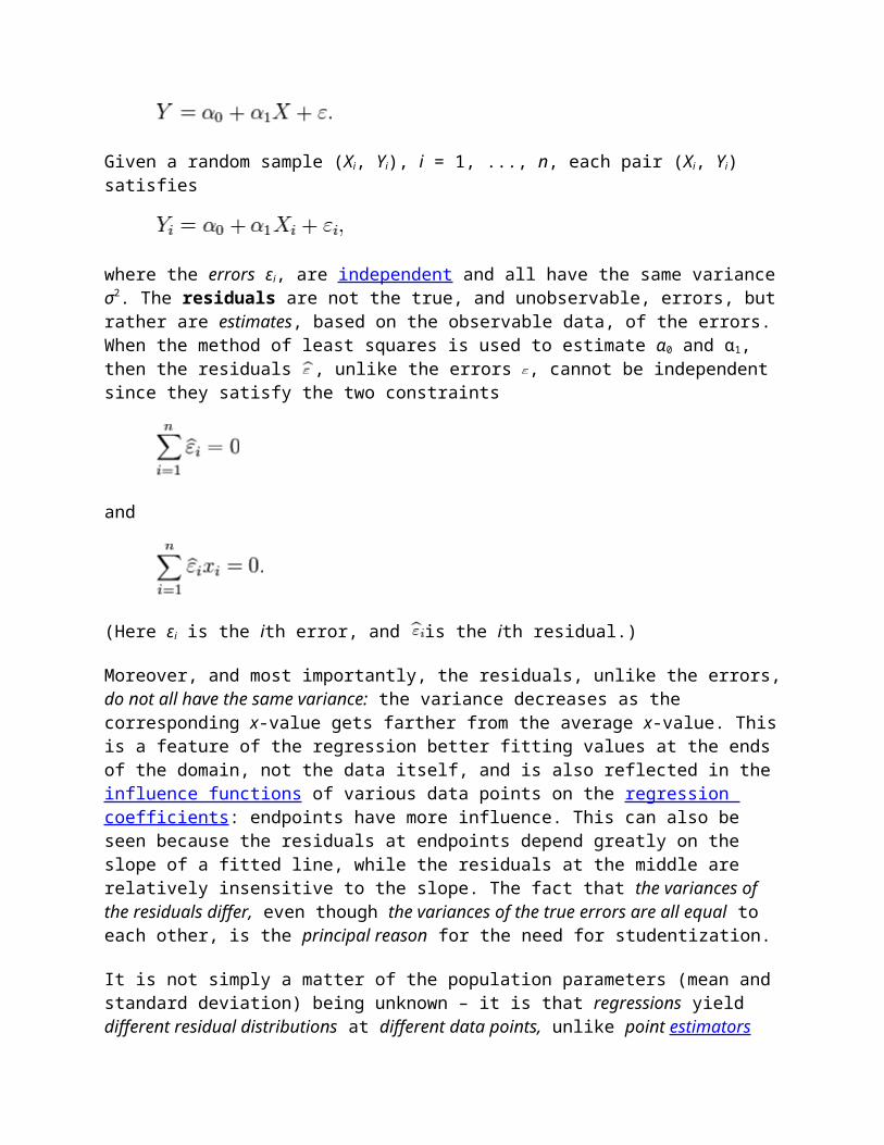
Given a random sample (Xi, Yi), i = 1, ..., n, each pair (Xi, Yi) satisfies

where the errors εi, are independent and all have the same varianceσ2. The residuals are not the true, and unobservable, errors, butrather are estimates, based on the observable data, of the errors.When the method of least squares is used to estimate α0 and α1, then the residuals , unlike the errors , cannot be independent since they satisfy the two constraints

and

(Here εi is the ith error, and is the ith residual.)

Moreover, and most importantly, the residuals, unlike the errors,do not all have the same variance: the variance decreases as the corresponding x-value gets farther from the average x-value. Thisis a feature of the regression better fitting values at the ends of the domain, not the data itself, and is also reflected in the influence functions of various data points on the regression coefficients: endpoints have more influence. This can also be seen because the residuals at endpoints depend greatly on the slope of a fitted line, while the residuals at the middle are relatively insensitive to the slope. The fact that the variances of the residuals differ, even though the variances of the true errors are all equal to each other, is the principal reason for the need for studentization.

It is not simply a matter of the population parameters (mean and standard deviation) being unknown – it is that regressions yield different residual distributions at different data points, unlike point estimators

of univariate distributions, which share a common distribution for residuals.

How to studentizeFor this simple model, the design matrix is

and the hat matrix H is the matrix of the orthogonal projection onto the column space of the design matrix:

The "leverage" hii is the ith diagonal entry in the hat matrix. Thevariance of the ith residual is

In case the design matrix X has only two columns (as in the example above), this is equal to

The corresponding studentized residual is then

where is an appropriate estimate of σ (see below).

Internal and external studentization]The usual estimate of σ2 is

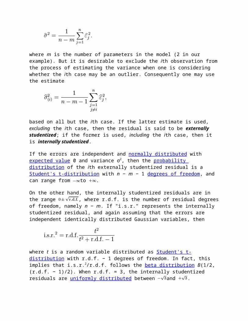
where m is the number of parameters in the model (2 in our example). But it is desirable to exclude the ith observation fromthe process of estimating the variance when one is considering whether the ith case may be an outlier. Consequently one may use the estimate

based on all but the ith case. If the latter estimate is used, excluding the ith case, then the residual is said to be externally studentized; if the former is used, including the ith case, then it is internally studentized.

If the errors are independent and normally distributed with expected value 0 and variance σ2, then the probability distribution of the ith externally studentized residual is a Student's t-distribution with n − m − 1 degrees of freedom, and can range from to .

On the other hand, the internally studentized residuals are in the range , where r.d.f. is the number of residual degreesof freedom, namely n − m. If "i.s.r." represents the internally studentized residual, and again assuming that the errors are independent identically distributed Gaussian variables, then

where t is a random variable distributed as Student's t-distribution with r.d.f. − 1 degrees of freedom. In fact, this implies that i.s.r.2/r.d.f. follows the beta distribution B(1/2,(r.d.f. − 1)/2). When r.d.f. = 3, the internally studentized residuals are uniformly distributed between and .

If there is only one residual degree of freedom, the above formula for the distribution of internally studentized residuals doesn't apply. In this case, the i.s.r.'s are all either +1 or −1, with 50% chance for each.

The standard deviation of the distribution of internally studentized residuals is always 1, but this does not imply that the standard deviation of all the i.s.r.'s of a particular experiment is 1. For instance, the internally studentized residuals when fitting a straight line going through (0, 0) to the points (1, 4), (2, −1), (2, −1) are , and the standard deviation of these is not

Residual Plots

Residual plot is a graph that shows the residuals on the vertical axis and theindependent variable on the horizontal axis. If the points in a residual plot are randomly dispersed around the horizontal axis, a linear regression model is appropriate for the data; otherwise, a non-linear model is more appropriate.

Below, the residual plots show three typical patterns. The first plot shows a random pattern, indicating a good fit for a linear model. The other plot patterns are non-random (U-shaped and inverted U), suggesting a better fit fora non-linear model.

Random pattern Non-random: U-shaped curve Non-random: Inverted U

http://stattrek.com/statistics/dictionary.aspx?

definition=residual_plot

Graph of Cumulative Frequency (Ogives)

Cumulative frequency curve or ogives is a graph of cumulative

frequency of any given data which are useful in the determination

of percentiles, quartiles, docile and median of the given

distribution. The cumulative frequencies of every class are

plotted against the upper limits of the class. This implies

plotting the cumulative frequency on the vertical y-axis and the

upper limit of the class on the horizontal or x-axis. In the

first instance the data are grouped into classes, which entail

ignoring the original positioning or scattering of the data in

question.

In certain occasion the data may cluster to the lower or the

upper end of the class but this will not be reflected in the

ogives. The data may even cluster to the middle of the class but

ogives will not reflect. Unlike the histogram which uses the

class mark (class midpoint) which is a representative status of

each class, the ogive uses the upper class which is an obvious

implication for the existence of residual. Let the following data

be taken into consideration to demonstrate nature of ogive.

25 28 18 17 35 8 9 85 93 62

49 46 57 54 63 72 88 64 56 51

14 23 38 47 47 66 55 57 59 72

94 88 87 72 65 59 57 49 56 63

58 59 62 63 57 82 72 42 63 47

Distribution Examination Scores of Candidates in STA 131 –

Inference

Table 1: Cumulative Frequency tableClass Class

markUpper ClassLimit

Frequency CumulativeFrequency

1 - 10 5.5 10 2 2

11 - 20 15.5 20 3 521 – 30 25.5 30 3 831 – 40 35.5 40 2 1041 – 50 45.5 50 7 1751 - 60 55.5 60 13 3061 – 70 65.5 70 9 3971 – 80 75.5 80 4 4381 – 90 85.5 90 5 4891 – 100 95.5 100 2 50

50

0 20 40 60 80 100 1200

10

20

30

40

50

60

Ogives

Figure 1

The above gives the ogives of the distribution. In order to studythe residual of the distribution score by score cumulativefrequency has to be constructed as below.

Table 2: Cumulative frequency table of the ScoresScore Cumulative

FrequencyScore Cumulative

Frequency

0 0 55 208 1 56 229 2 57 2614 3 58 2717 4 59 3018 5 62 3223 6 63 3625 7 64 3728 8 65 3835 9 66 3938 10 72 4342 11 82 4446 12 85 4547 15 87 4649 17 88 4851 18 93 4954 19 94 50

Figure 20 10 20 30 40 50 60 70 80 90 100

0

10

20

30

40

50

60

Residual Plot of Ogives

0 10 20 30 40 50 60 70 80 90 1000

10

20

30

40

50

60

Residual with Trend Line

Figure 3

0 20 40 60 80 100 1200

10

20

30

40

50

60

Ogives with Trend Line

The Residual of OgivesConsidering the nature of the curves in figure 1 to figure 4, itis obvious that though the graphs emanate from precisely the sameset of data their curvatures are slightly different. There existdifferent in the intercepts of the x-axis and y-axis, gradient atsome point, complete different in the gradient of their trendline. These variations invariable could be attributed to thepresence of residual.

Residual Surpluses of OgivesDiscretely and simply put, the curve in figure 1 starts at origin(0,0) whereas the one of figure 2 starts at (1,8). Thisdifference between (0,0) and (1,8) could be termed as inauguralresidual surplus. Similarly, the curve in figure 1 ends at (50,100),while figure 2 ends at (50, 94). This difference could also bedescribed as terminus residual surplus.Considering the trend lines in figure 3 and figure 4, theirequations are as following:

Figure 4

y = o.6x – 4 . . . (1) and y = 0.5x . . . (2)Equation 1, represent trend line equation for the residual curveof the ogive, while equation 2 is the trend line equation for theOgive. The different in the intercepts and gradient could also betermed as trend line intercept residual surplus or trend lineslope residual surplus as the case may be. Different data would give rise to different residualsurpluses. Though they may look insignificant in some cases, butwhen the data derive from ogives are used in making statisticalinferences for issues involving distribution of income ingovernment agencies, budgeting, crop production, sales of producethat value up millions and billions, it become inevitableevaluation and consideration of the residual surplus in thecomputation. Potency of Residual Surpluses of OgivesLet the trend line equation of the ogives be To = f(x) and thetrend line equation of the residual plot Tr = g(x), assuming thatf(x) and g(x) are different in intercept and gradients, let f(0)= D and g(0) = d, then the inaugural residual surplus of theogives could be given as f(0) – g(0) = D –d.

Similarly, if f(x) and g(x) are produced to a point x = ai ,where i = 0,1, 2, 3, … and ai being the upper limit of thelast class. If f(ai) = E and g(ai) = e then the terminal residualsurpluses f(ai) - g(ai) = E – e. This is likely to have someinfluence on the derived statistics. The gradient of the twotrend lines are given by f/(x) and g/(x), the first derivativesof the trend line function may slightly different by f/(x) -g/(x), since they are straight lines, for the purpose ofprojection and inferences, there supposed to be a compensationalaccommodation of the differences in estimation. This calls for

the assessment of the impact of the various residual differenceson the statistics.

Consider the median of a given distribution derived from theogives, by obtaining the data that is exactly at the middle ofthe cumulative frequency, assuming f = N, then ½(N+1) gives the∑

value of the median on the corresponding axis, assuming there isa shear between the ogives’ trend and the residual plot trend,then median will shift, though ½(N+1) will be applicable in thetwo cumulative frequency axis, the corresponding value of themedian may change. The change in value is primarily on variableaxis (x-axis) originating from the linear displacement resultingfrom the presence of inaugural residual and terminal residualsurpluses. Let the average surpluses be given by ε thecompensatory value to curb the effect of residual surpluses on

the median say λ0 = ; thus the median = XN/2 + λ0.In determining quantities with quartiles, the different

values of λ would be used. For the first quartile λ1 = ;thus the first quartile Q1 = XN/4 + λ1 ; for the third quartile

λ3 = and The third Quartile Q3 = X3N/4 + λ3. The docile canalso be determined in the same manner. The first docile could

have the residual λd1 = and the actual value of the firstdocile given as D1 = XN/10 + λd1, however other docile, i docile, can

be obtained by Di = Xi×N/10 + λdi = where i = 1, 2, 3, …Percentile are also affected by the residual surpluses of ogives,a given percentile say i percentile could be given by Pi = Xi×N/100 +

λpi, where λpi = .Other statistics derived from the ogives directly or in

directly are also affected by the present of the residualsurpluses. This category of statistics include quartiledeviation, percentile deviation and percentile coefficient of

kurtosis, the impact of residual surpluses of the ogives on themare checked by properly accumulating them in their componentstatistics. . References Borghers, E. and Wessa P. (2012) Descriptive Statistics –Simple Linear Regression -Residuals – Definition.. http://www.xycoon.com. 14/6/2013

Bowells, E. (2013). Calculation of Residual of AsteroidsPositions.

http://www.fitsblink.net/residuals. 14/6/2013 Guarisma, P. E. (2013). Least – Squares Regression.http://www.herkimershideway.org.

14/6/2013. Lane, D. M.(2013). Influential Observations. Introduction to

linear Regression http://onlinestatbook.com. 14/6/2013

Lawson, P. V. (2013). Module 4: Residual Analysis.http://statmaster.sdu.dk/courses/st111 18/6/2013

Loveday, R.. A(1981). First Course in Statistics. (2nd

Edition). London, CambridgeUniversity Press. pp.15-16.

Singh, T. R.(2013). Graphical Representation of FrequencyDistribution: Cumulative

Frequency Curve (Ogives). http://www.doeaccimphal.org. 20/06/2013Taylor, J. J.(2013). Confusing Stats Term Explained:Residual. Stats Make Me Cry.

http://www.statsmakemecry.com. 14/6/2013Wilcox, W. R. (2013). Explanation of Results Returned by

Regression Tool in Excel’s Data Analysis.http://people.clarkson.educ/~wwicox/ES100/regrnt.htm .14/6/2013.

Cook, R. Dennis; Weisberg, Sanford (1982). Residuals and Influence in Regression. (Repr. ed.). New York: Chapman and Hall. ISBN 041224280X. Retrieved 23 February 2013.

<img src="//en.wikipedia.org/wiki/Special:CentralAutoLogin/start?type=1x1" alt="" title="" width="1" height="1" style="border: none; position: absolute;" />Retrieved from "http://en.wikipedia.org/w/index.php?title=Studentized_residual&oldid=607170830"

1. ̂ Steel, Robert G. D.; Torrie, James H. (1960). Principles and Procedures of Statistics, with Special Reference to Biological Sciences. McGraw-Hill.p. 288.

Cook, R. Dennis; Weisberg, Sanford (1982). Residuals and Influence in Regression. (Repr. ed.). New York: Chapman and Hall. ISBN 041224280X. Retrieved 23 February 2013.

Weisberg, Sanford (1985). Applied Linear Regression (2nd ed.). New York: Wiley. ISBN 9780471879572. Retrieved 23 February 2013.

Hazewinkel, Michiel, ed. (2001), "Errors, theory of", Encyclopedia of Mathematics, Springer, ISBN 978-1-55608-010-4

Additional FactsAbsolute deviationFrom Wikipedia, the free encyclopediaJump to: navigation, search

"Mean deviation" redirects here. For the book, see Mean Deviation (book).

This article needs additional citations for verification. Please help improve this article by adding citations to reliable sources. Unsourced material may be challenged and removed. (April 2014)

In statistics, the absolute deviation of an element of a data setis the absolute difference between that element and a given point. Typically the deviation is reckoned from the central value, being construed as some type of average, most often the median or sometimes the mean of the data set.

where

Di is the absolute deviation,

xi is the data element

and m(X) is the chosen measure of central tendency of the data set—sometimes the mean ( ), but most often the median.

Contents [hide] 

1 Measures of dispersion o 1.1 Mean absolute deviation

1.1.1 Mean absolute deviation (MAD) o 1.2 Average absolute deviation about median

1.2.1 Median absolute deviation (MAD) 1.2.2 Maximum absolute deviation

2 Minimization 3 Estimation 4 See also 5 References 6 External links

Measures of dispersion[edit]Several measures of statistical dispersion are defined in terms of the absolute deviation.

Mean absolute deviation[edit]

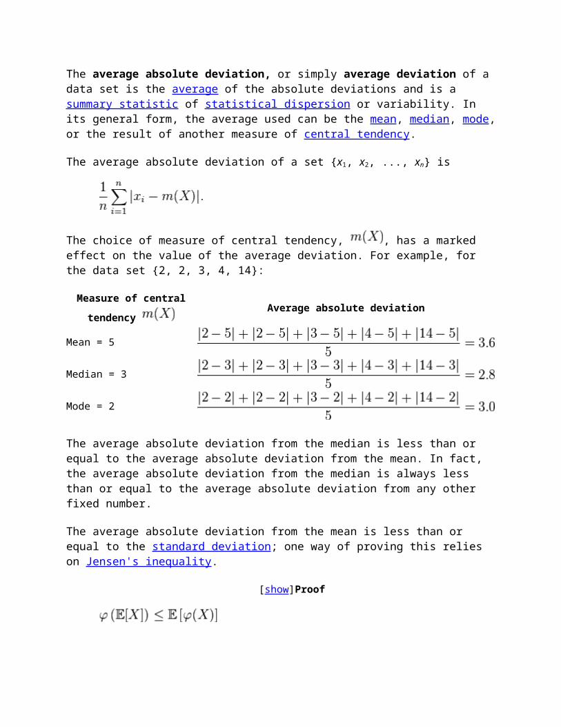
The average absolute deviation, or simply average deviation of a data set is the average of the absolute deviations and is a summary statistic of statistical dispersion or variability. In its general form, the average used can be the mean, median, mode,or the result of another measure of central tendency.

The average absolute deviation of a set {x1, x2, ..., xn} is

The choice of measure of central tendency, , has a marked effect on the value of the average deviation. For example, for the data set {2, 2, 3, 4, 14}:

Measure of centraltendency

Average absolute deviation

Mean = 5

Median = 3

Mode = 2

The average absolute deviation from the median is less than or equal to the average absolute deviation from the mean. In fact, the average absolute deviation from the median is always less than or equal to the average absolute deviation from any other fixed number.

The average absolute deviation from the mean is less than or equal to the standard deviation; one way of proving this relies on Jensen's inequality.

[show]Proof

For the normal distribution, the ratio of mean absolute deviationto standard deviation is . Thus if X is a normally distributed random variable with expected value 0 then, see Geary(1935):[1]

In other words, for a normal distribution, mean absolute deviation is about 0.8 times the standard deviation. However in-sample measurements deliver values of the ratio of mean average deviation / standard deviation for a given Gaussian sample n withthe following bounds: , with a bias for small n.[2]

Mean absolute deviation (MAD)[edit]

The mean absolute deviation (MAD), also referred to as the mean deviation (or sometimes average absolute deviation, though see above for a distinction), is the mean of the absolute deviations of a set of data about the data's mean. In other words, it is theaverage distance of the data set from its mean. MAD has been proposed to be used in place of standard deviation since it corresponds better to real life.[3] Because the MAD is a simpler measure of variability than the standard deviation, it can be used as pedagogical tool to help motivate the standard deviation.[4][5]

This method forecast accuracy is very closely related to the meansquared error (MSE) method which is just the average squared error of the forecasts. Although these methods are very closely related MAD is more commonly used[citation needed] because it does not require squaring.

More recently, the mean absolute deviation about mean is expressed as a covariance between a random variable and its under/over indicator functions;[6]

where

Dm is the expected value of the absolute deviation about mean,

"Cov" is the covariance between the random variable X and the over indicator function ( ).

and the over indicator function is defined as

Based on this representation new correlation coefficients are derived. These correlation coefficients ensure high stability of statistical inference when we deal with distributions that are not symmetric and for which the normal distribution is not an appropriate approximation. Moreover an easy and simple way for a semi decomposition of Pietra’s index of inequality is obtained.

Average absolute deviation about median[edit]

Mean absolute deviation about median (MAD median) offers a directmeasure of the scale of a random variable about its median

For the normal distribution we have . Since the median minimizes the average absolute distance, we have

. By using the general dispersion function Habib (2011) defined MAD about median as

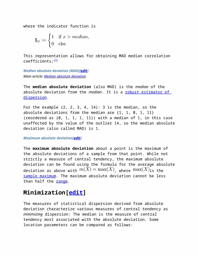
where the indicator function is

This representation allows for obtaining MAD median correlation coefficients;[7]

Median absolute deviation (MAD)[edit]Main article: Median absolute deviation

The median absolute deviation (also MAD) is the median of the absolute deviation from the median. It is a robust estimator of dispersion.

For the example {2, 2, 3, 4, 14}: 3 is the median, so the absolute deviations from the median are {1, 1, 0, 1, 11} (reordered as {0, 1, 1, 1, 11}) with a median of 1, in this case unaffected by the value of the outlier 14, so the median absolutedeviation (also called MAD) is 1.

Maximum absolute deviation[edit]

The maximum absolute deviation about a point is the maximum of the absolute deviations of a sample from that point. While not strictly a measure of central tendency, the maximum absolute deviation can be found using the formula for the average absolutedeviation as above with , where is the sample maximum. The maximum absolute deviation cannot be less than half the range.

Minimization[edit]The measures of statistical dispersion derived from absolute deviation characterize various measures of central tendency as minimizing dispersion: The median is the measure of central tendency most associated with the absolute deviation. Some location parameters can be compared as follows:

L 2 norm statistics: the mean minimizes the mean squared error L 1 norm statistics: the median minimizes average absolute

deviation, L ∞ norm statistics: the mid-range minimizes the maximum absolute

deviation trimmed L ∞ norm statistics: for example, the midhinge (average of

first and third quartiles) which minimizes the median absolute deviation of the whole distribution, also minimizes the maximum absolute deviation of the distribution after the top and bottom 25% have been trimmed off.

Estimation[edit]This section requires expansion. (March 2009)

The mean absolute deviation of a sample is a biased estimator of the mean absolute deviation of the population. In order for the absolute deviation to be an unbiased estimator, the expected value (average) of all the sample absolute deviations must equal the population absolute deviation. However, it does not. For the population 1,2,3 both the population absolute deviation about themedian and the population absolute deviation about the mean are 2/3. The average of all the sample absolute deviations about the mean of size 3 that can be drawn from the population is 44/81, while the average of all the sample absolute deviations about themedian is 4/9. Therefore the absolute deviation is a biased estimator.However, this argument is based on the notion of mean-unbiasedness. Each measure of location has its own form of unbiasedness (see entry on biased estimator. The relevant form ofunbiasedness here is median unbiasedness.

See also[edit] Deviation (statistics) Errors and residuals in statistics Least absolute deviations Loss function Mean difference

Median absolute deviation Squared deviations

References[edit]1. Jump up ̂ Geary, R. C. (1935). The ratio of the mean deviation to

the standard deviation as a test of normality. Biometrika, 27(3/4), 310-332.

2. Jump up ̂ See also Geary's 1936 and 1946 papers: Geary, R. C. (1936). Moments of the ratio of the mean deviation to the standard deviation for normal samples. Biometrika, 28(3/4), 295-307 and Geary, R. C. (1947). Testing for normality. Biometrika, 34(3/4), 209-242.

3. Jump up ̂ http://www.edge.org/response-detail/254014. Jump up ̂ Kader, Gary (March 1999). "Means and MADS". Mathematics

Teaching in the Middle School 4 (6): 398–403. Retrieved 20 February 2013.

5. Jump up ̂ Franklin, Christine, Gary Kader, Denise Mewborn, Jerry Moreno, Roxy Peck, Mike Perry, and Richard Scheaffer (2007). Guidelines for Assessment and Instruction in Statistics Education. American Statistical Association. ISBN 978-0-9791747-1-1.

6. Jump up ̂ Elamir, Elsayed A.H. (2012). "On uses of mean absolute deviation: decomposition, skewness and correlation coefficients".Metron: International Journal of Statistics LXX (2-3).

7. Jump up ̂ Habib, Elsayed A.E. (2011). "Correlation coefficients based on mean absolute deviation about median". International Journal ofStatistics and Systems 6 (4): pp. 413–428.

<img src="//en.wikipedia.org/wiki/Special:CentralAutoLogin/start?type=1x1" alt="" title="" width="1" height="1" style="border: none; position: absolute;" />Retrieved from "http://en.wikipedia.org/w/index.php?title=Absolute_deviation&oldid=621585280"

Categories:

Statistical deviation and dispersion

Hidden categories:

Articles needing additional references from April 2014 All articles needing additional references

All articles with unsourced statements Articles with unsourced statements from September 2013 Articles to be expanded from March 2009 All articles to be expanded

This page was last modified on 17 August 2014 at 06:09. Text is available under the Creative Commons Attribution-

ShareAlike License; additional terms may apply. By using this site, you agree to the Terms of Use and Privacy Policy. Wikipedia® is a registered trademark of the Wikimedia Foundation,Inc., a non-profit organization.

Why You Need to Check Your Residual Plots for Regression Analysis: Or, To Err is Human, To Err Randomly is StatisticallyDivine

Anyone who has performed ordinary least squares (OLS) regression analysis knows that you need to check the residual plots in order to validate your model. Have you ever wondered why? There are mathematical reasons, of course, but I’m going to focus on the conceptual reasons. The bottom line is that randomness and unpredictability are crucial components of any regression model. If youdon’t have those, your model is not valid.

Why? To start, let’s breakdown and define the 2 basic components of a valid regressionmodel:

Response = (Constant + Predictors) + Error 

Another way we can say this is:

Response = Deterministic + Stochastic

The Deterministic Portion

This is the part that is explained by the predictor variables in the model. The expected value of the response is a function of a set of predictor variables. All of the explanatory/predictive information of the model should be in this portion.

The Stochastic Error

Stochastic is a fancy word that means random and unpredictable. Error is the difference between the expected value and the observed value. Putting this together, the differences between the expected and observed values must be unpredictable. In other words, none of the explanatory/predictive information should be in the error.

The idea is that the deterministic portion of your model is so good at explaining (or predicting) the response that only the inherent randomness of any real-world phenomenon remains leftover for the error portion. If you observe explanatory or predictive power in the error, you know that your predictors are missing some of the predictive information. Residual plots help you check this!

Statistical caveat: Regression residuals are actually estimates of the true error, just like the regression coefficients are estimates of the true population coefficients.

Using Residual Plots

Using residual plots, you can assess whether the observed error (residuals) is consistent with stochastic error. This process is easy to understand with a die-rolling analogy. When you roll a die, you shouldn’t be able to predict which number will show on any given toss. However, you can assess a series of tosses to determine whether the displayed numbers follow a random pattern. If the number six shows up morefrequently than randomness dictates, you know something is wrong with your understanding (mental model) of how the die actually behaves. If a gambler looked at the analysis of die rolls, he could adjust his mental model, and playing style, to factor in the higher frequency of sixes. His new mental model better reflects the outcome.

The same principle applies to regression models. You shouldn’t be able to predict the error for any given observation. And, for a series of observations, you can determine whether the residuals are consistent with random error. Just like with the die, if the

residuals suggest that your model is systematically incorrect, you have an opportunityto improve the model.

So, what does random error look like for OLS regression? The residuals should not be either systematically high or low. So, the residuals should be centered on zero throughout the range of fitted values. In other words, the model is correct on averagefor all fitted values. Further, in the OLS context, random errors are assumed to produce residuals that are normally distributed. Therefore, the residuals should fall in a symmetrical pattern and have a constant spread throughout the range. Here's how residuals should look:

Now let’s look at a problematic residual plot. Keep in mind that the residuals should not contain any predictive information.

In the graph above, you can predict non-zero values for the residuals based on the fitted value. For example, a fitted value of 8 has an expected residual that is negative. Conversely, a fitted value of 5 or 11 has an expected residual that is positive.

The non-random pattern in the residuals indicates that the deterministic portion (predictor variables) of the model is not capturing some explanatory information that is “leaking” into the residuals. The graph could represent several ways in which the model is not explaining all that is possible. Possibilities include:

A missing variable A missing higher-order term of a variable in the model to explain the

curvature A missing interction between terms already in the model

Identifying and fixing the problem so that the predictors now explain the information that they missed before should produce a good-looking set of residuals!

In addition to the above, here are two more specific ways that predictive information can sneak into the residuals:

The residuals should not be correlated with another variable. If you can predict the residuals with another variable, that variable should be

included in the model. In Minitab’s regression, you can plot the residuals by other variables to look for this problem. 

Adjacent residuals should not be correlated with each other (autocorrelation). If you can use one residual to predict the next residual, there is some predictive information present that is not capturedby the predictors. Typically, this situation involves time-ordered observations. For example, if a residual is more likely to be followed by another residual that has the same sign, adjacent residuals are positively correlated. You can include a variable that captures the relevant time-related information, or use a time series analysis. In Minitab’s regression, you can perform the Durbin-Watson test to test for autocorrelation.

Are You Seeing Non-Random Patterns in Your Residuals?

I hope this gives you a different perspective and a more complete rationale for something that you are already doing, and that it’s clear why you need randomness in your residuals. You must explain everything that is possible with your predictors so that only random error is leftover. If you see non-random patterns in your residuals, it means that your predictors are missing something.

If you're learning about regression, read my regression tutorial!

You might like:

Applied Regression Analysis: How to Present and Use the Results to Avoid Costly Mistakes, part 2 | Minitab

How High Should R-squared Be in Regression Analysis? | Minitab

Regression Analysis: How Do I Interpret R-squared and Assess the Goodness-of-Fit? | Minitab

Guest Post: Did Ma's Diabetes Get Cured by Back Surgery?

Guest Post: Did Ma's Diabetes Get Cured by Back Surgery?

Regression Analysis: How Do I Interpret R-squared and Assess the Goodness-of-Fit? | Minitab

How High Should R-squared Be in Regression Analysis? | Minitab

Applied Regression Analysis: How to Present and Use the Results to Avoid Costly Mistakes, part 2 | Minitab

Recommended by

Prev Next

Comments for Why You Need to Check Your Residual Plots for Regression Analysis: Or, To Err is Human, To Err Randomly is Statistically Divine

Name: VijayTime: Sunday, March 3, 2013

Jim-excellent blog. Just learning about regression diagnostics in an MBAclass and this blog just did a beautiful job of explaining why we have to examine the residuals. Thanks

Name: MaggieTime: Monday, April 14, 2014

Thank you, Jim for your excellent explanations. Although I'm using PHStat2 in an MBA class, your Minitab insight works just as well for me!If only you'd written my text book! Thanks, again, and I'll continue to refer to your site.

Name: Jim FrostTime: Friday, April 18, 2014

Hi Maggie, thank you so much for your very kind words. I'm glad that youfound my blogs helpful! I hope you have your own fun adventures in statistics!

Jim

Name: ShilpaTime: Friday, June 13, 2014

This is really helpful. Thank you so much for sharing it.:)

Name: Ram subramanianTime: Wednesday, June 25, 2014

Very informative, Thanks a lot

Name: shivraj ghadgeTime: Tuesday, July 1, 2014

nice

Name: JustineTime: Friday, August 1, 2014

Authors

Categories Use a Line Plot to Show a Summary Statistic Over Time Using the G-Chart Control Chart for Rare Events to Predict Borewell Accidents Angst Over ANOVA Assumptions? Ask the Assistant. How Accurate are Fantasy Football Rankings? Part II “You’ve got a friend” in Minitab Support How Could You Benefit from Between / Within Control Charts? Taking the Training Wheels Off: Rethinking How Lean Six Sigma is Taught Making the Office Coffee Better with a Designed Experiment for Optimization

Patrick Runkel Joel Smith Kevin Rudy Jim Frost Carly Barry Full List of Authors Lean Six Sigma Statistics Quality Improvement Data Analysis Project Management Tools

Blog Map Newsletter Contact Us Legal Privacy Policy

Quality. Analysis. Results.®

Minitab®, Quality Companion by Minitab®, Quality Trainer by Minitab®, Quality. Analysis. Results® and the Minitab logo are all registered trademarks of Minitab, Inc.,in the United States and other countries.

Copyright 2014 Minitab Inc. All rights Reserved.   

ContinueThis article is about the statistical properties of unweighted linear regression analysis. For more general regression analysis, see regression analysis. For linear regression on a single variable, see simple linear regression. For the computation of least squares curve fits, see numerical methods for linear least squares.

Regression analysis

Models

Linear regression Simple regression

Ordinary least squares Polynomial regression General linear model

Generalized linear model Discrete choice

Logistic regression Multinomial logit

Mixed logit Probit

Multinomial probit Ordered logit Ordered probit

Poisson

Multilevel model Fixed effects Random effects

Mixed model

Nonlinear regression Nonparametric Semiparametric

Robust Quantile Isotonic

Principal components Least angle

Local

Segmented

Errors-in-variables

Estimation

Least squares Ordinary least squares

Linear (math) Partial Total

Generalized Weighted

Non-linear Iteratively reweighted

Ridge regression LASSO

Least absolute deviations Bayesian

Bayesian multivariate

Background

Regression model validation Mean and predicted response

Errors and residuals Goodness of fit

Studentized residual Gauss–Markov theorem

Statistics portal

v t e

Okun's law in macroeconomics states that in an economy the GDP growth should depend linearly on the changes in the unemployment rate. Here the ordinary least squares method is used to construct the regression line describing this law.

In statistics, ordinary least squares (OLS) or linear least squares is a method for estimating the unknown parameters in a linear regression model. This method minimizes the sum of squaredvertical distances between the observed responses in the dataset and the responses predicted by the linear approximation. The resulting estimator can be expressed by a simple formula, especially in the case of a single regressor on the right-hand side.

The OLS estimator is consistent when the regressors are exogenousand there is no perfect multicollinearity, and optimal in the class of linear unbiased estimators when the errors are homoscedastic and serially uncorrelated. Under these conditions, the method of OLS provides minimum-variance mean-unbiased estimation when the errors have finite variances. Under the additional assumption that the errors be normally distributed, OLS is the maximum likelihood estimator. OLS is used in economics(econometrics), political science and electrical engineering (control theory and signal processing), among many areas of application.

Contents

 [hide] 

1 Linear model o 1.1 Assumptions

1.1.1 Classical linear regression model 1.1.2 Independent and identically distributed 1.1.3 Time series model

2 Estimation o 2.1 Simple regression model

3 Alternative derivations o 3.1 Geometric approach o 3.2 Maximum likelihood o 3.3 Generalized method of moments

4 Finite sample properties o 4.1 Assuming normality o 4.2 Influential observations o 4.3 Partitioned regression o 4.4 Constrained estimation

5 Large sample properties 6 Hypothesis testing 7 Example with real data

o 7.1 Sensitivity to rounding 8 See also 9 References 10 Further reading

Linear model[edit]Main article: Linear regression model

Suppose the data consists of n observations { yi, xi }ni=1. Each observation includes a scalar response yi and a vector of p predictors (or regressors) xi. In a linear regression model the response variable is a linear function of the regressors:

where β is a p×1 vector of unknown parameters; εi's are unobservedscalar random variables (errors) which account for the discrepancy between the actually observed responses yi and the

"predicted outcomes" x′iβ; and ′ denotes matrix transpose, so thatx′ β is the dot product between the vectors x and β. This model can also be written in matrix notation as

where y and ε are n×1 vectors, and X is an n×p matrix of regressors, which is also sometimes called the design matrix.

As a rule, the constant term is always included in the set of regressors X, say, by taking xi1 = 1 for all i = 1, …, n. The coefficient β1 corresponding to this regressor is called the intercept.

There may be some relationship between the regressors. For instance, the third regressor may be the square of the second regressor. In this case (assuming that the first regressor is constant) we have a quadratic model in the second regressor. But this is still considered a linear model because it is linear in the βs.

Assumptions[edit]

There are several different frameworks in which the linear regression model can be cast in order to make the OLS technique applicable. Each of these settings produces the same formulas andsame results. The only difference is the interpretation and the assumptions which have to be imposed in order for the method to give meaningful results. The choice of the applicable framework depends mostly on the nature of data in hand, and on the inference task which has to be performed.

One of the lines of difference in interpretation is whether to treat the regressors as random variables, or as predefined constants. In the first case (random design) the regressors xi are random and sampled together with the yi's from some population, as in an observational study. This approach allows for more natural study of the asymptotic properties of the estimators. In the other interpretation (fixed design), the regressors X are treated as known constants set by a design, and

y is sampled conditionally on the values of X as in an experiment. For practical purposes, this distinction is often unimportant, since estimation and inference is carried out while conditioning on X. All results stated in this article are within the random design framework.

The primary assumption of OLS is that there is zero or negligibleerrors in the independent variable, since this method only attempts to minimise the mean squared error in the dependent variable.

Classical linear regression model[edit]

The classical model focuses on the "finite sample" estimation andinference, meaning that the number of observations n is fixed. This contrasts with the other approaches, which study the asymptotic behavior of OLS, and in which the number of observations is allowed to grow to infinity.

Correct specification. The linear functional form is correctly specified.

Strict exogeneity. The errors in the regression should have conditional mean zero:[1]

The immediate consequence of the exogeneity assumption is that the errors have mean zero: E[ε] = 0, and that the regressors are uncorrelated with the errors: E[X′ε] = 0.

The exogeneity assumption is critical for the OLS theory. If it holds then the regressor variables are called exogenous. If it doesn't, then those regressors that are correlated with the errorterm are called endogenous,[2] and then the OLS estimates become invalid. In such case the method of instrumental variables may beused to carry out inference.

No linear dependence. The regressors in X must all be linearly independent. Mathematically it means that the matrix X must have full column rank almost surely:[3]

Usually, it is also assumed that the regressors have finite moments up to at least second. In such case the matrix Qxx = E[X′X / n] will be finite and positive semi-definite.

When this assumption is violated the regressors are called linearly dependent or perfectly multicollinear. In such case the value of the regression coefficient β cannot be learned, althoughprediction of y values is still possible for new values of the regressors that lie in the same linearly dependent subspace.

Spherical errors:[3]

where In is an n×n identity matrix, and σ2 is a parameter which determines the variance of each observation. This σ2 is considered a nuisance parameter in the model, although usually itis also estimated. If this assumption is violated then the OLS estimates are still valid, but no longer efficient.

It is customary to split this assumption into two parts:

Homoscedasticity : E[ εi2 | X ] = σ2, which means that the

error term has the same variance σ2 in each observation. When this requirement is violated this is called heteroscedasticity, in such case a more efficient estimator would be weighted least squares. If the errors have infinitevariance then the OLS estimates will also have infinite variance (although by the law of large numbers they will nonetheless tend toward the true values so long as the errors have zero mean). In this case, robust estimation techniques are recommended.

Nonautocorrelation: the errors are uncorrelated between observations: E[ εiεj | X ] = 0 for i ≠ j. This assumption may be violated in the context of time series data, panel data, cluster samples, hierarchical data, repeated measures data, longitudinal data, and other data with dependencies. In suchcases generalized least squares provides a better alternative than the OLS.

Normality. It is sometimes additionally assumed that the errors have normal distribution conditional on the regressors:[4]

This assumption is not needed for the validity of the OLS method,although certain additional finite-sample properties can be established in case when it does (especially in the area of hypotheses testing). Also when the errors are normal, the OLS estimator is equivalent to the maximum likelihood estimator (MLE), and therefore it is asymptotically efficient in the class of all regular estimators.

Independent and identically distributed[edit]

In some applications, especially with cross-sectional data, an additional assumption is imposed — that all observations are independent and identically distributed (iid). This means that all observations are taken from a random sample which makes all the assumptions listed earlier simpler and easier to interpret. Also this framework allows one to state asymptotic results (as the sample size n → ∞), which are understood as a theoretical possibility of fetching new independent observations from the data generating process. The list of assumptions in this case is:

iid observations: (xi, yi) is independent from, and has the same distribution as, (xj, yj) for all i ≠L j;

no perfect multicollinearity: Qxx = E[ xix′i ] is a positive-definite matrix;

exogeneity: E[ εi | xi ] = 0; homoscedasticity: Var[ εi | xi ] = σ2.

Time series model[edit]

The stochastic process {xi, yi} is stationary and ergodic; The regressors are predetermined: E[xiεi] = 0 for all i = 1, …, n; The p×p matrix Qxx = E[ xix′i ] is of full rank, and hence positive-

definite; {xiεi} is a martingale difference sequence, with a finite matrix of

second moments Qxxε² = E[ εi2xix′i ].

Estimation[edit]Suppose b is a "candidate" value for the parameter β. The quantity yi − xi′b is called the residual for the i-th observation,it measures the vertical distance between the data point (xi, yi) and the hyperplane y ≠ x′b, and thus assesses the degree of fit between the actual data and the model. The sum of squared residuals (SSR) (also called the error sum of squares (ESS) or residual sum of squares (RSS))[5] is a measure of the overall model fit:

where T denotes the matrix transpose. The value of b which minimizes this sum is called the OLS estimator for β. The function S(b) is quadratic in b with positive-definite Hessian, and therefore this function possesses a unique global minimum at

, which can be given by the explicit formula:[6][proof]

or equivalently in matrix form,

After we have estimated β, the fitted values (or predicted values) from the regression will be

where P = X(XTX)−1XT is the projection matrix onto the space spanned by the columns of X. This matrix P is also sometimes called the hat matrix because it "puts a hat" onto the variable y. Another matrix, closely related to P is the annihilator matrix M= In − P, this is a projection matrix onto the space orthogonal to X. Both matrices P and M are symmetric and idempotent

(meaning that P2 = P), and relate to the data matrix X via identities PX ≠ X and MX = 0.[7] Matrix M creates the residuals from the regression:

Using these residuals we can estimate the value of σ2:

The numerator, n−p, is the statistical degrees of freedom. The first quantity, s2, is the OLS estimate for σ2, whereas the second, , is the MLE estimate for σ2. The two estimators are quite similar in large samples; the first one is always unbiased,while the second is biased but minimizes the mean squared error of the estimator. In practice s2 is used more often, since it is more convenient for the hypothesis testing. The square root of s2is called the standard error of the regression (SER), or standarderror of the equation (SEE).[7]

It is common to assess the goodness-of-fit of the OLS regression by comparing how much the initial variation in the sample can be reduced by regressing onto X. The coefficient of determination R2

is defined as a ratio of "explained" variance to the "total" variance of the dependent variable y:[8]

where TSS is the total sum of squares for the dependent variable,L = In − 11′/n, and 1 is an n×1 vector of ones. (L is a "centeringmatrix" which is equivalent to regression on a constant; it simply subtracts the mean from a variable.) In order for R2 to bemeaningful, the matrix X of data on regressors must contain a column vector of ones to represent the constant whose coefficientis the regression intercept. In that case, R2 will always be a number between 0 and 1, with values close to 1 indicating a good degree of fit.

Simple regression model[edit]

Main article: Simple linear regression

If the data matrix X contains only two variables: a constant, anda scalar regressor xi, then this is called the "simple regressionmodel".[9] This case is often considered in the beginner statistics classes, as it provides much simpler formulas even suitable for manual calculation. The vectors of parameters in such model is 2-dimensional, and is commonly denoted as (α, β):

The least squares estimates in this case are given by simple formulas

Alternative derivations[edit]In the previous section the least squares estimator was obtainedas a value that minimizes the sum of squared residuals of the model. However it is also possible to derive the same estimator from other approaches. In all cases the formula for OLS estimatorremains the same: ^β = (X′X)−1X′y, the only difference is in how we interpret this result.

Geometric approach[edit]

OLS estimation can be viewed as a projection onto the linear space spanned by the regressors.

Main article: Linear least squares (mathematics)

For mathematicians, OLS is an approximate solution to an overdetermined system of linear equations Xβ ≈ y, where β is the unknown. Assuming the system cannot be solved exactly (the numberof equations n is much larger than the number of unknowns p), we are looking for a solution that could provide the smallest discrepancy between the right- and left- hand sides. In other words, we are looking for the solution that satisfies

where ||·|| is the standard L 2   norm in the n-dimensional Euclidean space Rn. The predicted quantity Xβ is just a certain linear combination of the vectors of regressors. Thus, the residual vector y Xβ− will have the smallest length when y is projected orthogonally onto the linear subspace spanned by the columns of X. The OLS estimator in this case can be interpreted as the coefficients of vector decomposition of ^y ≠ Py along the basis of X.

Another way of looking at it is to consider the regression line to be a weighted average of the lines passing through the combination of any two points in the dataset.[10] Although this way of calculation is more computationally expensive, it providesa better intuition on OLS.

Maximum likelihood[edit]

The OLS estimator is identical to the maximum likelihood estimator (MLE) under the normality assumption for the error terms.[11][proof] This normality assumption has historical importance, as it provided the basis for the early work in linearregression analysis by Yule and Pearson.[citation needed] From the properties of MLE, we can infer that the OLS estimator is asymptotically efficient (in the sense of attaining the Cramér-

Rao bound for variance) if the normality assumption is satisfied.[12]

Generalized method of moments[edit]

In iid case the OLS estimator can also be viewed as a GMM estimator arising from the moment conditions

These moment conditions state that the regressors should be uncorrelated with the errors. Since xi is a p-vector, the number of moment conditions is equal to the dimension of the parameter vector β, and thus the system is exactly identified. This is the so-called classical GMM case, when the estimator does not depend on the choice of the weighting matrix.

Note that the original strict exogeneity assumption E[εi | xi] = 0implies a far richer set of moment conditions than stated above. In particular, this assumption implies that for any vector-function ƒ, the moment condition E[ƒ(xi)·εi] = 0 will hold. Howeverit can be shown using the Gauss–Markov theorem that the optimal choice of function ƒ is to take ƒ(x) = x, which results in the moment equation posted above.

Finite sample properties[edit]First of all, under the strict exogeneity assumption the OLS estimators and s2 are unbiased, meaning that their expected values coincide with the true values of the parameters:[13][proof]

If the strict exogeneity does not hold (as is the case with many time series models, where exogeneity is assumed only with respectto the past shocks but not the future ones), then these estimators will be biased in finite samples.

The variance-covariance matrix of is equal to [14]

In particular, the standard error of each coefficient is equal to square root of the j-th diagonal element of this matrix. The estimate of this standard error is obtained by replacing the unknown quantity σ2 with its estimate s2. Thus,

It can also be easily shown that the estimator is uncorrelated with the residuals from the model:[14]

The Gauss–Markov theorem states that under the spherical errors assumption (that is, the errors should be uncorrelated and homoscedastic) the estimator is efficient in the class of linearunbiased estimators. This is called the best linear unbiased estimator (BLUE). Efficiency should be understood as if we were to find some other estimator which would be linear in y and unbiased, then [14]

in the sense that this is a nonnegative-definite matrix. This theorem establishes optimality only in the class of linear unbiased estimators, which is quite restrictive. Depending on thedistribution of the error terms ε, other, non-linear estimators may provide better results than OLS.

Assuming normality[edit]

The properties listed so far are all valid regardless of the underlying distribution of the error terms. However if you are willing to assume that the normality assumption holds (that is, thatε ~ N(0, σ2In)), then additional properties of the OLS estimators can be stated.

The estimator is normally distributed, with mean and variance asgiven before:[15]

This estimator reaches the Cramér–Rao bound for the model, and thus is optimal in the class of all unbiased estimators.[12] Note that unlike the Gauss–Markov theorem, this result establishes optimality among both linear and non-linear estimators, but only in the case of normally distributed error terms.

The estimator s2 will be proportional to the chi-squared distribution:[16]

The variance of this estimator is equal to 2σ4/(n   p− ), which does not attain the Cramér–Rao bound of 2σ4/n. However it was shown that there are no unbiased estimators of σ2 with variance smallerthan that of the estimator s2.[17] If we are willing to allow biased estimators, and consider the class of estimators that are proportional to the sum of squared residuals (SSR) of the model, then the best (in the sense of the mean squared error) estimator in this class will be ~σ2 = SSR / (n   p−  + 2), which even beats theCramér–Rao bound in case when there is only one regressor (p = 1).[18]

Moreover, the estimators and s2 are independent,[19] the fact which comes in useful when constructing the t- and F-tests for the regression.

Influential observations[edit]

As was mentioned before, the estimator is linear in y, meaning that it represents a linear combination of the dependent variables yi's. The weights in this linear combination are functions of the regressors X, and generally are unequal. The

observations with high weights are called influential because they have a more pronounced effect on the value of the estimator.

To analyze which observations are influential we remove a specific j-th observation and consider how much the estimated quantities are going to change (similarly to the jackknife method). It can be shown that the change in the OLS estimator forβ will be equal to [20]

where hj = xj′ (X′X)−1xj is the j-th diagonal element of the hat matrix P, and xj is the vector of regressors corresponding to the j-th observation. Similarly, the change in the predicted value for j-th observation resulting from omitting that observation from the dataset will be equal to [20]

From the properties of the hat matrix, 0 ≤ hj ≤ 1, and they sum up to p, so that on average hj ≈ p/n. These quantities hj are called the leverages', and observations with high hjs — leverage points.[21] Usually the observations with high leverage ought to be scrutinized more carefully, in case they are erroneous, or outliers, or in some other way atypical of the rest of the dataset.

Partitioned regression[edit]

Sometimes the variables and corresponding parameters in the regression can be logically split into two groups, so that the regression takes form

where X1 and X2 have dimensions n×p1, n×p2, and β1, β2 are p1×1 and p2×1 vectors, with p1 + p2 = p.

The Frisch–Waugh–Lovell theorem states that in this regression the residuals and the OLS estimate will be numerically identical to the residuals and the OLS estimate for β2 in the following regression:[22]

where M1 is the annihilator matrix for regressors X1.

The theorem can be used to establish a number of theoretical results. For example, having a regression with a constant and another regressor is equivalent to subtracting the means from thedependent variable and the regressor and then running the regression for the demeaned variables but without the constant term.

Constrained estimation[edit]

Suppose it is known that the coefficients in the regression satisfy a system of linear equations

where Q is a p×q matrix of full rank, and c is a q×1 vector of known constants, where q < p. In this case least squares estimation is equivalent to minimizing the sum of squared residuals of the model subject to the constraint H0. The constrained least squares (CLS) estimator can be given by an explicit formula:[23]

This expression for the constrained estimator is valid as long asthe matrix X′X is invertible. It was assumed from the beginning of this article that this matrix is of full rank, and it was noted that when the rank condition fails, β will not be identifiable. However it may happen that adding the restriction H0 makes β identifiable, in which case one would like to find theformula for the estimator. The estimator is equal to [24]

where R is a p×(p q− ) matrix such that the matrix [Q R] is non-singular, and R′Q = 0. Such a matrix can always be found, although generally it is not unique. The second formula coincideswith the first in case when X′X is invertible.[24]

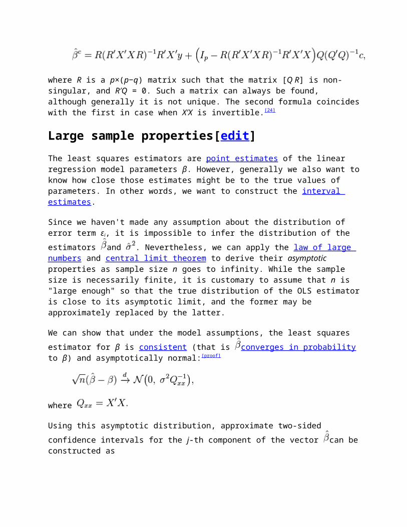
Large sample properties[edit]The least squares estimators are point estimates of the linear regression model parameters β. However, generally we also want toknow how close those estimates might be to the true values of parameters. In other words, we want to construct the interval estimates.

Since we haven't made any assumption about the distribution of error term εi, it is impossible to infer the distribution of the estimators and . Nevertheless, we can apply the law of large numbers and central limit theorem to derive their asymptotic properties as sample size n goes to infinity. While the sample size is necessarily finite, it is customary to assume that n is "large enough" so that the true distribution of the OLS estimatoris close to its asymptotic limit, and the former may be approximately replaced by the latter.

We can show that under the model assumptions, the least squares estimator for β is consistent (that is converges in probabilityto β) and asymptotically normal:[proof]

where

Using this asymptotic distribution, approximate two-sided confidence intervals for the j-th component of the vector can beconstructed as

  at the 1 − α confidence level,

where q denotes the quantile function of standard normal distribution, and [·]jj is the j-th diagonal element of a matrix.

Similarly, the least squares estimator for σ2 is also consistent and asymptotically normal (provided that the fourth moment of εi exists) with limiting distribution

These asymptotic distributions can be used for prediction, testing hypotheses, constructing other estimators, etc.. As an example consider the problem of prediction. Suppose is some point within the domain of distribution of the regressors, and one wants to know what the response variable would have been at that point. The mean response is the quantity , whereas the predicted response is . Clearly the predicted response is a random variable, its distribution can be derived from that of :

which allows construct confidence intervals for mean response to be constructed:

  at the 1 − α confidence level.

Hypothesis testing[edit]Main article: Hypothesis testing

This section is empty. You can help by adding to it. (July 2010)

Example with real data[edit]

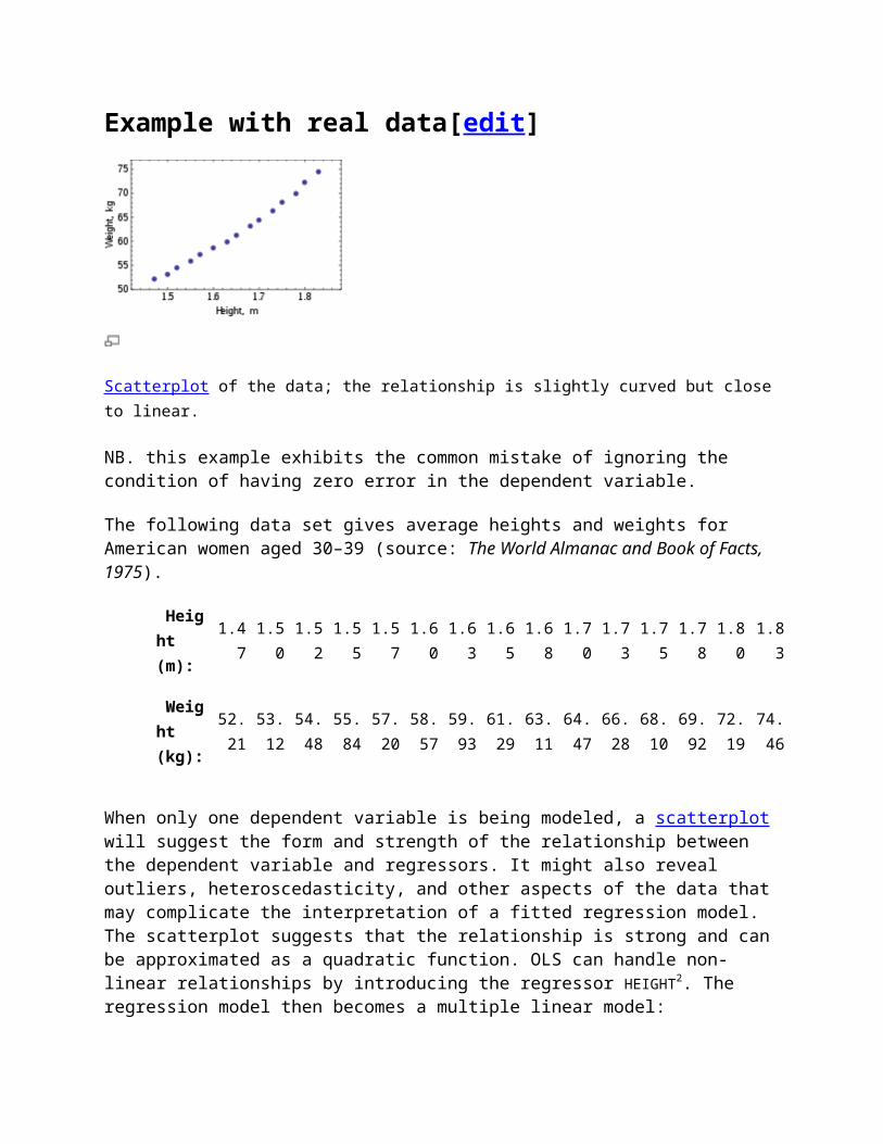
Scatterplot of the data; the relationship is slightly curved but closeto linear.

NB. this example exhibits the common mistake of ignoring the condition of having zero error in the dependent variable.

The following data set gives average heights and weights for American women aged 30–39 (source: The World Almanac and Book of Facts, 1975).

 Height (m):

1.47

1.50

1.52

1.55

1.57

1.60

1.63

1.65

1.68

1.70

1.73

1.75

1.78

1.80

1.83

 Weight (kg):

52.21

53.12

54.48

55.84

57.20

58.57

59.93

61.29

63.11

64.47

66.28

68.10

69.92

72.19

74.46

When only one dependent variable is being modeled, a scatterplot will suggest the form and strength of the relationship between the dependent variable and regressors. It might also reveal outliers, heteroscedasticity, and other aspects of the data that may complicate the interpretation of a fitted regression model. The scatterplot suggests that the relationship is strong and can be approximated as a quadratic function. OLS can handle non-linear relationships by introducing the regressor HEIGHT2. The regression model then becomes a multiple linear model:

The output from most popular statistical packages will look similar to this:

Fitted regression

Method: Least SquaresDependent variable: WEIGHTIncluded observations: 15

Variable Coefficient

Std.Error

t-statistic

p-value

128.8128

16.3083 7.8986 0.00

00

–143.162

0

19.8332

–7.2183

0.0000

61.9603 6.0084 10.312 0.00

2 00

R 2 0.9989 S.E. of regression

0.2516

Adjusted R2 0.9987 Model sum-of-sq 692.61

Log-likelihood 1.0890 Residual sum-of-sq

0.7595

Durbin–Watson stats. 2.1013 Total sum-of-sq 693.

37

Akaike criterion 0.2548 F-statistic 5471

.2

Schwarz criterion 0.3964 p-value (F-

stat)0.00

00

In this table:

The Coefficient column gives the least squares estimates of parameters βj

The Std. errors column shows standard errors of each coefficient

estimate: The t-statistic and p-value columns are testing whether any of the

coefficients might be equal to zero. The t-statistic is

calculated simply as . If the errors ε follow a normal distribution, t follows a Student-t distribution. Under weaker conditions, t is asymptotically normal. Large values of t indicatethat the null hypothesis can be rejected and that the corresponding coefficient is not zero. The second column, p - value, expresses the results of the hypothesis test as a significance level. Conventionally, p-values smaller than 0.05 are taken as evidence that the population coefficient is nonzero.

R-squared is the coefficient of determination indicating goodness-of-fit of the regression. This statistic will be equal to one if fit is perfect, and to zero when regressors X have no explanatorypower whatsoever. This is a biased estimate of the population R-squared, and will never decrease if additional regressors are added, even if they are irrelevant.

Adjusted R-squared is a slightly modified version of , designed topenalize for the excess number of regressors which do not add to the explanatory power of the regression. This statistic is alwayssmaller than , can decrease as new regressors are added, and even be negative for poorly fitting models:

Log-likelihood is calculated under the assumption that errors follow normal distribution. Even though the assumption is not very reasonable, this statistic may still find its use in conducting LR tests.

Durbin–Watson statistic tests whether there is any evidence of serial correlation between the residuals. As a rule of thumb, the value smaller than 2 will be an evidence of positive correlation.

Akaike information criterion and Schwarz criterion are both used for model selection. Generally when comparing two alternative models, smaller values of one of these criteria will indicate a better model.[25]

Standard error of regression is an estimate of σ, standard error of the error term.

Total sum of squares, model sum of squared, and residual sum of squares tell us how much of the initial variation in the sample were explainedby the regression.

F-statistic tries to test the hypothesis that all coefficients (except the intercept) are equal to zero. This statistic has F(p–1,n–p) distribution under the null hypothesis and normality assumption, and its p-value indicates probability that the hypothesis is indeed true. Note that when errors are not normal this statistic becomes invalid, and other tests such as for example Wald test or LR test should be used.

Residuals plot

Ordinary least squares analysis often includes the use of diagnostic plots designed to detect departures of the data from the assumed form of the model. These are some of the common diagnostic plots:

Residuals against the explanatory variables in the model. A non-linear relation between these variables suggests that the linearity of the conditional mean function may not hold. Different levels of variability in the residuals for different levels of the explanatory variables suggests possible heteroscedasticity.

Residuals against explanatory variables not in the model. Any relation of the residuals to these variables would suggest considering these variables for inclusion in the model.

Residuals against the fitted values, . Residuals against the preceding residual. This plot may identify

serial correlations in the residuals.

An important consideration when carrying out statistical inference using regression models is how the data were sampled. In this example, the data are averages rather than measurements on individual women. The fit of the model is very good, but this does not imply that the weight of an individual woman can be predicted with high accuracy based only on her height.

Sensitivity to rounding[edit]

This example also demonstrates that coefficients determined by these calculations are sensitive to how the data is prepared. The

heights were originally given rounded to the nearest inch and have been converted and rounded to the nearest centimetre. Since the conversion factor is one inch to 2.54 cm this is not an exactconversion. The original inches can be recovered by Round(x/0.0254) and then re-converted to metric without rounding.If this is done the results become:

const height Height2

128.8128 -143.162 61.96033 converted to metric with rounding.119.0205 -131.5076 58.5046 converted to metric without rounding.

Using either of these equations to predict the weight of a 5' 6" (1.6764m) woman gives similar values: 62.94 kg with rounding vs. 62.98 kg without rounding. Thus a seemingly small variation in the data has a real effect on the coefficients but a small effecton the results of the equation.

While this may look innocuous in the middle of the data range it could become significant at the extremes or in the case where thefitted model is used to project outside the data range (extrapolation ).

This highlights a common error: this example is an abuse of OLS which inherently requires that the errors in the dependent variable (in this case height) are zero or at least negligible. The initial rounding to nearest inch plus any actual measurement errors constitute a finite and non-negligible error. As a result the fitted parameters are not the best estimates they are presumed to be. Though not totally spurious the error in the estimation will depend upon relative size of the x and y errors.

See also[edit] Bayesian least squares Fama–MacBeth regression Non-linear least squares Numerical methods for linear least squares

References[edit]

1. Jump up ̂ Hayashi (2000, page 7)2. Jump up ̂ Hayashi (2000, page 187)3. ^ Jump up to: a b Hayashi (2000, page 10)4. Jump up ̂ Hayashi (2000, page 34)5. Jump up ̂ Hayashi (2000, page 15)6. Jump up ̂ Hayashi (2000, page 18)7. ^ Jump up to: a b Hayashi (2000, page 19)8. Jump up ̂ Hayashi (2000, page 20)9. Jump up ̂ Hayashi (2000, page 5)10. Jump up ̂ Akbarzadeh, Vahab. "Line Estimation".11. Jump up ̂ Hayashi (2000, page 49)12. ^ Jump up to: a b Hayashi (2000, page 52)13. Jump up ̂ Hayashi (2000, pages 27, 30)14. ^ Jump up to: a b c Hayashi (2000, page 27)15. Jump up ̂ Amemiya (1985, page 13)16. Jump up ̂ Amemiya (1985, page 14)17. Jump up ̂ Rao (1973, page 319)18. Jump up ̂ Amemiya (1985, page 20)19. Jump up ̂ Amemiya (1985, page 27)20. ^ Jump up to: a b Davidson & Mackinnon (1993, page 33)21. Jump up ̂ Davidson & Mackinnon (1993, page 36)22. Jump up ̂ Davidson & Mackinnon (1993, page 20)23. Jump up ̂ Amemiya (1985, page 21)24. ^ Jump up to: a b Amemiya (1985, page 22)25. Jump up ̂ Burnham, Kenneth P.; David Anderson (2002). Model Selection

and Multi-Model Inference (2nd ed.). Springer. ISBN 0-387-95364-7.

Further reading[edit] Amemiya, Takeshi (1985). Advanced econometrics. Harvard University

Press. ISBN 0-674-00560-0. Davidson, Russell; Mackinnon, James G. (1993). Estimation and inference

in econometrics. Oxford University Press. ISBN 978-0-19-506011-9. Greene, William H. (2002). Econometric analysis (5th ed.). New

Jersey: Prentice Hall. ISBN 0-13-066189-9. Retrieved 2010-04-26. Hayashi, Fumio (2000). Econometrics. Princeton University Press.

ISBN 0-691-01018-8. Rao, C.R. (1973). Linear statistical inference and its applications (2nd ed.).

New York: John Wiley & Sons. Wooldridge, Jeffrey M. (2013). Introductory Econometrics: A Modern

Approach (5th international ed.). Australia: South Western, Cengage Learning. ISBN 9781111534394.

[hide]

v t e

Least squares and regression analysis

Computationalstatistics

Least squares Linear least squares Non-linear least squares Iteratively reweighted least squares

Correlation anddependence

Pearson product-moment correlation Rank correlation (Spearman's rho Kendall's tau ) Partial correlation Confounding variable

Regression analysis

Ordinary least squares Partial least squares Total least squares Ridge regression

Regression as astatistical model Linear

regression

Simple linear regression Ordinary least squares Generalized least squares Weighted least squares General linear model

Predictorstructure

Polynomial regression Growth curve Segmented regression Local regression

Non-standard Nonlinear regression Nonparametric Semiparametric Robust Quantile

Isotonic

Non-normalerrors

Generalized linear model Binomial Poisson Logistic

Decomposition ofvariance

Analysis of variance Analysis of covariance Multivariate AOV

Model exploration

Mallows's C p

Stepwise regression Model selection Regression model validation

Background

Mean and predicted response Gauss–Markov theorem Errors and residuals Goodness of fit Studentized residual Minimum mean-square error

Design ofexperiments

Response surface methodology Optimal design Bayesian design

Numericalapproximation

Numerical analysis Approximation theory Numerical integration Gaussian quadrature Orthogonal polynomials Chebyshev polynomials Chebyshev nodes

Applications Curve fitting Calibration curve Numerical smoothing and differentiation System identification

Moving least squares

Regression analysis category Statistics category Statistics portal Statistics outline Statistics topics

<img src="//en.wikipedia.org/wiki/Special:CentralAutoLogin/start?type=1x1" alt="" title="" width="1" height="1" style="border: none; position: absolute;" />Retrieved from "http://en.wikipedia.org/w/index.php?title=Ordinary_least_squares&oldid=617626684"

Categories:

Regression analysis Estimation theory Parametric statistics Least squares

This page was last modified on 19 July 2014 at 21:12. Text is available under the Creative Commons Attribution-

ShareAlike License; additional terms may apply. By using this site, you agree to the Terms of Use and Privacy Policy. Wikipedia® is a registered trademark of the Wikimedia Founda

Search

https://fp.auburn.edu/kalinla/papers/JHE2008.pdf

http://en.youscribe.com

/catalogue/reports-and-

theses/knowledge/stochastic-errors-vs-

modeling-errors-in-distance-

based-

phylogenetic-2051641http://

www.almob.org/content/7/1/22

http://ageconsearch.umn.edu/bitstream/

22096/1/sp03bi05.pdf

http://www.math.uah.edu/stat/sample/

Covariance.html

What is stochastic error term?

Rushabh YapuramMath and Arithmetic Supervisor

A Stochastic error term is a term that is added to a regression equation to introduce all of the variation in Y that cannot be explained by the included Xs. It is, in effect, a symbol of the econometrician's ignorance or inability to model all the movements of the dependent variable.

A Stochastic error term is a term that is added to a regression equation to introduce all of the variation in Y that cannot be explained by the included Xs. It is, in effect, a symbol of the econometrician's ignorance or inability to model all the movements of the dependent variable.

W hat_is_stochas 20100928174150

Minor edit? Save Cancel

Answered

In Education

What is the difference between 'stochastic' and 'deterministic'? Answer They are antonyms. Stochastic means random, determined by chance. Deterministic means sure, determined ex-ante, not influenced by chance

Measurement AnalysisContentsIntroductionInstrument and MeasurementOf OrderStandard DeviationPrecision

A Stochastic error term is a ter

ErrorStochastic ErrorSystematic ErrorResolutionAccuracyCalibrationCalibration Drift

IntroductionWe use several simple concepts and phrases in our analysis of our measurements. Although they are simple,they are nevertheless difficult to understand. Well, maybe you can understand them easily, but it took us years to understand them properly. Here is an introduction to the fundamental principles and parameters of the measurement analysis we perform here in our lab. To serve as an example, we consider the development of a fictitious instrument: the microwave-reflection thermometer (MRT).

Instrument and MeasurementWe measure a physical quantity with an instrument. The physical quantity is something we assume has a true andabsolute value. All instruments measuring the physical quantity will come up with the same value if they are perfectly accurate. But real instruments are not perfectly accurate, so their measurements are not equalto the physical quantity. A measurement is a value produced by an instrument when it tries to determine a physical quantity.

Of OrderWhen we say the microwave power radiated by our MRT is "of order one hundred microwatts", we mean it could be 150 μW, it could be 50 μW, it could even be 200 μW. We are being vague. When we say of order, we mean not less than a third and not more than three times. You might think we should just say, "between 33 μW and 300 μW", but that would be misleading. It would suggest that thenumbers 33 and 300 had some significance. They don't. The only number that's significant is our 100, and we're saying it's hardly accurate at all. Despite beinghardly accurate at all, the estimate is good for a lot of things. For example, we might see that human safety regulations say that any emission less than 10,000 μW is harmless. So our of-order estimate of radiated powertells us that our MRT is quite safe, because 100 μW is a hundred times less than 10,000 μW.

Standard DeviationThe standard deviation of a set of measurements is an indication of how much the measurements vary from theiraverage value. We can't just take the average amount they vary from their average value, because that would be zero: the positive differences would cancel the negative. We could, instead, turn all the negative differences into positive differences so they would notcancel one another. But we don't do that, because the act of dropping the negative sign is difficult to handle in mathematics. To be specific: its slope is undefined at zero. Instead, we turn the negatives into positives by squaring them. The square of a negative number is always positive. To get the standard deviation of

a set of numbers, we square all the deviations from themean, add them together, divide by the number of measurements, and take the square root. The standard deviation is the root mean square of the deviations.

Suppose measure the temperature of a large metal table in our lab five times using our fictitious MRT instrument. We get the following results.

IndexResult

(°C)

Deviation(°C)

Squareof

Deviation

(°C2)1 28.0 +2 42 25.0 -1 13 26.0 0 04 27.0 +1 15 24.0 -2 4Averag

e 6 0.0 2

Table: MRT Measurements.

The mean square deviation is 2 °C2. The standard deviation isthe root mean square deviation, which is √2 = 1.4 °C.

PrecisionThe precision of a measurement is its standard deviation when the physical quantity remains constant. Suppose wemeasure the temperature of our large metal table with amercury thermometer we trust to 0.1 °C, and we find

that the temperature remained constant to within ±0.1 Cwhile we took our MRT measurements. The precision of our MRT is 1.4 °C, because the standard deviation of the MRT temperature was 1.4 °C while the actual temperature was constant. The 1.4 °C variation is due to the MRT itself, not the temperature of the table.

ErrorThe error in a measurement is the difference between themeasurement and the true value of the physical quantity. The variations in our MRT measurement are errors, because the temperature was constant during our MRT measurements. But the errors could be larger even than these variations. Suppose our mercury thermometer measured the temperature of the table to be 23°C. The error on each of our measurements will be the measurement value minus 23°C. Our MRT measurement errors were 5, 2, 3, 4, and 1 °C.

Stochastic ErrorThe stochastic error in a measurement is the error that is random from one measurement to the next. Stochastic errors tend to be gaussian, or normal, in their distribution. That's because the stochastic error is most often the sum of many random errors, and when we add many random errors together, the distribution of their sum looks guassuian, as shown by the Central Limit Theorem.

The standard deviation of the stochastic error is equalto the precision. The stochastic error of our MRT is 1.4°C.

Because most stochastic errors are guassian, and all have zero mean by definition, the stochastic error willbe less than twice the precision 95% of the time. So ifwe look at a plot of MRT measurement verses time, containing hundreds of measurements made while the table temperature remained constant, we can guess the precision easily. We just figure by eye how far apart two lines would have to be, one above zero and one below zero, to enclose almost all the measurements. These two lines will be at roughly two standard deviations above and two standard deviations below zero. So we divide the 95% spread in our measurements by four to get the precision.

Systematic ErrorThe systematic error in a measurement is the error that is not random from one measurement to the next. Suppose the mercury thermometer measured the temperature of thetable to be 23°C during our five MRT measurements. The average MRT measurement was 26°C. Its systematic error is 3°C.

ResolutionThe resolution of a measurement is how well it can distinguish between two values of the measured physicalquantity. The precision of our MRT is 1.4°C. If one endof the table is 0.1°C warmer than the other, the probability of our MRT being right when it says which end is warmer will be close to 50%, because our stochastic error is much larger than the difference we are trying to observe.

When a stochastic error is gaussian, which is most of the time, there is a 68% chance that the magnitude of the error will be less than one standard deviation of the distribution. If we measure the temperature at bothends of our table, and the far end measurement is one standard deviation higher than the near end, it is 68% likely that the MRT measurement of the far end will be higher than the MRT measurement of the near end. In other words, it's 68% likely that our MRT will be correct in telling us which end is warmer, provided that the warmer end is one standard deviation warmer than the other end.

That's how we arrive at our definition of resolution. The resolution of a measurement is the amount by which themeasured quantity must change for it to be 68% likely that our measurement will be correct in saying whether the change was up or down.

Because almost all stochastic errors are gaussian, the resolution of a measurement is almost always equal to its precision.

AccuracyThe accuracy of a measurement is an indication of size of its errors. To determine the accuracy of a measurement, we need to compare it to another far more accurate measurement. We can determine the accuracy of our MRT using our mercury thermometer. The accuracy of a measurement is the root mean square of its error. The accuracy of our MRT is 3.3°C.

Calibration

If our MRT has a constant systematic error of 3°C, thenwe can subtract this 3°C from the MRT measurement to get a better estimate of the actual temperature. To calibrate a measurement is to remove systematic errors by comparing the measurement to a more accurate measurement. We modify our MRT to that it subtracts 3°Cfrom its measurement. We no longer see the original measurement at all. The systematic error is gone, and all we have left is the 1.4°C stochastic error.

Calibration DriftIf they systematic error in a measurement changes slowly with time, the calibration we performed to remove the systematic error from the measurement will no longer be effective. This slow change is called calibration drift. In order to trust a calibration, we must monitor the systematic error of our instrument, or re-calibrate the instrument.

9. Sample Correlation and Regression IRecall the basic model of statistics: we have a population of objects of interest, and we have various measurements (variables)that we make on these objects. We select objects from the population and record the variables for the objects in the sample; these become our data. Our first discussion is from a purely descriptive point of view. That is, we do not assume that the data are generated by an underlying probability distribution.But as always, remember that the data themselves define a probability distribution, namely the empirical distribution.

Suppose that x  and y  are real-valued variables for a population, and that ((x 1 ,y 1 ),(x 2 ,y 2 ),…,(x n ,y n ))  is an observed sample of size n  from (x,y)  . We will let x=(x 1 ,x 2 ,…,x n )  denote the sample from x  and y=(y 1 ,y 2 ,…,y n )  the sample from y  . In this section, we are interested in statistics that are measures of association between the x  and y  , and in finding the line (or other curve) that best fits the data.

Recall that the sample means are

m(x)=1n ∑ i=1 n x i ,m(y)=1n ∑ i=1 n y i  

and the sample variances are

s 2 (x)=1n−1 ∑ i=1 n [x i −m(x)] 2 ,s 2 (y)=1n−1 ∑ i=1 n [y i −m(y)] 2  

Scatterplots

Often, the first step in exploratory data analysis is to draw a graph of the points; this is called a scatterplot an can give a visual sense of the statistical realtionship between the variables.

In particular, we are interested in whether the cloud of points seems to show a linear trend or whether some nonlinear curve might fit the cloud of points. We are interested in the extent towhich one variable x  can be used to predict the other variable y  .

DefintionsOur next goal is to define statistics that measure the association between the x  and y  data. The sample covariance is defined to be

s(x,y)=1n−1 ∑ i=1 n [x i −m(x)][y i −m(y)] 

Note that the sample covariance is an average of the product of the deviations of the x  and y  data from their means. Thus, thephysical unit of the sample covariance is the product of the units of x  and y  . The sample correlation is defined to be

r(x,y)=s(x,y)s(x)s(y)  

assuming that the data vectors are not constant, so that the standard deviations are positive. Correlation is a standardized version of covariance. In particular, correlation is dimensionless (has no physical units), since the covariance in the numerator and the product of the standard devations in the denominator have the same units (the product of the units of x  and y  ). Note also that covariance and correlation have the same sign: positive, negative, or zero. In the first case, the data x  and y  are said to be positively correlated; in the second case x  and y  are said to be negatively correlated; and in the third case x  and y  are said to be uncorrelatedTo see that the sample covariance is a measure of association, recall first that the point (m(x),m(y))  is a measure of the center of the bivariate data. Indeed, if each point is the location of a unit mass, then (m(x),m(y))  is the center of mass asdefined in phyiscs. Horizontal and vertical lines through this center point divide the plane into four quadrants. The product deviation [x i −m(x)][y i −m(y)]  is positive in the first and third quadrants and negative in the second and fourth quadrants. After we study linear regression below, we will have a much deeper sense of what covariance measures.

You may be perplexed that we average the product deviations by dividing by n−1  rather than n  . The best explanation is that in the bivariate probability model, the sample covariance is an unbiased estimator of the distribution covariance. However, the mode of averaging can also be understood in terms of degrees of freedom, as was done for sample variance. Initially, we have 2n  degrees of freedom in the bivariate data. We lose two by computing the sample means m(x)  and m(y)  . Of the remaining 2n−2  degrees of freedom, we lose n−1  by computing the product deviations. Thus, we are left with n−1  degrees of freedom total. As is typical in statistics, we average not by dividing bythe number of terms in the sum but rather by the number of degrees of freedom in those terms. However, from a purely descriptive point of view, it would also be reasonable to divide by n  .Recall that there is a natural probability distribution associated with the data, namely the empirical distribution that gives probability 1n   to each data point (x i ,y i )  . (Thus, if these points are distinct this is the discrete uniform distribution on the data.) The sample means are simply the expected values of this bivariate distribution, and except for a constant multiple (dividing by n−1  rather than n  ), the sample

variances are simply the variances of this bivarite distribution.Similarly, except for a constant multiple (again dividing by n−1  rather than n  ), the sample covariance is the covariance of the bivariate distribution and the sample correlation is the correlation of the bivariate distribution. All of the following results in our discussion of descriptive statistics are actually special cases of more general results for probability distributions.

Properties of CovarianceThe next few exercises establish some essential properties of sample covariance. As usual, bold symbols denote samples of a fixed size n  from the corresponding population variables (that is, vectors of length n  ), while symbols in regular type denotereal numbers. Our first result is a formula for sample covariancethat is sometimes better than the definition for computational purposes. To state the result succinctly, let xy=(x 1 y 1 ,x 2 y 2 ,…,x n y n )  denote the sample from the product variable xy  .

The sample covariance can be computed as follows:

s(x,y)=1n−1 ∑ i=1 n x i y i −nn−1 m(x)m(y)=nn−1 [m(xy)−m(x)m(y)] 

Proof:

Note that

∑ i=1 n [(x i −m(x)][y i −m(y)] =∑ i=1 n [x i y i −x i m(y)−y i m(x)+m(x)m(y)]=∑ i=1 n x i y i −m(y)∑ i=1 n x i −m(x)∑ i=1 n y i +nm(x)m(y)=∑ i=1 n x i y i −nm(y)m(x)−nm(x)m(y)+nm(x)m(y)=∑ i=1 

n x i y i −nm(x)m(y)  

The following theorem gives another formula for the sample covariance, one that does not require the computation of intermediate statistics.

The sample covariance can be computed as

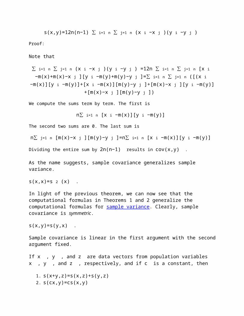
s(x,y)=12n(n−1) ∑ i=1 n ∑ j=1 n (x i −x j )(y i −y j ) 

Proof:

Note that

∑ i=1 n ∑ j=1 n (x i −x j )(y i −y j ) =12n ∑ i=1 n ∑ j=1 n [x i −m(x)+m(x)−x j ][y i −m(y)+m(y)−y j ]=∑ i=1 n ∑ j=1 n ([(x i 

−m(x)][y i −m(y)]+[x i −m(x)][m(y)−y j ]+[m(x)−x j ][y i −m(y)]+[m(x)−x j ][m(y)−y j ])  

We compute the sums term by term. The first is

n∑ i=1 n [x i −m(x)][y i −m(y)] 

The second two sums are 0. The last sum is

n∑ j=1 n [m(x)−x j ][m(y)−y j ]=n∑ i=1 n [x i −m(x)][y i −m(y)] 

Dividing the entire sum by 2n(n−1)  results in cov(x,y)  .

As the name suggests, sample covariance generalizes sample variance.

s(x,x)=s 2 (x)  .

In light of the previous theorem, we can now see that the computational formulas in Theorems 1 and 2 generalize the computational formulas for sample variance. Clearly, sample covariance is symmetric.

s(x,y)=s(y,x)  .

Sample covariance is linear in the first argument with the secondargument fixed.

If x  , y  , and z  are data vectors from population variables x  , y  , and z  , respectively, and if c  is a constant, then

1. s(x+y,z)=s(x,z)+s(y,z)  2. s(cx,y)=cs(x,y) 

Proof:

For part (a), recall that m(x+y)=m(x)+m(y)  . Hence s(x+y,z) =1n−1 ∑ i=1 n [x i +y i −m(x+y)][z i −m(z)]=1n−1 ∑ i=1 n ([x i −m(x)]+[y i −m(y)])[z i −m(z)]=1n−1 ∑ i=1 n [x i −m(x)][z i −m(z)]+1n−1 ∑ i=1 n [y i −m(y)][z i −m(z)]=s(x,z)+s(y,z)  

For part(b), recall that m(cx)=cm(x)  . Hence s(cx,y) =1n−1 ∑ i=1 n [cx i −m(cx)][y i −m(y)]=1n−1 ∑ i=1 n [cx 

i −cm(x)][y i −m(y)]=cs(x,y)  

By symmetry, sample covariance is also linear in the second argument with the first argument fixed, and hence is bilinear. The general version of the bilinear property is given in the following theorem:

Suppose that x i   is a data vector from a population variable x i   for i∈{1,2,…,k}  and that y j   is a data vector from a population variable y j   for j∈{1,2,…,l}  . Suppose also that a 1 ,a 2 ,…,a k   and b 1 ,b 2 ,…,b l   are constants. Thens⎛ ⎝ ∑ i=1 k a i x i ,∑ j=1 l b j y j ⎞ ⎠ =∑ i=1 k ∑ j=1 l a i b j 

s(x i ,y j ) 

A special case of the bilinear property provides a nice way to compute the sample variance of a sum.

s 2 (x+y)=s 2 (x)+2s(x,y)+s 2 (y)  .Proof:

From Theorems 3, 4, and 5,

s 2 (x+y) =s(x+y,x+y)=s(x,x)+s(x,y)+s(y,x)+s(y,y)=s 2 (x)+2s(x,y)+s 2 (y)  

The generalization of this result to sums of three or more vectors is completely straightforward: namely, the sample variance of a sum is the sum of all of the pairwise sample covariances. Note that the sample variance of a sum can be greater than, less than, or equal to the sum of the sample

variances, depending on the sign and magnitude of the pure covariance term. In particular, if the vectors are pairwise uncorrelated, then the variance of the sum is the sum of the variances.

If c  is a constant data set then s(x,c)=0  .Proof:

This follows directly from the definition. If c i =c  for each i  , then m(c)=c  and hence c i −m(c)=0  for each i  .Combining the result in the last exercise with the bilinear property, we see that covariance is unchanged if constants are added to the data sets. That is, if c  and d  are constant vectors then s(x+c,y+d)=s(x,y)  .

Properties of CorrelationA few simple properties of correlation are given in the followingexercises. Most of these follow easily from the corresponding properties of covariance. First, recall that the standard scores of x i   and y i   are, respectively,

u i =x i −m(x)s(x) ,v i =y i −m(y)s(y)  

The standard scores from a data set are dimensionless quantities that have mean 0 and variance 1.

The correlation between x  and y  is the covariance of their standard scores u  and v  . That is, r(x,y)=s(u,v)  .Proof:

In vector notation, note that

u=1s(x) [x−m(x)],v=1s(y) [y−m(y)] 

Hence the result follows immediatedly from Theorems 5 and 8:

s(u,v)=1s(x)s(y) s(x,y)=r(x,y) 

Correlation is symmetric.

r(x,y)=r(y,x)  .

Unlike covariance, correlation is unaffected by multiplying one of the data sets by a positive constant (recall that this can always be thought of as a change of scale in the underlying variable). On the other hand, muliplying a data set by a negativeconstant changes the sign of the correlation.

If c≠0  is a constant then

1. r(cx,y)=r(x,y)  if c>0  2. r(cx,y)=−r(x,y)  if c<0 

Proof:

By definition and from Theorem 5,

r(cx,y)=s(cx,y)s(cx)s(y) =cs(x,y)|c|s(x)s(y) =c|c| r(x,y) 

and of course, c/|c|=1  if c>0  and c/|c|=−1  if c<0  .

Like covariance, correlation is unaffected by adding constants tothe data sets. Adding a constant to a data set often corresponds to a change of location.

If c  and d  are constant vectors then r(x+c,y+d)=r(x,y)  .Proof:

This result follows directly from the corresponding properties ofcovariance and standard deviation:

r(x+c,y+d)=s(x+c,y+d)s(x+c)s(y+d) =s(x,y)s(x)s(y) =r(x,y) 

The last couple of properties reinforce the fact that correlationis a standardized measure of association that is not affected by changing the units of measurement. In the first Challenger data set, for example, the variables of interest are temperature at time of launch (in degrees Fahrenheit) and O-ring erosion (in millimeters). The correlation between these variables is of critical importance. If we were to measure temperature in degreesCelsius and O-ring erosion in inches, the correlation between thetwo variables would be unchanged.

The most important properties of correlation arise from studying the line that best fits the data, our next topic.

Linear RegressionWe are interested in finding the line y=a+bx  that best fits thesample points ((x 1 ,y 1 ),(x 2 ,y 2 ),…,(x n ,y n ))  . This is a basic and important problem in many areas of mathematics, not just statistics. We think of x  as the predictor variable and y  as the response variable. Thus, the term best means that we want to findthe line (that is, find the coefficients a  and b  ) that minimizes the average of the squared errors between the actual y  values in our data and the predicted y  values:

mse(a,b)=1n−1 ∑ i=1 n [y i −(a+bx i )] 2  

Note that the minimizing value of (a,b)  would be the same if the function were simply the sum of the squared errors, of if we averaged by dividing by n  rather than n−1  , or if we used the square root of any of these functions. Of course that actual minimum value of the function would be different if we changed thefunction, but again, not the point (a,b)  where the minimum occurs. Our particular choice of mse  as the error function is best for statistical purposes. Finding (a,b)  that minimize mse is a standard problem in calculus.The graph of mse  is a paraboloid opening upward. The function mse  is minimized whenb(x,y)a(x,y) =s(x,y)s 2 (x) =m(y)−b(x,y)m(x)=m(y)−s(x,y)s 2 

(x) m(x)  

Proof:

We can tell from the algebraic form of mse  that the graph is a paraboloid opening upward. To find the unique point that minimizes mse  , note that ∂∂a mse(a,b)∂∂b mse(a,b) =1n−1 ∑2[y i −(a+bx i )](−1)=2n−1 [−∑ i=1 n y i +na+b∑ i=1 n x i ]=1n−1 ∑2[y i −(a+bx i )](−x i )=2n−1 

[−∑ i=1 n x i y i +a∑ i=1 n x i +b∑ i=1 n x 2 i ]  

Solving ∂∂a mse(a,b)=0  , gives a=m(y)−bm(x)  . Substituting this into ∂∂b mse(a,b)=0  and solving for b  gives

b=n[m(xy)−m(x)m(y)]n[m(x 2 )−m 2 (x)]  

Dividing the numerator and denominator in the last expression by n−1  and using Theorem 1, we see that b=s(x,y)/s 2 (x)  .

Of course, the optimal values of a  and b  are statistics, that is, functions of the data. Thus the sample regression line is

y=m(y)+s(x,y)s 2 (x) [x−m(x)] 

Note that the regression line passes through the point (m(x),m(y))  , the center of the sample of points.

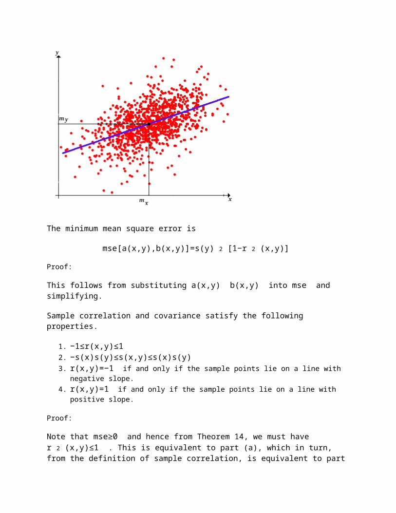
The minimum mean square error is

mse[a(x,y),b(x,y)]=s(y) 2 [1−r 2 (x,y)] 

Proof:

This follows from substituting a(x,y)  b(x,y)  into mse  and simplifying.

Sample correlation and covariance satisfy the following properties.

1. −1≤r(x,y)≤1  2. −s(x)s(y)≤s(x,y)≤s(x)s(y)  3. r(x,y)=−1  if and only if the sample points lie on a line with

negative slope.4. r(x,y)=1  if and only if the sample points lie on a line with

positive slope.

Proof:

Note that mse≥0  and hence from Theorem 14, we must have r 2 (x,y)≤1  . This is equivalent to part (a), which in turn, from the definition of sample correlation, is equivalent to part

(b). For parts (c) and (d), note that mse(a,b)=0  if and only ify i =a+bx i   for each i  , and moreover, b(x,y)  has the same sign as r(x,y)  .Thus, we now see in a deeper way that the sample covariance and correlation measure the degree of linearity of the sample points.Recall from our discussion of measures of center and spread that the constant a  that minimizes

mse(a)=1n−1 ∑ i=1 n (y i −a) 2  

is the sample mean m(y)  , and the minimum value of the mean square error is the sample variance s 2 (y)  . Thus, the difference between this value of the mean square error and the one in Exercise 14, namely s 2 (y)r 2 (x,y)  is the reduction inthe variability of the y  data when the linear term in x  is added to the predictor. The fractional reduction is r 2 (x,y)  ,and hence this statistics is called the (sample) coefficient of determination. Note that if the data vectors x  and y  are uncorrelated, then x  has no value as a predictor of y  ; the regression line in this case is the horizontal line y=m(y)  and the mean square error is s 2 (y)  .

The choice of predictor and response variables is important.

The sample regression line with predictor variable x  and response variable y  is not the same as the sample regression line with predictor variable y  and response variable x  , except in the extreme case r(x,y)=±1  where the sample points all lie on a line.

ResidualsThe difference between the actual y  value of a data point and the value predicted by the regression line is called the residual of that data point. Thus, the residual corresponding to (x i ,y i )  is d i =y i −y ^  i   where y ^  i   is the regression line at x i   :

y ^  i =m(y)+s(x,y)s(x) 2  [x i −m(x)] 

Note that the predicted value y ^  i   and the residual d i   arestatistics, that is, functions of the data (x,y)  , but we are suppressing this in the notation for simplicity.The residuals sum to 0: ∑ n i=1 d i =0  .Proof:

This follows from the definition, and is a restatement of the fact that the regression line passes through the center of the data set (m(x),m(y))  .Various plots of the residuals can help one understand the relationship between the x  and y  data. Some of the more commonare

A plot of (i,d i )  for i∈{1,2,…,n}  , that is, a plot of indices versus residuals.

A plot of (x i ,d i )  for i∈{1,2,…,n}  , that is, a plot of x  values versus residuals.

A plot of (d i ,y i )  for i∈{1,2,…,n}  , that is, a plot of residuals versus actual y  values.

A plot of (d i ,y ^  i )  for i∈{1,2,…,n}  , that is a plot ofresiduals versus predicted y  values.

A histogram of the residuals (d 1 ,d 2 ,…,d n )  .

Sums of SquaresFor our next discussion, we will re-interpret the minimum mean square error formula in Theorem 14. We define total sum of squares sst  , the regression sum of squares ssr  , and the error sum of squares sse  bysst(y)ssr(x,y)sse(x,y) =∑ i=1 n [y i −m(y)] 2 =∑ i=1 n [y ^  i −

m(y)] 2 =∑ i=1 n (y i −y ^  i ) 2   

Note that sst(y)  is simply n−1  times the variance s 2 (y)  andis the total of the sums of the squares of the deviations of the y  values from the mean of the y  values. Similarly, sse(x,y)  is simply n−1  times the minimum mean square error in Theorem 14. Of course, sst(y)  has n−1  degrees of freedom, while sse(x,y)  has n−2  degrees of freedom and ssr(x,y)  a single degree of freedom. The total sum of squares is the sum of the regression sum of squares and the error sum of squares:

The sums of squares are related as follows:

1. ssr(x,y)=r 2 (x,y)sst(y)  2. sst(y)=ssr(x,y)+sse(x,y) 

Proof:

By definition of sst  and r  , we see that r 2 (x,y)sst(y)=s 2 (x,y)/s 2 (x)  . But from the regression equation,

[y ^  i −m(y)] 2 =s 2 (x,y)s 4 (x) [x i −m(x)] 2  

Summing over i  givesssr(x,y)=∑ i=1 n [y ^  i −m(y)] 2 =s 2 (x,y)s 2 (x)  

Hence ssr(x,y)=r 2 (x,y)sst(y)  . Finally, multiplying the result in Theorem 14 by n−1  gives sse(x,y)=sst(y)−r 2 (x,y)sst(y)=sst(y)−ssr(x,y)  .Note that r 2 (x,y)=ssr(x,y)/sst(y)  , so once again, r 2 (x,y) is the coefficient of determination--the proportion of the variability in the y  data explained by the x  data. We can average sse  by dividing by its degrees of freedom and then takethe square root to obtain the standard error of estimate:

se(x,y)=sse(x,y)n−2  − − − − − − − −  √  

This really is a standard error in the same sense as a standard deviation. It's an average of the errors of sorts, but in the root mean square sense.

TransformationsLinear regression is a much more powerful idea than might first appear. By applying various transformations to y  or x  or both,we can fit a variety of two-parameter curves to the given data ((x 1 ,y 1 ),(x 2 ,y 2 ),…,(x n ,y n ))  . In this section, we will consider some of the most common transformations. Consider the function y=a+bx 2   .

1. Sketch the graph for some representative values of a  and b  .2. Note that y  is a linear function of x 2   , with intercept a 

and slope b  .

3. Hence, to fit this curve to our sample data, simply apply the standard regression procedure to the data from the variables x 2   and y  .

Consider the function y=1a+bx   .

1. Sketch the graph for some representative values of a  and b  .2. Note that 1y   is a linear function of x  , with intercept a  and

slope b  .3. Hence, to fit this curve to our sample data, simply apply the

standard regression procedure to the data from the variables x  and 1y   .

Consider the function y=xa+bx   .

1. Sketch the graph for some representative values of a  and b  .2. Note that 1y   is a linear function of 1x   , with intercept b 

and slope a  .3. Hence, to fit this curve to our sample data, simply apply the

standard regression procedure to the data from the variables 1x  and 1y   .

4. Note again that the names of the intercept and slope are reversedfrom the standard formulas.

Consider the function y=ae bx   .

1. Sketch the graph for some representative values of a  and b  .2. Note that ln(y)  is a linear function of x  , with intercept

ln(a)  and slope b  .3. Hence, to fit this curve to our sample data, simply apply the

standard regression procedure to the data from the variables x  and ln(y)  .

4. After solving for the intercept ln(a)  , recover the statistic a=e ln(a)   .

Consider the function y=ax b   .

1. Sketch the graph for some representative values of a  and b  .2. Note that ln(y)  is a linear function of ln(x)  , with

intercept ln(a)  and slope b  .

3. Hence, to fit this curve to our sample data, simply apply the standard regression procedure to the data from the variables ln(x)  and ln(y)  .

4. After solving for the intercept ln(a)  , recover the statistic a=e ln(a)   .

Exercises

Basic PropertiesSuppose that x  and y  are population variables, and x  and y  samples of size n  from x  and y  respectively. Suppose also that m(x)=3  , m(y)=−1  , s 2 (x)=4  , s 2 (y)=9  , and s(x,y)=5  . Find each of the following:

1. r(x,y)  2. m(2x+3y)  3. s 2 (2x+3y)  4. s(2x+3y−1,4x+2y−3) 

Suppose that x  is the temperature (in degrees Fahrenheit) and y  the resistance (in ohms) for a certain type of electronic component after 10 hours of operation. For a sample of 30 components, m(x)=113  , s(x)=18  , m(y)=100  , s(y)=10  , r(x,y)=0.6  .

1. Classify x  and y  by type and level of measurement.2. Find the sample covariance.3. Find the equation of the regression line.

Suppose now that temperature is converted to degrees Celsius (thetransformation is 59 (x−32)  ).

4. Find the sample means.5. Find the sample standard deviations.6. Find the sample covariance and correlation.7. Find the equation of the regression line.

Answer:

1. continuous, interval

2. m=45°  , s=10° 

Suppose that x  is the length and y  the width (in inches) of a leaf in a certain type of plant. For a sample of 50 leaves m(x)=10  , s(x)=2  , m(y)=4  , s(y)=1  , and r(x,y)=0.8  .

1. Classify x  and y  by type and level of measurement.2. Find the sample covariance.3. Find the equation of the regression line with x  as the predictor

variable and y  as the response variable.

Suppose now that x  and y  are converted to inches (0.3937 inches per centimeter).

4. Find the sample means.5. Find the sample standard deviations.6. Find the sample covariance and correlation.7. Find the equation of the regression line.

Answer:

1. continuous, ratio2. m=25.4  , s=5.08 

Scatterplot Exercises

Click in the interactive scatterplot, in various places, and watch how the means, standard deviations, correlation, and regression line change.

Click in the interactive scatterplot to define 20 points and try to come as close as possible to each of the following sample correlations:

1. 0  2. 0.5  3. −0.5  4. 0.7  5. −0.7  6. 0.9 

7. −0.9  .

Click in the interactive scatterplot to define 20 points. Try to generate a scatterplot in which the regression line has

1. slope 1, intercept 12. slope 3, intercept 03. slope −2  , intercept 1

Computational ExerciseAll statistical software packages will perform regression analysis. In addition to the regression line, most packages will typically report the coefficient of determination r 2 (x,y)  , the sums of squares sst(y)  , ssr(x,y)  , sse(x,y)  , and the standard error of estimate se(x,y)  . Most packages will also draw the scatterplot, with the regression line superimposed, and will draw the various graphs of residuals discussed above. Many packages also provide easy ways to transform the data. Thus, there is very little reason to perform the computations by hand, except with a small data set to master the definitions and formulas. In this subsection, do the computations and draw the graphs with minimal technological aids.Suppose that x  is the number of math courses completed and y  the number of science courses completed for a student at EnormousState University (ESU). A sample of 10 ESU students gives the following data: ((1,1),(3,3),(6,4),(2,1),(8,5),(2,2),(4,3),(6,4),(4,3),(4,4)  .

1. Classify x  and y  by type and level of measurement.2. Sketch the scatterplot.

Construct a table with rows corresponding to cases and columns corresponding to i  , x i   , y i   , x i −m(x)  , y i −m(y)  , [x i −m(x)] 2   , [y i −m(y)] 2   , [x i −m(x)][y i −m(y)]  , y ^  i   , y ^  i −m(y)  , [y ^  i −m(y)] 2   , y i −y ^  i   , and (y i −y ^  i ) 2   . Add a rows at the bottom for totals and means. Use precision arithmetic.

3. Complete the first 8 columns.4. Find the sample correlation and the coefficient of determination.

5. Find the sample regression equation.6. Complete the table.7. Verify the identities for the sums of squares.

Answer:

i x iy i

x i −m(x)

y i −m(y)

[x i −m(x)] 2

[y i −m(y)] 2

[x i −m(x)][y i −m(y)]

y ^  i

y ^  i −m(y)

[y ^  i −m(y)] 2

y i −y ^  i

(y i −y ^  i ) 2

1 1 1 −3 −2 9 4 6 9/7 −12/7 144/49 −2/7 4/49

2 3 3 −1 0 1 0 0 17/7 −4/7 16/49 4/7 16/49

3 6 4 2 1 4 1 2 29/7 8/7 64/49 −1/7 1/49

4 2 1 −2 −2 4 4 4 13/7 −8/7 64/49 −6/7 36/49

5 8 5 4 2 16 4 8 37/7 16/7 256/49 −2/7 4/49

6 2 2 −2 −1 4 1 2 13/7 −8/7 64/49 1/7 1/49

7 4 3 0 0 0 0 0 3 0 0 0 0

8 6 4 2 1 4 1 2 29/7 8/7 64/49 −1/7 1/49

9 4 3 0 0 0 0 0 3 0 0 0 0

10 4 4 0 1 0 1 0 3 0 0 1 1

Total40 30 0 0 40 16 24 30 0 96/7 0 16/7

Mean 4 3 0 0 14/3 16/9 8/3 3 0 96/7 0 2/7

1. discrete, ratio

4. r=23/14 − − − −  √ ≈0.926  , r 2 =6/7  5. y=3+47 (x−4) 

7. 16=96/7+16/7 

Data Analysis Exercises

Use statistical software for the problems in this subsection.

Consider the height variables in Pearson's height data.

1. Classify the variables by type and level of measurement.2. Compute the correlation coefficient and the coefficient of

determination3. Compute the least squares regression line, with the height of the

father as the predictor variable and the height of the son as theresponse variable.

4. Draw the scatterplot and the regression line together.5. Predict the height of a son whose father is 68 inches tall.6. Compute the regression line if the heights are converted to

centimeters (there are 2.54 centimeters per inch).

Answer:

1. Continuous, ratio2. r=0.501  , r 2 =0.251  3. y=33.893+0.514x 

5. 68.856. y=86.088+0.514x 

Consider the petal length, petal width, and species variables in Fisher's iris data.

1. Classify the variables by type and level of measurement.2. Compute the correlation between petal length and petal width.

3. Compute the correlation between petal length and petal width by species.

Answer:

1. Species: discrete, nominal; petal length and width: continuous ratio

2. 0.95593. Setosa: 0.3316, Verginica: 0.3496, Versicolor: 0.6162

Consider the number of candies and net weight variables in the M&M data.

1. Classify the variable by type and level of measurement.2. Compute the correlation coefficient and the coefficient of

determination.3. Compute the least squares regression line with number of candies

as the predictor variable and net weight as the response variable.

4. Draw the scatterplot and the regression line in part (b) together.

5. Predict the net weight of a bag of M&Ms with 56 candies.6. Naively, one might expect a much stronger correlation between the

number of candies and the net weight in a bag of M&Ms. What is another source of variability in net weight?

Answer:

1. Number of candies: discrete, ratio; net weight: continuous, ratio2. r=0.793  , r 2 =0.629  3. y=20.278+0.507x 

5. 48.6576. Variability in the weight of individual candies.

Consider the response rate and total SAT score variables in the SAT by state data set.

1. Classify the variables by type and level of measurement.2. Compute the correlation coefficient and the coefficient of

determination.

3. Compute the least squares regression line with response rate as the predictor variable and SAT score as the response variable.

4. Draw the scatterplot and regression line together.5. Give a possible explanation for the negative correlation.

Answer:

1. Response rate: continuous, ratio. SAT score could probably be considered either discrete or continuous, but is only at the interval level of measurement, since the smallest possible scoresis 400 (200 each on the verbal and math portions).

2. r=−0.849  , r 2 =0.721  3. y=1141.5−2.1x 

5. States with low response rate may be states for which the SAT is optional. In that case, the students who take the test are the better, college-bound students. Conversely, states with high response rates may be states for which the SAT is mandatory. In that case, all students including the weaker, non-college-bound students take the test.

Consider the verbal and math SAT scores (for all students) in theSAT by year data set.

1. Classify the variables by type and level of measurement.2. Compute the correlation coefficient and the coefficient of

determination.3. Compute the least squares regression line.4. Draw the scatterplot and regression line together.

Answer:

1. Continuous perhaps, but only at the interval level of measurementbecause the smallest possible score on each part is 200.

2. r=0.614  , r 2 =0.377  3. y=321.5+0.3x 

Consider the temperature and erosion variables in the first data set in the Challenger data.

1. Classify the variables by type and level of measurement.

2. Compute the correlation coefficient and the coefficient of determination.

3. Compute the least squares regression line.4. Draw the scatter plot and the regression line together.5. Predict the O-ring erosion with a temperature of 31° F.6. Is the prediction in part (c) meaningful? Explain.7. Find the regression line if temperature is converted to degrees

Celsius. Recall that the conversion is 59 (x−32)  .

Answer:

1. temperature: continuous, interval; erosion: continuous ratio2. r=−0.555  , r 2 =0.308  3. y=106.8−1.414x 

5. 62.9.6. This estimate is problematic, because 31° is far outside of the

range of the sample data.7. y=61.54−2.545x 

1. Virtual Laboratories 2. 5. Random Samples 3. 1 4. 2 5. 3 6. 4 7. 5 8. 6 9. 7 10. 8 11. 912. 10 13. 11 14.15.

Contents Applets Data Sets Biographies External Resources Feedback

©