Residual analysis of the equilibrium reconstruction quality on JET

A. Murari, D. Mazon, M. Gelfusa, M. Folschette, T.Quilichiniand JET EFDA contributors

EFDA–JET–PR(10)30

Residual Analysis of the Equilibrium Reconstruction Quality on JET

“This document is intended for publication in the open literature. It is made available on the understanding that it may not be further circulated and extracts or references may not be published prior to publication of the original when applicable, or without the consent of the Publications Officer, EFDA, Culham Science Centre, Abingdon, Oxon, OX14 3DB, UK.”

“Enquiries about Copyright and reproduction should be addressed to the Publications Officer, EFDA, Culham Science Centre, Abingdon, Oxon, OX14 3DB, UK.”

The contents of this preprint and all other JET EFDA Preprints and Conference Papers are available to view online free at www.iop.org/Jet. This site has full search facilities and e-mail alert options. The diagrams contained within the PDFs on this site are hyperlinked from the year 1996 onwards.

Residual Analysis of the Equilibrium Reconstruction Quality on JET

A. Murari1, D. Mazon2, M. Gelfusa3, M. Folschette4, T. Quilichini5

and JET EFDA contributors*

1Consorzio RFX-Associazione EURATOM ENEA per la Fusione, I-35127 Padova, Italy2Association EURATOM-CEA, CEA Cadarache, 13108 Saint-Paul-lez-Durance, France

3Associazione EURATOM-ENEA - University of Rome “Tor Vergata”, Roma, Italy4École Centrale de Nantes Engineering College, 44000 Nantes, France

5Arts et Métiers Paris Tech Engineering College (ENSAM), 13100 Aix-en-Provence, France* See annex of F. Romanelli et al, “Overview of JET Results”,

(23rd IAEA Fusion Energy Conference, Daejon, Republic of Korea (2010)).

JET-EFDA, Culham Science Centre, OX14 3DB, Abingdon, UK

Preprint of Paper to be submitted for publication inNuclear Fusion

1

AbstrActAn extended set of statistical tests, aimed at assessing the quality of the magnetic reconstructions in JET, obtained with the code EFIT using the external magnetic measurements, is described and the results reported in detail. In addition to the traditional analysis of the global distributions of the residuals, to determine to what extent they approximate a Gaussian, more sophisticated autocorrelation tests have been performed. Since EFIT solves a highly nonlinear equation, tests adequate for Multi Input Multi Output (MIMO), non linear systems have been implemented. Not only the reconstruction of the pickup coil signals but also the accuracy of the plasma boundary has been investigated. The results indicate quite clearly that the errors in the reconstruction of the pickup coils are not negligible. The coils, whose residuals present skewed monomodal distributions, are affected by average errors of the order of more than one millitesla and multimodal distributions of the residuals are quite common. Also the correlation of the residuals is typically outside the 95% limits for a good model in typically more that 70% of the cases. With regard to the plasma boundary, the errors in the distances of the plasma from the wall are typically of the order of 1 cm and also in this case the autocorrelations of the residuals are well outside the 95% confidence interval for random residuals. A detailed analysis of the correlations indicates that the main reasons for the imperfections in the reconstruction do not seem to reside in the measurements and therefore that improvements are to be expected more by refinements in the used equilibrium code EFIT.

1. IntroductIonIn Magnetic Confinement Nuclear Fusion (MCNF), the accurate determination of the magnetic topology is essential for both the operation of the devices and the scientific exploitation of the results. The plasma boundary, for example, is a fundamental aspect of any control strategy. The position of the strikes points in the divertor and the clearance from the wall have a strong relevance for machine protection. Other geometrical factors, such as elongation and triangularity, have also a very significant impact on performances [1]. The internal configuration of the magnetic fields is also becoming every day more important for the scientific interpretation of the results. For example the current profile is of crucial relevance for the advanced and the hybrid scenarios. Another very important issue, which is often underestimated, is the fact that the configuration of the magnetic fields is preliminary information which is required to interpret the measurements of many other diagnostics. On the other hand, notwithstanding the importance of the magnetic topology, no principled technique is available to validate the quality of the reconstructions and to compare the results of various alternative codes. In this paper the results obtained with the analysis of the residuals, the difference between the actual measurements and the values recalculated on the basis of the reconstructed equilibrium, are reported. Traditionally only the cumulative distribution of the residuals over a certain set of discharges is analysed to qualify the quality of the reconstruction codes. Even if this investigation is quite informative, and has been also included as a preliminary step in the

2

present study, it is far from sufficient not only to interpret the results but also to really quantify the accuracy of the reconstruction. Indeed, for example, from the simple overall distribution of the residuals, it is not possible to determine whether a multimodal distribution is really due to the poor quality of the model or to different Gaussian errors in different sets of experiments (each one producing a Gaussian distribution of the residuals but with its proper error means). Therefore a more sophisticated analysis is required to really assess the quality of the reconstructions and to get insight in the sources of their inadequacies. The main idea behind the technique developed in this paper is the consideration that, if the reconstruction of the magnetic fields was perfect and the noise additive, the residuals should simply consist of the noise. Therefore, in the case of additive white noise, the residuals should present the statistical distribution typical of white noise. If the statistical distribution of the residuals is not typical of white noise, within a certain confidence interval, the reconstruction cannot be considered correct and should be improved. The aim of these so called global tests is to determine the quality of the entire reconstruction. On the other hand they do not give any indication about what is wrong with the reconstruction, the equilibrium model or the measurements. To obtain guidance, about which aspects of the reconstruction are not adequate and should be improved, so called local tests can be performed. They consist of computing the correlation between the residuals and the inputs to and the outputs of the equilibrium model. The aforementioned main ideas can be formulated in rigorous mathematical terms, as described in detail in section 2, in which also a numerical example is provided to illustrate the main features of the proposed approach; but an important point to notice is that these techniques have been originally devised for application in the field of feedback control. In particular, the identification of the weaknesses of the models are based on the cross correlation between the residuals and the inputs and the outputs of the systems. In this context, the models are considered representations of MIMO systems and the response to input stimuli is in principle necessary to apply the validation techniques. In this paper the same methods are developed and applied for the first time to a magnetic field reconstruction model, which describes the plasma equilibrium but for which it is not easy to determine the response to specific stimuli. A very important result is that the validation techniques can be refined to provide very interesting results also when applied to models of inaccessible dynamical systems. In particular, they do not only give indications about the quality of the model but can also shed some light on the aspects which require to be improved. To investigate the potential of the developed validation techniques, they have been applied to the main code used at JET for the magnetic reconstruction: EFIT [2]. This code solves the Grad Shafranov equation and is briefly described in section 3. As far as the quality of the plasma boundary determination is concerned, the reference for the benchmarking is the code XLOC [3], which has been used since many years in the day to day operation of JET and is also described in section 3. The diagnostics providing the inputs to EFIT are described in section 4. The detailed residual distributions and a preliminary analysis of the results are summarized in section 5. The results of

3

the validation technique based on the correlation analysis of the residuals are reported in section 6. Conclusions about the most likely causes of the detected inadequacies of the reconstruction and the lines of future research are the subject of the last section of the paper.

2. the model vAlIdAtIon ApproAch bAsed on resIduAl correlAtIonsThe approach of the residual autocorrelations to model validation, described in intuitive terms in the previous section, can be formulated as a statistical hypothesis testing problem [4,5,6,7]. For the sake of clarity, the validation technique can be conceptually reduced to two main steps. The first one consists of formulating a parameter free statistics in such a way that the statistical distribution of the statistic variable is known if the hypothesis to be tested is valid. The second step defines the domain, in which the variable has to fall in order for the null hypothesis to be rejected. In our case, the null hypothesis to test is that the model is not adequate and therefore that the residuals are not random. It is therefore reasonable to assume the typical 95% confidence interval for normally distributed variables as the condition to reject the null hypothesis. Given our interpretation, that the residuals should be randomly distributed, if the model perfectly captures the phenomenon under study, the approach looks reasonable.From an experimental point of view, the most delicate problem is of course the definition of the parameter free statistics. In case of linear systems, it can be demonstrated that the autocorrelation function of the residuals and the cross correlations between the inputs and the residuals provide valid tests. Consider a general multi-input and multi-output (MIMO) discrete time model representation:

(1)

where t (t = 1,2,...) is a time index and )(tyr , )(txr and )(ter denote, respectively, the dependent

variable, independent variable and residual vectors. )(⋅fr

is a vector linear or non-linear function:

(2)

where q is the number of dependent variables and r is the number of independent variables. For a MIMO linear model, the global tests for autocorrelations among all the submodel residuals and cross-correlations among all the inputs and submodel residuals can be written as:

(3)

(4)

y(t) = ƒ(y t-1, x t-1, ε t-1) + ε (t)

y(t) = (y1(t),..., yq (t))T

x(t) = (y1(t),..., xr (t))T

ε(t) = (ε1(t),..., εq (t))T

f(t) = (f1,..., fq )T

φξξ (τ) = E ξ(τ)ξ(t + τ)

φϑξ (τ) = E ϑ(τ)ξ(t + τ)

4

where:(5)

(6)

In the previous relations E is the operator indicating the expectation (average) operation. In relation (6), the ui indicate the inputs to the model. In practice the functions above are replaced by normalized correlation functions, computed over a finite record length and, assuming ergodicity, defined as:

(7)

(8)

where N is the number of the data samples and the normalization implies that the average of the various quantities are subtracted. Under the null hypothesis that the model is valid, and the usual assumptions that the noise is additive and of white spectrum, the previous quantities should assume the values:

(9)

For N sufficiently large, the estimates of the correlation functions in (7) and (8) are asymptotically normal with zero mean and finite variance and therefore the 95% confidence interval is approximately 1.96/ N. If the correlations in (7) and (8) remain within this 95% confidence interval, then it is reasonable to consider the model adequate, at least for the noise level of the measurements. On the other hand, if the correlations exceed this value, the model is to be considered somehow defective and a series of tests can be performed to identify the main reason for the weakness. To isolate inadequacies in individual parts of the model under the following correlation matrices have to be calculated:

(10)

ξ(t) = ε1 (t) + ... + εq (t)

ϑ(t) = u1 (t) + ... + uq (t)

ξ norm (t) ξ norm (t + τ)ϕξξ (τ) =

ΣN

t=1

(ξ norm (t ))2ΣN

t=1

ξ norm (t) ξ norm (t + τ)ϕϑξ (τ) =

ΣN

t=1

(ϑ norm (t ))2 •1/2

ΣN

t=1(ξ norm (t ))2Σ

N

t=1

φξξ (τ) =

φϑξ (τ) = 0, ∀ τ

1,

0

τ = 0

otherwise

Φεε (τ) = E

φε1ε1 (τ) φε1εq (τ)...

φεqε1 (τ) φεqεq (τ)...

...... ...=ε(τ) εT (t + τ)

5

(11)

where

(12)

(13)

If the MIMO model is valid then:

(14)

(15)

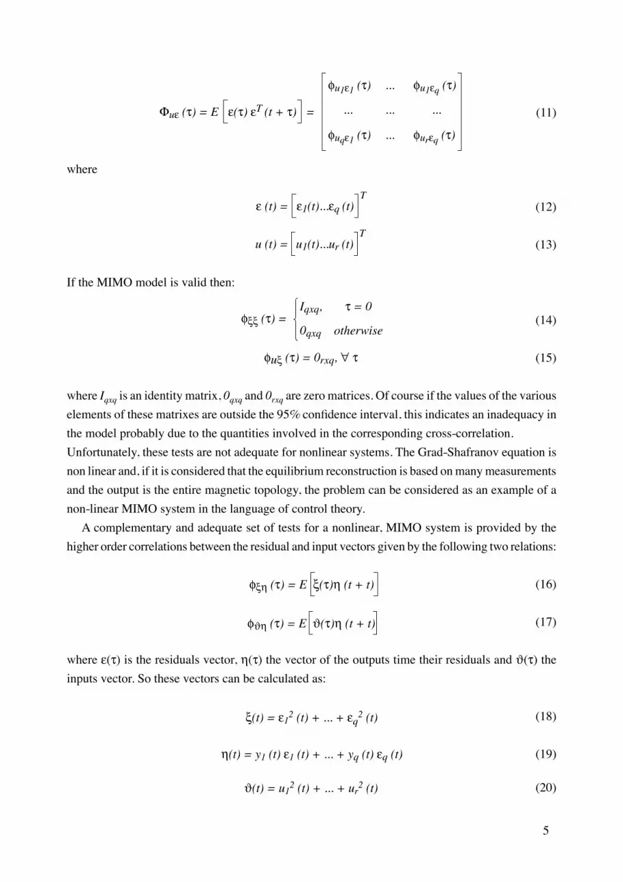
where Iqxq is an identity matrix, 0qxq and 0rxq are zero matrices. Of course if the values of the various elements of these matrixes are outside the 95% confidence interval, this indicates an inadequacy in the model probably due to the quantities involved in the corresponding cross-correlation.Unfortunately, these tests are not adequate for nonlinear systems. The Grad-Shafranov equation is non linear and, if it is considered that the equilibrium reconstruction is based on many measurements and the output is the entire magnetic topology, the problem can be considered as an example of a non-linear MIMO system in the language of control theory. A complementary and adequate set of tests for a nonlinear, MIMO system is provided by the higher order correlations between the residual and input vectors given by the following two relations:

(16)

(17)

where e(t) is the residuals vector, h(t) the vector of the outputs time their residuals and J(t) the inputs vector. So these vectors can be calculated as:

(18)

(19)

(20)

Φuε (τ) = E

φu1ε1 (τ) φu1εq (τ)...

φuqε1 (τ) φurεq (τ)...

...... ...=ε(τ) εT (t + τ)

ε (t) = ε1(t)...εq (t)T

u (t) = u1(t)...ur (t)T

φξξ (τ) =Iqxq,

0qxq

τ = 0

otherwise

φuξ (τ) = 0rxq, ∀ τ

φξη (τ) = E ξ(τ)η (t + t)

φϑη (τ) = E ϑ(τ)η (t + t)

ξ(t) = ε12 (t) + ... + εq2 (t)

η(t) = y1 (t) ε1 (t) + ... + yq (t) εq (t)

ϑ(t) = u12 (t) + ... + ur2 (t)

6

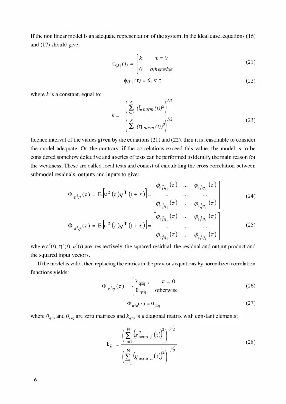
If the non linear model is an adequate representation of the system, in the ideal case, equations (16) and (17) should give:

(21)

(22)

where k is a constant, equal to:

(23)

fidence interval of the values given by the equations (21) and (22), then it is reasonable to consider the model adequate. On the contrary, if the correlations exceed this value, the model is to be considered somehow defective and a series of tests can be performed to identify the main reason for the weakness. These are called local tests and consist of calculating the cross correlation between submodel residuals, outputs and inputs to give:

(24)

(25)

where e2(t), h2(t), u2(t),are, respectively, the squared residual, the residual and output product and the squared input vectors. If the model is valid, then replacing the entries in the previous equations by normalized correlation functions yields:

(26)

(27)

where 0qxq and 0rxq are zero matrices and kqxq is a diagonal matrix with constant elements:

(28)

φξη (τ) =k

0

τ = 0

otherwise

φϑη (τ) = 0, ∀ τ

(ξ norm (t))2

k =ΣN

t=1

1/2

(η norm (t))2ΣN 1/2

( ) ( )[ ]( ) ( )

( ) ( )=+=Φ

τφτφ

τφτφτηττ

ηη

ηη

η

qqq

q

ee

eeT

e teE2

12

211

21

2

............

...)( 2

( ) ( )[ ]( ) ( )

( ) ( )=+=Φ

τφτφ

τφτφτηττ

ηη

ηη

η

qrr

q

uu

uuT

u tuE2

12

211

21

2

............

...)( 2

==Φ otherwise

kqxq

qxq0

0,)(2

ττηε

rxqu 0)(2 =Φ τη

( )( )

( )( ) 21

1

2,

21

1

22

,

=

∑

∑

=

=

N

tinorm

N

tinorm

ii

t

tk

η

ε

7

Relations (26) and (27) allow therefore determining which are the incorrect submodels. To summarize, with the global tests it is possible to assess the validity of the developed models. If the model is not valid within the required confidence interval, the local tests can be used to identify which of the submodels are the probable cause of the inadequacies.To illustrate the potential of the approach, in the following the described technique is applied to the case of the nonlinear pendulum. The equation of motion for the damped, driven pendulum can be written as:

(29)

where the various terms on the left represent acceleration, damping, and gravitation, while the term on the right is the driving force. Primes indicate derivatives with respect to time. Given appropriate initial conditions, equation (29) has been numerically integrated with a Runge-Kutta algorithm so to obtain a corresponding trajectory y (t). As an example, we have considered the following equation:

(30)

with g = 0.01, b = 0.008 and a = 0.196. To deal with a realistic situation, the signal is corrupted with an additive white noise )(tn of 5% of the signal amplitude:

(31)

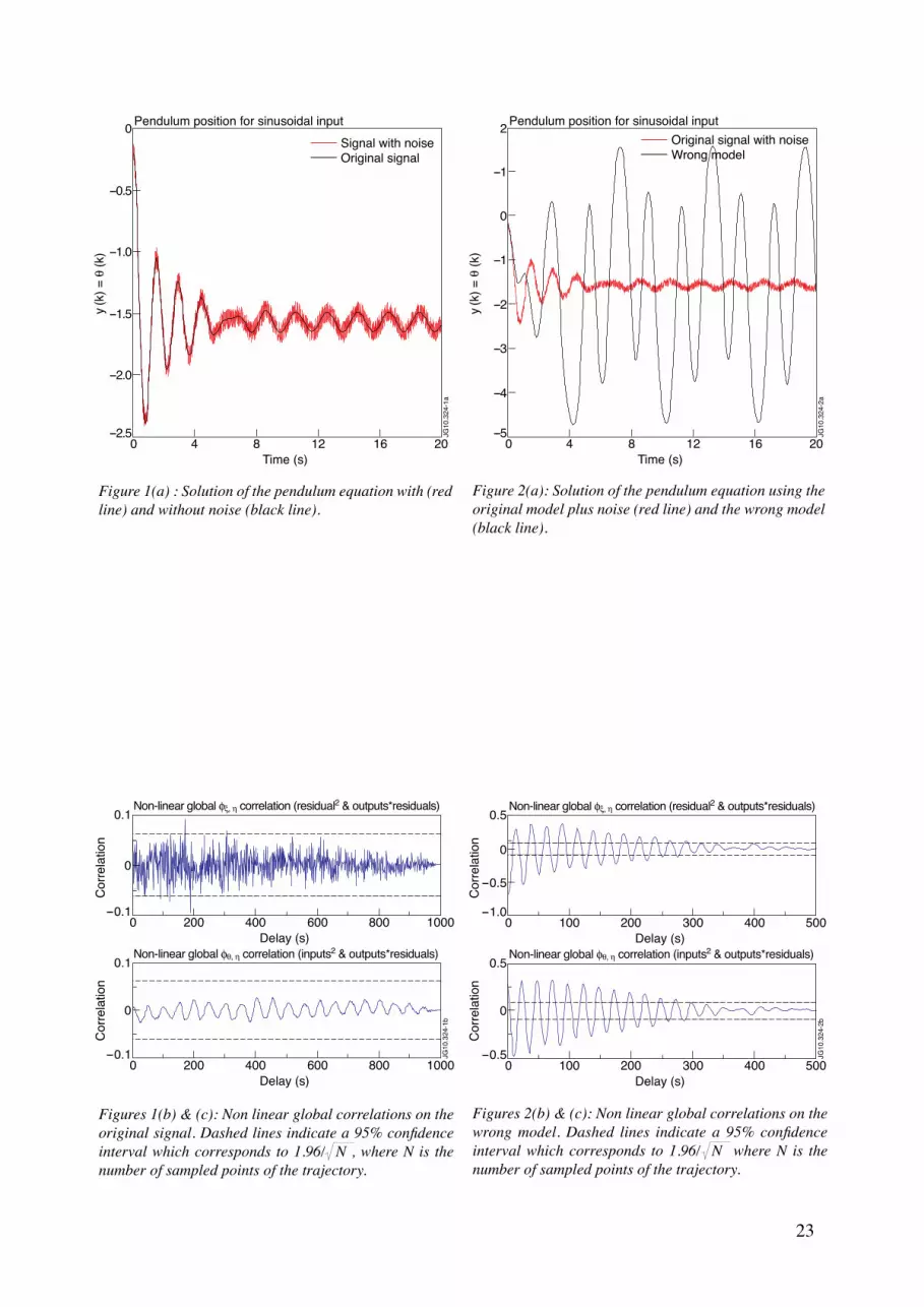
Since the pendulum is a non linear equation, to validate the developed model both the linear and the non-linear correlation tests have been performed. For brevity sake, only the results of the non-linear tests are reported in the following figures. The inputs of the model are considered to be the different terms of the equation, and the output is the solution y of the equation. Consequently, the residuals are the difference between the solution of the differential equation model and the original signal with noise. In figure 1.a, the pendulum equation solution with (red line) and without (black line) the additive white noise is reported. In figures 1.b and 1.c, results of correlation tests performed for the signal with noise are reported, indicating that this signal actually follows the original signal. To check the capabilities of the correlation tests to validate a model, some errors have been introduced in the model. Starting with the pendulum equation, described by relation (30), a wrong model (ywrong (t)) has been generated. In particular the constant of the torque term b • sin (p • t) has been set to the wrong value b = 0.12. Then the non-linear correlation tests of the residuals have been performed to determine to what extent they are capable not only to determine that the model is not adequate but also to identify the source of the errors. The plots of the original noisy model and of the wrong one are shown in figure 2.b. In this case,

g(t))(''' =++ yfyγy

)sin()sin(''' tbya⋅ y ⋅y y ⋅⋅ =++ π

)( )( )(tntytynoise +→

8

the autocorrelation of the residuals, between the two signals (e(t) = ynoise (t) - ywrong (t)), is not a white noise, as can be seen in figure 2.b, which represents the correlation between the squared residuals and the residuals and outputs product, and in figure 2.c, which shows the correlation between the squared residuals and the squared inputs (see definitions (24) and (25)). Given the results obtained with the non linear global tests, the non linear local tests have been performed to determine which submodels are incorrect in the full wave propagation code. In figures 3.a, 3.b and 3.c, the results of the non-linear local correlations on the different terms of the equation, considered as the inputs of the model, are reported. It can be noted that these correlation tests have points outside the confidence interval for several terms of the equation, which is due to the mutual influence between the different terms. However, given these results, it is possible to conclude that the fault is more likely to reside in the torque term, as this term leads to poorer correlation results.

3. overvIew of the reconstructIon code tested And the reference code for the boundAry

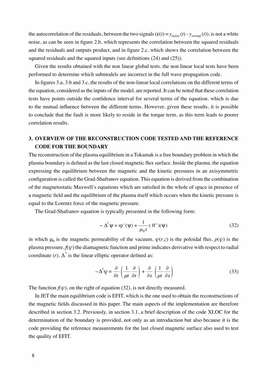
The reconstruction of the plasma equilibrium in a Tokamak is a free boundary problem in which the plasma boundary is defined as the last closed magnetic flux surface. Inside the plasma, the equation expressing the equilibrium between the magnetic and the kinetic pressures in an axisymmetric configuration is called the Grad-Shafranov equation. This equation is derived from the combination of the magnetostatic Maxwell’s equations which are satisfied in the whole of space in presence of a magnetic field and the equilibrium of the plasma itself which occurs when the kinetic pressure is equal to the Lorentz force of the magnetic pressure. The Grad-Shafranov equation is typically presented in the following form:

(32)

in which μ0 is the magnetic permeability of the vacuum, ψ(r,z) is the poloidal flux, p(ψ) is the plasma pressure, f(ψ) the diamagnetic function and prime indicates derivative with respect to radial coordinate (r). Δ* is the linear elliptic operator defined as:

(33)

The function f(ψ), on the right of equation (32), is not directly measured. In JET the main equilibrium code is EFIT, which is the one used to obtain the reconstructions of the magnetic fields discussed in this paper. The main aspects of the implementation are therefore described in section 3.2. Previously, in section 3.1, a brief description of the code XLOC for the determination of the boundary is provided, not only as an introduction but also because it is the code providing the reference measurements for the last closed magnetic surface also used to test the quality of EFIT.

))('(1)('0

*μ

ffr

rp +=Δ− y y y

ψ∂∂

∂∂+

∂∂

∂∂=-Δ

zrzrrr μμ11*

9

3.1. XLOCXLOC was originally introduced on JET in order to provide a fast and accurate determination of the plasma boundary in the neighbourhood of the X-point. This method has been extended to cover the whole plasma boundary and is now used for arbitrary plasma configurations. It is used routinely for plasma shape real-time control. Based on this code the main parameters of JET boundary, like the strike points position and the distance from the wall, are determined in less than 1ms. Nowadays, after an extensive use and benchmarking with other diagnostics, XLOC provides the most reliable and precise determination of the plasma boundary. On the other hand, with this algorithm it is not possible to compute the internal magnetic flux configuration. At the basis of the calculation are 6th order expansions of the poloidal flux in five sections of the poloidal cross section of the machine: at the top, bottom, inboard, upper and lower outboard parts of the vessel. The expansions are expressed mathematically by the relation:

(34)

where r = R2 - R02, z = Z – Z0, with R the radial coordinate, Z the vertical coordinate, and (R0,

Z0) the centre of the expansion. The variable ρ rather than R – R0 is chosen because of the symmetry of the Grad-Shafranov equation about the major axis of the torus (R = 0). The coefficients aij are determined by imposing the vacuum equation:magnetic field can be written in terms of these coefficients as:

(35)

and by fitting to the local flux and magnetic field measurements. In addition, the five expansions are constrained to match at chosen points around the vessel. Having imposed the vacuum equation, each expansion is left with 13 independent coefficients to be determined, leading to a total number of 65 coefficients for the five expansions. The flux and magnetic field can be written in terms of these coefficients as:

(35)

where Bc, refers to the component of B in the direction of the measuring coil. If no constraints on the matching between the expansions are used, each fit is independent, giving raise to five least squares calculations from the minimization of

ρ

+==

6

60

0

j ≤iji

jiij zaΣ

ψ∆

∆

0* =−

+=zrzrrr µµ

11*

Σ

Σψ ψ

=

=

=

=

13

1

13

1

),(),(

),(),(

iiic

α

α

α

α α

iiic

CzBzρ ρ

ρ ρ

B

Czz

α

α 5...1=

10

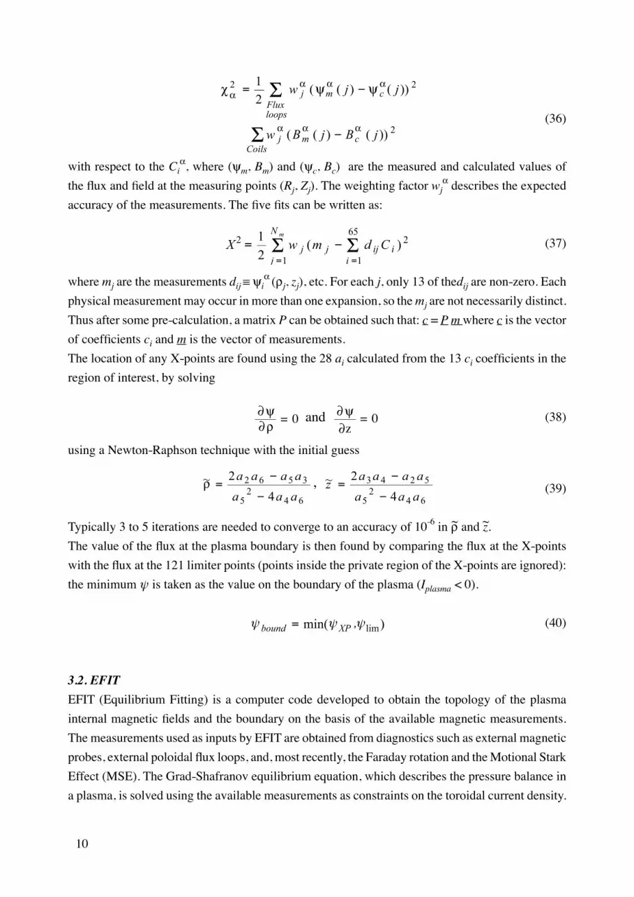
(36)

with respect to the Cia, where (ym, Bm) and (yc, Bc) are the measured and calculated values of

the flux and field at the measuring points (Rj, Zj). The weighting factor wja describes the expected

accuracy of the measurements. The five fits can be written as:

(37)

where mj are the measurements dij ≡ yi

a (rj, zj), etc. For each j, only 13 of thedij are non-zero. Each

physical measurement may occur in more than one expansion, so the mj are not necessarily distinct.Thus after some pre-calculation, a matrix P can be obtained such that: c = P m where c is the vector of coefficients ci and m is the vector of measurements.The location of any X-points are found using the 28 ai calculated from the 13 ci coefficients in the region of interest, by solving

(38)

using a Newton-Raphson technique with the initial guess

(39)

Typically 3 to 5 iterations are needed to converge to an accuracy of 10-6 in r and z.The value of the flux at the plasma boundary is then found by comparing the flux at the X-points with the flux at the 121 limiter points (points inside the private region of the X-points are ignored): the minimum ψ is taken as the value on the boundary of the plasma (Iplasma < 0).

(40)

3.2. EFITEFIT (Equilibrium Fitting) is a computer code developed to obtain the topology of the plasma internal magnetic fields and the boundary on the basis of the available magnetic measurements. The measurements used as inputs by EFIT are obtained from diagnostics such as external magnetic probes, external poloidal flux loops, and, most recently, the Faraday rotation and the Motional Stark Effect (MSE). The Grad-Shafranov equilibrium equation, which describes the pressure balance in a plasma, is solved using the available measurements as constraints on the toroidal current density.

~ ~

Σ

Σ

−=

loopsFlux

cmjα

αα α

ααα

jjwχ ψ ψ 22 ))()((2

1

−Coils

cmj jBjBw 2))()((

= =−=

mN

j iiijjj CdmwX

1

65

1

22 )(2

1 ΣΣ

∂ ψ∂ ρ

∂ ψ∂

0= and 0=z

642

5

3562

4

2~

aaaaaaar

−−= ,

642

5

5243

4

2~

aaaaaaaz

−−=

ψψ ,ψ )min( lim= XPbound

11

Since the current also depends on the solution of the equation, the poloidal flux function, this is a nonlinear optimization problem. The equilibrium of a plasma in a domain Ω representing the vacuum region is a free boundary problem. The plasma free boundary is defined at JET as being a magnetic separatrix (hyperbolic line with an X-point X) the region Ωp containing the plasma is defined as:

(41)

where ψb = ψ(X) in the X point configuration. Assuming Dirichlet boundary conditions, h, are given on Γ = ∂Ω, which is the poloidal cross section of the vacuum vessel, the final equations governing the behaviour of ψ(r,z) inside the vacuum vessel are:

(42)

with:

(43)

where the normalized flux is introduced so that A and B are defined on the interval [0,1]:

(44)

and χΩp is the characteristic function of Ωp. By means of least-square minimization of the difference between the measurements and the ones derived from the reconstructed field topology, the code identifies the source term of the non linear Grad-Shafranov equation. The experimental measurements that constitute the input to the identification can be the magnetics on the vacuum vessel, the polarimetric measurements on several chords and the motional Stark effect measurements. For the magnetic measurements the flux loops give the poloidal flux on particular nodes Mi such that ψ(Mi)=hi on Γ. The problem is thus resumed to find a solution that minimizes the cost function defined as:

(45)with:

(46)

( ) ( )=

+=−

on

in 0

0

*

h

Br

RARr

pψψ χψ

ψ Γ

( ) ( ) )μ

'1 and '00

0 ffR

BpRA ==ψ ψ ((( ) ) ψψ

ψ - max ψΩp

ψb - max ψψ = Ωp

-

J(ψ) = J0 + K1J1 + K2J2 + K3J3 + Jε

Ci

J0 = (Ni)-gi1 ∂ψ

r ∂ni

2

Σ

J1 = dl-aine ∂ψ

∂ni

2

Σ r

CiJ2 = nedl-βi

i

2

Σ

J3 = msei-γii

2

Σ

Ω ψψ Ω= )(, x ≥xp ∈

12

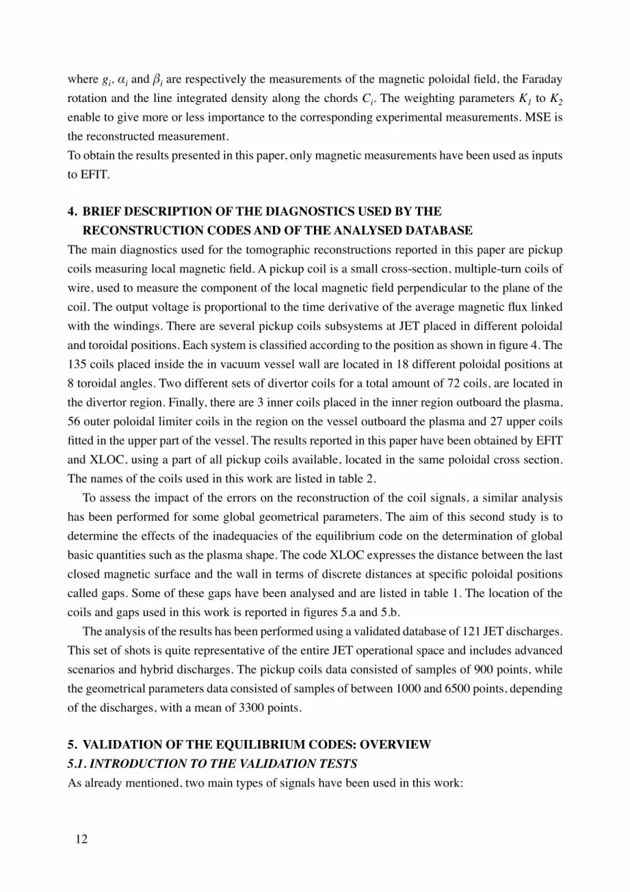
where gi, αi and βi are respectively the measurements of the magnetic poloidal field, the Faraday rotation and the line integrated density along the chords Ci. The weighting parameters K1 to K2 enable to give more or less importance to the corresponding experimental measurements. MSE is the reconstructed measurement.To obtain the results presented in this paper, only magnetic measurements have been used as inputs to EFIT.

4. brIef descrIptIon of the dIAgnostIcs used by the reconstructIon codes And of the AnAlysed dAtAbAse

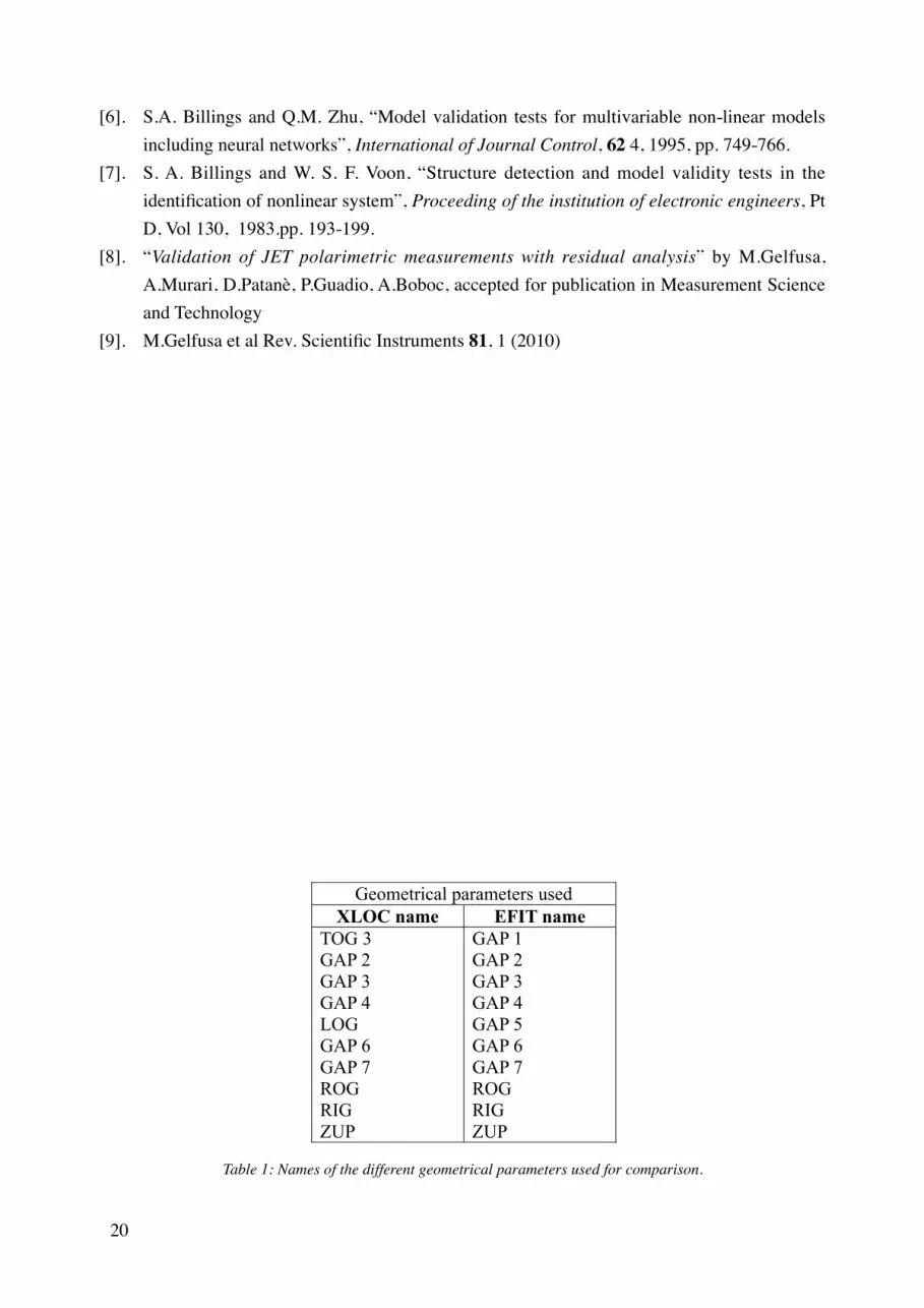
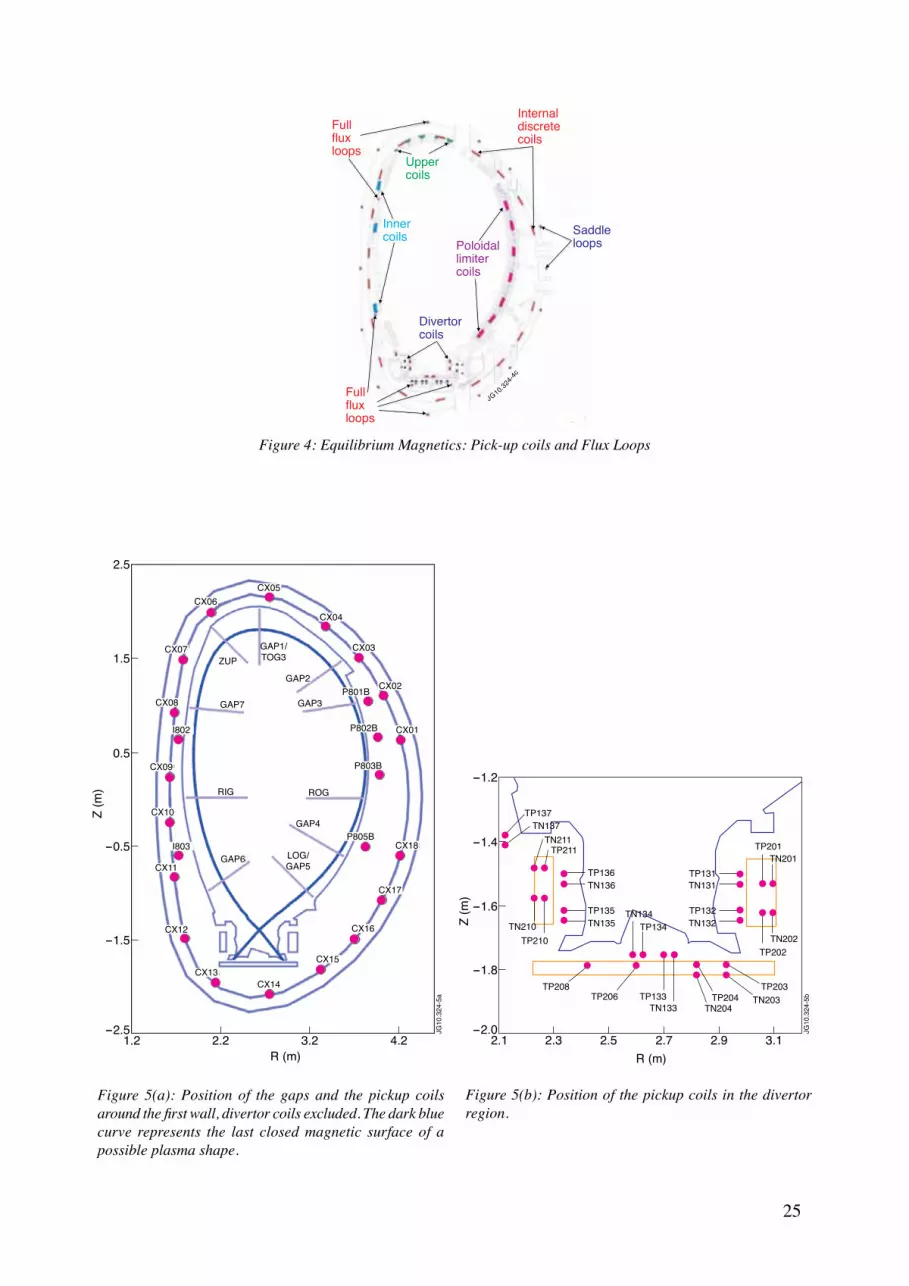
The main diagnostics used for the tomographic reconstructions reported in this paper are pickup coils measuring local magnetic field. A pickup coil is a small cross-section, multiple-turn coils of wire, used to measure the component of the local magnetic field perpendicular to the plane of the coil. The output voltage is proportional to the time derivative of the average magnetic flux linked with the windings. There are several pickup coils subsystems at JET placed in different poloidal and toroidal positions. Each system is classified according to the position as shown in figure 4. The 135 coils placed inside the in vacuum vessel wall are located in 18 different poloidal positions at 8 toroidal angles. Two different sets of divertor coils for a total amount of 72 coils, are located in the divertor region. Finally, there are 3 inner coils placed in the inner region outboard the plasma, 56 outer poloidal limiter coils in the region on the vessel outboard the plasma and 27 upper coils fitted in the upper part of the vessel. The results reported in this paper have been obtained by EFIT and XLOC, using a part of all pickup coils available, located in the same poloidal cross section. The names of the coils used in this work are listed in table 2. To assess the impact of the errors on the reconstruction of the coil signals, a similar analysis has been performed for some global geometrical parameters. The aim of this second study is to determine the effects of the inadequacies of the equilibrium code on the determination of global basic quantities such as the plasma shape. The code XLOC expresses the distance between the last closed magnetic surface and the wall in terms of discrete distances at specific poloidal positions called gaps. Some of these gaps have been analysed and are listed in table 1. The location of the coils and gaps used in this work is reported in figures 5.a and 5.b. The analysis of the results has been performed using a validated database of 121 JET discharges. This set of shots is quite representative of the entire JET operational space and includes advanced scenarios and hybrid discharges. The pickup coils data consisted of samples of 900 points, while the geometrical parameters data consisted of samples of between 1000 and 6500 points, depending of the discharges, with a mean of 3300 points.

5. vAlIdAtIon of the equIlIbrIum codes: overvIew5.1. InTrOduCTIOn TO ThE vaLIdaTIOn TEsTsAs already mentioned, two main types of signals have been used in this work:

13

• The magnetic field measurements, which are obtained by the pickup coils placed around the Tokamak. These coils provide the measurements, while the EFIT code provides the model results.

• The parameters describing the plasma shape, which are deduced from the magnetic measurements. The traditional code for computing these parameters is XLOC, known to be quite accurate, and considered here as a reference, while the EFIT code is seen as the model to be tested. Indeed XLOC has been used for many years for the control of the plasma last close magnetic surface and has been validated with non magnetic diagnostics such as cameras.

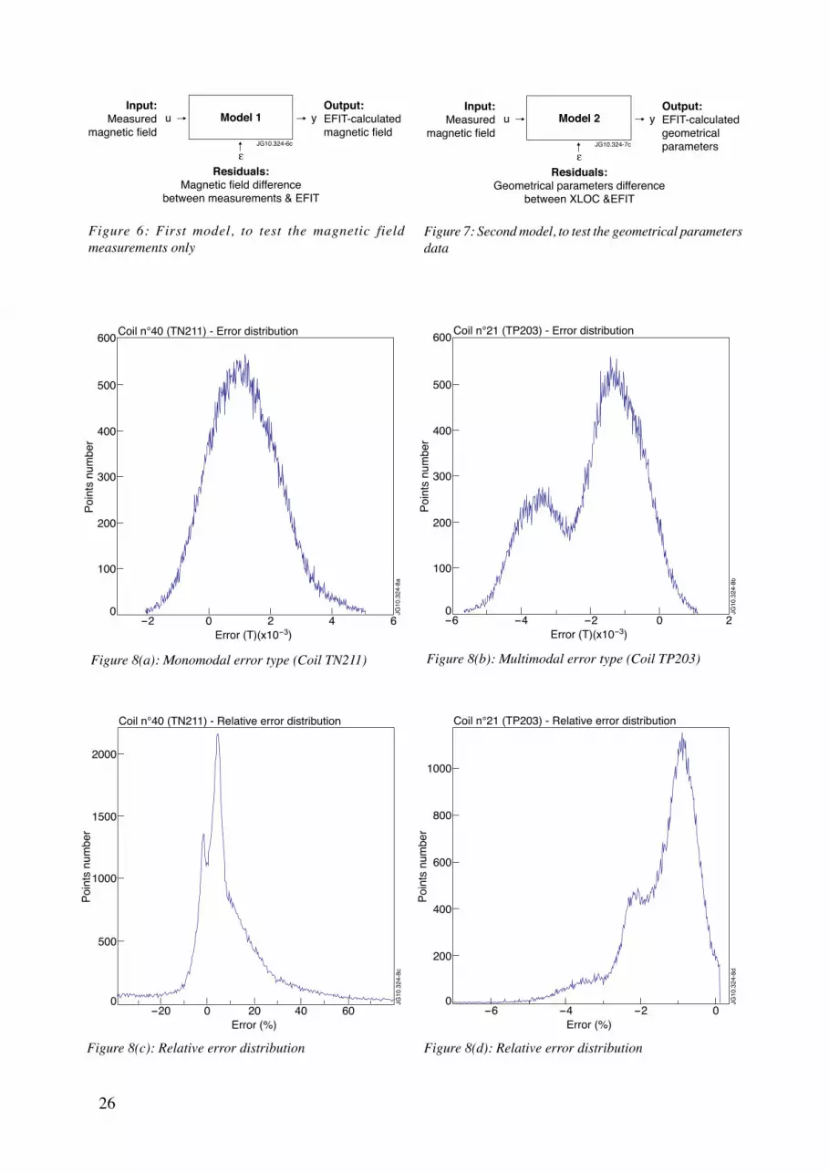
In terms of validation, the two models to be analysed are schematized in figures 6 and 7.

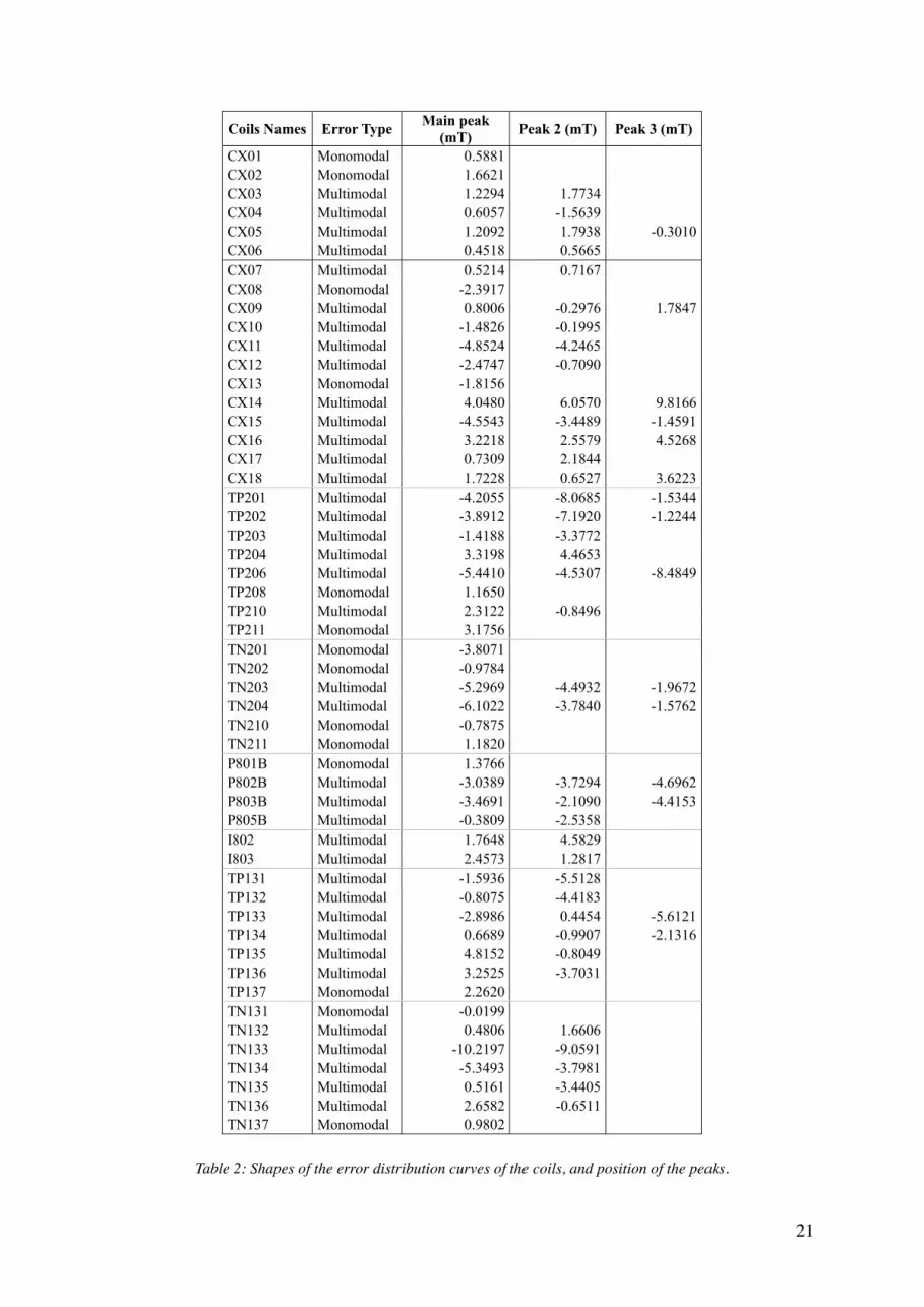
5.2. rEsuLTs OF ThE COmpLETE ErrOr dIsTrIbuTIOnsFirst of all, to provide a general overview of the results, the measured magnetic signals have been compared to the computed results of EFIT for the 121 selected shots. The cumulative distributions of the differences between the measurements and the EFIT reconstruction of the coil signals have been plotted for each coil (using the data of all shots), in order to understand where the errors are more severe. Ideally, if the reconstruction was really accurate, the error distributions should consist of, for each coils, Gaussian curves centred in zero. However, the results show that the error distributions do not present the shape of Gaussian curves. Typically they are asymmetric and, furthermore, their mean is, in most cases, quite different from zero. Finally, two different kinds of shapes have been found: monomodal error distributions, that show only one main peak, and multimodal error distributions that show several peaks (usually two). Figures 8.a and 8.b show two examples of both distributions, and table 2 summarises the results of this error distribution analysis. After performing this study, it is clear that there are much more coils with a multimodal error shape than coils with a monomodal error shape. Furthermore, the highest densities of the absolute errors are generally of about 1 militesla. Figures 8.c and 8.d show the relative error distributions, expressed in percentage of the value measured by the coils. These distributions differ from the absolute ones but they present qualitatively the same shape type (monomodal or multimodal). The reconstructions of coils with monomodal distributions of the residuals could at first sight be considered more accurate than the coils with multimodal error distributions. In reality, the situation is much more complex and the results cannot be properly interpreted on the basis of a simple analysis of the overall residual distributions. For example it turns out that coils with cumulative monomodal error types can hide multimodal error distributions on individual shots. On the contrary, multimodal distributions of the residuals can be due to different types of discharges, each one with a monomodal error distribution but with a different mean. Therefore, to really quantify the quality of the reconstruction code, a more involved analysis is required. The approach adopted is the one of the autocorrelation functions of the residuals, as described in the next subsections. Again to provide a general overview of the results, the same global analysis of the residuals

14

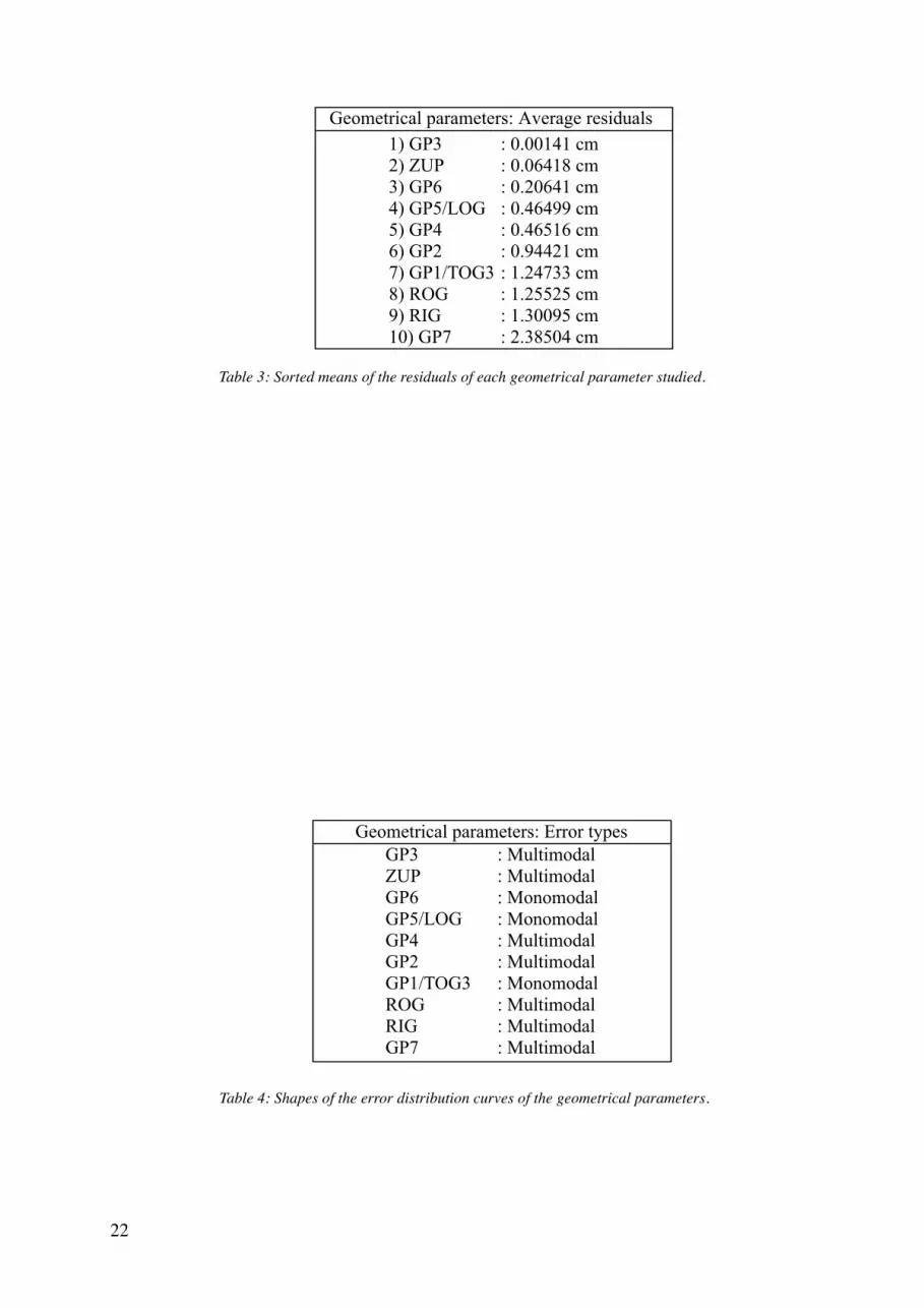
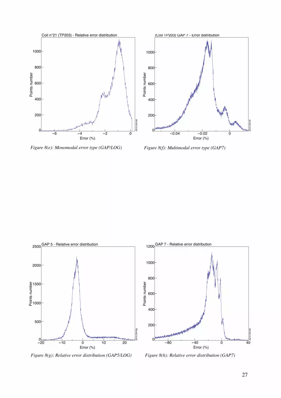
distributions has been performed for the geometrical parameters calculated by EFIT, considering the results of the XLOC code as the reference values. The study of the residuals (i.e. the difference between EFIT and XLOC estimates) leads to the results of tables 3 and 4. Some visual examples of absolute errors are reported in figures 8.e and 8.f, and examples of relative errors are reported in figures 8.g and 8.h. Once again, seven gaps show a multimodal error shape while only three of them show a monomodal error shape. The average errors are around 1 centimetre, and are generally under 1.5 centimetres, which means that the EFIT reconstruction of the gaps is globally rather accurate, particularly if one considers the fact that the reference estimates of the gaps, provided by XLOC, can also be affected by some errors. To better appreciate and summarise the analysis of this section, the results have been represented graphically in figures 9.a and 9.b, where the error distribution types of the coils and the gaps are reported. In order to ensure that the error in the coils reconstruction is not due to problems with the compensation of the toroidal field pick-up, a specific analysis has been performed to clarify this point. No indication of any major problem with this compensation has been found. For example no dependency has been detected between the value of the toroidal field and the errors in the coil reconstruction.

5.3. prELImInary vIsuaL anaLysIs OF ThE COrrELaTIOn TEsTsThe most direct and natural way to check the first correlation results is visual analysis. The resulting correlation functions have been plotted for independent shots and compared to the confidence intervals, in two different ways depending on their type:

- The results of the global correlation functions have been plotted versus time reporting the confidence limits directly on the figures.

- Local correlation function matrices have been plotted showing the results of the correlations between the different inputs of the local tests, using a colour scale in order to differentiate the terms inside and outside the confidence boundaries.

5.3.1. Linear global testsLinear global tests consist of computing the correlation functions defined in equations (7) and (8). These functions are the auto-correlation, involving only the residuals of the model (jxx), and the cross-correlation, involving both the residuals of the model and the experimental measurements (jqx). These correlations take into account all the significant coils, for all the time steps available for the considered pulse. Some examples of the linear global correlations are shown figures 10.a to 10.d. Although the different pulses present correlations of different shapes, almost all of them are outside the confidence limits. The example of figure 10.d is an exception which illustrates the importance of the statistical analysis, because the results of individual shots or coils can easily be very misleading.

15

5.3.2. Linear local testsPerforming local tests is then needed in order to find the origin of the defective parts of the model. In the case of plasmas, the objective consists of finding whether there is evidence of systematic errors in the coil measurements. To this end, the correlations between the coils have been calculated. The results for any pulse are then the two Fee and Fue matrices, where each term is a function related to a pair of coils, quantifying their correlation, as defined in (10) and (11).In order to perform a visual analysis, plots have been created from these matrix terms. A colour scale has been chosen in order to easily understand the different values obtained. The colour pixels represent the different absolute values of the matrix terms:

- The green to cyan shades are the values below the confidence boundaries,- The orange to red shades are the values above the confidence limits,- The white pixels are the terms equal to 1.

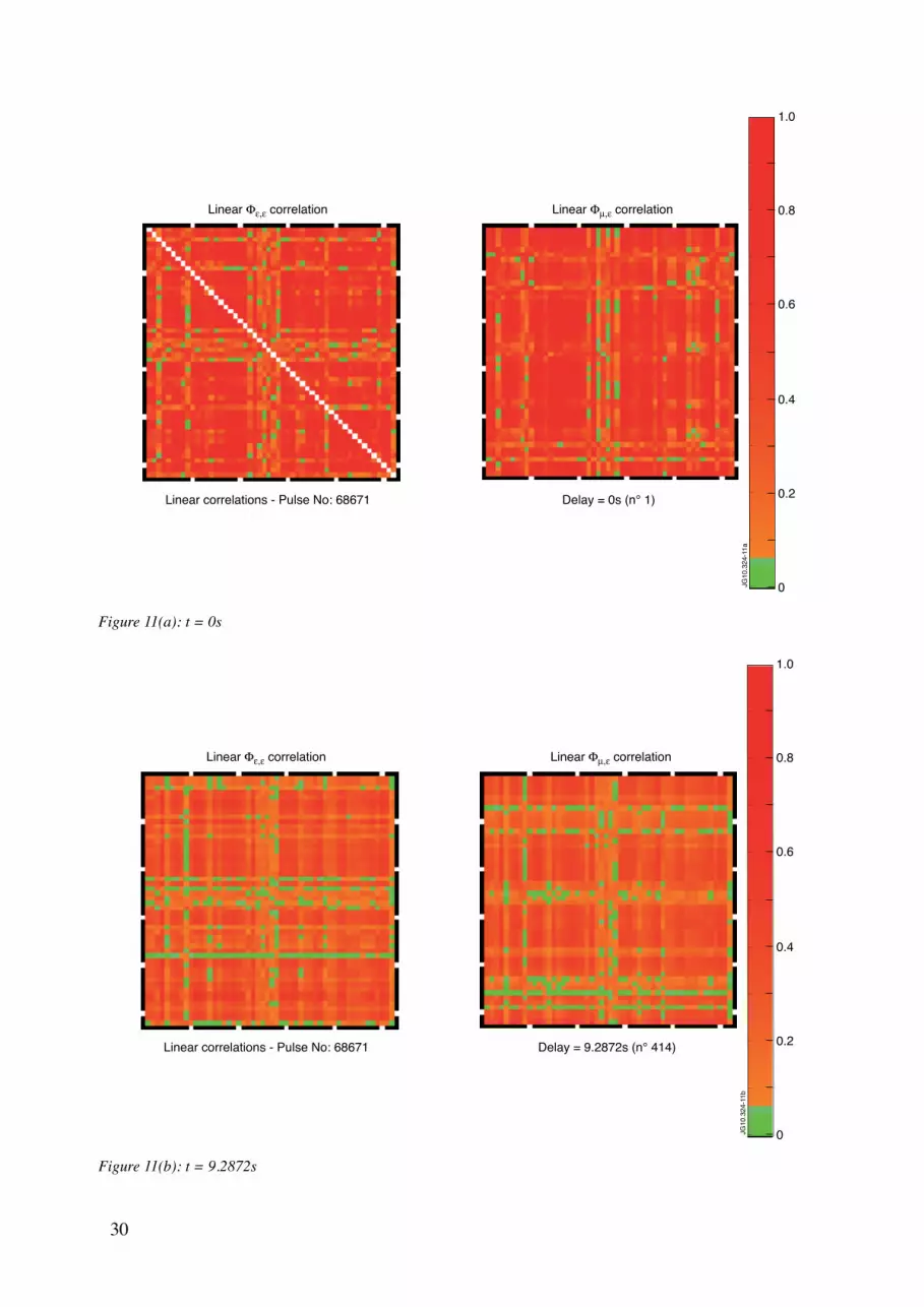
The white dots around the matrices are visual reference points, placed every ten values. Figures 11.a and 11.b are examples of two time steps of linear local correlations for one pulse. The diagonal of ones in the first time step matrix is intrinsic to the correlation method, and is predicted by (14). Different lines of mostly-correlated or mostly-uncorrelated coils clearly appear, showing that on certain shots, the reconstruction provides more accurate results for certain coils than others. On the other hand, the values of the cross correlations between coils change significantly not only between shots but even during different phases of the same shot. Therefore there is no clear indication of systematic errors emerging from this analysis. In any case, the general trend is for the autocorrelations of the residuals to be outside the 95% confidence limits, suggesting problems with the code EFIT.

5.3.3. Non‑linear global testsNon-linear global correlation tests use the same correlation formula as the linear correlations, but different inputs, as described in (16) and (17). The non-linear jxh correlation involves the residuals and the output values of the model, and jqh correlation involves the residuals, the computed results of the model, and the measurements. Figures 12.a and 12.b are examples of non-linear global correlations.

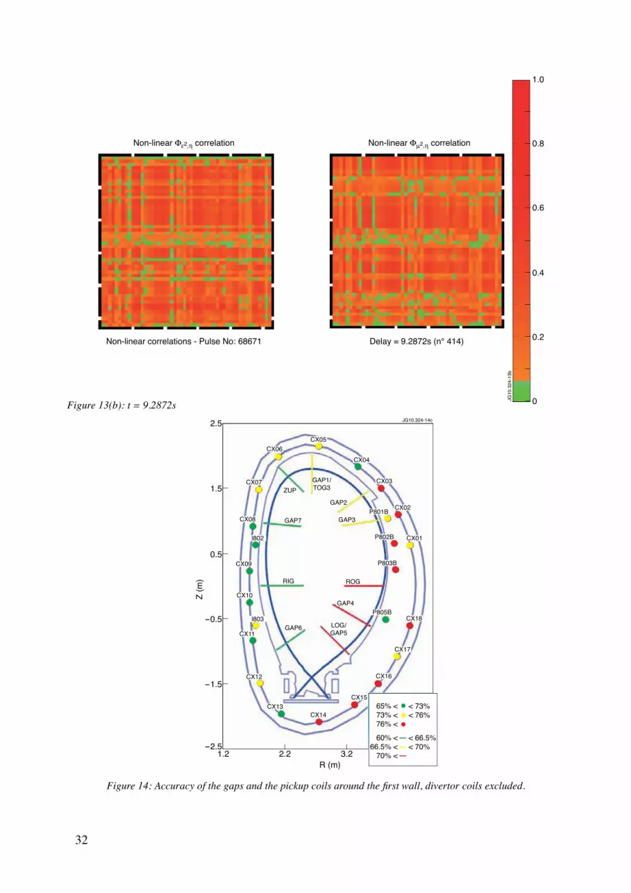
5.3.4. Non‑linear local testsNon-linear local tests consist of the same tests as the linear local tests, but using inputs related to non-linear tests. The results are the two correlation matrices Fe²h and Fu²h, given by (24) and (25). Examples of two different time steps are given in figures 13.a and 13.b. The same remarks than for linear local tests can be formulated: some high- and low-correlation lines appear, denoting clearly that some coils are more accurate than others. Again no regular pattern in the cross correlation of the residuals has been found and therefore the lack of evidence of systematic errors in the coils is confirmed. In general, as for linear local correlations, the matrices

16

show clearly that the autocorrelation of the residuals are outside the 95 % limits, falsifying the hypothesis of a good reconstruction.

6. detAIled locAl AnAlysIs of the correlAtIonsThe more quantitative analysis presented in this section consists of computing all the linear and non-linear correlations described previously from all the data available, and then counting the points outside the confidence intervals, in all local matrices computed (i.e. for every pulse and every time steps). Counting all points outside the confidence limits gives an estimate of the accuracy of the analysed signals. The counting is made separately for the two kinds of linear and non-linear correlations.

6.1. COrrELaTIOns OvEr ThE whOLE dIsChargEThe results of the analysis on the whole discharge are presented in graphical form in this subsection to provide a more intuitive interpretation of the results. The accuracy of the coils and the gaps are quantified by counting results of the non-linear local Fe²h (squared residuals versus outputs & residuals) and Fu²h (squared inputs versus outputs & residuals) correlation tests, explained in subsection 5.1. It is interesting to note in the figures related to Fe²h correlation that the best reconstructed coils (in blue) are exclusively gathered in the divertor region. This may be due to the higher number of coils in this part of the vessel. Furthermore, the coils in the inner part of the vessel (on the left in the figures) seem better reconstructed to the point of view of the correlation method than the outer part, and this tendency can also be seen in the divertor region.The gaps also follow the previous mentioned trend, and are better reconstructed in the inner part of the vessel. However, there is no clear trend around the divertor region. The results for Fu²h correlation follow the same trends: the best reconstructed coils are located in the divertor region, and the inner part of the vessel is globally better reconstructed. The gaps also follow the same tendencies.

6.2. COrrELaTIOns aT sTEady-sTaTEThe results of the analysis at steady-state are also presented in graphical form in this section. The accuracy of the coils and the gaps are quantified by the counting results of the non-linear local Fe²h (squared residuals versus outputs & residuals) and Fu²h (squared inputs versus outputs & residuals) correlation tests. The results related to the Fe²h correlations at steady-state are slightly different from the results on the whole discharge. The best correlated coils (in blue) don not lie only in the divertor region, as some appear in the other parts of the vessel. The inner part of the vessel still seems to be better reconstructed, but a few exceptions are found.Finally, the gaps are also better reconstructed in the inner part of the vessel, but other exceptions appear.

17

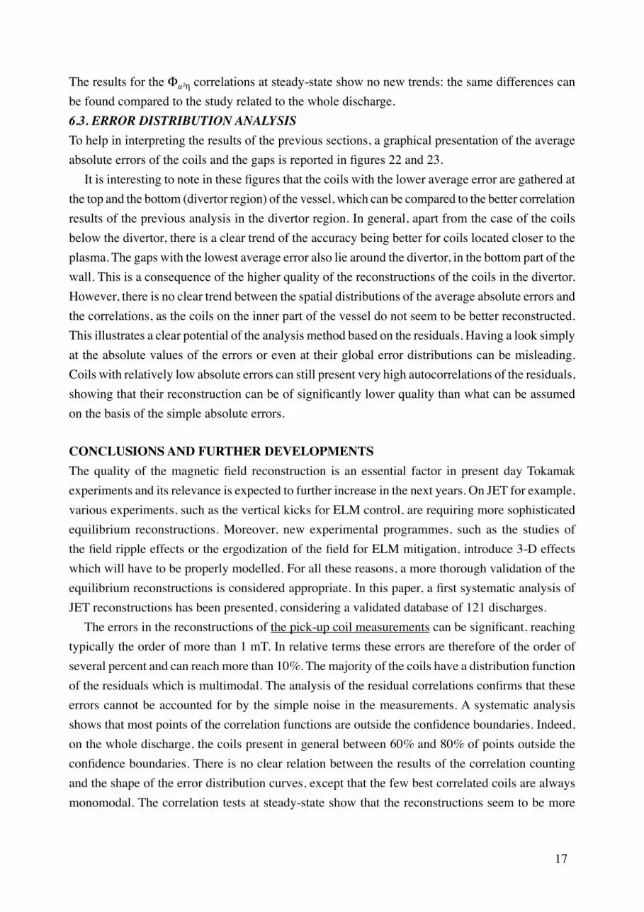
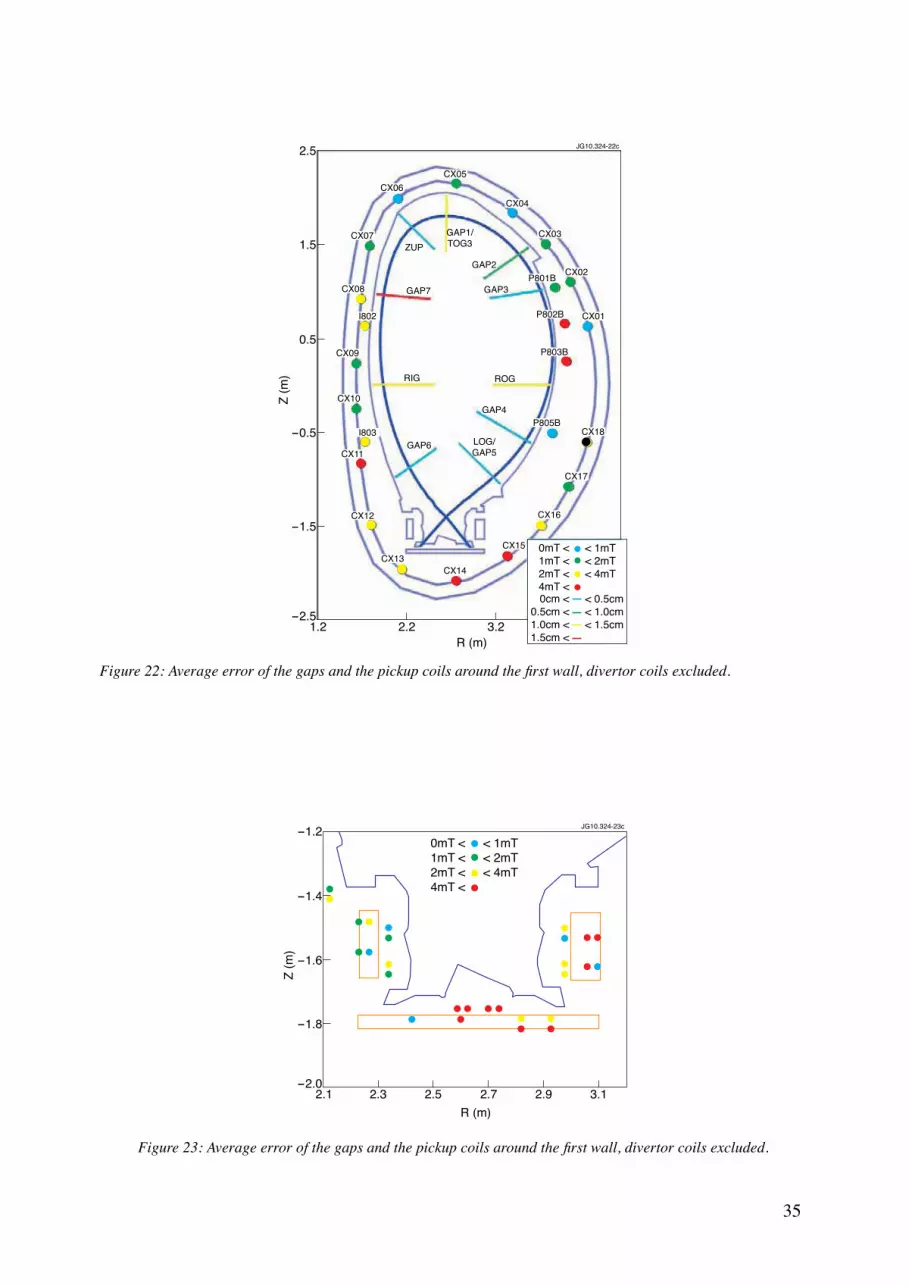
The results for the Fu²h correlations at steady-state show no new trends: the same differences can be found compared to the study related to the whole discharge.6.3. ErrOr dIsTrIbuTIOn anaLysIsTo help in interpreting the results of the previous sections, a graphical presentation of the average absolute errors of the coils and the gaps is reported in figures 22 and 23. It is interesting to note in these figures that the coils with the lower average error are gathered at the top and the bottom (divertor region) of the vessel, which can be compared to the better correlation results of the previous analysis in the divertor region. In general, apart from the case of the coils below the divertor, there is a clear trend of the accuracy being better for coils located closer to the plasma. The gaps with the lowest average error also lie around the divertor, in the bottom part of the wall. This is a consequence of the higher quality of the reconstructions of the coils in the divertor. However, there is no clear trend between the spatial distributions of the average absolute errors and the correlations, as the coils on the inner part of the vessel do not seem to be better reconstructed. This illustrates a clear potential of the analysis method based on the residuals. Having a look simply at the absolute values of the errors or even at their global error distributions can be misleading. Coils with relatively low absolute errors can still present very high autocorrelations of the residuals, showing that their reconstruction can be of significantly lower quality than what can be assumed on the basis of the simple absolute errors.

conclusIons And further developmentsThe quality of the magnetic field reconstruction is an essential factor in present day Tokamak experiments and its relevance is expected to further increase in the next years. On JET for example, various experiments, such as the vertical kicks for ELM control, are requiring more sophisticated equilibrium reconstructions. Moreover, new experimental programmes, such as the studies of the field ripple effects or the ergodization of the field for ELM mitigation, introduce 3-D effects which will have to be properly modelled. For all these reasons, a more thorough validation of the equilibrium reconstructions is considered appropriate. In this paper, a first systematic analysis of JET reconstructions has been presented, considering a validated database of 121 discharges. The errors in the reconstructions of the pick-up coil measurements can be significant, reaching typically the order of more than 1 mT. In relative terms these errors are therefore of the order of several percent and can reach more than 10%. The majority of the coils have a distribution function of the residuals which is multimodal. The analysis of the residual correlations confirms that these errors cannot be accounted for by the simple noise in the measurements. A systematic analysis shows that most points of the correlation functions are outside the confidence boundaries. Indeed, on the whole discharge, the coils present in general between 60% and 80% of points outside the confidence boundaries. There is no clear relation between the results of the correlation counting and the shape of the error distribution curves, except that the few best correlated coils are always monomodal. The correlation tests at steady-state show that the reconstructions seem to be more

18

accurate on this part of the discharge. Indeed, there are about 10% less points outside the confidence boundaries, and the coils present between 50% and 70% of points outside this confidence interval. It has also been noticed that the best correlated coils on the steady-state are mostly monomodal but overall the statistical analysis at steady-state confirms the problems in the reconstruction quality.With regard to the reconstruction of the gaps, a positive aspect of the performed analysis is that the errors in the magnetic field measurements do not seem to affect too much the determination of the plasma boundary. The regions of the poloidal cross section with poorer reconstructions of the pickup coils are also affected by higher errors in the plasma wall distances provided by the reconstructions but the absolute values of these errors are normally of the order of 1 cm and in any case not higher than 2.5 cm. On the other hand the correlations of the residuals reveal the presence of significant inadequacies of the model also for these quantities. To summarise the general overview of the results of the error analysis, it seems fair to say that the reconstructions of the magnetic fields obtained at JET with EFIT are quite adequate for the control of the boundary. On the other hand they seem to present significant statistical errors which have to be carefully taken into account when performing detailed studies of the physics. Since the statistical analysis described illustrates clearly that the quality of the magnetic reconstruction at JET is not limited by noise but that other problems are present, the obvious next step consists of trying to identify the probable main causes of the inadequacies. In this respect, it has been investigated to what extent the detected errors in the reconstructions could be attributed to the pickup coil measurements but with quite negative results. First of all the toroidal field compensation seems to be OK, since there is absolutely no trend of the residuals to increase with the amplitude of the toroidal field. Moreover the global distributions of the residuals have amplitudes and shapes which are not easily interpretable in terms of systematic errors in the measurements (large amplitudes, multimodal distributions, etc.). The correlation analysis also does not give any clear indication that systematic errors in the measurements play a significant role. The analysis of the cross correlations between the various coils, performed extensively with the plots of the type presented in figure 11 and with quantitative estimators, shows clearly that these cross correlations change too much not only between shots but even during the same discharge to be easily attributed to systematic effects in the measurements. Therefore the logical heuristic conclusion is to assume that the main inadequacies reside in the model solved by EFIT and try to make improvements in that direction. The fact that EFIT could introduce some significant errors in the reconstruction of the magnetic fields has also been obtained by a recent analysis of the polarimetric measurements [8]. Again a systematic analysis of the quantities required to model the propagation of a laser beam in JET plasmas has shown that the residuals of the polarimetric measurements are correlated mainly with the magnetic topology and not with the other inputs. This again indicates that improving the EFIT model is probably the right way to go in order to increase the quality of the magnetic reconstruction at JET. An interesting final point to note, for both the pickup coils and the residuals, is the tendency of the autocorrelations of the residuals to be better on the inner part of the vessel, whereas they are

19

worse in that part of the machines when the absolute values of the errors are considered. This can be interpreted as an effect of the poor modelling of the iron in EFIT. As a consequence, when the absolute values of the reconstruction errors are considered, the situation appears clearly worse near the iron. On the other hand, when the correlations of the residuals are considered, in which the average errors are subtracted, the coils on the high filed side being closer to the plasma are typically better reconstructed since the systematic bias due to the iron does not play a role anymore.With regard to future investigations, the next logical step would be to determine the effects of the internal measurements of the field on the quality of the reconstructions. Unfortunately on JET, particularly during the H mode phase of the discharges, not enough measurements of the Motional Stark Effect diagnostic are available to perform a residual analysis of statistical relevance. In any case, the preliminary indication, obtained analysing a very small subset of discharges, does not seem to change the conclusions obtained for EFIT with only the pickup magnetic measurements as inputs. This point on the other hand will require a more systematic analysis and, in order to obtain enough data, it is planned to use the polarimetric signals, which have been recently calibrated with a new technique [9]. To further assess the effects of the systematic errors in the measurements on the quality of the reconstructions, it would be worth repeating the same analysis reported in this paper using as inputs to EFIT sets of coils in different octants (a complete set of coils is available in JET in four different poloidal cross sections). The cross correlations between the residuals of the same coils but in different octants could really shed further light on the impact of the systematic errors in the coils. Another important further step would be to particularise the analysis and assess the equilibrium quality for the main types of scenarios run at JET. The obvious long term line of research will be the inclusion of more physical effects in the EFIT model in order to assess which could be the more relevant to improve the quality of the obtained magnetic topology.

AcknowledgmentsThis work, supported by the European Communities under the contract of Association between EURATOM/ENEA and CEA, was carried out under the framework of the European Fusion Development Agreement. The views and opinions expressed herein do not necessarily reflect those of the European Commission.

references[1]. J. Wesson “Tokamaks” Clarendon Press, Oxford, third edition, 2004[2]. Lao, et.al., Nucl. Fusion 30, 1035 (1990).[3]. D.P. O’Brien, J.J. Ellis and J. Lingertat Nuclear Fusion 33 (1993) 467[4]. S.A. Billings, and W.S.F. Voon, “Correlation based model validity tests for non linear models”,

International of Journal Control, 44, 1986, pp. 235-244.[5]. S.A. Billings and Q.H. Tao, “Model validity tests for non-linear signal processing applications”,

International of Journal Control, 54 1, 1991, pp. 157-194.

20

[6]. S.A. Billings and Q.M. Zhu, “Model validation tests for multivariable non-linear models including neural networks”, International of Journal Control, 62 4, 1995, pp. 749-766.

[7]. S. A. Billings and W. S. F. Voon, “Structure detection and model validity tests in the identification of nonlinear system”, Proceeding of the institution of electronic engineers, Pt D, Vol 130, 1983.pp. 193-199.

[8]. “Validation of JET polarimetric measurements with residual analysis” by M.Gelfusa, A.Murari, D.Patanè, P.Guadio, A.Boboc, accepted for publication in Measurement Science and Technology

[9]. M.Gelfusa et al Rev. Scientific Instruments 81, 1 (2010)

Table 1: Names of the different geometrical parameters used for comparison.

Geometrical parameters used

XLOC name EFIT name

TOG 3

GAP 2

GAP 3

GAP 4

LOG

GAP 6

GAP 7

ROG

RIG

ZUP

GAP 1

GAP 2

GAP 3

GAP 4

GAP 5

GAP 6

GAP 7

ROG

RIG

ZUP

21

Table 2: Shapes of the error distribution curves of the coils, and position of the peaks.

CX07 Multimodal 0.5214 0.7167

CX08 Monomodal -2.3917

CX09 Multimodal 0.8006 -0.2976 1.7847

CX10 Multimodal -1.4826 -0.1995

CX11 Multimodal -4.8524 -4.2465

CX12 Multimodal -2.4747 -0.7090

CX13 Monomodal -1.8156

CX14 Multimodal 4.0480 6.0570 9.8166

CX15 Multimodal -4.5543 -3.4489 -1.4591

CX16 Multimodal 3.2218 2.5579 4.5268


CX18 Multimodal 1.7228 0.6527 3.6223

TP201 Multimodal -4.2055 -8.0685 -1.5344

TP202 Multimodal -3.8912 -7.1920 -1.2244

TP203 Multimodal -1.4188 -3.3772

TP204 Multimodal 3.3198 4.4653

TP206 Multimodal -5.4410 -4.5307 -8.4849

TP208 Monomodal 1.1650

TP210 Multimodal 2.3122 -0.8496


TN201 Monomodal -3.8071


TN203 Multimodal -5.2969 -4.4932 -1.9672

TN204 Multimodal -6.1022 -3.7840 -1.5762


TN211 Monomodal 1.1820

P801B Monomodal 1.3766

P802B Multimodal -3.0389 -3.7294 -4.6962

P803B Multimodal -3.4691 -2.1090 -4.4153

P805B Multimodal -0.3809 -2.5358

I802 Multimodal 1.7648 4.5829

I803 Multimodal 2.4573 1.2817

TP131 Multimodal -1.5936 -5.5128

TP132 Multimodal -0.8075 -4.4183

TP133 Multimodal -2.8986 0.4454 -5.6121

TP134 Multimodal 0.6689 -0.9907 -2.1316

TP135 Multimodal 4.8152 -0.8049

TP136 Multimodal 3.2525 -3.7031



TN132 Multimodal 0.4806 1.6606

TN133 Multimodal -10.2197 -9.0591

TN134 Multimodal -5.3493 -3.7981

TN135 Multimodal 0.5161 -3.4405

TN136 Multimodal 2.6582 -0.6511

TN137 Monomodal 0.9802

Coils Names Error Type Main peak

(mT) Peak 2 (mT) Peak 3 (mT)

CX01 Monomodal 0.5881

CX02 Monomodal 1.6621


CX04 Multimodal 0.6057 -1.5639

CX05 Multimodal 1.2092 1.7938 -0.3010


22

Table 3: Sorted means of the residuals of each geometrical parameter studied.

Table 4: Shapes of the error distribution curves of the geometrical parameters.

1) GP3 : 0.00141 cm

2) ZUP : 0.06418 cm

3) GP6 : 0.20641 cm

4) GP5/LOG : 0.46499 cm

5) GP4 : 0.46516 cm

6) GP2 : 0.94421 cm

7) GP1/TOG3 : 1.24733 cm

8) ROG : 1.25525 cm

9) RIG : 1.30095 cm

10) GP7 : 2.38504 cm

Geometrical parameters: Average residuals

GP3 : Multimodal

Geometrical parameters: Error types

ZUP : Multimodal

GP6 : Monomodal

GP5/LOG : Monomodal

GP4 : Multimodal

GP2 : Multimodal

GP1/TOG3 : Monomodal

ROG : Multimodal

RIG : Multimodal

GP7 : Multimodal

23

Figure 1(a) : Solution of the pendulum equation with (red line) and without noise (black line).

Figure 2(a): Solution of the pendulum equation using the original model plus noise (red line) and the wrong model (black line).

Figures 1(b) & (c): Non linear global correlations on the original signal. Dashed lines indicate a 95% confidence interval which corresponds to 1.96/ N , where N is the number of sampled points of the trajectory.

Figures 2(b) & (c): Non linear global correlations on the wrong model. Dashed lines indicate a 95% confidence interval which corresponds to 1.96/ N where N is the number of sampled points of the trajectory.

-0.5

-1.0

-1.5

-2.0

-2.5

0

4 8 12 160 20

y (k)

= θ

(k)

Time (s)

Pendulum position for sinusoidal input

Signal with noiseOriginal signal

JG10

.324

-1a

0

0.1

-0.1200 400 600 8000 1000

Cor

rela

tion

Delay (s)

Non-linear global φθ, η correlation (inputs2 & outputs*residuals)

JG10

.324

-1b

0

0.1

-0.1200 400 600 8000 1000

Cor

rela

tion

Delay (s)

Non-linear global φξ, η correlation (residual2 & outputs*residuals)

-3

-4

-2

-1

0

-1

-5

2

4 8 12 160 20

y (k)

= θ

(k)

Time (s)

Pendulum position for sinusoidal inputOriginal signal with noiseWrong model

JG10

.324

-2a

0

0.5

-0.5100 200 300 4000 500

Cor

rela

tion

Delay (s)

JG10

.324

-2b

0

-0.5

0.5

-1.0100 200 300 4000 500

Cor

rela

tion

Delay (s)Non-linear global φθ, η correlation (inputs2 & outputs*residuals)

Non-linear global φξ, η correlation (residual2 & outputs*residuals)

24

Figure 3(a): Non‑linear correlation between the torque term of the equation: b • sin(π • t) , and the solution. Figure 3(b): Non-linear correlation between the γ • yʹ term of the equation and the solution. Figure 3(c): Non‑linear correlation between the a • sin(y) term of the equation and the solution.

-0.2

-0.4

0

0.2

0.4

100 200 300 4000 500

Cor

rela

tion

Delay (s)

JG10

.324

-3a

Non-linear local φµ12, η correlation (torque2 & outputs*residuals)

-0.4

-0.8

0

0.4

100 200 300 4000 500

Cor

rela

tion

Delay (s)

JG10

.324

-3b

Non-linear local φµ22, η correlation (term12 & outputs*residuals)

-0.2

-0.4

0

0.2

100 200 300 4000 500

Cor

rela

tion

Delay (s)

JG10

.324

-3c

Non-linear global φµ32, η correlation (term22 & outputs*residuals)

25

Figure 4: Equilibrium Magnetics: Pick‑up coils and Flux Loops

Figure 5(a): Position of the gaps and the pickup coils around the first wall, divertor coils excluded. The dark bluecurve represents the last closed magnetic surface of a possible plasma shape.

Figure 5(b): Position of the pickup coils in the divertor region.

Fullfluxloops

Fullfluxloops

Internaldiscretecoils

Uppercoils

Poloidallimitercoils

Divertorcoils

Saddleloops

Innercoils

JG10.324-4

c

0.5

1.5

-0.5

-1.5

-2.5

2.5

2.2 3.2 4.21.2

JG10

.324

-5a

Z (m

)

R (m)

CX06

CX03

CX02

CX01

P801B

P802B

P803B

P805B

RIG

GAP4

ROG

GAP6

CX17

CX18

CX16

CX15

CX14CX13

CX12

CX11

I803

CX10

CX09

CX07

CX08

I802

GAP7

ZUP

GAP3

GAP2

CX04

CX05

GAP1/TOG3

LOG/GAP5

-1.4

-1.6

-1.8

-2.0

-1.2

2.3 2.5

Z (m

)

R (m)

TP137TN137

TN211TP211

TP210

TP208TP206 TP133

TN133 TN204TN203

TP203TP204

TP202TN202

TN201TP201

TN134TP134TN210

TP136TN136

TP135TN135

TP131TN131

TP132TN132

2.7 2.9 3.12.1

JG10

.324

-5b

26

Figure 6: First model, to test the magnetic field measurements only

Figure 7: Second model, to test the geometrical parameters data

Figure 8(a): Monomodal error type (Coil TN211) Figure 8(b): Multimodal error type (Coil TP203)

Figure 8(c): Relative error distribution Figure 8(d): Relative error distribution

Residuals:Magnetic field difference

between measurements & EFIT

Input:Measured

magnetic fieldu y

Output:EFIT-calculatedmagnetic field

Model 1

εJG10.324-6c

Residuals:Geometrical parameters difference

between XLOC &EFIT

Input:Measured

magnetic fieldu y

Output:EFIT-calculatedgeometricalparameters

Model 2

εJG10.324-7c

500

400

300

200

100

0

600

0 2 4-2 6

Poin

ts n

umbe

r

Error (T)(x10-3)

Coil n°40 (TN211) - Error distribution

JG10

.324

-8a

500

400

300

200

100

0

600

0-4-6 -2 2

Poin

ts n

umbe

r

Error (T)(x10-3)

Coil n°21 (TP203) - Error distribution

JG10

.324

-8b

2000

1500

1000

500

00 20 40 60-20

Poin

ts n

umbe

r

Error (%)

Coil n°40 (TN211) - Relative error distribution

JG10

.324

-8c

800

600

400

200

1000

00-6 -4 -2

Poin

ts n

umbe

r

Error (%)

Coil n°21 (TP203) - Relative error distributionJG

10.3

24-8

d

27

Figure 8(e): Monomodal error type (GAP/LOG) Figure 8(f): Multimodal error type (GAP7)

Figure 8(g): Relative error distribution (GAP5/LOG) Figure 8(h): Relative error distribution (GAP7)

800

600

400

200

1000

00-6 -4 -2

Poin

ts n

umbe

r

Error (%)

Coil n°21 (TP203) - Relative error distribution

JG10

.324

-8d

800

600

400

200

1000

00-0.02-0.04

Poin

ts n

umbe

rError (%)

(Coil TP203) GAP 7 - Error distribution

JG10

.324

-8f

2000

1500

1000

500

2500

020100-10-20

Poin

ts n

umbe

r

Error (%)

GAP 5 - Relative error distribution

JG10

.324

-8g

1000

800

600

400

200

1200

0400-40-80

Poin

ts n

umbe

r

Error (%)

GAP 7 - Relative error distributionJG

10.3

24-8

h

28

Figure 9(a): Position of the gaps and the pickup coils around the first wall, divertor coils excluded. The green elements present a monomodal error distribution, while the red elements present a multimodal error distribution. The dark blue curve represents the last closed magnetic surface of a possible plasma shape.

Figure 9(b): Position of the pickup coils in the divertor region. The green coils present a monomodal error type, while the red coils presents a multimodal error distribution.

0.5

1.5

-0.5

-1.5

-2.5

2.5

2.2 3.2 4.21.2

JG10

.324

-9a

Z (m

)

R (m)

CX06

CX03

CX02

CX01

P801B

P802B

P803B

P805B

RIG

GAP4

ROG

GAP6

CX17

CX18

CX16

CX15

CX14CX13

CX12

CX11

I803

CX10

CX09

CX07

CX08

I802

GAP7

ZUP

GAP3

GAP2

CX04

CX05

GAP1/TOG3

LOG/GAP5

-1.4

-1.6

-1.8

-2.0

-1.2

2.3 2.5

Z (m

)

R (m)

TP137TN137

TN211TP211

TP210

TP208TP206 TP133

TN133 TN204TN203

TP203TP204

TP202TN202

TN201TP201

TN134TP134TN210

TP136TN136

TP135TN135

TP131TN131

TP132TN132

2.7 2.9 3.12.1

JG10

.324

-9b

29

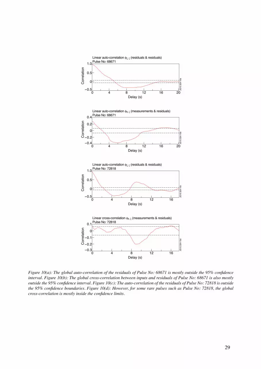
Figure 10(a): The global auto-correlation of the residuals of Pulse No: 68671 is mostly outside the 95% confidence interval. Figure 10(b): The global cross‑correlation between inputs and residuals of Pulse No: 68671 is also mostly outside the 95% confidence interval. Figure 10(c): The auto-correlation of the residuals of Pulse No: 72818 is outside the 95% confidence boundaries. Figure 10(d): However, for some rare pulses such as Pulse No: 72818, the global cross-correlation is mostly inside the confidence limits.

0

0.5

1.0

-0.54 8 12 16 200

Cor

rela

tion

Delay (s)

JG10

.324

-10a

Linear auto-correlation φξ, ξ (residuals & residuals)Pulse No: 68671

0

0.2

-0.2

0.4

-0.44 8 12 16 200

Cor

rela

tion

Delay (s)

JG10

.324

-10b

Linear auto-correlation φθ, ξ (measurements & residuals)Pulse No: 68671

0

0.5

1.0

-0.54 8 12 160

Cor

rela

tion

Delay (s)

JG10

.324

-10c

Linear auto-correlation φξ, ξ (residuals & residuals)Pulse No: 72818

0

-0.1

-0.2

0.1

-0.34 8 12 160

Cor

rela

tion

Delay (s)

JG10

.324

-10d

Linear cross-correlation φθ, ξ (measurements & residuals)Pulse No: 72818

30

Figure 11(a): t = 0s

Figure 11(b): t = 9.2872s

0.8

0.6

0.4

0.2

0

1.0

Delay = 0s (n° 1)Linear correlations - Pulse No: 68671

Linear Φε,ε correlation Linear Φµ,ε correlation

JG10

.324

-11a

0.8

0.6

0.4

0.2

0

1.0

Delay = 9.2872s (n° 414)Linear correlations - Pulse No: 68671

Linear Φε,ε correlation Linear Φµ,ε correlationJG

10.3

24-1

1b

31

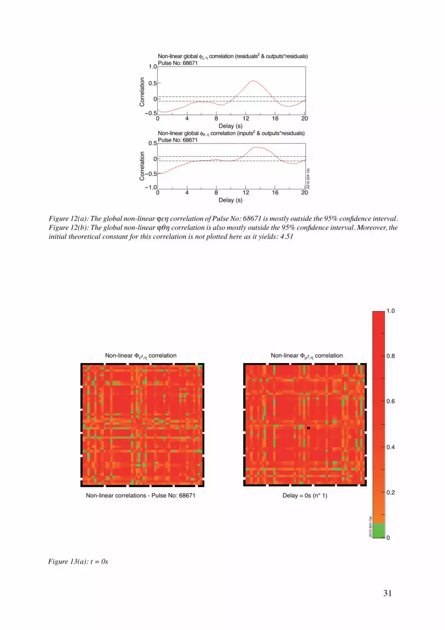
Figure 13(a): t = 0s

Figure 12(a): The global non‑linear jεη correlation of Pulse No: 68671 is mostly outside the 95% confidence interval. Figure 12(b): The global non‑linear jθη correlation is also mostly outside the 95% confidence interval. Moreover, the initial theoretical constant for this correlation is not plotted here as it yields: 4.51

0.5

-1.04 8 12 160

Cor

rela

tion

Delay (s)

Non-linear global φθ, η correlation (inputs2 & outputs*residuals)Pulse No: 68671

JG10

.324

-12c

0.5

0

0

-0.5

1.0

-0.54 8 12 16

20

200

Cor

rela

tion

Delay (s)

Non-linear global φξ, η correlation (residuals2 & outputs*residuals)Pulse No: 68671

0.8

0.6

0.4

0.2

0

1.0

Delay = 0s (n° 1)Non-linear correlations - Pulse No: 68671

Non-linear Φε2,η correlation Non-linear Φµ2,η correlation

JG10

.324

-13a

32

Figure 14: Accuracy of the gaps and the pickup coils around the first wall, divertor coils excluded.

Figure 13(b): t = 9.2872s

0.8

0.6

0.4

0.2

0

1.0

Delay = 9.2872s (n° 414)Non-linear correlations - Pulse No: 68671

Non-linear Φε2,η correlation Non-linear Φµ2,η correlation

JG10

.324

-13b

0.5

1.5

-0.5

-1.5

-2.5

2.5

2.2 3.21.2

JG10.324-14c

Z (m

)

R (m)

CX06

CX03

CX02

CX01

P801B

P802B

P803B

P805B

RIG

GAP4

ROG

GAP6

CX17

CX18

CX16

CX15

CX14CX13

CX12

CX11

I803

CX10

CX09

CX07

CX08

I802

GAP7

ZUP

GAP3

GAP2

CX04

CX05

GAP1/TOG3

LOG/GAP5

65% <73% <76% <

< 73%< 76%

60% <66.5% <

70% <

< 66.5%< 70%

33


Figure 17: Accuracy of the pickup coils in the divertor.


-1.4

-1.6

-1.8

-2.0

-1.2

2.3 2.5

Z (m

)

R (m)

65% <73% <76% <

< 65%< 73%< 76%

2.7 2.9 3.12.1

JG10.324-15c

0.5

1.5

-0.5

-1.5

-2.5

2.5

2.2 3.21.2

JG10.324-16c

Z (m

)

R (m)

CX06

CX03

CX02

CX01

P801B

P802B

P803B

P805B

RIG

GAP4

ROG

GAP6

CX17

CX18

CX16

CX15

CX14CX13

CX12

CX11

I803

CX10

CX09

CX07

CX08

I802

GAP7

ZUP

GAP3

GAP2

CX04

CX05

GAP1/TOG3

LOG/GAP5

70% <75.2% <

78% <

< 75.2%< 78%

78% <83% <86% <

< 83%< 86%

-1.4

-1.6

-1.8

-2.0

-1.2

2.3 2.5

Z (m

)

R (m)

70% <75.2% <

78% <

< 70%< 75.2%< 78%

2.7 2.9 3.12.1

JG10.324-17c

34





0.5

1.5

-0.5

-1.5

-2.5

2.5

2.2 3.21.2

JG10.324-18c

Z (m

)

R (m)

CX06

CX03

CX02

CX01

P801B

P802B

P803B

P805B

RIG

GAP4

ROG

GAP6

CX17

CX18

CX16

CX15

CX14CX13

CX12

CX11

I803

CX10

CX09

CX07

CX08

I802

GAP7

ZUP

GAP3

GAP2

CX04

CX05

GAP1/TOG3

LOG/GAP5

55% <61% <64% <

< 55%< 61%< 64%

60% <66% <68% <

< 66%< 68%

-1.4

-1.6

-1.8

-2.0

-1.2

2.3 2.5

Z (m

)

R (m)

55% <61% <64% <

< 55%< 61%< 64%

2.7 2.9 3.12.1

JG10.324-19c

0.5

1.5

-0.5

-1.5

-2.5

2.5

2.2 3.21.2

JG10.324-20c

Z (m

)

R (m)

CX06

CX03

CX02

CX01

P801B

P802B

P803B

P805B

RIG

GAP4

ROG

GAP6

CX17

CX18

CX16

CX15

CX14CX13

CX12

CX11

I803

CX10

CX09

CX07

CX08

I802

GAP7

ZUP

GAP3

GAP2

CX04

CX05

GAP1/TOG3

LOG/GAP5

65% <67% <69% <

< 65%< 67%< 69%

71% <73% <76% <

< 73%< 76%

-1.4

-1.6

-1.8

-2.0

-1.2

2.3 2.5

Z (m

)

R (m)

65% <67% <69% <

< 65%< 67%< 69%

2.7 2.9 3.12.1

JG10.324-21c

35

Figure 22: Average error of the gaps and the pickup coils around the first wall, divertor coils excluded.

Figure 23: Average error of the gaps and the pickup coils around the first wall, divertor coils excluded.

0.5

1.5

-0.5

-1.5

-2.5

2.5

2.2 3.21.2

JG10.324-22c

Z (m

)

R (m)

CX06

CX03

CX02

CX01

P801B

P802B

P803B

P805B

RIG

GAP4

ROG

GAP6

CX17

CX18

CX16

CX15

CX14CX13

CX12

CX11

I803

CX10

CX09

CX07

CX08

I802

GAP7

ZUP

GAP3

GAP2

CX04

CX05

GAP1/TOG3

LOG/GAP5

0mT <1mT <2mT <4mT <

< 1mT< 2mT< 4mT

0cm <0.5cm <1.0cm <1.5cm <

< 0.5cm< 1.0cm< 1.5cm

-1.4

-1.6

-1.8

-2.0

-1.2

2.3 2.5

Z (m

)

R (m)

0mT <1mT <2mT <4mT <

< 1mT< 2mT< 4mT

2.7 2.9 3.12.1

JG10.324-23c

Residual analysis of the equilibrium reconstruction quality on JET

Documents

Transcript of Residual analysis of the equilibrium reconstruction quality on JET