2nd Reading

June 16, 2015 15:49 WSPC/S0218-2718 142-IJMPD 1550067

International Journal of Modern Physics DVol. 24, No. 8 (2015) 1550067 (34 pages)c© World Scientific Publishing CompanyDOI: 10.1142/S0218271815500674

Post-Newtonian direct and mixed orbital effectsdue to the oblateness of the central body

L. Iorio

CNR-Istituto di Metodologie Inorganiche e dei Plasmi (IMIP),Via Amendola 122/D, 70126 Bari (BA), Italy

lorenzo.iorio@libero.it

Received 22 July 2014Revised 11 May 2015Accepted 13 May 2015Published 18 June 2015

The orbital dynamics of a test particle moving in the nonspherically symmetric fieldof a rotating oblate primary is impacted also by certain indirect, mixed effects arisingfrom the interplay of the different Newtonian and post-Newtonian accelerations whichinduce known direct perturbations. We systematically calculate the indirect gravitoelec-tromagnetic shifts per orbit of the Keplerian orbital elements of the test particle arisingfrom the crossing among the first even zonal harmonic J2 of the central body and thepost-Newtonian static and stationary components of its gravitational field. We also workout the Newtonian shifts per orbit of order J2

2 , and the direct post-Newtonian gravito-electric effects of order J2c−2 arising from the equations of motion. In the case of boththe indirect and direct gravitoelectric J2c−2 shifts, our calculation holds for an arbitraryorientation of the symmetry axis of the central body. We yield numerical estimates oftheir relative magnitudes for systems ranging from Earth’s artificial satellites to starsorbiting supermassive black holes. As far as their measurability is concerned, highlyelliptical orbital configuration are desirable.

Keywords: Classical general relativity; experimental studies of gravity; experimentaltests of gravitational theories; satellite orbits.

PACS Number(s): 04.20.−q, 04.80.−y, 04.80.Cc, 91.10.Sp

1. Introduction

Accurate tests of post-Newtonian gravity with either natural or artificial probes1–4

in a variety of astronomical and astrophysical scenarios as well as the long-termdynamics of hierarchical systems5 require an ever increasing accuracy in modelingtheir orbital dynamics. In this respect, first-order perturbative calculations, yieldingsome of the most renowned direct orbital consequences of the equations of motion6

like the Einstein perihelion precession7 and the Lense–Thirring effect,8 should becomplemented by second-order calculations. Indeed, they are able to capture alsocertain subtle consequences of the simultaneous presence of several terms in the

1550067-1

2nd Reading

June 16, 2015 15:49 WSPC/S0218-2718 142-IJMPD 1550067

L. Iorio

equations of motion. They are indirect, mixed effects arising from the interplayamong such terms which, in some cases, may have magnitudes comparable to someof the direct effects to the point that it has been recently stressed that they mightbe the subject of promising experimental investigations in a near future.9 Whileit is assumed that the orbital elements stay constant over one orbital revolutionin calculating perturbatively the direct effects to the first-order in some disturbingacceleration, accounting also for their instantaneous variations5 yields either second-order and mixed effects if the acceleration is, actually, made of the sum of morethan one term.

More specifically, let us consider a test particle moving in the nonsphericallysymmetric field of a rotating, oblate primary of mass M , mean equatorial radiusR, quadrupole moment J2 and angular momentum S: Apart from the Newtonianmonopole, the acceleration experienced by the particle (see Sec. 3) consists of thesum of a Newtonian term A(J2) accounting for the primary’s oblatenessa J2 and, toorder O(c−2), of some static and stationary post-Newtonian terms A(GE), A(GM),

A(J2 GE) yielding, to the first-order in each of them, direct effects like the grav-itoelectric Schwarzschild-type precession of the line of the apsides,7 the gravito-magnetic Lense–Thirring orbital precessions8 and some further orbital precessionsproportional to J2c

−2.10,11 Actually, a perturbative calculation accounting also forthe instantaneous shifts of the orbital elements during an orbital revolution is able todeliver, among other things, also mixed effects among such accelerations. It shouldbe recalled that, in the perturbed two-body Newtonian scenario, the second-ordershort term effects could be larger than the secular ones.12 As a result, mixed orbitalvariations of order O(J2c

−2), which are to be added to those directly arising fromthe equations of motion through A(J2 GE) (see Refs. 10 and 11), occur. As recog-nized long ago,6,13 they are of the same order of magnitude of the direct effects dueto A(J2 GE). The gravitoelectric mixed effects were calculated in Ref. 5, althoughthey were not explicitly displayed. A calculation of them, based on Lie series andthe Delaunay variables, can be found in Refs. 13 and 14. Moreover, there are alsoother mixed effects proportional to J2Sc−2 due to the interplay between the Newto-nian quadrupolar field and the post-Newtonian gravitomagnetic one; to the best ofour knowledge, they were never calculated in the literature. Direct orbital effects oforder O(J2Sc−2), calculated on the basis of a suitable multipolar expansion of thegravitomagnetic field of an axially symmetric source,15 can be found in Ref. 16. Forthe direct post-Newtonian effects pertaining to the precession of a gyroscope orbit-ing a rotating oblate body, see Refs. 16–19. As a by-product of such a calculation,also classical orbital shifts of order O(J2

2 ) can be obtained.In this paper, we will analytically work out all the aforementioned effects (see

Secs. 4 and 5) in a systematic and consistent way, outlined in Sec. 2, which, in

aHere and throughout the paper, the other even zonal coefficients J, = 4, 6, . . . of higher degreeof the Newtonian multipolar expansion of the gravitational potential of the central body will beneglected.

1550067-2

2nd Reading

June 16, 2015 15:49 WSPC/S0218-2718 142-IJMPD 1550067

Post-Newtonian orbital effects due to the oblateness of the central body

principle, can be applied also to other disturbing accelerations, irrespectively of theirphysical origin. As far as both the mixed and the direct effects proportional to J2c

−2

are concerned, we will calculate them for an arbitrary orientation of the spin axis ofthe central body. Our results, which are valid for generic orbital geometries of thetest particle, represent the limits to which full two-body calculations must reduce inthe point particle limit. They can be used for sensitivity analyses involving differentscenarios. Then, in Sec. 6 we will numerically evaluate the relative strengths of suchorbital shifts in various systems ranging from planetary artificial satellites20,21 tothe stellar system orbiting the supermassive black hole (BH) located in SagittariusA∗ (Sgr A∗) at the center of the Galaxy.22 Section 7 summarizes our findings.

Notations

Here, basic notations and definitions used in the text are presented.11,23

G : Newtonian constant of gravitationc : speed of light in vacuum

M : mass of the primaryµ = GM : gravitational parameter of the primary

Rs = 2µc−2 : Schwarzschild radius of the primaryR : mean equatorial radius of the primaryJ2 : dimensionless quadrupole mass moment of the primaryS : angular momentum of the primaryS : unit vector of the spin axis of the primaryr : radius vector of the test particle

r = r/r : unit vector of the radius vector of the test particlev : velocity vector of the test particle

k = r × v : orbital angular momentum per unit mass of the test particlek = k/k : unit vector of the orbital angular momentum per unit

mass of the test particlea : semimajor axis

nb =√

µa−3 : Keplerian mean motionPb = 2πn−1

b : Keplerian orbital periode : eccentricity

p = a(1 − e2) : semilatus rectumI : inclination of the orbital planeΩ : longitude of the ascending nodeω : argument of pericenterf : true anomaly

u = ω + f : argument of latitudel : unit vector directed along the line of the nodes toward the

ascending nodem : unit vector directed transversely to the line of the nodes in

the orbital plane

1550067-3

2nd Reading

June 16, 2015 15:49 WSPC/S0218-2718 142-IJMPD 1550067

L. Iorio

P : unit vector directed along the line of the apsides toward thepericenter

Q : unit vector directed transversely to the line of the apsides inthe orbital plane

A : disturbing accelerationAR = A · r : radial component of A

AT = A · (k × r) : transverse component of A

AN = A · k : normal component of A

2. General Scheme for Calculating the Second-Order and MixedOrbital Shifts

A suitable form of the Gauss equations12,24,25 for the variation of the Keplerianorbital elements in presence of a perturbing acceleration A is26–29

dp

df=

2r3γAT

µ, (1)

de

df=

r2γ

µ

[sin fAR +

(1 +

r

p

)cos fAT + e

(r

p

)AT

], (2)

dI

df=

r3γ cosuAN

µp, (3)

dΩ

df=

r3γ sin uAN

µp sin I, (4)

dω

df=

r2γ

µe

[−cos fAR +

(1 +

r

p

)sin fAT

]− cos I

dΩ

df, (5)

dt

df=

r2γ√µp

, (6)

with11,26–30

γ =1

1 − r2

õp

(dω

dt+ cos I

dΩ

dt

) . (7)

The γ factor arises because the true anomaly f is reckoned from the pericenterposition which, in general, is shifted by A through the changes of the longitude ofthe ascending node Ω and the argument of pericenter ω occurring during an orbitalrevolution.5 To the first-order in the perturbation, γ can be expressed as

γ 1 +r2

õp

(dω

dt+ cos I

dΩ

dt

)

= 1 +r2

µe

[−cos fAR +

(1 +

r

p

)sin fAT

]. (8)

1550067-4

2nd Reading

June 16, 2015 15:49 WSPC/S0218-2718 142-IJMPD 1550067

Post-Newtonian orbital effects due to the oblateness of the central body

To the second-order in A, the angular rate of change of a generic Keplerianorbital element ϕi, i = p, e, I, Ω, ω can be expanded asb

dϕi

df=

dϕi

df

0

+∑

j=p,e,I,Ω,ω

∂(dϕi/df)

∂ϕj

0

∆ϕ(1)j (f0, f)

+

dϕi

df

r2

µe

[−cos fAR +

(1 +

r

p

)sin fAT

]0

+ · · · . (9)

In Eq. (9), the curly brackets· · · 0 denote that the quantity inside has to be eval-uated onto the unperturbed Keplerian ellipse. The second term in Eq. (9) accountsfor the fact that, actually, all the orbital parameters slowly change during an orbitalrevolution because of A5; in a standard first-order calculation, such variations areusually neglected by assuming that the Keplerian elements can be considered asfixed to some fiducial values at an epoch t0. The instantaneous shifts in Eq. (9) arecalculated as

∆ϕ(1)j (f0, f) =

∫ f

f0

dϕj

df ′ df ′ (10)

by using Eqs. (1)–(5) with γ = 1; the superscript (1) in Eq. (10) denotes thatthey are accurate to the first-order in the perturbing acceleration. By integratingEq. (9) from f0 to f0 + 2π allows to obtain the shift per orbitc ∆ϕ

(2)i accurate to

the second-order in A.If the latter one can be expressed as the sum of two perturbations AA and AB,

the second and the third terms of Eq. (9) yield both the quadratic changes ∆ϕ(2)i

for each of the disturbing accelerations and the mixed shifts ∆ϕ(AB)i due to both

of them.

3. The Newtonian and Relativistic post-Keplerian DisturbingAccelerations and Their First-Order Orbital Shifts

In perturbative calculations, the disturbing acceleration A is usually projected ontothree mutually orthogonal directions; the resulting components are then evaluatedonto the unperturbed Keplerian ellipse. Here, we outline the general features of theprocedure which can be applied to any perturbation, independently of its physicalorigin.

In this section, we will treat the most important Newtonian and relativistic post-Keplerian accelerations by deriving also the instantaneous variations of the orbitalelements induced by them. Such expressions, which will be used in Secs. 4 and 5 incalculating the mixed and second-order effects, are also important per se because

bAn analogous approach is followed in the literature29,31 for dt/df, dt/du to calculate the anoma-listic and the draconitic perturbed periods to the first-order in A.cActually, it could be defined as an anomalistic shift. Indeed, the variable of integration is thetrue anomaly f , so that it refers to two consecutive passages at the pericenter, which, in general,does not stay constant in the presence of a perturbation.

1550067-5

2nd Reading

June 16, 2015 15:49 WSPC/S0218-2718 142-IJMPD 1550067

L. Iorio

the characteristic timescales of several astronomical and astrophysical scenarios ofpotential interest are quite longer than the observational time spans during whichdata are usually collected. Suffice it to say that, e.g. modern astrometric obser-vations do not yet cover a full orbital revolution of Neptune.32 About the stellarsystem orbiting the supermassive BH in SgrA∗, observations spanning at leastan orbital period have been collected so far only for two stars.22,33–35 Currentlyavailable data for, say, the Magellanic clouds necessarily refer to a tiny fraction oftheir orbital revolutions about the Galaxy36–38; general relativity has also been pro-posed to explain the dark matter-related issue of the galactic rotation curves.39–41

Thus, knowing accurately also such short-term effects is important because, overtimescales quite shorter than the orbital periods of the systems considered, theymay look as long-term, semisecular signatures, somewhat aliasing the recovery ofthe genuine secular trends of interest.42

The components of the unit vectors l, m, k are11

lx = cosΩ, (11)

ly = sinΩ, (12)

lz = 0, (13)

mx = −cos I sin Ω, (14)

my = cos I cosΩ, (15)

mz = sin I, (16)

kx = sin I sin Ω, (17)

ky = −sin I cosΩ, (18)

kz = cos I, (19)

so that it is11

P = l cosω + m sin ω, (20)

Q = −l sin ω + m cosω. (21)

Thus, the position vector can be expressed as11

r = r(P cos f + Q sin f), (22)

with

r =p

1 + e cos f. (23)

Moreover, the velocity vector is11

v =√

µ

p[−P sin f + Q(cos f + e)]. (24)

1550067-6

2nd Reading

June 16, 2015 15:49 WSPC/S0218-2718 142-IJMPD 1550067

Post-Newtonian orbital effects due to the oblateness of the central body

The radial, transverse and normal components of A can be finally calculatedas11

AR = A · r, (25)

AT = A · (k × r), (26)

AN = A · k. (27)

3.1. The post-Newtonian gravitoelectric acceleration

The post-Newtonian gravitoelectric acceleration due to a static mass M is6

A(GE) = − µ

c2r2

(v2 − 4µ

r

)r +

4µ

c2r2(r · v)v. (28)

Its radial, transverse and normal components are6

A(GE)R =

µ2(1 + e cos f)2(3 + e2 + 2e cos f − 2e2 cos 2f)c2p3

, (29)

A(GE)T =

4µ2(1 + e cos f)3e sin f

c2p3, (30)

A(GE)N = 0. (31)

The instantaneous shifts of the orbital elements, calculated as in Eq. (10), are

∆p(GE)(f, f0) =8eµ(cos f0 − cos f)

c2, (32)

∆e(GE)(f, f0) =µ(cos f0 − cos f)[3 + 7e2 + 5e(cos f0 + cos f)]

c2p, (33)

∆I(GE)(f, f0) = 0, (34)

∆Ω(GE)(f, f0) = 0, (35)

∆ω(GE)(f, f0) =µ

c2ep[3e(f − f0) + (3 − e2 + 5e cos f0)sin f0

− (3 − e2 + 5e cos f)sin f ]. (36)

Over one orbit, Eqs. (32)–(36) yield the shifts

∆p(GE) = 0, (37)

∆e(GE) = 0, (38)

∆I(GE) = 0, (39)

∆Ω(GE) = 0, (40)

∆ω(GE) =6πµ

c2p. (41)

1550067-7

2nd Reading

June 16, 2015 15:49 WSPC/S0218-2718 142-IJMPD 1550067

L. Iorio

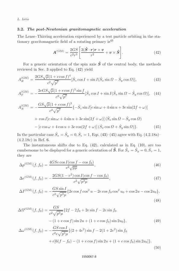
3.2. The post-Newtonian gravitomagnetic acceleration

The Lense–Thirring acceleration experienced by a test particle orbiting in the sta-tionary gravitomagnetic field of a rotating primary is43

A(GM) =2GS

c2r3

[3(S · r)r × v

r2+ v × S

]. (42)

For a generic orientation of the spin axis S of the central body, the methodsreviewed in Sec. 3 applied to Eq. (42) yield

A(GM)R =

2GS√

µ(1 + ecos f)4

c2√

p7[Sz cos I + sin I(Sx sinΩ − Sy cosΩ)], (43)

A(GM)T = −2eGS

õ(1 + ecos f)3 sin f

c2√

p7[Sz cos I + sin I(Sx sin Ω − Sy cosΩ)], (44)

A(GM)N = −GS

õ(1 + ecos f)3

c2√

p7−Sz sin I[e sin ω + 4 sinu + 3e sin(2f + ω)]

+ cos I[e sinω + 4 sinu + 3e sin(2f + ω)] (Sx sinΩ − Sy cosΩ)

− [e cosω + 4 cosu + 3e cos(2f + ω)] (Sx cosΩ + Sy sin Ω). (45)

In the particular case Sx = Sy = 0, Sz = 1, Eqs. (43)–(45) agree with Eq. (4.2.18a)–(4.2.18c) in Ref. 6.

The instantaneous shifts due to Eq. (42), calculated as in Eq. (10), are toocumbersome to be displayed for a generic orientation of S. For Sx = Sy = 0, Sz = 1,they are

∆p(GM)(f, f0) =4GSe cos I(cos f − cos f0)

c2√pµ, (46)

∆e(GM)(f, f0) = −2GS(1 − e2) cos I(cos f − cos f0)c2

√p3µ

, (47)

∆I(GM)(f, f0) = −GS sin I

c2√

p3µ2e cos f cos2 u − 2e cos f0 cos2 u0 + cos 2u − cos 2u0,

(48)

∆Ω(GM)(f, f0) =GS

c2√

p3µ2f − 2f0 + 2e sin f − 2e sin f0

− (1 + e cos f) sin 2u + (1 + e cos f0) sin 2u0, (49)

∆ω(GM)(f, f0) = − GS cos I

c2e√

p3µ(2 + 4e2) sin f − 2(1 + 2e2) sin f0

+ e[6(f − f0) − (1 + e cos f) sin 2u + (1 + e cos f0) sin 2u0].(50)

1550067-8

2nd Reading

June 16, 2015 15:49 WSPC/S0218-2718 142-IJMPD 1550067

Post-Newtonian orbital effects due to the oblateness of the central body

As a consequence, the gravitomagnetic shifts per orbit are

∆p(GM) = 0, (51)

∆e(GM) = 0, (52)

∆I(GM) = 0, (53)

∆Ω(GM) =4πGS

c2√

p3µ, (54)

∆ω(GM) = −12πGS cos I

c2√

p3µ. (55)

3.3. The Newtonian quadrupole acceleration

The acceleration due to the first even zonal harmonic coefficient J2 of the expansionin multipoles of the Newtonian component of the gravitational potential of thecentral body is

A(J2) =3J2µR2

2r4[5r(S · r)2 − 2S(S · r) − r]. (56)

According to Sec. 3, the radial, transverse and normal components of Eq. (56) foran arbitrary orientation of S are

A(J2)R =

3J2µR2(1 + e cos f)4

16p424Sz sin 2I(Sy cosΩ − Sx sin Ω) sin2 u

+ 6 cos 2I[−3S2z + (2S2

y + S2z − 1)cos 2Ω − 2SxSy sin 2Ω + 1] sin2 u

+ 24Sz sin I sin 2u(Sx cosΩ + Sy sin Ω)

+ 12 cos I sin 2u[2SxSy cos 2Ω + (2S2y + S2

z − 1)sin 2Ω]

− (1 + 3 cos 2u)[3S2z + 3(2S2

y + S2z − 1)cos 2Ω − 6SxSy sin 2Ω − 1],

(57)

A(J2)T = −3J2µR2(1 + e cos f)4

8p48Sz sin I cos 2u(Sx cosΩ + Sy sin Ω)

+ 4 cos I cos 2u[2SxSy cos 2Ω + (2S2y + S2

z − 1)sin 2Ω]

+ sin 2u[sin2 I(6S2z − 2) + (2S2

y + S2z − 1)(3 + cos 2I)cos 2Ω

+ 4Sz sin 2I(Sy cosΩ − Sx sinΩ) − 2SxSy(3 + cos 2I)sin 2Ω], (58)

A(J2)N = −3J2µR2(1 + e cos f)4

p4[Sz cos I + sin I(Sx sin Ω − Sy cosΩ)]

· [cosu(Sx cosΩ + Sy sin Ω) + sinu(Sz sin I + cos I(Sy cosΩ − Sx sin Ω))].

(59)

1550067-9

2nd Reading

June 16, 2015 15:49 WSPC/S0218-2718 142-IJMPD 1550067

L. Iorio

By using Eq. (10), the instantaneous shifts due to Eq. (56) can be obtained: Theyturn out to be too cumbersome to be displayed for an arbitrary orientation of S.For the particular case Sx = Sy = 0, Sz = 1, they are

∆p(J2)(f, f0) =J2R

2 sin2 I

2pe[3 cos(f + 2ω) + cos(3f + 2ω)− 3 cos(f0 + 2ω)

− cos(3f0 + 2ω)] − 6 sin(f − f0) sin(f + f0 + 2ω), (60)

∆e(J2)(f, f0) =J2R

2

16p2

(cos f − cos f0)(4(5 + 7e2 + 7 cos 2f + 7 cos 2f0)

+ cos f(8(7 + 5e2) cos f0 + 6e(13 + 6 cos 2f0 + e cos 3f0))

+ e(3e cos4f + 78 cos f0 + 6 cos 3f(3 + e cos f0)

+ 20e cos2f0 + cos 2f(6e cos 2f0 + 20e + 36 cos f0)

+ 18 cos3f0 + 3e cos 4f0)) cos 2ω sin2 I

−(

6(2 + 5e2) cos(

f + f0

2

)+ (28 + 17e2) cos

(3f + 3f0

2

)

+ 28(

cos(

5f + f0

2

)+ cos

(f + 5f0

2

))

+ e

(6(

10 cos(

3f + f0

2

)+ 3 cos

(7f + f0

2

)+ 10 cos

(f + 3f0

2

)

+ 3(

cos(

5f + 3f0

2

)+ cos

(3f + 5f0

2

)+ cos

(f + 7f0

2

)))

+ e

(3 cos

(5f + 5f0

2

)+ 17 cos

(5f + f0

2

)+ 3 cos

(9f + f0

2

)

+ 3 cos(

7f + 3f0

2

)+ 17 cos

(f + 5f0

2

)

+ 3(

cos(

3f + 7f0

2

)+ cos

(f + 9f0

2

)))))

· sin2 I sin 2ω sin(

f − f0

2

)+ (cos f − cos f0)(2(3 + e2)

+ e(6 cosf0 + 2 cos f(3 + e cos f0)

+ e(cos 2f + cos 2f0)))(1 + 3 cos 2I)

, (61)

∆I(J2)(f, f0) =J2R

2 sin 2I

8p2e[3 cos(f + 2ω) − 3 cos(f0 + 2ω) + cos(3f + 2ω)

− cos(3f0 + 2ω)] − 6 sin(f − f0) sin(f + f0 + 2ω), (62)

1550067-10

2nd Reading

June 16, 2015 15:49 WSPC/S0218-2718 142-IJMPD 1550067

Post-Newtonian orbital effects due to the oblateness of the central body

∆Ω(J2)(f, f0) =J2R

2 cos I

4p2−6f + 6f0 + 3 sin 2u − 3 sin 2u0 + e[−6 sin f + 6 sin f0

+ 3 sin(f + 2ω) − 3 sin(f0 + 2ω) + sin(3f + 2ω) − sin(3f0 + 2ω)],(63)

∆ω(J2)(f, f0) =J2R

2

64ep2120e(f − f0) cos 2I + 6(4 + 11e2) sin f + 8((−3 sin(f + 2ω)

+ 7 sin(3f + 2ω) + 3 sin(f0 + 2ω) − 7 sin(3f0 + 2ω)) sin2 I

+ 9e(f − f0) + 9 cos 2I(sin f − sin f0) − 3 sin f0) + e(12 sin 2f

+ 12(6 cos(2(f + f0 + ω)) sin(2f − 2f0) sin2 I + (6 cos(f + f0)

× cos 2I + 2(1 − 5 cos 2I) cos(f + f0 + 2ω)) sin(f − f0) − sin 2f0)

+ e(6(sin(f − 2ω) − sin(f0 − 2ω)) sin2 I + 2 sin 3f

− 66 sinf0 − 2 sin 3f0 + 51 sin(f + 2I) + 3 sin(3f + 2I)

− 51 sin(f0 + 2I) − 3 sin(3f0 + 2I) + 51 sin(f − 2I)

+ 3 sin(3f − 2I) − 51 sin(f0 − 2I) − 3 sin(3f0 − 2I)

− 6 cos f0 sin(4f0 + 2ω) − 3(1 + 15 cos 2I) sin(f + 2ω)

+ (3 − 19 cos 2I) sin(3f + 2ω) + 3(sin(5f + 2ω)

+ sin(f0 + 2ω)) + cos 2I(−3 sin(5f + 2ω)

+ 45 sin(f0 + 2ω) + 19 sin(3f0 + 2ω) + 3 sin(5f0 + 2ω)))). (64)

By evaluating Eqs. (60)–(64) for f = f0 + 2π, one obtains the following shiftsper orbit:

∆p(J2) = 0, (65)

∆e(J2) = 0, (66)

∆I(J2) = 0, (67)

∆Ω(J2) = −3πJ2R2 cos I

p2, (68)

∆ω(J2) =3πJ2R

2(3 + 5 cos 2I)4p2

. (69)

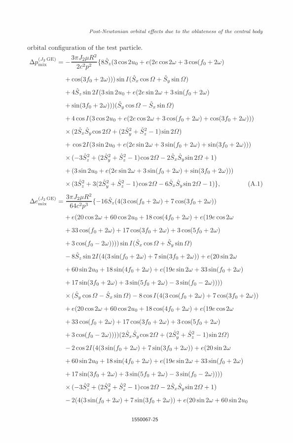
4. The Mixed Effects of Order J2c−2 and J2Sc−2

Here, the strategy outlined in Sec. 2 is applied to the perturbing accelerations ofSec. 3 to analytically calculate the mixed effects of order J2c

−2 and J2Sc−2 induced

1550067-11

2nd Reading

June 16, 2015 15:49 WSPC/S0218-2718 142-IJMPD 1550067

L. Iorio

by both the gravitoelectric and the gravitomagnetic post-Newtonian componentsof the gravitational field of the rotating primary.

4.1. The gravitoelectric effects

For the particular case Sx = Sy = 0, Sz = 1, a straightforward but tedious calcu-lation yields

∆p(J2 GE)mix = −6πJ2µR2 sin2 I

c2p2[3 sin 2u0 + 2e2 sin 2ω

+ 3e sin(f0 + 2ω) + e sin(3f0 + 2ω)], (70)

∆e(J2 GE)mix = −3πJ2µR2 sin2 I

8c2p3[12 sin(f0 + 2ω) + 28 sin(3f0 + 2ω)

− 3e2 sin(f0 − 2ω) + e(20 + 19e2) sin 2ω

+ 60e sin2u0 + 18e sin(4f0 + 2ω) + 33e2 sin(f0 + 2ω)

+ 17e2 sin(3f0 + 2ω) + 3e2 sin(5f0 + 2ω)], (71)

∆I(J2 GE)mix = −3πJ2µR2 sin 2I

2c2p3[3 sin 2u0 + 2e2 sin 2ω

+ 3e sin(f0 + 2ω) + e sin(3f0 + 2ω)], (72)

∆Ω(J2 GE)mix =

3πJ2µR2 cos I

c2p3[3 cos 2u0 − 5e2 + 16e cosf0 + 2e2 cos 2ω

+ 3e cos(f0 + 2ω) + e cos(3f0 + 2ω)], (73)

∆ω(J2 GE)mix =

3πJ2µR2

32c2ep3e(2(91e2 + 132) cos 2I

− e cos 2ω(68e− 4e + 48 cos 2I(cos 2f0 + 3) cos3 f0

− 36 cosf0 − 22 cos 3f0 − 6 cos 5f0)

+ 2e sin 2ω sin f0(6 cos 2I(cos 4f0 + 17)

+ 4(15 cos2I − 7) cos 2f0 − 6 cos 4f0 − 38)

− 320e cos(f0 + 2I) + 24(3 − 7 cos 2I) cos 2u0

+ 8 sin2 I(9 cos(4f0 + 2ω) − 10 cos 2ω))

+ 2(e(57e2 + 44) + 8 sin2 I(7 cos(3f0 + 2ω)

− 3 cos(f0 + 2ω))) − 320e2 cos(f0 − 2I) − 384e2 cos f0. (74)

No a priori simplifying assumptions on either e or I were assumed. The formulasvalid for an arbitrary orientation of S are quite cumbersome: They are explicitlydisplayed in Appendix A.

1550067-12

2nd Reading

June 16, 2015 15:49 WSPC/S0218-2718 142-IJMPD 1550067

Post-Newtonian orbital effects due to the oblateness of the central body

The total gravitoelectric shifts per orbit of order J2c−2 can be obtained by

adding the indirect, mixed effects of Eqs. (70)–(74) to the direct variations inducedby the post-Newtonian acceleration induced by the oblateness of the centralbody5,6,10,11:

A(J2 GE) =3J2µR2

2c2r4[5r(S · r)2 − 2S(S · r) − r]

(v2 − 4µ

r

)

− 6J2µR2

c2r4[5(r · v)(S · r)2 − 2(S · v)(S · r) − (r · v)]v

− 2J2µ2R2

c2r5[3(S · r)2 − 1]r. (75)

By using Eq. (75) into Eq. (10), evaluated for Sx = Sy = 0, Sz = 1, one obtainsthe direct shifts per orbit:

∆p(J2 GE)dir =

3πJ2µR2e2 sin2 I sin 2ω

c2p2, (76)

∆e(J2 GE)dir =

21πJ2µR2e(2 + e2) sin2 I sin 2ω

8c2p3, (77)

∆I(J2 GE)dir =

3πJ2µR2e2 sin 2I sin 2ω

4c2p3, (78)

∆Ω(J2 GE)dir =

3πJ2µR2 cos I(6 − e2 cos 2ω)2c2p3

, (79)

∆ω(J2 GE)dir =

3πJ2µR2

16c2p3−32 + 3e2 + 2(7 + 2e2) cos 2ω

+ cos 2I[−48 + 9e2 + 2(−7 + 2e2) cos 2ω]. (80)

The general expressions, valid for an arbitrary orientation of S, are displayed inAppendix B.

As a result, the total shifts per orbit turn out to be

∆p(J2 GE)tot =

3πJ2µR2 sin2 I

c2p26 sin2u0 + e[5e sin 2ω + 6 sin(f0 + 2ω)

+ 2 sin(3f0 + 2ω)], (81)

∆e(J2 GE)tot = −3πJ2µR2 sin2 I

8c2p312 sin(f0 + 2ω) + 28 sin(3f0 + 2ω)

+ e[−3e sin(f0 − 2ω) + 6(1 + 2e2) sin 2ω + 60 sin 2u0

+ 18 sin(4f0 + 2ω) + 33e sin(f0 + 2ω) + 17e sin(3f0 + 2ω)

+ 3e sin(5f0 + 2ω)], (82)

1550067-13

2nd Reading

June 16, 2015 15:49 WSPC/S0218-2718 142-IJMPD 1550067

L. Iorio

∆I(J2 GE)tot = −3πJ2µR2 sin 2I

4c2p36 sin2u0 + e[3e sin 2ω + 6 sin(f0 + 2ω)

+ 2 sin(3f0 + 2ω)], (83)

∆Ω(J2 GE)tot =

3πJ2µR2 cos I

2c2p36 − 10e2 + 6 cos 2u0 + e[32 cosf0

+ 3e cos 2ω + 6 cos(f0 + 2ω) + 2 cos(3f0 + 2ω)], (84)

∆ω(J2 GE)tot =

3πJ2µR2

32c2p34[6 + 30e2 + 42 cos2I + 7 cos 2ω + 18 cos 2u0]

+1e(4e2 sin f0(−6 sin2 I cos 4f0 + 51 cos 2I + 2(15 cos 2I − 7)

× cos 2f0 − 19) sin 2ω − 2e(24e(3 + cos 2f0) cos 2I cos 2ω cos3 f0

+ 2e(96 + 160 cos 2I − 9 cos 2ω) cos f0

− e(6e + 11 cos 3f0 + 3 cos 5f0) cos 2ω

+ 2 cos 2I(−50e2 + (15e2 + 7) cos 2ω + 42 cos2u0))

+ 8 sin2 I(−10e cos2ω + 9e cos(4f0 + 2ω)

− 6 cos(f0 + 2ω) + 14 cos(3f0 + 2ω))). (85)

Our results can be compared with those released ind Ref. 5 for p, e, I in the caseSx = Sy = 0, Sz = 1. It turns out that Eqs. (81) and (83) agree with Eqs. (2.12a)and (2.12c) of Ref. 5, respectively, and Eq. (82) agrees with the corrected form ofEq. (2.12b) in Ref. 44. No results for Ω, ω were released in Ref. 5.

From Eqs. (81)–(83) it turns out that the variations of p, e, I are not seculartrends because of the occurrence of the slowly varying ω as argument of the trigono-metrical functions entering them. Indeed, to first-order, the argument of pericenterundergoes secular precession whose dominant contribution is due to either the pri-mary’s quadrupole (Eq. (69)) or the post-Newtonian Schwarzschild-like gravitoelec-tric field (Eq. (41)), depending on the specific astronomical system considered. Assuch, the shifts of p, e, I average out over one full cycle of ω. When the Newtonianmultipolar precessions are dominant with respect to the post-Newtonian ones, it ispossible to have semisecular trends for p, e, I by adopting some critical inclinationscenarios45,46 yielding the so-called frozen-perigee configuration in which the clas-sical pericenter precession vanishes. See the scenario proposed in Sec. 6.2. This isnot the case for Ω and ω itself which, according to Eqs. (84) and (85), experiencesecular trends because of terms not containing explicitly ω. The same hold for thegravitomagnetic mixed effects calculated in Sec. 4.2.

dThe quadrupole mass moment Q2 in Ref. 5 has dimensions [Q2] = ML2: For a direct comparisonswith our results, the replacement Q2 → −J2MR2 in Eqs. (2.12a)–(2.12c) of Ref. 5 must be made.

1550067-14

2nd Reading

June 16, 2015 15:49 WSPC/S0218-2718 142-IJMPD 1550067

Post-Newtonian orbital effects due to the oblateness of the central body

4.2. The gravitomagnetic effects

The inclusion of Eqs. (42) and (56) in the disturbing acceleration entering Eq. (9)yields novel post-Newtonian mixed effects proportional to J2Sc−2. The resultingshifts per orbit for Sx = Sy = 0, Sz = 1 are

∆p(J2 GM)mix =

3πGSJ2R2 cos I sin2 I

c2√

p5µ12 sin 2u0 + e(4(3 sin(f0 + 2ω)

+ sin(3f0 + 2ω)) − e sin 2ω), (86)

∆e(J2 GM)mix =

3πGSJ2R2 cos I sin2 I

4c2√

p7µ12 sin(f0 + 2ω) + 28 sin(3f0 + 2ω)

+ e[−2(e2 − 10) sin 2ω + 60 sin 2u0 + 33e sin(f0 + 2ω)

+ 17e sin(3f0 + 2ω) + 18 sin(4f0 + 2ω)

+ 3e sin(5f0 + 2ω) − 3e sin(f0 − 2ω)], (87)

∆I(J2 GM)mix =

3πGSJ2R2 sin I

4c2√

p7µ2(2 cos f0(9 + 11 cos 2I) + e(13 cos 2I

+ cos 2f0(7 + 9 cos 2I) + 11)) cos 2ω sin f0

+ (2 cos 2f0(9 + 11 cos 2I) + e cos f0(15 + 17 cos 2I)

+ e(cos 3f0(7 + 9 cos 2I) − 2e cos2 I)) sin 2ω, (88)

∆Ω(J2 GM)mix =

3πGSJ2R2

8c2√

p7µ2(2 + e2 − 2e cos f0)(7 + 9 cos 2I)

+ [e2 − 8e(2 cosf0 + cos 3f0) − 20 cos 2f0](1 + 3 cos 2I) cos 2ω

+ 8[5 cosf0 + e(3 + 2 cos 2f0)](1 + 3 cos 2I) sin f0 sin 2ω, (89)

∆ω(J2 GM)mix = −3πGSJ2R

2 cos I

16c2e√

p7µ−56e2 cos f0 − 100e2 cos(f0 − 2I)

+ e(8(9 cos(4f0 + 2ω)− 10 cos 2ω) sin2 I + 4(64 + 21e2) cos 2I

− e cos(f0 + 2I) + 8(17 − 37 cos 2I) cos 2u0 − 2e cos 2ω

× (−6 sin2 I cos 5f0 + 3e − 46 cos f0 − 23 cos 3f0 − 7e cos 2I

+ 55(2 cosf0 + cos 3f0) cos 2I) + 2e(−6(13 + cos 4f0)

+ 6(29 + cos 4f0) cos 2I + 4 cos 2f0(29 cos 2I − 13)) sin f0 sin 2ω)

+ 4(4(7 cos(3f0 + 2ω) − 3 cos(f0 + 2ω)) sin2 I + e(40 + 11e2)).(90)

We do not shown the full expressions for a general S: They are far too cumbersome.

1550067-15

2nd Reading

June 16, 2015 15:49 WSPC/S0218-2718 142-IJMPD 1550067

L. Iorio

5. The Newtonian Effects of Order J22

The general formalism of Sec. 2 allows us to work out also the Newtonian shiftsper orbit quadratic in the oblateness of the primary. In certain scenarios of interest,they can become competitors not only of the mixed variations previously workedout but also of some of the most renowned direct orbital effects.

In the special case Sx = Sy = 0, Sz = 1, they turn out to be

∆p(J22 ) =

3πJ22R4 sin2 I

16p3[−16e(3 + 5 cos 2I) cos3 f0

− 12 cos 2f0(3 + 5 cos 2I) + e2(13 + 15 cos2I)] sin 2ω

− 8[3 cos f0 + e(2 + cos 2f0)](3 + 5 cos 2I) cos 2ω sin f0, (91)

∆e(J22 ) =

3πJ22R4 sin2 I

128p4−4[3e2 cos 4f0 + 25e2 + 78e cos f0

+ 18e cos3f0 + 4(7 + 5e2) cos 2f0 + 20](3 + 5 cos 2I) cos 2ω sin f0

− 2(−26e3 + 9e2 cos 5f0 + 54e cos4f0

+ 60e cos2f0(3 + 5 cos 2I)

+ 80e + 3(28 + 17e2) cos 3f0 + 5((28 + 17e2) cos 3f0

+ 3e(−2e2 + e cos 5f0 + 6 cos 4f0 + 8)) cos 2I

+ 12(1 + 3e2) cos f0(3 + 5 cos 2I)) sin 2ω, (92)

∆I(J22 ) =

3πJ22R4 sin 2I

64p4[−16e(3 + 5 cos 2I) cos3 f0

− 12(3 + 5 cos 2I) cos 2f0 + e2(13 + 15 cos2I)] sin 2ω

− 8[3 cos f0 + e(2 + cos 2f0)](3 + 5 cos 2I) cos 2ω sin f0, (93)

∆Ω(J22 ) = −3πJ2

2R4 cos I

32p4−2e2 cos 2ω + 13e2

+ 8e[3 cos(f0 + 2ω) + cos(3f0 + 2ω)] + 24 cos 2u0

− 5 cos 2I(−6e2 cos 2ω + e2 + 8e(3 cos(f0 + 2ω)

+ cos(3f0 + 2ω)) + 24 cos 2u0 − 8) + 32, (94)

∆ω(J22 ) =

3πJ22R4

512ep413e(82 + 13e2) − 24 cos(f0 + 2ω) + 56 cos(3f0 + 2ω)

+ 5 cos 4I(−9e3 + 6e2 cos(f0 − 2ω) + 6e(8 + 9e2) cos 2ω

− 2e(132 cos2u0 + 117e cos(f0 + 2ω) + 43e cos(3f0 + 2ω)

+ 18 cos(4f0 + 2ω)) + 86e + 24 cos(f0 + 2ω) − 56 cos(3f0 + 2ω))

1550067-16

2nd Reading

June 16, 2015 15:49 WSPC/S0218-2718 142-IJMPD 1550067

Post-Newtonian orbital effects due to the oblateness of the central body

+ 4 cos 2I(81e3 + 2e(15e sin2 I cos(5f0 + 2ω)

+ (23e2 − 20) cos 2ω − 12 cos 2u0 − 27e cos(f0 + 2ω)

− 5e cos(3f0 + 2ω) + 18 cos(4f0 + 2ω) − 3e cos(f0 − 2ω))

+ 394e− 24 cos(f0 + 2ω) + 56 cos(3f0 + 2ω))

− 2e(40 cos2ω + 60 cos2u0 − 18 cos(4f0 + 2ω)

+ 3e(−12 sin2 I cos(5f0 + 2ω) + e cos 2ω + 25 cos(f0 + 2ω)

+ 7 cos(3f0 + 2ω) + cos(f0 − 2ω))). (95)

The formulas for an arbitrary spatial orientation of S are too cumbersome to beexplicitly displayed.

Also in this case, p, e, I experience long-period harmonic variations because ofthe trigonometric functions in Eqs. (91)–(93) having ω as argument. Instead, Ω

and ω undergo secular variations since in Eqs. (94) and (95) there are terms notcontaining explicitly ω.

6. Phenomenological Aspects of the Mixed Orbital Effects

In this section, we numerically evaluate the relative strengths of the direct and indi-rect shifts calculated in Secs. 3–5 in some astronomical and astrophysical scenariosof interest.

6.1. Compact objects

Let us start from a test particle orbiting a central compact object like, say, aBH22,33,34 or a neutron star.47–50 The BH’s angular momentum is51

S = χgM2G

c, (96)

with51

χg ≤ 1. (97)

Recent measurements of the spin parameter of several BHs with a variety of tech-niques52–58 not implying the use of particle’s orbital dynamics confirm the bound ofEq. (97). The existence of a maximum value for the angular momentum of a rotat-ing BH is due to the fact that the Kerr metric is endowed with horizons.59,60 Avalue of the spin parameter larger than unity would imply the existence of a nakedsingularity;51 closed timelike curves could be considered, implying a causality vio-lation.61 The formation of naked singularities in gravitational collapse is prohibitedby the cosmic censorship conjecture,62 although it has not yet been demonstrated.For other rotating astrophysical objects there is no such a limit as of Eq. (97). Inparticular, for main-sequence stars, χg can be much larger than unity being strongly

1550067-17

2nd Reading

June 16, 2015 15:49 WSPC/S0218-2718 142-IJMPD 1550067

L. Iorio

dependent on the stellar mass.63–66 As far as compact stars are concerned, in Ref. 67it was shown that for neutron stars with M 1 M it should be χg 0.7, inde-pendently of the equation-of-state (EOS) governing the stellar matter. Even lowervalues are usually admitted.68 The angular momentum of hypothetical quark starsstrongly depends on the EOS and the stellar mass itself in such a way that theymay have χg > 1.67

As far as a BH quadrupole mass moment is concerned, as a consequence of the“no-hair” or uniqueness theorems,69,70 all the multipole moments of the externalspacetime are functions of M and S.71,72 In particular, the quadrupole moment ofthe BH is

Q2 =S2

c2M. (98)

In the case of spinning neutron stars, they acquire a nonzero quadrupolemoment73–76

Q2 = −qM3G2

c4, (99)

where q ranges from 1 to 11 for a variety of EOSs.By suitably expressing the semilatus rectum as

p = nRs(1 + e), n 3, (100)

where the minimum distance of an orbiting star from the BH was written as amultiple of the BH’s Schwarzschild radius, from Eqs. (96) and (98) it is possible toobtain ∣∣∣∣ ∆p(J2 GE)

∆p(J2 GM)

∣∣∣∣ =sec I

χg

√n2

+ O(e), (101)

∣∣∣∣∆p(J2 GE)

∆p(J22 )

∣∣∣∣ =16n

χ2g(3 + 5 cos 2I)

+ O(e), (102)

∣∣∣∣∆p(J2 GM)

∆p(J22 )

∣∣∣∣ =16 cos I

√2n

χg(3 + 5 cos 2I)+ O(e), (103)

∣∣∣∣ ∆e(J2 GE)

∆e(J2 GM)

∣∣∣∣ =sec I

χg

√n2

+ O(e), (104)

∣∣∣∣∆e(J2 GE)

∆e(J22 )

∣∣∣∣ =16n

χ2g(3 + 5 cos 2I)

+ O(e), (105)

∣∣∣∣∆e(J2 GM)

∆e(J22 )

∣∣∣∣ =16 cos I

√2n

χg(3 + 5 cos 2I)+ O(e), (106)

∣∣∣∣ ∆I(J2 GE)

∆I(J2 GM)

∣∣∣∣ =6 cos I

√2n

χg(9 + 11 cos2I)+ O(e), (107)

1550067-18

2nd Reading

June 16, 2015 15:49 WSPC/S0218-2718 142-IJMPD 1550067

Post-Newtonian orbital effects due to the oblateness of the central body

∣∣∣∣∆I(J2 GE)

∆I(J22 )

∣∣∣∣ =16n

χ2g(3 + 5 cos 2I)

+ O(e), (108)

∣∣∣∣∆I(J2 GM)

∆I(J22 )

∣∣∣∣ =4 sec I(9 + 11 cos 2I)

√2n

3χg(3 + 5 cos 2I)+ O(e). (109)

It must be recalled that p, e, I do note experience first-order, direct shifts per orbit,apart from those due to Eq. (75) which were included in the overall gravitoelectricJ2c

−2 effects. From Eqs. (101)–(109) it can be noticed that the following hierarchyexists: J2

2 < (J2 GM) < (J2 GE). For close orbits, the discrepancy among the grav-itomagnetic and the gravitoelectric inclination shifts tend to reduce, as shown byEq. (107).

In the case of the node Ω, also the direct Newtonian (Eq. (68)) and post-Newtonian gravitomagnetic (Eq. (54)) shifts are to be taken into account. Thus,one has∣∣∣∣∆Ω(GM)

∆Ω(J2)

∣∣∣∣ =4 sec I

√2n

3χg+ O(e), (110)

∣∣∣∣ ∆Ω(GM)

∆Ω(J2 GE)

∣∣∣∣ =4 sec I sec2(f0 + ω)

√2n3

9χg+ O(e), (111)

∣∣∣∣ ∆Ω(GM)

∆Ω(J2 GM)

∣∣∣∣ =32n2

3χ2g[7 + 9 cos 2I − 5(1 + 3 cos 2I) cos 2u0]

+ O(e), (112)

∣∣∣∣∆Ω(GM)

∆Ω(J22 )

∣∣∣∣ =64 sec I

√2n5

3χ3g[−4 − 5 cos 2I + 3(−1 + 5 cos 2I) cos 2u0]

+ O(e), (113)

∣∣∣∣ ∆Ω(J2)

∆Ω(J2 GE)

∣∣∣∣ =sec2(f0 + ω)n

3+ O(e), (114)

∣∣∣∣ ∆Ω(J2)

∆Ω(J2 GM)

∣∣∣∣ =4 cos I

√2n3

χg[7 + 9 cos 2I − 5(1 + 3 cos 2I) cos 2u0]+ O(e), (115)

∣∣∣∣∆Ω(J2)

∆Ω(J22 )

∣∣∣∣ =16n2

χ2g[−4 − 5 cos 2I + 3(−1 + 5 cos 2I) cos 2u0]

+ O(e), (116)

∣∣∣∣ ∆Ω(J2 GE)

∆Ω(J2 GM)

∣∣∣∣ =12 cos I cos2(f0 + ω)

√2n

χg[7 + 9 cos 2I − 5(1 + 3 cos 2I) cos 2u0]+ O(e), (117)

∣∣∣∣∆Ω(J2 GE)

∆Ω(J22 )

∣∣∣∣ =48 cos2(f0 + ω)n

χ2g[−4 − 5 cos 2I + 3(−1 + 5 cos 2I) cos 2u0]

+ O(e), (118)

∣∣∣∣∆Ω(J2 GM)

∆Ω(J22 )

∣∣∣∣ =2 sec I[7 + 9 cos 2I − 5(1 + 3 cos 2I) cos 2u0]

√2n

χg[−4 − 5 cos 2I + 3(−1 + 5 cos 2I) cos 2u0]+ O(e). (119)

eActually, this is not true for an arbitrary orientation of the primary’s spin axis.77

1550067-19

2nd Reading

June 16, 2015 15:49 WSPC/S0218-2718 142-IJMPD 1550067

L. Iorio

In the case of the pericenter, in addition to the same direct effects as for the node,there is also the direct, gravitoelectric shift of Eq. (41) to be taken into account.As a result, one has∣∣∣∣∆ω(GE)

∆ω(J2)

∣∣∣∣ =8n

χ2g(−4 + 5 sin2 I)

+ O(e), (120)

∣∣∣∣ ∆ω(GE)

∆ω(GM)

∣∣∣∣ =sec I

χg

√n2

+ O(e), (121)

∣∣∣∣ ∆ω(GE)

∆ω(J2 GE)

∣∣∣∣ =16en2 csc2 I

χ2g[7 cos(3f0 + 2ω)− 3 cos(f0 + 2ω)]

+ O(e2), (122)

∣∣∣∣ ∆ω(GE)

∆ω(J2 GM)

∣∣∣∣ =8e csc2 I sec I

√2n5

χ3g[7 cos(3f0 + 2ω)− 3 cos(f0 + 2ω)]

+ O(e2), (123)

∣∣∣∣∆ω(GE)

∆ω(J22 )

∣∣∣∣ =256en3 csc2 I

χ4g(3 + 5 cos 2I)[7 cos(3f0 + 2ω) − 3 cos(f0 + 2ω)]

+ O(e2), (124)

∣∣∣∣∆ω(GM)

∆ω(J2)

∣∣∣∣ =16 cos I

√2n

χg(3 + 5 cos 2I)+ O(e), (125)

∣∣∣∣ ∆ω(GM)

∆ω(J2 GE)

∣∣∣∣ =16e cot I csc I

√2n3

χg[−3 cos(f0 + 2ω) + 7 cos(3f0 + 2ω)]+ O(e2), (126)

∣∣∣∣ ∆ω(GM)

∆ω(J2 GM)

∣∣∣∣ =16en2 csc2 I

χ2g[−3 cos(f0 + 2ω) + 7 cos(3f0 + 2ω)]

+ O(e2), (127)

∣∣∣∣∆ω(GM)

∆ω(J22 )

∣∣∣∣ =256e cot I csc I

√2n5

χ3g(3 + 5 cos 2I)[3 cos(f0 + 2ω) − 7 cos(3f0 + 2ω)]

+ O(e2), (128)

∣∣∣∣ ∆ω(J2)

∆ω(J2 GE)

∣∣∣∣ =2e(−5 + 4 csc2 I)n

−7 cos(3f0 + 2ω) + 3 cos(f0 + 2ω)+ O(e2), (129)

∣∣∣∣ ∆ω(J2)

∆ω(J2 GM)

∣∣∣∣ =e(3 + 5 cos 2I) csc2 I sec I

√n3

χg

√2[−7 cos(3f0 + 2ω) + 3 cos(f0 + 2ω)]

+ O(e2), (130)

∣∣∣∣∆ω(J2)

∆ω(J22 )

∣∣∣∣ =16en2 csc2 I

χ2g[−7 cos(3f0 + 2ω) + 3 cos(f0 + 2ω)]

+ O(e2), (131)

∣∣∣∣ ∆ω(J2 GE)

∆ω(J2 GM)

∣∣∣∣ =sec I

χg

√n2

+ O(e), (132)

∣∣∣∣∆ω(J2 GE)

∆ω(J22 )

∣∣∣∣ =16n

χ2g(3 + 5 cos 2I)

+ O(e), (133)

∣∣∣∣∆ω(J2 GM)

∆ω(J22 )

∣∣∣∣ =16 cos I

√2n

χg(3 + 5 cos 2I)+ O(e). (134)

1550067-20

2nd Reading

June 16, 2015 15:49 WSPC/S0218-2718 142-IJMPD 1550067

Post-Newtonian orbital effects due to the oblateness of the central body

It must remarked that the previous expressions hold in coordinate system whosereference x, y plane coincides with the equatorial plane of the central body. Ingeneral, this is not true for BHs because the current uncertainties in the spatialorientation of their spin axes.78–80 In hypothetical binary systems made of a BHorbited by a radiopulsar (PSR-BH),81 useful information on the magnitude andorientation of the BH’s spin can be derived, in principle, from the binary’s orbitalprecession.82 As such, an accurate sensitivity analysis or error budget for somerealistic scenarios require to use the fully general expressions, not displayed herebecause of their cumbersomeness. In the case of the Solar System, the equatorialplane of the Sun does not coincide with, say, the ecliptic plane; for a transition fromone to another see, e.g. Refs. 12 and 42.

6.2. Planet–spacecraft scenarios

In this section, we will consider some spacecraft-based scenarios in which the pri-mary is a planet of our Solar System.

In Table 1, we look at Jupiter and the Juno mission,20 which seems promising fortesting some aspects of post-Newtonian gravity.9,83–85 We numerically maximizedthe various shifts per orbit viewed as functions of f0, ω. It can be noticed that thenominal values of the Newtonian shifts of order O(J2

2 ) are far not negligible: Theymust be carefully accounted for in accurate error budgets when their mismodelinghas to be evaluated. The mixed post-Newtonian effects proportional to J2Sc−2 arequite small, being at the level of about 90µm per orbit as far as the semilatusrectum is concerned; the angular orbital elements are shifted by far less than onemilliarcsecond (mas). The impact of the shifts of order O(J2c

−2) is at the level ofabout 70 cm per orbit (p), and of about 1mas or less for the other elements.

Table 2 shows the results for the recently launched terrestrial geodetic satelliteLARES.21,86 The post-Newtonian quadrupolar shifts of p are at the 1–100µm levelper orbit, while the angular shifts are below the mas level per orbit. Also in thiscase, the nominal shifts of the effects of order O(J2

2 ) are not negligible, althoughthe Earth’s oblateness is currently known with a high level of accuracy.

Table 1. Maximum nominal values for the direct and mixed shifts per orbit of theJupiter–Juno system as functions of f0, ω. The relevant physical parameters for the giantplanet are µ = 1.267×1017 m3 ·s−2, R = 71, 492 km, S = 6.9×1038 kg·m2 ·s−1, J2 = 0.014,while for Juno we adopted a = 20.03R, Pb = 11d, e = 0.947, I = 90.05. The figuresquoted hold in a planetary equatorial coordinate system.

p (m) e (mas) I (mas) Ω (mas) ω (mas)

GE — — — — 37.095GM — — — 2.07 0.005J2 — — — 5835.93 3 × 106

J2c−2 0.74 1.4 0.0004 0.0012 1.37

J2Sc−2 0.000087 0.0002 0.010 0.058 0.00027

J22 54,088.8 130,360 32.94 191.517 144,885

1550067-21

2nd Reading

June 16, 2015 15:49 WSPC/S0218-2718 142-IJMPD 1550067

L. Iorio

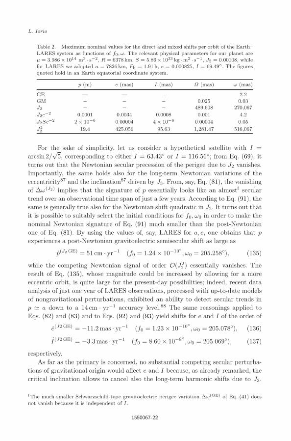
Table 2. Maximum nominal values for the direct and mixed shifts per orbit of the Earth–

LARES system as functions of f0, ω. The relevant physical parameters for our planet areµ = 3.986× 1014 m3 · s−2, R = 6378 km, S = 5.86× 1033 kg ·m2 · s−1, J2 = 0.00108, whilefor LARES we adopted a = 7826 km, Pb = 1.91 h, e = 0.000825, I = 69.49. The figuresquoted hold in an Earth equatorial coordinate system.

p (m) e (mas) I (mas) Ω (mas) ω (mas)

GE — — − − 2.2GM − − − 0.025 0.03J2 − − − 489,608 270,067

J2c−2 0.0001 0.0034 0.0008 0.001 4.2

J2Sc−2 2 × 10−6 0.00004 4 × 10−6 0.00004 0.05

J22 19.4 425.056 95.63 1,281.47 516,067

For the sake of simplicity, let us consider a hypothetical satellite with I =arcsin 2/

√5, corresponding to either I = 63.43 or I = 116.56; from Eq. (69), it

turns out that the Newtonian secular precession of the perigee due to J2 vanishes.Importantly, the same holds also for the long-term Newtonian variations of theeccentricity87 and the inclination87 driven by J3. From, say, Eq. (81), the vanishingof ∆ω(J2) implies that the signature of p essentially looks like an almostf seculartrend over an observational time span of just a few years. According to Eq. (91), thesame is generally true also for the Newtonian shift quadratic in J2. It turns out thatit is possible to suitably select the initial conditions for f0, ω0 in order to make thenominal Newtonian signature of Eq. (91) much smaller than the post-Newtonianone of Eq. (81). By using the values of, say, LARES for a, e, one obtains that p

experiences a post-Newtonian gravitoelectric semisecular shift as large as

p(J2 GE) = 51 cm · yr−1 (f0 = 1.24 × 10−10, ω0 = 205.258), (135)

while the competing Newtonian signal of order O(J22 ) essentially vanishes. The

result of Eq. (135), whose magnitude could be increased by allowing for a moreeccentric orbit, is quite large for the present-day possibilities; indeed, recent dataanalysis of just one year of LARES observations, processed with up-to-date modelsof nongravitational perturbations, exhibited an ability to detect secular trends inp a down to a 14 cm · yr−1 accuracy level.88 The same reasonings applied toEqs. (82) and (83) and to Eqs. (92) and (93) yield shifts for e and I of the order of

e(J2GE) = −11.2 mas · yr−1 (f0 = 1.23 × 10−10, ω0 = 205.078), (136)

I(J2GE) = −3.3 mas · yr−1 (f0 = 8.60 × 10−8, ω0 = 205.069), (137)

respectively.As far as the primary is concerned, no substantial competing secular perturba-

tions of gravitational origin would affect e and I because, as already remarked, thecritical inclination allows to cancel also the long-term harmonic shifts due to J3.

fThe much smaller Schwarzschild-type gravitoelectric perigee variation ∆ω(GE) of Eq. (41) doesnot vanish because it is independent of I.

1550067-22

2nd Reading

June 16, 2015 15:49 WSPC/S0218-2718 142-IJMPD 1550067

Post-Newtonian orbital effects due to the oblateness of the central body

In principle, gravitational perturbations on e, I, Ω, ω arise due to the action of athird body X like, for example, the Moon and the Sun.89 Their nominal magnitudeis proportional to P−2

X Pb = µXa−3X Pb. For, say, X = Moon and a LARES-type

orbit, they are of the order of 103 mas ·yr−1. However, since they are fully modeled,only their uncertainty, determined by the accuracy on µX, does matter. In the caseof the Moon and the Sun, the relative accuracies in their gravitational parameters µ

are several orders of magnitude better thang 10−3, so that their disturbances wouldbe negligible. By assuming the same physical properties of LARES, the impact ofthe main nongravitational perturbations91 able to induce secular rates on e and I

would be negligible. Indeed, according to Ref. 92, the nominal rates due to the atmo-spheric drag and the Rubincam effect would be as little as about 0.5 mas · yr−1.From Eq. (6.8) of Ref. 91, under the same assumptions as in Ref. 92, a seculardecrease of the eccentricity due to the atmospheric drag as little as 0.01mas · yr−1

can be inferred.Regarding the aforementioned Earth–satellite scenarios: In principle, a potential

source of systematic bias may be represented by the orbital perturbations inducedby the equinoctial precession.93 However, it must be recalled that laser data reduc-tions are usually performed in a coordinate system whose reference x, y plane isaligned with the mean Earth’s equator at the reference epoch J2000.0.

7. Summary and Conclusion

A first-order perturbative approach to particle dynamics in the post-Newtonian fieldof a rotating oblate primary is not adequate to capture the full richness of the actualorbital motion due to the simultaneous contributions of several disturbing classicaland relativistic accelerations (J2, Schwarzschild, Lense–Thirring, etc.). Indeed, thevery same fact that more than one enter the equations of motion induces certainindirect, mixed orbital perturbations due to a mutual cross-interaction in additionto second-order effects for each of them.

A consistent formalism able to reproduce such additional features of motion,which are not directly due to some new accelerations occurring in the equationsof motion, is a second-order perturbative approach which we consistently outlinedand applied to some known post-Keplerian accelerations of both Newtonian andpost-Newtonian origin.

In particular, we considered the Newtonian acceleration induced by the oblate-ness J2 of the central body, and the post-Newtonian gravitoelectromagnetic accel-erations of order O(c−2) which, to first-order, yield the well-known Einstein andLense–Thirring orbital precessions. We analytically calculated the indirect shiftsper orbit of all the standard Keplerian orbital elements proportional to J2c

−2 andJ2Sc−2. Our general approach is valid for an arbitrary orientation of the primary’sspin axis S. We also considered the Newtonian second-order effects in J2. As far as

gThey amount to90 10−11 for the Sun and 10−10 for the Moon, respectively.

1550067-23

2nd Reading

June 16, 2015 15:49 WSPC/S0218-2718 142-IJMPD 1550067

L. Iorio

the indirect gravitoelectric effects of order O(J2c−2) are concerned, they were added

to the direct ones caused by the specific post-Newtonian acceleration proportionalto J2c

−2 entering the equations of motion.It turned out that the semilatus rectum p, the eccentricity e and the inclination

I experience nonvanishing indirect shifts which are harmonic in the argument ofpericenter ω entering their expressions as argument of trigonometric functions. Thepericenter does not generally stay constant because of the direct perturbations oforder O(J2) and O(c−2) that make it precess slowly. Instead, the node Ω and thepericenter itself undergo also indirect secular precessions because of some terms notcontaining explicitly ω. Our formulas, which are valid for a generic orbital geometryof the test particle, represent the limit to which full two-body formulas will haveto reduce in the point particle limit.

Such indirect, mixed effects may play a role in realistic error budgets of accuratetests of post-Newtonian gravity and in the long-term evolutionary history of variousastrophysical systems of interest. In principle, it is possible to design a dedicatedsatellite-based mission aimed to detect the effects of order O(J2c

−2) by looking atp, e, I. Indeed, in the Earth scenario, the dominant perigee precession is due to theNewtonian multipoles of the expansion of the terrestrial gravitational potential.Thus, a suitable orbital configuration, based on the concepts of critical inclinationand frozen-perigee, may be adopted to suppress the largest part of the perigeeprecession as well as the long-term harmonic variations of the eccentricity andthe inclination. In such a way, the shifts of order O(J2c

−2) in p, e, I would looklike almost secular trends over typical observational time spans some years longbecause of the very slow Schwarzschild-like gravitoelectric perigee advance. As anexample, a hypothetical terrestrial satellite orbiting at an altitude of h = 1450kmin an almost circular orbit inclined to the Earth’s equator by an amount equal tothe critical inclination able to suppress the Newtonian secular perigee precessiondue to J2 as well as the long-term harmonic variations of the eccentricity and theinclination due to J3, would experience an almost secular rate in p as large as51 cm · yr−1. Recent data analysis of the existing geodetic satellite LARES showedan accuracy in determining secular trends in the semimajor axis a p of the orderof 14 cm ·yr−1 over just one year. The eccentricity and the inclination would changeat a rate of the order of −11 mas ·yr−1 and −3 mas ·yr−1, respectively. The nominalmagnitude of the competing rates due to the atmospheric drag are much smaller.

Appendix A. Mixed Orbital Shifts of Order J2c−2 for a GenericOrientation of the Spin Axis of the Primary

Here, the general expressions for the post-Newtonian gravitoelectric mixed orbitalshifts arising from Eqs. (28) and (56) are displayed for an arbitrary orientationof the primary’s spin axis. In this case, the inclination I does not necessarily referto the equatorial plane of the central body, which, in general, does not coincidewith the reference x, y plane. The following formulas are valid also for a general

1550067-24

2nd Reading

June 16, 2015 15:49 WSPC/S0218-2718 142-IJMPD 1550067

Post-Newtonian orbital effects due to the oblateness of the central body

orbital configuration of the test particle.

∆p(J2 GE)mix = −3πJ2µR2

2c2p28Sz(3 cos 2u0 + e(2e cos2ω + 3 cos(f0 + 2ω)

+ cos(3f0 + 2ω))) sin I(Sx cosΩ + Sy sin Ω)

+ 4Sz sin 2I(3 sin 2u0 + e(2e sin 2ω + 3 sin(f0 + 2ω)

+ sin(3f0 + 2ω)))(Sy cosΩ − Sx sin Ω)

+ 4 cos I(3 cos 2u0 + e(2e cos 2ω + 3 cos(f0 + 2ω) + cos(3f0 + 2ω)))

× (2SxSy cos 2Ω + (2S2y + S2

z − 1)sin 2Ω)

+ cos 2I(3 sin 2u0 + e(2e sin 2ω + 3 sin(f0 + 2ω) + sin(3f0 + 2ω)))

× (−3S2z + (2S2

y + S2z − 1)cos 2Ω − 2SxSy sin 2Ω + 1)

+ (3 sin 2u0 + e(2e sin 2ω + 3 sin(f0 + 2ω) + sin(3f0 + 2ω)))

× (3S2z + 3(2S2

y + S2z − 1)cos 2Ω − 6SxSy sin 2Ω − 1), (A.1)

∆e(J2 GE)mix =

3πJ2µR2

64c2p3−16Sz(4(3 cos(f0 + 2ω) + 7 cos(3f0 + 2ω))

+ e(20 cos 2ω + 60 cos 2u0 + 18 cos(4f0 + 2ω) + e(19e cos2ω

+ 33 cos(f0 + 2ω) + 17 cos(3f0 + 2ω) + 3 cos(5f0 + 2ω)

+ 3 cos(f0 − 2ω)))) sin I(Sx cosΩ + Sy sin Ω)

− 8Sz sin 2I(4(3 sin(f0 + 2ω) + 7 sin(3f0 + 2ω)) + e(20 sin 2ω

+ 60 sin2u0 + 18 sin(4f0 + 2ω) + e(19e sin 2ω + 33 sin(f0 + 2ω)

+ 17 sin(3f0 + 2ω) + 3 sin(5f0 + 2ω) − 3 sin(f0 − 2ω))))

× (Sy cosΩ − Sx sin Ω) − 8 cos I(4(3 cos(f0 + 2ω) + 7 cos(3f0 + 2ω))

+ e(20 cos 2ω + 60 cos 2u0 + 18 cos(4f0 + 2ω) + e(19e cos2ω

+ 33 cos(f0 + 2ω) + 17 cos(3f0 + 2ω) + 3 cos(5f0 + 2ω)

+ 3 cos(f0 − 2ω))))(2SxSy cos 2Ω + (2S2y + S2

z − 1)sin 2Ω)

− 2 cos 2I(4(3 sin(f0 + 2ω) + 7 sin(3f0 + 2ω)) + e(20 sin 2ω

+ 60 sin2u0 + 18 sin(4f0 + 2ω) + e(19e sin 2ω + 33 sin(f0 + 2ω)

+ 17 sin(3f0 + 2ω) + 3 sin(5f0 + 2ω) − 3 sin(f0 − 2ω))))

× (−3S2z + (2S2

y + S2z − 1)cos 2Ω − 2SxSy sin 2Ω + 1)

− 2(4(3 sin(f0 + 2ω) + 7 sin(3f0 + 2ω)) + e(20 sin 2ω + 60 sin 2u0

1550067-25

2nd Reading

June 16, 2015 15:49 WSPC/S0218-2718 142-IJMPD 1550067

L. Iorio

+ 18 sin(4f0 + 2ω) + e(19e sin 2ω + 33 sin(f0 + 2ω)

+ 17 sin(3f0 + 2ω) + 3 sin(5f0 + 2ω) − 3 sin(f0 − 2ω))))

× (3S2z + 3(2S2

y + S2z − 1)cos 2Ω − 6SxSy sin 2Ω − 1), (A.2)

∆I(J2 GE)mix = −3πJ2µR2

c2p3(Sz cos I + sin I(Sx sin Ω − Sy cosΩ))

× (Sz sin I(3 sin 2u0 + e(2e sin 2ω + 3 sin(f0 + 2ω)

+ sin(3f0 + 2ω))) + cos I(Sy cosΩ − Sx sin Ω)(3 sin 2u0

+ e(2e sin 2ω + 3 sin(f0 + 2ω) + sin(3f0 + 2ω)))

+ (5e2 + (−16 cos f0 + 2e cos 2ω + 3 cos(f0 + 2ω)

+ cos(3f0 + 2ω))e + 3 cos 2u0)(Sx cosΩ + Sy sin Ω)), (A.3)

∆Ω(J2 GE)mix =

3πJ2µR2

c2p3csc I(Sz cos I + sin I(Sx sin Ω − Sy cosΩ))

× (Sz(−5e2 + (16 cos f0 + 2e cos 2ω + 3 cos(f0 + 2ω)

+ cos(3f0 + 2ω))e + 3 cos 2u0) sin I − (3 sin 2u0

+ e(2e sin 2ω + 3 sin(f0 + 2ω) + sin(3f0 + 2ω)))(Sx cosΩ + Sy sin Ω)

+ cos I(−5e2 + (16 cos f0 + 2e cos 2ω + 3 cos(f0 + 2ω)

+ cos(3f0 + 2ω))e + 3 cos 2u0)(Sy cosΩ − Sx sin Ω)), (A.4)

∆ω(J2 GE)mix =

3πJ2µR2

64c2ep3−182 cos2Ie3 − 4 cos 2ωe3 + 34 cos(2I + 2ω)e3

+ 34 cos(2I − 2ω)e3 + 182 cos2I cos 2Ωe3 − 140 cos2ωcos 2Ωe3

− 34 cos(2I + 2ω)cos 2Ωe3 − 34 cos(2I − 2ω)cos 2Ωe3 − 22cos2Ωe3

+ 384 cosf0e2 + 320 cos(f0 + 2I)e2 + 320 cos(f0 − 2I)e2

− 144S2z cos3 f0(cos 2f0 + 3) cos 2I cos 2ωe2 − 42 cos(f0 + 2ω)e2

− 22 cos(3f0 + 2ω)e2 − 6 cos(5f0 + 2ω)e2 + 69 cos(f0 − 2I + 2ω)e2

+ 27 cos(3f0 − 2I + 2ω)e2 + 3 cos(5f0 − 2I + 2ω)e2

+ 6 cos(f0 − 2ω)e2 − 3 cos(f0 + 2I − 2ω)e2 + 69 cos(f0 + 2I + 2ω)e2

+ 27 cos(3f0 + 2I + 2ω)e2 + 3 cos(5f0 + 2I + 2ω)e2

− 3 cos(f0 − 2I + 2ω)e2 + 128 cosf0cos 2Ωe2

− 320 cos(f0 + 2I)cos 2Ωe2 − 320 cos(f0 − 2I)cos 2Ωe2

1550067-26

2nd Reading

June 16, 2015 15:49 WSPC/S0218-2718 142-IJMPD 1550067

Post-Newtonian orbital effects due to the oblateness of the central body

− 318 cos(f0 + 2ω)cos 2Ωe2 − 130 cos(3f0 + 2ω)cos 2Ωe2

− 18 cos(5f0 + 2ω)cos 2Ωe2 − 69 cos(f0 − 2I + 2ω)cos 2Ωe2

− 27 cos(3f0 − 2I + 2ω)cos 2Ωe2 − 3 cos(5f0 − 2I + 2ω)cos 2Ωe2

+ 18 cos(f0 − 2ω)cos2Ωe2 + 3 cos(f0 + 2I − 2ω)cos 2Ωe2

− 69 cos(f0 + 2I + 2ω)cos 2Ωe2 − 27 cos(3f0 + 2I + 2ω)cos 2Ωe2

− 3 cos(5f0 + 2I + 2ω)cos 2Ωe2 + 3 cos(f0 − 2I + 2ω)cos 2Ωe2

− 264e cos2I + 40 cos 2ωe − 72 cos 2u0e + 84 cos(2(f0 − I + ω))e

− 20 cos(2I + 2ω)e + 84 cos(2(f0 + I + ω))e + 18 cos(2(2f0 + I + ω))e

− 36 cos(4f0 + 2ω)e + 18 cos(4f0 − 2I + 2ω)e − 20 cos(2I − 2ω)e

+ 264 cos2I cos 2Ωe + 120 cos 2ωcos2Ωe − 408 cos 2u0cos 2Ωe

− 84 cos(2(f0 − I + ω))cos 2Ωe + 20 cos(2I + 2ω)cos 2Ωe

− 84 cos(2(f0 + I + ω))cos 2Ωe − 18 cos(2(2f0 + I + ω))cos 2Ωe

− 108 cos(4f0 + 2ω)cos 2Ωe − 18 cos(4f0 − 2I + 2ω)cos 2Ωe

+ 20 cos(2I − 2ω)cos 2Ωe − 264cos2Ωe + 72 cos(f0 + 2ω)cos 2Ω

− 168 cos(3f0 + 2ω)cos 2Ω + 4S2y(160 cos(f0 − 2I)e2 + 11(e2 + 12)e

+ (−60 cos 2ω + 204 cos 2u0 + 54 cos(4f0 + 2ω) + e(160 cos(f0 + 2I)

+ 70e cos2ω + 159 cos(f0 + 2ω) + 65 cos(3f0 + 2ω) + 9 cos(5f0 + 2ω)

− 9 cos(f0 − 2ω)))e − 36 cos(f0 + 2ω) + 84 cos(3f0 + 2ω)

+ cos 2I(−91e3 + ((34e2 − 20) cos 2ω + 84 cos 2u0 + 18 cos(4f0 + 2ω)

+ 3e(23 cos(f0 + 2ω) + 9 cos(3f0 + 2ω) + cos(5f0 + 2ω))

− 3e cos(f0 − 2ω))e − 132e− 12 cos(f0 + 2ω)

+ 28 cos(3f0 + 2ω)))cos 2Ω + 2S2z(160 cos(f0 − 2I)e2 + 11(e2 + 12)e

+ (−60 cos 2ω + 204 cos 2u0 + 54 cos(4f0 + 2ω) + e(160 cos(f0 + 2I)

+ 70e cos2ω + 159 cos(f0 + 2ω) + 65 cos(3f0 + 2ω) + 9 cos(5f0 + 2ω)

− 9 cos(f0 − 2ω)) + cos 2I(−91e2 + 3(23 cos(f0 + 2ω)

+ 9 cos(3f0 + 2ω) + cos(5f0 + 2ω))e − 3 cos(f0 − 2ω)e

+ (34e2 − 20) cos 2ω + 84 cos 2u0 + 18 cos(4f0 + 2ω) − 132))e

− 12(cos 2I + 3) cos(f0 + 2ω) + 28(cos 2I + 3) cos(3f0 + 2ω))cos 2Ω

1550067-27

2nd Reading

June 16, 2015 15:49 WSPC/S0218-2718 142-IJMPD 1550067

L. Iorio

+ 12 cos(f0 − 2I + 2ω)cos 2Ω − 28 cos(3f0 − 2I + 2ω)cos 2Ω

+ 12 cos(f0 + 2I + 2ω)cos 2Ω − 28 cos(3f0 + 2I + 2ω)cos 2Ω

+ 2(8(3 cos(f0 + 2ω) − 7 cos(3f0 + 2ω)) sin2 I

+ e(57e2 + 44)(3S2z − 1)) + 6S2

z (cos 2ω(−24 cosf0 sin2 I + 36e cos 2f0

+ (11e2 + 28) cos 3f0 + e(2e2 + 3 cos 5f0e + 18 cos 4f0 − 20))

− 2 sinf0(19e2 + 6(6 cos 3f0 + e cos 4f0) sin2 Ie + 54 cos f0e

+ 14(e2 + 2) cos 2f0 + 8) sin 2ω + cos 2I(e(91e2 − 320 cos f0e + 132)

− 2(42e cos2f0 + 14 cos 3f0 + e(17e2 + 9 cos 4f0 − 10)) cos 2ω

+ 2(51e2 + 102 cosf0e + (30e2 + 28) cos 2f0 + 8) sin f0 sin 2ω))

− 16SxSy cos I cos 2Ω(4(7 sin(3f0 + 2ω) − 3 sin(f0 + 2ω))

+ e((26e2 − 20) sin 2ω + 72 sin 2u0 + 57e sin(f0 + 2ω)

+ 23e sin(3f0 + 2ω) + 18 sin(4f0 + 2ω) + 3e sin(5f0 + 2ω)

+ 3e sin(f0 − 2ω))) + 8SxSz(8e cosΩ csc I(3 sin 2u0 + e(2e sin 2ω

+ 3 sin(f0 + 2ω) + sin(3f0 + 2ω))) − 2 cosΩ sin I(4(7 sin(3f0 + 2ω)

− 3 sin(f0 + 2ω)) + e((26e2 − 20) sin 2ω + 72 sin 2u0

+ 57e sin(f0 + 2ω) + 23e sin(3f0 + 2ω) + 18 sin(4f0 + 2ω)

+ 3e sin(5f0 + 2ω) + 3e sin(f0 − 2ω))) + ((51e3 − (2(9e2 − 10) cos 2ω

+ 60 cos2u0 + 45e cos(f0 + 2ω) + 19e cos(3f0 + 2ω)

− 3e cos(f0 − 2ω))e + 132e + 12 cos(f0 + 2ω) − 28 cos(3f0 + 2ω)

+ cos 2I(−91e3 + 69 cos(f0 + 2ω)e2 − 3 cos(f0 − 2ω)e2

+ 2(17e2 − 10) cos 2ωe + 84 cos2u0e − 132e− 12 cos(f0 + 2ω)

+ (27e2 + 28) cos(3f0 + 2ω))) cot I − 3e(6 cos(4f0 + 2ω)

+ e cos(5f0 + 2ω)) sin 2I) sinΩ) + 4SySz(cosΩ(cos 3I(91e3

− 80 cosf0e2 − (34e3 + 3(28 cos2f0 + 9e cos 3f0 + 6 cos 4f0

+ e cos5f0)e + 20e + 28 cos 3f0) cos 2ω) csc I − 4(51e2 + 3(6 cos 3f0

+ e cos4f0)e + (30e2 + 28) cos 2f0 + 8) sin f0 sin 2I sin 2ω

+ cot I(16(3 sin f0 + sin 3f0) sin 2ωe2 + (16e cos f0

− 11(e2 − 24 cos2I + 24))e + (36e cos 2f0 + (11e2 + 28) cos 3f0

1550067-28

2nd Reading

June 16, 2015 15:49 WSPC/S0218-2718 142-IJMPD 1550067

Post-Newtonian orbital effects due to the oblateness of the central body

+ e(2e2 + 3 cos 5f0e + 18 cos4f0 − 20)) cos 2ω)) + 2(8e csc I(3 sin 2u0

+ e(2e sin 2ω + 3 sin(f0 + 2ω) + sin(3f0 + 2ω)))

− 2 sin I(4(7 sin(3f0 + 2ω) − 3 sin(f0 + 2ω)) + e(−20 sin2ω

+ 18(4 sin2u0 + sin(4f0 + 2ω)) + e(26e sin 2ω + 57 sin(f0 + 2ω)

+ 23 sin(3f0 + 2ω) + 3 sin(5f0 + 2ω) + 3 sin(f0 − 2ω))))) sinΩ)

+ 4(−160SxSy cos(f0 − 2I)e2 + 160SxSy sin f0 sin 2Ie2

− SxSy cos 2I(−91e3 + (−20 cos 2ω + 84 cos 2u0 + 18 cos(4f0 + 2ω)

+ e(160 cosf0 + 34e cos2ω + 69 cos(f0 + 2ω) + 27 cos(3f0 + 2ω)

+ 3 cos(5f0 + 2ω)− 3 cos(f0 − 2ω)))e − 132e− 12 cos(f0 + 2ω)

+ 28 cos(3f0 + 2ω)) − SxSy(11e(e2 + 12) − 36 cos(f0 + 2ω)

+ 84 cos(3f0 + 2ω) + e(−60 cos2ω + 204 cos2u0 + 54 cos(4f0 + 2ω)

+ e(70e cos2ω + 159 cos(f0 + 2ω)+65 cos(3f0 +2ω) + 9 cos(5f0 + 2ω)

− 9 cos(f0 − 2ω)))) − 2(2S2y + S2

z − 1) cos I(4(7 sin(3f0 + 2ω)

− 3 sin(f0 + 2ω)) + e(−20 sin2ω + 72 sin2u0 + 18 sin(4f0 + 2ω)

+ e(26e sin 2ω + 57 sin(f0 + 2ω) + 23 sin(3f0 + 2ω) + 3 sin(5f0 + 2ω)

+ 3 sin(f0 − 2ω)))))sin 2Ω + 4 cos f0(3Sz cos 2ω(9Sze2 + 4Sy(7e2

+ (2 − 11e2) cos 2I − 2) cosΩ cot I) − 8e(8ecos2ΩS2y

+ 3Sz cosΩ(cot I(8e + (13 − 17 cos 2I) sin f0 sin 2ω) − 20e sin 2I)Sy

− 8eSxsin 2ΩSy + 4eS2z(cos 2Ω + 9)

+ 8eSxSz(cot I − 5 cos 3I csc I) sin Ω)). (A.5)

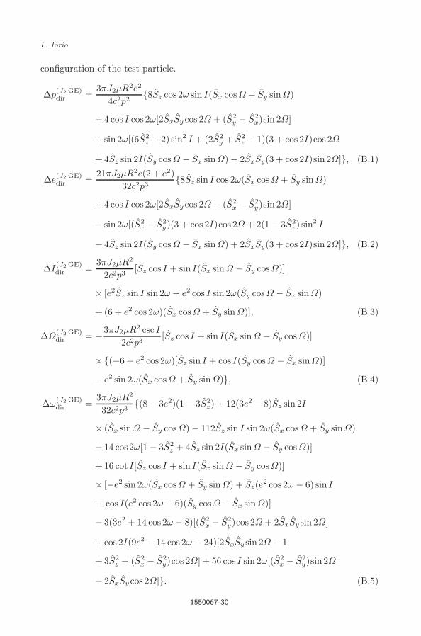
It can be noted that, in the special case Sx = Sy = 0, Sz = 1, Eqs. (A.1)–(A.5)reduce to Eqs. (70)–(74).

Appendix B. Direct Orbital Shifts of Order J2c−2 for a GenericOrientation of the Spin Axis of the Primary

Here, the general expressions for the post-Newtonian gravitoelectric direct orbitalshifts arising from Eq. (75) are displayed for an arbitrary orientation of the pri-mary’s spin axis. In this case, the inclination I does not necessarily refer to theequatorial plane of the central body, which, in general, does not coincide with thereference x, y axis. The following formulas are valid also for a general orbital

1550067-29

2nd Reading

June 16, 2015 15:49 WSPC/S0218-2718 142-IJMPD 1550067

L. Iorio

configuration of the test particle.

∆p(J2 GE)dir =

3πJ2µR2e2

4c2p28Sz cos 2ω sin I(Sx cosΩ + Sy sin Ω)

+ 4 cos I cos 2ω[2SxSy cos 2Ω + (S2y − S2

x)sin 2Ω]

+ sin 2ω[(6S2z − 2) sin2 I + (2S2

y + S2z − 1)(3 + cos 2I)cos 2Ω

+ 4Sz sin 2I(Sy cosΩ − Sx sinΩ) − 2SxSy(3 + cos 2I)sin 2Ω], (B.1)

∆e(J2 GE)dir =

21πJ2µR2e(2 + e2)32c2p3

8Sz sin I cos 2ω(Sx cosΩ + Sy sin Ω)

+ 4 cos I cos 2ω[2SxSy cos 2Ω − (S2x − S2

y)sin 2Ω]

− sin 2ω[(S2x − S2

y)(3 + cos 2I)cos 2Ω + 2(1 − 3S2z ) sin2 I

− 4Sz sin 2I(Sy cosΩ − Sx sinΩ) + 2SxSy(3 + cos 2I)sin 2Ω], (B.2)

∆I(J2 GE)dir =

3πJ2µR2

2c2p3[Sz cos I + sin I(Sx sin Ω − Sy cosΩ)]

× [e2Sz sin I sin 2ω + e2 cos I sin 2ω(Sy cosΩ − Sx sin Ω)

+ (6 + e2 cos 2ω)(Sx cosΩ + Sy sin Ω)], (B.3)

∆Ω(J2 GE)dir = −3πJ2µR2 csc I

2c2p3[Sz cos I + sin I(Sx sin Ω − Sy cosΩ)]

×(−6 + e2 cos 2ω)[Sz sin I + cos I(Sy cosΩ − Sx sinΩ)]

− e2 sin 2ω(Sx cosΩ + Sy sinΩ), (B.4)

∆ω(J2 GE)dir =

3πJ2µR2

32c2p3(8 − 3e2)(1 − 3S2

z) + 12(3e2 − 8)Sz sin 2I

× (Sx sin Ω − Sy cosΩ) − 112Sz sin I sin 2ω(Sx cosΩ + Sy sin Ω)

− 14 cos2ω[1 − 3S2z + 4Sz sin 2I(Sx sin Ω − Sy cosΩ)]

+ 16 cot I[Sz cos I + sin I(Sx sin Ω − Sy cosΩ)]

× [−e2 sin 2ω(Sx cosΩ + Sy sin Ω) + Sz(e2 cos 2ω − 6) sin I

+ cos I(e2 cos 2ω − 6)(Sy cosΩ − Sx sin Ω)]

− 3(3e2 + 14 cos 2ω − 8)[(S2x − S2

y)cos 2Ω + 2SxSy sin 2Ω]

+ cos 2I(9e2 − 14 cos 2ω − 24)[2SxSy sin 2Ω − 1

+ 3S2z + (S2

x − S2y)cos 2Ω] + 56 cos I sin 2ω[(S2

x − S2y)sin 2Ω

− 2SxSy cos 2Ω]. (B.5)

1550067-30

2nd Reading

June 16, 2015 15:49 WSPC/S0218-2718 142-IJMPD 1550067

Post-Newtonian orbital effects due to the oblateness of the central body

It can be noted that, in the special case Sx = Sy = 0, Sz = 1, Eqs. (B.1)–(B.5)reduce to Eqs. (76)–(80).

References

1. V. L. Ginzburg, Sci. Am. 200 (1959) 149.2. J. Overduin, The experimental verdict on spacetime from gravity probe B, in Space,

Time, and Spacetime, ed. Petkov, V., Fundamental Theories of Physics, Vol. 167(Springer, Heidelberg, 2010), pp. 25–59.

3. G. Renzetti, Cent. Eur. J. Phys. 11 (2013) 531.4. P. W. Worden and C. W. F. Everitt, Nucl. Phys. B, Proc. Suppl. 243–244 (2013)

172.5. C. M. Will, Phys. Rev. D 89 (2014) 044043, arXiv:1312.1289 [astro-ph.GA].6. M. H. Soffel, Relativity in Astrometry, Celestial Mechanics and Geodesy, Astronomy

and Astrophysics Library (Springer-Verlag, Heidelberg, 1989).7. A. Einstein, Sitz. ber. Preuß. Akad. Wiss. 47 (1915) 831.8. J. Lense and H. Thirring, Phys. Z. 19 (1918) 156.9. L. Iorio, Class. Quantum Grav. 30 (2013) 195011, arXiv:1302.6920 [gr-qc].

10. M. Soffel, R. Wirrer, J. Schastok, H. Ruder and M. Schneider, Celest. Mech. 42(1988) 81.

11. V. A. Brumberg, Essential Relativistic Celestial Mechanics (Adam Hilger, Bristol,1991).

12. G. Xu and J. Xu, Orbits: 2nd Order Singularity-Free Solutions (Springer, Berlin,2013).

13. J. Heimberger, M. Soffel and H. Ruder, Celest. Mech. Dyn. Astron. 47 (1990) 205.14. F. A. A. El-Salam, Int. J. Sci. Adv. Technol. 2 (2012) 1.15. P. Teyssandier, Phys. Rev. D 18 (1978) 1037.16. P. Teyssandier, Phys. Rev. D 16 (1977) 946.17. R. J. Adler, Gen. Relativ. Gravit. 31 (1999) 1837.18. M. Zimbres and P. S. Letelier, arXiv:0803.4133 [gr-qc].19. M. Panhans and M. H. Soffel, Class. Quantum Grav. 31 (2014) 245012.20. S. Matousek, Acta Astronaut. 61 (2007) 932.21. A. Paolozzi, I. Ciufolini and C. Vendittozzi, Acta Astronaut. 69 (2011) 127.22. A. M. Ghez, S. Salim, N. N. Weinberg, J. R. Lu, T. Do, J. K. Dunn, K. Matthews,

M. R. Morris, S. Yelda, E. E. Becklin, T. Kremenek, M. Milosavljevic and J. Naiman,Astrophys. J. 689 (2008) 1044, arXiv:0808.2870 [astro-ph].

23. O. Montenbruck and E. Gill, Satellite Orbits (Springer-Verlag, Heidelberg, 2000).24. G. Xu, X. Tianhe, W. Chen and T.-K. Yeh, Mon. Not. R. Astron. Soc. 410 (2011)

654.25. G. Xu and J. Xu, Mon. Not. R. Astron. Soc. 432 (2013) 584.26. G. P. Taratynova, Fortschr. Phys. 7 (1959) 55.27. D. Brouwer and G. M. Clemence, Methods of Celestial Mechanics (Academic Press,

New York, 1961).28. E. A. Roth, Celest. Mech. 2 (1970) 369.29. V. Mioc and E. Radu, Astron. Nachr. 300 (1979) 313.30. V. A. Egorov, Sov. Astron. 2 (1958) 147.31. V. Mioc and E. Radu, Astron. Nachr. 298 (1977) 107.32. G. L. Page, J. F. Wallin and D. S. Dixon, Astrophys. J. 697 (2009) 1226,

arXiv:0905.0030 [astro-ph.EP].

1550067-31

2nd Reading

June 16, 2015 15:49 WSPC/S0218-2718 142-IJMPD 1550067

L. Iorio

33. S. Gillessen, F. Eisenhauer, S. Trippe, T. Alexander, R. Genzel, F. Martins andT. Ott, Astrophys. J. 692 (2009) 1075, arXiv:0810.4674 [astro-ph].

34. L. Meyer, A. M. Ghez, R. Schodel, S. Yelda, A. Boehle, J. R. Lu, T. Do, M. R.Morris, E. E. Becklin and K. Matthews, Science 338 (2012) 84, arXiv:1210.1294[astro-ph.GA].

35. A. Boehle, R. Schodel, L. Meyer and A. M. Ghez, New orbital analysis of stars atthe Galactic center using speckle holography and orbital priors, in Proc. of the IAUSymp., eds. L. O. Sjouwerman, C. C. Lang and J. Ott, Vol. 303 (Cambridge UniversityPress, 2014), pp. 242–244.

36. N. Kallivayalil, R. P. van der Marel and C. Alcock, Astrophys. J. 652 (2006) 1213,arXiv:astro-ph/0606240.

37. N. Kallivayalil, R. P. van der Marel, C. Alcock, T. Axelrod, K. H. Cook, A. J. Drakeand M. Geha, Astrophys. J. 638 (2006) 772, arXiv:astro-ph/0508457.

38. J. Diaz and K. Bekki, Mon. Not. R. Astron. Soc. 413 (2011) 2015, arXiv:1101.2500[astro-ph.GA].

39. F. I. Cooperstock and S. Tieu, Mod. Phys. Lett. A 21 (2006) 2133.40. F. I. Cooperstock and S. Tieu, Mod. Phys. Lett. A 23 (2008) 1745, arXiv:0712.0019

[astro-ph].41. J. D. Carrick and F. I. Cooperstock, Astrophys. Space Sci. 337 (2012) 321,

arXiv:1101.3224 [astro-ph.GA].42. Y. Xu, Y. Yang, Q. Zhang and G. Xu, Mon. Not. R. Astron. Soc. 415 (2011) 3335.43. G. Petit and B. Luzum (eds.), IERS Conventions (2010), IERS Technical Note, No. 36,

IERS Conventions Centre (2010).44. C. M. Will, Phys. Rev. D 91 (2015) 029902.45. A. A. Orlov, Soobshch. Gos. Astron. Inst. Shternberg 88–89 (1953) 3.46. X. Liu, H. Baoyin and X. Ma, Astrophys. Space Sci. 334 (2011) 115, arXiv:1108.4639

[astro-ph.EP].47. A. Wolszczan and D. A. Frail, Nature 355 (1992) 145.48. M. Konacki and A. Wolszczan, Astrophys. J. Lett. 591 (2003) L147, arXiv:astro-

ph/0305536.49. M. Bailes, S. D. Bates, V. Bhalerao, N. D. R. Bhat, M. Burgay, S. Burke-Spolaor,

N. D’Amico, S. Johnston, M. J. Keith, M. Kramer, S. R. Kulkarni, L. Levin, A. G.Lyne, S. Milia, A. Possenti, L. Spitler, B. Stappers and W. van Straten, Science 333(2011) 1717, arXiv:1108.5201 [astro-ph.SR].

50. A. Wolszczan, New Astron. Rev. 56 (2012) 2.51. S. L. Shapiro and S. A. Teukolsky, Black Holes, White Dwarfs and Neutron Stars:

The Physics of Compact Objects (Wiley-VCH Verlag GmbH, Weinheim, 2004).52. R. Genzel, R. Schodel, T. Ott, A. Eckart, T. Alexander, F. Lacombe, D. Rouan and

B. Aschenbach, Nature 425 (2003) 934, arXiv:astro-ph/0310821.53. A. E. Broderick, V. L. Fish, S. S. Doeleman and A. Loeb, Astrophys. J. 697 (2009)

45, arXiv:0809.4490 [astro-ph].54. Y. Kato, M. Miyoshi, R. Takahashi, H. Negoro and R. Matsumoto, Mon. Not. R.

Astron. Soc. 403 (2010) L74, arXiv:0906.5423 [astro-ph.GA].55. A. E. Broderick, V. L. Fish, S. S. Doeleman and A. Loeb, Astrophys. J. 735 (2011)

110, arXiv:1011.2770 [astro-ph.HE].56. V. I. Dokuchaev, Gen. Relativ. Gravit. 46 (2014) 1832, arXiv:1306.2033 [astro-ph.HE].57. G. Risaliti, F. A. Harrison, K. K. Madsen, D. J. Walton, S. E. Boggs, F. E. Chris-

tensen, W. W. Craig, B. W. Grefenstette, C. J. Hailey, E. Nardini, D. Stern and W.W. Zhang, Nature 494 (2013) 449, arXiv:1302.7002 [astro-ph.HE].

1550067-32

2nd Reading

June 16, 2015 15:49 WSPC/S0218-2718 142-IJMPD 1550067

Post-Newtonian orbital effects due to the oblateness of the central body

58. R. C. Reis, M. T. Reynolds, J. M. Miller and D. J. Walton, Nature 507 (2014) 207,arXiv:1403.4973 [astro-ph.HE].

59. J. M. Bardeen, Nature 226 (1970) 64.60. J. M. Bardeen, W. H. Press and S. A. Teukolsky, Astrophys. J. 178 (1972) 347.61. S. Chandrasekhar, The Mathematical Theory of Black Holes (Oxford University Press,

New York, 1983).62. R. Penrose, Gen. Relativ. Gravit. 34 (2002) 1141.63. R. P. Kraft, Stellar rotation, in Stellar Astronomy, eds. H.-Y. Chiu, R. L. Warasila

and J. L. Remo, Vol. 2 (Gordon and Breach, New York, 1969), p. 317.64. R. P. Kraft, Stellar rotation, in Spectroscopic Astrophysics: An Assessment of the

Contributions of Otto Struve, ed. G. H. Herbig (University of California Press, Berke-ley, 1970), p. 385.

65. R. H. Dicke, The rotation of the Sun, in Stellar Rotation, ed. A. Slettebak (Kluwer,Dordrecht, 1970), pp. 289–317.

66. D. F. Gray, Astrophys. J. 261 (1982) 259.67. K.-W. Lo and L.-M. Lin, Astrophys. J. 728 (2011) 12, arXiv:1011.3563 [astro-ph.HE].68. M. Baubock, E. Berti, D. Psaltis and F. Ozel, Astrophys. J. 777 (2013) 68,

arXiv:1306.0569 [astro-ph.HE].69. P. T. Chrusciel, “No Hair” theorems: Folklore, conjectures, results, in Differential

Geometry and Mathematical Physics, eds. J. K. Beem and K. L. Duggal, Contem-porary Mathematics, Vol. 170 (American Mathematical Society, Providence, 1994),pp. 23–49.

70. M. Heusler, Uniqueness theorems for black hole space-times, in Black Holes: Theoryand Observation, eds. F. W. Hehl, C. Kiefer and R. J. K. Metzler, Lecture Notes inPhysics, Vol. 514 (Springer-Verlag, Heidelberg, 1998), pp. 157–186.

71. R. Geroch, J. Math. Phys. 11 (1970) 2580.72. R. O. Hansen, J. Math. Phys. 15 (1974) 46.73. W. G. Laarakkers and E. Poisson, Astrophys. J. 512 (1999) 282, arXiv:gr-qc/9709033.74. E. Berti and N. Stergioulas, Mon. Not. R. Astron. Soc. 350 (2004) 1416, arXiv:gr-

qc/0310061.75. G. Pappas and T. A. Apostolatos, Phys. Rev. Lett. 108 (2012) 231104,

arXiv:1201.6067 [gr-qc].76. M. Baubock, D. Psaltis, F. Ozel and T. Johannsen, Astrophys. J. 753 (2012) 175,

arXiv:1110.4389 [astro-ph.HE].77. L. Iorio, Phys. Rev. D 84 (2011) 124001, arXiv:1107.2916 [gr-qc].78. W. Kollatschny, Astron. Astrophys. 412 (2003) L61, arXiv:astro-ph/0311283.79. G. Lodato and D. Gerosa, Mon. Not. R. Astron. Soc. 429 (2013) L30, arXiv:1211.0284

[astro-ph.CO].80. Z. Li, M. R. Morris and F. K. Baganoff, Astrophys. J. 779 (2013) 154, arXiv:1310.0146

[astro-ph.HE].81. R. Narayan, T. Piran and A. Shemi, Astrophys. J. Lett. 379 (1991) L17.82. N. Wex and S. M. Kopeikin, Astrophys. J. 514 (1999) 388, arXiv:astro-ph/9811052.83. L. Iorio, New Astron. 15 (2010) 554, arXiv:0812.1485 [gr-qc].84. S. Finocchiaro, L. Iess, W. M. Folkner and S. Asmar, The determination of Jupiter’s

angular momentum from the Lense–Thirring precession of the Juno spacecraft, AGUFall Meeting Abstract No. P41B-1620, American Geophysical Union (2011).

85. R. Helled, J. D. Anderson, G. Schubert and D. J. Stevenson, Icarus 216 (2011) 440,arXiv:1109.1627 [astro-ph.EP].

86. G. Renzetti, New Astron. 23 (2013) 63.87. M. Capderou, Satellites: Orbits and Missions (Springer-Verlag, Paris, 2005).

1550067-33

2nd Reading

June 16, 2015 15:49 WSPC/S0218-2718 142-IJMPD 1550067

L. Iorio

88. K. Sosnica, C. Baumann, D. Thaller, A. Jaggi and R. Dach, Combined LARES–LAGEOS solutions, in Proc. of the 18th Int. Workshop on Laser Ranging: PursuingUltimate Accuracy and Creating New Synergies, Fujiyoshida, Japan, November 11–15,2013 (AIUB, 2014).

89. L. Iorio, Celest. Mech. Dyn. Astron. 112 (2012) 117, arXiv:1101.2634 [gr-qc].90. E. V. Pitjeva and N. P. Pitjev, Celest. Mech. Dyn. Astron. 119 (2014) 237–256.91. A. Milani, A. M. Nobili and P. Farinella, Non-Gravitational Perturbations and Satellite

Geodesy (Adam Hilger, Bristol, 1987).92. L. Iorio, Acta Phys. Pol. B 41 (2010) 753, arXiv:0809.3564 [gr-qc].93. P. Gurfil, J. Guid. Control Dyn. 30 (2007) 237.

1550067-34