988 IEEE TRANSACTIONS ON AUTOMATIC CONTROL, VOL. 54, NO. 5, MAY 2009

Positive Polynomial Constraints for POD-basedModel Predictive Controllers

Oscar Mauricio Agudelo, Michel Baes, Jairo José Espinosa, Senior Member, IEEE, Moritz Diehl, andBart De Moor, Fellow, IEEE

Abstract—This paper presents an application of positive polyno-mials to the reduction of the number of temperature constraints ofa proper orthogonal decomposition (POD)-based predictive con-troller for a non-isothermal tubular reactor. The objective of thecontroller is to maintain the reactor at a desired operating con-dition in spite of disturbances in the feed flow, while keeping themaximum temperature low enough to avoid the formation of un-desired byproducts. The controller is based on a model derived bymeans of POD, which reduces the high dimensionality of the dis-cretized system used to approximate the partial differential equa-tions that model the reactor. However, POD does not lead to a re-duction in the number of temperature constraints which is typi-cally very large. If we use univariate polynomials to approximatepart of the basis vectors derived with the POD technique, it is pos-sible to apply the theory of positive polynomials to find good ap-proximations of the temperature constraints by linear matrix in-equalities and to get a reduction in their number. This is the ap-proach that is followed in this paper. The simulation results showthat the predictive controller presented a good behavior and thatit dealt with the temperature constraints very well.

Index Terms—Distributed parameter systems, model reduction,polynomial approximation, predictive control.

I. INTRODUCTION

T UBULAR reactors are distributed parameter systems thattypically are modeled by coupled non-linear partial dif-

ferential equations (PDEs) which are derived from mass andenergy balance principles. A way of addressing the control ofthese systems is by approximating the PDEs by a large number

Manuscript received June 30, 2007; revised March 10, 2008. Currentversion published May 13, 2009. This work was supported by the ResearchCouncil KUL: CoE EF/05/006 Optimization in Engineering (OPTEC),GOA AMBioRICS, IOF-SCORES4CHEM, several PhD/Postdoc & FellowGrants; Flemish Government: FWO: PhD/Postdoc Grants, projects G.0452.04(new quantum algorithms), G.0499.04 (Statistics), G.0211.05 (Nonlinear),G.0226.06 (cooperative systems and optimization), G.0321.06 (Tensors),G.0302.07 (SVM/Kernel, research communities (ICCoS, ANMMM, MLDM);IWT: PhD Grants, McKnow-E, Eureka-Flite2 Belgian Federal SciencePolicy Office: IUAP P6/04 (Dynamical systems, control and optimization,2007–2011); EU: ERNS. Recommended by Guest Editors G. Chesi and D.Henrion.

O. M. Agudelo is with the Department of Electrical Engineering (ESAT), Re-search Group SCD-SISTA, Katholieke Universiteit Leuven, Heverlee B-3001,Belgium and also with the Department of Automation and Electronics, Univer-sidad Autónoma de Occidente,Calle 25 No. 115-85, Cali, Colombia (e-mail:mauricio.agudelo@esat.kuleuven.be).

M. Baes, B. De Moor, and M. Diehl are with the Department of ElectricalEngineering (ESAT), Research Group SCD-SISTA, Katholieke UniversiteitLeuven, Heverlee B-3001, Belgium (e-mail: michel.baes@esat.kuleuven.be;moritz.diehl@esat.kuleuven.be; bart.demoor@esat.kuleuven.be).

J. J. Espinosa is with the Facultad de Minas, Universidad Nacional deColombia, Carrera 80 No. 65-223, Medellín, Colombia (e-mail: jairo.es-pinosa@ieee.org).

Digital Object Identifier 10.1109/TAC.2009.2017136

of ordinary differential equations (ODEs). Afterwards, giventhe high-dimensionality of the resulting systems, reduced ordermodels are derived to make controller design possible. In thispaper, such reduced order models are found by means of properorthogonal decomposition (POD) and Galerkin projection. Theadvantage of applying these techniques is the incorporation ofsimulated or experimental data as well as the existing physicalrelationships from the original model [1].

In [2], a POD-based Predictive controller is proposed for con-trolling the temperature and concentration profiles of a non-isothermal tubular chemical reactor. The control goal is to rejectthe disturbances that affect the process, that is, the changes in thetemperature and concentration of the feed flow. One importantconstraint of the system is that the temperature inside the reactormust be below a given value in order to prevent undesirable sidereactions. Under typical disturbances, the controller proposedin [2] performs very well, and the temperature constraint is notviolated despite the fact that the predictive controller does notincorporate this constraint in its formulation. However, if largerdisturbances are applied, temporary violations of this constraintare observed.

In this paper we start by presenting an extension of the con-troller proposed in [2]. This new controller takes into accountthe temperature constraint of the reactor and uses a slack vari-able approach with -norm and time-dependent weights forhandling the infeasibilities that can emerge [3]. Although PODcan find a reduced order model for the reactor, it does not re-duce the number of temperature constraints, and therefore thecontroller has to deal with a very large number of them.

In this paper, we propose a method for approximating thetemperature constraints by means of the theory of positive poly-nomials. This approximation leads to a reduction in the numberof constraints by replacing many inequalities by a few linearmatrix inequalities (LMIs). This is the main contribution of thispaper.

Based on the polynomial approximations of the temperatureconstraints, a second POD-based MPC controller is proposed.This new controller also incorporates the mechanism for han-dling infeasibilities of the first predictive controller.

This paper is organized as follows. Section II presents adescription of the process. In Section III, the procedure forderiving the reduced order model of the reactor by means ofPOD and the Galerkin projection is discussed. Section IVdescribes a POD-based MPC control system that deals with avery large number of temperature constraints. In Section V, ournew method for approximating the temperature constraints isdescribed and a new MPC controller is presented. Section VIshows the simulation results of the control schemes presented

0018-9286/$25.00 © 2009 IEEE

Authorized licensed use limited to: Katholieke Universiteit Leuven. Downloaded on September 1, 2009 at 08:41 from IEEE Xplore. Restrictions apply.

AGUDELO et al.: POSITIVE POLYNOMIAL CONSTRAINTS 989

Fig. 1. Tubular reactor with three cooling/heating jackets.

in the previous two sections. Finally Section VII summarizesand concludes the paper.

II. DESCRIPTION OF THE PROCESS

The process to be controlled is a non-isothermal tubular re-actor where a single, first order, irreversible, exothermic reac-tion takes place . The reactor is surrounded by 3cooling/heating jackets as shown in Fig. 1. The temperature ofthe jacket fluids ( , and ) can be manipulated inde-pendently in order to control the concentration and temperatureprofiles in the reactor. In addition, the reactor is characterized bya plug-flow behavior because the diffusion and dispersion phe-nomena are not taken into account. Under these assumptions,the mathematical model of the tubular chemical reactor consistsof the following system of coupled non-linear PDEs:

(1)

with the following boundary conditions: at andat .

Here, is the reactant concentration in [mol/l],is the reactant temperature in [K], is the fluid superficial ve-locity in [m/s], is the heat of the reaction in [cal/mol],

and are the density in [kg/l] and the specific heat in[cal/kg/K] of the mix, respectively, is the kinetic constantin [1/s], is the activation energy in [cal/mol], is the idealgas constant in [cal/mol/K], is the heat transfer coefficient in

, is the reactor radius in [m], is the reactorlength in [m], and are the concentration in [mol/l] andthe temperature in [K] of the feed flow, is the axial coordinatein [m], is the time in [s] and is the reactor walltemperature in [K] defined as follows (see Fig. 1):

.

The parameters of the reactor model are taken from [4], whichwere inspired by the values given in [5]. These values are:

, , , ,, , ,

, and .The temperature of the jacket sections , and must

be between 280 K and 400 K. In addition, the temperature insidethe reactor must be below 400 K in order to avoid the formation

of side products. The kind of disturbances that affects the reactorare principally the variations in the temperature and concentra-tion of the feed flow. Typically, such variations are in the rangeof for the temperature and of the nominal valuefor the concentration. In this system, only the temperature ofthe feed flow is measured directly. In addition, the reactor has atemperature sensor at the output and 3 temperature sensors ( ,

and ) distributed in its interior as shown in Fig. 1.

A. Operating Profiles

In [2], an optimization algorithm (a kind of SQP) is proposedfor deriving the optimal operating profiles of the tubular reactordescribed by (1). The algorithm minimizes a given cost functionsubject to the steady-state equations of the reactor and the inputand output constraints of the system. The steady-state model ofthe reactor is given by the following ODEs:

(2)

with at and at , and the discreteversion of (2) can be found by replacing the spatial derivativesby forward difference approximations as follows:

(3)

where and are normalization factors, andare the normalized concentration and temperature

of the th section, is the normalized reactorwall temperature of the th section, is the number of sectionsin which the reactor is divided, and is the length of each sec-tion. The optimization problem that is solved in [2] for derivingthe operating profiles is defined as

(4)

subject to

where is the normalized desired concentration at the reactoroutput, is the normalized desired temperature inside the re-actor of the th section, is the normalized concentration atthe reactor output, is a trade-off parameter, andare the limits of the jackets temperatures, and is the max-imum allowed temperature inside the tubular reactor.

Authorized licensed use limited to: Katholieke Universiteit Leuven. Downloaded on September 1, 2009 at 08:41 from IEEE Xplore. Restrictions apply.

990 IEEE TRANSACTIONS ON AUTOMATIC CONTROL, VOL. 54, NO. 5, MAY 2009

Fig. 2. Steady-state concentration and temperature profiles (operating profiles)when � � ����� �, � � ����� �, and � � �� �.

The first term of the cost function corresponds to the squarederror of the normalized concentration at the reactor output (ter-minal cost), and the second term is related to the mean squarederror of the normalized temperature along the reactor (integralcost). In this problem was set to 0, and was selectedequal to the normalized temperature of the feeding flow

for . The trade-off parameter cantake values from 0 to 1. When goes to 1, the reduction of thereactant concentration at the reactor output becomes more im-portant than the temperature deviations. On the other hand when

goes to 0, the temperature deviations become more importantthan the concentration at the reactor output and the risk of theformation of hot spots is reduced.

The optimization problem stated by (4) was solvedby means of the algorithm proposed in [2] (a sort of SQP), andthe profiles derived are shown in Fig. 2 together with the corre-sponding jacket temperatures. The concentration at the reactoroutput is 1.57 , which is 12.7 times smaller than theconcentration of the feed flow (0.02 mol/l). Notice that the tem-perature of the hot spot is 390 K. In the steady-state optimizationalgorithm, the maximum temperature allowed inside the reactor

was set 10 degrees below the actual limit (400 K) in orderto give to the feedback controller enough room of maneuver-ability.

B. Linear Model

As it was done in [2], the linear model of the tubular reactor isobtained by linearizing (1) around the jacket temperatures andthe operating profiles presented in Fig. 2. Subsequently, the infi-nite dimensionality of the resulting linear PDEs is reduced by re-placing partial derivatives with respect to space by backward fi-nite difference approximations, leading to the following systemof ODEs:

(5)

where , are the steady state concentration and tempera-ture of the th section, and , are the steady state con-centration and temperature of the feed flow, , , arethe steady state jacket temperatures, and are normaliza-tion factors, , arethe normalized deviations from steady state of the concentra-tion and temperature of the th section,

and are the normalized deviations fromsteady state of the concentration and temperature of the feedflow, , and

are the normalized deviations of thejacket temperatures, is the number of sections in which thereactor is divided, , and are the matrices describing thesystem, is the state vector, is the vector of the inputs,and is the vector of the disturbances.

Since the spatial domain of the reactor is divided intosections, the number of states of (5) is equal to 600. This

large number of states makes the design and implementation offeedback controllers for the reactor difficult. Consequently, it isnecessary to find a reduced order model. In this study such areduced order model is found using Proper Orthogonal Decom-position (POD) and Galerkin projection [6]. A detailed expla-nation of the procedure is given in [2]. Nevertheless, in orderto make this paper self contained, this procedure is presentedbriefly in Section III.

III. MODEL REDUCTION BY MEANS OF POD

In proper orthogonal decomposition (POD) [7]–[15], we startby observing that can be expanded as a sum oforthonormal basis vectors

(6)

where is a set of orthonormal basisvectors (POD basis vectors or POD basis functions) in the dis-cretized spatial domain, and arethe time-varying coefficients, or POD coefficients, associatedto each basis vector. These POD basis vectors are ordered ac-cording to their relevance to .

The main dynamics of the system can be represented usingthe first most relevant basis vectors, since con-densates the main spatial correlations. An th order approxima-tion of (6) is then given by means of the truncated sequence

(7)

An approximate (reduced order) model of can be derivedby building a model for the first time-varying coefficients.This is the essence of model reduction by POD. The POD basisvectors are determined from simulation or experimental dataof the process. The dynamic model for the first time-varyingcoefficients can be found by means of Galerkin projection [6],[15]–[19] or using subspace identification techniques [20]–[22].

In Sections III-A–D, we describe the steps followed for de-riving the reduced order model of (5).

A. Generation of the Snapshot Matrix

We have constructed a snapshop matrixfrom the system response when independent step changes weremade in the input and perturbation signals of the linearmodel (5)

Authorized licensed use limited to: Katholieke Universiteit Leuven. Downloaded on September 1, 2009 at 08:41 from IEEE Xplore. Restrictions apply.

AGUDELO et al.: POSITIVE POLYNOMIAL CONSTRAINTS 991

Along the simulations, 1500 samples were collected. The ampli-tude of the step changes was chosen in such a way as to producechanges of similar magnitude in the temperature and concentra-tion profiles. This avoids a possible bias in the resulting model.

B. Derivation of the POD Basis Vectors

The POD basis vectors were derived by calculating the sin-gular value decomposition (SVD) of

where and are unitary ma-trices, and is a matrix that contains the singularvalues of in a decreasing order on its main diagonal. Thecolumns of are the POD basis vectors

C. Selection of the Most Relevant POD Basis Vectors

We have performed the selection by checking the singularvalues of (the larger the singular value the more relevantthe basis vector is) and the truncation degree of (7), whichis defined as follows:

(8)

where is the th singular value of . The number of PODbasis elements can be chosen so that the fraction of the first sin-gular values in (8) is large enough to capture most informationin the data [6]. An ad-hoc criterion commonly applied is thathas to be determined for [23]. In this problem, the first20 basis vectors were selected. The 20th order approximation of

is given by

(9)

where and .

D. Construction of the Model for the First PODCoefficients

In order to derive a dynamic model for the POD coefficients,we have used the Galerkin projection. If we define a residualfunction for (5) as follows:

(10)

and we replace by its th order approximation in(10), the projection of on the space spanned by thebasis vectors shall vanish. That is

(11)

where denotes the Euclidean inner product. Replacingby its th order approximation in (5), and ap-plying the inner product criterion (11) to the resulting equationwe have

The reduced order model of the reactor is then given by

(12)

where , and . The initialcondition for reads as .

Finally, the discrete-time version of (12) that is used by thepredictive controllers, was obtained using the bilinear transfor-mation [24] with a sampling time of 0.2 s

(13)

where , and are the matrices describing the new system.The sampling time was chosen by dividing the smallest timeconstant of the system (12) by 10.

IV. PREDICTIVE CONTROL SCHEME

The control objective is to reject the disturbances that affectthe reactor, that is the changes in the temperature and concen-tration of the feed flow. In addition, the control actions must sat-isfy the input constraints of the process, and the control systemshould keep the temperature inside the reactor below 400 K.

In [2], a POD-based MPC control scheme is proposed for con-trolling the reactor. Although this controller performs well inthe tests presented in [2] (the reactor is subject to typical dis-turbances as described in Section II), it does not incorporate thetemperature constraint of the reactor on its formulation. There-fore, when larger disturbances than the typical ones are applied,temporary violations of the temperature constraint will be ob-served. In this section we present an extension of the controlscheme described in [2], which takes into account the tempera-ture constraint of the reactor.

The control of the temperature and concentration profiles isachieved indirectly by controlling the POD coefficients. The ref-erences of these POD coefficients can be calculated by

(14)

where is the reference of the vector and is equal tosince the control system has to keep the reactor operating aroundthe profiles shown in Fig. 2.

Since in this MPC formulation the temperature constraintalong the reactor is taken into account, it is necessary to define amechanism for handling the infeasibilities that can emerge dueto the differences between the process and the model used by theMPC, the magnitude of the disturbances, the saturation of theactuators, etc. A way of dealing with these infeasibilities is by

Authorized licensed use limited to: Katholieke Universiteit Leuven. Downloaded on September 1, 2009 at 08:41 from IEEE Xplore. Restrictions apply.

992 IEEE TRANSACTIONS ON AUTOMATIC CONTROL, VOL. 54, NO. 5, MAY 2009

softening the temperature constraint through a slack variable ap-proach. A soft constraint formulation avoids infeasibility prob-lems by allowing violations in the temperature constraint, but atthe same time it tries to minimize such violations by penalizingthem in the objective function. In this paper a slack variable ap-proach with -norm and time-dependent weights is used [3],[25]. The MPC controller is formulated as follows:

(15a)

subject to

(15b)

(15c)

(15d)

where and are weighting matrices ,denotes , is the prediction horizon, is the con-trol horizon, and are the lower and upper bounds(these hard constraints are necessary due to physical limitationsof the actuators) of , is a vector whichcontains the normalized deviations of the temperature profile,

is the lower part (the last rows) of the matrix

that is associated to the temperature profile,

is a vector that contains themaximal allowed temperature for each point of the reactor, isthe slack variable (a scalar quantity), and are weightingfactors ( , ), is a vector of 1’s and

, is a time-dependent weight .In this formulation the maximum violation of the temperature

constraint along the reactor and the prediction horizon is penal-ized by means of the term . A sufficiently largewill ensure that the constraints are enforced as exact soft con-straints, that is, that constraint violations will only occur whenthere is not feasible solution of the original problem [3]. Thequadratic term is used as an additional tuning parameterand it also leads to a well-posed quadratic program (positive def-inite Hessian) [26].

The time-dependent weight penalizes future predictedconstraint violations increasingly, avoiding long-lasting con-straint violations [3].

Since the state vector is unknown and the changes in theconcentration of the feed flow are not measureddirectly, they are estimated by means of an observer (in this casea Kalman Filter) with the following formulation:

(16a)

(16b)

Fig. 3. Feasible regions delimited by the temperature constraints of a secondorder POD model. Dashed Line—Full set of constraints. Solid Line—Reducedset of constraints.

where is the estimated vector of the POD coefficients,is the estimation of , is the normalized tem-

perature deviation of the feed flow , is a vectorwhich contains the four temperature measurements (normalizeddeviations) along the reactor, is the estimate of ,and are the submatrices of the observer gain (Kalman gain),

and are the column vectors of andis a selection matrix which selects the measured temperaturesfrom the vector .

The control horizon was set to 10 samples and the predic-tion horizon was selected according to the following crite-rion: “Prediction Horizon Control Horizon Largest SettlingTime 80 samples”. and were selected accordingto the input constraints of the process and the operating tem-peratures of the jackets. The other parameters were selected asfollows: , , , and

.The optimization problem (15) that is solved by the MPC

controller is a quadratic programming (QP) problem which hastemperature constraints. Although

the POD technique has reduced the number of state variables of(5), the number of temperature constraints is still very large. Avery intuitive and simple way of reducing the number of con-straints is by choosing properly only some of them [27]. In spiteof the fact that the POD model of the reactor has 20 states, inFig. 3 a second order POD model is used for visualizing the fea-sible regions delimited by the temperature constraints. Noticethat with seven constraints we have a fair approximation of theoriginal feasible region (300 constraints). But with 21 tempera-ture constraints, the feasible region delimited by 300 constraintsis approximated very accurately. Note however that, with thisapproach, we do not have any command on the temperature be-tween the discretization points.

In this paper, we present an interesting new approach whichuses the positive polynomials theory to tackle the problem.Other ways to tackle it are also possible and might be efficient,like for example the method mentioned previously. Futurework will show which technique works best for which kindof applications. In the approach discussed in this manuscript,the large number of linear inequalities is replaced by a fewLMIs while maintaining a control of the temperature at everypoint of the reactor. In Section V we present the details of thistechnique.

Authorized licensed use limited to: Katholieke Universiteit Leuven. Downloaded on September 1, 2009 at 08:41 from IEEE Xplore. Restrictions apply.

AGUDELO et al.: POSITIVE POLYNOMIAL CONSTRAINTS 993

Fig. 4. Feasible regions delimited by the temperature constraints of a secondorder POD model. Dashed Line—Original temperature constraints. SolidLine—Polynomial Approximations of different degree given by (19). SolidLine with dots—Polynomial Approximations of different degree given by (22).

V. APPROXIMATION OF THE TEMPERATURE CONSTRAINTS

BY MEANS OF POSITIVE POLYNOMIALS

Similarly to the previous section, a second order POD modelis used to illustrate and explain the main idea of this positivepolynomial approach. Fig. 4 shows in dashed line the feasibleregion delimited by the temperature constraints

(17)

of a second order POD model.As it was mentioned before, is the lower part

of the matrix , therefore each column ofcorresponds to the part of the basis vectorsthat is associated to the temperature profile. That is

where .By taking advantage of the smoothness of the most relevant

columns of , we can find polynomial approximationsof the vectors by means of a least squaresregression. These approximations would satisfy

(18a)

(18b)

where is the th element of associated to the th gridpoint, is the th element of associated to the thgrid point, and are univariate real polynomialsof degree that approximate the vectors and respec-tively, is the spatial coordinate and is the value of the spatialcoordinate at the th grid point.

By using (18a) and (18b) we can approximate (17) by

(19)

......

. . ....

...

where and are the approximations of andrespectively, is the number of sections into which thereactor is divided (number of grid points) and is thenumber of the selected POD basis vectors.

Fig. 4 shows the feasible regions (in solid line) delimited by(19) for a second order POD model when polynomials of dif-ferent degree are used. From this Figure, it is clear that poly-nomials of degree 10 are accurate enough for approximating

and .Equation (19) imposes the temperature constraint only on the

grid points of the interval . However, we can impose thecondition (19) on every point of the interval , giving

which can be rewritten by defining

as follows:

(20)

The resulting polynomial of degree has to be nonneg-ative, at least in the interval .

Even though we have now seemingly complicated theproblem by replacing many by infinitely many inequalities,this new formulation can efficiently be handled by positivepolynomials techniques.

A. Semidefinite Representability of Positive Polynomials onan Interval

A sufficient condition for a multivariate real polynomial to benonnegative everywhere is whether it can be written as a sum ofsquared polynomials. We denote this property, as common, bythe acronym SOS, for Sum Of Squares. In general, SOS is notequivalent to the nonnegativity of a polynomial. Nevertheless, asa direct consequence of the Fundamental Theorem of Algebra,univariate real polynomials are nonnegative everywhere if andonly if they are SOS.

Further, the SOS representability of a polynomial can be ex-pressed as a semidefinite feasibility problem [28], [29], as thefollowing proposition states for univariate polynomials.

Authorized licensed use limited to: Katholieke Universiteit Leuven. Downloaded on September 1, 2009 at 08:41 from IEEE Xplore. Restrictions apply.

994 IEEE TRANSACTIONS ON AUTOMATIC CONTROL, VOL. 54, NO. 5, MAY 2009

Proposition 1: (see [28]) A univariate polynomial ofdegree is SOS if and only if there exists apositive semidefinite matrix such that

(21)

where .As the SOS representation of a polynomial is generically not

unique, the matrix can not be uniquely defined.It is possible to relate the positivity of a real univariate poly-

nomial on a compact interval to the positivity of some otherpolynomial on the whole real line by the following transforma-tion.

Proposition 2: (see [30, Section 4.2, Example 21.b]) A realunivariate polynomial of degree is nonnegative on the com-pact interval if and only if

The proof relies on the observation that the conditions:• the rational function has as

image;• the denominator is positive on ;• and on ;

are equivalent to on .For every , the condition (20):

can be converted into

and, denoting by the set of positivesemidefinite matrices, into

(22)

Observe that the coefficients of , and thus the coeffi-cients of depend linearly on .Therefore, the coefficients of are themselves linear func-tions of . Henceforth, the MPC optimization problem withthe polynomial approximation of the temperature constraintscan be written as a Semidefinite Program (SDP). SDP are a sub-class of self-scaled optimization problems (see [31]), that can besolved efficiently by Interior-Point Methods, such as the one im-plemented in the Matlab toolbox Sedumi [32].

Fig. 4 depicts the feasible regions (solid line with dots) de-limited by (22) for a second order POD model when polyno-mials of different degree are used. Notice how this approxima-tion overlaps completely the approximation given by (19) for allthe cases. It means that the error in the approximation given by(22) are mainly due to the errors of approximating the columnsof and by polynomials.

Fig. 5. Polynomial approximations of the vectors (a) ���� and (b) ���� . SolidLine—vector. Dashed line—Approximation with a polynomial of degree 12.

For degree 10, the feasible region induced by the polynomialapproximation (22) and by the original temperature constraints(17) are almost indistinguishable.

The formulation of the new MPC controller based on poly-nomial approximations of the temperature constraints would begiven by (15), but substituting (15c) by

with

Here, is the slack variable (a scalar quantity) and, is a time-dependent weight . As it was ex-

plained in Section IV, the slack variable and the time-depen-dent weight allow the MPC to deal with possible infeasibilities.Observe that the semidefinite representation of this constraintstill yields LMIs, which fall into the scope of interior-pointmethods for self-scaled programming.

This new MPC has the same tuning parameters as the MPCpresented in Section IV. We have set the degree of the poly-nomials and to .With this selection, the first seven vectors areapproximated very well. On the other hand, the last five vectors

(the less relevant ones) are approximated verypoorly (See Fig. 5). In general, the less important the POD basisfunction, the more oscillatory it is. If we want to improve thepolynomial approximations, we would have to increase , butthis would lead to an increment in the number of constraints.

Unlike the MPC presented in Section IV which deals with24 000 temperature constraints, this MPC has only

linear equality constraints andLMIs of dimension 13 13 for dealing with the temperatureconstraint of the reactor. Hence, a large reduction in the numberof temperature constraints has been achieved by means of thepolynomial approximations.

For the estimation of the state vector and the changes inthe concentration of the feed flow , this MPCuses the same observer (16) as described in Section IV.

Authorized licensed use limited to: Katholieke Universiteit Leuven. Downloaded on September 1, 2009 at 08:41 from IEEE Xplore. Restrictions apply.

AGUDELO et al.: POSITIVE POLYNOMIAL CONSTRAINTS 995

VI. SIMULATION RESULTS

In order to perform the closed-loop simulations of the controlsystems described in the previous sections, the nonlinear modelof the process given in (1) was discretized in space by replacingthe partial derivatives with respect to space by backward differ-ence approximations [4], [33].

In this study, we solve the optimization problem of the MPCcontrollers by means of Sedumi, a Matlab toolbox for opti-mization over symmetric cones [32]. It is important to remarkthat all the MPC controllers have been implemented using thecondensed form of the MPC formulations presented before. Itmeans that the cost function and constraints of (15) have beenexpressed in terms of and , and the formulation ofthe MPC controller based on the polynomial approximationshas been expressed in terms of , and the entries of thematrix .

From now on, the MPC controller (15) will be referred to asMPC-QP and the MPC based on the polynomial approximations(see last part of Section V-A) to as MPC-SDP.

Initially, in order to compare and evaluate the performance ofthe MPC controllers, we carried out the tests proposed in [2]:

• Test 1: the temperature and concentration of the feed floware increased by 10 K and , respectively.

• Test 2: the temperature and concentration of the feed floware decreased by 10 K and , respectively.

The simulation results of MPC-QP and MPC-SDP were quitesimilar to the ones shown in [2], where a POD-based MPC con-troller without temperature constraints is presented. The formu-lation of this controller is given by (15) after eliminating the(15c), (15d) and the term in the cost function. Thiscontroller with No Temperature Constraints will be referred toas MPC-NTC.

Along Tests 1 and 2, the MPC-QP, MPC-SDP and MPC-NTCcontrollers kept the reactor working around the nominal oper-ating profiles, there were no violations of the temperature con-straint, the concentration in steady state at the reactor outlet waskept quite close to its nominal value, and the control actionswere all the time within the allowed bounds.

The similarities in the results are due to the fact that the con-trol systems were not operating close to the temperature con-straints, and therefore during the tests, these constraints are notactive in the MPC-QP and MPC-SDP controllers. So, in orderto evaluate the ability of MPC-QP and MPC-SDP to deal withthe temperature constraints, we propose this new test:

• Test 3: the temperature and concentration of the feed floware increased by 24 K and 3 , respectively.These disturbances are large in comparison with the typ-ical ones.

Observe that under this test, the tubular reactor operates farfrom the operating profiles shown in Fig. 2, and therefore thedifferences between the nonlinear model of the process and thelinear POD model used by the controllers are considerable. Figs.6 and 7 present the simulation results of Test 3.

Notice that in Fig. 6 for all the cases, the steady state profilesof the reactor are overlapping.

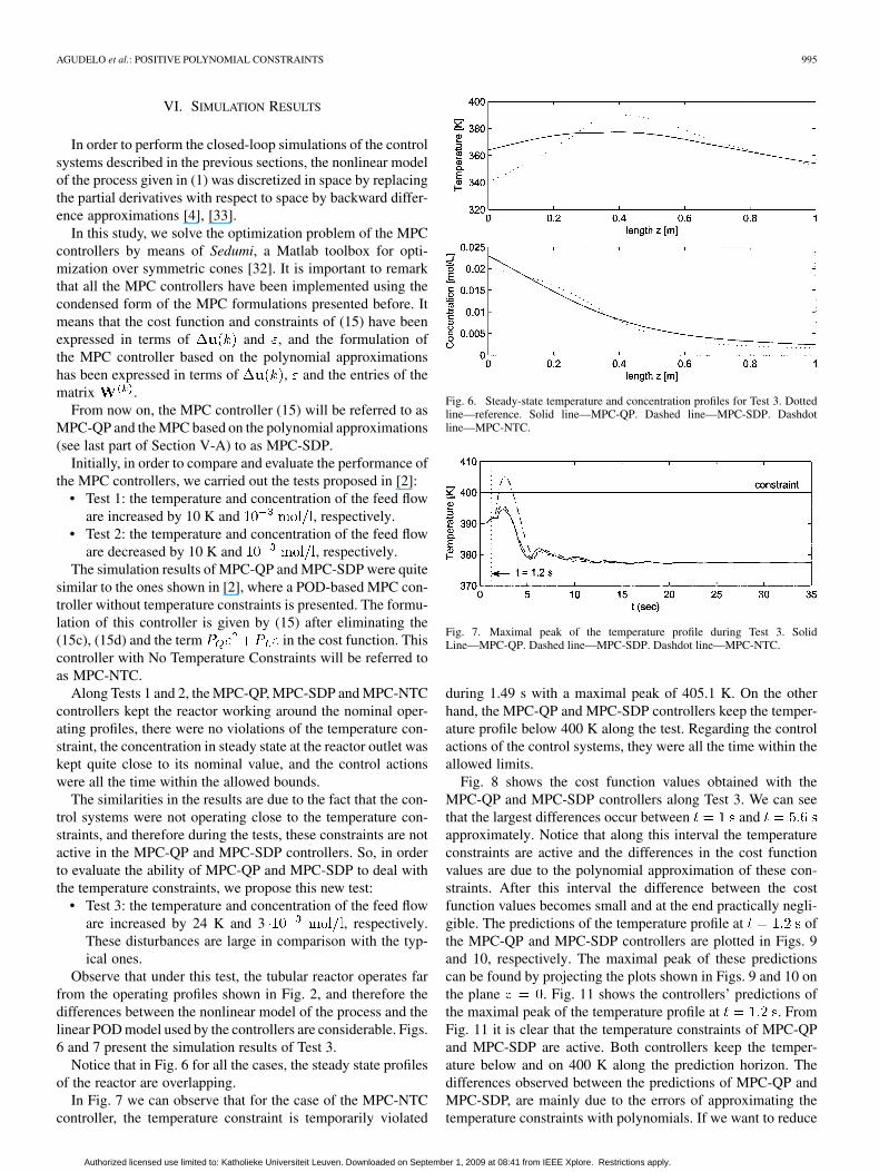
In Fig. 7 we can observe that for the case of the MPC-NTCcontroller, the temperature constraint is temporarily violated

Fig. 6. Steady-state temperature and concentration profiles for Test 3. Dottedline—reference. Solid line—MPC-QP. Dashed line—MPC-SDP. Dashdotline—MPC-NTC.

Fig. 7. Maximal peak of the temperature profile during Test 3. SolidLine—MPC-QP. Dashed line—MPC-SDP. Dashdot line—MPC-NTC.

during 1.49 s with a maximal peak of 405.1 K. On the otherhand, the MPC-QP and MPC-SDP controllers keep the temper-ature profile below 400 K along the test. Regarding the controlactions of the control systems, they were all the time within theallowed limits.

Fig. 8 shows the cost function values obtained with theMPC-QP and MPC-SDP controllers along Test 3. We can seethat the largest differences occur between andapproximately. Notice that along this interval the temperatureconstraints are active and the differences in the cost functionvalues are due to the polynomial approximation of these con-straints. After this interval the difference between the costfunction values becomes small and at the end practically negli-gible. The predictions of the temperature profile at ofthe MPC-QP and MPC-SDP controllers are plotted in Figs. 9and 10, respectively. The maximal peak of these predictionscan be found by projecting the plots shown in Figs. 9 and 10 onthe plane . Fig. 11 shows the controllers’ predictions ofthe maximal peak of the temperature profile at . FromFig. 11 it is clear that the temperature constraints of MPC-QPand MPC-SDP are active. Both controllers keep the temper-ature below and on 400 K along the prediction horizon. Thedifferences observed between the predictions of MPC-QP andMPC-SDP, are mainly due to the errors of approximating thetemperature constraints with polynomials. If we want to reduce

Authorized licensed use limited to: Katholieke Universiteit Leuven. Downloaded on September 1, 2009 at 08:41 from IEEE Xplore. Restrictions apply.

996 IEEE TRANSACTIONS ON AUTOMATIC CONTROL, VOL. 54, NO. 5, MAY 2009

Fig. 8. Cost function values during Test 3. Solid Line—MPC-QP. Dashedline—MPC-SDP.

Fig. 9. MPC-QP predictions of the temperature profile at � � ��� � (Test 3).

Fig. 10. MPC-SDP predictions of the temperature profile at � � ��� � (Test 3).

these discrepancies, we would have to increase the degree ofthe polynomials. However, this would lead to an increment inthe number of constraints and optimization variables whichwould increase the complexity of the optimization problem andtherefore the time required to solve it. Additionally, tests withlarger polynomial degrees would cause numerical instabilitieswithin Sedumi.

Notice that in Test 3, the closed-loop response of the con-trolled system is different than the predicted one. Also observe

Fig. 11. Predictions of the maximal peak of the temperature profile at � � ��� �

(Test 3). Solid Line—MPC-QP. Dashed line—MPC-SDP. Dashdot line—MPC-NTC.

that the steady state profiles of the reactor are far from the de-sired ones. None of these situations occurred during Tests 1 and2. All of this is mainly due to considerable differences betweenthe linear POD model used by the controllers and the observer,and the nonlinear model of the process. We have to keep in mindthat during Test 3 the reactor is operating far away from the pro-files (see Fig. 2) where the nonlinear model of the reactor waslinearized. It is quite clear that we have to incorporate the non-linearities of the process into the POD model used by the con-trollers if we want to improve the performance of the controlsystems. Nevertheless this would lead to non-convex optimiza-tion problems that would require more advanced solvers. Forinstance, the optimization problems of the nonlinear MPC-QPand MPC-SDP controllers could be addressed by SequentialQuadratic Programming (SQP) and sequential SDP methods, re-spectively.

Table I presents the average computation times (in a PC witha Dual Core of 3 Ghz and a RAM memory of 2 GB) for solvingthe optimization problems of the MPC controllers during Test3 for different control and prediction horizons. In Table I, wealso have included the time of solving the optimization of theMPC-QP controller when a specialized QP solver like Quad-prog is used. Quadprog is part of the Optimization Toolbox ofMatlab [34] and it uses an active set method similar to that de-scribed in [35]. From Table I it is clear that the optimization ofthe MPC-SDP controller requires less time than the optimiza-tion of the MPC-QP controller when we use the same solver(Sedumi) for both cases. However if we use Quadprog (in gen-eral it is more efficient to solve a QP problem using a QP solverlike Quadprog than using a more general tool like Sedumi ) forsolving the optimization of the MPC-QP controller, the time re-quired is between 14 to 19 times shorter than the time needed tosolve the optimization of the MPC-SDP controller.

Table II shows the number of optimization variables (in-cluding auxiliary variables), the number and kind of constraintsand the memory requirements of the predictive controllers.It is important to remark that the MPC-SDP controller hasbeen encoded using explicitly the primal representation inSedumi whereas the MPC-QP (Sedumi) controller has beenimplemented using the dual formulation. Therefore the valuesin Table II for these controllers correspond to the number of op-timization variables and constraints in the primal (MPC-SDP)and dual space (MPC-QP) respectively. Notice that for theMPC-SDP case, the LMI constraints introduce a large number

Authorized licensed use limited to: Katholieke Universiteit Leuven. Downloaded on September 1, 2009 at 08:41 from IEEE Xplore. Restrictions apply.

AGUDELO et al.: POSITIVE POLYNOMIAL CONSTRAINTS 997

TABLE IAVERAGE TIME FOR SOLVING THE OPTIMIZATION PROBLEM

TABLE IINUMBER OF VARIABLES, NUMBER OF CONSTRAINTS AND MEMORY

REQUIREMENTS WHEN � � �� AND � � ��

of variables. This is the main drawback of our approach. How-ever in spite of this, the optimization problem for the MPC-SDPcase requires less time than the case when Sedumi is used tosolve the optimization of the MPC-QP controller. NeverthelessIf we keep increasing the degree of the polynomials used toapproximate the temperature constraints, we will reach a pointwhere the time required for solving the optimization of theMPC-SDP controller would be larger than the time needed tosolve the optimization of MPC-QP with Sedumi.

Finally, from Table II we can see that the memory require-ments (the memory needed to store the matrices that are given tothe solver) of the MPC-SDP controller are significantly less thanthe memory requisites of the MPC-QP controller (it does notmatter the solver used). The MPC-SDP controller requires ap-proximately 9 times less memory than the MPC-QP controller.Although our approach has not led to a reduction in the compu-tational time (when the optimization of MPC-QP is performedwith Quadprog), it certainly has led to a remarkable saving ofmemory.

VII. CONCLUSION

In this paper, a method for approximating the temperatureconstraints of a POD-based predictive controller for a tubularreactor has been presented. In this method, part of the basisvectors derived with the POD technique are approximated withunivariate real polynomials. Afterwards, the theory of positivepolynomials is used for approximating the temperature con-straints by means of LMIs and linear equality constraints. Themethod leads to a significant reduction in the number of con-straints which conduces to a considerable saving of the memory.However the computational time needed for solving the opti-mization problem of the predictive controller based on the poly-nomial approximations, is much larger than the time required

for solving the original problem. What mainly limits the com-putational gain of this technique is the large number of variablesthat are introduced by the LMI constraints. From this study it isclear that with this positive polynomial approach the resultingoptimization problem is more complex than the original one.Nevertheless our approach guarantees the fulfillment of the tem-perature constraint at every point of the reactor. Other ways oftackling the problem are also possible and might be efficient.Future work is necessary in order to find out which approachworks best for which kind of applications.

The predictive controller based on the polynomial approxi-mation presented a good behavior, and it was able to deal withthe temperature constraints quite well.

An interesting topic for further investigation concerns robust-ness considerations with respect to model uncertainties. Noticethat at the moment of incorporating these uncertainties, we needto preserve the LMI representation of our model. This excludesthe use of multivariate polynomials, which are not exactly rep-resentable as LMIs. However, there is still some breathing spacefor robust approaches in our setting. Robustness of semidefiniteoptimization problems has been studied by Ben Tal, El Ghaoui,and Nemirovski in [36]. They show that robust semidefinite op-timization, while NP-hard even in simple uncertainty settings,can be approximated by a semidefinite relaxation. It is also pos-sible to obtain some accuracy bounds for some of these relax-ations, namely when they use an ellipsoidal uncertainty on thecoefficient of the affine constraints. In particular, we can applytheir theory if we consider that the coefficients of the interpola-tion theorems are only known within some prescribed accuracy.Our approach, that we only applied to linear system models sofar, can in a straightforward way be generalized to the case ofnonlinear MPC and would then lead to the interesting problemclass of nonlinear SDP problems that can e.g., be addressedby the sequential SDP methods proposed and investigated in[37]–[39].

ACKNOWLEDGMENT

The authors would like to thank the reviewers of this manu-script for their suggestions and remarks that undoubtedly con-tributed to the improvement of our initial submission.

REFERENCES

[1] M. Hazenberg, P. Astrid, and S. Weiland, “Low order modeling andoptimal control design of a heated plate,” in Proc. 5th Eur. ControlConf., Cambridge, U.K., Sep. 2003, [CD ROM].

[2] O. M. Agudelo, J. J. Espinosa, and B. De Moor, “Control of a tubularchemical reactor by means of POD and predictive control techniques,”in Proc. Eur. Control Conf. (ECC’07), Kos, Greece, Jul. 2007, pp.1046–1053.

[3] M. Hovd and R. D. Braatz, “Handling state and output constraints inMPC using time-dependent weights,” in Proc. Amer. Control Conf.(ACC), Arlington, VA, 2001, pp. 2418–2423.

[4] I. Y. Smets and J. F. Van Impe, “Optimal control of tubular chemicalreactors: Performance assessment under transient and diffuse condi-tions,” in Proc. 10th Med. Conf. Control Automat. (MED’02), Lisbon,Portugal, 2002, [CD ROM].

[5] M. Fjeld and B. Ursin, “Approximate lumped models of a tubular chem-ical reactor, and their use in feedback and feedforward control,” in Proc.2nd IFAC Symp. Multivariable Technical Control Syst., Amsterdam,The Netherlands, 1971, pp. 1–18.

[6] P. Astrid, “Reduction of Process Simulation Models: A Proper Orthog-onal Decomposition Approach,” Ph.D. dissertation, Technishche Uni-versiteit Eindhoven, Eindhoven, The Netherlands, 2004.

Authorized licensed use limited to: Katholieke Universiteit Leuven. Downloaded on September 1, 2009 at 08:41 from IEEE Xplore. Restrictions apply.

998 IEEE TRANSACTIONS ON AUTOMATIC CONTROL, VOL. 54, NO. 5, MAY 2009

[7] A. Chatterjee, “An introduction to the proper orthogonal decomposi-tion,” Current Sci., vol. 78, no. 7, pp. 808–817, Apr. 2000.

[8] Y. C. Liang, H. P. Lee, S. P. Lim, W. Z. Lin, K. H. Lee, and C. G. Wu,“Proper orthogonal decomposition and its applications-Part I: theory,”J. Sound Vibration, vol. 252, no. 3, pp. 527–544, May 2002.

[9] S. Chakravarti, M. Marek, and W. H. Ray, “Reaction-diffusion systemwith brusselator kinetics: Control of a quasiperiodic route to chaos,”Phys. Rev. E, vol. 52, no. 3, pp. 2407–2423, Sep. 1995.

[10] J. Lumley and P. Blossey, “Control of turbulence,” Annu. Rev. FluidMech., vol. 30, pp. 311–327, 1998.

[11] A. Theodoropoulou, R. A. Adomaitis, and E. Zafiriou, “Model re-duction for optimization of rapid thermal chemical vapor depositionsystems,” IEEE Trans. Semicond. Manufact., vol. 11, pp. 85–98, Feb.1998.

[12] W. R. Graham, J. Peraire, and K. Y. Tang, “Optimal control of vortexshedding using low-order models. Part I-open-loop model develop-ment,” Int. J. Numer. Methods Eng., vol. 44, no. 7, pp. 945–972, 1999.

[13] E. A. Gillies, “Low-dimensional control of the circular cylinder wake,”J. Fluid Mech., vol. 371, pp. 157–178, 1998.

[14] K. Kunisch and S. Volkwein, “Control of the burgers equation by areduced-order approach using proper orthogonal decomposition,” J.Optim. Theory Appl., vol. 102, no. 2, pp. 345–371, Aug. 1999.

[15] S. S. Ravindran, “A reduced-order approach for optimal control offluids using proper orthogonal decomposition,” Int. J. Numer. MethodsFluids, vol. 34, no. 5, pp. 425–448, Nov. 2000.

[16] P. Beyer, S. Benkadda, and X. Garbet, “Proper orthogonal decomposi-tion and Galerkin projection for a three-dimensional plasma dynamicalsystem,” Phys. Rev. E, vol. 61, no. 1, pp. 813–823, Jan. 2000.

[17] A. K. Bangia, P. F. Batcho, I. G. Kevrekidis, and G. E. Karniadakis,“Unsteady two-dimensional flows in complex geometries: Compara-tive bifurcation studies with global eigenfunction expansions,” SIAMJ. Sci. Comput., vol. 18, no. 3, pp. 775–805, 1997.

[18] A. Liakopoulos, P. A. Blythe, and H. Gunes, “A reduced dynamicalmodel of convective flows in tall laterally heated cavities,” Proc.Royal Soc. A: Math., Phys. Eng. Sci., vol. 453, no. 1958, pp.663–672, 1997.

[19] A. Iollo, S. Lanteri, and J. A. Désidéri, “Stability properties ofPOD-Galerkin approximations for the compressible Navier-stokesequations,” Theor. Computat. Fluid Dyn., vol. 13, no. 6, pp. 377–396,Mar. 2000.

[20] L. Huisman, “Control of Glass Melting Processes Based on ReducedCFD Models,” Ph.D. dissertation, Technishche Universiteit Eindhoven,Eindhoven, The Netherlands, 2005.

[21] L. Huisman and S. Weiland, “Reduced model based LQG control of anindustrial glass feeder,” in Proc. 10th IFAC/IFORS/IMACS/IFIP Symp.Large Scale Syst.: Theory Appl., Osaka, Japan, Jul. 2004, vol. 1, pp.421–426.

[22] L. Huisman and S. Weiland, “Identification and model predictivecontrol of an industrial glass feeder,” in Proc. 13th IFAC Symp. Syst.Identification (SYSID’03), Rotterdam, The Netherlands, Aug. 2003,pp. 1685–1689.

[23] P. Holmes, Lumley, and G. Berkooz, Turbulence, Coherence Structure,Dynamical Systems and Symmetry. Cambridge, U.K.: CambridgeUniversity Press, 1996.

[24] T. W. Parks and C. S. Burrus, Digital Filter Design. New York:Wiley, 1987.

[25] M. Hovd and R. D. Braatz, “On the use of soft constraints in MPCcontrollers for plants with inverse response,” in Proc. 6th IFAC Symp.Dyn. Control Process Syst., Jejudo, Korea, 2001, pp. 251–256.

[26] P. O. M. Scokaert and J. B. Rawlings, “Feasibility issues in linearmodel predictive control,” AIChE J., vol. 45, pp. 1649–1659, 1999.

[27] B. Pluymers, J. A. K. Suykens, and B. D. Moor, Construction of Re-duced Complexity Polyhedral Invariant Sets for LPV Systems UsingLinear Programming ESAT-SISTA, K.U. Leuven, Leuven, Belgium,Tech. Rep. 05-172, 2005.

[28] Y. Nesterov, “Squared functional systems and optimization problems,”in High Performance Optimization, H. Frenk, K. Roos, T. Terlaky, andS. Zhang, Eds. New York: Kluwer, 2000, pp. 405–440.

[29] P. A. Parrilo, “Structured Semidefinite Programs and SemialgebraicGeometry Methods in Robustness and Optimization,” Ph.D. disserta-tion, California Institute of Technology, Pasadena, 2000.

[30] A. Ben-Tal and A. Nemirovski, Lectures on Modern Convex Optimiza-tion: Analysis, Algorithms, and Engineering Applications, ser. MPS/SIAM Series on Optimization. Philadelphia, PA: SIAM, 2001.

[31] Y. Nesterov and M. Todd, “Self-scaled barriers and interior-pointmethods for convex programming,” Math. Operat. Res., vol. 22, pp.1–42, 1997.

[32] J. Sturm, “Using SeDuMi 1.02, a MATLAB toolbox for optimiza-tion over symmetric cones,” Optim. Methods Software, vol. 11, pp.625–653, 1999.

[33] D. D. Vecchio and N. Petit, “Boundary control for an industrial under-actuated tubular chemical reactor,” J. Process Control, vol. 15, pp.771–784, 2005.

[34] “Optimization Toolbox 3: User’s Guide,” Mathworks, 2006.[35] P. E. Gill, W. Murray, and M. H. Wright, Practical Optimization.

London, U.K.: Academic, 1981.[36] A. Ben-Tal, L. G. El, and A. Nemirovski, “Robustness,” in Handbook

of Semidefinite Programming, H. Wolkowicz, R. Saigal, and L. Ven-berghe, Eds. New York: Kluwer, 2000, pp. 139–162.

[37] B. Fares, D. Noll, and P. Apkarian, “Robust control via sequentialsemidefinite programming,” SIAM J. Control Optim., vol. 40, no. 6,pp. 1791–1820, 2002.

[38] R. W. Freund and F. Jarre, A Sensitivity Analysis and a ConvergenceResult for a Sequential Semidefinite Programming Method Bell Labo-ratories, Murray Hill, NJ, Tech. Rep., 2003.

[39] M. Diehl, F. Jarre, and C. Vogelbusch, “Loss of superlinear conver-gence for an SQP-type method with conic constraints,” SIAM J. Optim.,vol. 16, no. 4, pp. 1201–1210, 2006.

Oscar Mauricio Agudelo received the B.S. degreein electronics engineering from the UniversidadAutónoma de Occidente, Cali, Colombia, in 1997,the M.S. degree in Industrial Control engineeringfrom the Universidad de Ibagué (in cooperation withKatholieke Universiteit Leuven and UniversiteitGent), Ibagué, Colombia, in 2004, and is currentlypursuing the Ph.D. degree at the Department of Elec-trical Engineering (ESAT), Katholieke UniversiteitLeuven, Leuven, Belgium.

From 1997 to 2004, he worked at the UniversidadAutónoma de Occidente as a full time teacher of control and automation. Hisresearch interests are in model reduction techniques, proper orthogonal decom-position (POD), model predictive control, control of tubular chemical reactors,and analysis and design of intelligent control systems.

Michel Baes received the M.S. degree in appliedmathematics engineering and the Ph.D. degreefrom the Catholic University of Louvain-la-Neuve,Belgium, in 2002 and 2006, respectively.

He is a Postdoctoral Fellow of the Optimizationin Engineering Center (OPTEC), Katholieke Univer-siteit Leuven, Leuven, Belgium. His scientific inter-ests include convex optimization and its applications,development of algebraic techniques dedicated to thedesign and the study of optimization algorithms.

Jairo José Espinosa (SM’06) received the B.S. de-gree in electronics engineering from the UniversidadDistrital de Bogotá and the M.S. (with honors) andPh.D. (with high honors) degrees in electrical en-gineering from the Katholieke Universiteit Leuven,Leuven, Belgium.

Currently, he is an Associate Professor with theNational University of Colombia, Medellín. Formany years he was R & D Manager for the companyIPCOS N.V., Belgium, where he made researchin advanced process control systems. He has been

involved in the creation of products to construct inferential sensors, nonlinearmodel based predictive controllers and process optimization. He has hands onexperience in many industrial areas including oil, polymers, petrochemicals,automotive, power generation and iron production where he has applied manyof his developments. His research interests are intelligent control, nonlinearmodeling, model based predictive control, inferential sensors, and modelreduction techniques.

Authorized licensed use limited to: Katholieke Universiteit Leuven. Downloaded on September 1, 2009 at 08:41 from IEEE Xplore. Restrictions apply.

AGUDELO et al.: POSITIVE POLYNOMIAL CONSTRAINTS 999

Moritz Diehl received the Ph.D. degree from theInterdisciplinary Center for Scientific Computing(IWR), Heidelberg University, Heidelberg, Germany,in 2001.

Since 2006, he has been a Professor with the Uni-versity of Leuven (K.U. Leuven), Belgium, and prin-cipal investigator of K.U. Leuven’s Optimization inEngineering Center OPTEC. His research is centeredaround embedded optimization algorithms for use inmodel predictive control, real-time optimization, andmoving horizon estimation. His general interests are

in structure exploitation for optimization in engineering, convex optimization,dynamic optimization. He works on real-world applications of optimization andcontrol in mechatronics, robotics, sustainable energy, and chemical engineering.

Bart De Moor (SM’93–F’04) received the M.S.and Ph.D.degrees from the Katholieke UniversiteitLeuven, Leuven, Belgium (KU. Leuven), in 1983and 1988, respectively, both in electrical engineering.

He is a Full Professor with KU Leuven. He was aVisiting Research Associate at Stanford University,Stanford, CA, from 1988 to 1990. From 1991 to1999, he was the chief advisor on science andtechnology for the Belgian Federal and the FlandersRegional Governments. He has published more than250 journal papers, 350 conference proceedings

publications, five books, and numerous science popularizing contributions.His research interests are in numerical linear algebra and optimization, systemtheory, control and identification, quantum information theory, datamining,information retrieval and bio-informatics.

Dr. De Moor received the Leybold-Heraeus Prize (1986), Leslie Fox Prize(1989), Guillemin-Cauer Best Paper Award of the IEEE Transactions on Cir-cuits and Systems (1990), Laureate of the Belgian Royal Academy of Sciences(1992), bi-annual Siemens Award (1994), Best Paper Award of Automatica(IFAC, 1996), and the IEEE Signal Processing Society Best Paper Award(1999).

Authorized licensed use limited to: Katholieke Universiteit Leuven. Downloaded on September 1, 2009 at 08:41 from IEEE Xplore. Restrictions apply.