HAL Id: tel-03687092https://tel.archives-ouvertes.fr/tel-03687092

Submitted on 3 Jun 2022

HAL is a multi-disciplinary open accessarchive for the deposit and dissemination of sci-entific research documents, whether they are pub-lished or not. The documents may come fromteaching and research institutions in France orabroad, or from public or private research centers.

L’archive ouverte pluridisciplinaire HAL, estdestinée au dépôt et à la diffusion de documentsscientifiques de niveau recherche, publiés ou non,émanant des établissements d’enseignement et derecherche français ou étrangers, des laboratoirespublics ou privés.

Polyploid phasing algorithms and applicationsOmar Abou Saada

To cite this version:Omar Abou Saada. Polyploid phasing algorithms and applications. Human health and pathology.Université de Strasbourg, 2021. English. �NNT : 2021STRAJ038�. �tel-03687092�

UNIVERSITY OF STRASBOURG

DOCTORAL SCHOOL ED414

UMR7156 Genomics, Molecular Genetics, Microbiology

Doctoral dissertation presented by:

Omar ABOU SAADA

defended on: September 27th, 2021

In partial fulfillment of the requirements of a degree of: Doctor of Philosophy

Discipline/Specialty: Bioinformatics

Polyploid phasing algorithms

and applications

Ph.D. advised by:

FRIEDRICH Anne Associate professor, University of Strasbourg

SCHACHERER Joseph Professor, University of Strasbourg

REPORTER:

WEIGEL Detlef Professor, University of Tübingen

WOLFE Ken Professor, University College Dublin

OTHER MEMBERS OF THE COMMITTEE:

AURY Jean-Marc Researcher, Genoscope

LECOMPTE Odile Professor, University of Strasbourg

UNIVERSITÉ DE STRASBOURG

ÉCOLE DOCTORALE ED414

UMR7156 Génétique Moléculaire, Génomique, Microbiologie

THÈSE présentée par:

Omar ABOU SAADA

soutenue le : September 27th, 2021

pour obtenir le grade de : Docteur de l’Université de Stasbourg

Discipline/Spécialité: Bioinformatique

Algorithmes de phasage de polyploides et leurs

applications

THÈSE dirigée par:

FRIEDRICH Anne Maître de conférences, Université de Strasbourg

SCHACHERER Joseph Professeur, Université de Strasbourg

RAPPORTEURS:

WEIGEL Detlef Professeur, Université de Tübingen

WOLFE Ken Professeur, University College Dublin

AUTRES MEMBRES DU JURY:

AURY Jean-Marc Chercheur, Genoscope

LECOMPTE Odile Professeur, Université de Strasbourg

Acknowledgements

The following work has been completed at the department of molecular genetics,

genomics and microbiology, UMR7156/CNRS, University of Strasbourg, under the

co-supervision of Pr. Anne Friedrich and Pr. Joseph Schacherer.

I thank the members of the committee, Mr. Jean-Marc Aury, Pr. Odile Lecompte, Pr.

Detlef Weigel and Pr. Ken Wolfe for agreeing to judge this work. I would also be

remiss not to thank Dr. Anais Bardet, Dr. Todd Blevins and Dr. Olivier Poch for the

valuable comments and advice they provided during my mid-thesis committees.

My co-supervisors, Anne and Joseph, have consistently maintained a very

welcoming, constructive environment in which I had the autonomy to make mistakes

and their support and wisdom to show me how to overcome any challenge. I never

felt like there was something that could not be done, an idea that could not be

pursued, and they have always figured out how to steer me back into the right

direction.

Thank you Anne for always finding the time to discuss my ideas and all of your

helpful comments, especially for nPhase, and for being patient with my writing.

Thank you Joseph for trusting me to dig just a little bit deeper in projects, to always

try one more thing to solve a problem, and for providing consistently actionable ideas

and criticism.

Over the course of this thesis I have felt listened to, valued, supported and

encouraged to pursue projects I found interesting, and I cannot imagine a better work

environment.

I would like to thank everyone in the lab for contributing to this great environment:

Jackson for being kind enough to leave me with a survival guide to perform GWAS

using the 1,011 data, Jean-Seb for bringing life to the office I shared with him for a

time, Elodie who endured a thesis at the same time as me and, being far more serious

and competent than me, was always a lifesaver for administrative questions, Téo for

his ridiculously good sense of visual design, Sabrina for being so funny, the lab

hasn’t been the same without you! Of course, I also thank Fabien for always

transcending concepts, Claudia for very kindly asking me every now and then how

I’m doing, and bringing a lot of energy into the office, Emilien for that time he helped

me with that thing in that place for the guy, and to which he is now sworn to secrecy,

Elie for helping me coax people from the lab into going out to karaoke, and having

a ton of fun in the process, Marion for soon enthusiastically making the mistake of

joining us for karaoke, Andreas for all your hard work sequencing and selecting these

beer strains with me, and hopefully soon for all your hard work drinking the fruit of

their labor with me, Chris for just generally being such an open and kind person,

Abhishek for his seriously impressive knowledge of the literature, encouraging me

to want to be able to be a tenth as knowledgeable as him, Jing for just being an actual,

real-life legend of the lab, Emna for bringing such a cool project to the lab, and last

but not least, Claudine, whose project on retrotransposons was my introduction to

the lab!

There have been others I haven’t mentioned here, who did not stay as long but left

their own unique impressions and contributed to a lively lab.

I also want to thank the people I’ve had the opportunity to work with, in particular

but not limited to: Gilles Fischer, Gianni Liti, Samuel O’Donnel, Jia-Xing Yue,

Maitreya Dunham and Chris Large. Thank you for your comments and collaboration.

I’ve been incredibly lucky in my education. I would like to thank my parents for

listening to their scared 5-year-old child, intimidated by the large classrooms typical

of public education in Egypt. Thank you Josiane, my first elementary school teacher,

for confidently telling my mom that I would go far in education. Thank you Pr.

Bourguet, my high school biology teacher, for sparking my interest in molecular

genetics. Thank you, Pr. Potier, for welcoming us all into the community of scientists

and biologists in the first university class of the first year. Thank you Pr. Jossinet and

Dr. Lescure for convincing me to pursue bioinformatics. Thank you, Dr. Bardet, for

all that you’ve helped me learn during the Master’s degree project you supervised.

Thank you, Arielyn, for sharing so much with me, including our passion for data

analysis and puzzle pieces that can fit together in different ways.

Thank you, Justine, for agreeing to get on this rollercoaster with me and inspiring

me with your true strength and determination.

Thank you to my parents and sister for always being supportive, and Chadi for being

such a cool addition to the family. I’m always lost in my projects, and I don’t call

nearly as much as I should, but knowing I have a home in you all has always been a

source of confidence and serenity for me. Thank you to my uncle Pierre and his wife

Rosie for helping me get my bearings when I moved to France. I also want to thank

the rest of my family, in France and in Egypt, for their love, support, and patience

after asking me “So what do you do?”.

Finally, I want to thank all of the people whose paths I’ve crossed who I haven’t

mentioned directly here. The list is too long.

Thank you meme Sausan for letting me win at tawla when I was a kid.

I miss you.

Table of Contents

STATE OF THE ART .............................................................................................. 1

The genomic era and associated promises of population genomics ..................... 2

Missing nuances of population genomic studies .............................................. 4

Phasing genomes unlocks explanatory potential .............................................. 6

Saccharomyces cerevisiae, model organism, model population ...................... 9

Independent hybridization events in Brettanomyces bruxellensis .................. 12

Polyploid genomes and the phasing out of approximations ........................... 16

Polyploid phasing methods ................................................................................. 18

Trends in polyploid phasing solutions ............................................................ 18

A - Population inference ................................................................................. 20

B - Objective function optimization ............................................................... 22

C - Graph partitioning ..................................................................................... 26

D - Cluster building ........................................................................................ 29

Overview ........................................................................................................ 32

Validation datasets and performance metrics ................................................. 33

References .......................................................................................................... 39

Project summary ..................................................................................................... 44

References .......................................................................................................... 48

Chapter I – nPhase: an accurate and contiguous phasing method for polyploids ... 50

Background ......................................................................................................... 52

Results ................................................................................................................ 55

Phasing pipeline and strategy ......................................................................... 55

nPhase, a ploidy agnostic phasing algorithm .................................................. 58

Validation of the nPhase algorithm by combining reads of non-heterozygous

individuals ...................................................................................................... 59

Benchmarking nPhase against other polyploid phasing tools ........................ 66

Validation of the nPhase algorithm on a real Brettanomyces bruxellensis

triploid strain................................................................................................... 68

Implementing automated cleaning steps ......................................................... 72

Running the nPhase algorithm on chromosome 2 of the potato plant species

Solanum tuberosum ........................................................................................ 75

Discussion ........................................................................................................... 77

Methods .............................................................................................................. 81

Supplementary Material ..................................................................................... 93

References ........................................................................................................ 117

Chapter II – Phased polyploid genomes provide deeper insights into the different

evolutionary trajectories of the Saccharomyces cerevisiae beer yeasts................ 120

Background ....................................................................................................... 122

Results .............................................................................................................. 125

Selection of beer isolates, sequencing and genome phasing......................... 125

Inter-strain divergence reveals three groups of strains ................................. 127

Three main groups differ by proportions and origin of allele content .......... 129

Genes with highest divergence enriched in functions relevant to brewing

environment .................................................................................................. 133

Industrial domestication markers: the MAL11, PAD1 and FDC1 genes ...... 135

Phasing diverse populations reveals distinct evolutionary trajectories ......... 137

Haplotypes of the GAL2 gene are highly diverse in African beer strains ..... 137

The ADH2 and SFA1 genes present further evidence of domestication in Asian

dominant and European dominant strains ..................................................... 138

Discussion ......................................................................................................... 141

Methods ............................................................................................................ 143

Supplementary Material ................................................................................... 147

References ........................................................................................................ 183

Chapter III – Different trajectories of polyploidization shape the genomic landscape

of the Brettanomyces bruxellensis yeast species .................................................. 186

Introduction ...................................................................................................... 188

Results .............................................................................................................. 191

Conserved clusters of polyploid isolates ...................................................... 191

Strategies used to phase the B. bruxellensis polyploid genomes .................. 194

Genomic architecture of the polyploid wine 2 subpopulation ...................... 196

Three polyploid clades contain a genetically diverged genomic copy ......... 199

Acquired divergent copies highlight clade specific allopolyploidy events .. 204

LOH events shaping the genomic landscape of interspecific hybrids .......... 206

Discussion ......................................................................................................... 210

Methods ............................................................................................................ 213

Supplementary Material ................................................................................... 219

References ........................................................................................................ 232

Conclusion and perspectives ................................................................................ 236

Towards accurate, contiguous and complete polyploid phasing algorithms .... 236

Applications of polyploid phasing to population genomics ............................. 237

The phasing out of approximations .................................................................. 240

References ........................................................................................................ 242

APPENDIX .......................................................................................................... 244

Companion document ....................................................................................... 245

List of publications ........................................................................................... 246

List of oral communications ............................................................................. 247

Teaching ........................................................................................................... 247

1

STATE OF THE ART

2

The genomic era and associated promises of

population genomics

The completion of the Human Genome Project in 20031 was a massive achievement

which marked the beginning of the genomic era. This era is defined by the

availability not only of the human genome but also of reference sequences for other

model organisms, namely Saccharomyces cerevisiae2, Arabidopsis thaliana3 and

Mus musculus4 among many others. The availability of these reference sequences

was accompanied by the dramatic decrease in sequencing costs which enabled the

rise of several -omic strategies such as the eponymous genomics, but also

transcriptomics, epigenomics and associated high-throughput strategies such as

ChIP-seq and Chromatin Conformation Capture. At that time, sequencing projects

continued establishing reference sequences for more and more species, bringing the

genetic diversity of life into focus5 and greatly enriching the field of comparative

genomics6,7. Sequencing multiple individuals of the same species enabled studies to

start assessing the genetic diversity within a species, to investigate a population’s

evolutionary history and to identify commonly shared polymorphisms. Individuals

of a species present phenotypic variability, part of which is heritable and must be

driven in part by genetic differences. Uncovering the genetic part of heritability

became possible with recently established reference sequences and increasing

amounts of sequenced individuals. The prospect of deciphering the genetic

information of species stirred interest in larger datasets of genomes, motivated in

part by the idea that obtaining a wide range of genomes and associated phenotypes

would help uncover genotype-phenotype relations. The sequencing costs continued

decreasing until sequencing hundreds, even thousands of individuals was no longer

prohibitively expensive, prompting the start of large population sequencing projects.

3

Consequently, the limiting factor has strongly shifted from our ability to generate

biological data to our ability to analyze it. In 2014, the 3,000 rice genomes project

called upon the international community to analyze their dataset8. In 2015, the 1000

Genomes Project provided 2504 human genome sequences and their associated

variants9, including structural variants10 (SVs). Their paper and more importantly, its

associated data, has been cited over 6000 times as of 2021. The 1001 Genomes

Consortium published its study of 1,135 genomes of Arabidopsis thaliana in 2016,

reconstructing its natural history and emphasizing how well the population is adapted

for statistical association of genotype-phenotype relations11. In 2018, 1,011 strains

of the model organism Saccharomyces cerevisiae were published in the context of

the 1002 Yeast Genomes Project, characterizing the diversity of the species, noting

the phenotypic effects of Copy Number Variants (CNVs) and providing a resource

for population genomic studies in S. cerevisiae12.

Population genomic studies survey the genetic and phenotypic diversity within a

species. This variability can then be leveraged to identify genetic elements that are

statistically associated with phenotypic states. To this end, the Genome-Wide

Association Studies (GWAS) was developed, typically modelling the genetic

architecture of phenotypes as consisting of additive effects. GWAS seeks to

statistically infer genotype-phenotype relations using a phenotyped and genotyped

population of individuals of the same species. To have sufficient statistical power, a

large number of individuals is required, typically in the order of hundreds, or

thousands. A major risk factor for age-related macular degeneration, a cause of

irreversible loss of vision, was identified by a GWAS study on 226 individuals of

Chinese descent using 100,000 SNPs13. Another early success for GWAS identified

a gene associated with elevated risk of myocardial infarctions14. While a highly

successful strategy for monogenic traits, it soon became apparent that for many

common, highly heritable and complex traits, the alleles identified by GWAS

4

accounted for far less variability than was previously known to be heritable. The

genetic part of the heritability of complex diseases such as the highly studied

Alzheimer’s Disease (AD) had been inferred by sibling and twin studies, setting a

target of the heritability to explain. Still today, our understanding of the genetic basis

of AD is incomplete. This progressive neurological disorder comes in two forms: the

rare Early-Onset Alzheimer’s Disease (EOAD), which comprises 5% of cases of AD,

and Late-Onset Alzheimer’s Disease (LOAD). LOAD affects individuals over the

age of 65 and is estimated to be 58-79% heritable, while the heritability of EOAD is

estimated at >90%15. 58 risk loci are associated with AD, capturing around 50% of

the heritability of LOAD, with the remaining 50% still unaccounted for as of 202116.

Implementations of the GWAS method initially only considered common variants,

though the inability to fully capture the genetically heritable part of phenotypic

variability prompted a continual increase in the level of detail at which these

genomes are characterized. Population genomic studies provide resources of

unprecedented scale to the scientific community, with no signs of slowing down.

The pilot phase of the GenomeAsia 100K project was recently published17 and in

2019 the Sanger Institute announced it would sequence half a million whole human

genomes from the UK biobank by 2021.

Missing nuances of population genomic studies

By their nature, large-scale population genomic studies provide more data than can

be analyzed, and have yet to be fully exploitable. These population genomics efforts,

and in particular their staple GWAS method have repeatedly exposed the gaps in our

ability to link genotype and phenotype through such statistical associations.

Phenotypic variance not explained by the set of significantly associated alleles, such

as the missing 50% of heritability in LOAD, has been referred to as the missing

5

heritability. Behind the issue of extracting as much information as possible from

such large datasets is the issue of the approximations used to simplify the problem.

The typical, basic GWAS implementation does not take rare variants or ploidy into

account, instead approximating the genome to a series of independent, common,

biallelic variants. The initial focus on common variants was motivated by the

prohibitive costs of sequencing enough individuals to have sufficient statistical

power to identify rare variants associated with phenotypes. This focus lends itself

well to testing the Common Disease, Common Variant hypothesis, but precludes it

from testing the Common Disease, Rare Variant hypothesis18. The missing

heritability can be reduced by analyzing the data with increasingly complex models

which account for more of the variability observed in the genomes of a population.

These models are improved by including data that would otherwise be discarded or

unexplored, such as polyallelic sites, indels, SVs, CNVs and their allelic dosage or

by increasing the statistical power of the study enough to include rare, high-effect

variants19. In other words, all of the approximations and omissions leading up to a

GWAS analysis can contribute to obscuring a non-negligible part of the heritability.

Empowering GWAS studies with more types of genetic variation reduces the

missing heritability. In the 1,011 S. cerevisiae genomes study, GWAS analysis

incorporating CNV information was performed for 35 phenotypes. The significantly

associated CNVs accounted for an order of magnitude more of the phenotypic

variability than significantly associated SNPs (36.8% and 4.5%, respectively). For

example, the phenotype of resistance to copper sulfate was significantly associated

with CNV of the CUP1 locus, explaining 45% of phenotypic variation.

However, some of the genetic variability is omitted due to technical limitations of

the short read sequencing technology. Most population genomic studies are based on

high-throughput short read sequencing methods, which are limited by their short read

6

length. Short reads alone are unable to resolve large repetitive regions or complex

SVs such as translocations or inversions and have limited potential to distinguish

between alleles in a diploid or polyploid.

Fortunately, much longer reads have recently become available through single

molecule sequencing technologies such as those provided by Oxford Nanopore and

Pacific Biosciences, collectively referred to as long-read sequencing methods. While

more error-prone, these technologies have the potential to overcome all of the

limitations of short reads in a single sequencing step. These technologies directly

sequence the native DNA molecule, without resorting to an amplification step like

high-throughput short read sequencing methods. This allows them to avoid the phase

error, significantly increasing read length and direct identification of modified bases

such as cytosine methylation. Using long reads, repetitive regions can be sequenced

end to end and placed within their genomic context, structural variants can be fully

captured by individual reads and genomes of low heterozygosity can be phased by

reads which link together distant heterozygous variants.

Phasing genomes unlocks explanatory potential

When compared to each other, genomes of the same species are very commonly

reduced to sets of independent variable elements. A Single Nucleotide

Polymorphism (SNP) is not considered in relation to the other SNPs around it on the

same molecule, it is considered alone and independent (population structure

concerns excluded). Long-read sequencing methods are particularly well-suited to

addressing questions of phasing due to their ability to link many variable elements

together. Haplotype phase information has not been consistently exploited for

diploid species, much less for the more complex genomes of polyploids. Yet

7

haplotypes have known biological effects and should be included in models and

studies which seek to uncover genotype-phenotype relations.

Hybrid organisms sometimes outperform both parents in terms of fitness in a

phenomenon termed heterosis. The genetic basis of heterosis is dissected in a study

of maize by phasing generated hybrids, estimating most of the heterosis they observe

is due to complementation of recessive deleterious alleles, but not all20. The

grapevine cultivar, Chardonnay, is a cross between Gouais blanc and Pinot noir and

presents another example of heterosis21. By constructing a diploid-aware de novo

reference sequence using long reads, it was possible to identify gene families which

were expanded in one or the other haplotype. These expanded gene families,

revealed by phasing, improve the fitness of the hybrid through complementary

synergy.

Allele-Specific Expression (ASE), the preferred transcription of one allele over

others, has been linked in humans to cancer susceptibility and progression22, and

complex diseases such as asthma and Parkinson’s, among others23. Such far-ranging

effects of ASE on phenotype can be identified more precisely if the genomes are

phased, in particular for more complex polyploid samples in which the exact allele

being preferentially expressed cannot always be determined from its SNPs.

Compound heterozygosity, an effect observed when harboring different alleles of the

same gene, typically describes cases where two alleles in a diploid are recessive due

to different mutations. In these situations it is crucial to know if both deleterious

mutations are on the same copy of a gene or different ones. In 2011 a Gujarati Indian

individual’s genome was phased using fosmid libraries and short read sequencing

methods24. Using unphased data, this individual would present 44 cases of potential

compound heterozygosity. Upon phasing, only 10 cases of compound heterozygosity

8

were confirmed. This concept can easily be extended to other ploidies, or genes with

CNVs, such that the effect of compound heterozygosity is increasingly manifest

based on the proportion of non-functional copies. The compound heterozygosity

model has been proposed as a way to model complex diseases in GWAS and is

claimed to significantly reduce the missing heritability25. Use of this model

motivated the development of a new tool which takes compound heterozygosity into

account and led to the identification of enrichment in compound heterozygosity for

genes involved in neuronal development and growth26.

Modifications to the standard GWAS strategy to incorporate haplotype information

have also been implemented, resulting in increased statistical power in simulated

datasets27,28 and has been successfully applied to identify agriculturally relevant traits

in soybean29.

In addition to improving the predictive and explanatory power of statistical analyses,

phasing a polyploid population can be crucial in understanding its evolutionary

origins. Polyploids can be autopolyploid, obtaining multiple copies of their genome

through genome duplication, or allopolyploid, obtaining multiple copies through

hybridization. Phasing was crucial to uncovering the nature of the polyploidy of two

tetraploid Mediterranean shrubs, revealing them to be allopolyploids30. Population

genomic studies can uncover interesting patterns connecting ploidy to specific

environments, or reveal admixtures or hybrid individuals. The effects and analyses

discussed here can bring significant value to our understanding of the populations

we sequence.

9

Saccharomyces cerevisiae, model organism, model population

Yeasts are a good genetic model, these unicellular eukaryotes grow quickly and in

environments which are easy to control, making it possible to significantly limit the

role of the environment in phenotypic variability. S. cerevisiae in particular is a

highly studied model organism. Its small, compact genome of 12.5 Mb split among

16 chromosomes is well annotated. Genetic modification methods of S. cerevisiae

are well-established and the laboratory strains are very well characterized. It was not

only domesticated by scientists to serve as a genetic box to query and through which

to decipher genetic mechanisms, it was also domesticated in several human

environments and helps produce dairy, bread, wine, beer and bioethanol. Not all

isolates of S. cerevisiae are domesticated, however, and wild strains can be isolated

from environments such as forests or the surfaces of bruised fruits and the insects

that visit them. Its well-annotated genome, ecological and geographical diversity,

along with its history of multiple independent domestication events, make the

population of S. cerevisiae isolates a good model for population genomics studies.

The most complete study of this species to date is the 1,011 S. cerevisiae genome

population survey which sequenced the entire genomes of geographically and

ecologically diverse strains of S. cerevisiae, characterizing populations of wild and

domesticated strains at a fine level12. This analysis established the pangenome of the

species – the full set of genes found within the species. The reference genome of a

species is not fully representative of the genomic content of the population. Some

strains or subpopulations may have genes or other genetic elements not found in the

rest of the population, and more crucially, not found in the reference. Identifying

those genes then becomes necessary by assembling them de novo. The full set of

genes that can be found in a population is the pangenome, which contrasts with the

minimal set of genes shared within a population, the core genome. In the 1,011

10

dataset, the pangenome is a set of 7800 Open Reading Frames (ORFs), subdivided

into 5000 ORFs of the core genome and 2800 variable ORFs that complete the

pangenome. A significant proportion of the variable ORFs was found to correspond

to introgressions from Saccharomyces paradoxus, a closely related species with

orthologous genes introgressed into the genomes of S. cerevisiae strains.

The wide sampling of the diversity of the species also made it possible to retrace the

evolutionary history of the species to a single origin marked by several independent

domestication events. The evolution of wild isolates is characterized by SNP

accumulation, while domesticated isolates have evolutionary histories also marked

by variable ploidy, aneuploidy events and expanded gene families. The expanded

gene families are probably an adaptation to the human-shaped environments these

domesticated clades were identified in. Domesticated clades also display

considerable variation in CNVs, again likely adaptations to these artificial

environments. Evidently the highly specialized environments associated with human

domestication, such as brewing, baking or winemaking have necessitated specific

adaptations. The multiple independent domestication events and the clear differences

in genomic content between wild and domesticated strains provides a particularly

interesting view into the effects of domestication on genomic structure.

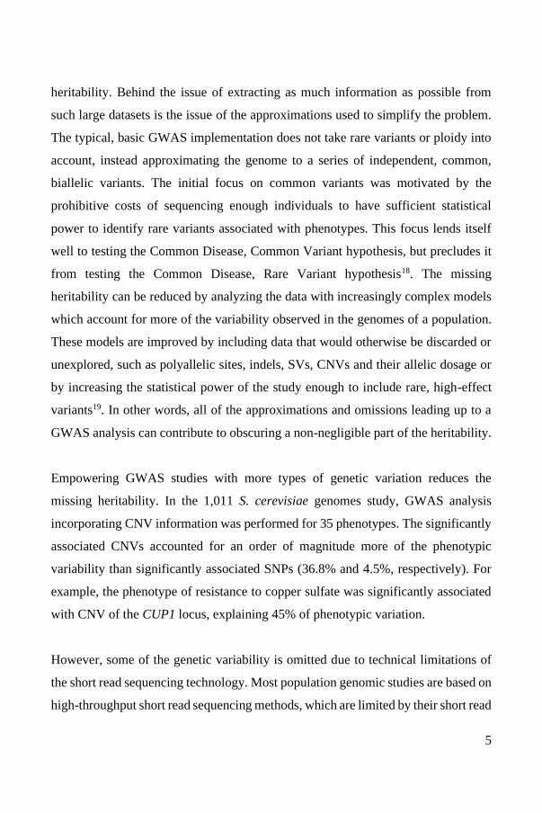
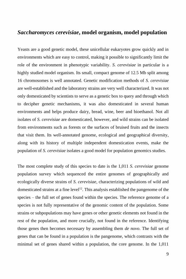
The untapped potential of polyploid beer isolates of Saccharomyces cerevisiae

While classically thought of as a diploid species, the 1,011 S. cerevisiae genome

population survey identified that 11.5% of the isolates were polyploid (>2n).

Polyploidy was not evenly distributed within the population, instead strongly

associated with specific domestication environments: all of the ale beer strains and

the large majority of African beer strains were polyploid (Figure 1). Additionally,

nearly 20% of isolates presented aneuploidy, again strongly associated with human

environments, mainly affecting the ale beer and sake clades. The strong link between

11

polyploidy in S. cerevisiae and the brewing environment is particularly interesting

given that beer-brewing S. cerevisiae strains are a polyphyletic group31 consisting of

at least three different clades. The polyploid ale beers, polyploid African beer strains

and partially polyploid mosaic beers suggest that polyploidy is important to S.

cerevisiae in the brewing environment and developed independently. Raising further

questions, not all domesticated environments lead to polyploidy, nor do

domesticated environments which lead to high ethanol concentrations. The wine and

bioethanol strains are typically diploids.

Figure 1 - Distribution and fraction of polyploids in the SNP dendrogram of 1,011

Saccharomyces cerevisiae isolates

This dendrogram is based on the genomic SNPs of 1,011 isolates of S. cerevisiae from diverse

geographical and ecological origins, including human environments. Nearly 12% of these

1,011 strains are polyploid (>2n), and interestingly these polyploids are not equally

distributed among the different subpopulations. All ale beer strains, most African beer strains,

and a large fraction of the mixed origin and mosaic strains are polyploid, while all remaining

subpopulations are 2n or lower. The grey pie chart represents mosaic region 3. Tree based on

data from Peter et al. (2018), figure adapted from Krogerus et al. (2019).

12

The ale beer strains have been shown through phasing to be a polyploid admixture

of Asian and European wine strains32. This answers the historical question of the

nature of the polyploidy of these strains. Ale beer strains are mainly tetraploid and

seem to derive from a hybrid of two diploid strains. The origins of the other beer

groups have not yet been elucidated. The apparent link between beer brewing and

polyploidy, along with the frequent aneuploidy events make it particularly

interesting to interrogate these strains through phasing.

Independent hybridization events in Brettanomyces

bruxellensis

Other, non-model yeasts such as Brettanomyces bruxellensis can also be of

significant interest due to their complex genomes, population structure and economic

importance. This yeast species is found in breweries of some specialty Belgian

beers33 such as Lambic and is one of the species in the symbiotic film associated

with kombucha production34. B. bruxellensis also gained notoriety in the wine

industry due to its spoiling effect in wine production35. Its genome was only

assembled at near-chromosome scale (15 contigs for 8 chromosomes) in 201536 and

at chromosome scale (8 contigs) in 201737. Both of these attempts to establish a high

quality de novo reference used long read sequencing to achieve their goal. Its current

reference genome is 13 Mb large, split unevenly among 8 chromosomes. Due to its

economic importance, large collections of B. bruxellensis were readily available and

interest in this species has been high despite not being as well-studied or widely

adopted for analysis as the model yeast S. cerevisiae.

13

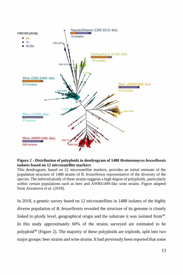
Figure 2 - Distribution of polyploids in dendrogram of 1488 Brettanomyces bruxellensis

isolates based on 12 microsatellite markers

This dendrogram, based on 12 microsatellite markers, provides an initial estimate of the

population structure of 1488 strains of B. bruxellensis representative of the diversity of the

species. The inferred ploidy of these strains suggests a high degree of polyploidy, particularly

within certain populations such as beer and AWRI1499-like wine strains. Figure adapted

from Avramova et al. (2018).

In 2018, a genetic survey based on 12 microsatellites in 1488 isolates of the highly

diverse population of B. bruxellensis revealed the structure of its genome is closely

linked to ploidy level, geographical origin and the substrate it was isolated from38.

In this study approximately 60% of the strains surveyed are estimated to be

polyploid38 (Figure 2). The majority of these polyploids are triploids, split into two

major groups: beer strains and wine strains. It had previously been reported that some

14

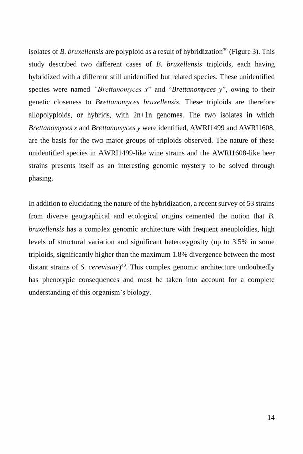
isolates of B. bruxellensis are polyploid as a result of hybridization39 (Figure 3). This

study described two different cases of B. bruxellensis triploids, each having

hybridized with a different still unidentified but related species. These unidentified

species were named “Brettanomyces x” and “Brettanomyces y”, owing to their

genetic closeness to Brettanomyces bruxellensis. These triploids are therefore

allopolyploids, or hybrids, with 2n+1n genomes. The two isolates in which

Brettanomyces x and Brettanomyces y were identified, AWRI1499 and AWRI1608,

are the basis for the two major groups of triploids observed. The nature of these

unidentified species in AWRI1499-like wine strains and the AWRI1608-like beer

strains presents itself as an interesting genomic mystery to be solved through

phasing.

In addition to elucidating the nature of the hybridization, a recent survey of 53 strains

from diverse geographical and ecological origins cemented the notion that B.

bruxellensis has a complex genomic architecture with frequent aneuploidies, high

levels of structural variation and significant heterozygosity (up to 3.5% in some

triploids, significantly higher than the maximum 1.8% divergence between the most

distant strains of S. cerevisiae)40. This complex genomic architecture undoubtedly

has phenotypic consequences and must be taken into account for a complete

understanding of this organism’s biology.

15

Figure 3 - Triploid Brettanomyces bruxellensis strains are suspected of being hybrids

(2n+1n)

Previous reports indicate that triploid B. bruxellensis strains appear to be hybrids containing

a core diploid genome and a more distantly related 1n genomic copy. The nature of this third

copy is unknown and it in fact appears that some strains harbor an extra genomic copy here

named Brettanomyces x, while other strains harbor a different extra copy, Brettanomyces y.

Figure adapted from Borneman et al., (2014).

16

Polyploid genomes and the phasing out of approximations

To better retrace the evolutionary history of a population and to assess the phenotypic

consequences of genetic sequences more accurately, it is important to take the entire

genome into account, in all its complexity and detail. In S. cerevisiae, the

polyphyletic group of beer strains presents higher ploidies, suggesting polyploidy is

a common adaptation to the brewing environment and raising the question of the

origins of these different beer groups. For B. bruxellensis the complex genomic

architecture and the mystery over the other species involved in the apparent multiple

independent hybridizations encourage a much closer look at the genomes of this

species. To fully explore both of these examples, as well as any other biological

system of a higher ploidy, would require phasing sequenced polyploid genomes. The

current processes to sequence a genome all involve a step which fragments the DNA

molecules. To obtain phase information, these DNA fragments, also called “reads”,

must then be pieced back together into the original chromosomes. For heterozygous

organisms, this fragmentation makes it difficult to know which SNPs co-occur on

the same chromosome. The phasing problem is the challenge of determining the

original sequences of the chromosomes, known as haplotypes.

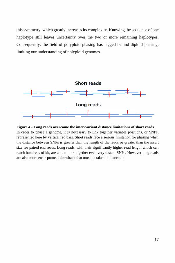
However, phasing has historically been difficult due to the read length of short read

sequencing methods being shorter than the distance between variants (Figure 4).

Long reads have led to highly performant methods for diploid phasing, notably

through the alignment-based method WhatsHap41 and the diploid aware de novo

assembly tool, Falcon Unzip42. However, polyploid phasing presents significant

additional complexity which is more difficult to resolve, even with long reads.

Crucially, for a heterozygous diploid, solutions to the problem can exploit an obvious

symmetry: finding the sequence of one haplotype necessarily leads to knowing the

sequence of the other. The polyploid phasing problem, however, does not display

17

this symmetry, which greatly increases its complexity. Knowing the sequence of one

haplotype still leaves uncertainty over the two or more remaining haplotypes.

Consequently, the field of polyploid phasing has lagged behind diploid phasing,

limiting our understanding of polyploid genomes.

Figure 4 - Long reads overcome the inter-variant distance limitations of short reads

In order to phase a genome, it is necessary to link together variable positions, or SNPs,

represented here by vertical red bars. Short reads face a serious limitation for phasing when

the distance between SNPs is greater than the length of the reads or greater than the insert

size for paired end reads. Long reads, with their significantly higher read length which can

reach hundreds of kb, are able to link together even very distant SNPs. However long reads

are also more error-prone, a drawback that must be taken into account.

18

Polyploid phasing methods

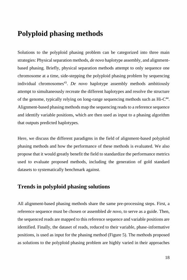
Solutions to the polyploid phasing problem can be categorized into three main

strategies: Physical separation methods, de novo haplotype assembly, and alignment-

based phasing. Briefly, physical separation methods attempt to only sequence one

chromosome at a time, side-stepping the polyploid phasing problem by sequencing

individual chromosomes43. De novo haplotype assembly methods ambitiously

attempt to simultaneously recreate the different haplotypes and resolve the structure

of the genome, typically relying on long-range sequencing methods such as Hi-C44.

Alignment-based phasing methods map the sequencing reads to a reference sequence

and identify variable positions, which are then used as input to a phasing algorithm

that outputs predicted haplotypes.

Here, we discuss the different paradigms in the field of alignment-based polyploid

phasing methods and how the performance of these methods is evaluated. We also

propose that it would greatly benefit the field to standardize the performance metrics

used to evaluate proposed methods, including the generation of gold standard

datasets to systematically benchmark against.

Trends in polyploid phasing solutions

All alignment-based phasing methods share the same pre-processing steps. First, a

reference sequence must be chosen or assembled de novo, to serve as a guide. Then,

the sequenced reads are mapped to this reference sequence and variable positions are

identified. Finally, the dataset of reads, reduced to their variable, phase-informative

positions, is used as input for the phasing method (Figure 5). The methods proposed

as solutions to the polyploid phasing problem are highly varied in their approaches

19

and mathematical and conceptual underpinnings. To provide a coherent framework

for this review, we delineate the development and usage of different strategies,

identifying four major trends:

Population inference methods, which leverage mapped reads of known genotypes

in related individuals or in a population to infer the haplotypes in a sample.

Objective function optimization methods, which typically represent the mapped

reads as a matrix and seek to minimize an objective function which typically

represents the amount of discrepancy between the predicted haplotypes and the

observed sequencing data.

Graph partitioning methods, which convert the mapped reads to a graph and seek

to split the graph into subgraphs that correspond to the haplotype predictions.

Cluster building methods, which rely on the similarity between mapped reads to

group them into clusters that correspond to predicted haplotypes.

We discuss these four paradigms, their implementations and limitations.

Figure 5 - Alignment-based phasing

Alignment-based phasing methods invariably require the following steps: DNA sequencing

of the sample, which fragments the DNA into sequenced reads. The reads are then mapped

to a reference sequence and heterozygous sites are identified by variant calling. The dataset

of reads associated with their variable positions is then input to a phasing method and

predicted haplotypes are output. These predicted haplotypes therefore conform to the

structure of the reference sequence that was aligned to initially.

20

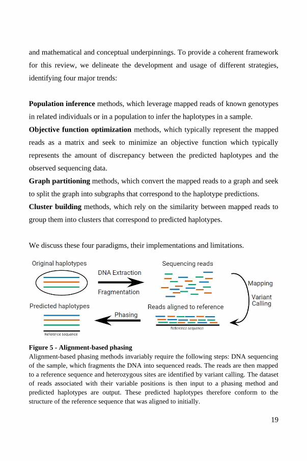
A - Population inference

To solve the polyploid phasing problem, population inference methods rely on the

availability of significant amounts of genomic data. Rather than attempt to phase

each genome individually, these methods leverage the genetic information of several

individuals to inform the phasing (Figure 6). The choice of population is important

to the strategy, and can range from large, non-specific populations of individuals of

the same species45–49, to highly specific, smaller populations such as parents or

siblings50–52.

Figure 6 - Population inference strategy

Population inference methods typically cast the mapped reads to a matrix and compare them

to a panel composed of haplotype information obtained from sequencing either a large

population of individuals, or a smaller group of individuals related to the sample. Haplotypes

are predicted through statistical inference based on the frequency of jointly observed

genotypes.

The first such methods, SATlotyper45 and polyHap46, used large populations of

unrelated individuals, while later methods such as TriPoly50, PopPoly51 and

mapPoly52 exploit pedigree information to inform their predictions. The methods

employed to leverage population data for phasing are highly varied: SATlotyper

casts the polyploid phasing problem as a boolean satisfiability problem45, polyHap46

21

and mapPoly52 both use Hidden Markov Models to leverage the statistical

information in populations of individuals, superMASSA47 frames it as a graphical

Bayesian problem, SHEsisPlus48 developed a formulation of the Expectation

Maximization algorithm to predict the most likely haplotypes, and TriPoly50 and

PopPoly51 both leverage pedigree information and Mendelian laws of inheritance to

phase haplotypes. Finally, while Poly-Harsh49 is not fully a population inference

algorithm, its authors describe a clustering algorithm using population inference to

connect fragmented phase blocks, improving the contiguity of phasing.

Population inference methods are particularly powerful when it comes to extending

the reach of short read sequencing using statistical information. This has a very

positive effect on contiguity without requiring the use of other sequencing methods.

The public availability of a significant amount of sequencing data for various

organisms is a very valuable resource for this method, though applying it to less

studied organisms can prove more costly than other strategies presented here. One

of the notable limitations inherent to population inference methods is the requirement

of a sequenced population. For the methods which require large populations, the

material and labor cost of obtaining and sequencing a large number of individuals

can be a significant limiting factor. For those which require fewer but related

individuals, the difficulty can lay in the existence or availability of such individuals.

This renders these methods inappropriate for situations with limited resources, such

as any study of a single individual, particularly if it is an individual of a species

which is not extensively studied and sequenced.

The choice of the reference sequence against which to map the population is also a

crucial one for these methods. The mapping and variant calling operations can be

computationally expensive, and their quality is dependent on the quality of the

reference sequence in use. Here, a seemingly intractable problem is apparent for

some applications of population inference methods. Any species with a propensity

22

for structural variation would be difficult to phase with these methods, as the

architecture of their genomes does not lend itself well to using the same reference

for all individuals of the population. This makes it impossible to pick a reference

sequence which accurately represents the population, and difficult to obtain

sufficiently many distinct individuals with the same genomic architecture. Not all

organisms have extensive structural variations within their population, however, and

for populations which maintain highly similar genomic architectures, this strategy

remains appropriate.

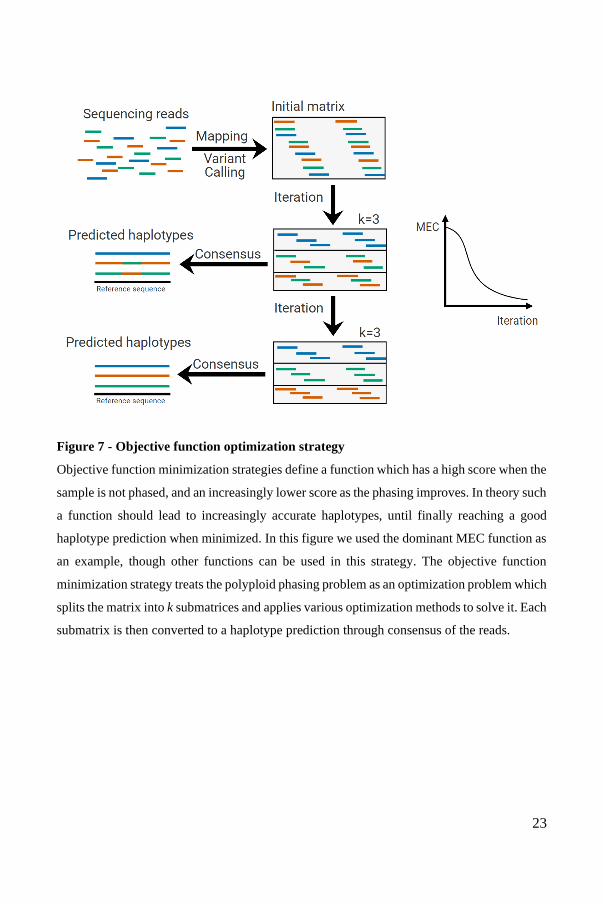
B - Objective function optimization

The objective function optimization strategy seeks to solve the phasing problem for

single individuals. This method defines an objective function, which it then

implements an algorithm to minimize (Figure 7). The objective function is typically

a measurement of how well the predicted haplotypes correspond to the reads in the

dataset. For example, for MEC (Minimum Error Correction) optimization, the

objective function counts how many mismatches there are between the predicted

haplotypes and the set of mapped reads. The intuition is that a low MEC score

implies a highly accurate phasing. Another variant of this method is the MFR

(Minimum Fragment Removal) method, in which the objective function is

minimized when the predicted haplotypes and the set of mapped reads are in perfect

agreement after the removal of as few reads as possible. Typically, but not always,

objective function optimization methods cast the dataset of reads as a matrix and

implement known or novel algorithms and heuristics intended to minimize the

chosen objective function in the matrix.

23

Figure 7 - Objective function optimization strategy

Objective function minimization strategies define a function which has a high score when the

sample is not phased, and an increasingly lower score as the phasing improves. In theory such

a function should lead to increasingly accurate haplotypes, until finally reaching a good

haplotype prediction when minimized. In this figure we used the dominant MEC function as

an example, though other functions can be used in this strategy. The objective function

minimization strategy treats the polyploid phasing problem as an optimization problem which

splits the matrix into k submatrices and applies various optimization methods to solve it. Each

submatrix is then converted to a haplotype prediction through consensus of the reads.

24

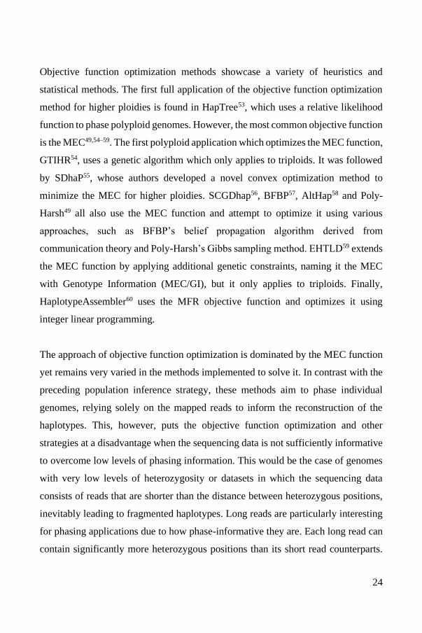
Objective function optimization methods showcase a variety of heuristics and

statistical methods. The first full application of the objective function optimization

method for higher ploidies is found in HapTree53, which uses a relative likelihood

function to phase polyploid genomes. However, the most common objective function

is the MEC49,54–59. The first polyploid application which optimizes the MEC function,

GTIHR54, uses a genetic algorithm which only applies to triploids. It was followed

by SDhaP55, whose authors developed a novel convex optimization method to

minimize the MEC for higher ploidies. SCGDhap56, BFBP57, AltHap58 and Poly-

Harsh49 all also use the MEC function and attempt to optimize it using various

approaches, such as BFBP’s belief propagation algorithm derived from

communication theory and Poly-Harsh’s Gibbs sampling method. EHTLD59 extends

the MEC function by applying additional genetic constraints, naming it the MEC

with Genotype Information (MEC/GI), but it only applies to triploids. Finally,

HaplotypeAssembler60 uses the MFR objective function and optimizes it using

integer linear programming.

The approach of objective function optimization is dominated by the MEC function

yet remains very varied in the methods implemented to solve it. In contrast with the

preceding population inference strategy, these methods aim to phase individual

genomes, relying solely on the mapped reads to inform the reconstruction of the

haplotypes. This, however, puts the objective function optimization and other

strategies at a disadvantage when the sequencing data is not sufficiently informative

to overcome low levels of phasing information. This would be the case of genomes

with very low levels of heterozygosity or datasets in which the sequencing data

consists of reads that are shorter than the distance between heterozygous positions,

inevitably leading to fragmented haplotypes. Long reads are particularly interesting

for phasing applications due to how phase-informative they are. Each long read can

contain significantly more heterozygous positions than its short read counterparts.

25

However, none of the objective function optimization methods cited here take long

reads into account. The intuition behind the optimization of an objective function is

typically guided by the notion that the predicted haplotypes must conform in some

way to the information present in the set of mapped reads. This assumption holds

fairly well only if the read dataset is known to be of high quality and not error-prone.

These methods are more appropriate for relatively error-free reads.

Objective function minimization strategies do not suffer from the same issues with

complex genomic architectures as the population inference methods do. However,

they all coerce the reads into a selectable ploidy k, which is incompatible with the

biological reality that a polyploid genome of ploidy n does not necessarily have n

haplotypes throughout its genome. For example, it may have an extra copy of one of

its chromosomes, with its own unique haplotype. Alternatively, it may have the exact

same haplotype for a large region of two of its chromosomes, effectively presenting

only n-1 haplotypes for that region. An algorithm that coerces exactly k haplotypes

on the entire genome will provide erroneous results if these edge cases are not

considered and explicitly handled in some way. For polyploid genomes with simpler

genomic architectures, where the ploidy and number of haplotypes remain stable,

these methods remain appropriate.

26

C - Graph partitioning

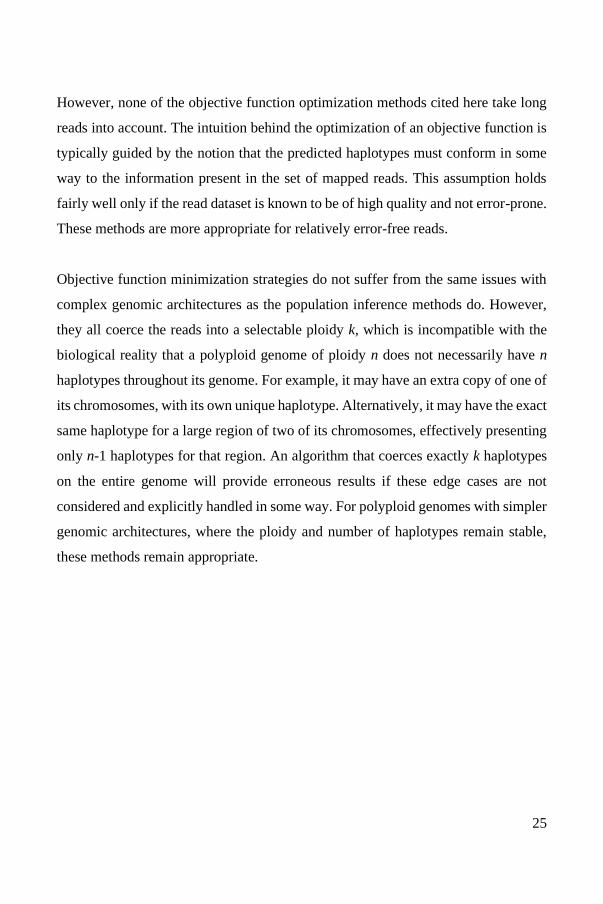
The graph partitioning strategy casts the dataset of mapped reads as a graph.

Typically, each mapped read is a node and each edge represents how similar two

nodes are. The goal is then to determine the optimal way to split the graph into

subgraphs that represent the different predicted haplotypes (Figure 8). It departs from

the objective function strategy by seeking to group similar mapped reads together,

away from dissimilar mapped reads, rather than seeking to optimize for coherence

of the predicted haplotypes with the set of mapped reads. It achieves this through the

use of the graph model and its associated mathematical tools and algorithms. To this

end, graph partitioning algorithms are implemented or developed and applied,

outputting subgraphs which are then converted to haplotype sequences, usually

through majority voting.

Typical graph partitioning solutions to the polyploid phasing problem cast the

mapped reads as nodes and give weights to overlapping nodes which penalize

differences between them. Then a graph partitioning algorithm is applied to the graph

in order to obtain the subgraphs which correspond to the haplotype predictions. In

HapColor61, the weight between mapped reads corresponds to the number of

mismatches between them. It then applies the DSatur (Degree of saturation)

algorithm, obtaining a high number of subgraphs, which it then iteratively merges

until only k subgraphs remain. For PolyCluster62, Hap1063, ComHapDet64 and

WhatsHap Polyphase65, the nodes are also mapped reads, and the weights are

negative if there are many mismatches between reads, and positive if there are many

matches. This then encourages their respective graph partitioning algorithm to cut

the graph along the lines of negatively weighted disagreement. Hap10 and WhatsHap

Polyphase distinguish themselves through their use of long reads. Hap10 uses 10X

linked reads and applies a max-k-cut algorithm, while WhatsHap Polyphase uses

27

PacBio and Oxford Nanopore long reads and applies heuristics to solve the cluster

editing problem. Notably, the initial cluster editing step of WhatsHap Polyphase is

ploidy agnostic, meaning it is not biased towards a specific ploidy. However,

WhatsHap Polyphase still coerces a specific ploidy, but it does so while explicitly

taking into account the edge case of local regions of similarity between haplotypes

in a process it terms haplotype threading.

Figure 8 - Graph partitioning strategy

Graph partitioning strategies cast the mapped reads to a graph in which typically the reads

are nodes and the edges between them correspond to a measure of how similar or dissimilar

the reads are to each other based on the variants they carry. The goal is to identify k subgraphs

of reads derived from the same haplotype, and to that end various graph partitioning methods

are applied. Each subgraph is then converted to a haplotype prediction through consensus of

the reads.

28

There have been two other graph partitioning methods which cast the mapped reads

to a graph in a different way. The first application of graph partitioning methods to

the polyploid phasing problem was an extension to HapCompass66 which made it

applicable to polyploids. Under the HapCompass model, each node is a SNP, and

the mapped reads are edges. The use of SNPs as nodes is uncommon, but observed

again recently with HRCH67, another non-standard example of a graph partitioning

method. HRCH uses a weighted SNP hypergraph, which it then partitions into

predicted haplotypes using the hypergraph partitioning algorithm hMETIS.

The graph partitioning strategy relies on the notion that reads which derive from the

same haplotype will be similar to each other, and dissimilar to reads derived from

other haplotypes. They should then naturally form tightly connected graphs if

attributed weights which correspond to their similarity (or dissimilarity). This

strategy leverages well-established algorithms which efficiently split graphs into

well-connected components. WhatsHap Polyphase’s application of a graph

partitioning strategy to long read datasets and its handling of part of the complexity

brought on by the variability in genomic architectures is encouraging for the

handling of the more complex problems of polyploid phasing. However, most graph

partitioning algorithms, and all methods presented here, coerce the graph into k

subgraphs. This leads to the same pitfalls as discussed for the objective function

strategy, notably with structural variants and aneuploidies. While it may be possible

to handle all edge cases in post-processing steps, careful consideration should be

placed upon the sample being studied and the limitations and biases inherent to the

phasing algorithm being used. There may be an existing or yet to be developed graph

partitioning method which is intrinsically capable of resolving complex genomes

containing aneuploidies, structural variants and a variable number of local

haplotypes, however this has not yet been shown. This strategy may prove to be the

29

model of choice for resolving complex polyploid genomes, particularly when

combined with long reads.

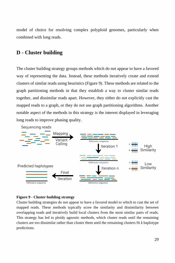
D - Cluster building

The cluster building strategy groups methods which do not appear to have a favored

way of representing the data. Instead, these methods iteratively create and extend

clusters of similar reads using heuristics (Figure 9). These methods are related to the

graph partitioning methods in that they establish a way to cluster similar reads

together, and dissimilar reads apart. However, they either do not explicitly cast the

mapped reads to a graph, or they do not use graph partitioning algorithms. Another

notable aspect of the methods in this strategy is the interest displayed in leveraging

long reads to improve phasing quality.

Figure 9 - Cluster building strategy

Cluster building strategies do not appear to have a favored model to which to cast the set of

mapped reads. These methods typically score the similarity and dissimilarity between

overlapping reads and iteratively build local clusters from the most similar pairs of reads.

This strategy has led to ploidy agnostic methods, which cluster reads until the remaining

clusters are too dissimilar rather than cluster them until the remaining clusters fit k haplotype

predictions.

30

H-Pop and H-PopG68 represent the read data as a matrix and seek to split the matrix

into k parts, with each part corresponding to a group of reads with maximal

similarity. Each group then represents a different haplotype, and it therefore

introduces a diversity measure, which seeks to maximize the difference between the

k groups, or predicted haplotypes. Similarly, Ranbow69 uses a seed and extend

paradigm to locally, iteratively cluster reads together based on similarity and

dissimilarity measures. While it does coerce k haplotypes, it also handles the edge

case where the number of haplotypes is less than k. While Ranbow is described only

for short reads, its authors express interest in extending it to use long reads.

All of the cluster building methods which do use long reads are ploidy agnostic,

meaning they do not coerce a specific ploidy. Chaisson et al., 2018 propose a

correlation clustering method to solve the polyploid phasing problem using long

reads, however it is designed to only phase parts of the genome, intended to resolve

multicopy duplications, and no tool was released.70 This is the first ploidy agnostic

phasing method applied to part of a genome. In an unnamed method32, Fay et al.,

2019 describe a custom phasing algorithm they developed in order to analyze

admixed polyploid yeasts. Using mapped long reads, they score similar reads

positively, and dissimilar ones negatively, then proceed to iteratively merge long

reads together for three rounds. This is the first example of a ploidy agnostic method

applied to entire genomes, though it is not compared to other methods or released as

a tool for the community to use. Finally, nPhase71, a method we recently developed,

solves the polyploid phasing problem by iteratively clustering similar reads together

until only unique haplotypes remain. It is the first ploidy agnostic phasing method

applicable to entire genomes to be released as a tool.

The cluster building strategy shares the same intuition that drives the graph

partitioning strategy. Reads derived from the same haplotype will resemble each

other and be different from reads derived from another haplotype. However, in

31

contrast with the graph partitioning strategy, these methods do not cast the set of

mapped reads to a graph. Instead, the cluster building methods are defined by the

strategy of iteratively growing clusters of reads while maintaining the diversity of

the clusters. Interestingly, this strategy has led to three ploidy agnostic phasing

methods, all of which leverage long reads. Ranbow handles the edge case where the

number of haplotypes is locally lower than the ploidy, and the ploidy agnostic

methods in theory adapt to the shape of the genomic architecture. While it should be

expected that ploidy agnostic methods are capable of handling aneuploidies and local

changes in the number of haplotypes, they do not provide any handling of other

structural variants such as heterozygous inversions and translocations. This is partly

a consequence of the nature of all of these strategies as alignment-based phasing

methods, since they are limited to the genomic architecture imposed by the haploid

reference sequence. However, long reads can provide a significant amount of

information about structural variants, notably through split reads. No method of

polyploid phasing attempts to use split reads to resolve heterozygous structural

variation. The development of such a method would be a significant step towards

complete polyploid phasing methods. For complex genomes, cluster building

methods, and in particular ploidy agnostic phasing methods are appropriate.

However, one major drawback of ploidy agnostic methods is the interpretability of

the results. It is less straight-forward to manipulate ploidy agnostic phasing results

than phasing results which neatly fit an expectation of k haplotypes.

32

Overview

The four strategies we described attempt to solve the same problem, and there are

large interfaces between them. The way a problem is modeled influences the solution

space that is intuitive and the mathematical tools which are at our disposal to solve

it. We find that the field of alignment-based polyploid phasing algorithms has

evolved to tackle increasingly complex formulations of the problem, using

increasingly sophisticated strategies and tools, yet still has significant room for

improvement. In particular, long reads are under-exploited despite representing a

very significant tool to obtain large amounts of phase information. The polyploid

phasing problem also needs to explicitly tackle and resolve the problems of

heterozygous structural variants, aneuploidies and local variations in the number of

haplotypes. The ploidy agnostic methods tackle some of the complexity of genomic

architecture, but not all. For brevity, we did not discuss whether or not each method

phases only biallelic SNPs, or also phases indels and multiallelic SNPs. However, it

is clear that the majority of methods limit themselves to only phasing biallelic SNPs,

sometimes also multiallelic SNPs, and indels seem to only be phased by Ranbow.

We also discussed the importance of the chosen reference sequence, and it may

become common practice to perform a collapsed de novo assembly to generate an

appropriate reference for each sample prior to alignment-based phasing. However,

this also entails having to generate a new genome annotation for downstream

analyses and can unnecessarily complicate comparisons between samples. Overall,

there is still room for improvement in the field of polyploid phasing algorithms and

recommended practices.

33

Validation datasets and performance metrics

Once a polyploid phasing method has been developed, its performance must be

evaluated. To that end, a validation dataset which corresponds to a set of reads

obtained from a polyploid must be given as input to the phasing method, and the

output haplotype predictions must be evaluated by performance metrics.

The validation dataset can be simulated or real. In the case of simulated datasets, it

is possible to know the optimal phasing result, which allows for the use of detailed

metrics to better understand the performance of the polyploid phasing algorithm. A

validation dataset can be fully simulated, such as in Haptree53, which randomly

generates haplotypes and simulates reads derived from these haplotypes. Validation

datasets can also be partially simulated, or reconstructed. This is the case for

WhatsHap Polyphase and nPhase, which both merge real sequencing reads of

organisms with known haplotypes. WhatsHap Polyphase combines human datasets

with known haplotypes, while nPhase combines S. cerevisiae datasets of haploid and

homozygous diploid individuals. Fully simulated datasets have a high degree of

control over all characteristics of the genome, which allows them to test the effects

of different ploidy levels, heterozygosity levels, genome architectures, coverage

levels. However, these methods are highly dependent on the accuracy of their

simulations of genomes and sequencing results. Partially simulated datasets are more

faithful simulations of real haplotype phasing scenarios as they use real genomes,

with real SNPs and real sequencing reads. However, these genomes are still

artificially produced, typically presenting relatively uniform distance between

haplotypes, and there is less control over their characteristics, which limits the testing

space. Some parameters, such as the effects of coverage level and heterozygosity

rate, can still be queried by downsampling the number of reads or the variable

34

positions input to the phasing algorithm, however this process is less straight-

forward than it is for a fully simulated dataset.

For all simulated datasets, the ground truth is known and can be used to evaluate the

predicted haplotypes. A variety of metrics have been implemented, here we discuss

those most commonly used in the field.

The MEC score is not only an objective function used in a number of phasing

methods, but also a metric which has been routinely used as evidence of good

phasing. The MEC score, as a performance metric, has received some criticism in

the context of the polyploid phasing problem. In their paper on Ranbow, Moeinzadeh

et al. note that the MEC metric is incomplete, only considering sequencing errors69,

while in their paper for WhatsHap Polyphase, Schrinner et al. point out that low

MEC scores can be obtained with objective worse phasing result65. Due to the

significantly higher error rate of long read sequencing, any method relying on these

reads will necessarily obtain worse MEC scores despite the obvious advantages of

long reads, further limiting the usefulness of this metric for the evaluation of

polyploid phasing methods.

35

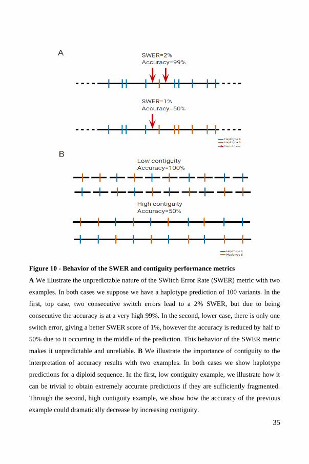
Figure 10 - Behavior of the SWER and contiguity performance metrics

A We illustrate the unpredictable nature of the SWitch Error Rate (SWER) metric with two

examples. In both cases we suppose we have a haplotype prediction of 100 variants. In the

first, top case, two consecutive switch errors lead to a 2% SWER, but due to being

consecutive the accuracy is at a very high 99%. In the second, lower case, there is only one

switch error, giving a better SWER score of 1%, however the accuracy is reduced by half to

50% due to it occurring in the middle of the prediction. This behavior of the SWER metric

makes it unpredictable and unreliable. B We illustrate the importance of contiguity to the

interpretation of accuracy results with two examples. In both cases we show haplotype

predictions for a diploid sequence. In the first, low contiguity example, we illustrate how it

can be trivial to obtain extremely accurate predictions if they are sufficiently fragmented.

Through the second, high contiguity example, we show how the accuracy of the previous

example could dramatically decrease by increasing contiguity.

36

The Switch Error Rate (SWER), also described as the Vector Error Rate (VER),

measures how frequently the predicted haplotype switches between true phases

(Figure 10A). Optimization of this metric does not necessarily lead to improved

phasing accuracy, as a single vector can reduce the accuracy by half. In a real use

case, the presence of a switch error has a much more significant consequence than

the presence of a few point errors. As we argued in our paper on nPhase71, the

interpretability of the SWER is further complicated by the fact that the presence of

more switch errors can result in significantly better phasing results, rendering the

metric fundamentally unpredictable. The use of this metric is no doubt motivated by

the observation that it is possible to phase several SNPs very well, yet a single switch

error can reduce the accuracy by up to 50%. Hence methods which produce longer

phase blocks, more susceptible to switch errors, may appear to have worse accuracy

despite having large stretches of correctly phased blocks. However, this metric

remains flawed and does not behave predictably. Some possible replacement metrics

would be to report the mean length of unbroken phase blocks, or the minimal

unbroken phased block length to cover 90% of the SNPs.

The accuracy, also described as the Reconstruction Rate or Hamming distance

measures how accurate the phasing is globally. Accuracy can be defined in two

forms. The first is the prediction accuracy, which at 99% can state that for every 100

SNP predictions it makes, on average 1 SNP will be in the wrong phase. The second

is the reconstruction accuracy, which at 99% states that for every 100 SNPs in the

genome, on average 1 SNP will be in the wrong phase or not phased. The latter is

more stringent by taking the missing rate into account. In both cases, the accuracy

metric gives an important notion of how accurate the predictions are, making it a

crucial performance metric to evaluate.

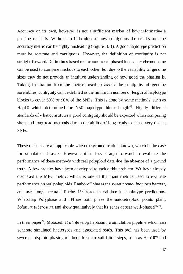
37

Accuracy on its own, however, is not a sufficient marker of how informative a

phasing result is. Without an indication of how contiguous the results are, the

accuracy metric can be highly misleading (Figure 10B). A good haplotype prediction

must be accurate and contiguous. However, the definition of contiguity is not

straight-forward. Definitions based on the number of phased blocks per chromosome

can be used to compare methods to each other, but due to the variability of genome

sizes they do not provide an intuitive understanding of how good the phasing is.

Taking inspiration from the metrics used to assess the contiguity of genome

assemblies, contiguity can be defined as the minimum number or length of haplotype

blocks to cover 50% or 90% of the SNPs. This is done by some methods, such as

Hap10 which determined the N50 haplotype block length63. Highly different

standards of what constitutes a good contiguity should be expected when comparing

short and long read methods due to the ability of long reads to phase very distant

SNPs.

These metrics are all applicable when the ground truth is known, which is the case

for simulated datasets. However, it is less straight-forward to evaluate the

performance of these methods with real polyploid data due the absence of a ground

truth. A few proxies have been developed to tackle this problem. We have already

discussed the MEC metric, which is one of the main metrics used to evaluate

performance on real polyploids. Ranbow69 phases the sweet potato, Ipomoea batatas,

and uses long, accurate Roche 454 reads to validate its haplotype predictions.

WhatsHap Polyphase and nPhase both phase the autotetraploid potato plant,

Solanum tuberosum, and show qualitatively that its genes appear well-phased65,71.

In their paper72, Motazedi et al. develop haplosim, a simulation pipeline which can

generate simulated haplotypes and associated reads. This tool has been used by

several polyploid phasing methods for their validation steps, such as Hap1063 and

38

Ranbow69. However, there is no widely used benchmarking dataset which can

systematically be compared against, and haplosim does not appear to have been

updated in the past three years to reflect the significant improvements in quality

achieved in long read sequencing methods. A well-maintained gold standard

benchmark would be of benefit to the field of polyploid phasing. It would be

interesting for such a resource to carefully consider the performance metrics to

evaluate, the diversity of read sequencing methods and the effects of variable ploidy,

genome architecture, heterozygosity level, genome size, structural variation, indels,

polyallelic sites and local variations in the number of haplotypes.

39

References

1. International Human Genome Sequencing Consortium. Finishing the euchromatic

sequence of the human genome. Nature 431, 931–945 (2004).

2. Mewes, H. W. et al. Overview of the yeast genome. Nature 387, 7–8 (1997).

3. The Arabidopsis Genome Initiative. Analysis of the genome sequence of the flowering

plant Arabidopsis thaliana. Nature 408, 796–815 (2000).

4. Chinwalla, A. T. et al. Initial sequencing and comparative analysis of the mouse genome.

Nature 420, 520–562 (2002).

5. Delsuc, F., Brinkmann, H. & Philippe, H. Phylogenomics and the reconstruction of the

tree of life. Nat. Rev. Genet. 6, 361–375 (2005).

6. Miller, W., Makova, K. D., Nekrutenko, A. & Hardison, R. C. Comparative genomics.

Annu. Rev. Genomics Hum. Genet. 5, 15–56 (2004).

7. Alföldi, J. & Lindblad-Toh, K. Comparative genomics as a tool to understand evolution

and disease. Genome Res. 23, 1063–1068 (2013).

8. The 3, 000 rice genomes project. The 3,000 rice genomes project. GigaScience 3, 7 (2014).

9. Auton, A. et al. A global reference for human genetic variation. Nature 526, 68–74 (2015).

10. Sudmant, P. H. et al. An integrated map of structural variation in 2,504 human genomes.

Nature 526, 75–81 (2015).

11. Alonso-Blanco, C. et al. 1,135 Genomes Reveal the Global Pattern of Polymorphism in

Arabidopsis thaliana. Cell 166, 481–491 (2016).

12. Peter, J. et al. Genome evolution across 1,011 Saccharomyces cerevisiae isolates. Nature

556, 339–344 (2018).

13. DeWan, A. et al. HTRA1 Promoter Polymorphism in Wet Age-Related Macular

Degeneration. Science 314, 989–992 (2006).

14. Ozaki, K. et al. Functional SNPs in the lymphotoxin-alpha gene that are associated with

susceptibility to myocardial infarction. Nat. Genet. 32, 650–654 (2002).

15. Sims, R., Hill, M. & Williams, J. The multiplex model of the genetics of Alzheimer’s

disease. Nat. Neurosci. 23, 311–322 (2020).

16. Raybould, R. & Sims, R. Searching the Dark Genome for Alzheimer’s Disease Risk

Variants. Brain Sci. 11, 332 (2021).

17. Wall, J. D. et al. The GenomeAsia 100K Project enables genetic discoveries across Asia.

Nature 576, 106–111 (2019).

18. Schork, N. J., Murray, S. S., Frazer, K. A. & Topol, E. J. Common vs. Rare Allele

Hypotheses for Complex Diseases. Curr. Opin. Genet. Dev. 19, 212–219 (2009).

19. Génin, E. Missing heritability of complex diseases: case solved? Hum. Genet. 139, 103–

113 (2020).

20. Yang, J. et al. Incomplete dominance of deleterious alleles contributes substantially to

trait variation and heterosis in maize. PLOS Genet. 13, e1007019 (2017).

40

21. Roach, M. J. et al. Population sequencing reveals clonal diversity and ancestral inbreeding

in the grapevine cultivar Chardonnay. PLOS Genet. 14, e1007807 (2018).

22. Robles-Espinoza, C. D., Mohammadi, P., Bonilla, X. & Gutierrez-Arcelus, M. Allele-

specific expression: applications in cancer and technical considerations. Curr. Opin. Genet.

Dev. 66, 10–19 (2021).

23. Vohra, M., Sharma, A. R., B, N. P. & Rai, P. S. SNPs in Sites for DNA Methylation,

Transcription Factor Binding, and miRNA Targets Leading to Allele-Specific Gene

Expression and Contributing to Complex Disease Risk: A Systematic Review. Public Health

Genomics 23, 155–170 (2020).

24. Kitzman, J. O. et al. Haplotype-resolved genome sequencing of a Gujarati Indian

individual. Nat. Biotechnol. 29, 59–63 (2011).

25. Sanjak, J. S., Long, A. D. & Thornton, K. R. A Model of Compound Heterozygous, Loss-

of-Function Alleles Is Broadly Consistent with Observations from Complex-Disease GWAS

Datasets. PLOS Genet. 13, e1006573 (2017).

26. Cox, A. J. et al. In trans variant calling reveals enrichment for compound heterozygous

variants in genes involved in neuronal development and growth. Genet. Res. 101, (2019).

27. Zhang, Z. et al. Ancestral haplotype-based association mapping with generalized linear

mixed models accounting for stratification. Bioinformatics 28, 2467–2473 (2012).

28. Hamazaki, K. & Iwata, H. RAINBOW: Haplotype-based genome-wide association study

using a novel SNP-set method. PLOS Comput. Biol. 16, e1007663 (2020).

29. A Genome-Wide Association Study for Agronomic Traits in Soybean Using SNP

Markers and SNP-Based Haplotype Analysis.

https://www.ncbi.nlm.nih.gov/pmc/articles/PMC5289539/.

30. Eriksson, J. S. et al. Allele phasing is critical to revealing a shared allopolyploid origin

of Medicago arborea and M. strasseri (Fabaceae). BMC Evol. Biol. 18, 9 (2018).

31. Gallone, B. et al. Domestication and Divergence of Saccharomyces cerevisiae Beer

Yeasts. Cell 166, 1397-1410.e16 (2016).

32. Fay, J. C. et al. A polyploid admixed origin of beer yeasts derived from European and

Asian wine populations. PLOS Biol. 17, e3000147 (2019).

33. Steensels, J. et al. Brettanomyces yeasts — From spoilage organisms to valuable

contributors to industrial fermentations. Int. J. Food Microbiol. 206, 24–38 (2015).

34. Teoh, A. L., Heard, G. & Cox, J. Yeast ecology of Kombucha fermentation. Int. J. Food

Microbiol. 95, 119–126 (2004).

35. Conterno, L., Joseph, C. M. L., Arvik, T. J., Henick-Kling, T. & Bisson, L. F. Genetic

and Physiological Characterization of Brettanomyces bruxellensis Strains Isolated from

Wines. Am. J. Enol. Vitic. 57, 139–147 (2006).

36. Olsen, R.-A. et al. De novo assembly of Dekkera bruxellensis: a multi technology

approach using short and long-read sequencing and optical mapping. GigaScience 4, 56

(2015).

41

37. Fournier, T. et al. High-Quality de Novo Genome Assembly of the Dekkera bruxellensis

Yeast Using Nanopore MinION Sequencing. G3 GenesGenomesGenetics 7, 3243–3250

(2017).

38. Avramova, M. et al. Brettanomyces bruxellensis population survey reveals a diploid-

triploid complex structured according to substrate of isolation and geographical distribution.

Sci. Rep. 8, 4136 (2018).

39. Borneman, A. R., Zeppel, R., Chambers, P. J. & Curtin, C. D. Insights into the Dekkera

bruxellensis Genomic Landscape: Comparative Genomics Reveals Variations in Ploidy and

Nutrient Utilisation Potential amongst Wine Isolates. PLOS Genet. 10, e1004161 (2014).

40. Gounot, J.-S. et al. High Complexity and Degree of Genetic Variation in Brettanomyces

bruxellensis Population. Genome Biol. Evol. 12, 795–807 (2020).

41. Patterson, M. et al. WhatsHap: Weighted Haplotype Assembly for Future-Generation

Sequencing Reads. J. Comput. Biol. 22, 498–509 (2015).

42. Chin, C.-S. et al. Phased diploid genome assembly with single-molecule real-time

sequencing. Nat. Methods 13, 1050–1054 (2016).

43. Ruo-Nan, Z. & Zan-Min, H. The Development of Chromosome Microdissection and

Microcloning Technique and its Applications in Genomic Research. Curr. Genomics 8, 67–

72 (2007).

44. Zhang, X., Zhang, S., Zhao, Q., Ming, R. & Tang, H. Assembly of allele-aware,

chromosomal-scale autopolyploid genomes based on Hi-C data. Nat. Plants 5, 833–845

(2019).

45. Neigenfind, J. et al. Haplotype inference from unphased SNP data in heterozygous

polyploids based on SAT. BMC Genomics 9, 356 (2008).

46. Su, S.-Y., White, J., Balding, D. J. & Coin, L. J. Inference of haplotypic phase and missing

genotypes in polyploid organisms and variable copy number genomic regions. BMC

Bioinformatics 9, 513 (2008).

47. Serang, O., Mollinari, M. & Garcia, A. A. F. Efficient Exact Maximum a Posteriori

Computation for Bayesian SNP Genotyping in Polyploids. PLOS ONE 7, e30906 (2012).

48. Shen, J. et al. SHEsisPlus, a toolset for genetic studies on polyploid species. Sci. Rep. 6,

24095 (2016).

49. He, D., Saha, S., Finkers, R. & Parida, L. Efficient algorithms for polyploid haplotype

phasing. BMC Genomics 19, 110 (2018).

50. Motazedi, E. et al. TriPoly: haplotype estimation for polyploids using sequencing data of

related individuals. Bioinformatics 34, 3864–3872 (2018).

51. Motazedi, E., Maliepaard, C., Finkers, R., Visser, R. & de Ridder, D. Family-Based

Haplotype Estimation and Allele Dosage Correction for Polyploids Using Short Sequence

Reads. Front. Genet. 0, (2019).

52. Mollinari, M. & Garcia, A. A. F. Linkage Analysis and Haplotype Phasing in

Experimental Autopolyploid Populations with High Ploidy Level Using Hidden Markov

Models. G3 GenesGenomesGenetics 9, 3297–3314 (2019).

42

53. Berger, E., Yorukoglu, D., Peng, J. & Berger, B. HapTree: A Novel Bayesian Framework

for Single Individual Polyplotyping Using NGS Data. PLOS Comput. Biol. 10, e1003502

(2014).

54. Wu, J., Chen, X. & Li, X. Haplotyping a single triploid individual based on genetic

algorithm. Biomed. Mater. Eng. 24, 3753–3762 (2014).

55. Das, S. & Vikalo, H. SDhaP: haplotype assembly for diploids and polyploids via semi-

definite programming. BMC Genomics 16, 260 (2015).

56. Cai, C., Sanghavi, S. & Vikalo, H. Structured Low-Rank Matrix Factorization for

Haplotype Assembly. IEEE J. Sel. Top. Signal Process. 10, 647–657 (2016).

57. Puljiz, Z. & Vikalo, H. Decoding Genetic Variations: Communications-Inspired

Haplotype Assembly. IEEE/ACM Trans. Comput. Biol. Bioinform. 13, 518–530 (2016).

58. Hashemi, A., Zhu, B. & Vikalo, H. Sparse Tensor Decomposition for Haplotype

Assembly of Diploids and Polyploids. BMC Genomics 19, 191 (2018).

59. Wu, J. & Zhang, Q. A fast and accurate enumeration-based algorithm for haplotyping a

triploid individual. Algorithms Mol. Biol. 13, 10 (2018).

60. Siragusa, E., Haiminen, N., Finkers, R., Visser, R. & Parida, L. Haplotype assembly of

autotetraploid potato using integer linear programing. Bioinformatics 35, 3279–3286 (2019).

61. Mazrouee, S. & Wang, W. HapColor: A graph coloring framework for polyploidy

phasing. in 2015 IEEE International Conference on Bioinformatics and Biomedicine (BIBM)

105–108 (2015). doi:10.1109/BIBM.2015.7359663.

62. Mazrouee, S. & Wang, W. PolyCluster: Minimum Fragment Disagreement Clustering

for Polyploid Phasing. IEEE/ACM Trans. Comput. Biol. Bioinform. 17, 264–277 (2020).

63. Majidian, S., Kahaei, M. H. & de Ridder, D. Hap10: reconstructing accurate and long

polyploid haplotypes using linked reads. BMC Bioinformatics 21, 253 (2020).

64. Sankararaman, A., Vikalo, H. & Baccelli, F. ComHapDet: a spatial community detection

algorithm for haplotype assembly. BMC Genomics 21, 586 (2020).

65. Schrinner, S. D. et al. Haplotype threading: accurate polyploid phasing from long reads.

Genome Biol. 21, 252 (2020).

66. Aguiar, D. & Istrail, S. Haplotype assembly in polyploid genomes and identical by

descent shared tracts. Bioinformatics 29, i352–i360 (2013).

67. Olyaee, M. H., Khanteymoori, A. & Khalifeh, K. A chaotic viewpoint-based approach to

solve haplotype assembly using hypergraph model. PLOS ONE 15, e0241291 (2020).

68. Xie, M., Wu, Q., Wang, J. & Jiang, T. H-PoP and H-PoPG: heuristic partitioning

algorithms for single individual haplotyping of polyploids. Bioinformatics 32, 3735–3744

(2016).

69. Moeinzadeh, M.-H. et al. Ranbow: A fast and accurate method for polyploid haplotype

reconstruction. PLOS Comput. Biol. 16, e1007843 (2020).

70. Chaisson, M. J., Mukherjee, S., Kannan, S. & Eichler, E. E. Resolving Multicopy

Duplications de novo Using Polyploid Phasing. in Research in Computational Molecular

43

Biology (ed. Sahinalp, S. C.) 117–133 (Springer International Publishing, 2017).

doi:10.1007/978-3-319-56970-3_8.

71. Abou Saada, O., Tsouris, A., Eberlein, C., Friedrich, A. & Schacherer, J. nPhase: an

accurate and contiguous phasing method for polyploids. Genome Biol. 22, 126 (2021).

72. Motazedi, E., Finkers, R., Maliepaard, C. & de Ridder, D. Exploiting next-generation

sequencing to solve the haplotyping puzzle in polyploids: a simulation study. Brief.

Bioinform. 19, 387–403 (2018).

44

Project summary

Phasing, and in particular polyploid phasing, have been challenging problems held

back by the limited read length of high-throughput short read sequencing methods

which can’t overcome the distance between heterozygous sites and the financial and

labor high cost of alternative methods such as the physical separation of

chromosomes or use of fosmid libraries. Recently developed single molecule long-

read sequencing methods provide much longer reads which overcome this previous

limitation at reasonable costs. However, the accuracy of these methods has been

lower than that of the previous short read methods, despite rapid and frequent

improvements. Significant strides in the diploid phasing problem were achieved by

leveraging the long read length of long-read sequencing methods. For diploid

phasing, each variable position can only have one of two states, to place in one of

two haplotypes. This simplifies the task by making it possible to deduce one phase

by knowing the other. Tools such as the alignment-based WhatsHap1 and the de novo

assembly tool Falcon-Unzip2 exploit this inherent symmetry to provide good phasing

results for diploids. Efforts to solve polyploid phasing, where the absence of

symmetry greatly complexifies the problem, still need to resolve significant

technical roadblocks. A large proportion of polyploid phasing methods designed for

short read data relied on the high accuracy of these reads and cannot be directly

applied or easily modified to accommodate the error profiles of long read methods.

The complex genomic architectures of polyploids such as the presence of

aneuploidies and regions of variable numbers of haplotypes also still need to be

addressed in order to obtain an accurate view of the structure of their genomes. The

absence of a reliable polyploid phasing strategy also translates to a dearth in

applications of polyploid phasing methods to populations of individuals.

45

In this context, we decided to develop a polyploid phasing algorithm which we

describe in Chapter I. Our tool, named nPhase, is a pipeline which takes as input a

reference sequence, a set of short reads and a set of long reads. The pipeline will

align the long and short read sequences to the reference, and it will variant call the

mapped short reads. Then this dataset is phased by our ploidy agnostic cluster

building method which adapts to the ploidy of the dataset and natively handles

aneuploidy and variations in the number of distinct haplotypes. Our method has a

few adjustable parameters and we describe how we selected the default parameters

through extensive testing on a simulated validation dataset. We also describe the

heuristics we developed to clean up raw phasing results obtained with nPhase.

Finally, we apply our algorithm to a triploid strain of the yeast species Brettanomyces

bruxellensis and to chromosome two of the autotetraploid plant Solanum tuberosum.

We also describe our observations regarding ways to validate results obtained on real

datasets, notably by introducing a new way to evaluate the quality of a phased cluster

based on the allelic frequencies observed within.

Having developed this ploidy agnostic phasing method, we then set out to apply it to

two real datasets. First, a large collection of 1,011 isolates of the yeast species

Saccharomyces cerevisiae were recently sequenced3. It was found that 11.5% of the

strains are polyploids. These polyploid isolates were not uniformly distributed

throughout the population, only affecting a few subpopulations. In particular we note

that the polyphyletic group of beers, mainly distributed across three main clades

(Beer 1, Beer 2 and African Beer), all were composed of a significant proportion of

polyploid strains. In Chapter II, we therefore sequenced 35 beer strains of S.

cerevisiae with Oxford Nanopore technology, obtaining long reads which we used

to phase this population with nPhase. We found that the three main beer yeast

subpopulations appear to derive from different admixtures of other populations. As

previously reported, strains of the Beer 1 clade were an admixture of Asian and

46

European wine strains. We found that strains of the Beer 2 clade were also composed

of a similar admixture, only with a higher proportion of European wine alleles. We

therefore renamed the Beer 1 and Beer 2 clades to the more evocative Asian

dominant and European dominant, respectively. Finally, the African Beer strains

mainly exhibited European wine alleles, with a background of French dairy alleles.

The phased data made it possible for us to estimate the genetic divergence of

haplotypes within and between strains. By comparing all haplotypes of genes and

selecting those with the highest levels of divergence (>4%), we identified significant

GO term enrichment for carbon metabolism, dehydrogenase activity, cell wall

remodeling and transporter activity. A deeper look at individual phased genes also

revealed different evolutionary trajectories of individual genes across

subpopulations, showing that the inactivation of the beer off-flavor forming gene

FDC1 was independently inactivated in the Asian dominant and African Beer

groups. We also found that the ADH2 and SFA1 genes which participate in the

formation of fusel alcohols, another source of off-flavors in beer, are inactivated in

Asian dominant strains.

Another species with an interesting polyploidization history is Brettanomyces

bruxellensis. This yeast species is used to brew some specialty Belgian beers and

participates in the microbial community that makes kombucha, but is also notorious

for contaminating bioethanol plants and wine. A very large collection of 1,500

isolates of B. bruxellensis was recently surveyed using microsatellite data and it was

identified that nearly 60% of isolates are polyploid4. It was previously known that

some triploid strains of B. bruxellensis genomes exhibit an interesting profile, their

genomes being composed of a core diploid genome and a distant third set of

chromosomes, likely obtained through hybridization with a sister species5. We

therefore sequenced 71 diverse strains of B. bruxellensis using short- and long-read

sequencing to phase these strains in Chapter III. In this chapter, we developed

47

another phasing strategy intended to separate reads from polyploid hybrids in which

some of the genomic copies are obtained from hybridization with a different species.

We found that each of the four triploid subpopulations (wine 2, wine 3, beer and

tequila/bioethanol) has a unique polyploidization history with a distinct trajectory.

Based on genetic distance, we determined that the wine 2 group likely underwent

autopolyploidization and that allopolyploidization occurred independently for the

wine 3, beer and the tequila/bioethanol subpopulations. We also identified that

hybridization of the allopolyploids occurred with a different species each time. We

ruled out known sister species of B. bruxellensis such as Brettanomyces anomala

and Brettanomyces nanus by sequencing them and assembling their genomes de

novo, finding that they were too distant to the genetic material we observe in our

allopolyploids. Finally, we also detail extensive loss of heterozygosity events which

shape the genomic architecture of these subpopulations.

Overall, in this project we first sought to develop a novel polyploid phasing

algorithm, opting for a ploidy agnostic method which adapts to the shape of the data.

Then, once the method was established, its application was explored in the contexts

of two different populations with contrasting polyploidization histories: on one hand

the S. cerevisiae beer strains, a polyphyletic group of strains which cluster into three

main clades, all of which have adapted to the brewing environment and on the other

hand the B. bruxellensis subpopulations which have adapted to different

environments and for the most part been derive from independent hybridization

events with different, still unknown species.

48

References

1. Patterson, M. et al. WhatsHap: Weighted Haplotype Assembly for Future-Generation

Sequencing Reads. J. Comput. Biol. 22, 498–509 (2015).

2. Chin, C.-S. et al. Phased diploid genome assembly with single-molecule real-time

sequencing. Nat. Methods 13, 1050–1054 (2016).

3. Peter, J. et al. Genome evolution across 1,011 Saccharomyces cerevisiae isolates. Nature

556, 339–344 (2018).

4. Avramova, M. et al. Brettanomyces bruxellensis population survey reveals a diploid-

triploid complex structured according to substrate of isolation and geographical distribution.

Sci. Rep. 8, 4136 (2018).

5. Borneman, A. R., Zeppel, R., Chambers, P. J. & Curtin, C. D. Insights into the

Dekkera bruxellensis Genomic Landscape: Comparative Genomics Reveals

Variations in Ploidy and Nutrient Utilisation Potential amongst Wine Isolates.

PLOS Genet. 10, e1004161 (2014).

49

50

Chapter I – nPhase: an accurate and contiguous

phasing method for polyploids

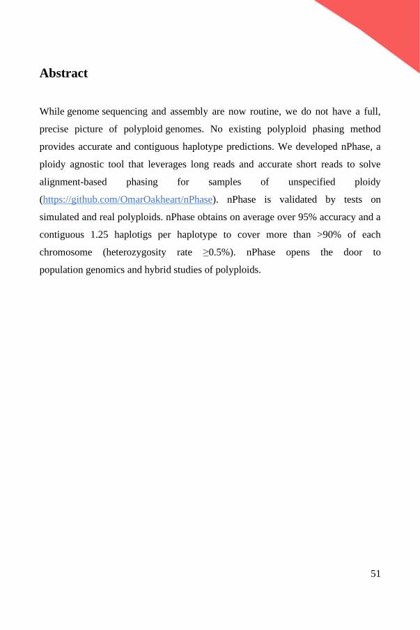
51

Abstract

While genome sequencing and assembly are now routine, we do not have a full,

precise picture of polyploid genomes. No existing polyploid phasing method

provides accurate and contiguous haplotype predictions. We developed nPhase, a

ploidy agnostic tool that leverages long reads and accurate short reads to solve

alignment-based phasing for samples of unspecified ploidy

(https://github.com/OmarOakheart/nPhase). nPhase is validated by tests on

simulated and real polyploids. nPhase obtains on average over 95% accuracy and a

contiguous 1.25 haplotigs per haplotype to cover more than >90% of each

chromosome (heterozygosity rate ≥0.5%). nPhase opens the door to

population genomics and hybrid studies of polyploids.

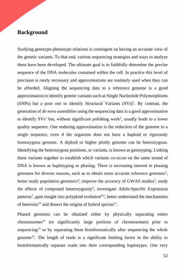
52

Background

Studying genotype-phenotype relations is contingent on having an accurate view of

the genetic variants. To that end, various sequencing strategies and ways to analyze

them have been developed. The ultimate goal is to faithfully determine the precise

sequence of the DNA molecules contained within the cell. In practice this level of

precision is rarely necessary and approximations are routinely used when they can

be afforded. Aligning the sequencing data to a reference genome is a good

approximation to identify genetic variants such as Single Nucleotide Polymorphisms

(SNPs) but a poor one to identify Structural Variants (SVs)1. By contrast, the

generation of de novo assemblies using the sequencing data is a good approximation

to identify SVs1 but, without significant polishing work2, usually leads to a lower

quality sequence. One enduring approximation is the reduction of the genome to a

single sequence, even if the organism does not have a haploid or rigorously

homozygous genome. A diploid or higher ploidy genome can be heterozygous.

Identifying the heterozygous positions, or variants, is known as genotyping. Linking

these variants together to establish which variants co-occur on the same strand of

DNA is known as haplotyping or phasing. There is increasing interest in phasing

genomes for diverse reasons, such as to obtain more accurate reference genomes3,

better study population genomics4, improve the accuracy of GWAS studies5, study

the effects of compound heterozygosity6, investigate Allele-Specific Expression

patterns7, gain insight into polyploid evolution8,9, better understand the mechanisms

of heterosis10 and dissect the origins of hybrid species11.

Phased genomes can be obtained either by physically separating entire

chromosomes12 (or significantly large portions of chromosomes) prior to

sequencing13 or by separating them bioinformatically after sequencing the whole

genome14. The length of reads is a significant limiting factor in the ability to

bioinformatically separate reads into their corresponding haplotypes. One very

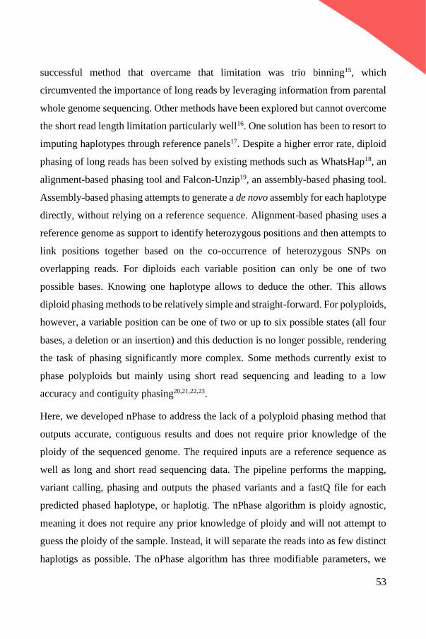
53

successful method that overcame that limitation was trio binning15, which

circumvented the importance of long reads by leveraging information from parental

whole genome sequencing. Other methods have been explored but cannot overcome

the short read length limitation particularly well16. One solution has been to resort to

imputing haplotypes through reference panels17. Despite a higher error rate, diploid

phasing of long reads has been solved by existing methods such as WhatsHap18, an

alignment-based phasing tool and Falcon-Unzip19, an assembly-based phasing tool.

Assembly-based phasing attempts to generate a de novo assembly for each haplotype

directly, without relying on a reference sequence. Alignment-based phasing uses a

reference genome as support to identify heterozygous positions and then attempts to

link positions together based on the co-occurrence of heterozygous SNPs on

overlapping reads. For diploids each variable position can only be one of two

possible bases. Knowing one haplotype allows to deduce the other. This allows

diploid phasing methods to be relatively simple and straight-forward. For polyploids,

however, a variable position can be one of two or up to six possible states (all four

bases, a deletion or an insertion) and this deduction is no longer possible, rendering

the task of phasing significantly more complex. Some methods currently exist to

phase polyploids but mainly using short read sequencing and leading to a low

accuracy and contiguity phasing20,21,22,23.

Here, we developed nPhase to address the lack of a polyploid phasing method that

outputs accurate, contiguous results and does not require prior knowledge of the

ploidy of the sequenced genome. The required inputs are a reference sequence as

well as long and short read sequencing data. The pipeline performs the mapping,

variant calling, phasing and outputs the phased variants and a fastQ file for each

predicted phased haplotype, or haplotig. The nPhase algorithm is ploidy agnostic,

meaning it does not require any prior knowledge of ploidy and will not attempt to

guess the ploidy of the sample. Instead, it will separate the reads into as few distinct

haplotigs as possible. The nPhase algorithm has three modifiable parameters, we

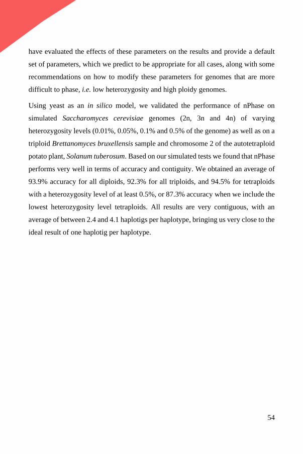
54

have evaluated the effects of these parameters on the results and provide a default

set of parameters, which we predict to be appropriate for all cases, along with some

recommendations on how to modify these parameters for genomes that are more

difficult to phase, i.e. low heterozygosity and high ploidy genomes.

Using yeast as an in silico model, we validated the performance of nPhase on

simulated Saccharomyces cerevisiae genomes (2n, 3n and 4n) of varying

heterozygosity levels (0.01%, 0.05%, 0.1% and 0.5% of the genome) as well as on a

triploid Brettanomyces bruxellensis sample and chromosome 2 of the autotetraploid

potato plant, Solanum tuberosum. Based on our simulated tests we found that nPhase

performs very well in terms of accuracy and contiguity. We obtained an average of

93.9% accuracy for all diploids, 92.3% for all triploids, and 94.5% for tetraploids

with a heterozygosity level of at least 0.5%, or 87.3% accuracy when we include the

lowest heterozygosity level tetraploids. All results are very contiguous, with an

average of between 2.4 and 4.1 haplotigs per haplotype, bringing us very close to the

ideal result of one haplotig per haplotype.

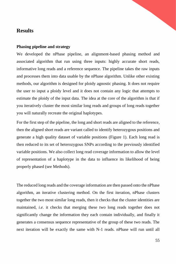
55

Results

Phasing pipeline and strategy

We developed the nPhase pipeline, an alignment-based phasing method and

associated algorithm that run using three inputs: highly accurate short reads,

informative long reads and a reference sequence. The pipeline takes the raw inputs

and processes them into data usable by the nPhase algorithm. Unlike other existing

methods, our algorithm is designed for ploidy agnostic phasing. It does not require

the user to input a ploidy level and it does not contain any logic that attempts to

estimate the ploidy of the input data. The idea at the core of the algorithm is that if

you iteratively cluster the most similar long reads and groups of long reads together

you will naturally recreate the original haplotypes.

For the first step of the pipeline, the long and short reads are aligned to the reference,

then the aligned short reads are variant called to identify heterozygous positions and

generate a high quality dataset of variable positions (Figure 1). Each long read is

then reduced to its set of heterozygous SNPs according to the previously identified

variable positions. We also collect long read coverage information to allow the level

of representation of a haplotype in the data to influence its likelihood of being

properly phased (see Methods).

The reduced long reads and the coverage information are then passed onto the nPhase

algorithm, an iterative clustering method. On the first iteration, nPhase clusters

together the two most similar long reads, then it checks that the cluster identities are

maintained, i.e. it checks that merging these two long reads together does not

significantly change the information they each contain individually, and finally it

generates a consensus sequence representative of the group of these two reads. The

next iteration will be exactly the same with N-1 reads. nPhase will run until all

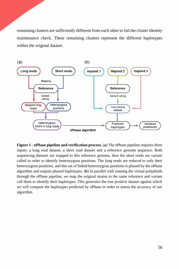
56

remaining clusters are sufficiently different from each other to fail the cluster identity

maintenance check. These remaining clusters represent the different haplotypes

within the original dataset.

Figure 1 - nPhase pipeline and verification process. (a) The nPhase pipeline requires three

inputs: a long read dataset, a short read dataset and a reference genome sequence. Both

sequencing datasets are mapped to this reference genome, then the short reads are variant

called in order to identify heterozygous positions. The long reads are reduced to only their

heterozygous positions, and this set of linked heterozygous positions is phased by the nPhase

algorithm and outputs phased haplotypes. (b) In parallel with running the virtual polyploids

through the nPhase pipeline, we map the original strains to the same reference and variant

call them to identify their haplotypes. This generates the true positive dataset against which

we will compare the haplotypes predicted by nPhase in order to assess the accuracy of our

algorithm.

57

Figure 2 - nPhase algorithm. Here we represent how a triploid's reads could align to a

reference sequence. Each read is one of three colors, one for each haplotype. The clustering,

consensus and cluster identity maintenance steps are iteratively repeated until all remaining

clusters are forbidden to merge. Clustering: Each vertical line represents a SNP; different

colors signify different haplotypic origins. Only two reads are clustered at a time, here we

show three clusters, so this is the result of the third step of nPhase's iterative clustering.

Consensus: A consensus sequence is generated by allowing every read in the cluster to vote

for a specific base for a given position. Votes are weighted by the pre-calculated context

coverage number to discourage sequencing errors. The consensus sequences that represent

clusters are treated just like aligned long reads and continue to be clustered. Cluster identity

maintenance: When all remaining clusters are very different from each other, they are not

allowed to merge, this is to prevent the algorithm from always outputting only one cluster

per region. The remaining clusters and their consensus sequences should correspond to the

haplotypes present in the original dataset.

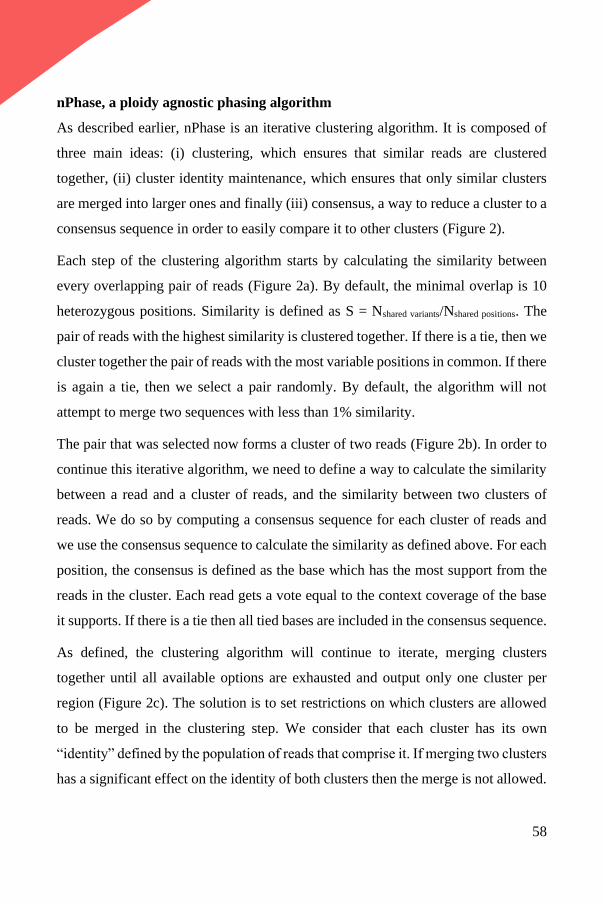
58

nPhase, a ploidy agnostic phasing algorithm

As described earlier, nPhase is an iterative clustering algorithm. It is composed of

three main ideas: (i) clustering, which ensures that similar reads are clustered

together, (ii) cluster identity maintenance, which ensures that only similar clusters

are merged into larger ones and finally (iii) consensus, a way to reduce a cluster to a

consensus sequence in order to easily compare it to other clusters (Figure 2).

Each step of the clustering algorithm starts by calculating the similarity between

every overlapping pair of reads (Figure 2a). By default, the minimal overlap is 10

heterozygous positions. Similarity is defined as S = Nshared variants/Nshared positions. The

pair of reads with the highest similarity is clustered together. If there is a tie, then we

cluster together the pair of reads with the most variable positions in common. If there

is again a tie, then we select a pair randomly. By default, the algorithm will not

attempt to merge two sequences with less than 1% similarity.

The pair that was selected now forms a cluster of two reads (Figure 2b). In order to

continue this iterative algorithm, we need to define a way to calculate the similarity

between a read and a cluster of reads, and the similarity between two clusters of

reads. We do so by computing a consensus sequence for each cluster of reads and

we use the consensus sequence to calculate the similarity as defined above. For each

position, the consensus is defined as the base which has the most support from the

reads in the cluster. Each read gets a vote equal to the context coverage of the base

it supports. If there is a tie then all tied bases are included in the consensus sequence.

As defined, the clustering algorithm will continue to iterate, merging clusters

together until all available options are exhausted and output only one cluster per

region (Figure 2c). The solution is to set restrictions on which clusters are allowed

to be merged in the clustering step. We consider that each cluster has its own

“identity” defined by the population of reads that comprise it. If merging two clusters

has a significant effect on the identity of both clusters then the merge is not allowed.

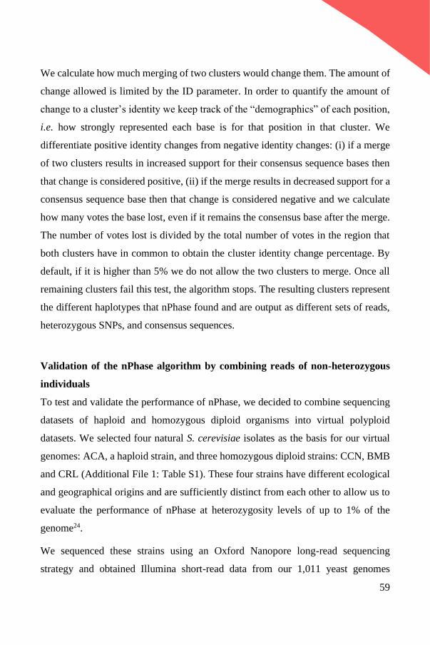
59

We calculate how much merging of two clusters would change them. The amount of

change allowed is limited by the ID parameter. In order to quantify the amount of

change to a cluster’s identity we keep track of the “demographics” of each position,

i.e. how strongly represented each base is for that position in that cluster. We

differentiate positive identity changes from negative identity changes: (i) if a merge

of two clusters results in increased support for their consensus sequence bases then

that change is considered positive, (ii) if the merge results in decreased support for a

consensus sequence base then that change is considered negative and we calculate

how many votes the base lost, even if it remains the consensus base after the merge.

The number of votes lost is divided by the total number of votes in the region that

both clusters have in common to obtain the cluster identity change percentage. By

default, if it is higher than 5% we do not allow the two clusters to merge. Once all

remaining clusters fail this test, the algorithm stops. The resulting clusters represent

the different haplotypes that nPhase found and are output as different sets of reads,

heterozygous SNPs, and consensus sequences.

Validation of the nPhase algorithm by combining reads of non-heterozygous

individuals

To test and validate the performance of nPhase, we decided to combine sequencing

datasets of haploid and homozygous diploid organisms into virtual polyploid

datasets. We selected four natural S. cerevisiae isolates as the basis for our virtual

genomes: ACA, a haploid strain, and three homozygous diploid strains: CCN, BMB

and CRL (Additional File 1: Table S1). These four strains have different ecological

and geographical origins and are sufficiently distinct from each other to allow us to

evaluate the performance of nPhase at heterozygosity levels of up to 1% of the

genome24.

We sequenced these strains using an Oxford Nanopore long-read sequencing

strategy and obtained Illumina short-read data from our 1,011 yeast genomes

60

project24. Since these strains do not have any heterozygosity, we could map their

short reads to the Saccharomyces cerevisiae reference genome and variant call them

to obtain their haplotypes (Figure 1). We then used these haplotypes as a truth set to

assess the performance of nPhase. With this truth set, we tested the influence of

dataset characteristics: coverage, ploidy, heterozygosity level and the inclusion or

exclusion of reads that map to distant regions of the genome, hereafter described as

split reads. We also investigated the influence of parameters that modulate the

behavior of the nPhase algorithm: minimum similarity, minimum overlap and

maximum ID change (for a description of them see Available Parameters in

Methods).

To assess the influence of ploidy, we used the three constructions of the different

virtual genomes previously mentioned. We also randomly sampled 6250, 12500,

62500 and 125000 heterozygous SNPs from each virtual genome to simulate datasets

where 0.05%, 0.1%, 0.5% and 1% of the positions in the genome are heterozygous.

This equates to three different ploidies and four heterozygosity levels, or 12

polyploid genomes to test.

By running a total of 6000 validation tests on varying ploidy, heterozygosity, and

coverage levels exploring the parameter space, we determined default parameters of

nPhase (see Methods). According to these tests, the parameters that result in optimal

results in terms of accuracy and contiguity are the following: 1% minimum

similarity, 10% minimum overlap and 5% maximum ID (see Identifying optimal

parameters in Methods). We then ran nPhase with these default parameters on our

previously described optimal datasets of varying ploidy (2n, 3n and 4n) and

heterozygosity levels (0.05%, 0.1%, 0.5% and 1%) of 20X long reads per haplotype

with split read information (Additional File 1: Table S2).

As an example, we phased the tetraploid genome showing a heterozygosity level of

0.5% using nPhase (Figure 3). Since we know the ground truth, we can assign each

61

haplotig to the strain whose haplotype it most closely represents and we can calculate

our accuracy metrics.

Figure 3 - Predicted haplotypes for the tetraploid genome with a 0.5% heterozygosity

level. The result of this test was an accuracy of 93.7%, an error rate of 4.0%, and a missing

rate of 2.2% with an average of 2.4 haplotigs per haplotype. Each subgraph displays the

predicted haplotigs for a different chromosome, each predicted haplotig is on a different row

on the Y axis, and the X axis displays the position along the chromosome. All predicted

haplotigs are color coded according to the haplotype they are the closest to.

In order to measure accuracy we distinguish between two forms of errors: standard

errors, i.e. heterozygous SNPs erroneously attributed to the wrong haplotype, and

missing errors, i.e. heterozygous SNPs which we know are present but which were

erroneously not represented in the predictions. The accuracy is the percentage of all

SNPs which were correctly attributed to their haplotype. The error rate is the

percentage of all predictions which were incorrect. The missing rate is the percentage

62

of all heterozygous SNPs which were never attributed to their haplotype. We use the

following formula:

Accuracy=TP/(TP+FP+FN)

TP=True Positive; the SNP was attributed to the correct haplotype

FP=False Positive; the SNP does not belong in this haplotype

FN=False Negative; the SNP is not represented in the results.

The result of this test was an accuracy of 93.7%, an error rate of 4.0%, and a missing

rate of 2.2% with an average of 2.4 haplotigs per haplotype. Seven of the sixteen

chromosomes have an L90 of 1, meaning that for all four haplotypes, more than 90%

of the heterozygous SNPs were assigned to one haplotig. For the nine remaining

chromosomes, seven have at least two chromosome-length haplotigs. In all cases,

the chromosomes are nearly fully covered by haplotigs that represent the four

different haplotypes, as confirmed by the low missing haplotype prediction rate

(2.2%). As a ploidy agnostic tool, nPhase was not given any information about the

ploidy of this sample and does not attempt to estimate its ploidy. Despite that, nPhase

reached a high accuracy (93.7%) and contiguity (2.4 haplotigs per haplotype),

demonstrating its ability to reliably phase a tetraploid of that heterozygosity level.

The same representation is available for the other datasets of different ploidy and

heterozygosity levels (Additional File 2: Fig S1).

Across the 12 phased genomes with variable ploidy and heterozygosity levels, we

noted little variation in terms of contiguity as we obtained between 2.4 and 4.3

haplotigs per haplotype (Figure 4a). At a heterozygosity level of 0.05%, the least

contiguous genomes are observed with around 4 haplotigs per haplotype (Figure 4a).

The triploid genomes decrease to around 3 haplotigs per haplotype for

heterozygosity levels greater than 0.1% (Figure 4a). The tetraploid tests continue the

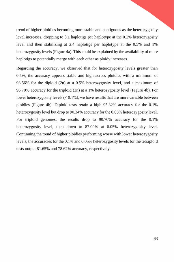
63

trend of higher ploidies becoming more stable and contiguous as the heterozygosity

level increases, dropping to 3.1 haplotigs per haplotype at the 0.1% heterozygosity

level and then stabilizing at 2.4 haplotigs per haplotype at the 0.5% and 1%

heterozygosity levels (Figure 4a). This could be explained by the availability of more

haplotigs to potentially merge with each other as ploidy increases.

Regarding the accuracy, we observed that for heterozygosity levels greater than

0.5%, the accuracy appears stable and high across ploidies with a minimum of

93.56% for the diploid (2n) at a 0.5% heterozygosity level, and a maximum of

96.70% accuracy for the triploid (3n) at a 1% heterozygosity level (Figure 4b). For

lower heterozygosity levels (≤ 0.1%), we have results that are more variable between

ploidies (Figure 4b). Diploid tests retain a high 95.32% accuracy for the 0.1%

heterozygosity level but drop to 90.34% accuracy for the 0.05% heterozygosity level.

For triploid genomes, the results drop to 90.70% accuracy for the 0.1%

heterozygosity level, then down to 87.00% at 0.05% heterozygosity level.

Continuing the trend of higher ploidies performing worse with lower heterozygosity

levels, the accuracies for the 0.1% and 0.05% heterozygosity levels for the tetraploid

tests output 81.65% and 78.62% accuracy, respectively.

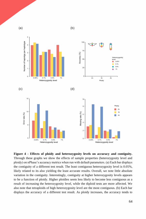
64

Figure 4 - Effects of ploidy and heterozygosity levels on accuracy and contiguity.

Through these graphs we show the effects of sample properties (heterozygosity level and

ploidy) on nPhase’s accuracy metrics when run with default parameters. (a) Each bar displays

the contiguity of a different test result. The least contiguous heterozygosity level is 0.05%,

likely related to its also yielding the least accurate results. Overall, we note little absolute

variation in the contiguity. Interestingly, contiguity at higher heterozygosity levels appears

to be a function of ploidy. Higher ploidies seem less likely to become less contiguous as a

result of increasing the heterozygosity level, while the diploid tests are more affected. We

also note that tetraploids of high heterozygosity level are the most contiguous. (b) Each bar

displays the accuracy of a different test result. As ploidy increases, the accuracy tends to

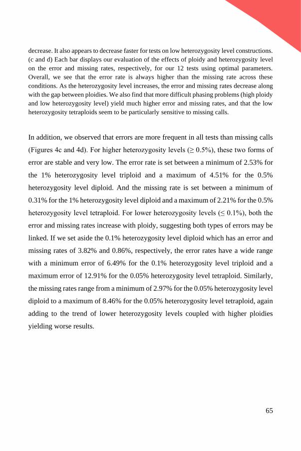
65

decrease. It also appears to decrease faster for tests on low heterozygosity level constructions.

(c and d) Each bar displays our evaluation of the effects of ploidy and heterozygosity level

on the error and missing rates, respectively, for our 12 tests using optimal parameters.

Overall, we see that the error rate is always higher than the missing rate across these

conditions. As the heterozygosity level increases, the error and missing rates decrease along

with the gap between ploidies. We also find that more difficult phasing problems (high ploidy

and low heterozygosity level) yield much higher error and missing rates, and that the low

heterozygosity tetraploids seem to be particularly sensitive to missing calls.

In addition, we observed that errors are more frequent in all tests than missing calls

(Figures 4c and 4d). For higher heterozygosity levels (≥ 0.5%), these two forms of

error are stable and very low. The error rate is set between a minimum of 2.53% for

the 1% heterozygosity level triploid and a maximum of 4.51% for the 0.5%

heterozygosity level diploid. And the missing rate is set between a minimum of

0.31% for the 1% heterozygosity level diploid and a maximum of 2.21% for the 0.5%

heterozygosity level tetraploid. For lower heterozygosity levels (≤ 0.1%), both the

error and missing rates increase with ploidy, suggesting both types of errors may be

linked. If we set aside the 0.1% heterozygosity level diploid which has an error and

missing rates of 3.82% and 0.86%, respectively, the error rates have a wide range

with a minimum error of 6.49% for the 0.1% heterozygosity level triploid and a

maximum error of 12.91% for the 0.05% heterozygosity level tetraploid. Similarly,

the missing rates range from a minimum of 2.97% for the 0.05% heterozygosity level

diploid to a maximum of 8.46% for the 0.05% heterozygosity level tetraploid, again

adding to the trend of lower heterozygosity levels coupled with higher ploidies

yielding worse results.

66

Benchmarking nPhase against other polyploid phasing tools

Some methods currently exist to phase polyploids using long read data such as

WhatsHap polyphase20, as well as other methods which were mostly designed to

work with short read sequencing data but can sometimes use long reads as

input21,22,23. Because nPhase is a phasing tool that leverages the linking power of long

reads to achieve its high accuracy and contiguity metrics, we did not benchmark it

against tools that rely exclusively on short reads for phasing, since these are

inherently limited by the size of their reads. We also did not benchmark nPhase

against tools that can only phase diploid genomes as this is not the intended use case

for our algorithm. We therefore compare nPhase to the recently released WhatsHap

polyphase, to our knowledge the only other polyploid phasing algorithm that handles

long reads.

We compared the results nPhase (default parameters) with WhatsHap polyphase on

the same samples (Figure 5). Since WhatsHap polyphase has a parameter named “--

block-cut-sensitivity” that can be set to determine the tradeoff between accuracy and

contiguity, we tested WhatsHap polyphase using all possible values for this

parameter (integers from 0 to 5) to compare all possible results to nPhase’s default

results. A value of 0 for this parameter means that WhatsHap polyphase will generate

the most contiguous results possible, and 5 means that it will generate the most

accurate results possible.

The performance of WhatsHap polyphase was measured in terms of switch error rate

and N50 block lengths. Instead we will talk about accuracy and average number of

haplotigs per haplotype, two metrics that are more direct representations of the

performance of the algorithms and answer two important questions: “How reliable

are the results?”, i.e. what are the proportions of accurate, erroneous and missing

calls? And “How informative are they?”, i.e. by how many haplotigs is each

haplotype represented? nPhase and WhatsHap polyphase were both applied to our

20X test datasets of different ploidy and heterozygosity levels. nPhase was tested

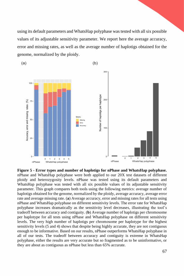
67

using its default parameters and WhatsHap polyphase was tested with all six possible

values of its adjustable sensitivity parameter. We report here the average accuracy,

error and missing rates, as well as the average number of haplotigs obtained for the

genome, normalized by the ploidy.

Figure 5 - Error types and number of haplotigs for nPhase and WhatsHap polyphase.

nPhase and WhatsHap polyphase were both applied to our 20X test datasets of different

ploidy and heterozygosity levels. nPhase was tested using its default parameters and

WhatsHap polyphase was tested with all six possible values of its adjustable sensitivity

parameter. This graph compares both tools using the following metrics: average number of

haplotigs obtained for the genome, normalized by the ploidy, average accuracy, average error

rate and average missing rate. (a) Average accuracy, error and missing rates for all tests using

nPhase and WhatsHap polyphase on different sensitivity levels. The error rate for WhatsHap

polyphase increases dramatically as the sensitivity level decreases, illustrating the tool’s

tradeoff between accuracy and contiguity. (b) Average number of haplotigs per chromosome

per haplotype for all tests using nPhase and WhatsHap polyphase on different sensitivity

levels. The very high number of haplotigs per chromosome per haplotype for the highest

sensitivity levels (5 and 4) shows that despite being highly accurate, they are not contiguous

enough to be informative. Based on our results, nPhase outperforms WhatsHap polyphase in

all of our tests. The tradeoff between accuracy and contiguity is extreme in WhatsHap

polyphase, either the results are very accurate but so fragmented as to be uninformative, or

they are about as contiguous as nPhase but less than 65% accurate.

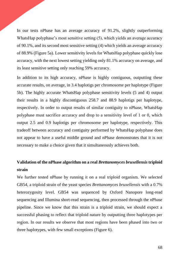
68

In our tests nPhase has an average accuracy of 91.2%, slightly outperforming

WhatsHap polyphase’s most sensitive setting (5), which yields an average accuracy

of 90.1%, and its second most sensitive setting (4) which yields an average accuracy

of 88.9% (Figure 5a). Lower sensitivity levels for WhatsHap polyphase quickly lose

accuracy, with the next lowest setting yielding only 81.1% accuracy on average, and

its least sensitive setting only reaching 59% accuracy.

In addition to its high accuracy, nPhase is highly contiguous, outputting these

accurate results, on average, in 3.4 haplotigs per chromosome per haplotype (Figure

5b). The highly accurate WhatsHap polyphase sensitivity levels (5 and 4) output

their results in a highly discontiguous 258.7 and 88.9 haplotigs per haplotype,

respectively. In order to output results of similar contiguity to nPhase, WhatsHap

polyphase must sacrifice accuracy and drop to a sensitivity level of 1 or 0, which

output 2.5 and 0.9 haplotigs per chromosome per haplotype, respectively. This

tradeoff between accuracy and contiguity performed by WhatsHap polyphase does

not appear to have a useful middle ground and nPhase demonstrates that it is not

necessary to make a choice given that it simultaneously achieves both.

Validation of the nPhase algorithm on a real Brettanomyces bruxellensis triploid

strain

We further tested nPhase by running it on a real triploid organism. We selected

GB54, a triploid strain of the yeast species Brettanomyces bruxellensis with a 0.7%

heterozygosity level. GB54 was sequenced by Oxford Nanopore long-read

sequencing and Illumina short-read sequencing, then processed through the nPhase

pipeline. Since we know that this strain is a triploid strain, we should expect a

successful phasing to reflect that triploid nature by outputting three haplotypes per

region. In our results we observe that most regions have been phased into two or

three haplotypes, with few small exceptions (Figure 6).

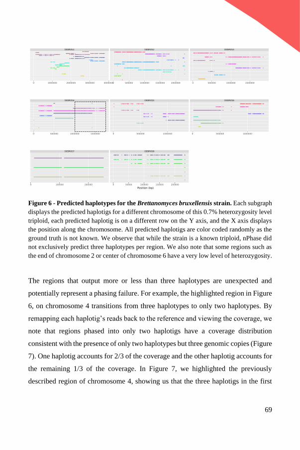
69

Figure 6 - Predicted haplotypes for the Brettanomyces bruxellensis strain. Each subgraph

displays the predicted haplotigs for a different chromosome of this 0.7% heterozygosity level

triploid, each predicted haplotig is on a different row on the Y axis, and the X axis displays

the position along the chromosome. All predicted haplotigs are color coded randomly as the

ground truth is not known. We observe that while the strain is a known triploid, nPhase did

not exclusively predict three haplotypes per region. We also note that some regions such as

the end of chromosome 2 or center of chromosome 6 have a very low level of heterozygosity.

The regions that output more or less than three haplotypes are unexpected and

potentially represent a phasing failure. For example, the highlighted region in Figure

6, on chromosome 4 transitions from three haplotypes to only two haplotypes. By

remapping each haplotig’s reads back to the reference and viewing the coverage, we

note that regions phased into only two haplotigs have a coverage distribution

consistent with the presence of only two haplotypes but three genomic copies (Figure

7). One haplotig accounts for 2/3 of the coverage and the other haplotig accounts for

the remaining 1/3 of the coverage. In Figure 7, we highlighted the previously

described region of chromosome 4, showing us that the three haplotigs in the first

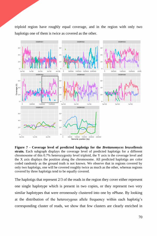
70

triploid region have roughly equal coverage, and in the region with only two

haplotigs one of them is twice as covered as the other.

Figure 7 - Coverage level of predicted haplotigs for the Brettanomyces bruxellensis

strain. Each subgraph displays the coverage level of predicted haplotigs for a different

chromosome of this 0.7% heterozygosity level triploid, the Y axis is the coverage level and

the X axis displays the position along the chromosome. All predicted haplotigs are color

coded randomly as the ground truth is not known. We observe that in regions covered by

only two haplotigs, one will be covered roughly twice as much as the other, whereas regions

covered by three haplotigs tend to be equally covered.

The haplotigs that represent 2/3 of the reads in the region they cover either represent

one single haplotype which is present in two copies, or they represent two very

similar haplotypes that were erroneously clustered into one by nPhase. By looking

at the distribution of the heterozygous allele frequency within each haplotig’s

corresponding cluster of reads, we show that few clusters are clearly enriched in

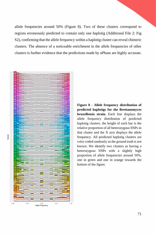
71

allele frequencies around 50% (Figure 8). Two of these clusters correspond to

regions erroneously predicted to contain only one haplotig (Additional File 2: Fig

S2), confirming that the allele frequency within a haplotig cluster can reveal chimeric

clusters. The absence of a noticeable enrichment in the allele frequencies of other

clusters is further evidence that the predictions made by nPhase are highly accurate.

Figure 8 - Allele frequency distribution of

predicted haplotigs for the Brettanomyces

bruxellensis strain. Each line displays the

allele frequency distribution of predicted

haplotig clusters. the height of each bar is the

relative proportion of all heterozygous SNPs in

that cluster and the X axis displays the allele

frequency. All predicted haplotig clusters are

color coded randomly as the ground truth is not

known. We identify two clusters as having a

heterozygous SNPs with a slightly high

proportion of allele frequencies around 50%,

one in green and one in orange towards the

bottom of the figure.

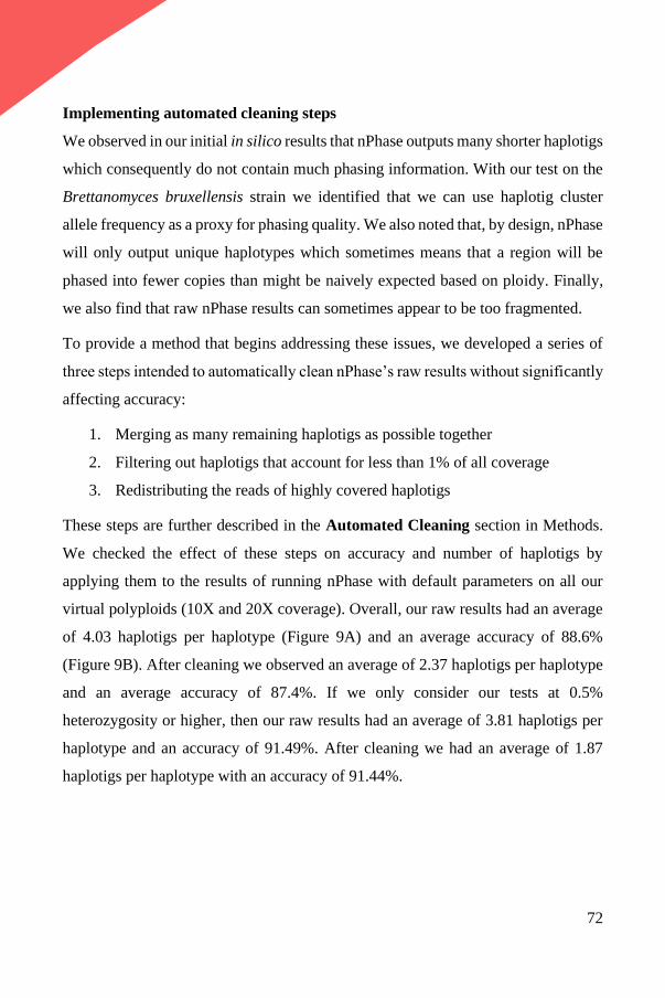
72

Implementing automated cleaning steps

We observed in our initial in silico results that nPhase outputs many shorter haplotigs

which consequently do not contain much phasing information. With our test on the

Brettanomyces bruxellensis strain we identified that we can use haplotig cluster

allele frequency as a proxy for phasing quality. We also noted that, by design, nPhase

will only output unique haplotypes which sometimes means that a region will be

phased into fewer copies than might be naively expected based on ploidy. Finally,

we also find that raw nPhase results can sometimes appear to be too fragmented.

To provide a method that begins addressing these issues, we developed a series of

three steps intended to automatically clean nPhase’s raw results without significantly

affecting accuracy:

1. Merging as many remaining haplotigs as possible together

2. Filtering out haplotigs that account for less than 1% of all coverage

3. Redistributing the reads of highly covered haplotigs

These steps are further described in the Automated Cleaning section in Methods.

We checked the effect of these steps on accuracy and number of haplotigs by

applying them to the results of running nPhase with default parameters on all our

virtual polyploids (10X and 20X coverage). Overall, our raw results had an average

of 4.03 haplotigs per haplotype (Figure 9A) and an average accuracy of 88.6%

(Figure 9B). After cleaning we observed an average of 2.37 haplotigs per haplotype

and an average accuracy of 87.4%. If we only consider our tests at 0.5%

heterozygosity or higher, then our raw results had an average of 3.81 haplotigs per

haplotype and an accuracy of 91.49%. After cleaning we had an average of 1.87

haplotigs per haplotype with an accuracy of 91.44%.

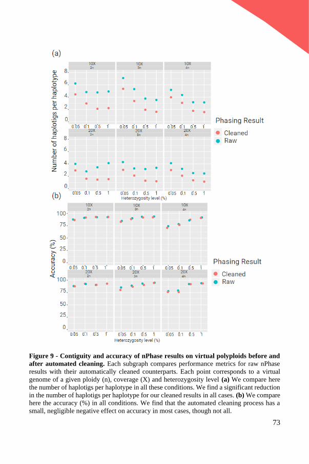
73

Figure 9 - Contiguity and accuracy of nPhase results on virtual polyploids before and

after automated cleaning. Each subgraph compares performance metrics for raw nPhase

results with their automatically cleaned counterparts. Each point corresponds to a virtual

genome of a given ploidy (n), coverage (X) and heterozygosity level (a) We compare here

the number of haplotigs per haplotype in all these conditions. We find a significant reduction

in the number of haplotigs per haplotype for our cleaned results in all cases. (b) We compare

here the accuracy (%) in all conditions. We find that the automated cleaning process has a

small, negligible negative effect on accuracy in most cases, though not all.

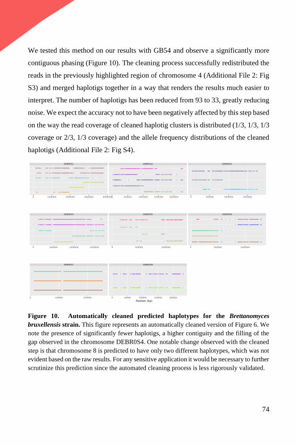
74

We tested this method on our results with GB54 and observe a significantly more

contiguous phasing (Figure 10). The cleaning process successfully redistributed the

reads in the previously highlighted region of chromosome 4 (Additional File 2: Fig

S3) and merged haplotigs together in a way that renders the results much easier to

interpret. The number of haplotigs has been reduced from 93 to 33, greatly reducing

noise. We expect the accuracy not to have been negatively affected by this step based

on the way the read coverage of cleaned haplotig clusters is distributed (1/3, 1/3, 1/3

coverage or 2/3, 1/3 coverage) and the allele frequency distributions of the cleaned

haplotigs (Additional File 2: Fig S4).

Figure 10. Automatically cleaned predicted haplotypes for the Brettanomyces

bruxellensis strain. This figure represents an automatically cleaned version of Figure 6. We

note the presence of significantly fewer haplotigs, a higher contiguity and the filling of the

gap observed in the chromosome DEBR0S4. One notable change observed with the cleaned

step is that chromosome 8 is predicted to have only two different haplotypes, which was not

evident based on the raw results. For any sensitive application it would be necessary to further

scrutinize this prediction since the automated cleaning process is less rigorously validated.

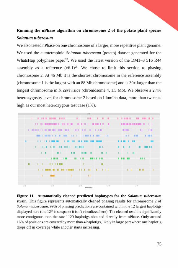
75

Running the nPhase algorithm on chromosome 2 of the potato plant species

Solanum tuberosum

We also tested nPhase on one chromosome of a larger, more repetitive plant genome.

We used the autotetraploid Solanum tuberosum (potato) dataset generated for the

WhatsHap polyphase paper20. We used the latest version of the DM1–3 516 R44

assembly as a reference (v6.1)25. We chose to limit this section to phasing

chromosome 2. At 46 Mb it is the shortest chromosome in the reference assembly

(chromosome 1 is the largest with an 88 Mb chromosome) and is 30x larger than the

longest chromosome in S. cerevisiae (chromosome 4, 1.5 Mb). We observe a 2.4%

heterozygosity level for chromosome 2 based on Illumina data, more than twice as

high as our most heterozygous test case (1%).

Figure 11. Automatically cleaned predicted haplotypes for the Solanum tuberosum

strain. This figure represents automatically cleaned phasing results for chromosome 2 of

Solanum tuberosum. 99% of phasing predictions are contained within the 12 largest haplotigs

displayed here (the 12th is so sparse it isn’t visualized here). The cleaned result is significantly

more contiguous than the raw 1129 haplotigs obtained directly from nPhase. Only around

16% of positions are covered by more than 4 haplotigs, likely in large part where one haplotig

drops off in coverage while another starts increasing.

76

To reduce computation time, we used a randomly sampled subset of heterozygous

variants, effectively phasing at a 0.5% heterozygosity level. The raw results of

nPhase yielded 1129 haplotigs, which were reduced to 25 haplotigs by a modified

version of the automated cleaning steps; the final gap filling step was disabled in

light of the fragmented nature of our raw results (Figure 11). Of the 25 cleaned

haplotigs output, we find 90% of predicted variants in the 9 largest cleaned haplotigs,

and 99% of predicted variants in the 12 largest cleaned haplotigs. The remaining 13

cleaned haplotigs account for less than 0.6% of predictions made and could

reasonably be filtered out.

We note that the haplotigs obtained skip around the chromosome, which may either

be due to structural variation or to long reads being mapped in error to the wrong

repetitive regions, thereby giving the illusion of widespread structural variation. We

also checked the phasing predictions for the 5 longest genes of chromosome 2

(Additional File 2: Fig S5) and found that they are coherent with our expectations

for an autotetraploid.

77

Discussion

We developed nPhase, an algorithm that relies on a few intuitive rules to process an

input dataset of long reads, reduced to heterozygous positions, outputting as few

clusters as possible which we have shown correspond to the true haplotypes with

>90% accuracy. By not specifying the ploidy of the sample in any step, we allow

nPhase to adapt to the particularities of the dataset and do not run the risk of forcing

an incorrect result to fit such an arbitrary algorithmic constraint. We provide nPhase

as part of a pipeline that enables anyone to use their short and long read sequences

of the same sample as inputs and obtain a list of SNPs and a fastQ file for each

predicted haplotig.

Through our validation tests, we determined that there is a set of parameters for

nPhase that performs optimally in nearly all of our test cases and that the algorithm

performs well even with very low levels of genetic distance between haplotypes. We

found that as little as 10X coverage can yield satisfying results. More complex cases,

such as when there is a high ploidy coupled with a low heterozygosity, should benefit

from higher coverage and a more stringent parameter for the minimum overlap (0.25

for example). Further investigation would be needed in order to more adequately

define how these difficult samples should be treated. We also demonstrated with our

benchmarking tests that nPhase outputs far more accurate and contiguous haplotigs

than alternative polyploid phasing methods, and that this contiguity can be greatly

improved at a very small cost to accuracy by using our simple automated cleaning

process.

By testing nPhase on a triploid strain of the yeast species Brettanomyces bruxellensis

we were able to demonstrate that our method can be used on a real polyploid sample

and provides a previously inaccessible insight into its haplotypic composition. We

were able to show through the chosen sample the usefulness of a ploidy agnostic

78

method which can adapt to a genome with a variable number of haplotypes. In the

process of validating this real test case, we established two ways of qualitatively

assessing phasing quality: checking the coverage plots of re-mapped haplotig reads

and checking the allele frequency of reads that comprise a cluster. Our automated

cleaning process yielded satisfying results, visibly improving the contiguity of the

phasing, reducing noise, and filling some of the gaps observed in the raw phasing

results.

We also tested nPhase on a much larger example, the 44 Mb long chromosome 2 of

the potato plant species Solanum tuberosum, 30 times longer than the longest

chromosome of Saccharomyces cerevisiae. This is a highly heterozygous

autotetraploid with a highly repetitive genome and represents an important test case

for nPhase. Despite the significantly increased complexity, we found that by using

nPhase coupled with our cleaning steps we were able to produce a remarkably

contiguous phasing prediction using only a fraction of the available data. The genes

in particular we expect to be correctly phased, while we did not test the effects of

nPhase on a highly repetitive test case with a known ground truth, limiting our

certainty that the phasing was equally accurate in repetitive regions of the genome.

In our analysis we did not take any extra steps to address the repetitive nature of the

potato genome: we used a reference in which the repeats were not masked, we used

all mapped reads, including those with low mapQ scores, and we did not check if

variants called by short reads were reflected in the long reads. These are a few areas

in which steps can be taken to improve the quality of the phasing. We also only used

a fraction of all available heterozygous positions, and devoting more computing

power and time to exploit more of that very relevant phasing information would

presumably yield even better results.

As an alignment-based phasing algorithm, the performance of nPhase is going to be

highly dependent on read length and the quality of the reference genome being

mapped against. Consequently, structural variants between the sample and the

79

reference, or even structural variants within the sample are presently not explicitly

identified and phased by the algorithm. In order to resolve structural variants

between the sample and the reference or even between haplotypes in the sample, we

need to rely on the information in split reads. Here, we used a simple strategy to

stitch together some of the haplotigs we obtain without using all of the information

contained within split reads. Leveraging the full potential of split reads is a crucial

next step to improve the contiguity of phased blocks. The main difficulty in using

split reads appears to be that these alignments are significantly less reliable and will

need to be processed differently to account for that.

We made the choice not to base our phased blocks on insertion or deletion

information. This information can still be obtained in the phased blocks by

generating a de novo assembly using nPhase’s fastQ output for the relevant haplotig

and could be integrated in future developments.

The rarity of raw accuracy numbers in the polyploid phasing literature derives from

the observation that a single well-placed haplotype switching error has the potential

to reduce the accuracy of a phased block by half. This led to the widespread adoption

of using the SWitch Error Rate (SWER) or Vector Error Rate (VER) as the

performance metric by which to compare polyploid phasing methods. This metric is

only relevant to methods that accept the inevitability of switch errors, for which the

raw measurement of the accuracy of predictions will not speak by itself. nPhase has

achieved a very high level of accuracy (>95%) and contiguity (1.25 haplotigs per

haplotype) across most of our validation tests (in particular where the heterozygosity

rate is of 0.5% of higher). The principal interest of providing performance metrics is

to make it easy to assess the trustworthiness of a method’s results. For these reasons,

we did not include the SWER in our performance metrics.

With the nPhase algorithm we believe that the problem of switch errors in polyploid

phasing is largely solved, the next important hurdle for polyploid phasing is finding

80

an appropriate way to handle split reads to solve the remaining problems of

contiguity and structural variants both within a sample and between the sample and

the reference we align to. nPhase can still be used as a preprocessing step for any

study of phased polyploid SVs and indels since that information is partially held

within its output of fastQ files of phased reads.

Overall, nPhase provides, for the first time, an accurate and contiguous picture of

polyploid genomes using only a reference genome and short and long reads. It paves

the way for a better understanding of the origins of hybrid polyploid organisms, the

true diversity of polyploid populations with potential hints on their origins and their

relation to other diploid or haploid strains, and provides a clearer picture to

investigate phenotypic effects tied to alleles which were previously inaccessible.

81

Methods

Total DNA extraction

Single colonies of each natural isolate were isolated by streaking on YPD media,

containing ampicillin (50 μg/mL). Cells from one colony of each isolate were grown

in 60 mL of YPD at 30°C for 24 hours. We extracted the total DNA of each isolate

using the QIAGEN Genomic-tip 100/G kit, according to manufacturer’s instructions.

Library preparation and sequencing

The kit NEBNext Ultra™ II DNA Library Prep Kit (Ipswich, USA) for Illumina

(San Diego, USA) was used for short read library preparation of the GB54

Brettanomyces bruxellensis isolate. The sample was sequenced on a single lane of

NextSeq (Illumina) at the European Molecular Laboratory (EMBL) in Heidelberg,

Germany. The strategy of sequencing was 75 paired-end (75PE).

For long read sequencing, we used the EXP-NBD104 native barcoding kit (Oxford

Nanopore) and the protocol provided by the manufacturer to barcode the total DNA

of each of the isolates. The barcoded DNA was then quantified with a Qubit®️ 1.0

fluorometer (Thermo Fisher) and pooled together with an equal amount of DNA

coming from each isolate. We then used the SQK-LSK109 ligation sequencing kit

(Oxford Nanopore) to finish the library preparation. Finally, the library was loaded

to a R9.3 flow cell for a 72 hour run.

Data pre-processing

The short reads are mapped to a reference genome using bwa26 with the command

bwa mem -M. We ran GATK27 MarkDuplicates then variant called with GATK 4.0’s

HaplotypeCaller --ploidy 2 to identify heterozygous positions. Long reads are

basecalled, adapter trimmed and demultiplexed by Guppy. They are then mapped to

82

the same reference using NGMLR28. We keep only primary alignments and split

reads with the samtools29 flag 260.

We determine the positions of heterozygous SNPs from the VCF obtained by GATK

by looking for positions where AF=1.00 in the file. We reduced each long read to

the set of variable positions it overlaps (Additional File 2: Fig S6a). To simplify later

computational steps, we remove long reads that are subsets of other long reads.

nPhase is only capable of phasing SNPs if they are identified by the variant calling

step. This is not necessarily always the case, and the accuracy metrics are based on

the total number of SNPs identified in the polyploid sample by the variant calling

step. However, unidentified SNPs will still exist in the reads, so if the algorithm

performs a proper clustering of the reads the information will still be available and

readily extracted by a closer view of the results.

Context coverage

Long reads are error-prone but it is important not to perform any form of error

correction to ensure that the heterozygosity is not incorrectly flattened or mis-

assigned. The nPhase pipeline works with raw long reads. In order to minimize the

influence of these errors we consider that SNP coverage is a useful indicator of

quality. We count the number of times each heterozygous SNP is present in a specific

context in our dataset. We define context as being the closest flanking heterozygous

SNPs (two heterozygous SNPs upstream and two heterozygous SNPs downstream).

The context information will be used to better inform the nPhase algorithm and allow

it to escape the situation where a sequencing error randomly converts a well-

supported SNP to another SNP that is well-supported in another haplotype

(Additional File 2: Fig S6b).

83

Output results

Once nPhase is done running it outputs several files:

(i) A fastQ file for each haplotig containing all of the reads that have been clustered

together for this haplotig, this file can then be used with a de novo assembly or

alignment tool for further analysis.

(ii) A tab separated file listing the consensus base for each heterozygous position

contained within each haplotig. There are three columns: chromosome, position and

consensus base. If two different bases are equally represented for a given position

and equally well supported within the cluster they will both be represented in this

file on separate lines. This file is sorted by position.

(iii) A plot representing the different haplotigs along the reference genome, similar

to the one displayed in Figure 3 but lacking the haplotype color code since the ground

truth is not known in a typical use case of nPhase.

nPhase parameter description

nPhase has a total of 4 parameters which can be adjusted to better fit the sample.

These parameters are the following (Additional File 2: Fig S7):

S, the minimum fraction of similarity between two reads. When two reads

overlap with each other we calculate their similarity by dividing the number of

heterozygous SNPs they share by the number of heterozygous positions they both

cover. If that fraction is smaller than the parameter S, then we will consider that these

two reads cannot be part of the same haplotype. This parameter can be set to any

fraction between 0 and 1, by default it is set at 0.01, or 1% similarity.

O, the minimum fraction of overlap between two reads. When two reads overlap

with each other we can count the number of heterozygous positions they both cover.

If they both cover more than 100 heterozygous positions, this parameter is ignored.

84

If they cover fewer than 100 heterozygous positions then we calculate the overlap

by dividing the number of heterozygous positions the two reads have in common by

the total number of heterozygous positions covered by the smaller of the two reads.

In this case, smaller does not necessarily mean a shorter read, it means a read that

covers fewer heterozygous positions. If this overlap is smaller than the parameter O,

then we consider that these two reads do not overlap enough for us to conclusively

determine if they’re part of the same haplotype. This parameter can be set to any

fraction between 0 and 1, by default it is set at 0.1, or 10% overlap.

L, the minimum number of reads supporting a haplotig. Once nPhase has

clustered all of the reads into different haplotigs, the user may want to filter out all

haplotigs that are supported by fewer than N reads. This parameter can be set to any

integer N ≥ 0, by default it is set at 0. If set to N, it will not output any cluster

supported by fewer than N reads.

ID, the maximum amount of change when merging clusters. When nPhase

considers merging two clusters of reads into one new cluster it must determine if

these two clusters are similar enough to warrant merging them together or if they

should remain unique clusters, representative of unique haplotypes. Since these are

clusters, every heterozygous position is potentially covered multiple times,

sometimes with different reads in the same cluster indicating conflicting bases for

the same position. We can calculate the number of reads voting for each base in a

given cluster and determine the “demographics” for that position. We can take this

further and have an overview of every heterozygous position in the cluster and how

well-supported each base is. The base that has the majority of support is considered

to be the “true” base for that cluster. When we merge two clusters together, we

potentially change these “demographics”. These changes either further strengthen

the position of the majority base for a given position, in which case there is no

negative change in the cluster’s “identity” or they weaken the majority base’s

position and cause a negative change to the cluster’s “identity”. When there are

85

negative changes to the cluster’s “identity” we can calculate the amount of change

that has occurred and if that amount is too high the clusters are not allowed to merge.

This parameter can be set to any fraction between 0 and 1, by default it is set at 0.05,

or a 5% ID change tolerance.

These parameters are set by default, though they can be modified if needed. The

nPhase algorithm will use these parameters as limitations to determine which reads

it is allowed to cluster together into haplotigs and which clusters of reads it can merge

together into longer haplotigs. Ideally, only the ID parameter needs to be modified,

keeping all other parameters very low and forcing the algorithm to merge clusters as

aggressively as allowed by the ID parameter.

Identifying optimal parameters

In order to determine which parameters nPhase should use by default, it is important

to understand how these parameters affect the results. Ideally, we will find that there

is a set of parameters which is optimal for all possible combinations of ploidy and

heterozygosity level, such a set would then become the default recommended

parameters for nPhase. If no such set of parameters appears to exist, the next best

case is to minimize the impact of as many of the available parameters as possible in

order to reduce the parameter a user would need to explore when using nPhase to

phase their dataset.

Through our tests, we find that there is a narrow range in the parameter space that

results in the optimal performance of nPhase. Intuitively, the optimal strategy

appears to be to set the minimum similarity and minimum overlap parameters down

to a low value so that all of the reads in the dataset are allowed to merge into a cluster,

and to only worry about finding an appropriate threshold for the ID change

parameter. Since the ID change parameter controls how dissimilar two clusters need

to be in order to be considered two different haplotypes, it is fitting for this parameter

86

alone to have the most pronounced impact on the quality of results. If set too low

nPhase will consider small sequencing errors to be evidence of alternate haplotypes,

and if set too high it will allow different haplotypes to merge into chimeric and wrong

results.

To demonstrate this, we ran nPhase 125 times on 24 different samples of varying

coverage, ploidy and number of heterozygous SNPs for a total of 3000 tests. These

125 tests represent every possible combination of the minimum similarity S,

minimum overlap O, and maximum identity change ID parameters for the following

values: 0.01, 0.05, 0.1, 0.15, 0.25.

The L parameter was set to 0 for these tests since it’s intended for use to clean up

results by removing small, lowly supported haplotigs and we wanted to determine

how nPhase performs without throwing away any of the data.

We found that S, the minimum similarity parameter, had no influence on the results

at these levels (Additional File 2: Fig S8a). O, the minimum overlap parameter,

needs to be at least at 0.1 and seems to show very minor improvements in accuracy

at higher levels (Additional File 2: Fig S8b). The ID parameter has the most influence

on the accuracy of the results, with values of 0.05 and 0.1 yielding the best results

(Additional File 2: Fig S8c).

We then looked at the effects of O and ID on the average number of haplotigs per

chromosome per parent. We found that the number of haplotigs slightly increases

with O (Additional File 2: Fig S9a), while ID has a strong effect on the contiguity of

the results (Additional File 2: Fig S9b). A higher value for ID leads to a more

contiguous assembly, though this comes at the cost of accuracy (Additional File 2:

Fig S9c). We again find that values held between 0.05 and 0.1 provide good results.

If we separate our tests by ploidy we can see that, as the ploidy increases the optimal

choice for the ID parameter narrows down around 0.05 (Additional File 2: Fig S10).

87

Based on our tests, we find that the following set of parameters is the best adapted

to handle any sample: S=0.01, O=0.1, L=0, ID=0.05. We use these as our default

parameters.

Influence of coverage

We sought to establish the effects of coverage on the quality metrics of nPhase's

predictions. To do so we performed our tests on a 10X per haplotype dataset and a

20X per haplotype dataset. We found that both accuracy and contiguity are improved

by the higher coverage level of 20X per haplotype (Additional File 2: Fig S11). This

effect is observed across ploidy and heterozygosity levels, though the accuracy

effects are more pronounced for higher ploidy, lower heterozygosity level samples.

A low number of haplotigs per haplotype is not always a good sign of high contiguity

as it can be compatible with a high rate of chimeric haplotigs. Therefore, we looked

at the contiguity effects of coverage for our tests using default parameters, which we

have previously determined output accurate results. Based on these tests we were

able to confirm that the 20X dataset is more contiguous than the 10X dataset

(Additional File 2: Fig S11b). We therefore used the 20X datasets as part of our

default analysis.

Split read stitching step

Some reads align to two or more very distant sequences in the reference genome.

These reads can represent a structural variation between the sample and the reference

being mapped to. We split them into the different segments that align to the reference

and refer to them to as split reads.

Split reads can be very misleading and trusting them blindly would result in chimeric

haplotigs. We developed a simple pre-processing strategy to integrate part of the

information contained by these split reads.

88

We run nPhase a first time to obtain our initial haplotigs. We expect some of the

edges of haplotigs to correspond to structural variants such as inversions or large

indels so we identify the SNPs at the edges of these clusters. These are the SNPs

which we expect to be included in the split reads that can connect two haplotigs

separated by a structural variant, so they are the most trustworthy SNPs in our split

read dataset. We reduce each split read to only the heterozygous SNPs that overlap

with these regions and re-run the nPhase algorithm with these reads included.

Clusters are currently not allowed to combine reads from different reference

chromosomes, so split reads can only be used to improve the contiguity of haplotigs

on the same reference chromosome.

As described, nPhase does not exploit the information contained in split reads to the

fullest extent, only attempting to improve contiguity by stitching together haplotigs

on the same chromosome. Once there are only a few remaining haplotigs, further

improving contiguity necessarily means stitching longer haplotigs together. This

presents a very real danger of creating chimeric haplotigs that have very strong

negative effects on accuracy. To validate the usefulness of these steps and this

method of using the split read data we ran 3000 tests of nPhase both with split read

information and 3000 tests without in order to determine the effects of our split read

stitching strategy on both contiguity and accuracy. We found that the contiguity did

significantly improve across all of our tests that included split read information,

compared to those that did not (Additional File 2: Fig S12a). Encouragingly, when

comparing the accuracy distributions of the two sets of tests they are virtually

identical (Additional File 2: Fig S12b). The tests that used split reads were very

slightly less accurate than their counterparts but much more contiguous, motivating

our decision to integrate the use of split read information in nPhase.

89

Automated Cleaning

We established a three step automated cleaning procedure to quickly reduce noise

and improve the contiguity of raw nPhase results. These steps have a negligible

negative effect on accuracy in our in silico tests while greatly reducing the number

of haplotigs per haplotype.

The first step of the automated cleaning process is the merging step. We first

calculate, for every raw cluster output by nPhase, the proportion of bases that

disagree with the consensus base. We call this the discordance level of the cluster,

and it is equivalent to the summed minor allele frequencies represented in this

cluster. We calculate the mean level of discordance across all clusters output by

nPhase and we use this number as our stopping point. Our goal is to find pairs of

clusters that merge together without increasing our risk of merging two different

haplotypes into one. For each pair of clusters, we calculate the discordance level that

we would obtain if we merged them together. If that discordance level is lower than

the average discordance level calculated previously, then we can allow the merge to

occur. If it is higher then we do not allow the merge. Once there are no pairs of

clusters left that are allowed to merge, we end this step.

The second step is a filtering step. We sort all remaining clusters by the total

coverage they represent, and we only remove clusters that account for the smallest

1% of coverage. This allows us to get rid of the small noisy clusters we have

observed in our results.

The third and final step is the filling of gaps. We calculate, for each chromosome,

the average coverage level of all the haplotigs (each haplotig counts as 1X, we are

not looking at the coverage level of the reads contained within the clusters that define

the haplotigs). We round this coverage level, and if it is rounded up to n (from 2.6 to

3 for example), then we identify the regions of the chromosome that are covered less

than n times. For each such region we identify the most covered cluster, split its reads

90

in half, and redistribute them such that we have effectively filled the gap. This step

presumes that the gap is due to a large region of the chromosome having the same

haplotype in at least two copies of the genome (as evidenced by the coverage level

being twice as high, for example).

We validated these steps by running them on our virtual polyploids and comparing

the accuracy and contiguity results to the raw nPhase results.

Performance limits

With default parameters the nPhase algorithm took between 1 minute and nearly 5

hours of runtime on a single CPU (the nPhase algorithm has not been parallelized),

and between 0.6 GB and 31.8 GB of memory (Additional File 1: Table S3). The

runtime and memory usage are clearly tied to the ploidy and heterozygosity level. A

higher ploidy and higher heterozygosity level translates to a significant increase in

runtime and memory usage. Each diploid test, up to 1% heterozygosity, ran in less

than an hour and ten minutes and used less than 8 GB of memory. Triploid tests took

a minimum of 3.5 minutes of CPU time and 0.9 GB of memory to run for the 0.05%

heterozygosity level example, and a maximum of three hours and ten minutes of

CPU time and 19 GB of memory for the 1% heterozygosity level test. The tetraploid

examples were the most resource intensive, using up a minimum of 6 minutes of

CPU time and 1.25 GB of memory for the 0.05% heterozygosity level, and a

maximum of four hours and fifty minutes of CPU time and 31.8 GB of memory to

run. nPhase can output results in a reasonable time using moderate memory

resources. If run on a particularly large genome in a time-sensitive context, nPhase

could be applied to individual chromosomes in parallel. It's also reasonable to

consider down-sampling the number of SNPs to a heterozygosity level of around

0.5% given the results obtained are comparable and run in less than half the time as

the 1% heterozygosity level tests. All of the heterozygous SNPs would still be

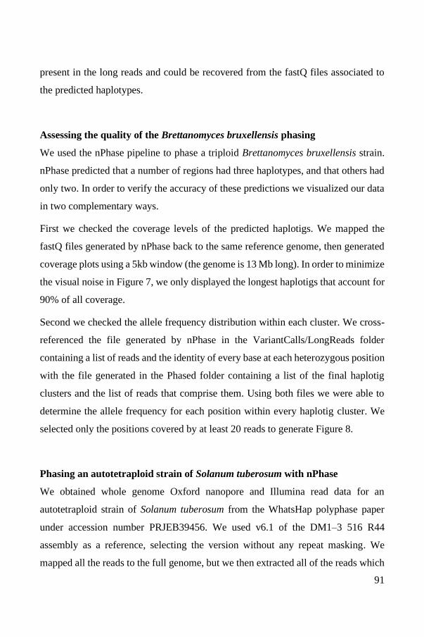
91

present in the long reads and could be recovered from the fastQ files associated to

the predicted haplotypes.

Assessing the quality of the Brettanomyces bruxellensis phasing

We used the nPhase pipeline to phase a triploid Brettanomyces bruxellensis strain.

nPhase predicted that a number of regions had three haplotypes, and that others had

only two. In order to verify the accuracy of these predictions we visualized our data

in two complementary ways.

First we checked the coverage levels of the predicted haplotigs. We mapped the

fastQ files generated by nPhase back to the same reference genome, then generated

coverage plots using a 5kb window (the genome is 13 Mb long). In order to minimize

the visual noise in Figure 7, we only displayed the longest haplotigs that account for

90% of all coverage.

Second we checked the allele frequency distribution within each cluster. We cross-

referenced the file generated by nPhase in the VariantCalls/LongReads folder

containing a list of reads and the identity of every base at each heterozygous position

with the file generated in the Phased folder containing a list of the final haplotig

clusters and the list of reads that comprise them. Using both files we were able to

determine the allele frequency for each position within every haplotig cluster. We

selected only the positions covered by at least 20 reads to generate Figure 8.

Phasing an autotetraploid strain of Solanum tuberosum with nPhase

We obtained whole genome Oxford nanopore and Illumina read data for an

autotetraploid strain of Solanum tuberosum from the WhatsHap polyphase paper

under accession number PRJEB39456. We used v6.1 of the DM1–3 516 R44

assembly as a reference, selecting the version without any repeat masking. We

mapped all the reads to the full genome, but we then extracted all of the reads which

92

mapped to chromosome 2 to run the phasing algorithm on. Of the 2.4% of

heterozygous positions observed in chromosome 2 according to variant calling on

Illumina data, we only kept a randomly sampled 0.5% for the phasing in order to

save calculation time.

Once we obtained raw nPhase results, we ran our automated cleaning steps in order

to improve contiguity and reduce the complexity of our results.

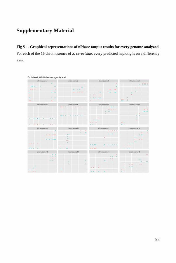
93

Supplementary Material

Fig S1 - Graphical representations of nPhase output results for every genome analyzed.

For each of the 16 chromosomes of S. cerevisiae, every predicted haplotig is on a different y

axis.

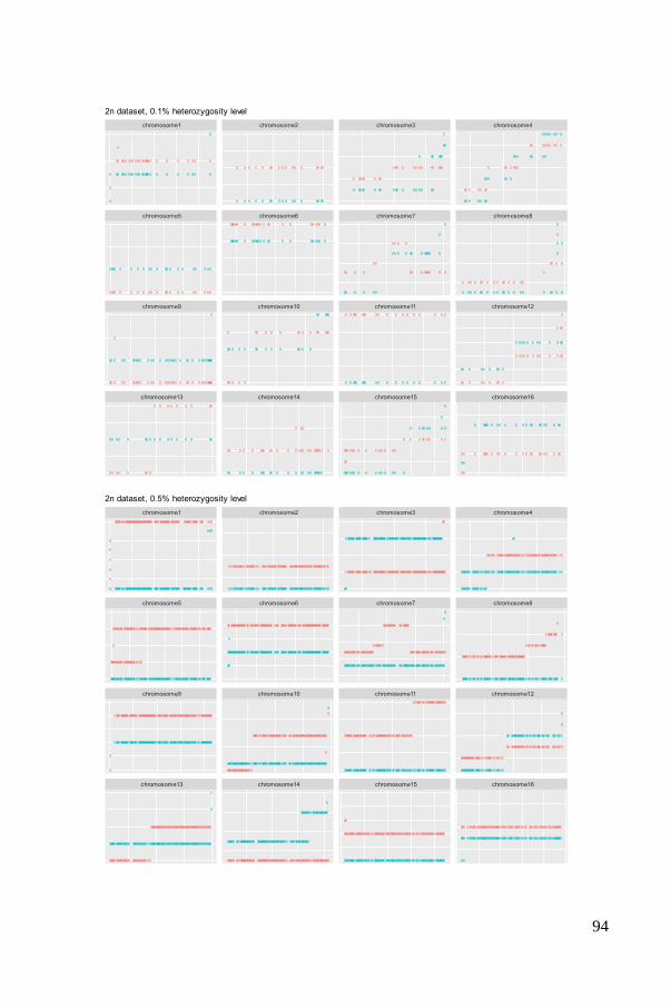
94

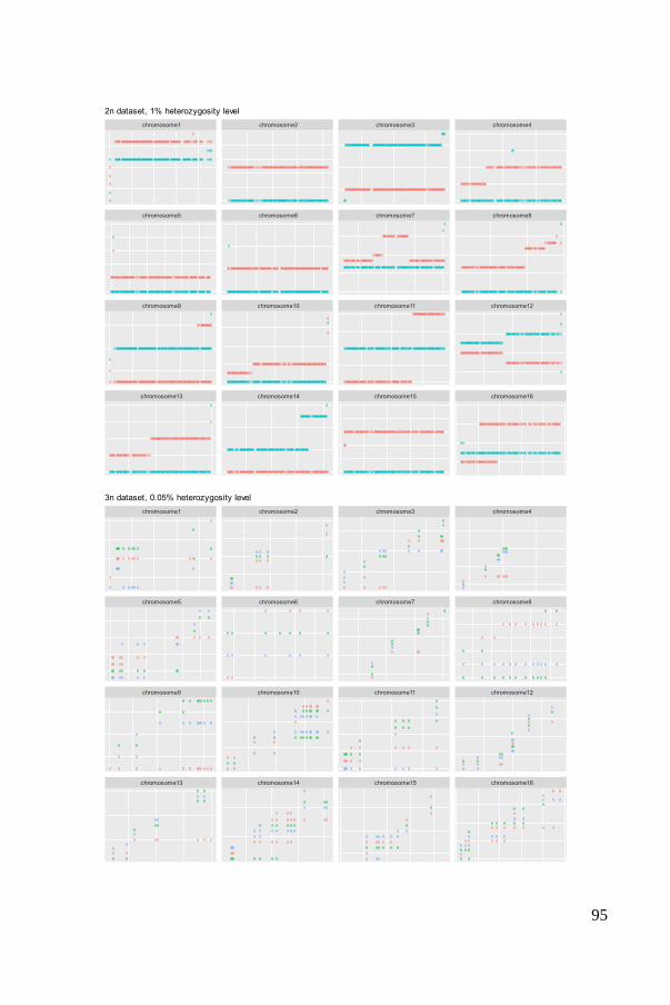
95

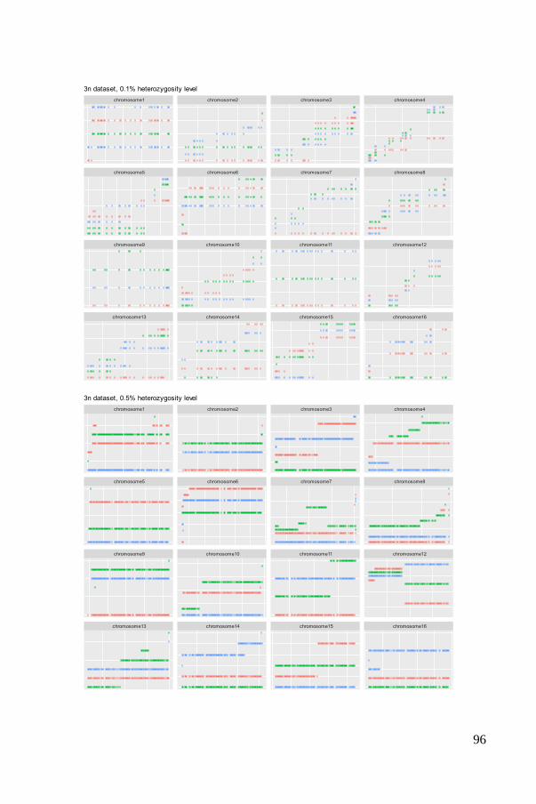
96

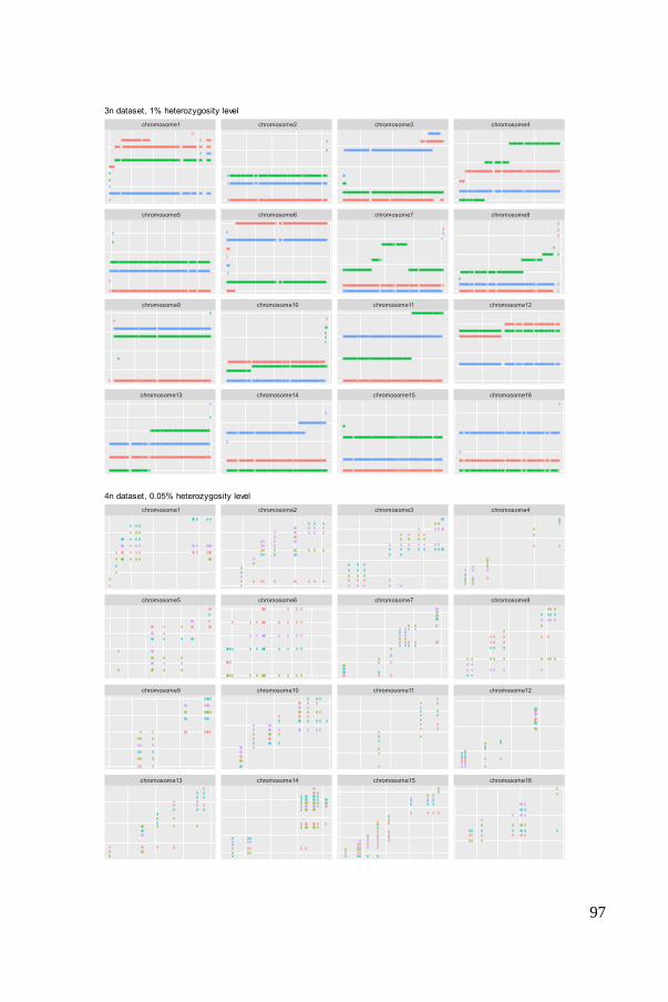
97

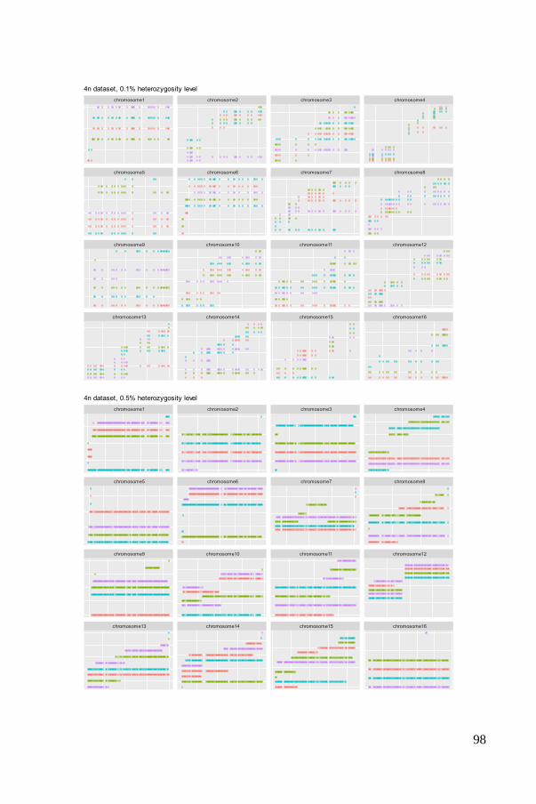
98

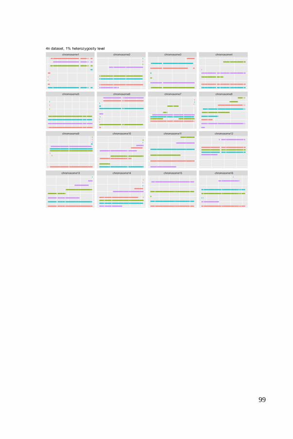
99

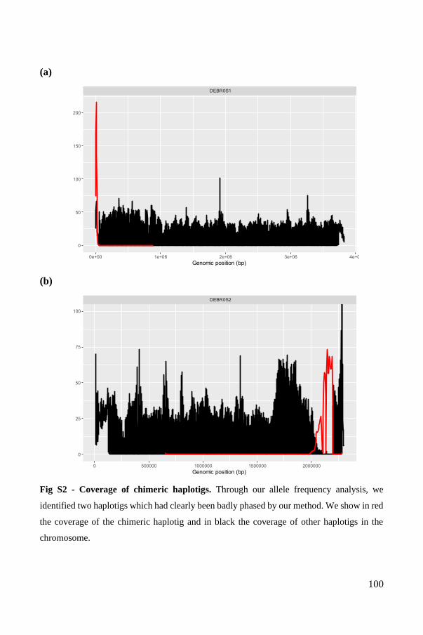
100

(a)

(b)

Fig S2 - Coverage of chimeric haplotigs. Through our allele frequency analysis, we

identified two haplotigs which had clearly been badly phased by our method. We show in red

the coverage of the chimeric haplotig and in black the coverage of other haplotigs in the

chromosome.

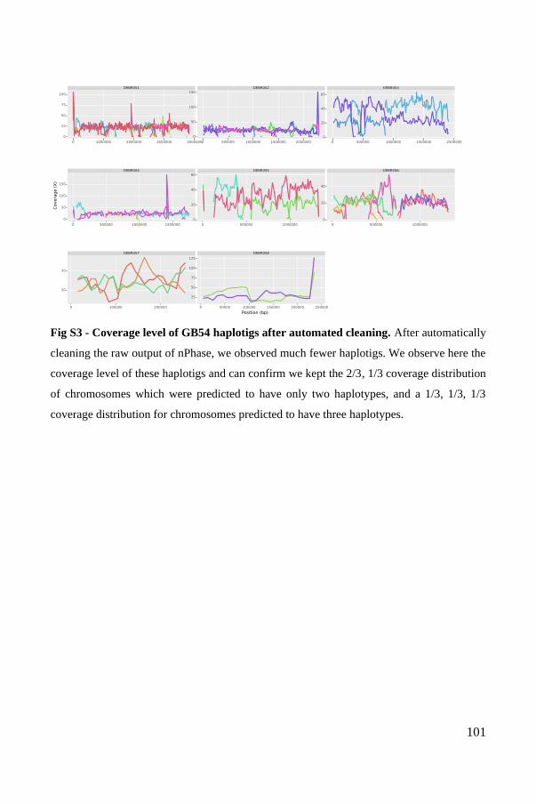
101

Fig S3 - Coverage level of GB54 haplotigs after automated cleaning. After automatically

cleaning the raw output of nPhase, we observed much fewer haplotigs. We observe here the

coverage level of these haplotigs and can confirm we kept the 2/3, 1/3 coverage distribution

of chromosomes which were predicted to have only two haplotypes, and a 1/3, 1/3, 1/3

coverage distribution for chromosomes predicted to have three haplotypes.

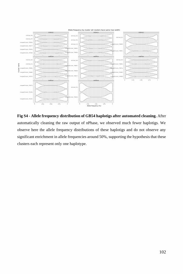
102

Fig S4 - Allele frequency distribution of GB54 haplotigs after automated cleaning. After

automatically cleaning the raw output of nPhase, we observed much fewer haplotigs. We

observe here the allele frequency distributions of these haplotigs and do not observe any

significant enrichment in allele frequencies around 50%, supporting the hypothesis that these

clusters each represent only one haplotype.

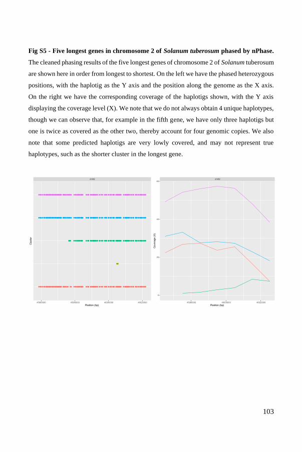
103

Fig S5 - Five longest genes in chromosome 2 of Solanum tuberosum phased by nPhase.

The cleaned phasing results of the five longest genes of chromosome 2 of Solanum tuberosum

are shown here in order from longest to shortest. On the left we have the phased heterozygous

positions, with the haplotig as the Y axis and the position along the genome as the X axis.

On the right we have the corresponding coverage of the haplotigs shown, with the Y axis

displaying the coverage level (X). We note that we do not always obtain 4 unique haplotypes,

though we can observe that, for example in the fifth gene, we have only three haplotigs but

one is twice as covered as the other two, thereby account for four genomic copies. We also

note that some predicted haplotigs are very lowly covered, and may not represent true

haplotypes, such as the shorter cluster in the longest gene.

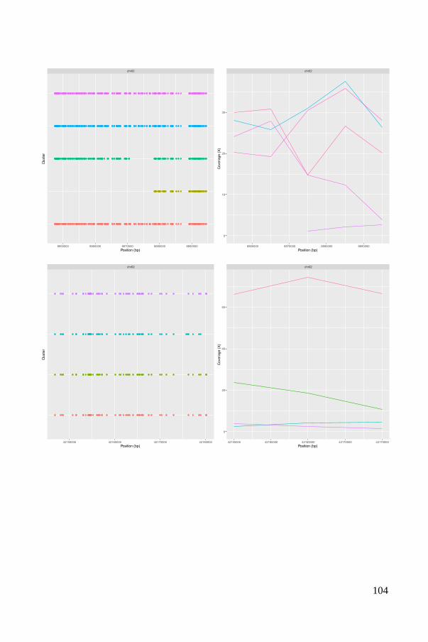
104

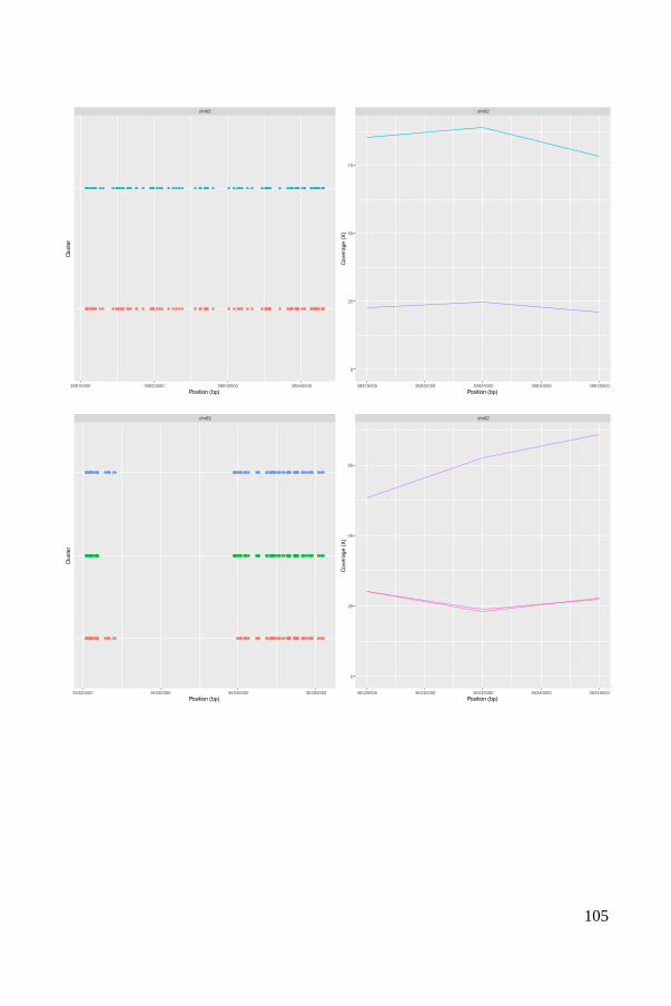
105

106

(a)

(b)

Fig S6 - Long read pre-processing steps. (a) Simplifying long reads. Each long read is

reduced to the set of variable positions it overlaps. Hence the first sequence becomes ATC,

the second becomes CGA and the third becomes AGC. We keep track of the position and

chromosome on which each SNP is found. (b) Context coverage. T and G are equally covered

without context, but with context we see that AGC and CTA are not as highly covered as

ATC and CGA.

Fig S7 - nPhase parameters. The parameters S, O, L and ID are the only parameters that

can be user-set in the nPhase algorithm.

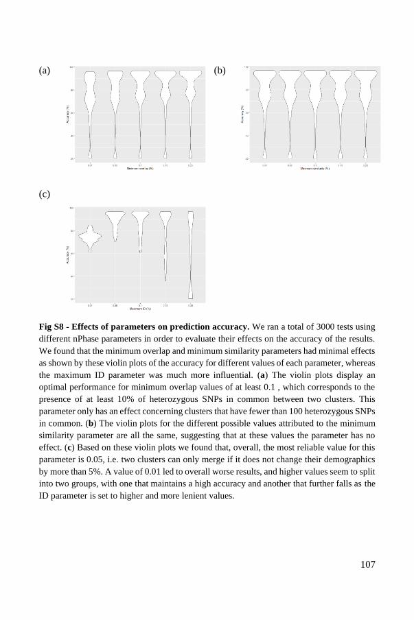
107

(a) (b)

(c)

Fig S8 - Effects of parameters on prediction accuracy. We ran a total of 3000 tests using

different nPhase parameters in order to evaluate their effects on the accuracy of the results.

We found that the minimum overlap and minimum similarity parameters had minimal effects

as shown by these violin plots of the accuracy for different values of each parameter, whereas

the maximum ID parameter was much more influential. (a) The violin plots display an

optimal performance for minimum overlap values of at least 0.1 , which corresponds to the

presence of at least 10% of heterozygous SNPs in common between two clusters. This

parameter only has an effect concerning clusters that have fewer than 100 heterozygous SNPs

in common. (b) The violin plots for the different possible values attributed to the minimum

similarity parameter are all the same, suggesting that at these values the parameter has no

effect. (c) Based on these violin plots we found that, overall, the most reliable value for this

parameter is 0.05, i.e. two clusters can only merge if it does not change their demographics

by more than 5%. A value of 0.01 led to overall worse results, and higher values seem to split

into two groups, with one that maintains a high accuracy and another that further falls as the

ID parameter is set to higher and more lenient values.

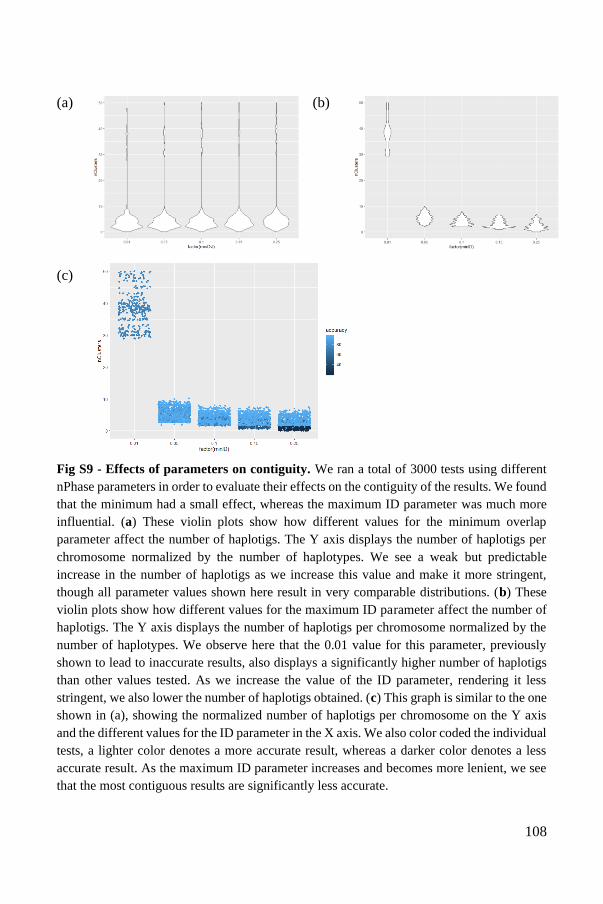
108

(a) (b)

(c)

Fig S9 - Effects of parameters on contiguity. We ran a total of 3000 tests using different

nPhase parameters in order to evaluate their effects on the contiguity of the results. We found

that the minimum had a small effect, whereas the maximum ID parameter was much more

influential. (a) These violin plots show how different values for the minimum overlap

parameter affect the number of haplotigs. The Y axis displays the number of haplotigs per

chromosome normalized by the number of haplotypes. We see a weak but predictable

increase in the number of haplotigs as we increase this value and make it more stringent,

though all parameter values shown here result in very comparable distributions. (b) These

violin plots show how different values for the maximum ID parameter affect the number of

haplotigs. The Y axis displays the number of haplotigs per chromosome normalized by the

number of haplotypes. We observe here that the 0.01 value for this parameter, previously

shown to lead to inaccurate results, also displays a significantly higher number of haplotigs

than other values tested. As we increase the value of the ID parameter, rendering it less

stringent, we also lower the number of haplotigs obtained. (c) This graph is similar to the one

shown in (a), showing the normalized number of haplotigs per chromosome on the Y axis

and the different values for the ID parameter in the X axis. We also color coded the individual

tests, a lighter color denotes a more accurate result, whereas a darker color denotes a less

accurate result. As the maximum ID parameter increases and becomes more lenient, we see

that the most contiguous results are significantly less accurate.

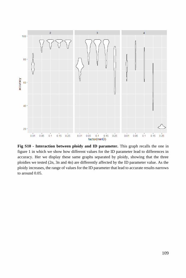
109

Fig S10 - Interaction between ploidy and ID parameter. This graph recalls the one in

figure 1 in which we show how different values for the ID parameter lead to differences in

accuracy. Her we display these same graphs separated by ploidy, showing that the three

ploidies we tested (2n, 3n and 4n) are differently affected by the ID parameter value. As the

ploidy increases, the range of values for the ID parameter that lead to accurate results narrows

to around 0.05.

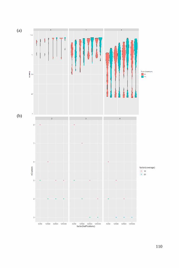
110

(a)

(b)

111

Fig S11 - Effects of coverage on accuracy and contiguity. We compared the results of all

3000 tests performed on 10X datasets to the 3000 tests performed on their 20X counterparts

and found that the 20X datasets had consistently more potential, reaching higher accuracy

values and better contiguity across ploidy and heterozygosity levels. (a) Here we compare

the accuracy distributions for tests of different ploidies and heterozygosity levels at the 10X

and 20X coverage levels. We see that the 20X dataset is consistently able to reach higher

accuracy levels, an effect which appears to be stronger when the ploidy is higher. (b) Since

we are only interested in a high contiguity when it is coupled with a high accuracy, we will

not look at a distribution of the number of haplotigs per haplotype across ploidy and

heterozygosity levels at the 10X and 20X coverage levels, instead we're focusing on that

contiguity metric for the tests using default parameters. We can clearly see a higher number

of haplotigs per haplotype for the 10X dataset, with the gap between the 10X and 20X

datasets deepening for lower heterozygosity level tests.

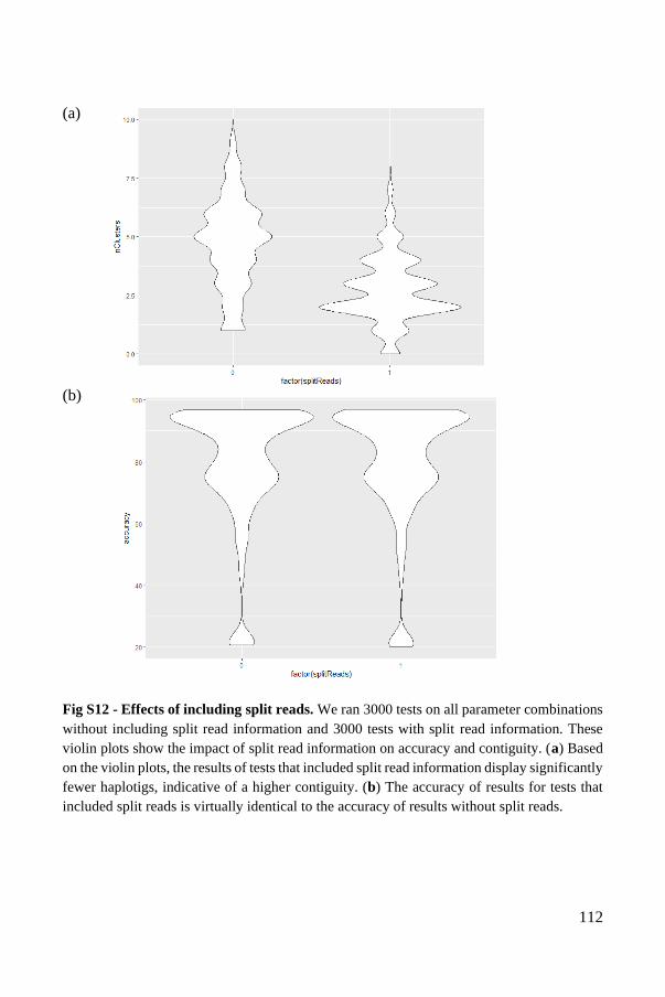
112

(a)

(b)

Fig S12 - Effects of including split reads. We ran 3000 tests on all parameter combinations

without including split read information and 3000 tests with split read information. These

violin plots show the impact of split read information on accuracy and contiguity. (a) Based

on the violin plots, the results of tests that included split read information display significantly

fewer haplotigs, indicative of a higher contiguity. (b) The accuracy of results for tests that

included split reads is virtually identical to the accuracy of results without split reads.

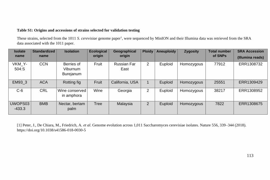
113

Table S1: Origins and accessions of strains selected for validation testing

These strains, selected from the 1011 S. cerevisiae genome paper1, were sequenced by MinION and their Illumina data was retrieved from the SRA

data associated with the 1011 paper.

Isolate

name

Standardized

name

Isolation Ecological

origin

Geographical

origin

Ploidy Aneuploidy Zygosity Total number

of SNPs

SRA Accession

(Illumina reads)

VKM_Y-

504:S

CCN Berries of

Viburnum

Burejanum

Fruit Russian Far

East

2 Euploid Homozygous 77912 ERR1308732

EM93_3 ACA Rotting fig Fruit California, USA 1 Euploid Homozygous 25551 ERR1309429

C-6 CRL Wine conserved

in amphora

Wine Georgia 2 Euploid Homozygous 38217 ERR1308952

UWOPS03

-433.3

BMB Nectar, bertam

palm

Tree Malaysia 2 Euploid Homozygous 7822 ERR1308675

[1] Peter, J., De Chiara, M., Friedrich, A. et al. Genome evolution across 1,011 Saccharomyces cerevisiae isolates. Nature 556, 339–344 (2018).

https://doi.org/10.1038/s41586-018-0030-5

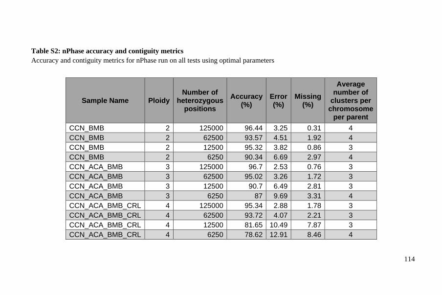
114

Table S2: nPhase accuracy and contiguity metrics

Accuracy and contiguity metrics for nPhase run on all tests using optimal parameters

Sample Name Ploidy Number of

heterozygous positions

Accuracy (%)

Error (%)

Missing (%)

Average number of

clusters per chromosome

per parent

CCN_BMB 2 125000 96.44 3.25 0.31 4

CCN_BMB 2 62500 93.57 4.51 1.92 4

CCN_BMB 2 12500 95.32 3.82 0.86 3

CCN_BMB 2 6250 90.34 6.69 2.97 4

CCN_ACA_BMB 3 125000 96.7 2.53 0.76 3

CCN_ACA_BMB 3 62500 95.02 3.26 1.72 3

CCN_ACA_BMB 3 12500 90.7 6.49 2.81 3

CCN_ACA_BMB 3 6250 87 9.69 3.31 4

CCN_ACA_BMB_CRL 4 125000 95.34 2.88 1.78 3

CCN_ACA_BMB_CRL 4 62500 93.72 4.07 2.21 3

CCN_ACA_BMB_CRL 4 12500 81.65 10.49 7.87 3

CCN_ACA_BMB_CRL 4 6250 78.62 12.91 8.46 4

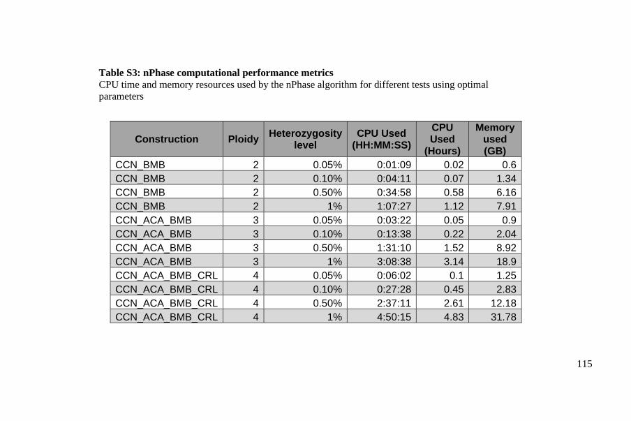
115

Table S3: nPhase computational performance metrics

CPU time and memory resources used by the nPhase algorithm for different tests using optimal

parameters

Construction Ploidy Heterozygosity

level CPU Used

(HH:MM:SS)

CPU Used

(Hours)

Memory used (GB)

CCN_BMB 2 0.05% 0:01:09 0.02 0.6

CCN_BMB 2 0.10% 0:04:11 0.07 1.34

CCN_BMB 2 0.50% 0:34:58 0.58 6.16

CCN_BMB 2 1% 1:07:27 1.12 7.91

CCN_ACA_BMB 3 0.05% 0:03:22 0.05 0.9

CCN_ACA_BMB 3 0.10% 0:13:38 0.22 2.04

CCN_ACA_BMB 3 0.50% 1:31:10 1.52 8.92

CCN_ACA_BMB 3 1% 3:08:38 3.14 18.9

CCN_ACA_BMB_CRL 4 0.05% 0:06:02 0.1 1.25

CCN_ACA_BMB_CRL 4 0.10% 0:27:28 0.45 2.83

CCN_ACA_BMB_CRL 4 0.50% 2:37:11 2.61 12.18

CCN_ACA_BMB_CRL 4 1% 4:50:15 4.83 31.78

116

Availability of data and materials

The nPhase algorithm and the nPhase pipeline are both available under the open

source GNU General Public License v3.0 at:

https://github.com/OmarOakheart/nPhase30

Oxford Nanopore sequencing data is available under the study accession number

PRJEB39456

Illumina short read data for the Saccharomyces cerevisiae strains are taken from the

1,011 yeast genomes project24 and their SRA accessions are the following:

ERR130873231, ERR130942931, ERR130895231, ERR130867531.

Illumina and Oxford Nanopore data for the Brettanomyces bruxellensis GB54 strain

is available under the study accession number PRJEB40511.

Illumina and Oxford Nanopore data for the Solanum tuberosum strain used is

available under the study accession number PRJNA58739732.

117

References

1. Mahmoud, M. et al. Structural variant calling: the long and the short of it. Genome

Biol 20, (2019).

2. Sohn, J. & Nam, J.-W. The present and future of de novo whole-genome assembly.

Brief Bioinform 19, 23–40 (2018).

3. Kitzman, J. O. et al. Haplotype-resolved genome sequencing of a Gujarati Indian

individual. Nat. Biotechnol. 29, 59–63 (2011).

4. Roach, M. J. et al. Population sequencing reveals clonal diversity and ancestral

inbreeding in the grapevine cultivar Chardonnay. PLoS Genet. 14, e1007807 (2018).

5. Hamazaki, K. & Iwata, H. Haplotype-based genome wide association study using

a novel SNP-set method : RAINBOW. bioRxiv 612028 (2019).

6. Sanjak, J. S., Long, A. D. & Thornton, K. R. A Model of Compound

Heterozygous, Loss-of-Function Alleles Is Broadly Consistent with Observations

from Complex-Disease GWAS Datasets. PLOS Genetics 13, e1006573 (2017).

7. Benitez, J. A., Cheng, S. & Deng, Q. Revealing allele-specific gene expression by

single-cell transcriptomics. Int. J. Biochem. Cell Biol. 90, 155–160 (2017).

8. Wagner, N. D., He, L. & Hörandl, E. Relationships and genome evolution of

polyploid Salix species revealed by RAD sequencing data. bioRxiv 864504 (2019).

9. Eriksson, J. S. et al. Allele phasing is critical to revealing a shared allopolyploid

origin of Medicago arborea and M. strasseri (Fabaceae). BMC Evol Biol 18, 9 (2018).

10. Yang, J. et al. Incomplete dominance of deleterious alleles contributes

substantially to trait variation and heterosis in maize. PLOS Genetics 13, e1007019

(2017).

11. Fay, J. C. et al. A polyploid admixed origin of beer yeasts derived from European

and Asian wine populations. PLOS Biology 17, e3000147 (2019).

12. Zhou, R.-N. & Hu, Z.-M. The Development of Chromosome Microdissection

and Microcloning Technique and its Applications in Genomic Research. Curr

Genomics 8, 67–72 (2007).

13. Snyder, M. W., Adey, A., Kitzman, J. O. & Shendure, J. Haplotype-resolved

genome sequencing: experimental methods and applications. Nature Reviews

Genetics 16, 344–358 (2015).

14. Zhang, X., Wu, R., Wang, Y., Yu, J. & Tang, H. Unzipping haplotypes in diploid

and polyploid genomes. Comput Struct Biotechnol J 18, 66–72 (2019).

15. Koren, S. et al. De novo assembly of haplotype-resolved genomes with trio

binning. Nat Biotechnol (2018).

16. He, D., Saha, S., Finkers, R. & Parida, L. Efficient algorithms for polyploid

haplotype phasing. BMC Genomics 19, 110 (2018).

17. Browning, S. R. & Browning, B. L. Rapid and Accurate Haplotype Phasing and

Missing-Data Inference for Whole-Genome Association Studies By Use of

118

Localized Haplotype Clustering. The American Journal of Human Genetics 81,

1084–1097 (2007).

18. Patterson, M. et al. WhatsHap: Weighted Haplotype Assembly for Future-

Generation Sequencing Reads. Journal of Computational Biology 22, 498–509

(2015).

19. Chin, C.-S. et al. Phased diploid genome assembly with single-molecule real-

time sequencing. Nat. Methods 13, 1050–1054 (2016).

20. Schrinner, S.D., Mari, R.S., Ebler, J., Rautiainen, M., Seillier, L., Reimer, J.J.,

Usadel, B., Marschall, T., and Klau, G.W. (2020). Haplotype threading: accurate

polyploid phasing from long reads. Genome Biology 21, 252.

21. Xie, M., Wu, Q., Wang, J. & Jiang, T. H-PoP and H-PoPG: heuristic partitioning

algorithms for single individual haplotyping of polyploids. Bioinformatics 32, 3735–

3744 (2016).

22. Motazedi, E., Finkers, R., Maliepaard, C. & de Ridder, D. Exploiting next-

generation sequencing to solve the haplotyping puzzle in polyploids: a simulation

study. Brief. Bioinformatics 19, 387–403 (2018).

23. Moeinzadeh, M.-H. et al. Ranbow: A fast and accurate method for polyploid

haplotype reconstruction. PLOS Computational Biology 16, e1007843 (2020).

24. Peter, J. et al. Genome evolution across 1,011 Saccharomyces cerevisiae isolates.

Nature 556, 339–344 (2018).

25. Pham, G. M. et al. Construction of a chromosome-scale long-read reference

genome assembly for potato. GigaScience 9, (2020).

26. Li, H. & Durbin, R. Fast and accurate short read alignment with Burrows–

Wheeler transform. Bioinformatics 25, 1754–1760 (2009).

27. Van der Auwera, G. A. et al. From FastQ data to high confidence variant calls:

the Genome Analysis Toolkit best practices pipeline. Curr Protoc Bioinformatics

43, 11.10.1-11.10.33 (2013).

28. Sedlazeck, F. J. et al. Accurate detection of complex structural variations using

single-molecule sequencing. Nature Methods 15, 461–468 (2018).

29. Li, H. et al. The Sequence Alignment/Map format and SAMtools. Bioinformatics

25, 2078–2079 (2009).

30. Abou Saada, O. et al. nPhase. Github. https://github.com/OmarOakheart/nPhase

10.5281/zenodo.4626656 (2021).

31. Peter, J. et al. Genome evolution across 1,011 Saccharomyces cerevisiae isolates.

Subset of four Saccharomyces cerevisiae short read sequencing files (ERR1308732,

ERR1309429, ERR1308952, ERR1308675). NCBI BioProject.

https://www.ncbi.nlm.nih.gov/bioproject/PRJEB13017 (2018).

32. Seillier, L. et al. Solanum tuberosum genome sequencing. Oxford Nanopore and

Illumina Data. NCBI BioProject.

https://www.ncbi.nlm.nih.gov/bioproject/PRJNA587397 (2019).

119

120

Chapter II – Phased polyploid genomes provide

deeper insights into the different evolutionary

trajectories of the Saccharomyces cerevisiae beer

yeasts

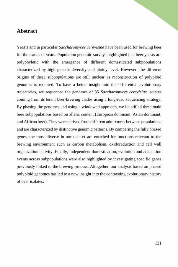
121

Abstract

Yeasts and in particular Saccharomyces cerevisiae have been used for brewing beer

for thousands of years. Population genomic surveys highlighted that beer yeasts are

polyphyletic with the emergence of different domesticated subpopulations

characterized by high genetic diversity and ploidy level. However, the different

origins of these subpopulations are still unclear as reconstruction of polyploid

genomes is required. To have a better insight into the differential evolutionary

trajectories, we sequenced the genomes of 35 Saccharomyces cerevisiae isolates

coming from different beer-brewing clades using a long-read sequencing strategy.

By phasing the genomes and using a windowed approach, we identified three main

beer subpopulations based on allelic content (European dominant, Asian dominant,

and African beer). They were derived from different admixtures between populations

and are characterized by distinctive genomic patterns. By comparing the fully phased

genes, the most diverse in our dataset are enriched for functions relevant to the

brewing environment such as carbon metabolism, oxidoreduction and cell wall

organization activity. Finally, independent domestication, evolution and adaptation

events across subpopulations were also highlighted by investigating specific genes

previously linked to the brewing process. Altogether, our analysis based on phased

polyploid genomes has led to a new insight into the contrasting evolutionary history

of beer isolates.

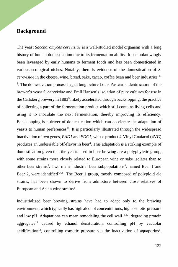
122

Background

The yeast Saccharomyces cerevisiae is a well-studied model organism with a long

history of human domestication due to its fermentation ability. It has unknowingly

been leveraged by early humans to ferment foods and has been domesticated in

various ecological niches. Notably, there is evidence of the domestication of S.

cerevisiae in the cheese, wine, bread, sake, cacao, coffee bean and beer industries 1–

8. The domestication process began long before Louis Pasteur’s identification of the

brewer’s yeast S. cerevisiae and Emil Hansen’s isolation of pure cultures for use in

the Carlsberg brewery in 18839, likely accelerated through backslopping: the practice

of collecting a part of the fermentation product which still contains living cells and

using it to inoculate the next fermentation, thereby improving its efficiency.

Backslopping is a driver of domestication which can accelerate the adaptation of

yeasts to human preferences10. It is particularly illustrated through the widespread

inactivation of two genes, PAD1 and FDC1, whose product 4-Vinyl Guaiacol (4VG)

produces an undesirable off-flavor in beer4. This adaptation is a striking example of

domestication given that the yeasts used in beer brewing are a polyphyletic group,

with some strains more closely related to European wine or sake isolates than to

other beer strains5. Two main industrial beer subpopulations4, named Beer 1 and

Beer 2, were identified4,5,8. The Beer 1 group, mostly composed of polyploid ale

strains, has been shown to derive from admixture between close relatives of

European and Asian wine strains8.

Industrialized beer brewing strains have had to adapt only to the brewing

environment, which typically has high alcohol concentrations, high osmotic pressure

and low pH. Adaptations can mean remodeling the cell wall11,12, degrading protein

aggregates13 caused by ethanol denaturation, controlling pH by vacuolar

acidification14, controlling osmotic pressure via the inactivation of aquaporins5.

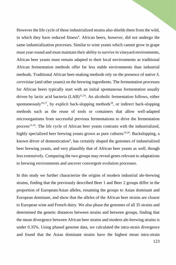
123

However the life cycle of these industrialized strains also shields them from the wild,

in which they have reduced fitness4. African beers, however, did not undergo the

same industrialization processes. Similar to wine yeasts which cannot grow in grape

must year-round and must maintain their ability to survive in vineyard environments,

African beer yeasts must remain adapted to their local environments as traditional

African fermentation methods offer far less stable environments than industrial

methods. Traditional African beer-making methods rely on the presence of native S.

cerevisiae (and other yeasts) on the brewing ingredients. The fermentation processes

for African beers typically start with an initial spontaneous fermentation usually

driven by lactic acid bacteria (LAB)15,16. An alcoholic fermentation follows, either

spontaneously16,17, by explicit back-slopping methods18, or indirect back-slopping

methods such as the reuse of tools or containers that allow well-adapted

microorganisms from successful previous fermentations to drive the fermentation

process15,16. The life cycle of African beer yeasts contrasts with the industrialized,

highly specialized beer brewing yeasts grown as pure cultures19,20. Backslopping, a

known driver of domestication4, has certainly shaped the genomes of industrialized

beer brewing yeasts, and very plausibly that of African beer yeasts as well, though

less extensively. Comparing the two groups may reveal genes relevant to adaptations

to brewing environments and uncover convergent evolution processes.

In this study we further characterize the origins of modern industrial ale-brewing

strains, finding that the previously described Beer 1 and Beer 2 groups differ in the

proportion of European/Asian alleles, renaming the groups to Asian dominant and

European dominant, and show that the alleles of the African beer strains are closest

to European wine and French dairy. We also phase the genomes of all 35 strains and

determined the genetic distances between strains and between groups, finding that

the mean divergence between African beer strains and modern ale-brewing strains is

under 0.35%. Using phased genome data, we calculated the intra-strain divergence

and found that the Asian dominant strains have the highest mean intra-strain

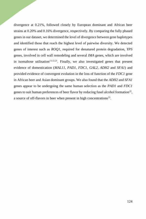
124

divergence at 0.21%, followed closely by European dominant and African beer

strains at 0.20% and 0.16% divergence, respectively. By comparing the fully phased

genes in our dataset, we determined the level of divergence between gene haplotypes

and identified those that reach the highest level of pairwise diversity. We detected

genes of interest such as ROQ1, required for denatured protein degradation, YPS

genes, involved in cell wall remodeling and several IMA genes, which are involved

in isomaltose utilisation13,12,21. Finally, we also investigated genes that present

evidence of domestication (MAL11, PAD1, FDC1, GAL2, ADH2 and SFA1) and

provided evidence of convergent evolution in the loss of function of the FDC1 gene

in African beer and Asian dominant groups. We also found that the ADH2 and SFA1

genes appear to be undergoing the same human selection as the PAD1 and FDC1

genes to suit human preferences of beer flavor by reducing fusel alcohol formation22,

a source of off-flavors in beer when present in high concentrations23.

125

Results

Selection of beer isolates, sequencing and genome phasing

To dissect the genetic diversity and genomic architecture of beer-brewing yeasts, we

selected 35 strains from diverse clades based either on their known use in fermenting

beers or on their high genetic similarity to beer-brewing strains (Supplementary

Table S1). Beer-brewing strains of S. cerevisiae are polyphyletic, forming at least

three distinct clades: one clade of African beer strains and two clades of modern ale

strains named Beer 1 and Beer 2, which are believed to have different origins4. It has

been shown that Beer 1 strains are a polyploid admixture of European and Asian

wine strains8. The African beer and Beer 1 groups typically have higher ploidies,

between 3n and 5n for the African beer group and typically 4n for the Beer 1 group.

Strains from the Beer 2 group are not typically polyploid. Adding to the diversity

and complexity of the population of beer yeasts, some isolates used in breweries

have genomes consistent with European wine strains, and others have genomes that

cluster with other strains of mixed origins. For our study, we selected 8 African beer

strains, 16 Beer 1 strains, and 5 Beer 2 strains. We also selected 6 beer-brewing

strains from outside of these three clades, including 2 European wine strains isolated

from breweries, 3 strains from the Mixed origin clade and 1 from the Mosaic Region

1 clade6.

Given the polyploid nature of a majority of the strains selected, we sequenced all 35

strains with Oxford Nanopore long reads in order to phase their genomes. We used

publicly available short read data for nearly all of the strains selected6,8

(Supplementary Table S2). Only strain YMD4285 was sequenced by Illumina for

this study. We aimed to obtain at least 80X theoretical coverage with our long reads

for most strains in order to obtain accurate and contiguous phasing results. We

reached the target of 80X coverage in 26 out of 35 strains, with the remaining 9

126

ranging from 14.4X theoretical coverage to 77.6X (Supplementary Table S2).

Whenever possible, we downsampled our long-read data to 80X of the best reads,

obtaining mean read lengths up to 37.7 kb (mean 21.2 kb) and mean read quality

scores up to 15.9 (mean 14.4). In cases where we could not downsample to 80X, we

used all of the sequencing reads for our analyses. The Illumina short read data we

used ranges from 144X to 368X (mean 281X), with mean quality scores ranging

from 28.8 to 34.8 (mean 32.9).

We recently developed a phasing algorithm and pipeline, nPhase24, which phases a

genome using short reads, long reads and a reference sequence. The short reads are

mapped to the reference sequence and variant called, which serves as a list of high-

confidence SNP positions. The long reads are also mapped to the same reference

sequence and iteratively clustered together according to the similarity between reads

at these previously defined SNP positions. The iterative clustering ends when only

distinct clusters remain, which are different from each other. nPhase is a ploidy

agnostic phasing method, it makes no attempt to coerce the results to a given or

estimated ploidy, it only detects when the existing clusters should not be merged

together. nPhase also provides a cleaning algorithm which removes small clusters

and attempts to improve the contiguity of phasing results and reduce noise at little

cost to accuracy by applying simple heuristics24. We used our dataset of accurate

short reads and phase-informative long reads to phase all 35 strains using nPhase24

and used the nPhase cleaning algorithm to improve the contiguity of our results

(Supplementary Figures S1 and S2).

Without a ground truth, we cannot assess the accuracy of our phasing results,

however we can assess their contiguity. We use the L90 metric which we define here

as the minimal number of haplotigs to cover at least 90% of all reads, and the L90

per chromosome, which is simply the L90 divided by the number of chromosomes

times the ploidy. The L90 per chromosome for the phasing of a triploid strain of S.

127

cerevisiae is therefore the L90 divided by 3*16. If the value is close to 1, we have

close to a contiguous phasing, if it is much higher, the phasing is increasingly

fragmented, and if much lower, increasingly likely not to have correctly

distinguished between haplotypes. We report in our raw results an L90 per

chromosome that ranges from 1 to 2.6 (with an outlier at 4.3 due to low long read

coverage), with a mean L90 per chromosome of 1.6 (Supplementary Table S3). After

applying the cleaning pipeline available for nPhase we improved the contiguity,

reducing the range of L90 per chromosome to between 0.8 and 2.3 (with the same

outlier at 3.6). The cleaning step also substantially reduced the average total number

of haplotigs from 198 to 100.

Aneuploidy information for most strains was obtained from Peter et al. 2018. For

the 7 remaining strains aneuploidy was determined based on allele frequency plots

(Supplementary Figure S3). The phasing correctly predicted a number of suspected

and known aneuploidies such as the 6 different chromosome losses of the tetraploid

strain BBG and the extra copy of chromosome 3 in the diploid strain CPB, though

not all, with aneuploidies in strains such as CFM remaining unclear after phasing,

potentially due to lower read lengths (Supplementary Table S4).

Inter-strain divergence reveals three groups of strains

The standard way of estimating the divergence between two strains uses unphased

genomes to calculate their distance based on allelic differences. Using this method,

we obtain a mean inter-strain divergence of 0.58% across all strains, with a

maximum divergence of 1% when comparing AVS and YMD4285 (Supplementary

Table S5). This method is not well adapted to polyploidy, as it does not take into

account the complexity of these genomes, leading to inaccurate representations of

the differences in genetic content between strains. It does not, for example, reveal if

two strains may have a subgenome or haplotype in common. There are two main

barriers to obtaining this type of information: it requires access to phased haplotypes,

128

and the question is complicated by recombination events and Loss of Heterozygosity

(LOH) events. Using our dataset of phased haplotypes, we propose a more accurate

metric of inter-strain divergence for polyploids that takes their haplotypes into

account. For each pair of strains, A and B for example, we calculate the distance

between 10 kb regions of all haplotypes, keeping only the match with the lowest

divergence. We allow a 10 kb region of a haplotype in strain B to match with several

10 kb regions in strain A’s haplotypes. This allows us to estimate divergence based

on the allelic content of each strain (Figure 1). Using this method, we updated our

mean inter-strain genetic divergence numbers from 0.58% to 0.36% and the highest

level of inter-strain divergence drops to 0.56%, obtained when comparing strains

ANL and YMD4285 (Supplementary Table S6). The previously most divergent

strains AVS and YMD4285 are 0.55% divergent using this calculation method.

This inter-strain divergence based on haplotypes reveals three main groups of strains

in our dataset defined by a higher similarity to each other than to other strains: the

African beer group (s8 strains), the Beer 2 group to which we can add two European

wine strains and the Mosaic Region 1 strains (8 strains), and finally the Beer 1 group

to which we can add the 3 mixed origin strains (19 strains). Two of the three mixed

origin strains, CFP and CFN, could arguably be assigned to either group though the

third, BDL, resembles the Beer 1 group more closely. Despite the polyphyletic nature

of the population, we can reorganize the strains in our dataset into three major

groups.

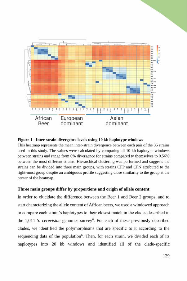
129

Figure 1 - Inter-strain divergence levels using 10 kb haplotype windows

This heatmap represents the mean inter-strain divergence between each pair of the 35 strains

used in this study. The values were calculated by comparing all 10 kb haplotype windows

between strains and range from 0% divergence for strains compared to themselves to 0.56%

between the most different strains. Hierarchical clustering was performed and suggests the

strains can be divided into three main groups, with strains CFP and CFN attributed to the

right-most group despite an ambiguous profile suggesting close similarity to the group at the

center of the heatmap.

Three main groups differ by proportions and origin of allele content

In order to elucidate the difference between the Beer 1 and Beer 2 groups, and to

start characterizing the allele content of African beers, we used a windowed approach

to compare each strain’s haplotypes to their closest match in the clades described in

the 1,011 S. cerevisiae genomes survey6. For each of these previously described

clades, we identified the polymorphisms that are specific to it according to the

sequencing data of the population6. Then, for each strain, we divided each of its

haplotypes into 20 kb windows and identified all of the clade-specific

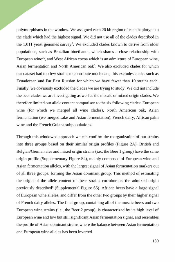
130

polymorphisms in the window. We assigned each 20 kb region of each haplotype to

the clade which had the highest signal. We did not use all of the clades described in

the 1,011 yeast genomes survey6. We excluded clades known to derive from older

populations, such as Brazilian bioethanol, which shares a close relationship with

European wine25, and West African cocoa which is an admixture of European wine,

Asian fermentation and North American oak3. We also excluded clades for which

our dataset had too few strains to contribute much data, this excludes clades such as

Ecuadorean and Far East Russian for which we have fewer than 10 strains each.

Finally, we obviously excluded the clades we are trying to study. We did not include

the beer clades we are investigating as well as the mosaic or mixed origin clades. We

therefore limited our allele content comparison to the six following clades: European

wine (for which we merged all wine clades), North American oak, Asian

fermentation (we merged sake and Asian fermentation), French dairy, African palm

wine and the French Guiana subpopulations.

Through this windowed approach we can confirm the reorganization of our strains

into three groups based on their similar origin profiles (Figure 2A). British and

Belgian/German ales and mixed origin strains (i.e., the Beer 1 group) have the same

origin profile (Supplementary Figure S4), mainly composed of European wine and

Asian fermentation alleles, with the largest signal of Asian fermentation markers out

of all three groups, forming the Asian dominant group. This method of estimating

the origin of the allele content of these strains corroborates the admixed origin

previously described8 (Supplemental Figure S5). African beers have a large signal

of European wine alleles, and differ from the other two groups by their higher signal

of French dairy alleles. The final group, containing all of the mosaic beers and two

European wine strains (i.e., the Beer 2 group), is characterized by its high level of

European wine and low but still significant Asian fermentation signal, and resembles

the profile of Asian dominant strains where the balance between Asian fermentation

and European wine alleles has been inverted.

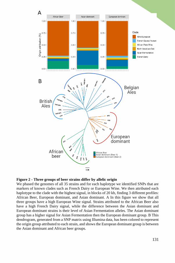
131

Figure 2 - Three groups of beer strains differ by allelic origin

We phased the genomes of all 35 strains and for each haplotype we identified SNPs that are

markers of known clades such as French Dairy or European Wine. We then attributed each

haplotype to the clade with the highest signal, in blocks of 20 kb, finding 3 different profiles:

African Beer, European dominant, and Asian dominant. A In this figure we show that all

three groups have a high European Wine signal. Strains attributed to the African Beer also

have a high French Dairy signal, while the difference between the Asian dominant and

European dominant strains is their level of Asian Fermentation alleles. The Asian dominant

group has a higher signal for Asian Fermentation then the European dominant group. B This

dendrogram, generated from a SNP matrix using Illumina data, has been colored to represent

the origin group attributed to each strain, and shows the European dominant group is between

the Asian dominant and African beer groups.

132

We then generated a dendrogram based on all genomic SNPs to place the strains in

relation to each other (Figure 2B). We find that the European dominant group is in

between the African beer group and the Asian dominant group. Consistent with

previous reports we also distinguish two ale groups that correspond to geographical

origin, British ales (CFG, CFH, YMD1864, YMD1870 and YMD1981) which

cluster together on one branch of the dendrogram along with USA strain CFM, and

Belgian/German ales which cluster on the adjacent branch (BRP, YMD1950, BSI,

AQT and YMD1871), alongside CGC, a USA strain isolated from an olive fly and

BBG, a strain isolated from the water of the Morava river in Slovakia. The

Belgian/German strains YMD1873, CFC and CFF are also found along the main

branch of the Asian dominant group on this dendrogram, alongside YMD4285, BDL

and CFN. We will hereafter refer to the 5 British strains and the USA strain that

clusters with them as the British ales, and all other Asian dominant strains as the

Belgian/German Ales.

We can modify the previously described method of calculating inter-strain

divergence to calculate intra-strain divergence, comparing haplotypes within a strain

to each other. Using this method, we found that overall African beers are the least

self-diverse, with 0.16% mean self-divergence, likely owing to their highly

polyploid nature. The most self-diverse are Asian dominant strains with 0.21% self-

divergence and the European dominant strains are not far behind with 0.20% mean

self-divergence. The Asian dominant and European dominant strains reach slightly

higher self-divergence levels than African beers. The lower extremes of African beer

strains are likely due to its higher ploidy, and therefore higher likelihood for each 10

kb region not to be too distant from one of the several other haplotypes.

Intra-strain divergence of African beers varies from 0.12% in the least self-divergent

strain to 0.17% in the most self-divergent strain. In European dominant it varies from

0.05% to 0.27%. The two least self-divergent European dominant strains are at

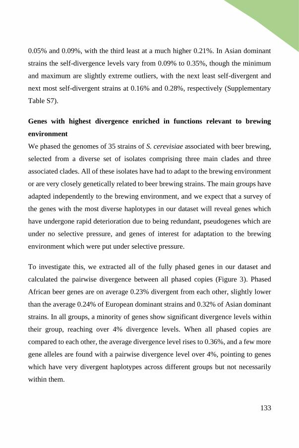
133

0.05% and 0.09%, with the third least at a much higher 0.21%. In Asian dominant

strains the self-divergence levels vary from 0.09% to 0.35%, though the minimum

and maximum are slightly extreme outliers, with the next least self-divergent and

next most self-divergent strains at 0.16% and 0.28%, respectively (Supplementary

Table S7).

Genes with highest divergence enriched in functions relevant to brewing

environment

We phased the genomes of 35 strains of S. cerevisiae associated with beer brewing,

selected from a diverse set of isolates comprising three main clades and three

associated clades. All of these isolates have had to adapt to the brewing environment

or are very closely genetically related to beer brewing strains. The main groups have

adapted independently to the brewing environment, and we expect that a survey of

the genes with the most diverse haplotypes in our dataset will reveal genes which

have undergone rapid deterioration due to being redundant, pseudogenes which are

under no selective pressure, and genes of interest for adaptation to the brewing

environment which were put under selective pressure.

To investigate this, we extracted all of the fully phased genes in our dataset and

calculated the pairwise divergence between all phased copies (Figure 3). Phased

African beer genes are on average 0.23% divergent from each other, slightly lower

than the average 0.24% of European dominant strains and 0.32% of Asian dominant

strains. In all groups, a minority of genes show significant divergence levels within

their group, reaching over 4% divergence levels. When all phased copies are

compared to each other, the average divergence level rises to 0.36%, and a few more

gene alleles are found with a pairwise divergence level over 4%, pointing to genes

which have very divergent haplotypes across different groups but not necessarily

within them.

134

Figure 3 - Distribution of divergence levels for fully phased genes using all strains

We identified all of the fully phased genes in our dataset and compared them to each other in

a pairwise manner, then plotted the divergence levels and their distribution along the genome

as a heatmap. The y axis represents the divergence level as a percentage, and the x axis is the

position along the chromosome. The color represents the number of supporting pairwise

comparisons, implemented here using a log scale for visual clarity. We observe that more

highly divergent genes tend to be less frequent and rarely reach above 4% divergence. The

subtelomeric appear to have more highly divergent genes, however we also observe many

other regions within the chromosomes with high levels of divergence so they are not limited

to the telomeres.

We then identified the 144 genes which have a pairwise divergence level of 4% or

higher (Supplementary Table S8). Of these 144 genes, 57 had a verified annotation,

54 were uncharacterized and the remaining 33 were dubious genes. We subjected

our list of 57 verified genes to a GO term finder analysis to identify enrichment in

processes, function and cellular component localization. We found that our list of 57

highly divergent genes is enriched for carbon metabolic processes for various carbon

sources (e.g., maltose, galactose, sucrose), galactose transport and cell wall

organization. These genes are also enriched in cell wall structural constituents,

dehydrogenase activity and transmembrane sugar transporters and enriched in genes

135

whose products localize to the cell periphery, cell wall and vacuoles (Supplementary

Table S9).

Notable genes of interest include ROQ1, which directs the SHRED pathway to

degrade proteins denatured by high alcohol concentrations10, YPS genes involved in

cell wall remodeling to resist oxidative and osmotic stress12,26, and CTT1, a catalase

expressed in response to oxidative stress27. Deeper investigation into the genes

highlighted and the diverse haplotypes observed and their potential functional

consequences would be of significant interest for further understanding the changes

required for wild yeast to adapt to the brewing environment, examples of convergent

and/or divergent evolutionary trajectories.

Industrial domestication markers: the MAL11, PAD1 and FDC1 genes

Our dataset corroborates and expands on previously reported findings for the

MAL11, PAD1 and FDC1 genes4. These genes, highlighted in Gallone et al. 2016,

are evidence of the domestication of beer yeasts to suit industrial needs and human

flavor preferences. We describe here our observations for these genes in our dataset

(Supplementary Table S10).

Maltose utilization is an industrially relevant phenotype in beer brewing, due to the

high maltose content obtained after malting grain. Maltose is typically the main

fermentable carbon source in wort, the brewing solution to undergo fermentation.

The MAL11 gene codes for an effective maltose transporter, shown to be present in

the Asian dominant strains but inactivated in the European dominant group by

frameshift-inducing indels4. There are two reported frameshift-inducing indels,

1772CA➞C and 1175A➞AT. We report that MAL11 is present and intact in half of

the African beer strains and absent in the others (Supplemental Figure S6). In our

dataset, MAL11 suffered inactivation by homozygous frameshift-inducing indels in

all European dominant strains, except for ARE, which displays both known

136

frameshift-inducing indels heterozygously, and ASD which is intact. Similarly, all

of the Belgian ale strains have at least a heterozygous indel except for BBG which

is intact. Finally, we find that none of the British ale strains in our dataset display

any frameshift-inducing indels.

The PAD1 and FDC1 genes code for proteins which participate in the formation of

4VG, a compound that yields a potent off-flavor in beer4, and their function therefore

leads to an inferior product by human standards. The inactivation of these genes has

previously been identified as evidence of human domestication of beer yeasts due to

their effects on beer flavor4. In our dataset we make corroborating observations. In

fact, the PAD1 gene presents no frameshift-inducing indels, and appears intact in all

European dominant and African Beer strains, however it is fully inactivated by

nonsense mutations in all haplotypes of British ale strains and in over half of the

Belgian ale strains. In addition, the FDC1 gene appears to be intact in European

dominant strains. In Asian dominant strains it is inactivated through the frameshift-

inducing indel 495T➞TA. This indel is present homozygously in all haplotypes of

British ale strains, and in the majority of Belgian ale strains. Only three Belgian ale

strains appear to have intact copies of FDC1. African beers also present a frameshift-

inducing indel which inactivates their copy of FDC1, however it’s a different indel

than the one observed in Asian dominant strains. In African beers we have the indel

35AC➞A which is present at least heterozygously in half of the strains in our

dataset. The other African beer strains have an intact copy of FDC1.

Overall, we find that the African beer strains bear previously reported markers of

domestication through the presence of MAL11 and the independent inactivating indel

observed in FDC1 for some of the strains. In contrast, the industrialized Beer 2

strains do not present the industrially favorable genotypes, consistent with the

previously reported observation that they exhibit fewer signs of domestication than

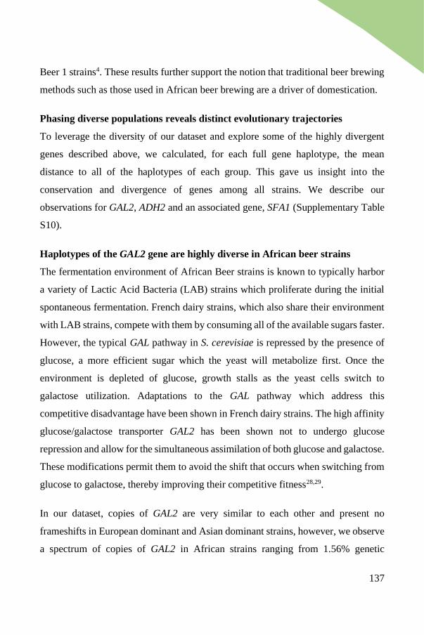
137

Beer 1 strains4. These results further support the notion that traditional beer brewing

methods such as those used in African beer brewing are a driver of domestication.

Phasing diverse populations reveals distinct evolutionary trajectories

To leverage the diversity of our dataset and explore some of the highly divergent

genes described above, we calculated, for each full gene haplotype, the mean

distance to all of the haplotypes of each group. This gave us insight into the

conservation and divergence of genes among all strains. We describe our

observations for GAL2, ADH2 and an associated gene, SFA1 (Supplementary Table

S10).

Haplotypes of the GAL2 gene are highly diverse in African beer strains

The fermentation environment of African Beer strains is known to typically harbor

a variety of Lactic Acid Bacteria (LAB) strains which proliferate during the initial

spontaneous fermentation. French dairy strains, which also share their environment

with LAB strains, compete with them by consuming all of the available sugars faster.

However, the typical GAL pathway in S. cerevisiae is repressed by the presence of

glucose, a more efficient sugar which the yeast will metabolize first. Once the

environment is depleted of glucose, growth stalls as the yeast cells switch to

galactose utilization. Adaptations to the GAL pathway which address this

competitive disadvantage have been shown in French dairy strains. The high affinity

glucose/galactose transporter GAL2 has been shown not to undergo glucose

repression and allow for the simultaneous assimilation of both glucose and galactose.

These modifications permit them to avoid the shift that occurs when switching from

glucose to galactose, thereby improving their competitive fitness28,29.

In our dataset, copies of GAL2 are very similar to each other and present no

frameshifts in European dominant and Asian dominant strains, however, we observe

a spectrum of copies of GAL2 in African strains ranging from 1.56% genetic

138

divergence to the closest non-African versions of GAL2 to 4.05% genetic divergence

with the most distant versions (Supplementary Table S11, Supplementary figure S7).

Four African beer strains harbor haplotypes at divergence levels with non-African

strains between 1.5% and 4.0% (Supplementary figure S8). The remaining four

African beer strains all have a narrower range of haplotype divergence, around 2.5%

for one and over 3.0% for the other three. The four strains with the higher range of

diversity between their own haplotypes are the same ones harboring frameshift-

inducing indels, homozygously for one strain and heterozygously for the other three

(Supplementary Table S10).

This diversity in copies and the inactivation of certain alleles of GAL2 exclusively

found in African beer strains may represent adaptations to sharing their environment

with LAB strains which would parallel but remain independent with the adaptations

observed in French dairy strains.

The ADH2 and SFA1 genes present further evidence of domestication in Asian

dominant and European dominant strains

At high concentrations, fusel alcohols are considered a potent off-flavor in beer. S.

cerevisiae has six genes involved in the final step of the Ehrlich pathway for fusel

alcohol formation22, the ADH alcohol dehydrogenase family ADH1 to ADH5, and

SFA1, an alcohol dehydrogenase and glutathione-dependent formaldehyde

dehydrogenase. ADH1, ADH3, ADH4 and ADH5 convert acetaldehyde to ethanol,

however ADH2 performs the inverse reaction and oxidizes ethanol into

acetaldehyde.

In our dataset, all African beer strains and British ale strains have at least one intact

copy of ADH2. Half of the European dominant strains and the majority of Belgian

ale strains suffer from homozygous deletions. And 9 Belgian ale strains and one

European dominant strain all present a homozygous deletion of approximately 26 bp

139

in the middle of ADH2, which is much larger in strains CFN and YMD1873 (Figure

4). A different deletion of about 25 bp at the beginning of the gene is observed in

three European dominant strains. The ADH2 gene has previously been a target for

inactivation for industrial beer brewing purposes owing to its role in forming the off-

flavors acetaldehyde and diacetyl and reducing alcohol content30. These observed

deletions and high genetic diversity may reflect evidence of domestication.

Figure 4 - Coverage levels of the ADH2 gene reveal homozygous internal deletions

We extracted the coverage levels of Illumina reads in the region corresponding to the gene

ADH2 (chromosome XIII: 873291-874337). This graph shows the coverage level of ADH2

for each strain, using a log scale on the Y axis to represent coverage for ease of interpretation.

The X axis represents the position along the gene, starting at 0 for the first position of the

CDS. The strains are colored according to the group, except for the Asian dominant group

which is subdivided into British ales and Belgian ales. We observe a shared homozygous

deletion in the middle of ADH2 among 9 of the 13 Belgian ale strains and one of the European

dominant strains. We also note the presence of a shared homozygous deletion in the

beginning of ADH2 in 3 of the 8 European dominant strains.

140

This potential domestication event does not affect British ale strains. However, we

make complementary in our dataset, as all strains appear to have intact copies of the

SFA1 gene except for 4 of 6 British ale strains. These strains present either a deletion

leading to a frameshift and a subsequent premature stop or have at least one

haplotype with a nonsense mutation. This inactivation of several alleles of SFA1 only

in British ale strains may be evidence of a domestication event that runs parallels

and complements the disruption of ADH2 in Belgian ale and European dominant

strains, likely in connection to their role in fusel alcohol production23.

141

Discussion

We phased 35 strains of S. cerevisiae which are either used in beer brewing, or are

in clades that have a large proportion of beer brewing strains according to the 1,011

Saccharomyces cerevisiae genomes survey6. A little under a quarter strains are

diploids (n=8), all others being polyploids that range from 3n to 5n. We phased all

35 strains using nPhase, obtaining contiguous results with an average of 1.2 haplotigs

per chromosome to phase 90% of reads.

We used a windowed approach on these phased haplotypes to estimate their pairwise

divergence levels based on phased genetic content, revealing that our dataset seems

to comprise three large groups of strains that are more similar to each other than to

other strains. Using a different windowed approach, we then estimated the allelic

origins of these beer strains by assigning their haplotypes to different clades6. We

found that they all contain an important proportion of European wine alleles, and

that we can categorize them into the same three distinct groups, this time based on

their allelic origin profiles: Asian dominant strains, European dominant strains, and

African beer strains. The Asian dominant strains correspond to the previously

defined Beer 1 group4 and whose origin as a polyploid admixture of Asian and

European wine alleles has previously been described8. The European dominant

group corresponds to the previously defined Beer 2 group4, and is again an admixture

of Asian and European wine, however it differs from the Asian dominant group by

its lower proportion of Asian fermentation alleles. Finally, we characterize the allele

content of the African Beers as having a strong European wine signal, and a higher

French dairy signal than the other groups.

African beer brewing methods are significantly less industrialized and typically

follow traditional means15, which for S. cerevisiae translates to a mode of life that

must remain adapted to the wild and to environments with other microorganisms,

142

notably the LAB which proliferate during the initial spontaneous fermentation step

that typically precedes S. cerevisiae’s alcoholic fermentation15,16. French dairy

strains of S. cerevisiae which share an environment with LAB have been shown to

adapt their GAL pathway to disable its glucose repression and more rapidly drain the

environment of sugar to outcompete other organisms 28,29. We find possible evidence

of a similar adaptation to sharing an environment with LAB in the extensive changes

to GAL2 we observe in African Beer strains, and the presence of multiple different

haplotypes of GAL2 within each strain. We propose that these modifications may

disable or attenuate glucose repression, or confer some other advantage to S.

cerevisiae strains sharing an environment with LAB.

We also found that despite less obvious domestication pressures, some African beer

strains show known signs of domestication. It has been shown that the FDC1 gene

is inactivated in a large number of industrialized beer strains, and not in wild strains,

due to its role in forming the undesirable off-flavor compound 4VG4. In half of the

African beer strains in our dataset, we observed that FDC1 was inactivated by a

frameshift mutation different from the one that affects Asian dominant strains,

suggesting an independent domestication event for this gene.

Finally, we propose that two complementary domestication events occurred in

European dominant strains and British and Belgian ale strains. The alcohol

dehydrogenases SFA1 and ADH2 can both contribute to the last step of the formation

of fusel alcohol22, which in high concentrations are undesirable23 (in fact, fusel is a

German word for bad or cheap liquor). A deletion in the middle of ADH2 is widely

present in Belgian Ale strains and at the beginning of ADH2 in half of the European

dominant strains in our dataset, while premature stops in SFA1 are observed in

British Ale strains, suggesting independent and complementary domestication

events which should have a similar effect of lowering the overall concentration of

fusel alcohol in the final brew.

143

Methods

Selection of strains, DNA extraction and sequencing

For this study, we focused on a subset of 35 of Saccharomyces cerevisiae isolates

from diverse clades based either on their known use in fermenting beers or on their

high genetic similarity to beer-brewing strains (Supplementary Table S1).

The DNA of 35 strains was extracted from 30 mL cultures (single colony, 48h

growth at 30°C) using the QIAGEN Genomic-tip 100/G kit with the recommended

manufacture’s genomic DNA buffer set. The manufacture’s protocol was followed

as recommended and final DNA was eluded in 100-200 µl water. DNA was

quantified with the broad-range DNA quantification kit from Qubit. Genomic DNA

was migrated on a 1.5% agarose gel to check for degradation.

For the long-read sequencing we used the Oxford Nanopore Technology (Oxford,

UK). Libraries for sequencing using the MinION and were prepared as described in

Istace et al.31 using the Ligation Sequencing Kit SQK-LSK109. We barcoded strains

with the Native Barcoding Expansion 1-12 (EXP-NBD104) to multiplex up to 12

samples per sequencing reaction.

Phasing and cleaning using nPhase

We used filtlong v0.2.0 (https://github.com/rrwick/Filtlong) to subset our nanopore

long reads to 80X (estimated as 12 500 000 * 80 bases), then used the nPhase

pipeline24 v1.1.3 with default parameters to phase each strain using its long and short

reads and the R64 reference sequence of S. cerevisiae. Once we obtained raw results

using the nPhase pipeline command, we ran the nPhase cleaning command using

default parameters to improve contiguity and eliminate short, uninformative

haplotigs.

144

Calculating pairwise haplotype divergence between strains within strains

nPhase outputs a file with the suffix “.variants.tsv” which indicates, for each

predicted haplotig, the SNPs that were phased. We use this file along with the

reference sequence of S. cerevisiae to infer the full sequences of our haplotypes and

split them into 10kb windows. Then, for each pair of strains, we compared every full

10 kb haplotype window to all of the haplotypes fully covering the same window in

the opposite strain and only kept the lowest divergence value.

This method extends to the calculation of internal divergence levels, with the

difference that instead of comparing the haplotypes of one strain to the haplotypes

of another, we compared the haplotypes of one strain to each other. We again keep

the lowest value, but we do not allow a 10 kb haplotype block to compare to itself.

Being ploidy agnostic, nPhase tends to group homozygous regions together so there

may be an over-estimation of divergence, however nPhase also doesn’t take indels

into account so there may be an under-estimation of divergence. It’s unclear which

bias has the stronger effect, or the extent of the effect of these limitations.

Dendrogram creation

A genotyping matrix was constructed with the GenotypeGVCFs function of GATK32

that was run on individual gvcf files generated by GATK’s HaplotypeCaller method.

This matrix was used to build a neighbor-joining tree with the R packages ape33 and

SNPrelate34. To that end, the gvcf matrix was converted into a gds file and individual

dissimilarities were estimated for each pair of isolates with the snpgdsDiss function.

The bionj algorithm was then run on the obtained distance matrix.

Pairwise differences between the studied strains was estimated from the non-shared

SNPs positions obtained with bcftool35 isec with -n -1 -c all options run on individual

gvcf files.

145

Allele content origin attribution

In order to investigate the origins of these beer strains we used a windowed approach

to split the haplotypes predicted by nPhase into 20 kb windows and compared them

to 6 of the clades described in Peter et al. 2018: European wine (we merged all of

the European wine subclades), the clinical French Guiana human, African palm

wine, North American Oak, Asian fermentation (we merged the Sake and Asian

fermentation clades) and French Dairy.

For each clade, we consider that a position is a marker of this clade if it has a Minor

Allele Frequency (MAF) ≥ 25% within the clade and is not present in more than one

of the other 5 clades at a MAF ≥ 25%. Then for each 20kb window of each haplotype

we attributed the clade with the highest number of markers.

Calculating divergence between gene haplotypes

To calculate the pairwise divergence between genes we used the latest annotation of

S. cerevisiae available on SGD (Release 64-2-1 of the S288C reference genome36)

and extracted the positions of genes. We then extracted each gene’s sequence in the

reference genome and for each strain we used the strainName.variant.tsv file

generated by nPhase to extract all predicted haplotypes, only keeping the variants

that fall within each gene’s sequence and inferring them into the reference sequence.

We only kept gene haplotypes which had full predictions, we did not keep any

incompletely inferred genes. We then proceeded to a pairwise comparison of every

gene haplotype in our dataset, calculating the divergence as the number of

mismatching positions divided by the length of the gene.

Gene Ontology Term Finder calculations on SGD

Based on the divergence calculations described above, we then identified all genes

for which at least one pairwise comparison led to a divergence level ≥ 4%. We only

keep genes whose ORF classification is listed as “Verified” in the annotation, not

146

“Uncharacterized” or “Dubious”. Then we input that list with default parameters into

the Gene Ontology Term Finder37 available on the Saccharomyces Genome Database

(SGD) website at the following url: https://www.yeastgenome.org/goTermFinder

Identifying frameshifts & premature stops

We identified indels that cause frameshift mutations by manual inspection of the

Illumina VCF files generated by the nPhase pipeline using bwa-mem38 for mapping

and GATK 4.032 for variant calling. Premature stops were identified by identifying

stop codons in the previously generated inferred gene haplotypes.

Coverage plots for the MAL11, and ADH2 genes

We generated the data for our gene coverage plots of MAL11 and ADH2 using

bamCoverage39 v3.5.0 with a window size of 1.

Data visualization tools

The heatmap with clustering (Figure 1) was generated using pheatmap v1.0.12

(https://cran.r-project.org/web/packages/pheatmap/index.html), the dendrogram is

viewed in FigTree v1.4.4 (http://tree.bio.ed.ac.uk/software/figtree/) and other figures

were generated using ggplot2 v3.3.3 (https://ggplot2.tidyverse.org) on the R

programming language v4.0.2 (https://www.r-project.org/about.html). We used a

color palette intended for interpretability by people with colorblindness40.

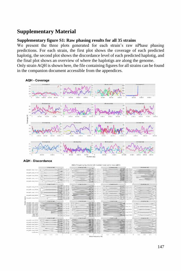
147

Supplementary Material

Supplementary figure S1: Raw phasing results for all 35 strains We present the three plots generated for each strain’s raw nPhase phasing

predictions. For each strain, the first plot shows the coverage of each predicted

haplotig, the second plot shows the discordance level of each predicted haplotig, and

the final plot shows an overview of where the haplotigs are along the genome.

Only strain AQH is shown here, the file containing figures for all strains can be found

in the companion document accessible from the appendices.

148

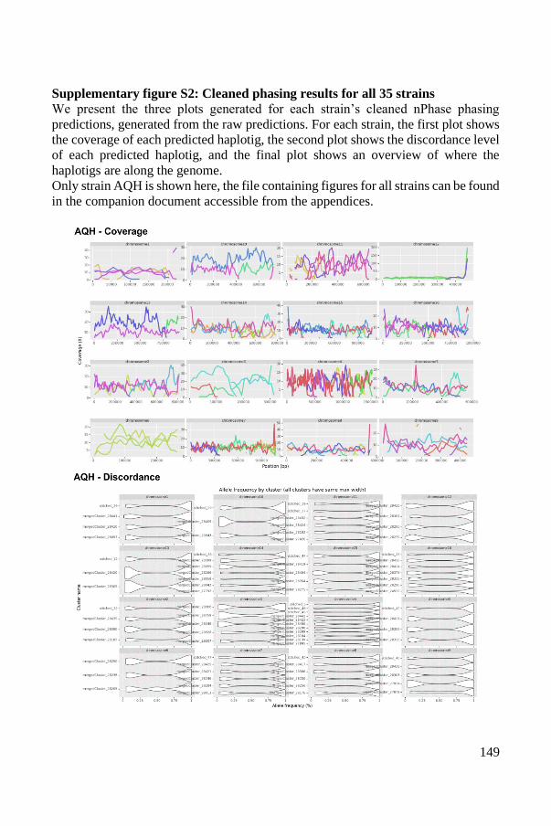
149

Supplementary figure S2: Cleaned phasing results for all 35 strains We present the three plots generated for each strain’s cleaned nPhase phasing

predictions, generated from the raw predictions. For each strain, the first plot shows

the coverage of each predicted haplotig, the second plot shows the discordance level

of each predicted haplotig, and the final plot shows an overview of where the

haplotigs are along the genome.

Only strain AQH is shown here, the file containing figures for all strains can be found

in the companion document accessible from the appendices.

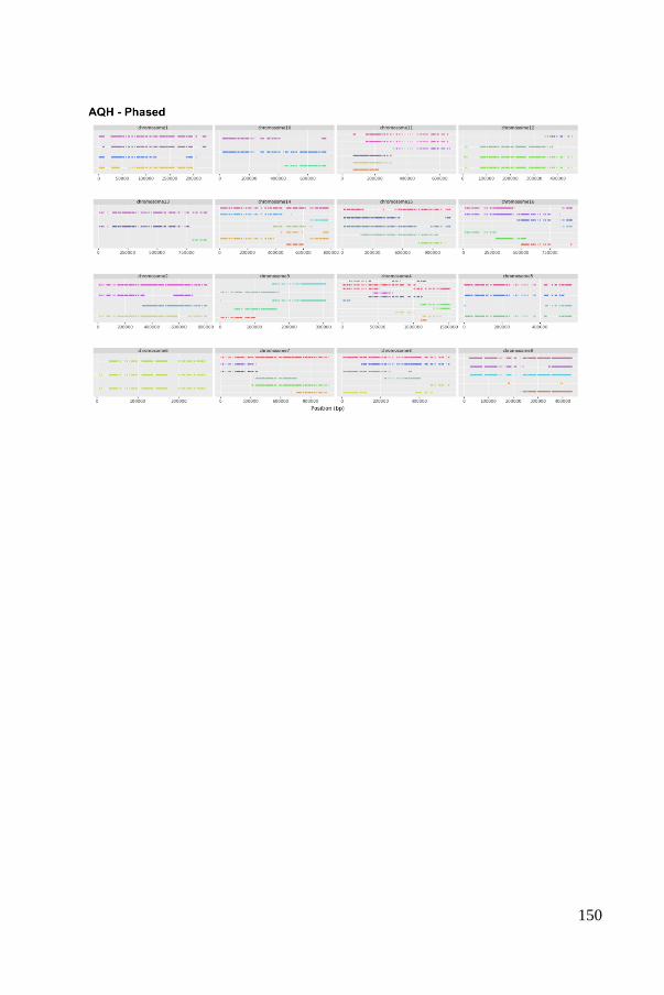
150

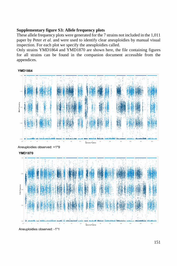
151

Supplementary figure S3: Allele frequency plots These allele frequency plots were generated for the 7 strains not included in the 1,011

paper by Peter et al. and were used to identify clear aneuploidies by manual visual

inspection. For each plot we specify the aneuploidies called.

Only strains YMD1864 and YMD1870 are shown here, the file containing figures

for all strains can be found in the companion document accessible from the

appendices.

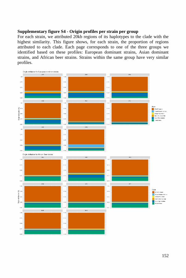
152

Supplementary figure S4 - Origin profiles per strain per group For each strain, we attributed 20kb regions of its haplotypes to the clade with the

highest similarity. This figure shows, for each strain, the proportion of regions

attributed to each clade. Each page corresponds to one of the three groups we

identified based on these profiles: European dominant strains, Asian dominant

strains, and African beer strains. Strains within the same group have very similar

profiles.

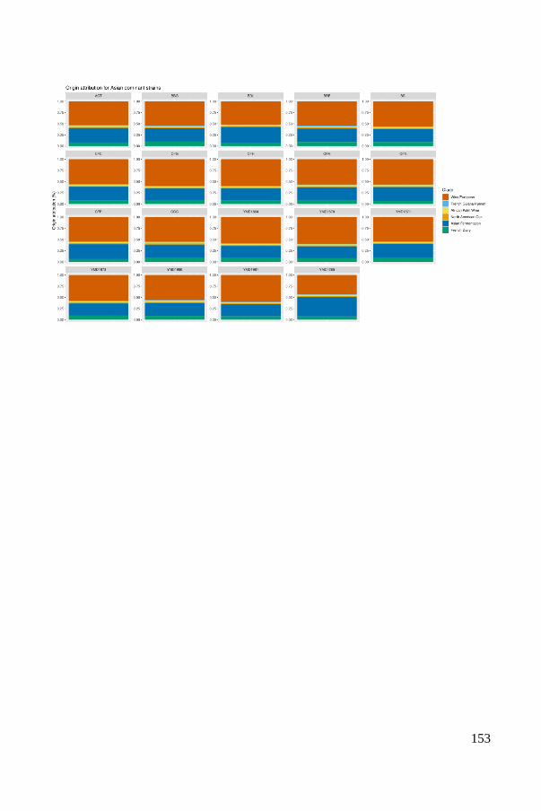
153

154

Supplementary figure S5 - Allele similarity across the genome for different groups Once each strain’s different haplotypes have been assigned to a clade, we can generate a graph that shows, for each 20kb window along the genome,

what proportion of haplotypes support each allelic origin. This representation reveals which parts of the genome are mostly similar to one or the other

clade, and gives a general overview of the allele content of each group, showing them to have very different profiles. The Asian dominant group and

European dominant group look similar, though with almost inverted proportions of European Wine alleles and Asian Fermentation alleles, and the

African Beer group has the highest proportion of French dairy, but also appears to have less contested origins.

155

156

157

Supplementary figure S6 - MAL11 coverage plots We extracted the coverage levels of Illumina reads in the region corresponding to

the gene MAL11 (ChromosomeVII:1073963-1075813). This graph shows the

coverage level of MAL11 for each strain, using a log scale on the Y axis to

represent coverage for ease of interpretation. The X axis represents the position

along the gene, starting at 0 for the first position of the CDS. We note the

extremely low coverage for strains ANL, ASC and AVN, and the total absence of

coverage for strain BEM.

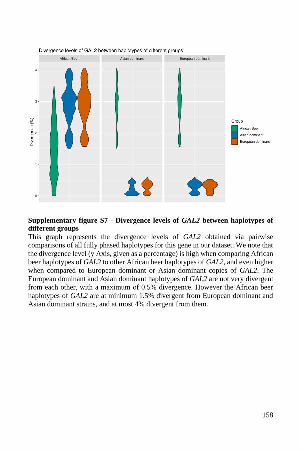
158

Supplementary figure S7 - Divergence levels of GAL2 between haplotypes of

different groups This graph represents the divergence levels of GAL2 obtained via pairwise

comparisons of all fully phased haplotypes for this gene in our dataset. We note that

the divergence level (y Axis, given as a percentage) is high when comparing African

beer haplotypes of GAL2 to other African beer haplotypes of GAL2, and even higher

when compared to European dominant or Asian dominant copies of GAL2. The

European dominant and Asian dominant haplotypes of GAL2 are not very divergent

from each other, with a maximum of 0.5% divergence. However the African beer

haplotypes of GAL2 are at minimum 1.5% divergent from European dominant and

Asian dominant strains, and at most 4% divergent from them.

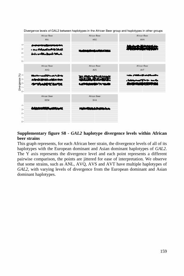
159

Supplementary figure S8 - GAL2 haplotype divergence levels within African

beer strains This graph represents, for each African beer strain, the divergence levels of all of its

haplotypes with the European dominant and Asian dominant haplotypes of GAL2.

The Y axis represents the divergence level and each point represents a different

pairwise comparison, the points are jittered for ease of interpretation. We observe

that some strains, such as ANL, AVQ, AVS and AVT have multiple haplotypes of

GAL2, with varying levels of divergence from the European dominant and Asian

dominant haplotypes.

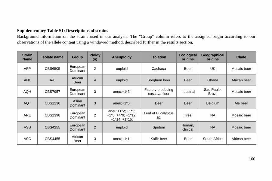
160

Supplementary Table S1: Descriptions of strains

Background information on the strains used in our analysis. The "Group" column refers to the assigned origin according to our

observations of the allele content using a windowed method, described further in the results section.

Strain Name

Isolate name Group Ploidy

(n) Aneuploidy Isolation

Ecological origins

Geographical origins

Clade

AFP CBS6505 European Dominant

2 euploid Cachaça Beer UK Mosaic beer

ANL A-6 African Beer

4 euploid Sorghum beer Beer Ghana African beer

AQH CBS7957 European Dominant

3 aneu;+1*3; Factory producing

cassava flour Industrial

Sao Paulo, Brazil

Mosaic beer

AQT CBS1230 Asian

Dominant 3 aneu;+1*6; Beer Beer Belgium Ale beer

ARE CBS1398 European Dominant

2 aneu;+1*2; +1*3;

+1*6; +4*9; +1*12; +1*14; +1*15;

Leaf of Eucalyptus sp.

Tree NA Mosaic beer

ASB CBS4255 European Dominant

2 euploid Sputum Human, clinical

NA Mosaic beer

ASC CBS4455 African Beer

3 aneu;+1*1; Kaffir beer Beer South Africa African beer

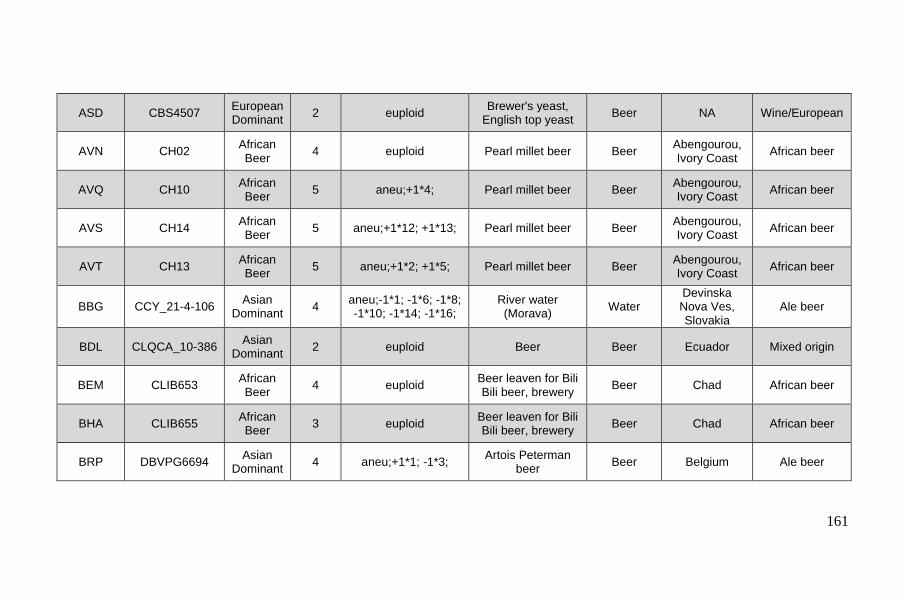
161

ASD CBS4507 European Dominant

2 euploid Brewer's yeast,

English top yeast Beer NA Wine/European

AVN CH02 African Beer

4 euploid Pearl millet beer Beer Abengourou, Ivory Coast

African beer

AVQ CH10 African Beer

5 aneu;+1*4; Pearl millet beer Beer Abengourou, Ivory Coast

African beer

AVS CH14 African Beer

5 aneu;+1*12; +1*13; Pearl millet beer Beer Abengourou, Ivory Coast

African beer

AVT CH13 African Beer

5 aneu;+1*2; +1*5; Pearl millet beer Beer Abengourou, Ivory Coast

African beer

BBG CCY_21-4-106 Asian

Dominant 4

aneu;-1*1; -1*6; -1*8; -1*10; -1*14; -1*16;

River water (Morava)

Water Devinska Nova Ves, Slovakia

Ale beer

BDL CLQCA_10-386 Asian

Dominant 2 euploid Beer Beer Ecuador Mixed origin

BEM CLIB653 African Beer

4 euploid Beer leaven for Bili Bili beer, brewery

Beer Chad African beer

BHA CLIB655 African Beer

3 euploid Beer leaven for Bili Bili beer, brewery

Beer Chad African beer

BRP DBVPG6694 Asian

Dominant 4 aneu;+1*1; -1*3;

Artois Peterman beer

Beer Belgium Ale beer

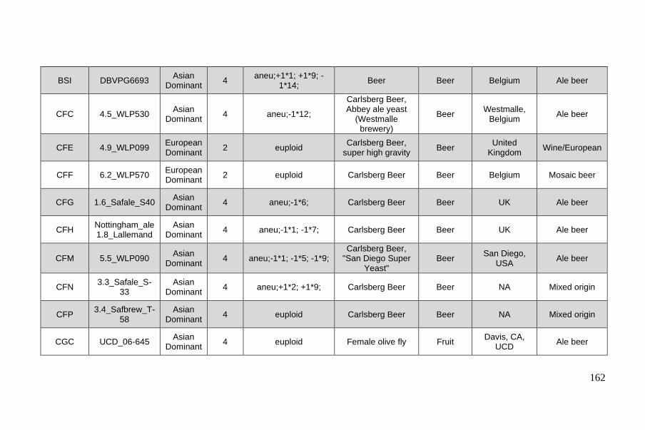
162

BSI DBVPG6693 Asian

Dominant 4

aneu;+1*1; +1*9; -1*14;

Beer Beer Belgium Ale beer

CFC 4.5_WLP530 Asian

Dominant 4 aneu;-1*12;

Carlsberg Beer, Abbey ale yeast

(Westmalle brewery)

Beer Westmalle,

Belgium Ale beer

CFE 4.9_WLP099 European Dominant

2 euploid Carlsberg Beer,

super high gravity Beer

United Kingdom

Wine/European

CFF 6.2_WLP570 European Dominant

2 euploid Carlsberg Beer Beer Belgium Mosaic beer

CFG 1.6_Safale_S40 Asian

Dominant 4 aneu;-1*6; Carlsberg Beer Beer UK Ale beer

CFH Nottingham_ale 1.8_Lallemand

Asian Dominant

4 aneu;-1*1; -1*7; Carlsberg Beer Beer UK Ale beer

CFM 5.5_WLP090 Asian

Dominant 4 aneu;-1*1; -1*5; -1*9;

Carlsberg Beer, "San Diego Super

Yeast" Beer

San Diego, USA

Ale beer

CFN 3.3_Safale_S-

33 Asian

Dominant 4 aneu;+1*2; +1*9; Carlsberg Beer Beer NA Mixed origin

CFP 3.4_Safbrew_T-

58 Asian

Dominant 4 euploid Carlsberg Beer Beer NA Mixed origin

CGC UCD_06-645 Asian

Dominant 4 euploid Female olive fly Fruit

Davis, CA, UCD

Ale beer

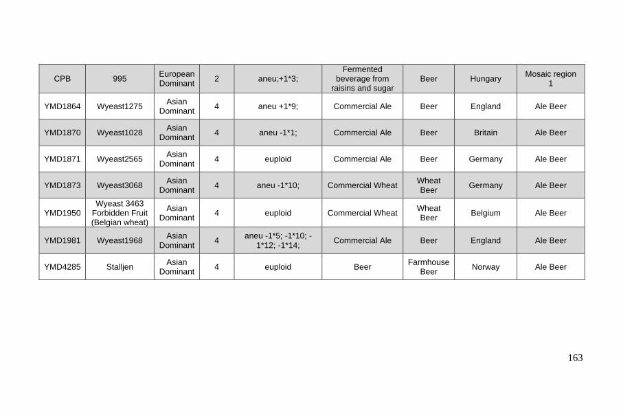
163

CPB 995 European Dominant

2 aneu;+1*3; Fermented

beverage from raisins and sugar

Beer Hungary Mosaic region

1

YMD1864 Wyeast1275 Asian

Dominant 4 aneu +1*9; Commercial Ale Beer England Ale Beer

YMD1870 Wyeast1028 Asian

Dominant 4 aneu -1*1; Commercial Ale Beer Britain Ale Beer

YMD1871 Wyeast2565 Asian

Dominant 4 euploid Commercial Ale Beer Germany Ale Beer

YMD1873 Wyeast3068 Asian

Dominant 4 aneu -1*10; Commercial Wheat

Wheat Beer

Germany Ale Beer

YMD1950 Wyeast 3463

Forbidden Fruit (Belgian wheat)

Asian Dominant

4 euploid Commercial Wheat Wheat Beer

Belgium Ale Beer

YMD1981 Wyeast1968 Asian

Dominant 4

aneu -1*5; -1*10; -1*12; -1*14;

Commercial Ale Beer England Ale Beer

YMD4285 Stalljen Asian

Dominant 4 euploid Beer

Farmhouse Beer

Norway Ale Beer

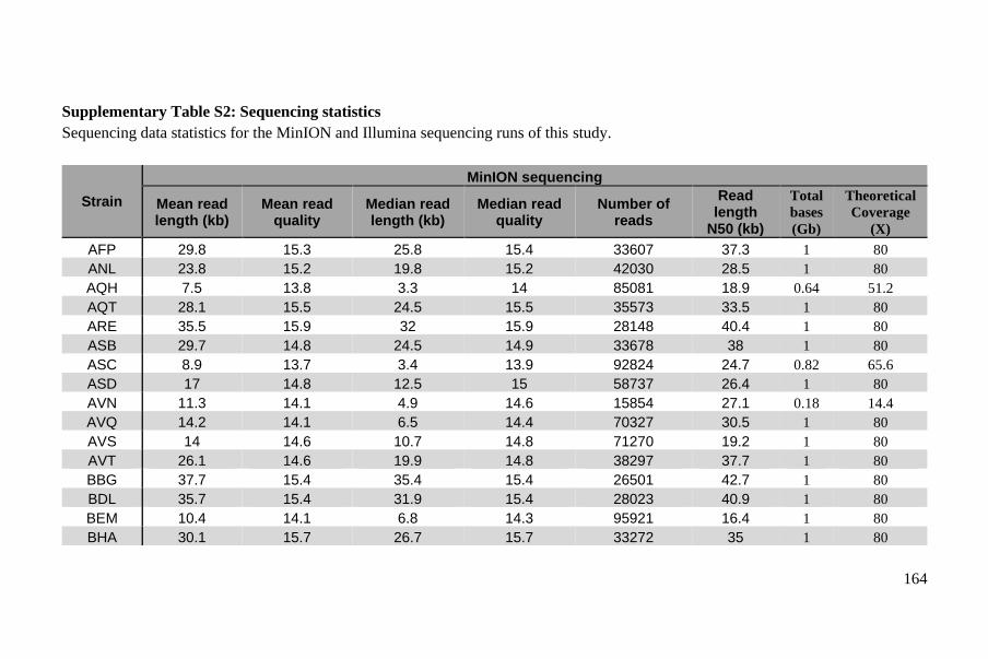
164

Supplementary Table S2: Sequencing statistics

Sequencing data statistics for the MinION and Illumina sequencing runs of this study.

Strain

MinION sequencing

Mean read length (kb)

Mean read quality

Median read length (kb)

Median read quality

Number of reads

Read length

N50 (kb)

Total

bases

(Gb)

Theoretical

Coverage

(X)

AFP 29.8 15.3 25.8 15.4 33607 37.3 1 80

ANL 23.8 15.2 19.8 15.2 42030 28.5 1 80

AQH 7.5 13.8 3.3 14 85081 18.9 0.64 51.2

AQT 28.1 15.5 24.5 15.5 35573 33.5 1 80

ARE 35.5 15.9 32 15.9 28148 40.4 1 80

ASB 29.7 14.8 24.5 14.9 33678 38 1 80

ASC 8.9 13.7 3.4 13.9 92824 24.7 0.82 65.6

ASD 17 14.8 12.5 15 58737 26.4 1 80

AVN 11.3 14.1 4.9 14.6 15854 27.1 0.18 14.4

AVQ 14.2 14.1 6.5 14.4 70327 30.5 1 80

AVS 14 14.6 10.7 14.8 71270 19.2 1 80

AVT 26.1 14.6 19.9 14.8 38297 37.7 1 80

BBG 37.7 15.4 35.4 15.4 26501 42.7 1 80

BDL 35.7 15.4 31.9 15.4 28023 40.9 1 80

BEM 10.4 14.1 6.8 14.3 95921 16.4 1 80

BHA 30.1 15.7 26.7 15.7 33272 35 1 80

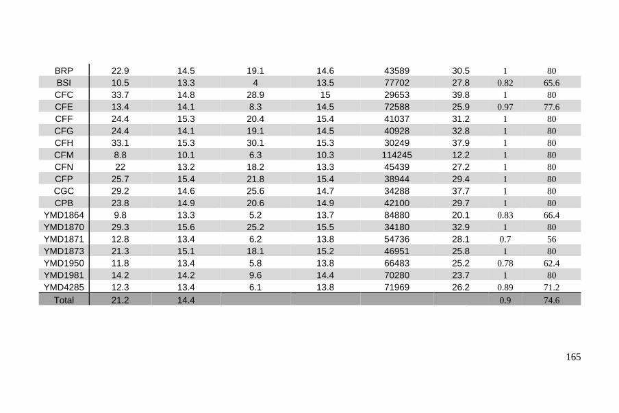
165

BRP 22.9 14.5 19.1 14.6 43589 30.5 1 80

BSI 10.5 13.3 4 13.5 77702 27.8 0.82 65.6

CFC 33.7 14.8 28.9 15 29653 39.8 1 80

CFE 13.4 14.1 8.3 14.5 72588 25.9 0.97 77.6

CFF 24.4 15.3 20.4 15.4 41037 31.2 1 80

CFG 24.4 14.1 19.1 14.5 40928 32.8 1 80

CFH 33.1 15.3 30.1 15.3 30249 37.9 1 80

CFM 8.8 10.1 6.3 10.3 114245 12.2 1 80

CFN 22 13.2 18.2 13.3 45439 27.2 1 80

CFP 25.7 15.4 21.8 15.4 38944 29.4 1 80

CGC 29.2 14.6 25.6 14.7 34288 37.7 1 80

CPB 23.8 14.9 20.6 14.9 42100 29.7 1 80

YMD1864 9.8 13.3 5.2 13.7 84880 20.1 0.83 66.4

YMD1870 29.3 15.6 25.2 15.5 34180 32.9 1 80

YMD1871 12.8 13.4 6.2 13.8 54736 28.1 0.7 56

YMD1873 21.3 15.1 18.1 15.2 46951 25.8 1 80

YMD1950 11.8 13.4 5.8 13.8 66483 25.2 0.78 62.4

YMD1981 14.2 14.2 9.6 14.4 70280 23.7 1 80

YMD4285 12.3 13.4 6.1 13.8 71969 26.2 0.89 71.2

Total 21.2 14.4 0.9 74.6

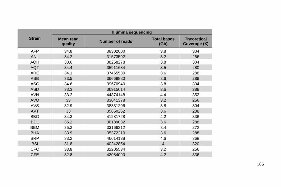
166

Strain

Illumina sequencing

Mean read quality

Number of reads Total bases

(Gb) Theoretical

Coverage (X)

AFP 34.8 38302000 3.8 304

ANL 34.2 31573592 3.2 256

AQH 33.6 38258278 3.8 304

AQT 34.4 35911684 3.5 280

ARE 34.1 37465530 3.6 288

ASB 33.5 36669880 3.6 288

ASC 34.6 39670940 3.8 304

ASD 33.3 36915614 3.6 288

AVN 33.2 44874148 4.4 352

AVQ 33 33041378 3.2 256

AVS 32.9 38331296 3.8 304

AVT 33 35650262 3.6 288

BBG 34.3 41281728 4.2 336

BDL 35.2 36189032 3.6 288

BEM 35.2 33166312 3.4 272

BHA 33.9 35372210 3.6 288

BRP 33.2 46614138 4.6 368

BSI 31.8 40242854 4 320

CFC 33.8 32205534 3.2 256

CFE 32.8 42084090 4.2 336

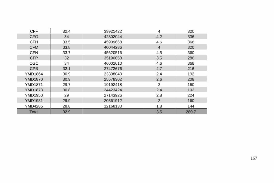
167

CFF 32.4 39921422 4 320

CFG 34 42302044 4.2 336

CFH 33.5 45909668 4.6 368

CFM 33.8 40044236 4 320

CFN 33.7 45620516 4.5 360

CFP 32 35190058 3.5 280

CGC 34 46002610 4.6 368

CPB 32.1 27472676 2.7 216

YMD1864 30.9 23398040 2.4 192

YMD1870 30.9 25578302 2.6 208

YMD1871 29.7 19192418 2 160

YMD1873 30.8 24423424 2.4 192

YMD1950 29 27143926 2.8 224

YMD1981 29.9 20361912 2 160

YMD4285 28.8 12168130 1.8 144

Total 32.9 3.5 280.7

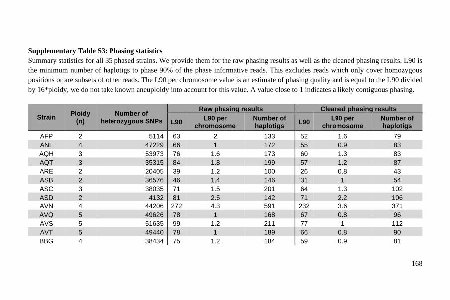
168

Supplementary Table S3: Phasing statistics

Summary statistics for all 35 phased strains. We provide them for the raw phasing results as well as the cleaned phasing results. L90 is

the minimum number of haplotigs to phase 90% of the phase informative reads. This excludes reads which only cover homozygous

positions or are subsets of other reads. The L90 per chromosome value is an estimate of phasing quality and is equal to the L90 divided

by 16*ploidy, we do not take known aneuploidy into account for this value. A value close to 1 indicates a likely contiguous phasing.

Strain Ploidy

(n) Number of

heterozygous SNPs

Raw phasing results Cleaned phasing results

L90 L90 per

chromosome Number of haplotigs

L90 L90 per

chromosome Number of haplotigs

AFP 2 5114 63 2 133 52 1.6 79

ANL 4 47229 66 1 172 55 0.9 83

AQH 3 53973 76 1.6 173 60 1.3 83

AQT 3 35315 84 1.8 199 57 1.2 87

ARE 2 20405 39 1.2 100 26 0.8 43

ASB 2 36576 46 1.4 146 31 1 54

ASC 3 38035 71 1.5 201 64 1.3 102

ASD 2 4132 81 2.5 142 71 2.2 106

AVN 4 44206 272 4.3 591 232 3.6 371

AVQ 5 49626 78 1 168 67 0.8 96

AVS 5 51635 99 1.2 211 77 1 112

AVT 5 49440 78 1 189 66 0.8 90

BBG 4 38434 75 1.2 184 59 0.9 81

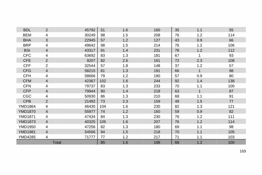
169

BDL 2 45792 51 1.6 160 35 1.1 55

BEM 4 30249 98 1.5 208 76 1.2 114

BHA 3 22945 57 1.2 127 43 0.9 66

BRP 4 49642 98 1.5 214 76 1.2 106

BSI 4 43317 91 1.4 231 78 1.2 112

CFC 4 63692 83 1.3 181 67 1 93

CFE 2 9207 82 2.6 161 72 2.3 108

CFF 2 32544 57 1.8 148 37 1.2 57

CFG 4 58215 81 1.3 191 66 1 98

CFH 4 58666 79 1.2 190 57 0.9 80

CFM 4 42367 102 1.6 244 92 1.4 138

CFN 4 79737 83 1.3 233 70 1.1 100

CFP 4 79944 90 1.4 218 63 1 87

CGC 4 50930 86 1.3 210 68 1.1 91

CPB 2 21492 73 2.3 159 49 1.5 77

YMD1864 4 46430 104 1.6 230 82 1.3 121

YMD1870 4 55977 74 1.2 160 59 0.9 82

YMD1871 4 47434 84 1.3 230 76 1.2 111

YMD1873 4 40325 105 1.6 207 76 1.2 114

YMD1950 4 47256 82 1.3 180 69 1.1 98

YMD1981 4 54566 94 1.5 218 70 1.1 105

YMD4285 4 71777 77 1.2 217 71 1.1 103

Total 85 1.6 198 68 1.2 100

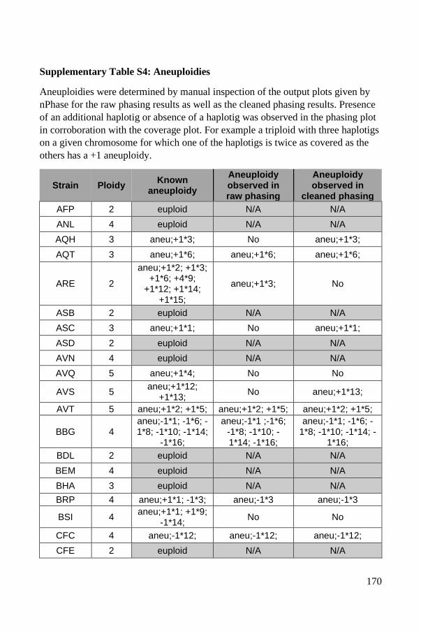
170

Supplementary Table S4: Aneuploidies

Aneuploidies were determined by manual inspection of the output plots given by

nPhase for the raw phasing results as well as the cleaned phasing results. Presence

of an additional haplotig or absence of a haplotig was observed in the phasing plot

in corroboration with the coverage plot. For example a triploid with three haplotigs

on a given chromosome for which one of the haplotigs is twice as covered as the

others has a +1 aneuploidy.

Strain Ploidy Known

aneuploidy

Aneuploidy observed in raw phasing

Aneuploidy observed in

cleaned phasing

AFP 2 euploid N/A N/A

ANL 4 euploid N/A N/A

AQH 3 aneu;+1*3; No aneu;+1*3;

AQT 3 aneu;+1*6; aneu;+1*6; aneu;+1*6;

ARE 2

aneu;+1*2; +1*3; +1*6; +4*9;

+1*12; +1*14; +1*15;

aneu;+1*3; No

ASB 2 euploid N/A N/A

ASC 3 aneu;+1*1; No aneu;+1*1;

ASD 2 euploid N/A N/A

AVN 4 euploid N/A N/A

AVQ 5 aneu;+1*4; No No

AVS 5 aneu;+1*12;

+1*13; No aneu;+1*13;

AVT 5 aneu;+1*2; +1*5; aneu;+1*2; +1*5; aneu;+1*2; +1*5;

BBG 4 aneu;-1*1; -1*6; -1*8; -1*10; -1*14;

-1*16;

aneu;-1*1 ;-1*6; -1*8; -1*10; -1*14; -1*16;

aneu;-1*1; -1*6; -1*8; -1*10; -1*14; -

1*16;

BDL 2 euploid N/A N/A

BEM 4 euploid N/A N/A

BHA 3 euploid N/A N/A

BRP 4 aneu;+1*1; -1*3; aneu;-1*3 aneu;-1*3

BSI 4 aneu;+1*1; +1*9;

-1*14; No No

CFC 4 aneu;-1*12; aneu;-1*12; aneu;-1*12;

CFE 2 euploid N/A N/A

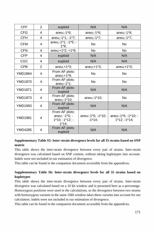
171

CFF 2 euploid N/A N/A

CFG 4 aneu;-1*6; aneu;-1*6; aneu;-1*6;

CFH 4 aneu;-1*1; -1*7; aneu;-1*7; aneu;-1*7;

CFM 4 aneu;-1*1; -1*5; -

1*9; No No

CFN 4 aneu;+1*2; +1*9; No No

CFP 4 euploid N/A N/A

CGC 4 euploid N/A N/A

CPB 2 aneu;+1*3; aneu;+1*3; aneu;+1*3;

YMD1864 4 From AF plots:

aneu;+1*9; No No

YMD1870 4 From AF plots:

aneu;-1*1; No No

YMD1871 4 From AF plots:

euploid N/A N/A

YMD1873 4 From AF plots:

aneu;-1*10; aneu;-1*10; No

YMD1950 4 From AF plots:

euploid N/A N/A

YMD1981 4

From AF plots: aneu; -1*5; -1*10; -1*12; -

1*14;

aneu;-1*5; -1*10; -1*14;

aneu;-1*5; -1*10; -1*12; -1*14;

YMD4285 4 From AF plots:

euploid N/A N/A

Supplementary Table S5: Inter-strain divergence levels for all 35 strains based on SNP

matrix

This table shows the inter-strain divergence between every pair of strains. Inter-strain

divergence was calculated based on SNP content, without taking haplotypes into account.

Indels were not included in our estimation of divergence.

This table can be found in the companion document accessible from the appendices.

Supplementary Table S6: Inter-strain divergence levels for all 35 strains based on

haplotypes

This table shows the inter-strain divergence between every pair of strains. Inter-strain

divergence was calculated based on a 10 kb window and is presented here as a percentage.

Homozygous positions were used in the calculations, so the divergence between two strains

with homozygous variants in the same 10kb window takes these variants into account for our

calculation. Indels were not included in our estimation of divergence.

This table can be found in the companion document accessible from the appendices.

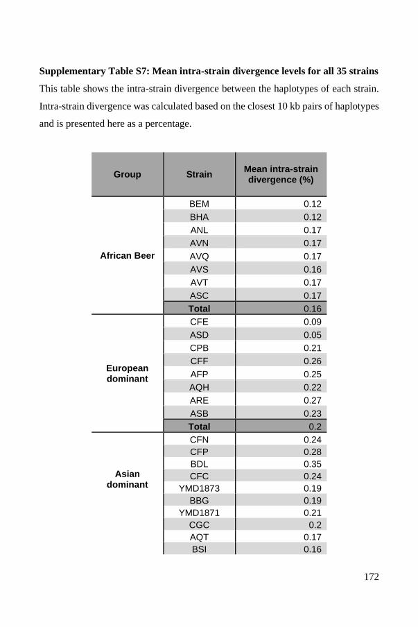
172

Supplementary Table S7: Mean intra-strain divergence levels for all 35 strains

This table shows the intra-strain divergence between the haplotypes of each strain.

Intra-strain divergence was calculated based on the closest 10 kb pairs of haplotypes

and is presented here as a percentage.

Group Strain Mean intra-strain divergence (%)

African Beer

BEM 0.12

BHA 0.12

ANL 0.17

AVN 0.17

AVQ 0.17

AVS 0.16

AVT 0.17

ASC 0.17

Total 0.16

European dominant

CFE 0.09

ASD 0.05

CPB 0.21

CFF 0.26

AFP 0.25

AQH 0.22

ARE 0.27

ASB 0.23

Total 0.2

Asian

dominant

CFN 0.24

CFP 0.28

BDL 0.35

CFC 0.24

YMD1873 0.19

BBG 0.19

YMD1871 0.21

CGC 0.2

AQT 0.17

BSI 0.16

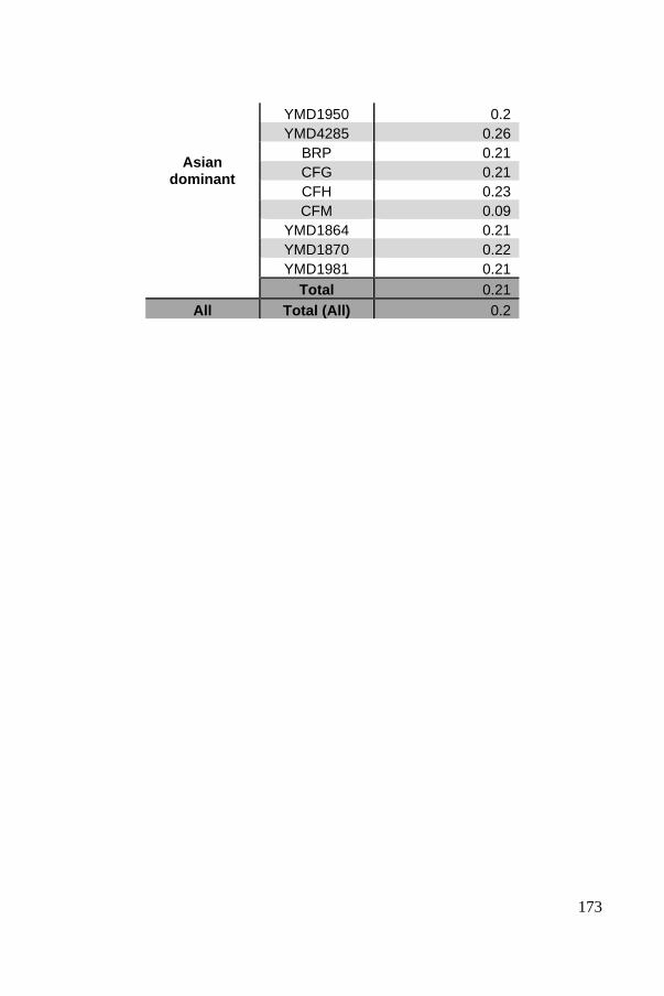
173

Asian dominant

YMD1950 0.2

YMD4285 0.26

BRP 0.21

CFG 0.21

CFH 0.23

CFM 0.09

YMD1864 0.21

YMD1870 0.22

YMD1981 0.21

Total 0.21

All Total (All) 0.2

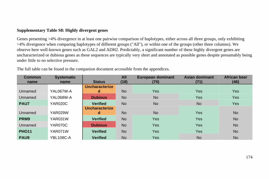
174

Supplementary Table S8: Highly divergent genes

Genes presenting >4% divergence in at least one pairwise comparison of haplotypes, either across all three groups, only exhibiting

>4% divergence when comparing haplotypes of different groups ("All"), or within one of the groups (other three columns). We

observe here well-known genes such as GAL2 and ADH2. Predictably, a significant number of these highly divergent genes are

uncharacterized or dubious genes as these sequences are typically very short and annotated as possible genes despite presumably being

under little to no selective pressure.

The full table can be found in the companion document accessible from the appendices.

Common name

Systematic name Status

All (18)

European dominant (70)

Asian dominant (71)

African beer (46)

Unnamed YAL067W-A Uncharacterize

d No Yes Yes Yes

Unnamed YAL068W-A Dubious No No Yes Yes

PAU7 YAR020C Verified No No No Yes

Unnamed YAR029W Uncharacterize

d No No Yes No

PRM9 YAR031W Verified No Yes Yes No

Unnamed YAR070C Dubious No Yes Yes No

PHO11 YAR071W Verified No Yes Yes No

PAU9 YBL108C-A Verified No Yes No No

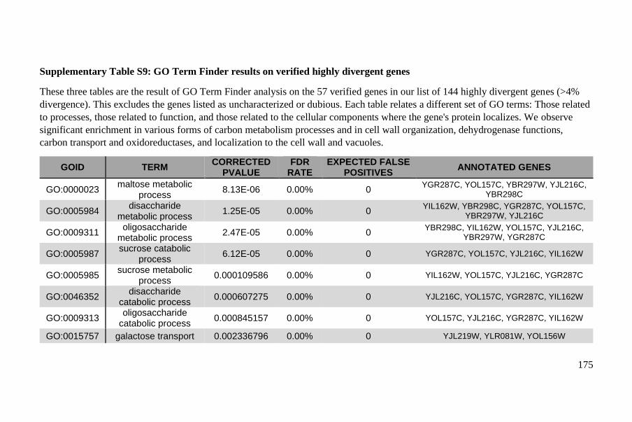
175

Supplementary Table S9: GO Term Finder results on verified highly divergent genes

These three tables are the result of GO Term Finder analysis on the 57 verified genes in our list of 144 highly divergent genes (>4%

divergence). This excludes the genes listed as uncharacterized or dubious. Each table relates a different set of GO terms: Those related

to processes, those related to function, and those related to the cellular components where the gene's protein localizes. We observe

significant enrichment in various forms of carbon metabolism processes and in cell wall organization, dehydrogenase functions,

carbon transport and oxidoreductases, and localization to the cell wall and vacuoles.

GOID TERM CORRECTED

PVALUE FDR

RATE EXPECTED FALSE

POSITIVES ANNOTATED GENES

GO:0000023 maltose metabolic

process 8.13E-06 0.00% 0

YGR287C, YOL157C, YBR297W, YJL216C, YBR298C

GO:0005984 disaccharide

metabolic process 1.25E-05 0.00% 0

YIL162W, YBR298C, YGR287C, YOL157C, YBR297W, YJL216C

GO:0009311 oligosaccharide

metabolic process 2.47E-05 0.00% 0

YBR298C, YIL162W, YOL157C, YJL216C, YBR297W, YGR287C

GO:0005987 sucrose catabolic

process 6.12E-05 0.00% 0 YGR287C, YOL157C, YJL216C, YIL162W

GO:0005985 sucrose metabolic

process 0.000109586 0.00% 0 YIL162W, YOL157C, YJL216C, YGR287C

GO:0046352 disaccharide

catabolic process 0.000607275 0.00% 0 YJL216C, YOL157C, YGR287C, YIL162W

GO:0009313 oligosaccharide

catabolic process 0.000845157 0.00% 0 YOL157C, YJL216C, YGR287C, YIL162W

GO:0015757 galactose transport 0.002336796 0.00% 0 YJL219W, YLR081W, YOL156W

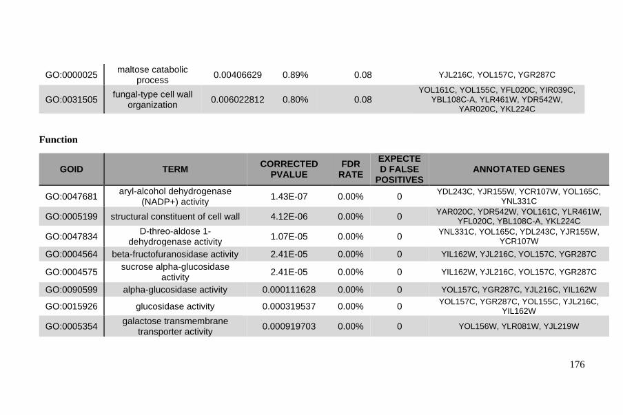
176

GO:0000025 maltose catabolic

process 0.00406629 0.89% 0.08 YJL216C, YOL157C, YGR287C

GO:0031505 fungal-type cell wall

organization 0.006022812 0.80% 0.08

YOL161C, YOL155C, YFL020C, YIR039C, YBL108C-A, YLR461W, YDR542W,

YAR020C, YKL224C

Function

GOID TERM CORRECTED

PVALUE FDR

RATE

EXPECTED FALSE

POSITIVES ANNOTATED GENES

GO:0047681 aryl-alcohol dehydrogenase

(NADP+) activity 1.43E-07 0.00% 0

YDL243C, YJR155W, YCR107W, YOL165C, YNL331C

GO:0005199 structural constituent of cell wall 4.12E-06 0.00% 0 YAR020C, YDR542W, YOL161C, YLR461W,

YFL020C, YBL108C-A, YKL224C

GO:0047834 D-threo-aldose 1-

dehydrogenase activity 1.07E-05 0.00% 0

YNL331C, YOL165C, YDL243C, YJR155W, YCR107W

GO:0004564 beta-fructofuranosidase activity 2.41E-05 0.00% 0 YIL162W, YJL216C, YOL157C, YGR287C

GO:0004575 sucrose alpha-glucosidase

activity 2.41E-05 0.00% 0 YIL162W, YJL216C, YOL157C, YGR287C

GO:0090599 alpha-glucosidase activity 0.000111628 0.00% 0 YOL157C, YGR287C, YJL216C, YIL162W

GO:0015926 glucosidase activity 0.000319537 0.00% 0 YOL157C, YGR287C, YOL155C, YJL216C,

YIL162W

GO:0005354 galactose transmembrane

transporter activity 0.000919703 0.00% 0 YOL156W, YLR081W, YJL219W

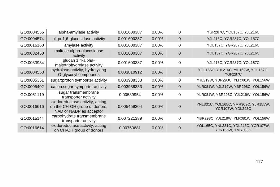
177

GO:0004556 alpha-amylase activity 0.001600387 0.00% 0 YGR287C, YOL157C, YJL216C

GO:0004574 oligo-1,6-glucosidase activity 0.001600387 0.00% 0 YJL216C, YGR287C, YOL157C

GO:0016160 amylase activity 0.001600387 0.00% 0 YOL157C, YGR287C, YJL216C

GO:0032450 maltose alpha-glucosidase

activity 0.001600387 0.00% 0 YOL157C, YGR287C, YJL216C

GO:0033934 glucan 1,4-alpha-

maltotriohydrolase activity 0.001600387 0.00% 0 YJL216C, YGR287C, YOL157C

GO:0004553 hydrolase activity, hydrolyzing

O-glycosyl compounds 0.003810912 0.00% 0

YOL155C, YJL216C, YIL162W, YOL157C, YGR287C

GO:0005351 sugar:proton symporter activity 0.003938333 0.00% 0 YJL219W, YBR298C, YLR081W, YOL156W

GO:0005402 cation:sugar symporter activity 0.003938333 0.00% 0 YLR081W, YJL219W, YBR298C, YOL156W

GO:0051119 sugar transmembrane

transporter activity 0.00539954 0.00% 0 YLR081W, YBR298C, YJL219W, YOL156W

GO:0016616 oxidoreductase activity, acting

on the CH-OH group of donors, NAD or NADP as acceptor

0.005459304 0.00% 0 YNL331C, YOL165C, YMR303C, YJR155W,

YCR107W, YDL243C

GO:0015144 carbohydrate transmembrane

transporter activity 0.007221389 0.00% 0 YBR298C, YJL219W, YLR081W, YOL156W

GO:0016614 oxidoreductase activity, acting

on CH-OH group of donors 0.00750681 0.00% 0

YOL165C, YNL331C, YDL243C, YCR107W, YJR155W, YMR303C

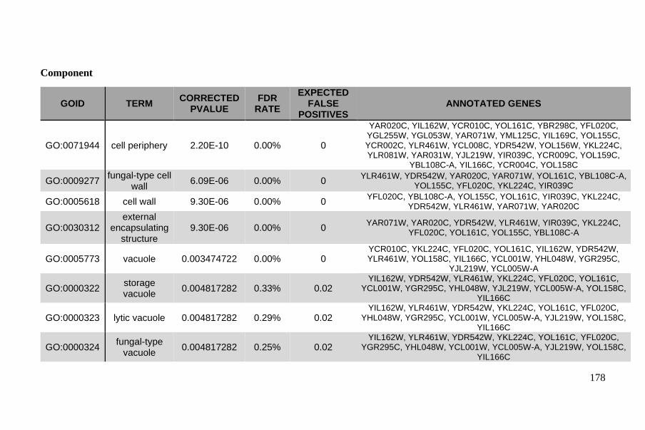
178

Component

GOID TERM CORRECTED

PVALUE FDR

RATE

EXPECTED FALSE

POSITIVES ANNOTATED GENES

GO:0071944 cell periphery 2.20E-10 0.00% 0

YAR020C, YIL162W, YCR010C, YOL161C, YBR298C, YFL020C, YGL255W, YGL053W, YAR071W, YML125C, YIL169C, YOL155C, YCR002C, YLR461W, YCL008C, YDR542W, YOL156W, YKL224C, YLR081W, YAR031W, YJL219W, YIR039C, YCR009C, YOL159C,

YBL108C-A, YIL166C, YCR004C, YOL158C

GO:0009277 fungal-type cell

wall 6.09E-06 0.00% 0

YLR461W, YDR542W, YAR020C, YAR071W, YOL161C, YBL108C-A, YOL155C, YFL020C, YKL224C, YIR039C

GO:0005618 cell wall 9.30E-06 0.00% 0 YFL020C, YBL108C-A, YOL155C, YOL161C, YIR039C, YKL224C,

YDR542W, YLR461W, YAR071W, YAR020C

GO:0030312 external

encapsulating structure

9.30E-06 0.00% 0 YAR071W, YAR020C, YDR542W, YLR461W, YIR039C, YKL224C,

YFL020C, YOL161C, YOL155C, YBL108C-A

GO:0005773 vacuole 0.003474722 0.00% 0 YCR010C, YKL224C, YFL020C, YOL161C, YIL162W, YDR542W, YLR461W, YOL158C, YIL166C, YCL001W, YHL048W, YGR295C,

YJL219W, YCL005W-A

GO:0000322 storage vacuole

0.004817282 0.33% 0.02 YIL162W, YDR542W, YLR461W, YKL224C, YFL020C, YOL161C,

YCL001W, YGR295C, YHL048W, YJL219W, YCL005W-A, YOL158C, YIL166C

GO:0000323 lytic vacuole 0.004817282 0.29% 0.02 YIL162W, YLR461W, YDR542W, YKL224C, YOL161C, YFL020C,

YHL048W, YGR295C, YCL001W, YCL005W-A, YJL219W, YOL158C, YIL166C

GO:0000324 fungal-type

vacuole 0.004817282 0.25% 0.02

YIL162W, YLR461W, YDR542W, YKL224C, YOL161C, YFL020C, YGR295C, YHL048W, YCL001W, YCL005W-A, YJL219W, YOL158C,

YIL166C

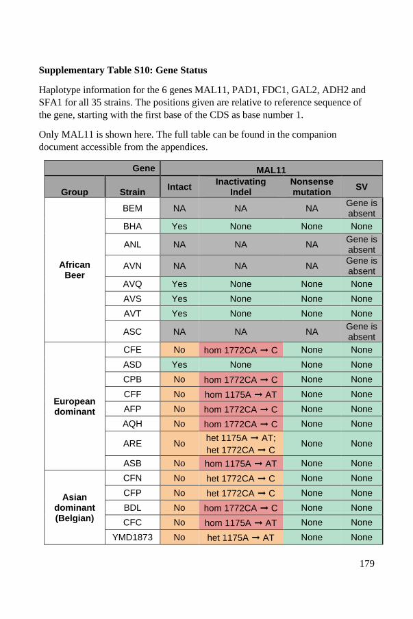
179

Supplementary Table S10: Gene Status

Haplotype information for the 6 genes MAL11, PAD1, FDC1, GAL2, ADH2 and

SFA1 for all 35 strains. The positions given are relative to reference sequence of

the gene, starting with the first base of the CDS as base number 1.

Only MAL11 is shown here. The full table can be found in the companion

document accessible from the appendices.

Gene MAL11

Group Strain Intact

Inactivating Indel

Nonsense mutation

SV

African Beer

BEM NA NA NA Gene is absent

BHA Yes None None None

ANL NA NA NA Gene is absent

AVN NA NA NA Gene is absent

AVQ Yes None None None

AVS Yes None None None

AVT Yes None None None

ASC NA NA NA Gene is absent

European dominant

CFE No hom 1772CA ➞ C None None

ASD Yes None None None

CPB No hom 1772CA ➞ C None None

CFF No hom 1175A ➞ AT None None

AFP No hom 1772CA ➞ C None None

AQH No hom 1772CA ➞ C None None

ARE No het 1175A ➞ AT;

het 1772CA ➞ C None None

ASB No hom 1175A ➞ AT None None

Asian dominant (Belgian)

CFN No het 1772CA ➞ C None None

CFP No het 1772CA ➞ C None None

BDL No hom 1772CA ➞ C None None

CFC No hom 1175A ➞ AT None None

YMD1873 No het 1175A ➞ AT None None

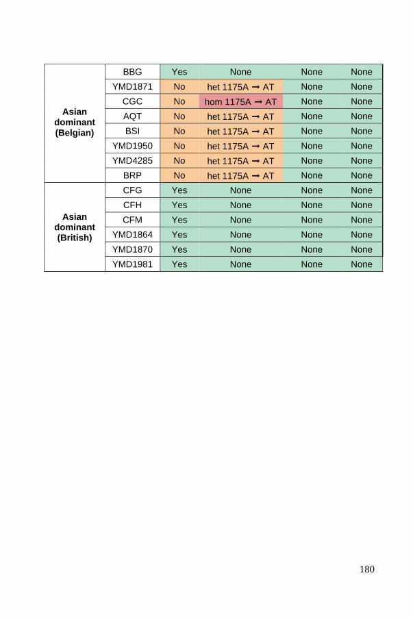
180

Asian dominant (Belgian)

BBG Yes None None None

YMD1871 No het 1175A ➞ AT None None

CGC No hom 1175A ➞ AT None None

AQT No het 1175A ➞ AT None None

BSI No het 1175A ➞ AT None None

YMD1950 No het 1175A ➞ AT None None

YMD4285 No het 1175A ➞ AT None None

BRP No het 1175A ➞ AT None None

Asian dominant (British)

CFG Yes None None None

CFH Yes None None None

CFM Yes None None None

YMD1864 Yes None None None

YMD1870 Yes None None None

YMD1981 Yes None None None

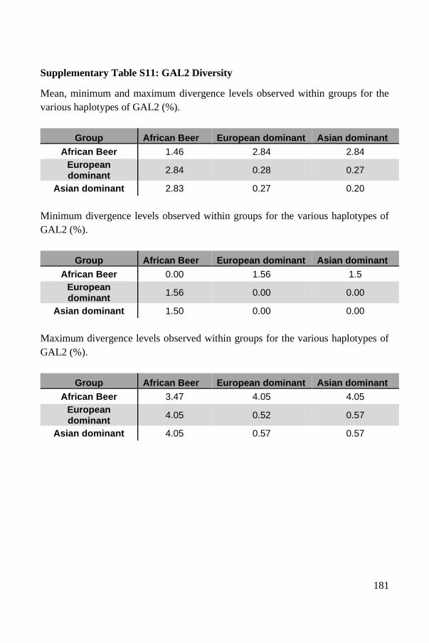
181

Supplementary Table S11: GAL2 Diversity

Mean, minimum and maximum divergence levels observed within groups for the

various haplotypes of GAL2 (%).

Group African Beer European dominant Asian dominant

African Beer 1.46 2.84 2.84

European dominant

2.84 0.28 0.27

Asian dominant 2.83 0.27 0.20

Minimum divergence levels observed within groups for the various haplotypes of

GAL2 (%).

Group African Beer European dominant Asian dominant

African Beer 0.00 1.56 1.5

European dominant

1.56 0.00 0.00

Asian dominant 1.50 0.00 0.00

Maximum divergence levels observed within groups for the various haplotypes of

GAL2 (%).

Group African Beer European dominant Asian dominant

African Beer 3.47 4.05 4.05

European dominant

4.05 0.52 0.57

Asian dominant 4.05 0.57 0.57

182

Availability of data

Oxford Nanopore and Illumina sequencing data are available under the study

accession number PRJEB46384.

Illumina short read data for the Saccharomyces cerevisiae strains is taken from the

1,011 yeast genomes project and their SRA accession numbers are given in

Supplemental Table 1.

183

References

1. Legras, J.-L., Merdinoglu, D., Cornuet, J.-M. & Karst, F. Bread, beer and wine:

Saccharomyces cerevisiae diversity reflects human history. Mol. Ecol. 16, 2091–

2102 (2007).

2. Schacherer, J., Shapiro, J. A., Ruderfer, D. M. & Kruglyak, L. Comprehensive

polymorphism survey elucidates population structure of Saccharomyces cerevisiae.

Nature 458, 342–345 (2009).

3. Ludlow, C. L. et al. Independent Origins of Yeast Associated with Coffee and

Cacao Fermentation. Curr. Biol. 26, 965–971 (2016).

4. Gallone, B. et al. Domestication and Divergence of Saccharomyces cerevisiae

Beer Yeasts. Cell 166, 1397-1410.e16 (2016).

5. Gonçalves, M. et al. Distinct Domestication Trajectories in Top-Fermenting Beer

Yeasts and Wine Yeasts. Curr. Biol. 26, 2750–2761 (2016).

6. Peter, J. et al. Genome evolution across 1,011 Saccharomyces cerevisiae isolates.

Nature 556, 339–344 (2018).

7. Legras, J.-L. et al. Adaptation of S. cerevisiae to Fermented Food Environments

Reveals Remarkable Genome Plasticity and the Footprints of Domestication. Mol.

Biol. Evol. 35, 1712–1727 (2018).

8. Fay, J. C. et al. A polyploid admixed origin of beer yeasts derived from European

and Asian wine populations. PLoS Biol. 17, e3000147 (2019).

9. Barnett, J. A. & Lichtenthaler, F. W. A history of research on yeasts 3: Emil

Fischer, Eduard Buchner and their contemporaries, 1880-1900. Yeast Chichester

Engl. 18, 363–388 (2001).

10. Steensels, J., Gallone, B., Voordeckers, K. & Verstrepen, K. J. Domestication of

Industrial Microbes. Curr. Biol. 29, R381–R393 (2019).

11. Udom, N., Chansongkrow, P., Charoensawan, V. & Auesukaree, C.

Coordination of the Cell Wall Integrity and High-Osmolarity Glycerol Pathways in

Response to Ethanol Stress in Saccharomyces cerevisiae. Appl. Environ. Microbiol.

85, e00551-19 (2019).

12. Gagnon-Arsenault, I., Tremblay, J. & Bourbonnais, Y. Fungal yapsins and cell

wall: a unique family of aspartic peptidases for a distinctive cellular function. FEMS

Yeast Res. 6, 966–978 (2006).

13. Szoradi, T. et al. SHRED Is a Regulatory Cascade that Reprograms Ubr1

Substrate Specificity for Enhanced Protein Quality Control during Stress. Mol. Cell

70, 1025-1037.e5 (2018).

14. Charoenbhakdi, S., Dokpikul, T., Burphan, T., Techo, T. & Auesukaree, C.

Vacuolar H+-ATPase Protects Saccharomyces cerevisiae Cells against Ethanol-

Induced Oxidative and Cell Wall Stresses. Appl. Environ. Microbiol. 82, 3121–3130

(2016).

184

15. Holzapfel, W. H. Appropriate starter culture technologies for small-scale

fermentation in developing countries. Int. J. Food Microbiol. 75, 197–212 (2002).

16. Johansen, P. G., Owusu-Kwarteng, J., Parkouda, C., Padonou, S. W. & Jespersen,

L. Occurrence and Importance of Yeasts in Indigenous Fermented Food and

Beverages Produced in Sub-Saharan Africa. Front. Microbiol. 10, 1789 (2019).

17. Adebo, O. A. African Sorghum-Based Fermented Foods: Past, Current and

Future Prospects. Nutrients 12, 1111 (2020).

18. Bokulich, N. A. & Bamforth, C. W. The Microbiology of Malting and Brewing.

Microbiol. Mol. Biol. Rev. 77, 157–172 (2013).

19. Lengeler, K. B., Stovicek, V., Fennessy, R. T., Katz, M. & Förster, J. Never

Change a Brewing Yeast? Why Not, There Are Plenty to Choose From. Front. Genet.

11, (2020).

20. Whittington, H. D., Dagher, S. F. & Bruno-Bárcena, J. M. Production and

Conservation of Starter Cultures: From “Backslopping” to Controlled

Fermentations. in How Fermented Foods Feed a Healthy Gut Microbiota: A

Nutrition Continuum (eds. Azcarate-Peril, M. A., Arnold, R. R. & Bruno-Bárcena,

J. M.) 125–138 (Springer International Publishing, 2019). doi:10.1007/978-3-030-

28737-5_5.

21. Teste, M.-A., François, J. M. & Parrou, J.-L. Characterization of a new multigene

family encoding isomaltases in the yeast Saccharomyces cerevisiae, the IMA family.

J. Biol. Chem. 285, 26815–26824 (2010).

22. Dickinson, J. R., Salgado, L. E. J. & Hewlins, M. J. E. The Catabolism of Amino

Acids to Long Chain and Complex Alcohols in Saccharomyces cerevisiae *. J. Biol.

Chem. 278, 8028–8034 (2003).

23. Hazelwood, L. A., Daran, J.-M., van Maris, A. J. A., Pronk, J. T. & Dickinson,

J. R. The Ehrlich Pathway for Fusel Alcohol Production: a Century of Research on

Saccharomyces cerevisiae Metabolism. Appl. Environ. Microbiol. 74, 2259–2266

(2008).

24. Abou Saada, O., Tsouris, A., Eberlein, C., Friedrich, A. & Schacherer, J. nPhase:

an accurate and contiguous phasing method for polyploids. Genome Biol. 22, 1–27

(2021).

25. Jacobus, A. P. et al. Comparative Genomics Supports That Brazilian Bioethanol

Saccharomyces cerevisiae Comprise a Unified Group of Domesticated Strains

Related to Cachaça Spirit Yeasts. Front. Microbiol. 12, (2021).

26. Krysan, D. J., Ting, E. L., Abeijon, C., Kroos, L. & Fuller, R. S. Yapsins Are a

Family of Aspartyl Proteases Required for Cell Wall Integrity in Saccharomyces

cerevisiae. Eukaryot. Cell 4, 1364–1374 (2005).

27. Verbelen, P. J., Saerens, S. M. G., Van Mulders, S. E., Delvaux, F. & Delvaux,

F. R. The role of oxygen in yeast metabolism during high cell density brewery

fermentations. Appl. Microbiol. Biotechnol. 82, 1143–1156 (2009).

28. Duan, S.-F. et al. Reverse Evolution of a Classic Gene Network in Yeast Offers

a Competitive Advantage. Curr. Biol. CB 29, 1126-1136.e5 (2019).

185

29. Boocock, J., Sadhu, M. J., Durvasula, A., Bloom, J. S. & Kruglyak, L. Ancient

balancing selection maintains incompatible versions of the galactose pathway in

yeast. Science 371, 415–419 (2021).

30. Wang, Z.-Y., Wang, J.-J., Liu, X.-F., He, X.-P. & Zhang, B.-R. Recombinant

industrial brewing yeast strains with ADH2 interruption using self-cloning

GSH1+CUP1 cassette. FEMS Yeast Res. 9, 574–581 (2009).

31. Istace, B. et al. de novo assembly and population genomic survey of natural yeast

isolates with the Oxford Nanopore MinION sequencer. GigaScience 6, 1–13 (2017).

32. McKenna, A. et al. The Genome Analysis Toolkit: a MapReduce framework for

analyzing next-generation DNA sequencing data. Genome Res. 20, 1297–1303

(2010).

33. Paradis, E., Claude, J. & Strimmer, K. APE: Analyses of Phylogenetics and

Evolution in R language. Bioinformatics 20, 289–290 (2004).

34. Zheng, X. et al. A high-performance computing toolset for relatedness and

principal component analysis of SNP data. Bioinformatics 28, 3326–3328 (2012).

35. Danecek, P. et al. Twelve years of SAMtools and BCFtools. GigaScience 10,

giab008 (2021).

36. Engel, S. R. et al. The Reference Genome Sequence of Saccharomyces

cerevisiae: Then and Now. G3 GenesGenomesGenetics 4, 389–398 (2013).

37. Boyle, E. I. et al. GO::TermFinder--open source software for accessing Gene

Ontology information and finding significantly enriched Gene Ontology terms

associated with a list of genes. Bioinforma. Oxf. Engl. 20, 3710–3715 (2004).

38. Li, H. Aligning sequence reads, clone sequences and assembly contigs with

BWA-MEM. ArXiv13033997 Q-Bio (2013).

39. Ramírez, F. et al. deepTools2: a next generation web server for deep-sequencing

data analysis. Nucleic Acids Res. 44, W160–W165 (2016).

40. Wong, B. Points of view: Color blindness. Nat. Methods 8, 441–441 (2011).

186

Chapter III – Different trajectories of

polyploidization shape the genomic landscape of

the Brettanomyces bruxellensis yeast species

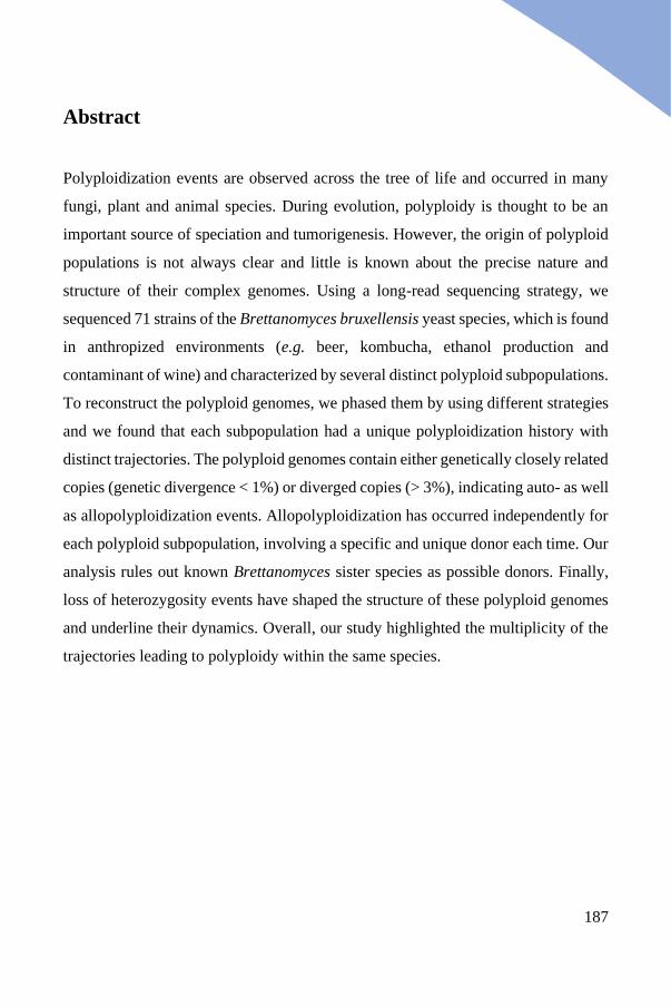
187

Abstract

Polyploidization events are observed across the tree of life and occurred in many

fungi, plant and animal species. During evolution, polyploidy is thought to be an

important source of speciation and tumorigenesis. However, the origin of polyploid

populations is not always clear and little is known about the precise nature and

structure of their complex genomes. Using a long-read sequencing strategy, we

sequenced 71 strains of the Brettanomyces bruxellensis yeast species, which is found

in anthropized environments (e.g. beer, kombucha, ethanol production and

contaminant of wine) and characterized by several distinct polyploid subpopulations.

To reconstruct the polyploid genomes, we phased them by using different strategies

and we found that each subpopulation had a unique polyploidization history with

distinct trajectories. The polyploid genomes contain either genetically closely related

copies (genetic divergence < 1%) or diverged copies (> 3%), indicating auto- as well

as allopolyploidization events. Allopolyploidization has occurred independently for

each polyploid subpopulation, involving a specific and unique donor each time. Our

analysis rules out known Brettanomyces sister species as possible donors. Finally,

loss of heterozygosity events have shaped the structure of these polyploid genomes

and underline their dynamics. Overall, our study highlighted the multiplicity of the

trajectories leading to polyploidy within the same species.

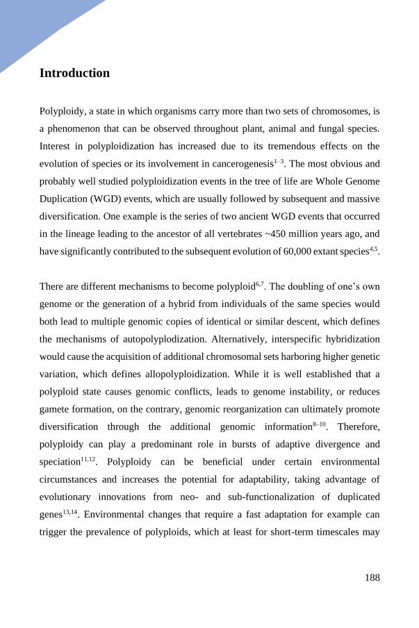
188

Introduction

Polyploidy, a state in which organisms carry more than two sets of chromosomes, is

a phenomenon that can be observed throughout plant, animal and fungal species.

Interest in polyploidization has increased due to its tremendous effects on the

evolution of species or its involvement in cancerogenesis1–3. The most obvious and

probably well studied polyploidization events in the tree of life are Whole Genome

Duplication (WGD) events, which are usually followed by subsequent and massive

diversification. One example is the series of two ancient WGD events that occurred

in the lineage leading to the ancestor of all vertebrates ~450 million years ago, and

have significantly contributed to the subsequent evolution of 60,000 extant species4,5.

There are different mechanisms to become polyploid6,7. The doubling of one’s own

genome or the generation of a hybrid from individuals of the same species would

both lead to multiple genomic copies of identical or similar descent, which defines

the mechanisms of autopolyplodization. Alternatively, interspecific hybridization

would cause the acquisition of additional chromosomal sets harboring higher genetic

variation, which defines allopolyploidization. While it is well established that a

polyploid state causes genomic conflicts, leads to genome instability, or reduces

gamete formation, on the contrary, genomic reorganization can ultimately promote

diversification through the additional genomic information8–10. Therefore,

polyploidy can play a predominant role in bursts of adaptive divergence and

speciation11,12. Polyploidy can be beneficial under certain environmental

circumstances and increases the potential for adaptability, taking advantage of

evolutionary innovations from neo- and sub-functionalization of duplicated

genes13,14. Environmental changes that require a fast adaptation for example can

trigger the prevalence of polyploids, which at least for short-term timescales may

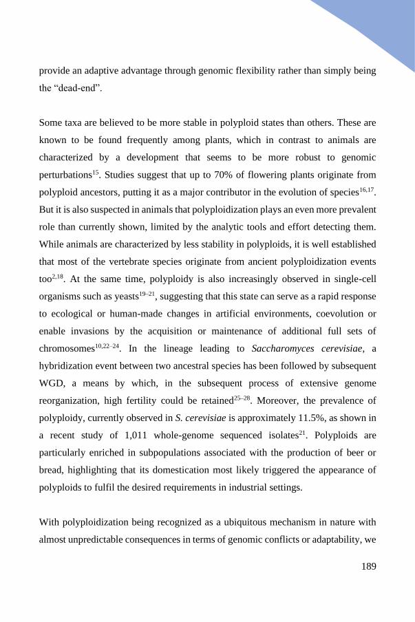
189

provide an adaptive advantage through genomic flexibility rather than simply being

the “dead-end”.

Some taxa are believed to be more stable in polyploid states than others. These are

known to be found frequently among plants, which in contrast to animals are

characterized by a development that seems to be more robust to genomic

perturbations15. Studies suggest that up to 70% of flowering plants originate from

polyploid ancestors, putting it as a major contributor in the evolution of species16,17.

But it is also suspected in animals that polyploidization plays an even more prevalent

role than currently shown, limited by the analytic tools and effort detecting them.

While animals are characterized by less stability in polyploids, it is well established

that most of the vertebrate species originate from ancient polyploidization events

too2,18. At the same time, polyploidy is also increasingly observed in single-cell

organisms such as yeasts19–21, suggesting that this state can serve as a rapid response

to ecological or human-made changes in artificial environments, coevolution or

enable invasions by the acquisition or maintenance of additional full sets of

chromosomes10,22–24. In the lineage leading to Saccharomyces cerevisiae, a

hybridization event between two ancestral species has been followed by subsequent

WGD, a means by which, in the subsequent process of extensive genome

reorganization, high fertility could be retained25–28. Moreover, the prevalence of

polyploidy, currently observed in S. cerevisiae is approximately 11.5%, as shown in

a recent study of 1,011 whole-genome sequenced isolates21. Polyploids are

particularly enriched in subpopulations associated with the production of beer or

bread, highlighting that its domestication most likely triggered the appearance of

polyploids to fulfil the desired requirements in industrial settings.

With polyploidization being recognized as a ubiquitous mechanism in nature with

almost unpredictable consequences in terms of genomic conflicts or adaptability, we

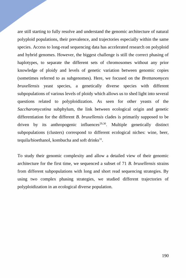
190

are still starting to fully resolve and understand the genomic architecture of natural

polyploid populations, their prevalence, and trajectories especially within the same

species. Access to long-read sequencing data has accelerated research on polyploid

and hybrid genomes. However, the biggest challenge is still the correct phasing of

haplotypes, to separate the different sets of chromosomes without any prior

knowledge of ploidy and levels of genetic variation between genomic copies

(sometimes referred to as subgenomes). Here, we focused on the Brettanomyces

bruxellensis yeast species, a genetically diverse species with different

subpopulations of various levels of ploidy which allows us to shed light into several

questions related to polyploidization. As seen for other yeasts of the

Saccharomycotina subphylum, the link between ecological origin and genetic

differentiation for the different B. bruxellensis clades is primarily supposed to be

driven by its anthropogenic influences29,30. Multiple genetically distinct

subpopulations (clusters) correspond to different ecological niches: wine, beer,

tequila/bioethanol, kombucha and soft drinks31.

To study their genomic complexity and allow a detailed view of their genomic

architecture for the first time, we sequenced a subset of 71 B. bruxellensis strains

from different subpopulations with long and short read sequencing strategies. By

using two complex phasing strategies, we studied different trajectories of

polyploidization in an ecological diverse population.

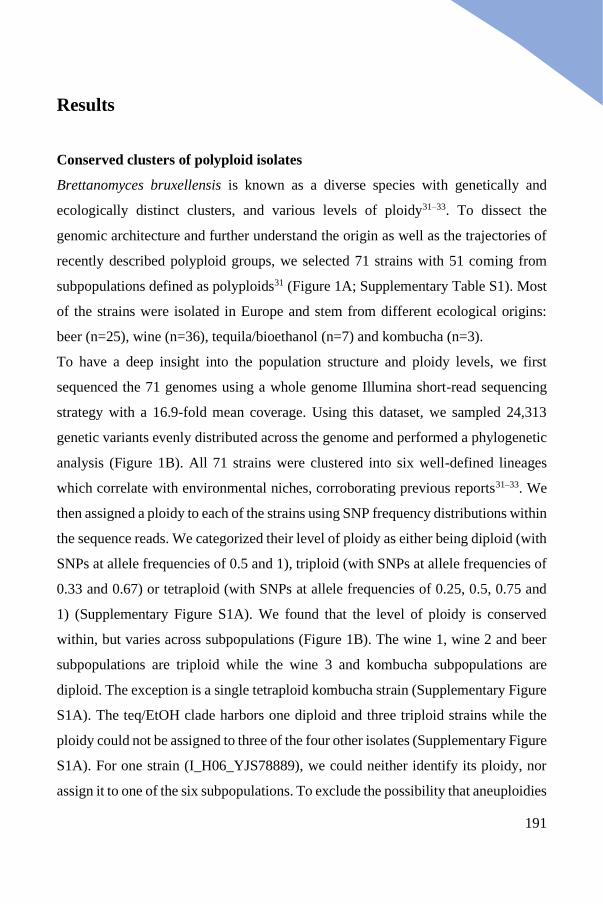
191

Results

Conserved clusters of polyploid isolates

Brettanomyces bruxellensis is known as a diverse species with genetically and

ecologically distinct clusters, and various levels of ploidy31–33. To dissect the

genomic architecture and further understand the origin as well as the trajectories of

recently described polyploid groups, we selected 71 strains with 51 coming from

subpopulations defined as polyploids31 (Figure 1A; Supplementary Table S1). Most

of the strains were isolated in Europe and stem from different ecological origins:

beer (n=25), wine (n=36), tequila/bioethanol (n=7) and kombucha (n=3).

To have a deep insight into the population structure and ploidy levels, we first

sequenced the 71 genomes using a whole genome Illumina short-read sequencing

strategy with a 16.9-fold mean coverage. Using this dataset, we sampled 24,313

genetic variants evenly distributed across the genome and performed a phylogenetic

analysis (Figure 1B). All 71 strains were clustered into six well-defined lineages

which correlate with environmental niches, corroborating previous reports31–33. We

then assigned a ploidy to each of the strains using SNP frequency distributions within

the sequence reads. We categorized their level of ploidy as either being diploid (with

SNPs at allele frequencies of 0.5 and 1), triploid (with SNPs at allele frequencies of

0.33 and 0.67) or tetraploid (with SNPs at allele frequencies of 0.25, 0.5, 0.75 and

1) (Supplementary Figure S1A). We found that the level of ploidy is conserved

within, but varies across subpopulations (Figure 1B). The wine 1, wine 2 and beer

subpopulations are triploid while the wine 3 and kombucha subpopulations are

diploid. The exception is a single tetraploid kombucha strain (Supplementary Figure

S1A). The teq/EtOH clade harbors one diploid and three triploid strains while the

ploidy could not be assigned to three of the four other isolates (Supplementary Figure

S1A). For one strain (I_H06_YJS78889), we could neither identify its ploidy, nor

assign it to one of the six subpopulations. To exclude the possibility that aneuploidies

192

are causing the non-assignment of ploidy levels for the four strains, we looked at

read coverage across their genome to identify regions that are absent or present in

multiple copies (Supplementary Figure S1B-C). We showed that the coverage is

stable and that these strains do not contain regions with varying coverage explaining

our results.

Overall, we highlight that the level of ploidy is conserved within genetically diverged

subpopulations, but not across them. We showed that the teq/EtOH strains are the

most diverse subpopulation and confirmed previous data that additionally suggested

this subpopulation as the oldest of the different B. bruxellensis clades33. The

teq/EtOH strains stand in contrast to other subpopulations like wine 3, which shows

the lowest degree of genetic variation, suggesting a single ancestral origin with a

recent expansion.

193

Figure 1 - Ploidy and intra-genomic variation

A. Strain collection. The 71 sequenced strains come from the collection of 1,500 isolates31

and were isolated in different regions worldwide, where they are associated with anthropized

environments such as tequila/bioethanol, beer, wine and kombucha production.

B. Genetic relationship and ploidy level. The sequenced strains, here clustered based on

Illumina short read sequencing data (75PE), segregate into six genetically distinct

subpopulations, namely tequila/bioethanol (teq/EtOH), beer, wine (1-3) and kombucha

(based on 24,313 genome-wide distributed variants). Forty-eight strains were detected as

triploids (69%) coming from five of the six subpopulations: teq/EtOH, beer, wine (1,2) and

kombucha (inferred from genome-wide allele frequencies).

C. Genetic diversity within clades inferred from long-read sequencing data. The three

subpopulations teq/EtOH (n=5), beer (n=22) and wine 1 (n=7) harbor strains with two

clusters of reads bearing low and high genetic variation (underlaid in grey) compared to the

reference genome Brettanomyces bruxellensis36. The subpopulation wine 2 (n=9), although

being polyploid (B), lacks genomic regions with high genetic variation to the reference

genome. The three lines within each distribution show the 25%, 50 and 75% quartiles.

194

Strategies used to phase the B. bruxellensis polyploid genomes

In order to resolve the genomic structure of polyploid isolates, we sequenced the

genomes of the 71 strains using the Oxford Nanopore sequencing strategy. Long-

read sequencing has become the strategy of choice to best resolve structural variation

and build high quality de novo reference assemblies. The difficulty of resolving

polyploid genomes, however, lies especially in the attempt to distinguish between

the different haplotypes, which are present as independent genomic copies within

the same genomes. We will hereafter refer to distinct genomic entities of different

descendants within the same genome as genomic copies. While de novo assemblers

are not capable of fully differentiating between different haplotypes in polyploids,

seeking instead to provide collapsed haplotypes, several alignment-based algorithms

have been developed recently to cope with the genomic architecture of polyploid

genomes34,35. They all aim to phase haplotypes into independent entities, but they

vary in performance based on factors such as ploidy, coverage, and the level of

genetic divergence between genomic copies of the polyploid genomes.

To properly phase our polyploid genomes, we sought to apply different strategies

depending on the level of divergence of the copies constituting these genomes to the

B. bruxellensis reference genome36. Reasons to expect that there are different levels

of variation relative to the reference have been identified by previous studies, which

indicated that at least two individual polyploid isolates from the wine 1 and beer

subpopulations have likely experienced polyploidization events by acquiring an

additional genomic copy of high genetic variation37.

To estimate the genetic divergence, we aligned the long reads of each strain to the

B. bruxellensis reference genome (Supplementary Figure S2A). We identified three

subpopulations (teq/EtOH, beer and wine 1) for which the genetic variation results

in a bimodal distribution with a cluster of reads that have a low level of genetic

195

variation relative to the reference and a second cluster of reads that have a high

genetic variation level relative to the reference (Figure 1C). These subpopulations

stand in contrast to the other three subpopulations (wine 2, wine 3 and kombucha),

which solely consist of low genetic divergence reads. Strikingly, wine 2 is the only

polyploid subpopulation which bears reads with only low genetic diversity. It is

hereafter assumed that “low genetic diversity/genomic variation” and “high genetic

diversity/genomic variation” are understood to refer to the distance to the B.

bruxellensis reference genome.

Given two types of polyploid subpopulations exhibiting either low or high genomic

variation, we applied two different phasing strategies to study their genomic

architecture.

(1) To resolve the origin of the genetic diversity, and to determine if the cluster with

reads of high genetic variation corresponds to an additional genomic copy, we

separated the long reads into distinct clusters based on their diversity level. We

clustered reads with peaks of low genetic variation at 2 SNPs per kb and high genetic

variation exhibiting 24.4 SNPs per kb, yielding a set of lowly divergent reads and

one of highly divergent reads (Supplementary Figure S2A-B). Reads between the

two distributions (i.e. with a variation between 10 and 14 SNPs per kb) were

conservatively ignored due to the ambiguity of which cluster they should be assigned

to (Supplementary Figure S2B). Using these two sets of reads, we generated de novo

assemblies to recreate phased copies of these polyploid genomes.

(2) The low genetic variation observed in the polyploid wine 2 subpopulation did

not allow us to separate reads based on their genetic divergence (Figure 1C).

Consequently, we used nPhase, a phasing algorithm that we recently developed35.

Briefly, nPhase resolves the genome into distinct haplotypes and provides accurate

196

and contiguous haplotype predictions using short and long read sequencing data

without any prior information of the true ploidy. It accurately identifies heterozygous

positions using highly accurate short reads and clusters long reads into haplotypes

based on the presence of similar heterozygous SNP profiles35.

Genomic architecture of the polyploid wine 2 subpopulation

We applied the nPhase phasing algorithm to the sequenced genomes of the wine 2

subpopulation which exhibit exclusively low intra-genomic variation. We focused

on six of the ten strains for which we had high quality long and short read sequencing

data, allowing us to phase their genome properly into independent haplotigs (Figure

2; Supplementary Figure S3A).

We observed that the chromosomes are phased into regions underlying in most cases

two or three haplotigs (Supplementary Figure S3A). Some regions bear multiple and

often small haplotigs, and underline the difficulty in phasing polyploid genomes with

haplotypes that reflect high genetic similarity. In addition, the level of genetic

divergence varies along the genomes of the six strains. Whenever nPhase resolves a

region into two haplotigs, the genetic variation in these regions is lower compared

to regions where it distinguishes between three haplotigs (Figure 2A). Here, the

highest genetic variation in the presence of two haplotigs is 0.93%, while on average

it is as low as 0.09% (Figure 2B, Supplementary Figure S3B). In the presence of a

third phased haplotig, the genetic variation can be as high as 1.79% with an average

genetic variation of 0.54% (Figure 2B, Supplementary Figure S3C). Consistent

coverage levels support the hypothesis that the prediction of only two haplotypes is

not due to the absence of a third copy for part of the chromosome (Figure 2A).

Therefore, while the differentiation of three haplotigs underlines the existence of

three genetically different genomic copies at that site, the phasing resolving into two

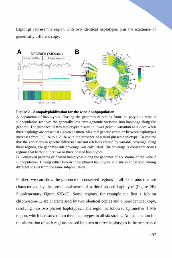
197

haplotigs represent a region with two identical haplotypes plus the existence of

genetically different copy.

Figure 2 - Autopolyploidization for the wine 2 subpopulation

A Separation of haplotypes. Phasing the genomes of strains from the polyploid wine 2

subpopulation resolves the generally low intra-genomic variation into haplotigs along the

genome. The presence of two haplotypes results in lower genetic variation as it does when

three haplotigs are present at a given position. Maximal genetic variation between haplotypes

increases from 0.93 % to 1.79 % with the presence of a third phased haplotype. To control

that the variations in genetic difference are not artefacts caused by variable coverage along

these regions, the genome-wide coverage was calculated. The coverage is consistent across

regions that harbor either two or three phased haplotypes.

B. Conserved patterns of phased haplotypes along the genomes of six strains of the wine 2

subpopulation. Having either two or three phased haplotypes at a site is conserved among

different strains from the same subpopulation.

Further, we can show the presence of conserved regions in all six strains that are

characterized by the presence/absence of a third phased haplotype (Figure 2B;

Supplementary Figure S3B-C). Some regions, for example the first 1 Mb on

chromosome 1, are characterised by two identical copies and a non-identical copy,

resolving into two phased haplotypes. This region is followed by another 1 Mb

region, which is resolved into three haplotypes in all six strains. An explanation for

the alternation of such regions phased into two or three haplotypes is the occurrence

198

of loss of heterozygosity (LOH) events. LOH events are characterized by the absence

of polymorphic markers that distinguish different genomic copies in otherwise

heterozygous diploid or polyploid individuals and consequently reduce the genetic

variation. nPhase outputs only unique haplotypes present in the data, even if one

haplotype contains twice the number of reads as the other, directly showing how

LOH events shape the haplotypes found in a genome.

Moreover, the existence of the conserved regions of LOH events among the six

strains could suggest hotspots for LOH events. Such hotspots have been shown in

other species like S. cerevisiae21 where they frequently reduce genetic variation.

Alternatively, this conserved pattern could also hint at a recent common ancestor.

However these strains were isolated from two countries on different continents

(Supplementary Table S1), making this explanation less likely.

Overall, the utilization of long and short read sequences in combination with

complex phasing strategies enables us to decipher the genomic structure of polyploid

genomes of low genetic variation and allows us to study its dynamics. In the wine 2

subpopulation, the only polyploid clade with a low intra-genomic variation, the

genomes of six strains revealed conserved regions having undergone LOH events.

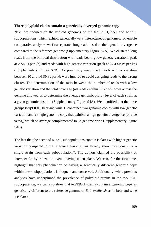
199

Three polyploid clades contain a genetically diverged genomic copy

Next, we focused on the triploid genomes of the teq/EtOH, beer and wine 1

subpopulations, which exhibit genetically very heterogeneous genomes. To enable

comparative analyses, we first separated long reads based on their genetic divergence

compared to the reference genome (Supplementary Figure S2A). We clustered long

reads from the bimodal distribution with reads bearing low genetic variation (peak

at 2 SNPs per kb) and reads with high genetic variation (peak at 24.4 SNPs per kb)

(Supplementary Figure S2B). As previously mentioned, reads with a variation

between 10 and 14 SNPs per kb were ignored to avoid assigning reads to the wrong

cluster. The determination of the ratio between the number of reads with a low

genetic variation and the total coverage (all reads) within 10 kb windows across the

genome allowed us to determine the average genomic ploidy level of each strain at

a given genomic position (Supplementary Figure S4A). We identified that the three

groups (teq/EtOH, beer and wine 1) contained two genomic copies with low genetic

variation and a single genomic copy that exhibits a high genetic divergence (or vice

versa), which on average complemented to 3n genome-wide (Supplementary Figure

S4B).

The fact that the beer and wine 1 subpopulations contain isolates with higher genetic

variation compared to the reference genome was already shown previously for a

single strain from each subpopulation37. The authors claimed the possibility of

interspecific hybridization events having taken place. We can, for the first time,

highlight that this phenomenon of having a genetically different genomic copy

within these subpopulations is frequent and conserved. Additionally, while previous

analyses have underpinned the prevalence of polyploid strains in the teq/EtOH

subpopulation, we can also show that teq/EtOH strains contain a genomic copy as

genetically different to the reference genome of B. bruxellensis as in beer and wine

1 isolates.

200

To ultimately allow comparative studies between the different genomic copies

among these genomes as well as with genomes from the other subpopulations, we

first performed de novo genome assemblies using SMARTdenovo38. First, we used

only the long reads that contained low genetic variation for all strains from the three

subpopulations (teq/EtOH, beer and wine 1). We repeated this step independently

for the long reads that were exclusively bearing high genetic variation to the

reference genome to prepare de novo assemblies (Supplementary Figure S5;

Supplementary Table S2). Then, we created group-specific reference genomes by

concatenating the de novo assemblies generated from low and high genomic

variation reads (See Material and Methods). This was done for a representative strain

from each group. By performing a competitive mapping approach using these group-

specific reference genomes with scaffolds made from low and high genetic variation,

we separated the short reads for each strain from the three groups into two groups:

short reads with low genetic variation and short reads with high genetic variation

(teq/EtOH, beer and wine 1) (Supplementary Figure S5). Then, we aligned the short

reads independently back to the B. bruxellensis reference genome. For strains that

were either diploid, or polyploid with exclusively low genetic variation, we aligned

short read sequences directly to the reference genome (wine 2, wine 3 and kombucha

subpopulations).

First, we determined if there was any bias in the mapping rates of short reads to the

reference genome/assemblies, comparing the high diversity strains aligned to the de

novo assemblies and the low diversity strains aligned to the B. bruxellensis reference

genome. Both showed similar alignment rates, respectively 94% and 92.5%

indicating no bias in the alignment due to the applied phasing strategy. Then, we

determined the genetic diversity of the 71 strains by performing a principal

component analysis (Figure 3A). By looking at the first two principal components

explaining 53.7% of the variation from 24,110 sampled genome-wide distributed

201

SNPs, we can show that the genomic copies with high genetic variation (‘High’) of

40 strains from the teq/EtOH, beer and wine 1 subpopulations are clearly distinct

from the genomic copies with low genetic variation (‘Low’), and cluster in a group-

specific way.

We then checked the genetic relationships of the genomic copies with only low

genomic variation, since such genomic copies were present in all 71 strains (Figure

3B). We can show that the strains cluster in the six subpopulations as previously

observed using raw Illumina data (Figure 1B). The strain I_H06_YJS7889, initially

unable to be associated with a subpopulation, now clusters with other teq/EtOH

strains.

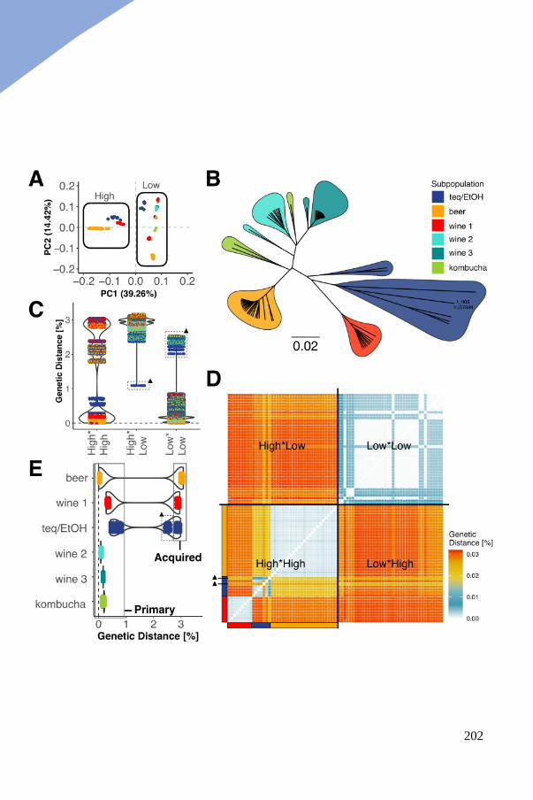
202

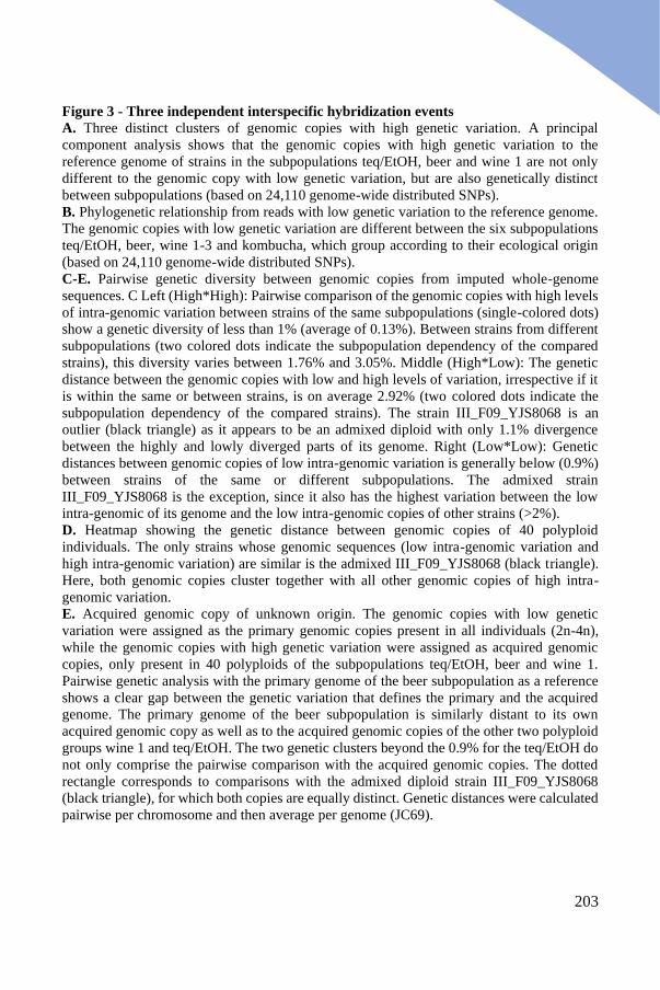
203

Figure 3 - Three independent interspecific hybridization events

A. Three distinct clusters of genomic copies with high genetic variation. A principal

component analysis shows that the genomic copies with high genetic variation to the

reference genome of strains in the subpopulations teq/EtOH, beer and wine 1 are not only

different to the genomic copy with low genetic variation, but are also genetically distinct

between subpopulations (based on 24,110 genome-wide distributed SNPs).

B. Phylogenetic relationship from reads with low genetic variation to the reference genome.

The genomic copies with low genetic variation are different between the six subpopulations

teq/EtOH, beer, wine 1-3 and kombucha, which group according to their ecological origin

(based on 24,110 genome-wide distributed SNPs).

C-E. Pairwise genetic diversity between genomic copies from imputed whole-genome

sequences. C Left (High*High): Pairwise comparison of the genomic copies with high levels

of intra-genomic variation between strains of the same subpopulations (single-colored dots)

show a genetic diversity of less than 1% (average of 0.13%). Between strains from different

subpopulations (two colored dots indicate the subpopulation dependency of the compared

strains), this diversity varies between 1.76% and 3.05%. Middle (High*Low): The genetic

distance between the genomic copies with low and high levels of variation, irrespective if it

is within the same or between strains, is on average 2.92% (two colored dots indicate the

subpopulation dependency of the compared strains). The strain III_F09_YJS8068 is an

outlier (black triangle) as it appears to be an admixed diploid with only 1.1% divergence

between the highly and lowly diverged parts of its genome. Right (Low*Low): Genetic

distances between genomic copies of low intra-genomic variation is generally below (0.9%)

between strains of the same or different subpopulations. The admixed strain

III_F09_YJS8068 is the exception, since it also has the highest variation between the low

intra-genomic of its genome and the low intra-genomic copies of other strains (>2%).

D. Heatmap showing the genetic distance between genomic copies of 40 polyploid

individuals. The only strains whose genomic sequences (low intra-genomic variation and

high intra-genomic variation) are similar is the admixed III_F09_YJS8068 (black triangle).

Here, both genomic copies cluster together with all other genomic copies of high intra-

genomic variation.

E. Acquired genomic copy of unknown origin. The genomic copies with low genetic

variation were assigned as the primary genomic copies present in all individuals (2n-4n),

while the genomic copies with high genetic variation were assigned as acquired genomic

copies, only present in 40 polyploids of the subpopulations teq/EtOH, beer and wine 1.

Pairwise genetic analysis with the primary genome of the beer subpopulation as a reference

shows a clear gap between the genetic variation that defines the primary and the acquired

genome. The primary genome of the beer subpopulation is similarly distant to its own

acquired genomic copy as well as to the acquired genomic copies of the other two polyploid

groups wine 1 and teq/EtOH. The two genetic clusters beyond the 0.9% for the teq/EtOH do

not only comprise the pairwise comparison with the acquired genomic copies. The dotted

rectangle corresponds to comparisons with the admixed diploid strain III_F09_YJS8068

(black triangle), for which both copies are equally distinct. Genetic distances were calculated

pairwise per chromosome and then average per genome (JC69).

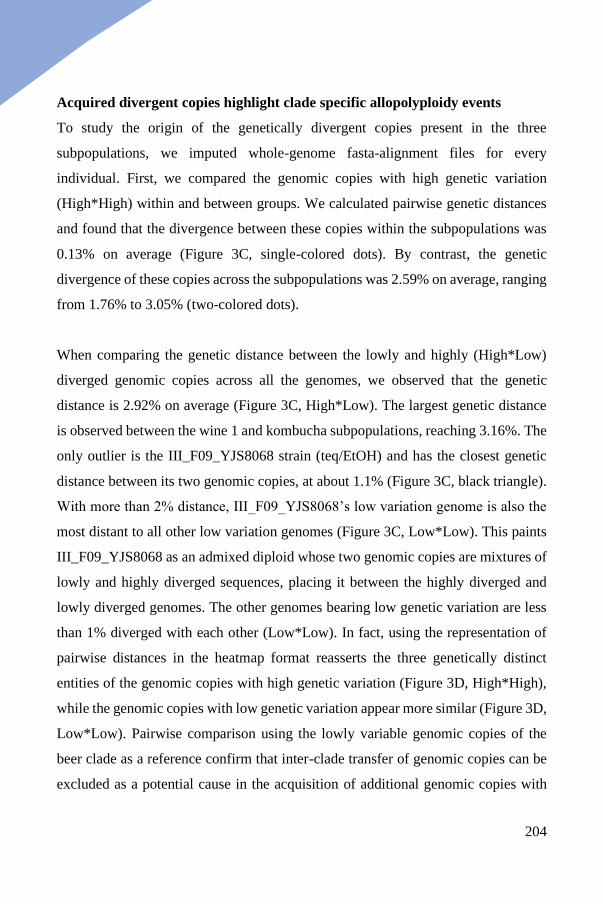
204

Acquired divergent copies highlight clade specific allopolyploidy events

To study the origin of the genetically divergent copies present in the three

subpopulations, we imputed whole-genome fasta-alignment files for every

individual. First, we compared the genomic copies with high genetic variation

(High*High) within and between groups. We calculated pairwise genetic distances

and found that the divergence between these copies within the subpopulations was

0.13% on average (Figure 3C, single-colored dots). By contrast, the genetic

divergence of these copies across the subpopulations was 2.59% on average, ranging

from 1.76% to 3.05% (two-colored dots).

When comparing the genetic distance between the lowly and highly (High*Low)

diverged genomic copies across all the genomes, we observed that the genetic

distance is 2.92% on average (Figure 3C, High*Low). The largest genetic distance

is observed between the wine 1 and kombucha subpopulations, reaching 3.16%. The

only outlier is the III_F09_YJS8068 strain (teq/EtOH) and has the closest genetic

distance between its two genomic copies, at about 1.1% (Figure 3C, black triangle).

With more than 2% distance, III_F09_YJS8068’s low variation genome is also the

most distant to all other low variation genomes (Figure 3C, Low*Low). This paints

III_F09_YJS8068 as an admixed diploid whose two genomic copies are mixtures of

lowly and highly diverged sequences, placing it between the highly diverged and

lowly diverged genomes. The other genomes bearing low genetic variation are less

than 1% diverged with each other (Low*Low). In fact, using the representation of

pairwise distances in the heatmap format reasserts the three genetically distinct

entities of the genomic copies with high genetic variation (Figure 3D, High*High),

while the genomic copies with low genetic variation appear more similar (Figure 3D,

Low*Low). Pairwise comparison using the lowly variable genomic copies of the

beer clade as a reference confirm that inter-clade transfer of genomic copies can be

excluded as a potential cause in the acquisition of additional genomic copies with

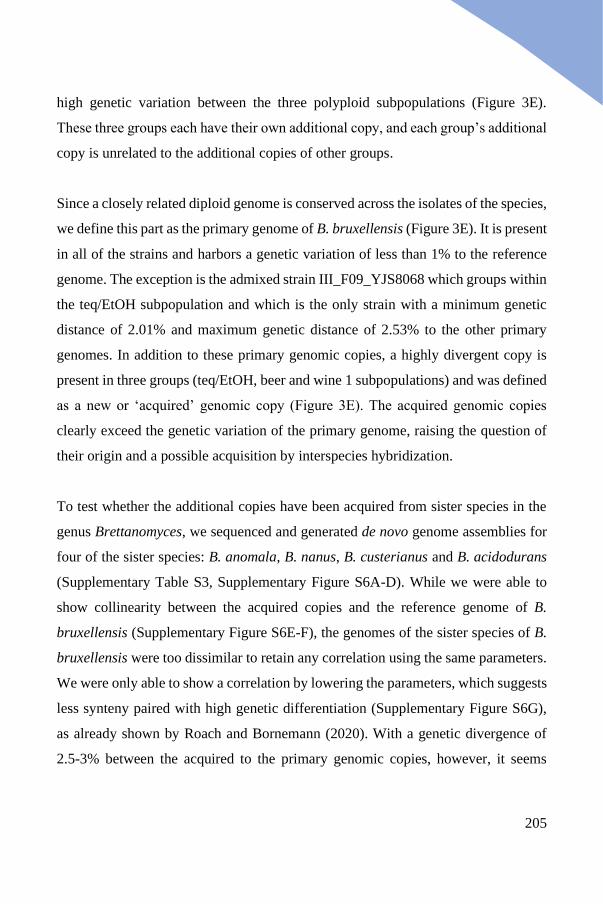
205

high genetic variation between the three polyploid subpopulations (Figure 3E).

These three groups each have their own additional copy, and each group’s additional

copy is unrelated to the additional copies of other groups.

Since a closely related diploid genome is conserved across the isolates of the species,

we define this part as the primary genome of B. bruxellensis (Figure 3E). It is present

in all of the strains and harbors a genetic variation of less than 1% to the reference

genome. The exception is the admixed strain III_F09_YJS8068 which groups within

the teq/EtOH subpopulation and which is the only strain with a minimum genetic

distance of 2.01% and maximum genetic distance of 2.53% to the other primary

genomes. In addition to these primary genomic copies, a highly divergent copy is

present in three groups (teq/EtOH, beer and wine 1 subpopulations) and was defined

as a new or ‘acquired’ genomic copy (Figure 3E). The acquired genomic copies

clearly exceed the genetic variation of the primary genome, raising the question of

their origin and a possible acquisition by interspecies hybridization.

To test whether the additional copies have been acquired from sister species in the

genus Brettanomyces, we sequenced and generated de novo genome assemblies for

four of the sister species: B. anomala, B. nanus, B. custerianus and B. acidodurans

(Supplementary Table S3, Supplementary Figure S6A-D). While we were able to

show collinearity between the acquired copies and the reference genome of B.

bruxellensis (Supplementary Figure S6E-F), the genomes of the sister species of B.

bruxellensis were too dissimilar to retain any correlation using the same parameters.

We were only able to show a correlation by lowering the parameters, which suggests

less synteny paired with high genetic differentiation (Supplementary Figure S6G),

as already shown by Roach and Bornemann (2020). With a genetic divergence of

2.5-3% between the acquired to the primary genomic copies, however, it seems

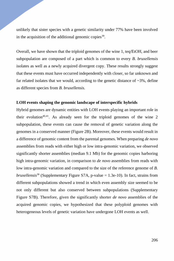
206

unlikely that sister species with a genetic similarity under 77% have been involved

in the acquisition of the additional genomic copies39.

Overall, we have shown that the triploid genomes of the wine 1, teq/EtOH, and beer

subpopulation are composed of a part which is common to every B. bruxellensis

isolates as well as a newly acquired divergent copy. These results strongly suggest

that these events must have occurred independently with closer, so far unknown and

far related isolates that we would, according to the genetic distance of ~3%, define

as different species from B. bruxellensis.

LOH events shaping the genomic landscape of interspecific hybrids

Hybrid genomes are dynamic entities with LOH events playing an important role in

their evolution40,41. As already seen for the triploid genomes of the wine 2

subpopulation, these events can cause the removal of genetic variation along the

genomes in a conserved manner (Figure 2B). Moreover, these events would result in

a difference of genomic content from the parental genomes. When preparing de novo

assemblies from reads with either high or low intra-genomic variation, we observed

significantly shorter assemblies (median 9.1 Mb) for the genomic copies harboring

high intra-genomic variation, in comparison to de novo assemblies from reads with

low intra-genomic variation and compared to the size of the reference genome of B.

bruxellensis36 (Supplementary Figure S7A, p-value = 1.3e-10). In fact, strains from

different subpopulations showed a trend in which even assembly size seemed to be

not only different but also conserved between subpopulations (Supplementary

Figure S7B). Therefore, given the significantly shorter de novo assemblies of the

acquired genomic copies, we hypothesized that these polyploid genomes with

heterogeneous levels of genetic variation have undergone LOH events as well.

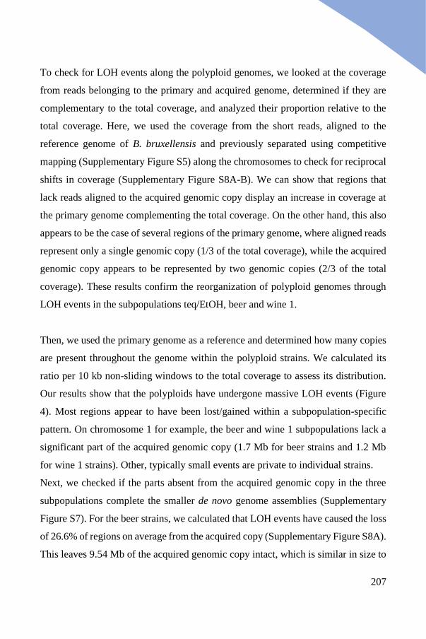
207

To check for LOH events along the polyploid genomes, we looked at the coverage

from reads belonging to the primary and acquired genome, determined if they are

complementary to the total coverage, and analyzed their proportion relative to the

total coverage. Here, we used the coverage from the short reads, aligned to the

reference genome of B. bruxellensis and previously separated using competitive

mapping (Supplementary Figure S5) along the chromosomes to check for reciprocal

shifts in coverage (Supplementary Figure S8A-B). We can show that regions that

lack reads aligned to the acquired genomic copy display an increase in coverage at

the primary genome complementing the total coverage. On the other hand, this also

appears to be the case of several regions of the primary genome, where aligned reads

represent only a single genomic copy (1/3 of the total coverage), while the acquired

genomic copy appears to be represented by two genomic copies (2/3 of the total

coverage). These results confirm the reorganization of polyploid genomes through

LOH events in the subpopulations teq/EtOH, beer and wine 1.

Then, we used the primary genome as a reference and determined how many copies

are present throughout the genome within the polyploid strains. We calculated its

ratio per 10 kb non-sliding windows to the total coverage to assess its distribution.

Our results show that the polyploids have undergone massive LOH events (Figure

4). Most regions appear to have been lost/gained within a subpopulation-specific

pattern. On chromosome 1 for example, the beer and wine 1 subpopulations lack a

significant part of the acquired genomic copy (1.7 Mb for beer strains and 1.2 Mb

for wine 1 strains). Other, typically small events are private to individual strains.

Next, we checked if the parts absent from the acquired genomic copy in the three

subpopulations complete the smaller de novo genome assemblies (Supplementary

Figure S7). For the beer strains, we calculated that LOH events have caused the loss

of 26.6% of regions on average from the acquired copy (Supplementary Figure S8A).

This leaves 9.54 Mb of the acquired genomic copy intact, which is similar in size to

208

the de novo assembly of 8.9 Mb (Supplementary Figure S7B). For the wine 1

subpopulation, 22.3% of the acquired genomic copy is lost on average, leaving 10.1

Mb still present (Supplementary Figure S8B). Here, the de novo assembly size (10.1

Mb) matches exactly the size of retained regions in our analysis (Supplementary

Figure S7B).

Figure 4 - Dynamic genomic landscape of polyploid strains

The polyploid genomes of the three subpopulations beer, wine 1 and teq/EtOH contain

massive modifications through LOH events. The primary genome (low genetic variation) was

used as a reference. Conserved patterns of modified regions for the primary genome were

identified by determining the gain or loss of its copies in each strain, here varying between

three (3×) and zero (0×). Only a few modified regions are unique to single or few strains.

There are no common regions which show the same patterns across subpopulations. The

teq/EtOH subpopulation shows a division into two clusters, each consisting of three

individuals. The ploidy level was estimated in 10 kb windows.

The teq/EtOH strains display a pattern of loss/gain of genomic regions from the

primary genome that enables the distinction of two subgroups, denoted as teq/EtOH

1 and teq/EtOH 2. The teq/EtOH 2 has almost entirely lost the second copy of the

primary genome, replaced by a second copy of the acquired genome (Figure 4). Both

subclades have lost 10.5% of the acquired genomic copy on average (12.1% for

teq/EtOH 1 and 8.8% for teq/EtOH 2). The average of both (11.64 Mb) is comparable

to the average de novo assembly size of 10.7 Mb.

209

The conserved patterns of LOH within each subpopulation raises the question of

whether these patterns are the consequence of adaptation, random processes, or point

at a recent shared ancestry. In the evolution of species, polyploidy has been shown

to potentially play an important role in the acquisition of new traits or the

amplification of already existing traits in the context of the acquisition of

resistances42,43, interactions44,45, coping with changing environments46, or the

occupation of novel ecological niches47. The different environments B. bruxellensis’

polyploid subpopulations are associated with such as bioethanol production, wine or

beer fermentation, are harsh environments and require different adaptations such as

a high tolerance to alcohol and acidity. As already seen for the polyploid wine 2

subpopulation, LOH events are shared among strains and, with LOH events at

similar positions (e.g. DEBR0S1), hotspots for LOH might be involved.

Overall, the three subpopulations with polyploid genomes derived from interspecific

hybridization events are highly dynamic, while LOH events have caused conserved

patterns of low genetic diversity within each subpopulation. Further insight into how

these variations at the gene level are expressed at a phenotypic level will have to be

queried in future studies investigating the phenotypic landscape of the different

subpopulations.

210

Discussion

The Brettanomyces bruxellensis yeast species is known to harbor subpopulations

with various levels of ploidy31–33. For the first time, we provide a detailed insight

into the complex genomic architecture of these polyploid subpopulations.

Interestingly, we noticed that there is a high conservation of ploidy in each

subpopulation and four of them, associated with three different ecological

environments (tequila/ethanol production, wine making and beer brewing) are

exclusively characterized by triploids.

Because polyploidy can be achieved in different ways (allopolyploidization or

autopolyploidization), the final genomic composition might vary by distinct levels

of intra-genomic information. At the same time, the intra-genomic variation will

define the boundaries of genomic flexibility, and therefore drive evolution in almost

unpredictable and different ways46,48.

By using two different phasing strategies, we elucidated the genomic architecture of

polyploid subpopulations of B. bruxellensis with various levels of intra-genomic

variation. We highlighted that all six populations harbor a primary genome

irrespective of their ploidy, which is defined as the genetic variation that does not go

beyond 1% when compared to the reference genome of B. bruxellensis36. This is

lower but in accordance with previous papers characterizing the genetic variation of

B. bruxellensis, since they did not phase the genomes into distinct haplotypes

(1.2%32). Furthermore, we show the existence of three allopolyploid subpopulations

(teq/EtOH, beer, and wine 1) with an acquired genomic copy with a genetic

divergence of about 3% compared to the reference genome. They clearly exceed the

average intra-genomic variation of the primary genome, demonstrating the

occurrence of interspecific hybridization events in these subpopulations. The known

211

sister species within the same genus are rejected as donors for the interspecific

hybrids due to high genetic divergence of at least 23%39.

We further highlight the fact that to our knowledge, the B. bruxellensis species is

one (or the) rare case, in which these different scenarios, respectively allo- and

autopolyploidy, can be observed in closely related subpopulations. We identified

different trajectories for strains not only associated with different environments

(teq/EtOH, beer and wine) but also associated with the same environment, while

being part of a genetically distinct cluster. The “wine”-associated strains fall in three

genetically diverged subpopulations. With the two subpopulations wine 1 and wine

2 being triploid and wine 3 being diploid, only wine 1 has acquired a third genomic

copy from interspecific hybridization, while wine 2 has solely genetically similar

haplotypes.

Different trajectories of polyploidization in nature were mostly studied (and

observed) in plants, which yields no clues as to the importance or prevalence of

polyploidization and its trajectories in animal or fungal systems2,49,50. These

mechanisms, when observed and studied in extant polyploids, have mostly (when

not exclusively) been determined between species, rather than within species. We

highlight that future studies which screen individuals on a large scale to study

prevalence and trajectories of polyploids across ecologically diverged, naturally

occurring subpopulations are required, especially in the animal and fungi kingdom,

Indications that polyploidy could be a more common state were shown by two recent

studies, which genotyped more than 1,000 individuals from the S. cerevisiae and B.

bruxellensis yeast species, with a prevalence of polyploids of 11.4%21 and 54%31,

respectively.

212

Finally, we speculate that the different trajectories of polyploids in the

subpopulations of B. bruxellensis are linked to the adaptation to the different

anthropized environments. Polyploids in general have received a lot of attention in

the context of adaptivity and diversification, in which many extant species originate

from ancient polyploid states25–28. While a polyploid state itself can allow

adaptability, it is often seen as a transient state which is followed by massive

modifications to cope with genetic incompatibilities and to regain fertility in the long

term. Evidence for this process has been gained through the detection of paralogous

gene sets with different historical trajectories in many naturally diploid taxa,

establishing the process of genomic modifications after polyploidization. With a

prevalence of 54% polyploids, plus evidence for three independent interspecific

hybridization events, polyploidy is abundant and most likely has significant effects

for B. bruxellensis. The genomes of the allo- and autopolyploid subpopulations are

characterized by massive genomic modifications, which have established a

conserved pattern of rearranged blocks. These underline on the one hand the

independent acquisition of genetically diverse genomic copies for the allopolyploid

subpopulations, but most likely also reflect the recovery of fitness and overcoming

of genomic incompatibilities. These acquired copies likely play a role in the

adaptation of these subpopulations to the harsh and changing conditions of their

anthropized environments. For example, sulfur dioxide is used to protect wine

fermentation from spoilage by B. bruxellensis. The high tolerance against sulfur

dioxide, mostly observed for the wine 1 subpopulation30, could be the adaptation of

this yeast to the recently increased usage of this agent in the industry.

Our study clearly highlights for the first time the coexistence of a large repertoire of

evolution punctuated by various independent polyploidization events within a

species and addresses the need to further resolve the genomic architecture of

polyploid species complexes from diverse ecological settings.

213

Methods

Strain selection and DNA extraction

For this study, we focused on a subset of 71 strains of Brettanomyces bruxellensis.

These strains are part of the collection of 1,500 strains31 which was previously

analyzed using microsatellites and partially with whole genome sequencing data32.

The 71 strains were selected to represent the different clades of B. bruxellensis in

terms of genetic diversity, ecological origin (origin of isolation) and variation in

ploidy (Supplementary Table S1). Additional to 71 B. bruxellensis strains, four sister

species (B. anomala, B. custersianus, B. nanus, B. acidodurans) including the

reference strain of B. bruxellensis were selected for this study (Supplementary Table

S3).

The DNA of 71 strains was extracted from 20ml cultures (single colony, 48h growth

at 25°C) using the QIAGEN Genomic-tip 100/G kit (Hilden, Germany) with the

recommended manufacturer’s genomic DNA buffer set. The manufacturer's protocol

was followed as recommended and final DNA was eluted in 100-200µl water. DNA

was quantified with the broad-range or high-sensitivity DNA quantification kit from

Qubit (Thermo Fisher Scientific, Waltham, USA) with the use of the automated plate

reading platform from TECAN (Männedorf, Switzerland). Genomic DNA was

migrated on a 1.5% agarose gel to check for degradation.

Library preparation and sequencing

The kit NEBNext® Ultra™ II DNA Library Prep Kit (Ipswich, USA) for Illumina®️

(San Diego, USA) was used for library preparation. The dual-barcoding strategy was

applied and samples were sequenced on two lanes of NextSeq (Illumina®) at the

European Molecular Laboratory (EMBL) in Heidelberg, Germany. The strategy of

214

sequencing was 75 paired-end (75PE) and sequences from two independent

sequencing lanes were concatenated prior to any analysis.

For the long-read sequencing we used the Oxford Nanopore Technology (Oxford,

UK). Libraries for sequencing using the MinION and were prepared as described in

Istace et al. (2017)51 using the Ligation Sequencing Kit SQK-LSK109. We barcoded

strains with the Native Barcoding Expansion 1-12 (EXP-NBD104) to multiplex up

to 12 samples per sequencing reaction.

Data analyses: long reads (Oxford Nanopore)

Base-calling, de-multiplexing and adapter trimming

Raw sequencing reads were processed as described in Fournier et al. (2017)36.

Briefly, the base-calling and de-multiplexing steps were performed with guppy

(https://nanoporetech.com/). Adapters were trimmed with Porechop (Porechop

GitHub Repository https://github.com/rrwick/Porechop).

Separating reads with different degrees of genetic variation to the reference

genome

We distinguish reads depending on their genetic distance to the reference genome

Brettanomyces bruxellensis. For this, long reads of each sample were first aligned to

the reference genome of B. bruxellensis36 using NGM-LR52 (v0.2.7). We separated

reads into two groups based on their number of SNPs/kb. Here, reads comprising

less than 10 variants per kb were assigned to the low intra-genomic variation cluster

and reads with more than 14 variants per kb to the high intra-genomic variation

cluster. Reads containing between 10 to 14 variants per kb were considered

ambiguous and ignored to avoid misassignment which could strongly impact de novo

genome assemblies.

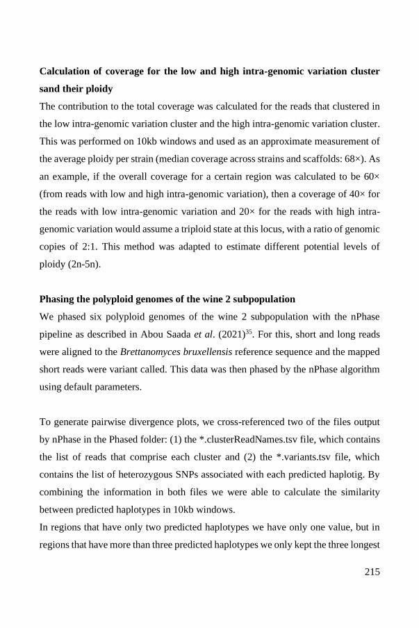
215

Calculation of coverage for the low and high intra-genomic variation cluster

sand their ploidy

The contribution to the total coverage was calculated for the reads that clustered in

the low intra-genomic variation cluster and the high intra-genomic variation cluster.

This was performed on 10kb windows and used as an approximate measurement of

the average ploidy per strain (median coverage across strains and scaffolds: 68×). As

an example, if the overall coverage for a certain region was calculated to be 60×

(from reads with low and high intra-genomic variation), then a coverage of 40× for

the reads with low intra-genomic variation and 20× for the reads with high intra-

genomic variation would assume a triploid state at this locus, with a ratio of genomic

copies of 2:1. This method was adapted to estimate different potential levels of

ploidy (2n-5n).

Phasing the polyploid genomes of the wine 2 subpopulation

We phased six polyploid genomes of the wine 2 subpopulation with the nPhase

pipeline as described in Abou Saada et al. (2021)35. For this, short and long reads

were aligned to the Brettanomyces bruxellensis reference sequence and the mapped

short reads were variant called. This data was then phased by the nPhase algorithm

using default parameters.

To generate pairwise divergence plots, we cross-referenced two of the files output

by nPhase in the Phased folder: (1) the *.clusterReadNames.tsv file, which contains

the list of reads that comprise each cluster and (2) the *.variants.tsv file, which

contains the list of heterozygous SNPs associated with each predicted haplotig. By

combining the information in both files we were able to calculate the similarity

between predicted haplotypes in 10kb windows.

In regions that have only two predicted haplotypes we have only one value, but in

regions that have more than three predicted haplotypes we only kept the three longest

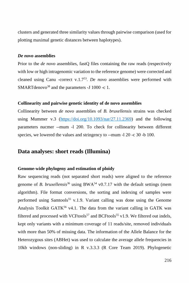
216

clusters and generated three similarity values through pairwise comparison (used for

plotting maximal genetic distances between haplotypes).

De novo assemblies

Prior to the de novo assemblies, fastQ files containing the raw reads (respectively

with low or high intragenomic variation to the reference genome) were corrected and

cleaned using Canu -correct v.1.753. De novo assemblies were performed with

SMARTdenovo38 and the parameters -J 1000 -c 1.

Collinearity and pairwise genetic identity of de novo assemblies

Collinearity between de novo assemblies of B. bruxellensis strains was checked

using Mummer v.3 (https://doi.org/10.1093/nar/27.11.2369) and the following

parameters nucmer --mum -l 200. To check for collinearity between different

species, we lowered the values and stringency to --mum -l 20 -c 30 -b 100.

Data analyses: short reads (Illumina)

Genome-wide phylogeny and estimation of ploidy

Raw sequencing reads (not separated short reads) were aligned to the reference

genome of B. bruxellensis36 using BWA54 v0.7.17 with the default settings (mem

algorithm). File format conversions, the sorting and indexing of samples were

performed using Samtools55 v.1.9. Variant calling was done using the Genome

Analysis Toolkit GATK56 v4.1. The data from the variant calling in GATK was

filtered and processed with VCFtools57 and BCFtools55 v1.9. We filtered out indels,

kept only variants with a minimum coverage of 11 reads/site, removed individuals

with more than 50% of missing data. The information of the Allele Balance for the

Heterozygous sites (ABHet) was used to calculate the average allele frequencies in

10kb windows (non-sliding) in R v.3.3.3 (R Core Team 2019). Phylogenetic

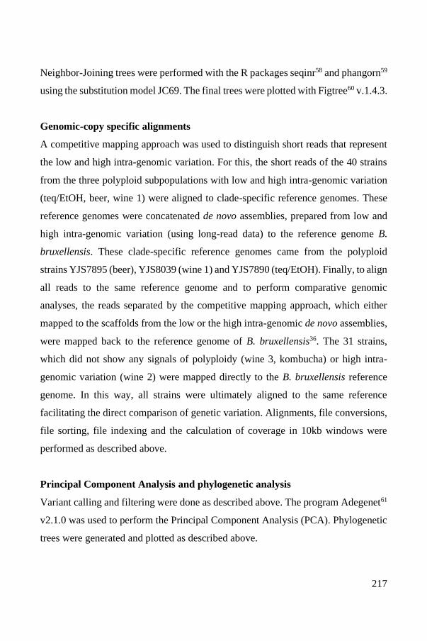
217

Neighbor-Joining trees were performed with the R packages seqinr58 and phangorn59

using the substitution model JC69. The final trees were plotted with Figtree60 v.1.4.3.

Genomic-copy specific alignments

A competitive mapping approach was used to distinguish short reads that represent

the low and high intra-genomic variation. For this, the short reads of the 40 strains

from the three polyploid subpopulations with low and high intra-genomic variation

(teq/EtOH, beer, wine 1) were aligned to clade-specific reference genomes. These

reference genomes were concatenated de novo assemblies, prepared from low and

high intra-genomic variation (using long-read data) to the reference genome B.

bruxellensis. These clade-specific reference genomes came from the polyploid

strains YJS7895 (beer), YJS8039 (wine 1) and YJS7890 (teq/EtOH). Finally, to align

all reads to the same reference genome and to perform comparative genomic

analyses, the reads separated by the competitive mapping approach, which either

mapped to the scaffolds from the low or the high intra-genomic de novo assemblies,

were mapped back to the reference genome of B. bruxellensis36. The 31 strains,

which did not show any signals of polyploidy (wine 3, kombucha) or high intra-

genomic variation (wine 2) were mapped directly to the B. bruxellensis reference

genome. In this way, all strains were ultimately aligned to the same reference

facilitating the direct comparison of genetic variation. Alignments, file conversions,

file sorting, file indexing and the calculation of coverage in 10kb windows were

performed as described above.

Principal Component Analysis and phylogenetic analysis

Variant calling and filtering were done as described above. The program Adegenet61

v2.1.0 was used to perform the Principal Component Analysis (PCA). Phylogenetic

trees were generated and plotted as described above.

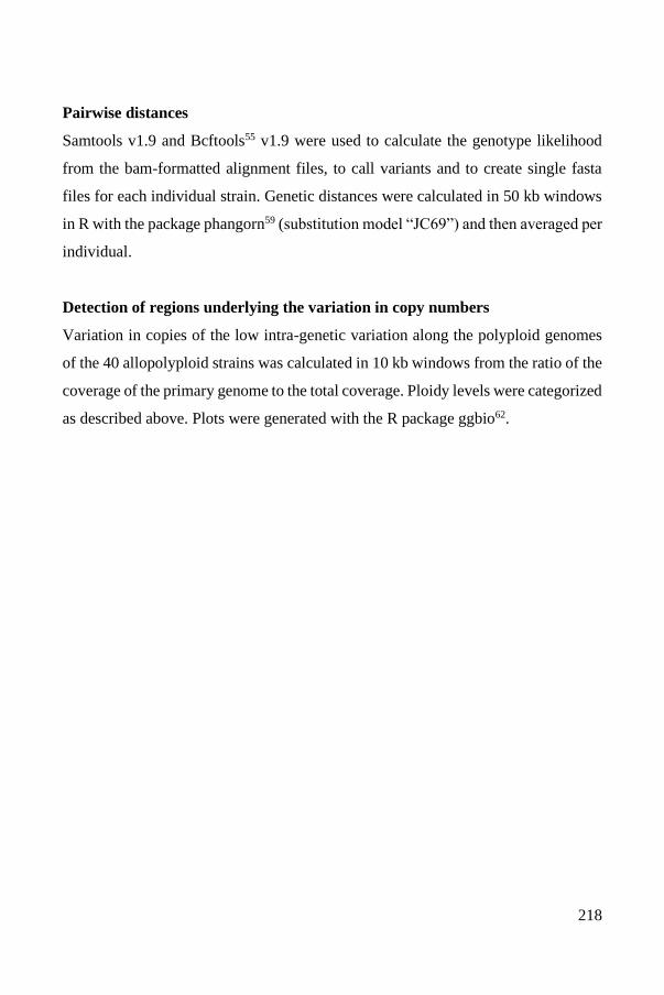
218

Pairwise distances

Samtools v1.9 and Bcftools55 v1.9 were used to calculate the genotype likelihood

from the bam-formatted alignment files, to call variants and to create single fasta

files for each individual strain. Genetic distances were calculated in 50 kb windows

in R with the package phangorn59 (substitution model “JC69”) and then averaged per

individual.

Detection of regions underlying the variation in copy numbers

Variation in copies of the low intra-genetic variation along the polyploid genomes

of the 40 allopolyploid strains was calculated in 10 kb windows from the ratio of the

coverage of the primary genome to the total coverage. Ploidy levels were categorized

as described above. Plots were generated with the R package ggbio62.

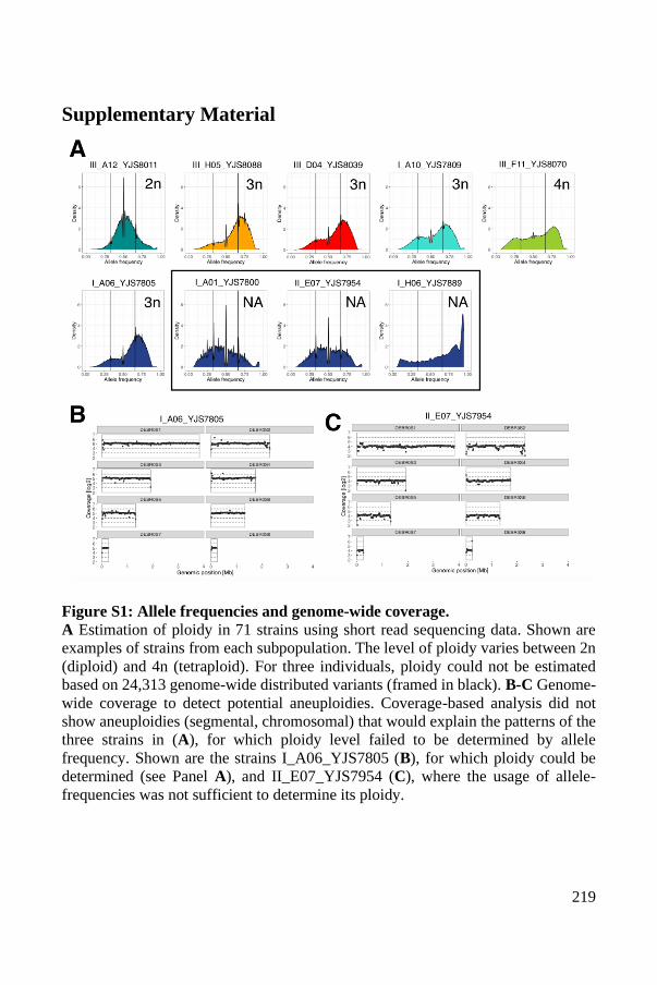
219

Supplementary Material

Figure S1: Allele frequencies and genome-wide coverage. A Estimation of ploidy in 71 strains using short read sequencing data. Shown are

examples of strains from each subpopulation. The level of ploidy varies between 2n

(diploid) and 4n (tetraploid). For three individuals, ploidy could not be estimated

based on 24,313 genome-wide distributed variants (framed in black). B-C Genome-

wide coverage to detect potential aneuploidies. Coverage-based analysis did not

show aneuploidies (segmental, chromosomal) that would explain the patterns of the

three strains in (A), for which ploidy level failed to be determined by allele

frequency. Shown are the strains I_A06_YJS7805 (B), for which ploidy could be

determined (see Panel A), and II_E07_YJS7954 (C), where the usage of allele-

frequencies was not sufficient to determine its ploidy.

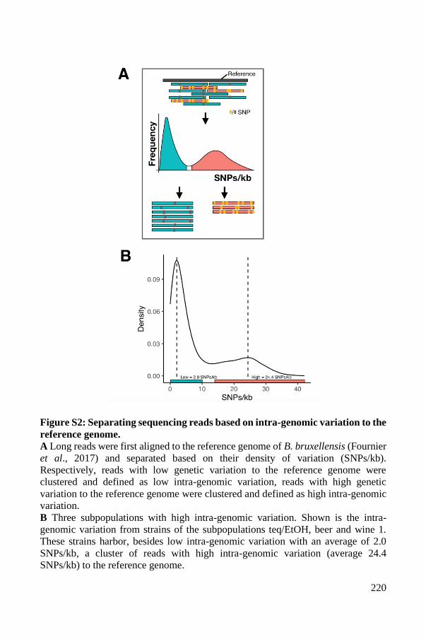
220

Figure S2: Separating sequencing reads based on intra-genomic variation to the

reference genome. A Long reads were first aligned to the reference genome of B. bruxellensis (Fournier

et al., 2017) and separated based on their density of variation (SNPs/kb).

Respectively, reads with low genetic variation to the reference genome were

clustered and defined as low intra-genomic variation, reads with high genetic

variation to the reference genome were clustered and defined as high intra-genomic

variation. B Three subpopulations with high intra-genomic variation. Shown is the intra-

genomic variation from strains of the subpopulations teq/EtOH, beer and wine 1.

These strains harbor, besides low intra-genomic variation with an average of 2.0

SNPs/kb, a cluster of reads with high intra-genomic variation (average 24.4

SNPs/kb) to the reference genome.

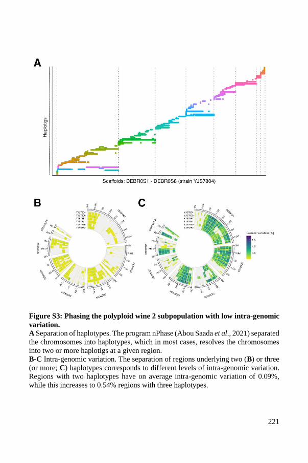
221

Figure S3: Phasing the polyploid wine 2 subpopulation with low intra-genomic

variation. A Separation of haplotypes. The program nPhase (Abou Saada et al., 2021) separated

the chromosomes into haplotypes, which in most cases, resolves the chromosomes

into two or more haplotigs at a given region. B-C Intra-genomic variation. The separation of regions underlying two (B) or three

(or more; C) haplotypes corresponds to different levels of intra-genomic variation.

Regions with two haplotypes have on average intra-genomic variation of 0.09%,

while this increases to 0.54% regions with three haplotypes.

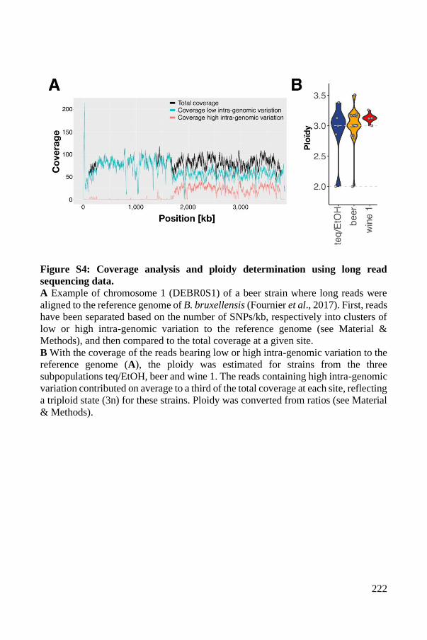
222

Figure S4: Coverage analysis and ploidy determination using long read

sequencing data. A Example of chromosome 1 (DEBR0S1) of a beer strain where long reads were

aligned to the reference genome of B. bruxellensis (Fournier et al., 2017). First, reads

have been separated based on the number of SNPs/kb, respectively into clusters of

low or high intra-genomic variation to the reference genome (see Material &

Methods), and then compared to the total coverage at a given site. B With the coverage of the reads bearing low or high intra-genomic variation to the

reference genome (A), the ploidy was estimated for strains from the three

subpopulations teq/EtOH, beer and wine 1. The reads containing high intra-genomic

variation contributed on average to a third of the total coverage at each site, reflecting

a triploid state (3n) for these strains. Ploidy was converted from ratios (see Material

& Methods).

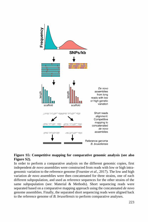
223

Figure S5: Competitive mapping for comparative genomic analysis (see also

Figure S2). In order to perform a comparative analysis on the different genomic copies, first

independent de novo assemblies were constructed from reads with low or high intra-

genomic variation to the reference genome (Fournier et al., 2017). The low and high

variation de novo assemblies were then concatenated for three strains, one of each

different subpopulation, and used as reference sequences for the other strains of the

same subpopulation (see: Material & Methods). Short sequencing reads were

separated based on a comparative mapping approach using the concatenated de novo

genome assemblies. Finally, the separated short sequencing reads were aligned back

to the reference genome of B. bruxellensis to perform comparative analyses.

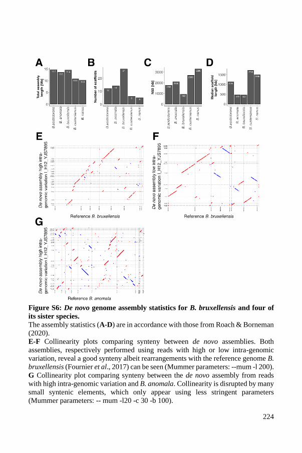
224

Figure S6: De novo genome assembly statistics for B. bruxellensis and four of

its sister species. The assembly statistics (A-D) are in accordance with those from Roach & Borneman

(2020). E-F Collinearity plots comparing synteny between de novo assemblies. Both

assemblies, respectively performed using reads with high or low intra-genomic

variation, reveal a good synteny albeit rearrangements with the reference genome B.

bruxellensis (Fournier et al., 2017) can be seen (Mummer parameters: --mum -l 200). G Collinearity plot comparing synteny between the de novo assembly from reads

with high intra-genomic variation and B. anomala. Collinearity is disrupted by many

small syntenic elements, which only appear using less stringent parameters

(Mummer parameters: -- mum -l20 -c 30 -b 100).

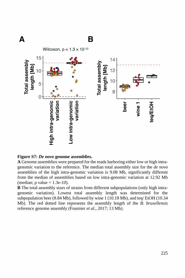
225

Figure S7: De novo genome assemblies. A Genome assemblies were prepared for the reads harboring either low or high intra-

genomic variation to the reference. The median total assembly size for the de novo

assemblies of the high intra-genomic variation is 9.08 Mb, significantly different

from the median of assemblies based on low intra-genomic variation at 12.92 Mb

(median; p value = 1.3e-10). B The total assembly sizes of strains from different subpopulations (only high intra-

genomic variation). Lowest total assembly length was determined for the

subpopulation beer (8.84 Mb), followed by wine 1 (10.18 Mb), and teq/ EtOH (10.34

Mb). The red dotted line represents the assembly length of the B. bruxellensis

reference genome assembly (Fournier et al., 2017; 13 Mb).

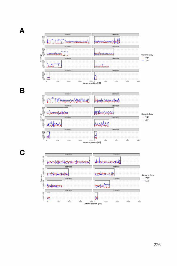
226

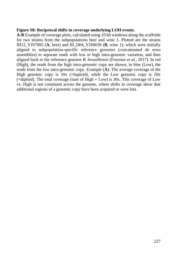
227

Figure S8: Reciprocal shifts in coverage underlying LOH events. A-B Example of coverage plots, calculated using 10 kb windows along the scaffolds

for two strains from the subpopulations beer and wine 1. Plotted are the strains

IH12_YJS7895 (A; beer) and III_D04_YJS8039 (B; wine 1), which were initially

aligned to subpopulation-specific reference genomes (concatenated de novo

assemblies) to separate reads with low or high intra-genomic variation, and then

aligned back to the reference genome B. bruxellensis (Fournier et al., 2017). In red

(High), the reads from the high intra-genomic copy are shown, in blue (Low), the

reads from the low intra-genomic copy. Example (A): The average coverage of the

High genomic copy is 10x (=haploid), while the Low genomic copy is 20x

(=diploid). The total coverage (sum of High + Low) is 30x. This coverage of Low

vs. High is not consistent across the genome, where shifts in coverage show that

additional regions of a genomic copy have been acquired or were lost.

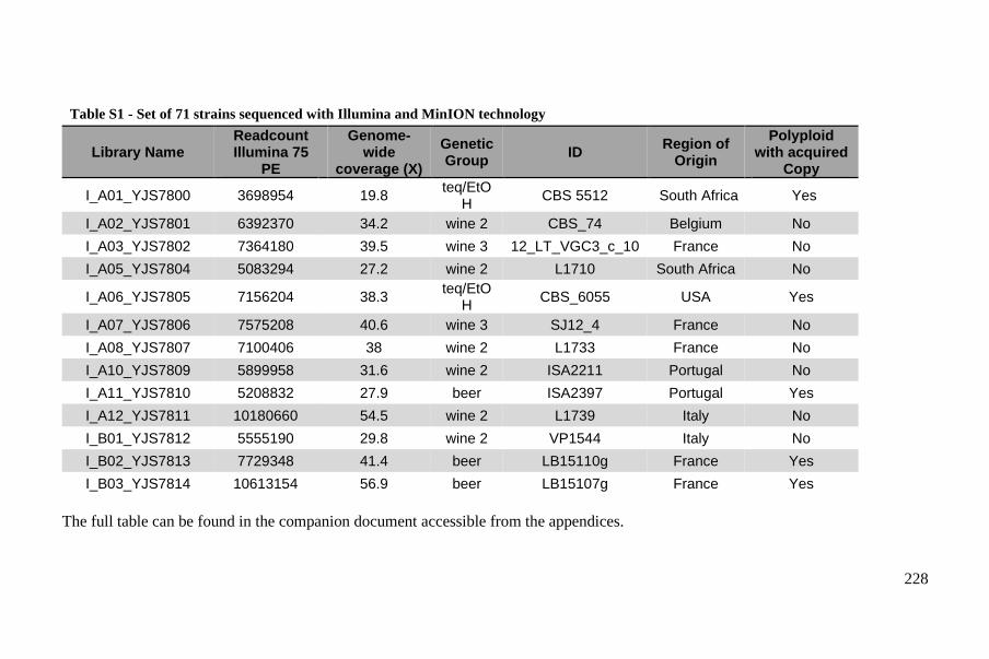
228

Table S1 - Set of 71 strains sequenced with Illumina and MinION technology

Library Name Readcount Illumina 75

PE

Genome-wide

coverage (X)

Genetic Group

ID Region of

Origin

Polyploid with acquired

Copy

I_A01_YJS7800 3698954 19.8 teq/EtO

H CBS 5512 South Africa Yes

I_A02_YJS7801 6392370 34.2 wine 2 CBS_74 Belgium No

I_A03_YJS7802 7364180 39.5 wine 3 12_LT_VGC3_c_10 France No

I_A05_YJS7804 5083294 27.2 wine 2 L1710 South Africa No

I_A06_YJS7805 7156204 38.3 teq/EtO

H CBS_6055 USA Yes

I_A07_YJS7806 7575208 40.6 wine 3 SJ12_4 France No

I_A08_YJS7807 7100406 38 wine 2 L1733 France No

I_A10_YJS7809 5899958 31.6 wine 2 ISA2211 Portugal No

I_A11_YJS7810 5208832 27.9 beer ISA2397 Portugal Yes

I_A12_YJS7811 10180660 54.5 wine 2 L1739 Italy No

I_B01_YJS7812 5555190 29.8 wine 2 VP1544 Italy No

I_B02_YJS7813 7729348 41.4 beer LB15110g France Yes

I_B03_YJS7814 10613154 56.9 beer LB15107g France Yes

The full table can be found in the companion document accessible from the appendices.

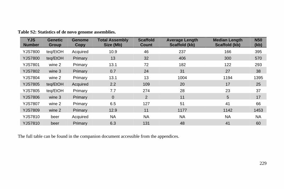
229

Table S2: Statistics of de novo genome assemblies.

YJS Number

Genetic Group

Genome Copy

Total Assembly Size (Mb)

Scaffold Count

Average Length Scaffold (kb)

Median Length Scaffold (kb)

N50 (kb)

YJS7800 teq/EtOH Acquired 10.9 46 237 166 395

YJS7800 teq/EtOH Primary 13 32 406 300 570

YJS7801 wine 2 Primary 13.1 72 182 122 293

YJS7802 wine 3 Primary 0.7 24 31 27 38

YJS7804 wine 2 Primary 13.1 13 1004 1194 1395

YJS7805 teq/EtOH Acquired 2.2 109 20 17 25

YJS7805 teq/EtOH Primary 7.7 274 28 23 37

YJS7806 wine 3 Primary 0 2 11 5 17

YJS7807 wine 2 Primary 6.5 127 51 41 66

YJS7809 wine 2 Primary 12.9 11 1177 1142 1453

YJS7810 beer Acquired NA NA NA NA NA

YJS7810 beer Primary 6.3 131 48 41 60

The full table can be found in the companion document accessible from the appendices.

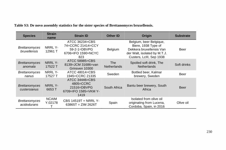
230

Table S3: De novo assembly statistics for the sister species of Brettanomyces bruxellensis.

Species Strain name

Strain ID Other ID Origin Substrate

Brettanomyces bruxellensis

NRRL Y-12961 T

ATCC 36234=CBS 74=CCRC 21414=CCY

59-2-1=DBVPG 6706=IFO 1590=NCYC

823

Belgium

Belgium, beer Belgique, Biere, 1938 Type of

Dekkera bruxellensis Van der Walt, isolated by M.T.J.

Custers, LcIII, Sep 1938

Beer

Brettanomyces anomala

NRRL Y-17522 T

ATCC 58985=CBS 8139=JCM 31686=van

Grinsven 10300

The Netherlands

Spoiled soft drink, The Netherlands

Soft drinks

Brettanomyces nanus

NRRL Y-17527 T

ATCC 48014=CBS 1945=CCRC 21335

Sweden Bottled beer, Kalmar

brewery, Sweden Beer

Brettanomyces custersianus

NRRL Y-6653 T

ATCC 34446=CBS 4805=CCRC

21516=DBVPG 6709=IFO 1585=VKM Y-

1419

South Africa Bantu beer brewery, South

Africa Beer

Brettanomyces acidodurans

NCAIM Y.02178

T

CBS 14519T = NRRL Y-63865T = ZIM 2626T

Spain Isolated from olive oil

originating from Lucena, Cordoba, Spain, in 2016

Olive oil

231

Availability of data

Illumina and Oxford Nanopore data for the 71 Brettanomyces bruxellensis isolates

are available under the study accession number PRJEB41126.

Oxford Nanopore sequencing data for the B. anomala, B. nanus, B. custerianus and

B. acidodurans species is available under the study accession number PRJEB41125.

232

References

1. Adams, K. L. & Wendel, J. F. Polyploidy and genome evolution in plants. Curr.

Opin. Plant Biol. 8, 135–141 (2005).

2. Gregory, T. R. & Mable, B. K. Polyploidy in Animals. in The Evolution of the

Genome 427–517 (Elsevier, 2005). doi:10.1016/B978-012301463-4/50010-3.

3. Gjelsvik, K. J., Besen-McNally, R. & Losick, V. P. Solving the Polyploid Mystery

in Health and Disease. Trends Genet. 35, 6–14 (2019).

4. Dehal, P. & Boore, J. L. Two Rounds of Whole Genome Duplication in the

Ancestral Vertebrate. PLoS Biol. 3, e314 (2005).

5. Sacerdot, C., Louis, A., Bon, C., Berthelot, C. & Roest Crollius, H. Chromosome

evolution at the origin of the ancestral vertebrate genome. Genome Biol. 19, 166

(2018).

6. Comai, L. The advantages and disadvantages of being polyploid. Nat. Rev. Genet.

6, 836–846 (2005).

7. Fox, D. T., Soltis, D. E., Soltis, P. S., Ashman, T.-L. & Van de Peer, Y.

Polyploidy: A Biological Force From Cells to Ecosystems. Trends Cell Biol. 30,

688–694 (2020).

8. Mayer, V. W. & Aguilera, A. High levels of chromosome instability in polyploids

of Saccharomyces cerevisiae. Mutat. Res. Mol. Mech. Mutagen. 231, 177–186

(1990).

9. Wood, T. E. et al. The frequency of polyploid speciation in vascular plants. Proc.

Natl. Acad. Sci. 106, 13875–13879 (2009).

10. Van de Peer, Y., Mizrachi, E. & Marchal, K. The evolutionary significance of

polyploidy. Nat. Rev. Genet. 18, 411–424 (2017).

11. Leitch, A. R. & Leitch, I. J. Genomic Plasticity and the Diversity of Polyploid

Plants. Science 320, 481–483 (2008).

12. Soltis, P. S., Marchant, D. B., Van de Peer, Y. & Soltis, D. E. Polyploidy and

genome evolution in plants. Curr. Opin. Genet. Dev. 35, 119–125 (2015).

13. Sanchez-Perez, G., Mira, A., Nyirő, G., Pašić, L. & Rodriguez-Valera, F.

Adapting to environmental changes using specialized paralogs. Trends Genet. 24,

154–158 (2008).

14. Eberlein, C. et al. The Rapid Evolution of an Ohnolog Contributes to the

Ecological Specialization of Incipient Yeast Species. Mol. Biol. Evol. 34, 2173–

2186 (2017).

15. Orr, H. A. ‘Why Polyploidy is Rarer in Animals Than in Plants’ Revisited. Am.

Nat. 136, 759–770 (1990).

16. Masterson, J. Stomatal Size in Fossil Plants: Evidence for Polyploidy in Majority

of Angiosperms. Science 264, 421–424 (1994).

17. Levin, D. A. The Role of Chromosomal Change in Plant Evolution. (Oxford

University Press, 2002).

233

18. Wertheim, B., Beukeboom, L. W. & van de Zande, L. Polyploidy in Animals:

Effects of Gene Expression on Sex Determination, Evolution and Ecology.

Cytogenet. Genome Res. 140, 256–269 (2013).

19. Bellon, J. R. et al. Newly generated interspecific wine yeast hybrids introduce

flavour and aroma diversity to wines. Appl. Microbiol. Biotechnol. 91, 603–612

(2011).

20. Krogerus, K., Magalhães, F., Vidgren, V. & Gibson, B. New lager yeast strains

generated by interspecific hybridization. J. Ind. Microbiol. Biotechnol. 42, 769–778

(2015).

21. Peter, J. et al. Genome evolution across 1,011 Saccharomyces cerevisiae isolates.

Nature 556, 339–344 (2018).

22. te Beest, M. et al. The more the better? The role of polyploidy in facilitating plant

invasions. Ann. Bot. 109, 19–45 (2012).

23. Bertier, L., Leus, L., D’hondt, L., de Cock, A. W. A. M. & Höfte, M. Host

Adaptation and Speciation through Hybridization and Polyploidy in Phytophthora.

PLoS ONE 8, e85385 (2013).

24. Morrow, C. A. & Fraser, J. A. Ploidy variation as an adaptive mechanism in

human pathogenic fungi. Semin. Cell Dev. Biol. 24, 339–346 (2013).

25. Seoighe, C. & Wolfe, K. H. Extent of genomic rearrangement after genome

duplication in yeast. Proc. Natl. Acad. Sci. 95, 4447–4452 (1998).

26. Gerstein, A. C. & Otto, S. P. Ploidy and the Causes of Genomic Evolution. J.

Hered. 100, 571–581 (2009).

27. Gordon, J. L., Byrne, K. P. & Wolfe, K. H. Additions, Losses, and

Rearrangements on the Evolutionary Route from a Reconstructed Ancestor to the

Modern Saccharomyces cerevisiae Genome. PLoS Genet. 5, e1000485 (2009).

28. Marcet-Houben, M. & Gabaldón, T. Beyond the Whole-Genome Duplication:

Phylogenetic Evidence for an Ancient Interspecies Hybridization in the Baker’s

Yeast Lineage. PLOS Biol. 13, e1002220 (2015).

29. de Barros Pita, W., Leite, F. C. B., de Souza Liberal, A. T., Simões, D. A. & de

Morais, M. A. The ability to use nitrate confers advantage to Dekkera bruxellensis

over S. cerevisiae and can explain its adaptation to industrial fermentation processes.

Antonie Van Leeuwenhoek 100, 99–107 (2011).

30. Avramova, M. et al. Competition experiments between Brettanomyces

bruxellensis strains reveal specific adaptation to sulfur dioxide and complex

interactions at intraspecies level. FEMS Yeast Res. 19, (2019).

31. Avramova, M. et al. Brettanomyces bruxellensis population survey reveals a

diploid-triploid complex structured according to substrate of isolation and

geographical distribution. Sci. Rep. 8, 4136 (2018).

32. Gounot, J.-S. et al. High Complexity and Degree of Genetic Variation in

Brettanomyces bruxellensis Population. Genome Biol. Evol. 12, 795–807 (2020).

234

33. Colomer, M. S. et al. Assessing Population Diversity of Brettanomyces Yeast

Species and Identification of Strains for Brewing Applications. Front. Microbiol. 11,

637 (2020).

34. Schrinner, S. D. et al. Haplotype threading: accurate polyploid phasing from long

reads. Genome Biol. 21, 252 (2020).

35. Abou Saada, O., Tsouris, A., Eberlein, C., Friedrich, A. & Schacherer, J. nPhase:

an accurate and contiguous phasing method for polyploids. Genome Biol. 22, 126

(2021).

36. Fournier, T. et al. High-Quality de Novo Genome Assembly of the Dekkera

bruxellensis Yeast Using Nanopore MinION Sequencing. G3

GenesGenomesGenetics 7, 3243–3250 (2017).

37. Borneman, A. R., Zeppel, R., Chambers, P. J. & Curtin, C. D. Insights into the

Dekkera bruxellensis Genomic Landscape: Comparative Genomics Reveals

Variations in Ploidy and Nutrient Utilisation Potential amongst Wine Isolates. PLOS

Genet. 10, e1004161 (2014).

38. Liu, H., Wu, S., Li, A. & Ruan, J. SMARTdenovo: a de novo assembler using

long noisy reads. Gigabyte 2021, 1–9 (2021).

39. Roach, M. J. & Borneman, A. R. New genome assemblies reveal patterns of

domestication and adaptation across Brettanomyces (Dekkera) species. BMC

Genomics 21, 194 (2020).

40. Smukowski Heil, C. S. et al. Loss of Heterozygosity Drives Adaptation in Hybrid

Yeast. Mol. Biol. Evol. 34, 1596–1612 (2017).

41. Lancaster, S. M., Payen, C., Smukowski Heil, C. & Dunham, M. J. Fitness

benefits of loss of heterozygosity in Saccharomyces hybrids. Genome Res. 29, 1685–

1692 (2019).

42. Jackson, J. A. & Tinsley, R. C. Parasite infectivity to hybridising host species: a

link between hybrid resistance and allopolyploid speciation? Int. J. Parasitol. 33,

137–144 (2003).

43. Augustine, R., Majee, M., Gershenzon, J. & Bisht, N. C. Four genes encoding

MYB28, a major transcriptional regulator of the aliphatic glucosinolate pathway, are

differentially expressed in the allopolyploid Brassica juncea. J. Exp. Bot. 64, 4907–

4921 (2013).

44. Thompson, J. N., Nuismer, S. L. & Merg, K. Plant polyploidy and the

evolutionary ecology of plant/animal interactions: PLANT POLYPLOIDY AND

PLANT/ANIMAL INTERACTIONS. Biol. J. Linn. Soc. 82, 511–519 (2004).

45. Těšitelová, T. et al. Ploidy‐specific symbiotic interactions: divergence of

mycorrhizal fungi between cytotypes of the Gymnadenia conopsea group

(Orchidaceae). New Phytol. 199, 1022–1033 (2013).

46. Selmecki, A. M. et al. Polyploidy can drive rapid adaptation in yeast. Nature 519,

349–352 (2015).

235

47. Wani, G. A., Shah, M. A., Reshi, Z. A. & Dar, M. A. Polyploidy determines the

stage of invasion: clues from Kashmir Himalayan aquatic flora. Acta Physiol. Plant.

40, 58 (2018).

48. Ng, D. W.-K. et al. Proteomic divergence in Arabidopsis autopolyploids and

allopolyploids and their progenitors. Heredity 108, 419–430 (2012).

49. Leggatt, R. A. & Iwama, G. K. Occurrence of polyploidy in the fishes. Rev. Fish

Biol. Fish. 13, 237–246 (2003).

50. Barker, M. S., Arrigo, N., Baniaga, A. E., Li, Z. & Levin, D. A. On the relative

abundance of autopolyploids and allopolyploids. New Phytol. 210, 391–398 (2016).

51. Istace, B. et al. de novo assembly and population genomic survey of natural yeast

isolates with the Oxford Nanopore MinION sequencer. GigaScience 6, (2017).

52. Sedlazeck, F. J. et al. Accurate detection of complex structural variations using

single-molecule sequencing. Nat. Methods 15, 461–468 (2018).

53. Koren, S. et al. Canu: scalable and accurate long-read assembly via adaptive k -

mer weighting and repeat separation. Genome Res. 27, 722–736 (2017).

54. Li, H. & Durbin, R. Fast and accurate short read alignment with Burrows-

Wheeler transform. Bioinformatics 25, 1754–1760 (2009).

55. Li, H. et al. The Sequence Alignment/Map format and SAMtools. Bioinformatics

25, 2078–2079 (2009).

56. McKenna, A. et al. The Genome Analysis Toolkit: A MapReduce framework for

analyzing next-generation DNA sequencing data. Genome Res. 20, 1297–1303

(2010).

57. Danecek, P. et al. The variant call format and VCFtools. Bioinformatics 27,

2156–2158 (2011).

58. Charif, D. & Lobry, J. R. SeqinR 1.0-2: A Contributed Package to the R Project

for Statistical Computing Devoted to Biological Sequences Retrieval and Analysis.

in Structural Approaches to Sequence Evolution (eds. Bastolla, U., Porto, M.,

Roman, H. E. & Vendruscolo, M.) 207–232 (Springer Berlin Heidelberg, 2007).

doi:10.1007/978-3-540-35306-5_10.

59. Schliep, K. P. phangorn: phylogenetic analysis in R. Bioinformatics 27, 592–593

(2011).

60. Rambaut, A. FigTree, a graphical viewer of phylogenetic trees. Institute of

Evolutionary Biology University of Edinburgh. FigTree, a graphical viewer of

phylogenetic trees http://tree.bio.ed.ac.uk/software/figtree/ (2009).

61. Jombart, T. adegenet: a R package for the multivariate analysis of genetic

markers. Bioinformatics 24, 1403–1405 (2008).

62. Yin, T., Cook, D. & Lawrence, M. ggbio: an R package for extending the

grammar of graphics for genomic data. Genome Biol. 13, R77 (2012).

236

Conclusion and perspectives

Towards accurate, contiguous and complete polyploid phasing

algorithms

Despite extensive efforts, polyploid phasing algorithms have been held back by the

limited read length of short read sequencing methods. The arrival of long-read

sequencing methods has led to very efficient diploid phasing methods, such as

WhatsHap1 and Falcon-Unzip2. However, the problem of polyploid phasing

remained. In part due to the non-negligible error rate of these new sequencing

technologies, but also due to a euploid bias which presumes that a polyploid with n

copies of its genome has n haplotypes throughout its genome. We are now in the

midst of a paradigm shift, with the short read polyploid phasing methods being

phased out in favor of long read methods and an increasing acknowledgement of the

complexity of the genomic structures being phased. The recently published

polyploid phasing tool Ranbow handles the edge case of having fewer distinct

haplotypes than genomic copies in a region3, and the long-read polyploid phasing

method WhatsHap polyphase explicitly tackles this problem through its solution of

“haplotype threading” which uses coverage information to determine which

haplotype is present multiple times4. With our phasing algorithm, nPhase, we

explicitly consider that ploidy is uncertain and present a ploidy agnostic method

which allows for variation in the number of haplotypes, making it possible to handle

aneuploidy, large LOH events and relieving the user from the task of estimating and

selecting a ploidy5. We also question the usefulness of the SWitch Error Rate metric,

which we argue is fundamentally unpredictable, and consider that more attention

should be given to the inseparable notions of accuracy and contiguity in this field.

In the future, solutions to the polyploid phasing problem need to go beyond the

237

innovations of nPhase and tackle remaining issues and improvements. Since nPhase

is a reference alignment phasing method, it does not natively resolve structural

variants. Currently, the phasing results of nPhase can only be used to heterozygous

structural variation by performing additional analysis, such as de novo assembly of

the phased reads followed by comparison of the assembled sequences. Phasing indels

is crucial to identifying frameshift events in polyploids to determine if there is a

functional copy of a given gene, however nPhase doesn’t phase these events. Further

analysis is required to determine the impact of including indels in the phaseable

genetic markers, particularly given the propensity of long-read sequencing methods

to suffer from homopolymer errors. Finally, future methods would greatly benefit

from incorporating metadata that aids in the interpretation of results such as

confidence metrics or phasing quality scores. Taking base-calling quality and

mapping quality into account can also serve to improve the accuracy of these

methods. Finally, we also find it would be highly beneficial to generate simulated

and real validation datasets against which to systematically benchmark all polyploid

phasing tools with carefully selected performance metrics. This practice would not

only allow for a standardization of the highly diverse methods used in the

benchmarking step, it would also highlight the strengths and weaknesses of

polyploid phasing tools, providing deeper insight into their differences and helping

users select the most appropriate method.

Applications of polyploid phasing to population genomics

Due to the lack of effective polyploid phasing methods, there has been very little

application of polyploid phasing to populations. In a paper on S. cerevisiae beer

strains, Fay et al. (2019)6 developed what is arguably the first polyploid phasing

method in order to show that one of the three main clades of beer strains is composed

of a polyploid admixture of Asian and European wine strains. Using nPhase and a

238

population of 35 beer strains of S. cerevisiae stemming from different clades, we

were able to characterize two other groups of beer strains. The European dominant

group was shown to be a similar admixture to the Asian dominant clade, but with

different proportions, and the African Beer group was shown to mostly have

European wine and French dairy alleles. Both French dairy strains and African Beer

strains of S. cerevisiae share their environment with lactic acid bacteria, which we

hypothesize is a driver of the allelic similarities between them. We developed the

notion of intra-strain divergence, where we calculate the divergence between the

different haplotypes within a strain, and the notion of estimating the divergence

between the haplotypes of strains, showing that the distance between strains is

typically lower than would be estimated with unphased data. Having phased genes

in this polyphyletic group of strains exposed to similar environments allowed us to

identify the genes with the highest levels of divergence (>4%), which we found to

be enriched for GO terms relevant for adaptations to the brewing environment.

Polyploid strains of S. cerevisiae are only found in a few clades, including all of the

clades containing beer strains. Our study did not uncover any further connection

between beer brewing strains and polyploidy, though this dataset may provide

important insight into the mechanisms which seem to pressure S. cerevisiae beer-

brewing strains into polyploidy.

We also studied a population of 71 diverse strains of B. bruxellensis, in which many

triploid strains were suspected of being composed of a core diploid genome

hybridized with a set of chromosomes from a different species7. We found that the

long reads of such hybrid strains were easily identified by calculating the density of

SNPs that don’t match with the B. bruxellensis reference genome and plotting their

distribution. Hybrid strains output a bimodal distribution, with a set of reads which

have few mismatches relative to the reference (<10 SNPs/kb) and a set of reads,

belonging to the extra set of chromosomes, which has many mismatches to the

239

reference (>14 SNPs/kb). We could then simply phase these strains by separating

reads based on their SNP density. This phasing method could not apply to strains of

another specific polyploid subpopulation (wine 3 triploids) which do not exhibit this

bimodal distribution, prompting us to phase them using nPhase. This allowed us to

show that while the core genomes were always very similar, even across

subpopulations, the diverged set of chromosomes is not the same in any two

subpopulations, and therefore was acquired independently from different species by

each subpopulation of B. bruxellensis, potentially as adaptations to their respective

environments. We ruled out known sister species of B. bruxellensis such as

Brettanomyces anomala and Brettanomyces nanus as the hybridization candidates,

prompting the need for a search to identify them.

Performing these studies highlighted the need for accessory tools and analytical

methods which leverage polyploid phasing data to improve insight into the data. The

tools which need to be developed range from simple ones, such as a tool which

performs comparisons between haplotypes within a strain which expose simple

statistics such as the similarity between haplotypes or the basecall quality and

mapping quality scores throughout the genome, to more complex tools such as a tool

which identifies missense, nonsense and frameshift states in genes of phased

haplotypes. The latter would require a tool which handles indels at minimum, and

structural variants at best. We now have the possibility to perform population

genomic studies with polyploid genomes which exploit phased data, and there is

significant room for the development and application of novel tools and methods to

analyze this data.

In a future project, our dataset of high-quality real phased genomes could be

leveraged to develop a ploidy agnostic polyploid de novo assembly algorithm. These

real genomes, containing aneuploidies, large LOH events and highly likely to contain

240

structural variants, can serve as a crucial validation dataset to direct the development

of such an algorithm. Our high confidence in the phasing provided by nPhase allows

us to reasonably expect that improvement in the de novo assembly’s similarity to the

predictions of nPhase will translate to improvement in de novo assembly quality. A

ploidy agnostic de novo assembly algorithm loses the guide of a reference genome,

complexifying the problem, but also gains the freedom to faithfully reconstruct

structural variants, sequences not present in the reference and duplication events.

The core idea of nPhase is to allow like reads to cluster based on similarity, with an

emphasis on the weight of variable positions as identified by Illumina. A first step in

an endeavor to develop a novel de novo assembly algorithm could be to identify

variable positions within similar blocks through mapping and variant calling reads,

and then subsequently perform de novo assembly with an additional constraint based

on the same rules as nPhase. If results are promising, the next phase would seek to

make the identification of variable positions not require lengthy mapping and variant

calling steps. Such a tool would take us closer to an accurate picture of polyploid

genomes, permitting deeper insights into genotype-phenotype relationships.

The phasing out of approximations

Earlier this year, the Telomere-To-Telomere (T2T) consortium pre-published the

complete human genome8, analysis of segmental duplications9, epigenetic patterns

of the complete genome10, the centromeres11 and repeat elements12. If the genomic

era is in part defined by the sequencing boom afforded by short read high-throughput

sequencing methods and the promises of population genomic studies and GWAS

methods, the next era may be in part defined by the unprecedented detail afforded

by long-read sequencing methods. Individual molecules will be sequenced directly,

obtaining high-quality de novo assemblies will be considered a pre-processing step,

reference sequences will be replaced by genome graphs, multi-omics will routinely

241

be integrated in population genomics projects and approximations will become

increasingly rare.

We need highly modular, integrated toolkits, analysis platforms and standardized

analysis and benchmarking protocols to catch up with the immense quantity of data

we routinely generate and tip the scale towards analyzing data faster than we can

generate it.

242

References

1. Patterson, M. et al. WhatsHap: Weighted Haplotype Assembly for Future-

Generation Sequencing Reads. J. Comput. Biol. 22, 498–509 (2015).

2. Chin, C.-S. et al. Phased diploid genome assembly with single-molecule real-time

sequencing. Nat. Methods 13, 1050–1054 (2016).

3. Moeinzadeh, M.-H. et al. Ranbow: A fast and accurate method for polyploid

haplotype reconstruction. PLOS Comput. Biol. 16, e1007843 (2020).

4. Schrinner, S. D. et al. Haplotype threading: accurate polyploid phasing from long

reads. Genome Biol. 21, 252 (2020).

5. Abou Saada, O., Tsouris, A., Eberlein, C., Friedrich, A. & Schacherer, J. nPhase:

an accurate and contiguous phasing method for polyploids. Genome Biol. 22, 126

(2021).

6. Fay, J. C. et al. A polyploid admixed origin of beer yeasts derived from European

and Asian wine populations. PLOS Biol. 17, e3000147 (2019).

7. Borneman, A. R., Zeppel, R., Chambers, P. J. & Curtin, C. D. Insights into the

Dekkera bruxellensis Genomic Landscape: Comparative Genomics Reveals

Variations in Ploidy and Nutrient Utilisation Potential amongst Wine Isolates. PLOS

Genet. 10, e1004161 (2014).

8. Nurk, S. et al. The complete sequence of a human genome. bioRxiv

2021.05.26.445798 (2021) doi:10.1101/2021.05.26.445798.

9. Vollger, M. R. et al. Segmental duplications and their variation in a complete

human genome. bioRxiv 2021.05.26.445678 (2021)

doi:10.1101/2021.05.26.445678.

10. Gershman, A. et al. Epigenetic Patterns in a Complete Human Genome. bioRxiv

2021.05.26.443420 (2021) doi:10.1101/2021.05.26.443420.

11. Altemose, N. et al. Complete genomic and epigenetic maps of human

centromeres. bioRxiv 2021.07.12.452052 (2021) doi:10.1101/2021.07.12.452052.

12. Hoyt, S. J. et al. From telomere to telomere: the transcriptional and epigenetic

state of human repeat elements. bioRxiv 2021.07.12.451456 (2021)

doi:10.1101/2021.07.12.451456.

243

244

APPENDIX

245

Companion document

Some supplemental figures and tables from chapters II and III take too much space

and have been added to a companion document available online at

https://doi.org/10.5281/zenodo.5207333

246

List of publications

- Fournier T., Abou Saada O., Hou J., Peter J., Caudal E., Schacherer J.

Extensive impact of low-frequency variants on the phenotypic landscape at

population-scale. eLife. 2019 Oct 24;8:e49258.

- Abou Saada O., Tsouris A., Eberlein C., Friedrich A., Schacherer J.

nPhase: an accurate and contiguous phasing method for polyploids. Genome Biol.

2021 Apr 29;22(1):126.

- Eberlein, C., Abou Saada, O., Friedrich, A., Albertin, W. & Schacherer, J.

Different trajectories of polyploidization shape the genomic landscape of the

Brettanomyces bruxellensis yeast species. (Accepted for publication in Genome

Research)

- Peltier, E.,Vion, C., Abou Saada, O., Friedrich, A., Schacherer J., Marullo P.

Flor yeasts rewire the central carbon metabolism during wine alcoholic fermentation.

(Under review in Frontiers in Fungal Biology)

- Abou Saada, O., Tsouris, A., Large, C., Friedrich A., Dunham M., Schacherer J.

Phased polyploid genomes provide deeper insights into the different evolutionary

trajectories of the Saccharomyces cerevisiae beer yeasts. (In preparation)

- Abou Saada, O., Friedrich A., Schacherer J. Towards accurate, contiguous and

complete polyploid phasing algorithms. (Review, in preparation)

247

List of oral communications

Pint of Science – scientific popularization

Strasbourg, France, May 2018

Comment trouver un gène dans une botte de foin [How to find a gene in a haystack]

Oxford Nanopore event - The state of Nanopore sequencing in 2018: technical

updates and applications in Strasbourg

Strasbourg, France, October 2018

Exploration of the structural variant landscape in yeast using Oxford Nanopore

sequencing

EMBO Workshop – Comparative genomics of eukaryotic microbes: Genomes in

flux, and flux between genomes

Sant Feliu de Guixols, Spain, October 2019

Ploidy agnostic phasing method with short and long read sequencing,

Lightning talk for Oxford Nanopore event initially planned in Paris.

Presented online, March 2020

nPhase – Ploidy agnostic pipeline

Teaching

University of Strasbourg

2018-2020

Classes for doctoral students

o Français Langue Étrangère [French as a foreign language]

2020-2021

Classes for master’s degree students

o Génétique Quantitative Appliquée [Applied Quantitative Genetics]

o Génomique Fonctionelle et Évolutive [Functional and Evolutionary Genomics]